HAL Id: tel-00623090 https://tel.archives-ouvertes.fr/tel-00623090 Submitted on 13 Sep 2011 HAL is a multi-disciplinary open access archive for the deposit and dissemination of sci- entific research documents, whether they are pub- lished or not. The documents may come from teaching and research institutions in France or abroad, or from public or private research centers. L’archive ouverte pluridisciplinaire HAL, est destinée au dépôt et à la diffusion de documents scientifiques de niveau recherche, publiés ou non, émanant des établissements d’enseignement et de recherche français ou étrangers, des laboratoires publics ou privés. COMBUSTION STUDY OF MIXTURES RESULTING FROM A GASIFICATION PROCESS OF FOREST BIOMASS Eliseu Monteiro Magalhaes To cite this version: Eliseu Monteiro Magalhaes. COMBUSTION STUDY OF MIXTURES RESULTING FROM A GASI- FICATION PROCESS OF FOREST BIOMASS. Engineering Sciences [physics]. ISAE-ENSMA Ecole Nationale Supérieure de Mécanique et d’Aérotechique - Poitiers, 2011. English. tel-00623090

Welcome message from author
This document is posted to help you gain knowledge. Please leave a comment to let me know what you think about it! Share it to your friends and learn new things together.
Transcript

HAL Id: tel-00623090https://tel.archives-ouvertes.fr/tel-00623090
Submitted on 13 Sep 2011
HAL is a multi-disciplinary open accessarchive for the deposit and dissemination of sci-entific research documents, whether they are pub-lished or not. The documents may come fromteaching and research institutions in France orabroad, or from public or private research centers.
L’archive ouverte pluridisciplinaire HAL, estdestinée au dépôt et à la diffusion de documentsscientifiques de niveau recherche, publiés ou non,émanant des établissements d’enseignement et derecherche français ou étrangers, des laboratoirespublics ou privés.
COMBUSTION STUDY OF MIXTURES RESULTINGFROM A GASIFICATION PROCESS OF FOREST
BIOMASSEliseu Monteiro Magalhaes
To cite this version:Eliseu Monteiro Magalhaes. COMBUSTION STUDY OF MIXTURES RESULTING FROM A GASI-FICATION PROCESS OF FOREST BIOMASS. Engineering Sciences [physics]. ISAE-ENSMA EcoleNationale Supérieure de Mécanique et d’Aérotechique - Poitiers, 2011. English. �tel-00623090�

THÈSE Pour l’obtention du Grade de
DOCTEUR DE L'ENSMA
ÉCOLE NATIONALE SUPÉRIEURE DE MÉCANIQUE ET D’AÉROTECHNIQUE
(Diplôme National – Arrêté du 7 Août 2006)
École Doctorale: SIMMEA
Secteur de Recherche: Énergétique, Thermique, Combustion
Présentée par:
Eliseu MONTEIRO MAGALHAES
***********
COMBUSTION STUDY OF MIXTURES RESULTING FROM A GASIFICATION PROCESS OF FOREST BIOMASS
***********
Directeurs de Thèse: Marc BELLENOUE et Nuno MOREIRA
***********
Soutenue le 13 Mai 2011
JURY
Rapporteurs Mme Christine ROUSSELLE, Professeur des Universités, POLYTECH’Orléans M. Edgar FERNANDES, Professeur des Universités, IST, Lisbonne Examinateurs Mr. Marc Bellenoue, Professeur des Universités, ENSMA, Institut P’, Poitiers Mr. Nuno Afonso Moreira, Professeur des Universités, UTAD, Vila Real Mr. Jérôme Bellètre, Professeur des Universités, Polytech Nantes, Nantes Mr. Julien Sotton, Maître de Conférences, ENSMA, Institut P’, Poitiers Mr. Abel Rouboa, Professeur des Universités, UTAD, Vila Real Mr. Salvador Malheiro, Ingénieur, Docteur ès Sciences, ENGASP, Portugal


Acknowledgements
2
Acknowledgements This dissertation has greatly benefited from the help, interest and support of many
people from many parts of the world at who I would like to extend my deepest
gratitude. Additional commendation goes to Fundação para a Ciência e a Tecnologia
for the financial support through the research grant SFRH/BD/32699/2006.
First and foremost I am grateful to Professor Marc Bellenoue (ENSMA), Professor
Nuno Afonso Moreira (UTAD) and Prof. Salvador Malheiro (UTAD) for their valuable
help and research guidance. I am also indebted to Professor Julien Sotton (ENSMA)
and Dr. Serguei Labouda (ENSMA) for guiding me to perform experimental work at the
laboratory; to Dr. Bastien Boust (ENSMA), Dr. Camile Strozzi (ENSMA) and Mr. Djamel
Karmed (ENSMA) for the assistance on numerical simulations.
Furthermore, I am grateful to Professor Zuohua Huang, from Xi’an JiaoTong University,
China, and Dr. Xiaojun Gu, from Daresbury Laboratory, Warrington, United Kingdom,
for the useful comments on laminar burning velocity calculations; to Professor Federico
Perini, from University of Modena, Italy, for providing experimental data on methane
engine; to Professor Sebastian Verhelst, from University of Gent, Belgium, for providing
experimental data on hydrogen engine.
My sympathy goes also to the ENSMA staff especially to Mrs. Jocelyne Bardeau for
her administrative support.
Finally, and most important, my thanks to my family and friends, who have continually
demonstrated support in this long journey.


Résumé __________________________________________________________________________
__________________________________________________________________________ 3
Résumé
Les gaz de synthèse (Syngas) sont reconnus comme sources d’énergie viables, en
particulier pour la production d’électricité. Lors de cette étude, trois compositions de syngas
ont été retenues. Elles sont représentatives de gaz issus de la gazéification de la biomasse
forestière. Leur potentiel dans des systèmes de production d'énergie utilisant un Moteur à
Combustion Interne (MCI) a été étudié. Leur vitesse de flamme en régime laminaire a été
déterminée à partir de visualisation par strioscopie. Les effets du taux d'étirement ont été
quantifiés au travers de la détermination du nombre de Karlovitz et de Markstein. En raison
des lacunes de la littérature sur les caractéristiques de combustion de ces syngaz, la
méthode de combustion sphérique a été utilisée pour déterminer la vitesse de flamme sur un
domaine de pression de 1 à 20 bars. Ces résultats ont ensuite été utilisés dans un code de
simulation multi-zones prenant en compte les transferts de chaleur aux parois afin d’estimer
la distance de coincement.
Une analyse en régime turbulent a été menée en Machine à Compression Rapide (MCR),
machine capable de reproduire un cycle compression-détente d'un moteur à combustion
interne. En général, les applications stationnaires de production électrique utilisent le gaz
naturel comme carburant, mélange majoritairement constitué de méthane. Pour servir de
référence à la comparaison des capacités des trois syngaz retenus, un mélange méthane-air
a été testé également. Afin d'identifier les différents paramètres liés au fonctionnement de la
MRC, en particulier les transferts de chaleur aux parois, des essais sans combustion ont été
réalisées.
Enfin un code de simulation du cycle d'un moteur à piston utilisant ces syngaz comme
combustible a été développé. Sa validation a été réalisée en utilisant les données
expérimentales disponibles dans la littérature concernant des mélanges hydrogène-air et
méthane-air, et également à l'aide des données obtenues sur la MCR. Le modèle a
finalement été utilisé pour déterminer les performances d'un moteur à piston fonctionnant
avec ces sysngaz. Il a été observé que les compositions typiques de syngas, même avec
des capacités calorifiques et la vitesse de flamme plus faibles, peuvent être utilisées pour les
moteurs à allumage commandée et ceci à des vitesses de rotation élevées.
Mots-clés : Gazéification – Syngas -Combustion – Vitesse de flamme – Machine à
compression rapide – Modélisation multizone.

Resumo
4
Resumo O syngas é mundialmente reconhecido como uma fonte de energia viável em
particular para aplicações estacionárias. Neste trabalho, três composições típicas de
syngas foram consideradas representativas do gás proveniente da gaseificação de
biomassa florestal e estudada a possibilidade da sua utilização em motores de
combustão interna. Primeiro, a velocidade de chama laminar fora determinada a partir
de fotografia de schlieren a pressão constante. Em adição, o estudo dos efeitos da
perturbação da chama é realizado através da obtenção dos números de Karlovitz e
Markstein. Em segundo lugar, e dado existir lacunas na compreensão das
características fundamentais da combustão de gás de síntese, em especial a pressões
elevadas relevantes para aplicações práticas da combustão, é determinada a
velocidade de chama laminar a volume constante para pressões até 20 bar. Esta
informação é aplicada num código de simulação multi-zona da interacção chama-
parede de modo a determinar a distância de extinção de chama. A combustão
turbulenta em condições semelhantes ao motor de combustão interna (MCI) é
reproduzida em máquina de compressão rápida (MCR) funcionando em modo de
compressão seguido de expansão simulando o ciclo de potência de um MCI. As
aplicações de produção de energia de pequena escala usam habitualmente gás
natural como combustível, deste modo o metano é também incluído neste trabalho por
questões de comparação de performance com as composições típicas de syngas em
estudo. Testes de compressão são também realizados em MCR operando com e sem
combustão de modo a identificar os diferentes parâmetros de funcionamento,
nomeadamente a transferência de calor na parede. Um modelo termodinâmico de
simulação do ciclo de potência de um MCI é desenvolvido. A sua validação é
efectuada por comparação com dados de pressão obtidos na literatura para hidrogénio
e metano. O modelo é ainda adaptado para a MCR por alteração de vários aspectos
do mesmo, nomeadamente a função de volume do cilindro e o modelo de velocidade
de chama. O código mostrou-se adequado para simular a evolução da pressão no
interior do cilindro. O modelo validado é então aplicado a MCI a syngas de modo a
determinar a sua performance. Conclui-se que as composições típicas de syngas,
apesar do seu baixo poder calorífico e velocidade de chama, podem ser utilizadas em
MCI a elevada velocidade de rotação.
Palavras-chave: Gaseificação – Syngas – Combustão – Velocidade de chama –
Máquina de compressão rápida – Modelação multi-zona.

Nomenclature
5
Nomenclature
Roman
A Area of flame surface (m2)
a Cross section (m2)
B Bore (m)
cp Specific heat under constant pressure (J/kg.K)
cv Specific heat under constant volume (J/kg.K)
D Diameter (m)
Ei Ignition energy (J)
f Focal length (m)
gp Pressure gain (bar)
h Convective heat transfer coefficient (W/m2.K)
hg Global heat transfer coefficient (W/m2.K)
H(t) Instantaneous height of chamber (m)
I Current intensity (A)
k Turbulence kinetic energy (m2/s2)
Ka Karlovitz number
L(t) Instantaneous combustion chamber height (m)
Lb Markstein length of burned gases (m)
Le Lewis number
Lu Markstein length of unburned gases (m)
m Mass (kg)
M Molar mass (mol)
Ma Markstein number
N Engine speed (rpm)
n Normal
P Pressure (bar)
Pe Peclet number
Pmot (t) Instantaneous motored cylinder pressure (bar)
QWC Convective heat flux (W)
Qwr Radiative heat radiative flux (W)
r Radius of burned gases sphere (m)
R Radius of the spherical vessel (m)
Nomenclature
6
Ru Universal gas constant =8.314 J/Kmol.K
sp Mean piston speed (m/s)
Sg Unburned gas velocity (m/s)
Sn Stretched Flame speed (m/s) 0nS Unstretched Flame speed (m/s)
Su Stretched laminar burning velocity (m/s) 0uS Unstretched laminar burning velocity (m/s)
T Temperature (K)
t Time (s)
U Internal energy (J)
W Lambert function
V Volume (m3); Voltage (V)
Vs Swept volume (m3)
x,y,z Cartesian coordinates
Greek
α Thermal diffusivity (W/m.K)
δ Flame thickness (m)
δq Quenching distance (m)
Δt Time step (s)
ε Compression ratio; emissivity
φ Equivalence ratio
ϕ Crank radius to piston rod length ratio
γ Ratio of specific heat capacities (cp/cv)
η Combustion efficiency (%)
κ Stretch rate (s-1)
λ Thermal conductivity (W/m.K)
μ Kinematic viscosity (m2/s)
θ Angle
ρ Density (kg/m3)
σ Stefan’s constant ; Expansion factor
τ Combustion time (s)

Nomenclature
7
Subscripts b Burned
c Curvature
d Discharge
e Final (end) condition
i Initial conditions
g Fresh gas
m Mixture
n Normal
max Maximum
r, θ, φ Spherical coordinates
s Strain
u Unburned
w Wall
v Adiabatic
0 Reference conditions
Superscripts 0 Unstretched
α Temperature parameter
β Pressure parameter
Abbreviations ATDC After top dead center
BDC Bottom dead center
BTDC Before top dead center
ºCA Degrees of crank angle
CI Compression ignition
EVC Exhaust valve closing time
EVO Exhaust valve opening time
HHV Higher heating value
ICE Internal combustion engine
IPCC Intergovernmental Panel on Climate Change

Nomenclature
8
IVC Intake valve closing time
IVO Intake valve opening time
LFL Lower flammability limit
LHV Lower heating value
RCM Rapid compression machine
SI Spark ignition
TDC Top dead center
UFL Upper flammability limit

Contents
9
Contents ACKNOWLEDGEMENTS ....................................................................................................................... 2
RESUME ..................................................................................................................................................... 3
RESUMO .................................................................................................................................................... 4
NOMENCLATURE ................................................................................................................................... 5
CONTENTS ................................................................................................................................................ 9
CHAPTER 1 INTRODUCTION ............................................................................................................. 12
1.1 MOTIVATION AND OBJECTIVE ........................................................................................................... 14 1.2 THESIS LAYOUT ................................................................................................................................ 15
CHAPTER 2 BIBLIOGRAPHIC REVISION ....................................................................................... 18
2.1 BIOMASS GASIFICATION .................................................................................................................... 18 2.1.1 Historical development ............................................................................................................ 18 2.1.2 Gasification process ................................................................................................................. 20 2.1.3 Gasification plant ..................................................................................................................... 23
2.1.3.1 Gasifier types .................................................................................................................................... 23 2.1.3.2 Fixed bed gasifiers............................................................................................................................ 24 2.1.3.3 Fluidized bed gasifiers ...................................................................................................................... 26 2.1.3.4 Syngas conditioning ......................................................................................................................... 29
2.2. SYNGAS APPLICATIONS .................................................................................................................... 30 2.2.1 Power production ..................................................................................................................... 31 2.2.2 Fuels ........................................................................................................................................ 33
2.3. SYNGAS CHARACTERIZATION .......................................................................................................... 34 2.3.1 Influence of biomass type ......................................................................................................... 35 2.3.2. Influence of reactor type ......................................................................................................... 36 2.3.3 Influence of operational conditions ......................................................................................... 36
2.3.3.1 Temperature ..................................................................................................................................... 36 2.3.3.2. Pressure ........................................................................................................................................... 37
2.3.4 Influence of the oxidizer ........................................................................................................... 38 2.4. CONCLUDING REMARKS ABOUT BIOMASS GASIFICATION ................................................................. 39 2.5. LAMINAR PREMIXED FLAMES ........................................................................................................... 40
2.5.1 Flame stretch ........................................................................................................................... 41 2.5.1.1 Karlovitz number .............................................................................................................................. 46 2.5.1.2 Markstein number............................................................................................................................. 46
2.5.2 Burning velocity measurement methods ................................................................................... 49 2.5.2.1 Tube method ..................................................................................................................................... 50 2.5.2.2 Soap bubble method ......................................................................................................................... 51 2.5.2.3 Constant volume method .................................................................................................................. 52 2.5.2.4 Constant pressure method ................................................................................................................. 57
2.5.3 Burning velocity empirical correlations .................................................................................. 59 2.6 CONCLUDING REMARKS ABOUT LAMINAR PREMIXED FLAMES .......................................................... 61
CHAPTER 3 EXPERIMENTAL SET UPS AND DIAGNOSTICS ..................................................... 62
3.1. EXPERIMENTAL SET UPS .................................................................................................................. 62 3.1.1. Syngas mixtures ...................................................................................................................... 62 3.1.2 Rectangular chamber ............................................................................................................... 63 3.1.3 Spherical chamber ................................................................................................................... 64 3.1.4 Rapid compression machine .................................................................................................... 65
3.2. COMBUSTION DIAGNOSTICS ............................................................................................................. 67 3.2.1 Flammability limits .................................................................................................................. 68 3.2.3 Pressure measurement on static chambers .............................................................................. 71 3.2.4 Pressure measurement on RCM ............................................................................................... 73 3.2.5 Aerodynamics inside a RCM .................................................................................................... 77
3.2.5.1 Velocity fluctuations ..................................................................................................................... 78 3.2.5.2 Analysis of the flow at the chamber core .................................................................................. 81
3.2.6 Schlieren photography ............................................................................................................. 82
CHAPTER 4 EXPERIMENTAL AND NUMERICAL LAMINAR SYNGAS COMBUSTION ...... 85

Contents
10
4.1 LAMINAR BURNING VELOCITY .......................................................................................................... 87 4.1.1 Constant pressure method ........................................................................................................ 87
4.1.1.1 Flame morphology ........................................................................................................................ 89 4.1.1.2 Flame Radius .............................................................................................................................. 100 4.1.1.3 Flame speed ............................................................................................................................... 102 4.1.1.4 Laminar burning velocity ........................................................................................................... 104 4.1.1.5 Karlovitz and Markstein numbers ............................................................................................. 106 4.1.1.6 Comparison with other fuels ..................................................................................................... 109
4.1.2 Constant volume method ........................................................................................................ 111 4.1.2.1 Pressure evolution ...................................................................................................................... 112 4.1.2.2 Burning velocity .......................................................................................................................... 114 4.1.2.3 Laminar burning velocity correlations ...................................................................................... 119
4.2. MULTI-ZONE SPHERICAL COMBUSTION .......................................................................................... 123 4.2.1 Mathematical model ............................................................................................................... 123
4.2.1.1 Flame propagation ..................................................................................................................... 123 4.2.1.2 Chemical equilibrium .................................................................................................................. 124 4.2.1.3 Heat transfer ............................................................................................................................... 124
4.2.2 Calculation procedure ........................................................................................................... 126 4.2.3 Results discussion and code validation .................................................................................. 128
4.2.3.1 Influence of the heat transfer model ........................................................................................ 129 4.2.3.2 Influence of equivalence ratio ................................................................................................... 129 4.2.3.3 Influence of the pressure ........................................................................................................... 133 4.2.3.4 Quenching distance and heat flux estimations ....................................................................... 135
4.3 CONCLUSION .................................................................................................................................. 137
CHAPTER 5 EXPERIMENTAL STUDY OF ENGINE-LIKE TURBULENT COMBUSTION ... 139
5.1 RCM SINGLE COMPRESSION ........................................................................................................... 139 5.1.1 Sensibility analysis ................................................................................................................. 140
5.1.1.1 TDC position ............................................................................................................................... 140 5.1.1.2 Initial piston position ................................................................................................................... 141 5.1.1.3 Spark time ................................................................................................................................... 143 5.1.1.4 In-cylinder pressure reproducibility .......................................................................................... 145 5.1.1.5 Conclusion ................................................................................................................................... 146
5.1.2 In-cylinder pressure ............................................................................................................... 147 5.1.3 In-cylinder flame propagation ............................................................................................... 148
5.2 RCM COMPRESSION-EXPANSION .................................................................................................... 150 5.2.1 Sensibility analysis ................................................................................................................. 150
5.2.1.1 Piston position ............................................................................................................................. 150 5.2.1.2 Equivalent rotation speed .......................................................................................................... 153 5.2.1.3 In-cylinder pressure repeatability ............................................................................................. 155 5.2.1.4 Conclusion ................................................................................................................................... 157
5.2.2 In-cylinder pressure ............................................................................................................... 157 5.2.3 Ignition timing ........................................................................................................................ 160 5.2.4 In-cylinder flame propagation ............................................................................................... 161
5.3 CONCLUSION .................................................................................................................................. 165
CHAPTER 6 NUMERICAL SIMULATION OF A SYNGAS- FUELLED ENGINE ..................... 167
6.1 THERMODYNAMIC MODEL .............................................................................................................. 168 6.1.1 Conservation and state equations .......................................................................................... 169 6.1.2 Chemical composition and thermodynamic properties .......................................................... 170 6.1.3 Heat Transfer ......................................................................................................................... 173 6.1.4 Mass burning rate .................................................................................................................. 174
6.2. NUMERICAL SOLUTION PROCEDURE .............................................................................................. 175 6.3 CODE VALIDATION.......................................................................................................................... 178
6.3.1 CFR engine ............................................................................................................................ 178 6.3.1.1 Sub-models ................................................................................................................................. 178 6.3.1.2 Results and discussion .............................................................................................................. 181
6.3.2 RCM ....................................................................................................................................... 182 6.3.2.1 Flame propagation ..................................................................................................................... 182 6.3.2.2 In-cylinder volume ...................................................................................................................... 183 6.2.2.3 Heat transfer ............................................................................................................................... 184 6.3.2.4 Turbulent burning velocity ......................................................................................................... 185 6.3.2.5 Results and discussion .............................................................................................................. 185

Contents
11
6.4. SYNGAS FUELLED-ENGINE ............................................................................................................. 188 6.4.1 Results and discussion ........................................................................................................... 188
6.5 CONCLUSION .................................................................................................................................. 192
CHAPTER 7 CONCLUSIONS ............................................................................................................. 194
7.1 SUMMARY OF PRESENT WORK AND PRINCIPAL FINDINGS ................................................................ 194 7.2 RECOMMENDATIONS FOR FUTURE WORK ........................................................................................ 199
REFERENCES ....................................................................................................................................... 201
APPENDIX A - OVERDETERMINED LINEAR EQUATIONS SYSTEMS ................................... 215
APPENDIX B - SYNGAS-AIR MIXTURE PROPERTIES ............................................................... 219
APPENDIX C – RIVÈRE MODEL ...................................................................................................... 220


Introduction
12
CHAPTER 1
INTRODUCTION
One of the most debated environmental issues of the actuality is the global warming,
which is caused by an enhanced greenhouse effect. Even though this issue is
connected with large uncertainties, for instance the effects of climate change that might
result in, the majority of scientists now agree that global warming is taking place and is
caused by increased concentrations of greenhouse gases in the atmosphere.
Earth’s temperature is determined by the greenhouse effect process, where the
incoming short wave radiation from the sun is balanced by outgoing long wave
radiation of the Earth’s surface (Elvingson and Luften, 2001). This balance is, for
example, affected by the absorption of outgoing radiation, which occurs in the
atmosphere. Carbon dioxide (CO2), water vapor (H2O) and methane (CH4) are
examples of greenhouse gases absorbing long wave radiation in the atmosphere,
hence contributing to a higher temperature at the Earth’s surface. The share of the
reflected radiation is known as the greenhouse effect and this is part of radiation that
raises the mean temperature of the surface of the planet about 40°C above than they
would be if there is no absorption. That is, the mean temperature on Earth would be
about -15ºC (Hinrichs and Kleinbach, 2004). However, increased man-made
concentrations of atmospheric greenhouse gases enhance the natural greenhouse
effect and thus raise the mean temperature further. The Intergovernmental Panel on
Climate Change, has estimated that the average temperature at the Earth’s surface
has increased by 0.6°C (with an uncertainty interval of ±0.2°C) during the last century.
The most significant greenhouse gas is CO2, which contributes to the major part of the
global warming. The main anthropogenic source of CO2 is the burning of the fossil fuels
such as coal, oil and natural gas. Energy supply is, to a large extent, comprised by
fossil fuels, which have resulted in an increased atmospheric concentration of CO2. The
demand for energy has grown steadily last century and continues to grow nowadays.
At the same time, the demand to decrease the use of fossil fuels is imperative in order
to avoid severe consequences due to a changed climate. The main determinations of
Kyoto Protocol, in order to tackle the climate change problem on a long-term basis, are
the need of industrialized countries to reduce significantly their greenhouse gas
emissions. To do this, different measures can be applied, for example a strong reduced
energy use due to improved efficiencies and a shift from fossil fuels to renewable fuels.

Chapter 1
13
The effort in recent years has enabled renewable energy to become more competitive
compared with fossil fuels and nuclear energy. Biomass is an example of renewable
energy that has been considered an interesting source of energy, particularly because:
- allows null net emission of CO2 into the atmosphere, due to photosynthesis
(Bhattacharya, 2001). The CO2 assimilated by the biomass during growing
phase corresponds to the amount of carbon in the biomass composition, about
48% in mass (Capintieri et al., 2005). Thus, for each kilogram of carbon in the
biomass about 3,67 kg of CO2 have been subtracted from the atmosphere;
- It is a by-product of low cost in agriculture or forest;
- It has enormous potential especially in the northern hemisphere.
Biomass has always been a major source of energy for mankind and is presently
estimated to contribute of the order 10–14% of the world’s energy supply. The IPCC
advances that biomass will represent approximately 32% of global energy use in the
year 2050. Their thermochemical conversion helps to improve the balance of carbon
dioxide, nitrogen oxides and sulphur in the atmosphere, which is one of the main
reasons that make the growing trend towards the use of biomass.
According with the European Directive 2001/77/EC biomass is the "biodegradable
fraction of products and waste from agriculture (including plant and animal substances)
of forest and related industries as well as the biodegradable fraction of industrial waste
and urban.” Thus, all belong to biomass plants and animals including all wastes and,
more broadly, the organic waste processed as the wood processing industry and food
industry.
Biomass can be converted into three main products: two related to energy –
power/heat generation and transportation fuels – and one as a chemical feedstock
(McKendry, 2002a). Conversion of biomass to energy is undertaken using two main
process technologies: thermo-chemical and bio-chemical/biological. Bio-chemical
conversion encompasses two process options: digestion (production of biogas, a
mixture of mainly methane and carbon dioxide) and fermentation (production of
ethanol). Within thermo-chemical conversion four process options are available:
combustion, pyrolysis, gasification and liquefaction. A distinction can be made between
the energy carriers produced from biomass by their ability to provide heat, electricity
and engine fuels. Only pyrolysis and gasification can provide fuel as end product.
Pyrolysis is adequate to produce liquid fuels and gasification to produce gaseous fuel.
Table 1.1 shows the conversion efficiencies of both technologies, where gasification

Introduction
14
proves to have higher efficiency. In fact, gasification is seen as one of the most
promising ways to produce energy from biomass (Knoef, 2003).
Table 1.1 - Thermo-chemical processes efficiency (Bridgwater, 2003)
Process Liquid Coal Gas
Pyrolysis 75% 12% 13%
Gasification 5% 10% 85%
The main attraction of this technology is the production of a fuel gas, elsewhere called
produced gas or syngas, which can be used into an engine or turbine for power
production. Besides, the low heating value of syngas its advantages over conventional
combustion in terms of pollutants emissions, particularly of nitrous oxides (NOx) and
soot are determinant for its use.
1.1 Motivation and objective
Syngas obtained from gasification of biomass is considered to be an attractive new
fuel, especially for stationary power generation. The research in this field has been
focused upstream the syngas production, and therefore there is a lack of knowledge at
the downstream level of the syngas production manly as far as combustion
characteristics is concerned.
The considerable variation of syngas composition is a challenge in designing efficient
end use applications such as burners and combustion chambers to suit changes in fuel
composition. Designing such combustion appliances needs fundamental understanding
of the implications of variation of different constituents of syngas fuel for its combustion
characteristics, such as the burning velocity.
Burning velocity values for single component fuels such as methane and hydrogen are
abundantly available in the literature for various operating conditions. Some studies on
burning velocities are also available for binary fuel mixtures such as H2–CH4 (Halter et
al., 2005; Coppens et al., 2007), and H2–CO (Vagelopoulos and Egolfopoulos, 1994;
McLean et al., 1994; Brown et al., 1996; Sun et al., 2007). Natarajan et al., (2007) test an equally weighted, 50:50 H2-CO, fuel mixture with 0 and
20% CO2 dilution. Prathap et al. (2008) study the effect of N2 dilution on laminar
burning velocity and flame structure for H2–CO (50% H2–50% CO by volume) fuel
mixtures. All these studies use unreal syngas compositions. Therefore, there is lack of
knowledge in the fundamental combustion characteristics of actual syngas
compositions where there is a combined effect of N2 and CO2 dilution in the H2-CO-CH4
fuel gases that composes the actual syngas fuel. This motivated the present work to
Chapter 1
15
choose three typical compositions of syngas considered as mixture of five gases (H2-
CO-CH4-CO2-N2) and make its combustion characterization under laminar and
turbulent conditions with the objective to its application in stationary energy production
systems based on internal combustion engines.
1.2 Thesis layout This work was divided into seven chapters with the following contains:
Chapter 1– Introduction
In this introductory chapter a brief overview about the environmental problems caused
by the extensively use of fossil fuels is given in order to provide reasons for the
increasing use of renewable energy sources with focus on biomass. The technologies
for converting biomass into fuels are summarized. The use of gasification as the right
technology to apply when a gas fuel is the final product is justified, which was the spark
that motivates this work. The objectives are defined.
Chapter 2 – Bibliographic revision
This chapter touches upon two topics of interest for the present work - gasification and
combustion. A global perspective of the gasification process is given, namely: its
definition, the main chemical reactions, the main types of reactors, the typical
composition of the syngas, the end use for the syngas as well as the technical
problems that still remains in this technology, pointing out the necessary research lines.
The influence of various process parameters in the final composition of the syngas is
evaluated based on bibliographical data. It is evaluated the influence in the final
composition of the syngas of biomass kind, reactor type, oxidizer and the reactor
operational conditions.
The syngas coming from a gasification process is under study for energy proposes.
This is accomplished by combustion. Therefore, premixed flames combustion theory is
revised. Stretch rate and the corresponding Karlovitz and Markstein numbers are
defined. Following, the experimental methods for burning velocity determination are
described with emphasis for the constant volume and constant pressure methods.

Introduction
16
Chapter 3 – Experimental set up and diagnostics
In this chapter the experimental devices used in this work are illustrated. The
experimental procedures are described. The flammability limits of typical syngas
syngas compositions are determined and several other combustion parameters like the
combustion efficiency and pressure gain.
Chapter 4 – Experimental and numerical laminar syngas combustion In this chapter, the experimental study of three typical syngas compositions is
presented in terms of burning velocity, Markstein lengths and Karlovitz number.
Constant volume spherically expanding flames are used to determine a burning
velocity correlation valid for engine conditions.
This information about laminar burning velocity of syngas-air flames is then applied on
a multi-zone numerical heat transfer simulation code of the wall-flame interaction. The
adapted code allows simulating the combustion of homogeneous premixed gas
mixtures within constant volume spherical chamber in order to predict the quenching
distance of typical syngas-air flames.
Chapter 5 – Experimental study of engine-like turbulent syngas combustion
An experimental approach to syngas engine-like conditions on a rapid compression
machine is made. Engine-like conditions can be reproduced in a RCM when working
on two strokes mode simulating a single cycle of an internal combustion engine
working with typical syngas compositions. Together with pressure measurements,
direct visualizations are also carried out to follow the early stage of the ignition process.
The study of the compression process in a RCM operating without combustion is useful
to identify different parameters related with its operation, namely the heat transfer to
the walls. Once determined, these parameters can also be used during the usual firing
cycle. In fact, a common practice in engine testing for combustion diagnostic is, prior to
the usual firing tests. Stationary power applications usually use natural gas as fuel,
thus a methane-air mixture, the main constituent of the natural gas, is also included in
our work as a reference for comparison with syngas compositions.
Chapter 6 – Numerical simulation of a syngas engine
In this chapter a multi-zone thermodynamic combustion model is presented. The
purpose is the prediction of the engine in-cylinder pressure. The validation of the code
is made by comparison with experimental literature data and in addition with the rapid

Chapter 1
17
compression machine results obtained in this work. For this propose some adaptations
to the engine-like code are needed and are shown in advance.
Chapter 7 – Conclusions
In this last chapter a summary of the present work is made emphasizing the principal
findings. As any research project is an open narrative some perspectives for future
developments are also presented.

Bibliographic revision
18
CHAPTER 2
BIBLIOGRAPHIC REVISION
This work touches upon mainly the topics of gasification and combustion. The syngas
coming from a gasification process is under study for energy proposes. Therefore, a
global perspective of the gasification process is given with emphasis in the gasification
technologies and the dependence of the final syngas composition from the various
parameters of the process.
Energy production based on syngas is accomplished by combustion. Therefore,
premixed flames combustion theory is revised. Following, the experimental methods for
burning velocity determination are described with emphasis for the constant volume
and constant pressure methods.
2.1 Biomass gasification
2.1.1 Historical development
Wood, coal and charcoal gasifiers have been used for operation of internal combustion
engines in various applications since the beginning of the 20th century. The utilization
peaked during the Second World War when almost a million gasifiers were used all
over the world, mainly vehicles operating on domestic solid fuels instead of gasoline.
Interest in the technology of gasification has shown a number of ups and downs since
its first appearance. It appears that interest in gasification research correlates closely
with the relative cost and availability of liquid and gaseous fossil fuels. These are the
cases of the Second World War, the double fuel crises of 1973 and 1979, and
nowadays the scarcity and rising oil prices. The relevant historical dates of gasification
development are the following:
1788: Robert Gardner obtained the first patent with regard to gasification;
1792: First confirmed use of syngas reported, William Murdoch used the gas generated
from coal to light a room in his house. Since then, for many years coal gas was used
for cooking and heating;
1801: Lampodium proved the possibility of using waste gases escaping from charring
of wood;

Chapter 2
19
1812: Developed first gasifier which uses oil as fuel;
1840: First commercially used gasifier was built in France;
1850: most of the city of London was illuminated by ‘‘town gas’’ produced from the
gasification of coal.
1861: Real breakthrough in technology with introduction of Siemens gasifier. This
gasifier is considered to be first successful unit;
1878: Gasifiers were successfully used with engines for power generation;
1900: First 600 hp gasifier was exhibited in Paris. Thereafter, larger engines up to 5400
hp were put into service;
1901: J.W. Parker runs a passenger vehicle with syngas;
1901 to 1920: In the period 1901-1920, many gasifier-engine systems were sold and
used for power and electricity generation;
1930: Nazi Germany accelerated effort to convert existing vehicles to syngas drive as
part of plan for national security and independence from imported oil. Begin
development of small automotive and portable gasifiers. British and French
Governments felt that automotive charcoal syngas is more suitable for their colonies
where supply of gasoline was scarce and wood that could charred to charcoal was
readily available
1939: About 250,000 vehicles were registered in Sweden. Out of them, 90% were
converted to syngas drive. Almost all of the 20,000 tractors were operated on syngas.
40% of the fuel used was wood and remainder charcoal.
Figure 2.1- Motor vehicle and tractor converted to run on syngas.
1940 to 1945: more than one million vehicles run in Europe during World War II with
syngas due to shortages of gasoline (Reed and Das, 1988). However, the low value of
fossil fuels soon after the war caused by the interruption and disaffection gasification

Bibliographic revision
20
point today to be difficult to reproduce in the laboratory that was routine in the decade
of 40.
Figure 2.2 - Inland Sea and converted vehicles to run on syngas
1945: After end of Second World War, with plentiful gasoline and diesel available at low
cost, gasification technology lost glory and importance.
1950 - 1970: During these decades, gasification was a “Forgotten Technology ". Many
governments in Europe felt that consumption of wood at the prevailing rate will reduce
the forest, creating several environmental problems.
The year 1970´s brought a renewed interest in the technology for power generation at
small scale. Since then work is also concentrated to use fuels other than wood and
charcoal.
Currently, due to the rising petroleum prices and the environmental problems
associated with its use, it becomes imperative to search for alternatives and
gasification is historically the chosen technology.
2.1.2 Gasification process
Gasification is the thermo-chemical conversion of a carbonaceous fuel at high
temperatures, involving partial oxidation of the fuel elements (Higman and Burgt,
2003). The result of the gasification is a fuel gas - the so-called syngas - consisting
mainly of carbon monoxide (CO), hydrogen (H2), carbon dioxide (CO2), water vapor
(H2O), methane (CH4), nitrogen (N2), some hydrocarbons in very low quantity and
contaminants, such as carbon particles, tar and ash.
Gasification takes place in a reactor, called gasifier, in the presence of an oxidizing
agent that may be the pure oxygen, steam, air or combinations of these. Inside the
gasifier, regardless of their nature, occur simultaneously in several cases for which
there is still no consensus within the scientific community. Three or four steps are
usually referred to. In the context of thermal sciences, the reactions of gasification are

Chapter 2
21
only those that occur between the gas and solid fuel devolatilized excluding the oxygen
(Sousa-Santos, 2004). However, in general terms gasification is the partial or total
transformation of a solid fuel into gas. Thus also the devolatilization and oxidation are
an integral part of gasification.
In this work it is considered that gasification occurs in a set of four steps: drying,
pyrolysis, oxidation and reduction (Demirbaş, 2002) with the following description:
- Drying – biomass fuels consist of moisture ranging from 5 to 35%. At
temperatures above 373 K, the water is removed and converted into steam. In
the drying, fuels do not experience any kind of decomposition.
- Pyrolysis – is the thermal decomposition of biomass in the absence of oxygen
whereby the volatile components of a solid carbonaceous feedstock are
vaporized in primary reactions by heating, leaving a residue consisting of char
and ash. The ratio of products is influenced by the chemical composition of
biomass fuels and the operating conditions.
- Oxidation – introduced air in the oxidation zone contains, besides oxygen and
water vapors, inert gases such nitrogen and argon. These inert gases are
considered nonreactive with fuel constituents. The oxidation takes place at
temperatures of 975 to 1275 K. Heterogeneous reaction takes place between
oxygen in the air and solid carbonized fuel, producing carbon monoxide. Plus
and minus signs indicate the release and supply of heat energy during the
process, respectively:
C + O2 = CO2 + 393.8 MJ / kmol
Hydrogen in the fuel reacts with oxygen in the air blast, producing steam.
H2 + 1/2 O2 = H2O + 242 MJ / kmol.
- Reduction - in the reduction zone, a number of high temperature chemical
reactions occur in the absence of oxygen. Assuming a gasification process
using biomass as a feedstock, the first step of the process is the
thermochemical decomposition of the lignocelluloses components with
production of char and volatiles. The main gasification reactions that occur in
the reduction are mentioned below (Maschio et al., 1994; Demirbaş, 2000; Neto
et al., 2005):

Bibliographic revision
22
- Boudouard reaction - balance between the reaction of carbon and its
phases gaseous CO and CO2. It is the reaction of Boudouard the limiting step of
the reduction process.
CO2 + C = 2CO - 172.6 MJ / kmol
- steam reaction
C + H2O = CO + H2 – 131.4 MJ / kmol
- water-shift reaction
CO2 + H2 = CO + H2O + 41.2 MJ / kmol
- methanation
C + 2H2 = CH4 + 75 MJ / kmol
Main reactions show that heat is required during the reduction process. Thus, the
temperature of the gas goes down during this stage. If complete gasification occurs, all
the carbon is burned or reduced to carbon monoxide, and some other mineral matter
that is vaporized. The remains are ash and some char (unburned carbon). Other
reactions occur during the gasification process, such as: C + CO2 = 2CO and
CH4 + H2O = CO + 3H2.
Gasification process can be classified according to various criteria. The most important
are:
Gasification process:
o Atmospheric;
o Pressurized.
Gasifier type:
o Fixed;
o Fluidized.
Oxidizing agent:
o Air;

Chapter 2
23
o Oxygen;
o Steam;
o Other gases containing oxygen, such as CO2 (Gañan et al., 2005).
Gasifier heating:
o Direct ;
o Indirect.
Heating value (McKendry, 2002b):
o Low: 4 -6 MJ/Nm3 (using air or air / steam);
o Medium: 12 -18 MJ/Nm3 (using oxygen and steam);
o High: 40 MJ/Nm3, using hydrogen and hydrogenation.
2.1.3 Gasification plant
A gasification plant consists into three main units (McKendry, 2002a):
o Gasification unit – the reactor,
o Cleaning unit - filtration and cooling, and
o Energy conversion unit.
These are briefly described in the following sections.
2.1.3.1 Gasifier types
A variety of biomass gasifier types have been developed. They can be grouped into
four major classifications: fixed-bed updraft, fixed-bed downdraft, bubbling fluidized-bed
and circulating fluidized bed. Differentiation is based on the means of supporting the
biomass in the reactor vessel, the direction of flow of both the biomass and oxidant,
and the way heat is supplied to the reactor (Rampling and Gill, 1993). Table 2.1 lists
the most commonly used configurations.

Bibliographic revision
24
Table 2.1 – Gasifier classification (Reed and Siddhartha, 2001; Bridgwater and Evans, 1993)
Gasifier Flow direction
Support Heat source Fuel Oxidant
Fixed bed -Updraft Descending Ascending Grate Coal partial combustion
Fixed bed- Downdraft Descending Descending Grate Volatile partial combustion
Fluidized bed - Bubbling Ascending Ascending None Coal and volatile partial
combustion
Fluidized bed- Circulating Ascending Ascending None Coal and volatile partial
combustion
These types are reviewed separately below.
2.1.3.2 Fixed bed gasifiers
Typically the fixed bed gasifiers have a grate that serves to support the solid fuel and to
maintain the area's reaction stationary. They are relatively easy to deploy and operate,
and more suitable for applications from small or medium power (under 1 MW).
However, there is some difficulty in maintaining uniform temperatures and ensure
appropriate mixtures in the area of reaction. As a result, income is variable and the final
composition of the gas fuel obtained. The two main types of fixed bed gasifiers are:
counter-current (updraft) and co-current (downdraft).
Updraft
The oldest and simplest type of gasifier is the counter current or updraft gasifier shown
schematically in Fig.2.3.
In the updraft gasifier the downward-moving biomass is first dried by the upflowing hot
product gas. After drying, the solid fuel is pyrolysed, giving char which continues to
move down to be gasified, and pyrolysis vapours which are carried upward by the
upflowing hot product gas. The tars in the vapour either condense on the cool
descending fuel or are carried out of the reactor with the product gas, contributing to its
high tar content. The extent of this tar ‘bypassing’ is believed to be up to 20% of the
pyrolysis products. The condensed tars are recycled back to the reaction zones, where
they are further cracked to gas and char. In the bottom gasification zone the solid char
from pyrolysis and tar cracking is partially oxidized by the incoming air or oxygen.
Steam may also be added to provide a higher level of hydrogen in the gas.

Chapter 2
25
Figure 2.3 – Updraft gasifier
The advantages of updraft gasification are:
- simple, low cost process;
- able to handle biomass with a high moisture and high inorganic content;
- proven technology.
The primary disadvantage of updraft gasification is:
- syngas contains 10-20% tar by weight, requiring extensive syngas cleanup before
engine, turbine or synthesis applications.
Downdraft
Downdraft gasification also known as co-current-flow gasification is simple, reliable and
proven for certain fuels. The downdraft gasifier has the same mechanical configuration
as the updraft gasifier except that the oxidant and product gases flow down the reactor,
in the same direction as the biomass. A major difference is that this process can
combust up to 99 % of the tars formed (Reed and Das, 1988). Low moisture biomass
(<20%) and air or oxygen are ignited in the reaction zone at the top of the reactor. The
flame generates pyrolysis gas/steam, which burns intensely leaving 5 to 15% char and
hot combustion gas. These gases flow downward and react with the char at 800 to
1200ºC, generating more CO and H2 while cooled to below 800ºC. Finally, unconverted
char and ash (< 1 wt%) pass through the bottom of the grate and are sent to disposal.
Owing to the low content of tars in the gas, this configuration is generally favoured for
small-scale electricity generation with an internal combustion engine. The physical
limitations of the diameter and particle size relation mean that there is a practical upper
limit to the capacity of this configuration of about 500 kg/h or 500 kWe.
Gas Biomass
Reduction
Pyrolysis
Oxidation
Drying
Oxidant
Grate
Ashs

Bibliographic revision
26
Gas
Biomass
Oxidation
Reduction
Oxidant
Grate
Oxidant
Ash
Drying
Pyrolysis
Figure 2.4 – Downdraft gasifier
The advantages of this gasifier are (Ciferno and Marano, 2002):
- About 99,9% of tar formed is consumed, requiring minimal or no tar cleanup;
- Minerals remain with the char /ash, reducing the need for a cyclone;
- Proven technology, simple and low cost process.
The disadvantages are:
- Requires feed drying to a low moisture content (<20%);
- The fuel gas produced leaves the gasifier the high temperatures, requiring
cooling before use;
- 4 to 7% of carbon is not converted.
2.1.3.3 Fluidized bed gasifiers
Fluidized bed (FB) gasification has been used extensively for coal gasification for many
years, its advantage over fixed bed gasifiers being the uniform temperature distribution
achieved in the gasification zone. The uniformity of temperature is achieved using a
bed of fine grained material into which air is introduced, fluidizing the bed material and
ensuring intimate mixing of the hot bed material, the hot combustion gas and the
biomass feed. Two main types of FB gasifier are in use:
- Circulating fluidized bed,
- Bubbling bed.

Chapter 2
27
A third type of FB is currently being developed, termed a fast, internally circulating
gasifier, which combines the design features of the other two types. The reactor is still
at the pilot-stage of development (McKendry, 2002a).
Bubbling fluidized bed (BFB)
Bubbling FB gasifiers consist of a vessel with a grate at the bottom through which air is
introduced. Above the grate is the moving bed of fine-grained material into which the
prepared biomass feed is introduced. Regulation of the bed temperature to 700–900º C
is maintained by controlling the air/biomass ratio. The biomass is pyrolysed in the hot
bed to form a char with gaseous compounds, the high molecular weight compounds
being cracked by contact with the hot bed material, giving a product gas with a low tar
content, typically <1–3 g/Nm3.
Figure 2.5 – Bubbling Fluidized Bed
The advantages of bubbling fluidized bed gasification are (Bridgwater and Evans,
1993):
- Yields a uniform syngas;
- Nearly uniform temperature distribution throughout the reactor;
- Able to accept a wide range of fuel particles sizes;
- Provides high rates of heat transfer between the inert material, fuel and gas;
- High conversion possible with low tar and unconverted carbon.
The disadvantages are the large bubble size may result in gas bypass through the bed.
Biomass
Gas
Oxidant 2-3 m.s-1
Bubbling Fluidized Bed
Ashes Grate
Pyrolysis
Oxidation
Reduction
Bibliographic revision
28
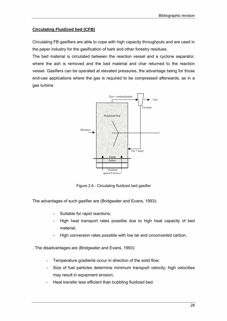
Circulating Fluidized bed (CFB)
Circulating FB gasifiers are able to cope with high capacity throughputs and are used in
the paper industry for the gasification of bark and other forestry residues.
The bed material is circulated between the reaction vessel and a cyclone separator,
where the ash is removed and the bed material and char returned to the reaction
vessel. Gasifiers can be operated at elevated pressures, the advantage being for those
end-use applications where the gas is required to be compressed afterwards, as in a
gas turbine.
Figure 2.6 - Circulating fluidized bed gasifier
The advantages of such gasifier are (Bridgwater and Evans, 1993):
- Suitable for rapid reactions;
- High heat transport rates possible due to high heat capacity of bed
material;
- High conversion rates possible with low tar and unconverted carbon.
. The disadvantages are (Bridgwater and Evans, 1993):
- Temperature gradients occur in direction of the solid flow;
- Size of fuel particles determine minimum transport velocity; high velocities
may result in equipment erosion;
- Heat transfer less efficient than bubbling fluidized bed.
Fluidized bed
Ashes
Biomass
Gas + contaminants
Oxidant speed 5-10 m.s-1
Grate
Cyclone
Tar + inert
Gas

Chapter 2
29
Apart from the described gasifiers, there are several other models that have been
developed to improve the quality of the produced gas, such as: twin fluidized bed and
entrained bed (Bridgwater, 1995). The first one aims to increase the heat value of the
produced gas by promoting the production of H2. The second operates at high
temperatures 1200 to 1500°C in order to eliminate tar and condensable gases in the
produced gas. In fact, it has conversion efficiencies close to 100%. However, some
problems arise in the materials selection to withstand the high temperatures and
liquefaction of ash. Readers interested in deepening this topic may consult the cited
reference.
2.1.3.4 Syngas conditioning
Gases formed by gasification are contaminated by some or all of the constituents listed
in Table 2.2. The level of contamination varies, depending on the gasification process
and the feedstock. Gas cleaning must be applied to prevent erosion, corrosion and
environmental problems in downstream equipment. Table 2.3 also summarizes the
main problems resulting from these contaminants, and common cleanup methods.
Table 2.2 - Syngas contaminants (Bridgwater, 1995)
Contaminant Examples Problems Cleanup method
Particulates Ash, char, fluid bed
material Erosion Filtration, scrubbing
Alkali metals Sodium and potassium
compounds Hot corrosion
Cooling, condensation,
filtration, adsorption
Nitrogen
components NH3 e HCN NOx formation
Scrubbing, Selective
catalytic reduction
Tars Aromatics
Clog filters, difficult to
burn, deposit
internally
Tar cracking; Tar removal
Sulfur, Chloride H2S , HCl Corrosion, emissions Lime or dolomite scrubbing
or absorption
Tars are mostly heavy hydrocarbons (such as pyrene and anthracene) that can clog
engine valves, cause deposition on turbine blades or fouling of a turbine system
leading to decreased performance and increased maintenance. In addition, these
heavy hydrocarbons interfere with synthesis of fuels and chemicals. Conventional
scrubbing systems are generally the technology of choice for tar removal from the
product syngas. However, scrubbing cools the gas and produces an unwanted waste
stream. Removal of the tars by catalytically cracking the larger hydrocarbons reduces

Bibliographic revision
30
or eliminates this waste stream, eliminates the cooling inefficiency of scrubbing, and
enhances the product gas quality and quantity.
2.2. Syngas applications
Applications for syngas can be divided into two main groups: fuels or chemical
products and power or heat. Table 2.3 summarizes desirable syngas characteristics for
various end-use options. In general, syngas characteristics and conditioning are more
critical for fuels and chemical synthesis applications than for hydrogen and fuel gas
applications.
Table 2.3 – Desirable syngas characteristics for different applications (Ciferno and Marano, 2002)
Product Synthetic fuels Methanol Hydrogen Fuel gas
Boiler Turbine
H2/CO 0.6 (a) ~2.0 High Unimportant Unimportant
CO2 Low Low (c) Unimportant (b) Not critical Not critical
Hydrocarbons Low (d) Low (d) Low (d) High High
N2 Low Low Low (e) (e)
H2O Low Low High (f) Low (g)
Contaminants <1ppm sulfur
Low particulates
<1ppm sulfur
Low particulates
<<1ppm sulfur
Low particulates (k)
Low particulates
and metals
Heating value Unimportant (h) Unimportant (h) Unimportant (h) High (i) High (i)
Pressure
(bar) ~20-30
~50 (liquid phase)
~140 (vapor phase) ~28 Low ~400
Temperature
(ºC)
200-300 (j)
300-400 100-200 100-200 250 500-600
(a) It depends on the catalyst type. For iron catalysts, value shown is satisfactory; for cobalt catalysts, near 2.0 should be used. (b) Water gas shift will have to be used to convert CO to H2; CO2 in syngas can be removed at same as CO2 is generated by the water gas shift reaction. (c) Some CO2 could be tolerated if the H2/CO ratio remains above 2.0; if excess of H2 is available, the CO2 will be converted to methanol. (d) Methane and heavier hydrocarbons need to be recycled for conversion to syngas and represent system inefficiency. (e) N2 lowers the heating value, but their percentage is not important as long as syngas can be burned with a stable flame. (f) Water is required for the water gas shift reaction. (g) Can tolerate relatively high water levels; steam sometimes added to moderate combustion temperature to control NOx. (h) As long as H2/CO ratio and impurities levels of impurities are met, heating value is not critical. (i) Efficiency improves as heating value increases. (j) Depends on the catalyst type, iron catalysts typically operate at temperatures higher than cobalt catalyst. (k) Small amounts of contaminants can be tolerated.
A synthetic gas of high purity (i.e., low quantities of inerts such as N2) is extremely
beneficial for fuels and chemical synthesis since it substantially reduces the size and
cost of downstream equipment. However, the guidelines provided in Table 2.3 should
not be interpreted as stringent requirements. Supporting process equipment (e.g.,
scrubbers, compressors, coolers, etc.) can be used to adjust the condition of the

Chapter 2
31
product syngas to match those optimal for the desired end-use, although, at added
complexity and cost. Specific applications are discussed in more detail below.
2.2.1 Power production Electricity generation is carried out by ICE, Stirling engines or turbines. Fuel cells have
been proposed, but considerable development work is needed before these can be
seriously considered. Data are available for gas turbines and engines operating on
fossil fuels, but few robust data have been found on biomass-derived fuel gas
machines, owing to the unknown costs of modification and maintenance and machine
life.
Essentially all biomass power plants today operate on a steam-Rankine cycle.
Biomass-steam turbine systems are less efficient than modern electricity coal-fired
systems in large part due to more modest steam conditions. The modest steam
conditions in biomass plants arise primarily because of the strong scale-dependence of
the unit capital cost of steam turbine systems-the main reason coal and nuclear steam-
electric plants are built at a large scale. Biomass plants are usually of modest scale
(less than 100 MW), because of the dispersed nature of biomass supplies, which must
be gathered from the countryside and transported to the power plant. If bio-electric
plants were as large as coal or nuclear power stations (500-1000 MW), the cost of
delivering the fuel to the plant would often be prohibitive. To help minimize the
dependence of unit cost on scale, vendors use lower grade steels in the boiler tubes of
small-scale steam-electric plants and make other modifications which reduce capital
cost, but also require more modest steam temperatures and pressures, thereby leading
to reduced efficiency. The best biomass steam-electric plants have efficiencies of 20-
25% (Bridgwater, 1995). In order to make higher cost biomass resources economically
interesting for power generation, it is necessary to have technologies which offer higher
efficiency and lower unit capital cost at modest scale. One technological initiative
aimed at improving the economics and efficiency of utility-scale steam cycle systems
would use whole trees as fuel rather than more costly forms of biomass (e.g.
woodchips).
Gasification with turbines
Gas turbines are noted for their efficiency; low emissions; low specific capital cost;
short lead times by virtue of modular construction; high reliability and simple operation
(Brander and Chase, 1992). Gas turbine integration with biomass gasification is not

Bibliographic revision
32
established but there are many demonstration projects active with capacities 0.2-27
MWe. There are several issues that must be resolved in the integration of gas turbines
with biomass gasification, including:
- The reliable and environmentally sound operation of gas turbines with low
heating value gases;
- The selection of gasification operating pressure and the consequent
integration of the air flow to the gasifier and fuel gas flow to the gas turbine
combustor with the rest of the system;
- Fuel gas cleaning and cooling;
- The selection of the gas turbine cycle, although generally combined cycles
are preferred.
Gasification with engines
The operation of diesel and spark-ignition engines using a variety of low heating value
gases is an established practice (Nolting and Leuchs, 1995; Vielhaber, 1996;
Tschalamoff, 1997). Both dual fuel diesel and spark ignition engines for operation using
low heating value gases may be regarded as fully developed, although integration of a
biomass gasifier and engine is not fully established.
The main issue that must be resolved is the effective treatment of the fuel gas to cool
and clean it to the specifications demanded by the engine. The fuel gas must be cool at
injection to the engine and therefore wet scrubbing is the preferred gas treatment
method (Bridgwater et al., 2002). In this approach the gases are cooled to under 150ºC
and then passed though a wet gas scrubber. This removes particulates, alkali metals,
tars and soluble nitrogen compounds such as ammonia.
Fuel cells
Fuel cells are static equipments that convert the chemical energy in the fuel directly
into electrical energy. The operation principle of a fuel cell is similar to a battery. It is
composed of a porous anode and a cathode, each coated on one side by a layer of
platinum catalyst, and separated by an electrolyte. The anode is powered by the fuel,
while the cathode is powered by the oxidant.
There are various different types of fuel cells:
- AFC - Alkaline Fuel Cell

Chapter 2
33
- PEFC / PEM - Polymer Electrolyte Fuel Cell / Proton Exchange Membrane
- PAFC - Phosphoric Acid Fuel Cell
- MCFC - Molten Carbonate Fuel Cell
- SOFC - Solid Oxid Fuel Cell
SOFC fuel cell is the most suitable for integration with a gasifier (Klein, 2002). The
kinetics of this cell is fast, and the CO in the syngas is a directly useable fuel. This type
of fuel cell operates at a high temperature, and over 900°C the syngas can be reformed
within the cell.
2.2.2 Fuels
Several synthetic fuels can be produced from syngas via the Fischer-Tropsch (FT)
process. There are several commercial FT plants in South Africa producing gasoline
and diesel from coal and natural gas.
The FT synthesis involves the catalytic reaction of H2 and CO to form hydrocarbons
chains of various lengths (CH4, C2H6, C3H8, etc.). The FT synthesis reaction can be
written in the general form (Ciferno and Marano, 2002):
2 2( 2 ) m nn m H mCO C H mH O+ + = + (2.1)
where m is the average chain length of the hydrocarbons formed, and n equals 2m+2
when only paraffins are formed, and 2m when only olefins are formed.
Iron catalyst has water gas shift activity, which allows the use of syngas with low H2/CO
ratios. Syngas with H2/CO ratios of 0.5 to 0.7 is recommended for iron catalysts. The
water - gas shift reaction adjusts the ratio to match the requirements for hydrocarbon
and produce CO2 as the largest by-product.
On the other hand, cobalt catalysts do not have water-gas shift reaction activity, and
H2/CO ratio required is then (2m + 2)/m. Water is the primary by-product of FT
synthesis over a cobalt catalyst.
As shown in Table 2.3, the composition of syngas required for fuel gas application is
different from that required for the synthetic fuel or chemical synthesis. A high H2, low
CO2 and low CH4 content is essential for fuel or chemical production. In opposite, a
high H2 is not necessary for power production, as long as a high enough heating value
is supplied by the CH4.

Bibliographic revision
34
Hydrogen
Hydrogen is currently produced in large quantities via steam reforming of hydrocarbons
over a nickel catalyst at about 800ºC (Nieminen, 2004). This process produces a
syngas that must be further processed to produce high-purity hydrogen. The syngas
conditioning required for steam reforming is similar to that which would be required for
a biomass gasification derived syngas. However, tars and particulates are not so
worrying. To raise the hydrogen content, the syngas is fed to one or more water gas
shift reactors, which converts CO in H2 according with the reaction CO + H2O = H2 +
CO2.
Methanol
Methanol synthesis involves the reaction of CO, H2 and steam in a copper-zinc oxide
catalyst in the presence of small amounts of CO2 at a temperature of about 260ºC and
a pressure of about 70 bar (Paisley and Anson, 1997). The formation of methanol from
syngas proceeds via the following reactions:
CO + H2O = H2 + CO2 (water-gas shift reaction)
3H2 + CO2 = CH3OH + H2O (hydrogenation of carbon dioxide)
2H2 + CO = CH3OH
Methanol production also occurs by means of direct hydrogenation of CO, but at a
much slower rate (Engstrom, 1999):
2H2 + CO = CH3OH (hydrogenation of carbon monoxide)
To best use the raw product syngas in methanol synthesis and limit the extent of
additional treatment or steam reforming, it is essential to maintain the parameters
indicated in Table 2.3.
2.3. Syngas characterization
The quality of the producer gas depends upon several factors including type of fuel,
gasifier type and operational conditions (temperature, pressure and oxidizing agent).
Following each one is described.

Chapter 2
35
2.3.1 Influence of biomass type
In large samples there is a relatively constant atomic ratio of C10H14O6 for all biomass
kinds (Reed and Das, 1988). A direct link between the chemical composition of
biomass and gas obtained by gasification exists. Table 2.4 shows experimental values
of the chemical composition of syngas for different types of biomass in a downdraft
gasifier.
Table 2.4 - Characteristics of syngas by biomass type
Residues Gas produced (mol/kg) HHV
(MJ/m3) H2 CO CO2 CH4 C2H2 C2H4 C2H6
Rice husk (a) 0.00236 0.00651 0.00717 0.00209 6.2×10⁻⁵ 7.6×10⁻⁴ 1.1×10⁻⁴ 11.11
Nut shell (a) 0.00485 0.00788 0.00477 0.00293 4.9×10⁻⁵ 6.1×10⁻⁴ 2.1×10⁻⁴ 14.55
Pine (a) 0.00529 0.00722 0.00505 0.00272 1.2×10⁻⁴ 8.1×10⁻⁴ 1.7×10⁻⁵ 14.68
Eucalyptus (a) 0.00275 0.00712 0.00380 0.00316 2.6×10⁻⁵ 5.5×10⁻⁴ 1.5×10⁻⁴ 13.41
Vine Pruning (b) 0.0104 0.02378 - 0.00641 0.00199 8.8×10⁻⁴ 0.00121 11.41
Cherry Stone © 0.00639 0.00668 - 0.00371 0.00103 0.00217 0.00173 -
a (Gañan et. al., 2005) ; b (Cuellar, 2003), c (González et al., 2003).
As shown in Table 2.4 the influence of biomass type is not considerable. The highest
heat value of the syngas obtained with pine and almond shell, being the lowest heat
value obtained with husks.
The woods in the Table 2.4 (pine and eucalyptus) are largely the most available
biomass resource in Portugal (Ferreira et al., 2009) and therefore some special
attention should be given to them. The main combustible components of wood are
cellulose, hemicelluloses, and lignin, which are compounds of carbon, hydrogen, and
oxygen. Other minor combustible components in wood are fats, resins, and waxes. The
major non-combustible component of wood is water, which makes up to 50% of freshly
cut wood. Though the ash content is low (<1%), because of high oxygen content, the
heat value is low (16-20 MJ/kg). Most wood species have ash contents below two
percent and are therefore suitable fuels for fixed bed gasifiers. As wood contains high
volatile matter, an updraft gasifier system produces gas containing tar, which needs to
be cleaned out before use in engines. Cleaning of gas is a difficult and labour-intensive
process. Hence wood is not suitable in updraft gasifier coupled with internal
combustion engines. However, the gas containing tar from an updraft gasifier can be
used for direct burning. Downdraft systems can be designed to deliver a virtually tar-
free product gas in a certain capacity range when fuelled by wood blocks or wood chips

Bibliographic revision
36
of low moisture content. After passing through a relatively simple cleanup train the gas
can be used in internal combustion engines.
2.3.2. Influence of reactor type
Dry wood was experimental used by several workers in different types of gasifiers
being the results shown in Table 2.5. Some values are just indicative due to unknown
gasification conditions.
Table 2.5 – Characteristics of the produced gas for atmospheric gasifiers (Mehrling and Vierrath, 1989; Graham and Bain, 1993; Hasler et. al., 1994; Hasler and Nussbaumer, 1999)
Property Downdraft Updraft BFB CFB
Tar (mg/Nm3) 10-6000 10000-150000 Not defined 2000 – 30000
Particules (mg/Nm3) 100-8000 100-3000 Not defined 8000-100000
LHV (MJ/Nm3) 4.0 – 5.6 3.7 – 5.1 3.7 – 8.4 3.6 – 5.9
H2 (vol%) 15-21 10-14 5 – 16.3 15-22
CO (vol%) 10-22 15-20 9.9 – 22.4 13-15
CO2 (vol%) 11-13 8-10 9 – 19.4 13-15
CH4 (vol%) 1-5 2-3 2.2 – 6.2 2-4
CnHm (vol%) 0.5 -2 Not defined 0.2 – 3.3 0.1-1.2
N2 (vol%) Remaining Remaining 41.6 – 61.6 Remaining
In the Table 2.6 typical syngas compositions are given relatively to the same type of
reactors using air as oxidant.
Table 2.6 – Typical syngas compositions by reactor type (Bridgwater, 1995).
Gasifier Gas composition (vol. %, dry) HHV
(MJ/m3) H2 CO CO2 CH4 N2
Bubbling fluidized bed 9 14 20 7 50 5.4
Updraft 11 24 9 3 53 5.5
Downdraft 17 21 13 1 48 5.7
Comparing both Tables 2.5 and 2.6 is possible to see some discrepancies especially
related to CO content. This situation emphasizes the influence of the gasification
conditions in the final composition of the produced gas.
2.3.3 Influence of operational conditions
2.3.3.1 Temperature
Several authors have reported the increase of gas yield and the decrease in gas heat
value with temperature, even when different feedstocks were employed and installation

Chapter 2
37
with different characteristics were used, namely Herguido et al., (1992); Javier et al.,
(1997); Kim et al., (2001) and Rolando et al., (2002).
It is expected that the rise of temperature leads to an increase in the rate of the several
reactions that took place during gasification process, which, globally, produce hydrogen
and carbon monoxide and eliminates hydrocarbons. At higher gasification
temperatures lower solids and tar emissions are observed, which means that the
produced gas may require a lower cost on gas cleaning processes.
2.3.3.2. Pressure
Gasifiers can be operated at elevated pressures, the advantage being for those end
use applications where the gas is required to be compressed afterwards, as in a gas
turbine.
Pressurized gasifiers have the following significant features:
- Feeding is more complex and very costly, and has a high inert gas requirement
for purging.
- Capital costs of pressure equipment are much higher than for atmospheric
equipment, although equipment sizes are much smaller.
- Pressurized gasification systems can cost up to four times as much as
atmospheric systems at power outputs up to 20 MWe. This disadvantage is
countered by the higher efficiency, and this effect becomes significant at 30-50
MWe, above which pressure systems are believed likely to be more economic
than atmospheric systems.
- Gas is supplied to the turbine at adequate pressure, removing the need for gas
compression and also permitting relatively high tar contents in the gas; such tar
needs to be completely burned in the turbine combustor.
- Hot gas cleanup with mechanical filters (such as sintered metal or ceramic
candles) is usually used, which reduces thermal and pressure energy losses
and in principle in simpler and of lower cost than are scrubbing systems.
- Overall system efficiency is higher owing to retention of sensible heat and
chemical energy of tars in the product gas and the avoidance of a fuel gas
compression stage ahead of the turbine. The only significant energy losses are
to the environment and in provision of inert gas to the pressure feeders, and
these can be as low as 5-8%, giving energy conversion efficiency for the
gasifier itself of 92-95%. A corresponding atmospheric gasifier with water
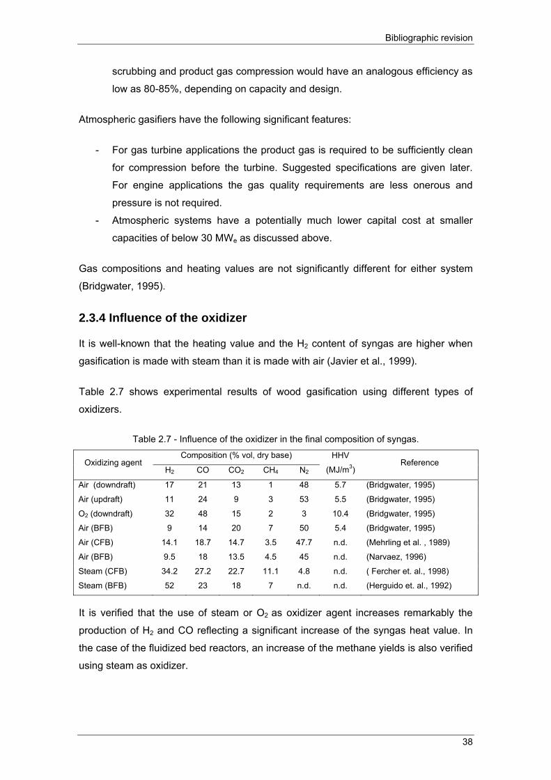
Bibliographic revision
38
scrubbing and product gas compression would have an analogous efficiency as
low as 80-85%, depending on capacity and design.
Atmospheric gasifiers have the following significant features:
- For gas turbine applications the product gas is required to be sufficiently clean
for compression before the turbine. Suggested specifications are given later.
For engine applications the gas quality requirements are less onerous and
pressure is not required.
- Atmospheric systems have a potentially much lower capital cost at smaller
capacities of below 30 MWe as discussed above.
Gas compositions and heating values are not significantly different for either system
(Bridgwater, 1995).
2.3.4 Influence of the oxidizer
It is well-known that the heating value and the H2 content of syngas are higher when
gasification is made with steam than it is made with air (Javier et al., 1999).
Table 2.7 shows experimental results of wood gasification using different types of
oxidizers.
Table 2.7 - Influence of the oxidizer in the final composition of syngas.
It is verified that the use of steam or O2 as oxidizer agent increases remarkably the
production of H2 and CO reflecting a significant increase of the syngas heat value. In
the case of the fluidized bed reactors, an increase of the methane yields is also verified
using steam as oxidizer.
Oxidizing agent Composition (% vol, dry base) HHV
(MJ/m3) Reference
H2 CO CO2 CH4 N2
Air (downdraft) 17 21 13 1 48 5.7 (Bridgwater, 1995)
Air (updraft) 11 24 9 3 53 5.5 (Bridgwater, 1995)
O2 (downdraft) 32 48 15 2 3 10.4 (Bridgwater, 1995)
Air (BFB) 9 14 20 7 50 5.4 (Bridgwater, 1995)
Air (CFB) 14.1 18.7 14.7 3.5 47.7 n.d. (Mehrling et al. , 1989)
Air (BFB) 9.5 18 13.5 4.5 45 n.d. (Narvaez, 1996)
Steam (CFB) 34.2 27.2 22.7 11.1 4.8 n.d. ( Fercher et. al., 1998)
Steam (BFB) 52 23 18 7 n.d. n.d. (Herguido et. al., 1992)

Chapter 2
39
Table 2.8 shows a comparison performed by Javier et al. (1999) based on results from
Herguido et al. (1992), Javier et al. (1997) and Narváez et al. (1996) in order to
determine the effect of gasifying agent on other results like tar content in the produced
gas. Three basic ratios were used for comparison of results using different gasifying
agents in a bubbling fluidized bed gasifier running with small chips of pine:
- Equivalence ratio (φ) for air;
- Gasifying ratio (GR) [(H2O+O2)/Biomass (kg/h)/(kg dry-ash free/h)], for steam-
O2 mixtures;
- Steam to biomass ratio (SB) [H2O/Biomass (kg/h)/(kg dry-ash free/h).
Table 2.8 – Effect of gasifying agent on syngas composition Parameter Air (φ=0.3) Steam/O2 GR = 0.9 Steam SB=0.90
H2 (vol.% dry basis) 8-10 25-30 53-54
CO (vol.% dry basis) 16-18 43-47 21-22
LHV (MJ/m3, dry basis) 4.5-6.5 12.5-13.0 12.7-13.3
Ygas (m3, dry basis/kg daf) 1.7-2.0 1.0-1.1 1.3-1.4
Ytar (g/kg daf) 6-30 8-40 70
Tar (g/m3) 2-20 4-30 30-80
Gasification with air produces a higher syngas yield. Tar yields are quite different
between the gasifying agents being the lowest values obtained with air.
2.4. Concluding remarks about biomass gasification
Gasification is a versatile thermochemical conversion process which produces a gas
mixture of H2, CO and CH4 the proportions being determined by the use of air, oxygen
or steam as the gasification medium, with a concomitant range of heat values, low (4–6
MJ/Nm3), medium (12–18 MJ/Nm3) and high (40 MJ/Nm3). Key parameters for
successful gasification are the feedstock properties (moisture, ash, alkalis and
volatiles) and feedstock pre-treatment (drying, particle size, fractionation and leaching).
Gasifiers are of two main types, fixed bed and fluidized bed, with variations within each
type and specific characteristics which determine the need for and extent of feedstock
preparation/pre-treatment.
For use in gas engines gas produced from a fixed bed, downdraft gasifier provides a
low tar gas, with a high particulates loading: as tar is a major contaminant for engine
operation and particulates can be relatively easily removed, this system is considered
best for fuelling gas engines. Extensive development of wood gas-fuelled IC engines,

Bibliographic revision
40
suggests that diesel-based engines, with large cylinder volumes/valve areas, operating
at constant load and low rpm, provide optimum power output.
Regarding the influence of various parameters involved in the process of gasification in
the final features of syngas, there is some discrepancy in the values given by various
authors. This highlights the strong dependence on the final composition of the syngas
on condition of biomass used, the type of gasifier and conditions of pressure and
temperature. Thus, in order to make precise studies on the use of syngas it will be
necessary to consider that its composition will be very difficult to maintain constant.
The development of mathematical models for numerical simulation fully validated
experimentally may be a very useful tool to determine the final composition of syngas
by changes in initial conditions without laborious and expensive experimental tests.
2.5. Laminar premixed flames
A flame may be described as a reaction zone that moves with respect to the initial
mixture. In practice the term is usually reserved for fast exothermic reactions of this
type, and these are often also accompanied by emission of light. Flames may be either
stationary flames on a burner and propagating into a flow of gas from a burner tube, or
they may be freely propagating flames travelling in a gas mixture. There are two types
of stationary flames:
- Premixed flames where the reactants are mixed before approaching the flame
region. These flames can only be obtained if the initial fuel and oxidant mixture
lies between certain composition limits called the composition limits of
flammability.
- Diffusion flames where both fuel and air are separated and the combustion
occur at the interface.
For defined thermodynamic starting conditions, the premixed system has a defined
equilibrium adiabatic flame temperature and for the idealized situation of planar flame
in a one-dimensional flow field, premixed flame has a defined adiabatic burning velocity
or equivalent mass flux in a direction normal to its surface. An unstrained diffusion
flame has no such simply defined parameters.
Many practical combustion problems are concerned with turbulent combustion, but
laminar flame must firstly be well controlled. In premixed flames, the laminar burning
velocity and flame structure data can be extremely useful in the analysis of
Chapter 2
41
fundamental processes such as ignition, NO, and soot formation, and flame quenching.
Moreover, some turbulent flame models prescribe the turbulent burning velocity as a
function of laminar burning velocity. Thus, detailed information describing the
dependence of the laminar burning velocity, flame thickness, ignition temperature, heat
release rate and flame quenching on various system parameters can be a valuable
diagnostic and design aid.
There is a significant discrepancy in measuring burning velocities, which gives an
indication of the difficulties and uncertainties associated with experimental
determination of flame properties. In the light of the earlier experimental studies of
Markstein, (1964), the asymptotic analysis of Klimov, (1963), and the computations of
laminar flame structure with detailed chemical kinetics by several researchers, all of
which show the importance of the flame stretch rate (Dixon-Lewis, 1991). There can be
little doubt that this is often neglected key variable (Law, 1989). It follows that any
experimental or computed value of laminar burning velocity should be associated with
a value of the flame stretch rate. Ideally, the stretch-free value of the burning velocity
should be quoted and the influence of stretch rate upon this value should be indicated
by the value of the appropriated Markstein length.
For these reasons this chapter begins with the definition of stretch rate and the
corresponding Karlovitz and Markstein numbers. Following, the theory evolved with the
burning velocity determination are described with emphasis for the constant volume
and constant pressure methods due to be extensively used. This part of the chapter
ends with the flammability limits description as is another important parameter of
premixed laminar flames.
2.5.1 Flame stretch
A flame surface propagating in a uniform flow field is submitted to strain and curvature
effects leading to changes in the frontal area. Karlovitz et al., (1953) and Markstein,
(1964) initiated the study of stretched premixed flames and demonstrated the
importance of the aerodynamic stretching and the preferential diffusion on the flame
response in terms of flame front instability.
The flame stretch factor (κ) is defined as the relative rate of change of flame surface
area (A) (Williams, 1985):

Bibliographic revision
42
1 1( )d A dAA dt A dt
δκδ
= = (2.2)
The effect of stretch on the flame is to reduce the thickness of the flame front and
hence the flame speed and influence the flame structure through its coupled effect with
mass and heat diffusion. The concept of flame stretch can be applied to laminar flame
speed; flame stabilization; flammability limits; and modeling of turbulent flames.
Let’s first derive the basic relationship between the stretch rate and the strain rate,
dilatation of the fluid element, and curvature of the flame surface. The three
perpendicular coordinates on a curved flame surface are shown in Fig. 2.7, which has
two unit vectors (ν and η ) tangent to the flame surface and an outward normal unit
vector n , at the spatial point ( ), ,ν ηr n as a function of the three independent coordinates.
Figure 2.7 - Curved laminar flame front with three perpendicular curvilinear coordinates.
The elemental arc ( )dsν in the directionν and the elemental arc ( )ds
ηin the direction η
are given by:
( ) ( ),r rds d ds dν η
δ δν ηδν δη
⎛ ⎞⎛ ⎞= = ⎜ ⎟⎜ ⎟⎝ ⎠ ⎝ ⎠
(2.3)
The elemental flame surface can be calculated by:
( ) ( )( )r rdA t n d dδ δ ν ηδν δη
⎛ ⎞= × ⋅⎜ ⎟
⎝ ⎠ (2.4)
In the orthogonal curvilinear coordinates system, the two unit vectors ,e eν η can be
given by:
, andr re e e e nr rν η ν η
δ δν δ δηδ δν δ δη
= = × = (2.5)
Thus:
nη
ν

Chapter 2
43
( ) ( )( )r rdA t d dδ δ ν ηδν δη
= (2.6)
Now let another surface that is close to the flame surface be represented by ( )* *, ,r nν η ,
such that:
* ** , ,r r a r r ar r a
ν ν ν η η η∂ ∂ ∂ ∂ ∂ ∂
= + = + = +∂ ∂ ∂ ∂ ∂ ∂
(2.7)
Where a is a small magnitude displacement vector; then:
( ) ( )( ) ( )( )
( )( ) ( )1 1
* * * ** *
. .t t
r r r rdA t n d d d d
r r a d d a dA t
δ δ δ δν η ν ηδν δη δν δη
δ δ ν ηδν δη
⎛ ⎞= × ⋅⎜ ⎟
⎝ ⎠
≅ + ∇ = + ∇⎡ ⎤ ⎡ ⎤⎣ ⎦ ⎣ ⎦
(2.8)
Where t e eν ην η∂ ∂
∇ = +∂ ∂
, which represents the gradient operator along the tangential
plane of the flame surface (Chung and Law, 1988).
It is useful to note that we can always decompose any arbitrary velocity into two
components: a tangential to the flame surface and another normal to the flame surface
as follows:
( ).n t tV V V V n n V= + = + (2.9)
Now considering a curved flame surface A(t) moving in the space with local velocity W
(note that each spatial point has its own velocity). Then, the rate of change of the flux
of a vector G across the flame surface is given by the following expression based on
the Reynolds’ transport theorem.
( ) ( ). . . . .
A t A t
d GG ndA W G G W G W ndAdt t
⎡ ⎤∂= + ∇ − ∇ + ∇⎢ ⎥
∂⎢ ⎥⎣ ⎦∫ ∫ (2.10)
By specifying G n= , Eq. (2.10) yields:
( ) ( ). . . .
A t A t
d ndA W n n W n W ndAdt t
∂⎡ ⎤= + ∇ − ∇ + ∇⎢ ⎥∂⎣ ⎦∫ ∫ (2.11)

Bibliographic revision
44
Since n is a unit normal vector, we have:
21 02
.n nnt t
∂ ∂= =
∂ ∂ (2.12)
( )2
02
. . . nW n n W⎛ ⎞
∇ = ∇ =⎜ ⎟⎝ ⎠
(2.13)
Therefore, the transport equation (2.11) can be written as follows:
( ) ( ): .
A t A t
d dA n n W W dAdt
⎡ ⎤= − ∇ + ∇⎣ ⎦∫ ∫ (2.14)
Note that in tensor notation, the first term of the right side of the Eq. (2.14) can be
written as:
: ii j
j
wn n W n n
x∂
− ∇ = −∂
(2.15)
If we consider a surface element, then A(t) can be substituted by δΑ. The flame stretch
rate κ can be expressed as:
1 ( ) : .d A n n W WA dt
δκδ
= = − ∇ + ∇ (2.16)
The general velocity W can be considered to have two components: one in the normal
direction at a speed Su and the other is the local fluid velocity. Thus:
uW S S n= + (2.17)
Several vector operations can be applied to Eq. (2.17) to give:
u uW S S n n S∇ = ∇ + ∇ + ∇ (2.18)
: : unn W nn S n S∇ = ∇ + ∇ (2.19)
. . . .u uW S S n n S∇ = ∇ + ∇ + ∇ (2.20)
Substituting these expressions in the Eq. (2.16), we have:
1 1( ) : . . uiu i j
j c
SSd A n n S S S n n nA dt x t r
δ ρκδ ρ
∂ ∂= = − ∇ + ∇ + ∇ = − + − +
∂ ∂ (2.21)

Chapter 2
45
Where, rc represents the local radius of the flame curvature. The first term of Eq. (2.21)
represents the effect of the strain; the second term represents the effect of the fluid
expansion of fluid (dilatation) and, the third term, the effect of the flame curvature. It is
evident that the flame can be stretched by the combined effect of strain, volume
expansion of the fluid and the curvature of the flame, which arises from the
nonuniformities of the flow and the normal propagation of the flame front.
For the present purposes, an appropriate unified tensor expression, in terms of strain
rate, κs, and the stretch rate due to flame curvature, κc, is that of Candel and Poinsot,
(1990).
s cκ κ κ= + (2.22)
With
: .s n n S Sκ = − ∇ + ∇ (2.23)
κ = ∇.c uS n (2.24)
In spherical expanding flames it is convenient to use spherical coordinates (r, θ, φ), the
components of n and S are written as (nr, nθ, nφ) and (sr, sθ, sφ), respectively. Then:
( )
2 2 2
2
2
1 1
1 1
1 1
1 1
cotsin
sincot
sinsi
sin
r r rs r
r rr r
r
ss ss s sn n n
r r r r r rs ss ss s
n n n nr r r r r rs s
n n sr r rr s s
r rr
φθ θθ φ
φ φθ θθ φ
φ θθ φ φ
θ
θκ
θ φ φ
θ θ φθ
θ θ φ
θ
∂⎛ ⎞⎡ ∂∂ ⎛ ⎞⎛ ⎞= − + + + + +⎜ ⎟⎢ ⎜ ⎟⎜ ⎟∂ ∂ ∂⎝ ⎠ ⎝ ⎠⎣ ⎝ ⎠∂⎛ ⎞∂ ∂ ∂⎛ ⎞+ + − + + −⎜ ⎟⎜ ⎟∂ ∂ ∂ ∂⎝ ⎠ ⎝ ⎠
⎤∂⎛ ⎞∂+ + − ⎥⎜ ⎟∂ ∂ ⎥⎝ ⎠ ⎦
∂ ∂+ +
∂( ) 1n
sins
rφθ
θ θ φ∂
+∂ ∂
(2.25)
( ) ( )2
2
1 1 1sinsin sin
rc n
r n nnu
r r rrφθ θ
κθ θ θ φ
⎡ ⎤∂ ∂∂⎢ ⎥= + + +
∂ ∂ ∂⎢ ⎥⎣ ⎦ (2.26)
For an outward spherically propagating flame, the flame surface is identified by the cold
front of radius ru, nr =1, nθ=nφ=0, and sr=sg, sθ=sφ=0 (Bradley et al., 1996). The burning
velocity, su, is associated with this surface and the gas velocity ahead of it is sg. The
flame speed, dru/dt, is equal to sg + nrsu, and is indicated by Sn. Applying this conditions
to Eqs. 2.25 and 2.26 gives

Bibliographic revision
46
( )22
2
1 2r grs r
u
r s ssn
r r rrκ
∂∂⎛ ⎞= + =⎜ ⎟∂ ∂⎝ ⎠ (2.27)
( )2
2
1 2r uc n r
u
r n su n
r rrκ
∂= =
∂ (2.28)
and the total stretch rate is:
2 n
u
sr
κ = (2.29)
The outwardly propagating flame, ignited from a central ignition point, is the most
common spherical flame and because the stretch rates to which it is subjected are well
defined, it is well suited to burning velocity measurements.
2.5.1.1 Karlovitz number
The Karlovitz number (Ka) is defined as the nondimensional stretch factor, using the
thickness of the unstretched flame (δu0) and the normal unstretched laminar flame
velocity (Su0) to form a reference time (Kuo, 2005):
0
0
Residence time for crossing an unstretched flameCharacteristic time for flame stretching
u
u
KaSδ
κ= = (2.30)
For convenience, the Karlovitz number can be written as a sum of two parts due to the
contribution from strain and curvature as follows:
s cKa Ka Ka= + (2.31)
Where
( )0 0 0
0 0 0
: ;u u u us c u
u u u
SKa SS S Ka S n
S S R Sδ δ δ
ηη= + ∇ = ∇ = (2.32)
2.5.1.2 Markstein number
Flame stretch can change the burning velocity of premixed flames significantly. It is
important to know the relation between these two parameters, because the burning
velocity is a crucial parameter in premixed combustion processes. Markstein, (1964)
was the first to propose a phenomenological relation between the laminar burning
velocity and the curvature of the flame front. Notice that the straining of the flow is not

Chapter 2
47
taken into account here. In this relation the proportionality of the burning velocity to the
flame stretch is represented by a parameter that was considered as a characteristic
length scale of the flame. This parameter is now generally known as the Markstein
length, which denotes the sensitivity of a flame to flame stretch. Asymptotic analyses of
Clavin and Williams, (1982) and Matalon and Matkowsky, (1982) and detailed modeling
of Warnatz and Peters, (1984) show a linear relationship between stretch rate and
burning velocity in the low-stretch regime. Thus, it is assumed that,
0n n bS S L κ− = (2.33)
Where 0nS is the unstretched flame speed and Lb is the Markstein length of burned
gases.
When the observation is limited to the initial part of the flame expansion where the
pressure does not vary yet, then a simple relationship links the unstretched flame
speed to the unstretched burning velocity. 0
0un
bu
SS
ρσ
ρ= = (2.34)
Where σ is the expansion factor and ρu and ρb are, respectively, the unburned and
burned densities.
The same behavior of the unstretched burning velocity regarding the stretch can be
observed (Lamoureux et al., 2003): 0u u uS S L κ− = (2.35)
where Lu represents the unburned Markstein length, which is obtained dividing the
burned Markstein length by the expansion factor.
The normalization of the laminar burning velocity by the unstretched one introduces
two numbers which characterize the stretch that is applied to the flame, the Karlovitz
number (Ka), and its response to it, the Markstein Number (Ma):
0 1u
u
SMaKa
S= − (2.36)
0u
KaSδκ= (2.37)
uLMa
δ= (2.38)
where δ is the flame thickness defined, in this work, using the thermal diffusivity, α:
0uS
αδ = (2.39)

Bibliographic revision
48
This evolution of the laminar flame velocity with the stretch rate was verified by Aung et
al., (1997) for moderate stretch rate. As one can see, different definitions of a
characteristic flame thickness lead to different Karlovitz and Markstein numbers.
Bradley et al., (1996) use the kinematic viscosity of the unburned mixture to derive the
flame thickness while Aung et al., (1997) use the mass diffusivity of the fuel in the
unburned gas. However, this effect disappears in Eq. (2.36) since the flame thickness
cancels out.
Clavin and Joulin, (1989) proposed a phenomenological law to take the effects of
curvature and strain in flame stretch into account separately, thereby introducing a
Markstein length for the curvature part of the flame and another one for the flow
straining through the flame. This separation is used by several workers as Bradley et
al., (1996) or Gu et al., (2000). However, Groot et al., (2002) investigated theoretically
these separate contributions demonstrating that the Markstein number for curvature
and the combined one for both curvature and strain are unique. However, it is not
possible to introduce a separate and unique Markstein number for the flow straining
that can be used to describe its influence in different combustion situations. Therefore,
the modification of the burning velocity is characterized by the total stretch rate, and it
is impossible to introduce the separate contributions into an arbitrary combustion
situation.
A new methodology based on the resolution of Clavin’s equation, linking the flame
speed and the stretch linearly, was recently proposed by Tahtouh et al. (2009). This
methodology is based on the following. Combining Eqs. 2.33-2.29 leads to:
0 2n bdr drS Ldt rdt
= − (2.40)
Which exact solution, allows avoiding noise generation due to the differentiation
process. The function that solves Eq. (2.40) is:
0( ) 2 ( )br t L W Z= (2.41)
With W the Lambert function and:
01
2
2
n
b
S t CL
b
eZL
+
= (2.42)

Chapter 2
49
Where C1 is a constant to be determined. The Lambert function W is defined as the
inverse function of ( ) Wf W We= . By definition, dW W ZdZ Z W Z
=+
( )(1 ( ))
for 1 and ( ) 1Z W Ze−
≠ ≠ − .
If Lb>0, Z>0, and consequently W0(Z) is a positive real number. Thus Lb, 0nS and C1 can
be found by minimizing the following equation:
2 20
1 1( ( ) ( )) ( ( ) 2 ( ))
N N
original original br t r t r t L W Z− = −∑ ∑ (2.43)
The flame speed and the stretch could also be linked based on a nonlinear
methodology proposed by Buckmaster, (1977):
2 2
0 0 0
2ln bn n
n n n
LS SS S S
κ⎛ ⎞⎛ ⎞ ⎛ ⎞⎜ ⎟ =⎜ ⎟ ⎜ ⎟⎜ ⎟⎝ ⎠ ⎝ ⎠⎝ ⎠
(2.44)
The derivation of this equation is based on the asymptotic hypothesis. The structure of
the flames considered is characterized by a small flame thickness to which all the
reaction is confined. Moreover, deformations occur on a long scale of the order of the
dimensionless activation energy.
Based on Eq. (2.44), unstretched flame speed and burned gas Markstein length can be
deduced by a minimization of the following expression:
2 2
0 0 01
2ln
nbn n
n n n
LS SS S S
κ⎡ ⎤⎛ ⎞⎛ ⎞ ⎛ ⎞⎢ ⎥⎜ ⎟ +⎜ ⎟ ⎜ ⎟⎜ ⎟⎢ ⎥⎝ ⎠ ⎝ ⎠⎝ ⎠⎣ ⎦∑ (2.45)
Where n is the number of flame images.
2.5.2 Burning velocity measurement methods
Burning velocity is a physicochemical constant for a given mixture. It is the velocity,
relative of unburned gas, which a plane, one-dimensional flame front travels along the
normal to its surface. Clearly, it is the volume of combustible mixture, at its own
temperature and pressure, consumed in unit time by unit area of flame front. It is
independent of flame geometry, burner size and flow rate. As indicated above, the
burning velocity is essentially a measure of the overall reaction rate in the flame and is
important, both in the stabilization of flames and in determining rates of heat release.

Bibliographic revision
50
The burning velocity of a flame is affected by flame radiation, and hence by flame
temperature, by local gas properties such as viscosity, thermal conductivity and
diffusion coefficient, and by the imposed variables of pressure, temperature, air-fuel
ratio and heat of reaction of mole of mixture. However, although its theoretical definition
is straightforward, its practical measurement undoubtedly is not, and there is a
considerable discrepancy between the results obtained by the various methods. One of
the main problems in measuring the normal burning velocity is that a plane flame front
can be observed only under very special condition. In nearly all-practical cases, the
flame front is either curved or is not normal to the direction of velocity of the gas
stream. Broadly speaking there are two types of measurements for burning velocity;
one uses flames travelling through stagnant mixtures, whereas the other employs
flames that are held stationary in space by a counter flow of fresh mixture.
The following will describe briefly some of the different techniques for measuring the
laminar burning velocity for non-stationary flames. Emphasis will be given to
propagating flames at constant volume and constant pressure since they are
extensively used.
In these methods of measurements, the flame moves through the initially quiescent
mixtures. The subsequent spread of such a flame is determined by the nature of the
bounding surface between the mixture and its surroundings. These types of bounding
surface have been used: rigid cylindrical tube, either closed at both ends or open at
one end or both ends; soap bubble solution or thin elastic membranes; and rigid
spherical vessels.
Burning velocity measurement can be made by direct measurement of flame
propagation. This requires locating the position of the flame front at two (or more)
known times. Rapid visualization is required, and it is necessary to know the flame front
geometry and the flow constraints, and often the density change across the flame front.
The followings are the measurement techniques, which have been used for measuring
the laminar burning velocity with non-stationary flames.
2.5.2.1 Tube method
This is one of the earliest methods and was first used by Mallard and LeChatelier,
(1883) in which the mixture is ignited at the open end of a tube and the flame front is
photographed as propagating toward the closed end. The expression for the burning

Chapter 2
51
velocity is obtained from the equation of mass conservation for the unburned gas. It
follows from the definition of burning velocity that:
u uu u
VAS
tρ
ρ∂
= −∂
(2.46)
This assumes that Su is a constant value over the entire cross section of the tube. If ρu
is also constant, then:
uu
VAS
t∂
= −∂
(2.47)
If the flame speed Sn is uniform over the tube cross section, then
uVa
x∂
= −∂
(2.48)
Where a is the cross-sectional area of the tube and x the abscissa along the tube axis.
As =nS dx dt , it follows from equations (2.46) and (2.48) that
= −u naS SA
(2.49)
This is the expression founded experimentally by Coward and Hartwell, (1932).
Unfortunately, the flame aerodynamics change as the flame propagates along the tube
and invalidates the assumption of constant flame speed over the cross section. The
flame area is also variable. For these reasons, there are significant errors (±20%) in the
use of this method for burning velocity measurements.
2.5.2.2 Soap bubble method
Guénoche et al., (1948) have demonstrated theoretically and experimentally that an
orifice placed at the ignition end of the tube reduces the pressure waves which disturb
the flame. This give arise to the soap bubble method, where a homogeneous
combustible mixture is used to blow a soap bubble around a pair of spark electrodes.
At time zero, the gas mixture contained in the spherical soap bubble is ignited by the
spark. Eq. (2.46) and (2.47) are still applicable, Eq. (2.49) is not. Consideration of the
volume of unburned gas now gives:

Bibliographic revision
52
δ δ δ= − +G gV a x S a t (2.50)
In which Sg, is the mean unburned gas velocity averaged over the tube cross-sectional
area a. Equations (2.47) and (2.50) give
( )= − −u n gaS S SA
(2.51)
This equation was given by Coward and Payman, (1937) and applied by Gerstein et
al., (1951), who measured the gas velocity from the growth of a soap bubble formed
over the orifice. As the flame propagates along the tube, the viscous drag of the burned
gas at the wall increasingly retards this gas flow and the pressure in both the burned
gas near the flame front and the unburned gas increases.
2.5.2.3 Constant volume method
In this method, a containing envelope surrounds the explosive mixture. It is assumed
that central ignition occurs and that laminar flame that is smooth and spherical
propagates outwards without any significant movement due to natural convection. The
pressure is equalized throughout the vessel and the unburned gas is isotropic.
Starting from the above assumptions, a differential equation for the pressure can be
derived. Mass conservation gives:
u bm m m= + (2.52)
u bi
dm dm dxVdt dt dt
ρ= − = (2.53)
In which m is the mass of gas and subscripts u, b indicate de unburned and burned gas
states at time t, and the initial reference state at time t equal to zero, V is the vessel
volume. The burned mass fraction x is uniquely related to the pressure, so
dx dx dpdt dp dt
= (2.54)
It follows from the definition of burning velocity, Su, that:
24ub u u
dmr S
dtπ ρ= − (2.55)

Chapter 2
53
Where rb is the radius of the inner boundary of the unburned gas of density ρu.
Combining the above relations results in
1b u
ui
Adp dx Sdt V dp
ρρ
−⎛ ⎞
= ⎜ ⎟⎝ ⎠
(2.56)
Isentropic compression of the unburned gases gives
1 u
u
i i
pp
γρρ
−⎛ ⎞
= ⎜ ⎟⎝ ⎠
(2.57)
Or, alternatively,
( 1)
.u u
u ii
pT Tp
γ γ−⎛ ⎞
= ⎜ ⎟⎝ ⎠
(2.58)
Where γu = cpu/cvu, is the isentropic exponent of the unburned mixture. Surface area
and volume of the flame are related to its radius as Ab = 4πr2 and 343bV rπ= ,
respectively. Realizing that mu = ρi V (1 − x), and pi = ρi Ru Ti , the volume of the
unburned mixture can be written as
( )1u u u uiu
i
m R T TpV X V
p p T= = − (2.59)
Inserting 343bV Rπ= , R is the effective radius of the vessel and the above relations into
V=Vu+Vb yields:
( )1/3
1 1 uib
i
Tpr R x
p T⎡ ⎤
= − −⎢ ⎥⎣ ⎦
(2.60)
The area-to-volume ratio in Eq. (2.56) now becomes:
( )2/3
3 1 1b ui
i
A Tpx
V R p T⎡ ⎤
= − −⎢ ⎥⎣ ⎦
(2.61)
Inserting Eqs. (2.57), (2.58) and (2.61) into Eq.(2.56) we finally obtain

Bibliographic revision
54
( )
211 31
3 1 1uui
ui
pdp dx px Sdt R dp p p
γγ
−−− −⎡ ⎤ ⎛ ⎞⎛ ⎞ ⎛ ⎞⎢ ⎥= − − ⎜ ⎟⎜ ⎟ ⎜ ⎟⎢ ⎥⎝ ⎠ ⎝ ⎠ ⎝ ⎠⎢ ⎥⎣ ⎦
(2.62)
A result first derived by O´Donovan and Rallis, (1959). Rearranging Eq. (2.62) gives:
( )
211 3
1 13
uuiu
i
pR dx p dpS xdp p p dt
γγ
−−⎡ ⎤ ⎛ ⎞⎛ ⎞ ⎛ ⎞ ⎛ ⎞⎢ ⎥= − − ⎜ ⎟⎜ ⎟ ⎜ ⎟ ⎜ ⎟⎢ ⎥ ⎝ ⎠⎝ ⎠ ⎝ ⎠ ⎝ ⎠⎢ ⎥⎣ ⎦
(2.63)
In this equation, R is the effective radius of the vessel and γu = cpu/cvu, the isentropic
exponent of the unburned mixture. Both x and its derivative dx/dp depend on pressure.
The advantage of this expression of the burning velocity is the possibility of exploring a
wide range of pressures and temperatures with one explosion. This is the main reason
of its utilization for burning velocity determination in engine conditions. Several x(p)
relations have been proposed in the literature. The most important of which are:
- O’Donovan and Rallis (1959)
Based on the same assumptions mentioned, O’Donovan and Rallis (1959) present an
x(p) relation that in the present symbols reads,
( )( )
1
1
( )/
( )/
/( / )( / ) ( / ) ( / ) /
u u
u u
i ii u i e
e b e i u i b e b e i i
p p p pp p T T Tx
p T T p T T T p T T p p p
γ γ
γ γ
−
−
⎛ ⎞−− ⎜ ⎟= =⎜ ⎟− −⎝ ⎠
(2.64)
bT is the mass averaged burnt temperature during combustion, with end value eT . Tb is
determined for every burned shell from 3 consecutive increases. First its unburned
temperature is determined from adiabatic compression. Its burned temperature is then
obtained from energy conservation for the shell at constant pressure. Finally, the
burned shell is further compressed (and heated) adiabatically.
As a further simplification to their model, O’Donovan and Rallis assume that bT and eT
are equal during the whole combustion period. In this case one finds
1
1
( )/
( )/
( / )( / )
u u
u u
i i
e i i
p p p px
p p p p
γ γ
γ γ
−
−
−=
− (2.65)

Chapter 2
55
This is compatible with the assumption that the (mass averaged) burned temperature
does not vary over time in this model. O’Donovan and Rallis agree that this is a severe
simplification, and suggest to measure the burned temperature at the centre of the
bomb Tb,c immediately after the start of combustion to evaluated Te/Tb.
- Lewis and von Elbe (1987)
The most cited x(p) relation in literature equates the burnt mass fraction to the
fractional pressure rise originally proposed by Lewis and von Elbe, (1987):
i
e i
p px
p p−
=−
(2.66)
Because its appealing simplicity and reasonable accuracy, the linear relation has been
used a lot for obtaining laminar burning velocities. Dahoe et al., (1996) give a derivation
similar to the above, but immediately start from the linear relation (2.66). Eq. (2.62)
then turns into
( ) ( )( )
211 3
31
uue i eiu
e i i
p p p ppdp p Sdt R p p p p
γγ⎡ ⎤− − ⎛ ⎞⎛ ⎞⎢ ⎥= − ⎜ ⎟⎜ ⎟⎢ ⎥−⎝ ⎠ ⎝ ⎠⎢ ⎥⎣ ⎦
(2.67)
- Nagy et al., (1969)
Nagy et al., (1969) assume isentropic compression of the burned mixture and have
used the following x(p) expression:
- Luijten et al., (2009)
Luijten et al. proposed an extended linear analytical two-zone model, where both the
burned and unburned zones have uniform temperatures and compositions.
Conservation of specific volume v and internal energy e is expressed by
1( )t b uv xv x v= + − (2.69)
1( )t b ue xe x e= + − (2.70)
1/ 1/
1/ (1/ 1/ ) 1/( )u u
b u b u
i
e i
p px p
p p p
γ γ
γ γ γ γ−
−=
− (2.68)

Bibliographic revision
56
where the subscript t denotes ‘total’, hence vt = V /mi and et = U/mi where U is the total
internal energy. For ideal gases Eq. (2.69) can be written as
1( )u i b b u u
i
R T R T R Tx x
p p p= + − (2.71)
The internal energy for a perfect gas can be written as e = e0 + cv (T − T0), where e0 is
the chemical energy stored in the mixture at a reference temperature T0. Without loss
of generality we can write,
0( ) ( )u u vu ue T C T T e= − + Δ (2.72)
0( ) ( )b b vb be T C T T= − (2.73)
where Δe = e0,u −e0,b. Inserting Eqs. (2.72) and (2.73) into Eq. (2.70) and rearranging
gives
[ ]0 0 01 1( ) ( ) ( )b vu i vu u
vb
T T x e C T T x C T TxC
= + Δ + − − − − (2.74)
Now Tb can be eliminated from Eq. (2.71) resulting in
[ ]00 0
1(1 ) ( ) (1 ) ( )u bvu i vu u
i i u i vb i
T R Tp x x x e C T T x C T Tp T R T C T
⎛ ⎞= − + + Δ + − − − −⎜ ⎟
⎝ ⎠ (2.75)
For the limiting case x =1 at p = pe, we have
[ ]00
1 ( )e bvu i
i u i vb i
p R Te C T T
p R T C T⎛ ⎞
= + Δ + −⎜ ⎟⎝ ⎠
(2.76)
Inserting this expression for pe back into Eq. (2.75) gives
(1 ) (1 )u e b vu i u
i i i u vb i
T p R C T Tp x x xp T p R C T
⎡ ⎤−= − + + − +⎢ ⎥
⎣ ⎦ (2.77)
The term in square brackets can be rewritten as
11
1b vu i u b u
u vb i u i
R C T T TR C T T
γγ
⎛ ⎞− −+ = −⎜ ⎟− ⎝ ⎠
(2.78)
Inserting into Eq. (2.77) and rearranging for x we obtain

Chapter 2
57
( ) ( )( ) ( )
11 1
11 1
b u u b
u i u
b u u b
u i u
Ti T
Te i T
p px
p p
γ γ γγ γ
γ γ γγ γ
− −− −
− −− −
⎡ ⎤− +⎣ ⎦=⎡ ⎤− +⎣ ⎦
(2.79)
As a final step, the above result is written fully in terms of pressure using Eq. (2.62).
For later use, the result is given in a more concise form:
( )( )
i
e i
p p f px
p p f p−
=−
(2.80)
Where
( )1 /1
( )1 1
u u
b u b
u u i
pf pp
γ γγ γ γγ γ
−⎛ ⎞ ⎛ ⎞⎛ ⎞− −
= +⎜ ⎟ ⎜ ⎟⎜ ⎟− − ⎝ ⎠⎝ ⎠ ⎝ ⎠ (2.81)
Differentiation is straightforward, yielding
[ ][ ]2
'( ) ( )1 '( )( ) ( )
i ii
e i e i
p f p p p f pp f pdxdp p p f p p p f p
−−= +
− − (2.82)
Where
1/
'( )u
u bi
u i
pp f pp
γγ γ
γ
−⎛ ⎞⎛ ⎞−
= ⎜ ⎟⎜ ⎟⎝ ⎠⎝ ⎠
(2.83)
The above methodology was extended to multiple zones by Luijten et al., (2009)
without considerable improvement in the results.
The linear approximation, introduced by Lewis and Von Elbe, is still the most
widespread analytical relation to interpret burning velocity data. Differences in laminar
burning velocities between the varieties of x(p) were quantified by Luijten et al., (2009)
for the example case of stoichiometric methane–air combustion, demonstrating that
deviations between burning velocities from bomb data and other methods can at least
partly be ascribed to the limited accuracy of the linear approximation. For the example
case, differences up to 8% were found.
2.5.2.4 Constant pressure method
Laminar burning velocity and Markstein length can be deduced from schlieren
photographs as described by Bradley et al., (1998). For a spherically expending flame,

Bibliographic revision
58
the stretched flame velocity, Sn, reflecting the flame propagation speed, is derived from
the flame radius versus time data as:
un
drS
dt= (2.84)
where ru is the radius of the flame in schlieren photographs and t is the time. Sn can be
directly obtained from the flame photo.
For expanding spherical flame with instantaneous surface area A= 4πru2, the flame
stretch rate is solely due to the change in curvature with time. From Eq. (2.2) and
(2.29) the stretch rate can be simplified as
1 2 2un
u u
drdA SA dt r dt r
α = = = (2.85)
Where ru is the instantaneous radius of the flame. Asymptotic analyses of Matalon and
Matkowsky, (1982) and detailed modelling of Warnatz and Peters, (1984) show a linear
relationship between stretch rate and burning velocity in the low-stretch regime. Thus, it
is assumed that,
0n n bS S L κ− = (2.86)
where 0nS is the unstretched flame speed, and Lb is the Markstein length of burned
gases. From Eqs. (2.84) and (2.85), the stretched flame speed, Sn, and flame stretch
rate, κ, can be calculated.
The unstretched flame speed is obtained as the intercept value at κ = 0, in the plot of
Sn against κ, and the burned gas Markstein length is the slope of Sn–κ curve. Markstein
length can reflect the stability of flame (Liao et al., 2004). Positive values of Lb indicate
that the flame speed decreases with the increase of flame stretch rate. In this case, if
any kind of perturbation or small structure appears on the flame front (stretch
increasing), this structure tends to be suppressed during flame propagation, and this
makes the flame stability. In contrast to this, a negative value of Lb means that the
flame speed increases with the increase of flame stretch rate. In this case, if any kinds
of protuberances appear at the flame front, the flame speed in the flame protruding
position will be increased, and this increases the instability of the flame.

Chapter 2
59
2.5.3 Burning velocity empirical correlations The simultaneous change in the pressure and temperature of the unburned mixture
during a closed vessel explosion makes it necessary to rely on correlations which take
these effects into account. While correlations for the laminar flame thickness are
scarce, many have been proposed to describe the behavior of the laminar burning
velocity. Because of their simplicity and the minimal computational burden they impose,
this section is restricted to correlations which express the laminar burning velocity in
terms of properties of the unburned mixture only (i.e. Su = f(T,P,φ)). These relationships
may be classified as follows:
- Equations that separately describe the influence of pressure and temperature
on the laminar burning velocity for a given equivalence ratio.
- Correlations describing the simultaneous influence of pressure and temperature
on the burning velocity for a given equivalence ratio.
- Correlations describing the simultaneous influence of pressure, temperature
and equivalence ratio.
The first group of correlations, when applied to closed vessel explosions, has the
disadvantage that not all combinations of pressure and temperature, as these occur in
the course of the combustion process, are covered. Clearly, correlations are needed
which describe the simultaneous influence of pressure and temperature on the burning
velocity. In the second group, this combined influence of pressure and temperature on
burning velocity is covered for a given equivalence ratio. In the third group of
correlations, in addition to describing the simultaneous effect of pressure and
temperature on the burning velocity, also include the influence of equivalence ratio.
Clearly, this latter group of correlations are more robust an practical and so it will be
described and used in this work.
Sharma et al. (1981) proposed, for methane-air mixtures, a system of equations for
predicting the laminar burning velocity (in cm.s-1) for pressures from 1 to 8 atm,
temperatures from 300 to 600 K, and equivalence ratios from 0.8 to 1.2:
( )( )
1.68
0
1.680
102 3
/ if 1
/ if 1
1287 1196 360418 15 log
u
C T TS
C T T
C P
φ
φ
φ
φ
φφ φ φ
⎧ ≤⎪= ⎨⎪ >⎩
= − + − + −
(2.87)
Iijima and Takeno (1986) proposed a correlation which expresses the laminar burning
velocity, Su (P, T), at an arbitrary pressure and temperature, in terms of the laminar

Bibliographic revision
60
burning velocity at reference conditions, Su0 (P0,T0). The reference temperature, T0,
must be set equal to 291 K and the reference pressure, P0, is 1 atm.
00 0
1 lnu uT PS ST P
α
β⎡ ⎤⎛ ⎞ ⎛ ⎞
= +⎢ ⎥⎜ ⎟ ⎜ ⎟⎢ ⎥⎝ ⎠ ⎝ ⎠⎣ ⎦
(2.88)
Metghalchi and Keck (1980) found that
00 0
u uT PS ST P
α β⎛ ⎞ ⎛ ⎞
= ⎜ ⎟ ⎜ ⎟⎝ ⎠ ⎝ ⎠
(2.89)
Where, T0 and P0, are the reference temperature and pressure, respectively. The
influence of the equivalence ratio is incorporated through the temperature and pressure
exponents, α and β, as a linear function and through the reference burning velocity Su0
as a square function.
Only the last two correlations are general, and the latter has been used extensively,
namely by: Bradley et al., (1998); Gu et al., (2000); Dahoe and Goey, (2003); Liao et
al., (2004), due to its simplicity and will also be used in this in work to correlate the
laminar burning velocity obtained the constant volume method.
The determination of the coefficients of Eq. (2.89) is made as follows. Applying Neper
logarithmic, we have:
00 0
Ln Ln Ln Lnu uT PS ST P
α β⎛ ⎞ ⎛ ⎞
= + +⎜ ⎟ ⎜ ⎟⎝ ⎠ ⎝ ⎠
(2.90)
Rewriting Eq. (2.90) into the form of linear equation system AX=b, the coefficients
matrix A is defined to be rectangular with 3 columns and n lines as follows:
( )( )
( )
( )( )
( )
1 0 1 0
2 0 1 0
0 0
1 ln ln
1 ln ln. . .. . .1 ln lnn n
T T P P
T T P PA
T T P P
⎡ ⎤⎢ ⎥⎢ ⎥⎢ ⎥= ⎢ ⎥⎢ ⎥⎢ ⎥⎢ ⎥⎣ ⎦
(2.91)
The vector b is represented by:

Chapter 2
61
1
2
lnln..ln
u
u
un
SS
b
S
⎡ ⎤⎢ ⎥⎢ ⎥⎢ ⎥=⎢ ⎥⎢ ⎥⎢ ⎥⎣ ⎦
(2.92)
And the vector of unknowns X as:
0ln uSX α
β
⎡ ⎤⎢ ⎥= ⎢ ⎥⎢ ⎥⎣ ⎦
(2.93)
This linear equations system is solved applying expression (A-7) of the appendix A.
2.6 Concluding remarks about laminar premixed flames
The bibliographic revision made herein allows concluding that any experimental or
computed value of laminar burning velocity should be associated with a value of the
flame stretch rate. Ideally, the stretch-free value of the burning velocity should be
quoted and the influence of stretch rate upon this value should be indicated by the
value of the appropriated Markstein length. This is the main reason of the increasing
use of the constant pressure method in which the stretch rate is clearly defined.
The main advantage of the constant volume method for the determination of the
burning velocity is the possibility of exploring a wide range of pressures and
temperatures with one explosion. This is the main reason of its utilization for burning
velocity determination in engine conditions.
Experimental set ups and diagnostics
62
CHAPTER 3
EXPERIMENTAL SET UPS AND DIAGNOSTICS
In order to characterize the combustion of typical syngas-air mixtures, various
experimental devices are required. Two static combustion chambers were used for
burning velocity measurements by constant pressure and constant volume methods. A
rapid compression machine (RCM) was also used for simulate the
compression/expansion events of an engine. In the following subsections all this
devices are described as well as the experimental procedures.
3.1. Experimental set ups
3.1.1. Syngas mixtures
The syngas-air mixtures were prepared using pressurized containers, vacuum pump
and pressure transducer by the partial pressure method. The purity of all used gases is
at least 99.9%.
The simplified chemical reaction that expresses the stoichiometric combustion of
syngas for syngas typical compositions is:
( ) ( )
2 4 2 2 2 2
2 2 2
2 ( 3.76 )2 2
2 3.76 22 2
a baH bCO cCH dCO eN c O N
a bb c d CO a c H O e c N
+ + + + + + + + →
+ + + + + + + +
(3.1)
The partial pressure of each gas of the syngas-air mixture is given by:
2
2 4.76( )
H
H m m
m
n aP P P
n a b c d e f φ= =
+ + + + + (3.2)
4.76( )CO
CO m m
m
n bP P P
n a b c d e f φ= =
+ + + + + (3.3)
4
4 4.76( )
CH
CH m m
m
n cP P P
n a b c d e f φ= =
+ + + + + (3.4)
2
2 4.76 ( )
CO
CO m m
m
n dP P P
n a b c d e f φ= =
+ + + + + (3.5)
2
2 4.76( )
N
N m m
m
n eP P P
n a b c d e f φ= =
+ + + + + (3.6)

Chapter 3
63
4.76( )
4.76 ( )air
air m m
m
n fP P P
n a b c d e f
φ
φ= =
+ + + + + (3.7)
Where φ is the equivalence ratio. The syngas-air mixture was prepared within the
combustion chamber. The initial conditions were strictly controlled in the experiments to
realize the same initial pressure and temperature. For avoiding the influence of wall
temperature on mixture temperature, an enough interval between two experiments is
set, providing enough time for wall to cool down to the room temperature.
3.1.2 Rectangular chamber
The static rectangular combustion chamber shown in figure 3.1 has two transparent
sides in ordinary glass (BK7) providing large enough optical access to schlieren
photography. The inside size of the rectangular chamber is 70 mm width, 58 mm length
and 120 mm height. The material of the chamber is duraluminum (AU4G).
Figure 3.1 – Rectangular combustion chamber
The pressure is recorded by a dynamic sensor Kistler 601A installed in the bottom side
of the chamber with resolution of 0.1 mbar. The chamber has an admission/exhaustion
valve for mixture admission and combustion gases exhaustion.
The Synerjet-Orbital injector installed on the top surface of the chamber was conceived
by Malheiro, (2002). This chamber is able to embrace the ignition electrode in three
different positions. This type of electrodes conception allows the possibility to change
the spark position in the combustion chamber and also allows the variation of the
electrode gap. Such as Malheiro, (2002), the electrode gap employed in the
experiments was 2.0 mm.
Electrode
Exhaust valve
Injector

Experimental set ups and diagnostics
64
The ignition coil used is a traditional automobile spark coil (Siemens S10203000A),
supplied by a 12 V battery, in which the load could be supplied by an electrical signal or
optical command. In this work an electrical signal command was used with a load time
of 5 ms.
The procedure to use this chamber for any combustion experiment is:
- Combustion chamber at vacuum. The vacuum was considered in this work to
be 12 mbar or less;
- Mixture preparation within the chamber;
- Central ignition of the mixture by a spark;
- Burned gases exhaustion;
- Maximum initial pressure of 3.0 bar.
3.1.3 Spherical chamber
The spherical combustion chamber shown schematically in figure 3.2 is composed by
three main parts. Two of which, are the spherical calottes and the third, supports the
different devices such as the fast response pressure sensor, ignition electrodes and
ionization probes. The inside sphere cavity is lodged in a stainless steel cylindrical
block.
Figure 3.2– Spherical combustion chamber
Two typical automobile electrodes with 0.6 mm diameter are symmetrically introduced
at the center of the sphere. The electrodes are feed by the coils at 12 Volts.
An electronic device developed by Fisson et al., (1994) is used to protect the ignition
circuit from the measurement system. When current crosses the secondary circuit of
the ignition coil, one diode in series generates an optic signal and a phototransistor
creates a proportional voltage to the current. This signal is the command to the
pressure signal to be recorded.
The pressure is measured during combustion through a piezo-electric pressure
transducer KISTLER 601A. This sensor is connected to an amplifier Kistler 5011
Ǿ 160 mm
Electrode

Chapter 3
65
regulated for pressures up to 40 bar. The dynamic response of the sensor is 2 µs. The
signal acquisition is made by a digital oscilloscope with memory (Tektronix TDS 420A).
The acquisition frequency may be varied from 10-200 kHz depending on the duration of
the phenomena.
Pressure measurements are used to evaluate the quality of the combustion and the
burning velocity in the constant volume method.
3.1.4 Rapid compression machine
A rapid compression machine (RCM) is an instrument to simulate a single cycle of an
internal combustion engine, thus also allowing the study of spontaneous ignition under
more comparable conditions than those existing in real engines (Strozzi et al., 2008).
The rapid compression machine of the Institute Pprime used in this work has the
following configuration (Fig.3.3). All the characteristics of the RCM are summarized in
Table 3.1.
Table 3.1 – Geometric and kinematic characteristics of the RCM.
Cylinder volume (cm
3)
Stroke (cm)
Square piston (cm)
Cylinder section (cm
2)
Compression time (ms)
Dead volume (cm
3)
Compression
ratio (ε)
1043 41.9 5.63 24.89 44 58.5-128.5 9.1 – 18.8
This experimental set up is well-suited for optical visualization purposes. It features
both large lateral and vertical optical accesses.
Figure 3.3 – RCM scheme. (1) cylinder/combustion chamber, (2) return cylinder, (3) guiding
wheel, (4) Brake system, (5) Piston, (6) Connecting rod, (7) Cam, (8) hydraulic cylinder, (9)
lever (Strozzi, 2008).
1
3
2
4
6 7 9 8
5

Experimental set ups and diagnostics
66
Running principle
Compression of reactive mixtures is obtained as follows. A hydraulic cylinder sets a
cam into motion. The horizontal translation is transformed into a vertical motion via a
guiding wheel. The RCM is equipped with a return cylinder to maintain the contact
between the cam and the guiding wheel; this ensures that the volume of the chamber is
well stabilized at top dead center (TDC).
RCM generally carry out the compression at constant piston velocity. In opposite, the
cam of the Institute Pprime RCM has been designed in such a manner that the piston
velocity evolves similarly as it does in a real engine. Acceleration and deceleration are
moderate and the effect of the compression stroke becomes perceptible only several
milliseconds after bottom dead center (BDC).
The RCM is fitted with a heating system in the chamber walls to vary the initial
temperature at BDC between 293 and 373 ±1.5K. Moreover, by changing the
clearance volume, volumetric compression ratio of the RCM can be varied from ε =9.1
to ε=18.8.
The RCM features a square cross/section with rounded corners piston (50×50, r=3.6
mm), allowing flat windows to be mounted on lateral sides of the chamber; this enables
direct visualizations and planar laser sheet measurements within the whole dead
volume. The windows are sealed with specifically designed square flat rings and
circular rings are used for the cylinder head. The piston is equipped with a squared
sealing ring but also with a square shaped guiding ring, to avoid asymmetric formation
of corner vortex. Moreover the RCM features a long compression stroke (S=419 mm),
providing a wider visualization window at TDC for a given compression ratio.
Mechanical part of RCM
The mechanical part of the RCM is based on the principle of the catapult. A cylinder,
commanded by a high-speed servo valve (response time of approximately 5 ms) and
supplied with a hydro-electric power station allowing a flow of 400 l/min, drives a steel
rod of large dimensions (length 775 mm, thickness 50 mm, H section) which in turns
drive a carriage of 40 kg at high speed installed horizontally on rails. This carriage is
equipped with a cam whose profile actuates a roller that supports the piston vertical
movement. The profile is calculated to reproduce the movement of an engine running
at around 700 rpm. It was necessary to install hydraulic brakes (ordered in a

Chapter 3
67
mechanical way, by safety) on the way of the carriage in order to stop it, which passes
from 0 to 40 km/h and then from 40 km/h to 0. Everything will take 60 ms, which
explains the 5 meters length of the machine.
Diagnostic systems of RCM
The RCM is equipped with various means of measurement: a laser sensor to measure
displacement, inductive sensors positioned along the axis of the piston to start the
optical instrumentation and to generate the spark, a sensor to measure the dynamic
pressure in the combustion chamber, as well as a thermocouple used during special
tests where the chamber is heated, and controlled in temperature. The chamber is
equipped with valves intended for the draining and filling of gas mixtures, as well as a
secondary cylinder to create controlled aerodynamic effects representative of those
found in engines (swirl movement, tumble or homogeneous turbulence).
Acquisition and control
The RCM control is managed by a PC. The measuring signs (pressure, piston position,
wall temperature, heat flux, etc.) are registered simultaneously by a data acquisition
(National Instrument 6259) and integrated in the interface. Also some RCM controlling
parameters (brakes pressure, hydraulic pressure, piston position, contact cam/lever,
etc.) are taking into account for security reasons. The interface also controls the signals
of the lasers and camera.
Pressure measurement
Pressure is measured by a piezoelectric sensor Kistler 601A coupled with an amplifier
Kistler 5011B10. This system allows the dynamic measuring of pressure during
compression, combustion and expansion. The theoretical precision is about ±1 bar
before a significant heat release occurs and ±1.5 bar during and after the ignition.
These values include sensor non-linearity error (±0.75 bar) and amplification error.
Coupled with an amplifier this measuring system allows registering frequencies higher
than 100 kHz in agreement with the used samples.
3.2. Combustion diagnostics
Combustion diagnostics used in this work are pressure measurements used for the
determination of the flammability limits and burning velocity at constant volume,

Experimental set ups and diagnostics
68
schlieren visualizations used for the determination of the burning velocity at constant
pressure. Each one is described in the next sub-sections.
3.2.1 Flammability limits
The flammability limit is a most widely used index for representing the flammability
characteristics of gases. In accordance with generally accepted usage, the flammability
limits are known as those regions of fuel–air ratio within which flame propagation can
be possible and beyond which flame cannot propagate. And there are two distinct
separate flammability limits for the fuel–air mixture, namely, the leanest fuel-limit up to
which the flame can propagate is termed as lower flammability limit (LFL), and the
richest limit is called as upper flammability limit (UFL).
There are several criteria to determine the flammability limits. A successful attempt can
be determined by one or a combination of the following criteria: (1) inspection of the
visualization of the flame kernel produced by the spark, namely visual criterion, and (2)
measurements of pressure or temperature histories in the vessel and appropriate
pressure or temperature rise criteria can be used to designate flammability rather than
the purely visual observation of flame development. As we know, a successful ignition
would induce a rapid pressure increase and temperature rise within a short time, as
well as produce a propagating flame front that could be readily observed.
Previous gas flammability limit data were obtained mainly in flammability tubes, in
those tests, a gas mixture in a vertical tube was ignited and flame propagation was
inspected by a visual criterion. The wall quenching has a significant effect on the
flammability measurement in flammability tube. The larger size of combustion chamber
can minimize wall effects and can allow for the potential use of stronger igniters to
ensure the absence of ignition limitations, so most of the flammability measurements
are conducted in closed chambers recently (Liekhus et al., 2000).
For safety reasons, to prevent accidental explosions during chemical processes and to
classify gas and gas mixtures for storage and transport, there are standards for the
determination of the explosion limit in atmospheric conditions that can be found in
Schroder and Molnarne, (2005). In general, the explosion limits are affected by the
apparatus and material parameters. The most important are:
- Flammable mixture composition, type and amount of inert gas, fuel and
oxidizer;
- Initial pressure and initial temperature;

Chapter 3
69
- Flow state;
- Determination procedure (step size, criterion);
- Type and size of the ignition vessel (closed, open, dimensions, material);
- Ignition source (type, power, duration and location);
- Direction of flame propagation.
The purpose of this study is to determine the flammability limits of syngas-air mixtures
as guidance for stationary energy production systems. As the conditions in an energy
production scenario are different, namely in terms of pressure, some apparatus
characteristics referred in the standards described above are not followed. The
flammable region obtained will be narrower than the actual flammable region.
In this context, prior to our experimental work, we carry out measurements of the
flammable region of syngas-air mixtures (at rest, initial conditions 293K, 1.0 bar and 3.0
bar) with our specific ignition system.
The syngas-air mixtures were prepared within the spherical chamber using two 10L
bottles previously prepared with the syngas composition and another with compressed
atmospheric air by the partial pressure method. The equivalence ratio was varied in 0.1
steps. The flammability limits using for different initial conditions of pressure is shown in
figures 3.4 to 3.6. In the boundaries of the flammable region ten shots were made in
order to get the ignition success.
0%
20%
40%
60%
80%
100%
0.3 0.4 0.5 0.6 0.7 0.8 0.9 1.0 1.1 1.2 1.3 1.4 1.5
Equivalence ratio
Ignitio
n s
uccess (
%)
Pi=1.0 bar
Pi=3.0 bar
Figure 3.4– Flammability limits of the updraft syngas-air mixture.

Experimental set ups and diagnostics
70
0%
20%
40%
60%
80%
100%
0.2 0.4 0.6 0.8 1.0 1.2 1.4 1.6 1.8
Equivalence ratio
Ignitio
n s
uccess (
%)
Pi=1.0 bar
Pi=3.0 bar
Figure 3.5– Flammability limits of the downdraft syngas-air mixture.
0%
20%
40%
60%
80%
100%
0.4 0.5 0.6 0.7 0.8 0.9 1.0 1.1
Equivalence ratio
Ignitio
n s
uccess (
%)
Pi=1.0 bar
Pi=3.0 bar
Figure 3.6 – Flammability limits of the fluidized bed syngas-air mixture.
Figure 3.4 shows that the flammable region for the updraft syngas-air mixture for 1.0
bar and 293K is between 0.4 and 1.4 equivalence ratios. Increasing the initial pressure
to 3.0 bar, the lean flammability limit is reduced to φ=0.5.
Figure 3.5 shows that the flammable region for the downdraft syngas-air mixture for 1.0
bar and 293K is between 0.3 and 1.6 equivalence ratios. Pressure increase for φ=0.3 is
only 20% of the initial pressure. Increasing the initial pressure to 3.0 bar, the lean
flammability limit is reduced to φ=0.4.
Figure 3.6 shows that the flammable region for the fluidized bed syngas-air mixture for
1.0 bar and 293K is between 0.5 and 1.0 equivalence ratios. Increasing the initial
pressure to 3.0 bar, the lean flammability limit is reduced to φ=0.6.

Chapter 3
71
These results show that the pressure has a definite effect on flammability limits of the
syngas-air mixtures reducing the flammable region in the lean side.
For hydrocarbon-air mixtures the rich limit become much wider with increasing
pressure and the lean limit is not appreciably affected (Kuo, 2005). There is a
dependence of the width of flammable region on the order of chemical reactions. The
second order reactions that occur at low pressures give room to first order reactions at
high pressures. To compare hydrocarbons flammability limits behavior with syngas
higher pressure experiments are needed.
3.2.3 Pressure measurement on static chambers
A set of experiments were made in order to determine the repetition of the measured
pressure versus time during the combustion of syngas-air mixtures. Figure 3.7 shows a
set of three experiments with updraft syngas-air mixture in spherical chamber. Figure
3.8 shows a set of three experiments with updraft syngas-air mixture in rectangular
chamber. In both cases the following initial conditions, Pi= 1.0 bar, Ti = 293 K and
stoichiometric equivalence ratio where used. A very good repetition of the pressure
signal was obtained in both cases. This behavior was verified for every syngas
composition except for very lean mixtures. In those cases the number of experiments
was increased to five, especially in the rectangular chamber due to higher leakages.
0
1
2
3
4
5
6
7
0 10 20 30 40 50 60 70 80 90 100
Time (ms)
Pre
ssure
(bar)
Shot 1
Shot 2
Shot 3
(2)(1) (3)
Figure 3.7 - Pressure versus time in spherical chamber

Experimental set ups and diagnostics
72
0
1
2
3
4
5
6
7
0 10 20 30 40 50 60 70 80 90 100
Time (ms)
Pre
ssure
(bar)
Shot 1
Shot 2
Shot 3
(1) (2) (3)
Figure 3.8 - Pressure versus time in rectangular chamber
Three combustion stages can be observed from the pressure versus time curves
shown in the figures 3.7 and 3.8: (1) development of a flame kernel followed by flame
propagation at constant pressure; (2) flame development followed by rapid pressure
increase and (3) flame quenching followed by burned gases cooling.
The first stage, that has a changeable duration in accordance with the initial conditions
of the mixture, corresponds to the formation of the initial flame kernel. The ignition is
provoked by a spark of duration of approximately 5 ms and allows inflaming the mixture
creating a flame kernel that develops at sensibly constant pressure. During this phase,
flame development could be difficult. In one hand, the reduced flame radius makes the
curvature effect more significant. On the other hand, the electrodes can provoke the
quenching of the flame due to heat absorption. In the second stage, a stable flame is
established. It begins when the pressure starts to increase and ends when the
pressure reaches its maximum value. Fisson et al. (1994), shown that a well
established flame is obtained when the pressure reaches 1.5 times the initial pressure.
At the end of this stage, the flame approaches the wall magnifying the heat losses,
which can violate the hypothesis of adiabatic compression. For this reason, the
maximum pressure Pmax is lower than the adiabatic pressure Pv which would be
obtained if the process were adiabatic throughout all this phase. The third and last
phase represents the end of combustion, where the flame reaches the wall non-
uniformly. On the double effect of the thermal losses and the deactivation of the free
radicals, the flame is quenched followed by the burned gases cooling.
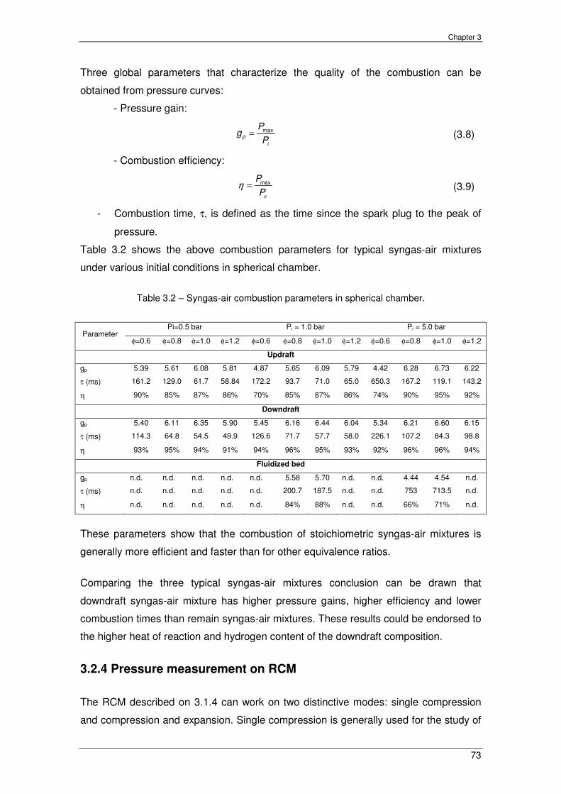
Chapter 3
73
Three global parameters that characterize the quality of the combustion can be
obtained from pressure curves:
- Pressure gain:
maxp
i
Pg
P= (3.8)
- Combustion efficiency:
max
v
P
Pη = (3.9)
- Combustion time, τ, is defined as the time since the spark plug to the peak of
pressure.
Table 3.2 shows the above combustion parameters for typical syngas-air mixtures
under various initial conditions in spherical chamber.
Table 3.2 – Syngas-air combustion parameters in spherical chamber.
Parameter Pi=0.5 bar Pi = 1.0 bar Pi = 5.0 bar
φ=0.6 φ=0.8 φ=1.0 φ=1.2 φ=0.6 φ=0.8 φ=1.0 φ=1.2 φ=0.6 φ=0.8 φ=1.0 φ=1.2
Updraft
gp 5.39 5.61 6.08 5.81 4.87 5.65 6.09 5.79 4.42 6.28 6.73 6.22
τ (ms) 161.2 129.0 61.7 58.84 172.2 93.7 71.0 65.0 650.3 167.2 119.1 143.2
η 90% 85% 87% 86% 70% 85% 87% 86% 74% 90% 95% 92%
Downdraft
gp 5.40 6.11 6.35 5.90 5.45 6.16 6.44 6.04 5.34 6.21 6.60 6.15
τ (ms) 114.3 64.8 54.5 49.9 126.6 71.7 57.7 58.0 226.1 107.2 84.3 98.8
η 93% 95% 94% 91% 94% 96% 95% 93% 92% 96% 96% 94%
Fluidized bed
gp n.d. n.d. n.d. n.d. n.d. 5.58 5.70 n.d. n.d. 4.44 4.54 n.d.
τ (ms) n.d. n.d. n.d. n.d. n.d. 200.7 187.5 n.d. n.d. 753 713.5 n.d.
η n.d. n.d. n.d. n.d. n.d. 84% 88% n.d. n.d. 66% 71% n.d.
These parameters show that the combustion of stoichiometric syngas-air mixtures is
generally more efficient and faster than for other equivalence ratios.
Comparing the three typical syngas-air mixtures conclusion can be drawn that
downdraft syngas-air mixture has higher pressure gains, higher efficiency and lower
combustion times than remain syngas-air mixtures. These results could be endorsed to
the higher heat of reaction and hydrogen content of the downdraft composition.
3.2.4 Pressure measurement on RCM
The RCM described on 3.1.4 can work on two distinctive modes: single compression
and compression and expansion. Single compression is generally used for the study of

Experimental set ups and diagnostics
74
high pressure auto-ignition of combustible mixtures as it gives direct measure of
ignition delay (Mittal, 2006). When the interest is the heat transfer to the walls then it is
usually used an inert gas, with equal adiabatic coefficient as the reacting mixture, as a
test gas. In this work instead of an inert gas a stoichiometric syngas-air mixture was
used out of auto-ignition conditions. A set of three experiments were made for each
syngas composition without combustion in order to verify its repetition. The pressure
traces are shown in figure 3.9 for downdraft syngas composition.
Figure 3.9 shows rapid rise in pressure during the compression stroke followed by
gradual decrease in pressure due to heat loss from a constant volume chamber, the
clearance volume, at the end of compression. A very good repetition of signals was
found during compression experiments being the maximum difference between
pressure peaks around 0.3 bar (25 bar on average) from one experiment to another.
0
5
10
15
20
25
30
90 100 110 120 130 140 150 160 170 180Time (ms)
Pre
ssure
(bar)
Shot 1
Shot 2
Shot 3
Figure 3.9 - Pressure versus time for compression of stoichiometric downdraft syngas-air in a
RCM. Initial conditions: Pi = 1.0 bar; Ti = 293 K, ε=11.
0
200
400
600
800
1000
1200
0 5 10 15 20 25 30 35 40 45 50
Time (ms)
Volu
me (
cm
3)
Figure 3.10 - Typical volume trace for compression of stoichiometric downdraft syngas -air in an
RCM. Initial conditions: Pi = 1.0 bar; Ti = 293 K, ε=11.

Chapter 3
75
In-cylinder volume during compression is reported in the figure 3.10. The volume is
determined thanks to a laser piston positioning sensor being the compression time
estimated on 44 ms. The piston velocity is comprised between 0 and 15 m/s, and it is
around 9.5 m/s on average. In order to avoid measurements uncertainties, another
laser piston position sensor was placed at TDC and the pressure and piston position
signals synchronized.
The same procedure was followed when working with compression-expansion strokes
without combustion (motored) being the pressure trace repetition verified in the figure
3.11.
0
5
10
15
20
25
30
90 100 110 120 130 140 150 160 170 180
Time (ms)
Pre
ssure
(bar)
Shot 1
Shot 2
Shot 3
Figure 3.11 - Typical pressure trace for compression expansion of stoichiometric downdraft
syngas-air mixture in a RCM. Initial Conditions: Pi = 1.0 bar; Ti = 293 K.
A very good repetition of signals was found during compression expansion experiments
being the maximum difference between peak pressures around 0.4 bar (27 bar on
average) from one experiment to another. Notice the higher pressure peak (>2.0 bar,
8%) of the compression expansion strokes compared with single compression stroke of
the figure 3.9. To explain this difference the average piston displacement without
combustion during the compression stroke for both working modes are shown in the
figure 3.12.

Experimental set ups and diagnostics
76
0
100
200
300
400
500
90 95 100 105 110 115 120 125 130 135 140
Time (ms)
Pis
ton p
ositio
n (
mm
)Compression-Expansion
Single compression
Figure 3.12 – Piston displacement during one and two strokes without combustion.
The difference on the figure 3.12 is around 2.0 ms in the initial, which indicates that the
RCM cam of the compression-expansion strokes is shorter than the compression one.
The corresponding in-cylinder volume versus time is lower for the compression-
expansion case, which corresponds to higher in-cylinder pressures.
In an ideal spark-ignited internal combustion engine one can distingue three stages:
compression, combustion and expansion. The entire pressure rise during combustion
takes place at constant volume at TDC. However in an actual engine this does not
happen as well as in the RCM. The pressure variation due to combustion in a
compression and expansion rapid compression machine is shown in figure 3.13, where
three stages of combustion can be distinguished.
0
10
20
30
40
50
60
70
90 100 110 120 130 140 150 160 170 180
Time (ms)
Pre
ssure
(bar)
12.5 ms BTDC
Motoring
A
B
C
D
Figure 3.13 – Stages of combustion in a RCM.

Chapter 3
77
In this figure, A is the point of passage of spark, B is point at which the beginning of
pressure rise can be detected and C the attainment of peak pressure. Thus, AB
represents the first stage, BC the second stage and CD the third stage (Ganesan,
1995).
The first stage is referred to as ignition lag or preparation phase in which growth and
development of a self propagating nucleus of flame takes place. This is a chemical
process depending upon both pressure and temperature and the nature of the fuel.
Further, it is also dependent of the relationship between the temperature and the rate
of reaction.
The second stage is a physical one and is concerned with the spread of the flame
throughout the combustion chamber. The starting point of the second stage is where
the first measurable rise of pressure is seen, i.e. the point where the line of combustion
departs from the compression line (point B). This can be seen from the deviation from
the compression (motoring) curve.
During the second stage the flame propagates practically at a constant velocity. Heat
transfer to the cylinder wall is low, because only a small part of the burning mixture
comes in contact with the cylinder wall during this period. The rate of heat release
depends largely of the turbulence intensity and also of the reaction rate which is
dependent on the mixture composition. The rate of pressure rise is proportional to the
rate of heat release because during this stage, the combustion chamber volume
remains practically constant (since the piston is near the TDC).
The starting point of the third stage is usually taken at the instant at which the
maximum pressure is reached (point C). The flame velocity decreases during this
stage. The rate of combustion becomes low due to lower flame velocity and reduced
flame front surface. Since the expansion stroke starts before this stage of combustion,
with the piston moving away from the TDC, there can be no pressure rise during this
stage.
3.2.5 Aerodynamics inside a RCM
Although in principle RCM simulates a single compression event, complex
aerodynamic features can affect the state of the reacting core in the reaction chamber.
Previous studies of Griffiths et al., (1993) and Clarkson et al., (2001) have shown that
the motion of the piston creates a roll-up vortex, which results in mixing of the cold gas

Experimental set ups and diagnostics
78
pockets from the boundary layer with the hot gases in the core region. However,
substantial discrepancies have been observed between data taken from different rapid
compression machines even under similar conditions of temperature and pressure
(Minetti et al., 1996). These discrepancies are attributed partly to the different heat loss
characteristics after the end of the compression stroke and partly to the difference in
aerodynamics between various machines. The effect of aerodynamics is particularly
more complicated because it does not show up in the pressure trace and it may lead to
significant temperature gradients and ultimately to the failure of the adiabatic core
hypothesis.
The aerodynamics inside a rapid compression machine is highly unsteady in nature; it
plays a role in pre-ignition through turbulent mixing, but also because it drives the
evolution of the temperature distribution. In order to characterize the temporal evolution
of the flow, and quantify the distribution and turbulence intensity associated to the
Institute Pprime RCM, the previous work of Strozzi, (2008) is referred.
Measurements on the total extent of the clearance volume and at the center of the
chamber were made using an inert gas N2 to simplify the diagnosis and avoiding the
disruption of PIV images by possible oxidation of unwanted particles. The flow remains
representative of the reactive case when the heat release is negligible. For more
details on the experimental protocol see Strozzi, (2008).
3.2.5.1 Velocity fluctuations
The study of turbulent flows is generally based on the Reynolds decomposition, where
the instantaneous velocity is decomposed into a mean part and a fluctuating part: U =
<U> + u.
In most cases, a global average is used to estimate mean velocity <U>. Using this
approach in an engine results in substantial overestimation of the turbulent intensity
that can reach a factor of 2 (Liou and Santavicca, 1985). Indeed, the cyclical
fluctuations of the overall movement (such as large eddy scale movement) are included
in the fluctuating field as well as fluctuations in velocity caused by the turbulent nature
of the flow.
Instantaneous velocity
Figure 3.14 shows the time evolution of the velocity field during an inert gas
compression. It is observed 10 ms BTDC a laminar one-dimensional compression flow.

Chapter 3
79
A zone of high velocities (5 to 8 m/s), where the flow is turbulent, that come in the
center of the clearance volume 5 ms after. The laminar flow of this zone becomes two-
dimensional and diverging to the walls. The turbulent zone reaches TDC and occupies
a large part of the chamber at that moment. The flow in this zone is structured by two
counter-rotating vortices, which is consistent with the literature where the movement of
the piston brings the gas from the side wall toward the center of the chamber, forming
vortices on the corners. These vortices then move to the side walls and after down the
chamber. Simultaneously, the maximum velocity of the flow gradually decreases, and
the size of the 'laminar' zone observed at the end of compression decreases. The
disappearance of this zone occurs approximately 17 ms after TDC, although some low
velocity zones remain. 40 ms after TDC, the corner vortices are replaced by a
fragmented and highly three-dimensional flow.
The coexistence of laminar and turbulent regions is characteristic of MCR flat piston
flow, where the gases are at rest before compression. One can observe a certain
asymmetry in vortices velocity, with lower values at TDC and close to the walls (figure
3.14). This asymmetry reflects the exchange of kinetic energy that occurs in the strain
layer between the vortex and the zone of lower flow. The velocity gradient direction at
the zone interface may also be parallel to the mean flow, as is in the case of few
milliseconds before TDC. In this case, if the inertia of the high speed zone regrowth
clearly the core zone, the turbulent nature of the flow at the interface is also likely to
accelerate the decrease in the extent of the core zone. This emphasis the existence of
two ranges of scales associated with mixing phenomenon: those of the overall
movement, and those of turbulence. Moreover, the overall velocity of the movement
decreases rapidly if the flow stops. Thus, reflecting the kinetic energy transfer from
large scales to the turbulent scales.

Experimental set ups and diagnostics
80
Figure 3.14 – Inert compression velocity fields (m/s) in the RCM (reprinted from Strozzi, 2008).
-10 ms
TDC
10 ms
30 ms
-5 ms
5 ms
20 ms
40 ms

Chapter 3
81
3.2.5.2 Analysis of the flow at the chamber core
The whole movement has been analyzed, and an initial assessment of turbulent
fluctuations was provided from the whole filed measurements. Specific field
measurements are now exposed to evaluate the properties of turbulence in detail. The
turbulent characteristics are evaluated thanks to PIV measurements with time
resolution of 5 kHz along one field of 13x13 mm and image resolution of 512x512
pixels. The investigated zone is close to the center of the chamber (1.5 mm to the left),
where the mean and fluctuating velocities remain relatively elevated along a 10 ms
period after TDC. Figure 3.15 shows the fluctuation velocity components in this zone.
Figure 3.15 – Time evolution of the space speed fluctuations variation (reprinted from Strozzi, 2008). The zone 1 corresponds to the bottom left corner of PIV field, and the zone 4
corresponds to the entire field.
It is observed that both velocity components fluctuations decrease after TDC with
similar amplitude. The kinetic energy is evaluated only from two velocity components
as follows:
2 2' 'k u v= + (3.10)
It is therefore, slightly underestimated (~20%) due to the lack of the third component.

Experimental set ups and diagnostics
82
A,C E D F E G H
A,C E F D,G H
Figure 3.16 represents the kinetic turbulent energy. The maximum of kinetic energy is
obtained 2-3 ms before TDC. It is followed by a rapid decrease that reflects both the
overall decrease of the turbulent kinetic energy but also the convection of the fastest
zones outside the measured field.
Figure 3.16– Kinetic energy (left) and turbulence intensity (right). Reprinted from Strozzi, (2008)
The turbulent intensity calculated in zone 1 is moderate, with a value of about 20% with
minor variations over time. One should remind that this value corresponds to a high
velocity turbulent zone. Furthermore, figure 3.16 suggests turbulence intensity much
higher at the interface between the turbulent zones and low velocity zones.
3.2.6 Schlieren photography
Schliere (pl. Schlieren) is a German word denoting optical inhomogeneity in an
otherwise transparent region. Such inhomogeneity causes refraction of light, which can
be displayed on a screen and used as a source of information on the disturbance
(Chomiak, 1990). The method is illustrated in Figure 3.17.
Figure 3.17– Typical (top) and single-lens (bottom) schlieren systems.

Chapter 3
83
Light from a point source A is transformed into a parallel beam and let through the zone
to be investigated, E. All the rays which are not deflected converge at the focus of lens
D and are cut off by diaphragm F. refracted rays bypass the diaphragm and are
collected by lens G, which projects them onto screen H. Lens G is placed in such a
way as to produce a sharply defined image of plane E on the screen. Simple
geometrical considerations are not sufficient to determine precisely the changes in
screen illumination due to a given disturbance, since they are greatly influenced by the
diffraction of light on the diaphragm and by the source dimensions. Approximately,
however, the relative illumination at the image plane, ∆I/I, is proportional to the beam
deflection angle θ and the focal length f of lens D, as follows:
If
Iθ
∆≈ (3.11)
The schlieren image is greatly influenced by the form and size of the light source and
diaphragm. Placing a diaphragm at the lens focus amounts to removing a specific
group of harmonics from the diffraction pattern, this, of course, introduces significant
changes in the schlieren image. Hence all schlieren photography apparatus should
consist of a large choice of diaphragms from which selection can be made
experimentally to obtain the most contrasting picture of a given effect. By using a slit
source of white light and a slit diaphragm color schlieren images can also be achieved.
The dependence of changes in illumination at the screen on the refraction angle
implies that the schlieren image visualizes density gradients of the flame:
I Q
I n
∆ ∂≈
∂ (3.12)
Where n represents a normal to the surface of constant density. Superimposed on this
relationship is a spatial function dependent on the structure of the system and its
arrangement relative to the disturbance. The situation is therefore largely qualitative,
although an appropriate setting of the apparatus (on removing the diaphragm, a sharm
image of the flame should appear on the screen) should ensure fairly faithful
representation of the disturbance pattern. To obtain quantitative estimates of the
density gradients at a given setting of the apparatus, optical calibrations are used with
known refraction angles.
Figure 3.18 shows a scheme of the used schlieren apparatus. The laser source (Laser
Árgon Spectra Physics Series 2000) with a maximum power of 6 W generates a

Experimental set ups and diagnostics
84
continuous beam of light, composed for two respectively equal main rays with wave
length of 488 and 514.5 nm. This laser beam is cut, by the acoustic-optical deflector
(Errol) in a succession of luminous impulses of adjustable duration and frequency. At
the exit of the acoustic-optical deflector, the rays cross a convergent lens making them
to converge into a focal point in the image where is placed a diaphragm of 50µ
diameter. The diaphragm is placed in the center of the object of a spherical mirror with
focal length of 1m, in order to reflecting the luminous rays into a parallel beam that
crosses the combustion chamber (Taillefet, 1999).
Figure 3.18– Schlieren scheme (Malheiro, 2002)
When a phenomenon in the chamber cause a change of the refractive index, the light
is deviated and passes with the same dimensions to the screen that can be record by a
camera. To this end, a fast camera APX RS PHOTRON (CMOS, 10 bits, run at 6000
fps, 1024×512 pixels) is used to record the schlieren flame images during combustion.
Exposure time is imposed by the acoustic-optical deflector and is fixed to 5 ms.


Chapter 4
85
CHAPTER 4
EXPERIMENTAL AND NUMERICAL LAMINAR SYNGAS COMBUSTION
Syngas obtained from gasification of biomass is considered to be an attractive new
fuel, especially for stationary power generation.
As reported in chapter 2 there is considerable variation in the composition of syngas
due to various sources and processing methods. Continuous variation in the
composition of the generated syngas from a given gasification source is another
challenge in designing efficient end use applications such as burners and combustion
chambers to suit changes in fuel composition. Designing such combustion appliances
needs fundamental understanding of the implications of syngas composition for its
combustion characteristics, such as laminar burning velocity and flammability limits.
Laminar burning velocity for single component fuels such as methane (Hassan et al.,
1998; Gu et al., 2000); and hydrogen (Aung et al., 1997; Bradley et al., 2007) are
abundantly available in the literature for various operating conditions. Burning velocity
studies on H2–O2–inert (such as N2, CO2, Ar, and He) are also available (Aung et al.,
1998; Lamoureux et al., 2003). Some studies on burning velocities are also available
for binary fuel mixtures such as H2–CH4 (Halter et al., 2005; Coppens et al., 2007), and
H2–CO (Vagelopoulos and Egolfopoulos, 1994; Sun et al., 2007). Vagelopoulos and
Egolfopoulos, (1994) measured burning velocities of H2–CO mixtures using a counter
flow flame technique and reported that addition of 6% or more hydrogen to H2–CO
made the response of the H2–CO mixture more similar to the kinetics of hydrogen than
to that of CO. McLean et al., (1994) measured unstretched laminar burning velocities
for 5%H2 – 95%CO and 50%H2 – 50%CO mixtures using constant-pressure outwardly
propagating spherical flames to evaluate the rate of the CO + OH reaction. Brown et
al., (1996) reported flame stretch effects on burning velocities of H2–air, 50%H2–
50%CO–air and 5%H2–95%CO–air mixtures under atmospheric condition. Values of
Markstein length for 50%H2–50%CO–air mixtures were found to be very similar to
those of pure H2–air mixtures. It was concluded that H2 was the dominant species and
governed the Markstein length behavior for the 50% H2– 50% CO–air mixture. Hassan
et al., (1997) reported the effects of positive stretch rate on burning velocities of H2–CO
mixtures under different mixture conditions by varying the H2 fraction in the fuel from 3
to 50% by volume using constant-pressure outwardly propagating spherical flames.

Experimental and numerical laminar syngas combustion
86
They stated that as the H2 concentration in the H2–CO mixture increased, the mixture
started behaving similarly to the H2–air mixture and the effect of flame stretch on
burning velocity also became more pronounced. Sun et al., (2007) measured stretch-
free burning velocities for CO–H2–air mixtures at different mixing ratios (the values of
the CO/H2 ratio used were 50:50, 75:25, 95:5, and 99:1), equivalence ratios and
pressures using expanding spherical flames at constant pressure. They used artificial
air with helium instead of nitrogen to have stable flames at higher pressures. Burke et
al., (2007) studied the effects of CO2 on the burning velocity of a 25% H2–75% CO
mixture with 12.5%O2–87.5%He oxidizer under stoichiometric conditions and they
varied the CO2 concentration in the fuel from 0 to 25% using spherically expanding
flames. They stated that the largest flame radius for calculation of unstretched burning
velocity should be less than 30% of the radius wall in a cylindrical chamber. Natarajan
et al., (2007) investigated the effects of CO2 on burning velocities of H2–CO mixtures
for different H2/CO ratios, varying the CO2 mole fraction in the fuel (0% and 20%), the
equivalence ratio (0.5–1.0), the initial temperature (300–700K), and pressure (1–5
atm). Two measurement techniques were used: one using flame area images of a
conical Bunsen flame and the other based on velocity profile measurements in a one-
dimensional stagnation flame.
No extensive combustion study is available in the literature for typical syngas
compositions like the ones expressed in chapter 2. This motivated the present work to
choose three typical compositions of syngas and to study the laminar burning velocity
and flame stability. These typical syngas compositions were selected from Bridgwater,
(1995) and are shown in the Table 4.1.
Table 4.1 – Syngas compositions (% by volume)
Gasifier
Gas composition (% by volume) HHV
(MJ/m3) H2 CO CO2 CH4 N2
Updraft 11 24 9 3 53 5.5
Downdraft 17 21 13 1 48 5.7
Fluidized bed 9 14 20 7 50 5.4
There are also gaps in the fundamental understanding of syngas combustion
characteristics, especially at elevated pressures that are relevant to practical
combustors. In this chapter, constant volume spherically expanding flames are used to
determine a burning velocity correlation valid for engine conditions.
Chapter 4
87
4.1 Laminar burning velocity
4.1.1 Constant pressure method
Laminar burning velocity and Markstein length can be deduced from schlieren
photographs of the flame (Bradley et al., 1998). For an outwardly spherical propagating
flame, the stretched flame speed, Sn, is derived from the flame radius versus time data
as follows:
fn
drS
dt= (4.1)
where rf represents the flame radius in the schlieren photographs and t the time. The
total stretch rate acting on a spherical expanding flame, κ, is defined as Bradley et al.,
(1996):
1 2 2fn
f f
drdA SA dt r dt r
κ = = = (4.2)
where A is the flame surface area. A linear relationship between the flame speed and
the total stretch exists (Clavin, 1985), and this is quantified by a burned Markstein
length, Lb, as follows:
0n n bS S L κ− = (4.3)
where 0nS is the unstretched flame speed, and Lb the Markstein length of burned gases.
The unstretched flame speed is obtained as the intercept value at κ = 0, in the plot of
Sn against κ, and the burned gas Markstein length is the negative slope of Sn–κ curve.
Markstein length can reflect the stability of flame (Liao et al., 2004). Positive values of
Lb indicate that the flame speed decreases with the increase of flame stretch rate. In
this case, if any kind of perturbation or small structure appears on the flame front
(stretch increasing), this structure tends to be suppressed during flame propagation,
and this makes the flame stability. In contrast to this, a negative value of Lb means that
the flame speed increases with the increase of flame stretch rate. In this case, if any
kinds of perturbation appear on the flame front, the flame speed in the flame front will
be increased, and this increases the instability of the flame. When the observation is
limited to the initial part of the flame expansion where the pressure does not vary yet,
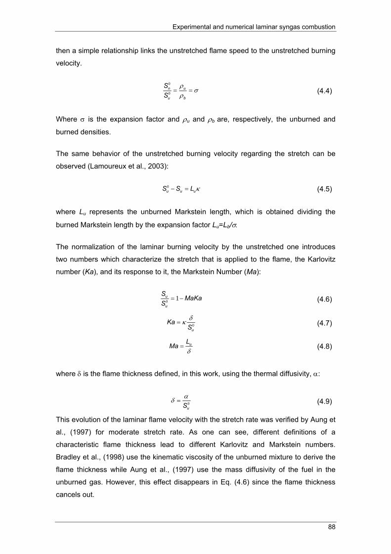
Experimental and numerical laminar syngas combustion
88
then a simple relationship links the unstretched flame speed to the unstretched burning
velocity.
0
0un
bu
SS
ρσ
ρ= = (4.4)
Where σ is the expansion factor and ρu and ρb are, respectively, the unburned and
burned densities.
The same behavior of the unstretched burning velocity regarding the stretch can be
observed (Lamoureux et al., 2003):
0u u uS S L κ− = (4.5)
where Lu represents the unburned Markstein length, which is obtained dividing the
burned Markstein length by the expansion factor Lu=Lb/σ.
The normalization of the laminar burning velocity by the unstretched one introduces
two numbers which characterize the stretch that is applied to the flame, the Karlovitz
number (Ka), and its response to it, the Markstein Number (Ma):
0 1u
u
SMaKa
S= − (4.6)
0u
KaSδκ= (4.7)
uLMa
δ= (4.8)
where δ is the flame thickness defined, in this work, using the thermal diffusivity, α:
0uS
αδ = (4.9)
This evolution of the laminar flame velocity with the stretch rate was verified by Aung et
al., (1997) for moderate stretch rate. As one can see, different definitions of a
characteristic flame thickness lead to different Karlovitz and Markstein numbers.
Bradley et al., (1998) use the kinematic viscosity of the unburned mixture to derive the
flame thickness while Aung et al., (1997) use the mass diffusivity of the fuel in the
unburned gas. However, this effect disappears in Eq. (4.6) since the flame thickness
cancels out.

Chapter 4
89
4.1.1.1 Flame morphology
Bradley et al., (1998) shown that flame speeds become independent of ignition energy
when flame radius is greater than 6 mm. The existence of the critical flame radius was
also observed by Lamoureux et al., (2003) and Liao et al., (2004). Their studies also
gave approximately the same value. Thus, the flame radius is analyzed only beyond
that radius, at which the spark effects could be discounted. In order to define the upper
limit of the flame radius data exploration, the spherical pattern of the flame expansion
and the corresponding pressure should be taking into account. The criterion used for
sphericity considerations was a 0.5 mm radius difference between horizontal and
vertical directions, which gives in our experimental conditions an upper limit for the
radius of 20.0 mm. The maximum estimated experimental uncertainty is 8% for the
radius 6.0 mm using this criterion. This also arises from the pixel resolution of the
digital camera. Figure 4.1 shows schlieren images of updraft syngas-air flames at
various equivalence ratios and initial pressure of 1.0 bar and 293 K.
Pi = 1.0 bar , Ti = 293 K, φ=0.6
Time (ms) 4 5 6 7 8 9 10 11 12 13 14 Radius (mm) 6.5 7.6 8.6 9.5 10.5 11.4 12.2 13.2 13.9 14.9 15.6
Pi = 1.0 bar, Ti = 293 K. φ=0.8
Time (ms) 3 4 5 6 7 8 9 10 11 12 13 Radius (mm) 6.5 7.9 9.4 10.9 12.3 13.6 15.0 16.3 17.4 18.7 21.1
Pi = 1 bar, Ti = 293 K. φ=1.0
Time (ms) 3 4 5 6 7 8 9 10 11
Radius (mm) 6.9 8.7 10.6 12.3 14.1 15.7 17.4 18.9 20.6 Pi = 1.0 bar, Ti = 293 K. φ=1.2
Time (ms) 3 4 5 6 7 8 9 10 11 12
Radius (mm) 6.7 8.0 9.7 11.1 12.6 14.1 15.5 16.9 18.3 19.7
Figure 4.1 – Schlieren images of updraft syngas-air mixture flames at 1.0 bar.

Experimental and numerical laminar syngas combustion
90
These schlieren images show generally a spherical pattern. Stoichiometric mixture is
the faster one, followed by the rich mixture (φ=1.2). Lean mixtures are slower and for
φ=0.6 spherical flame start to be critical with a small crack formation. Figure 4.2 shows
updraft flame speed and pressure rise versus flame radius under stoichiometric
conditions.
1.0
1.2
1.4
1.6
1.8
2.0
0 5 10 15 20 25 30Radius (mm)
Sn
(m/s
)
1.0
1.1
1.2
1.3
1.4
1.5
Pre
ssur
e (b
ar)
SnP
Figure 4.2 – Flame speed and pressure versus radius for updraft syngas-air mixture at 1.0 bar.
The radius range where the flame speed keeps a spherical pattern is defined between
6 -18 mm, where the pressure rise is only 0.05 bar and no influence of the chamber
wall geometry is observed from flame images.
Figure 4.3 shows schlieren images of downdraft syngas-air mixtures for various
equivalence ratios at 1.0 bar.
From figure 4.3 is possible to observe the spherical pattern of the flame expansion.
Again, stoichiometric mixture is the faster one, followed closely by the rich mixture.
Lean mixtures show to be slower. Another, finding is that downdraft syngas-air flames
are a bit faster than updraft syngas-air flames for every equivalence ratios.
Figure 4.4 shows flame speed and pressure rise during stoichiometric combustion of
downdraft syngas–air mixture. The radius range to explore is defined between 6 -18
mm, where the flame speed keeps a linear behavior. Pressure rise is only 0.03 bar and
no influence of the chamber wall geometry is observed from flame images. This radius
range is kept for the remaining equivalence ratios has similar behavior was found.

Chapter 4
91
Pi = 1.0 bar, Ti = 293 K, φ=0.6
Time (ms) 5.0 6.0 7.0 8.0 9.0 10.0 11.0 12.0 13.0 14.0 15.0
Radius (mm) 6.4 7.4 8.5 9.4 10.5 11.5 12.4 13.3 14.2 15.1 15.9
16.0 17.0 18.0 19.0 20.0 16.7 17.6 18.5 19.3 20.1
Pi = 1.0 bar, Ti = 293 K, φ=0.8
Time (ms) 3.5 4.5 5.5 6.5 7.5 8.5 9.5 10.5 11.5 12.5 13.5
Radius (mm) 6.0 7.6 9.2 10.8 12.4 13.9 15.5 17.0 18.4 19.7 21.0
Pi = 1.0 bar, Ti = 293 K, φ=1.0
Time (ms) 4.0 5.0 6.0 7.0 8.0 9.0 10.0 11.0 Radius (mm) 6.6 8.7 10.9 13.0 15.0 17.1 19.1 21.0
Pi = 1.0 bar, Ti = 293 K, φ=1.2
Time (ms) 4.0 5.0 6.0 7.0 8.0 9.0 10.0 11.0 Radius (mm) 6.4 8.5 10.4 12.5 14.5 16.6 18.6 20.5
Figure 4.3 - Schlieren images of downdraft syngas-air mixture flames at 1.0 bar.
1.0
1.3
1.6
1.9
2.2
2.5
0 5 10 15 20 25 30 35 Radius (mm)
Sn
(m/s
)
1.0
1.1
1.2
1.3
1.4
Pre
ssur
e (b
ar)
SnP
Figure 4.4- Flame speed and pressure versus radius for stoichiometric downdraft syngas-air
mixture at 1.0 bar.

Experimental and numerical laminar syngas combustion
92
Pi = 1.0 bar, Ti = 293 K, φ=0.6
Time (ms) 8.0 10.0 12.0 14.0 16.0 18.0 20.0 22.0 24.0 26.0 28.0
Time (ms) 100 110 120 130 140 150 160 170 180 190 200
Pi= 1.0 bar, Ti = 293 K, φ=0.8
Time (ms) 5.0 6.0 7.0 8.0 9.0 10.0 11.0 12.0 13.0 14.0 15.0
Radius (mm) 6.5 7.2 8.0 8.8 9.6 10.3 11.07 11.9 12.6 13.5 14.3
16.0 17.0 18.0 19.0 20.0 21.0 22.0 23.0
15.0 15.7 16.4 17.3 18.1 18.8 19.5 20.3
Pi = 1.0 bar, Ti = 293 K, φ=1.0
Time (ms) 5.0 6.0 7.0 8.0 9.0 10.0 11.0 12.0 13.0 14.0 15.0
Radius (mm) 6.5 7.2 8.1 8.9 9.7 10.4 11.2 12.0 12.9 13.7 14.6
16.0 17.0 18.0 19.0 20.0 21.0
15.3 16.2 17.1 18.0 19.0 20.0
Figure 4.5 - Schlieren images of fluidized bed syngas-air mixture flames at 1.0 bar.
0.4
0.6
0.8
1.0
1.2
0 5 10 15 20 25 30 35 40Radius (mm)
Sn(
m/s
)
1.00
1.05
1.10
1.15
1.20
Pre
ssur
e (b
ar)
Sn
P
Figure 4.6 - Flame speed and pressure versus radius for stoichiometric fluidized bed syngas-air
mixture at 1.0 bar.
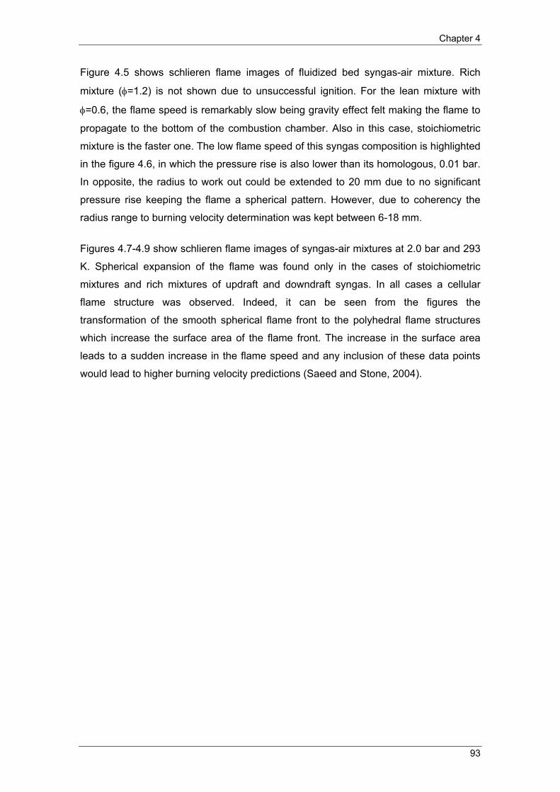
Chapter 4
93
Figure 4.5 shows schlieren flame images of fluidized bed syngas-air mixture. Rich
mixture (φ=1.2) is not shown due to unsuccessful ignition. For the lean mixture with
φ=0.6, the flame speed is remarkably slow being gravity effect felt making the flame to
propagate to the bottom of the combustion chamber. Also in this case, stoichiometric
mixture is the faster one. The low flame speed of this syngas composition is highlighted
in the figure 4.6, in which the pressure rise is also lower than its homologous, 0.01 bar.
In opposite, the radius to work out could be extended to 20 mm due to no significant
pressure rise keeping the flame a spherical pattern. However, due to coherency the
radius range to burning velocity determination was kept between 6-18 mm.
Figures 4.7-4.9 show schlieren flame images of syngas-air mixtures at 2.0 bar and 293
K. Spherical expansion of the flame was found only in the cases of stoichiometric
mixtures and rich mixtures of updraft and downdraft syngas. In all cases a cellular
flame structure was observed. Indeed, it can be seen from the figures the
transformation of the smooth spherical flame front to the polyhedral flame structures
which increase the surface area of the flame front. The increase in the surface area
leads to a sudden increase in the flame speed and any inclusion of these data points
would lead to higher burning velocity predictions (Saeed and Stone, 2004).

Experimental and numerical laminar syngas combustion
94
Pi = 2.0 bar, Ti = 293 K, φ=0.6
Time (ms) 5 6 7 8 9 10 11 12 13 14 15
Pi = 2.0 bar, Ti = 293 K, φ=0.8
Time (ms) 3 4 5 6 7 8 9 10 11 12 13
Radius (mm) 5.8 7.1 8.8 10.1 11.1 12.3 13.5 14.5 15.6 16.6 17.8
14 15 16
18.7 19.6 20.7
Pi =2.0 bar, Ti = 293 K, φ=1.0
Time (ms) 3 4 5 6 7 8 9 10 11 12 13
Radius (mm) 6.0 7.8 9.2 10.6 11.9 13.3 14.6 15.9 17.2 18.4 19.6
Pi = 2.0 bar, Ti = 293 K, φ=1.2
Time (ms) 4 5 6 7 8 9 10 11 12 13 14
Radius (mm) 6.0 7.2 8.3 9.3 10.5 11.5 12.8 13.9 15.0 15.9 17.0
15 16 17
18.0 19.0 20.1
Figure 4.7- Schlieren flame images of the updraft syngas-air mixtures at 2.0 bar.

Chapter 4
95
Pi = 2.0 bar, Ti = 293 K, φ=0.6
Time (ms) 5.0 6.0 7.0 8.0 9.0 10.0 11.0 12.0 13.0 14.0 15.0
Radius (mm) 6.3 7.3 8.3 9.3 10.2 11.1 11.9 12.7 13.6 14.3 15.2
16.0 17.0 18.0 19.0 20.0 21.0
15.9 16.7 17.4 18.2 19.0 19.8
Pi = 2.0 bar, Ti = 293 K, φ=0.8
Time (ms) 4.0 5.0 6.0 7.0 8.0 9.0 10.0 11.0 12.0 13.0 14.0
Radius (mm) 6.5 7.9 9.5 10.9 12.5 13.9 15.2 16.5 17.8 19.0 20.4
Pi = 2.0 bar, Ti = 293 K, φ=1.0
Time (ms) 3.0 4.0 5.0 6.0 7.0 8.0 9.0 10.0 11.0
Radius (mm) 6.5 8.2 10.0 11.9 13.7 15.3 17.0 18.7 20.4
Pi = 2.0 bar, Ti = 293 K, φ=1.2
Time (ms) 4.0 5.0 6.0 7.0 8.0 9.0 10.0 11.0 12.0 13.0
Radius (mm) 6.4 8.0 9.6 11.3 12.7 14.3 15.9 17.4 18.9 20.4
Figure 4.8 - Schlieren flame images of the downdraft syngas-air mixtures at 2.0 bar.
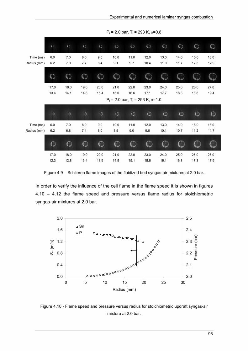
Experimental and numerical laminar syngas combustion
96
Pi = 2.0 bar, Ti = 293 K, φ=0.8
Time (ms) 6.0 7.0 8.0 9.0 10.0 11.0 12.0 13.0 14.0 15.0 16.0
Radius (mm) 6.2 7.0 7.7 8.4 9.1 9.7 10.4 11.0 11.7 12.3 12.9
17.0 18.0 19.0 20.0 21.0 22.0 23.0 24.0 25.0 26.0 27.0
13.4 14.1 14.8 15.4 16.0 16.6 17.1 17.7 18.3 18.8 19.4
Pi = 2.0 bar, Ti = 293 K, φ=1.0
Time (ms) 6.0 7.0 8.0 9.0 10.0 11.0 12.0 13.0 14.0 15.0 16.0
Radius (mm) 6.2 6.8 7.4 8.0 8.5 9.0 9.6 10.1 10.7 11.2 11.7
17.0 18.0 19.0 20.0 21.0 22.0 23.0 24.0 25.0 26.0 27.0
12.3 12.8 13.4 13.9 14.5 15.1 15.6 16.1 16.8 17.3 17.9
Figure 4.9 – Schlieren flame images of the fluidized bed syngas-air mixtures at 2.0 bar.
In order to verify the influence of the cell flame in the flame speed it is shown in figures
4.10 – 4.12 the flame speed and pressure versus flame radius for stoichiometric
syngas-air mixtures at 2.0 bar.
0.0
0.4
0.8
1.2
1.6
2.0
0 5 10 15 20 25 30
Radius (mm)
Sn
(m/s
)
2.0
2.1
2.2
2.3
2.4
2.5
Pre
ssur
e (b
ar)
SnP
Figure 4.10 - Flame speed and pressure versus radius for stoichiometric updraft syngas-air
mixture at 2.0 bar.

Chapter 4
97
0.0
0.5
1.0
1.5
2.0
2.5
3.0
0 5 10 15 20 25
Radius (mm)
Sn
(m/s
)
2
2.1
2.2
2.3
2.4
2.5
Pre
ssur
e (b
ar)
SnP
Figure 4.11 - Flame speed and pressure versus radius for stoichiometric downdraft syngas-air
mixture at 2.0 bar.
0.0
0.2
0.4
0.6
0.8
0 5 10 15 20 25
Radius (mm)
Sn
(m/s
)
2.00
2.02
2.04
2.06
2.08
2.10
2.12
Pre
ssur
e (b
ar)
SnP
Figure 4.12 - Flame speed and pressure versus radius for stoichiometric fluidized bed syngas-
air mixture at 2.0 bar
From figures 4.10 – 4.12 is not possible to observe the influence of cellular flame on
the mean flame speed. According to Bradley and Harper, (1994) the onset of instability
in a spherically propagating flame is associated with the surface propagation of
discontinuities in the flame structure that have the appearance of cracks. Moreover,
cells cannot form if their growth rate is smaller than that of flame expansion (Kwon et
al., 2002). Since the expanding flame suffers the strongest stretch during the initial
phase of its propagation when its radius is small, the tendency for cell development is
expected to increase as the flame propagates outwardly. These situations are more
clearly observed in the figures 4.13-4.15. In order to make the cellular flame effect on
flame speed observable a larger combustion chamber is needed.

Experimental and numerical laminar syngas combustion
98
2 ms 5 ms 8 ms
10 ms 12 ms 15 ms
20 ms 25 ms 30 ms
Figure 4.13 – Schlieren flame images of updraft syngas-air mixture at 3.0 bar.
2 ms 5 ms 8 ms
10 ms 12 ms 15 ms
17 ms 20 ms 22 ms
Figure 4.14 - Schlieren flame images of downdraft syngas-air mixture at 3.0 bar.

Chapter 4
99
5 ms 10 ms 15 ms
20 ms 25 ms 30 ms
35 ms 40 ms 45 ms
50 ms 55 ms 60 ms
65 ms 70 ms 75 ms
80 ms 85 ms 90 ms
Figure 4.15 – schlieren flame images of fluidized bed syngas-air mixture at 3.0 bar.
The hydrodynamic theory of Darrieus (1938) and Landau (1944) shows that, in the limit
of an infinitely thin flame propagating with a constant velocity, the flame is unstable to
disturbances of all wavelengths. The growth rate is proportional to the density jump

Experimental and numerical laminar syngas combustion
100
across the flame, increasing with increasing density ratio, σ. Thus σ is probably the
most sensitive parameter controlling the onset of hydrodynamic instability. Next to σ,
the flame thickness, δ, is also expected to have a strong influence on the hydrodynamic
instability, for two reasons. First, it measures the influence of curvature which, being
positive for the outwardly propagating spherical flame, has a stabilizing effect on the
cellular development. The thinner the flame, the weaker is the influence of curvature
and consequently the stronger is the destabilizing propensity. The second influence is
that it controls the intensity of the baroclinic torque developed over a slightly wrinkled
flame surface, which depends on the density gradient across the flame and the
pressure gradient along the flame (Sun et al., 1999).
For the development of the diffusional-thermal instability, an appropriate parameter
representing the effect of non-equidiffusion is the flame Lewis number, Le [Markstein,
(1951); Matalon and Matkowsky, (1982); Law and Sung, (2000)]. It is well established
and understood theoretically that unstretched flames are diffusionally unstable (stable)
for Le that are smaller (greater) than a value slightly less than unity. However, the
calculation of effective Lewis number for a multi-component fuel mixture is not as
straightforward as for pure fuel-air mixtures and is a subject that is out of the scope of
the present work.
4.1.1.2 Flame Radius
Fig. 4.16 gives the variations of flame radius versus the time for syngas-air mixtures.
The study shows that flame expands spherically after the ignition, and the flame radius
will increase rapidly in the subsequent process. There are a quasi-linear correlation
between flame radius and time for all syngas cases. The higher gradient of radius-time
curves is obtained for stoichiometric syngas-air mixtures. The lean (φ=0.8) and rich
(φ=1.2) syngas-air mixtures have similar gradients in the updraft case. This difference
increases for the downdraft syngas case. Fluidized syngas has the lowest radius-time
curve gradients. Information for rich mixture of fluidized syngas is missing due to
ignition difficulties.
According to the Markstein view the gradient of the radius-time curve reflects the
stretching effectiveness of flame. For an unstable flame, the gradient of the radius-time
curve will decrease with the flame expansion, while for a stable flame; the gradient of
the radius-time curve will increase with the flame expansion. The quasi-linear

Chapter 4
101
behaviour of the curves radius-time shows that that the stretch rate has low effect in
the syngas-air mixtures.
0
5
10
15
20
25
0 5 10 15 20Time (ms)
Rad
ius
(mm
)
0.60.81.01.2
φ
(a)
0
5
10
15
20
25
0 5 10 15 20Time (ms)
Rad
ius
(mm
)
0.60.81.01.2
φ
(b)
0
5
10
15
20
25
0 5 10 15 20Time (ms)
Rad
ius
(mm
)
0.81.0
φ
(c)
Figure 4.16 – Flame radius versus time for syngas-air mixtures at various equivalence ratios
and 1.0 bar. (a) Updtraft. (b) Downdraft (c) Fluidized bed.

Experimental and numerical laminar syngas combustion
102
4.1.1.3 Flame speed
Fig. 4.17 gives the stretched flame speed versus the flame stretch rate for three typical
syngas compositions. Removing the parts influenced by ignition energy and high
pressure at late stages of flame propagation. A linear correlation between the stretched
flame speed and the flame stretch rate is found. The unstretched flame speed is
obtained by extrapolating the line to κ= 0, while the gradient of the Sn–κ curve gives the
value of the Markstein length.
The maximum value of syngas-air flame speeds is presented at the stoichiometric
equivalence ratio, while lean or rich mixtures decrease the flame speeds. Downdraft
syngas composition shows the highest flames speeds for all the equivalence ratios
considered. The stretched flame speed increases with the increase of flame stretch
rate for lean (φ=0.8) syngas-air mixtures. This behavior remains for stoichiometric and
rich (φ=1.2) mixtures in the case of updraft and downdraft compositions.
A remarkable decrease of the stretched flame speed versus the stretch rate is
demonstrated for stoichiometric fluidized composition. This might result from the
occurrence of incomplete combustion.
Positive gradients of Sn–κ curves are derived for three equivalence ratios in the updraft
and downdraft syngas cases. A positive gradient of Sn–κ curve is also shown by the
lean fluidized syngas. These correspond to negative values of Markstein number,
indicating the instability of flames.
On the other hand, positive values of Markstein number indicate stability of flames of
mixture combustion. These correspond to stoichiometric fluidized syngas.

Chapter 4
103
0.00
0.25
0.50
0.75
1.00
1.25
1.50
0 50 100 150 200 250 300 350 κ (s-1)
Sn
(m/s
)
Updraft
Dow ndraft
φ =0.6
0.0
0.5
1.0
1.5
2.0
2.5
3.0
0 100 200 300 400 500 600 κ (s-1)
Sn (m
/s)
Updraft
Downdraft
Fluidized
φ =0.8
0.0
0.5
1.0
1.5
2.0
2.5
3.0
0 100 200 300 400 500 600 700 κ (s-1)
Sn (
m/s
)
Updraft
Downdraft
Fluidized
φ =1.0
0.0
0.5
1.0
1.5
2.0
2.5
3.0
0 100 200 300 400 500 600 700 κ (s-1)
S n (m
/s)
Updraft
Downdraft
φ =1.2
Figure 4.17 - Stretched flame speed versus stretch rate for syngas-air mixtures at various
equivalence ratios and 1.0 bar.
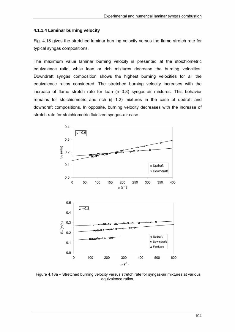
Experimental and numerical laminar syngas combustion
104
4.1.1.4 Laminar burning velocity
Fig. 4.18 gives the stretched laminar burning velocity versus the flame stretch rate for
typical syngas compositions.
The maximum value laminar burning velocity is presented at the stoichiometric
equivalence ratio, while lean or rich mixtures decrease the burning velocities.
Downdraft syngas composition shows the highest burning velocities for all the
equivalence ratios considered. The stretched burning velocity increases with the
increase of flame stretch rate for lean (φ=0.8) syngas-air mixtures. This behavior
remains for stoichiometric and rich (φ=1.2) mixtures in the case of updraft and
downdraft compositions. In opposite, burning velocity decreases with the increase of
stretch rate for stoichiometric fluidized syngas-air case.
0.0
0.1
0.2
0.3
0.4
0 50 100 150 200 250 300 350 400κ (s-1)
Su
(m/s
)
UpdraftDowndraft
φ =0.6
0.0
0.1
0.2
0.3
0.4
0.5
0 100 200 300 400 500 600
κ (s-1)
Su
(m/s
)
Updraft
Dow ndraft
Fluidized
φ =0.8
Figure 4.18a – Stretched burning velocity versus stretch rate for syngas-air mixtures at various equivalence ratios.

Chapter 4
105
0.0
0.1
0.2
0.3
0.4
0.5
0 100 200 300 400 500 600
κ (s-1)
Su
(m/s
)Updraft
Dow ndraft
Fluidized
φ =1.0
0.0
0.1
0.2
0.3
0.4
0.5
0 100 200 300 400 500 600 700κ (s-1)
Su
(m/s
)
UpdraftDowndraft
φ=1.2
Figure 4.18b – Stretched burning velocity versus stretch rate for syngas-air mixtures at various equivalence ratios.
The unstretched laminar burning velocity, 0uS , shown in Fig. 4.19 is derived from the
value of the unstretched flame speed and the expansion factor which is evaluated
using the adiabatic flame calculation via the Gaseq code package, which can be found
in the Appendix B.
0
0.1
0.2
0.3
0.4
0.6 0.8 1 1.2
Equivalence ratio
S0 u
(m/s
)
Updraft
Dow ndraft
Fluidized
Figure 4.19- Unstretched flame speed versus equivalence ratio of syngas-air mixtures.

Experimental and numerical laminar syngas combustion
106
Similar curves are obtained for all syngas compositions under study being shifted by a
value around 0.06 m/s in average between downdraft and updraft compositions and
about 0.1 m/s between fluidized and updraft syngas. These results could be endorsed
to:
- the heat value of the syngas compositions. This value varies from 5.4 (fluidized
bed syngas) to 5.7 MJ/m3 (downdraft syngas), which is in agreement, however
not proportional to the burning velocities.
- the amount of H2, due to its high reactivity, is a very important parameter to be
considered. As shown in the Table 3.1 the amount of H2 of fluidized bed syngas
(9% by volume) is very close to the updraft syngas (11% by volume) and about
half of the downdraft syngas (17% by volume). This explains the lowest burning
velocity of the fluidized bed syngas and the highest shift when compared to
downdraft syngas. However, the close amount of H2 between fluidized bed and
updraft syngas is not reflected in the burning velocity values shown in the Fig.
4.19.
- and the amount of dilution by N2 and CO2 in the fuel gases H2-CO-CH4 that
compose the typical syngas mixtures. Again, fluidized bed syngas is he highest
diluted syngas (70% by volume), being updraft and downdraft less diluted with
61% and 62% by volume, respectively. Therefore, the highest shift in burning
velocity of fluidized bed syngas could be explained by its highest dilution.
Based on the experimental data the correlations of unstretched laminar burning
velocities as function of equivalence ratio can be fitted as follows:
0 20.8125 1.6375 0.5725uS φ φ= − + − (Updraft) (4.10)
0 20.7313 1.5428 0.4924uS φ φ= − + − (Downdraft) (4.11)
0 20.7500 1.5450 0.6210uS φ φ= − + − (Fluidized) (4.12)
for updraft, downdraft and fluidized bed syngas–air mixture combustion, respectively.
Information for fluidized syngas is limited due to ignition difficulties of this mixture.
Formula (4.12) was fitted for equivalence ratios between 0.8 and 1.0.
4.1.1.5 Karlovitz and Markstein numbers
Figures 4.20-4.22 illustrates the evolution of the normalized laminar burning velocity,
Su/S0u, as a function of the normalized stretch rate, the Karlovitz number for typical
syngas compositions at various equivalence ratios. From Fig. 4.20 one can see that the

Chapter 4
107
variation of the normalized burning velocity of updraft syngas with the Karlovitz number
is linear. From Fig. 4.21 one can see that the variation of the normalized burning
velocity of downdraft syngas with the Karlovitz number is generally linear and quasi-
linear for φ=0.8. From Fig. 4.22 one can see that the variation of the normalized
burning velocity of fluidized bed syngas with the Karlovitz number is linear for φ=0.8
and quasi-linear for φ =1.0.
1.0
1.2
1.4
1.6
1.8
2.0
0.00 0.05 0.10 0.15 0.20 0.25 0.30 0.35 0.40Karlovitz Number
Su/
S0 u
1.21.00.80.6
φ
Figure 4.20 – Evolution of the laminar burning velocity versus Karlovitz number for updraft
syngas-air mixture at different equivalence ratios and 1.0 bar.
1.0
1.1
1.2
1.3
1.4
0.00 0.05 0.10 0.15 0.20 0.25 0.30 0.35 0.40
Karlovitz Number
Su/
S0 u
1.21.00.80.6
φ
Figure 4.21 – Evolution of the laminar burning velocity versus Karlovitz number for downdraft syngas-air mixture at different equivalence ratios and 1.0 bar.

Experimental and numerical laminar syngas combustion
108
0.6
0.8
1.0
1.2
1.4
0.00 0.05 0.10 0.15 0.20 0.25 0.30
Karlovitz number
Su/
S0 u
1.00.8
φ
Figure 4.22 – Evolution of the laminar burning velocity versus Karlovitz number for fluidized bed syngas-air mixture at different equivalence ratios and 1.0 bar.
The linear behavior of the normalized burning velocity with Karlovitz number supports
that the Markstein number is independent of the Karlovitz number as it was verified by
Aung et al. (1997). Also the generally low Karlovitz numbers obtained for all the typical
syngas compositions and equivalence ratios indicates small influence of stretch rate on
the syngas-air flames.
As it was pointed out by Aung at al., (1997) and Bradley et al., (1996) the Markstein
length is a fundamental property of premixed laminar flames and it is necessary to
measure it precisely. Table 4.2 shows Markstein lengths and Markstein numbers for
syngas-air mixture at various equivalence ratios. If Ma<0, the flame is in the
preferential diffusion instability regime, and if Ma>0, It is in the stable regime (Law,
2006). If Ma=0, the flame is neutrally stable, and Su= 0uS at all values of stretch rate.
Table 4.2– Markstein lengths and Markstein numbers versus equivalence ratio of syngas-air mixtures at 1.0 bar and 293 K.
Eq.
Ratio Updraft Downdraft Fluidized bed
Lb Lu Ma Lb Lu Ma Lb Lu Ma φ=0.6 -2×10⁻³ -4.1×10⁻⁴ -1.55 -9×10⁻⁴ -1.9×10⁻⁴ -1.4 n.d. n.d. n.d.
φ=0.8 -7×10⁻⁴ -1.3×10⁻⁴ -1.21 -4×10⁻⁴ -7.4×10⁻⁵ -0.84 -4×10⁻⁴ -7.5×10⁻⁵ -0.5
φ=1.0 -7×10⁻⁴ -1.2×10⁻⁴ -1.39 -5×10⁻⁴ -8.7×10⁻⁵ -1.17 8×10⁻⁴ 1.4×10⁻⁴ 1.18
φ=1.2 -5×10⁻⁴ -8.9×10⁻⁵ -0.90 -4×10⁻⁴ -7.4×10⁻⁵ -0.94 n.d. n.d. n.d.
Updraft and downdraft syngas shows to be in the preferential diffusion instability
regime as the Markstein number is negative for all cases. The flame can be seen to be
neutrally stable for fluidized bed syngas somewhat between φ=0.8 and φ =1.0 as the
Markstein number changes from a negative to a positive value.

Chapter 4
109
4.1.1.6 Comparison with other fuels
The experimental values of the syngas are compared in Fig. 4.23 with those for other
fuels obtained by other workers. The laminar burning velocity of typical syngas
compositions besides its lower heat of reaction is not dissimilar to that of methane
especially the downdraft syngas case, although somewhat slower than propane.
For lean mixtures (φ=0.6) the burning velocity of methane is the same as the updraft
syngas while the burning of propane is equal to the downdraft syngas. For
stoichiometric mixtures 0uS of downdraft and updraft typical syngas–air mixtures is
respectively 15% and 42% slower than those of methane–air mixtures, being lower for
other equivalence ratio.
In the case of propane, it is observed an increasing difference of the laminar burning
velocity of the typical syngas mixtures from lean to rich mixtures. For φ=1.2. 0uS is 25%
and 75% slower for downdraft and updraft cases, respectively. For these results
contributes the fact that the syngas stoichiometric air–fuel ratio ranges between 1.0
(downdraft) to 1.2 (fluidized bed) compared with the value of 9.52 for the methane and
23.8 for the propane. Thus, the energy content per unit quantity of mixture (air + fuel)
inducted to the chamber is only marginally lower when using syngas, compared with
the corresponding common gas fuels.
0
0.1
0.2
0.3
0.4
0.5
0.6 0.8 1.0 1.2Equivalence ratio
S0 u
(m/s
)
Updraft
Downdraft
Methane
Propane
Figure 4.23 – Comparison of laminar burning velocity for different fuels: syngas (this work).
Methane (Gu et al., 2000) and Propane (Bosschaart and Goey, 2004)

Experimental and numerical laminar syngas combustion
110
A number of other workers (Huang et al., 2004; Hassan et al., 1997; Prathap et al.,
2008; Natarajan et al., 2007) have published laminar burning velocity data over a range
of equivalence ratios at 1.0 bar and room temperature for various other H2/CO fuels
(with and without excess nitrogen or carbon dioxide), which could bring more insightful
understanding of the syngas burning velocity behaviour. The results obtained in these
various studies are compared in Fig.4.24.
0.0
0.2
0.4
0.6
0.8
1.0
1.2
1.4
1.6
1.8
2.0
0.6 0.8 1.0 1.2 1.4 1.6 1.8 2.0
Equivalence ratio
S0 u (m
/s)
Updraft (11H2-24CO-9CO2-3CH4-53N2)
Downdraft (17H2-21CO-13CO2-1CH4-48N2)
5H2-95CO
10H2-90CO
20H2-20CO-60N2
30H2-30CO-40N2
40H2-40CO-20N2
40H2-40CO-20CO225H2-75CO
50H2-50CO
28H2-25CO-47N2
Figure 4.24 - Comparison of laminar burning velocity for different fuels: syngas (this work). H2-CO mixtures (Hassan et al., 1997), H2-CO-N2 mixtures (Prathap et al., 2008), 40H2-40CO-
20CO2 (Natarajan et al., 2007) and 28H2-25CO-47CO2 (Huang et al., 2004).
The continuous lines in Fig. 4.24 show the laminar burning velocity values for a range
of H2/CO mixtures obtained by Hassan et al., (1997); these data clearly show that 0uS
increases proportionally with H2/CO ratio at any given equivalence ratio.
The dashed lines in Fig. 4.24 show the laminar burning velocity values for a range of
H2/CO/N2 mixtures obtained by Prathap et al., (2008); these data clearly show that 0uS
decreases as dilution by N2 increases but not proportionally. The reason for this
behaviour is the contribution of nitrogen dilution in reducing the thermal diffusivity and
flame temperature of the mixture. Also a shift to higher equivalence ratios in the
burning velocity peak is observed. By crossing both collections of curves one can say
that the effect of dilution is to reduce the burning velocity and the shift to latter
equivalence ratios of the burning velocity peak is primarily due to the amount of CO in
the mixture.

Chapter 4
111
The values of laminar burning velocity reported by Natarajan et al. (2007) for syngas
(40H2-40CO-20CO2) (dot symbols in Fig. 4.24) show that CO2 has higher influence on
the reduction of the burning velocity than N2, when compared with the (40H2-40CO-
20N2) mixture. The reason for the substantial reduction on burning velocity when
dilution is made with CO2 (37.28 J/mol K) instead of N2 (29.07 J/mol K) is the increase
in heat capacity of the mixture. Consequently, the flame temperature also decreases.
Adiabatic flame temperature obtained by Gaseq gives 2535 K for the mixture
comprising CO2 and 2624 K for the mixture comprising N2.
The values of laminar burning velocity reported by Huang et al. (2004) for syngas
(28H2-25CO-47N2) (circular symbols in Fig. 4.24) can be seen to be higher than those
obtained for the syngas in the current study; this is associated with the lower H2
content, greater N2 content and the presence of CO2 in the typical syngas compositions
considered in this work. Similar behaviour of the laminar burning velocity is found
between (30H2-30CO-40N2) and (28H2-25CO-47N2) mixtures given its analogous
composition.
Downdraft syngas has a similar composition as 20H2-20CO-60N2 mixture. Therefore,
the comparison shows that for very lean mixtures (φ=0.6) the burning velocity values
are similar. However, an increasing difference in burning velocity is observed for latter
equivalence ratios. Thus, emphasis the influence of the H2 amount in the mixture,
which in this case is only 3% by volume lower and the increased heat capacity of the
mixture due to the dilution by CO2 (13%) instead of N2.
It can be observed that the magnitude of laminar burning velocity for the typical syngas
compositions is similar to that of a mixture comprising 5%H2/95%CO, although the
value of 0uS of the former peaks at a lower equivalence ratio than that of the latter. The
heat value of this mixture is more than three times higher than the typical syngas
composition. In opposite, the air-fuel ratio is about the double. Thus, the energy content
per unit quantity of mixture (air + fuel) introduced in the chamber is only marginally
lower when using typical syngas compositions.
4.1.2 Constant volume method
For a spherical flame, laminar burning velocity is a function of radius because of its
dependency on flame curvature (Markstein, 1964). The stretched laminar burning
velocity, Su, at a given radius can be calculated by the pressure history of combustion
according to Lewis and von Elbe, (1987), as follows:

Experimental and numerical laminar syngas combustion
112
Pi
Pv
Typical inquiry region
Time
1
13
1b i v
v v i
r P P Pr P P P
γ⎡ ⎤−⎛ ⎞⎢ ⎥= − ⎜ ⎟ −⎢ ⎥⎝ ⎠⎣ ⎦ (4.13)
Where Pi and Pv are the initial and maximum pressure, respectively. The maximum
pressure was obtained by the chemical equilibrium calculation in the constant volume
condition. γ is the specific heat ratio of the mixture. Pv and γ were calculated by Gaseq
package, which values are shown in the appendix B. rv is the radius of the chamber.
The stretched burning velocity, Su, of the propagating flame is calculated by the
following expression (Lewis and von Elbe, 1987): 2
1 1 3
13
-
--
( - ) -v i i v
uv i v i
r P P P P dPSP P P P P P dt
γ γ⎛ ⎞
⎛ ⎞ ⎛ ⎞⎜ ⎟= ⎜ ⎟ ⎜ ⎟⎜ ⎟⎝ ⎠ ⎝ ⎠⎜ ⎟⎝ ⎠
(4.14)
A typical pressure curve is shown in the figure 4.25:
Figure 4.25 – Typical pressure curve and inquiry region for burning velocity calculation.
Burning velocity is calculated from this type of pressure records in all points of the
pressure curve within the inquiry region indicated in figure 4.25. Low pressures are
excluded due to imprecision of the pressure derivative. High pressures are excluded
due to the inflection of the pressure curve caused by increasing thermal losses when
the flame approaches the chamber walls.
4.1.2.1 Pressure evolution
Figure 4.26 to 4.28 shows pressure evolution for typical syngas-air mixtures under
various equivalence ratios.
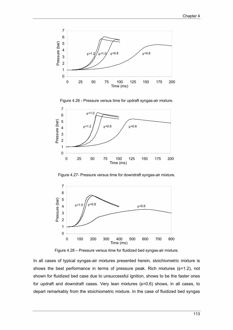
Chapter 4
113
0
1
2
3
4
5
6
7
0 25 50 75 100 125 150 175 200Time (ms)
Pre
ssur
e (b
ar)
φ=0.6φ=0.8φ=1.0φ=1.2
Figure 4.26 - Pressure versus time for updraft syngas-air mixture.
01
23
45
67
0 25 50 75 100 125 150 175 200Time (ms)
Pre
ssur
e (b
ar)
φ=0.6φ=0.8φ=1.2
φ=1.0
Figure 4.27- Pressure versus time for downdraft syngas-air mixture.
0
1
2
3
4
5
6
7
0 100 200 300 400 500 600 700 800Time (ms)
Pre
ssur
e (b
ar)
φ=0.6φ=0.8φ=1.0
Figure 4.28 – Pressure versus time for fluidized bed syngas-air mixture.
In all cases of typical syngas-air mixtures presented herein, stoichiometric mixture is
shows the best performance in terms of pressure peak. Rich mixtures (φ=1.2), not
shown for fluidized bed case due to unsuccessful ignition, shows to be the faster ones
for updraft and downdraft cases. Very lean mixtures (φ=0.6) shows, in all cases, to
depart remarkably from the stoichiometric mixture. In the case of fluidized bed syngas

Experimental and numerical laminar syngas combustion
114
this is endorsed to no spherical propagation as shown above by schilieren flame
images.
Tests runs with initial pressures of 0.5, 2.0, 5.0, and in some cases 6.0 bar were also
performed in order to increase the burning velocity range of pressures. At initial
pressure of 7.0 bar and room temperature (293 K) all typical syngas-air mixtures fail to
ignite.
4.1.2.2 Burning velocity
Figures 4.29 - 4.31 shows stretched burning velocity for typical syngas-air mixtures for
various equivalence ratios using Eq. (4.14). At this stage all the range of points are
shown to emphasize the inaccuracy of the burning velocity calculation due to the
pressure derivative fluctuation in the early stage of flame propagation, where the
pressure does not change to much. After this stage a fast increase in pressure makes
the burning velocity to increase rapidly up to a stable value. Afterwards, a nearly linear
increase in burning velocity is observed. In some cases there is a sudden increase in
burning velocity, which according to Saeed and Stone, (2004) is attributed to the
development of cellular flame. In the final stage burning velocity start to decrease due
to inflection in the pressure curve which gives place to lower pressure derivatives. The
highest pressure derivative defines the upper limit of the inquiry region.
Workers such as Gülder (1984), Metghalchi and Keck, (1982), and Ryan and Lestz
(1980) who used the constant-volume method for the determination of the burning
velocities have assumed that the flame front is smooth, with no cellular or wrinkling
flames. However, cellular flames can be formed under certain conditions, and in the
present study cellularity was found for syngas flames. When cellularity triggers, the
increase in the surface area leads to a sudden increase in the burning velocity and any
inclusion of these data points would lead to higher burning velocity predictions. This is
due to the transformation of the smooth spherical flame front to the polyhedral flame
structures which increase the surface area of the flame front, thereby invalidating the
smooth flame assumption of Eq. (4.14). Therefore, in this work the sudden increase of
burning velocity was removed from the inquiry region.

Chapter 4
115
0.0
0.1
0.2
0.3
0.4
0.5
1 2 3 4 5 6 7Pressure (bar)
Su
(m/s
)
φ=1.2
0.0
0.1
0.2
0.3
0.4
0.5
1 2 3 4 5 6 7Pressure (bar)
Su
(m/s
)
φ=1.0
0.0
0.1
0.2
0.3
0.4
0.5
1 2 3 4 5 6 7Pressure (bar)
Su
(m/s
)
φ=0.8
0.0
0.1
0.2
0.3
0.4
0.5
1 2 3 4 5 6 7Pressure (bar)
Su
(m/s
)
φ=0.6
Figure 4.29 - Burning velocity versus pressure for updraft syngas-air mixture at various
equivalence ratios

Experimental and numerical laminar syngas combustion
116
0.0
0.1
0.2
0.3
0.4
0.5
0.6
0.7
1 2 3 4 5 6 7Pressure (bar)
Su
(m/s
)
φ=0.6
0.0
0.1
0.2
0.3
0.4
0.5
0.6
0.7
1 2 3 4 5 6 7Pressure (bar)
Su
(m/s
)
φ=0.8
0.0
0.1
0.2
0.3
0.4
0.5
0.6
0.7
1 2 3 4 5 6 7Pressure (bar)
Su
(m/s
)
φ=1.0
0.0
0.1
0.2
0.3
0.4
0.5
0.6
0.7
1 2 3 4 5 6 7Pressure (bar)
Su
(m/s
)
φ=1.2
Figure 4.30 – Burning velocity versus pressure for downdraft syngas-air mixture at various
equivalence ratios.
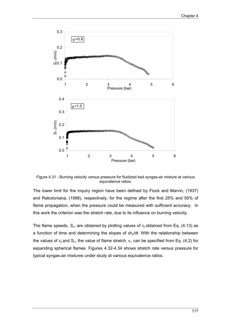
Chapter 4
117
0.0
0.1
0.2
0.3
1 2 3 4 5 6Pressure (bar)
Su
(m/s
)
φ=0.8
0.0
0.1
0.2
0.3
0.4
1 2 3 4 5 6Pressure (bar)
Su
(m/s
)
φ=1.0
Figure 4.31 - Burning velocity versus pressure for fluidized bed syngas-air mixture at various equivalence ratios.
The lower limit for the inquiry region have been defined by Fiock and Marvin, (1937)
and Rakotoniana, (1998), respectively, for the regime after the first 25% and 50% of
flame propagation, when the pressure could be measured with sufficient accuracy. In
this work the criterion was the stretch rate, due to its influence on burning velocity.
The flame speeds, Sn, are obtained by plotting values of rb obtained from Eq. (4.13) as
a function of time and determining the slopes of drb/dt. With the relationship between
the values of rb and Sn, the value of flame stretch, κ, can be specified from Eq. (4.2) for
expanding spherical flames. Figures 4.32-4.34 shows stretch rate versus pressure for
typical syngas-air mixtures under study at various equivalence ratios.

Experimental and numerical laminar syngas combustion
118
0
50
100
150
200
1 2 3 4 5 6 7Pressure (bar)
Stre
tch
(s-1
) 1.2
1.0
0.8
0.6
φ
Figure 4.32 – Stretch rate versus pressure for updraft syngas-air mixture at 1.0 bar.
0
50
100
150
200
1 2 3 4 5 6 7Pressure (bar)
Stre
tch
(s-1
) 1.2
1.0
0.8
0.6
φ
Figure 4.33 – Stretch rate versus pressure for downdraft syngas-air mixture at 1.0 bar.
0
50
100
150
200
1 2 3 4 5 6 7Pressure (bar)
Stre
tch
(s-1
)
1.0
0.8
0.6
φ
Figure 4.34 – Stretch rate versus pressure for fluidized bed syngas-air mixture at 1.0 bar.
These figures show a very similar behavior of the stretch rate versus pressure for all
the syngas–air mixtures and equivalence ratios. Stoichiometric mixtures are highly
stretched and stretch decreases with the equivalence ratio. The criterion of establishing

Chapter 4
119
a minimum pressure to explore the burning velocity is doubtful because it corresponds
to different stretch rate values, as easily could be seen from figures 4.32-4.34.
Therefore, in this work, the criterion is a fixed stretch rate of 50 s-1. For this level of
stretch, the stretched burning velocity is close to the unstretched burning velocity.
4.1.2.3 Laminar burning velocity correlations
The simultaneous change in the pressure and temperature of the unburned mixture
during a closed vessel explosion makes it necessary to rely on correlations which take
these effects into account like the one proposed by Metghalchi and Keck, (1980):
00 0
u uT PS ST P
α β⎛ ⎞ ⎛ ⎞
= ⎜ ⎟ ⎜ ⎟⎝ ⎠ ⎝ ⎠
(4.15)
Where, T0 and P0, are the reference temperature and pressure, respectively. The
influence of the equivalence ratio is incorporated through the temperature and pressure
exponents, α and β, and through the reference burning velocity Su0 as square or linear
functions.
Following the procedure described in the appendix A, this three unknowns are obtained
for the three typical syngas compositions and are shown in the table 4.3.
In all syngas cases the temperature coefficient is positive and the pressure coefficient
negative. This means that the burning velocity increases with temperature increase and
decreases with the increase of pressure. The stretch rate in these correlations is lower
than 50 s-1. This means that these values of the stretched burning velocity are close to
the unstretched ones. Notice the different range of validity of the expressions with the
equivalence ratio and syngas composition. This is due to the unsuccessful ignition.

Experimental and numerical laminar syngas combustion
120
Table 4.3– Parameters α, β and Su0 (m/s) in function of the of the mixture syngas-air.
Parameter P0 = 1.0 bar; T0 = 293 K
φ= 0.6 φ= 0.8 φ= 1.0 φ= 1.2
Updraft syngas
α 2.466 2.047 1.507 1.869
β -0.428 -0.289 -0.259 -0.355
Su0 (m/s) 0.135 0.212 0.303 0.314
Validity range 0.75<P(bar)<9.5
293 <T(K) <425
0.75<P(bar)<20
293 <T(K) <443
0.75<P(bar)<20
293 <T(K) <450
0.75<P(bar)<14.5
293 <T(K) <445
Downdraft syngas
α 1.698 1.581 1.559 1.600
β -0.181 -0.120 -0.159 -0.289
Su0 (m/s) 0.174 0.282 0.345 0.381
Validity range 0.75<P(bar)<15.5
293 <T(K) <413
0.75<P(bar)<20
293 <T(K) <443
0.75<P(bar)<20
293 <T(K) <450
0.75<P(bar)<20
293 <T(K) <450
Fluidized bed syngas
α - 1.827 2.124 -
β - -0.238 -0.518 -
Su0 (m/s) - 0.095 0.137 -
Validity range - 1.0<P(bar)<9.5
293 <T(K) <408
1.0<P(bar)<10
293 <T(K) <430 -
Figure 4.35 shows laminar burning velocity on the reference conditions of pressure and
temperature as a function of the equivalence ratio of the mixture syngas-air.
0
0.1
0.2
0.3
0.4
0.5
0.6 0.8 1.0 1.2Equivalence ratio
Su0
(m/s
)
UpdraftDowndraftFluidized
Figure 4.35 – Evolution of the reference laminar flame speed as a function of the equivalence ratio.
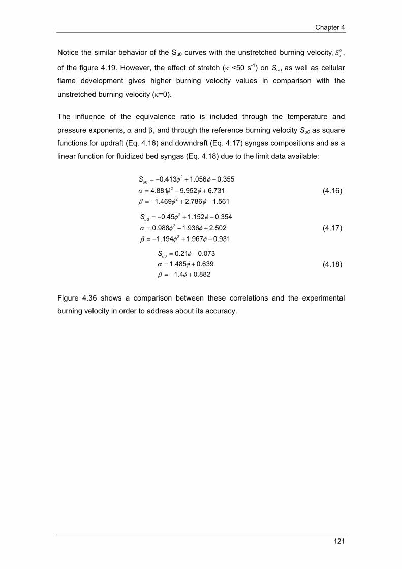
Chapter 4
121
Notice the similar behavior of the Su0 curves with the unstretched burning velocity, 0uS ,
of the figure 4.19. However, the effect of stretch (κ <50 s-1) on Suo as well as cellular
flame development gives higher burning velocity values in comparison with the
unstretched burning velocity (κ=0).
The influence of the equivalence ratio is included through the temperature and
pressure exponents, α and β, and through the reference burning velocity Su0 as square
functions for updraft (Eq. 4.16) and downdraft (Eq. 4.17) syngas compositions and as a
linear function for fluidized bed syngas (Eq. 4.18) due to the limit data available:
20
2
2
0.413 1.056 0.355
4.881 9.952 6.7311.469 2.786 1.561
uS φ φ
α φ φ
β φ φ
= − + −
= − +
= − + −
(4.16)
20
2
2
0.45 1.152 0.354
0.988 1.936 2.5021.194 1.967 0.931
uS φ φ
α φ φ
β φ φ
= − + −
= − +
= − + −
(4.17)
0 0.21 0.0731.485 0.639
1.4 0.882
uS φα φβ φ
= −
= += − +
(4.18)
Figure 4.36 shows a comparison between these correlations and the experimental
burning velocity in order to address about its accuracy.

Experimental and numerical laminar syngas combustion
122
0
0.1
0.2
0.3
0.4
0.5
0.6
0 5 10 15 20 25Pressure (bar)
Su
(m/s
)
ExperimentalCorrelation
2.0 bar
5.0 bar
1.0 bar
0.5 bar
(a)
0
0.1
0.2
0.3
0.4
0.5
0.6
0.7
0 5 10 15 20 25Pressure (bar)
Su
(m/s
)
ExperimentalCorrelation
2.0 bar
5.0 bar
1.0 bar0.5 bar
(b)
0
0.05
0.1
0.15
0.2
0 2 4 6 8 10 12Pressure (bar)
Su
(m/s
)
ExperimentalCorrelation
2.0 bar
5.0 bar
1.0 bar
0.8 bar
(c)
Figure 4.36 – Comparison between experimental and correlated burning velocities of syngas-air stoichiometric mixtures at different initial pressures within the chamber. (a) updraft; (b)
downdraft; (c) fluidized bed.

Chapter 4
123
A very good agreement between the correlation and the experimental burning velocity
is found for every initial pressure test runs performed. Notice that for fluidized bed
syngas the lower initial pressure with successful ignition was 0.8 bar. The maximum
error of the burning velocity correlation is 8% for updraft syngas, 9% for downdraft
syngas and 5% for fluidized bed syngas. These errors are perfectly reasonable and the
discrepancy between syngas compositions errors has to do with experimental burning
velocity scattering.
4.2. Multi-zone spherical combustion
In an engine cycle, the heat losses could be endorsed 25% to wall-flame interaction
and 75% to the wall-burned gases interaction (Boust, 2006). Therefore, robust heat
transfer models of wall-flame interaction should be employed. A multi-zone numerical
heat transfer simulation code developed at the Laboratoire de Combustion et
Détonique for methane-air mixtures by Boust, (2006) is adapted herein to syngas-air
mixtures. The code allows simulating the combustion of homogeneous premixed gas
mixtures within constant volume spherical chamber centrally ignited. In spherical
combustion conditions, the model could also be used for predicting the quenching
distance.
4.2.1 Mathematical model
4.2.1.1 Flame propagation
The flame is considered a perfect sphere without thickness. The propagation of the
flame is imposed by its burning velocity that determines the thickness of the zone to
burn during a predefined time Δt. The combustion is supposed isobaric, being the
burning velocity Su given by the empirical correlation of Metghalchi and Keck, (1980)
expressed by the Eqs. 4.16 - 4.18.
The criterion that defines the end of combustion is the flame quenching distance. The
quenching distance defines how close the flame approaches the wall and plays a
definitive role on the wall-flame interaction as shown by Boust, (2006). The quenching
implementation in the computational code consists of stopping the propagation of the
flame when it approaches the wall in an equal distance to the frontal quenching
distance δq. In order to estimate the quenching distance, the correlation of Westbrook
et al., (1981) is used:

Experimental and numerical laminar syngas combustion
124
0 060 3 5 ..q
bb u u pb
Pe PS C
δλ ρ
−= = (4.19)
Where Peb is the Peclet number and P the pressure in MPa. This correlation was
obtained for stoichiometric methane-air and methanol-air mixtures for pressures 1-40
atm. Recently Boust, (2006) shows that this correlation is also valid for lean (φ=0.7)
methane-air mixtures and stoichiometric hydrogen-air mixtures. For these reasons, we
shall use correlation (4.19) for syngas-air mixtures.
4.2.1.2 Chemical equilibrium
Gases can have two possible states, burned and unburned. The composition of the
burned gases is calculated by the Brinkley method, suggested by Heuzé et al., (1985).
This method is based on the determination of the free energy of Gibbs from the Gordon
& McBride, (1971) polynomials. The chemical equilibrium is calculated by canceling the
chemical affinity in the chemical reactions. It appeals to the thermodynamic properties
of the species instead of the equilibrium constants.
The combustion products considered are H2O, CO2, CO, O2, N2, NO, OH and H2. As
pressure and temperature conditions change during the compression and cooling
phases, is possible to previously recalculate the composition of burned gases.
4.2.1.3 Heat transfer
A common approach exploiting a combined convective and radiative heat transfer
coefficient has been implemented as representative of heat transfer through the
chamber walls, Qw. The formulation couples a convective-equivalent heat transfer
coefficient to a radiative term, for taking into account the effects due to high
temperature burned gases:
w c rQ Q Q= + (4.20)
Where Qc and Qr represents the convective and radiative heat transfer, respectively.
The unburned gases in contact with the wall are heated by compression under the
effect of expansion flame. Due to the higher temperature of the unburned gases in
comparison with the chamber wall, which is at room temperature, they yield heat by
conduction. This conductive heat transfer is simulated using a convective model
(Boust, 2006).

Chapter 4
125
( )c g wQ h T T= − (4.21)
with Tg and Tw, respectively, the temperature of the gases and wall and, h, the
convective heat transfer coefficient. Tw is considered constant as it varies less than 10
K during combustion as reported by Boust, (2006). Tg is the local temperature of the
gases. The determination of the convective heat transfer coefficient is case sensitive
and several models are available in the literature [Annand (1963), Woschni (1967), or
Hohenberg (1979)]. In this code the Woschni, (1967) model, which is based on the
hypotheses of forced convection is applied and compared with the recent heat transfer
model of Rivère, (2005) based on the gases kinetic theory (see appendix C). The
Woschni (1967) heat transfer correlation is given as:
0 2 0 8 0 55 0 8130 − −= . . . .( ) ( ) ( ) ( )gh t B P t T t v t (4.22)
where B is the bore (m), P and T are the instantaneous cylinder pressure (bar) and gas
temperature (K), respectively. The instantaneous characteristic velocity, v is defined as:
2 28 0 00324r
. . ( )P
⎛ ⎞= + −⎜ ⎟
⎝ ⎠s r
p motr
V Tv S P PV
(4.23)
Where Pmot=Pr(Vr/V)γ is the motored pressure. Sp is mean piston speed (m/s), Vs is
swept volume (m3), Vr, Tr and Pr are volume, temperature and pressure (m3, K, bar)
evaluated at any reference condition, such as inlet valve closure, V is instantaneous
cylinder volume (m3) and γ is the specific heat ratio. The second term in the velocity
expression allows for movement of the gases as they are compressed by the
advancing flame.
In the model of Rivère, (2005) the heat transfer coefficient is obtained as follows:
322.g g
ww
Rh TM TT
χ λρ ηπ
⎛ ⎞⎛ ⎞= + −⎜ ⎟⎜ ⎟ ⎜ ⎟⎝ ⎠ ⎝ ⎠ (4.24)
where ρg, Tg and M are, respectively, the density, the temperature and molar mass of
the gases. The last parenthesis in the right side of the Eq. (4.26) represents the heat
transfer coefficient that depends on the gases temperature that determines the length
of the boundary layer. χ and λ are the material constants and η a function of the
aerodynamic conditions equal to zero in the advection absence.

Experimental and numerical laminar syngas combustion
126
Heat radiation of the burned gases to the chamber walls are modeled neglecting the
radiation of the particles. This assumption is reasonable due to the high purity of the
tested mixtures. During combustion, heat radiation can have origin on unburned gases,
which contains: H2, CO, CH4, CO2, N2 and O2, and also on the burned gases, which
mainly contains: CO2, H2O and N2, being irrelevant the remaining combustion products.
Only molecules that have a non null dipolar moment are susceptible to emit thermal
radiation (Boust, 2006). Therefore only CO2, H2O and CH4 are considered. In practical
terms, the radiation of the unburned gases heated by compression is insignificant
comparatively with the burned gases, which temperature is 6-7 times higher. Thus, it is
assumed that only CO2 and H2O radiates significantly.
The radiation heat transfer is modeled by the Stefan’s law considering the burned
gases as a grey body with uniform temperature Tg and ε the apparent grey-body
emissivity calculated from the contributions of H2O and CO2. As the spectral
emissivities of these species are similar, the emissivity variation term Δε is included.
2 2CO H Oε ε ε ε= + − Δ (4.25)
At the end of combustion, only burned gases are inside the chamber. Then, the net
superficial radiative flow Q,r received by the wall, with absorption factor α, from the
burned gases is given by the Stefan’s constant.
( )4 4r g wQ T Tα ε σ= − (4.26)
When the sphere of burned gases (radius r) does not occupy the entire chamber
(radius R), the sphere surface ratio gives the radiative flow.
2
2
44
( )r rrQ r QR
ππ
= (4.27)
The emissivity of H2O and CO2 as well as the variation term are calculated using the
correlation of Leckner, (1972). This correlation reproduces the gases temperature
influence, the partial pressure of each species and the length of the average radius.
4.2.2 Calculation procedure
In the multi-zone model, flame propagation is seen as the consecutive consumption of
unburned mixture within the zones with an equal mass distribution between the zones

Chapter 4
127
in the spherical vessel (Fig. 4.37). Before ignition, the mass in the spherical vessel is
divided into n zones. At the time when combustion has just begun in the bomb, the
flame front will consume zone 1 first. As a result, the temperature and hence pressure
of zone 1 will increase, thereby compressing the rest of the unburned gas (considered
as single entity) and increasing the pressure inside the vessel to a higher value. After
the consumption of the first zone, combustion of the second and subsequent zones will
take place at a higher pressure than the initial pressure. At any instant of time when the
flame front is passing through the nth zone, the combustion of this zone takes place at a
temperature of Tu,n−1 (> Ti) and a constant pressure Pu,n−1 (> Pi). The combustion within
a given zone takes place progressively. After the flame has consumed the nth zone, it is
then assumed to be adiabatic. Subsequent combustion further compresses the burned
gas and the unburned gas. As a result, temperature and density gradients are
established in the burned gas region. At the end of combustion, the burned gas cooling
is computed.
Figure 4.37 – Radial distribution of the multiple zones inside a spherical vessel. Hatched portion indicates the position of the flame front at an instant of time.
Figure 4.38 shows the flowchart of the adapted Fortran code. The output data of the
code are: the burned gas temperature, flame radius and flame speed, pressure, as well
as the wall thermal flux. At the end of combustion, an energy balance is made.

Experimental and numerical laminar syngas combustion
128
Figure 4.38 – Combust flowchart.
4.2.3 Results discussion and code validation
The numerical results are validated for syngas-air mixtures by comparison with
experimental results of pressure evolution. Different equivalence ratios and pressures

Chapter 4
129
are tested and discussed. The numerical code described above is then used to
estimate the heat flux and quenching distance of syngas-air mixtures.
4.2.3.1 Influence of the heat transfer model
In order to define the heat transfer model to use, one first compare two formulations
already mentioned above: the classical Woschni (1967) correlation and the recent
Rivère (2005) formulation. The comparison of both formulations is made in the figure
4.39.
0
1
2
3
4
5
6
7
0 10 20 30 40 50 60 70 80 90 100Time (ms)
Pre
ssur
e (b
ar)
0
100
200
300
400
500
Qw
(kW
/m2 )
Experimental P
Woschni P
Rivère P
Woschni Qw
Rivère Qw
Figure 4.39 – Influence of the heat transfer model – stoichiometric downdraft syngas-air, P=1.0 bar.
From figure 4.39 is possible to conclude that the heat transfer model has only marginal
influence on pressure curve. However, the Rivère model shows to better follow the
pressure curve on the cooling side. The reason is the higher value of the heat flux
through the wall using this model. This result is in agreement with Boust, (2006), who
compared these models with experimental heat flux values for methane-air mixtures
and concluded that Rivère model is most suitable to simulate the wall-flame heat
transfer and that Woschni model is inadequate in the absence of a strong flow. Thus,
Rivère model is applied throughout the following results.
4.2.3.2 Influence of equivalence ratio
The influence of the equivalence ratio in the burning velocity and pressure was
experimentally determined for the syngas compositions under study. It was seen that
the pressure and burning velocity decreases when departing from stoichiometric

Experimental and numerical laminar syngas combustion
130
conditions. Figures 4.40 – 4.42 shows experimental and numerical pressure and the
heat flux for updraft syngas-air mixture at φ=0.8, φ=1.0 and φ=1.2, respectively.
0
1
2
3
4
5
6
7
0 10 20 30 40 50 60 70 80 90 100Time (ms)
Pre
ssur
e (b
ar)
0
100
200
300
400
500
Qw
(kW
/m2 )
Experimental P
Numerical P
Qw
Figure 4.40 – Pressure and heat flux for updraft syngas-air at φ=0.8, P=1.0 bar, T= 293 K.
0
1
2
3
4
5
6
7
0 10 20 30 40 50 60 70 80 90 100Time (ms)
Pre
ssur
e (b
ar)
0
100
200
300
400
500
Qw
(kW
/m2 )
Experimental P
Numerical P
Qw
Figure 4.41– Pressure and heat flux for updraft syngas-air at φ=1.0, P=1.0 bar, T= 293 K.

Chapter 4
131
0
1
2
3
4
5
6
7
0 10 20 30 40 50 60 70 80 90 100Time (ms)
Pre
ssur
e (b
ar)
0
100
200
300
400
500
Qw
(kW
/m2 )
Experimental P
Numerical P
Qw
Figure 4.42 – Pressure and heat flux for updraft syngas-air at φ=1.2, P=1.0 bar, T= 293 K.
From figures 4.40-4.42 one can conclude that pressure evolution of updraft syngas-air
mixtures is accurately reproduced by the code for each equivalence ratio. However,
pressure peak is always higher than the experimental measurement as well as in the
cooling phase. It was found important chamber leakages at this stage, and so the
chamber was repaired. The following results were obtained after the reparation.
Figures 4.43 - 4.45 shows experimental and numerical pressure and the heat flux for
downdraft syngas-air mixture at φ=0.8, φ=1.0 and φ=1.2, respectively.
0
1
2
3
4
5
6
7
0 10 20 30 40 50 60 70 80 90 100Time (ms)
Pre
ssur
e (b
ar)
0
100
200
300
400
500
Qw
(kW
/m2 )
Experimental P
Numerical P
Qw
Figure 4.43 – Pressure and heat flux for downdraft syngas-air at φ=0.8, P=1.0 bar, T= 293 K.

Experimental and numerical laminar syngas combustion
132
0
1
2
3
4
5
6
7
0 10 20 30 40 50 60 70 80 90 100
Time (ms)
Pre
ssur
e (b
ar)
0
100
200
300
400
500
Qw
(kW
/m2 )
Experimental P
Numerical P
Qw
Figure 4.44 – Pressure and heat flux for downdraft syngas-air at φ=1.0, P=1.0 bar, T= 293K.
0
1
2
3
4
5
6
7
0 10 20 30 40 50 60 70 80 90 100Time (ms)
Pre
ssur
e (b
ar)
0
100
200
300
400
500
Qw
(kW
/m2 )
Experimental P
Numerical P
Qw
Figure 4.45 – Pressure and heat flux for downdraft syngas-air at φ=1.2, P=1.0 bar, T= 293 K.
Figures 4.46 - 4.47 shows experimental and numerical pressure and the heat flux for
fluidized bed syngas-air mixture at φ=0.8 and φ=1.0, respectively.

Chapter 4
133
0
1
2
3
4
5
6
7
0 50 100 150 200 250 300Time (ms)
Pre
ssur
e (b
ar)
0
100
200
300
400
500
Qw
(kW
/m2 )
Experimental P
Numerical P
Qw
Figure 4.46 – Pressure and heat flux for fluidized bed syngas-air at φ=0.8, P=1.0 bar, T= 293 K.
0
1
2
3
4
5
6
7
0 50 100 150 200 250 300Time (ms)
Pre
ssur
e (b
ar)
0
100
200
300
400
500
Qw
(kW
/m2 )
Experimental P
Numerical P
Qw
Figure 4.47 – Pressure and heat flux for fluidized bed syngas-air at φ=1.0, P=1.0 bar, T= 293 K.
From these figures, it is possible to conclude that the code over-estimates the pressure
for fluidized bed syngas. The extremely low burning velocity of this syngas composition
makes gravity forces being felt within the chamber, which makes the burned gases to
move to the top of the chamber and the flame to propagate to the bottom as shown in
the figure 4.5. Therefore, the assumption of spherical combustion is no longer valid.
4.2.3.3 Influence of the pressure
Let us now verify if pressure effect is accurately reproduced by the code. Figures 4.48 -
4.49 shows pressure and heat flux for stoichiometric syngas-air mixtures at 5.0 bar.
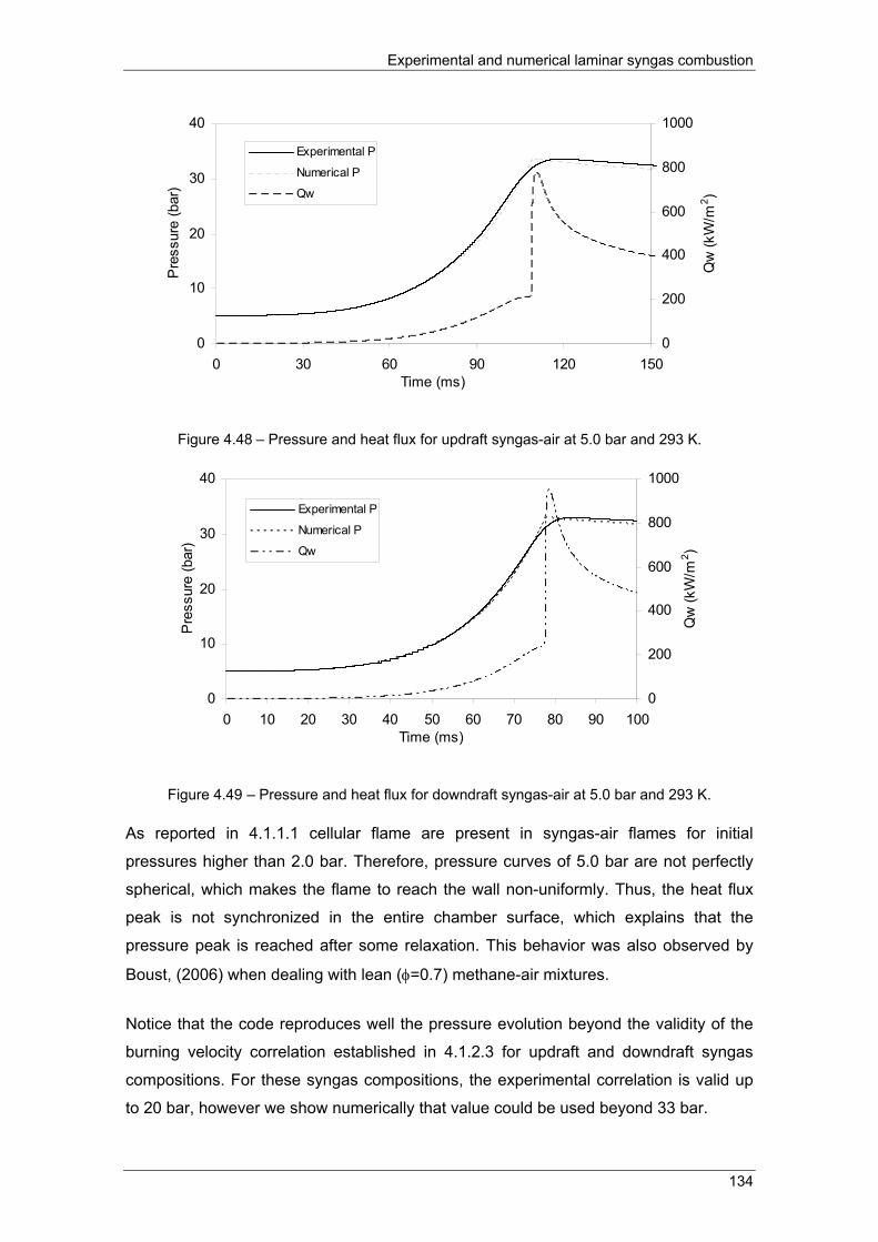
Experimental and numerical laminar syngas combustion
134
0
10
20
30
40
0 30 60 90 120 150Time (ms)
Pre
ssur
e (b
ar)
0
200
400
600
800
1000
Qw
(kW
/m2 )
Experimental P
Numerical P
Qw
Figure 4.48 – Pressure and heat flux for updraft syngas-air at 5.0 bar and 293 K.
0
10
20
30
40
0 10 20 30 40 50 60 70 80 90 100Time (ms)
Pre
ssur
e (b
ar)
0
200
400
600
800
1000
Qw
(kW
/m2 )
Experimental P
Numerical P
Qw
Figure 4.49 – Pressure and heat flux for downdraft syngas-air at 5.0 bar and 293 K.
As reported in 4.1.1.1 cellular flame are present in syngas-air flames for initial
pressures higher than 2.0 bar. Therefore, pressure curves of 5.0 bar are not perfectly
spherical, which makes the flame to reach the wall non-uniformly. Thus, the heat flux
peak is not synchronized in the entire chamber surface, which explains that the
pressure peak is reached after some relaxation. This behavior was also observed by
Boust, (2006) when dealing with lean (φ=0.7) methane-air mixtures.
Notice that the code reproduces well the pressure evolution beyond the validity of the
burning velocity correlation established in 4.1.2.3 for updraft and downdraft syngas
compositions. For these syngas compositions, the experimental correlation is valid up
to 20 bar, however we show numerically that value could be used beyond 33 bar.

Chapter 4
135
4.2.3.4 Quenching distance and heat flux estimations
After validating the numerical code for updraft and downdraft syngas compositions,
under various conditions of pressure and equivalence ratios, one can then use it to
predict the quenching distance and heat flux of syngas-air mixtures.
As flame propagates from the centre of the chamber, pressure increases, and
consequently the temperature also increases. This is the compression phase (1) in the
figure 4.50. The heat transfer from the unburned gases to the wall, manly by
conduction, but also marginally by radiation. The heat flux through the wall increases
up to the flame quenching.
During wall-flame interaction, the flame transfer in average one third of its thermal
power to the wall (Boust, 2006), which makes a heat flux peak to appear. The flame is
quenched at a finite distance to the wall, the quenching distance. It remains, therefore,
a thin layer of unburned gases between the burned gases and the wall. The instant of
the heat flux peak is less reproducible than its amplitude. In fact, such instant is
somewhere between the inflexion point of the pressure curve and the instant of
maximum pressure. During this phase (2), the wall-flame interaction is gradually
dispersed throughout the chamber, which explains the inflexion point in the pressure
curve. The existence of the phase (2) indicates that combustion is not strictly spherical.
After the peak of pressure, the combustion phase gives place to the cooling phase (3).
The wall heat losses are now only due to the burned gases heat source. The heat
transfer is made through the thin layer of unburned gases between the burned gases
and wall.
0.0
0.2
0.4
0.6
0.8
1.0
0 50 100 150 200 250 300
Time (ms)
P (M
Pa)
; Q
w (M
W/m
2 )
P
Qw
d2P/dt2
(3)(2)(1)
---------
Figure 4.50 – Combustion development in spherical chamber fluidized bed syngas.

Experimental and numerical laminar syngas combustion
136
In order to quantify the thermal losses of different mixtures special care must be taken
in the heat flux integration. The integration time should capture the entire phenomenon.
The cooling time is possible to control by establishing a certain cooling period.
However, the combustion time changes with the fuel, initial pressure and equivalence
ratio, which calculation is not straightforward. Therefore, the comparison of heat flux
estimative already shown in figures 4.41-4.49 is made based on the heat flux peaks
(Table 4.4).
Table 4.4 – Heat Flux peaks for stoichiometric syngas-air and methane-air mixtures.
Qw (kW/m2) Updraft Downdraft Methane (Boust, 2006)
1.0 bar, φ=0.8 216 kW/m2 350 kW/m2 -
1.0 bar, φ=1.0 368 kW/m2 402 kW/m2 649 kW/m2
1.0 bar, φ=1.2 220 kW/m2 313 kW/m2 -
5.0 bar, φ=1.0 777 kW/m2 949 kW/m2 (*) 1622 kW/m2
(*) linear interpolation.
From Table 4.4 some conclusions can be drawn:
- The heat flux increases with initial pressure increase for all cases. The amount
(volume and energy) of the explosive mixture inside the vessel increases with
initial pressure increase.
- The heat flux increases with the heat value of the fuel-air mixture. In this case,
one should also take into account the air-fuel ratio.
- The equivalence ratio has the influence of decreasing the heat flux compared to
stoichiometric mixtures and follows the behavior of pressure peak.
The thickness of wall quench layers is a primary source of unburned fuels (Saeed and
Stone, 2004). Thus, this combustion characteristic is very important and was predicted
for stoichiometric updraft and downdraft syngas compositions by the Westbrook
criterion defined by a zero flame stretch (figure 4.51). This is practically the case when
the flame reaches the wall given the large curvature radius. The Westbrook criterion is
valid in pressure range 1-40 bar and burning velocity correlation used in the code
shows to be valid up to 33 bar, thus one impose this limit to quenching distance
estimation.

Chapter 4
137
1
10
100
1000
10000
1 10 100 1000Pressure (bar)
Que
nchi
ng d
ista
nce
(10-6
m)
Updraft
Dow ndraft
Methane
Figure 4.51 – Quenching distance estimation for stoichiometric syngas-air mixtures and comparison with stoichiometric methane-air mixture (Boust, 2006).
Figure 4.51 also includes quenching distance of stoichiometric methane-air mixture for
comparison reasons. The following correlation determined by Boust, (2006) was
adopted δq =50 P-0.45 (P>3.0 bar) with P in Mpa and δq in μm. One can conclude that
quenching distance decreases with the increase of pressure and is higher for lower
heating value mixtures.
The following correlations are developed for stoichiometric updraft and downdraft
syngas-air mixtures, similar to the one presented by Westbrook et al., (1981) and
Boust, (2006) for methane-air mixtures:
δq=450 P-0.79 , P>0.3 MPa (Updraft) (4.28)
δq=300 P-0.89 , P>0.3 MPa (Downdraft) (4.29)
With δq in μm and P in MPa.
4.3 Conclusion
Laminar flame characteristics of three typical syngas compositions were studied in a
constant volume chamber for various equivalence ratios. The influence of stretch rate
on flame was determined by the correspondent Markstein and Karlovitz numbers.
Combustion demonstrates a linear relationship between flame radius and time for
syngas–air flames. The maximum value of syngas-air flame speeds is presented at the
stoichiometric equivalence ratio, while lean or rich mixtures decrease the flame speeds.

Experimental and numerical laminar syngas combustion
138
Tendency observed on the unstretched burning velocity is in agreement with the heat
of reaction of the syngas composition. The higher heat value is associated with the
higher amount of H2 and lower dilution by N2 and CO2 in the syngas composition. The
incomplete combustion and ignition difficulty of the typical fluidized bed syngas
composition makes it a less candidate to stationary power applications without addition
of another fuel. Markstein numbers shows that syngas-air flames are generally
unstable. Karlovitz numbers indicates that syngas-air flames are little influenced by
stretch rate. Based on the experimental data a formula for calculating the laminar
burning velocities of syngas–air flames is proposed.
The laminar burning velocity of typical syngas compositions is not dissimilar to that of
methane especially the downdraft syngas case, although somewhat slower than
propane. This could be due to the syngas stoichiometric air–fuel ratio that is ten times
lower than the methane air-fuel ratio and more than twenty times in the case of
propane. Thus, the energy content per unit quantity of mixture (air + fuel) inducted to
the chamber is only marginally lower when using syngas, compared with the
corresponding common gas fuels. The values of laminar burning velocity reported for
syngas (28H2-25CO-47N2) can be seen to be higher than those obtained for the
syngas in the current study; this is associated with the lower H2 content, greater N2
content and the presence of CO2 in the typical syngas compositions. The simulated
syngas mixture that better matches the magnitude of laminar burning velocity for the
typical syngas compositions is the mixture comprising 5%H2/95%CO.
Base on the experimental data some empirical formulations of the burning velocities
have been establish for pressure range 0.75-20 bar and temperature range 293K-
450K.
The numerical simulation code of the laminar spherical combustion allows the pressure
and wall heat flux reproduction under a various conditions of pressure, equivalence
ratio and fuel. Quenching distance correlations for typical syngas-air flames were
developed tanks to this code. One can conclude that quenching distance decreases
with the increase of pressure and is higher for lower heating value mixtures.

Chapter 5
139
CHAPTER 5
EXPERIMENTAL STUDY OF ENGINE-LIKE TURBULENT COMBUSTION The main advantage that comes from the use of syngas (as well as other gases) in SI
engines over the conventional liquid, petroleum-based fuels is the potential for
increased thermal efficiency (Rakopoulus and Michos, 2008). This is attributed to the
relatively high compression ratios permitted, usually by converting Diesel engines for
gaseous fuel operation in the SI mode (Stone and Ladommatos, 1991), since CO and
CH4 are characterized by high anti-knock behavior (Li and Karim, 2006). On the
contrary, the relatively increased end-gas temperature, which the fast flame
propagation rate of H2 can produce during combustion and can be responsible for
knock onset, is compensated for by the presence of diluents in the fuel (N2 and CO2).
Their effect on combustion is to lower flame speed and consequently decrease the in-
cylinder pressures and temperatures. The lean-burn combustion mode usually adopted
in gas engines also contributes to this aim. They are charged with fresh mixtures
having air–fuel ratios sufficiently greater than stoichiometric (Rousseau et al., 1999).
The moderation of peak gas temperatures during combustion, attributed to the last two
features, has also a reduction effect on NOx emissions (Heywood, 1988).
Besides, the drawback of reduced power output using fuels with relatively low heating
values can be partially balanced by turbo-charging the engine. Towards the direction of
minimizing this power derating when, for example, syngas with low heating value equal
to 4–6 MJ/Nm3 is used instead of natural gas with low heating value of approximately
30 MJ/Nm3, contributes the fact that the syngas stoichiometric air–fuel ratio is about 1.2
compared with the value of 17 for the natural gas case (Rakopoulos and Michos,
2008). Thus, the energy content per unit quantity of mixture (air + fuel) inducted to the
cylinder is only marginally lower when using syngas, compared with the corresponding
natural gas case (Sridhar et al., 2001).
In this chapter an experimental approach to syngas engine performance on a rapid
compression machine (RCM) is made.
5.1 RCM single compression
A rapid compression machine (RCM) is an instrument to simulate a single cycle of an
internal combustion engine, thus also allowing the study of various parameters under

Experimental study of engine-like turbulent combustion
140
more favorable conditions than those existing in real engines (Strozzi et al., 2008),
specially the spontaneous ignition (Brett et al., 2001). RCM can operate under two
different modes: single compression and compression – expansion.
The study of the compression process in a RCM operating without combustion is useful
to identify different parameters related with its operation, namely the heat transfer to
the walls. Once determined, these parameters can also be used during the usual firing
cycle. In fact, a common practice in engine testing for combustion diagnostic is, prior to
the usual firing tests, to test the engine in motored conditions, with air as the only
working gas (Lapuerta et al., 2003).
5.1.1 Sensibility analysis
In this section a sensibility analysis is made with the objective of evaluating the
influence of errors in measurement techniques and in the estimation of various
parameters on the main experimental results. In this analysis the chamber wall
temperature is considered as constant.
5.1.1.1 TDC position
In order to determine the precision of the RCM top dead center (TDC) position, a
position sensor was placed at TDC and various tests performed without combustion in
order to eliminate the effect of the spark time scattering. The analysis of the TDC signal
for the whole single compression experiments without combustion performed with
syngas-air and methane-air mixtures enables to define a typical scattering of the TDC
position on less than 1.67 ms. Considering that the compression stroke duration is 44
ms, this gives an overall uncertainty of 3.8% on the TDC position. In order to determine
the influence of this scattering on pressure signal for the updraft-syngas case both
signals are plotted in figure 5.1.

Chapter 5
141
0
5
10
15
20
25
30
100 110 120 130 140 150 160
Time (ms)
Pre
ssur
e (b
ar)
0
2
4
6
8
10
Vol
tage
(V)
Figure 5.1 – TDC position: compression of updraft syngas-air mixture.
In this case, the jitter on the TDC position is 1.67 ms, which makes the pressure signal
being shifted to the right. Therefore, synchronization with reference to TDC is needed.
Figure 5.2 shows the result after TDC synchronization, where both signals are
overlapped.
0
5
10
15
20
25
30
100 110 120 130 140 150 160
Time (ms)
Pre
ssur
e (b
ar)
0
2
4
6
8
10
Vol
tage
(V)
Figure 5.2 – Pressure signal after TDC synchronization for compression of updraft syngas-air mixture
This procedure was followed for every RCM experimental data.
5.1.1.2 Initial piston position
The initial piston position is only dependent of piston mechanical adjustment at the
bottom dead center (BDC). The analysis of the initial position of the piston for the whole

Experimental study of engine-like turbulent combustion
142
single compression experiments performed enables to define a typical scattering on
less than 4.0 mm (from -13 mm to -17 mm).
The TDC position has also some scattering but only of 1 mm (from 419 mm to 420 mm)
which could be endorsed to some mechanical deformation imposed by elevated in-
cylinder pressures. Considering a piston stroke of 419 mm, the overall uncertainty of
the piston initial position is lower than 1.0%. This jitter on the initial position can be
converted to time scale by considering the average piston speed of 9.5 m/s. This
conversion gives a maximum value of 0.42 ms.
Considering that the volume inside the chamber is obtained from the piston position,
the influence of this jitter on the piston position from one experiment to another is then
analyzed in figure 5.3 for the case of updraft syngas without combustion in order to
avoid the effect of the spark time scattering. The choice of the same fuel also avoids
differences in the polytropic coefficient of the mixture being compressed.
In the case shown in the figure 5.3, the difference in the initial piston position is 1.75
mm. It is observed that there is no significant difference on the piston position along
time.
Figure 5.3- Piston displacement during single compression of updraft syngas-air.
From figure 5.3 it is also observed the evolution in a “stair” mode of the laser piston
position signal. As the in-cylinder volume variation is obtained from this signal,
therefore a peak detection filter was applied to this signal (figure 5.4).
0
90
180
270
360
450
90 100 110 120 130 140Time (ms)
Pis
ton
posi
tion
(mm
)

Chapter 5
143
0
10
20
30
92 93 94 95 96 97 98 99 100
Time (ms)
Pis
ton
posi
tion
(mm
)
Figure 5.4 – Peak detection filter.
5.1.1.3 Spark time
Spark time is defined by the diagnostic system of the RCM in a time scale. Thus, this
signal is independent of the piston displacement. In order to analyze the jitter of the
spark time, figure 5.5 shows the three signals for the case of ignition at TDC and in
addition the TDC position in a time scale.
0
1
2
3
4
5
6
135 136 137 138 139 140 141 142 143 144 145Time (ms)
Vol
tage
(V)
Figure 5.5 – Spark time at TDC and TDC position signals.
Analysing the figure 5.5 it is observed that the spark signal varies slightly (<0.5 ms)
from experiment to experiment while keeping the duration of 5.0 ms. Comparing with
the TDC position given by the laser position sensor at TDC it is observed that they are
not synchronized. The maximum unsynchronized signals are out of phase 0.7 ms.
Spark
Piston position

Experimental study of engine-like turbulent combustion
144
Let us now verify the influence of spark time jitter on the pressure signal. For this
analysis two cases with similar scatter of spark time (0.84 ms and 0.87 ms,
respectively) are presented for different ignition timings, 5.0 ms BTDC and 12.5 ms
BTDC.
0
10
20
30
40
50
60
70
100 105 110 115 120 125 130 135 140 145 150 155 160Time (ms)
Pre
ssur
e (b
ar)
0
2
4
6
8
10
12
Vol
tage
(V)
Figure 5.6 – Pressure and spark signals for updraft syngas: ignition at 5.0 ms BTDC.
0
10
20
30
40
50
60
70
100 110 120 130 140 150 160Time (ms)
Pre
ssur
e (b
ar)
0
2
4
6
8
10
12
Vol
tage
(V)
Figure 5.7 – Pressure and spark signals for downdraft syngas: ignition at 12.5 ms BTDC.
Analyzing figures 5.6 and 5.7 is observed that the effect of the spark time scatter has
higher influence on in-cylinder pressure when the ignition is made close to TDC. This
could also justify the fact of lower reproducibility of pressure signal for ignition timings
close to TDC as shown in the next section.

Chapter 5
145
5.1.1.4 In-cylinder pressure reproducibility
A set of three experiments was carried out for each syngas composition with various
ignition timings in order to verify its repetition. The pressure traces are shown in figure
5.8 for downdraft syngas composition after TDC synchronization.
0
20
40
60
80
90 100 110 120 130 140 150 160 170 180
Time (ms)
Pre
ssur
e (b
ar)
Shot 1
Shot 2
Shot 3
(a)
0
20
40
60
80
90 100 110 120 130 140 150 160 170 180Time (ms)
Pre
ssur
e (b
ar)
Shot 1
Shot 2
shot 3
(b) Figure 5.8a – Pressure signals for various ignition timings. (a) TDC. (b) 5 ms BTDC. (c) 7.5 ms
BTDC.

Experimental study of engine-like turbulent combustion
146
0
20
40
60
80
90 100 110 120 130 140 150 160 170 180Time (ms)
Pre
ssur
e (b
ar)
Shot 1
Shot 2
Shot 3
(c)
0
20
40
60
80
90 100 110 120 130 140 150 160 170 180Time (ms)
Pre
ssur
e (b
ar)
Shot 1
Shot 2
Shot 3
(d)
Figure 5.8 b – Pressure signals for various ignition timings. (c) 7.5 ms BTDC. (d) 12.5 ms
BTDC. Figure 5.8 shows the good reproducibility of the pressure signal for various ignition
timings. The maximum difference between peak pressures is: 1.8 bar for ignition at
TDC (70 bar on average, which represents an error of 2.5%); 0.8 bar for ignition timing
at 5 ms BTDC (69.2 bar on average representing an error of 1.1%); 0.5 bar for ignition
timing at 7.5 ms BTDC (68.8 bar on average, which represents an error of 0.7%);0.5
bar for ignition timing at 12.5 ms BTDC (68.4 bar on average representing an error of
0.7%).
5.1.1.5 Conclusion
The quality of the RCM experimental measurements was evaluated on this section
throughout a sensibility analysis of errors in measurement techniques and in the

Chapter 5
147
estimation of various parameters on the main experimental results: in-cylinder pressure
and volume. This analysis shows the high precision of the Institute Pprime RCM for
every measured parameter, which ensures about the quality of the results that will be
shown in the following sections.
5.1.2 In-cylinder pressure
Figures 5.9-5.10 show RCM experimental pressure histories of stoichiometric syngas-
air mixtures for various spark times and compression ratio ε =11. Four ignition timings
were tested: TDC, 5.0, 7.5 and 12.5 ms before TDC, respectively.
0
20
40
60
80
80 90 100 110 120 130 140 150 160 170 180 190 200
Time (ms)
Pre
ssur
e (b
ar)
0.0 ms BTDC
5.0 ms BTDC
7.5 ms BTDC
12.5 ms BTDC
Compression
Figure 5.9 – Pressure versus time for stoichiometric updraft syngas-air mixture at various spark
times.
0
20
40
60
80
80 90 100 110 120 130 140 150 160 170 180 190 200Time (ms)
Pre
ssur
e (b
ar)
0.0 ms BTDC
5.0 ms BTDC7.5 ms BTDC
12.5 ms BTDCCompression
Figure 5.10– Pressure versus time for stoichiometric downdraft syngas-air mixture at various spark times.

Experimental study of engine-like turbulent combustion
148
In both syngas cases, peak pressure decreases as the ignition time increases. When
ignition is made at TDC, combustion occurs at constant volume, in the clearance
volume. In this case, one has higher initial pressure and temperature and no influence
of the flow of the fresh mixture being compressed by the piston movement. This
reduces turbulence and, in turns, the heat transfer. As far as ignition timing is
concerned, the deviation from TDC allows lower initial pressure and temperature for
combustion in the compression stroke. It is also observed a reduction in the pressure
gradient after TDC, which means that the heat released by combustion of syngas-air
mixtures is not high enough to keep the same pressure gradient.
As mentioned above stoichiometric methane-air mixture was also used for comparison
reasons and the results are shown in figure 5.11.
0
20
40
60
80
100
80 90 100 110 120 130 140 150 160 170 180 190 200
Time (ms)
Pre
ssur
e (b
ar)
0.0 ms BTDC
5.0 ms BTDC7.5 ms BTDC
12.5 ms BTDCCompression
Figure 5.11– Pressure versus time for stoichiometric methane-air mixture at various spark times.
This mixture follows the same behaviour of the typical syngas compositions,
nevertheless with higher pressures. For these results contributes the higher heat value
of methane, meanwhile counter-balanced by the higher air to fuel ratio.
5.1.3 In-cylinder flame propagation
Direct visualizations of the flame propagation in a RCM are shown in the figure 5.12 for
updraft syngas and for two distinctive ignition times, TDC and 12.5 ms BTDC, to clearly
set the difference.

Chapter 5
149
TDC 1.25 ms 2.5 ms 3.75 ms 5.0 ms
6.25 ms 7.5 ms 8.75 ms 10.0 ms 11.25 ms
12.5 ms 13.75 ms 15.0 ms 16.25 ms 17.5 ms
(a)
-12.5 ms -11.25 ms -10.0 ms -8.75 ms -7.5 ms
-6.25 ms -5.0 ms -3.75 ms -2.5 ms -1.25 ms
TDC 1.25 ms 2.5 ms 3.75 ms 5.0 ms
6.25 ms 7.5 ms 8.25 ms 10.0 ms
(b) Figure 5.12 –Direct visualization of stoichiometric updraft syngas-air mixtures combustion in a
RCM. (a) Ignition at TDC; (b) ignition at 12.5 ms BTDC.
When the ignition is made at TDC the combustion occurs at constant volume, in the
clearance volume. Direct visualizations show an explosion with fast and turbulent flame
propagation with combustion duration of about 17.5 ms. In opposite, the initial phase of
combustion shows a quasi-spherical relatively smooth flame kernel specially for ignition
timing of 12.5 ms BTDC. The flame kernel propagation is laminar and at some point
experience flattening due to piston movement reaching the TDC. After that, a change
to constant volume combustion occurs. The whole combustion duration is around 22.5
ms, a remarkable increase compared with the full constant volume combustion. This is
due to the deviation from TDC ignition that allows lower initial pressure and
temperature for combustion in the compression stroke, lower turbulence intensity as
seen in 3.2.5 and higher heat transfer areas.

Experimental study of engine-like turbulent combustion
150
5.2 RCM Compression-expansion
Engine-like conditions can be reproduced in a RCM when working on two strokes
mode simulating a single cycle of an internal combustion engine. Together with in-
cylinder pressure measurements, direct visualizations are also carried out to follow the
early stage of the ignition process.
Stationary power applications usually use natural gas as fuel, thus a methane-air
mixture, the main constituent of the natural gas, is also included in this work as a
reference fuel for comparison with the typical syngas compositions under study.
5.2.1 Sensibility analysis
In this section a sensibility analysis is made with the objective of evaluating the
influence of the fuel in the estimation of various parameters such as equivalent rotation
speed and ignition timing.
5.2.1.1 Piston position
The compression stroke is imposed by the RCM hydraulic system. Thus, it is not
expected to be influenced by the ignition timing and fuel type. The same is not true for
the expansion stroke that is expected to be a function of the heat release of the mixture
being burned.
In order to evaluate the influence of the ignition timing and fuel type on piston
displacement, the average the piston position signal is plotted against time in figure
5.13 for stoichiometric updraft syngas-air mixture and for various ignition timings. The
same is shown in figure 5.14 for the three fuels under study at the same ignition timing
of 12.5 ms BTDC.

Chapter 5
151
0
100
200
300
400
500
90 100 110 120 130 140 150 160 170 180 190 200
Time (ms)
Pis
ton
posi
tion
(mm
)5 ms BTDC
7.5 ms BTDC
12.5 ms BTDC
(a)
0
100
200
300
400
500
90 100 110 120 130 140 150 160 170 180 190 200
Time (ms)
Pis
ton
posi
tion
(mm
)
5 ms BTDC
7.5 ms BTDC
12.5 ms BTDC
(b)
0
100
200
300
400
500
90 100 110 120 130 140 150 160 170 180 190 200Time (ms)
Pis
ton
posi
tion
(mm
)
5 ms BTDC
7.5 ms BTDC
12.5 ms BTDC
Figure 5.13- Piston position for various fuels and ignition timings. (a) updraft, (b) downdraft,
(c) methane.
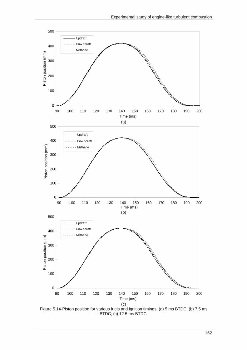
Experimental study of engine-like turbulent combustion
152
0
100
200
300
400
500
90 100 110 120 130 140 150 160 170 180 190 200Time (ms)
Pis
ton
posi
tion
(mm
)Updraft
Dow ndraft
Methane
(a)
0
100
200
300
400
500
90 100 110 120 130 140 150 160 170 180 190 200Time (ms)
Pis
ton
posi
tion
(mm
)
Updraft
Dow ndraft
Methane
(b)
0
100
200
300
400
500
90 100 110 120 130 140 150 160 170 180 190 200Time (ms)
Pis
ton
posi
tion
(mm
)
Updraft
Dow ndraft
Methane
(c)
Figure 5.14-Piston position for various fuels and ignition timings. (a) 5 ms BTDC; (b) 7.5 ms BTDC; (c) 12.5 ms BTDC.
Chapter 5
153
From figure 5.13 it is observed that the compression stroke is independent of the
ignition timing. The TDC position is reached at 137 ms and is kept during around 4 ms
to 141 ms. The measured compression stroke duration is about 44 ms. Expansion
stroke is indeed slightly influenced by the ignition timing, which become slower when
the ignition is made far from TDC. However, as seen in the figure 5.13 the ignition
timings of 5 ms BTDC and 7.5 ms BTDC could be considered to have the same piston
displacement along time. The 12.5 ms BTDC ignition timing is the one with lower
displacement for every fuel under study. Therefore, considering a criterion of 1.0 mm
for the final piston position the duration of the expansion stroke is around 49 ms for
ignition timing of 5 ms and 7.5 ms BTDC and 51 ms for 12.5 ms BTDC ignition timing.
This could be explained by the fact that when the combustion starts to earlier in relation
to TDC (12.5 ms BTDC) a large part of heat is released when the piston is still moving
up. Therefore, when the ignition is made close to TDC the heat released is available on
the expansion stroke to push the piston down. Thus, it is expected that some influence
of the fuel type on the expansion stroke exists (figure 5.14).
From figure 5.14 it is observed that both syngas compositions show similar time
evolution of the piston position. However, methane shows a different time evolution of
the piston position in the expansion stroke to the whole igniting timings. This is
explained by the combustion time of the mixtures that are lower for methane, followed
by the downdraft and finally by updraft. Thus, the heat released is not so much
available on the expansion stroke for methane as it is for updraft syngas. This also
indicates that the turbulent burning velocity of methane should be higher than the
syngas compositions ones.
5.2.1.2 Equivalent rotation speed
The compression stroke is imposed by the RCM hydraulic system; the expansion
stroke is a function of the heat release of the mixture being burned. Thus, the
equivalent rotation speed is not constant and its variation should be evaluated taking
into account the fuel and the ignition timing.
Figure 5.15 shows the average of the piston velocity during various experiments
without combustion and different spark times and after TDC synchronization.

Experimental study of engine-like turbulent combustion
154
0
5
10
15
20
90 100 110 120 130 140 150 160 170 180 190 200
Time (ms)
Vel
ocity
(m/s
)
0
100
200
300
400
500
Pis
ton
posi
tion
(mm
)
(a)
0
5
10
15
20
90 100 110 120 130 140 150 160 170 180 190 200
Time (ms)
Vel
ocity
(m/s
)
0
100
200
300
400
500
Pis
ton
posi
tion
(mm
)
(b)
0
5
10
15
20
90 100 110 120 130 140 150 160 170 180 190 200
Time (ms)
Vel
ocity
(m/s
)
0
100
200
300
400
500
Pis
ton
posi
tion
(mm
)
(c)
0
5
10
15
20
90 100 110 120 130 140 150 160 170 180 190 200
Time (ms)
Vel
ocity
(m/s
)
0
100
200
300
400
500
Pis
ton
posi
tion
(mm
)
(d)
Figure 5.15 - Piston velocity: (a) Without combustion. (b) 5 ms BTDC. (c) 7.5 ms BTDC. (d) 12.5 ms BTDC

Chapter 5
155
From figure 5.15 is possible to conclude that the piston velocity is higher on the
compression stroke than on the expansion stroke for every case. The maximum
velocity on the compression stroke is around 15 m/s decreasing to around 14 m/s on
the expansion stroke. The piston speed of the movement is constantly changing in the
cylinder. Relatively great in the middle of the stroke, some nearby the dead centre
speed is relatively small and it is zero in the dead centre. On the compression stroke
the maximum velocity occurs around 110 ms and is not influenced by combustion
because ignition is made after that instant for the whole cases. On the expansion
stroke the maximum speed occurs at around 162 ms for ignition timing of 5.0 ms
BTDC, around 165 ms for 7.5 ms BTDC and 166 ms for 12.5 ms BTDC. An equivalent
rotation speed could be defined by the following expression:
6N tθΔ = Δ (5.1)
Where θ is the crank angle in degrees, N the rotation speed and t the time. Taking into
account that each stroke represents 180 crank angle degrees, the mean equivalent
rotation speed for the compression stroke is 682 rpm. Considering the differences
verified on the piston displacement on the expansion stroke for the different fuels and
ignition timings, the mean equivalent rotation speed is also slightly changed.
Considering a criterion of 1.0 mm for the final piston position, we have an equivalent
rotation speed for the expansion stroke of 612 rpm for ignition timing of 5 ms BTDC
and 588 rpm for other ignitions timings for updraft syngas.
5.2.1.3 In-cylinder pressure repeatability
A set of three experiments was made for each syngas composition with various ignition
timings in order to verify its repetition. The pressure traces are shown in figure 5.16 for
updraft syngas after TDC synchronization.

Experimental study of engine-like turbulent combustion
156
0
10
20
30
40
50
90 100 110 120 130 140 150 160 170 180
Time (ms)
Pre
ssur
e (b
ar)
Shot 1
Shot 2
Shot 3
(a)
0
10
20
30
40
50
80 90 100 110 120 130 140 150 160 170 180
Time (ms)
Pre
ssur
e (b
ar)
Shot 1
Shot 2
Shot 3
(b)
0
10
20
30
40
50
90 100 110 120 130 140 150 160 170 180Time (ms)
Pre
ssur
e (b
ar)
Shot 1
Shot 2
Shot 3
(c)
Figure 5.16 – In-cylinder pressure reproducibility: updraft-syngas. (a) 5 ms BTDC; (b) 7.5 ms BTDC; (c) 12.5 ms BTDC

Chapter 5
157
From figure 5.16 is observed a good reproducibility of the pressure signal for the
various ignition timings. The maximum difference between peak pressures is: 0.2 bar
for ignition timing at 5 ms BTDC (30 bar on average representing an error of 0.7%); 0.1
bar for ignition timing at 7.5 ms BTDC (38 bar on average, which represents an error of
0.03%); 0.8 bar for ignition timing at 12.5 ms BTDC (47.5 bar on average representing
an error of 1.7%).
5.2.1.4 Conclusion
The quality of the RCM experimental measurements was evaluated on this section
throughout a sensibility analysis of errors in measurements techniques or in the
estimation of various parameters on the main experimental results: in-cylinder pressure
and piston displacement. This analysis shows high precision of the Institute Pprime
RCM for every measured parameter also on the two strokes mode, which ensures
about the quality of the results that will be shown in the following sections.
5.2.2 In-cylinder pressure
Ignition timing of typical stoichiometric syngas-air mixtures are determined in the RCM
described in 3.1.4. Together with pressure measurements, direct visualizations from
chemiluminescence emission are also carried out to follow the early stage of the
ignition process.
Figures 5.17-5.19 show RCM experimental pressure histories of stoichiometric syngas-
air mixtures and methane-air for various spark times and compression ratio ε =11. The
ignition timings tested were 5.0 ms, 7.5 ms and 12.5 ms BTDC.

Experimental study of engine-like turbulent combustion
158
0
10
20
30
40
50
60
90 100 110 120 130 140 150 160 170 180Time (ms)
Pre
ssur
e (b
ar)
5 ms BTDC
7.5 ms BTDC
12.5 ms BTDC
Figure 5.17 – Pressure versus time for stoichiometric updraft syngas-air mixture at various spark times.
0
10
20
30
40
50
60
70
90 100 110 120 130 140 150 160 170 180
Time (ms)
Pre
ssur
e (b
ar)
5 ms BTDC
7.5 ms BTDC
12.5 ms BTDC
Figure 5.18– Pressure versus time for stoichiometric downdraft syngas-air mixture at various spark times.

Chapter 5
159
0
10
20
30
40
50
60
70
80
90 100 110 120 130 140 150 160 170 180
Time (ms)
Pre
ssur
e (b
ar)
5 ms BTDC
7.5 ms BTDC
12.5 ms BTDC
Figure 5.19– Pressure versus time for stoichiometric methane-air mixture at various spark times.
From figures 5.17-5.19 it is observed that the in-cylinder pressure increases as the
spark time deviates from TDC. If combustion starts too early in the cycle, the work
transfer from the piston to the gases in the cylinder at the end of the compression
stroke is too large. If the combustion starts too late, the peak cylinder pressure is
reduced, and the stroke work transfer from the gas to the piston decreases.
Another observation that is brought out from these figures is that higher pressures are
obtained with methane-air mixture followed by downdraft syngas-air mixture and lastly
by updraft syngas-air mixture. These results could be endorsed to the energy
introduced into the RCM chamber, which can be determined by the heating value of the
fuels and the air to fuel ratio. Taking into account that the RCM chamber has 1.0 Litre,
the energy introduced in to the chamber is 2.60 KJ in the updraft case, 2.85 KJ in the
downdraft case and 3.38 KJ in the methane case for stoichiometric conditions. These
values are in agreement with the obtained cylinder pressures, however not proportional
in terms of peak pressures due to the influence of heat losses. These are mainly
dependent of the quenching distance as well as thermal conductivity of the mixture.
The higher burning velocity of methane compared to syngas compositions also cause a
more intensified convection.
Making a parallel with the laminar combustion case where the performances of updraft
and downdraft syngas are similar, one can observe that the same behaviour is not
found in turbulent conditions. On turbulent conditions peak pressures higher in about

Experimental study of engine-like turbulent combustion
160
25% higher are obtained with the downdraft syngas. As the turbulent burning velocity
could be considered proportional to the laminar one (Verhelst and Sierens, 2007), this
result could be endorsed to:
- the effect of pressure on the laminar burning velocity. The correlations of laminar
burning velocity of the typical syngas compositions developed on 4.1.2.3 show
that the effect of pressure is very significant (coefficient β for updraft is 40%
higher when compared to downdraft syngas β coefficient). For example, at the
same temperature an increase in pressure from 1.0 to 20.0 bar results in an
increasing difference on burning velocity from 12% to 35%.
- The higher pressure used on RCM also implies temperature to increase due to
compression but the effect of temperature on burning velocity of syngas typical
compositions is irrelevant since the coefficient α is of the same order (see
4.1.2.3).
5.2.3 Ignition timing
Timing advance is required because it takes time to burn the air-fuel mixture. Igniting
the mixture before the piston reaches TDC will allow the mixture to fully burn soon after
the piston reaches TDC. If the air-fuel mixture is ignited at the correct instant, maximum
pressure in the cylinder will occur sometime after the piston reaches TDC allowing the
ignited mixture to push the piston down the cylinder. Ideally, the time at which the
mixture should be fully burned is about 20º ATDC (Hartman, 2004). This will utilize the
engine power producing potential. If the ignition spark occurs at a position that is too
advanced relatively to piston position, the rapidly expanding air-fuel mixture can
actually push against the piston still moving up, causing detonation and lost power. If
the spark occurs too retarded relatively to the piston position, maximum cylinder
pressure will occur after the piston has already traveled too far down the cylinder. This
results in lost power, high emissions, and unburned fuel. For further analysis of these
experimental results, figure 5.20 synthesizes the peak pressure Pmax, and the position
of peak pressure θmax expressed in milliseconds ATDC for the variable ignition timing in
milliseconds BTDC.

Chapter 5
161
0
10
20
30
40
50
60
70
80
2.5 5 7.5 10 12.5 15Ignition Timing (ms BTDC)
Pm
ax (b
ar)
0
2
4
6
8
10
θmax
(ms
ATD
C)
Updraft
Dow ndraft
Methane
Figure 5.20 – Peak pressure (continuous lines) and peak pressure position (dashed lines) versus ignition timing for stoichiometric syngas-air and methane-air mixtures.
From figure 5.20 it is clear that the in-cylinder pressure increases as the ignition timing
is retarded. The peak pressure occurs later as the ignition timing decreases. In
opposite to the static chamber combustion, the peak pressure does not represent the
end of combustion. However, it is possible to conclude that the peak pressure occurs
always after TDC.
5.2.4 In-cylinder flame propagation
Burning of a mixture in a cylinder of a SI engine may be divided into the following
phases: (1) spark ignition, (2) laminar flame kernel growth and transition to turbulent
combustion, (3) turbulent flame development and propagation, (4) near-wall
combustion and after burning. Figures 5.21-5.23 show flame propagation images of
stoichiometric syngas-air mixtures combustion and stoichiometric methane-air mixtures
in a RCM, where it is possible to observe these first three phases of combustion.

Experimental study of engine-like turbulent combustion
162
-3.75 ms -2.5 ms -1.25 ms TDC 1.25 ms
2.5 ms 3.75 ms 5.0 ms 6.25 ms 7.5 ms
(a)
-6.25 ms - 5.0 ms -3.75 ms -2.5 ms -1.25 ms
TDC 1.25 ms 2.5 ms 3.75 ms 5.0 ms
(b)
-12.5 ms -11.25 ms -10.0 ms -8.75 ms - 7.5 ms
-6.25 ms - 5.0 ms - 3.75 ms -2.5 ms -1.25 ms
TDC 1.25 ms 2.5 ms 3.75 ms 5.0 ms
(c)
Figure 5.21 – Direct visualization of stoichiometric updraft syngas-air flame in a RCM for various Ignition timings. (a) 5 ms BTDC; (b) 7.5 ms BTDC; (c) 12.5 ms BTDC.

Chapter 5
163
-5.0 ms -3.75 ms -2.5 ms -1.25 ms TDC
1.25 ms 2.5 ms 3.75 ms 5.0 ms 6.25ms
(a)
-6.25 ms - 5.0 ms -3.75 ms -2.5 ms -1.25 ms
TDC 1.25 ms 2.5 ms 3.75 ms 5.0 ms
(b)
-12.5 ms -11.25 ms -10.0 ms -8.75 ms - 7.5 ms
-6.25 ms - 5.0 ms - 3.75 ms -2.5 ms -1.25 ms
TDC 1.25 ms 2.5 ms 3.75 ms 5.0 ms
(c)
Figure 5. 22 – Direct visualization of stoichiometric downdraft syngas-air flame in a RCM for various Ignition timings. (a) 5 ms BTDC; (b) 7.5 ms BTDC; (c) 12.5 ms BTDC.

Experimental study of engine-like turbulent combustion
164
-5.0 ms -3.75 ms -2.5 ms -1.25 ms TDC
1.25 ms 2.5 ms 3.75 ms 5.0 ms 6.25ms
(a)
-6.25 ms - 5.0 ms -3.75 ms -2.5 ms -1.25 ms
TDC 1.25 ms 2.5 ms 3.75 ms 5.0 ms
(b)
-12.5 ms -11.25 ms -10.0 ms -8.75 ms - 7.5 ms
-6.25 ms - 5.0 ms - 3.75 ms -2.5 ms -1.25 ms
TDC 1.25 ms 2.5 ms 3.75 ms
(c)
Figure 5.23- Direct visualization of stoichiometric methane-air flame in a RCM for various Ignition timings. (a) 5 ms BTDC; (b) 7.5 ms BTDC; (c) 12.5 ms BTDC.
Pictures of the initial phase of combustion show an initially quasi-spherical, relatively
smooth flame kernel for syngas compositions and methane cases for the various
ignition timings. The laminar behavior of the flame remains longer time as the ignition is
made far from TDC. In the case of ignition timing at 12.5 ms BTDC, the flame kernel
grows and experience flattening when piston is close to TDC position before the
transition to turbulent combustion.
Because the combustion continues in the expansion stroke, it is not possible to
determine from direct flame visualizations of the combustion chamber the combustion
duration. However, estimation about the rapidity of the combustion can be made from
figures 5.21-5.23. It is observed that the time at which the flame occupies the entire
chamber increases as the igniting timing increases for the whole fuels. This

Chapter 5
165
observation emphasis the fact of the lower peak pressures for ignition timings close to
TDC. As seen on 3.2.5 turbulence intensity is higher close to TDC on the RCM, thus
the increased turbulence in the unburned mixture at the time of combustion will
increase the burning rate (Alla, 2002).
Comparing the three fuels, it is observed that combustion is faster for methane,
followed by downdraft syngas and finally by updraft syngas. This behavior is in
agreement with the heat of reaction of the mixtures as well as with the laminar burning
velocity determined on 4.1.2.3 for typical syngas compositions.
5.3 Conclusion
An experimental approach to syngas engine-like conditions on a rapid compression
machine is made.
There is an opposite behavior of the in-cylinder pressure between single compression
and compression-expansion strokes. The first is that one gets higher in-cylinder
pressures on single compression event than for compression-expansion events, which
emphasis the fact of the constant volume combustion to be the way of getting higher
pressures. The second is that for single compression peak pressure decreases as the
ignition delay increases. In opposite, for compression-expansion the peak pressure
increases with the ignition delay increase. This opposite behaviour in relation to the
ignition timing has to do with the deviation of the spark from TDC position that
influences the extent of the combustion in the compression stroke and this extent has
different consequences on peak pressure regarding to the number of strokes events.
For single compression it reduces the constant volume combustion duration. For
compression-expansion strokes it increases the combustion duration on the
compression stroke where the heat released has the effect of generate pressure before
expansion.
In both experimental events, higher pressures are obtained with methane-air mixture
followed by downdraft-syngas and lastly by updraft-syngas. These results could be
endorsed to the heat of reaction of the fuels and air to fuel ratio under stoichiometric
conditions, but also to burning velocity. Crossing the heat value with the air to fuel ratio
conclusion could be drawn that the energy content inside the combustion chamber is in
agreement, however not proportional with the obtained pressures.

Experimental study of engine-like turbulent combustion
166
Updraft and downdraft syngas compositions have similar burning velocities in laminar
conditions but the same is not found in turbulent conditions, where the difference on
peak pressure is higher by about 25%. As the turbulent burning velocity is proportional
to the laminar burning velocity, analysing the correlations for laminar burning velocity of
the typical syngas compositions developed on this work show that the effect of
pressure is very significant (coefficient β for updraft is 40% higher in relation to
downdraft syngas). The higher pressure used on RCM also makes temperature to
increase due to compression but the effect of temperature on burning velocity for
typical syngas compositions is irrelevant since the coefficient α is of the same order.
Another major finding is that syngas typical compositions are characterized by high
ignition timings due to their low burning velocities. One should be aware of the low
equivalent rotation speed used on the RCM. This could compromise the use of typical
syngas compositions on high rotation speed engines.
Chapter 6
167
CHAPTER 6
NUMERICAL SIMULATION OF A SYNGAS- FUELLED ENGINE
Over the past years, several simulation codes of varying degree of sophistication of the
SI engine combustion process have been developed and applied to predict engine
performance (Rakopoulus, 1993). However, sparse theoretical studies have been
reported so far in the literature as regards modeling syngas combustion in SI engines
(Sridhar et al. 2006; Rakopoulus et al., 2008). Therefore, computational models of
syngas combustion in SI engines are strongly desirable; in order to supplement the
relevant experimental studies that usually concern operation of pure syngas.
Several model frameworks are used for the simulation of the ‘closed’ part of the spark-
ignition engine cycle; these can be classified as ‘zero-’, ‘multi-zone’ and ‘multi-
dimensional’ models. The first two types are classified as thermodynamic models,
where the equations constituting the basic structure of the model are based on
conservation of mass and energy and are only dependent on time (resulting in ordinary
differential equations). Multidimensional models are also termed fluid mechanic or fluid
dynamic models, where the governing equations are the Navier–Stokes equations in
addition to conservation of mass and energy. Multi-zone models are distinguished from
zero-dimensional models by the inclusion of certain geometrical parameters in the
basic thermodynamic approach.
The choice of multi-zone or multi-dimensional model is largely determined by the
application. If the objective is to evaluate a large range of conditions, perform
parametric studies and/or predict optimum engine settings, a reasonable accuracy and
fast computation on a PC system is desirable. These conditions are satisfied by multi-
zone models. Recent examples are the investigations of causes for cycle-to-cycle
variations in engines (Aghdam et al., 2007) and causes for the increased combustion
variability leading to lean limits (Ayala and Heywood, 2007). Multi-dimensional models
are inappropriate for such studies as they are computationally too demanding. Their
best use is for more detailed studies for limited conditions or particular features (e.g.
flow through valves, fuel injection, bulk in-cylinder flow and turbulence development), or
to support theory and model development.
The following reports in detail the development and validation of a multi-zone
thermodynamic combustion model. The purpose is the prediction of the engine in-
cylinder pressure. The validation of the code is made by comparison with experimental

Numerical simulation of a syngas-fuelled engine
168
literature data and in addition with the rapid compression machine results obtained in
this work. For this propose some adaptations to the engine-like code are needed and
are shown in advance.
6.1 Thermodynamic model
The basis for multi-zone models is formed by consideration of conservation of mass
and energy. In the following, the equations for the cylinder pressure and temperature(s)
are derived. This will show where additional information, in the form of sub-models, is
necessary in order to close these equations.
Before conservation of energy is written down for the cylinder volume, from inlet valve
closing (IVC) time to exhaust valve opening (EVO) time (i.e. the power cycle), some
assumptions are generally adopted to simplify the equations. During compression and
expansion, pressure is invariably assumed uniform throughout the cylinder; with fixed
unburned and burned gas regions in chemical equilibrium. During flame propagation,
burned and unburned zones are assumed to be separated by an infinitely thin flame
front, with no heat exchange between the two zones. All gases are considered ideal
gases; possible invalidity of the ideal gas law at high pressures is countered by the
associated high temperatures under engine combustion conditions. As the model is
zero-dimensional in nature, it does not account for any geometrical considerations of
the flame front position during combustion. As an example, figure 6.1 shows a
schematic, only of qualitative nature, of the combustion chamber.
Figure 6.1– Schematic of the combustion chamber with four burned zones.
This is the most frequently used approach for engine combustion models, where the
flame area is a spherical flame front truncated by the cylinder walls and the piston,
Vb4
Vb1
Vu VuVb4 Vb3
Vb2

Chapter 6
169
centered at the spark plug (Verhelst and Sheppard, 2009). The multi-zone approach is
retained throughout the expansion phase, i.e. from the end of combustion until the
EVO.
6.1.1 Conservation and state equations
The governing equations are presented for the combustion process. During
compression and expansion the same equations are retained, with adaptations
regarding the number of zones included.
Assuming that ‘n’ is the number of the current burned zones, with the latest-generated
burned zone indicated by subscript ‘n’, the energy conservation equation is applied for
the unburned zone, the n-1 already burned zones and the total cylinder charge,
yielding, respectively.
u u u bu
dQ dU dV dmp hd d d dθ θ θ θ
= + + (6.1)
1 1, , , ( ,..., )θ θ θ
= + = −b i b i b idQ dU dVp i n
d d d (6.2)
dQ dU dVpd d dθ θ θ
= + (6.3)
Zero blow-by rate is assumed during the whole closed cycle period. The instantaneous
cylinder volume is equal to the sum of the volumes of the unburned and burned zones,
resulting in the following relation after differentiating with respect to crank angle:
1
,n
b i u
i
dV dVdVd d dθ θ θ=
= +∑ (6.4)
where V is the instantaneous cylinder volume, calculated from the engine geometric
characteristics as a function of crank angle:
( )21 11 1 1 12
cos sincTDC
rV V θ ϕ θϕ
⎧ ⎫− ⎡ ⎤= + − + − −⎨ ⎬⎢ ⎥
⎣ ⎦⎩ ⎭ (6.5)
with ϕ being the crank radius to piston rod length ratio. The rate of change of the
instantaneous cylinder volume against crank angle is

Numerical simulation of a syngas-fuelled engine
170
2 2
11
2 1cossin
sinc
TDCrdV V
dϕ θθ
θ ϕ θ
⎛ ⎞−⎛ ⎞ ⎜ ⎟= +⎜ ⎟ ⎜ ⎟⎝ ⎠ −⎝ ⎠ (6.6)
The mass fraction of each burned zone is defined as
1,, ( ,..., )= =b i
b i
mx i n
m (6.7)
with the result for the total burned zone
1,
nb
b b ii
mx x
m =
= = ∑ (6.8)
The mass conservation equation is also applied to the cylinder charge, assuming zero
blow-by, providing
0,b nu b u dmdm dm dmdmd d d d dθ θ θ θ θ
= + = + = (6.9)
The previous relation has been derived assuming that the mass of each of the already
burned zones remains constant after its combustion: dmb,i/dθ = 0 (i=1,…, n-1), resulting
for the rate of change of mass of the total burned zone:
1 , ,n
b b i b nidm d dm d dm dθ θ θ
== =∑ (6.10)
Also, the perfect gas state equation is applied to each zone.
1( , )j j j j npV m R T j u b b= = − (6.11)
6.1.2 Chemical composition and thermodynamic properties
The unburned zone is considered to be a mixture of air and fuel, while also allowance
is made for the presence of residual gas trapped in the engine cylinder. The
composition and thermodynamic properties of the unburned mixture during
compression and combustion are determined from the values of pressure, temperature,
fuel–air equivalence ratio and residual gas mass fraction (Ferguson, 1986).
After the start of combustion and until the end of expansion at EVO, the combustion
products of each burned zone consist of a set of eleven chemical species: (1) CO2, (2)

Chapter 6
171
H2O, (3) N2, (4) O2, (5) CO, (6) H2, (7) H, (8) O, (9) OH, (10) NO, and (11) N, which are
considered to be in chemical equilibrium. The calculation of their concentrations and,
subsequently, each zone’s thermodynamic properties is based on the values of
pressure, temperature and fuel–air equivalence ratio. For this reason, the atom balance
equations of the C–H–O–N system are considered along with the following eight
equilibrium reactions (Ferguson, 1986):
12 2 22
12 22
4 2 2 2
1 12 22 2
1 12 22 2
122
122
122
2 2
H O H O
CO O CO
CH O CO H O
H O OH
O N NO
H H
O O
N N
+ ⇔
+ ⇔
+ ⇔ +
+ ⇔
+ ⇔
⇔
⇔
⇔
(6.12)
The various thermodynamic properties (specific enthalpy, specific internal energy,
specific volume, specific heat capacity at constant pressure) and thermodynamic
derivatives (derivative of logarithmic specific volume with respect to logarithmic
temperature and pressure) of the unburned and burned mixtures, needed for the
calculations, are computed according to the mole fraction of each species and the gas
mixture rule. For this purpose, the well established coefficients (Heywood, 1988) of the
polynomial curves that have been fitted to the various species thermodynamic data
from JANAF tables are used. For the evaluation of specific internal energy of species i,
the following relation can be applied according to JANAF Table thermodynamic data
(Gordon and McBride, 1971; Heywood, 1988):
5
61
( ) nini si i
n
au T R T a Tn=
⎡ ⎤⎛ ⎞= + −⎢ ⎥⎜ ⎟
⎝ ⎠⎣ ⎦∑ (6.13)
where constants ain for the above polynomial relation can be found, for example, in
(Ferguson, 1986; Heywood, 1988). Two sets of data are available for constants ain, one
for temperatures up to 1000 K and another for temperatures from 1000 to 5000 K. The
reference temperature is 298 K. Also,
( ) ( )i i sih T u T R T= + (6.14)

Numerical simulation of a syngas-fuelled engine
172
The rate of internal energy change for a mixture is given by:
ii i vi
i i
dmdh dTu m cd d dθ θ θ
= +∑ ∑ (6.15)
where mi is the mass of species i (O2, N2, CO2,H2O, N, NO, OH, H, O, etc.) and cv is
the specific heat under constant volume (a function of temperature only cv=du/dT), with
1 1,( ) nv i si i n
nc T R a T −⎡ ⎤⎛ ⎞
= −⎢ ⎥⎜ ⎟⎝ ⎠⎣ ⎦∑ (6.16)
with the values of mi, dmi, T, dT found from the corresponding first-law analysis of the
cylinder contents. The rate of entropy change is:
( ),i ii i pi
i i
dm mdS dT V dpS T x p cd d T d T dθ θ θ θ
= + −∑ ∑ (6.17)
With
( ) ( )', , ln ii i i i si
i
x pS T x p S T p Rp
⎛ ⎞= − ⎜ ⎟
⎝ ⎠ (6.18)
and ( )' ,i iS T p the standard state entropy of species i, which is a function of temperature
only, with xi the molar fraction of species i in the mixture (Ferguson, 1986; Heywood,
1988), given by the following property relation:
15
1 72 1
',( , ) ln
n
i i si i i n in
Ts T p R a T a an
−
=
⎡ ⎤⎛ ⎞= +⎢ ⎥⎜ ⎟−⎝ ⎠⎣ ⎦
∑ (6.19)
For the Gibbs free enthalpy or energy:
ii
i
dmdGd d
μθ θ
= ∑ (6.20)
where μi=gi (T,pi) is the chemical potential of species i in the mixture, with
( , ) ( , ) ( ) ( , )
( ) ( , ) ln
i i i i i i i
ii i i si
i
g T p g T x p h T Ts T x px ph T T s T p Rp
= = −⎡ ⎤⎛ ⎞
= − −⎢ ⎥⎜ ⎟⎢ ⎥⎝ ⎠⎣ ⎦
(6.21)

Chapter 6
173
For all the above expressions, it is assumed that the unburned mixture is frozen in
composition and the burned mixture is always in equilibrium. Finally, the well-known
ideal gas relation is given by:
spV mR T= (6.22)
6.1.3 Heat Transfer
The heat transfer from gas to the walls is formulated as:
( )= −g g wQ h A T T (6.23)
where hg is the heat transfer coefficient, A is the area in contact with the gas, Tg is the
gas temperature and Tw is the wall temperature. In the single zone analysis, the heat
transfer coefficient is the same for all surfaces in the cylinder. In general, a classic
global heat transfer model is applied to calculate the heat transfer coefficient and an
area-averaged heat transfer rate.
Several correlations for calculating the heat transfer coefficient in SI and CI engines
have been published in the literature. These studies have generally relied on
dimensional analysis for turbulent flow that correlates the Nusselt, Reynolds, and
Prandtl numbers. Using experiments in spherical vessels or engines and applying the
assumption of quasi-steady conditions has led to empirical correlations for both SI and
CI engine heat transfer. These correlations provide a heat transfer coefficient
representing a spatially-averaged value for the cylinder. Hence, they are commonly
referred to as global heat transfer models, e.g. Woschni (1967), Annand (1963), or
Hohenberg (1979). In this code one applies the classical Woschni’s correlation.
The Woschni heat transfer correlation is given as:
0 2 0 8 0 55 0 8. . . .( ) ( ) ( ) ( )g sh t a B P t T t v t− −= (6.24)
where as is a scaling factor used for tuning of the coefficient to match a specific engine
geometry calculated and used by Hohenberg, (1979) as 130, B is the bore (m), P and T
are the instantaneous cylinder pressure (bar) and gas temperature (K), respectively.
The instantaneous characteristic velocity, v is defined as:

Numerical simulation of a syngas-fuelled engine
174
2 28 0 00324r
. . ( )P
⎛ ⎞= + −⎜ ⎟
⎝ ⎠s r
p motr
V Tv S P PV
(6.25)
Where Pmot=Pr(Vr/V)γ is the motored pressure. Sp is mean piston speed (m/s), Vs is
swept volume (m3), Vr, Tr and Pr are volume, temperature and pressure (m3, K, bar)
evaluated at any reference condition, such as inlet valve closure, V is instantaneous
cylinder volume (m3) and γ is the specific heat ratio. The second term in the velocity
expression allows for movement of the gases as they are compressed by the
advancing flame.
6.1.4 Mass burning rate
In the combustion modeling studies, the main purpose is to specify the mass fraction of
burned gases at any time during the combustion process. This is achieved by using
several approaches. In general, two approaches have been widely used for
determining the mass fraction burned. In the first approach, the mass fraction burned at
any crank angle is specified by using empirical burning laws, such as the cosine burn
rate formula and Wiebe function (Heywood et al., 1979). This approach does not
necessitate detailed combustion modeling, hence modeling of combustion in this
manner is more practical, but it gives less reliable or less sensitive results about SI
engine combustion [Heywood et al., (1979); Bayraktar and Durgun, (2003)]. Empirical
burning equations include some constants that must be determined suitably at the
beginning of computation. In the case of using the Wiebe function, these are the
efficiency parameter, the form factor, the crank angle at the start of combustion and the
combustion duration. For the cosine burn rate formula, these are spark advance and
combustion duration. In such models, these parameters are generally determined
either by matching the experimental mass fraction burned curves obtained from the
cylinder pressure measurements with the calculated ones or by making an engineering
judgment [Zeleknik (1976); Heywood et al. (1979)]. If sufficient agreement is achieved
between the calculated and measured pressures, then the chosen parameters are
used for parametric studies. In the second approach, the combustion is modeled by
considering the turbulent flame propagation process (Heywood, 1988). This modeling
technique is generally called quasi-dimensional modeling because it accounts for the
details of engine geometry and the flame propagation process and therefore will be
followed in this work.
The role of in-cylinder air motion begins from the very start of the engine cycle. During
the intake stroke, the incoming air generates flow structures with large-scale turbulent

Chapter 6
175
motions within the cylinder, which in turn determines the extent of mixing between the
fresh charge and the residuals, as well as internal and external heat transfer rates. The
key to the premixed combustion modeling is the prediction of Ste, the turbulent flame
speed normal to the surface of the flame. In turbulent flames, the flame speed depends
on both chemical kinetics and the local turbulence characteristics.
Many methods for describing and calculating the turbulent flame speed have been
developed (see for instance the excellent review of Lipatnikov and Chomiak, (2002)).
The goal of this work is to develop a fast simulation program for the combustion of
syngas in spark ignition engines. The main interest is the pressure development in the
engine cylinders, which is directly related to the power output and the efficiency.
Therefore, in this work the so-called DamkÖhler method is used and according to this
model turbulent flame speed is as follows (Blizard and Keck, 1974):
2 'te uS C u S= + (6.26)
Where, u’ is the root mean square (rms) turbulent velocity, C2 a calibration constant
dependent of the engine geometry and Su the laminar burning velocity.
Obviously, proper in-cylinder turbulence modeling needs to be estimated. For this
propose, a simple turbulence model, firstly proposed by Hall and Bracco, (1987) and
used by several authors [Verhelst and Sierens, (2007); Farhad et al., (2009); Federico
et al., (2010)] has been considered:
360' 0.75 0.75(2 ), ' ' 1 0.545TDC p TDCu u s n u u θ −⎛ ⎞= = = −⎜ ⎟
⎝ ⎠ (6.27)
where u’TDC is the rms turbulent velocity at TDC, taken to be 0.75 times the mean
piston speed; θ is the crank angle and, s, is the stoke. A linear decay of the rms
turbulent velocity u’ from top dead center is imposed.
6.2. Numerical solution procedure
The basic concept of the model is the division of the burned gas region into several
distinct zones for taking into account the temperature stratification of the burned gas.
The multi-zone simulation model is applied throughout the closed part of the engine
cycle, between IVC and EVO, i.e. compression, combustion and expansion. Admission
phase is also included in the code in order to take into account the heating of the

Numerical simulation of a syngas-fuelled engine
176
mixture due to wall interaction. The entire flowchart of the developed code is shown in
figure 6.2.
It requires as input data the engine geometric characteristics, engine speed, fuel–air
equivalence ratio, combustion chamber walls temperature, compression ratio, ignition
delay, and temperature and pressure of charge at IVC event. It is assumed that during
compression the cylinder content, consisting of air–fuel mixture and any residual
gases, comprises one zone. From the start of combustion, multiple burned zones
(whose number is user-defined) are sequentially generated, with the latest-generated
burned zone being separated from the unburned zone by an infinitesimally thin flame
front. The multi-zone approach is retained throughout the expansion phase, i.e. from
the end of combustion until the EVO.
All zones considered are assigned spatially uniform pressure, temperature and
composition at any instant of time. During all phases, the pressure is uniform
throughout the cylinder at any instant of time. It is noted that the model, being zero-
dimensional in nature, does not predict geometrically the actual position of the flame
front and the various zones inside the cylinder. Rather, simulation follows purely the
thermodynamic approach.

Chapter 6
177
Figure 6.2 – Engine-like code flowchart.

Numerical simulation of a syngas-fuelled engine
178
6.3 Code validation
Due to the lack of experimental apparatus, model testing has been carried on over
detailed experimental data available in literature and, in particular, the standard CFR,
single cylinder, engine has been chosen for the simulations. Two fuels were selected
that are present on syngas: hydrogen and methane. As far as hydrogen fueling is
concerned, the extensive measurements of Verhelst, (2005) have been chosen as a
reference, while the in-cylinder pressures traces by Bade and Karim, (2001) have been
considered when dealing with methane. An attempt to validate the code by comparison
with experimental results obtained in this work in the RCM is made.
6.3.1 CFR engine
A Cooperative Fuel Research engine, known as the CFR engine, is an engine originally
used for the determination of fuel octane numbers, now also equipped for gaseous
fuels. It is characterized by its engine speed kept constant by coupled electric motor,
and its variable compression ratio. The main engine specifications are given in Table
6.1.
Table 6.1 - Basic CFR engine data
Items Specification
Engine type Cooperative Fuel Research (CFR)
Number of cylinders 1
Bore × Stroke 82.55 × 114.2 (mm)
Connecting rod length 254 mm
Displacement 611.7 cm3
Compression ratio Variable
Engine speed Variable
6.3.1.1 Sub-models
Most of the predictive capability of a quasi-dimensional model relies on the accuracy of
the implemented sub-models. Sub-models are needed for closing the equations for
pressure, temperatures and masses of the two zones: in particular, a combustion sub-
model for computing the mass burning rate, and a model of heat transfer through the
walls; a detailed description of them is given in the following for hydrogen-air and
methane-air mixtures.

Chapter 6
179
Heat transfer
Wei et al., (2001) and Shudo and Suzuki, (2002) have measured instantaneous heat
transfer coefficients in hydrogen fuelled engines. Wei et al. (2001) found transient heat
transfer coefficients during hydrogen combustion to be twice as high as during gasoline
combustion. They evaluate heat transfer correlations and found Woschni’s equation to
underpredict the heat transfer coefficient by a factor of two.
Shudo and Suzuki (2002) compared the heat transfer coefficients during stoichiometric
hydrogen and methane combustion, finding them to be larger in the case of hydrogen.
The shorter quenching distance of a hydrogen flame is put forward as the cause of this
increased heat transfer, leading to a thinner thermal boundary layer. Furthermore, for
near-stoichiometric combustion, flame speeds are high and cause intensified
convection. Hydrogen has also a higher thermal conductivity compared to
hydrocarbons. Shudo and Suzuki, (2002) construct an alternative heat transfer
correlation with an improved correspondence with their measurements. However, the
correlation contains two calibration parameters, dependent on ignition timing and
equivalence ratio. These dependencies are started to be the subject of further studies,
so the correlation is not useful for the present work.
The correlation by Woschni and Annand have cited to be inadequate [Borman and
Nishiwaki, (1987)], even for gasoline and diesel engines, although the correlations
have been based on measurements on such engines and use hydrocarbon mixture
properties. However, the development of heat transfer correlation for SI engines is not
within the scope of this work, it was decided to use the standard model of Woschni with
separate values during compression, combustion and expansion as reported by
Verhelst and Sierens, (2007). This calibration was made by matching a simulated
cylinder pressure trace to a measured pressure trace. The compression heat transfer
coefficient can be calibrated to a motored pressure trace. The other coefficients need
to be set more or less simultaneously.
Turbulent burning velocity
The turbulent burning velocity models need laminar burning velocity data of the
air/fuel/residuals mixture at the instantaneous pressure and temperature. As most
models use the laminar burning velocity as the local burning velocity, such as the
DamkÖhler model, the stretched burning velocity should be used.

Numerical simulation of a syngas-fuelled engine
180
Concerning hydrogen-air flames, the extensive experimental work done by Verhelst,
(2005) has been chosen for including the dependence on the air-fuel ratio,
temperature, pressure and residual burned gas content:
( )0
0 0
1u uT PS S fT P
α β
γ⎛ ⎞ ⎛ ⎞
= −⎜ ⎟ ⎜ ⎟⎝ ⎠ ⎝ ⎠
(6.28)
Here, the reference conditions T0 and P0 are 365K and 5 bar, respectively. The
influence of the equivalence ratio at these conditions is embodied in Su0 and is
estimated at:
0
3 24.77 8.65 0.394 0.296uS φ φ φ= − + − − (6.29)
The values for α, β and γ are the following:
3 2
1.2322.9 6.69 5.06 1.16 , 0.60.0246 0.0781, 0.62.715 0.5
α
β φ φ φ φβ φ φγ φ
=
= − + − <= + ≥= −
(6.30)
Where γ expresses the effect of residual gases. Verhelst and Sierens, (2007) selected
a residual mass fraction of 27% given the best correspondence for the pressure trace
during compression and maximum combustion pressure.
Concerning methane–air flames, the correlation expressing the laminar burning velocity
of Muller et al., (1997) has been adopted, since it is reliable for a wide range of
pressures and preheats temperatures:
( )
( )
00
, 0
00exp
n
m u bu F u
b u
T T TS A T y
T TT
GA T FT
⎛ ⎞−= ⎜ ⎟
−⎝ ⎠⎛ ⎞= −⎜ ⎟⎝ ⎠
(6.31)
Where, yF,u = (1+AFRs/φ) represents the mass fuel fraction in the unburned mixture,
AFRs is the stoichiometric air–fuel ratio;T0=-E/ln(p/B) is a representative temperature of
the inner layer, defined by Peters and Williams, (1987) as the thin layer within which
the first oxidation of methane into CO, hydrogen and water occurs; p is pressure, and
the fuel-dependent constants are equal to: B=3.1557×10⁸ (bar), E=23873 (K),
F=2.21760×101(cm/s) ,G=-6444.27 (K), m =0.565175 and n=2.5158.

Chapter 6
181
The calibration coefficient C2 in the DamkÖhler model was set equal 1.7 as reported by
Verhelst and Sierens, (2007).
6.3.1.2 Results and discussion
The simulations results, compared to the respective references, have been presented
in figures 6.3 and 6.4.
0
10
20
30
40
50
240 270 300 330 360 390 420 450 480
Crank Angle (degrees)
Pre
ssur
e (b
ar)
Numerical
Experimental (Bade and Karim, 2001)
Figure 6.3 – In cylinder pressure validation for CFR engine fueled by methane: ε=8.5, 900 rpm, IT=20º BTDC, φ=0.99.
0
10
20
30
40
50
60
240 270 300 330 360 390 420 450 480
Crank Angle (degrees)
Pre
ssur
e (b
ar)
Numerical
Experimental (Verhelst, 2005)
Figure 6.4 – In cylinder pressure validation for CFR engine fueled by hydrogen: ε=9.0, 600 rpm, IT=20º BTDC, φ=0.59.
As clearly visible from these figures, a very good agreement is found. This allows
validate the developed model and applied it to typical syngas compositions.

Numerical simulation of a syngas-fuelled engine
182
6.3.2 RCM
As shown in chapter 5, RCM simulates a single engine cycle and some adaptations to
the model presented above are needed in order to take into account the dynamic and
geometrical specificness of the RCM. Three main aspects should be considered, the
instantaneous volume, heat transfer and burning rate. Two distinctive cases are
considered in the code: single compression, and compression and expansion strokes.
6.3.2.1 Flame propagation
The flame development in the combustion chamber of a RCM was shown above for the
compression and expansion strokes. In order two verify the assumption frequently used
for engine combustion models, where the flame area is a spherical flame front
truncated by the cylinder walls and the piston, centered at the spark plug adopted in
this work, the flame images are used in an image treatment Matlab code developed by
Strozzi, (2008), which allows visualizing the flame contours.
Figures 6.5 show the flame contours in a RCM combustion chamber for downdraft
syngas-air stoichiometric mixture. The window has 613×337 pixels with resolution of
2.835 pixels/mm. The frequency of the each contour is kept to 1.4 KHz.
Figure 6.5 - RCM flame contours of stoichiometric downdraft syngas-air mixture with ignition at
12.5 ms BTDC.
The earlier stage of flame kernel with influence of the spark plug was removed from the
contours due to lack of definition. After around 5.0 ms (the duration of the spark), the
flame contours are well defined and shows that the propagation is spherical. At this
moment the piston is reaching TDC and the flame shows a remarkable slow down due
to piston deadening, which is felt on the pressure signal by a decreasing gradient. After
TDC, the flame contour shows to near double the displacement due to expansion.

Chapter 6
183
6.3.2.2 In-cylinder volume
The instantaneous cylinder volume is calculated based on the piston position as a
function of crank angle and fitted by polynomial functions in order to be implemented in
the code. Thus, first one evaluates the error in the polynomial approach.
Figure 6.6 shows the comparison between the experimental volume inside the cylinder
and the corresponding six degree polynomial expression applied up to top dead center
to better fitting. The remaining part is constant and equal to the clearance volume. The
maximum error is about 0.5% (5 cm3).
0
200
400
600
800
1000
1200
180 210 240 270 300 330 360 390 420 450 480 510 540
Crank Angle (degrees)
Vol
ume
(cm
3 )
Experimental
Polynomial
Figure 6.6 – In-cylinder volume polynomial fitting: single compression downdraft syngas case, ignition timing at 12.5 ms BTDC.
Figure 6.7 shows in-cylinder volume variation during compression and expansion and
the corresponding six degree polynomial. The maximum error is 1.5% (15 cm3)
obtained at TDC.
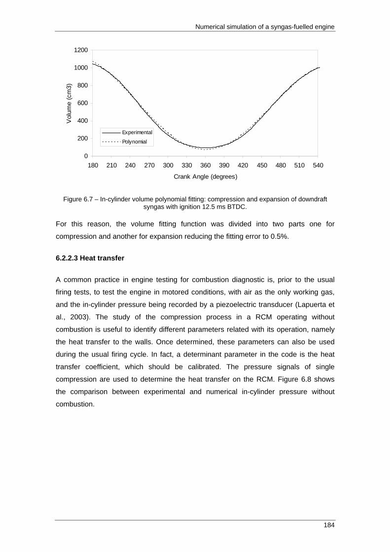
Numerical simulation of a syngas-fuelled engine
184
0
200
400
600
800
1000
1200
180 210 240 270 300 330 360 390 420 450 480 510 540
Crank Angle (degrees)
Vol
ume
(cm
3)
Experimental
Polynomial
Figure 6.7 – In-cylinder volume polynomial fitting: compression and expansion of downdraft syngas with ignition 12.5 ms BTDC.
For this reason, the volume fitting function was divided into two parts one for
compression and another for expansion reducing the fitting error to 0.5%.
6.2.2.3 Heat transfer
A common practice in engine testing for combustion diagnostic is, prior to the usual
firing tests, to test the engine in motored conditions, with air as the only working gas,
and the in-cylinder pressure being recorded by a piezoelectric transducer (Lapuerta et
al., 2003). The study of the compression process in a RCM operating without
combustion is useful to identify different parameters related with its operation, namely
the heat transfer to the walls. Once determined, these parameters can also be used
during the usual firing cycle. In fact, a determinant parameter in the code is the heat
transfer coefficient, which should be calibrated. The pressure signals of single
compression are used to determine the heat transfer on the RCM. Figure 6.8 shows
the comparison between experimental and numerical in-cylinder pressure without
combustion.

Chapter 6
185
0
10
20
30
40
180 210 240 270 300 330 360
Crank Angle (degrees)
Pre
ssur
e (b
ar)
Experimental
Numerical
Figure 6.8 - Comparison between experimental and numerical in-cylinder pressure during
compression of downdraft syngas without combustion.
From figure 6.8 is seen that the Woschni model works well in its original formulation
and represent the heat transfer of the RCM compression stroke.
6.3.2.4 Turbulent burning velocity
As reported in section 3.2.5 the turbulence intensity was experimentally determined for
the RCM, and was implemented in the code in the expression (6.26) for validation
proposes. The laminar burning velocity formulation obtained in the section 4.1.2.3 was
also used to close expression (6.26).
6.3.2.5 Results and discussion
Figures 6.9-6.10 show experimental and numerical cylinder pressure for typical
downdraft syngas-air mixture and methane-air mixture for various ignition timings,
respectively.

Numerical simulation of a syngas-fuelled engine
186
0
10
20
30
40
50
60
70
180 210 240 270 300 330 360 390 420 450 480 510 540Crank Angle (degrees)
Pre
ssur
e (b
ar)
Numerical
Experimental
(a)
0
10
20
30
40
50
60
70
180 210 240 270 300 330 360 390 420 450 480 510 540Crank Angle (degrees)
Pre
ssur
e (b
ar)
Numerical
Experimental
(b)
0
10
20
30
40
50
60
70
180 210 240 270 300 330 360 390 420 450 480 510 540Crank Angle (degrees)
Pre
ssur
e (b
ar)
Numerical
Experimental
(c)
Figure 6.9 – Experimental and predicted cylinder pressure diagrams as a function of crank angle for downdraft syngas. (a) ignition timing 20º BTDC, (b) 30º BTDC, (c) 50º BTDC.
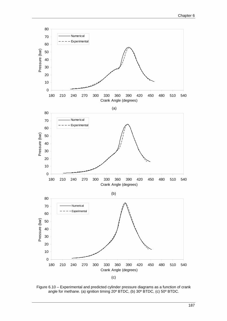
Chapter 6
187
0
10
20
30
40
50
60
70
80
180 210 240 270 300 330 360 390 420 450 480 510 540Crank Angle (degrees)
Pre
ssur
e (b
ar)
Numerical
Experimental
(a)
0
10
20
30
40
50
60
70
80
180 210 240 270 300 330 360 390 420 450 480 510 540Crank Angle (degrees)
Pre
ssur
e (b
ar)
Numerical
Experimental
(b)
0
10
20
30
40
50
60
70
80
180 210 240 270 300 330 360 390 420 450 480 510 540Crank Angle (degrees)
Pre
ssur
e (b
ar)
Numerical
Experimental
(c)
Figure 6.10 – Experimental and predicted cylinder pressure diagrams as a function of crank angle for methane. (a) ignition timing 20º BTDC, (b) 30º BTDC, (c) 50º BTDC.

Numerical simulation of a syngas-fuelled engine
188
Figures 6.9-6.10 show that the adapted code is able to reproduce fairly good the RCM
in-cylinder pressure. Main discrepancies are found in the combustion phase especially
for short ignition timings. On the expansion phase, pressure curve come back to match
with experimental result fairly well. These discrepancies can be explained from both the
experimental and numerical results. From the experimental point of view, RCM
leakages, which correspond to mass losses especially at elevated pressures, can be a
reasonable cause for the lower pressures. From the numerical point of view, there are
various factors that can be source of errors due to the code adaptation to the RCM
characteristics, namely:
- The heat transfer coefficient that was tested on the compression stroke with
very good performance, however it lacks of verification for the expansion stroke.
- The turbulence intensity used on the burning rate model was tacked from
experimental results of the single compression, thus it lacks of verification for
the expansion stroke;
- Other minor errors like the in-cylinder volume polynomial fitting and the
equivalent rotation speed. The latter directly affects the heat transfer coefficient.
6.4. Syngas fuelled-engine
For small scale cogeneration units (<1.0 MW), the engine rotation speed is generally
about 1500 rpm. Another division is made for cogeneration units below 50 kW, which
are known as micro-CHP units (Monteiro et al., 2009). In this power range rotation
speed of 3000 rpm is often found. Thus, in this study three rotation speeds are tested
of 750, 1500 and 3000 rpm and stoichiometric syngas-air mixtures.
Once the model was calibrated for the CFR engine it is wise to use it for testing the
syngas performance for different rotation speeds. Compression ratio is equal to 11 in
order to be somewhat comparable with RCM results.
6.4.1 Results and discussion
Spark timing is the major operating variable that affects spark ignition engine
performance, efficiency and emissions (Alla, 2002). Therefore, ignition timing ranging
for syngas-air mixtures was selected in order to keep the combustion end between 10º
to 20º crank angle degrees after top dead center. Figures 6.11-6.12 depicts the
simulated in-cylinder pressure traces during the closed part of the cycle for various
ignition timings and rotation speeds. These figures show that the possible ignition
timings are very similar for typical syngas compositions. However, they are lower for

Chapter 6
189
downdraft syngas than for updraft syngas, which agrees with the heat of reaction of the
fuels and with the burning velocities. Another conclusion is that varying the ignition
timing is possible to keep closely the same peak pressure for different rotation speeds.
As far as pressure is concerned, one obtains higher pressures for downdraft syngas,
which follows the results obtained experimentally in the RCM. The increase of
maximum cylinder pressure with ignition timing is evident. Pressure varied between 49-
62 bar for updraft syngas, 48-61 bar for downdraft syngas. These levels of peak
pressure are in agreement with the ones obtained in RCM in the section 5.2.2.
Conclusion can be drawn that typical syngas compositions besides its lower heat value
and burning velocities can be used on SI engines even at elevated rotation speeds.

Numerical simulation of a syngas-fuelled engine
190
0
20
40
60
80
180 210 240 270 300 330 360 390 420 450 480 510 540
Crank Angle (degrees)
Pre
ssur
e (b
ar)
24º BTDC
30º BTDC
(a)
0
20
40
60
80
180 210 240 270 300 330 360 390 420 450 480 510 540
Crank Angle (degrees)
Pre
ssur
e (b
ar)
26º BTDC
32º BTDC
(b)
0
20
40
60
80
180 210 240 270 300 330 360 390 420 450 480 510 540
Crank Angle (degrees)
Pre
ssur
e (b
ar)
26.5º BTDC
32º BTDC
(c)
Figure 6.11 – Cylinder pressure versus crank angle for updraft syngas at various ignition
timings. (a) 750 rpm, (b) 1500 rpm, (c) 3000rpm.
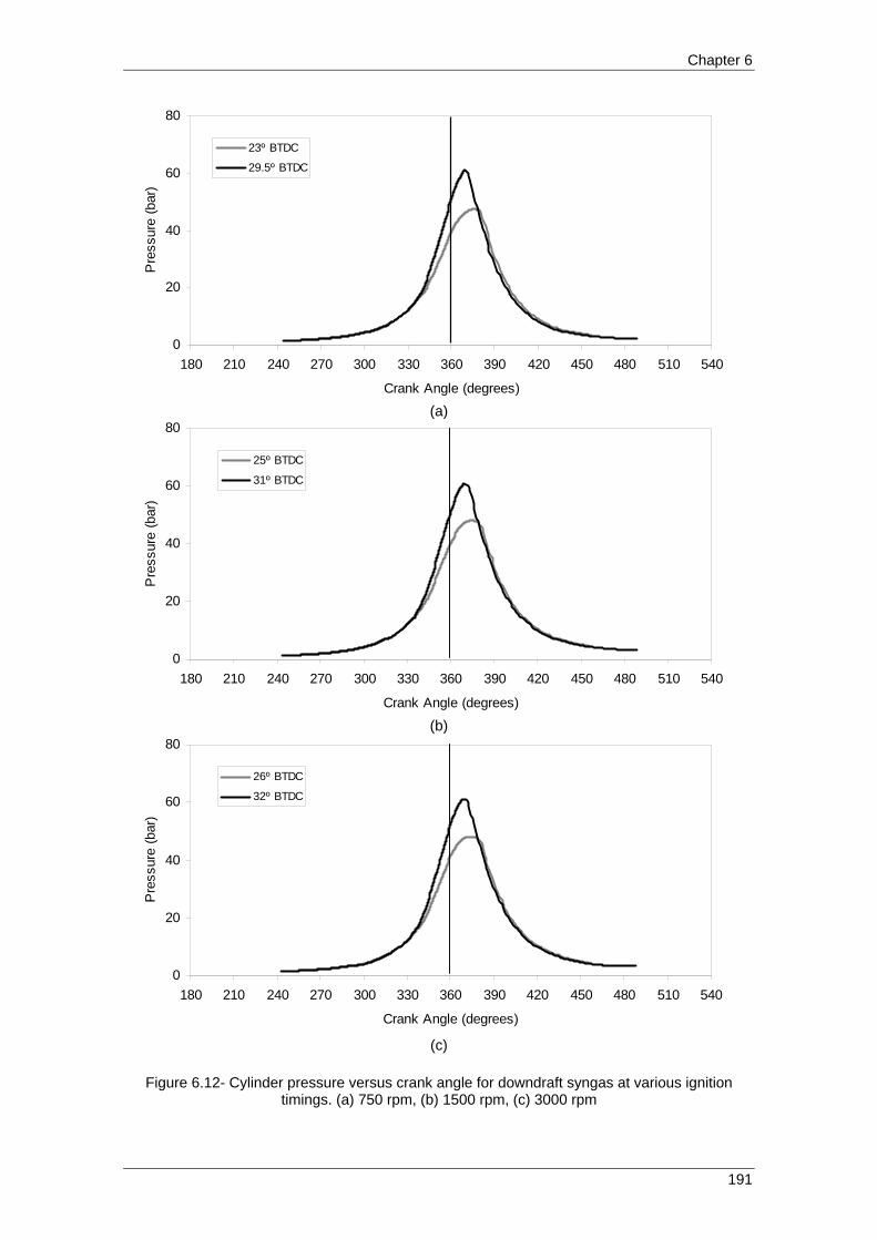
Chapter 6
191
0
20
40
60
80
180 210 240 270 300 330 360 390 420 450 480 510 540
Crank Angle (degrees)
Pre
ssur
e (b
ar)
23º BTDC
29.5º BTDC
(a)
0
20
40
60
80
180 210 240 270 300 330 360 390 420 450 480 510 540
Crank Angle (degrees)
Pre
ssur
e (b
ar)
25º BTDC
31º BTDC
(b)
0
20
40
60
80
180 210 240 270 300 330 360 390 420 450 480 510 540
Crank Angle (degrees)
Pre
ssur
e (b
ar)
26º BTDC
32º BTDC
(c)
Figure 6.12- Cylinder pressure versus crank angle for downdraft syngas at various ignition timings. (a) 750 rpm, (b) 1500 rpm, (c) 3000 rpm

Numerical simulation of a syngas-fuelled engine
192
In order to compare pressure evolution of the different fuels at the same ignition timing,
figure 6.13 shows this cylinder pressure comparison.
0
10
20
30
40
50
240 270 300 330 360 390 420 450 480
Crank Angle (degrees)
Pre
ssur
e (b
ar)
UpdraftDow ndraft
Methane
Figure 6.13- Cylinder pressure versus crank angle for various fuels. ε= 8.5, IT= 20º BTDC, 900
rpm. Figure 6.13 shows that higher peak pressure is obtained for methane-air (39 bar)
mixture in comparison to both syngas compositions. Syngas compositions have similar
behavior. Peak pressures are 35 bar for downdraft syngas and 34 bar for updraft
syngas. These results are qualitatively in agreement with the RCM experimental
results. However, quantitatively the difference in the maximum pressure is not as high
as in RCM. This could be endorsed to the different characteristics of the experimental
set ups, emphasized in sections 6.3.1 and 6.3.2.
6.5 Conclusion
A simulation code for the power cycle of syngas-fuelled engines has been described,
using a quasi-dimensional model with ‘standard’ modeling assumptions. A combustion
model consisting of two differential equations was used, one for the mass conservation
and one for energy conservation.
Model testing has been carried on over detailed experimental data available in
literature for hydrogen and methane, two of the main constituents of syngas. The very
good agreement found allows validating the developed model and applied it to typical
syngas compositions.
An attempt to adapt the model to the RCM is made by changing several aspects of the
model namely the in-cylinder volume function and burning rate model. The comparison

Chapter 6
193
with experimental results obtained in this work in the RCM shows that the adapted
code is able to reproduce fairly well the in-cylinder pressure.
The validated model is then applied to a syngas-fuelled engine in order determine its
performance. Conclusions can be drawn that typical syngas compositions besides its
lower heat value and burning velocities can be used on SI engines even at elevated
rotation speeds. Another conclusion is that varying the ignition timing is possible to
keep closely the same peak pressure for different rotation speeds.


Conclusions
194
CHAPTER 7
CONCLUSIONS
7.1 Summary of present work and principal findings
In the currently reported work, three typical syngas mixtures of H2, CO, CH4, CO2 and
N2 have been considered as representative of the producer gas coming from forest
biomass gasification, and its combustion characterization is made in order to improve
current knowledge and provide reference data for modeling and simulation with the
objective of its application in stationary energy production systems based on internal
combustion engines.
A detailed bibliographic study was performed concerning two fundamental topics
evolving this work - gasification and combustion. First, in its widest sense the term
gasification covers the conversion of any carbonaceous fuel to a gaseous product with
an useable heating value. The result of the gasification is a fuel gas - the so-called
syngas - consisting mainly of CO, H2, CO2, H2O, CH4, N2, some hydrocarbons in very
low quantity and contaminants, such as carbon particles, tar and ash. Key parameters
for successful gasification are the feedstock properties (moisture, ash, alkalis and
volatiles) and feedstock pre-treatment (drying, particle size, fractionation and leaching).
The main advantage of gasification over direct combustion of biomass is the improved
balance of carbon dioxide, nitrogen oxides and sulphur in the atmosphere. The main
attraction of this technology is the production of a fuel gas, which can be used into an
engine or turbine for power production. This is remarkable important if one considerer
that biomass power plants today operate on a steam-Rankine cycle with low
efficiencies due to modest steam conditions. Gasification is being used to improve the
efficiency and to reduce investment costs of biomass electricity generation through the
use of gas turbines and combined cycles where efficiencies of 50% are obtained.
Gasifiers are of two main types, fixed bed and fluidized bed, with variations within each
type and specific characteristics which determine the need for and extent of feedstock
preparation/pre-treatment. For use in gas engines gas produced from a fixed bed,
downdraft gasifier provides a low tar gas, with a high particulates loading: as tar is a
major contaminant for engine operation and particulates can be relatively easily
removed, this system is considered best for fuelling gas engines. There is a significant
discrepancy in the final composition of the syngas, even considering the same type of
biomass and type of gasifier. This highlights the strong dependence of the syngas

Chapter 7
195
composition on the condition of biomass used, the type of gasifier and conditions of
pressure and temperature.
Another issue evolved in this work is the combustion, which detailed bibliographic
revision allows to verify that in premixed flames, the laminar burning velocity and flame
structure data can be extremely useful in the analysis of fundamental processes such
as ignition, NO, and soot formation, and flame quenching. Also, turbulent flame models
often prescribe the turbulent burning velocity as a function of laminar burning velocity.
Thus, detailed information describing the dependence of the laminar burning velocity,
flame thickness, ignition temperature, heat release rate and flame quenching on
various system parameters can be a valuable diagnostic and design aid. Burning
velocity is a physicochemical constant for a given mixture. It is the velocity, relative of
unburned gas, which a plane, one-dimensional flame front travels along the normal to
its surface. Clearly, it is the volume of combustible mixture, at its own temperature and
pressure, consumed in unit time by unit area of flame front. It is independent of flame
geometry, burner size and flow rate. The experimental methods for burning velocity
determination are described with emphasis for the constant volume and constant
pressure methods. In the constant pressure method the laminar burning velocity and
Markstein length are deduced from schlieren photographs. Moreover, any experimental
or computed value of laminar burning velocity should be associated with a value of the
flame stretch rate. Ideally, the stretch-free value of the burning velocity should be
quoted and the influence of stretch rate upon this value should be indicated by the
value of the appropriated Markstein length. This is the main reason of the increasing
use of the constant pressure method in which the stretch rate is clearly defined. The
main advantage of the constant volume method for determining the burning velocity is
the possibility of exploring a wide range of pressures and temperatures with one
explosion. This is the main reason of its utilization for burning velocity determination in
engine conditions.
Following the biographic revision, the combustion characterization of typical syngas-air
mixtures was initiated by the determination of the flammability limits in spherical
chamber. These results show that the pressure has a definite effect on flammability
limits of the syngas-air mixtures reducing the flammable region in the lean side. The
syngas combustion characterization continues with the laminar flame characteristics to
four equivalence ratios (0.6, 0.8, 1.0 and 1.2) within the flammability limits. The
influence of stretch rate on flame was determined by the correspondent Markstein and
Karlovitz numbers. Combustion demonstrates a linear relationship between flame

Conclusions
196
radius and time for syngas–air flames. The maximum value of syngas-air flame speeds
is presented at the stoichiometric equivalence ratio, while lean or rich mixtures
decrease the flame speeds. Tendency observed on the unstretched burning velocity is
in agreement with the heat of reaction of the syngas composition. The higher heat
value is associated with the higher amount of H2 and lower dilution by N2 and CO2 in
the syngas composition. Markstein numbers shows that syngas-air flames are
generally unstable. Karlovitz numbers indicates that syngas-air flames are little
influenced by stretch rate. Based on the experimental data a formula for calculating the
laminar burning velocities of syngas–air flames is proposed,
0 20.8125 1.6375 0.5725uS φ φ= − + − (Updraft)
0 20.7313 1.5428 0.4924uS φ φ= − + − (Downdraft)
0 20.7500 1.5450 0.6210uS φ φ= − + − (Fluidized bed)
for updraft, downdraft and fluidized bed syngas–air mixture combustion, respectively.
When compared with common gas fuels like methane and propane, the laminar
burning velocity of typical syngas compositions shows to be similar to that of methane,
especially the downdraft syngas case, although somewhat slower than propane. This
could be due to the syngas stoichiometric air–fuel ratio that is ten times lower than the
methane air-fuel ratio and more than twenty times in the case of propane. Thus, the
energy content per unit quantity of mixture (air + fuel) inducted to the chamber is only
marginally lower when using syngas, compared with the corresponding common gas
fuels. The values of laminar burning velocity reported for simulated syngas can be seen
to be higher than those obtained for typical syngas compositions. The simulated
syngas mixture that better matches the magnitude of laminar burning velocity for the
typical syngas compositions is the mixture comprising 5%H2/95%CO.
In order to determine laminar burning velocity at elevated pressures relevant to engine
applications, the constant volume method was used. Based on the experimental data
obtained, empirical formulations of the form 0 0 0( ) ( )u uS S T T P Pα β= have been establish
for pressure range 0.75-20 bar and temperature range 293-450 K tanking into account
the stretch effect. The influence of the equivalence ratio is included through the
temperature and pressure exponents, α and β, and through the reference burning
velocity Su0 as square functions for updraft and downdraft syngas compositions and as
a linear function for fluidized bed syngas due to the limited possible data:

Chapter 7
197
(Updtraft)
20
2
2
0.413 1.056 0.355
4.881 9.952 6.7311.469 2.786 1.561
uS φ φ
α φ φ
β φ φ
⎧ = − + −⎪⎪ = − +⎨⎪ = − + −⎪⎩
(Downdraft)
φ φ
α φ φ
β φ φ
⎧ = − + −⎪⎪ = − +⎨⎪ = − + −⎪⎩
20
2
2
0.45 1.152 0.354
0.988 1.936 2.5021.194 1.967 0.931
uS
(Fluidized bed)0 0.21 0.073
1.485 0.6391.4 0.882
uS φα φβ φ
= −⎧⎪ = +⎨⎪ = − +⎩
Conclusion can be drawn that the burning velocity decreases with the increase of
pressure. In opposite, an increase in temperature induces an increase of burning
velocity. The higher burning velocity value is obtained for downdraft syngas. This result
is endorsed to the higher heat value, lower dilution and higher volume percentage of
hydrogen in the downdraft syngas.
This information about laminar burning velocity of syngas-air flames is then applied on
a multi-zone numerical heat transfer simulation code of the wall-flame interaction
developed at the Laboratoire de Combustion et Détonique. The adapted code allows
simulating the combustion of homogeneous premixed gas mixtures within constant
volume spherical chamber in order to predict the quenching distance of typical syngas-
air flames. Thus, it was possible to establish analytical expressions of quenching
distance for typical stoichiometric syngas-air flames.
δq=450 P-0.79 (μm), P>0.3 MPa (Updraft)
δq=300 P-0.89 (μm), P>0.3 MPa (Downdraft)
Another major finding is that the code reproduces well the pressure evolution beyond
the validity of the burning velocity correlation established in this work for updraft and
downdraft syngas compositions. Fluidized bed syngas composition due to cellular
flame development, which violates the assumption of spherical flame was removed
from this study.
Engine-like conditions were experimentally reproduced in a rapid compression machine
(RCM) when working on two strokes mode simulating a single cycle of an internal
combustion engine. Stationary power applications usually use natural gas as fuel, thus
a methane-air mixture is also included in this work as a reference fuel for comparison
with the typical syngas compositions under study. A common practice in engine testing
for combustion diagnostic is, prior to the usual firing tests, to test the engine in motored

Conclusions
198
conditions, therefore single compression tests were also performed in the RCM
operating with and without combustion in order to identify different parameters related
with its operation, namely the heat transfer to the walls.
Higher pressures are obtained with methane-air mixture followed by downdraft-syngas
and lastly by updraft-syngas. These results could be endorsed to the heat of reaction of
the fuels and air to fuel ratio under stoichiometric conditions, but also to burning
velocities. Updraft and downdraft syngas compositions have similar burning velocities
in laminar conditions but the same is not found in turbulent conditions, where the
difference in peak pressure is higher by about 25%. As the turbulent burning velocity is
proportional to the laminar burning velocity, analysing the correlations for laminar
burning velocity of the typical syngas compositions developed on this work show that
the effect of pressure is very significant (coefficient β for updraft is 40% higher in
relation to downdraft syngas coefficient). The higher pressure used on RCM also
makes temperature to increase due to compression but the effect of temperature on
burning velocity for typical syngas compositions is irrelevant since the coefficient α is of
the order. Another major finding is that syngas typical compositions are characterized
by high ignition timings due to their low burning velocities.
A simulation code for the power cycle of syngas-fuelled engines has been developed,
using a quasi-dimensional model with ‘standard’ modeling assumptions. Model testing
has been carried on over detailed experimental data available in literature for hydrogen
and methane, two of the main constituents of syngas. The very good agreement found
allows validating the developed model and applied it to typical syngas compositions. An
attempt to adapt the model to the RCM is made by changing several aspects of the
model namely the in-cylinder volume function and burning rate model. The comparison
with experimental results obtained in this work in the RCM shows that the adapted
code is able to reproduce fairly well the in-cylinder pressure and that the Woschni
model works well in its original formulation and represent the heat transfer of the RCM
compression stroke.
The validated model is then applied to a syngas-fuelled engine in order determine its
performance. Conclusions can be drawn that typical syngas compositions besides its
lower heat value and burning velocities can be used on SI engines even at elevated
rotation speeds.

Chapter 7
199
7.2 Recommendations for future work
Research works are open narratives and hence some recommendations are made for
possible developments.
In order to make precise studies on the use of syngas will be necessary to consider
that its composition will be rather constant. The development of mathematical models
fully validated experimentally may be a very useful tool to determine the final
composition of syngas by changes in initial conditions without laborious and expensive
experimental tests. Besides the best performance of the downdraft syngas
composition, fluidized bed gasification is the technology that has been topic of the most
recent developments. This is due to the fact that downdraft gasification is the ultimate
technology and is limited to low scale systems. In opposite, fluidized bed gasification
can be significant improved by optimizing all the variables evolved to a determined
biomass kind or multi-biomass systems.
Various methods for burning velocity determination are available in the literature, and
thus, some comparison between them could be done in order to determine the error.
The linear methodology adopted in the constant pressure method is currently the most
used, however a novel linear methodology of Tahtouh, (2009) as well as the non-linear
theory of Buckmaster, (1977) could be follow. Thus a research line is open in this case
in terms of comparison between linear and non-linear theories.
In the constant volume method there are also various approaches to the mass burning
rate that could be compared. The linear approximation, introduced by Lewis and Von
Elbe (1961), is still the most widespread analytical relation to interpret burning velocity
data. Differences in laminar burning velocities between the varieties of fractional
pressure rise were quantified by Luijten et al., (2009) for the example case of
stoichiometric methane–air combustion, demonstrating that deviations between burning
velocities from bomb data and other methods can at least partly be ascribed to the
limited accuracy of the linear approximation. For the example case, differences up to
8% were found.
Several simulation codes of varying degree of sophistication of the SI engine
combustion process have been developed and applied to predict engine performance
over the past years. Multi-zone models are useful when the objective is to evaluate a
large range of conditions, perform parametric studies and/or predict optimum engine
settings. The main drawback of this kind of modeling is presence of calibration

Conclusions
200
coefficients, dependent of engine characteristics, on the turbulent burning velocity and
heat transfer models. A number of turbulent burning velocity models are available, such
as Blizard and Keck, (1974); Tabaczynski et al. (1980); Gülder (1990); Matthews and
Chin, (1991); Bradley et al., (1992); Zimont, (2000); Peters, (2000). These models
could be applied in the code in order to verify each one best reproduce the turbulence
of syngas-air flames. Several correlations for calculating the heat transfer coefficient in
SI engines have been published in the literature. These correlations provide a heat
transfer coefficient representing a spatially-averaged value for the cylinder. Hence, they
are commonly referred to as global heat transfer models, e.g. Annand (1963), Woschni
(1967), Hohenberg (1979) and Chiodi and Bargende, (2001). The developed multi-
zone model has shown to predict the in-cylinder pressure with very good accuracy.
Additional simulations can then be run to evaluate the potential of supercharging the
engine, which allow increasing the power and maybe the use of even poor syngas
compositions like the fluidized bed composition. Improvements could be made adding a
pollutants formation model including out of equilibrium reactions. An additional model to
specific fuel consumption could be developed as this parameter is one of the most
important to determine the viability of stationary power production systems IC engine
based.


References
201
References 1. Aghdam A. E., Burluka A.A., Hattrell T., Liu K., Sheppard CGW, Neumeister J.
Study of cyclic variation in an engine using quasi-dimensional combustion model.
SAE technical paper 2007-01-0939 (2007).
2. Alla A.G.H. Computer simulation of a four stroke spark ignition engine. Energy
Conversion and Management 43, 1043-1061 (2002).
3. Annand W.J.D. Heat transfer in the cylinders of reciprocating internal combustion
engines. Proc. Instru Mech Eng.177 (36), 973-990 (1963).
4. Aung K.T., Hassan M.I., Faeth G.M. Flame stretch interactions of laminar
premixed hydrogen/air flames at normal temperature and pressure. Combustion
and Flame 109, 1-24 (1997).
5. Aung K.T., Hassan M.I., Faeth G.M. Effects of pressure and nitrogen dilution on
flame/stretch interactions of laminar premixed H2/O2/N2 flames. Combustion and
Flame 112, 1-15 (1998).
6. Ayala F.A., Heywood J.B. Lean SI engines: the role of combustion variability in
defining lean limits. SAE technical paper 2007-24-0030 (2007).
7. Bade S.O., Karim G.A. Predicting the effects of the presence of diluents with
methane on spark ignition engine performance. Applied Thermal Engineering 21,
331-342 (2001).
8. Bayraktar H., Durgun O. Mathematical modeling of spark-ignition engine cycles.
Energy Sources 25 (5), 439–455 (2003).
9. Bhattacharya S.C. Commercialization options for biomass energy technologies in
ESCAP countries. Economic and Social Commission for Asia and the Pacific,
Asian Institute of Technology, 2001.
10. Blizard N.C., Keck J.C. Experimental and theoretical investigation of turbulent
burning model for internal combustion engines. SAE Paper no. 740191 (1974).
11. Borman G. and Nishiwaki K. Internal-combustion engine heat transfer. Progress
in Energy and Combustion Science 13, 1-46 (1987).
12. Bosschaart K.J., L.P.H. de Goey. Detailed analysis of the heat flux method for
measuring burning velocities. Combustion and Flame 136, 261–269 (2004).
13. Boust B., (2006). Etude expérimentale et modélisation des pertes thermiques
pariétales lors of l'interaction flame-paroi instationnaire. PhD Thesis, University of
Poitiers, France.

References
202
14. Bradley D., Lau A.K.C., Lawes M. Flame stretch rate as a determinant of
turbulent burning velocity. Philosophical Transactions of the Real Society of
London A338, 359-387 (1992).
15. Bradley D., Harper C.M. The development of instabilities in laminar explosion
flames. Combustion and Flame 99, 562-572 (1994).
16. Bradley D., Gaskell P.H., Gu X.J. Burning Velocities, Markstein Lengths, and
Flame Quenching for Spherical Methane- Air Flames: A computational Study.
Combustion and Flame 104 (1 –2), 176 –198 (1996).
17. Bradley D., Hicks R.A., Lawes M., Sheppard C.G.W., Wooley R. The
Measurement of Laminar Burning Velocities and Markstein Numbers for Iso-
octane-Air and iso-octane-n-heptane-Air mixtures at elevated temperatures and
pressures in an Explosion bomb. Combustion and Flame 115 (1–2), 126–144
(1998).
18. Bradley D., Lawes M., Kexin L., Verhelst S., Woolley R. Laminar burning
velocities of lean hydrogen–air mixtures at pressures up to 1.0 MPa. Combustion
and Flame 149, 162-172 (2007).
19. Brander J.A., Chase D.L. Repowering application considerations. Trans. ASME
A.J. Eng. Gas Turb. Power 114, 643-652 (1992).
20. Brett L., Macnamara J., Musch P., Simmie J.M. Simulation of methane
autoignition in a rapid compression machine with creviced pistons. Combustion
and Flame 124, 326-329 (2001).
21. Bridgwater A.V., Evans G.D. An Assessment of Thermochemical Conversion
Systems for Processing Biomass and Refuse. Energy Technology Support Unit
(ETSU) on behalf of the Department of Trade, ETSU B/T1/00207/REP, 1993.
22. Bridgwater A.V. The technical and economic feasibility of biomass gasification for
power generation. Fuel 74 (5), 631-653 (1995).
23. Bridgwater AV. Towards the ‘bio-refinery’ fast pyrolysis of biomass. Renewable
Energy World, James & James, London Vol. 4, (1), 66-83 (2001).
24. Bridgwater A.V., Toft A.J., Brammer J.G. A Techno-economic comparison of
power production by biomass fast pyrolysis with gasification and combustion.
Journal of Renewable & Sustainable Energy Reviews, 181-248 (2002).
25. Bridgwater A.V. Renewable fuels and chemicals by thermal processing of
biomass. Chemical Engineering Journal 91, 87–102 (2003).
26. Brown M.J., McLean I.C., Smith D.B., Taylor S.C. Markstein lengths of CO/H2/Air
flames, using expanding spherical flames. Proceedings of the Combustion
Institute 26, 875-881 (1996).

References
203
27. Buckmaster J. Slowly varying laminar flames. Combustion and Flame 28, 225-
239 (1977).
28. Burke M.P., Qin X., Ju Y., Dryer F.L. Measurements of hydrogen syngas flame
speeds at elevated pressures. 5th US Combustion Meeting, March 25–28, 2007.
29. Candel S.M., Poinsot T.J. Flame Stretch and the Balance Equation for the Flame
Area. Combustion Science Technology 70, 1-15 (1990).
30. Carpentieri M., Corti A., Lombardi L. Life cycle assessment (LCA) of an integrated
biomass gasification combined cycle (IBGCC) with CO2 removal. Journal of
Energy Conversion and Management 46, 1790–1808 (2005).
31. Ciferno J.P., Marano J.J. Benchmarking Biomass Gasification Technologies for
Fuels, Chemicals and Hydrogen Production. U.S. Department of Energy, National
Energy Technology Laboratory, 2002.
32. Chiodi M., Bargende M. Improvement of Engine Heat-Transfer Calculation in the
Three-Dimensional Simulation Using a Phenomenological Heat-Transfer Model.
SAE Technical Paper 2001-01-3601 (2001).
33. Chomiak J. Combustion: A study in Theory, Fact and Application (Energy and
Engineering Science Series). Gordon and Breach Science Publishers, 1990.
34. Chung S.H., Law C.K. An Integral Analysis of the Structure and Propagation of
Stretched Premixed Flames. Combustion and Flame 72, 325-336 (1988).
35. Clarkson J., Griffiths J.F., Macnamara J.P., Whitaker B.J. Temperature fields
during the development of combustion in a rapid compression machine.
Combustion and Flame 125, 1162-1175 (2001).
36. Clavin P., Williams F.A. Effects of molecular diffusion and of thermal expansion
on the structure and dynamics of premixed flames in turbulent flows of large scale
and low intensity. J. Fluid Mechanics 116, 251-282 (1982).
37. Clavin. P. Dynamic behavior of premixed flame fronts in laminar and turbulent
flows. Progress in Energy Combustion Sciences 11, 1-59 (1985).
38. Clavin P., Joulin G. Flamelet library for turbulent wrinkled flames. Lecture Notes
in Engineering:Turbulent Reactive Flows 40, 213–239 (1989).
39. Coppens F.H.V., Ruyck J., Konnov A. The effects of composition on burning
velocity and nitric oxide formation in laminar premixed flames of CH4+H2+O2+N2.
Combustion and Flame 149, 409-417 (2007).
40. Coward H.F., Hartwell F.J. Studies in the mechanism of flame movement. Part II.
The fundamental speed of flame in mixtures of methane and air. J. Chem. Soc.
2672-2874 (1932).
41. Coward H. F., Payman W. Problems in flame propagation. Chemical Reviews 21
(3), 359-366 (1937).

References
204
42. Cuellar B.S. Aplicaciones de las fracciones obtenidas en la pirolisis del sarmiento
de la vid Proyecto Fin de carrera. EE.II. Universidad de Extremadura, 2003.
43. Dahoe A. E., Zevenbergen J. F., Lemkowitz S. M., Scarlett B. Dust explosions in
spherical vessels: the role of flame thickness in the validity of the ‘cube-root-law’.
Journal of Loss Prevention in the Process Industries 9, 33–44 (1996).
44. Dahoe A.E., Goey L.P.H. On the determination of the laminar burning velocity
from closed vessel gas explosions. Journal of Loss Prevention in the Process
Industries 16, 457–478 (2003).
45. Darrieus G. unpublished work presented at La Technique Moderne, and at Le
Congrès de Mécanique Appliqué (1945) and (1938).
46. Demirbaş A. Recent advances in biomass conversion technologies. Energy Educ.
Sci. Technology 6, 19-41 (2000).
47. Demirbaş A. Hydrogen Production from Biomass by the Gasification Process.
Energy Sources 24, 59-68 (2002).
48. Directive 2001/77/EC, Journal of European Community, 2001.
49. Dixon-Lewis G. Structure of laminar flames. Symposium (International) on
Combustion. The Combustion Institute 23 (1), 305-324 (1991).
50. Elvingson P., Luften och MiljÖn. Department of Applied Environmental Science,
Goteborg University, 2001.
51. Engstrom F. Overview of Power Generation from Biomass. Foster Wheeler
development Corporation, Presented at the Gasification Technology conference,
San Francisco CA, October 1999.
52. Etlicher A. Différentes approches de la détermination de la vitesse de combustion
laminaire d’un mélange gazeux explosif par la méthode de la bombe sphérique à
volume constant. Rapport de stage ingénieur, ENSMA, 1995.
53. Evans A.A. Deflagrations in spherical vessels: a comparison among four
approximate burning velocity formulae. Combustion and Flame 97, 429-434
(1994).
54. Farhad S., Shamecki A. H., Ali M. P. Effects of spark advance, A/F ratio and
valve timing on emissions and performance characteristics of hydrogen internal
combustion engine. SAE paper 2009-01-1424, (2009).
55. Federico P., Fabrizio P., Enrico M. A quasi-dimensional combustion model for
performance and emissions of SI engines running on hydrogen-methane blends.
Int. J. Hydrogen Energy 35, 4687-4701 (2010).
56. Fercher E., Hofbauer H., Fleck T., Rauch T., Veronik G. Two years experience
with the FICFB-gasification process. In: Proceedings of the 10th European
conference and technology exhibition, Wurzburg, 1998.
References
205
57. Ferguson C.R. Internal combustion engines. New York: Wiley, 1986.
58. Ferreira S., Moreira N.A., Monteiro E. Bioenergy overview for Portugal. Biomass
and Bionergy 33, 1567-1576 (2009).
59. Fiock E.F., Marvin C.F. The measurement of flame speeds. Chemical Reviews 21
(3), 367-387 (1937).
60. Fisson F., Henry J.D., Kageyma T. Influence of la turbulence sur la phase initiale
du développement of flammes of mélanges préalables. Final Rapport du Contract
ELF, 1994.
61. Floch A., (1990). Etude de la Turbulence Instationnaire dans une Chambre de
Combustion à Volume Constant-Interaction avec la Propagation d’une Flamme
Allumée par Etincelle. PhD Thesis, University of Rouen, France.
62. Gañan J., A. Al-Kassir Abdulla, A.B. Mirandab, J. Turegano, S. Correia, E.M.
Cuerda. Energy production by means of gasification process of residuals sourced
in Extremadura (Spain). Renewable Energy 30, 1759–1769 (2005).
63. Ganesan V. Internal Combustion Engines. McGraw-Hill companies, 1995.
64. Gerstein M., Levine O., Wong E. L. Flame Propagation. II. The Determination of
Fundamental Burning Velocities of Hydrocarbons by a Revised Tube Method.
Journal of the American Chemical Society 73 (1), 418-422 (1951).
65. González J.F., Encinar J.M., Canito J.L., Sabio E., Chacón M. Pyrolysis of cherry
stones: energy uses of the different fractions and kinetic study. J. Analytical and
Applied Pyrolysis 67 (1), 165–190 (2003).
66. Gordon S., McBride J. Computer program for calculation of complex chemical
equilibrium compositions, rocket performance, incident and reflected shocks, and
Chapman-Jouguet detonations. Scientific and Technical Information Office NASA,
1971.
67. Graham R.G., Bain R. Biomass gasification - hot gas cleanup. Report submitted
to the International Energy Agency Biomass Gasification Working Group, IEA
1993.
68. Griffiths J.F, Liao Q., Schreiber A., Meyer J., Knoche K.F, Kardylewski W.
Experimental and numerical studies of ditertiary butyl peroxide combustion at
high pressures in a rapid compression machine. Combustion and Flame 93, 303-
315 (1993).
69. Groot G. R. A., Oijen J. A., Goey L. P. H., Seshadri K., Peters N. The Effects of
Strain and Curvature on the Mass Burning Rate of Premixed Laminar Flames,
Combustion Theory and Modeling 6, 675-695 (2002).

References
206
70. Gu X. J., M. Z. Haq, M. Lawes, and R. Woolley. Laminar Burning Velocity and
Markstein Lengths of Methane–Air Mixtures. Combustion and Flame 121, 41–58
(2000).
71. Guénoche H., Manson N., Mannot G. La propagation uniforme d’une déflagration
dans une tube cylindrique lisse. Comptes Rendus 226, 163-164, (1948).
72. Guézet J., (1996). Étude de l’interaction entre l´aérodynamique et la combustion
dans une machine à compression rapide. PhD. Thesis, University of Poitiers,
France.
73. Gülder O.L. Turbulent premixed flame propagation models for different
combustion regimes. Proc. Combustion Institute, 743-750 (1990)
74. Hall M.J. and Bracco F.V. A study of velocities and turbulence intensities
measured in firing and motored engines. SAE paper 870453, (1987).
75. Halter C. Chauveau, Djebaili-Chaumeix N., Gokalp I. Characterization of the
effects of pressure and hydrogen concentration on laminar burning velocities of
methane-hydrogen-air mixtures. Proc. Combustion Institute 30, 201-208 (2005).
76. Hartman J. How to Tune and Modify Engine Management Systems. Motorbooks,
2004.
77. Hasler P., Nussbaumer T., Buhler R. Vergasung von Biomasse fur die Methanol-
Synthese [Biomass gasification for methanol synthesis]. Swiss Federal Office of
Energy, Berne, 1994.
78. Hasler P., Nussbaumer T. Gas cleaning for IC engine applications from fixed bed
biomass gasification. Biomass and Bioenergy 16, 385-395 (1999).
79. Hassan M.I., Aung K.T., Faeth G.M. Properties of laminar premixed CO/H2/air
flames at various pressures. J. Propulsion Power 13 (2), 239–245 (1997).
80. Hassan M.I., Aung K.T. Faeth G.M. Measured and Predicted Properties of
Laminar premixed Methane/Air Flames at Various Pressures. Combustion and
Flame 115, 539-550 (1998).
81. Henry J. D., (1996). Contribution à l’Etude de l’Influence des Conditions
Hydrodynamiques sur la Combustion d’un Mélange Préalable dans un Milieu
Confiné. PhD Thesis, University of Poitiers, France.
82. Herguido J., Corella J., Gonzalez-Saiz J. Steam gasification of lignocellulosic
residues in a fluidized bed at a small pilot scale. Industrial Engineering Chemical
Research 31, 1274-1282 (1992).
83. Heuzé O., Presles H-N, Bauer P. Computation of Chemical Equilibria. Journal of
Chemistry and Physics 83, 4734-4737 (1985).

References
207
84. Heywood J.B., Higgins J.M., Watts P.A., Tabaczynski, R.J. Development and use
of a cycle simulation to predict SI engine efficiency and NOx emissions. SAE
Paper 790291, (1979).
85. Heywood J.B. Internal combustion engine fundamentals. New York: McGraw-Hill,
1988.
86. Higman C., M. van der Burgt. Gasification. Elsevier Science, 2003.
87. Hill P.G., Zhang D. The Effects of Swirl and Tumble on Combustion in Spark-
Ignition Engines. Prog. Energy Combustion Sciences 20, 373-429 (1994).
88. Hinrichs, R. A. and Merlin Kleninbach. Energy: its use and the environment.
Thompson Learning, Inc. 2004.
89. Hohenberg G.F Advanced Approaches for Heat Transfer Calculations. SAE
Paper 790825, (1979).
90. Huang Y., Sung CJ. Eng J.A. Laminar flame speeds of primary reference fuels
and reformer gas mixtures. Combustion and Flame 139, 239–251 (2004).
91. Iijima T., Takeno T. Effects of temperature and pressure on burning velocity.
Combustion and Flame 65, 35–43 (1986).
92. Javier G., Aznar M.P., Caballero Eva Frances M.A., Corella J., Biomass
Gasification in Fluidized Bed at Pilot Scale with Steam- Oxigen Mixtures. Product
Distribution for Very Different Operating Conditions. Energy & Fuels 11(6), 1109–
1118 (1997).
93. Javier G., Corella J., Aznar M., Caballero M. Biomass gasification in atmospheric
and bubbling fluidized bed: Effect of the type of gasifying agent on the product
distribution. Biomass and Bioenergy 17, 389-403 (1999).
94. Karlovitz B., Deninston D. W., Knappschaefer D. H., Wells F. Studies on turbulent
flames. Fourth Symposium on Combustion. Williams and Wilkins. Baltimore 613-
620, (1953).
95. Kim Y.J., Lee S.H., Kim S.D. Coal gasification characteristics in a downer reactor.
Fuel 80, 1915–1922 (2001).
96. Kitagwawa T. Effects of pressure on burning velocity and instabilities of propane-
air premixed flames. JSME Int. Journal, Serie B, 48 (1), 2-8 (2005).
97. Klein A., (2002). Gasification: An Alternative Process for Energy Recovery and
Disposal of Municipal Solid Wastes. MSc Thesis in Earth Resources Engineering,
Columbia University, USA.
98. Klimov A. M. Laminar flame in a turbulent flow. Zhournal Prikladnaya Mekhanika i
Tekhnicheskaya Fizika 3, 49-58 (1963).
99. Knoef H. Gasification of Biomass & Waste – Practical Experience. III International
Slovach Biomass Forum, 2003.

References
208
100. Kuo K. K. Principles of Combustion. 2nd edition John Wiley & Sons, 2005.
101. Kurkela E., Stshlberg P. Air Gasification of peat, wood and brown coal in a
pressurized fluidized bed reactor. I. Carbon conversion, gas yields and tar
formation. Fuel Processing Technology 31(1), 1-21 (1992).
102. Kwon O.C., Rozenchan G., Law C.K. Cellular instabilities and self-acceleration of
outwardly propagating spherical flames. Proceedings of the combustion Institute
29, 1775-1763 (2002).
103. Lamoureux N., Djebaili – Chaumeix.N., Paillard. C.–E. Laminar flame velocity
determination for H2–air–He–CO2 mixtures using the spherical bomb method.
Experimental Thermal and Fluid Science 27, 385–393 (2003).
104. Landau L. D. On the theory of slow combustion. Acta Physicochim (URSS) 19,
77-85 (1944).
105. Lapuerta M., Armas O., Molina S. Study of the compression cycle of a
reciprocating engine through the polytropic coefficient. Applied Thermal
Engineering 23, 313-323 (2003).
106. Launder B.E., Spalding D.B. The numerical computation of turbulent flows.
Comput. Methods Appl. Mech. Eng. 3, 269-289 (1974).
107. Law C. K. Dynamics of stretched flames. Symposium (International) on
Combustion 22 (1), 1381-1402 (1989).
108. Law C.K., Sung C. J. Structure, Aerodynamics, and Geometry of Premixed
Flamelets. Prog. Energy Combustion Sciences 26, 459-505 (2000).
109. Law C.K. Combustion Physics. Cambridge University Press, Cambridge, UK,
2006.
110. Leckner B. Spectral and total emissivity of water vapor and carbon dioxide.
Combustion and Flame 19, 33-48, (1972).
111. Lewis B., von Elbe G. Combustion, Flames and Explosions of Gases, 3rd Edition,
Academic Press, 1987.
112. Li H., Karim G.A. Experimental investigation of the knock and combustion
characteristics of CH4, H2, CO, and some of their mixtures. Proc Inst Mech Eng,
J Power Energy 220, 459–71 (2006).
113. Liao S.Y., Jiang D.M., Cheng Q. Determination of laminar burning velocities for
natural gas. Fuel 83, 1247-1250 (2004).
114. Lide D. R. Handbook of Chemistry and Physics. 84th edition, CRC Press, 2003.
115. Liekhus K.J., Zlochower I.A., Cashdollar K. L., Djordjevic S.M., Loehr C.A.
Flammability of gas mixtures containing volatile organic compounds and
hydrogen. Journal of Loss Prevention in the Process Industries 13, 377-384
(2000).

References
209
116. Lipatnikov A.N., Chomiak J. Turbulent flame speed and thickness:
phenomenology, evaluation, and application in multi-dimensional simulations.
Progress in Energy and Combustion Science 28, 1-74 (2002).
117. Liou T.M., Santavicca D.A. Cycle resolved LDV measurements in a motored IC
engine. Transactions of the ASME 107, (1985).
118. Luijten C.C.M., Doosje E., Goey L.P.H. Accurate analytical models for fractional
pressure rise in constant volume combustion. International Journal of Thermal
Sciences 48, 1213–1222 (2009).
119. Mallard E. and LeChatelier H. Recherches Experimentales et Theoriques sur la
Combustion des Melanges Gaseux Explosifs. Ann. Mines 8 (4), 274-568 (1883).
120. Malheiro S., (2002). Etude Expérimentale de la Combustion d’un Mélange
Méthane-Air Hétérogène Globalement Pauvre. PhD Thesis, University of Poitiers,
France.
121. Markstein G. H. Experimental and theoretical studies of flame instability. J.
Aeronautical Sciences 18, 199-209 (1951).
122. Markstein G. H. Nonsteady Flame Propagation. Pergamon Press, Oxford, 1964.
123. Maroteaux, D. Détermination de la vitesse fondamentale de flamme et de la limite
d’inflammabilité de mélanges pauvres d’hydrocarbures saturés et d’air en
présence ou non d’éthylène. Rapport de DEA, ENSMA, 1987.
124. Maschio G., Lucchesi A., Stoppato G. Production of syngas from biomass.
Bioresource Technology 48, 119-126 (1994).
125. Matalon M., Matkowsky B. J. Flames as Gasdynamic discontinuities. J. Fluid
Mechanics 124, 239-259 (1982).
126. Matthews R.D, Chin Y-W. A fractal-based SI engine model: comparisons of
predictions with experimental data. SAE Paper 910079, (1991).
127. McKendry P. Energy production from biomass (part 2): conversion technologies.
Journal of Bioresource Technology 83, 47-54 (2002a).
128. McKendry P. Energy production from biomass (part 3): gasification technologies.
Journal of Bioresource Technology 83, 55-63 (2002b).
129. McLean I.C., Smith D.B, Taylor S.C. The use of carbon monoxide/hydrogen
burning velocities to examine the rate of the CO+OH reaction. Proc. Combustion
Institute 25, 749-757 (1994).
130. Mehrling P., Vierrath H., Mannot G. gasification of lignite and wood in the Lurgi
circulating fluidized bed gasifier. Electric Power Research Institute EPRI, Final
Report GS-6436, Portland. 1989.
131. Metghalchi M., Keck J. C. Laminar Burning velocity of propane-air mixtures at
high temperatures and pressure. Combustion and Flame 38, 143-154 (1980).

References
210
132. Metghalchi M., Keck J. C. Burning velocities of air with methanol, isooctane, and
indolene at high pressure and temperature. Combustion and Flame 48, 191-210
(1982).
133. Miccio F. Gasification of two Biomass Fuels in Bubbling Fluidized Bed.
Proceedings of the 15th International Conference on Fluidized Bed Combustion,
Savannah GA, May 16 – 19, 1999.
134. Minetti R., Carlier M., Ribaucour M., E. Therssen, L.R. Sochet. Comparison of
oxidation and autoignition of the two primary reference fuels by rapid
compression. Proc. Combustion Institute 26, 747-753 (1996).
135. Mittall G. (2006). A rapid compression machine – design, characterization, and
autoignition investigations. Phd Thesis, Case Western Reserve University. USA.
Available from: < http://etd.ohiolink.edu/send-pdf.cgi?case1130184196 >
136. Monteiro E., Moreira N.A., Ferreira S. Planning of Micro-CHP Units in the
Portuguese Scenario. Applied Energy 86, 290–298 (2009).
137. Muller U.C., Bollig M., Peters N. Approximations for burning velocities and
Markstein numbers for lean hydrocarbon and methanol flames. Combustion and
Flame 108, 349–56 (1997).
138. Nagy J. C.,Conn J., Verakis H. Explosion development in a spherical vessel.
Tech. Rep. RI 7279, US Dept. of Interior, Bureau of Mines, 1969.
139. Natarajan J., Lieuwen T., Seitzman J. Laminar flame speeds of H2/CO mixtures:
Effect of CO2 dilution, preheat temperature, and pressure. Combustion and Flame
151, 104–119 (2007).
140. Narváez I., Grio A., Aznar M.P., Corella J. Biomass gasification with air in an
atmospheric bubbling fluidized bed. Effect of six operational variables on the
quality of the produced raw gas. Ind. Eng. Chem. Res. 35 (7), 2110-2120 (1996).
141. Nieminen J. Biomass CFB Gasifier Connected to a 350 MWth Steam Boiler Fired
with Coal and Natural Gas -Thermie Demonstration Project in Lahti, Finland.
Foster Wheeler Development Corporation, 2004.
142. Nolting E., Leuchs M. The use of gas from biomass in engines. Muich: M.A.N. –
Neue Technologies, 1995.
143. O’Donovan K., Rallis C. A modified analysis for the determination of the burning
velocity of a gas mixture in a spherical constant volume combustion vessel.
Combustion and Flame 3, 201-204, (1959).
144. Paisley M.A., Anson D. Biomass Gasification for Gas Turbine Based Power
Generation. Presented at the International Gas Turbine & Aeroengine Congress
& Exhibition, 1997.

References
211
145. Peters N., Williams F.A. The asymptotic structure of stoichiometric methane-air
flames. Combustion and Flame 68, 185-207 (1987).
146. Peters N. Turbulent combustion. Cambridge: Cambridge University Press, 2000.
147. Prathap C., Ray A., Ravi M.R. Investigation of nitrogen dilution effects on the
laminar burning velocity and flame stability of syngas fuel at atmospheric
condition. Combustion and Flame 155, 145-160 (2008).
148. Rakopoulos C.D. Evaluation of a spark ignition engine cycle using first and
second law analysis techniques. Energy Conversion Management 34, 1299–1314
(1993)
149. Rakopoulos C.D, Antonopoulos K.A, Rakopoulos D.C, Hountalas D.T. Multi-zone
modeling of combustion and emissions formation in a DI Diesel engine operating
on ethanol–diesel fuel blends. Energy Conversion Management 49, 625–643
(2008).
150. Rakopoulus C.D, Michos C.N. Development and validation of a multi-zone
combustion model for performance and nitric oxide formation in syngas fueled
spark ignition engine. Energy Conversion and Management 49 (10), 2924-2938
(2008).
151. Rakotoniaina, Jean-Elysée., (1998). Études de la célérité fondamentale de la
flamme laminaire de mélanges préalables par la méthode de la chambre de
combustion sphérique. PhD Thesis, University of Poitiers, France.
152. Rampling T., Gill P. Fundamental Research on the thermal treatment of wastes
and biomass: thermal treatment characteristics of biomass. ETSU
B/T1/00208/Rep/2., 1993.
153. Reed T., Das A. Biomass Handbook of Downdraft Gasifier Engine Systems. Solar
Energy Research Institute, U.S. Department of Energy, 1988.
154. Reed T., Siddhartha G. A Survey of Biomass Gasification, 2nd edition, 2001.
155. Rivère J.P., Mechkor M. Modélisation des échanges thermiques sur la paroi de la
chambre de combustion, Rapport RENAULT, 2005.
156. Rolando Z., Krister S., Emilia B. Rapid pyrolysis of agricultural residues at high
temperature. Biomass and Bioenergy 23, 357 – 366 (2002).
157. Rousseau S., Lemoult B., Tazerout M. Combustion characterization of natural
gas in a lean burn spark-ignition engine. Proc. Inst. Mech Eng. J. Autom Engng
213, 481-489 (1999).
158. Neto R.A., Filomena P., Carlos F., M. Dias, I. Gulyurtlu, M. Matos, I. Cabrita.
Fluidised bed co-gasification of coal and olive oil industry wastes. Fuel 84, 1635–
1644 (2005).
References
212
159. Ryan T.W., Lestz S.J. The laminar burning velocity of isooctane, N-Heptane,
Methanol, Methane and Propane at Elevated Temperature and Pressures in the
presence of a diluent. SAE Paper 800103, (1980).
160. Saeed K., Stone C.R. Measurements of the laminar burning velocity for mixtures
of methanol and air from constant-volume vessel using a multizone model.
Combustion and Flame 139, 152 –166 (2004).
161. Schuster G., Loffler G., Weigl K., Hofbauer H. Biomass steam gasification - an
extensive parametric modeling study. Bioresource Technology 77, 71-79 (2001).
162. Schroder V., Molnarne M. Flammability of gas mixtures Part 1: Fire potential.
Journal of Hazardous Materials A121, 37-44 (2005).
163. Settles, G.S. Schlieren and shadowgraph techniques: visualizing phenomena in
transparent media. Springer - Verlag, Berlin, 2001.
164. Sharma S.P., Agrawal D.D., Gupta C.P. The pressure and temperature
dependence of burning velocity in a spherical combustion bomb. In Proceedings
of the eighteenth symposium on combustion. The Combustion Institute, 493–501
(1981).
165. Shudo T., Suzuki H. New heat transfer equation applicable to hydrogen-fuelled
engines. ASME Fall Technical Conference, paper ICEF2005-515, New Orleans,
Louisiana, 2002.
166. Souza-Santos M. L. Solid Fuels Combustion and Gasification: modelling,
simulation, and equipment operation. Marcel Dekker Inc. 2004
167. Sridhar G., Paul P.J., Mukunda H.S. Biomass derived producer gas as a
reciprocating engine fuel-an experimental analysis. Biomass Bioenergy 21, 61–72
(2001).
168. Sridhar G., Paul P.J., Mukunda H.S. Zero-dimensional modeling of a producer
gas-based reciprocating engine. Proc Inst Mech. Eng, J. Power Energy 220, 923–
931 (2006).
169. Staiss C., Pereira H. Instituto Superior de Agronomia, Centro de Estudos
Florestais, 2001.
170. Stone C.R., Ladommatos N. Design and evaluation of a fast-burn spark-ignition
combustion system for gaseous fuels at high compression ratios. J. Inst. Energy
64, 202–211 (1991).
171. Stone R. Introduction to internal combustion engines. London: MacMillan; 1999.
172. Strozzi C., Sotton J., Mura A., Bellenoue M. Experimental and numerical study of
the influence of temperature heterogeneities on self-ignition process of methane-
air mixtures in a rapid compression machine. Combust. Sci. and Tech. 180, 1829-
1857 (2008).

References
213
173. Strozzi C., (2008). Étude expérimentale de l’auto-inflammation de mélanges
gazeux en milieux confines et sa modélisation avec une description cinétique
chimique détaille. PhD Thesis, University of Poitiers, France.
174. Stultz S.C., Kitto J.B. Steam - its generation and use. The Babcock & Wilcox
Company, Barberton, Ohio USA, 1992.
175. Sun C.J., Sung C.J., He L., Law C K. Dynamics of weakly stretched flames:
quantitative description and extraction of global flame parameters. Combustion
and Flame 118, 108-128 (1999).
176. Sun H., Yang S.I., Jomaas G., Law C.K. High-pressure laminar flame speeds and
kinetic modelling of carbon monoxide/hydrogen combustion. Proc. Combust. Inst.
31, 439-446 (2007).
177. Taillefet T., (1999). Combustion en Milieu Confiné d'un mélange pauvre initiée
pair un jet of gaz chauds. PhD Thesis, University of Poitiers, France.
178. Tahtouh T., Fabien H., Christine R. Measurements of laminar burning speeds and
Markstein lengths using a novel methodology. Combustion and Flame 156 (9),
1735-1743 (2009).
179. Tschalamoff T. Wood gas operation of spark ignited gas engines in the power
range 100-2000 kW. Proceedings of the International Energy Agency Seminar: IC
Engines for LCV Gas from Biomass Gasifiers, Zurich, 1997.
180. Tutare, Chandrrkant, Biomass Gasification - Technology and Utilisation. ARTES
Institute, Glucksburg, Germany. 1999.
181. Vagelopoulos C.M., Egolfopoulos F.N. Laminar flame speeds and extinction
strain rates of mixtures of carbon monoxide with hydrogen, methane, and air
Proc. Combust. Inst. 25 1317-1327 (1994).
182. Verhelst, S., (2005). A study of the combustion in hydrogen-fuelled internal
combustion engines. Ph.D. Thesis, Ghent University, Belgium. Available at:
http://hdl.handle.net/1854/3378.
183. Verhelst S., Sierens R. A quasi-dimensional model for power cycle of a hydrogen-
fuelled ICE. Int. J. of Hydrogen Energy 32, 3545-3554 (2007)
184. Verhelst S., Sheppard C.G.W. Multi-zone thermodynamic modeling of spark-
ignition engine combustion – An overview. Energy Conversion Management 50,
1326-1335 (2009).
185. Vielhaber K. The use of process gases as sources of heat and power using spark
ignition gas engines. Proceedings of the Institution of Diesel and Gas Turbine
Engineers. INPOWER 96, London, 1996.

References
214
186. Wang D. Czernik S., Montane D., Mann M., Chornet E. Biomass to hydrogen via
fast pyrolysis and catalytic steam reforming of the pyrolysis oil or its fractions. Ind.
Eng. Chem. Res. 36, 1507-1518 (1997).
187. Warnatz J., Peters N. Stretch effects in plane premixed hydrogen-air-flames.
Progress in Astronautics and Aeronautics 95, 61-74 (1984).
188. Wei S. W., kim Y.Y., kim H.J., Lee J.T. A study on transient heat transfer
coefficient of in-cylinder gas in the hydrogen fuelled engine. 6th Korea-Kapan
Joint Symposium on Hydrogen Energy, 2001.
189. Westbrook C.K., Adamczyk A.A., Lavoie G.A. A numerical study of laminar flame
wall quenching. Combustion and Flame 40, 81-89 (1981).
190. Williams F.A. Combustion Theory, 2nd ed., Adison Wesley. 1985.
191. Woschni G. A universal applicable equation for the instantaneous heat transfer
coefficient in the internal combustion engine. SAE Technical Paper 670931,
(1967).
192. Zeleknik F.J. Combustion modeling in internal combustion engines. Combustion
Sci Technol 12, 159–164 (1976).
193. Zimont V.L. Gas premixed combustion at high turbulence. Turbulent flame
closure combustion model. Experimental Thermal Fluid Science 21, 179-186
(2000).

Appendix A – Overdetermined linear equations systems
215
Appendix A - OVERDETERMINED LINEAR EQUATIONS SYSTEMS The system of linear algebraic equations of the form:
AX b= , (A-1)
Where ,m n nA IR X IR×∈ ∈ , and nb IR∈ is said to be an overdetermined system if m>n
i.e., there are more equations than unknowns.
This type of systems appears as a consequence of experimental errors; in order to
obtain a more accurate result one requires more measurements than the strictly
necessary ones. For example, curve fitting which is the process of constructing a curve
that has the best fit to a series of data points. Given m data points (xi, yj) for i = 1,…m,
we want to adjust these points to a curve of the form:
( ) ( ) ( ) ( )0 0 1 11
( )n
n n j jj
P x a u x a u x a u x a u x=
= + + + = ∑ (A-2)
Where uj (j=0,…,n) are linearly independent given functions and aj (j=0,…,n)
parameters to be determine.
The linear systems (A-1) only as a solution when b belongs to the column space of A.
However, it is also possible to determine X such that it minimizes some vector norm of
the residual
r b AX= − (A-3)
i.e., determine X such that the residual vector r is as small as possible.
Due to the differentiability of the Euclidean norm, allowing determining the minimum by
the usual process is in general the used norm to minimize the residual. This is called
least squares method.
The goal of the least squares method is to determine the vector X which minimizes the
sum of the squared residuals, i.e.,

Appendix A – Overdetermined linear equations systems
216
22r b A X= − (A-4)
in other words, determine X such that b AX− is close to zero.
Developing the expression (A-4), we obtain:
( ) ( )22
2
T
T T T T T
r b A X b AX b AX
X A AX X A b b b
= − = − −
= − + (A-5)
The expression (A-5) is minimized when its gradient with respect to each parameter is
equal to zero. The elements of the gradient vector are the partial derivatives of 2r with
respect to each parameter
2
12 .
mj
jji i
r rr
x x=
∂ ∂=
∂ ∂∑ (A-6)
Substituting1
n
j j ji ii
r b A x=
= −∑ and its derivative jji
i
rA
x∂
= −∂
in equation (A-6) follows:
2
1 12
m n
ji j jk kj ki
rA b A x
x = =
∂ ⎛ ⎞= − −⎜ ⎟∂ ⎝ ⎠
∑ ∑ (A-7)
Taking 2
0,i
rx
∂=
∂ for all i=1,…n and upon a rearrangement of (A-7) we obtain the
following normal equations
1 1 10.
m m n
ji j ji jk kj j k
A b A A x= = =
+ =∑ ∑∑ (A-8)
Using matrix notation, the normal equations are given by
0T TA AX A b− = (A-9)
or equivalently by
T TA AX A b= (A-10)

Appendix A – Overdetermined linear equations systems
217
This is a system of n equations and n unknowns for which a solution is expected.
In order to prove the existence and unicity of solution of the normal equations (A-10) it
is necessary to prove that: The matrix TA A is invertible if and only if the columns of the
matrix A are linearly independent.
If the columns of A would be linearly independent, then it implies that 0AX ≠ .
Therefore, we have:
( ) ( ) ( )20 0,
T T TA X AX AX X A A X X= = > ∀ ≠ (A-11)
which means that TA A is a symmetric positive definite matrix, consequently invertible.
Let us now assume that TA A it is not invertible. In this case there exits a vector 0X ≠
such that 0TA AX = , i.e.,
( ) ( ) 20 0 0
TT TX A AX AX AX AX AX= ⇒ = = ⇒ = (A-12)
Therefore, we concluded that the columns of A are not linearly independent.
The existence and unicity of a solution of the normal equations depend on the linear
independence of the columns matrix associated. In the case of curve fitting, where the
curve P takes the form
( )1
( )n
j jj
P x a u x=
= ∑ (A-13)
we have that the elements of the matrix A are given by
( )ij j iA u x= (A-14)
Therefore, the linear independence of the columns of A depends on the functions uj
and on the number and localization of the points xi, In general, it is not easy to know a
priori if that linear independence is verified.
At this point we guaranty the existence and unicity of solutions of normal equations (A-
10). Our next goal is to prove that this solution gives us the minimum residue, i.e., the
solution X of the equation (A-10) satisfies the relation

Appendix A – Overdetermined linear equations systems
218
, nb A X b AY Y R− ≤ − ∀ ∈ (A-15)
Rewriting b AY− as
( ) ( )b AY b AX A X Y− = − + − (A-16)
and taking the norm, we obtain
( ) ( )( ) ( )( ) ( ) ( )( )( ) ( )( ) ( ) ( )
22
2 2
2
T
T
b AY b AX A X Y
b AX A X Y b AX A X Y
b AX A X Y b AX A X Y
− = − + −
= − + − − + −
= − + − − + −
(A-17)
Moreover, by (A-9) we have
( )( ) ( ) ( ) ( ) 0T T TA X Y b AX X Y A b AX− − = − − = (A-18)
Therefore, we conclude:
( ) ( ) ( )2 2 22
b AY b AX A X Y b AX− = − + − ≥ − (A-19)
The equality in (A-19) only occurs when ( ) 0A X Y− = . Furthermore, once the columns
of the matrix A are linearly independent, then ( ) 0A X Y− = which implies
that ( ) 0X Y− = , i.e., X Y= .

Appendix B- Syngas-air mixtures properties
219
Appendix B - SYNGAS-AIR MIXTURE PROPERTIES Pi (bar) φ Pv
(bar) Cp/Cv Tv (K) ρu (kg/m3)
ρb (kg/m3)
μ (m2/s)
α (m2/s)
Updraft syngas-air mixture properties
0.5
0.6 2.980 1.395 1859.5 0.581 0.09621 3.08E-05 4.24E-05 0.8 3.312 1.394 2091.2 0.5773 0.10426 3.08E-05 4.32E-05 1 3.494 1.393 2218.6 0.5743 0.09624 3.09E-05 4.39E-05
1.2 3.373 1.392 2125.2 0.5718 0.10298 3.09E-05 4.44E-05
1.0
0.6 5.962 1.395 1860.2 1.162 0.23535 1.54E-05 2.12E-05 0.8 6.637 1.394 2095.8 1.1546 0.20854 1.54E-05 2.16E-05 1 7.026 1.393 2232.7 1.1486 0.19289 1.54E-05 2.19E-05
1.2 6.752 1.392 2127.3 1.1437 0.20415 1.54E-05 2.22E-05
2.0
0.6 11.927 1.395 1860.8 2.324 0.38485 7.69E-06 1.06E-05 0.8 13.293 1.394 2099.3 2.3093 0.41702 7.70E-06 1.08E-05 1 14.119 1.393 2245.2 2.2973 0.38508 7.71E-06 1.10E-05
1.2 13.511 1.392 2128.7 2.2874 0.41192 7.72E-06 1.11E-05
5.0
0.6 29.825 1.395 1861.3 5.8101 1.17669 3.08E-06 4.24E-06 0.8 33.281 1.394 2102.7 5.7731 1.04223 3.08E-06 4.32E-06 1 35.491 1.393 2259.5 5.7432 0.9608 3.09E-06 4.39E-06
1.2 33.796 1.392 2129.9 5.7184 1.02068 3.09E-06 4.44E-06 Downdraft syngas-air mixture properties
0.5
0.6 2.914 1.393 1838.2 0.5743 0.1187 3.10E-05 4.54E-05 0.8 3.218 1.392 2057.5 0.5695 0.10573 3.11E-05 4.67E-05 1 3.383 1.391 2179.4 0.5657 0.09825 3.12E-05 4.77E-05
1.2 3.252 1.390 2080.8 0.5626 0.10387 3.13E-05 4.86E-05
1.0
0.6 5.829 1.393 1838.8 1.1486 0.23738 1.55E-05 2.27E-05 0.8 6.447 1.392 2061.4 1.139 0.2114 1.56E-05 2.33E-05 1 6.800 1.391 2192.1 1.1314 0.19613 1.56E-05 2.39E-05
1.2 6.508 1.390 2082.4 1.1252 0.20774 1.56E-05 2.43E-05
2.0
0.6 11.662 1.393 1839.8 2.2971 0.47475 7.76E-06 1.13E-05 0.8 12.910 1.392 2064.5 2.2781 0.42271 7.78E-06 1.17E-05 1 13.660 1.391 2203.2 2.2628 0.39163 7.80E-06 1.19E-05
1.2 13.021 1.390 2083.5 2.2504 0.41546 7.82E-06 1.21E-05
5.0
0.6 29.162 1.393 1839.9 5.7428 1.18683 3.10E-06 4.54E-06 0.8 32.314 1.392 2067.4 5.6952 1.05657 3.11E-06 4.67E-06 1 34.318 1.391 2215.8 5.6571 0.97742 3.12E-06 4.77E-06
1.2 32.566 1.390 2084.4 5.6259 1.03903 3.13E-06 4.86E-06 Fluidized-bed syngas-air mixture properties
0.5
0.6 2.851 1.388 1736.5 0.5944 0.12579 2.97E-05 4.03E-05 0.8 3.186 1.386 1955.5 0.5933 0.11167 2.96E-05 4.07E-05 1 3.395 1.384 2091.4 0.5923 0.10314 2.95E-05 4.11E-05
1.2 3.203 1.382 1946.7 0.5916 0.11111 2.94E-05 4.13E-05
1.0
0.6 5.703 1.388 1736.8 1.1888 0.25158 1.49E-05 2.02E-05 0.8 6.378 1.386 1957.4 1.1865 0.22329 1.48E-05 2.04E-05 1 6.816 1.384 2100.4 1.1847 0.20604 1.47E-05 2.05E-05
1.2 6.406 1.382 1947.1 1.1831 0.22221 1.47E-05 2.07E-05
2.0
0.6 11.406 1.388 1737 2.3776 0.50315 7.43E-06 1.01E-05 0.8 12.764 1.386 1958.9 2.3731 0.44653 7.40E-06 1.02E-05 1 13.675 1.384 2108.1 2.3694 0.41168 7.37E-06 1.03E-05
1.2 12.814 1.382 1947.4 2.3663 0.44441 7.34E-06 1.03E-05
5.0
0.6 28.52 1.388 1737.3 5.9439 1.25785 2.97E-06 4.03E-06 0.8 31.931 1.386 1960.3 5.9327 1.11623 2.96E-06 4.07E-06 1 34.307 1.384 2116.7 5.9234 1.02815 2.95E-06 4.11E-06
1.2 32.04 1.382 1947.7 5.9157 1.11102 2.94E-06 4.13E-06

Appendix C -Rivère model
220
Appendix C – RIVÈRE MODEL
The heat flux received by the wall is modelled using an original heat conduction
approach in the fluid-wall boundary based on the kinetic theory of gases developed by
Rivère, (2005), from Renault. The heat flux appears as a statistic result of the gas
molecules over the wall. Random reflection is assumed in direction, not in module.
Each gas molecule yields kinetic energy ΔEc when collides with the wall, characterized
by the kinetic energy fraction K:
( )( )' 2 '2
' 2 '22
1 cos2
c cc c c g
c
E E V VE E E m V V KE V
θ− −
Δ = − = − = = (C.1)
With mg the molecular mass, θ the impact angle, V and V’ the impact and reflection
speeds (Figure C.1).
Figure C.1 – Fraction of energy received by the wall.
In order to know the kinetic energy fraction K yielded by one molecule of gas during
rebound, the wall is modelled by a linear chain of atoms vibrating by translation along x
only. The calculus shows that n=2 atoms are enough to take into account the
phenomenon (Figure C.2). The cases of harmonic and non-harmonic systems are
considered.
Figure C.2 – Molecules translation movement.
As a result of this calculation, the transfer coefficient K is obtained with error of about
2%. This coefficient is dependent of the gas temperature, which in turns determines the
thickness of the thermal boundary layer.
gg
KTT
χ λη= + − (C.2)
With η,λ, and χ the integration constants to be determined using experimental results.

Appendix C -Rivère model
221
Heat flux
The gases, with a mean speed U0 along X, are supposed to follow the speed
distribution of Maxwell-Boltzmann. The particles volume density dng, which the thermal
stirring speed is in the range [V; V+dV] is then:
20
32
( )24 ga V Ugg g
adn n V e dVπ
π− −⎛ ⎞
= ⎜ ⎟⎝ ⎠
(C.3)
With 2ga M RT= , M is the gas molar mass and R the ideal gases constant. The
number of particles dNg with impact speed V on a surface dS during dt is:
1 sin cos . . . . .2g gdN V dt dn dS dθ θ θ= (C.4)
The elementary heat flux is then:
20( )3 5sin( )cos ( ). . . . . .ga V Ug
c g g
adQ E dN K V e dV dt dS dρ θ θ π θ
π− −⎛ ⎞
= Δ = ⎜ ⎟⎝ ⎠
(C.5)
Heat flux integration
Back to the heat flux actually received by the wall, the elementary flux dQ must be
integrated on the thermal boundary layer thickness δ (Figure C.3) . This thickness is
discretized with a step equal to the mean gas molecules path λ .
Figure C.3 – Thermal boundary layer.
The thickness can be estimated based on the mean free path λ :
Tk-1
Tg T1 T2
δ
λTW
Gas Wall Q1 Qk
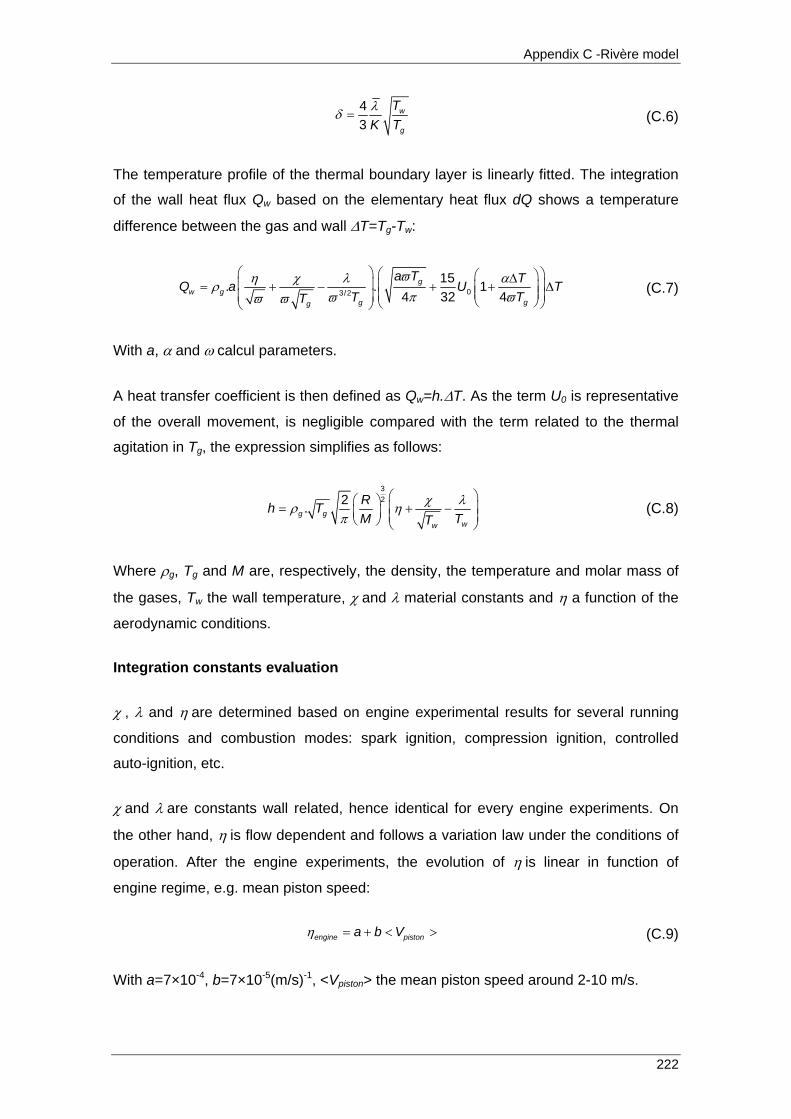
Appendix C -Rivère model
222
43
w
g
TK Tλδ = (C.6)
The temperature profile of the thermal boundary layer is linearly fitted. The integration
of the wall heat flux Qw based on the elementary heat flux dQ shows a temperature
difference between the gas and wall ΔT=Tg-Tw:
03/2
15. . 14 32 4
gw g
ggg
a T TQ a U TTTT
ϖη χ λ αρπ ϖϖϖ ϖ
⎛ ⎞ ⎛ ⎞⎛ ⎞Δ⎜ ⎟ ⎜ ⎟= + − + + Δ⎜ ⎟⎜ ⎟⎜ ⎟⎜ ⎟ ⎝ ⎠⎝ ⎠⎝ ⎠ (C.7)
With a, α and ω calcul parameters.
A heat transfer coefficient is then defined as Qw=h.ΔT. As the term U0 is representative
of the overall movement, is negligible compared with the term related to the thermal
agitation in Tg, the expression simplifies as follows:
322.g g
ww
Rh TM TT
χ λρ ηπ
⎛ ⎞⎛ ⎞ ⎜ ⎟= + −⎜ ⎟ ⎜ ⎟⎝ ⎠ ⎝ ⎠ (C.8)
Where ρg, Tg and M are, respectively, the density, the temperature and molar mass of
the gases, Tw the wall temperature, χ and λ material constants and η a function of the
aerodynamic conditions.
Integration constants evaluation
χ , λ and η are determined based on engine experimental results for several running
conditions and combustion modes: spark ignition, compression ignition, controlled
auto-ignition, etc.
χ and λ are constants wall related, hence identical for every engine experiments. On
the other hand, η is flow dependent and follows a variation law under the conditions of
operation. After the engine experiments, the evolution of η is linear in function of
engine regime, e.g. mean piston speed:
engine pistona b Vη = + < > (C.9)
With a=7×10⁻⁴, b=7×10⁻⁵(m/s)-1, <Vpiston> the mean piston speed around 2-10 m/s.

Appendix C -Rivère model
223
The work of Boust, (2006) also defines the evolution of η based on “fluid” speed seen
by the wall instead of the mean piston speed, as follows:
( )0.5 0.2min ' , ''b V b Vη = (C.10)
With b’=5×10⁻⁴ (m/s)-0.5 and b’’= 8×10⁻⁴ (m/s)-0.2, V is the local speed around 0-25 m/s.
Final formulation
The model of heat losses by conduction can be summarized as follows:
( )w g wQ h T T= −
with 322.g g
ww
Rh TM TT
χ λρ ηπ
⎛ ⎞⎛ ⎞ ⎜ ⎟= + −⎜ ⎟ ⎜ ⎟⎝ ⎠ ⎝ ⎠
Where:
ρg, the gases density local
Tg the gases local temperature
R = 8.314 J/mol K, ideal gas constant.
M the gases molar mass
Tw the local wall temperature,
χ =0.0318 K1/2 and λ= 0.37 K material constants
Engine (Rivère, 2005):
engine pistona b Vη = + < >
With a=7×10⁻⁴, b=7×10⁻⁵(m/s)-1, <Vpiston> the mean piston speed around 2-10 m/s
Other conditions (Boust, 2006):
( )0.5 0.2min ' , ''b V b Vη =
With b’=5×10⁻⁴ (m/s)-0.5 and b’’= 8×10⁻⁴(m/s)-0.2, V is the local speed around 0-25 m/s.


COMBUSTION STUDY OF MIXTURES RESULTING FROM A GASIFICATION PROCESS OF FOREST BIOMASS
Abstract
Syngas is being recognized as a viable energy source worldwide, particularly for
stationary power generation. In the current work, three typical syngas compositions
have been considered as representative of the syngas resultant from forest biomass
gasification, and the possibility of using it in internal combustion engines is studied.
First, laminar burning velocities have been determined from schlieren flame images at
normal temperature and pressure, over a range of equivalence ratios within the
flammability limits. The study of the effects of flame stretch rate is performed through
the determination of Karlovitz and Markstein numbers. Second, because of the gaps in
the fundamental understand of syngas combustion characteristics, especially at
elevated pressures that are relevant to practical combustors, constant volume spherical
expanding flames were employed to measure the laminar burning velocity for
pressures ranges up to 20 bar. This information on laminar burning velocity of syngas-
air flames is then applied in a multi-zone heat transfer simulation code of the wall-flame
interaction in order to predict the quenching distance of typical syngas-air flames.
Engine-like turbulent conditions were experimentally reproduced in a rapid
compression machine (RCM) when working on two strokes mode simulating a single
cycle of an internal combustion engine. Stationary power applications usually use
natural gas as fuel, thus a methane-air mixture is also included in this work as a
reference fuel for comparison with the typical syngas compositions under study. Single
compression tests were also performed in the RCM operating with and without
combustion in order to identify different parameters related with its operation, namely
the heat transfer to the walls. A simulation code for the power cycle of syngas-fuelled
engines has been developed. Model validation has been carried on over detailed
experimental data available in literature for hydrogen and methane. An attempt to
adapt the model to the RCM is made by changing several aspects of the model namely
the in-cylinder volume function and burning rate model. Conclusion could e drawn that
the adapted code is able to reproduce the in-cylinder pressure. The validated model is
then applied to a syngas-fuelled engine in order determine its performance. Conclusion
can be drawn that typical syngas compositions besides its lower heat values and
burning velocities can be used on SI engines even at elevated rotation speeds.
Keywords: Gasification – Syngas - Combustion – Burning velocity – Rapid compression machine - Multi-zone modeling.
Related Documents