Combining Seminorms in Adaptive Lifting Schemes and Applications to Image Analysis and Compression

J Math Imaging Vis 25: 203–226, 2006

c© 2006 Springer Science + Business Media, LLC. Manufactured in The Netherlands.DOI: 10.1007/s10851-006-6711-y

Combining Seminorms in Adaptive Lifting Schemes and Applicationsto Image Analysis and Compression

GEMMA PIELLA AND BEATRICE PESQUET-POPESCUSignal and Image Proc. Dep., Ecole Nationale Superieure des Telecommunications, 37-39 rue Dareau,

75014 Paris, France

HENK J.A.M. HEIJMANSCWI, P.O. Box 94079, 1090 GB Amsterdam, The Netherlands

GREGOIRE PAUSignal and Image Proc. Dep., Ecole Nationale Superieure des Telecommunications, 37-39 rue Dareau, 75014

Paris, France

Published online: 22 July 2006

Abstract. In this paper, we present some adaptive wavelet decompositions that can capture the directional natureof images. Our method exploits the properties of seminorms to build lifting structures able to choose betweendifferent update filters, the choice being triggered by the local gradient-type features of the input. In order to dealwith the variety and wealth of images, one has to be able to use multiple criteria, giving rise to multiple choice ofupdate filters. We establish the conditions under these decisions can be recovered at synthesis, without the needfor transmitting overhead information. Thus, we are able to design invertible and non-redundant schemes thatdiscriminate between different geometrical information to efficiently represent images for lossless compressionmethods.

Keywords: adaptive wavelets, perfect reconstruction filter bank, seminorms, lifting scheme, adaptive filter, imagecompression

1. Introduction

Wavelets have had a tremendous impact on signal pro-cessing, both because of their unifying role and theirsuccess in several applications. The applicability of thewavelet transform (as well as for other multiresolutiondecompositions) is somewhat limited, however, by thelinearity assumption. Coarsening a signal by means oflinear operators may not be compatible with a naturalcoarsening of some signal attribute of interest (e.g., the

The work of Piella is supported by a Marie-Curie Intra-European

Fellowships within the 6th European Community Framework

Programme.

shape of an object), and hence the use of linear pro-cedures may be inconsistent in such applications. Ingeneral, linear filters smear the singularities of a sig-nal and displaces their locations, causing undesirableeffects.

Moreover, standard wavelets are often not suitedfor higher dimensional signals because they are notadapted to the ‘geometry’ of higher dimensional sig-nal singularities. For example, an image comprisessmooth regions separated by piecewise regular curves.Wavelets, however, are good at isolating the dis-continuity across the curve, but they do not ‘see’the smoothness along the curve. These observationsindicate the need for new representations which are

204 Piella et al.

data-dependent. In the literature, one can find severalapproaches to introduce different kinds of adaptivityor geometrical representations into multiresolution de-compositions [1–7, 11, 14].

In [8, 12] we have introduced an adaptive waveletdecomposition based on an adaptive update lifting step.In particular, we have studied the case where the up-date filter coefficients are triggered by a binary deci-sion obtained by thresholding the seminorm of the localgradient-type features of the input. The lifting scheme[13] can therefore choose between two different updatelinear filters: if the seminorm of the gradient is abovethe threshold, it chooses one filter, otherwise it choosesthe other. At synthesis, the decision is obtained in thesame way but using the gradient computed from thebands available at synthesis. With such a thresholding-decision scheme, perfect reconstruction (i.e., invertibil-ity of the scheme) amounts to the so-called ThresholdCriterion, which says that the seminorm of the gradi-ent at synthesis should be above the threshold only ifthe seminorm of the original gradient is. An importantfeature of this adaptive wavelet decomposition schemeis that it is neither causal nor requires any bookkeep-ing in order to perform perfect reconstruction. In [8],we have derived necessary and sufficient conditions forthe invertibility of such adaptive schemes for variousscenarios. Several simulation results have been givento illustrate the potential of adaptive schemes for pre-serving the discontinuities in signals and images evenat low resolutions. Furthermore, it has been shown thatadaptive schemes often yield decompositions that havelower entropies than schemes with fixed update filters,a property that is highly relevant in the context of com-pression. In [9], we have analyzed the quantization ef-fects on our adaptive scheme. In fact, we have beenable to derive conditions that guarantee perfect recon-struction of the decision map (i.e., the choice of theupdate filters).

Despite all these attractive properties, the adaptivescheme proposed in [8] is not very flexible in the sensethat it can only discriminate between two ‘geometricevents’ (e.g., edge region or homogeneous region). Inthis paper, we extend the aforementioned scheme soit can use multiple criteria giving rise to multi-valueddecision for choosing the update filters. In this way,we can discriminate between different geometric struc-tures in order to capture the directional nature of im-ages.

The paper is organized as follows. Section 2 gives abrief overview of the threshold-based adaptive waveletschemes. Section 3 and Section 4 study a new decisioncriterion based on comparing two or more seminorms.

General conditions for the invertibility of the result-ing adaptive decompositions are provided. Section 5shows how this comparing-seminorm criterion can beeasily combined with the Threshold Criterion. Section6 presents some simulation results and analyzes thepotential of the proposed schemes for lossless com-pression purposes. Finally, in Section 7 we draw someconclusions and discuss future directions of research.

2. Previous Work

In this section, we describe a technique for buildingadaptive wavelets by means of an adaptive update stepfollowed by a fixed prediction lifting step. The adap-tivity of the system lies in the choice between two dif-ferent update filters. This choice depends on the localinformation provided by all input bands.

An input signal x0 : Zd → R is split into two signalsx , y where, possibly, y comprises more than one sub-band, say ys1

, ys2, . . . , ysM . The bands x, ys1

, . . . , ysM ,which generally represent the polyphase componentsof the analyzed signal x0, are the input bands for ourlifting scheme. In any case, we assume that the decom-position x0 �→ (x, y) is invertible and hence we canperfectly reconstruct x0 from its components x and y.The first signal x will be updated in order to obtainan approximation signal x ′ whereas ys1

, . . . , ysM willbe further predicted so as to generate a detail signaly′ = {y′

s1, . . . , y′

sM}. In our lifting scheme, the update

step is adaptive while the prediction step is fixed. Thisimplies that the signal y can be easily recovered fromthe approximation x ′ and the detail y′. The recovery ofx from x ′ and y is less obvious.

The basic idea underlying our adaptive scheme isthat the update parameters depend on the informa-tion locally available within both signals x and y, asshown in Fig. 1. In this scheme D is a decision mapwhich uses inputs from all bands, i.e., D = D(x, y) =D(x, ys1

, . . . , ysP ), and whose output is a decision pa-rameter d ∈ {0, 1} which governs the choice of theupdate step. More precisely, if dn is the output of D atlocation n ∈ Zd , then the updated value x ′(n) is given

Figure 1. Adaptive update lifting scheme

Combining Seminorms in Adaptive Lifting Schemes and Applications 205

by

x ′(n) = αdn x(n) +J∑

j=1

μdn, j y j (n) , (1)

with y j (n) = ys j (n + l j ), s j ∈ {s1, . . . , sM}, l j ∈ L .Here L is a window in Zd centered around the origin.Note that the filter coefficients depend on the outputd ∈ {0, 1} of the decision map D. Thus, presumedthat d is known for every location n, we can recoverthe original signal x. One says in this case that PerfectReconstruction is possible.

We assume that

D(v(n)) = [p(v(n)) > T ] ,

where [P] returns 1 if the predicate P is true, and 0otherwise; p is a seminorm, T is a threshold and v(n) ∈RJ is the gradient vector with components v j (n) givenby

v j (n) = x(n) − y j (n), j = 1, . . . , J.

For the coefficients in (1) we assume that

α0 +J∑

j=1

μ0, j = α1 +J∑

j=1

μ1, j = 1

with αd �= 0 for both d = 0, 1, and μ0, j �= μ1, j forsome j ∈ {1, . . . , J }.

It is easy to show that the gradient vector at syn-thesis v′(n) ∈ RJ with components v′

j (n) = x ′(n) −y j (n), j = 1, . . . , J , is related to v(n) by means of thelinear relation

v′(n) = Adv(n) ,

where Ad = I −ubTd , I is the J × J identity matrix, and

u = (1, . . . , 1)T , bd = (μd,1, . . . , μd,J )T are vectorsof length J.

Thus the adaptive update lifting step is described by:{v ′ = Adv

d = [p(v) > T ] ,(2)

where we have suppressed the argument ‘n’ from ournotation. Note that the determinant of the matrix Ad

is det(Ad ) = 1 − uT bd = 1 − ∑Jj=1 μd, j = αd . By

assumption αd �= 0, hence Ad is invertible. It is notdifficult to show that A−1

d = I − ub′Td where b′

d =−bd/αd

Consider the adaptive update lifting step in (2). Ifp(v) ≤ T at analysis, then the decision equals d = 0and v ′ = A0v . If, on the other hand, p(v) > T , thend = 1 and v ′ = A1v . To have perfect reconstruction wemust be able to recover the decision d from the gradientvector at synthesis v ′. Here we shall restrict ourselvesto the case where d can be recovered by thresholdingthe seminorm p(v ′), i.e., the case that

d = [p(v) > T ] = [p(v ′) > T ′] ,

for some T ′ > 0. We formalize this condition in thefollowing criterion.

Threshold Criterion. Given a threshold T > 0, thereexists a (possibly different) threshold T ′ > 0 such that

(i) if p(v) ≤ T then p(A0v) ≤ T ′;(i i) if p(v) > T then p(A1v) > T ′.

It is obvious that the Threshold Criterion (TC) guar-antees Perfect Reconstruction. In [8] we provide nec-essary and sufficient conditions for the TC to holdand analyze several different choices for the semi-norm, among which the quadratic seminorms and theweighted gradient seminorms.

Before introducing new decision criteria, we givesome definitions and properties which will be used fur-ther on.

Let V be a vector space with seminorm p. For a linearoperator A : V → V we define the operator seminormp(A) and the inverse operator seminorm p−1(A) as

p(A) = sup{p(Av) | v ∈ V and p(v) = 1}p−1(A) = sup{p(v) | v ∈ V and p(Av) = 1}.

In the last expression we use the convention thatp−1(A) = ∞ if p(Av) = 0 for all v ∈ V , unless p isidentically zero, in which case both p(A) and p−1(A)are zero. Throughout the remainder, we will discardthe case where p is identically zero and, consequently,we will always have p−1(A) > 0.

Note that we cannot have p(A) = 0. Indeed, ifp(A) = 0, then by definition we have that for allv ∈ V, p(Av) = 0 and, for invertible operators A,this means that for all v ∈ V, p(v) = 0, which is incontradiction with the assumption that p is not the nullfunction.

Proposition 2.1. Let V be a Hilbert space, let p: V →R+ be a seminorm and A : V → V be a bounded linear

206 Piella et al.

operator. If p(A) < ∞, the

p(Av) ≤ p(A)p(v) f or all v ∈ V .

Proof: The property straightforwardly follows fromthe definition of p(A) when p(v) �= 0. If p(v) = 0, itis a consequence of property (b) of seminorms givenby Proposition 3 in [8], that is, p(A) < ∞ is equiv-alent to the implication p(v) = 0 ⇒ p(Av) = 0 forv ∈ V .

3. Comparing Two Seminorms

3.1. Main Results

The goal of this section is to find a decision rule al-lowing to compare two seminorms and which allowsPerfect Reconstruction. The conditions at analysis willbe given by:{

d = 0 ⇔ p0(v) ≤ p1(v)

d = 1 ⇔ p0(v) > p1(v) ,(3)

where p0 and p1 are two seminorms not equal to thenull function. Once the decision is obtained, the updatestep is performed as in (1).

At synthesis, similar conditions will be used, replac-ing v by the modified gradient vector v ′ = Adv:{

(i) p0(v ′) ≤ p1(v ′) ⇔ d ′ = 0

(i) p0(v ′) > p1(v ′) ⇔ d ′ = 1.(4)

It is evident that Perfect Reconstruction (PR) arises ifd = d ′.

The result providing necessary and sufficient condi-tions for PR is similar to that for the TC.

Proposition 3.1. Perfect reconstruction holds if andonly if the following two conditions are satisfied:

∀v ∈ V,

{p0(v) ≤ p1(v) ⇒ p0(A0v) ≤ p1(A0v)

p0(v) > p1(v) ⇒ p0(A1v) > p1(A1v).

(5)

Proof: Assume first that (5) holds. We show that PRis achieved only if d = d ′.

Suppose p0(v ′) ≤ p1(v ′) (i.e. d ′ = 1) and d = 1. Inthis case, we get p0(A1v) ≤ p1(A1v). From the sec-ond equation in (5), we obtain p0(v) < p1(v) which,

according to (3), is equivalent to d = 0. This contra-diction with the starting assumption d = 1 shows thatin order to have PR we need d = 0.

Suppose p0(v ′) > p1(v ′) (i.e. d ′ = 1) and d = 0.We get p0(A0v) > p1(A0v). From the first equationin (5), it follows that p0(v) > p1(v) and this leads tod = 1 for PR.

If we now assume that PR holds, (3) and (4) clearlyshow that (5) is satisfied.

Remark 3.2. Conditions in (5) show that the admis-sible domain for (A0, A1) (resp. (b0, b1)) correspond-ing to the necessary and sufficient conditions for PRis separable, i.e., it may be separated in an admissi-ble domain for A0 (resp. b0) and another one for A1

(resp. b1). Besides, the second condition in (5) may berewritten as:

∀v ∈ V, p0(A1v) ≤ p1(A1v) ⇒ p0(v) ≤ p1(v).

As A1 is invertible, by introducing w = A1v , the aboveexpression is equivalent to

∀w ∈ V, p0(w) ≤ p1(w)⇒p0

(A−1

1 w) ≤ p1

(A−1

1 w).

The second condition for PR is therefore identical tothe first one, by replacing A0 by A−1

1 . Moreover, since

A0 = I − ubT0 and A1 = I − ub

′T1 , where b′

1 =−α−1

1 b1, we have a symmetry between the admissibledomains for b0 and b1: the second one is derived fromthe first one by replacing b0 by −α−1

1 b1.Let us now introduce some definitions that will be

useful in the sequel:

p10(A0) = inf{p1(A0v) | v ∈ V and p0(v)

≤ p1(v) = 1} (6)

p01(A1) = inf{p0(A1v) | v ∈ V and p1(v)

≤ p0(v) = 1}. (7)

Observe that in order to define p10 the set

S10 = {v | p0(v) ≤ p1(v) = 1}

needs to be non-empty. 1 Analogously, in order to de-fine p01, the set S01 = v | p1(v) ≤ p0(v) = 1} needs tobe non-empty.

Another important observation is that, in case theabove quantities exist, they are finite.

Lemma 3.3. The following implications hold.


(a) If S10 �= ∅ and p0(v) ≤ p1(v), then p1(A0v) ≥p10(A0)p1(v).

(b) If S10 �= ∅ and p1(v) ≤ p0(v), then p0(A1v) ≥p01(A1)p0(v).

Proof: We proof statement (a). The proof of (b) isanalogous.

If p1(v) �= 0 we can choose v ′ = vp1(v)

.Then,p0(v ′) ≤ p1(v ′) = p1(v)

p1(v)= 1 and, by definition,

p1(A0v ′) ≥ p10(A0). Therefore, we get p1(A0v)p1(v)

≥p10(A0), which implies p1(A0v) ≥ p10(A0)p1(v).

If p1(v) = 0, then p1(A0v) ≥ 0 is always true.

Note that statements (a) and (b) from the previouslemma imply, respectively,

p10(A0) ≤ p1(A0) if p1(A0) < ∞ and

p01(A1) ≤ p0(A1) if p0(A1) < ∞.

The main result of this section provides sufficient con-ditions for (5) to hold.

Proposition 3.4. Sufficient conditions for the perfectreconstruction relations in (5) to be satisfied are:

S10 �= ∅, S01 �= ∅, (8)

p10(A0) ≥ p0(A0) (9)

p01(A1) ≥ p1(A1) (10)

Proof: We have to prove that if conditions (8)–(10)hold, then (5) is satisfied. We use the fact that sincep10, p01 exist, they are bounded and hence, accordingto (9)–(10), pd (Ad ) < ∞, d = 0, 1.

In order to prove the first relation in (5), we sup-pose that p0(v) ≤ p1(v). As p0(A0) < ∞, we getp0(A0v) ≤ p0(A0)p0(v) (see Proposition 2.1). FromLemma 3.3(a), we have p1(A0v) ≥ p10(A0)p1(v),and since p10(A0) ≥ p0(A0) we obtain p1(A0v) ≥p0(A0)p1(v) ≥ p0(A0)p0(v) ≥ p0(A0v). This provesthe first relation.

Now we show the second condition in (5). Sup-pose p0(v) > p1(v). We know that p1(A1v) ≤p1(A1)p1(v). From Lemma 3.3(b), we have p0(A1v) ≥p01(A1)p0(v), and since p01(A1) ≥ p1(A1) �= 0, it fol-lows that p0(A1v) ≥ p1(A1)p0(v) > p1(A1)p1(v) ≥p1(A1v), which implies p0(A1v) > p1(A1v) and provesthe second relation in (5).

Note that if (9)–(10) are satisfied, since pd (Ad ) �= 0,

one necessarily has:

p10(A0) �= 0, p01(A1) �= 0.

3.2. A Case of Study: The Weighted Seminormp(v) = |aT v|

Consider an adaptive wavelet scheme with the deci-sion rules described in the previous subsection (i.e.,(3) at analysis and (4) at synthesis). Let p0, p1 be theweighted seminorms [8]:

p0(v) = ∣∣aT0 v

∣∣, p1(v) = ∣∣aT1 v

∣∣ ,

where a0 �= 0 and a1 �= 0. In order to study the PRconditions (8)–(10), we should calculate p10(A0) andp01(A1). Here we illustrate how to compute p10(A0).By definition,

p10(A0) = inf{∣∣aT

1 A0v∣∣ ∣∣aT

0 v∣∣ ≤ ∣∣aT

1 v∣∣ = 1

}.

We distinguish two cases, namely a0 and a1 are or arenot collinear.

(i) a0 and a1 are collinear. In this case, we can writea0=γ a1, γ∈R∗, which is of no practical interestsince it leads to a non-adaptive scheme.2

(i i) a0 and a1 are not collinear. Define c = AT0 a1. In

this case, we can express

c = c0a0 + c1a1 + c,

where (c0, c1) ∈ R2, c ∈ Span⊥{a0, a1}. We get:

p1(A0v) = ∣∣aT1 A0v

∣∣ = |cT v| = ∣∣c0aT0 v + c1aT

1 v

+ cT v∣∣ ≥ 0.

In order to find p10(A0), we have to minimize the aboveexpression under the constraint |aT

0 v| ≤ |aT1 v| = 1. We

get the result below (see Appendix A for the proof).

Lemma 3.5. Consider the two seminorms: p0(v) =|aT

0 v|, p1(v) = |aT1 v| with a0 and a1 non-collinear

vectors, and define c = AT0 a1 = c0a0 + c1a1 + c.

Then,p10(A0)

=

⎧⎪⎪⎪⎪⎨⎪⎪⎪⎪⎩|c1| − |c0| i f uT a1 �= 0 and b0

= (1 − c1) − a1 − c0a0

uT a1

, wi th|c1|> |c0| and c = 0

0 otherwise.

208 Piella et al.

A similar reasoning yields an analogous result forp01(A1).

We are now able to study the sufficient PR con-ditions (8)–(10). We slightly modify our notation byintroducing:

c0 = AT0 a1 = c0

0a0 + c01a1 + c0,

c1 = AT1 a0 = c1

0a0 + c11a1 + c1,

where (c0, c1) ∈ Span⊥{a0, a1}.Assume (80)–(10) hold. Thus p10(A0) �= 0, p01

(A1) �= 0 and pd (Ad ) < ∞. From this last condition,we get [8] either uT ad = 0, which implies pd (Ad ) = 1,or uT ad �= 0 and bd = γdad , γd ∈ R which impliespd (Ad ) = |αd |.

On the other hand, according to Lemma 3.5, we havean equivalence between the fact that p10(A0) �= 0 (resp.p01(A1) �= 0) and the expression of b0 (resp. b1):

b0 =(1 − c0

1

)a1 − c0

0a0

uT a1

, with uT a1 �= 0,∣∣c0

1

∣∣ >∣∣c0

0

∣∣and c0 = 0 ,

which leads to p10(A0) = ∣∣c01

∣∣ − ∣∣c00

∣∣.By discarding non-compatible constraints, for con-

ditions (9)–(10) in Proposition 3.4 to be satisfied, weobtain:

uT a0 �= 0, uT a1 �= 0

b0 = γ0a0 =(1 − c0

1

)a1 − c0

0a0

uT a1

, with∣∣c0

1

∣∣ >∣∣c0

0

∣∣b1 = γ1a1 =

(1 − c1

0

)a0 − c1

1a1

uT a0

, with∣∣c1

0

∣∣ >∣∣c1

1

∣∣.As we have made the hypothesis that a0 and a1 are notcollinear, we finally get:

c01 = c1

0 = 1,∣∣c0

0

∣∣ < 1,∣∣c1

1

∣∣ < 1 ,

hence

b0 = − c00

uT a1

a0, b1 = c11

uT a0

a1.

Thus p01(A1) = 1 − |c11| and p10(A0) = 1 − |c0

0|.By gathering these conditions, we have the followingresult.

Proposition 3.6. Sufficient conditions for PR to holdfor a criterion based on the comparison of the twoseminorms p0(v) = |aT

0 v| and p1(v) = |aT1 v|, where a0

and a1 are not collinear, are that uT a0 �= 0, uT a1 �= 0and

b0 = β0

uT a1

a0, b1 = β1

uT a0

a1 , (11)

where 0 < |α0| ≤ 1 − |β0| and 0 < |α1| ≤ 1 − |β1|.

The last two conditions stem from the inequalities1 − |β0| = p10(A0) ≥ p0(A0) = |α0| and 1 − |β1| =p01(A1) ≥ p1(A1) = |α1|.

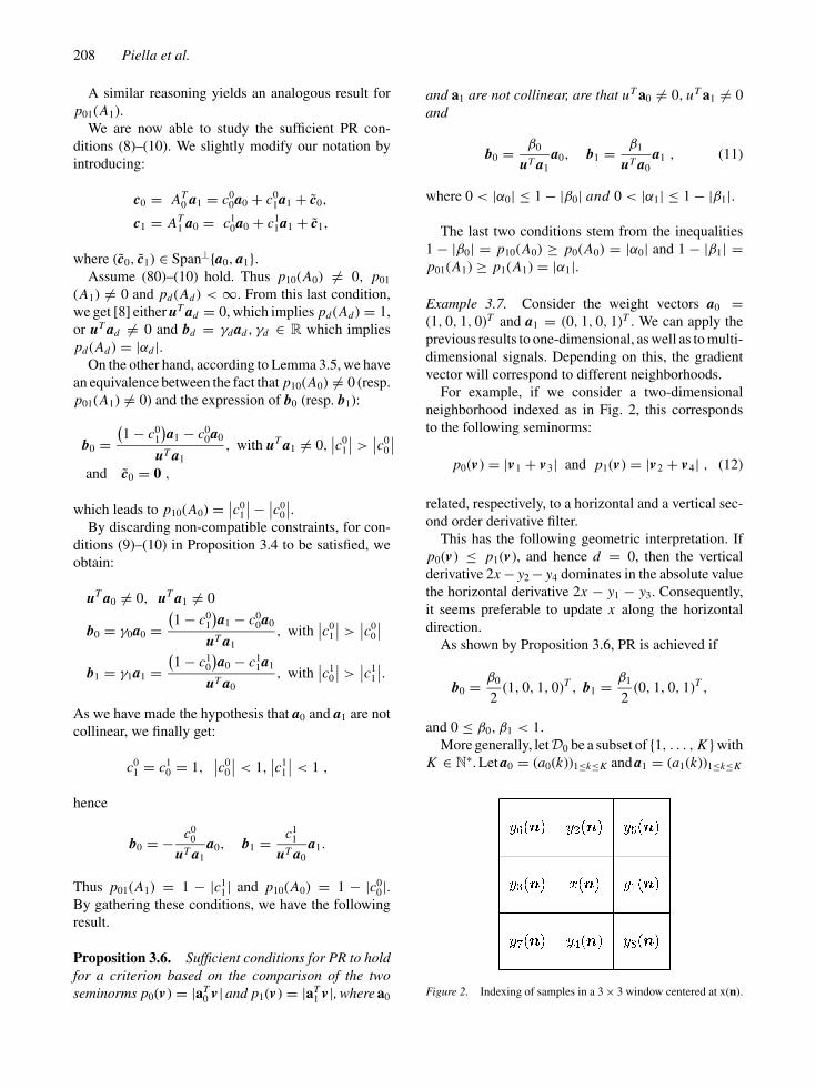
Example 3.7. Consider the weight vectors a0 =(1, 0, 1, 0)T and a1 = (0, 1, 0, 1)T . We can apply theprevious results to one-dimensional, as well as to multi-dimensional signals. Depending on this, the gradientvector will correspond to different neighborhoods.

For example, if we consider a two-dimensionalneighborhood indexed as in Fig. 2, this correspondsto the following seminorms:

p0(v) = |v1 + v3| and p1(v) = |v2 + v4| , (12)

related, respectively, to a horizontal and a vertical sec-ond order derivative filter.

This has the following geometric interpretation. Ifp0(v) ≤ p1(v), and hence d = 0, then the verticalderivative 2x − y2 − y4 dominates in the absolute valuethe horizontal derivative 2x − y1 − y3. Consequently,it seems preferable to update x along the horizontaldirection.

As shown by Proposition 3.6, PR is achieved if

b0 = β0

2(1, 0, 1, 0)T , b1 = β1

2(0, 1, 0, 1)T ,

and 0 ≤ β0, β1 < 1.

More generally, letD0 be a subset of {1, . . . , K } withK ∈ N∗. Let a0 = (a0(k))1≤k≤K and a1 = (a1(k))1≤k≤K

Figure 2. Indexing of samples in a 3 × 3 window centered at x(n).


with, for all k ∈ {1, . . . , K }

a0(k) ={

1 if k ∈ D0

0 otherwisea1(k) =

{1 if k /∈ D0

0 otherwise

In other words, the components of a0 and a1 arecomplementary in binary representation. This allowsto compare the decision made on two disjoint sets ofneighbors {yk, k ∈ D0} and {yk, k /∈ D0}. For instance,if we choose

a0 = (1, 0, 1, 0, . . . , 0)T ∈ R2K ,

a1 = (0, 1, 0, 1 . . . , 1)T ∈ R2K ,

we are looking for the lowest gradient value betweenK x − ∑K

k=0 y2k+1 and K x − ∑Kk=0 y2k .

In the general case, by applying Proposition 3.6, asufficient condition for PR is that

b0 = β0

Ka0, b1 = β1

K0

a1,

with K0 = card D0, K1 = K − K0, 0 ≤ β0 < 1 and0 ≤ β1 < 1.

As, in this case, the update is proportional with thearithmetic mean of the neighboring samples, we can,for example, take α0 equal to the coefficients of theupdate filter, i.e., α0 = β0/K0, and therefore

β0 = K0

K0 + 1.

In a similar manner, we obtain α1 = β1/K1 and β1 =K1/(K1 + 1).

Example 3.8. Consider now the vectors a0 =(1, 1, 0, 0)T and a1 = (1/2, 1/2, 1/2, 1/2)T . We com-pare their corresponding seminorms:

p0(v) = |v1 + v2| and

p1(v) = |v1 + v2 + v3 + v4|2

,

or, in other words, we want to know which one of theaverages (y1 + y2)/2 or (y1 + y2 + y3 + y4)/4 is closerto the sample x to be updated.

The filter coefficients in (11) are given by:

b0 = β0

2(1, 1, 0, 0)T , b1 = β1

4(1, 1, 1, 1)T ,

and again 0 ≤ β0, β1 < 1.

More generally, we can compare two ‘averages’,computed on arbitrary nested neighborhoods. LetD0 �=∅ ⊂ {1, . . . , K } with K ∈ N∗ and

p0(v) =∣∣∣∣x −

∑k∈D0

yk

K0

∣∣∣∣, p1(v) =∣∣∣∣x −

∑Kk=1 yk

K

∣∣∣∣,with K0 = card D0.

Then, a0 = (a0(k))1≤k≤K where, for all k ∈ {1, . . . ,K },we have:

a0(k) =⎧⎨⎩

1

K0

if k ∈ D0

0 otherwise ,

and a1 = uK . According to Proposition 3.6, we get

b0 = β0a0, b1 = β1a1, with 0 ≤ β0, β1 < 1.

3.2.1. Counter-Example: Switching Between Hori-zontal and Vertical Filters. Proposition 3.6 (or moregenerally Proposition 3.4) provides sufficient condi-tions for PR to hold. However, as we will show in thiscounter-example, they are not necessary.

Let us consider again the derivative criteria intro-duced at the beginning of Example 3.7. The two semi-norms used in the decision map govern respectivelythe horizontal and the vertical gradient, as definedin (12).

We assume that the update filters Ud have 4 tapscorresponding with the detail coefficients labeled byy1, . . . , y4. The filter coefficients bd are chosen now asfollows:

bd = (μd , ηd , μd , ηd )T for d = 0, 1. (13)

This means in particular that only the four horizontaland vertical neighbors y1, y2, y3, y4 are used to updatethe approximation signal. For example, if d = 0, thenthe update operation reduces to:

x ′ = α0x + μ0(y1 + y3) + η0(y2 + y4). (14)

Let v ′ be the gradient vector at synthesis, i.e.,v ′

j = x ′ − y j . A straightforward calculation showsthat

|v ′1 + v ′

3| = |(1 − 2μd )(v1 + v3) − 2ηd (v2 + v4)||v ′

2 + v ′4| = | − 2μd (v1 + v3) + (1 − 2ηd )(v2 + v4)|.

If we can choose the coefficients μ0, η0, μ1, η1 in such

210 Piella et al.

a way that

p0(v) ≤ p1(v) ⇐⇒ p0(v ′) ≤ p1(v ′) ,

then we can recover the original decision from the gra-dient vector at synthesis, and hence perfect reconstruc-tion is possible in this case.

Proposition 3.9. Let p0 and p1 be defined by (12)and consider the update filters given by (13). Then, inorder to have perfect reconstruction it is necessary andsufficient that

η0 ≤ μ0 and μ0 + η0 <1

2,

μ1 ≤ η1 and μ1 + η1 <1

2.

Proof: See Appendix B.

The obtained necessary and sufficient conditions areclearly less restrictive than those derived from Propo-sition 3.6, since the vectors b0 and b1 are not re-stricted to be collinear to a0 and a1, respectively.The sufficient condition (see Example 3.7) providesthe segments η0 = 0, μ0 ∈ [0, 1

2) and μ1 = 0,

η1 ∈ [0, 12), which are the longest segments con-

tained in the admissible domains for (μ0, η0) and(μ1, η1).

3.2.1.1. Experiment (Switching Between Horizontaland Vertical Filters - Fig. 3). We consider a 2D squaresampling scheme such as depicted in Fig. 2. We adopta new notation yv , yh, yd of the y-bands, replacingy1, y4, y8. This reflects the fact that, after the predic-tion stage, the corresponding outputs y′

v , y′h, y′

d are of-ten called the vertical, the horizontal, and the diagonaldetail bands, respectively.

We choose the update filter coefficients like in (13)with μ0 = η1 = 0 and μ1 = η0 − 1/4. Obviouslythe conditions in Proposition 3.9 are satisfied. Afterthe update step, we compute the detail images with theprediction scheme:

y′h = yh − x ′ (15)

y′v = yv − x ′ (16)

y′d = yd − x ′ − y′

v − y′h . (17)

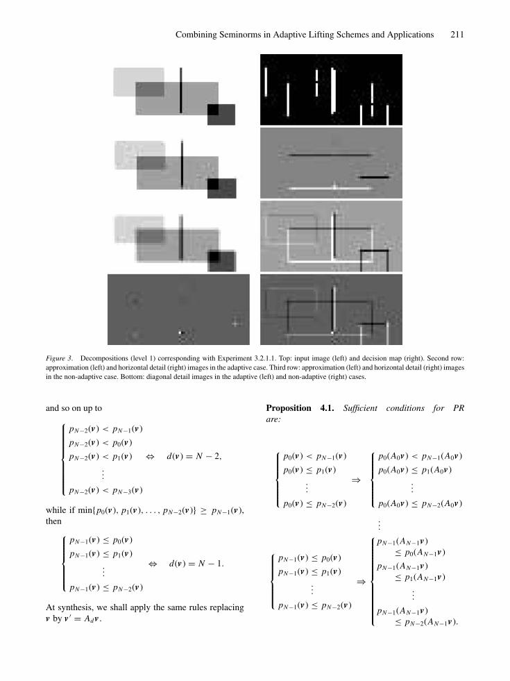
We apply this decomposition to the original imagedepicted at the top left of Fig. 3. The decision map isshown at the top right. White pixels show the regionswhere the horizontal gradient was larger than the verti-cal. In such regions, the vertical-oriented update filterwill be used. The approximation and horizontal detailimages are shown in the second row. The diagonal de-tail is displayed in the bottom row, on the left. We com-pare this scheme with the non-adaptive scheme wherewe perform an isotropic filtering (in the vertical andhorizontal directions), i.e., μ = η = 1/8. The corre-sponding approximation and horizontal images are dis-played in the third row of Fig. 3, and the diagonal detailimage on the right of the bottom row. We can easily seethat the approximation image obtained in the adaptivecase preserves the edges in contrast with the one ob-tained in the non-adaptive scheme. Consequently, thedetail images obtained in the adaptive case ‘capture’ theedges in a more compact way than in the non-adaptivecase.

4. Case of N Seminorms

In this section, we shall consider N seminorms, de-noted by p0, p1, . . . , pN−1. The decision map will nolonger be binary, but it will take N values, d(v) ∈{0, 1, . . . , N − 1}. The same is true for the decisionvalues at synthesis, d(v ′). The decision criterion willbe based on the comparison, at each point, between thevalues of the seminorms.

At analysis, without loss of generality, if min{p0(v), p1(v), . . . , pN−2(v)} < pN−1(v), then we haveone of the following situations:

⎧⎪⎪⎪⎪⎨⎪⎪⎪⎪⎩p0(v) < pN−1(v)

p0(v) ≤ p1(v)... ⇔ d(v) = 0

p0(v) ≤ pN−2(v)

⎧⎪⎪⎪⎪⎪⎪⎪⎨⎪⎪⎪⎪⎪⎪⎪⎩

p1(v) < pN−1(v)

p1(v) < p0(v)

p1(v) ≤ p2(v) ⇔ d(v) = 1

...

p1(v) ≤ pN−2(v)


Figure 3. Decompositions (level 1) corresponding with Experiment 3.2.1.1. Top: input image (left) and decision map (right). Second row:

approximation (left) and horizontal detail (right) images in the adaptive case. Third row: approximation (left) and horizontal detail (right) images

in the non-adaptive case. Bottom: diagonal detail images in the adaptive (left) and non-adaptive (right) cases.

and so on up to⎧⎪⎪⎪⎪⎪⎪⎪⎨⎪⎪⎪⎪⎪⎪⎪⎩

pN−2(v) < pN−1(v)

pN−2(v) < p0(v)

pN−2(v) < p1(v) ⇔ d(v) = N − 2,

...

pN−2(v) < pN−3(v)

while if min{p0(v), p1(v), . . . , pN−2(v)} ≥ pN−1(v),then⎧⎪⎪⎪⎪⎨⎪⎪⎪⎪⎩

pN−1(v) ≤ p0(v)

pN−1(v) ≤ p1(v)

...

pN−1(v) ≤ pN−2(v)

⇔ d(v) = N − 1.

At synthesis, we shall apply the same rules replacingv by v ′ = Adv .

Proposition 4.1. Sufficient conditions for PRare:

⎧⎪⎪⎪⎪⎨⎪⎪⎪⎪⎩p0(v) < pN−1(v)

p0(v) ≤ p1(v)

...

p0(v) ≤ pN−2(v)

⇒

⎧⎪⎪⎪⎪⎨⎪⎪⎪⎪⎩p0(A0v) < pN−1(A0v)

p0(A0v) ≤ p1(A0v)

...

p0(A0v) ≤ pN−2(A0v)

...

⎧⎪⎪⎪⎪⎨⎪⎪⎪⎪⎩pN−1(v) ≤ p0(v)

pN−1(v) ≤ p1(v)

...

pN−1(v) ≤ pN−2(v)

⇒

⎧⎪⎪⎪⎪⎪⎪⎪⎪⎪⎪⎨⎪⎪⎪⎪⎪⎪⎪⎪⎪⎪⎩

pN−1(AN−1v)≤ p0(AN−1v)

pN−1(AN−1v)≤ p1(AN−1v)

...

pN−1(AN−1v)≤ pN−2(AN−1v).

212 Piella et al.

Proof: Let us consider the first implication in theproposition. Assume that d ′ = 0. If d �= 0, then dcan take any value in {1, . . . , N − 1}. For example, letd = 1. By hypothesis, it follows that:⎧⎪⎪⎪⎪⎪⎪⎪⎨⎪⎪⎪⎪⎪⎪⎪⎩

p1(A1v) < pN−1(A1v)

p1(A1v) < p0(A1v)

p1(A1v) ≤ p2(A1v)

...

p1(A1v) ≤ pN−2(A1v).

The second inequality from the above system,p1(A1v) < p0(A1v), is in contradiction with the hy-pothesis p0(Adv) ≤ p1(Adv), when d=1. A similarargument can be used for d∈{2, . . . , N − 1}. There-fore, we have proven by contradiction that d = 0. Theother implications follow in the same way.

The previous proposition also appears as a consequenceof the following more general result.

Proposition 4.2. Let us consider at analysis a deci-sion map defined by

d : V → {0, . . . , N − 1}v �→ d(v) ,

and the decision regions

∀i ∈ {0, . . . , N − 1}, Di = {v ∈ V | d(v) = i}

forming a partition of V:

V =N−1⋃i=0

Di , Di �= ∅ and Di ∩ D j = φ

i f i �= j.

At synthesis, we have v′ = Ad(v)v , and the decisionrule is:

d ′(v ′) = d(Ad(v)v).

Then, we have that:

(i) PR holds if and only if ∀v, d(Ad(v)v) = d(v).(ii) A necessary and sufficient condition for this to be

satisfied is:

∀i ∈ {0, 1, . . . , N − 1},i f d(v) = i then d(Ai v) = i. (18)

Proof: The proof of (i) is straightforward. We prove(ii).

Assume that (18) holds. As before, we supposed(Ad(v)v) = i and d(v) �= i . In this case, as {Di }, i =0, . . . , N − 1, is a partition of V, there exists j �= i ∈{0, . . . , N − 1} such that d(v) = j , which, accordingto (18), implies that d(A j v) = j . But we also haved(A j v) = i , which obviously leads to a contradictionas Di ∩ D j = ∅. This shows that PR is satisfied.

Conversely, if PR condition holds, (18) is straight-forwardly satisfied.

A weaker condition for PR (i.e., sufficient in orderto have the previous necessary and sufficient con-ditions satisfied) is to have simultaneously all thefollowing implications:⎧⎪⎪⎪⎪⎪⎪⎪⎪⎪⎪⎪⎪⎪⎪⎪⎪⎪⎪⎪⎪⎪⎪⎪⎪⎪⎪⎪⎪⎪⎪⎪⎪⎨⎪⎪⎪⎪⎪⎪⎪⎪⎪⎪⎪⎪⎪⎪⎪⎪⎪⎪⎪⎪⎪⎪⎪⎪⎪⎪⎪⎪⎪⎪⎪⎪⎩

p0(v) < pN−1(v) ⇒ p0(A0v) < pN−1(A0v)

p0(v) ≤ p1(v) ⇒ p0(A0v) ≤ p1(A0v)

...

p0(v) ≤ pN−2(v) ⇒ p0(A0v) ≤ pN−2(A0v)

p1(v) < pN−1(v) ⇒ p1(A1v) < pN−1(A1v)

p1(v) < p0(v) ⇒ p1(A1v) < p0(A1v)

...

p1(v) ≤ pN−2(v) ⇒ p1(A1v) ≤ pN−2(A1v)

...

pN−1(v) ≤ p0(v) ⇒ pN−1(AN−1v)≤ p0(AN−1v)

...

pN−1(v) ≤ pN−2(v) ⇒ pN−1(AN−1v)≤ pN−2(AN−1v).

The above conditions can be combined pairwise, so asto get:{

pN−1(v) ≤ p0(v) ⇒ pN−1(AN−1v) ≤ p0(AN−1v)

pN−1(v) > p0(v) ⇒ pN−1(A0v) > p0(A0v){p0(v) ≤ p1(v) ⇒ p0(A0v) ≤ p1(A0v)

p0(v) > p1(v) ⇒ p0(A1v) > p1(A1v)

and so on. In this way, a sufficient condition for PR isexpressed as a set of N (N − 1)/2 conditions, each ofthem involving only two seminorms. These conditionsare actually similar to those in (5) and the results inSection 2 can therefore be applied to translate theminto more practical conditions.


Example 4.3. Necessary and sufficient conditions forPR in Proposition 4.2 for N = 3 can be writtenas:

{p0(v) < p2(v)

p0(v) ≤ p1(v)=⇒

{p0(A0v) < p2(A0v)

p0(A0v) ≤ p1(A0v){p1(v) < p2(v)

p1(v) < p0(v)=⇒

{p1(A1v) < p2(A1v)

p1(A1v) < p0(A1v){p2(v) ≤ p0(v)

p2(v) ≤ p1(v)=⇒

{p2(A2v) ≤ p0(A2v)

p2(A2v) ≤ p1(A2v),

and a sufficient condition for this is:{p2(v) ≤ p0(v) =⇒ p2(A2v) ≤ p0(A2v)

p2(v) > p0(v) =⇒ p2(A0v) > p0(A0v){p2(v) ≤ p1(v) =⇒ p2(A2v) ≤ p1(A2v)

p2(v) > p1(v) =⇒ p2(A1v) > p1(A1v){p0(v) ≤ p1(v) =⇒ p0(A0v) ≤ p1(A0v)

p0(v) > p1(v) =⇒ p0(A1v) > p1(A1v)

In particular, let p0(v) = |aT0 v|, p1(v) = |aT

1 v| andp2(v) = |aT

2 v|. Assume that a0, a1, a2 are not pairwisecollinear and such that uT a0 = uT a1 = uT a2 = ξ �= 0.Then we have the following sufficient conditions forPR:

bi = βi ai

ξ, where 0 ≤ βi < 1, i = 0, 1, 2.

For example, if a0 = (1, 0, 1, 0)T , a1 = (0, 1, 0, 1)T

and a2 = 12(1, 1, 1, 1)T , then

b0 = β0

2(1, 0, 1, 0)T , b1 = β1

2(0, 1, 0, 1)T ,

b2 = β2

4(1, 1, 1, 1)T ,

where 0 ≤ βi < 1, i = 0, 1, 2.For 1D signals (see indexing in Fig. 4), this

corresponds to comparing the gradient informationon the left-hand side of the sample to be updated

Figure 4. Example of indexing the input samples for one-dimensional signals.

with the gradient information on the right-hand sideand also with the gradient computed from bothsides.

For images (see indexing in Fig. 2), this crite-rion amounts to comparing gradients in horizontaland vertical directions with a gradient taking intoaccount isotropic information from the closest fourneighbors.

5. Combining two Seminormswith the Threshold Criterion

We can also combine the comparison of two seminormswith a TC for each one of them. We end up with fourdecision regions, described by, e.g.,

p0(v) ≤ p1(v) and p0(v) ≤ T0 ⇔ d = 0 (19)

p0(v) ≤ p1(v) and p0(v) > T0 ⇔ d = 1 (20)

p0(v) > p1(v) and p1(v) ≤ T1 ⇔ d = 2 (21)

p0(v) > p1(v) and p1(v) > T1 ⇔ d = 3, (22)

where T0, T1 are two positive threshold values. Asimilar rule with threshold values T ′

0, T ′1 is used at

synthesis.By Proposition 4.2, the following necessary and suf-

ficient conditions for PR are obtained:

{p0(v) ≤ p1(v)

p0(v) ≤ T0

⇒{

p0(A0v) ≤ p1(A0v)

p0(A0v) ≤ T ′0{

p0(v) ≤ p1(v)

p0(v) > T0

⇒{

p0(A1v) ≤ p1(A1v)

p0(A1v) > T ′0{

p0(v) > p1(v)

p1(v) ≤ T1

⇒{

p0(A2v) > p1(A2v)

p1(A2v) ≤ T ′1{

p0(v) > p1(v)

p1(v) > T1

⇒{

p0(A3v) > p1(A3v)

p0(A3v) > T ′1

Again, a sufficient condition for the above relations tohold is that all the implications be met individually, that

214 Piella et al.

is, {p0(v) ≤ T0 ⇒ p0(A0v) ≤ T ′

0

p0(v) > T0 ⇒ p0(A1v) > T ′0

(23)

{p0(v) ≤ T1 ⇒ p0(A2v) ≤ T ′

1

p0(v) > T1 ⇒ p0(A3v) > T ′1

(24)

{p0(v) ≤ p1(v) ⇒ p0(A0v) ≤ p1(A0v)

p0(v) > p1(v) ⇒ p0(A2v) > p1(A2v)(25)

{p0(v) ≤ p1(v) ⇒ p0(A1v) ≤ p1(A1v)

p0(v) > p1(v) ⇒ p0(A3v) > p1(A3v).

(26)

Note that the TC can be combined in an obvious mannerwith several seminorms. In Section 6, we give threeexamples (Experiments 6.3–6.5).

Proposition 5.1. Consider the decision rule given by(19)–(22), with p0(v) = |aT

0 v| and p1(v) = |aT1 v|,

where a0 and a1 are not collinear. A sufficient conditionfor PR is that uT a0 �= 0, uT a1 �= 0, T ′

0 = |α0|T0, T ′1 =

|α2|T1 and

b0 = β0

uT a1

a0, b1 = β1

uT a1

a0, (27)

b2 = β2

uT a0

a1, b3 = β3

uT a0

a1, (28)

where ∀i ∈ {0, 1, 2, 3}, 0 < |αi | ≤ 1 −|βi | and |α0| ≤|α1|, |α2| ≤ |α3|.

Proof: In order to satisfy the threshold criteria (23)–(24), it is necessary and sufficient [8] to have:

b0 = γ0a0, b1 = γ1a0,

with γ0, γ1 such that |α0| ≤ |α1|b2 = γ2a1, b3 = γ3a1,

with γ2, γ3 such that |α2| ≤ |α3|,

and choose T ′0 ∈ [| α0 | T0, | α1 | T0], T ′

1 ∈ [| α2 | T1,

|α3 | T1]. The above collinearity relations are consis-tent with (27)–(28). On the other hand, Eqs. (27)–(28) (by Proposition 3.6) guarantee that (25)–(26) aresatisfied.

Example 5.2. Consider the case where a0 =(1, 0, 1, 0)T , a1 = (0, 1, 0, 1)T , and T0 = T1 = T .

According to the previous proposition, we can havePR by taking

b0 = β0

2(1, 0, 1, 0)T , b1 = β1

2(1, 0, 1, 0)T ,

b2 = β2

2(0, 1, 0, 1)T , b3 = β3

2(0, 1, 0, 1)T ,

with 0 ≤ β1 ≤ β0 < 1, 0 ≤ β3 ≤ β2 < 1, andchoosing synthesis thresholds T ′

0 = (1 − β0)T, T ′1 =

(1 − β2)T .In particular, we can take β1 = β3 = 0, which

corresponds to an identity update filter (no up-date) when a discontinuity is detected, that is, whenmin{p0(v), p1(v)} > T . Otherwise, the update is per-formed using either b0 or b2, depending on the lowestgradient value.

6. Simulations

6.1. Experimental Setup

For the experiments, we consider the labeling shown inFig. 2, and the same prediction scheme than in Exper-iment 3.2.1.1; see (15)–(17). As input image we willfirst consider the synthetic image ‘Rect2’ depicted atthe top left of Fig. 5. Further on, we will repeat thesimulations for some other synthetic images as well asfor various natural images.

For coding purposes, it is important to normal-ize the approximation and detail coefficients at eachlevel of decomposition. The approximation coeffi-cients are multiplied by a constant s whereas the de-tail coefficients are multiplied by 1/s. If we imposethe approximation signal to preserve the energy ofthe input signal, then the (low-pass) filter coefficientsshould be scaled such that their l2-norm is 1. Thatis,

s2

(α2 +

J∑j=1

μ2j

)= 1,

which leads to s = 1/

√(α2 + ∑J

j=1 μ2j ).

The threshold T, when used, is chosen rather heuris-tically, with its value depending on the test image andthe seminorm p(u).


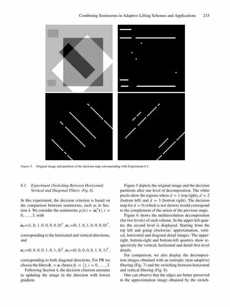
Figure 5. Original image and partition of the decision map corresponding with Experiment 6.1.

6.1. Experiment (Switching Between Horizontal,Vertical and Diagonal Filters -Fig. 6)

In this experiment, the decision criterion is based onthe comparison between seminorms, such as in Sec-tion 4. We consider the seminorms pi (v) = |aT

i v|, i =0, . . . , 3, with

a0=(1, 0, 1, 0, 0, 0, 0, 0)T , a1=(0, 1, 0, 1, 0, 0, 0, 0)T ,

corresponding to the horizontal and vertical directions,and

a2=(0, 0, 0, 0, 1, 0, 1, 0)T , a3=(0, 0, 0, 0, 0, 1, 0, 1)T ,

corresponding to both diagonal directions. For PR wechoose the filters bi = ai (hence βi = 1

2), i = 0, . . . , 3.

Following Section 4, the decision criterion amountsto updating the image in the direction with lowestgradient.

Figure 5 depicts the original image and the decisionpartitions after one level of decomposition. The whitepixels show the regions where d = 1 (top right), d = 2(bottom left) and d = 3 (bottom right). The decisionmap for d = 0 (which is not shown) would correspondto the complement of the union of the previous maps.

Figure 6 shows the multiresolution decomposition(for two levels) of such scheme. In the upper-left quar-ter, the second level is displayed. Starting from thetop left and going clockwise: approximation, verti-cal, horizontal and diagonal detail images. The upper-right, bottom-right and bottom-left quarters show re-spectively the vertical, horizontal and detail first-leveldetails.

For comparison, we also display the decomposi-tion images obtained with an isotropic (non-adaptive)filtering (Fig. 7) and the switching between horizontaland vertical filtering (Fig. 8).

One can observe that the edges are better preservedin the approximation image obtained by the switch-

216 Piella et al.

Figure 6. Multiresolution decomposition by switching between horizontal, vertical and both diagonal filters corresponding with Experiment

6.1.

ing of the four possible directional update filters. Thedecision map of these scheme is able to distinguish be-tween horizontal, vertical and both diagonal directions,and apply the low-pass filter along the correspondingdirection. This avoids blurring the edges in the approx-imation as well as obtaining detail images with lessdetail information.

6.2. Experiment (Switching Between Horizontal,Vertical and Isotropic Filters -Fig. 10)

Similarly to the previous experiment, we switch be-tween update filters in the horizontal, vertical andisotropic direction. That is, we compare the semi-norms pi (v) = |aT

i v|, i = 0, . . . , 2, with weightvectors:

a0 = (1, 0, 1, 0, 0, 0, 0, 0)T ,

a1 = (0, 1, 0, 1, 0, 0, 0, 0)T ,

corresponding to the horizontal and vertical directions,respectively, and

a2 = (1, 1, 1, 1, 0, 0, 0, 0)T ,

corresponding to an isotropic (in the vertical and hori-zontal sense) direction. As in the previous experiment,the decision criterion amounts to updating the imagein the direction with lowest gradient. We use againβi = 1/2 for i = 0, . . . , 2, which yields the filtersbi = 1

4ai for i = 0, 1 and b2 = 1

8a2.

Figure 9 shows the decision partitions for d =0 (left) and d = 1 (right). The decision map ford = 2 (which is not shown) would correspond tothe complement of the union of the previous mapsand it would indicate the regions where the isotropicfiltering has been applied. Figure 10 shows the mul-tiresolution decomposition (for two levels) of suchscheme. Compared with the previous experiment, onecan observe a more blurred approximation image and


Figure 7. Multiresolution decomposition by isotropic filtering.

less sparser detail images, especially in the diagonaldirections.

6.3. Experiment (Combining Comparing-Seminorms Criterion with the TC - Fig. 11)

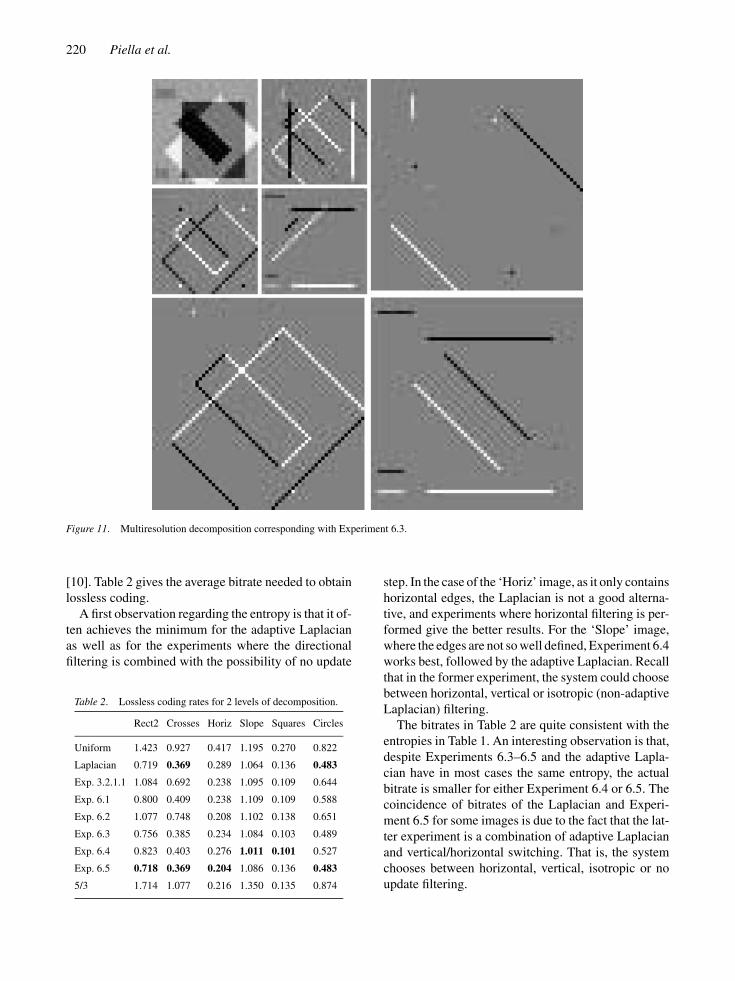
Figure 11 corresponds to Example 5.2, where we havetaken β0 = β2 = 1/2 and β1 = β3 = 0. Taking thesame input image as before, we perform two levelsof decomposition. We can compare the results with theprevious schemes shown in Figs. 6–8 and Fig. 10. Notethat the detail images obtained with this new schemecontain fewer details than those in the previous exper-iments (Figs. 6 and 10).

6.4. Experiment (Combining Switching Criterionwith the TC - Fig. 12)

Figure 12 corresponds to an example of combining thecomparison of two seminorms with a TC applied totwo other seminorms. Each seminorm pi is associated

with its corresponding vector ai . More specifically,

p0(v) ≤ p1(v) and p2(v) ≤ T0 ⇔ d = 0p0(v) ≤ p1(v) and p2(v) > T0 ⇔ d = 1p0(v) > p1(v) and p3(v) ≤ T1 ⇔ d = 2p0(v) > p1(v) and p3(v) > T1 ⇔ d = 3

where p0(v) = |v1 + v3|, p1(v) = |v2 + v4|, p2(v) =|v1+ 1

2v2+v3+ 1

2v4| and p3(v) = | 1

2v1+v2+ 1

2v3+v4|.

We choose T0 = T1,

b0 = 1

4a2, b2 = 1

4a3,

corresponding respectively to a horizontal and vertical-predominant filtering, and

b1 = b3 = 0,

which implies that no update filtering is performed.The multiresolution decomposition is shown in

Fig. 12. It turns out that for this synthetic image theobtained decomposition is visually indistinguishable tothat obtained by the adaptive Laplacian3 and slightlysparser than in the previous experiment.

218 Piella et al.

Figure 8. Multiresolution decomposition by switching between horizontal and vertical filters.

Figure 9. Partition of the decision map corresponding with Experiment 6.2.

6.5. Experiment (Combining Switching Criterionwith the TC)

We combine the switching criterion in Experiment 6.2with the Threshold Criterion, such that if either of the

seminorms pi is above a given threshold we do notupdate.

Figure 13 shows the decision partitions for d = 0(top right), d = 2 (top left), d = 4 (bottom left) andthe union of d = i for i = 1, 3, 5, (bottom right).


Figure 10. Multiresolution decomposition by switching between horizontal, vertical and isotropic filters corresponding with Experiment

6.2.

The latter figure shows the regions where no update isperformed.

6.2. Evaluation for Lossless Compression Purposes

6.2.1. Synthetic images. We repeat the same experi-ments4 with the synthetic images depicted in Fig. 14.We compute the first order entropy of each origi-nal image and the overall empirical entropy of eachdecomposition:

h = 2−2K H (x K ) +K∑

k=1

2−2k3∑

j=1

H(yk

b j

)(29)

where K is the number of decomposition levels andH (x) denotes the first order entropy of image x.

Table 1 shows the entropy values for K = 2 levelsof decomposition for various schemes. The ‘uniform’scheme corresponds to the isotropic filtering (in thehorizontal and vertical sense) and the ‘5/3’ to the 5/3

integer wavelet transform used in lossless JPEG2000.The entropy of the original images is shown in thesecond row of the table.

We further evaluate the wavelet schemes by attach-ing a coder to compute the actual bitrate. We use theembedded image coding algorithm EZBC proposed in

Table 1. Entropy values using 2 levels of decomposition.

Rect2 Crosses Horiz Slope Squares Circles

Original 2.016 0.188 0.449 7.517 1.077 1.781

Uniform 1.257 0.933 0.877 2.210 0.441 0.859

Laplacian 0.428 0.375 0.566 2.035 0.187 0.366

Exp. 3.2.1.1 0.783 0.689 0.356 2.132 0.192 0.597

Exp. 6.1 0.498 0.399 0.356 2.184 0.193 0.514

Exp. 6.2 0.785 0.689 0.357 2.111 0.193 0.596

Exp. 6.3 0.428 0.375 0.351 2.113 0.187 0.366

Exp. 6.4 0.428 0.375 0.560 1.970 0.187 0.366

Exp. 6.5 0.428 0.375 0.351 2.048 0.187 0.366

5/3 1.757 1.056 0.318 2.133 0.257 0.964

220 Piella et al.

Figure 11. Multiresolution decomposition corresponding with Experiment 6.3.

[10]. Table 2 gives the average bitrate needed to obtainlossless coding.

A first observation regarding the entropy is that it of-ten achieves the minimum for the adaptive Laplacianas well as for the experiments where the directionalfiltering is combined with the possibility of no update

Table 2. Lossless coding rates for 2 levels of decomposition.

Rect2 Crosses Horiz Slope Squares Circles

Uniform 1.423 0.927 0.417 1.195 0.270 0.822

Laplacian 0.719 0.369 0.289 1.064 0.136 0.483

Exp. 3.2.1.1 1.084 0.692 0.238 1.095 0.109 0.644

Exp. 6.1 0.800 0.409 0.238 1.109 0.109 0.588

Exp. 6.2 1.077 0.748 0.208 1.102 0.138 0.651

Exp. 6.3 0.756 0.385 0.234 1.084 0.103 0.489

Exp. 6.4 0.823 0.403 0.276 1.011 0.101 0.527

Exp. 6.5 0.718 0.369 0.204 1.086 0.136 0.483

5/3 1.714 1.077 0.216 1.350 0.135 0.874

step. In the case of the ‘Horiz’ image, as it only containshorizontal edges, the Laplacian is not a good alterna-tive, and experiments where horizontal filtering is per-formed give the better results. For the ‘Slope’ image,where the edges are not so well defined, Experiment 6.4works best, followed by the adaptive Laplacian. Recallthat in the former experiment, the system could choosebetween horizontal, vertical or isotropic (non-adaptiveLaplacian) filtering.

The bitrates in Table 2 are quite consistent with theentropies in Table 1. An interesting observation is that,despite Experiments 6.3–6.5 and the adaptive Lapla-cian have in most cases the same entropy, the actualbitrate is smaller for either Experiment 6.4 or 6.5. Thecoincidence of bitrates of the Laplacian and Experi-ment 6.5 for some images is due to the fact that the lat-ter experiment is a combination of adaptive Laplacianand vertical/horizontal switching. That is, the systemchooses between horizontal, vertical, isotropic or noupdate filtering.


Figure 12. Multiresolution decomposition corresponding with Experiment 6.4.

6.2.2. Natural Images. Tables 3–4 show the entropyvalues for K = 2 and K = 4 levels of decomposition,respectively, for various schemes when applied to somewell-known natural images. The entropy of the origi-nal images is shown in the second rows of each ta-ble. We observe that, in terms of the proposed en-tropy measure and for the chosen set of images, theadaptive transform in Experiment 6.4 performs thebest. We can also see that the 4-level decomposi-tions (Table 4) provide a more compact representa-tion (lower entropy) than the 2-level decompositions(Table 3).

Tables 5–6give the average bitrate needed to losslessencode the 2 and 4-level decompositions of the vari-ous schemes. Again, Experiment 6.4 outperforms theothers.

The adaptive Laplacian scheme gives poorer resultsthan the (non-adaptive) uniform scheme in textured im-ages as ‘Lenna’ or ‘Barbara’. In textured regions, thedecision map oscillates between 0 and 1 and a uniformfiltering works better.

As can be seen from the tables, numbers computedfrom entropies provide a good indication of the actualperformance of the wavelet scheme.

As the examples and simulations illustrate, we have agreat freedom to combine different decision rules. Ad-


House Camera Lenna Peppers Barbara Harbour

Original 6.232 7.009 7.445 7.402 7.632 7.305

Uniform 4.258 4.479 4.099 3.892 5.021 4.613

Laplacian 4.220 4.450 4.098 3.834 5.026 4.592

Exp. 3.2.1.1 4.363 4.545 4.211 3.931 5.097 4.593

Exp. 6.1 4.396 4.582 4.247 3.949 5.156 4.592

Exp. 6.2 4.267 4.462 4.121 3.850 5.019 4.515

Exp. 6.3 4.363 4.550 4.211 3.934 5.101 4.593

Exp. 6.4 4.052 4.300 3.917 3.673 4.857 4.436

Exp. 6.5 4.267 4.469 4.121 3.851 5.019 4.515

5/3 4.633 4.869 4.655 4.071 5.252 4.476

222 Piella et al.

Figure 13. Partitions of the decision map corresponding with Experiment 6.5.

ditionally, by varying the thresholds and/or the weightvectors a, we can tune the filters to behave in one par-ticular way, for example, by giving more importanceto some direction. The change of threshold and weightvectors affects the entropy and bitrate values. In the ex-



Original 6.232 7.009 7.445 7.402 7.632 7.305

Uniform 4.139 4.319 3.926 3.730 4.864 4.511

Laplacian 4.099 4.291 3.927 3.670 4.873 4.496

Exp. 3.2.1.1 4.257 4.403 4.051 3.779 4.958 4.500

Exp. 6.1 4.299 4.446 4.095 3.801 5.035 4.501

Exp. 6.2 4.154 4.311 3.954 3.690 4.783 4.415

Exp. 6.3 4.257 4.409 4.051 3.782 4.965 4.500

Exp. 6.4 3.913 4.123 3.727 3.493 4.692 4.328

Exp. 6.5 4.154 4.318 3.954 3.691 4.874 4.415

5/3 4.562 4.772 4.346 3.954 5.146 4.418



Uniform 3.377 3.565 3.346 3.096 4.065 3.859

Laplacian 3.375 3.565 3.346 3.055 4.076 3.843

Exp. 3.2.1.1 3.489 3.684 3.505 3.169 4.180 3.771

Exp. 6.1 3.546 3.738 3.581 3.204 4.268 3.774

Exp. 6.2 3.410 3.597 3.408 3.079 4.088 3.693

Exp. 6.3 3.489 3.688 3.505 3.169 4.182 3.771

Exp. 6.4 3.134 3.349 3.079 2.822 3.858 3.662

Exp. 6.5 3.410 3.603 3.408 3.079 4.090 3.693

5/3 4.229 4.445 4.157 3.785 4.639 4.002

periments where the Threshold Criterion was used, thethreshold was chosen empirically and no optimizationwas done. It would be interesting to automaticallyfind the thresholds to be used such that, for ex-ample, the bitrate of the resulting decomposition isminimized.


Figure 14. Synthetic images (from right to left and from top to bottom): Rect2, Crosses, Horiz, Slope, Squares and Circles.



Uniform 3.252 3.463 3.262 3.016 3.999 3.810

Laplacian 3.244 3.461 3.262 2.974 4.011 3.802

Exp. 3.2.1.1 3.387 3.597 3.430 3.095 4.115 3.727

Exp. 6.1 3.455 3.658 3.515 3.135 4.210 3.731

Exp. 6.2 3.300 3.503 3.331 3.001 4.023 3.644

Exp.6.3 3.387 3.603 3.430 3.095 4.118 3.727

Exp.6.4 3.015 3.221 2.985 2.731 3.776 3.613

Exp.6.5 3.299 3.508 3.331 3.001 4.026 3.644

5/3 4.190 4.400 4.122 3.751 4.607 3.987

7. Conclusions

In this paper, we have constructed multi-valued de-cision criteria that discriminate different ‘geometric’events. These criteria are then used to choose betweendifferent update lifting steps, giving rise to an adaptivemultiresolution analysis. We have been able to findgeneral conditions for the invertibility of such adap-tive systems. The challenge we addressed was to de-sign these invertible and non-redundant schemes suchas the resulting decomposition yields a perceptuallygood approximation image while providing a sparserepresentation, where most of the visual informationis ‘packed’ into a small number of samples. Severalexamples and simulations have been provided to il-

lustrate both the theory and the applicability of thesenon-redundant adaptive systems. In particular, in orderto evaluate the potential of these new schemes in loss-less image compression, we have used a state-of-the-artimage codec, the EZBC.

A number of open theoretical and practical ques-tions need to be addressed before such schemes be-come useful in image processing and analysis appli-cations. For example, we need to get a better un-derstanding how to design update and prediction op-erators that lead to adaptive wavelet decompositionsthat satisfy properties key to a given application athand.

Appendix A

Proof of Lemma 3.5

First we show that, if c �= 0, then p10(A0) = 0.

Proof: Choose v = v0a0 + v1a1 + v with v ∈ Span⊥{a0, a1}, such that{

aT0 v = 0

aT1 v = 1.

(30)

This implies ‖a0‖2v0 + aT0 a1v1 = 0 and aT

1 a0v0 +‖a1‖2v1 = 1; hence the determinant of the system (30)

224 Piella et al.

is

‖a0‖2‖a1‖2 − (aT

0 a1

)2 �= 0,

because a0 and a1 are not collinear. This meansthat the system has a unique solution which satisfiesp1(A0v) = |c1 + cT v|. Now, since ‖c‖ �= 0, we cantake v = − c1

‖c‖2 c which leads to p1(A0v) = 0, and thus

p10(A0) = 0.

If c = 0, we have

p1(A0v) = ∣∣c0aT0 v + c1aT

1 v∣∣ ≥ |c1

∥∥aT1 v

∣∣ − |c0

∥∥aT0 v

∣∣.• If |c1| > |c0| we next show that p10(A0) = |c1|−|c0|.

Proof: Choose v such that{aT

0 v = −sign c0

aT0 v = sign c1.

(31)

These conditions are compatible with the constraint|aT

0 v| ≤ |aT1 v| = 1.

Putting v = a0v0+a1v1 we get a system of equationswith the same determinant as (30), so there is a uniquesolution (v0, v1) ∈ R2, allowing (31) to be satisfied.Therefore, p1(A0v) = |c1| − |c0| = p10(A0).

• If |c1| ≤ |c0| we show that p10(A0) = 0.

Proof: It is sufficient to find v ∈ V such that |aT1 v| =

1 and p1(A0v) = c0aT0 v + c1aT

1 v = 0. For instance,we can choose v such that⎧⎨⎩aT

1 v = 1

aT0 v = −c1

c0

,

which is compatible with the condition |aT0 v| = | c1

c0| ≤

1. Using the same arguments as before, the system hasa unique solution. Thus p10(A0) = 0.

In conclusion, if a0 and a1 are not collinear, we have:

p10(A0) =⎧⎨⎩

|c1 − |c0|,if c = c0a0 + c1a1 and |c1| > |c0|0, otherwise

In the first case, since

c = AT0 a1 = (

I − ubT0

)Ta1 = a1 − uT a1b0,

we obtain aT a1b0 = (1 − c1)a1 − c0a0.

If uT a1 = 0 then a0 and a1 would be collinear,

which is impossible.

If uT a1 �= 0, then b0 = (1−c1)a1−c0a0

uT a1.

Appendix B

Proof of Proposition 3.9

Let H = v1 + v3 and V = v2 + v4. We have thenp0(v) ≤ p1(v) ⇔ |H | ≤ |V |. This is realized ifand only if H = V = 0 or V �= 0 and |H/V |≤ 1.

Now, put v ′ = A0v . We have p0(v ′) ≤ p1(v ′) ⇔|(1−2μ0)H −2η0V | ≤ |−2μ0 H +(1−2η0)V |. This isalso equivalent to (H −V )[(1−4μ0)H +(1−4η0)V ] ≤0.

If V = 0, then H = 0 or μ0 ≥ 1/4.

If V �= 0, then we can write(H

V− 1

)[(1 − 4μ0)

H

V+ 1 − 4η0

]≤ 0.

Thus, an inequality involving one variable, H/V is ob-tained. It is satisfied if and only if

H

V− 1 ≤ 0 and (1 − 4μ0)

H

V+ 1 − 4η0 ≥ 0

or

H

V− 1 ≥ 0 and (1 − 4μ0)

H

V+ 1 − 4η0 ≤ 0.

We distinguish three cases:

• 1 − 4μ0 > 0. In this case, the previous inequalitiesbecome:

4η0 − 1

1 − 4μ0

≤ H

V≤ 1

or

1 ≤ H

V≤ 4η0 − 1

1 − 4μ0

.


• 1 − 4μ0 = 0 ⇔ μ0 = 1/4. This leads to

H

V≤ 1 and η0 ≤ 1

4

or

H

V≥ 1 and η0 ≥ 1

4.

• 1 − 4μ0 < 0. In this case, we get:

H

V≤ 1 and

H

V≤ 1 − 4η0

4μ0 − 1

or

H

V≥ 1 and

H

V≥ 1 − 4η0

4μ0 − 1.

In conclusion, we have p0(A0v) ≤ p1(A0v) ⇔(H, V ) ∈ A′

0 with:

− if μ0 < 14, then

A′0 =

{(H/V)|V = H = 0

or V �= 0 and

[4η0 − 1

1 − 4μ0

≤ H

V≤ 1

or 1 ≤ H

V≤ 4η0 − 1

1 − 4μ0

]}.

− if μ0 = 14

and η0 ≤ 1/4, then

A′0=

{(H, V )|V = 0 or

[V �= 0 and

H

V≤ 1

]}.

− if μ0 = 14

and η0 > 1/4, then

A′0=

{(H, V )|V = 0 or

[V �= 0 and

H

V> 1

]}.

− if μ0 >1

4, then

A′0=

{(H, V )|V = 0

or V �= 0 and

[(H

V≤ 1 and

H

V≤ 4η0 − 1

1 − 4μ0

)or

(H

V≥ 1 and

H

V≥ 4η0 − 1

1 − 4μ0

)]}.

Therefore, for all v , we have the first condition for PRsatisfied: p0(v) ≤ p1(v) ⇒ p0(A0v) ≤ p1(A0v) if andonly if A0 ⊂ A′

0, where A0 = {(V, H )|V = H = 0or [V �= 0 and | H

V | ≤ 1]}. We can examine the fourprevious cases:

− if μ0 < 14, then A0 ⊂ A′

0 ⇔ 4η0−11−4μ0

≤ −1 ⇔η0 ≤ μ0.

− if μ0 = 14, and η0 ≤ 1

4, then A0 ⊂ A′

0.

− if μ0 = 14, and η0 > 1

4, then A0 �⊂ A′

0.

− if μ0 > 14, then A0 ⊂ A′

0 ⇔ 4η0−11−4μ0

≥ 1 ⇔ η0 +μ0 ≤ 1

2.

Finally, A0 ⊂ A′0 if and only if η0 ≤ μ0 ≤ 1/4 or

[μ0 > 1/4 and μ0 + η0 ≤ 1/2]. Additionally, we havethe condition α0 �= 0 ⇔ μ0 + η0 �= 1/2. This readilyyields the first condition in the theorem.

In order to prove the second one, we use the sym-metry property noticed in Remark 3.2. By replacing b0

by −b1/α1 we obtain:−η1

1 − 2μ1 − 2η1

≤ −μ1

1 − 2μ1 − 2η1

and − μ + η1

1 − 2μ1 − 2η1

≤ 1

2which is straightforwardly shown to be equivalent tothe second condition of the proposition.

Notes

1. In fact, S10 = ∅ is equivalent to:∀v ∈ V, p0(v) > p1(v) = 0. This

corresponds to the degenerate case: ∀v ∈ V, d = 1 or p0(v) = 0.

2. Indeed, if a0 = γ a1, then d is fixed: either d = 0 if |γ | ≤ 1 or

d = 1 otherwise. Note however that p10(A0) is defined only if

|γ | ≤ 1.

3. The decision criterion in the adaptive Laplacian is d = [p(v) >

T] with p(v) = |aT v|, a = (1, 1, 1, 1, 0, 0, 0, 0)T . For the two

possible filters: bd = γd a, d = 0, 1, we take γ0 = 1/8 and

γ1 = 0.

4. For comparison purposes with the 5/3 lifting scheme, we use

now a symmetric prediction step. More specifically, if n =(n, m), y′

h (n) = yh (n)− (x ′(n +1, m)+ x(n)/2, y′v(n) = yv(n)−

(x ′(n, m + 1) + x(n))/2 and y′d (n) = yd (n) − (x ′(n, m + 1)) +

x(n))/2 − y′h (n) − y′

v(n).

References

1. E.J. Candes. “The curvelet transform for image denoising,” in

Proceedings of the IEEE International Conference on ImageProcessing, Thessaloniki, Greece, pp. 7–10, 2001.

2. R.L. Claypoole, G.M. Davis, W. Sweldens, and R.G. Baraniuk,

“Nonlinear wavelet transforms for image coding via lifting,”

IEEE Transactions on Image Processing, Vol. 12, No. 12, pp.

1449–1459, 2003.

3. A. Cohen and B. Matei, “Compact representation of images by

edge adapted multiscale transforms,” in Proceeding of the IEEEInternational Conference on Image Processing, Thessaloniki,

Greece, 2001, pp. 7–10.

226 Piella et al.

4. A. Cohen, I. Daubechies, O.G. Guleryuz, and M.T. Orchard.

IEEE Transactions on Information Theory, Vol. 48, No. 7,

pp. 1895–1921, July 2002.

5. M.N. Do and M. Vetterli, “The contourlet transform: an effi-

cient directional multiresolution image representation,” Vol. 14,

No. 12, pp. 2091–2106, December 2005.

6. O. Gerek and A.E. Cetin, “Adaptive polyphase subband decom-

position structures for image compression,” IEEE Transactionson Image Processing, Vol. 9, No. 10, pp. 1649–1659, 2000.

7. H.J.A.M. Heijmans and J. Goutsias, “Nonlinear multiresolu-

tion signal decomposition schemes,” Part II: Morphological

wavelets. IEEE Transactions on Image Processing, Vol. 9,

No. 11, pp. 1897–1913, 2000.

8. H.J.A.M. Heijmans, B. Pesquet-Popescu, and G. Piella, “Build-

ing nonredundant adaptive wavelets by update lifting,” Appliedand Computational Harmonic Analysis, Vol. 18, No. 3, pp. 252–

281, May 2005.

9. H.J.A.M. Heijmans, G. Piella, and B. Pesquet-Popescu, “Adap-

tive wavelets for image compression using update lifting: Quan-

tisation and error analysis,” International Journal of Wavelets,Multiresolution and Information Processing, Vol. 4, No. 1, 2006.

10. S. Hsiang and J. Woods, “Embedded image coding using zer-

oblocks of subband/wavelet coefficients and context modeling,”

in Proceedings of the IEEE International Symposium on Circuitsand Systems (Geneva, Switzerland, May 2000). pp. 662–664.

11. E. Le Pennec and S.G. Mallat, “Sparse geometric image rep-

resentation with bandelets,” IEEE Transactions on Image Pro-cessing, Vol. 14, No. 4, pp. 423–438, April 2005.

12. G. Piella, B. Pesquet-Popescu, and H.J.A.M. Heijmans, “Adap-

tive update lifting with a decision rule based on derivative filters”

IEEE Signal Processing Letters 9, Vol. 10, pp. 329–332, 2002

13. W. Sweldens, “The lifting scheme: A new philosophy in

biorthogonal wavelet constructions,” in Proceedings of SPIE,

Vol. 2569, San Diego, California, July 1995, pp. 68–79.

14. W. Trappe and K.J.R. Liu, “Adaptivity in the lifting scheme,”

In Proceedings of the 33rd Annual Conference on InformationSciences and Systems, Baltimore, Maryland, March 1999, pp.

950–955.

Gemma Piella received the M.S. degree in electrical engineering

from the Polytechnical University of Catalonia (UPC), Barcelona,

Spain, and the Ph.D. degree from the University of Amsterdam, The

Netherlands, in 2003.

From 2003 to 2004, she was at UPC as a visiting professor. She

then stayed at the Ecole Nationale des Telecommunications, Paris,

as a Post-doctoral Fellow. Since September 2005 she is at the Tech-

nology Department in the Pompeu Fabra University.

Her main research interests include wavelets, geometrical image

processing, image fusion and various other aspects of digital image

and video processing.

Beatrice Pesquet-Popescu received the engineering degree in

telecommunications from the “Politehnica” Institute in Bucharest

in 1995 and the Ph.D. thesis from the Ecole Normale Supérieure de

Cachan in 1998. In 1998 she was a Research and Teaching Assis-

tant at Université Paris XI and in 1999 she joined Philips Research

France, where she worked for two years as a research scientist, then

project leader, in scalable video coding. Since Oct. 2000 she is an

Associate Professor in multimedia at the Ecole Nationale Supérieure

des Télécommunications (ENST).

Her current research interests are in scalable and robust video

coding, adaptive wavelets and multimedia applications.

EURASIP gave her a “Best Student Paper Award” in the IEEE

Signal Processing Workshop on Higher-Order Statistics in 1997, and

in 1998 she received a “Young Investigator Award” granted by the

French Physical Society. She is a member of IEEE SPS Multime-

dia Signal Processing (MMSP) Technical Committee and a Senior

Member IEEE. She holds 20 patents in wavelet-based video coding

and has authored more than 80 book chapters, journal and conference

papers in the field.

Henk Heijmans received his masters degree in mathematics from

the Technical University in Eindhoven and his PhD degree from the

University of Amsterdam in 1985. Since then he has been in the

Centre for Mathematics and Computer Science, Amsterdam, where

he had been directing the “signals and images” research theme.

His research interest are focused towards mathematical techniques

for image and signal processing, with an emphasis on mathematical

morphology and wavelet analysis.

Gregoire Pau was born in Toulouse, France in 1977 and received

the M.S. degree in Signal Processing in 2000 from Ecole Centrale

de Nantes. From 2000 to 2002, he worked as a Research Engineer at

Expway where he actively contributed to the standardization of the

MPEG-7 binary format. He is currently a PhD candidate in the Signal

and Image Processing Departement of ENST-Telecom Paris. His re-

search interests include subband video coding, motion compensated

temporal filtering and adaptive non-linear wavelet transforms.

Combining Seminorms in Adaptive Lifting Schemes and Applications to Image Analysis and Compression

Documents