This item was submitted to Loughborough's Research Repository by the author. Items in Figshare are protected by copyright, with all rights reserved, unless otherwise indicated. Combining qualitative and quantitative reasoning to support hazard Combining qualitative and quantitative reasoning to support hazard identification by computer identification by computer PLEASE CITE THE PUBLISHED VERSION PUBLISHER © Stephen McCoy PUBLISHER STATEMENT This work is made available according to the conditions of the Creative Commons Attribution-NonCommercial- NoDerivatives 4.0 International (CC BY-NC-ND 4.0) licence. Full details of this licence are available at: https://creativecommons.org/licenses/by-nc-nd/4.0/ LICENCE CC BY-NC-ND 4.0 REPOSITORY RECORD McCoy, Stephen A.. 2017. “Combining Qualitative and Quantitative Reasoning to Support Hazard Identification by Computer”. figshare. https://hdl.handle.net/2134/25406.

Welcome message from author
This document is posted to help you gain knowledge. Please leave a comment to let me know what you think about it! Share it to your friends and learn new things together.
Transcript

This item was submitted to Loughborough's Research Repository by the author. Items in Figshare are protected by copyright, with all rights reserved, unless otherwise indicated.
Combining qualitative and quantitative reasoning to support hazardCombining qualitative and quantitative reasoning to support hazardidentification by computeridentification by computer
PLEASE CITE THE PUBLISHED VERSION
PUBLISHER
© Stephen McCoy
PUBLISHER STATEMENT
This work is made available according to the conditions of the Creative Commons Attribution-NonCommercial-NoDerivatives 4.0 International (CC BY-NC-ND 4.0) licence. Full details of this licence are available at:https://creativecommons.org/licenses/by-nc-nd/4.0/
LICENCE
CC BY-NC-ND 4.0
REPOSITORY RECORD
McCoy, Stephen A.. 2017. “Combining Qualitative and Quantitative Reasoning to Support Hazard Identificationby Computer”. figshare. https://hdl.handle.net/2134/25406.
Pilkington Library
·~ Loughborough • University
AuthorlFiling Title ...... ~.~.~.'?:t ......................... .
T Vol. No. ...... ...... Class Mark ............ '" ........... .
Please note that fines are charged on ALL overdue items.
04021
I I I III~IIIIIIIIIIIIIIIII

I
I
I
I
I
I
I
I
. I
Combining Qualitative and Quantitative
Reasoning to support Hazard Identification
by Computer
by
Stephen McCoy
A Doctoral Thesis
Submitted in partial fulfilment of the requirements for the award of
Doctor of Philosophy of Loughborough University
23,d March, 1999
..
. - . '. ..
'. ..'
© by ~tephel! McCoy, 19Q9.:' .

Abstract
This thesis investigates the proposition that use must be made of quantitative infonnation to control the reporting of hazard scenarios in automatically generated HAZOP reports.
HAZOP is a successful and widely accepted technique for identification of process hazards. However, it requires an expensive commitment of time and personnel near the end of a project. Use of a HAZOP emulation tool before conventional HAZOP could speed up the examination of routine hazards, or identify deficiencies I in the design of a plant.
Qualitative models of process equipment can efficiently model fault propagation in chemical plants. However, purely qualitative models lack the representational power to model many constraints in real plants, resulting in indiscriminate reporting of failure scenarios.
In the AutoHAZID computer program, qualitative reasoning is used to emulate HAZOP. Signed-directed graph (SDG) models of equipment are used to build a graph model of the plant. This graph is searched to find links between faults and consequences, which are reported as hazardous scenarios associated with process variable deviations. However, factors not represented in the SDG, such as the fluids in the plant, often affect the feasibility of scenarios.
Support for the qualitative model system, in the form of quantitative judgements to assess the feasibility of certain hazards, was investigated and is reported here. This thesis also describes the novel "Fluid Modelling System" (FMS) which now provides this quantitative support mechanism in AutoHAZID. The FMS allows the attachment of conditions to SDG arcs. Fault paths are validated by testing the conditions along their arcs. Infeasible scenarios are removed.
In the FMS, numerical limits on process variable deviations have been used to assess the sufficiency of a given fault to cause any linked consequence. In a number of case studies, use of the FMS in AutoHAZID has improved the focus of the automatically generated HAZOP results.
This thesis describes qualitative model-based methods for identifying process hazards by computer, in particular AutoHAZID. It identifies'! range of problems where the purely qualitative approach is inadequate and demonstrates how such problems can be tackled by selective use of quantitative infonnatiol) apout the plant or the fluids in it. The conclusion is that quantitative knowledge is' required to support the qualitative reasoning in hazard identification by computer.
, . ""~'" ... ' '.' ..... -', ~ Keywords: HAZOP Emulation, Qualitative Modelling, I.'rocess Safety,
Hazard Identification, STOPHAZ,Eault Propagation.

Acknowledgements
I would like, first and foremost, to thank Andy Rushton and Paul Chung for the
invaluable guidance they have provided as my supervisors in this work - this thesis
would be far poorer than it is without them! I am grateful also to Frank Lees for the
valuable advice and inspiration he gave me while I was at Loughborough. I would also
like to acknowledge my colleagues at Loughborough, Felim Larkin and Steve
Wakeman, as well as the numerous other people around Europe, with whom I had the
pleasure of working, on the STOPHAZ project. Lastly, thanks are certainly due to the
AI Group in the Dept. of Engineering Mathematics, Bristol University, where I have
been working for the past 12 months as a "Post-Doc R.A." - so far without a PhD!
Table of Contents
CHAPTER 1 : INTRODUCTION ................................................................................................. 1
1.1 NOMENCLATURE ........................................................................................................ 3
1.2 HAZARD IDENTIFICATION AND RISK ASSESSMENT ......................................... .4
1.3 HAZARD AND OPERABILITY STUDIES (HAZOP) ................................................. 8
1.4 AUTOMATION OF SAFETY ASSESSMENT ........................................................... 12
1.5 FAULT PROPAGATION ............................................................................................. 14
1.6 GRAPHS, SEARCH AND COMPLEXITy ................................................................. 18
1.6.1 DEPTH· FIRST (BACKTRACKING) SEARCH ................................................... 25
1.6.2 BREADTH-FIRST SEARCH ............................................................. .................. 26
1.6.3 COMPLEXITY ANALySiS ............................................................... ................... 26
1.7 JUSTIFICATION .......................................................................................................... 29
CHAPTER 2 : LITERATURE REVIEW , .. " ...... ,., ............. , ....... , ... " .......................................... 31
2.1 CONVENTIONAL PROCESS SAFETY METHODS ................................................. 31
2.1.1 MANAGEMENT AND SAFETY AUDITS ........................................................... 33
2.1.2 MATERIALS PROPERTIES AND PROCESS SCREENING .............................. 34
2.1.3 HAZARD INDICES ............................................................................................ 35
2.1.4 PILOT PLANTS .................................................................................................. 36
2.1.5 CHECKLISTS .......................................................... .......................................... 36
2.1.6 WHAT IF? ANALySIS ....................................................................................... 37
2.1.7 PRELIMINARY HAZARD ANALYSIS ............................................................... 39
2.1.8 COARSE HAZARD STUDIES ............................................................................ 39
2.1.9 FAILURE MODES, EFFECTS AND CRITICALITY ANALYSIS (FMECA) ...... .41
2.1.10 EVENT TREE AND FAULT TREE ANALYSIS ................................................... 42
2.1.1 I COMPUTER HAZOP ......................................................................................... 42
2.1.12 SNEAK ANALYSIS .............................................................. , .............................. 44
2.1.13 HUMAN ERROR ANALySIS .............................................................................. 47
2.1.14 HAZARD IDENTIFICATION IN THE CONTEXT OF PROCESS DESIGN ...... 48
2.2 QUALITATIVE PHySICS ........................................................................................... 49
2.2.1 GENERAL ISSUES TO BE TACKLED BY QUALITA TlVE FORMALISMS ...... 50
2.2.2 AMBIGUITY . ..................................................................................................... 52
2.2.3 NAivE PHYSICS AND COMMONSENSE REASONING .............................. ... 53
2.2.4 THE PROCESS-BASED APPROACH. ........................................................ ...... 54
2.2.5 QUALITATIVE SIMULATION· QSIM .............................................................. 59
2.2.6 CONSTRAINT-BASED QUALITATIVE REASONING - "CONFLUENCES" .... 61
2.3 APPLICATIONS OF QUALITATNE PHYSICS IN PROCESS SAFETY ................ 63
2.3.1 PURDUE ............................................................................................................ 64
2.3.2 DOW BENELUX ...................................................... .......................................... 71
2.3.3 LOUGHBOROUGH ........................................................................................... 72
2.3.4 PENNSYLVANIA ................................................................................................ 75
2.3.5 SEOUL ............................................................................................................... 79
2.3.6 VTT ..................................................... ...................................................... .......... 81
2.3.7 TAIWAN ................................................. ............................................................. 83
2.3.8 ARGENTINA ...................................................................................................... 83
2.3.9 JAPAN ................................................. ............................................................... 84
2.4 SUMMARY .................................................................................................................. 85
CHAPTER 3: DESCRIPTION OF AUTOHAZID AND ITS QUALITATIVE
MODELLING SYSTEM .............................................................................................................. 88
3.1 SCOPE OF THE HAZID PACKAGE .......................................................................... 88
3.2 DESCRIPTION OF THE HAZID SOFTWARE PACKAGE ....................................... 90
3.2. I PLANT DESCRIPTIONS
FROM DATABASE APT AND GRAPHICAL TOOL.. ............................. ........... 92
3.2.2 PHYSICAL PROPERTIES CALCULATIONS .................................................... 93
3.2.3 INTERNAL ORGANISATION OF AUTOHAZID ............................................... 93
3.2.4 HAZOP OUTPUT FORMATS ............................................... ............................. 95
3.3 MODELS IN AUTOHAZID ......................................................................................... 95
3.3.1 DATA REQUIREMENTS FOR THE PLANT MODEL.. ..................................... 98
3.3.2 SIGNED DIRECTED GRAPH (SDG) ................................................................ 99
3.3.3 EQUIPMENT MODELS· FRAMES AND INSTANCES .................................. 102
3.3.4 HIERARCHY OF EQUIPMENT MODELS ...................................................... 103
3.3.5 SLOTS AND THEIR INHERITANCE IN AUTOHAZID MODELS ................... 104
3.3.6 ATTRIBUTE·CONDITIONAL MODELLING SYSTEM ................................... 107
3.3.7 CUSTOM MODELS AND THE MODEL GENERATION TOOL ..................... 108
3.3.8 CONSEQUENCE TYPES AND RANKING ...................................................... 109
3.4 TEMPLATES AND SCRIPTS FOR MODELLING
PARTS OF EQUIPMENT ITEMS ............................................................................. 11 0
3.5 METHODOLOGY FOR MODEL DEVELOPMENT ................................................ 111
3.5.1 FLOW PATH SYSTEM DEFlNlTlON ............................................... ............... 112
3.5.2 THE "NO FUNCTION IN STRUCTURE" PRINCIPLE .................................. I 13
3.5.3 CHOICE AND DEFlNlTlON OF VARIABLES ................................................ I 14
3.5.4 CAUSAL HIERARCHY IN FLOW MODELLING ............................................ 1 15
3.5.5 THE FLOW PATH SDG MODEL.. .................................................................. 116
3.5.6 MODEWNG NO FWW AND REVERSE FLOW. .......................................... 119
NoFlow ............................................................................................................................ 119
Reverse Row .................................................................................................................... " .. 120
3.5.7 KNOWLEDGE ELlCITATION METHODS ...................................................... 121
Trial and Error in Modelling ................................................................................................ 122
Conventional HAZOP Studies ...................................... _ ...................................................... 123
Equipment Modelling Seminars ........................................................................................... 125
Criticism of Equipment Library Models ............................................................................... 126
Expert Criticism of HAZOP Results for Test Cases ............................................................. 126
3.6 CONCLUSIONS ......................................................................................................... 127
CHAPTER 4: SOME PROBLEMS WITH QUALITATIVE SDG-BASED
HAZARD IDENTIFICATION ................................................................................................... 129
4.1 THE SDG REPRESENTS ONLY TWO DEVIATIONS ........................................... 129
4.2 SINGLE MAPPING INFLUENCES .......................................................................... 130
4.2.1 USE OF DIRECTED GRAPH INSTEAD OF SDG .......................................... 132
4.2.2 EXTRA CODE NUMBERS FOR SDG ARCS ................................................... 133
4.3 REASONING THROUGH UNHEALTHY UNITS ................................................... 135
4.4 SPARSE RESULTS FOR HAZOP ............................................................................. 138
4.5 SPECIFIC HAZARDS FLAGGED INDISCRIMINATELy ..................................... 140
4.6 HAZARDS DO NOT APPEAR WHERE EXPECTED IN HAZOP REPORT .......... 141
4.7 CHANGE THE FORMAT OF THE AUTOHAZID REPORT ................................... 142
4.8 MODELS IN AUTOHAZID NOT APPLICABLE TO EARLY HAZOP ON PPD ... 142
4.9 QUALITATIVE AMBIGUITY .................................................................................. 143
4.9.1 MULTIPLE PATHS IN THE SDG .................................................................... 144
4.9.2 CYCLICAL PATHS ........................................................................................... 145
4.9.3 AMBIGUOUS PREDICTED FLOW DEVIATIONS ......................................... 146
4.10 SHORTEST PATH HEURISTIC NOT SOUND ....................................................... 147
4.11 COMPUTATIONAL COMPLEXITY ........................................................................ 153
4.12 CONCLUDING REMARKS ...................................................................................... 156
CHAPTER 5: CONDITIONALITY IN FAULT PATH MODELLING AND THE FLUID
MODELLING SYSTEM ............................................................................................................ 157
5.1 IMPROVING ON FAULT PROPAGATION ............................................................. 158
5.2 THE FLUID MODELLING SYSTEM ....................................................................... 162
5.2.1 FA ULT PATH VALIDATION .......................................................................... 164
5.2.2 FLUID INFORMATION AND ITS PROPAGATION ....................................... 165
5.2.3 FUNCTIONS AND PREDlCATES ................................................................... 168
5.2.4 INFORMATION USED IN FAULT PATH VALlDATlON. ............................... 172
5.2.5 INTEGRATION OF FLUID MODEL SUBSYSTEMS ....................................... 174
5.2.5.1 Outline of Function and Predicate Evaluation in the FMS ................................. 175
5.2.5.2 Operating System Dependencies and A vailability of Software Packages ........... 179
5.2.6 FLUID LIBRARY INFORMATION .................................................................. 180
5.2.7 PHYSICAL PROPERTIES CALCULATIONS .................................................. 182
5.2.8 COMPATIBILITY CHECKS FOR FLUIDS ..................................................... 183
5.3 REASONING USING NUMERICAL LIMITS ON DEVIATIONS .......................... 187
5.3.1 EXAMPLE I: DESIGN PRESSURE FOR PUMPS AND OTHER UNITS ...... 188
5.3.2 EXAMPLE 2 : ATMOSPHERIC PRESSURE
IS (APPROXIMATELY) I BARA ...................................................... ................ 189
5.3.3 EXAMPLE 3: PRESSURE LIMITS WHEN VALVES OPEN ........................... 190
5.3.4 EXAMPLE 4: METHANOL COOLER ............................................................. /93
5.3.5 EXAMPLE 5: PRESSURE LIMITS
DUE TO VAPOUR-LIQUID EQUILIBRIUM .................................................. /96
5.3.6 MANAGING PROPAGATION OF INFORMATION
ABOUT NUMERICAL LIMITS ....................................................................... /98
5.4 CONCLUSiONS ......................................................................................................... 199
CHAPTER 6: DISCUSSION AND FUTURE WORK ............................................................ 201
6.1 STRENGTHS AND WEAKNESSES OF HAZID ...................................................... 201
6.2 FUTURE WORK ........................................................................................................ 204
6.3 ACCESS TO PLANT DESCRIPTIONS ..................................................................... 211
6.4 METHODOLOGY ISSUES IN UNIT AND FLUID MODELLING SYSTEMS ...... 212
6.4.1 A GENERAL APPROACH TO MODEL BU/LDING ....................................... 214
6.4.2 UNIT MODEL DOCUMENTATION ................................................................ 2/7
6.4.3 IMPROVING MODEL PERFORMANCE ........................................................ 219
6.5 MODELLING STATE-DEPENDENT BEHAVIOUR
AND TEMPORAL SEQUENCES .............................................................................. 220
6.6 NON-PROCESS PROPAGATION OF FAULTS ....................................................... 224
6.7 LOOPS. PLANT TOPOLOGY AND HIGHER LEVEL CONSTRAINTS ................ 225
6.8 AN EXTENDED REPRESENTATION FOR FAULT PROPAGATION .................. 226
6.9 OPTIMISA TION OF THE HAZOP ALGORITHM
AND FLUID MODELLING SYSTEM ...................................................................... 228
6.10 CONCLUSIONS ......................................................................................................... 229
CHAPTER 7 : CONCLUSIONS ................................................................................................ 231
REFERENCES ............................................................................................................................ 236

APPENDICES
Appendix A : Outline of the AutoHAZID Package ................................................................ 247
Appendix B : Improved Algorithm for HAZOP Search ......................................................... 260
Appendix C : Flow and Pressure Modelling in Dividers and Headers ................................... 266
Appendix D : Object Types in AutoHAZID .......................................................................... 273
Appendix E: Table of Functions and Predicates in the Fluid Modelling System .................. 284
Appendix F: Minutes of Meeting to Discuss Limits of Variable Deviations ........................ 302
Appendix G : Future work changes to HAZID ...................................................................... 309

Chapter 1 : Introduction
The thesis stated here is that quantitative information is needed to control the
reporting of hazard scenarios in qualitative emulation of HAZOP by computer.
Without such support, hazards are reported indiscriminately, which reduces the value
of the output io human users of the program.
HAZOP is a very useful technique for process hazard identification. However, it
requires an expensive commitment of time and resources at the end of the process
design phase. Therefore, a strong economic argument exists for automating this
technique.
Qualitative methods, among them graph based methods, can be used to efficiently
model plant behaviour. By modelling fault propagation in the plant, programs can
emulate the hazard identification of the HAZOP study method.
However, qualitative methods are weak representations, which often do not permit
unambiguous simulation of the plant. This leads to indiscriminate reporting of process
hazards, which reduces the value of the resulting hazard study reports. 11 is thought
likely that this problem cannot be solved without the use of quantitative information
of some kind. An example of the type of information often represented weakly in the
plant model, is the details of the fluids present in the plant, and their properties. Fluid
properties can be used to assess the feasibility of hazards which otherwise would be
reported indiscriminately.
The AutoHAZID computer program was developed as part of STOPHAZ, a 3\1, year
long ESPRIT-funded collaborative project. In AutoHAZID, qualitative reasoning
using signed directed graphs (SDGs) is supported by conditions for judging the
feasibility of fault-consequence scenarios. These conditions are based on the fluids
present in the plant, and are implemented by the Fluid Modelling System (FMS) in
AutoHAZID. The FMS also allows verification of scenarios by checking the possible
limits of deviations in process variables. The result of applying these conditions is that
the results of computer-based HAZOP become more focussed.
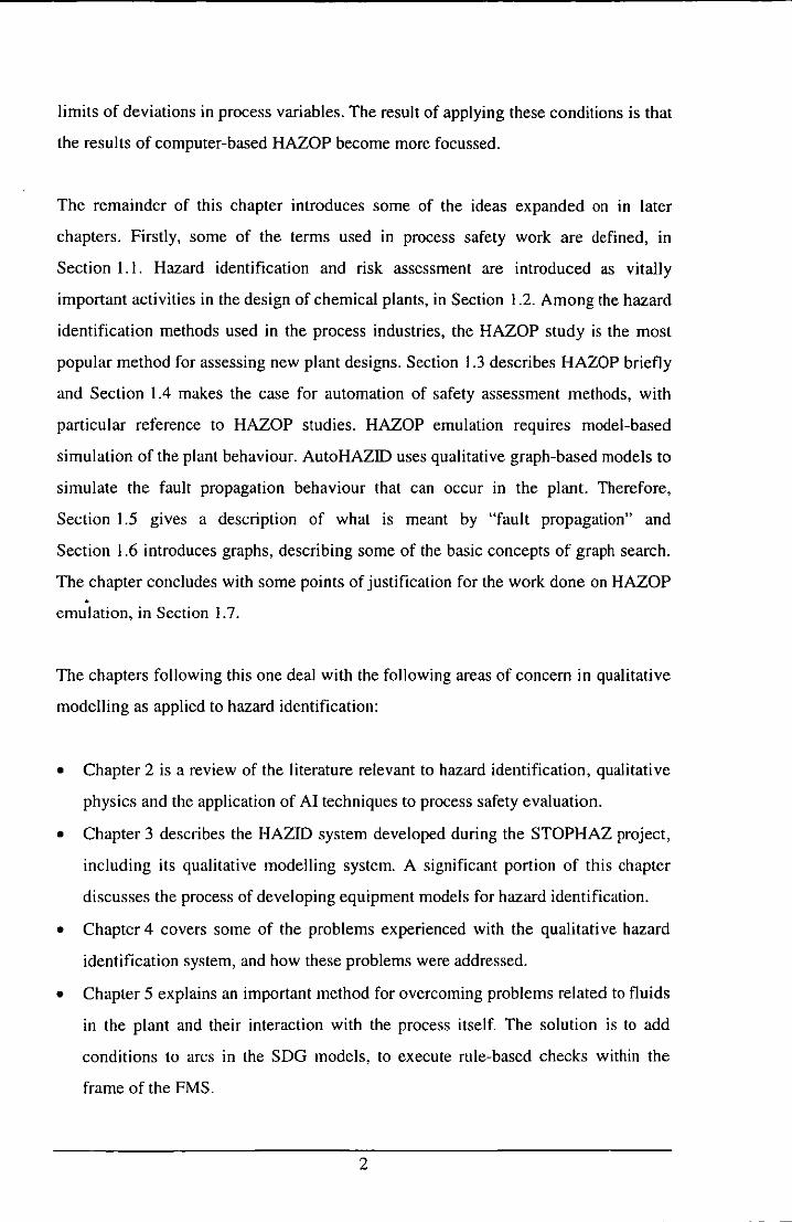
The remainder of this chapter introduces some of the ideas expanded on in later
chapters. Firstly, some of the terms used in process safety work are defined, in
Section 1.1. Hazard identification and risk assessment are introduced as vitally
important activities in the design of chemical plants, in Section 1.2. Among the hazard
identification methods used in the process industries, the HAZOP study is the most
popular method for assessing new plant designs. Section 1.3 describes HAZOP briefly
and Section 1.4 makes the case for automation of safety assessment methods, with
particular reference to HAZOP studies. HAZOP emulation requires model-based
simulation of the plant behaviour. AutoHAZID uses qualitative graph-based models to
simulate the fault propagation behaviour that can occur in the plant. Therefore,
Section 1.5 gives a description of what is meant by "fault propagation" and
Section 1.6 introduces graphs, describing some of the basic concepts of graph search.
The chapter concludes with some points of justification for the work done on HAZOP . emulation, in Section 1.7.
The chapters following this one deal with the following areas of concern in qualitative
modelling as applied to hazard identification:
• Chapter 2 is a review of the literature relevant to hazard identification, qualitative
physics and the application of AI techniques to process safety evaluation.
• Chapter 3 describes the HAZID system developed during the STOPHAZ project,
including its qualitative modelling system. A significant portion of this chapter
discusses the process of developing equipment models for hazard identification.
• Chapter 4 covers some of the problems experienced with the qualitative hazard
identification system, and how these problems were addressed.
• Chapter 5 explains an important method for overcoming problems related to fluids
in the plant and their interaction with the process itself. The solution is to add
conditions to arcs in the SDG models, to execute rule-based checks within the
frame of the FMS.
2

• Chapter 6 discusses topics raised by the work described here, and pinpoints some
areas of future work.
• Chapter 7 fonnulates some overall conclusions about qualitative hazard
identification and its extension, using the FMS.
1.1 Nomenclature
Before addressing hazard identification and other aspects of process safety, we must
clarify the meaning of some tenns used in safety work. A valuable reference for
"standard" nomenclature in this field has been prepared by Jones (1992). This guide is
the result of a working party set up by the Institution of Chemical Engineers
(IChemE), with the aim to help standardise some of the (sometimes rather freely
adapted) terminology in use in industry.
The terms of most relevance to this thesis are defined by Jones as follows:
Hazard
Chemical hazard
Risk
Loss prevention
Hazard analysis
A physical situation with a potential for human injury, damage
to property, damage to the environment or some combination of
these.
A hazard involving chemicals or processes which may realize
its potential through agencies such as fire, explosion, toxic or
corrosive effects.
The likelihood of a specified undesired event occurring within a
specified period or in specified circumstances. It may be either
a frequency (the number of specified events occurring in unit
time) or a probability (the probability of a specified event
following a prior event), depending on the circumstances.
A systematic approach to preventing accidents or minimizing
their effects. The activities may be associated with financial
loss or safety issues and will often include many of the
techniques defined in this [Jones'] report.
The identification of undesired events that lead to the
materialization of a hazard, the analysis of the mechanisms by
3

Risk assessment
which these undesired events could occur and usually the
estimation of the extent, magnitude and likelihood of any
harmful effects.
The quantitative evaluation of the likelihood of undesired
events and the likelihood of harm or damage being caused
together with the value judgements made concerning the
significance of the results.
Throughout this thesis, I will attempt to use these terms consistently. It should be
noted that there is still a good deal of variability in the usage of these terms in the
chemical industry as well as confusion with similar terms in other fields (e.g. "risk
assessment" as applied to financial risk).
1.2 Hazard Identification and Risk Assessment
Process safety is vitally important to any operating company In the chemical
industries, not only because of the human cost of accidents, but also for economic
reasons. A serious accident on plant can mean loss of production and consequent loss
of customers, compensation payments to injured workers and possibly a serious loss
of the considerable investment in plant and machinery.
Such losses can be prevented by two complementary means. Firstly, the philosophy of
management of the plant and its personnel should encourage safe working and "good
housekeeping" in day-to-day operation. Systems of communication, training and
control of access to plant items should be installed, to ensure that people are aware of
potential hazards and do their work safely. Increased awareness of safety and
operability issues among staff will reduce the frequency of accidents, near-misses and
environmentally damaging releases of process materials, thereby increasing
productivity and profitability.
Plant safety can also be helped at a much earlier stage by use of safe plant design
practices, where the plans for a plant are examined at various stages of the design
process. By identifying hazards and possible concerns for plant operation early, and
4
asseSSing the risks they pose to safety, costly changes in the later design can be
minimised, or avoided altogether. Information on potential hazards can be used even
before a process or specific product has been decided upon, so that (possibly) a more
benign product or an inherently safer process can be chosen for development.
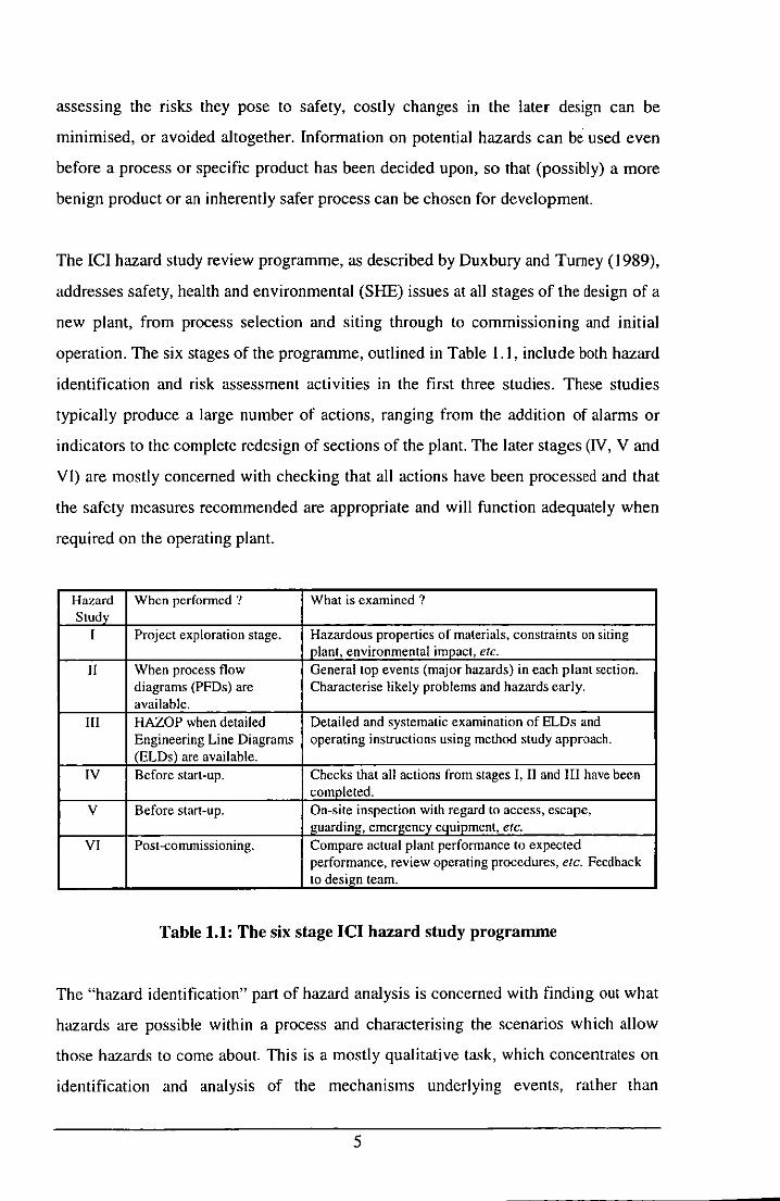
The ICI hazard study review programme, as described by Duxbury and Turney (1989),
addresses safety, health and environmental (SHE) issues at all stages of the design of a
new plant, from process selection and siting through to commissioning and initial
operation. The six stages of the programme, outlined in Table 1.1, include both hazard
identification and risk assessment activities in the first three studies. These studies
typically produce a large number of actions, ranging from the addition of alarms or
indicators to the complete redesign of sections of the plant. The later stages (N, V and
VI) are mostly concerned with checking that all actions have been processed and that
the safety measures recommended are appropriate and will function adequately when
required on the operating plant.
Hazard When pcrfonncd ? What is examined? Study
I Project exploration stage. Hazardous properties of materials, constraints on siting plant, environmental impact, ete.
II When process flow General top events (major hazards) in each plant section. diagrams (PFDs) are Characterise likely problems and hazards early. available.
III HAZOP when detailed Detailed and systematic examination of ELDs and Engineering Line Diagrams operating instructions using method study approach. (ELDs) are available.
IV Before start-up. Checks that all actions from stages I, II and III have been completed.
V Before start-up. On-site inspection with regard to access, escape, guarding, emergency equipment, etc.
VI Post-commissioning. Compare actual plant performance to expected performance. review operating procedures, etc. Feedback to design team.
Table 1.1: The six stage lel hazard study programme
The "hazard identification" part of hazard analysis is concerned with finding out what
hazards are possible within a process and characterising the scenarios which allow
those hazards to come about. This is a mostly qualitative task, which concentrates on
identification and analysis of the mechanisms underlying events, rather than
5
quantifying specific risks. "Risk assessment" is a more pains-taking, quantitative
technique, which is applied to a small number of the most important or complicated
hazards identified. The objective is to analyse the risk associated with a scenario in
terms of the logic for its development, probabilities of various events occurring and
consequent losses which could occur.
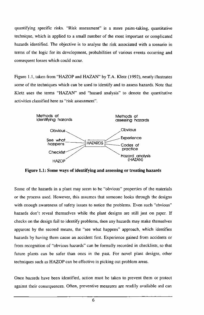
Figure 1.1, taken from "HAZOP and HAZAN" by T.A. Kletz (1992), neatly illustrates
some of the techniques which can be used to identify and to assess hazards. Note that
Kletz uses the terms "HAZAN" and "hazard analysis" to denote the quantitative
activities classified here as "risk assessment".
Methods of identifying hazards
Obvious
Methods of assessing hazards
Obvious
See what ___ ::::::fH:(;.ij;;Rr);;-r: Experience happens 0:LH~N.AA~~D::::Sl::::--codes of
Checklist practice
Hazard analysis HAZOP (H.AZ.AN)
Figure 1.1: Some ways of identifying and assessing or treating hazards
Some of the hazards in a plant may seem to be "obvious" properties of the materials
or the process used. However, this assumes that someone looks through the designs
with enough awareness of safety issues to notice the problems. Even such "obvious"
hazards don't reveal themselves while the plant designs are still just on paper. If
checks on the design fail to identify problems, then any hazards may make themselves
apparent by the second means, the "see what happens" approach, which identifies
hazards by having them cause an accident first. Experience gained from accidents or
from recognition of "obvious hazards" can be formally recorded in checklists, so that
future plants can be safer than ones in the past. For novel plant designs, other
techniques such as HAZOP can be effective in picking out problem areas.
Once hazards have been identified, action must be taken to prevent them or protect
against their consequences. Often, preventive measures are readily available and can
6
be easily implemented, or engineers' experience in previous cases can be used to solve
the problems. Codes of practice are a more formal approach to design, which ensure
safety by avoiding specific known hazards or by managing them using methods
known to have been effective in the past. Risk assessment is used to quantify the risks
associated with the most significant hazards and decide what action is needed. This
approach must be used selectively, however, because of the time and effort required.
To be effective, hazard identification and risk assessment must be integrated with the
activity of process design which proceeds via a number of stages. Firstly, the design
team must obtain a detailed statement of requirements from management or the
customer. This allows them to decide what product(s) to make, what reactants to use
and the details of intermediates and process chemistry involved. It is also important to
decide on the likely siting of the plant, to allow capital cost estimation, environmental
impact assessment and safety assessment to proceed from an early stage.
When these basic process details have been decided, the team develops a preliminary
process design in the form of a block diagram of the process steps. The block diagram
identifies main flows into and out of each plant section, as well as unit operations in
each section. This design is refined into a process flow diagram (PFD) by performing
heat and mass balance calculations and doing some preliminary equipment selection
and design. Several different process options may be worked through to this stage.
After preliminary cost estimation, funds are authorised for one process option.
Detailed process design and piping and instrumentation design follows, producing the
"Engineering Line Diagrams" (ELDs) for the plant. ELDs are also sometimes known
as "Piping and Instrumentation Diagrams" (P&IDs), but the usage of these terms is
not standardised in industry - where some companies refer to the P&ID as a more
detailed level of specification than the ELD, others use the opposite convention.
Further design tasks include layout planning, mechanical engineering and civil
engineering. Design is followed by procurement, fabrication, construction and
commissioning of the new plant.
7

As mentioned earlier, awareness of process hazards at each stage can simplify the
design and cut down on expensive redesign due to late discovery of problems. A wide
range of techniques can be used for hazard identification during process design, as
reviewed in Section 2.1. However, HAZOP is described in this chapter because it
plays a much larger part in the work described in the rest of the thesis.
1.3 Hazard and Operability Studies (HAZOP)
The most commonly used hazard identification technique in the process industries is
the hazard and operability study (HAZOP), which is Hazard Study ill in the lCl
programme mentioned above. This method has been widely used for many years and
is described in detail in many publications, such as Kletz (1992), CIA (1977),
Knowlton (1981 and 1992), Lees (1996) and Lawley (1974).
HAZOP is a systematic critical examination of the process and engineering design of
a plant, to identify all possible deviations of the plant from its intended operating
condition. For each deviation, any possible associated hazards and problems with
operability are recorded. The design of the plant is characterised by its Engineering
Line Diagrams (ELDs) and operating instructions.) The study takes the form of a
series of "brainstorming" sessions, attended by a cross-section of project personnel,
under the control of a team leader who directs the procedure of the meetings.
The team leader must be familiar with the HAZOP method and be trained for the job
of leading a HAZOP team, but he/she need not be involved in the rest of the project.
The decisions and points discussed by the team must be recorded - the team leader
may do this, but it is generally better to employ a secretary (or "scribe"), to avoid
holding up the progress of the study. The remainder of the team should represent all
parties with an interest in the project, including each main engineering discipline. The
team should not be too large; six members is probably a good maximum.
I Operating instructions are an important part of the plant design, which should be available for
HAZOP, but frequently are not complete at this stage.
8

For each ELD in the plant, the team leader chooses the equipment items to be grouped
together as "lines", transferring fluid between the equipment items allocated as
"vessels" in the drawing. This grouping of equipment should allow the study to
proceed at a reasonable pace, without the risk of missing any hazards. The choice of
lines is a matter of judgement on the part of the team leader.
The drawing is examined line by linc and vessel by vessel, with the group considering
deviations from intended operation in each line. This requires that the intentions of all
lines and vessels are declared as and when they are encountered. Deviations are
formed by combining a guide word (more, less, no, other-than) with a relevant
variable in the line or vessel (flow, pressure, temperature, liquid level), or with
intended operations or processes (e.g. mixing, crystallisation). The following
questions are addressed for each deviation:
• Is the deviation meaningful?
• Could it arise, and how?
• What consequences would result, and are those consequences hazardous, or do
they prevent efficient operation?
• If so, can the deviation be prevented from occurring, or can the consequences be
protected against by changing the design or operation of the plant? Redesign must
be avoided in the HAZOP meeting, but may be a recommended action.
Any significant findings of the HAZOP team are recorded, typically in a table
including columns for identifying the deviation, possible causes and consequences of
the scenario, and any suggested actions to tackle the identified hazard. Common
practice in modern HAZOPs also includes listing any existing protections against the
identified hazard, such as trip systems, alarms, etc.
Figure 1.2, taken from CIA (1977), illustrates the sequence of examination of the
HAZOP, emphasizing the methodical and systematic approach of the technique.
Clearly, a lot of very creative activity is implied in the central steps (7, 8 and 9),
examining possible causes, consequences and detecting hazards, but the method
appears highly algorithmic when seen at the level shown here.
9

Start
End
Select a vessel
Explain the general intention of the vessel and its lines
Select a line
Explain the intention of the line
Apply the first guide word
Develop a meaningful deviation
Examine possible causes
Examine possible consequences
Detect hazards
Make suitable record
Repeat 6-10 for a1l meaningful deviations derived from first guide word
Repeat 5-11 for alllhe guide words
Mark line ashaving been examined
Repeat 3-13 for each line
Select an auxiliary (e.g. heating system)
Explain the intention of the auxiliary
Repeal 5-12 forthe auxiliary
Markauxiliary as having been examined
Repeat 15-18 for all auxiliaries
Explain intention of the vessel
Repeat 5-12 forthe vessel
Mark vessel ascompleted
Repeat 1-22 for all vessels on flowsheet
MarkflowSleet as completed
Repeat 1-24 for all flowsheets
Figure 1.2: Sequence of examination for HAZOP meeting
10
HAZOP is usually carried out after most of the detailed process design has been
completed. Large-scale changes to the design are very expensive at this stage.
Therefore, early use of other hazard identification techniques (as discussed in
Section 2.1) must have already eliminated the major problems in the process design
wherever possible. Simple checks on equipment designs should be dealt with before
HAZOP, by checklists relating to equipment items or fluids present in the process.
These checks can be performed more cost-effectively by a single engineer than by a
team. It is also important to make sure that all information on the safety and control
systems proposed for the plant is available before the HAZOP meeting, to avoid delay
in getting hold of this information.
Much of the strength of HAZOP arises from systematically examining the interactions
between separate parts of the process and from the creative interaction of the team
members in looking at the problem. These are factors which are absent from many
simpler hazard identification methods. The method involves a lot of redundancy, as
the same scenarios are examined from many different viewpoints. This reduces the
chance that significant hazards will be overlooked, but the requirement for a group of
experts to be present for the full duration of the study means that HAZOP can be
rather expensive.
Because HAZOP meetings are so painstaking and methodical, they can be very tiring
for the people involved, who must remain motivated and alert throughout. It is not
usually productive to run sessions for longer than about three hours, and the frequency
of meetings should be kept low, too. The time and personnel required for HAZOP
studies at such a late stage in the project often mean that this stage delays final
delivery of the project (i.e. HAZOP is on the "critical path" of the project plan).
Therefore, there is a lot of interest in automating safety verification tasks such as
HAZOP.
In the discussion of computer emulation of HAZOP which follows in this and later
chapters, a particular approach is taken. This is to consider how deviations of the
process variables in a plant could arise, and how they could give rise to hazards.
11

Although this does comprise a large part of the work of a conventional study, there is
more involved. A full HAZOP, conducted by a team of experts, considers all possible
deviations of the plant from its intended operation, which includes many phenomena
which are not process variable deviations. Examples include maintenance and
operation in abnormal modes, such as start-up, shut-down or process upsets.
1.4 Automation of Safety Assessment
Computers have been used to increase the speed and efficiency of many process
engineering tasks. Examples include computer aided design (CAD), flowsheet
simulation, layout planning and visualisation, and project planning. The automation of
safety-related tasks is an area where appropriate use of computers could greatly reduce
costs. Applications of Information Technology (IT) in this area so far fall into four
main types:
I. General-purpose office software packages, such as word processors,
spreadsheets and databases, are widely used to process and present information
in connection with the work of safety assessment.
11. More structured IT applications have also been developed, to facilitate specific
safety tasks, such as documenting HAZOP studies. Here, basic IT has been
used in a tightly structured domain, to aid a well-defined task.
Ill. Many computer packages exist for performing detailed (often numerical) tasks
in risk assessment. These include numerical simulations of vapour cloud
dispersal, fires and explosions, or support tools for fault tree development.
IV. The most interesting software developments apply Artificial Intelligence (AI)
techniques to diagnosis of process disturbances, real-time monitoring of plant
performance using control system data, hazard identification, etc. This is the
area in which the Plant Engineering Group at Loughborough University has
been working. In particular, the group has developed qualitative simulations of
plant behaviour for automated hazard identification.
12

The advantages of using a computer-based approach for hazard identification include:
• Repeatability. Given the same input, a computer program will always produce the
same set of results. This is not necessarily true for a human team-based task.
• The computer is impervious to boredom, so that it will examine everything it is
asked to, without loss of interest part way through.
• Systematic and thorough approach. Given results from a computer study, we can
be reasonably certain that everything has been examined to a consistent level of
detail, so that the quality of analysis is consistent throughout.
There are a number of disadvantages to using even a well-designed computer aid for
hazard identification. As with the advantages listed above, many of these are shared
with programs in other domains of application:
• The results may be lacking in originality, with a "mechanical" feel to them. Partly
this is a result of the use of language in the computer results - inevitably the
phrases used seem artificial after many repetitions.
• Programs are usually unable to indicate clearly where they do not have the
expertise to solve a particular problem, so that weak areas of knowledge may not
be appreciated by the human reader of the report.
• The level of detai I produced by computer programs can be inappropriate. Often,
the report is too detailed in areas which are not very interesting or important.
• Human users often accept, without question, the correctness of results produced by
computer. This acceptance is a dangerous tendency in safety-critical work. The
assumptions and processing behind safety-related results should be stated, and
questioned, wherever appropriate. High quality presentation of results can also
mask poor quality content.
• Because of the systematic nature of any computer aid, weaknesses and errors in
programs or models will be systematic, too. In this way, single weaknesses can be
greatly magnified.
13
Despite these problems, it is still deemed to be a worthwhile aim to develop computer
programs which can automate certain tasks in the safety analysis arena, not least
because the attempt at automation may reveal weaknesses in conventional hazard
identification approaches and thereby lead to their remedy.
The economic argument for automating HAZOP is that, even if the software can only
identify a small class of routine problems, the time and effort saved during the
HAZOP study probably makes using the program worthwhile. A consistent quality of
hazard identification can also be expected from the software tool. By comparison, a
HAZOP team may occasionally have a "bad day".
A software tool for hazard identification should allow initial failures and final
consequences to be brought together, to bring potential hazards to light. It should not
attempt to model all classes of fault in full detail, but should instead allow the full
range of safety concerns to be identified by users when working through the output
generated.
HAZOP emulation software could be used by a design engmeer, to evaluate a
substantially completed design, just before the conventional HAZOP study.
Alternatively, the tool could be used at earlier stages of design, before detailed ELDs
are available, to screen for problems when the cost of design changes is lower.
1.5 Fault Propagation
To automate the identification of hazards in a process plant design, some formal
representation of the plant itself must be constructed. With such a plant model, a
computer program can then be designed, to reason about it symbolically or
numerically, to determine how the process system could behave in ways that lead to a
hazardous situation.
A promising approach is to build a qualitative model of the plant from individual
models of the equipment items present and the connections between them. In
conjunction with an appropriate computer program (an "inference engine"), the model
14
should predict the behaviour of the plant under nonnal conditions, as well as
predicting its response to individual things that can go wrong. It is not usually
necessary to predict in detail what will happen after a hazard has occurred -
identification of the hazard is enough.
The approach used in most of our work, to model the development of hazards in
process systems, is known as "fault propagation". This is not the only way to model
the (sometimes complex) sequences of causes and effects which comprise real-life
accident scenarios, but it is a simple approach to tackling many such scenarios. Fault
propagation can also be fonnalised (and therefore automated) quite easily. The wider
issues of hazard modelling and how best to model equipment for hazard identification,
are discussed in Chapter 3 and, later, in Section 6.4 of Chapter 6.
Fault propagation distinguishes two types of event, or states of affairs, as important:
"faults" and "consequences". Both are simply modelled as named events and are
usually associated with some equipment item in the plant. Faults model the initial
causes of hazards in the plant, such as equipment failures. An example for a pump
might be "seal failure". Consequences model the final, reportable, hazards or
operability concerns in the hazardous scenario. An example might be "possible
explosion" .
Faults and consequences are linked together by what is known as a "fault propagation
chain". This may be a single link between the initial fault and final consequence, or it
may be a sequence of links via a number of process variables in the plant. In the latter
case, each variable is deviated from its normal value enough to propagate a
disturbance from an initial fault to a final, possibly quite remote, consequence.
15
--- -----------------
The single link type of fault propagation chain characterises local failures of
equipment which give rise to immediate problems at the same location. For a pump
containing a toxic and volatile fluid, we might have:
'seal failure' (fault)
1 'toxic gas release'
(consequence)
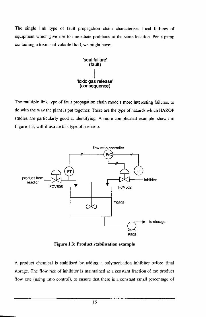
The multiple link type of fault propagation chain models more interesting failures, to
do with the way the plant is put together. These are the type of hazards which HAZOP
studies are particularly good at identifying. A more complicated example, shown in
Figure 1.3, will illustrate this type of scenario.
product from reactor
flow ratio controller
1---1-- inhibitor
FCV502
11<505
to storage
P505
Figure 1.3: Product stabilisation example
A product chemical is stabilised by adding a polymerisation inhibitor before final
storage. The flow rate of inhibitor is maintained at a constant fraction of the product
flow rate (using ratio control), to ensure that there is a constant small percentage of
16
------------
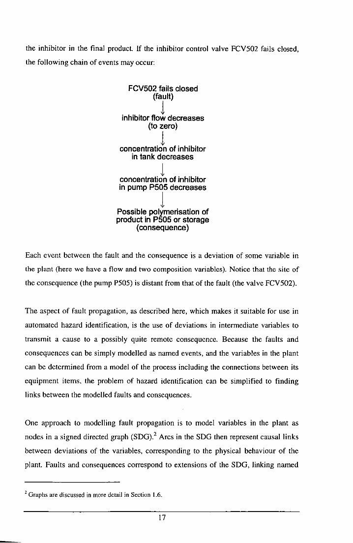
the inhibitor in the final product If the inhibitor control valve FCV502 fails closed,
the following chain of events may occur:
FCV502 fails closed (fault)
1 inhibitor flow decreases
(to zero)
1 concentration of inhibitor
in tank decreases
1 concentration of inhibitor in pump P505 decreases
1 Possible polymerisation of product in P505 or storage
(consequence)
Each event between the fault and the consequence is a deviation of some variable in
the plant (here we have a flow and two composition variables). Notice that the site of
the consequence (the pump P505) is distant from that of the fault (the valve FCV502).
The aspect of fault propagation, as described here, which makes it suitable for use in
automated hazard identification, is the use of deviations in intermediate variables to
transmit a cause to a possibly quite remote consequence. Because the faults and
consequences can be simply modelled as named events, and the variables in the plant
can be determined from a model of the process including the connections between its
equipment items, the problem of hazard identification can be simplified to finding
links between the modelled faults and consequences.
One approach to modelling fault propagation is to model variables in the plant as
nodes in a signed directed graph (SDG).2 Arcs in the SDG then represent causal links
between deviations of the variables, corresponding to the physical behaviour of the
plant. Faults and consequences correspond to extensions of the SDG, linking named
2 Graphs are discussed in more detail in Section 1.6.
17
events to specific deviations of variables. This graph-based representation is the one
used in AutoHAZID and is explained in Section 3.3. It allows fault-consequence
scenarios to be modelled by paths in the SDG from faults to consequences.
Given a qualitative modelling framework of this nature, there are a number of things
one can do with it. One might use a graph search algorithm to search in a model
forwards from selected faults to determine their eventual consequences. One might
use the ability of the system to qualitatively model process plants and analyse the
causation of major hazards to produce fault trees automatically, as Hunt et al. did with
the FAULTFINDER program (Hunt, 1992, Hunt et aI., 1993). Alternatively, one
might choose to emulate HAZOP, as we have with the STOPHAZ project.
The approach used In HAZOP emulation is to first compile a list of sensible
deviations for each of the process variables in the plant model. Then, for each
deviation, backwards search is used to find possible causes, in terms of initiating
faults. Any direct consequences of the deviation being considered may therefore be
caused by the faults identified. In this way, a list of fault-consequence scenarios can
be associated with each deviation. These results are presented in a tabular form,
similar to the format used to record conventional HAZOP findings.
The following section discusses graphical representations and the search methods
used wi th them. It can be seen as an introduction to the SDGs used in AutoHAZID
models, referred to briefly above and presented in more detail in Chapter 3.
1.6 Graphs, Search and Complexity
Since fault propagation is implemented in AutoHAZID (and in some other systems)
using a graphical representation for process variables and their effects on one another,
this section gives a brief general introduction to graphs. Graph search algorithms and
their complexity are inevitable concerns, and are also dealt with briefly. The
descriptions given owe much to "Artificial Intelligence and the Design of Expert
Systems", by Luger and Stubblefield (1989), which gives a particularly clear
explanation of these concepts.
18

A graph can be defined as a set of nodes and the arcs which connect those nodes to
each other. It is possible to add information to a graph, in the form of labels attached
to either the nodes or the arcs in the graph, or both. This labelling information can be
simple or complex, depending on what the graph is to be used for (its "domain
problem"). Typically, a directionality is attached to arcs in the graph, in the form of
arrowheads, so that arcs can be considered as uni-directional or bi-directional. The
nodes in the graph may also be labelled with names. An example of such a "directed
graph" is shown in Figure 1.4.
s
Figure 1.4: An example of a labelled directed graph
The usual purpose of defining graphs is to examine how different parts of a problem
are connected, so the concept of a "path" through a graph is usually very important to
solving the problems which graphs are used to represent. A path is characterised either
by a list of nodes, or a list of arcs in the graph, defining a list of nodes "visited" in
sequence, between a'starting point and an end point in the graph. An example from
Figure 1.4 above is the path from S to G via the nodes [S,D,C,B,G]. There can in
general be multiple paths between any two nodes in a graph.
An important consideration in solving problems using graphs is the topology of the
graph, which includes such questions as whether it contains circuits or not. A path
contains a circuit, or cycle, if it passes through some node in the graph more than
once. A graph contains a circuit if there is some path in it containing a circuit. A
19

"rooted" graph is one where a single node is identified as the root node, such that
there is a path from the root node to every other node in the graph. This sort of graph
is usually drawn with the root node at the top of the page.
A "tree" is a graph in which there is a maximum of one path between any two nodes
in the graph. This sort of graph is often drawn as a rooted graph, with the branches of
the tree drawn out below the root node. A particular example of this kind of
"hierarchical" relationship is a family tree, and the terminology of family relationships
is usually used in talking about relationships between nodes in a tree, using terms such
as "parent", "child" and "sibling" (brother/sister).
Whenever graphs are used to represent a problem in some domain, the interpretation
of what the nodes and arcs "mean" is of course dependent on the problem. A
frequently used type of interpretation is that of the graph as a "state space
representation". In this case, each node represents a possible state of the world, with
respect to the problem at hand, and each arc represents a possible change between
states, consistent with some rule about the system. Typically, each node stores a
description of the state of the world at each point in the graph. Taken as a whole, the
graph (which may not contain a finite number of arcs or nodes!i forms a description
of the whole scope of the problem. This whole description is often referred to as the
"state space" of the problem.
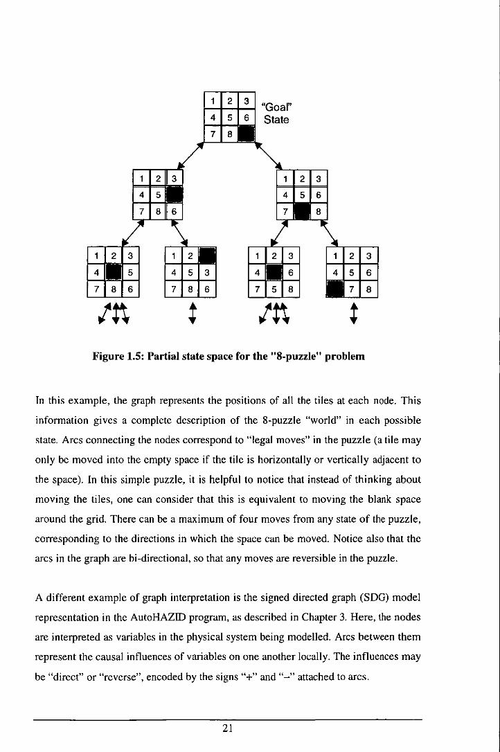
An example of a partial state space representation is shown in Figure 1.5 for the
problem of the "8-puzzle". This puzzle consists of a 3x3 grid of tiles, from which one
tile has been removed, leaving 8 numbered tiles and an empty space. The tiles can be
slid past one another into the empty space, one at a time, allowing the player to
rearrange the pattern of numbers in the puzzle. To solve the puzzle, the user must
rearrange the tiles from an initial, unsorted configuration into numerical order, as in
the "goal state" of Figure 1.5, without removing them from the grid.
3 Any explicit representation of a graph! in terms of arcs and nodes, must contain a finite number of arcs
and nodes. However, where a graph is specified in terms of a node and a set of rules to generate new
nodes, then such a graph could be infinite (or extremely large, as in chess, for example).
20
4 5 3
7 8 6
123
4 5 6 "Goal" State
2 3
5 6
7 8
Figure 1.5: Partial state space for the "8-puzzle" problem
In this example, the graph represents the positions of all the tiles at each node. This
information gives a complete description of the 8-puzzle "world" in each possible
state. Arcs connecting the nodes correspond to "legal moves" in the puzzle (a tile may
only be moved into the empty space if the tile is horizontally or vertically adjacent to
the space). In this simple puzzle, it is helpful to notice that instead of thinking about
moving the tiles, one can consider that this is equivalent to moving the blank space
around the grid. There can be a maximum of four moves from any state of the puzzle,
corresponding to the directions in which the space can be moved. Notice also that the
arcs in the graph are bi-directional, so that any moves are reversible in the puzzle.
A different example of graph interpretation is the signed directed graph (SDG) model
representation in the AutoHAZID program, as described in Chapter 3. Here, the nodes
are interpreted as variables in the physical system being modelled. Arcs between them
represent the causal influences of variables on one another locally. The influences may
be "direct" or "reverse", encoded by the signs "+" and "-" attached to arcs.
21
In the 8-puzzle graph, paths through the graph represent how the state of the puzzle
may be changed, which might include solving it. The path corresponding to a solution
of the puzzle would therefore terminate at the goal state shown above, and one might
imagine that a program could be used to find paths from any other node in the graph
to the goal state. Such a program would be able to solve the 8-puzzle problem, or
direct its solution, using graph search to find the paths to the goal state.
Paths in the SDG model correspond not to "moves in the game", or changes in a
world state, but rather to (possibly remotely propagated) influences between variables.
This is quite a different interpretation from the one used for the state space
representation above. At no point is there a state description corresponding to the
plant being considered, unless the whole graph, with associated variable values at
each node, is considered as a description of a state in some larger graph.4
Finding paths in a graph therefore serves different purposes dependent on the
application domain for that graph. For the 8-puzzle, the goal might be to solve the
puzzle from some pseudo-random start position. For the SDG system used in
AutoHAZID, the path-finding activity is directed at finding what the wider effects of
process equipment failures will be, within the scope of fault propagation, discussed in
Section 1.5. Here, finding paths between variables establishes a possible causal
influence between potentially quite distant state changes, which may give rise to a
hazard by fault propagation.
Graph search algorithms are implemented to find paths through graphs from some set
of specified start points, to some set of goal nodes, which may not be fully specified in
advance. In the 8-puzzle example, the starting (pseudo-random) position is given, and
the goal state is a single known configuration of the tiles. For the SDG-based fault
propagation model the starting positions are the faults known about in the models of
the equipment in the plant model. The goal nodes correspond to deviations which can
give rise to consequences in the plant model.
4 Even in such a larger "super-graph" it would be difficult to describe or define the arcs which connect
the states of the system, defining "legal changes" in the state of the world.
22

The specification of a search problem must include the following information:
• The nodes and arcs which comprise the graph itself, also known as the "search
space" of the problem.
• A set of starting information defining the starting node(s) of the problem.
• Some definition of the goal of the search, either in terms of a list of nodes, some
property of the nodes, or some property of the paths to be found in the graph.
• Some definition of the termination conditions for the search as a whole. This may
involve finding the first path, the shortest path, or the "best" path with respect to
some scoring criterion, or it may involve finding all solution paths in the graph, by
exhaustive search.
Given this specification, the next choice is what direction to search the graph:
• Either: Work from the starting nodes using the data given to develop the problem
forwards, hopefully finding the goal state(s) at some stage (this is known as data
driven, forward chaining search).
• Or: Work backwards from the goal, producing successive subgoals, in order to
find the starting nodes (this is goal-driven, backward chaining search).
• Or: Some graph search procedures develop paths simultaneously from goal nodes
backwards and from start nodes forwards, until a path is found which meets up in
the middle (this is known as "bi-directional" search).
The choice of which direction to use is dependent on the nature of the problem. Some
problems can only be formulated in one direction, and some may be very difficult to
express in anything other than the "obvious" form. The "branching factor" of the
search space in forwards and reverse directions will also influence the choice of
whether to search forwards or backwards, for computational reasons.
The branching factor of a graph is a number expressing the (typical or maximum)
number of arcs attached to each node in the graph. If the arcs have an associated
23

direction, there will be a forwards and a backwards branching factor for the graph,
which may have quite different values, depending on the problem being considered.
The reason branching is important is because, unless an algorithm has perfect
judgement at each step in the search, each node offers many possible paths to explore,
most of which will not lead to a solution path. Therefore, the wasted search effort
involved in exploring these paths is the main computational cost in searching a graph.
This effort can be reduced by reducing the number of alternative branches to be
considered at each node. Some problems have a characteristically larger branching
factor in one direction than the other, meaning that a clear-cut decision can be made
between forward and backward chaining search.
As an example, if we want to check the truth of the proposition "I am a descendant of
William Shakespeare", we need to find a path of lineage between the "I" and the "S"
(there is a maximum of one such path). Considering that Shakespeare was born in
1564 and I was born in 1968, there are about 400 years between us. Assuming a gap of
about 25 years between generations, this means that the line of descent (if there is one)
will be about 16 steps long.
The choice is therefore between searching backwards from "I", to find out if "S"
appears as an ancestor, or of searching forwards from "S" to find if "I" appears as a
descendant of "S". We can analyse the branching factors in each direction to decide
which is the best way to search. Everyone has exactly two biological parents, so the
branching factor for backwards search is 2. However, in the past, people tended to
have more than 2 children, so that the branching factor for forwards search is greater
than 2. If we assume that the forwards branch factor is 3, the potential number of steps
in exhaustive forwards search could be 316 = 43,046,721, compared to 2 16 = 65,536
for backwards search. Clearly, the backwards search will be more efficient in this
case, but still of exponential complexity.
Note, however, that the notion of a typical branching factor can be niisleading in some
problems because of the nature of the search space. A particular example is the
24

travelling salesman problem described in Section 1.6.3 below, and illustrated In
Figure 1.6.
One factor which affects the choice of how to conduct search is the possibility of
finding either multiple or cyclical paths between nodes in the graph. Multiple paths
which do not include cycles are mostly a nuisance, giving rise to repeated search, or
overhead in checking for previously seen nodes in the search. But cycles can cause
infinite cycling in the search if the algorithm does not include a check for previously
seen nodes within the same path. If it is possible to say with certainty that the graph is
a tree, then the overhead of looking for previously seen nodes can be eliminated from
the algorithm. Therefore, it is important to consider the topology of the graph before
implementing any search algorithms for it.
Having decided whether to search forwards or backwards, the next decision is what
search algorithm to use. Two of the most common are discussed briefly below.
1.6.1 Depth-first (backtracking) search
This search procedure works by expanding paths as far as they will go, until either a
dead-end is reached or a solution path is found. In the case that a dead-end is found,
the search "backtracks" to the nearest node which still has unexamined branch nodes.
If a goal node is found, the search finishes, returning the path developed to that node.
This is best explained as a search which recursively examines each of the nodes
attached to the current node in turn, to see if there is a solution path along that route.
Whenever possible, the search goes deeper in the graph. The general algorithms which
implement this search must include a record of nodes which have already been
examined, or found to lead to dead-ends, so that cyclical and redundant paths can be
avoided in the search.
Depth-first search is not guaranteed to find the shortest path in the search space,
unless the search space is finite and search continues until the whole space is
25
searched. The strength of depth-first search lies in the fact that it does not require
much storage, because it only stores one partially completed path at any time.
In the example of Figure 1.4, forward-chaining depth-first search from S to F might
examine the following nodes in turn: S, A, B, G, no way forwards - backtrack to B, to
A, to S, then D, C, (B and G already visited), E, F (goal found - stop).
1.6.2 Breadth-first search
In breadth-first search, the paths examined in the graph are all extended by one step
before any of them is further examined. This results in an expanding "search front" of
nodes to be examined next, and guarantees that search progresses through the graph so
that the shortest paths between start and goal nodes are found first.
This method typically uses a lot more storage space than the depth-first method,
because all the paths still under consideration have to be stored at the same time. It
can therefore be intractable for highly branched search spaces, but is guaranteed to
find the shortest path between start and goal nodes before any longer paths.
In the example of Figure 1.4, searching breadth-first from S to F would examine the
following nodes in order: S, A, D, B, C, G, E, F (goal found).
1.6.3 Complexity Analysis
Much of the theoretical work of computer science is concerned with the development
of algorithms for performing well-defined tasks on large amounts of data. Computer
scientists are therefore concerned with the following questions about an algorithm:
• Is it guaranteed to terminate in a finite amount of time?
• What is the maximum length of time the algorithm will take?
• How much space will it need?
26

The first question is the most difficult one to answer in general for algorithms and I
will therefore not consider it further, beyond making the point that any search on a
finite graph must terminate in a finite amount of time if it does not examine cyclical
paths in the graph. The time and space required for exhaustive search in this case may
make such an algorithm intractable for any realistically sized computer, but the
problem is not in any fundamental sense insoluble.
The computational complexity of an algorithm is a measure of the amount of time or
space it requires for it to do its job. This is usually expressed in terms of the size of
the problem to be solved. For example, the complexity of a procedure for sorting
elements in a list may be expressed in terms of the number of elements in the list, N,
such that the time taken is "of the order of NZ ", or O(N\ meaning that the most
significant part of the time taken is proportional to NZ.
The estimation of search complexity depends heavily on knowledge about the
topology of the search space, as well as the termination conditions and the goals of the
problem at hand. It is not always possible to use a typical branching factor constant in
assessing the number of paths to be examined.
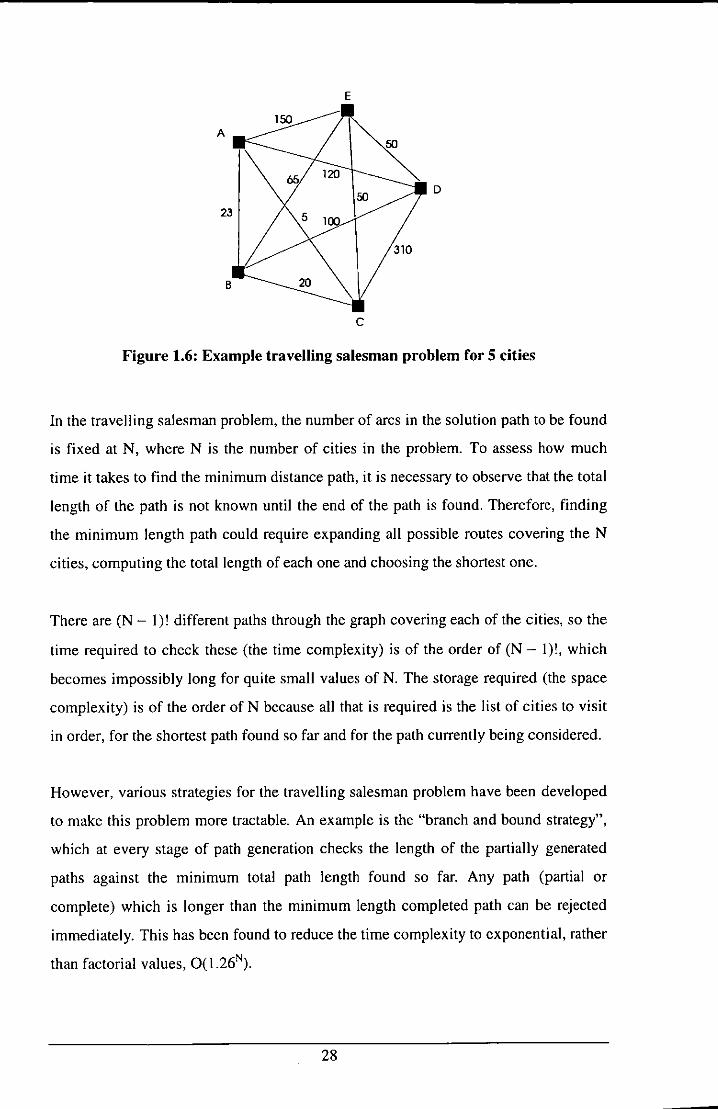
As an example, consider the travelling salesman problem, as illustrated in Figure 1.6
below. A travelling salesman has to start at his home city (A) and visit all the other
cities in the graph once only before returning home. The distances between the cities
are used to label the arcs between them. The objecti ve of the problem is to find the
route which minimises the total distance the salesman must travel.
27
E
A
D
c
Figure 1.6: Example travelling salesman problem for 5 cities
In the travelling salesman problem, the number of arcs in the solution path to be found
is fixed at N, where N is the number of cities in the problem. To assess how much
time it takes to find the minimum distance path, it is necessary to observe that the total
length of the path is not known until the end of the path is found. Therefore, finding
the minimum length path could require expanding all possible routes covering the N
cities, computing the total length of each one and choosing the shortest one.
There are (N - I)! different paths through the graph covering each of the cities, so the
time required to check these (the time complexity) is of the order of (N - I)!, which
becomes impossibly long for quite small values of N. The storage required (the space
complexity) is of the order of N because all that is required is the list of cities to visit
in order, for the shortest path found so far and for the path currently being considered.
However, various strategies for the travelling salesman problem have been developed
to make this problem more tractable. An example is the "branch and bound strategy",
which at every stage of path generation checks the length of the partially generated
paths against the minimum total path length found so far. Any path (partial or
complete) which is longer than the minimum length completed path can be rejected
immediately. This has been found to reduce the time complexity to exponential, rather
than factorial values, O( 1.26N).
28
Exponential' complexity is typical for exhaustive graph searches in search spaces
where a branching factor is found which remains more or less constant throughout the
search space. In cases like these, the time complexity for finding a path of length N in
a graph, with a branching factor of B branches for each node, will be O(BN). This is
equivalent to the number of nodes which will typically have to be examined in the
graph to find the first solution path. This time complexity applies equally well to
depth-first as to breadth-first search, but the space complexity of breadth-first is
O(BN), while that of depth-first is only O(N).
Despite the space requirements, breadth-first search is often a good choice for
problems where the aim is to generate (and store for later reference) all the shortest
paths between a number of starting nodes and a number of goals. This is the case with
the fault propagation model used for AutoHAZID.
1.7 Justification
HAZOP is an effective means of identifying hazards, but it is also very expensive, in
terms of personnel, time and money. The technique is also highly structured and, in
overall structure, appears almost algorithmic in nature. These considerations support
the view that HAZOP automation is a useful and feasible task to attempt.
The techniques for qualitative modelling of process plants developed at
Loughborough are novel and therefore exploratory in nature. However, they promise
efficient hazard identification for test cases much larger than those commonly
reported in the literature. The model formalism used is a graph-based one, which uses
the well-proven AI technique of graph search to reason about fault propagation in the
plant.
The Plant Engineering Group at Loughborough University has been active in fault
propagation modelling and the automation of safety assessment tasks for many years
now. Some of the early work, reported by Parmar and Lees (l987a, 1987b), used rule
based systems to identify equipment hazards. In parallel, Hunt et al. (1993) developed
the FAULTFINDER system for synthesising fault trees from models of the behaviour
29

of plant components. The latest hazard identification system, AutoHAZID, was based
on the QUEEN codes developed by Chung (1993) and in turn builds on the work of
Zerkani and Rushton (1992, 1993).
So, Loughborough has extensive experience in this area, the techniques we are using
build on mature AI techniques of knowledge representation and inference by search,
and there is a strong economic argument for automation. These are the main reasons
for the effort, in the STOPHAZ project, to build a prototype HAZOP emulator capable
of analysing reasonably large problems. Our partners in the STOPHAZ project were
Aspentech (Belgium), Bureau Veritas (France), Hyprotech (Spain), ICI Engineering
(UK), Intrasoft (Greece), SfK (UK), Snamprogetti (Italy), TXT (Italy) and VTT
(Finland).
30

Chapter 2 : Literature Review
This chapter reviews three main areas of work which form a background to this thesis:
• Conventional hazard identification, as practised In the process industries
(Section 2.1).
• Qualitative Physics and the problem of emulating commonsense reasoning within
a computer program (Section 2.2).
• Applications of ideas from qualitative physics and knowledge based systems to
hazard identification, process engineering and particularly to emulation of the
HAZOP study (Section 2.3).
This review does not attempt to comment at any length on related areas, such as
failure diagnosis or process monitoring by computer. There is also no attempt to
review the various "new technologies" of fuzzy matching, neural networks, etc. The
number of papers in these areas is huge, and they arc of only limited relevance to the
work presented here.
2.1 Conventional Process Safety Methods
This section covers some of the methods used to identify potential hazards in a
process design and to ensure the safe operation of chemical plant. A particularly good
overview of the commonly used techniques is gi ven in Chapter 8 of ''Loss Prevention
in the Process Industries" by F.P. Lees (1996), which has been used as a guide for the
material gi ven here.
As discussed in Section 1.2, the safety of a process plant can be promoted by two
complementary means: management systems which encourage safe practices in the
workplace, and safe plant design methods.
A broad range of hazard identification and risk assessment techniques are available,
covering all stages of design, from process selection through to fully detailed process
31
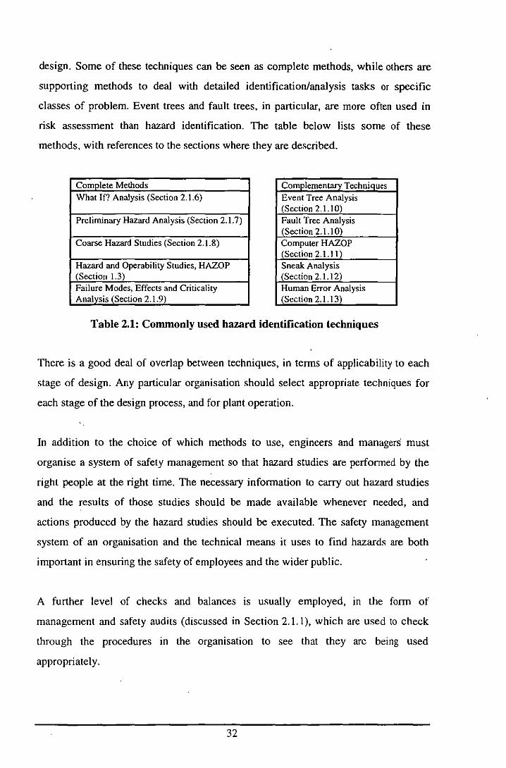
design. Some of these techniques can be seen as complete methods, while others are
supporting methods to deal with detailed identification/analysis tasks or specific
classes of problem. Event trees and fault trees, in particular, are more often used in
risk assessment than hazard identification. The table below lists some of these
methods, with references to the sections where they are described.
Complete Methods COl1lJ'lementarv Techni'lues What If? Analysis (Section 2.1.6) Event Tree Analysis
(Section 2.1.1 0) Preliminary Hazard Analysis (Section 2.1.7) Fault Tree Analysis
(Section 2.1.1 0) Coarse Hazard Studies (Section 2.1.8) Computer HAZOP
(Section 2.1.11) Hazard and Operability Studies, HAZOP Sneak Analysis (Section 1.3) (Section 2.1.12) Failure Modes, Effects and Criticality Human Error Analysis Analysis (Section 2.1.9) (Section 2.1.13)
Table 2.1: Commonly used hazard identification techniques
There is a good deal of overlap between techniques, in terms of applicability to each
stage of design. Any particular organisation should select appropriate techniques for
each stage of the design process, and for plant operation.
In addition to the choice of which methods to use, engineers and managers must
organise a system of safety management so that hazard studies are performed by the
right people at the right time. The necessary information to carry out hazard studies
and the results of those studies should be made available whenever needed, and
actions produced by the hazard studies should be executed. The safety management
system of an organisation and the technical means it uses to find hazards are both
important in ensuring the safety of employees and the wider public.
A further level of checks and balances is usually employed, in the form of
management and safety audits (discussed in Section 2.1.1), which are used to check
through the procedures in the organisation to see that they are being used
appropriately.
32

Following on from the discussion of audit methods is a discussion of materials
properties and how they can be used to screen process options for early process route
selection, in Section 2.1.2. Knowledge of material properties is required in any case,
for adequate assessment of the hazards in a process. Hazard indices (Section 2.1.3) are
another instrument used to assess the hazards presented by a process or its equipment,
and pilot plants (Section 2.1.4) can also provide valuable information about the
hazards of novel process options.
Checklists, as mentioned above and discussed in Section 2.1.5, are a good way of
preserving the "lessons learnt" information gained from accidents, but only if they are
used and maintained regularly. The subsections following Section 2.1.5 cover each of
the techniques mentioned in Table 2.1 in turn, and in Section 2.1.14 the techniques
discussed are put in the context of the activities which go on during the design of a
new process plant.
2.1.1 Management and Safety Audits
As a part of the management structure of an organisation, procedures ami codes of
practice for management and operation of plant, as well as the more technical aspects
of process engineering, are important in maintaining a safe place of work for
employees. In the UK, management has a responsibility for the safety of employees
covered by the Health and Safety at Work Act, HSE (1990).
Audits of the safety systems in use in an organisation are directed at discovering areas
of strength, weakness and vulnerability in the activities of that organisation. Typically
this sort of investigation will cover the control of maintenance through a permits to
work scheme, reponing procedures for accidents and "near misses", etc. The safety
audit can be quite detailed in its scope, including some identification of main hazards
as well as the assessment of site systems of work and reporting. An example of this
type of check is given in "Safety Audits", by BCISC (1973).
Management system audits are usually focused on a wider range of commercial
activities, but also form the main type of inspection carried out in the UK by the HSE.
33

All techniques are directed at ensuring the optimum levels of performance throughout
the company, including profitable and safe operation of its plant.
2.1.2 Materials Properties and Process Screening
Many hazards associated with a process are related to the properties of materials or
intermediates used. Therefore, considerations of safety, operability and environmental
problems can take place even before process chemistry or plant siting have been
decided.
By considering safety problems for each process option, designers can choose an
inherently safer plant. This could be achieved by using a more benign process, which
avoids extreme temperatures and pressures, or by eliminating hazardous chemicals
altogether. Alternatively, process intensification can be used to reduce inventories of
hazardous materials, or plans for siting the plant can be changed to minimise the
impact of accidents on local people or the environment.
Screening process routes requires that certain information is available about the
process materials, such as physical and chemical properties, as well as safety related
information, relating to flammability and toxicity. Standard safety data sheets usually
provide some of this information, and some of the rest can be found in reference
books. It should be noted, however, that information on likely impurities and their
effects on the process chemistry and safety can be difficult to obtain.
According to the EC Safety Data Sheet Directive, CONCA WE (1992), the contents of
a material data sheet should include the following items:
• Identification of • Composition/information on
substance/preparation and company ingredients
• Hazards identification • First-aid measures
• Fire-fighting measures • Accidental release measures
• Handling and storage • Exposure controls/personal protection
34

• Physical and chemical properties • Stability and reactivity
• Toxicological information • Ecological information
• Disposal considerations • Transport information
• Regulatory information • Other information
Information about the thermal stability of materials in the process can be vital to
ensuring the operability of a process as well as its safety. Two factors come into play
here. One is the inherent stability of single components, with regard to physical
changes in plant and storage conditions. The second factor is the stability of reaction
mixtures in the reactor environment and the question of exothermic runaway. For
some compounds explosion caused by mechanical shock, rather than straightforward
thermal stability may be the dominant issue. Care must be taken to identify what sort
of hazards will be present due to the compounds and reactions in the system.
A certain amount of "desk screening", using book data, guidance on chemical bond
groupings, computer programs, etc. can be used to filter out compounds which are
likely to be highly unstable. Then, preliminary tests can be performed to detect the
presence of all exotherm or gas evolution when a material is heated. Further tests can
also be used (using various forms of calorimetry) to get more detailed information
about the stability of compounds or reactions of interest.
2.1.3 Hazard Indices
A number of index methods are available to assess the losses that could be caused by
fires, explosions and releases of process materials. These are applicable where a
preliminary flowsheet and site plan are available, so that process fluids, inventories,
pressures and temperatures are known. Examples of these techniques include:
• Dow Fire and Explosion Index (Dow Chemical Company, 1994).
• Mond Index - Similar to the Dow Index, for fires, explosions and the acute
toxicity effects of releases.
• Dow Chemical Exposure Index.
3S
• Instantaneous Fractional Annual Loss (IF AL).
• Mortality Index, which relates to materials with a major hazard potential.
These indices can be used to inform process selection decisions or to identify the main
hazards in the process design, with a view to controlling them.
2.1.4 Pilot Plants
A large quantity of potentially useful data can be gained from pilot plant studies,
which help in clarifying the safety and operability issues in a process, as well as
informing the scale-up of the process from lab experiments to full scale operation. It is
very important that the experience gained on the pilot scale is used to good effect
when full scale production is considered. Due consideration must also be given to the
hazards presented by the pilot plant itself, before it is built.
2.1.5 Checklists
If used appropriately, checklists are an effective way of passing on information about
the characteristic hazards of a process or piece of equipment. They are based on past
experience of hazards or accidents and may therefore be less useful when developing
novel processes, than when reusing or mOdifying an existing design.
Checklists are often used at the design check stage, when developing a process flow
diagram into an ELD, to quickly examine the proposed design for any problems. They
should therefore be used only as a final check that nothing has been missed, and not as
a protocol to guide the design process itself.
Some guidance on the use of checklists is given by Miller and Howard (1971). There
are a huge number of references on the subject, a selection of which is offered in
Table 8.4 of Lees (1996).
A useful checklist should provoke enough thought to prevent the user from simply
answering "yes" or "no" to each question. This requires a careful choice of questions,
36

which must be worded appropriately. The user of the checklist must of course raise
appropriate actions if he/she finds any problems with the design.
Lastly, checklists must be used regularly and updated as necessary, in the light of
experience with their use. Ownership and responsibility for the lists need to be
maintained and passed on within an organisation.
2.1.6 What If? Analysis
This method is described by Burk (1992) and by CCPS (1985). It is best used at the
stage in design when a process flow diagram (PFD) has been produced. All available
design information is examined, including the PFD, any operating instructions and
equipment design parameters.
The objective is to produce a list of potential safety problems or actions to be
considered in revising the design, by considering the effect on the plant of abnormal
situations. A group of design team personnel meet to examine the design and ask
questions about possible things that could go wrong. The method uses the team's
collective imagination to identify more obscure problems than might be possible using
a checklist alone.
Burk (1992) combines the "What If?" method with a checklist approach, to give more
comprehensive coverage of process hazards. This method can be used to evaluate new
plant designs, review an operating plant periodically, or to check for hazards when
making modifications. The study is performed by a multi disciplinary group, aided by a
team leader to conduct the meetings and a scribe to record the questions raised. The
analysis proceeds through a number of st"ges:
• Organisational Meeting - The team leader explains the method to be used, and the
scope of the review, to the whole group. Information packages, containing all
necessary drawings, technical details and a timetable of meetings, are distributed
to each team member.
37

• In-Depth Review of Process - For tearn members unfamiliar with the process, the
main features of the plant are explained and a tour of the plant takes place, if
appropriate.
• Question Formulation Meeting - When the team members have familiarised
themselves with the information available, the plant is studied in detail, from feed
to product storage. The team formulates questions focusing on potential hazards or
incidents, and their causes:
• There is no attempt to answer any questions at this stage, as this impedes
the generation of further questions.
• Questions are recorded in full sentences on a flip-chart visible to the whole
group.
• All points raised are recorded, even if they appear to be "dumb questions".
o Questions do not have to begin with the phrase "What IT?".
• Closely related questions are grouped together, as some questions will give
rise to other related ones.
• When the whole process has been reviewed in this "brain-storming" way, the team
leader hands out a checklist of possible areas of concern. The group works through
the list, to see if any further questions are raised by this. Burk provides an example
of a I ist which could be used here.
• After the question formulation meeting, questions are allocated to team members,
who take them away and prepare draft answers to them. When the answers have
been prepared, they are distributed to all tcam members before the next meeting.
• Question Response Meeting - The group reviews the questions raised and answers
produced, to agree on what to do about each problem area. It is very important that
all agree with the actions produced by this meeting.
• The report should (at minimum) document the identified hazards, their causes and
the agreed actions to eliminate or control these hazards. Burk suggests that the
report should not be presented in a tabular format, but instead should use complete
sentences to record the questions and answers. This is felt to be more effective in
communicating the full meaning of what has been discussed.
38
2.1.7 Preliminary Hazard Analysis
Methods for identifying hazards during early design, when only a block diagram of the
process may be available, vary widely. Therefore, use of the term "preliminary hazard
analysis" (PHA) is quite loose. The usual objective of PHA (as described by, for
example, CCPS, \985) is to raise awareness of the major hazards in equipment
proposed for the design, as early as possible. Analysis should produce a set of causes
and consequences of specific scenarios, with associated corrective measures.
The following aspects of the design should be considered, with regard to the hazards
that may be present:
• Properties of the raw materials, intermediates and products in the process, as weIJ
as utility fluids such as steam, nitrogen, fuels, etc.
• Types of equipment used in the process, their temperatures and pressures.
• Interfaces between components of the designed system, such as fluid interactions
and compatibility with materials of construction, fire initiation and propagation,
etc.
• Operating environment. Consider external factors such as temperature limits,
humidity, earthquakes, etc.
• Operation of the plant (maintenance, testing, start-up and shut-down, etc.).
• Facilities support, such as storage, staff training, utilities required.
• Safety Equipment (e.g. emergency shutdown instruments, personal protective
equipment, fire protection).
2.1.8 Coarse Hazard Studies
Coarse hazard studies, such as the method outlined in Section 4.1 of the CIA Guide to
Hazard and Operability Studies (1977), aim to identify problems caused by missing
data or hazard information, or features of the basic design, layout and plant siting.
39
This assessment is carried out early, when a block layout of plant items and (possibly)
a basic flowsheet is available. It should clarify to all those taking part what the main
sources of hazards and problems with operation will be, as well as indicating
deficiencies in data about the process and the materials in it.
A method study approach similar to that used in HAZOP (Section 1.3) is common,
where a team of experts reviews the design under the supervision of a chairman.
Guide words provoke generation of ideas in combination with the general design
parameters decided so far and a number of potential hazards. The guide word lists
given by Knowlton (1981), as the "creative checklist" approach are:
General Design Parameters:
• Materials
• Raw materials
• Intermediates
• Products
• Effluents
• Unit Operations
• Mixing
• Distillation
• Drying
• etc.
• Layout
• Arrangement between unit operations within the plant
• Spatial relationships with other facilities
Potential Hazards:
• Fire • Noise • Explosion
• Vibration • Detonation • Noxious material
• Toxicity • Electrocution • Corrosion
• Asphyxia • Radiation • Mechanical failure
40

The actions produced by the study may be queries for infonnation on equipment or
materials, or actions to plan for, or design out, certain hazards highlighted in the
study.
2.1.9 Failure Modes, Effects and Criticality Analysis (FMECA)
Failure modes and effects analysis (FMEA) revIews specific failures of system
components and the consequent effects of each failure mode on the whole system.
Criticality analysis can be added to this cause-effect analysis, so that the severity of
the effects of failure, and the frequencies of the root cause failure modes, are
estimated. When this additional method is used, FMEA becomes FMECA, "failure
modes, effects and criticality analysis".
The two methods are described in the CC PS hazard evaluation guidelines (CCPS,
1985) and are also covered by a British Standard, BS5760: Part 5 (BSI, 1991). An
example of the results of application of FMEA to a liquefied natural gas terminal is
given by Aldwinckle and Slater (l983). An example for a differential pressure
transmitter is given in Appendix 3 of Green (1983).
FMEA is a systematic and laborious procedure which requIres detailed design
infonnation. It therefore can only be used selectively, late in a project, on the more
critical parts of the process, control or safety system.
Before starting the study, it is important to decide what equipment is to be examined
and in how much detail, as well as collecting all available information on the
functions of the equipment items.
Each element of the system is examined in turn (by a team or a single analyst), and all
conceivable failure modes are noted. Failure modes are malfunctions that change the
normal operation or function of equipment items. For each failure, the effects on the
system are detennined and the results recorded in a standard format. This requires a
detailed understanding of the events involved in the fault-consequence scenario. For
41
FMECA, the criticality of each failure mode is added, in tenns of a severity and
probability class (e.g. a rank number in the range 1-4), for each identified scenario
The results of the study should record the failure modes of equipment, causes of these
failure modes and the further effects on other components, and the system as a whole.
It is also important, if possible, to classify the failure mode in tenns of how it can be
detected, the possibility of testing or replacing components to eliminate the problem,
and any provisions made to compensate for the failure if it occurs.
FMEA and FMECA are best for considering components whose failure could have a
serious effect on a large part of the (process) system. They are good for serial failure
logic, where causes and effects chain together one after another but for more
complicated logic, fault tree and event tree analysis are more suitable techniques.
2.1.10 Event Tree and Fault Tree Analysis
Event trees are logic diagrams illustrating the development or escalation of a
hazardous consequence, or scenario. Fault trees are logic diagrams which show the
mechanisms by which a hazardous event can be caused (sequences of events in the
fault tree are known as "fault paths").
Both types of tree are used mainly for risk assessment, to quantify the risk or the
losses resulting from an incident. Nevertheless, constructing them can be a useful
exercise in focusing thinking during hazard identification. The use of event trees and
fault trees for hazard analysis is described in Chapter 9 of Lees (1996).
2.1.11 Computer HAZOP
The failure modes of computer systems can be quite different to those of process or
mechanical equipment, and the use of computers in modern process plants is
increasingly pervasive. For this reason there has been a lot of recent interest In
techniques for analysing the reliability of programmable systems, and in methods to
42
identify the hazards which could arise due to failure of components in computerised
systems.
A number of factors combine to make safety assessment of computer-controlled plant
more complicated than for plant which does not involve any programmed component.
Relevant considerations include:
• Failure of process equipment.
• Failure of computer hardware.
• Common mode failures across the whole plant, related to problems with the
computer control system, other services or plant-wide utilities.
• Latent errors in computer programs. These coding errors are systematic and are
only revealed under certain conditions of operation.
• Errors in specification of the computer software due to poor communication
between cngineers and programmers.
• Communication errors between machines, due to unforeseen conditions ill the
plant, or within the equipment items themselves.
Computer HAZOP is carried out at the same time as, or after, the process-related
HAZOP of a plant. Details of the instrumentation and control systems, including loop
diagrams for instruments and control program documentation, must be available. The
project instrument and control engineer and someone responsible for the technical
programming and configuration of the computer system must be present, as well as
the usual HAZOP team members.
The method deals with computers by adding extra guide words to the traditionally
used set, describing possible faiiures in relation (normally) lo instrument signals and
the output signals from controllers. Normally the computer has no power to affect the
operation of the process, except through actuators connected to the process. In this
sense, the guide word approach proposed by Andow (1991) makes sense for inputs
and outputs.
43
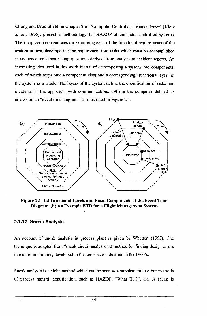
Chung and Broomfield, in Chapter 2 of "Computer Control and Human Error" (Kletz
et al., 1995), present a methodology for HAZOP of computer-controlled systems.
Their approach concentrates on examining each of the functional requirements of the
system in turn, decomposing the requirement into tasks which must be accomplished
in sequence, and then asking questions derived from analysis of incident reports. An
interesting idea used in this work is that of decomposing a system into components,
each of which maps onto a component class and a corresponding "functional layer" in
the system as a whole. The layers of the system define the classification of tasks and
incidents in the approach, with communications to/from the computer defined as
arrows on an "event time diagram", as illustrated in Figure 2.1.
(a) Intervention
Input/Output
mmunication
Sensor. Hurran input device, Actuator.
Dis /a
Utility, Opetator
~ (b)
Figure 2.1: (a) Functional Levels and Basic Components of the Event Time Diagram, (b) An Example ETD for a Flight Management System
2.1.12 Sneak Analysis
An account of slleak analysis in process plant is given by Whetton (1993). The
technique is adapted from "sneak circuit analysis", a method for finding design errors
in electronic circuits, developed in the aerospace industries in the 1960's.
Sneak analysis is a niche method which can be seen as a supplement to other methods
of process hazard identification, such as HAZOP, "What 1f...?", etc. A sneak is
44

· defined as "an undesired condition which occurs as a consequence of a design error,
sometimes but not necessarily in conjunction with a failure".
For process systems, Whetton (1993) identifies six categories of sneak. The categories
may occasionally overlap, for some incidents:
I. Sneak Flow - An unintended flow from a source to a target location, possibly due
to a valve being opened erroneously. A simple example of this is shown in Figure
2.2. If the two drain valves are opened simultaneously, fluid from the high
pressure vessel can get into the low pressure vessel, with potentially hazardous
results.
2. Sneak Indication - Incorrect or ambiguous indication by instruments or safety
systems. An example of this type of problem is one from the Three Mile Island
incident, where an indicator intended to show the state of a remotely operated
valve actually showed the state of the switch operating the valve (Figure 2.3).
Clearly if the valve is faulty and cannot operate, the lamp does not indicate this.
3. Sneak Label - An incorrect or ambiguous label on instrumentation or process
equipment.
4. Sneak Energy - Unintended presence or absence of energy. Examples of this
include reactor vessels where a mixer, which has been switched off for a while, is
reacti vatcd causing a reaction to run out of control, or cases where pressure
remains in a system after shutdown, injuring personnel when the process is opened
for maintenance.
5. Sneak Reaction - Unintended reactions, such as side-reactions in a reactor, or
reaction of materials outside the reactor environment.
6. Sneak Procedure or Sequence - Where events occur in the wrong order or in
conflict with one another.
45
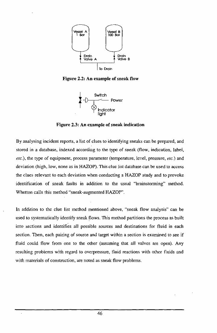
" " Vessel A Vessel B
1 Bar 100 Bar
'- /' "- /'
Drain ~ Oral Valve A Volv
n e B
I To Drain
Figure 2.2: An example of sneak flow
t~ItCh - Power
Indicator light
Figure 2.3: An example of sneak indication
By analysing incident reports, a list of clues to identifying sneaks can be prepared, and
stored in a database, indexed according to the type of sneak (flow, indication, labei,
etc.), the type of equipment, process parameter (temperature, level, pressure, etc.) and
deviation (high, low, none as in HAZOP). This clue list database can be used to access
the clues relevant to each deviation when conducting a HAZOP study and to provoke
identification of sneak faults in addition to the usual "brainstorming" method.
Whetton calls this method "sneak-augmented HAZOP".
In addition to the clue list method mentioned above, "sneak flow analysis" can be
used to systematically identify sneak flows. This method partitions the process as built
into sections and identifies all possible sources and destinations for fluid in each
section. Then, each pairing of source and target within a section is examined to see if
fluid could flow from one to the other (assuming that all valves are open). Any
resulting problems with regard to overpressure, tluid reactions with other fluids and
with materials of construction, are noted as sneak flow problems.
46
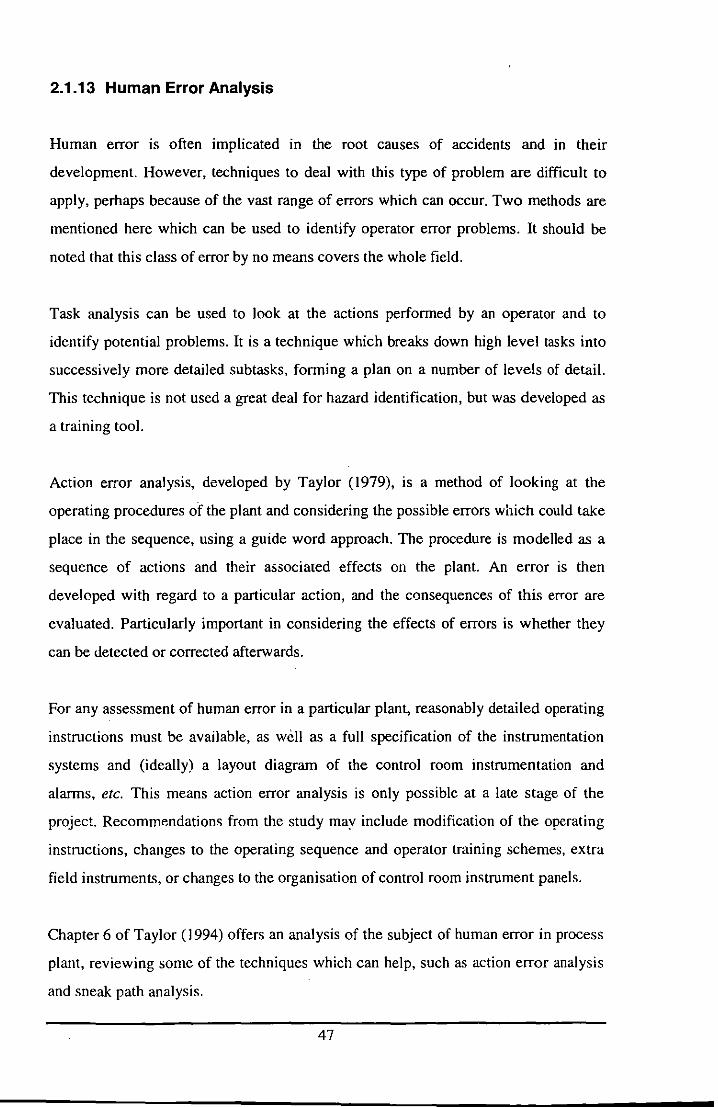
2.1.13 Human Error Analysis
Human error is often implicated in the root causes of accidents and in their
development. However, techniques to deal with this type of problem are difficult to
apply, perhaps because of the vast range of errors which can occur. Two methods are
mentioned here which can be used to identify operator error problems. It should be
noted that this class of error by no means covers the whole field.
Task analysis can be used to look at the actions performed by an operator and to
identify potential problems. It is a technique which breaks down high level tasks into
successively more detailed subtasks, forming a plan on a number of levels of detail.
This technique is not used a great deal for hazard identification, but was developed as
a training tool.
Action error analysis, developed by Taylor (1979), is a method of looking at the
operating procedures of the plant and considering the possible errors which could take
place in the sequence, using a guide word approach. The procedure is modelled as a
sequence of actions and their associated effects on the plant. An error is then
developed with regard to a particular action, and the consequences of this error are
evaluated. Particularly important in considering the effects of errors is whether they
can be detected or corrected afterwards.
For any assessment of human error in a particular plant, reasonably detailed operating
instructions must be available, as well as a full specification of the instrumentation
systems and (ideally) a layout diagram of the control room instrumentation and
alarms, etc. This means action error analysis is only possible at a late stage of the
project. Recomm'mdations from the study may include modification of the operating
instructions, changes to the operating sequence and operator training schemes, extra
field instruments, or changes to the organisation of control room instrument panels.
Chapter 6 of Taylor (1994) offers an analysis of the subject of human error in process
plant, reviewing some of the techniques which can help, such as action error analysis
and sneak path analysis.
47
2.1.14 Hazard Identification in the Context of Process Design
The methods discussed so far form a menu of options from which safety managers can
choose in formulating their own system for safe plant design. These will now be put in
the context of the time-line from process conception through to checking on the final,
detailed process design.
First of all, the design team must decide what product to make, where, and with what
process chemistry. A basic process outline must be produced for a number of
candidate options. At this stage, collecting data on process materials, screening them
for potential hazards and testing for thermal stability are important concerns.
Experience gained in pilot plant studies, or from previous operation of similar
processes, should also be used, at this process definition stage and later. The use of
checklists should also be encouraged at all stages of the project where a process
design exists at such a level that specific aspects of it can be usefully questioned.
Once a block diagram of the process has been developed, index methods such as the
Dow Fire and Explosion index can be used. These inform decisions on inventories of
hazardous materials, layout of plant sections, etc. Later, when a PFD has been drawn,
a more specific view of the hazards to be expected in the plant can be gained by using
either "What If?" Analysis, PHA, or a Coarse Hazard Study method.
For hazard identification on the detailed process design, HAZOP can be combined
with a number of the supporting methods, as appropriate for the plant being designed:
• Sneak analysis can help to look at potential hazards from a different angle.
• FMECA can be used to investigate the more important components of the system,
to evaluate the implications of their failure.
• Fault trees and event trees may be chosen for risk assessment, or to clarify the
causation of complex events.
48

• Computer HAZOP may be used to review the potential problems associated with
programmed components in the plant, including the control system.
• Human error analysis is most useful for plants involving a lot of operator
intervention (e.g. batch or semi-batch operations).
There must be a sensible choice of a range of the above techniques, to cover the
specific characteristics of the plant being designed. The technical studies must be
integrated into a system of management and communication, so that all involved are
aware of how the information generated is to be used.
2.2 Qualitative Physics
Qualitative Physics (QP) is an active field of research in Artificial Intelligence (AI). In
QP, models of physical systems are based on qualitative variables with discrete
val ues, rather than the real numbers typically used in the differential equation models
of classical physics (De Kleer, 1992). Study in this area is justified by a number of
points:
• QP can provide more causally satisfying explanations for physical behaviour than
the mathematical equations most often used in classical physics.
• Solutions to problems in QP may be simpler to obtain, compared with those of
quantitative physics problems.
• Computationally, QP simulations are cheaper than numerical simulations.
• More intuitive explanations of behaviour may be offered by QP. It seems likely
that the mental physical understanding we use (our own "naIve physics") is
fundamentally qualitative in nature.
• QP may be able to solve problems where only an incomplete specification is
available.
• The precision required in specifying parameters in a quantitative simulation
ensures that only one behaviour is produced from any given starting point. By
contrast, a qualitative simulation can deal with uncertain or imprecise values and
can therefore represent a wider range of physical scenarios. This means that QP
49
can be made to produce all physically possible behaviours of the physical system
corresponding to the qualitative model studied.
• QP models can be used to focus attention on areas of concern and simplify later
quantitative analysis.
2.2.1 General Issues to be Tackled by Qualitative Formalisms
Whatever approach is chosen for studying Qualitative Physics, a number of important
issues must be addressed (De Kleer, 1992). Firstly, there is the question of what to
represent in the QP system - for instance, whether the fundamental "units" in the
system are physical processes which mayor may not be in operation (Forbus, 1984),
components of a mechanism (Kuipers, 1986), or constraints operating between
variables (De KIeer and Brown, 1984). These three most common standpoints in the
field are discussed later, in Sections 2.2.4, 2.2.5 and 2.2.6 resIJectively.
A second issue is the treatment of variables and values. We have established that the
values of variables in QP are discrete, but what values those variables may take, under
what conditions, etc., is a separate argument. Most of the time, the qualitative variable
under consideration is produced by segmentation of the real number line
(corresponding to the related quantitative variable) into a number of non-overlapping
intervals.
The most commonly used value set is {-,O,+}, corresponding to quantitative values
which are negative, zero or positive: For a particular material in pure form and at
ambient pressure, there may be five qualitative temperature values, corresponding to
the temperature ranges where the material is solid, melting, liquid, boiling or gaseous.
The points on the number line where the qualitative value of the variable changes are
known as "landmark values" and they usually correspond to significant qualitative
changes of applicable laws or behaviour.
In addition to the definition of qualitative variables, algebraic axioms and rules must
be provided to allow mathematical operations to be defined on the variables. Often,
these axioms and rules are derived from the mathematical analysis of real numbers.
50
Some generic and some problem specific constraints must also be brought into play in
order to establish relationships between the variables in the model system. How
constraints are expressed depends on how the concepts of "structure" and
"mechanism" are treated. Some workers (e.g. De K1eer and Brown, 1984) represent
constraints directly, avoiding the construction of a constraint set from some other
form. In the component based approach to modelling, constraints are specified
between variables within the same component, and inferred from linkages between
components, so that a network of constraints is formed in the composite system.
The principle of "no function in structure" is a guiding principle for developing
models. The laws of individual parts of a system (its "units") must never presuppose
the function of the whole. The purpose of this principle is to prevent the development
of context-specific models where the answers to questions put to them are built into
the laws governing individual units and their linkage. In such a situation, difficulties
will be encountered when the unit is presented wiL'1 a different context.
A major problem with QP systems is that of representing time, and therefore change,
in physical systems. As variables change, they may reach landmark values, changing
the beh~viour of the system. Which variables reach landmark values first is the
question addressed by transition analysis, or limit analysis (Forbus, 1984). Time is
usually represented qualitatively as a sequence of "intervals", optionally separated by
"instants". Having decided on a representation for time, predictions can be made using
a qualitati ve calculus which allows simulation of behaviour forwards in time from a
given initial state. This is particularly illustrated by De K1eer and Brown (1984), who
describe the concept of "envisioning" the behaviour of a mechanism.
Causality (the issue of what events can cause other events in the system) mayor may
not be addressed explicitly in a QP model, as with any physical explanation. There is a
problem here, in that the scientific community has not yet come up with a satisfying
formal definition of causality. As a minimum for causal linkage, dependency must be
demonstrated between two events. If A and B are assignments of values to qualitative
variables ("events"), then for A to cause B, the occurren,ce of B must depend on A
51
--- -------------
occurring. Usually, the constraints of spatial and temporal order are also imposed to
determine if the causal link exists: only physically connected components may
interact, and for A to cause B, A must precede B.
2.2.2 Ambiguity
Ambiguity in qualitative simulation arises when the simulator cannot decide which of
a number of possible outcomes actually takes place. This leads to a branched "tree" of
possible states of the system being simulated, where every one of the possible
outcomes must be considered. Computational complexity becomes a problem when
this sort of ambiguity is widespread.
Ambigui ty of various kinds is inherent in the nature of most models in Qualitative
Physics. One important type of ambiguity is that of certain arithmetical operations,
such as addition. If two qualitative variables A and B each take values from the set
{-,a, +} then their sum, (A+B), is highly ambiguous (the sum of a "+" and a "-" may
be "+" or "-", or even "0"). This is a problem when considering mass balances around
dividers or headers in simulations of chemical plant, for example.
Another significant source of ambiguity is where a model uses a very loose functional
constraint between two variables. Such constraints are needed to allow a wide range
of mathematical functions to be generalised within the qualitative framework. The
downside is that a whole family of functions are implied, every time the qualitative
constraint is used, so that the simulated behaviours of the system include all those
consistent with the different interpretations of the constraint.
Temporal ordering of state changes in qualitative simlllations also increases
ambiguity. Where the system is unable to decide which of a number of possible
changes in the system will occur first, it must consider each of them as equally
possible. This occurs when a number of variables are changing, moving towards
different landmark values, so that there is a problem in determining the order in which
these landmarks are reached.
52
In QP, we want to be able to distinguish real behaviours of the system as specified
from physically impossible predictions. There may actually be multiple real
behaviours consistent with the model used, in which case we want to know about
them all. Impossible behaviours may arise due to the inability of the model to capture
real constraints which exist between objects in the world.
Usually, such constraints are high level ones, such as conservation of mass or energy,
which cannot be captured very easily in localised qualitative models. However, some
attempt to capture these types of constraints may be made by inspecting the
configurations of units in the model of the system as a whole.
2.2.3 NaIve Physics and Commonsense Reasoning
In his "Na'ive Physics Manifesto", Hayes (1979) criticises AI research for being too
limited to so-called "toy worlds" and simple, well-defined puzzles and games. While
the programs developed may possess an ability to play chess, or to reason about
blocks on a table top, there is no sign of the general intelligence we are accustomed to
making use of in the real world. As a first step towards intelligent systems, Hayes
proposes formalising large parts of the commonsense knowledge we have about the
world (our "na'ive physics").
Among the many interesting topics discussed by Hayes (1979), the idea of histories is
particularly useful for its potential in tackling a long-standing AI problem known as
the "frame problem". A frequently used representation in AI models the state of the
world using a set of propositions about individuals in that world. Rules are used to
define possible transitions between states of the world, in terms of changes in the set
of propositions. This model of change is known as the "situational calculus" and is
described by (among others) McCarthy and Hayes, (1969).
Although this model is mathematically and computationally attractive, it suffers from
a serious problem: one must specify, for each individual in the world, whether it
changes or does not change in response to each possible action defined in that world.
This is known as the frame problem, and it causes an explosion in the number of
53

rules, as each variable must have a "frame axiom" to state if it does or does not
change when some particular operation is carried out. The situational calculus allows
the state of an object to depend on all the other elements of the world model.
The real world (when viewed in a deterministic way) is somewhat different. We
intuitively know that two objects must physically interact with one another, typically
through the action of some force or exchange of material, in order to affect their
behaviour. Hayes calls for a state representation of objects that includes a limited
spatial extent, but potentially unlimited temporal extent. This is the idea of a
"history": a projection of the spatial extent relevant for an object through time.
Histories are associated with an object and the places which can physically interact
with that object over the temporal history of the object. These places are not
necessarily fixed in size and they can overlap or be nested inside one another - and
therefore so too can histories. The history of a composite object is defined as the
union of the histories of each of its component objects.
Objects may only interact if their histories intersect in space-time. This substantially
tames the frame problem because it restricts candidates for variables changes to those
changes caused by the intersection of histories of adjacent objects in the world. Such a
restriction embodies the two important causal considerations of spatial and temporal
order, mentioned in the previous section.
2.2.4 The Process-Based Approach
"Qualitative Process Theory" (QPT) was developed by Forbus (1984). In this theory,
changes in the world arc caused by the operation of physical "processes",
corresponding to such phenomena as motion, heating, bending, boiling, etc.
According to Forbus, this model of change is more descriptive than solving constraint
equations to yield evolving patterns of variation in state variables (as in QSIM, for
example - see Section 2.2.5 below). Hayes' idea of spatially limited histories,
described in Section 2.2.3, is used to tackle the frame problem, so that only objects
whose histories overlap in time and space are permitted to interact.
54
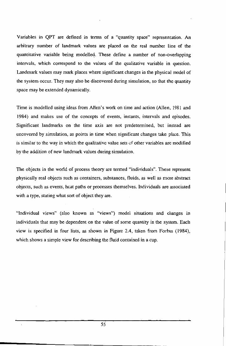
Variables in QPT are defined in terms of a "quantity space" representation. An
arbitrary number of landmark values are placed on the real number line of the
quantitative variable being modelleq. These define a number of non-overlapping
intervals, which correspond to the values of the qualitative variable in question.
Landmark values may mark places where significant changes in the physical model of
the system occur. They may also be discovered during simulation, so that the quantity
space may be extended dynamically.
Time is modelled using ideas from Alien's work on time and action (Alien, 1981 and
1984) and makes use of the concepts of events, instants, intervals and episodes.
Significant landmarks on the time axis are not predetermined, but instead are
uncovered by simulation, as points in time when significant changes take place. This
is similar to the way in which the qualitative value sets of other variables are modified
by the addition of new landmark values during simulation.
The objects in the world of process theory are termed "individuals". These represent
phYSically real objects such as containers, substances, fluids, as well as more abstract
objects, such as events, hcat paths or processes themselves. Individuals are associated
with a type, stating what sort of object they are.
"Individual views" (also known as "views") model situations and changes in
individuals that may be dependent on the value of some quantity in the system. Each
view is specified in four lists, as shown in Figure 2.4, taken from Forbus (1984),
which shows a simple view for describing the fluid contained in a cup.
55
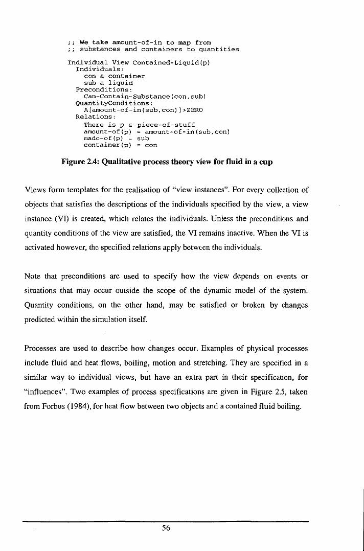
ii We take amount-of-in to map from ii substances and containers to quantities
Individual View Contained-Liquid(p) Individuals:
con a container sub a liquid
Preconditions: Can-Contain-Substance (con, sub)
QuantitYConditions: A(amount-of-in(sub,con)]>ZERO
Relations: There is p E piece-of-stuff amount-of{p) = amount-of-in(sub,con) rnade-of(p) = sub container{p) = con
Figure 2.4: Qualitative process theory view for fluid in a cup
Views form templates for the realisation of "view instances". For every collection of
objects that satisfies the descriptions of the individuals specified by the view, a view
instance (VI) is created, which relates the individuals. Unless the preconditions and
quantity conditions of the view are satisfied, the VI remains inactive. When the VI is
activated however, the specified relations apply between the individuals.
Note that preconditions are used to specify how the view depends on events or
situations that may occur outside the scope of the dynamic model of the system.
Quantity conditions, on the other hand, may be satisfied or broken by changes
predicted within the simulation itself.
Processes are used to describe how changes occur. Examples of physical processes
include fluid and heat flows, boiling, motion and stretching. They are specified in a
similar way to individual views, but have an extra part in their specification, for
"influences". Two examples of process specifications are given in Figure 2.5, taken
from Forbus (1984), for heat flow between two objects and a contained fluid boiling.
56
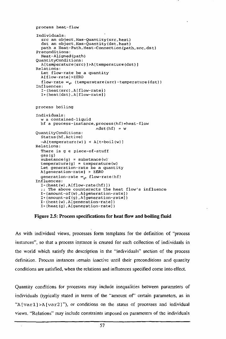
process heat-flow
Individuals: src an object,Has-Quantity(src,heat} dst an object,Has-Quantity(dst,heat) path a Heat-Path,Heat-Connection(path,src,dst)
Preconditions: Heat-Aligned (path)
QuantityConditions: A[ternperature(src)]>A[temperature(dst)]
Relations: Let flow-rate be a quantity A[flow-rate]>ZERO flow-rate ~~ (ternperature(src)-ternperature(dst»
Influences: I-(heat(src),A[flow-rate]) I+(heat(dst),A[flow-rate])
process boiling
Individuals: w a contained-liquid hf a process-instance,process(hf)=heat-flow
Adst (hf) ; w QuantityConditions:
Status (hf,Active) -A[ternperature(w)] < A[t-boil(w)]
Relations: There is 9 E piece-of-stuff gas (g) substance (g) ; substance ("1) temperature (g) ; ternperature(w) Let generation-rate be a quantity A [generation-rate] > ZERO generation-rate 0<:0+ flow-rate (hf)
Influences: I-(heat(w),A[flow-rate(hf)]) ;; The above counteracts the heat flow's influence I-(arnount-of(w),A[generation-rate]) I+(arnount-of(g),A[generation-rate]) I-(heat(w),A[generation-rate]) 1+ (heat (g), A[generation-rate] )
Figure 2.5: Process specifications for heat flow and boiling fluid
As with individual views, processes form templates for the definition of "process
instances", so that a process instance is created for each collection of individuals in
the world which satisfy the description in the "individuals" section of the process
definition. Process instances lemain inactive until their preconditions and quantity
conditions are satisfied, when the relations and influences specified come into effect.
Quantity conditions for processes may include inequalities between parameters of
individuals (typically stated in terms of the "amount of' certain parameters, as in
HA [varl] >A [var2] "), or conditions on the status of processes and individual
views. "Relations" may include constraints imposed on parameters of the individuals
57

and any new entities created by the process. The indirect effects imposed by functional
relationships are represented in the "Relations" part of the process description. The
"Influences" section is for specifying the direct causal effects of the process. In the
heat flow example of Figure 2.5, influence statements describe how the heat flow
negativei"y affects the heat content of the source object and positively affects the heat
content of the destination object.
Implementation of QPT requires a simulator which is capable of monitoring a set of
individuals and their parameters, automatically creating and activating appropriate
view and process instances as appropriate. The views and processes should be taken
from a library of models, the "process vocabulary", which defines the sorts of
phenomena that can be modelled by the theory.
Simulation of system behavio<!r typically involves a process called "limit analysis".
Changes in variables are observed, to detennine which landmark values could he
crossed, and in what order, and thereby determine the behaviour in the new qualitative
state. This may give rise to more than one possible outcome from any particular state,
so that simulation may produce a branching, tree-like pattern of possible behaviours.
Limit analysis may uncover new landmark values during simulation, requiring that the
quantity spaces of the variables are added to. It is not clear whether aB these new
landmarks necessarily correspond to physically significant events with respect to the
variable concerned.
58
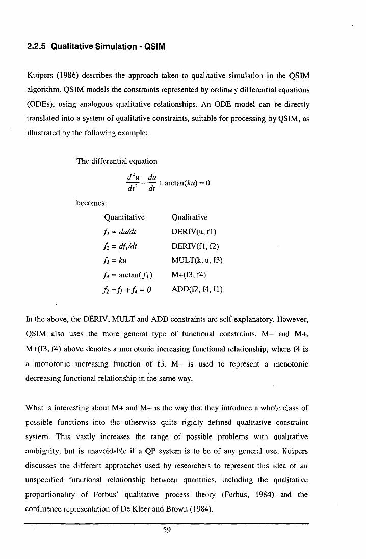
2.2.5 Qualitative Simulation - QSIM
Kuipers (1986) describes the approach taken to qualitative simulation in the QSIM
algorithm. QSIM models the constraints represented by ordinary differential equations
(ODEs), using analogous qualitative relationships. An ODE model can be directly
translated into a system of qualitative constraints, suitable for processing by QSIM, as
illustrated by the following example:
The differential equation
d'u du dt' - dt + arctan(ku) = 0
becomes:
Quantitative Qualitative
IJ = duldt DERN(u, fl)
fz = d!JIdt DERIV(fl, f2)
13 = ku MULT(k, u, f3)
!4 = arctan(h ) M+(f3, f4)
/z-IJ+14=O ADD(f2, f4, fl)
In the above, the DERN, MULT and ADD constraints are self-explanatory. However,
QSIM also uses the more general type of functional constraints, M- and M+.
M+(f3, f4) above denotes a monotonic increasing functional relationship, where f4 is
a monotonic increasing function of f3. M- is used to represent a monotonic
decreasing functional relationship in the same way.
What is interesting about M+ and M- is the way that they introduce a whole class of
possible functions into the otherwise quite rigidly defined qualitative constraint
system. This vastly increases the range of possible problems with qualitative
ambiguity, but is unavoidable if a QP system is to be of any general use. Kuipers
discusses the different approaches used by researchers to represent this idea of an
unspecified functional relationship between quantities, including the qualitative
proportionality of Forbus' qualitative process theory (Forbus, 1984) and the
confluence representation of De Kleer and Brown (1984).
59
The variables in QSIM are often known as "functions", because each is a function of
time in the system. Kuipers uses the quantity space idea of Forbus (1984) to define
qualitative values by comparison with a set of landmark values (a function can have a
value at, or between, landmark values, and can be increasing, steady or decreasing).
As with Forbus, the quantity space can be extended by discovering new landmark
values.
Transitions of variables between states are governed by well-defined rules borrowed
from the analysis of real numbers. For example, a variable cannot move from a value
of "between I, and lz and increasing" « (11, 12)' inc» to a value of "between 12
and 13 and increasing" « ( 12 ' 13 ) , inc» without first passing through "equal to lz
and increasing" «12, inc».
At each step, QSIM uses the basic rules for transitions between function states to
generate possible transitions which may be considered for the function. These are then
filtered for consistency with the constraint set describing the problem at hand, checked
for internal inconsistency and filtered down to a final set of possible successor states.
In general, QSIM will produce a branching tree of states, linked by function
transitions, as a description of the possible behaviours of a system.
QSIM constrains the relationships between functions in its constraint set models only
very loosely (e.g. the M+ constraint described above). Therefore, each set of
qualitative"constraints corresponds to a larger number of equivalent ODE models.
Simulation in QSIM produces a branch for every physically real behaviour of each of
these ODE models, which means that the tree produced can be highly branched.
Unfortunately, physically impossible behaviours are sometimes also predicted. This is
due to a combination of localised constraints and qualitative variable values.
Localised constraints do not capture global considerations, such as conservation of
energy, while arithmetic on qualitative variables is often inherently ambiguous.
As an example, for a friction less oscillating spring, QSIM produces three branches,
for steady, increasing or decreasing oscillation. The three-way branch occurs in the
60
simulation at every cycle, so that the behaviour predicted by QSIM could change
arbitrarily, from steady, to increasing, to decreasing oscillation. Steady oscillation is
the only physically real solution - the others are produced because the QSIM model
does not represent conservation of energy. Kuipers identifies the problem of
modelling high level constraints as particularly important for qualitative simulation.
2.2.6 Constraint-Based Qualitative Reasoning - "Confluences"
In the work of De Kleer and Brown (1984), explicitly represented constraint equations
(referred to as "confluences") take centre stage, in partnership with a strong
component-based approach to modelling complex mechanisms. This is a similar
approach to that in QSIM (described above), but De Kleer and Brown's approach to
modelling physical components is much stronger.
The objective is dynamic qualitative simulation, using qualitative differential
equations (QDEs), which are analogous to the ordinary differential equations (ODEs)
of real number physics. As demonstrated for QSIM in Section 2.2.5, direct translation
from ODEs to QDEs is possible. However, this is not the only way to derive
confluence models - one can develop models specifically for the qualitative domain.
The world view in De Kleer and Brown's ENVISION program is highly mechanistic.
Mechanisms are put together from "components" which process "materials" (such as
fluids electrons, force, mass, etc.) and are connected by "conduits". The task of
simulation consists of describing how the attributes of materials in the model change
over time. De Kleer and Brown call this activity "envisioning" the behaviour of the
mechanism. They also make the observation that attributes often occur in pairs, with
one a flow-iike variable and the other a pressure-like variable. This shows certain
parallels with the fluid modelling approach for AutoHAZID described in Section 3.5.
State dependent behaviour plays a very important role in the ENVISION models. Each
component may be in one of a number of different states, depending on the values of
its attributes. A different set of confluence equations applies to the component in each
of its states, which gives rise to different types of behaviour in simulation. The
61
applicability conditions of the component states are dependent on landmark values of
certain variables, so that when a landmark value is crossed, the behaviour may change
significantly.
Qualitative variables in ENVISION use a standard set of values, {-,O,+}, rather than
any more complicated scheme, such as Forbus' quantity space idea. Using this
convention, De Kleer and Brown have developed a large body of arithmetic and
calculus theory for confluence equations, based on similar results in the analysis of
real numbers.
At the start of simulation, the components in the system are all in known states and
the attributes are all known (in terms of their values and directions of change). At each
stage of simulation, the constraints applicable to each component are examined, to see
what possible changes in attributes are possible. In general, many possible changes are
possible, so that the behaviour of the system may branch at each step of the
simulation. For each component, the state of the component mayor may not change,
depending on the constraints in operation. According to De Kleer and Brown, every
one of the paths in the envisioned behaviour tree should correspond to a consistent
interpretation of some physical system formally identical to the model being
simulated.
De Kleer and Brown address at length the problem of how a qualitative system can be
made to offer causal analyses of its reasoning. They favour a state transition diagram
explanation, rather than any form of symbolic "proof' method using manipulation of
constraint equations.
The reason for this preference is that variables in constraint equations must change in
such a way that the confluences themselves are always satisfied. Thus, for the value of
any variable to change in a confluence, others must also change (simultaneously). This
removes the notion of cause and effect from this part of the behaviour, as one cannot
establish a temporal or causal ordering between variable changes within a confluence.
62
The search for a useful way of constructing causal explanations of ENVISION results
forms a large part of the De Kleer and Brown (1984) paper. It certainly is an important
problem area for "purists" in QP, who want satisfying explanations of which events
cause which other events, as well as workable models. The problem of explaining
behaviour (changes of attribute values) within a single state is particularly difficult,
and the authors invent a system of "mythical causality" to build candidate orderings of
attribute changes for this behaviour.
2.3 Applications of Qualitative Physics in Process Safety
The most commonly seen. applications of Qualitative Reasoning in Process
Engineering are in the area of safety for process plants. Usually, a component-based
modelling system, based around models of individual equipment types, is used. The
models may use rules of the traditional "IF-THEN" expert system format, or they may
rely on a graphical formalism to represent causal links between variables. The
application types most commonly seen in the papers reviewed here are diagnosis of
faults in operating plants and identification of potential hazards in a plant design. The
latter type of application most often uses the framework of a HAZOP study as an
organising structure.
In a review for the European Process Safety Centre (EPSC) of work being done in
"Knowledge Based HAZOPs", Rushton (1997) identified a number of groups doing
work on HAZOP emulation by computer. These were:
• Dow Benelux, Netherlands [Rootsaert and Harrington (1992)].
• Loughborough University, UK [e.g. Parmar and Lees (1987a, 1987b), Zerkani and
Rushton (1992, 1993), Chung (1993)].
• University of Pennsylvania, USA [e.g. Catino et al. (1991), Grantham and
Ungar (1990)].
• Purdue University, USA [e.g. Venkatasubramanian and Vaidhyanathan (1994)].
• Seoul National University, Korea [e.g. Chae et al. (I 994)].
63
• VTI, Technical Research Centre of Finland [e.g. Heino et al. (1994), Suokas et al.
(1990)].
To this list should be added the following groups, active in areas connected with
qualitative physics and process safety:
• Taiwan (two groups) [e.g. Chang et al. (1994), Kuo et al. (1997)].
• Argentina [e.g. Martinez et al. (\992), Vecchietti and Leone (1996)].
• Japan (two groups) [e.g. Iri et al. (1979), Shimada et al. (1993)].
Of the above, Pennsylvania are the only group who have taken a process-based
approach to modelling, concentrating on "phenomena" in a plant. This approach may
be very powerful in the long run, but suffers from problems of complexity even for
very simple systems, because of the frequent need to recompile models.
The other groups have systems which use a component-based "hybrid" approach,
typically using some Qualitative Physics and some Expert System ideas.
Discrimination between trivial and significant results seems to he an area where
problems are often encountered, where a purely qualitative treatment can give
ambiguous results.
The following subsections outline some of the work done by the groups mentioned
above. Attention has been concentrated on hazard identification and the qualitative
modelling techniques of interest in this area. This means that many papers on fault
diagnosis, process monitoring, etc. have been omitted from this review.
2.3.1 Purdue
The Laboratory for Intelligent Process Systems at Purdue University is led by Venkat
Venkatasubramanian. This group has made a good deal of progress in recent years in
developing a tool for emulating HAZOP, known as HAZOPExpert. Because of the
similarity of this 'system to the work done at Loughborough on AutoHAZID, this
64

section concentrates almost exclusively on HAZOPExpert, although one other area of
application is mentioned at the end.
HAZOPExpert uses Gensym's G2 system as a framework for development. G2
provides an object-oriented shell for development of on-line process-related expert
systems, supported by a strong Graphical User Interface (GUl). Using this GUI, users
of HAZOPExpert can easily specify process descriptions to the program as P&IDs (an
example is shown in Figure 2.6 below, from Srinivasan et ai., 1998).
AEFINERY.(JHtTB 1("".1111
L-______ ~----~+-------~~,~.
L·STU,IIIII
Figure 2.6 : Example P&ID created using HAZOPExpert
Venkatasubrarnanian and Vaidhyanathan (1994) justify computer emulation of
HAZOP by reference to the time-saving potential of a tool capable of automating the
routine parts of the HAZOP analysis. Given that all process plant installations in the
U.S.A. are now required to formally assess their process hazards at regular intervals,
the demand for HAZOP studies is bound to increase.
65
A principle which underpins HAZOPExpert is the separation of process specific from
process generic parts of the knowledge base. I This means that models of equipment
items and fluids are used which are not dependent on a particular plant and can be
used in any plant model. The process specific parts of the knowledge base are the
specifications of what equipment items are present, how they are connected together
and what fluids are present. Also included are the values of attributes belonging to the
equipment in the plant model, to specify information about the operation of those
equipment items.
The object-oriented system in 02 allows equipment and fluid models (the generic
process information) to be defined as classes of object, which can be related to other
classes using inheritance and thereby organised in a hierarchy. Model information also
includes methods for diagnosing causes of deviations in process variables, for doing
fault propagation through the plant, and for finding possible consequences of a
deviation.
The information stored in HAZOPExpert concerning process fluids consists of simple
data, such as whether the fluid is flammable, toxic, corrosive, what its physical state
is, etc. Such information is used in connection with the rest of the plant description to
provide better information about the hazards identified by the program. This form of
fluid model system adds to the list of hazards found by the system, rather than acting
as a filter for ensuring the validity of hazards found (the latter is the approach used in
the AutoHAZID program developed at Loughborough).
The first models for HAZOPExpert, described by Venkatasubramanian and
Vaidhyanathan (1994), used a propagation equation approach for qualitatively relating
variables te one another. This method has also been used at Loughborough by Parmar
and Lees (l987a, 1987b) and Hunt et al. (1993), for example. Propagation equations
can be seen as implementations of the confluences described by De Kleer and Brown
(1984). In process systems they typically characterise the relevant balance equations
(heat and mass balances) in the equipment. In papers after 1994, by Vaidhyanathan
1 The importance of this principle was noted in an carly paper by Venkatasubramanian and Rich (1988).
66
and others (1995, I 996a, 1996b and I 996c), the representation used by Purdue
changes to the "HAZOP Digraph" (HOG). This is a form of the signed directed graph
(SDG) representation to which are added further nodes representing faults and
consequences related to process variable deviations.
The HDG allows nodes for process variables to take values from the set
{-, +, Normal, Zero}, which correspond to the variable being lower than intended,
higher than intended, within the intended range of values, or zero, respectively. This
compares with the more usual SDG model, where the value set excludes the "Zero"
value, representing only the values "+" and "-" explicitly (all nodes which are not
given a value are assumed to be "Normal"). Purdue do not explain how their HOG
model handles propagation of "Zero" values in the graph.
The normal mode of use for HAZOPExpert, as described by Vaidhy~nathan and
Venkatasubramanian (1995), is interactive. A user initiates "HAZOP" of a variable by
selecting it on the P&ID and giving it a deviated value (High, Low or Zero), after
which the computer performs a search in the HOG and produces results on the P&ID
and in a separate window. The program searches in an upstream direction for causes
of the deviation and in a downstream dircction for adverse consequences. Because
causes may not be downstream and consequences may not be upstream in the plant,
HAZOPExpert has problems if there are recycles in the plant model, and will fail to
identify scenarios where propagation of effects occurs in an upstream direction.
Recycles are examples of feedback in the plant model. Feedback occurs in a physical
system wherever a physical variable, such as a flow, has an effect on other variables in
the system, such that a part of the original change is propagated back to .influence that
variable itself. Feedback may arise due to control loops in the plant, which give rise to
a link via feedback of information, or due to material recycle in the plant, or due to
any number of physical phenomena which tend to remain in a stable state if not
disturbed.
Feedback mechanisms give rise to cyclical paths in the graph, if the components of the
loop are modelled individually. Handling and interpreting cycles as they are found by
67
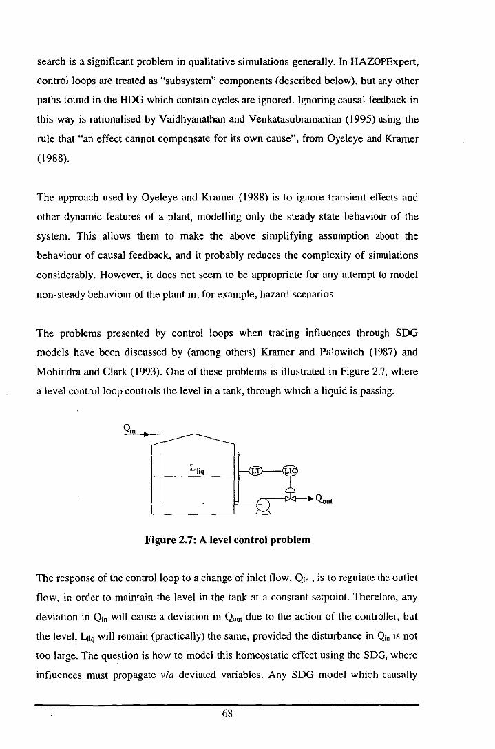
search is a significant problem in qualitative simulations generally. In HAZOPExpert,
control loops are treated as "subsystem" components (described below), but any other
paths found in the HDG which contain cycles are ignored. Ignoring causal feedback in
this way is rationalised by Vaidhyanathan and Venkatasubrarnanian (1995) using the
rule that "an effect cannot compensate for its own cause", from Oyeleye and Kramer
(1988).
The approach used by Oyeleye and Kramer (1988) is to ignore transient effects and
other dynamic features of a plant, modelling only the steady state behaviour of the
system. This allows them to make the above simplifying assumption about the
behaviour of causal feedback, and it probably reduces the complexity of simulations
considerably. However, it does not seem to be appropriate for any attempt to model
non-steady behaviour of the plant in, for example, hazard scenarios.
The problems presented by control loops when tracing influences through SOG
models have been discussed by (among others) Kramer and Palowitch (1987) and
Mohindra and Clark (1993). One of these problems is illustrated in Figure 2.7, where
a level control loop controls the level in a tank, through which a liquid is passing.
Figure 2.7: A level control problem
The response of the control loop to a change of inlet flow, Qin , is to reguiate the outlet
flow, in order to maintain the level in the tank at a constant setpoint. Therefore, any
deviation in Qin will cause a deviation in Qout due to the action of the controller, but
the level~ Lliq will remain (practically) the same, provided the disturbance in Qin is not
too large. The question is how to model this homeostatic effect using the SOG, where
influences must propagate via deviated variables. Any SOG model which causally
68
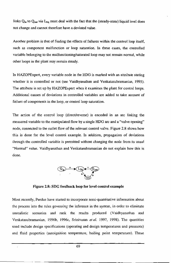
links Qin to QOUI via Ltiq must deal with the fact that the (steady-state) liquid level does
not change and cannot therefore have a deviated value.
Another problem is that of finding the effects of failures within the control loop itself,
such as component malfunction or loop saturation. In these cases, the controlled
variable belonging to the malfunctioning/saturated loop may not remain nonnal, while
other loops in the plant may remain steady.
In HAZOPExpert, every variable node in the HDG is marked with an attribute stating
whether it is controlled or not (see Vaidhyanathan and Venkatasubramanian, 1995).
The attribute is set up by HAZOPExpert when it examines the plant for control loops.
Additional causes of deviations in controlled variables are added to take account of
failure of components in the loop, or control loop saturation.
The action of the control loop (direct/reverse) is encoded in an arc linking the
measured variable to the manipulated flow by a single HDG arc and a "valve opening"
node, connected to the outlet flow of the relevant control valve. Figure 2.8 shows how
this is done for the level control example. In addition, propagation of deviations
through the controlled variable is pennitted without changing the node from its usual
"Normal" value. Vaidhyanathan and Venkatasubramanian do not explain how this is
done.
Figure 2.8: SnG feedback loop for level control example
Most recently, Purdue have started to incorporate semi-quantitative information about
the process into the rules governing the inference in the system, in order to eliminate
unrealistic scenarios and rank the results produced (Vaidhyanathan and
Venkatasubramanian, 1996b, I 996c, Srinivasan et at. 1997, 1998). The quantities
used include design specifications (operating and design temperatures and pressures)
and fluid properties (autoignition temperature, boiling point temperature). These
69
properties are integrated into the HDG model of the process and are used to make
order of magnitude estimates of whether identified hazards are likely to occur. If loss
of containment is identified, for instance, the operating temperature of the unit is
compared to the (ambient pressure) boiling point of the fluid (both are stored as single
fields in the frame data for the unit). If this temperature is exceeded by a certain
(fixed) margin, then the hazard of flashing release is indicated. There is also some
order of magnitude reasoning in the treatment of qualitative ambiguity in equipment
involving flow splits, based on the relative sizes of the normal flows through the
branches of the tee piece.
The work presented by Srinivasan et al. (1997 and 1998) uses a quantitative method
developed by one of the authors, Dimitriadis, (including "mixed integer linear
programme optimisation") to evaluate a small number of chosen scenarios for
credibility. The example, given relate to evaluating the time required to overfill a
surge drum or the base of a stripping column, based on the mass balance and likely
flowrates into or out of these equipment. By considering the time taken for a fault to
cause a problem, the importance of the scenario can be evaluated and problems of low
importance can be screened out. Additionally, this sort of method may reduce the
number of ambiguous predictions made by the system.
It is interesting to note that, in all their work on model-based HAZOP emulation,
Purdue view the situation as one where process generic (model based) knowledge
interacts with process specific knowledge. The view at Loughborough has usually
been that unit models are instantiated by being used in a plant description, so that the
plant model used for simulation is an essentially separate entity from the equipment
models, which are kept in a library. Another difference is that, while we at
Loughborough have organised equipment models into a hierarchy of types, placing
similar models close together in the tree, Purdue have not made so much use of this
sort of structure with the smaller number of models they have developed.
The whole approach to semi-quantitative reasoning in the Purdue papers is quite
simplistic and seems to be based on a small number of ad hoc rules about hazards. It is
questionable whether the reasoning methods used are sound enough to reject many of
70
the hazards they do reject. By use of just these simple rules, Purdue claim that they
halve the size of the results file for their case study plant.
Other work of interest at Purdue includes that of Srini vasan and Venkatasubramanian
(1996). They describe a combination of digraphs and Petri nets, used to model batch
processes, and to tackle the mixed continuous and discrete nature of such processes. A
batch process consists of a network of tasks comprising the product "recipe",
represented as a Petri net. The sequence of tasks need not be entirely linear, as some
tasks can be performed in separate equipment concurrently. Each task in the recipe
consists of a linear sequence of subtasks.
Within each subtask, the dependencies between variables are represented as a digraph,
with additional nodes for quantities such as "amount of masslheatltime". These nodes
are referred to as "integral quantities", because they generally change over time as the
subtask progresses. The digraphs for adjacent subtasks may be connected through
these nodes, allowing disturbances to be propagated through the different subtasks in
the task. The aim of this approach is to capture the different behaviours of equipment
items as their uses are changed throughout the batch.
2.3.2 Dow Benelux
The program developed by Dow is known as COMHAZOP (Rootsaert and
Harrington, 1992). It is a rule based expert system for HAZOP emulation which
produces RAZOP output tables and also makes recommendations for solving the
problems it finds.
From the limited information available, it is clear that Dow have recognised the
importance of separating the generic knowledge base of information on equipment
types, hazards and recommendations, from the description of the plant and its
configuration. This separation is analogous to the use, in AutoHAZID, of a library of
equipment models and a plant description file.
71

2.3.3 Loughborough
The Plant Engineering Group at Loughborough University has been working in safety
and fault propagation since the early 1970's. Applications of fault propagation
investigated during this time include alarm analysis, fault tree synthesis, on-line
process diagnosis and hazard identification (typically by emulation of HAZOP).
Andow and Lees (1974 and 1975) describe some early work on the design and
organisation of alarm systems. Human factors are often not considered sufficiently in
designing alarm annunciator panels or computer displays. In particular, if too many
alarms operate simultaneously when a process upset occurs, operators can be unable
to identify the true cause of the upset and take appropriate action. Andow and Lees
(1975) outline a program used to group process variables together into networks, so
that alarms can be assigned to the variables of most use in identifying the root cause
of an upset. In this work, cause and effect variables are related to one another using
qualitative "functional equations" (or "propagation equations"), similar to the
confluence equations described by De Kleer and Brown (1984).
Later, Lees (1984) considers on-line fault diagnosis and analysis of alarms. Two
approaches to automatic generation of data structures, suitable for producing fault
trees in response to alarm events, are considered. One uses the functional equations
and alarm networks of Andow and Lees (I975). The other uses mini-fault trees for
each process variable as components for on-line construction of fault trees. Included
are many ideas stilI used in fault propagation modelling, in terms of the pattern of
fault initiation followed by propagation of deviations and termination in significant
·final events. The problems recognised here are also still relevant to current work in
fault propagation modelline. Some of these- are:
• The problem of ambiguity in qualitative models.
• In fault trees, much useful information about the time ordering of events is lost.
Such information can help diagnose the causes of alarm sequences, particularly in
batch plant operation.
72

• Building models is laborious, so a library of reusable models is collected, and
methods for systematic conversion of models from one form to another are
investigated.
• Models containing just propagation are not much good. Some initiating faults and
final consequences must be present, to produce interesting results.
• AND logic is hard to model in mini-fault trees or functional equations.
• Fault propagation must go upstream as well as downstream.
• Instrument failures and control system failures complicate the analysis of
disturbances. Instrument reliability is a worry for the operator in interpreting plant
disturbances and instrument failure is a possible root cause of deviations on plant.
Fault tree synthesis has been a significant area of work at Loughborough in the past,
culminating in the development of the FAULTFlNDER program, described by Hunt
et at. (1993). Kelly and Lees (1986) built on some early work by Martin-Solis et at.
(1977), producing a fault tree synthesis system based on a component-based
equipment modelling system and fault propagation modelling. In a plant model,
several units (equipment items) are connected together. Each unit is described by a
model taken from a library of commonly used unit types.
Initiation of faults is represented by event statements, propagation of deviations by
propagation equations, and undesired consequences are modelled by event models.
Each unit model may contain any of these types of entities, as well as decision tables,
used for relationships which cannot be covered by the propagation equations, such as
AND logic. Fault tree construction proceeds by converting (automatically) all the
relevant parts of the unit models into mini-fault trees, which are then combined to
construct the fault tree for the chosen top event.
This fault tree synthesis system was further developed by Hunt et at. (1993). In
FAULTFINDER, decision tables for modelling AND logic were used far more,
particularly for problems like reverse flow, etc. Hunt also investigated automatic
construction of customised vessel models, where a small amount of information about
the inputs and outputs of a vessel is used to classify the connections between units
into one of a number of types. The connection type determines the flow and pressure
73
relationships appropriate for the associated ports. This work is of interest because a
tool was developed for creating new vessel models in the AutoHAZID system.
As an interesting alternative to unit modelling, Shafaghi et aL (1984) systematically
constructed fault trees based on the control loops in a process, by connecting together
sub-trees encapsulating the failure modes of loops. The aim is to produce better
structured fault trees which are easier to understand than those produced by a unit
modelling approach. However, automatic construction of the plant model may pose
significant problems for this method.
Hazard identification is the .problem tackled by Parrnar and Lees (I 987a). They
describe an early system which uses fault propagation to emulate HAZOP, by finding
causes and consequences for plausible deviations in the plant. The plant model is
decomposed quite coarsely into units which correspond to control loops, large items
such as storage tanks, etc. Propagation equations and event statements are used in
models, but are converted to a rule format for fault propagation. Consequence models
can be conditional on properties of process materials or materials of construction, and
there are models for each type of material in the system to support this. During fault
propagation, checks on these properties are used to search for "specific realisations"
of hazards in the plant. Parrnar and Lees see fault propagation as only one part of the
hazard identification solution and suggest that their system could be deployed as part
of a larger expert system for hazard identification.
In the case study described by Parrnar and Lees (1987b), which is the water separator
example also used by Law ley (\ 974), the authors show how their program can be used
to produce HAZOP-like results. The results are compared to those reported by
Law!cy. They also point out that their program is not able to consider consequences
which occur outside the line which the program is examining, meaning that forward
fault propagation is limited to components within the line under examination.
Zerkani and Rushton (1992 and 1993) present a hazard identification package for
HAZOP emulation developed in Poplog. It uses a unit model library in combination
with a plant description file to build a process model which is used in backwards
74
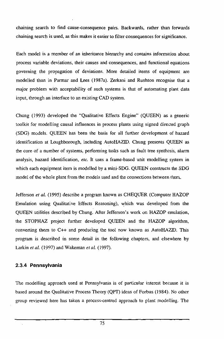
chaining search to find cause-consequence pairs. Backwards, rather than forwards
chaining search is used, as this makes it easier to filter consequences for significance.
Each model is a member of an inheritance hierarchy and contains information about
process variable deviations, their causes and consequences, and functional equations
governing the propagation of deviations. More detailed items of equipment are
modelled than in Parmar and Lees (l987a). Zerkani and Rushton recognise that a
major problem with acceptability of such systems is that of automating plant data
input, through an interface to an existing CAD system.
Chung (\ 993) developed the "Qualitative Effects Engine" (QUEEN) as a generic
tool kit for modelling causal influences in process plants using signed directed graph
(SOG) models. QUEEN has been the basis for all further development of hazard
identification at Loughborough, including AutoHAZID. Chung presents QUEEN as
the core of a number of systems, performing tasks such as fault tree synthesis, alarm
analysis, hazard identification, etc. It uses a frame-based unit modelling system in
which each equipment item is modelled by a mini-SOG. QUEEN constructs the SOG
model of the whole plant from the models used and the connections between them.
lefferson et at. (1995) describe a program known as CHEQUER (Computer HAZOP
Emulation using Qualitative Effects Reasoning), which was developed from the
QUEEN utilities described by Chung. After 1efferson's work on HAZOP emulation,
the STOPHAZ project further developed QUEEN and the HAZOP algorithm,
converting them to C++ and produCing the tool now known as AutoHAZID. This
program is described in some detail in the following chapters, and elsewhere by
Larkin et at. (\ 997) and Wakeman et at. (1997).
2.3.4 Pennsylvania
The modelling approach used at Pennsylvania is of particular interest because it is
based around the Qualitative Process Theory (QPT) ideas of Forbus (1984). No other
group reviewed here has taken a process-centred approach to plant modelling. The
75
authors claim that this approach avoids some of the difficulties in terms of
completeness and correctness encountered in component-based modelling?
As described by, for example, Catino et al. (1991), typical input is a structural model
of the plant, describing the objects in it. The model system includes the concept of
different "zones" in complex equipment, and a classification of equipment items into
"homogeneous" (i.e. well-mixed), "plug flow" and "stream pair". The structural
model is matched to models of processes and views stored in a library, to produce a
process-centred description of the plant. The process model can be used to compile a
set of constraints between qualitative variables, which are then used to determine the
state of the plant and its possible behaviours. The constraints generated can be
expressed either as SDG models or as QSIM constraint sets.
One major strength of the approach taken by Pennsylvania is that the process models
are produced automatically, so that they can be changed by the program at run-time
and therefore used to model the plant in various different states, rather than relying on
a single model of the "healthy" plant. This capability may give advantages in
diagnostic ability, but comes at the price of increased computational complexity, so
that the solution of anything other than trivial problems can be intractable.
The approach usually taken therefore, is to tackle small plant subsystems in detail and
to offer detailed explanations of faults, rather than attempting to model large plant
sections with many interconnected component units. The authors acknowledge that
the component-based modelling techniques investigated elsewhere are more suited to
the latter class of problem than their own method.
GraDlham and Ungar (1990) considerthe problem of fault diagnosis as that of finding
sets of assumptions in the plant model which give rise to discrepancies between
simulated behaviour and that of the plant itself. A generate and test method is used,
where heuristic knowledge is used to select additions or removals of processes from
2 It seems that this claim rests on the ability of the system to automatically rebuild constraint models
and to model state changes in the plant.
76

the model, to account for the observed differences. After the model is changed, the
process model is rebuilt automatically, its behaviour is simulated and compared to the
plant behaviour, to evaluate how successful the changes made are in explaining the
discrepancies observed. The methods used for comparison are discussed by Grantham
and Ungar (1991).
Complexity of qualitative simulations is a particular problem with the Pennsylvania
model system. Catino et al. (1991) discuss some techniques for focusing the
examination of simulation results on more interesting possibilities first. These
focusing techniques concentrate on reducing the number of variables in models,
limiting attention to only one vessel in the system, or adding further constraints to the
system to produce only steady state behaviours, for example.
The "Qualitative Hazard Identifier" (QHI), described by Catino and Ungar (1995),
exhaustively tests all possible instances in a plant of a small number of fault types.
The applicability of faults in this library is governed by a set of rules, which typically
dictate the appropriate equipment where the fault can occur. The consequences of
each specific fault are simulated to see if any hazards arise. The procedure is therefore
more similar to FMEA than to HAZOP.
The structural plant model used in QHI includes not only the equipment itt:ms present
and connections between them, but also fluids present and assumptions about the
operating conditions of equipment. The process-based model constructed from this
structural model is converted into QSIM constraints for simulating plant behaviour,
and the results of QSIM simulation are examined to identify resulting hazards.
Faults can either <::ause a perturhation in some variahle, or they can cause some of the
assumptions, upon which the current process-based model rests, to be changed. In the
former case, simulation of a single model will accurately predict the behaviour of the
system. However, if some assumptions have been changed, the process model must be
reconstructed, converted to QSIM and simulated, to determine the correct behaviour
of the plant.
77
Because of the frequent rebuilding of process models, computational complexity is a
big problem for QID. However, this approach does have a theoretical advantage over
less rigorous systems, in that it simulates fault propagation in a model of the process
which accurately describes the faulty condition.
Two simplifying assumptions are used by Catino and Ungar (1995) to reduce
problems with interpreting the results of QSIM simulations. The first is the "perfect
controller" assumption, where transients associated with controlled variables are
ignored, and control is considered to operate instantaneously. The second assumption
is the "pseudo-steady state" assumption, which ignores all transients in the plant, so
that the results of simulation show only transitions between steady states of the plant.
Despite the complexity and ambiguity problems, the fundamental modelling approach
by Catino and Ungar (1995) is sound. To get a workable system, however, it seems
likely that some compromises must be made in the modelling and simulation system.
Vinson and Ungar (1992 and 1995) concentrate on on-line process monitoring for
fault diagnosis. The "Qualitative Modelling and Interpretation" (QMI) system, takes
noisy plant data and interprets it in comparison to qualitative models of expected
process performance in different states. By finding the model which matches the
observed qualitative state of the plant, faults are diagnosed.
Qualitative models are prepared using off-line QSIM simulation and organised into a
tree of system states, each describing the qualitative value of all parameters in the
plant. Possible transitions between states correspond to the occurrence of a fault or its
development in the plant. Comparing the current state of the plant (extracted from
suitably conoitioned sensor data) with the states in thl! tree. the system can tell what
fault has occurred in the plant.
The Qmimic system, compared to QMI by Vinson and Ungar (1995), uses seml
quantitative information to rule out some predictions. It uses an updated version of the
QSIM simulator to handle the numerical information. An on-line, incremental
simulator updates thc simulation of the plant one step at a time. This simulation
78
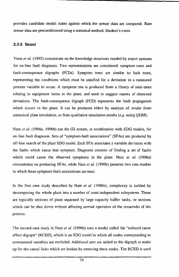
provides candidate model states against which the sensor data are compared. Raw
sensor data are preconditioned using a statistical method, Student's t-test.
2.3.5 Seoul
Yoon et al. (1992) concentrate on the knowledge structures needed by expert systems
for on-line fault diagnosis. Two representations are considered: symptom trees and
fault-consequence digraphs (FCDs). Symptom trees are similar to fault trees,
representing the conditions which must be satisfied for a deviation in a measured
process variable to occur. A symptom tree is produced from a library of mini-trees
relating to equipment items. in the plant, and used to suggest causes of observed
deviations. The fault-consequence digraph (FCD) represents the fault propagation
which occurs in the plant. It can be produced either by analysis of results from
numerical plant simulation, or from qualitative simulation results (e.g. using QSIM).
Nam et al. (I996a, 1996b) use the G2 system, in combination with SDG models, for
on-line fault diagnosis. Sets of "symptom-fault associations" (SFAs) are produced by
off-line search of the plant SDG model. Each SFA associates a variable deviation with
the faults which cause that symptom. Diagnosis consists of finding a set of faults
which could cause the observed symptoms in the plant. Nam et at. (\996a)
concentrates on producing SFAs, while Nam et at. (l996b) presents two case studies
in which these symptom-fault associations are useu.
In the first case study described by Nam et at. (I 996b), complexity is tackled by
decomposing the whole plant into a number of semi-independent subsystems. These
are typically sections of plant separated by large capacity buffer tanks, or sections
which can he shut down \'lithout affecting normal operation of the remainder of the
process.
The second case study in Nam et at. (l996b) uses a model called the "reduced cause
effect digraph" (RCED), which is an SDG model in which all nodes corresponding to
unmeasured variables are excluded. Additional arcs are added to the digraph to make
up for the causal links which are broken by removing these nodes. The ReED is used
79
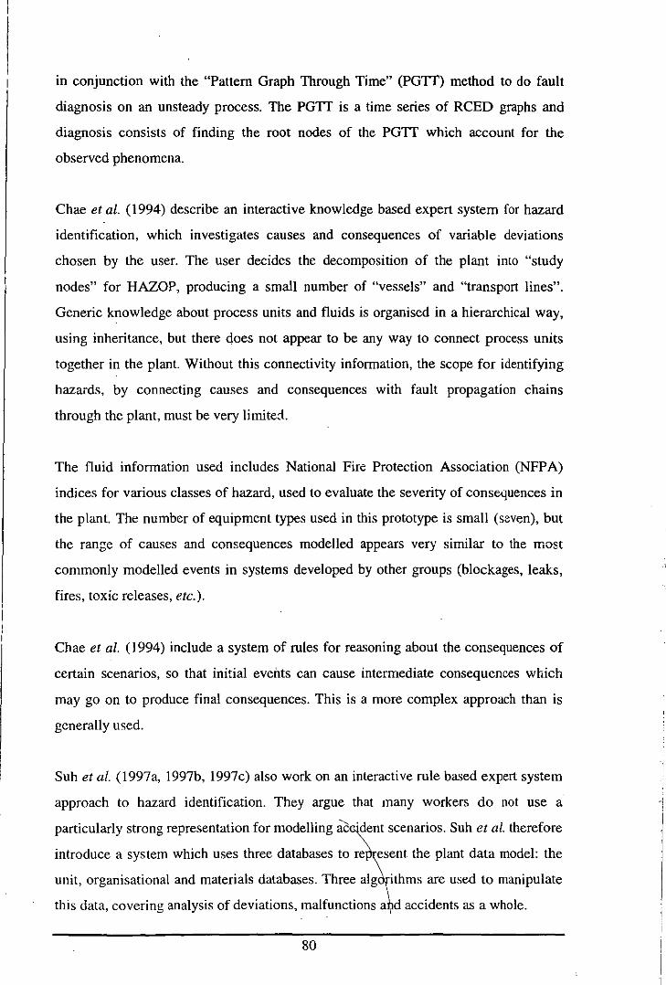
in conjunction with the "Pattern Graph Through Time" (PGTT) method to do fault
diagnosis on an unsteady process. The PGTT is a time series of RCED graphs and
diagnosis consists of finding the root nodes of the PGTT which account for the
observed phenomena.
Chae et al. (1994) describe an interactive knowledge based expert system for hazard
identification, which investigates causes and consequences of variable deviations
chosen by the user. The user decides the decomposition of the plant into "study
nodes" for HAZOP, producing a small number of "vessels" and "transport lines".
Generic knowledge about process units and fluids is organised in a hierarchical way,
using inheritance, but there does not appear to be any way to connect process units
together in the plant. Without this connectivity information, the scope for identifying
hazards, by connecting causes and consequences with fault propagation chains
through the plant, must be very limited.
The fluid information used includes National Fire Protection Association (NFPA)
indices for various classes of hazard, used to evaluate the severity of consequences in
the plant. The number of equipment types used in this prototype is small (seven), but
the range of causes and consequences modelled appears very similar to the most
commonly modelled events in systems developed by other groups (blockages, leaks,
fires, toxic releases, etc.).
Chae et at. (1994) include a system of rules for reasoning about the consequences of
certain scenarios, so that initial events can cause intermediate consequences which
may go on to produce final consequences. This is a more complex approach than is
generally used.
Suh et al. (l997a, 1997b, 1997c) also work on an interactive rule based expert system
approach to hazard identification. They argue that many workers do not use a
particularly strong representation for modelling ac~nt scenarios. Suh et al. therefore
introduce a system which uses three databases to re:\sent the plant data model: the
unit, organisational and materials databases. Three alg~ithms are used to manipulate
this data, covering analysis of deviations, malfunctions a~d accidents as a whole.
80
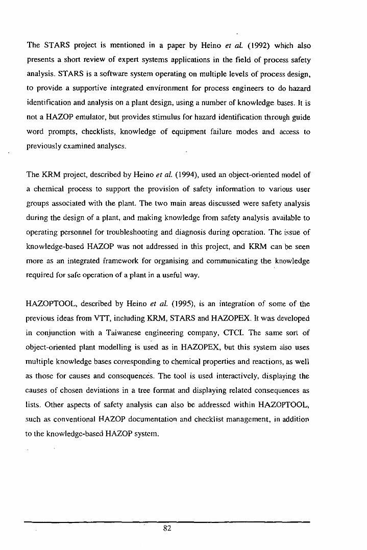
The STARS project is mentioned in a paper by Heino et al. (1992) which also
presents a short review of expert systems applications in the field of process safety
analysis. STARS is a software system operating on multiple levels of process design,
to provide a supportive integrated environment for process engineers to do hazard
identification and analysis on a plant design, using a number of knowledge bases. It is
not a HAZOP emulator, but provides stimulus for hazard identification through guide
word prompts, checklists, knowledge of equipment failure modes and access to
previously examined analyses.
The KRM project, described by Heino et al. (1994), used an object-oriented model of
a chemical process to support the provision of safety information to various user
groups associated with the plant. The two main areas discussed were safety analysis
during the design of a plant, and making knowledge from safety analysis available to
operating personnel for troubleshooting and diagnosis during operation. The issue of
knowledge-based HAZOP was not addressed in this project, and KRM can be seen
more as an integrated framework for organising and communicating the knowledge
required for safe operation of a plant in a useful way.
HAZOPTOOL, described by Heino et al. (1995), is an integration of some of the
previous ideas from VTT, including KRM, STARS and HAZOPEX. It was developed
in conjunction with a Taiwanese engineering company, CTCI. The same sort of
object-oriented plant modelling is used as in HAZOPEX, but this system also uses
mUltiple knowledge bases corresponding to chemical properties and reactions, as well
as those for causes and consequences. The tool is used interactively, displaying the
causes of chosen deviations in a tree format and displaying related consequences as
lists. Other aspects of safety analysis can also be addressed within HAZOPTOOL,
such as conventional RAZOP documentation and checklist management, in addition
to the knowledge-based HAZOP system.
82
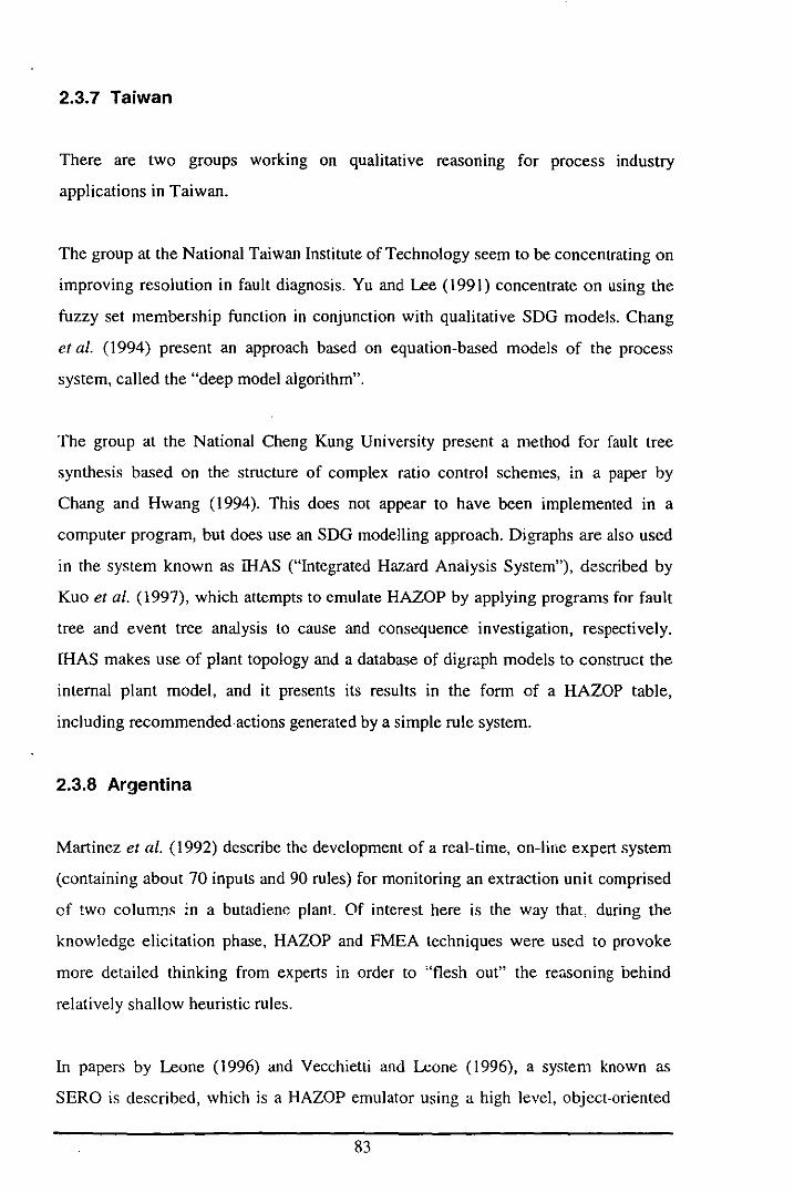
2.3.7 Taiwan
There are two groups working on qualitative reasoning for process industry
applications in Taiwan.
The group at the National Taiwan Institute of Technology seem to be concentrating on
improving resolution in fault diagnosis. Yu and Lee (1991) concentrate on using the
fuzzy set membership function in conjunction with qualitative SDG models. Chang
et al. (1994) present an approach based on equation-based models of the process
system, called the "deep model algorithm".
The group at the National Cheng Kung University present a method for fault tree
synthesis based on the structure of complex ratio control schemes, in a paper by
Chang and Hwang (1994). This does not appear to have been implemented in a
computer program, but does use an SDG modelling approach. Digraphs are also used
in the system known as IHAS ("Integrated Hazard Analysis System"), described by
Kuo et al. (1997), which attempts to emulate HAZOP by applying programs for fault
tree and event tree analysis to cause and consequence investigation, respectively.
IHAS makes use of plant topology and a database of digraph models to construct the
internal plant model, and it presents its results in the form of a HAZOP table,
including recommended actions generated by a simple rule system.
2.3.8 Argentina
Martinez et al. (1992) describe the development of a real-time, on-line expert system
(containing about 70 inputs and 90 rules) for monitoring an extraction unit comprised
ef two columns in a butadiene plant Of interest here is the way that. during the
knowledge elicitation phase, HAZOP and FMEA techniques were used to provoke
more detailed thinking from experts in order to "flesh out" the reasoning behind
relatively shallow heuristic rules.
In papers by Leone (1996) and Vecchietti and Leone (1996), a system known as
SERO is described, which is a HAZOP emulator using a high level, object·oriented
83

representation language to model fault propagation. SOGs represent influences
between variables and HAZOP emulation seems to rely on local fault propagation at
the interfaces between objects, using message passing. This "distributed" method can
be contrasted with the more common approach of compiling a plant SOG from a plant
model and then searching it using a global HAZOP algorithm.
2.3.9 Japan
There are a number of research groups working in Japan on problems related to
knowledge based safety analysis, fault diagnosis and control. Just two are mentioned
here: the group associated with Iri, 0' Shima and Matsuyama, and the group associated
with Shimada, Suzuki and Sayama.
In a frequently cited paper, Iri et al. (1979) describe the SOG-based modelling of
chemical processes for fault diagnosis. The state of the plant is seen as a pattern of
variable disturbances across the SOG model, and non-deviated variables are of no
interest. The problem of finding a cause for the observed deviations in the plant is
simplified by the assumption that there is only one root cause for the deviations, and
characterised as the search for a "maximal strongly connected" node in the graph.
lri et al. recognise the problem presented by controlled variables which may
themselves remain normal while propagating a deviated value to other variables
around them. The "trick" of using two extra qualitative values to represent controlled
variables which remain normal, but would be deviated in a certain direction if they
were not controlled, is introduced in this paper. Some improvements to the basic
algorithm presented by Iri et aI., in terms of enhanced diagnostic and computational
efficiency, are discussed by Shiozaki et al. (1985).
In work from another group, Shimada et al. (1993) describe a computer system which
uses information from fault tree analysis to build IF-THEN rules for use in a rule
based expert system for fault diagnosis. Later work by Shimada et al. (1996) moves
on to the operability study as an application, and the authors present a knowledge
based system in Prolog for performing a type of HAZOP study. This system contains
84
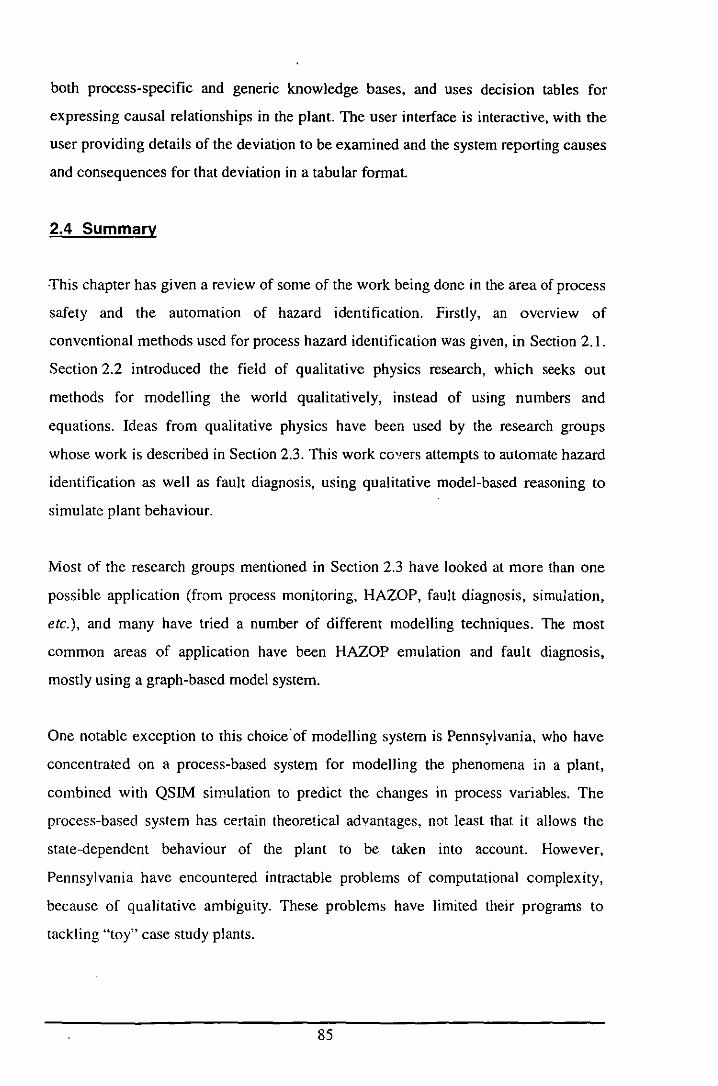
both process-specific and genenc knowledge bases, and uses decision tables for
expressing causal relationships in the plant. The user interface is interactive, with the
user providing details of the deviation to be examined and the system reporting causes
and consequences for that deviation in a tabu lar format.
2.4 Summary
This chapter has given a review of some of the work being done in the area of process
safety and the automation of hazard identification. Firstly, an overview of
conventional methods used for process hazard identification was given, in Section 2.1.
Section 2.2 introduced the field of qualitative physics research, which seeks out
methods for modelling the world qualitatively, instead of using numbers and
equations. Ideas from qualitative physics have been used by the research groups
whose work is described in Section 2.3. This work co"ers attempts to automate hazard
identification as well as fault diagnosis, using qualitative model-based reasoning to
simulate plant behaviour.
Most of the research groups mentioned in Section 2.3 have looked at more than one
possible application (from process monitoring, HAZOP, fault diagnosis, simulation,
etc.), and many have tried a number of different modelling techniques. The most
common areas of application have been HAZOP emulation and fault diagnosis,
mostly using a graph-based model system.
One notable exception to this choice 'of modelling system is Pennsylvania, who have
concentrated on a process-based system for modelling the phenomena in a plant,
combined with QSIM simulation to predict the changes in process variables. The
process-based system has certain theoretical advantages, not least that it allows the
state-dependent behaviour of the plant to be taken into account. However,
Pennsylvania have encountered intractable problems of computational complexity,
because of qualitative ambiguity. These problems have limited their programs to
tackling "toy" case study plants.
85
The HAZOPExpert program developed by Purdue aims to emulate HAZOP and uses a
SOO-based model system. In terms of development, it is the system closest to
Loughborough's AutoHAZID system (described later). It benefits from the graphical
user interface of the 02 expert system shell, which allows the same environment to be
used for developing SOO models and plant description P&IDs. However, the range of
equipment modelled does not appear to be as wide as that attempted in AutoHAZID,
and the HAZOP results presented in papers from Purdue suggest that they have not
attempted to model a very wide range of failure modes.
In common with Loughborough, Purdue have recognised that quantitative information
is needed to improve the focus of HAZOP results and reduce the number of spuriously
reported hazards. Their approach to the problem uses a linear programming method
based on a quantitative dynamic model of the relevant process units, and relies on
optimisation to determine whether scenarios predicted by SOO search are realistic
(Sriniv~san et aI., 1998). The fluid modelling system in AutoHAZID, as described in
Chapter 5, adds quantitative conditions to the SOO arcs in order to validate fault paths
found by graph search. It seems that the latter approach involves much less numerical
computation than the method used in HAZOPExpert, and so may be more efficient.
It is clear that no group has yet succeeded in developing a fully rigorous qualitative
treatment of process hazards. Problem areas include modelling the behaviour of plant
items in different states, dealing with the sometimes complex logic underlying
scenario development, and reasoning with sequences of events in time. There is no
reason why these problems should' not eventually be solved, once the somewhat
simpler problem of modelling continuous plant has been solved.
There remain quite a few methods mentioned ip. Section 2.1 which can be considered
for automation. One example is sneak analysis, which could be integrated into
AutoHAZID as a preliminary task - the plant model would be examined, before
HAZOP, looking for and reporting sources and destinations of sneak flows. Another
possibility is to add further models or rules to an existing hazard identifier system,
such as AutoHAZID, to cover computer HAZOP and/or human error analysis.
Management of the plant-specific safety data and generic expertise used in safety
86

assessment, is another important area. The work reported in Heino et a/. (1994),
which integrates diverse information resources for common access throughout an
organisation, is of particular interest here.
87
Chapter 3 : Description of AutoHAZID and its Qualitative Modelling System
The HAZID software package was developed for automated hazard identification as
part of the STOPHAZ project. Its central module is AutoHAZID, a program
developed mostly at Loughborough University, which coordinates the HAZOP
emulation that HAZID does.
This chapter first outlines the intended purpose and scope of the HAZID tool. Then
the modules of HAZID and the internal modules within AutoHAZID are described.
The main part of the chapter describes the qualitative modelling system used by
AutoHAZID in modelling plant behaviour. A methodology for model development is
described by reference to an example problem - that of modelling flow and pressure
propagation. Finally, some conclusions are drawn from the material covered.
3.1 Scope of the HAZID Packaae
It is intended that AutoHAZID emulate the hazard identification activities of HAZOP,
to save some of the time spent by conventional HAZOP teams. Qualitative simulation,
using SOG models, is used to find causes and consequences of variable deviations,
corresponding to characteristic failure modes of equipment and possible resulting
hazards on the plant. An option is also available, to identify items of equipment in the
plant (such as trips, alarms, etc.) which will protect against the identified hazards.
The range of things detected in conventional HAZOP studies depends on how much
previous scrutiny the plant design has been subjected to. Many problems are most
cost-effectively detected by simple use of checklists by a single engineer, but are often
found at the HAZOP stage. The best use of group time is made by considering
previously unexamined combinations of equipment failures and susceptibilities, using
the HAZOP guide word method to detect possible hazardous scenarios.
88

AutoHAZID does not attempt to deal with checklists of concerns relevant to single
items of equipment. It also does not seek to check the correctness of equipment
designs, except by detecting a small number of errors related to the configuration of
equipment. Instead, the approach used in AutoHAZID is to search for links between
faults and consequences in a qualitative model of the plant, by constructing fault
propagation chains. I
Some of the other scope limitations, applying to the type of HAZOP emulation
attempted by AutoHAZID program, are listed below:
• The usual emphasis is on predicting the behaviour of a continuous plant during
normal operation, where only single faults occur.
• As originally defined, HAZOP examines all deviations from intended operation,
which covers a quite wide variety of guide words and considerations. AutoHAZID
only addresses the hazards which can be modelled in terms of the effect they have
in causing deviations in process variables. To widen the scope, AutoHAZID
would have to model the design intent of equipment, as well as the influences
between variables.
• Time is not represented in the AutoHAZID models, except in so far as the causes
represented in SDO arcs must precede their consequences. It is therefore difficult
to reason about sequences of events (temporal ordering), duration and relative
speeds of changes, etc. An example of the type of problem here is where a leak of
fluid out of the process can result in a (later) leak of material into the plant.
• Transitions between states of equipment items, or of the plant as a whole, are not
modelled. Because AutoHAZID uses only one SDO model for each equipment
item, any serious attempt to model batch or semi-batch processes in detail, is
limited. AutoHAZID allows models to be instantiated in particular states, by "sub
typing" them, but does not allow the state to change during analysis. Specifically,
1 The creation of an environment for integrating and systematically applying software components for hazard identification and risk assessment would be a worthwhile project, but was not an objective of STOPHAZ. The AutoHAZID plant models contain the information needed, but the necessary number of rules and checks is too large to make a system like AutoHAZID practical for this sort of application.
89
AutoHAZID does not model changes in the behaviour of equipment items when
those items have failed.
• Complex fault trees or event trees, involving logic and (potentially) probabilities
cannot be directly modelled in the SDG-based system. This is usually not a
problem for hazard identification, where enabling conditions for faults can be
assumed to be satisfied. Complex logic is more closely associated with risk
assessment than with hazard identification.
Some of the above limitations are further discussed in Chapter 6, where possible
future improvements to AutoHAZID are considered.
3.2 Description of the HAZIO Software Package
HAZID was intended for delivery in a Windows 95 or Windows NT environment. A
UNIX version of the AutoHAZID program exists, but this is not able to take
advantage of the links to the other modules present in the Windows version.
The various HAZID modules are linked together as illustrated in Figure 3.1. The
modules were developed by a number of partners in STOPHAZ. This section explains
briefly the connections between the HAZID modules shown, as well as the internal
modules within AutoHAZID.
As shown in Figure 3.1, AutoHAZID has a parser, which allows it to read in data from
library files and plant description files. It also links to two other modules in the
STOPHAZ software package, the Database "Applications Programming Interface"
(API) and the Physical Property Calculation packages. These links are described in
Sections 3.2.1 and 3.2.2 below, and an overview of the information flows in HAZID is
shown in Figure 3.2.
90
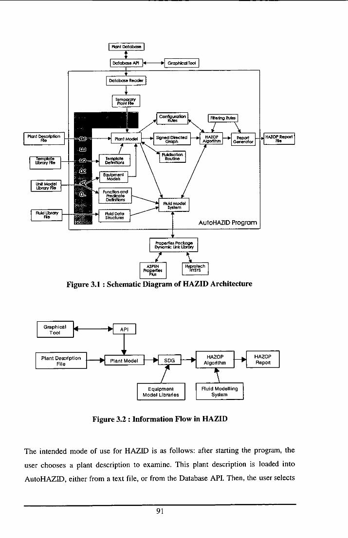
AutoHAZID Program
Figure 3.1 : Schematic Diagram of HAZID Architecture
Graphical Tool
Plant Des:::ription File
API
Plant Model
Figure 3.2 : Information Flow in HAZID
The intended mode of use for HAZID is as follows: after starting the program, the
user chooses a plant description to examine. This plant description is loaded into
AutoHAZID, either from a text file, or from the Database API. Then, the user selects
91
filtering options for HAZOP and initiates the HAZOP emulation stage, which
executes without further user intervention. Output is produced in an ASCII text file, in
tabular form, with columns for deviation, cause, consequence and (if selected)
protections, for each hazardous scenario identified. The start-up procedure and various
menu options available in AutoHAZID are described in Appendix A, which also
includes (in Section A.8) a sample of the type of output report produced by HAZOP
emulation.
The units in AutoHAZID which are treated as potential protections against hazardous
scenarios are: alarms, indicators, relief valves (including emergency vent manholes),
check (non-return) valves and control valves. When the option to detect protections is
enabled during HAZOP, the program looks for any such equipment which respond to
the deviations in the fault paths identified by the program. It reports these protective
equipment items in the "protections" column of the HAZOP report table.
3.2.1 Plant Descriptions from Database API and Graphical Tool
Plant descriptions can be prepared in the form of graphical ELDs, using the HAZID
Graphical Tool (developed by TXT). This is an alternative to laboriously keying in a
text file containing the description of the plant.
The plant descriptions produced by the Graphical Tool are stored in a database.
Access to the database from the Graphical Tool is mediated by the library of functions
known as the Database API. The API was implemented by Intrasoft in the STOPHAZ
project. AutoHAZID has access to this API and can retrieve the plant descriptions
from the database using the same set of functions.
AutoHAZID first reads all information on a plant of interest, through the API. It then
writes a text file containing this information, in the same format as a keyed in plant
description. This file is read into AutoHAZID using the parser, to create an internal
plant representation. Using this approach allowed AutoHAZID to be developed
independently, in a text-based UNIX environment, before the other components of
92
HAZID were available. It also allowed the links to the API to be tested by examining
the text files generated.
3.2.2 Physical Properties Calculations
The Fluid Modelling System (FMS) makes use of physical properties of the fluids in
the plant, as described in Chapter 5. These properties can be accessed by look-up in
the fluid model library, or estimated by calls to external software packages. The two
packages considered in the STOPHAZ project were Properties Plus, developed by
Aspentech, and HYSYS, developed by Hyprotech. Both are based on the technology
of flowsheet simulators and the property estimation methods used in them.
A library of functions and data structures was defined to implement the property
requests interface as a Windows "dynamic link library" (DLL). The library is common
to the FMS and the external properties packages, and it allows AutoHAZID to make
use of whichever software package is available. The link to a chosen properties
package is made when AutoHAZID starts up.
3.2.3 Internal Organisation of AutoHAZID
The constituent parts of AutoHAZID, shown in the shaded areas of Figure 3.1, are:
• Parser - AutoHAZID reads most of its input data through a parser. The parser
module reads characters from a text file and interprets them to generate the
internal models used in the program.
• Database Reader and Temporary Plant File - The method for reading in plant
descriptions from the Database API was described in Section 3.2.1. The database
reader is the part of AutoHAZID which does this.
• Plant Model - This is the internal model of the plant, composed of a list of
instances of equipment models. It is constructed from data read in from external
plant descriptions, from the Equipment Models and from Template Definitions
used in the plant. The plant model is the starting point for constructing the Signed
Directed Graph of the plant, used in HAZOP emulation. The Configuration
93
Rules (for detecting plant design errors) and the Fluidisation Routine (for
propagating fluid information through the plant) both also make use of the
information in the internal plant model.
• (Internal) Equipment Models - These are the frame models, defining the types
of equipment used in plant descriptions. The models are read in from a library file
when the program starts.
• Template Definitions - Templates are commonly used groups of SDG arcs which
can be used within an equipment model, as described in Section 3.4. When the
program starts, all template definitions are read in through the parser.
• Functions and Predicates, Fluid Data Structures and the Fluid Modelling
System - The FMS influences the results of the HAZOP algorithm by applying
conditions to check the validity of fault paths produced by graph search. The
conditions are defined by functions and predicates, and make use of fluid
information from the plant description, the fluid library and properties packages.
• HAZOP Algorithm - This module coordinates the graph search which forms the
core of HAZOP emulation in AutoHAZID. An exhaustive two-stage breadth-first
search algorithm is used, as described in Appendix B. This search produces a
record of deviations, faults which cause them and possible consequences of these
deviations and faults. The checks in the FMS can be used to improve the focus of
results, but AutoHAZID is not dependent on this link. The HAZOP algorithm also
initiates a number of extra checks on the configuration of plant items, using the
Configuration Rules. The results of these checks are integrated with the HAZOP
results, and provide a way of detecting elementary design flaws in the plant
description, as passed to AutoHAZID. The configuration rules are complementary
to the fault propagation approach, permitting the identification of faults which are
not easily identified by fault propagation.
• Report Generator - This part of the program takes the results of exhaustive
search, as produced by the HAZOP algorithm, and formats them in an appropriate
order, eliminating duplicated results as necessary. It produces a formatted text file
containing the results of the HAZOP study.
94
• Filtering Rules - These influence the HAZOP algorithm and the report generator
by controlling the amount of repetition in reports, by dictating the scope of the
HAZOP and by defining the order in which deviations are considered.
3.2.4 HAZOP Output Formats
The main output from HAZOP emulation in AutoHAZID is a text file containing two
or three sections. The first section is a header, giving details of files used, filtering
options selected and settings in use when the results were produced. The next section
is the main HAZOP results table, containing identified hazards in a tabular form. The
table has columns for deviations, causes, consequences and (if a search for protections
has been enabled) protections. The third part of the report is produced by the fluid
compatibility checker (see Section 5.2.8), and gives details of adverse fluid
interactions detected during HAZOP. This last section can only be produced in the
Windows version of AutoHAZID, when given a sufficient plant description.
One alternative, more structured, form of output has been implemented already - an
option to produce results in the format required by PrimaTech's "PHAWorks"
software package. Information on this package is available on the world-wide web, at
http://www.primatech.com/. Other types of structured output (as opposed to
simple text file formats) could be implemented with little difficulty, when a format
has been agreed.
3.3 Models in AutoHAZID
The most basic, qualitative SDG models in AutoHAZID use no information about
numerical quantities in a plant, and no numerical calculations. Influences between
process variables are modelled by SDG arcs and hazardous scenarios are identified by
finding fault propagation chains, by which consequences may result from initial
failures.
The real chemical plant can be seen as a collection of equipment items, connected by
streams carrying fluids between them. Most of the individual items in the plant are
95
taken from a small set of commonly used equipment types, such as valves, pumps,
vessels or pipes. This makes the task of process design much easier and cheaper
because standard components are mass-produced and are better understood than
customised, one-off items.
Because of this process design method, a component -based modelling approach is
used in AutoHAZID for plant representation. Each piece of equipment in the plant is
modelled as an instance of an equipment model, taken from a library of process
equipment types. The SDG model of the plant is constructed from the SDG models of
the units in it and links are added to model the propagation of deviations, via streams,
to other units. The simplest plant description therefore consists of a list of equipment
instances and their interconnections.
Using models for types of equipment in this way is economical in terms of the amount
of information required by the program for assessing each plant. Once an equipment
model is present in the library, it can be used in a large number of plants, or indeed
many times within the same plant. It should be noted, however, that this modelling
approach makes the implicit assumption that most interesting causal influences (from
the point of view of identifying hazards) propagate via variable deviations in streams
between units. This assumption is challenged in the case of non-process propagation
of faults, which is discussed in Section 6.6.
The decomposition of the plant model is carried one step further for template models,
which group together commonly used groups of arcs to model parts of equipment
models. Templates are described in Section 3.4.
The failure modes of equipment are modelled in AutoHAZID by including faults and
consequences in the SDG models, associating them with deviations of process
variables. The elicitation from human experts of the knowledge upon which these
failure modes are based, is a very important part of the model development process.
Every variable in the plant model is associated with a port located in some unit in the
plant. As an example, the discharge pressure for a pump, plOl, would be referred to
96

as [plOl, out, pressure], where out indicates the discharge port. In the library
model of the pump, from which plOl is derived, the same variable would be referred
to as [out, pressure] , because the unit name is unknown within the model.
Ports are required for locating variables and for connecting equipment items together
in the plant, so that deviations in process variables can be propagated to other units.
The process ports are of three types: input ports are locations where fluid may flow
into the equipment, output ports are locations where fluid may flow out, and internal
ports are internal locations not directly connected to other units at all. Only input ports
and output ports are used for connecting process equipment items.
When a plant description is loaded, in the form of a number of "instances" of
equipment models, the connections specified are translated into SOG arcs connecting
the units. The SOG arcs belonging to the units themselves are "instantiated" by adding
information about the units to which they belong (unit names and specified attributes).
The resulting complete set of arcs is the SOG model of the whole plant, and this is
used to simulate the plant'S behaviour during HAZOP emulation.
Arcs corresponding to propagation of effects between units allow some deviations to
propagate downstream (in the direction of intended flow), some to propagate upstream
(against the direction of flow), and some to propagate in both directions. Deviations in
some variables, such as level, are not defined in relation to inlet or outlet ports and are
not propagated at all between units.
The remaining subsections of Section 3.3 discuss various aspects of the AutoHAZID
system as follows:
• The minimum data requirements for generating the plant model are outlined In
Section 3.3.1.
• Section 3.3.2 describes the SOG in AutoHAZID in some detail.
• The frame-based system of equipment models, which allows inheritance and a
hierarchical arrangement of equipment models, is described in Section 3.3.3. The
instantiation of those equipment models, in plant descriptions, is also discussed.
97
• The hierarchy of models in the equipment model library IS introduced In
Section 3.3.4.
• The slots which make up the majority of the information given in the models in
AutoHAZID, and the mechanism of inheritance operating between models in the
model hierarchy, are described together in Section 3.3.5.
• Section 3.3.6 describes the system which allows the basic, generic equipment
models to be specialised, based on the values of attributes specified for the
equipment item. This is the "attribute conditional model" system.
• Customised models of vessels can be generated in HAZID using the Model
Generation Tool (MGT), which is briefly described in Section 3.3.7.
• AutoHAZID allows consequences to be classified in terms of severity, whether the
event is a hazard or operability problem,· and in terms of a number of standard
consequence types. This part of the modelling system is mentioned in
Section 3.3.8.
3.3.1 Data Requirements for the Plant Model
The minimum plant specification is just a statement of the equipment items present,
their types and the connections between them. This corresponds roughly to the
minimum information provided on an ELD and to the basic information required in a
HAZOP study. It is surprising how much useful work can be done by AutoHAZID
(and by HAZOP teams!) using just this basic information.
Additional information which may be presented In a real-life plant description
includes:
• General description of the process and its chemistry.
• Fluid components present, and percentage compositions, throughout the plant.
• Fluid flowrates, temperatures and pressures.
• Physical properties of process materials.
• Materials of construction.
• Operating modes of equipment items.
98

• Design temperatures and pressures (permitted maximum and minimum values).
• Operating instructions for the plant.
This additional information is not vital to making some progress in hazard
identification. However, if the additional information is present, less time will be
wasted on unnecessary consideration of scenarios, so that the results of the analysis
will be more specific and relevant. Some, but not all, of these classes of information
are used by AutoHAZID in HAZOP emulation and are therefore (optionally) present
in the plant model.
3.3.2 Signed Directed Graph (SDG)
Nodes in the AutoHAZID SDG represent variables in the plant model which can, in
principle, have qualitative values of "+" and "_". The values correspond to deviations
in the variable equivalent to applying the HAZOP guide words "more" and "less",
respectively. Arcs in the SDG represent direct or reverse influences of one variable on
another, according to whether the sign on the arc is "+" or "-", respectively. The arcs
are usually found listed in propLinks slots within equipment model frames in the
unit model library.
Fault propagation is modelled quite naturally using this representation of influences
between variable deviations. The local influence of deviations in one variable on its
neighbours in the graph models the propagation of disturbances. Paths through the
SDG represent potential fault propagation chains. The influence of one variable on a
distant one ("direct" or "reverse", represented as a "+" or "-,, sign) is the product of
the signs of all arcs along the path connecting the two variables, if such a path exists.
99

In addition to the nodes (corresponding to variables at particular places, or ports, in
the plant), three other types of entity are used to construct SDO arcs in AutoHAZID:
• faults represent initiating events which give rise to variable deviations in the unit
with which they are associated. Faults are declared as textual descriptors, which
are the strings reported in the "causes" column of the HAZOP output table.
• consequences are the hazardous final events which are to be linked, via some fault
propagation chain, to deviations of process variables and ultimately to faults at the
start of fault propagation chains. Consequences, like faults, are associated with a
particular equipment item in the plant and have a textual descriptor, which appears
in the HAZOP report when the hazard is reported.
• deviations are nodes with an associated HAZOP guide word ("less" or "more")
attached to them. They are only used to specify which deviation of a node gives
rise to a consequence in the plant.
In addition to the simple text of a descriptor and the name of an associated unit, faults
and consequences can (optionally) be linked to conditions for evaluation within the
fluid modelling system. The FMS is described in Chapter 5. Therefore, in the
discussion below the optional "Condition" part of the arc definitions is ignored.
Arcs in the SDO can take any of the following forms, as presented in the unit model
library of AutoHAZID, depending on their purpose:
• arc (Node, Sign, Node, Condition) These arcs represent propagation
of process variable deviations through the plant model.
• arc (Fault, Sign, Node, Condition) These arcs represent the
deviations caused by initial failures. The given node is deviated in the direction
indicated by the sign of the arc.
• arc(Deviation,l,Consequence,Condition)Arcs representing the
termination of the fault propagation chain have this form. The deviation given may
cause the consequence given.
100
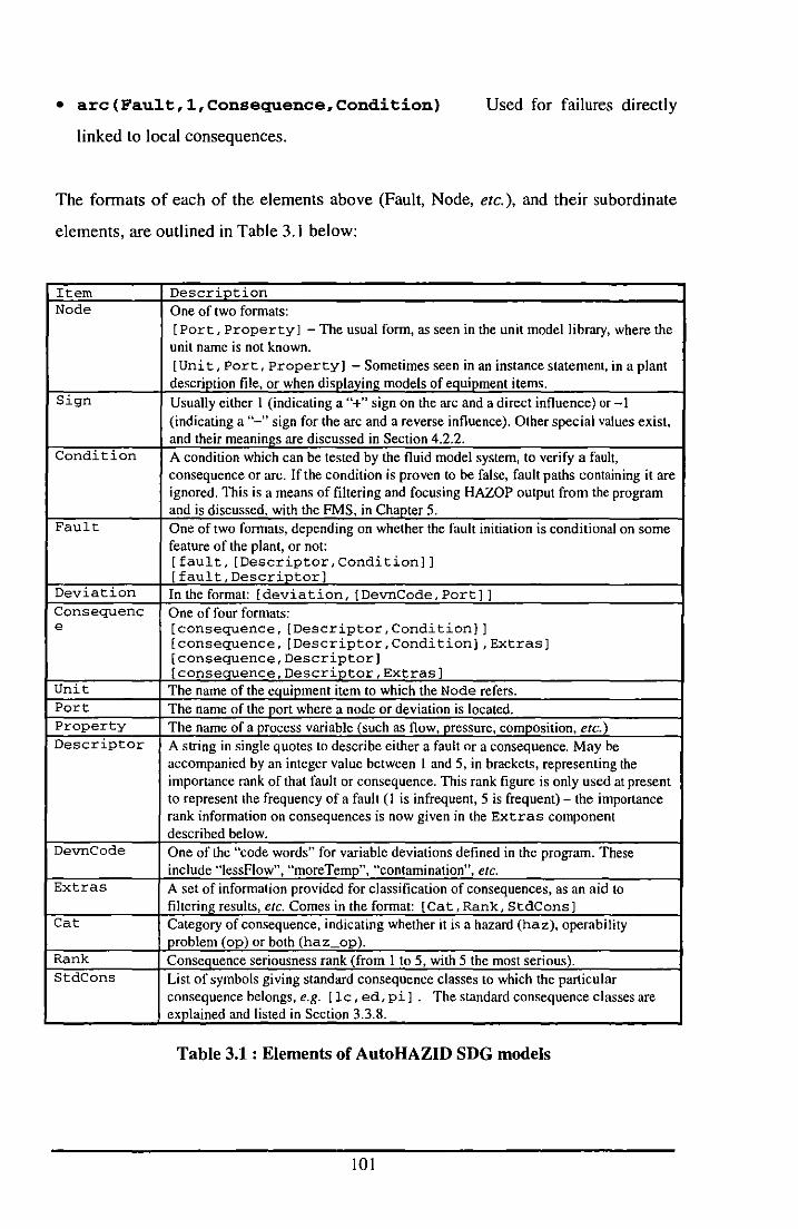
• arc(Fault,l,Consequence,Condition) Used for failures directly
linked to local consequences.
The fonnats of each of the elements above (Fault, Node, etc.), and their subordinate
elements, are outlined in Table 3.1 below:
Item Description Node One of two formats:
[Port, Property] - The usual form, as seen in the unit model library, where the unit name is not known. [Uni t I Port, Property] - Sometimes seen in an instance statement, in a plant description file, or when displaying models of equipment items.
Sign Usually either I (indicating a "+" sign on the arc and a direct influence) or-I (indicating a "-" sign for the arc and a reverse influence). Other special values exist, and their meanings are discussed in Section 4.2.2.
Condition A condition which can be tested by the fluid model system, to verify a fault, consequence or arc. If the condition is proven to be false, fault paths containing it are ignored. This is a means of filtering and focusing HAZOP output from the program and is discussed, with the FMS, in Chapter 5.
Fault One of two formats, depending on whether the fault initiation is conditional on some feature of the plant, or not: [fault, [Deseriptor,Condition]] [fault,Deseriptor]
Deviation In the format: [deviation, [DevnCode, Port]] Consequenc One of four formats: e [consequence, [Descriptor,Condition]]
[consequence, [Descriptor,Condition),Extras] (consequence, Descriptor] [eonsequenee, Deseriptor, Extras]
Unit The name of the equipment item to which the Node refers. Port The name of the port where a node or deviation is located. Property The name of a process variable (such as flow, pressure, composition, etc.) Descriptor A string in single quotes to describe either a fault or a consequence. May be
accompanied by an integer value between I and 5, in brackets, representing the importance rank of that fault or consequence. This rank figure is only used at present to represent the frequency of a fault (I is infrequent, 5 is frequent) - the importance rank information on consequences is now given in the Extras component described below.
DevnCode One of the "code words" for variable deviations defined in the program. These include "lessFlow", "moreTemp", "contamination", etc.
Extras A set of information provided for classification of consequences, as an aid to filtering results, etc. Comes in the format: [Cat, Rank, StdCons]
Cat Category of consequence, indicating whether it is a hazard (haz), operability problem (op) or both (haz op).
Rank Consequence seriousness rank (from 1 to 5, with 5 the most serious). StdCons List of symbols giving standard consequence classes to which the particular
consequence belongs, e.g. [le, ed, pi] . The standard consequence classes are explained and listed in Section 3.3.8.
Table 3.1 : Elements of AutoHAZID SDG models
101

3.3.3 Equipment Models - Frames and Instances
Generic equipment models in AutoHAZID are known as "frames", and their
realisations in plant models are referred to as "instances". Both are stored internally in
Frame objects. The frame models are loaded into AutoHAZID from a single library
file when the program starts. Instances are created by reading a plant description into
the program, through the parser. Each frame or instance possesses the following data:
• A name.
• A "parent name", which is the name of a frame from which it is derived. Frames
are arranged in an inheritance hierarchy, described in Section 3.3.4, which allows
closely related models to be placed together.
• A list of slots, which specify all the information comprising the equipment model.
These slots are more fully described in Section 3.3.5 below.
So, all .frames and instances must be defined in terms of another frame. The one
exception to this is the root of the hierarchy ("unit" in Figure 3.3 below), which has no
parent frame. Inheritance operates from parent frame to child frame within the
hierarchy, and from a frame to instances of that frame in a plant description. This
means that the slots (and slot values) of the parent are inherited by the child. The
inherited values may then be overwritten or supplemented by information given in
slots in the child. Details of how inheritance works are given in Section 3.3.5 below.
The information typically provided in frames is different to that provided in instances,
so that the slots used are different. Briefly, frame models specify the information
needed to define the SDG of the unit, including the ports in the unit, SDG arcs, default
values of attributes, etc. The information given for instances of equipment models is
related to connecting the unit to others in the plant via process port connections,
specifying fluids and their properties in the unit, and giving values to the attributes of
the unit.
102
3.3.4 Hierarchy of Equipment Models
Models in the unit model library are arranged into a hierarchy, in which the principles
of inheritance operate. Inheritance allows a model to be defined "by exception" from
its parent, so that a child frame is the same as its parent, except for specified
differences. A hierarchical organising structure helps to group together similar models
and to accentuate their similarity by modelling common behaviours of equipment at
the highest possible level. Instances of models at any level of the hierarchy can be
used in plant models. The current hierarchy of models is shown in Figure 3.3.
A number of guidelines were observed in organising the hierarchy. These include:
• The hierarchy must be intuitively sensible to an engineer, as an end-user. This
facilitates rapid and correct selection of an appropriate unit model.
• The lower levels of the hierarchy should correspond to more detailed specification
of equipment, the upper ones to more general equipment (e.g. a centrifugal pump
is defined as a type of a pump, and so appears below pump in the hierarchy).
• The designer should avoid unnecessary proliferation of models, by using attribute
conditional model sections, as described in Section 3.3.6.
• Future additions to the library should be anticipated where possible, and
appropriate space provided. If necessary, extra layers should be added, to deepen
the hierarchy. An example is the pressureRaiser model, which was created
as a common parent of the compressor and pump models, even before the
compressor model was added to the library.
New models should be placed in the hierarchy nearest to those equipment models to
which they are most closely related, functionally. The temptation to maximise the use
of the inheritance features of the system, and define models in terms of others which
have similar sets of arcs but which are otherwise unrelated, should be resisted.
103
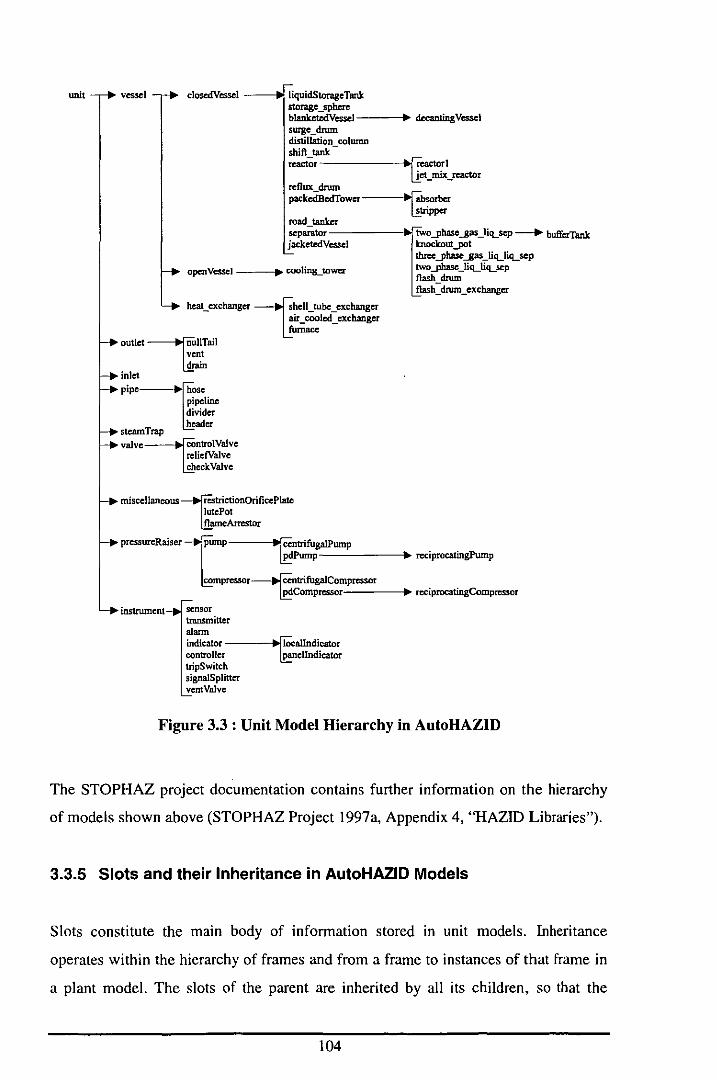
unit vessel
miscellaneous ~cstrictiOnOrificePlate lutePot flameArrestor
.. pressureRaiser lump IIIfCCntrifugalPump l!:..dPump ----'-----.... reciprocatingPump
compressor-t[centrifugalCompressor ~Compressor'----"" rcciprocatingCompressor
instrument sensor transmitter aiMlll indicator ---~ .. flOcallndicator controller ~cUndicator tripSwitch signalSplitter ventValvc
Figure 3.3 : Unit Model Hierarchy in AutoHAZID
The STOPHAZ project documentation contains further information on the hierarchy
of models shown above (STOPHAZ Project 1997a, Appendix 4, "HAZID Libraries").
3.3.5 Slots and their Inheritance in AutoHAZID Models
Slots constitute the mam body of information stored in unit models. Inheritance
operates within the hierarchy of frames and from a frame to instances of that frame in
a plant model. The slots of the parent are inherited by all its children, so that the
104

information provided in a child model is in the form of additions or replacements for
slots inherited from the parent frame.
Each slot has a name, a type and a list of values. The name of the slot does not have to
be unique within a frame or instance, but if there are multiple slots with the same
name, they will be reduced to a single slot at run time, giving preference to
information supplied later. This principle of slot value resolution applies to
inheritance between frames and instances, and to multiple slots within a single model.
The values in slots inherited from the parent are considered to be "earlier" than, and
therefore subject to overwriting by, the values in slots of the child.
Slots are of three types: "is", "info" and "include". The "is" slots specify simple
attributes of the model in terms of constant symbols (e.g. for a pump, we may have
status is running). The "info" type slots each specify a list of values. For "is"
and "info" slots, inheritance operates such that every slot which the parent frame has
is inherited to the child, but if the child has a slot with the same name, then the value
of the child slot overwrites the value inherited from the parent.
The third type of slot is the "include" type. This type of slot has a list of items as its
value, in the same way that the "info" slot does, but the "include" slot behaves
differently with respect to inheritance. If the child has an "include" slot for some slot
name, then provided the parent frame has no slot with that name, the "include" slot is
converted to an "info" slot with the same list of values. If the child has an "include"
slot for some slot name and there is an "info" slot with the same name in the parent
frame, then the value list of the "include" slot is added to the value list of the "info"
slot. The resulting list of values is put into the child as a new "info" slot, replacing the
"include" slot. This mechanism allows additive changes, possibly specialisations of
the SDG model, to be made to the information provided in the parent model.
Although info and include are implemented as different sUbtypes of slot, an
alternative view of the inheritance system is to consider them to be functional
modifiers of the slot. In this view, info and include determine how the value of
the appropriate slot is produced in inheritance.
105
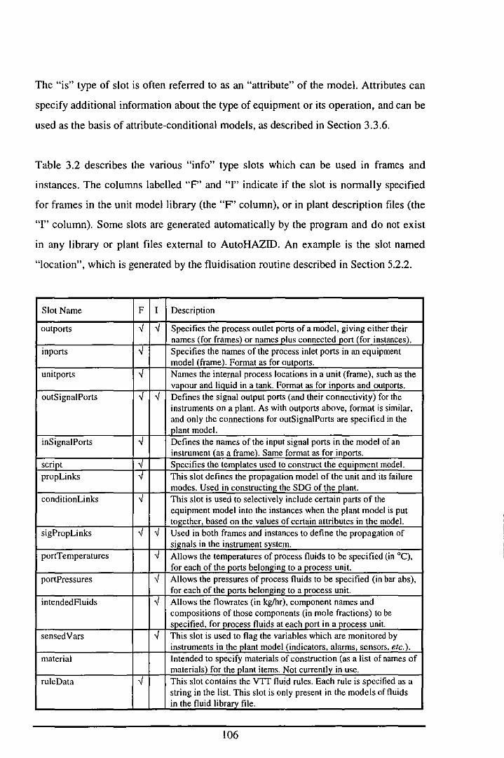
The "is" type of slot is often referred to as an "attribute" of the model. Attributes can
specify additional information about the type of equipment or its operation, and can be
used as the basis of attribute-conditional models, as described in Section 3.3.6.
Table 3.2 describes the various "info" type slots which can be used in frames and
instances. The columns labelled "F' and 'T' indicate if the slot is normally specified
for frames in the unit model library (the "F' column), or in plant description files (the
"I" column). Some slots are generated automatically by the program and do not exist
in any library or plant files external to AutoHAZID. An example is the slot named
"location", which is generated by the fluidisation routine described in Section 5.2.2.
Slot Name F I Description
outports V V Specifies the process outlet ports of a model, giving either their names (for frames) or names plus connected port (for instances).
inports V Specifies the names of the process inlet ports in an equipment model (frame). Fonnat as for outports.
unitports V Names the internal process locations in a unit (frame), such as the vapour and liquid in a tank. Format as for inports and outports.
outSignalPorts V V Defines the signal output ports (and their connectivity) for the instruments on a plant. As with outports above, format is similar. and only the connections for outSignalPorts are specified in the plant model.
inSignalPorts V Defines the names of the input signal ports in the model of an instrument (as a frame). Same format as for inports.
script V Specifies the templates used to construct the equipment model. propLinks V This slot defines the propagation model of the unit and its failure
modes. Used in constructing the SDO of the plant. conditionLinks V This slot is used to selectively include certain parts of the
equipment model into the instances when the plant model is put together, based on the values of certain attributes in the model.
sigPropLinks V V Used in both frames and instances to define the propagation of signals in the instrument system.
portTemperatures V Allows the temperatures of process fluids to be specified (in 0c), for each of the ports belonging to a process unit.
portPressures V Allows the pressures of process fluids to be specified (in bar abs), for each of the_ports belonging to a process unit.
intendedFluids V Allows the flowrates (in kglhr), component names and compositions of those components (in mole fractions) to be specified, for process fluids at each port in a process unit.
senscdVars V This slot is used to flag the variables which are monitored by instruments in the plant model (indicators, alarms, sensors, etc.).
material Intended to specify materials of construction (as a list of names of materials) for the plant items. Not currentk in use.
ruleData V This slot contains the VTT fluid rules. Each rule is specified as a string in the list. This slot is only present in the models of fluids in the fluid library file.
106

Slot Name F I Description
location Records data generated by the plant fluidisation routine, for fluids at various places in the plant model. Not specified in the plant or eauivment models.
<generalSlot> A type of slot defined in the parser so that any named info slot can be created without changing the parser. This is a relatively
(there is no slot with new development compared to the slots named in the previous this actual name) parts of this table. Note that there is no control over the internal
syntax of the items in the value list, so that anything which can be parsed will be accepted - the programmer must take care to check the data appropriately when it has been read into the program.
must_connect -J Defines the names of the process (inports and outports) ports which must be connected in the plant model. This slot is usually defined in the frame for the equipment model and checked against the actual instance found on plant. If ports are found in the instance which are not connected but should be, this is flagged as an error. This slot is an example of the <generalSlot> type shown above.
comp_connections -J Specifies the pairs of ports in the model of a unit which are connected together for the purposes of fluid propagation. This slot is an example of the <generalSlot> type shown above.
Table 3.2 : Slots in use in AutoHAZID
3.3.6 Attribute-Conditional Modelling System
When developing increasingly specialised equipment models in a hierarchical system,
such as the one outlined above, there is a danger that models proliferate to cover all
the possible combinations of optional features in similar equipment. An example is for
models of pipe, where the pipe may be lagged or unlagged, welded or flanged, etc. If
each possibility is addressed by a new model, many models are needed, one for each
combination of attribute values. The solution adopted in AutoHAZID is to add a
feature to the modelling system which allows sets of arcs and slots to be selected
depending on the value of certain attributes in instances of the equipment.
The condi tionLinks slot provides this feature. It allows generic models of
equipment to be specialised in a limited way, by specifying a number of pairings of
attribute and value, each associated with a list of slots to be added to the instance if
the value of the attribute matches that specified. The values of the attributes are
matched when an equipment model is instantiated in a plant.
107
The attribute-conditional parts of instances are processed after the plant model is
loaded and the values of slots are resolved from inheritance and from values supplied
by the instance itself. After the matching associated with the attribute-conditional
parts of the models, the slots in all instances are resolved again, to integrate any
information that has been added. Typically, an inc 1 ude slot is used to add new arcs
to the model if the attribute condition is met.
3.3.7 Custom Models and the Model Generation Tool
Most equipment items in a plant can be modelled with commonly used models in the
unit model library. However, some units may not correspond to models in the library.
These are often vessels, made to order as "one-off' items for a particular plant. In
these cases, a tool is needed to help the user of HAZID construct anew, customised,
model for the equipment item. This is the task addressed by the Model Generation
Tool (MGT) program, developed by Or. F.O. Larkin at Loughborough.
The MGT uses an interactive question and answer session to elucidate a structural
model of the new vessel from the user. The structural details include details of internal
chambers, their interconnections, fluids present, etc. Additional questions are used to
add details of equipment failure modes and consequences. The MGT uses the
information provided to construct an SOG model of the vessel, which can be added to
the unit model library for later use.
Templates (see Section 3.4) are used to model the different parts of the model, and the
content of the template library has been heavily influenced by the development of the
MGT. Numerous templates were defined to model different types of liquid and gas
inlets and outlets for vessels, interfaces between fluids, etc.
The MGT is described further in the "Model Generation Tool User Manual",
(STOPHAZ 1997b, Appendix 7). The software and its documentation were prepared
by Or. Larkin.
108
3.3.8 Consequence Types and Ranking
The consequences represented in AutoHAZID equipment models cover a broad range
of undesirable events, from minor inconveniences for plant operation to major
catastrophic events with the potential for loss of many lives. Therefore, a method for
focussing attention on the more important consequences is important in a system
which produces a large volume of results, as AutoHAZID frequently does.
For this reason, a consequence classification and ranking system was devised by Prof.
F.P. Lees and Or. FO. Larkin. Every consequence in the model library is associated
with three types of classification information, added to the model definition by the
model designer:
• A default2 severity rank in the range I to 5, indicating the scale of the event, where
I is least severe and 5 is most severe. The user may ask the program to screen out
consequences below a certain severity, when reporting HAZOP results. The
severity is reported next to the consequence descriptor in the HAZOP report and is
used to sort consequences so that the most important ones are reported first.
• A consequence class, which is a symbol defining whether the consequence is an
operability problem (op), a hazard (haz), or both (haz_op).
• A list of codes, each one taken from a list of standard consequence types, defining
how the given consequence is classified. The standard consequence types are
listed in Table 3.3 below. Every consequence should be a member of at least one
of these classes.
2 The rank given is a default because.! the severity of many consequences depends heavily on processspecific parameters, such as the fluids involved, which cannot be known to the generic unit model. For loss of containment, AutoHAZID can adjust the default severity according to particular process details (if those details are given) using methods from the Dow Chemical Exposure Index Guide.
109

Standard Consequence Categories Code personal iniury pi loss of containment le equipment damage ed operating problem op loss of outlet flow If contamination of outlet flow cf explosive mixture em unintended reaction ur vibration vb ignition source ig device malfunction dm
Table 3.3 : Standard Consequence Categories in AutoHAZID
3.4Templates and Scripts for Modellinq Parts of Equipment Items
The observation that equipment in a plant tends to be chosen from a small number of
types led to the structural decomposition of the plant model into a number of units,
each based on one of a limited set of models stored in a library. It is found that models
of equipment themselves possess an internal structure, midway between the level of a
unit and that of a single SDG arc. Moreover, the structural or functional components
of an equipment model are taken from a limited set of possible types (e.g. heat transfer
between two fluids, flow of a liquid into a vessel, etc.).
In AutoHAZID, these repeated structural or functional components are modelled using
"template models", whose definitions are read in from a library file when the program
starts. Each template is a group of arcs which are often found together, and can be
thought of as a model of a phenomenon or of a part of an equipment item.
Templates can be used to build up parts of equipment models anywhere in the unit
model library. However, since their context varies, some elements of the arcs (e.g. the
names of ports in the unit) must be varied also. Therefore, each template is associated
with a name, a list of arguments or parameters and a list of associated arcs. The
arguments of the template are variables, which also appear in the arcs listed.
110
When a template is used (in a script slot in a unit model), values are given to its
arguments. These values are substituted wherever they occur in the associated arc list,
before those arcs are added to the SDG model of the unit, as defined by other slots
(e.g. propLinks) elsewhere in the frame.
This approach to "sub-component" model decomposition is limited to the addition of
groups of arcs, typically using variable port names, as described above. However, the
use of a library of templates does reduce the effort required to make some types of
changes to models, significantly simplifying model maintenance.
3.5 Methodology for Model Development
This section builds on the description of the AutoHAZID modelling system offered in
Sections 3.3 and 3.4, giving some guidelines on how to apply the tools just described.
The objective is to allow for models to be developed in a disciplined and structured
way, so that a consistently high quality of model performance may be expected. This
method was not used for all models in the unit model library, due to time constraints.
The proposed methodology is described in this section, in relation to an example
which was examined in detail during the STOPHAZ project - that of modelling flow
and pressure propagation. Firstly, a system boundary for the flow and pressure
modelling case study is defined, in Section 3.5.1. Then, Section 3.5.2 discusses the
"no function in structure" principle and its application to the flow modelling problem.
The formalisation of the flow path model, in terms of the choice of variables in the
model, is addressed in Section 3.5.3. The idea of "causal hierarchy", outlined in
Section 3.5.4, was found useful in the flow path model, and may be of use elsewhere.
The flow path SDG model itself is presented in Section 3.5.5, along with the list of
assumptions which define this particular template model.
The conventions used to model no flow and reverse flow in AutoHAZID flow paths,
are described in Section 3.5.6. Finally, Section 3.5.7 finishes this section of the
chapter by describing the techniques used to discover weaknesses in the models of
AutoHAZID, and to direct their improvement. This topic is labelled as "Knowledge
II 1
Elicitation" because it consists partly of extracting knowledge from human experts,
and partly of formalising that knowledge in SDG models.
3.5.1 Flow Path System Definition
The case study problem for modelling is to "build a model of flow and pressure
propagation for chemical plants". A first model for flow cannot be expected to cover
all the potential complications of flow geometry, multiple phases, non-Newtonian
fluids, etc., so we concentrate on a limited, but commonly occurring, case. The system
to be studied first is the simple "flow path" - a path between an inlet and outlet
location, through which a fluid can flow. This system is typified by a rigid pipe or an
open valve filled with a single fluid.
The restriction assumptions, which define the system, are:
• The model deals with propagation of flow and pressure deviations in a "flow path".
Other phenomena, such as heat transfer, etc., must be modelled separately.
• The flow path is an unbranched space, filled with a single phase fluid and enclosed
by rigid walls, with one inlet location and one outlet location.
• The fluid may be liquid or vapour.
• Density changes in the fluid are not modelled, so that the fluid is assumed to be
incompressible, within the scope of the flow path model.
• The normal direction of fluid movement (flow) is from the inlet location to the
outlet location.
• No shaft work is done on the fluid within the flow path.
Known variations on the above assumptions include:
• Where the flow path is branched, so that it has either many inlets or many outlets.
These cases are represented by the header and divider models, respectively,
and discussed in Appendix C.
• Where heat transfer, or a phase change, occurs between the inlet and outlet.
112
• Where the fluid flows in an open channel, as opposed to an enclosed "pipe".
• Where shaft work is done on the fluid, or extracted from it, between inlet and
outlet.
3.5.2 The "No Function in Structure" Principle
The "no function in structure" principle, as given in De Kleer and Brown (1984),
states that: "The laws of the parts of a device may not presume the functioning of the
device as a whole". This means that the model of a device component (such as a unit
in a process plant) should be developed free of the context in which it will be placed.
In practice, this is an unattainable goal, not only because it is almost impossible to
imagine a component functioning completely free of context, but also because the
very act of decomposition presupposes the mode of interaction or connection between
pieces. Thus, one must at the very least state how components are connected together,
in order to construct a feasible model of a composite device.
The principle of locality follows naturally from the no function in structure principle.
It states that the components of a physical system can interact only with adjacent
components, to which they have a connection. The mode of connection between
components therefore determines how causes and effects may propagate.
Clearly, the no function in structure principle is particularly appropriate to unit-based
modelling systems, such as the AutoHAZID SDGs. If the principle is violated, the
models produced will be of limited use, and may produce erroneous results when used
in other plants or other contexts.
In AutoHAZID local causal input-output mappings, expressed as SDG arcs, define the
fault propagation functions of the components. Any influences propagated through the
model are mediated by deviations in variables present in the ports connecting units
together. Physical "adjacency" in this system is therefore defined by stream
connections between units. The overall behaviour of the plant model in simulation
results from the interaction of the devices in it. The only assumed context information
113
in this model is the mode of connection between units (using SDG arcs in the plant
model), and the variables used in those connections.
The no function in structure principle requires that a level of decomposition, a "basic
unit", be chosen for the phenomenon to be modelled. In the case of flow and pressure
modelling, this is the flow path, and communication with adjacent units is achieved by
propagation of pressure deviations.
3.5.3 Choice and Definition of Variables
To build a model of the fault path "basic unit", at least three things must be done:
• Choose a formalism for implementing the models. In this case, the choice has
already been made: it is the signed-directed graph (SDG) used in all AutoHAZID
equipment models.
• Decide which are the important variables in the problem area and characterise
them. Any restrictions imposed on the type of variable, by the choice of
implementation, should be considered. Also, the meanings of variables, as well as
issues of how and when they should be used, should be agreed by convention. For
flow path models, three variables were chosen:
• Pressure, P, is the pressure at a single point in the plant. The qualitative
values of this variable are lessPressure and morePressure, corresponding to
the HAZOP guide words. Pressure is an entirely local property of the fluid
present at a particular location in the plant.
• Flow, Q, is the variable chosen to represent the bulk flow of fluid from one
location to another in the plant. In a HAZOP study, four deviations are
commonly used to examine changes in flow (more flow, less flow, no flow and
reverse flow). The SDG does not permit variables with more than two
qualitative values, so flow has only two associated deviations (moreFlow and
lessFlow). The separate deviations noFlow and revFlow are modelled using
other variables (see Section 3.5.6 below). Note that flow is not modelled as a
property of a single location in the plant, but rather of the path between two
114

points. In that respect it is different from properties, such as pressure and
temperature, which can be stated uniquely for any single location.
• Flow Resistance, R, represents the frictional resistance to fluid flow which
exists between the inlet and outlet locations. Resistance has two qualitative
values corresponding to deviations (lessResistance and moreResistance), and
can be seen as a variable similar to flow in nature, because it is a "path
property" rather than a localised property.
• Once the variables have been decided upon, the next task is to link them to each
other in an appropriate way. The objective here may be to build a model
displaying some known set of behaviours (failure modes, perhaps), or to work
from first principles, guided by the assumptions made in the model scoping step.
3.5.4 Causal Hierarchy in Flow Modelling
Previous attempts to model fluid behaviour in process systems have often suffered
from difficulty in disengaging the effects of flow and pressure. Frequently, the
designer would worry about whether deviations in flow caused deviations in pressure,
or vice versa. The result could be a poorly explained model (possibly containing
circular influences between variables) in which the reasons for different parts, and the
action to take when the model failed to produce appropriate results, were unclear.
The practice of stating all known assumptions in a model as it is developed, should
help to clarify the influences involved, and prevent the occurrence of confusing
circular relationships in the model. In addition, a "causal hierarchy" is introduced
here, which is an arbitrary convention governing the allowed causal relations in SDG
arcs modelling flow.
The flow modelling causal hierarchy shown in Figure 3.4 states the "can influence"
relationships between variables. Deviations in resistance may cause deviations in
pressure or flow, pressure deviations may cause deviations in flow or pressure, but
flow may not cause deviations in pressure, resistance, or other flows. Outside the
scope of the flow path, flow may cause effects on other variables, such as the level of
liquid in a tank, temperatures in a heat exchanger, etc. Note that the causal hierarchy
115
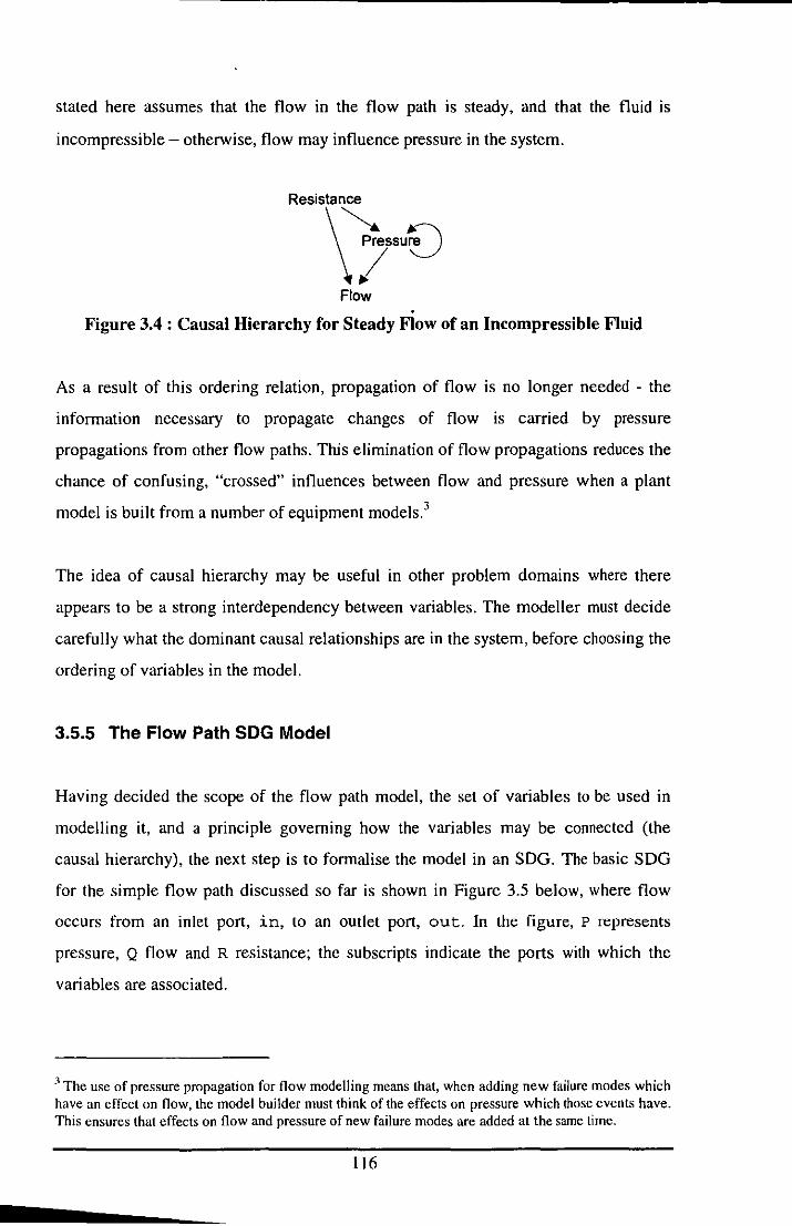
stated here assumes that the flow In the flow path is steady, and that the fluid is
incompressible - otherwise, flow may influence pressure in the system.
Resistance
\7§'8 Flow
Figure 3.4 : Causal Hierarchy for Steady Flow of an Incompressible Fluid
As a result of this ordering relation, propagation of flow is no longer needed - the
information necessary to propagate changes of flow is carried by pressure
propagations from other flow paths. This elimination of flow propagations reduces the
chance of confusing, "crossed" influences between flow and pressure when a plant
model is built from a number of equipment models.)
The idea of causal hierarchy may be useful in other problem domains where there
appears to be a strong interdependency between variables. The modeller must decide
carefully what the dominant causal relationships are in the system, before choosing the
ordering of variables in the model.
3.5.5 The Flow Path SDG Model
Having decided the scope of the flow path model, the set of variables to be used in
modelling it, and a principle governing how the variables may be connected (the
causal hierarchy), the next step is to formalise the model in an SDG. The basic SDG
for the simple flow path discussed so far is shown in Figure 3.5 below, where flow
occurs from an inlet port, in, to an outlet port, out. In the figure, P represents
pressure, Q flow and R resistance; the subscripts indicate the ports with which the
variables are associated.
J The use of pressure propagation for flow modelling means that, when adding new failure modes which have an effect on flow, the model builder must think of the effects on pressure which those events have. This ensures that effects on flow and pressure of new failure modes are added at the same time.
116
.----~
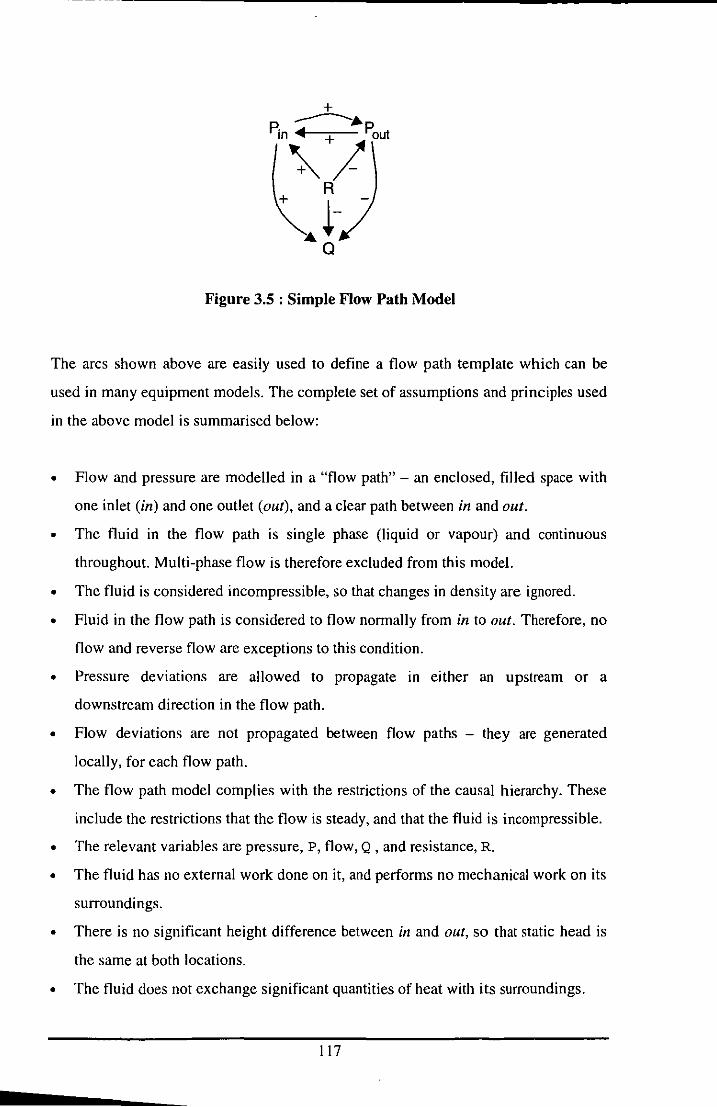
Figure 3.5 : Simple Flow Path Model
The arcs shown above are easily used to define a flow path template which can be
used in many equipment models. The complete set of assumptions and principles used
in the above model is summarised below:
o Flow and pressure are modelled in a "flow path" - an enclosed, filled space with
one inlet (in) and one outlet (out), and a clear path between in and out.
o The fluid in the flow path is single phase (liquid or vapour) and continuous
throughout. Multi-phase flow is therefore excluded from this model.
o The fluid is considered incompressible, so that changes in density are ignored.
o Fluid in the flow path is considered to flow normally from in to out. Therefore, no
flow and reverse flow are exceptions to this condition.
o Pressure deviations are allowed to propagate in either an upstream or a
downstream direction in the flow path.
o Flow deviations are not propagated between flow paths - they are generated
locally, for each flow path.
o The flow path model complies with the restrictions of the causal hierarchy. These
include the restrictions that the flow is steady, and that the fluid is incompressible.
o The relevant variables are pressure, P, flow, Q , and resistance, R.
o The fluid has no external work done on it, and performs no mechanical work on its
surroundings.
o There is no significant height difference between in and out, so that static head is
the same at both locations.
o The fluid does not exchange significant quantities of heat with its surroundings.
117

• Within the SDG model of the flow path, the shortest path between two nodes
determines the appropriate influence between those nodes. This "shortest path
heuristic" is used in all AutoHAZID models, and is discussed in Section 4.10.
• Friction has an effect on the flow in the flow path, and the amount of friction is
represented by the resistance, R. Partially blocking the flow path tends to restrict
the flow path, increasing R and therefore decreasing the flow, Q. The increase in
resistance also tends to increase the pressure upstream of the flow path and to
decrease it downstream.
• The driving force for flow in the path between in and out is the pressure difference
between the two locations, which is not represented explicitly. The upstream
pressure Pin has a direct effect on the flow and the downstream pressure Pout has a
reverse effect.
Wherever the above assumptions hold for a path between two locations in a piece of
equipment, the flow path model template is used to model the pressure and flow
propagation effects. A single equipment model may contain a number of flow paths
connected together, with each one declared in the scr ipt slot for the unit. The flow
paths in the plant model are linked together by a pressure propagation "back-bone",
which forms a communication path between remote units. This seems to be an
efficient method for constructing large models of process flow systems, as all flow
related propagation occurs via a single network of pressure deviations.
By varying the assumptions In the above list, one can tackle other pieces of
equipment. Dividers and headers ("tee" pieces) are exceptions to the single inlet,
single outlet assumption - they are addressed in Appendix C.
The deviations no flow (noFlow) and reverse flow (revFlow) challenge the
assumption, in the above flow path model, that fluid flows forward. These deviations
are qualitatively different from the cases of moreFlow and lessFlow, and the landmark
value of zero defines the domains of forward flow, no flow and reverse flow. The
problem of no flow and reverse flow modelling is dealt with in the following section.
118
3.5.6 Modelling No Flow and Reverse Flow
The approach used to model the deviations "no flow" and "reverse flow", in the
AutoHAZID SDG, is to use additional nodes to represent these deviations, separately
from the flow nodes already present in the SDG. The revFlow and noFlow nodes,
whose deviations are also called revFlow and noFlow, are used for this purpose. By
convention, these nodes have only one possible qualitative value, "+". A value of "-"
associated with these nodes has no meaning.
Two problems with this new scheme immediately present themselves. The first is that
of ensuring that the new nodes are never used during fault propagation in such a way
that they are associated with a value of "_". This is solved by adding checks to the
HAZOP algorithm which make sure that deviations encountered in all fault paths are
permitted ones. The second problem is one of model maintenance. New arcs must be
added to all models, so that noFlow and revFlow propagate through the plant model in
the same way that pressures propagate to cause the other deviations of flow. To a
certain extent, the use of templates can help with this problem.
The problem of four deviations for flow in HAZOP could have been sol ved in other
ways, possibly using a more powerful graph representation than the SDG. However,
the SDG was retained because it is efficient and because it is powerful enough to
represent most of the problems tackled in qualitative models for HAZOP emulation.
The deviations of noFlow and revFlow will now be considered separately.
No Flow
Flow can cease in a flow path because of two physically distinct causes. Firstly, the
pressure difference between in and out becomes zero due to some change in the
pressures. Secondly, the flow path may become completely blocked somehow, so that
the flow path no longer exists. This is an interesting distinction not explicitly made
clear in many descriptions of HAZOP.
119
The former case is not considered to be an example of the noFlow deviation in
AutoHAZID, but instead is an extreme case of the low Flow deviation. It is thought
likely that this form of zero flow is not distinct from the lowFlow condition in any
meaningful way, so that the lowFlow guide word should capture all the relevant
hazards in the HAZOP report.
The second cause of no flow is more important for hazard identification, and defines
the only case where noFlow takes place in AutoHAZID. Because some event has
caused the flow path to be blocked, the plant model has changed in some way, and
this may be an important consideration.
Therefore, noFlow may not be caused by pressure deviations in flow paths, but must
instead be caused directly by initiating faults, or propagated from other flow paths in
which such a fault has occurred. The information that a blockage event has occurred is
propagated through noFlow nodes in the SDG, upstream and downstream.
It is important to bear in mind the special meaning applied to the noFlow deviation,
when reading the results of HAZOP emulation, and when designing new models.
Reverse Flow
Reverse flow may be caused by a reversal of the pressure gradient in a flow path, for
example by leakage out of the path, leading to flow in the opposite sense to that
intended. However, the basic flow path modelling system in AutoHAZID, using only
pressure propagation, cannot represent the magnitude of a pressure change. This
means that it is difficult to judge whether a (qualitative) pressure deviation will cause
a decrease in flow, or a flow reversal.
In trials, problems occurred with flow path models which linked pressure directly to
revFlow. A typical problem was where a partial blockage in a line caused the pressure
at a point to change; the pressure deviation then propagated and caused a revFlow
deviation elsewhere in the line. It is absurd that a partial blockage could cause flow to
120
go backwards in the same line. This is an example where the pressure propagation
chain does not carry enough information on the magnitude of changes taking place.
Therefore, revFlow is propagated separately from pressure in AutoHAZID, in order to
preserve the information that a flow reversal has taken place. For the same reason,
pressure and reverse flow are not linked at every point in the flow path chains. The
working assumption is made that flow reversals are caused either by faults, such as
large-scale leakages from the flow path, by pressure changes in process vessels or in
tee pieces (dividers and headers). Ideally, points where revFlow is initiated should be
tested for the magnitude of change which can be considered to occur (perhaps such
tests will reveal that only lowFlow is possible in response to a particular change in
pressure). These sorts of numerical tests can be carried out by the fluid modelling
system, which is described in Chapter 5.
Taking the example of a pressure increase in a vessel causing a flow reversal in an
inlet to that vessel: pressure deviations will be propagated upstream, allowing
lowFlow and morePressure to be predicted anywhere in the inlet line. However,
revFlow will also be propagated upstream, along an independent propagation channel.
This arrangement allows all possible deviations to be predicted correctly, if the
magnitude of the pressure change is not known.
3.5.7 Knowledge Elicitation Methods
Once an adequate model of the links between variables in a unit has been developed,
perhaps from first principles, failure modes need to be added to the unit model.
Failure modes are very important parts of the model, and identifying them requires
expert knowledge of the equipment.
Knowledge elicitation was traditionally used in developing rule-based expert systems.
A "knowledge engineer" would talk to a "domain expert", to extract the most
important knowledge, rules, techniques, etc. from the expert. The knowledge engineer
was an expert in developing expert systems and the domain expert was someone who
knew a lot about the subject matter to be encapsulated in the expert system. This type
121

of knowledge elicitation can be very difficult, because often the expert does not use
knowledge in any explicitly formal way, but instead relies on rules of thumb, previous
experience, etc. to guide hislher judgement.
The knowledge elicitation techniques outlined in this section were used to stimulate
thought about the nature of equipment, the ways it could fail and the susceptibilities it
may have to various conditions. The "domain experts" in STOPHAZ were typically
safety and process engineering experts. The "knowledge engineers" were members of
the AutoHAZID development team. Many techniques are based around the group
"brainstorming" type of meeting, using guide words, as in the method study approach.
Equipment failure is often caused by taking a unit outside its safe operating regime.
Therefore, failure modes may be identified by systematically challenging the details of
the operating regime, using a "what if?" method. This is partly what the knowledge
elicitation techniques are designed to do. By identifying the underlying function of the
equipment, it may also be possible to identify "enabling faults" for some items (these
arc events not leading to immediate hazards, but which reduce the degree to which the
equipment is protected against the consequences of some other failure).
The following subsections cover the various techniques used to improve the accuracy
and range of phenomena modelled in AutoHAZID. Some require an organised group
meeting, and some are better carried out by a single model builder.
Trial and Error in Modelling
The usual means of evaluating library models was to test them out in case study plants
and examine the HAZOP results produced by AutoHAZID. By examining the
scenarios identified, an experienced model developer can quickly pin-point where an
error has been made in a model, where an inappropriate fault propagation path has
been produced, etc.
This job was usually done by a member of the Loughborough team, after changes to
the models, to verify improvement and to see that no unexpected side-effects
122
occurred. Output criticism was also used as a method of provoking comment from
safety experts, to get new ideas for improvements.
The test cases used during STOPHAZ are outlined in paper 7 of the series submitted
for publication in the IChemE Transactions on "Process Safety and Environmental
Protection" (McCoy et al.).
Conventional HAZOP Studies
The largest test case plant, analysed so far using AutoHAZID, is a benzene plant taken
from Wells (1980). This plant was subjected to a conventional HAZOP study by two
separate HAZOP teams early in the project, to provide a set of results for measuring
the success of automated HAZOP. These results have been valuable, in setting targets
for improvement during the project, though we cannot yet claim to identify 100% of
the results produced by the human HAZOP team in these meetings. A P&ID of the
plant, as annotated for the HAZOP study, is included as Figure 3.6.
123

:I";I!I: -I :
Figure 3.6: Benzene Plant Test Case (after Wells, 1980)· Annotated P&ID
124
Equipment Modelling Seminars
Several seminars were hosted by Loughborough, where experts from process-based
companies in the STOPHAZ consortium were assembled to look at single equipment
models. The objective was to encourage remarks about possible failure modes of
equipment and thereby elicit information for improving models.
These seminars were conducted as "mini-HAZOP" studies. A single equipment type
would be chosen for study by (typically) two experts and a member of the
Loughborough project team. The team would discuss the equipment item in a way
similar to that of a HAZOP meeting, but without considering any specific installation
of the equipment item (i.e. free of any particular plant context).
First, the purpose of the equipment was agreed and the scope of discussions fixed,
particularly in order to decide what not to discuss. A number of equipment ports were
then identified as study node locations to focus on. Following the HAZOP method,
deviations of variables at each study node were considered. The questions of how the
deviations could arise, and what consequences they could have locally, were asked.
In all these discussions, it was important to keep the team focussed on the equipment
at hand, while also encouraging them to imagine the item in a variety of plant
contexts. It was hoped that, if this could be achieved, the model which would be later
developed from the notes of the meeting would be as general as possible. The role of
the Loughborough team member was to take notes, and to encourage comments which
could be easily formulated in terms of rules or arcs in the SDG.
The minutes of these meetings were noted on sheets in a similar format to the HAZOP
report sheets typically used during conventional plant HAZOPs. However, this format
was very often insufficient to record all the notes which arose during the meeting,
because much of the knowledge gleaned from our experts turned out to be in terms of
different or more useful ways of looking at situations on the plant. An example is the
observation that reciprocating pumps can cause problems with flow measuring
devices installed downstream, because pulsations caused by the piston stroke cause
125
such instruments to read too high. This is an important problem which doesn't
obviously fit into the fault path model of hazards typical for AutoHAZID scenarios.
The modelling seminars produced material which it was sometimes difficult to
implement in AutoHAZID because of the format of the information, or because of the
limited stage of development of the program itself. Nevertheless, some of the
information obtained could be used to add new failure modes to the existing models,
and this has been achieved for a number of cases.
Criticism of Equipment Library Models
Another technique, similar to the modelling seminar approach in some ways, was for a
single safety expert to examine models in the equipment model library, and to criticise
them, pointing out what was right or wrong, what missing, etc. This was attempted in
at least two cases, with some success. However, to provide the most useful criticism,
the expert needed a quite deep understanding of fault propagation behaviour in plant
models, to see how the models were designed to work together. This presented a
barrier to effective use of the technique. Nevertheless, some useful pointers were
identified.
Although this method was used during STOPHAZ as an "off-line" study of models in
the library, it could be adapted so that AutoHAZID would construct a plant model
with a single instance of a model to be examined. Then, the user would examine the
inputs and outputs of the model in a systematic way, using AutoHAZID results. This
approach would also insulate the user from the internal detail of fault propagation.
Expert Criticism of HAZOP Results for Test Cases
At around the middle of the project, when AutoHAZID was substantially complete in
its simpler, basic form, a reasonably formal series of test case evaluations was carried
out. Critical input from the process expert partners in the consortium was sought, to
find out what the shortcomings of the system were.
126
Automated HAZOPs were performed on a series of plant models, of successively
more complex design, using AutoHAZID. The results were sent to the partners for
comment. Ideally, comments on one test case would have been used to improve the
performance of AutoHAZID before the next test case in the series, so that continual
improvement of the system could be demonstrated over a number of weeks. A number
of problems were identified and fixed quite quickly, but very often the solutions to the
problems involved larger pieces of work, on a longer timescale.
3.6 Conclusions
This chapter has described HAZID and AutoHAZID in some detail, covering the
architecture of the integrated HAZID system and the modelling system in
AutoHAZID. The models are based on the signed directed graph (SDG), and represent
the influences between physical variables, faults and consequences in a piece of plant
equipment. The chapter has described all the main features of this qualitative
modelling system, as well as stressing the importance of principled development of
new models, illustrating this by the example of the flow path model in AutoHAZID.
The component-based modelling approach to the plant model and the SDG includes
many useful ideas, such as inheritance, the use of template models and the flow path
approach to flow and pressure modelling. The chosen SDG modelling formalism has a
natural interpretation in the way it mimics the causal nature of simple fault
propagation chains. Luckily, it is also probably the most efficient way of doing the
sort of qualitative reasoning required for HAZOP emulation.
In order to manage a potentially quite large and diverse library of models, some form
of structured development procedure, in terms of knowledge elicitation,
implementation and documentation, should be adopted. This is particularly important
when developing novel unit models, as these often contain new assumptions and may
require modelling techniques not used elsewhere in the model libraries.
The AutoHAZID program now performs efficiently on large test case plants and, now
that the model library has been enriched by the knowledge and experience of a
127
number of process industry experts, the program produces increasingly valuable
HAZOP results. There are still many situations, however, where problems arise,
which it is difficult to address using the SDO model system described so far. Some of
these problems (and possible solutions to them) are discussed in Chapters 4 and 5.
128
Chapter 4 : Some Problems with Qualitative SDG-based Hazard Identification
This chapter discusses some of the problems encountered with HAZID as described in
Chapter 3. Many of these problems are shared with other systems based on a
qualitative modelling system, or which use a graph search model for inference. Some
of these problems have been tackled successfully - the approaches used to solve these
are also discussed here.
However, some of the recognised weaknesses of HAZID have not been tackled. Some
improvements were ruled out because they were, strictly speaking, "out of scope" for
HAZID (the scope of application for HAZID was discussed in Section 3.1). Other
problems were not dealt with because the effort required to do justice to them would
have diverted attention away from more important priorities in the project. It was
important during STOPHAZ, to keep the development of HAZID focussed on the core
objective: hazard identification by HAZOP emulation.
4.1 The SDG represents only two deviations
As discussed in Section 3.5.6, the mam case where there is a problem with the
limitation of two deviations per SDG node, is that of modelling flow deviations,
specifically "no flow" and "reverse flow". However, it is conceivable that other
variables, which require more than two deviations, may need to be modelled at some
stage.
For the four deviations of flow, the solution adopted is to allow pressure to propagate
through the plant, causing lessFlow and moreFlow deviations, while noFlow and
revFlow are propagated as separate variables in the SDG. Depending on the details of
the case, this approach may well be useful with other similar problems.
129
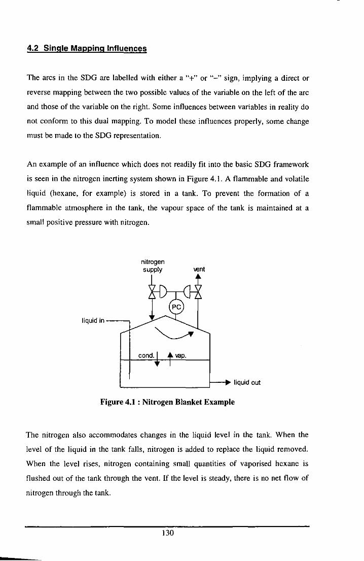
4.2 Single Mapping Influences
The arcs in the SDG are labelled with either a "+" or "-" sign, implying a direct or
reverse mapping between the two possible values of the variable on the left of the arc
and those of the variable on the right. Some influences between variables in reality do
not conform to this dual mapping. To model these influences properly, some change
must be made to the SDG representation.
An example of an influence which does not readily fit into the basic SDG framework
is seen in the nitrogen inerting system shown in Figure 4.1. A flammable and volatile
liquid (hexane, for example) is stored in a tank. To prevent the formation of a
flammable atmosphere in the tank, the vapour space of the tank is maintained at a
small positive pressure with nitrogen.
nitrogen supply \en!
liquid in ----,
cond. vap.
L _________ J-.. liquid out
Figure 4.1 : Nitrogen Blanket Example
The nitrogen also accommodates changes in the liquid level in the tank. When the
level of the liquid in the tank falls, nitrogen is added to replace the liquid removed.
When the level rises, nitrogen containing small quantities of vaporised hexane is
flushed out of the tank through the vent. If the level is steady, there is no net flow of
nitrogen through the tank.
130

If the control valve for the nitrogen vent fails open, the other one also opens in
response to the low pressure, so that nitrogen flows through the tank at a maximum
rate. In this situation, much more hexane vapour than usual is removed and an
evaporative cooling effect is observed - the liquid is cooled by the removal of the
vapour, and its temperature drops. However, the relationship between flow and
temperature does not work both ways. If the flow of nitrogen is low, no change in
temperature can be expected.
This phenomenon can be understood by considering that the hexane in the tank exists
in vapour and liquid form, and the vapour will tend to equilibrium with the liquid,
according to the equation:
Liquid + Heat <=} Vapour
When nitrogen flows through the tank, vapour is removed, driving the equilibrium to
produce more vapour (i.e. towards the right hand side of the above equation). In doing
this, heat is required to produce the vapour, and this is removed from the body of the
liquid, cooling the liquid that remains. When very little nitrogen flows through the
tank, the vapour-liquid system is close to equilibrium, so a negligible amount of heat
is produced or consumed.
A further example is the overheating problem that occurs if a running pump is not
able to discharge its usual quantity of process fluid. In normal operation, any heat
generated by the pump is carried away from it by a large volume of process fluid, so
that the increase in temperature of that fluid is negligible.
When the fluid in the pump cannot escape, however, all the energy supplied by the
pump (including much of that which would otherwise be transferred to the fluid as
work) goes into heating up a much smaller volume of fluid. In this case, the
temperature of the fluid can rise much higher, possibly causing a leakage or other
problem for the plant.
131
Here a relationship is established where low flow of fluid through the pump causes
high temperature in that fluid. High flow through the pump has no meaningful effect
on the fluid temperature, as an already negligible temperature rise is made even
smaller by the change.
This is another case where a balanced process is perturbed from its normal state,
although here the balance point is not strictly speaking an equilibrium, but rather a
steady state. It seems likely that wherever the "normal" state of a physical system is at
a balance or equilibrium point, as with the nitrogen blanket and pump examples, there
will be a problem with representing a single mapping influence within the SDG.
4.2.1 Use of Directed Graph instead of SDG
One approach which solves the problems of modelling single mapping influences
described in the examples above, is to use a directed graph representation, rather than
the signed directed graph, to model the plant. In this scheme, the nodes in the graph
represent deviations of process variables, rather than the process variables themselves.
Therefore, the digraph nodes do not have a range of qualitative values; they represent
single qualitative values which would otherwise belong to SDG nodes. A sign is not
needed on the arcs between nodes, since arcs in the digraph represent simple cause
effect links between deviations.
In converting SDG models to the digraph system, each SDG arc would translate
directly to two DG arcs, in most cases. Exceptions are arcs involving revFlow or
noFlow, which would translate to only one DG arc each. Within the DG, such
deviations would look far less out of place than they do in the SDG.
Representing other deviations, where no appropriate process variable relates to both a
"+" and a "-" value, would not be a problem for the DG representation. An example
of this is contamination, where moreContamination and lessContamination deviations
are inappropriate, and the only sensible deviation is contamination itself.
132

The single mapping influences in the examples above would be easily represented in
this scheme as highFlow ~ lowTemp, for the nitrogen blanket, or
lowFlow ~ highTemp, for the pump. It seems that all such cases, where only a single
mapping between deviations is required, can be dealt with using this digraph method.
In the DG, tracing fault propagation through the plant just consists of finding paths
between deviations - there is no need to take account of signs attached to the arcs
along the path. The presence of any path between deviations in the graph indicates a
causal link between them.
One problem with the digraph representation is that it would almost double the
number of arcs in any model of the plant. This mayor may not lead to problems with
computational complexity in search.
After some experimentation during the development of AutoHAZID, it was decided
not to proceed with a change to DG models. Apart from the upheaval of changing
every equipment model, and the risk associated with a new system, it was found that
moving to a digraph makes it more difficult to detect ambiguous predicted deviations
during search. Checking a set of paths for contradictory influences on a process
variable (e.g. lessFlow vs. moreFlow for the same flow) is more costly, as the
deviations no longer correspond to the same node in the graph. To get around this
problem would require an association between deviations of the same process variable
which would negate the benefits of the DG approach.
4.2.2 Extra Code Numbers for SDG Arcs
The SDG uses two labels for its arcs, usually shown in figures as "+" and "-", but
represented in AutoHAZID as two integer values, 1 and -1. These code values
represent dual mappings of input values to output values, where the input and output
values are both taken from the set {-,+}. To model single mappings between input
and output values, a minimum of four possible link types need to be defined.
133
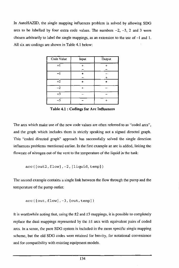
In AutoHAZID, the single mapping influences problem is solved by allowing SDG
arcs to be labelled by four extra code values. The numbers -2, -3, 2 and 3 were
chosen arbitrarily to label the single mappings, as an extension to the use of -I and I.
All six arc codings are shown in Table 4.1 below:
Code Value Input Output
+1 + + - -
-I + -- +
+2 + +
-2 + -
+3 - -
-3 - +
Table 4.1 : Codings for Arc Influences
The arcs which make use of the new code values are often referred to as "coded arcs",
and the graph which includes them is strictly speaking not a signed directed graph.
This "coded directed graph" approach has successfully solved the single direction
influences problems mentioned earlier. In the first example an arc is added, linking the
flowrate of nitrogen out of the vent to the temperature of the liquid in the tank:
arc( [out2, flow] ,-2, [liquid,temp])
The second example contains a single link between the flow through the pump and the
temperature of the pump outlet:
arc ( [out, flow] , -3, [out, temp] )
It is worthwhile noting that, using the ±2 and ±3 mappings, it is possible to completely
replace the dual mappings represented by the ±I arcs with equivalent pairs of coded
arcs. In a sense, the pure SDG system is included in the more specific single mapping
scheme, but the old SDG codes were retained for brevity, for notational convenience
and for compatibility with existing equipment models.
134
Taking this approach, the risk associated with the move to a new system is reduced.
Users can continue to use the existing SDa models, whilst deploying the new arcs in a
small number of places first, to demonstrate their usefulness before making any large
scale changes. This allows an overall policy of incremental upgrade, minimising
disruption to the users, model libraries and the AutoHAZID program code.
The system of coded arcs does not impose any great burden on the search algorithm,
as all that is required is a small amount of extra checking when paths are verified. If a
coded arc is found in a fault path, the input influence to the arc is determined, from
the initiating fault and subsequent arc codes, and checked to see that it has the value
("+" or "_") required by Table 4.1. If not, the path is rejected. This does not impose
any significant penalty in efficiency.
Note also that the extra codes for the arcs do not introduce any fundamentally new
concept to the SDa models. Arcs still represent influences between variables and
those variables are still represented by graph nodes having values from the set {+, -}.
Further, the coded digraph is the most specific enhancement that can be made, whilst
retaining the basic framework of the SDa and the search techniques used on it. Any
further change, such as extending or restricting the value set for nodes in the graph,
would break the system or be a fundamentally new addition to it.
It would be possible to add new concepts to the system, such as particularly strong
influences, transient effects, delays, probability ranks, etc. This could also be done by
encoding this information in the arc labels, using extra numbers. However, doing this
would be a fundamental change to the SDa system and could give problems requiring
the SDa models to be replaced entirely by a newer system. This sort of change would
involve a higher risk than the single mapping codes discussed here.
4.3 Reasoning through unhealthy units
AutoHAZID relies on the assumption that the single SDa model of the plant it
constructs from equipment models is valid, even when the scenario being constructed
135
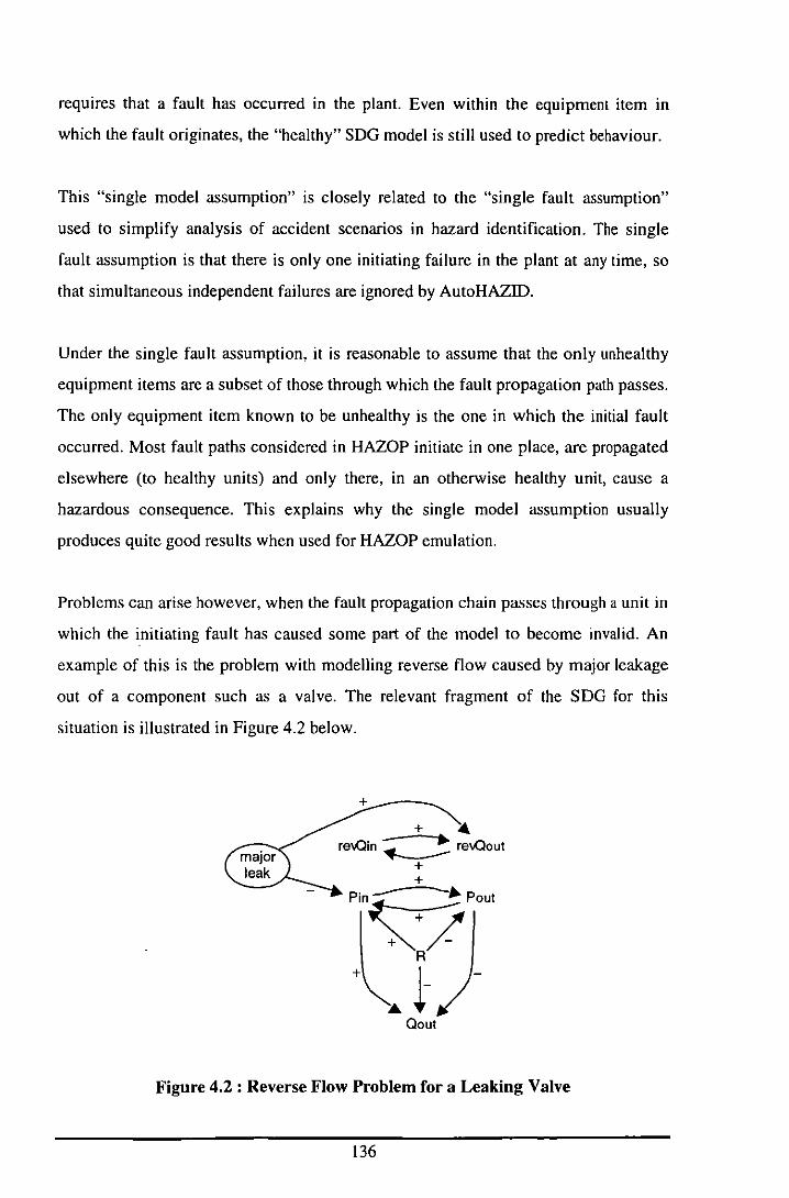
requires that a fault has occurred in the plant. Even within the equipment item in
which the fault originates, the "healthy" SDa model is still used to predict behaviour.
This "single model assumption" is closely related to the "single fault assumption"
used to simplify analysis of accident scenarios in hazard identification. The single
fault assumption is that there is only one initiating failure in the plant at any time, so
that simultaneous independent failures are ignored by AutoHAZID.
Under the single fault assumption, it is reasonable to assume that the only unhealthy
equipment items are a subset of those through which the fault propagation path passes.
The only equipment item known to be unhealthy is the one in which the initial fault
occurred. Most fault paths considered in HAZOP initiate in one place, are propagated
elsewhere (to healthy units) and only there, in an otherwise healthy unit, cause a
hazardous consequence. This explains why the single model assumption usually
produces quite good results when used for HAZOP emulation.
Problems can arise however, when the fault propagation chain passes through a unit in
which the initiating fault has caused some part of the model to become invalid. An
example of this is the problem with modelling reverse flow caused by major leakage
out of a component such as a valve. The relevant fragment of the SDa for this
situation is illustrated in Figure 4.2 below.
+-----+ '"
re\Qin ~ re\Qou!
+ +
Pin0pou!
R
+ ~ l-Qou!
Figure 4.2: Reverse Flow Problem for a Leaking Valve
136
The problem in this case is that the fault should give rise to a potential reverse flow at
the outlet and downstream of the valve, but not at the inlet or upstream of the valve.
Unfortunately, the normal model of the valve allows revFlow to propagate in both
directions, meaning that reverse flow is predicted upstream as well as downstream of
the valve.
The leak event has "invalidated" the normal model of the valve, in the sense that the
model should no longer allow reverse flow to propagate through it. AutoHAZID
cannot model the sort of state-based model dependency implied by this situation. t
Instead, it uses a rule in the HAZOP search engine, to detect any fault paths found in
the graph which start at a leak fault and subsequently propagate through any two
reverse flow nodes in the unit where the leak occurred. Leaks out of pressurised
systems or into vacuum systems are covered by the same rule.
This state of affairs is not very aesthetically satisfying, relying as it does on filtering
out bad results after they are generated, using a rule which is outside the scope of the
models themselves. But, it works well so far. It is not clear if this rule eliminates any
valid scenarios which would otherwise be found by AutoHAZID, but it seems sound
enough reasoning for any simple single input, single output unit.
Note that, when air leaks into a vacuum system, the leak gives rise to revFlow at the
inlet to the unit, rather than the outlet from it, so that the SDG model shown in Figure
4.2 is not relevant for the vacuum case. It is still true, however, that reasoning through
revFlow nodes when a leak into vacuum has occurred, is wrong. The different cases
(of pressurised and vacuum systems) are handled in AutoHAZID by using conditional
arcs, which are discussed in Chapter 5.
I Unlike the systems developed by Pennsylvania and described in Section 2.3.4, which allow the plant
to be remodelled automatically whenever such a state change occurs.
137
4.4 Sparse Results for HAZOP
Early versions of AutoHAZID produced very large HAZOP report files, containing
only very few interesting hazards. As a result, users needed a long time to analyse the
output, to extract results of only limited value. The large size of the output reports was
a result of the systematic nature of the HAZOP algorithm, combined with the inability
of the program to filter important results from trivial ones.
The results were perceived as repetitious, due to the narrow range of phenomena
tackled by the modelling system at the time. Although all reportings of a particular
hazard may have been accurate, they were not necessarily important or interesting new
failure modes discovered by the program. Because all results were reported in the
same way, the program was unable to distinguish more interesting or important
hazards from other, less important ones. Such a filtering mechanism is one of the
natural strengths of the human involvement in HAZOP studies and complements the
systematic method study approach, ensuring that maximum value is extracted from
the study.
When ensuring the correctness of results produced by HAZOP emulation, a lot of time
was spent examining scenarios to find the causes of any problems with them. If the
report files had been smaller, this task would have been less laborious.
Some of the techniques developed to tackle these problems were discussed by
Wakeman et al. (1997), who showed significant improvements in the readability of
HAZOP results from AutoHAZID. In newer versions of AutoHAZID, the bulk of the
report is reduced by a number of filters, each of which can be used or not used, at the
user's discretion. These filters are outlined below and further information is given in
Section A.S of Appendix A:
• Scenarios in the HAZOP results are sorted in order of the importance rank of their
consequences. This helps focus attention on the most important scenarios first.
• Using the consequence threshold feature allows the user to significantly reduce the
bulk of the report, by ignoring consequences below a certain importance rank.
138
• The Fluid Modelling System (FMS), based on conditional fault propagation,
allows fluid properties to be checked so that highly specific failure modes can be
included in SDG models and spurious reporting of hazards dependent on fluid
properties (such as fires, toxicity hazards, etc.) can be reduced. This increases the
relevance and importance of the results.
• Identified faults which cause deviations, but are associated with no identified
consequences, can be eliminated froin the report. Similarly, consequences not
associated with any identified faults can also be left out.
• If identification of protections is enabled, the HAZOP report can be reduced by
displaying only scenarios against which there are no protective devices reported.
• Repetitions are tackled by removing any fault-consequence pair from the report if
that same pair has appeared in the report already.
• During fault propagation, each deviation is associated with a set of faults which
cause it. If the deviation itself can cause some further deviation by fault
propagation, then the set of faults causing the first deviation will be repeated as
causes of the second deviation. This can be a source of significant repetition in the
report produced by AutoHAZID. Repetition is reduced by allowing some
deviations to be reported as causes of others in the HAZOP report, replacing the
set of faults which cause the intermediate deviation. Fault propagation search is
effectively stopped at that point in the longer fault propagation chain. Therefore,
this method was known (in AutoHAZID) as the "stopping point" method.
• AutoHAZID groups equipment items into "lines" for the purposes of examination,
in an attempt to emulate the grouping performed by the HAZOP leader in a
conventional study. Equipment items are examined by AutoHAZID in a line-by
line fashion, so that the order in which deviations appear in the report emulates the
order of examination in a conventional HAZOP. This makes the report more
readable for users with experience of HAZOP studies.
• A frequent source of repetition is where many similar faults are reported as causes
of a deviation, for the same type of equipment. An example is where the deviation
"noFlow" could be caused by the blockage of a number of valves in the same line.
AutoHAZID allows such faults to be grouped together and reported for only one
of the offending units, adding the string "etc" to the fault descriptor, as in
139

"valve8 etc blockage". All units grouped using "ete" must be in the same
line (as identified by AutoHAZID) and they must be the same type.
One of the most important ways of improving the HAZOP results is to add more
interesting failure modes to the models. This should not be attempted on an ad hoc
basis, but should use the knowledge elicitation and modelling techniques mentioned
in Chapter 3. The Fluid Modelling System, as discussed in Chapter 5, can help
improve the focus of results, as well as making possible the addition of more detailed,
specific failure modes.
4.5 Specific Hazards Flagged Indiscriminately
In the most basic qualitative, fault propagation-based version of AutoHAZID, faults
and consequences are paired up and reported solely on the basis of whether a valid
fault propagation path can be found between them. This means that the faults and
consequences are constrained only by their location in the plant (associated with a
particular piece of equipment) and by the SDG which (potentially) provides a causal
path between them.
In reality, many hazards are dependent on other factors, such as the nature of the fluids
in the plant, as well as the equipment items present and their connectivity. An obvious
example is the fire hazard posed by a leak of fluid out of the process. This can only be
a true hazard if the process fluid contains a flammable component - a leak of water
would not pose a fire hazard.
Clearly, if a tool such as AutoHAZID is not able to refer to information telling it
whether the material is flammable or not, it must either report every leak as a fire
hazard, or ignore fire hazards altogether. Therefore, information about the properties
of the process fluids is used to decide the relevance of specific faults and
consequences in the plant model.
This capability has been present in AutoHAZID since an early stage. Initially, the
information stored on fluid components included a small number of characteristics
140
which a fluid either possessed or lacked, such as "flammable", "toxic", "corrosive",
etc. When a fault or consequence was conditional on one of these properties, reference
was made to the library of fluid properties for each component of the relevant process
fluid.
Now, the fluid modelling system contains more data on the fluids present in the plant
model, and has access to a wider variety of information (numerical as well as logical)
on the chemical components present in those fluids. The newer system is described in
Chapter 5. However, the objective is still to verify specific hazards by reference to
fluid properties, in order to make the HAZOP report more interesting and reduce the
bulk of irrelevant false positives.
4.6 Hazards do not appear where expected in HAZOP report
Users of the AutoHAZID program who are experts in traditional HAZOP often
criticise the form, or order, of the results produced by HAZOP emulation. A typical
comment is "Why doesn't the program identify this hazard next to this deviation?".
There is probably no acceptable solution to this problem, because experts will
disagree over where any specified scenario should be identified, which is largely a
matter of personal taste.
AutoHAZID's efforts to make the output table more readable (Section 4.4) partly
cause this problem and partly improve it. Sorting process units into lines arranges the
HAZOP results into an order which makes more sense to a human reader. However,
filtering out repetitions in the report, which vastly reduces the volume of output,
sometimes causes deletion of a "preferred" reporting of a hazard.
It would be possible to apply further rules to the report generator in AutoHAZID, so
that the program would report certain classes of hazard next to "appropriate"
deviations. Such a facility could perhaps be customised to particular user preferences.
However, this was never a priority during STOPHAZ, and was never implemented.
141
4.7 Change the Format of the AutoHAZID Report
A radical approach to reducing the bulk of the results produced by AutoHAZID is to
consider abandoning the HAZOP table as a vehicle for these results. Since the results
are really only a set of fault paths, linking initiating faults to final deviations or
consequences, the faults and consequences could be tabulated against one other,
without stating the intermediate deviations.
Alternatively, a graphical user interface could be developed, allowing the user to
interactively browse through the fault paths with full access to the fault propagation
chain as well as the terminal events. The fault tree is another model of how results
could be presented.
Although none of these ideas were developed into software during STOPHAZ, it
seems clear that much of the effort made by users to read the results of AutoHAZID
could be saved if they were presented in a more concise and usable format.
4.8 Models in AutoHAZID not applicable to early HAZOP on PFD
There is no fundamental reason why a tool like AutoHAZID cannot be used to
perform HAZOP-like analyses at an earlier design stage, on PFD-Ievel plant
descriptions. Although there was no serious attempt to apply AutoHAZID to PFDs, it
is clear that identifying safety problems at this stage can save a lot of time and money.
A PFD is essentially the same kind of input as a P&ID, with less detail on it. The main
problem is likely to be that the models developed for HAZOP analysis of P&IDs
concentrate on problems of components on a fairly detailed level. Output from the
system when examining a PFD may therefore not be very interesting or informative
due to lack of detail in the PFD description.
There may also be a problem with PFDs in that the items on the PFD may not
correspond to single items in the AutoHAZID library of equipment models. What is
required is probably a set of models covering operations at the level of detail likely to
142

apply to PFDs. One issue to be addressed is how to link these models to the existing
hierarchy of equipment models. Another is to what extent the PFD models would
correspond to functionally distinct "modules" performing well-defined unit
operations, specified at quite a high level, in the plant.
4.9 Qualitative Ambiguity
The problem of ambiguity is one that faces all qualitative modelling systems and has
been introduced, in general terms, in Section 2.2.2. This section discusses how
ambiguity causes problems for AutoHAZID, mainly through increased complexity in
graph search.
An example of the ambiguity of qualitative addition, which often occurs in
AutoHAZID, is the problem of deciding what flow deviations occur in the branches of
a divider or header as a result of a pressure deviation in one of the branches. To
resolve this ambiguity requires information (possibly numerical) on components
connected upstream and downstream. Sometimes, using higher level qualitative mass
balance constraints can reduce ambiguity, as reported by Fanti et at. (1993).
It should be noted that this inability to incorporate higher level constraints is due to a
great strength of the SDO models in AutoHAZID, namely locality. It is not desirable
to build balance constraints into otherwise completely local unit models, but some
approach to automatically generating these sorts of constraints, at the level of the plant
model, may be useful.
AutoHAZID is not a rigorous qualitative simulation package. It simply attempts to
implement hazard identification techniques, searching for evidence that a hazard is
possible without simulating the hazard in great detail. Most of the time, ambiguity is a
nuisance rather than a threat to the integrity of the results produced. The result of
ambiguous models is that the program over-reports hazards which may in fact not
exist, rather than missing out hazards.
143
4.9.1 Multiple Paths in the SDG
The most important type of ambiguity in the SDG is related to the problem of multiple
paths between nodes in the graph. Given two process variable nodes, A and B,
searching the graph exhaustively may yield a number of paths, of various lengths,
from A to B. Each of these paths can be associated with an overall effect of A on B,
either a "+" or a "_". There is no guarantee that all the paths found will have the same
overall influence, so they may contradict one another.
In assessing the paths produced by exhaustive search, the first task is to eliminate
those paths that represent "unreal", or physically impossible, scenarios. The remaining
paths may represent "real influences" between A and B, operating via a number of
alternative causal mechanisms.
Further analysis of how these causal paths relate to one another is not a simple matter.
They could be treated as simultaneous and potentially competing influences in the
plant, or as alternative (mutually exclusive) situations, only one of which is relevant at
a time. This level of analysis is not addressed in AutoHAZID at present.
If possible, the real influence paths should be assessed in terms of their relative
strengths of influence, so that the dominant influence between A and B can be
identified. At this stage, the most dominant path may be chosen as the only one to
proceed with, or a number of the more dominant influences could be considered.
A number of problems arise with this theoretical model for search path evaluation.
Most importantly, there is no secure way of deciding within the program if a given
path represents a real or unreal influence between variables. Therefore, much of the
effort in this area has to be put in during model design and implementation, well
before any HAZOP search. In searching the SDG, AutoHAZID must assume that all
paths it finds are equally "real". Secondly, the question of comparing paths to find the
more dominant influences may be possible in theory, but is not supported by any
existing data or models for causal strengths in the SDG.
144
In the absence of information to allow the strengths of influences to be determined
and compared, the path which represents the worst case from a safety point of view
can be chosen. Frequently, however, identifying the worst case is not possible until the
expansion of all fault paths has been completed, which means that the computational
costs of searching the SOG cannot be reduced in this way.
The simplistic approach to the problem of mUltiple paths used in AutoHAZID is to
take the set of paths produced by exhaustive search and eliminate all but the ones of
shortest length in terms of number of SOG arcs. The resulting set may still contain
more than one path, and these paths may themselves predict contradictory influences
between the variables A and B. From the point of view of qualitative hazard
identification, however, all that matters is the overall influence between the variables.
If this is still ambiguous, AutoHAZID must proceed with the assumption that both
influences are possible. This may cause problems with the credibility of the results
obtained, of course. This "shortest path heuristic" is discussed further in Section 4.10
and, elsewhere, by Chung (1993).
4.9.2 Cyclical Paths
If the nodes A and B are the same in the above discussion, then the paths produced are
cycles in the SOG. Sometimes, these represent the influences that a deviation in one
variable has on that variable itself, but this is not always the case. Because the
presence of cyclical paths in the SOG is ignored by the search algorithm used in
AutoHAZID, models are very often designed to take advantage of this feature. In such
cases, no cyclical influence is intended by the model designer.
An example is the frequent use of one variable to propagate deviations in both
upstream and downstream directions using the same set of nodes. This situation is
illustrated quite well in Figure 4.3 in Section 4.10, where flow nodes are chained
together by pairs of arcs forming tight cyclical paths in the SDG at each point along
the chain. Making use of such an arrangement is practical, provided that the algorithm
used to search the graph ignores the presence of cycles.
145
Real plants certainly do include real cyclical influences. They are in operation in every
feedback loop in the plant, including many of the physical processes as well as the
control loops which maintain the plant at steady state.
Cyclical paths are ignored in the search procedure in AutoHAZID because they
potentially lead to fault paths of infinite length. It is also rather difficult to deduce
anything from the presence of a cyclical path unless some of the numerical properties
of the feedback system are understood, so that questions of dynamic behaviour and
stability can be answered.
In other work, feedback loops (particularly control loops) have formed an integral part
of the decomposition of plant models, in Shafaghi et al. (1984), for example. There
may be some value in identifying feedback in the plant in order to simplify the
analysis of behaviour, but this idea has not so far been developed within AutoHAZID.
4.9.3 Ambiguous Predicted Flow Deviations
Within the flow path modelling system in use within AutoHAZID models, pressure
deviations can give rise to changes in flow. However, it is often impossible to check
whether reverse flow (revFlow) or simply reduced flow (lessFlow) are possible in a
given scenario, because of lack of specific (numerical) information about the cause.
At other times, both deviations are genuinely possible given the situation as specified.
In either case, ambiguous predictions are produced.
One must bear in mind also that deviations of process variables are defined in terms of
their sufficiency to cause some final consequence. The sufficiency of each deviation
can only be judged in the context of a complete fault path, and may depend on the
magnitude of the deviation or on other factors, including the nature of fluids in the
plant. Therefore, the sort of uncertainty shown when we cannot decide which of
revFlow or lessFlow occur, is an example of the more general problem of deciding the
magnitude of deviations in a fault path. The issues of reasoning with fluid properties
and the quantitative magnitudes of deviations, in order to assess the sufficiency of
fault paths generated by SDO search, are discussed further in Section 5.3.
146
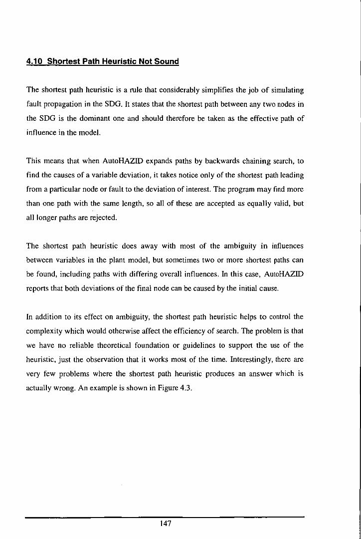
4.10 Shortest Path Heuristic Not Sound
The shortest path heuristic is a rule that considerably simplifies the job of simulating
fault propagation in the SOG. It states that the shortest path between any two nodes in
the SOG is the dominant one and should therefore be taken as the effecti ve path of
influence in the model.
This means that when AutoHAZID expands paths by backwards chaining search, to
find the causes of a variable deviation, it takes notice only of the shortest path leading
from a particular node or fault to the deviation of interest. The program may find more
than one path with the same length, so all of these are accepted as equally valid, but
all longer paths are rejected.
The shortest path heuristic does away with most of the ambiguity in influences
between variables in the plant model, but sometimes two or more shortest paths can
be found, including paths with differing overall influences. In this case, AutoHAZID
reports that both deviations of the final node can be caused by the initial cause.
In addition to its effect on ambiguity, the shortest path heuristic helps to control the
complexity which would otherwise affect the efficiency of search. The problem is that
we have no reliable theoretical foundation or guidelines to support the use of the
heuristic, just the observation that it works most of the time. Interestingly, there are
very few problems where the shortest path heuristic produces an answer which is
actually wrong. An example is shown in Figure 4.3.
147
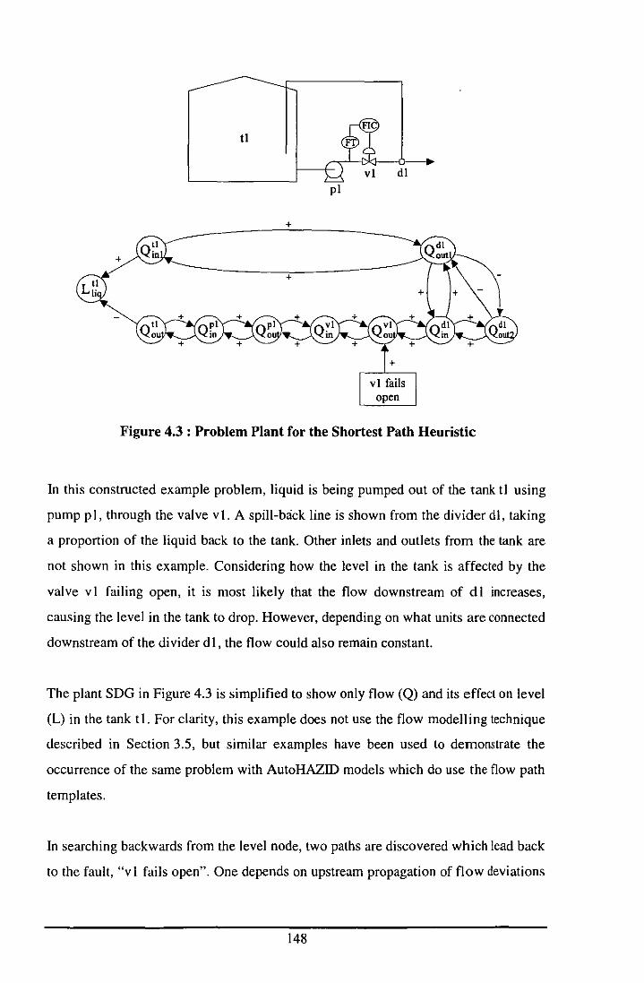
tI
dl pi
+
+
Figure 4.3 : Problem Plant for the Shortest Path Heuristic
In this constructed example problem, liquid is being pumped out of the tank tl using
pump pi, through the valve v I. A spill-back line is shown from the divider dl, taking
a proportion of the liquid back to the tank. Other inlets and outlets from the tank are
not shown in this example. Considering how the level in the tank is affected by the
valve v I failing open, it is most likely that the flow downstream of d I increases,
causing the level in the tank to drop. However, depending on what units are connected
downstream of the divider d I, the flow could also remain constant.
The plant SDG in Figure 4.3 is simplified to show only flow (Q) and its effect on level
(L) in the tank tl. For clarity, this example does not use the flow modelling technique
described in Section 3.5, but similar examples have been used to demonstrate the
occurrence of the same problem with AutoHAZID models which do use the flow path
templates.
In searching backwards from the level node, two paths are discovered which lead back
to the fault, "vI fails open". One depends on upstream propagation of flow deviations
148
through v I and p I, to t I at the main outlet of the tank. The other path propagates flow
downstream via v I and the divider d I, through the spill-back line and into the tank t I.
The former path is the correct one, leading to a low level in the tank - what we would
expect if the valve were to open fully. However, the propagation path via the spill
back line is the shorter one (5 arcs, compared to 6 for the other path), so it is the one
which is reported. That is, in this example, the valve failing open is reported as a
cause of an increase in the tank level.
In AutoHAZID, this problem is solved using rules which are activated by the HAZOP
algorithm itself. The rules look out for situations where a path has been found which
propagates deviations through the "feedback" section of a loop, from an event in the
"forward" section of the loop. If such a path exists, in conjunction with another path
having a contradictory influence and not using the feedback section of the loop, then
the longer path is adopted in preference to the potentially erroneous shorter one.
The use of ad hoc rules for fixing problems like this is not very palatable, especially
when they are resident in the inference engine part of the system, rather than
embedded in the model system. It may be that there is little option in this case,
because of the non-local nature of the problem - the real behaviour of the tank level
depends on a mass balance over the elements of the loop which cannot be expressed
in the unit models at a local level.
One reason for the success of the shortest path heuristic is that models are usually
designed in the knowledge that the heuristic will be applied. That is, the modeller
makes the assumption that the shortest path is the most valid, as well as the most
efficient, link between nodes in the SDG. Therefore, good practice in modelling
means using the minimum number of arcs necessary to represent the infl uences
present in the unit, without allowing false influences to be created in the model by
unintended paths.
149
Even assuming that models are constructed using the best practice in modelling, the
question still remains: "Why does the shortest path between two nodes in the plant
SDG usually represent the correct causal influence between them?"
To look at the problem in more detail, the first thing to note is that the plant SDG
consists of a number of mini-SDGs, representing equipment items connected by links
which correspond to stream connections between the equipment items. All the stream
connection links are parallel sets of SDG arcs connecting variables in one unit to the
same variable in another unit. The "cross-over" between variables, representing
interesting physical influences, takes place within the units themselves.
Next, we observe that the shortest paths between node pairs within the same unit are
likely to be correct because the models were designed in this way, with all variables
visible to the model builder at the same time. It should be part of the methodology
used whenever constructing or updating models of equipment, that every distinct pair
of nodes in the model is checked to see that there is at most one shortest path between
them. The influence represented by this shortest path must also be correct (or at least
feasible), and appropriate for the model.
Given these observations, we can go on to examine how alternate paths between two
nodes, aj and bj , arise in the plant SDG. If aj and bj are present in the same unit, then
the shortest path must be the correct one, as the model builder made it so.
If aj and bj are in adjacent units, then these units are connected by a stream,
represented by a parallel set of arcs, each arc linking a propagation variable in one unit
to the same variable in the other unit. The simplest case is shown in Case I of Figure
4.4, where node al in unit A is connected to a2 by a shortest path of 0 or more arcs. a2
in unit A connects to bl in unit B via a single arc, and bl is connected to b2 via a
shortest path of 0 or more arcs.
150
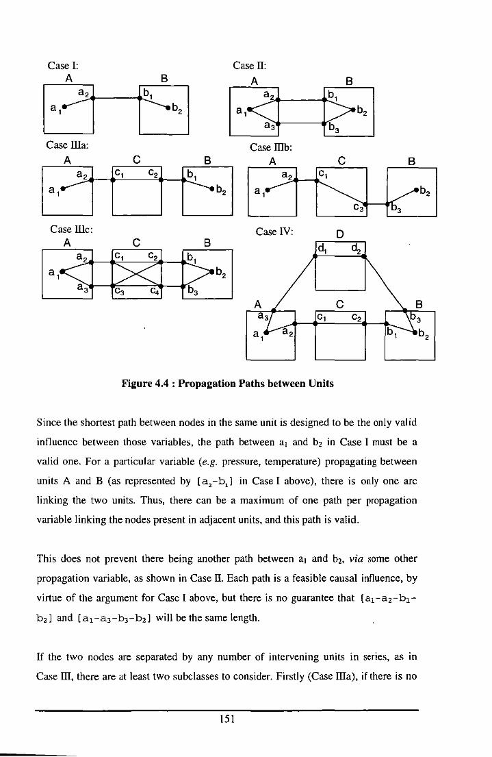
Case I: Case II: A B A B
la·1 Eb'l a 2 b l
a l b2
a3 b3
Case ma: Case IIlb:
1 a'1 r c ~j Eb' 11 a'~1 rSJ-fb'l Case mc: Case IV: D
A C B dl a 2 Cl C2 bl
a l b2 a 3 C3 C4 b3
A C Cl C2 3
a l
Figure 4.4 : Propagation Paths between Units
Since the shortest path between nodes in the same unit is designed to be the only valid
influence between those variables, the path between al and bz in Case I must be a
valid one. For a particular variable (e.g. pressure, temperature) propagating between
units A and B (as represented by [a,-b1l in Case I above), there is only one arc
linking the two units. Thus, there can be a maximum of one path per propagation
variable linking the nodes present in adjacent units, and this path is valid.
This does not prevent there being another path between al and bz, via some other
propagation variable, as shown in Case IT. Each path is a feasible causal influence, by
virtue of the argument for Case I above, but there is no guarantee that [al-az-b1 -
bzl and [a,-arbrbzl will be the same length.
If the two nodes are separated by any number of intervening units in series, as in
Case m, there are at least two subclasses to consider. Firstly (Case mal, if there is no
ISl
b2

cross-over within the intermediate unit C, then propagation goes straight through C
and the system is equivalent to Case I. Secondly, if the propagation crosses over from
one variable to another within unit C, as in Case llIb, the path [Cl -c31 is still a valid
shortest path and a valid path in C between those nodes, by virtue of the same
argument as before. Therefore, the path [al-a2-cl-C3-brb21 is valid.
Systems where there is more than one unit interposed between units A and B can be
dealt with in the same way as Cases ma and llIb. Case mc shows that, as units are
increasingly separated, there is more scope for ambiguity. In this case there are four
possible paths between a) and b2, all of which can be shown to be valid. Not all of
these will necessarily have the same length or path influence, so some will normally
be neglected using the shortest path heuristic.
A similar argument to that used with Cases ma, llIb and mc, can be used for the
example of Case IV, which is similar to the example problem of the tank in Figure 4.3
above. The propagation paths via unit C and via unit D are both equally valid as far as
the information in the SDG models is concerned.
Thus, to make an informed judgement of which paths are appropriate, all possible
paths should be examined, and information outside the scope of the pure SDG model
is required. The information required should support the evaluation of which paths are
most "relevant". This question could involve some evaluation of the relative strengths
of causal influence in candidate paths, or assessment of time-based aspects of the
system, such as transient behaviour and ordering of the events which may occur, rate
information, etc. As mentioned in Section 4.9.1, causal analysis of this depth was
never attempted in AutoHAZID.
It should be noted that preliminary results with AutoHAZID indicate that the shortest
path heuristic can be made into an "option" without too many computational
penalties. Comparing the results of running the program on the test case plant reported
by Lawley (1974) reveals that without using the shortest path heuristic, the HAZOP
report produced is not much more bulky, and the HAZOP run time is only doubled.
152
Analysing the Lawley results file reveals that the only problems caused by the loss of
the shortest path heuristic concern the flow path templates used in the plant. The flow
path allows two conflicting paths linking pressure and flow, one of which is
eliminated by the shortest path heuristic. Therefore, the predicted flow effect due to a
pressure deviation sometimes operates in the wrong direction. The use of the shortest
path heuristic has been effectively designed into the flow path template (see
Figure 3.5). Unless an alternative flow path model can be produced without multiple
internal paths, it is impractical to discard the shortest path heuristic.2
4.11 Computational Complexity
The problem of complexity has been described in general terms in Chapter I. It is not
clear whether the complexity of the search space examined by AutoHAZID is
exponential, or less complex than that (e.g. polynomial). This judgement is dependent
on the nature of the SDG, which in turn is ruled by the connections in the plant model
and the models of equipment items in it.
It is easy to see that an upper bound on the branching factor for any given plant can be
identified, as the maximum branching factor in units within the plant. For a range of
plants of various sizes, using the same library of unit models, the maximum may be
identified as the maximum branch factor of nodes in equipment items modelled in the
library. Therefore, the branching factor has an upper bound which is not dependent on
size of the plant model, so that the search procedure is definitely not "super
exponential".
Considering the topology of typical plants, and the corresponding SDa topology, it
seems that much of the plant consists of straight-line propagation, without much
branching. Most branching occurs within major equipment models. This suggests that,
2 If the flow path template were the only case where multiple internal paths occurred, then it might be
possible to discard the shortest path heuristic, if some means were provided to filter out the ambiguities.
Tu date, we do not know how widespread multiple internal paths are, so the wisdom of making such a
change is doubtful.
153
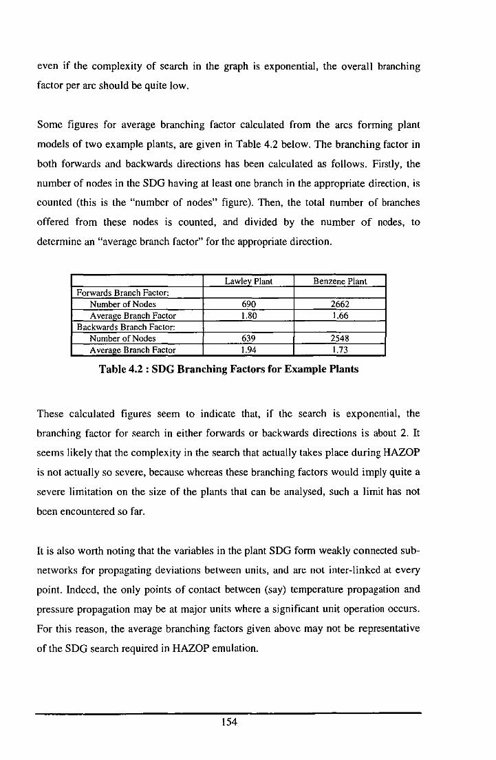
even if the complexity of search in the graph is exponential, the overall branching
factor per arc should be quite low.
Some figures for average branching factor calculated from the arcs forming plant
models of two example plants, are given in Table 4.2 below. The branching factor in
both forwards and backwards directions has been calculated as follows. Firstly, the
number of nodes in the SOG having at least one branch in the appropriate direction, is
counted (this is the "number of nodes" figure). Then, the total number of branches
offered from these nodes is counted, and divided by the number of nodes, to
determine an "average branch factor" for the appropriate direction.
Lawley Plant Benzene Plant Forwards Branch Factor:
Number of Nodes 690 2662 Average Branch Factor 1.80 1.66
Backwards Branch Factor: Number of Nodes 639 2548 Average Branch Factor 1.94 1.73
Table 4.2 : SDG Branching Factors for Example Plants
These calculated figures seem to indicate that, if the search is exponential, the
branching factor for search in either forwards or backwards directions is about 2. It
seems likely that the complexity in the search that actually takes place during HAZOP
is not actually so severe, because whereas these branching factors would imply quite a
severe limitation on the size of the plants that can be analysed, such a limit has not
been encountered so far.
It is also worth noting that the variables in the plant SOG form weakly connected sub
networks for propagating deviations between units, and are not inter-linked at every
point. Indeed, the only points of contact between (say) temperature propagation and
pressure propagation may be at major units where a significant unit operation occurs.
For this reason, the average branching factors given above may not be representative
of the SOG search required in HAZOP emulation.
154
The problem of complexity in AutoHAZID SDG search can be tackled in a number of
ways:
• Particularly important, for reducing the potentially enormous branching factors
which could make search much more difficult, are sensible conventions for
modelling which eliminate unnecessary cross-linking between variables. If
possible, branching fault paths should be limited to modelling phenomena within
complex units, rather than being a commonplace feature of the fault propagation
pathways throughout the plant model.
• The AutoHAZID HAZOP emulation algorithm was rewritten, to cut down on the
amount of repeated search work that was being done with the old version (see
Appendix B). The search for causes of HAZOP deviations is now a two-stage
process: let L) be the list of nodes corresponding to variables of interest in the
HAZOP study. In a first stage, AutoHAZID expands paths for causes of deviations
in the node, as far as the nearest other node also in L). When this has been done for
each node in L), the program takes the partial paths produced by the first stage and
combines them into full paths from faults to final deviations. This algorithm
considerably reduces the search required for HAZOP.
• The shortest path heuristic can help to reduce the amount of work done in the
second stage of the HAZOP search algorithm, and the number of resulting
completed fault paths. This works by removing partial paths where they share the
same starting point as other shorter partial paths for the deviation being examined.
As discussed in Section 4.10, the shortest path heuristic is not a particularly sound
rule of inference, but it does seem to work effectively and has been in operation for
the whole time that AutoHAZID has been in development.
• The HAZOP search is usually exhaustive and finds all the paths in the SDG, no
matter how long they are. AutoHAZID can also operate in a mode where a fixed
limit to the length of the fault paths is prescribed. In this mode, as soon as a path
reaches the specified number of arcs in length, the algorithm does not attempt to
expand it any further. Good results can be obtained with this (non-rigorous)
method, but there is a small possibility (in theory) that some relevant hazard
scenario may be overlooked.
155
• The SDO can be pruned to remove arcs which are not required by the HAZOP.
This reduces the number of arcs present and therefore reduces the time taken to
look up nodes in the SDO. Under certain conditions, pruning the SDO can also cut
the amount of search done, if it can be shown that such search will produce no
results of interest to the HAZOP study requested. There may be no consequences of
interest in a particular part of the graph, for instance, which may justify removing
arcs from the SDO.
4.12 Concluding Remarks
The strengths of the SDO are related to its weaknesses. Computational efficiency is
achieved by using a representation based in the middle ground of representational
strength, between simple digraph models and some more highly structured model of
causal mechanism in the physical plant. It is a weak but efficient representation.
Very frequently, the way an equipment model is constructed is the cause of the
problems encountered with it. In these cases, all that may be required to side-step the
problem is a rethink of the approach used in producing the model. This can only be
done on a case-by-case basis and the evidence in favour of a large scale redesign of
the system, to solve numerous problems of a fundamental nature, must be
accumulated over some time, to justify such a redesign.
Fluid models will be used to focus the applicability of the output generated by the
program. The problem is the quantity and paucity of output from the simple SDO
model, where scenarios In reality may be valid only for specific
conditions/circumstances in the plant. Additional expertise is needed, to improve the
judgement of AutoHAZID by tempering the qualitative fault propagation with
quantitative calculation or estimation. This may be achieved by links to the physical
properties calculation packages, or making arcs in the SDO conditional in places.
The next chapter addresses the inherent limits of the purely qualitative approach and
proposes a method for making use of quantitative information related to fluids in the
plant, which is implemented in the fluid modelling system.
156
Chapter 5 : Conditionality in Fault Path Modelling and the Fluid Modelling System
Chapter 4 (in particular Sections 4.1, 4.3, 4.5, 4.9 and 4.10) has demonstrated that, for
many important hazard identification problems, the qualitative SDG models of
AutoHAZID are insufficient. This is an inherent limitation of the SDG, which allows
the representation of only qualitative information in the AutoHAZID models.
This limitation is addressed in AutoHAZID using the fluid modelling system, which is
described in this chapter. First of all, the issue of how to improve the results produced
by AutoHAZID, is discussed, in Section 5.1. The approach chosen is to add more
specific faults and consequences to the models in the SDG, and to control how these
are reported in the HAZOP report by adding conditions to arcs, faults and
consequences in the SDG. By verifying the conditions present in completed fault
paths, using properties of fluids present in the plant, the validity of generated
scenarios can be checked.
The fluid modelling system is described at length in Section 5.2, which explains the
approach of fault path validation and the system of functions and predicates which
implements this validation method. Section 5.2 also describes how the different
subsystems making up the FMS are integrated.
An interesting appliStion of the FMS is to monitor the quantitative limits on
deviations in fault paths. This allows some scenarios to be ruled out because the
deviations present can be demonstrated as not severe enough to cause the final
consequence. This approach is illustrated in Section 5.3 using five case study
problems. The chapter concludes with some overall comments on the FMS, problems
encountered with it, and possible improvements for the future.
157
5.1 Improving on Fault Propagation
AutoHAZID uses "simple" fault propagation, where a fault is linked to a consequence
by a linear strand of deviations, to formalise cause and effect in the development of a
hazardous scenario. Real scenarios often do not match exactly with this model, so that
the fault propagation method does not capture all details of the real situation. In such
cases, careful analysis of the scenario is required, to ensure the most important
features of the problem are captured in the model. An appropriate modelling
methodology can help ensure completeness, as discussed in Section 3.5 and (later) in
Section 6.4.
A difficult class of problems for the qualitative SDG system is where, at some stage, a
combination of events or conditions is required for the scenario to develop. This
"conjunction" of events corresponds to an "AND" gate in the fault tree for the
development of the scenario. The basic SDG does not represent this sort of ("AND
logic") step at alI.I
If, for a recognised hazard scenario, no acceptable model can be constructed within
the existing modelling system, one must consider what approach should be taken:
• Proceed with an unsatisfactory model. In this case, the hazard may be reported
indiscriminately and the program may produce misleading output because it cannot
apply the hazard model selectively enough.
• Abandon the new scenario and do not model it at all. This reduces the value of the
results produced, because a hazard which may exist in some real plant cannot be
identified by the HAZOP emulator.
• Enhance the model representation, by improving or replacing the SDG. This is a
costly option, in terms of rewriting program code and equipment models.
Forethought and planning are essential to avoid wasted effort and ensure an elegant
and efficient solution to the problem. Often, new functionality can be added as an
I AND is sometimes presumed in modelling certain situations. For example, we may assume that
alarms are ignored when identifying hazards and modelling their development.
158

optional feature, so that existing models can still be used. This approach reduces
the risk associated with a change.
Some idea of how the SDG might be improved can be gained by analysing how
existing models tend to fail when used for hazard identification. The usual signs of
poor quality models are incorrect hazard identification and sparse reporting of
interesting hazards in an otherwise uninteresting report, as discussed in Section 4.4.
Incorrect hazard identification, giving rise to an increased number of "false positive"
results, may be due to:
• Incorrect fault propagation arcs. Where a particular arc in some equipment
model can be identified as incorrect, the arc can be removed, or the equipment item
can be remodelled in a different way. This sort of problem is detected by
examining the HAZOP results critically and analysing the fault paths giving rise to
suspect results. A number of tools provided in the AutoHAZID program itself can
be used for this task.
• Incorrect fault propagation paths that are locally sound. Sometimes, one finds
that every link in a fault propagation chain is locally valid, that each arc relates a
variable to its neighbour in a valid way, but nevertheless the whole chain does not
predict a real effect. This can occur because some higher level constraint, such as
heat or mass balance, is not captured in the arcs concerned. Problems of this nature
can be difficult to solve using localised causal relations, such as the arcs of the
SDG, because the SDG does not carry much information between nodes. 2
• Indiscriminate reporting of hazards. Some hazards can appear everywhere in a
HAZOP report. This may be due to a fault or consequence being modelled as
generally applicable, where it actually has a more limited scope in reality. In this
case, a restriction/check on the applicability of the fault or consequence is needed.
2 An example of a problem where the application of high level constraints resulted in the solution to an
ambiguity problem. is discussed in Fanti et al. (1993). This was a case where local qualitative mass
balances were not sufficient to unambiguously specify a system state, but higher level balance
constraints solved the problem.
159
The most important issue to be addressed by any improvement to the SDG system is
how to enrich the range of failure modes represented in equipment models. It must be
possible to model highly specific faults and consequences within unit models, and to
manipulate them so that they are only reported when relevant within the plant being
examined. Therefore, the applicability of new faults and consequences should be
made conditional on the context within the plant that makes them relevant.
The aim is to eliminate "blanket" reporting of hazards, by verifying the accuracy of
fault propagation paths as far as possible. In this way, AutoHAZID can reduce the
number of false or irrelevant hazards identified and it should become possible to
model more interesting failure modes and hazards within the system. As a result, the
number of interesting items in the HAZOP report should increase and its size should
decrease, improving the richness and usefulness of the results produced.
Some terms will be used in the following discussion, which it may be helpful to define
here:
• The objective is to enable AutoHAZID to produce highly focussed results, where
all the hazardous scenarios reported are relevant and interesting in the context of
the plant being studied.
• To do this, it is necessary to add more specific faults and consequences to the
equipment models. Such faults and consequences provide more detail about the
events concerned, compared to the generic faults and consequences often seen in
AutoHAZID results. For example, one might consider reporting a "flammable leak
to environment", rather than simply a "leak to environment".
• In order to prevent these more specific faults and consequences being reported
indiscriminately, conditions are attached to faults, consequences and propagation
arcs in the SDG. Such conditions must be satisfied (where present) for an arc to be
valid in a fault path.
• Conditionality is the property possessed by arcs, faults and consequences which
have conditions attached. Such arcs, faults and consequences can be referred to as
conditional.
160
The factors of most use, in determining whether a hazardous scenario is feasible, are
related to the types of fluids present. Luckily, information on the main fluids present
in a plant is usually available in the process description for that plant.
Therefore, the first attempts to make SDG models in AutoHAZID conditional
focussed on fluid-related factors, applying optional conditions to the faults and
consequences in unit models. Using these conditions, the relevance of a fault or
consequence could be checked when it was processed in a fault path. Once conditions
had been applied to faults and consequences, it was a short step to allowing fault
propagation between nodes to become conditional too.
Using the present "fluid modelling system" (FMS) to evaluate these conditions,
scenarios in the basic SDG models can be tested during the HAZOP search, reducing
ambiguity. The particular case of checking the magnitude of deviations in propagation
chains, to reject infeasible chains, is discussed in Section 5.3.
In designing the FMS, care was taken that the library of qualitative equipment models
could still be used in AutoHAZID without change. This means that conditions are
optional - changes to models are made as and when new conditions are added to
existing arcs, or new arcs are added. Also, the (highly efficient) graph search
algorithm was not removed. It is used to produce fault paths in the SDG, which are
then evaluated by the FMS. Conditions are evaluated whenever they are encountered
in a fault path, and if any condition is found not to be valid, the fault path is removed.
The HAZOP reports produced by AutoHAZID are more focussed as a result of this
filtering.
This form of conditionality in the SDG is important for any hazard identification
system which attempts to model potentially complex hazardous scenarios. The FMS,
described in the next section, uses information about units in the plant model, fluid
properties and quantitative data to verify the correctness of fault paths produced by
search on the SDG.
161
5.2 The Fluid Modelling System
The earliest attempts at making the SDO conditional in AutoHAZID involved simple
properties of the fluids present in the plant model. The names of fluid components
were specified in lists associated with particular units in the plant, thereby identifying
which fluids could be present where in the plant. These named fluid components
corresponded to pure compounds for which the early AutoHAZID system could look
up data in a "fluid model library" .
The early fluid model library (which is still a subsystem within the current FMS)
included a few properties which a compound mayor may not be deemed to possess.
For example, the consequence' environmental contamination' is relevant
only if the fluid present in the equipment is toxic. Properties of the fluids in the
system, such as toxicity and flammability, were defined in this early work and some
consequences were made conditional on the fluid in the equipment item having a
certain property. For instance, if no component of the fluid in a unit had the property
toxic, then the consequence' environmental contamination' would not
be reported within that unit.
This early system did not allow specification of where in a piece of equipment the
given fluids were to be found, and it used a very simple algorithm for propagating
information about expected fluids to other units. All fluid components in a unit were
passed on to downstream units, which led to problems in heat exchangers, for instance
- the program predicted that the shell and tube-side fluids would mix and that all
downstream units would receive the same mixture. The present FMS associates fluids
with ports in the equipment items, so that the fluids in the shell and tube sides of a
heat exchanger are kept distinct unless an interface failure occurs.
The FMS is now quite a general-purpose rule system, which maintains information
about currently applicable fluids at each point in a fault path, as well as allowing
calculations to be included in rules. The sort of rules in the FMS include, but are not
limited to, reasoning about numerical properties of the fluids present. Systems are
included for dealing with logical operations, arithmetical comparisons and, most
162

importantly, a number of different software systems for answering queries about fluids
are integrated into one system.
Fluid Library
ASPEN Properties Plus
Hyprotech HVSVS
Plant Model
properties of pure compounds, parameters
tor calculations
equipment attributes, fluid data, etc.
properties of mixtures
predicate checks
Figure 5.1 : Fluid Modelling System and associated Information Sources
A schematic view of the FMS subsystems and some of their associated data sources, is
given above, in Figure 5.1. The various elements of the system will be described more
fully in the sections which follow:
• Section 5.2.1 outlines the principle of fault path validation, which forms the basis
of what the FMS does.
• The propagation, through the plant model, of user-supplied information about
fluids is described in Section 5.2.2.
• Rules in the FMS make use of predicates and functions, which are described in
Section 5.2.3.
• Section 5.2.4 outlines the types of information needed by the FMS to evaluate
predicates and functions, including details of the "current fluids" in the plant.
• The integrated subsystems of the FMS are discussed in' Section 5.2.5, which
describes the evaluation of predicates and functions, as well as examining some
operating system issues in the HAZID system.
• Section 5.2.6 describes the information stored in the fluid library, a precursor to the
FMS which is still used a~ an information source on fluids.
163
• The calculation of fluid properties, by external packages and within AutoHAZID,
is the subject of Section 5.2.7.
• The reactivity group-based system for detecting fluid compatibility problems has
an interface in the FMS, which is described in Section 5.2.8.
5.2.1 Fault Path Validation
The chains of influence produced by SDG search during HAZOP emulation are
known as "fault paths". They are validated by checking conditions attached to the
faults, consequences and arcs, using calculations, qualitative and quantitative
information. Rules are therefore defined to specify the checks to be performed.
The validation checks are activated in the HAZOP algorithm by the function which
verifies completed paths produced by the search algorithm: acceptable-path ( ).
The meaning of each condition is such that, if it is proven to be false, then the arc
which contained the condition is no longer considered to be valid and the fault path
containing that arc is removed. If the FMS cannot prove a condition to be false, even
if this is due to a lack of data, then the condition is deemed to be true - this is to
ensure that scenarios aren't rejected unless it is known for sure that they are not
feasible.
It is also possible to associate a list of conditions (rather than a single condition) with
a fault, consequence or arc, so that all conditions in the list must be satisfied for the
fault, consequence or arc to be valid.
Validation proceeds by taking the fault path as a whole and evaluating the condition
(if any) attached to the fault at the start of the path. If this condition fails, the fault
path is rejected. Otherwise, each arc in the chain is examined in turn, and any
conditions present are evaluated, until the last link in the chain is reached.
In general, the last arc in the chain need not be connected to a consequence - the same
validation technique is used to check partially constructed paths during HAZOP
emulation, and paths created by "causes of a deviation" queries raised by the user. If
164
the last arc in the fault path does link to a consequence, however, then any condition
on the consequence is evaluated as a final step in the validation check. If all these tests
succeed, then the path is accepted, otherwise it is rejected.
5.2.2 Fluid Information and its Propagation
Infonnation loaded into AutoHAZID from the plant description may include details of
the intended fluids in the plant, either within individual equipment items or flowing
between them. The system has been designed to respond in the absence of fluid
infonnation, but nonnally this infonnation would be specified.
The fluid infonnation is associated with ports, which may be defined as inputs to a
unit, outputs from it, or internal locations within the unit. The following infonnation
may be given:
• "Amount" of fluid. For streams between units, this is the flowrate, in kglhr; for
internal ports it is the inventory of the fluid, in kg.
• Names of chemical components in the fluid and their mole fractions.
• Pressure, in bara.
• Temperature, in cC.
This infonnation is presented to the program in intendedFl uids,
portPressures and portTemperatures slots in the plant model.
in tendedF 1 uids slots provide infonnation about the "amount" and composition
of the fluid in question. Within the program, this information is stored in Location
objects, one for each port in the unit where some infonnation is known. The
Location class is described in Appendix D. Any fields which are not known within
the Location objects are given a special undef_number value.
Fluids do not have to be specified for every place in the plant model. A procedure
known in AutoHAZID as "fluidisation" is used to infer, from the data given, other
infonnation about the fluids in the plant. By propagating information about fluids
forwards in the plant wherever possible, using rules for managing incomplete data, the
165

maximum use can be made of the information given, and data will then be available
wherever the fluid identity has been inferred.
The connectivity of the plant, which determines where fluid can go and where it
cannot, is defined in terms of [uni t, port 1 locations linked by SDO arcs
propagating the variable composi tion. This variable was chosen because it seemed
that, of all the variables in the models, composition most closely mirrored the
propagation of fluids themselves. In particular, composition is (usually) only
propagated in one direction - the downstream direction of flow. The connectivity
information extracted from the SDO is stored in a Net object.
When fluidisation finishes, Location objects corresponding to all the places in the
plant where something is known about the fluids present are put into info slots with
the name "location". This information is referred to in later analysis by the FMS.
A number of principles are observed when propagating fluids throughout the plant:
• Data may only be propagated between ports which are directly connected by a
single link in the fluid connection network.
• Fluid propagation never overwrites the information specified in the plant model, so
that information may only be propagated from Location Ll to Location L2
if the relevant property is known at Ll and not known at L2. If properties are
unknown, they are stored with the value undef_number.
• Propagation of flowrate information is considered separately from pressure,
temperature, composition and component names. This is because flows can be
added together at branch points, whereas the other properties cannot.
• Non-zero flowrates may be propagated directly downstream in unbranched lines.
• Flowrates in dead-end sections of the plant must be zero. If any non-zero flows are
found in dead-end parts of the plant, they are reported and fluidisation fails. In this
case, the fluid information is not propagated in the plant model at all. Units which
comprise legitimate inlets or outlets for fluids in the plant are labelled in the unit
166
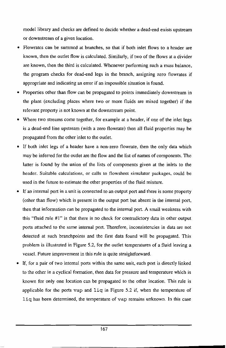
model library and checks are defined to decide whether a dead-end exists upstream
or downstream of a given location.
• Flowrates can be summed at branches, so that if both inlet flows to a header are
known, then the outlet flow is calculated. Similarly, if two of the flows at a divider
are known, then the third is calculated. Whenever performing such a mass balance,
the program checks for dead-end legs in the branch, assigning zero flowrates if
appropriate and indicating an error if an impossible situation is found.
• Properties other than flow can be propagated to points immediately downstream in
the plant (excluding places where two or more fluids are mixed together) if the
relevant property is not known at the downstream point.
• Where two streams come together, for example at a header, if one of the inlet legs
is a dead-end line upstream (with a zero flowrate) then all fluid properties may be
propagated from the other inlet to the outlet.
• If both inlet legs of a header have a non-zero flowrate, then the only data which
may be inferred for the outlet are the flow and the list of names of components. The
latter is found by the union of the lists of components given at the inlets to the
header. Suitable calculations, or calls to flowsheet simulator packages, could be
used in the future to estimate the other properties of the fluid mixture.
• If an internal port in a unit is connected to an output port and there is some property
(other than flow) which is present in the output port but absent in the internal port,
then that information can be propagated to the internal port. A small weakness with
this "fluid rule #1" is that there is no check for contradictory data in other output
ports attached to the same internal port. Therefore, inconsistencies in data are not
detected at such branchpoints and the first data found will be propagated. This
problem is illustrated in Figure 5.2, for the outlet temperatures of a fluid leaving a
vessel. Future improvement in this rule is quite straightforward.
• If, for a pair of two internal ports within the same unit, each port is directly linked
to the other in a cyclical formation, then data for pressure and temperature which is
known for only one location can be propagated to the other location. This rule is
applicable for the ports vap and liq in Figure 5.2 if, when the temperature of
1 iq has been determined, the temperature of vap remains unknown. In this case
167
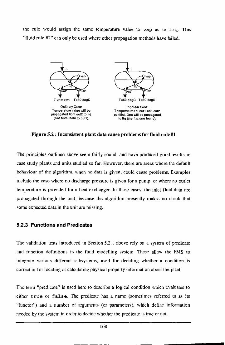
the rule would assign the same temperature value to vap as to 1 iq. This
"fluid rule #2" can only be used where other propagation methods have failed.
T unmown T =50 degC
Ordinary Caoo: Temperature value will be
propagated from oul2 to liq (and from there to oUll).
T =60 degC T =50 dogC
Problem Case: Temperatures of oull and oul2 conflict. One will be propagated
to liq (the first one found).
Figure 5.2 : Inconsistent plant data cause problems for fluid rule #1
The principles outlined above seem fairly sound, and have produced good results in
case study plants and units studied so far. However, there are areas where the default
behaviour of the algorithm, when no data is given, could cause problems. Examples
include the case where no discharge pressure is given for a pump, or where no outlet
temperature is provided for a heat exchanger. In these cases, the inlet fluid data are
propagated through the unit, because the algorithm presently makes no check that
some expected data in the unit are missing.
5.2.3 Functions and Predicates
The validation tests introduced in Section 5.2.1 above rely on a system of predicate
and function definitions in the fluid modelling system. These allow the FMS to
integrate various different subsystems, used for deciding whether a condition IS
correct or for locating or calculating physical property information about the plant.
The term "predicate" is used here to describe a logical condition which evaluates to
either true or false. The predicate has a name (sometimes referred to as its
"functor") and a number of arguments (or parameters), which define information
needed by the system in order to decide whether the predicate is true or not.
168
An example of a predicate is flanunable (Port), which is used to decide whether
the fluid present at a given port in the plant model is flammable or not. Here, Port is
a variable (symbols with initial capital letters are variables, as in the Prolog language)
which can be given a value, such as 'out'. When the arguments of the predicate are
given values, the FMS can evaluate the condition and return an answer (true or
false). Predicates may sometimes be defined without arguments, in which case the
brackets are usually omitted.
The FMS also allows the definition of "functions". These look similar to predicates in
that they involve a name and a list of arguments given in brackets, but they return
values which may be of any type in general. Each function returns a particular data
type, but this can be anything which fits in with the types defined for the DObj ec t
class. These types are listed in Appendix D and include constants, integer and real
numbers, lists, strings and "structures", similar in form to predicate calls. The FMS
functions allow the person defining predicates to do a limited amount of computation3
using function calls within the predicate definition.
An example of an FMS function is get_f 1 uid (Port) , which consults the plant
model to find the fluid at the given port location and returns the data known about the
fluid in a specific structure. The structure used corresponds to the data stored in the
Location object class. Another example is vapour-pressure (Fluid), which
takes an argument in the same format as that returned from get_fluid (Port) and
returns the vapour pressure of the fluid at its temperature and pressure (these data are
provided within the Fluid argument).
Within the FMS, some special predicates and functions are defined which can be used
in a shorthand form as "infix" operators. These correspond to the commonly used
operators for arithmetic and logical operations and numerical comparisons, and can be
used in between the items on which they operate. In addition to their infix form, each
3 The computation possible within the FMS is limited in the sense that iterative loops and recursion are
not permitted.
169
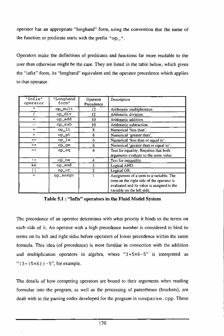
operator has an appropriate "longhand" fonn, using the convention that the name of
the function or predicate starts with the prefix "op_".
Operators make the definitions of predicates and functions far more readable to the
user than otherwise might be the case. They are listed in the table below, which gives
the "infix" fonn, its "longhand" equivalent and the operator precedence which applies
to that operator.
"Infix" "Longhand Operator Description operator form" Precedence
* op_rnult 12 Arithmetic multiplication. / op div 12 Arithmetic division. + op add ID Arithmetic addition. - op_sub ID Arithmetic subtraction. < op_lt 8 Numerical 'less than'. > op gt 8 Numerical 'greater than'.
<- op le 6 Numerical 'less than or equal to'. >- op_ge 6 Numerical 'greater than or equal to'. -- op_eq 4 Test for equality. Requires that both
3!guments evaluate to the same value. !- op ne 4 Test for inequality. && op_and 3 Logical AND.
II op or 2 Logical OR. - op_assgn I Assignment of a term to a variable. The
term on the right side of the operator is evaluated and its value is assigned to the variable on the left side.
Table 5.1 : "Infix" operators in the Fluid Model System
The precedence of an operator detennines with what priority it binds to the tenns on
each side of it. An operator with a high precedence number is considered to bind to
terms on its left and right sides before operators of lower precedence within the same
fonnula. This idea (of precedence) is most familiar in connection with the addition
and multiplication operators in algebra, where "3+5x6-5" is interpreted as
"(3+ (5X6)) -5", for example.
The details of how competing operators are bound to their arguments when reading
fonnulae into the program, as well as the processing of parentheses (brackets), are
dealt with in the parsing codes developed for the program in newparse. cpp. These
170
functions allow data compatible with the DObj ect class to be read directly from
strings of characters, stored in Str objects.
The functions and predicates used in the arcs of the SDG are defined in the start of the
unit model library, using predicate () and function () statements. These
specify the name and arguments of the function/predicate as a "functional prototype"
format, containing dummy variables for each of the arguments. Also specified is a
type string, which maps the function or predicate that is being defined onto a specific
system which is able to evaluate it:
• "C" - If the type string is the letter C, the function or predicate is defined within
the AutoHAZID program. Thus, when it is evaluated, the query goes to a specific
C++ function in the program which produces the appropriate result.
• "V" - If the type string is a V, the query is handled by the fluid rule system,
developed in STOPHAZ by VTT. This has a separate handler function which
maps these queries to rules in that subsystem of the FMS. Only predicates may be
specified in this way.
• "D" - If the type string is D, then the function or predicate is defined in terms of
other functions or predicates, and the definition is given following the type string.
This definition takes the form of a list of functions or predicates to be evaluated,
to determine the value of the function or predicate being defined.
The func t ion and predicate statements in the unit model library are read into
the program at start-up, and are stored in two lists for later reference by the FMS.
Using these lists, the FMS can access the types and definitions of all known functions
and predicates in the program. If a term, in either a unit model or a predicate
definition, does not match with the "prototype" pattern stored for some item in these
lists, then it cannot be evaluated as a FMS function or predicate.
A full record of the functions and predicates so far implemented in the fluid model
system, is given in Appendix E, which attempts to give a very short summary of the
items, and also classifies each of them into one of a number of groups:
171
l. Logical operations
2. Mathematical operations
3. General-purpose operations
4. Plant, fluid and fault path data access
5. Limit data access
6. Combining fluids (including compatibility checks)
7. Properties of single fluids
8. Consequence evaluation
9. Contamination
10. Design parameter checks
11. Miscellaneous physical checks
12. Leakage checks and limitations
13. Checks on VLE pressure limitations
14. Pressure deviation limits corresponding to resistance changes in flow paths
5.2.4 Information used in Fault Path Validation
In evaluating the predicates attached to the faults, consequences and arcs of a
candidate fault path, the FMS uses two forms of information:
• The name of the predicate and values for its arguments are given in the condition
as it appears in the unit model or in the fault path. These allow the form of the
predicate appearing in the fault path to be matched against the definitions of known
predicates stored in the program.
• A set of "context information" is also used in evaluation. This consists of data
which are required so often that they are best supplied routinely by the FMS.
The same two types of information are also used to evaluate the FMS function calls
which may appear in the definitions of type "D" predicates.
Since conditions are most often used to validate fault paths, the fault path object (class
FPa th, described in Appendix D) stores most of the context information needed for
172

FMS evaluation. The procedures for updating context information in FPath objects
are also called from the code which validates the fault path objects:
• FPa th stores a full list of the arcs in the propagation path. This allows access to
the initial fault and final consequence, if required, during validation of any part of
the path.
• The "current fluids" present at each point in the fault path are stored, as well as
information on the limits of process variable deviations for those fluids. The latter
information is used to solve the problems described in Section 5.3.
• Some information is stored on the classification, categorisation and ranking of the
fault path. This information is calculated using methods and rules developed by
Prof. Lees and Dr. Larkin within the STOPHAZ project.
In addition to the above "context" data, the name of the unit in which the condition
currently being examined is resident, is also used. This data is not stored in the
FPa th object, as the FPa th usually refers to a number of process units along its
propagation path, and so cannot be readily associated with one single unit.
An important distinction in the FMS is between "nominal fluid data" and "current
fluid data". The nominal fluids are the fluids in the plant under normal operation (i.e.
in the absence of deviations). This information contains fluid data provided in the
input model loaded into AutoHAZID, plus the information inferred by the
"fluidisation" routine described in Section 5.2.2.
"Current fluid data" is a term used here to denote the conditions of fluids in the plant
when a fault has occurred, i.e. at points along the fault path currently being examined.
This information is derived from nominal fluid data, with property differences arising
from contamination events or deviations in temperature and pressure, for example.
Fault path validation requires that the conditions at each link in the chain be evaluated
in relation to fluids which are expected to be present at the relevant locations in the
supposed fault scenario, rather than fluids which would be present there in normal
operation. Thus, each FPa th object maintains a list of Location objects to store
173
this current fluid data. The current fluid data associated with ports can be examined or
changed by the program during validation.
It is important to take account of the differences which may arise between nominal
and current fluids during fault path validation, when determining how current fluids
information propagates forwards in the plant. Differences may arise due to
contamination event~, or due to deviations in the values of process variables.
AutoHAZID includes a prototype system to track the limits in numerical deviations of
pressure and temperature during scenario development. This method is outlined in
Section 5.3.
5.2.5 Integration of Fluid Model Subsystems
The fluid modelling system (FMS) provides a uniform way for AutoHAZID to make
use of the various software subsystems developed by different partners in STOPHAZ,
using predicate conditions on arcs in the SDG. Some of the queries handled by the
FMS are directly related to fluids and their properties. Others relate to plant model
data and some have a more general-purpose nature, providing the arithmetical and
logical "glue" which allows complex checks to be formulated.
An additional complication is that AutoHAZID has been developed for use in both
UNIX and Windows. Some parts of the system are not available in UNIX, and some
external parts of the software system in a Windows environment may not be available
at run-time, so the FMS must deal with this in producing the best available answer.
A sensible integration strategy should make the best use of available subsystems and
data in answering fluid queries. If the FMS is not able to determine a predicate, it
~hould default to returning an answer which enables HAZOP emulation to be
completed, and only allows hazards to be rejected if they can be proven not to be
feasible.
174
The subsystems involved in the FMS are outlined as follows:
• An important internal part of the FMS, implemented by C++ functions, is the set of
general purpose operations in logic and arithmetic, including the operators
described in Section 5.2.3. These allow convenient expression of the checks and
evaluations needed to formulate FMS conditions.
• A number of properties of pure compounds are provided in the fluid library and
read into AutoHAZID when it starts. This is the earliest version of the fluid model
still in HAZID and is described in Section 5.2.6.
• Physical properties of mixtures and pure compounds are determined by calling on
external packages such as Properties Plus or HYSYS, via a "Properties Package
Link" (see Section 5.2.7).
• Alternatively, some properties of mixtures may be estimated by calculations within
AutoHAZID, using data provided in the fluid library.
• The fluid rule system developed by VTT is an internal part of AutoHAZID, but
was not developed at Loughborough. It is implemented as a subsystem for
resolving predicate tests within the FMS.
• An external information source is used for the fluid compatibility checks developed
by VTT, as outlined in Section 5.2.8. The data required is accessed through the
functions of the database API and consists of a "reactivity group matrix", giving
information about adverse reactions between fluid components.
• The internal model of the plant, constructed from the data read into AutoHAZID
from plant descriptions and the unit model library, is an important source of
information for resolving the FMS queries. It includes details of the fluids present
in the plant and of the attributes of various units.
5.2.5.1 Outline of Function and Predicate Evaluation in the FMS
As noted above, the evaluation of a function or predicate in general relies on context
information in addition to its arguments. Therefore, the C++ functions which evaluate
these terms have a common list of arguments which communicates the context
175
information between them. This common list is shown below for the function
eval ua te ( ) , which is used to evaluate both functions and predicates:
DObject evaluate (
const DObject& Dl, BindList& BLl, FPath& FPl, const Str& UName)
In the above, the function or predicate to be evaluated is the argument 01. A list of
variable bindings currently in force is given in BLl - the first thing that happens when
a term is evaluated is that the bindings list is applied to 01. The 'FPath object FPl
represents the fault path in which the function or predicate call occurs. It can be used
to access the data on current fluids or on the arcs in the fault path. The contents of
FPl may be changed by the evaluation, particularly the list of current fluids. Lastly,
the argument UName gives the name of the unit in which the function or predicate is
evaluated.
The "handler functions" which make up the system for evaluating FMS conditions,
are outlined in Figure 5.3 below. The purpose of these functions is to determine the
appropriate subsystem for resolving a query and to manage the call to that subsystem,
providing arguments as required and handling returned values. The figure below
shows only the relationships between the handler functions (in tenns of which
functions call which others) and omits the many functions which do the work of
evaluating functions and predicates of the FMS.
176
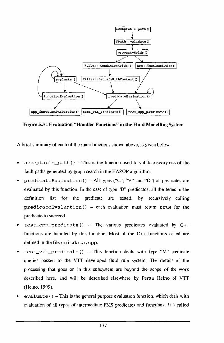
Filler:;ConditionHolds()
Filler::SatisfyWithContext()
Figure 5.3 : Evaluation "Handler Functions" in the Fluid Modelling System
A brief summary of each of the main functions shown above, is given below:
• acceptable-path () - This is the function used to validate every one of the
fault paths generated by graph search in the HAZOP algorithm.
• predicateEvaluation () - All types ("C", "V" and "0") of predicates are
evaluated by this function. In the case of type "0" predicates, all the terms in the
definition list for the predicate are tested, by recursively calling
predicateEvaluation () - each evaluation must return true for the
predicate to succeed.
• test_cpp-predicate () - The vanous predicates evaluated by C++
functions are handled by this function. Most of the C++ functions called are
defined in the file uni tda ta. cpp.
• test_vtt-predicate () - This function deals with type "V" predicate
queries passed to the VTT developed fluid rule system. The details of the
processing that goes on in this subsystem are beyond the scope of the work
described here, and will be described elsewhere by Perttu Heino of VTT
(Heino, 1999).
• evaluate () - This is the general purpose evaluation function, which deals with
evaluation of all types of intermediate FMS predicates and functions. It is called
177
by various C++ functions which evaluate type "C" functions and predicates, as
well as the links shown in the figure above. Whenever an expression in the
parameter list of some predicate or function requires evaluation, this is the
function that is used. If it finds that a term cannot be evaluated as a function or a
predicate, it returns the term unchanged.
• functionEvaluation () - This function manages the evaluation of FMS
functions of types "C" and "D" (FMS functions of type "V" are not supported). In
the case of a type "D" function, each term in the definition list of the function is
evaluated in turn (by calls to eval ua te ( ) ) and the return value of the function
is the result of evaluating the final term.
• cpp_functionEvaluation ( ) - FMS functions of type "C" are evaluated by
this function. It manages calls to a number of C++ functions, defined in file
fns .cpp.
The FMS is accessed at present from only two places. The first is the fault path
validation code which operates during the HAZOP analysis of a plant model. This
results in calls to the predicateEvaluation () function originating ultimately
from the function acceptable-path (), as shown in Figure 5.3.
The second point of access to the FMS is a user option ("Evaluate a
function/predicate") on the main menu in AutoHAZID, defined in the C++ function
opt_doEvaluation (). This option requests a term from the user for the program
to evaluate as a function or predicate, as well as an appropriate unit in whose context
the term is to be evaluated. The original term, and its evaluation, are displayed to the
user after evaluation has been attempted. This menu option makes use of the general
FMS evaluator function, evaluate () .
Functions may be embedded in a predicate by appearing as values in the argument list
of a predicate, or by appearing in the body of the predicate in an assignment or
comparison statement, such as:
P = vapour-pressure(Fluid)
178
In the latter case, the function call appears as the second argument of the assignment
operator (op_assgn(P,vapour-pressure(Fluid) », so the two cases are
actually equivalent. Function evaluation therefore occurs when the arguments passed
to a predicate are being evaluated.
5.2.5.2 Operating System Dependencies and Availability of Software Packages
AutoHAZID is written so that it compiles equally well for Windows and for UNIX.
Wherever some part of the program needs to be different under Windows, compared
to UNIX, "conditional compilation" selects the appropriate part of the code to
compile. As far as functions and predicates in the FMS are concerned, however, the
main issue is the availability of external software packages in Windows and UNIX.
Compatibility checks for fluid interactions (see Section 5.2.8) are not available in the
UNIX version of AutoHAZID because the reactivity group table is present in the PC
based database used to store plant descriptions from the Graphical Tool. Therefore,
the UNIX version of AutoHAZID always produces a blank report in response to calls
to the FMS function compatibility_check (Fl, F2). Compatibility checks are
available for all versions of AutoHAZID under Windows.
The availability of an external package in which physical property calculations can be
done (see Section 5.2.7) is determined at start-up when the program may attempt to
link to a particular package as directed in its configuration file. The user is notified of
whether a properties package was detected by the program and if a link was
successfully made to it.
When a property package link is active in AutoHAZID, the function
physical-property_request () attempts to evaluate queries using that
package. If no link is present, or if an initial query to the external package fails, the
function uses any appropriate C++ based routines in AutoHAZID to evaluate the
query.
179
The availability of the properties package links is determined by the following
considerations:
• If the operating system is UNIX, links to these packages do not exist in the current
version of AutoHAZID.
• If the operating system is Windows 3.1, then the packages cannot be accessed
because they rely on library functions accessed in 32 bit libraries, and Windows 3.1
is a 16 bit system.
• If the operating system is Windows NT or Windows 95, which are 32 bit systems,
then the physical properties packages can be accessed from AutoHAZID, provided
the following conditions are satisfied:
• The user has one of the packages installed, HYSYS or Properties Plus.
• All the libraries (. DLL files) required for the package are resident in the
same directory as the AutoHAZID executable files (HAZ 107 . EXE and
HAZID. EXE).
• The configuration file, hazpaths. dos, is set up correctly, with the
variable PropPackageType set to either ASPEN or HYPRO and the
appropriate variable (ASPEN_DLL or HYPRO_DLL) set to point to the
library file for the package which is to be used.
The system for deciding physical properties requests is discussed in Section 5.2.7.
5.2.6 Fluid Library Information
Physical data on pure compounds are stored in a fluid library file and read into the
program at start-up. These data are stored in Fluid objects and can be accessed later,
when required to answer a FMS query. Additionally, the fluid library is used to store
parameters required for calculations to estimate certain physical properties, such as
Antoine constants to estimate vapour pressure. A third use of the fluid library is to
store data on reactivity groups needed by the compatibility checking code for
determining unwanted fluid interactions (see Section 5.2.8).
180
Since the fluid library only contains information on specific pure compounds, it is of
limited use when applied to determining accurate property values for mixtures.
However, if appropriate "safe" assumptions are used in combining data on pure
compounds, then good use can be made of the information available.
The data stored in the fluid library, for each pure compound, are:
• CAS Number.
• Average Molecular Weight, g/mole.
• Freezing Temperature, QC.
• Decomposition Temperature, QC.
• Flashpoint Temperature, QC.
• Autoignition Temperature, QC.
• Lower Flammability Limit, (%v/v).
• Toxicity Classification, measured on a scale of 0 to 3, where the classes have the
following meanings:
• 0 Non-toxic (e.g. air, water)
• I Slightly toxic (e.g. nitrogen, which can asphyxiate)
• 2 Toxic (e.g. toluene)
• 3 Very toxic (e.g. benzene)
• Latent Heat at normal boiling point, J/mole.
• Boiling Temperature at atmospheric pressure, QC.
• List of three Antoine Constants for vapour pressure estimation.
• Liquid Density, kg/m3.
• List of four constants for the evaluation of vapour heat capacity, J/mole.
• ERPG_3 value, a measure of toxicity for the Dow exposure index, mg/m3.
• Liquid heat capacity, J/kgQC.
• List of four reactivity group codes, for use in the compatibility checking routines
(see Section 5.2.8).
Some of the data in this list are used in calculations of physical properties which can
be used as alternatives to the external packages discussed in the following section.
181
5.2.7 Physical Properties Calculations
During the STOPHAZ project, links from AutoHAZID to external packages were
explored, to provide access to the physical properties data and calculations typically
used in flowsheeting packages. Links to Aspentech's Properties Plus and Hyprotech's
HYSYS packages, were explored. The link to Properties Plus was successfully
demonstrated during the project.
The interface to the properties packages was specified by ASPEN, in conjunction with
Loughborough University. ASPEN developed the library of functions which provides
common access to the routines in individual calculation packages.
The following are the property calculations specified by ASPEN:
• Physical State (C)
• Average Molecular Weight (C)
• Boiling Temperature Range (C)
• Freezing Temperature (C)
• Vapour Pressure (C)
• Viscosity
• Density (C)
• Enthalpy
• Specific Heat (C)
• Latent Heat of Fusion
• Latent Heat of Evaporation (C)
• CAS Number
• Phase Temperatures (for the given pressure, these are the temperatures where
changes of physical state will take place).
• Phase Pressures (for the given temperature, these are the pressures where changes
of physical state will take place).
• Flashpoint Temperature
182
• Autoignition Temperature
• Lower Flammable Limit
• Upper Flammable Limit
Access to the physical properties packages is provided through FMS functions and
predicates in the same way as for other properties. Some of these properties can be
calculated either in external packages or in C++ functions relying on data in the fluid
library. These are indicated by a (C) in the above list.
Calculations for various types of flash were also specified as part of the physical
properties system. So far these have not been used within the FMS.
The fluid properties provided by the external packages allow better estimation of the
properties of mixtures than is the case with the data provided in the fluid library, or in
calculations carried out within AutoHAZID itself. It is also likely that the level of
quality and consistency provided by using external data is better than using ad hoc
properties based in the C++ code itself.
5.2.8 Compatibility Checks for Fluids
Unwanted interactions can occur within the plant, particularly when fluid compounds
are mixed together, either deliberately or inadvertently. These sorts of interactions
depend mostly on the nature of the fluids which come together and are not particularly
affected by the process equipment in which they occur.4 Therefore, the plant models
represented by the SDO are not very useful for modelling the wide range of
phenomena caused by such interactions.
Part of the STOPHAZ project involved building a software module within
AutoHAZID for predicting the effects of unwanted interactions in the plant. To
predict these effects requires knowledge of which compounds are present. This
information is available through the fluid information in the plant model.
4 Of course. the consequences of such tluid interactions may depend on where in the plant they occur.
183
Detecting interactions requires some knowledge of the effects of mixing chemical
components together. An attempt to capture this knowledge was made in STOPHAZ,
using a reactivity group tagging scheme for classifying chemical species, combined
with a compatibility table method for predicting the effects of mixing species together.
Each chemical species in the fluid is associated with up to four numeric identifiers
that label it as belonging to a certain group of chemicals, having certain properties.
Members of the same reactivity group will tend to behave in similar ways when mixed
with chemicals belonging to another particular group. This is the basis of the
"compatibility table" which tabulates the reactivity group identifiers against each
other and records a set of effects in each cell in the table, which are the consequences
of mixing chemicals from the corresponding two groups together. An example of the
type of compatibility table used is given in Figure 5.4 below. The effects recorded are
taken from the following standard set of consequence types:
• heat generation caused by component interactions
• gas generation caused by component interactions
• toxic interaction between components
• flammable interaction between components
• explosive interaction between components
• violent polymerisation due to component interactions
• solubilisation of toxic substances due to component interactions
• possible unknown hazard due to component interactions
By examining the components of a fluid, one can predict the possible interactions
which will occur due to the chemicals present. This is the basis of the compatibility
checks carried out in the FMS whenever two fluids are considered to mix together in
the HAZOP algorithm. The checks are carried out by the FMS function
compatibility_check, which calls a function written by VTT. The VTT code
consults a table of reactivity groups and produces a report consisting of a list of effects
taken from the list above, each one associated with a pair of component names,
184
identifying the species responsible for the interaction. This report object is added to a
global report using the FMS function, add_to_compat_report, so that all the
compatibility check results produced during HAZOP can be collected into a single
report.
The collected report is appended to the end of the main HAZOP report, rather than
integrating the results into the HAZOP table at the point where they were produced.
This is because of the many problems of storing reported interactions in association
with the fault path from which they originated, and reporting these clearly within the
HAZOP table. The compatibility report declares the fluids which mixed (including
their locations in the plant), the interactions produced by mixing and the fluid
components responsible for those interactions, for each mixing event considered.
185
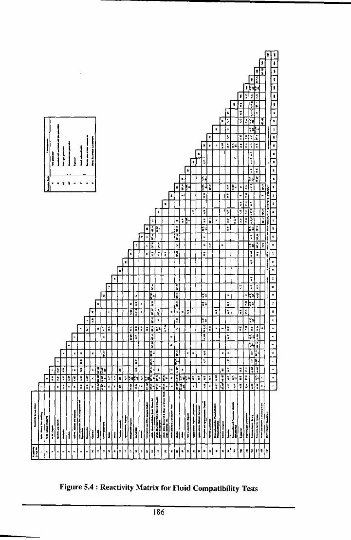
1 • . I
11 t 1 1, 11[' !!l lulJfU
• ,
. " ,
'. . . , ..
'" 1;-"
,
, ,
,
tI .. " " , .
. •
• , , ,
• •
, · ~ I!' , •• ; • , ; ; , , , • ,
; ; ; ;
, • ; ., ;
; · , , ; · . .. . · • ,
· ·
~. ; ,
'. ,
· • , ,
; · , ;
, • r.,
· , ~
;
, ,
" • · · , • :
, • , ;
J! " 'If! t
i
•
~
, : ; •
:
,
,
~
; ~
, . ;
:
. , ~
, :
! I
!: I
I ~ I
I I
; ;
. , • •
· , ; • · •
• . .
.. ;; .. B ... :.. ... " " t J! Jid Z .: ,. '
r;r;r, I:" I:" I:" r. t:" t: t: t: I:"
Ii - .. ~ ........... , !: \J :: : 'l! ! ':: it , I li 11 11 a 11 11 I:; 11 11 11 ;;; 11 11 ~ i , 11 f I !I !
Figure 5.4 : Reactivity Matrix for Fluid Compatibility Tests
186
5.3 Reasoning using Numerical Limits on Deviations
Fault propagation often produces paths which are not credible, because the magnitude
of deviation required to cause a final consequence cannot be realised within the
scenario produced by the fault concerned. To tackle this problem, a method has been
developed within the FMS to model the propagation of numerical limits on the size of
deviations in process variables.
This means that maximum and minimum limits for deviations caused by certain faults
are available for propagation through the fault path. Conditions can also be attached to
deviation-consequence arcs, so that the magnitude of the deviation is checked against
some limit, to test if it is severe enough to cause the consequence.
The aim is to capture some of the more usual commonsense rules which a human
team would use in a conventional HAZOP study. An attempt to identify some of these
rules has been made (by myself and Prof. Lees) in the meeting documented In
Appendix F. The rules so far implemented in the FMS, for limiting the size of
pressure and temperature deviations, are listed in full in the table given in
Appendix E. A subset of these will be discussed in the following subsections.
In the FMS, Location objects are used to communicate information about current
fluids in the plant during fault path validation. The system for maintaining
information on numerical limits of deviations makes use of the Notes field of the
Location object, to manipulate limit values using functions and predicates in the
FMS, such as get_max_temperature (), set_min-pressure (), etc.
The following subsections illustrate how reasoning with numerical limits works in
relation to a number of case study problems. These examples show possible strategies
for implementing solutions to complex plant modelling problems in the FMS
generally, not just in relation to numerical limits on deviations. It is important to note
the way a semi-formal analysis of the scenario is used as a starting point for
considering how that scenario could be formalised in the rule system.
187
5.3.1 Example 1 : Design Pressure for Pumps and other Units
High pressure can cause the casing of a pump to rupture. but the high pressure is only
considered relevant if it rises above the design pressure of the pump. This can often
only be achieved by specific causes. possibly including dead-heading the pump. which
occurs when there is a complete blockage in the discharge side of the pump.
corresponding to a noFlow deviation.
As an example of the use of design pressure checks In the models. consider the
following arcs. taken from a pump model:
arc([deviation, [morePressure,outJ],l, [consequence, ['possible casing overpressure rupture', exceed_design-pressure(out)]]),
arc ( [out, nOFlow] ,1, [out, pressure1, assign_max-pressure(out, full_dh-pressure(in,out»)) ,
The predicate exceed_design-pressure (Port) checks the maximum
pressure for the given port against the maximum design pressure (in the attribute
"max_allowable-pressure"). to see if the design pressure is exceeded. This
check is used to validate the overpressure rupture consequence. A similar predicate.
exceed_design_vacuum (Port) checks the minimum pressure of a unit against
the minimum allowable design pressure. to check for the possibility of vacuum
collapse. These two predicates can be used for any unit. not just pumps. It is a
convention of the plant database that design pressures and temperatures are stored in
the attributes max_allowable-pressure. min_allowable....Pressure.
max_allowable_tempera ture and min_allowable_ tempera ture.
The arc linking noFlow to pressure represents the rIse In pressure caused by
completely blocking the pump discharge. The maximum pressure in this case is the
dead-heading pressure of the pump. added to the operating pressure at the inlet. and
this limit is set by the assign_max-pressure () predicate attached to the arc.
When the two arcs are present in a fault path. validation succeeds only if this limit
pressure is sufficient to exceed the pump's design pressure.
188
Note that, in the absence of infonnation detennining the size of a pressure deviation, it
is necessary for AutoHAZID to report overpressure rupture as a potential consequence
wherever morePres sure could occur. Clearly, when there is no information
available for the fault path on the size of the pressure deviation, the program must
cautiously predict that the consequence could occur.
5.3.2 Example 2 : Atmospheric Pressure is (approximately) 1 bara
When a pressurised vessel leaks to atmosphere and the pressure inside it drops, the
minimum pressure reached is about I bara. Similarly, when a vacuum system leaks
and air goes in, the pressure inside it rises to a maximum of around I bara.
These observations are of course, quite trivial, but it was necessary to introduce limits
on pressure deviations caused by leaks, to reduce the number of spurious results in the
HAZOP report. Leaks are identified as causes of pressure deviations in many places in
the HAZOP reports produced by AutoHAZID. Pressure deviations are also frequently
associated with equipment damage (e.g. vessel rupture, vacuum collapse).
Therefore, unless pressure limits are considered and handled correctly, leaks out of a
process can be quoted as causes of vacuum collapse in a vessel, and leaks into a
vacuum system can be quoted as causes of overpressure rupture. In reality, unless the
pressure deviation crosses one of the design limits of the system, no mechanical
damage will actually be caused.
In order to prevent spurious output, I bara is therefore stated throughout the model
libraries as the numerical limit on pressure deviations caused by leakage faults. When
this infonnation is propagated to a pressure damage consequence for the plant, the
limit can be compared to the design pressure of the vessel (as described in Example I
above) and the fault path can be found to be invalid.
189
Two predicates have been developed to deal with these features of leaks. They are
pressureLeak (Port) and vacuumLeak (Port) shown below. These have
been attached to leak faults throughout the library:
predicate (pressureLeak(Port) , -0·, [ pressurised(Port),
assign_min-pressure(Port, 1.0) J) •
predicate(vacuumLeak(Port),-D-, ( vacuum(Port),
J) .
assign_max-pressure(Port, 1.0) , % Put air into the system, too add_air_contaminationCPortl
Notice that the above predicates test that the process is under pressure (or vacuum)
before they apply any limit to the pressure deviation. Therefore, the faults to which
these predicates are attached will only be considered where the process operates under
pressure or under vacuum respectively. Also, leakage into a vacuum system not only
increases the pressure, it also contaminates the process with air (which will often be
more significant, from a safety point of view, than the pressure change).
5.3.3 Example 3 : Pressure Limits When Valves Open
The flow path model uses the idea of flow path resistance to model blockages in pipes
and the effects of a valve being opened or closed. Resistance therefore has an effect on
the flow through the unit and the pressures at its inlet and outlet.
When a control valve fails open or closed, there will be certain limits on the pressure
and flow deviations caused by the failure. If the valve fails closed, the upstream
pressure will rise and the downstream one fall, but it is not very easy to determine
limits for the pressures in this case, without using information from equipment
attached upstream and downstream of the valve.
When the control valve fails to an open position, the resistance falls to a minimum of
zero, and the flow rises to some maximum value which is not readily determined
without analysing the overall flow system in some detail. The pressures also change in
response to the valve opening - the upstream pressure drops and the downstream
190
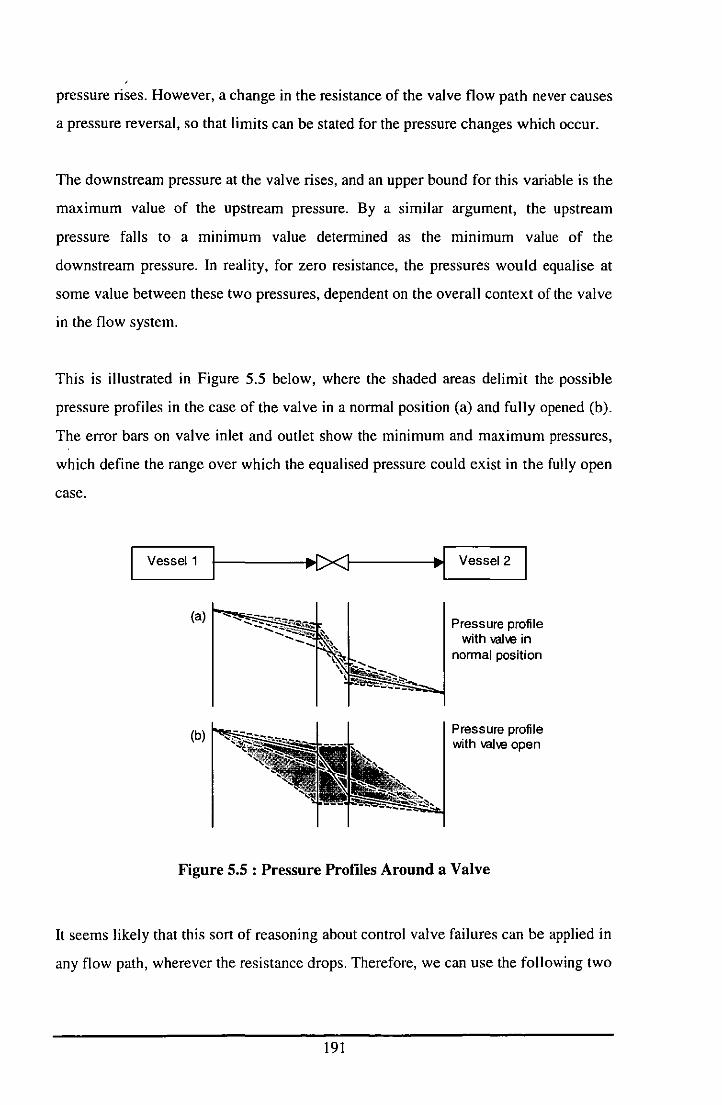
pressure rises. However, a change in the resistance of the valve flow path never causes
a pressure reversal, so that limits can be stated for the pressure changes which occur.
The downstream pressure at the valve rises, and an upper bound for this variable is the
maximum value of the upstream pressure. By a similar argument, the upstream
pressure falls to a minimum value determined as the mInImum value of the
downstream pressure. In reality, for zero resistance, the pressures would equalise at
some value between these two pressures, dependent on the overall context of the valve
in the flow system.
This is illustrated in Figure 5.5 below, where the shaded areas delimit the possible
pressure profiles in the case of the valve in a normal position Ca) and fully opened Cb).
The error bars on valve inlet and outlet show the minimum and maximum pressures,
which define the range over which the equalised pressure could exist in the fully open
case.
'--v_e_s_s_el_1--'t------I~~C><lI------1~~1 Vessel 2
(b)
Pressure profile with vall.e in
normal position
Pressure profile with vall.e open
Figure 5.5: Pressure Profiles Around a Valve
It seems likely that this sort of reasoning about control valve failures can be applied in
any flow path, wherever the resistance drops. Therefore, we can use the following two
191
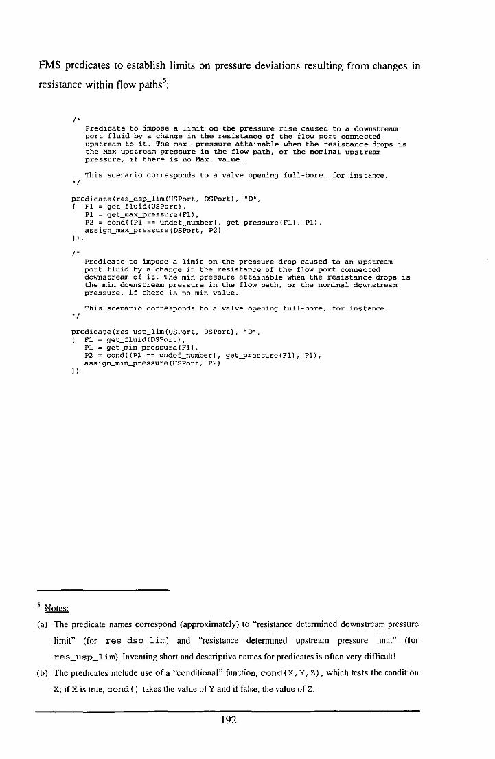
FMS predicates to establish limits on pressure deviations resulting from changes 10
resistance within flow paths5:
5 Notes:
f'
'f
Predicate to impose a limit on the pressure rise caused to a downstream port fluid by a change in the resistance of the flow port connected upstream to it. The max. pressure attainable when the resistance drops is the Max upstream pressure in the flow path, or the nominal upstream pressure, if there is no Max. value.
This scenario corresponds to a valve opening full-bore, for instance.
predicate (res_dsp_lim(USPort, DSPortl, ~D·, ( Fl get_fluid(USPort),
J I.
f'
'f
PI = get_max-pressure(Fll, P2 = cond«Pl == undef_number), get-pressure(Fl), Pl), assign_max-pressure(DSPort, P2)
Predicate to impose a limit on the pressure drop caused to an upstream port fluid by a change in the resistance of the flow port connected downstream of it. The min pressure attainable when the resistance drops is the min downstream pressure in the flow path, or the nominal downstream pressure, if there is no min value.
This scenario corresponds to a valve opening full-bore, for instance.
predicate (res_usp_lim(USPort, DSPort), MO-, [ FI get_fluid(DSPort),
J I.
PI = get_rnin-pressure(FI), P2 = cond«PI == undef_numberl, get-pressure(FI), PI), assign_min-pressure(USPort, P2)
(a) The predicate names correspond (approximately) to "resistance determined downstream pressure
limit" (for res_dsp_lim) and "resistance determined upstream pressure limit" (for
res_usp_lirn). Inventing short and descriptive names for predicates is often very difficult!
(b) The predicates include use of a "conditional" function, cond(X, Y, Z), which tests the condition
x; if X is true, cond() takes the value ofYand if false, the value ofz.
192

These predicates are attached to the arcs in the f lowpa th template, where there is a
resistance effect on the appropriate pressure node (upstream or downstream), as
shown in arcs 5 and 6 below:
% Flowpath from X to z, where Y is used to label % flow and resistance nodes
template(flowpath(X,Y,Z) , (
% Propagation (flow path X->Z):
arc«(X,pressure),l, [Z,pressure), % (1) arc{[Z,pres5ure),1. [X,pressure), % (2) arc([X,pressure),l, (Y,flow)). % (3) arc([Z,pressure),-l, [y,flow»), % (4) arc([Y,resistance],l, [X,pressureJ. res_usp_lim(X,ZI ), % (5)
) .
arc([Y,resistance],-l, (Z,pressure]. res_dsp_lim(X,Z) ), % (6) arc([Y,resistance],-l, (Y.flow]), % (7)
% Simple things for fluid flow : arc([X,temp).l, [Z,temp]1 , arc{[X,composition),l, [Z,composition), arc([X,contamination] ,2. [Z,contarnination]),
% (S) % (9) % (iD)
% Other things which happen by virtue of fluid flow. These arcs are % for propagating unintended phases, produced by phenomena elsewhere, % through the flow path : arc([X,solid],2, [Z,solid]), % (11) arc([X,liquid],2, [Z,liquid]) , % (12) arc( [X,gas]'2, [Z,gasJ), , (13) arc( [X,vapour] ,2, (Z,vapour]) , (14)
5.3.4 Example 4 : Methanol Cooler
This example (which is also discussed in McCoy and Rushton, 1997) relates to the
methanol cooler shown in Figure 5.6 below, where hot methanol is cooled by water in
a countercurrent shell and tube heat exchanger. The SDO model shown in Figure 5.7
correctly predicts that high flow or low temperature of the coolant causes a lower
process fluid temperature. In the heat exchanger model this is linked to the possibility
of the process fluid freezing. In this case, however, since the freezing point of
methanol is -94°C, compared to DOC for water, the cooling water will never succeed in
freezing the methanol, because the water would have ceased to flow long before
reaching the freezing point of methanol.
193
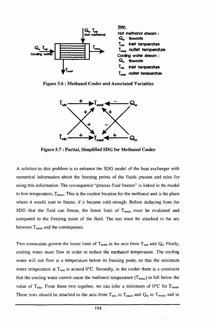
Q", Too. ()IDI mro .. lIilthc .. nllA>oO
T.
T ....
~ Hot methanol stream : Q", fIawJaIe
Too. hIet fen1;leraIIn T.... outlet temperoture
CooIklg water stream : Q,. fIawJaIe
T.... hIet fen1;leraIIn
T_ outIat~
Figure 5.6: Methanol Cooler and Associated Variables
Figure 5.7: Partial, Simplified SDG for Methanol Cooler
A solution to this problem is to enhance the SDG model of the heat exchanger with
numerical information about the freezing points of the fluids present and rules for
using this information. The consequence "process fluid freezes" is linked in the model
to low temperature, T mOll" This is the coolest location for the methanol and is the place
where it would start to freeze, if it became cold enough. Before deducing from the
SDG that the fluid can freeze, the lower limit of T mOllt must be evaluated and
compared to the freezing point of the fluid. The test must be attached to the arc
between T mOllt and the consequence.
Two constraints govern the lower limit of T mOllt in the arcs from Twin and Qw. Firstly,
cooling water must flow in order to reduce the methanol temperature. The cooling
water will not flow at a temperature below its freezing point, so that the minimum
water temperature at Twin is around O°C. Secondly, in the cooler there is a constraint
that the cooling water cannot cause the methanol temperature (T moUl) to fall below the
value of Twin. From these two together, we can infer a minimum of ooe for T mOllt.
These tests should be attached to the arcs from Twin to Tlllollt and Qw to T mOll" and in
194
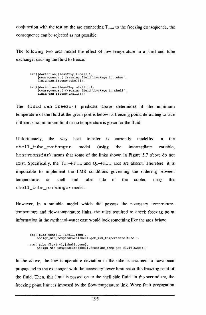
conjunction with the test on the arc connecting T moUl to the freezing consequence, the
consequence can be rejected as not possible.
The following two arcs model the effect of low temperature In a shell and tube
exchanger causing the fluid to freeze:
arc«(deviation. [leSSTemp,tube]],l, [consequence, ['freezing fluid blockage in tubes', fluid_can_freeze(tube)]]),
arc«(deviation. [lessTemp,shell] 1,1, (consequence, ['freezing fluid blockage in shell', fluid_can_freeze(shell) 1])
The fluid_can_freeze () predicate above determines if the minimum
temperature of the fluid at the given port is below its freezing point, defaulting to true
if there is no minimum limit or no temperature is given for the fluid.
Unfortunately, the way heat transfer IS currently modelled In the
model (using the intermediate variable,
heatTransfer) means that some of the links shown in Figure 5.7 above do not
exist. Specifically, the Twin--7T mout and Qw--7T mout arcs are absent. Therefore, it is
impossible to implement the FMS conditions governing the ordering between
temperatures on shell and tube side of the cooler,
shell_tube_exchanger model.
using the
However, in a suitable model which did possess the necessary temperature
temperature and flow-temperature links, the rules required to check freezing point
information in the methanol-water case would look something like the arcs below:
arc([tube,temp1,1, [shell,temp). assign_rnin_temperature (shell,get_min_temperature (tube) 1.
arc«(tube,flow),-l, [shell,temp], assign_min_temperature(shell,freezing_temp(get_fluid(tube»)
In the above, the low temperature deviation in the tube is assumed to have been
propagated to the exchanger with the necessary lower limit set at the freezing point of
the fluid. Then, this limit is passed on to the shell-side fluid. In the second arc, the
freezing point limit is imposed by the flow-temperature link. When fault propagation
195
considers the freezing consequences for the shell-side (containing methanol), it
discovers that the limit temperature for the shell-side fluid does not allow it to freeze,
in the case of the methanol-water system. The ability of AutoHAZID to reject
infeasible scenarios in such a plant has been demonstrated using a modified heat
exchanger model.
5.3.5 Example 5 : Pressure Limits due to Vapour-Liquid Equilibrium
In a vessel containing liquid and vapour at the same time, there will be an equilibrium
between the two fluids. If there are no inert gases present in the vapour space the
pressure will be the vapour pressure of the liquid at the fluid temperature. In this case,
one can detennine limits on the pressure deviations expected for the vessel, resulting
from deviations in the temperature of the liquid, if the temperature variations can be
estimated.
The crucial condition for application of this limit calculation (for the upper limit of
pressure) is that there should not be an appreciable partial pressure of inert gas in the
vessel. Therefore, where nitrogen blanketing is used to maintain a non-flammable
atmosphere, the calculation of vapour pressure is not so helpful, as the pressure of the
nitrogen must be taken into account. Where inerts are effectively excluded, as may be
the case in distillation, then the vapour pressure may be used.
196
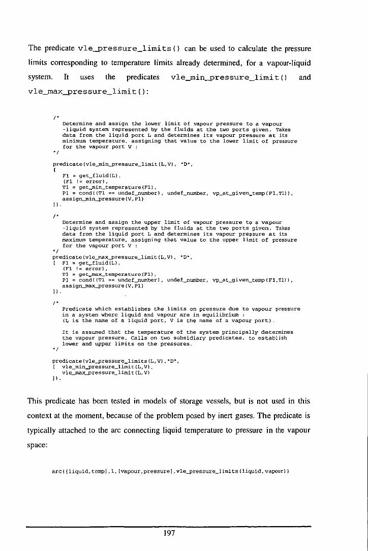
The predicate vle~ressure_limits () can be used to calculate the pressure
limits corresponding to temperature limits already determined, for a vapour-liquid
system. It uses the predicates and
"
"
Determine and assign the lower limit of vapour pressure to a vapour -liquid system represented by the fluids at the two ports given. Takes data from the liquid port L and determines its vapour pressure at its minimum temperature, assigning that value to the lower limit of pressure for the vapour port V :
predicate (vle_min-pressure_lirnit(L,V), -0·, (
11.
"
"
Fl = get_fluid(L), (Fl ! = error). Tl = get~in_temperature(Fl), PI = cond«Tl == undef_numberl, unde£_nurnber, vp_at_given_ternp(Fl,Tl», assign_min-pressure(V,Pl)
Determine and assign the upper limit of vapour pressure to a vapour -liquid system represented by the fluids at the two ports given. Takes data from the liquid port L and determines its vapour pressure at its maximum temperature, assigning that value to the upper limit of pressure for the vapour port V :
predicate (vle_max-pressure_limit(L,V), -D-, [ FI = get_fluid(L),
11.
"
"
(Fl ! = error), Tl = get_ffiax_ternperaturc(Fl), PI = cond«Tl == undef_number), undef_number, vp_at_given_temp(FI,Tl», assign_max-pressure(V,Pl)
Predicate which establishes the limits on pressure due to vapour pressure in a system where liquid and vapour are in equilibrium : (L is the name of a liquid port, V is the name of a vapour port) .
It is assumed that the temperature of the system principally determines the vapour pressure. Calls on two subsidiary predicates, to establish lower and upper limits on the pressures.
predicate (vle-pressure_limits (L,V) ,"D-, [ vle_min-pressure_limit(L,V),
vle_ma~ressure_Iimit{L,V)
11.
This predicate has been tested in models of storage vessels, but is not used in this
context at the moment, because of the problem posed by inert gases. The predicate is
typically attached to the arc connecting liquid temperature to pressure in the vapour
space:
arc({liquid,temp],l, [vapour,pressure],vle-pressure_limits(liquid,vapour)
197
5.3.6 Managing Propagation of Information about Numerical Limits
As described above, infonnation detennining the limits on deviations is typically
generated at one point in the plant, but may be used quite remotely, at a distant
consequence, for example. It is vital that a coherent method is used to manage the
propagation of this infonnation, so that limits are not propagated to inappropriate
places. Also, a workable strategy is required for dealing with cases where limit
infonnation is needed by a predicate, but is not available.
Where limits on variable deviations are requested but not available, the default
behaviour should be to allow the condition on the arc or consequence concerned to
succeed. The functions which access limit values of pressures, temperatures and
compositions have been designed to return the value undef_number where the
limit is not known, so that functions or predicates can detect this value. Absence of
limit infonnation is taken to imply that the deviation being considered is "unlimited",
so that it should be assumed to be severe enough to cause any consequence it is linked
to in the SDG.
Propagation of numerical limit infonnation is at present limited to two simple rules
for pressure and temperature deviations. These are:
I. Limits infonnation is propagated forwards in arcs linking pressure to pressure or
temperature to temperature.
2. Limits infonnation is discarded when propagating to pressure or temperature from
any other variable.
In due course, other rules could be developed to deal with other propagation variables
(e.g. composition). The fluidisation heuristics mentioned in Section 5.2.2 are a
possible source of guidance for this venture, although the correctness of rules needs to
be assured within the system.
198
5.4 Conclusions
This chapter has described the basics of the fluid modelling system in AutoHAZID.
On the whole, it seems that predicate conditions and fault path validation are good,
general-purpose techniques for improving the SDO models. The model of SDO
conditionality offered in the FMS is one that is suitably general to tackle a very large
range of problems. What's more, as time goes on, there are fewer cases where new
predicates need to be defined in terms of internal C++ functions (requiring program
recompilation) and more cases where the new predicates can be defined in terms of
already defined operations. This is an indication that the basic machinery is now in
place to deliver big improvements to the models in AutoHAZID.
Many of the tests implemented in the FMS so far have had an impact by reducing the
number of spurious results produced by AutoHAZID. This means that their
contribution is, in some senses, an invisible one - they contribute to making the
overall results more correct by controlling what is left out of the final HAZOP report.
This development has been dictated by the need to remove obviously wrong hazards
from the results during STOPHAZ, to attain a basic level of performance in
AutoHAZID. In future, however, there should be more emphasis on the enrichment of
models to include new, more interesting faults and consequences. If this is supported
by the FMS, the quality of the HAZOP results can be maintained.
Clearly, the system is still in development, and some aspects of the fault path
validation technique are still relatively primitive. The various rules, conventions and
methods used for limit propagation are an example area where there is still much work
to be done. I think that the most practical way to formulate these methods and
conventions is by tackling real problems using the system as it is - this will identify to
the developer where the weaknesses lie and how one may tackle them.
The approach used in the development of the FMS, of applying conditions to highly
specific faults and consequences, seems to be well-justified, given the need for richer
and more interesting scenarios to be identified in HAZOP emulation. This approach is
one of the more important ideas behind the Fluid Modelling System. The other
199
important or novel ideas in the work described here include the use of fault path
validation and the propagation of fluid information through the plant model from data
given in the input plant description.
The most interesting application of the FMS so far has been in the processing and
propagation of limit information to verify propagation of deviations. This is probably
one of the smartest prospective solutions to the problem of increasing the value of
individual scenarios in the HAZOP report. It also uses methods which can be
compared to the sort of na"ive reasoning which might be used by participants in a
conventional HAZOP.
The limits processing system in the FMS is still in a very early stage of development,
and may need to be redesigned at some later date, in addition to the need to widen the
scope of deviations treated to include (at least) composition. There are many areas like ....
this within the AutoHAZID program and the FMS. Some of the possible areas for
future improvement are mentioned in the next chapter, which discusses the thesis and
the work on AutoHAZID as a whole.
200

Chapter 6 . Discussion and Future Work
This chapter discusses some of the issues raised by the preceding chapters and looks
to possible future areas of work on AutoHAZID, and on hazard identification by
computer more generally. The objective is also to record some thoughts about the
subject which did not fit into the framework of the rest of the thesis.
First of all, a brief review is given of the strengths and weaknesses of AutoHAZID
and the HAZID package, in Section 6.1. Then, Section 6.2 gives an overview of the
main areas considered for future work, some of which are discussed at more length in
Sections 6.3 to 6.9. Section 6. \0 concludes the chapter with a recap of the topics
covered.
6.1 Strengths and Weaknesses of HAZID
Some of the strengths of the HAZID package (including AutoHAZID as its central
component), in comparison to other groups working on similar areas, are:
• Inclusion of a wide range of techniques related to hazard identification, in an
integrated software environment. Examples include the fluid compatibility checks,
the HAZOP emulation algorithm, fluid model system, consequence ranking, etc.
No similar software package (as far as I am aware) tackles such a wide range of
safety·related tasks.
• The large, hierarchically organised library of equipment models, which covers a
wide variety of failure modes and a large number of equipment types. None of the
other groups reviewed in Chapter 2 have attempted to model this range of
equipment.
• The modular modelling approach usmg templates is quite novel, and allows
repeated features of diverse models to be described concisely. This makes
maintaining consistency in existing models easier and allows rapid prototyping of
new models.
201
• A "Model Generation Tool" (MGT) for developing new, user-defined equipment
models. This makes extensive use of templates, building whole models of vessels
from components taken from the template library.
• Use of a "Fluid Modelling System" (FMS) to distinguish between feasible and
infeasible scenarios. The rule-based system used to validate conditions on faults,
consequences and propagation arcs is, as far as I know, unique in this field. I
• A promising prototype system within the FMS for handling numerical limits on
propagated deviations of (so far) pressure and temperature. The aim of this system
is to validate whether the deviations in a fault path are sufficient to cause the final
consequence with which they are associated. Since this is a very novel approach
within HAZOP emulation, I have not had time to develop the system completely.
• Ability of the system to model single mapping influences, using a new type of
extension to the SDG, as discussed in Section 4.2. This method for extending the
models was developed by myself and Dr. Rushton in response to problems
recognised in HAZOP emulation results.
• Two-stage, breadth-first graph search algorithm used for identification of fault
paths in the SDG. I developed the two-stage approach to prevent repetition in
searching the graph.
• Compatibility checks between fluids which mix In the plant, to detect possible
interactions and problems.
• Fully integrated access to physical properties data in the FMS, using external
calculation packages, internally stored fluid data and calculations within
AutoHAZID. These provide the numbers required for selective quantitative
assessment of scenarios.
• The Graphical Tool and Database API allow entry of plant descriptions in a
graphical format and their automatic transfer to AutoHAZID for HAZOP.
• A novel classification system has been developed for consequence types and
ranking of consequences.
I It should be noted that conditions have been added to SDO models by other workers (e.g. in the
"extended signed directed graphs" of Oyeleye and Kramer, 1988). However, I believe that the
flexibility of the FMS rule b.<ed system used in AutoHAZID is a unique development in Ihis field.
202

• Demonstration of a small set of "configuration rules", which detect design faults in
the plant model and warn the user about them. While the rules are fairly
elementary, their automation is probably quite new.
• Consideration of protections in the plant.
Some of the weaknesses in HAZID are:
• Input of the plant model into HAZID can be a problem, and will affect the future
acceptance of the tool by industry. This problem is discussed in Section 6.3.
• The equipment models are not all at the same level of development or validation,
so that some of the newer ideas, particularly in the FMS, have not been uniformly
implemented in the models.
• Hazards still sometimes don't appear where expected in the AutoHAZID output,
according to human experts in HAZOP.
• The efficiency of the program, in terms of slow execution speed or excessive
memory requirements during graph search, remains a problem for large plant
models.
• Many identified rules, models and scenarios have not been added to the libraries
so far, due to time limitations or difficulties with knowledge representation.
• Qualitative ambiguity and computational complexity can be problems, as
discussed in Chapter 4.
• AutoHAZID is not capable of modelling state-dependent plant behaviour, or
temporal sequences of events, so that its ability to tackle batch plants, or abnormal
states of continuous ones, is quite limited. This problem is discussed in
Section 6.5.
• The single fault assumption, as discussed in Section 4.3, limits AutoHAZID to
considering a limited range of possible scenarios (those with a simple, linear
development sequence). However, it should be noted that this is actually how
HAZOP is usually carried out, so the HAZOP emulation method is sound in this
respect.
203
• Recursive calls between functions and predicates in the FMS are not prevented at
the moment. This could give rise to problems of infinite recursion in FMS
calculations, at some future stage.
• Debugging and testing of functions and predicates In the FMS is difficult at
present, because there is no debugging utility.
• Comparing HAZOP results files for the same plant model, to find differences,
must be done by eye, which is a tedious and error-prone procedure.
6.2 Future Work
This section briefly mentions some possible areas of work to improve HAZOP
emulation. Some items tackle the problems identified above. Others extend the
functions of HAZID to cover activities previously seen as out of scope for the tool. A
few topics are discussed in greater depth in the sections following this one.
Some of the future work items are quite trivial changes and are outlined in
Appendix G. In addition to these "trivial" changes to the existing system, a number of
larger pieces of work were not completed during the project due to time limits:
• The equipment and template models in the HAZID libraries are not all at the same
level of development. For industrial acceptance of a HAZOP emulation tool,
consistent levels of performance have to be produced, so quality assurance of the
expertise present in models is very important. Therefore, the equipment models
must be examined to determine a core of functionality which can be expected of
everyone of them. Then, in a second sweep, the models can be systematically
upgraded so that they all meet the minimum requirement. Using this method will
ensure that the new features which have been selectively added to some models
during a "test" phase get disseminated to all other appropriate models in the
library. It will also help to document the features of the package and to locate
areas for improvement, new rules to add, etc.
• A large quantity of information, comment and expertise was collected from
process industry users during the STOPHAZ project (STOPHAZ, 1997a). In
addition to the feedback on test cases, output from modelling seminars and other
204
information collected during the development of HAZID, two other parts of
STOPHAZ produced results. CHOPIN investigated how to improve the
development of operating instructions prior to HAZOP. ELDER was developed as
a hypertext resource, containing safety-related design advice for engineers to use
when developing process designs from PFD to P&ID stage. Systematic use should
be made of these information sources, to enrich models by adding new failure
modes, for example.
• Related to the previous point, wider use should be made of the fluid modelling
system, using quantitative rules and landmark values, etc. for fault path validation.
The integrated links to the properties packages should also be fully utilised.
• Further use should be made of flags and filters to improve the way the results of
HAZOP emulation are presented.
• In principle, any weaknesses in templates, equipment models and FMS rules
should be tackled by a systematic methodology for model improvement. This area
of development is discussed in Section 6.4.
• To move HAZID forward to market, success must be demonstrated with a very
large plant model, if possible a "live" example of an industrial plant design.
Program efficiency is less an issue here than the quality of output produced,
compared to conventional HAZOP studies carried out on the same plant. The
range of equipment in the model libraries would need to be widened as a result of
the trial. Issues of information management in evaluating a large plant design have
not been explored within STOPHAZ, so these will probably be discovered in such
a trial.
• So far, the links to external physical properties packages have been demonstrated,
in practice, for only a subset of the functions specified in the link to ASP~N
Properties Plus. It would be good to demonstrate access to the full range of
calculations in HYSYS as well as Properties Plus, to show the generality of this
particular part of HAZID. Work on this would consist of debugging some
problems in the interface between the external packages and AutoHAZID.
Clearly, progress in the above work areas would significantly improve the
performance of HAZOP emulation across the board. By encoding a broader range of
205

expertise In models developed to a consistent depth, the quality of output from
HAZID can be made far more consistent.
The next group of future work topics require quite significant effort, in software
design and analysis. Some of these involve optimising the user interfaces to the
software tools in HAZID, as well as encouraging closer integration and further
development of the functions demonstrated as "proof of concept" in STOPHAZ:
• AutoHAZID itself is largely text-based in the current version of HAZID. While
there is nothing inherently wrong about this, some parts of the user interface could
be improved, and it is natural nowadays to expect a graphical user interface (GUn
to any commercial software package. Therefore, the user interface of HAZID
should be redesigned, with a view to optimising the input of plant data, user
interaction with the HAZOP emulator, and viewing output reports.
• A properly designed graphical interface to the model generation tool (MGT)
would also help, by reducing the repetition of user input typical in the question
and answer session carried out at present. The MGT should also be integrated with
the design of icons for the Graphical Tool and tools to define the attribute data of
new units for storage in the Database APl. In short, a fully-fledged model
development workbench should be developed.
• The Graphical Tool GUI should be redesigned, to make it easIer to specify
properties of fluids, component chemicals, etc.
• In entering models into the MGT or other model development tool, it would be
helpful to be able to use different representations, to suit the user's past
experience. Functional equations, SDG arcs and truth tables are examples of
qualitative representations that are equivalent, and so could be used as alternative
input formats for models.
• Redevelopment of the interface to HAZID should be carried out in conjunction
with a critical appraisal of the features to be implemented in the tool, and a more
object-oriented reimplementation of the system. Clearly, many "expert" features of
the STOPHAZ prototypes were put in as proof of concept only. There needs to be
a full functional specification for any features developed to a commercial stage.
206
• In the longer term, HAZID may form part of an integrated safety software
environment, combining tools for maintaining checklists, emulating FMEA,
HAZOP, sneak analysis, performing routine calculations for water hammer, vent
sizing, etc. The experience gained so far in integrating the parts of HAZID would
be quite valuable in building such an over-arching system.
A number of new features could be added to HAZID, to extend its functionality
beyond HAZOP, or to support the HAZOP emulation done at present:
• A debugging environment for AutoHAZID and the FMS, to allow the developer of
new equipment models, functions and predicates to test these without having to
construct demonstration plant models and do HAZOPs on these.
• Preliminary check of the plant design to detect the unwanted reactions and
inherent problems in the plant, before HAZOP emulation. The check could take
place when the plant model is fluidised, to examine every case where fluids are
detected to be mixing.
• Preliminary checks to identify sneak flows, where fluids may be unintentionally
discharged through vents or drains due to errors in plant operation, for instance.
• In addition to the tabular report produced during HAZOP emulation, HAZID
should also produce a concise summary of equipment and fluids in the plant. This
summary would remind the user of the plant structure and likely resident hazards.
• The interface to HAZID could be changed, so that it operates as an interactive
browser for fault paths, instead of a "batch mode" HAZOP emulator, as mentioned
in Section 4.7.
• A utility is required, so that results sets can be compared, to quickly identify
differences between HAZOP reports. This requires a way of saving results in files
so that the fault-deviation-consequence structure is retained. Such a file format
would also help in developing other means of presenting results.
• Selective quantitative simulation could be considered for certain hazardous
scenarios, to validate their feasibility or to estimate the seriousness of
consequences. Such an approach may use f10wsheeting packages, or implement
the sort of mathematical programming simulation described by Purdue.
207
• Links to external HAZAN software and selective hazard analysis could also be
considered, possibly making use of fault tree analysis to estimate the likelihood
and magnitude of identified hazards.
• Non-process propagation of faults can be important in escalation of faults, as
discussed in Section 6.6. Some effort should therefore be spent examining how to
model the human factors issues inherent in operating procedures, as well as the
escalation of scenarios by the "domino effect".
The varIOUS rule-based systems contained within AutoHAZID should also be
improved or re-examined in future work:
• During plant fluidisation, when a pump is encountered, the program does not
check that a discharge pressure is given. If no value is given, the inlet pressure
value is propagated straight through the unit. The same is true for temperatures in
heat exchangers. A similar policy is used when propagating limit infonnation on
pressures and temperatures, which may not be entirely safe. There should be a
warning for these conditions, instead of the program silently propagating values
through the unit. These problems are due to the fact that the models do not define
the function of equipment items. One idea which may be useful is that of "fluid
breakpoints", as mentioned in Paper 9 of McCoy et al. A breakpoint is a point
where a stream undergoes some sort of change, such as a change in pressure,
temperature or composition. The concept of breakpoints, defined for certain
variables in the model of the equipment, may be a good way of representing those
variables whose values should be specified in the plant model. For example, a
pump is designed to raise pressure, so that its outlet is a breakpoint for pressure.
The aim of HAZOP is to examine the causes of deviation from intended operation.
If full equipment specification data is represented in equipment models, HAZOP
emulation can be extended to consider more than just deviation of process
variables.
• In the fluidisation routine, the fluid rule #1 does not include a check for
conflicting information where a number of output ports are attached to the same
internal port (e.g. where two different outlet temperatures are given for outlets
from the same chamber of a vessel). It just finds the first output port that has data
208
which can be transferred and propagates this data. There should be a check for
such conflicts in the input data, possibly before any fluidisation or application of
fluid rule # I.
• The set of rules given in Section 5.3.6, used to propagate information about the
limits of deviations, should be expanded. In particular, these rules should be
extended to cover other variables (such as composition), as well as pressure and
temperature, which are the only deviations whose limits are monitored so far.
• An ad hoc rule has been used to decide ambiguous causal influences operating in a
feedback loop, as outlined in Section 4.10, so that the shortest path is not always
used to determine the fault paths in these parts of the graph. The need for such
rules should be reviewed, with a view to justifying the approach theoretically, or
doing something more general to prevent incorrect fault paths propagating through
loops. The issues of loops and other topological features of the plant and the SDG,
are discussed further in Section 6.7.
• Similarly, an ad hoc rule is used to disallow reverse flow propagation in faulty
units, as described in Section 4.3. The issue of how to control reasoning through
unhealthy units should be examined in detail, as these sorts of problems are likely
to be quite common.
• The set of configuration rules, for detecting design faults in the plant model, could
be extended in the future. These sort of rules are useful, but are not best reported
in a HAZOP report format - a separate section of the HAZID report should be
devoted to such problems detected in the plant.
Some other possible areas of future work include:
• The model of fault propagation used in HAZOP emulation can be extended to
include the idea of generic faults and consequences, as described in Section 6.8.
• The HAZOP algorithm should be optimised, to reduce the number of repeat
validation checks carried out during fault path generation. As outlined in
Section 6.9, a new object class for fault paths is needed, to allow the results of
fault path validation (current fluids, deviation limits, etc.) to be stored with the
fault path.
209
• Another area for optimisation is the use of graph pruning. By removing parts of
the SOO which are not required, the speed of search could be increased.
• The treatment of chemical interactions and reactions, whether intended reactions
or not, should be improved, and this facility should be more widely used in
equipment models.
• Reverse propagation of temperature and concentration deviations, under
conditions where reverse flow is occurring, should be modelled, The sort of
scenario where reverse flow takes hot material to an upstream location, causing a
problem related to high Temp, rather than revFlow, has never been satisfactorily
treated in AutoHAZID so far. It might be possible to deal with this by propagating
composition and temperature values upstream in revFlow propagation chains, so
long as a link from revFlow to temp (or composition) is made in the upstream
model.
• The representation of instrument systems and protective devices In the plant
model should be improved.
• Consider abandoning the shortest path heuristic for graph search, accepting that
multiple paths will be generated. The relevance of competing fault paths could be
determined by comparing the strength of their causal links in some way, as
discussed in Section 4.10.
• The single fault assumption, as discussed in Section 4.3, should be challenged,
with a view to modelling more complex scenarios than is now possible with
AutoHAZID.
• The process-based approach to qualitative modelling, as used by Forbus
(Section 2.2.4) and the group at Pennsylvania (Section 2.3.4) should be revisited.
The main problem with this approach was perceived to be computational
complexity, which it may be possible to avoid by careful formulation of the
models and the inference methods used on them. Certainly, the power of a system
capable of representing phenomena in a plant, and reasoning about changes in
their activation over time, is worth having. The histories idea of Hayes (1979),
discussed in Section 2.2.3, could be useful in taming the complexity problems in
this type of model.
210
• Potentially the biggest improvement to the equipment modelling system would be
to introduce a representation capable of handling landmark values and state
dependent behaviour, if possible including temporal reasoning within fault paths.
With such capability, modelling the plant in off-normal or alternative operational
states (start-up, shutdown, maintenance, batch, etc.) would be possible. This type
of improvement is discussed in Section 6.S.
6.3 Access to Plant Descriptions
One of the most critical success factors for a commercial HAZOP emulator will be
ease of use, in respect of the input and output interfaces. Because the tool is intended
to support hazard identification, potentially at a late design stage, one cannot expect
users to struggle with a difficult interface to access the benefits of HAZOP emulation.
The effort required to input plant descriptions to HAZID is quite considerable at
present, especially for larger plants. This problem has been improved significantly
during the STOPHAZ project using the "intelligent CAD" interface of the Graphical
Tool, developed by TXT. Nevertheless, if any re-typing or re-entering of plant details
is needed, the input task quickly becomes unviable for larger plants.
User compames often have a CAD representation of the plant design in some
electronic format already, before a HAZOP emulator is used. The ideal situation
would be where a representation of the plant P&IDs can be read into HAZID, possibly
via some neutral file format. This requires that there is some "intelligent CAD"
system in place, so that the equipment items in the plant correspond to objects on the
drawing. Otherwise, one has to consider how to recognise the plant components from
the line segments and arcs used to draw them.
The main problem at present and into the near future is likely to be the proliferation of
non-standard file formats for structured CAD data, where each format is proprietary to
a particular CAD program. Communication between diverse software packages is the
aim of the initiative known as STEP. Ultimately, STEP-compliant file formats will be
defined for the exchange of process plant information, so that any program able to
211

read in and write out data in STEP format will be able to communicate with a large
number of other programs with the same capability. So far, STEP has not been
developed to this stage, so "seamless data exchange" between software is still some
way off.
Future work in developing HAZID should investigate the options for intelligent CAD
on the market, and look at the possibility of automatic transfer of P&IDs from the
CAD system to HAZID. It is important to make sure that the effort of building such
interface software is well spent - the file format considered must be technically
capable of transferring the required data into HAZID and the associated CAD
package(s) must be widely used in industry. Proof of the viability of HAZID on
industrial scale plant designs would greatly improve its long-term prospects of
success.
An alternative strategy is to shift the focus of automatic hazard identification to an
earlier stage of design, namely flowsheeting. At this stage, the user is likely to be
using a graphical interface to a flowsheeting package for sorting out the overall mass
and heat flows in the plant. Therefore, much of the basic process information is
available at this stage, such as the main unit operations and materials involved,
together with flowrates, temperatures and pressures. Clearly, transfer of electronic
information is still an issue, but the level of detail is less with this option, and re
entering the flowsheet may be less of a headache. As discussed in Section 4.8, the
current HAZID models are not suitable for analysis of flowsheets, but it may be
worthwhile developing a new set - advantages include early hazard identification and
a reduced volume of results for the user to look through.
6.4 Methodology Issues in Unit and Fluid Modelling Systems
To encourage the development of a range of models whose quality is assured to be of
a certain level, a procedure should be set up to govern how models are created,
maintained and documented. Following the procedure should ensure that a minimum
level of competence is achieved in the models produced. This section addresses some
212
issues related to such a modelling methodology, from a general point of view, rather
than with reference to AutoHAZID.
Methodology has been mentioned before now, in Section 3.5, where the development
of the flow path template model was used to illustrate a method for development and
documentation of new models. Section 6.4.1 offers a view of the general modelling
process, which can be used as the basis of developing models in the way illustrated by
Section 3.5. Section 6.4.2 gives guidelines for the sort of documentation that should
be provided by the model designer, so that the new model is comprehensible to other
workers, who may need to modify it at a later stage. Section 6.4.3 looks at how
pointers for model improvement can be identified, and is therefore quite strongly
linked to Section 3.5.7, which discussed the knowledge elicitation techniques used in
STOPHAZ.
Additional possible sources of information for model development include the
following, which were not used systematically during the development of HAZID:
• Characteristic failure modes of equipment, as identified by other techniques, such
asFMEA.
• Codes and Standards for best practice design.
• The advice in the STOPHAZ ELDER tool, which was designed as a repository of
information about safe design.
• Other sources, such as standardised incident reports, could be used. These often
include analyses of the causal principles behind accidents, and are therefore useful
for identifying the mechanism of the incident. A good example of this type of
expertise is the Accident Database package published by the Institution of
Chemical Engineers (1997).
In addition to the advice offered here, Paper 9 of McCoy et al. (\ 998) contains some
suggestions for methodologies to be followed in processing HAZOP results into
formal qualitative equipment models. Such methods are needed to make the best use
of information from modelling seminars and other meetings, where experts are
questioned about the expertise they use in hazard identification.
213
6.4.1 A General Approach to Model Building
This subsection presents a general view of the process of building fonnal models of
equipment or phenomena. Although the emphasis during development of this
methodology has been on qualitative models for HAZOP emulation, there is no reason
why such an approach could not also be used for other types of model or application.
The aim of the methodology is to build robust and maintainable models, in which all
assumptions, restrictions and dependencies are clearly stated.
The view of the modelling process adopted here is presented in Figure 6.1, where the
equipment or phenomenon model is a formal representation which can be manipulated
using mathematical or other symbolic means. The model must represent some portion
of the real world in such a way that the behaviour predicted by the model, when used
in simulation, is similar to that which would be observed in reality.
The designer determines the development of the model, as illustrated schematically in
Figure 6.1. The first task is to define a "system boundary" around that part of the real
world which is to be modelled, effectively cutting off the "system" from the rest of the
world. This is shown as a process of "restriction", and determines the scope of the
model's applicability.
The next step is for the designer to form an understanding of the functioning of the
system. This can be seen as a process of "abstraction", producing an "internal mental
model" in the designer's head. It can be very useful if the designer writes down what
they understand about the system at this stage, even if it is not possible to state this
very precisely, as this can be used as the basis of a later structured investigation of the
problem.
The process of "formalisation" consists of translating as much as possible of the
internal mental model into the formal language of the model system. The formal
model so produced can then be used in simulation and any weaknesses of the model
214
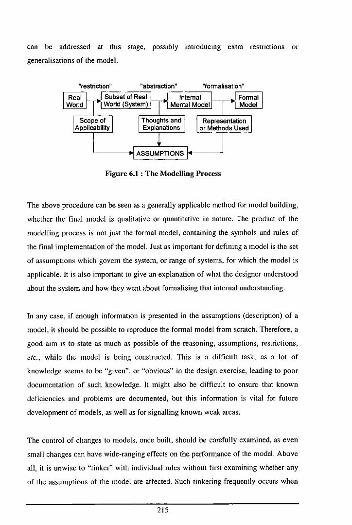
can be addressed at this stage, possibly introducing extra restrictions or
generalisations of the model.
"restriction" "abstraction" ''formalisation''
'-----.I ASSUMPTIONS 14----'
Figure 6,1 : The Modelling Process
The above procedure can be seen as a generally applicable method for model building,
whether the final model is qualitative or quantitative in nature. The product of the
modelling process is not just the formal model, containing the symbols and rules of
the final implementation of the model. Just as important for defining a model is the set
of assumptions which govern the system, or range of systems, for which the model is
applicable. It is also important to give an explanation of what the designer understood
about the system and how they went about formalising that internal understanding.
In any case, if enough information is presented in the assumptions (description) of a
model, it should be possible to reproduce the formal model from scratch. Therefore, a
good aim is to state as much as possible of the reasoning, assumptions, restrictions,
etc., while the model is being constructed. This is a difficult task, as a lot of
knowledge seems to be "given", or "obvious" in the design exercise, leading to poor
documentation of such knowledge. It might also be difficult to ensure that known
deficiencies and problems are documented, but this information is vital for future
development of models, as well as for signalling known weak areas.
The control of changes to models, once built, should be carefully examined, as even
small changes can have wide-ranging effects on the performance of the model. Above
all, it is unwise to "tinker" with individual rules without first examining whether any
of the assumptions of the model are affected. Such tinkering frequently occurs when
215

there are small problems with the results produced by the model and there is a
temptation to go in and do a "quick fix".
The process of model development as described conceptually above does not address
the question of how to get started on a particular problem. Typically the brief for a
problem may be as complex or ill-defined as "model flow and pressure propagation in
a chemical plant" (see Section 3.5). When given an open-ended problem like this, the
best approach is to target a single fairly well-defined system which captures the most
commonly observed types of behaviour in the problem area. This target definition is
an activity in the "restriction" part of Figure 6.1, and gives rise to a number of scope
limiting assumptions, which should be documented at this stage.
By concentrating attention on a well-understood instance of the phenomenon or item
which needs to be modelled, the models will more likely be correct and well
populated by known assumptions, and will hopefully be re-usable in a wide variety of
situations. This approach should also prove economical in quickly producing models
to be used as "base models" for further development. Such development is made by
varying the assumptions used in a base model, so that the new model becomes either
more general, or applicable to a different problem area. Clear statement of model
assumptions is vital for this process.
The ultimate goal (in developing from a base model) might be elimination of
restricting assumptions, giving a fully general model for the phenomenon being
studied, but it need not be. Some of the "base" assumptions in a model may be harder
to eliminate than others. Whereas some assumptions are made for the sake of agreeing
conventions for the models, others may be made to render the problem tractable or
understandable, and so could be more closely tied to the nature of the model itself. An
example of the latter might be the assumption, in the flow path model developed in
Section 3.5, that no work is done on the fluid in the flow path. It is much more
complicated to model a fluid where shaft work is involved, than in the simple flow
path model.
216

6.4.2 Unit Model Documentation
For a knowledge-based system to be acceptable to industry, all models need to be
developed to a consistent level, and the assumptions made during this modelling must
be documented. As a minimum standard of documentation, the following types of
information should be provided, where appropriate, for any template or equipment
model:
• SCOPE OF MODEL
• Give the common name of the entity to be modelled and a basic description of
its function(s).
• State any known subtypes of the entity modelled, and indicate whether they are
modelled.
• State any known entities which the modelled entity is a subtype of.
• Give some impression of how general/specific the model is.
• Describe the known internal features/subcomponents of the real object and
state if they are modelled/not modelled.
• State any other features known but not modelled.
• Define how connections are made to other models.
• Describe the context/applicability of the model.
• DESCRIPTION OF MODEL
• Give details of the component parts of the model:
• Ports, for connection to other units, or for definition of internal locations.
• Chambers, as separate spaces within the equipment.
• Other structures (packing, etc.).
• Fluids present, where these can be stated without presupposing the context
of the model in a plant.
• Materials of construction, if appropriate.
• Phenomena operating within the model.
• What variables are relevant to the model.
• Connections between parts of the model, and to other modelled entities:
• Internally, between ports.
217
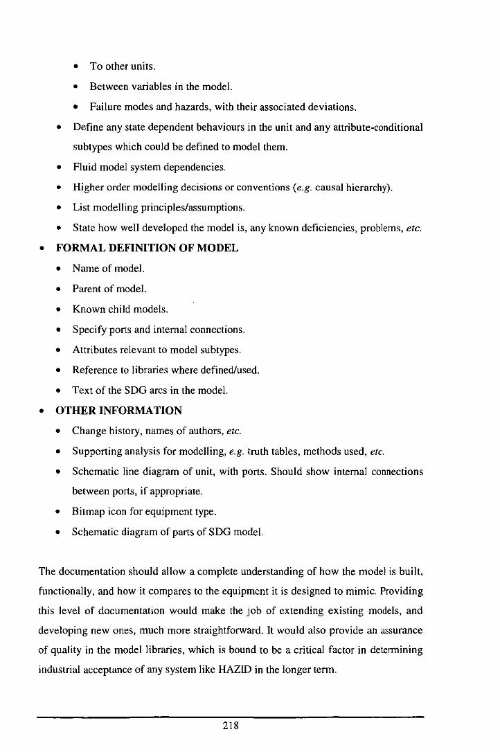
•
•
• To other units.
• Between variables in the model.
• Failure modes and hazards, with their associated deviations.
• Define any state dependent behaviours in the unit and any attribute-conditional
subtypes which could be defined to model them.
• Fluid model system dependencies.
• Higher order modelling decisions or conventions (e.g. causal hierarchy).
• List modelling principles/assumptions.
• State how well developed the model is, any known deficiencies, problems, etc.
FORMAL DEFINITION OF MODEL
• Name of model.
• Parent of model.
• Known child models.
• Specify ports and internal connections.
• Attributes relevant to model sUbtypes.
• Reference to libraries where defined/used.
• Text of the SDG arcs in the model.
OTHER INFORMATION
• Change history, names of authors, etc.
• Supporting analysis for modelling, e.g. truth tables, methods used, etc.
• Schematic line diagram of unit, with ports. Should show internal connections
between ports, if appropriate.
• Bitmap icon for equipment type.
• Schematic diagram of parts of SDG model.
The documentation should allow a complete understanding of how the model is built,
functionally, and how it compares to the equipment it is designed to mimic. Providing
this level of documentation would make the job of extending existing models, and
developing new ones, much more straightforward. It would also provide an assurance
of quality in the model libraries, which is bound to be a critical factor in determining
industrial acceptance of any system like HAZID in the longer term.
218
6.4.3 Improving Model Performance
In the same way that equipment models in the HAZID unit model library benefit from
the use of a sound development methodology, it is important to use sound methods for
identifying, developing and maintaining rules within the FMS. So far, little work has
been done on the methodology of FMS development.
As with unit models, any improvement policy should combine methods to tackle both
"false negatives" and "false positives", with respect to the results of HAZOP
emulation. False negatives are scenarios not present in the results, which should be,
whereas false positives are identified scenarios which are not interesting, or not
feasible.
To enrich the fluid modelling system, so that it represents a wider scope of real
problems (eliminating false negatives), "brainstorming" techniques can be used to
identify candidates for new fluid rules. This approach can be used in addition to the
method of criticising results produced by HAZOP emulation on case study plants. An
example of this sort of "brainstorming" was attempted by myself and Prof. Lees, to try
to identify rules governing limits on pressure and temperature deviations. The minutes
of our meeting are reproduced as Appendix F and can be seen as an information
resource, containing ideas for further development in the FMS.
To tackle the false positives In the HAZOP results, a methodology needs to be
adopted for identifying problem areas and for formulating and implementing solutions
to them. This sort of activity concentrates on criticism of the results of HAZOP
analyses and might include the following elements:
• The starting point is a result (fault-consequence pairing) which does not make
sense in some way. Therefore, this is a "false positive" which should be removed.
• First, the fault path(s) giving rise to the result should be examined carefully, to find
out where the weak or incorrect link is.
• If the fault or consequence is not valid in the specific case identified, an FMS
condition could be added, to restrict the applicability of the item.
219
• If some arc in the path is clearly not a feasible influence in the model, then it
should be removed. However, it is important to determine that the arc is genuinely
incorrect, and wasn't put into the model for some other specific reason.
• Where there is no obviously wrong link, each component of the fault path must be
examined, to see where there is a gap between model and reality. If a weak link can
be identified, this is a candidate position for applying a conditional rule. Identifying
this point requires a good understanding of the hazardous scenario identified. Such
an understanding should be documented, so that the basis for modelling the
scenario is understood at a later date.
• Possible strategies for dealing with the model weakness include use of new or
different variables for propagation, use of single mapping influences, as described
in Section 4.2, or adding propagation conditions to arcs.
• To add new conditions to the arcs in the graph, one must consider what information
is required to decide the new condition and whether that information is present
locally or needs to be propagated somehow. Using fault propagation, faults cause
local effects which may be propagated via deviations to remote locations, where a
susceptibility to some deviation gives rise to a consequence. Maintaining the local
nature of these events embodies the "no function in structure" principle and ensures
that the equipment models developed are usable in many different contexts.
• Once any fluid rule has been created, the rationale for its development should be
documented. Such documentation should include an explanation of the real-world
problem it is designed to solve, as well as the information it uses and any
assumptions it makes about the plant data available in the system.
6.5 Modellinq State-Dependent Behaviour and Temporal Sequences
A very significant improvement to the AutoHAZID modelling system would be to
develop a representation capable of handling landmark values and state-dependent
behaviour, if possible including temporal reasoning within fault paths. With such a
capability, modelling the plant in off-normal or alternative operational states (start-up,
shutdown, maintenance, batch and semi-batch, etc.) would be possible.
220

The references to state-dependent behaviour mentioned in this thesis, which may be of
use when considering how to tackle the subject, are:
• De Kleer and Brown (1984) discuss the issue of state-based models and their
relationship to causal reasoning.
• In the work published by Purdue University, Srinivasan and Venkatasubramanian
(1996) discuss a method for using Petri nets and digraphs for modelling the
progress of a batch processing recipe.
• The work of the group at Pennsylvania University, as reviewed in Section 2.3.4,
illustrates a process-based approach to simulation, which relies on model
rebuilding in response to state changes. It may also provide pointers to the types of
ambiguity and complexity problems to be tackled when building state-dependent
simulators.
There are at least two big issues to tackle within a representation which is to handle
the state-dependent behaviour of plant components. One is the state-dependency issue
- how to represent the fact that parts of the model change when the state changes. The
other is how to detennine what state transitions are possible when simulating the
model behaviour.
The fonner problem can be tackled using rules of the fonn: "if equipment is in state I
then use model_section!", or some equivalent. That is, the use of each different
section of the model would depend on the state the equipment was in. Such a system
could be implemented using the rules of the FMS, by attaching state-dependent
conditions to the relevant SDO arcs in the equipment models.
The latter problem, that of detennining legal state transitions, can be tackled by
defining the applicability of a state transition in a number of ways:
• A state is dependent on a certain variable being within a range, defined by
landmark values of that variable. The state is only valid when the variable is
within the landmark values.
22!
• State transitions may be caused by faults, which effectively change the model of
the equipment item.
• State changes can also be caused by operator actions, such as opening or closing
valves, switching machines on or off, etc.
• Alternatively, no cause can be sought for the state change - it may be assumed to
occur spontaneously, or at least one may not be interested in the cause of it.
In certain cases, the above definitions of state applicability may be muddied by the
possibility that a state transition is not guaranteed by the cause given. A probability
may be associated with a statement like: "if the control valve fails closed, then a
change to state I may be caused". In this case, both possibilities (i.e. change or no
change) should be followed up, and computational complexity becomes a problem if
this sort of "forking" occurs too often.
States should be defined, either in relation to individual equipment items (e.g.
"pumpJ I is running"), or in terms of a certain number of global conditions which may
affect many units in the plant (e.g. "electric power is failed"). Using the latter type of
state-dependence, some types of common-mode failures could be examined, and
systematic "what-if?" studies could be carried out on the plant to see how it would
respond in the event of a power or cooling water failure, for example. The constraints
imposed by operating instructions (or safety interlocks) on the states of valves in the
plant, may also be represented by this sort of global constraint.
It should be noted that allowing some of the above types of state transition to occur,
outside the immediate causal pathway of the fault path being considered, amounts to
relaxing the single fault assumption. The result is that the fault paths are no longer
simple or linear, as before. An example is: "the flow into the tank increases and,
because the level control loop is in manual state, the tank overfills". The operator
leaving a control loop in manual is not an immediate cause of the tank overfill, but is
a plausible state of affairs for the plant when that event is caused by the increased
flow.
222

It is important, therefore, to address the single fault assumption in the context of this
type of state-dependent behaviour. A certain number of state changes may be
plausible, but a large number of independent and coincident events of this nature are
highly unlikely. One might imagine relaxing the single fault assumption slightly, to
allow a limited number of additional state changes in a fault path. The ambiguity
introduced to the SDG by allowing equipment state changes may be tamed using this
sort of method. However, the logic used in arguing that events are independent, and
therefore unlikely to occur together, could be rather difficult to formalise.
The present FMS rule system could, in principle, be used to implement state
dependency in equipment models. A number of attributes would be defined, giving
the states of each equipment item in the plant, and a smaller number of "global states"
for the plant as a whole, as mentioned above. These state attributes would be
accessible by functions of the FMS.
State-dependent parts of models would be expressed with conditions, dependent on
the state attributes, attached to the relevant parts of the SDG model. Some parts of this
"attachment" could be automated, so that the model builder would not have to
explicitly code these "activating conditions" into models. They would be added by the
system in response to the relevant syntax (e.g. defining state-dependent blocks of arcs)
in the model library.
HAZOP search would operate as it does at present, generating fault paths for later
validation by the FMS. Therefore, arcs belonging to all states of the equipment would
be treated as equally valid in the search (this would certainly cause complexity
problems!). Only at the validation stage would infeasible paths be rejected, including
those where the states of equipment were found to be inconsistent with one another.
During validation, legal state transitions would be allowed, as discussed above,
subject to some limit on the number of simultaneous "failure" events. The current
states of equipment items in the fault path (and elsewhere) would have to be recorded
by the FMS as the validation proceeded, in much the same way that "current fluids"
are tracked by the FMS at present.
223
It may be that the suggested solution above (using the FMS) is flawed, and that the
simulation of state-dependent processes requires some new system to be developed. I
feel that the biggest problem, after designing an adequate representation for the state
dependent models, will be the complexity introduced by the state changes in the
system. Finding means to localise the effects of these changes and manage the "single
fault assumption" (or its successor, the "maximum N faults assumption") may be the
key to tackling this problem.
6.6 Non-Process Propagation of Faults
AutoHAZID concentrates on modelling fault propagation using an almost entirely
process-based view of propagation - deviations cause other deviations by virtue of the
interconnection of process equipment via streams between them. "Real World"
propagation of hazards can also occur by other means, due to the other types of
connections present in the plant. Connections between components in the plant can be
viewed as types of constraint in the model. The types of connections/constraints
present in a real plant include the following:
• Process streams connect one equipment item to another. These are well-modelled
at present.
• Signal connections from sensors to controllers to control valves constitute (in part)
the control and protective systems in the plant, which further constrain its
behaviour. Instruments, trips, relief devices and control loops are represented to a
limited extent in AutoHAZID - improvement is possible in this area.
• Physical proximity and spatial layout are often important factors in the escalation
of hazardous scenarios, where the "domino effect" comes into play. An example is
where an explosion in one part of a plant causes a missile to be propelled through
a pipeline, or into a vessel in another part of the plant. The two damaged pieces of
the plant may be entirely unrelated, from a process viewpoint, so that such factors
may be overlooked in a study of the plant design.
• A further level of constraint is that imposed by the operating procedures of the
plant. These "soft constraints" rely on the operators following the instructions and
impose restrictions on the possible states of the plant, defining some of these
224
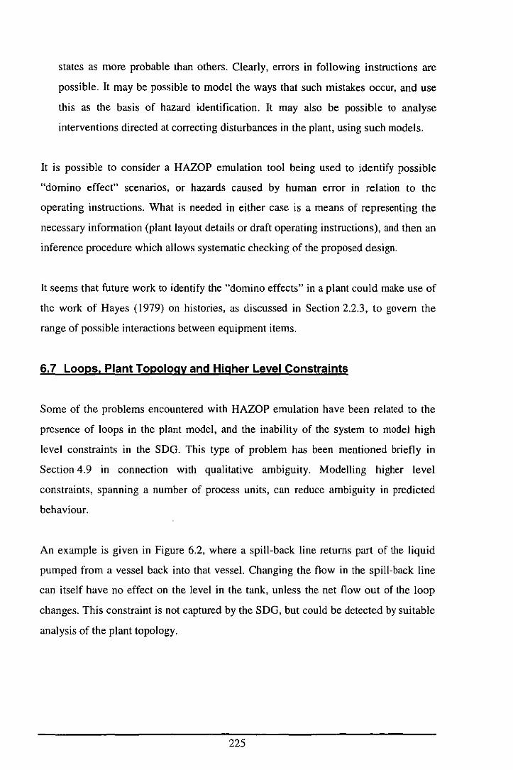
states as more probable than others. Clearly, errors in following instructions are
possible. It may be possible to model the ways that such mistakes occur, and use
this as the basis of hazard identification. It may also be possible to analyse
interventions directed at correcting disturbances in the plant, using such models.
It is possible to consider a HAZOP emulation tool being used to identify possible
"domino effect" scenarios, or hazards caused by human error in relation to the
operating instructions. What is needed in either case is a means of representing the
necessary information (plant layout details or draft operating instructions), and then an
inference procedure which allows systematic checking of the proposed design.
It seems that future work to identify the "domino effects" in a plant could make use of
the work of Hayes (l979) on histories, as discussed in Section 2.2.3, to govern the
range of possible interactions between equipment items.
6.7 Loops, Plant Topology and Higher Level Constraints
Some of the problems encountered with HAZOP emulation have been related to the
presence of loops in the plant model, and the inability of the system to model high
level constraints in the SDG. This type of problem has been mentioned briefly in
Section 4.9 in connection with qualitative ambiguity. Modelling higher level
constraints, spanning a number of process units, can reduce ambiguity in predicted
behaviour.
An example is given in Figure 6.2, where a spill-back line returns part of the liquid
pumped from a vessel back into that vessel. Changing the flow in the spill-back line
can itself have no effect on the level in the tank, unless the net flow out of the loop
changes. This constraint is not captured by the SDG, but could be detected by suitable
analysis of the plant topology.
225
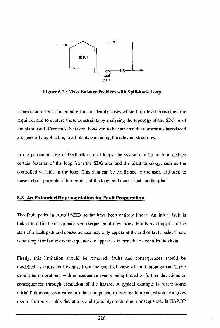
tklOI
plOI
Figure 6.2 : Mass Balance Problem with Spill-back Loop
There should be a concerted effort to identify cases where high level constraints are
required, and to capture those constraints by analysing the topology of the SOG or of
the plant itself. Care must be taken, however, to be sure that the constraints introduced
are generally applicable, in all plants containing the relevant structures.
In the particular case of feedback control loops, the system can be made to deduce
certain features of the loop from the SDG arcs and the plant topology, such as the
controlled variable in the loop. This data can be confirmed to the user, and used to
reason about possible failure modes of the loop, and their effects on the plant.
6.8 An Extended Representation for Fault Propagation
The fault paths in AutoHAZID so far have been entirely linear. An initial fault is
linked to a final consequence via a sequence of deviations. Faults must appear at the
start of a fault path and consequences may only appear at the end of fault paths. There
is no scope for faults or consequences to appear as intermediate events in the chain.
Firstly, this limitation should be removed: faults and consequences should be
modelled as equivalent events, from the point of view of fault propagation. There
should be no problem with consequence events being linked to further deviations or
consequences through escalation of the hazard. A typical example is where some
initial failure causes a valve or other component to become blocked, which then gives
rise to further variable deviations and (possibly) to another consequence. In HAZOP
226
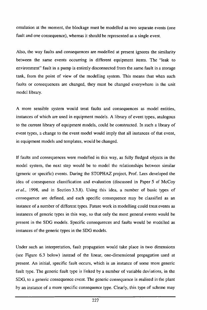
emulation at the moment, the blockage must be modelled as two separate events (one
fault and one consequence), whereas it should be represented as a single event.
Also, the way faults and consequences are modelled at present ignores the similarity
between the same events occurring in different equipment items. The "leak to
environment" fault in a pump is entirely disconnected from the same fault in a storage
tank, from the point of view of the modelling system. This means that when such
faults or consequences are changed, they must be changed everywhere in the unit
model library.
A more sensible system would treat faults and consequences as model entities,
instances of which are used in equipment models. A library of event types, analogous
to the current library of equipment models, could be constructed. In such a library of
event types, a change to the event model would imply that all instances of that event,
in equipment models and templates, would be changed.
If faults and consequences were modelled in this way, as fully fledged objects in the
model system, the next step would be to model the relationships between similar
(generic or specific) events. During the STOPHAZ project, Prof. Lees developed the
idea of consequence classification and evaluation (discussed in Paper 5 of McCoy
et aI., 1998, and in Section 3.3.8). Using this idea, a number of basic types of
consequence are defined, and each specific consequence may be classified as an
instance of a number of different types. Future work in modelling could treat events as
instances of generic types in this way, so that only the most general events would be
present in the SDG models. Specific consequences and faults would be modelled as
instances of the generic types in the SDG models.
Under such an interpretation, fault propagation would take place in two dimensions
(see Figure 6.3 below) instead of the linear, one-dimensional propagation used at
present. An initial, specific fault occurs, which is an instance of some more generic
fault type. The generic fault type is linked by a number of variable deviations, in the
SDG, to a generic consequence event. The generic consequence is realised in the plant
by an instance of a more specific consequence type. Clearly, this type of scheme may
227
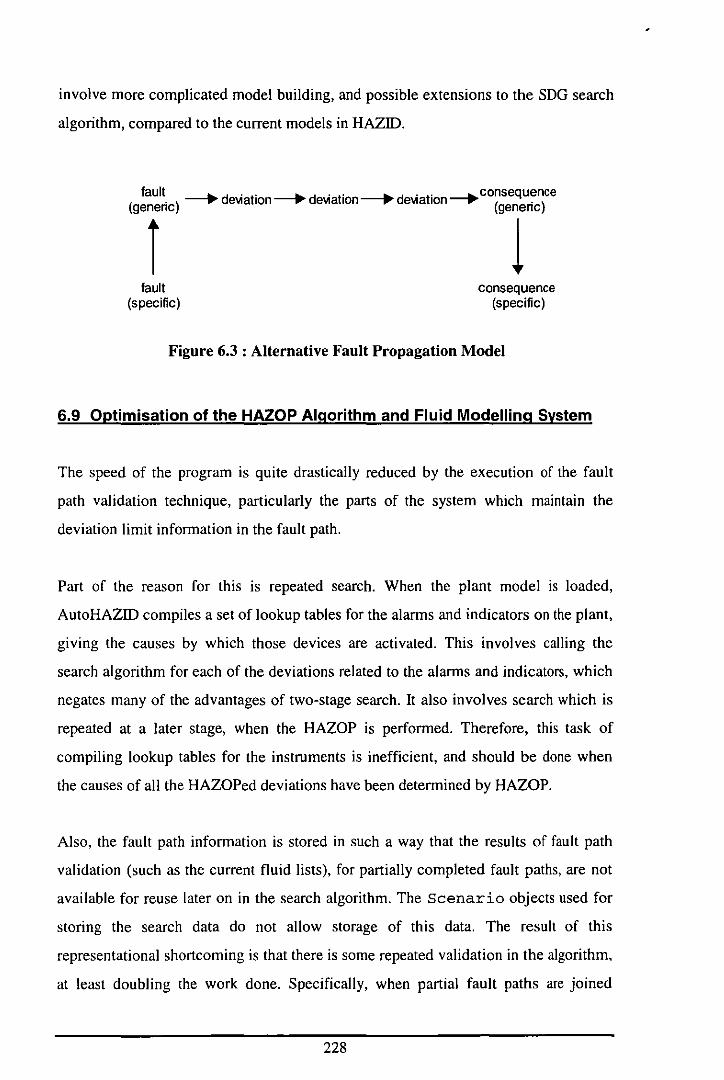
involve more complicated model building, and possible extensions to the SOG search
algorithm, compared to the current models in HAZID.
fault (specific)
consequence (specific)
Figure 6.3 : Alternative Fault Propagation Model
6.9 Optimisation of the HAZOP Algorithm and Fluid Modelling System
The speed of the program is quite drastically reduced by the execution of the fault
path validation technique, particularly the parts of the system which maintain the
deviation limit information in the fault path.
Part of the reason for this is repeated search. When the plant model is loaded,
AutoHAZID compiles a set of lookup tables for the alarms and indicators on the plant,
giving the causes by which those devices are activated. This involves calling the
search algorithm for each of the deviations related to the alarms and indicators, which
negates many of the advantages of two-stage search. It also involves search which is
repeated at a later stage, when the HAZOP is performed. Therefore, this task of
compiling lookup tables for the instruments is inefficient, and should be done when
the causes of all the HAZOPed deviations have been determined by HAZOP.
Also, the fault path information is stored in such a way that the results of fault path
validation (such as the current fluid lists), for partially completed fault paths, are not
available for reuse later on in the search algorithm. The scenario objects used for
storing the search data do not allow storage of this data. The result of this
representational shortcoming is that there is some repeated validation in the algorithm.
at least doubling the work done. Specifically, when partial fault paths are joined
228
together producing longer paths, the whole long path has to be re-validated and when
consequences are added to the fault paths at the end of the HAZOP search phase, all
the fault paths have to be validated once again.
This is a strong argument for changing the data structures used in the HAZOP
algorithm, so that fault paths and partial fault paths can be represented as objects
which record all the context information generated by validation, including current
fluids. The validation of these paths could be updated whenever they were extended,
with minimal effort, and the fault path objects would be copied whenever necessary,
so that repeat validation of the same partial paths could be avoided.
6.10 Conclusions
This chapter has discussed the strengths and weaknesses of the HAZID approach to
hazard identification, and outlined a number of areas of possible work to improve
HAZOP emulation in the future. A small number of these topics have been discussed
at length - I hope that the sketches offered by Sections 6.3 to 6.9 are sufficient to
allow another person to continue the work done on HAZID and, in particular, on its
Fluid Modelling System.
The seven areas of future work discussed in detail were:
I. Access to Plant Descriptions
2. Methodology Issues in Unit and Fluid Modelling Systems
3. Modelling State-Dependent Behaviour and Temporal Sequences
4. Non-Process Propagation of Faults
5. Loops, Plant Topology and Higher Level Constraints
6. An Extended Representation for Fault Propagation
7. Optimisation of the HAZOP Algorithm and Fluid Modelling System
229
The main areas of concern reflected in these headings are:
• Improving the representational strength of models used.
• Management of large volumes of information, in the form of models encapsulating
expert knowledge.
• Optimisation of program performance.
• Developing interfaces to external systems.
These summarised concerns seem representative of the sorts of problems which need
to be tackled, to gain an even more acceptable level of performance from a model
based hazard identifier, such as AutoHAZID. The next chapter attempts to summarise
the conclusions that may be drawn from the work presented in the thesis.
230
Chapter 7 : Conclusions
The automation of HAZOP analysis, using qualitative plant models for process
simulation, is motivated by the prospect of saving some of the time and money
traditionally spent in HAZOP studies conducted by teams. The AutoHAZID computer
program was developed in the STOPHAZ project to emulate HAZOP, using
qualitative reasoning methods.
This thesis has described how qualitative reasoning can be successfully applied to
hazard identification by emulation of HAZOP. It has also demonstrated, however, that
purely qualitative models are not sufficient to provide the accuracy required in
reported hazards. Checks based on quantitative information are needed to prevent
spurious identification of hazards.
The qualitative model system in HAZID proved to be a highly efficient way of
modelling fault propagation in the majority of simple hazard scenarios. However,
there were some problems with the method, as outlined in Chapter 4 and summarised
below:
• Indiscriminate reporting of hazards and repetition in HAZOP reports.
• Qualitative ambiguity, leading to undecidable influences in the SOG and to
problems with computational complexity.
• The SOO only represents two types of deviations in process variables, which is a
problem for flow, for instance.
• The "shortest path heuristic", used in the graph searching algorithm at the heart of
HAZOP emulation in HAZIO, is not theoretically sound.
• The SOO model of an equipment item does not change when that equipment fails,
so that it is possible to reason through unhealthy equipment, with erroneous
results.
231
• Single mappIng influences In the plant are not represented In the SDG as
originally formulated.
An important method used to tackle many of these problems was by using quantitative
information, typically concerning the fluids in the plant, implemented in the Fluid
Modelling System (FMS). The FMS was described in Chapter 5 and is summarised
briefly below:
• The FMS verifies the feasibility of fault-consequence scenarios produced by the
(qualitative) HAZOP search algorithm.
• It does this by evaluating (optional) conditions attached to the fault, the
consequence and the propagation arcs that link fault to consequence in a scenario.
If any condition in the chain fails, the scenario is suppressed.
• The FMS conditions are implemented by a system of predicates and functions,
which use information on the fluids in the plant, and their properties.
• A number of sources of information are integrated by the FMS in providing the
rule-based checks. These sources include information provided in the plant model
on fluids present, their temperatures and pressures, as well as internal and external
program modules for determining physical property values.
• The FMS also does some reasoning about the limits of process variable deviations
in scenarios, and their ability to cause the consequences they are linked to.
The choice of fault propagation as a model for scenario development was a good one,
despite the consequent limitation of HAZOP emulation to single fault, single
consequence scenarios. Once the capability to conduct practically useful HAZOP
emulation studies on real industrial problems has been demonstrated, the model of
scenario development may be widened to include more complicated constraints
between events.
The SDG is a very useful formalism for building models of equipment suitable for
representing fault propagation. It allows the causal links between variables to be stated
232
in a quite natural way. Search on the SDG is also probably the most efficient model
for inference which could have been chosen.
The frame-based models in AutoHAZID make use of inheritance and are organised
into a hierarchy of types within the unit model library. The definition of equipment
models in this way facilitates the easy construction of plant models with a minimum
of externally supplied information. Maintenance of the unit model library is eased by
the hierarchical nature of the model frames, and by use of template models, which cut
down on the number of arcs in the unit models by modelling commonly observed
features of equipment models. Proliferation of unit models in the library, to cover
multiple subtypes of more general models, is reduced by the use of attribute
conditional model sections in the more general model frames. These factors all
contribute to making the model library easy to use when creating plant models or
adding new unit models.
Despite the success of the qualitative SDG based approach to modelling hazardous
scenarios, there are problems which cannot be solved using just qualitative fault
propagation. Such problems are related to dependencies which are not represented in
the qualitative graph models. For example, the linear model of fault propagation in
AutoHAZID does not allow for simultaneous events to be modelled (i.e. no "AND"
logic). Also, there is no representation of the dependency of scenarios on the
properties of plant fluids, in the simple SDG.
The FMS was introduced as a means of adding dependencies outside the immediate
scope of linear propagation of process variable deviations. It allows properties of the
fluids in the plant (as well as other plant information) to be used in the evaluation of
conditions which allow the verification of fault paths. The model of fault path
verification used in the FMS mimics some features of scenario development in the
real plant. In order for a deviation to cause a consequence, it must have a sufficient
magnitude, for instance.
In formulating conditions for the FMS, the modeller is given the option of making use
of external physical properties packages to determine fluid property values, or of using
233

information resources within the AutoHAZID program itself. This demonstrates the
versatility of the integrated HAZIO package, which also provides access to plant
descriptions prepared in the Graphical Tool.
Due to the application of the FMS, the focus of HAZOP results produced by
AutoHAZIO was improved and the quantity of irrelevant output was reduced. This
added significantly to the value of the HAZOP emulation results.
Quite separately from the development of the FMS, an innovative new extension to
the SDG was developed, to model single mapping influences, where the usual dual
mapping SDG arcs are not sufficient to capture the real influences in some equipment.
This extension (using code numbers to represent the single mapping influences) seems
to be the most specific enhancement possible within the framework of the SDG - any
further change would require a more radical change to the model system.
The experience of developing the "flow path" modelling technique, for fluid flow and
pressure propagation, was particularly valuable. A number of methodological issues
were highlighted by this effort, including the use of the "causal hierarchy" idea for
controlling and simplifying the scope of permitted influences between variables. It is
likely that this approach to solving modelling problems could be used elsewhere.
None of the research groups reviewed in Chapter 2 have tackled the HAZOP
emulation problem as comprehensively as we have at Loughborough. It appears that
we have a program capable of making use of a wider range of equipment to study
much larger case study plants. However, there are still problem areas in this domain,
as discussed in Chapter 6. A few of these are summarised below:
• There is no means at present to model state-dependent behaviour and temporal
sequences of events.
• Non-process aspects of the plant model are not represented well. The constraints
imposed by operating instructions, instrument systems, and spatial relationships
between equipment (for domino effect prediction), could all be modelled.
234
• The topology of SDG models, and that of the plant itself, can be examined to
extract infonnation about higher level constraints in the plant (e.g. mass balance
constraints). This could help tackle ambiguity problems in HAZO? emulation.
• The representation of fault propagation could be extended, in terms of making
fault and consequence events equivalent in the SDG, and allowing a taxonomy of
such events. The latter measure could simplify equipment models greatly.
• The use of ad hoc rules, outside the equipment and fluid modelling systems,
should be re-examined. Examples are the rules to prevent propagating reverse
flow deviations through leaking units, or to prevent anomalous influences being
reported in feedback loops.
• For industrial acceptability, all model development should be carried out using a
methodology which ensures consistent model quality and documentation.
Solving the problems above, related to representation of all aspects of the plant and its
behaviour, will significantly widen the scope of hazards which can be identified.
The most immediate problem for the future use of HAZO? emulation is (automated)
access to plant descriptions. Software links to existing CAD or intelligent CAD
packages must be defined (possibly using STE? file transfer) in order to make the use
of a HAZO? emulator worthwhile.
In conclusion, HAZOP emulation by computer is potentially worthwhile, and the
qualitative approach is the right one for basic modelling of fault propagation.
Qualitative reasoning is an efficient fonn of simulation which mimics human-like
thought processes. However, there are unavoidable problems with a purely qualitative
approach, which cannot be solved without the use of some quantitative information.
Such infonnation should not rely on numerical simulation of the process, because this
requires too much numerical data. Verifying hazard scenarios, by testing fluid
dependent conditions attached to the qualitative models in the hazard identifier, seems
to tackle the problem at an appropriate level of detail.
235
References
Aldwinckle, D.S. and Slater, D.H. (1983) - "Risk and reliability methods used in the
analysis of an offshore LNG liquefaction and storage ship" - Proc 4th 1nt Symp on
Loss Prevention and Safety Promotion in the Process 1ndustries,4, vo!. 2.
Alien, J.E (1981) - "Maintaining Knowledge about Temporal Intervals" - TR-86,
Computer Science Department, University of Rochester, Rochester, NY.
Alien, J.E (1984) - "Towards a General Theory of Action and Time" - Artificial
Intelligence, 23 (1984), ppI23-154.
Andow, P.K. (1991) - "Guidance on HAZOP Procedures for computer-controlled
plants" - H.M. Stationery Office (London).
Andow, P.K. and Lees, EP. (1974) - "Process Plant Alarm Systems: General
Considerations" - Proc 1st Int Symp on Loss Prevention, (ed. Buschmann),
pp299-307.
Andow, P.K. and Lees, EP. (1975) - "Process Computer Alarm Analysis: Outline of a
Method Based on List Processing" - Trans IChemE, Vol. 53, ppI95-208.
BCISC, British Chemical Industry Safety Council (1973) - "Safety Audits: A Guide
for the Chemical Industry".
BSI, British Standards Institution (1991) - "BS5760. Reliability of Systems,
Equipment and Components, Part 5: 1991 - Guide to Failure Modes, Effects and
Criticality Analysis (FMEA and FMECA)".
Bunn, AR and Lees, EP. (1988) - "Expert design of plant handling hazardous
materials: Design expertise and computer aided design methods with illustrative
examples" - Trans IChemE, Vo!. 66, p4l9.
Burk, AE (1992) - "Strengthen Process Hazards Reviews" - Chem Eng Prog, 88(6).
236
Catino, e.A., Grantharn, S.D. and Ungar, L.H. (1991) - "Automatic generation of
qualitative models of chemical process units" - Comp Chem Eng, 15(8),
pp583-599.
Catino, e.A. and Ungar, L.H. (1995) - "Model based approach to automated hazard
identification of chemical plants" - AIChE Journal, 41(1), pp97-109.
CCPS, Center for Chemical Process Safety (1985) - "Guidelines for Hazard
Evaluation Procedures" - published by AIChE.
Chae, H., Yoon, Y.H. and Yoon, E.S. (1994) - "Safety analysis using an expert
system in chemical processes" - Korean Journal of Chemical Engineering, 11(3),
ppI53-16l.
Chang, e.T. and Hwang, K.S. (1994) - "Studies on the Digraph-Based Approach for
Fault-Tree Synthesis. I. The Ratio-Control Systems" - Ind Eng Chem Res, 33,
ppI520-1529.
Chang, Le., Yu, c.e. and Liou, C.T. (1994) - "Model-Based Approach for Fault
Diagnosis. L Principles of Deep Mode! Algorithm" - Ind Eng Chem Res, 33,
pp I 542-1 555.
Chung, P.W.H. (1993) - "Qualitative analysis of process plant behaviour" - 6th
International Conference on Industrial and Engineering Applications of Artificial
Intelligence (published by Gordon and Breach), pp277-283.
CIA, Chemical Industries Association Limited (1977) - "A Guide to Hazard and
Operability Studies" - published by the Chemical Industry Safety and Health
Council of the Chemical Industries Association.
CONCA WE (1992) - "The EC Safety Data Sheet Directive".
Coplien, 1.0. (1992) - "Advanced C++ : Programming Styles and Idioms" -
published by Addison· Wesley, ISBN 0-201-54855-0.
237
De Kleer, J. (1992) - "Physics, Qualitative" - entry in Encyclopedia of Artificial
Intelligence, 2nd Edition, (ed. S. Shapiro), published by John Wiley & Sons,
ppl 149-1 159.
De K1eer, J. and Brown, J.S. (1984) - "A Qualitative Physics based on Confluences"
Artificial Intelligence, 24, pp7-83.
Dow Chemical Company (1994) - "Dow's fire and explosion index. Hazard
classification guide".
Duxbury, H.A. and Turney, RD. (1989) - "Techniques for the analysis and
assessment of hazards in the process industries" - presented to New Mexico Tech
Research Centre for Energetic Materials Open Seminar on Safety and Hazards
Evaluation, 11th April 1989.
Fanti, M .. , Chung, P.W.H. and Rushton, A.G. (1993) - "Resolving Ambiguity in
Qualitative Models (Applied to Fault Propagation) through High Level
Constraints" - IChemE Research Event, pp630-632.
Forbus, KD. (1984) - "Qualitative Process Theory" - Artificial Intelligence, 24,
pp85-!68.
Grantham, S.D. and Ungar, L.H. (1990) - "A first principles approach to automated
troubleshooting of chemical plants" - Camp Chem Eng, 14(7), pp783-798.
Grantham, S.D. and Ungar, L.H. (1991) - "Comparative analysis of qualitative
models when the model changes" - AIChE Journal, 37(6), pp93 1.,.943.
Green, AE. (1983) - "Safety Systems Reliability" - published by John Wiley & Sons.
Hayes, PJ. (979) - "The Naive. Physics Manifesto" - from "Expert Systems in the
Microelectronic Age", D. Michie (ed.), published by Edinburgh University Press.
Heino, P. (1999) - PhD Thesis, Loughborough University.
238
Heino, P., Karvonen, I., Pettersen, T., Wennersten, R. and Andersen, T. (1994) -
"Monitoring and analysis of hazards using HAZOP-based plant safety model" -
Reliability Engineering and System Safety 44 (1994), pp335-343.
Heino, P., Kotikunnas, E., Shei, W.F., Shao, c.c. and Chen, C.H. (1995) -
"Computer-aided HAZOP with knowledge-based identification of hazardous event
chains" - Loss Prevention and Safety Promotion in the Process Industries,
Volume I, pp645-656.
Heino, P., Poucet, A. and Suokas, 1. (1992) - "Computer tools for hazard
identification, modelling and analysis" - Journal of Hazardous Materials, 29,
pp445-463.
HSE, Health and Safety Executive (1990) - "A Guide to the Health and Safety at
Work etc. Act 1974" - published by HMSO, London.
Hunt, A. (1992) - "Ruies for modelling in computer aided fault tree synthesis" - PhD
Thesis, Loughborough University.
Hunt, A., Kelly, B.E., Mullhi, 1.S., Lees, F.P. and Rushton, A.G. (1993) - "The
propagation of faults in process plants (parts 6-10)" - Reliability Engineering and
System Safety, 39, pp 173-250.
Institution of Chemical Engineers (1997) - "The Accident Database" - Software
package available from: IChemE, Davis Building, 165-189 Railway Terrace,
Rugby, CV21 3HQ. UK.
iri, M., Aoki, K., O'Shima, E. and Matsuyama, H. (1979) - "An algorithm for
diagnosis of system failures in the chemical process" - Comp Chem Eng, Vol 3,
pp489-4<)3.
lefferson, M., Chung, P.W.H. and Rushton, A.G. (1995) - "Automated hazard
identification by emulation of hazard and operability studies" - Proceedings of the
8th International Conference on Industrial and Engineering Applications of
Artificial Intelligence and Expert Systems, Forsyth, G.F. and Ali, M. (eds), Gordon
and Breach, Melbourne, Australia, pp765-770, ISBN 2-88449-198-8.
239
10nes, D.A. (1992) - "Nomenclature for Hazard and Risk Assessment in the Process
Industries (2nd edition)" - published by the Institution of Chemical Engineers.
Karvonen, L, Heino, P. and Suokas, 1. (1990) - "Knowledge based approach to
support Hazop-studies" - VTT Research Report 704, Espoo, August 1990.
Kelly, B.E. and Lees, EP. (1986) - "The Propagation of Faults in Process Plants: 1.
Modelling of Fault Propagation" - Reliability Engineering, 16, pp3-38.
Kletz, T.A. (1992) - "HAZOP and HAZAN - Identifying and Assessing Process
Industry Hazards (3,d edition)" - published by the Institution of Chemical
Engineers.
Kletz, T.A., Chung, P.W.H., Broomfield, E. and Shen-Orr, C. (1995) - "Computer
Control and Human Error" - published by the Institution of Chemical Engineers.
Knowlton, R.E. (1981) - "An Introduction to Hazard and Operability Studies: The
Guide Word Approach" - published by Chemetics International Ltd.
Knowlton, R.E. (1992) - "A Manual of Hazard and Operability Studies: The creative
identification of deviations and disturbances" - published by Chemetics
International Ltd. (Vancouver, RC.).
Kramer, M.A. and Palowitch, B.L. (1987) - hA rule based approach (Q fault diagnosis
using the signed directed graph" -AIChE Journal, 33, ppJ067-J078.
Kuipers, B. (1986) - "Qualitative Simulation" - Artificial Intelligence, 29, pp289-388.
Kuo, D.H., Hsu, D.S. and Chang, c.T. (1997) - "A Prototype for Integrating
Automatic Fault TreelEvent TreelHAZOP Analysis" - Comp Chem Eng, 21,
SuppJ., ppS923-S928.
Larkin, EO., Rushton, A.G., Chung, P.W.H., Lees, EP., McCoy, S.A. and
Wakeman, S.l. (1997) - "Computer Aided Hazard Identification: Methodology and
System Architecture" - IChemE Symposium Series No. 141 (HAZARDS XIll).
240
Larkin, ED. (1996) - "Comparison of Old and New Search Algorithms" - internal
file note prepared during the STOPHAZ project (re£. FDL\WP\HAZID\
newtime.doc, 13 November, 1996).
Lawley, H.G. (1974) - "Operability studies and hazard analysis" - Chem Eng Prog,
70(4).
Lees, F.P. (1984) - "Process Computer Alarm and Disturbance Analysis: Outline of
Methods for Systematic Synthesis of the Fault Propagation Structure" - Comp
Chem Eng, 8(2), pp91-103.
Lees, EP. (1996) - "Loss Prevention In the Process Industries (2nd edition)" -
published by Butterworth Heinemann.
Leone, H. (1996) - "A Knowledge-Based System for HAZOP Studies. The
Knowledge Representation Structure"- Comp Chem Eng, 20, Suppl.,
ppS369-S374.
Luger, G.E and Stubblefield, W.A. (1989) - "Artificial Intelligence and the Design of
Expert Systems" - published by Benjamin Cummings.
Martinez, E., Beltramini, L., Leone, H., Ruiz, c.A. and Huete, E. (1992) -
"Knowledge elicitation and structuring for a real-time expert system for monitoring
a butadiene extraction system" - Comp Chem Eng, 16, Suppl., ppS345-S352.
Martin-Solis, G.A., Andow, P.K. and Lees, EP. (1977) - "An Approach to Fault Tree
Synthesis for Process Plants" - 2nd Int Symp on Loss Prevention and Safety
Promotion in the Process Industries, pp367-375.
McCarthy, J. and Hayes, PJ. (1969) - "Some Philosophical Problems from the
Standpoint of Artificial Intelligence" - from Machine Intelligence 4, (ed.
B. Meltzer and D. Michie), published by Edinburgh University Press.
McCoy, S.A. and Rushton, A.G. (1997) - "A Case Study in Qualitative Reasoning
about Process Plant Hazards" - IChemE Jubilee Research Event, pp665-668.
241
Rushton, A.G. (1997) - "Knowledge-Based HAZOPs: Progress in computer
emulation (Parts I & 2)" - European Process Safety Centre (EPSC) Technical
Reports Nos. 4 & 5.
Shafaghi, A., Andow, P.K. and Lees, F.P. (1984) - "Fault Tree Synthesis based on
Control Loop Structure" - Chem Eng Res Des, 62, March 1984, pplOl-llO.
Shimada, Y., Yang, Z.x., Song, J., Suzuki, K. and Sayama, H. (1993) - "Fault
diagnostic expert system using information from fault tree analysis" - Asia Pacific
Confed Chem Eng 6th Conf., Barton Australia, Vo12, pp44112-445/2.
Shimada, Y., Suzuki, K. and Sayama, H. (1996) - "Computer-aided operability study"
- Comp Chem Eng, VoI20(617), pp905-913.
Shiozaki, J., Matsuyama, H., O'Shima, E. and Iri, M. (1985) - "An improved
algorithm for diagnosis of system failures in the chemical process" - Comp Chem
Elig, Vol 9(3), pp285-293.
Srinivasan, R., Dimitriadis, V.D., Shah, N. and Venkatasubramanian, V. (1997) -
"Integrating Knowledge-Based and Mathematical Programming Approaches for
Process Safety Verification" - Comp Chem Eng, 21, Suppl., ppS905-S910.
Srinivasan, R., Dimitriadis, V.D., Shah, N. and Venkatasubramaniar:., V. (1998) -
"Safety Verification Using a Hybrid Knowledge-Based Mathematical
Programming Framework" - AIChE Journal, 44(2), pp361-371.
Srinivasan, R. and Venkatasubramanian, V. (1996) - "Petri net digraph models for
automating HAZOP analysis of batch process plants" - Comp Chem Eng, 20,
Suppl., ppS719-S725.
STOPHAZ Project (I997a) - "STOPHAZ Project Deliverable, D7.3 : Final Technical
Report" - Project documentation produced May 1997.
STOPHAZ Project (I997b) - "STOPHAZ Project Deliverable, D7.5 : User Guide" -
Project documentation produced May 1997.
243
Suh, l.C., Lee, S. and Yoon, E.S. (J997a) - "New strategy for automated hazard
analysis of chemical plants. Part I: Knowledge Modelling" - J. Loss Prev. Process
Ind., 10(2), ppll3-126.
Suh, l.C., Lee, S. and Yoon, E.S. (I997b) - "New strategy for automated hazard
analysis of chemical plants. Part 2: Reasoning algorithm and case study" - J. Loss
Prev. Process Ind., 10(2), ppI27-134.
Suh, l.C., Lee, B., Kang, I.K. and Yoon, E.S. (l997c) - "An expert system for
automated hazard analysis based on multimodel approach" - Camp Chem Eng, 21,
Suppl., ppS917-S922.
Suokas, l., Heino, P. and Karvonen, I. (1990) - "Knowledge-based safety analysis in
the CAD environment" - Chapter 24 of "Computer-Aided Ergonomics : A
Researcher's Guide", (Edited by W. Karwowski, A.M. Genaidy and S.S. Asfour),
published by Taylor & Francis.
Taylor, l.R. (1979) - "A Background to Risk Analysis" - Vols 1-4 (report), Riso
National Laboratory, Riso, Denmark.
Taylor, l.R. (1994) - "Risk Analysis for Process Plant, Pipelines and Transport" -
published by E&FN Spon (imprint of Chapman & Hall).
Vaidhyanathan, R. and Venkatasubramanian, V. (1995) - "Digraph-based models for
automated HAZOP analysis" - Reliability and System Safety, 50, pp33-49.
Vaidhyanathan, R., Venkatasubramanian, V. and Dyke, F.T. (I 996a)
"HAZOPExpert: An expert system for automating HAZOP analysis" - Process
Safety Progress, 15(2), pp80-88.
Vaidhyanathan, R. and Venkatasubramanian, V. (1996b) - "Experience with an expert
system for automated BAZOP analysis" - Camp Chem Eng, 20, Suppl.,
ppS 1589-S 1594.
244

Vaidhyanathan,R. and Venkatasubrarnanian,V. (1996c) - "A semi-quantitative
reasoning methodology for filtering and ranking HAZOP results in HAZOPExpert"
_ Reliability Engineering and System Safety, 53, pp 185-203.
Vecchietti, A. and Leone, H. (1996) - "SERO: A Knowledge-Based System for
HAZOP Studies" - AIChE Symposium Series No. 312 (Intelligent Systems in
Process Engineering), pp287-290.
Venkatasubramanian, V. and Rich, S.H. (1988) - "An object-oriented two-tier
architecture for integrating compiled and deep-level knowledge for process
diagnosis" - Camp Chem Eng, 12(9/10), pp903-921.
Venkatasubramanian, V. and Vaidhyanathan, R. (1994) - "A knowledge-based
framework for automating HAZOP analysis" - AIChE Journal, 40(3), pp496-505.
Vinson, 1.M. and Ungar, L.H. (1992) - "Fault Detection and Diagnosis using
Qualitative Modelling and Interpretation" - IFAC Symposium Series (I. Online
Fault Detection and Supervision in the Chemical Process Industries), ppI21-126.
Vinson, 1.M. and Ungar, L.H. (1995) - "Dynamic Process Monitoring and Fault
Diagnosis with Qualitative Models" - IEEE Transactions on Systems, Man and
Cybernetics, 25(1).
Wakeman, S.l., Chung, P.W.H., Rushton, A.G., Lees, F.P., Larkin, F.D. and
McCoy, S.A. (1997) - "Computer Aided Hazard Identification: Fault Propagation
and Fault-Consequence Scenario Filtering" - IChemE Symposium Series No. 141
(HAZARDS XIII).
Wells, G. (1980) - "Safety in Process Plant Design" - published by IChemElGodwin.
Whetton, C.P. (1993) - "Sneak Analysis of Process Systems" - Trans IChemE, 71,
Part B, ppI69-179.
Yoon, Y.H., Yoon, E.S. and Chang, K.S. (1992) - "Process fault diagnosis using the
integrated graph model" - IF AC, On-line Fault Detection and Supervision in the
Chemical Process Industries, Delaware, USA, 1992.
245

Yu, C.C. and Lee, C. (1991) - "Fault Diagnosis Based on Qualitative/Quantitative
Process Knowledge" - AIChE JournaL, 37(4), pp617-628.
Zerkani, H. and Rushton, A.G. (1992) - "Computer Emulation of Hazard
Identification" - InternationaL Federation of Automatic ControL Workshop,
pp22 1-226.
Zerkani, H. and Rushton, A.G. (1993) - "Computer Aid for Hazard Identification" -
6th InternationaL Conference on IndustriaL and Engineering Applications of
ArtificiaL Intelligence (pubLished by Gordon and Breach), ppI02-109.
246
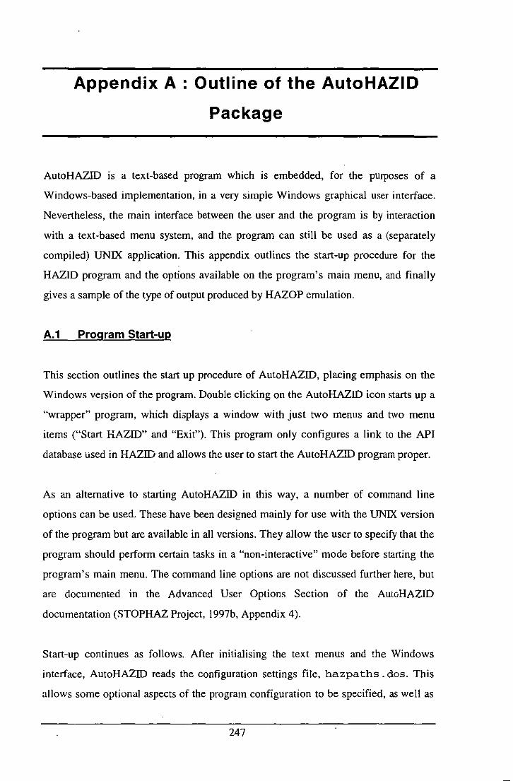
Appendix A . Outline of the AutoHAZID
Package
AutoHAZID is a text-based program which is embedded, for the purposes of a
Windows-based implementation, in a very simple Windows graphical user interface.
Nevertheless, the main interface between the user and the program is by interaction
with a text-based menu system, and the program can still be used as a (separately
compiled) UNIX application. This appendix outlines the start-up procedure for the
HAZID program and the options available on the program's main menu, and finally
gives a sample of the type of output produced by HAZOP emulation.
A.1 Program Start-up
This section outlines the start up procedure of AutoHAZID, placing emphasis on the
Windows version of the program. Double clicking on the AutoHAZID icon starts up a
"wrapper" program, which displays a window with just two menns and two menu
items ("Start HAZID" and "Exit"). This program only configures a link to the API
database used in HAZID and allows the user to start the AutoHAZID program proper.
As an alternative to starting AutoHAZID in this way, a number of command line
options can be used. These have been designed mainly for use with the UNIX version
of the program but are available in all versions. They allow the user to specify that the
program should perform certain tasks in a "non-interactive" mode before starting the
program's main menu. The command line options are not discussed further here, but
are documented in the Advanced User Options Section of the AuloHAZID
documentation (STOPHAZ Project, 1997b, Appendix 4).
Start-up continues as follows. After initialising the text menus and the Windows
interface, AutoHAZID reads the configuration settings file, hazpaths. dos. This
allows some optional aspects of the program configuration to be specified, as well as
247
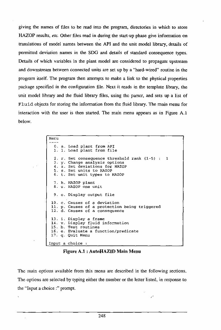
giving the names of files to be read into the program, directories in which to store
HAZOP results, etc. Other files read in during the start-up phase give information on
translations of model names between the API and the unit model library, details of
permitted deviation names in the SDG and details of standard consequence types.
Details of which variables in the plant model are considered to propagate upstream
and downstream between connected units are set up by a "hard-wired" routine in the
program itself. The program then attempts to make a link to the physical properties
package specified in the configuration file. Next it reads in the template library, the
unit model library and the fluid library files, using the parser, and sets up a list of
Fluid objects for storing the information from the fluid library. The main menu for
interaction with the user is then started. The main menu appears as in Figure A.I
below.
Menu
O. a. Load plant from API 1. l. Load plant from file
2. r. Set consequence threshold rank (1-5) 1 3. y. Change analysis options 4. z. Set deviations for HAZOP 5. s. Set units to HAZOP 6. t. Set unit types to HAZOP
7. h. HAZOP plant 8. u. HAZOP one unit
9. o. Display output file
10. c. Causes of a deviation 11. p. Causes of a protection being triggered 12. d. Causes of a consequence
13. i. Display a frame 14. v. Display fluid information 15. b. Test routines 16. e. Evaluate a function/predicate 17. q. Quit Menu
Input a choice :
Figure A.I : AutoHAZID Main Menu
The main options available from this menu are described in the following sections.
The options are selected by typing either the number or the letter listed, in response to
the "Input a choice ;" prompt.
248
A.2 Load Plant from API or Text File
In the Windows implementation of AutoHAZID, there are two options for loading a
plant description into the program: from the Database API or from a manually keyed
text file. The UNIX version of the program only offers the latter option.
If the user elects to load a plant description from the API, the first action of the
program is to remove from memory details of any previously loaded plant. It then asks
the user to choose a plant description from the list of those available in the database.
The next step is for the program to read all the data in the database associated with
this plant and write the information to a text file in the same format as would be
required for a keyed-in plant description. Once the file has been produced, it is read
back into AutoHAZID through the parser, and various internal data are initialised as
in the case below, where a plant model is read from a file.
If the option to load a plant description from a text file is chosen, the user is prompted
to give the name of the file (the existence of which is verified); then the details of any
previous plant description are removed from memory. The file is read into the
program through the parser and the various data structures associated with the plant
model are initialised. Initialisation includes connecting units to one another within the
plant model, checking that mandatory POlt connections have been made, preparing
lists of information concerned with splitting the plant up into "lines" for HAZOP,
checking protection devices, etc. The SDG model of the plant is constructed and
indexed for efficient access at this point, and the information on the fluids present in
the plant is propagated throughout the plant model.
A.3 HAZOP Analysis of Whole Plant or Single Unit
Once a plant model has been loaded into AutoHAZID, a HAZOP study can be carried
out on it. From the main menu, the user can choose to perform a full HAZOP on the
whole plant model, or to HAZOP only one unit, in the sense that only the deviations
belonging to that unit will be examined for causes and consequences.
249
In the "HAZOP plant" option, the whole plant is examined, subject to the scope
settings described in Section A.4. These allow the user to choose which units, unit
types or deviations to include in the analysis.
When the user chooses to run a HAZOP on the whole plant, the program first asks for
an output file name (which must not exist already in the results directory) and then
asks the user if they wish to define the order in which units are examined. If the user
does not want to order the units, the program will do this automatically, using its own
breakdown of the plant into flow lines. Manually choosing the order of units requires
that the user type the identifying numbers of units, which are indicated by
AutoHAZID in a list, in the user's preferred order. When the order of units has been
decided, the program goes on to perform a HAZOP analysis of the plant, printing
results to the specified file when it has finished. An example of the type of results file
typically produced by HAZOP emulation is given in Section A.8 of this appendix.
The "HAZOP one unit" option is simpler, in that it asks for a unit name and a fiie
name to send the results to, then goes on to examine the named unit and print the
results to the named output fiie. The menu option "Display output file" can be used in
the Windows version of AutoHAZID to display the results produced by HAZOP
emulation, or the text file can be examined using any text editor or similar program.
Some details of the processing that goes on in the HAZOP algorithm arc given in
Appendix B.
A.4 Scope of HAZOP
AutoHAZID allows the user to set up a restricted scope for the units and/or deviations
to be examined in the HAZOP analysis. Options are presented for the user to choose
which units, unit types or deviations will be examined in the HAZOP which is
subsequently initiated as described in Section A.3 above. This is implemented in three
"toggle menus", which allow the user to switch on or off different options in the lists
given.
250
A.S Flags for Reporting and Filtering
A number of features of the HAZOP analysis and reporting procedure are controlled
by flags which may be manipulated by the user. These are present in the "Set
consequence threshold" item on the main menu and in the "Change analysis options"
sub-menu, accessible from the main menu:
• Set consequence threshold. This option allows for consequences below the given
severity threshold to be eliminated from the results set produced by HAZOP. Each
of the consequences in the unit models has an associated consequence severity
ranking, in the range I to 5, where I is least severe and 5 is most severe.
In the "Change analysis options" sub-menu the following choices can be made:
• Display faults with no consequences. If this reporting option is on, then faults not
associated with any consequence will be reported in the HAZOP report. This
increases the size of the report significantly.
• Display consequences with no causes. If on, this reporting option will leave in the
report all consequences found linked to a deviatior., including those which were not
associated with any cause found by fault propagation.
• Filter out repeat faults. When many similar faults are reported as causes of the
same deviation, the repetition can be distracting. Therefore, it is possible to remove
all but one of the similar faults in the results, incidentally modifying the fault
description by adding "etc." to it. if this filtering option is switched on, the program
will eliminate repetitions of faults with the same descriptor string, belonging to
units in the same "line", with the same unit type.
• Filter out repeat fault-consequence pairs. This IS a reporting option to remove
repetitions of scenarios, which otherwise may be reported for a number of different
deviations.
• Display protections present. This option controls whether the program will look for
(and report) any protective devices in association with scenarios it identifies.
251
• Only display faults with no protections. When the "Display protections" option is
turned on, this option controls whether scenarios which have protections associated
with them will be reported.
• Use fluid model defaults. This is a switch for de-activating the fluid modelling
system, so that certain queries will return default answers.
Section 4.4 also discusses the above features for filtering and reporting, in the context
of the methods used in AutoHAZID to improve on the unfiltered output from fault
propagation.
A.6 "Causes-Of" Options
Three options are provided in AutoHAZID to allow the user to request explanations of
HAZOP results from the program. These give a way for the human user to look
directly at the fault paths generated by the machine, to see if there is some problem or
unappreciated feature in the HAZOP results as produced. The options are:
• Causes of a deviation. The user identifies a variable deviation to the program,
which then performs a search to find all faults which cause the· deviation. It
displays the fault paths in order of length.
• Causes of a protection being triggered. For a plant in which there are some
protective units, this option is used to find fault paths which will cause those
protections to operate. The user chooses a protection in the plant and the program
displays the fault paths it finds, in urder of length.
• Causes of a consequence. The user chooses one of the defined consequences for a
unit in the plant model and the program then searches for fault paths leading to that
consequence. It displays the fault paths in order of length.
252
A.7 Other Options
A few options are available on the AutoHAZID menu which have been used mainly
for testing the program and accessing information about the plant or models within it.
These are not present in the released versions of the program, but are nevertheless
quite useful sometimes:
• Display frame. This allows the user to see the information in the program on
particular unit models or instances of those models in the plant.
• Display fluid information. This option allows the information on fluids present in
the plant to be displayed, either for the whole plant model or for a single particular
unit in the plant.
• Test routines. Used during program development, this option may be attached to
any function which needs to be tested in isolation from the mainstream activities of
AutoHAZID. At the moment, this option activates a simple function to analyse the
forwards and backwards branching factors of the plant SDG in memory at the time.
• Evaluate function or predicate. This option provides access to the functions and
predicates of the fluid modelling system (see Chapter 5). The user types an item to
be evaluated and a "context" unit for the query, and the program activates an FMS
query to evaluate the item.
253
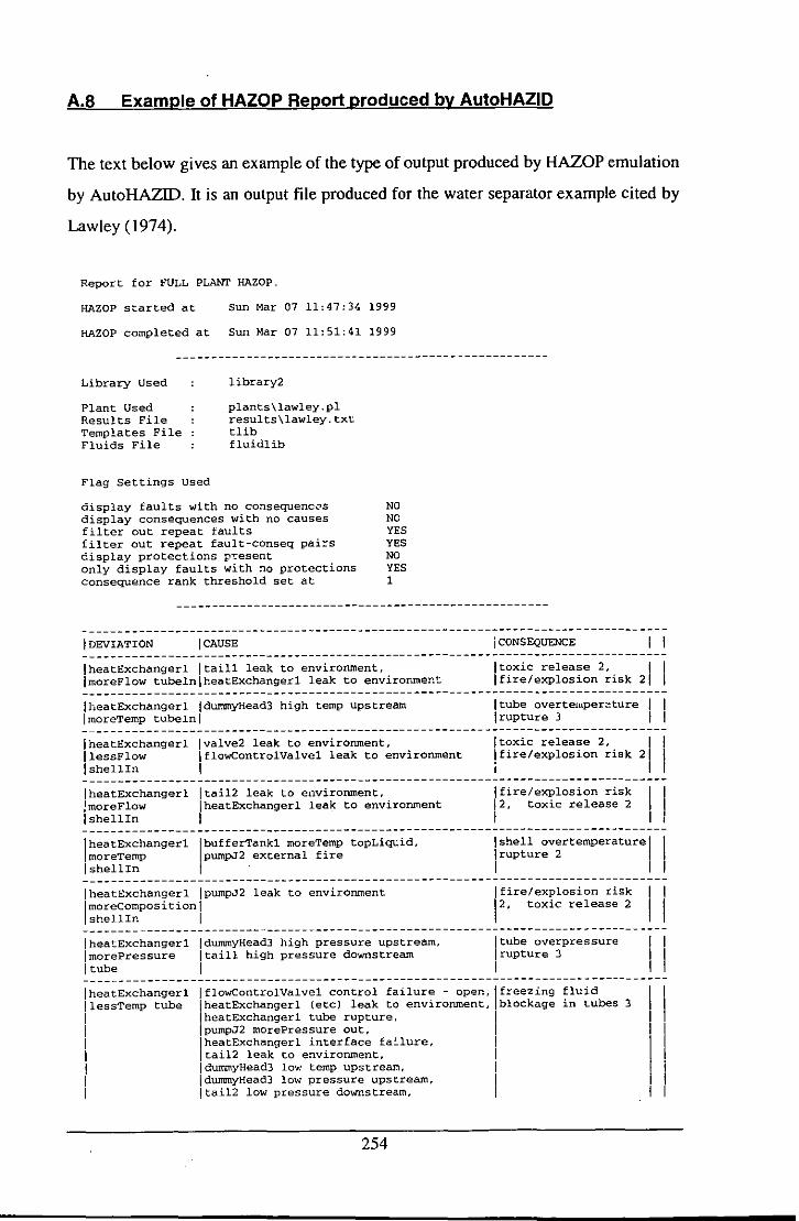
A.a Example of HAZOP Report produced by AutoHAZID
The text below gives an example of the type of output produced by HAZOP emulation
by AutoHAZID. It is an output file produced for the water separator example cited by
Lawley (1974).
Report for FULL PLANT HAZOP.
HAZOP started at Sun Mar 07 11:47:34 1999
HAZOP completed at Sun Mar 07 11:51:41 1999
Library Used
Plant Used Results File Templates File Fluids File
Flag Settings used
library2
plants\lawley.pl results\lawley.txt tlib fluidlib
display faults with no consequenc05 NO display consequences with no causes NO filter out repeat faults YES filter out repeat fault-conseq pai~s YES display protections p-.:esent NO only display faults with no protections YES consequence rank threshold set at 1
-----------------------------------------------------------------------------------I DEVIATION I CAUSE iCONSEQUENCE I I -----------------------------------------------------------------------------------IheatExchangerl Itaill leak to environment, ImoreFlow tubeln heatExchangerl leak to environment I
toxic release 2, I I fire/explosion risk 2
-----------------------------------------------------------------------------------IheatExchangerl IdummyHead3 high temp upstream ImoreTernp tubelnj
I tube overte1Uper~ture I I I rupture 3 I I
-----------------------------------------------------------------------------------IheatExchangerl IlessFlow I shellln
IheatExchangerl lmoreFlow Ishellln
Ivalve2 leak to environment, IflowControlvalvel leak to environment I I tail2 leak to environment, IheatExchangerl leak to environment I
ItoXiC release 2, I I
jfire/eXPlosion risk 2 I I fire/explosion risk 12, toxic release 2
11 -----------------------------------------------------------------------------------IheatExchangerl IbUfferTankl moreTemp topLiquid, moreTemp pumpJ2 external fire
I shellIn I
Ishell overtemperaturel I Irupture 2 I
-----------------------------------------------------------------------------------lheatExchangerl IpumpJ2 leak to environment I moreComposition 1 I sheUln I
I fire/explosion risk III 12, toxic release 2
-----------------------------------------------------------------------------------lheatExchangerl ImorePressure I tube
IdurnmyHead3 high pressure upstream, Itaill high pressure downstream I
I tube overpressure Irupture 3 I 11
-----------------------------------------------------------------------------------IheatExchangerl IlessTemp tube I I
1 I I
]flowControlvalvel control failure - open, I freezing IheatExchangerl (etc) leak to environment, blockage IheatExchangerl tube rupture, I IpumpJ2 morePressure out, I lheatExchangerl interface failure, I I taU2 leak to environment, I I dummyHead3 low temp upstream, I IdurnmyHead3 low pressure upstream, I I tail2 low pressure downstream, I
254
fluid in tubes 3
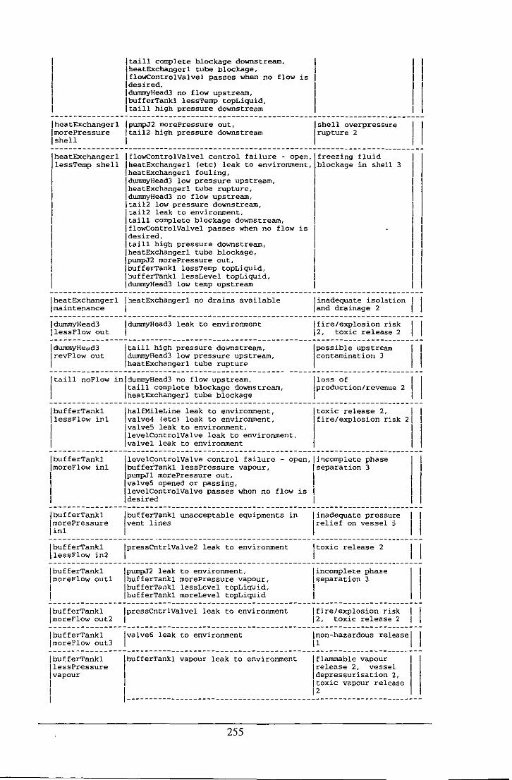
IheatExchanger! Imorepressure 1 shell
Itaill complete blockage downstream, IheatExchangerl tube blockage, IfloWControlValvel passes when no flow is Idesired, IdummyHead3 no flow upstream, IbufferTankl lessTemp topLiquid, Itaill high pressure downstream
IpumpJ2 morePressure out, Itai12 high pressure downstream 1
Ishell overpressure lrupture 2 I 1
1 I -----------------------------------------------------------------------------------
IheatExchangerl lessTemp shell
I
I 1
I
IfloWControlvalvel control failure - open, I freezing IheatExchangerl (etc) leak to environment, blockage !heatExchangerl fouling, I dummyHead3 low pressure upstream, I IheatExchangerl tube rupture, I ! dummyHead3 no flow upstream, I I tail2 low pressure downstream, I I tai12 leak to environment, I Itail! complete blockage downstream, I IflowControlValvel passes when no flow is Idesired, I Itaill high pressure downstream, IheatExchangerl tube blockage, I IpumpJ2 morePressure out, IbufferTankl lessTemp topLiquid, IbufferTankl lesSLevel topLiquid, IdummyHead3 low temp upstream
fluid in shell 3
IheatExchangerl IheatExchangerl no drains available linadequate isolation! I Imaintenance I I and drainage 2 I
IdummyHead3 IlessFlow out
IdummyHead3 leak to environment 1 Ifire/exPlosion risk
2, toxic release 2 I I -----------------------------------------------------------------------------------IdummyHead3 IrevFlow out 1
Itaill high pressure downstream, IdummyHead3 low pressure upstream, IheatExchangerl tube rupture I
Possible upstream contamination 3
11
I tail! noFlow inldummyHead3 no flow upstream,
110SS of I I
I IbufferTankl llessFlow i:nl
I IbufferTankl ImoreFlow in!
I IbufferTankl ImorePressure linl
lbufferTankl IlessFlow in2
IbufferTankl ImoreFlow outl I 1
IbufferTankl ImoreFlow out2
lbufferTankl ImoreFlow out3
IbufferTankl IlessPressure I vapour 1
I
Itaill complete blockage downstream, IheatExchangerl tube blockage
IhalfMileLine leak to environment, Ivalve4 (etc) leak to environment, IvalveS leak to environment, IlevelControlvalve leak to environment, Ivalvel leak to environment
production/revenue 2
Itoxic release 2, I fire/explosion risk 2
1
!levelControlValve control failure - open, li~complete phase 3 IbuffeiTankl less Pressure vapour, I separation
pumpJl morePressure out, IvalveS opened or passing, IlevelControlValve passes when no flow is I I desired I
IbufferTankl unacceptable equipments in Ivent lines 1
IpressCntrlValve2 leak to environment
I pumpJ2 leak bufferTankl
1bufferTankl IbufferTankl
to environment, morePressure vapour, lessLev€l topLiquid, moreLevel topLiquid
IpressCntrlValvel leak to environment
I inadequate pressure relief on vessel 5
1
1toxic release 2 1
lincomplete phase Iseparation 3
I jfire/explosion risk 12, toxic release 2
11 I I
I I I~on-hazardous release [ I jvalve6 leak to environment
1
jbufferTankl vapour leak to environment I flammable vapour I lrelease 2, vessel I ldepressurisation 2, I I toxic vapour release 1 12 1------------------------------------------------------------------
255

IbufferTankl
Imorepressure vapour
I I
IpressCntrlValvel control failure - open, IpressCntrlValve2 control failure -Iclosed, IbufferTankl lessTemp topLiquid, IpressCntrlValvel (etc) leak to I environment , pressCntrlValve2 (etc) leak to environment. dummyHead2 low pressure upstream, pressCntrlValvel passes when no flow is
I desired
IpressCntrlValve2 control failure - open, IpressCntrlValvel control failure -Iclosed, IpressCntrlValve2 passes when no flow is Idesired. IbufferTankl moreTemp topLiquid. \dummyHead2 high pressure upstream, Itail3 incorrect sizing
Ivessel depressurisation 2
I Ipossible overpres5urel Irupture 2 I 1 1
I IbufferTankl IdumrnyHead2 high temp upstream. moreTemp vapourlbufferTankl external fire, I
design temp exceeded I I - structural I
I IbufferTankl moreTemp topLiquid weakening 2 I I
IbufferTankl moreLiquid
1 vapour
1
IbufferTankl ImoreTemp I tOPLiquid 1
!levelControlValve control failure - open, IbufferTankl moreLevel tOPLiquid, IlevelControlValve passes when no flow is Idesired, IbufferTankl less Pressure vapour, IpumpJl morePressure out, IvalveS opened or passing
IpumpJl external fire, IbufferTankl external fire, IdummyHeadl high temp upstream, IhalfMileLine external fire
liquid droplet entrainment 3
IdeSign temp exce..:ded I I - structural I I weakening 2 I I
1 1 1 -----------------------------------------------------------------------------------I bufferTankl I contamination ItopLiquid
lbufferTankl IlessLevel ItopLiquid
I
I
I IbufferTankl ImoreLevel ItopLiquid
I I
I
I dumrnyHeadl upstream contamination, Iliquid contents IpumpJl ingress of lubricant or seal fluidlcontaminated 3 I into pump 11 IbufferTankl
I liquid leak to environment I gas breakthrough 3, I
toxic liquid release I
1
2, flammable liquid I I release 2 I l~~~~~~~~~~~~~~i;~-~~i~;-~~~;~~~-----------I~;;-b~~;~~~;~~~~-;---T--I IlevelControlvalve control failure - 1 closed, I valveS (etc) leak to environment, 1 I I pumpJ2 leak to environment, I bufferTankl liquid leak to environment, I valve6 (etc) leak to environment, bufferTankl more Pressure vapour,
Ivalvel partly closed, 1 valve4 (etc) leak to envi.ronment, valvel (etc) leak to environment, valve4 (etc) closed, pumpJl nOFlow out, pumpJl less Pressure out,
Ilev~lControlvalve (etc) leak to env~ronment,
valve3 (etc) partly closed, IhalfMileLine (etc) leak to environment, IhalfMileLine blockage, Ivalve! closed,
IpumpJl revFlow out, dummyHeadl low composition upstream
IlevelControlValve control failure - open Ivessel overfilling 2 I IbufferTankl less Pressure vapour, ' I I pumpJl morePressure out, I I IvalveS opened or passing, 11 1 1 IlevelControlvalve passes when no flow is 1 1 desired 1 1
l~;i;~~-~~~~i;-~i~~~~~--------------------,ii~i~-~~~~i~~---------I 1 pumpJ2 noFlow in. I entrainment 3, I I tail4 high pressure, Ivessel overfilling 2 1 IpumpJ2 revFlow out,
256
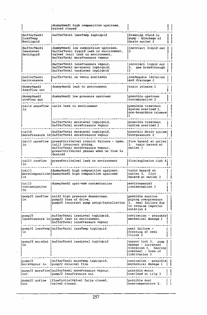
1 bufferTank1
IlessTemp botLiquid
IbufferTankl \lessLevel IbotLiquid
I I bU~ferTankl ma1ntenance
IdurrunyHead2 IlessFlowout
IdurnmyHead2 IrevFlow out
I tai 14 moreFlow
lin
I
IdummyHeadl high composition upstream, valveG closed
IbufferTank1 1essTemp topLiquid
IdummyHeadl low composition upstream,
IbufferTankl liquid leak to environment, valve6 (etc) leak to environment,
IfreeZing fluid in sump - blockage of
Idrain outlet 2
1 1 1 1
11 I incorrect liquid out I 1 13 1
1 1 1
\bufferTankl morePressure vapour I I
1------------------------------------------------------------------bufferTankl lessPressure vapour. I incorrect liquid out I I
IbufferTankl moreLevel topLiquid, \3, gas breakthrough I I IbufferTankl lessLevel topLiquid 13 I I
!bufferTankl no vents available 1
IdummyHead2 leak to environment 1
IdumrnyHead2 low pressure upstream 1
1
inadequate isolation I I and drainage 2 I I
I toxic release 2 1
lpossible upstream Icontamination 3
I I 1 1 1 1
Itai14 leak to environment IPoSSible treatment I 1 I system overload 3, 1 I non-hazardous release 1 1 1 11 l~~~~~;;~~;~-~~;;~;~;i-~~~~~~~~~---------I~~;;~~i~-~~~~~~~~---I-I IbufferTankl morePressure vapour Isystem overload 3 1 I
Itail4 IbufferTankl moreLevel topLiquid, morePressure in bufferTankl more?ressure vapour I
possible drain systeml I overpressure 2 I I
I
tai13 moreFlow IpressCntrlValvel contr0l failure - open, \fire hazard at outlet I I in I tai13 incorrect sizing, 3, toxic hazard at 11
1 bufferTankl more Pressure vapour, outlet 3 I I IpressCntrlValvel passes when no flow is I 1
1 1 desired 1 1
1
~ai13 revFlow 1ll
IpressCntrlValvel leak to environment 1
Itai13 IdummyHeadl high composition upstrea~, moreComposition durnmyHead2 high composition upstream
lin
1
taiD :,ontamination 1ll
IduromyHead2
I upstream contamination
I fire/explosion risk 41 I ltoxic hazard at
loutlet 3, fire hazard at outlet 3
1
environmental contamination 3
1
11
11 -----------------------------------------------------------------------------------
purnpJ2 revFlow in
I
tail2 high pressure downstream, pumpJ2 loss of drive, pumpJ2 incorrect pump setup/installation
1
I
PurnPJ2 IbufferTankl lessLevel topLiquid, less Pressure in pumpJ2 leak to environment,
buffe.r:rankl lesspressure vapour
IpurnpJ2 lin
lessTempI bufferTankl lessTemp topLiquid
1
I ~UmPJ2 1ll
1
IpumpJ2 Imorevapour in
I 1 bufferTank1 lessLevel topLiquid
1
IbufferTankl moreTemp topLiquid, purnpJ2 external fire
lpumpJ2 moreFlowlbufferTankl morePressure vapour, lout lpumpJ2 less Pressure out
IpumpJ2 noFlow lout
IfloWControlvalvel fails closed, Ivalve2 closed,
257
possible suction piping overpressure 2, seal failure due to revelse impeller rotation 2 I
I
cavitation - possible 1 1 mechanical damage 3 I
1
seal failure -freezing of seal
I fluids 2 11 Ivapour lock 3, pump I
Idamage - increased I vibration 3, bearing I
loverheat - loss of 1
Ilubrication 3
Icavitation - possible 1 1 Imechanical damage 3
Ipossible motor loverload or trip 3
I possible seal lovertemperature 2,
11
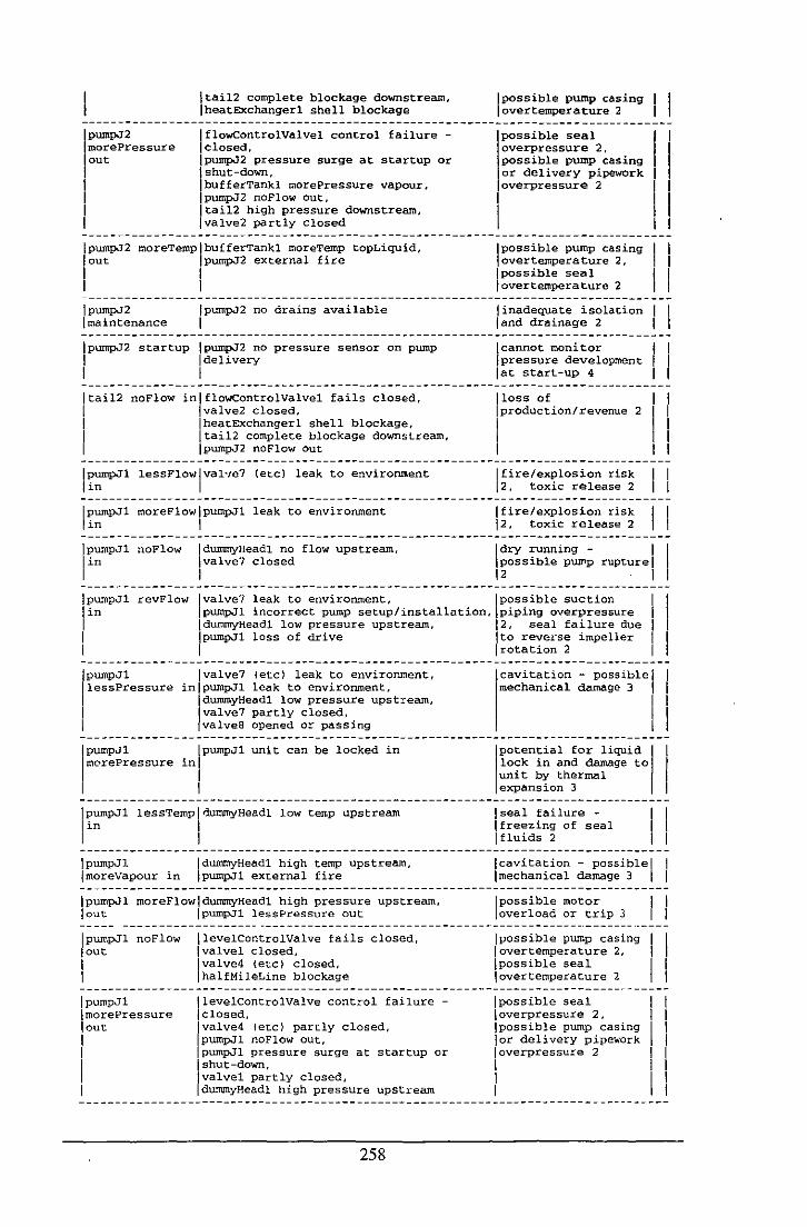
I
PumpJ2 morePreS5Ure out
I
Itai12 complete blockage downstream, heatExchangerl shell blockage
IflowControlvalvel control failure -Iclosed, IpumpJ2 pressure surge at startup or
I shut-down, bufferTankl morePressure vapour,
IpumpJ2 nOFlow out, Itai12 high pressure downstream. Ivalve2 partly closed
Ipossible pump casing I overtemper a ture 2
IposSible seal overpressure 2,
IPossible ~ casing or delivery pipework overpressure 2
1
I
I I
I -----------------------------------------------------------------------------------IpumpJ2
lout
moreTemplbufferTankl moreTemp IpumpJ2 external fire
topLiquid,
IpumpJ2 [maintenance
I IpumpJ2 no drains available 1
IpumpJ2 startup IpumpJ2 no pressure sensor on pump I delivery
1 1
Itai12 noFlow inlfloWControlValvel fails closed, Ivalve2 closed,
I IheatExchangerl shell blockage, tai12 complete blockage downstream,
IpumpJ2 nOFlow out
IpumpJl lessFlowlval'/e? (etc) leak to environment in I
IpurnPJl moreFlowlpurnpJl leak to environment in I
lI?urnPJl noFlow 1n
1
IdurnmyHeadl no flow upstream, Ivalve7 closed 1
Ipossible pump casing lovertemperature 2,
lpossible seal overternpera ture 2 I
I inadequate isolation I I land drainage 2 I
Icannot monitor I I pressure development 1 1
lat start-up 4 I
Iloss of Iproduction/revenue 2
I 1 fire/explosion risk 1 1 2, toxic release 2
Ifire/explosion risk 12, toxic release 2 I I 1 dry running - 1 1 possible p~p rupture
12 1 1 IpurnpJl revFlow lin
Ivalve? leak to environment, Ipossible suction 1 1 IpumpJl incorrect pump setup/installation, Ipiping overpressure 1 I
I 1 durnmyHeadl low pressure upstream, 12, seal failure due purnpJl loss of drive to reVel"Se impeller
1 I I Irotation 2
IpumpJl Ivalve7 (etc) leak to environment,
Ilesspressure in purnpJl leak to environment,
durnmyHeadl low pressure upstream, valve? partly closed,
I valveS opened or passing
cavitation - possible I 1
mechanical damage 3 I
I1 -----------------------------------------------------------------------------------morePressure l.n I purnpJl . I purnpJl uni t can be locked in
1 1
potential for liquid lock in and damage to uni t by thermal expansion 3 I
-----------------------------------------------------------------------------------Il~PJl leSSTempldummYHeadl low temp upstream
IpumpJl !morevapour in I
dummYHeadl high temp upstream, pumpJl external fire
Ip urnPJl moreFlowldurornyHeadl high pressure upstream, out I pumpJl less Pressure out
purnpJl noFlow out
IlevelControlvalve fails Ivalvel closed, Ivalve4 (etc) closed, IhalfMileLine blockage
closed,
I seal failure -freezing of seal fluids 2
1 1 1 1
Icavitation - possible 1 1 mechanical damage 3 I
1
possible motor overload or trip 3
Ipossible pump casing
lovertemperature 2, possible seal overtemperature 2
1 1 1 1
11 -----------------------------------------------------------------------------------IpumpJl
Imorepressure out
I 1
IlevelControlValve control failure -Iclosed, Ivalve4 (etc) partly closed,
1
purnpJl noFlow out, purnpJl pressure surge at startup or
I shut-down, Ivalvel partly closed, IdummyHeadl high pressure upstream
258
IPossible seal overpressure 2. possible pump casing
lor delivery pipework loverpressure 2
1
I 1
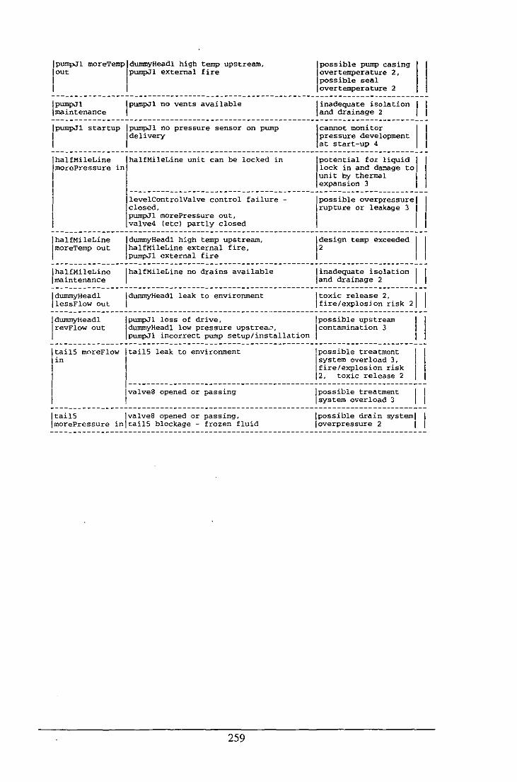
IpumpJl lout 1 1
moreTempldummyHeadl high IpumpJl external
temp upstream. fire
possible pump casing Qvertemperature 2, possible seal
IpUInpJl maintenance
IpumpJl startup
I
1
IpumpJl no vents available 1
IpumpJl no pressure sensor on pump I delivery 1
over temperature 2
I inadequate isolation I I and drainage 2 I
1
cannot monitor 11 pressure development at start-up 4
lhalfMileLine IhalfMileLine unit can be locked in ImorePressure in Ipotential for liquid I I
lock in and damage tol 1 1
I I 1
I hal fMi le Line lmoreTernp out 1
IhalfMileLine I maintenance
IdummyHeadl IlessFlowout
IdumrnyHeadl IrevFlow out 1
ItailS moreFlow jin 1
I
levelControlValve control failure -lclosed,
IpumpJl morePressure out, valve4 (ete) partly closed
IdummyHeadl high temp upstream,
IhalfMileLine external fire, pumpJl external fire
IhalfMileLine no drains available
IdurnmyHeadl leak to environment 1
lunit ~ thermal I expans~on 3
I pass ible overpressure I I I rupture or leakage 3 I
I I I l~eSign temp exceeded I I 1 1 1
linadequate isolation I I and drainage 2
I toxic release 2, I I fire/explosjon risk 2
IpumpJl loss of drive, Ipossible upstream I I IdurnmYHeadl low pressure upstrea.:>, Icontamination 3 pumpJl incorrect pump setup/installation I 1 1
[tailS leak to environment lpossible treatment I I
I I system overload 3, I I fire/explosion risk I
1 12, toxic release 2 1 1------------------------------------------------------------------IvalveS opened or passing [possible treatment I 1 I I system overload 3 I
ItailS IvalveS opened or passing, [possible drain system I 1 [overpressure 2 I lmorepressure in1tailS blockage - frozen fluid
259
Appendix B : Improved Algorithm for
HAZOP Search
This appendix briefly describes the HAZOP algorithm used in AutoHAZID, which
was developed to reduce the amount of repeated search which took place in an earlier
version. The approach to graph search outlined here may be of general interest for
applications other than HAZOP emulation. Firstly, the "traditional" way of modelling
the HAZOP study, which forms the basis of the older HAZOP algorithm in
AutoHAZID, is outlined. Then, some disadvantages of this method are identified and
a more efficient method is suggested.
The purpose of the HAZOP emulation algorithm in HAZID is to imitate the procedure
followed by a conventional HAZOP study team in examining the design of a plant,
and to produce a table of resu;ts in a similar format, using the headings of "deviation",
"cause", "consequence" and "protection".
Therefore, the algorithm must examine every deviation of a process variable in the
plant model and find faults which could cause that deviation. It must also report
consequences of the deviation and consequences of any faults which cause the
deviation, as well as the presence of any protective devices which could prevent, or
reduce the impact of, the hazardous scenarios found.
From this definition, which closely mirrors the definition of the conventional RAZOP
study procedure, the HAZOP algorithm is shown in Figure B.l below.
260
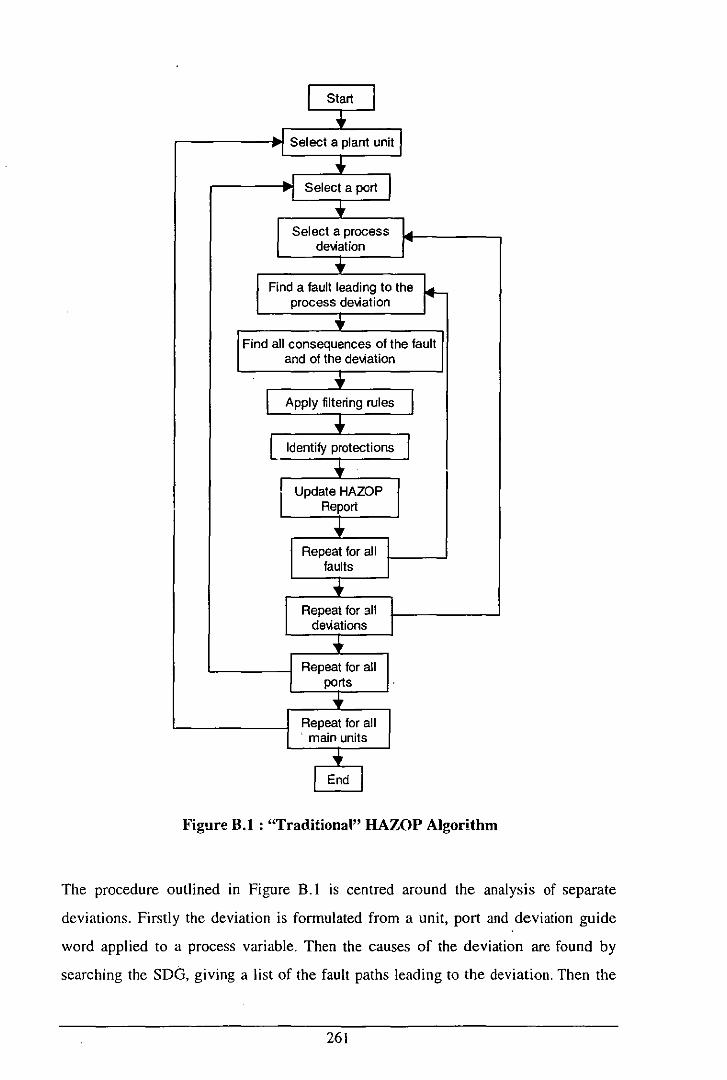
I Start I +
c ~ Select a plant unit
... 'I Select a port I
... Select a process ~
deloiation ~ ..
Find a fault leading to the ~ process deloiation ..
Find all consequences of the fault and of the deloiation
~
L Apply filtering rules I + L Identify protections I +
Update HAZOP Report
+ Repeat for all
faults
... Repeat for all
deloiations
+ Repeat for all
ports
-+ Repeat for all . main units
... I End I
Figure B.1 : "Traditional" HAZOP Algorithm
The procedure outlined in Figure B.1 is centred around the analysis of separate
deviations. Firstly the deviation is fonnulated from a unit, port and deviation guide
word applied to a process variable. Then the causes of the deviation are found by
searching the SDG, giving a list of the fault paths leading to the deviation. Then the
261
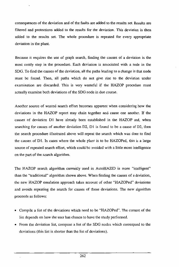
consequences of the deviation and of the faults are added to the results set. Results are
filtered and protections added to the results for the deviation. This deviation is then
added to the results set. The whole procedure is repeated for every appropriate
deviation in the plant.
Because it requires the use of graph search, finding the causes of a deviation is the
most costly step in the procedure. Each deviation is associated with a node in the
SDG. To find the causes of the deviation, all the paths leading to a change in that node
must be found. Then, all paths which do not give rise to the deviation under
examination are discarded. This is very wasteful if the HAZOP procedure must
actually examine both deviations of the SDG node in due course.
Another source of wasted search effort becomes apparent when considering how the
deviations in the HAZOP report may chain together and cause one another. If the
causes of deviation D I have already been established in the HAZOP and, when
searching for causes of another deviation D2, D I is found to be a cause of D2, then
the search procedure illustrated above will repeat the search which was done to find
the causes of D I. In cases where the whole plant is to be HAZOPed, this is a large
source of repeated search effort, which could be avoided with a little more intelligence
on the part of the search algorithm.
The HAZOP search algorithm currently used in AutoHAZID is more "intelligent"
than the "traditional" algorithm shown above. When finding the causes of a deviation,
the new HAZOP emulation approach takes account of other "HAZOPed" deviations
and avoids repeating the search for causes of those deviations. The new algorithm
proceeds as follows:
• Compile a list of the deviations which need to be "HAZOPed". The content of the
list depends on how the user has chosen to have the study performed.
• From the deviation list, compose a list of the SDG nodes which correspond to the
deviations (this list is shorter than the list of deviations).
262

• Search for the causes of any effect on the nodes in this list, using graph search in
the SDG. This is a two-stage graph search procedure, which produces a list of fault
propagation paths for each node in the list:
• The first stage of the search involves searching backwards from a subject
node, expanding lists of paths backwards, either to originating faults or as
far as the first other node also found to be in the list of subject nodes being
examined. A number of completed paths will be formed, from a fault to a
node, but a number of partial fault paths will also be formed, leading from
one "HAZOPed" node to another.
• The second stage of the search "knits together" the partial paths produced in
the previous stage, .to form lists of completed paths. Therefore, if there is a
partial path linking node NI to node N2, then all the causes of NI will be
used to compose new paths which end in N2. This second stage search is an
iterative procedure, but it avoids a lot of the repeated search inherent in
earlier versions of the search algorithm.
• Partition the results of the search into the paths which give rise to each of the
deviations in the original deviation list. For each node, paths will usually be
produced with both "direct" and "reverse" influences; these usually correspond to
"less" and "more" deviations of some process variable in the plallt.
• Identify the consequences of the deviations and the faults which cause them, and
add information about any protections which operate, putting all these results into
lists suitable for transfer to HazRes result objects, prior to formatting and filtering.
• Transfer the results just prepared into new HazRes objects, adding the results of the
configuration checking rules.
The function which starts up HAZOP emulation and deals with the collection of
resuits, preparation of deviation lists, different options for ~nalysis, etc., is
PerformFullHazop (). The function which coordinates the emulation procedure
to do a HAZOP on a list of deviations is full_hazop2 ( ) . The structure of these
functions is outlined in Figure B.2 and Figure B.3 below.
263
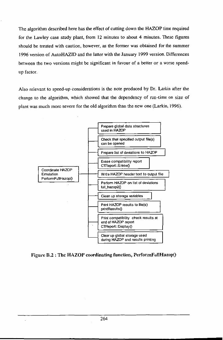
The algorithm described here has the effect of cutting down the RAZOP time required
for the Lawley case study plant, from 12 minutes to about 4 minutes. These figures
should be treated with caution, however, as the former was obtained for the summer
1996 version of AutoRAZID and the latter with the January 1999 version. Differences
between the two versions might be significant in favour of a better or a worse speed
up factor.
Also relevant to speed-up considerations is the note produced by Or. Larkin after the
change to the algorithm, which showed that the dependency of run-time on size of
plant was much more severe for the old algorithm than the new one (Larkin, 1996).
~ Prepare global data structures used in HAZOP
I-- Check that specified output file(s) can be opened
~1 Prepare list of deliations to HAZOP I H Erase compatibility report Cmeport::EraseO
Coordinate HAZOP Emulation - I Write HAZOP header text to output file I PertormFullHazopO
I- Pertorm HAZOP on list of deliations fulLhazop20
H Ciean L.ip storage variables I I- Pnnt HAZOP results to file(s)
pnntResultsO
Pnnt compatibility check resulls at I- end of HAZOP report
CTReport::Display()
'-. Clear up global storage used dunng HAZOP and results printing
Figure 8.2 : The HAZOP coordinating function, PerformFullHazopO
264
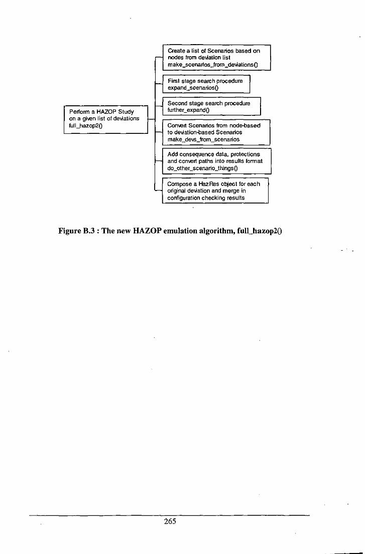
Create a list of Scenarios based on r--- nodes from de"'ation list
make_scenarios_frorn_de",ationsO
H First stage search procedure I expand_scenariosQ
Pertonn a HAZOP Study H Second stage search procedure
further_expandO I on a giwn list of de\'iations I-fulLhazop2O Comert Scenarios from node-based
- to de"'ation-based Scenarios make_de'wS_frorn_scenarios
Add consequence data, protections - and conwrt paths into results format
do_other_scenario_thingsO
Compose a HazRes object for each - original de\1ation and merge in
configuration checking results
Figure B.3 : The new RAZOP emulation algorithm, full_hazop20
265
Appendix C : Flow and Pressure Modelling in
Dividers and Headers
The flow path models for flow and pressure propagation presented in Chapter 3 rely
on the assumption that the flow path in which flow is considered to occur has only
one inlet port and one outlet. For equipment in which that assumption is not valid, the
appropriate qualitative model is somewhat more tricky to develop, because of the
inherent ambiguity in the mass balance equation (e.g. Qin = Qo",' + Q,",,), for a
qualitati ve model. This appendix considers the models of flow and pressure
propagation for "tee-pieces": pipes which either split an input flow (dividers), or join
multiple flows together (headers). Two of the simplest models are considered here.
Both models contain four locations (ports) where pressure is defined. The divider
model has onc inlet (in), one internal port (self) and two outlet ports (outl and out2).
The header model has two inlet ports (inl and in2), one internal port (self) and one
outlet port (out).
The divider and header models do not contain faults or consequences, just the arcs
governing fault propagation through them. There are not many interesting things that
can go wrong with a tee-piece, which cannot also occur in other equipment types.
The parts of each model which deal with pressure deviation propagation and the flow
deviations lessFlow and moreFlow are constructed by putting three flow path models
together and removing the nodes for resistance in each flow path. Resistance nodes
are used in modelling blockages and other faults, so they are not needed.
In use, the flow path models seem to predict accurately most of the expected
behaviour of a "tee-piece", with respect to propagation of pressure and the flow
deviations, lessFlow and moreFlow. However, as was the case for unbranched flow
paths, noFlow and revFlow cause significant problems in dividers and headers. No
flow is considered in Section C.2 and reverse flow in Section C.3.
266
A number of possible definitions for the model of a tee-piece are possible. In the
divider model presented below, an attempt has been made to make the model as
general as possible, so that both legs of the divider are considered to be usually
carrying fluid flows. This may not always be the case for actual dividers, where one
or both of the legs may be connected to a "blocking" component, such as a closed
valve. Such a situation may be best handled by a check on the configuration of the
component in the plant model, followed by selection of an appropriate, simpler,
model for the divider. AutoHAZID uses this approach.
Another possible complication for building models of general tee-piece components is
that controllers may constrain the actual behaviours of the flows and/or pressures in
the plant. Typically, in the case of a real divider, some control system would control
either the f10wrate into the divider, or the pressure near it. It turns out that the
deviations possible in the two constrained cases are subsets of those for the
unconstrained case. Therefore, the general divider model is suitable for all cases
where a control loop is in operation, but will over-predict deviations in these cases.
267
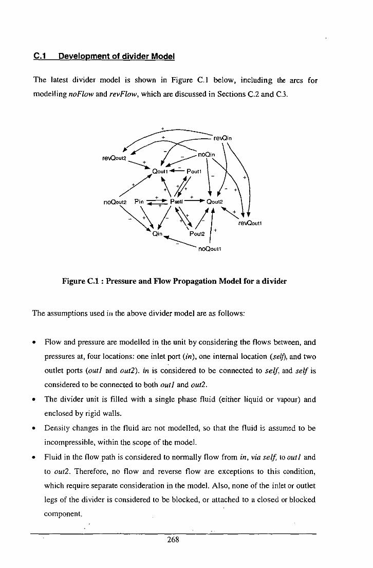
C.1 Development of divider Model
The latest divider model is shown in Figure C.l below, including the arcs for
modelling noFlow and revFlow, which are discussed in Sections C.2 and C.3.
+
Figure C.l : Pressure and Flow Propagation Model for a divider
The assumptions used ill the above divider model are as follows:
• Flow and pressure are modelled in the unit by considering the flows between, and
pressures at, four locations: one inlet port (in), one internal location (self), and two
outlet ports (outl and out2). in is considered to be connected to self, and self is
considered to be connected to both outl and out2.
• The divider unit is filled with a single phase fluid (either liquid or vapour) and
enclosed by rigid walls.
• Density changes in the fluid are not modelled, so that the fluid is assumed to be
incompressible, within the scope of the model.
• Fluid in the flow path is considered to normally flow from in, via self, to outl and
to out2. Therefore, no flow and reverse flow are exceptions to this condition,
which require separate consideration in the model. Also, none of the inlet or outlet
legs of the divider is considered to be blocked, or attached to a closed or blocked
component.
268

• The flows and pressures in the unit are not constrained by any control system, so
that the divider provides modelling for an unconstrained, general case.
• Pressure deviations are allowed to propagate freely from any inlet or outlet to any
other port in the unit, upstream or downstream.
• Row deviations (lessFlow and moreFlow) are not propagated - they are only
generated locally, for each part of the divider.
• The causal hierarchy described in Section 3.5.4 is considered to operate In the
divider unit.
• The relevant variables are P and Q, representing pressure and flow. Resistance, R,
is not used in this model. noFlow and revFlow are also present as deviations.
• There is no significant height difference between the locations in, outl and out2,
so that static head is the same everywhere within the unit.
• No shaft work is done on the fluid within the flow path.
• The fluid does not exchange sig!1ificant quantities of heat with its surroundings.
• Within the SDG model, the shortest path between two nodes determines what the
appropriate influence is between those nodes.
• The driving force for flow is pressure difference, which is not represented
explicitly in the model. As in the unbranching flow path model presented in
Section 3.5.5, upstream pressures have a direct effect on flow, and downstream
pressures have a reverse effect.
• Deviations in pressure within the divider are considered never to be sufficient to
cause the flow to reverse in the flow path.
C.2 Modelling noFlowfor the divider
In the unbranched flow path model, noFlow was simply propagated between the inlet
and outlet, without linkage to other variables in the flow path model. For a divider.
however, it is reasonable to expect blockage of one leg to cause deviations in flow and
pressure in the other legs.
Unfortunately, it is not possible to put arcs into the model to represent the pressure
changes caused by noFlow in one of the legs of the divider, because of the effect this
has on the flow variable in the same leg as the blockage - the deviation lessFlow
269
would be predicted at the same time as the deviation noFlow in an outlet leg, for
example.
Therefore, the model in Figure C.l only links noFlow to deviations in flow
throughout the unit, and to reverse flow in the outlet legs. It may well be the case,
however, that the fault which is the root cause of noFlow also causes a pressure
change, so that these same effects will be propagated independently.
Note that, due to the interpretation of noFlow as a blockage event, noFlow in anyone
of the legs of the divider does not imply noFlow in either of the other legs - because
there is a split in the flow path, fluid is not necessarily blocked by any single
blockage.
C.3 Modelling revFlowfor the divider
As with the unbranched flow path model, pressure is not linked to reverse flow in a
divider. This means that the real effect of lessPressure in one of the outlets causing
revFlow ill the other outlet is missed in the model presented in Figure C.l, but to put
the necessary arc in to achieve this effect would mean that a whole host of other
spurious predictions would appear.
The effects that !ill< represented by the revFlow model for a divider, are those of
revFlow on the outlet flows from the unit, and the possible effects of revFlow in the
inlet port on revFlow in the two outlet ports. Reverse flow of fluid in one of the
outlets causing a possible reduction in the inlet flow to the divider is not explicitly
represented because o( thc difficulties this would cause. However, the initial fault
causing reverse flow should include an effect on pressure, which can propagate to the
divider and cause the necessary flow deviations. This underlines the importance once
again of llsing consistent methods for developing failure modes information for
equipment in the plant model system.
One further area in which the model fails to represent a recognised real effect, is that
the possible reverse flow effect in the inlet, caused by revFlow in either outlet leg, is
270
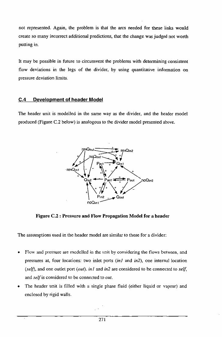
not represented. Again, the problem is that the arcs needed for these links would
create so many incorrect additional predictions, that the change was judged not worth
putting in.
It may be possible in future to circumvent the problems with determining consistent
flow deviations in the legs of the divider, by using quantitative infonnation on
pressure deviation limits.
C.4 Development of header Model
The header unit is modelled in the same way as the di vider, and the header model
produced (Figure C.2 below) is analogous to the divider model presented above.
Figure C.2 : Pressure and Flow Propagation Model for a header
The assumptions used in the header model are similar to those for a divider:
• Flow and pressure are modelled in the n!lit by considering the flows between. and
pressures at, four locations: two inlet ports (in] and in2), one internal location
(self), and one outlet port (out). in] and in2 are considered to be connected to self,
and self is considered to be connected to out.
• The header unit is filled with a single phase fluid (either liquid or vapour) and
enclosed by rigid walls.
271

• Density changes in the fluid are not modelled, so that the fluid is assumed to be
incompressible, within the scope of the model.
• Fluid in the flow path is considered to normally flow from in] and in2, via self, to
out. Therefore, no flow and reverse flow are exceptions to this condition, which
require separate consideration in the model. Also, none of the inlet or outlet legs
of the header is considered to be blocked, or attached to a closed or blocked
component.
• The flows and pressures in the unit are not constrained by any control system, so
that the header provides modelling for an unconstrained, general case.
• Pressure deviations are allowed to propagate freely from any inlet or outlet to any
other in the unit, upstream or downstream.
• Flow deviations (lessFlow and moreFlow) are not propagated - they are only
generated locally, for each flow path.
• The causal hierarchy described in Section 3.5.4 is considered to operate in the
header unit.
• The relevant variables are P and Q, representing pressure and flow. Resistance, R,
is not used in this model. noFlow and revFlow are also present as deviations.
• There is no significant height difference between the locations in], in2 and out, so
that static head is the same everywhere within the unit.
• No shaft work is done on the fluid within the flow path.
• The fluid does not exchange significant quantities of heat with its surroundings.
• Within the SDG model, the shortest path between two nodes determines what the
appropriate influence is between those nodes.
• The driving force for flow is ·pressure difference, which is not represented
explicitly in the model. As in the unbranching flow path model presented in
Section 3.5.5, upstream pressures have a direct effect on flow, and downstream
pressures have a reverse effect.
• Deviations in pressure within the header are considered never to be sufficient to
cause the flow to reverse in the flow path.
272
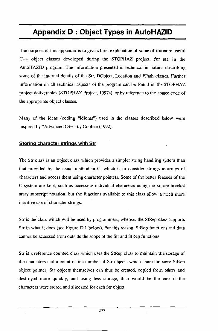
Appendix 0 : Object Types in AutoHAZID
The purpose of this appendix is to give a brief explanation of some of the more useful
C++ object classes developed during the STOPHAZ project, for use in the
AutoHAZID program. The information presented is technical in nature, describing
some of the internal details of the Str, DObject, Location and FPath classes. Further
information on all technical aspects of the program can be found in the STOPHAZ
project deliverables (STOPHAZ Project, 1997a), or by reference to the source code of
the appropriate object classes.
Many of the ideas (coding "idioms") used in the classes described below were
inspired by "Advanced C++" by Coplien (1992).
Storing character strings with Str
The Str class is an object class which provides a simpler string handling system than
that provided by the usual method in C, which is to consider strings as arr~ys of
characters and access them using character pointers. Some of the better features of the
C system are kept, such as accessing individual characters using the square bracket
array subscript notation, but the functions available to this class allow a much more
intuitive use of character strings.
Str is the class which will be used by programmers, whereas the StRep class supports
Str in what it does (see Figure D.l below). For this reason, StRep functions and data
cannot be accessed from outside the scope of the Str and StRep functions.
Str is a reference counted class which uses the StRep class to maintain the storage of
the characters and a count of the number of Str objects which share the same StRep
object pointer. Str objects themselves can thus be created, copied from others and
destroyed more quickly, and using less storage, than would be the case if the
characters were stored and allocated for each Str object.
273
Any number of Str objects can share the same characters using this reference counting
method. The StRep object maintains a count of the number of objects which contain a
pointer to it. When this count falls to zero the StRep object is destroyed, recovering its
own storage and that of the characters in the string. When a Str object is destroyed,
only the Str is recovered, unless the count for its StRep object goes to zero.
Str:: Str::
StRep "lpRep StRep "lpRep
L StRep:: Int IICount char "lszRep -~
IIII ... II
Figure 0.1 : Many Strs can share the same characters using StRep objects
Summary Features of the Str class:
• Initialisation from the following types: Str, char*, char, int and double.
• Conversion to the following types: char* (should be used with caution).
• Assignment, copying, construction and destruction without the need to worry
about assigning memory.
• Output to streams using the Display () function and left shift operator.
• Input from streams using the right shift operator and the ReadLine ( ) function.
• Uses integer indexing scheme similar to that used by C arrays, with subscripts
running from 0 to (length - 1). Use of array subscript notation (square brackets) in
reading single characters in the strin·g. Users of this class should be aware that
usmg an index outside the legal range for a Str object will cause an error or
warning.
• Concatenation of Str with Str or char* type character string, uses the
functions Append () and Prepend ( ) .
• Comparison of strings is possible using the equality and inequality operators
which are overloaded for this class. Also, an equivalent to the s trcmp ( )
function is provided in the form of Compare ( ) .
274
• Various "sub-string" operations are defined for splitting up strings. These are
modelled on equivalent operations in the BASIC language: Left (int),
Right (int), Mid(int, int) , ToRight(int), After(int).
• Searching for occurrences of strings within a Str is provided by the Find ( )
function.
• Conversion to and recognition of numbers is provided In the functions
IsInteger (int&) and IsDouble (double&).
• Conversion to upper and lower case characters is provided by ToUpper () and
ToLower ( ) , respectively.
DObject
The DObject class is designed to offer many of the symbolic manipulation and pattern
matching features of the clauses found in Prolog. This class can store data of many
different types and forms quite transparently and can be used to develop prototype
applications relatively quickly. However, one concern which may arise from the
widespread use of this class is the efficiency of the programs which result.
The motivation for developing this class was that there are many different data types
in the AutoHAZID system and there are some areas of the program where a flexible
"untyped" data object would be of great use in making the operation of the program
more powerful. Examples include the system which is used to represent the rules
belonging to the fluid model system, which should allow quite complex structures to
be put together to represent rules. Also, the representation of plant models in the
system should provide the ability to store new slots and their values in Frame objects,
without requiring too many changes to the parser and other code in the system.
DObjects here allow the definition of a generalised slot type which stores a list of
DObjects as its values.
The DObject class allows objects to be of several types, which are implemented via a
type field in the object, rather than using some other method (such as C++ based
inheritance). The types are enumerated in the enum type DObType, which is declared
in the file dobtype. h. The types are as listed in Table 0.1 below.
275

Type Description
Atom "Constant symbols", as in Prolog. These should start with a lower case letter and include
no spaces. Alternatively, they may be enclosed in single quotes (e.g.
constant_symbol or 'flammable a tmosphere I ).
Integer Integer constant values.
Real Real number values, implemented using double precision floating point numbers in C++.
Variable Variable symbols, as in Prolog. The variable name should start with an upper case letter or
an underscore character (e.g. Uni tName or _ var iable12 5).
Structure Similar in form to a predicate term in Prolog. An identifier which has the same format as
an Atom, followed by a list of terms (each of which may be an object of one of the types
listed here), separated by commas and enclosed in round brackets
(e.g. equals (4, plus(2,2» ).
StrType Strings of characters, enclosed in double quotes (e.g. "hello world" ).
ListType Lists of terms, which may be any of the types listed here) separated by commas and
enclosed in square brackets (e.g. [a, b, [4,5. 02J ,VarlJ ).
Table D.l : Data types stored in the DObject class
With a class which allows this sort of flexibility in the range of information it can
store, it is possible to build programs which perform quite powerful symbolic
operations, such as pattern matching. This feature is built into the DObject class, in
the form of the UnifyMatch () function, which allows one DObject to be matched
against another, making allowances for variables in each term.
The DObject class is a reference counted class, using the DObRep class to store the
data which it manipulates. The DObRep class remains invisible to the user, hidden
behind the public interface of the DObject class. The data which are stored include the
following (which may not.all be in use at anyone time):
• A string giving the "name" of the DObject, used for Atom, Variable, Structure and
StrType objects.
• An integer value for the DObject, used only for Integer type DObjects.
• A double precision floating point number value, used for the Real type.
276

• A DObList (list of DObjects) which comprises the argument list of a Structure
type DObject, or the list elements of a ListType DObject.
The relevant files for defining and implementing the DObject class are: dobj ec t . h,
dobject.cpp, dobrep.h, dobrep.cpp, doblist.h, doblist.cpp,
dobtype . h, newparse. h, and newparse. cpp. The Binding class is also
closely related to the DObject class and must be present for any of the advanced
matching functions of DObject to be used.
The main features of the DObject class are:
• The usual set of constructors, destructor and assignment definitions are provided
so that DObjects can be declared, assigned and copied, destroyed and passed as
function arguments, just as if they were a built-in type of the C++ language, such
as int or double.
• Other constructors allow the programmer to initialise DObjects of any type given
in Table D.1, by providing the data needed to set up the new object.
• The DObject type can be automatically assigned or constructed from a Str object,
using parsing code implemented in the file newparse. cpp. It can also be
converted back to Str form, using a conversion operator defined for that purpose.
• Read and write access to the data members of the DObject is provided by a set of
member functions, which include functions to read or change specific elements of
a ListType or Structure DObject and to add new elements to a Structure or
ListType.
• Two functions are provided for displaying the contents of the DObject. The
function Display () simply prints the contents of the object out to a single line
on the output stream given, while the Pret ty () function prints tll", DObjcct out
to the output stream on multiple lines if needed, making sure that the length of
each line is not greater than a given number of characters.
• The function ExactMatch () allows the programmer to compare DObjects
together where every part of one object must match the other one exactly.
277
• UnifyMatch () is a function which allows a less rigorous matching process to
take place, known as "unification matching". This means that the two terms must
be formally identical, in such a way that all the non-variable components must
match exactly between the two objects, but variables may be allowed to match
single terms in the other DObject, subject to the provision that the variable
bindings produced are not inconsistent. The procedure therefore produces a yes/no
answer saying whether the match succeeded, plus a list of variable bindings
generated by the match. This is a very powerful symbolic technique, widely used
in Prolog.
• DoBinding () and DoAllBindings () are used in UnifyMatch () to
perform variable binding substitutions on a DObject.
• MakeVarsDistinct () is also used in UnifyMatch () and ensures that any
variable names in a DObject are not also used in another DObject to which it is to
be matched, which would cause confusion. In the case where variables have to be
renamed, UniqueVar iableName () is used to generate a variable name which
has never so far been used.
• VariablesUsed () is used to find out the names of the variables used in the
DObject, and Grounded () simply tests if the list so produced is empty. These
are both support functions fur uni fyMa tch ( ) .
• The DObject and DObRep classes both use customised memory management
primitives, new and delete, which use a simple first-fit allocation routine.
A number of functions of the BindList class are particularly useful in supporting the
unification matching of DObjects. These are:
• The function BindList: : AddBinding () attempts to add a new Binding to
thl:! list currently stored, whilst maintaining the integrity of the Bindings already in
the table. The arguments to this function are DObjects giving the variable and its
value to be added to the table.
• If the variable is not so far in the BindList, then the new binding can be
added.
278
• If the variable is in the BindList and the value of the new Binding does not
unify with the value in the BindList already, then the Binding is not added
and the function fails.
• If a unification match succeeds, then the variable bindings produced by the
match are added to the BindList by a recursive call to AddBinding ( ) . If
all bindings are inserted properly, the function succeeds, otherwise it fails .
• BindList:: CollapseBindings () is a function which attempts to simplify
the variable Bindings in the list by reducing chains of variables. This does not
reduce the number of elements in the BindList, but converts the values of any
which can be so reduced to constants where this is possible.
• The function BindLi s t: : LookupBinding () retrieves the value recorded for
a variable, if there is one in the BindList.
• BindList:: ResolveFinalValue () gets a value for a variable from the
BindList, converting it to a non-variable tenn, if this is possible.
Location
The Location class stores, and allows for the manipulation of, infonnation concerning
fluids at particular places in the plant (characterised by a [unit,port] pair). The
checks and predicates of the fluid modelling system rely on objects of this class to
communicate infonnation about fluids.
The Location object is a reference counted object class which uses the LocRep class to
carry the data for any number of copy Locations. The implementation of reference
counting is similar to the method used for the Str class. The relevant source code files
for these classes are location.h, location.cpp, locrep.h and
locrep. cpp.
279
The specific data stored in the LocRep object (on behalf of Location objects) are:
• Strs indicating the relevant unit and port names for the Location.
• A Str object indicating the type of the process port to which the Location refers:
• 'T' indicates that it is an input port of the unit.
• "0" indicates that it is an output port of the unit.
• "U" indicates that it is an internal (uni tports) port in the unit.
• Numerical values for the temperature of the fluid (in 0c), its pressure (in bar abs)
and its quantity (in kg inventory for internal ports, or kglhr flow rate for input and
output ports).
• A list of names of chemical components of the fluid, and a corresponding list of
compositions (mole fraction values) for the fluid components. There is also an
integer value for each component, to store flags concerning the component, such
a~ whether it is a contaminant or not.
• A DObList list of DObjects is provided to record miscellaneous information
(notes) on behalf of the fluid modelling system. This is mostly used to record the
limits of deviations of process variables during validation of the fault paths
uncovered in the HAZOP search.
The main user-uccessible features of the Location class are:
• The usual set of constructors, destructor and assignment definitions are provided
so that Location objects can be declared, assigned and copied, destroyed and
passed as function arguments, just as if they were a buiit-in type of the C++
language, such as int or double.
• Location objects can be converted to or from appropriate DObject Structures. The
form used is: location (Uni t, Port, Type, Temperature, Pressure,
Quantity, [[Componentl,Compositionl,Flagsl], .. ],Notes)
• Functions are provided to allow the class user to read the data stored in the
Location object. These are: Uni tName ( ), PortName ( ), PortType ( ) ,
Pressure (), Temperature (), Quantity (), NoComps (),
CompName ( ), CompValue ( ), CompFlags ( ). The last three requIre an
280
integer index of the component In the Location, between 0 and
(NoComps ( ) -1). This can be found from the name using the function
FindComplndex ( ) .
• Similar functions are defined to change the values of the data stored in the object,
or to give them "undefined" values. These are: SetUnitName (),
SetPortName ( ) ,
SetTemperature(),
SetPortType (), SetPressure (),
SetQuanti ty (), UnSetTemperature (),
UnSetPressure () and UnSetQuanti ty ( ) .
• Components of the fluid can be added to or removed from the Location using the
functions AddComponent () and RemComponent ( ) .
• The flags which indicate whether a component is a contaminant or not can be
changed using the functions SetContaminantF1ag ( ) and
ResetContaminantFlag (), or read USIng the function
IsContaminant ().
• The Display () function can be used to output a representation of the
information in the Location to an output stream. This is the same function used by
the left shift operator, '«'. The function Describe (), which uses'
DescriptionString ( ), produces a more intelligible format for all the
information except for the "notes" field.
• Two functions are provided to compare Locations for equality. The equality
operator, '==', tests all the fields, so that numerical data, unit, port and component
data must match between two Locations. A less strict comparison is the function
Same Place ( ) , which tests to see if the unit and port fields of the two Locations
are the same.
• A number of functions are provided to read, add, remove, search through and
change the contents of the notes in the Location. These are: Ge tNotes ( ) ,
SeUJotes (), AddNol:e (), RemNote (), RemMat.chingNotes ( ),
FindMatchingNotes () and HasNotes () .
• The function Mixture () takes two Locations and produces a new Location
corresponding to mixing together the fluids from each one. The two Location
objects need not refer to the same place in the plant, but the resulting mixture
281

object is defined at the same place as the "host" object which initiated the function
call.
FPath
The FPath class is used in the validation of fault paths which is perfonned during the
HAZOP search algorithm and elsewhere when the program searches for the causes of
some deviation. The FPath represents the path to be validated, along with data such as
the list of fluids relating to that path, and various classification data generated by the
validation process.
The data stored in this object type are as follows:
• A List of pointers ,0 Arcs, defining the path which is the subject of the FPath.
• A List of currently defined fluids, in Location objects, which defines the necessary
infonnation about fluids relevant to the nodes visited along the fault path.
• Fields to store infonnation concerning the classification and ranking of the
consequences of the fault path (see Section 3.3.8). These are:
• An importance number, between 0 and 5.
• A consequence rank number, between 0 and 5.
• A category for the consequence of the path, taken from the list ('none',
'haz', 'op' and 'haz_op').
• A bit field of up to 16 bits, encoding whether the consequence of the FPath
is a member of the various standard classes of consequences.
The main features of this class are as follows:
• The usual constructors, destructor and assignment are defined in order to make the
type into a "concrete class". The FPath can also be initialised from a List of Arc
pointers, which represents the fault path.
• FPath objects can be compared for equality using the '==' operator.
• FPath object~ can be printed to an output stream using the function Display ().
282
• The current fluid list belonging to the FPath can be accessed (for reading or
changing) using the function Fluids ( ) .
• The List of Arc pointers which makes up the path in the FPath object can be
accessed (for reading or changing) using the function Pa th ( ) .
• The last Filler in the path can be referenced using the EndOfPath () member
function.
• The steps in the fault path represented by the FPath object can be checked using
the fluid modelling system, with the function Valida te ( ). This function
performs all the necessary tests on the links in the fault propagation chain, and
maintains the necessary information on the numerical limits of deviations, as
described in Chapter 5.· It makes particular use of the extemal function
propertyHolds () and the private member functions Fwd_Limits () and
RemoveLimits ().
283
Appendix E : Table of Functions and Predicates in the Fluid Modelling System
This appendix provides a complete listing of the functions and predicates developed
for the fluid modelling system described in Chapter 5. The columns in Table E.I give
the following information:
• Prototype: An indication of the prototype (i.e. name and list of arguments) for the
function or predicate.
• P/F: A flag indicating whether the item is a function ("F') or predicate ("P").
• Imp?: An indication of whether the function or predicate has been fully
implemented in the FMS ("Y" indicates that the item has been implemented and
tested in AutoHAZID).
• Used?: Indicates whether the item is actually used in the FMS.
• System: This shows whether the item is implemented in a C++ function ("C"),
defined in terms of other items ("D"), or corresponds to a rule in the VIT fluid rule
system ("V").
• Group: This is the group of the FMS in which thl:! function or predicate IS
considered to belong. The groups are listed below.
• Description: A short description of what the predicate is supposed to test, or what
the function is supposed to evaluate.
Functions and predicates in the FMS' are considered to belong to one of a number of
groups, covering the type of activity that it deals with. The complete list of groups is:
I. Logical operations
2. Mathematical operations
3. General-purpose operations
4. Plant, fluid and fault path data access
5. Limit data access
6. Combining fluids (including compatibility checks)
7. Properties of single fluids
284

8. Consequence evaluation
9. Contamination
IO.Design parameter checks
II.Miscellaneous physical checks
12.Leakage checks and limitations
13.Checks on VLE pressure limitations
14.Pressure deviation limits corresponding to resistance changes in flow paths
Table E.I : Functions and Predicates in the Fluid Modelling System
Prototype P I U S G Description
/ m s y r . F P e s 0
? d t u
? e p
m
GROUP 1. LOGJ:CAL OPERATJ:ONS
true P Y Y C 1 Logical constant.
false P Y Y C 1 Logical constant.
op_and (Tl. T2) P Y Y C 1 Logical AND operator. Also valid as
infix operator n && n •
op_or(Tl.T2) P Y Y C 1 Logical OR operator. Also val id as
infix operator " I I " . not(Tl) P Y Y C 1 Logical NOT operator.
GROUP 2. MATHEMATJ:CAL OPERATJ:ONS
op_add(Tl.T2) F Y Y C 2 Addition of numerical values. Also
valid as infix operator "+" . Multiple
arguments possible.
op_mult(Tl.T2) F Y Y C 2 Multiplication of numerical values.
Also valid as infix operator "* " Multiple arguments possible.
op_sllb (Tl. T2) F Y Y C 2 S'lbtraction of numerical values. Also
valid as infix operator " - "
op_div(Tl,T2) F Y Y C 2 Division of numerical values. Also
valid as infix operator .. /" . power (Base, F Y N C 2 Exponentiation of numerical values.
Exponent)
285
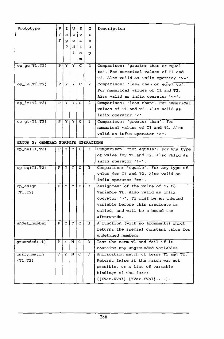
Prototype P I U S G Description
/ m s y r
F p e s 0
? d t u
? e p
m
op_ge (T1, T2) p Y Y C 2 Comparison: ngreater than or equal
to· . For numerical values of T1 and
T2. Also valid as infix operator n>;::n.
op_le(T1,T2) P Y Y C 2 Comparison: "less t.han or equal to" .
For numerical values of T1 and T2.
Also valid as infix operator .<;::n.
op_lt(T1,T2) P Y Y C 2 Comparison: "less thana. For numerical
values of T1 and T2. Also valid as
infix operator "<".
op_gt(T1,T2) P Y Y C 2 Comparison: ngreater than" . For
numerical values of T1 and T2. Also
valid as infix operator n>".
GROUP 3: GENERAL PURPOSE OPERATJ:ONS
op_ne (T1, T2) p Y Y C 3 Comparison: "not equals· . For any type
of value for T1 and '1'2. Also valid as
infix operator 11 ! ::: n •
op_eq(T1, T2) P Y Y C 3 Comparison: "equals". For any type of
value for T1 and T2. Also valid as
infix operator n::::::n
op_assgn P Y Y C 3 Assignment of the value of T2 to
(T1,T2) variable Tl. Also valid as infix
operator ":::" T1 m'-".st be an unbound
variable before this predicate is
called, and will be a bound one
afterwards.
undef_number F Y Y C 3 A function (with no arguments) which
returns the special constant value for
undefined numbers.
grounded (T1 ) P Y N C 3 Test the term Tl and fail if it
contains any ungrounded variables.
unify_match F Y N C 3 Unification IT'.atch of terms Tl ann T2.
(T1,T2) Returns false if the match was not
possible, or a list of variable
bindings of the form:
[[XVar,XValJ, [YVar,YValJ, ... J.
286
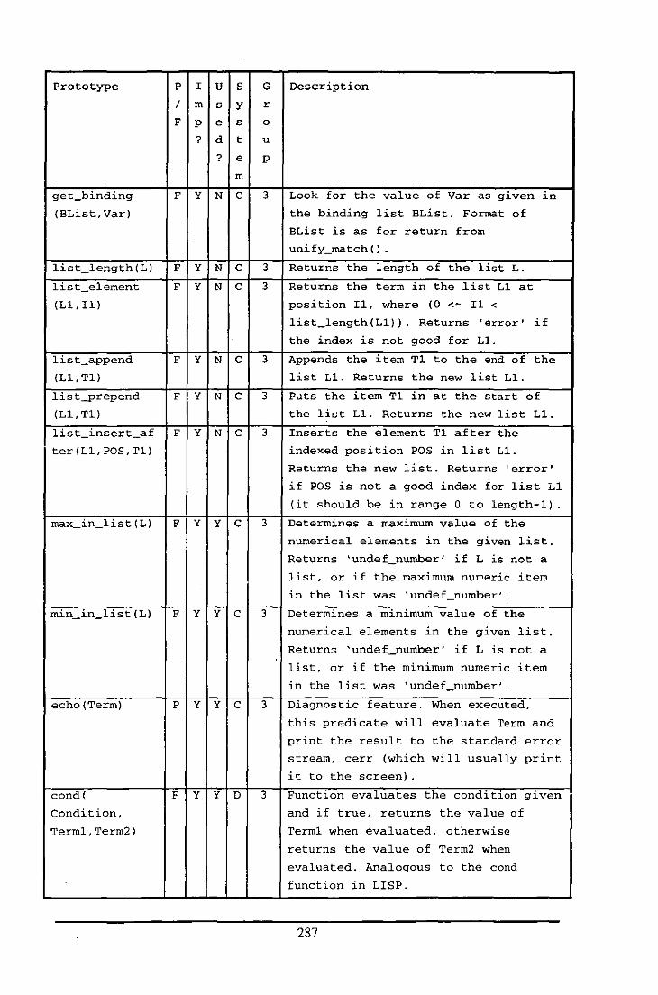
Prototype P I U S G Description
/ m s y r
F p e s 0
? d t u
? e p
m
get_binding F Y N C 3 Look for the value of Var as given in
(BList,Var) the binding list BList. Format of
BList is as for return from
unify_match () .
list _length(L) F Y N C 3 Returns the length of the list L.
list_element F Y N C 3 Returns the term in the list Ll at
(Ll,Il) position Il, where (0 <= Il <
list_length(Ll)) . Returns 'error' if
the index is not good for Ll.
list_append F Y N C 3 Appends the item Tl to the end of the
(Ll,Tl) list Ll. Returns the new list Ll.
list-prepend F Y N C 3 Puts the item Tl in at the start of
(Ll,Tl) the li::;t Ll. Returns the new list Ll.
list_insert_af F Y N C 3 Inserts the element Tl after the
ter(Ll,POS,Tl) indexed position POS in list Ll.
Returns the new list. Returns 'error'
if POS is not a good index for list Ll
(it should be in range 0 to length-l) .
max_in_list(L) F Y Y C 3 Determines a maximum value of the
numerical elements in the given list.
Returns 'undef _number' if L is not a
list, or if the maximum nUI!'.eric item
in the list was 'undef _number' .
min_in_list(L) F Y Y C 3 Determines a minimum value of the
numerical elements in the given list.
Return3 'undef_number' if L is not a
list, or if the minimum numeric item
in the list was 'undef _number' .
echo (Term) P Y Y C 3 Diagnostic feature. When executed,
this predicate will evaluate Term and
I print the result to the standard error
stream, cerr (which will usually print
it to the screen) .
cond( F y Y D 3 Function evaluates the condition given
Condition, and if true, returns the value of
Terml , Term2 ) Terml when evaluated, otherwise
returns the value of Terrn2 when
evaluated. Analogous to the cond
function in LISP.
287

Prototype P I U S G Description
/ m s y r
F p e s 0
? d t u
? e p
m
GROtJ'P 4: PLANT, FLm:D AND FAULT PATH DATA ACCESS
max-port F Y N D 4 Determines the largest diameter of the
_diameter ports associated with the current
context unit.
get_attribute F Y Y C 4 Returns the value of the named
(AttName) attribute for the current context unit
in the plant model. Returns an Atom
for ' is' slots, or a ListType for
'info' slots. If the attribute is not
found or doesn't have a value, returns , 'undefined' .
get_fluid F Y Y C 4 Access to the current fluid for the
(Port) given· port. Returns 'error' if the
fluid cannot be retrieved.
get_nominal F Y Y C 4 Access to the nominal (plant
_fluid(Port) description) fluid for the port given.
set_fluid P Y Y C 4 Set the current fluid information for
(Port, FI) the given port to be the fluid FI.
get 'pressure F Y Y C 4 Returns the numerical value of the
(Fluid) pressure for the given fluid.
get F Y Y C 4 Returns the numerical value of the
_temperature temperature for the given fluid.
(Fluid)
get F Y N C 4 Returns the mole fraction of the
_composition component in the fluid given.
(Fluid,Ccmp)
set-pressure F Y N C 4 Sets the pressure of the given fluid
(Fluid,Value) to be Value, returning the modi fied
fluid.
set F Y Y C 4 Sets the temperature of the given
_temperature fluid to be Value, returning the
(Fluid, Value) modified fluid.
set F Y N C 4 Sets the composition of the component
_composition in the given fluid, returning the
(Fluid,Comp, modified fluid. If the named component
Val) is not in the fluid, a warning is
issued and the function returns the
unchanged fluid.
288
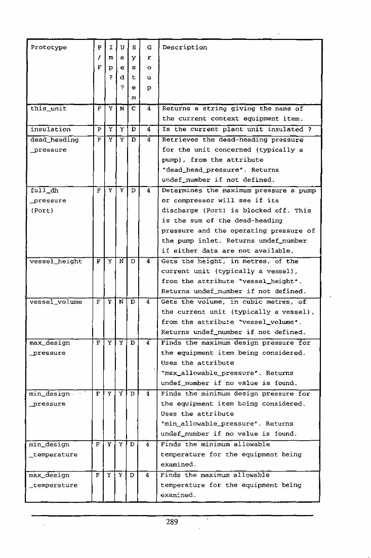
Prototype P I U S G Description
/ In S Y r
F p e s 0
? d t u
? e p
In
this _unit F Y N C 4 Returns a string giving the name of
the current context equipment item.
insulation P Y Y D 4 Is the current plant unit insulated ?
dead_heading F Y Y D 4 Retrieves the dead-heading pressure
-pressure for the unit concerned (typically a
pump) , from the attribute
~dead_head-pressure-. Returns
undef_number if not defined.
full _dh F Y Y ·D 4 Determines the maximum pressure a pump
-pressure or compressor will see if its
(Port) discharge (Port) is blocked off. This
is the sum of the dead-heading
pressure and the operating pressure of
the pump inlet. Returns undef_number . < ~4 either data are not available .
vessel_height F Y N D 4 Gets the height, in metres, of the
current unit (typically a vessel) ,
from the attribute "vessel_height".
Returns undef_number if not defined.
vessel_volume F Y N D 4 Gets the volume, in cubic metres, of
the current unit (typically a vessel) ,
from the attribute "vessel_volume- .
Returns undef_number if not defined.
max_design F Y Y D 4 Finds the maximum design pressure for
-pressure the equipment item being considered.
Uses the attribute
"max_allowable-pressure-. Returns
undef_nurnber if no value is found.
min_design F Y Y D 1 Finds the minimum design pressure for
-pressure the equipment item being considered.
Uses the attribute
"min_allowable-pressure N• Returns
undef_nurnber if no value is found.
min_design F Y Y D 4 Finds the minimum allowable
_temperature temperature for the equipment being
examined.
max_design F Y Y D 4 Finds the maximum allowable
_temperature temperature for the equipment being
examined.
289
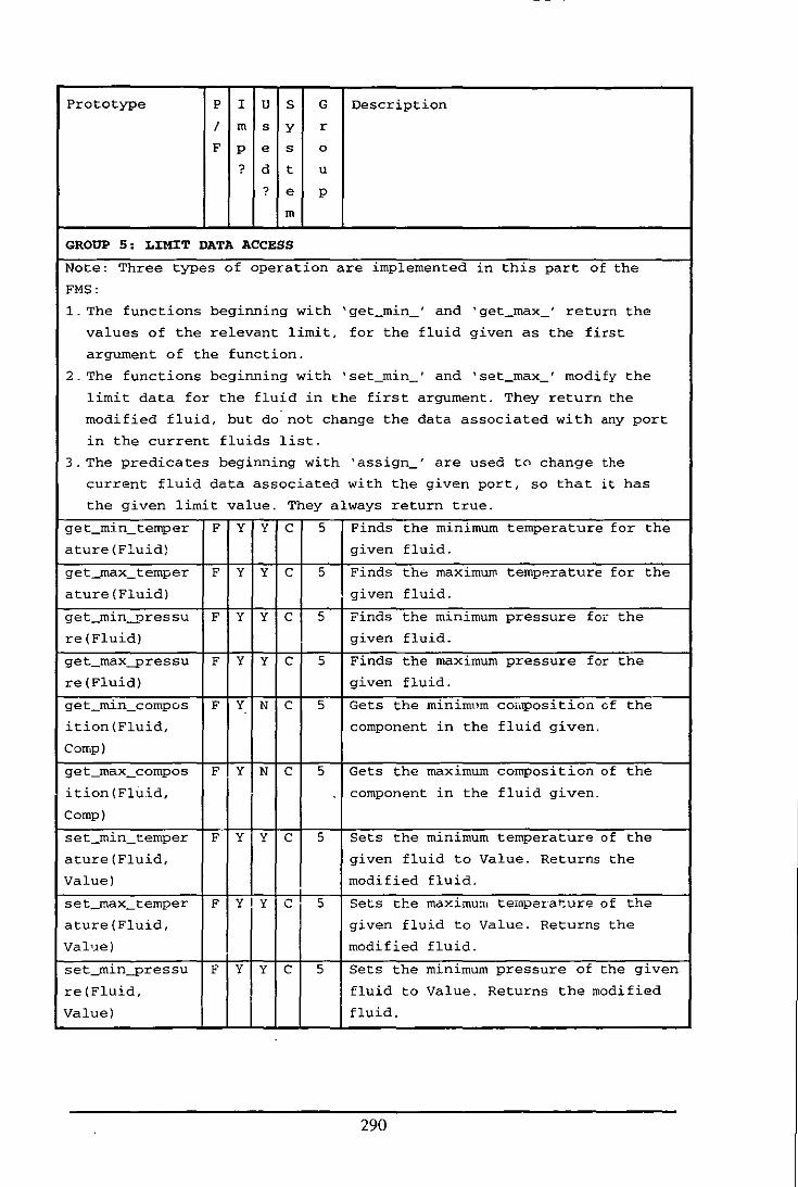
Prototype P I U S G Description
I m s y r
F p e s 0
? d t u
? e p
m
GROUP 5: LJ:MJ:T DATA ACCESS
Note: Three types of operation are implemented in this part of the
FMS:
1. The functions beginning with 'get_min_' and 'get_max_' return the
values of the relevant limit, for the fluid given as the first
argument of the function.
2. The functions beginning with 'set _min -, and 'set_max_' modify the
limit data for the fluid in the first argument. They return the
modified fluid, but do not change the data associated with any port
in the current fluids list.
3. The predicates beginning with 'assign_' are used to change the
current fluid data associated with the given port, so that it has
the given limit value. They always return true.
get_min_temper F Y Y C 5 Finds the minimum temperature for the
ature (Fluid} given fluid.
get_max_temper F Y Y C 5 Finds th8 maximum temperature for the
ature(Fluid) given fluid.
get_rnin-pressu F Y Y C 5 Finds the minimum pressure for the
re (Fluid) given fluid.
get_max-pressu F Y Y C 5 Finds the maximum pressure for the
re(Fluid) given fluid.
get_min_compos F Y N C 5 Gets the minimum cOILlposi tion ef the
i tion (Fluid, component in the fluid given.
Comp)
get_max_compos F Y N C 5 Gets the maximum composition of the
ition(Fluid, component in the fluid given.
Comp)
set_min_temper F Y Y C 5 Sets the minimum temperature of the
ature(Fluid, given fluid to Value. Returns the
Value) modified fluid.
set_rnax_temper F Yly C 5 Sets the maximu!H tempera t: urt;! 0 f the
ature(Fluid, given fluid to Value. Returns the
Value) modified fluid.
set_min-pressu F Y Y C 5 Sets the minimum pressure of the given
re(Fluid, fluid to Value. Returns the modified
Value) fluid.
290
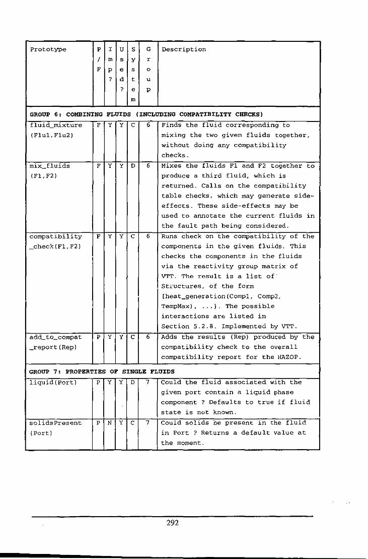
Prototype P I U S G Description
/ m s y r
F p e s 0
? d t u
? e p
m
GROUP 6: COMBJ:NJ:NG FLUJ:DS (J:NCLUDJ:NG COMPATJ:BJ:LJ:TY CHECKS)
fluid_mixture F Y Y C 6 Finds the fluid corresponding to
(Flul,Flu2) mixing the two given fluids together,
without doing any compatibility
checks.
mix_ fluids F Y Y D 6 Mixes the fluids Fl and F2 together to
(Fl,F2) produce a third fluid, which is
returned. Calls on the compatibility
table checks, which may generate side-
effects. These side-effects may be
used to annotate the current fluids in
the fault path being considered.
compatibility F Y Y C 6 Runs check on the compatibility of the
_check(Fl,F2) components in the given fluids. This
checks the components in the fluids
via the reactivity group matrix of
VTT. The result is a list oC
Stl-uctures, of the form
[heat_generation (Compl, Comp2,
TempMax) , ••• J . The possible
interactions are listed in
Section 5.2.8. Implementea by VTT.
add_to_cornpat P y Y C 6 Adds the results (Rep) produced by the
_report (Rep) co,"patibility check to the overall
compatibility report for the HAZOP.
GROUP 7: PROPERTJ:ES OF SJ:NGLE FLUJ:DS
liquid(Port) P Y Y D 7 Could the fluid associated with the
given port contain a liquid phase
component ? Defaults to true if fluid
state is not known.
solids Present P N Y C 7 Could solids oe present in the fluid
(Port) in Port ? Returns a default value at
the moment.
292

Prototype P I U S G Description
/ m s y r
F p e s 0
? d t u
? e p
m
freezing (Port) P Y Y C 7 Determines if any of the components of
the fluid associated with the given
port are below their freezing point at
the current temperature. Does not use
limit temperatures, just the current
fluid data.
flammable P Y Y C 7 Determines if the fluid in the given
(Port) port is flammable. Simply tests each
of the components to see if any
qualify.
toxic (Port) P Y Y D 7 Determines if the fluid in the given
port is toxic. Uses the function
toxici ty () , which relies on fluid
library info.
crystalliser P N Y C 7 Determines if the fluid in the given
(Port) port is likely to crystallise. Uses a
default return value at the moment,
because no data are available to test
the condition.
polymeriser P N Y C 7 Determines if the fluid in the given
(Port) port is likely to polymerise. Uses a
default rE:turn value at the moment,
because no data are available to test
the condition.
dissolvedGas P N Y C 7 Determines if the fluid in the given
(Port) port contains dissolved gas
components. Uses a default return
value at the moment, because no data
dre available to test the condition.
brittle(Port) P N Y C 7 Determines if the materials of
construction I
associated with the given
port are lik2ly to become brittle at a
low temperature.
decomp (Port) P N Y C 7 Determines if the fluid in the given
port is likely to undergo
decomposition.
293
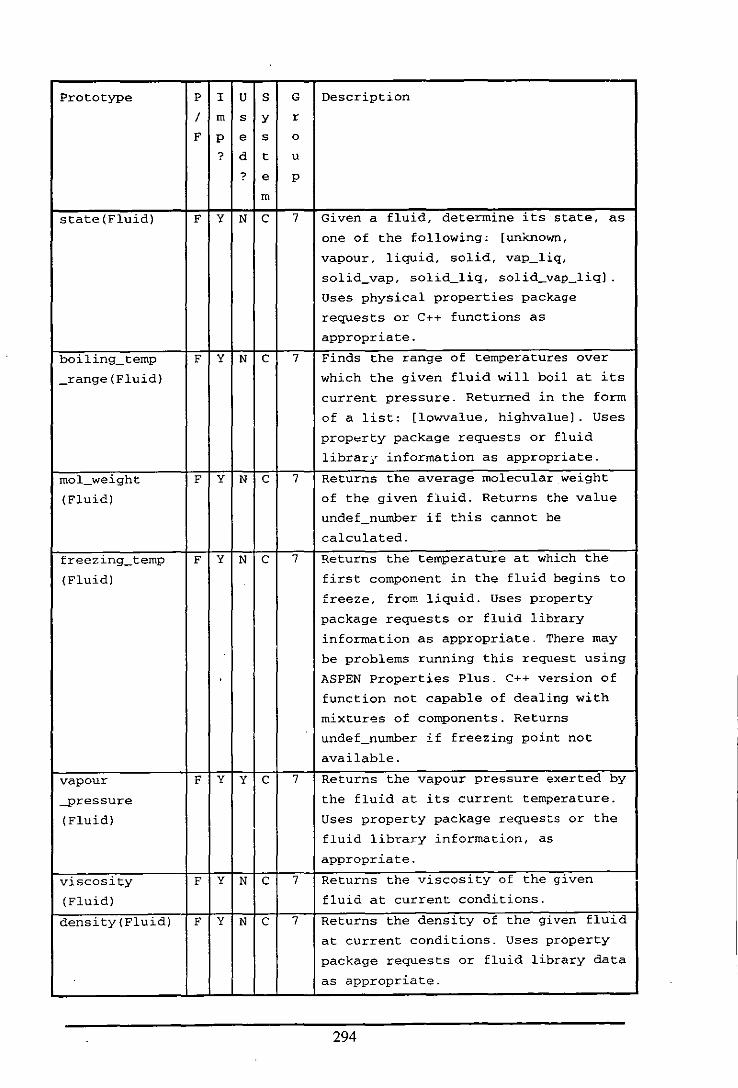
Prototype P I U S G Description
/ m s y r
F p e s 0
? d t u
? e p
m
state(Fluid) F y N C 7 Given a fluid, determine its state, as
one of the following: [unknown,
vapour, liquid, solid, vap_liq,
solid_vap, solid_l iq, sol id_vap_l iq)
Uses physical properties package
requests or c++ functions as
appropriate.
boiling_temp F y N C 7 Finds the range of temperatures over
_range (Fluid) which the given fluid will boil at its
current pressure. Returned in the form
of a list: [lowvalue, highvalue) . Uses
prop~rty package requests or fluid
librarI information as appropriate.
mol_weight F y N C 7 Returns the average molecular weight
(Fluid) of the given fluid. Returns the value
undef number if this cannot be -calculated.
freezing_temp F y N C 7 Returns the temperature at which the
(Fluid) . first component in the fluid begins to
freeze, from liquid. Uses property
package requests or fluid library
information as appropriate. There may
be problems running this request using
ASPEN Properties Plus. C++ version of
function not capable of dealing with
mixtures of components. Returns
undef _number if freezing point not
available.
vapour F y Y C 7 Returns the vapour pressure exerted by
-pressure the fluid at its current temperature.
(Fluid) Uses property package requests or the
fluid library information, as
appropriate.
viscosity F y N C 7 Returns the viscosity of the given
(Fluid) fluid at current conditions.
density(Fluid) F y N C 7 Returns the density of the given fluid
at current conditions. Uses property
package requests or fluid library data
as appropriate.
294
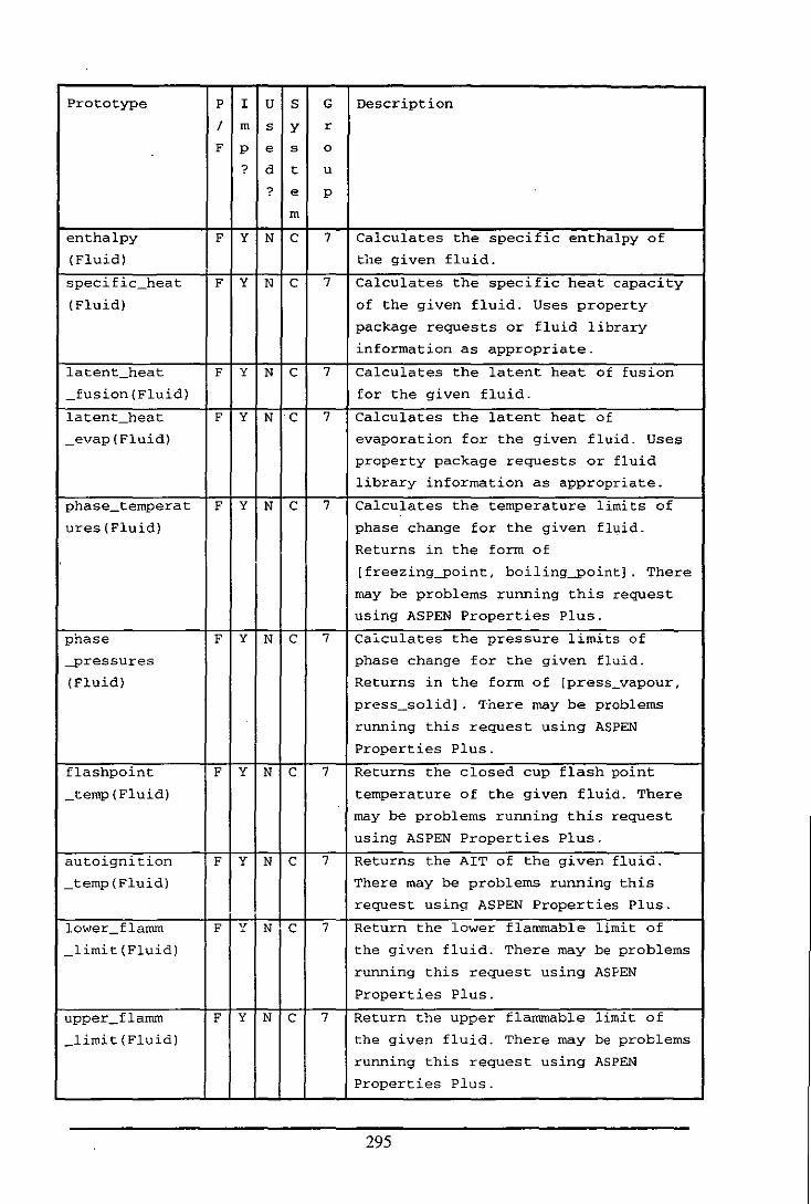
Prototype P I U S G Description
/ m s y r
F p e s 0
? d t u
? e p
m
enthalpy F Y N C 7 Calculates the specific enthalpy of
(Fluid) the given fluid.
specific_heat F Y N C 7 Calculates the specific heat capacity
(Fluid) of the given fluid. Uses property
package requests or fluid library
information as appropriate.
latent _heat F Y N C 7 Calculates the latent heat of fusion
_fusion(Fluid) for the given fluid.
latent_heat F Y N ·c 7 Calculates the latent heat of
_evap(Fluid) evaporation for the given fluid. Uses
property package requests or fluid
library information as appropriate.
phase_temperat F Y N C 7 Calculates the temperature limits of
ures(Fluid) phase change for the given fluid.
Returns in the form of
[freezing-point, boiling-pointj . There
may be problems running this request
using ASPEN Properties Plus.
phase F Y N C 7 Calculates the pressure limits of
--pressures phase change for the given fluid.
(Fluid) Returns in the form of [press_vapour,
press_solid] . 'I·here may be problems
running this request using ASPEN
Properties Plus.
flashpoint F Y N C 7 Returns the closed cup flash point
_temp (Fluid) temperature of the given fluid. There
may be problems running this request
using ASPEN Properties Plus.
autoignition F Y N C 7 Returns the AIT of the given fluid.
_temp (Fluid) There may be problems running this
request using ASPEN Properties Plus.
lower_flarorn F Y N C 7 Return the lower flammable limit of
_limit (Fluid) the given fluid. There may be problems
running this request using ASPEN
Properties Plus.
upper_flamm F y N C 7 Return the upper flammable limit of
_limit (Fluid) the given fluid. There may be problems
running this request using ASPEN
Properties Plus.
295
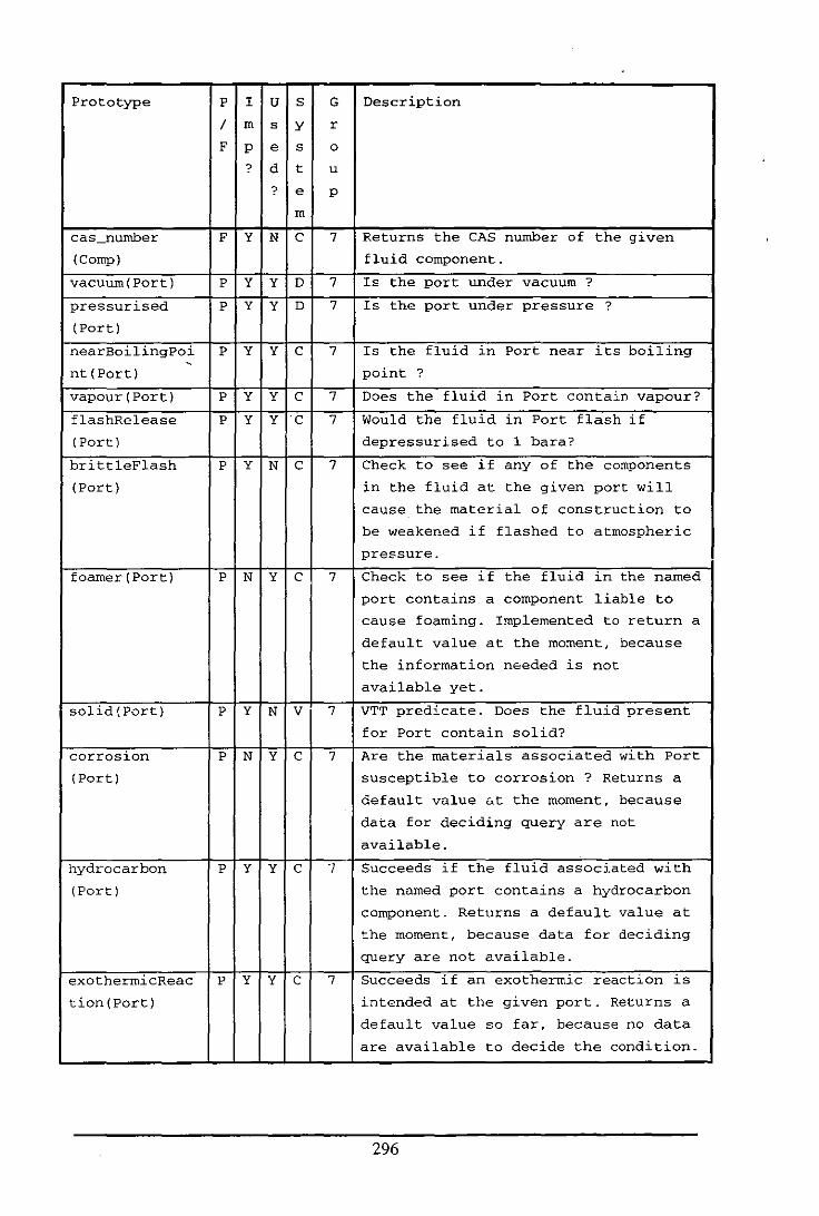
Prototype P I U S G Description
/ m s y r
F p e s 0
? d t u
? e p
m
cas_number F Y N C 7 Returns the CAS number of the given
(Comp) fluid component.
vacuum (Port) P Y Y D 7 Is the port under vacuum ?
pressurised P Y Y D 7 Is the port under pressure ?
(Port)
nearBoilingPoi P Y Y C 7 Is the fluid in Port near its boiling ,
nt(Port) point ?
vapour (Port) P Y Y C 7 Does the fluid in Port contain vapour?
flashRelease P Y Y ·C 7 Would the fluid in Port flash if
(Port) depressurised to 1 bara?
brittleFlash P Y N C 7 Check to see if any of the components
(Port) in the fluid at the given port will
cause the material of construction to
be weakened if flashed to atmospheric
pressure.
foamer (Port) P N Y C 7 Check to see if the fluid in the named
port contains a component liable to
cause foaming. Implemented to return a
default value at the moment, because
the information needed is not
available yet.
solid(Port) P Y N V 7 VTT predicate. Does the fluid present
for Port contain solid?
corrosion P N Y C 7 Are the materials associated with Port
(Port) susceptible to corrosion ? Returns a
default value Eit the moment, because .
data for deciding query are not
available.
hydrocarbon P Y Y C 7 Succeeds if the fluid associated with
(Port) the named port contains a hydrocarbon
component. Returns a default value at
the moment, because data for deciding
query are not available.
exothermicReac P y Y C 7 Succeeds if an exothermic reaction is
tion(Port) intended at the given port. Returns a
default value so far, because no data
are available to decide the condition.
296
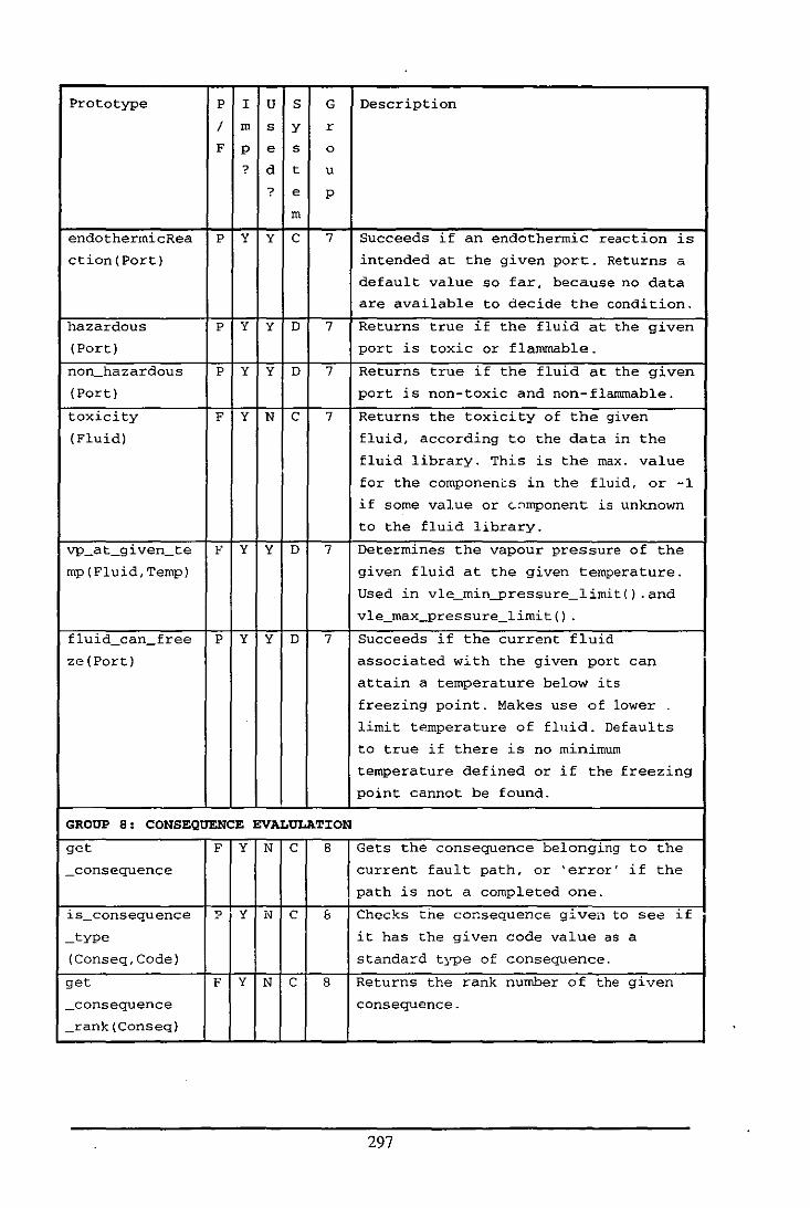
Prototype P I U S G Description
/ m s y r
F p e s 0
? d t u
? e p
m
endothermicRea P Y Y C 7 Succeeds if an endothermic reaction is
ction(Port) intended at the given port. Returns a
default value so far, because no data
are available to decide the condition.
hazardous P Y Y D 7 Returns true if the fluid at the given
(Port) port is toxic or flammable.
non_hazardous P Y Y D 7 Returns true if the fluid at the given
(Port) port is non-toxic and non-flammable.
toxicity F Y N C 7 Returns the toxicity of the given
(Fluid) fluid, according to the data in the
fluid library. This is the max. value
for the componencs in the fluid, or -1
if some value or <":'Imponent is unknown
to the fluid library.
vp_at_given_te F Y Y D 7 Determines the vapour pressure of the
mp(Fluid,Temp) given fluid at the given temperature.
Used in vle_min-pressure_limit() . and
vle_max-pressure_limit() .
fluid_can_free P Y Y D 7 Succeeds if the current fluid
ze (Port) associated with the given port can
attain a temperature below its
freezing point. Makes use of lower
limit tE>..mperature of fluid. Defaults
to true if there is no minimum
temperature defined or if the freezing
point cannot be found.
GROUP 8: CONSEQUENCE EVALOLAT:ION
get F Y N C 8 Gets the consequence belonging to the
_consequence current fault path, or 'error' if the
path is not a completed one.
is_consequence p Y N C 5 Checks the co~sequenc€: givei1 to se" if
_type it has the given code value as a
(Conseq,Code) standa"d type of consequence.
get F Y N C 8 Returns the rank number of the given
_consequence consequence.
_rank (Conseq)
297
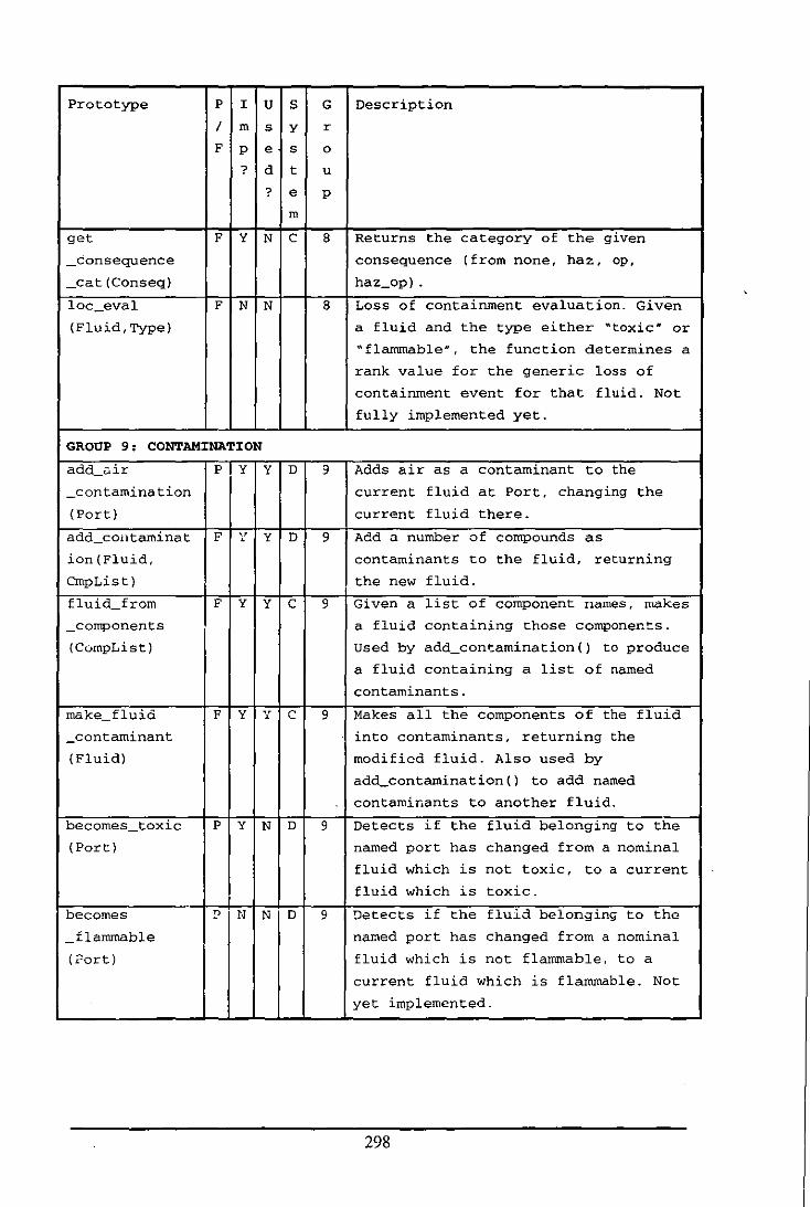
Prototype P I U S G Description
/ m s y r
F p e s 0
? d t u
? e p
m
get F Y N C 8 Returns the category of the given
_consequence consequence (from none, haz, op.
_cat (Conseq) haz_op) .
loc _€val F N N 8 Loss of containment evaluation. Given
(Fluid. Type) a fluid and the type either "toxic· or
"flammable N, the function determines a
rank value for the generic loss of
containment event for that fluid. Not
fully implemented yet.
GROUP 9: CONTAM:INAT:ION
add_air P Y Y D 3 Adds air as a contaminant to the
_contamination current fluid at Port. changing the
(Port) current fluid there.
add_coiltarninat F " Y D 9 Add a number of compounds as ~
ion (Fluid, contaminants to the fluid. returning
CrnpList) the new fluid.
fluid_ from F Y Y C 9 Given a list of component names, makes
_components a fluid containing those components.
(CompList) Used by add_contamination() to produce
a fluid containing a list of named
contaminants.
rnake_fl uid F Y " C 9 Makes all the components of the fluid " _contaminant into contaminants, returning the
(Fluid) modified fluid. Also used by
add_contamination() to add named
contamir~ants to another fluid.
becomes_toxic P Y N D 9 Detects if the fluid belonging to the
(Port) named port has changed from a nominal
fluid which is not toxic, to a current
fluid which is toxic.
becomes I' N N D 9 Detects if the fluid belonging to the
- flammable named port has changed from a nominal
(<'ort) fluid which is not flammable. to a
current fluid which is flammable. Not
yet implemented.
298
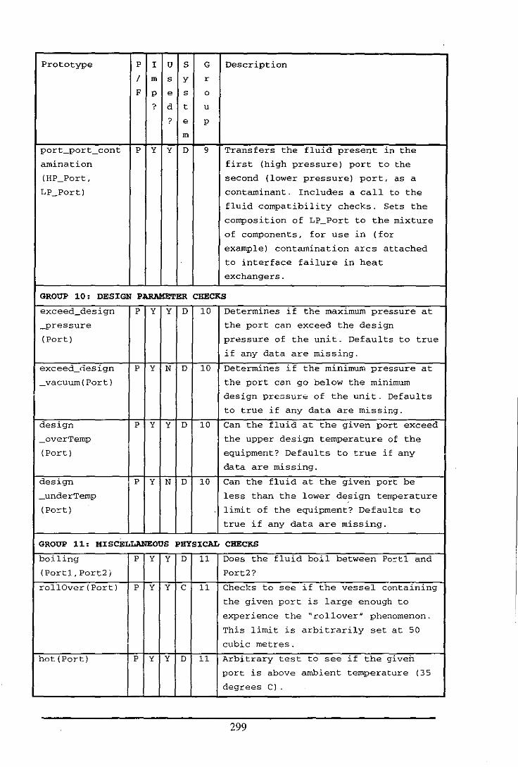
Prototype P I U S G Description
/ m s y r
F p e s 0
? d t u
? e p
m
port-port_cont P Y Y D 9 Transfers the fluid present in the
amination first (high pressure) port to the
(HP_Port, second (lower pressure) port. as a
LP_Port) contaminant. Includes a call to the
fluid compatibility checks. Sets the
composition of LP_Port to the mixture
of components, for use in (for
example) contamination arcs attached
to interface failure in heat
exchangers.
GROUP 10 : DESIGN PARAMETER CHECKS
exceed_design P Y Y D 10 Determines if the maximum pressure at
-pressure the port can exceed the design
(Port) pressure of the unit. Defaults to true
if any data are missing.
exceed_design P Y N D 10 Determines if the minimum pressure at
_vacuurn(Port) the port can go below the minimum
design pressurE: of the unit. Defaults
to true if any data are missing.
design P Y Y D 10 Can the fluid at the given port exceed
_overTemp the upper design temperature of the
(Port) equipment? Defaults to true if any
data are missing.
design P Y N D 10 Can the fluid at the given port be
_underTemp less than the lower design temperature
(Po""t) limit of the equipment? Defaults to
true if any data are missing.
GROUP 11: MISCELLANEOUS PHYSICAL CHECKS
boiling P Y Y D 11 Does the fluid boil between Portl and
(Port1,Port2) Port2?
rollOver(Port) P Y Y C 11 Checks to see if the vessel containing
the given port is large enough to
experience the "rollover H phenomenon.
This limit is arbitrarily set at 50
cubic metres.
hot (Port) P Y Y D 11 Arbitrary test to see if the given
port is above ambient temperature (35
degrees C) .
299
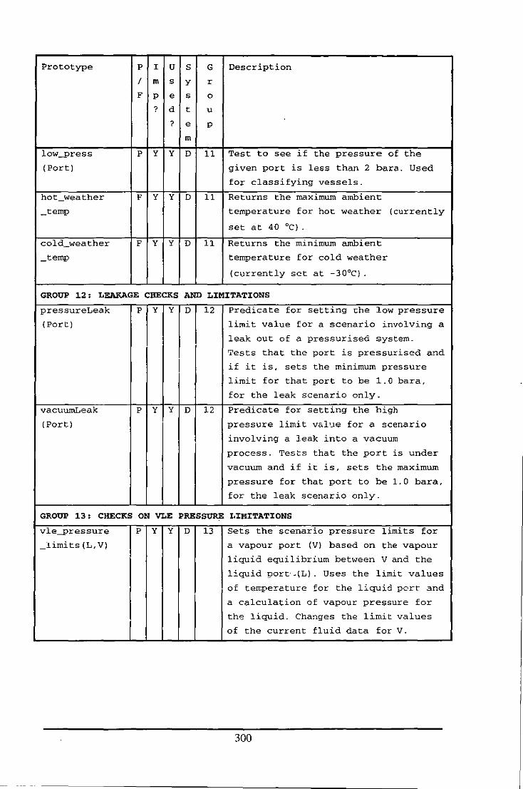
Prototype P I U S G Description
/ rn s y r
F p e s 0
? d t u
? e p
rn
low-press P Y Y D 11 Test to see if the pressure of the
(Port) given port is less than 2 bara. Used
for classifying vessels.
hot_weather F Y Y D 11 Returns the maximum ambient
_temp temperature for hot weather (currently
set at 40 CC) .
cold_weather F Y Y D 11 Returns the minimum ambient
_temp temperature for cold weather
(currently set at -30°C) .
GROUP 12 : LEAKAGE CHECKS AND LJ:MJ:TATJ:ONS
pressureLeak P Y Y D 12 Predicate for setting che low pressure
(Port) limit value for a scenario involving a
leak out of a pressurised system.
Tests that the port is pressurised and
I if it is, sets the minimum pressure
limit for that port to be 1.0 bara,
for the leak scenario only.
vacuurnLeak P Y Y D 12 Predicate for setting the high
(Port) pressure limit Value for a scenario
involving a leak into a vacuum
process. Tests that the port is under
vacuum and if it is, sets the maximum
pressure for that port to be 1.0 bara,
for the leak scenario only.
GROUP 13: CHECKS ON VLE PRESSURE LJ:MJ:TATJ:ONS
vle-pressure P Y Y D 13 Sets the scenario pressure limits for
_lirnits(L,V) a vapour port (V) based on the vapour
liquid equilibrium between V and the
liquid port· .(L) . Uses the limit values
of terr:pe!:"ature for the liquid pert and
a calculation of vapour pressure for
th~ liquid. Changes the limit values
of the current fluid data for V.
300
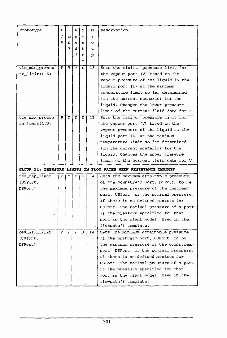
Prototype P I U S G Description
/ m s y r
F p e s 0
? d t u
? e p
m
vle_min-pressu P Y Y D 13 Sets the minimum pressure limit for
re_limit (L, V) the vapour port (V) based on the
vapour pressure of the liquid in the
liquid port (L) at the minimum
temperature limit so far determined
(in the current scenario) for the
liquid. Changes the lower pressure
limit of the current fluid data for V.
vle_max..-pressu P Y Y D 13 Sets the maximum pressure limit for
re_limit(L,V) the vapour port (V) based on the
vapour pressure of the liquid in the
liquid port (L) at the maximum
temperature limit so far dete~mined
(in the current scenario) for the
liquid. Changes the upper pressure
limit of the current fluid data for V.
GROUP 14: PRESSURE LIMITS IN FLOW PATHS WHEN RESISTANCE CHANGES
res_dsp_limit
(USPort,
DSPort)
res_usp_limit
(USPort,
DSPort)
P Y Y D 14 Sets the maximum attainable pressure
of the downstream port, DSPort, to be
the maximum pressure of the upstream
port, USPort, or the nominal pressure,
if there is no defined maximum for
USPort. The nominal pressure of a port
is the pressure specified for that
port in the plant model. Used in the
flowpath() template.
P Y Y D 14 Sets the minimum attainable pressure
of the upstream port, USPort, to be
the minimum pressure of the downstream
port, DSPort, or the nominal pressure:
if tbere ..ls no defined minimum for
DSPort. The nominal pressure of a port
is the pressure specified for that
port in the plant model. Used in the
flowpath() template.
301
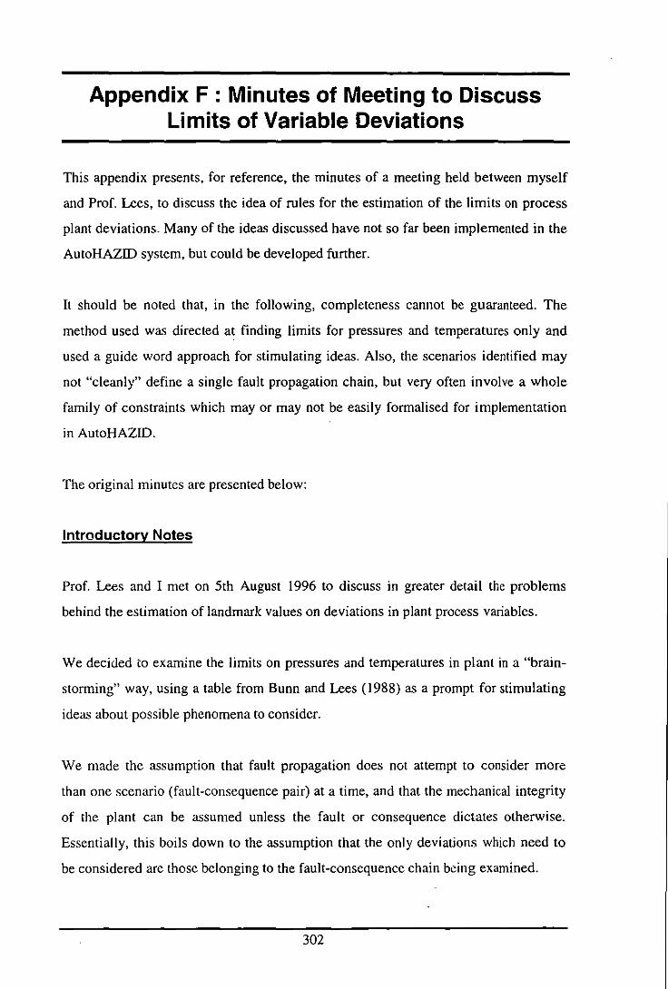
Appendix F : Minutes of Meeting to Discuss Limits of Variable Deviations
This appendix presents, for reference, the minutes of a meeting held between myself
and Prof. Lees, to discuss the idea of rules for the estimation of the limits on process
plant deviations. Many of the ideas discussed have not so far been implemented in the
AutoHAZID system, but could be developed further.
It should be noted that, in the following, completeness cannot be guaranteed. The
method used was directed at finding limits for pressures and temperatures only and
used a guide word approach for stimulating ideas. Also, the scenarios identified may
not "cleanly" define a single fault propagation chain, but very often involve a whole
family of constraints which mayor may not be easily formalised for implementation
in AutoHAZID.
The original minutes are presented below:
Introductory Notes
Prof. Lees and I met on 5th August 1996 to discuss in greater detail the problems
behind the estimation of landmark values on deviations in plant process variables.
We decided to examine the limits on pressures and temperatures in plant in a "brain
storming" way, using a table from Bunn and Lees (1988) as a prompt for stimulating
ideas about possible phenomena to consider.
We made the assumption that fault propagation does not attempt to consider more
than one scenario (fault-consequence pair) at a time, and that the mechanical integrity
of the plant can be assumed unless the fault or consequence dictates otherwise.
Essentially, this boils down to the assumption that the only deviations which need to
be considered are those belonging to the fault-consequence chain being examined.
302
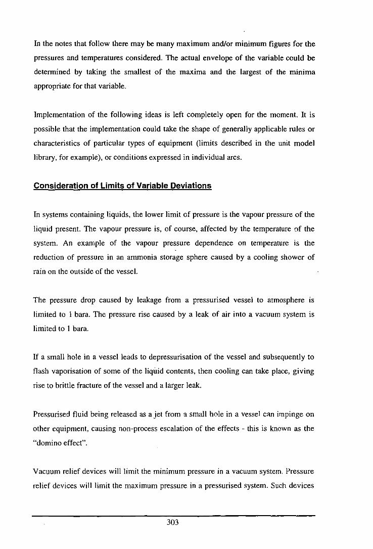
In the notes that follow there may be many maximum and/or minimum figures for the
pressures and temperatures considered. The actual envelope of the variable could be
determined by taking the smallest of the maxima and the largest of the minima
appropriate for that variable.
Implementation of the following ideas is left completely open for the moment. It is
possible that the implementation could take the shape of generally applicable rules or
characteristics of particular types of equipment (limits described in the unit model
library, for example), or conditions expressed in individual arcs.
Consideration of Limits of Variable Deviations
In systems containing liquids, the lower limit ef pressure is the vapour pressure of the
liquid present. The vapour pressure is, of course, affected by the temperature af the
system. An example of the vapour pressure dependence on temperature is the
reduction of pressure in an ammonia storage sphere caused by a cooling shower of
rain on the outside of the vessel.
The pressure drop caused by leakage from a pressurised vessel to atmosphere is
limited to I bara. The pressure rise caused by a leak of air into a vacuum system is
limited to 1 bara.
If a small hole in a vessel leads to depressurisation of the vessel and subsequently to
flash vaporisation of some of the liquid contents, then cooling can take place, giving
rise to brittle fracture of the vessel and a larger leak.
Pressurised fluid being released as a jet from a small hole in a vessel can impinge on
other equipment, causing non-process escalation of the effects - this is known as the
"domino effect".
Vacuum relief devices will limit the minimum pressure in a vacuum system. Pressure
relief devices will limit the maximum pressure in a pressurised system. Such devices
303
may include bursting disks as well as relief valves. Note that these are protection
devices, which may fail - how should we deal with these?
Mechanical "burst pressure" for a pressurised system, if there is no relief device
attached to it.
Nominal minimum/maximum inlet pressures and temperatures may be given. Care
should be taken that these can be trusted to be the real limits of these variables, as they
may correspond to the design condition envelope for the plant.
Maximum delivery pressure .of a pressure raiser. Note that this maximum IS also
dependent on the pressure on the suction side of the pressure raiser. If the pressure
raiser is a positive-displacement type, the pressure due to dead-heading it will he
much higher - the possibility of isolating the pressure raiser discharge must be
considered in detennining the maximum here.
Minimum suction pressure of a vacuum pump. Note also the limit of vapour pressure
in systems with liquid in them, as mentioned above.
Gas breakthrough at the base of a column, or in a vessel, could expose some usually
liquid-filled components of the plant to the pressure of the gas or vapour-filled parts.
In this case, the relevant pressure to consider is the nominal pressure of the vapour
filled sections (e.g. the nominal discharge pressure of the compressor used in that
system).
Heat exchanger interface failure will cause the low pressure side of the exchanger to
be exposed to the full pressure of the high pressme side. The maximum here is the
nominal pressure of the inlet to the high pressure side of the exchanger.
Hi'gh pressures generated by non-intentional combustion of gases in process
equipment are limited by the appropriate constant volume combustion calculation.
The most pessimistic estimate of pressure-rise would use a stoichiometric basis for the
combustion, but very often this is not realistic.
304
In the case of heating due to an external fire, where relief or fire valves are not
present, the pressure limit may be that pressure generated by the system fluid at the
temperature where the metal in the system fails. In this case, the other effect, of
overpressure failure of the system, may also take place. The examination of the
interplay of these two effects is potentially quite complicated.
Thermal expansion of liquid-filled systems is relevant when considering locked in
fluids subject to a temperature rise caused by heat exchange with the environment.
Some calculation involving the coefficient of thermal expansion, ~, would be
appropriate here, to calculate the highest expected pressure, dependent on an
estimated maximum ambient temperature.
The problem of water in hot oil (the "chip-pan effect") is typical of those effects
where the magnitude of the pressure increase is not easy to detennine. In this case,
some quantity of water makes its way into a hot oil system anJ there boils rapidly,
causing an expansion. The amount of water and the volume of the system, temperature
of the oil, etc., are all needed for this calculation. Since the amount of the contaminant
(water) in the system is highly uncertain, the possibility of making a reasonably
confident "safe" calculation of the pressure rise is very slim.
In this problem, it is enough to detect that the water contamination would in fact boil
when it gets into the hot oil.
A similar sort of quantification problem occurs when we consider the Bhopal disaster.
It is thought that a quantity of water got into a storage tank containing methyl
isocyanate, and therc caused a runaway reaction, leading to an overpressure release
from the vessel. Here it is also difficult to quantify the amount of the contaminant and,
although the runaway phenomenon is quite different from the hot oil problem, the
magnitude of the pressure change cannot be deduced for the same reasons. Here, a
compatibility matrix should warn of the dangerous runaway reaction between the
process fluid and contaminant.
305
Accumulation of inertlnon-condensable gases at high points In a plant may cause
blockages and other problems too.
For heat exchangers, where the process fluid is heated by some heat transfer fluid or
steam, the maximum temperature for the process fluid is the maximum temperature
expected from the heat transfer medium. The maximum process pressure IS
determined by considering the process fluid blocked in at such a temperature.
In furnaces and burners, which can be extremely hot, the best estimate of the
maximum process side .conditions is the failure of the tube metal due to heat or
overpressure. This establishes limits on the maximum temperature and pressure in the
process fluid side of the furnace tubes.
In the event of loss of cooling medium in a cooler, the maximum process fluid
temperature. at the outlet of the exchanger will be the nominal process fluid inlet
temperature.
Loss of cooling in a condenser will lead to vapour accumulation ill the process side
and possible breakthrough of vapour into the condensate outlet. In the case of a
distillation column, the pressure of the column will increase until the process
temperature in the reboiler is the same as the steam temperature, or the relief pressure
is reached, or the burst pressure of the column is reached, whichever is the lowest.
The coolant in a cooler must remain flowing in order to cool the process fluid.
Therefore, the minimum temperature that the process fluid can get to is either its own
freezing point or the freezing point of the coolant, whichever is higher.
The weather will have certain characteristic temperature limits, depending on the part
of the world in which the plant is situated. These will define the envelope for
environmental temperature.
The brittle fracture temperature of the materials of construction IS an important
temperature minimum.
306
Freezing expansion of water in pipes, as a result of cold weather, gives rise to
blockage and a pressure effect on the pipes, possibly damaging them. Some
calculation might be devised to determine if the pipe will be endangered by freezing in
this way. Do any other fluids expand on freezing, as water does?
For systems containing liquids, when a leak to environment occurs the liquid will
depressurise. If the fluid would normally be vapour at ambient conditions, it will
flash. The evaporation of the process fluid can chill the equipment to a minimum of
the boiling temperature of the fluid at I bara. A similar principle applies where the
evaporative cooling happens within a system: the minimum temperature is the
saturation temperature at the lower pressure.
For gases/vapours, typically, cooling occurs on expansIOn and heating 0n
compression, due to the Joule-Thompson effect. It is likely that calculations could be
found to estimate the size of these effects, for application in processes where
expanders or compressors are found.
Mixing with another cold fluid can cause some process materials to freeze, e.g.
benzene plus cold slugs of ethylene in a flare stack, freezing the benzene.
If fluid is erroneously introduced (in a batch process, for example) to a cold vessel, it
could freeze, causing problems, such as freezing the impeller in a reaction vessel,
plugging inlets or outlets in the vessel, or measurement points, inconvenience
generally ...
Tn runaway reactions, one temperature limit is the "adiabatic reaction temperature"
(typically for batch or semi-batch reactors). Another is the temperature at which the
venting on the reactor operates.
Pumps and compressors are a source of high temperature when dead-heading or
overheating, or when recycling fluid (under spill-back, for example). In all these
307
cases, the magnitude of the effect is not easy to quantify without some arbitrary
judgements about the process.
For compressors, if the coolers which should remove the heat of compression from the
process fluid are lost, then it may be possible to calculate the maximum to which the
discharge temperature would go. This is not straightforward, however.
Loss of tracing (steam or electric) on traced pipework could drop the temperature to
ambient.
If steam tracing goes wrong and more heat than intended is given to the process, then
the trace steam temperature could be a useful guide to the maximum process
temperature reached.
Some materials have a very high heat of solution, and this could be a factor in some
cases. Calculations of temperatures here have the same problem as the water in hot oil
example above - that too many data are needed for the calculation which cannot
usually be pinned down exactly. Detection of the problem using compatibility
matrices, plus the judgement that the temperature cannot go above the boiling point of
the solvent, may help in this case.
Shock compression of gas by slugs of fast-moving liquid may give rise to large
compressive heat effects, which sometimes are big enough to cause problems.
308
Appendix G : Future work changes to HAZID
A number of important but quite trivial changes should be made to the HAZID system
in the future. These are in addition to the more difficult changes noted in Chapter 6:
• Consequences without a defined importance rank in the model library are always
screened out of the results set, because of the way the consequence thresholding
operation has been implemented. There are no such consequences in the library at
the moment, but they could be added in future. Consequences without rank
information should instead be reported wherever they are found (or a warning
should be issued when a consequence is found without a rank number). This is a
trivial coding change to the thresholding function.
• A user option (flag) could be added, to switch the fluid compatibility checking
functionality in AutoHAZID on or off.
• Consider making the "stopping points" feature an option on the flags menu.
• Consider making all flag options configurable from the hazpaths. dos
configuration file.
• The numerical value -999.0 is used for undefined values in the fluid model
system and elsewhere. In the future, this value may be required as a legitimate
defined value. The functions and predicates of the FMS should use some type of
"not a number" symbol (e.g. the Atom, 'undef ined'), instead of a valid
numerical value, when they are not capable of giving a value for a calculation.
This is part of the larger problem of developing a consistent approach to missing
information in the FMS.
• The definitions of fluid model system predicates and functions should be
separated from the unit model lihrary and put in a library file of their own.
• Recursive calls between fluid model functions or predicates should be detected
and prevented, or warnings should be issued. Until there is some reliable way of
eliminating infinite recursion in the FMS, recursion and iteration should be
avoided.
309


Related Documents