Combining Forecasts in the Presence of Ambiguity over ...

Combining Forecasts in the Presence of Ambiguityover Correlation Structures

Gilat Levy and Ronny Razin, LSE1

Abstract: We suggest a framework to analyse how sophisticated decision makers combine

multiple sources of information to form predictions. In particular, we focus on situations in

which: (i) Decision makers understand each information source in isolation but are uncertain

about the correlation between the sources; (ii) Decision makers consider a range of bounded

correlation scenarios to yield a set of possible predictions. (iii) Decision makers face ambigu-

ity in relation to the set of predictions they consider. In our model the set of predictions the

decision makers considers is completely characterised by two parameters: the naïve inter-

pretation of forecasts which ignores correlation, and the bound on the correlation between

information sources that the decision maker considers. The analysis yields two countervailing

effects on behaviour. First, when the naïve interpretation of information is relatively precise,

it can induce risky behaviour, irrespective of what correlation scenario is chosen. Second,

a higher correlation bound creates more uncertainty and therefore more conservative be-

haviour. We show how this trade-off affects behaviour in different applications, including

financial investments and CDO ratings. We show that when faced with complex assets,

decision makers are likely to behave in ways that are consistent with complete correlation

neglect.

1 Introduction

When confronted with multiple forecasts, we often have a better understanding of each

forecast separately than we do of how the sources relate to one another. This is apparent in

1We thank Eddie Dekel, Andrew Ellis, Jeff Ely, Erik Eyster, Daniel Krahmer, Francesco Nava, Alp

Simsek and Joel Sobel for helpful comments. We also thank seminar participants at the Queen Mary

Theory workshop, Bocconi, Cornell, PSE, ESSET 2015, Manchester University, University of Bonn, LBS,

Ecole Polytechnique, Bristol University, University of Bath, St. Andrews, Rotterdam, Zurich, York-RES

Game Theory symposium, Warwick/Princeton Political Economy workshop, King’s College and Queen Mary

Political Economy workshop, and the UCL-LSE Theory workshop. This project has received funding from the

European Union’s Horizon 2020 research and innovation programme under grant agreement No SEC-C413.

1

many situations when experts or organisations make predictions. In the finance literature

this has been long recognised.2 Jiang and Tian (2016) point to several problems in estimating

correlation, including the lack of suffi cient market data, instabilities in the correlation process

and the increasingly interconnected market patterns. The US financial crisis inquiry (FCIC)

report from 2011 cites the acknowledgment of the rating agency Moody’s that “In the absence

of meaningful default data, it is impossible to develop empirical default correlation measures

based on actual observations of defaults.”

In the face of such uncertainty about correlation structures, decision makers in practice

often entertain multiple scenarios, constructing a set of possible models to interpret the fore-

casts they are confronted with. Risk analysis in financial firms that evaluate CDOs uses the

individual level data of the loans making up a CDO, and then considers different correlation

scenarios. For example the FCIC report documents how analysts constructed correlation

scenarios: “The M3 Prime model let Moody’s automate more of the process...Relying on

loan-to-value ratios, borrower credit scores, originator quality, and loan terms and other

information, the model simulated the performance of each loan in 1250 scenarios.”

When decision makers, or committees, choose their final decision given these scenarios,

individual preferences and the culture of the organisation plays an important part. Anil K

Kashyap’s paper prepared for the FCIC observes that before the crisis there was an: “...inher-

ent tendency for the optimists about the products to push aside the more cautious within the

organization”. After the crisis became apparent, “pessimism”prevailed: “Moody’s offi cials

told the FCIC they recognized that stress scenarios were not suffi ciently severe, so they ap-

plied additional weight to the most stressful scenario..the output was manually “calibrated”

to be more conservative...analysts took the “single worst case”from the M3 Subprime model

simulations and multiplied it by a factor in order to add deterioration.”This suggests that

something akin to attitudes towards ambiguity might play a role when making decisions

based on multiple predictions.3

In this paper we suggest a framework to model how sophisticated individuals combine

2This is the motivation behind papers such as Duffi e et al (2009).3Related to what we do in this paper a few recent papers have assumed ambiguity over correlation in

different applications. Jiang and Tian (2016) analyze a financial market in which investors have ambiguity

about the correlation between assets. They derive results relating to the volume of trade and asset prices.

Easley and O’hara (2009) look more generally at the role of ambiguity in financial markets.

2

forecasts in complex environments. In particular, we focus on situations as above in which: (i)

Decision makers understand each information source in isolation but are uncertain about the

correlation between the sources; (ii) Decision makers consider a range of bounded correlation

scenarios to yield a set of possible predictions. (iii) Decision makers face ambiguity in relation

to the set of predictions they consider.

In practice, the set of correlation structures that are considered has a particular structure.

Treating forecasts as independent is often used as a benchmark; The Naïve-Bayes classifier,

a method to analyse data by assuming different aspects of it are independent, is one of the

work horses of operations research and machine learning. This method has had surprising

success and is extensively used. Querubin and Dell (2017) document how this approach

was employed by the US military in the Vietnam war to assess which hamlets should be

bombed based on multidimensional data collected from each hamlet.4 While successful to

some degree, decision makers are often concerned about the “correlation neglect” that is

implicit in the Naïve-Bayes approach which leads them to consider correlation scenarios.

The level of correlation implicit in the scenarios that decision makers consider in practice

is typically bounded. Tractability and simplicity imply that the different models used for

generating correlation only allow for modest levels of correlation. One reason for this is

that many of these models have a limited number of correlation parameters. When dealing

with large numbers of components (e.g., the number of loans in a CDO), this implies bunch-

ing many assets to have the same correlation patterns (the “homogenous pool”problem).

This bounds the correlation levels that are considered. Similarly, the families of correlation

structures (copulas) that are often used, implicitly limit the levels of correlation. Finally,

arbitrary historical correlation data, which typically exhibits moderate levels of correlation

over time, is often used to generate scenarios.5

The recent attempts of the polling industry to predict the results of the 2016 US Pres-

idential election followed a similar pattern, where only limited correlation was considered.

Poll aggregators produced predictions that were based on survey data from the different US

states. The perception on the eve of the election that a win for Donald Trump is unlikely

was often motivated by the low probability that he might win in a combination of states,

such as Pennsylvania, Michigan and North Carolina. The low probability given to this event

4For more on the Naive Bayes approach see Russell and Norvig (2003) and Domingo and Pazzani (1996).5See MacKenzie and Spears (2014) and the FCIC report mentioned above.

3

stems from an assumption that state polls are independent.

Different analysts might have different bounds on correlation. FiveThirtyEight provided

one of the most cautious predictions for Hillary Clinton winning. Nate Silver remarks that:

“If we assumed that states had the same overall error as in the FiveThirtyEight’s polls-only

model but that the error in each state was independent, Clinton’s chances would be 99.8

percent, and Trump’s chances just 0.2 percent. So assumptions about the correlation between

states make a huge difference. Most other models also assume that state-by-state outcomes

are correlated to some degree, but based on their probability distributions, FiveThirtyEight’s

seem to be more emphatic about this assumption.”6

Our model combines two central ingredients. First, we suggest a model of the set of

information structures that the decision maker entertains, which is characterised by one

parameter, a bound on point-wise mutual information. Second, we use preferences over

ambiguity to determine how the decision maker takes an action based on a set of predictions

that are generated by the set of information structures that they consider.

In particular, we consider an environment in which an agent observes forecasts about a

potentially multidimensional state of the world, ω ∈ Ωn. For each element ωi in ω, the agent

observes possibly multiple forecasts, each a probability distribution over Ω. To combine the

multiple forecasts into a prediction about ω, the agent considers a set of possible ‘scenarios’,

modelled as joint information structures that could have yielded these forecasts. We allow

for two types of correlation in the consideration set of the agent: across the fundamentals

(the elements in ω), and across the predictions (e.g., due to biases in polling techniques).

For each joint information structure in this set, that is consistent with the multiple forecasts,

the agent derives a Bayesian prediction over the state of the world. This process yields a set

of predictions about ω that is the focus of our analysis.

Our main modeling assumption is to use a bound on the pointwise mutual information

(PMI) of information structures as the bound on the correlation scenarios the decision maker

considers. PMI relates to the distance between the joint distribution and the independent

benchmark, that is, the multiplication of the marginal distributions. The higher is the

bound on the PMI, the more correlation levels can be considered. As we show, modelling

the perceptions of individuals about correlation in this way is general, distribution free, and

6Nate Silver, “Election Update: Why Our Model Is More Bullish Than Others On Trump”,

http://fivethirtyeight.com/features/election-update-why-our-model-is-more-bullish-than-others-on-trump/

4

allows us to complete the model by using ambiguity aversion as a model of decision making

when decision makers face multiple predictions.

We characterise the set of predictions of a decision maker who considers scenarios with

bounded correlation structures. We show that the set of predictions is convex and compact,

and is monotonic (set-wise) in the PMI bound. Moreover, it can be fully characterised by

two suffi cient statistics: The PMI-bound and the Naïve-Bayes (NB) belief that assumes

independence.7

We show that when the NB prediction becomes very informative all decision makers,

whatever their preferences, will make similar decisions. In particular, for any PMI-bound if

the NB belief becomes very informative, the set of predictions shrinks and converges to the

NB prediction. This might happen, for example, when there is a large number of individual

components and the naïve interpretation of the data leads to a very precise (but possibly

wrong) belief. In these cases the NB belief dominates, which implies decisions that are

consistent with correlation neglect. In an application to the evaluation of a CDO we show

that as the number of individual mortgages in a CDO increases, its evaluation becomes

highly dependent on the NB belief. Thus, evaluation of complex assets or predictions in

complicated environments such as the US elections might suffer from correlation neglect

even when experts allow for a wide family of correlation scenarios.

When the NB prediction is not precise, attitudes towards ambiguity will play a role. The

monotonicity result that the set of predictions increases with the PMI bound lends itself

easily to thinking about ambiguity. Specifically, larger ambiguity over correlation structures

can translate to larger ambiguity over the state of the world.8 As a result, this can lead to

more cautious behaviour.

We thus unravel an intuitive relation between the set of correlation structures the decision

maker generates and her confidence in the decision she takes. First, when the NB belief is

relatively precise, the decision maker behaves as if she completely neglects correlation, which,

as already explored in the literature, implies more extreme beliefs, with lower variance.9

7The Naive-Bayes (NB) belief is computed when considering only joint information structures that are

conditionally independent. There is a unique such rational belief, which is proportional to a simple multi-

plication of the forecasts.8The set of predictions can then be thought of as the set of priors in the ambiguity literature.9This arises -with standard information structures such as the normal distribution- in Ortoleva and

Snowberg (2015) and Glaeser and Sunstein (2009). In contrast, Sobel (2014) shows that correlation neglect

5

Second, correlation will affect confidence through a Knightian notion of uncertainty. A

decision maker who is ambiguity averse and who entertains different possible models of

correlations will have a set of predictions, which will imply more cautious behaviour.

We analyze a simple investment application that highlights the tension between the two

effects. We show that when the number of investors is low, investors with a high correlation

capacity will reduce their risky investment due to the cautiousness effect described above.

However, when the number of investors is large, the NB belief might become more precise,

which can result in substantial risky behaviour. These results can shed light on behaviour

before and after the 2008 financial crisis. First, the capacity for correlation might have

increased post 2008, contributing to a shift from more risky to more cautious behaviour.

Second, the volume of trade in a market can be linked to the precision of the NB belief; a

low volume of trade will indicate a less precise belief, resulting in more cautiousness.

A recent literature has studied correlation neglect, i.e., a behavioral assumption that indi-

viduals neglect taking account of possible correlation between multiple sources of informa-

tion.10 Enke and Zimmerman (2013), Kallir and Sonsino (2009) and Eyster and Weiszacker

(2011) show how correlation neglect arises in experiments, with the latter two focusing on

financial decision making. We contribute to this literature by showing how correlation ne-

glect can arise endogenously: We show that the set of rationalisable beliefs shrinks to the

NB belief if it is precise enough.

Since the 2008 financial crisis, the issue of the uncertainty about correlation in default rates

as well as across stress tests has received attention in the literature.11 The contribution

of our paper to this literature is as follows. Our framework rationalises the procedures

employed by rating agencies and investment banks when these evaluate complex assets.

We also show that the neglect of correlation is fundamental to the rating of such assets.

Finally, we make the connection between the uncertainty that exists about these types

is not a necessary condition for extreme beliefs.10DeMarzo et al (2003) and Glaeser and Sunstein (2009) study how this affects individual beliefs in groups,

Ortoleva and Snowberg (2015) study its implications for individual political beliefs and Levy and Razin

(2015a, 2015b) focus on the implication of correlation neglect in voting contexts. Alternatively, Ellis and

Piccione (forthcoming) use an axiomatic approach to represent decision makers affected by the complexity

of correlations among the consequences of feasible actions.11Duffi e et al (2009), Brunnermeier (2009), Coval et al. (2009), and Ellis and Piccione (forthcoming),

examine the effects of such misperceptions on financial markets.

6

of correlations and ambiguity. We show that cautious or risky financial decisions can be

interpreted as a tension between ambiguity aversion and the Naïve-Bayes updating rule. A

recent complementary paper that also relates uncertainty about correlation to ambiguity is

Epstein and Halevy (2017). They provide an axiomatic foundation to this relation and also

verify it in experiments.

Finally, our approach is also related to the social learning literature (see Bikhchandani et al

1992 and Banerjee 1992). In social learning models, individuals may not extract all private

information of others from their actions. Our model highlights the possibility that even

if all private information was available and shared, it would still be insuffi cient; knowing

for example all signals and marginal distributions is not enough to understand potential

correlation in the joint information structures.12

2 The model

In this Section we present a theoretical model in which we define: (i) what a decision maker

observes, namely the set of forecasts; (ii) how she uses a joint information structure to

rationalise a set of forecasts and form a prediction on the state of the world; (iii) the level

of ambiguity she faces over joint information structures. We then use this model to derive

the set of predictions a decision maker can reach when combining forecasts.

2.1 Information

We first describe the information of the decision maker, which includes the state space, some

prior knowledge, and observed forecasts.

The decision maker knows the following aspects of the environment:

1. The state space. The state is a n− tuple vector ω =ω1, ..., ωn, ωi ∈ Ω, ω ∈ Ωn, where

n ≥ 1 and Ω is a finite space (in Section 5.2 we consider the case of continuous distributions

which may be more suitable for some applications).

12In that sense we also differ from the naïve social learning literature (Bohren 2014, Eyster and Rabin

2010, 2014, Gagnon-Bartsch and Rabin 2015). In that literature individuals neglect the strategic relation

between others’actions and their information. We stress the possibility that agents may still be in the dark

even if they share all information known individually.

7

2. Priors. The agent only knows the marginal prior distributions, pi(ωi), over all elements

i ∈ N .

3. Observed forecasts. The agent observes K forecasts. Specifically, there are ki forecasts

about each ωi, so that∑n

i=1 ki ≡ K. A typical forecast j on element i is a (full support)

probability distribution, qji (ωi), over Ω. Let q denote the vector of theK observable forecasts.

The model allows us to consider both correlations between forecasts (even when n = 1)

as well as correlations across the different elements of the state (when n > 1). For example,

correlation across forecasts arises when pollsters’strategies systematically neglect parts of

the population across US states, or when banks that conduct stress tests persistently ignore

the same type of information. Correlation across the elements of the state arises for example

when the returns of assets are correlated, or when the voting outcome across US states

depends on a common shock.

The decision maker will combine these forecasts to reach a set of predictions about the

state. A prediction about the state is a probability distribution η over Ωn and we are

interested in the set of rationalisable predictions, as we define formally below.

2.2 Rational predictions

To combine forecasts into rationalisable predictions, the agent will need to consider the

process according to which the observed forecasts were derived, that is, a joint information

structure.

A joint information structure is a vector (S, Ωn, p(ω), q(s,ω)) consisting of:

1. A joint prior distribution, p(ω), for which the marginal on element i is pi(ωi).

2. A set of K − tuple vectors of signals S = ×ni=1 ×kij=1 Sji , where S

ji is finite and denotes

the set of signals for information source j about element i.

3. A joint probability distribution of signals and states, q(s,ω), where s ∈S. Specifically,

let q(s,ω) = p(ω)q(s|ω), where q(s|ω) is the distribution over signals generated by ω. Also

let qji (s|ωi) denote the marginal information structure for source j on element i that is derived

from q(s|ω).

Note that in a joint information structure, both the elements of the state can be correlated,

8

through p(ω), and the signals generating the different forecasts could be correlated, through

q(s|ω).

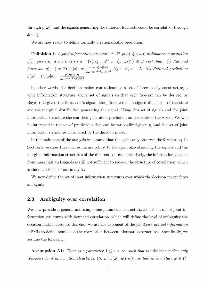
We are now ready to define formally a rationalisable prediction:

Definition 1: A joint information structure (S, Ωn, p(ω), q(s,ω)) rationalizes a prediction

η(.), given q, if there exists s = s11, s

21, .., s

k11 , ..., s

12, ..., s

knn ∈ S such that: (i) Rational

forecasts: qji (ωi) = Pr(ωi|sji ) =pi(ωi)q

ji (sji |ωi)∑

v∈Ω pi(v)qji (sji |v), ∀j ∈ Ki, i ∈ N, (ii) Rational prediction:

η(ω) = Pr(ω|s) = p(ω)q(s|ω)∑v∈Ωn p(v)q(s|v)

.

In other words, the decision maker can ratioanlize a set of forecasts by constructing a

joint information structure and a set of signals so that each forecast can be derived by

Bayes rule given the forecaster’s signal, the prior over his assigned dimension of the state

and the marginal distribution generating the signal. Using this set of signals and the joint

information structure she can then generate a prediction on the state of the world. We will

be interested in the set of predictions that can be rationalized given q, and the set of joint

information structures considered by the decision maker.

In the main part of the analysis we assume that the agent only observes the forecasts q. In

Section 5 we show that our results are robust to the agent also observing the signals and the

marginal information structures of the different sources. Intuitively, the information gleaned

from marginals and signals is still not suffi cient to recover the structure of correlation, which

is the main focus of our analysis.

We now define the set of joint information structures over which the decision maker faces

ambiguity.

2.3 Ambiguity over correlation

We now provide a general and simple one-parameter characterization for a set of joint in-

formation structures with bounded correlation, which will define the level of ambiguity the

decision maker faces. To this end, we use the exponent of the pointwise mutual information

(ePMI) to define bounds on the correlation between information structures. Specifically, we

assume the following:

Assumption A1: There is a parameter 1 ≤ a < ∞, such that the decision maker only

considers joint information structures, (S, Ωn, p(ω), q(s,ω)), so that at any state ω ∈ Ωn

9

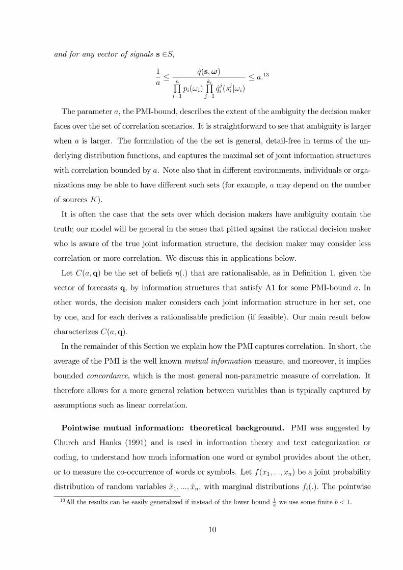
and for any vector of signals s ∈S,

1

a≤ q(s,ω)

n∏i=1

pi(ωi)ki∏j=1

qji (sji |ωi)

≤ a.13

The parameter a, the PMI-bound, describes the extent of the ambiguity the decision maker

faces over the set of correlation scenarios. It is straightforward to see that ambiguity is larger

when a is larger. The formulation of the the set is general, detail-free in terms of the un-

derlying distribution functions, and captures the maximal set of joint information structures

with correlation bounded by a. Note also that in different environments, individuals or orga-

nizations may be able to have different such sets (for example, a may depend on the number

of sources K).

It is often the case that the sets over which decision makers have ambiguity contain the

truth; our model will be general in the sense that pitted against the rational decision maker

who is aware of the true joint information structure, the decision maker may consider less

correlation or more correlation. We discuss this in applications below.

Let C(a,q) be the set of beliefs η(.) that are rationalisable, as in Definition 1, given the

vector of forecasts q, by information structures that satisfy A1 for some PMI-bound a. In

other words, the decision maker considers each joint information structure in her set, one

by one, and for each derives a rationalisable prediction (if feasible). Our main result below

characterizes C(a,q).

In the remainder of this Section we explain how the PMI captures correlation. In short, the

average of the PMI is the well known mutual information measure, and moreover, it implies

bounded concordance, which is the most general non-parametric measure of correlation. It

therefore allows for a more general relation between variables than is typically captured by

assumptions such as linear correlation.

Pointwise mutual information: theoretical background. PMI was suggested by

Church and Hanks (1991) and is used in information theory and text categorization or

coding, to understand how much information one word or symbol provides about the other,

or to measure the co-occurrence of words or symbols. Let f(x1, ..., xn) be a joint probability

distribution of random variables x1, ..., xn, with marginal distributions fi(.). The pointwise

13All the results can be easily generalized if instead of the lower bound 1a we use some finite b < 1.

10

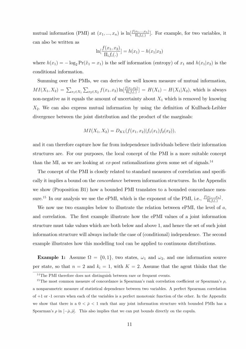
mutual information (PMI) at (x1, ..., xn) is ln[f(x1,...,xn)Πifi(.)

]. For example, for two variables, it

can also be written as

ln[f(x1, x2)

Πifi(.)] = h(x1)− h(x1|x2)

where h(x1) = − log2 Pr(x1 = x1) is the self information (entropy) of x1 and h(x1|x2) is the

conditional information.

Summing over the PMIs, we can derive the well known measure of mutual information,

MI(X1, X2) =∑

x1∈X1

∑x2∈X2

f(x1, x2) ln[f(x1,x2)Πifi(.)

] = H(X1) − H(X1|X2), which is always

non-negative as it equals the amount of uncertainty about X1 which is removed by knowing

X2. We can also express mutual information by using the definition of Kullback-Leibler

divergence between the joint distribution and the product of the marginals:

MI(X1, X2) = DKL(f(x1, x2)|f1(x1)f2(x2)),

and it can therefore capture how far from independence individuals believe their information

structures are. For our purposes, the local concept of the PMI is a more suitable concept

than the MI, as we are looking at ex-post rationalizations given some set of signals.14

The concept of the PMI is closely related to standard measures of correlation and specifi-

cally it implies a bound on the concordance between information structures. In the Appendix

we show (Proposition B1) how a bounded PMI translates to a bounded concordance mea-

sure.15 In our analysis we use the ePMI, which is the exponent of the PMI, i.e., f(x1,...,xn)Πifi(.)

.

We now use two examples below to illustrate the relation between ePMI, the level of a,

and correlation. The first example illustrate how the ePMI values of a joint information

structure must take values which are both below and above 1, and hence the set of such joint

information structure will always include the case of (conditional) independence. The second

example illustrates how this modelling tool can be applied to continuous distributions.

Example 1: Assume Ω = 0, 1, two states, ω1 and ω2, and one information source

per state, so that n = 2 and ki = 1, with K = 2. Assume that the agent thinks that the

14The PMI therefore does not distinguish between rare or frequent events.15The most common measure of concordance is Spearman’s rank correlation coeffi cient or Spearman’s ρ,

a nonparametric measure of statistical dependence between two variables. A perfect Spearman correlation

of +1 or -1 occurs when each of the variables is a perfect monotonic function of the other. In the Appendix

we show that there is a 0 < ρ < 1 such that any joint information structure with bounded PMIs has a

Spearman’s ρ in [−ρ, ρ]. This also implies that we can put bounds directly on the copula.

11

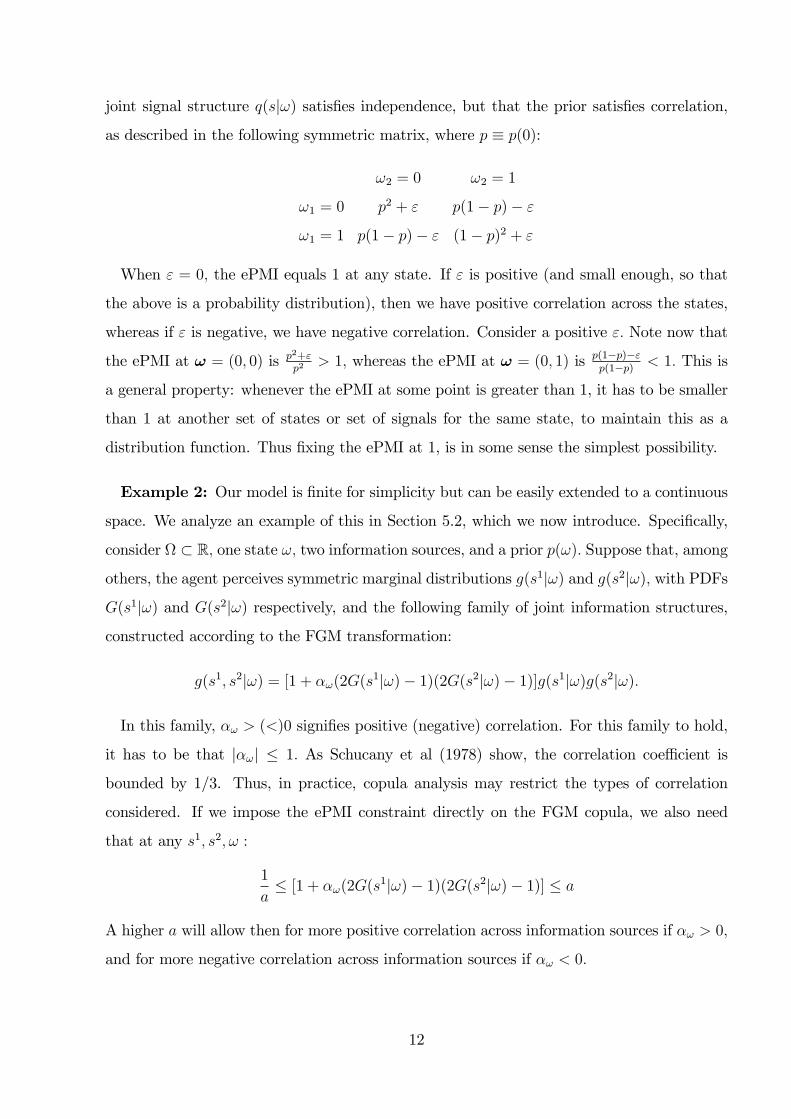
joint signal structure q(s|ω) satisfies independence, but that the prior satisfies correlation,

as described in the following symmetric matrix, where p ≡ p(0):

ω2 = 0 ω2 = 1

ω1 = 0 p2 + ε p(1− p)− ε

ω1 = 1 p(1− p)− ε (1− p)2 + ε

When ε = 0, the ePMI equals 1 at any state. If ε is positive (and small enough, so that

the above is a probability distribution), then we have positive correlation across the states,

whereas if ε is negative, we have negative correlation. Consider a positive ε. Note now that

the ePMI at ω = (0, 0) is p2+εp2 > 1, whereas the ePMI at ω = (0, 1) is p(1−p)−ε

p(1−p) < 1. This is

a general property: whenever the ePMI at some point is greater than 1, it has to be smaller

than 1 at another set of states or set of signals for the same state, to maintain this as a

distribution function. Thus fixing the ePMI at 1, is in some sense the simplest possibility.

Example 2: Our model is finite for simplicity but can be easily extended to a continuous

space. We analyze an example of this in Section 5.2, which we now introduce. Specifically,

consider Ω ⊂ R, one state ω, two information sources, and a prior p(ω). Suppose that, among

others, the agent perceives symmetric marginal distributions g(s1|ω) and g(s2|ω), with PDFs

G(s1|ω) and G(s2|ω) respectively, and the following family of joint information structures,

constructed according to the FGM transformation:

g(s1, s2|ω) = [1 + αω(2G(s1|ω)− 1)(2G(s2|ω)− 1)]g(s1|ω)g(s2|ω).

In this family, αω > (<)0 signifies positive (negative) correlation. For this family to hold,

it has to be that |αω| ≤ 1. As Schucany et al (1978) show, the correlation coeffi cient is

bounded by 1/3. Thus, in practice, copula analysis may restrict the types of correlation

considered. If we impose the ePMI constraint directly on the FGM copula, we also need

that at any s1, s2, ω :

1

a≤ [1 + αω(2G(s1|ω)− 1)(2G(s2|ω)− 1)] ≤ a

A higher a will allow then for more positive correlation across information sources if αω > 0,

and for more negative correlation across information sources if αω < 0.

12

3 Analysis

In this Section we characterise C(a,q), the set of rationalisable beliefs of the decision maker

that are derived from the set of joint information structure she considers, as defined in A1, for

a PMI-bound a.We are interested in understanding how ambiguity over information sources

translates into ambiguity over the state of the world.

We first consider two benchmarks and show that they both yield a unique belief. Suppose

that the individual considers only joint information structures that deliver conditionally

independent signals or states. In other words, a = 1 (note that she may still have ambiguity

as there are many such information structures). We then have:

Lemma 1: The set C(1,q) is a singleton and the unique belief, denoted ηNB(ω) satisfies,

for any ω = (ω1, .., ωi, .., ωn) and ω′ = (ω′1, .., ω′i, .., ω

′n):

ηNB(ω)

ηNB(ω′)=

n∏i=1

ki∏j=1

qji (ωi)

p(ωi)ki−1

n∏i=1

ki∏j=1

qji (ωi)

p(ω′i)ki−1

To see this, note that by Bayes rule, any belief needs to satisfy the following likelihood

ratio for some vector of signals and marginal information structures:

n∏i=1

(pi(ωi)ki∏j=1

qji (sji |ωi))

n∏i=1

(pi(ω′i)ki∏j=1

qji (sji |ω′i))

By rationalisability however:

n∏i=1

(pi(ωi)ki∏j=1

qji (sji |ωi))

n∏i=1

(pi(ω′i)ki∏j=1

qji (sji |ω′i))

=

n∏i=1

(pi(ωi)ki∏j=1

qji (ωi)∑vipi(vi)q

ji (sji |vi)

pi(ωi))

n∏i=1

(pi(ω′i)ki∏j=1

qji (ω′i)∑vipi(vi)q

ji (sji |vi)

pi(ω′i))

=

n∏i=1

ki∏j=1

qji (ωi)

pi(ωi)ki−1

n∏i=1

ki∏j=1

qji (ω′i)

pi(ω′i)ki−1

Thus when individuals do not consider correlation, ambiguity over joint information struc-

tures does not translate into ambiguity over the state, as there is a unique rationalisable

belief.

13

Another benchmark can arise is when a > 1 but n = 1 and K = 1, so that there is only

one forecast. Does ambiguity over joint information sources play a role when there are no

observation of multiple sources? It is easy to see that again, only a unique belief arises:

Lemma 2: When there is only one forecast q(ω), the set C(a, q) is a singleton and equals

q(ω).

Formally, for any joint information structure that the agent can imagine, we know thatp(ω)q(s|ω)∑v p(v)q(s|v)

has to equal q(ω) by rationalisability. Thus each such information structure

delivers the same belief, q(ω). Correlation and ambiguity do not play a role.

3.1 The main result

We now proceed to provide the main result, characterising C(a,q) :

Proposition 1: With n states and ki ≥ 1 for any i ∈ N, η(.) ∈ C(a,q) for 1 ≤ a < ∞

if and only if it satisfies

η(ω)

η(ω′)=λωλω′

ηNB(ω)

ηNB(ω′), for any ω and ω′,

for a vector λ = (λω)ω∈Ωn satisfying λω ∈ [ 1a, a] for all ω. Thus the minimum (maximum)

belief on state ω is derived when λω = 1a

(a) and for all other v, λv = a ( 1a). (iii) The set

C(a,q) is compact and convex.

The result shows that there are two suffi cient statistics that allow us to characterize the set

of beliefs held by the agent: the PMI-bound a and the NB posterior ηNB(.). Thus, while the

decision maker is faced with a complicated environment, her Bayesian combined forecasts

can be derived with a simple heuristic-like behavior. She needs to consider the Naïve-

Bayes benchmark, as if she neglects correlation, and to adjust this by different “scenarios”

as determined by a.This is also helpful for the modeler as we had not made any specific

assumptions on distributions. We discuss in Section 4.4 how a modeler can also identify a.

When a > 1, the set of beliefs is not unique once we have multiple forecasts. When the

decision maker considers also joint information structures with some level of correlation, she

can rationalise a larger set of beliefs about the state of the world. Thus, ambiguity over joint

information structures now translates into ambiguity over the state of the world. This arises

14

only when two conditions are met, as gleaned from Lemmata 1 and 2: the decision maker

is exposed to multiple forecasts (arising possibly from n > 1), and she considers correlation

across the forecasts/states (a > 1). Specifically, when there is more than one forecast, then

the different levels of correlation considered “kick”in to induce different beliefs, while when

only one forecast exists, this effect does not arise. Thus, the decision maker becomes less

confident in terms of facing larger ambiguity over the state of the world when she considers

correlation and when she has more than one forecast.16

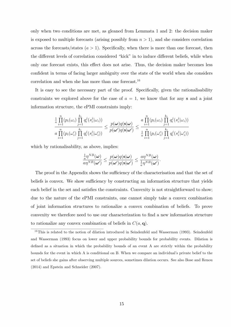
It is easy to see the necessary part of the proof. Specifically, given the rationalisability

constraints we explored above for the case of a = 1, we know that for any s and a joint

information structure, the ePMI constraints imply:

1a

n∏i=1

(pi(ωi)ki∏j=1

qji (sji |ωi))

an∏i=1

(pi(ω′i)ki∏j=1

qji (sji |ω′i))

≤ p(ω)q(s|ω)

p(ω′)q(s|ω′) ≤a

n∏i=1

(pi(ωi)ki∏j=1

qji (sji |ωi))

1a

n∏i=1

(pi(ω′i)ki∏j=1

qji (sji |ω′i))

which by rationalisability, as above, implies:

1aηNB(ω)

aηNB(ω′)≤ p(ω)q(s|ω)

p(ω′)q(s|ω′) ≤aηNB(ω)1aηNB(ω′)

.

The proof in the Appendix shows the suffi ciency of the characterisation and that the set of

beliefs is convex. We show suffi ciency by constructing an information structure that yields

each belief in the set and satisfies the constraints. Convexity is not straightforward to show;

due to the nature of the ePMI constraints, one cannot simply take a convex combination

of joint information structures to rationalize a convex combination of beliefs. To prove

convexity we therefore need to use our characterization to find a new information structure

to rationalize any convex combination of beliefs in C(a,q).

16This is related to the notion of dilation introduced in Seindenfeld and Wasserman (1993). Seindenfeld

and Wasserman (1993) focus on lower and upper probability bounds for probability events. Dilation is

defined as a situation in which the probability bounds of an event A are strictly within the probability

bounds for the event in which A is conditional on B. When we compare an individual’s private belief to the

set of beliefs she gains after observing multiple sources, sometimes dilation occurs. See also Bose and Renou

(2014) and Epstein and Schneider (2007).

15

3.2 The Naïve-Bayes and cautiousness effects

The characterisation of the maximal set of beliefs allows us to make two simple observations.

The first observation -which we call the Naive-Bayes effect- is that if the NB belief is very

precise, then the set C(a,q) will in some cases coincide with it, implying that individual will

behave as if they have correlation neglect. The second observation is that C(a,q) is larger

when a is larger. In other words, a decision maker with a larger a will face more ambiguity.

In the presence of ambiguity aversion, this may imply greater cautiousness. In the next

Section we show how the interaction between these two effects induces sometimes risky and

sometimes cautious shifts in investment behaviour.

The Naïve-Bayes effect: The characterisation in Proposition 1 allows us to see how the

precision of ηNB(.) affects the size of C(a,q). Consider the case where ηNB(.) is very precise

(but not necessarily correct). This could arise for example when the number of forecasts K

grows large and when the Naïve-Bayes belief converges to be degenerate. Consider a sequence

of decision making problems with a sequence of vectors of forecasts qK and a sequence of

ambiguity sets characterised by aK . These imply a sequence of Naïve-Bayes beliefs ηNBqK (.)

and sets of beliefs C(aK ,qK) which are the focus of the observation below.

Observation 1: Suppose that there exists a ω′ ∈ Ωn such that ηNBqK (ω′) →K→∞ 1. If

limK→∞(aK)2(1 − ηNBqK (ω′)) = 0 then C(aK ,qK) converges to the singleton belief which is

the degenerate belief on ω′.

To see this, note that by Proposition 1 we have that with n states and K information

sources, η(.) ∈ C(aK ,qK) is rationalisable if and only if it satisfies

η(ω)

η(ω′)=λωλω′

ηNBqK (ω)

ηNBqK (ω′),

for a vector λ = (λω)ω∈Ωn satisfying λω ∈ [ 1aK, aK ] for all ω 6= ω′. Note that λω

λω′<

(aK)2 1−ηNBqK (ω′)

ηNBqK(ω′) but as limK→∞(aK)2(1 − ηNBqK (ω′)) = 0 this implies that η(ω)

η(ω′) has to con-

verge to zero.

The observation above illustrates that even when the decision maker considers high degrees

of correlation, a very precise Naïve-Bayes belief may overwhelm considerations of correla-

tion. This implies that behaving as if one has correlation neglect can arise. Thus, not only

16

ambiguity over the state of the world becomes insignificant, the belief that arises coincides

with that of a decision maker who has a = 1.

As our set of predictions is the maximal set for all rational decision makers who consider

bounded correlation, the observation that the set of predictions can shrink to a singleton

NB belief implies that behaviour à la correlation neglect can arise endogenously for all types

of assumptions on the decision maker. In other words, even when the decision maker does

not have ambiguity over the set of joint information structures, but has a prior over these,

the result is the same. Finally note that the Naïve-Bayes benchmark -while relying on many

pieces of information- can still differ substantially from the rational belief given the true

joint information structure.

The cautiousness effect: The Proposition unravels a simple relation between confidence

and correlation:

Observation 2: If a < a′, then C(a,q) ⊂ C(a′,q).

Individuals who face a higher ambiguity over joint information structures will then end

up with a larger set of predictions. Thus, considering more joint information structures will

reduce confidence in the sense that individuals may not be sure what is the right belief.

One way to interpret this is that individuals or organizations who consider a larger set of

correlation scenarios (hence a larger PMI-bound a) will have greater ambiguity over the state

of the world.

For any ηNB(.), a high enough a can generate a low enough minimum belief in this set.

Along with ambiguity aversion, or alternatively with pessimists taking hold in organizations,

this can result in a more cautious behaviour. Thus the level of a will create the cautiousness

effect. This effect can explain pessimistic behavior in financial markets when investors believe

they face unknown levels of correlation as we now explore.

4 Applications: Investment shifts and CDO rating

In this Section we consider two applications. The first one will highlight the interaction

between the two effects we have described, the Naïve-Bayes effect and the cautiousness

effect. We will show how these two effects combine to create different levels of “confidence”.

In the second application we illustrate how the Naive-Bayes effect influences CDO rating.

17

4.1 Risky and cautious investment shifts

Assume a binary model with two equally likely states of the world, ω ∈ 0, 1. Assume that

there is a safe asset which provides the same returns L > 0 at any state, and a risky asset

which provides 0 at state 0 and H > L in state 1. Each investor has one unit of income to

invest which she can split across these two assets. Assume a standard concave utility V (.)

of wealth. Thus in this simple model the agent would invest a higher share in the risky asset

the higher are her beliefs that the state is 1.17

There are k informed investors. Let each hold a prediction qj(ω). Thus, in the first period,

they invest according to qj(1).18 Investments in the first period are observed; assume that

investors can then backtrack the beliefs of others, qj(1) for all j.19 Finally, in the second

period, the investors can adjust their investments following their observation of q.

For simplicity we assume that the PMI-bound, or the extent of ambiguity, of each investor

j, aj, is fixed. As Observation 1 shows, our results will remain if we consider that these

depend on k for example. To take into consideration the cautiousness effect that can arise

with ambiguity as described following Observation 2, we assume here that when individuals

are faced with ambiguity, they use the max-min preferences as in Gilboa and Schmeidler

(1989).20 Thus, in the second period, following exposure to multiple previous investments,

an individual j with ambiguity aversion will then base her investment decision on the belief

17Here we abstract from prices. See the discussion at the end of the section.18We can assume that each investor receives a signal sj on ω, knows the marginal qj(sj |ω), and updates

her prediction to qj(ω).We show in Appendix B how all our analysis also holds when the agents who combine

forecasts also have their own information. Specifically, we need to show that when the individual receives her

signal, her uncertainty about the joint information structure (but her knowledge of her marginal distribution)

leads her still to a unique belief, which is straightforward to show. Another issue is that as she needs her

marginal to update her belief to qj(ω), the set of rationalisable beliefs may depend on her marginal. One

possibility is to assume that when combining forecasts the investors only remember their posterior belief and

not the process that lead to it. Alternatively we can conduct the same analysis as in Proposition 1, with the

knowledge of the marginals and signals (see Section 5).19Of course this assumption is somewhat extreme but it not neccessary and is made here for simplicity.

One can easily assume a weaker version in which just the quantity invested is observed. In that case, after

observing investments, agents will not infer the beliefs exactly but rather will be able to compute lower

bounds on these beliefs.20Note that given the convexity of the set of beliefs C(a,q), we can use other attitudes towards ambiguity

to generate similar results.

18

which minimises her utility, which is minηj(1)∈C(aj ,q) ηj(1).

Given Proposition 1, and as we are in the binary model with only two states of the world,

we can further simplify ηNB(.). Let q(1) be the belief such that q(1)1−q(1)

is the geometric average

of qj(1)1−qj(1)

j∈K , i.e., q(1)1−q(1)

= (Πj∈Kqj(1)

1−qj(1))

1k . We can now express ηNB(1) as (recall that k is

the number of investors),

ηNB(1) = q(1)k

(1−q(1))k+q(1)k.

And j′s minimum combined forecast can be then written as:

minη(1)∈C(aj ,q(1))

η(1) =1

ajq(1)k

aj(1−q(1))k+ 1

ajq(1)k

. (1)

Thus the agent invests more in the second period if and only if:

qj(1)

1− qj(1)<

1

(aj)2(

q(1)

1− q(1))k. (2)

Lemma 3: In the second period, following exposure to q: (i) If aj < aj′, then investor j

will invest more in the risky asset compared with j′. (ii) For any k, there is γ > 1 such that

if aj > γ then individual j will lower her investment in the risky asset compared to her first

period’s investment; (iii) For a large enough k, if q(1) > 12, all investors will increase their

investment in the risky asset compared to their first period’s investment and if q(1) < 12,

then all will decrease their investment in the risky asset.

Part (i) illustrates that individuals with lower ambiguity over information sources will

behave in a more risky manner.21 This result also implies that we can identify the individual

PMI-bounds from choice data, as long as there is general data on behavior of individuals in

the face of ambiguity. Once we use such data and identify individuals who have the same

attitudes towards ambiguity, we can differentiate those with lower ambiguity by their more

risky behavior.

To see how parts (ii) and (iii) arise, recall that we have identified the cautiousness effect

and the Naïve-Bayes effect. If beliefs are in general pessimistic (that is, q(1) < 12), then

21Note that “standard” results in the literature on correlation neglect are typically of the form that

individuals with more correlation neglect will take more extreme decisions, but depending on the state of the

world these could be either on the risky or on the cautious side (see Glaeser and Sunstein 2009 or Ortoleva

and Snowberg 2015). The result above is different; it applies to any state of the world and any set of signals,

and arises from the reduced ambiguity that comes with lower perception of correlation.

19

both go in the same direction inducing a cautious investment behaviour following exposure

to multiple sources. If on the other hand beliefs are optimistic (namely, q(1) > 12) the two

effects go in opposite direction. When the number of forecasts is small, the Naïve-Bayes

effect is weak, as ηNB(.) is not likely to be informative. We can then always find a high

enough level of ambiguity so that the cautiousness effect will dominate.22 On the other

hand, when the number of forecasts is large, ( q(1)1−q(1)

)k becomes very large, and the NB belief

overcomes cautiousness to induce a substantial risky behaviour. To recap, confidence can

arise when a is small or ηNB(.) is relatively precise. On the other hand, cautiousness arises

when a is large, and ηNB(.) is relatively imprecise.

While cautiousness is directly related to ambiguity, a cautious shift will not always arise

with “standard”forms of ambiguity. Suppose for example that individuals have ambiguity

over the prior in the set [12− εi, 1

2+ εi] for some εi. Suppose that the information structures

satisfy independence and that this is known, and that all individuals start from some beliefs

qi(1) = q > 12, as above. Following the first period, individuals will always become more

optimistic and increase their level of investment. Ambiguity over the prior implies that first

and second period investment are both lower compared to the case of no ambiguity, but that

second period investment increases for any k.

Both of the effects we unravel can potentially shed light on the behaviour of investors

before and after the 2008 financial crisis. Many investors had realized after 2008 that the

level of correlation in assets and across forecasts was much higher than initially perceived.

In response, as we document in the introduction, the worst case scenarios did not only

receive more weight in the overall assessment, but were also downgraded to capture a more

pessimistic outlook. This corresponds to a possible shift of the value of a which, as we show,

can contribute to a “confidence crisis”and lower investment levels.

Another element that changes in the market is the informativeness of ηNB(.) which depends

on the number of investors involved. A market with many investors (even small ones) is such

that individuals can observe many forecasts. Even if each investment is slightly optimistic,

it can be aggregated to a precise and very optimistic ηNB(.), which will overshadow the

cautiousness effect. On the other hand, once some skepticism arises, as happened after the

22This result has a flavour of dynamic inconsistency results in the Ambiguity literature. See Hanani and

Klibanoff (2007) for updating that restricts the set of priors and avoids dynamic inconsistency, and the

discussions in Al-Najjar and Weinstein (2009) and Siniscalchi (2011).

20

crisis, the market will consist of less investors. In this case, the benchmark ηNB(.) would be

imprecise, and the cautiousness effect will dominate.

Finally note that there are several ways in which one can extend the model above. First,

we can consider a model with more than two periods; our qualitative results will still be

maintained. Second, we can endogenise k, the number of active investors. Finally, we

can extend the above analysis to include prices determined by market makers, with some

added assumptions which guarantee that there is asymmetric information between informed

investors and market makers, as in Avery and Zemsky (1998).23

4.2 Complex CDO rating

In this Section we provide a simple model of risk management for CDOs. Relying on Ob-

servation 1, we will show that for complex CDOs, for any copula or bounded dependence

across loans that one considers, the CDO can receive the highest rating.

Consider the case in which a CDO consists of n loans, each with a binary state of default

(D) or no default (ND), Ω = D,ND. Suppose that a particular tranche of the CDO

defaults if at least a share α of the individual loans included in it will default, meaning that

for at least dαne i elements of the state, we have ωi = D.

In this application the uncertainty over correlation will be about the correlation between

the defaults of the individual loans, i.e., through the prior p over the state. Therefore,

we assume that there are no observable forecasts. The prior marginal probability of each

loan defaulting (or ωi = D) is pi(ωi = D) = pi, and therefore we have n Bernoulli trials,

each with a marginal probability of D equal to pi. When the trials are independent, this

is a Poisson Binomial distribution. Below, when we take n to be large we will assume that

limn→∞∑ni=1 pin

= µ <∞. Again, we assume a to be fixed although the result can be extended

to consider a sequence an.

This is the simplest static model that can describe a CDO (alternatively, one can consider

a dynamic probability of default, meaning a Poisson distribution, which our model can easily

be extended to). Moreover, other models typically assume a particular parametric family of

copulas to assess the cumulative risk of assets.24 We instead describe correlation capacity

without resorting to any functional forms.

23See the surveys of Vayanos and Wang (2013) and Bikchandani and Sharma (2000).24See for example Wang et al (2009).

21

By Proposition 1, for any state ω, we have that a belief η(.) is in the set C(a,q) iff:

η(ω)

η(ω′)=

λωηNB(ω)

λω′ηNB(ω′)=

λωn∏i=1

pi(ωi)

λω′n∏i=1

pi(ω′i)

for any λω, λω′ ∈ [ 1a, a].

Let Ωl be the set of states which have exactly l loans withD and let ωl be a generic element

of this set. Then the probability that the CDO defaults when no correlation is considered is:

n∑l=dαne

∑ωl∈Ωl

ηNB(ωl)

To illustrate how this model works, let us consider the worst case scenario among the

scenarios determined by the extent of correlation a. This can be derived by using Proposition

1 as now stated:

Lemma 4: The worst-case scenario is that the CDO fails with probability

a2n∑

l=dαne

∑ωl∈Ωl

ηNB(ωl)

1 + (a2 − 1)n∑

l=dαne

∑ωl∈Ωl

ηNB(ωl).

In other words, our analysis easily carries through for a combination of states.

Suppose that the rating agency chooses a triple A rating to the CDO if its probability of

default is lower than some cutoff x.We now focus on what rating is awarded when the CDO

is complex, i.e., when n is large. For a large n, one can approximate the Poisson Binomial

distribution with a Poisson distribution with a mean∑n

i=1 pi.25 We will then use Observation

1, implying that our limit results will hold for all types of preferences or priors over the set

of correlation scenarios:

Lemma 5: For large enough n, if α > µ, the CDO receives the highest rating for all a.

The probability of each feasible state ω does not become degenerate here, as opposed to

the previous application. But the cumulative probability of many states together -which

is the relevant one for the case of the CDO failing or not- does converge to be degenerate

for some parameters, which therefore renders a immaterial. This implies that with complex

25See Hodges and Le Cam (1960).

22

securities composed of many assets, there are environments in which taking correlation into

consideration will not change investors’behaviour. Even if the pessimists get their say in an

organization, their recommendation would be to provide a high rating. We therefore unravel

a relation between complexity and correlation neglect.

We can use the above to derive some normative conclusions. Suppose that for all loans

pi = p for some p. Suppose first that the loans are completely independent. In that case,

when n is small, some investors with a large a would be too cautious. For a large n, investors

would behave effi ciently, as treating information as independent leads to the correct beliefs.

Suppose now that the assets are fully correlated. Specifically, suppose the state is generated

by the following process. A common state ω∗ ∈ D,ND is drawn, with a probability p of

D. For any loan i, we have ωi = ω∗. The true probability of the CDO defaulting is therefore

p. The effi cient course of action is to award a triple A rating only if x < p and not otherwise,

irrespective of α. However, whenever α > p, the CDO will be rated triple A for any x and

for all a, ineffi ciently.

5 Extensions

We complete our analysis by providing two technical extensions to illustrate the robustness

of Proposition 1.

5.1 Observing signals and marginals

In the analysis above we have assumed that the agent only observes the forecasts. This had

allowed us to derive a set of rationalisable beliefs that is determined by the forecasts q and

not by the particulars of any information structure. An alternative assumption is that the

agent also observes the marginal information structures of the sources or their signals.

In this Section we illustrate that relaxing these assumptions will not affect our qualitative

results, that combining forecasts in the face of ambiguity over correlation creates a set of

rationalisable beliefs, that the set of combined forecasts is centered around the Naïve-Bayes

belief, and that it is convex. What does change is that the set of beliefs might depend on

the particulars of these marginal information structures.

23

Consider for example the following information structure.26 Assume that there are two

information sources, (1 and 2) and consider for simplicity the case in which both have sym-

metric marginal information structures with binary signals (s∗ and s∗∗) about two possible

realisations of the state (0 and 1). The agent then considers the set of possible symmetric

joint information structures which is given by:

ω = 0 s∗ s∗∗

s∗ q(s∗|0)− q0 q0

s∗∗ q0 1− q(s∗|0)− q0

ω = 1 s∗ s∗∗

s∗ q(s∗|1)− q1 q1

s∗∗ q1 1− q(s∗|1)− q1

Note that even though the individual knows q(s|ω), she still does not know q0 and q1.

Suppose now that she observes the forecasts as well as q(s|ω), which is equivalent to observing

the signals and marginals. Below, for expositional purposes, we focus on the case in which

both information sources observed the signal s∗, i.e., q = ( q(s∗|1)q(s∗|1)+q(s∗|0)

, q(s∗|1)q(s∗|1)+q(s∗|0)

).

We now characterize the set of rationalisable beliefs that can be derived from an informa-

tion structure as above and which satisfies A1. As can be seen, our qualitative results hold

in this case as well.

Lemma 6: Given marginals q(s∗|ω) and forecasts q = ( q(s∗|1)q(s∗|1)+q(s∗|0)

, q(s∗|1)q(s∗|1)+q(s∗|0)

), the

set of rationalisable beliefs is: (i) C(a,q) as in Proposition 1 if q(s∗|1)1−q(s∗|1)

≤ a ≤ 1−q(s∗|0)q(s∗|0)

,

(ii) Contained in C(a,q), convex and contains the Naïve-Bayes belief if a < q(s∗|1)1−q(s∗|1)

or1−q(s∗|0)q(s∗|0)

< a.

5.2 Continuous distributions: The FGM transformation

In this subsection we show that our analysis can be extended to continuous distributions.

We use the FGM transformation to derive a family of information structures starting from

particular marginal information structures. This can then be useful in applications in which

continuous signal structures are more relevant.27

26As we show in the appendix, any information structure that rationalizes a set of forecasts can be repli-

cated by a structure with two signals only for each forecaster. Thus, the example below, symmetry aside, is

general for the case of two realisations of the state.27In Laohakunakorn, Levy and Razin (2016) we use this transformation to analyze the effects of corelation

capacity on common value auctions.

24

Suppose as above that the agent knows the marginal distributions as well as the signals

of his information sources. Suppose that n = 1, and that the marginals distributions are

symmetric, g(s1|ω) and g(s2|ω), with PDFs G(s1|ω) and G(s2|ω) respectively, as in Example

2 in Section 2. We assume that the agent perceives the following family of joint information

structures, constructed according to the FGM transformation:

g(s1, s2|ω) = [1 + αω(2G(s1|ω)− 1)(2G(s2|ω)− 1)]g(s1|ω)g(s2|ω).

In this family, αω > (<)0 signifies positive (negative) correlation. For this family to hold,

it has to be that |α| ≤ 1. Furthermore, to satisfy the ePMI constraints for some a, we also

need:1

a− 1 ≤ αω ≤ 1− 1

a.

It is then easy to show that Proposition 1 holds as well.28 The set of rationalisable beliefs

given some s, s′ is the set of all beliefs η(.|s, s′) satisfying:

η(ω|s, s′)η(ω′|s, s′) =

γω(s, s′)g(s|ω)g(s′|ω)

γω′(s, s′)g(s|ω′)g(s′|ω′) =

γω(s, s′)ηNB(ω|s, s′)γω′(s, s

′)ηNB(ω′|s, s′) ,

for any γv(s, s′) ∈ 1 +αv(2G(s|v)− 1)(2G(s′|v)− 1), and αv ∈ [ 1

a− 1, 1− 1

a], for v ∈ ω, ω′.

Note that when αv = 0 for all v, we have the Naïve-Bayes benchmark as before.

6 Conclusion

We suggest a new framework to analyse how sophisticated decision makers make decisions

when they face ambiguity over the correlation of multiple sources of information. The deci-

sion makers generate a set of predictions based on a set of “correlation scenarios”and take

a decision based on their attitudes towards ambiguity. Their set of predictions are fully

characterised by the level of correlation they consider and the Naïve-Bayes interpretation

of the information. A larger consideration set of correlation scenarios increases ambiguity

and therefore induces more conservative or cautious behaviour. On the other hand the level

of information implicit in a Naïve-Bayes interpretation of forecasts pushes individuals or

organisations to be more confident and sometimes engage in risky behaviour.

28The suffi ciency part is as in Section 4. The necessity part follows from directly from the assumption of

the FGM family of functions.

25

As we have discussed in the introduction, combining forecasts is also relevant in many

political environments. Poll aggregation is an obvious candidate for future analysis. In our

applications above we considered two extreme cases; in one we focused on the correlation

across fundamentals and in the other on the correlation across information sources. A simple

electoral system, e.g., a referendum with a majority rule, can be captured by the latter

case: The state of the world can be interpreted as a binary variable (e.g., Remain in the

EU or Leave in the context of the EU referendum in Britain), and polls’predictions are

clearly correlated to some degree as in many cases all use the same data set. A more

complicated electoral system, such as the Electoral College for the US election, or the UK

electoral system, are determined by a combination of outcomes in different regions (states

in US states, constituencies in the UK). This case is similar to the CDO application in

which correlation across the fundamentals is more pronounced, and a candidate wins if a

some share of the regions votes in her favour. This latter case may be a more complicated

environment for combining forecasts as the correlation across voters’preferences in different

regions may be compounded with the correlation across polls. It may be an interesting

question for future research to determine whether pollsters are less successful -perhaps due

to the endogenous correlation neglect we had identified- in predicting outcomes in these more

complicated environments.

References

[1] Al-Najjar, N. and J. Weinstein (2009). The Ambiguity Aversion Literature: A Critical

Assessment. Economics and Philosophy 25, 249-284.

[2] Avery, C. and P. Zemsky. (1998). Multidimensional Uncertainty and Herd Behavior in

Financial Markets. The American Economic Review, Vol. 88, No. 4. pp. 724-748.

[3] Baliga, S. E. Hanany, and P. Klibanoff (2013). Polarization and Ambiguity, American

Economic Review 103(7): 3071—3083.

[4] Banerjee, A. (1992). A Simple Model of Herd Behavior.Quarterly Journal of Economics,

vol. 107, 797-817.

26

[5] Bikhchandani, S. and S. Sharma (2000). Herd Behaviour in Financial Markets- A Re-

view. IMF working paper WP/00/48.

[6] Bikhchandani, S., D. Hirshleifer and I. Welch (1992), “A Theory of Fads, Fashion, Cus-

tom, and Cultural Change as Informational Cascades”, Journal of Political Economy,

vol. 100, 992-1026.

[7] Bohren, A. (2014), Informational Herding with Model Misspecification, mimeo.

[8] Bose, S. and Renou, L. (2014). Mechanism Design with Ambiguous Communication

Devices. Econometrica 82: 1853-1872.

[9] Brunnermeier M.K. (2009). Deciphering the Liquidity and Credit Crunch 2007-2008.

Journal of Economic Perspectives, 23, 77—100.

[10] Church, K.W and P. Hanks (1991), Word association norms, mutual information, and

lexicography. Comput. Linguist. 16 (1): 22—29.

[11] Coval, J., J. Jurek, and E. Stafford (2009). The Economics of Structured Finance.

Journal of Economic Perspectives 23, 3—25.

[12] Dell, M. and P. Querbin (2017). Nation Building Through Foreign Intervention: Evi-

dence from Discontinuities in Military Strategies. Working paper, Harvard and NBER.

[13] De Marzo PM, Vayanos D, and Zwiebel J. (2003). Persuasion bias, social influence and

unidimensional opinions. Q. J. Econ. 118:909—68.

[14] Domingos, P., and M. J. Pazzani. 1996. Beyond Independence: conditions for the opti-

mality of the simple Bayesian classifier.Machine Learning: Proceedings of the Thirteenth

International Conference, L. Saitta, eds. : Morgan Kaufman.

[15] Duffi e, D., A. Eckner, G. Horel, and L. Saita. (2009). Frailty Correlated Default. The

Journal of Finance, Vol. LXIV, No. 5, October.

[16] Easley, D. and M. O’hara (2009), Ambiguity and Nonparticipation: The Role of Regu-

lation, Review of Financial Studies 22, 1817-1843.

[17] Ellis, A. and M. Piccione. Correlation Misperception in Choice. Forthcoming. American

Economic Review.

27

[18] Enke, B. and F. Zimmerman (2013). Correlation Neglect in Belief Formation. mimeo.

[19] Epstein, L. and M. Schneider. (2007). Learning under Ambiguity. Review of Economic

Studies. 74, 1275—1303.

[20] Epstein, L. and Y. Halevy, (2017), Ambiguous Correlation, mimeo.

[21] Eyster, E. and M.Rabin. (2014). Extensive imitation is irrational and harmful. The

Quarterly Journal of Economics [Internet]. 2014:qju021.

[22] Eyster, E. and M. Rabin (2010). Naïve Herding in Rich-Information Settings. American

Economic Journal: Microeconomics, 2(4): 221-43.

[23] Eyster, E. and G. Weizsäcker (2011). Correlation Neglect in Financial Decision-Making.

Discussion Papers of DIW Berlin 1104.

[24] Gagnon-Bartsch, T. and M. Rabin (2015), Naïve Social Learning, Mislearning, and

Unlearning, mimeo.

[25] Gilboa, I. and D. Schmeidler (1989), Maxmin expected utility with non-unique prior,

Journal of Mathematical Economics 18, 141-153.

[26] Glaeser, E. and Cass R. Sunstein (2009), Extremism and social learning.” Journal of

Legal Analysis, Volume 1(1), 262 - 324.

[27] Hanani, E. and P. Klibanoff (2007). Updating preferences with multiple priors. Theo-

retical Economics 2, 261-298.

[28] Hodges J. and L. Le Cam (1960). The Poisson Approximation to the Poisson Binomial

Distribution. The Annals of Mathematical Statistics. 737-740.

[29] Jiang, J. and W. Tian (2016). Correlation Uncertainty, Heterogeneous Beliefs and Asset

Prices. mimeo, University of North Carolina.

[30] Kallir, I. and Sonsino, D. (2009). The Perception of Correlation in Investment Decisions.

Southern Economic Journal 75 (4): 1045-66.

[31] Laohakunakorn, K., G. Levy and R. Razin (2016). Common Value Auctions with Am-

biguity over Information Structures and Correlation Capacities. mimeo.

28

[32] Levy, G. and R. Razin. (2015a). Correlation Neglect, Voting Behaviour and Information

Aggregation. American Economic Review 105: 1634-1645.

[33] Levy, G. and R. Razin. (2015b). Does Polarisation of Opinions lead to Polarisation of

Platforms? The Case of Correlation Neglect, Quarterly Journal of Political Science,

Volume 10, Issue 3.

[34] Li, David X. (2000). On Default Correlation: A Copula Function Approach. Journal of

Fixed Income. 9 (4): 43—54.

[35] Lord, C., Lee Ross, and Mark R. Lepper. (1979). Biased Assimilation and Attitude Po-

larization: The Effects of Prior Theories on Subsequently Considered Evidence. Journal

of Personality and Social Psychology 37(11), 2098-2109.

[36] MacKenzie D, Spears T (2014). ‘The formula that killed Wall Street’: The Gaussian

copula and modelling practices in investment banking. Social Studies of Science 44(3):

393—417

[37] Nelsen, R. (2006). An Introduction to Copulas. Springer.

[38] Ortoleva, P. and E. Snowberg. (2015). Overconfidence in political economy. American

Economic Review, 105: 504-535.

[39] Querubin, P. and M. Dell, M. (2016): “Nation Building Through Foreign Intervention:

Evidence from Discontinuities in Military Strategies,”mimeo.

[40] Russell, Stuart; Norvig, Peter (2003). Artificial Intelligence: A Modern Approach (2nd

ed.). Prentice Hall.

[41] Schmid, F. and R. Schmidt (2007). Multivariate Extensions of Spearman’s rho and

Related Statistics, Statistics & Probability Letters, Volume 77, Issue 4, Pages 407—416.

[42] Schucany, W.R., Parr, W.C., Boyer, J.E.: Correlation structure in Farlie—Gumbel—

Morgenstern distributions. Biometrika 65, 650—653 (1978)

[43] Seidenfeld, T. and Wasserman, L. (1993), Dilation for Sets of Probabilities. Annals of

Statistics. 21 no. 3, 1139—1154.

29

[44] Siniscalchi, M. (2011). Dynamic choice under ambiguity. Theoretical Economics 6, 379—

421.

[45] Sobel, J. (2014). On the relationship between individual and group decisions, Theoretical

Economics 9, 163—185.

[46] Vayanos, D. and J. Wang (2013). Market Liquidity|Theory and Empirical Evidence, in

the Handbook of the Economics of Finance, edited by George Constantinides, Milton

Harris, and Rene Stulz.

[47] Wang. D., S.T. Rachev, F.J. Fabozzi (2009). Pricing Tranches of a CDO and a CDS

Index: Recent Advances and Future Research. Part of the series Contributions to Eco-

nomics pp 263-286.

7 Appendix

7.1 Appendix A

Proof of Proposition 1.

We first consider n = 1 and K > 1.

Step 1: Let η(.) ∈ C(a,q). Then there exists an information structure (S ′, q′) with S ′ =

s∗, s−∗k which rationalises η(.) and satisfies A1.

Assume that an information structure (S = ×j∈KSj, q(s|ω)) rationalises η(.).Without loss

of generality relabel signals so that the vector of signals that rationalises η(ω) is (s∗, s∗..., s∗)

so that η(ω) = q(ω|s∗, s∗..., s∗). In addition we have that the following rationalizability and

ePMI constraints are satisfied,

∀j ∈ K and ∀ω ∈ Ω, qj(ω) = qj(ω|s∗)

∀s =(s1, ..., sk) ∈ ×j∈KSj and ∀ω ∈ Ω,1

a≤ q(s|ω)∏

j∈Kqj(sj|ω)

≤ a.

Construct the new information structure (S ′, q′(.|ω)) by keeping the same distribution over

signals as in (S, q), while keeping the label s∗ and bundling all possible signals s 6= s∗ under

30

one signal s−∗. In particular, ∀ω ∈ Ω,

q′(s∗, ..., s∗|ω) = q(s∗, ..., s∗|ω)

q′(s−∗, s∗, ..., s∗|ω) =∑

s∈S1/s∗q(s, s∗, ..., s∗|ω),

and so on. Note that (S ′, q′) rationalises η(.) by definition.

It remains to show that the ePMI constraints hold for (S ′, q′) so that it satisfies A1. Note

first that the ePMI constraint for (s∗, ..., s∗) holds by definition of (S ′, q′). Consider any

other profile of signals s ∈s∗, s−∗k. The ePMI constraint for s can be expressed in terms

of the information structure (S, q) as∑ml=1 cl∑ml=1 c

′lwhere cl = q(sl|ω) for some sl = (s1

l , ..., skl ) ∈ S

where we sum over all sl that compose s, and c′l =∏j∈K

qj(sjl |ω). But as the original ePMI

constraints hold, this also implies that 1a≤∑m

l=1cl∑m

l=1c′l≤ a. Thus the ePMI constraints are

satisfied also for (S ′, q′).

Wlog assume that the agent rationalizes the set of posteriors she observes by believing

that all sources have received the signal s∗. For any v ∈ Ω, let αv = Pr(all receive s∗|v) and

let δiv = Pr(i receives s∗|v).

Step 2: Suppose n=1 and K>1. For any η(ω) that satisfies the necessary condition in

the Proposition, there exists an information structure that satisfies A1 and rationalizes this

belief.

Take any vector (λω)ω∈Ω that satisfies 1a≤ λω ≤ a for any realisation of ω and consider

the belief

η(ω) =λω

1

p(ω)k−1

∏j∈K

qj(ω)∑v∈Ω

λv1

p(v)k−1

∏j∈K

qj(v).

Using this vector (λω)ω∈Ω we now construct an information structure that will satisfy all

ePMI constraints and the rationalisability constraints, and will rationalise the belief η(ω).

Let αω = λω∏j∈K

δjω and let δjω = ε q

j(ω)p(ω)

. This implies that this information structure

generates the belief as desired as η(ω) = p(ω)αω∑v∈Ω

p(v)αv=

λω1

p(ω)k−1

∏j∈K

qj(ω)∑v∈Ω

λv1

p(v)k−1

∏j∈K

qj(v).

Note that p(ω)δjω∑v∈Ω

p(v)δjv= qj(ω)∑

v∈Ω

qj(v)= qj(ω) which implies that the posterior beliefs of all

individuals are rationalized.

31

We now specify the joint distribution over signals, making sure that all the ePMI con-

straints are satisfied. For all ω ∈ Ω, set the joint probability of each event in which two or

more sources receive s∗, but not when all sources receive s∗, to satisfy independence. For

example, the probability that all m sources in the set M and only these individuals receive

s∗ in state ω, for 1 < m < k, is∏j∈M

δjω∏

j∈K/M(1 − δjω). Thus for all these cases the ePMI

constraints are satisfied.

At any state, we then need to verify the ePMI constraints in the following events: when

one source exactly had received s∗, or when all received s−∗. Let us focus on some realisation

ω. Consider first the event in which only one source had received s∗.

P r(sj = s∗, all others receive s−∗|ω) = εqj(ω)

p(ω)−αω−ε

qj(ω)

p(ω)(

∑M⊂K/j|M |≥1

∏i∈M

δiω∏

l∈K/M∪j(1−δlω))

The ePMI is:

ε qj(ω)p(ω)− αω − ε q

j(ω)p(ω)

(∑

M⊂K/j|M |≥1

∏i∈M

δiω∏

l∈K/M∪j(1− δlω))

ε qj(ω)p(ω)

∏l 6=j

(1− ε ql(ω)p(ω)

)

=

1− λω∏

l∈K/j(ε q

l(ω)p(ω)

)− (∑

M⊂K/j|M |≥1

∏i∈M

δiω∏

l∈K/M∪j(1− δlω))∏

l 6=j(1− ε ql(ω)

p(ω))

→ε→0 1,

as for all k, δkω goes to 0 with ε. Thus, the ePMI can be made smaller than a and greater

than 1a, if ε is small enough.

Consider now the event that all sources had received s−∗ in state ω:

Pr(all received signal s−∗|ω) = (1− εqj(ω)

p(ω))− (1− εq

j(ω)

p(ω))(

∑M⊂K/j|M |≥2

∏i∈M

δiω∏

l∈K/M∪j(1− δlω))

−(k − 1)(εqj(ω)

p(ω)− αω − ε

qj(ω)

p(ω)(

∑M⊂K/j|M |≥1

∏i∈M

δiω∏

l∈K/M∪j(1− δlω))),

where here we subtract all the events in which two or more received s∗ (but at most k−1),

and the k− 1 events in which just one player had received s∗ which we had described above.

32

The ePMI is:

(1−ε qj(ω)p(ω)

)

(1−ε qj(ω)p(ω)

)∏l 6=j

(1−ε qj(ω)p(ω)

)

−(1−ε q

j(ω)p(ω)

)(∑

M⊂K/j|M |≥2

∏i∈M

δiω

∏l∈K/M∪j

(1−δlω))−(k−1)(εqj(ω)p(ω)

−αω−ε qj(ω)p(ω)

(∑

M⊂K/j|M |≥1

∏i∈M

δiω

∏l∈K/M∪j

(1−δlω)))

(1−ε qj(ω)p(ω)

)∏l 6=j

(1−ε qj(ω)p(ω)

)

=

1−(∑

M⊂K/j|M |≥2

∏i∈M

δiω

∏l∈K/M∪j

(1−δlω))∏l6=j

(1−ε qj(ω)p(ω)

)

−ε(k−1)(

qj(ω)p(ω)

−λωεk−1∏i∈K

(qi(ω)p(ω)

)− qj(ω)p(ω)

(∑

M⊂K/j|M |≥1

∏i∈M

δiω

∏l∈K/M∪j

(1−δlω)))

(1−ε qj(ω)p(ω)

)∏l 6=j

(1−ε qj(ω)p(ω)

)

→ ε→01.

which again can be made smaller than a and larger than 1afor low enough ε. Thus all

constraints in state ω can be satisfied. .

Step 3: Suppose now that n>1. For any η(.) that satisfies the necessary condition in

the Proposition, there exists an information structure that satisfies A1 and rationalizes this

belief.

Consider the belief η(ω) = λωηNB(ω)∑v

λvηNB(v). Let q(s,ω) =

∏j∈K

qji (sji |ωi). Let q

ji (s

ji |ωi) =

qji (ωi)

pi(ωi)

and let p(ω) = λω∏i∈N

pi(ωi). The ePMI constraints are satisfied as well as the rationalisability

constraints as pi(ωi)qji (sji |ωi)∑

vipi(vi)q

ji (sji |vi)

=qji (ωi)∑viqji (vi)

= qji (ωi). Moreover the belief can be generated by

η(ω) =

p(ω)∏i∈N

∏j∈Ki

qji (sji |ωi)∑v p(v)

∏i∈N

∏j∈Ki

qji (sji |vi)=

p(ω)∏i∈N

∏j∈Ki

qji (sji |ωi)∑v p(v)

∏i∈N

∏j∈Ki

qji (sji |vi)= λωηNB(ω)∑

v

λvηNB(v)as desired.

Step 4: C(a,q) is compact and convex.

Compactness comes from the proof in the text and the previous steps. To prove convexity

consider two beliefs η and η′ that are in C(a,q). Note that from the above a belief η(.) is in

C(a,q) if and only if for any v, ω ∈ Ω we have,

η(ω)

η(v)=λωλv

ηNB(ω)

ηNB(v).

Thus all likelihood ratios satisfy,

1

a2

ηNB(ω)

ηNB(v)≤ η(ω)

η(v)≤ a2η

NB(ω)

ηNB(v). (3)

33

To prove convexity we show that we can find a vector λβ with elements between 1aand a

that spans βη+ (1−β)η′. It will be enough to show that βη+ (1−β)η′ has likelihood ratios

in the bounds in (3). Note that η, η′ satisfy

1

a

2ηNB(ω)

ηNB(v)≤ η(ω)

η(v)≤ a2η

NB(ω)

ηNB(v),

1

a

2ηNB(ω)

ηNB(v)≤ η′(ω)

η′(v)≤ a2η

NB(ω)

ηNB(v),

we have that:

βη(ω) + (1− β)η′(ω)

βη(v) + (1− β)η′(v)≤ βη(v) + (1− β)η′(v)

βη(v) + (1− β)η′(v)a2η

NB(ω)

ηNB(v)= a2η

NB(ω)

ηNB(v),

and similarly that,

βη(ω) + (1− β)η′(ω)

βη(v) + (1− β)η′(v)≥ 1

a

2ηNB(ω)

ηNB(v).

So there must exist λβ that spans βη + (1− β)η′.

Proof of Lemma 3: (i) The proof follows from the construction in Proposition 1, Ob-

servation 1 and maxmin preferences. These imply that an individual i who has a lower

perception of correlation than an individual j, will choose to invest according to a higher

belief about state 1 and hence will invest more in risky asset. (ii) The proof follows from

the construction in Proposition 1. Fix K,N and q, as a goes to infinity, the set C(a,q)

converges to span all possible beliefs. Therefore there is a γ > 1 such that if γ < a, each

investor will have a minimum belief that is lower than his qi(1) and hence will experience a

cautious shift. (iii) This is explained in the text.

Proof of Lemma 4: First note that our results extend to a combination of states. That

is, we know that the maximum belief in the set

η(ω) =λωη

NB(ω)

λωηNB(ω) +∑

ω′ 6=ω λω′ηNB(ω′)

where λv ∈ [1/a, a], is attained when λω = a and λω′ = 1/a for all other ω′. But also the

maximum in the set

η(ω) + η(ω′) =λωη

NB(ω)+λω′ηNB(ω′)

λωηNB(ω) + +λω′ηNB(ω′) +∑

v 6=ω′,ω′′ λvηNB(v)

,

by taking derivatives w.r.t. the λ′s, is attained when λω, λω′ = a and λv = 1/a for all others.

34

Thus the worst case scenario is the highest belief that the CDO fails meaning:

an∑

l=dαne

∑ωl∈Ωl

ηNB(ωl)

an∑

l=dαne

∑ωl∈Ωl

ηNB(ωl) + 1a(1−

n∑l=dαne

∑ωl∈Ωl

ηNB(ωl))

which equals the formulation in the text.

Proof of Lemma 5: By the approximation and from Lemma 4, we know that the worst

case scenario is

a(1− e−µnbαnc∑i=0

(µn)i

i!)

a(1− e−µnbαnc∑i=0

(µn)i

i!) + (1/a)(e−µn

bαnc∑i=0

(µn)i

i!)

But note that for any α > µ we have limn→∞(1− e−µnbαnc∑i=0

µni

i!) = 0, implying that

limn→∞

a(1− e−µnbαnc∑i=0

(µn)i

i!)

a(1− e−µnbαnc∑i=0

(µn)i

i!) + (1/a)(e−µn

bαnc∑i=0

(µn)i

i!)

= 0

Therefore, for any α > µ we have that, for all x and for all a, the CDO is deemed safe.

Proof of Lemma 6: The ePMI constraints are:

1

a≤ q(s∗|ω)− qω

q(s∗|ω)2≤ a

1

a≤ qω

q(s∗|ω)(1− q(s∗|ω))≤ a

1

a≤ 1− q(s∗|ω)− qω

(1− q(s∗|ω))2≤ a

First note that the Naïve-Bayes belief satisfies all the constraints. Note that the belief

that the state is one is α1

α0+α1.We proceed by charecterising the highest and lowest values we

can get for αω.

From the first ePMI constraints we have that: aq(s∗|ω)2 ≥ q(s∗|ω)2 − qω ≥ 1aq(s∗|ω)2.

Note the third ePMI constraints above do not bind at the extremes of the above inequalities:

1

a≤

1− 2q(s∗|ω) + 1aq(s∗|ω)2

(1− q(s∗|ω))2<

1− 2q(s∗|ω) + q(s∗|ω)2

(1− q(s∗|ω))2= 1 < a,

35

where the LHS inequality is derived from

1

a≤

1− 2q(s∗|ω) + 1aq(s∗|ω)2

(1− q(s∗|ω))2⇔ (1− 2q(s∗|ω)) ≤ a(1− 2q(s∗|ω))⇔ 1 ≤ a.

Similarly,

1

a≤ 1 =

1− 2q(s∗|ω) + q(s∗|ω)2

(1− q(s∗|ω))2≤ 1− 2q(s∗|ω) + aq(s∗|ω)2

(1− q(s∗|ω))2≤ a,

where the RHS inequality is derived from

1− 2q(s∗|ω) + aq(s∗|ω)2

(1− q(s∗|ω))2≤ a⇔ 1− 2q(s∗|ω) ≤ a(1− 2q(s∗|ω))⇔ 1 ≤ a.

So the only constraints left are 1a≤ qω

q(s∗|ω)(1−q(s∗|ω))≤ a. For this the extremes could

matter as while 1a≤ q(s∗|ω)− 1

aq(s∗|ω)2

q(s∗|ω)(1−q(s∗|ω))is satisfied as q(s∗|ω)− 1

aq(s∗|ω)2

q(s∗|ω)(1−q(s∗|ω))> q(s∗|ω)−q(s∗|ω)2

q(s∗|ω)(1−q(s∗|ω))= 1 ≥ 1

a,

the other side has q(s∗|ω)− 1aq(s∗|ω)2

q(s∗|ω)(1−q(s∗|ω))≤ a⇔ q(s∗|ω)

(1−q(s∗|ω))≤ a and similarly, for the other extreme,

we will need 1a≤ q(s∗|ω)−aq(s∗|ω)2

q(s∗|ω)(1−q(s∗|ω))⇔ q(s∗|ω)(a+ 1) ≤ 1⇔ a ≤ 1−q(s∗|ω)

q(s∗|ω).

7.2 Appendix B: Other results

7.2.1 Pointwise mutual information and concordance

Proposition B1: Assume that there are two information sources, k and j. There is a

0 < ρ < 1 such that any joint information structure that satisfies A1 has a Spearman’s ρ

(Kendal’s τ) in [−ρ, ρ].

Proof of Proposition B1: The bounds on the ePMI imply that there is an ε such

that q(sk,sj |ω)qk(sk|ω)qj(sj |ω)

∈ [1 − ε, 1 + ε]. This implies that |q(sk, sj|ω) − qk(sk|ω)qj(sj|ω)| ≤

εqk(sk|ω)qj(sj|ω). Summing up over all (sk, sj) and given x, y we get that |Q(x, y|ω) −

Qk(x|ω)Qj(y|ω)| ≤ εQk(x|ω)Qj(y|ω) ≤ ε. This implies that the distance between the copula

of any such information structure to the product copula is bounded by ε.

Among all such information structures, take the supremum according to the highest copula.

That information structure has a Spearman’s ρ (Kendall’s τ) that is strictly smaller than 1

(See Theorem 5.9.6 and Theorem 5.1.3 in Nelsen 2006).

Among all such information structures, take the infimum according to the lowest copula.

That information structure has a Spearman’s ρ (or Kendall’s τ) that is strictly larger than

-1 (See Theorem 5.9.6 and Theorem 5.1.3 in Nelsen 2006).

By Theorem 5.1.9 in Nelsen (2006), any other information structure will have a Spearman’s

ρ (Kendall’s τ) in between the two copulas above.

36

7.2.2 Agents with private information

In the application in Section 4.1, each agent receives a signal and generates a prediction.

There are two subtleties to consider in order to extend the model described in Section 2.

First, when the agent receives a signal, knows his marginal distribution, and updates his

belief, we need to show that she ends up with a unique rationalised belief even though she

can imagine many joint information structures. This we do in Lemma B1 below. Second,

to extend our model directly from there, we need to assume that individuals forget their

marginals and signals when they combine forecasts, so the only information they have is the

vector q. In this case we are exactly in the same model as in Section 2. But note that if not,

our results still hold. Specifically, in Lemma 5 we show that the results extend to the case

in which the agent knows the marginal distributions and signals.

Lemma B1: Suppose that each agent receives a signal and knows his marginal . Then

each agent has a unique posterior. That is, given an observation of some s′ ∈ Sj, individual

j updates his belief to qj(ω|s′) = p(ω)qj(s′|ω)∑v∈Ω

p(v)qj(s′|v).

Proof: Individual j observes s′ ∈ Sj and considers all joint information structures which

have a marginal information structure that accords with his own. That is, all (×kl=1Sl, q(s, ω))

for which∑

s−j∈×j 6=lSl q(s′, s−j|ω) = qj(s′|ω) for all ω. For any such joint information structure

(×kl=1Sl, q(s, ω)), we generate the posterior belief about state ω as

qj(ω|s′) =

∑s−j∈×j 6=lSl p(ω)q(s′, s−j|ω)∑

v∈Ω

∑s−j∈×j 6=lSl p(v)q(s′, s−j|v)

=p(ω)qj(s′|ω)∑v∈Ω p(v)qj(s′|v)

for all ω.

37