Combining Dense Structure From Motion and Visual SLAM in a Behavior-Based Robot Control Architecture

International Journal of Advanced Robotic Systems, Vol. 7, No. 1 (2010) ISSN 1729-8806, pp. 027-038

27

Combining Dense Structure From Motion and Visual SLAM in a Behavior-Based Robot Control Architecture Geert De Cubber1,2, Sid Ahmed Berrabah1,2, Daniela Doroftei2, Yvan Baudoin2 and Hichem Sahli1 1 Vrije Universiteit Brussel (VUB), Pleilaan 2, B-1050 Brussels – Belgium 2 Royal Military Academy of Belgium (RMA), Av. de la Renaissance 30, B1000 Brussels, Belgium Corresponding author E-mail: [email protected] Abstract: In this paper, we present a control architecture for an intelligent outdoor mobile robot. This enables the robot to navigate in a complex, natural outdoor environment, relying on only a single on-board camera as sensory input. This is achieved through a twofold analysis of the visual data stream: a dense structure from motion algorithm calculates a depth map of the environment and a visual simultaneous localization and mapping algorithm builds a map of the surroundings using image features. This information enables a behavior-based robot motion and path planner to navigate the robot through the environment. In this paper, we show the theoretical aspects of setting up this architecture. Keywords: Visually guided robots, Dense Structure from Motion, Visual Simultaneous Localization and Mapping, Behavior-based Robot Control, Intelligent Mobile Robots

1. Introduction

1.1. Goal and Problem Statement Modern intelligent robots are generally equipped with an abundance of sensors like for example GPS, laser, ultrasound sensors, etc to be able to navigate in an environment. However, this stands in contrast to the ultimate biological example for these robots: us humans. Indeed, humans seem perfectly capable to navigate in a complex, dynamic environment using only vision as a sensing modality. This constatation inspired us to develop a visually guided intelligent mobile robot. As the goal of this research project is to develop an intelligent autonomous mobile robot, one should first pose the question: "What is an intelligent autonomous mobile robot or what does it do?" This is of course largely task-dependent, yet there are some capabilities which should necessarily be present. First, to navigate autonomously in an unknown environment, the robot needs to dispose of a means to detect and avoid obstacles. Numerous sensors exist which can detect obstacles in the path of the robot. These include ultrasound sensors, laser range finders, infrared sensors, etc. When using visual input, obstacles can be detected through 3D reconstruction. In this paper, a technique to perform dense 3D reconstruction using input data from only one camera is presented. Next, the robot needs some degree of self-consciousness, meaning that it needs to be able to infer its current status in relation to the outside world from its sensor readings. This problem is also referred to as the Simultaneous

Localization and Mapping (SLAM) problem. Classical SLAM solving techniques use input data from laser range scanners or ultrasound sensors. In this paper, a technique to perform SLAM using only visual input data is presented. Third, the robot must dispose of some sort of "intelligence" to execute the tasks or objectives it has been given. These objectives can be multiple and may be in contradiction with one another. In this paper, a technique to solve the multi-objective decision making problem is presented. We will now introduce a solution to solve these three issues and relate this to classical approaches.

1.2. The proposed approach towards 3D reconstruction and its relation to previous work Recovering 3D-information has been in the focus of attention of the computer vision community for a few decades now, yet no all-satisfying method has been found so far. Most attention in this area has been on stereo-vision based methods, which use the displacement of objects in two (or more) images. The problem with these vision algorithms is that they require the matching of feature points, which is not easy for untextured surfaces. Where stereo vision must be seen as a spatial integration of multiple viewpoints to recover depth, it is also possible to perform a temporal integration. The problem arising in this situation is known as the "Structure from Motion" (SfM) problem and deals with extracting 3-dimensional information about the environment from the motion of its projection onto a two-dimensional surface (Chiuso, A.; Favaro, P.; Jin, H. & Soatto, S., 2002).

International Journal of Advanced Robotic Systems, Vol. 7, No. 1 (2010)

28

In general, there are two approaches to SfM. The first, feature based method is closely related to stereo vision. It uses corresponding features in multiple images of the same scene, taken from different viewpoints. The basis for feature-based approaches lies in the early work of Longuet-Higgins (Longuet-Higgins, H.C., 1981), describing how to use the epipolar geometry for the estimation of relative motion. These techniques have matured a lot over the past two decades, but a remaining problem is that they deliver only sparse 3D information. The second approach for SfM uses the optical flow field as an input instead of feature correspondences. The applicability of the optical flow field for SfM calculation originates from the epipolar constraint equation which relates the optical flow u(u,v) to the relative camera motion (translation t and rotation ω) and 3D structure, represented by the depth parameter d=1/Z, in a non-linear fashion, as indicated by equation 1:

u = Qωω + dQtt (1)

with the matrices Qω and Qt, defined as:

2

2

0= ; =

0t

xy xf yf xf f

Q Qf yy xyf x

f f

ω

⎡ ⎤− −⎢ ⎥ ⎡ ⎤−⎢ ⎥ ⎢ ⎥⎢ ⎥ −⎣ ⎦+ − −⎢ ⎥

⎢ ⎥⎣ ⎦

(2)

with f the focal length of the camera. In (Hanna, K.J., 1991), Hanna proposed a method to solve the motion and structure reconstruction problem by parameterizing the optical flow and inserting it in the image brightness constancy equation. More popular methods try to eliminate the depth information first from the epipolar constraint and regard the problem as an egomotion estimation problem. Bruss and Horn already showed this technique in the early eighties using substitution of the depth equation (Bruss, A.R. & Horn, B.K.P., 1983), while Jepson and Heeger later used algebraic manipulation to come to a similar formulation (Heeger, D.J. & Jepson, A.D., 1992). Optical flow based SfM approaches are more suited to address dense reconstruction problem, as they can go out from the optical flow over the whole image field.

Fig. 1. The general approach of the proposed dense 3D reconstruction algorithm: merging sparse information (epipolar geometry represented by the fundamental matrix F) with dense information (the optical flow u).

In order to bring together the advantages of both sparse and dense SfM theorems, we aim to fuse both methods into an integrated structure recovery algorithm. This leads to an approach as sketched by Fig. 1, showing two main input paths to the dense reconstruction: sparse epipolar reconstruction and dense optical flow estimation.

1.2. The proposed approach towards Visual SLAM and its relation to previous work In case of navigation in an unknown environment starting from an unknown location with no a priori knowledge, a SLAM system (Davison, A. J.; Reid, I. D.; Molton, N. D. & Stasse, O., 2007) simultaneously computes an estimate of the robot location and the landmark locations. While continuing its motion, the robot builds a complete map of landmarks and uses these to provide continuous estimates of the vehicle location. Techniques for solving the SLAM problem have focused in using probabilistic methods, taking account the uncertainty in the measurement. Two main groups of techniques have been considered depending on the way of representing such uncertainty: a) Gaussian filters and b) non-parametric filters, which are discussed in the following paragraphs. The most well-known Gaussian filter for treating the SLAM problem is the Extended Kalman Filter (EKF), where the belief is represented by a Gaussian distribution. The EKF estimates recursively the state of a dynamic system using data from sensors. It uses only information from previous steps and the actual measurements in order to estimate the current state and update the system. Whenever a landmark is observed by the on-board sensors of the robot, the system determines whether it has been already registered and updates the filter. In addition, when a part of the scene is revisited, all the gathered information from past observations is used by the system to reduce uncertainty in the whole mapping. This strategy is known as closing-the-loop. In EKF-based SLAM approaches (Davison, A. J.; Reid, I. D.; Molton, N. D. & Stasse, O., 2007), the environment is represented by a stochastic map ˆ= ( , )x PM , where x̂ is the estimated state vector, containing the location of the vehicle Ry and the features of the environment

1F Fnx x ,

and P is the estimated error covariance matrix, where all the correlations between the elements of the state vector are defined. All data is represented in the same reference system. The map M is built incrementally, using the set of measurements kz obtained by sensors such as cameras or lasers. For each new acquisition, a data association process is carried out, searching correspondences between the new acquired features and the previously perceived ones. Simultaneous Localization and Mapping (SLAM) problem has also been tackled by using non-parametric filters such as the histogram filter or the particle filter (PF) (Stachniss, C.; Grisetti, G. & Burgard, W., 2005). The main difference compared to Gaussian filters is the possibility

Geert De Cubber, Sid Ahmed Berrabah, Daniela Doroftei, Yvan Baudoin and Hichem Sahli: Combining Dense Structure From Motion and Visual SLAM in a Behavior-Based Robot Control Architecture

29

of dealing with multimodal data distribution, using multiple values (particles) to represent the belief. That is, each estate yt of the environment can be represented for multiple particles, one for each hypothesis. In comparison with EKF-based filters, a PF presents more robustness to periods of considerably uncertainty and sensor noise, due to its multi-modal data distribution. However, Gaussian filters usually have a polynomic computational cost, whereas the computational cost of a non-parametric filter may be exponential. During last years, several interesting approaches based on particle filters have been presented as an alternative to EKF-based techniques, with the aim of solving the SLAM problem. Stachniss et al. propose in (Stachniss, C.; Grisetti, G. & Burgard, W., 2005) the use of a Rao-Blackwellized particle filter for local map representation, combined with some techniques for particle reduction and a "Closing the loop" strategy. The strongest point of this approach is the possibility of dealing with periods of great uncertainty, due to its ability to recover already vanished hypotheses. This represents a considerable improvement with respect to EKF-based approaches, which do not allow to recover hypotheses that have been already vanished in the past. Alternatively, Montemerlo et al. propose in (Montemerlo, M.; Thrun, S.; Koller, D. & Wegbreit, B. 2002) a new PF-based approach named FastSlam, which combines the use of particles with Kalman filters for map representation. That is, each particle [ ]

tmy (composed by all the

hypothesis of the robot pose estimation at time state t) has, at the same time, K Kalman filters representing each landmark pose estimation with respect to the vehicle pose. This hybrid method has provided reliable solutions to several problems of EKF-based approaches such as the high computational cost that requires updating filters containing a considerable amount of data. That is, since the problem is divided into multiple small Kalman Filters containing only Gaussians of two dimensions (for 2D feature location), the computational cost can be reduced to O(MlogK), where M is the number of particles and K the number of landmarks. However, if the complexity of the environment requires the use of 3D data, then the computational cost increases considerably, forcing the reduction of the number of features at each step, which has a direct effect on the quality of the results. The main open problem of the current state of the art SLAM approaches and particularly vision based approaches is mapping large-scale areas (Davison, A. J.; Reid, I. D.; Molton, N. D. & Stasse, O., 2007). Relevant shortcomings of this problem are, on the one hand, the computational burden, which limits the applicability of the EKF-based SLAM in large-scale real time applications and, on the other hand, the use of linearized solutions which compromises the consistency of the estimation process. Added to this, vision poses an extra challenge over lasers for the SLAM problem, due to the very high input data rate, the inherent 3D quality of visual data, the lack of direct depth measurement and the difficulty in

extracting long-term features to map (Davison, A. J.; Reid, I. D.; Molton, N. D. & Stasse, O., 2007). Due to those factors, there have been relatively few successful vision-only SLAM systems which are able to construct persistent and consistent maps while closing loops. The computational complexity of the EKF stems from the fact that covariance matrix Pt represents every pairwise correlation between the state variables. Incorporating an observation of a single landmark will necessarily have an affect on every other state variable. This makes the EKF computationally infeasible for SLAM in large environments. Methods like Network Coupled Feature Maps (Bailey, I. 2002), Sequential Map Joining (Estrada, C.; Neira, J. & Tardos, J. D., 2005), and the Constrained Local Submap Filter (CRSF) (Williams, S. B., 2001) have been proposed to solve the problem of SLAM in large spaces by breaking the global map into submaps. This leads to a more sparse description of the correlations between map elements. When the robot moves out of one submap, it either creates a new submap or relocates itself in a previously defined submap. By limiting the size of the local map, this operation requires a constant time per step. Local maps are joined periodically into a global absolute map in a O(N 2) step. However, these computational gains come at the cost of slowing down the overall rate of convergence.The Constrained Relative Submap Filter (Williams, S. B., 2001) proposes to maintain the local map structure. Each map contains links to other neighboring maps, forming a tree. The method converges by revisiting the local maps and updating the links through correlations. This method allows to reduce the computation time and memory requirements and to obtain accurate maps of large environments in real time. In our study, we are interested in the visual navigation of a mobile robot in large spaces. We proposed a procedure to build a global representation of the environment based on several size limited local maps built using a modified version of the vision based SLAM approach called monoSLAM algorithm of Davdison et al. (Davison, A. J.; Reid, I. D.; Molton, N. D. & Stasse, O., 2007). The monoSLAM algorithm is a real-time SLAM approach for indoors in room-size domains, which uses an Extended Kalman Filer (EKF) to recover the 3D trajectory of a monocular camera, moving rapidly through an unknown scene. The role of the map, in this work, is primarily to permit real-time localization rather than to serve as a complete scene description.

1.3. The proposed approach towards behavior-based navigation and its relation to previous work In the behavior-based spirit, a complex control problem is divided into a set of simpler control problems that collectively solve the original complex control problem. To do this, it is thus necessary to address the problem of coordination of the activities of the behaviors so to satisfy the initial complex system's control objectives. The behavior fusion problem can be formulated as a multiple objective decision making (MODM) problem


30

(Pirjanian, P., 1998). The formalism of MODM can be cast to encompass ideas from behavior-based system synthesis, where each behavior is cast as an objective function estimator. This means that each behavior calculates an objective function over a set of permissible actions. The action that maximizes the objective function corresponds to the action which best satisfies that objective. Multiple behaviors are blended into a single more complex behavior that seeks to select the action that satisfies simultaneously all the objectives as well as possible. In this approach action selection is comprised of generating and then selecting a (feasible) set of satisfying solutions among the set of solutions that are optimal. An important characteristic of MODM problems is that the multiple objectives can be competitive and conflicting, i.e., the improvement in one can be associated with a deterioration in another. Thus ranking of the alternatives according to a single measure of attainability (criterion) becomes more difficult if not impractical. Additionally, optimal solutions might not exist and thus the concept of optimality should be modified to endow similar and useful concepts in MODM problems (Keen, P.G.W., 1977). Mathematically, a multi-objective decision problem can be represented in the following way:

1( ),..., ( ) .arg max nx

o x o x⎡ ⎤⎣ ⎦ (3)

Where 1( ),..., ( )no x o x are a set of system objectives, tasks

or criteria and where ( )1= ,..., nnx x x R∈ is a

n-dimensional decision variable vector. The degree of attainment of a particular alternative x, with respect to the kth objective is given by ( )ko x . nX R⊆ defines the set of feasible alternatives. A common method for solving a MODM problem is the weighting method. This method is based on scalar vector optimization and is formulated in the following way:

*

=1( ) .= arg max

n

i ix X i

w o xx∈

∑ (4)

where wi are weights normalized so that =1

= 1n

ii

w∑ .

This method appears simple, but has some serious disadvantages: • It is not possible for a human decision maker to input

subjective knowledge or preferences into the decision making process.

• It is not possible to take into account the inherent errors in the sensor measurements used by the different behaviors into the decision making process.

To address these issues, we present a MODM solving technique that: • Incorporates a human decision maker's preferences by

allowing goal programming. • Takes into account the inherent errors in the sensor

measurements when fusing the behaviors.

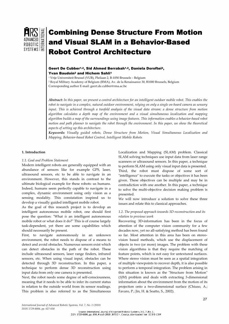
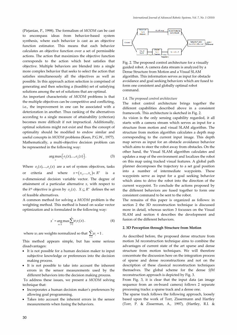
Fig. 2. The proposed control architecture for a visually guided robot. A camera data stream is analyzed by a Dense Structure from Motion and a Visual SLAM algorithm. This information serves as input for obstacle avoidance and goal seeking behaviors which are fused to form one consistent and globally optimal robot command.

1.4. The proposed control architecture The robot control architecture brings together the different capabilities described above in a consistent framework. This architecture is sketched in Fig. 2. As vision is the only sensing capability regarded, it all starts with a camera stream which serves as input for a structure from motion and visual SLAM algorithm. The structure from motion algorithm calculates a depth map corresponding to the current input image. This depth map serves as input for an obstacle avoidance behavior which aims to steer the robot away from obstacles. On the other hand, the Visual SLAM algorithm calculates and updates a map of the environment and localizes the robot on this map using tracked visual features. A global path planner decomposes the trajectory to a set goal position into a number of intermediate waypoints. These waypoints serve as input for a goal seeking behavior which aims to drive the robot into the direction of the current waypoint. To conclude the actions proposed by the different behaviors are fused together to form one consistent command to be sent to the robot. The remains of this paper is organized as follows: in section 2 the 3D reconstruction technique is discussed more in detail, whereas section 3 focusses on the Visual SLAM and section 4 describes the development and fusion of the different behaviors.

2. 3D Perception through Structure from Motion

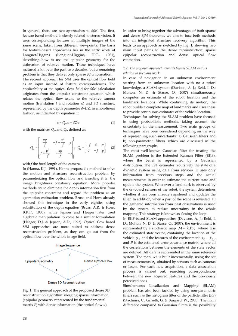
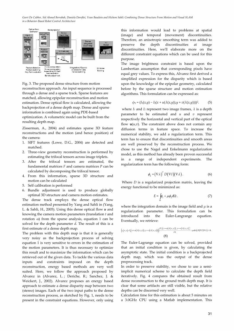
As described before, the proposed dense structure from motion 3d reconstruction technique aims to combine the advantages of current state of the art sparse and dense structure from motion techniques. We will therefore concentrate the discussion here on the integration process of sparse and dense reconstructions and not on the description of these classical reconstruction techniques themselves. The global scheme for the dense SfM reconstruction approach is depicted by Fig. 3. From Fig. 3, it is clear that the input data (an image sequence from an on-board camera) follows 2 separate processing tracks: a sparse track and a dense one. The sparse track follows the following approach, loosely based upon the work of Torr, Zissermann and Hartley (Torr, P. & Zisserman, A., 1997), (Hartley, R.I. &


31

Fig. 3. The proposed dense structure from motion reconstruction approach. An input sequence is processed through a dense and a sparse track. Sparse features are matched, allowing epipolar reconstruction and motion estimation. Dense optical flow is calculated, allowing the backprojection of a dense depth map. Dense and sparse information is combined again using PDE-based optimization. A volumetric model can be built from the resulting depth map.

Zisserman, A., 2004) and estimates sparse 3D feature reconstructions and the motion (and hence position) of the camera: 1. SIFT features (Lowe, D.G., 2004) are detected and

matched. 2. Three-view geometry reconstruction is performed by

estimating the trifocal tensors across image triplets. 3. After the trifocal tensors are estimated, the

fundamental matrices F and camera matrices P can be calculated by decomposing the trifocal tensor.

4. From this information, sparse 3D structure and motion can be calculated

5. Self calibration is performed 6. Bundle adjustment is used to produce globally

optimal 3D structure and camera motion estimates. The dense track employs the dense optical flow estimation method presented by Yang and Sahli in (Yang, L. & Sahli, H., 2005). Using this dense optical flow u and knowing the camera motion parameters (translation t and rotation ω) from the sparse analysis, equation 1 can be solved for the depth parameter d. The result of this is a first estimate of a dense depth map. The problem with this depth map is that it is generally very noisy as the backprojection process of solving equation 1 is very sensitive to errors in the estimation of the motion parameters. It is thus necessary to optimize this result and to maximize the information which can be retrieved out of the given data. To tackle the various data inputs and constraints imposed on the depth reconstruction, energy based methods are very well suited. Here, we follow the approach proposed by Alvarez in (Alvarez, L. ; Deriche, R.; Sanchez, J. & Weickert, J., 2002). Alvarez proposes an energy based approach to estimate a dense disparity map between two (stereo) images. Each of the two input paths to the dense reconstruction process, as sketched by Fig. 1, needs to be present in the constraint equations. However, only using

this information would lead to problems at spatial (image) and temporal (movement) discontinuities. Therefore, an anisotropic smoothing term was added to preserve the depth discontinuities at image discontinuities. Here, we'll elaborate more on the different constraint equations which can be used for this purpose. The image brightness constraint is based upon the Lambertian assumption that corresponding pixels have equal grey values. To express this, Alvarez first derived a simplified expression for the disparity which is based upon the knowledge of the epipolar geometry, calculated before by the sparse structure and motion estimation algorithms. This formulation can be expressed as:

φ1 = (I1(x,y) − I2(x + u(λ(x,y)),y + v(λ(x,y))))2. (5)

where I1 and I2 represent two image frames, λ is a depth parameter to be estimated and u and v represent respectively the horizontal and vertical part of the optical flow u(u,v). The constraint above does not contain any diffusion terms in feature space. To increase the numerical stability, we add a regularization term. This term has to ensure that discontinuities and smooth areas are well preserved by the reconstruction process. We chose to use the Nagel and Enkelmann regularization model, as this method has already been proven successful in a range of independent experiments. The regularization term has the following form:

( ) ( )( )2 = .T

D Iφ λ λ∇ ∇ ∇ (6)

Where D is a regularized projection matrix, leaving the energy functional to be minimized as:

1 2= .E dφ μφΩ

+ Ω∫ (7)

where the integration domain is the image field and μ is a regularization parameter. This formulation can be introduced into the Euler-Langrange equation. Eventually, we retrieve:

( ) ( )( ) ( )( )( )( ) ( )( ) ( )( )( )( )( )2

1 2

, , ,, , , , = 0 .I

I x u x y y v x yx y I x u x y y v x y div D I

λ λλ λ μ λ

λ

∂ + +− + + − ∇ ∇

∂

(8)

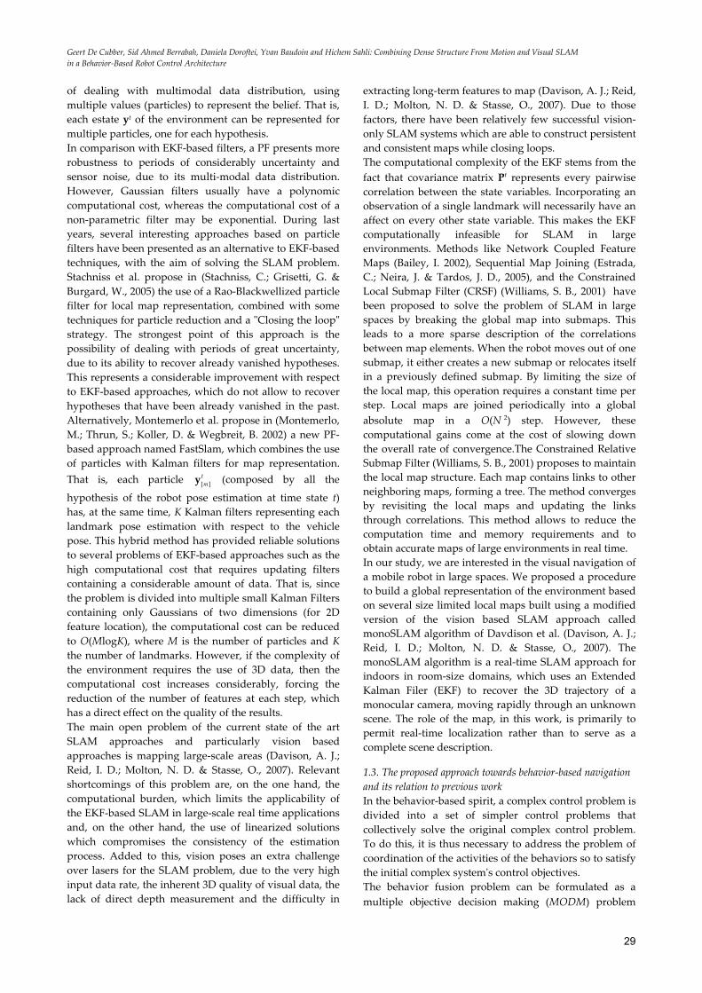
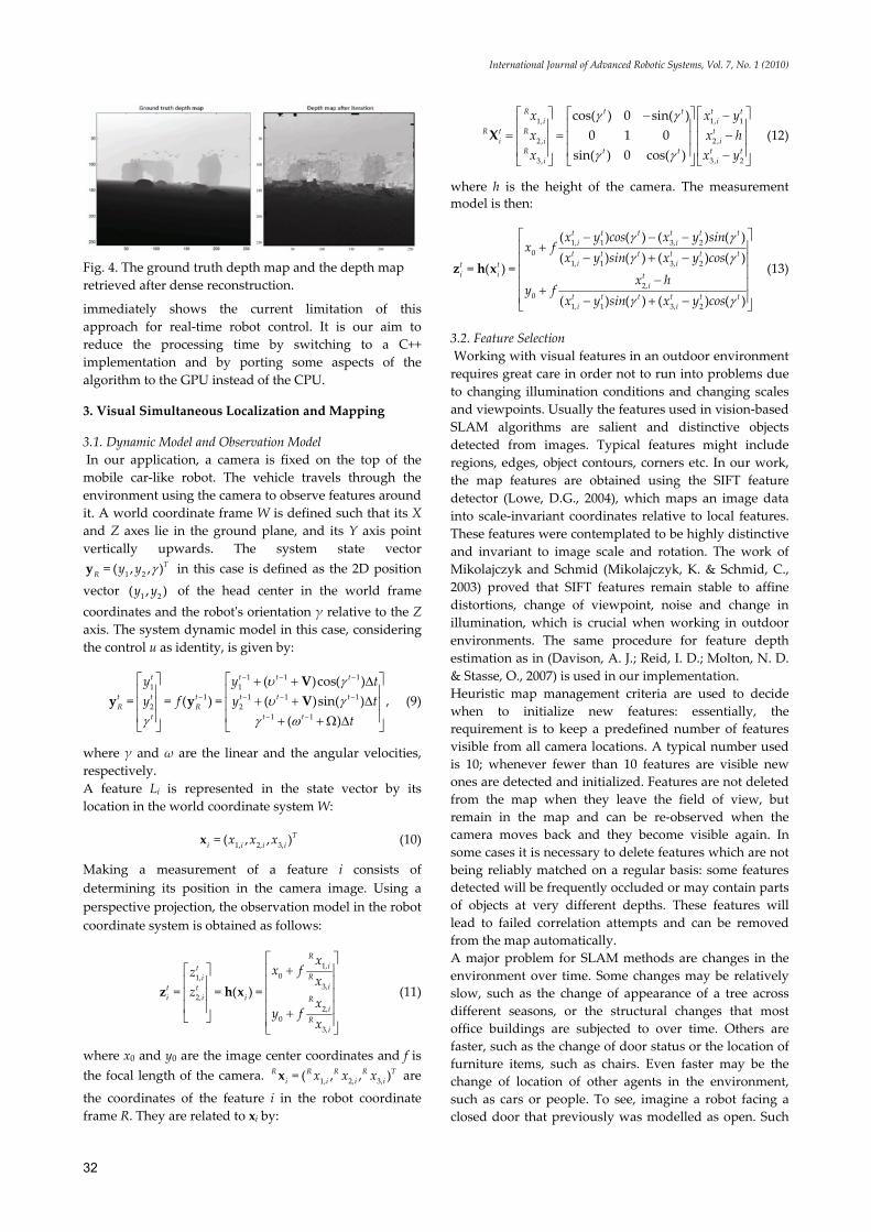
The Euler-Lagrange equation can be solved, provided that an initial condition is given, by calculating the asymptotic state. The initial condition is a backprojected depth map, which was the output of the dense preprocessing track. In order to preserve stability, we chose to use a semi-implicit numerical scheme to calculate the depth field iteratively. Fig. 4 compares the obtained result from dense reconstruction to the ground truth depth map. It is clear that some artifacts are still visible, but the relative depths can be discerned very well. Calculation time for this estimation is about 5 minutes on a 3.0GHz CPU using a Matlab implementation. This


32

Fig. 4. The ground truth depth map and the depth map retrieved after dense reconstruction.

immediately shows the current limitation of this approach for real-time robot control. It is our aim to reduce the processing time by switching to a C++ implementation and by porting some aspects of the algorithm to the GPU instead of the CPU.

3. Visual Simultaneous Localization and Mapping

3.1. Dynamic Model and Observation Model In our application, a camera is fixed on the top of the mobile car-like robot. The vehicle travels through the environment using the camera to observe features around it. A world coordinate frame W is defined such that its X and Z axes lie in the ground plane, and its Y axis point vertically upwards. The system state vector

1 2= ( , , )TR y y γy in this case is defined as the 2D position

vector 1 2( , )y y of the head center in the world frame coordinates and the robot's orientation γ relative to the Z axis. The system dynamic model in this case, considering the control u as identity, is given by:

1 1 11 1

1 1 1 12 2

1 1

( )cos( )= = ( ) = ( )sin( ) ,

( )

t t t t

t t t t t tR R

t t t

y y ty f y t

t

υ γυ γ

γ γ ω

− − −

− − − −

− −

⎡ ⎤ ⎡ ⎤+ + Δ⎢ ⎥ ⎢ ⎥

+ + Δ⎢ ⎥ ⎢ ⎥⎢ ⎥ ⎢ ⎥+ + Ω Δ⎣ ⎦ ⎣ ⎦

Vy y V (9)

where γ and ω are the linear and the angular velocities, respectively. A feature Li is represented in the state vector by its location in the world coordinate system W:

1, 2, 3,= ( , , )Ti i i ix x xx (10)

Making a measurement of a feature i consists of determining its position in the camera image. Using a perspective projection, the observation model in the robot coordinate system is obtained as follows:

1,01,

3,2,

2,0

3,

= = ( ) =

Rit

Riit t

i i i Ri

Ri

xx fz

xz

xy f

x

⎡ ⎤+⎡ ⎤ ⎢ ⎥

⎢ ⎥ ⎢ ⎥⎢ ⎥ ⎢ ⎥⎢ ⎥ ⎢ ⎥+⎣ ⎦ ⎢ ⎥

⎣ ⎦

z h x (11)

where x0 and y0 are the image center coordinates and f is the focal length of the camera. 1, 2, 3,= ( , , )R R R R T

i i i ix x xx are

the coordinates of the feature i in the robot coordinate frame R. They are related to xi by:

1, 1, 1

2, 2 ,

3, 3, 2

cos( ) 0 sin( )0 1 0

sin( ) 0 cos( )

R t t t ti i

R t R ti i i

R t t t ti i

x x yx x hx x y

γ γ

γ γ

⎡ ⎤ ⎡ ⎤ ⎡ ⎤− −⎢ ⎥ ⎢ ⎥ ⎢ ⎥

= = −⎢ ⎥ ⎢ ⎥ ⎢ ⎥⎢ ⎥ ⎢ ⎥ ⎢ ⎥−⎣ ⎦ ⎣ ⎦ ⎣ ⎦

X (12)

where h is the height of the camera. The measurement model is then:

1, 1 3, 20

1, 1 3, 2

2,0

1, 1 3, 2

( ) ( ) ( ) ( )( ) ( ) ( ) ( )

= ( ) =

( ) ( ) ( ) ( )

t t t t t ti i

t t t t t ti it t

i i ti

t t t t t ti i

x y cos x y sinx f

x y sin x y cos

x hy f

x y sin x y cos

γ γγ γ

γ γ

⎡ ⎤− − −+⎢ ⎥

− + −⎢ ⎥⎢ ⎥−⎢ ⎥+⎢ ⎥− + −⎣ ⎦

z h x (13)

3.2. Feature Selection Working with visual features in an outdoor environment requires great care in order not to run into problems due to changing illumination conditions and changing scales and viewpoints. Usually the features used in vision-based SLAM algorithms are salient and distinctive objects detected from images. Typical features might include regions, edges, object contours, corners etc. In our work, the map features are obtained using the SIFT feature detector (Lowe, D.G., 2004), which maps an image data into scale-invariant coordinates relative to local features. These features were contemplated to be highly distinctive and invariant to image scale and rotation. The work of Mikolajczyk and Schmid (Mikolajczyk, K. & Schmid, C., 2003) proved that SIFT features remain stable to affine distortions, change of viewpoint, noise and change in illumination, which is crucial when working in outdoor environments. The same procedure for feature depth estimation as in (Davison, A. J.; Reid, I. D.; Molton, N. D. & Stasse, O., 2007) is used in our implementation. Heuristic map management criteria are used to decide when to initialize new features: essentially, the requirement is to keep a predefined number of features visible from all camera locations. A typical number used is 10; whenever fewer than 10 features are visible new ones are detected and initialized. Features are not deleted from the map when they leave the field of view, but remain in the map and can be re-observed when the camera moves back and they become visible again. In some cases it is necessary to delete features which are not being reliably matched on a regular basis: some features detected will be frequently occluded or may contain parts of objects at very different depths. These features will lead to failed correlation attempts and can be removed from the map automatically. A major problem for SLAM methods are changes in the environment over time. Some changes may be relatively slow, such as the change of appearance of a tree across different seasons, or the structural changes that most office buildings are subjected to over time. Others are faster, such as the change of door status or the location of furniture items, such as chairs. Even faster may be the change of location of other agents in the environment, such as cars or people. To see, imagine a robot facing a closed door that previously was modelled as open. Such


33

50

100

150

200

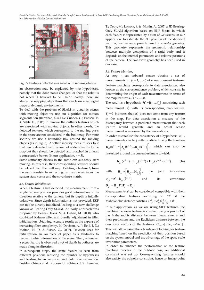
250 Fig. 5. Features detected in a scene with moving objects

an observation may be explained by two hypotheses, namely that the door status changed, or that the robot is not where it believes to be. Unfortunately, there are almost no mapping algorithms that can learn meaningful maps of dynamic environments. To deal with the problem of SLAM in dynamic scenes with moving object we use our algorithm for motion segmentation (Berrabah, S.A.; De Cubber, G.; Enescu, V. & Sahli, H., 2006) to remove the outliers features which are associated with moving objects. In other words, the detected features which correspond to the moving parts in the scene are not considered in the built map. For more security we use a bounding box around the moving objects (as in Fig. 5). Another security measure sees to it that newly detected features are not added directly to the map but they should be detected and matched in at least n consecutive frames (in our application, n = 5). Some stationary objects in the scene can suddenly start moving. In this case, their corresponding features should be deleted from the built map. Deleting a feature Li from the map consists in extracting its parameters from the system state vector and the covariance matrix.

3.3. Feature Initialization When a feature is first detected, the measurement from a single camera position provides good information on its direction relative to the camera, but its depth is initially unknown. Since depth information is not provided, EKF can not be directly initialized, leading to a new challenge known as Bearing-Only SLAM. An early approach was proposed by Deans (Deans, M. & Hebert, M., 2000), who combined Kalman filter and bundle adjustment in filter initialization, obtaining accurate results at the expense of increasing filter complexity. In (Davison, A. J.; Reid, I. D.; Molton, N. D. & Stasse, O., 2007), Davison uses for initialization an A4 piece of paper as a landmark to recover metric information of the scene. Then, whenever a scene feature is observed a set of depth hypotheses are made along its direction. In subsequent steps, the same feature is seen from different positions reducing the number of hypotheses and leading to an accurate landmark pose estimation. Besides, Ortega et al. proposed in (Ortega, J. S.; Lemaire,

T.; Devy, M.; Lacroix, S. & Monin, A., 2005) a 3D Bearing-Only SLAM algorithm based on EKF filters, in which each feature is represented by a sum of Gaussians. In our application, to estimate the 3D position of the detected features, we use an approach based on epipolar geometry. This geometry represents the geometric relationship between multiple viewpoints of a rigid body and it depends on the internal parameters and relative positions of the camera. The two-view geometry has been used in our case.

3.4. Feature Matching At step t, an onboard sensor obtains a set of measurements t

iz (i = 1,…,m) of m environment features. Feature matching corresponds to data association, also known as the correspondence problem, which consists in determining the origin of each measurement, in terms of the map features Lj, j = 1,…,n. The result is a hypothesis 1= [ ,..., ]t t t

mH h h associating each

measurement tiz with its corresponding map feature.

= 0tih indicates that t

iz does not come from any feature in the map. For data association a measure of the discrepancy between a predicted measurement that each feature would generate and an actual sensor measurement is measured by the innovation ε. In order to establish the consistency of a hypothesis tH , measurements can be jointly predicted using the function

| 1 | 1 | 1

1( ) = ( ) ( )

Tt t t t t t

t t tm

− − −⎡ ⎤⎢ ⎥⎣ ⎦

h x h x h x…H h h

, which can also be

linearized around the current estimate to yield:

| 1 | 1 | 1 | 1ˆ ˆ( ) ( ) ( ),t t t t t t t tt t t

− − − −+ −h x h x H x xH H H

(14)

with 1

=T

t t tm

⎡ ⎤⎢ ⎥⎣ ⎦

H H H…H h h

, the joint innovation

| 1ˆ= ( )t t t tt tε −−z h x

H H and its covariance

= t Tt t t t+S H P H R

H H H H.

Measurements zt can be considered compatible with their corresponding features according to tH if the Mahalanobis distance satisfies 2 1= <T

t t t tD thε ε−SH H H H

.

In our application, as we are using SIFT features, the matching between feature is checked using a product of the Mahalanobis distance between measurements and their predictions and the Euclidean distance between the descriptor vectors of the features 2

1 2=descD desc desc− . This will allow using the advantage of looking for feature matching based on the prediction of their position based on the system model and the advantage of the space-scale invariance parameters. In order to enhance the performance of the feature matching process in the outdoor case, an additional constraint was set up. Corresponding features should also satisfy the epipolar constraint, hence an image point


34

tix that corresponds to 1t

i−x is located on or near the

epipolar line that is induced by 1ti−x . The distance of the

image point tix from that epipolar line is computed as

follows:

1 2

2

1 2 1 21 1

( )( ) ( )

tT ti i

epi t ti i

D−

− −=

+

x xx x

FF F

(15)

where 1ti j−xF is the j component of the vector 1t

i−xF . F is

the fundamental matrix which is computed based on the estimations from the Extended Kalman Filter. Knowing the camera position at instants t, the estimated camera position at instant t - 1, and the camera calibration matrix K, the fundamental matrix F is computed as follows:

1[ ]T− −×= K R t KF (16)

where R is the rotation matrix and [t]× is the skew matrix corresponding to the translation vector t. The notation K-T denotes the transpose of the inverse K. As a result, the cost function for feature matching is defined as D2 and 2

epiD

2 2 2 2match t dect epiD D D D= + +

H (17)

Measurements for which correspondences in the map cannot be found by data association can be directly added to the current stochastic state vector as new features.

3.5. Local and Global Mapping In our study, we are interested in robot navigation in large spaces. For that, we propose a procedure to build a global representation of the environment based on several size limited local maps built using the previously described approach. Two methods for local map joining are proposed. The first method consists in transforming each local map into a global frame before to start building a new local map. In the second method, the global map consists only of a set of robot positions where new local maps started (i.e. the base references of the local maps). In both methods, the base frame for the global map is the robot position at instant t0. Each local map is built as follows: at a given instant tk, a new map is initialized using the current vehicle location,

tkRy , as base reference = tk

k RB y , k = 1,2,… being the local map order. Then, the vehicle performs a limited motion acquiring sensor information about the Li neighboring environment features. An EKF-based technique is used to model the local maps. The kth local map is defined by

= ( , )k k kX PM , where Xk is the state vector in the base reference Bk of the Lk detected features and Pk is their covariance matrix. The decision to start building a new local map at an instant tk is based on two criteria: the number of features in the current local map and the scene cut detection

result. The instant tk is called a key-instant. In our application we defined two thresholds for the number of features in the local maps: a lower Th− and a higher Th+ threshold. A key-instant is selected if the number of features k

ln in the current local map k is bigger then the lower threshold and a scene cut has been detected or the number of features has reached the higher threshold. This allows kipping reasonable dimensions of the local maps and avoids building too small maps. At the key-instants tk some frames are selected to be used for features initialization in the new local map. These frames are called key-frames. The motion between two frames must be sufficiently large to accurately compute the 3D positions of matched points. For that we select frames relatively far from each other but that have enough common points. In the first method for global map building, the first local map is used as global map. Each finalized local map is transferred to the global map before starting a new one, by computing the state vectors and the covariance matrix. The goal of map joining is to obtain one full stochastic map 0 0

(0 1 2 ...) (0 1 2 ...)= ( , )⊕ ⊕ ⊕ ⊕ ⊕ ⊕X PM , where 0(0 1 2 ...)⊕ ⊕ ⊕X is a

concatenation in the frame B0 of all sets of features from local maps 0M , 1M , 2M , ... As each camera position,

tkRy corresponding to the frame reference Bk is given in

the previous frame reference Bk-1, the transformation of feature i coordinates vector from frame Bk to B0 is obtained by successive transformations:

0

( 1) ( 1) ( 2) 1 2...1 1

ki i

k k k k→ − − → − →

⎛ ⎞ ⎛ ⎞= ⋅⎜ ⎟ ⎜ ⎟⎜ ⎟ ⎜ ⎟

⎝ ⎠ ⎝ ⎠

x xT T T (18)

( 1) = ( | )k k→ − tT R is the space transformation matrix corresponding to rotation R and t from frame Bk to Bk-1

and is given by:

1

( 1)2

cos( ) 0 sin( )0 1 0 0

sin( ) 0 cos( )0 0 0 1

k k k

k k k

t t t

k k t t t

y

y

γ γ

γ γ→ −

⎛ ⎞−⎜ ⎟⎜ ⎟= ⎜ ⎟⎜ ⎟⎜ ⎟⎝ ⎠

T (19)

The covariance 0(0 1 2 ...)⊕ ⊕ ⊕P of the joint map is obtained

from the linearization of the state transition function f. As the local maps are independents, the Jacobian (from linearization) is then applied separately to the local map covariance:

0(0 1 2 ...) 0 1

0 0 1 1

= ... ...T T T

iR R R R R Ri i

P P P⊕ ⊕ ⊕

∂ ∂ ∂ ∂ ∂ ∂+ + + +

∂ ∂ ∂ ∂ ∂ ∂f f f f f fPy y y y y y

(20)

where R k

∂∂

fy

is the Jacobian of the state transition

function f with respect to yR in the reference frame k. In the second method for global map building, the global map is limited to the set of the coordinates of the local


35

maps frame origins 0 1 2= ( , , ,...)BG R R Ry y yM , where k

Ry are the robot coordinates in B0, where it decides to build the local map kM at instant tk. These robot coordinates are updated via

( 1) ,1 1

ktkR R

k k→ −

⎛ ⎞⎛ ⎞= ⋅ ⎜ ⎟⎜ ⎟⎜ ⎟ ⎜ ⎟⎝ ⎠ ⎝ ⎠

y yT (21)

with t0 = 0 and 0 0= = (0,0,0)tR Ry y and the transformation

matrix 0k→T is obtained by successive transformations:

0 1 0 2 1 ( 1) ( 2)... ,k k k→ → → − → −= ⋅T T T T (22)

where 1 = ( | )k k→ − tT R is the transformation matrix given by equation 19. In this case, for feature matching at instant t, the robot uses the local map with the closest base frame to its current location, by evaluating the function:

( )arg min ,k tR Ri−y y (23)

where tRy is the robot position at instant t in B0.

4. Behavior-based Robot Control

The robot control mechanism integrates the proposed 3D reconstruction and visual SLAM techniques. The 3D reconstruction results are used for the detection of objects. This information is used by an obstacle avoidance behavior to steer the robot away from these obstacles. On the other hand, the robot position and map calculated by visual SLAM are used as base information for a goal seeking behavior, which directs the robot into the direction of a goal point. As explained in the introduction, each behavior needs to be cast as an objective function estimator. This means that each behavior calculates an objective function over a set of permissible actions. In the case of our mobile robot, the action space consists of a velocity command v and a heading direction θrobot. Each behavior thus needs to calculate an objective function o,(v, θrobot).

4.1. Development of the Obstacle Avoidance behavior The obstacle avoidance has two main responsibilities: • It points the robot away from obstacles. Thus, it must

assign low values to actions that cause the robot to face obstacles and high values to actions that do the opposite.

• It varies the velocity respective to obstacle distance. High velocities are preferred when the distance to obstacles is large and and low velocities when this distance is small.

The objective function ( , )OA roboto v θ can now be composed

by making the product of a factor ( )OA robotoθ θ taking into

account the first, heading constraint and a factor ( )vOAo v

taking into account the second constraint. In order to calculate these objective functions, the dense depth map as estimated by the structure from motion

0

0

0

0

0

0

0

100

200

300

400

500

600

700

200 400 600

100

200

300

400

500

600

7000 200 400 600 800

0

0.2

0.4

0.6

0.8

1

Rel

ativ

e D

epth

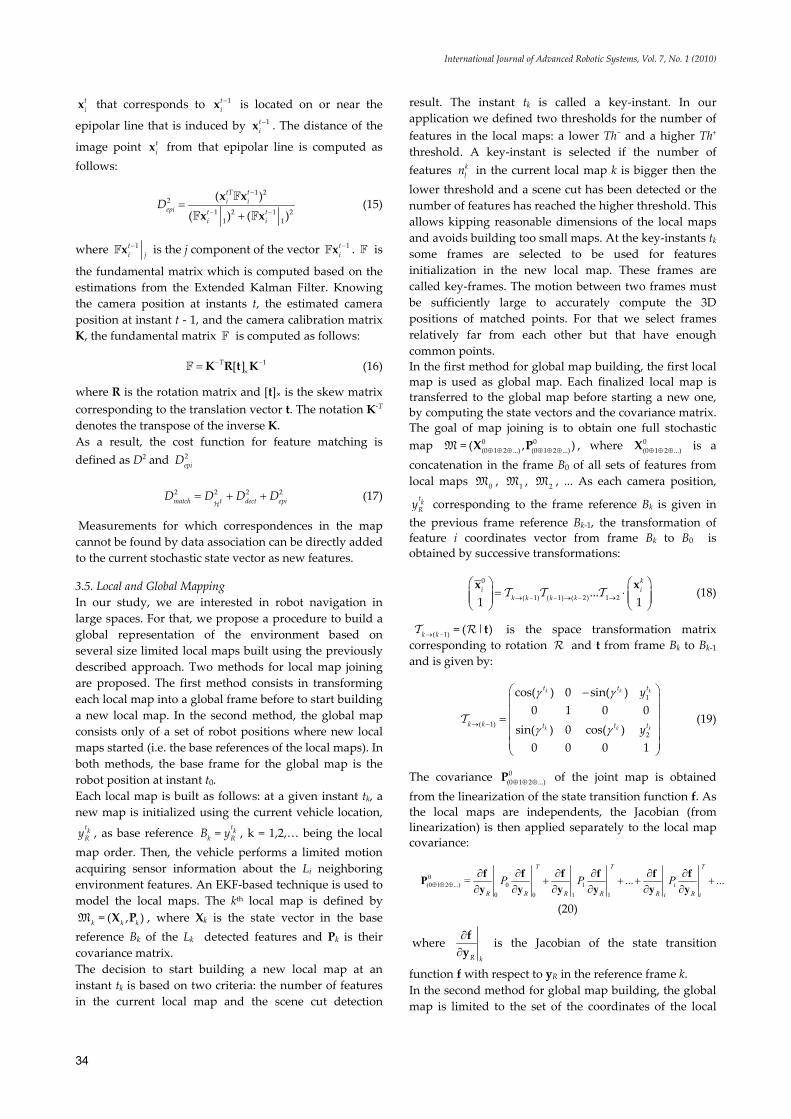
Fig. 6. The different steps of the depth map analysis: Upper Left: A dense depth map is calculated through structure from motion; Upper Right: This depth map is thresholded in order to not take into account far away objects; Lower Left: The ground plane is removed from the depth map; Lower Right: The remaining part of the depth map is downprojected onto the ground plane, such that a one-dimensional function of relative depth over the image plane is obtained.

algorithm is analyzed. This analysis process is illustrated in Fig. 6. This process, involves the following steps: • A dense depth map is estimated by the structure from

motion algorithm, as described in section 2. • Far away objects which are not important for the local

obstacle avoidance behavior are removed from this depth map by setting a threshold for the depth

• The majority of the remaining depth map still consists of perfectly traversable terrain. In order not to perceive this terrain as an obstacle itself, the ground plane is removed from the depth map. This is achieved by searching for edges in the depth map. The foreground is supposed to be quite uniform, whereas obstacles will give rise to strong edges. Only depth information in the region of edges is retained.

• Finally, the remaining part of the depth map is downprojected onto the ground plane, such that a one-dimensional function f of relative depth over the image plane is obtained.

The relative depth function f is a direct indicator of the presence of obstacles and is a function in the interval [0,1]. It can thus be directly related to the objective function controlling the robot heading: ( ) =OA roboto fθ θ . The velocity of the robot should in general be as high as possible. Only when obstacles are near, the velocity should be decreased. This can be expressed as:

2

obstacle thresholdmax

obstacle threshold2

max

if >

( ) = 1 if <

1

vOA

v d dv

o vd d

vv

⎧⎛ ⎞⎪ ⎜ ⎟⎜ ⎟⎪ ⎝ ⎠⎪⎨⎪

⎛ ⎞⎪ + ⎜ ⎟⎪⎝ ⎠⎩

(24)


36

with dobstacle = min(f), dthreshold a set threshold distance and vmax the maximum robot velocity.

4.2. Development of the Goal seeking behavior The goal seeking behavior is assigned two tasks as well: • It points the robot to the goal position and must thus

assign high values to actions that cause the robot to face the target and low values to actions that do the opposite.

• It varies the velocity respective to the distance to the goal. High velocities are preferred when the distance to the goal is large and and lower velocities when the distance is small.

Again, this means the development of the objective function can be split up as ( , ) = ( ). ( )v

GS robot GS robot GSo v o o vθθ θ . To calculate these objective functions, the (Euclidian) distance to the goal dgoal and heading to this goal θgoal are calculated from the current robot position given by the Visual SLAM algorithm, described in section 3, and the current waypoint given by the global path planner. It is now obvious that the goal seeking behavior needs to minimize the difference between the robot heading θrobot and the goal heading θgoal, which we can formulate as:

2

robot goal

1( ) = .

1GS robotoθ θ

θ θβ

⎛ ⎞−+ ⎜ ⎟⎜ ⎟⎝ ⎠

(25)

with β the window size which is considered. For ( )v

GSo v , a similar reasoning as been done before for

( )vOAo v can be performed, as the velocity should always

be high, with the exception of near the goal positions. This can be expressed as:

2

goal thresholdmax

goal threshold2

max

if >

( ) = .1 if <

1

vGS

v d dv

o vd d

vv

⎧ ⎛ ⎞⎪ ⎜ ⎟⎜ ⎟⎪ ⎝ ⎠⎪⎨⎪

⎛ ⎞⎪ + ⎜ ⎟⎪⎝ ⎠⎩

(26)

This methodology allows to compose the objective functions ( , )GS roboto v θ and ( , )OA roboto v θ . The remaining problem is how to fuse these objectives to form one globally optimal command, leading to intelligent robot behavior.

4.3. Behavior Fusion As mentioned above in the introduction, the classical weight optimization methods for behavior fusion have some serious disadvantages. The first one is that they do not allow introducing some a priori knowledge from a human decision maker. This issue is addressed by so-called goal programming methods. Goal programming methods define a class of techniques for generating satisfying solutions also known as compromise solutions in this context. The decision maker gives his/her preferences in terms of weights, priorities, goals, and

ideals. The concept of best alternative is then defined in terms of how much the actual achievement of each objective deviates from the desired goals or ideals. Further, the concept of best compromise alternative is defined to have the minimum combined deviation from the desired goals or ideals. Goal programming methods thus choose an alternative having the minimum combined deviation from the decision maker's ideal goals

* *1 ,..., no o , given the weights or priorities of the objective

functions. This can be formulated as (Pirjanian, P., 1998):

*

=1( ) .arg min

n p

i i ix X i

w o x o∈

−∑ (27)

where 1 ≤ p ≤ ∞, o* is the ideal goal, wi is the weight or priority given to the ith objective.

pwx is a solution to this equation for a given p and weight

vector ( )1= ,..., nw w w and represents an action to be

performed. A second disadvantage of the weight optimization which is still not solved by the goal programming method is that it does not take into account errors on the sensor measurements which will also make the output of a behavior which use this data less reliable. In (Doroftei, D. ; Colon, E. & De Cubber, G., 2007), we proposed a method to choose the weights based upon a reliability measure associated to each behavior. The principle behind the calculation of the activity levels is that the output of a behavior should be stable over time in order to trust it. Therefore, the degree of relevance or activity is calculated by observing the history of the output of each behavior. This history-analysis is performed by

comparing the current output ,bij kϖ to a running average

of previous outputs, which leads to a standard deviation, which is then normalized. For a behavior bi with outputs j

these standard deviations bijσ are:

2

,=1

,=

= ,

N bij lib b li i

j j j kk i h

cN

ϖσ ϖ

−

⎛ ⎞⎜ ⎟⎜ ⎟−⎜ ⎟⎜ ⎟⎝ ⎠

∑∑ (28)

with cj some normalization constants. The bigger this standard deviation, the more unstable the output values of the behavior are, so the less they can be trusted. The same approach is followed all behaviors. This leads to an estimate for the activity levels or weights for each behavior:

1

(1 )i

numberofoutputsbi

b jj

w σ=

= −∑ (29)

As such it is now possible to take into account the unreliability of the behavior output. On the other hand, this architecture again does not offer a human decision maker the ability to interact with the decision process.


37

One could thus argue that while reliability analysis-based approaches are too robot centric, these second set of approaches is too human-centric. In the following, we present an approach to integrate the advantages of both theorems. This can be achieved by minimizing the goal programming and reliability analysis constraints in an integrated way, following:

( ) ( )numberofoutputs

*

=1 =1 =1( ) 1 1 ,arg min

pn np bi

i i i i jx X i i j

w wi

w o x o wλ λ σ∈

∈

⎡ ⎤⎛ ⎞⎢ ⎥− + − − −⎜ ⎟⎢ ⎥⎝ ⎠⎣ ⎦∑ ∑ ∑

(30)

with λ a parameter describing the relative influence of both constraints. This parameter indirectly influences the control behavior of the robot. Large values of λ will lead to a human-centered control strategy, whereas lower values will lead to a robot-centered control strategy. The value of λ would therefore depend on the expertise or the availability of human experts interacting with the robot. It is obvious that this method increases the numerical complexity of finding a solution to MODM, but this does not necessarily leads to increased processing time, as the search interval can be further reduced by incorporating constraints from both data sources.

5. Conclusions and Future Work

In this paper, we presented a navigation solution for an outdoor mobile robot, which uses only a single on-board camera as sensory input. The development of such a control strategy for an outdoor mobile robot which uses vision as its only sensing modality, requires the careful consideration of multiple design aspects. A main problem is caused by the outdoor nature of the application. The outdoor changing lighting condition cause problems for image processing algorithms which are based on feature matching, such as 3D reconstruction and visual SLAM. Also the dimensions of the outdoor environments cause problems, as it is hard to model such extended environments. In this paper, we have presented 3 main methodologies which tackle these problems and which work together to provide an integrated control architecture for an intelligent mobile robot. The first constituent of this integrated control architecture is a 3D reconstruction approach, operating on monocular images. The main novelty of the presented 3D reconstruction approach lies in the fact that it fuses dense and sparse information in an integrated variational framework. This allows to combine the robustness of sparse reconstruction techniques with the completeness of dense reconstruction approaches. The presented approach achieves its goal of reconstructing complex outdoor environments, but its practical application is still limited due to the required processing time, due to the computational complexity. Therefore, future research will go out into optimizing the presented approach to (near) real-time applications.

A second technology which was presented is a visual simultaneous localization and mapping approach. The presented visual SLAM technique differentiates itself from the state of the art by its capability to build large outdoor maps, without exploding the computational complexity. This is achieved by integrating different local maps. The presented approach has proven its applicatbility from a theoretical point of view and will in the future be tested in large outdoor environments. Finally, a behavior-based control method was proposed, which presents a novel methodology for integrating the traditional goal programming approach for action selection, with a more recent approach using reliability analysis. The advantage of this method is that it combines the advantages of both approaches, such that a good balance is reached between human centric and robot centric robot control.

6. References

Alvarez, L.; Deriche, R.; Sanchez, J. & Weickert, J. (2002). Dense disparity map estimation respecting image derivatives: a PDE and scale-space based approach. Journal of Visual Communication and Image Representation, Vol. 13, No. 1, pp. 3-21

Bailey, I. (2002). Mobile robot localisation and maping in extensive outdoor environments. PhD thesis, Australian Centre for Field Robotics, University of Sydney, Australia

Berrabah, S.A.; De Cubber, G.; Enescu, V. & Sahli, H. (2006). MRF-Based Foreground Detection in Image Sequences from a Moving Camera, Proceedings of IEEE International Conference on Image Processing, pp. 1125-1128

Bruss, A.R. & Horn, B.K.P. (1983). Passive navigation. Computer Vision, Graphics and Image Processing, Vol. 21, pp. 3-20

Chiuso, A.; Favaro, P.; Jin, H. & Soatto, S. (2002). Structure from motion causally integrated over time. IEEE Trans. on Pattern Analysis and Machine Intelligence, Vol. 24, No. 4, pp. 523-535

Davison, A. J.; Reid, I. D.; Molton, N. D. & Stasse, O. (2007) MonoSLAM: Real-Time Single Camera SLAM, IEEE Transaction on Pattern Analysis and Machine Intelligence, Vol.29, No.6

Deans, M. & Hebert, M. (2000). Experimental comparison of techniques for localization and mapping using a bearing-only sensor, Proceedings of Seventh International Symposium on Experimental Robotics, Vol. 271, pp. 395- 404

Doroftei, D.; Colon, E. & De Cubber, G. (2007). A behaviour-based control and software architecture for the visually guided Robudem outdoor mobile robot. Proceedings of International Symposium on Measurement and Control in Robotics

Estrada, C.; Neira, J. & Tardos, J. D. (2005). Hierarchical SLAM: real-time accurate mapping of large


38

environments, IEEE Transactions on Robotics, Vol.21, No.4, pp. 588-596

Hanna, K.J. (1991). Direct multi-resolution estimation of ego-motion and structure from motion. Proceedings of Workshop on Visual Motion, pp. 156-162

Hartley, R.I. & Zisserman, A. (2004): Multiple View Geometry in Computer Vision. Cambridge University Press, pp. 31-57

Heeger, D.J. & Jepson, A.D. (1992). Subspace methods for recovering rigid motion: Algorithm and implementation. International Journal of Computer Vision, Vol. 7, No. 2, pp. 95-117

Keen, P.G.W. (1977). The Evolving Concept of Optimality. Multiple Criteria Decision Making, Vol. 6, pp. 31-57

Longuet-Higgins, H.C. (1981). A computer algorithm for reconstructing a scene from two projections. Nature, Vol. 293, No. 5828, pp. 133-135

Lowe, D.G. (2004). Distinctive image features from scale-invariant keypoints. International Journal of Computer Vision, Vol. 60, No. 2, pp. 91-110

Mikolajczyk, K. & Schmid, C. (2003). A performance evaluation of local descriptors, Proceedings of Computer Vision and Pattern Recognition

Montemerlo, M.; Thrun, S.; Koller, D. & Wegbreit, B. (2002). Fastslam: A factored solution to the

simultaneous localization and mapping problem, Proceedings of National Conference on Artificial Intelligence, pp. 593-598

Ortega, J. S.; Lemaire, T.; Devy, M. ; Lacroix, S. & Monin, A. (2005). Delayed vs Undelayed Landmark Initialization for Bearing Only SLAM, Proceedings of IEEE International Conference on Robotics and Automation

Pirjanian, P. (1998). Multiple Objective Action Selection and Behavior Fusion using Voting. Ph.D.-thesis, Faculty of Technical Sciences, Aalborg University

Stachniss, C.; Grisetti, G. & Burgard, W. (2005) Recovering particle diversity in a rao-blackwellized particle filter for slam after actively closing loops, Proceedings of IEEE International Conference on Robotics and Automation, pp. 667-672

Torr, P. & Zisserman, A. (1997). Computing multiple view relations. OUEL Report

Williams, S. B. (2001). Efficient Solutions to Autonomous Mapping and Navigation Problems, PhD thesis, Australian Centre for Field Robotics, University of Sydney, Australia

Yang, L. & Sahli, H. (2005). A Nonlinear Multigrid Diffusion Model for Efficient Dense Optical Flow estimation. Proceedings of ICIP05, Vol. 1, pp. 149-152

Combining Dense Structure From Motion and Visual SLAM in a Behavior-Based Robot Control Architecture

Documents