Combined use of hyperspectral VNIR reflectance spectroscopy and kriging to predict soil variables spatially A. Volkan Bilgili • Fevzi Akbas • Harold M. van Es Published online: 11 June 2010 Ó Springer Science+Business Media, LLC 2010 Abstract Hyperspectral visible near infrared reflectance spectroscopy (VNIRRS) and geostatistical methods are considered for precision soil mapping. This study evaluated whether VNIR or geostatistics, or their combined use, could provide efficient approaches for assessing the soil spatially and associated reductions in sample size using soil samples from a 32 ha area (800 9 400 m) in northern Turkey. Soil variables considered were CaCO 3 , organic matter, clay, sand and silt contents, pH, electrical conductivity, cation exchange capacity (CEC) and exchangeable cations (Ca, Mg, Na and K). Cross-validation was used to compare the two approaches using all grid data (n = 512), systematic selections of 13, 25 and 50% of the data and random selections of 13 and 25% for calibration; the remaining data were used for validation. Partial least squares regression (PLSR) analysis was used for calibrating soil properties from first derivative VNIR reflectance spectra (VNIRRS), whereas ordinary-, co- and regression-kriging were used for spatial prediction. The VNIRRS-PLSR method provided better prediction results than ordinary kriging for soil organic matter, clay and sand contents, (R 2 values of 0.56–0.73, 0.79–0.85, 0.65–0.79, respectively) and smaller root mean squared errors of prediction (values of 2.7–4.1, 37.4–43, 46.9–61, respectively). The EC, pH, Na, K and silt content were predicted poorly by both approaches because either the variables showed little var- iation or the data were not spatially correlated. Overall, the prediction accuracy of VNIRRS-PLSR was not affected by sample size as much as it was for ordinary kriging. Cokriging (COK) and regression kriging (RK) were applied to a combination of values predicted by VNIR reflectance spectroscopy and measured in the laboratory to improve the accuracy of prediction of the soil properties. The results showed that both COK and RK A. V. Bilgili (&) Department of Soil Science, Agriculture Faculty, Harran University, Sanliurfa 63300, Turkey e-mail: [email protected]; [email protected] F. Akbas Department of Soil Science, Agriculture Faculty, Gaziosmanpasa University, Tokat 60100, Turkey e-mail: [email protected] H. M. van Es Department of Crop and Soil Science, Cornell University, Ithaca, NY 14853-1901, USA e-mail: [email protected] 123 Precision Agric (2011) 12:395–420 DOI 10.1007/s11119-010-9173-6

Welcome message from author
This document is posted to help you gain knowledge. Please leave a comment to let me know what you think about it! Share it to your friends and learn new things together.
Transcript
Combined use of hyperspectral VNIR reflectancespectroscopy and kriging to predict soil variablesspatially
A. Volkan Bilgili • Fevzi Akbas • Harold M. van Es
Published online: 11 June 2010� Springer Science+Business Media, LLC 2010
Abstract Hyperspectral visible near infrared reflectance spectroscopy (VNIRRS) and
geostatistical methods are considered for precision soil mapping. This study evaluated
whether VNIR or geostatistics, or their combined use, could provide efficient approaches
for assessing the soil spatially and associated reductions in sample size using soil samples
from a 32 ha area (800 9 400 m) in northern Turkey. Soil variables considered were
CaCO3, organic matter, clay, sand and silt contents, pH, electrical conductivity, cation
exchange capacity (CEC) and exchangeable cations (Ca, Mg, Na and K). Cross-validation
was used to compare the two approaches using all grid data (n = 512), systematic
selections of 13, 25 and 50% of the data and random selections of 13 and 25% for
calibration; the remaining data were used for validation. Partial least squares regression
(PLSR) analysis was used for calibrating soil properties from first derivative VNIR
reflectance spectra (VNIRRS), whereas ordinary-, co- and regression-kriging were used for
spatial prediction. The VNIRRS-PLSR method provided better prediction results than
ordinary kriging for soil organic matter, clay and sand contents, (R2 values of 0.56–0.73,
0.79–0.85, 0.65–0.79, respectively) and smaller root mean squared errors of prediction
(values of 2.7–4.1, 37.4–43, 46.9–61, respectively). The EC, pH, Na, K and silt content
were predicted poorly by both approaches because either the variables showed little var-
iation or the data were not spatially correlated. Overall, the prediction accuracy of
VNIRRS-PLSR was not affected by sample size as much as it was for ordinary kriging.
Cokriging (COK) and regression kriging (RK) were applied to a combination of values
predicted by VNIR reflectance spectroscopy and measured in the laboratory to improve the
accuracy of prediction of the soil properties. The results showed that both COK and RK
A. V. Bilgili (&)Department of Soil Science, Agriculture Faculty, Harran University, Sanliurfa 63300, Turkeye-mail: [email protected]; [email protected]
F. AkbasDepartment of Soil Science, Agriculture Faculty, Gaziosmanpasa University, Tokat 60100, Turkeye-mail: [email protected]
H. M. van EsDepartment of Crop and Soil Science, Cornell University, Ithaca, NY 14853-1901, USAe-mail: [email protected]
123
Precision Agric (2011) 12:395–420DOI 10.1007/s11119-010-9173-6
with VNIRRS estimates improved the predictions of soil variables compared to VNIRRS
and OK. The combined use of VNIRRS and multivariate geostatistics results in better
spatial prediction of soil properties and enables a reduction in sampling and laboratory
analyses.
Keywords Soil variation � Visible near infrared reflectance spectroscopy (VNIRRS) �Partial least square regression (PLSR) � Kriging � Cokriging � Regression kriging
Introduction
Soil is heterogeneous and tends to be very variable spatially. Intensive soil sampling is
required, therefore, to quantify this spatial variation within and across fields for site-
specific management. Conventional sampling methods may be expensive in terms of labor
and chemicals (Viscarra Rossel and McBratney 1998). In precision agriculture, techniques
such as diffuse reflectance spectroscopy (visible-near and mid-infrared) and geostatistics
are considered increasingly for the prediction of soil characteristics at unvisited locations
and to characterize within-field spatial variation (Ben-Dor and Banin 1995; Chang et al.
2001; Shepherd and Walsh 2002). Visible-near infrared reflectance spectroscopy is a
promising method for rapid estimation of a range of soil properties. It has been used to
characterize soil and to quantify its spatial variation, as well as to evaluate soil quality,
contamination and degradation (Chang et al. 2001; Wu et al. 2005; Idowu, et al. 2008).
Brown et al. (2006) used more than 4100 surface and subsurface soil samples from across
the USA, Africa and Asia to evaluate the accuracy of VNIR empirical models for global
soil characterization. They reported strong relationships between VNIR reflectance and
kaolinite, montmorillonite and clay contents, CEC, SOC, IC and citrate dithionite
extractable Fe. The method has also been applied successfully to predict soil nitrogen
(Reeves et al. 2002), Fe2O3, Al2O3, CaCO3 (Ben-Dor and Banin 1995), potentially min-
eralizable nitrogen, (Reeves and van Kessel 1999), heavy metals, micronutrients (Coz-
zolino and Moron 2003; Udelhoven et al. 2003), C:N ratio and soil biological properties
(Ludwig et al. 2002; Chodak et al. 2002). In addition, it may be possible to predict soil
constituents that are spectrally inactive within the VNIR range through their correlations
with spectrally active constituents (Ben-Dor and Banin 1995).
The accuracy and robustness of VNIRRS predictions is affected by factors such as
spectral data pretreatment (first- and second-order derivatives with various smoothing
methods), intercorrelation among soil properties and between soil constituents and spectra,
the methods of chemical analysis used for training data sets and the presence of outliers. In
general, better results were obtained when calibrations were developed for samples from
similar parent materials (Shepherd and Walsh 2002).
Several techniques may be used to predict soil properties, including simple and multiple
linear regression, nearest neighbor interpolation, splines (Voltz and Webster 1990; Laslett
1994), principal component regression (Chang et al. 2001), data mining techniques such as
regression trees (Bishop and McBratney 2001) and spatial interpolation methods such as
inverse distance weighting (IDW; Mueller et al. 2004), ordinary and universal kriging
(Odeh et al. 1994) and cokriging (Ersahin 2003). More recently hybrid methods of spatial
prediction such as regression kriging (Hengl et al. 2004; Kravchenko and Robertson 2007)
and kriging with external drift (Bourennane et al. 2006) have been applied. These latter
techniques use one or more auxiliary variables that are well correlated with the primary
variables, but are more densely sampled and generally less expensive to obtain. Common
396 Precision Agric (2011) 12:395–420
123
auxiliary variables are terrain attributes derived from digital elevation models, such as
slope, curvature and aspect as well as elevation (Odeh et al. 2004; Kravchenko and
Robertsen 2007), satellite imagery data (Sullivan et al. 2005) or combinations of terrain
attributes and remotely sensed data (Takata et al. 2007) and various soil properties (Tarr
et al. 2005). Bishop and McBratney (2001) used terrain attributes, aerial photography, crop
yield and apparent soil electrical conductivity at different depths as secondary information
to improve the prediction of soil CEC. Wu et al. (2006) used cokriging with pH and soil
organic carbon as covariates to map DTPA-extractable Zn.
Sampling density and design also affect the accuracy of mapping soil properties
(Mueller et al. 2001). The choice of optimal sampling intervals with an adequate
number of observations is critical for efficient soil mapping (Kravchenko 2003). The
most widely used sampling designs are simple random, systematic grid, stratified ran-
dom or nested (Webster and Oliver 1992). Factors such as time and cost of sampling,
together with the degree of variation and any anisotropy associated with individual soil
properties need to be taken into consideration (Burgess et al. 1981; McBratney and
Webster 1983; Voltz and Webster 1990). Grid sampling of agricultural fields combined
with geostatistics are considered effective for representing the status of soil properties
in the field and to guide variable-rate applications (McBratney and Webster 1983;
Viscarra Rossel and McBratney 1998). However, grid sampling may require a large
number of samples to be taken and analyzed, which is time consuming and expensive.
Thus, methods such as reflectance spectroscopy can be valuable for achieving this goal
of providing information on soil properties at unvisited locations. Recently, the feasi-
bility of combining the information obtained from visible and near infrared spectros-
copy techniques with geostatistics to characterize various soil properties has been
investigated (Ge et al. 2007).
The objectives of this study were to: (i) determine the relative prediction accuracy of
VNIRRS and ordinary kriging (OK) for various soil properties, (ii) evaluate the combined
use of VNIRRS with co-kriging (COK) and regression kriging (RK) and (iii) evaluate the
performance of methods of prediction in terms of different sampling schemes and sample
sizes to evaluate the effects of reduced sampling effort and loss of accuracy.
Materials and methods
Study site and sample collection
Soil samples were collected from a study area on the experimental farm of the Tokat
Province Research Institute in northern Turkey (40� 320 N lat, 36� 320 E long and 580 m
above sea level). The study area has a semi-arid climate with a mean annual precipitation
of 445 mm, mean annual evaporation of 881 mm, mean annual temperature of 12�C and
mean annual relative humidity of 61%. It covers 32 ha (800 9 400 m), which was
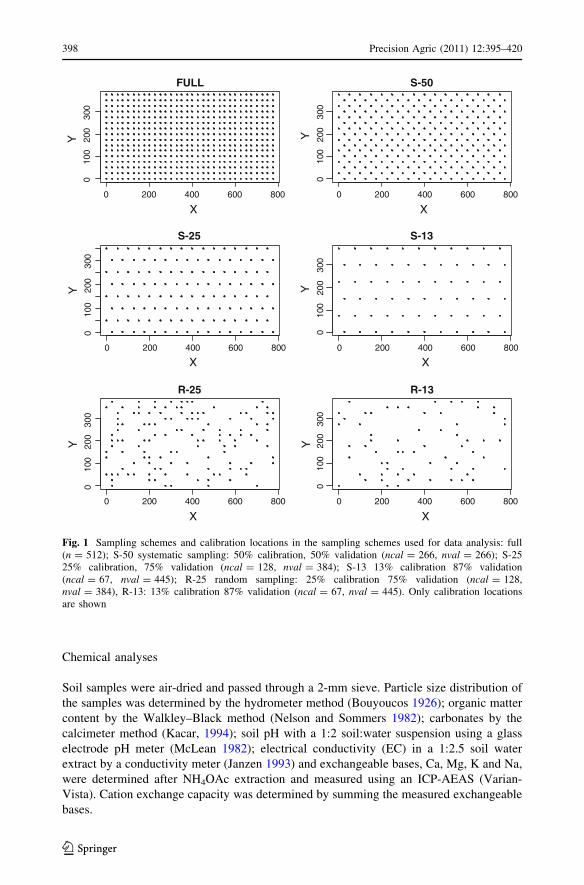
divided into 25 9 25 m grid squares (Fig. 1). A total of 512 soil samples (16 9 32) were
taken in 2000 from the midpoint of each square and from a depth of 0–30 cm. The soil is
classified from north to south as Mollic Ustifluvent, Typic Ustifluvent and Typic
Ustorthent (Yıldız 1997). It is mainly fine-textured (clay loam), with small to moderate
amounts of organic matter (3.9–68.7 g kg-1) and moderate amounts of CaCO3 (25.7–
98.7 g kg-1).
Precision Agric (2011) 12:395–420 397
123
Chemical analyses
Soil samples were air-dried and passed through a 2-mm sieve. Particle size distribution of
the samples was determined by the hydrometer method (Bouyoucos 1926); organic matter
content by the Walkley–Black method (Nelson and Sommers 1982); carbonates by the
calcimeter method (Kacar, 1994); soil pH with a 1:2 soil:water suspension using a glass
electrode pH meter (McLean 1982); electrical conductivity (EC) in a 1:2.5 soil water
extract by a conductivity meter (Janzen 1993) and exchangeable bases, Ca, Mg, K and Na,
were determined after NH4OAc extraction and measured using an ICP-AEAS (Varian-
Vista). Cation exchange capacity was determined by summing the measured exchangeable
bases.
X
YFULL
X
Y
S-50
X
Y
S-25
X
Y
S-13
X
Y
R-25
0 200 400 600 800 0 200 400 600 800
0 200 400 600 800 0 200 400 600 800
0 200 400 600 800 0 200 400 600 800
010
020
030
0
010
020
030
0
010
020
030
0
010
020
030
0
010
020
030
0
010
020
030
0
X
Y
R-13
Fig. 1 Sampling schemes and calibration locations in the sampling schemes used for data analysis: full(n = 512); S-50 systematic sampling: 50% calibration, 50% validation (ncal = 266, nval = 266); S-2525% calibration, 75% validation (ncal = 128, nval = 384); S-13 13% calibration 87% validation(ncal = 67, nval = 445); R-25 random sampling: 25% calibration 75% validation (ncal = 128,nval = 384), R-13: 13% calibration 87% validation (ncal = 67, nval = 445). Only calibration locationsare shown
398 Precision Agric (2011) 12:395–420
123
Visible near infrared reflectance spectroscopy (VNIRRS)
Soil samples were scanned and their absolute reflectance was recorded from 350 to
2500 nm at a 1-nm resolution resulting in 2150 data points per spectrum using a FieldSpec
Pro hyperspectral sensor (Analytical Spectral Devices, Inc., Boulder, Colorado: ASD
1997). Air-dried soil samples were put into 4 cm diameter optical quality petri dishes and
reflectance was recorded through the glass bottom at a constant angle (55� from horizontal)
and distance of 4 cm from the fiber optic sensor cable using a tungsten quartz halogen
lamp light source (Muglight sensor attachment; http://www.asdi.com/products-
accessories-hisp.asp). After five consecutive readings, averaged from ten sequential spec-
tra, the sample was rotated 90� and five additional readings were recorded. The accuracy and
detector response were calibrated using standards (white spectralon, soil sample and kao-
linite). If the white spectralon reading was not stable, the instrument was reset.
Data processing
Reflectance data were translated from binary to ASCII and exported in batches, using
Analytical Spectral Devices ViewspecPro software. Ten readings obtained at two different
positions per sample were averaged using Splus 8.0 (Insightful Corp., WA) to obtain a
master data set with one reflectance spectrum per soil sample. Spectral data were trans-
formed with first derivative processing using the Savitsky-Golay transformation procedure
(Savitzky and Golay 1964) to remove signal noise unrelated to physico-chemical properties
of the soil. This uses the mathematical treatment of 1 4 1 2, which refers to the order of
derivative, first smoothing, second smoothing and order of polynomial, respectively, in
Unscrambler�8.05 (CAMO Process, Oslo, Norway 2003). The first derivative spectra
generally amplify the absorption features that indicate the composition of the soil mate-
rials. It is also known to reduce variation among samples (Martens and Naes 1989).
Sampling schemes
The performance of estimation methods was tested using two general approaches: cross-
validation and separate calibration–validation data sets (Fig. 2). For the latter, different
sample sizes were selected by systematic sampling, using 50, 25 and 13% of the full sample
set for calibration and the remaining 50, 75 and 87%, respectively, for validation. Two
additional calibration sets were established by randomly selecting 25 and 13% of the full
sample with the remaining 75 and 87%, respectively, for validation. For the random sam-
pling, five different randomly selected calibration and validation sets were created and the
results of those sets were averaged; this was done to avoid artifacts of clustering or outliers
that might originate because of the nature of random sampling, as was suggested by Bishop
and McBratney (2001). All estimates were compared with the remaining actual observations.
VNIRRS modeling
Calibrations between soil reflectance and soil properties were done using partial least
squares regression (PLSR) analysis, which is a method for relating two data matrices, Xand Y, by a linear multivariate model and is widely used in VNIR reflectance spectroscopy.
The PLSR decomposes both X and Y variables and finds new components or latent vari-
ables, which are both orthogonal and weighted linear combinations of the X variables. The
new X variables are then used for predicting the Y variables; in this study X is soil
Precision Agric (2011) 12:395–420 399
123
reflectance and Y is a soil property. Unlike multiple linear regression (MLR), PLSR can
handle data with strong collinearity in the independent (X) variables, which may also be
more numerous than the observations (Y). The X and Y variables are centered by sub-
tracting column averages from each observation before analysis. In PLSR, selection of the
number of latent variables is critical to prevent over- or under-fitting the data, which would
create models with poor prediction capability. Proper fitting was achieved with cross-
validation where the models were constructed each time by leaving some samples out of
the calibration data set for use in the validation process until all samples or groups were
tested. The PLSR was performed with Unscrambler�V.8.0.5.
Geostatistical analyses
Ordinary kriging (OK) is a commonly-used linear method of spatial prediction to provide
estimates of variables at unvisited sites. The procedure uses information from neighboring
points to predict at a target point; weights are assigned to these points based on their
distance from the target. The equation for ordinary punctual kriging is
Z�OKðx0Þ ¼Xn
i¼1
wizðxiÞ; ð1Þ
where Z�OKðx0Þ is the OK estimate at an unsampled location (x0), n is the number of
samples in the search neighborhood, wi are the weights assigned to the ith observation z(xi).
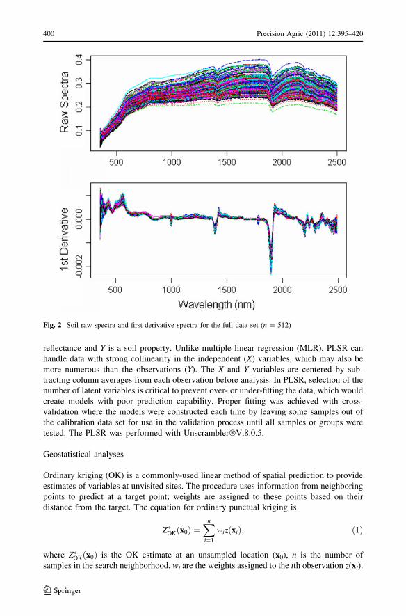
Fig. 2 Soil raw spectra and first derivative spectra for the full data set (n = 512)
400 Precision Agric (2011) 12:395–420
123
Weights are assigned to each sample such that the estimation or kriging variance,
E½fZ�ðx0Þ � Zðx0Þg2�, is minimized and the estimates are unbiased (Webster and Oliver
2007). The weights depend on the relative positions of the samples in the neighborhood
both to one another and to the target point, and on the variogram. The latter describes the
spatial correlation and covariance structure between data points for each variable. The
variogram can be computed by Matheron’s (1965) usual method of moments as follows
cðhÞ ¼ 1
2mðhÞXmðhÞ
i¼1
zðxi þ hÞ � zðxiÞ½ �2; ð2Þ
where cðhÞis the semivariance between two observation points, z(xi) and z(xi ? h), sep-
arated by a distance h, and m(h) is the number of pairs at h.
Cokriging
Cokriging (COK) is an extension of ordinary kriging and uses one or more secondary
variables, or covariables, (Z2) which are spatially correlated with the primary variable (Z1).
The equation for COK is given by
Z�COKðx0Þ ¼Xn1
i¼1
wiz1ðxiÞ þXn2
j¼1
wjz2ðxjÞ; ð3Þ
where Z�COKðx0Þ is the cokriging estimate at an unsampled location (x0), wi and wj are
cokriging weights associated with the primary variable z1(xi) and the secondary variable
z2(xj) at ith and jth locations, respectively, which are based on the cross-variogram
cðhÞ ¼ 1
2mðhÞXmðhÞ
i¼1
z1ðxi þ hÞ � z1ðxiÞ½ � z2ðxj þ hÞ � z2ðxjÞ� �
: ð4Þ
Cross-variograms were fitted using the linear model of coregionalization (LMC) which
ensures that the two auto-variograms for the primary variables and one cross-variogram for
the covariable have the same range and spatial structure (e.g. spherical or exponential
function). The LMCR ensures that the co-kriging system is positive-definite (i.e. all pos-
sible combinations of random variables have a positive variance), which is a prerequisite
for cokriging (Goovaerts 1997).
In this study, the primary variables (Z;Z1) were the laboratory measurements at the
calibration locations. The covariables (Z2) were the estimates from VNIRRS-PLSR at the
validation points (Fig. 2); there were 512 validation points for each soil property. Cokri-
ging was applied to all the sample schemes except for the first, which consisted of all
observation points.
Regression kriging
Regression kriging (RK) is another method of spatial prediction that uses secondary var-
iable(s) to improve the predictions of the primary variable at unsampled locations.
Regression kriging combines regression between the primary (target) variable and sec-
ondary variable(s) by kriging residuals derived from the regression (Hengl et al. 2007)
Precision Agric (2011) 12:395–420 401
123
Z�RKðx0Þ ¼Xp
k¼0
bk:qkðx0ÞþXn
i¼1
wi:eðxiÞ; ð5Þ
where ZRKðx0Þ is the RK estimate at unsampled locations (x0), bk and e(xi) are the
regression coefficients and residuals, respectively, obtained from the regression between
the primary and secondary variables (laboratory observations) at the sampling locations
(xi), wi are kriging weights determined from the variogram of residuals, qk (x0) are the
values of secondary variables at the target locations, which are VNIRRS-PLSR estimates
in our case, and p is the number of predictor (secondary) variables.
Regression coefficients and residuals were obtained by ordinary least square (OLS)
regression and simple kriging was used to krige the residuals (Hengl et al. 2007). The
secondary variables were selected by stepwise regression analysis. Clay, sand and silt
contents were not included in the stepwise regression for the prediction of each other, and
similarly CEC and exchangeable cations were excluded, because of inherent collinearity.
Accuracy of prediction
The prediction techniques were evaluated using the coefficient of determination (R2) and
the root mean square error of prediction (RMSEP) between measured and predicted values
of samples in the validation data set. The RMSEP is given by
RMSEP ¼
ffiffiffiffiffiffiffiffiffiffiffiffiffiffiffiffiffiffiffiffiffiffiffiffiffiffiffiffiffiffiffiffiffiffiffiffiffiffiffiffiffiffiffiffiffiffiffiffiffiffiffiffiffiffiPNi¼1 ðYpredicted � YobservedÞ2
n� 1
s
ð6Þ
The performance of RK and COK over the other two methods was assessed by per-
centage relative improvement (RI) as adapted by Mueller et al. (2001):
RI ¼ 100% � RMSEPkriging
� �� RMSEPcokriging
� ��RMSEPkriging
� �ð7Þ
where RI is the percentage improvement or reduction in the estimation errors, (positive RI
indicates improvement and negative RI a reduction in accuracy).
Ordinary kriging, COK and RK were performed with the R 2.4.1 programming lan-
guage software (R Development Core Team 2006). Common logarithmic transformation
was applied to variables with skewness coefficients [1 or \–1 (Kerry and Oliver 2007).
For both VNIRRS and variogram model fitting, the best model was selected by cross-
validation in which each sample in the data set is discarded once and the remaining
samples were used to estimate it (Warrick et al. 1986). The best model was the one giving
the smallest RMSEP from cross-validation.
Results and discussion
Soil properties
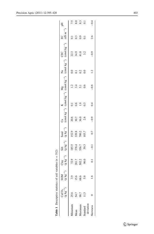
The soil variables EC, pH and Na have small ranges of values (Table 1). Soil EC has the
largest skewness followed by SOM and exchangeable Na. The correlations among the soil
variables are statistically significant (Table 2). Clay and SOM contents are moderately to
strongly correlated with almost all soil variables except for silt and Na. Other important
402 Precision Agric (2011) 12:395–420
123
Ta
ble
1D
escr
ipti
ve
stat
isti
csof
soil
var
iable
s(n
=5
12
)
CaC
O3
(gk
g-
1)
SO
M(g
kg
-1)
Cla
y(g
kg
-1)
Sil
t(g
kg
-1)
San
d(g
kg
-1)
Ca
(cm
ol
kg
-1)
K (cm
ol
kg
-1)
Mg
(cm
ol
kg
-1)
Na
(cm
ol
kg
-1)
CE
C(c
mo
lk
g-
1)
EC
(dS
m-
1)
pH
Min
um
um
25
.63
.97
2.9
18
5.5
15
2.9
20
.60
.11
.20
.02
2.3
0.1
7.5
Mea
n5
4.7
15
.62
81
.73
78
.43
39
.83
0.7
0.8
3.4
0.1
34
.90
.38
.0
Max
imu
m9
8.7
68
.65
02
.25
56
.77
00
.23
6.0
1.9
5.1
0.2
41
.00
.98
.3
Sta
nd
ard
dev
iati
on
11
.55
.89
6.0
59
.31
03
.72
.60
.30
.60
.03
.20
.10
.1
Sk
ewnes
s0
1.8
0.1
-0
.10
.7-
0.9
0.4
-0
.81
.2-
0.9
2.6
-0
.4
Precision Agric (2011) 12:395–420 403
123
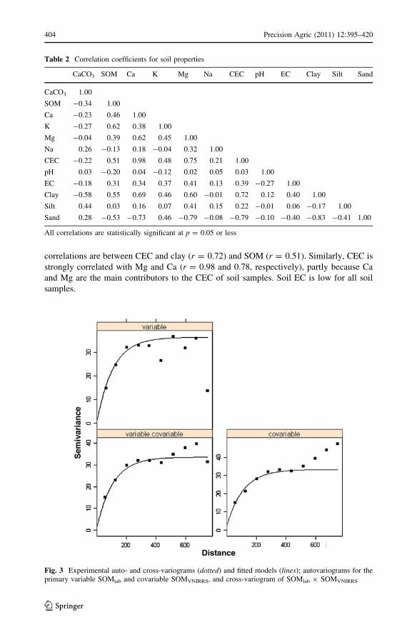
correlations are between CEC and clay (r = 0.72) and SOM (r = 0.51). Similarly, CEC is
strongly correlated with Mg and Ca (r = 0.98 and 0.78, respectively), partly because Ca
and Mg are the main contributors to the CEC of soil samples. Soil EC is low for all soil
samples.
Table 2 Correlation coefficients for soil properties
CaCO3 SOM Ca K Mg Na CEC pH EC Clay Silt Sand
CaCO3 1.00
SOM -0.34 1.00
Ca -0.23 0.46 1.00
K -0.27 0.62 0.38 1.00
Mg -0.04 0.39 0.62 0.45 1.00
Na 0.26 -0.13 0.18 -0.04 0.32 1.00
CEC -0.22 0.51 0.98 0.48 0.75 0.21 1.00
pH 0.03 -0.20 0.04 -0.12 0.02 0.05 0.03 1.00
EC -0.18 0.31 0.34 0.37 0.41 0.13 0.39 -0.27 1.00
Clay -0.58 0.55 0.69 0.46 0.60 -0.01 0.72 0.12 0.40 1.00
Silt 0.44 0.03 0.16 0.07 0.41 0.15 0.22 -0.01 0.06 -0.17 1.00
Sand 0.28 -0.53 -0.73 0.46 -0.79 -0.08 -0.79 -0.10 -0.40 -0.83 -0.41 1.00
All correlations are statistically significant at p = 0.05 or less
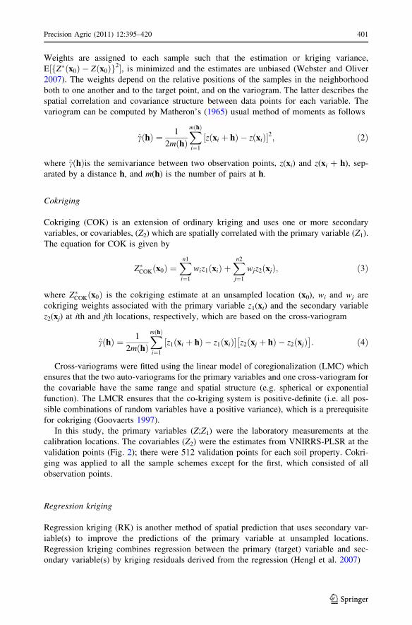
Fig. 3 Experimental auto- and cross-variograms (dotted) and fitted models (lines); autovariograms for theprimary variable SOMlab and covariable SOMVNIRRS, and cross-variogram of SOMlab 9 SOMVNIRRS
404 Precision Agric (2011) 12:395–420
123
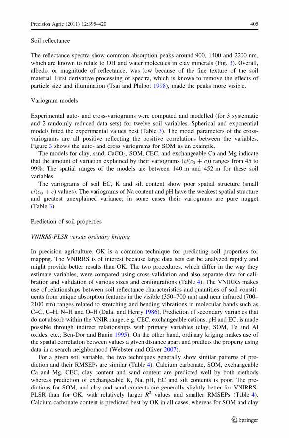
Soil reflectance
The reflectance spectra show common absorption peaks around 900, 1400 and 2200 nm,
which are known to relate to OH and water molecules in clay minerals (Fig. 3). Overall,
albedo, or magnitude of reflectance, was low because of the fine texture of the soil
material. First derivative processing of spectra, which is known to remove the effects of
particle size and illumination (Tsai and Philpot 1998), made the peaks more visible.
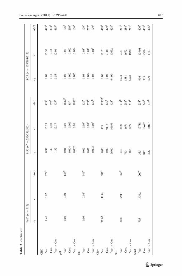
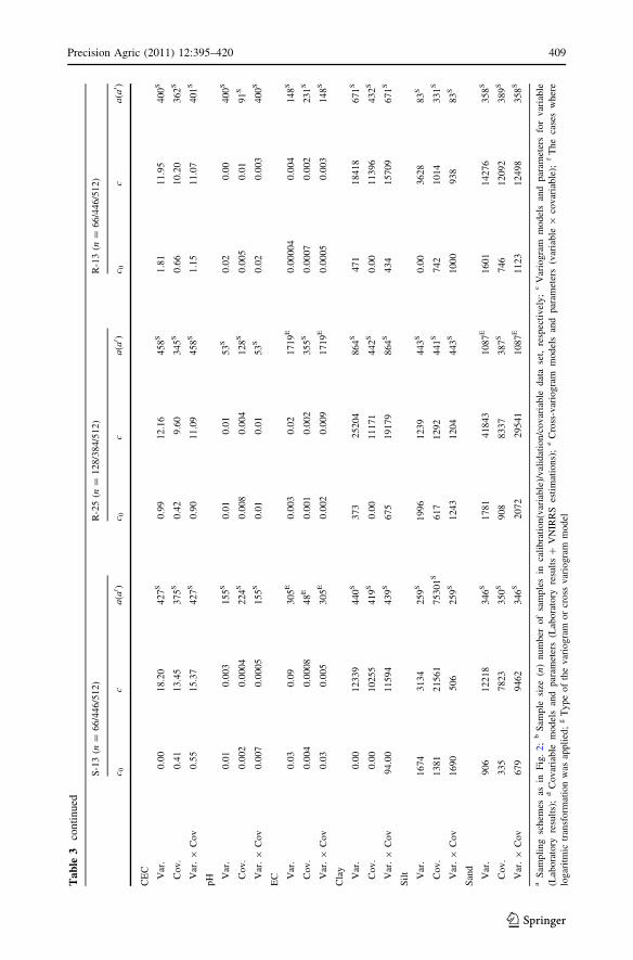
Variogram models
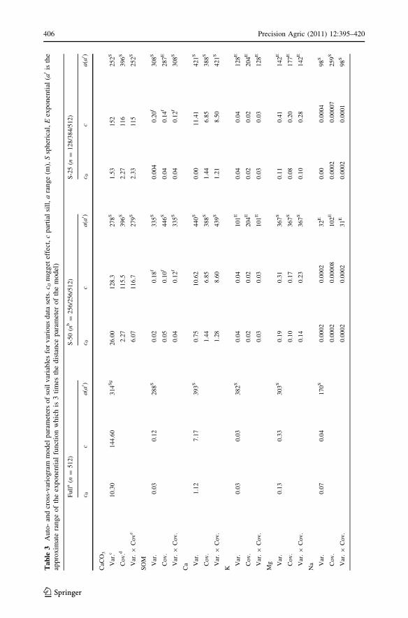
Experimental auto- and cross-variograms were computed and modelled (for 3 systematic
and 2 randomly reduced data sets) for twelve soil variables. Spherical and exponential
models fitted the experimental values best (Table 3). The model parameters of the cross-
variograms are all positive reflecting the positive correlations between the variables.
Figure 3 shows the auto- and cross variograms for SOM as an example.
The models for clay, sand, CaCO3, SOM, CEC, and exchangeable Ca and Mg indicate
that the amount of variation explained by their variograms (c/(c0 ? c)) ranges from 45 to
99%. The spatial ranges of the models are between 140 m and 452 m for these soil
variables.
The variograms of soil EC, K and silt content show poor spatial structure (small
c/(c0 ? c) values). The variograms of Na content and pH have the weakest spatial structure
and greatest unexplained variance; in some cases their variograms are pure nugget
(Table 3).
Prediction of soil properties
VNIRRS-PLSR versus ordinary kriging
In precision agriculture, OK is a common technique for predicting soil properties for
mappng. The VNIRRS is of interest because large data sets can be analyzed rapidly and
might provide better results than OK. The two procedures, which differ in the way they
estimate variables, were compared using cross-validation and also separate data for cali-
bration and validation of various sizes and configurations (Table 4). The VNIRRS makes
use of relationships between soil reflectance characteristics and quantities of soil constit-
uents from unique absorption features in the visible (350–700 nm) and near infrared (700–
2100 nm) ranges related to stretching and bending vibrations in molecular bands such as
C–C, C–H, N–H and O–H (Dalal and Henry 1986). Prediction of secondary variables that
do not absorb within the VNIR range, e.g. CEC, exchangeable cations, pH and EC, is made
possible through indirect relationships with primary variables (clay, SOM, Fe and Al
oxides, etc.; Ben-Dor and Banin 1995). On the other hand, ordinary kriging makes use of
the spatial correlation between values a given distance apart and predicts the property using
data in a search neighborhood (Webster and Oliver 2007).
For a given soil variable, the two techniques generally show similar patterns of pre-
diction and their RMSEPs are similar (Table 4). Calcium carbonate, SOM, exchangeable
Ca and Mg, CEC, clay content and sand content are predicted well by both methods
whereas prediction of exchangeable K, Na, pH, EC and silt contents is poor. The pre-
dictions for SOM, and clay and sand contents are generally slightly better for VNIRRS-
PLSR than for OK, with relatively larger R2 values and smaller RMSEPs (Table 4).
Calcium carbonate content is predicted best by OK in all cases, whereas for SOM and clay
Precision Agric (2011) 12:395–420 405
123
Ta
ble
3A
uto
-an
dcr
oss
-var
iog
ram
mod
elp
aram
eter
so
fso
ilv
aria
ble
sfo
rv
ario
us
dat
ase
ts.
c 0n
ug
get
effe
ct,
cp
arti
alsi
ll,
ara
ng
e(m
),S
sph
eric
al,
Eex
po
nen
tial
(a0
isth
eap
pro
xim
ate
range
of
the
exponen
tial
funct
ion
whic
his
3ti
mes
the
dis
tance
par
amet
ero
fth
em
odel
)
Full
a(n
=512)
S-5
0(n
b=
256/2
56/5
12)
S-2
5(n
=128/3
84/5
12)
c 0c
a(a0 )
c 0c
a(a0 )
c 0c
a(a0 )
CaC
O3
Var
.c10.3
0144.6
0314
Sg
26.0
0128.3
278
S1.5
3152
252
S
Cov.d
2.2
7115.5
396
S2.2
7116
396
S
Var
.9
Cov
e6.0
7116.7
279
S2.3
3115
252
S
SO
M
Var
.0.0
30.1
2288
S0.0
20.1
8f
335
S0.0
04
0.2
0f
308
S
Cov.
0.0
50.1
0f
446
S0.0
40.1
4f
287
E
Var
.9
Cov.
0.0
40.1
2f
335
S0.0
40.1
2f
308
S
Ca V
ar.
1.1
27.1
7393
S0.7
510.6
2440
S0.0
011.4
1421
S
Cov.
1.4
46.8
5388
S1.4
46.8
5388
S
Var
.9
Cov.
1.2
88.6
0439
S1.2
18.5
0421
S
K
Var
.0.0
30.0
3382
S0.0
40.0
4101
E0.0
40.0
4128
E
Cov.
0.0
20.0
2204
E0.0
20.0
2204
E
Var
.9
Cov.
0.0
30.0
3101
E0.0
30.0
3128
E
Mg Var
.0.1
30.3
3303
S0.1
90.3
1367
S0.1
10.4
1142
E
Cov.
0.1
00.1
7367
S0.0
80.2
0177
E
Var
.9
Cov.
0.1
40.2
3367
S0.1
00.2
8142
E
Na V
ar.
0.0
70.0
4170
S0.0
002
0.0
002
32
E0.0
00.0
004
98
S
Cov.
0.0
002
0.0
0008
102
E0.0
002
0.0
0007
259
S
Var
.9
Cov.
0.0
002
0.0
002
31
E0.0
002
0.0
001
98
S
406 Precision Agric (2011) 12:395–420
123
Ta
ble
3co
nti
nu
ed
Full
a(n
=512)
S-5
0(n
b=
256/2
56/5
12)
S-2
5(n
=128/3
84/5
12)
c 0c
a(a0 )
c 0c
a(a0 )
c 0c
a(a0 )
CE
C
Var
.1.4
010.6
2379
S0.9
715.2
3427
S0.0
016.3
0415
S
Cov.
1.4
09.4
0393
S0.4
19.3
8394
S
Var
.9
Cov
1.3
212.1
7427
S0.5
512.0
6415
S
pH V
ar.
0.0
20.0
0136
S0.0
10.0
11812
E0.0
10.0
1106
S
Cov.
0.0
04
0.0
03
85
E0.0
02
0.0
02
210
S
Var
.9
Cov
0.0
07
0.0
11812
E0.0
07
0.0
04
106
S
EC V
ar.
0.0
30.0
4f
346
E0.0
20.0
5f
129
E0.0
30.0
5f
129
E
Cov.
0.0
20.0
3f
277
E0.0
04
0.0
3f
277
S
Var
.9
Cov
0.0
02
0.0
0f
129
E0.0
30.0
4f
129
E
Cla
y
Var
.77.6
211184
387
S0.0
0429
12137
S0.0
012131
428
S
Cov.
0.0
09115
429
S0.0
09118
429
S
Var
.9
Cov
76.0
010695
428
S94.0
010692
428
S
Sil
t Var
.2033
1794
366
S1740
2431
211
E1674
2431
211
E
Cov.
763
1671
284
E1381
1672
284
S
Var
.9
Cov
1186
1929
211
E1690
1929
211
E
San
d
Var
.705
14362
200
E355
17788
233
E906
13966
406
S
Cov.
842
10692
248
E335
8356
405
S
Var
.9
Cov
496
14077
233
E679
1103
406
S
Precision Agric (2011) 12:395–420 407
123

Ta
ble
3co
nti
nu
ed
S-1
3(n
=66/4
46/5
12)
R-2
5(n
=128/3
84/5
12)
R-1
3(n
=66/4
46/5
12)
c 0c
a(a0 )
c 0c
a(a0 )
c 0c
a(a0 )
CaC
O3
Var
.c0.0
0153.0
0352
S13.6
0159.0
0341
S9.2
0152.0
0323
S
Cov.d
0.0
0103.0
0457
S0.0
01.1
8400
S0.0
00.9
6413
S
Var
.9
Cov
e1.2
0116.7
0352
S0.0
31.3
3341
S0.0
30.8
7323
S
SO
M
Var
.0.0
028.7
0210
E0.0
50.1
3f
385
S2.0
033.0
5110
E
Cov.
10.4
018.5
9193
S0.0
50.1
0f
386
S7.8
832.3
9220
E
Var
.9
Cov.
6.7
916.4
1210
S0.0
50.1
2f
385
S1.4
132.1
5110
E
Ca V
ar.
0.0
012.6
0441
S0.7
08.0
7417
S1.8
48.2
7532
S
Cov.
0.2
79.7
73.8
S0.2
36.7
7350
S0.4
77.0
9348
S
Var
.9
Cov.
0.4
011.0
2441
S0.5
57.4
7417
S1.2
08.1
5532
S
K
Var
.0.0
30.0
5511
S0.0
30.0
5353
S0.0
50.0
2320
S
Cov.
0.0
40.0
07
199
S0.0
20.0
2376
S0.0
20.0
8539
E
Var
.9
Cov.
0.0
40.0
1511
S0.0
30.0
3353
S0.0
30.0
3320
S
Mg Var
.0.0
04
0.5
0276
S0.1
10.3
7335
S0.1
00.4
2153
S
Cov.
0.1
80.0
7273
S0.0
80.2
2352
S0.0
80.2
7364
S
Var
.9
Cov.
0.1
50.1
3276
S0.1
20.2
4335
S0.0
80.2
6153
S
Na V
ar.
0.0
00.0
005
185
S0.0
0009
0.0
003
63
S0.0
004
0.0
0002
320
S
Cov.
0.0
0004
0.0
001
250
S0.0
001
0.0
0004
168
S0.0
0004
0.0
0007
350
E
Var
.9
Cov.
0.0
0008
0.0
002
185
S0.0
004
0.0
007
62
S0.0
002
0.0
0004
320
S
408 Precision Agric (2011) 12:395–420
123
Ta
ble
3co
nti
nu
ed
S-1
3(n
=66/4
46/5
12)
R-2
5(n
=128/3
84/5
12)
R-1
3(n
=66/4
46/5
12)
c 0c
a(a0 )
c 0c
a(a0 )
c 0c
a(a0 )
CE
C
Var
.0.0
018.2
0427
S0.9
912.1
6458
S1.8
111.9
5400
S
Cov.
0.4
113.4
5375
S0.4
29.6
0345
S0.6
610.2
0362
S
Var
.9
Cov
0.5
515.3
7427
S0.9
011.0
9458
S1.1
511.0
7401
S
pH V
ar.
0.0
10.0
03
155
S0.0
10.0
153
S0.0
20.0
0400
S
Cov.
0.0
02
0.0
004
224
S0.0
08
0.0
04
128
S0.0
05
0.0
191
S
Var
.9
Cov
0.0
07
0.0
005
155
S0.0
10.0
153
S0.0
20.0
03
400
S
EC V
ar.
0.0
30.0
9305
E0.0
03
0.0
21719
E0.0
0004
0.0
04
148
S
Cov.
0.0
04
0.0
008
48
E0.0
01
0.0
02
355
S0.0
007
0.0
02
231
S
Var
.9
Cov
0.0
30.0
05
305
E0.0
02
0.0
09
1719
E0.0
005
0.0
03
148
S
Cla
y
Var
.0.0
012339
440
S373
25204
864
S471
18418
671
S
Cov.
0.0
010255
419
S0.0
011171
442
S0.0
011396
432
S
Var
.9
Cov
94.0
011594
439
S675
19179
864
S434
15709
671
S
Sil
t Var
.1674
3134
259
S1996
1239
443
S0.0
03628
83
S
Cov.
1381
21561
75301
S617
1292
441
S742
1014
331
S
Var
.9
Cov
1690
506
259
S1243
1204
443
S1000
938
83
S
San
d
Var
.906
12218
346
S1781
41843
1087
E1601
14276
358
S
Cov.
335
7823
350
S908
8337
387
S746
12092
389
S
Var
.9
Cov
679
9462
346
S2072
29541
1087
E1123
12498
358
S
aS
ampli
ng
schem
esas
inF
ig.
2;
bS
ample
size
(n)
num
ber
of
sam
ple
sin
cali
bra
tion(v
aria
ble
)/val
idat
ion/c
ovar
iable
dat
ase
t,re
spec
tivel
y;
cV
ario
gra
mm
odel
san
dpar
amet
ers
for
var
iable
(Lab
ora
tory
resu
lts)
;d
Covar
iable
model
san
dpar
amet
ers
(Lab
ora
tory
resu
lts
?V
NIR
RS
esti
mat
ions)
;e
Cro
ss-v
ario
gra
mm
odel
san
dpar
amet
ers
(var
iable
9co
var
iable
);f
The
case
sw
her
e
logar
itm
ictr
ansf
orm
atio
nw
asap
pli
ed;
gT
ype
of
the
var
iogra
mor
cross
var
iogra
mm
odel
Precision Agric (2011) 12:395–420 409
123
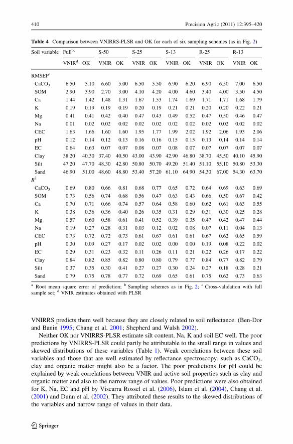
VNIRRS predicts them well because they are closely related to soil reflectance. (Ben-Dor
and Banin 1995; Chang et al. 2001; Shepherd and Walsh 2002).
Neither OK nor VNIRRS-PLSR estimate silt content, Na, K and soil EC well. The poor
predictions by VNIRRS-PLSR could partly be attributable to the small range in values and
skewed distributions of these variables (Table 1). Weak correlations between these soil
variables and those that are well estimated by reflectance spectroscopy, such as CaCO3,
clay and organic matter might also be a factor. The poor predictions for pH could be
explained by weak correlations between VNIR and active soil properties such as clay and
organic matter and also to the narrow range of values. Poor predictions were also obtained
for K, Na, EC and pH by Viscarra Rossel et al. (2006), Islam et al. (2004), Chang et al.
(2001) and Dunn et al. (2002). They attributed these results to the skewed distributions of
the variables and narrow range of values in their data.
Table 4 Comparison between VNIRRS-PLSR and OK for each of six sampling schemes (as in Fig. 2)
Soil variable Fullbc S-50 S-25 S-13 R-25 R-13
VNIRd OK VNIR OK VNIR OK VNIR OK VNIR OK VNIR OK
RMSEPa
CaCO3 6.50 5.10 6.60 5.00 6.50 5.50 6.90 6.20 6.90 6.50 7.00 6.50
SOM 2.90 3.90 2.70 3.00 4.10 4.20 4.00 4.60 3.40 4.00 3.50 4.50
Ca 1.44 1.42 1.48 1.31 1.67 1.53 1.74 1.69 1.71 1.71 1.68 1.79
K 0.19 0.19 0.19 0.19 0.20 0.19 0.21 0.21 0.20 0.20 0.22 0.21
Mg 0.41 0.41 0.42 0.40 0.47 0.43 0.49 0.52 0.47 0.50 0.46 0.47
Na 0.01 0.02 0.02 0.02 0.02 0.02 0.02 0.02 0.02 0.02 0.02 0.02
CEC 1.63 1.66 1.60 1.60 1.95 1.77 1.99 2.02 1.92 2.06 1.93 2.06
pH 0.12 0.14 0.12 0.13 0.16 0.16 0.15 0.15 0.13 0.14 0.14 0.14
EC 0.64 0.63 0.07 0.07 0.08 0.07 0.08 0.07 0.07 0.07 0.07 0.07
Clay 38.20 40.30 37.40 40.50 43.00 43.90 42.90 46.80 38.70 45.50 40.10 45.90
Silt 47.20 47.70 48.30 42.80 50.80 50.70 49.20 51.40 51.10 55.10 50.80 53.30
Sand 46.90 51.00 48.60 48.80 53.40 57.20 61.10 64.90 54.30 67.00 54.30 63.70
R2
CaCO3 0.69 0.80 0.66 0.81 0.68 0.77 0.65 0.72 0.64 0.69 0.63 0.69
SOM 0.73 0.56 0.74 0.68 0.56 0.47 0.63 0.43 0.66 0.50 0.67 0.42
Ca 0.70 0.71 0.66 0.74 0.57 0.64 0.58 0.60 0.62 0.61 0.63 0.55
K 0.38 0.36 0.36 0.40 0.26 0.35 0.31 0.29 0.31 0.30 0.25 0.28
Mg 0.57 0.60 0.58 0.61 0.41 0.52 0.39 0.35 0.47 0.42 0.47 0.44
Na 0.19 0.27 0.28 0.31 0.03 0.12 0.02 0.08 0.07 0.11 0.04 0.13
CEC 0.73 0.72 0.72 0.73 0.61 0.67 0.61 0.61 0.67 0.62 0.65 0.59
pH 0.30 0.09 0.27 0.17 0.02 0.02 0.00 0.00 0.19 0.08 0.22 0.02
EC 0.29 0.31 0.23 0.32 0.11 0.26 0.11 0.21 0.22 0.26 0.17 0.22
Clay 0.84 0.82 0.85 0.82 0.80 0.80 0.79 0.77 0.84 0.77 0.82 0.79
Silt 0.37 0.35 0.30 0.41 0.27 0.27 0.30 0.24 0.27 0.18 0.28 0.21
Sand 0.79 0.75 0.78 0.77 0.72 0.69 0.65 0.61 0.75 0.62 0.73 0.63
a Root mean square error of prediction; b Sampling schemes as in Fig. 2; c Cross-validation with fullsample set; d VNIR estimates obtained with PLSR
410 Precision Agric (2011) 12:395–420
123
Silt content, Na, K, EC and pH are also poorly estimated by OK in general (Table 4).
The quality of OK estimates depends mostly on the degree of variation resolved, which is
characterized by the variogram. Table 3 gives the variogram model parameters of soil
variables for the full and sub-sampled data sets. The poor results from OK for pH, Na, K
and EC relate to the weak spatial structure (small c/(c0 ? c)) of these variables (Mueller
et al. 2001; Kravchenko 2003).
In general, the results for VNIRRS-PLSR and OK are comparable; they can both
estimate soil properties cost-effectively and reduce the number of samples to be analyzed
in the laboratory. However, each has shortcomings. Ordinary kriging is a local method of
prediction based on spatial dependence between sampling points, whereas VNIRRS can
predict globally over larger areas. Accurate prediction by VNIRRS requires the soil
variables to have a wide range of values and strong correlations with those variables that
have direct relationships with soil reflectance spectra.
Cokriging
For COK, the VNIRRS-PLSR predictions at the validation sites were used together with
the systematically and randomly sampled laboratory observations at the calibration loca-
tions to predict at unsampled locations. Cokriged estimates were compared with those
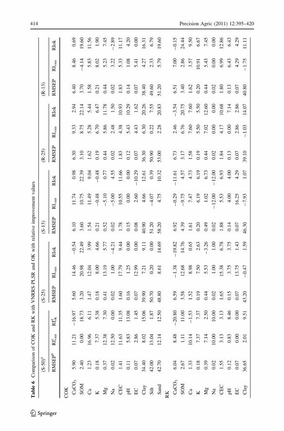
obtained by VNIRRS-PLSR and OK. The errors of prediction (RMSEP) for COK are
smaller and the correlation coefficients between the observations and estimates are larger
than for the other methods (Table 6). Relative improvement values, RIOK and RIVNIRRS,
were computed to evaluate the performance of COK over OK and VNIRRS-PLSR,
respectively (Table 6). Overall, RI values are positive indicating that combining VNIRRS-
PLSR estimates and soil data in cokriging improves the accuracy of prediction, except for
K, Na, pH, EC and silt content, which are poorly estimated by both methods, and CaCO3.
Predictions of SOM, sand, clay and CEC by COK show improvements of up to 22%, 21%,
20% and 11%, respectively, for the random sample subsets with only 25% and 13% of the
full data. Zhang et al. (1992) suggested that they obtained up to 33% improvement for
particle size distributions when using soil reflectance data as an auxiliary variable.
Gains related to the use of COK vary depending on the predictive power of the
covariables that were estimated by VNIRRS-PLSR (Table 6). In cases where those esti-
mates are better than those by OK, RIOK is larger than RIVNIRRS and vice versa. Better
prediction is possible with COK if the covariables are moderately to strongly correlated
with the main variable. If estimates by VNIRRS are accurate, then so are those from COK.
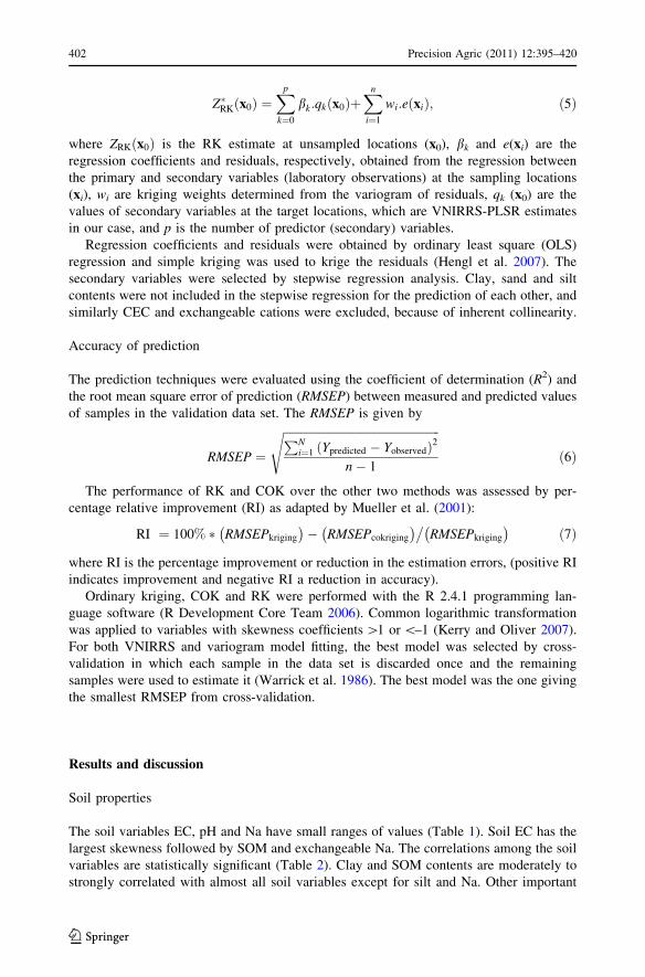
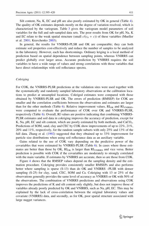
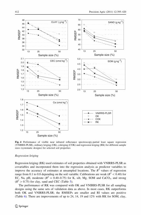
Figure 4 shows that the RMSEP values depend on the sampling density and the esti-
mation procedure. Cokriging provides consistently smaller RMSEPs and also performs
better where sampling is sparse (S-13) than do OK and VNIRRS –PLSR with denser
sampling (S-25) for clay, sand, CEC, SOM and Ca. Cokriging with 13 or 25% of the
observations generally provides the same level of accuracy as VNIRRS or OK with 50% of
the observations. The combination of VNIRRS predictions and observations using COK
improves the predictions of K and silt content only slightly, but does not improve those of
variables already poorly predicted by OK and VNIRRS, such as Na, pH, EC. This may be
explained by the lack of cross-correlation between the original laboratory values and
covariate (VNIRRS) data, and secondly, as for OK, poor spatial structure associated with
large nugget variances.
Precision Agric (2011) 12:395–420 411
123
Regression kriging
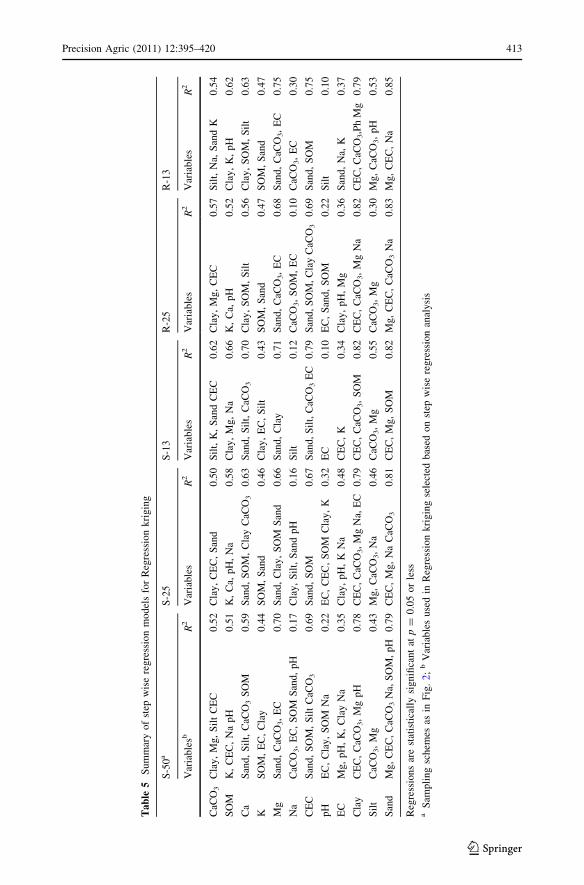
Regression kriging (RK) used estimates of soil properties obtained with VNIRRS-PLSR as
covariables and incorporated them into the regression analysis as predictor variables to
improve the accuracy of estimates at unsampled locations. The R2 values of regression
range from 0.1 to 0.8 depending on the soil variable. Calibrations are weak (R2 \ 0.40) for
EC, Na, pH, moderate (R2 = 0.40–0.75) for K, silt, Mg, SOM and CaCO3, and strong
(R2 [ 0.75) for clay, sand and CEC (Table 5).
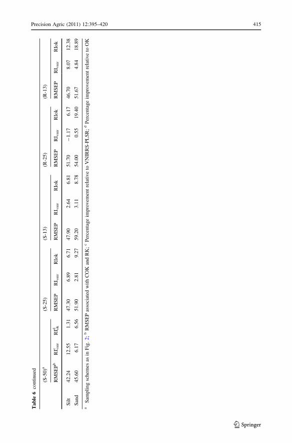
The performance of RK was compared with OK and VNIRRS-PLSR for all sampling
designs using the same sets of validation data as above. In most cases, RK outperforms
both OK and VNIRRS-PLSR; the RMSEPs are smaller and RI values are positive
(Table 6). There are improvements of up to 24, 14, 19 and 12% with RK for SOM, clay,
CLAY ( g kg-1)
Sample size (%)
RM
SE
P
32
34
36
38
40
42
44
46
48
VNIRRS-PLSROKCOKRK
SAND (g kg-1)
Sample size (%)13 25 50 13 25 50
RM
SE
P
40
45
50
55
60
65
70
CEC (cmol kg-1)
Sample size (%)
502513
RM
SE
P
1.3
1.4
1.5
1.6
1.7
1.8
1.9
2.0
2.1SOM (g kg-1)
Sample size (%)
502513
RM
SE
P
2.0
2.5
3.0
3.5
4.0
4.5
5.0
Ca (cmol kg-1)
Sample size (%)502531
RM
SE
P
1.2
1.3
1.4
1.5
1.6
1.7
1.8
Fig. 4 Performance of visible near infrared reflectance spectroscopy-partial least square regression(VNIRRS-PLSR), ordinary kriging (OK), cokriging (COK) and regression kriging (RK) for different samplesizes (systematic designs) for selected soil properties
412 Precision Agric (2011) 12:395–420
123
Tab
le5
Sum
mar
yof
step
wis
ere
gre
ssio
nm
odel
sfo
rR
egre
ssio
nkri
gin
g
S-5
0a
S-2
5S
-13
R-2
5R
-13
Var
iable
sbR
2V
aria
ble
sR
2V
aria
ble
sR
2V
aria
ble
sR
2V
aria
ble
sR
2
CaC
O3
Cla
y,
Mg
,S
ilt
CE
C0
.52
Cla
y,
CE
C,
San
d0
.50
Sil
t,K
,S
and
CE
C0
.62
Cla
y,
Mg
,C
EC
0.5
7S
ilt,
Na,
San
dK
0.5
4
SO
MK
,C
EC
,N
ap
H0
.51
K,
Ca,
pH
,N
a0
.58
Cla
y,
Mg
,N
a0
.66
K,
Ca,
pH
0.5
2C
lay
,K
,p
H0
.62
Ca
San
d,
Sil
t,C
aCO
3S
OM
0.5
9S
and,
SO
M,
Cla
yC
aCO
30
.63
San
d,
Sil
t,C
aCO
30
.70
Cla
y,
SO
M,
Sil
t0
.56
Cla
y,
SO
M,
Sil
t0
.63
KS
OM
,E
C,
Cla
y0
.44
SO
M,
San
d0
.46
Cla
y,
EC
,S
ilt
0.4
3S
OM
,S
and
0.4
7S
OM
,S
and
0.4
7
Mg
San
d,
CaC
O3,
EC
0.7
0S
and,
Cla
y,
SO
MS
and
0.6
6S
and,
Cla
y0
.71
San
d,
CaC
O3,
EC
0.6
8S
and
,C
aCO
3,
EC
0.7
5
Na
CaC
O3,
EC
,S
OM
San
d,
pH
0.1
7C
lay
,S
ilt,
San
dp
H0
.16
Sil
t0
.12
CaC
O3,
SO
M,
EC
0.1
0C
aCO
3,
EC
0.3
0
CE
CS
and
,S
OM
,S
ilt
CaC
O3
0.6
9S
and,
SO
M0
.67
San
d,
Sil
t,C
aCO
3E
C0
.79
San
d,
SO
M,
Cla
yC
aCO
30
.69
San
d,
SO
M0
.75
pH
EC
,C
lay
,S
OM
Na
0.2
2E
C,
CE
C,
SO
MC
lay
,K
0.3
2E
C0
.10
EC
,S
and,
SO
M0
.22
Sil
t0
.10
EC
Mg
,p
H,
K,
Cla
yN
a0
.35
Cla
y,
pH
,K
Na
0.4
8C
EC
,K
0.3
4C
lay
,p
H,
Mg
0.3
6S
and
,N
a,K
0.3
7
Cla
yC
EC
,C
aCO
3,
Mg
pH
0.7
8C
EC
,C
aCO
3,
Mg
Na,
EC
0.7
9C
EC
,C
aCO
3,
SO
M0
.82
CE
C,
CaC
O3,
Mg
Na
0.8
2C
EC
,C
aCO
3,P
hM
g0
.79
Sil
tC
aCO
3,
Mg
0.4
3M
g,
CaC
O3,
Na
0.4
6C
aCO
3,
Mg
0.5
5C
aCO
3,
Mg
0.3
0M
g,
CaC
O3,
pH
0.5
3
San
dM
g,
CE
C,
CaC
O3
Na,
SO
M,
pH
0.7
9C
EC
,M
g,
Na
CaC
O3
0.8
1C
EC
,M
g,
SO
M0
.82
Mg
,C
EC
,C
aCO
3N
a0
.83
Mg
,C
EC
,N
a0
.85
Reg
ress
ions
are
stat
isti
call
ysi
gnifi
cant
atp
=0
.05
or
less
aS
amp
lin
gsc
hem
esas
inF
ig.
2;
bV
aria
ble
suse
din
Reg
ress
ion
kri
gin
gse
lect
edbas
edon
step
wis
ere
gre
ssio
nan
alysi
s
Precision Agric (2011) 12:395–420 413
123
Ta
ble
6C
om
par
iso
no
fC
OK
and
RK
wit
hV
NR
RS
-PL
SR
and
OK
wit
hre
lati
ve
imp
rovem
ent
val
ues
(S-5
0)a
(S-2
5)
(S-1
3)
(R-2
5)
(R-1
3)
RM
SE
Pb
RI v
nir
cR
I ok
dR
MS
EP
RI v
nir
RIo
kR
MS
EP
RI v
nir
RIo
kR
MS
EP
RI v
nir
RIo
kR
MS
EP
RI v
nir
RIo
k
CO
K
CaC
O3
5.9
01
1.2
1-
16
.97
5.6
01
4.4
6-
0.5
46
.10
11
.74
0.9
86
.30
9.3
32
.94
6.4
08
.46
0.6
9
SO
M2
.40
0.0
01
8.7
33
.20
20
.98
22
.49
3.6
01
0.7
52
2.3
93
.10
8.7
52
2.1
43
.70
-4
.14
19
.60
Ca
1.2
31
6.9
66
.11
1.4
71
2.0
43
.99
1.5
41
1.4
99
.04
1.6
25
.28
5.4
41
.58
5.8
31
1.5
6
K0
.18
7.3
75
.38
0.1
88
.00
4.6
60
.21
-0
.48
-0
.48
0.1
96
.70
6.4
70
.21
8.0
21
.90
Mg
0.3
71
2.3
87
.30
0.4
11
3.1
95
.77
0.5
2-
5.1
00
.77
0.4
45
.86
11
.78
0.4
45
.23
7.4
5
Na
0.0
21
2.5
00
.00
0.0
21
.00
-4
.21
0.0
2-
5.0
04
.55
0.0
22
.48
1.5
00
.02
3.2
2-
2.8
9
CE
C1
.41
11
.63
11
.35
1.6
01
7.7
99
.44
1.7
81
0.5
51
1.6
61
.83
4.3
81
0.9
31
.83
5.3
31
1.1
7
pH
0.1
15
.83
13
.08
0.1
61
.25
0.0
00
.15
0.0
00
.00
0.1
25
.43
10
.29
0.1
41
.08
4.2
0
EC
0.0
72
.86
1.4
50
.07
12
.99
0.0
00
.08
2.6
0-
10
.29
0.0
74
.43
1.6
20
.07
5.4
10
.00
Cla
y3
4.4
08
.02
15
.06
39
.90
7.2
19
.11
40
.90
4.6
61
2.6
13
6.3
06
.30
20
.26
38
.40
4.2
71
6.3
1
Sil
t4
2.0
01
3.0
41
.87
50
.70
0.2
00
.00
51
.20
-4
.07
0.3
95
0.9
00
.22
7.5
54
9.6
02
.33
6.7
9
San
d4
2.7
01
2.1
41
2.5
04
8.8
08
.61
14
.69
58
.20
4.7
51
0.3
25
3.0
02
.28
20
.83
51
.20
5.7
91
9.6
0
RK C
aCO
36
.04
8.4
8-
20
.80
6.5
9-
1.3
8-
19
.82
6.9
2-
0.2
9-
11
.61
6.7
32
.46
-3
.54
6.5
17
.00
-0
.15
SO
M2
.67
1.1
11
1.0
03
.58
12
.68
14
.76
4.3
9-
9.7
54
.57
3.1
76
.76
20
.75
3.4
02
.86
24
.44
Ca
1.3
31
0.1
4-
1.5
31
.52
8.9
80
.65
1.6
17
.47
4.7
31
.58
7.6
07
.60
1.6
23
.57
9.5
0
K0
.18
7.3
77
.37
0.1
97
.50
2.6
30
.20
6.1
96
.19
0.1
95
.50
5.5
00
.20
10
.91
6.6
7
Mg
0.3
97
.14
2.5
00
.44
5.5
3-
3.2
60
.49
1.0
26
.73
0.4
47
.02
12
.60
0.4
45
.43
7.4
5
Na
0.0
21
0.0
01
0.0
00
.02
1.0
01
.00
0.0
2-
12
.00
-1
2.0
00
.02
0.0
00
.00
0.0
20
.00
0.0
0
CE
C1
.55
3.1
33
.13
1.6
51
5.3
86
.78
1.8
85
.53
6.9
31
.84
4.1
71
0.6
81
.80
6.9
91
2.8
6
pH
0.1
20
.83
8.4
60
.15
3.7
53
.75
0.1
44
.00
4.0
00
.13
0.0
07
.14
0.1
36
.43
6.4
3
EC
0.0
70
.00
0.0
00
.07
13
.75
1.4
30
.07
16
.25
4.2
90
.07
2.8
62
.86
0.0
74
.29
4.2
9
Cla
y3
6.6
52
.01
9.5
14
3.2
0-
0.4
71
.59
46
.30
-7
.93
1.0
73
9.1
0-
1.0
31
4.0
74
0.8
0-
1.7
51
1.1
1
414 Precision Agric (2011) 12:395–420
123
Ta
ble
6co
nti
nu
ed
(S-5
0)a
(S-2
5)
(S-1
3)
(R-2
5)
(R-1
3)
RM
SE
Pb
RI v
nir
cR
I ok
dR
MS
EP
RI v
nir
RIo
kR
MS
EP
RI v
nir
RIo
kR
MS
EP
RI v
nir
RIo
kR
MS
EP
RI v
nir
RIo
k
Sil
t4
2.2
41
2.5
51
.31
47
.30
6.8
96
.71
47
.90
2.6
46
.81
51
.70
-1
.17
6.1
74
6.7
08
.07
12
.38
San
d4
5.6
06
.17
6.5
65
1.9
02
.81
9.2
75
9.2
03
.11
8.7
85
4.0
00
.55
19
.40
51
.67
4.8
41
8.8
9
aS
amp
lin
gsc
hem
esas
inF
ig.
2;
bR
MS
EP
asso
ciat
edw
ith
CO
Kan
dR
K;
cP
erce
nta
ge
imp
rovem
ent
rela
tiv
eto
VN
IRR
S-P
LS
R;
dP
erce
nta
ge
imp
rovem
ent
rela
tiv
eto
OK
Precision Agric (2011) 12:395–420 415
123
sand and CEC. In some cases, the RI values are \10% and negative for Na, pH and EC
indicating that there is no improvement or advantage in using RK. These variables are also
poorly estimated by either OK or VNIRRS-PLSR (Table 4). The RIOK values for CaCO3
are always negative indicating that predictions by OK are more accurate than are those by
RK. As for COK, RK has not improved the accuracy of estimates of Na, pH and EC, and
only in a few cases does it provide slightly better estimates. Small and negative RI values
for Na, pH and EC probably reflect their poor correlations with secondary variables in the
data. Odeh et al. (2004) and Hengl et al. (2007) reported that the performance of RK is
affected by the strength of relationship between primary and secondary variables and
spatial dependence of the residuals. For some variables such as clay, however, there is little
improvement despite their strong correlations with auxiliary variables. The RIOK and
RIVNIR values for clay are small and negative for S-25 and S-13. Kravchenko and Rob-
ertsen (2007) also reported little to no improvement by RK relative to OK for estimates of
soil carbon using a secondary terrain variable because of the strong spatial correlation of
carbon. Similarly clay content in this study is strongly spatially dependent, and so OK was
sufficient to give accurate predictions as for CaCO3.
In most cases, the improvements with RK over VNIRRS-PLSR and OK are less than
with COK (Table 6). Odeh and McBratney (1995) reported smaller RMSEPs for estimates
of subsoil clay and topsoil gravel using terrain properties as covariable in the study where
they compared different cokriging and regression kriging methods.
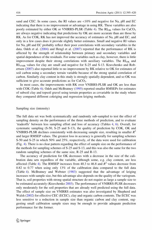
Sampling size (intensity)
The full data set was both systematically and randomly sub-sampled to test the effect of
sampling density on the performance of the three methods of prediction, and to evaluate
‘tradeoffs’ between less sampling effort and loss of accuracy (Tables 4, 6). Overall, for
systematic sampling (S-50, S-25 and S-13), the quality of prediction by COK, OK and
VNIRRS-PLSR declines consistently with decreasing sample size, resulting in smaller R2
and larger RMSEP values. The greatest loss in accuracy is generally for sampling schemes
S-50 and S-25 in which 50% and 25%, respectively, of the data were used for calibration
(Fig. 4). There is no clear pattern regarding the effect of sample size on the performance of
the methods for sampling schemes of S-25 and S-13, and this was also the same for the two
random sampling schemes of the same size, R-25 and R-13.
The accuracy of prediction for OK decreases with a decrease in the size of the cali-
bration data sets regardless of the variable, although some, e.g. clay content, are less
affected (Table 4). The RMSEP increases from 40.3 to 46.8 and R2 values decrease from
0.82 to 0.77 when using only 13% of the calibration data compared to the full data
(Table 4). McBratney and Webster (1983) suggested that the advantage of kriging
increases with sample size, but this advantage also depends on the quality of the variogram.
That is, soil properties with strong spatial structure do not require as large a sample size to
be estimated accurately (Kravchenko 2003). The performance of VNIRRS-PLSR decreases
only moderately for the soil properties that are already well predicted using the full data.
The effect of sample size on VNIRRS estimates was also investigated by Shepherd and
Walsh (2002) for effective CEC (ECEC), clay and organic carbon contents. The ECEC was
less sensitive to a reduction in sample size than organic carbon and clay content, sug-
gesting small calibration sample sizes may be enough to provide adequate prediction
performance for the former.
416 Precision Agric (2011) 12:395–420
123

Similarly, the accuracy of COK and RK predictions improves with sample size, and for
some soil properties the improvements are greater than for the other methods as was also
observed by Tarr et al. (2005).
Sampling scheme
In both systematic sampling and random sampling designs, some soil variables are con-
sistently predicted more accurately by either VNRRS-PLSR or OK, e.g. CaCO3. SOM, and
silt and clay contents are best estimated by VNIRRS-PLSR regardless of the sampling
configuration (Table 4).
Ordinary kriging generally results in less accurate estimates for random sampling
designs than for systematic ones for the same variables. For example, the RMSEPs for
CaCO3, Ca, Mg, CEC, clay and silt for S-25 and R-25 are smaller than those for S-13 and
R-25, respectively, (Table 4). Systematic (grid) sampling is advantageous with kriging
because it makes more consistent use of the spatial correlation information (McBratney
and Webster 1983; Burgess et al. 1981). With random designs, the kriging variances are
more affected by localized under- and over-sampling, which reduces the benefits of
information on spatial correlation.
The VNIRRS-PLSR predictions, however, do not degrade with random relative to
systematic sampling for the same sample size (Table 4) because VNIRRS does not use
spatial correlation information. It is generally superior to OK for random sampling.
The quality of prediction with cokriging and regression kriging for different sampling
schemes varies among soil variables (Table 6). Cokriging results in smaller RMSEPs and
more accurate predictions for CaCO3, Ca and CEC with systematic sampling and for clay
with random sampling. Regression kriging results in more accurate estimates for SOM and
clay for random sampling and for Ca with systematic sampling. Overall, improvements in
accuracy are greater with COK and RK for random than systematic sampling compared
with OK. More of the RIOK values are positive for R-25 and R-13 than for S-25 and S-13,
indicating that combining original and VNIRRS-PLSR estimates improves the predictions
more for random than systematic sampling. Cokriging and RK combined the benefits of
spatial information with nonspatial predictions from reflectance spectroscopy.
Conclusions
Four methods of prediction, OK, VNIRRS-PLSR, COK and RK were compared for various
soil variables using both systematic and random sampling schemes and different sample
sizes. Overall, VNIRRS and OK provided comparable results; VNIRRS-PLSR consistently
provided better results for SOM, clay, and sand, whereas OK performed better for CaCO3.
Accuracy of prediction increased with sample size, but RMSEP values increased by less
than 25% with a decrease in sample size of 87%.
Cokriging and regression kriging, which combined VNIRRS estimates with laboratory
measurements, performed better than the simpler OK and VNIRRS-PLSR methods, and
resulted in relatively smaller prediction errors for important variables such as SOM, clay
and sand. Dense data sets provided by inexpensive VNIR reflectance spectroscopy com-
bined with less dense sampling for analysis in the laboratory can effectively improve
spatial predictions in field surveys. On the other hand, soil variables with narrow ranges of
values, weak spatial structure and weak correlations with spectrally active soil variables
were predicted poorly by all of the methods, and there was no advantage in using cokriging
Precision Agric (2011) 12:395–420 417
123
or regression kriging. Overall, this study suggests that combinations of VNIRRS and
geostatistical methods can be used to map soil properties more cost-effectively than
conventional methods.
Acknowledgements This study was sponsored in part by USDA-CSREES Special Grant on Computa-tional Agriculture and Scientific Research Administration of Gaziosmanpasa University, Tokat, Turkey.
References
Ben-Dor, E., & Banin, A. (1995). Near infrared analysis as a rapid method to simultaneously evaluateseveral soil properties. Soil Science Society of America Journal, 59, 364–372.
Bishop, T. F. A., & McBratney, A. B. (2001). A comparison of prediction methods for the creation of field-extent soil property maps. Geoderma, 103, 149–160.
Bourennane, H., Dere, Ch., Lamy, I., Cornu, S., Baize, D., van Oort, F., et al. (2006). Enhancing spatialestimates of metal pollutants in raw wastewater irrigated fields using a topsoil organic carbon mappredicted from aerial photography. Science of the Total Environment, 361, 229–248.
Bouyoucos, G. J. (1926). Estimation of the colloidal material in soils. Science, 64, 362.Brown, D. J., Shepherd, K. D., Walsh, M. G., Mays, M. D., & Reinsch, T. G. (2006). Global soil char-
acterization with VNIR diffuse reflectance spectroscopy. Geoderma, 132, 273–290.Burgess, T. M., Webster, R., & McBratney, A. B. (1981). Optimal interpolation and isarithmic mapping of
soil properties. IV sampling strategy. Journal of Soil Science, 32, 643–659.Chang, C. W., Laird, D. A., Mausbach, M. J., Maurice, J., & Hurburgh, J. R. (2001). Near-infrared
reflectance spectroscopy—Principal components regression analyses of soil properties. Soil ScienceSociety of America Journal, 65, 480–490.
Chodak, M., Ludwig, B., Khanna, P., & Beese, F. (2002). Use of near infrared spectroscopy to determinebiological and chemical characteristics of organic layers under spruce and beech stands. Journal ofPlant Nutrition and Soil Science, 165, 27–33.
Cozzolino, D., & Moron, A. (2003). The potential of near-infrared reflectance spectroscopy to analyse soilchemical and physical characteristics. Journal of Agricultural Science, 140, 65–71.
Dalal, R. C., & Henry, R. J. (1986). Simultaneous determination of moisture, organic carbon, and total nitrogenby near infrared reflectance spectrophotometry. Soil Science Society of America Journal, 50, 120–123.
Dunn, B. W., Beecher, H. G., Batten, G. D., & Ciavarella, S. (2002). The potential of near-infraredreflectance spectroscopy for soil analysis—A case study from the Riverine Plain of south-easternAustralia. Australian Journal of Experiment Agriculture, 42, 607–614.
Ersahin, S. (2003). Comparing ordinary kriging and cokriging to estimate infiltration rate. Soil ScienceSociety of America Journal, 67, 1848–1855.
Ge, Y., Thomasson, J. A., Morgan, C. L., & Searcy, S. W. (2007). VNIR diffuse reflectance spectroscopy foragricultural soil property determination based on regression-kriging. Transactions of the ASABE, 50,1081–1092.
Goovaerts, P. (1997). Geostatistics for natural resources evaluation. New York: Oxford University Press.Hengl, T., Heuvelink, G. B. M., & Rossiter, D. G. (2007). About regression-kriging: From equations to case
studies. Computers and Geosciences, 33, 1301–1315.Hengl, T., Heuvelink, G. B. M., & Stein, A. (2004). A generic framework for spatial prediction of soil
variables based on regression-kriging. Geoderma, 120, 75–93.Idowu, O. J., van Es, H. M., Abawi, G. S., Wolfe, D. W., Ball, J. I., Gugino, B. K., et al. (2008). Farmer-
oriented assessment of soil quality using field, laboratory, and VNIR spectroscopy methods. Plant andSoil, 307, 243–253.
Islam, K., Singh, B., Schwenke, G., & McBratney, A. B. (2004). Evaluation of vertosol soil fertility usingultra-violet, visible and near-infrared reflectance spectroscopy. In B. Singh (Ed.), SuperSoil 2004: 3rdAustralian New Zealand soil conference. Symposium 4: Emerging soil analytical techniques in thelaboratory and the field. Sydney, Australia: University of Sydney.
Janzen, H. H. (1993). Soluble salts. In M. R. Carter (Ed.), Soil sampling and methods of analysis (pp. 161–166). Boca Raton, FL: CRC Press Inc.
Kacar, B. (1994). Soil and plant analysis III—Soil analysis. No. 3. Ankara, Turkey: Faculty of Agriculture,University of Ankara.
Kerry, R., & Oliver, M. A. (2007). Determining the effect of asymmetric data on the variogram. I.Underlying asymmetry. Computers and Geosciences, 33, 1212–1232.
418 Precision Agric (2011) 12:395–420
123
Kravchenko, A. N. (2003). Influence of spatial structure on accuracy of interpolation methods. Soil ScienceSociety America Journal, 67, 1564–1571.
Kravchenko, A. N., & Robertsen, G. P. (2007). Can topographical and yield data substantially improve totalsoil carbon mapping by regression kriging ? Agronomy Journal, 99, 12–17.
Laslett, G. M. (1994). Kriging and splines: An emprical comparison of their predictive performances insome applications. Journal of American Statistical Association, 89, 391–400.
Ludwig, B., Khanna, P. K., Bauhus, P., & Hopmans, P. (2002). Near infrared spectroscopy of forest soils todetermine chemical and biological properties related to soil sustainability. Forest Ecology and Man-agement, 171, 121–132.
Martens, H., & Naes, T. (1989). Multivariate calibration. Chichester, UK: Wiley.Matheron, G. (1965). Les variables regionalisees et leur estimation: une application de la theorie de
fonctions aleatoires aux sciences de la nature. Paris: Masson et Cie.McBratney, A. B., & Webster, R. (1983). Coregionalization and multiple sampling strategy. Journal of Soil
Science, 34, 249–263.McLean, E. O. (1982). Soil pH and lime requirement. In A. L. Page, R. H. Miller, & D. R. Keeney (Eds.),
Methods of soil analysis (Part II) (pp. 199–223). Agronomy Monography No: 9. Madison, WI: ASASSSA.
Mueller, T. G., Pierce, F. J., Schabenberger, O., & Warncke, D. D. (2001). Map quality for site specificfertility management. Soil Science Society America Journal, 65, 1547–1558.
Mueller, T. G., Pusuluri, N. B., Mathias, K. K., Cornelius, P. L., Barnhisel, R. I., & Shearer, S. A. (2004).Map quality for ordinary kriging and inverse distance weighted interpolation. Soil Science SocietyAmerica Journal, 68, 2042–2047.
Nelson, D. W., & Sommers, L. E. (1982). Total carbon, organic carbon and organic matter. In A. L. Page, R.H. Miller, & D. R. Keeney (Eds.), Methods of soil analysis (Part II) (pp. 570–571). AgronomyMonography No: 9. Madison, WI: ASA SSSA.
Odeh, I. O. A., & McBratney, A. B. (1995). Further results on prediction of soil properties from terrainattributes: Heterotopic cokriging and regression-kriging. Geoderma, 67, 215–226.
Odeh, I. O. A., McBratney, A. B., & Chittleborough, D. J. (1994). Spatial prediction of soil properties fromlandform attributes derived from a digital elevation model. Geoderma, 63, 197–214.
Odeh, I. O. A., McBratney, A. B., & Chittleborough, D. J. (2004). Spatial prediction of soil properties fromlandform attributes derived from a digital elevation model. Geoderma, 63, 197–215.
R Development Core Team. (2006). R; A language and environment for statistical computing. R Foundationfor Statistical Computing. Vienna, Austria.
Reeves, J., McCarty, G., & Mimmo, T. (2002). The potential of diffuse reflectance spectroscopy for thedetermination of carbon inventories in soils. Environmental Pollution, 116, 277–284.
Reeves, J. B., & Van Kessel, J. S. (1999). Investigations into near-infrared analysis as an alternative totraditional procedures in manure N and C mineralization studies. Journal Near Infrared Spectroscopy,7, 197–212.
Savitzky, A., & Golay, M. J. E. (1964). Smoothing and differentiation of data by simplified least squareprocedure. Analytical Chemistry, 36, 1627–1639.
Shepherd, K. D., & Walsh, M. G. (2002). Development of reflectance spectral libraries for characterizationof soil properties. Soil Science Society America Journal, 66, 988–998.
Sullivan, D. G., Shaw, J. N., & Rickman, D. (2005). IKONOS imagery to estimate surface soil property intwo Alabama physiographies. Soil Science America Journal, 69, 1789–1798.
Takata, Y., Funakawa, S., Akshalov, K., Ishida, N., & Kosaki, T. (2007). Spatial prediction of soil organicmatter in northern Kazakhstan based on topographic and vegetation information. Soil Science andPlant Nutrition, 53, 289–299.
Tarr, A. B., Kenneth, J. M., & Dixon, P. M. (2005). Spectral reflectance as a covariate for estimating pastureproductivity and composition. Crop Science Society of America, 45, 996–1003.
Tsai, F., & Philpot, W. (1998). Derivative analysis of hyperspectral data. Remote Sensing Environment, 66,41–51.
Udelhoven, T., Emmerling, C., & Jarmer, T. (2003). Quantitative analysis of soil chemical properties withdiffuse reflectance spectrometry and partial-least square regression: A feasibility study. Plant and Soil,251, 319–329.
Viscarra Rossel, R. A., & McBratney, A. B. (1998). Laboratory evaluation of a proximal sensing techniquefor simultaneous measurement of soil clay and water content. Geoderma, 85, 19–39.
Viscarra Rossel, R. A., Walvoort, D. J. J., McBratney, A. B., Janik, L. J., & Skjemstad, J. O. (2006). Visible,near infrared, mid infrared or combined diffuse reflectance spectroscopy for simultaneous assessmentof various soil properties. Geoderma, 131, 59–75.
Precision Agric (2011) 12:395–420 419
123

Voltz, M., & Webster, R. (1990). A comparison of kriging, cubic splines and classification for predictingsoil properties from sample information. Journal of Soil Science, 41, 473–490.
Warrick, A. W., Myers, D. E., & Nielsen, D. R. (1986). Geostatistical methods applied to soil science. In A.Klute (Ed.), Methods of soil analysis (Part I) (pp. 53–82). Agronomy Monography No: 9. Madison,WI: ASA SSSA.
Webster, R., & Oliver, M. A. (1992). Sampling adequately to estimate variograms of soil properties. Journalof Soil Science, 43, 177–192.
Webster, R., & Oliver, M. A. (2007). Geostatistics for environmental scientists. Chichester, England: Wiley.Wu, Y. Z., Chen, J., Ji, J. F., Tian, Q. J., & Wu, X. M. (2005). Feasibility of reflectance spectroscopy for the
assessment of soil mercury contamination. Environmental Science and Technology, 39, 873–878.Wu, J., Norvell, W. A., & Welch, R. M. (2006). Kriging on highly skewed data for DTPA-extractable soil
Zn with auxiliary information for pH and organic carbon. Geoderma, 134, 187–199.Yıldız, H. (1997). Detailed soil survey and mapping of Tokat fruit production stations soils. (In Turkish,
with English abstract.) MSc Thesis, Gaziosmanpasa University, Tokat, Turkey.Zhang, R., Warrick, A. W., & Myers, D. E. (1992). Improvement of the prediction of soil particle-size
fractions using spectral properties. Geoderma, 52, 223–234.
420 Precision Agric (2011) 12:395–420
123
Related Documents