Combined triangular FV-triangular FE method for nonlinear convection-diffusion problems

Combined Triangular FV – Triangular FE Methodfor Nonlinear Convection-Diffusion Problems 1

Michal Bejcek2, Miloslav Feistauer2, Thierry Gallouet3 ,Jaroslav Hajek2 and Raphaele Herbin3

2Charles University PragueFaculty of Mathematics and Physics

Sokolovska 83, 186 75 Praha 8Czech Republic

e-mail: [email protected]

3 Universite de Provence, MarseilleLaboratoire d’Analyse, Topologie et Probabilits,

39 rue Joliot–Curie, 13453 Marseille, Francee-mail: gallouet,[email protected]

Dedicated to Professor W.-L. Wendland on the occasion of his 70th birthday

Introduction

The finite volume method (FVM) represents an efficient and robust method for thesolution of conservation laws and inviscid compressible flow. This technique is based onexpressing the balance of fluxes of conserved quantities through boundaries of controlvolumes, combined with approximate Riemann solvers. On the other hand, the finiteelement method (FEM), based on the concept of a weak solution defined with theaid of suitable test functions is quite natural for the solution of elliptic and parabolicproblems. However, it is not mandatory to adhere to these paths of discretization in theirrespective regimes of common use. The finite (control) volume method (cell–centred orvertex centred) may also be used for the discretization of elliptic problems (see [9], [23]).Often the control volume approach is used in the framework of the FE methods in orderto gain stability from an upwinding ([2], [27], [28]). For applications to compressibleflow, see e. g. [17], [18], [19],...

In the solution of convection–diffusion problems, including viscous compressible flow,it is quite natural to try to employ the advantages of both FV and FE methods in such away that the FVM is used for the discretization of inviscid Euler fluxes, whereas the FEMis applied to the approximation of viscous terms. This idea leads us to the combinedfinite volume–finite element method (FV–FE method) proposed in [13]. (Sometimes it

1The research of M. Feistauer was a part of the research project MSM 0021620839 financed by theMinistry of Education of the Czech Republic.

1

is also called the mixed FV–FE method.) The analysis and applications of this methodwere investigated in [14], [15], [16], [1] [8]. The numerical computations for the systemof compressible viscous flow ([7], [12], [8], [6], [24]) demonstrate that the combinedFV–FE method is feasible and produces good numerical results for technically relevantproblems. The idea of using a combination of the FV and FE methods appears also in[3]), [21] and [22]. In [5] the combined FV–FE method was applied to the solution of acomplex coupled problem.

In [15] the convergence and error estimates were studied for the combination of piece-wise linear finite elements and the dual finite volumes constructed over a triangular mesh.The paper [8] is concerned with the combination of nonconforming Crouzeix-Raviartpiecewise linear finite elements and barycentric finite volumes. Numerical experimentsusing combined FV–FE techniques for the solution of compressible viscous flow howevershow that in some complicated problems the best results can be achieved with the aidof comforming triangular piecewise linear finite elements for the discretization of vis-cous terms, combined with triangular finite volumes for the discretization of convectiveterms. The theoretical analysis of this method has been still missing. Therefore, ourgoal is to fill in this gap and to derive error estimates for this combined FV–FE method.

1 Continuous problem

Let Ω ⊂ R2 be a bounded polygonal domain and (0, T ), where T > 0, time interval. Weconsider the following initial-boundary value problem: Find the solution of the equation

∂u

∂t+

2∑s=1

∂fs(u)

∂xs

= ε ∆u + g v QT = Ω× (0, T ) (1.1)

with the initial conditionu(x, 0) = u0(x), x ∈ Ω, (1.2)

and the boundary conditionu|∂Ω×(0,T ) = 0. (1.3)

We assume that the data have the following properties:a) fs ∈ C1(R), fs(0) = 0, s = 1, 2,b) ε > 0,c) g ∈ C([0, T ]; L2(Ω)),d) u0 ∈ L2(Ω).Let the functions fs, s = 1, 2, have a bounded derivative: |f ′s| ≤ Cf ′ . Then they

satisfy the Lipschitz condition with the constant C∗L = Cf ′ . The constant ε is the

diffusion coefficient and the functions fs are fluxes of the quantity u in the direction xs.In what follows we shall use the standard notation for function spaces: Lp(ω) –

Lebesgue space, W k,p(ω), Hk(ω) = W k,2(ω) Sobolev spaces, Lp(0, T ; X) – Bochner spaceof functions defined in (0, T ) with values in a Banach space X, Ck([0, T ]; X) – space of

2

k-times continuously differentiable mappings of the interval [0, T ] with values in X (ωis a bounded domain, k ≥ 0 integer, p ∈ [1,∞]) – see, e. g. [25].

If p ∈ [1,∞) and | · |X is a seminorm in X, then by | · |Lp(0,T ;X) we denote a seminormin Lp(0, T ; X) defined by

|u|Lp(0,T ;X) =

(∫ T

0

|u(t)|pX dt

)1/p

for u ∈ Lp(0, T ; X). (1.4)

We shall use the following notation:

(u, v) =

∫Ω

u v dx, u, v ∈ L2(Ω), (1.5)

a(u, v) = ε

∫Ω

∇u · ∇v dx, u, v ∈ H1(Ω), (1.6)

b(u, v) =2∑

s=1

∂fs(u)

∂xs

v dx, u ∈ H1(Ω) ∩ L∞(Ω), v ∈ L2(Ω), (1.7)

|u|H1(Ω) =

∫Ω

|∇u|2dx

1/2

, u ∈ H1(Ω) (1.8)

(seminorm in H1(Ω)).

2 Discrete problem

2.1 Triangulation

Let Th be a partition of the closure Ω of the domain Ω formed by a finite number ofclosed triangles K called finite elements. We number all elements in such a way thatwe can write Th = Kii∈I , where I ⊂ Z+ = 0, 1, 2, . . . is a suitable index set. Weassume that the triangulation Th satisfies the following conditions:

Ω =⋃i∈I

K (2.9)

and two different elements Ki, Kj are either disjoint or have a common vertex or acommon side.

Further, we shall consider a mesh Dh = Dii∈J formed by closed convex polygonalsetsDi, which will be called finite volumes. Symbol J ⊂ Z+ denotes a suitable indexset. We assume that the mesh Dh has the same properties as the triangulation Th. Iftwo finite volumes Di, Dj ∈ Dh have a common side, we call them neighbours. Then weset

Γij = ∂Di ∩ ∂Dj = Γji (2.10)

3

ands(i) = j ∈ J ; j 6= i, Dj is a neighbour of Di. (2.11)

The sides of finite volumes adjacent to the boundary ∂Ω, which form this boundary,will be denoted by Sj and numbered by indices j ∈ JB ⊂ Z− = −1,−2, . . . . Thus,J ∩ JB = ∅ and ∂Ω =

⋃j∈JB

Sj. For a finite volume Di adjacent to the boundary ∂Ωwe write

γ(i) = j ∈ JB; Sj ⊂ ∂Ω ∩ ∂Di , (2.12)

Γij = Sj, for j ∈ γ(i).

If Di is not adjacent to ∂ Ω, then we set γ(i) = ∅. We set

S(i) = s(i) ∪ γ(i), (2.13)

Then

∂Di =⋃

j∈S(i)

Γij, (2.14)

∂Di ∩ ∂Ω =⋃

j∈γ(i)

Γij,

|∂Di| =∑

j∈S(i)

|Γij|,

where |∂Di| is the length of ∂Di and |Γij| is the length of the side Γij. By nij we shalldenote the unit outer normal to ∂Ki on the side Γij.

For k ∈ Z+, K ∈ Th we denote by Pk(K) the space of all polynomials on K of degree≤ k. In what follows the following finite element spaces

Xh = vh ∈ C(Ω); vh|K ∈ P1(K) ∀K ∈ Th, (2.15)

Vh = vh ∈ Xh; vh|∂Ω = 0. (2.16)

and the finite volume space

Yh = vh ∈ L2(Ω); vh|Di∈ P0(Di) ∀i ∈ J (2.17)

will be used.The relation between the FE and FV spaces is given by the so-called lumping oper-

ator Lh : Xh → Yh or, more general, Lh : C(Ω) → Yh.

4

2.2 Derivation of the method

Let u be a classical solution of problem (1.1) – (1.3). We multiply equation (1.1) bya test function v ∈ Vh, integrate over Ω and apply Green’s theorem. We obtain theidentity (

∂u

∂t, v

)+∑i∈J

∫Di

2∑s=1

∂fs(u)

∂xs

v dx + a(u, v) = (g, v). (2.18)

In order to approximate the terms with fluxes fs, the test function v is replaced by Lhv:

∑i∈J

∫Di

2∑s=1

∂fs(u)

∂xs

v dx ≈∑i∈J

Lhv|Di

∫Di

2∑s=1

∂fs(u)

∂xs

dx (2.19)

If we apply Green’s theorem to the right-hand side and approximate fluxes with the aidof a so-called numerical flux H, we get∫

Di

2∑s=1

∂fs(u)

∂xs

dx =

∫∂Di

2∑s=1

fs(u) ns dS =∑

j∈S(i)

∫Γij

2∑s=1

fs(u) ns dS

≈∑

j∈S(i)

H(Lhu|Di, Lhu|Dj

, nij) |Γij| (2.20)

For the faces Γij ⊂ ∂Ω (i. e. j ∈ γ(i)) we use the boundary condition (1.3), on the basisof which we set H(Lhu|Di

, Lhu|Dj, nij) = 0. As a result we obtain the approximation of

the convective terms represented by the form

bh(u, v) =∑i∈J

Lhv|Di

∑j∈s(i)

H(Lhu|Di, Lhu|Dj

, nij) |Γij|. (2.21)

Definition 1. We define an approximate solution of problem (1.1) – (1.3) as a functionuh ∈ C1([0, T ]; Vh) satisfying the conditions

a)

(∂uh

∂t, vh

)+ bh(uh, vh) + a(uh, vh) = (g, vh), ∀vh ∈ Vh (2.22)

b) uh(0) = u0h = Πhu

0,

where Πh is the operator of Xh-interpolation.

Condition (2.22) a) is equivalent to a system of ordinary differential equations, whichcan be solved, e. g. by the Runge-Kutta method.

3 Theoretical analysis

In what follows, in the domain Ω, we shall consider systems Thh∈(0,h0) of finite elementmeshes and Dhh∈(0,h0) of finite volume meshes, with h0 > 0. (For simplicity, we shall

5

not emphasize the dependence of index sets I and J on h by notation.) We shall usethe notation hK = diam(K), h = maxK∈Th

hK and by ρK we denote the radius of thelargest circle inscribed into the element K ∈ Th.

3.1 Assumptions

Let us assume that the system Thh∈(0,h0) is shape regular. This means that thereexists a constant CT independent of K and h such that

hK

ρK

≤ CT , K ∈ Th, h ∈ (0, h0). (3.1)

Further, letdiam(Di) ≤ CD h, ∀i ∈ J, (3.2)

with a constant CD > 0 independent of i and h.Let us define the set ω(Di) by

ω(Di) = ∪K ∈ Th; K ∩Di 6= ∅ . (3.3)

For a given element K ∈ Th, let RK be the number of sets ω(Di) containing the elementK; we assume that there exists R < +∞, independent of h, such that RK ≤ R for anyK ∈ Th. This means that each element K ∈ Th intersects at most R finite volumes Di.Then ∑

i∈J

|vh|2H1(ω(Di))≤ R |vh|2H1(Ω). (3.4)

Moreover, let the inverse assumption be satisfied: There exists a constant CI > 0such that

h ≤ CIhK ∀K ∈ Th, h ∈ (0, h0). (3.5)

Now we shall specify properties of the numerical flux H:Assumptions (H):

1. H(u, v, n) is defined in R2 × B1, where B1 = n ∈ R2; |n| = 1, and Lipschitz-continuous with respect to u, v:

|H(u, v, n)−H(u∗, v∗, n)| ≤ CH(|u− u∗|+ |v − v∗|), (3.6)

u, v, u∗, v∗ ∈ R, n ∈ B1.

2. H(u, v, n) is consistent:

H(u, u, n) =2∑

s=1

fs(u) ns, u ∈ R, n = (n1, n2) ∈ B1. (3.7)

3. H(u, v, n) is conservative:

H(u, v, n) = −H(v, u,−n), u, v ∈ R, n ∈ B1. (3.8)

6

In view of (3.6) and (3.7), the functions fs, s = 1, 2, are Lipschitz-continuous withconstant 2CH .

In the sequel we shall consider the lumping operator Lh defined by

Lhv|Di=

1

|Di|

∫Di

v dx, i ∈ J, (3.9)

for functions v locally integrable in Ω.

Remark 1. Other choices of lumping operators are possible. For instance, if one as-sumes that the triangular finite element mesh Th satisfies the Delaunay condition, andone takes for Dh the dual Voronoı mesh, a possible choice for Lh is:

Lhv|Di= v(Si), i ∈ J,

With this choice, the piecewise linear method on the mesh Th yields a diffusion matrixwhich is identical to that of the finite volume method on the dual Voronoı mesh. Hence,with the spatial discretization given in Definition 1, and an explicit or implicit Eulerscheme together with a mass lumping technique for the time derivative term, using amonotone flux H, we get a scheme which is identical, up to the right–hand–side, to afinite volume scheme which was previously studied in [10, 26]. In fact in these latterpapers, convergence is proven for a more general operator, namely a degenerate nonlinearparabolic equation, using a Kruzkov-like technique. This proof can easily be adpated tothe right hand side which occurs when using the scheme of Definition 1. However, noerror estimate is known yet.

In virtue of (1.6) and (2.18), the exact solution of problem (1.1) satisfies the identity(∂u

∂t, vh

)+ b(u, vh) + a(u, vh) = (g, vh), ∀vh ∈ Vh, (3.10)

where

b(u, v) =

∫Ω

2∑s=1

∂fs(u)

∂xs

v dx. (3.11)

Substituting here the approximate solution uh insted of u, we obtain(∂uh

∂t, vh

)+ b(uh, vh) + a(uh, vh) = (g, vh) + εh(uh, vh), (3.12)

where the term εh = εh(uh, vh) represents the truncation error for the convection term.By (2.22) a), it is possible to express the truncation error εh in the form

εh(uh, vh) = b(uh, vh)− bh(uh, vh). (3.13)

7

Subtracting (3.10) from (3.12), we find that(∂(uh − u)

∂t, vh

)+ b(uh, vh)− b(u, vh) + a(uh − u, vh) = εh(uh, vh). (3.14)

Our main goal is to derive the estimate for the error of the method eh = uh − u.By Πh we shall denote the operator of the Xh-interpolation. One possibility is to usethe Lagrange interpolation: For a function ϕ ∈ C(Ω) we define Πh ϕ as an elementΠhϕ ∈ Xh such that (Πhϕ)(P ) = ϕ(P ) for all vertices P of the triangulation Th. Theerror eh can be expressed as eh = ξ + η, where

ξ = uh − Πhu, η = Πhu− u. (3.15)

Since ξ ∈ Vh, we can use vh := ξ in (3.14). This yields the identity(∂ξ

∂t, ξ

)+ a(ξ, ξ) = εh(uh, ξ) + b(u, ξ)− b(uh, ξ)−

(∂η

∂t, ξ

)− a(η, ξ), (3.16)

which will serve as the basis for the derivation of the error estimate.

3.2 Auxiliary results

The symbols C and c will denote generic constants which can attain different values atdifferent places.

Lemma 1. There exists a constant CL > 0 such that

|b(u, vh)− b(w, vh)| ≤ CL ||u− w||L2(Ω) |vh|H1(Ω), u, w ∈ H1(Ω), vh ∈ Vh. (3.17)

Proof Using the definition of the form b, apply Green’s theorem and equality vh|∂Ω = 0,we find that

|b(u, vh)− b(w, vh)| =

∣∣∣∣∣∣∫Ω

2∑s=1

(∂fs(u)

∂xs

− ∂fs(w)

∂xs

)vh dx

∣∣∣∣∣∣=

∣∣∣∣∣∣−∫Ω

2∑s=1

(fs(u)− fs(w))∂vh

∂xs

dx

∣∣∣∣∣∣≤ C∗

L

∫Ω

|u− w| |∇vh| dx

≤ C∗L ||u− w||L2(Ω) |vh|H1(Ω)

Thus, we have (3.17) with CL = C∗L.

In what follows, we shall derive several estimates important for the proof of theconsistency of the method. Namely, we shall verify the validity of the estimate

|bh(uh, vh)− b(uh, vh)| ≤ C h |uh|H1(Ω) |vh|H1(Ω), uh, vh ∈ Vh. (3.18)

8

Lemma 2. For vh ∈ Vh, x ∈ Di, Di ∈ Dh, we have

|vh(x)− Lhvh|Di| ≤ C |vh|H1(ω(Di)), (3.19)

where ω(Di) is defined by (3.3).

Proof By the definition (3.9) of the lumping operator, we can write

vh(x)− Lhvh|Di= vh(x)− 1

|Di|

∫Di

vh(y) dy

=1

|Di|

∫Di

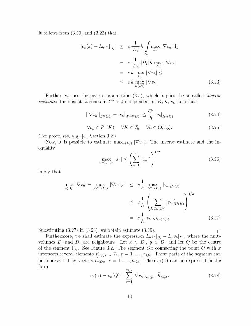
(vh(x)− vh(y)) dy (3.20)

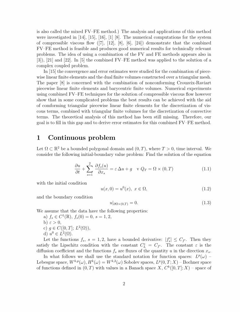
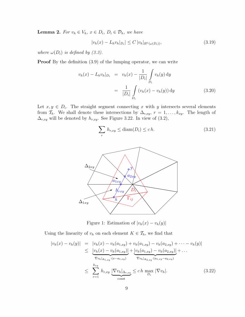
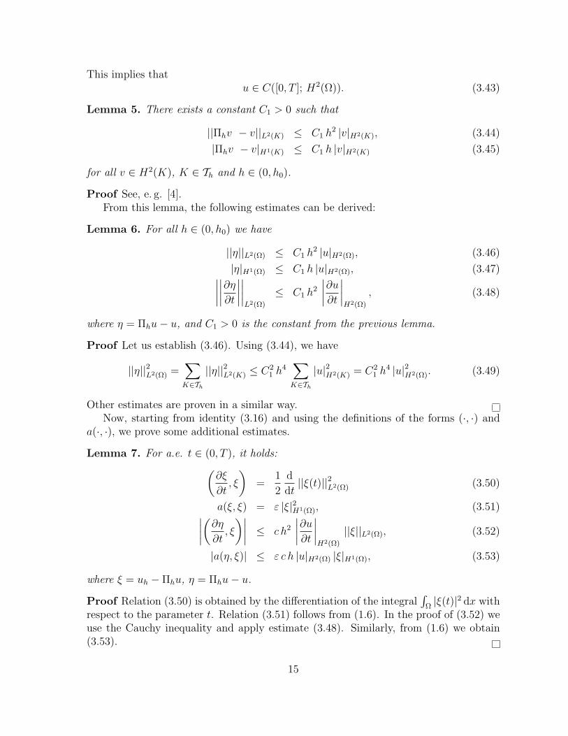
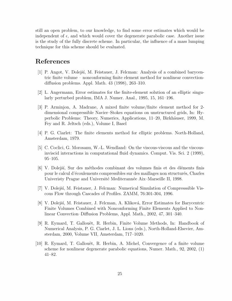
Let x, y ∈ Di. The straight segment connecting x with y intersects several elementsfrom Th. We shall denote these intersections by ∆r,xy, r = 1, . . . , kxy. The length of∆r,xy will be denoted by hr,xy. See Figure 3.22. In view of (3.2),∑

r

hr,xy ≤ diam(Di) ≤ c h. (3.21)

y

x

∆2xy

Γij

a1xy

a2xy

hrxy

∆1xy

Di

Figure 1: Estimation of |vh(x)− vh(y)|

Using the linearity of vh on each element K ∈ Th, we find that

|vh(x)− vh(y)| = |vh(x)− vh(a1,xy) + vh(a1,xy)− vh(a2,xy) + · · · − vh(y)|≤ |vh(x)− vh(a1,xy)|︸ ︷︷ ︸

∇vh|∆1,xy·(x−a1,xy)

+ |vh(a1,xy)− vh(a2,xy)|︸ ︷︷ ︸∇vh|∆2,xy

·(a1,xy−a2,xy)

+ . . .

≤kxy∑r=1

hr,xy |∇vh|∆r,xy︸ ︷︷ ︸const

≤ c h maxDi

|∇vh|. (3.22)

9

It follows from (3.20) and (3.22) that

|vh(x)− Lhvh|Di| ≤ c

1

|Di|h

∫Di

maxDi

|∇vh| dy

= c1

|Di||Di|h max

Di

|∇vh|

= c h maxDi

|∇vh| ≤

≤ c h maxω(Di)

|∇vh| (3.23)

Further, we use the inverse assumption (3.5), which implies the so-called inverseestimate: there exists a constant C? > 0 independent of K, h, vh such that

||∇vh||L∞(K) = |vh|W 1,∞(K) ≤C?

h|vh|H1(K) (3.24)

∀vh ∈ P 1(K), ∀K ∈ Th, ∀h ∈ (0, h0). (3.25)

(For proof, see, e. g. [4], Section 3.2.)Now, it is possible to estimate maxω(Di) |∇vh|. The inverse estimate and the in-

equality

maxn=1,...,m

|an| ≤

(m∑

n=1

|an|2)1/2

(3.26)

imply that

maxω(Di)

|∇vh| = maxK⊂ω(Di)

|∇vh|K | ≤ c1

hmax

K⊂ω(Di)|vh|H1(K)

≤ c1

h

∑K⊂ω(Di)

|vh|2H1(K)

1/2

= c1

h|vh|H1(ω(Di)). (3.27)

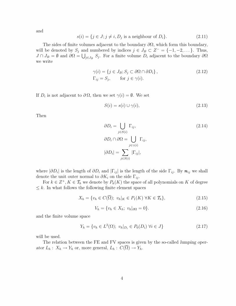
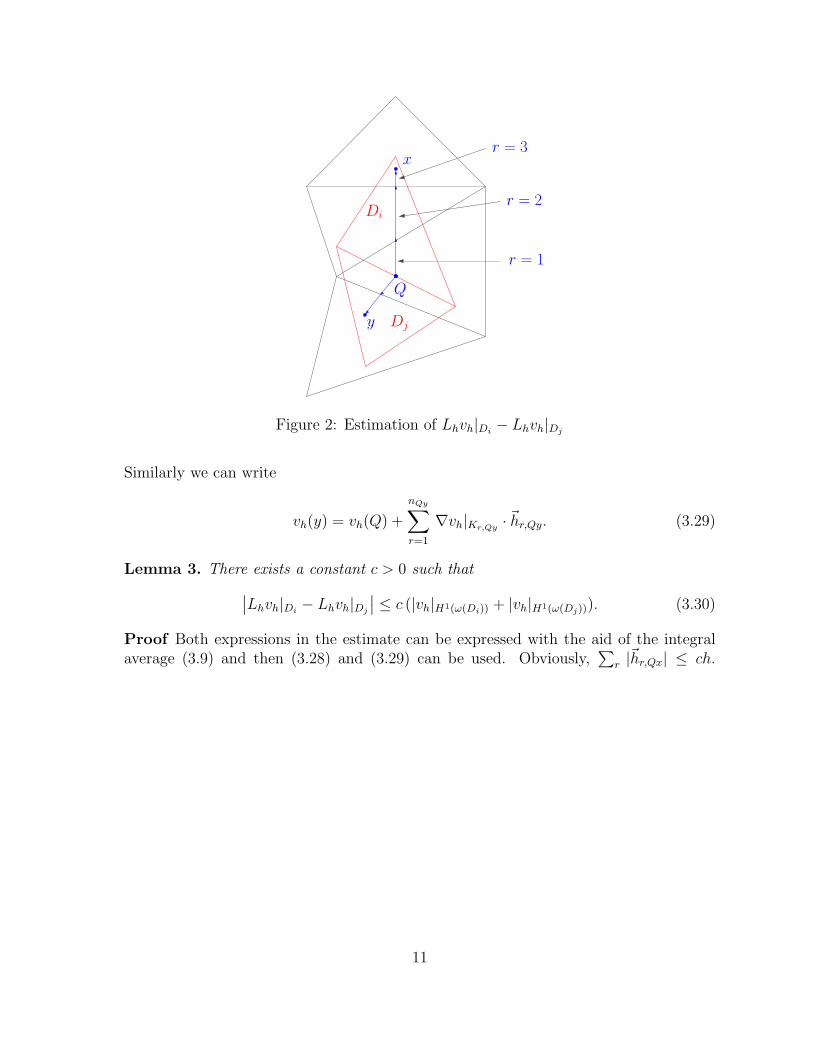
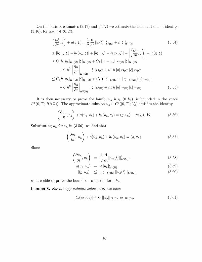
Substituting (3.27) in (3.23), we obtain estimate (3.19).Furthermore, we shall estimate the expression Lhvh|Di

− Lhvh|Dj, where the finite

volumes Di and Dj are neighbours. Let x ∈ Di, y ∈ Dj and let Q be the centreof the segment Γij. See Figure 3.2. The segment Qx connecting the point Q with xintersects several elements Kr,Qx ∈ Th, r = 1, . . . , nQx. These parts of the segment can

be represented by vectors ~hr,Qx, r = 1, . . . , nQx. Then vh(x) can be expressed in theform

vh(x) = vh(Q) +

nQx∑r=1

∇vh|Kr,Qx· ~hr,Qx. (3.28)

10

Dj

x

y

r = 3

r = 2

r = 1

Q

Di

Figure 2: Estimation of Lhvh|Di− Lhvh|Dj

Similarly we can write

vh(y) = vh(Q) +

nQy∑r=1

∇vh|Kr,Qy· ~hr,Qy. (3.29)

Lemma 3. There exists a constant c > 0 such that∣∣Lhvh|Di− Lhvh|Dj

∣∣ ≤ c (|vh|H1(ω(Di)) + |vh|H1(ω(Dj))). (3.30)

Proof Both expressions in the estimate can be expressed with the aid of the integralaverage (3.9) and then (3.28) and (3.29) can be used. Obviously,

∑r |~hr,Qx| ≤ ch.

11

Further, in view of (3.22) and the inverse estimate,

|Lhvh|Di− Lhvh|Dj

| =

∣∣∣∣∣∣∣1

|Di|

∫Di

vh(x) dx− 1

|Dj|

∫Dj

vh(y) dy

∣∣∣∣∣∣∣=

∣∣∣∣∣∣∣1

|Di|

∫Di

vh(Q) dx− 1

|Dj|

∫Dj

vh(Q) dy

+1

|Di|

∫Di

nQx∑r=1

∇vh|Kr,Qx· ~hr,Qx dx

− 1

|Dj|

∫Dj

nQy∑r=1

∇vh|Kr,Qy· ~hr,Qy dy

∣∣∣∣∣∣∣≤ c h (max

Di

|∇vh|+ maxDj

|∇vh|)

≤ c h (maxω(Di)

|∇vh|+ maxω(Dj)

|∇vh|)

≤ C (|vh|H1(ω(Di))+ |vh|H1(ω(Dj))

) (3.31)

This proves estimate (3.30).

Lemma 4. There exists a constant Cc > 0 such that

|εh(uh, vh)| = |bh(uh, vh)− b(uh, vh)| ≤ Cc h |uh|H1(Ω) |vh|H1(Ω). (3.32)

Proof We can write

|εh(uh, vh)| = |b(uh, vh)− bh(uh, vh)| ≤ (3.33)

≤ |b(uh, vh)− b(uh, Lhvh)|︸ ︷︷ ︸σ1

+ |b(uh, Lhvh)− bh(uh, vh)|︸ ︷︷ ︸σ2

.

Our goal is to estimate σ1 and σ2. We have

|σ1| ≤

∣∣∣∣∣∣∫Ω

2∑s=1

∂fs(uh)

∂xs

(vh − Lhvh) dx

∣∣∣∣∣∣=

∣∣∣∣∣∣∫Ω

2∑s=1

fs′(uh)

∂uh

∂xs

(vh − Lhvh)dx

∣∣∣∣∣∣≤ 2 Cf ′

∫Ω

|∇uh| |vh − Lhvh|

≤ 2 Cf ′ |uh|H1(Ω) ||vh − Lhvh||2L2(Ω). (3.34)

12

Now it is necessary to estimate the norm ||vh − Lhvh||L2(Ω). In virtue of Lemma 2,for x ∈ Di we can write

|vh(x)− Lhvh|Di| ≤ C |vh|H1(ω(Di)). (3.35)

Due to (3.2), it holds that |Di| ≤ c h2. The use of (3.4) yields

||vh − Lhvh||2L2(Ω) =∑i∈J

∫Di

|vh(x)− Lhvh|Di|2 dx

≤ C∑i∈J

|Di| |vh|2H1(ω(Di))

≤ C h2∑i∈J

|vh|2H1(ω(Di))

≤ R C h2 |vh|2H1(Ω) (3.36)

where we recall that R is a bound of RK , which is the number of sets ω(Di) containingthe element K. It follows from (3.36) that

||vh − Lhvh||L2(Ω) ≤ c h |vh|H1(Ω). (3.37)

Now the substitution into (3.34) implies that

|σ1| ≤ c h |uh|H1(Ω) |vh|H1(Ω). (3.38)

Further, we shall estimate the expression σ2. By Green’s theorem,

|σ2| = |b(uh, Lhvh)− bh(uh, vh)| (3.39)

=

∣∣∣∣∣∣∑i∈J

∫Di

2∑s=1

∂fs(uh)

∂xs

Lhvh dx−∑i∈J

∑j∈s(i)

Lhvh|DiH(Lhuh|Di

, Lhuh|Dj, nij) |Γij|

∣∣∣∣∣∣=

∣∣∣∣∣∣∑i∈J

∫∂Di

2∑s=1

fs(uh)LhvhnsdS −∑i∈J

∑j∈s(i)

Lhvh|DiH(Lhuh|Di

, Lhuh|Dj, nij)

∣∣∣∣∣∣ .Since the numerical flux H is consistent, we can write

|σ2| =

∣∣∣∣∣∣∣∑i∈J

Lhvh|Di

∑j∈s(i)

∫Γij

H(uh, uh, nij) dS −H(Lhuh|Di, Lhuh|Dj

, nij) |Γij|

∣∣∣∣∣∣∣ .

Now we shall use the Lipschitz continuity and conservativity of H. For given i ∈ J and

13

j ∈ s(i), when we exchange i and j, it is possible to write

Lhuh|Di

∫Γij

H(uh, uh, nij) dS −H(Lhuh|Di, Lhuh|Dj

, nij)|Γij|

+ Lhuh|Dj

∫Γij

H(uh, uh, nji) dS −H(Lhuh|Dj, Lhuh|Di

, nji)|Γij|

= (Lhuh|Di

− Lhuh|Dj)

∫Γij

H(uh, uh, nij) dS −H(Lhuh|Di, Lhuh|Dj

, nij)|Γij|

.

Summing over i ∈ J and j ∈ s(i) and dividing by 2 yields

|σ2| (3.40)

=1

2

∣∣∣∣∣∣∣∑i∈J

∑j∈s(i)

(Lhvh|Di− Lhvh|Dj

)

∫Γij

(H(uh, uh, nij)−H(Lhuh|Di

, Lhuh|Dj, nij)

)dS

∣∣∣∣∣∣∣≤ 1

2

∑i∈J

∑j∈s(i)

∣∣Lhvh|Di− Lhvh|Dj

∣∣ CL

∫Γij

(|uh(x)− Lhuh|Di

|+ |uh(x)− Lhuh|Dj)|)dS.

In virtue of Lemma (2), the estimates |Γij| ≤ c h and (3.4) and the Cauchy inequality,we obtain

|σ2| ≤ C∑i∈J

∑j∈s(i)

(|vh|H1(ω(Di)) + |vh|H1(ω(Dj))

)·∫Γij

(|uh|H1(ω(Di)) + |uh|H1(ω(Dj))

)dS

≤ C h∑i∈J

∑j∈s(i)

(|vh|H1(ω(Di)) + |vh|H1(ω(Dj))

)(|uh|H1(ω(Di)) + |uh|H1(ω(Dj))

)≤ 4 C h

∑i∈J

|vh|H1(ω(Di)) |uh|H1(ω(Di))

≤ 4 R C h |vh|H1(Ω) |uh|H1(Ω). (3.41)

Now, (3.38) and (3.41) already imply (3.32).

Lemma 4 gives a consistency property of the method, and will lead to the errorestimate.

3.3 Error estimate

In what follows, we shall assume that the exact solution u is sufficiently regular, namely,it satisfies the condition

∂u

∂t∈ L2(0, T ; H2(Ω)). (3.42)

14

This implies thatu ∈ C([0, T ]; H2(Ω)). (3.43)

Lemma 5. There exists a constant C1 > 0 such that

||Πhv − v||L2(K) ≤ C1 h2 |v|H2(K), (3.44)

|Πhv − v|H1(K) ≤ C1 h |v|H2(K) (3.45)

for all v ∈ H2(K), K ∈ Th and h ∈ (0, h0).

Proof See, e. g. [4].From this lemma, the following estimates can be derived:

Lemma 6. For all h ∈ (0, h0) we have

||η||L2(Ω) ≤ C1 h2 |u|H2(Ω), (3.46)

|η|H1(Ω) ≤ C1 h |u|H2(Ω), (3.47)∣∣∣∣∣∣∣∣∂η

∂t

∣∣∣∣∣∣∣∣L2(Ω)

≤ C1 h2

∣∣∣∣∂u

∂t

∣∣∣∣H2(Ω)

, (3.48)

where η = Πhu− u, and C1 > 0 is the constant from the previous lemma.

Proof Let us establish (3.46). Using (3.44), we have

||η||2L2(Ω) =∑

K∈Th

||η||2L2(K) ≤ C21 h4

∑K∈Th

|u|2H2(K) = C21 h4 |u|2H2(Ω). (3.49)

Other estimates are proven in a similar way.Now, starting from identity (3.16) and using the definitions of the forms (·, ·) and

a(·, ·), we prove some additional estimates.

Lemma 7. For a.e. t ∈ (0, T ), it holds:(∂ξ

∂t, ξ

)=

1

2

d

dt||ξ(t)||2L2(Ω) (3.50)

a(ξ, ξ) = ε |ξ|2H1(Ω), (3.51)∣∣∣∣(∂η

∂t, ξ

)∣∣∣∣ ≤ c h2

∣∣∣∣∂u

∂t

∣∣∣∣H2(Ω)

||ξ||L2(Ω), (3.52)

|a(η, ξ)| ≤ ε c h |u|H2(Ω) |ξ|H1(Ω), (3.53)

where ξ = uh − Πhu, η = Πhu− u.

Proof Relation (3.50) is obtained by the differentiation of the integral∫

Ω|ξ(t)|2 dx with

respect to the parameter t. Relation (3.51) follows from (1.6). In the proof of (3.52) weuse the Cauchy inequality and apply estimate (3.48). Similarly, from (1.6) we obtain(3.53).

15

On the basis of estimates (3.17) and (3.32) we estimate the left-hand side of identity(3.16), for a.e. t ∈ (0, T ):(

∂ξ

∂t, ξ

)+ a(ξ, ξ) =

1

2

d

dt||ξ(t)||2L2(Ω) + ε |ξ|2H1(Ω) (3.54)

≤ |b(uh, ξ)− bh(uh, ξ)|+ |b(u, ξ)− b(uh, ξ)|+∣∣∣∣(∂η

∂t, ξ

)∣∣∣∣+ |a(η, ξ)|

≤ Cc h |uh|H1(Ω) |ξ|H1(Ω) + Cf ||u− uh||L2(Ω) |ξ|H1(Ω)

+ C h2

∣∣∣∣∂u

∂t

∣∣∣∣H2(Ω)

||ξ||L2(Ω) + ε c h |u|H2(Ω) |ξ|H1(Ω)

≤ Cc h |uh|H1(Ω) |ξ|H1(Ω) + Cf

(||ξ||L2(Ω) + ||η||L2(Ω)

)|ξ|H1(Ω)

+ C h2

∣∣∣∣∂u

∂t

∣∣∣∣H2(Ω)

||ξ||L2(Ω) + ε c h |u|H2(Ω) |ξ|H1(Ω) (3.55)

It is then necessary to prove the family uh, h ∈ (0, h0), is bounded in the spaceL2 (0, T ; H1(Ω)). The approximate solution uh ∈ C1([0, T ]; Vh) satisfies the identity(

∂uh

∂t, vh

)+ a(uh, vh) + bh(uh, vh) = (g, vh), ∀vh ∈ Vh. (3.56)

Substituting uh for vh in (3.56), we find that(∂uh

∂t, uh

)+ a(uh, uh) + bh(uh, uh) = (g, uh). (3.57)

Since (∂uh

∂t, uh

)=

1

2

d

dt||uh(t)||2L2(Ω), (3.58)

a(uh, uh) = ε |uh|2H1(Ω), (3.59)

|(g, uh)| ≤ ||g||L2(Ω) ||uh(t)||L2(Ω), (3.60)

we are able to prove the boundedness of the form bh.

Lemma 8. For the approximate solution uh we have

|bh(uh, uh)| ≤ C ||uh||L2(Ω) |uh|H1(Ω). (3.61)

16

Proof First we estimate |Lhuh|Di|. From the definition (3.9) of the lumping operator,

using the Cauchy inequality and the inequality |Di| ≥ c h2, we get

|Lhuh|Di| =

∣∣∣∣ 1

|Di|

∫Di

uh dx

∣∣∣∣ ≤ |Di|1/2

|Di|||uh||L2(Di) ≤

c

h||uh||L2(Di). (3.62)

Now we can already estimate the form bh. We use (2.21), (3.30), (3.62), the inequality|Γij| ≤ c h and the conservativity of the numerical flux. For a given i ∈ J and j ∈ s(i)and the situation obtained by interchanging i and j we can write

Lhuh|DiH(Lhuh|Di

, Lhuh|Dj, nij)|Γij|+ Lhuh|Dj

H(Lhuh|Dj, Lhuh|Di

, nji)|Γij|= Lhuh|Di

H(Lhuh|Di, Lhuh|Dj

, nij)|Γij| − Lhuh|DjH(Lhuh|Di

, Lhuh|Dj, nij)|Γij|

=(Lhuh|Di

− Lhuh|Dj

)H(Lhuh|Di

, Lhuh|Dj, nij)|Γij|. (3.63)

Summation over all i ∈ J and j ∈ s(i) and dividing by two yield

|bh(uh, uh)| =

∣∣∣∣∣∣∑i∈J

Lhuh|Di

∑j∈s(i)

H(Lhuh|Di, Lhuh|Dj

, nij) |Γij|

∣∣∣∣∣∣ (3.64)

=

∣∣∣∣∣∣ 12∑i∈J

∑j∈s(i)

(Lhuh|Di

− Lhuh|Dj

)H(Lhuh|Di

, Lhuh|Dj, nij)|Γij|

∣∣∣∣∣∣≤ 1

2CL h

∑i∈J

∑j∈s(i)

∣∣Lhuh|Di− Lhuh|Dj

∣∣ (|Lhuh|Di|+ |Lhuh|Dj

|)

≤ C∑i∈J

∑j∈s(i)

(|uh|H1(ω(Di)) + |uh|H1(ω(Dj))

) (||uh||L2(Di) + ||uh||L2(Dj)

)≤ C ||uh||L2(Ω)|uh|H1(Ω),

which we wanted to prove.

In the sequel, we shall apply the following version of Gronwall’s lemma:

Lemma 9. Let y, q, z, r ∈ C([0, T ]) be nonnegative functions and

y(t) + q(t) ≤ z(t) +

t∫0

r(s) y(s) ds, t ∈ [0, T ]. (3.65)

Then

y(t) + q(t) ≤ z(t) +

t∫0

r(ϑ) z(ϑ) exp

t∫ϑ

r(s)ds

dϑ, t ∈ [0, T ]. (3.66)

17

Proof can be carried out similarly as in [11], Section 8.2.29

For the proof of the error estimate we shall still need the following result:

Lemma 10. For all t ∈ [0, T ] it holds

||uh(t)||2L2(Ω) ≤ K(ε), (3.67)

ε

T∫0

|uh(ϑ)|2H1(Ω)dϑ ≤ K(ε), (3.68)

whereK(ε) = C4 exp(CT/ε), (3.69)

with constants C4 and C independent of h and ε.

Proof We start from identity (3.57), use (3.58), (3.60) and (3.61):

d

dt||uh(t)||2L2(Ω) + 2 ε|uh(t)|2H1(Ω)

≤ 2 ||g||L2(Ω) ||uh(t)||L2(Ω) + 2 C ||uh(t)||L2(Ω) |uh(t)|H1(Ω) (3.70)

Using Young’s inequality

a b ≤ 1

2

(a2 δ +

b2

δ

)(3.71)

(valid for a, b ≥ 0, δ > 0) with δ = C/ε, we get

d

dt||uh(t)||2L2(Ω) + ε |uh(t)|2H1(Ω) ≤ ||g||2L2(Ω) +

(1 +

C2

ε

)||uh(t)||2L2(Ω). (3.72)

The integration∫ t

0of this inequality yields

||uh(t)||2L2(Ω) + ε

t∫0

|uh(ϑ)|2H1(Ω)dϑ

≤ ||uh(0)||2L2(Ω) +

t∫0

||g||2L2(Ω)dϑ +

t∫0

(1 +

C

ε

)||uh(ϑ)||2L2(Ω)dϑ

≤ C +

(1 +

C

ε

) t∫0

||uh(ϑ)||2L2(Ω)dϑ. (3.73)

18

Now we shall aplly Gronwall’s lemma 9, where we set

y(t) = ||uh(t)||2L2(Ω)

q(t) = ε

t∫0

|uh(ϑ)|2H1(Ω)dϑ

z(t) = C

r(s) = 1 +C

ε.

We obtain

||uh(t)||2L2(Ω) + ε

t∫0

|uh(ϑ)|2H1(Ω)dϑ

≤ C +

t∫0

(1 +

C

ε

)C exp

t∫ϑ

(1 +

C

ε

)ds

dϑ

= C +

(1 +

C

ε

)C

t∫0

exp

((1 +

C

ε

)(t− ϑ)

)dϑ.

Since

t∫0

exp

((1 +

C

ε

)(t− ϑ)

)dϑ = − 1

1 + Cε

[exp

((1 +

C

ε

)(t− ϑ)

)]t

0

= − 1

1 + Cε

(1− exp

(t

(1 +

C

ε

)))= C3

(exp

(t

(1 +

C

ε

))− 1

)≤ C3 exp

((1 +

C

ε

)T

)= C4 exp

(CT

ε

), (3.74)

we get

||uh(t)||2L2(Ω) + ε

T∫0

|uh(ϑ)|2H1(Ω) dθ ≤ C + (1 +C

ε) C C4 exp

(CT

ε

):= K(ε). (3.75)

This inequality already implies estimates (3.67) and (3.68).Now we can already formulate the main result of our paper.

Theorem 1. Let assumptions a) - d) on data be satisfied, let the numerical flux be Lip-schitz continuous, consistent and conservative and let the triangulations have propertiesfrom 2.1. Then the error of the method eh = u − uh, where u is the exact solution of

19

problem (3.10) – (1.3) satisfying (3.43) and uh is the approximate solution defined by(2.22), satisfies the estimates

maxt∈[0,T ]

||eh||L2(Ω) ≤ C h (3.76)

and

√ε

√√√√√ T∫0

|eh(ϑ)|2H1(Ω)dϑ ≤ C h. (3.77)

Proof The error eh is expressed in the form eh = ξ + η, where

ξ = uh − Πh ∈ Vh, η = Πhu− u. (3.78)

As we have already mentioned, from (3.16), (3.50) and (3.51) we have

1

2

d

dt||ξ(t)||2L2(Ω) + ε |ξ|2H1(Ω)

≤ c h |uh|H1(Ω) |ξ|H1(Ω) + Cf

(||ξ||L2(Ω) + ||η||L2(Ω)

)|ξ|H1(Ω)

+ C h2

∣∣∣∣∂u

∂t

∣∣∣∣H2(Ω)

||ξ||L2(Ω) + ε c h |u|H2(Ω) |ξ|H1(Ω) (3.79)

By Young’s inequality and Lemma 6,

d

dt||ξ(t)||2L2(Ω) + 2 ε |ξ|2H1(Ω) (3.80)

≤ 4c2 h2

ε|uh|2H1(Ω) +

ε

4|ξ|2H1(Ω) + 4

(C2

f

ε+ 1

)||ξ||2L2(Ω) +

ε

4|ξ|2H1(Ω)

+ 4C2

f C12 h4

ε|u|2H2(ω) +

ε

4|ξ|2H1(Ω) + C2 h4

∣∣∣∣∂u

∂t

∣∣∣∣2H2(Ω)

+ ||ξ||2L2(Ω)

+ 4 ε c2 h2 |u|2H2(ω) +ε

4|ξ|2H1(Ω).

The integration∫ t

0and the use of Lemmas 5 and 10 yield

||ξ(t)||2L2(Ω) + ε

t∫0

|ξ(ϑ)|2H1(Ω)dϑ (3.81)

≤ 4c2 h2

ε2C4 exp(CT/ε) + C2 h4

∣∣∣∣∣∣∣∣∂u

∂t

∣∣∣∣∣∣∣∣2L2(0,T ;H2(Ω))

+ C h4 |u(0)|2H(Ω)

+ 4 (C2f C1

2 h4 + ε2 C2 h2) ||u||2L2(0,T ;H2(Ω)) + 4

(C2

f

ε+ 1

) t∫0

||ξ(ϑ)||2L2(Ω)dϑ.

20

Now it is possible to apply Gronwall’s Lemma 9, where we define the individual termsby

y(t) = ||ξ(t)||2L2(Ω),

q(t) = ε

t∫0

|ξ(ϑ)|2H1(Ω)dϑ,

z = C7 h2 exp(CT/ε) + C2 h4

∣∣∣∣∣∣∣∣∂u

∂t

∣∣∣∣∣∣∣∣2L2(0,T ;H2(Ω))

+ 4 (C8 h4 + ε2 C2 h2) ||u||2L2(0,T ;H2(Ω))

+ C h4 |u(0)|2H2(Ω),

r = 4

(C2

f

ε+ 1

)ane denote C7 = C4 C2/ε2, C8 = C2

f C12. Further, we have

t∫ϑ

r(s) ds = 4

(C2

f

ε+ 1

)(t− ϑ), (3.82)

t∫0

r(ϑ) z exp

t∫ϑ

r(s) ds

dϑ =

t∫0

4

(C2

f

ε+ 1

)z exp

(4

(C2

f

ε+ 1

)(t− ϑ)

)dϑ

= 4

(C2

f

ε+ 1

)z

t∫0

exp

(4

(C2

f

ε+ 1

)(t− ϑ)

)dϑ

= z

[exp

(4

(C2

f

ε+ 1

)(t− ϑ)

)]t

ϑ=0

=

= z exp

(4

(C2

f

ε+ 1

)t

)− z.

Hence,

||ξ(t)||2L2(Ω) + ε

t∫0

|ξ(ϑ)|2H1(Ω)dϑ (3.83)

≤(C7 h2 exp(CT/ε) + C2 h4 ||∂u/∂t||2L2(0,T ;H2(Ω)) + 4 (C8 h4 + ε2 C2 h2) ||u||2L2(0,T ;H2(Ω))

+ C h4 |u(0)|2H2(Ω)

)exp

(4

(C2

f

ε+ 1

)t

).

If we use the notation

Z(ε, h) := h2(C7 exp(CT/ε) + C2 h2 ||∂u/∂t||2L2(0,T ;H2(Ω)) (3.84)

+ 4(C8 h2 + ε2 C2) ||u||2L2(0,T ;H2(Ω)) + C h2 |u(0)|2H2(Ω)

)exp

(4

(C2

f

ε+ 1

)T

),

21

then, in virtue of the previous inequality, we have

||ξ(t)||2L2(Ω) ≤ Z(ε, h), ∀t ∈ [0, T ] thus

maxt∈[0,T ]

||ξ(t)||2L2(Ω) ≤√

Z(ε, h). (3.85)

The triangular and Young’s inequalities imply that

||eh||2L2(Ω) ≤ 2 ||ξ||2L2(Ω) + 2 ||η||2L2(Ω), (3.86)

|eh|2H1(Ω) ≤ 2 |ξ|2H1(Ω) + 2 |η|2H1(Ω).

In (3.86) we use the relation eh = u − uh, inequality (3.85), estimates from Lemma 6and assumption (3.43). We find that

||eh||2L2(Ω) ≤ 2 Z(ε, h) + 2 C21 h2|u(t)|2H2(Ω). (3.87)

Taking the square root, we get

||eh||L2(Ω) ≤√

2 Z(ε, h) + 2 C21 h2|u(t)|2H2(Ω). (3.88)

This already implies the final estimate

maxt∈[0,T ]

||eh(t)|| ≤√

2 Z(ε, h) + 2 C21 h2 max

t∈[0,T ]|u(t)|2H2(Ω) ≤ C h. (3.89)

Finally we shall prove the estimate for εt∫

0

|eh(ϑ)|2H1(Ω)dϑ. We know that

ε

T∫0

|ξ(ϑ)|2H1(Ω)dϑ ≤ Z(ε, h). (3.90)

Thus, we can write

ε

T∫0

|eh(ϑ)|2H1(Ω)dϑ ≤ Z(ε, h)2 ε

T∫0

|ξ(ϑ)|2H1(Ω)dϑ + 2 ε

T∫0

|η(ϑ)|2H1(Ω)dϑ

≤ 2 Z(ε, h) + 2C21 h2

T∫0

|u(ϑ)|2H2(Ω)dϑ (3.91)

= 2 Z(ε, h) + 2C21 h2 ||u||2L2(0,T ;H2(Ω)) ≤ C h2,

which implies the estimate

√ε

√√√√√ T∫0

|eh(ϑ)|2H1(Ω)dϑ ≤ C h. (3.92)

This concludes the proof.

22

4 Numerical experiments

We verified our results by numerical experiments. We applied the combined FV-FEmethod to scalar 2D viscous Burgers equation:

∂u

∂t+ u

∂u

∂x1

+ u∂u

∂x2

− ε∆u = g (4.93)

in the space-time domain QT = Ω × (0, 1), Ω = (−1, 1)2, equipped with Dirichletboundary condition u|∂Ω = 0, and initial condition u|t=0 = 0. The right-hand side g ischosen so that it conforms to the exact solution

uex = (1− e−2t)(1− x21)

2(1− x22)

2.

The time discretization is carried by a semiimplicit Euler scheme:(uk

h − uk−1h

τ, vh

)+ bh(u

k−1h , vh) + ah(u

kh, vh) = (gk−1, vh) (4.94)

which should have better stability properties than a purely explicit scheme with no addedcomputational cost, because the FE mass and stiffness matrices share their sparsitystructure. In the definition (2.21) of the form bh we use the numerical flux

H(u1, u2, n) =

∑2s=1 fs(u1)ns, if A > 0∑2s=1 fs(u2)ns, if A ≤ 0 , (4.95)

where

A =2∑

s=1

f ′s(u)ns, u =1

2(u1 + u2) and n = (n1, n2). (4.96)

As we want to examine the error of the space discretization, we overkill the timestep so that the time discretization error is negligible.

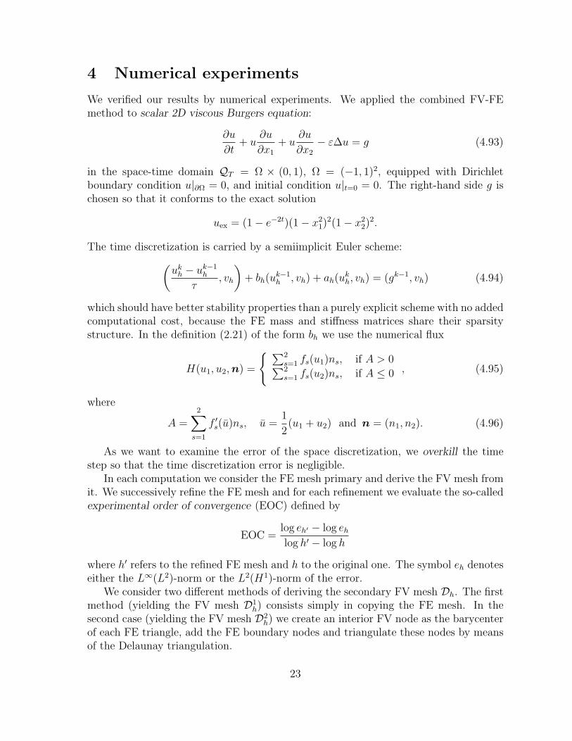
In each computation we consider the FE mesh primary and derive the FV mesh fromit. We successively refine the FE mesh and for each refinement we evaluate the so-calledexperimental order of convergence (EOC) defined by

EOC =log eh′ − log eh

log h′ − log h

where h′ refers to the refined FE mesh and h to the original one. The symbol eh denoteseither the L∞(L2)-norm or the L2(H1)-norm of the error.

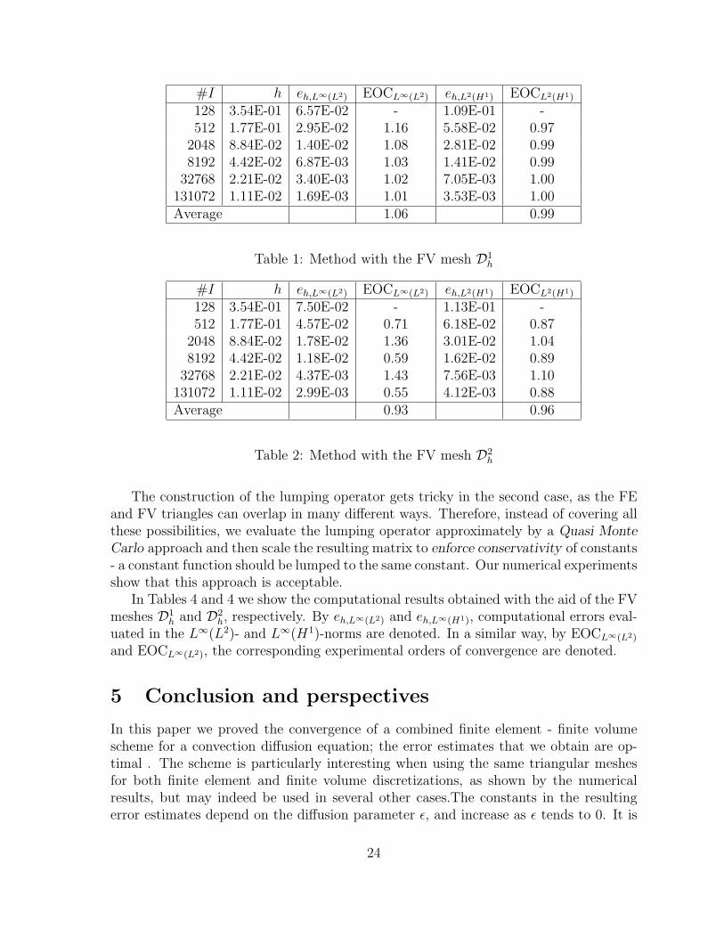
We consider two different methods of deriving the secondary FV mesh Dh. The firstmethod (yielding the FV mesh D1

h) consists simply in copying the FE mesh. In thesecond case (yielding the FV mesh D2

h) we create an interior FV node as the barycenterof each FE triangle, add the FE boundary nodes and triangulate these nodes by meansof the Delaunay triangulation.

23

#I h eh,L∞(L2) EOCL∞(L2) eh,L2(H1) EOCL2(H1)

128 3.54E-01 6.57E-02 - 1.09E-01 -512 1.77E-01 2.95E-02 1.16 5.58E-02 0.97

2048 8.84E-02 1.40E-02 1.08 2.81E-02 0.998192 4.42E-02 6.87E-03 1.03 1.41E-02 0.99

32768 2.21E-02 3.40E-03 1.02 7.05E-03 1.00131072 1.11E-02 1.69E-03 1.01 3.53E-03 1.00Average 1.06 0.99

Table 1: Method with the FV mesh D1h

#I h eh,L∞(L2) EOCL∞(L2) eh,L2(H1) EOCL2(H1)

128 3.54E-01 7.50E-02 - 1.13E-01 -512 1.77E-01 4.57E-02 0.71 6.18E-02 0.87

2048 8.84E-02 1.78E-02 1.36 3.01E-02 1.048192 4.42E-02 1.18E-02 0.59 1.62E-02 0.89

32768 2.21E-02 4.37E-03 1.43 7.56E-03 1.10131072 1.11E-02 2.99E-03 0.55 4.12E-03 0.88Average 0.93 0.96

Table 2: Method with the FV mesh D2h

The construction of the lumping operator gets tricky in the second case, as the FEand FV triangles can overlap in many different ways. Therefore, instead of covering allthese possibilities, we evaluate the lumping operator approximately by a Quasi MonteCarlo approach and then scale the resulting matrix to enforce conservativity of constants- a constant function should be lumped to the same constant. Our numerical experimentsshow that this approach is acceptable.

In Tables 4 and 4 we show the computational results obtained with the aid of the FVmeshes D1

h and D2h, respectively. By eh,L∞(L2) and eh,L∞(H1), computational errors eval-

uated in the L∞(L2)- and L∞(H1)-norms are denoted. In a similar way, by EOCL∞(L2)

and EOCL∞(L2), the corresponding experimental orders of convergence are denoted.

5 Conclusion and perspectives

In this paper we proved the convergence of a combined finite element - finite volumescheme for a convection diffusion equation; the error estimates that we obtain are op-timal . The scheme is particularly interesting when using the same triangular meshesfor both finite element and finite volume discretizations, as shown by the numericalresults, but may indeed be used in several other cases.The constants in the resultingerror estimates depend on the diffusion parameter ε, and increase as ε tends to 0. It is

24

still an open problem, to our knowledge, to find some error estimates which would beindependent of ε, and which would cover the degenerate parabolic case. Another issueis the study of the fully discrete scheme. In particular, the influence of a mass lumpingtechnique for this scheme should be evaluated.

References

[1] P. Angot, V. Dolejsı, M. Feistauer, J. Felcman: Analysis of a combined barycen-tric finite volume – nonconforming finite element method for nonlinear convection-diffusion problems. Appl. Math. 43 (1998), 263–310.

[2] L. Angermann, Error estimates for the finite-element solution of an elliptic singu-larly perturbed problem, IMA J. Numer. Anal., 1995, 15, 161–196.

[3] P. Arminjon, A. Madrane, A mixed finite volume/finite element method for 2-dimensional compressible Navier–Stokes equations on unstructured grids, In: Hy-perbolic Problems: Theory, Numerics, Applications, 11–20, Birkhauser, 1999, M.Fey and R. Jeltsch (eds.), Volume I, Basel

[4] P. G. Ciarlet: The finite elements method for elliptic problems. North-Holland,Amsterdam, 1979.

[5] C. Coclici, G. Morosanu, W.-L. Wendland: On the viscous-viscous and the viscous-inviscid interactions in computational fluid dynamics. Comput. Vis. Sci. 2 (1999),95–105.

[6] V. Dolejsı, Sur des methodes combinant des volumes finis et des elements finispour le calcul d’ecoulements compressibles sur des maillages non structures, CharlesUniveristy Prague and Universite Mediterannee Aix–Marseille II, 1998.

[7] V. Dolejsı, M. Feistauer, J. Felcman: Numerical Simulation of Compresssible Vis-cous Flow through Cascades of Profiles. ZAMM, 76:301-304, 1996.

[8] V. Dolejsı, M. Feistauer, J. Felcman, A. Klikova, Error Estimates for BarycentricFinite Volumes Combined with Nonconforming Finite Elements Applied to Non-linear Convection–Diffusion Problems, Appl. Math., 2002, 47, 301–340.

[9] R. Eymard, T. Gallouet, R. Herbin, Finite Volume Methods, In: Handbook ofNumerical Analysis, P. G. Ciarlet, J. L. Lions (eds.), North-Holland-Elsevier, Am-sterdam, 2000, Volume VII, Amsterdam, 717–1020.

[10] R. Eymard, T. Gallouet, R. Herbin, A. Michel, Convergence of a finite volumescheme for nonlinear degenerate parabolic equations, Numer. Math., 92, 2002, (1)41–82.

25

[11] M. Feistauer: Mathematical Methods in Fluid Dynamics. Pitman Monographs andSurveys in Pure and Applied Mathematics 67, Longman Scientific & Technical,Harlow, UK, 1993.

[12] M. Feistauer, J. Felcman: Theory and applications of numerical schemes for nonlin-ear convection-diffusion problems and compressible Navier-Stokes equations. TheMathematics of Finite Elements and Applications. Highlights 1996 (J. R. White-man, ed.), Wiley, Chichester, 1997, 175-194.

[13] M. Feistauer, J. Felcman, M. Lukacova, Combined finite element–finite volumesolution of compressible flow, J. Comput. Appl. Math., 1995, 63, 179-199.

[14] M. Feistauer, J. Felcman, M. Lukacova, On the Convergence of a Combined Fi-nite Volume–Finite Element Method for Nonlinear Convection–Diffusion Problems,Numer. Methods Partial Differ. Equations, 1997, 13, 163-190.

[15] M. Feistauer, J. Felcman, M. Lukacova, G. Warnecke: Error estimates of a com-bined finite volume - finite element method for nonlinear convection - diffusionproblems. SIAM J. Numer. Anal. 36, 1528-1548, 1999.

[16] M. Feistauer, J. Slavık, P. Stupka: Convergence of the combined finite ele-ment -finite volume method for nonlinear convection - diffusion problems. Explicitschemes. Numer Methods Partial Differential Eq 15: 215-235, 1999.

[17] M. Feistauer, J. Felcman, I. Straskraba: Mathematical and Computational Methodsfor Compressible Flow. Clarendon Press, Oxford, 2003

[18] J. Fort, K. Kozel: Numerical solution of inviscid and viscous flows using modernschemes and quadrilateral or triangular mesh. Mathematica Bohemica, no. 2., 2001,379 – 39

[19] J. Fort, K. Kozel: Modern finite volume methods solving internal flow problems.Task quarterly 6 No 1, 2002, 127 – 142

[20] J. Furst, K. Kozel: Numerical solution of transonic flows through 2D and 3D turbinecascades. Computing and Visualization in Science, vol. 4, number 3, Springer 2002

[21] J. M. Ghidaglia, F. Pascal: Footbridges finite volume-finite elements. C. R. Acd.Sci., Ser. I, Math. 328, vol. 8, 711–716, 1999

[22] J. M. Ghidaglia, F. Pascal: Footbridges between finite volume-finite elements withapplications to CFD. Technical report, University Paris-Sud, 2001 (preprint)

[23] B. Heinrich, Finite Difference Methods on Irregular Networks, Birkhauser, Basel,1987.

[24] A. Klikova: Finite volume-finite element solution of compressible flow. PhD. Dis-sertation, Charles University Prague, Faculty of Mathematics and Physics, 2000.

26

[25] A. Kufner, O. John, S. Fucık: Function Spaces. Academia, Praha, 1977

[26] A.Michel, J. Vovelle, A finite volume method for parabolic degenerate problemswith general Dirichlet boundary conditions”. SIAM J. Numer. Anal. 41 (2003) no.6, 2262–2293

[27] K. Ohmori, T. Ushijima, A technique of upstream type applied to a linear non-conforming finite element approximation of convective diffusion equations, RAIROAnal. Numer., 1984, 18, 309-322.

[28] F. Schieweck and L. Tobiska, A nonconforming finite element method of upstreamtype applied to the stationary Navier–Stokes equations, RAIRO Anal. Numer.,1989, 23, 627–647.

27