Combined study by direct numerical simulation and optical diagnostics of the flame stabilization in a Diesel spray Thèse de doctorat de l'Université Paris-Saclay préparée à CentraleSupélec École doctorale n°579 Sciences Mécaniques et Energétiques, Matériaux et Géosciences (SMEMaG) Spécialité de doctorat : Combustion Thèse soutenue à Rueil-Malmaison, le 11 Mars 2019, par Fabien Tagliante-Saracino Composition du Jury : Andreas Kempf Professeur, Université Duisburg-Essen Rapporteur Jose M. Garcia-Oliver Professeur, Université polytechnique de Valence Rapporteur Sébastien Ducruix Directeur de recherche, CentraleSupélec (EM2C) Président du Jury Bart Somers Professeur associé, Université de technologie d'Eindhoven Examinateur Lyle M. Pickett Docteur, Sandia National Laboratories Examinateur Gilles Bruneaux Docteur, IFP Energies nouvelles Directeur de thèse Christian Angelberger Docteur, IFP Energies nouvelles Co-Directeur de thèse Louis-Marie Malbec Docteur, IFP Energies nouvelles Invité NNT : 2019SACLC017

Welcome message from author
This document is posted to help you gain knowledge. Please leave a comment to let me know what you think about it! Share it to your friends and learn new things together.
Transcript
Combined study by direct numerical simulation and optical
diagnostics of the flame stabilization in a Diesel spray
Thèse de doctorat de l'Université Paris-Saclay préparée à CentraleSupélec
École doctorale n°579 Sciences Mécaniques et Energétiques, Matériaux et Géosciences
(SMEMaG) Spécialité de doctorat : Combustion
Thèse soutenue à Rueil-Malmaison, le 11 Mars 2019, par
Fabien Tagliante-Saracino
Composition du Jury :
Andreas Kempf Professeur, Université Duisburg-Essen Rapporteur
Jose M. Garcia-Oliver Professeur, Université polytechnique de Valence Rapporteur
Sébastien Ducruix Directeur de recherche, CentraleSupélec (EM2C) Président du Jury
Bart Somers Professeur associé, Université de technologie d'Eindhoven Examinateur
Lyle M. Pickett Docteur, Sandia National Laboratories Examinateur
Gilles Bruneaux Docteur, IFP Energies nouvelles Directeur de thèse
Christian Angelberger Docteur, IFP Energies nouvelles Co-Directeur de thèse
Louis-Marie Malbec Docteur, IFP Energies nouvelles Invité
NN
T : 2
019S
AC
LC
017


Université Paris-Saclay
Espace Technologique / Immeuble Discovery
Route de l’Orme aux Merisiers RD 128 / 91190 Saint-Aubin, France
Titre : Etude combinée par simulation numérique direct et diagnostics optiques de la stabilisation de
la flamme d'un spray Diesel
Mots clés : Moteurs à Combustion Interne, Stabilisation de la flamme, Diagnostics optiques,
Simulation numérique direct.
Résumé : La compréhension du processus de
stabilisation des flammes Diesel constitue un
défi majeur en raison de son effet sur les
émissions de polluants. En effet, la relation
étroite entre la distance de lift-off (distance entre
la flamme et l’injecteur) et la production de suie
est maintenant bien établie. Cependant,
différents mécanismes de stabilisation ont été
proposés mais sont toujours sujets à discussion.
L'objectif de cette thèse est de fournir une
contribution expérimentale et numérique pour
identifier les mécanismes de stabilisation
majeurs.
La combustion d'un spray n-dodécane issu d'un
injecteur mono-trou a été étudiée dans une
cellule à volume constant en utilisant une
combinaison de diagnostics optiques : mesures
hautes cadences et simultanées de schlieren, LIF
à 355 nm, chimiluminescence haute température
ou de chimiluminescence OH *. Des expériences
complémentaires sont effectuées au cours
desquelles le mélange est allumé entre
l’injecteur et le lift-off par plasma induit par
laser. L’évolution du lift-off jusqu’à son retour à
une position d’équilibre plus en aval est ensuite
étudiée pour différentes conditions opératoires.
L'analyse de l'évolution du lift-off sans allumage
laser révèle deux types principaux de
comportement : des sauts brusques en amont et
un déplacement plus progressif en aval. Alors
que le premier comportement est attribué à des
événements d'auto-inflammation, le second est
analysé grâce aux résultats obtenus par allumage
laser. Il a été constaté que l'emplacement du
formaldéhyde avait un impact important sur la
vitesse de retour du lift-off.
Une simulation numérique directe (DNS en
anglais) bidimensionnelle d'une flamme liftée
turbulente se développant spatialement dans les
mêmes conditions opératoires que les
expériences et reproduisant l'évolution
temporelle de la distance de lift-off est proposée.
Du fait que les expériences montrent que la
flamme se stabilise en aval du spray liquide, la
DNS ne couvre qu'une région en aval où
l’écoulement est réduit à un jet gazeux. La
chimie de l’n-dodécane est modélisée à l'aide
d'un schéma cinétique (28 espèces transportées)
prenant en compte les chemins réactionnels
basse et haute température.
Comme observé expérimentalement, la
stabilisation de la flamme est intermittente : des
auto-inflammations se produisent tout d'abord
puis se font convecter en aval jusqu'à ce qu'une
nouvelle auto-inflammation se produise. Le
mécanisme principal de stabilisation est l'auto-
inflammation. Toutefois, on observe également à
la périphérie du jet diverses topologies de
flammes, telles que des flammes triples, qui
aident la flamme à se stabiliser en remplissant
des réservoirs de gaz brûlés à haute température
localisés à la périphérie, ce qui déclenche des
auto-inflammations. Toutes ces observations
sont résumées dans un modèle conceptuel
décrivant la stabilisation de la flamme.
Enfin, un modèle prédisant les fluctuations de la
distance du lift-off autour de sa valeur moyenne
temporelle est proposé. Ce modèle a été
développé sur la base d’observations faites dans
l’étude expérimentale et numérique :
premièrement, le suivi temporel du lift-off a été
décomposé en une succession d’auto-
inflammations et d’évolutions en aval.
Deuxièmement, la période entre deux auto-
inflammations et la vitesse d'évolution en aval
ont été modélisées à l'aide de corrélations
expérimentales disponibles dans la littérature.
Troisièmement, le modèle a été adapté afin de
prendre en compte l’effet des réservoirs à haute
température sur les fluctuations de la flamme. Et
enfin, le modèle a été comparé aux données
expérimentales, au cours desquelles des
variations de la température ambiante, de la
concentration en oxygène et de la pression
d'injection ont été effectuées. Dès lors que le
modèle a montré une bonne correspondance avec
les données expérimentales, il peut être utilisé en
complément du modèle prédisant la distance du
lift-off moyen afin de mieux décrire la
stabilisation d’une flamme Diesel.
Université Paris-Saclay
Espace Technologique / Immeuble Discovery
Route de l’Orme aux Merisiers RD 128 / 91190 Saint-Aubin, France
Title: Combined study by Direct Numerical Simulation and optical diagnostics of the flame
stabilization in a Diesel spray
Keywords : Internal Combustion Engines, Flame stabilization, Optical diagnostics, Direct numerical
simulation
Abstract: The understanding of the stabilization
process of Diesel spray flames is a key challenge
because of its effect on pollutant emissions. In
particular, the close relationship between lift-off
length and soot production is now well
established. However, different stabilization
mechanisms have been proposed and are still
under debate. The objective of this PhD is to
provide an experimental and numerical
contribution to the investigation of these
governing mechanisms.
Combustion of an n-dodecane spray issued from
a single-hole nozzle was studied in a constant-
volume precombustion vessel using a
combination of optical diagnostic techniques.
Simultaneous high frame rate schlieren, 355
LIF (laser-induced fluorescence) and high-
temperature chemiluminescence or OH*
chemiluminescence are respectively used to
follow the evolution of the gaseous jet envelope,
formaldehyde location and lift-off position.
Additional experiments are performed where the
ignition of the mixture is forced at a location
upstream of the natural lift-off position by laser-
induced plasma ignition. The analysis of the
evolution of the lift off position without laser
ignition reveals two main types of behaviors:
sudden jumps in the upstream direction and
more progressive displacement towards the
downstream direction. While the former is
attributed to auto-ignition events, the latter is
studied through the forced laser ignition results.
It is found that the location of formaldehyde
greatly impacts the return velocity of the lift-off
position.
A two-dimensional Direct Numerical
Simulation (DNS) of a spatially developing
turbulent lifted flame at the same operating
conditions than the experiments and
reproducing the temporal evolution of the lift-
off length is proposed to provide a better
understanding of the flame stabilization
mechanisms. The DNS only covers a
downstream region where the flow can be
reduced to a gaseous jet, since experimental
observations have shown that the flame
stabilized downstream of the liquid spray. N-
dodecane chemistry is modeled using a reduced
chemical kinetics scheme (28 species
transported) accounting for the low- and high
temperature reaction pathways. Similar to what
has been observed in the experiments, the flame
stabilization is intermittent: flame elements first
auto-ignite before being convected downstream
until another sudden auto-ignition event occurs
closer to the fuel injector. The flame topologies,
associated to such events, are discussed in detail,
using the DNS results, and a conceptual model
summarizing the observations made is
proposed. Results show that the main flame
stabilization mechanism is auto-ignition.
However, multiple reaction zone topologies,
such as triple flames, are also observed at the jet
periphery of the fuel jet helping the flame to
stabilize by filling high-temperature burnt gases
reservoirs localized at the periphery, which
trigger in its turn auto-ignitions.
Finally, a model predicting the fluctuations of
the lift-off length around its time-averaged value
is proposed. This model has been developed
based on observations made in the experimental
and numerical study: first, the lift-off length
time-evolution was decomposed into a
succession of auto-ignition events and
downstream evolutions. Second, the period
between two auto-ignition and the velocity of
the downstream evolution was modeled using
experimental correlations available in the
literature. Third, the model has been adapted to
take into account the effect of the high-
temperature reservoirs on the flame fluctuations.
Last, the model was compared to experimental
data, where the ambient temperature, oxygen
concentration and injection pressure were
varied. Since the model showed good agreement
with the experimental data, it can be used in
addition to the model predicting the time-
averaged lift-off length to better describe the
Diesel flame stabilization.

Université Paris-Saclay
Espace Technologique / Immeuble Discovery
Route de l’Orme aux Merisiers RD 128 / 91190 Saint-Aubin, France
Remerciement
Je souhaite tout d’abord remercier les membres de mon jury de thèse, le ProfesseurSébastien Ducruix, Président du jury, les Professeurs Andreas Kempf et José M. Garcia-Oliver qui m’ont fait l’honneur d’être rapporteurs, ainsi que le Professeur Bart Somers etle Docteur Lyle M. Pickett pour leur participation en tant qu’examinateurs.
Je tiens à remercier chaleureusement mon Directeur et co-Directeur de thèse : GillesBruneaux et Christian Angelberger. Vos conseils avisés et votre expérience dans le mondede la recherche m’ont appris énormément d’un point de vue scientifique et rédactionnel(avec plus de douleur). Je n’oublierai sans doute jamais ces bons moments de correctionapprofondis que vous m’avez offerts lors de l’écriture de ma thèse ou des papiers... Je suiségalement très reconnaissant envers Louis-Marie Malbec pour son encadrement sans failleet sa disponibilité tout au long de ces 3 années.
Cette thèse n’aurait pas été la même sans l’aide de Maîtres de la combustion nom-mément Thierry Poinsot et Lyle M. Pickett. En effet je souhaite remercier Thierry pourson implication dans ma thèse et pour m’avoir accueilli au CERFACS quelques semaines.Par-delà les océans, les réunions régulières avec Lyle, malgré le décalage horaire, ont étéextrêmement enrichissantes. C’est principalement grâce à vous, Gilles, Christian, Louis-Marie, Thierry et Lyle que j’ai pu m’épanouir dans mon travail durant ces 3 années, etpour cela je vous en suis infiniment reconnaissant.
Je souhaite également remercier la team des expérimentateurs de l’IFPEN pour leursoutien technique et leur bonne humeur. Un grand merci à Clément pour son expertisetechnique sans qui il m’aurait été impossible de mener à bien la partie expérimentale.Je le remercie en outre de m’avoir permis d’intégrer la grande et prestigieuse équipe defoot de l’IFPEN. Je suis également heureux d’avoir pu échanger avec Jérôme, Laurent,Thomas, Francis et Vincent tout au long de ma thèse. Je souhaite enfin exprimer magratitude à mes collègues ingénieurs de recherche de l’IFPEN pour leur aide précieuse enréponse à tous types de problèmes.
Cette aventure de trois ans m’a permis d’interagir avec mes collègues doctorants, quisont ensuite devenus mes amis. Ma première pensée vient à Edouard (Bobbit boo), nosnombreux débats sur la société et le football ont été, pour moi, une bouffée d’air pur du-rant les longues périodes de rédaction. Je remercie également chaleureusement, Antoinepour son sifflotement, Matthieu pour ses connaissances sportives, Louise pour sa maîtrisedu ballon rond, Benoît pour sa bonne humeur à absolument toute épreuve, Alexis pour saforce tranquille et son fromage du Jura, Julien pour son amour des radis, Gorka pour sonaide sur AVBP et pour son lancer de type « arbalète » aux fléchettes, Andreas pour safougue et sa capacité à oublier des affaires dans le monde entier (que Louise récupère parla suite), Maxime pour ses fameux jeux de mots et sa passion des réacteurs 0D, Hassanpour sa cool altitude, Stéphane pour avoir été faible aux fléchettes, et pour finir, Detlevpour m’avoir fait découvrir la Russie un peu plus chaque jour. Cette fin de thèse est aussipour moi l’occasion de faire un bilan sur le tournoi international de fléchettes, en effet je
peux dire en tout modestie : j’étais le meilleur.
Il me tient également à cœur de remercier mes encadrants de stage de M2 qui m’ont faitdécouvrir le monde de la recherche : Bénédetta Franzelli, Philippe Scouflaire et SébastienCandel. Je vous suis très reconnaissant pour le soutien que vous m’avez apporté tout aulong de mon stage et également pour m’avoir aidé à trouver la thèse dans laquelle j’ai pum’épanouir.
Je voudrais par ailleurs remercier mes chers amis de Paris et de Tournefeuille pourm’avoir permis de garder le contact avec la vie réelle, merci à Zakaria, Victoire, Raphaël etAuriane. Mes derniers remerciements vont à ma famille. Tout d’abord à mes parents et masœur qui m’ont toujours soutenu ! Plus spécialement à ma mère qui s’est particulièrementinvestie dans mes études dès le plus jeune âge. Je ne pouvais pas finir ces remerciementssans un énorme merci à ma douce et tendre épouse. Marie s’est fortement investie dansce travail de thèse, allant jusqu’à dessiner de sa main la ligne stoechiométrique du modèleconceptuel (Fig. 4.15). Son soutien et son réconfort dans les moments difficiles ont été,pour moi, capitaux dans cette folle aventure qu’est la thèse.
2
Abstract
The understanding of the stabilization process of Diesel spray flames is a key challengebecause of its effect on pollutant emissions. In particular, the close relationship betweenlift-off length and soot production is now well established. However, different stabilizationmechanisms have been proposed and are still under debate. The objective of this PhDis to provide an experimental and numerical contribution to the investigation of thesegoverning mechanisms.
Combustion of an n-dodecane spray issued from a single-hole nozzle (90 µm orifice,ECN spray A injector) was studied in a constant-volume precombustion vessel using acombination of optical diagnostic techniques. Simultaneous high frame rate schlieren, 355LIF (laser-induced fluorescence) and high-temperature chemiluminescence or OH* chemi-luminescence are respectively used to follow the evolution of the gaseous jet envelope,formaldehyde location and lift-off position. Additional experiments are performed wherethe ignition of the mixture is forced at a location upstream of the natural lift-off positionby laser-induced plasma ignition. The evolution of the lift-off position until its returnto the natural steady-state position is then studied for different ambient temperatures(800 K to 850 K), densities (11 kg/m3 to 14.8 kg/m3) and rail pressures (100 MPa to150 MPa) using the same set of optical diagnostics. The analysis of the evolution of thelift off position without laser ignition reveals two main types of behaviors: sudden jumpsin the upstream direction and more progressive displacement towards the downstreamdirection. While the former is attributed to auto-ignition events, the latter is studiedthrough the forced laser ignition results. It is found that the location of formaldehydegreatly impacts the return velocity of the lift-off position: if laser ignition occurs upstreamof the zone where formaldehyde is naturally present, the lift-off position convects rapidlyuntil it reaches the region where formaldehyde is present and then returns more slowlytowards its natural position, suggesting that cool-flame greatly assists lift-off stabilization.
A two-dimensional Direct Numerical Simulation (DNS) of a spatially developing tur-bulent lifted flame at the same operating conditions than the experiments and reproducingthe temporal evolution of the lift-off length is proposed to provide a better understandingof the flame stabilization mechanisms. As experimental evidence for the simulated condi-tions shows a flame stabilization downstream of the zone where the two-phase spray hasa major impact on local flow, the DNS only covers a downstream region where the flowcan be reduced to a gaseous jet. The inflow conditions for the DNS are imposed based onexperimental studies at the considered position. N -dodecane chemistry is modeled usinga reduced chemical kinetics scheme comprising 28 species and 198 reactions to account forthe low- and high temperature reaction pathways, and its predictions have been validatedagainst experimental auto-ignition delays and laminar flame speeds at conditions relevantto the simulated cases. Similar to what has been observed in the experiments, the flamestabilization is intermittent: flame elements first auto-ignite before being convected down-stream until another sudden auto-ignition event occurs closer to the fuel injector. Theflame topologies, associated to such events, are discussed in detail, using the DNS results,and a conceptual model summarizing the observations made is proposed. Results show

that the main flame stabilization mechanism is auto-ignition. However, multiple reactionzone topologies, such as triple flames, are also observed at the jet periphery of the fuel jethelping the flame to stabilize by filling high-temperature burnt gases reservoirs localizedat the periphery, which trigger in its turn auto-ignitions.
Finally, a model predicting the fluctuations of the lift-off length around its time-averaged value is proposed. This model has been developed based on observations madein the experimental and numerical study: first, the lift-off length time-evolution wasdecomposed into a succession of auto-ignition events and downstream evolutions. Second,the period between two auto-ignition and the velocity of the downstream evolution wasmodeled using experimental correlations available in the literature. Third, the modelhas been adapted to take into account the effect of the high-temperature reservoirs onthe flame fluctuations. Last, the model was compared to experimental data, where theambient temperature, oxygen concentration and injection pressure were varied. Since themodel showed good agreement with the experimental data, it can be used in addition tothe model predicting the time-averaged lift-off length [1, 2] to better describe the Dieselflame stabilization.
2

3

Résumé
La compréhension du processus de stabilisation des flammes Diesel constitue un défimajeur en raison de son effet sur les émissions de polluants. En effet, la relation étroiteentre la distance de lift-off (distance entre la flamme et l’injecteur) et la production desuie est maintenant bien établie. Cependant, différents mécanismes de stabilisation ontété proposés mais sont toujours sujets à discussion. L’objectif de cette thèse est de fournirune contribution expérimentale et numérique pour identifier les mécanismes de stabilisa-tion majeurs.
La combustion d’un spray n-dodécane issu d’un injecteur mono-trou (orifice de 90 µmde diamètre, injecteur ECN spray A) a été étudiée dans une cellule à volume constanten utilisant une combinaison de diagnostics optiques. Des mesures hautes cadences etsimultanées de schlieren, LIF à 355 nm, chimiluminescence haute température ou de chi-miluminescence OH * sont respectivement utilisées pour suivre l’évolution de l’enveloppedu jet gazeux, la localisation du formaldéhyde et la position de la flamme. Des expériencescomplémentaires sont effectuées au cours desquelles le mélange est allumé entre l’injecteuret le lift-off par plasma induit par laser. L’évolution du lift-off jusqu’à son retour à une po-sition d’équilibre plus en aval est ensuite étudiée pour différentes températures ambiantes(de 800 à 850 K), densités (11 kg/m3 à 14,8 kg/m3) et des pressions d’injections (100 MPaà 150 MPa) en utilisant les mêmes diagnostics optiques. L’analyse de l’évolution du lift-offsans allumage laser révèle deux types principaux de comportement : des sauts brusques enamont et un déplacement plus progressif en aval. Alors que le premier comportement estattribué à des événements d’auto-inflammation, le second est analysé grâce aux résultatsobtenus par allumage laser. Il a été constaté que l’emplacement du formaldéhyde avait unimpact important sur la vitesse de retour du lift-off : si un allumage laser se produisaiten amont de la zone où le formaldéhyde est naturellement présent, le lift-off est convectérapidement jusqu’à atteindre la région où le formaldéhyde est présent et revient ensuiteplus lentement vers sa position naturelle, suggérant que la flamme froide aide grandementà la stabilisation du lift-off.
Une simulation numérique directe (DNS pour Direct Numerical Simulation en an-glais) bidimensionnelle d’une flamme liftée turbulente se développant spatialement dansles mêmes conditions opératoires que les expériences et reproduisant l’évolution tempo-relle de la distance de lift-off est proposée afin de mieux comprendre les mécanismes destabilisation de la flamme. Du fait que les expériences montrent que la flamme se stabi-lise en aval de la zone où le spray liquide a un impact majeur sur l’écoulement local, laDNS ne couvre qu’une région en aval où l’écoulement peut être réduit à un jet gazeux.Les conditions d’entrée de la DNS sont imposées sur la base d’études expérimentales. Lachimie de l’n-dodécane est modélisée à l’aide d’un schéma cinétique réduit comprenant 28espèces et 198 réactions afin de prendre en compte les chemins réactionnels basse et hautetempérature. Le schéma réduit a été validé en comparant les délais d’auto-inflammationet les vitesses de flamme laminaire de pré-mélange par rapport aux expériences. D’unefaçon analogue à ce qui a été observé expérimentalement, la stabilisation de la flamme estintermittente : des auto-inflammations se produisent tout d’abord puis se font convecter
en aval jusqu’à ce qu’une nouvelle auto-inflammation se produise plus près de l’injecteur.Les topologies de flammes, associées à de tels événements, sont discutées en détail à l’aidedes résultats de la DNS puis un modèle conceptuel résumant les observations est pro-posé. Les résultats indiquent que le mécanisme principal de stabilisation de la flammeest l’auto-inflammation. Toutefois, on observe également à la périphérie du jet diversestopologies de flammes, telles que des flammes triples, qui aident la flamme à se stabiliseren remplissant des réservoirs de gaz brûlés à haute température localisés à la périphérie,ce qui déclenche des auto-inflammations.
Enfin, un modèle prédisant les fluctuations de la distance du lift-off autour de sa valeurmoyenne (moyenne temporelle) est proposé. Ce modèle a été développé sur la base d’obser-vations faites dans l’étude expérimentale et numérique : premièrement, le suivi temporeldu lift-off a été décomposé en une succession d’auto-inflammations et d’évolutions en aval.Deuxièmement, la période entre deux auto-inflammations et la vitesse d’évolution en avalont été modélisées à l’aide de corrélations expérimentales disponibles dans la littérature.Troisièmement, le modèle a été adapté afin de prendre en compte l’effet des réservoirs àhaute température sur les fluctuations de la flamme. Et enfin, le modèle a été comparé auxdonnées expérimentales, au cours desquelles des variations de la température ambiante,de la concentration en oxygène et de la pression d’injection ont été effectuées. Dès lors quele modèle a montré une bonne correspondance avec les données expérimentales, il peutêtre utilisé en complément du modèle prédisant la distance du lift-off moyen [1, 2] afin demieux décrire la stabilisation d’une flamme Diesel.
2

3
Contents
1 Introduction 71.1 Environmental context . . . . . . . . . . . . . . . . . . . . . . . . . . . . 71.2 Diesel engine . . . . . . . . . . . . . . . . . . . . . . . . . . . . . . . . . . 8
1.2.1 Basic functioning of a Diesel engine . . . . . . . . . . . . . . . . . . 81.2.2 Exhaust after-treatment systems . . . . . . . . . . . . . . . . . . . 9
1.3 Soot production in Diesel engines . . . . . . . . . . . . . . . . . . . . . . . 101.4 Objective of the thesis . . . . . . . . . . . . . . . . . . . . . . . . . . . . . 131.5 Structure of the manuscript . . . . . . . . . . . . . . . . . . . . . . . . . . 15
2 Flame stabilization mechanisms: A literature review 172.1 Diesel spray combustion . . . . . . . . . . . . . . . . . . . . . . . . . . . . 17
2.1.1 Chemistry of Diesel-type fuels . . . . . . . . . . . . . . . . . . . . 172.1.2 Conceptual models of Diesel spray combustion . . . . . . . . . . . 19
2.2 Non-premixed gaseous jet flames . . . . . . . . . . . . . . . . . . . . . . . 222.2.1 Stabilization by premixed flame propagation at the flame base . . 22
2.2.1.1 Stabilization by perfectly premixed flame . . . . . . . . . 222.2.1.2 Stabilization by partially premixed flame . . . . . . . . . 24
2.2.2 Impact of scalar dissipation . . . . . . . . . . . . . . . . . . . . . . 262.2.3 Stabilization by recirculation of burnt gases . . . . . . . . . . . . . 28
2.3 Diesel spray flames . . . . . . . . . . . . . . . . . . . . . . . . . . . . . . . 292.3.1 Stabilization by a premixed flame at the flame base . . . . . . . . 302.3.2 Role of flame extinction . . . . . . . . . . . . . . . . . . . . . . . . 332.3.3 Role of auto-ignition . . . . . . . . . . . . . . . . . . . . . . . . . . 342.3.4 Combined role of edge-flames and auto-ignition . . . . . . . . . . . 36
2.3.4.1 2D-DNS of a laminar mixing layer . . . . . . . . . . . . . 362.3.4.2 2D-DNS of a turbulent decreasing mixing layer . . . . . . 392.3.4.3 DNS of a temporally evolving turbulent mixing layer . . 402.3.4.4 3D-DNS of a spatially developing slot jet flame . . . . . . 41
2.3.5 Stabilization by recirculation of burnt gases . . . . . . . . . . . . . 422.4 Conclusion . . . . . . . . . . . . . . . . . . . . . . . . . . . . . . . . . . . . 44
3 Experimental study of the stabilization mechanisms of a lifted Diesel-type flame using optical diagnostics and laser plasma ignition 473.1 Brief introduction . . . . . . . . . . . . . . . . . . . . . . . . . . . . . . . 473.2 Experimental details . . . . . . . . . . . . . . . . . . . . . . . . . . . . . . 48
3.2.1 Experimental conditions . . . . . . . . . . . . . . . . . . . . . . . . 48
4
CONTENTS
3.2.2 Optical diagnostics and laser ignition . . . . . . . . . . . . . . . . 493.2.2.1 Schlieren imaging . . . . . . . . . . . . . . . . . . . . . . 503.2.2.2 355 LIF . . . . . . . . . . . . . . . . . . . . . . . . . . . 503.2.2.3 High-temperature chemiluminescence . . . . . . . . . . . 523.2.2.4 Laser ignition . . . . . . . . . . . . . . . . . . . . . . . . 54
3.3 Results and Discussion . . . . . . . . . . . . . . . . . . . . . . . . . . . . 543.3.1 Flame structure . . . . . . . . . . . . . . . . . . . . . . . . . . . . . 553.3.2 Results for natural flame evolution . . . . . . . . . . . . . . . . . . 563.3.3 Forced laser ignition . . . . . . . . . . . . . . . . . . . . . . . . . . 58
3.4 Conclusion . . . . . . . . . . . . . . . . . . . . . . . . . . . . . . . . . . . . 65
4 A conceptual model of the flame stabilization mechanisms for a liftedDiesel-type flame based on direct numerical simulation and experiments
674.1 Brief introduction . . . . . . . . . . . . . . . . . . . . . . . . . . . . . . . 674.2 Configuration . . . . . . . . . . . . . . . . . . . . . . . . . . . . . . . . . . 69
4.2.1 Simplifying assumptions . . . . . . . . . . . . . . . . . . . . . . . . 694.2.2 Numerical set-up . . . . . . . . . . . . . . . . . . . . . . . . . . . . 70
4.3 Chemical mechanism . . . . . . . . . . . . . . . . . . . . . . . . . . . . . 734.3.1 Development of the reduced scheme . . . . . . . . . . . . . . . . . . 734.3.2 Estimation of the thermal flame thickness . . . . . . . . . . . . . . 75
4.4 Analysis tools for DNS . . . . . . . . . . . . . . . . . . . . . . . . . . . . 764.4.1 LOL definition . . . . . . . . . . . . . . . . . . . . . . . . . . . . . 764.4.2 Identification of the reaction zone topologies . . . . . . . . . . . . 76
4.4.2.1 Reaction zone topologies during auto-ignition events . . . 764.4.2.2 Reaction zone topologies during continuous evolution of
the lift-off . . . . . . . . . . . . . . . . . . . . . . . . . . 774.5 Comparison between DNS and experiments . . . . . . . . . . . . . . . . . 794.6 Analysis of stabilization mechanisms . . . . . . . . . . . . . . . . . . . . . 82
4.6.1 LOL tracking with reaction zone topologies . . . . . . . . . . . . . 824.6.2 Analysis of Event A . . . . . . . . . . . . . . . . . . . . . . . . . . 844.6.3 Analysis of Evolutions B . . . . . . . . . . . . . . . . . . . . . . . 86
4.7 Conceptual model of flame stabilization . . . . . . . . . . . . . . . . . . . 904.8 Conclusion . . . . . . . . . . . . . . . . . . . . . . . . . . . . . . . . . . . 92
4.8.1 Complementary elements . . . . . . . . . . . . . . . . . . . . . . . 934.8.2 Non-reactive profiles . . . . . . . . . . . . . . . . . . . . . . . . . . 934.8.3 Calculation of the mesh resolution for the DNS . . . . . . . . . . . 95
4.8.3.1 Criteria to simulate 1D premixed flames under autoigni-tive conditions . . . . . . . . . . . . . . . . . . . . . . . . 96
4.8.3.2 Grid convergence . . . . . . . . . . . . . . . . . . . . . . . 97
5 A Lift-Off Length fluctuations model 995.1 Motivation . . . . . . . . . . . . . . . . . . . . . . . . . . . . . . . . . . . 995.2 The lift-off length fluctuations model . . . . . . . . . . . . . . . . . . . . . 101
5.2.1 Sa model . . . . . . . . . . . . . . . . . . . . . . . . . . . . . . . . 1025.2.2 θ model . . . . . . . . . . . . . . . . . . . . . . . . . . . . . . . . . 1035.2.3 ∆LOLTh model . . . . . . . . . . . . . . . . . . . . . . . . . . . . . 104
5

CONTENTS
5.3 Lift-off length fluctuations experimental database . . . . . . . . . . . . . . 1055.4 Calibration and validation of the LOL fluctuation model . . . . . . . . . . 1075.5 Conclusion . . . . . . . . . . . . . . . . . . . . . . . . . . . . . . . . . . . . 109
6 Conclusions and perspectives 1106.1 Summary of main findings . . . . . . . . . . . . . . . . . . . . . . . . . . . 1106.2 Perspectives . . . . . . . . . . . . . . . . . . . . . . . . . . . . . . . . . . . 112
6.2.1 Validation of the assumptions and models . . . . . . . . . . . . . . 1126.2.2 Lines of research to improve understating of flame stabilization
mechanisms . . . . . . . . . . . . . . . . . . . . . . . . . . . . . . 1146.2.3 Towards a technical solution to reduce the soot emissions . . . . . 115
A Criteria to distinguish combustion regimes 116A.1 Transport budget analysis . . . . . . . . . . . . . . . . . . . . . . . . . . . 116A.2 Chemical criteria to distinguish auto-ignition and flame propagation . . . 120
B Regime diagram for the flame stabilization mechanisms 123
C Impact of a high co-flow on the flame stabilization 126
D Setup of a ”coarse DNS” 129
Bibliography 140
6

Chapter 1
Introduction
1.1 Environmental contextFossil fuels are, nowadays, the main source of energy in all modern societies. The
transportation sector is responsible for a significant part of the consumption of thesehydrocarbons, which are burnt to produce energy. However, the combustion of hydrocar-bons, in Internal Combustion Engines (ICE), is causing two main problems that requireimprovements in combustion processes.
First, pollutants produced during combustion such as CO, NO, NO2 and soot particlespose serious public health problems. Among those, soot particles are particularly danger-ous for humans. They are 98 % carbon by weight and typically spherical in shape. Whilemost are only around 0.03 µm in size, they can aggregate to form larger non-sphericalparticles of typical sizes of up to 10 µm. If not oxidized or treated after combustion,they can be inhaled by humans. Numerous studies have shown that this has a number ofnegative impacts on their health [3].
Second, ICE also contribute to the greenhouse gas (GHG) emissions through the emis-sion of CO2, which is identified as the main GHG. Transport is the only domain whichincreases its contribution to GHG emissions in European Union (EU): between 1990 and2015, in the transport sector, the GHG emissions went from 15 % to 23 % of the totalemissions of GHG (Eurostat source).
For these reasons, legislators, all over the world, are imposing continuously morestringent limits to the pollutant emissions of new ICE. Fig. 1.1 shows the evolution ofthe standards between 1993 and 2015 for the Diesel engines. It clearly appears thatthe different Euro standards (Euro 1 to 6) have led to drastically decrease the pollutantemissions. Engine manufacturers have invested heavily to reach the objectives imposedby the governments.
Furthermore, the Volkswagen Diesel emissions scandal has revealed that the NewEuropean Driving Cycle (NEDC), used to measure the pollutant emissions (designed inthe 1980s) is far from the real driving emissions. This is why Europe will introduce aReal Driving Emissions (RDE) test to measure the pollutants emitted by cars driven onthe road. RDE serves to confirm NEDC results in real life, thereby ensuring that carsdeliver low pollutant emissions, not only in the laboratory but also on the road. The
7

1.2. DIESEL ENGINE
RDE will require manufacturers to make major investments in developing new vehiclesand updating their testing facilities to pass this new test.
Figure 1.1 – Relative evolution (1993 reference) of the regulatory emissions for Dieselvehicles in Europe from 1993 to 2015 for 4 pollutants: nitrogen oxides NOx, carbonmonoxide CO, the sum of nitrogen oxides NOx and HC unburned hydrocarbons andfinally the particles [4].
In this context, electric cars appear as a promising alternative to ICE. However, al-though the sales of electric vehicles are in constant expansion, they only represented 1.5%of the new vehicles registrations in 2016. This low percentage of electric cars can beexplained by the limited autonomy and high price of this type of vehicles compared tocombustion-powered cars. From this perspective and because of the current context ofclimate change, car manufacturers have no choice but to develop new ICE models andimprove their efficiency in terms of pollutant emissions and performance.
1.2 Diesel engine
1.2.1 Basic functioning of a Diesel engineMost ICE produced in the automotive industry consist in two technologies: compression-
ignition (Diesel) engine and spark-ignition (gasoline) engine. They are both designed toconvert the chemical energy available in fuel into mechanical energy. This mechanical en-ergy moves pistons up and down inside cylinders (see Fig. 1.2). The pistons are connectedto a crankshaft, and the up-and-down motion of the pistons, known as linear motion, cre-ates the rotary motion needed to turn the wheels of a car forward. Both, Diesel enginesand gasoline engines, convert fuel into mechanical energy through a series of fast com-bustions. The major difference between Diesel and gasoline is the way these combustionshappen. In a gasoline engine, fuel is mixed with air, compressed by pistons, and ignitedby sparks from spark plugs. In a Diesel engine, the air is compressed first, and then thefuel is injected. Because air heats up when it’s compressed, the fuel auto-ignites. TheDiesel engine uses a four-stroke combustion cycle as shown in Fig. 1.2.
8

1.2. DIESEL ENGINE
Figure 1.2 – Four-stroke cycle Diesel engine [5].
• Intake stroke: The intake valve opens up, letting in air and moving the piston down.On a recent Diesel engine, a turbocharger increases the density of the gas in orderto increase the mass admitted into the combustion chamber.
• Compression stroke: The piston moves back up and compresses the air. Pressureand temperature increase significantly in the cylinder. The temperature can reach950 K and the pressure 80 bars before the injection.
• Combustion stroke (working stroke): As the piston reaches the top, fuel is injected.The high injection pressure (between 300 and 2500 bar) allows a very fine atomiza-tion of the liquid and a high air entrainment rate ensuring rapid evaporation, andon the other hand promotes mixing, the jet being highly turbulent. The combustionis initiated in areas where the mixture is most favorable, then spreads to the entirejet. A direct visualization of the combustion is shown in Fig. 1.3 for 4 instants in aconstant volume chamber.
Figure 1.3 – Diesel spray combustion where the injection pressure is 700 bar inside aconstant volume combustion chamber at 1100 K [6].
• Exhaust stroke: The piston moves back to the top, pushing out the exhaust gasescreated from the combustion out of the exhaust valve.
1.2.2 Exhaust after-treatment systemsThe two major pollutants emitted after Diesel combustion are nitrogen oxides NOx
and soot particles. In order to reduce these pollutant emissions, two main approaches
9
1.3. SOOT PRODUCTION IN DIESEL ENGINES
have been adopted.
The first technique consists in using a portion of the exhaust gas back to the enginecylinder to reduce the NOx emissions (technique named EGR for exhaust gas recircu-lation). The exhaust gas replaces some of the excesses oxygen in the pre-combustionmixture. Because NOx forms primarily when a mixture of nitrogen and oxygen is sub-jected to high temperature, the lower combustion chamber temperatures caused by EGRreduces the amount of NOx the combustion generates.
The second technique is to use exhaust gas after-treatment technologies. The DieselOxidation Catalyst (DOC) allows to oxidize NOx to nitrogen dioxide NO2. The NOx
treatment is completed by a Selective Catalytic Reduction (SCR), where NO2 is neededto support the performance of the SCR. In SCR, urea, a liquid-reluctant agent is injectedthrough a catalyst into the exhaust fumes. The urea starts the chemical reaction thatproduces NOx into N2 and H2O, which is then ejected through the engine exhaust pipe.Finally Diesel Particulate filter (DPF) is used to trap the soot particles. DPF is madeof thousands of tiny channels. When exhausts gases pass through these channels, sootis trapped along the walls of the channels. The exhaust gases pass through the poroussurface of the ceramic filter. Note that only the big particles are trapped in this filter,while the smallest are released in the environment.
However, all these exhaust gas after-treatment systems, do not allow to avoid thepollutant emissions in the atmosphere on the one hand, and on the other hand they arevery expensive and complex. In this context, a deeper and better understanding of theprocesses occurring during Diesel combustion, and of the driving physical and chemicalphenomena, appears as one of the major steps in order to propose a cleaner combustion.By so doing, the pollutant emissions could be minimized from the combustion.
1.3 Soot production in Diesel enginesFig. 1.4 illustrates the different physical phenomena involved during the Diesel spray
combustion.
10

1.3. SOOT PRODUCTION IN DIESEL ENGINES
Figure 1.4 – Illustration of the different physical phenomena occurring during Diesel spraycombustion. Figure adapted from [7].
First, inside the nozzle, the fuel is ejected at very high injection pressure leading to theformation of vapor cavities in the liquid fuel. This phenomenon is called cavitation andis studied in [8, 9] for Diesel spray. Experimental results have shown that the cavitationwithin the nozzle modifies the characteristics of the nozzle exit spray, which has an impacton the spray formation and atomization [10, 11].
When the liquid fuel flows out of the injector, a primary breakup regime occurs, wherethe interaction between the gas and liquid phase causes waves to develop along the liquidsurface. Once the wave becomes unstable, it shears off creating elongated ligaments dueto the Kelvin-Helmholtz instabilities. These ligaments then further breakdown into largedroplets.
Then, the large droplets start to reduce in size due to the Rayleigh-Taylor instabilitiesand finally vaporize due to the high ambient temperature. The resulting vapor fuel mixeswith air, and then auto-ignites (more details are available in Section 2.1.2) leading to astabilized diffusion flame at a certain distance from the injector. The corresponding axialdistance between the injector and the stabilized spray flame is called the Lift-off Length(LOL), which is of the order of few tens of millimeters. Fig. 1.5 illustrates an example ofLOL for a multi-hole injector. During the diffusion combustion, as much as 20 % of theair required to burn the fuel injected is entrained in the zone between the injector tip andthe location where the spray flame base is stabilized.
11

1.3. SOOT PRODUCTION IN DIESEL ENGINES
Figure 1.5 – Illustration of the lift-off length (LOL) using broadband luminosity techniquein constant volume combustion chamber extracted from [12].
Fig. 1.6 shows the soot production as a function of the inverse of the equivalence ratioat the lift-off (1/ΦLOL, defined as the inverse of the ratio of the fuel-to-oxidizer ratio tothe stoichiometric fuel-to-oxidizer ratio) for a Diesel spray in a constant volume vessel fordifferent test conditions. It appears that, the higher the premixing of fuel and air is beforeit reaches the flame, the leaner it burns and the less soot is produced [13, 14]. Accordingto [15], there is a limit (1/ΦLOL > 0.5) for which the mixture at the lift-off is sufficientlylean so that the soot production is almost non-existent.
Moreover, the arrow on the top of Fig. 1.6 indicates that 1/ΦLOL increases as theLOL increase. For example, when the flame is stabilized close to the injector, the LOL isshort, the mixture at the lift-off is rich and stratified, thus 1/ΦLOL is low and the level ofsoot produced is high. Therefore, the order of magnitude of the LOL can be used as anindirect measure for the level of soot particles produced in a Diesel engine.
12

1.4. OBJECTIVE OF THE THESIS
Figure 1.6 – Soot production as a function of the inverse of the equivalence ratio at thelift-off 1/ΦLOL for a Diesel spray in a constant volume vessel and for different ambienttemperatures, densities and injection pressure. Figure adapted from [13].
Consequently, there is a very high interest to be able to predict and ultimately controlthe LOL in order to achieve the desired compromise between soot levels, other emissionsand efficiency. However, the flame stabilization is still nowadays poorly understood dueto the high-temperature, high-pressure conditions, complex chemistry (e.g. the presenceof a cool-flame), very high Reynolds numbers (100,000-200,000 [16]) and two phases flow.
1.4 Objective of the thesisIn this context, the overall objective of the present PhD thesis is to contribute to a
better understanding of the stabilization mechanisms of a lifted liquid spray flame underDiesel engine conditions. The expected long-term contribution is to suggest methods for abetter prediction and control of the LOL, as a key point of innovative Diesel engine designs.
The proposed research work is based on the extensive experimental and modelingwork undertaken in the context of the ECN network [17]. The originality of the presentapproach is to combine elements from optical diagnostics and Computational Fluid Dy-namics (CFD) to overcome the drawbacks of the two approaches. Indeed, experimentalmeasurements do not allow to measure small scale quantities. On the other hand, itis almost impossible to simulate the very constraining Diesel spray conditions withoutsimplifying assumptions. Therefore, combining both approaches allows to measure realquantities using optical diagnostics, and have access to small scale quantities using nu-
13

1.4. OBJECTIVE OF THE THESIS
merical simulations. In our methodology, the simplifying assumptions of the numericalsimulation have been proposed based on experimental observations. This challengingmethodology allows to quantify the role and relative importance of the two major stabi-lization mechanisms proposed so far in the literature:
• Auto-ignition pockets ahead of the lift-off: local auto-ignition spots regularly formahead of the lift-off and ultimately merge with it, leading to upstream/downstreamvariations of the flame.
• Premixed flame propagation at the lift-off: Premixed flames could appear at thelift-off located in a zone where fuel and air are premixed stabilizing the flame bypremixed flame propagation.
The following points outline the overall research approach taken in the present PhD,relying on a combined usage of optical diagnostics and numerical simulations:
• Optical diagnostics to explore the stabilization mechanisms:Work in this first phase is largely based on the extensive experience acquired atIFPEN, Sandia National Laboratories and other laboratories on the flow and com-bustion of Diesel spray combustion in a constant volume vessel. The objective inthe present PhD is to complement existing measurements in the following way:
– LOL characterization during a long injection duration:The objective is to apply high temperature chemiluminescence to measure theLOL and its temporal fluctuations for a steady fuel injection rate. Thesemeasurements shall be complemented by 355 LIF in order to characterize theformaldehyde zone ahead of the flame basis, and to explore how much formalde-hyde could be linked to the auto-ignition pockets. These measurements shallbe repeated for different conditions to try and identify the respective impactof key parameters of the studied case.
– Characterize forced auto-ignition and resulting LOL evolution:Similar to published researches by Pickett et al. [14], a forced ignition of aDiesel spray by means of a laser will be studied. The advantage of this ap-proach is that the point of ignition can be varied. It allows to observe howthe local conditions at the ignition points lead to the establishment of a flame,and to quantify the speed with which it will return to a stabilized LOL. Thesame diagnostics than for the natural ignition shall be employed. The idea isto exploit the observations on the LOL and its speed of evolution towards astabilized value. In combination with knowledge on the local flow and mixingconditions, this study will explore whether premixed flame propagation phe-nomena could be a plausible mechanism.
• Numerical simulation to identify and quantify stabilization mechanisms:A second phase of the research work will be to set up, perform and post-processsimulations of the same test conditions than studied experimentally. We decided to
14
1.5. STRUCTURE OF THE MANUSCRIPT
perform a Direct Numerical Simulation (DNS) to resolve all space and time scalesof the turbulent flow, mixing and chemical reactions. This approach allows to avoidany assumptions on the combustion regime imposed by a combustion model. As afull DNS of such a spray flame is impossible owing to the very high Reynolds num-bers, to the complexity of a Diesel-type chemistry and to the complexity of liquidsprays, the aim will be to perform simplified simulations that should neverthelessbe representative of real local spray conditions. The methodology will consist indevising a 2D-DNS of a gaseous jet with a reduced chemistry, limited to a domainaround the auto-ignition zone and the LOL, and that would be representative ofthe flow and mixing conditions found in the same zone of the real spray. This willrely on a number of a priori simplifying hypothesis, the justifications of which will aposteriori have to be checked using available experimental evidences from the firstphase. The objective will be to post-process the simulation results using existing, ordeveloping new criteria able to distinguish zones exhibiting auto-ignition, premixedflames, or combinations of those. This will allow identifying the relative importanceof different stabilization mechanisms.
Finally, the confrontation of the different experimental and numerical results and theiranalysis is aimed at yielding the expected improved understanding and quantification ofthe stabilization mechanisms of a lifted Diesel spray flame.
1.5 Structure of the manuscriptThis manuscript is organized as follows:
• Chapter 2 proposes a bibliographic review of the flame stabilization mechanisms.First, applied to gaseous turbulent lifted diffusion flame in order to review all thepossible flame stabilization mechanisms published. Then, based on this first analysisand considering the difference of Diesel spray combustion, a review of the Dieselflame stabilization mechanisms is proposed.
• Chapter 3 presents an experimental study of the flame stabilization, where simul-taneous and time-resolved optical diagnostics are performed to track the cool- andhigh-temperature flame. This Chapter is also an article published in Combustionand Flame:F. Tagliante, G. Bruneaux, L. M. Malbec, C. Angelberger, L. M. Pick-ett, Experimental study of the stabilization mechanism of a lifted Diesel–type flameusing combined optical diagnostics and laser-induced plasma ignition. Combustionand Flame 197 (2018) 215–226.
• Chapter 4 is dedicated to a numerical study proposed in order to develop the ob-servations made during the experimental study thanks to local values. Resultingconceptual model of flame stabilization under Diesel conditions summarizing theobservations made. This Chapter is also an extended version (Section 4.8.1 hasbeen added) of an article published in Combustion and Flame:F. Tagliante, T. Poinsot, L. M. Pickett, P. Pepiot, L. M. Malbec, G.
15

1.5. STRUCTURE OF THE MANUSCRIPT
Bruneaux, C. Angelberger, A conceptual model of the flame stabilization mech-anisms for a lifted Diesel-type flame based on direct numerical simulation and ex-periments. Combustion and Flame 201 (2019) 65–77.
• Chapter 5 proposes a model predicting the fluctuations of the LOL based on theobservations made in the previous Chapters. The developed model is then comparedto the experimental data.
• Chapter 6 concludes this report and provides perspectives for future works.
16
Chapter 2
Flame stabilization mechanisms: Aliterature review
The objective of the present literature review is to discuss the major published mech-anism theories of Diesel spray flames. First, a description of the Diesel spray combustionis proposed in Section 2.1 through a description of the chemical characteristics of Diesel-type fuel and different conceptual models describing the stages of combustion from thestart of injection to a stabilized lifted flame. Second, since Diesel combustion presentssome similarities to gaseous turbulent lifted diffusion flame, Section 2.2 proposes a reviewof the flame stabilization mechanisms for these flames. This approach allows to take theadvantage of decades of studies on atmospheric diffusion flame stabilization, and can beused as a starting point to better understand the Diesel flame stabilization. Finally, basedon the flame stabilization theories published for atmospheric flames and considering thedifference of Diesel spray combustion, Section 2.3 proposes a review of the Diesel flamestabilization mechanisms.
2.1 Diesel spray combustion
2.1.1 Chemistry of Diesel-type fuelsUnlike many ”simple” fuels such as hydrogen, methane or ethylene, combustion of
Diesel or Diesel-type fuels (like n-dodecane, dimethyl ether (DME)) involves two auto-ignition stages as illustrated in Fig. 2.1 through the temporal evolution of the temperatureand heat release. These curves come from a 0D reactor calculation at constant pressurewhere a homogeneous stoichiometric mixture of n-dodecane/air is initialized at 25 barand 900 K. Two stages of auto-ignition can be distinguished:
17

2.1. DIESEL SPRAY COMBUSTION
Figure 2.1 – Temporal evolution of temperature (black solid line) and heat release (reddotted line) for a n-dodecane/air mixture computed in 0D homogeneous constant pressurereactor. Figure adapted from [18].
• 1st stage of ignition: a Low-Temperature Heat Release (LTHR) or cool-flame isobserved [19]. Kinetically, the cool-flame process is characterized by alkylperoxyradical isomerization, which is the dominant oxidation mechanism in the tempera-ture range 600-950 K [20]. The cool-flame process involves just a few percentage ofthe total heat release [21]. During this stage, intermediate species such as HCHOcan be observed before being consumed [19] in the transition stage.
• Transition stage: as the temperature in the reactor slowly continues to rise, a poolof hydrogen peroxide (H2O2) is produced. This region has been reported to liebetween 800 and 1100 K for alkanes [20]. Due to the complex chemistry of theDiesel-type fuels, the heat release rate decreases by increasing temperature. Thisstage is considered as a transition between the cool-flame and the High-TemperatureHeat Release (HTHR).
• 2nd stage of ignition: hydrogen peroxide becomes unstable at higher temperatures,and its decomposition into hydroxyl (OH) radicals triggers the exothermic HTHRreactions of the second stage. Most of the heat releases occur in this stage.
One of the key parameters to describe ignition processes is the auto-ignition delay(τAI). It represents the time for a homogeneous air-fuel mixture to reach the 2nd stageof ignition. Fig. 2.2 shows τAI for a stoichiometric mixture and for different Diesel-type
18
2.1. DIESEL SPRAY COMBUSTION
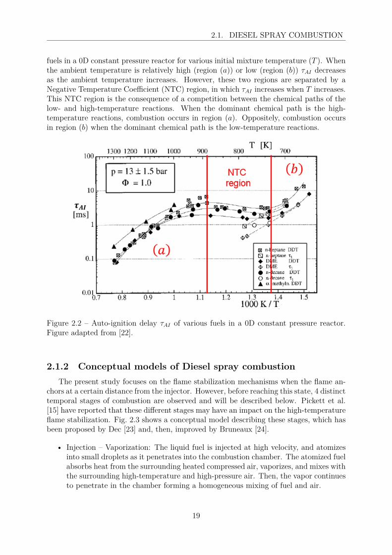
fuels in a 0D constant pressure reactor for various initial mixture temperature (T ). Whenthe ambient temperature is relatively high (region (a)) or low (region (b)) τAI decreasesas the ambient temperature increases. However, these two regions are separated by aNegative Temperature Coefficient (NTC) region, in which τAI increases when T increases.This NTC region is the consequence of a competition between the chemical paths of thelow- and high-temperature reactions. When the dominant chemical path is the high-temperature reactions, combustion occurs in region (a). Oppositely, combustion occursin region (b) when the dominant chemical path is the low-temperature reactions.
Figure 2.2 – Auto-ignition delay τAI of various fuels in a 0D constant pressure reactor.Figure adapted from [22].
2.1.2 Conceptual models of Diesel spray combustionThe present study focuses on the flame stabilization mechanisms when the flame an-
chors at a certain distance from the injector. However, before reaching this state, 4 distincttemporal stages of combustion are observed and will be described below. Pickett et al.[15] have reported that these different stages may have an impact on the high-temperatureflame stabilization. Fig. 2.3 shows a conceptual model describing these stages, which hasbeen proposed by Dec [23] and, then, improved by Bruneaux [24].
• Injection – Vaporization: The liquid fuel is injected at high velocity, and atomizesinto small droplets as it penetrates into the combustion chamber. The atomized fuelabsorbs heat from the surrounding heated compressed air, vaporizes, and mixes withthe surrounding high-temperature and high-pressure air. Then, the vapor continuesto penetrate in the chamber forming a homogeneous mixing of fuel and air.
19

2.1. DIESEL SPRAY COMBUSTION
• Premixed auto-ignition start (stage 1− Fig. 2.3-bottom): Auto-ignition appearsdownstream of the liquid jet where the fuel has been vaporized. This stage isidentified by formaldehyde pockets, as indication of fuel reaction decomposition atrelatively low temperature (cool-flame). The location of auto-ignition correspondsto fuel-rich areas of the jet where the mixture and temperature history are favorableto auto-ignition.
• Premixed auto-ignition extension (stage 1* stage 1+): During this stage, an exten-sion of formaldehyde until it reaches a homogeneous cloud is observed. Small regionsof OH are observed inside the formaldehyde cloud. OH radicals are a characteristicmarker of high temperature combustion, they have been detected by LIF measure-ments. Therefore, OH LIF detection indicates the set-up of high-temperature reac-tions: auto-ignition. Then, high temperature reactions region increases consumingthe formaldehyde.
• Transition to diffusion combustion (stage 2− and 2*): During the premixed combus-tion, a diffusion flame grows at the jet periphery. At the same time, the cool-flameis also present upstream of the flame base in a fuel rich premixed zone. Soot pre-cursors, namely Polycyclic Aromatic Hydrocarbons (PAH), are formed in the centerof the jet due to mixing of fuel rich pockets with the hot diffusion flame products.Then, formaldehyde is getting consumed at the jet periphery due to the progressionof the diffusion flame.
• Stabilized diffusion combustion (stage 2+) : The diffusion flame has now consumedall the formaldehyde at the jet periphery. In the centerline, OH radicals are con-sumed leading to the formation of high concentration of PAH and soot. Largelevel of OH is observed at the jet periphery. During this stage, there is still someformaldehyde in the centerline upstream of the LOL where the small temperaturereactions occur [24].
20

2.1. DIESEL SPRAY COMBUSTION
Figure 2.3 – Schematic of a conceptual combustion model describing from the injectionto the stabilized diffusion combustion [24].
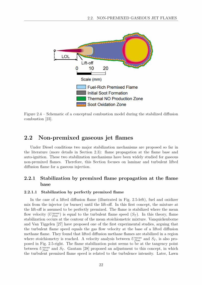
Fig. 2.4 shows a representation of the stabilized diffusion combustion characterized bya diffusion flame at the jet periphery with a rich-partially premixed area upstream of thelift-off. The lift-off is the most upstream point of the flame and the corresponding axialdistance between the injector and the flame is called the Lift-off Length (LOL). Because ofthe rich-partially premixed area upstream of the lift-off, the Diesel flames are traditionallyclassified as non-premixed flames [25] similar to those found under atmospheric conditions[26].
21
2.2. NON-PREMIXED GASEOUS JET FLAMES
Figure 2.4 – Schematic of a conceptual combustion model during the stabilized diffusioncombustion [23].
2.2 Non-premixed gaseous jet flamesUnder Diesel conditions two major stabilization mechanisms are proposed so far in
the literature (more details in Section 2.3): flame propagation at the flame base andauto-ignition. These two stabilization mechanisms have been widely studied for gaseousnon-premixed flames. Therefore, this Section focuses on laminar and turbulent lifteddiffusion flame for a gaseous injection.
2.2.1 Stabilization by premixed flame propagation at the flamebase
2.2.1.1 Stabilization by perfectly premixed flame
In the case of a lifted diffusion flame (illustrated in Fig. 2.5-left), fuel and oxidizermix from the injector (or burner) until the lift-off. In this first concept, the mixture atthe lift-off is assumed to be perfectly premixed. The flame is stabilized where the meanflow velocity (Umean
flow ) is equal to the turbulent flame speed (ST ). In this theory, flamestabilization occurs at the contour of the mean stoichiometric mixture. Vanquickenborneand Van Tiggelen [27] have proposed one of the first experimental studies, arguing thatthe turbulent flame speed equals the gas flow velocity at the base of a lifted diffusionmethane flame. They found that lifted diffusion methane flames are stabilized in a regionwhere stoichiometry is reached. A velocity analysis between Umean
flow and ST , is also pro-posed in Fig. 2.5-right. The flame stabilization point seems to be at the tangency pointbetween Umean
flow and ST . Gautam [28] proposed an adjustment to this concept, in whichthe turbulent premixed flame speed is related to the turbulence intensity. Later, Lawn
22

2.2. NON-PREMIXED GASEOUS JET FLAMES
et al. [29] have confirmed that the flame base is stabilized at an equilibrium between themean flow velocity and the turbulent flame speed.
Figure 2.5 – Hypothetical shape of premixed flame (left) and experimental verification ofthe hypothetical stabilization mechanisms. Figures adapted from [27].
These studies raised the question of the turbulent flame speed estimation. Poinsotand Veynante [25] proposed the following definition: ST is the velocity needed at the inletof a control volume to keep a turbulent flame stationary in the mean inside this volume.In practice Eq. (2.1) (from [25]) has been used to estimate ST .
ST = S0L
AT
A, (2.1)
where S0L is the laminar planar unstretched propagating flame speed. A representation
of the area A and AT is provided in Fig. 2.6 for greater clarity, where A is the area of across section of the control volume and AT is the total flame area contained in the controlvolume. The main difficulty to compute ST according to Eq. (2.1) is the prediction of theratio AT/A. Many semi-phenomenological models for ST can be found in the literature(see [30] for a review and [31, 32] for more details) but both experimental and theoreticalresults show considerable scatterings. This discrepancy may be due to measurement errorsand poor modeling according to Poinsot and Veynante [25]. According to [27], ST rangesfrom 0.9 to 5S0
L for methane flames and for a Reynolds number (Re = (ρ.u.d)/µ) varyingfrom 1900 to 7600. Numerical simulation of Kaplan [33] indicates that the axial flowvelocity at the base of methane flames (Re=12,500) ranges from 1.6 to 2.6S0
L. Thesevalues of velocity are of the same order of magnitude as the estimated ST in [27], whichtends to confirm flame stabilization as an equilibrium between turbulent flame speed andmean jet velocity.
However, Namazian et al. [34] measured the flow velocity at the flame base of a liftedmethane flame (Re=7000). They reported flow velocity at approx. 5 m/s (13SL) with apeak velocity of 15 m/s (39SL) at the lift-off, which is much higher than the turbulentflame velocity.
23

2.2. NON-PREMIXED GASEOUS JET FLAMES
Figure 2.6 – Flame wrinkling by turbulence where A and AT are displayed. Figure adaptedfrom [25].
2.2.1.2 Stabilization by partially premixed flame
In most configurations where fuel and air are injected separately, the mixing in theflame base region is not perfectly premixed. As a result, the concept developed in theabove Section cannot be applied without adaptations. In this context, triple flames(schematic representation in Fig. 2.7-top), also called edge-flames, have been proposedas one of the most convincing approaches to explain the flame stabilization of lifted dif-fusion flames when the mixture is partially premixed.
Figure 2.7 – Triple flames structure by [25] (top) and triple flames visualization in alaminar flow by [35] (bottom).
24
2.2. NON-PREMIXED GASEOUS JET FLAMES
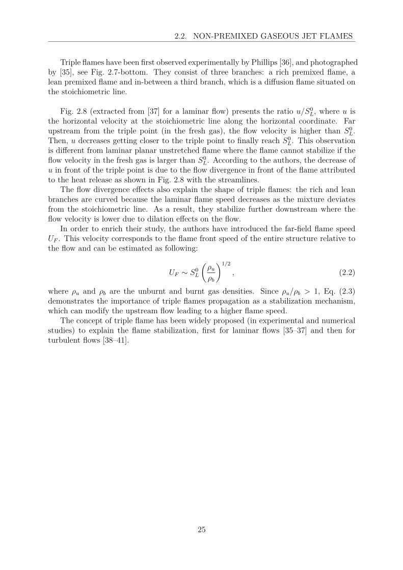
Triple flames have been first observed experimentally by Phillips [36], and photographedby [35], see Fig. 2.7-bottom. They consist of three branches: a rich premixed flame, alean premixed flame and in-between a third branch, which is a diffusion flame situated onthe stoichiometric line.
Fig. 2.8 (extracted from [37] for a laminar flow) presents the ratio u/S0L, where u is
the horizontal velocity at the stoichiometric line along the horizontal coordinate. Farupstream from the triple point (in the fresh gas), the flow velocity is higher than S0
L.Then, u decreases getting closer to the triple point to finally reach S0
L. This observationis different from laminar planar unstretched flame where the flame cannot stabilize if theflow velocity in the fresh gas is larger than S0
L. According to the authors, the decrease ofu in front of the triple point is due to the flow divergence in front of the flame attributedto the heat release as shown in Fig. 2.8 with the streamlines.
The flow divergence effects also explain the shape of triple flames: the rich and leanbranches are curved because the laminar flame speed decreases as the mixture deviatesfrom the stoichiometric line. As a result, they stabilize further downstream where theflow velocity is lower due to dilation effects on the flow.
In order to enrich their study, the authors have introduced the far-field flame speedUF . This velocity corresponds to the flame front speed of the entire structure relative tothe flow and can be estimated as following:
UF ∼ S0L
(ρuρb
)1/2
, (2.2)
where ρu and ρb are the unburnt and burnt gas densities. Since ρu/ρb > 1, Eq. (2.3)demonstrates the importance of triple flames propagation as a stabilization mechanism,which can modify the upstream flow leading to a higher flame speed.
The concept of triple flame has been widely proposed (in experimental and numericalstudies) to explain the flame stabilization, first for laminar flows [35–37] and then forturbulent flows [38–41].
25
2.2. NON-PREMIXED GASEOUS JET FLAMES
Figure 2.8 – Top: contour lines of the reaction rate showing a triple flame with streamlines. Bottom: ratio u/S0
L as a function of the axial coordinate on the stoichiometric line.Figure adapted from [37].
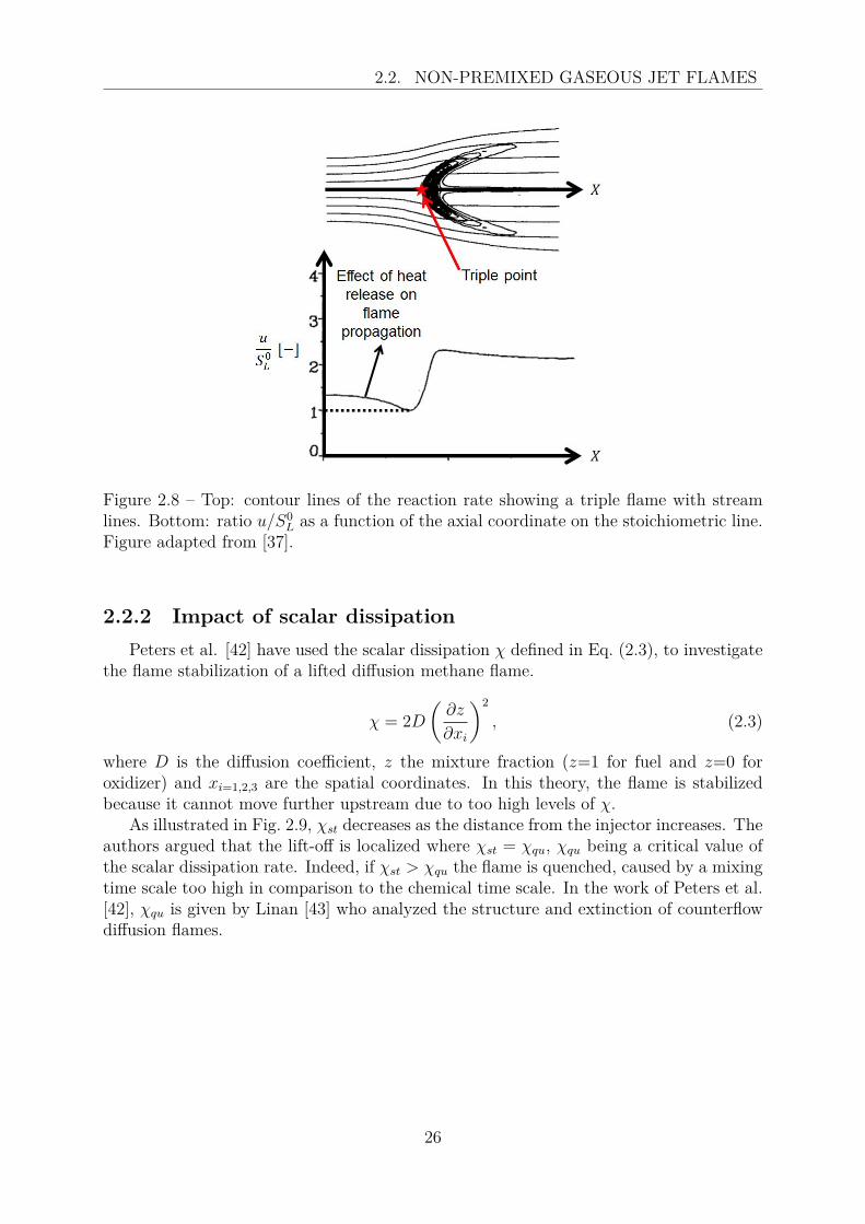
2.2.2 Impact of scalar dissipationPeters et al. [42] have used the scalar dissipation χ defined in Eq. (2.3), to investigate
the flame stabilization of a lifted diffusion methane flame.
χ = 2D
(∂z
∂xi
)2
, (2.3)
where D is the diffusion coefficient, z the mixture fraction (z=1 for fuel and z=0 foroxidizer) and xi=1,2,3 are the spatial coordinates. In this theory, the flame is stabilizedbecause it cannot move further upstream due to too high levels of χ.
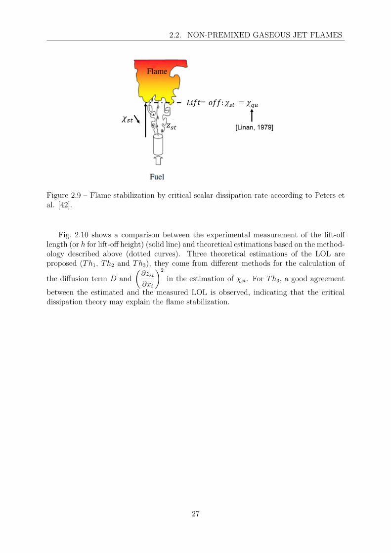
As illustrated in Fig. 2.9, χst decreases as the distance from the injector increases. Theauthors argued that the lift-off is localized where χst = χqu, χqu being a critical value ofthe scalar dissipation rate. Indeed, if χst > χqu the flame is quenched, caused by a mixingtime scale too high in comparison to the chemical time scale. In the work of Peters et al.[42], χqu is given by Linan [43] who analyzed the structure and extinction of counterflowdiffusion flames.
26
2.2. NON-PREMIXED GASEOUS JET FLAMES
Figure 2.9 – Flame stabilization by critical scalar dissipation rate according to Peters etal. [42].
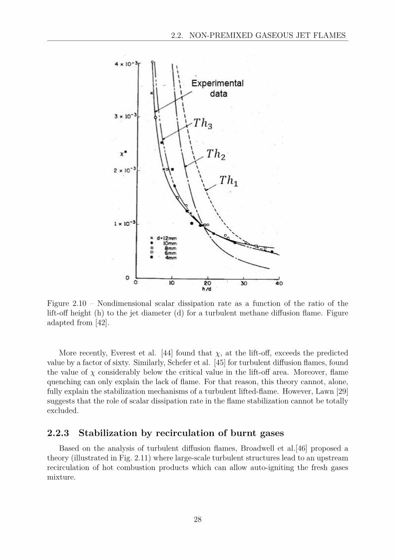
Fig. 2.10 shows a comparison between the experimental measurement of the lift-offlength (or h for lift-off height) (solid line) and theoretical estimations based on the method-ology described above (dotted curves). Three theoretical estimations of the LOL areproposed (Th1, Th2 and Th3), they come from different methods for the calculation of
the diffusion term D and(∂zst∂xi
)2
in the estimation of χst. For Th3, a good agreement
between the estimated and the measured LOL is observed, indicating that the criticaldissipation theory may explain the flame stabilization.
27
2.2. NON-PREMIXED GASEOUS JET FLAMES
Figure 2.10 – Nondimensional scalar dissipation rate as a function of the ratio of thelift-off height (h) to the jet diameter (d) for a turbulent methane diffusion flame. Figureadapted from [42].
More recently, Everest et al. [44] found that χ, at the lift-off, exceeds the predictedvalue by a factor of sixty. Similarly, Schefer et al. [45] for turbulent diffusion flames, foundthe value of χ considerably below the critical value in the lift-off area. Moreover, flamequenching can only explain the lack of flame. For that reason, this theory cannot, alone,fully explain the stabilization mechanisms of a turbulent lifted-flame. However, Lawn [29]suggests that the role of scalar dissipation rate in the flame stabilization cannot be totallyexcluded.
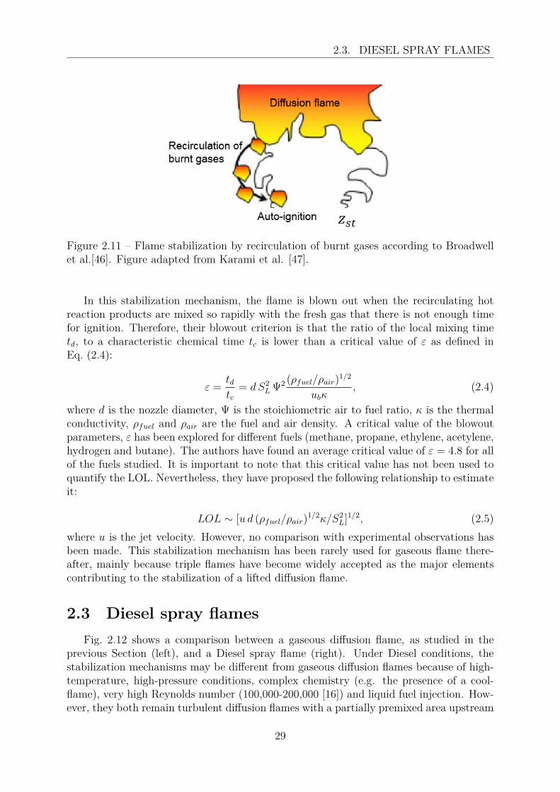
2.2.3 Stabilization by recirculation of burnt gasesBased on the analysis of turbulent diffusion flames, Broadwell et al.[46] proposed a
theory (illustrated in Fig. 2.11) where large-scale turbulent structures lead to an upstreamrecirculation of hot combustion products which can allow auto-igniting the fresh gasesmixture.
28
2.3. DIESEL SPRAY FLAMES
Figure 2.11 – Flame stabilization by recirculation of burnt gases according to Broadwellet al.[46]. Figure adapted from Karami et al. [47].
In this stabilization mechanism, the flame is blown out when the recirculating hotreaction products are mixed so rapidly with the fresh gas that there is not enough timefor ignition. Therefore, their blowout criterion is that the ratio of the local mixing timetd, to a characteristic chemical time tc is lower than a critical value of ε as defined inEq. (2.4):
ε =tdtc
= dS2LΨ
2 (ρfuel/ρair)1/2
ubκ, (2.4)
where d is the nozzle diameter, Ψ is the stoichiometric air to fuel ratio, κ is the thermalconductivity, ρfuel and ρair are the fuel and air density. A critical value of the blowoutparameters, ε has been explored for different fuels (methane, propane, ethylene, acetylene,hydrogen and butane). The authors have found an average critical value of ε = 4.8 for allof the fuels studied. It is important to note that this critical value has not been used toquantify the LOL. Nevertheless, they have proposed the following relationship to estimateit:
LOL ∼ [u d (ρfuel/ρair)1/2κ/S2
L]1/2, (2.5)
where u is the jet velocity. However, no comparison with experimental observations hasbeen made. This stabilization mechanism has been rarely used for gaseous flame there-after, mainly because triple flames have become widely accepted as the major elementscontributing to the stabilization of a lifted diffusion flame.
2.3 Diesel spray flamesFig. 2.12 shows a comparison between a gaseous diffusion flame, as studied in the
previous Section (left), and a Diesel spray flame (right). Under Diesel conditions, thestabilization mechanisms may be different from gaseous diffusion flames because of high-temperature, high-pressure conditions, complex chemistry (e.g. the presence of a cool-flame), very high Reynolds number (100,000-200,000 [16]) and liquid fuel injection. How-ever, they both remain turbulent diffusion flames with a partially premixed area upstream
29
2.3. DIESEL SPRAY FLAMES
the lift-off. Thus, some of the previous stabilization mechanisms may be also involved inthe diesel combustion.
Figure 2.12 – Illustration of a turbulent gaseous diffusion flame (left) and a Diesel sprayflame (right).
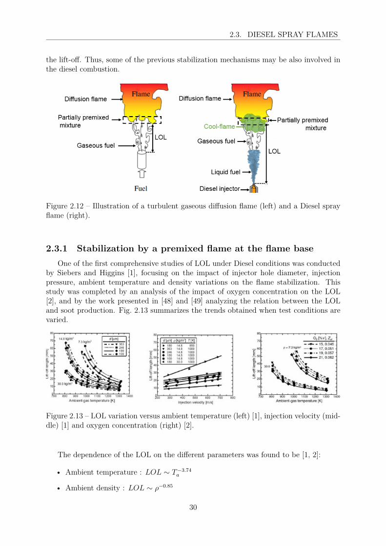
2.3.1 Stabilization by a premixed flame at the flame baseOne of the first comprehensive studies of LOL under Diesel conditions was conducted
by Siebers and Higgins [1], focusing on the impact of injector hole diameter, injectionpressure, ambient temperature and density variations on the flame stabilization. Thisstudy was completed by an analysis of the impact of oxygen concentration on the LOL[2], and by the work presented in [48] and [49] analyzing the relation between the LOLand soot production. Fig. 2.13 summarizes the trends obtained when test conditions arevaried.
Figure 2.13 – LOL variation versus ambient temperature (left) [1], injection velocity (mid-dle) [1] and oxygen concentration (right) [2].
The dependence of the LOL on the different parameters was found to be [1, 2]:
• Ambient temperature : LOL ∼ T−3.74a
• Ambient density : LOL ∼ ρ−0.85
30

2.3. DIESEL SPRAY FLAMES
• Diameter of the injector hole : LOL ∼ d0.34
• Dioxygen concentration (proportional to zst [2]) : LOL ∼ z−1st
• Injection velocity : LOL ∼ U0
Combining these dependencies, Siebers, Higgins and Pickett [1, 2] proposed an experi-mental correlation which predicts the time-averaged LOL when the flame is stabilized:
LOL ∼ U0T−3.74a ρ−0.85d0.34z−1
st . (2.6)
Siebers et al. [2] have, then, compared the experimental correlation (Eq. 2.6) to thefollowing relationship:
LOL ∼ U0κ
S2L(zst)
zst, (2.7)
which has been proposed by Peters [50] assuming a flame stabilization based on premixedflame propagation as detailed in Section 2.2.1.1. In Eq. 2.7, κ is the thermic diffusivityand SL(zst) is the laminar flame speed at stoichiometry. The similarities and differencesbetween the predictions by Eq. 2.6 and Eq. 2.7 can be summarized as follows:
• Temperature effect: In Eq. 2.7, two parameters are function of temperature: thethermal diffusivity κ and the laminar flame speed SL(zst). Metghalchi and Keck[51] have proposed the following relation to predict the flame speed as a function oftemperature and pressure:
SL ∼ T aP b. (2.8)
Higgins and Siebers [52] have chosen the value of a and b for gasoline (a = 2.1 andb = −0.36). According to [53], a and b should not change with Diesel. Using Eq. 2.8along an iso-density profile (constant pressure) gives:
SL ∼ T 2.1. (2.9)
Moreover, the thermal diffusivity of a gas increases with the square root of thetemperature:
κ ∼ T 0.5. (2.10)
Injecting Eq. 2.9 and Eq. 2.10 in Eq. 2.7, we obtain:
LOL ∼ κ
S2L(Zst)
∼ T 0.5
T 2.1∗2 ∼ T−3.7. (2.11)
Eq. 2.11 shows that the temperature dependence between the theoretical (T−3.7)formulation and the experimental correlation (T−3.74) is in excellent agreement.
31

2.3. DIESEL SPRAY FLAMES
• Density effect: Following the same logic than for ambient temperature, Eq. 2.7can be written as a function of density assuming the thermal diffusivity κ is inverselyproportional to density and SL ∼ ρ−0.2
a according to [54]:
LOL ∼ κ
S2L(zst)
=ρ−1
ρ−0.2∗2 = ρ−0.6a . (2.12)
This relation is different from the experimental correlation (LOL ∼ ρ−0.85a ), but it
is without taking into account the spreading angle of the spray which depends onthe ambient density [55]. After correction of the vapor angle, the new correlationbinding LOL and density is:
LOL ∼ ρ−0.8a , (2.13)
which is very close from the experimental measurement (LOL ∼ ρ−0.85a ) according
to [2].
• Diameter of the injector hole: Eq. 2.7 does not take into account the diameterof the injector hole, whereas it has been experimentally observed that it has animpact on the lift-off stabilization (proportional to d0.34). According to [52], thisweak dependency can be explained by the fact that Eq. 2.6 is obtained from a flamespray while Eq. 2.7 is proposed for a gaseous jet flame.
• Dioxygen concentration effect: Dugger et al. [56] proposed that the laminarflame speed is proportional to the dioxygen concentration. Thus, only consideringthe dioxygen concentration, Eq. 2.7 can be expressed as follows:
LOL ∼ zstS2L(zst)
∼ zst
z−2st
= z−1st , (2.14)
Therefore, Eq. 2.14 presents the same proportionality relation than Eq. 2.6 varyingdioxygen concentration.
• Injection velocity effect: Eq. 2.7 presents a linear dependence of the LOL withthe injection velocity. This dependence has been validated by experiments as shownin Fig. 2.13.
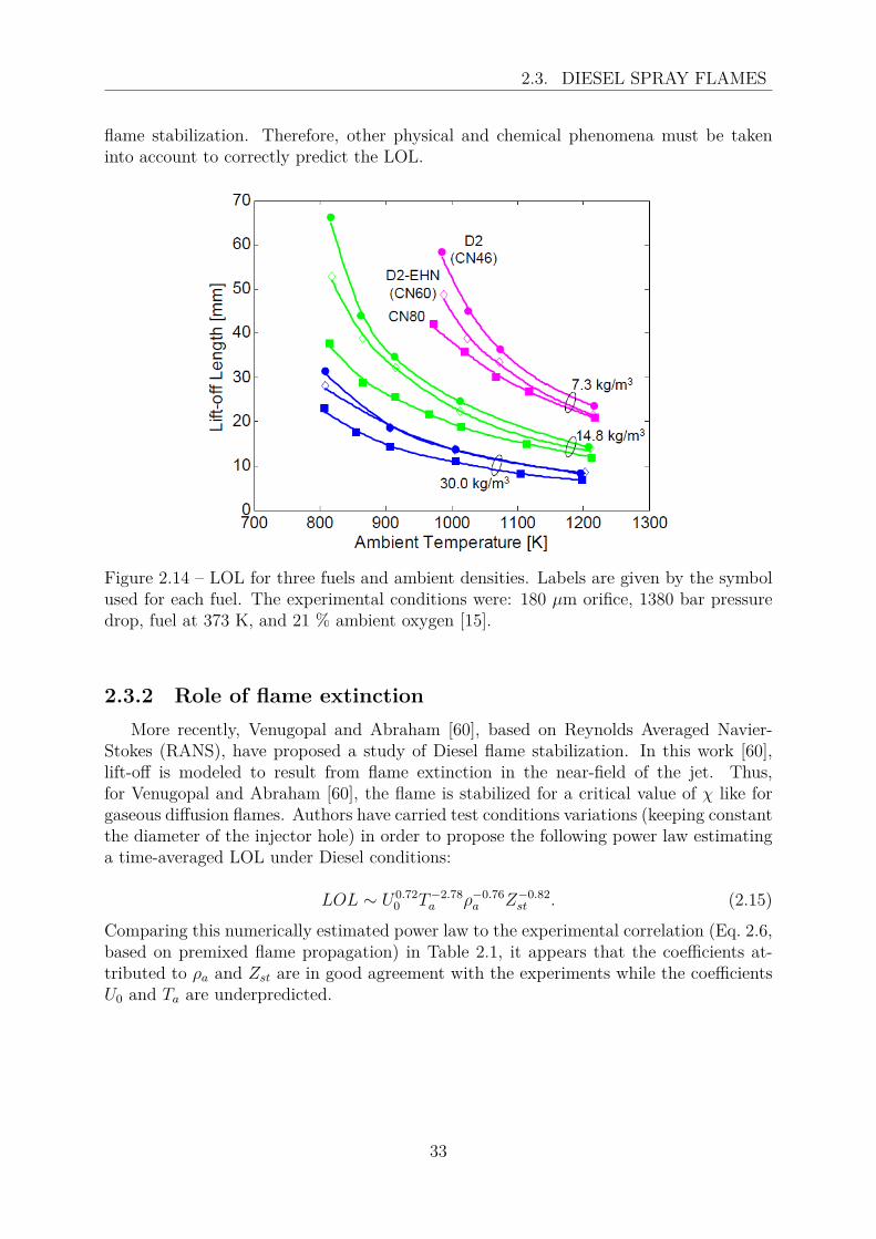
The experimental correlation (Eq. 2.6) seems to be in good agreement with the theory.However, other experiments performed at Sandia [15, 57–59] seem to indicate the limitof this theory: Fig. 2.14 shows the time-averaged LOL of Diesel-type spray flame as afunction of the ambient temperature for different fuels (with different Cetane numbers,42, 60 and 80). It clearly shows some significant differences of the LOL varying the fuel,especially for low temperature conditions. This strong dependence of the fuel type onthe prediction of the LOL was not expected in Eq. 2.7. This lack of prediction highlightsthe fact that Eq. 2.7, based on premixed flame propagation does not fully explain the
32
2.3. DIESEL SPRAY FLAMES
flame stabilization. Therefore, other physical and chemical phenomena must be takeninto account to correctly predict the LOL.
Figure 2.14 – LOL for three fuels and ambient densities. Labels are given by the symbolused for each fuel. The experimental conditions were: 180 µm orifice, 1380 bar pressuredrop, fuel at 373 K, and 21 % ambient oxygen [15].
2.3.2 Role of flame extinctionMore recently, Venugopal and Abraham [60], based on Reynolds Averaged Navier-
Stokes (RANS), have proposed a study of Diesel flame stabilization. In this work [60],lift-off is modeled to result from flame extinction in the near-field of the jet. Thus,for Venugopal and Abraham [60], the flame is stabilized for a critical value of χ like forgaseous diffusion flames. Authors have carried test conditions variations (keeping constantthe diameter of the injector hole) in order to propose the following power law estimatinga time-averaged LOL under Diesel conditions:
LOL ∼ U0.720 T−2.78
a ρ−0.76a Z−0.82
st . (2.15)
Comparing this numerically estimated power law to the experimental correlation (Eq. 2.6,based on premixed flame propagation) in Table 2.1, it appears that the coefficients at-tributed to ρa and Zst are in good agreement with the experiments while the coefficientsU0 and Ta are underpredicted.
33

2.3. DIESEL SPRAY FLAMES
Table 2.1 – Comparison of the coefficients predicting the time-averaged LOL betweenexperiments and simulations (RANS). The experiments assumed a flame stabilization bypremixed flame at the flame base while the RANS estimated the LOL by flame extinction.
LOL ∼ Ua0 T b
a ρca dd Zest
a b c d eSiebers et al. [2] (experiments) 1 -3.74 -0.85 0.34 -1Venugopal and Abraham [60] (RANS) 0.72 -2.78 -0.76 not addressed -0.82
In conclusion, Venugopal and Abraham [60] argued that the flame seems to stabilizein the region where the local scalar dissipation reaches a critical extinction value, sincethe coefficients of the power law found by the authors (last line Table 2.1) are fairly closeto the experimental coefficients (penultimate line Table 2.1). However, the authors alsostated that it would be inappropriated to conclude that, locally, high scalar dissipationrates are the only factor explaining the flame stabilization.
2.3.3 Role of auto-ignitionPauls et al. [61] have proposed an experimental and numerical study to evaluate the
relative importance of auto-ignition and flame propagation in the stabilization of differentDiesel fuels and ambient test conditions. The measurements have been performed by OHchemiluminescence. The Unsteady Reynolds Averaged Navier-Stokes-URANS approachwas chosen for the numerical study. The URANS were run using G-equation coupledwith the Multiple Representative Interactive Flamelet (G-MRIF model described in [61])which predicts both auto-ignition and flame propagation. The combination of these twotechniques allowed the authors to propose a new concept illustrated in Fig. 2.15.
Figure 2.15 – Stabilization of the flame-front by auto-ignition and flame propagation [61].
Between t0 and t1, the flame is convected downstream due to the high flow velocity.Because of relatively slow flame propagation speed (compared to the jet velocity), a slowdownstream drift of the flame can be observed (also named as a downstream propagation).At t2, a separated ignition-spot occurs. Fig. 2.16 shows a visualization of such event for
34

2.3. DIESEL SPRAY FLAMES
a bio-Diesel spray flame (see proprieties of the fuel in Table of [61]). At t3, the separatedignition-spot merges the main flame creating a new flame front, which is then convecteddownstream until a new auto-ignition occurs.
For the authors, the main flame stabilization mechanism is auto-ignition. Nevertheless,flame propagation is also playing a (minor) role in the downstream propagation.
Figure 2.16 – Typical OH chemiluminescence single-shot showing a separated ignitionspot [61].
Pickett et al. [15] have investigated the effect of cool-flame on the Diesel-type flamestabilization. Fig. 2.17 shows the cool-flame shortly before the auto-ignition delay and thecorresponding LOL, for different fuels. It appears that a fuel leading to a short distancebetween the injector and the cool-flame base leads to a short LOL, or vice versa. Thus,the authors argued that the location of the cool-flame has some bearings on the flamestabilization. Many studies have focused on the interactions between the cool- and thehigh-temperature flame [18, 62–66]. However, to the best of our knowledge, no studieshave clearly shown how the cool-flame can help the high-temperature flame to stabilize.Therefore, the importance of the cool-flame upstream the high-temperature flame will beinvestigated in Chapter 4.
35

2.3. DIESEL SPRAY FLAMES
Figure 2.17 – Cool-flame chemiluminescence images shortly before auto-ignition. The fuelis given on the lower left corner and on the right side the auto-ignition delay is displayed.Quasi-steady LOL is shown as a vertical dashed white line [15].
2.3.4 Combined role of edge-flames and auto-ignitionSince 2015, with the work of Krisman et al. [67], many DNS have shown the presence
of edge-flames under Diesel conditions, which plays a role in the flame stabilization. DNSallow to resolve all space and time scales of the turbulent flow, mixing and chemical reac-tions without any simplifying assumption on the interactions between flow and chemicalreactions. However, because of the prohibitive computational cost of performing 3D-DNSof the full spray flame (mesh resolution in the range of few micrometers due to very fineflame thickness), simplified DNS (detailed in the four sub-sections below) have been runto analyze the interactions between edge-flames and auto-ignition:
• 2D-DNS of a spatially stabilized flame in a laminar mixing layer
• 2D-DNS of a temporally evolving mixing layer subject to decaying isotropic turbu-lence
• 2D and 3D-DNS of a temporally evolving turbulent mixing layer where ignitiontakes place in a reference frame traveling at the mean speed of the two streams
• 3D-DNS of a spatially developing gaseous slot jet flame
2.3.4.1 2D-DNS of a laminar mixing layer
Krisman et al. [67] have performed a 2D-DNS under near-diesel conditions. The do-main was initialized with a mixing layer between a pure oxidizer (air) and a pure fuel(DME) according to a hyperbolic tangent profile at a pressure of 40 atmospheres. Afixed uniform velocity is imposed in the x direction (see Fig. 2.18), while the transverse
36

2.3. DIESEL SPRAY FLAMES
velocity, in the y direction, is set to zero. The composition and temperature inlet profilesare convected at uniform velocity UX . This study has been conducted with a reducedmechanism including 30 species, taking into account auto-ignition, cool-flame chemistryand NTC. They have simulated different test conditions (different oxidizer temperaturesand flow velocities) to analyze the flame stabilization mechanisms.
Fig. 2.18 shows the heat-release rate for the different test conditions. The stabilizationmechanism was found to be temperature dependent:
• For ambient oxidizer temperature at 700 K, we can recognize a triple flame shape.In this case, the flame is stabilized where the flow velocity is equal to the tripleflame displacement speed.
• At 900 K, in addition to the main triple flame, there is an upstream fourth branchdue to the low-temperature chemistry. This leads to call this flame a quadrupleflame. However, even with this extra branch, the authors argued that the flame isstabilized by premixed flame propagation.
• At 1100 and 1300 K, the flame keeps the same structure downstream but, upstream,there are two more branches (due to low-temperature chemistry), leading to call thisflame a quintuple flame. In these cases, the flames are stabilized by auto-ignition.
• At 1500 K, the flame reverts to a quadruple flame stabilized by auto-ignition.
Figure 2.18 – The color shows the edge-flames through heat release rate fields, the solidline indicates the zst contour, the star marker indicates the flame base position and thesquare marker indicates the closer distance to the injector of the cool-flame [67].
Following the same methodology than proposed by Krisman et al. [67], Deng et al.[68, 69] have also simulated a 2D-DNS of a laminar mixing layer using DME as fuel. They
37

2.3. DIESEL SPRAY FLAMES
have varied the oxidizer (air) temperature between 700 and 1100 K [68], then, in [69] theyhave varied the uniform inlet flow velocities between 2.4 and 8 m/s. In both cases ([68]and [69]), the ambient pressure was 30 atmospheres. The same flame structures thanobserved in [67] were found.
The authors [68, 69] proposed a qualitative regime diagram for the flame stabilizationmechanisms as the boundary temperature and the inlet velocity vary (Fig. 2.19) based on aChemical Explosive Mode Analysis (CEMA) [70, 71], (briefly described in Appendix A.1)and on a Lagrangian Flamelet Analysis (LFA) (described in [72]).
Figure 2.19 – Qualitative regime diagram for the stabilization mechanisms as the boundarytemperature and inlet velocity vary. The left cartoon is a zoom of a flame topology duringthe ”kinetic” stabilization mode while the right cartoon shows an edge-flame during the”multi-mode” stabilization. The meaning of the acronyms is: RB: Rich Branch, LB: LeanBranch, RPF: Rich Premixed Flame, LPF: Lean Premixed Flame, NPF: Non-PremixedFlame. Figure adapted from [69].
Fig. 2.19 is described following the vertical arrow in the middle of the figure from αto δ:
• α: When the inlet flow velocity is below a certain threshold value, the flame isattached to the burner in both autoignitive and non-autoignitive conditions (notedas α).
• β: Increasing the inlet velocity while keeping constant the boundary temperature,the flame stabilization mechanism transits from a burner stabilization to a kinematicbalance between flame speed and incoming flow velocity.
• γ: Then, a multi-mode stabilization is observed, where the flame is stabilized byboth flame propagation and auto-ignition as reported in [67].
38
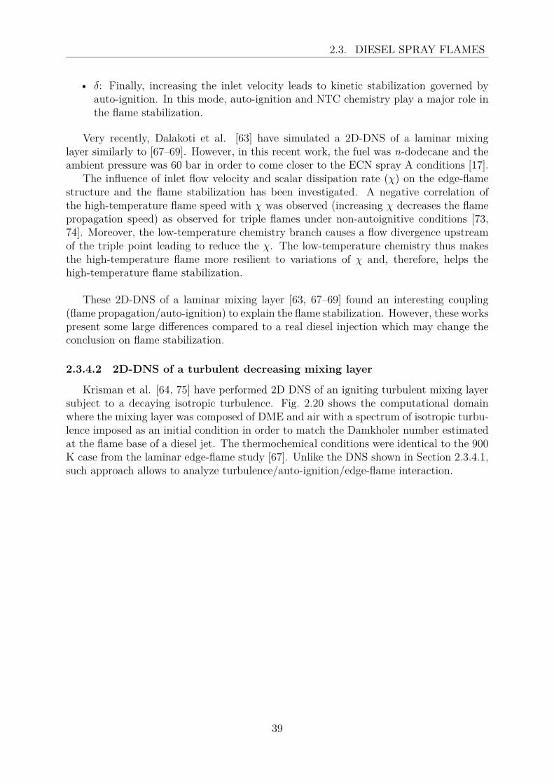
2.3. DIESEL SPRAY FLAMES
• δ: Finally, increasing the inlet velocity leads to kinetic stabilization governed byauto-ignition. In this mode, auto-ignition and NTC chemistry play a major role inthe flame stabilization.
Very recently, Dalakoti et al. [63] have simulated a 2D-DNS of a laminar mixinglayer similarly to [67–69]. However, in this recent work, the fuel was n-dodecane and theambient pressure was 60 bar in order to come closer to the ECN spray A conditions [17].
The influence of inlet flow velocity and scalar dissipation rate (χ) on the edge-flamestructure and the flame stabilization has been investigated. A negative correlation ofthe high-temperature flame speed with χ was observed (increasing χ decreases the flamepropagation speed) as observed for triple flames under non-autoignitive conditions [73,74]. Moreover, the low-temperature chemistry branch causes a flow divergence upstreamof the triple point leading to reduce the χ. The low-temperature chemistry thus makesthe high-temperature flame more resilient to variations of χ and, therefore, helps thehigh-temperature flame stabilization.
These 2D-DNS of a laminar mixing layer [63, 67–69] found an interesting coupling(flame propagation/auto-ignition) to explain the flame stabilization. However, these workspresent some large differences compared to a real diesel injection which may change theconclusion on flame stabilization.
2.3.4.2 2D-DNS of a turbulent decreasing mixing layer
Krisman et al. [64, 75] have performed 2D DNS of an igniting turbulent mixing layersubject to a decaying isotropic turbulence. Fig. 2.20 shows the computational domainwhere the mixing layer was composed of DME and air with a spectrum of isotropic turbu-lence imposed as an initial condition in order to match the Damkholer number estimatedat the flame base of a diesel jet. The thermochemical conditions were identical to the 900K case from the laminar edge-flame study [67]. Unlike the DNS shown in Section 2.3.4.1,such approach allows to analyze turbulence/auto-ignition/edge-flame interaction.
39

2.3. DIESEL SPRAY FLAMES
Figure 2.20 – ”Initial domain configuration. Black shading patern shows high vorticityregions. Grey/blue shading in top of figure represents the fuel and the white shading inthe bottom represents the oxidiser.” [65].
Fig. 2.21 shows heat release rate fields at different instants: t∗ = t/τmr, where t is thetime and τMR is the ignition delay of the most reactive mixture fraction. For t∗ = 1.2, theauthors [75] show an auto-ignition kernel close to the stoichiometric line. At t∗ = 1.4, thiskernel has created two edge-flames propagating in opposite directions. This observation,added to previous studies in laminar configurations, shows a temporal transition betweenauto-ignition and edge-flame propagation.
Figure 2.21 – Heat release rate for a fixed window in the domain. The dashed line is zst.Figure adapted from [75].
2.3.4.3 DNS of a temporally evolving turbulent mixing layer
More recent studies [18, 65] have investigated turbulence/auto-ignition/edge-flameinteractions through temporally evolving planar jet (computational domain illustratedin Fig. 2.22). As a first step [65] used n-heptane as fuel with a chemistry model whichdid not take into account the NTC. Then, in [18], used n-dodecane with a 35-speciesreduced mechanism which included both low- and high- temperature reaction pathways.In [18, 65], a deeper analysis of the edge-flame speed, χ and the classification of Dieselcombustion modes is proposed. They found that the propagation speed of the edge-flamesin regions with low χ ranges between 1.9 SL and 3.4 SL. An analysis of χ shows that
40
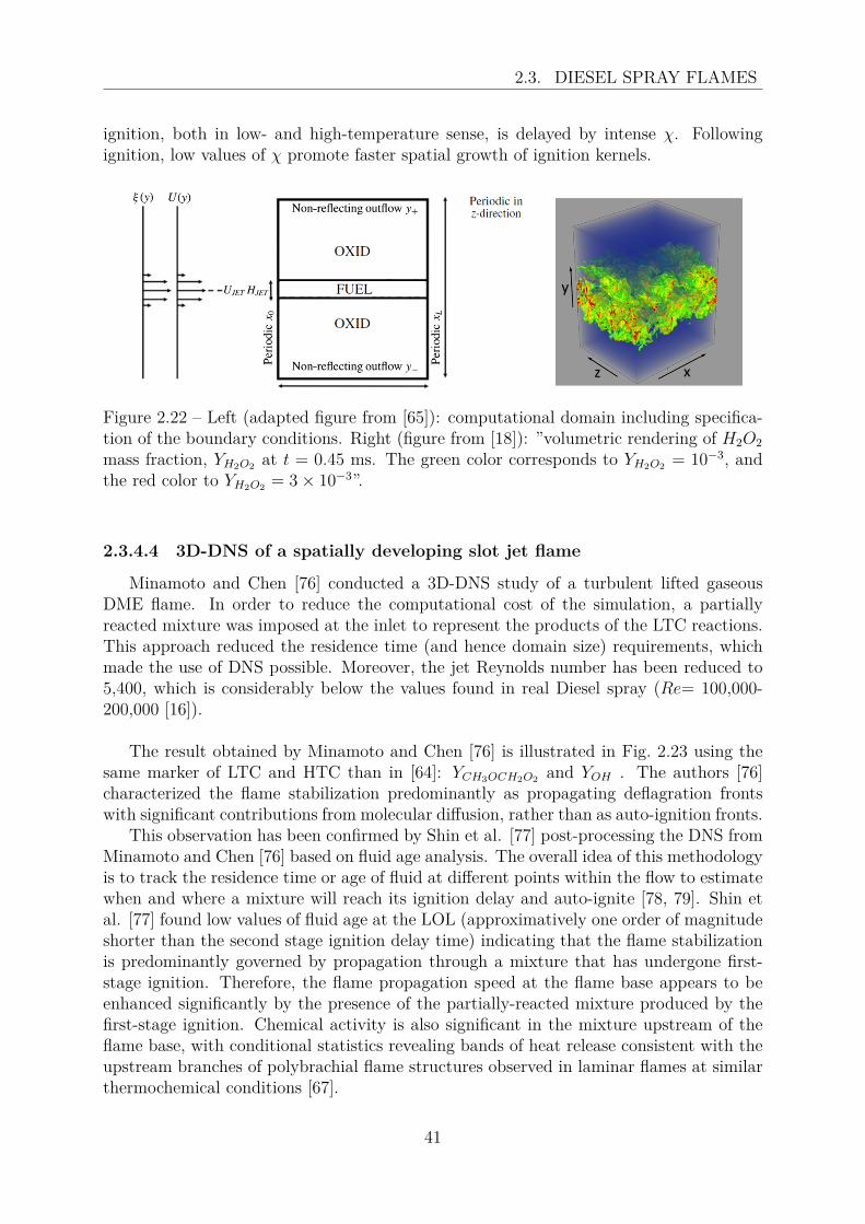
2.3. DIESEL SPRAY FLAMES
ignition, both in low- and high-temperature sense, is delayed by intense χ. Followingignition, low values of χ promote faster spatial growth of ignition kernels.
Figure 2.22 – Left (adapted figure from [65]): computational domain including specifica-tion of the boundary conditions. Right (figure from [18]): ”volumetric rendering of H2O2
mass fraction, YH2O2 at t = 0.45 ms. The green color corresponds to YH2O2 = 10−3, andthe red color to YH2O2 = 3× 10⁻³”.
2.3.4.4 3D-DNS of a spatially developing slot jet flame
Minamoto and Chen [76] conducted a 3D-DNS study of a turbulent lifted gaseousDME flame. In order to reduce the computational cost of the simulation, a partiallyreacted mixture was imposed at the inlet to represent the products of the LTC reactions.This approach reduced the residence time (and hence domain size) requirements, whichmade the use of DNS possible. Moreover, the jet Reynolds number has been reduced to5,400, which is considerably below the values found in real Diesel spray (Re= 100,000-200,000 [16]).
The result obtained by Minamoto and Chen [76] is illustrated in Fig. 2.23 using thesame marker of LTC and HTC than in [64]: YCH3OCH2O2 and YOH . The authors [76]characterized the flame stabilization predominantly as propagating deflagration frontswith significant contributions from molecular diffusion, rather than as auto-ignition fronts.
This observation has been confirmed by Shin et al. [77] post-processing the DNS fromMinamoto and Chen [76] based on fluid age analysis. The overall idea of this methodologyis to track the residence time or age of fluid at different points within the flow to estimatewhen and where a mixture will reach its ignition delay and auto-ignite [78, 79]. Shin etal. [77] found low values of fluid age at the LOL (approximatively one order of magnitudeshorter than the second stage ignition delay time) indicating that the flame stabilizationis predominantly governed by propagation through a mixture that has undergone first-stage ignition. Therefore, the flame propagation speed at the flame base appears to beenhanced significantly by the presence of the partially-reacted mixture produced by thefirst-stage ignition. Chemical activity is also significant in the mixture upstream of theflame base, with conditional statistics revealing bands of heat release consistent with theupstream branches of polybrachial flame structures observed in laminar flames at similarthermochemical conditions [67].
41
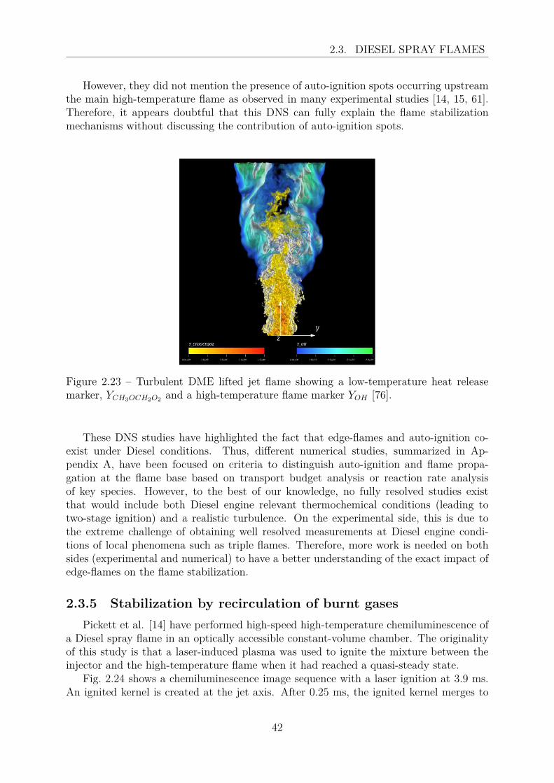
2.3. DIESEL SPRAY FLAMES
However, they did not mention the presence of auto-ignition spots occurring upstreamthe main high-temperature flame as observed in many experimental studies [14, 15, 61].Therefore, it appears doubtful that this DNS can fully explain the flame stabilizationmechanisms without discussing the contribution of auto-ignition spots.
Figure 2.23 – Turbulent DME lifted jet flame showing a low-temperature heat releasemarker, YCH3OCH2O2 and a high-temperature flame marker YOH [76].
These DNS studies have highlighted the fact that edge-flames and auto-ignition co-exist under Diesel conditions. Thus, different numerical studies, summarized in Ap-pendix A, have been focused on criteria to distinguish auto-ignition and flame propa-gation at the flame base based on transport budget analysis or reaction rate analysisof key species. However, to the best of our knowledge, no fully resolved studies existthat would include both Diesel engine relevant thermochemical conditions (leading totwo-stage ignition) and a realistic turbulence. On the experimental side, this is due tothe extreme challenge of obtaining well resolved measurements at Diesel engine condi-tions of local phenomena such as triple flames. Therefore, more work is needed on bothsides (experimental and numerical) to have a better understanding of the exact impact ofedge-flames on the flame stabilization.
2.3.5 Stabilization by recirculation of burnt gasesPickett et al. [14] have performed high-speed high-temperature chemiluminescence of
a Diesel spray flame in an optically accessible constant-volume chamber. The originalityof this study is that a laser-induced plasma was used to ignite the mixture between theinjector and the high-temperature flame when it had reached a quasi-steady state.
Fig. 2.24 shows a chemiluminescence image sequence with a laser ignition at 3.9 ms.An ignited kernel is created at the jet axis. After 0.25 ms, the ignited kernel merges to
42
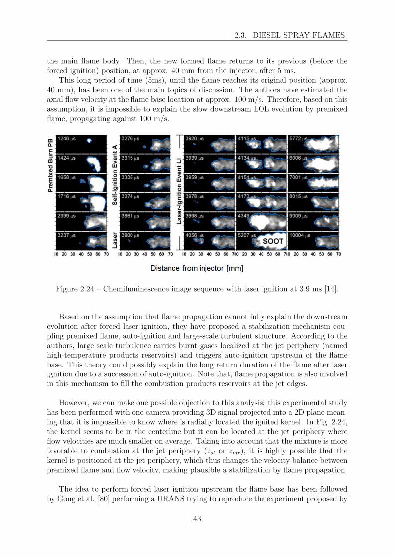
2.3. DIESEL SPRAY FLAMES
the main flame body. Then, the new formed flame returns to its previous (before theforced ignition) position, at approx. 40 mm from the injector, after 5 ms.
This long period of time (5ms), until the flame reaches its original position (approx.40 mm), has been one of the main topics of discussion. The authors have estimated theaxial flow velocity at the flame base location at approx. 100 m/s. Therefore, based on thisassumption, it is impossible to explain the slow downstream LOL evolution by premixedflame, propagating against 100 m/s.
Figure 2.24 – Chemiluminescence image sequence with laser ignition at 3.9 ms [14].
Based on the assumption that flame propagation cannot fully explain the downstreamevolution after forced laser ignition, they have proposed a stabilization mechanism cou-pling premixed flame, auto-ignition and large-scale turbulent structure. According to theauthors, large scale turbulence carries burnt gases localized at the jet periphery (namedhigh-temperature products reservoirs) and triggers auto-ignition upstream of the flamebase. This theory could possibly explain the long return duration of the flame after laserignition due to a succession of auto-ignition. Note that, flame propagation is also involvedin this mechanism to fill the combustion products reservoirs at the jet edges.
However, we can make one possible objection to this analysis: this experimental studyhas been performed with one camera providing 3D signal projected into a 2D plane mean-ing that it is impossible to know where is radially located the ignited kernel. In Fig. 2.24,the kernel seems to be in the centerline but it can be located at the jet periphery whereflow velocities are much smaller on average. Taking into account that the mixture is morefavorable to combustion at the jet periphery (zst or zmr), it is highly possible that thekernel is positioned at the jet periphery, which thus changes the velocity balance betweenpremixed flame and flow velocity, making plausible a stabilization by flame propagation.
The idea to perform forced laser ignition upstream the flame base has been followedby Gong et al. [80] performing a URANS trying to reproduce the experiment proposed by
43

2.4. CONCLUSION
Pickett et al. [15]. In order to investigate the stabilization mechanisms, they studied thebudget term of the diffusion transport term and the reaction rate term in the transportequation for the mass fraction of CO2. This methodology is described in Appendix A.1.Gong et al. [80] argued that the displacement speed of the reaction front was smallerbut comparable to the local jet velocity which is consistent with a stabilization by flamepropagation. Thus, for the authors [80], the dominant flame stabilization mechanism afterforced ignition is flame propagation which is different from the conclusion of Pickett etal. [14]. It is important to note that for Gong et al. [80] the stabilization mechanismwithout forced ignition is due to auto-ignition like agreed in [14, 15, 61, 67].
2.4 ConclusionThe flame stabilization mechanisms of gaseous turbulent diffusion flames have been
widely discussed for the past four decades. Different theories have been proposed to ex-plain flame stabilization based on experimental and numerical studies and are summarizedin review articles [29, 40, 47, 81]. Triple flames have become widely accepted as the mainelements contributing to the stabilization of lifted diffusion flames.
Under Diesel conditions, no single stabilization mechanism could be identified. How-ever, because of the diffusion flame structure of a Diesel flame with partially premixedmixture upstream the flame base, the stabilization mechanisms for gas jets have been usedas a starting point to propose new flame stabilization mechanisms. Fig. 2.25 proposes asummary of the five possible flame stabilization mechanisms identified in the literature.
44

2.4. CONCLUSION
Figure 2.25 – Schematic of a lifted spray flame under Diesel conditions (center), anddifferent theories for the stabilization. Authors, associated to the flame stabilization the-ories, are noted in bold character above the illustrations. The flame cartoons are adaptedfrom [47], which have been originally used to illustrate the stabilization mechanisms ofatmospheric lifted diffusion flame.
• Stabilization by premixed flame propagation (Section 2.3.1): the Lift-Off-Length (LOL) is defined by an equilibrium between turbulent flame speed and localflow velocity.
• Stabilization by critical scalar dissipation (Section 2.3.2): the flame is sta-bilized because it cannot move further upstream due to a too high level of scalardissipation rate (i.e. too high species gradients).
• Stabilization by auto-ignition (Section 2.3.3): an auto-ignition kernel appearsupstream the main flame. The upstream part of this kernel stays stable, while thedownstream part propagates toward the main flame (localized further downstream).The large flame resulting from this merging is stabilized further upstream, comparedto before the auto-ignition. Because the flow velocity is very high at the flame base,it is convected until another auto-ignition occurs.
• Stabilization by edge-flame (Section 2.3.4): similarly to gaseous lifted diffu-sion flames, edge-flames stabilize the Diesel spray flame where the local flow ve-locity equals the edge-flame displacement speed. Unlike edge-flames under non-autoignitive conditions, they have other branches due to the high reactivity of themixture upstream the triple point. However, it is still unclear how these extrabranches affect the edge-flames.
• Stabilization by recirculation of burnt gases (Section 2.3.5): pockets of hot
45

2.4. CONCLUSION
burnt products are recirculated upstream and ignite the fuel/air mixture. In thistheory, premixed flame helps to generate hot burnt products.
Many experimental and numerical studies have been performed allowing to identifythese different stabilization mechanisms. As argued by Venugopal and Abraham [16],the answer is most likely a combination of the theories proposed in Fig. 2.25. However,since 2007 almost all the works published identify edge-flames (based on DNS) or auto-ignition (mainly driven by experimental observations) as having a major impact in theflame stabilization. Therefore, considering the complexity of this problematic, we proposeto combine elements from optical diagnostics and DNS in order to quantify the relativeimportance of each stabilization mechanism.
46
Chapter 3
Experimental study of thestabilization mechanisms of a liftedDiesel-type flame using opticaldiagnostics and laser plasma ignition
Based on the extensive experience acquired at IFPEN, Sandia and other laboratorieson the flow and combustion of Diesel-type spray in a constant volume vessel, we firstpropose an experimental study to investigate the flame stabilization mechanisms.
Section 3.2, first presents a sophisticated setup allowing simultaneous and time-resolvedoptical measurement of the cool- and high-temperature flame base dynamic. Additionally,forced laser ignition is performed upstream the flame base in order to observe the flamedynamic when it returns to a more stable position downstream as proposed in [14]. InSection 3.3, an analysis of the coo-flame and the LOL is proposed for a long injection du-ration (10 ms), as a first step without laser ignition and in a second step with laser ignition.
This experimental study is presented here as an adapted version for the thesis manuscriptof an article entitled ”Experimental study of the stabilization mechanisms of a liftedDiesel-type flame using combined optical diagnostics and laser-induced plasma ignition”,published in the journal Combustion and Flame [82]. The abstract, present in the orig-inal paper, is removed and the introduction has been modified to avoid repetitions withChapter 2.
3.1 Brief introductionDespite the numerous studies on the flame stabilization mechanisms, there is still a
need of further investigations to better understand the stabilization mechanisms of lift-offfor Diesel sprays. The objective of the work presented in this paper is to contribute tothis understanding effort by performing an experimental investigation of the Diesel liftoff stabilization process using advanced high-speed diagnostics. In particular, comparedto previous experimental studies, the present work provide additional information on theeffect of the low temperature chemistry on the stabilization process. Therefore, as a firststep, simultaneous and time-resolved optical diagnostics are used to follow the evolution
47

3.2. EXPERIMENTAL DETAILS
of low-temperature and high-temperature chemical activity around the lift-off length lo-cation. In a second step, using the same experimental setup than for the first step, forcedlaser ignitions upstream the LOL have been performed following the same methodologythan [14], since the latter has proved to be a pertinent approach for providing relevantinformation on the stabilization process. Thus, the low- and high-temperature flame arespatially and temporally tracked after a forced ignition to investigate the stabilizationmechanisms. The results are discussed to provide new information on the stabilizationprocess of Diesel spray flames.
3.2 Experimental details
3.2.1 Experimental conditionsExperiments were conducted in an optically-accessible constant-volume combustion
vessel. The vessel geometry and operation have already been extensively described inprevious work [83], therefore only the main features will be recalled here. It has a cubicalcombustion chamber (125 mm per side) with five optical accesses provided by sapphirewindows (120 mm diameter) providing a 80 mm optical access. Pressure and temperatureare increased by the combustion of a flammable mixture, and injection is triggered duringthe cool-down process following the combustion, when the desired temperature is reached.
A single-hole Diesel Bosch injector (90 µm orifice, ECN spray A injector [17]) ishorizontally mounted on the vessel. Long injection durations (10 ms) are performed inambient gases simulating Diesel engine thermodynamic conditions. These long injectionsallow for the flame to reach and stay in a steady-state regime. Specifications for theinjector and ambient operating conditions are given in Table 3.1. The ambient oxygenpercentage (volumetric) is 16 %. Variations of ambient temperature, density and injectionpressure have been tested and are summarized in Table 3.2, where the reference case iscondition α. The fuel is n-dodecane. The injection setup respects ECN recommendations.
Table 3.1 – Operating condition.
Common rail fuel injector Bosh solenoid-activated, generation 2.2Injector serial # 306.22Fuel injector nominal nozzle outlet diameter 90 µmNozzle K factor K = (dinlet − doutlet)/10[µm] = 1.5Nozzle shaping Hydro-erodedMini-sac volume 0.2 mm3
Discharge coefficient Cd=0.86Spray full include angle 0◦
Fuel n-dodecaneFuel temperature at nozzle 363 K (90◦)Common rail volume/length 22 cm3/28 cmDistance from the injector inlet to common rail 24 cmFuel pressure measurement 7 cm from injector inlet
48

3.2. EXPERIMENTAL DETAILS
Table 3.2 – The different test conditions. The parameters that change compared to thereference case α are in bold characters.
Test condition name α α′ β γ δAmbient temperature [K] 800 850 800 850 800Ambient density [kg/m3] 14.8 14.8 12 11 14.8Injection pressure [MPa] 150 150 150 150 100Ambient gas oxygen (by volume) [%] 16Effective injection duration [ms] 10
3.2.2 Optical diagnostics and laser ignitionThe experimental setup presented in Figure 3.1 simultaneously tracks the evolution
of the gaseous jet envelope, the formaldehyde location, and the lift-off position, with andwithout a forced laser ignition event during injection. The characteristics of the lightexcitation and collection are detailed in Table 3.3 and are also developed in the nextsub-sections.
Figure 3.1 – Experimental setup for simultaneous schlieren, 355 LIF and broadband chemi-luminescence images with forced laser ignition.
49
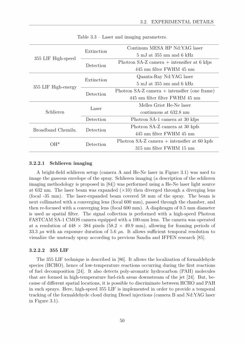
3.2. EXPERIMENTAL DETAILS
Table 3.3 – Laser and imaging parameters.
355 LIF High-speedExtinction Continum MESA HP Nd:YAG laser
5 mJ at 355 nm and 6 kHz
Detection Photron SA-Z camera + intensifier at 6 kfps445 nm filter FWHM 45 nm
355 LIF High-energyExtinction Quanta-Ray Nd:YAG laser
5 mJ at 355 nm and 6 kHz
Detection Photron SA-Z camera + intensifier (one frame)445 nm filter filter FWHM 45 nm
SchlierenLaser Melles Griot He-Ne laser
continuous at 632.8 nmDetection Photron SA-1 camera at 30 kfps
Broadband Chemilu. Detection Photron SA-Z camera at 30 kpfs445 nm filter FWHM 45 nm
OH* Detection Photron SA-Z camera + intensifier at 60 kpfs315 nm filter FWHM 15 nm
3.2.2.1 Schlieren imaging
A bright-field schlieren setup (camera A and He-Ne laser in Figure 3.1) was used toimage the gaseous envelope of the spray. Schlieren imaging (a description of the schlierenimaging methodology is proposed in [84]) was performed using a He-Ne laser light sourceat 632 nm. The laser beam was expanded (×10) then diverged through a diverging lens(focal -35 mm). The laser-expanded beam covered 58 mm of the spray. The beam isnext collimated with a converging lens (focal 600 mm), passed through the chamber, andthen re-focused with a converging lens (focal 600 mm). A diaphragm of 0.5 mm diameteris used as spatial filter. The signal collection is performed with a high-speed PhotronFASTCAM SA-1 CMOS camera equipped with a 100-mm lens. The camera was operatedat a resolution of 448 × 384 pixels (58.2 × 49.9 mm), allowing for framing periods of33.3 µs with an exposure duration of 5.6 µs. It allows sufficient temporal resolution tovisualize the unsteady spray according to previous Sandia and IFPEN research [85].
3.2.2.2 355 LIF
The 355 LIF technique is described in [86]. It allows the localization of formaldehydespecies (HCHO), hence of low-temperature reactions occurring during the first reactionsof fuel decomposition [24]. It also detects poly-aromatic hydrocarbon (PAH) moleculesthat are formed in high-temperature fuel-rich areas downstream of the jet [24]. But, be-cause of different spatial locations, it is possible to discriminate between HCHO and PAHin such sprays. Here, high-speed 355 LIF is implemented in order to provide a temporaltracking of the formaldehyde cloud during Diesel injections (camera B and Nd:YAG laserin Figure 3.1).
50
3.2. EXPERIMENTAL DETAILS
High-speed 355 LIF was performed using the third harmonic of a Continuum MESAHP Nd:YAG laser generating a 355 nm pulsed beam up to 40kHz. The laser sheet measur-ing 35 mm long and 1 mm thick (starting at 13 mm from the injector), has been createdby a collection of three lenses. The first one is a diverging lens (focal -76.2 mm), then thebeam went through two converging lenses, (focal 300 mm and 500 mm) to create the finallaser sheet. The signal was collected by a high-speed Photron FASTCAM SA-Z CMOScamera coupled with a Lambert Instruments HiCATT intensifier, gain set to 850. Thecamera was operated at a resolution of 1024 × 256 pixels (152.7 × 38.1 mm) with an85 mm f/1.4 lens and a 455 nm filter (FWHM 45 nm). This wavelength range has beenchosen to collect the spectral bands of formaldehyde in the range 410-440 nm after a 355nm excitation [24]. A compromise has to be found between the laser repetition rate andthe energy per pulse, which must be high enough to obtain enough LIF signal, which willbe detailed in the Results section. To the best of our knowledge, high-speed 355 LIF hasnot yet been proposed in a similar configuration, thus no recommendations can be foundin the literature on the minimum energy level. Therefore, conventional single-shot LIFis proposed as the reference optical diagnostics to measure formaldehyde. For that pur-pose, single-shot 355 LIF was performed using a Quanta-Ray Nd:YAG laser generatinga 100 mJ laser beam at 355 nm and 10 Hz (one pulse per injection event). The samelenses combination as for the high-speed 355 LIF technique has been used, resulting inwider laser sheet (45 mm instead of 35 mm). The laser sheet starts at 8 mm and finishesat 53 mm from the injector. Because of the higher fluence of the laser, a gain of 750(instead of 850) for the intensifier was sufficient to collect enough signal while increasingthe signal/noise ratio. Only one frame per injection is acquired, 4 ms After the Startof Injection (ASI) during the quasi-steady state of the combustion. For each technique,10 injections have been performed in order to compare ensemble-averaged images. Thesignals are integrated along the radial direction to obtain an average axial profile, whichis then normalized by its maximum value. The results obtained with a repetition rate of6 kHz (i.e. 5mJ per pulse) and for test condition α are presented in Figure 3.2. The twoimages on the top and in the middle are normalized by the maximum intensity of a squarepixel area made of 9 pixels. The profiles are the integration of the normalized intensityalong the radial axis. First of all, the spatial location of the collected signal, which isupstream of high-temperature, soot forming regions, leads to the assumption that thissignal comes only from formaldehyde fluorescence and not from PAH. Indeed, previousresults published in [86] for comparable ambient conditions show that it is very unlikelyto collect PAH fluorescence signal for axial distances below 35 mm. Therefore, as a firststep, we assumed that the acquired images are not contaminated with PAH fluorescence.
The global spatial locations of the formaldehyde clouds are similar between the twosetups. However, it appears that the single-shot 355 LIF (high-energy LIF) allows abetter detection of the HCHO for axial distances below approx. 25mm. To go further,the normalized average 355 LIF profiles (Figure 3.2 - bottom) are compared. Similar tothe lift-off length defined for the high-temperature flame, a formaldehyde lift-off lengthLOLHCHO can be computed. This is defined as the most upstream axial position wherethe normalized profile reaches 10% of the maximum signal. For the α test condition pre-sented in Figure 3.2, it leads to a position of 22 mm for the single shot 355 LIF and 25mm for the high-speed 355 LIF. Increasing the repetition rate of the high-speed 355 nm
51

3.2. EXPERIMENTAL DETAILS
laser (and thus decreasing the energy per pulse) would lead to a further deterioration ofthe collected fluorescence signal. Test at 10 kHz and 2.2 mJ per pulses have shown avery bad signal-to-noise ratio and have been discarded. A decrease in the repetition ratewould allow to increase the energy per pulse, but that would be to the detriment of tem-poral resolution. Therefore, a good compromise between temporal resolution and signalcollected is obtained at 6 kHz and 5 mJ per pulse. However, in the following analysis,this lack of sensitivity for axial positions below 25 mm where there is low formaldehydeconcentration must be kept in mind.
Figure 3.2 – Average formaldehyde cloud from 355 LIF at 100 mJ (top image) and 5 mJ(middle image), normalized average 355 LIF profiles integrated radially (bottom image).
3.2.2.3 High-temperature chemiluminescence
Two different techniques have been used to track the high-temperature flame: OH*and broadband chemiluminescence. The former is the recommended technique, in partic-ular within the ECN framework, because UV-range imaging minimizes contamination bysoot incandescence, but it requires the use of a high-speed UV-sensitive camera (intensi-fier). Since only one high-speed intensifier was available for the experiments, when thelatter was required for another diagnostic (high-speed 355 LIF), broadband chemilumi-nescence was used to determine the LOL position.
The OH* signal has been collected with a high-speed Photron FASTCAM SA-Z CMOS
52
3.2. EXPERIMENTAL DETAILS
camera at 60 kfps coupled with a high-speed intensifier (same intensifier as for the 355LIF). The camera was equipped with an ultraviolet transmitting lens (UV-Cerco 100-mm, f/2.8) and with a 315 nm filter (FWHM 10 nm), as recommended setup [52, 87].The resolution was 1024 × 256 pixels (117.5 × 29.3 mm) and the exposure time was 10 µs.
Broadband chemiluminescence has been collected with a high-speed FASTCAM SA-ZCMOS camera at 30 kfps, equipped with a 85mm f/1.8 lens and a 455 nm filter (FWHM45 nm) collecting around the CH* radical band, while rejecting the strongest emissionfrom soot incandescence. The exposure duration was 25 µs and the resolution was 1024× 384 pixels (113.7 × 42.6 mm).
Since broadband chemiluminescence may lack of sensitivity near the flame base andcould also be polluted by soot natural incandescence signal [1, 52, 87], a detailed com-parison of the two techniques was performed. OH* and broadband chemiluminescencehave been collected simultaneously though not at the same frame-rate. Figure 3.3 showsa comparison between the broadband and the OH* chemiluminescence images for 8 dif-ferent timings. First, an auto-ignited kernel appears, then, this kernel merges the mainflame while being convected downstream by the flow. These two techniques show goodagreement, since the observed flame structures are similar. Especially, broadband chemi-luminescence is able to catch the signal from the kernel appearing upstream of the flamebase. However, the signal is weaker with the Broadband chemiluminescence setup, andsome information can be lost in the very upstream locations of the flame. For example, at7967 µs ASI an auto-ignited kernel appears on the OH* images whereas this kernel is notyet observed on the broadband images. However 66 µs after, the kernel is observed on bothdiagnostics. Therefore, high-speed OH* chemiluminescence is the preferred technique toobtain quantitative information on LOL because of its higher time and spatial resolution.A Previous study [88] performing simultaneously single-shot images of OH and formalde-hyde PLIF has shown that formaldehyde is disappearing at the same position where thehigh-temperature flame is measured. The formaldehyde is mainly localized at the centerof jet as shown in Figure 3.2, while OH PLIF identifies the high-temperature flame at thejet periphery. A more detailed description of the interaction between formaldehyde andthe high-temperature flame is proposed in Section 3.3.
53
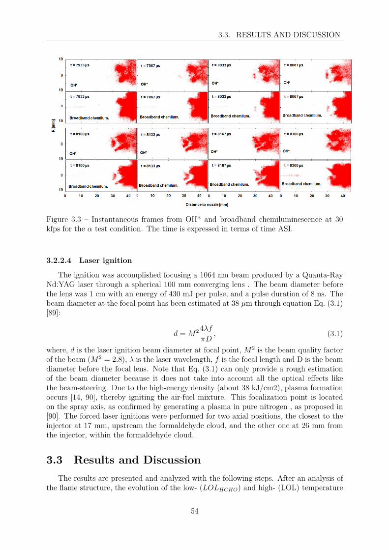
3.3. RESULTS AND DISCUSSION
Figure 3.3 – Instantaneous frames from OH* and broadband chemiluminescence at 30kfps for the α test condition. The time is expressed in terms of time ASI.
3.2.2.4 Laser ignition
The ignition was accomplished focusing a 1064 nm beam produced by a Quanta-RayNd:YAG laser through a spherical 100 mm converging lens . The beam diameter beforethe lens was 1 cm with an energy of 430 mJ per pulse, and a pulse duration of 8 ns. Thebeam diameter at the focal point has been estimated at 38 µm through equation Eq. (3.1)[89]:
d = M24λf
πD, (3.1)
where, d is the laser ignition beam diameter at focal point, M2 is the beam quality factorof the beam (M2 = 2.8), λ is the laser wavelength, f is the focal length and D is the beamdiameter before the focal lens. Note that Eq. (3.1) can only provide a rough estimationof the beam diameter because it does not take into account all the optical effects likethe beam-steering. Due to the high-energy density (about 38 kJ/cm2), plasma formationoccurs [14, 90], thereby igniting the air-fuel mixture. This focalization point is locatedon the spray axis, as confirmed by generating a plasma in pure nitrogen , as proposed in[90]. The forced laser ignitions were performed for two axial positions, the closest to theinjector at 17 mm, upstream the formaldehyde cloud, and the other one at 26 mm fromthe injector, within the formaldehyde cloud.
3.3 Results and DiscussionThe results are presented and analyzed with the following steps. After an analysis of
the flame structure, the evolution of the low- (LOLHCHO) and high- (LOL) temperature
54
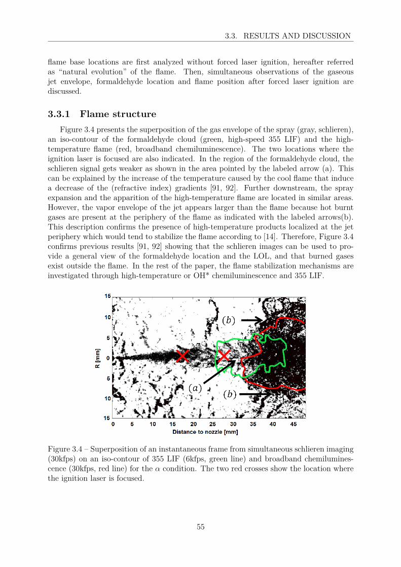
3.3. RESULTS AND DISCUSSION
flame base locations are first analyzed without forced laser ignition, hereafter referredas “natural evolution” of the flame. Then, simultaneous observations of the gaseousjet envelope, formaldehyde location and flame position after forced laser ignition arediscussed.
3.3.1 Flame structureFigure 3.4 presents the superposition of the gas envelope of the spray (gray, schlieren),
an iso-contour of the formaldehyde cloud (green, high-speed 355 LIF) and the high-temperature flame (red, broadband chemiluminescence). The two locations where theignition laser is focused are also indicated. In the region of the formaldehyde cloud, theschlieren signal gets weaker as shown in the area pointed by the labeled arrow (a). Thiscan be explained by the increase of the temperature caused by the cool flame that inducea decrease of the (refractive index) gradients [91, 92]. Further downstream, the sprayexpansion and the apparition of the high-temperature flame are located in similar areas.However, the vapor envelope of the jet appears larger than the flame because hot burntgases are present at the periphery of the flame as indicated with the labeled arrows(b).This description confirms the presence of high-temperature products localized at the jetperiphery which would tend to stabilize the flame according to [14]. Therefore, Figure 3.4confirms previous results [91, 92] showing that the schlieren images can be used to pro-vide a general view of the formaldehyde location and the LOL, and that burned gasesexist outside the flame. In the rest of the paper, the flame stabilization mechanisms areinvestigated through high-temperature or OH* chemiluminescence and 355 LIF.
Figure 3.4 – Superposition of an instantaneous frame from simultaneous schlieren imaging(30kfps) on an iso-contour of 355 LIF (6kfps, green line) and broadband chemilumines-cence (30kfps, red line) for the α condition. The two red crosses show the location wherethe ignition laser is focused.
55

3.3. RESULTS AND DISCUSSION
3.3.2 Results for natural flame evolutionLOL and LOLHCHO evolutions have been compared for all the test conditions without
laser ignition. The results are presented in Table 3.4. HCHO results, obtained with bothhigh-speed and low-speed techniques, are presented, while the high-temperature chemilu-minescence results are provided through high-speed OH* chemiluminescence imaging. Inthe following, ensemble averages are noted 〈X〉 while time averages are noted X. Timeand ensemble averages are noted 〈X〉. The standard deviation of X is noted σ(X). TheHigh-Speed 355 LIF is indexed as follows XHS while the High-Energy 355 LIF is notedXHE .
Table 3.4 – LOL and LOLHCHO averages for the different test conditions.
Test condition name α β γ δ
〈LOLOH∗〉 [mm] 35.5 49.1 44.9 31.6
σ(〈LOLOH∗〉) [mm] 2.5 3.5 4.3 3.1
〈LOLHCHO〉HE [mm] 22.7 24.1 22.6 20.0
σ(〈LOLHCHO〉HE) [mm] 0.3 0.4 0.9 0.9
〈LOLHCHO〉HS [mm] 24.5 24.0 22.7 22.7
σ(〈LOLHCHO〉HS) [mm] 0.8 0.3 0.8 1.2
〈LOLOH∗〉 is the average LOL during a 1.65 ms steady period (between 1.35 and 3 msASI) from 10 realizations collected by high-speed OH* chemiluminescence imaging at 60kHz. 〈LOLHCHO〉HE is the ensemble average of LOLHCHO at high-energy. Images wereacquired at 2.8 ms ASI. 〈LOLHCHO〉HS is the results of ensemble average formaldehydelocation 〈LOLHCHO〉 obtained from 10 realizations of high-speed 355 LIF. Note that noneof these three diagnostics have been performed simultaneously.
As described in Section 3.2.2.2, the high-speed 355 LIF presents a lack of sensitiv-ity upstream the formaldehyde cloud caused by the lower energy level of the excitation.Comparing the HE and the HS LIF, for test condition α and δ confirm this lack of sensi-tivity while conditions β and γ (with higher 〈LOLOH∗〉) show a good agreement betweenthe high-speed and the high-energy setup. It is not straightforward why test conditionspresenting a short LOL (α and δ) present a lack of signal detection upstream the formalde-hyde measured with the high-speed 355 LIF in comparison to the high energy LIF setup.The standard deviation results of 〈LOLHCHO〉HS and 〈LOLHCHO〉HE are of the sameorder of magnitude, with the latter being 24% higher. It shows that the high-speed 355LIF reasonably detects the LOLHCHO fluctuations, even if not perfectly.
The standard deviation results shown for OH* and HE LIF show that on averageσ(〈LOLOH∗〉) is 3 to 4 times greater than σ(〈LOLHCHO〉HE) hence, the upstream positionof the formaldehyde cloud is much more stable than that of the high-temperature flame.In addition the fact that the standard deviations of 〈LOLHCHO〉HE is low shows that theaverage position of the formaldehyde cloud, detected with the high-energy 355 LIF, can
56

3.3. RESULTS AND DISCUSSION
be used to correctly define the instantaneous upstream position of the formaldehyde cloud.
Figure 3.5 presents LOL temporal evolutions provided by OH* chemiluminescence fortwo different conditions (800 K, 850 K). From a general point of view, comparing thedifferent test conditions shows that the higher the temperature, the shorter the LOL andthe weaker the absolute dispersion around the mean LOL. More specifically, two types ofcharacteristic evolutions are observed: event A (red rectangle) and evolution B (red line).
• Event A is characterized by very rapid upstream displacements of the LOL: in somecases, the LOL can decrease by 5 mm in less than 50 µs. These displacementsare very probably caused by auto-ignitions events and will be called ”large scale”auto-ignitions in the following. This evolution can be observed on Figure 3 7967µs ASI for the α condition and also in Figure 3.5 (right) 5233 µs ASI for the α′condition. In both cases an isolated auto-ignited kernel appears upstream the mainflame resulting in an upstream jump of the LOL.
• Evolution B is usually observed just after event A when, following a “large scale”auto-ignition event, a progressive downstream evolution is observed for a givenperiod of time. Figure 3.5 (right) illustrates this downstream evolution through twoimages taken at 5333 and 6000 µs ASI where the LOL progressively increase. Figure3 also shows evolution B after a “large scale” auto-ignition. Another “large scale”auto-ignition event often occurs ending phase B, significantly decreasing the LOL.The characteristic time of this evolution is approx. 0.25 ms to 1 ms.
Event A is more often observed at 800 K than at 850 K, the same remark also stands forevolution B. Indeed, the more the flame is stabilized downstream, the more auto-ignitionsare detached far from the main flame, and thus the longer evolution B is. Interestingly,these auto-ignition sites are always located in the formaldehyde cloud for the referencecase α. Figure 3.5 (for the α condition) shows that auto-ignitions can reduce the LOL upto 28 mm from the injector. Moreover, it has been shown in Table 3.4 that 〈LOLHCHO〉HE
stays relatively stable at 22.7 mm from the injector. From all the realizations performedin this study, no auto-ignitions have been detected upstream the formaldehyde cloud. Itis not possible to perform the same analysis for the α′ case since no formaldehyde mea-surement have been performed in this cases.
The natural flame stabilization seems to be mainly governed by an alternation ofevent A and evolution B. The rest of the paper focuses on the analysis of the mechanismsgoverning the evolution B with the aim to discriminate between different potential mech-anisms, in particular flame propagation, auto-ignition, or others.
Assuming a constant speed during evolution B, as illustrated by the solid lines inFigure 3.5, the average absolute flame front speed Sa relative to a fixed reference can bedetermined using Eq. (3.2)
Sa =∆LOL
∆t, (3.2)
where ∆LOL and ∆t are the LOL and time variation during phase B. For condition α,Sa is found equal to 6.6 m/s in average with a standard deviation of 2.8 m/s based on
57

3.3. RESULTS AND DISCUSSION
the eight evolutions B displayed in Figure 3.5. However, as can be seen on Figure 3.5,the apparition of phases A and B are random, which makes a systematic analysis of thesephenomena on a large number of injections, or for varied ambient conditions, difficult.Forced laser ignition, whose setup is described in Section 3.3.3, is therefore used to havereproducible and controlled apparitions of evolution B. It also allows a forcing of theignition either in the formaldehyde cloud, or upstream of this cloud.
Figure 3.5 – Left: LOL time tracking using OH* chemiluminescence imaging for ambienttemperatures of 800 K and 850 K, respectively named α and α′ conditions. Events Aare shown as red rectangles and evolutions B as red lines for the α conditions. Right:snapshot of OH* images illustrating event A and evolution B.
3.3.3 Forced laser ignitionForced laser-induced plasma ignition was used to perform a systematic analysis of
phase B (downstream propagation). Indeed the advantage of laser-induced plasma ig-nition is that it enables to set the LOL in a location upstream of its natural position,where the conditions for natural ignition are not present and therefore where large scaleauto-ignition is unlikely to occur, hence enabling to focus on the study of phase B. Laserignition was triggered 3 ms after the effective start of injection, hence when the naturalLOL is already stabilized. As detailed in the experimental setup section, two axial po-sitions have been selected for the forced ignition as shown in Figure 3.4: upstream theformaldehyde cloud (17 mm downstream the orifice), and within the formaldehyde cloud(26 mm downstream the orifice).
A broadband chemiluminescence sequence at 30 kfps, showing the first 400 mus tran-sient lift-off after a forced laser ignition is shown in Figure 3.6 for condition α. High-speedformaldehyde imaging is not available at such frame rate and therefore formaldehyde LIFis not shown in the Figure 3.6. The case shown in Figure 3.6 corresponds to a forcedignition at 26 mm from the nozzle orifice, hence upstream of the natural mean LOL (35mm) but inside the formaldehyde cloud (〈LOLHCHO〉 = 22 mm).
58

3.3. RESULTS AND DISCUSSION
After laser ignition, the broadband chemiluminescence images present a saturation(non convected signal at the plasma location for more than 1 ms) on the top of the im-ages. This saturation is attributed to the high plasma emission collected by the camerawith a large gate width (25 µs). In comparison, OH* chemiluminescence, with a shortergate width (10 µs), presents this saturation for less than 150 µs due to less plasma emis-sion collected. Therefore, the saturation is ignored for the LOL detection.
The ignited kernel, created just after laser ignition, can split into two parts for anal-ysis: the upstream part of the kernel and the downstream part. The downstream partwhich propagates towards the main flame in the same observation was made in [14], whereit was proposed that this downwards propagation occurs in premixed flame mode. Theupstream part of the kernel remains at a fixed position then after starts a slow down-stream evolution. This slow downstream evolution is analyzed in more detail later in thepaper using high-speed OH* chemiluminescence (60 kfps).
Interestingly, a statistical analysis, in which the radial position of the ignition loca-tion has been measured for all the test conditions, shows that although the laser beamis focused on the spray axis forced ignition occurs at a radial position between 3 and4 mm from the jet axis. This is very probably the result of the balance between laserlocal fluence and local mixture ignitability. A 1D spray model [55, 93] used to calculatethe average mixture fraction field showed that the stoichiometric line, corresponding toa mixture fraction zst = 0.048, is 2.85 mm from the centerline at this axial position. So,laser ignition occurs on the lean side of the average stoichiometric line. To further an-alyze this, most reactive mixture fractions have been computed with Cantera [94] usinga 53-species skeletal model for n-dodecane oxidation [95] in a constant pressure reactor.The initial temperature is determined from the stoichiometric mixture fraction assumingan adiabatic mixing process. The computed most reactive mixture fractions are 0.048at 800 K, and 0.054 for at 850 K, corresponding to a range from stoichiometric to richmixtures. This is not consistent with the observed locations of the forced ignition, onthe lean side of the average stoichiometric line. Therefore it seems that laser ignitionhas no requirement that it be near a preferred self-ignition zone. The high-temperaturekernels detected just after forced ignition are probably governed by plasma dynamics ina stratified mixture. Plasma breakdown begins when there is enough hydrogen, but doesnot mandate that this is lean or rich of stoichiometric. Once plasma forms, it becomesoptically thick and absorbs the next laser radiation, which can bias the energy deposi-tion to the lean side. Then the flame is sustained at the jet periphery for mixture near zst .
59
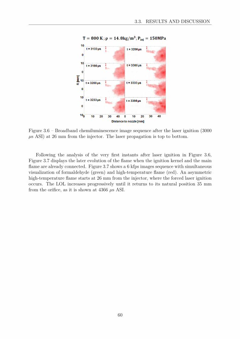
3.3. RESULTS AND DISCUSSION
Figure 3.6 – Broadband chemiluminescence image sequence after the laser ignition (3000µs ASI) at 26 mm from the injector. The laser propagation is top to bottom.
Following the analysis of the very first instants after laser ignition in Figure 3.6,Figure 3.7 displays the later evolution of the flame when the ignition kernel and the mainflame are already connected. Figure 3.7 shows a 6 kfps images sequence with simultaneousvisualization of formaldehyde (green) and high-temperature flame (red). An asymmetrichigh-temperature flame starts at 26 mm from the injector, where the forced laser ignitionoccurs. The LOL increases progressively until it returns to its natural position 35 mmfrom the orifice, as it is shown at 4366 µs ASI.
60

3.3. RESULTS AND DISCUSSION
Figure 3.7 – Broadband chemiluminescence (red, first and third columns) and 355 LIF(green, second and fourth columns) image sequence after the laser ignition (3000 µs ASI)at 26 mm from the injector, for condition α. The two dotted lines show the LOL justafter the laser ignition (left line) and the average position of the “natural” LOL.
Under the limiting factor that signal to noise ratio of 355 LIF imaging is low, theformaldehyde location does not seem to be significantly affected by the ignition kernel,ignited inside the formaldehyde as shown in Figure 3.7. In order to further analyze theevolution of the formaldehyde cloud, Figure 3.8 (two top images) shows ensemble (10realizations) and time (500 µs before and after forced ignition) averaged images providedby high-speed 355 LIF. The time is expressed in terms of time After Laser Ignition (ALI):tALI < 0 before the laser ignition and tALI > 0 after the laser ignition. In addition Fig-ure 3.8 (bottom image) displays different timings of high-speed 355 LIF signal integratedalong the radial direction. The left column is for laser ignition at 17 mm, upstream theformaldehyde cloud, the right column is for laser ignition at 26 mm, inside the formalde-hyde cloud. The ensemble and time averaged images show a weak decrease of the LIFsignal after laser ignition (tALI > 0), in the upper part of the formaldehyde cloud atapprox. 35 mm from the injector, for both locations of laser ignition. Laser ignitionalso occurs in the upper part of the spray. This decrease of signal is presumably dueto the formaldehyde consumption by the larger high-temperature flame generate afterforced ignition like shown in Figure 3.7. However, 355 LIF is a planar measurement whilehigh-temperature chemiluminescence is a line-of-sight technique. Therefore, the collectedsignal from broadband chemiluminescence is not necessarily located in the same planeas the formaldehyde cloud. The integrated intensity profiles shown on the bottom partof Figure 3.8 show that the most upstream location of the formaldehyde cloud is notaffected by laser ignition. The zoomed plots shown on Figure 3.8 indicate that the riseof the formaldehyde signal appears at the same axial distance before and after the laserignition, thus proving that LOLHCHO is not modified by laser ignition. The small bump
61
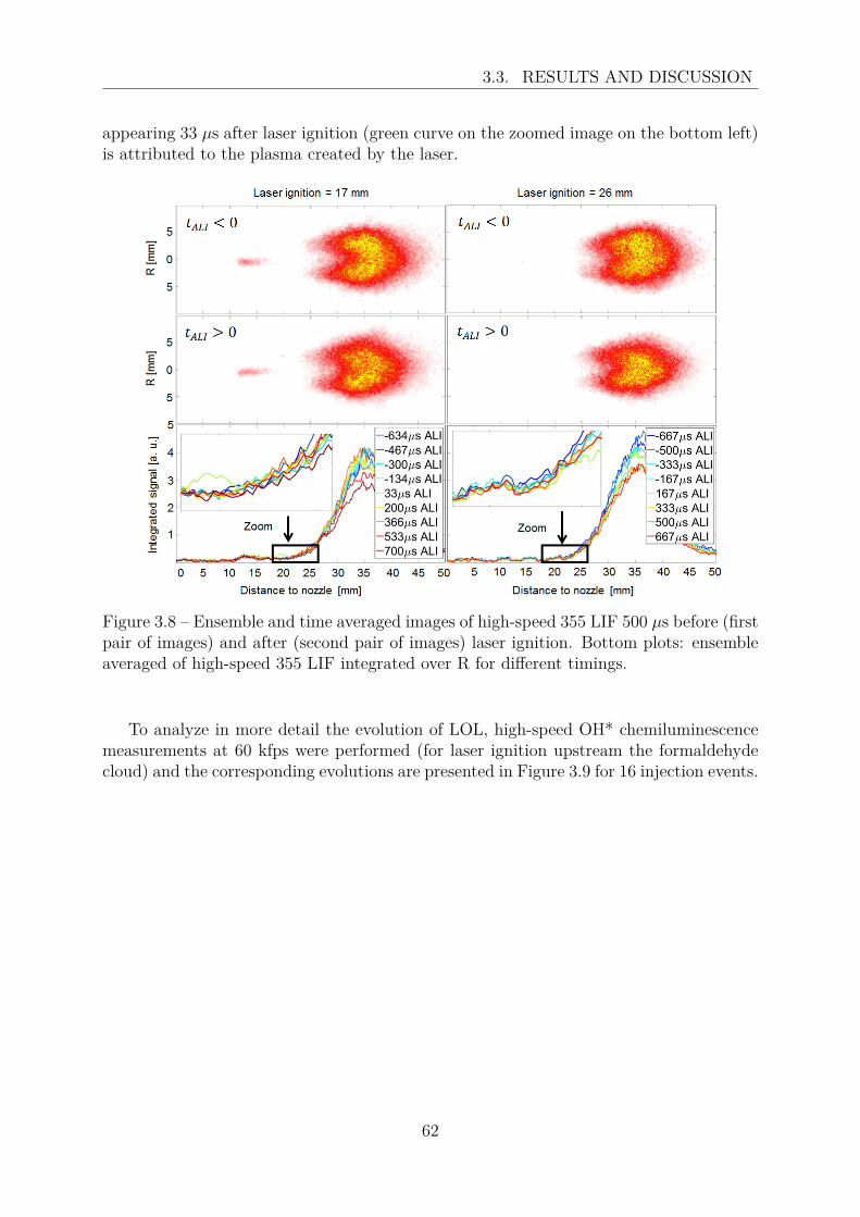
3.3. RESULTS AND DISCUSSION
appearing 33 µs after laser ignition (green curve on the zoomed image on the bottom left)is attributed to the plasma created by the laser.
Figure 3.8 – Ensemble and time averaged images of high-speed 355 LIF 500 µs before (firstpair of images) and after (second pair of images) laser ignition. Bottom plots: ensembleaveraged of high-speed 355 LIF integrated over R for different timings.
To analyze in more detail the evolution of LOL, high-speed OH* chemiluminescencemeasurements at 60 kfps were performed (for laser ignition upstream the formaldehydecloud) and the corresponding evolutions are presented in Figure 3.9 for 16 injection events.
62
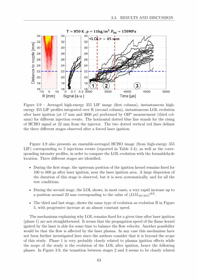
3.3. RESULTS AND DISCUSSION
Figure 3.9 – Averaged high-energy 355 LIF image (first column), instantaneous high-energy 355 LIF profiles integrated over R (second column), instantaneous LOL evolutionafter laser ignition (at 17 mm and 3000 µs) performed by OH* measurement (third col-umn) for different injection events. The horizontal dotted blue line stands for the risingof HCHO signal at 22 mm from the injector. The two dotted vertical red lines delimitthe three different stages observed after a forced laser ignition.
Figure 3.9 also presents an ensemble-averaged HCHO image (from high-energy 355LIF) corresponding to 5 injections events (reported in Table 3.4), as well as the corre-sponding intensity profiles, in order to compare the LOL evolution with the formaldehydelocation. Three different stages are identified.
• During the first stage, the upstream position of the ignition kernel remains fixed for100 to 600 µs after laser ignition, near the laser ignition area. A large dispersion ofthe duration of this stage is observed, but it is seen systematically, and for all thetest conditions.
• During the second stage, the LOL shows, in most cases, a very rapid increase up toa position around 22 mm corresponding to the value of 〈LOLHCHO〉HE.
• The third and last stage, shows the same type of evolution as evolution B in Figure5, with progressive increase at an almost constant speed.
The mechanisms explaining why LOL remains fixed for a given time after laser ignition(phase 1) are not straightforward. It seems that the propagation speed of the flame kernelignited by the laser is able for some time to balance the flow velocity. Another possibilitywould be that the flow is affected by the laser plasma. In any case this mechanism havenot been further investigated here since the authors consider that it is beyond the scopeof this study. Phase 1 is very probably closely related to plasma ignition effects whilethe scope of the study is the evolution of the LOL after ignition, hence the followingphases. In Figure 3.9, the transition between stages 2 and 3 seems to be closely related
63

3.3. RESULTS AND DISCUSSION
to the location of formaldehyde. To confirm this observation, an analysis of the axialposition corresponding to transition between stages 2 and 3 has been repeated for theother conditions and is summarized in Table 3.5. For laser ignition at 17 mm from theinjector, the α, β and γ test conditions mostly show the 3 stages, however 40 % ofthe δ case exhibits only the first stage and, then, directly starts a progressive evolutionwithout showing the second stage. Table 3.5 also displays an ensemble average of thetransition position between the second and the third stage. Comparing these results to〈LOLHCHO〉HE in Table 3.4, it appears that the turning point between the second and thelast stage corresponds to the beginning of the formaldehyde cloud. Indeed, the maximumdifference between 〈LOLHCHO〉HE and the transition point given in Table 3.5 is 5 %for the δ case. The fact that only 60 % of the realizations of the δ case shows the 3stages is attributed to the close distance between the laser ignition and the formaldehydecloud. Even if the laser is focused at 17 mm, due to turbulence, the ignited kernelcan start growing further downstream. Additionally, regarding the standard deviationof 〈LOLHCHO〉HE (0.9 mm), for the δ condition, laser ignition inside the formaldehydecloud can be statistically considered for this condition and thus, can explain the 40 % ofrealizations not showing the 3 stages. This hypothesis is confirmed by performing laserignition within the formaldehyde cloud for the α condition. In this case, neither of therealizations show the 3 stages. When laser ignition occurs within the formaldehyde region,there is no rapid LOL increase stage, and the evolution of the LOL is more progressive, ascan be observed during stage 3 (Figure 3.9). These results emphasize the role of the lowtemperature reaction region on the LOL progression speed. Upstream of the formaldehydecloud, rapid evolutions are observed and inside the formaldehyde cloud systematic slowerprogression of the LOL location is observed. The mechanisms explaining the effect ofthe presence of formaldehyde on the LOL progression requires further analysis, but theresults obtained here show that the cool flame products appear to play an important rolein the LOL stabilization process.
Table 3.5 – Statistical analysis of the three different stages identified for laser ignition at17 mm from the injector. Standard deviations are noted in parenthesis.
Test condition name α β γ δPercentage of realizations showingthe 3 stages [%] 83 72 75 60Ensemble average of the transition positionbetween stages 2 and 3 [mm] 22.4(2.3) 23.1(2.4) 22.0(0.9) 21.0(1.4)Ensemble average of Sa during stage 3 [m/s] 5.0(1.5) 7.3(2.1) 6.5(2.2) 3.6(1.5)
The fairly linear return to the natural lift-off position (stage 3) is analyzed throughEq. (3.2) to determine if there are compelling observations that govern this phase for allconditions. A statistical analysis of the near-constant absolute downstream velocities (Sa)measured during stage 3 for all the test conditions are summarized in last line Table 3.5.Table 3.5 is illustrated by Figure 10, where each curve was selected as being representativeof the position of the transition stage 2/3 and the downstream evolution during stage 3under the corresponding condition.
64
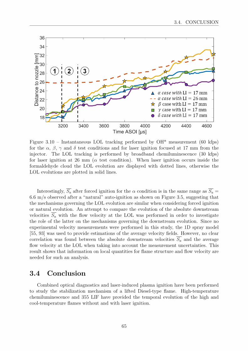
3.4. CONCLUSION
Figure 3.10 – Instantaneous LOL tracking performed by OH* measurement (60 kfps)for the α, β, γ and δ test conditions and for laser ignition focused at 17 mm from theinjector. The LOL tracking is performed by broadband chemiluminescence (30 kfps)for laser ignition at 26 mm (α test condition). When laser ignition occurs inside theformaldehyde cloud the LOL evolution are displayed with dotted lines, otherwise theLOL evolutions are plotted in solid lines.
Interestingly, Sa after forced ignition for the α condition is in the same range as Sa =6.6 m/s observed after a “natural” auto-ignition as shown on Figure 3.5, suggesting thatthe mechanisms governing the LOL evolution are similar when considering forced ignitionor natural evolution. An attempt to compare the evolution of the absolute downstreamvelocities Sa with the flow velocity at the LOL was performed in order to investigatethe role of the latter on the mechanisms governing the downstream evolution. Since noexperimental velocity measurements were performed in this study, the 1D spray model[55, 93] was used to provide estimations of the average velocity fields. However, no clearcorrelation was found between the absolute downstream velocities Sa and the averageflow velocity at the LOL when taking into account the measurement uncertainties. Thisresult shows that information on local quantities for flame structure and flow velocity areneeded for such an analysis.
3.4 ConclusionCombined optical diagnostics and laser-induced plasma ignition have been performed
to study the stabilization mechanism of a lifted Diesel-type flame. High-temperaturechemiluminescence and 355 LIF have provided the temporal evolution of the high andcool-temperature flames without and with laser ignition.
65
3.4. CONCLUSION
The natural LOL and LOLHCHO evolutions were first analyzed. The formaldehydecloud has been found to be much more stable than the high-temperature flame location.Auto-ignited detached kernels have always been localized inside the formaldehyde cloudand lead to a rapid decrease in the LOL while the LOLHCHO remains stable. The “nat-ural” LOL temporal evolution was analyzed for different test conditions and two typicalfeatures have been identified:
• Very rapid upstream displacement of the LOL very probably linked to auto-ignitionand called “large scale” auto-ignition indicated by detached kernel upstream themain high-temperature flame
• A progressive downstream evolution of the LOL for a given period of time untilanother “large scale” auto-ignition occurs
The natural high-temperature flame seems to be driven by an alternation of the twoabove evolutions. Forced laser ignition was performed to highlight the “natural” down-stream evolution occurring after a “large scale” auto-ignition and, consequently, to in-vestigate the main stabilization mechanism during this stage. The laser ignition wasperformed upstream and inside the formaldehyde cloud, demonstrating the leading roleof low-temperature reaction on the downstream evolution. Upstream the formaldehyde,rapid LOL temporal evolutions are observed whereas inside the formaldehyde cloud sys-tematic slower progression is observed.
Finally, the stabilization mechanism seems to be governed by an alternation of “largescale” auto-ignition and downstream evolution which can be governed by “small scale”auto-ignition or/and flame propagation. Moreover, the impact of the flow velocity onthe possible auto-ignition fronts or/and premixed flame needs to be investigated duringthis downstream evolution. More investigations are needed to clarify these points and todiscriminate between the propagation and auto-ignition processes.
66
Chapter 4
A conceptual model of the flamestabilization mechanisms for a liftedDiesel-type flame based on directnumerical simulation andexperiments
This Chapter proposes to use the results from a DNS in combination with the ob-servations made in the experimental study to complete our understanding of the flamestabilization mechanisms under Diesel conditions. Section 4.2 first presents the numericalsetup of the DNS. Then, a description of the chemical mechanism is proposed in Sec-tion 4.3. Section 4.4 describes the different tools developed to analyze the local reactionzone topologies at the flame base. In Section 4.5, a comparison between the DNS andthe experiments is proposed. Based on the tools developed in Section 4.4, Section 4.6presents an analysis of the flame stabilization mechanisms. Finally, Section 4.7 shows aconceptual model of the flame stabilization mechanisms for a lifted Diesel-type flame.
This study is presented here as an adapted version for the thesis manuscript of anarticle entitled ”A conceptual model of the flame stabilization mechanisms for a liftedDiesel-type flame based on direct numerical simulation and experiments”, published inthe journal Combustion and Flame [96]. The abstract, present in the original paper, isremoved and the introduction has been modified to avoid repetitions with Chapter 2.Furthermore, Section 4.8.1 has been added to provide complementary elements.
4.1 Brief introductionThe objective of the present work was to perform a DNS study of the spatial and
temporal evolution of a Diesel-type spray previously studied experimentally [82] in orderto explore in detail the phenomena contributing to the spray-flame stabilization.
Ideally, such a DNS would have to simulate the full spray, including in particularthe liquid fuel spray originated from the injector nozzle. A DNS including the latter
67

4.1. BRIEF INTRODUCTION
would be a challenge in itself and has not been addressed by published research due to itsinherent complexity and extreme requirements in terms of spatial and temporal resolution.Published DNS have therefore restricted the computational domain to the gaseous part ofthe spray where chemical reactions essentially take place. A first approach was to performtemporal DNS of the turbulent mixing layer created downstream of the liquid part of thespray [18, 64, 65, 75]. While this allowed addressing realistic Damköhler numbers, itmay not account for spatial recirculation of hot burnt gases that have been found topossibly be of importance for the flame stabilization of ACDF [14]. Another type of DNSsimulated a spatially stabilized gaseous flame set up to be as representative as possibleto Diesel-spray conditions [76]. While this allowed addressing Damköhler numbers underDiesel-spray conditions, the studied Reynolds numbers were considerably smaller thanthat of a Diesel spray.
In the present work, we chose to perform a DNS of the spatial evolution of the gaseouspart of the spray studied in [82] (α condition), in order to account both for realisticReynolds and Damköhler numbers, and to address in particular the recirculation of burntgases and their suspected impact on flame stabilization. To limit the computational costof such an approach, the simulations were restricted to 2D, which allowed ensuring asufficient resolution of the small spatial scales of premixed flames under the studied con-ditions. 1
Unlike many turbulent flames, which can be computed with simplified chemical de-scriptions [97, 98], the simulation of ACDF requires more complex chemical kinetics. TheLOL time evolution is a discontinuous quantity, characterized by frequent jumps whenthe flame auto-ignites. Experiments reveal that these auto-ignition events (called “EventsA” in [82]) are followed by the formation and the downstream convection of flames (called“Evolution B” [82]) before a new auto-ignition event occurs upstream and brings theflame back closer to the injector. Low-temperature chemistry has been shown to play animportant role in that dynamic process [82]. Reproducing these low-temperature chem-istry phenomena, especially in the NTC (Negative Temperature Coefficient) regime, isimpossible with global schemes [65] and requires more complex chemistry descriptions.
In the present DNS, chemistry was modelled using an ARC (Analytically ReducedChemistry) scheme [99–103] adapted for n-dodecane / air flames at 3.4 MPa.
The paper is organized as follows: the computational domain and numerical methodemployed in the DNS of the ACDF configuration is described in Section 4.2, followed bythe chemical scheme reduction methodology and its validation in Section 4.3. The analysistools, used to identify the instantaneous LOL as well as the local reaction zone topologiesaround it, are detailed in Section 4.4. Then, Section 4.5 presents a comparison betweenexperiments [82] and the performed DNS in order to validate the strong hypothesis andin particular those related to a 2D simulation and a synthetic simplified turbulence at theinflow of the gas jet allow realistic predictions. In Section 4.6, each discrete instantaneouslift-off predicted by the DNS is identified to be either of the Event A or Evolution B typesfollowing the definitions proposed in [82]. Furthermore, the developed automatic toolsanalysis are used to identify the local reaction zone topologies around discrete instanta-
1Care was taken to base the 2D DNS of the gaseous part of the spray on a sufficiently realistic chemicalmechanism including low-temperature chemistry.
68

4.2. CONFIGURATION
neous lift-off positions. Finally, a conceptual model for flame stabilization in ACDF-typeconfigurations is proposed in Section 4.7 based on the performed analyses and resultingobservations.
4.2 ConfigurationThe case simulated in the present work had previously been studied experimentally.
Details on the employed techniques and obtained results can be found in [82], where it isreferred to as the α condition.The configuration consists of a n-dodecane liquid fuel injected into a large constant volumevessel containing a mixture with a 16% (by volume) oxygen concentration, at an initialpressure of 3.4MPa and temperature of 800K.
4.2.1 Simplifying assumptionsPerforming a 3D DNS of the full liquid spray, and its combustion under such Diesel
engine-like conditions, would require a very fine spatial and temporal discretization in or-der to capture the smallest scales. An estimation of the resulting necessary computationaleffort indicated that the cost of performing such a 3D DNS would be prohibitive.
In order to define an affordable computational framework able to reproduce essentialaspects of ACDF flame stabilization, the following simplifying assumptions were made:
• The simulation was simplified to be two-dimensional. Despite the related limi-tations, in terms of an accurate reproduction of all features of a turbulent flow,comparisons with experimental findings indicated that this strong simplification al-lowed capturing key features at a fraction of the cost of a 3D DNS. It also simplifiedthe analysis of the reaction zone dynamics significantly.
• As experimental observations for the simulated condition showed a flame stabiliza-tion downstream of the zone where the liquid spray impacts the local flow dynamics,the liquid injection was not included in the simulations. As shown in Fig. 4.1, thecomputational domain was therefore started 20mm downstream the injector outlet,i.e. downstream of the liquid length that was estimated to be 18mm [104].
• The computational domain was chosen to include an area of interest axially situatedbetween 25mm and 50mm downstream of the injector. As illustrated in Fig. 4.1(top), experimental findings [82] indicate that this well-resolved area of interestincludes the spatially relatively stable low-temperature-chemistry (e.g. formalde-hyde), as well as the region situated axially between 26 and 45mm downstream theinjector in which the LOL varies. In the radial direction, the area of interest encom-passes a region containing high-temperature products localized at the jet periphery,which, according to [14], may contribute to the flame stabilization.
• Inflow boundary conditions imposed in the central part of the jet were not chosen toreproduce the complex turbulent multi-species and possibly reactive flow found atthat axial position 20mm downstream the injector. These complex flow conditionsare not known from published research, and would indeed require performing a full
69
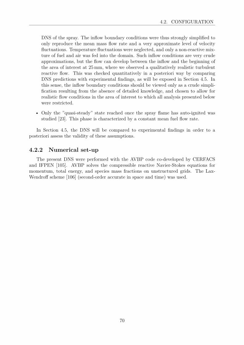
4.2. CONFIGURATION
DNS of the spray. The inflow boundary conditions were thus strongly simplified toonly reproduce the mean mass flow rate and a very approximate level of velocityfluctuations. Temperature fluctuations were neglected, and only a non-reactive mix-ture of fuel and air was fed into the domain. Such inflow conditions are very crudeapproximations, but the flow can develop between the inflow and the beginning ofthe area of interest at 25mm, where we observed a qualitatively realistic turbulentreactive flow. This was checked quantitatively in a posteriori way by comparingDNS predictions with experimental findings, as will be exposed in Section 4.5. Inthis sense, the inflow boundary conditions should be viewed only as a crude simpli-fication resulting from the absence of detailed knowledge, and chosen to allow forrealistic flow conditions in the area of interest to which all analysis presented belowwere restricted.
• Only the ”quasi-steady” state reached once the spray flame has auto-ignited wasstudied [23]. This phase is characterized by a constant mean fuel flow rate.
In Section 4.5, the DNS will be compared to experimental findings in order to aposteriori assess the validity of these assumptions.
4.2.2 Numerical set-upThe present DNS were performed with the AVBP code co-developed by CERFACS
and IFPEN [105]. AVBP solves the compressible reactive Navier-Stokes equations formomentum, total energy, and species mass fractions on unstructured grids. The Lax-Wendroff scheme [106] (second-order accurate in space and time) was used.
70

4.2. CONFIGURATION
Figure 4.1 – Top: Superposition of the gas envelope of the spray (Schlieren imaging) onan iso-contour of the formaldehyde cloud (green line, high-speed 355 LIF), and the high-temperature flame (yellow line, broadband chemiluminescence). This image was obtainedfrom the experimental setup presented in [82]. Bottom: Computational domain showingthe used tetrahedral grid which is refined in the area of interest to capture combustionphenomena.
Fig. 4.1 (bottom) shows the 2D square computation domain. Spatial discretizationis based on an unstructured tetrahedral mesh. The highest spatial resolution of 6µmis imposed in the area of interest that covers the region where key mechanisms of flamestabilization take place and were analyzed. This cell size was chosen to achieve a sufficientresolution of the estimated premixed flame thickness under the simulated conditions, asoutlined in Section 4.3.2. The cell size is progressively coarsened laterally and downstreamof the area of interest in order to impose lateral and downstream boundary conditions farenough to mimic the large size of the real constant volume vessel used in the experiments.
71
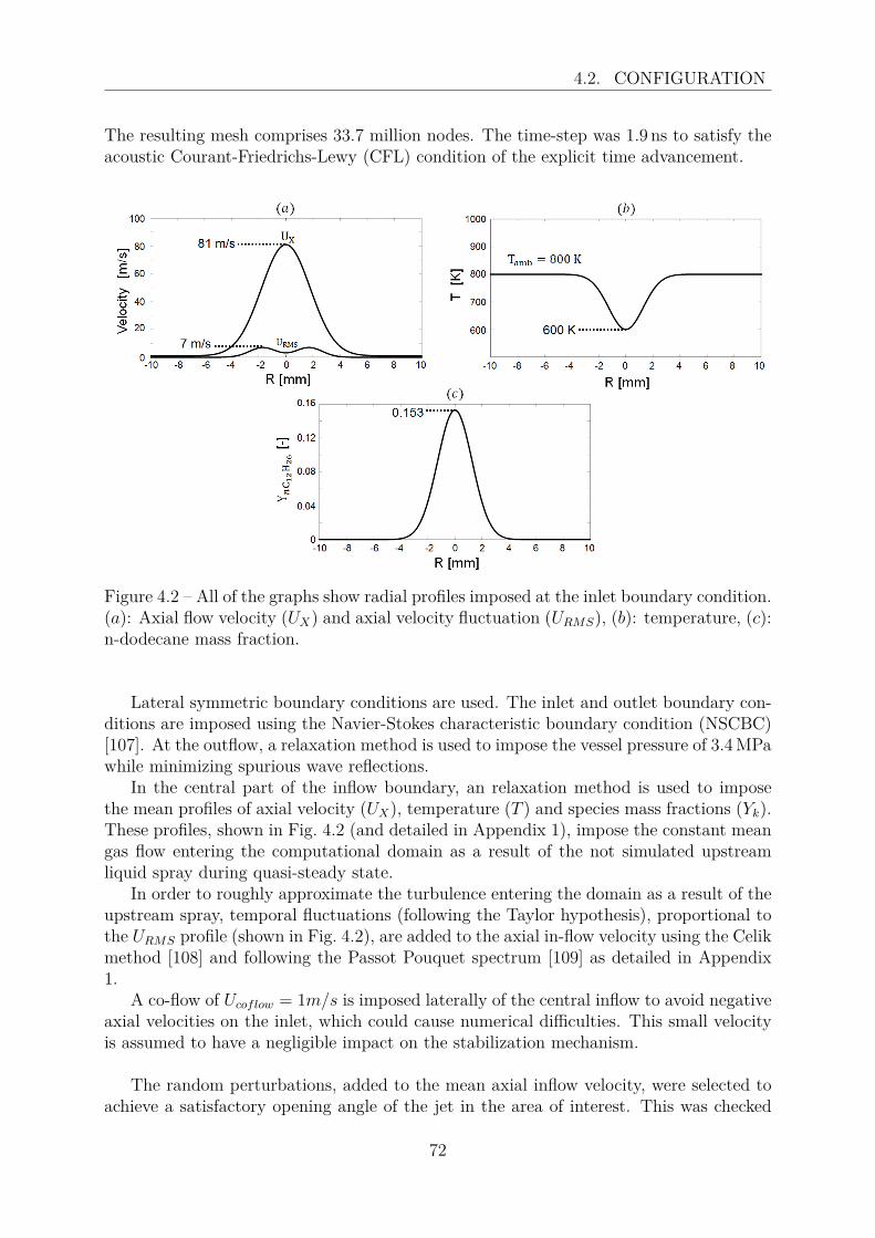
4.2. CONFIGURATION
The resulting mesh comprises 33.7 million nodes. The time-step was 1.9 ns to satisfy theacoustic Courant-Friedrichs-Lewy (CFL) condition of the explicit time advancement.
Figure 4.2 – All of the graphs show radial profiles imposed at the inlet boundary condition.(a): Axial flow velocity (UX) and axial velocity fluctuation (URMS), (b): temperature, (c):n-dodecane mass fraction.
Lateral symmetric boundary conditions are used. The inlet and outlet boundary con-ditions are imposed using the Navier-Stokes characteristic boundary condition (NSCBC)[107]. At the outflow, a relaxation method is used to impose the vessel pressure of 3.4MPawhile minimizing spurious wave reflections.
In the central part of the inflow boundary, an relaxation method is used to imposethe mean profiles of axial velocity (UX), temperature (T ) and species mass fractions (Yk).These profiles, shown in Fig. 4.2 (and detailed in Appendix 1), impose the constant meangas flow entering the computational domain as a result of the not simulated upstreamliquid spray during quasi-steady state.
In order to roughly approximate the turbulence entering the domain as a result of theupstream spray, temporal fluctuations (following the Taylor hypothesis), proportional tothe URMS profile (shown in Fig. 4.2), are added to the axial in-flow velocity using the Celikmethod [108] and following the Passot Pouquet spectrum [109] as detailed in Appendix1.
A co-flow of Ucoflow = 1m/s is imposed laterally of the central inflow to avoid negativeaxial velocities on the inlet, which could cause numerical difficulties. This small velocityis assumed to have a negligible impact on the stabilization mechanism.
The random perturbations, added to the mean axial inflow velocity, were selected toachieve a satisfactory opening angle of the jet in the area of interest. This was checked
72

4.3. CHEMICAL MECHANISM
by performing a non-reactive simulation and comparing time-averaged radial profiles ofvelocity, temperature, and fuel mass fraction obtained by post-processing instantaneousDNS fields with profiles given by experimentally established correlations. This allowed(shown in Section 4.8.2) to check that the imposed boundary conditions yielded satis-factory mean profiles in the area of interest where flame stabilization mechanisms werestudied. Therefore, the chosen inflow boundary conditions allow to investigate the flamestabilization mechanisms, unlike temporally developing jets created by a mixing layer be-tween fuel and air [18, 64, 65, 75].
The initial condition for the DNS was a flow at rest at the initial temperature, pressureand composition known from the experiments. The initial mass fractions of N2, O2, CO2,and H2O are imposed to be spatially homogeneous and equal to the values given inTable 4.1. The CO2 and H2O species are products of the lean pre-combustion used in theexperiments to bring the vessel to its initial conditions at the start of injection.
Table 4.1 – Initial species mass fractions in the vessel.
Species N2 O2 CO2 H2O nC12H26
Mass fraction [-] 0.7016 0.1746 0.1001 0.0237 0
The simulated physical time was 12ms. A first initial phase of 3ms was necessaryto have the flame ignite and for the flow to reach a stabilized state in the mean. Flamestabilization was only analyzed after this initial stage.The computational cost was 120,000 CPU hours per simulated physical millisecond.AVBP allowed achieving a return time of approximately 24h per simulated millisecondon 4992 cores.
4.3 Chemical mechanismThe reference chemical kinetics scheme used in this work is the 54-species skeletal
model for n-dodecane oxidation developed by Yao et al. [95], itself based on the detailedkinetic scheme for a variety of alkanes by Sarathy et al. [110].
4.3.1 Development of the reduced schemeThis reference mechanism is further reduced for the conditions relevant to the DNS
presented here using the YARC reduction tools [99]. The resulting analytically reducedchemistry (ARC) model is then validated against experimental and simulation data ob-tained using Yao’s model. Comparison are shown in Fig. 4.3 for laminar flame speed (leftcolumn) and auto-ignition delay (right column). Laminar premixed flame values wereobtained for equivalence ratios in the range 0.7-1.3 for atmospheric and high pressure(3.5 MPa). Auto-ignition delays are checked for pressures of 2.0-5.0 MPa, equivalenceratios of 0.5-1.2, and initial temperatures of 700-1200 K. The first step of the reductionmethodology is to identify species and reactions which can be removed without affectingthe laminar flame speed and the auto-ignition delay using the directed relation graphmethod with error propagation [100]. At the end of this stage, 7 species are removed.
73

4.3. CHEMICAL MECHANISM
Species for which a Quasi-Steady State Approximation (QSSA) can be used are, then,chosen using the Level Of Importance criterion [111]. The resulting ARC scheme is com-posed of 28 transported species, 19 QSS species (Table 4.2) and 198 reactions. As shownin Fig. 4.3, the 28-species reduced scheme correctly reproduces the laminar flame speedsand the auto-ignition delays over the selected range of conditions, also capturing the NTCregion for a fixed composition with varying temperature.
Table 4.2 – Summary of the reduced mechanism (28 ARC): transported (left) and QuasiSteady State (QSS) (right) species.
Transported species (28) QSS species (19)N2, O, H2, CH2, HCO, CH*
2,H, OH, H2O, CH3O, C2H3, CH2CHO,H2O2, O2, HO2, C2H5, a C3H5, C2H3CHO,CH2O, CO2, CH3, n C3H7, C4H7, p C4H9,CO, C2H6, CH4, p C5H11, p C7H15, p C12H25,C2H4, C2H2, C3H6, s3 C12H25, s C12H25, C12OOH,C4H8, C5H10, C6H12, O2C12H24OOHC7H14, C8H16, C9H18,C10H20, C12H25O2, n C12H26,OC12H23OOH
74
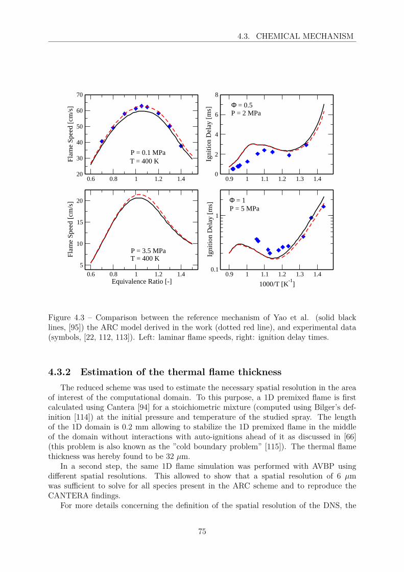
4.3. CHEMICAL MECHANISM
0.6 0.8 1 1.2 1.420
30
40
50
60
70
Flam
e Sp
eed
[cm
/s]
0.9 1 1.1 1.2 1.3 1.40
2
4
6
8
Igni
tion
Del
ay [m
s]
0.6 0.8 1 1.2 1.4Equivalence Ratio [-]
5
10
15
20
Flam
e Sp
eed
[cm
/s]
0.9 1 1.1 1.2 1.3 1.41000/T [K-1]
0.1
1Ig
nitio
n D
elay
[ms] Φ = 1
P = 3.5 MPa
T = 400 K
P = 2 MPa
P = 5 MPa
Φ = 0.5
T = 400 K
P = 0.1 MPa
Figure 4.3 – Comparison between the reference mechanism of Yao et al. (solid blacklines, [95]) the ARC model derived in the work (dotted red line), and experimental data(symbols, [22, 112, 113]). Left: laminar flame speeds, right: ignition delay times.
4.3.2 Estimation of the thermal flame thicknessThe reduced scheme was used to estimate the necessary spatial resolution in the area
of interest of the computational domain. To this purpose, a 1D premixed flame is firstcalculated using Cantera [94] for a stoichiometric mixture (computed using Bilger’s def-inition [114]) at the initial pressure and temperature of the studied spray. The lengthof the 1D domain is 0.2 mm allowing to stabilize the 1D premixed flame in the middleof the domain without interactions with auto-ignitions ahead of it as discussed in [66](this problem is also known as the ”cold boundary problem” [115]). The thermal flamethickness was hereby found to be 32 µm.
In a second step, the same 1D flame simulation was performed with AVBP usingdifferent spatial resolutions. This allowed to show that a spatial resolution of 6 µmwas sufficient to solve for all species present in the ARC scheme and to reproduce theCANTERA findings.
For more details concerning the definition of the spatial resolution of the DNS, the
75

4.4. ANALYSIS TOOLS FOR DNS
reader can refer to Section 4.8.3.
4.4 Analysis tools for DNSAn important issue to analyze the stabilization mechanisms is to build adapted post-
processing tools for the DNS results. To this purpose, we first developed a method fortracking the temporal variations of LOL, which then exploited for identifying four differentreaction zone topologies of importance for the flame stabilization.
4.4.1 LOL definitionFor each instantaneous DNS solution, two distinct LOL are identified: the LOL for
the flame base located above (R > 0, see Fig. 4.1) and below (R < 0) the injector. Thisdecomposition was possible because the upper flame branch interacts weakly with thelower one, and presented the advantage of increasing the number of lift-off tracked. Here,we chose to track the lift-off according to a double criterion: First, the local heat releaserate needs to exceed a threshold value of ω̇T,crit = 4× 10¹¹W/m3, corresponding to 83 %of the maximum ω̇T reached in the corresponding premixed stoichiometric laminar flame.Second, if the first criterion is met, the temperature must exceed a value of Tcrit = 1900Kin a region of 0.15 mm around the point closest to the injector for which the first criterionis met. This double criterion is required to eliminate events where heat release peaksoccur for a short period of time, but for which the kernel fails to grow, indicating that aminimum flame radius is not reached. The lift-off is then defined as the closest point tothe nozzle, meeting this double criterion, and allows to compute the LOL, which is thedistance between the lift-off and the fuel injector. Following the methodology proposedin [82], the LOL are tracked between 3 and 12 ms After the Start of Injection (ASI) witha time resolution of 0.01 ms leading to 1,802 (901× 2) LOL.
4.4.2 Identification of the reaction zone topologiesOnce the tracking of the evolution of the lift-off is made possible, an analysis of the
local reaction zone structure in its neighborhood allows identifying different events linkedto the stabilization.
4.4.2.1 Reaction zone topologies during auto-ignition events
Auto-ignition is identified by a discontinuity of the LOL time-tracking leading tovery rapid upstream displacements of the LOL, as observed in a previous experimentalstudy [82]. Therefore, in this paper, auto-ignition is defined by the following expression:−∆LOL / ∆t > 80 m/s, where ∆LOL and ∆t are the LOL and time variation betweentwo instants (here, ∆t is set to 0.01 ms). We found that the identification process is fairlyinsensitive to the value of the threshold. In the following, a value of 80 m/s has beenchosen.
In order to provide a deeper understanding of the auto-ignition events, two typesof auto-ignitions were identified: isolated auto-ignition (AI-I), and auto-ignition assistedby burnt gases (AI-BG). An AI-I is identified as an auto-ignition event occurring in
76
4.4. ANALYSIS TOOLS FOR DNS
fresh gases, so without being affected by any surrounding burnt gases. The appellation“isolated” is given if the temperature is below Tcrit within the edge (0.04 mm thick) ofa square box of 3.8 × 3.8 mm centered at the lift-off. Otherwise, (if Tcrit > 1900K) theappellation ”assisted by burnt gases” is given, which corresponds to an auto-ignition eventclose to a high-temperature zone.
4.4.2.2 Reaction zone topologies during continuous evolution of the lift-off
In the absence of auto-ignition events or flame extinctions, the lift-off has been dividedinto two reaction zone topologies: Triple Flames (TF) and Lean/Rich Reaction Zones(L/R RZ).
TF can be identified for certain LOL, as shown in Fig. 4.4, where a zoom on the flamebase reveals the existence of the conventional branches of a TF [37, 116]: branch A is alean premixed flame, branch B designates a rich premixed flame, and branch C, a diffusionflame. The TF are detected by post-processing the mixture fraction, temperature, andheat release rate fields within a square area of 0.3 × 0.3 mm2 around the flame baselocation. The conditions used to detect a TF are:
• The TF must have two intersection points between zst and ω̇T,crit.
• The TF must propagate towards fresh gases on the stoichiometric line where T <Tcrit, while the downstream branch C is defined as a stoichiometric line where T >Tcrit.
• One branch of the reaction zone must be on the lean side (zbranchA < zst), while theother branch needs to be on the rich side (zbranchB > zst).
77
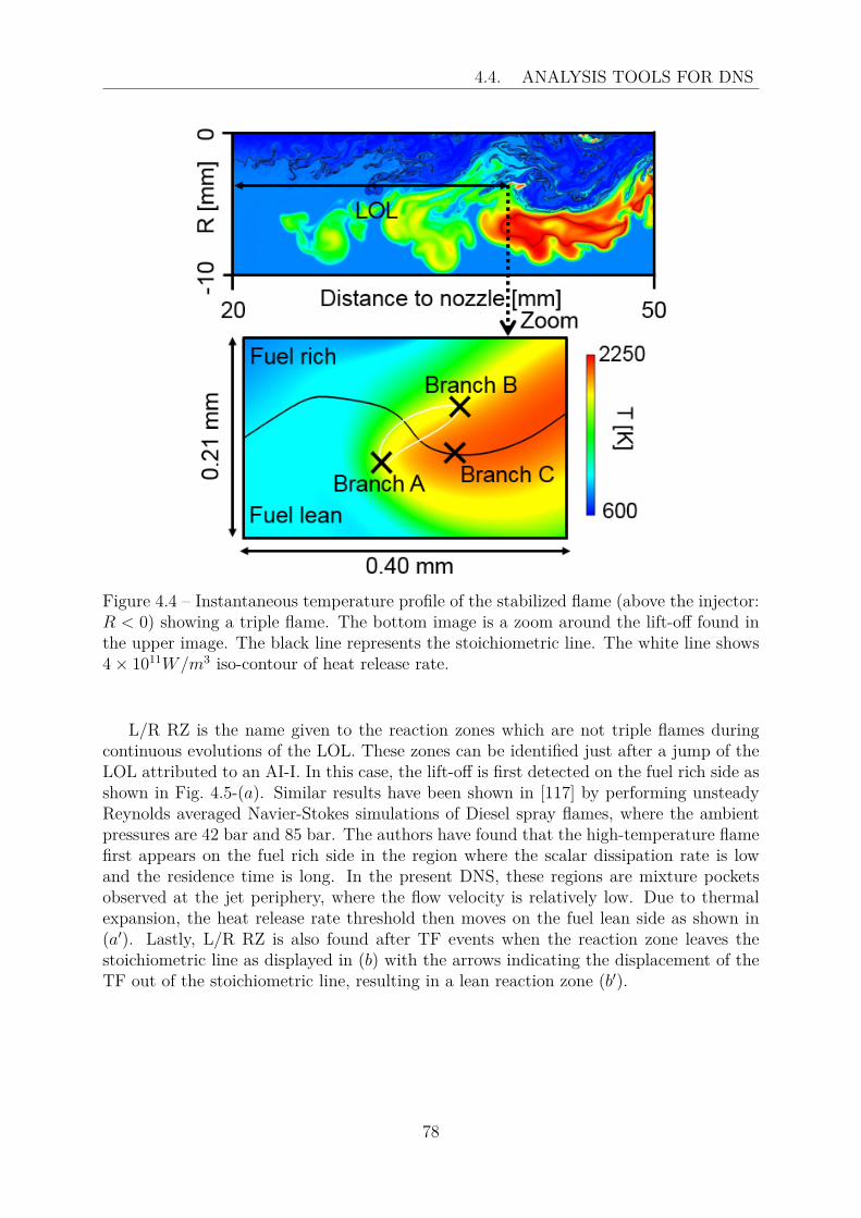
4.4. ANALYSIS TOOLS FOR DNS
Figure 4.4 – Instantaneous temperature profile of the stabilized flame (above the injector:R < 0) showing a triple flame. The bottom image is a zoom around the lift-off found inthe upper image. The black line represents the stoichiometric line. The white line shows4× 1011W/m3 iso-contour of heat release rate.
L/R RZ is the name given to the reaction zones which are not triple flames duringcontinuous evolutions of the LOL. These zones can be identified just after a jump of theLOL attributed to an AI-I. In this case, the lift-off is first detected on the fuel rich side asshown in Fig. 4.5-(a). Similar results have been shown in [117] by performing unsteadyReynolds averaged Navier-Stokes simulations of Diesel spray flames, where the ambientpressures are 42 bar and 85 bar. The authors have found that the high-temperature flamefirst appears on the fuel rich side in the region where the scalar dissipation rate is lowand the residence time is long. In the present DNS, these regions are mixture pocketsobserved at the jet periphery, where the flow velocity is relatively low. Due to thermalexpansion, the heat release rate threshold then moves on the fuel lean side as shown in(a′). Lastly, L/R RZ is also found after TF events when the reaction zone leaves thestoichiometric line as displayed in (b) with the arrows indicating the displacement of theTF out of the stoichiometric line, resulting in a lean reaction zone (b′).
78

4.5. COMPARISON BETWEEN DNS AND EXPERIMENTS
Figure 4.5 – (a) and (a′): two different instantaneous views illustrating a rich reactionzone (a) and a lean reaction zone (a′) after an auto-ignition event. (b) and (b′): timesequence showing triple flames leaving the stoichiometric line. The black line representsthe stoichiometric line. The white line shows the contour of heat release rate of 4 ×10¹¹W/m3.
4.5 Comparison between DNS and experimentsIn order to assess the accuracy/validity of the DNS, a comparison between experiments
and the DNS when the flame has reached a quasi-steady state is proposed. Fig. 4.6 shows asnapshot of mixture fraction (z) and formaldehyde mass fraction (YCH2O) fields at 3.53 msASI. The high-temperature flame can be visualized through the iso-lines of temperature(Fig. 4.6-top) or OH mass fraction (Fig. 4.6-bottom). As in the experiments (Fig. 4.1-top),the flame is lifted between 30 and 40 mm from the injector. Fig. 4.6, for R > 0, showsa detached auto-ignited kernel upstream of the main flame which suddenly decreases theLOL as observed experimentally [14, 15, 61, 82]. Moreover, as observed in [82, 86, 88],DNS predicts formaldehyde upstream the high-temperature reaction zone.
79

4.5. COMPARISON BETWEEN DNS AND EXPERIMENTS
Figure 4.6 – DNS fields at 3.53 ms After the Start of Injection (ASI). Top image: mixturefraction field with an iso-line of temperature at 1900 K (black line). Bottom image:formaldehyde field with an iso-line of OH mass fraction at 1.5× 10⁻⁴ in white.
Additionally, a comparison of the cool-flame structure (identified by CH2O) betweenexperiments and DNS is proposed through averaged images in Fig. 4.7-(a). CH2O isexperimentally measured with 355 LIF (laser generating a 100 mJ laser beam at 355 nmand collected between 400 and 490 nm). The experimental CH2O averaged image is builtby averaging 10 images collected at 4 ms, when the flame has reached a ”quasi-steady”state. The DNS field of YCH2O is averaged between 3 and 12 ms. A comparison betweenexperiments and DNS shows that the upstream location of the stabilized cool-flame issimilar. However, the DNS CH2O levels are lower than experimental levels in the centerjet of the DNS. Nevertheless, the lack of CH2O in the center jet is expected not tohave a strong impact on the stabilization mechanisms since the high-temperature flameis stabilized at the jet periphery, where CH2O is correctly predicted.
Fig. 4.7-(b) also shows a comparison of the high-temperature flame between experi-ments (OH∗) and DNS (OH). The OH∗ image is generated by temporal (between 1.35and 3 ms) and ensemble (10 realizations) averaging using data, collected by high-speedOH∗ chemiluminescence imaging at 60 kHz. The DNS field of YOH is averaged between
80
4.5. COMPARISON BETWEEN DNS AND EXPERIMENTS
3 and 12 ms. Regarding the high-temperature flames, the difference of signal collected inthe center jet between the experiments and the DNS is attributed to the line of sight 3Dcollection of OH∗ chemiluminescence. Indeed, OH PLIF has shown OH species at the jetperiphery [88] as observed in the DNS. OH∗ chemiluminescence image allows to visualizethe average LOL of the high temperature flame, which corresponds to the DNS results.
In conclusion, even if differences between experiments and DNS exist, the simulationreproduces the main features observed experimentally:
• The upstream position of the low- and high-temperature flame, in the DNS, issimilar to the experiments.
• The DNS reproduces the presence of auto-ignited kernels upstream of the high-temperature flame. Such events are responsible for high LOL variation, which havebeen identified as a capital parameter in the flame stabilization [82].
81

4.6. ANALYSIS OF STABILIZATION MECHANISMS
Figure 4.7 – (a): Average images of the high-temperature flame visualized by OH∗ andOH species. (b): Average images of the cool-flame visualized by CH2O species. Theexperimental data are generated using the experimental setup presented in [82].
4.6 Analysis of stabilization mechanisms
4.6.1 LOL tracking with reaction zone topologiesA description of the flame stabilization mechanisms is proposed using the time-tracking
of the different reaction zone topologies identified at the lift-off defined in Section 4.4.2.Fig. 4.8 presents the LOL evolutions where, for the sake of clarity, only 3 ms are displayed,but the full physical time simulated is 12 ms. Each discrete point in time, obtained from
82
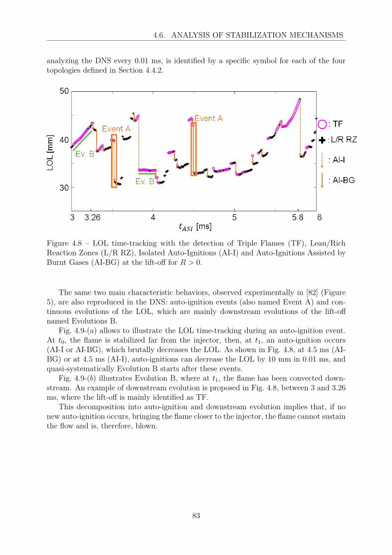
4.6. ANALYSIS OF STABILIZATION MECHANISMS
analyzing the DNS every 0.01 ms, is identified by a specific symbol for each of the fourtopologies defined in Section 4.4.2.
Figure 4.8 – LOL time-tracking with the detection of Triple Flames (TF), Lean/RichReaction Zones (L/R RZ), Isolated Auto-Ignitions (AI-I) and Auto-Ignitions Assisted byBurnt Gases (AI-BG) at the lift-off for R > 0.
The same two main characteristic behaviors, observed experimentally in [82] (Figure5), are also reproduced in the DNS: auto-ignition events (also named Event A) and con-tinuous evolutions of the LOL, which are mainly downstream evolutions of the lift-offnamed Evolutions B.
Fig. 4.9-(a) allows to illustrate the LOL time-tracking during an auto-ignition event.At t0, the flame is stabilized far from the injector, then, at t1, an auto-ignition occurs(AI-I or AI-BG), which brutally decreases the LOL. As shown in Fig. 4.8, at 4.5 ms (AI-BG) or at 4.5 ms (AI-I), auto-ignitions can decrease the LOL by 10 mm in 0.01 ms, andquasi-systematically Evolution B starts after these events.
Fig. 4.9-(b) illustrates Evolution B, where at t1, the flame has been convected down-stream. An example of downstream evolution is proposed in Fig. 4.8, between 3 and 3.26ms, where the lift-off is mainly identified as TF.
This decomposition into auto-ignition and downstream evolution implies that, if nonew auto-ignition occurs, bringing the flame closer to the injector, the flame cannot sustainthe flow and is, therefore, blown.
83
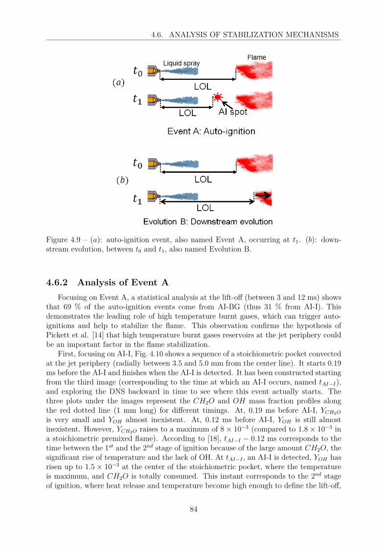
4.6. ANALYSIS OF STABILIZATION MECHANISMS
Figure 4.9 – (a): auto-ignition event, also named Event A, occurring at t1. (b): down-stream evolution, between t0 and t1, also named Evolution B.
4.6.2 Analysis of Event AFocusing on Event A, a statistical analysis at the lift-off (between 3 and 12 ms) shows
that 69 % of the auto-ignition events come from AI-BG (thus 31 % from AI-I). Thisdemonstrates the leading role of high temperature burnt gases, which can trigger auto-ignitions and help to stabilize the flame. This observation confirms the hypothesis ofPickett et al. [14] that high temperature burnt gases reservoirs at the jet periphery couldbe an important factor in the flame stabilization.
First, focusing on AI-I, Fig. 4.10 shows a sequence of a stoichiometric pocket convectedat the jet periphery (radially between 3.5 and 5.0 mm from the center line). It starts 0.19ms before the AI-I and finishes when the AI-I is detected. It has been constructed startingfrom the third image (corresponding to the time at which an AI-I occurs, named tAI−I),and exploring the DNS backward in time to see where this event actually starts. Thethree plots under the images represent the CH2O and OH mass fraction profiles alongthe red dotted line (1 mm long) for different timings. At, 0.19 ms before AI-I, YCH2O
is very small and YOH almost inexistent. At, 0.12 ms before AI-I, YOH is still almostinexistent. However, YCH2O raises to a maximum of 8× 10⁻³ (compared to 1.8× 10⁻³ ina stoichiometric premixed flame). According to [18], tAI−I − 0.12 ms corresponds to thetime between the 1st and the 2nd stage of ignition because of the large amount CH2O, thesignificant rise of temperature and the lack of OH. At tAI−I , an AI-I is detected, YOH hasrisen up to 1.5× 10⁻³ at the center of the stoichiometric pocket, where the temperatureis maximum, and CH2O is totally consumed. This instant corresponds to the 2nd stageof ignition, where heat release and temperature become high enough to define the lift-off,
84

4.6. ANALYSIS OF STABILIZATION MECHANISMS
according to our double criterion (described in Section 4.4.1). In conclusion, the differentstages, shown between tAI−I − 0.19 ms and tAI−I , follow the same well-known steps thanauto-ignition in 0D homogenous reactor configurations.
Figure 4.10 – Image sequence illustrating an isolated auto-ignition (AI-I) at the lift-off.The black line represents the stoichiometric line and the white line shows the contour ofheat release rate of 4 × 10¹¹W/m3 (top images). The three bottom plots show OH andCH2O mass fraction profiles along the red dotted line (measuring 1 mm long) shown onthe top image sequence.
Fig. 4.11 illustrates an AI-BG event, where combustion starts near a zone of hot gases:auto-ignition occurs between the stoichiometric line and a burnt gases pocket, withoutpresenting the two stages observed for AI-I. In this case, burnt gases pockets move, dueto the flow convection, and when they are close enough to the stoichiometric line, theytrigger AI-BG.
85

4.6. ANALYSIS OF STABILIZATION MECHANISMS
Figure 4.11 – Image sequence leading to an AI-BG event. The black line represents thestoichiometric line. The white line shows 4× 10¹¹W/m3 iso-contour of heat release rate.
4.6.3 Analysis of Evolutions BAn illustration of Evolution B is proposed in Fig. 4.12. At 3.03 ms ASI, a TF is
detected at the lift-off, then 0.23 ms later, the LOL has increased by 4.4 mm (still definedas a TF) showing that this flame is convected downstream. The proportion of TF, L/RRZ is almost the same during Evolution B: 45 % TF and 55 % L/R RZ. It indicates thatedge-flames must be taken into account to correctly model spray combustion under Dieselconditions as suggested in [18, 64, 65, 67, 75, 76].
86
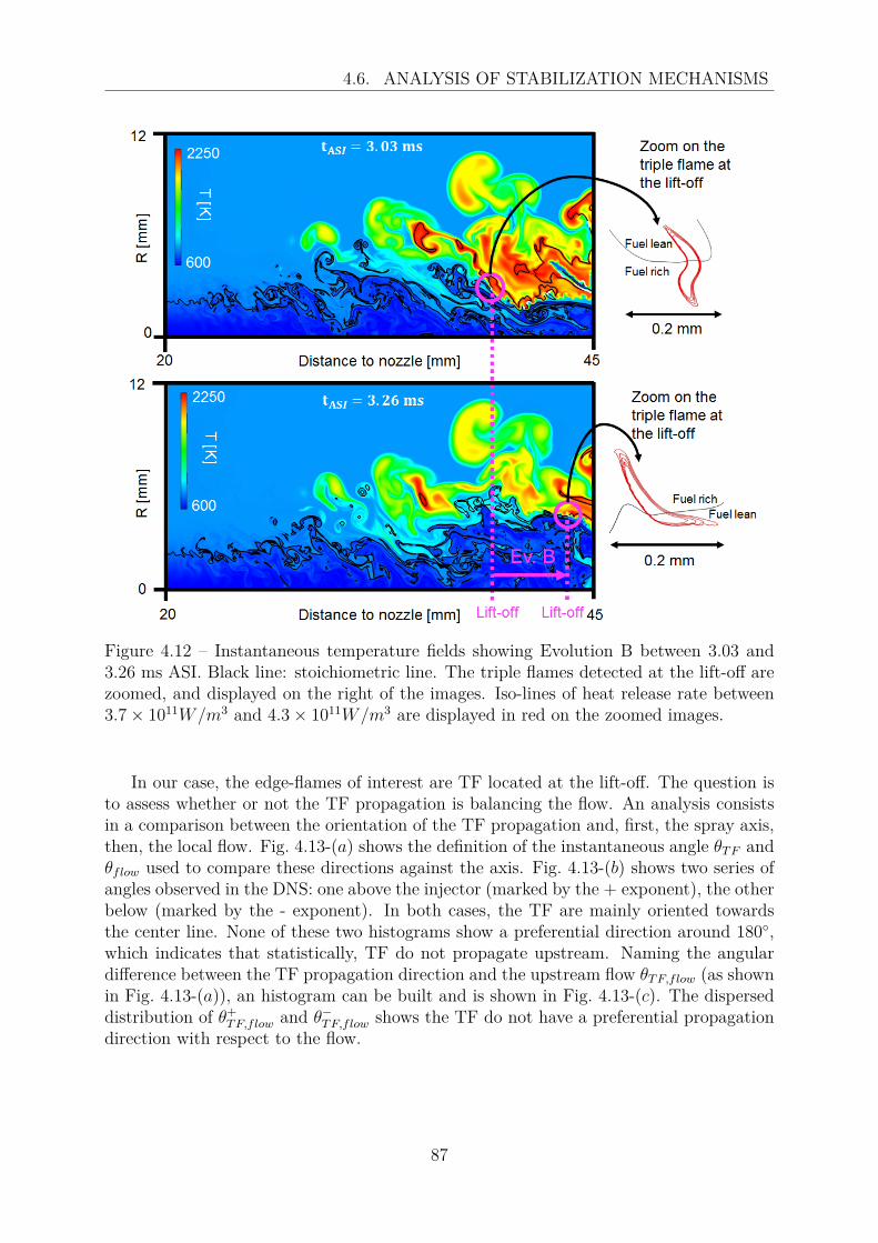
4.6. ANALYSIS OF STABILIZATION MECHANISMS
Figure 4.12 – Instantaneous temperature fields showing Evolution B between 3.03 and3.26 ms ASI. Black line: stoichiometric line. The triple flames detected at the lift-off arezoomed, and displayed on the right of the images. Iso-lines of heat release rate between3.7× 1011W/m3 and 4.3× 10¹¹W/m3 are displayed in red on the zoomed images.
In our case, the edge-flames of interest are TF located at the lift-off. The question isto assess whether or not the TF propagation is balancing the flow. An analysis consistsin a comparison between the orientation of the TF propagation and, first, the spray axis,then, the local flow. Fig. 4.13-(a) shows the definition of the instantaneous angle θTF andθflow used to compare these directions against the axis. Fig. 4.13-(b) shows two series ofangles observed in the DNS: one above the injector (marked by the + exponent), the otherbelow (marked by the - exponent). In both cases, the TF are mainly oriented towardsthe center line. None of these two histograms show a preferential direction around 180◦,which indicates that statistically, TF do not propagate upstream. Naming the angulardifference between the TF propagation direction and the upstream flow θTF,flow (as shownin Fig. 4.13-(a)), an histogram can be built and is shown in Fig. 4.13-(c). The disperseddistribution of θ+TF,flow and θ−TF,flow shows the TF do not have a preferential propagationdirection with respect to the flow.
87

4.6. ANALYSIS OF STABILIZATION MECHANISMS
Figure 4.13 – (a): cartoon of a triple flame propagating along zst. The red solid linerepresents the ω̇T,crit = 4 × 10¹¹W/m3 iso-line. The red arrow shows the triple flamepropagation direction (θTF ) while the green arrow shows the flow direction (θflow). (b):histograms of θ+TF and θ−TF . (c): histograms of θ+TF,flow and θ−TF,flow (right).
Since the flame stabilization is defined by axial displacement of the flame, a comparisonbetween the axial flow velocity at the lift-off (UX,flow,LO) and the absolute axial flame frontspeed relative to a fixed reference (Sa) is proposed trough the ratio UX,flow,LO/Sa. Sa isdefined as the temporal variation of LOL. In order to eliminate spurious behaviors, onlytriplets of consecutive LOL values with correlation coefficient r2 > 0.98 are considered.UX,flow,LO are computed by averaging the corresponding three instantaneous axial flowvelocities at the lift-off.
Fig. 4.14-(a) shows a histogram of the ratio UX,flow,LO/Sa computed between 3 and12 ms for both positive and negative radial coordinates of TF at the lift-off. The meanvalue of this distribution is 0.83, which indicates that Sa is statistically the same orderof magnitude than UX,flow,LO, and thus that the flow controls the evolution of the LOL.However, this analysis can be further detailed. The ratio UX,flow,LO/Sa is plotted as afunction of UX,flow,LO in Fig. 4.14-(b). It appears that for UX,flow,LO > 15, the ratio isvery close to 1, meaning that Sa is governed by the flow. In order to interpret the pointscorresponding to UX,flow,LO < 15, DNS of flames under Diesel-like conditions [18, 76]have indicated that the order of magnitude of the TF displacement speed Sd is between1 and 2 m/s. Assuming Sd = 1.5 m/s, these TF should, therefore, correspond to a curveUX,flow,LO/(UX,flow,LO − 1.5). Fig. 4.14-(b) indeed shows that the points corresponding toUX,flow,LO < 15 lie very close to this curve.
Thus, there are regions where the flow velocity is of the same order of magnitude
88
4.6. ANALYSIS OF STABILIZATION MECHANISMS
than Sd, i.e. regions where the TF can resist to the convection by the fresh gases flow.However, in most regions of the jet, the flow has a much higher velocity than Sd, andtherefore Evolution B is governed by the local flow velocity. This conclusion is differentfrom what is observed for lifted diffusion flames under non-autoignitive conditions [35–38,116], for which the flame is locally stabilized by an equilibrium between flow velocity andSd.
Not shown here, plotting a similar histogram to the one, shown in Fig. 4.14-(a) forthe L/R RZ, shows that Evolution B for these zones is also governed by the local flowvelocity.
89
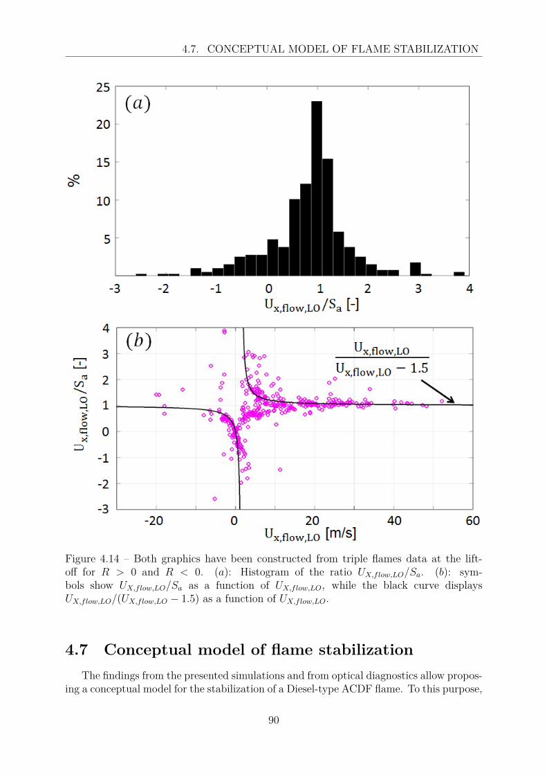
4.7. CONCEPTUAL MODEL OF FLAME STABILIZATION
Figure 4.14 – Both graphics have been constructed from triple flames data at the lift-off for R > 0 and R < 0. (a): Histogram of the ratio UX,flow,LO/Sa. (b): sym-bols show UX,flow,LO/Sa as a function of UX,flow,LO, while the black curve displaysUX,flow,LO/(UX,flow,LO − 1.5) as a function of UX,flow,LO.
4.7 Conceptual model of flame stabilizationThe findings from the presented simulations and from optical diagnostics allow propos-
ing a conceptual model for the stabilization of a Diesel-type ACDF flame. To this purpose,
90

4.7. CONCEPTUAL MODEL OF FLAME STABILIZATION
Fig. 4.15 shows an idealized cross-sectional slice through the mid plane of a spray flame.Only the top branch of the jet is displayed (R > 0). Labelled (a) to (f), six basic localreaction zone topologies are shown on relation to an idealized instantaneous stoichiomet-ric line in the downstream gaseous part of the jet.
Figure 4.15 – Sketch illustrating the conceptual model of flame stabilization under Dieselcondition derived from optical diagnostics and DNS.
As found above, the key necessary stabilization mechanism is auto-ignition. Twodifferent types of auto-ignition can be found, both pertaining to Event A introducedabove: isolated spontaneous auto-ignition, leading to the local topology (a); and auto-ignition assisted by burnt gases, corresponding to the local topology (b). Depending onwhether an (a) or (b) topology creates an Event A, two different stabilization scenarioscan be distinguished in Fig. 4.15:
Scenario 1 starts with an isolated auto-ignition spot (a) localized in a stoichiometricpocket detached from the main jet. This results in an upstream jump of LOL as seenin Fig. 4.8 (dotted arrows). The lift-off is first detected on the fuel-rich side of the localmixture pocket for a few microseconds as displayed in Fig. 4.5-(a). The resulting reactionzone growths in size, and as a result of thermal expansion, the LOL is detected on the fuel-lean side of the mixture pocket as shown in Fig. 4.5-(a′), corresponding to a local topologyof type (d) in Fig. 4.15. During the transition from (a) to (d), the lift-off axially remainsrelatively stable due to thermal expansion that opposes to convection by the flow [118].At the same time, the resulting burnt gases feed high-temperature reservoirs situated inexternal low-velocity or recirculation regions of the jet. Such burnt gases reservoirs remainaxially quite stable, and can ultimately lead to topologies (b) at the origin of scenario 2(see below). Topologies of type (d) can then either extinguish, or reach the stoichiometricline, leading to the appearance of a TF corresponding to topology (c). According toSection 4.6.3, the absolute flame speed of the TF is mainly governed by the flow velocity,
91

4.8. CONCLUSION
and the TF is convected downstream resulting in Evolution B. During this evolution, theTF also feeds burnt gases to the high-temperature reservoirs because of the displacementof their diffusion flame branch.Finally, a TF can deviate from the stoichiometric line, leading to the appearance of atopology of type (e), corresponding to a lean or rich reaction zone as shown in Fig. 4.5-(b′).Transitions between topologies (e) and (c) can happen in both directions until a new auto-ignition occurs or local extinction is encountered.
Scenario 2 starts with a topology of type (b), i.e. an assisted auto-ignition by burntgases coming from high-temperature reservoirs that are fed by the topologies (c)-(f).Topology (b) mainly transitions to (f) which corresponds to fuel-lean reaction zones asillustrated in Fig. 4.11. Unlike topology (d), the reaction zones of topology (f) are sur-rounded by burnt gases which limit the thermal expansion. They are thus growing slower,and are convected downstream by the flow following Evolution B. During this evolution,they feed burnt gases to the high-temperature reservoirs, which, thus, potentially facili-tating the appearance of future scenarios 2. Topologies (f) can also reach a stoichiometricline and form TF corresponding to topology (c). The latter also feeds burnt gases to thehigh-temperature reservoirs, and follows an Evolution B.
In summary, auto-ignition is indispensable for allowing to stabilize a spray flame un-der Diesel-like conditions. Auto-ignition events appear intermittently in the upstreampart of the jet, leading to the strong discontinuities in LOL observed in experiments andsimulations. In-between such auto-ignitions, the leading edge of the reaction zones thatcan have any of the four topologies (c) - (f) are convected downstream by the strongvelocities resulting from the high-pressure liquid jet. Even if these secondary topolo-gies are ultimately blown, they allow sustaining combustion by feeding burnt gases tohigh-temperature reservoirs situated at the periphery of the jet. These reservoirs, indeed,facilitate the appearance of upstream auto-ignition by burnt gases, which combined withspontaneous auto-ignition allows intermittent strong reductions of the LOL, which ulti-mately allows an overall stabilization of the flame.The flame stabilization mechanism is a coupling between the main mechanism auto-ignition and secondary mechanisms linked to the downstream convection of reaction zones.The two mechanisms are linked by the high temperature burnt gases reservoirs at the jetperiphery, confirming the hypothesis proposed in [14].
4.8 ConclusionThis joint experimental/numerical study focused on the stabilization mechanisms of
Autoignitive Conditions Diffusion Flames (ACDF) created when a high speed fuel jetwas injected into hot air. Starting from experimental observations of n-dodecane jetsinto hot air, a specific DNS was built to elucidate mechanisms which control the LOL(Lift-Off Length). The analysis of the DNS showed that two types of mechanisms controlthe flame stabilization: auto-ignition events, where the LOL jumped rapidly to smallvalues, followed by evolutions where the flames, created by auto-ignition events, wereconvected downstream by the flow without significant flame propagation effects. To obtainthese results, a post-processing methodology to extract information, from DNS fields, wasderived. The main conclusion is that auto-ignition was the key stabilization mechanism,while triple flames, even if they exist, had insufficient propagation speeds to contribute to
92
4.8. CONCLUSION
the flame stabilization. These flames were visible in multiple points of the flame brush,but they cannot be expected to provide a stabilization mechanism. Future studies shouldfurther explore the behavior of the presented conceptual model according to test conditionvariations (e.g. ambient temperature, and injection pressure variation). Finally, a Dieselengine environment is wall bounded and characterized by jet-jet interactions in the contextof a swirling flow [119, 120]. These differences with the presently studied unboundedisolated spray could impact the stabilization mechanisms and their interactions. Thiswould have to be explored in future experimental and simulation work.
Appendix 1The inlet NSCBC [107] boundary condition (left edge of the computational domain) is
addressed imposing radial profiles of mean axial velocity (Eq. 4.1), temperature (Eq. 4.2),mass fraction species (Eq. 4.3) and synthetic isotropic turbulence (Eq. 4.4):{
UX(R) = UmaxX exp(−R2/2σ2
1) + Ucoflow
UmaxX = 80 m/s
(4.1)
T (R) = Tamb + (600− Tamb) exp(−R2/σ21) (4.2){
YnC12H26(R) = 0.153 exp(−R2/σ21)
Yk(R) = (1− YnC12H26)Y0k with k = N2, O2, CO2, H2O
(4.3)
{URMS(R) = Umax
RMS exp(−(R− µ)2/σ22) + Umax
RMS exp(−(R + µ)2/σ22),
UmaxRMS = 7 m/s
(4.4)
where:
• R is the radial coordinate
• σ1, σ2 and µ are constant respectively equal to 1.8, 1.4 and 1.7 mm
• Ucoflow is a co-flow used to avoid negative axial velocity on the inlet boundarycondition set to 1 m/s
• Tamb is the ambient temperature (800 K)
• Y 0N2, Y 0
O2, Y 0
CO2, Y 0
H2Oare given in Table 4.1
4.8.1 Complementary elements
4.8.2 Non-reactive profilesThis section presents the methodology adopted to compare the characteristics of the
mixing between the DNS and the experiments.
First, a non-reactive DNS is performed from 0 to 10 ms. In this simulation, thenumerical setup is identical to the reactive DNS. The only difference between the two
93
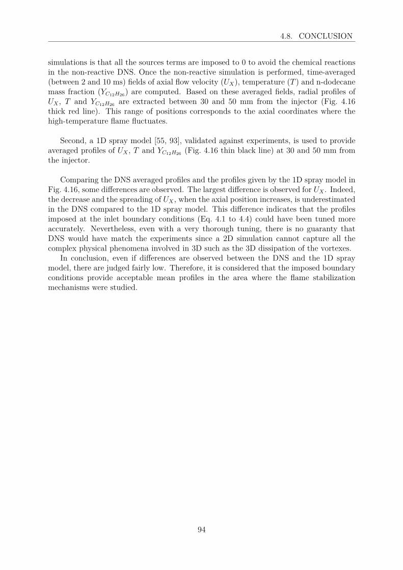
4.8. CONCLUSION
simulations is that all the sources terms are imposed to 0 to avoid the chemical reactionsin the non-reactive DNS. Once the non-reactive simulation is performed, time-averaged(between 2 and 10 ms) fields of axial flow velocity (UX), temperature (T ) and n-dodecanemass fraction (YC12H26) are computed. Based on these averaged fields, radial profiles ofUX , T and YC12H26 are extracted between 30 and 50 mm from the injector (Fig. 4.16thick red line). This range of positions corresponds to the axial coordinates where thehigh-temperature flame fluctuates.
Second, a 1D spray model [55, 93], validated against experiments, is used to provideaveraged profiles of UX , T and YC12H26 (Fig. 4.16 thin black line) at 30 and 50 mm fromthe injector.
Comparing the DNS averaged profiles and the profiles given by the 1D spray model inFig. 4.16, some differences are observed. The largest difference is observed for UX . Indeed,the decrease and the spreading of UX , when the axial position increases, is underestimatedin the DNS compared to the 1D spray model. This difference indicates that the profilesimposed at the inlet boundary conditions (Eq. 4.1 to 4.4) could have been tuned moreaccurately. Nevertheless, even with a very thorough tuning, there is no guaranty thatDNS would have match the experiments since a 2D simulation cannot capture all thecomplex physical phenomena involved in 3D such as the 3D dissipation of the vortexes.
In conclusion, even if differences are observed between the DNS and the 1D spraymodel, there are judged fairly low. Therefore, it is considered that the imposed boundaryconditions provide acceptable mean profiles in the area where the flame stabilizationmechanisms were studied.
94
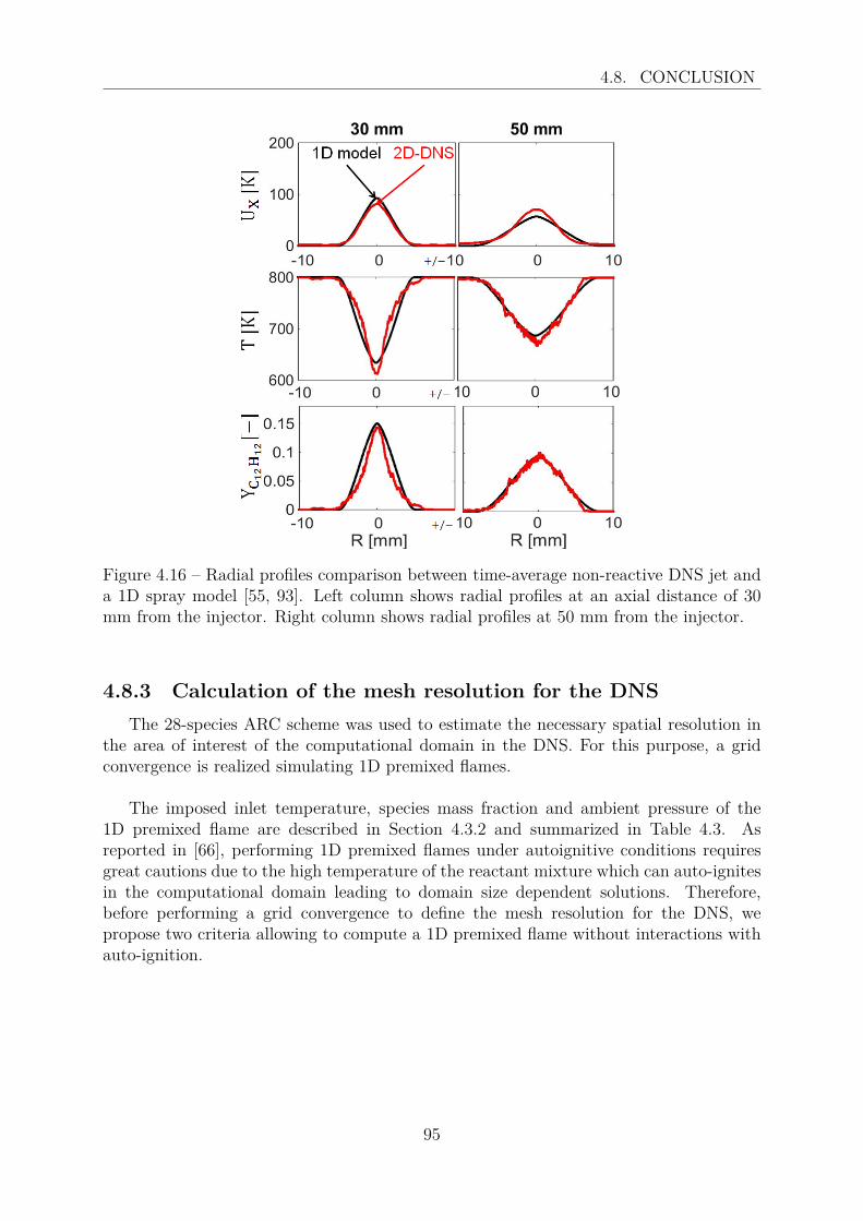
4.8. CONCLUSION
Figure 4.16 – Radial profiles comparison between time-average non-reactive DNS jet anda 1D spray model [55, 93]. Left column shows radial profiles at an axial distance of 30mm from the injector. Right column shows radial profiles at 50 mm from the injector.
4.8.3 Calculation of the mesh resolution for the DNSThe 28-species ARC scheme was used to estimate the necessary spatial resolution in
the area of interest of the computational domain in the DNS. For this purpose, a gridconvergence is realized simulating 1D premixed flames.
The imposed inlet temperature, species mass fraction and ambient pressure of the1D premixed flame are described in Section 4.3.2 and summarized in Table 4.3. Asreported in [66], performing 1D premixed flames under autoignitive conditions requiresgreat cautions due to the high temperature of the reactant mixture which can auto-ignitesin the computational domain leading to domain size dependent solutions. Therefore,before performing a grid convergence to define the mesh resolution for the DNS, wepropose two criteria allowing to compute a 1D premixed flame without interactions withauto-ignition.
95

4.8. CONCLUSION
Table 4.3 – 1D premixed flame initial conditions.
Inlet temperature [K] 739Inlet YN2 [-] 0.668Inlet YO2 [-] 0.166Inlet YCO2 [-] 0.095Inlet YC12H26 [-] 0.048Inlet YH2O [-] 0.023Pressure [bar] 34
4.8.3.1 Criteria to simulate 1D premixed flames under autoignitive conditions
For a 1D premixed flame the mixture is convected at UI in the fresh gas. This velocityis equal to the laminar premixed flame velocity if the flame is stabilized. However, whenthe inlet temperature and ambient pressure are high enough, the mixture can auto-ignitebefore the premixed flame front.
In such case, illustrated in Fig. 4.17, there is a gradual increase in temperature beforethe flame front. This rise of temperature is attributed to the low-temperature chemicalreactions. Then the high-temperature flame stabilized by auto-ignition at approx. UI ×τAI , where τAI in the auto-ignition delay of the mixture.
Figure 4.17 – Illustration of 1D flame stabilized by auto-ignition.
The methodology to avoid auto-ignition in the 1D computational domain consistsin reducing the length of domain (LX , see Fig. 4.17). So that, the residence time of themixture is too low to auto-ignite in the domain. For this purpose, the following parameteris defined:
CAI =min(τAI , τAI,coolflame).UI
LX
, (4.5)
where, τAI,coolflame and τAI are the delays corresponding to the 1st and 2nd stage ignition[18, 62] computed in a 0D constant pressure reactor. We consider that if the criterionCAI > 1 is met, the cool-flame and the auto-ignition front is localized outside of thecomputational domain.
96

4.8. CONCLUSION
Taking into account only the above criterion would lead to infinitely reduce the lengthof the domain. However, the length of the domain needs to be large enough to cor-rectly model the diffusion phenomena in a 1D premixed flame. Therefore, the followingparameter is defined:
CδT =δTLf
, (4.6)
where, δT is the thermal thickness [25] and Lf is the distance between the inlet boundaryconditions and the front flame. In the case where the flame is stabilized in the middleof the domain Lf = LX/2. Verifying CδT < 0.5 is judged to be acceptable to properlyresolve the 1D premixed flame.
A 1D premixed flame is computed using Cantera with the 28-species ARC scheme forthe conditions shown in Table 4.3. The length of the domain is 0.2 mm and the flamefront is localized in the middle of the domain (Lf = 0.1 mm). Table 4.4 shows the valuesof CAI and CδT . As the two criteria are both satisfied (CAI > 1 and CδT < 0.5), the meshresolution can be varied in order to define mesh resolution in the area of interest of theDNS.
Table 4.4 – 1D premixed flame characteristics.
CAI [-] 1.7δT [µm] 32CδT [-] 0.32UI = SL [m/s] 0.34
4.8.3.2 Grid convergence
In a second step, 1D premixed flame simulations are performed with AVBP for differentspatial resolutions. They are all simulated in a computational domain with a length of 0.2mm and for the conditions described in Table 4.3. Fig. 4.18 shows four grids resolutionstested: 1, 5, 6 and 7 µm. The first three (1, 5 and 6 µm) cases present a flame stabilized.However, the 7 µm case shows two curves because the flame is not able to stabilize andoscillates between two positions for t1 and t2. Therefore, the area of interest for the DNSis set to 6 µm since we assume that this resolution is sufficient to correctly resolve theflame front.
97
4.8. CONCLUSION
Figure 4.18 – Grid convergence for 1D premixed flames at the stoichiometric mixturefraction. Temperature (top) and heat release rate (bottom) profiles are plotted for aspatial resolution varying between 1 and 7 µm.
98
Chapter 5
A Lift-Off Length fluctuations model
Experimental correlations such as the one proposed by Siebers et al. [1, 2] or byVenugopal and Abraham [60] aim at predicting the time-averaged LOL when the flame isstabilized (see Eq. 2.6 and Eq. 2.15). They are very useful and are widely used but, sincethey predict the time-averaged LOL, they do not account for the spatial fluctuations ofthat value. It has been shown in the previous Chapters that the high-temperature flamecan significantly fluctuate around the time-averaged LOL. These spatial fluctuations leadto fluctuations of the local mixing at the lift-off, which may result in significant fluctuationsof soot production, since it was shown in Bardi et al. [121] that the latter is highlysensitive to small variations of the LOL. In the previous chapters, a detailed investigationof the mechanisms responsible for the LOL stabilization process lead to the proposalof a conceptual model. The objective of this Chapter is to take advantage of this newknowledge to propose a numerical model that aims at predicting the LOL fluctuationsaround the time-averaged value.
The motivations for such a LOL fluctuations model are first detailed (Section 5.1)before deriving an expression of the fluctuations of the LOL based on the understandingof the stabilization mechanisms acquired during this work (Section 5.2). Then, a databaseof LOL fluctuations measurements for various test conditions is presented (Section 5.3).The latter has been acquired in a previous experimental campaign [121]. Finally, inSection 5.4, the theoretical LOL fluctuations model is compared to the experimental LOLfluctuations database in order to analyze the performance of the model.
5.1 MotivationExperimental results available in the literature [13] show that the soot level evolves
linearly with the inverse of the equivalence ratio at the time-averaged LOL, and that itis reduced to zero for an equivalence ratio lower than a threshold. Fig. 5.1 is reproducedfrom [13] and illustrates this result. It displays the density-normalized peak of the opticalthickness (KL) (used as a representation of relative soot level in a fuel jet) as a functionof the inverse of the equivalence ratio at the time-averaged LOL (1/ΦLOL).
When the flame is stabilized close enough to the injector, the local mixture at the lift-off is fuel-rich (equivalence ratio between 2 and 10) resulting in soot formation. However,
99

5.1. MOTIVATION
when the flame is stabilized far enough from the injector, in regions where the equivalenceratio is below 2 (above 1/ΦLOL = 0.5), no soot are produced.
In order to illustrate the interest of predicting the LOL fluctuations, we take here theexample of a case where the LOL is stabilized such that the equivalence ratio is 1.82 (i.e.the inverse of the equivalence ratio is 0.55). This latter value is illustrated by a red starin Fig. 5.1. The outcome of this latter figure shows that the soot production is supposedto be negligible in this case. But this is the result of an average representation thatdoes not take into account fluctuations of the LOL. Indeed, experimental and numericalresults presented in Chapter 3 and 4 have shown high fluctuations around the averagedLOL, mainly attributed to auto-ignition processes. For convenience, we note ∆LOLthe magnitude of the LOL fluctuations around the time-averaged LOL. A double arrowindicating the magnitude of equivalence ratio fluctuations corresponding to ∆LOL andset to an arbitrary value is displayed in Fig. 5.1. It illustrates this fluctuation of the LOLposition and their effect on the equivalence ratio at the lift-off. This illustration showsthat although soot production is zero in average, the LOL can fluctuate in regions wherethe equivalence ratio is higher and therefore one can expect that soot are generated asillustrated by the dashed area. This case clearly illustrates the interest of taking intoaccount LOL position fluctuations and therefore of having a model able to predict thesefluctuations. Having clearly demonstrated the interest of predicting LOL fluctuations,the objective of the next sections will be to propose and validate such a lift-off lengthfluctuations model.
100
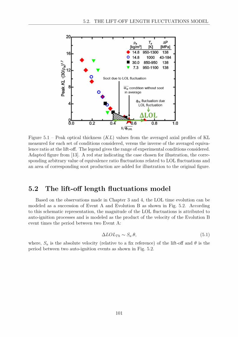
5.2. THE LIFT-OFF LENGTH FLUCTUATIONS MODEL
Figure 5.1 – Peak optical thickness (KL) values from the averaged axial profiles of KLmeasured for each set of conditions considered, versus the inverse of the averaged equiva-lence ratio at the lift-off. The legend gives the range of experimental conditions considered.Adapted figure from [13]. A red star indicating the case chosen for illustration, the corre-sponding arbitrary value of equivalence ratio fluctuations related to LOL fluctuations andan area of corresponding soot production are added for illustration to the original figure.
5.2 The lift-off length fluctuations modelBased on the observations made in Chapter 3 and 4, the LOL time evolution can be
modeled as a succession of Event A and Evolution B as shown in Fig. 5.2. Accordingto this schematic representation, the magnitude of the LOL fluctuations is attributed toauto-ignition processes and is modeled as the product of the velocity of the Evolution Bevent times the period between two Event A:
∆LOLTh ∼ Sa.θ, (5.1)
where, Sa is the absolute velocity (relative to a fix reference) of the lift-off and θ is theperiod between two auto-ignition events as shown in Fig. 5.2.
101

5.2. THE LIFT-OFF LENGTH FLUCTUATIONS MODEL
Figure 5.2 – Schematic representation of the Lift-off length as a function of time.
Once this primary expression of the LOL fluctuations is proposed, a modeling of Sa
and θ are required. The latter is proposed in the next sections using the knowledge of thelift-off stabilization mechanisms acquired in Chapter 3 and 4.
5.2.1 Sa modelAccording to the results obtained in Chapter 4, and illustrated by the conceptual
model, the flow velocity governs the downstream evolution of the LOL (evolution B).Therefore we assume:
Sa ≈ uLO, (5.2)
where uLO is the flow velocity at the lift-off. In order to derive an expression for uLO,we assume that it varies proportionally to the axial flow velocity in the center of the jet,UX;R=0. The latter can be derived using a 1D spray model [55, 93]. Fig. 5.3 displays theresult of this model and shows how UX;R=0 evolves as a function of the axial position (X)for the α test condition (see Chapter 3 for the definition of α). At X = 0, the flow velocityis U0, then UX;R=0 decays as a function of 1/X. Thus, assuming that the flow velocityat the lift-off follows the same 1/X trend, we obtain: uLO ∼ U0/LOL. Furthermoreaccording to the conservation of momentum [55, 93] the flow velocity at the lift-off alsodepends on the fuel and air density (ρf and ρa) and the nozzle diameter (d0). Thereforeit leads to the following relationship:
uLO ∼ U0
LOL.d0.
(ρfρa
)0.5
(5.3)
102
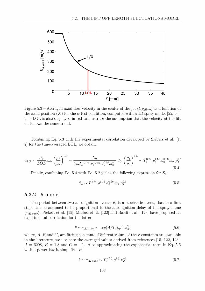
5.2. THE LIFT-OFF LENGTH FLUCTUATIONS MODEL
Figure 5.3 – Averaged axial flow velocity in the center of the jet (UX;R=0) as a function ofthe axial position (X) for the α test condition, computed with a 1D spray model [55, 93].The LOL is also displayed in red to illustrate the assumption that the velocity at the liftoff follows the same trend.
Combining Eq. 5.3 with the experimental correlation developed by Siebers et al. [1,2] for the time-averaged LOL, we obtain:
uLO ∼ U0
LOL.d0.
(ρfρa
)0.5
∼ U0
U0.T−3.74a .ρ−0.85
a .d0.340 .z−1st
.d0.
(ρfρa
)0.5
∼ T 3.74a .ρ1.35a .d0.660 .zst.ρ
0.5f
(5.4)Finally, combining Eq. 5.4 with Eq. 5.2 yields the following expression for Sa:
Sa ∼ T 3.74a .ρ1.35a .d0.660 .zst.ρ
0.5f (5.5)
5.2.2 θ modelThe period between two auto-ignition events, θ, is a stochastic event, that in a first
step, can be assumed to be proportional to the auto-ignition delay of the spray flame(τAI,turb). Pickett et al. [15], Malbec et al. [122] and Bardi et al. [123] have proposed anexperimental correlation for the latter:
θ ∼ τAI,turb ∼ exp(A/Ta).ρB.zCst, (5.6)
where, A, B and C, are fitting constants. Different values of these constants are availablein the literature, we use here the averaged values derived from references [15, 122, 123]:A = 6298, B = 1.3 and C = −1. Also approximating the exponential term in Eq. 5.6with a power law it simplifies to:
θ ∼ τAI,turb ∼ T−7.0a .ρ1.3.z−1
st (5.7)
103
5.2. THE LIFT-OFF LENGTH FLUCTUATIONS MODEL
The results of Chapter 3 and 4 demonstrate that in addition to isolated auto-ignition,High-Temperature Reservoirs (HTR) have a significant effect on the LOL stabilizationprocess by enabling auto-ignition assisted by burnt gases. This mechanism is not takeninto account in Eq. 5.6, therefore a second modeling step is proposed.
Based on the results of Chapter 3 and 4, two parameters are found to have a significanteffect on the mechanism of auto-ignition assisted by burnt gases: ambient temperatureand injection velocity.
Indeed, the HTR are filled by burnt gases formed after an auto-ignition or a premixedflame. Increasing the ambient temperature leads to increase the temperature of freshgases locally before an auto-ignition event and in front of a triple flame. This leads toan increase of the temperature of the burnt gases in both cases. As a result, it is likelythat increasing the temperature of the HTR facilitates assisted auto-ignition, thereforedecreasing the time between two auto-ignition events.
Also, the injection velocity is expected to modify the flow field surrounding the sprayand therefore the ability of the HTR to remain at the jet periphery. In particular, we canexpect that if the injection velocity is high the probability of the HTR to be blown offis higher. Finally, no corrections are proposed for the density and the mixture fractionterms since no influence of these parameters has been observed in the previous chapters.Based on these observations, the following modifications are proposed to Eq. 5.7:
θ ∼ τAI,turb ∼ T−7.0+aa .ρ1.3.z−1
st .Ub0 , (5.8)
where a is a negative coefficient to take into account the fact that increasing Ta facili-tates assisted auto-ignition and therefore reduces time between two auto-ignition events,and b is a positive coefficient taking into account the fact that with higher velocity, theprobability of the HTR to be blown off is higher hence increasing the time between twoauto-ignition events. The value of these coefficients has to be determined based on exper-imental correlation, this is the purpose on the next sections.
5.2.3 ∆LOLTh modelCombining the modeled expressions of Sa (Eq. 5.5) and θ (Eq. 5.8) with Eq. 5.1, we
finally propose the following expression of the LOL fluctuations:
∆LOLTh ∼ T−3.26+aa .ρ2.65a .d0.660 .U b
0 .ρ0.5f (5.9)
The results obtained with this LOL fluctuations model are compared to an experimen-tal database in the next sections for validation purpose and to calibrate the coefficient aand b.
104

5.3. LIFT-OFF LENGTH FLUCTUATIONS EXPERIMENTAL DATABASE
5.3 Lift-off length fluctuations experimental database
In order to calibrate and validate the LOL fluctuations model, an experimental databasealready available has been used. The latter was performed within the ASMAPE 1 projectat IFPEN. Detailed information on this database are available in [121]. Therefore, onlya brief description, relevant in the context of the present work is presented here.
The constant volume pre-burn facility, used for the database, is the same than theone described in Chapter 3. The fuel injector also presents the same characteristics thanthe one in Chapter 3 even if the injector is different: injector # 306.15 in this section(injector # 306.22 in Chapter 3).
The high-speed OH* chemiluminescence technique is used to track the LOL over timein order to analyze its fluctuations noted ∆LOLexpe . Similarly to Chapter 3, a high-speedintensifier (Lambert Instruments - HiCATT) is coupled to a high-speed camera (PhotronSA-Z) enabling low-noise high-speed image acquisition. The flame radiation was filteredusing a band-pass filter (315 ± 15 nm), and collected using a 100 mm UV lens between1.5 and 5.5 ms after the start of injection. The details of the high-speed OH* chemilumi-nescence setup are presented in Table 5.1.
Fig. 5.4 shows the time evolution of LOLexpe for conditions similar to spray A [17],but with a lower (800 K) ambient temperature. Similarly to the results described inChapter 3, the LOLexpe time evolution (LOLexpe(t)) can be decomposed into auto-ignitionevents (Event A) and downstream evolution (Evolution B). The fluctuations of LOLexpe
(shown with an orange double arrow) are derived from the standard deviation of the LOLtime-tracking, σ(LOLexpe(t)), as illustrated in the figure with the blue double arrow andaccording to the following equation:
∆LOLexpe ∼ σ(LOLexpe(t)) (5.10)1Advanced Soot Models for Aeronautic and Piston Engines
105

5.3. LIFT-OFF LENGTH FLUCTUATIONS EXPERIMENTAL DATABASE
Figure 5.4 – LOL time evolution using OH∗ chemiluminescence imaging. Test conditionsare: Pinj = 150MPa, PrctO2 = 15%, Tamb = 800K and ρamb = 22.8kg/m3.
Table 5.2 presents the different test conditions available in the database. Variations ofambient temperature, injection pressure and ambient oxygen concentration were carriedout and are available to observe the variations of ∆LOLexpe when test conditions change.Table 5.3 shows the number of realizations for each parametric variation. For everyrealization, the LOL time tracking is performed (as shown in Fig. 5.4), resulting in acalculation of σ(LOLexpe(t)) for each realization.
Table 5.1 – High-speed OH* chemiluminescence optical setup.
Camera Photron SA-Z camera + HS intensifierLens UV 100 mm -f/2.8Filter 315 ± 15 nmShutter time 5 µs (gate time)Frame rate 47.2 kHz
106
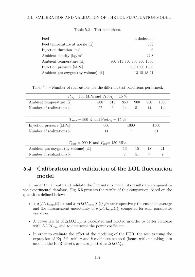
5.4. CALIBRATION AND VALIDATION OF THE LOL FLUCTUATION MODEL
Table 5.2 – Test conditions.
Fuel n-dodecaneFuel temperature at nozzle [K] 363Injection duration [ms] 6Ambient density [kg/m3] 22.8Ambient temperature [K] 800 815 850 900 950 1000Injection pressure [MPa] 600 1000 1500Ambient gas oxygen (by volume) [%] 13 15 18 21
Table 5.3 – Number of realizations for the different test conditions performed.
Pinj= 150 MPa and PrctO2 = 15 %Ambient temperature [K] 800 815 850 900 950 1000Number of realizations [-] 27 6 14 51 14 14
Tamb = 900 K and PrctO2 = 15 %Injection pressure [MPa] 600 1000 1500Number of realizations [-] 14 7 51
Tamb = 900 K and Pinj= 150 MPaAmbient gas oxygen (by volume) [%] 13 15 18 21Number of realizations [-] 7 51 7 7
5.4 Calibration and validation of the LOL fluctuationmodel
In order to calibrate and validate the fluctuations model, its results are compared tothe experimental database. Fig. 5.5 presents the results of this comparison, based on thequantities defined below:
• < σ(LOLexpe(t)) > and σ[σ(LOLexpe(t))]/√n are respectively the ensemble average
and the measurement uncertainty of σ(LOLexpe(t)) computed for each parametricvariation.
• A power law fit of ∆LOLexpe is calculated and plotted in order to better comparewith ∆LOLTh, and to determine the power coefficient.
• In order to evaluate the effect of the modeling of the HTR, the results using theexpression of Eq. 5.9, with a and b coefficient set to 0 (hence without taking intoaccount the HTR effect), are also plotted as ∆LOL∗
Th.
107

5.4. CALIBRATION AND VALIDATION OF THE LOL FLUCTUATION MODEL
The upper left graph of Fig. 5.5 presents a comparison for the ambient temperaturevariations. When the HTR effect is not taken into account, ∆LOL∗
Th reproduces theexperimental trend, but with a lower negative power coefficient. With a coefficient a setto -0.80, the evolution of ∆LOLTh and the ∆LOLexpe fit match perfectly. This value willtherefore be chosen for the final expression of the model.
The upper right graph presents a comparison for the oxygen concentration variations.It shows that ∆LOL∗
Th is not affected by oxygen concentration. A different evolutionfor the ∆LOLexpe fit is found. Indeed, the latter is constant for oxygen concentrationbetween 15 and 21 %, but it is higher in the 13 % of oxygen case. Such a behavior is notstraightforward to explain and requires more investigation. This is beyond the scope ofthe present work.
Finally, the lower left graph presents a comparison for the injection pressure variations.∆LOLexpe clearly shows an increase when the injection pressure is increased. When HTReffects are not taken into account, ∆LOL∗
Th does not reproduces this trend, thereforeshowing the necessity to take these effects into account. Adjusting the coefficient b to0.54 (0.27× 2) enables to correctly follow the experimentally observed trend.
The results displayed in Fig. 5.5 demonstrate that the LOL fluctuations model avail-able in Eq. 5.9 well reproduces the variations of the LOL fluctuations observed experi-mentally, once the a and b coefficients are calibrated. Taking the latter into account, thefinal expression of the model is:
∆LOLTh ∼ T−4.06a .ρ2.65a .d0.66.U0.54
0 .ρ0.50f (5.11)
108

5.5. CONCLUSION
Figure 5.5 – Plot of the experimental and theoretical magnitude of the LOL fluctuationsaccording to ambient temperature (Tamb), oxygen concentration (PrctO2) and injectionpressure (Pinj) variations.
5.5 ConclusionA model predicting the variations of the LOL fluctuations (∆LOL) has been pro-
posed and is available in Eq. 5.9. This model was derived from observations made inChapter 3 and 4, where it was found that the LOL time evolution is characterized byauto-ignition events and downstream evolution. The auto-ignition period and the veloc-ity of the downstream evolution were modeled using experimental correlations available inthe literature. Moreover, the role of high-temperature reservoirs on the flame stabilizationprocess, demonstrated in Chapter 4, is taken into account through additional coefficientsfor ambient temperature and injection velocity.
The resulting model has been compared to an experimental database, where the am-bient temperature, oxygen concentration and injection pressure were varied. The trendsof the variations of LOL experimentally measured were in good agreement with the modeldeveloped in Eq. 5.9. Moreover, the experimental data allowed to calibrate the coefficientsproposed for the effect of high temperature reservoirs. The final expression of the modelavailable in Eq. 5.11, based on the conceptual model shown Fig. 4.15, correctly reproducesthe experimental measurements.
109

Chapter 6
Conclusions and perspectives
6.1 Summary of main findingsThe overall objective of the present PhD thesis was to contribute to a better under-
standing of the stabilization mechanisms of a lifted liquid spray flame under diesel engineconditions. This investigation has been conducted because the stabilization process ofdiesel spray flames has a strong link to the soot production. However, the fundamentalnature of the stabilization mechanisms is still a subject of research.
The bibliographic review presented in Chapter 2 has shown two main candidates toexplain the flame stabilization under diesel conditions: auto-ignition and premixed flamepropagation. The proposed research combined a experimental and numerical approach inorder to quantify the role and relative importance of these two stabilization mechanisms,and to identify other phenomena possibly implicated in the spray flame stabilization.
In Chapter 3, the stabilization processes were experimentally studied using long n-dodecane injection duration (10 ms) under conditions close to the ECN spray A [17].High-temperature chemiluminescence and 355 LIF have confirmed the existence of aformaldehyde cloud upstream of the lift-off. Moreover, the formaldehyde cloud was foundto be stable in comparison to the high-temperature flame zone which on the contraryexhibits large lift-off length (LOL) fluctuations. The latter are due to the sporadic ap-pearance of auto-ignition spots upstream the stabilized lift-off. The temporal variationsof the LOL presented two typical features: very rapid upstream evolution events linked toauto-ignition, and more progressive downstream evolution, both of them occurring withinthe formaldehyde cloud.
In order to investigate the stabilization mechanisms involved during the downstreamevolution stage, a forced ignition at different positions upstream the lift-off using laser-induced plasma was performed. This allowed to emphasize the role of low-temperaturereactions on the downstream evolution: when located upstream the formaldehyde cloud,rapid LOL temporal evolutions was observed, whereas inside the formaldehyde cloud asystematic slower progression was observed. This lead to the conclusion that, the sta-bilization mechanism was governed by an alternation of auto-ignition and downstreamevolution, in which the low-temperature reactions play a leading role.
110

6.1. SUMMARY OF MAIN FINDINGS
In order to provide a better understanding of the local instantaneous flame stabiliza-tion mechanisms, a two-dimensional Direct Numerical Simulation (DNS) of a spatiallydeveloping turbulent lifted gaseous flame was presented in Chapter 4. This DNS yieldedlocal conditions similar to those found for the α test conditions experimentally studiedin Chapter 3. The DNS only covers a downstream region where the flow can be reducedto a gaseous jet, since experimental observations have shown that the flame stabilizeddownstream of the liquid spray. The inflow conditions for the DNS were imposed basedon experimental studies. The chemistry was modeled using a reduced chemical kineticsscheme comprising 28 species and 198 reactions. This scheme was formulated to accountfor the low- and high temperature reaction pathways, and its predictions have been val-idated against experimental auto-ignition delays and laminar flame speeds at conditionsrelevant to the simulated cases.
The analysis of DNS results showed the same two types of mechanisms controllingthe flame stabilization than observed experimentally: auto-ignition events, where the lift-off jumped rapidly to smaller values, followed by downstream evolution of the lift-off.However, the analysis of local values of velocities, gas composition and chemical reactionconditions in the lift-off zone allowed to further detail these mechanisms:
• Auto-ignition events have been subdivided into two types:
– Isolated auto-ignitions (AI-I) appearing in fresh gasses regions– Auto-ignition assisted by burned gases (AI-BG), appearing in regions where
combustion products were in contact with fuel and fresh gasses. This provesthat high-temperature reservoirs, as hypothesized in [14], play a leading rolein the stabilization of the lift-off.
• Downstream evolutions have also been divided into two types, depending on thenature of the reaction zone at lift-off:
– Triple flames (TF), presenting the same characteristics than the TF observedfor non-autoignitive flame (Section2.2.1.2).
– Lean/Rich reaction zones (L/R RZ) was the name given to the reaction zoneswhich were not triple flames during continuous evolutions of the LOL. Thesezones have been identified just after a jump of the LOL attributed to an AI-I.
An analysis of the local velocities at the lift-off showed that downstream evolution wasmainly governed by the flow velocity. The flame propagation speed had only a minor con-tribution. Therefore, auto-ignition was the key mechanism allowing to stabilize the flame,that would otherwise be blown away by the flow. These observations were summarized ina conceptual model at the end of Chapter 4.
The fluctuations of LOL have been observed and explained in Chapter 3 and 4. Interms of soot emissions, these fluctuations are of great importance because they mean thata flame can alternatively be non-sooting (when the LOL moves downstream) or sooting(when the LOL moves upstream). Based on the results of Chapter 3 and 4, a scaling-lawestimating the amplitude of these fluctuations was proposed in Chapter 5. It accounted
111

6.2. PERSPECTIVES
for the isolated and assisted auto-ignitions mechanisms, and for the flow velocity that gov-erns downstream evolution. This scaling law had been validated against an experimentaldatabase and the comparison showed that ambient temperature and injection pressureeffects were correctly modeled, while oxygen concentration effect still needs a better un-derstanding.
In conclusion, the two main results of this thesis were: a conceptual model for the flamestabilization and a model predicting the fluctuations of the LOL. These results presenta significant advance toward a better understanding of the Diesel flame stabilization.However, a lot of work is still needed to fully understand the Diesel flame stabilization,particularly under real engine conditions. Moreover, several assumptions have been madein this thesis and need to be validated.
6.2 PerspectivesBased on the results presented in this thesis, we can distinguish several types of per-
spectives: those aimed at confirming and reinforcing the results obtained (Section 6.2.1),those aimed at improving understanding of flame stabilization mechanisms (Section 6.2.2)and finally those proposing ideas for the elaboration of a technical solution to reduce thesoot emissions (Section 6.2.3).
6.2.1 Validation of the assumptions and modelsPerforming a DNS under Diesel conditions, several simplifying assumptions have been
proposed (see Section 4.2.1):
• The DNS were run on a 2D mesh, where real turbulence cannot be simulated.
• A pure gaseous mixture was injected where the inlet boundary condition was axi-ally shifted by 20 mm from the injector without taking into account the chemicalreactions between 0 and 20 mm.
• The chemical reactions were modeled with a reduced chemical mechanism (28 speciestransported).
Consequently, differences between the experiments and the DNS were observed, such asthe lack of formaldehyde in the center jet in the DNS. Therefore, new numerical studiesare needed to confirm the main results presented in Chapter 4. These studies could beLES simulating the full spray, 2D-DNS of a Diesel-type flame with a more accurate chem-ical mechanism or even 3D-DNS of a Diesel-type flame with a reduced Reynolds number(performing a 3D-DNS of the full spray is not practicable). It would be interesting to ob-serve if these different types of simulations (each with different assumptions) can confirmour conceptual model of flame stabilization.
The developed conceptual model showed that the high-temperature reservoirs (HTR),located at the jet periphery, played a leading role in the flame stabilization by triggeringauto-ignition assisted by burnt gases (AI-BG). However, to the best of our knowledge,
112

6.2. PERSPECTIVES
no experimental study has shown interactions between HTR and auto-ignition. Pickettet al. [14] have proposed to combine high-temperature chemiluminescence and schlierenimaging to observe the HTR. Therefore, we propose to use high-speed high-temperaturechemiluminescence and schlieren imaging (available data in this thesis) to observe theHTR over time, and observe if these HTR can be associated to auto-ignition events.
Furthermore, in the conceptual model, the lift-off evolution was governed by the flowvelocity between two auto-ignition events. This observation could be experimentally ver-ified by performing high-speed PIV measurements in addition to high-speed OH LIF inthe same plane. It would allow to compare the flow velocity and the absolute velocity ofthe high-temperature flame resulting from its spatial fluctuations.
In Chapter 3, the flame stabilization mechanisms were studied by performing a laserignition between the injector and the high-temperature flame. This methodology allowedus to highlight the leading role of the cool-flame on the flame stabilization. However,when tracking the LOL just after laser ignition some questions remain open:
• The LOL remained fixed for a certain period of time just after laser ignition. Thephysical phenomena involved in such case are not clearly identified. It could be abalance between the flow velocity and the propagation speed of the ignited kernelin regions where the flow velocity is very low (at the jet periphery), or the flowcould be affected by the laser plasma. In order to clarify this point, time-resolvedtomographic OH LIF (as performed in [124]) could be envisaged to study the spatialand temporal evolution of the ignited kernel.
• The LOL time-evolution was different when the lift-off propagates upstream orwithin the formaldehyde cloud. This change of evolution could be explained byauto-ignition events (a priori not possible outside the formaldehyde) occurring at thejet periphery as suggested in the DNS results. This point could be clarified by per-forming simultaneous and time-resolved tracking of the cool- and high-temperatureflame, but with some improvements compared to the measurements performed inthis thesis. First, increase the 355 LIF signal used to track the cool-flame. Indeed,the high-speed 355 LIF (5 mJ at 6 kHz), in this thesis, presented a lack of signalupstream of the cool-flame compared to high-energy 355 lIF (100 mJ at 10 Hz).Second, increase the time resolution of the 355 LIF in order to gain a better visu-alization of the kernel when it enters in the formaldehyde cloud. Third, performhigh-speed OH LIF in the same plane as the 355 LIF. It will allow to track theignited kernel in the same plane unlike the OH* chemiluminescence technique.The change of the absolute speed of the lift-off when it enters in the formaldehydecould also be investigated by numerical simulations. The main advantage of thisapproach is the access to local values. However, it requires a simulation which re-produces the flow, mixing and the chemistry (low- and high-temperature chemicalreactions) upstream of the formaldehyde cloud, which was not the case of the DNSin this thesis.
In Chapter 5 we proposed a model estimating the amplitude of the LOL fluctuations.This model was tuned, and then validated, based on a limited range of experimental test
113
6.2. PERSPECTIVES
conditions. Therefore, more test conditions variations (e. g. ambient density variations),are needed to confirm the model in a wider range of operating conditions. Moreover,the model has shown some discrepancies with the experiments for oxygen concentrationvariations, thus more measurements need to be performed to observe if this tendency isconfirmed.
6.2.2 Lines of research to improve understating of flame stabi-lization mechanisms
This work has shown that auto-ignition (mainly) and partially premixed flames (sec-ondly) played a role in the flame stabilization processes, for the test conditions studied.However, it is likely that the relative importance of auto-ignition and partially premixedflames, on the flame stabilization, changes depending on the operating test conditions.Therefore, we suggest to build a regime diagram for diffusion flame stabilization allowingto identify the main stabilization mechanisms according to the operating conditions. Asa first step, we decided to focus on the Diesel-type flames. To build such a diagram,we propose to perform many DNS varying the operating conditions, such as the ambienttemperature or the injection pressure. Then, we suggest to use the same post-processingmethodology than developed in Chapter 4 to investigate the stabilization mechanisms foreach simulation:
• A LOL time-tracking with the identification of four reaction zone topologies in orderto observe the distribution of the different topologies according to test conditionsvariations.
• A velocity analysis at the lift-off between the flow velocity and the displacementspeed of the lift-off in order to observe the importance of the premixed flamespropagation on the flame stabilization.
However, performing many DNS, even 2D-DNS, is very expensive in term of CPU cost (1.4million CPU.hrs for one simulation with a mesh resolution of 6µm). Thus, we propose torun ”coarse DNS” with a decreased mesh resolution to reduce the CPU cost. Nevertheless,the ”coarse DNS” need to be validated against reference DNS following the methodologyproposed in Appendix D whenever the ambient temperature changes (because the flamethickness changes).
Appendix B presents a qualitative regime diagram for the flame stabilization mecha-nisms based on the different observations made using optical diagnostics and numericalsimulations. This graph is a first step toward a quantitative graph and needs to be com-pleted by many DNS especially in the Autoignitive Conditions Diffusion Flames (ACDF)region.
Focusing of the ACDF region, we propose to use the LOL fluctuations model in com-bination with the models predicting the time-averaged LOL in order to find optimalparameters (e.g. ambient temperature or injection pressure) leading to a non-sootingflame. Since the soot production is linked to the equivalence ratio at the lift-off, theaverage position and the fluctuations of the lift-off first need to be expressed in term ofequivalence ratio. Then, the objective is to find operating test conditions, which allows to
114
6.2. PERSPECTIVES
reduce the equivalence ratio at the lift-off in average, and also minimizes the fluctuationsof the lift-off in fuel-rich regions.
Finally, the Diesel-type flames investigated in this thesis are isolated sprays in constantvolume cells, which avoids wall/flame interactions. Whereas, a Diesel engine environmentis wall bounded and characterized by jet-jet interactions in the context of a swirling flow[119, 120]. Therefore, the influence of these differences on the flame stabilization needsto be explored in future experimental and simulation works.
6.2.3 Towards a technical solution to reduce the soot emissionsThe DNS results showed that 69 % of the auto-ignition were assisted by burnt gases.
Therefore, it is clear that the high-temperature reservoirs (HTR) help the flame to stabilizein fuel-rich regions, leading to a high level of soot produced.
In order to reduce the soot emissions, we propose to impose a co-flow of air. It wouldlead to blow out the HTR and consequently stabilize the flame further downstream inmore homogeneous and leaner regions.
Appendix C presents a DNS in which a co-flow of air is imposed at 8 m/s. Comparingthe α test conditions with and without high co-flow, it appears that the lift-off, in thehigh co-flow case, is convected faster and fluctuates further downstream.
Based on this observation, blowing a co-flow of air at the jet periphery seems to bea promising approach to reduce the soot production. Therefore, future works could beenvisaged in this direction by working on a technical solution to reduce the soot emissionsby blowing the HTR.
115

Appendix A
Criteria to distinguish combustionregimes
The need to distinguish combustion regimes such as premixed and diffusion flame isnot a recent research endeavor topic. Yamashita et al. [125] have defined the flame index(also known as the Takeno index), based on the fuel and oxidizer mass fraction profilevariations, as written in Eq. (A.1):
FI = ∇YF .∇YO, (A.1)where YF and YO are the fuel and oxidizer mass fractions. If the flame index is superiorto zero, the authors concluded to premixed flame regime because fuel and oxidizer arecoming from the same way and are both decreasing during the combustion. If this indexis inferior to zero the authors proposed a diffusion regime. This criterion is one of thefirst indexes allowing to catch premixed regime. However, this index is not appropri-ated when considering complex chemistry where the fuel is decomposed into many specieswhich react together. Moreover, it does not allow to distinguish auto-ignition and flamepropagation.
Numerical simulations are able to provide turbulent local values which make possibleto define a criterion to distinguish flame propagation and auto-ignition. Two main ap-proaches are proposed to distinguish auto-ignition and flame propagation in this section:transport budget analysis and reaction rate analysis of key species.
A.1 Transport budget analysisExamining the contribution of transport and reaction in species continuity equations
(Eq. (A.2)) provides a measure of the relative importance of auto-ignition versus premixedflame propagation. This analysis is performed by evaluating and comparing the terms inthe transport equation for species k:
∂ρYk
∂t+
∂(ρuiYk)
∂xi
=∂
∂xi
(ρDk∂
∂xi
(Yk)) + ω̇k, (A.2)
where• ρ is the density and Yk is the specie mass fraction of k
116
A.1. TRANSPORT BUDGET ANALYSIS
• the term ∂(ρuiYk)∂xi
describes the convection of k where, xi=1,2,3 is the three dimensionsand ui is the three dimensional velocity field
• the term ∂∂xi
(ρDk∂∂xi
(Yk)) describes the diffusion contribution of k, where Dk is thespecie molecular diffusion coefficient
• ω̇k is the reaction rate of k
In this approach, the budget contribution of diffusion and chemistry is in the same orderof magnitude for premixed flame propagation while auto-ignition is identified by a highchemical activity and a negligible molecular transport [126–128].
Many studies have performed transport budget analysis of OH specie [64, 67, 75, 129].Fig. A.1 (from Krisman et al. [64]) shows an example of transport budget analysis for YOH ,as well the scalar dissipation rate χ. The evaluations are performed along lines normalto the reaction front. Lines marked from A to F are fully described in the paper [64],only a brief description of the key observations is proposed here. The authors identifiedan auto-ignition event labeled A and premixed flame at B, E and F. Plot showing thecontribution of the reaction and the diffusion term on line A (Fig. A.1) clearly showsthat the diffusion term is much smaller than the reaction term and also the χ is verylow, as expected for auto-ignition. Event B shows an expending flame front followingthe formation of an auto-ignited kernel. The same structure is found in event E which isevaluated through the rich premixed branch of the nearby edge-flame identified as eventF. In these three cases, a balance between the reaction and the diffusion term is observed.Moreover, significant peaks in χ are shown which is consistent with the premixed flameregime.
117
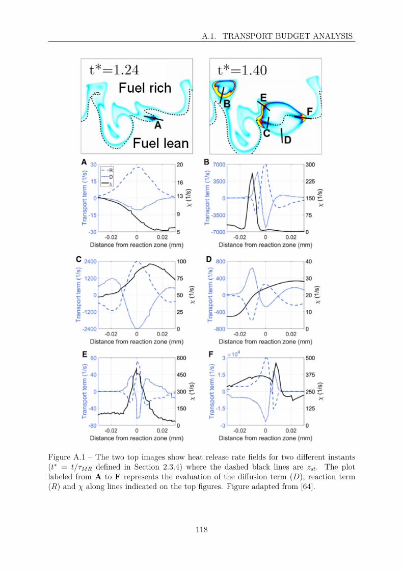
A.1. TRANSPORT BUDGET ANALYSIS
Figure A.1 – The two top images show heat release rate fields for two different instants(t∗ = t/τMR defined in Section 2.3.4) where the dashed black lines are zst. The plotlabeled from A to F represents the evaluation of the diffusion term (D), reaction term(R) and χ along lines indicated on the top figures. Figure adapted from [64].
118
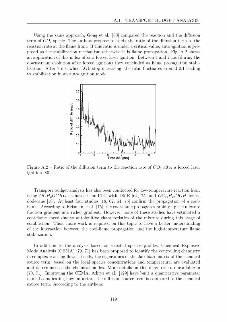
A.1. TRANSPORT BUDGET ANALYSIS
Using the same approach, Gong et al. [80] compared the reaction and the diffusionterm of CO2 specie. The authors propose to study the ratio of the diffusion term to thereaction rate at the flame front. If this ratio is under a critical value, auto-ignition is pro-posed as the stabilization mechanism otherwise it is flame propagation. Fig. A.2 showsan application of this index after a forced laser ignition. Between 4 and 7 ms (during thedownstream evolution after forced ignition) they concluded as flame propagation stabi-lization. After 7 ms, when LOL stop increasing, the ratio fluctuates around 0.1 leadingto stabilization in an auto-ignition mode.
Figure A.2 – Ratio of the diffusion term to the reaction rate of CO2 after a forced laserignition [80].
Transport budget analysis has also been conducted for low-temperature reaction frontusing OCH2OCHO as marker for LTC with DME [64, 75] and OC12H23OOH for n-dodecane [18]. At least four studies [18, 62, 64, 75] confirm the propagation of a cool-flame. According to Krisman et al. [75], the cool-flame propagates rapidly up the mixturefraction gradient into richer gradient. However, none of these studies have estimated acool-flame speed due to autoignitive characteristics of the mixture during this stage ofcombustion. Thus, more work is required on this topic to have a better understandingof the interaction between the cool-flame propagation and the high-temperature flamestabilization.
In addition to the analysis based on selected species profiles, Chemical ExplosiveMode Analysis (CEMA) [70, 71] has been proposed to identify the controlling chemistryin complex reacting flows. Briefly, the eigenvalues of the Jacobian matrix of the chemicalsource term, based on the local species concentrations and temperature, are evaluatedand determined as the chemical modes. More details on this diagnostic are available in[70, 71]. Improving the CEMA, Aditya et al. [129] have built a quantitative parameternamed α indicating how important the diffusion source term is compared to the chemicalsource term. According to the authors:
119
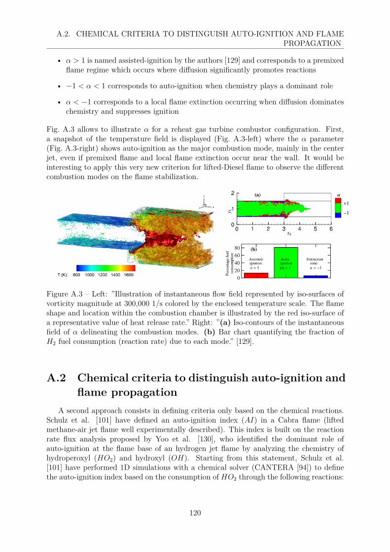
A.2. CHEMICAL CRITERIA TO DISTINGUISH AUTO-IGNITION AND FLAMEPROPAGATION
• α > 1 is named assisted-ignition by the authors [129] and corresponds to a premixedflame regime which occurs where diffusion significantly promotes reactions
• −1 < α < 1 corresponds to auto-ignition when chemistry plays a dominant role
• α < −1 corresponds to a local flame extinction occurring when diffusion dominateschemistry and suppresses ignition
Fig. A.3 allows to illustrate α for a reheat gas turbine combustor configuration. First,a snapshot of the temperature field is displayed (Fig. A.3-left) where the α parameter(Fig. A.3-right) shows auto-ignition as the major combustion mode, mainly in the centerjet, even if premixed flame and local flame extinction occur near the wall. It would beinteresting to apply this very new criterion for lifted-Diesel flame to observe the differentcombustion modes on the flame stabilization.
Figure A.3 – Left: ”Illustration of instantaneous flow field represented by iso-surfaces ofvorticity magnitude at 300,000 1/s colored by the enclosed temperature scale. The flameshape and location within the combustion chamber is illustrated by the red iso-surface ofa representative value of heat release rate.” Right: ”(a) Iso-contours of the instantaneousfield of α delineating the combustion modes. (b) Bar chart quantifying the fraction ofH2 fuel consumption (reaction rate) due to each mode.” [129].
A.2 Chemical criteria to distinguish auto-ignition andflame propagation
A second approach consists in defining criteria only based on the chemical reactions.Schulz et al. [101] have defined an auto-ignition index (AI) in a Cabra flame (liftedmethane-air jet flame well experimentally described). This index is built on the reactionrate flux analysis proposed by Yoo et al. [130], who identified the dominant role ofauto-ignition at the flame base of an hydrogen jet flame by analyzing the chemistry ofhydroperoxyl (HO2) and hydroxyl (OH). Starting from this statement, Schulz et al.[101] have performed 1D simulations with a chemical solver (CANTERA [94]) to definethe auto-ignition index based on the consumption of HO2 through the following reactions:
120
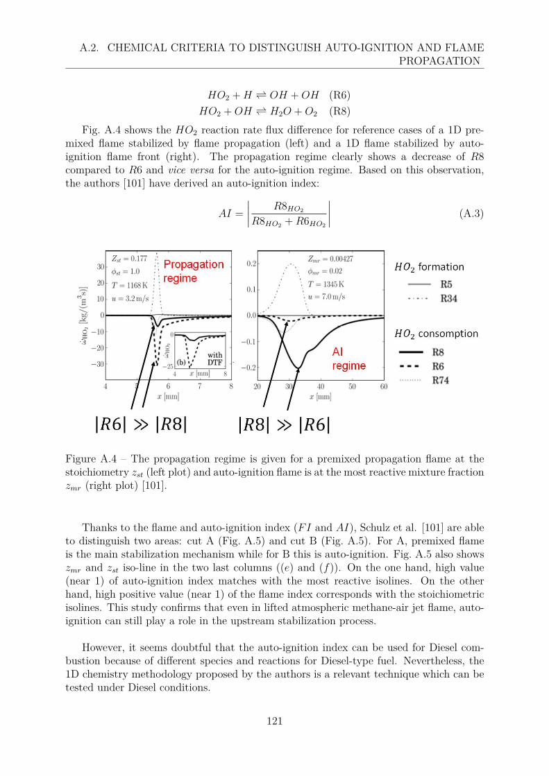
A.2. CHEMICAL CRITERIA TO DISTINGUISH AUTO-IGNITION AND FLAMEPROPAGATION
HO2 +H ⇀↽ OH +OH (R6)HO2 +OH ⇀↽ H2O +O2 (R8)
Fig. A.4 shows the HO2 reaction rate flux difference for reference cases of a 1D pre-mixed flame stabilized by flame propagation (left) and a 1D flame stabilized by auto-ignition flame front (right). The propagation regime clearly shows a decrease of R8compared to R6 and vice versa for the auto-ignition regime. Based on this observation,the authors [101] have derived an auto-ignition index:
AI =
∣∣∣∣ R8HO2
R8HO2 +R6HO2
∣∣∣∣ (A.3)
Figure A.4 – The propagation regime is given for a premixed propagation flame at thestoichiometry zst (left plot) and auto-ignition flame is at the most reactive mixture fractionzmr (right plot) [101].
Thanks to the flame and auto-ignition index (FI and AI), Schulz et al. [101] are ableto distinguish two areas: cut A (Fig. A.5) and cut B (Fig. A.5). For A, premixed flameis the main stabilization mechanism while for B this is auto-ignition. Fig. A.5 also showszmr and zst iso-line in the two last columns ((e) and (f)). On the one hand, high value(near 1) of auto-ignition index matches with the most reactive isolines. On the otherhand, high positive value (near 1) of the flame index corresponds with the stoichiometricisolines. This study confirms that even in lifted atmospheric methane-air jet flame, auto-ignition can still play a role in the upstream stabilization process.
However, it seems doubtful that the auto-ignition index can be used for Diesel com-bustion because of different species and reactions for Diesel-type fuel. Nevertheless, the1D chemistry methodology proposed by the authors is a relevant technique which can betested under Diesel conditions.
121
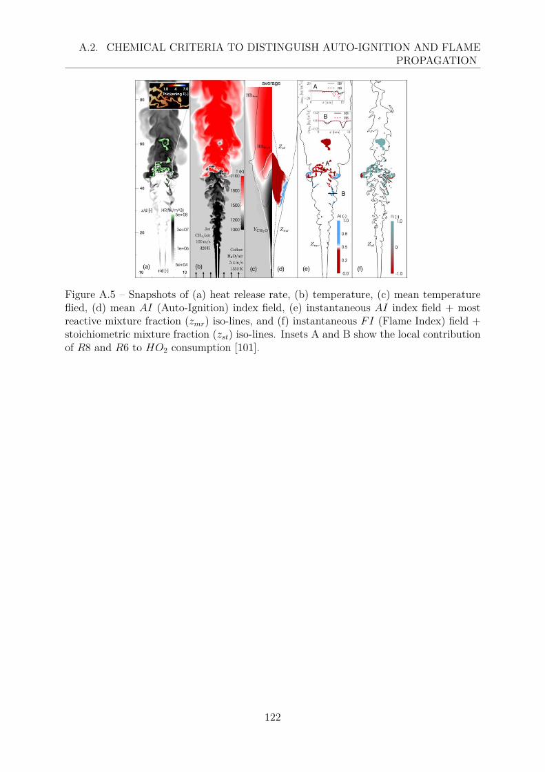
A.2. CHEMICAL CRITERIA TO DISTINGUISH AUTO-IGNITION AND FLAMEPROPAGATION
Figure A.5 – Snapshots of (a) heat release rate, (b) temperature, (c) mean temperatureflied, (d) mean AI (Auto-Ignition) index field, (e) instantaneous AI index field + mostreactive mixture fraction (zmr) iso-lines, and (f) instantaneous FI (Flame Index) field +stoichiometric mixture fraction (zst) iso-lines. Insets A and B show the local contributionof R8 and R6 to HO2 consumption [101].
122

Appendix B
Regime diagram for the flamestabilization mechanisms
Based on different observations made using optical diagnostics and numerical simu-lations, Fig. B.1 proposes a qualitative regime diagram for the flame stabilization. Thisdiagram can be used for all type of diffusion flames, since the inputs of the diagram are:the auto-ignition delay of the most reactive mixture (τAI,mr) and the flow velocity on thestoichiometric line at the flame base (Ust). The diagram comprises 5 different regions,which are delimited by the average flow velocity at the lift-off (uLO), the displacementspeed of the flame (Sd) and a quantity C (defined in Eq. B.1).
Figure B.1 – Qualitative regime diagram for the flame stabilization as the most reactivemixture fraction (τAI,mr) and the axial flow velocity on the stoichiometric line (Ust) vary.The triple flame image is extracted from [25], the Cabra flame from [131], the burnerflame stabilized from [68], while the n-dodecane spray flame image is obtained with theexperimental setup presented in Section 3.2.2.
123
• Attached flame (uLO < Sd): As reported in many works [25, 50, 69], when uLO
is lower than Sd, the flame is anchored to the burner.
• Non-autoignitive flame (uLO = Sd and high τAI,mr): Increasing Ust, while keep-ing a high τAI,mr leads to stabilize a lifted diffusion flame with a partially premixedand not auto-ignited mixture upstream of the flame base. In this configuration,triple flames have become widely accepted to explain the flame stabilization asdetailed in Section 2.2.
• Diffusion flame with auto-ignition (uLO = Sd and low τAI,mr): This regioncorresponds to test conditions where τAI,mr is low enough to auto-ignite the mix-ture. The flames are stabilized by triple flames in regions where the flow velocityis low. However, auto-ignition also appears as a driving mechanism for the flamestabilization in the high velocity flow regions as reported by Schulz et al. [101] forthe methane-air Cabra jet flame [131]. In the present diagram, this transition zoneis illustrated by the Cabra flame (see illustration on the right of the figure). In thisconfiguration, τAI,mr is reduced by a hot vitiated co-flow.
• ACDF (uLO > Sd and C < 1): Keeping a low τAI,mr and increasing Ust leadsto enter in the ACDF region as illustrated with the n-dodecane spray flame at theright of the diagram. In the ACDF region, the flame stabilization is decomposed intoauto-ignition (isolated auto-ignition (AI-I) and auto-ignition assisted by burnt gases(AI-BG)) and downstream evolution of the lift-off (triple flames (TF) and lean/richreaction zones (L/R RZ)). In average, the flow velocity at the lift-off is higher thanthe displacement speed of the partially premixed flame. Thus, contrary to the otherregions in the diagram, the main stabilization mechanism is auto-ignition. As aresult, for ACDF, the blow out limit is no longer a speed equilibrium between uLO
and Ust.For these ACDF, we propose to estimate the blow out limit through the followingparameter, based on auto-ignition:
C =τAI,mruLO
L− LL, (B.1)
where τAI,mr has been estimated using Eq. 5.6, L corresponds to the distance be-tween the fuel injector and the opposite wall of the combustion chamber, LL is theliquid length, which can be estimated through the expression provided in [122]. InEq. B.1 we assume that the auto-igniting mixture is convected at a constant speeduLO along the stoichiometric line and can stabilize the flame by auto-ignition beforereaching the limit of the combustion chamber. The assumption of uLO constant isonly realistic far enough from the injector. Therefore, C is computed in the vaporphase. For that reason, LL is subtracted from L in Eq. B.1.
Taking the example of the reference cases (α) studied in Chapter 3 and 4, we canestimate C for the α operating conditions. The auto-ignition delay of the sprayflame is 1.1 ms. The axial flow velocity at the lift-off (at 35 mm from the injector)is 26 m/s according to the 1D spray model [55, 93]. The distance between the
124
injector and the opposite wall is 125 mm and the liquid length is 18 mm. Therefore,C is equal to 0.3, which is inferior to 1 as expected, since the flame is stabilized.
• Blown flame (uLO > Sd and C > 1): Under non-autoignitive conditions the flameis blown out when uLO > Sd. However, we assume that the ACDF is blown out ifC is higher than 1. In such case, the mixture is convected too fast or is not reactiveenough and thus, cannot stabilize the flame by auto-ignition within the combustionchamber.
125
Appendix C
Impact of a high co-flow on theflame stabilization
In order to have a better understanding of the importance of the high-temperatureburnt gases reservoirs on the flame stabilization, we propose to artificially considerablydecrease these reservoirs by imposing a high co-flow of air for the α test conditions. Thus,a new simulation named αcoflow has been run from 0 to 12 ms after the start of injectionimposing a co-flow of 8 m/s. Note that the only difference between α and αcoflow is theco-flow at the inlet boundary condition, the maximum axial flow velocity (UX,max) andURMS are the same.
However, because of the very high computational cost of performing DNS with a veryfine spatial mesh resolution, the α and αcoflow cases have been simulated on a coarse mesh(highest spatial resolution set to 20 µm instead of 6 µm in Chapter 4). The simulationswith a poor resolution are referred as ”coarse DNS” and have been compared to the ref-erence DNS and experimental data in Appendix D. Since the ”coarse DNS” shows goodagreement with reference DNS, all the results presented below come from the ”coarseDNS”.
Fig. C.1 shows a comparison of instantaneous temperature fields between cases α andαcoflow. It clearly appears that the high-temperature reservoirs are considerably reducedwith a high co-flow. Consequently, the number of auto-ignition assisted by burnt gases(AI-BG) is reduced by 39 % in case αcoflow compared to α.
Fig. C.2 shows the LOL time-tracking for α and αcoflow with the four different reactionzone topologies. It appears that when the AI-BG are reduced, the lift-off is convectedfaster and fluctuates further downstream. In case αcoflow 39 % of the instantaneouslift-off are located outside the area of interest. This result demonstrates that the high-temperature reservoirs, triggering AI-BG, considerably help the flame to stabilize.
126

Figure C.1 – Instantaneous temperature fields for case α and αcoflow, both of these imagesare displayed at 3.26 ms ASI for R > 0. The black line represents the stoichiometric line.(The bottom image has been rotated to provide a symmetrical comparison with the topimage).
127
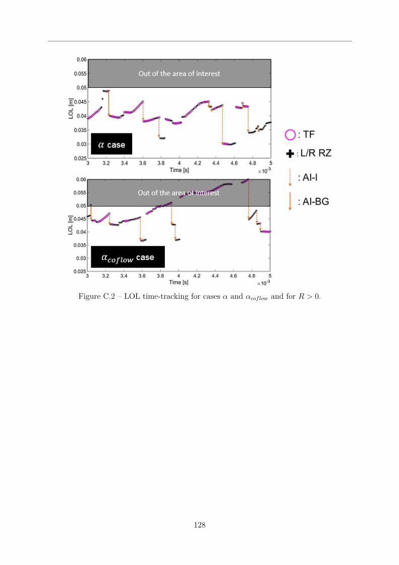
Figure C.2 – LOL time-tracking for cases α and αcoflow and for R > 0.
128

Appendix D
Setup of a ”coarse DNS”
Performing multiple DNS, with a mesh resolution of 6 µm, was not possible becauseof the very high computational cost (120,000 CPU hours per simulated physical millisec-ond). Consequently, we chose to perform simulations named ”coarse DNS” with a highestspatial resolution of 20 µm in the area of interest (see Fig. 4.1 in Chapter 4). It leads todecrease the computational cost by approx. a factor 40.
The methodology to validate the ”coarse DNS” consists in performing the same testconditions that studied in the experiments and the 6 µm DNS: α test conditions. The”coarse DNS” has been run using the same numerical setup (excepted the mesh) andphysical parameters than the 6 µm DNS: same inlet profiles, initialization and simulatedphysical time. The only difference between the coarse and the 6 µm DNS is an iso-factorapplied on the cells of the mesh leading to reduce their size by a factor 0.3.
Following the same methodology than developed in Section 4.8.2, first a non-reactivesimulation is performed to ensure that the mixing is well reproduced in the ”coarse DNS”.Therefore, time-averaged (between 2 and 10 ms) radial profiles of velocity, tempera-ture and fuel mass fraction are obtained by post-processing instantaneous ”coarse DNS”.Fig. D.1 shows these radial profiles at 30 and 50 mm from the injector, from the coarseand 6 µm DNS, but also profiles given by experimentally established correlations [55,93]. Regarding the very small gap between the two simulations, it appears that the meshchange has a very weak influence on the time-averaged profiles. Therefore, the conclusionson the ”coarse DNS” are the same than for the 6 µm DNS: the imposed boundary con-ditions yielded satisfactory mean profiles in the area of interest where flame stabilizationmechanisms were studied.
129

Figure D.1 – Radial profiles comparison between time-averaged non-reactive 6 µm DNS(thin red line), ”coarse DNS” (thick green line) jet and a 1D spray model [55, 93] (dottedblack line) for the α test conditions. Left column shows radial profiles at an axial distanceof 30 mm from the injector. Right column shows radial profiles at 50 mm from the injector.
Second, a reactive simulation is run for 0 to 12 ms on the coarse mesh. Fig. D.2 showsaveraged profiles of cool- (through CH2O) and high-temperature (through OH and OH∗)flame, computed from the experimental data, 6 µm and coarse DNS. Note that the 6 µmDNS and the experimental images have already been described in Fig. 4.7, thus the readercan refer to Fig. 4.7 for more details on the construction of the averaged images.
Fig. D.2 is used to compare the structures of the cool- and high-temperature flamefor the ”coarse DNS” in comparison to the 6 µm DNS and experimental data. As forthe 6 µm DNS, the ”coarse DNS” fields of YCH2O and YOH are time-averaged between3 and 12 ms. The cool-flame structures between the two simulations are very similar.First, the upstream locations of the stabilized cool-flame, in both simulations, are similarto the experiments. Second, the CH2O level in the center of the jet are lower in thesimulations compared to the experiments. However, this difference is assumed to have aminor impact on the flame stabilization. Comparing the high-temperature flame betweenthe two simulations, it appears that, some small differences exist: the bottom branch
130
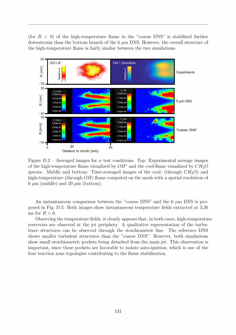
(for R < 0) of the high-temperature flame in the ”coarse DNS” is stabilized furtherdownstream than the bottom branch of the 6 µm DNS. However, the overall structure ofthe high-temperature flame is fairly similar between the two simulations.
Figure D.2 – Averaged images for α test conditions. Top: Experimental average imagesof the high-temperature flame visualized by OH∗ and the cool-flame visualized by CH2Ospecies. Middle and bottom: Time-averaged images of the cool- (through CH2O) andhigh-temperature (through OH) flame computed on the mesh with a spatial resolution of6 µm (middle) and 20 µm (bottom).
An instantaneous comparison between the ”coarse DNS” and the 6 µm DNS is pro-posed in Fig. D.3. Both images show instantaneous temperature fields extracted at 3.26ms for R > 0.
Observing the temperature fields, it clearly appears that, in both cases, high-temperaturereservoirs are observed at the jet periphery. A qualitative representation of the turbu-lence structures can be observed through the stoichiometric line. The reference DNSshows smaller turbulent structures than the ”coarse DNS”. However, both simulationsshow small stoichiometric pockets being detached from the main jet. This observation isimportant, since these pockets are favorable to isolate auto-ignition, which is one of thefour reaction zone topologies contributing to the flame stabilization.
131
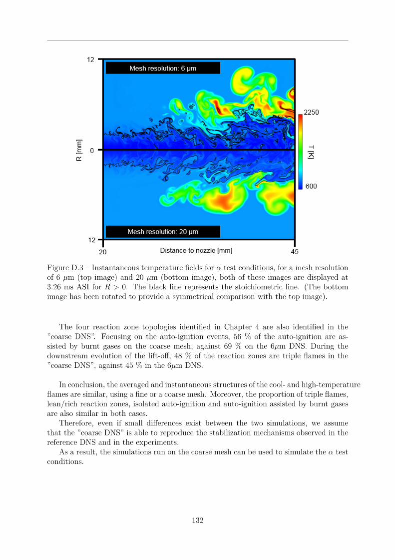
Figure D.3 – Instantaneous temperature fields for α test conditions, for a mesh resolutionof 6 µm (top image) and 20 µm (bottom image), both of these images are displayed at3.26 ms ASI for R > 0. The black line represents the stoichiometric line. (The bottomimage has been rotated to provide a symmetrical comparison with the top image).
The four reaction zone topologies identified in Chapter 4 are also identified in the”coarse DNS”. Focusing on the auto-ignition events, 56 % of the auto-ignition are as-sisted by burnt gases on the coarse mesh, against 69 % on the 6µm DNS. During thedownstream evolution of the lift-off, 48 % of the reaction zones are triple flames in the”coarse DNS”, against 45 % in the 6µm DNS.
In conclusion, the averaged and instantaneous structures of the cool- and high-temperatureflames are similar, using a fine or a coarse mesh. Moreover, the proportion of triple flames,lean/rich reaction zones, isolated auto-ignition and auto-ignition assisted by burnt gasesare also similar in both cases.
Therefore, even if small differences exist between the two simulations, we assumethat the ”coarse DNS” is able to reproduce the stabilization mechanisms observed in thereference DNS and in the experiments.
As a result, the simulations run on the coarse mesh can be used to simulate the α testconditions.
132

List of Figures
1.1 Relative evolution (1993 reference) of the regulatory emissions for Dieselvehicles in Europe from 1993 to 2015 for 4 pollutants: nitrogen oxidesNOx,carbon monoxide CO, the sum of nitrogen oxides NOx and HC unburnedhydrocarbons and finally the particles [4]. . . . . . . . . . . . . . . . . . . 8
1.2 Four-stroke cycle Diesel engine [5]. . . . . . . . . . . . . . . . . . . . . . . 91.3 Diesel spray combustion where the injection pressure is 700 bar inside a
constant volume combustion chamber at 1100 K [6]. . . . . . . . . . . . . . 91.4 Illustration of the different physical phenomena occurring during Diesel
spray combustion. Figure adapted from [7]. . . . . . . . . . . . . . . . . . 111.5 Illustration of the lift-off length (LOL) using broadband luminosity tech-
nique in constant volume combustion chamber extracted from [12]. . . . . 121.6 Soot production as a function of the inverse of the equivalence ratio at
the lift-off 1/ΦLOL for a Diesel spray in a constant volume vessel and fordifferent ambient temperatures, densities and injection pressure. Figureadapted from [13]. . . . . . . . . . . . . . . . . . . . . . . . . . . . . . . . 13
2.1 Temporal evolution of temperature (black solid line) and heat release (reddotted line) for a n-dodecane/air mixture computed in 0D homogeneousconstant pressure reactor. Figure adapted from [18]. . . . . . . . . . . . . . 18
2.2 Auto-ignition delay τAI of various fuels in a 0D constant pressure reactor.Figure adapted from [22]. . . . . . . . . . . . . . . . . . . . . . . . . . . . 19
2.3 Schematic of a conceptual combustion model describing from the injectionto the stabilized diffusion combustion [24]. . . . . . . . . . . . . . . . . . . 21
2.4 Schematic of a conceptual combustion model during the stabilized diffusioncombustion [23]. . . . . . . . . . . . . . . . . . . . . . . . . . . . . . . . . . 22
2.5 Hypothetical shape of a premixed flame (left) and experimental verificationof the hypothetical stabilization mechanism. Figures adapted from [27]. . . 23
2.6 Flame wrinkling by turbulence where A and AT are displayed. Figureadapted from [25]. . . . . . . . . . . . . . . . . . . . . . . . . . . . . . . . 24
2.7 Triple flames structure by [25] (top) and triple flames visualization in alaminar flow by [35] (bottom). . . . . . . . . . . . . . . . . . . . . . . . . . 24
2.8 Top: contour lines of the reaction rate showing a triple flame with streamlines. Bottom: ratio u/S0
L as a function of the axial coordinate on thestoichiometric line. Figure adapted from [37]. . . . . . . . . . . . . . . . . 26
2.9 Flame stabilization by critical scalar dissipation rate according to Peterset al. [42]. . . . . . . . . . . . . . . . . . . . . . . . . . . . . . . . . . . . . 27
133
LIST OF FIGURES
2.10 Nondimensional scalar dissipation rate as a function of the ratio of thelift-off height (h) to the jet diameter (d) for a turbulent methane diffusionflame. Figure adapted from [42]. . . . . . . . . . . . . . . . . . . . . . . . . 28
2.11 Flame stabilization by recirculation of burnt gases according to Broadwellet al.[46]. Figure adapted from Karami et al. [47]. . . . . . . . . . . . . . . 29
2.12 Illustration of a turbulent gaseous diffusion flame (left) and a Diesel sprayflame (right). . . . . . . . . . . . . . . . . . . . . . . . . . . . . . . . . . . 30
2.13 LOL variations versus ambient temperature (left) [1], injection velocity(middle) [1] and oxygen concentration (right) [2]. . . . . . . . . . . . . . . 30
2.14 LOL for three fuels and ambient densities. Labels are given by the symbolused for each fuel. The experimental conditions were: 180 µm orifice, 1380bar pressure drop, fuel at 373 K, and 21 % ambient oxygen [15]. . . . . . . 33
2.15 Stabilization of the flame-front by auto-ignition and flame propagation [61]. 342.16 Typical OH chemiluminescence single-shot showing a separated ignition
spot [61]. . . . . . . . . . . . . . . . . . . . . . . . . . . . . . . . . . . . . 352.17 Cool-flame chemiluminescence images shortly before auto-ignition. The
fuel is given on the lower left corner, and on the right side the auto-ignitiondelay is displayed. Quasi-steady LOL is shown as a vertical dashed whiteline [15]. . . . . . . . . . . . . . . . . . . . . . . . . . . . . . . . . . . . . . 36
2.18 The color shows the edge-flames through heat release rate fields, the solidline indicates the zst contour, the star marker indicates the flame baseposition and the square markers indicates the closer distance to the injectorof the cool-flame [67]. . . . . . . . . . . . . . . . . . . . . . . . . . . . . . . 37
2.19 Qualitative regime diagram for the stabilization mechanisms as the bound-ary temperature and inlet velocity vary. The left cartoon is a zoom ofa flame topology during the ”kinetic” stabilization mode while the rightcartoon shows an edge-flame during the ”multi-mode” stabilization. Themeaning of the acronyms is: RB: Rich Branch, LB: Lean Branch, RPF:Rich Premixed Flame, LPF: Lean Premixed Flame, NPF: Non-PremixedFlame. Figure adapted from [69]. . . . . . . . . . . . . . . . . . . . . . . . 38
2.20 ”Initial domain configuration. Black shading patern shows high vorticityregions. Grey/blue shading in top of figure represents the fuel and thewhite shading in the bottom represents the oxidiser.” [65]. . . . . . . . . . 40
2.21 Heat release rate for a fixed window in the domain. The dashed line is zst.Figure adapted from [75]. . . . . . . . . . . . . . . . . . . . . . . . . . . . 40
2.22 Left (adapted figure from [65]): computational domain including specifi-cation of the boundary condition. Right (figure from [18]): ”volumetricrendering of H2O2 mass fraction, YH2O2 at t = 0.45 ms. The green colorcorresponds to YH2O2 = 10−3, and the red color to YH2O2 = 3× 10⁻³”. . . . 41
2.23 Turbulent DME lifted jet flame showing a low-temperature heat releasemarker, YCH3OCH2O2 and a high-temperature flame marker YOH [76]. . . . . 42
2.24 Chemiluminescence image sequence with laser ignition at 3.9 ms [14]. . . . 432.25 Schematic of a lifted spray flame under Diesel conditions (center), and
different theories for the stabilization. Authors associated to the flamestabilization theories are noted in bold character above the illustrations.The flame cartoons is adapted from [47] . . . . . . . . . . . . . . . . . . . 45
134

LIST OF FIGURES
3.1 Experimental setup for simultaneous schlieren, 355 LIF and broadbandchemiluminescence images with forced laser ignition. . . . . . . . . . . . . 49
3.2 Average formaldehyde cloud from 355 LIF at 100 mJ (top image) and 5mJ (middle image), normalized average 355 LIF profiles integrated radially(bottom image). . . . . . . . . . . . . . . . . . . . . . . . . . . . . . . . . . 52
3.3 Instantaneous frames from OH* and broadband chemiluminescence at 30kfps for the α test condition. The time is expressed in terms of time ASI. . 54
3.4 Superposition of an instantaneous frame from simultaneous schlieren imag-ing (30kfps) on an iso-contour of 355 LIF (6kfps, green line) and broad-band chemiluminescence (30kfps, red line) for the α condition. The twored crosses show the location where the ignition laser is focused. . . . . . . 55
3.5 Left: LOL time tracking using OH* chemiluminescence imaging for am-bient temperatures of 800 K and 850 K, respectively named α and α′conditions. Events A are shown as red rectangles and evolutions B as redlines for the α conditions. Right: snapshot of OH* images illustratingevent A and evolution B. . . . . . . . . . . . . . . . . . . . . . . . . . . . . 58
3.6 Broadband chemiluminescence image sequence after the laser ignition (3000µs ASI) at 26 mm from the injector. The laser propagation is top to bottom. 60
3.7 Broadband chemiluminescence (red, first and third columns) and 355 LIF(green, second and fourth columns) image sequence after the laser ignition(3000 µs ASI) at 26 mm from the injector, for condition α. The two dottedlines show the LOL just after the laser ignition (left line) and the averageposition of the “natural” LOL. . . . . . . . . . . . . . . . . . . . . . . . . . 61
3.8 Ensemble and time averaged images of high-speed 355 LIF 500 µs before(first pair of images) and after (second pair of images) laser ignition. Bot-tom plots: ensemble averaged of high-speed 355 LIF integrated over R fordifferent timings. . . . . . . . . . . . . . . . . . . . . . . . . . . . . . . . . 62
3.9 Averaged high-energy 355 LIF image (first column), instantaneous high-energy 355 LIF profiles integrated over R (second column), instantaneousLOL evolution after laser ignition (at 17 mm and 3000 µs) performedby OH* measurement (third column) for different injection events. Thehorizontal dotted blue line stands for the rising of HCHO signal at 22mm from the injector. The two dotted vertical red lines delimit the threedifferent stages observed after a forced laser ignition. . . . . . . . . . . . . 63
3.10 Instantaneous LOL tracking performed by OH* measurement (60 kfps) forthe α, β, γ and δ test conditions and for laser ignition focused at 17 mmfrom the injector. The LOL tracking is performed by broadband chemilu-minescence (30 kfps) for laser ignition at 26 mm (α test condition). Whenlaser ignition occurs inside the formaldehyde cloud the LOL evolution aredisplayed with dotted lines, otherwise the LOL evolutions are plotted insolid lines. . . . . . . . . . . . . . . . . . . . . . . . . . . . . . . . . . . . . 65
135

LIST OF FIGURES
4.1 Top: Superposition of the gas envelope of the spray (Schlieren imaging)on an iso-contour of the formaldehyde cloud (green line, high-speed 355LIF), and the high-temperature flame (yellow line, broadband chemilumi-nescence). This image was obtained from the experimental setup presentedin [82]. Bottom: Computational domain showing the used tetrahedral gridwhich is refined in the area of interest to capture combustion phenomena. . 71
4.2 All of the graphs show radial profiles imposed at the inlet boundary condi-tion. (a): Axial flow velocity (UX) and axial velocity fluctuation (URMS),(b): temperature, (c): n-dodecane mass fraction. . . . . . . . . . . . . . . . 72
4.3 Comparison between the reference mechanism of Yao et al. (solid blacklines, [95]) the ARC model derived in the work (dotted red line), andexperimental data (symbols, [22, 112, 113]). Left: laminar flame speeds,right: ignition delay times. . . . . . . . . . . . . . . . . . . . . . . . . . . . 75
4.4 Instantaneous temperature profile of the stabilized flame (above the injec-tor: R < 0) showing a triple flame. The bottom image is a zoom aroundthe lift-off found in the upper image. The black line represents the stoi-chiometric line. The white line shows 4 × 10¹¹W/m3 iso-contour of heatrelease rate. . . . . . . . . . . . . . . . . . . . . . . . . . . . . . . . . . . . 78
4.5 (a) and (a′): two different instantaneous views illustrating a rich reactionzone (a) and a lean reaction zone (a′) after an auto-ignition event. (b) and(b′): time sequence showing triple flames leaving the stoichiometric line.The black line represents the stoichiometric line. The white line shows thecontour of heat release rate of 4× 10¹¹W/m3. . . . . . . . . . . . . . . . . 79
4.6 DNS fields at 3.53 ms After the Start of Injection (ASI). Top image: mix-ture fraction field with an iso-line of temperature at 1900 K (black line).Bottom image: formaldehyde field with an iso-line of OH mass fraction at1.5× 10−4 in white. . . . . . . . . . . . . . . . . . . . . . . . . . . . . . . . 80
4.7 (a): Average images of the high-temperature flame visualized by OH∗ andOH species. (b): Average images of the cool-flame visualized by CH2Ospecies. The experimental data are generated using the experimental setuppresented in [82]. . . . . . . . . . . . . . . . . . . . . . . . . . . . . . . . . 82
4.8 LOL time-tracking with the detection of Triple Flames (TF), Lean/RichReaction Zones (L/R RZ), Isolated Auto-Ignitions (AI-I) and Auto-IgnitionsAssisted by Burnt Gases (AI-BG) at the lift-off for R > 0. . . . . . . . . . 83
4.9 (a): auto-ignition event, also named Event A, occurring at t1. (b): down-stream evolution, between t0 and t1, also named Evolution B. . . . . . . . 84
4.10 Image sequence illustrating an isolated auto-ignition (AI-I) at the lift-off.The black line represents the stoichiometric line and the white line showsthe contour of heat release rate of 4× 10¹¹W/m3 (top images). The threebottom plots show OH and CH2O mass fraction profiles along the reddotted line (measuring 1 mm long) shown on the top image sequence. . . . 85
4.11 Image sequence leading to an AI-BG event. The black line represents thestoichiometric line. The white line shows 4×10¹¹W/m3 iso-contour of heatrelease rate. . . . . . . . . . . . . . . . . . . . . . . . . . . . . . . . . . . . 86
136
LIST OF FIGURES
4.12 Instantaneous temperature fields showing Evolution B between 3.03 and3.26 ms ASI. Black line: stoichiometric line. The triple flames detectedat the lift-off are zoomed, and displayed on the right of the images. Iso-lines of heat release rate between 3.7×10¹¹W/m3 and 4.3×10¹¹W/m3 aredisplayed in red on the zoomed images. . . . . . . . . . . . . . . . . . . . . 87
4.13 (a): cartoon of a triple flame propagating along zst. The red solid linerepresents the ω̇T,crit = 4 × 10¹¹W/m3 iso-line. The red arrow shows thetriple flame propagation direction (θTF ) while the green arrow shows theflow direction (θflow). (b): histograms of θ+TF and θ−TF . (c): histograms ofθ+TF,flow and θ−TF,flow (right). . . . . . . . . . . . . . . . . . . . . . . . . . . 88
4.14 Both graphics have been constructed from triple flames data at the lift-offfor R > 0 and R < 0. (a): Histogram of the ratio UX,flow,LO/Sa. (b):symbols show UX,flow,LO/Sa as a function of UX,flow,LO, while the blackcurve displays UX,flow,LO/(UX,flow,LO − 1.5) as a function of UX,flow,LO. . . 90
4.15 Sketch illustrating the conceptual model of flame stabilization under Dieselcondition derived from optical diagnostics and DNS. . . . . . . . . . . . . 91
4.16 Radial profiles comparison between time-average non-reactive DNS jet anda 1D spray model [55, 93]. Left column shows radial profiles at an axialdistance of 30 mm from the injector. Right column shows radial profilesat 50 mm from the injector. . . . . . . . . . . . . . . . . . . . . . . . . . . 95
4.17 Illustration of a 1D flame stabilized by auto-ignition. . . . . . . . . . . . . 964.18 Grid convergence for 1D premixed flames at the stoichiometric mixture
fraction. Temperature (top) and heat release rate (bottom) profiles areplotted for a spatial resolution varying between 1 and 7 µm. . . . . . . . . 98
5.1 Peak optical thickness (KL) values from the averaged axial profiles ofKL measured for each set of conditions considered, versus the inverse ofthe averaged equivalence ratio at the lift-off. The legend gives the rangeof experimental conditions considered. Adapted figure from [13]. A redstar indicating the case chosen for illustration, the corresponding arbitraryvalue of equivalence ratio fluctuations related to LOL fluctuations and anarea of corresponding soot production are added for illustration to theoriginal figure. . . . . . . . . . . . . . . . . . . . . . . . . . . . . . . . . . . 101
5.2 Schematic representation of the Lift-off length as a function of time. . . . . 1025.3 Averaged axial flow velocity in the center of the jet (UX;R=0) as a function
of the axial position (X) for the α test condition, computed with a 1Dspray model [55, 93]. The LOL is also displayed in red to illustrate theassumption that the velocity at the lift off follows the same trend. . . . . . 103
5.4 LOL time evolution using OH∗ chemiluminescence imaging. Test condi-tions are: Pinj = 150MPa, PrctO2 = 15%, Tamb = 800K and ρamb =22.8kg/m3. . . . . . . . . . . . . . . . . . . . . . . . . . . . . . . . . . . . 106
5.5 Plot of the experimental and theoretical magnitude of the LOL fluctuationsaccording to ambient temperature (Tamb), oxygen concentration (PrctO2)and injection pressure (Pinj) variations. . . . . . . . . . . . . . . . . . . . . 109
137

LIST OF FIGURES
A.1 The two top images show heat release rate fields for two different instants(t∗ = t/τMR defined in Section 2.3.4) where the dashed black lines are zst.The plot labeled from A to F represents the evaluation of the diffusionterm (D), reaction term (R) and χ along lines indicated on the top figures.Figure has adapted from [64]. . . . . . . . . . . . . . . . . . . . . . . . . . 118
A.2 Ratio of the diffusion term to the reaction rate of CO2 after a forced laserignition [80]. . . . . . . . . . . . . . . . . . . . . . . . . . . . . . . . . . . . 119
A.3 Left: ”Illustration of instantaneous flow field represented by iso-surfacesof vorticity magnitude at 300,000 1/s colored by the enclosed temperaturescale. The flame shape and location within the combustion chamber isillustrated by the red iso-surface of a representative value of heat releaserate.” Right: ”(a) Iso-contours of the instantaneous field of α delineatingthe combustion modes. (b) Bar chart quantifying the fraction of H2 fuelconsumption (reaction rate) due to each mode.” [129]. . . . . . . . . . . . . 120
A.4 The propagation regime is given for a premixed propagation flame at thestoichiometry zst (left plot) and auto-ignition flame is at the most reactivemixture fraction zmr (right plot) [101]. . . . . . . . . . . . . . . . . . . . . 121
A.5 Snapshots of (a) heat release rate, (b) temperature, (c) mean tempera-ture field, (d) mean AI (Auto-Ignition) index field, (e) instantaneous AIindex field + most reactive mixture fraction (zmr) iso-lines, and (f) in-stantaneous FI (Flame Index) field + stoichiometric mixture fraction (zst)iso-lines. Insets A and B show the local contribution of R8 and R6 to HO2
consumption [101]. . . . . . . . . . . . . . . . . . . . . . . . . . . . . . . . 122
B.1 Qualitative regime diagram for the flame stabilization as the most reactivemixture fraction (τAI,mr) and the axial flow velocity on the stoichiomet-ric line (Ust) vary. The triple flame image is extracted from [25], theCabra flame from [131], the burner flame stabilized from [68], while then-dodecane spray flame image is obtained with the experimental setuppresented in Section 3.2.2. . . . . . . . . . . . . . . . . . . . . . . . . . . . 123
C.1 Instantaneous temperature fields for case α and αcoflow, both of these im-ages are displayed at 3.26 ms ASI for R > 0. The black line representsthe stoichiometric line. (The bottom image has been rotated to provide asymmetrical comparison with the top image). . . . . . . . . . . . . . . . . 127
C.2 LOL time-tracking for cases α and αcoflow and for R > 0. . . . . . . . . . . 128
D.1 Radial profiles comparison between time-averaged non-reactive 6 µm DNS(thin red line), ”coarse DNS” (thick green line) jet and a 1D spray model[55, 93] (dotted black line) for the α test conditions. Left column showsradial profiles at an axial distance of 30 mm from the injector. Rightcolumn shows radial profiles at 50 mm from the injector. . . . . . . . . . . 130
138

LIST OF FIGURES
D.2 Averaged images for α test conditions. Top: Experimental average im-ages of the high-temperature flame visualized by OH∗ and the cool-flamevisualized by CH2O species. Middle and bottom: Time-averaged imagesof the cool- (through CH2O) and high-temperature (through OH) flamecomputed on the mesh with a spatial resolution of 6 µm (middle) and 20µm (bottom). . . . . . . . . . . . . . . . . . . . . . . . . . . . . . . . . . . 131
D.3 Instantaneous temperature fields for α test conditions, for a mesh reso-lution of 6 µm (top image) and 20 µm (bottom image), both of theseimages are displayed at 3.26 ms ASI for R > 0. The black line representsthe stoichiometric line. (The bottom image has been rotated to provide asymmetrical comparison with the top image). . . . . . . . . . . . . . . . . 132
139
List of Tables
2.1 Comparison of the coefficients predicting the time-averaged LOL betweenexperiments and simulations (RANS). The experiments assumed a flamestabilization by premixed flame at the flame base while the RANS esti-mated the LOL by flame extinction. . . . . . . . . . . . . . . . . . . . . . 34
3.1 Operating condition. . . . . . . . . . . . . . . . . . . . . . . . . . . . . . . 483.2 The different test conditions. The parameters that change compared to
the reference case α are in bold characters. . . . . . . . . . . . . . . . . . . 493.3 Laser and imaging parameters. . . . . . . . . . . . . . . . . . . . . . . . . 503.4 LOL and LOLHCHO averages for the different test conditions. . . . . . . . 563.5 Statistical analysis of the three different stages identified for laser ignition
at 17 mm from the injector. Standard deviations are noted in parenthesis. 64
4.1 Initial species mass fractions in the vessel. . . . . . . . . . . . . . . . . . . 734.2 Summary of the reduced mechanism (28 ARC): transported (left) and
Quasi Steady State (QSS) (right) species. . . . . . . . . . . . . . . . . . . 744.3 1D premixed flame initial conditions. . . . . . . . . . . . . . . . . . . . . . 964.4 1D premixed flame characteristics. . . . . . . . . . . . . . . . . . . . . . . 97
5.1 High-speed OH* chemiluminescence optical setup. . . . . . . . . . . . . . . 1065.2 Test conditions. . . . . . . . . . . . . . . . . . . . . . . . . . . . . . . . . . 1075.3 Number of realizations for the different test conditions performed. . . . . . 107
140
Bibliography
[1] D.L. Siebers, B. Higgins, Flame Lift-Off on Direct-Injection Diesel SpraysUnder Quiescent Conditions, SAE Technical Paper 2001-01-0530 (2001).(Cit. on pp. 2, 30, 31, 53, 99, 103).
[2] D.L. Siebers, B. Higgins, L.M. Pickett, Flame Lift-Off on Direct-InjectionDiesel Fuel Jets: Oxygen Concentration Effects, SAE Technical Paper2002-01-0890 (2002). (Cit. on pp. 2, 30–32, 34, 99, 103).
[3] A. Nel, Air Pollution-Related Illness: Effects of Particles, Science 308(2005) 804-806. (Cit. on p. 7).
[4] J. Tillou, Développement d’une modélisation basée sur la tabulation desschémas cinétiques complexes pour la simulation aux grandes échellesde l’auto-inflammation et de la combustion turbulente non-pré mélangédans les moteurs à pistons, PhD (2013). (Cit. on p. 8).
[5] Diesel Engine Registry Website: https://dieselengineregistry.wordpress.com/2-stroke-vs-4-stroke-engines/ (cit. on p. 9).
[6] L. Yossapong, Diesel Spray at 700bar Inj inside constant volume com-bustion chamber (CVCC) of 1100K. Photron Fastcam SA-X2- 10,000fps (1024x1024 pixels), Department of Mechanical Engineering KingMongkut’s University of Technology Thonburi, 22 May, 2015 (cit. onp. 9).
[7] G. Theotokatos, The CFD Development of Non-premixed Dual FuelCombustion Diesel Engine injected by High-pressure Gas in the Cylin-der Chamber, ARCHIE-WeSt Webiste. (Cit. on p. 11).
[8] F. Payri, V. Bermúdez, R. Payri, F. J. Salvador, The influence of cavita-tion on the internal flow and the spray characteristics in diesel injectionnozzles, Fuel 83 (2004) 419-431. (Cit. on p. 11).
[9] F. R. Westlye, M. Battistoni, S. A. Skeen, J. Manin, L. M. Pickett,A. Ivarsson, Penetration and combustion characterization of cavitatingand non-cavitating fuel injectors under diesel engine conditions, SAETechnical Paper 2016-04-05 (2016). (Cit. on p. 11).
[10] L. He,F. Ruiz, Effect of cavitation on flow and turbulence in plain orificesfor high-speed atomization. Atom Sprays 1995;5:569–84. (Cit. on p. 11).
[11] C. Soteriou, R. Andrews ,M. Smith, Direct injection diesel sprays andthe effect of cavitation and hydraulic flip on atomization. SAE Paper950080; 1995. (Cit. on p. 11).
141
BIBLIOGRAPHY
[12] M. Huo, S. Lin, H. Liu, C-F. F. Lee, Study on the spray and combustioncharacteristics of water–emulsified diesel, Fuel 123 (2014) 218-229. (Cit.on p. 12).
[13] L. M. Picketta and D. L. Siebers, Soot in diesel fuel jets: Effects of am-bient temperature, ambient density, and injection pressure, Combust.Flame 138 (2004) 114-135. (Cit. on pp. 12, 13, 99, 101).
[14] L.M. Pickett, S. Kook, H. Persson, Ö. Andersson, Diesel fuel jet lift-off stabilization in the presence of laser-induced plasma ignition, Proc.Combust. Inst. 32 (2009) 2793-2800. (Cit. on pp. 12, 14, 42–44, 47, 48, 54,55, 59, 68, 69, 79, 84, 92, 111, 113).
[15] L.M. Pickett, D.L. Siebers, C.A. Idicheria, Relationship between igni-tion processes and the lift-off length of diesel fuel jets, SAE TechnicalPaper 2005-01-3843 (2005). (Cit. on pp. 12, 19, 32, 33, 35, 36, 42, 44, 79, 103).
[16] R. Venugopal, J. Abraham, A Review of Fundamental Studies Rele-vant to Flame Lift-off in Diesel Jets, SAE Technical Paper 2007-01-0134(2007). (Cit. on pp. 13, 29, 41, 46).
[17] L. M. Pickett, ECN available at http://www.sandia.gov/ecn/ 2015 (cit.on pp. 13, 39, 48, 105, 110).
[18] G. Borghesi, A. Krisman, T. Lu, J.H. Chen, Direct numerical simulationof a temporally evolving air/n-dodecane jet at low-temperature diesel-relevant conditions, Combust. Flame 195 (2018) 183-202. (Cit. on pp. 18,35, 40, 41, 68, 73, 84, 86, 88, 96, 119).
[19] M. Jansons, A. Brar, F. Estefanous, R. Florea, D. Taraza, N. Henein, W.Bryzik, Experimental Investigation of Single and Two-Stage Ignition ina Diesel Engine, SAE Technical Paper 2008-04-14 (2008). (Cit. on p. 18).
[20] C. K. Westbrook, Y. Mizobuchi, T. Poinsot, P. J. Smith, Computationalcombustion, Proc. Combust. Inst. 30 (2005) 125-157. (Cit. on p. 18).
[21] L-M. Malbec, E. W. Eagle, M. P. B. Musculus, P. Schihl, Influence ofInjection Duration and Ambient Temperature on the Ignition Delay ina 2.34L Optical Diesel Engine, SAE Technical Paper 2015-09-01 (2015).(Cit. on p. 18).
[22] U. Pfahl, K. Fieweger, G. Adomeit, Self-ignition of diesel-relevant hydrocarbon-air mixtures under engine conditions, Symp. (Int.) Combust. 26 (1996)781-789. (Cit. on pp. 19, 75).
[23] J.E. Dec, A Conceptual Model of DI Diesel Combustion Based on Laser-Sheet Imaging, SAE Technical Paper 970873 (1997). (Cit. on pp. 19, 22,70).
[24] G. Bruneaux, Combustion structure of free and wall-impinging dieseljets by simultaneous laser-induced fluorescence of formaldehyde, poly-aromatic hydrocarbons, and hydroxides, Int. J. Eng. Res. 9 (3) (2008)249–265. (Cit. on pp. 19–21, 50, 51).
142

BIBLIOGRAPHY
[25] T. Poinsot and D. Veynante, Theoretical and Numerical Combustion,Third Edition, 2005. (Cit. on pp. 21, 23, 24, 97, 123, 124).
[26] K. Wohl, N.M. Kapp, C. Gazley, The stability of open flames, Symp.(Int.) Combust. 3 (1948) 3–21. (Cit. on p. 21).
[27] L. Vanquickenborne, A. Van Tiggelen, The stabilization mechanism oflifted diffusion flames, Combust. Flame 10 (1966) 59–69. (Cit. on pp. 22,23).
[28] T. Gautam, Lift-off Heights and Visible Lengths of Vertical TurbulentJet Diffusion Flames in Still Air, Combust. Sci. Technol. 41 (1984) 17-29.(Cit. on p. 22).
[29] C.J. Lawn, Lifted flames on fuel jets in co-flowing air, Prog. EnergyCombust. Sci. 35 (2009) 1–30. (Cit. on pp. 23, 28, 44).
[30] K. K. Kuo, Principles of combustion, Book published in 2005. DOI 10.1007/s00162-006-0039-5 (cit. on p. 23).
[31] J. H. Chen and I. G. Im, Correlation of flame speed with stretch in tur-bulent premixed methane/air flames, Symp. (Int.) Combust. 27 (1998)819-826. (Cit. on p. 23).
[32] S. Daniele, P. Jansohn, K. Boulouchos, Turbulent flame speed for syngasat gas turbine relevant conditions, Proc. Combust. Inst. 33 (2011) 2937-2944. (Cit. on p. 23).
[33] C. R. Kaplan, S. W. Beak, E. S. Oran, J. L. Ellzey, Dynamics of aStrongly Radiating Unsteady Ethylene Jet Diffusion Flame, Combust.Flame 96 (1994) 1-21. (Cit. on p. 23).
[34] M. Namazian, R. W. Schefer, J. Kelly, Scalar dissipation measurementsin the developing region of a jet, Combust. Flame 74 (1988) 147-160.(Cit. on p. 23).
[35] P.N. Kioni, B. Rogg, K. Bray, A. Liñán, Flame spread in laminar mixinglayers, Combust. Flame 95 (1993) 276-290. (Cit. on pp. 24, 25, 89).
[36] H. Phillips, Flame in a buoyant methane layer, Symp. (Int.) Combust.10 (1965) 1277-1283. (Cit. on pp. 25, 89).
[37] G.R. Ruetsch, L. Vervisch, A. Liñán, Effects of heat release on tripleflames, Phys. Fluids 7 (1995) 1447-1454 (cit. on pp. 25, 26, 77, 89).
[38] P. Domingo, L. Vervisch, Triple flames and partially premixed combus-tion in autoignition of non-premixed turbulent mixtures, Symp. (Int.)Combust. 26 (1996) 233-240. (Cit. on pp. 25, 89).
[39] M. Chen, M. Herrmann, N. Peters, Flamelet modeling of lifted turbu-lent methane/air and propane/air jet diffusion flames, Proc. Combust.Inst. 32 (2000) 167-174. (Cit. on p. 25).
[40] K.M. Lyons, Toward an understanding of the stabilization mechanismsof lifted turbulent jet flames, Prog. Energy Combust. Sci. 33 (2007)211–231. (Cit. on pp. 25, 44).
143

BIBLIOGRAPHY
[41] S. Karami, E. R. Hawkes, M. Talei, J. H. Chen, Edge flame structure ina turbulent lifted flame: A direct numerical simulation study, Combust.Flame 169 (2016) 110-128. (Cit. on p. 25).
[42] N. Peters, F.A. Williams, Liftoff characteristics of turbulent jet diffusionflames, AIAA J. 21 (1983) 423–429. (Cit. on pp. 26–28).
[43] A. Liñán, The asymptotic structure of counterflow diffusion flames forlarge activation energies, Acta Astronautica 1 (1974) 1007-1039. (Cit. onp. 26).
[44] D.A. Everest, D.A. Feikema, J.F. Driscoll, Images of the strained flammablelayer used to study the liftoff of turbulent jet flames, Symp. (Int.) Com-bust. 26 (1996) 129–136. (Cit. on p. 28).
[45] R.W. Schefer, M. Namazian, E. Filtopoulos, J. Kelly, Temporal evolu-tion of turbulence/chemistry interactions in lifted, turbulent-jet flames,Symp. (Int.) Combust. 25 (1994) 1223–1231. (Cit. on p. 28).
[46] J.E. Broadwell, W.J. Dahm, M.G. Mungal, Blowout of turbulent dif-fusion flames, Symp. (Int.) Combust. 20 (1985) 303–310. (Cit. on pp. 28,29).
[47] S. Karami, E.R. Hawkes, M. Talei, J.H. Chen, Mechanisms of flamestabilisation at low lifted height in a turbulent lifted slot-jet flame, J.Fluid Mech. 777 (2015) 633-689. (Cit. on pp. 29, 44, 45).
[48] T. Ito, T. Kitamura, M. Ueda, T. Matsumoto, J. Senda, H. Fujimoto,Effects of flame lift-off and flame temperature on soot formation inoxygenated fuel sprays, SAE Technical Paper 2003-01-0073 (2003). (Cit.on p. 30).
[49] W. Zhang, J-P. Tian, K. Nishida, Effects of Nozzle Hole Diameter andInjection Pressure on Flame Lift-Off and Soot Formation in D.I. DieselCombustion, SAE Technical Paper 2011-08-30 (2011). (Cit. on p. 30).
[50] N. Peters, Turbulent Combustion, Cambridge University Press, 2000.(Cit. on pp. 31, 124).
[51] M. Metghalchi and J. C. Keck, Burning velocities of mixtures of air withmethanol, isooctane, and indolene at high pressure and temperature,Combust. Flame 48 (1982) 191-210. (Cit. on p. 31).
[52] B. Higgins, D.L. Siebers, Measurement of the flame Lift-Off locationon DI diesel sprays using OH chemiluminescence, SAE Technical Paper2001-01-0918 (2001). (Cit. on pp. 31, 32, 53).
[53] J. B. Heywood, Internal combustion engine fundamentals, Book pub-lished in 1988, ISBN: 978-0-07-028637-5. (Cit. on p. 31).
[54] E. N. Balles and J. B. Heywood, Fuel-Air Mixing and Diesel Combustionin a Rapid Compression Machine, SAE Transactions (1988). DOI 10.4271/880206 (cit. on p. 32).
144

BIBLIOGRAPHY
[55] J. Naber, D.L. Siebers, Effects of gas density and vaporization on pen-etration and dispersion of diesel sprays, SAE Technical Paper 960034(1996). (Cit. on pp. 32, 59, 65, 94, 95, 102, 103, 124, 129, 130).
[56] G. Dugger, D. Simon, M. Gerstein, Basic Considerations in the Combus-tion of Hydrocarbon Fuels with Air, (1959) NACA report 1300, chapitreLaminar Flame Propagation, p. 321-356. (Cit. on p. 32).
[57] C. J. Mueller, W.J. Pitz, L. M. Pickett, G. C. Martin, D. L. Siebers,C. K. Westbrook, Effects of oxygenates on soot processes in DI dieselengines: experiments and numerical simulations, SAE Technical Paper2003-01-1791 (2003). (Cit. on p. 32).
[58] M.P.B Musculus, J.E. Dec, D.R. Tree, Effects of fuel parameters anddiffusion flame lift-off on soot formation in a heavy-duty DI diesel en-gine, SAE Technical Paper 2002-01-0889 (2002). (Cit. on p. 32).
[59] L.M. Pickett, D.L. Siebers, Fuel effects on soot processes of fuel jets atDI diesel conditions, SAE Technical Paper 2003-01-3080 (2003). (Cit. onp. 32).
[60] R. Venugopal and J. Abraham, A numerical investigation of flame lift-off in diesel Jets, Combust. Sci. Technol. 179 (2007) 2599–2618. (Cit. onpp. 33, 34, 99).
[61] C. Pauls, G. Grünefeld, S. Vogel, N. Peters, Combined simulation andOH-chemiluminescence measurements of the combustion process usingdifferent fuels under diesel-engine like conditions, SAE Technical Paper,2007-01-0020 (2007). (Cit. on pp. 34, 35, 42, 44, 79).
[62] R.N. Dahms, G.A. Paczko, S.A. Skeen, L.M. Pickett, Understandingthe ignition mechanism of high-pressure spray flames, Proc. Combust.Inst. 36 (2017) 2615–2623. (Cit. on pp. 35, 96, 119).
[63] D.K. Dalakoti, A. Krisman, B. Savard, A.Wehrfritz, H. Wang, M.S. Day,J.B Bell, E.R. Hawkes, Structure and propagation of two-dimensional,partially premixed, laminar flames in diesel engine conditions, Proc.Combust. Inst. (2018). DOI 10.1016/j.proci.2018.06.169 (cit. on pp. 35,39).
[64] A. Krisman, E.R. Hawkes, M. Talei, A. Bhagatwala, J.H. Chen, Char-acterisation of two-stage ignition in diesel engine-relevant thermochem-ical conditions using direct numerical simulation, Combust. Flame 172(2016) 326-341. (Cit. on pp. 35, 39, 41, 68, 73, 86, 117–119).
[65] A. Krisman, E.R. Hawkes, M. Talei, A. Bhagatwala, J.H. Chen, A di-rect numerical simulation of cool-flame affected auto-ignition in dieselengine-relevant conditions, Proc. Combust. Inst. 36 (2017) 3567-3575.(Cit. on pp. 35, 40, 41, 68, 73, 86).
[66] A. Krisman, E.R. Hawkes, J.H. Chen, The structure and propagationof laminar flames under autoignitive conditions, Combust. Flame 188(2018) 399-411. (Cit. on pp. 35, 75, 95).
145

BIBLIOGRAPHY
[67] A. Krisman, E.R. Hawkes, M. Talei, A. Bhagatwala, J.H. Chen, Poly-brachial structures in dimethyl ether edge-flames at negative temper-ature coefficient conditions, Proc. Combust. Inst. 35 (2015) 999-1006.(Cit. on pp. 36–39, 41, 44, 86, 117).
[68] S. Deng, P. Zhao, M.E. Mueller, C.K. Law, Autoignition-affected sta-bilization of laminar nonpremixed DME/air coflow flames, Combust.Flame 162 (2015) 3437-3445. (Cit. on pp. 37–39, 123).
[69] S. Deng, P. Zhao, M.E. Mueller, C.K. Law, Stabilization of laminarnonpremixed DME/air coflow flames at elevated temperatures and pres-sures, Combust. Flame 162 (2015) 4471-4478. (Cit. on pp. 37–39, 124).
[70] T. F. Lu, C. S. Yoo, J. H. Chen, C. K. Law, Three-dimensional directnumerical simulation of a turbulent lifted hydrogen jet flame in heatedcoflow: A chemical explosive mode analysis, J. Fluid Mech. 652 (2010)45-64. (Cit. on pp. 38, 119).
[71] R. Shan, C. S. Yoo, J. H Chen, T. Lu, Computational diagnostics for n-heptane flames with chemical explosive mode analysis, Combust. Flame159 (2012) 3119-3127. (Cit. on pp. 38, 119).
[72] H. Pitsch, M. Chen, N. Peters, Unsteady flamelet modeling of turbulenthydrogen-air diffusion flames, Symp. (Int.) Combust. 27 (1998) 1057-1064. (Cit. on p. 38).
[73] H. G. Im, J. H. Chen, Effects of flow strain on triple flame propagation,Combust. Flame 126 (2001) 1384-1392. (Cit. on p. 39).
[74] J. Boulanger, L. Vervisch, J. Reveillon, S. Ghosal, Effects of heat releasein laminar diffusion flames lifted on round jets, Combust. Flame 134(2003) 355–368. (Cit. on p. 39).
[75] A. Krisman, E.R. Hawkes, J.H. Chen, Two-stage auto-ignition and edgeflames in a high pressure turbulent jet, J. Fluid Mech. 824 (2017) 5-41.(Cit. on pp. 39, 40, 68, 73, 86, 117, 119).
[76] Y. Minamoto, J.H. Chen, DNS of a turbulent lifted DME jet flame,Combust. Flame 169 (2016) 38-50. (Cit. on pp. 41, 42, 68, 86, 88).
[77] D-H. Shin, E.S. Richardson, V. Aparece-Scutariu, Y. Minamoto, J.H.Chen, Fluid age-based analysis of a lifted turbulent DME jet flame DNS,Proc. Combust. Inst. (2018). DOI 10.1016/j.proci.2018.06.126 (cit. onp. 41).
[78] L. Gomet, V. Robin, A. Mura, Influence of Residence and Scalar Mix-ing Time Scales in Non-Premixed Combustion in Supersonic TurbulentFlows, Combust. Sci. Technol. 184 (2012) 1471-1501. (Cit. on p. 41).
[79] N. Enjalbert, P. Domingo, L. Vervisch, Mixing time-history effects inLarge Eddy Simulation of non-premixed turbulent flames: Flow-ControlledChemistry Tabulation, Combust. Flame 159 (2012) 336-352. (Cit. onp. 41).
146
BIBLIOGRAPHY
[80] C. Gong, M. Jangi, X.-S. Bai, Diesel flame lift-off stabilization in thepresence of laser-ignition, Combust. Theor. Model. 19 (2015) 696-713.(Cit. on pp. 43, 44, 119).
[81] W.M. Pitts, Assessment of theories for the behavior and blowout oflifted turbulent jet diffusion flames, Symp. (Int.) Combust. 22 (1989)809–816. (Cit. on p. 44).
[82] F. Tagliante, L-M. Malbec, G. Bruneaux, L. M. Pickett, C. Angel-berger, Experimental study of the stabilization mechanism of a liftedDiesel –type flame using combined optical diagnostics and laser-inducedplasma ignition, Combust. Flame 197 (2018) 215-226. (Cit. on pp. 47, 67–69, 71, 76, 79, 81–83).
[83] D. Verhoeven, J.-L. Vanhemelryck, T. Baritaud, Macroscopic and ig-nition characteristics of high-pressure sprays of single-component fuels,SAE Technical Paper 981069 (1998). (Cit. on p. 48).
[84] Panigrahi and Muralidhar Schlieren and Shadowgraph Methods in Heatand Mass Transfer (2012). (Cit. on p. 50).
[85] L.M. Pickett, C.L. Genzale, G. Bruneaux, L.-M. Malbec, L. Hermant,C. Christiansen, J. Schramm, Comparison of diesel spray combustion indifferent high-temperature, high-pressure facilities, SAE Int. J. Engines3 (2010) 156–181. (Cit. on p. 50).
[86] J.M. García -Oliver, L.-M. Malbec, H.B. Toda, G. Bruneaux, A studyon the interaction between local flow and flame structure for mixing-controlled diesel sprays, Combust. Flame 179 (2017) 157-171. (Cit. onpp. 50, 51, 79).
[87] R. Payri, F.J. Salvador, J.Manin, A. Viera, Diesel ignition delay and lift-off length through different methodologies using a multi-hole injector,Appl. Energy 162 (2016) 541-550. (Cit. on p. 53).
[88] N. Maes, M. Meijer, N. Dam, B. Somers, H. Baya Toda, G. Bruneaux,S.A. Skeen, L.M. Pickett, J. Manin, Characterization of Spray A flamestructure for parametric variations in ECN constant-volume vessels us-ing chemiluminescence and laser-induced fluorescence, Combust. Flame174 (2016) 138-151. (Cit. on pp. 53, 79, 81).
[89] Idex optics and photonics, Gaussian beam optics. (Cit. on p. 54).[90] C.L. Genzale, L.M. Pickett, A.A. Hoops, J.M. Headrick, Laser ignition
of multi-injection gasoline sprays, SAE Technical Paper 2011-01-0659(2011). (Cit. on p. 54).
[91] P.M. Lillo, L.M. Pickett, H. Persson, O. Andersson, S. Kook, Dieselspray ignition detection and spatial/temporal correction, SAE Int. J.Engines 5 (2012) 1330–1346. (Cit. on p. 55).
[92] S.A. Skeen, J. Manin, L.M. Pickett, Simultaneous formaldehyde PLIFand high-speed schlieren imaging for ignition visualization in high-pressurespray flames, Proc. Combust. Inst. 35 (2015) 3167–3174. (Cit. on p. 55).
147
BIBLIOGRAPHY
[93] M.P.B Musculus, K. Kattke, Entrainment waves in diesel jets, SAE Int.J. Engines 2 (2009) 1170–1193. (Cit. on pp. 59, 65, 94, 95, 102, 103, 124, 129,130).
[94] D. G. Goodwin, H. K. Moffat, R. L. Speth, 2015, URL: http://www.can-tera.org. (Cit. on pp. 59, 75, 120).
[95] T. Yao, Y. Pei, B.-J. Zhong, S. Som, T. Lu, K.H. Luo, A compact skeletalmechanism for n -dodecane with optimized semi-global low-temperaturechemistry for diesel engine simulations, Fuel 191 (2017) 339-349. (Cit. onpp. 59, 73, 75).
[96] F. Tagliante, T. Poinsot, L. M. Pickett, P. Pepiot, L-M. Malbec, G.Bruneaux, C. Angelberger, A conceptual model of the flame stabiliza-tion mechanisms for a lifted Diesel-type flame based on direct numericalsimulation and experiments, Combust. Flame 201 (2019) 65-77. (Cit. onp. 67).
[97] B. Franzelli, E. Riber, M. Sanjosé, T. Poinsot, A two-step chemicalscheme for kerosene-air premixed flames, Combust. Flame 157 (2010)1364-1373. (Cit. on p. 68).
[98] B. Franzelli, E. Riber, L. Gicquel, T. Poinsot, Large Eddy Simulationof combustion instabilities in a lean partially premixed swirled flame,Combust. Flame 159 (2012) 621-637. (Cit. on p. 68).
[99] P.Pepiot, Automatic strategies to model transportation fuel surrogates(Doctoral dissertation, Stanford University 2008). (Cit. on pp. 68, 73).
[100] P. Pepiot-Desjardins and H. Pitsch, An efficient error-propagation-basedreduction method for large chemical kinetic mechanisms, Combust. Flame154 (2008) 67-81. (Cit. on pp. 68, 73).
[101] O. Schulz, T. Jaravel, T. Poinsot, B. Cuenot, N. Noiray, A criterion todistinguish auto-ignition and propagation applied to a lifted methane–airjet flame, Proc. Combust. Inst. 36 (2017) 1637-1644. (Cit. on pp. 68, 120–122, 124).
[102] O. Schulz, N. Noiray, Autoignition flame dynamics in sequential com-bustors, Combust. Flame 192 (2018) 86-100. (Cit. on p. 68).
[103] T. Jaravel, E. Riber, B. Cuenot, G. Bulat, Large Eddy Simulation of anindustrial gas turbine combustor using reduced chemistry with accuratepollutant prediction, Proc. Combust. Inst. 36 (2017) 3817-3825. (Cit. onp. 68).
[104] R. Payri, J. García-Oliver, M. Bardi, J. Manin, Fuel temperature in-fluence on diesel sprays in inert and reacting conditions, Appl. Therm.Eng. 38 (2012) 185-195. (Cit. on p. 69).
[105] V.Moureau, G. Lartigue, Y. Sommerer, C. Angelberger, O. Colin, T.Poinsot, Numerical methods for unsteady compressible multi-componentreacting flows on fixed and moving grids, J. Comput. Phys. 202 (2005)710-736. (Cit. on p. 70).
148
BIBLIOGRAPHY
[106] P.D. Lax , B. Wendroff, Difference schemes for hyperbolic equationswith high order of accuracy, Commun. Pure Appl. Math. 17 (1964)381–398. (Cit. on p. 70).
[107] T. Poinsot , S. Lele , Boundary conditions for direct simulations ofcompressible viscous flows, J. Comput. Phys. 101 (1992) 104-129. (Cit.on pp. 72, 93).
[108] A. Smirnov, S. Shi, I. Celik, Random flow generation technique forlarge eddy simulations and particle-dynamics modeling, J. Fluids Eng.123 (2001) 359-371. (Cit. on p. 72).
[109] T. Passot and A. Pouquet, Numerical simulation of compressible ho-mogeneous flows in the turbulent regime, J. Fluid Mech. 181 (1987)441-466. (Cit. on p. 72).
[110] S. M. Sarathy, C. K. Westbrook, M. Mehl, W. J. Pitz, C. Togbe, P.Dagaut, H. Wang, M. A. Oehlschlaeger, U. Niemann, K. Seshadri, P. S.Veloo, C. Ji, F. N. Egolfopoulos, T. Lu, Comprehensive chemical kineticmodeling of the oxidation of 2-methylalkanes from C7 to C20, Combust.Flame 158 (2011) 2338-2357. (Cit. on p. 73).
[111] T. Lovs, D. Nilsson, F. Mauss, Automatic reduction procedure for chem-ical mechanisms applied to premixed methane/air flames, Proc. Com-bust. Inst. 28 (2000) 1809-1815. (Cit. on p. 74).
[112] C. Ji, E. Enoch, Y. L. Wang, H. Wang, F. N. Egolfopoulos, Propagationand extinction of premixed C5-C12 n-alkane flames, Combust. Flame157 (2010) 277-287. (Cit. on p. 75).
[113] S. S. Vasu, D. F. Davidson, Z. Hong, V. Vasudevan, R. K. Hanson, N-Dodecane oxidation at high-pressures: Measurements of ignition delaytimes and OH concentration time-histories, Proc. Combust. Inst. 32(2009) 173-180. (Cit. on p. 75).
[114] R. W. Bilger, S.H. Stårner, R. J. Kee, On reduced mechanisms formethane air combustion in nonpremixed flames, Combust. Flame 80(1990) 135-149. (Cit. on p. 75).
[115] J. Hirschfelder , C. Curtiss , D.E. Campbell , The theory of flames anddetonations, Symp. (Int.) Combust. 4 (1953) 190–211. (Cit. on p. 75).
[116] L. Muñiz, M.G. Mungal, Instantaneous flame-stabilization velocities inlifted-jet diffusion flames, Combust. Flame 111 (1997) 16-31. (Cit. onpp. 77, 89).
[117] K. M. Pang, M. Jangi, X-S. Bai, J. Schramn, J. H. Walther, P. Glarborg,Effects of ambient pressure on ignition and flame characteristics in dieselspray combustion, Fuel 237 (2019) 676-685. (Cit. on p. 78).
[118] M. EidiAttarZade, S. Tabejamaat, M. Mani, M. Farshchi, NumericalStudy of Ignition Process in Turbulent Shear-less Methane-air MixingLayer, Flow Turbul. Combust. 99 (2017) 411-436. (Cit. on p. 91).
149

BIBLIOGRAPHY
[119] C. Chartier, U. Aronsson, Ö. Andersson, R. Egnell, B. Johansson, Influ-ence of jet–jet interactions on the lift-off length in an optical heavy-dutyDI diesel engine, Fuel 112 (2013) 311-318. (Cit. on pp. 93, 115).
[120] A. M. Rusly, M. K. Le, S. Kook, E. R. Hawkes, The shortening of lift-offlength associated with jet–wall and jet-jet interaction in a small-boreoptical diesel engine , Fuel 125 (2014) 1-14. (Cit. on pp. 93, 115).
[121] M. Bardi, G. Bruneaux, A. Nicolle, O.Colin, Experimental Methodologyfor the Understanding of Soot-Fuel Relationship in Diesel Combustion:Fuel Characterization and Surrogate Validation, SAE Technical Paper2017-03-23 (2017). (Cit. on pp. 99, 105).
[122] L-M. Malbec, J. Egúsquiza, G. Bruneaux, M. Meijer, Characteriza-tion of a Set of ECN Spray A Injectors: Nozzle to Nozzle Variationsand Effect on Spray Characteristics, SAE Technical Paper 2013-24-0037(2013). (Cit. on pp. 103, 124).
[123] B. Michele, G. Bruneaux, L-M. Malbec, Study of ECN Injectors’ Be-havior Repeatability with Focus on Aging Effect and Soot Fluctuations,SAE Technical Paper 2016-01-0845 (2016). (Cit. on p. 103).
[124] J. Pareja, A. Johchi, T. Li, A. Dreizler, B. Böhm, A study of the spatialand temporal evolution of auto-ignition kernels using time-resolved to-mographic OH-LIF, Proc. Combust. (2018). DOI 10.1016/j.proci.2018.06.028 (cit. on p. 113).
[125] H. Yamashita, M. Shimada, T. Takeno, A numerical study on flamestability at the transition point of jet diffusion flames, Symp. (Int.)Combust. 26 (1996) 27-34. (Cit. on p. 116).
[126] J. H.Chen, E. R. Hawkes, R. Sankaran, S. D. Mason, H. G. Im, Directnumerical simulation of ignition front propagation in a constant volumewith temperature inhomogeneities, Combust. Flame 145 (2006) 128-144.(Cit. on p. 117).
[127] C. S. Yoo and H. G. Im, Transient soot dynamics in turbulent non-premixed ethylene–air counterflow flames, Proc. Combust. Inst. 31 (2007)701-708. (Cit. on p. 117).
[128] R. L. Gordon, A. R. Masri, S. B. Pope, G. M. Goldin, Transport budgetsin turbulent lifted flames of methane autoigniting in a vitiated co-flow,Combust. Flame 151 (2007) 495-511. (Cit. on p. 117).
[129] K. Aditya, A. Gruber, C. Xu, T. Lu, A. Krisman, M. R. Bothien, J.H. Chen, Direct numerical simulation of flame stabilization assisted byautoignition in a reheat gas turbine combustor, Proc. Combust. Inst.(2018). DOI 10.1016/j.proci.2018.06.084 (cit. on pp. 117, 119, 120).
[130] C. S. Yoo, R. Sankaran, J. H. Chen, Three-dimensional direct numericalsimulation of a turbulent lifted hydrogen jet flame in heated coflow:Flame stabilization and structure, J. Fluid Mech. 640 (2009) 453-481.(Cit. on p. 120).
150

BIBLIOGRAPHY
[131] R. Cabra, J-Y. Chen, R.W Dibble, A.N Karpetis, R. S. Barlow, Liftedmethane–air jet flames in a vitiated coflow, Combust. Flame 143 (2005)491-506. (Cit. on pp. 123, 124).
151
Related Documents


