Combined planning and scheduling in a divergent production system with co-production: A case study in the lumber industry

Computers & Operations Research 38 (2011) 1238–1250

Contents lists available at ScienceDirect

Computers & Operations Research

0305-05

doi:10.1

� Corr

Univers

E-m

jean-ma

sophie.d

journal homepage: www.elsevier.com/locate/caor

Combined planning and scheduling in a divergent production systemwith co-production: A case study in the lumber industry

Jonathan Gaudreault a,b,�, Jean-Marc Frayret a,b, Alain Rousseau a, Sophie D’Amours a,b

a FORAC Research Consortium, Pavillon Adrien-Pouliot, Universite Laval, Quebec (QC), Canada G1K 7P4b CIRRELT, Centre Interuniversitaire de Recherche sur les Reseaux d’Entreprise, la Logistique et le Transport, Canada

a r t i c l e i n f o

Available online 20 November 2010

Keywords:

Integrated planning and scheduling

Mathematical programming

Constraint programming

Wood drying and finishing

Anytime algorithm

Lumber industry

48/$ - see front matter & 2010 Elsevier Ltd. A

016/j.cor.2010.10.013

esponding author at: FORAC Research Consort

ite Laval, Quebec (QC), Canada G1K 7P4.

ail addresses: [email protected]

[email protected] (J.-M. Frayret),

[email protected] (S. D’Amours).

a b s t r a c t

Many research initiatives carried out in production management consider process planning and

operations scheduling as two separate and sequential functions. However, in certain contexts, the two

functions must be better integrated. This is the case in divergent production systems with co-production

(i.e. production of different products at the same time from a single product input) when alternative

production processes are available. This paper studies such a context and focuses on the case of drying and

finishing operations in a softwood lumber facility. The situation is addressed using a single model that

simultaneously performs process planning and scheduling. We evaluate two alternative formulations.

The first one is based on mixed integer programming (MIP) and the second on constraint programming

(CP). We also propose a search procedure to improve the performance of the CP approach. Both

approaches are compared with respect to their capacity to generate good solutions in short

computation time.

& 2010 Elsevier Ltd. All rights reserved.

1. Introduction

This paper addresses a real industrial process planning andoperations scheduling problem from the softwood lumber indus-try. More specifically, it deals with the planning and scheduling ofdrying and finishing operations. This production system is char-acterized as being (1) a divergent system with co-production (i.e., itproduces different products at the same time from a single inputproduct), (2) with alternative production processes.

This section first introduces the nature of these processes, thenexplains the complexity of the intertwined problems of decidingwhat processes to implement (i.e., process planning), when torealize them and using which machines (i.e., operations schedul-ing). This section also introduces the objective and the experi-mentation approach used to address this planning and schedulingproblem.

1.1. Wood drying and finishing

Softwood drying is a transformation operation which aims atdecreasing the moisture content of lumber in order to meetcustomer requirements. These requirements are usually specified

ll rights reserved.

ium, Pavillon Adrien-Pouliot,

al.ca (J. Gaudreault),

by industry standards, although some customers may requirespecific levels of moisture content. Softwood lumber drying is alengthy process to carry out. It takes days and is done in batches inlarge kiln dryers at high temperature. In certain circumstances,special sections of the wood yard may be used to perform airdrying. Air drying, which precedes kiln drying, may take severalweeks but allows for the reduction of the drying time in the kiln.The same principle applies to the time spent in the wood yard afterkiln drying. This is called air equalizing. Both air drying andequalizing also play a role in increasing the overall quality of thefinished products.

Once dry, lumber is planed, sorted and trimmed. These opera-tions are referred to in this paper as the finishing process. Afterbeing planed, each piece of lumber is sorted according to its grade(i.e., quality) determined by its moisture content and its physicaldefects (most defects are not perceivable before planing). A piece oflumber may be trimmed in order to produce shorter lumber of ahigher grade (the process is usually optimized online to producethe products with the highest market value, with no considerationfor actual customer demand). This causes the finishing process toproduce multiple product types at the same time (co-production)from a single product type at input (divergence). It is important tonote that co-production cannot be avoided at the planning level,but is embedded within the industrial process. Moreover, for agiven batch of lumber to be dried and finished, the resulting mix ofproducts (each product type is defined by a combination of lengthand grade) is a function of the way both drying and finishingprocesses are carried out.

www.elsevier.com/locate/caor

dx.doi.org/10.1016/j.cor.2010.10.013

mailto:[email protected]



dx.doi.org/10.1016/j.cor.2010.10.013

dx.doi.org/10.1016/j.cor.2010.10.013

Kiln dry 1 Finish 1

Finish 2

Kiln dry 2

Kiln dry 3

Air dry 1

Air dry 2

Equalize 2

Equalize 1

Finish 3

Finish 4

Green andrough lumber Air drying Kiln drying Equalizing Finishing Dry and planned

lumber

Fig. 1. Alternative processes for a specific lot of lumber.

J. Gaudreault et al. / Computers & Operations Research 38 (2011) 1238–1250 1239

In brief, lumber drying and finishing can be described as a four-stage transformation process which includes air drying, kiln drying,air equalizing and finishing. For a given batch, there are differentpossible operations at each stage (see example in Fig. 1). For airdrying and equalizing, the different possible operations are mostlydifferentiated according to their durations, which is the result ofapplying different drying programs (sequence of stepwise airtemperature and humidity variations in time). Therefore, eachallowed combination of these operations (i.e. each path in Fig. 1)defines an alternative process that produces a specific mix ofoutput products and has a different usage rate of resources.

A graph similar to Fig. 1 must be defined for each product typethat can be processed by the drying and finishing facility. Mostsawmills allow the processing of batches that contain different butcompatible product types. In industry, these allowed combinationsare called the ‘‘kiln loading patterns.’’ Again, alternative processesmust be defined for each of these patterns.

In order to design a planning system for drying and finishingoperations, some characteristics of the problem need to be takeninto account:

�
Due to co-production, one batch of raw materials will contributeto fulfilling many customer orders for different product types,even if the batch contains only one product type at thebeginning of the process; � As the volume of each customer order for a specific product is
usually larger than the amount that can be produced with onesingle batch, many batches are usually needed to fulfill anyparticular need;
� The capacity of a process to satisfy customer orders is not only
linked to the co-product output mix associated with the process,but also to the moment the process can be done (scheduling).With this kind of problem, process planning and schedulingmust be tightly integrated.

1.2. Objective and research methodology

The models and experimentation results provided in this paperaim to address this planning situation, and consequently,to simultaneously perform process planning and scheduling,which is sometimes referred to as combined planning and scheduling

[1]. To do so, we propose two alternative models. The first modelis a mixed integer mathematical program (MIP). The secondmodel uses a constraint programming (CP) representation of theproblem.

The two models were compared using real industrial data from alumber producer in eastern Canada. In particular, we evaluated thecapacity of the models to provide good solutions in short computa-tion time, a requirement for them to be used within a supply chaincoordination system (see [2]).

Standard approaches for solving the MIP and CP formulationswere shown to be inefficient for the large industrial problemsstudied. Therefore, we proposed a search procedure that aims atproducing good solutions in a short period of time.

The remainder of this paper is organized as follows. Section 2presents a review of the literature. Section 3 then elaborates amathematical and a constraint programming model to solve theproblem being discussed. Section 4 discusses the quantitativeevaluation and comparison of these two approaches, accordingto the real-time expectations presented in Section 1.1 and Section 5presents our conclusions.

2. Literature review

This review of the literature includes three sub-sections in orderto address the main features of the proposed production planningproblem: divergence and co-production (2.1), integration of plan-ning and scheduling (2.2) and the specific applications of wooddrying operations planning (2.3).

2.1. Divergence and co-production

In the manufacturing problem previously introduced, lumber ofthe same type is processed and transformed into a number ofdistinct finished product types. Such a divergent process refers to atype of plant that is known as the V-Plant type [3] which ischaracterized by the existence of divergent points in the manu-facturing process. In other words, the number of finished goodsis greater than the amount of raw materials or component parts.V-Plants are also characterized by the fact that all end items sold bythe plant are processed in essentially the same way. In Ref. [3], theauthor also points out that a focus on efficiency may cause materialto be processed through V-plants in large batch sizes resulting inexcess work-in-process and finished-good inventories and inflatedlead times, a situation that is common in the softwood lumberindustry. Usually, the divergent product flow of a V-Plant can becontrolled, like if there was ‘‘switch’’ allowing operators to choosewhich product to produce. However, in the context of drying andfinishing, we face both divergence and co-production at the sametime; we produce many product types at the same time from a

J. Gaudreault et al. / Computers & Operations Research 38 (2011) 1238–12501240

given input product. There are some (but few) industries facingsuch problems, for example some chemical processes, meat cuttersor petroleum refineries. Vila et al. [4] propose a mathematicalformulation for divergent processes in the specific application ofthe softwood lumber sector.

2.2. Integration of process planning and operations scheduling

Many research initiatives carried out in production manage-ment consider process planning (i.e., a set of sequentially inter-dependent operations to be carried out) and operations scheduling(i.e., a set of machine/operation allocations in time) as two separatefunctions. In a context with no co-production, it is possible tospecify a distinct process plan to fulfill each job. To simplify theoverall planning process, a plan is usually specified independentlybefore operations are scheduled. In practice, this is usually handledthrough what Myers et al. [5] refer to as an iterative waterfall model,where (1) process planning and operations scheduling are carriedout sequentially and independently, generating a new process planonly when a problem is encountered during scheduling.

However, process planning and scheduling are interdependentoperations. Indeed, on the one hand, the performance of a manu-facturing system to carry out a process plan depends on machinecapabilities and availabilities. On the other hand, the performance of amanufacturing system to carry out a schedule depends on the abilityof the process plans to avoid creating bottleneck machines. Therefore,process plans should be generated taking into account machinecapabilities and their available capacity.

A common approach in the field of operations management tosolve such a problem, referred to as non-linear process planning [6], isto first identify multiple alternative process plans based on the designfeatures of the product to manufacture. When production must takeplace, each process plan is evaluated taking into account theindividual schedule of each machine. A particular feasible plan andits corresponding schedule are then selected either automatically orinteractively by the user who will carry out the plan. Many authors([7–10], among others) exploit this general approach to iterativelyschedule jobs, one after the other. Because alternative process plansare designed without any reference to real-time shop status, the maindrawback of this general approach is related to the possible largenumber of process plan alternatives needed to produce efficientoperations schedules. Furthermore, some of these plans may beinfeasible with respect to the real-time shop status.

Another generic approach, referred to as closed-loop process

planning [6], is to generate a feasible process plan using the real-time status of the machines in the shop. Khoshnevis and Chen [11]propose a solution based on this generic approach. For each part thatcan be manufactured, two lists are dynamically maintained. The firstlist contains the machines that are available to process the part, andthe second list contains the part design features that can be processedon each machine. When a part is needed, a heuristic algorithmgenerates a process plan by matching elements of the two lists toproduce all the design features of that part. In this way, the processplan is generated using the real-time status of the machines in theshop. However, a bottleneck machine may appear during scheduling,the resulting schedule may be inefficient or even infeasible.

In order to reduce this drawback, another generic approach,referred to as distributed process planning [6], consists in simulta-neously generating the process plan of a job along with thescheduling of the identified operations. Similarly, processingrequirements are identified during a preplanning phase by recog-nizing design features and analyzing the machine processingpotential based on their capabilities. However, here operation/machine allocation alternatives are investigated during a pairingplanning phase using the actual or estimated availability of the

machines. For instance, Huang et al. [12] propose a progressiveapproach of integrated process planning and scheduling. Processplan alternatives are first generated off-line. Next, for each part tobe manufactured a process plan is selected based on the shortestmanufacturing anticipated lead time by tentatively allocatingoperations to machine groups. McDonnell et al. [13] propose anauction protocol in a distributed decision making context wheremachine agents use their resource availability to guide, in a cascademanner, the simultaneous specification of the next operations tocarry out, its machine allocation and the schedule of that machine.Other contributions, such as Refs. [14,15] consider the schedulingof many jobs simultaneously, each having many alternative processplans. Here the emphasis is generally put on the scheduling processrather than on the generation of alternative process plans, whichare considered as parameters of the scheduling problem.

The approach used in this paper is referred to as combined process

planning and scheduling [1]. It is also referred to as integrated planning

and scheduling or centralized optimization approaches [16]. Thisapproach has as its main feature to optimize a single model in orderto decide what to do, when to do it, and with which resources. Someauthors have proposed specific algorithms to solve such combinedproblems. Several methodological approaches have been investi-gated, including mathematical programming [17], simulated anneal-ing [18], genetic and evolutionary algorithms [19–21], constraintprogramming [22], as well as agent-based technology [16]. The readeris referred to Tan and Khoshnevis [23] for a review.

2.3. Wood drying and finishing operations planning

Drying operations planning in the softwood lumber industryconsists in determining which batch of wood will be dried, when, inwhich kiln and according to which process alternative, all the whiletaking into account demand (or production target), availablequantities of green lumber and resource availability.

Different authors propose partial solutions to these problems.For instance, Gascon et al. [24] address the scheduling of a set ofoperations to be carried out in various kiln dryers located indifferent facilities so as to meet the needs of a floor factory. Here, nodivergence is explicitly considered. The authors develop a heuristicwhich aims at scheduling drying activities in a multi-item, multi-machine and multi-site production environment. The objectivefunction consists in keeping inventories as low as possible whilemeeting demand and avoiding stock outs. Similarly, Yaghubianet al. [25] model the problem as a special case of the scheduling ofmultiple independent jobs with no alternative process plan tomultiple non-identical parallel machines, with the objective ofminimizing the maximum tardiness of orders. A heuristic isproposed. Along the same lines, Joines and Culbreth [26] proposean approach that takes into account job sequencing as well asinventory control in a wood furniture manufacturing context. Here,production capacity consists in a series of parallel processors,which includes both in-house kiln dryers and external capacityfrom service providers. The objective of the approach is to minimizedrying costs plus any inventory and carrying costs. A genetic-LPhybrid heuristic is proposed.

The problems addressed in these works are different from thoseaddressed here because they do not explicitly consider divergingflow (finishing operations are not considered, so there is no co-production). Furthermore, they address the scheduling of appear-ance wood drying jobs that usually take more time, which tends toreduce the combinatorial complexity of the problem (i.e., for thesame planning horizon length, there are fewer jobs to schedule).Finally, they do not consider drying process alternatives since noneof the authors consider process planning as being part of theproblem to solve.


3. Problem formulations

This section outlines the proposed models for combined plan-ning and scheduling. Two alternative models based, respectively,on mixed integer programming (MIP) and constraint programming(CP) are proposed. It will be shown that these two formulationsallow for the implementation of radically opposed resolutionstrategies and response time. They were developed for our dryingand finishing planning problem but can also address other pro-blems with co-production and divergent processes.

We chose not to explicitly model the different process alter-natives; instead, we modeled the individual activities that can becombined in different ways to give different process alternatives.Fig. 2 presents the main idea involved in these models. We havedifferent activity types aAA. Each can be executed on any machinemAMaDM, and has a specific duration da. The parameters qconsume

a,p

and qproducea,p specify the consumption and production of products

pAP for the activity type a. In this context, building a plan can beseen as deciding which activities to perform, when to perform themand using which machines. A solution can be represented by aGantt chart of activities. Note that each type of activity can beinserted as many times as needed in the plan. Inserted activitieshave an impact on product inventories (Ip,t) by increasing ordecreasing it since they produce and consume different products.Customer demand (dp,t) also influences product inventories.

This kind of model is referred to as a timetable model or time-line

model by Bartak [1,27]. According to Bartak, the main limitations ofthese kinds of models are the following: (1) each resource canperform only one activity per period, (2) the duration of the periodsmust be a common divisor of the activities’ duration and (3) it isdifficult to model complex dependencies between activities. For (1)and (2), this is not a problem as 12 or 24 h is commonly used as atime unit in this industry. Concerning (3), this was similarly not anissue because all constraints regarding dependencies betweenactivities can be enforced by making sure that the consumedproducts are in stock at the right time.

Fig. 2. Intuitive idea sup

3.1. Objective

Within our real world application, it is impractical to considerdemand as a hard constraint. For all the datasets we had access to, latedeliveries were inevitable. Therefore, we chose to minimize tardinessmultiplied by quantity as the objective. We propose the followingmethod to easily compute it in a time-line model. First, we allow theinventory variables in the model to take negative values. For eachproduct/period, a negative inventory corresponds to a backorderedquantity, and a positive one corresponds to a volume physically instock. The sum of all daily backorder quantities is equal to thetardiness. For example, a backlog of 10 units for 5 days (10�5¼50) isequivalent to a tardiness of 5 days of 10 units (5�10¼50). Of course,for this approach to be mathematically valid, negative inventoriesmust be restricted in order to prevent the model from consumingunavailable products.

The next section describes the variables, parameters andobjective common to our MIP and CP formulations. The two modelsare then introduced.

3.2. Sets, variables, parameters, constraints and objective common

to both MIP and CP models

Sets

M set of machines m

P set of products p

Pdemanded subset of P containing products with demandPdemandedDP

A set of all types of activities a

Aconsumep subset of activities which consume the product p

Aconsumep DA

Aproducep subset of activities which produce the product p

Aproducep DA

Am subset containing all types of activities that can beprocessed on machine m AmDA

porting the models.


Ma set of machines that can carry out activity a

Ma¼{mAM|aAAm}

Parameters

T number of periods in the planning horizonip,0 quantity of product p in stock at the beginning of the

planning horizonsp,t quantity of product p supplied at the beginning of period t

dp,t demand for product p at period t. Must be delivered at theend of period t

da number of consecutive periods needed to perform activ-ity a

qconsumea,p quantity of product p consumed by activity a

qproducea,p quantity of product p produced by activity a

cm,t

1, if machine m is available during period t

0, otherwise

(

Variables

TCp,t total consumption of product p at period t

TPp,t total production of product p at period t

Ip,t volume of product p that would be in stock if thecumulated demand were satisfied. This variable can takenegative values (see constraint (1.3)); therefore, the‘‘real’’ volume physically in stock is equal to maxð0,Ip,tÞ

BOp,t backorder of product p at the end of period t. Defined onlyfor pAPdemanded

In addition to these variables, each of the proposed models (MIPand constraint programming) will define its own decision variables(see Sections 3.2 and 2.3).

Constraints

The flow conservation constraints (1.1) and (1.2) balanceequations linking inventory, supply, consumption, productionand demand variables. The particularity of these equations is thata product p can be both consumed and sold.

Ip,1 ¼ ip,0þsp,1�TCp,1�dp,1 8pAP ð1:1Þ

Ip,t ¼ Ip,t�1þsp,t�TCp,tþTPp,t�1�dp,t 8pAP, t¼ 2, . . . ,T ð1:2Þ

Constraint (1.3) defines a lower bound for inventories. Anegative inventory corresponds to a backorder situation. Back-orders are allowed only for products with demand. Its level cancover the part of the cumulated demand that is not satisfied bystarting inventory plus external supply, not more. This prevents usfrom consuming a product that is not in stock (that would lead to anunfeasible solution).

Ip,t Zmin�

0,ip,0þXt

t ¼ 1

ðsp,t�dp,tÞ�8pAP, t¼ 1, . . . ,T ð1:3Þ

Eq. (1.4) expresses that the consumption variables for a productare set to 0 if there is no activity consuming that product. Similarly,Eq. (1.5) set that all production is set to 0 if there is no activityproducing that product.

TCp,t ¼ 0 8pjAconsumep ¼+, t¼ 1, . . . ,T ð1:4Þ

TPp,t ¼ 0 8pjAproducep ¼+, t¼ 1, . . . ,T ð1:5Þ

Objective function

The primary goal of the objective function (1.6) is to minimizetardiness of the quantities ordered by customers, measured as the

sum of backorder quantities.

MinX

pAPdemanded

XT

t ¼ 1

BOp,t ð1:6Þ

3.3. Mixed integer programming model

This model includes the following decision variables:

S(a,m),t
Binary decision variable. It takes the value 1 if an activityof type a starts on machine m at period t, 0 otherwise. It isdefined for each (a,m)|aAAm
Additionally, the variables introduced in Section 3.2 are presentin this model as continuous variables.

Constraints

The following variables are restricted to positive values: TCp,t,TPp,t and BOp,t. Constraint (2.1), together with the minimization ofthe objective function, defines backorder as the minimum positivequantity that covers negative inventories up to 0.

Ip,tþBOp,t Z0 8pAPdemanded, t¼ 1, . . . ,T ð2:1Þ

The consumption constraint (2.2) defines TCp,t as the totalconsumption of activities starting during period t and consumingproduct p. The sum is computed only for the pairs of activities a andmachines m for which a consumes p and m can carry out a. Theproduction constraint (2.3) is the counterpart of the previousconstraint. It sets that total production is the sum of what isproduced by activities a ending during period t (i.e. those starting atperiod t�da+1) and producing product p.

TCp,t ¼X

ða,mÞ

�� aAAm

aAAconsumep

Sða,mÞ,t � qconsumea,p 8pAP, t¼ 1, . . . ,T ð2:2Þ

TPp,t ¼X

ða,mÞ

��aAAm

aAAproducep

t�daþ1Z1

Sða,mÞ,t�daþ1 � qproducea,p 8pAP, t¼ 1, . . . ,T

ð2:3Þ

The capacity constraint (2.4) sets that the number of activitiesrunning on a machine m at period t must be smaller than or equal to1. For each type of activity a, there is an instance running at period t

if and only if one started during the interval [t�da+1,y,t].

XaAAm

Xt

t ¼ max½t�daþ1,1�

Sða,mÞ,trcm,t 8mAM, t¼ 1, . . . ,T ð2:4Þ

3.3.1. MIP model implementation and resolution

The implementation of this model was made with OPL Studiofrom ILOG. The model was then solved using ILOG CPLEX 9.1(results are presented in Section 4.1). Because the results did notmeet our expectations regarding response time (see Section 4), wealso developed a constraint programming (CP) model introduced inthe next section.

3.4. Constraint programming model

This section proposes an alternative formulation of the previousplanning and scheduling problem based on constraint program-ming, and proposes a search procedure for its resolution.

Constraint programming (CP) [28] is rooted in the field of artificialintelligence (AI). CP proposes logic-based methods for optimization


[29] that search through a tree representation of the solution spaceby iteratively and tentatively fixing variables and by propagatingconstraints in order to reduce the domain (i.e., possible values) ofthe remaining variables so as to find feasible solutions. From theperspective of the OR community, CP provides an alternative para-digm, complementary to mathematical programming (MP), formodeling and solving problems. Modeling in CP is easier thanmodeling in MP for problems where constraints are expressed interms of logic-based discrete choices such as If A¼3 and Bo5 then

either C¼4 or D410, which is rather complex to model using MP.Although they are different and lead to radically different kinds ofmodels, mathematical and constraint programming are sometimesused in conjunction to solve large scale problems [30]. Being able tocombine the strengths of both even appears as a challenge that isgaining more and more importance in the OR community.

Variables

In CP, the value of a variable is not necessarily restricted tonumerical values. For example, a variable named ‘‘color’’ could takeany value from a set ‘‘{blue, white, red}’’. The set of the allowedvalues is called the domain of the variable. This situation would bemodeled with mathematical programming by defining threebinary variables and a constraint stating that the sum of the threemust be equal to 1, while no constraint is necessary in CP. Themodel proposed here uses this type of variable. The CP decisionvariables Sm,t specify the type of activity starting on processor m atperiod t. It can take the value ‘‘null’’ (meaning that no activity isstarting) or any ‘‘compatible activity type’’ (a set of objects definedin the same way as the set of colors presented previously).

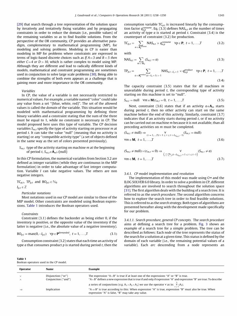
Table 1Boolean

Opera

34

)

Sm,t
type of the activity starting on machine m at the beginningof period t, Sm,tAAm[{null}
In this CP formulation, the numerical variables from Section 3.2 aredefined as integer variables (while they are continuous in the MIPformulation) in order to take advantage of fast integer computa-tion. Variable I can take negative values. The others are nonnegative integers.

TCp,t , TPp,t and BOp,t AN0

Ip,t AZ

Particular notations

Most notations used in our CP model are similar to those of theMIP model. Other constraints are modeled using Boolean expres-sions. Table 1 introduces the Boolean operators used.

Constraints

Constraint (3.1) defines the backorder as being either 0, if theinventory is positive, or the opposite value of the inventory if thelatter is negative (i.e., the absolute value of a negative inventory).

BOp,t ¼maxð0,�Ip,tÞ 8pAPdemanded, t¼ 1, . . . ,T ð3:1Þ

Consumption constraint (3.2) states that each time an activity oftype a that consumes product p is started during period t, then the

operators used in the CP model.

tor Name Example

Disjunction (‘‘or’’) The expression ‘‘A3B’’ is tru

Conjunction (‘‘and’’) ‘‘A4B’’ defines a new express

a series of conjunctions (e.g.

Implication ‘‘A)B’’ is true according to

expression ‘‘A’’ is false, ‘‘B’’ m

consumption variable TCp,t is increased linearly by the consump-tion factor qconsume

a,p . Eq. (3.3) defines NASa,t as the number of timesan activity of type a is started at period t. Constraint (3.4) is thecounterpart of constraint (3.2) for production.

TCp,t ¼X

aAAconsumep

NASa,t � qconsumea,p 8pAP, t¼ 1, . . . ,T ð3:2Þ

with

NASa,t ¼X

mAMa

ðSm,t ¼ aÞ ð3:3Þ

TPp,t ¼X

aAAproducep jðt�daþ1Þ41

NASa,t�daþ1 � qproducea,p 8pAP, t¼ 1, . . . ,T

ð3:4Þ

The capacity constraint (3.5) states that for all machines m

unavailable during period t, the corresponding type of activitystarting on this machine is set to ‘‘null’’.

Sm,t ¼ null 8mAMjcm,t ¼ 0, t¼ 1, . . . ,T ð3:5Þ

Next, constraint (3.6) states that if an activity aAAm startsduring period t, then no other activity can start on the samemachine before the end of this activity. Similarly, constraint (3.7)indicates that if an activity starts during period t, or if no activitycan be carried out on machine m because it is not available, than allpreceding activities on m must be completed.

ðSm,t anullÞ ) 8ðt ¼ 1,...,Tjtþ1rtr tþdðSm,t Þ

�1ÞðSm,t ¼ nullÞ

8mAM, t¼ 1, . . . ,T ð3:6Þ

ðSm,t anullÞ3ðcm,t ¼ 0Þ ) 8a A Am

t ¼ 1,...,Tjt�dðSm,t Þþ1rtr t�1

� �ðSm,taaÞ

8mAM, t¼ 1, . . . ,T ð3:7Þ

3.4.1. CP model implementation and resolution

The implementation of this model was made using C++ and theILOG SOLVER 6.0 library. In order to solve a problem in CP, differentalgorithms are involved to search throughout the solution space[31]. The first algorithm deals with the building of a search tree. It isreferred to as the search procedure. The second algorithm concernshow to explore the search tree in order to find feasible solutions.This is referred to as the search strategy. Both types of algorithms arepresented hereafter along with the development made specificallyfor our problem.

3.4.1.1. Search procedure, general CP concepts. The search procedure

aims at defining a search tree for a problem. Fig. 3 shows anexample of a search tree for a simple problem. The tree can bedescribed as follows: Each node of the tree represents the status ofthe search for a solution at a given time. This status is defined by thedomain of each variable (i.e., the remaining potential values of avariable). Each arc descending from a node represents an

e if at least one of the expressions ‘‘A’’ or ‘‘B’’ is true.

ion that is true if and only if expression ‘‘A’’ and expression ‘‘B’’ are true. To describe

A14A24A3) we use the operator 8 as in: 83

i ¼ 1ðAiÞ.

this: When expression ‘‘A’’ is true, expression ‘‘B’’ must also be true. When

ay take any value.

X = 1 X = 2

Y = 2

X = {1,2}Y = {1,2,3}

Y = 3

X = {1}Y = {2,3}

X = {2}Y = {3}

X = {1}Y = {2}

X = {1}Y = {3}

Fig. 3. Search tree for a simple problem (XA{1,2}; YA{1,2,3} s.c. Y4X).Fig. 4. Intuitive representation of the tree; each node corresponds to a partial plan.


alternative way to reduce the domain of one or many variables.These alternatives are specified by the search procedure. A node forwhich all variables have one and only one value in their domain(those variables are said to be valued) corresponds to a solution. It isimportant to note that different search trees (that is, differentsearch procedures) could be defined for the same problem.

A search procedure generates the tree during the search; it is notgenerated beforehand. Each time a node is investigated, constraintsare propagated to reduce the domain of the variables (andconsequently, the number of arcs descending from that node).This is illustrated in Fig. 3. This propagation mechanism applieswith our actual model. Constraints (3.6) and (3.7) have thefollowing effect. Each time a value is assigned to a variable (e.g.Sm,t¼aanull) the domains of the other variables related to thismachine (e.g. Sm,t, 8tat) are updated to prevent any double-use ofthis machine. Similarly, the propagation of constraint (3.2) togetherwith flow conservation constraints (1.1)–(1.3) has the followingeffect. The activity type a consuming product p is withdrawn fromthe domain Sm,t if the upper bound of inventory Ip,t is such that theinsertion of a would cause a negative inventory level that could notbe compensated by any other activity producing p and carried outbefore (the next section explains how this propagation is carriedout in more detail).

The propagation of constraints during the investigation of thesolution space contributes to decrease the size of the tree. However,in general constraint propagation is not sufficient to prevent theinvestigation of arcs leading to sub-trees with no solution at all.This search process can be very costly.

In the next section, we describe an efficient but incompletesearch procedure (it does not explore the entire solution space).This search procedure has the advantage of preventing inefficientbacktracking to produce good solutions in a short amount oftime. It was developed as the complete search procedures wereunable to find feasible solutions, even for large computationtimes (412 h).

3.4.1.2. Proposed search procedure. As the studied case leads tohuge combinatorial problems, a search procedure that does notsystematically investigate all possible solutions has been devel-oped. This search procedure focuses the search for a solution in a

small part of the solution space in order to obtain good solutions ina short period of time.

Our search procedure defines a tree that can be interpreted inthe following way. Each node of the tree can be considered as apartial plan, defined by the variables Sm,t already valued. The rootnode corresponds to an empty plan. From a given node, differentactivities could be added to the partial plan. The arcs representpotential branching decisions, each one leading to a new node/partial plan. Fig. 4 shows an intuitive representation of thismechanism.

We propose to allow branching on processes instead of onindividual activities. We define a process as any sequence ofactivities that produces at least one product for which there is ademand (Pdemanded). Consequently, a finishing activity alone isconsidered a process. A finishing activity preceded by a dryingactivity is also considered a process. However, a drying activitycannot be considered a process, unless there is a demand forunfinished products. The identification of these processes is carriedout during a pre-treatment before the search. This provides thefollowing set of data:

W
set of processes wAW. For each process wAW, card(w)designates the number of activities involved in w, and aw
i

designates the activity aAA associated with the ith step of w,for i¼1,y,card(w). The same activity a can be part of morethan one process.

Each time we branch on a specific process, its activities must beadded to the current partial plan. To do so, we must schedule eachof these activities (i.e., select a machine and a period) and thescheduling is performed using the following set of rules:

�
Using the current partial plan, compute the earliest date forwhich one of the products produced by the selected process isbackordered; � By considering this as the due date, backward schedule the
activities of the process in just-in-time (machines have nopriority).

Consequently, for a given node (partial plan) and a given arc(a process to add), there is only one schedule possible for each


activity of the process (i.e., there is only one possible assignment forvariables Sm,t). The main consequence is that the solution space ofthe problem is not entirely represented by this tree. However, evenif the optimal solution was missed by this search, the speed of thesearch for a good solution is increased.

Two rules have been introduced to reduce the number ofbranching alternatives (but without additional restriction of thesolution space explored). First (R1), the inclusion of a processmust always lead to a plan that is better than the current plan; and(R2) the inclusion of a process must always lead to a feasiblepartial plan.

Rule R1 ensures that branching always contributes to improvethe solution of the current node with regard to the objectivefunction. Due to the fact that a process is defined as a sequence ofactivities that produces demanded products, it is useless to branchon a process that does not contribute to the objective in the currentnode: this process will not help in any of the nodes deriving fromthe current node.

Rule R2 ensures that the partial plans of every node in thesearch tree is a feasible plan. This rule makes sense in thecontext where we branch on processes rather than on activities:it removes unproductive sections from the tree that would leadto no feasible solutions. Another advantage is that one can stopthe search for a solution at anytime as the algorithm alwaysgives a feasible solution. This is called an anytime algorithm (see[32]).

From a given node, it is easy to deterministically compute thecontribution of each branching alternative before branching (actu-ally, we need to do this to enforce rule R1). It is therefore possible tosort the branching alternatives according to this contribution level(this will be our rule R3). By doing so, the search process willperform a gradient descent (equivalent to hill climbing, but here in aminimization context).

3.4.2. Enforcing rule R2

To implement rule R2 (the inclusion of a process must alwayslead to a feasible partial plan), we introduce a new variable inthe model. However, the value of this variable is not part of thesolution (we do not want this variable to take a value). It is onlymeant to guide the search procedure; the domain of this variablewill help identify the processes that could be inserted into a partialplan.

Swi
the domain of this variable specifies the periods where
it is possible to start the ith activity of process w.Originally (before the search), the domain of the variable is{null, 1yT}. In a given node, the domain of Sw

i specifies

where the activity awi of process w could be inserted into the

current partial plan. If the domain is reduced to {null}, thenthe process w cannot be inserted into the plan. Therefore,the domain of Sw

i defines the branching alternatives

available from a node.

It is important not to interpret the variable Swi as the ‘start date of

the activity awi , taking a value when we insert this activity into the plan’

(as we would do in a scheduling problem). Indeed, when buildingthe plan the same process w can be inserted several times. Eachtime we do so, the domains of variables Sw

i are updated to showwhich activities/processes can be further inserted from the newpartial plan.

Constraints (3.8) and (3.9) are added to the model to ensure theconsistency of these domains. Constraint (3.8) models the pre-cedence between the activities of a process. Constraint (3.9)specifies that an activity can be inserted at period t only if amachine is available, and if the new plan would be feasible in terms

of consumed product inventory.

Swi 4Sw

i�1þdðawiÞ�1 8ðw,iÞjðwAWÞ4i¼ 2, . . . ,cardðwÞ ð3:8Þ

domðSwi Þ ¼ null

� �

[ tA1,:::,T

��(

mAMðawiÞ

½awi AdomðSm,tÞ4:boundðSm,tÞ�

4 8p A Pjqconsumed

ðawiÞ,p

4 0

tA t::T

½currentðp,tÞZ�qnetw,p,i�

2666664

3777775

9>>>>>=>>>>>;

8>>>>><>>>>>:

8ðw,iÞ

��ðwAWÞ4i¼ 1, . . . ,cardðwÞ ð3:9Þ

where dom(X) is the represents the set of all possible values inthe domain of variable X; bound(X) is a Boolean function thatindicates if variable X is valued, i.e. if its domain contains only one

value. In other words, boundðXÞ :¼ ðcardðdomðXÞÞ ¼ 1Þ; current(p,t)is the function that indicates the inventory level of product p atperiod t that would result if no other activity were inserted in the

current plan. In other words, currentðp,tÞ :¼ ip,0þPt

t ¼ 1sp,tþ

dminðTPp,tÞ�dp,t�dminðTCp,tÞ; dmin(X) is the function that returns

the smallest value of the domain of variable X. Formally,

dminðXÞ :¼ minvAdomðXÞ

ðvÞ. In the present context, dmin(TPp,t) repre-

sents the quantity of product p that is produced during period t

given the current partial plan; qnetw,p is a new parameter (computed in

pre-treatment) that represents the production of product p by aprocess w, minus its consumption of the same product. In other

words, qnetw,p :¼

PcardðwÞi ¼ 1 qproduce

ðawiÞ,p �qconsume

ðawiÞ,p ; qnet

w,p,i is a parameter that

represents the production of product p by a process w minus itsconsumption, when the ith activity of process w starts. In other

words, qnetw,p,i :¼

Pi�1j ¼ 1qproduce

ðawjÞ,p �

Pij ¼ 1qconsume

ðawjÞ,p .

3.4.3. Enforcing rule R1 and R3

To implement rules R1 (branch only on processes with positivecontribution) and R3 (branch first on the process with the greatercontribution), we must be able to compute the contribution thatwould be gained from the insertion of process w in the current plan.To do so, we define the following functions that will be used in thesearch procedure. First, the contribution of a process w (3.10) ismeasured as the reduction of the objective function it allowed (thereduction of backorders for the products with demand it produces).The contribution for a specific product p (3.11) can be computed bycomparing the current inventory curve with the one obtained whentaking the consumptions and productions of the process intoaccount. To compute this we must know when the activities ofthe process would be carried out. Functions (3.12) and (3.13)compute this by analyzing the domain of Sw

i .

contributionðwÞ :¼X

pAPdemandedjqnet

w,p 40

contributionðw,pÞ ð3:10Þ

contributionðw,pÞ :¼

XT

t ¼ endðw,cardðwÞÞþ1

minð0, currentðp,tÞþqnetw,pÞ

�minð0, currentðp,tÞÞ

" #

þXcardðwÞ

i ¼ 1

Xendðw,iÞ

t ¼ startðw,iÞ

minð0, currentðp,tÞþqnetw,p,iÞ

�minð0, currentðp,tÞÞ

" #

ð3:11Þ

startðw,iÞ :¼ dminðSwi Þ ð3:12Þ

endðw,iÞ :¼ startðw,iÞþdðawiÞ�1 ð3:13Þ

Fig. 5. Proposed search procedure.

i = 1

i = 2

i = 3

i = 4

i = 5

Fig. 6. Exploration of a binary tree using DDS.

Table 2Summary of the datasets shows total demand (in millions of units) and its relative

distribution between product families.

Case #1 Case #2 Case #3 Case #4

2�3 3–4 1.8% 14.3% 4.0% 2.7%

2�4 1–2 39.3% 29.1% 34.0% 59.6%

2�4 3–4 11.1% 31.4% 10.4% 16.8%

2�6 1–2 30.2% 11.1% 23.6% 4.4%

2�6 3–4 7.7% 8.0% 6.1% 1.3%

Total 13.0 15.5 14.0 11.6


3.4.4. Overall procedure

Fig. 5 presents the pseudocode for the whole search procedure.It is presented in a style that recalls Optimization Programming

Language (OPL) [31].Line 1 specifies that some processes must be inserted into the

current partial plan as long as it is possible and useful to do so. Ituses the Boolean function (3.14) to check if the contribution of aprocess w is positive and if each activity of the process can beinserted into the plan.

possibleðwÞ :¼ ðcontributionðwÞ40Þ4 8cardðwÞ

i ¼ 1ðSw

i anullÞ

� �ð3:14Þ

For a given node (i.e. partial plan), line 3 tries the availableprocesses ordered by increasing contribution. Lines 5 and 6compute the ideal start date of the last activity of the process w,

given the remaining unsatisfied demand. It uses the function (3.15)that looks for the first period where a product produced by theprocess is expected to be backordered.

idealðwÞ :¼ min�

tA1, . . . ,Tj�

(pAPdemanded

jcurrentðp,tÞo0oqnetw,p

��ð3:15Þ

Lines 7 to 12 compute the start dates (ti) for the activities awi of

process w. It applies just-in-time backward scheduling. Then, lines 13to 18 choose a machine to execute each activity and insert them intothe plan. For each activity, the first available machine is selected.

3.4.5. Search strategy

If, for a given node there is no branching alternative, then it isnot possible to improve the plan without redrawing or movingactivities already in the plan. It is therefore possible to generatealternative solutions by backtracking in the tree to explore otherbranching alternatives. Many backtracking strategies (or search

strategies) are already available in the ILOG SOLVER library. Duringour computational study, we tested depth-first search (DFS) anddepth-bounded discrepancy search (DDS).

DFS is the most simple and natural way to explore a tree. Once asolution is found, the search backtracks to the last visited node forwhich there is at least one unexplored alternative. Then, branching isdone with the next alternative. This is also termed chronological

backtracking.

DDS, introduced by Walsh in Ref. [32], exploits the idea that‘‘mistakes are more likely to be made near the top of the search treerather than further down.’’ Consequently, DDS uses the concept ofdiscrepancy, which is defined as: ‘‘A discrepancy is any decision point ina search tree where we go against the heuristic’’ and ‘‘the depth of adiscrepancy is the level in a binary tree at which we would see thediscrepancy.’’ The search is done using successive iterations. At the firstiteration, no discrepancy is allowed. For the second iteration, discre-pancy is allowed (and mandatory) at the root of the tree. In furtheriterations (e.g. iteration i¼3) discrepancies are allowed in the first i�2levels of the tree and mandatory at level i�1. Fig. 6, inspired from Ref.Walsh [32], shows how a binary tree would be explored using DDS.

For a tree that is not binary, ILOG SOLVER transforms itautomatically. A node that has n children is replaced by a binarysub-tree where each node represents the alternative betweenbranching on a child or on one of its right neighbors.

Generally, implementations of DDS are slower than DFS fortrivial reasons. However, if the search procedure exploits aheuristic that is ‘‘good’’, then DDS can give better solutions thanDFS for the same computation time.

4. Quantitative evaluation

4.1. Data collection and solving

The two proposed models were tested with real dataset from arepresentative mid-sized lumber sawmill from the province ofQuebec (Canada). Data on products, machines and activities wereidentified with the manager responsible for the production plan-ning of the entire company. These data define 166 product types, 12machines of 3 different types and 525 different types of activities.Next, data concerning initial stocks, supply and demand wereexported from the enterprise database at four different times in theyear (with 2 to 4 weeks between each export). In the models, weused 24 h periods, the same granularity as used by the company.The planning horizon is 60 days. In the MIP formulation this resultsin 79,200 binary variables. Table 2 summarizes the four cases.


The current planning procedure of the company, which we usedas a benchmark, is done manually using a spreadsheet. It takes halfa day for the expert to build a plan for one mill. There are nocommercial computerized planning tools available for this specificproblem.

In accordance with Section 1.1, the performances of bothapproaches (MIP and CP) were evaluated with regard to the solutionquality according to computation time. The MIP model was solvedusing ILOG CPLEX 9.1 with an emphasis on the generation of feasiblesolutions. Computations were stopped after 11 h. The CP model wassolved for the same computation time using the proposed searchprocedure (with DFS and DDS strategies). The first solution for DFSand DDS are the same (for trivial reasons). After that, DDS quicklyimproves solution quality. As for DFS, solution quality does notimprove during the remainder of the 11 h. Therefore, DFS resultswere removed from the charts with no loss of information.

4.2. Results

Figs. 7–10 show results for the four studied cases. The gapbetween LB and UB represents the maximum reduction of back-orders theoretically achievable by the company. The upper bound(UB) is obtained using the manual planning procedure. The lowerbound (LB) is obtained as follows. At the end of the allowedcomputation time, CPLEX provides the best feasible (but notoptimal) solution it has found. It also provides the value calledlower bound (LB). It computes it using a relaxed version of theproblem and the value is tightened all along the solving process.This value indicates CPLEX has proved there exists no feasiblesolution better than LB. However, that does not mean a feasiblesolution such as good exists.

Considering the size of our test problems, neither the MIP northe CP approach completed their search within 11 h. The optimalsolution is thus not obtained for any of the problems.

0.0

0.2

0.4

0.6

0.8

1.0

0CP-DDS M

2 4

Fig. 7. Case #1, Backorders (millions of u

0.0

0.2

0.4

0.6

0.8

1.0

0CP-DDS M

2 4

Fig. 8. Case #2, Backorders (millions of units) vs. computa

For all datasets, the CP approach gives a first solution within afew seconds (12.8; 11.6; 11.9; 12.3). The use of the DDS strategyprovides good improvements in solution quality at the beginning ofthe search. After this it tends to an asymptote. On average, the CPapproach provides 75% of the total improvement within 5 min. Thisresult is rather usual with DDS when the branching heuristic used is‘‘informed’’, therefore making more mistakes close to the root node.DDS first focuses on branching alternatives at the top of the tree,which results in the quick identification of good alternativesolutions. Then, DDS focuses on branching alternatives closer tothe bottom of the tree, which tends to produce solutions similar tothe previous ones [32].

Concerning the MIP, results are very different for each probleminstance. In general, it takes a long time to obtain a first solution andit is very poor when compared to CP solutions. For the first case, thebest MIP solution after 11 h is worse than the first solution of the CP.However, for cases 2 and 3 the MIP is better than the CP, but onlyafter a few hours. For the last case, there is no feasible solution withthe MIP after 11 h.

4.2.1. MIP with starting values

In order to improve the performance of the MIP approach, wetested a mixed approach where the MIP is initialized with thesolution provided by the CP approach (after five minutes of search).This mixed approach obtains a good solution quickly (the CP one),while continuing the search with branch-and-bound. Thisapproach was tested with the same four datasets (Figs. 11–13).

In the first case (Fig. 11), the MIP with starting value (MIP-SV) isbetter than the original MIP and is better than the CP for acomputation time greater than 3 h. Furthermore, the quality of thesolutions obtained with this approach also increased. For the secondcase (Fig. 12), the mixed approach is better than the CP approach forcomputation times greater than 8 h. However, the solution is alwaysworse than the non-initialized MIP. For the third case (Fig. 13), the

10IP LB UB

6 8

nits) vs. computation time (hours).

10IP LB UB

6 8

tion time (hours). Upper bound at 15.1 (not shown).

0.0

2.0

4.0

0 10CP-DDS MIP LB UB

2 4 6 8

Fig. 10. Case #4, Backorders (millions of units) vs. computation time (hours). No integer solution for the MIP.

0.00

0.05

0.10

0.15

0 10

CP-DDS MIP-SV LB

2 4 6 8

Fig. 11. Case #1, MIP with starting values. MIP and upper bound not shown (see Fig. 7).

0.0

1.0

2.0

3.0

4.0

0 10CP-DDS MIP LB UB

2 4 6 8

Fig. 9. Case #3, Backorders (millions of units) vs. computation time (hours).

0.0

0.2

0.4

0.6

0.8

1.0

0 10CP-DDS MIP MIP-SV LB UB

2 4 6 8

Fig. 12. Case #2, MIP with starting values. Upper bound at 15.1 not shown.


mixed approach is better than the CP approach after 2.5 h, but thenon-initialized MIP found a better solution after 8 h. For the fourthcase, the approach did not improve the initial solution.

In short, whether or not the MIP is initialized with startingvalues, solution quality is rather unequal. Due to the large amountof binary variables, the branch-and-bound algorithm is only able tosearch a small part of the tree.

4.2.2. Quality of the solutions

Table 3 summarizes solution quality provided by the differenttested approaches at different moments of the search. The perfor-mance indicators (Fig. 14) used to assess this quality are: (%Gap)the relative gap of the solution ([BEST-LB]/BEST); (%Red) therelative reduction of backorders in comparison to the manualsolution ([UB-BEST]/UB); and (%MaxRed) the relative reduction of

0.0

1.0

2.0

3.0

4.0

0 10CP-DDS MIP MIP-SV LB UB2 4 6 8

Fig. 13. Case #3, MIP with starting values.

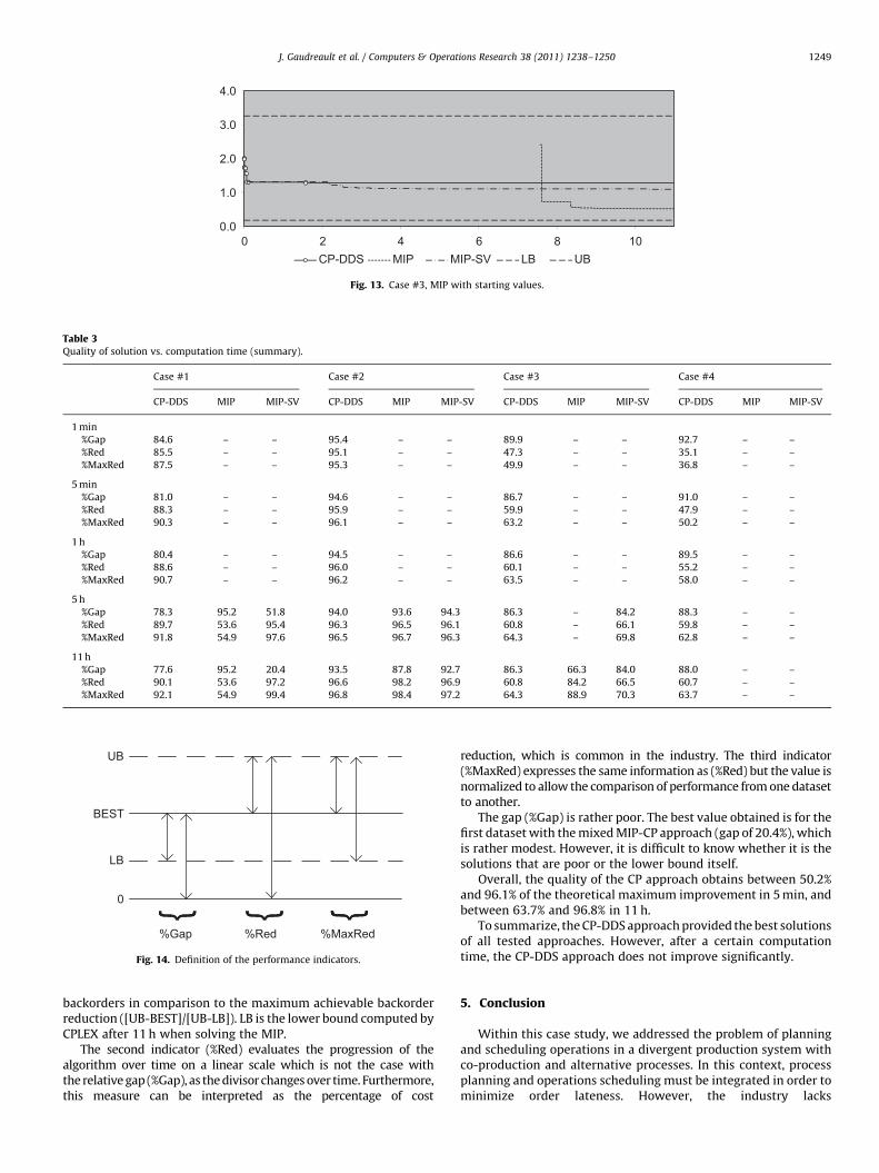
Table 3Quality of solution vs. computation time (summary).

Case #1 Case #2 Case #3 Case #4

CP-DDS MIP MIP-SV CP-DDS MIP MIP-SV CP-DDS MIP MIP-SV CP-DDS MIP MIP-SV

1 min

%Gap 84.6 – – 95.4 – – 89.9 – – 92.7 – –

%Red 85.5 – – 95.1 – – 47.3 – – 35.1 – –

%MaxRed 87.5 – – 95.3 – – 49.9 – – 36.8 – –

5 min

%Gap 81.0 – – 94.6 – – 86.7 – – 91.0 – –

%Red 88.3 – – 95.9 – – 59.9 – – 47.9 – –

%MaxRed 90.3 – – 96.1 – – 63.2 – – 50.2 – –

1 h

%Gap 80.4 – – 94.5 – – 86.6 – – 89.5 – –

%Red 88.6 – – 96.0 – – 60.1 – – 55.2 – –

%MaxRed 90.7 – – 96.2 – – 63.5 – – 58.0 – –

5 h

%Gap 78.3 95.2 51.8 94.0 93.6 94.3 86.3 – 84.2 88.3 – –

%Red 89.7 53.6 95.4 96.3 96.5 96.1 60.8 – 66.1 59.8 – –

%MaxRed 91.8 54.9 97.6 96.5 96.7 96.3 64.3 – 69.8 62.8 – –

11 h

%Gap 77.6 95.2 20.4 93.5 87.8 92.7 86.3 66.3 84.0 88.0 – –

%Red 90.1 53.6 97.2 96.6 98.2 96.9 60.8 84.2 66.5 60.7 – –

%MaxRed 92.1 54.9 99.4 96.8 98.4 97.2 64.3 88.9 70.3 63.7 – –

UB

BEST

LB

0

%Gap %Red %MaxRed

Fig. 14. Definition of the performance indicators.


backorders in comparison to the maximum achievable backorderreduction ([UB-BEST]/[UB-LB]). LB is the lower bound computed byCPLEX after 11 h when solving the MIP.

The second indicator (%Red) evaluates the progression of thealgorithm over time on a linear scale which is not the case withthe relative gap (%Gap), as the divisor changes over time. Furthermore,this measure can be interpreted as the percentage of cost

reduction, which is common in the industry. The third indicator(%MaxRed) expresses the same information as (%Red) but the value isnormalized to allow the comparison of performance from one datasetto another.

The gap (%Gap) is rather poor. The best value obtained is for thefirst dataset with the mixed MIP-CP approach (gap of 20.4%), whichis rather modest. However, it is difficult to know whether it is thesolutions that are poor or the lower bound itself.

Overall, the quality of the CP approach obtains between 50.2%and 96.1% of the theoretical maximum improvement in 5 min, andbetween 63.7% and 96.8% in 11 h.

To summarize, the CP-DDS approach provided the best solutionsof all tested approaches. However, after a certain computationtime, the CP-DDS approach does not improve significantly.

5. Conclusion

Within this case study, we addressed the problem of planningand scheduling operations in a divergent production system withco-production and alternative processes. In this context, processplanning and operations scheduling must be integrated in order tominimize order lateness. However, the industry lacks


computerized planning tools supporting this problem. To give anexample, in the lumber industry, planning and scheduling is donemanually using spreadsheet applications.

In order to tackle this problem, we first proposed mathematicalprogramming (MIP) and constraint programming (CP) formula-tions, which introduced a novel mechanism to model orderlateness within a time-line model.

However, standard approaches for solving MIP and CP formula-tions were shown to be inefficient for the large industrial problemsstudied. Consequently, we proposed a search procedure that aims atproducing good solutions in a short computation time. It providedmuch better solutions than current industrial practice and metindustrial expectations in order to include this planning-schedulingtool within an agent-based supply chain coordination system.

References

[1] Bartak R. Conceptual models for combined planning and scheduling. In:Proceedings of CP99 workshop on large scale combinatorial optimisationand constraints. 1999, p. 2–14.

[2] Frayret JM, D’Amours S, Rousseau A, Harvey S, Gaudreault J. Agent-basedsupply chain planning in the forest products industry. International Journal ofFlexible Manufacturing Systems 2007;19:4:358–391.

[3] Umble MM. Analyzing manufacturing problems using V-A-T analysis. Produc-tion and Inventory Management Journal 1992;33(2):55–60.

[4] Vila D, Martel A, Beauregard R. Designing logistics networks in divergentprocess industries: a methodology and its application to the lumber industry.International Journal of Production Economics 2006;102(2):358–78.

[5] Myers KL, Smith SF. Issues in the integration of planning and scheduling forenterprise control. In: Proceedings of the DARPA symposium on advances inenterprise control. San Diego; 1999.

[6] Larsen NE, Alting L. Simultaneous engineering within process and productionplanning. In: Proceedings of the pacific conference on manufacturing. Sydney;1990, p. 1024–31.

[7] Sormaz DN, Khoshnevis B. Generation of alternative process plans in integratedmanufacturing system. Journal of Intelligent Manufacturing 2003;14(6):509–26.

[8] Yang YN, Parsaei HR, Leep HR. A prototype of a feature-based multiple-alternative process planning system with scheduling verification. Computer &Industrial Engineering 2001;39(1-2):109–24.

[9] Husbands P, McIlhagga M, Ives R. Experiments with an ecosystems model forintegrated production planning. In: Back T, Fogel DB, Michalewicz Z, editors.Handbook of Evolutionary Computation. Oxford: Oxford University Press;1995.

[10] Numao M. Integrated scheduling/planning environment for petrochemicalproduction processes. Expert Systems with Applications 1995;8(2):263–73.

[11] Khoshnevis B, Qingmei Chen. Integration of process planning and schedulingfunctions. Journal of Intelligent Manufacturing 1991;2(3):165–76.

[12] Huang SH, Zhang HC, Smith ML. A progressive approach for the integration ofprocess planning and scheduling. IIE Transactions 1995;27:4.

[13] McDonnell P, Smith G, Joshi SJ, Kumara SRT. Cascading auction protocol as aframework for integrating process planning and heterarchical shop floorcontrol. International Journal of Flexible Manufacturing Systems 1999;11:1:37–62.

[14] Lee YH, Jeong CS, Moon C. Advanced planning and scheduling with outsourcingin manufacturing supply chain. Computers & Industrial Engineering2002;43(1–2):351–74.

[15] Weintraub A, Cormier D, Hodgson T, King R, Wilson J, Zozom A. Scheduling withalternatives: a link between process planning and scheduling. IIE Transactions1999;31(11):1093–102.

[16] Shen W, Wang L, Hao Q. Agent-based distributed manufacturing processplanning and scheduling: A state-of-the-art survey. IEEE Transactions onSystems, Man and Cybernetics, Part C 2006/07;36(4):563–77.

[17] Tan W, Khoshnevis B. A linearized polynomial mixed integer programmingmodel for the integration of process planning and scheduling. Journal ofIntelligent Manufacturing 2004/10;15(5):593–605.

[18] Li WD, McMahon CA. A simulated annealing-based optimization approach forintegrated process planning and scheduling. International Journal of ComputerIntegrated Manufacturing 2007/01;20(1):80–95.

[19] Lee H, Kim S-S. Integration of process planning and scheduling using simula-tion based genetic algorithms. International Journal of Advanced Manufactur-ing Technology 2001;18(8):586–90.

[20] Kim YK, Park K, Ko J. A symbiotic evolutionary algorithm for the integration ofprocess planning and job shop scheduling. Computers & Operations Research2003;30(8):1151–71.

[21] Moon C, Seo Y. Evolutionary algorithm for advanced process planning andscheduling in a multi-plant. Computers & Industrial Engineering 2005;48(2):311–25.

[22] Bartak R. Visopt ShopFloor: on the edge of planning and scheduling. Principlesand Practice of Constraint Programming - CP 2002. In: Proceeding so the eighthinternational conference, CP 2002, 9–13 Sept. 2002. 2002, p. 587–602.

[23] Tan W, Khoshnevis B. Integration of process planning and scheduling—areview. Journal of Intelligent Manufacturing 2000/03;11(1):51–63.

[24] Gascon A, Lefrancois P, Cloutier L. Computer-assisted multi-item, multi-machine and multi-site scheduling in a hardwood flooring factory. Computersin Industry 1998;36(3):231–44.

[25] Yaghubian AR, Hodgson TJ, Joines JA. Dry-or-buy decision support for dry kilnscheduling in furniture production. IIE Transactions 2001;33(2):131–6.

[26] Joines JA, Culbreth CT. Job sequencing and inventory control for a parallelmachine problem: a hybrid-GA approach. In: Proceedings of the 1999 congresson evolutionary computation. 1999, p. 1130–7.

[27] Bartak R. On the boundary of planning and scheduling: a study. In: Proceedingsof the eighteenth workshop of the UK planning and scheduling special interestgroup (PlanSIG). Manchester, UK; 1999, p. 28–39.

[28] Bartak R. Constraint programming—what is behind? In: Proceedings of theconstraint programming for decision control workshop. Gliwice; 1999.

[29] Hooker JN. Logic-based methods for optimization: combining optimizationand constraint satisfaction. New York: John Wiley & Sons; 2000.

[30] Milano M. Constraint and integer programming toward a unified methodology.Berlin: Springer; 2004.

[31] Van Hentenryck P, Perron L, Puget JF. Search and strategies in OPL. ACMTransactions on Computational Logic 2000;1(2):285–320.

[32] Walsh T. Depth-bounded discrepancy search. In: International joint conferenceon artificial intelligence. 1997, p. 1388–93.

Combined planning and scheduling in a divergent production system with co-production: A case study in the lumber industry

Documents