Combined evaluation of MPIESM land surface water and energy fluxes

Combined evaluation of MPI-ESM land surface water and energy

fluxes

Stefan Hagemann,1 Alexander Loew,1 and A. Andersson2

Received 29 May 2012; revised 1 October 2012; accepted 27 November 2012.

[1] To assess the robustness of projected changes of the hydrological cycle simulatedby an Earth system model (ESM), it is fundamental to validate the ESM and tocharacterize its major deficits. As the hydrological cycle is closely coupled to theenergy cycle, a common large-scale evaluation of these fundamental components ofthe Earth system is highly beneficial, even though this has been rarely done up to now.Consequently, the purpose of the present study is the combined evaluation of landsurface water and energy fluxes from the newest ESM version of the Max PlanckInstitute for Meteorology (MPI-ESM), which was used to produce an ensemble ofCoupled Model Intercomparison Project Phase 5 (CMIP5) simulations. With regardto energy fluxes, we especially make use of recent satellite data sets. Additionally,MPI-ESM results are compared with CMIP3 results from the predecessor ofMPI-ESM, ECHAM5/MPIOM, as well as to results from the atmosphere/land partof MPI-ESM (ECHAM6/JSBACH) forced by observed sea surface temperature(SST). Analyses focus on regions where notable differences occur between the twoESM versions as well as between the fully coupled and the uncoupled SST-drivensimulations. In general, our results show a considerable improvement of MPI-ESM insimulating surface shortwave radiation fluxes. The precipitation of the fully coupledsimulations notably differs from those of the SST-forced simulations over a few rivercatchments. Over the Amazon catchment, the coupling to the ocean leads to a largenegative precipitation bias, while for the Ganges/Brahmaputra, the couplingsignificantly improves the simulated precipitation.

Citation: Hagemann, S., A. Loew, and A. Andersson (2013), Combined evaluation of MPI-ESM land surface water and energy

fluxes, J. Adv. Model. Earth Syst., 5, 10.1029/2012MS000173.

1. Introduction

[2] The climate of the Earth is influenced by increasinggreenhouse gas concentrations, changing aerosol compo-sitions and loads as well as land surface changes. In cli-mate research, a special emphasis is placed on thehydrological cycle, which is crucial to life on Earth. Itsimportance is highlighted by the Global Energy andWater Cycle Experiment (GEWEX) [e.g., Sorooshianet al. 2005]. The implications of changes in the hydrologi-cal cycle induced by climate change may affect societymore than any other changes, e.g., with regard to floodrisks, and changes in water availability and water quality.

[3] An accurate representation of the exchange ofwater between the atmosphere, the ocean, the cryosphere,and the land surface is one of the biggest challenges in

earth system modeling. Simulating these fluxes is extremelydifficult, because they depend on processes occurring onspatial scales that are generally several orders of magnitudesmaller than the typical grid size in an Earth system model(ESM). The formation of precipitation, for example, iscontrolled by a multitude of processes such as cloud micro-physics and particle growth, radiative transfer, atmos-pheric dynamics on a variety of space and timescales, andinhomogeneities of the Earth’s surface. All of these proc-esses have to be properly represented in an ESM.

[4] The surface water and energy fluxes are closelyrelated with each other as well as the terrestrial carbonfluxes. A strong coupling of the land surface dynamicswith the atmosphere exists, especially in transitional cli-mate regions [see, e.g., Koster et al., 2004; Seneviratneet al., 2010]. The feedback from the land surface cantherefore have a strong effect on regional patterns ofsurface water and energy fluxes. Consequently, the focusof this study is on evaluating the skill of the currentESM version of the Max Planck Institute for Meteorol-ogy (MPI-ESM) to simulate land surface water andenergy fluxes. MPI-ESM was used to produce an ensem-ble of Coupled Model Intercomparison Project Phase 5

1Max Planck Institute for Meteorology, Klima Campus, Ham-burg, Germany.

2Deutscher Wetterdienst, CM-SAF, Offenbach, Germany.

©2012. American Geophysical Union. All Rights Reserved.1942-2466/13/2012MS000173

1

JOURNAL OF ADVANCES IN MODELING EARTH SYSTEMS, VOL. 5, 1–28, doi:10.1029/2012MS000173, 2013

(CMIP5) simulations for the forthcoming fifth Intergov-ernmental Panel on Climate Change (IPCC) assessmentreport. The evaluation mainly comprises the comparisonof simulated and observed land surface climatologies of2m temperature, precipitation, evaporation, and riverrunoff as well as surface solar radiation fluxes. In partic-ular, we assess the dependence of biases in land surfacewater and energy fluxes on cases of fully or partiallycoupled MPI-ESM experiments to quantify differencesdue to the coupling with a dynamic ocean model. Wealso compare the results from the present MPI-ESM toresults from its precedent version to quantify the differ-ences between the two considerably different model ver-sions of MPI-ESM (see section 2.1). Moreover, wequantify their accuracy compared with independentdata sets. The analysis of other components of thehydrological cycle such as clouds, snow or soil moisture,is beyond the scope of this study and will therefore notbe discussed.

[5] The model and the simulations considered in thisstudy are briefly described in section 2. Simulated andobserved components of the hydrological and energycycle at the land surface are compared in section 3 on alarge scale, and in section 4 for specific regions. Particu-lar model biases in specific regions are discussed inmore detail in section 5, and the main findings are sum-marized in section 6.

2. Description of MPI-ESM, Model SimulationsUsed and Observations

2.1. ESM of the Max Planck Institute for Meteorology

[6] The coupled MPI-ESM consists of the followingmodel components: ECHAM6 in the atmosphere[Stevens et al., 2012], MPIOM in the ocean [Jungclauset al., 2012], and JSBACH [Raddatz et al., 2007; Brovkinet al., 2009] for land surfaces. It takes into accountobserved concentrations of CO2, CH4, N2O, CFCs, O3

(tropospheric and stratospheric), and sulphate aerosols,thereby considering the direct and first indirect aerosoleffect. Major differences of MPI-ESM to its predecessorECHAM5/MPIOM [Roeckner et al., 2003; Jungclauset al., 2006] are a new radiative transfer scheme in theatmosphere, the use of a new aerosol climatology, andthe incorporation of the carbon cycle including oceanbiogeochemistry and an interactive and dynamic vegeta-tion scheme at the land surface. Also the standard setupof MPI-ESM with 47 vertical atmospheric levels (LR)reaches to higher atmospheric layers than the previousone with 31 levels.

2.2. Model Simulations

[7] The experiments analyzed in this study were con-ducted following the CMIP5 protocol [Taylor et al.,2012]. The following ESM ensemble simulations wereconsidered in this study, comprising three memberseach. (1) An ensemble of fully coupled MPI-ESM ‘‘his-torical’’ (twentieth century) simulations conducted withthe CMIP5 model setup, thereby focusing on the period1971–2000 representing the current climate. This ensem-ble is referred as MPI-ESMh in the following. (2) An

ensemble of Atmospheric Model IntercomparisonProject 2 (AMIP2) type simulations where the land/atmosphere component of MPI-ESM (ECHAM6/JSBACH) was forced with observed sea surface temper-ature (SST) and sea ice from 1979 onward. Here, weconsider the period 1979–2000 and refer to this ensem-ble as MPI-ESMa in the following. (3) An ensemble offully coupled ECHAM5/MPIOM historical twentiethcentury simulations that was conducted for CMIP3[Program for Climate Model Diagnosis and Intercom-parison (PCMDI), 2007] and used in fourth IPCCassessment report [Solomon et al., 2007]. Comparisonsfocus on the period 1971–2000 and the ensemble isreferred as ECHAM5h in the following. (4) In sections4 and 5, we also show results from an AMIP2 simula-tion (1979–1999) using ECHAM5 with T63 horizontalresolution and 31 vertical atmospheric levels(ECHAM5a). This simulation has been evaluated byHagemann et al. [2006], where the impact of differenthorizontal and vertical resolutions on the simulatedhydrological cycle of ECHAM5 was considered.

[8] A notable difference of the setup of the land sur-face scheme JSBACH in MPI-ESM to those within theAMIP2 simulations is the use of a dynamical vegetationalgorithm [Brovkin et al., 2009] while in the latter a pre-scribed distribution of vegetation (i.e., Plant FunctionalTypes (PFTs)) is used that is based on a 1 km global dis-tribution of major ecosystem types [Loveland et al.,2000]. Note also the difference of the land surface repre-sentation between ECHAM5 and MPI-ESM, where thefirst uses a static description of the land surface follow-ing Hagemann [2002], while the latter uses a dynamicmodel (see above) with interactive vegetation, e.g., com-prising the phenological simulation of leaf area indexand surface background albedo.

[9] We conducted climatological comparisons toobservations and previous analogous ECHAM5 simula-tions. The time periods considered depend on the avail-ability of model and observational data (see section 2.3).Note that for the coupled simulations MPI-ESMh andECHAM5h we focus on the period 1971–2000 as thiswill be the common reference period for the quantifica-tion of climate change signals in studies of future globalwarming. With regard to the SST forced simulations,the available subset of this period will be used, i.e.,1979–2000 for MPI-ESMa. Results obtained with MPI-ESMh show that in general climatological differencesbetween 1971–2000 and 1979–2000 are relatively smallfor the variables considered in this study, especiallywhen compared with the differences to observations asreported in sections 3 and 4.

[10] Generally, simulated climatologies are directlytaken from the model output of the respective variable.An exception is the surface albedo, which was calcu-lated as the ratio of the monthly means of the upwardand downward shortwave radiation fluxes to appropri-ately take into account changes in the fractions of directand diffuse radiation during a month. This is necessarysince the JSBACH land surface model in MPI-ESMand also ECHAM5 calculate the surface albedo as afunction of the actual state of the vegetation, the

HAGEMANN ET AL.: EVALUATION: MPI-ESM LAND SURFACE FLUXES

2

background albedo below the canopy and the amountof snow cover in a model grid cell [Roesch and Roeck-ner, 2006; Vamborg, 2011].

2.3. Observational Data

[11] For the evaluation of surface water and energyfluxes, various global observational data sets are used,which are summarized in Table 1 and introduced in thefollowing. As the observations comprise some veryrecent data sets of surface solar irradiance (SSI), theseare discussed in more detail.2.3.1. Hydrological Observations

[12] As observations, temperature and precipitationfrom the newly available global WATCH data set ofhydrological forcing data (henceforth referred to asWFD [Weedon et al., 2011]) were used. The WFD com-bine the daily statistics of the 40-years reanalysis of theEuropean Centre for Medium-Range Weather Forecasts(ERA40 [Uppala et al., 2005]) with the monthly meanobserved characteristics of temperature from the ClimateResearch Unit data set TS2.1 [Mitchell and Jones, 2005]and precipitation from the Global Precipitation Clima-tology Centre full data set version 4 [Fuchs et al., 2007].For the latter, a gauge-undercatch correction followingAdam and Lettenmaier [2003] was used, which takes intoaccount the systematic underestimation of precipitationmeasurements that have an error of up to 10%–50% [see,e.g., Rudolf and Rubel, 2005]. Note that the uncertaintiesin the precipitation data are still high in regions with asparse station density and those with significant snowfallamounts, especially in mountainous areas [see, e.g.,Rudolf and Rubel, 2005; Biemans et al., 2009]. In addition,climatological observed discharge data were taken formajor rivers from the Global Runoff Data Centre(GRDC; see, e.g., D€umenil Gates et al., [2000]).2.3.2. Surface Albedo

[13] Ten years of Moderate Resolution Imaging Spec-troradiometer (MODIS) surface albedo (MCD43C3, ver.5) observations [Schaaf et al., 2002] are used for compari-son with MPI-ESM results. The albedo observations arefiltered in accordance to the product quality flags toensure that only best quality observations are consideredfor the reference data set. The data are then reprojectedto the MPI-ESM model grid (T63 resolution, Gaussiangrid). The mean surface albedo and its variance are cal-culated from the 10-year time series for each month andgrid cell, respectively. With a record of just ten years of

observations, the estimation of robust climatic mean val-ues of surface albedo is difficult. On the other hand,changes in vegetation cover might already change signifi-cantly the surface albedo on decadal timescales andtherefore affect climate [Loew and Govaerts, 2010; Fen-sholt et al., 2012]. Results shown in this paper are basedon the full 10-year record of MODIS observations. How-ever, we also analyzed the effect of sampling of theMODIS observations as well as the MPI-ESM simula-tions on shorter timescales (5 years) and found no signifi-cant differences to those shown in the present study.2.3.3. Surface Solar Irradiance

[14] Satellite based methods enable the estimation ofthe surface solar flux at high temporal and spatial resolu-tions at global scales. Satellite-based estimates of atmos-pheric radiation fluxes have been developed throughoutthe last 20 years. Different global products exist, whichalso allow to assess the interproduct variability of SSI.Four different surface solar radiation data sets are usedfor the present study. The Clouds and Earth RadiationEnergy System (CERES) surface solar radiation fluxesare provided at global scale and are derived from meas-urements onboard of the Earth Observing System (EOS)Terra and Aqua satellites [Loeb et al., 2012]. The CERESsurface fluxes are obtained from the monthly TOA/Sur-face Averages (SRBAVG; edition 2) product for a limitedtime period (2000–2003). A new reprocessed and flux cor-rected Energy Balanced And Filled (EBAF) surface fluxproduct, covering the period 2000–2010, became availableafter the analysis of the present paper had been finalized[D. R. Doelling, 2012, personal communication]. An anal-ysis of the differences between climatologies derived fromthe two different data sets revealed no major differencesand no impact on the results and conclusions of the pres-ent paper are therefore expected by using the time-limitedCERES data for the present study.

[15] Although the CERES data record is limited to afew years, the recently released SSI data set of the Euro-pean Organisation for the Exploitation of Meteorologi-cal Satellites (EUMETSAT) Satellite ApplicationFacility on Climate Monitoring (CMSAF) covers theperiod from 1983 to 2005. The product is distributed ona regular latitude/longitude grid with a grid spacing of0.03� in both directions and is limited to the spatial do-main of Meteosat centered at 0�E (see Figure A1).Details on the retrieval scheme can be found in M€ulleret al. [2009, 2011]. A recent study investigated the

Table 1. Used Observational Data Sets

Variable Data SetOriginal Spatial

ResolutionOriginal Temporal

Resolution References

Surface albedo MODIS MCD43C3, ver. 5 0.05� 3 0.05� 8 days Schaaf et al. [2002]Meteosat albedo EUMETSAT <5 3 5 km 10 days Loew and Govaerts [2010]SSI CMSAF 0.03� 3 0.03� Hourly, monthly M€uller et al. [2009, 2011]

CERES 1.0� 3 1.0� Monthly Loeb et al. [2012]BSRN Point Hourly Ohmura et al. [1998]SRB 1� 3 1� 3 hourly, monthly Cox et al. [2006]

ISCCP 280 km 3 hourly, monthly Zhang et al. [2004]Temperature WFD 0.5� Daily, monthly Weedon et al. [2011]Precipitation WFD 0.5� Daily, monthly Weedon et al. [2011]Discharge GRDC Stations Monthly D€umenil Gates et al. [2000]


3

potential for the generation of a seamless surface solarradiation product from first and second generation ofMeteosat satellites [Posselt et al., 2011a].

[16] The accuracy of the CMSAF surface solar radia-tion product has been carefully investigated using refer-ence measurements from the Baseline Surface RadiationNetwork (BSRN) [Ohmura et al., 1998]. Ineichen et al.[2009] compared the CMSAF data product at hourlybasis for eight stations in Europe and estimated accura-cies of 80 to 100 W m22. Posselt et al. [2011b] showedthat the accuracy of the monthly mean product is betterthan 10 W m22 and better than other existing availablesurface radiation data products.

[17] The International Satellite Cloud Climatologyproject (ISCCP) Flux Data (FD) product provides in-formation on estimated SSI at a spatial scale of 280 kmand with a temporal resolution of 3 h to monthly values[Rossow and Zhang, 1995]. Further details on the esti-mation of surface fluxes for ISCCP are given in Zhanget al. [2004]. Data from 1989 to 2005 were used for thepresent analysis.

[18] The National Aeronautics and Space Adminis-tration (NASA)/GEWEX surface radiation budget(SRB) project aims at the production of long-term datasets of shortwave and longwave surface and top-of-atmosphere radiation fluxes. It provides 3 hourly tomonthly flux estimates at global scale with a resolutionof 1� 3 1�. The fluxes are calculated based on cloud pa-rameters obtained from ISCCP and meteorologicalfields from the NASA Global Modeling and Assimila-tion Office (GMAO) reanalysis data sets. This studyuses monthly means of the SRB shortwave surface radi-ation flux product (version 3.0 [Cox et al., 2006.]).

[19] All satellite data sets were reprojected to theMPI-ESM model grid at T63 resolution before furtheranalysis using a conservative remapping procedure. Thedifferent SSI observational data sets exhibit systematicdifferences that may have to be considered in the com-parisons to the model output. To illustrate these sys-tematic differences, seasonal means of SSI differencesare shown in Figure 1 using CERES data as a reference.Similar plots using CMSAF data are given in the Ap-pendix. A comprehensive analysis of the accuracy of thedifferent satellite flux estimates is beyond the scope ofthe present paper. A detailed analysis of the differentdata sets is conducted in the frame of the GEWEX radi-ation assessment (E. Raschke et al., GEWEX radiativeflux assessment (RFA), A project of the World ClimateResearch Programme Global Energy and Water CycleExperiment (GEWEX) Radiation Panel, WCRP-Report,in preparation, 2013), which is also addressing temporalinconsistencies in the long-term data records caused byperturbations such as the Pinatubo eruption, El-Ni~no, aswell as artifacts resulting from data processing. The sig-nificance of the difference between the seasonal means(Figure 1) was tested using a Student’s t test.

[20] The ISCCP data set shows consistent differencesto CERES as well as to the CMSAF data set. Largestdifferences are observed over the tropical Atlantic, theSahara, as well as over Eurasia during the northernhemispheric summer and over the Antarctic ocean

during the southern hemispheric summer. These differ-ences might be due to a different characterization of seaice in the different data products.

[21] Although the SRB data set is based on ISCCPcloud properties as an input, differences in the surfaceradiation fluxes can be observed, which are due to dif-ferent algorithms employed as well as different ancillarydata used for flux calculations. While the flux differen-ces to CERES and CMSAF data are rather similar tothose for ISCCP in the Extratropics, SRB shows smallersurface solar radiation fluxes in the tropical areas thanISCCP. The difference plot in Figure 1 also shows arti-facts caused by the spatial coverage of the different sat-ellites used for the derivation of the data products. OverAfrica, the spatial coverage of the Meteosat satellites isclearly visible in the difference images, which is likely tobe an artifact of the data processing.

[22] However, it needs to be emphasized that theobserved differences between the different data productsare not statistically significant in most cases. Only for avery few grid boxes, statistically significant differencesbetween the seasonal means can be detected, which isdue to the large variability of SSI between the differentyears. Thus, mostly a comparison of simulated SSI toone data set, in this case CERES data, is sufficient forthe evaluation. For better illustration, additional com-parisons to CMSAF data are provided in the Appendix.2.3.4. BSRN Data

[23] The BSRN provides high quality in situ measure-ments of the surface solar radiation flux at the localscale. A total of 61 stations collect surface radiationdata on a regular basis [Ohmura et al., 1998]. BSRN sta-tion measurements are used for an intercomparison withthe model simulations on a climatological timescale.While the in situ data correspond to point like observa-tions, the radiation simulated in the model correspondsto an average flux over an entire model grid box. How-ever, characteristic seasonal patterns of the radiationflux can be extracted from both, model simulations andin situ measurements and be compared. From the avail-able 61 BSRN stations, only those were used where atleast 60 continuous months of measurements were avail-able to compile a monthly climatology of SSI. Thisresulted in a total of 39 BSRN stations worldwide (seeFigure 2). As the CMSAF SSI data cover only a limitedpart of the globe, only 16 BSRN stations can be used forcomparison. The data were obtained from the BSRNarchive (http://www.bsrn.awi.de/). Climatological meanSSI and its variability were then calculated for each sta-tion from the entire available record of a BSRN station.

3. Results of Model Evaluation

[24] Results of the MPI-ESM evaluation are analysedin the following, focusing on global difference mapsand zonal mean statistics for the different variables ana-lysed in this study.

3.1. Precipitation

[25] Considering the zonal distribution of precipita-tion over land (Figure 3), the general shape of the


4

distribution is captured well by all models for all sea-sons. Common deviations from the WFD denote a pro-nounced dry bias in the Tropics north of the equator,which also extends to south of the equator during theboreal spring and summer, a dry bias in the low precipi-tation region in the southern Subtropics accompaniedby a wet bias around 50�S, and a wet bias in the north-ern high latitudes during boreal spring and summer.

The most notable difference between the models isthat MPI-ESMh and MPI-ESMa generally have animproved simulation of peak rainfall in the tropics com-pared with ECHAM5h. In the boreal summer, MPI-ESMh even simulates a better peak than MPI-ESMawhile this peak is better captured by MPI-ESMa duringthe boreal winter and spring. Over the high northernlatitudes in the boreal spring and summer, the slightly

Figure 1. Differences of seasonal cycle of SSI between different observational data sets: ISCCP compared to(top) CERES, SRB compared to (bottom) CERES. Statistically significant differences (p > 0.05) between the satel-lite products are indicated by stippled areas.


5

lower precipitation in ECHAM5h is somewhat closer toWFD than for the other two models.

[26] Considering the spatial differences to WFD(Figure 4), further common deficiencies are the overesti-mation of precipitation along steep mountain slopes(Andes, Himalayas, Rocky Mountains), distinct drybiases in the northern part of South America andaround the Sahel zone that extend further south duringthe boreal summer. In the boreal winter, a large wetbias over eastern Asia can be noted. The pronounceddry bias in ECHAM5h over central and southern

Europe during the boreal summer is largely reduced inboth MPI-ESM simulations.

3.2. Temperature

[27] Figure 5 shows the zonal distribution of the 2mtemperature difference to the WFD over land averagedover the four seasons. All models are close (within61K) to the WFD in the tropics in all seasons, butshow pronounced warm biases in the northern mid- andhigh latitudes in the boreal winter and spring, which isreplaced in the northern hemisphere by a cold bias inthe boreal summer. Further, a warm bias around 30�Scan be noted that might be related to the dry bias in thesouthern Subtropics (see above). In the boreal summer,this extends to the southern mid-latitudes while in theboreal autumn and winter, a cold bias becomes appa-rent. MPI-ESMh tends to be colder than the other twomodels south of 30�N and shows the smallest bias com-pared with the WFD in the tropics and southern sub-tropics in the boreal summer and autumn (reduced oreven no warm bias around 30�S). In the northern highlatitudes, ECHAM5h is colder than MPI-ESMh andMPI-ESMa, the latter being the warmest in this region.Thus, ECHAM5h has the smallest warm bias in winterand spring, while MPI-ESMa has a strongly reducedcold bias around 60�N in the boreal summer.

Figure 2. Distribution of 39 BSRN stations with long-term SSI measurements.

Figure 3. Zonal distribution of precipitation over land in the boreal (a) winter, (b) spring, (c) summer, and (d)autumn. Unit: mm d21.


6

[28] Maps of the 2m temperature difference to theWFD (Figure 6) reveal that the winter warm bias isspread throughout the whole range of northern latitudesexcept for Greenland and the west coasts of NorthAmerica and Europe, and it is most pronounced in East-ern Siberia. The reduced warm bias in ECHAM5h stemsfrom generally colder simulation of temperatures overnorthern Eurasia. In the boreal summer, the reducedcold bias of MPI-ESMa in the high northern latitudes isnot only related to a strongly improved simulation oftemperatures over Eurasia but also to the compensatingeffect of a warm bias over Central United States that

does not appear for the other two models. The generalcold bias over Greenland is likely related to the too sim-ple treatment of the glacier ice sheets in the models.

3.3. Surface Solar Radiation

[29] The differences in SSI between the different mod-els and experiments are illustrated in Figure 7. TheMPI-ESM simulations are very similar for the globalmean field with a global average of 162.5 6 94.2 W m22

and 162.2 6 94.2 W m22 for MPI-ESMa and MPI-ESMh experiments, respectively. Observed seasonal dif-ferences are not significant except for small regions in

Figure 4. Relative precipitation difference to the WFD over land in the boreal winter (left column) and summer(right column) for MPI-ESMh (upper row), MPI-ESMa (middle row), and ECHAM5h (lower row). Unit: %.


7

the inner tropics during boreal winter as well as over theBenguela current during June–July–August/September–October–November (JJA/SON). Spatial differences inSSI are mainly related to changes in the cloud patternthat also reflect in changes in the simulated precipitationpatterns (A. Andersson et al., Evaluation of MPI-ESMocean surface fluxes, J. Adv. Model. Earth Syst., in prep-aration, 2013, hereinafter referred to as Anderssonet al., in preparation, 2013).

[30] Figure 7b shows the SSI differences betweenMPI-ESMh and ECHAM5h. The global mean ofECHAM5h is lower (156.1 6 95.5 W m22) than the cor-responding simulation results from MPI-ESM. Largestdifferences are observed over Eurasia and the tropicalAfrica with deviations >20 W m22. However, theestimated differences are only statistically significant incentral Africa as well as in the Eastern Pacific. Theobserved differences between the model versions are dueto different cloud coverage as well as aerosol opticaldepth.3.3.1. Evaluation Using BSRN Station Data

[31] Comparison of simulated SSI fields with BSRNstation data shows high correlations for all stations andmodels. Figure 8 shows the distribution of obtainedPearson correlation coefficients and root-mean-squareerror (RMSE; W m22) for a total of 39 stations theglobal radiation products and 16 stations for CMSAF.

Overall, the CMSAF SSI product shows highest corre-lations and smallest RMSE for this climatological com-parison, which is also the case if RMSE and correlationof CERES, SRB, and ISCCP are calculated only for the16 stations covered by the CMSAF data. This result isconsistent with validation results of the CMSAF dataproduct (see also section 2.3), which showed that thissatellite-based product has an accuracy better than10 W m22 and shows smaller errors compared withother existing solar irradiance products [Posselt et al.,2011b]. The RMSE obtained in this study is slightlylarger, which is explained by the much larger scale dis-crepancy between the BSRN stations and the model gridscale. The other satellite data sets show slightly higherRMSE compared with the CMSAF data. While ISCCPand CERES show an almost similar spread in theRMSE as the CMSAF data (r < 10 W m22 inner quar-tile range), the SRB inner quartile range is 14 W m22.

[32] The MPI-ESM model simulations have a medianRMSE of 14 (12) W m22 for MPI-ESMa (MPI-ESMh)with a similar variability. Contrary, ECHAM5h has ahigher RMSE of 18 W m22 with a much larger spread.This indicates that the improvements in the new radia-tion scheme applied in MPI-ESM as well as the new aer-osol climatology have improved the skill of the model tosimulate SSI. In the following, we will compare themodel results against the satellite-based estimates of SSI.

Figure 5. Zonal distribution of 2m temperature difference to the WFD over land in the boreal (a) winter,(b) spring, (c) summer, and (d) autumn. Unit: K.


8

3.3.2. Results of Spatial SSI Comparison[33] The differences between the various satellite-

based surface radiation products were discussed in sec-tion 2.3. Table 2 summarizes the global mean annualand seasonal SSI for the various model simulations andobservations, whereas Figure 9 shows correspondingzonal means of SSI over land. In general, there is agood agreement between the different data sets and themodels. Largest differences occur during the summerseason of each hemisphere. The estimated global meansurface solar radiation flux is 162 W m22 for MPI-ESM, for both the coupled and uncoupled simulations

and therefore well within the range of uncertaintiesobtained from the analysis of reanalysis data [Trenberthet al., 2009, 2011]. The satellite-derived global mean SSIflux is 169.3, 164.7, and 160.8 W m22 for CERES,ISCCP, and SRB, respectively. ECHAM5h has a muchlower global mean of 156.1 W m22. Overall, the differen-ces between ECHAM5h and the new MPI-ESM are largerthan the differences between the coupled and uncoupledexperiments of MPI-ESM. Statistically different seasonalmeans occur between MPI-ESM, ECHAM5h, and thevarious observational data sets. The same regions withsignificant differences are identified in both MPI-ESM

Figure 6. The 2m temperature difference to the WFD over land in the boreal winter (left column) and summer(right column) for MPI-ESMh (upper row), MPI-ESMa (middle row), and ECHAM5h (lower row). Unit: K.


9

experiments. We therefore only show results for MPI-ESMh in Figure 10 (and Figure A2). Consistent differen-ces of MPI-ESM occur with all observational data sets.Statistically significant differences of SSI are mainly evi-dent during December-January-February (DJF) and JJAwhen comparing against CERES data. For DJF, SSI isunderestimated for the southern hemispherical tropicalocean and land surfaces. In JJA, a statistically significantunderestimation of SSI is shown over large parts of the

northern hemisphere Atlantic and Pacific oceans. Signifi-cant positive differences occur in the western Pacificthroughout all seasons. In general, similar patterns aresimulated by ECHAM5h.

[34] While the differences between simulated andobserved SSI reveal generally consistent patterns and arevery useful to identify regions with significant differences,an overall assessment of the accuracy of the differentmodel experiments is difficult. We therefore calculate a

Figure 7. Differences in seasonal SSI (W m22) between (a) MPI-ESMh and MPI-ESMa and (b) between MPI-ESMh and ECHAM5h. Statistical significant differences (p > 0.05) are indicated by stippled areas.


10

single scalar normalized difference (e2) between the modelresults (SSIm) and a reference data set (SSIref), followingReichler and Kim [2008] as

e25X

n

�wnðSSIm;n2SSIref ;nÞ2=r2

ref ;n

�;

whereas wn are proper weights for changes in grid cellarea, r2

ref corresponds to the interannual variance of thereference data set, and n is an index over all grid boxesinvestigated. The normalized error provides a relativeranking of different data sets. The CERES as well asCMSAF data sets were used as references for the calcu-lation of e2. Figure 11 shows results of this ranking withthe dimensionless e2 on the x axis, stratified by season.The differences in e2 between CMSAF and CERESdata are due to the different spatial domains covered bythe two data sets. In general, the observational data sets(ISCCP, SRB) show smaller errors than the model simula-tions, indicating a general higher agreement between thedifferent observational data sets, as could be expected.SRB tends to have slightly larger values for e2 for bothCERES and CMSAF data used as a reference.

[36] The ECHAM5h simulations show the highesterrors and a considerable improvement of the simulatedSSI is found for both MPI-ESM experiments, provingthe increased capability of MPI-ESM to simulate SSIusing its refined atmospheric radiative transfer schemeand new aerosol climatology. The relative ranking ofthe different data sets remains consistent throughoutthe seasons and between the two reference data sets.Major changes in e2 are observed between the seasonswith highest errors in DJF and JJA respectively.

3.4. Surface Albedo

[37] The surface albedo of the MPI-ESM simulationsis very similar. Seasonal values of zonal means of sur-face albedo are shown in Figure 12. On average, theMPI-ESM simulations show good agreement with theMODIS observations, except for high latitudes wherelarger differences occur due to snow. However, theselarger absolute deviations have a small effect on thetotal surface radiative fluxes, as the SSI is small duringboreal winter. Zonal means of ECHAM5h show a simi-lar performance as the MPI-ESM simulations com-pared with the MODIS observations. To better assessthe importance of the albedo differences for the surfaceradiation fluxes, the differences between model simula-tions and MODIS observations are expressed in termsof differences of the upward shortwave radiation fluxwhich is obtained by scaling the surface albedo by themodel SSI. As mentioned in section 2.2, all results arepresented for the ensemble mean of three ensemble mem-bers of the model experiments. However, a sensitivityanalysis (not shown) revealed that the differences causedby the internal variability of the model are much smallerthan the differences yielded between the model simula-tions and the satellite observations. Figure 13 shows dif-ference maps of upward shortwave flux between theESM simulations and MODIS data.

[38] In general, the land surface albedo (upward flux)is slightly overestimated by the model almost every-where during summertime, except for the Sahel regionand some desert regions in Asia and Australia. A signif-icance test of the differences between simulated andobserved surface shortwave upward flux showed thatthe observed differences are significant (p < 0.05) nearlyeverywhere on the globe. Differences between modeland observations are most pronounced during borealwinter (DJF) and spring (March-April-May (MAM))season with snow cover in high latitudes. In this period,the surface albedo dynamics are affected by snow coverand its masking by tree cover [e.g., Essery et al., 2009].In the northwestern part of North America (British

Figure 8. BSRN error statistics: correlation and RMSEof climatological mean seasonal cycle of SSI. Boxes cor-respond to lower and upper quartiles, whiskers corre-spond to the data range, and red lines signify the medianvalue.

Table 2. Global Means of Seasonal SSI for the Simulations and Observational Data Setsa

Data Set DJF MAM JJA SON Mean

MPI-ESMa (1979–2000) 177.7 (111.9) 157.4 (82.2) 152.1 (96.5) 162.9 (81.0) 162.5 (94.2)MPI-ESMh (1979–2000) 176.7 (111.5) 157.9 (82.7) 151.8 (96.1) 162.5 (81.5) 162.2 (94.2)ECHAM5h (1971–2000) 172.6 (111.6) 150.4 (85.6) 144.3 (94.7) 157.3 (85.3) 156.1 (95.5)CERES (2000–2003) 179.8 (110.0) 165.7 (83.8) 167.8 (101.9) 163.8 (82.4) 169.3 (95.5)ISCCP (1989–2004) 179.1 (111.4) 158.3 (82.1) 159.3 (97.5) 162.2 (80.5) 164.7 (94.1)SRB (1989–2004) 172.2 (105.1) 155.5 (81.6) 158.7 (96.0) 156.8 (79.6) 160.8 (91.4)

aValues in brackets correspond to spatial standard deviations. All values are in W m22.


11

Columbia), the model significantly overestimates thesurface albedo (upward flux) throughout the year. Brov-kin et al. [2012] concluded that this positive bias ismainly due to an underestimation of the tree coverageby the model in this area. It also can be noted that theSahara is brighter in ECHAM5h compared with MPI-ESMh, which is closer to the observations in this area.This can be attributed to the bare soil correction of albedowith Meteosat data in the LSP2 data set [Hagemann,2002] that was used in ECHAM5h. Here, these data seemto be more adequate than the soil albedo data in MPI-ESMh that were derived from MODIS data by Rechidet al. [2009].

[39] The overall performance of the three models tosimulate the surface albedo was estimated by calculatingthe intermodel performance index of Reichler and Kim[2008], similar to the analysis performed for the SSI,which provides a relative ranking of the individualexperiments compared with the multimodel mean. Both

experiments with MPI-ESM clearly outperform its pred-ecessor ECHAM5. The experiment with forced SST(MPI-ESMa) is by 39% better than the average, whilethe MPI-ESMh is still 15% better. Contrary, ECHAM5his by 54% worse than the multimodel mean. It should beemphasized that the Reichler and Kim [2008] skill scoreprovides only a relative ranking of the different modelsand experiments and is not an absolute measure ofmodel performance. Nevertheless, it clearly demonstratesthe improvement of surface albedo simulations by MPI-ESM using a dynamic surface albedo scheme, comparedto its predecessor.

4. Regional Validation Over Large Catchments

[40] Results from a regional analysis for selectedmajor catchments are shown in the following. The dis-tribution of catchments selected for the model valida-tion is shown in Figure 14. To represent closed

Figure 9. Zonal distribution of SSI over land in the boreal (a) winter, (b) spring, (c) summer, and (d) autumn.Unit: W m22.


12

hydrological units over the different continents, thelargest rivers on Earth are included as well as a fewsmaller ones in Europe (Baltic Sea, Danube) and Aus-tralia (Murray). Biases of annual mean 2m temperature,precipitation (P), evapotranspiration (E), and runoff(R) are shown in Figures 15 and 16. As the accuracy ofglobal observational evapotranspiration data sets [e.g.,Jim�enez et al., 2011; Mueller et al., 2011] is highly uncer-tain, evapotranspiration has been diagnosed as E 5P 2 R by assuming that the long-term storage of soilwater and snow is negligible. The observational values

used to calculate the biases are given in Table 3. Inaddition to MPI-ESMh, MPI-ESMa, and ECHAM5h,results from an AMIP2 simulation (1979–1999) usingECHAM5 are also shown (ECHAM5a, see section 2.2).

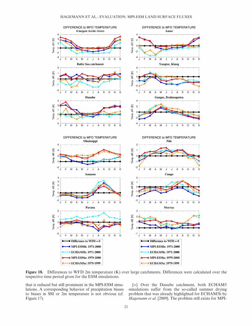
[41] For the Eurasian high and mid-latitude catchments(Arctic rivers, Amur, Baltic Sea, Danube), the MPI-ESMsimulations are warmer than their ECHAM5 counter-parts (Figure 15a; see also section 3.2), which for the Dan-ube shows up in a warm bias of about 1 K that does notoccur in both ECHAM5 simulations. For most of thecatchments, MPI-ESMh has the smallest temperature

Figure 10. SSI differences of (top) MPI-ESMh and (bottom) ECHAM5h to CERES.


13

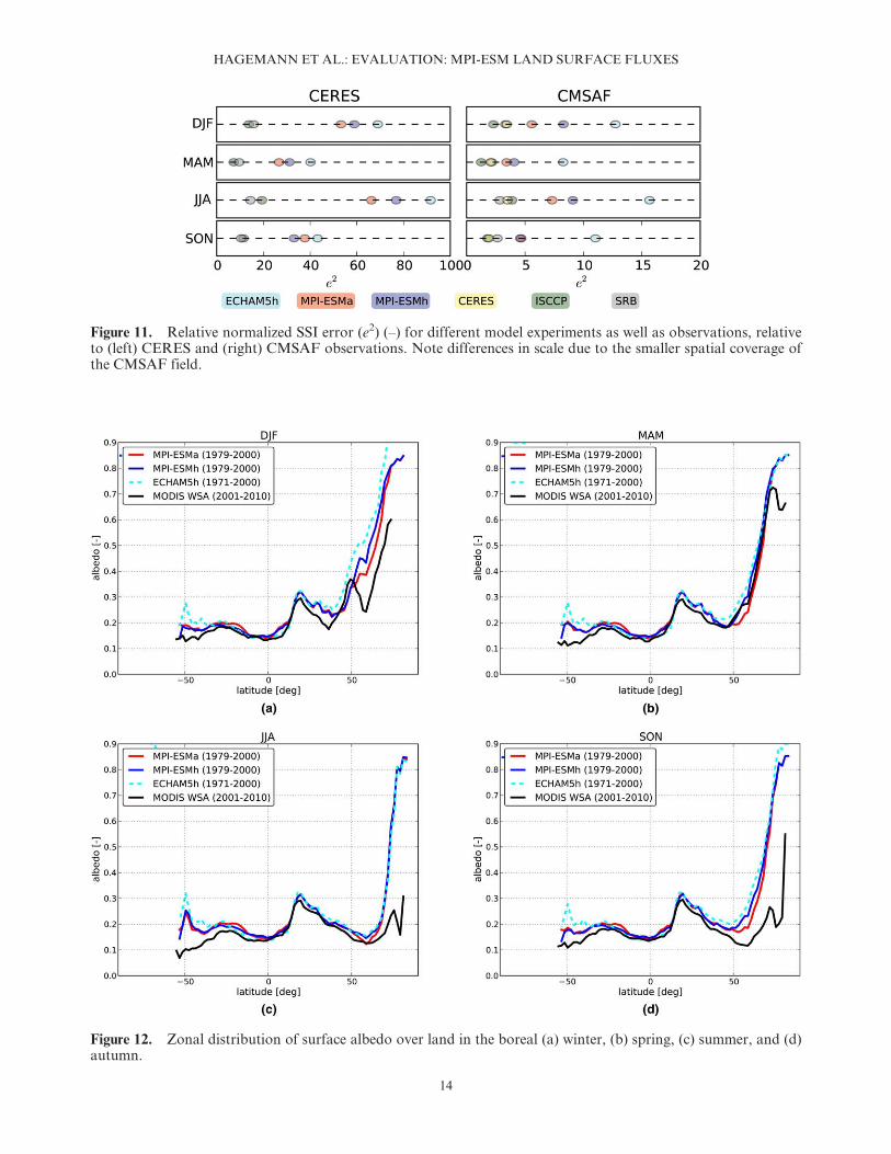
Figure 11. Relative normalized SSI error (e2) (–) for different model experiments as well as observations, relativeto (left) CERES and (right) CMSAF observations. Note differences in scale due to the smaller spatial coverage ofthe CMSAF field.

Figure 12. Zonal distribution of surface albedo over land in the boreal (a) winter, (b) spring, (c) summer, and (d)autumn.


14

bias, or is at least close to the smallest bias. Here, apartfrom the Danube (see above) only the Congo and Yang-tze Kiang stick out where MPI-ESMh shows a muchstronger cold bias than the other three models.

[42] With regard to precipitation (Figure 15b), differen-ces between the two historical simulations seem to be ofminor importance. For most catchments, MPI-ESMh pre-cipitation is somewhat larger than for ECHAM5h, therebyleading to some enhancement of the wet biases over the

Arctic rivers, Amur, Baltic Sea, and Yangtze Kiang, andto an apparent reduction of dry biases over the Danube,Congo and Parana. For the Ganges/Brahmaputra, the wetbias is almost halved in MPI-ESMa compared withECHAM5a. Further difference between the two AMIP2simulations can be noted for the Arctic rivers (increasedwet bias in MPI-ESMa), Yangtze Kiang (decreased wetbias), Murray (removed dry bias), and Nile (10% dry biasinstead of a similar wet bias).

Figure 13. Differences in upward shortwave flux (W m22) compared to MODIS data scaled with model incomingradiation for (top) MPI-ESMh and (bottom) ECHAM5h.


15

[43] Biases and differences between the models inevapotranspiration (Figure 16a) generally follow thosein precipitation, e.g., the positive biases over Arctic Riv-ers, Amur, Baltic Sea and Yangtze Kiang of all modelsas well as the reduced negative bias for the Murray andthe enhanced negative biases for the Nile of MPI-ESMacompared with ECHAM5a. It seems that all modelsproduce a too enhanced evapotranspiration over theAmazon, which becomes obvious by the positive biasesfor the AMIP2 simulations where the precipitationshows no bias (Figure 15b), but also for the historicalsimulations that show no evapotranspiration bias eventhough precipitation is largely underestimated. Simi-larly over the Danube, evapotranspiration is overesti-mated by MPI-ESMh after the removal of the dryprecipitation bias, while the dry precipitation bias inECHAM5h also leads to a negative evapotranspirationbias. For the Ganges/Brahmaputra, evapotranspirationgenerally seems to be underestimated by the models aseven in the AMIP2 simulations the surplus of water dueto the wet precipitation bias only leads to a removal ofthe negative bias shown for the historical simulations.

[44] Positive or negative biases in precipitation oftenexceed the biased amounts of evapotranspiration so thatalso wet (Arctic rivers, Amur, Baltic Sea, YangtzeKiang) and dry (Congo for ECHAM5h and MPI-ESMa,Missisippi for AMIP2 simulations) biases in runoff(Figure 16b) occur, respectively. Differences between themodels in precipitation and evapotranspiration mostlyseem to be of the same order so that they often compen-sate each other, which causes model differences in therunoff and the associated bias to be rather similar with afew exceptions. The too enhanced evapotranspirationover the Amazon leads to a dry runoff bias for all mod-els, which is more severe for both historical simulationsdue to their too low precipitation. Overestimated evapo-transpiration also leads to dry runoff biases over the

Danube catchment for all models except ECHAM5hwhere the dry bias in precipitation dominates the dryrunoff bias. Underestimated evapotranspiration causeswet runoff biases over the Ganges/Brahmaputra andMurray catchments for all models. For the first, theseare largely enhanced by the wet precipitation biases forthe two AMIP2 simulations. As for precipitation (seeabove), the wet runoff bias in MPI-ESMa is only abouthalf the bias of ECHAM5a. For the Murray, wet runoffbias of ECHAM5a is less severe due to the larger drybias in precipitation. For the Nile, negative biases in pre-cipitation and evapotranspiration compensate each otherexcept for ECHAM5a where the overestimation of pre-cipitation causes a large overestimation of runoff. Notethat for the Nile climatological discharge, observationsare used before the Aswan dam was built as this is notconsidered in the models either. For the Parana, thereduction in the dry precipitation bias of MPI-ESMhcompared with ECHAM5h leads also to an analogue re-moval of the dry runoff bias. For both AMIP2 simula-tions, large positive runoff biases occur that are relatedto a wet precipitation bias for ECHAM5a, while forMPI-ESMa it seems to be caused by an adding up ofsmaller positive and negative biases in precipitation andevapotranspiration, respectively.

5. Annual Cycles and Differences BetweenModel Families

[45] In this section, we are considering noticeable dif-ferences of the different model families (historical/AMIP2 and MPI-ESM/ECHAM5) in more detail,thereby considering the mean annual cycles of precipita-tion, 2m temperature, surface albedo, and SSI over theselected major catchments (Figure 14). Here, we alsoinvestigated why some of these differences occur andhow they relate to the model setup.

Figure 14. Selected large catchments of the globe at 0.5� resolution.


16

5.1. Historical Versus AMIP2 Simulations

[46] The fully coupled historical and the uncoupledAMIP2 SST driven simulations do not show any signifi-cance differences for surface albedo. With regard to SSI(Figure 11), the SST driven simulation (MPI-ESMa)generally shows a relatively better performance than thecoupled model simulation (MPI-ESMh), except forSON, indicating a general increase of SSI uncertaintiesdue to the coupling. However, the difference between the

MPI-ESM experiments is in general much smaller thanthe difference to ECHAM5h. For 2m temperature(Figure 15a), it can be noted that the historical simula-tions are consistently colder over Eurasian high and mid-latitude catchments (Arctic rivers, Amur, Baltic Sea,Danube) than the corresponding AMIP2 simulations.The latter is also the case for the Mississippi catchmentwhere both historical simulations have a reduced warmbias. The most apparent differences between the historical

Figure 15. Annual mean biases in simulated (a) 2m temperature and (b) precipitation over several catchments.The bias were calculated from the differences of the simulations to the WFD data.


17

and the SST driven simulations occur for the land surfacewater fluxes, especially for precipitation (Figure 15b).For the Amazon, Ganges/Brahmaputra, and the Missis-sippi, both historical simulations behave strongly differ-ently than the AMIP2 simulations. For the Amazon, adry precipitation bias of about 20% occurs that is notpresent in the AMIP2 simulations, while for the Ganges/Brahmaputra, the wet precipitation bias of the AMIP2

simulations is reduced almost to zero. Consequently, weconsider these three catchments in more detail in thefollowing.

[47] For the Amazon, the dry biases in the hydrologicalcycle are partially caused by the too enhanced evapo-transpiration (see section 4), which points to deficits inthe representation of associated land surface processes.These deficits seem to affect the simulated precipitation of

Figure 16. Annual mean biases in simulated (a) evapotranspiration and (b) runoff over several catchments. Theobserved evaporation was calculated from the difference of WFD precipitation and observed climatological dis-charge [D€umenil Gates et al., 2000]. The runoff bias was calculated from the difference of the simulated runoff andthe observed climatological discharge.


18

all models during the boreal summer, where precipitationis significantly lower than the WFD (Figure 17). But thelarge underestimation of precipitation in the historicalsimulations throughout the first nine months of the yearis not caused by these deficits as no dry bias occurs in theSST driven AMIP2 simulations during winter and spring.During most parts of this period, the moisture availablefor precipitation is mainly transported from the TropicalAtlantic north of the equator, i.e., passing over the north-east (NE) coast of South America [see e.g., Trenberth,1998]. Andersson et al. (in preparation, 2013) showedthat both coupled simulations have annual mean coldSST bias at the NE coast of South America that is notpresent in MPI-ESMa. This bias is associated with lowerevaporation rates and a subsequent dry bias in the inte-grated water vapor. The latter is spatially enhanced by alarge-scale low bias in 10 m wind speed in the northernTropical Atlantic. These biases lead to a reduced mois-ture transport into the Amazon catchment that is causingthe dry precipitation bias in the coupled simulations.These biases along the NE coast of South America arenot present in MPI-ESMa, thereby leading to a more re-alistic moisture transport and associated precipitation.

[48] For the Ganges/Brahmaputra, the improved sim-ulation of precipitation induced by the coupling occursduring the South Asian summer monsoon season, whereAMIP2 simulations, especially ECHAM5a, overesti-mate the precipitation compared with WFD (Figure 17).We speculate that in the AMIP2 simulations, the oceanact as a too enhanced heat and moisture source as thereis no counteracting feedback by ocean SST. This is lead-ing to a too strong moisture transport from the ArabianSea to northern India. As the models do not representthe large irrigation ongoing over northern India andPakistan, there is too little moisture supply from the asso-ciated areas [see, e.g., Saeed et al., 2009], which inhibitsthe formation of precipitation indicated by the dry biasover the northern Indian plains (Figure 4). Therefore, themoisture is transported further inland toward the Hima-layas, where it is causing a surplus of precipitation overthe Ganges/Brahmaputra catchment and a subsequent tooenhanced hydrological cycle over the region. In thecoupled simulations, the large moisture fluxes over theocean are reduced by the response of the ocean SST so

that the associated precipitation over the Ganges/Brahma-putra catchment agrees well with the WFD. This is sup-ported by Andersson et al. (in preparation, 2013), whoseresults indicate a reasonable simulation of SST over theArabian Sea in the coupled simulations compared withHamburg Ocean Atmosphere Parameters and Fluxesfrom Satellite Data (HOAPS) [Andersson et al., 2010]being slightly colder than the AMIP SST, while the windspeed in the AMIP simulation exhibits a positive bias forthis region. The latter and the missing coupling leads tostrongly overestimated evaporation fluxes in MPI-ESMaover the Arabian Sea that are not present in the coupledsimulations.

[49] Noticeable differences between the coupled andthe AMIP2 simulations can be also seen in summer andautumn over the Mississippi catchment, where a warmbias of up 2–3�C in the AMIP2 simulations is almostcompletely eliminated in both coupled simulations(Figure F1818). Figure 19 indicates that the coupling leadsto a lower simulation of SSI, which is closer to CERESdata and, hence, causes the reduction of the warm bias.Between April and September, the coupling also leadsto an increased precipitation (Figure 17). While thiscauses a wet bias until July, the prominent dry bias ofthe AMIP2 simulations from August to October isreduced. These results suggest that the coupling causesmore cloud cover and enhanced precipitation duringthe summer half year, thereby overcompensating thedry bias of the AMIP2 simulations in the annual mean(Figure 15b). This enhanced precipitation subsequentlyleads to a removal of the negative bias in runoff (Figure16b). During the summer, the moisture is mainly trans-ported from the northern subtropical Atlantic via Gulf ofMexico into the catchment [see, e.g., Trenberth, 1998].Here, both coupled models simulated a warm SST biasthat is inducing larger evaporation fluxes than in MPI-ESMa (Andersson et al., in preparation, 2013). Thesefluxes lead to a wet bias in the integrated water vapor,and, very likely to the enhanced moisture flux into theMississippi catchment that is compensating the dry pre-cipitation bias which is present in the AMIP simulations.Part of the moisture flux into the Mississippi catchmentduring the hurricane season (June–November) is relatedto tropical cyclone activity that may contribute up to

Table 3. Observed Values for WFD 2m Temperature (1971–2000; �C), WFD Precipitation (1971–2000), Evaporation (WFD

Precipitation Minus Climatological Discharge), and Runoff (Climatological)a

Catchment Temperature Precipitation Evaporation Runoff

Amazon 24.6 2242 1189 1053Amur 21.3 540 367 173Six largest Arctic Rivers 25.0 455 264 191Baltic Sea catchment 4.4 692 413 279Congo 24.1 1576 1211 365Danube 9.1 797 545 251Ganges/Brahmaputra 17.7 1397 725 672Mississippi 10.2 893 697 196Murray 17.8 510 502 8Nile 25.5 646 597 49Parana 21.5 1308 1085 223Yangtze Kiang 12.0 1069 532 537

aUnit: mm a21.


19

10%–15% of the seasonal rainfall in the southern parts ofthe catchment [Larson et al., 2005]. We speculate that thesummer/autumn dry bias is partially caused by the factthat tropical cyclones cannot be adequately representedat the used model resolution of about 200 km grid size.

5.2. MPI-ESM Versus ECHAM5

[50] As pointed out in section 3.2, larger differences inthe simulated 2m temperature occur between MPI-ESMand ECHAM5, especially over northern Eurasia that are

most pronounced in the boreal winter half year. Here, theMPI-ESM simulations are considerably warmer than theECHAM5 simulations and the WFD data, such as shownfor the Arctic Rivers, Danube, Amur, and Baltic Sea inFigure 18. This behavior seems to be mainly imposed by alower simulation of surface albedo by MPI-ESM thatis closer to MODIS data than those simulated byECHAM5 (Figure 20). In summer time, cold biases ofECHAM5h over the Arctic and Baltic Sea catchmentsseem to be caused by a large negative SSI bias (Figure 19)

Figure 17. Simulated and observed precipitation (m3 s21) over large catchments.


20

that is reduced but still prominent in the MPI-ESM simu-lations. A corresponding behavior of precipitation biasesto biases in SSI or 2m temperature is not obvious (cf.Figure 17).

[51] Over the Danube catchment, both ECHAM5simulations suffer from the so-called summer dryingproblem that was already highlighted for ECHAM5h byHagemann et al. [2009]. The problem still exists for MPI-

Figure 18. Differences to WFD 2m temperature (K) over large catchments. Differences were calculated over therespective time period given for the ESM simulations.


21

ESM, but it is largely reduced compared with ECHAM5.The representation of land surface hydrology is very sim-ilar in both model versions, as is the surface albedo dur-ing summer time (Figure 20), which is close to MODISdata. This indicates that the treatment of land surfaceprocesses is not responsible for the reduction of thesummer drying problem in MPI-ESM. This is consistentwith results from a regional climate modeling study ofHagemann et al. [2004], who pointed out that for two re-gional climate models using ECHAM4 physics (HIR-HAM, REMO), systematic errors in the atmosphericdynamics appear to be causing the summer drying prob-

lem over the Danube catchment. These are likely alsoleading to the positive evapotranspiration bias in theMPI-ESM simulations over this region (Figure 16a, seealso section 4). The strong improvement in the simula-tion of SSI (Figure 19) suggests that this reduction ismainly caused by changes in the atmospheric componentof MPI-ESM, ECHAM6 [Stevens et al., 2012].

[52] In section 3.3, the better performance of MPI-ESM in simulating SSI was already pointed out. Thiscannot only be seen for the Danube, but also overmany other catchments (Arctic rivers, Baltic Sea, Ama-zon, Nile, Congo, and Murray) where the simulated SSI

Figure 19. Differences to CERES SSI (W m22) over large catchments.


22

(Figure 19) of MPI-ESM is closer to the satellite obser-vations of CERES and CMSAF than the ECHAM5SSI. For the Parana, ECHAM5 SSI is closer to CERESdata than MPI-ESM SSI (CMSAF data does not fullycover this catchment). However, a systematic impact on

the simulated temperatures (Figure 18) is only visiblefor the Parana in the southern winter and the Murrayin the southern summer half year. For the latter, theoverestimated SSI in the ECHAM5 simulations leadsto a related warm bias which is largely reduced in

Figure 20. Simulated and observed surface albedo (%) over large catchments.


23

MPI-ESM where also the simulated SSI is closer to theCERES data. For the Parana, the deviations of simu-lated SSI to CERES data look rather similar to the tem-peratures biases compared with WFD during July toOctober.

[53] Despite the fact that MPI-ESMh was run with adynamic vegetation scheme while MPI-ESMa uses aprescribed PFT distribution, the surface albedo oversnow free areas does not differ significantly betweenboth simulations (cf. section 3.4). Some noticeable dif-ferences occur over the Amazon (Parana) catchment,where MPI-ESMa surface albedo is systematicallylower (higher) by about 2% (1%) than in MPI-ESMh(Figure 20). For the Amazon, MPI-ESMa agrees quitewell with MODIS data while for the Parana MPI-ESMhhas lower positive bias than MPI-ESMa compared withMODIS. This implies that the dynamic vegetation schemesimulates a too low tree cover over the Amazon catchmentas a direct consequence of the dry bias in MPI-ESMh.Over the Parana instead, the dynamic vegetation schemeseems to reduce a bias in the PFT distribution that ispresent in MPI-ESMa. A direct effect on the simulatedtemperature cannot be concluded from Figure 18, eventhough it seems that over the Amazon, the overestimatedsurface albedo of MPI-ESMh might be associated with aslightly increased cold bias compared with MPI-ESMa inthe first half of the year. In the second half of the year, thiseffect is exceeded by the warm bias that is likely related tothe dry bias in the boreal summer (Figure 17).

6. Summary and Concluding Remarks

[54] In the present study, we have jointly evaluatedland surface water and energy fluxes from the very recentsimulations that have been conducted with the MPI-ESM for CMIP5 exercise. These simulations comprisethree-member ensembles of AMIP2 SST forced simula-tions of the land/atmosphere component of MPI-ESMand of the fully coupled ESM. MPI-ESM model outputwas compared with various observational data sets aswell as to simulations by its predecessor ECHAM5.Apart from a general evaluation of the fluxes, wefocused on differences between the two ESM versions aswell as on differences between the fully coupled simula-tion and the SST-driven simulations.

[55] The study has proven that the simulated surfaceshortwave radiation fluxes and land surface albedohave considerably improved in MPI-ESM comparedwith its predecessor ECHAM5. This has led to subse-quent differences in simulated 2m temperature betweenMPI-ESM and ECHAM5. To a large extent, these arecaused by the improved simulation of SSI in MPI-ESM. Over the high northern latitudes in the winter,these differences mainly originate from an improved sim-ulation of surface albedo related to the associated snowcover. But compared with WFD data, the MPI-ESMsimulated 2m temperature did not necessarily improve inthe same way as SSI and surface albedo. The latter is thecase for the reduction of the boreal summer cold bias inthe high northern latitudes that can be attributed to theimproved SSI in the MPI-ESM simulations. During the

boreal winter, the cold bias over Europe is removed byMPI-ESM, but the northern Asian warm bias is largelyextended in the MPI-ESM simulations, which is mainlylimited over Eastern Siberia in ECHAM5h.

[56] For the hydrological cycle, large-scale bias pat-terns are rather similar between the different modelsover many regions. For precipitation, common devia-tions from the WFD denote a pronounced dry bias inthe Tropics north of the equator, which also extends tosouth of the equator during the boreal spring andsummer, a dry bias in the low precipitation region in thesouthern Subtropics accompanied by a wet bias around50�S, a wet bias in the northern high latitudes during bo-real spring and summer and an overestimation of precip-itation along steep mountain slopes. The most notabledifference between the models is that MPI-ESMh andMPI-ESMa generally have an improved simulation ofpeak rainfall in the Tropics compared with ECHAM5h.Also, the summer drying problem over southern andeastern Europe (especially over the Danube catchment)is largely reduced in the MPI-ESM simulations.

[57] For many land areas, the coupling to an oceanmodel does not lead to significant differences in landsurface water and energy fluxes compared to the simu-lations forced with observed SST. But three areas canbe highlighted where the coupling causes noticeableeffects. On one hand, the coupling induces a dry biasover the Amazon catchment, while on the other hand itleads to an improved precipitation over the Ganges/Brahmaputra and Mississippi catchments. For theAmazon, this deficit of the coupled simulations cannotbe attributed to land surface processes, but instead it isprimarily induced by biases in simulated SST patternsand associated moisture transport. Here, it can be notedthat an insufficient representation of land surface proc-esses is probably only causing the dry bias during theboreal summer that is persistent in all models. For theMississippi, warm biases in SST of the coupled simula-tions and associated wet biases in the associated moisturetransport lead to increased summer precipitation that iscompensating a dry bias caused by other model deficitsthat are likely associated with the coarse spatial resolutionof the ESMs. For the Ganges/Brahmaputra, the missinginteraction of the ocean with the atmosphere over theArabian Sea has been identified as the main cause of thetoo enhanced precipitation in the SST-forced simulations.This conclusion is supported by results of Wang et al.[2005], who found that state-of-the-art atmosphericGCMs, when forced by observed SST, are unable to sim-ulate properly Asian-Pacific summer monsoon rainfall.

[58] In summary, the combined evaluation of land sur-face water and energy fluxes has shown that MPI-ESMhas generally improved compared with ECHAM5, espe-cially with regard to SSI and surface albedo. Bias patternfor precipitation and 2m temperature are similar forboth ESM versions, and improvements slightly outweighworsenings. As ECHAM5h was already one of the bestperforming models in the CMIP3 exercise [Reichler andKim, 2008], it can be concluded that MPI-ESM is wellsuited for climate change studies focusing on the waterand energy cycle at the land surface.


24

Appendix A

[59] In order to provide complementary informationfor the usage of CERES as reference SSI in the spatialmaps of the manuscript, we added comparisons toCMSAF SSI in this appendix. CMSAF data are avail-able for a longer period (1989–2005) than CERES data,but they cover only a limited part of the globe. Figure

A1 compares the seasonal SSI cycles of ISCCP andSRB data to CMSAF data, and is, thus, complementaryto Figure 1. Figure A2 shows an analogue comparisonof MPI-ESMh and ECHAM5h to CMSAF data that iscomplementary to Figure 10.

Figure A1. Differences of seasonal cycle of SSI between different observational datasets: ISCCP compared toCMSAF (top), SRB compared to CMSAF (bottom). Statistically significant differences (p>0.05) between thesatellite products are indicated by stippled areas.


25

[60] Acknowledgments. This work was partly supported by fund-ing from the European Union within the EMBRACE project (grant282672) and through the Cluster of Excellence ‘‘CliSAP’’ (EXC177),KlimaCampus, University of Hamburg, funded by the German Sci-ence Foundation (DFG). The GCM data were obtained from theCERA database at the German Climate Computing Center (DKRZ)in Hamburg. CERES data were obtained from the NASA atmosphericscience data center. The Meteosat surface radiation data were pro-vided by the EUMETSAT CMSAF, which is gratefully acknowl-edged. BSRN surface radiation data were obtained from the WRMC-BSRN hosted at AWI, Bremerhaven.

ReferencesAdam, J. C., and D. P. Lettenmaier (2003), Adjustment of global

gridded precipitation for systematic bias, J. Geophys. Res., 108(D9),4257, doi:10.1029/2002JD002499.

Andersson, A., K. Fennig, C. Klepp, S. Bakan, H. Graßl, and J. Schulz(2010), The Hamburg Ocean atmosphere parameters and fluxesfrom satellite data—HOAPS-3, Earth Syst. Sci. Data, 2, 215–234,doi:10.5194/essd-2-215-2010.

Biemans, H., R.W.A. Hutjes, P. Kabat, B. Strengers, D. Gerten, andS. Rost (2009), Effects of precipitation uncertainty on discharge

Figure A2. SSI differences of MPI-ESMh (top) and ECHAM5h (bottom) to CMSAF.


26

calculations for main river basins, J. Hydrometeor., 10, 1011–1025,doi:10.1175/2008JHM1067.1.

Brovkin, V., T. Raddatz, C. H. Reick, M. Claussen, and V. Gayler(2009), Global biogeophysical interactions between forest and cli-mate, Geophys. Res. Lett., 36, L07405, doi:10.1029/2009GL037543.

Brovkin, V., L. Boysen, T. Raddatz, V. Gayler, A. Loew, andM. Claussen (2012), Evaluation of vegetation cover and land-surfacealbedo in MPI-ESM CMIP5 simulations, J. Adv. Model. EarthSyst., doi:10.1029/2012MS000169.

Cox, S. J., P. W. Stackhouse Jr., S. K. Gupta, J. C. Mikovitz,T. Zhang, L. M. Hinkelman, M. Wild, and A. Ohmura (2006), TheNASA/GEWEX surface radiation budget project: Overview andanalysis, Preprints, in Proceedings of the 12th Conference on Atmos-pheric Radiation, Madison, Wis., Amer. Meteor. Soc., 10.1 [Avail-able at http://ams.confex.com/ams/pdfpapers/112990.pdf].

D€umenil Gates, L., S. Hagemann, and C. Golz (2000), Observedhistorical discharge data from major rivers for climate model valida-tion, Max Planck Institute for Meteor. Rep., 307, MPI for Meteorol-ogy, Hamburg, Germany.

Essery, R., N. Rutter, J. Pomeroy, R. Baxter, M. Stahli, D. Gustafs-son, A. Barr, P. Bartlett, and K. Elder (2009), An evaluation of for-est snow process simulations, Bull. Am. Meteorol. Soc., 90, 1120–1135, doi:10.1175/2009bams2629.1.

Fensholt, R., et al. (2012), Greenness in semi-arid areas across the globe1981–2007—An Earth Observing Satellite based analysis of trendsand drivers, Remote Sens. Environ., 121, 144–158, doi:10.1016/j.rse.2012.01.017.

Fuchs, T., U. Schneider, and B. Rudolf (2007), Global precipitationanalysis products of the GPCC, Global Precipitation ClimatologyCentre (GPCC), Deutscher Wetterdienst, Offenbach, Germany.

Hagemann, S. (2002), An improved land surface parameter dataset forglobal and regional climate models, Max Planck Institute forMeteor. Rep., 336, Hamburg, Germany [Available at http://www.mpimet.mpg.de/en/wissenschaft/publikationen.html].

Hagemann, S., B. Machenhauer, R. Jones, O. B. Christensen, M. D�equ�e,D. Jacob, and P. L. Vidale (2004), Evaluation of water and energybudgets in regional climate models applied over Europe, Clim. Dyn.,23, 547–567.

Hagemann. S., K. Arpe, and E. Roeckner (2006), Evaluation of thehydrological cycle in the ECHAM5 model, J. Clim., 19, 3810–3827.

Hagemann, S., H. Gottel, D. Jacob, P. Lorenz, and E. Roeckner(2009), Improved regional scale processes reflected in projectedhydrological changes over large European catchments, Clim. Dyn.,32, 767–781.

Ineichen, P., C. Barroso, B. Geiger, R. Hollmann, A. Marsouin, andR. M€uller (2009), Satellite application facilities irradiance products:Hourly time step comparison and validation over Europe, Int. J.Remote Sens., 30(10), 5549–5571.

Jim�enez, C., et al. (2011), Global inter-comparison of 12 land surfaceheat flux estimates, J. Geophys. Res., 116, D02102, doi:10.1029/2010JD014545.

Jungclaus, J. H., M. Botzet, H. Haak, N. Keenlyside, J.-J. Luo, M. Latif,J. Marotzke, U. Mikolajewicz, and E. Roeckner (2006), Ocean circu-lation and tropical variability in the coupled model ECHAM5/MPI-OM, J Clim., 19, 3952–3972.

Jungclaus, J. H., N. Fischer, H. Haak, K. Lohmann, J. Marotzke,D. Matei, U. Mikolajewicz, D. Notz, and J. S. von Storch (2012),Characteristics of the ocean simulations in MPIOM, the ocean com-ponent of the MPI-Earth System Model, J. Adv. Model. Earth Syst.,doi:10.1002/jame.20023.

Koster, R. D., et al. (2004), Regions of strong coupling between soilmoisture and precipitation, Science, 305(5687), 1138–1140.

Larson, J., Y. Zhou, and R. W. Higgins (2005), Characteristics of land-falling tropical cyclones in the United States and Mexico: Climatol-ogy and interannual variability, J. Clim., 18, 1247–1262.

Loeb, N. G., S. Kato, W. Su, T. Wong, F. G. Rose, D. R. Doelling,and J. Norris (2012), Advances in understanding top-of-atmosphereradiation variability from satellite observations, Surv. Geophys., 33.359-385, doi:10.1007/s10712-012-9175-1.

Loew, A. and Y. Govaerts (2010), Towards mulitdecadal consistentMeteosat surface albedo time series, Remote Sens. 2(4), 957–967.

Loveland, T. R., B. C. Reed, J. F. Brown, D. O. Ohlen, J. Zhu,L. Yang, and J. W. Merchant (2000), Development of a global land

cover characteristics database and IGBP DISCover from 1-kmAVHRR data, Int. J. Remote Sens. 21, 1303–1330.

Mitchell, T. D., and P. D. Jones (2005), An improved method of con-structing a database of monthly climate observations and associatedhigh-resolution grids, Int. J. Climatol., 25, 693–712.

Mueller, B., et al. (2011), Evaluation of global observations-basedevapotranspiration datasets and IPCC AR4 simulations, Geophys.Res. Lett., 38, L06402, doi:10.1029/2010GL046230.

M€uller, R. W., C. Matsoukas, A. Gratzki, H. D. Behr, and R. Hollmann(2009), The CMSAF operational scheme for the satellite based re-trieval of solar surface irradiance—A LUT based eigenvector hybridapproach, Remote Sens. Environ., 113(5), 1012–1024.

M€uller, R., J. Trentmann, R. Stockli, and R. Posselt (2011), Algorithmtheoretical baseline document: Meteosat (MVIRI) solar irradianceand effective cloud albedo climate datasets—The MAGICSOLmethod, Tech. Rep., EUMETSAT Satellite Application Facility onClimate Monitoring, SAF/CM/DWD/ATBD/MVIRI HEL v1.1.

Ohmura, A., et al. (1998), Baseline surface radiation network (BSRN/WCRP): New precision radiometry for climate research, Bull. Am.Meteorol. Soc., 79(10), 2115–2136.

Program for Climate Model Diagnosis and Intercomparison (PCMDI)(2007), IPCC model output [Available at www-pcmdi.llnl.gov/ipcc/about_ipcc.php].

Posselt, R., R. M€uller, R. Stockli, and J. Trentmann (2011a), Spatialand temporal homogeneity of solar surface irradiance across satellitegenerations, Remote Sens., 3, 1029–1046.

Posselt, R., R. M€uller, J. Trentmann, and R. Stockli (2011b), CMSAFvalidation report: Meteosat (MVIRI) climate data sets of SIS, SIDand CAL, Tech. Rep., Satellite Application Facility on ClimateMonitoring, SAF/CM/DWD/VAL/MVIRI HEL, v.1.1.

Raddatz, T. J., C. Reick, W. Knorr, J. Kattge, E. Roeckner, R. Schnur,K.-G. Schnitzler, P. Wetzel, and J. H. Jungclaus (2007), Will thetropical land biosphere dominate the climate-carbon cycle feedbackduring the twenty-first century?, Clim. Dyn., 29, 565–574,doi:10.1007/s00382-007-0247-8.

Rechid D., T. J. Raddatz, and D. Jacob (2009), Parameterization ofsnow-free land surface albedo as a function of vegetation phenologybased on MODIS data and applied in climate modelling, Theor.Appl. Climatol., 95, 245–255, doi 10.1007/s00704-008-0003-y.

Reichler, T., and J. Kim (2008), How well do coupled models simulatetoday’s climate? Bull. Am. Meteorol. Soc., 89(3), 303–311, doi:10.1175/BAMS-89-3-303.

Roeckner, E., et al. (2003), The atmospheric general circulation modelECHAM5. Part I: Model description, Max Planck Institute for Meteor.Rep., 349, 127 pp., MPI for Meteorology, Hamburg, Germany.

Roesch, A., and E. Roeckner (2006), Assessment of snow cover andsurface albedo in the ECHAM5 general circulation model, J. Clim.,19, 3828–3843.

Rossow, W. B., and Y.-C. Zhang (1995), Calculation of surface andtop-of-atmosphere radiative fluxes from physical quantities basedon ISCCP datasets, Part II: Validation and first results, J. Geophys.Res., 100, 1167–1197.

Rudolf, B., and F. Rubel (2005), Global precipitation, in ObservedGlobal Climate, Landolt–Boernstein: Numerical Data And FunctionalRelationships in Science and Technology—New Series, Group 5: Geo-physics, vol. 6, edited by M. Hantel, chap. 11, p. 567, Springer,Berlin.

Saeed, F., S. Hagemann, and D. Jacob (2009), Impact of irrigation onthe South Asian Summer Monsoon, Geophys. Res. Lett., 36,L20711, doi:10.1029/2009GL040625.

Schaaf, C. B., et al. (2002), First operational BRDF, albedo and nadirreflectance products from MODIS, Remote Sens. Environ., 83, 135–148.

Seneviratne, S. I., T. Corti, E. L. Davin, M. Hirschi, E. B. Jaeger,I. Lehner, B. Orlowsky, and A. J. Teuling (2010), Investigating soilmoisture-climate interactions in a changing climate: A review, EarthSci. Rev., 99, 125–161, doi:10.1016/j.earscirev.2010.02.004.

Solomon, S., D. Qin, M. Manning, M. Marquis, K. Averyt, M. M. B.Tignor, H. L. Miller Jr., and Z. Chen, Eds. (2007), Climate Change2007: The Physical Science Basis, Cambridge Univ. Press, Cam-bridge, United Kingdom and New York, NY, USA, 996 pp.

Sorooshian, S., J. Roads, J. Polcher, R. Schiffer, R. Lawford, P. Try,W. Rossow, and G. Sommeria (2005), Water and energy cycles:Investigating the links, WMO Bull., 54(2), 58–64.


27

Stevens, B., et al. (2012), The atmospheric component of the MPI-MEarth system model: ECHAM6, J. Adv. Model. Earth Syst.doi:10.1002/jame.20015.

Taylor, K. E., R. J. Stouffer, and G. A. Meehl (2012), An overview ofCMIP5 and the experiment design, Bull. Am. Meteor. Soc., 93(4),485–498.

Trenberth, K. E. (1998), Atmospheric moisture recycling: Role ofadvection and local evaporation, J. Clim., 12, 1368–1381.

Trenberth, K. E., J. T. Fasullo, and J. Kiehl (2009), Earth’s globalenergy budget, Bull. Am. Meteorol. Soc., 90, 311–323.

Trenberth, K. E., J. T. Fasullo, and J. Mackaro (2011), Atmosphericmoisture transports from ocean to land and global energy flows inreanalyses, J. Clim., 24, 4907–4924, doi:http://dx.doi.org/10.1175/2011JCLI4171.1.

Uppala, S. M., et al. (2005), The ERA-40 Re-analysis, Q. J. R. Meteorol.Soc., Oct. 2005 Part B.

Vamborg, F. S. E. (2011), Vegetation-albedo-precipitation interactions inNorth Africa during the Holocene, Rep. Earth System Science 94, MaxPlanck Institute for Meteorology, Hamburg, Germany [Available athttp://www.mpimet.mpg.de/wissenschaft/publikationen/berichte-erdsystemforschung.html].

Wang, B., Q. Ding, X. Fu, I.-S. Kang, K. Jin, J. Shukla, andF. Doblas-Reyes (2005), Fundamental challenge in simulation andprediction of summer monsoon rainfall, Geophys. Res. Lett., 32,L15711, doi:10.1029/2005GL022734.

Weedon, G. P., S. Gomes, P. Viterbo, W. J. Shuttleworth, E. Blyth,H. €Osterle, J. C. Adam, N. Bellouin, O. Boucher, and M. Best(2011), Creation of the WATCH forcing data and its use to assessglobal and regional reference crop evaporation over land during thetwentieth century, J. Hydrometeorol., 12, 823–848, doi:10.1175/2011JHM1369.1.

Zhang, Y.-C., W. B. Rossow, A. A. Lacis, V. Oinas, and M. I.Mishchenko (2004), Calculation of radiative fluxes from the surfaceto top of atmosphere based on ISCCP and other global data sets:Refinements of the radiative transfer model and the input data, J.Geophys. Res., 109, D19105, doi:10.1029/2003JD004457.

Corresponding author: S. Hagemann, Max Planck Institute for Meteor-ology, Bundesstr. 53, 20146 Hamburg, Germany. ([email protected])

28


Combined evaluation of MPIESM land surface water and energy fluxes

Documents