Combined classifier quantifier model: A 2-phases neural ...

Author's personal copy

Combined classifier–quantifier model: A 2-phases neural model forprediction of wave overtopping at coastal structures

Hadewych Verhaeghe a,⁎,1, Julien De Rouck a, Jentsje van der Meer b

a Ghent University, Technologiepark 904, B-9052 Ghent, Belgiumb Van der Meer Consulting, P.O. Box 423, 8440 AK Heerenveen, The Netherlands

Received 3 July 2007; received in revised form 19 October 2007; accepted 5 December 2007Available online 6 February 2008

Abstract

A 2-phases neural prediction method for wave overtopping is developed. The ‘classifier’ predicts whether overtopping occurs or not, i.e. q=0or qN0. If the classifier predicts overtopping qN0, then the ‘quantifier’ is used to determine the mean overtopping discharge. The overtoppingdatabase set up within the EC project CLASH (De Rouck, J., Geeraerts, J., 2005. CLASH Final Report, Full Scientific and Technical Report,Ghent University, Belgium) is used to train the networks of the prediction method.

The method has an overall predictive capacity, and is able to distinguish negligible from significant overtopping, avoiding large overtoppingoverpredictions in the area of low overtopping. The prediction method is freely available on http://awww.ugent.be/awww/coastal/verhaeghe2005.html.© 2008 Elsevier B.V. All rights reserved.

Keywords: Wave overtopping; Artificial neural network; Neural model; Prediction method; Coastal structures

1. Introduction and motivation

Coastal structures are designed to protect (often denselypopulated) coastal regions against wave attack, storm surges,flooding and erosion. The crest height plays a predominant rolein the protective function of these structures. Due to climatechanges, the sea level is rising at an increased rate, and stormssubstantially increase in intensity and duration (IPCC, 2007).This emphasises the importance of the design of these protectivestructures. The amount of sea water transported over the crest ofa coastal structure, referred to as ‘wave overtopping’, is a criticaldesign or safety assessment factor in this context.

Design of coastal structures should lead to an ‘acceptable’overtopping amount. Which amount is assessed as acceptable isrevealed by socio-economical reasons. High crested coastalstructures preventing any overtopping are often very expensive.

Moreover, such structures impose visual obstructions where thebroad view on the sea is an important tourist attraction with aneconomical impact. However, the design of (lower crested)coastal structures should provide safety for people and vehicleson the structure, and avoid structural damage as well as damageto properties behind the structure. The preservation of theeconomical function of the structure under bad weatherconditions is an additional important factor and has an influenceon the design.

Various research on tolerable overtopping limits has beenperformed, resulting in guidance on allowable overtoppinglimits which provide safety for people and vehicles on thestructure on the one hand, and structural safety on the otherhand. Results of several studies are summarised in the CoastalEngineering Manual (U.S. Army Corps of Engineers, 2002) andmore recently, in the Eurotop Assessment manual (Eurotop,2007). Recent research on tolerable overtopping limits isperformed within the CLASH project (Bouma et al., 2004 andAllsop, 2005).

There is a lack of reliable and robust prediction methods forwave overtopping at all kinds of coastal structures. Mostfrequently applied for structure design are empirical models, setup based on laboratory overtopping measurements. However,

Available online at www.sciencedirect.com

Coastal Engineering 55 (2008) 357–374www.elsevier.com/locate/coastaleng

⁎ Corresponding author. Tel.: +32 92645489.E-mail addresses: [email protected] (H. Verhaeghe),

[email protected] (J. De Rouck), [email protected](J. van der Meer).1 Tel.: +32 92645489; fax: +32 92645837.

0378-3839/$ - see front matter © 2008 Elsevier B.V. All rights reserved.doi:10.1016/j.coastaleng.2007.12.002


such models can only be applied within a restricted range (i.e.the test range of the data on which the model is based), and onlya single structure configuration is covered. In addition, it is hardto find suitable prediction methods applicable for structures nothaving standard structure geometry. Finally models developeduntil now use a restricted number of wave parameters andstructural parameters to predict mean overtopping discharges.The fact that each model is valid for only one specific structuretype contributes to this. Considering various proposed over-topping models, it is seen that overtopping is influenced bymany wave and structure characteristics.

Motivated by these findings, two generic prediction methodspredicting wave overtopping at a variety of structure types andwith an extensive range of applicability are developed. Bothmethods, developed at the same time, are trained with theextensive, screened overtopping database (Verhaeghe, 2005,Van der Meer et al., in press) set up within the CLASH project.Within the latter project Van Gent et al. (2007) developed aprediction method composed of a single neural model. The 2-phases neural prediction model described in this paper (see alsoVerhaeghe, 2005) is composed of two neural networks: a so-called ‘classifier’ followed by a so-called ‘quantifier’.

The single CLASH network and the quantifier described inthis paper are comparable; both networks are trained with aspecific combination of data with measured overtoppingdischarge qmeasuredN0. In contrast to the CLASH network, the2-phases neural model described in this paper is furtherdeveloped also using data with qmeasured=0. This has resultedin the classifier, able to distinguish negligible from significantovertopping, and to be used as filter for the quantifier.

It is shown in this paper that the use of 2 subsequent neuralmodels has a significant added value versus the use of only 1neural model: large overpredictions due to the inability of asingle neural model to predict zero or small overtoppingdischarges are avoided.

In Section 2 a concise overall view is given of the variouswave overtopping models which have been developed inthe past. Further the overtopping database set up withinthe CLASH project is briefly discussed. In Section 3 thedevelopment of the 2-phases neural model is described indetail. After the overall methodology, the implications of theuse of scale models for the development of an overtoppingprediction method are treated. The development of thequantifier is discussed as third point in this section. Furtherthe data which are used to train the classifier are examined,followed by the development of the classifier itself. In Section4, four application examples are treated. Finally conclusionsare drawn in Section 5.

2. Wave overtopping models and wave overtopping database

2.1. Wave overtopping models

Initial research on the overtopping phenomenon started inthe 1950's. Saville (1955) was one of the first researchers toperform overtopping tests with regular waves. Ever since,overtopping research has gained more and more attention and

several models to predict wave overtopping at differentstructures have been developed. Mainly physical modelexperiments provide the basic data for these models. Duringthe first few decades overtopping was simulated in laboratorieswith regular waves only. Later on, irregular wave generationbecame standard, resulting in an improved accuracy of thedeveloped prediction methods. The first well-known over-topping model based on irregular wave experiments in labo-ratory is the formula of Owen (1980). Even now, Owen'sformula is used for the design of sloping structure types.

The most common approach to design coastal structures is toconsider mean overtopping discharges q, expressed as flowrates per meter run (m3/s/m or l/s/m). Also limits for tolerableovertopping are most frequently expressed using mean over-topping discharges. A typical example are the ‘guidelines forsafety assessment for dikes’ set up in the Netherlands by theTechnical Advisory Committee on Flood Defence (TAW, 2002).The reason for the use of a ‘mean’ overtopping discharge is thatthis is a ‘stable’ parameter over about 1000 waves, in contrast tothe volume of an individual overtopping wave.

Considering mean overtopping discharges, several types ofovertopping models have been developed. The most importantmodels can be summarised as follows:

• empirical models (=regression models)➢ simple regression models➢ weir-models➢ models based on run-up➢ graphical models

• numerical models

Empirical models are regression models, based on availableovertopping data from physical model experiments. The firstand most extensive examined group concerns simple regressionmodels. Typically, in these models a relationship between adimensionless discharge and a dimensionless crest freeboard isproposed, with certain parameters to be estimated starting fromthe available physical model tests. Typically, one concentrateson one specific structure type, which has resulted in overtoppingmodels only applicable for vertical structures (a.o. Franco et al.,1994; Franco and Franco, 1999; Allsop et al., 1995) and inovertopping models only applicable for sloping structure types(a.o. Owen, 1980; TAW, 2002). Also for composite structuretypes overtopping models are developed (a.o. Ahrens et al.,1986; Ahrens and Heimbaugh, 1988). Nowadays simpleregression models are still the basis of the design of manycoastal structures. Weir-models are based on the weir analogy.Kikkawa et al. (1968) introduced this theoretical approach ofovertopping. In models based on run-up, overtopping dis-charges are theoretically derived from run-up measurements.Some researchers present their results graphically, which leadsto design diagrams for overtopping. The design diagrams ofGoda (1985) are a well-known example.

Although empirical models are the most studied and appliedmodels through the years, numerical models should also bementioned. Numerical models simulate overtopping events innumerical wave flumes. Basically, the latter models solve a

358 H. Verhaeghe et al. / Coastal Engineering 55 (2008) 357–374


series of differential equations describing fluid flow in front ofand on the structure. The main disadvantage of numericalmodels is the huge amount of computation time which isrequired for precise models.

2.2. Wave overtopping database

As a consequence of the extensive study of wave over-topping over the last decades, large numbers of data sets onovertopping are widely spread over research institutes anduniversities all over the world. It concerns prototype over-topping measurements as well as many laboratory tests whereovertopping at specific structures is measured. Within theCLASH project as much of these overtopping data werecollected. In Table 1 the origin and nature of the collected dataare summarised.

In total more than 10,000 overtopping data were gathered.All these data were put in a large database: ‘the new overtoppingdatabase for coastal structures’ (Verhaeghe 2005; Van der Meeret al., in press). This database, developed within the CLASHproject and further referred to as the ‘overtopping database’, isused as the basis for the development of the 2-phases neuralmodel.

As the aim of the set up of the overtopping database was touse it for multiple purposes, as much information as possible oneach data set was searched for. Not only the raw data (waveparameters, geometry and corresponding overtopping dis-charges) were gathered, but also details of measurementmethods (such as wave measurement methods and overtoppingmeasurement methods) and analysis methods were collected.Each overtopping test is included in the database by means of31 parameters. Eleven hydraulic parameters describe the wavecharacteristics and the wave overtopping. Seventeen structuralparameters describe the test structure and 3 general parametersare related to general information about the overtopping test.The complexity factor CF and the reliability factor RF are twoof these general parameters. They refer to the degree ofapproximation which is obtained by describing a test structureby means of the structural parameters in the database, respec-tively to the reliability of the considered overtopping test(Table 2). Further the database contains for part of the tests aremark and a reference to a report or paper describing themeasurements.

The set-up of the overtopping database is described inVerhaeghe et al. (2003) and Steendam et al. (2004). Mostdetailed information can be found in Verhaeghe (2005), and in

Table 1Origin and nature of tests in CLASH overtopping database

Country Institution Tests M1 PT2

Belgium (661)– Flanders Community Coastal Division (FCCD) 11 11– Ghent University (UGent) 528 528– Waterbouwkundig Laboratorium Borgerhout (WLB) 122 122

Canada– Canadian Hydraulics Centre (CHC) 225 225

Denmark (1390)– Aalborg University (AAU) 1294 1294– Danish Hydraulic Institute (DHI) 96 96

Germany– Leichtweiβ-Institut für Wasserbau (LWI) 1191 1191

Iceland 39 39Italy (Modimar) (1108)

– Enel-Hydro 309 309– Estramed laboratory 126 126– Modimar 194 117 77– University of Florence 479 479

Japan 367 346 21The Netherlands (1247)

– Delta Marine Consultants (DMC) 64 64– Delft Hydraulics (DH) 524 524– Infram 659 659

Norway 22 22Spain

– Universitat Politècnica de València (UPV) 284 284United Kingdom (3211)

– Hydraulic Research Wallingford (HRW) 2177 2154 23– University of Edinburgh (UEDIN) 794 794– Others 240 240

United States– Waterways Experiment Station (WES) 787 787

TOTAL 10532 10400 132

1Model test.2Prototype measurement.

359H. Verhaeghe et al. / Coastal Engineering 55 (2008) 357–374


Van der Meer et al. (in press). The final CLASH overtoppingdatabase is publicly available (Van der Meer et al., in press).

3. Development of a neural overtopping prediction method

3.1. Methodology

Artificial neural networks, often simply called neuralnetworks (NNs), fall within the field of artificial intelligence.They can be defined as systems that simulate intelligence byattempting to reproduce the structure of human brains and canbe trained on given input–output patterns. Typically, NNsconsist of many inputs and outputs what makes these attractivefor modelling multivariable systems and establishing nonlinearrelationships between several variables in large databases. NNshave been applied successfully in various fields of coastalengineering research. The work by Mase et al. (1995), Van Gentand Van den Boogaard (1998), Medina (1999), Medina et al.(2002), Panizzo et al. (2003), Pozueta et al. (2004a) and VanOosten and Peixo Marco (2005) can be mentioned in thiscontext. The technique of using a 2-phases neural model hasbeen proposed before by Medina (1998), to estimate run-up indissipating basin breakwaters.

Both networks of the 2-phases neural model described in thispaper are multilayer perceptrons (MLPs). They consist ofmultiple input parameters, one hidden layer with several hiddenneurons and one output parameter. The single hidden layer issufficient for the considered function approximation (universalapproximation quality of NN's, Hornik, 1989). The output ofboth MLPs can be represented by:

y ¼Xmr¼1

wr fXnj¼1

vr jxj þ br

!ð1Þ

with input X∈Rn, output y∈R, weight matrices W∈R1 ×m,V∈Rm × n en bias vector β∈Rm , where n is the dimension ofthe input space, m is the number of neurons in the hidden layerand ℝ is the set of real numbers.

Starting from a specific model structure, the NN problem isreduced to the determination of the unknown interconnection

weights and biases. These parameters are established during the‘training’ or ‘learning’ process. The MLPs are trained with datafrom the overtopping database using the Levenberg-Marquardttraining algorithm (Levenberg, 1944; Marquardt, 1963).‘Bayesian optimalisation’ of the parameters is applied, whichensures a good generalisation of the networks (Foresee andHagan, 1997).

In a first attempt an optimal network configuration isdetermined for the neural classifier and quantifier. In both casesthe selected data are split up in a random ‘training set’ (85%)and ‘test set’ (15%) for each network configuration. Thetraining set is used to train the various models, whereas the testset is used to compare the performance of the developedmodels, using its root-mean-square error (rmse), defined as:

rmse−test ¼ffiffiffiffiffiffiffiffiffiffiffiffiffiffiffiffiffiffiffiffiffiffiffiffiffiffiffiffiffiffiffiffiffiffiffiffiffiffiffiffiffiffiffiffiffiffiffiffiffiffiffiffiffiffiffiffiffiffiffiffiffiffiffiffiffiffiffiffiffiffiffiffi1

Ntest

XNtest

n¼1

otest measuredð Þn� otest NNð Þn� �2

vuut ð2Þ

where Ntest is the number of (weighed) test data, Otest_measured

the wanted (i.e. measured) output and Otest_NN the outputpredicted by the network. The lower the value of rmse_testthe better the overall prediction capacity of the considerednetwork.

In a second attempt, the bootstrap technique is applied to therestrained optimal classifier and quantifier model configura-tions. The advantage of this resampling technique is that theentire data set can be used for the development of the finalmodel. Originally, the bootstrap technique was introduced byEfron for determining the standard error of an estimator (Efron,1982). In the bootstrap method subsets of the original data setare analysed, where a subset is generated by random selectionwith replacement from the original data set. The obtainedbootstrap sets are each supposed to be a fair representative of theoriginal data set, and of the entire input space. Several NNs,trained on the basis of different bootstrap sets, can be combinedto reach a better, ensemble prediction, often called ‘committeesof networks’. If fb(x) refers to the model obtained by onebootstrap training b, and B to the total number of generated

Table 2Meaning of values assigned to CF and RF

Value Complexity factor CF Reliability factor RF

1 Simple section Very reliable testThe structural parameters describe the sectionexactly or as good as exactly

All needed information is available, measurements and analysiswere performed in a reliable way

2 Quite simple section Reliable testThe structural parameters describe the sectionvery well, although not exactly

Some estimations/calculations had to be made and/or someuncertainties about measurements/analysis exist, but the overalltest can be classified as reliable

3 Quite complicated section Less reliable testThe structural parameters describe the section appropriate,but some difficulties and uncertainties appear

Some estimations/calculations had to be made and/or some uncertaintiesabout measurements/analysis exist, leading to a classification of the test as less reliable

4 Very complicated section Unreliable testThe section is too complicated to describe with thestructural parameters, the representation of the section bythese is unreliable

No acceptable estimations/calculations could be made and/ormeasurements/analysis include faults, leading to an unreliable test



bootstrap sets, then the prediction of the committee of networks,f (x), is defined as:

f xð Þ ¼ 1B

XBb¼1

fb xð Þ ð3Þ

The rationale is here that if each bootstrap network is biasedfor a particular part of the input space, the mean prediction overthe ensemble of networks can reduce the prediction errorsignificantly. Further the bootstrap technique allows todetermine confidence intervals for the neural approximation.Efron and Tibshirani (1993) describe several methods toapproximate confidence intervals with the bootstrap method.In this work bootstrap confidence intervals based on percentilesof the distribution of the bootstrap replications are considered.The 90% interval for the prediction f(x) is determined by thesmallest except 5% prediction fb(x) and the largest except 5%prediction fb(x) (with b=1, …, B).

The use of 2 subsequent NNs for the neural overtoppingprediction method instead of 1 single network originates fromthe approximately exponential relationship between measuredovertopping discharge and crest freeboard of a structure (e.g.TAW, 2002). As a consequence, if a network is trained withnon-preprocessed q-values as output, the network only performswell for the largest q-values (q≈10− 1m3/s/m–10− 2m3/s/m).Such network is not able to distinguish the smaller overtoppingdischarges from each other, as during the training processdifferences between qmeasured (=measured q-value) and qNN(predicted q-value) are minimised.

A much better result is obtained when the output value q ispreprocessed to its logarithm log(q) during training. Suchnetwork is also able to distinguish the smaller overtoppingdischarges, with equal relative errors for small and largeovertopping discharges. Training a network with log(q) asoutput results in the quantifier in the first phase of the networkdevelopment. However, as log(0) equals minus infinity, trainingon this preprocessed output suppresses the inclusion of datawith q=0 m3/s/m in the training data of the quantifier. As willbe shown further in this paper, the consequence is that thequantifier does not generalise well for small and zeroovertopping discharges. This finding resulted in the develop-ment of the classifier, able to classify overtopping as significantor negligible, and to be used as a filter for the quantifier. For thedevelopment of the classifier, the output parameter q is replacedby 2 discrete values, i.e.+1 and −1, referring to a situation withsignificant respectively negligible overtopping.

Only 17 of the 31 parameters included in the overtoppingdatabase are selected for the development of the neuralovertopping prediction method. The selected parameters give abrief but complete overall view of an overtopping test. Table 3lists these parameters, together with their function in the models.

In contrast to Van Gent et al. (2007), the authors prefer theuse of the parameter ‘Bh’ (width of the horizontally schematisedberm) over the use of the two parameters ‘B’ (width of the berm,measured horizontally) and ‘tanαB’ (tangent of angle thatsloping berm makes with horizontal), as the (small number of)sloping berms included in the database concern only slightly

inclined parts, and as an extra input parameter concerns asubstantial increase of the neural model complexity.

Fig. 1 shows a cross-section of a rubble mound structure witha berm. The 15 selected input and output parameters aremarked. For detailed information on each parameter is referredto Verhaeghe (2005).

For the development of classifier and quantifier, thereliability factor RF and the complexity factor CF are combinedinto one ‘weight factor’, which gives an indication of the overallreliability of the test. The weight factor is determined as(Pozueta et al. (2004b)):

weight factor ¼ 4� RFð Þ⁎ 4� CFð Þ ð4ÞThe value of the weight factor is linked to the number of

times the corresponding test is used as input during the trainingand testing process. The more the same test is used as inputduring the training process, the more the trained NN will takeaccount of the result of the corresponding test. This implies thatthe NN is forced to draw more attention to tests with highreliability and low complexity compared to tests with lowreliability and high complexity. The most reliable tests are used9 times as input. On the other side, unreliable tests or unreliablyrepresented tests (i.e. RF=4 or CF=4) are not used for thedevelopment of the networks (~10% of all tests).

3.2. Implications of scale models

The overtopping database used as basis for the developmentof the prediction model is composed of model tests performedon different model scales as well as of prototype measurements.The laboratory tests are all models of (real or fictive) prototypesituations, obtained by scaling the prototype situations accord-ing to the Froude model law.

To allow internal comparison of the tests, all tests are scaledaccording the Froude model law before using them as input-output patterns during the training of the NNs. The parameter

Table 3Database parameters selected for development of neural prediction method

Nature Parameter Function

Hydraulic 1 Hm0 toe [m] (Wave height) Input2 Tm− 1,0 toe [s] (Wave period) Input3 β [°] (Wave angle) Input4 q [m3/s/m] (Overtopping discharge) Output

Structural 1 h [m] (Water depth in frontof structure)

Input

2 ht [m] (Water depth on toe) Input3 Bt [m] (Width of toe) Input4 γf [−] (Roughness factor) Input5 cotαd [−] (Structure slope) Input6 cotαu [−] (Structure slope) Input7 Rc [m] (Crest freeboard) Input8 hb [m] (Water depth on berm) Input9 Bh [m] (Berm width) Input10 Ac [m] (Armour freeboard) Input11 Gc [m] (Crest width) Input

General 1 RF[−] (Reliablility factor) Weight factor2 CF[−] (Complexity factor) Weight factor



Hm0 toe is used as length scale NL for all input and outputparameters, e.g. Rc→

sRc=Rc /Hm0 toe , q→sq=q / (Hm0 toe )

3/2,… (scaled parameters are marked with an ‘s’ in superscriptbefore the parameter). This scaling procedure corresponds tothe scaling of all tests to a fictive situation with a wave heightHm0 toe=1 m. Consequently the parameter Hm0 toe disappears asdirect input parameter of the NNs.

For the parameters cotαu , cotαd , γf and β the value of thescaled parameter equals the original parameter, i.e. sβ=β,sγf =γf ,

scotαu=cotαu andscotαd=cotαd.

Overtopping studies within the CLASH project have shownthat model and scale effects do affect overtopping measure-ments under certain circumstances, resulting in differences

between prototype and model response. A quantification ofthese model and scale effects resulted in a ‘scaling procedure’(the CLASH scaling procedure) to apply to overtoppingmeasured during small scale tests (Kortenhaus et al., 2005).Further improvements to this scaling procedure are subject toresearch, see e.g. De Rouck et al., 2005).

As the majority of overtopping tests included in the databaseconcern small scale overtopping tests, a neural predictionmethod for small scale overtopping is developed. To avoidconfusion of the NNs, large scale tests (including prototypemeasurements), which would possibly be affected by model andscale effects if performed on a small scale, are excluded duringthe training of the neural models.

Fig. 2. Network architecture of overtopping quantifier.

Fig. 1. Database input/output parameters selected for development of neural prediction method.



As the 2-phases neural model is a small scale model(comparable to many existing empirical models), one shouldapply a scaling procedure to the result to obtain the corre-sponding expected overtopping in prototype or at large scale.

3.3. Neural quantifier forquantification of significant overtopping

As the output of the quantifier is taken the logarithm of the(scaled) overtopping discharge, only overtopping data withqN0 m3/s/m are used for the training of the quantifier. It con-cerns 8195 reliable overtopping tests (Van der Meer, in press),or 46328 ‘weighed’ tests, i.e. the number of tests obtained wheneach test is multiplied by its weight factor. In contrast to VanGent et al. (2007), also data with small q-values are assigned aweight factor according to Eq. (4). Although the relative erroron such data is higher, a good ‘mean prediction’ of these data isobtained when using these. Moreover, using sufficiently datawith small q-values is needed to allow the quantifier to learn topredict these small q-values.

The architecture of the neural quantifier is shown in Fig. 2.The network consists of 13 scaled input parameters, 1 hiddenlayer with 25 hidden neurons and 1 output parameter, i.e. log(sq). The number of hidden neurons is determined by trainingseveral models, where the number of hidden neurons is varied.The performance of the models is compared for their test set(Eq.2), taking account of the fact that one extra hidden neuroncorresponds to a significant increase of the network complexity.The multiplication of the data according to their weight factor isperformed after splitting up the data in training and test set. Thisprocedure leads to an independent test set, necessary to assessthe model's performance.

The quantifier is further developed using the bootstrapmethod. One hundred bootstrap networks are trained on thebasis of 100 bootstrap subsets. Each subset contains as manydata as the original, weighed data set (i.e. 46328 data), and is

sampled with replacement from the original, weighed data set.The bootstrap networks form a committee of networks (Eq. 3): aprediction with the quantifier is determined as the mean value of100 predictions, obtained with the 100 bootstrap networks.Further for each prediction the 90% interval is given, calculatedon the basis of the distribution of the bootstrap predictions.

Fig. 3 shows the final result of the committee of networks forthe original data set. Predicted values sqNN are representedversus measured values sqmeasured. The weighed rms-errorequals 0.3100.

The performance of the quantifier for the original data set canalso be assessed by means of the maximum error factorsobtained for this data set. The error factor for overprediction(sqNNN

sqmeasured) is defined as sqNN/sqmeasured, while the error

factor for underprediction (sqNNbsqmeasured) is defined as

sqmeasured/sqNN.

Table 4 shows the maximum error factors obtained when aspecified percentage of the data is not considered. Considering(100−x)% of the data set, the 0.5⁎x% largest factors foroverprediction and the 0.5⁎x % largest factors for under-prediction are not considered.

The maximum error factors obtained when 5% the data areomitted are marked in bold in Table 4. These values may beconsidered as a good indication of the general performance ofthe committee of networks.

As a NN is only able to predict well within the ranges of thedata on which it was trained, and as in addition extrapolation of

Table 4Maximum error factors for the original data set (weighed values)

% of data set considered (100%) 99% 95% 90%

Maximum overprediction factor (203.55) 31.35 5.35 3.34Maximum underprediction factor (27.48) 10.21 3.62 2.78

Fig. 3. Prediction by the committee of networks for the original data set (8195 data).



a network outside these ranges may lead to pointless results, it isimportant to indicate ranges of applicability for the quantifier.

Table 5 shows the ranges of applicability determined for thequantifier. Structure types with a value of γf =1 are distin-guished from structure types with a value of γfb1, whichcorresponds approximately to the distinction between smoothstructure types and rough structure types. The parameter rangesare chosen in this way that outliers are excluded.

The data with qmeasured=0 m3/s/m in the overtoppingdatabase can be used to check if the quantifier is able togeneralise for the trend of zero overtopping (Table 6, singlequantifier simulation). Low values for sqNN should be predictedby the quantifier for these data, i.e. preferably lower thanapproximately 10−6 m3/s/m. The number of reliable and‘precise’ data with qmeasured=0 m3/s/m is 657 (3521 weigheddata). Herewith ‘precise’ refers to an accurate measurementsystem, assuring that zero overtopping measurements reallyconcern zero or at least negligible discharges. Almost half of theweighed zero data (43.06%) have at least one of the inputparameters outside the ranges of applicability of the quantifier. Areason for this high percentage is that zero measurements areoften caused by specific combinations of parameters on whichthe quantifier has not been trained. These data can not besimulated by the quantifier (at least not with a reliable result).The results of the simulation of the remaining 56.94% of the

weighed zero data (i.e. 2005) are represented in Table 6 (singlequantifier simulation).

In contrast to what might be expected, Table 6 (singlequantifier simulation) shows that the majority of the quantifiersimulations of zero overtopping measurements results in quitehigh overtopping predictions. Values of sqNN even larger than10− 3 m3/s/m occur. This result shows that the quantifier is notable to generalise for overtopping discharges q=0 m3/s/m,which was the direct boost for the development of the classifieras filter for the quantifier.

3.4. Data for development of the classifier

As the classifier only has to classify overtopping as q=0 orqN0, the output value of the classifier is restricted to twopossible values:+1=significant overtopping (further referred toas class+1) and −1=(zero or) negligible overtopping (furtherreferred to as class−1). The limit of significant overtopping is setto sq=10− 6 m3/s/m, i.e. all data with sqmeasuredb10

− 6 m3/s/mare assigned to class−1. Table 7 shows the available data fordevelopment of the classifier.

Two reasons may be quoted for the fact that the number ofzero data is quite low compared to the non-zero data.

The first reason is that researchers performing overtoppingtests are more interested in non-zero overtopping measurements(e.g. to compare with admissible overtopping rates) than in datawhere no overtopping is measured. Many researchers simply donot report their zero measurements.

The second reason can be attributed to the fact that manylaboratories perform parametric tests, which are stopped once

Table 6Values of sqNN for simulation of zero data by single quantifier/combined classifier–quantifier

Single quantifier simulation Combined classifier-quantifier simulation

% of all zero data (3521 weighed data) % of all data from class−1 (3710 weighed data)

(Input out of range) (43.06) (1.07)sqNNN10

−6 m3/s/m of which 54.50 18.22sqNNN10

−2 m3/s/m (1 wrong zero measurement: 0.09) 010−2 m3/s/m≥ sqNNN10

−3 m3/s/m 1.53 0.9710−3 m3/s/m≥ sqNNN10

−4 m3/s/m 7.36 4.1910−4 m3/s/m≥ sqNNN10

−5 m3/s/m 28.40 11.6310−5 m3/s/m≥ sqNNN10

−6 m3/s/m 17.12 1.42sqNN≤10−6 m3/s/m 2.44 0Total 100.00 19.29

Table 7Reliable and precise data for development of the classifier

Original Weighed

Database Database

Total # reliable and precise data 8852 49849of which# data in class−1 698 3710

of which# data with sqmeasured=0 m3/s/m 657 3521

# data in class+1 8154 46139

Table 5Ranges of applicability for the quantifier

γf =1 γfb1

1 3.00 ≤sTm− 1,0 toe [s]≤ 22.00 3.00 ≤sTm− 1,0 toe [s]≤ 12.002 0 ≤sβ [°]≤ 60.00 0 ≤sβ [°]≤ 60.003 1.00 ≤sh [m]≤ 20.60 1.00 ≤sh [m]≤ 13.304 1.00 ≤sht [m]≤ 20.50 0.65 ≤sht [m]≤ 13.305 0 ≤sBt [m]≤ 11.40 0 ≤sBt [m]≤ 5.006 1.00 ≤sγf [−]≤ 1.00 0.35 ≤sγf [−]≤ 0.957 0 ≤scotαd [−]≤ 7.00 0 ≤scotαd [−]≤ 5.308 −5.00 ≤scotαu [−]≤ 6.00 0 ≤scotαu [−]≤ 8.009 0 ≤sRc [m]≤ 5.00 0.25 ≤sRc [m]≤ 2.8010 −1.00 ≤shb [m]≤ 3.60 −1.00 ≤shb [m]≤ 1.2011 0 ≤sBh [m]≤ 16.20 0 ≤sBh [m]≤ 6.2012 0 ≤sAc [m]≤ 4.00 0.10 ≤sAc [m]≤ 2.9013 0 ≤sGc [m]≤ 7.60 0 ≤sGc [m]≤ 5.40



no overtopping is measured anymore. In a parametric test series,the influence of one or some parameters is studied, keeping theremaining test configuration unchanged. Examples are testswhere the crest height of a structure is varied. The moment nosignificant overtopping is measured anymore, the test series isoften stopped, as the researcher knows for sure that higher crestlevels will result in more zero measurements. Few zero values inthe overtopping results is then a consequence. Anotherconsequence is that only near the border of overtopping — noovertopping, zeros are included in the database, although it isknown that for e.g. larger crest heights also zero overtoppingwould be measured. Consequently it may be expected that thedata from class−1 only constitute a part of the entire ‘negligibleovertopping’ space, i.e. the data included in class−1 are not arepresentative sample for all possible negligible overtoppingmeasurements. By developing a classifier on these restrictedzero values only, classifying problems will raise for e.g. crestheights which are slightly higher than the value correspondingto a zero measurement for a specific structure.

To force the classifier to pay as much attention to thenegligible overtopping data as to the significant overtoppingdata, a comparable number of data from both classes should beused to develop the model (see Medina et al., 2002). To avoid ahuge loss of information by not using the majority of availabledata for class+1 and in addition to improve the problem of thebad distribution of the data within the entire ‘negligibleovertopping’-space, the number of data in class−1 is increasedby creating artificial zero data. The available zero measurementsare used as a starting point, and the zero space is extended intwo directions:

• artificial data with higher values of sRc are added and• artificial data with higher values of sGc are added.

By adding artificial data with higher sRc andsGc-values, the

zero space is only filled in two single directions. Moreparameters can be thought of which could, by increasing or

decreasing their value, result in more zero data. However, onlythe parameters sRc and

sGc are used in this work. Artificial datawith higher sRc values are emphasised.

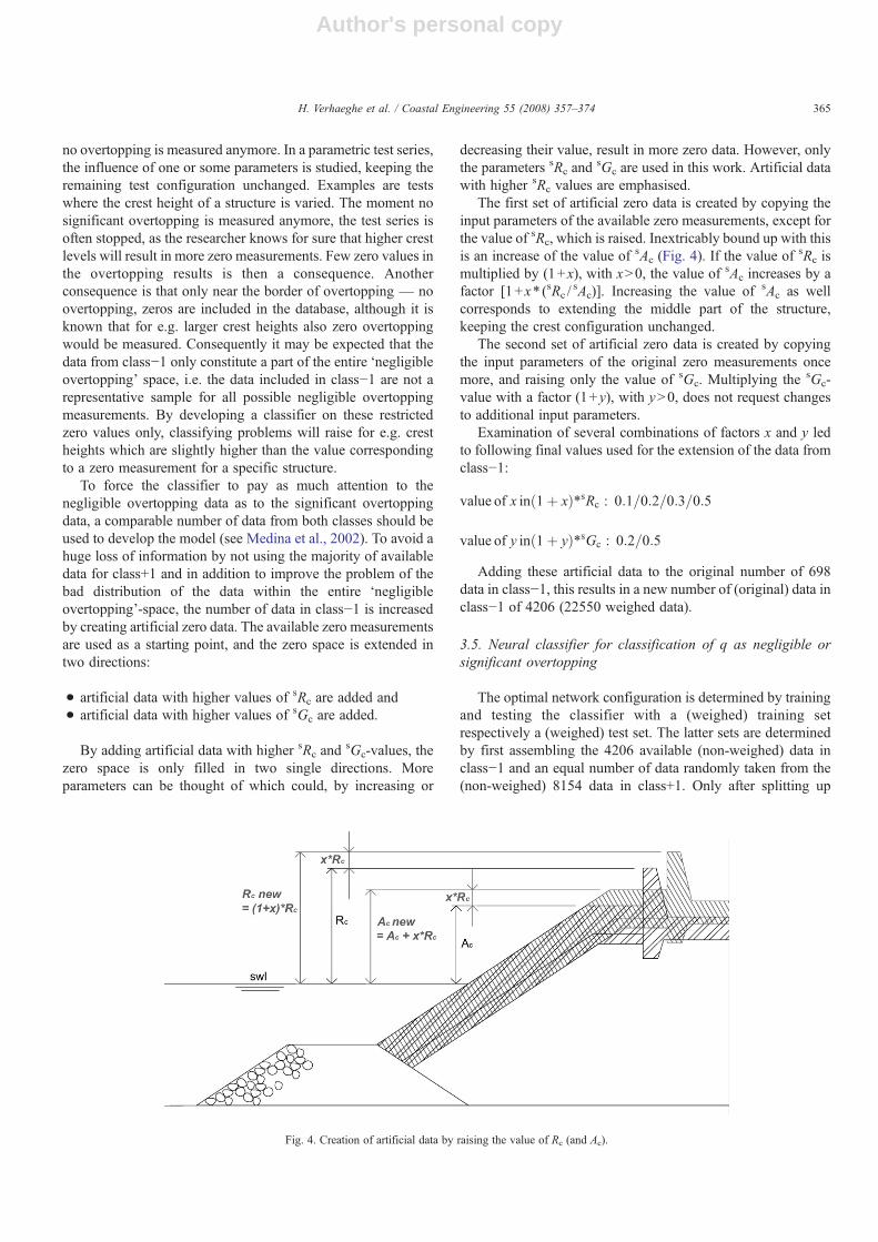
The first set of artificial zero data is created by copying theinput parameters of the available zero measurements, except forthe value of sRc, which is raised. Inextricably bound up with thisis an increase of the value of sAc (Fig. 4). If the value of

sRc ismultiplied by (1+x), with xN0, the value of sAc increases by afactor [1+x⁎ (sRc /

sAc)]. Increasing the value of sAc as wellcorresponds to extending the middle part of the structure,keeping the crest configuration unchanged.

The second set of artificial zero data is created by copyingthe input parameters of the original zero measurements oncemore, and raising only the value of sGc. Multiplying the sGc-value with a factor (1+y), with yN0, does not request changesto additional input parameters.

Examination of several combinations of factors x and y ledto following final values used for the extension of the data fromclass−1:

value of x in 1þ xð ÞTsRc : 0:1=0:2=0:3=0:5

value of y in 1þ yð ÞTsGc : 0:2=0:5

Adding these artificial data to the original number of 698data in class−1, this results in a new number of (original) data inclass−1 of 4206 (22550 weighed data).

3.5. Neural classifier for classification of q as negligible orsignificant overtopping

The optimal network configuration is determined by trainingand testing the classifier with a (weighed) training setrespectively a (weighed) test set. The latter sets are determinedby first assembling the 4206 available (non-weighed) data inclass−1 and an equal number of data randomly taken from the(non-weighed) 8154 data in class+1. Only after splitting up

Fig. 4. Creation of artificial data by raising the value of Rc (and Ac).



these assembled data in a training and test set, the data aremultiplied according to their weight factor.

The architecture of the overtopping classifier is similar tothat of the quantifier (Fig. 2). As both networks are meant tofunction in series, the input layer of the classifier consists of thesame 13 input parameters as the input layer of the finalquantifier. The output of the classifier logically differs from thequantifier output, and can adapt only 2 possible values, i.e.+1for significant overtopping and −1 for negligible overtopping.The number of hidden neurons is determined to be 20.

The classifier is further developed using the bootstrap method.Sixty-one bootstrap networks are trained on the basis of 61bootstrap subsets, each containing 45,100 data (22,550 data fromclass−1 and 22,550 data from class+1). The 61 bootstrapnetworks are used to determine an optimal decision border forthe classification of a data point to class+1 or −1. Based on theobservation that the wrongly classified data from class+1 concernrather high values of sqmeasured , and considering the importantaspect of safety in overtopping design, a selection criterion which

gives priority to minimise the number of wrongly classified non-zero data is chosen: a data point is assigned to class+1 ifmore than5 bootstrap models predict class+1. The criterion allows for somemodels to lead to bad predictions in some parts of the input spacedue to local scarce occupation, without causing consequentoverprediction of overtopping.

Of all available reliable weighed data from the overtoppingdatabase (i.e. 49849 data, see Table 7), 3.09% is wronglyclassified by the classifier. This corresponds to a misclassificationof less than 20% of the data from class−1, versus a misclassifica-tion of only 1.80% of the data from class+1. Table 8 gives anoverall view of the nature of the misclassifications of the datafrom class+1.

As the goal of the classifier is to serve as filter for the data to beput into the quantifier, all data assessed by the classifier as +1, i.e.showing significant overtopping, have to be simulated by thequantifier to obtain a prediction of the value of the overtoppingdischarge. The results of the quantifier simulation of the wronglyclassified data from class−1 (19.29%), sqNN , are given in Table 6(combined classifier–quantifier simulation).

Due to the choice of a strict selection criterion for class−1,data which are on the border of zero overtopping will beinclined to be classified as non-zero overtopping, (sometimes)leading to rather high overtopping discharges predicted by thequantifier.

However, compared to the single quantifier performance, thenumber of overtopping overpredictions is significantly reducedusing the classifier. In Fig. 5 (see also Table 6) the predictionperformance of the combined classifier–quantifier (black italic) iscompared with the prediction performance of the single quantifier(grey italic), for the available data in class−1. The numbers are

Table 8Values of sqmeasured corresponding with wrongly classified data from class+1 byclassifier

Values of sqmeasured % wrongly classified(of 46139 data)

sqmeasuredN10−2 m3/s/m 0

10−2 m3/s/m≥ sqmeasuredN10−3 m3/s/m 0.02




TOTAL: 1.80

Fig. 5. Performance of single quantifier (grey italic) versus performance of combined classifier–quantifier (black italic) for data in class−1.



expressed in percentages of the total number of data. Although theresults for the combined classifier–quantifier refers to 3710weighed negligible overtopping data, whereas the results for thesingle quantifier only refer to the zero overtoppingmeasurements,i.e. 3521 weighed data, the percentages give an idea of thesignificantly better performance of the combination classifier–quantifier. It has been found in Table 6 that (54.50%–0.09%)=54.41% of the considered zero data are predicted by the singlequantifier as sqNNN10

− 6 m3/s/m. The use of the classifier reducesthe quantifier predictions sqNNN10

− 6 m3/s/m to 18.22% of theconsidered zero data. This is a reduction of approximately a factor3. In addition, the percentage of zero overtopping measurementsfor which no overtopping prediction can be given, decreases from43.06% for the single quantifier, to only 1.07% if the classifier isused as filter for the quantifier. The classifier classifies (100%–19.29%)=80.71% of the considered zero overtopping measure-ments correctly as negligible overtopping.

This noticeably better prediction of the zero overtoppingmeasurements when using the classifier as a filter for the

quantifier has as negative consequence the classification of1.80% of the non-zero measurements as zero. However, thispercentage is very low and is therefore considered asacceptable.

Analogous to the quantifier, ranges of applicability aredefined for the classifier. As the data set on which the classifierhas been trained, encloses the data set onwhich the quantifier hasbeen trained, the minimum/maximum-intervals for individualinput parameters of the classifier are at least evenly wide as theseof the quantifier. The classifier has not only been trained on extrazero measurements, but especially the artificially created zerodata enlarge the ranges of applicability: the maximum values forthe input parameters sRc,

sAc andsGc are multiplied with a factor

1.5 (Table 9). This factor originates from the methodologyapplied to create the artificial data, where the input parameterssRc and

sGc were multiplied with a maximum factor of 1.5.Analogous to the quantifier, new input for the classifier should

always be situated within the given ranges of applicability.

4. Application examples

In this section, the ‘combined classifier–quantifier predic-tions’ are discussed for some specific test series.

In Section 4.1 and Section 4.2 the 2-phases neural model isapplied to two artificial test series of which the overtoppingdischarge can be estimated quite accurately with available empi-rical formulae. It concerns overtopping at a rubble mound struc-ture and at a vertical wall.

In Section 4.3 and Section 4.4 the 2-phases neural model isused for the simulation of overtopping at a prototype site inOstia (Italy) respectively at a prototype site in Zeebrugge(Belgium). As the prediction model concerns a small scaleprediction method, a scaling procedure is applied to theseresults, allowing comparison with the real measured over-topping values.

Fig. 6. Combined classifier–quantifier prediction of overtopping at rubble mound structure with rocks.

Table 9Ranges of applicability for the classifier

γf =1 γfb1

1 3.00 ≤sTm− 1,0 toe [s]≤ 22.00 3.00 ≤sTm− 1,0 toe [s]≤ 12.002 0 ≤sβ [°]≤ 60.00 0 ≤sβ [°]≤ 60.003 1.00 ≤sh [m]≤ 20.60 1.00 ≤sh [m]≤ 13.304 1.00 ≤sht [m]≤ 20.50 0.65 ≤sht [m]≤ 13.305 0 ≤sBt [m]≤ 11.40 0 ≤sBt [m]≤ 5.006 1.00 ≤sγf [−]≤ 1.00 0.35 ≤sγf [−]≤ 0.957 0 ≤scotαd [−]≤ 7.00 0 ≤scotαd [−]≤ 5.308 −5.00 ≤scotαu [−]≤ 6.00 0 ≤scotαu [−]≤ 8.009 0 ≤sRc [m]≤ 7.50 0.25 ≤sRc [m]≤ 4.2010 −1.00 ≤shb [m]≤ 3.60 −1.00 ≤ shb [m]≤ 1.2011 0 ≤sBh [m]≤ 16.20 0 ≤sBh [m]≤ 6.2012 0 ≤ sAc [m]≤ 6.00 0.10 ≤ sAc [m]≤ 4.3513 0 ≤sGc [m]≤ 11.40 0 ≤sGc [m]≤ 8.10



4.1. Application example 1: overtopping at a rubble moundstructure

An artificial data set on wave overtopping at a rubble moundstructure has been generated, and the predicted overtopping bythe 2-phases neural model is compared with an existingdeterministic formula. Following wave and structure character-istics are considered: sβ=0° (perpendicular wave attack),sTm− 1,0 toe =4.91 s (corresponding to a wave steepnesss0=0.043),

sh=7.14 m, the armour is supposed to consist of 2layers of rock, i.e. γf =0.4 (Verhaeghe, 2005), and the slope ofthe structure is supposed to equal 1:2. sGc is supposed to beequal to 0.9 m (approximately 3 armour units).

The classifier simulation is performed for values of0.25 m≤ sRc≤4.2 m (see Table 9). The classifier predictsnegligible overtopping for values of sRcN2 m. For values ofsRc≤2 m consistent significant overtopping is predicted. InFig. 6 the combined classifier–quantifier predictions+90%intervals are shown. For comparison the TAW-line for smoothdikes and the TAW-line for rough structure slopes with γf =0.4are represented (TAW, 2002).

The quantifier predictions which are obtained for values ofsRcN2 m are represented in Fig. 6 in grey. However, as theclassifier predicts negligible overtopping for these crest heights,the corresponding quantifier predictions should not be con-sidered. The outcome of the combined classifier–quantifiernetwork can thus be summarised as follows:

• The classifier only predicts significant overtopping at theconsidered rubble mound structure under above specifiedwave attack for values of 0.25 m≤ sRc≤2 m. For values of2 mb sRc≤4.2 m no significant overtopping is expected. Forvalues of sRcN4.2 m and values of sRcb0.25 m the classifieris not able to make a reliable classification.

• For values of 0.25 m≤ sRc≤2 m the quantifier can be used topredict values for the overtopping discharges. The results arerepresented in Fig. 6.

The predicted overtopping discharge by the final model isslightly higher for values of sRcN1.2 m than the values obtainedwith the TAW-formula. For values of sRcb0.8 m the quantifierpredicts slightly lower values compared to the ones obtainedwith the TAW-formula. The latter trend is in accordance with thefindings of Schüttrumpf (2001) who investigated overtopping atsmooth slopes for zero crest freeboard. The 90% intervals aresmallest for values of sRc=0.5 m à 1.5 m. The percentileintervals show that the quantifier encounters more uncertaintiesfor the smallest and largest values of sRc, corresponding to sRc-values in the vicinity of the limit of applicability.

In case the classifier would not be used as filter for thequantifier, the prediction would be very poor for large sRc-values.Fig. 6 shows that for large sRc-values, the quantifier keepspredicting quite high values of the dimensionless overtoppingdischarge, whereas a trend to zero overtopping is expected(comparable to the predictions by the TAW-formula). Thequantifier has difficulties to predict dimensionless overtoppingdischarges qffiffiffiffiffiffiffiffiffiffiffi

gH3m0toe

p lower than≈10− 5–10− 6. In a prototype

situation with Hm0 toe=3 or 5 m the value of 10− 5 correspondsto q≈1.5⁎10− 4 m3/s/m respectively q≈3.5⁎10− 4 m3/s/m.

It is very clear from Fig. 6 that the obtained overtoppingpredictionwith the combination classifier–quantifier is a significantimprovement over the result obtained by the quantifier only.

4.2. Application example 2: overtopping at a vertical wall

An artificial data set on wave overtopping at a vertical wall isgenerated, and the predicted overtopping by the 2-phases neural

Fig. 7. Combined classifier–quantifier prediction of overtopping at vertical wall.



model is compared with existing deterministic formulae.Following wave and structure characteristics are considered:sβ=0° (perpendicular wave attack), sTm− 1,0 toe=4.91 s (corre-sponding to a wave steepness s0=0.043),

sh=7.14 m, sGc =0 m.The classifier simulation is performed for values of 0 m≤ sRc≤

6m (see Table 9). The classifier predicts negligible overtopping forvalues of sRcN6 m. For values of sRc≤6 m consistent significantovertopping is predicted. In Fig. 7 the combined classifier–quantifier predictions+90% intervals are shown. For comparisonthe formulae of Franco et al. (1994) and of Allsop et al. (1995) arerepresented. Both formulae are set up for overtopping at verticalwalls in relatively deep water, which is in accordance with theconsidered artifical data set.

The outcome of the combined classifier–quantifier networkcan be summarised as follows:

• Overtopping at the considered vertical wall under previouslyspecified wave attack may be expected for values of sRc up to6 m. For higher values of sRc the classifier is not able to makea reliable classification.

• The predictions obtained with the quantifier for values of0 m≤ sRc≤4 m are shown in Fig. 6. For values of 4 mb sRc≤6 m, it is only known that overtopping may be expected, butno reliable discharges can be quantified with the developedmodel as sRc=4 m is the limit of applicability of thequantifier.

The quantifier prediction follows the line proposed by Allsopet al. (1995) very well for values of sRcb3 m. For larger valuesof sRc the quantifier predicts slightly higher overtoppingdischarges. The same remark as for the previous data set canbe made here, i.e. the quantifier seems to have difficultiespredicting low overtopping discharges.

In contrast to the sloping structure considered in Section 4.1,also small 90% intervals are obtained for values of sRc=0 m.The availability of overtopping tests with vertical walls whereRc=0 m in the database explains this.

4.3. Application example 3: prototype overtopping at the Ostiabreakwater

In Ostia (Italy, near Rome) prototype overtopping wasmeasured at a rubble mound breakwater armoured with rocks.

In Fig. 8 a picture of overtopping at the Ostia breakwater isrepresented. Detailed information on the Ostia prototype siteand the corresponding measurements is given in Franco et al.(2004 and in press).

There are 77 prototype overtopping measurements available atOstia, originating from7measured storms (2003–2004), ofwhichthe overtopping results are processed per hour. For the measuredmean wave periods Tm toe≈6–9 s; this corresponds to processingovertopping events per 600 à 400 waves. Especially for the longerwaves (Tm toe≈9 s) this processing time is rather short.

The needed scaled hydraulic and structural parameters aredetermined for all 77 data, leading to values (ranges) of theinput parameters for the neural prediction model as summarisedin Table 10.

All data fall within the ranges of applicability of theclassifier. Eight of the 77 data are assessed by the classifier asnegligible overtopping in small scale tests, versus 69 assignificant overtopping. As all these 69 data fall within theranges of applicability of the quantifier, 69 (small scale)overtopping predictions sqNN are obtained.

Before comparison with the prototype measurements ispossible, the predictions are to be corrected for expected modeland scale effects. According to De Rouck et al. (2005)significant model and scale effects are expected for rough, flatbreakwater slopes:

qproto ¼ qss⁎ fscale wind ð5Þ

withqproto=prototype wave overtopping discharge in m3/s/mqss=wave overtopping discharge in m3/s/m originating from

small scale model test which has been scaled to prototype resultusing Froude (qsmall_scale)

fscale_wind=scale factor accounting for possible scale andwind effects for rough, flat breakwater slopes:

for qss b 1:10�5m3=s=m : fscale wind ¼ 24

for 1:10�5m3=s=m V qss V 1:10�2m3=s=m :

fscale wind ¼ 1þ 23:�logqss � 2

3

� �3

for qss N1:10�2m3=s=m : fscale wind ¼ 1Fig. 8. Ostia measurement site (courtesy prof. Franco).

Table 10Ranges of input parameters of prototype data for neural prediction model

Ostia breakwater Zeebrugge breakwatersTm− 1,0 toe [s] 4.57−6.66 3.60–3.77sβ [°] 1.00–40.00 0sh [m] 1.74–2.32 2.28–3.65sht [m] 1.74–2.32 1.87–3.04sBt [m] 0 2.66–4.01sγf [−] 0.40 0.47scotαd [−] 4.00 1.40scotαu [−] 4.00 1.40sRc [m] 1.72–2.56 1.37–2.30shb [m] 0 0sBh [m] 0 0sAc [m] 1.72–2.56 1.89–3.01sGc [m] 2.00–2.75 1.33–2.01



The (small scale) predicted values sqNN by the quantifier canbe corrected with formula (5) by first scaling up to prototypewith Froude, i.e. qNN=qss=

sqNN⁎ (Hm0 toe )3/2.

For the 8 data points classified as negligible overtopping, thescaling procedure (5) cannot be applied (zero overtoppingremains zero overtopping). A procedure was developed todetermine a small non-zero prototype overtopping discharge inthese cases. The rationale is that the zero is obtained through thelimited measurement accuracy present in small scale tests. Theprocedure uses available non-zero q-values of the same test series(i.e. identical structure geometry) with comparable wavecharacteristics, to estimate small non-zero q-values correspondingto the zero small scale results.

The starting point is a graphwith the dimensionless overtoppingdischarge qffiffiffiffiffiffiffiffiffiffiffi

gH3m0 toe

p versus the dimensionless crest heightRc/Hm0 toe

(or armour heightAc/Hm0 toe, depending on the structure geometry)where an empirical formula is fitted through the non-zero q-values.Starting from the value of Rc/Hm0 toe (or Ac/Hm0 toe) of the testwith q=0 m3/s/m, the empirically predicted value qss estffiffiffiffiffiffiffiffiffiffiffi

gH3m0 toe

p is

determined, resulting in a (small) estimated value of q, i.e. qss_est.The correction formodel and scale effects (formula (5)) can then beapplied, starting from this small non-zero estimation qss_est.

Fig. 9 shows the procedure applied for the Ostia data points.The best matching TAW prediction line (TAW, 2002)corresponds to a value of γf=0.38.

The outcome of the combined classifier–quantifier model forthe Ostia data can be summarised as follows (Fig. 10):

• Eight of the 77 prototype data are assessed by the classifier asresulting in negligible overtopping in small scale tests. As theaim of the simulation is to obtain a prototype prediction, aprocedure to estimate prototype predictions from zero smallscale predictions is applied. The estimations for the zeropredictions all concern values of sqss_est≤10−6 m3/s/m.

• Applying a scaling factor fscale_wind to the 8 converted zeropredictions qss_est and to the 69 quantifier predictions qNN,results in values of sqNN_corr_final as represented in the figure.The rms-error of the final corrected network predictionsqNN_corr_final is found to be 0.5249.

• For the final corrected values sqNN_corr_final originating fromthe quantifier predictions the 90% intervals are given. Theyare calculated by correcting the 90% values obtained for theoriginal results sqNN for the expected model and scaleeffects.

One can see that the corrected values result in a rather goodmatch between the predictions and the prototype measurements,although for small values of sqmeasured, the corrected resultsseem to overpredict the measured discharges.

It is expected that the overpredictions for small values ofsqmeasured are due to the fact that the data are situated in thevicinity of the limit of applicability of the quantifier. Supposethe applied scaling procedure provides appropriate correctionfactors (which is to be studied in more detail), the networkshould predict values of sqNN near 10− 7–10− 8 m3/s/m for thelowest values of sqmeasured. Fig. 3 shows that this value is belowthe sq-values on which the quantifier has been trained, i.e. theminimum value in Fig. 3 concerns sq≈10−7 m3/s/m.

4.4. Application example 4: prototype overtopping at theZeebrugge breakwater

In Zeebrugge (Belgium) prototype overtopping is mea-sured at a rubble mound breakwater armoured with 25 tongrooved cubes. A picture of overtopping at the Zeebruggebreakwater is given in Fig. 11. Detailed information on theZeebrugge prototype site and the corresponding measure-ments is given in Troch et al. (1998) and Geeraerts and Boone(2004).

Fig. 9. Small (non-zero) overtopping estimation for zero classified Ostia measurements based on quantifier predictions of non-zero classified Ostia measurements.



Between 1999 and 2004, 9 storms with overtopping wererecorded, leading to 11 prototype overtopping measurements.The overtopping results are processed per 1 hour (3 data) or per2 hours (8 data). For the measured mean wave periods Tm toe≈5.5–6.5 s. This corresponds to processing overtopping eventsper 550 à 600 waves for the 1 h measurements versus per 1100 à1300 waves for the 2 h measurements.

The needed scaled hydraulic and structural parameters aredetermined for all 11 data, leading to values (ranges) of the inputparameters for the neural prediction model as summarised inTable 10.

All data fall within the ranges of applicability of theclassifier. For one data point the classifier predicts negligibleovertopping. For the remaining 10 data, significant overtoppingis predicted. Consequently a quantifier simulation of these 10data is performed. As all 10 data fall within the ranges ofapplicability of the quantifier, 10 (small scale) overtoppingpredictions sqNN in m3/s/m are obtained.

The (small scale) predicted values sqNN by the quantifier arecorrected with formula (5) for expected model and scale effects,

where following value of fscale_wind is proposed by De Roucket al. (2005) for rough, steep breakwater slopes:

for qss b 1:10�4m3=s=m : fscale wind ¼ 8

for 1:10�4m3=s=m V qss V 1:10−2m3=s=m :

fscale wind ¼ 1þ 7:�logqss � 2

2

� �3

for qss N1:10�2m3=s=m : fscale wind ¼ 1

For the data point classified as negligible overtopping, theprocedure to determine a small non-zero prototype overtoppingdischarge is applied (Fig. 12). The dimensionless armourfreeboard Ac

Hm0 toeisAc is plotted on the x-axis instead of the

dimensionless crest freeboard Rc/Hm0 toe , as the maximumarmour level is situated higher than the point determining thecrest freeboard. The best matching TAW prediction line (TAW,2002) corresponds to a value of γf =0.60.

The outcome of the combined classifier–quantifier model forthe Zeebrugge data can be summarised as follows (Fig. 13):

• One of the 11 prototype data is assessed by the classifier asresulting in zero or negligible overtopping in small scaletests. A procedure to estimate a small non-zero value for thezero prediction by the classifier is applied, resulting in avalue of sqss_est =1.30⁎10

−6 m3/s/m.• Applying a scaling factor fscale_wind to the 10 by thequantifier predicted overtopping values qNN and to thesingle converted zero prediction qss_est, results in values ofsqNN_corr_final as represented in the figure. The rms-error ofthe final corrected network prediction sqNN_corr_final is foundto be 0.8442.

Fig. 10. Combined classifier–quantifier prediction of Ostia measurements.

Fig. 11. Zeebrugge measurement site.



• For the final corrected values sqNN_corr_final originating fromthe quantifier predictions the 90% intervals are given. Theyare calculated by correcting the 90% values obtained for theoriginal results sqNN for the expected model and scale effects.

Fig. 13 shows that the corrected values sqNN_corr_final areconservative. For the lowest corrected overtopping discharge sqpredicted by the quantifier, an overprediction of a factor 31.2occurs! The overprediction results in a rather large value for therms-error, i.e. rmse=0.8442. It is not yet clear at this momentwhat lies on the origin of these overpredictions. As the largestoverpredictions occur for the lowest values of sqmeasured , the

vicinity of the limit of applicability may be noticeable. However,the overpredictions are clearly present for larger values ofsqmeasured as well, which raises the question whether the appliedscaling procedure is not too conservative for this structure.

5. Discussion and conclusions

The development of a 2-phases neural prediction method forwave overtopping at coastal structures has been presented. Theneural prediction method has been trained using an overtoppingdatabase in which all structure types are integrated (Verhaeghe,2005; Van der Meer et al., in press). The result consists of a

Fig. 12. Small (non-zero) overtopping estimation of zero classified Zeebrugge measurement based on quantifier predictions of non-zero classified Zeebruggemeasurements.

Fig. 13. Combined classifier–quantifier prediction of Zeebrugge measurements.



single model, which is able to predict overtopping at any coastalstructure type. It is clear that the overall predictive capacity ofthe neural prediction method is particularly advantageous. Theneural prediction method is composed of 2 subsequent neuralnetworks:

• The ‘classifier’ predicts whether overtopping occurs or not, i.e.q=0 m3/s/m or qN0 m3/s/m.

• If the classifier predicts overtopping qN0 m3/s/m, then the‘quantifier’ is used to determine the mean overtoppingdischarge, expressed as q in m3/s/m, i.e. the classifier servesas filter for the application of the quantifier.

Not all of the information included in the database is used forthe set-up of the neural prediction method. Large scaleovertopping measurements are excluded from the trainingprocess of the models, resulting in a prediction method for smallscale overtopping. In addition, only 17 of the 31 parametersincluded in the overtopping database are used for thedevelopment of the neural prediction method, i.e.:

• 13 input parameters, consisting of wave parameters andstructural parameters,

• 1 output parameter, q in m3/s/m, which is preprocessed for thequantifier and replaced by 2 discrete values for the classifier,

• 1 scaling parameter used to scale the input parameters, andfor the quantifier also the output parameter, according to theFroude model law (to Hm0 toe=1 m),

•• 2 general parameters, i.e. the reliability factor RF and thecomplexity factor CF, combined into 1 weight factor, used toforce the classifier and quantifier to draw more attention tooverall more reliable data.

The gathered information within the CLASH project regardingmodel and scale effects affecting small scale overtoppingmeasurements, may be used to estimate prototype overtoppingdischarges corresponding to the small scale neural predictions.

For both classifier and quantifier, a multilayer perceptronwith 1 hidden layer is proposed. After the determination of anoptimal lay-out for both networks, the bootstrap technique isapplied, allowing for the classifier to determine an optimiseddecision boundary, which is inclined to predict non-zero over-topping in case of doubt (prediction on the safe side). For thequantifier a ‘committee of networks’ is determined with thebootstrap method. In addition, the bootstrap method results inpercentile intervals for the quantifier, providing a certainprobability around the point prediction. Application ranges forboth classifier and quantifier are set up, which avoids the use ofthe models outside their ranges of applicability.

It is found that the additional use of the classifier in theprediction method results in a significant improvement over theuse of the single quantifier. Due to the filter-effect of theclassifier, which is able to distinguish situations where no ornegligible overtopping occurs from significant overtoppingsituations, large overpredictions by the quantifier are avoided.

The developed neural prediction method is validated insection 4 for some specific test series.

The first two test series concern artificial data sets. Overtoppingat a rough sloping structure and a vertical wall are studied for avarying dimensionless crest height. Comparison of the combinedclassifier–quantifier predictions with overtopping dischargesestimated with existing empirical models for these artificial datasets shows that the neural predictionmethod performs very well forthe considered structure types. As expected, the percentile intervalsare found to be wider in sparsely occupied parts of the input space.

The third and fourth test series concern prototype measure-ments. The combined classifier–quantifier results obtained forthese data are corrected according to expected model and scaleeffects. For the considered cases, both rough sloping structuretypes, the combination neural prediction method — appliedscaling procedure is found to generally overpredict the smallestmeasured overtopping discharges. For the Ostia case theoverpredictions are rather small and are suggested to originatefrom the vicinity of the limit of applicability of the quantifier. Itmay be concluded that a good result is obtained for the Ostia case.For the Zeebrugge case rather large overpredictions are found. It isnot clear whether these overpredictions originate from thequantifier prediction or from the scaling factors included in theapplied scaling map. Further research on both, the Zeebruggequantifier predictions and the scaling factors, is therefore advised.

Although it is found that the classifier predicts rather ‘safe’overtopping, which was exactly the intention of the decisioncriterion, it is shown that the combined classifier–quantifierresult clearly improves the single quantifier result.

Acknowledgements

The authors would like to acknowledge those who deliveredovertopping data for their technical contributions.

The financial contribution of the Research Foundation-Flanders (FWO) is very much acknowledged. A part of thisresearch was performed within the EC-project CLASH (EVK3-CT-2001-00058); the financial contribution of the EuropeanCommunity is also acknowledged.

References

Ahrens, J.P., Heimbaugh, M.S., Davidson, D.D., 1986. Irregular waveovertopping of seawall/revetment configurations, Roughans Point, Massa-chusetts, USA, final report of experimental model investigation, CoastalEngineering Research Centre, Department of the Army, Mississippi.

Ahrens, J.P., Heimbaugh, M.S., 1988. Seawall overtopping model. Proceedingsof the 21st International Conference on Coastal Engineering, Malaga, Spain.ASCE, pp. 795–806.

Allsop, N.W.H., Besley, P., Madurini, L., 1995. Overtopping performance ofvertical and composite breakwaters, seawalls and low reflection alternatives.Paper to the final MCS Project Workshop, Alderney, United Kingdom.

Allsop, N.W.H., 2005. Report on hazard analysis, CLASH WP6 report. HRWallingford, United Kingdom.

Bouma, J.J., Schram, A., François, D., 2004. Report on socio-economic impacts,CLASH WP6 report, Ghent University, Belgium.

De Rouck, J., Geeraerts, J., Troch, P., Kortenhaus, A., Pullen, T., Franco, L.,2005. New results on scale effects for wave overtopping at coastal structures.Proceedings of the ICE Conference on Coastlines, Structures and Break-waters. London, United Kingdom, pp. 29–43.

Efron, B., 1982. The Jackknife, the Bootstrap and other resampling plans.Society for Industrial and Applied Mathematics. Philadelphia, USA.



Efron, B., Tibshirani, R.J., 1993. An Introduction to the Bootstrap. Chapman &Hall, New York, USA.

Eurotop, 2007. Wave Overtopping of Sea Defences and Related Structures-Assessment Manual. May 2007, www.overtopping-manual.com.

Foresee, F.D., Hagan, M.T., 1997. Gauss–Newton approximation to Bayesianlearning. Proceedings of the International Joint Conference on NeuralNetworks.

Franco, L., De Gerloni, M., Van der Meer, J.W., 1994. Wave overtopping onvertical and composite breakwaters. Proceedings of the 24th InternationalConference on Coastal Engineering, Kobe, Japan. ASCE, pp. 1030–1045.

Franco, C., Franco, L., 1999. Overtopping formulas for caisson breakwaterswith nonbreaking 3d waves. Journal of Waterway, Port, Coastal and OceanEngineering vol. 125(2), 98–108.

Franco, L., Briganti, R., Bellotti, G., 2004. Report on full scale measurements,Ostia, 2nd full winter season, CLASH WP3 report, Modimar, Rome, Italy.

Franco, L., Geeraerts, J., Briganti, R., Willems, M.L., Bellotti, G., De Rouck, J.,in press. Prototype and small-scale model tests of wave overtopping atshallow rubble mound breakwaters: the Ostia-Rome yacht harbour case.Accepted for publication in Special Issue of Coastal Engineering on theCLASH project.

Geeraerts, J., Boone, C., 2004. Report on full scale measurements Zeebrugge,2nd full winter season, CLASH WP3 report, Ghent University, Belgium.

Goda, Y., 1985. Random seas and design of maritime structures. University ofTokyo Press, Japan0-86008-369-1.

Hornik, K., Stinchcombe, M., White, H., 1989. Multilayer feedforwardnetworks are universal approximators. Neural networks vol. 2, 359–366.

IPCC, 2007. Climate change 2007: The physical science basis. In: Solomon, S.,Qin, D., Manning, M., Chen, Z., Marquis, M., Averyt, K.B., Tignor, M.,Miller, H.L. (Eds.), Contribution of Working Group I to the FourthAssessment Report of the Intergovernmental Panel on Climate Change.Cambridge University Press, Cambridge.

Kikkawa, H., Shi-igai, H., Kono, T., 1968. Fundamental study of waveovertopping on levees. Coastal Engineering in Japan vol. 11, 107–115.

Kortenhaus, A., Van der Meer, J.W., Burcharth, H.F., Geeraerts, J., Pullen, T.,Ingram, D., Troch, P., 2005. Quantification of measurement errors, modeland scale effects related to wave overtopping, CLASH WP7 report,Leichtweiβ Institute for Hydraulics, Technical University of Braunschweig,Germany.

Levenberg, K., 1944. A method for the solution of certain non-linear problemsin least squares. Quarterly of Applied Mathematics 2 (2), 164–168.

Marquardt, D.W., 1963. An algorithm for the least-squares estimation of non-linear parameters. SIAM Journal of Applied Mathematics 11 (2), 431–441.

Mase, H., Sakamoto, M., Sakai, T., 1995. Neural network for stability analysisof rubble mound breakwaters. Journal of Waterway, Port, Coastal, andOcean Engineering vol.121 (6), 294–299.

Medina, J.R., 1998. Wind effects on run-up and breakwater crest design.Proceedings of the 26th International Conference on Coastal Engineering,Copenhagen, Denmark. ASCE, pp. 1068–1081.

Medina, J.R., 1999. Neural network modelling of run-up and overtopping.Proceedings of the International Conference on Coastal Structures,Santander, Spain, pp. 421–429.

Medina, J.R., Gonzalez-Escriva, J.A., Garrido, J., De Rouck, J., 2002.Overtopping analysis using neural networks. Proceedings of the 28th

International Conference on Coastal Engineering, Cardiff, United Kingdom.ASCE, pp. 2165–2177.

Owen, M.W., 1980. Design of seawalls allowing for wave overtopping. ReportNo. EX 924. HR Wallingford, United Kingdom.

Panizzo, A., Briganti, R., Van der Meer, J.W., Franco, L., 2003. Analysis ofwave transmission behind low-crested structures using neural networks.Proceedings of the International Conference on Coastal Structures. Portland,USA, pp. 555–566.

Pozueta, B., Van Gent, M.R.A., Van den Boogaard, H.F.P., 2004a. Neuralnetwork prediction method. CLASH WP8 Neural Network. Delft Hydrau-lics, The Netherlands.

Pozueta, B., Van Gent, M.R.A., Van den Boogaard, H.F.P., Medina, J.R., 2004b.Final report on generic prediction method. CLASH WP8 report. DelftHydraulics, The Netherlands.

Saville Jr., T., 1955. Laboratory data on wave run-up and overtopping on shorestructures. TM-64, Beach Erosion Board. US Army Corps of Engineers,USA.

Schüttrumpf, H., 2001. Wellenüberlaufströmung bei Seedeichen- Experimen-telle und Theoretische Untersuchungen, Ph.D. Thesis (Wave OvertoppingFlow at Seadikes- Experimental and Theoretical Investigations).

Steendam, G.J., Van der Meer, J.W., Verhaeghe, H., Besley, P., Franco, L., VanGent, M.R.A., 2004. The international database on wave overtopping.Proceedings of the 29th International Conference on Coastal Engineering,Lisbon, Portugal. ASCE, pp. 4301–4313.

TAW, 2002. Technical report wave run-up and wave overtopping at dikes.Technical Advisory Committee on Flood Defence, Author: J.W. van derMeer, The Netherlands.

Troch, P., De Rouck, J., Van Damme, L., 1998. Instrumentation and prototypemeasurements at the Zeebrugge rubble mound breakwater. CoastalEngineering vol. 35, 141–166 issues 1-2.

U.S. Army Corps of Engineers, 2002. Coastal Engineering Manual, EngineerManual 1110-2-1100, Washington D.C., USA. (in 6 volumes).

Van der Meer, J.W., Verhaeghe, H., Steendam, G.J., in press. The new waveovertopping database for coastal structures. Accepted for publication inSpecial Issue of Coastal Engineering on the CLASH project. Databaseavailable on: http://www.clash-eu.org.

Van Gent, M.R.A., van den Boogaard, H.F.P., 1998. Neural networkmodelling of forces on vertical structures. Proceedings of the 26thInternational Conference Coastal Engineering, Copenhagen, Denmark.ASCE, pp. 2096–2109.

Van Gent, M.R.A., van den Boogaard, H.F.P., Pozueta, B., Medina, J.R., 2007.Neural network modelling of wave overtopping at coastal structures. CoastalEngineering vol. 54 (Issue 8), 586–593.

Van Oosten, R.P., Peixo Marco, J., 2005. Wave transmission at various types oflow-crested structures using neural networks, student thesis, TechnischeUniversiteit Delft, Delft, The Netherlands.

Verhaeghe, H., Van der Meer, J.W., Steendam, G.J., 2003. Database on waveovertopping at coastal structures. CLASH WP2 internal report, GhentUniversity, Belgium.

Verhaeghe, H., 2005. Neural network prediction of wave overtopping at coastalstructures, Ph.D. Thesis, Universiteit Gent, Gent, Belgium, ISBN 90-8578-018-7 (available on: http://awww.ugent.be/awww/coastal/verhaeghe2005.html and http://www.clash-eu.org).


Combined classifier quantifier model: A 2-phases neural ...

Documents