Combinatorial Problems in Energy Networks Graph-theoretic Models and Algorithms zur Erlangung des akademischen Grades eines Doktors der Naturwissenschaen von der KIT-Fakultät für Informatik des Karlsruher Instituts für Technologie (KIT) genehmigte Dissertation von Franziska Wegner aus Potsdam Tag der mündlichen Prüfung: 12. Dezember 2019 Erste Gutachterin: Prof. Dr. Dorothea Wagner Zweite Gutachterin: Prof. Dr. Sylvie Thiébaux

Welcome message from author
This document is posted to help you gain knowledge. Please leave a comment to let me know what you think about it! Share it to your friends and learn new things together.
Transcript

Combinatorial Problems in Energy NetworksGraph-theoretic Models and Algorithms
zur Erlangung des akademischen Grades eines
Doktors der Naturwissenschaen
von der KIT-Fakultät für Informatikdes Karlsruher Instituts für Technologie (KIT)
genehmigte
Dissertation
von
Franziska Wegner
aus Potsdam
Tag der mündlichen Prüfung: 12. Dezember 2019Erste Gutachterin: Prof. Dr. Dorothea WagnerZweite Gutachterin: Prof. Dr. Sylvie Thiébaux


„Nach Wahrheit forschen, Schönheit lieben, Gutes wollen, das Beste thun, das ist die Bestimmung desMenschen.“ Moses Mendelssohn (1729–1786)
I dedicate this work to my beloved parents and my beloved deceased brother Nico.


0Acknowledgements
This thesis would not have been possible without the help of dierent people. I wouldlike to thank Dorothea Wagner for giving me the opportunity to work in her groupand to take care of the funding. During that time I was part in dierent projects such asthe Helmholtz Program Storage and Cross-linked Infrastructure (SCI), Energy SystemIntegration (ESI), and as an associate in the GRK Energy Status Data, where I learneda lot. In addition, I would like to thank my reviewers Sylvie Thiébaux and DorotheaWagner for their comments and their advises.
Working on such a complex topic alone would have been impossible and thus,I would like to thank my coauthors Alban Grastien, Sebastian Lehmann, ThomasLeibfried, Tamara Mchedlidze, Nico Meyer-Hübner, Martin Nöllenburg, Ignaz Rutter,Peter Sanders, Dorothea Wagner, and Matthias Wolf for their discussions and collabo-ration. I owe a big thanks to Andreas Gemsa, Sascha Gritzbach, Matthias Wolf, andPhilipp Bohnenstengel who proofread parts of my thesis. A special thanks goes toPhilipp, who read the whole thesis and xed my “-ly”, and “analysis” problems, andfound the “conjured complex” to be a bit magical.
To get a broader knowledge, I was lucky to work on other topics, collaborate withother groups, and learn from dierent colleagues. A special thanks here goes to MoritzBaum from whom I learned how to collaborate on a paper and who gave me verygood advises. In addition, I would like to thank for the numerous colleagues MoritzBaum, Thomas Bläsius, Johannes Garttner, Andreas Gemsa, Sascha Gritzbach, SörenHohmann, Heiko Maaß, Carina Mieth, Martin Pfeifer, Ignaz Rutter, Philipp Staudt,Torsten Ueckerdt, Dorothea Wagner, Christof Weinhardt, and Matthias Wolf withwhom I was allowed to work together on dierent papers in external projects.
Research is one thing, but we have also the responsibility to communicate ourknowledge in a better and more understandable way. I was very lucky to work withAnna Caroline Hein on an article that describes our work in a more accessible way.She taught me how to write an article for non-specialists and what are common toolsto spread our knowledge.
I thank the colleagues at NICTA for the very good working atmosphere. I learned alot from the team about electrical ows and optimization. Major parts of the switchingpaper were developed during that time and afterwards with Matthias Wolf, fromwhom I learned theoretical techniques and who is a kind reviewer of my writings.Furthermore, I thank also my colleagues at the institute from whom I learned a lotin algorithmics and theoretical computer science. Especially, I would like to thankSpyros Kontogiannis, who was my rst temporary oce mate in the “exile” oce, and
v

my oce mates Benjamin Niedermann and Matthias Wolf with whom I enjoyed thedaily vending machine trips and “apple walks” a lot. In addition, I recall the times withmost of my coworkers when we spent long nights at the institute, the Dibbelt ghostand its hectic squeak of shoe soles, the weekends at work with the Italian course at thePizzahaus and the pizza “Quattro Fromage”, the Saboteur counterpart, the members ofthe Escorial committee, the Obstfreunde meetings, the soccer games after work, thelegendary “Frauenwasserballweltmeisterschaft” in Gernsbach, and the illegal ocechair race. I would like to thank especially these colleagues that made long or baddays enjoyable.
There are people in the background that help out with all the administration andtechnical belongings, which helped me to focus on my main work. This part wasperfectly done by Lilian Becker, Isabelle Junge, Ralf Kölmel, Laurette Lauer, and TanjaWehrmann, whom I would particularly like to thank.
Starting a thesis template from scratch would take a lot of time. I inherited thetemplate and improvements from Thomas Bläsius and Moritz Baum, respectively. Iwould like to thank both, since it was super easy to add additional xes and ideas tothe template.
In the end, I would like to thank my friends, my family, dedicated teachers (especiallyEva Pudewell and Jana Schreiber), inspiring research sta such as Ingo Boersch thatinvested time for students from school, and all people who brought me back on trackand supported me over all this years. A special thanks goes to Katja and Marius Rothe,Philipp Bohnenstengel, Moritz Baum, Anna Caroline Hein, Andreas Gemsa, ThomasBläsius, Benjamin Niedermann, and Cli Mändl, who supported me mentally andemotionally very much.
vi

0Abstract
In this thesis, we study combinatorial problems in energy networks with the focus onpower grids. At present we see a paradigm shift in power grids towards renewableenergy, while making use of the traditional power grid. This shift changes the pro-duction pattern from a centralized way towards a distributed production, leading tobottlenecks and other problems. We try to eciently exploit the existing infrastructureby analyzing the structure of and developing algorithms for electrical ows, placementproblems, and layout problems to improve the existing power grid. We remark thatthe results of this work might be applicable to other energy networks as well [Gro+19]and certain phenomena such as the Braess’s Paradox (i. e., for road network it meansthat adding a road to the trac network can cause longer travel times) indicate thatthe provided techniques in this thesis could be used for trac networks, too.
One main task of this work was the identication of problem statements in energynetworks. We rst translate the problems to graph-theoretical models such that we areable to analyze the problems, study their complexity, develop algorithms, and evaluatethem using either existing data sets or generated data if there are no publicly availablesuitable data sets. We develop algorithms that provide in most cases quality guaranteeson certain graph classes that can be then used as good heuristics on general graphs.At rst we focus on the modeling of power grids and the behavior of electrical owsin power grids using a linearized model that makes use of some simplications. Thesesimplications are based on realistic assumptions for high-voltage power grids onwhich we lay our focus.
This thesis has four main content chapters. The rst part focuses on algorithmsto compute electrical ows. We describe the mathematical structure and focus onsome major properties of electrical ows. Note that apart from solving a system oflinear equations or an exponential time algorithm there are no known algorithms tocompute electrical ows. One way to tackle this problem are electrical preservingtransformations. Electrical preserving transformations are common techniques inthe electrical ow analysis. Based on these transformations, we will present a rstalgorithm for electrical ows on s-t-planar biconnected graphs. In addition to that, wediscuss dierent representations and formulations of electrical ows that increase theunderstanding of the electrical ow’s behavior. We make use of these representationsto describe the balancing property by separating the quadratic relationship of voltageand current. This leads us to the duality of the two Kirchho laws and anotheralgorithmic approach.
vii

The second and third part of this thesis focus on the increasing of the eciency of theelectrical network. We exploit the Braess’ Paradox by switching lines (i. e., temporarilyremoval of a line or cable) or by using an edge weight scaling (i. e., susceptancescaling). We design novel algorithms that improve the throughput of the power grid ordecrease the overall operating costs. These algorithms are the rst that provide somequality guarantees or bounds. Each of these parts includes simulations to evaluate thealgorithms on a realistic data set.
The last part of this thesis is about transmission network expansion planning on agreeneld motivated by the wind farm cabling problem. Algorithmically, it representsa layout problem. Within this part, we present a rst proper model formulation for thisparticular problem, give a benchmark generator, and design a meta-heuristic approachto tackle the wind farm cabling problem that is then evaluated on a generated data set.
viii

0Contents
1 Introduction 11.1 Main Contributions . . . . . . . . . . . . . . . . . . . . . . . . . . . . 41.2 Thesis Outline . . . . . . . . . . . . . . . . . . . . . . . . . . . . . . . 7
2 Literature Overview 112.1 Graph-theoretical Flows and Electrical Flows . . . . . . . . . . . . . . 122.2 Reduction Rules for the Analysis of Power Grids . . . . . . . . . . . . 132.3 Braess’s Paradox – Eects that Inuence the Power Grid Eciency
and Stability . . . . . . . . . . . . . . . . . . . . . . . . . . . . . . . . 172.3.1 Switching – A Discrete Manipulation of the Power Grid Topology 182.3.2 FACTS – A Continuous Manipulation of the Power Grid Topology 19
2.4 The Wind Farm Cabling Problem . . . . . . . . . . . . . . . . . . . . 21
3 Fundamentals 253.1 Fundamental Graph-theoretic Terminology . . . . . . . . . . . . . . . 253.2 Fundamentals in Graph-theoretic Flows . . . . . . . . . . . . . . . . . 293.3 The Power Flow Feasibility Problem . . . . . . . . . . . . . . . . . . . 31
3.3.1 Alternating Current Power Flow Model . . . . . . . . . . . . 323.3.2 Linearized Alternating Current Power Flow Model . . . . . . 493.3.3 The Voltage Normalized Lossless Real Power Flow Model – A
Model between AC and DC Model . . . . . . . . . . . . . . . 523.3.4 Alternating vs. Direct Current Model . . . . . . . . . . . . . . 54
4 The Direct Current Feasibility ProblemAn Algorithmic Approach to Computing Electrical Flows 574.1 A Mathematical Model for the Feasibility Problem of Electrical Flows 58
4.1.1 Properties of Electrical Flows . . . . . . . . . . . . . . . . . . 674.1.2 Scalability of Electrical Flows . . . . . . . . . . . . . . . . . . 714.1.3 Integral Electrical Flows . . . . . . . . . . . . . . . . . . . . . 734.1.4 Planar Graphs . . . . . . . . . . . . . . . . . . . . . . . . . . . 744.1.5 Matroids and Independence Systems . . . . . . . . . . . . . . 75
4.2 Electrical Preserving Transformations . . . . . . . . . . . . . . . . . . 764.3 Representations and Formulations of Electrical Flows . . . . . . . . . 85
4.3.1 The Duality Concept for Graphs . . . . . . . . . . . . . . . . 854.3.2 Simultaneous Flow Representation . . . . . . . . . . . . . . . 86
ix

4.3.3 Rectangular Representation . . . . . . . . . . . . . . . . . . . 894.4 The Balancing Property . . . . . . . . . . . . . . . . . . . . . . . . . . 904.5 An Algorithm for Electrical Flows on s-t Planar Graphs . . . . . . . . 94
4.5.1 Bipolar Orientation . . . . . . . . . . . . . . . . . . . . . . . . 954.5.2 Planar Embedding and Dual Graph Construction . . . . . . . 964.5.3 KCL Conict Resolution . . . . . . . . . . . . . . . . . . . . . 97
4.6 Conclusion . . . . . . . . . . . . . . . . . . . . . . . . . . . . . . . . . 100
5 Discrete Control UnitsSwitching – A Temporary Removal of Links and Cables 1035.1 A Mathematical Model for the Placement of Discrete Control Units . 1045.2 Complexity Considerations of using Discrete Control Units . . . . . . 111
5.2.1 Literature Overview . . . . . . . . . . . . . . . . . . . . . . . 1135.2.2 NP-hardness of Source-Sink-MTSF on Series-Parallel-Graphs 113
5.3 Network Modeling . . . . . . . . . . . . . . . . . . . . . . . . . . . . . 1165.4 MTSF on Source-Sink-Networks . . . . . . . . . . . . . . . . . . . . . 119
5.4.1 The Dominating Theta Path (DTP) . . . . . . . . . . . . . . . 1205.4.2 DTP without Merging the Labels . . . . . . . . . . . . . . . . 1245.4.3 Reachability Test . . . . . . . . . . . . . . . . . . . . . . . . . 1255.4.4 Analyses of the DTP . . . . . . . . . . . . . . . . . . . . . . . 127
5.5 Computing one DTP in Polynomial Time . . . . . . . . . . . . . . . . 1305.6 Approximation Algorithm on Cacti . . . . . . . . . . . . . . . . . . . 1325.7 Simulations . . . . . . . . . . . . . . . . . . . . . . . . . . . . . . . . . 1345.8 Conclusion . . . . . . . . . . . . . . . . . . . . . . . . . . . . . . . . . 137
6 Continuous Control UnitsIdeal FACTS Placement – A Susceptance Scaling Approach 1396.1 Preliminaries . . . . . . . . . . . . . . . . . . . . . . . . . . . . . . . . 1436.2 A Hybrid Mathematical Model for the Placement of Continuous Con-
trol Units . . . . . . . . . . . . . . . . . . . . . . . . . . . . . . . . . . 1466.2.1 The Objective Function . . . . . . . . . . . . . . . . . . . . . 1466.2.2 Power Flow Models . . . . . . . . . . . . . . . . . . . . . . . . 1476.2.3 Flow Control Units on Vertices . . . . . . . . . . . . . . . . . 1486.2.4 Flow Control Units on Edges . . . . . . . . . . . . . . . . . . 1496.2.5 Reduction to MinCostFlow . . . . . . . . . . . . . . . . . . . . 150
6.3 Complexity . . . . . . . . . . . . . . . . . . . . . . . . . . . . . . . . . 1526.4 Planar Problem Reinterpretation . . . . . . . . . . . . . . . . . . . . . 1576.5 Placing Flow Control Buses . . . . . . . . . . . . . . . . . . . . . . . . 158
6.5.1 Experiments . . . . . . . . . . . . . . . . . . . . . . . . . . . . 1586.5.2 Structure of Optimal Solutions . . . . . . . . . . . . . . . . . 160
6.6 Grid Operation Under Increasing Loads . . . . . . . . . . . . . . . . . 164
x

6.7 Evaluation of Placing Flow Control Edges . . . . . . . . . . . . . . . . 1666.8 Eect of FCEs in Comparision to FCVs . . . . . . . . . . . . . . . . . 1676.9 Conclusion . . . . . . . . . . . . . . . . . . . . . . . . . . . . . . . . . 169
7 Transmission Network Expansion PlanningThe Wind Farm Cabling Problem – A Greeneld Approach 1717.1 A Mathematical Model for the Wind Farm Cabling Problem . . . . . . 1747.2 Simulated Annealing-based Approach . . . . . . . . . . . . . . . . . . 1787.3 Benchmark Generation . . . . . . . . . . . . . . . . . . . . . . . . . . 1817.4 Simulations . . . . . . . . . . . . . . . . . . . . . . . . . . . . . . . . . 1827.5 Conclusion . . . . . . . . . . . . . . . . . . . . . . . . . . . . . . . . . 184
8 Conclusion 1878.1 Summary . . . . . . . . . . . . . . . . . . . . . . . . . . . . . . . . . . 1878.2 Outlook . . . . . . . . . . . . . . . . . . . . . . . . . . . . . . . . . . . 188
Bibliography 191
List of Figures 225
List of Tables 227
Glossary 229
A Problem Definitions 241A.1 Flow Feasibility Problems . . . . . . . . . . . . . . . . . . . . . . . . . 241A.2 Flow Optimization Problems . . . . . . . . . . . . . . . . . . . . . . . 242A.3 Discrete Placement Problems . . . . . . . . . . . . . . . . . . . . . . . 243A.4 Continuous Placement Problems . . . . . . . . . . . . . . . . . . . . . 244A.5 Others . . . . . . . . . . . . . . . . . . . . . . . . . . . . . . . . . . . 246
B Fundamentals 249B.1 Instantaneous Curves . . . . . . . . . . . . . . . . . . . . . . . . . . . 249B.2 Complex Power Injection . . . . . . . . . . . . . . . . . . . . . . . . . 250B.3 Complex Power Flow . . . . . . . . . . . . . . . . . . . . . . . . . . . 251B.4 Complex Current Flow . . . . . . . . . . . . . . . . . . . . . . . . . . 252B.5 Formulations . . . . . . . . . . . . . . . . . . . . . . . . . . . . . . . . 253
B.5.1 Polar PQV Formulation . . . . . . . . . . . . . . . . . . . . . 253B.5.2 Rectangular PQV Formulation . . . . . . . . . . . . . . . . . . 254B.5.3 Polar IV Formulation . . . . . . . . . . . . . . . . . . . . . . . 255B.5.4 Rectangular IV Formulation . . . . . . . . . . . . . . . . . . . 256B.5.5 DC Assumption 3 . . . . . . . . . . . . . . . . . . . . . . . . . 257
xi

C Discrete Changes to the Power Grid 259
D Continuous Changes in the Power Grid 263
E Curriculum Vitæ 267
F List of Publications 271
G Deutsche Zusammenfassung 273
xii

1 Introduction
The power grid represents one of the major backbones of the human civilization. Itdetermines our supply chain, which includes important infrastructures such as watersupply and heating. Elsberg [Els17] gives an impression—although ctional—of howessential the power grid is and which parts of our daily life are actually aected by ablackout. However, to sustain the basic human needs we have to change towards amore sustainable and environmentally friendly behavior in general and in power gridsin particular. Thus, the future power grid has to become more ecient to handle theincreasing demand for energy as well as the planned increasing number of generatorsthat transform renewable energies [Jus14], e. g., wind into electrical energy. We callthese generators renewable energy producers. Renewable energy producers such aswind turbines are independent power producers (IPP) that have a volatile powerproduction pattern—meaning that the amount of production is inuenced by manyuncertainties such as the weather—that is totally dierent from conventional power
generators (e. g., nuclear and coal power plants), where the production is stable.The power grid has evolved historically and the traditional structure interconnects
few central conventional power generators with many consumers (Figure 1.1 left side)in such a way that the demand of the consumers is always satised. Similar to theroad network, where we distinguish roads by their speed limits and size into ruralroads, highways, and motorways, we are able to distinguish the lines in the powergrid depending on the amount of power they are able to transfer. The power grid’s hi-erarchical structure in Germany consists of high (110 kV, 220 kV, and 380 kV), medium(1 to 50 kV), and low voltage layers (230V and 400V; see Figure 1.1) representingtransmission and distribution power grids, respectively. In a conventional powergrid the power producers are connected to the high voltage layer directly and theconsumers are either connected to the medium voltage layer (e. g., industries), or lowvoltage layer (e. g., households and small industries). Within this hierarchical structurethe power grid consists of edges that are represented by power lines or cables thatinterconnect producers with consumers. These edges are often denoted as elements(or branches) as they could also represent power electronics such as transformers,resistors, and conductors.
Renewable energy producers are often added to the medium and low voltage layer(Figure 1.1 right side). This eventually causes a bidirectional power ow which theconventional power grid was not designed for. This change in the power grid usagemight cause instabilities and new critical lines. Critical lines represent lines, whichremoval might cause a blackout. The idea of the latter problem is exemplary shown
1

Chapter 1 Introduction
PRODUCER
FACTS
POWER GRID
MED
IUM
VO
LTAG
EL
AY
ERH
IGH
VO
LTAG
EL
AY
ERL
OW
VO
LTAG
EL
AY
ER
CONSUMER PROSUMER
FAC
TS
Figure 1.1: Two exemplary power grids showing the conventional power grid (left) and thecurrent development of the power grid (right). Both power grids consists of three voltagelayers. On the high voltage layer there are the conventional power plants (e. g., coal andnuclear power plants) as well as bigger collections of wind farms and virtual power plantslocated. The industrial consumers are usually located on the medium voltage layer that mainlypresents a distribution layer. In the low voltage layer, we have the households and smallindustrial consumers. Note that on the right side, participants of the last two layer might havephotovoltaics and wind turbines and are thus denoted by the term prosumers (i. e., acting asproducer and consumer simultaneously).
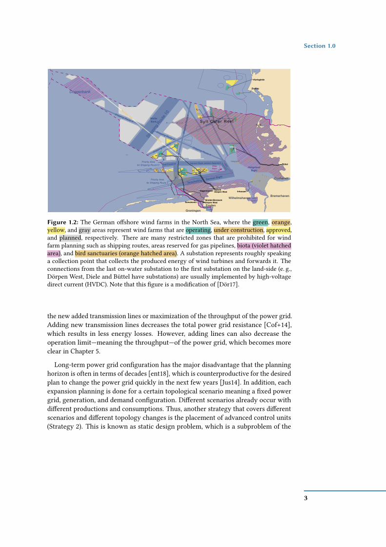
in [Wit+16]. Oshore wind farms in the North and Baltic Sea (see Figure 1.2) provideanother example for such producers. In this particular case, the suitability of a locationfor such farms highly depends on the wind prole and available space. Thus, thelocation for wind farms is not as exible as for conventional power plants. Theseoshore wind farms produce—similar to conventional power plants—a high amount ofelectrical energy that is not used on-site. However, it is largely required in areas suchas the Ruhr region, and southern regions of Germany [ent18, ent19a, ent19b, ent19c],since a large number of industrial consumers are located there. Sending such an amountof energy through the power grid causes new bottlenecks or is simply impossible.Switching these wind farms o to sustain the grid safety is not a desirable solution.Thus, to cope with these new challenges the transmission system operator (TSO) canfollow at least two possible strategies.
(S1) The expansion of the power grid by adding new transmission lines and
(S2) the installation of advanced control units such as Flexible AC TransmissionSystems (FACTS) and switches for a better utilization of the existing power grid.
The mentioned power grid structure and strategies lead to the dynamic and static
transmission design problem [BPG01a]. Binato et al. [BPG01a] consider Strategy 1as dynamic transmission design problems [BPG01a, Cho+06, GMM92] under whichlong-term power grid conguration such as Transmission Network ExpansionPlanning (TNEP) is encountered. TNEP [HHK13] is the design problem of adding newtransmission lines or circuits under dierent objectives such as the cost minimization of
2
Section 1.0
Shipping Route 4
Shipping Route 4
Shipping Route 4Shipping Route 6
Shipping Route 6
Shi
ppin
gR
oute
5
German Bight western ApproachEast Friesland
Terschelling - German Bight
Jade
Approach
WeißeBank
HeligolandBight
Priority Areafor Shipping Route 3
Priority Areafor Shipping Route12 Deep
WaterRoadstead
Doggerbank
Southern Amrumbank
Jade-busen
W e i ß e B a n k
Restricted Area
for
Pipelines
Emden
WilhelmshavenBremerhaven
Cuxhaven
Groningen
Endrup
Karlsgarde
Buttel
DieleDorpen WestHagermarsch
Emden/BorssumDorpen WestEemshaven
Heligoland
Sylt
Inhausen
Shipp
ingRou
te10
Dollard
Outer ReefS y l t
Figure 1.2: The German oshore wind farms in the North Sea, where the green, orange,yellow, and gray areas represent wind farms that are operating, under construction, approved,and planned, respectively. There are many restricted zones that are prohibited for windfarm planning such as shipping routes, areas reserved for gas pipelines, biota (violet hatchedarea), and bird sanctuaries (orange hatched area). A substation represents roughly speakinga collection point that collects the produced energy of wind turbines and forwards it. Theconnections from the last on-water substation to the rst substation on the land-side (e. g.,Dörpen West, Diele and Büttel have substations) are usually implemented by high-voltagedirect current (HVDC). Note that this gure is a modication of [Dör17].
the new added transmission lines or maximization of the throughput of the power grid.Adding new transmission lines decreases the total power grid resistance [Cof+14],which results in less energy losses. However, adding lines can also decrease theoperation limit—meaning the throughput—of the power grid, which becomes moreclear in Chapter 5.
Long-term power grid conguration has the major disadvantage that the planninghorizon is often in terms of decades [ent18], which is counterproductive for the desiredplan to change the power grid quickly in the next few years [Jus14]. In addition, eachexpansion planning is done for a certain topological scenario meaning a xed powergrid, generation, and demand conguration. Dierent scenarios already occur withdierent productions and consumptions. Thus, another strategy that covers dierentscenarios and dierent topology changes is the placement of advanced control units(Strategy 2). This is known as static design problem, which is a subproblem of the
3

Chapter 1 Introduction
dynamic design problem. The latter is less cost intensive and represents a short-termconguration.
For Strategy 2 devices such as circuit breakers (known as switches) and Flexible ACTransmission Systems (FACTS) are able to manipulate the power ow by openinga circuit (switching a transmission line o) or rerouting a certain fraction of powerby changing the susceptance of a transmission line in a device-specied interval,respectively. Both switches and FACTS are able to reduce the generation cost whileincreasing the power grid operation limit and satisfying the N − 1 criterion [Li+13].The N − 1 criterion is a security and reliability criterion to ensure a stable operationwhile one element is removed or has a failure. Fisher et al. [FOF08] mentioned thatswitching is already used by TSOs in certain cases of emergency to decouple parts ofthe grid, avoid abnormal voltage situations, or improve voltage proles. However, it iscurrently not used to extend the operability of the grid or reduce costs and losses, sincethe TSOs wish to interfere as little as possible in the power grid to avoid instabilities.
Since power grids are one of the major backbones, their reliability is crucial. Acommon and natural belief is that only TNEP has the ability to maintain and im-prove the reliability and operability of the power grid. However, placing switchesand FACTS is another way—though counterintuitive—to improve the eciency andreliability of the power grid. This counterintuitive behavior is known as Braess’sParadox [BNW05, Bra68] that is a common phenomenon in many physical networks(see Section 2.3). Furthermore, Schnyder and Glavitsch [SG90] mentioned that bothswitches and FACTS have the possibility to control over- and under-voltage situations,and line overloads. Other papers conrm loss and cost reductions [SG90], systemsecurity improvements [SG88], and combinations of all [HOO11a].
In this work, we mainly focus on Strategy 2 by placing elements such as switchesor FACTS in such a way that we increase the operability of the power grid and thus,the power grid’s capacity. Note that increasing the power grid capacity makes thepower grid more reliable. Both electrical elements can increase the maximum load.Switching provides a possibility to remove a transmission line from the power gridtemporarily. To the contrary, FACTS are control units that are able to inuence thepower ow in a certain range. However, FACTS are also more expensive and complex.We will look on Strategy 1 from the perspective of a plane grid with generators andconsumers, but no preinstalled interconnection. We motivate this scenario by a windfarm planning problem denoted by wind farm cabling problem.
1.1 Main Contributions
The contributions of this thesis are mainly covered by four parts. The rst part is aboutalgorithms and structural results on electrical ows (also known by the term power
ows) and is called the Direct Current Feasibility Problem. The following two
4

Main Contributions Section 1.1
parts cover an overview of the results that concern the ecient utilization of theexisting power grid by placing switches (i. e., discrete changes to the power grid)and Flexible AC Transmission Systems (FACTS; i. e., continuous changes to the powergrid), respectively. In the fourth part of this work, the wind farm cabling results areoutlined that cover Strategy 1.
The Direct Current Feasibility Problem. One main tool that we use in this thesisare electrical ows commonly known under the term power ows. In this part, we willfocus on the Direct Current Feasibility Problem (DC FEAS) that is an approxima-tion of the Alternating Current Feasibility Problem (AC FEAS) (see Section 3.3).An algorithmic approach to computing electrical ows will be our rst contribution inthis thesis and our most fundamental result. We rst give a mathematical descriptionand structural overview of the problem structure. This description is used to developalgorithms for the electrical ow. One result shows that electrical ows do not consti-tute totally unimodular (TUM) bases. However, we show a possible way to solve theinteger DC FEAS.
The rst algorithm for DC FEAS is based on commonly known reduction rules thatwill give us an algorithm that runs in O(|V |3) time for an s-t planar power grid (i. e., apower grid with one generator and one consumer). We give another algorithmic ideafor planar graphs that separates the quadratic relationship of voltage and current byusing two graphs and a mapping of their edges. In addition to that, we are able to use ageometric interpretation of the problem to improve the understanding for discrete andcontinuous changes. Note that for linear systems the superposition principle holdsin the physics and thus, calculating DC FEAS for all generator and consumer pairsresults in an electrical ow for the whole power grid.
Discrete Changes in Power Grids. The placement of switches represents a dis-crete change in the power grid and is the rst placement contribution we will focus onin this work. Note that a discrete change represents a topology change. In particular,we address a subproblem of the static design problem called Maximum TransmissionSwitching Flow Problem (MTSFP), which we model based on the DC electrical ow(see Section 5.1). The problem’s combinatorial nature makes it hard to solve [LGH14]and the current ways to tackle the problem are exact but slow methods such as Mixed-integer Linear Program (MILP) [FOF08] or even more complex models [Hag15,KGD13], or heuristics without provable quality guarantees. In contrast, we focuson structural properties and algorithms with provable performance guarantees forthe MTSFP. While it was known that MTSFP is NP-hard in general [LGH14], we showthat it is also NP-hard if the network contains only one generator and one consumer(s-t-networks). The latter is a generalization of another NP-hardness proof given
5

Chapter 1 Introduction
by Kocuk et al. [Koc+16]1. For s-t-networks on restricted graph classes (includingcacti) we present an exact algorithm based on Dominating Theta Paths (DTPs;see Section 5.4.1). These paths can be computed on general graphs and form the basisfor a new centrality measure resulting in a new algorithm that works well in practice.To the best of our knowledge, we are the rst to provide an approximation and anexact algorithm for MTSFP on special graph classes. Simulations on the NICTA EnergySystem Test Case Archive (NESTA) benchmark set show that these algorithms producenear-optimal results on most of the practical instances and thus, much better solutionscompared to the proven guarantee.
Continuous Changes in Power Grids. Another way to use the grid more e-ciently is by placing FACTS. Contrary to switches that allow discrete changes, FACTSrepresent a control unit that change the electrical ow by scaling the susceptance. Thisrepresents another static design problem and makes use of the existing power grid, too.We assume that a ow control unit is an ideal FACTS [GAG96] controlling the electricalow on its branch without any restrictions. In the rst work, we placed FACTS on busesand in the follow-up, we considered ideal FACTS as elements that can be only placedon branches. In general, the FACTS placement was shown to be NP-hard [LGH16].Thus, most of the literature uses exact methods such as Quadratic Programming (QP)for the general formulation and for ideal FACTS we will use an MILP.
Using the well-known IEEE power systems test cases [Alb+79, AS74, Bil70, Cro15,Dem+77, GJ03, Gri+99, Jos+16, LB10, Les+11, Mat13, Uni14, WWS13, ZMT11], weperformed simulation experiments related to two key questions, which take intoaccount that the FACTS needed for implementing our ow control vertices in the realpower grid constitute a signicant and expensive investment and hence their numbershould be as small as possible. We investigate the following two research questions.
(Q1) How many ideal FACTS are required and where do they have to be placed inorder to obtain a lower bound for the operating costs?
(Q2) If the number of available ideal FACTS is given, do we still see a positive eecton the operating costs and on the operability of the grid during peak periods ofthe grid?
In our simulations we determine the minimum number of ow control units necessaryto achieve the same solution quality as in a power grid in which each element iscontrollable and which clearly admits a best bound on what can be achieved withthe network topology. Interestingly, it turns out that a relatively small number ofideal FACTS are sucient for this. In fact, we can prove a theorem stating a structural
1We thank Thomas William Brown for mentioning the paper of Kocuk et al. [Koc+16] to us after theconference talk of our paper [Gra+18], since this work was not known to us.
6
Thesis Outline Section 1.2
graph-theoretic property, which, if met by the placement of ow control units, impliesthe optimality of the power ow and serves as a theoretical explanation of the observedbehavior. Research Question 1 becomes increasingly relevant as the consumption ofelectrical energy grows faster than the grid capacities. The Optimal Power Flow(OPF) minimizes the total generation costs of the power grid while maintaining afeasible electrical ow. Our experiments indicate that installing few ideal FACTS in apower grid is sucient not only to achieve lower costs compared to an OPF solution,but also allows to operate the grid at capacities for which no feasible OPF solutionexists any more.
Transmission Network Expansion Planning on the Green Field. Wind farmsare an important and powerful possibility to convert wind into electricity. There aredierent challenges that come with the planning of wind farms such as the placementof turbines, the conguration/prole of turbines and substations, and the cabling ofturbines. The conguration of the whole farm is computationally too expensive andeven the cabling with multiple cable types is in general NP-hard (see Section 2.4). Tosolve this NP-hard problem, we use a heuristic approach called Simulated Annealing(see Section 7.2). We structure the problem into multiple layers that decrease theoverall complexity of the problem. The problem is decomposed into circuits, substationproblem, and full wind farm cabling problem. We created a rst openly available windfarm benchmark set that is generated randomly and therefore is less structured thanthe standard wind farm.
1.2 Thesis Outline
We give a brief overview of the organization of this thesis. In particular, we would liketo emphasize that parts of this thesis appeared in previously published proceedings,and reports [Gra+18, Leh+17, Lei+15a, Lei+15b, Mch+15].
Chapter 2 To understand the state of the art, we give a literature overview that isrelated to our research and dierentiate our work to the known literature. Inthe beginning, we give a short summary on results concerning (electrical) owsand the development of digital techniques to compute such ows. A synergyof techniques known from graph-theoretical and power grid analysis is givenin Section 2.2 that will provide us with techniques to understand and analyzepower grids. Since our focus is on combinatorial problems in power grids, wedescribe the paradox (see Section 2.3) that makes switching a possible way toextend the operability of the power grid. Note that a similar eect is observedwith FACTS. We show that there are works describing the Braess’s Paradoxnot only for power grids and present known theoretical results. As alreadymentioned, switching increases the operability of the power grid. In Section 2.3.1,
7

Chapter 1 Introduction
we give an overview of known techniques to tackle the switching problem andshow how we classify our work in the current literature. We analyze similarthings for the FACTS placement in Section 2.3.2 and for the wind farm cablingproblem in Section 2.4.
Chapter 3 In this chapter, we introduce basic terms and notions that will be used inthis thesis with regards to graph theory (see Section 3.1), graph-theoretical ows(see Section 3.2), and electrical ows (see Section 3.3). For the two latter sections,we dene the feasibility problems and show the relationships between thedierent models. In Section 3.3, we do not only dene the feasibility problems,but give a broad overview of the models, describe the assumptions, advantagesand disadvantages of certain model assumptions as well as common problemsand the complexity of the power ow analysis.
Chapter 4 To analyze networks, we describe that the electrical ow (see Section 3.3)is a subproblem of many problems that optimize and analyze power grids.In the literature overview, we commonly see the usage of the mathematicalformulation that is solved using a solver such as Gurobi [Gur16]. However, inthis chapter, we analyze the mathematical structure of the Direct CurrentFeasibility Problem. We develop some algorithms for the DC electrical owusing the developed structural knowledge of the problem and show that thematrices are separately totally unimodular (TUM). The whole system is not TUM.The rst algorithm is based on contraction rules with worse runtime thansolving the system of linear equations of the mathematical formulation. Using areformulation of the electrical ow, we are able to design another algorithmicapproach that is much simpler.
Chapter 5 This chapter is published in [Gra+18]. Switching is one of the problemsthat show the existence of Braess’s Paradox. We classied our work alreadyin Section 2.3.1. A fundamental problem denition of Optimal TransmissionSwitching Problem (OTSP) and Maximum Transmission Switching FlowProblem (MTSFP) is given in Section 5.1 describing the relationships betweendierent problems. Several transformations of the network model are introducedin Section 5.3. In Section 5.4, we describe algorithms and structural propertiesof switching on s-t-networks as well as showing when it becomes NP-hard. A2-approximation on special graph structures is provided in Section 5.6. In Sec-tion 5.7, we evaluate our algorithms with methodical extensions. We concludeour work in Section 5.8 by summarizing the obtained results and outline futurework including open problems.
Chapter 6 This chapter is published in [Lei+15a, Lei+15b, Mch+15]. Whereas switch-ing represents a discrete change in the power grid, FACTS allow a change of
8

Thesis Outline Section 1.2
the electrical ow within an interval by scaling parameters such as the suscep-tance. Thus, it represents another possibility to “rebalance” the electrical owby changing line parameters that have temporary inuence on the topology ofthe power grid. In this chapter, we show that FACTS as well as switches areable to increase the operability of the power grid, while decreasing the overallgeneration costs. In addition, we give theoretical evidence that certain graphstructures provide an optimal electrical ow that is equivalent to the min-costow.
Chapter 7 This chapter is published in [Leh+17]. A fundamental problem denitionfor the wind farm cabling problem is given in Section 7.1, where we introducea rst formal hierarchical structure denition of the wind farm problem; wefurther dierentiate the full farm problem into the substation and circuit problem.The basic simulated annealing algorithm is introduced in Section 7.2 and wegive our methodical extensions to this algorithm for the wind farm cablingproblem. In Section 7.4, we evaluate our algorithm by using generated graphsas benchmark set. These benchmark sets are often harder than the current realworld wind farms. We conclude our work in Section 7.5 by summarizing theobtained results and outline future work.
Chapter 8 This chapter summarizes the work we have done on the previously intro-duced placement problems in power grids that can inuence the eect of theBraess’s Paradox and thus, are able to improve the eciency of power grids.However, this work is just a start to look at these problems from an algorithmicpoint of view and a lot of further investigations are necessary to improve existingalgorithms and to understand these problems in more detail. Some ideas forpossible future investigations are outlined in this chapter.
9


2 Literature Overview
In this chapter, we give a literature overview of the state of the art that is relevant forthis thesis. We start with a brief literature summary with regards to (electrical) ows.Note that we will discuss (electrical) ows formally in more detail in Chapter 3. Fornow it suces that an electrical ow represents some physical ow that diers froma graph-theoretical ow in the sense that it has some (roughly speaking) balancingproperties that makes it inecient in most cases with regards to optimization criteriathat we focus on (e. g., maximizing the throughput). However, it reduces the overallenergy loss (see Equation 4.26) making it more energy ecient. In addition, there aredierent approximation levels for electrical ows that are used for certain scenarios,which we discuss in more detail in Chapter 3. A common way to calculate electricalows is by using solvers that search for a feasible solution. However, this gives us verylittle structural insights in how electrical ows work and thus, we give an overviewof common reduction and transformation rules from the literature in Section 2.2 thatmake use of the superposition principle for linear systems. Note that we use the termnetwork analysis in the context of calculating an electrical ow by using techniquesthat give more insights into the problem structure. There is currently not much knownabout structural insights to solve electrical ows using algorithms. We only foundreduction and transformation rules that are not much investigated for a more complexpower grid analysis. The only problem specic algorithm known is an exponentialtime algorithm [Sha87, SR61].
A major contribution of this work are placement problems. Placement problemsexploit the structure in the sense that they modify the electrical ow such that someobjective is optimized such as the throughput. This optimization is possible since theelectrical ow has the property of balancing itself and thus, does not represent the bestpossible ow for a given topology. A literature overview on the behavior of electricalows and the placement problems we focus on is given in Section 2.3. For the placementproblems, we distinguish between discrete (see Section 2.3.1) and continuous placementproblems (see Section 2.3.2), on which we give literature overviews by considering theplacement of switches and Flexible AC Transmission Systems (FACTS), respectively.For transmission network expansion planning, we will focus on literature for the windfarm planning with the focus on wind farm cabling in Section 2.4. In this literatureoverview, we will see that there is little known about the problem with regards tostructural results. Since there are not a lot of structural results, there are not a lot ofalgorithms to tackle electrical ows and because of that to tackle the aforementionedplacement problems using algorithms.
11
Chapter 2 Literature Overview
2.1 Graph-theoretical Flows and Electrical Flows
The graph-theoretical ow complies with the conservation of ow meaning thatthe incoming ow is equal to the outgoing ow. This is similar to the principle ofconservation of energy. If maximized it is called Maximum Flow Problem (MFP;Section 3.2). If each edge has a cost function, the problem of minimizing the totalcost is called Minimum Cost Flow Problem (MCFP; Section 3.2). Both optimizationvariants are well known problems with ecient algorithms for both MFP [GT14]and MCFP [EK72, GT89, GT90, Kle67, Orl97]. The graph-theoretical ow complieswith the conservation of ow (i. e., incoming is equivalent to the outgoing ow ateach vertex) and the capacity constraints at each edge. However, electrical ows thatwe also call power ows have to obey some physical laws. The physical relationshipbetween current, voltage, and resistance was rst formalized by Kirchho [Kir47]in Kirchho’s Voltage Law (KVL) and Kirchho’s Current Law (KCL). The latter isequivalent to the ow conservation of graph-theoretical ows. The KVL represents aconservation of ow on cycles and not on vertices. The latter law states that the owsin a cycle (also known as mesh) sum up to zero. A base is a maximum independent set.Kirchho introduces for the KVL the concept of cycle bases, which we will discussin more detail in Chapter 4. He shows which equations form a cycle base (i. e., anumber of equations that suce to compute the KVL), and he reformulates the voltagelaw in terms of a cycle base. This basically means that the number of equations forthe KVL is reduced from potentially exponentially many equations to polynomiallymany equations while assuming simple graphs. Later, Maxwell [Max65] describes theelectrical charge, electrical current, electrical eld and magnetic eld in more detail.These works formalize the operation of power grids and thus, build the foundationthat is used in the power ow literature.
(Optimal) Electrical Flow Solution Techniques. In the aforementioned para-graph, we described that an electrical ow complies with the KCL and KVL. Theselaws constrain the electrical ow. A usual question in power grids is if the demand canbe fullled with the currently available generation. This problem is called FeasibilityProblem (FEAS). If we constraint the ow with the KCL and KVL law, we call it theelectrical ow feasibility problem. We will see in Section 3.3 that there are dierentapproximations for electrical ow and thus, dierent feasibility problems. In thefollowing, we will give a brief overview of existing solution techniques for electricalow feasibility problems in general. We will also mention the Optimal Power FlowProblem (OPFP) that is an optimization problem that minimizes the generation costswhile complying with an electrical ow (here called power ow).
There are dierent techniques to solve electrical ow feasibility problems. Oneof the rst surveys outlines digital techniques to solve the electrical ow [SJ67].Another survey of electrical ow and optimal electrical ow solution techniques is
12

Reduction Rules for the Analysis of Power Grids Section 2.2
given by Huneault and Galiana [HG91] outlining the rst automated digital solutiontechnique by Ward and Hale [WH56], and the Gauss-Seidel method introduced by Car-pentier [Car62, Car79], that is later replaced by the Newton-Raphson method [dMP99,Pes+68].
The problem of generating the required amount of power while obtaining minimumoperation cost is called Economic Dispatch Problem (EDP). To cope with the EDPwhile incorporating an electrical ow feasibility problem is called the Optimal PowerFlow Problem (OPFP) that was introduced by Carpentier [Car62]. The developmentof solution techniques on OPFP is summarized by Frank et al. [FSR12a, FSR12b].
Stott [Sto74] reduces the memory consumption and running time for electrical owfeasibility problems by introducing sparsity techniques for the admittance matrixand compares it to other methods. The idea behind the approach of Stott is that thepower grid has a very sparse network structure [COC12, p.17] and thus, techniquesthat exploit the sparsity improve the running time and memory consumption. Acomparison of dierent power formulations (see Section 3.3.1) is given by da Costaand Rosa [dR08]. Molzahn and Hiskens [MH19] give a survey of relaxations andapproximations of the electrical ow equations. In Section 2.2, we outline someliterature that mention possible ways to analyze power grids. Note that as far as weknow there is no “purely” algorithmical approach to solve the power ow problemapart from an exponential time algorithm [Sha87, SR61]. For linear systems there arereduction and transformation rules known, which are not used so far to create analgorithm for electrical ows. A literature overview including known applications ofthese rules is given in the following.
2.2 Reduction Rules for the Analysis of Power Grids
In this work, we focus on a linear approximation of the electrical ow. Thus, allequations, constraints, and objectives are linear functions. The goal of the networkanalysis is to design algorithms that exploit the structure of the problem such that thesealgorithms run in polynomial time in the input size. There are dierent possibilities toanalyze power grids. The common way to compute electrical ows is to solve a set oflinear equations using solvers such as the Gurobi Optimizer [GUR13, Gur16]. However,the input size has often a big inuence on the running time to solve a problem. Apossibility to reduce the input size is to use reduction rules. However, reduction rules inpower grids include contraction and transformation rules. Contraction rules are series(see Figure 2.1a) and parallel contractions (see Figure 2.1b) and transformation rulesare ∆-Y - (delta-wye) and Y -∆- (wye-delta) transformations (see Figure 2.1c). The latterrule transforms a triangle to a star by adding one vertex into the center and adding edgesfrom the center to the already existing vertices, while removing the original edges, andvice versa for the inverse transformation, respectively. The generalization of the ∆-Y -
13

Chapter 2 Literature Overview
(a) (b) (c)
t
s
t
s
t
s
s
s
v
x
t
tu
Figure 2.1: Three dierent subgraphs that lead to dierent transformation rules each. Thesecommon transformation rules provide possibilities to reduce the network size. (a) In a seriescontraction a path with vertices of degree two can be contracted to a single edge. (b) In aparallel contraction multiple parallel edges can be contracted to a single edge. (c) The ∆-Y -transformation (delta-wye; respectively Y -∆-transformation known as wye-delta) represent apossibility to increase (respectively decrease) the number of vertices and reduce (respectivelyincrease) the number of triangles by one.
andY -∆-transformations are the star-mesh- (or star-polygon-) transformations [Bed61,LO73]. Other common rules are self-loop and degree-1 removals.
These reduction rules are applied on dierent problems in dierent elds of researchsuch as in statistical physics involving the evolution of crystal lattice energy [Bax16],network reliability [Leh63, ST93, Tra02], knot theory [Rei83, Tra02], and graph the-ory [Ake60, CE17]. We start with some initial algorithmic results on the transformationrules in the following.
Reducibility of Graphs and Complexity of Reduction Algorithms. The rstmore general structural observations concerning reduction rules are by Akers [Ake60]and Lehman [Leh63]. Both independently introduce the conjecture that by usinga combination of Y -∆- and ∆-Y -transformations, as well as series and parallel con-tractions the connected, two-terminal, undirected, planar graph can be reduced to asingle edge connecting the given terminals [Leh63, pp.795.]. The latter conjecture isthen independently proven by Grünbaum and Kaibel [GK03] using a graph withoutterminals, and a complicated and non-constructive proof by Epifanov [Epi66]. Us-ing ∆-Y - and Y -∆-transformations Epifanov proves that any polyhedral graph (i. e., anundirected graph that is a representation of a convex polyhedron) can be reduced toa K4 (i. e., complete graph with four vertices). The proofs of the conjecture is simpliedby Truemper [Tru89] using a constructive proof incorporating graph minors. Onemajor property used in Truemper’s proof is that planar graphs can be embedded asgrid graphs. Truemper provides a much simpler polynomial time algorithm for planargraphs than the one by Feo [Feo85]. Truemper’s [Tru89] algorithm requires O(|V |2)space, but he did not mentioned the running time of the algorithm. However, Feo[Feo85] designed a more complex algorithm that runs in O(|V |2) time and needs O(|V |)
14
Reduction Rules for the Analysis of Power Grids Section 2.2
space. Valdes et al. [VTL79] showed that the series, parallel, loop, and single degreereductions for series-parallel-graphs can be done in O(|V |) time. In addition, Politof[Pol83] showed that every Y -∆ graph (i. e., a graph that can be reduced to a vertex bythe aforementioned reduction rules) is planar. The term Ci (also known as i-cyclicgraph) represents a closed walk of length i ∈ N with i being the number of vertices. Aplanar graph is a Y -∆ graph if and only if it is a (C5 + 2K1,K2 ×C4)-free graph [Pol83]or (K5,K2,2,2,C8(1, 4),K2 ×C5)-free graph [APC90, ST90], respectively. To the extentof our knowledge, it is unknown whether these algorithms are applicable to powergrids or not. Some application to graph-theoretical problems are given in the nextparagraph.
Preservation of Optimization Properties. Regardless of the structural point ofview, these transformations are used when solving algorithmic problems. Dependenton the problem, it is necessary to show that the transformation and contraction rulespreserve a solution space. This is roughly done by Akers [Ake60] for the MaximumFlow Problem (MFP) and Shortest Path Problem (SPP). He used the transforma-tions to simplify the network such that algorithmic problems become easier to solve.Akers [Ake60] applied the transformations to solve SPP and MFP on undirected 2-and 3-terminal graphs while preserving the optimal length or ow value. Interestingly,the transformations shown in Akers [Ake60] also behave dually meaning that, e. g.,the calculation of the capacities of the series reduction is the calculation of the parallelreduction in the dual problem. The duality of the transformations is shown for examplein Akers [Ake60]. Another work by Chang and Erickson [CE17] uses these reductionrules to untangle planar curves meaning to simplify a planar graph with a certainnumber of self-crossings. In the next paragraph, we show the usage of the reductionrules with regards to network reliability. Within network reliability there is a lot ofliterature available that gives structural results on the hardness of the problem anduses methodology to tackle NP-hard problems, which we will use for some placementproblems.
Preservation of Network Reliability. In network reliability these reductions rulesare used extensively. Network reliability studies the probability that at least onepath connecting two terminals operates successfully. The edges in such a networkhave success probabilities. The problem of computing the all-terminal reliability forarbitrary networks is known to be NP-hard [PB83, Val79]. The hardness remains evenfor planar graphs [Ver05]. Lehman [Leh63] showed that series, parallel, degree-1, andloop reductions preserve reliability in the two-terminal and undirected network case.The ∆-Y - and Y -∆-transformations for boolean functions (also known as switching-functions) are introduced by Lehman [Leh63, Section 4]. However, he shows thatthese transformations do not calculate the exact probability, but an approximation
15

Chapter 2 Literature Overview
to it. Since the problem is in general NP-hard, Satyanarayana and Tindell [ST93]developed ecient algorithms for special graph classes, which run in O(|V | log|V |)time. The latter work [ST93] uses the technique of forbidden minors (i. e., a minor His a graph that can be extracted from a graph G by applying vertex and edge deletionsand edge contractions) to develop ecient algorithms for reliability analysis on graphsubclasses. Satyanarayana and Tindell not only focused on the two terminal case, buton theK-terminal reliability that focuses on the probability that there is a path betweenevery pair of terminals. Where Lehman [Leh63] showed that not all transformationsare reliability preserving reductions, Satyanarayana and Tindell [ST93] focused onreliability preserving reductions and introduced a trisubgraph-Y-reduction. Theyfocused on block-cut-trees, 3-connected graphs, and series-parallel graphs. For thelatter graph structure they observed that it depends on the distribution of the terminalswhether the graph is reducible or irreducible and thus, reliability preserving using thestandard reduction rules or not. The K-terminal reliability on series-parallel-reduciblenetworks can be computed in O(|E |) time using series, parallel, degree-1, and -2contractions [SW85, pp.827.]. However, for series-parallel-irreducible graphs thesereduction rules are not sucient and thus, Satyanarayana and Wood [SW85] designeda linear time algorithm using the polygon-to-chain reduction that reduces two parallelpaths π 1(s, t) and π 2(s, t) with inner vertices of degree-2 to one path having a lengthof max|π 1(s, t)|, |π 2(s, t)|. For basically series-parallel directed graphs (i. e., graphswhere the underlying graph is a series-parallel graph) Agrawal and Satyanarayana[AS84, AS85] provide an O(|E |) time algorithm to compute source-to-K-terminalreliability. Politof and Satyanarayana [PS86, PS90] show that for K2 ×C4-free graphsthe reliability can be computed in linear time and Politof et al. [PST92] show that theall-terminal reliability of a (K5,K2,2,2)-free graph can be computed in O(|V | log|V |)time. Satyanarayana and Tindell [ST93, p.13, Proposition 2] show that a Y -∆ graphallows a trisubgraph-Y reduction resulting in a Y -∆ graph.
Further Results. There are results on reducibility for planar graphs, non-planargraphs, and special graphs that we outline here. Gitler [Git91] proofs for reducibilityfor graphs with no K5 minor and graphs with no K3,3 minor. The reducibility forprojective-planar graphs (i. e., a projective plane is an extension of the euclidean space,where parallel edges intersect in a point and thus, all edges intersect in some point)and graphs with crossing number one was shown by Archdeacon et al. [Arc+00].For 4-terminal reducibility of planar graphs, Demasi and Mohar [DM15] show that asuciently connected cubic graph (i. e., a graph, where all vertices have a degree ofthree) are reducible if and only if it does not contain a Petersen graph as minor. LaterWagner [Wag15] presents a reducibility for almost-planar graphs with the conditionthat all graphs in the reduction sequence remain almost-planar. Other works denethe reducibility with a set of forbidden minors [Yu04, Yu06] and design algorithm for
16

Braess’s Paradox – Eects that Influence the Power Grid Eiciency and Stability Section 2.3
3-terminals, special cases of 4-terminal planar graphs, k-cofacial terminals in planargraphs [Git91, GS].
2.3 Braess’s Paradox – Eects that Influence the PowerGrid Eiciency and Stability
The main focus of this thesis is on placement problems with additional physicalproperties. In the introduction (see Chapter 1), we discuss two strategies to improvethe power grid eciency. In contrast to our intuition, not only the expansion of thepower grid (TNEP; Strategy 1 in Chapter 1), but also switching can be used to improvethe eciency of the power grid. This implies that adding a new line to the power gridcan also decrease the throughput of the power grid or increase the overall generationcosts.
A similar phenomenon exists for road networks and is called Braess’s paradox[BNW05, Bra68]. Introducing a new road to the trac network might cause longertravel times [YGJ08]. The main reason is that every participant wants to indepen-dently minimize its own travel time, while ignoring the decision’s eect on othertravelers [PP97]. In addition, Pas and Principio [PP97] show that the occurrence ofthe Braess’s paradox highly depends on the instance parameters, i. e., demand andcongestion functions. Thus, the paradox usually occurs within some bounds thatmake it possible that the network might “grow in” and “grow out” of the paradoxicalsituation with increasing (trac) demand.
Cohen and Horowitz [CH91] describe the existence of the paradox in mechani-cal [PV12] and electrical networks (for both see [PP03]). Other works show that theparadox also appears in oscillator networks [WT12], where adding a line can causeinstabilities and even power outages, which conrms once more the existence of theBraess’s paradox in real power grids [WT12, p.11]. Another example for this exists inquantum physics [Pal+12].
Cohen and Horowitz [CH91] also emphasize the non-intuitive behavior of the Nashequilibrium that arises in most physical networks. We know from Dubey [Dub86, p.4,Section 3] that Nash Equilibria “tend to be inecient in the Pareto sense”. We willgive an explanation of that in Chapter 4. The Nash Equilibrium is a known x pointin Game Theory and represents a state, where no player wants to change its choice.In contrast, the Pareto optimum means that there is no possible better choice of oneplayer that does not decrease the payo of another player. Thus, it is the optimumwith regards to a cost function. The Pareto front represents the set of Pareto optima.However, the Pareto optimization plays a crucial role in the multi-criteria optimization.We show an example for a Pareto front in Figure 6.7a. An easy example that showsPareto optima and Nash Equilibriums is given in Dubey [Dub86, p.5, Figures 2–4].
17
Chapter 2 Literature Overview
Another theoretical insight given by Valiant and Roughgarden [VR06] explainingthat the Braess’s paradox occurs very often in random graphs. Note that many of thenetworks in the real world have properties similar to random graphs [Hof19, p.xiii].Thus, in Chapter 5, we exploit the Braess’s paradox to improve the eciency of thepower grid, whereas in the TNEP problem, we have to add lines in a way that theeciency of the power grid increases and thus, the eect of the Braess’s paradoxdoes not appear. The eect that the Braess’s Paradox highly depends on the instanceparameters [PP97] is shown in Chapters 5 and 6, where we use switches and FACTSto inuence these parameters.
2.3.1 Switching – A Discrete Manipulation of the Power GridTopology
Recall that switching is the process of temporarily removing a transmission line fromthe power grid by using devices such as circuit breakers. Kirchho model this behaviorby changing the resistance to innity [Kir47, p.501]. Switching was rst analyzed asa negative eect in the power grid [Gla85] responsible for overloads, voltage drops,and the loss of network stability. Koglin and Müller [KM80] introduce transmissionswitching as a corrective control action to reduce transmission line overloads. Laterother positive switching eects were recognized such as improving currents, decreasingloads and angles, creating voltage drops, and changing the short-circuit power [Gla85,HOO11a, RM99].
O’Neill et al. [ONe+05] and Fisher et al. [FOF08] introduce the Optimal Trans-mission Switching Problem (OTSP) and its formulation based on the Direct Cur-rent Optimal Power Flow (DCOPF) [Cho+06], respectively. The OTSP using DC-constraints is called DCOTS. Fisher et al. [FOF08] observe that switching may im-prove the economic eciency of the Economic Dispatch Problem (EDP). How-ever, they could not nd any general trend in the physical characteristics of theswitched lines. Many models were presented that are more complex [Bai+15, SF14] orminimize either the overload [MTB89, MWH86, Wru+96], voltage problems [BM87,RIM95], losses [BG88], or generation costs [FOF08, ONe+10]. Others enhance thesecurity [BDD89, SG90], reliability [DK15, ZS17, ZW14], economic seasonal [JWV15],or Transmission Network Expansion Planning (TNEP) costs [KSK10, VP12].
DCOTS is known to be NP-hard [LGH14, LGH15] and solving it by running an Inte-ger Linear Programming (ILP) has impracticable running times [FOF08]. The complex-ity is reduced by limiting the solution set, i. e., number of switches [Hed+08, Hed+09,SV05]. Often a small number of switches is sucient to reach the optimum. This isa central property in most heuristics [CW14, FRC12, Hed+11] that use a ranking ofthe transmission lines based on dierent criteria. Pourahmadi et al. [PJH16] showthat switching lines with high congestion costs is a reasonable criterion to reducethe overall cost. Other pre-screening techniques rank the lines on their dual prices
18

Braess’s Paradox – Eects that Influence the Power Grid Eiciency and Stability Section 2.3
for each bus [LWO12]. Other approaches are Evolutionary Algorithms [AF09, DV01],branch-and-bound [TC14b], and partitioning [Bai+17, Li+13, Mäk+14]. Yang et al.[YZX14] use a soft rounding heuristic [Jün+10, p.629] not xing all variables to avalue but obtaining this by changing the objective function coecient of the binaryvariables.
However, there is not a lot known with regards to structural exploits of the powergrid topology. Ostrowski et al. [OWL12, OWL14] exploited the symmetry of trans-mission lines for the switching problem by removing identical parallel transmissionlines. Dierent network parameters lead to a dierent system performance and areconnected in some sense to switching [Ari+09, BNX09, HB08]. Barrows et al. [BB11,BB12, BBB13] use topological and electrical parameters as a heuristic. In addition, theyinvestigate parameters concerning OTS such as resistance, reactance, susceptance,vertex degree, thermal limits, and edge-betweenness centrality [HB08] (number ofshortest paths through an edge) but nd no statistically signicant relationship. Recallthat Pas and Principio [PP97] show that the Braess’s Paradox highly depends on theinstance parameters and that a single parameter evaluation lacks in this particularcase as it is inuenced by multiple parameters such as topology, susceptance, andcapacity. In addition, there exist also screening and ranking systems based on networkows [MWH86, Wru+96].
Most of the work so far tries to adapt OTS to other problems, reformulates themodel, or analyzes it for dierent power grids. However, the majority of the papershave problems to solve their models to optimality even on small instances. Thus, mostheuristics try to decrease the search space, a few concentrate on structural aspects ofpower grids, while others try to nd correlations between power grid parameters andswitching. A common observation is that the eects of transmission switching arerelatively localized [BB11, BB12, Gla85]. This observation is debatable as it is madewithout solving the problem to optimality and using test cases such as the reliability
test system 1996 RTS-96 test case that is three copies of the 24-bus power system linkedtogether. However, in general there is no network property found to distinguish theswitched lines [BB11]. Thus, current techniques do not provide a deeper understandingof the problem structure. The latter will be our contribution to the community forcertain graph structures, which we give in Chapter 5.
2.3.2 FACTS – A Continuous Manipulation of the Power GridTopology
Recall that the graph-theoretical ow is a ow mainly controlled by the KCL andcapacity constraints, whereas the electrical ow has to obey physical laws. The graph-theoretical ow and the electrical ow give us, while maximized (respectively whenthe generation cost is minimized), the upper and lower bounds (respectively lower andupper bounds), respectively (more on that in Chapter 4). In addition, Pas and Principio
19

Chapter 2 Literature Overview
[PP97] show that dierent instance parameters inuence the eect of the Braess’sParadox. Thus, changing the parameter helps to change the eect the Braess’s Paradoxhas on the network. With FACTS the idea is to exploit the network structure such thatthe ow behaves more like a graph-theoretical ow and thus, closer to the best bound.Recall that a similar approach is done by switching.
With the increasing availability and technological advancement of FACTS researchersbegan to study the possible benets of their installation in power grids from dierentperspectives to approach the Research Questions 1–2 (see Section 1.1 on Page 6).
From an economic perspective, it is of interest to support investment decisions inpower grid expansion planning by considering alternative investment strategies thateither focus on new transmission lines or allow mixed approaches including FACTSplacement. Blanco et al. [Bla+11] present a least-squares Monte-Carlo method forevaluating investment strategies and argue that FACTS allow for a more exible, mixedstrategy that fares better under uncertainty. Tee and Ilić present an optimal decision-making framework for comparing investment decisions, including FACTS [TI12].
From the perspective of operating a power grid, the main question is how manyideal FACTS are required and where do they have to be placed in order to optimize acertain criterion. Cai et al. [CES04] propose and experimentally evaluate a geneticalgorithm for allocating dierent types of FACTS in a power grid in order to optimallysupport a deregulated energy market. Gerbex et al. [GCG01] and Ongsakul andJirapong [OJ05] study the placement of FACTS with the goal of increasing the amountof energy that can be transferred. Gerbex et al. [GCG01] present a genetic algorithmthat simultaneously optimizes the energy generation costs, transmission losses, lineoverload, and the acquisition costs for FACTS. Ongsakul and Jirapong [OJ05] useevolutionary programming to place FACTS such that the total amount of energythat can be transferred from producers to consumers is maximized. In contrast to oursetting, they may also increase the demands of consumers arbitrarily. Contrary to theseheuristic approaches Melo Lima et al. [Mel+03] use mixed-integer linear programmingto optimally increase the loadability of a system by placing FACTS subject to limitson their number or cost. Similar to our approach, they do not distinguish dierenttypes of FACTS but rather assume “ideal” FACTS that can control all transmissionparameters of a branch. However, they focus only on loadability and do not considergeneration costs and line losses. The latter two objectives will be considered in ourwork.
All related work mentioned so far considers the DC model for electrical networks asan approximation to the AC model (more on that in Section 3.3) and aims at providing apreliminary step in an actual planning process, where this approximation is sucient.There are also a few attempts to solve the placement problem for FACTS in themore realistic but also more complicated AC models [MEA99]. These models can becategorized as follows:
20

The Wind Farm Cabling Problem Section 2.4
Collector System
Full Wind Farm
Circuit
Collector System
Full Wind Farm
Circuit
Com
plex
ity Circuit ProblemP (MST)
NP-hard (Heuristics) Full Farm Problem NP-hard
NP-hard (CMST) NP-hardSubstation Problem
NP-hard
150 e/m2 Turbines300 e/m7 Turbines600 e/m9 Turbines
Costs permeter m CableCapacity
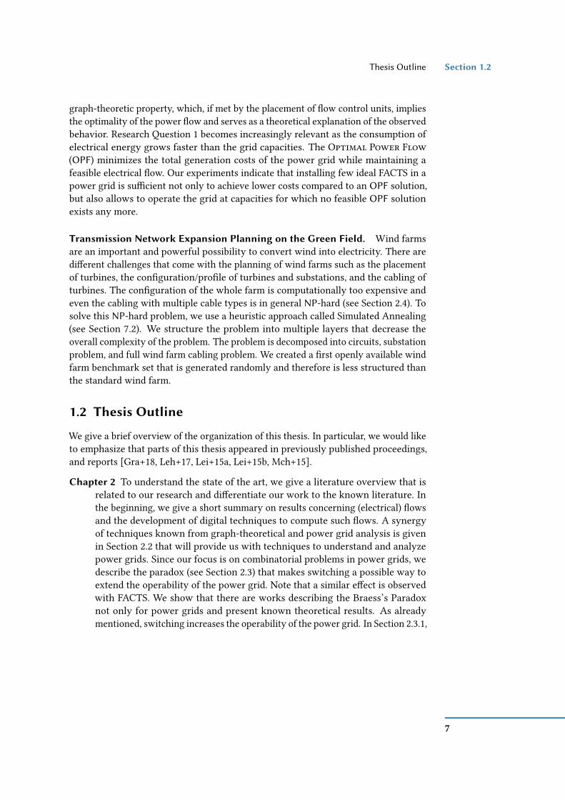
Figure 2.2: The wind farm topology consists typically of turbines ⊗ and substations . Thecomplexity of cabling a wind farm diers depending on the cost function. If we assume unitcosts—meaning we have only one cable type available—then the problem is slightly easierto solve (see left side) than when allowing multiple cable types (see right side). The dierentcable types are shown in the table. The complexity of the problem also increases dependent onthe problem layers. The easiest layer is the Circuit Problem (CP), followed by the SubstationProblem (SP) and Full Farm Problem (FFP).
• AC models with sinusoidal loads (non-convex and non-linear formulation),
• AC quadratic approximations (non-convex and quadratic formulation),
• AC piece-wise-linearization (non-convex and integer linear programming for-mulation), and
• AC linearization (convex and linear formulation).
Sharma et al. [SGV03] develop an evaluation whether transmission lines are criticaland propose to place FACTS at critical lines in order to improve voltage stability in thegrid. Ippolito and Siano [IS04] present a genetic algorithm for FACTS placement in ACnetworks and experimentally evaluate it in a case study. In contrast to these heuristicapproaches, Farivar and Low [FL13] observe exact OPF evaluation in a relaxed AC-model. In this context, they place phase shifters to exploit structural characteristicsthat are similar to our approach.
2.4 The Wind Farm Cabling Problem
The amount of renewable energy producers started to increase signicantly a fewyears ago. However, there is not a lot of research done in the eld of wind farmplanning. From an algorithmic point of view and using just a single cable type,
21

Chapter 2 Literature Overview
the Circuit Problem (CP) can be solved using a Minimum Spanning Tree (MST)algorithm [Gab+86, HK71], whereas the Substation Problem (SP) can be solvedusing Capacitated Minimum Spanning Tree (CMST) [Voß09]. However, CMST isalready NP-hard, but approximation algorithms and heuristics exist for this type ofproblem [EW66, Mar67, Voß09]. This is visualized in Figure 2.2. We are interestedin the layout problem using multiple cable types with dierent capacities and costsper meter, which is already NP-hard for two cable types in the Circuit Problem.Using brute force for |K | dierent cable types and |E | possible interconnections wouldmean that there are |K | |E | possible combinations to compute. However, to computecabling layouts with multiple cable types some work is done in the area of cluster-based, MST-based and genetic algorithms. Dutta and Overbye [DO11] used the QualityThreshold (QT) Clustering algorithm to group the turbines into collector systems oreven groups within a collector system. They evaluate—based on reliability, powerlosses and cabling costs—three dierent layouts namely the radial, cluster-based, andmixed layout.
If the wind farm planning does not consider the cabling of turbines, but the connec-tion of entire oshore wind farms among themselves and to the mainland, then theclustering approach based on k-mean [Kan+02] from Svendsen [Sve13] tries to modeland propose an algorithm for that kind of problem by taking investment costs andoperational costs with dierent stakeholders into account.
A more general attempt—not using clustering, but a MST-based approach—wasgiven by Berzan et al. [Ber+]. It solves the circuit problem for multiple cable types.
In contrast, evolutionary algorithms present a very promising approach to solvecomplex, multi-variable and multi-objective optimization problems with many designvariables (see Chapter 7). Within evolutionary algorithms, a genetic algorithm (GA) isusually applied to problems with huge solution space and discrete variables. Thereare GA approaches introducing dierent encodings and solution methods for electricalsystems integrating dierent electrical components to be optimized such as type ofturbine and substation [Gon+12, LYX09, ZCB04, ZCB09, ZCH06].
A dierent modeling approach was proposed by Hertz et al. [Her+12] includingunsplittable electrical ows into the Mixed-integer Linear Program (MILP) for thewind farm design problem, which forbids to split the incoming power from one cable.
In general, the cabling problem has a lot in common with transportation of goods,where the cost of laying a cable does not necessarily depend on the actual amount ofpower it transports. If the maximum power exceeds the capacity (thermal limit) ofa cable, a dierent and more expensive cable is deployed. This raises the costs in anon-convex manner and makes it NP-hard [YK12]. In transportation of goods, trucksand goods are an analogous example of cables and power, respectively. Heuristicalapproaches to solve the problem in logistics are Tabu Search [GL99], Ant ColonyOptimization [Dor01] and simulated annealing (SA) [OL96]. Yaghini and Kazemzadeh
22

The Wind Farm Cabling Problem Section 2.4
solved the Multicommodity Capacitated Network Design (MCND) Problem in theeld of logistics with a SA approach. This algorithm serves as basis for our algorithmand is improved for the wind farm cabling problem.
In contrast to the GA approaches, we are not interested in solving the conguration,but the physical layout. Furthermore, the choice of the GA’s cost function is debatable,since integrating the throughput of a farm might be also important. Our model omitsunsplittable ows, since it increases the complexity of the problem without bringingan additional benet and distorts the electrical reality.
Most of the papers evaluate their algorithms on a small instance or on a small set ofbenchmark data. Especially for evolutionary algorithms, this can lead to a falsicationof the results, since the conguration of the algorithm is improved with regards toone specic data set, but might perform poorly on others. Thus, we generate a testdata benchmark set on which we perform our simulations to avoid such eects andgive a more general statement.
23

3 Fundamentals
In this chapter, we introduce fundamental terms concerning graph theory (Section 3.1)and graph-theoretical ows (Section 3.2). For complexity theory, we refer to the com-mon literature [Aus+99, GJ79]. The Feasibility Problem (FEAS) checks whether fora given supply and demand there is a feasible (electrical) ow. We give an overviewof the dierent feasibility problems in power grids in Section 3.3 that form the basisof any problem in the power grid analysis. We start with the Alternating Cur-rent Feasibility Problem (AC FEAS) and its dierent formulations in Section 3.3.1.In the latter section, we dene dierent functions that are used in this thesis and givea short overview of the common transmission line representations that are used inthe literature. Furthermore, we give an idea of how we are able to add more complexelements such as transformers and Flexible AC Transmission Systems (FACTS) to themodels without changing the models themselves, but a component of the analysis.
AC FEAS is NP-hard [LGH16, Ver10]. Since FEAS is a subproblem of all placementproblems, we use an approximation of AC FEAS that is polynomial time solvable toincrease the (structural) understanding. In Section 3.3.2, we introduce dierent as-sumptions that result in such a (linear) feasibility problem commonly known as DirectCurrent (DC) FEAS. While the model is derived from an AC model, we will give theanalogies to the DC model of the DC network to understand the meaning of the name.A feasibility problem that uses one assumption less than the DC feasibility problemis denoted by the Voltage Normalized Lossless Real Power Flow FEAS (VNLP),which is described in Section 3.3.3. The problem is known to be NP-hard [BV19,Ver10]. Afterwards, we discuss the practicability of the simplifying model assumptionin Section 3.3.4.
3.1 Fundamental Graph-theoretic Terminology
The underlying power grid is in our case reciprocal (also known as bilateral), i. e., abidirectional power ow is allowed, and it is common to give each edge an orien-tation for notational convenience. Thus, the power grid’s topological structure canbe represented by a (simple) undirected graph G = (V ,
←→E ) with a set V (G) of vertices,
representing buses in our case, and a set ←→E (G) ⊆(V2)
of edges that is represented byunordered pairs of vertices ←→e = u,v ∈ ←→E (G) representing electrical elements suchas cables or lines. Note that buses represent electrical junction points and that an edgecan represent devices such as transformers, circuit breakers, or FACTS; or simpler
25
Chapter 3 Fundamentals
elements such as inductors, resistors, or capacitors. Depending on the literature edgesare sometimes denoted as branches or circuits. The term simple denotes that there isat most one edge per vertex pair allowed.
Even though the underlying power grid is in our case reciprocal, it is commonto give each edge an orientation for notational convenience. A directed graph is atuple G = (V , E), where each edge in the set E(G) of edges has an orientation thatis represented by an ordered pair of vertices e = (u,v) ∈ E(G). If not ambiguous,for V (G), ←→E (G), and E(G) we simply write V , ←→E , and E, respectively.
In general, power grids can have multiple edges between to vertices. There aremulti-graphs G = (V , E, µpara) with the multiset E ⊆ V × V of edges. Thus, thereis a mapping µpara :
←→E → u,v | u,v ∈ V ;u , v identifying edges ←→e i : u,vi
with 1 ≤ i ≤ k being the k parallel edges (i. e., in our case conductors) that belongto the same electricity link u,v. Note that in terms of power grids a multi-graphcan be easily simplied to a simple graph (see Section 4.2). Thus, if not mentionedotherwise, we assume that our graphs are simple and for notational simplicity useboth the directed graph and the underlying undirected graph that are distinguishedby the notation of the edge set.
Vertices that have an edge in common are called adjacent and are neighbors. Theset of neighbors, i. e., the neighborhood, of a vertex v in an undirected graph isdenoted by N (v) = u ∈ V | u,v ∈
←→E . For a vertex v in a directed graph, we
distinguish between incoming edges (u,v) ∈ E and outgoing edges (v,w) ∈ E forall u,w ∈ V . The neighborhood created by incoming and outgoing edges is denotedby N +(v) B u ∈ V | (u,v) ∈ E and N −(v) B u ∈ V | (v,u) ∈ E, respectively.A vertex that represents an endpoint of an edge is incident to that very edge. Thedegree of a vertex v denotes the number of edges it is incident to. We distinguishbetween degree, in-degree, and out-degree dened by |N (v)|, |N +(v)|, and |N −(v)|,respectively.
Cain et al. [COC12, p.13] mention that power grids are planar. A graph is called pla-
nar if it can be embedded into the plane without any edge crossings, i. e., the edgeshave no common point, but the two vertices representing the endpoints of an edge.However, note that there is usually more than one embedding for a graph G that isplanar. Thus, let us assume a xed planar embedding E of a graph G into the planewithG(E) G (i. e.,G(E) is isomorphic toG) and an injective function µE : V → R×R
meaning there is a correspondence between the vertices V of the graph and the ge-ometrical points P of the plane embedding. An edge set E(G) of G(E) is a subsetof a topological space T , where each edge in G(E) is a Jordan curve in T and theincidences and adjacencies are dened accordingly [GT01].
An induced subgraphG[V ′] of a graphG is a graphH = (V ′ ⊆ V (G), (u,v) ∈ E(G) |u,v ∈ V ′) whose vertices V ′ are a subset of V (G) and that has exactly these edgesthat have both endpoints in V ′. Note that this denition also applies to undirected
26
Fundamental Graph-theoretic Terminology Section 3.1
graphs with the set of edges ←→E . Note that a subgraph that is not induced does notnecessarily incorporate all edges, where both endpoints are in V ′.
A path from a vertex s to a vertex t (or s-t-path) is a sequence of edges π (s, t) B((s,v1), (v1,v2), . . . , (vk−1,vk ), (vk , t)
), where two successive edges have an endpoint in
common. We call a path simple if no vertex is visited twice and thus, all vertices s,v1,v2,. . . ,vk , t are distinct. In general, there is more than one path from s to t . We denotethe set of simple paths from s to t by Π(s, t). A cycle c is a path π (s, t), where the rstand the last vertex are identical meaning s = t . A cycle is called simple if all verticesare distinct with the exception of s and t . A graph with no cycles is called acyclic.
A connected component is a subgraph, where there is a path between each pair ofvertices. Furthermore, we call a graph G connected if it has one connected component.A tree is a connected graphT = (V ,←→E ) that has no simple cycles. A treeT that connectsall vertices of a connected graphG = (V ,←→E ) is called a spanning tree withV (T ) = V (G)and ←→E (T ) ⊆ ←→E (G) with |←→E (T )| = |V | − 1 being the number of edges. If graph G isnot connected and has k connected components then we construct a spanning treefor each connected component. The set of spanning trees is called spanning forest Tand thus, the number of edges in a spanning forest is |V | − k . Let T be some xedspanning forest inG . Edges of graphG that are not branches of that spanning forest Tare given by ←→E (G) \ ←→E (T ) and are called chords with respect to T . The number ofchords is given by |←→E | − |V | + k , where k is the number of connected components.
An edge cut-set K (←→E is a set of edges with ←→E \ K that decomposes the graph G
into at least two new components. In terms of Whitney [Whi32] or Seshu and Reed[SR61, p.27] this means that the rank rk(G) of the graphG reduces by at least one. Therank of a graph is dened by |V | −k , where k is the number of connected components.Note that cycles and cut-sets are closely related to each other as shown in Chapter 4.
A graph can be represented in dierent ways as a matrix. Note that we representa matrix with bold capital letters and vectors with an overhead arrow. The oriented
adjacency matrix A ∈ −1, 0, 1 |V |× |V | represents the connections of a graph by vertexadjacencies meaning an entry in row u and column v is 1 (respectively −1) if thereis an edge (u,v) ∈ E(G) (respectively (v,u) ∈ E(G)). The entry is 0, if there is nosuch edge in the graph. The oriented incidence matrix I ∈ −1, 0, 1 |V |× |E | is anothermatrix that represents connections of a graph. An entry in row u and column e of theoriented incidence matrix I is 1 (respectively −1) if e is an incoming edge (respectivelyoutgoing edge) at vertex u, and 0 otherwise (see for example Figure 4.6 on Page 69).The following properties of the incidence matrix illustrate the importance of spanningforests.
(I–P1) The rank rk(I) of the incidence matrix I is |V | − k , where k is the number ofconnected components [SR61, p.62, Theorem 4-3], and
(I–P2) a square submatrix of the incidence matrix I of size rk(I) × rk(I) is nonsingular(i. e., the determinant is either 1 or −1) if and only if the submatrix’s columns
27
Chapter 3 Fundamentals
constitute a spanning forest T , otherwise the determinant is 0 [SR61, p.69,Theorem 4-10].
An example for incidence property I–P2 is given in Figure 4.6 on Page 69. Within thisexample adding a cycle edge (e. g., edge д) and removing a spanning tree edge (e. g.,edge d) would destroy the consecutive one diagonal in the upper left partition andthus, the determinant becomes 0. Note that the subgraph with the latter congurationis disconnected.
Another possibility to represent the graph G is the oriented circuit matrix B ∈−1, 0, 1 |C |× |E | , where C is the set of simple cycles. Assume we dene a direction foreach cycle. The matrix has a 1-entry if the edge is in the cycle and aligned with thecycle direction, −1 if it is opposite to the dened direction, and 0 otherwise (see forexample Figure 4.6 on Page 69). The properties of the circuit matrix give a hint of theduality of the incidence and circuit matrix that we describe in more detail in Section 4.1.
(B–P1) The rank rk(B) of a circuit matrix B is |E | − |V | + k , where k is the number ofconnected components, and
(B–P2) a square submatrix of B of size rk(B) × rk(B) is nonsingular if the submatricescolumns constitute a set of chords that belong to a spanning forest T .
Note that the circuit matrix property B–P2 becomes clear from Figure 4.6 on Page 69.Swapping a chord with a spanning tree edge destroys the consecutive one diagonal ofthe bottom right section.
The oriented cut-set matrix Q ∈ −1, 0, 1 |K |×|E | , where K is the set of cut-sets. Theentry is 1 (respectively −1) if the edge is in the cut-set and oriented in the arbitrarilypredened direction (respectively in the opposite direction), otherwise it is 0. Theoriented cut-set matrix Q has rank rk(Q) = |V | − 1 for any connected graph.
Note that all previously shown matrices exist also in a nonoriented fashion thatrepresent undirected graphs with entries 0, 1 representing if an element is in thegraph, i. e., 1, or if it is not an element, i. e., 0, of the graph G.
The unnormalized Kirchho matrix—better known as Laplacian matrix—is denedby L B I Iᵀ = D − A, where D is the diagonal matrix with the vertices’ degrees. Therelationship I Iᵀ = D − A comes from the matrix multiplication, where the diagonalentries are the scalar product of the row vector ai with its transposed aᵀi , where i ∈ V .The latter means the scalar product ai · aᵀi , which is equivalent to entry Di . Otherwise,the entries are −1 if two vertices have an edge in common, since we take the scalarproduct of a row au of u ∈ V with another transposed row aᵀw ofw ∈ V . The entries ofboth rows have a 1 or −1 entry if they are incident to an edge. Thus, if both verticesare incident to the same edge the scalar product is −1. The latter is represented by thesubtraction of the adjacency matrix A.
28

Fundamentals in Graph-theoretic Flows Section 3.2
3.2 Fundamentals in Graph-theoretic Flows
Problems in dierent domains are modeled with graph-theoretic ows. We usuallydistinguish between the Maximum Flow Problem (MFP), and the Minimum Cost Flow
Problem (MCFP).Assume a graph G as mentioned in the previous section with additional properties
of the edges and certain vertices that inuence a ow. Thus, they become part of thegraph’s description. The edge property is the capacity that are functions cap : ←→E →R≥0 associating each edge with a capacity. In terms of power grids, the capacityrepresents a thermal line limit. In addition, we introduce two special vertices to thetopology of a graph that are denoted by source s and sink t with s, t ∈ V . These verticesare usually called terminals. Often such a graph is denoted as capacitated source-sink-graph that is a tuple G = (V , E, cap, s, t). We prefer to distinguish between the puretopology that is given by the tuple G = (V , E) and the properties that have inuenceon the topology by introducing the tuple N = (G = (V , E), s, t, cap,pд,pд,pd ,pd ) withminimum and maximum generation pд,pд : s → R≥0 ∪ ∞, and minimum andmaximum demand pd ,pd : t → R≥0 ∪ ∞. Note that the p will later stand for realpower, but this is of no importance in this section. We call such a tuple a ow network.
With these terms it is possible to describe ows. A ow is a function f : E → R
that maps each edge to a value representing its ow. Recall that we give each edge anorientation and thus, the graph is directed. In general, we allow a bidirectional owon each edge. The ow f satises the skew-symmetry property f (u,v) = −f (v,u) forall (u,v) ∈ E. The net ow fnet(u) describes the behavior of a ow at a vertex u and isdened by fnet(u) B
∑u ,v ∈
←→E f (u,v) for all u ∈ V . It basically denes the dierence
of incoming and outgoing ow. We distinguish between the net ow at the source s(Equation 3.2), sink t (Equation 3.3), and all other vertices v ∈ V \ s, t (Equation 3.1).
fnet(u) = 0 ∀u ∈ V \ s, t, (3.1)pд(s) ≤ fnet(s) ≤ pд(s), (3.2)
−pd (t) ≤ fnet(t) ≤ −pd (t). (3.3)
The Equations 3.1–3.3 that describe the behavior at each vertex are known as conser-vation of ow. In the electrical engineering community these constraints are morecommonly known under the name Kirchho’s Current Law (KCL) as we will see laterin this chapter.
The capacity cap : ←→E → R≥0 is a function that represents a property of each edgethat restricts the ow on each edge (see Equation 3.4).
| f (u,v)| ≤ cap(u,v) ∀(u,v) ∈ E. (3.4)
Note that we allow negative ows and the skew symmetry describes the interpretationof such ows meaning f (u,w) = −f (w,u). We call a ow complying with Equa-
29
Chapter 3 Fundamentals
tions 3.1–3.4 a feasible ow. If the generation and demand bounds permit zero genera-tion and consumption, respectively, then a possible feasible ow f can be the trivialsolution with f ≡ 0. The decision problem is dened in the following problem box.
Flow Feasibility Problem FEAS(N)
Instance: A ow network N = (G, s, t, cap,pд,pд,pd ,pd ).Question: Is there a feasible ow f complying with the constraints in Equa-
tions 3.1–3.4?We will see that the ow feasibility problem is a subproblem of all power ow
feasibility problems. A one terminal-pair graph is a graph with one source s andone sink t that are directly connected by an edge, which is often used for circula-tion problems. The latter simulates a ow circulation that simplies the constraintsin Equations 3.1–3.3 to one constraint of the form shown in Equation 3.1 for all vertices.
The Maximum Flow Problem. As mentioned above, the ow feasibility problemis a subproblem of many problems that exist in ecology, economics, and informationtheory (see for example Ahuja et al. [AMO93]). The ow FEAS is a decision problemand the Maximum Flow Problem (MFP) is an optimization problem that maximizesthe throughput of the network. Note that we are always able to transform an opti-mization problem into a decision problem. To formalize the problem, we introducethe ow value F (N, f ) of a ow f and a ow network N that is dened by fnet(s). Afeasible ow f that maximizes fnet(s) is called a maximum ow and its value is givenby OPTMFP(N). We dene the optimization problem as follows.
Maximum Flow Problem MFP(N)
Instance: A ow network N = ( G, s , t , cap, pд , pд , pd , pd ) .Objective: Is there a feasible ow f that maximizes the ow value F (N, f ).
The MFP is a well known problem [GTT89, pp.19.]. The dual problem is the Mini-mum Cut Problem (MCP) that asks for an edge cut-set with minimum capacity. Themax-ow min-cut theorem is proved by Dantzig and Fulkerson [DF57] and shows theduality of both problems.
The Minimum Cost Flow Problem. Another problem that incorporates the fea-sibility problem is the Minimum Cost Flow Problem (MCFP), where we introducefor the ow on an edge e ∈ E a cost function γe : R → R≥0 representing the costfor a ow of f (e), where γe is an even function, i. e., γe (x) = γe (−x). We requirethat the generations or the demands have a positive lower bound meaning pд(s) > 0or pd (t) > 0. The optimization problem is dened as follows.
30
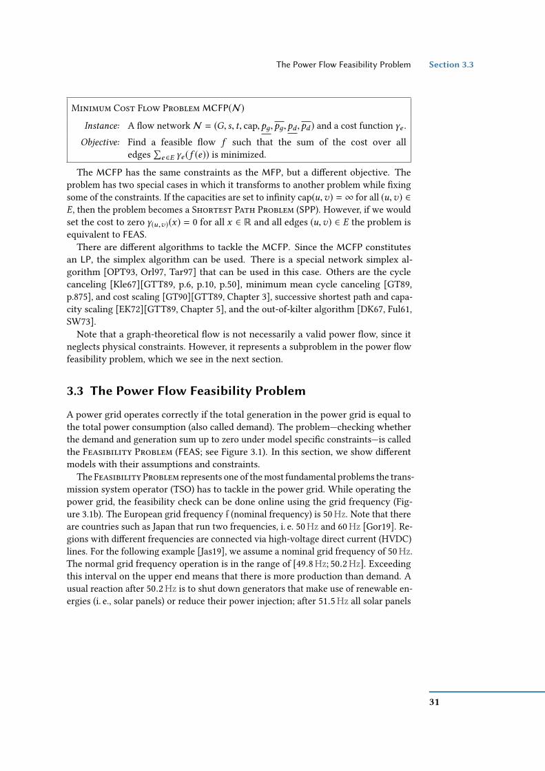
The Power Flow Feasibility Problem Section 3.3
Minimum Cost Flow Problem MCFP(N)
Instance: A ow networkN = (G, s, t, cap,pд,pд,pd ,pd ) and a cost function γe .Objective: Find a feasible ow f such that the sum of the cost over all
edges∑
e ∈E γe (f (e)) is minimized.
The MCFP has the same constraints as the MFP, but a dierent objective. Theproblem has two special cases in which it transforms to another problem while xingsome of the constraints. If the capacities are set to innity cap(u,v) = ∞ for all (u,v) ∈E, then the problem becomes a Shortest Path Problem (SPP). However, if we wouldset the cost to zero γ(u ,v)(x) = 0 for all x ∈ R and all edges (u,v) ∈ E the problem isequivalent to FEAS.
There are dierent algorithms to tackle the MCFP. Since the MCFP constitutesan LP, the simplex algorithm can be used. There is a special network simplex al-gorithm [OPT93, Orl97, Tar97] that can be used in this case. Others are the cyclecanceling [Kle67][GTT89, p.6, p.10, p.50], minimum mean cycle canceling [GT89,p.875], and cost scaling [GT90][GTT89, Chapter 3], successive shortest path and capa-city scaling [EK72][GTT89, Chapter 5], and the out-of-kilter algorithm [DK67, Ful61,SW73].
Note that a graph-theoretical ow is not necessarily a valid power ow, since itneglects physical constraints. However, it represents a subproblem in the power owfeasibility problem, which we see in the next section.
3.3 The Power Flow Feasibility Problem
A power grid operates correctly if the total generation in the power grid is equal tothe total power consumption (also called demand). The problem—checking whetherthe demand and generation sum up to zero under model specic constraints—is calledthe Feasibility Problem (FEAS; see Figure 3.1). In this section, we show dierentmodels with their assumptions and constraints.
The Feasibility Problem represents one of the most fundamental problems the trans-mission system operator (TSO) has to tackle in the power grid. While operating thepower grid, the feasibility check can be done online using the grid frequency (Fig-ure 3.1b). The European grid frequency s (nominal frequency) is 50Hz. Note that thereare countries such as Japan that run two frequencies, i. e. 50Hz and 60Hz [Gor19]. Re-gions with dierent frequencies are connected via high-voltage direct current (HVDC)lines. For the following example [Jas19], we assume a nominal grid frequency of 50Hz.The normal grid frequency operation is in the range of [49.8Hz; 50.2Hz]. Exceedingthis interval on the upper end means that there is more production than demand. Ausual reaction after 50.2Hz is to shut down generators that make use of renewable en-ergies (i. e., solar panels) or reduce their power injection; after 51.5Hz all solar panels
31
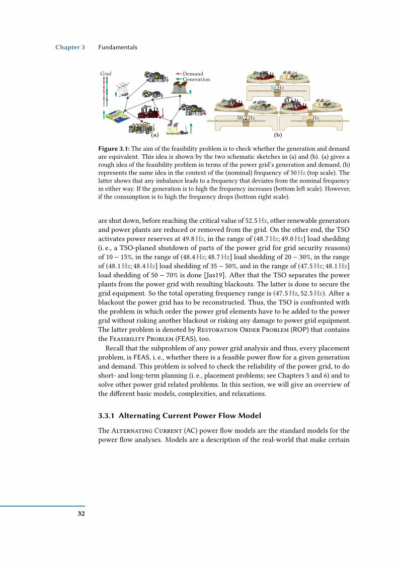
Chapter 3 Fundamentals
(a) (b)
DemandGeneration
Goal
50.2 Hz
50 Hz
49.8 Hz
Figure 3.1: The aim of the feasibility problem is to check whether the generation and demandare equivalent. This idea is shown by the two schematic sketches in (a) and (b). (a) gives arough idea of the feasibility problem in terms of the power grid’s generation and demand, (b)represents the same idea in the context of the (nominal) frequency of 50Hz (top scale). Thelatter shows that any imbalance leads to a frequency that deviates from the nominal frequencyin either way. If the generation is to high the frequency increases (bottom left scale). However,if the consumption is to high the frequency drops (bottom right scale).
are shut down, before reaching the critical value of 52.5Hz, other renewable generatorsand power plants are reduced or removed from the grid. On the other end, the TSOactivates power reserves at 49.8Hz, in the range of (48.7Hz; 49.0Hz] load shedding(i. e., a TSO-planed shutdown of parts of the power grid for grid security reasons)of 10 − 15%, in the range of (48.4Hz; 48.7Hz] load shedding of 20 − 30%, in the rangeof (48.1Hz; 48.4Hz] load shedding of 35 − 50%, and in the range of (47.5Hz; 48.1Hz]load shedding of 50 − 70% is done [Jas19]. After that the TSO separates the powerplants from the power grid with resulting blackouts. The latter is done to secure thegrid equipment. So the total operating frequency range is (47.5Hz, 52.5Hz). After ablackout the power grid has to be reconstructed. Thus, the TSO is confronted withthe problem in which order the power grid elements have to be added to the powergrid without risking another blackout or risking any damage to power grid equipment.The latter problem is denoted by Restoration Order Problem (ROP) that containsthe Feasibility Problem (FEAS), too.
Recall that the subproblem of any power grid analysis and thus, every placementproblem, is FEAS, i. e., whether there is a feasible power ow for a given generationand demand. This problem is solved to check the reliability of the power grid, to doshort- and long-term planning (i. e., placement problems; see Chapters 5 and 6) and tosolve other power grid related problems. In this section, we will give an overview ofthe dierent basic models, complexities, and relaxations.
3.3.1 Alternating Current Power Flow Model
The Alternating Current (AC) power ow models are the standard models for thepower ow analyses. Models are a description of the real-world that make certain
32

The Power Flow Feasibility Problem Section 3.3
assumptions such that we have to explain why the models that we use are reasonablefor the problems that we tackle in this thesis. In this section, we briey introduce anddescribe AC FEAS that describes the power ow in an AC power grid. We start with thedynamic AC model that is a very precise model, but also a very complex model. Notethat most placement problems in power grids are long-term decisions. For long-termscenarios, it is reasonable—since the power grid converges towards a stable state—tomake an assumption such that the AC model becomes time-independent (see Equa-tion 3.7). The time-independent model is called static AC model. Using dierent trans-formations, we derive dierent formulations for AC FEAS shifting the non-convexand non-linear formulas in dierent parts of the system of equations (see Table 3.2).For problems that are long-term decisions these models are good approximations.However, AC FEAS is already NP-hard on star-shaped networks [LGH16]. In thiswork, we focus on high-voltage power grids only, so we can make some assumptionthat lead to a linearization of AC models. The linearization is called DC FEAS, whichwill be described in the next section (Section 3.3.2).
Typically, the theoretical structure of an AC model represents a subproblem ofdierent power grid problems that have to be solved within dierent time rangesdepending on the purpose. For instance, for power grid planning (i. e., TransmissionNetwork Expansion Planning; in short TNEP) the model has to be solved everyyear [COC12], whereas for day-ahead markets the particular model has to be solvedevery day [COC12]. For the AC model there are no known fast and robust solutiontechniques [COC12], which is due to the solver technologies not being able to guaranteeglobal optimality since they get stuck in local optima [Fou96, p.391, Chapter 18].
Dynamic AC Model. The AC power ow in general consists of functions rep-resenting complex current injection i : V × R → C and complex voltages injec-tion v : V ×R→ C at a vertex u ∈ V and timestamp t ∈ R that are sinusoid functionswith amplitude |i | and |v |, respectively, angular frequency ω B dθ/dt (i. e., s being thefrequency; e. g., 50Hz or 60Hz), initial phases for voltage and current θv : V → R
and θ i : V → R, respectively, and complex coecients.The electrical power is dened by complex current i and complex voltage v such
that the complex power s(u, t) is dened by Equation 3.5.
s(u, t) B v(u, t) · i(u, t)? ∀u ∈ V , t ∈ R, (3.5)
where i(u, t)? is the complex conjugate of the current. Since we use the complexconjugate of the current, we get the relationship between voltage and current (seealso Figure 3.2) that is the dierence between the voltage angle θv and the currentangle θ i meaning θv − θ i (see Equation 3.7). The latter dierence is also called power
angle. Thus, the function that represents the complex power injection is denedby s : V × R → C. The real and imaginary part of a complex number z ∈ C is
33

Chapter 3 Fundamentals
v is
π2
π 3π2
2π
−1
1
ωt
v(u, t), i(u, t), s(u, t)
0
π4
π23π
4
π
5π4 3π
2
7π4
.8 1v
i
θv − θi
θv− θi
|v| |i|
Im
Re|s|VRMS
IRMS
Figure 3.2: The left side of the gure presents voltage v(u, t), current i(u, t), and total in-stantaneous electric power s(u, t) in terms of trigonometric function for timestamp t ∈ R
and vertex u ∈ V . The Argand diagram is shown on the right side of the gure, where volt-age v(u, t) and current i(u, t) are described by polar coordinates. The current i(u, t) is shiftedby π/2 to the right of voltage v(u, t) (i. e., voltage acts as reference point). The shift betweenvoltage v(u, t) and current i(u, t) by θv − θ i is also called power angle. In the right diagram attimestamp t = 0 the voltage vector v(u, t) completes a full cycle (i. e., a time period), whereasthe current vector i(u, t) is on the negative imaginary axis and thus, lags behind the voltagevector v(u, t) by π/2. An inductive load could be a cause of that particular shift, since thevoltage v(u, t) leads the current i(u, t). The product of voltage v(u, t) and current i(u, t) isequivalent to the total instantaneous electric power s(u, t). Note that the magnitude of thetotal instantaneous electric power corresponds to the product of the root-mean-squared (RMS)of the voltage magnitude |v(u)| denoted by VRMS(u) and the current magnitude |i(u)| denotedby IRMS(u). The derivation of this gure can be found in Appendix B.1.
denoted by Re(z) and Im(z), respectively. The voltage magnitude |v(u)| (Equation 3.6)represents the wave crest (see left side of Figure 3.2) at vertex u ∈ V .
|v(u)| =
√Re(v(u, t))2 + Im(v(u, t))2. (3.6)
The current magnitude |i(u)| is dened accordingly to Equation 3.6. The voltageand current magnitude are time independent, since Equation 3.6 can be written us-ing trigonometric function |v(u)|·
√cos2(θv (u) + ωt) + sin2(θv (u) + ωt), where the
Pythagorean identity√cos2(θv (u) + ωt) + sin2(θv (u) + ωt) = 1 follows from the com-
plex plane representation.The idea behind this is that the assumption of time-invariance results in an un-
changing (i. e., constant) wave crest over time. If we assume that all functions aretime-invariant—having the same behavior for the same input at any timestamp, i. e., theangular frequency dθ/dt = 2π s is constant—then we call them current and voltage pha-sors. This allows us to use the phasor transform of Charles Proteus Steinmetz [RM12,YL08] such that we can use simple algebraic equations on the phasors instead of dier-ential equations of the sinusoid signals. Note that the assumption of time-invariancemight be acceptable for some power ow analyses and planning problems. However,for smaller periods of time such as the inuence of switching processes on the grid
34

The Power Flow Feasibility Problem Section 3.3
stability this assumption might not be suitable anymore. However, then we get intothe range of dynamic analyses [Roh+12, Str18, TC14a, Tim18].
We get the trigonometric relationship depicted in Equation 3.7. The derivation canbe found in Equation B.2.s(u, t) = v(u, t) · i(u, t)? (3.7a)
= Re(v(u, t)) · Re(i(u, t)) + Im(v(u, t)) · Im(i(u, t))︸ ︷︷ ︸Cp(u)
− j ·(Re(v(u, t)) · Im(i(u, t)) − Im(v(u, t)) · Re(i(u, t))
)︸ ︷︷ ︸Cq(u)
(3.7b)
= |v(u)| |i(u)|(cos
(θv (u) + ωt − θ i (u) − ωt
)+ j · sin
(θv (u) + ωt − θ i (u) − ωt
) )(3.7c)
= |v(u)| |i(u)| cos(θv (u) − θ i (u)
)︸ ︷︷ ︸=p(u)
+ j · |v(u)| |i(u)| sin(θv (u) − θ i (u)
)︸ ︷︷ ︸=q(u)
(3.7d)
Note that we have to use the root-mean-squared (RMS) values in Equation 3.7c,since |v(u)| |i(u)| would lead in a magnitude that is twice as high as of v(u, t) · i(u, t)?,which is graphically illustrated in Figure 3.2. To illustrate the time-varying powerin Figure 3.2, we use the concept of instantaneous electric power (see Appendix B.1),since the complex power becomes time-independent in Equation 3.7 and thus, constant.To illustrate the signals of the complex power a common way is to use the real part ofa signal (in our case the real part of the current i and voltage v , see Appendix B.1 formore details).
The penultimate step in Equation 3.7 follows from the trigonometric addition andproduct formulas. In the last step, the complex power equation becomes independentfrom time t and angle frequency ω. The intuition behind this is that in an ideal ACnetwork we start with the initial phase angles θv and θ i , but the angular frequencystays constant meaning ω B dθ/dt = 2π s. Thus, the rotation velocity is the same forboth current and voltage. This simplies the system such that it only depends onthe initial phases (see Figure 3.2) and leads to a static analysis by using the resultingtime-independent models that are also called static models.
Static AC Models. For general cases a common way to analyze power grids is touse a constant angular frequency and analyze steady-state power grids that have onexed timestamp per analysis. This will be our main focus in this work. However, theidealization of the angular frequency to a constant is not suitable for certain scenarios,as mentioned above. For this work it means that all previous functions f becometime-independent f : S → F , where F is a eld and S is the set we do the mappingfrom such that for example the voltage function becomes v : V → R.
Equation 3.7c can be rewritten to s(u) B |v(u)| |i(u)|e j·(θv (u)−θ i (u)) using Euler’s
formula. The functions p : V → R and q : V → R represent the real and the reactive
35

Chapter 3 Fundamentals
(b)
(d)(c)
π2
π 3π2
2π
−1
1
ωt
v(u, t), i(u, t), s(u, t), p(u, t), q(u, t)
p(u)
q(u)
VRMSIRMS
(a)
iv
q
ps
π2
π 3π2
2π
−1
1
ωt
v(u, t), i(u, t), s(u, t), p(u, t), q(u, t)
VRMSIRMS
iv
q
ps
π2
π 3π2
2π
−1
1
ωt
v(u, t), i(u, t), s(u, t), p(u, t), q(u, t)
VRMSIRMS
iv
q
p s
π2
π 3π2
2π
−1
1
ωt
v(u, t), i(u, t), s(u, t), p(u, t), q(u, t)
VRMSIRMS
iv
q
p s
p(u)q(u)
q(u)p(u) q(u)
p(u)
Figure 3.3: The time varying sinusoid curves of voltage v(u, t) with magnitude |v(u)| = 1and eective value VRMS(u) = 1/
√2, current i(u, t) with magnitude |i(u)| = 0.8 and eective
value IRMS(u) = 0.8/√2, total instantaneous electric power s(u, t), its real part p(u, t), and its
imaginary part q(u, t) are given for dierent voltage angle dierences ∆θv . The voltageangle dierences are (a) ∆θv = π/4, (b) ∆θv = −π/2, (c) ∆θv = 3π/4, and (d) ∆θv = π . Thetotal instantaneous electric power s(u, t) is the sum of the real part p(u, t) and the imaginarypart q(u, t) of the power. The same behavior is shown for the complex power s(u) and its realpower p(u) and reactive power q(u). (a) A stable case is represented that is an operation ofcurrent i and voltage v within an angle shift of [−π/2; π/2]. (b) One of the stability bordersis −π/2, where the real part of the total instantaneous electric power s(u, t) is zero over time t .(c) With a voltage angle dierence of 3π/4 the power is within the instable section. All powercurves are in the negative part. (d) The current i(u, t) and voltage v(u, t) waves are in a state,where the waves cancel each other out. The reactive part of the total instantaneous electricpower curve is zero and the real power part is negative. The derivation of this gure can befound in Appendix B.1.
power, respectively. This equation shows very clearly the current angle θ i and voltageangle θv that describe the real and reactive power on each edge. Figure 3.2 shows therelationship of current i and voltage v . The dierence between voltage and currentis the phase angle dierence. The more we increase the phase angle dierence (e. g.,see Figure 3.3 on Page 36) between current and voltage the smaller the real powergets until a certain point (see Figure 3.3b), where the real power becomes zero. Thecase, where the wave crests of voltage and current cancel each other out is shownin Figure 3.3d. Note that the reactive power (also known as phantom power) increaseswhile the real power decreases, since current and voltage amplitudes do not decrease.The latter basically describes the principle of conservation of energy. The described
36

The Power Flow Feasibility Problem Section 3.3
relationship between voltage, current, and power can be used to maintain the voltagestability by changing real power demands. A decrease in real power demand can bemaintained by an increase in reactive power by changing the phase angle dierencebetween voltage and current. This mechanism helps to maintain voltage on a certainlevel.
The complex power injection can be written in terms of real and reactive powerinjection that represent decoupled parts (see Equation 3.8 and its derivation in Equa-tion 3.7).
s(u) = Re(s(u)) + j · Im(s(u)) = p(u) + j · q(u) ∀u ∈ V . (3.8)
This relationship is shown in Figure 3.3, where the total instantaneous power s(u, t)(respectively complex power s(u)) is the sum of the real part p(u, t) and imaginarypart q(u, t) of the power (respectively real power p(u) and reactive power q(u)). Thetotal instantaneous power curve s(u, t) (respectively complex power s(u)) has the samemagnitude independent of the power angle. The latter emphasize the principle ofconservation of energy.
The real power p is the power that is actually doing work such as heating. However,reactive power is seldom consumed by consumers. Exceptions are motors, generatorsand transformers that use a magnetic eld (inductive components) of industrial con-sumers that need reactive power. In general reactive power is used to maintain thevoltage stability. Increasing the amount of reactive power increases the voltage thathas to be kept in a certain range. So reactive power is necessary for the power grid tohave a more ecient real power ow. The stability of the power grid is maintainedby a balance between real and reactive power and the latter depends highly on theconsumed real power.
We usually do a vertex-based analysis meaning that ows are usually modeled bydisturbance and injection at a vertex. We introduced for each vertex eight variablesdenoted bypд(u), qд(u), pd (u), qd (u),v(u), i(u), θv (u), and θ i (u) for allu ∈ V . However,we can always reformulate current i and current angles θ i in terms of voltage v andvoltage angle θv using Ohm’s law and thus, we have just six variables. We will see laterthat depending on the vertex type (see Table 3.1) or on the problem some variables aregiven and thus, xed to a certain value.
Up to now, we just looked at the power injections and not the power ows. However,the complex, real, and reactive power ow, as well as the complex current ow aredened by the functions s : E → C (in Volt Ampere; short VA), p : E → R (in W),q : E → R (in Volt Ampere Reactive; short VAr), and i : E → C (in Ampere; short A),respectively. We distinguish between the injection at the source and sink vertex ofeach edge, since there are power losses at each electrical element.
Network Parameters. The AC network N = ( G = (V , E), VG , VD , cap, r , x , b, д,∆θv , ∆θv , v , v , pд , pд , qд , qд , pd , pd , qd , qd ) is dened by the topological structure
37

Chapter 3 Fundamentals
(a)
NeutronsProtonesElectrons Og
Oganesson
118
RnRadon
86
XeXenon
54
KrKrypton
36
ArArgon
18
NeNeon
10
HeHelium
2
FFluorine
9
ClChlorine
17
BrBromine
35
IIodine
53
AtAstatine
85
TsTennessine
117Lv
Livermorium
116
PoPolonium
84
TeTellurium
52
SeSelenium
34
SSulfur
16
OOxygen
8N
Nitrogen
7
PPhosphorus
15
AsArsenic
33
SbAntimony
51
BiBismuth
83
McMoscovium
115Fl
Flerovium
114
PbLead
82
SnTin
50
GeGermanium
32
SiSilicium
14
CCarbon
6B
Boron
5
AlAluminium
13
GaGallium
31
InIndium
49
TlThallium
81
NhNihonium
113
ZnZinc
30
CdCadmium
48
HgMercury
80
CnCopernicium
112
CuCopper
29
AgSilver
47
AuGold
79
RgRoentgenium
111Ds
Darmstadtium
110
PtPlatinum
78
PdPalladium
46
NiNickel
26CoCobalt
25
RhRhodium
45
IrIridium
77
MtMeitnerium
109
FeIron
26
RuRuthenium
44
OsOsmium
76
HsHassium
108
MnManganese
25
TcTechnetium
43
ReRhenium
75
BhBohrium
107
CrChromium
24
MoMolybdenum
42
WTungsten
74
SgSeaborgium
106Db
Dubnium
105
TaTantalum
73
NbNiobium
41
VVanadium
23Ti
Titanium
22
ZrZirconium
40
HfHafnium
72
ScScandium
107
YYttrium
39
La-LuLanthanides
57-71
Ac-LrActinides
89-103Ra
Radium
88
BaBarium
56
SrStrontium
38
CaCalcium
20
MgMagnesium
12
BeBeryllium
4
HHydrogen
1
LiLithium
3
NaSodium
11
KPotassium
19
RbRubidium
37
CsCesium
55
FrFrancium
87Rf
Rutherfordium
104
LuLutetium
71
LrLawrencium
103No
Nobelium
102
YbYtterbium
70Tm
Thulium
69
MdMendelevium
101Fm
Fermium
100
ErErbium
68Ho
Holmium
67
EsEinsteinium
99Cf
Californium
98
DyDysprosium
66Tb
Terbium
65
BkBerkelium
97CmCurium
96
GdGadolinium
64Eu
Europium
63
AmAmericium
95Pu
Plutonium
94
SmSamarium
62Pm
Promethium
61
NpNeptunium
93U
Uranium
92
NdNeodymium
60Pr
Praseodymium
59
PaProtactinium
91Th
Thorium
90
CeCerium
58La
Lanthanum
57
AcActinium
89
Al: (2, 8, 3)
Au: (2, 8, 18, 32, 18, 1)Ag: (2, 8, 18, 18, 1)Cu: (2, 8, 18, 1)
Ne: (2, 8)He: (2)
(b)
Figure 3.4: Both (a) and (b) represent the atomic structure of one element and of multipleelements, respectively. The conductivity is dependent on the outermost shell denoted byvalence shell. (a) The copper-29 isotope that has fully lled electron shells, but the valenceshell (outermost shell). The valence shell has just one electron that is highly reactive. (b) Partof the description of the atomic structure of elements. The green marked elements representcommon conductors and the red marked elements are strong insulators that are all in the lastcolumn.
that is given by the graph G = (V , E), the set VG ⊆ V of generators, the set VD ⊆ V ofconsumers, the resistance function r : ←→E → R≥0∪∞, the reactance functionx : ←→E →R≥0 ∪ ∞, the susceptance function b : ←→E → R (Equation 3.12), the conductancefunctionд : ←→E → R (Equation 3.11), the admittance functiony : ←→E → C (Equation 3.9),and the apparent power’s thermal line limit function cap : ←→E → R, which can beeither i, s,p, or q, and combinations of them. The resistance r and the reactance xare measured in Ohm Ω. The admittance y(u,v) (Equation 3.9) is dened by theconductance д(u,v) (Equation 3.11) and the susceptance b(u,v) (Equation 3.12) thatdenes how easy the current is able to ow through an element such as a transmissionline u,v ∈ ←→E . Note that all three are measured in Siemens S. The conductivity ofan electrical element is mainly inuenced by the conductance of the material, length,and wire gauge. The conductance of the material is mainly inuenced by the atomicstructure (see Figure 3.4). Elements that have just one electron on the valence shell (i. e.,outermost shell) have a high conductivity such as copper, gold, and silver (Column 11 ofthe periodic system; see Figure 3.4b green markers). However, elements that have a fullvalence shell are very good insulators since the conductivity is very low, e. g., helium(last column of the periodic system; see Figure 3.4 red markers). The admittance y,
38

The Power Flow Feasibility Problem Section 3.3
impedance z, conductance д, and susceptance b are dened in Equations 3.9–3.12.
y(u,w) B1
z(u,w)= д(u,w) + j · b(u,w) ∀u,w ∈
←→E , (3.9)
z(u,w) =1
y(u,w)= r (u,w) + j · x(u,w) ∀u,w ∈
←→E , (3.10)
д(u,w) Br (u,w)
r (u,w)2 + x(u,w)2∀u,w ∈
←→E , (3.11)
b(u,w) B −x(u,w)
r (u,w)2 + x(u,w)2∀u,w ∈
←→E . (3.12)
Note that the admittance matrixY is dened by the self-admittances representing thediagonal entries y(u,u) = y(u, 0) −
∑u ,w ∈
←→E y(u,w), where y(u, 0) is the admittance
to ground, and the entries of Equation 3.9 that represent the entries for the incidentedge.
Power Grid Bounds. There are lower and upper bounds restricting the voltageangle dierences ∆θv and ∆θv , the voltages v and v , the real power generation pд , pд ,the reactive power generation qд , qд , the real power demand pd , pd , and the reactivepower demand qd , qd , respectively. The constraint of the voltage angle dierence(Equation 3.13) restricts the power ow on each edge (Equation 3.7).
∆θv (u,w) ≤ θv (u) −θv (w) ≤ ∆θv (u,w), (3.13a)
∆θv (u,w) ≤ arctan(Im(v(u))
Re(v(u))
)− arctan
(Im(v(w))
Re(v(w))
)≤ ∆θv (u,w), (3.13b)
for all u,w ∈ ←→E . In Equation 3.13b, we use the trigonometric relationship ofthe real part Re(v(u)) and imaginary part Im(v(u)) that is dened by tan
(θv (u)
)=
adjacent/opposite = Im(v(u))/Re(v(u)) = sin(θv (u)
)/cos
(θv (u)
). The voltage angle dierence is
often restricted to the interval of [−π/2; π/2] for stability reasons (see Figure 3.3 fordierent voltage angle dierences). If the balance between real power generation anddemand cannot be maintained (i. e., is not zero), then there is an issue in the anglestability, i. e., the voltage angle dierence cannot be maintained within the stabilityinterval. This in particular means the smaller the angle dierence the more balancebetween real power generation and demand exists. This is due to the fact that thereactive power is used to compensate the lack of real power generation and demandby shifting voltage and current using devices such as capacitor banks. Figure 3.3explains why exceeding the π/2 would lead to instabilities in the power grid. Notethat mainly generators are able to inuence the voltage, power curves, and the powerangle (see Table 3.1). Thus, the network stability is mainly driven by generators(including devices such as capacitor banks). If the power angle exceeds the stability
39

Chapter 3 Fundamentals
range the power curves shift into the negative quadrant and the eective powervalues are negative, too (see Figure 3.3b–d). However, a power grid has a predenedow direction and a negative real power can be interpreted as a “backward powermovement” (see Figure 3.3a). A rough idea of the latter is given by a simple DC circuitwith a preinstalled diode. Note that a diode has a predened direction making thenetwork nonreciprocal. The predened direction denes the anode and cathode forthe battery connection. Connecting the battery in the wrong sense would lead to adiode that does not ash.
In addition, the smaller the shift the less losses and the more stable the power gridworks. In Section 3.3.4, we will see that the dierences are often smaller than π/6.However, the voltage angle dierence ∆θv also correlates with the real power thatows from one vertex to another over the power grid. The relationship becomes muchclearer if we look at the linearization of the AC model in Section 3.3.2.
In some literature there is a constraint restricting the voltage angles θv (u) forall u ∈ V themselves (see Equation 3.14).
θv (u) ≤ θv (u) ≤ θv (u) ∀u ∈ V . (3.14)
The latter restricts the solution space and might exclude feasible solutions, but doesnot represent a physical constraint. However, it improves the running times to solvethe feasibility problem and to fulll assumptions such as the stability range or laterthe Assumption 2 in Section 3.3.2.
The voltage magnitude is bounded by either Equation 3.15a, or by Equation 3.15band Equation 3.15c depending on the formulation that is either polar or rectangular,respectively.
|v(u)| ≤ |v(u)| ≤|v(u)| , (3.15a)v(u)2 ≤ Re(v(u))2 + Im(v(u))2 , (3.15b)
Re(v(u))2 + Im(v(u))2 ≤ v(u)2, (3.15c)
for all vertices u ∈ V . This is mainly motivated by the power grid elements that workwithin a certain voltage range. Most elements perform poorly on the lower voltageend—e. g., inductive motors overheat—and on the upper end the elements can getdestroyed. The thermal line limits can be represented in dierent ways that mainlydepend on the formulation. If the formulation uses current and voltage, Equations 3.16aand 3.16b are used. Otherwise, if it uses real power, reactive power, and voltage angles,Equations 3.16c and 3.16d are used.
i(u,w) ∈ C | Re(i(u,w))2 +Im(i(u,w))2 ≤ i(u,w)2, (3.16a)|i(u,w)| ≤ i(u,w), (3.16b)
s(u,w) ∈ C | Re(s(u,w))2+Im(s(u,w))2 ≤ s(u,w)2, (3.16c)|s(u,w)| ≤ s(u,w), (3.16d)
40

The Power Flow Feasibility Problem Section 3.3
for all (u,w) ∈ E. Note that these constraints are convex and quadratic as the geometricgure of its boundary is a closed disk. In addition, the reactive power might increasethe voltage stability, but it also consumes bandwidth of the transmission line capacity.Thus, to maximize the throughput of real power in the power grid the reactive powerhas to be minimized such that the voltage stays in its range. Note that increasing thereal power decreases the losses.
The power injection constraints basically constrain the injection (Equations 3.17aand 3.17b) or demand (Equations 3.17c and 3.17d) of a vertex depending on it being agenerator or demand, respectively.
pд(u) ≤ pд(u) ≤ pд(u) ∀u ∈ VG , (3.17a)
qд(u) ≤ qд(u) ≤ qд(u) ∀u ∈ VG , (3.17b)
pd (u) ≤ pd (u) ≤ pd (u) ∀u ∈ VD, (3.17c)
qd (u) ≤ qd (u) ≤ qd (u) ∀u ∈ VD . (3.17d)
The losses heavily depend on the voltage level (Figure 1.1) and the amount of realpower that ow through an element.
Real powerp and voltage angles θv strongly depend on each other, as well as reactivepowerq and voltage magnitudes |v | (see Section 3.3.2 Assumption 3 with Equation 3.31).The P-θv and Q-V problems are weakly dependent on each other. Thus, the ACpower ow is usually solved in a decoupled way (see for example [Gao+18]). This isreasonable if we follow the assumption that phase angle dierences ∆θv (u,v) are smalland high-voltage transmission lines are mainly reactive meaning r (u,v) x(u,v) forall u,v ∈ ←→E (note that the latter relationship is used in Assumption 1 in Section 3.3.2).The approach separates both subproblems and iterates between them. The decoupledversion decouples the AC power ow into two separate problems. However, the full ACpower ow includes both problems without these assumptions.
Assuming that the demands are xed, then out of the six variables ∆θv ,v,pд,qд,pd ,and qd only four remain. Each vertex species a certain type that is denoted by vertex
type that actually denes which variables are xed. The common vertex types areshown in Table 3.1. In Chapter 4, we describe the mathematical structure and rela-tionship of the linearized AC model. Within that structure it becomes obvious whywe chose exactly one vertex per connected component as slack vertex. The basic ideais that a slack vertex represents a reference for the voltage angles of the system andthus, choosing a voltage angle for that vertex denes the voltage angles for all others.In Table 3.1 there are exactly two types that are able to work as slack vertex that aredenoted by slack, or slack demand. The PQ vertices are vertices without generationand thus are, pure demand vertices. The PV is separated into two classes that areboth able to control voltage by adjusting the reactive power within certain limits byeither controlling the reactive power generation or demand. A source of reactive
41
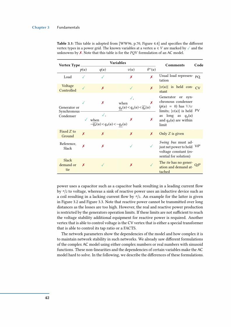
Chapter 3 Fundamentals
Table 3.1: This table is adopted from [WW96, p.70, Figure 4.4] and species the dierentvertex types in a power grid. The known variables at a vertex u ∈ V are marked by X and theunknowns by 7. Note that this table is for the PQV formulation of an AC model.
Vertex Type Variables Comments Codep(u) q(u) v(u) θv (u)
Load X X 7 7 Usual load represen-tation
PQ
VoltageControlled X 7 X 7 |v(u)| is held con-
stantCV
Generator orSynchronousCondenser
X 7X,
whenqд(u)<qд(u)<qд(u)
7
Generator or syn-chronous condenser(p(u) = 0) has VArlimits; |v(u)| is heldas long as qд(u)and qd (u) are withinlimit
PV
XX,
when−qd (u)<qd (u)<−qd (u)
7 7
Fixed Z toGround 7 7 7 7 Only Z is given
Reference,Slack 7 7 X X
Swing bus must ad-just net power to holdvoltage constant (es-sential for solution)
Vθ v
Slackdemand or
tie7 X 7 X
The tie has no gener-ation and demand at-tached
Qθ v
power uses a capacitor such as a capacitor bank resulting in a leading current owby π/2 to voltage, whereas a sink of reactive power uses an inductive device such asa coil resulting in a lacking current ow by π/2. An example for the latter is givenin Figure 3.2 and Figure 3.3. Note that reactive power cannot be transmitted over longdistances as the losses are too high. However, the real and reactive power productionis restricted by the generators operation limits. If these limits are not sucient to reachthe voltage stability additional equipment for reactive power is required. Anothervertex that is able to control voltage is the CV vertex that is either a special transformerthat is able to control its tap ratio or a FACTS.
The network parameters show the dependencies of the model and how complex it isto maintain network stability in such networks. We already saw dierent formulationsof the complex AC model using either complex numbers or real numbers with sinusoidfunctions. These non-linearities and the dependencies of certain variables make the ACmodel hard to solve. In the following, we describe the dierences of these formulations.
42

The Power Flow Feasibility Problem Section 3.3
Polar and Rectangular Formulations. In the previous part, we could see thedierent formulations of the voltage angle dierences and the power grid bounds.Depending on which formulation we choose, we shift the complexity of the AC modelto dierent parts as shown in Table 3.2. We distinguish between the rectangular andthe polar formulation of the complex terms.
The polar formulation is given by the magnitude (i. e., length of the vector) and theangle of its vector. We represented the complex power in its polar form in Equation 3.7d,where |v(u)| is the voltage magnitude (also known as voltage amplitude) and θv (u)represents the corresponding voltage angle. Contrary to that, the rectangular form ofa complex number is given by the real Re(·) and imaginary part Im(·) of the complexnumber representing the horizontal (x-axes) and vertical (y-axis) components in theArgand diagram (i. e., geometric interpretation of a complex number; see Equation 3.7band Figure 3.2 right side). In addition to that we are able to reformulate the power owto calculate it in terms of real powerp, reactive powerq, and voltagev . This formulationis often denoted as PQV model (see Equations B.5 and B.6). Another alternativeis the IV model that formulates the AC model in terms of current i and voltage v(see Equations B.7 and B.8). We already saw parameter-dependent formulations in thepower grid bounds part.
Note that the literature standard is the polar PQV model [WW96, ZM11] (see Equa-tion B.5).
PQV Formulations. The complex power injection at a vertex was introducedin Equation 3.7d using voltage and current as unknowns, which is denoted as IVformulation. However, the formula can be restated to a complex power ow on anedge by introducing the relationship that the current on an edge is dened by i(u,w) By(u,w) ·
(v(w) −v(u)
)for all (u,w) ∈ E. Using this relationship we get Equation 3.18
in its rectangular formulation. The derivation can be found in Equation B.3.
s(u,w) = v(u) · i(u,w)? (3.18a)= v(u) · y(u,w)? ·
(v(w)? −v(u)?
)(3.18b)
= д(u,w)(Re(v(u)) Re(v(w)) + Im(v(u)) Im(v(w)) − Re(v(u))2 − Im(v(u))2
)+b(u,w)
(Re(v(w)) Im(v(u)) − Re(v(u)) Im(v(w))
) C p(u,w)
+j ·(д(u,w)
(Re(v(w)) Im(v(u)) − Re(v(u)) Im(v(w))
)+b(u,w)
(Re(v(u))2 + Im(v(u))2 − Re(v(u)) Re(v(w)) − Im(v(u)) Im(v(w))
) ) C q(u,w)
(3.18c)
for all (u,w) ∈ E. The rectangular Equation 3.18c has only quadratic terms. It ispossible to decompose the equation into the real and reactive part of the complex power,which we already saw in Equations 3.7d and 3.8. The real part can be transformed into
43

Chapter 3 Fundamentals
the polar form (see Equation 3.19).
p(u,w) = д(u,w)(|v(u)| |v(w)| cos
(θv (u) − θv (w)
)− |v(u)|2
)+ b(u,w)|v(u)| |v(w)| sin
(θv (u) − θv (w)
) (3.19a)
Similar, the reactive part can be transformed into the polar form (see Equation 3.20).
q(u,w) = д(u,w)|v(u)| |v(w)| sin(θv (u) − θv (w)
)− b(u,w)
(|v(u)| |v(w)| cos
(θv (u) − θv (w)
)− |v(u)|2
) (3.20a)
The disadvantage of the polar formulations of the real and reactive power in Equa-tions 3.19 and 3.20 are the quadratic terms of the voltages and the trigonometricfunctions of the voltage angle dierences.
IV Formulation. The KCL describes the ow of current at a vertex (see Equa-tion 3.21). It states that the net ow of current at each vertex is equal to zero that issimilar to the graph-theoretical conservation of ow shown in Equation 3.1.
i(u) B∑
w : u ,w ∈←→E
i(u,w) ∀u ∈ V . (3.21)
The complex current can be restated in terms of voltages using Ohm’s law. This isshown in Equation 3.22 that is a linear function of complex voltages.
i(u) = y(u, 0) · v(u) +∑
w : u ,w ∈←→E |u,w
(y(u,w)(v(w) −v(u))︸ ︷︷ ︸
Ci(u ,w )
)∀u ∈ V (3.22)
The current injection i(u) at a vertexu ∈ V is described by the voltage to ground—usingadmittance to ground y(u, 0)—and the current-based net ow. Note that the voltageto ground represents disturbances at the vertex. The complex current ow can berewritten into two decoupled parts representing the real and imaginary part of thecomplex current ow of an edge (u,w) ∈ E (see Equation 3.23). The derivation can befound in Equation B.4.
i(u,w) =(д(u,w) + j · b(u,w)
) (v(w) −v(u)
)=
(д(u,w) + j · b(u,w)
) (Re(v(w)) + j · Im(v(w)) − Re(v(u)) − j · Im(v(u))
)= д(u,w)
(Re(v(w)) − Re(v(u))
)− b(u,w)
(Im(v(w)) − Im(v(u))
)︸ ︷︷ ︸CRe(i(u ,w ))
+
j ·(
д(u,w)(Im(v(w)) − Im(v(u))
)+ b(u,w)
(Re(v(w)) − Re(v(u))
)︸ ︷︷ ︸CIm(i(u ,w ))
)(3.23)
44

The Power Flow Feasibility Problem Section 3.3
More generally, we can write the problem of checking whether generation and con-sumption agree as AC FEAS, which decision problem depends on the formulation(see Table 3.2) and is dened in the following problem box.
Alternating Current Feasibility Problem AC FEAS(N)
Instance: An AC network N = (G = (V , E), VG ,VD , cap, r , x , b, д, ∆θv , ∆θv , v ,v , pд , pд , qд , qд , pd , pd , qd , qd ) .
Question: Is there a feasible electrical ow complying with one of these modelconstraints in Table 3.2?
Summarizing the AC FEAS problem is a non-linear non-convex problem that isunder the assumption of time-invariance a model that is a good approximation to arealistic power grid. Furthermore, it represents a subproblem of all problems that havethe power grid as an input.
Lehmann et al. [LGH16] discuss that the decoupled AC power ow model is weaklyNP-hard on trees (stars). It represents a stronger result in terms of graph classes, butincludes real and reactive power as decoupled formulation. An outline of the proof isgiven by Lavaei and Low [LL12].
Normalization. Note that for the power ow analysis it is common to normalizethe system using the per-unit-system (p.u.). The normalization is done for the complexpower, real power, reactive power, and voltage using the base units Sbase, Pbase, Qbase,and Vbase, respectively. The other units can be normalized by the bases derived fromthe previous power and voltage base such that Ibase = Sbase/Vbase, Zbase = Vbase/Ibase,and Ybase = 1/Zbase.
45

Chapter
3Fundam
entals
Table 3.2: This table is inspired by Cain et al. [COC12] from FERC that analyzed AC OPF and compares the dierent AC models. Thecolumns represent dierent constraint types that are related with the network ow, voltage angle dierences, and vertices. For eachformulation, the property describes the complexity of the constraint and the Ref. represents the equation’s reference number either in thischapter or for some of the complete models in the appendix.
Constraints
Polar Rectangular DC
PQV IV PQV IV
Property Ref. Property Ref. Property Ref. Property Ref. Property Ref.
Network Flow
Quadraticequation andtrigonomet-ric functions
3.19,3.20.
Quadraticequation andtrigonometricfunctions
basedon
3.22,3.23.
Quadraticequations 3.18c. Linear
constraints
3.21,3.22,3.23.
Linearequations 3.37
Voltage AngleDierence ∆θv
Linearconstraints 3.13a. Linear
constraints 3.13a.
Non-convexconstraintswith trigono-metric func-tions
3.13b.
Non-convexconstraintswith trigono-metric func-tions
3.13b. Linearconstraints 3.38.
Vertices &Edges
Linearconstraints
3.15a,3.17.
Linearconstraints
3.15a,3.16a,3.16b,3.7dineq.
Quadraticinequali-ties (somenon-convex)
3.15b,3.15c,3.7bwith3.16a.
Quadraticinequali-ties (somenon-convex)
3.15b,3.15c,3.16b.
Linearconstraints
3.33–3.36
Models Equation B.5 Equation B.7 Equation B.6 Equation B.8 Equations 3.33–3.38
46

The Power Flow Feasibility Problem Section 3.3
(b)(a)
j bch2 j bch
2
i(u) i(w)
v(u) v(w)
y = 1r+jx = z
j bch2 j bch
2
i(u) N · i(u)
N = τejθvshift
i(w)
v(u)N
|N | : 1
v(u) v(w)
y = 1r+jx = z
Figure 3.5: The Pi-equivalent circuit represents a model of a transmission line with mediumlength. Note that this gure is partly adopted from Zimmerman and Murillo-Sanchez [ZM11,p.17, Figure 3-1]. (a)&(b) The two capacitors model the transmission line charging bch, theimpedance z models the resistive behavior of a transmission line (red). (b) If the line representsa phase shift transformer then the transformer is modeled on one of the two end vertices (blue).The transformer (blue) is usually modeled at the vertex with the primary coil with a x tapratio τ and in that particular case with a x phase shift angle θvshi. The voltage v and current ichange with respect to the number of windings |N | on the side of the secondary coil.
Transmission Line Representation. We use transmission line representations(also known as branch or transmission line models) to simplify the power ow analysisto a purely vertex-based analysis using the admittances between adjacent vertices(see Equations 3.18b and 3.22).
For the model formulation of the previous part of this section, we used a single linemodel and considered a transmission line model that is denoted by short transmission
line representation that neglects shunt elements such as the shunt capacitance bchrepresenting the charging of a line (see Figure 3.5). The short transmission linerepresentation approximates lines that are up to 80 km long by using a similar modelas the RLC circuit, meaning resistance, impedance, and capacitance are in series (seealso Kirchho’s 3rd postulate [SR61, p.127]). Note that the assumption for the shorttransmission line representation is reasonable, since the line charging is negligible.Within the AC model terminology, we often model the shunt conductance and shunt
susceptance as elements connected to the vertices. These elements are purely model-based theoretical elements used to model elements such as transmission lines orsynchronous condensers. Depending on which transmission line representation isused, the shunt elements are included or not.
For high voltage power grids it is more common to model the transmission linesusing the medium line approximation that includes a lumped shunt admittance. Thereare two dierent models denoted by pi representation (see Figure 3.5(a)) and T represen-
tation. Wood and Wollenberg [WW96, p.75] and applications such as Matpower [ZM11,pp.16.] and Pypower [Lin11] use the pi representation. However, there is much moreinvestigation in this topic as can be seen by Cano et al. [Can+17], who introducedierent transmission line representations. Note that the standard pi representation
47
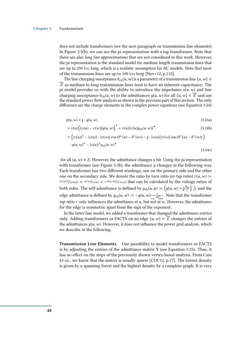
Chapter 3 Fundamentals
does not include transformers (see the next paragraph on transmission line elements).In Figure 3.5(b), we can see the pi representation with a tap transformer. Note thatthere are also long line approximations that are not considered in this work. However,the pi representation is the standard model for medium length transmission lines thatare up to 250 km long, which is a realistic assumption for AC models. Note that mostof the transmission lines are up to 100 km long [Nov+12, p.112].
The line charging susceptancebch(u,w) is a parameter of a transmission line u,w ∈←→E as medium to long transmission lines tend to have an inherent capacitance. Thepi model provides us with the ability to introduce the impedance z(u,w) and linecharging susceptance bch(u,w) to the admittances y(u,w) for all u,w ∈ ←→E and usethe standard power ow analysis as shown in the previous part of this section. The onlydierence are the charge elements in the complex power equations (see Equation 3.24).
p(u,w) + j · q(u,w) (3.24a)
= v(u)( (v(u) −v(w)
)y(u,w)
)?+v(u)
(v(u)ych(u,w)
)? (3.24b)
=(|v(u)|2 − |v(u)| · |v(w)| cos (θv (u) − θv (w)) − j · |v(u)| |v(w)| sin (θv (u) − θv (w))
)· y(u,w)? − |v(u)|2ych(u,w)
?
(3.24c)
for all (u,w) ∈ E. However, the admittance changes a bit. Using the pi representationwith transformer (see Figure 3.5b), the admittance y changes in the following way.Each transformer has two dierent windings, one on the primary side and the otherone on the secondary side. We denote the ratio by turn ratio (or tap ratio) τ (u,w) B|v(w ) |/|v(u) | = v(w )/v(u) = −i(u ,w )/i(w ,u) that can be calculated by the voltage ratios ofboth sides. The self-admittance is dened by ych(u,u) B
(y(u,w) + jbch2
)1τ 2 and the
edge admittance is dened by ych(u,w) B −y(u,w) 1τ e−jθ
vshi
. Note that the transformertap ratio τ only inuences the admittance at u, but not at w . However, the admittancefor the edge is symmetric apart from the sign of the exponent.
In the latter line model, we added a transformer that changed the admittance entriesonly. Adding transformers or FACTS on an edge u,w ∈ ←→E changes the entries ofthe admittances y(u,w). However, it does not inuence the power grid analysis, whichwe describe in the following.
Transmission Line Elements. One possibility to model transformers or FACTSis by adjusting the entries of the admittance matrix Y (see Equation 3.25). Thus, ithas no eect on the steps of the previously shown vertex-based analysis. From Cainet al., we know that the matrix is usually sparse [COC12, p.17]. The lowest densityis given by a spanning forest and the highest density by a complete graph. It is very
48

The Power Flow Feasibility Problem Section 3.3
uncommon for power grids to correspond to the latter graph structure for more thanthree vertices.
An ideal in-phase transformer usually has two sides denoted by primary and sec-ondary side that we denote by u and w , respectively. Ideal means that there is noresistance in the windings, no leaking ux, and no hysteresis losses [COC12, p.17].Thus, the phases on both ends are assumed to be equal meaning θv (u) = θv (w).Recall from the previous paragraph that each transformer has two dierent wind-ings, one on the primary side and the other one on the secondary side and that theturn ratio is dened by τ (u,w) B |v(w ) |/|v(u) | = v(w )/v(u) = −i(u ,w )/i(w ,u) that can becalculated by the voltage ratios of both sides. However, the voltage angles at theprimary and secondary coil change for a phase shift transformer. Thus, we havean additional parameter that is called the phase angle shift θvshi that changes thevoltage angle dierence to θv (u) − θv (w) − θvshi(u,w). Thus, the ratios are denedby |v(w ) |/|v(u) | = τ (u,w)e jθ
vshi(u ,w ) and i(u ,w )/i(w ,u) = −τ (u,w)e−jθ
vshi(u ,w ). In Equa-
tion 3.25 the entries of the admittance matrix Y for an edge (u,w) ∈ E are given fortwo dierent transformers and the third setting is when there is no transformer (i. e.,standard pi representation).
Y =
y(u,w) = y ′(u,w) No Transformery(u,w) · τ (u,w)2 = y ′(u,w) Ideal Transformerτ (u,w)2y(u,u) = y ′(u,u)
−τ (u,w)e−jθvshi(u ,w )y(u,w) = y ′(u,w)
y(w,w) = y ′(w,w)
−τ (u,w)e jθvshi(u ,w )y(w,u) = y ′(w,u)
Phase Shift Transformer
(3.25)The self-admittancesy(u,u) is dened by the admittance-to-groundy(u, 0) and the sumof the admittances of all adjacent edges, where y(u,w) is dened as above (see Equa-tion 3.26).
y(u,u) = y(u, 0) +∑
w : u ,w ∈←→E
y(u,w) ∀u ∈ V . (3.26)
This shows that the integration of transmission elements such as dierent line typesor transformers can be done by the admittances in the vertex-based analysis.
3.3.2 Linearized Alternating Current Power Flow Model
The Alternating Current power ow models represent the standard models toanalyze the networks. However, they are non-linear, complex, and slow to compute.Since the feasibility problem for the AC power ow model is already NP-hard ontrees [LGH16], an approximation of that model might be reasonable. We go throughthe dierent steps of the approximation until we reach the linearized AC power ow
49

Chapter 3 Fundamentals
model that is often denoted as DC power ow model. After reaching the DC powerow model, we will discuss the analogies to the model for DC networks to understandthe meaning of the name. The DC assumptions of the power ow model are as follows.(A1) The series resistance is negligible, i. e., r (u,w) x(u,w) for all u,w ∈ ←→E ,
(A2) the voltage angle dierences θv (u) − θv (w) are small for all (u,w) ∈ E, and
(A3) the voltage magnitudes are equal among all vertices’ voltages, meaning |v(u)| =|v(w)| for all u,w ∈ V .
In the DC Assumption 1, we assume that the ratio between resistance r (u,w) andreactance x(u,w) is very small such that we may approximate the resistance tobe r (u,w) ≈ 0 for all edges u,w ∈ ←→E . Zimmerman and Murillo-Sanchez [ZM11,p.20] neglects the resistance r and the line charging capacitance bch meaning bch ≈ 0.This means that we assume that the network is lossless as has no charging eects.Thus, all models using these assumption are denoted as lossless models. If we applythis assumption to the AC model this simplies in particular the conductance д(u,w)in Equation 3.11 and the susceptanceb(u,w) in Equation 3.12 to Equation 3.27 and Equa-tion 3.28 for all edges u,w ∈ ←→E , respectively.
д(u,w) Br (u,w)
r (u,w)2 + x(u,w)2r≈0= 0 ∀u,w ∈
←→E , (3.27)
b(u,w) B −x(u,w)
r (u,w)2 + x(u,w)2r≈0= −
1x(u,w)
∀u,w ∈←→E . (3.28)
Thus, the conductance д(u,w) is zero and the susceptance b(u,w) is purely recip-rocal to the reactance. This simplies Equations 3.19a and 3.20a to Equation 3.29aand Equation 3.29b, respectively.
p(u,w)(A1)= |v(u)| |v(w)|
(b(u,w) sin
(θv (u) − θv (w)
) )(3.29a)
q(u,w)(A1)= −b(u,w)
(|v(u)| |v(w)| cos
(θv (u) − θv (w)
)− |v(u)|2
)(3.29b)
Recall from the transmission line representation (see Section 3.3.1) that in literature thestandard representation of a transmission line is the pi representation (see Figure 3.5).
In the DC Assumption 2 , we assume that the voltage angle dierence θv (u)−θv (w)is small such that the cosine is approximately 1 (i. e., constant) and we are able toapproximate the sine by sin(x) ≈ x . The voltage angle dierence—when assumedto be small—is at most 30 (i. e., π/6) that corresponds to 0.52 radian. However, atypical value is 15 or even less [Pur+05]. Applying this assumption to Equation 3.29aand Equation 3.29b yields Equation 3.30a and Equation 3.30b, respectively.
p(u,w)(A2)= |v(u)| |v(w)|b(u,w)
(θv (u) − θv (w)
)(3.30a)
q(u,w)(A2)= −|v(u)| |v(w)|b(u,w) + |v(u)|2b(u,w) (3.30b)
50

The Power Flow Feasibility Problem Section 3.3
In the DC Assumption 3 the voltage magnitudes |v(u)| for all u ∈ V are assumed tobe equal. Thus, we can normalize all voltage magnitudes to 1 p.u.. The idea behind thisassumption is that the voltage range should be in a certain bound such that all electricaldevices work properly or (at least) are not damaged. The voltages in p.u. typicallyrange in practice between 0.95 p.u. and 1.05 p.u. [Pur+05]. Thus, the maximum voltagemagnitude dierence is 0.1 p.u..
p(u,w)(A3)= b(u,w)
(θv (u) − θv (w)
)∀(u,w) ∈ E (3.31a)
Reformulating Equation 3.30b into a vertex-based equation, since we do a vertex-basedanalysis, the reactive power is given in Equation 3.32 (derivation Equation B.9).
q(u)(A3)= −b(u,u) −
∑w : u ,w ∈←→E
b(u,w) (|v(w)| − |v(u)|) ∀u ∈ V (3.32a)
A similar transformation can be done for the real power yielding a similar equation in-cluding the sum over all adjacent edges, but with the phase angle dierences. Note thatthe real and reactive power both depend on the susceptance, but are either dependenton the voltage angle dierence or on the voltage magnitude dierences, respectively.From the maximum value of the voltage angle dierence and the voltage magnitudedierence, we know that p q, which implies that we can neglect the reactive power.The net ow at a vertex u ∈ V is dened by fnet(u) B
∑w : u ,w ∈←→E p(u,w).
fnet(u) = 0 ∀u ∈ V \ (VG ∪VD ) (3.33)−pd (u) ≤ fnet(u) ≤ −pd (u) ∀u ∈ VD (3.34)
pд(u) ≤ fnet(u) ≤ pд(u) ∀u ∈ VG (3.35)
|p(u,w)| ≤ cap(u,w) ∀(u,w) ∈ E (3.36)b(u,w) ·
(θv (u) − θv (w) − θvshi
)= p(u,w) ∀(u,w) ∈ E (3.37)
∆θv (u,w) ≤ θv (u) − θv (w) ≤ ∆θv (u,w) ∀(u,w) ∈ E (3.38)
The above Equations 3.33–3.38 describe a linearization of the AC model. The DC Fea-sibility Problem is a linear convex model that can be solved in O(|V |2.5) time [BC75,Vai89] and its decision problem is dened in the following box.
Direct Current Feasibility Problem DC FEAS(N)
Instance: A DC network N = ( G, VG , VD , cap, b, pд , pд , pd , pd ) .Question: Is there a feasible electrical ow complying with the Equations 3.33–
3.38?Note that the DC FEAS(N) constitutes a system of linear equations that can be
solved in polynomial-time.
51
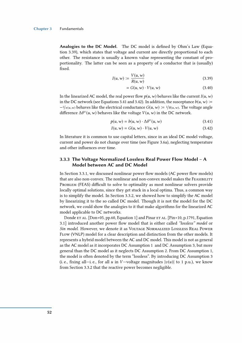
Chapter 3 Fundamentals
Analogies to the DC Model. The DC model is dened by Ohm’s Law (Equa-tion 3.39), which states that voltage and current are directly proportional to eachother. The resistance is usually a known value representing the constant of pro-portionality. The latter can be seen as a property of a conductor that is (usually)xed.
I (u,w) BV (u,w)
R(u,w)(3.39)
= G(u,w) ·V (u,w) (3.40)
In the linearized AC model, the real power ow p(u,w) behaves like the current I (u,w)in the DC network (see Equations 3.41 and 3.42). In addition, the susceptanceb(u,w) B−1/x (u ,w ) behaves like the electrical conductanceG(u,w) B 1/R(u ,w ). The voltage angledierence ∆θv (u,w) behaves like the voltage V (u,w) in the DC network.
p(u,w) = b(u,w) · ∆θv (u,w) (3.41)I (u,w) = G(u,w) ·V (u,w) (3.42)
In literature it is common to use capital letters, since in an ideal DC model voltage,current and power do not change over time (see Figure 3.6a), neglecting temperatureand other inuences over time.
3.3.3 The Voltage Normalized Lossless Real Power Flow Model – AModel between AC and DC Model
In Section 3.3.1, we discussed nonlinear power ow models (AC power ow models)that are also non-convex. The nonlinear and non-convex model makes the FeasibilityProblem (FEAS) dicult to solve to optimality as most nonlinear solvers providelocally optimal solutions, since they get stuck in a local optima. Thus, a common wayis to simplify the model. In Section 3.3.2, we showed how to simplify the AC modelby linearizing it to the so called DC model. Though it is not the model for the DCnetwork, we could show the analogies to it that make algorithms for the linearized ACmodel applicable to DC networks.
Donde et al. [Don+05, pp.60, Equation 1] and Pinar et al. [Pin+10, p.1791, Equation3.1] introduced another power ow model that is either called “lossless” model orSin model. However, we denote it as Voltage Normalized Lossless Real PowerFlow (VNLP) model for a clear description and distinction from the other models. Itrepresents a hybrid model between the AC and DC model. This model is not as generalas the AC model as it incorporates DC Assumption 1 and DC Assumption 3, but moregeneral than the DC model as it neglects DC Assumption 2. From DC Assumption 1,the model is often denoted by the term “lossless”. By introducing DC Assumption 3(i. e., xing all—i. e., for all u in V—voltage magnitudes |v(u)| to 1 p.u.), we knowfrom Section 3.3.2 that the reactive power becomes negligible.
52

The Power Flow Feasibility Problem Section 3.3
As the previous models do, the VNLP model incorporates the conservation of ow(KCL; Equations 3.43a–3.43c), the power ow equation (KVL-like; Equation 3.43d),and the voltage angle dierence bounds (Equation 3.43e). The latter constraints modelthe steady-state stability [Ver10, p.113]. Recall that fnet(u) B
∑w : u ,w ∈←→E p(u,w).
fnet(u) = 0 ∀u ∈ V \ (VG ∪VD ), (3.43a)pд(u) ≤ fnet(u) ≤ pд(u) ∀u ∈ VG , (3.43b)
−pd (u) ≤ fnet(u) ≤ −pd (u) ∀u ∈ VD . (3.43c)
b(u,w) · sin(θv (u) − θv (w)
)= f (u,w) ∀(u,w) ∈ E (3.43d)
|θv (u) − θv (w)| ≤π
2 ∀(u,w) ∈ E (3.43e)
| f (u,w)| ≤ cap(u,w) ∀(u,w) ∈ E (3.43f)
Recall that we look at the real part Re(·) of the power ow model and that the angledierences are restricted to [−π/2; π/2]. The Equations 3.43d–3.43f can be reformulatedto Equations 3.44 and 3.45, respectively. Note that Equation 3.44 is just a reformulationof Equation 3.43d. Since the sine for ±π/2 (voltage angle dierence restriction; Equa-tion 3.43e) is ±1 the voltage angle dierence is the minimum of 1 and x(u,w) ·cap(u,w).
θv (u) − θv (w) = arcsin(x(u,w) · f (u,w)
)(u,w) ∈ E, (3.44)
|θv (u) − θv (w)| ≤ arcsin(min1, x(u,w) · cap(u,w)) (u,w) ∈ E. (3.45)
Equation 3.45 incorporates the voltage angle dierences (Equation 3.43e) and thecapacity constraint (Equation 3.43f). Verma [Ver10, p.114, Lemma 4.2.1 & Theorem4.2.2] showed the uniqueness of a feasible power ow in the VNLP-model. Notethat in general the power grid has no hard capacities. The thermal line limits forthe calculation is usually to maintain the safety of the lines such that they are notoverheating. Since the power ows are unique, we can neglect the capacity constraintsfor the Feasibility Problem. Note that we prove and use the same observationin Chapter 4 in a dierent way. When neglecting the capacity constraint the right-hand side of Equation 3.45 becomes arcsin(1). The decision problem of the VNLP isdened in the following problem box.
Voltage Normalized Lossless Real Power Flow Feasibility Problem
Instance: A VNLP network N = ( G, VG , VD , cap, b, pд , pд , pd , pd ) .Question: Is there a feasible electrical ow complying with Equations 3.43a–
3.43f?Note that the model is non-linear and non-convex [Ver10]. On general graphs, Verma
[Ver10] shows that the capacitated version of VNLP is NP-complete (see Section 3.3.3).
53
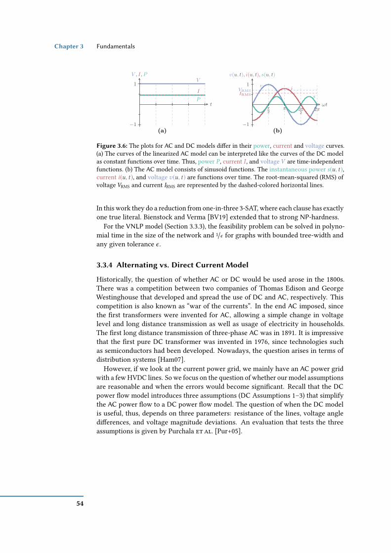
Chapter 3 Fundamentals
(b)(a)
V
I
P
−1
1
t
V , I, P
vi
s
π2
π 3π2
2π
−1
1
ωt
v(u, t), i(u, t), s(u, t)
VRMSIRMS
Figure 3.6: The plots for AC and DC models dier in their power, current and voltage curves.(a) The curves of the linearized AC model can be interpreted like the curves of the DC modelas constant functions over time. Thus, power P , current I , and voltageV are time-independentfunctions. (b) The AC model consists of sinusoid functions. The instantaneous power s(u, t),current i(u, t), and voltage v(u, t) are functions over time. The root-mean-squared (RMS) ofvoltage VRMS and current IRMS are represented by the dashed-colored horizontal lines.
In this work they do a reduction from one-in-three 3-SAT, where each clause has exactlyone true literal. Bienstock and Verma [BV19] extended that to strong NP-hardness.
For the VNLP model (Section 3.3.3), the feasibility problem can be solved in polyno-mial time in the size of the network and 1/ϵ for graphs with bounded tree-width andany given tolerance ϵ .
3.3.4 Alternating vs. Direct Current Model
Historically, the question of whether AC or DC would be used arose in the 1800s.There was a competition between two companies of Thomas Edison and GeorgeWestinghouse that developed and spread the use of DC and AC, respectively. Thiscompetition is also known as “war of the currents”. In the end AC imposed, sincethe rst transformers were invented for AC, allowing a simple change in voltagelevel and long distance transmission as well as usage of electricity in households.The rst long distance transmission of three-phase AC was in 1891. It is impressivethat the rst pure DC transformer was invented in 1976, since technologies suchas semiconductors had been developed. Nowadays, the question arises in terms ofdistribution systems [Ham07].
However, if we look at the current power grid, we mainly have an AC power gridwith a few HVDC lines. So we focus on the question of whether our model assumptionsare reasonable and when the errors would become signicant. Recall that the DCpower ow model introduces three assumptions (DC Assumptions 1–3) that simplifythe AC power ow to a DC power ow model. The question of when the DC modelis useful, thus, depends on three parameters: resistance of the lines, voltage angledierences, and voltage magnitude deviations. An evaluation that tests the threeassumptions is given by Purchala et al. [Pur+05].
54

The Power Flow Feasibility Problem Section 3.3
The TSOs usually say that the resistance of the transmission network is negligible.This statement is basically covered in DC Assumption 1. The transmission networkin Germany has voltages of 110 kV, 220 kV, and 380 kV. These voltage layers denethe high voltage level. The higher the voltage the lower the current and thus, thelower the inuence of the resistance (see Equations 3.18b and 3.39). So our expectationwould be that this assumption mainly depends on the voltage level and on the lineresistances. Purchala et al. [Pur+05, p.4] show that for the Belgian grid with voltagelevels of 70 kV, 150 kV, 220 kV, and 380 kV the X/R ratio ranges from 0.8 for the 70 kVvoltage level to 12.5 for the 380 kV voltage level. The real power estimation error (thatincreases with increasing resistance) for these voltage levels is less than 5% and forthe 380 kV power grid drops below 2.5%. Both errors are small and thus, the resistancefor such X/R ratios in high voltage levels is negligible.
The DC Assumption 2 assumes that the voltage angle dierence is small enoughsuch that the sine function is negligible. The system’s stability is guaranteed in therange of [−π/2; π/2]. However, 30 or [−π/6; π/6] is the range where the sine can beapproximated by sin(x) = x . Thus, if the dierence is within this range, the real powererror should be small. Purchala et al. [Pur+05, p.2] evaluate for the Belgian power gridwith voltages ranging from 70 kV to 380 kV that the highest voltage angle dierencewas 7 and in 94% of the lines it was less than 2. One explanation is that the inductiveand conductive properties of an edge are quite small. However, the lines inductiveproperty is usually slightly higher, though for long distances the capacitive propertyincreases (see the transmission line representation section in Section 3.3.1 on Page 47).
The last assumption—DC Assumption 3—is about a at voltage prole, e. g., allvoltages are equal to 1 p.u.. If there is a voltage deviation then this would automaticallylead to a voltage dierence that is simply not modeled in the DC model. The realpower error increases with increasing voltage deviation [Pur+05, p.4, Figure 7]. Thus,a at voltage prole is important but dicult to establish in power grids.
This particularly means that the most critical assumption is the at voltage prole.The others can be at least established quite well in a high voltage power grid. However,at voltage proles are dicult to establish and thus, the results have to be carefullyinterpreted in terms of an AC power grid. However, this discussion also shows that themore complex Sin-model including the sine function might be a more realistic model,but that the assumption is not critical for the real power error and thus, it might increasethe complexity unnecessarily. However, from a theoretical perspective this model isquite interesting as the feasibility problem is already strongly NP-hard Bienstock andVerma [BV19].
Problems. The AC feasibility problem is a subproblem of many optimization prob-lems such as the Transmission Network Expansion Planning (TNEP) problem,
55

Chapter 3 Fundamentals
the Optimal Transmission Switching Problem (OTSP) and the Maximum PowerFlow Problem (MPFP).
The Economic Dispatch Problem (EDP) minimizes the total cost represented bythe sum of all generator cost functions γ . It is the simplest problem formulation thatchecks whether demand and supply match by abstracting from the power grid andincorporates the energy balance equation, and the generator constraints (see Equa-tions 3.17a and 3.17b). After adding the power grid specics, the problem is calledeither AC or DC Optimal Power Flow Problem (OPFP). All the problems mentionedso far have continuous variables only. In terms of planning problems, we introduceinteger or binary variables. The most commonly known problems for nding anoptimal topology are TNEP, OTSP, and MTSFP.
56

4 The Direct Current Feasibility Problem 1
An Algorithmic Approach to Computing Electrical Flows
The Alternating Current Feasibility Problem (AC FEAS; see Section 3.3.1) and Di-rect Current Feasibility Problem (DC FEAS; see Section 3.3.2) are subproblems ofmost power grid related problems such as switching (see Chapter 5) and ideal FACTSplacement (see Chapter 6). In this chapter, we formalize the operation of the powergrid in such a way that we are able to develop algorithmic approaches for the elec-trical ow computation. With the latter formulations, we are able to develop betteralgorithms for problems that incorporate the electrical ow computation as a subprob-lem. Recall that one of the rst persons who increased the knowledge in DC FEASwas Kirchho [Kir47], who formalized the electrical ow and introduced structuralproperties.
In Section 3.3, we described dierent models and approximations to analyze thenetwork by calculating the power ow, which we call more generally electrical ow.In this chapter, we focus on the Direct Current Feasibility Problem (DC FEAS;commonly known as Power Flow; in short PF) and the DC Maximum Power FlowProblem (DC MPFP). We describe their mathematical models using dierent formula-tions and give some structural insights that will be important to develop algorithmsfor DC FEAS and DC MPFP (see Section 3.3.2). Note that one of the rst algorithms—though with exponential running time—to compute electrical ows uses spanning trees(see Lemma 4.6; [Sha87, SR61]). We describe the latter algorithm [Sha87, SR61] brieyin Section 4.1. This algorithm was used by Felsner [Fel13] to construct a squaring of arectangle [Fel13, pp.17.]. Felsner shows that the ow of a graph that represents sucha squaring of a rectangle is equivalent to a solution of an integer DC FEAS, meaningall ows have to be integral. Since this problem uses integral electrical ows (i. e., theow is a function f : E → Z), we usually cannot apply an LP from Section 3.3.2, buthave to use an ILP. In general solving ILPs is NP-hard [GJ79, p.245, MP1]. However, ifthe solution space has some properties, it is possible to solve it with other techniquesand algorithms in polynomial time. One possibility would be to relax the variablesof DC FEAS, which means that a solution of an LP yields an integral solution. However,we show that this technique does not necessarily result in an integral ow. However,if we do not have a xed generation, a xed demand, and neglect the capacities, mean-ing cap ≡ ∞, but ask for a generation and demand such that we get integral electricalows, we can make use of some properties of the solution space.
1I would like to thank especially Matthias Wolf and Torsten Ueckerdt for questions, discussions, andcomments. In addition, I would like to thank Marc Timme for some initial conversations, his time,and that he encouraged me (more or less) to write this chapter.
57

Chapter 4 An Algorithmic Approach to Computing Electrical Flows
In Section 4.2, we rst give an overview over known transformation and contractionrules. In the end of Section 4.2, we give an algorithm for the s-t-DC FEAS and -MPFP onplanar biconnected graphs that runs in O(|V |3) time. Recall that DC FEAS and MPFPcan be formulated as a linear system of equations and an LP, respectively, that can besolved in O(|E |2.5) time [BC75, Vai89]. Thus, using the contraction and transformationrules in the fashion described in Section 4.2 does not yield an algorithm that has abetter running time than the known mathematical methods. However, it gives somestructural information.
While restricting our graphs to biconnected planar s-t-graphs, we develop an al-gorithm that transforms the formulation given in Section 3.3 and Section 4.1 to anequivalent formulation of simultaneous ows (Section 4.3.2). For this formulation, weare able to develop an algorithmic approach for s-t- DC FEAS and -MPF algorithm forbiconnected graphs (Section 4.5) that can be extended to an algorithm for multiplesources and multiple sinks on planar graphs by using the superposition principle forlinear physical systems.
4.1 A Mathematical Model for theFeasibility Problem of Electrical Flows
Cain et al. [COC12, p.13] give the structural hint that power grids are often planar.Note that this might not be true in general. In addition, power grids are quite sparse.The electrical network’s topology is described by a bidirected graph G = (V , E),where V is the set of vertices representing the buses (i. e., line junctions), and E isthe set of edges representing the lines or cables (the conventional name is branch).Though the underlying graph is undirected [COC12, p.13], we are always able to directits edges u,w ∈ ←→E by inserting two edges in opposite direction (u,w), (w,u) ∈ E.Introducing the direction is motivated by the electrical network’s direction that isusually dened by the voltage or current source representing the reference vertex (alsoknown as slack or datum; see Table 3.1 on Page 42). The direction is used for notationalconvenience and for electrical networks that are nonreciprocal. Nonreciprocal electricalnetworks have components on their edge that have a predened direction such asdiodes. However, in our case the electrical network is reciprocal (also known asbilateral) and thus, the ow on each edge is allowed to ow in both directions. Theunderlying graph is undirected, and we dene for notational convenience the set ←→E ofundirected edges by ←→E = ←→e | e ∈ E, i. e.,
←−−−−→(u,w) =
←−−−−→(w,u) = u,w.
Each edge has a thermal limit and a susceptance that are represented by the func-tions cap : ←→E → R and b : ←→E → R, respectively. The set VG of generators repre-sents the energy sources and the demands are represented by a set VD of consumers.Without loss of generality, we assume that VG ∩ VD = ∅ and VG ∪ VD ⊆ V . Anelectrical network is dened by a tuple N = (G,VG ,VD, cap,b,pд,pд,pd ,pd ) with min-
58
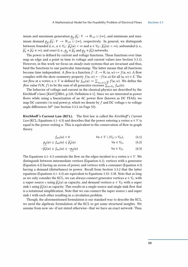
A Mathematical Model for the Feasibility Problem of Electrical Flows Section 4.1
imum and maximum generation pд,pд : V → R≥0 ∪ ∞, and minimum and max-imum demand pd ,pd : V → R≥0 ∪ ∞, respectively. In general, we distinguishbetween bounded (i. e., u ∈ VG : pд(u) < ∞ and u ∈ VD : pd (u) < ∞), unbounded (i. e.,pд ≡ pd ≡ ∞), and exact (i. e., pд ≡ pд and pd ≡ pd ) networks.
The power is dened by current and voltage functions. These functions over timemap an edge and a point in time to voltage and current values (see Section 3.3.1).However, in this work we focus on steady-state systems that are invariant and thus,bind the functions to one particular timestamp. The latter means that all functionsbecome time independent. A ow is a function f : E → R, (u,w) 7→ f (u,w). A owcomplies with the skew-symmetry property f (u,w) = −f (w,u) for all (u,w) ∈ E. Thenet ow at a vertex u ∈ V is dened by fnet(u) B
∑u ,w ∈
←→E f (u,w). We dene the
ow value F (N, f ) to be the sum of all generator excesses∑u ∈VG fnet(u).
The behavior of voltage and current in the classical physics are described by theKirchho’s laws [Kir47][SR61, p.120, Denition 6-1]. Since we are interested in powerows while using a linearization of an AC power ow (known as DC FEAS), wemap DC currents i to real power p, which we denote by f and DC voltage v to voltageangle dierences ∆θv (see Section 3.3.2 on Page 52).
Kirchho’s Current Law (KCL). The rst law is called the Kirchho’s Current
Law (KCL; Equations 4.1–4.3) and describes that the power entering a vertex u ∈ V isequal to the power exiting u. This is equivalent to the conservation of ow in graphtheory.
fnet(u) = 0 ∀u ∈ V \ (VG ∪VD ), (4.1)pд(u) ≤ fnet(u) ≤ pд(u) ∀u ∈ VG , (4.2)
−pd (u) ≤ fnet(u) ≤ −pd (u) ∀u ∈ VD . (4.3)
The Equations 4.1–4.3 constrain the ow on the edges incident to a vertex u ∈ V . Wedistinguish between intermediate vertices (Equation 4.1), vertices with a generator(Equation 4.2) having an excess of power, and vertices with a consumer (Equation 4.3)having a demand (disturbance) in power. Recall from Section 3.3.2 that the latterequations (Equations 4.1–4.3) are equivalent to Equations 3.33–3.38. Note that as longas we only consider the KCL, we can always connect generator vertices u ∈ VG witha super source s using pд(u) as capacity, and demand vertices u ∈ VD with a supersink t using pd (u) as capacity. This results in a single-source and single-sink ow thatis a notational simplication. Note that we can connect the super source s and supersink t with each other resulting in a circulation problem.
Though, the aforementioned formulation is our standard way to describe the KCL,we need the algebraic formulation of the KCL to get some structural insights. Weassume from now on—if not stated otherwise—that we have an exact network. Thus,
59

Chapter 4 An Algorithmic Approach to Computing Electrical Flows
Equations 4.2 and 4.3 become Equations 4.5 and 4.6 withpд ≡ pд ≡ pд andpd ≡ pd ≡ pd ,respectively. Recall from Section 3.1 that an oriented incidence matrix (also knownas connection matrix) represents the graph’s connections in terms of the vertex-edgeincidence relations, i. e., an entry in row u and column e is 1 (respectively −1) ifedge e is an incoming (respectively outgoing) edge, and 0 otherwise. The properties ofsuch a matrix are given in Section 3.1. The Equations 4.1–4.3 can be restated usingthe oriented incidence matrix I ∈ −1, 0, 1 |V |× |E | and the vector of ows #»
f ∈ R |E |
with #»
f B(f (u,w)
)(u ,w )∈E . The KCL in matrix form is given in Equations 4.4–4.6.
IV \(VG∪VD )#»
f =#»0 , (4.4)
IVG#»
f = #»pд, (4.5)IVD
#»
f = #»pd , (4.6)
where #»0 is the zero vector of size |V \ (VG ∪VD )|, IV \(VG∪VD ) is a submatrix of theincidence matrix I constituted by the vertices that are neither generators nor con-sumers. Similar notion is used for the submatrix of the generators and consumersin Equation 4.5 and Equation 4.6. Note when (s, t) ∈ E the ow vector #»
f wouldhave a xed entry with #»
f (s ,t ) =∑u ∈VG pд(u) =
∑w ∈VD pd (w) and Equation 4.4 is
sucient. Equations 4.4–4.6 constitute an incidence matrix I ∈ R |V |× |E | with I B(IV \(VG∪VD ), IVG , IVD )
ᵀ and right-hand side vector #»pI ∈ R |V | with #»pI B (#»0 , #»pд,
#»pd )ᵀ .
The whole system of linear equations is given in Equation 4.7.
I ·#»
f = #»pI . (4.7)
The system I ·#»
f = #»pI represents a translation of the solution set I · #»
f =#»0 . The
latter equation is also called homogeneous equation (or homogeneous problem) and hasalways the trivial solution #»
f =#»0 . If we have a solution #»
f nh for the nonhomogeneoussystem then the whole solution space can be described by #»
f nh + #»
f h |#»
f h ∈ R|E |, I ·
#»
f h =#»0 , where #»
f h is a solution vector of the homogeneous system.
KCL Flow. We call a ow f complying with the KCL as a KCL ow. Recall thatwe can interpret vectors in the euclidean space geometrically as a line segment fromthe origin with magnitude and direction. Two vectors are orthogonal to each otherif the angle α between them is 90 and cos(π/2) = 0. Thus, the dot product is zeromeaning #»
iu ·#»
f =#»0 , since #»
iu#»
f = #»iu
2
#»
f 2cos(α) for all vertices u ∈ V . If we
have I ·#»
f =#»0 this implies that every vector #»
iu in the vector space (here a row u in I)is orthogonal to the vector #»
f .
Properties of the Incidence Matrix. Note that Equation 4.4 means that the inci-dence matrix I and the vector #»
f are orthogonal to each other—meaning every row
60

A Mathematical Model for the Feasibility Problem of Electrical Flows Section 4.1
vector of I is orthogonal to #»
f . Note that this implies that the vectors are also linearindependent, since there is no scalar that makes #»
f colinear to one of the vertices in I.The latter is equivalent to #»
f ∈ ker (I) with ker (I) B #»
f ∈ R |E | | I ·#»
f =#»0 ⊆ R |E | .
img (I)ker (I)
#»0#»pI1
#»pIi
#»f I #»
f
#»0
I #»f =#»0
I #»f =#»pI
trivial element
R|E| R|V |
Figure 4.1: The image img (I)and kernel ker (I) of the inci-dence matrix I for the linearmap I : R |E | → R |V | .
Note that a trivial element of the kernel is the neutralelement, i. e., in the vector space this is the zero vec-tor #»0 (see Figure 4.1 left side). If the kernel consistsof the neutral element only then the linear map isinjective. From Seshu and Reed [SR61, p.66, The-orem 4–3], we know that the rank of the matrix Iis rk(I) = |V | − k with k being the number of con-nected components. The idea is that summing up therows leads to one row of zeros per connected compo-nent, since every column of the incidence matrix I—representing an edge—consists of exactly one 1 entry
and one −1 entry, which gives us rk(I) ≤ |V | − k (see Figure 4.6b on Page 69 as ex-ample). The aforementioned structure of the incidence matrix I leads to an uppertriangle matrix for each connected component that cannot be reduced further leadingto rk(I) ≥ |V | −k and thus, rk(I) = |V | −k . Recall that the rank of the incidence matrix I(i. e., rk(I)) corresponds to the number of edges in a spanning forest. To determinethe nullity n(I) B dim(ker (I)) of the incidence matrix I, we introduce the rank-nullity
theorem.
Theorem 4.1 (Rank-nullity Theorem). For any matrix A ∈ Rr×cwith r rows and c
columns the rank rk(A) and nullity n(A) sum up to the number of columns.
rk(A) + n(A) = c .
The generalization to linear maps A : R |C | → R |R | is given by
dim(img (A)) + dim(ker (A)) = dim(R |C |) = |C |.
The incidence matrix I can be viewed as a linear map I : R |E | → R |V | with #»
f 7→ I ·#»
f .The kernel ker (I) and image img (I) of the incidence matrix I are given in Equation 4.8.
ker (I) B #»
f ∈ R |E | | I ·#»
f =#»0 ⊆ R |E | (4.8a)
img (I) B #»pI ∈ R|V | | ∃
#»
f ∈ R |E | : I · #»
f = #»pI ⊆ R |V | (4.8b)
A kernel ker (I) of the incidence matrix I is a set ker (I) of vectors #»
f such that thehomogeneous system I ·
#»
f =#»0 holds for all vectors in that set (see Figure 4.1 red
61

Chapter 4 An Algorithmic Approach to Computing Electrical Flows
area and text). The image img (I) of the incidence matrix are all vectors #»pI for which asolution exist (see Figure 4.1 green area and text).
Using the rank-nullity theorem (see Theorem 4.1) we get the dimension of the kernel(i. e., the nullity when talking about matrices) of dim(ker (I)) = dim(E)−dim(img (I)) =|E | − |V | + k that corresponds to the number of chords (i. e., edges not on a spanningforest). A common way to construct the incidence matrix I (see Chapter 3 on Page 27)of row size |V | − k is to dene one vertex u ∈ VG per connected component as slack
R|E|
R|V |−k
R|V |
I′
I
Remove arow u perconnectedcomponent
Figure 4.2: Linear mapsof the incidence matrix Iand I′, where k is thenumber of connectedcomponents.
vertex and remove its row u (see example Figure 4.6 b onPage 69, where we remove vertex 3). From the property ofthe incidence matrix I we know that every square subma-trix of I has a determinant that is either −1, 0, or 1. Sinceevery square non-singular submatrix of the incidence ma-trix I of size (|V | −k)×(|V | −k) that is the maximum squaresubmatrix that constitutes a spanning tree is unimodular(i. e., the determinant takes ±1 values only) and all determi-nants are either 0, 1, or −1, the incidence matrix I is totallyunimodular (in short TUM).If not noted otherwise, if we speak from now on of theincidence matrix I, we mean the reduced incidence matrix
that has |V | − k rows and thus, is dened by I ∈ −1, 0, 1( |V |−k )×|E | (see Figure 4.2).
Feasible Flows and Thermal Line Limit. As already mentioned each edge hasa natural limit of ow it is able to carry. This is usually modeled by the capacityconstraint that basically models the thermal line limit (Equation 4.9).
| f (u,w)| ≤ cap(u,w) ∀(u,w) ∈ E. (4.9)
We denote a ow f complying with the capacity constraints as feasible ow. A KCLow (see KCL ow on Page 60) complying with the capacity constraint is thus calleda feasible KCL ow.
Kirchho’s Voltage Law (KVL). Kirchho’s second law is known as Kirchho’sVoltage Law (KVL) and describes the voltage angles in a cycle (also known as mesh). Acycle is a path π (s, t) B
((s,u1), (u1,u2), . . . , (ui , t)
), where at least s = t , otherwise it
would not be closed. Cycles have by denition an even degree. The set C of cyclesincludes all cycles of a graphG , which can be exponentially many in general. Note thatwe distinguish between cycles and circuits. A circuit has a degree of 2. Thus, circuitsare the same as simple cycles. Kirchho’s Voltage Law states that the voltages in acycle sum up to zero (Equation 4.10). Recall from Section 3.3.2 that in DC FEAS thevoltages are substituted by the voltage angle dierences ∆θv and the resistances r by 1/b.The KVL-like equation is given by
∑(u ,w )∈C b(u,w) ·
(θv (w) − θv (u) − θvshi(u,w)
)= 0.
62

A Mathematical Model for the Feasibility Problem of Electrical Flows Section 4.1
In this section, we assume that θvshi(u,w) = 0, i. e., we assume that there are nophase transformers or FACTS (see the discussion in Section 3.3.1). In terms of linearalgebra, we can rewrite the latter by using the circuit matrix B and the # »
∆θv vector(Equation 4.10). The oriented circuit matrix B ∈ −1, 0, 1 |C |× |E | is a matrix, whereeach row c represents a cycle c ∈ C and a column e represents an edge e ∈ E. The entryof B is either 1 (respectively −1) when an edge e is in cycle c in direction (respectivelyopposite) with some predened direction for each cycle c ∈ C , or 0 if the edge is notin the cycle c . The KVL using the circuit matrix is dened in Equation 4.10.
B# »
∆θv =#»0 , (4.10)
whereB ∈ −1, 0, 1 |C |× |E | [SR61, p.91] is the oriented circuit matrix (e. g., see Figure 4.6a or b on Page 69; bottom partition), and # »
∆θv ∈ R |E | with∆θv B (θv (w)−θv (u))(u ,w )∈Eis a vector of voltage angle dierences at an edge with # »
∆θv ∈ ker (B), and #»0 is thezero vector of size |C |. The formulation in Equation 4.10 represents a homogeneousequation and thus, has always the trivial solution # »
∆θv =#»0 .
Properties of the Circuit Matrix. Recall that the set C of cycles includes poten-tially exponentially many cycles. However, it suces to work with a base of thecycle space [Kir47, pp.498.] and thus, the circuit matrix B will only incorporate afundamental cycle base in this work.
If we speak of the circuit matrix B and we did not mention anything else, we speakof the circuit matrix that only has fundamental cycles as row vectors.
Denition 4.2 (Base). A base in a vector space is a maximum independent set of vectors
that suce to span the vector space.
In general there are multiple bases that span the same vector space, which we willsee soon. Note that all bases have the same size [Whi35, p.514, Theorem 6].
Denition 4.3 (Fundamental Cycle Base). Let G = (V , E) be a graph, let T = (V , E)be a spanning forest, and let Echords B E(G) \ E(T ) be a set of chords. A walk from
one endpoint u of the chord (u,w) to the other endpoint w using the spanning forest
branches E(T ) denes a cycle that diers from the other cycles in B by at least the chord
edge (u,w). A fundamental cycle base is dened by a spanning forest (by a spanning
tree if the graph is connected), and a cycle in that base is dened by a chord (i. e., non-tree
edge).
Note that a spanning forest has |V | − k edges—also denoted as tree branches—and |E | − |V | + k chords, where k is the number of connected components. The rankof the circuit matrix is rk(B) = |E | − |V | + k [SR61, p.66, Theorem 4-5] and the nullityis n(B) = |V | − k [SR61, p.64, Corollary 4-4]. In general, the circuit matrix B does nothave a determinant of ±1 [Oka55][Kav+09, p.12, Lemma 3.3].
63

Chapter 4 An Algorithmic Approach to Computing Electrical Flows
The circuit matrix B is a linear map B : R |E | → R |C | with # »
∆θv 7→ B ·# »
∆θv . Thekernel ker(B) and image img(B) of the circuit matrix B are dened in Equation 4.11and illustrated in Figure 4.3 by the red or green area, respectively.
ker (B) B # »
∆θv ∈ R |E | | B ·# »
∆θv =#»0 ⊆ R |E | (4.11a)
img (B) B #»pB ∈ R|C | | ∃
# »
∆θv ∈ R |E | : B ·# »
∆θv = #»pB ⊆ R |C | (4.11b)
A kernel ker (B) of the circuit matrix B is a set ker (B) of vectors # »
∆θv such that the
img (B)ker (B)
#»0# »pB1
# »pBi
# »∆θv B# »∆θv
#»0
B# »∆θv=#»0
B# »∆θv=# »pB
trivial element
R|E| R|C|
Figure 4.3: The image img (B)and kernel ker (B) of the cir-cuit matrix B for the linearmap B : R |E | → R |C | .
homogeneous system B ·# »
∆θv =#»0 holds for all vec-
tors in that set (see Figure 4.3 red area and text). Theimage img (B) of the circuit matrix are all vectors #»pBfor which a solution exist (see Figure 4.3 green areaand text).Using the rank-nullity theorem (see Theorem 4.1)we get the dimension of the kernel (nullity whentalking about matrices) of dim(ker (B)) = dim(E) −dim(img (B)) = |E | − |E | + |V | − k = |V | − k .However, Cederbaum [Ced55] showed that for a fun-damental system of circuits—that is used in our case—the determinant can only take values of −1, 0, or 1
for every square submatrix and ±1 for a set of chords that represents a maximal squarematrix (see Figure 4.6a or b bottom right partition). As for the incidence matrix I abovethis means that the matrix B is TUM.
Lemma 4.4 (TUM bases). The incidence matrix I and the circuit matrix B are TUM
bases.
Relationship between Incidence and Circuit Matrix. We get the relationshipbetween the incidence matrix I and the circuit matrix B in Equation 4.12.
IBᵀ = 0 and BIᵀ = 0, (4.12)
where 0 is a matrix with zeros only of dimension |V | × |C | (respectively |C | × |V |).Thus, the incidence matrix I is orthogonal to the circuit matrix B. One way to provethat is given by Seshu and Reed [SR61, p.66, Theorem 4-6] that uses the property ofcircuits that have a degree of deg(u) = 2 at all vertices u ∈ V . Again note that bothmatrices I and B are orthogonal to each other (i. e., every vector of I is orthogonalto every vector in B). Note that this also means that the vectors are linear indepen-dent to each other. By doing a vertex transformation, we are able to describe thevoltage angle dierence ∆θv (u,w) vector by voltage angles θv (u) and θv (w) for alledges (u,w) ∈ E. However, this simple transformation is based on the connection
64

A Mathematical Model for the Feasibility Problem of Electrical Flows Section 4.1
that B # »
∆θv =#»0 and based on the relationship shown in Equation 4.12. The connection
given in Equation 4.12 allows us to describe # »
∆θv by the linear combination of the treebranches # »
∆θv = Iᵀ# »
θv for each connected component (compare also Equations 3.31aand 4.13), where # »
θv ∈ R |V |−k with k representing the number of connected compo-nents [SR61, Theorem 6-6, p. 123]. This means, we can nd B
# »
∆θv =#»0 , which is
equivalent of nding a BIᵀ# »
θv =#»0 . Since we know from Equation 4.12 that BIᵀ = 0
this equation holds independent of the voltage angle vector # »
θv . In addition, we wouldlike to know when there is a # »
θv ∈ R |V | such that # »
∆θv = Iᵀ# »
θv . The latter is equivalentto the question of when # »
∆θv ∈ img (Iᵀ). We have to show when ker (B) ⊆ img (Iᵀ).This is the case when we chose the same spanning tree to construct both matrices.Note that it suces to compute the voltage angle dierences along a spanning tree,since the others result from these voltage angles.
KVL Flow. Applying the latter to Ohm’s law gives us the typical equation knownfrom literature (Equation 4.13).
b(u,w) ·(θv (w) − θv (u)
)= f (u,w). (4.13)
A ow f complying with Equation 4.13 is called KVL ow and if it complies with thecapacity constraint it is called feasible KVL ow.
Using the aforementioned relationship (Equation 4.13), we can reformulate Equa-tion 4.10 such that we replace voltage angle dierences # »
∆θv by ows #»
f . Notethat b(u,w) = 1/x (u ,w ) and that “” is the Schur product (or entrywise product).
#»
f =#»
b # »
∆θv ⇔# »
∆θv = #»x #»
f (4.14a)
B# »
∆θv =#»0 ⇔
(B (1 |E |×1 · #»x ᵀ)
)︸ ︷︷ ︸
CB′
·#»
f =#»0 (4.14b)
Since #»x is a vector of constant values, we just multiply the entries in the circuitmatrix B by #»x resulting in a new circuit matrix B′, which results in Equation 4.15.
B′ ·#»
f =#»0 (4.15)
Feasible Electrical Flow. In the following, we dene feasible electrical ows thatrepresent solutions to DC FEAS.
Denition 4.5 (Feasible Electrical Flow). A KVL ow that is also a KCL ow is
called electrical ow and if it complies to the capacity constraint, too, it is called a feasibleelectrical ow.
65

Chapter 4 An Algorithmic Approach to Computing Electrical Flows
DC FEAS and DC MPFP constitute a system of linear equations and an LP, respec-tively. In the following, we summarize the problem denitions of DC FEAS and MPFP.
Direct Current Feasibility Problem DC-FEAS(N)
Instance: An exact bounded network N = ( G, VG , VD , cap, b, pд , pд , pd , pd ) ,i. e., pд ≡ pд ≡ pд and pd ≡ pd ≡ pd .
Question: Is there a feasible electrical ow f (see Equations 4.7, 4.9 and 4.10)?
A feasible electrical ow that maximizes the ow value F (N, f ) B∑u ∈VG fnet(u) is
called MPFP(N) and its value is denoted by OPTMPFP(N). The optimization problemis stated in the following.
Direct Current Maximum Power Flow Problem DC-MPFP(N)
Instance: A network N = ( G, VG , VD , cap, b, pд , pд , pd , pd ) .Objective: Find a feasible electrical ow f (see Equations 4.7, 4.9 and 4.10) such
that the ow value F (N) is maximum among all choices of f .
Algorithms to Solve DC FEAS. Possibilities to get a feasible power ow are toformulate the system of linear equations or LP and run it using a solver such asGurobi [Gur16], or to apply the following algorithm.
Lemma 4.6 (Shapiro [Sha87, p.36, Lemma 1]). Let every edge ofG have a resistance r ≡1. Let T denote the number of spanning trees and let T (s,u → w, t) be the number
of spanning trees that contain the edge (u,w) in that particular direction meaning the
spanning tree has a path from s to t that visits vertex u rst and then vertexw by using
the edge (u,w) ∈ E. Let pд ≡ pd ≡ 1 and let f (u,w) =(T (s ,u→w ,t )−T (s ,w→u ,t )
)/T . Then f
is a feasible electrical ow in G.
The generalization—where we have no unit resistances r , but arbitrary ones—givenby Shapiro [Sha87, p.38] was already given by Seshu and Reed [SR61, pp.155.]. Insteadof just using the number of spanning trees, we calculate for each spanning tree theproduct of the admittances of the branches of that spanning tree and sum over allspanning trees. The proof of the lemma uses the Binet-Cauchy-Theorem [SR61, p.32].Note that a graph can have exponentially many spanning trees and computing the owfor each edge using this techniques is quite inecient, but provides an exponentialtime algorithm to compute the electrical ow of the power grid.
66

A Mathematical Model for the Feasibility Problem of Electrical Flows Section 4.1
4.1.1 Properties of Electrical Flows
Note that we use a base for the columns of the incidence and circuit matrix denotedby I and B, respectively, where all equations are linear independent. Since the wholesystem of equations has full rank the solution to a feasible electrical ow is unique,which we show in the following.
Lemma 4.7 (Uniqueness of DC Electrical Flows). There is a unique solution to DCelectrical ows if we have exact bounds.
Proof. Recall that the incidence matrix I with I ∈ R( |V |−k )×|E | and the circuit matrix Bwith B ∈ R( |E |− |V |+k )×|E | are bases. Since both matrices are bases the vectors are linearindependent in each matrix (i. e., this is a property of a base shown in Equations 4.4and 4.10). We now dene a matrix A by A B
( IB′)
with B′ from Equation 4.15,whereA ∈ R |E |× |E | can be generalized to a linear mapA : R |E | → R |E | with #»
f 7→ A·#»
f .Thus, the system of equations is dened by A ·
#»
f = # »pA B( #»pI
#»0)
with vector #»0 of size |C |.The kernel ker (A) and the image img (A) of matrix A are dened in Equation 4.16.
ker (A) B #»
f ∈ R |E | | A ·#»
f =#»0 ⊆ R |E | (4.16a)
img (A) B # »pA ∈ R|E | | ∃
#»
f ∈ R |E | : A · #»
f = # »pA ⊆ R |E | (4.16b)
From Equation 4.12, we know that IBᵀ = 0 and BIᵀ = 0, which means that thedimension of the image of A is the sum of the dimension of the images of the incidencematrix I and circuit matrix B given by dim(img (A)) = dim(img (I)) + dim(img (B)) =|V | −k+ |E | − |V |+k = |E |. Using the rank-nullity theorem (see Theorem 4.1), we knowthat the dimension of the kernel is dim(ker (A)) = 0. Thus, A as linear map is injective.The dimension of the image of A is |E |, which means that the matrix has full rank. Weconclude that the system has a unique non-trivial solution (see Figure 4.4).
y = −x + 3
y = x − 1y = 3/2x + 3
y = −x/2 − 2
Py is xed to 1
−4 −3 −2 −1 1 2 3 4
−3−2−1
123
x
y
Figure 4.4: The Polytope P constitutedby y ≤ 3/2x + 3, y ≥ x − 1, y ≤ −x + 3,and y ≥ −x/2 − 2. If y = 1, we reduce thesolution space to x ∈ [−4/3, 2]. However,if y = −5/3 the solution is unique x = −2/3. Soa unique solution corresponds to one point .
Note that the system has no non-trivial solution if the generations anddemands are exact and the capacitiesare chosen in such a way that thesegenerations and demands cannot befullled. In the following, we extendthe system by capacity constraints dis-cussed in Equation 4.9.
The capacity constraint can be refor-mulated in a matrix writing by 1 |E |× |E | ·#»
f ≤ # »cap, where 1 |E |× |E | is the identitymatrix of size |E | × |E | and the vectorof capacities is # »cap ∈ R |E | . With the
67
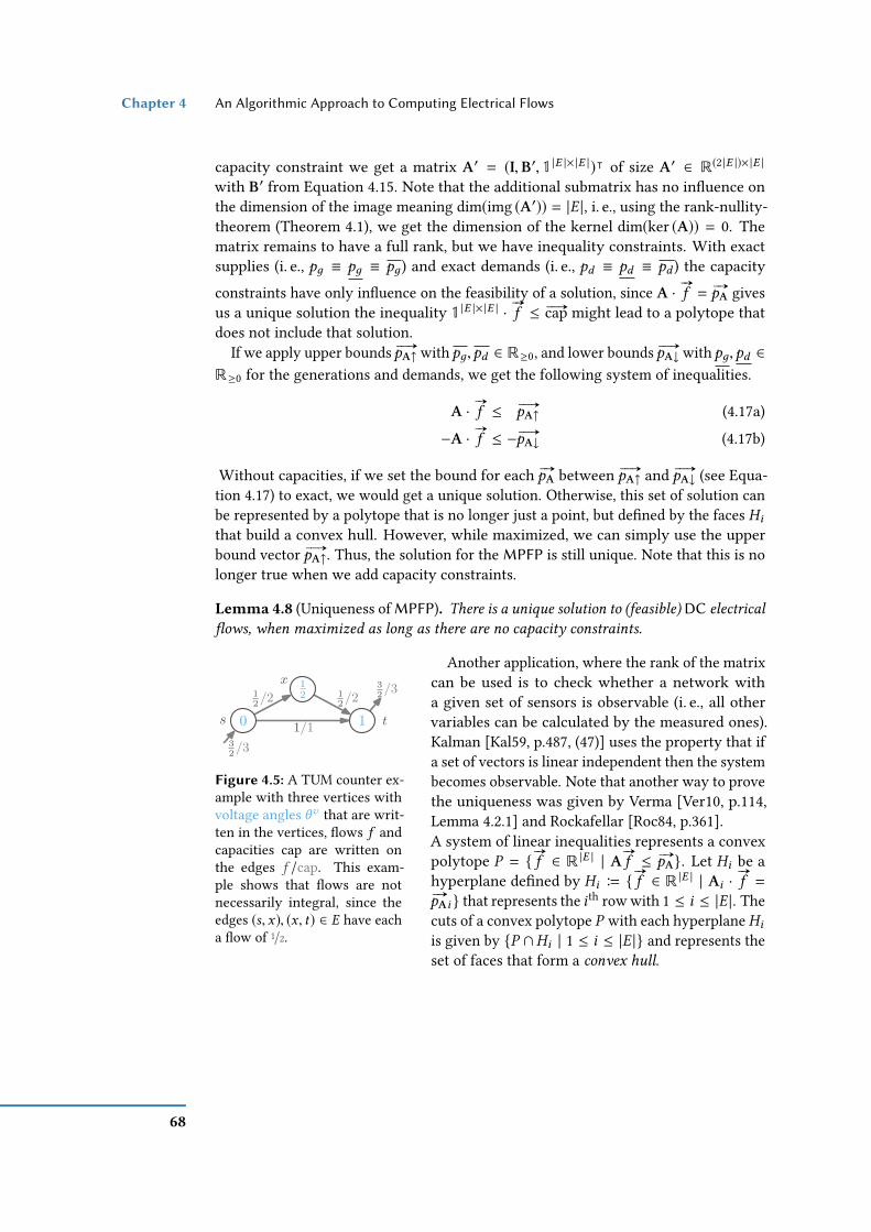
Chapter 4 An Algorithmic Approach to Computing Electrical Flows
capacity constraint we get a matrix A′ = (I,B′, 1 |E |× |E |)ᵀ of size A′ ∈ R(2 |E |)× |E |
with B′ from Equation 4.15. Note that the additional submatrix has no inuence onthe dimension of the image meaning dim(img (A′)) = |E |, i. e., using the rank-nullity-theorem (Theorem 4.1), we get the dimension of the kernel dim(ker (A)) = 0. Thematrix remains to have a full rank, but we have inequality constraints. With exactsupplies (i. e., pд ≡ pд ≡ pд) and exact demands (i. e., pd ≡ pd ≡ pd ) the capacityconstraints have only inuence on the feasibility of a solution, since A ·
#»
f = # »pA givesus a unique solution the inequality 1 |E |× |E | ·
#»
f ≤ # »cap might lead to a polytope thatdoes not include that solution.
If we apply upper bounds # »pA↑ with pд,pd ∈ R≥0, and lower bounds # »pA↓ with pд,pd ∈R≥0 for the generations and demands, we get the following system of inequalities.
A ·#»
f ≤ # »pA↑ (4.17a)−A ·
#»
f ≤ − # »pA↓ (4.17b)
Without capacities, if we set the bound for each # »pA between # »pA↑ and # »pA↓ (see Equa-tion 4.17) to exact, we would get a unique solution. Otherwise, this set of solution canbe represented by a polytope that is no longer just a point, but dened by the faces Hithat build a convex hull. However, while maximized, we can simply use the upperbound vector # »pA↑. Thus, the solution for the MPFP is still unique. Note that this is nolonger true when we add capacity constraints.
Lemma 4.8 (Uniqueness of MPFP). There is a unique solution to (feasible) DC electrical
ows, when maximized as long as there are no capacity constraints.
s t
x12 /2 1
2 /2
32 /3
32 /3
0
12
11/1
Figure 4.5: A TUM counter ex-ample with three vertices withvoltage angles θv that are writ-ten in the vertices, ows f andcapacities cap are written onthe edges f /cap. This exam-ple shows that ows are notnecessarily integral, since theedges (s, x), (x, t) ∈ E have eacha ow of 1/2.
Another application, where the rank of the matrixcan be used is to check whether a network witha given set of sensors is observable (i. e., all othervariables can be calculated by the measured ones).Kalman [Kal59, p.487, (47)] uses the property that ifa set of vectors is linear independent then the systembecomes observable. Note that another way to provethe uniqueness was given by Verma [Ver10, p.114,Lemma 4.2.1] and Rockafellar [Roc84, p.361].A system of linear inequalities represents a convexpolytope P =
#»
f ∈ R |E | | A#»
f ≤ # »pA. Let Hi be ahyperplane dened by Hi B
#»
f ∈ R |E | | Ai ·#»
f =# »pAi that represents the ith row with 1 ≤ i ≤ |E |. Thecuts of a convex polytope P with each hyperplane Hiis given by P ∩Hi | 1 ≤ i ≤ |E | and represents theset of faces that form a convex hull.
68

A Mathematical Model for the Feasibility Problem of Electrical Flows Section 4.1
(a) (b) (c)
a
b
c d
e
f
1
2
4
3
6
5
c1
c2
g
g e
ChordsSpanning Tree
25
b
10
−1
−1
1
00
0
10
−10
0
−1 −10 1
000 1 −1
2
5
7
7
0
−101
100
0 0
0 0 000
0−1
0
314256
a d
c1c2
1
f c
−100
0
1
−1
−110
00
1
000
0
unimodularsubmatrices
e`+2 e|E|. . .
Chords
|E(G)|−|E(B)|Spanning Forest
|E(B)|
|E(G)|−|V (G)|+k|V (G)|−k
e1 e2 eke`+1 . . .
±1±1
±1
±1
0. . . ...
±1±1
±1
0 000 0 0
0 0
±10 0. . . . . .
......
±1
±10
...
0
±1±1±1
±1 0
00
0
00
00
...
...
...
...
0 00 0
±1±1±1±1
. . .±1±1 . . .
unimodularsubmatrices
±1
|E(G
)|−
|V(G
)|+
k|V
(G)|−
k
|E(G)|
|E(G
)|±1
00
00
0...
0
...
0
. . .
Figure 4.6: The structure of the matrix A B( IB
)that is a construction of the incidence matrix I
(top partition) and circuit matrix B (bottom partition). The left partition of size |V | − k , with kbeing the number of connected components (for (b) and (c) with one connected component k =1), represents some spanning forest (for k = 1 a spanning tree) of the graph G. The rightpartition represents the edges that are not in the spanning forest of the left partition (alsocalled chords). The latter partition has a size of |E | − |V | + k . The green areas have entries thatare all zero and the main diagonal with entries all ±1 is marked in red. The general structureis given in (a) and a small example is given in (b) with the corresponding graph in (c).
Consider any objective then an optimal solution of a convex polytope P is on thevertices of P . Thus, if the vertices of a convex polytope P lie on integral coordinatesthan P is called an integral polytope. If all square submatrices of A have a determinantof −1, 0, or 1 then A is TUM. This in particular means that the polytope of such a TUMmatrix is integral independent on the vector # »pA.
Recall that we know that the incidence matrix I and circuit matrix B are each TUMby itself (see Lemma 4.4). In the following, we prove that the whole system A B
( IB)
isnot TUM and thus, the convex polytope is not necessarily integral.
Lemma 4.9. The bases of the incidence matrix I and the circuit matrix B are each TUM.
However, the whole system of linear equations A B( IB)to compute a feasible electrical
ow using the KCL (Equation 4.7) and KVL (Equation 4.10) is not TUM.
Proof. A counter example is shown in Figure 4.5 that basically describes why a feasibleelectrical ow f is not integral for every right hand-side vector # »pA.
The KCL (see Equation 4.7) and the KVL (see Equation 4.10) do not incorporatenetwork elements in any sense—i. e., these equations are purely topological [SR61,p.127, Section 6-3]—the vector of voltage angle dierences # »
∆θv can be replaced by theow vector #»
f .
69
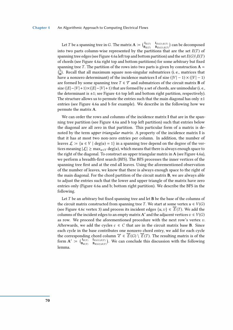
Chapter 4 An Algorithmic Approach to Computing Electrical Flows
LetT be a spanning tree inG . The matrix A B( IE(T ) IE(G )\E(T )BE(T ) BE(G )\E(T )
)can be decomposed
into two parts column-wise represented by the partitions that are the set E(T ) ofspanning tree edges (see Figure 4.6a left top and bottom partition) and the set E(G)\E(T )of chords (see Figure 4.6a right top and bottom partitions) for some arbitrary but xedspanning treeT . The partition of the rows into two parts is given by construction A =( IB). Recall that all maximum square non-singular submatrices (i. e., matrices that
have a nonzero determinant) of the incidence matrices I of size (|V | − 1) × (|V | − 1)are formed by some spanning tree T ∈ T and submatrices of the circuit matrix B ofsize (|E |− |V |+1)×(|E |− |V |+1) that are formed by a set of chords, are unimodular (i. e.,the determinant is ±1; see Figure 4.6 top left and bottom right partition, respectively).The structure allows us to permute the entries such that the main diagonal has only ±1entries (see Figure 4.6a and b for example). We describe in the following how wepermute the matrix A.
We can order the rows and columns of the incidence matrix I that are in the span-ning tree partition (see Figure 4.6a and b top left partition) such that entries belowthe diagonal are all zero in that partition. This particular form of a matrix is de-noted by the term upper triangular matrix. A property of the incidence matrix I isthat it has at most two non-zero entries per column. In addition, the number ofleaves L B u ∈ V | deg(u) = 1 in a spanning tree depend on the degree of the ver-tices meaning |L| ≥ maxu ∈V deg(u), which means that there is always enough space tothe right of the diagonal. To construct an upper triangular matrix in A (see Figure 4.6a),we perform a breadth-rst search (BFS). The BFS processes the inner vertices of thespanning tree rst and at the end all leaves. Using the aforementioned observationof the number of leaves, we know that there is always enough space to the right ofthe main diagonal. For the chord partition of the circuit matrix B, we are always ableto adjust the entries such that the lower and upper triangle of the matrix have zeroentries only (Figure 4.6a and b; bottom right partition). We describe the BFS in thefollowing.
LetT be an arbitrary but xed spanning tree and let B be the base of the columns ofthe circuit matrix constructed from spanning treeT . We start at some vertex u ∈ V (G)(see Figure 4.6c vertex 3) and process its incident edges u,v ∈ ←→E (T ). We add thecolumns of the incident edges to an empty matrixA′ and the adjacent verticesv ∈ V (G)as row. We proceed the aforementioned procedure with the next row’s vertex v .Afterwards, we add the cycles c ∈ C that are in the circuit matrix base B. Sinceeach cycle in the base contributes one nonzero chord entry, we add for each cyclethe corresponding chord column ←→e ∈ ←→E (G) \ ←→E (T ). The resulting matrix is of theform A′ B
( IE(T ) IE(G )\E(T )BE(T ) BE(G )\E(T )
). We can conclude this discussion with the following
lemma.
70

A Mathematical Model for the Feasibility Problem of Electrical Flows Section 4.1
Lemma 4.10. Let A =( IB)be the matrix formed by the incidence matrix I and circuit
matrix B. The matrix’s columns and rows can be permuted such that we get the form
shown in Figure 4.6a.
To investigate the TUM property, we take a look at the intersections of the matrix Athat are represented by all four partitions (see Figure 4.6a). Thus, we distinguishbetween the following three main cases.Case 1: The intersection between the chord and spanning tree partition of
(a) the incidence matrix I (Figure 4.6a & b; top left and top right partition),(b) the circuit matrix B (Figure 4.6a & b; bottom left and bottom right partition).
Case 2: The intersection between the incidence matrix I and the circuit matrix B of(a) the spanning tree partition (Figure 4.6a & b; top left and bottom left partition),(b) the chord partition (Figure 4.6a & b; top right and bottom right partition).
Case 3: The intersection of all four partitions.Since each matrix is TUM by itself Case 1 is unproblematic (see Lemma 4.4). In Case 2,we are already able to nd a square submatrix with determinant unequal ±1 or 0(see Figure 4.6b row 5 columns e and d). In Case 3 it is also possible to construct agraph such that there is a submatrix, where the determinant is 2 (see the examplein Figure 4.6a and b). Inverting the direction of all cycles or edges has no inuenceson the determinant. Same holds for Case 2. Note that inverting the direction of theedges does not help, since the direction changes in the incidence and circuit matrixand thus, it only changes the sign of the determinant.
Assume that a ow is a function f : E → Z that is an integral ow, we get a systemof integral equations (IE). Such integral systems of equations or ILPs are usually ahint that the underlying problem is NP-hard [GJ79, p.245, MP1]. A relaxation of thefunction f (i. e., mapping to R instead of Z) does not necessarily yield an integralsolution, since the polytope vertices do not lie on integral coordinates (see Lemma 4.9).
Thus, with this technique we are not able to solve the problem by Felsner [Fel13,pp.17., Theorem 4.1] in polynomial time. However, in Section 4.1.2 we see a techniquethat leads to an integral electrical ow. Another possibility would be to restrict thealgorithm in Section 4.5 to integral ows only.
4.1.2 Scalability of Electrical Flows
As already mentioned by Goldberg and Tarjan [GT89, p.114] a lot of ow algorithms usescaling techniques. Whether it is the scaling of the capacity—introduced by Edmondsand Karp [EK72]—or the scaling of the excess that was introduced by Ahuja and Orlin[AO89]. For electrical ows, we will use scaling, too. The following scaling lemmafollows directly from Equations 4.1–4.3 and 4.13.
71

Chapter 4 An Algorithmic Approach to Computing Electrical Flows
Lemma 4.11 (Scaling). Every non-zero electrical ow f ′ : E → R>0 can be rescaled to
a feasible electrical ow f by applying a scaling factor χ , where
χ B max(maxu ∈VD
pd (u)
pd (u),maxu ∈VG
pд(u)
pд(u),
)≤ χ ≤ min
(mine ′∈E
cap(e ′)f ′(e ′)
, minu ∈VD
pd (u)
pd (u), minu ∈VG
pд(u)
pд(u)
)C χ
to f (e) = f ′(e) · χ for all e ∈ E.
Proof. Assume #»
f ′ is an electrical ow complying Equations 4.7 and 4.10 or alterna-tively Equations 4.1–4.3 and 4.13. Multiplying #»
f ′ by a scalar χ yields in a ow χ ·#»
f ′ =#»
f that is still an electrical ow, since it is only a scaling of an unrestricted vector.The latter means that multiplying Equations 4.7 and 4.10 (assuming ∆θv ≡ f ) by ascalar (standard operation on a eld) yields in a magnitude increase of all vectorsincluding #»
f . However, to scale an electrical ow to a feasible electrical ow the owhas to comply with the capacity constraints (Equation 4.9).
For χ ≤ χ we have
f (e) = χ · f ′(e)
≤ χ · f ′(e)
= mine ′∈E
cap(e ′)f ′(e ′)
· f ′(e)
≤cap(e)f ′(e)
· f ′(e)
= cap(e).
Note that we included the maximum generation and demand pд = χ · pд′(u) ≤
χ · pд′(u) = minu ∈VG pд (u)/pд ′(u) · pд
′(u) = pд(u).
Note that the last lemma would be much simpler if we make the bounded network toan unbounded network. For this we will use Lemma 5.3 on Page 118 (see also Figure 5.5).
Lemma 4.12 (Scaling Restatement). Let N = (G,VG ,VD, cap,b,pд,pд,pd ,pd ) be apower grid with minimum and maximum generations and demands. We model the upper
and lower bounds of the generations and demands in the same fashion as in Lemma 5.3
(Figure 5.5 on page 117) as lower and upper capacities. The edge capacities are cap ≡ 0and cap ≡ cap. Every non-zero electrical ow f ′ : E → R>0 can be rescaled to a feasible
electrical ow f by applying a scaling factor χ , where
χ B maxe ′∈←→E
cap(e ′)f ′(e ′)
≤ χ ≤ mine ′∈←→E
cap(e ′)f ′(e ′)
C χ
to f (e) = f ′(e) · χ for all e ∈ E.
72
A Mathematical Model for the Feasibility Problem of Electrical Flows Section 4.1
We can use the latter two results to up scale or down scale electrical ows. An s-t-network is a network with one generator s C VG (i. e., |VG | = 1) and one con-sumer t C VD (i. e., |VD | = 1). Since there is a unique solution to a feasible elec-trical ow f (see Lemma 4.7) and we can rescale every electrical ow by a factor χ(Lemma 4.12), we chose an edge with the maximum violation of the capacity constraint,compute the factor χ , and scale the ow on all edges in the network down accord-ing to χ . The next lemma follows directly from Lemma 4.12, since χ is the largestpossible scaling such that #»
f yields a feasible electrical ow. This ow represents themaximum possible feasible electrical ow for an s-t-network that is equivalent toa DC maximum power ow (DC MPF). Note that for s-t-networks there is only onecontrollable generator that means the MPF is unique, too.
Lemma 4.13. For an s-t-network N any non-zero electrical ow f ′ : E → R>0 can be
rescaled to an MPF by using a scaling factor of χ (see Lemma 4.12).
Note that for multiple generators the MPF is not necessarily unique, since dierentreal power generations pд can lead to the same optimal value OPTMPFP(N).
4.1.3 Integral Electrical Flows
In general, we can assume that the parameters of a DC power grid N , such as the sus-ceptance b, are rational Q and thus, the equations constitute a rational polytope, sincethe cuts of the hyperplanes can only constitute rational numbers (see Denition 4.14).
Denition 4.14 (Rational Polytope; Schrijver [Sch03, p.61]). A system of linear in-
equalities of the form #»
f ∈ Rm | A#»
f ≤ # »pA, where A ∈ Qn×mand
# »pA ∈ Qn, is
called a rational system of linear inequalities. A rational system of linear inequalities
constitutes a rational polytope. The latter means that all vertices of the polytope lie on
rational coordinates. Such a rational polytope represents the convex hull of a nite set of
rational vectors.
Naturally, feasible electrical ows are not integral (see Lemma 4.9), which meansthat feasible electrical ows are not integral for every right-hand side vector # »pA. Let fbe a feasible electrical ow. If we neglect the capacity constraints (see Equation 4.9;or equivalently dene cap ≡ ∞) and relax the generation and demand constraints.Assuming that the ow f ∈ Q then we can rescale the ow to an integral ow usingthe least common multiplier (LCM) and the technique presented in Lemma 4.12.
Theorem 4.15 (Integral Electrical Flow). If there is a (nonzero) solution to an electrical
ow f with f ∈ Q then there is a nonzero integral electrical ow that can be reached by
scaling.
Unfortunately, the scaling to integral electrical ows (Theorem 4.15) does not answerthe question of the worst case size of integral electrical ows. This highly depends onthe right-hand side vector.
73
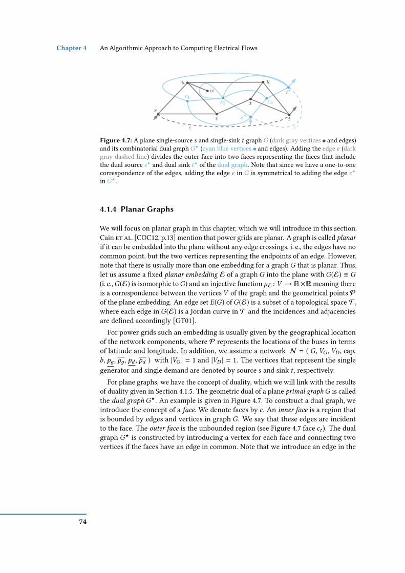
Chapter 4 An Algorithmic Approach to Computing Electrical Flows
t
y
s?
x
t?
c1c2 c3
u
w
v
e e?
s
Figure 4.7: A plane single-source s and single-sink t graph G (dark gray vertices and edges)and its combinatorial dual graph G? (cyan blue vertices and edges). Adding the edge e (darkgray dashed line) divides the outer face into two faces representing the faces that includethe dual source s? and dual sink t? of the dual graph. Note that since we have a one-to-onecorrespondence of the edges, adding the edge e in G is symmetrical to adding the edge e?
in G?.
4.1.4 Planar Graphs
We will focus on planar graph in this chapter, which we will introduce in this section.Cain et al. [COC12, p.13] mention that power grids are planar. A graph is called planar
if it can be embedded into the plane without any edge crossings, i. e., the edges have nocommon point, but the two vertices representing the endpoints of an edge. However,note that there is usually more than one embedding for a graph G that is planar. Thus,let us assume a xed planar embedding E of a graph G into the plane with G(E) G(i. e.,G(E) is isomorphic toG) and an injective function µE : V → R×R meaning thereis a correspondence between the vertices V of the graph and the geometrical points Pof the plane embedding. An edge set E(G) of G(E) is a subset of a topological space T ,where each edge in G(E) is a Jordan curve in T and the incidences and adjacenciesare dened accordingly [GT01].
For power grids such an embedding is usually given by the geographical locationof the network components, where P represents the locations of the buses in termsof latitude and longitude. In addition, we assume a network N = ( G, VG , VD , cap,b, pд , pд , pd , pd ) with |VG | = 1 and |VD | = 1. The vertices that represent the singlegenerator and single demand are denoted by source s and sink t , respectively.
For plane graphs, we have the concept of duality, which we will link with the resultsof duality given in Section 4.1.5. The geometric dual of a plane primal graphG is calledthe dual graph G?. An example is given in Figure 4.7. To construct a dual graph, weintroduce the concept of a face. We denote faces by c . An inner face is a region thatis bounded by edges and vertices in graph G. We say that these edges are incidentto the face. The outer face is the unbounded region (see Figure 4.7 face ct ). The dualgraph G? is constructed by introducing a vertex for each face and connecting twovertices if the faces have an edge in common. Note that we introduce an edge in the
74

A Mathematical Model for the Feasibility Problem of Electrical Flows Section 4.1
dual graph G? for each edge in the primal graph G. Note that a face might representmore than just a cycle, e. g., if vertex w in Figure 4.7 is a graph itself.
4.1.5 Matroids and Independence Systems
A lot of model transformations, properties, and relationships that we use in thefollowing with regard to matroids (see the postulates of Whitney [Whi35, p.510,Theorem 1]) are based on the discussion by Seshu and Reed [SR61] and Whitney[Whi31, Whi35]. A matroid [Whi35] represents a generalization of a graph [Whi31]. Amatroid is an abstraction of the independence term that is used in dierent elds suchas graph theory and geometry. Though dierent matroids are considered in dierentelds, the consensus stays the same. We recall the denition of a matroid by Korte andVygen [KV00, pp.279] (rst version was given by Whitney [Whi35, p.510]). A matroid
is an ordered pair (U ,I), where U is the universe and I ⊆ P(U ) is an independence
system, which satises the following three axioms.
Axiom 1. ∅ ∈ I (neutral element).
Axiom 2. If I ∈ I and I ′ ⊆ I then I ′ ∈ I (monotonicity).
Axiom 3. If I1, I2 ∈ I with |I1 | < |I2 | then there is an e ∈ (I2 \I1) such that I1∪e ∈ I(augmentation).
Note that the Axiom 1 and Axiom 2 represent axioms that also hold for any indepen-dence system. However, the Axiom 3 makes it a matroid that is a generalization of theterm linear independence. Whitney [Whi35] denes a base as a maximal independentsubmatroid and a cycle as a minimal dependent submatroid.
Denition 4.16 (Whitney [Whi35, p.509]). A subgraph of a graph is independent if it
contains no cycles.
In this work, we use an important mathematical principle called duality. In dierentresearch areas it has dierent meanings. However, for us it basically means that ifthere is a bijection between the edges (i. e., columns) in I and the edges in B and for asubmatroid I′ of I and the corresponding dual B′ in B, we have the relationship rk(B′) =rk(B) − n(I′), then I is a dual of B and B is a dual of I [Whi35, pp.521.]. The latter iscalled involution implying that the dual of the dual of I is I itself. Though “every matroidhas a dual” [Whi35, p.522, Theorem 22] the concept applies from a graph-theoreticalperspective to plane graphs only. Only plane graphs have a dual graph.
The following theorems state very central results that are used in this work.
Theorem 4.17 (Whitney [Whi35, p.527, Theorem 31]). For any graph G the matroids
corresponding to its incidence matrix I and its circuit matrix B are duals.
75

Chapter 4 An Algorithmic Approach to Computing Electrical Flows
For graphs we restricted the duality to plane graphs, since there is only a dual graphif the primal graph is planar. For matroids this restriction does not hold and thus, if wedo not restrict ourself to the plane (i. e., sphere with genus 0) but other surfaces withgenus greater 0, we can still embed a non-planar graph on a more complex surfacewithout any crossing by making use of the holes. An example is the embedding ofthe K5 on a torus (i. e., surface of genus 1). Note that we focus on planar graph andgenus 0.
The aforementioned duality (see Theorem 4.17) applies to the matroids I and B.The next theorem follows from Axiom 2 and the aforementioned discussion of theincidence matrix.
Theorem 4.18 (Whitney [Whi35, p.510, Theorem 1]). A set I′ ⊆ I is independent ifand only if it is contained in a base, or, if and only if it contains no cycles.
The next lemma follows from Theorem 4.17 and is illustrated in Figure 4.7.
Lemma 4.19 (Seshu and Reed [SR61, p.85, Corollary 4-24]). If G1 and G2 are dualgraphs, the incidence matrix of either graph is a circuit matrix of the other (with the
proper rank, and each row representing a cycle); that is
I1 = B2 and I2 = B1.
The lemma concludes the duality and is extensively used in this chapter (see Sec-tions 4.3.2 and 4.5).
4.2 Electrical Preserving Transformations
In this section, we introduce some standard reduction rules used in literature that leadin the end to an algorithm to solve the DC FEAS. Most transformations make use of thesuperposition principle for linear power grids, e. g., the ∆-Y - and Y -∆-transformations.The superposition principle holds (i. e., used for the superposition of, e. g., forces),since the constraint matrix A is a linear map and thus, superposition becomes a simpleaddition of linear equations (i. e., standard operation in a eld F ). Though we giverules to compute the capacity cap, these formulas can be dependent on the actualow (see Reduction Rule 4.26). Computing any electrical ow becomes trivial if wecontract the graph to one edge since on trees the electrical ow is equivalent to agraph-theoretical ow [Lei+15a][LGH15, p.9, Lemma 4].
Recall that we have a unique electrical ow in s-t-graphs (see Lemma 4.7), we canscale it to a multiple such that it complies with the capacity constrains (Equation 4.9).Thus, we are able to neglect the capacity constraints and rescale the electrical ow
76

Electrical Preserving Transformations Section 4.2
(a) (b) (c)
x
t0s
1312
13x12 /3x
−/1
−/1
−/1
−/1−/1
−/1
−/1
x
u1
u2
u3vnv
vi
v2
v1
u1
u2
u3
u v−/1
−/1
−/1
−/1
−/1 −/1−/3
−/1
vnv
vi
v2
v1
10s
x
t
13
12
14
x4 /x
x3 /x
x2 /x
0s
43 x
u
103 x
t
34
12
x/x x/x
103 x
t0s
310
x/x
Figure 4.8: Three example graphs in which we label each vertex u ∈ V that is representedby a cycle with a voltage angle θv (u). If the voltage angles are not important, we justuse standard bullets . On the edges, we write the ow f and the edge’s capacity cap in theform f /cap. If the susceptance b is important for the transformation, we write it on the edge.The series-parallel-contraction and contraction of superuous edges in energy networkssimplies the graph structure. (a) In a series-contraction a path is contracted to a single edge.(b) In a parallel-contraction multiple parallel edges (multi-edges) are contracted to one edge.(c) A scenario where shortening of superuous edges (Reduction Rule 4.25) is reasonable.This gure is adapted from [Ake60, p.313, Figure 4]. The upper gure is an example, wherethe capacity of edge cap(u,v) ≥ min
( ∑ui ,u ∈E cap(ui ,u),
∑vi ,v ∈E cap(vi ,v)
). In the bottom
gure the resulting graph after contracting the superuous edge u,v to a vertex x is shown.
afterwards such that the capacity constraints are fullled using Lemma 4.13. Fromthe Equations 4.1–4.3 and 4.13, we have only one component that has a crucial inuenceon the electrical ow and that is the susceptance b. The susceptance represents a ratiothat can be interpreted as how many electrons go through a path. Thus, the notion ofelectrical preserving is purely susceptance based.
Denition 4.20 (Electrical Preserving Transformation). Let f be a given ow and
let θv (u) be the voltage angles before the transformation for all u ∈ V (G) with regard
to f . An electrical preserving transformation T onN is a function T : M(N) →M(N)with (G = (V ,
←→E ),b) 7→ (G ′ = (V ′,
←→E ′),b ′) and new voltage angle assignments θv ′(u)
for all u ∈ V ′ such that the susceptances are transformed in such a way that for the
ow f we have θv ′(u) = θv (u) for all vertices u ∈ (V ∩V ′).
Transformation rules are useful to simplify the network and compute networkparameter more eciently. Examples are the eective values, e. g., eective resis-tance, conductance/susceptance, the “eect of earth admittances on the balance of aWheatstone bridge and earth capacity eects in AC” [But21, Ros24], and the eectiveunbalanced capacity [Ros24, p.916].
77
Chapter 4 An Algorithmic Approach to Computing Electrical Flows
For edges that operate in series—meaning they represent a path—where there is nogenerator or demand vertex in between, we know that the ow f on each edge alongthe path is the same. Lets assume a path with two edges u,v, v,w ∈ ←→E . Since allmappings are linear and we work on a eld F (i. e., here it is R), we get the followingrelationship
(∆θv 1(u ,v)+∆θv 2(v ,w )
)/f = 1/b1(u ,v) + 1/b2(v ,w ) = 1/b(u ,w ) with f (u,v) =
f (v,w) = f , which we will generalize in the following rule.
Reduction Rule 4.21 (Series Contraction). Let π (u,w) be a simple terminal-free path
(i. e., for internal vertices of the path holds that v ∈ V \(u,w ∪ VG ∪ VD
)) whose
internal vertices v ∈ π (u,w) with v , u,w have degree deg(v) = 2. Then, such a
path π (s, t) B((s,u1), (u1,u2), . . . , (ui , t)
)is equivalent to one edge (s, t) (see Figure 4.8a)
with the susceptance, voltage angle dierence, and capacity being
b(u,w) =©«
∑e ∈π (u ,w )
b(e)−1ª®¬−1
, (4.18a)
∆θv (u,w) =mine ∈π (u ,w ) cap(e)
b(u,w), (4.18b)
cap(u,w) = b(u,w) · ∆θv (u,w), (4.18c)
respectively.
For multiple parallel edges between two vertices u,v ∈ V (G), we can make theobservation that the voltage angles θv (u) and θv (v) are the same for each edge. Thus,the voltage angle dierence ∆θv (u,v) is the same. Since we work on a eld F andhave linear maps only, we do a simple addition operation on a eld such that weget
(f (u ,v 1)+f (u ,v 2)
)/∆θv (u ,v) = b(u,v1) + b(u,v2) = b(u,v) for two parallel
edges u,v1, u,v2 ∈ ←→E . We generalize this to multiple edges in the following rule.
Reduction Rule 4.22 (Parallel Contraction). Let p : ←→E → u,v | u,v ∈ V ;u , vwith u,vi 7→ u,v with 1 ≤ i ≤ k being k parallel edges. Let the parallel edges
be ei : u,vi ∈←→E with 1 ≤ i ≤ k , i. e., p(ei ) = p(ei+1) for all 1 ≤ i ≤ k − 1. These
parallel edges are equivalent to one edge (see Figure 4.8b) with the susceptance b, voltageangle dierence ∆θv , and capacity cap being
b(u,v) =∑
u ,v i ∈←→E
b(u,vi
), (4.19a)
∆θv (u,v) = minu ,v i ∈
←→E
(∆θv
(u,vi
) ), (4.19b)
cap(u,v) = b(u,v) · ∆θv (u,v), (4.19c)
respectively.
78

Electrical Preserving Transformations Section 4.2
Every vertex v ∈ V has a voltage angle θv (v) that can be interpreted as a potential.For a self-loop the voltage angles at both ends are the same and thus, the ow f onthe self-loop is zero (see Equation 4.13).
Reduction Rule 4.23 (Self-loop Contraction). Let p : ←→E → u,v | u,v ∈ V be afunction with u,u 7→ u, where p(e) = u with e ∈
←→E is a self-loop with both ends
of edge e ending in u. Then the edge e can be removed without any electrical eect, but
with one edge less (see Equation 4.13 with the additional note that both voltage angles
are the same and thus, the dierence is zero).
Reduction Rule 4.24 (Degree-1 Contraction). Let u ∈ V \ (VG ∪VD ) be a vertex withdegree deg(u) = 1 with its only edge (u,v). Then u can be removed.
The next reduction rule can be used for shortest paths and graph-theoretical ows.However, in general it is not applicable for electrical networks. We remark that in thenext section we only work with shortest paths and graph-theoretical ows.
Reduction Rule 4.25 (Shortening of Superuous Edges [Ake60, p. 313, Rule 3]).Let u ∈ V and let u,w ∈
←→E be an incident edge with capacity
cap(u,w) ≥ min ©«∑
u ,v ∈←→E \u ,w
cap(u,v),∑
w ,v ∈←→E \u ,w
cap(w,v)ª®¬(see Figure 4.8c top) then we can contract verticesu andv to a new vertex x (see Figure 4.8c
bottom).
A more general example of the latter transformation is applied on [Ake60, p. 316,Figure 7] in the third transformation.
The next graph transformations are more complex and were rst introduced by Ken-nelly [Ken99]. The ∆-Y -Transformation (also known as Delta-Wye- or Triangle-Star-Transformation) and Y -∆-Transformation are inversions to each other.
Reduction Rule 4.26 (∆-Y -Transformation). Let u, v , andw form a complete graph
with the edge set
←→E ∆ ⊆
←→E (see Figure 4.9a). This delta ∆ can be transformed to a wye Y
by adding a new vertex c representing the center of the wye Y to V and new edges to the
triangle’s vertices
←→E ∪
c,u | u,v ∈
←→E ∆
\←→E ∆ (see Figure 4.9b).
b(u, c) =b(u,v) · b(u,w) + b(u,v) · b(v,w) + b(u,w) · b(v,w)
b(v,w)(4.20a)
cap(u, c) = cap(u,v) + cap(u,w) −(f (v, c) − f (w, c)
)(4.20b)
The inverse rule of the ∆-Y -transformation is denoted by Y -∆-Transformation.
79

Chapter 4 An Algorithmic Approach to Computing Electrical Flows
1 34
3(c)
2
68
c
v
uw
(a) (b)
2
68
(d)
1 34
3
v
uw
c
∆θY (u, v)pY (u, v)
v
wu
∆θ∆(u, v)p∆(u, v)
v
wu
c
Figure 4.9: The delta-wye- (Reduction Rule 4.26) and wye-delta-transformations (ReductionRule 4.27) represent possible transformation rules in electrical networks. In this example, wehave a graph with three (respectively four) vertices . If we explicitly compute the susceptanceswe write the susceptance b on each edge. (a) The triangle ∆ can be transformed to a star Y .Recall that we have only linear maps and work on a eld F (here R). Thus, we can superposethe paths that is a simple addition operation, e. g., (v,w) is equal to the series circuit of (v,u)and (u,w), which is parallel to (v,w) meaning
((v,u), (u,w)
)| |(v,w). This electrical addition
can be done for the susceptances b and electrical (e. g., power) ows p. The voltage angle(potential) dierence stays the same ∆θv . (b) This star Y can be transformed to a triangle ∆ andcan use similar properties as described in (a). (c) The ∆-Y -transformation increases the numberof vertices by one and decreases the number of cycles by one. (d) The Y -∆-transformationincreases the number of cycles by one and decreases the number of vertices by one.
Reduction Rule 4.27 (Y -∆-Transformation). Let c ∈ V \ (VG ∪VD ) be a vertex with a
degree of deg(c) = 3 (see Figure 4.9b and d). Thus, vertex c forms the center of a wyeY with
neighbors u, v , andw . The transformation of the wye Y results in a equivalent network
that is a delta ∆ by
←→E ′′ ∪
u,v | c,u ∈
←→E , c,v ∈
←→E with u , v
\c,u ∈
←→E
and V \ c (see Figure 4.9a and c) with the susceptances
b(u,v) =b(u, c) · b(v, c)
b(u, c) + b(v, c) + b(w, c). (4.21)
The basic idea of the latter transformation is that we remove a vertex c that is thecenter of a wye Y and connect all its neighbors by an edge. Note that the previoustransformation removes a vertex from the graph, which reduces the size of the network.The next transformation is a generalization of Reduction Rule 4.27.
Note that a star of arbitrary degree deg(c), where c is the center of a star, is amore general notation for wye and in this case a polygon is a complete graph Kdeg(c)representing a generalization of a triangle (i. e., K3).
80
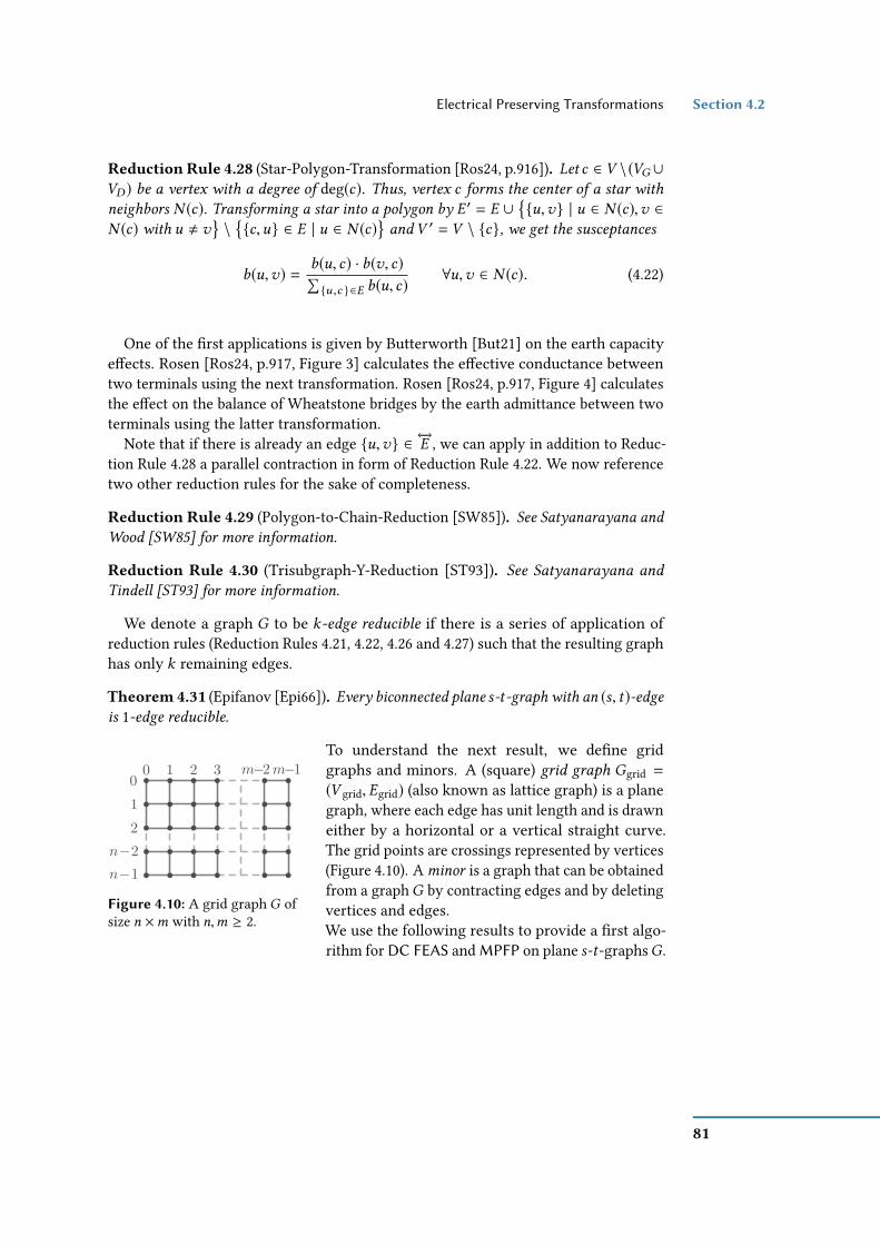
Electrical Preserving Transformations Section 4.2
Reduction Rule 4.28 (Star-Polygon-Transformation [Ros24, p.916]). Let c ∈ V \(VG ∪VD ) be a vertex with a degree of deg(c). Thus, vertex c forms the center of a star with
neighbors N (c). Transforming a star into a polygon by E ′ = E ∪u,v | u ∈ N (c),v ∈
N (c) with u , v\c,u ∈ E | u ∈ N (c)
and V ′ = V \ c, we get the susceptances
b(u,v) =b(u, c) · b(v, c)∑u ,c ∈E b(u, c)
∀u,v ∈ N (c). (4.22)
One of the rst applications is given by Butterworth [But21] on the earth capacityeects. Rosen [Ros24, p.917, Figure 3] calculates the eective conductance betweentwo terminals using the next transformation. Rosen [Ros24, p.917, Figure 4] calculatesthe eect on the balance of Wheatstone bridges by the earth admittance between twoterminals using the latter transformation.
Note that if there is already an edge u,v ∈ ←→E , we can apply in addition to Reduc-tion Rule 4.28 a parallel contraction in form of Reduction Rule 4.22. We now referencetwo other reduction rules for the sake of completeness.
Reduction Rule 4.29 (Polygon-to-Chain-Reduction [SW85]). See Satyanarayana andWood [SW85] for more information.
Reduction Rule 4.30 (Trisubgraph-Y-Reduction [ST93]). See Satyanarayana and
Tindell [ST93] for more information.
We denote a graph G to be k-edge reducible if there is a series of application ofreduction rules (Reduction Rules 4.21, 4.22, 4.26 and 4.27) such that the resulting graphhas only k remaining edges.
Theorem 4.31 (Epifanov [Epi66]). Every biconnected plane s-t-graph with an (s, t)-edgeis 1-edge reducible.
0 1 2 3
n−1
1
n−2
0m−2 m−1
2
Figure 4.10: A grid graph G ofsize n ×m with n,m ≥ 2.
To understand the next result, we dene gridgraphs and minors. A (square) grid graph Ggrid =(V grid, Egrid) (also known as lattice graph) is a planegraph, where each edge has unit length and is drawneither by a horizontal or a vertical straight curve.The grid points are crossings represented by vertices(Figure 4.10). A minor is a graph that can be obtainedfrom a graphG by contracting edges and by deletingvertices and edges.We use the following results to provide a rst algo-rithm for DC FEAS and MPFP on plane s-t-graphsG .
81

Chapter 4 An Algorithmic Approach to Computing Electrical Flows
Algorithm 1: s-t Planar DC FEAS(N ) & s-t Planar MPFP(N )Data: A network N = ( G, VG , VD , cap, b, pд , pд , pd , pd ) with |VG | = 1 (i. e.,
s = VG ), |VD | = 1 (i. e., t = VD ), pд = pд = pд , and pd = pd = pd .Result: Flow f (u,w) for all (u,w) ∈ E, ow value F (f ,N), and voltage angles θv (u)
with u ∈ V .1 E = planarEmbeddingOf(G) ; . PQ-Tree; see Section 4.5.22 Egrid = gridEmbeddingOf(G(E)) ; . see Lemma 4.343
(N = N 0, . . . ,Nk =
((s, t, e ′), s, t, cap′,b ′,pд,pd )
) )= contractGridGraphToEdge(N(Egrid)) ; . see Lemma 4.35
4 f (e ′) = pд = pd ;5 f = decontractEdgeToGridGraph((N 0, . . . ,Nk ), f (e
′)) ;6 f = rescalePowerFlow(N, f ); . see Lemma 4.127 return f ;
Lemma 4.32 ([Tru89, p.144, Lemma 6]). Every plane graph is a minor of some grid
graph.
Let a grid graphGgrid = (V grid, Egrid) be a graph that is numbered column-wise fromleft to right with 1, . . . ,m and row-wise from top to bottom with 1, . . . ,n (see Fig-ure 4.10). Similar to Truemper [Tru89], we dene an extended grid graph G`
ex as agraph on a grid with ` ≥ 2, where ` ∈ N represents the number of columns androws with 0 ≤ i ≤ ` − 1. Since the grid is quadratic, we have `2 vertices, and edgesconnecting a vertex vi ,0 on the left border at row i
t
s v -1,1 v -1, -1
v0,0
Figure 4.11: An extendedgrid graph G`
ex with a grid ofdimension `×` and `2 vertices.
column 0 of the grid to a vertex v`−1,i on the bottomborder (see Figure 4.11) such that either the source sor the sink t is located on the inner face (in Figure 4.11the source s is on the inner face). We illustrated sucha graph G`
ex in Figure 4.11.
Lemma 4.33 ([Tru89, p.145, Lemma 13]). Any planegraphG with (s, t) ∈ E and with one of the two terminals
(i. e., source s or sink t) on the outer face, is a minor of
some extended grid graph G`ex with ` ≥ 2.
Note that it is always possible to use the inverse ofall reduction rules but Reduction Rule 4.28. In the following, we try to embed thegraph G such that the embedding has the form of an extended grid graph. We needthe concept of a face in the following (Section 4.1.4). For a plane graph G a face c is aregion that is bounded by the edges and vertices of G. Two faces are incident if theyshare at least one edge.
Lemma 4.34. Any plane s-t-electrical-networkN with at least one terminal on the outer
face can be embedded into a grid in O(|V |) time.
82
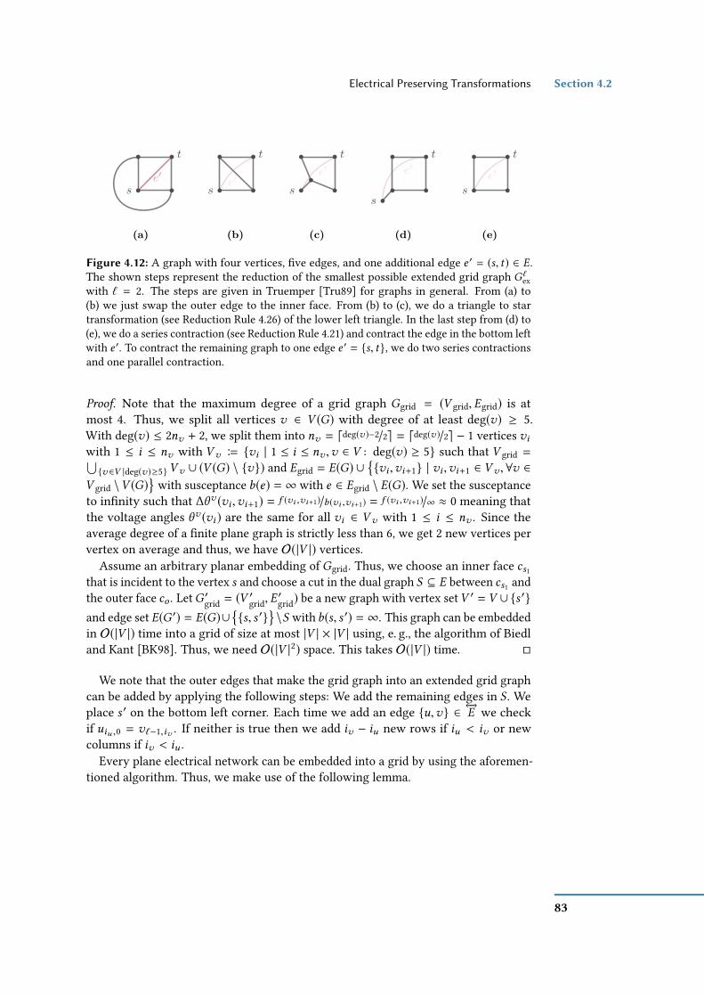
Electrical Preserving Transformations Section 4.2
(a)
t
se′
t
s
e′t
s
e′
e′
t
s
t
se′
(b) (c) (d) (e)
Figure 4.12: A graph with four vertices, ve edges, and one additional edge e ′ = (s, t) ∈ E.The shown steps represent the reduction of the smallest possible extended grid graph G`
exwith ` = 2. The steps are given in Truemper [Tru89] for graphs in general. From (a) to(b) we just swap the outer edge to the inner face. From (b) to (c), we do a triangle to startransformation (see Reduction Rule 4.26) of the lower left triangle. In the last step from (d) to(e), we do a series contraction (see Reduction Rule 4.21) and contract the edge in the bottom leftwith e ′. To contract the remaining graph to one edge e ′ = s, t, we do two series contractionsand one parallel contraction.
Proof. Note that the maximum degree of a grid graph Ggrid = (V grid, Egrid) is atmost 4. Thus, we split all vertices v ∈ V (G) with degree of at least deg(v) ≥ 5.With deg(v) ≤ 2nv + 2, we split them into nv = ddeg(v)−2/2e = ddeg(v)/2e − 1 vertices viwith 1 ≤ i ≤ nv with Vv B vi | 1 ≤ i ≤ nv ,v ∈ V : deg(v) ≥ 5 such that V grid =⋃v ∈V |deg(v)≥5Vv ∪ (V (G) \ v) and Egrid = E(G) ∪
vi ,vi+1 | vi ,vi+1 ∈ Vv ,∀v ∈
V grid \V (G)
with susceptance b(e) = ∞ with e ∈ Egrid \ E(G). We set the susceptanceto innity such that ∆θv (vi ,vi+1) = f (vi ,vi+1)/b(vi ,vi+1) = f (vi ,vi+1)/∞ ≈ 0 meaning thatthe voltage angles θv (vi ) are the same for all vi ∈ Vv with 1 ≤ i ≤ nv . Since theaverage degree of a nite plane graph is strictly less than 6, we get 2 new vertices pervertex on average and thus, we have O(|V |) vertices.
Assume an arbitrary planar embedding of Ggrid. Thus, we choose an inner face cs1that is incident to the vertex s and choose a cut in the dual graph S ⊆ E between cs1 andthe outer face co . LetG ′grid = (V
′grid, E
′grid) be a new graph with vertex setV ′ = V ∪s ′
and edge set E(G ′) = E(G)∪s, s ′
\S with b(s, s ′) = ∞. This graph can be embedded
in O(|V |) time into a grid of size at most |V | × |V | using, e. g., the algorithm of Biedland Kant [BK98]. Thus, we need O(|V |2) space. This takes O(|V |) time.
We note that the outer edges that make the grid graph into an extended grid graphcan be added by applying the following steps: We add the remaining edges in S . Weplace s ′ on the bottom left corner. Each time we add an edge u,v ∈ ←→E we checkif uiu ,0 = v`−1,iv . If neither is true then we add iv − iu new rows if iu < iv or newcolumns if iv < iu .
Every plane electrical network can be embedded into a grid by using the aforemen-tioned algorithm. Thus, we make use of the following lemma.
83

Chapter 4 An Algorithmic Approach to Computing Electrical Flows
Lemma 4.35 ([Tru89, pp.142., Theorem 2 & Lemma 14]). Every (extended) grid graphwith one source and one sink is 1-edge reducible.
So far we explained the dierent parts of the algorithm. Note that we assume aplane s-t-graphG for the algorithm. The algorithm (see Algorithm 1) works as follows.From Lemmas 4.34 and 4.35, we know that any plane graph can be embedded intoa grid (see Algorithm 1 Line 2) and that every grid graph can be contracted to asingle edge e ′ (see Algorithm 1 Line 3 and Figure 4.12). In each ∆-Y -reduction, wecompute the susceptances by the aforementioned rules (see Reduction Rules 4.26and 4.27). In the decontraction step (see Algorithm 1 Line 5), we compute based onthe given susceptances on the dierent contraction levels the voltage angles θv (u)with u ∈ V i and the ow for each contraction level i . We start withNk consisting of asingle edge e ′, over Nk−1, and in the end we compute the voltage angles and the owfor the original network N 0. For each level transition, we apply the reverse of theapplied transformation rules given in Reduction Rules 4.21–4.24, 4.26 and 4.27. Notefrom Lemma 4.12 on Page 72 that the capacities can be neglected, since we are alwaysable to rescale a nontrivial electrical ow. This rescaling is not necessary for DC FEAS,since a capacity violation would imply a non-existing feasible electrical ow. However,assume that we apply an arbitrary ow on e ′ (see Algorithm 1 Line 4) resulting inan electrical ow that is not necessarily feasible, since the capacity constraint mightbe violated. To x the violation, we use Lemma 4.13 on Page 73 on the decontractedgraphG with ow f to rescale the ow to a feasible, e. g. MPF (see Algorithm 1 Line 6).From Truemper [Tru89], we get the following running time.
Lemma 4.36. The algorithm runs in O(|V |3) time.
The contraction step of the algorithm Algorithm 1 Line 3 is illustrated in Figures 4.12and 4.13 for an extended grid graph.
Lemma 4.37. A planar s-t-graph G can always be contracted to one edge by a series of
reduction rules (see [Tru89]).
For the reverse operation, we remark that the voltage angles in a parallel and seriescontraction do not change. For the series contraction, we have to compute the voltageangles for the inner vertices using Equation 4.13. For the ∆-Y - andY -∆-transformation,the voltage angles at the three outer vertices do not change. For the center of the star,we have to compute the voltage angle using Equation 4.13. The reconstruction stepscan be done during the recursive return. If the capacities are violated, we rescale theow f using Lemma 4.12. From the previous discussion follows the next theorem.
Theorem 4.38. The algorithm computes a feasible electrical ow for a planar s-t-graph G.
84

Representations and Formulations of Electrical Flows Section 4.3
(a) (b) (c) (d) (e)
(i)(h)(g)(f)
e′
s s
e′
e′
s
t
s
e′ t
s
e′
s
e′
s
e′
s
e′
s
e′
Figure 4.13: A general extended grid graph G`ex with `2 vertices. Blue edges and blue vertices
represent the edges and vertices of the transformation and replace the orange marked edges.The steps are basically given by Truemper [Tru89] for graphs in general. From (a) to (b) weuse the steps already shown in Figure 4.12.
4.3 Representations and Formulations of Electrical Flows
Cain et al. [COC12, p.13] mention that power grids are planar (see Section 4.1.4) andundirected. Recall from Section 3.1 that we can transform any undirected graph to adirected graph, which we do for notational conveniences. The planarity of graph G isa crucial property of the network N for this section. In addition, we assume that thegraph G is biconnected.
4.3.1 The Duality Concept for Graphs
Using the duality of the incidence matrix I and circuit matrix B that was shownin Section 4.1.5, we translate the algebraic duality of the two matrices into a graphtheoretical duality (Section 4.1.4). Recall that a base of a matroid (see Denition 4.2) isa maximum independent set. The complement of a base in the primal graph G is thebase in the dual graph G? (see Lemma 4.19).
Theorem 4.39 ([Whi35, p.522, Theorem 23]). Let E be a planar embedding of a graphG .The graphs G and G?
are duals if and only if there is a bijection µdual : E(G) → E(G?)
between their edges such that bases in one correspond to base complements in the other.
The construction in Section 4.1.4 implies a bijection of edges in the primal graph Gto edges in its dual graph G?. It is called a combinatorial dual in terms of the Whitney
85

Chapter 4 An Algorithmic Approach to Computing Electrical Flows
duality (bijection of edges; and a set of edges forming a cut corresponds to a cycle inthe combinatorial dual). Note that the dual of a dual graph G? is isomorphic to theprimal graph G as long as G is connected.
From Equations 4.1–4.3, we know that a feasible KCL ow on the primal graph G isequivalent to a graph theoretical ow in the primal graphG . It follows from Lemma 4.19that a feasible KVL ow corresponds to a graph theoretical ow in the dual graph.Thus, we get the following lemma.
Lemma 4.40. A feasible KVL ow f G in the primal graph G is equivalent to a feasi-
ble KCL ow f G? in the corresponding dual graph G?.
Note that we can apply any ow f on a self-loop e = (u,u), since it is redundant.Thus, we get the following observation.
Observation 4.41. Let the primal graphG be a tree. Thus, there is only one face that is
equivalent to the outer-face ct . The dual graph consists of self-loops only. Let f be any
feasible ow on G. Then, ow f is also a feasible electrical ow.
Recall from Section 4.2 that every self-loop can be removed (see Reduction Rule 4.23).The aforementioned observation is a geometrical explanation for planar graphs of theresults of Lehmann et al. [LGH15, p.9, Lemma 4] and Leibfried et al. [Lei+15a] thaton trees any graph-theoretical ow is also electrical feasible.
We note that a series contraction (see Reduction Rule 4.21) inG is an equivalent trans-formation to the parallel contraction (see Reduction Rule 4.22) in the dual graph G?.We highlight that by the following structural observation.
Observation 4.42. The series contraction in the primal graph G is equivalent to the
parallel contraction in its dual G?and vice versa.
Observation 4.43. The ∆-Y -transformation in the primal graph G is equivalent to
the Y -∆-transformation in the dual graph G?and vice versa.
In the following section, we will make use of the duality by reformulating theproblem.
4.3.2 Simultaneous Flow Representation
We use the aforementioned duality and structure of the problem to reformulate DC FEASin terms of the Simultaneous Flow Problem (SFP). For SFP the graphs are not neces-sarily duals, but share some edges.
86

Representations and Formulations of Electrical Flows Section 4.3
(a) (b) (c)
23
19
14
32
12
1224
23
14
1912
12 24
32
9955
56
55
∆θ
vorv
p or is
t
s? t?12
12 19
245
932 23
14
32
12
12
19
23
145
9
24u1
12
12
24
19
1459
2332t
s
120
19
3356
24u3
u2
u4
u1
u3
u2
u4
s
t
u4
u2u1
u3
Figure 4.14: We use the example graph of Felsner [Fel13, p.18]. The susceptances are b ≡ 1,the feasible electrical ow f (e) is written on each edge e ∈ E, and we neglect the capacitiesmeaning cap ≡ ∞. (a) The example graph’s feasible electrical ow is in this case the minimuminteger feasible electrical ow f and the corresponding voltage angles θv . (b) The ow f andthe voltage angle dierences ∆θv can be separated into two graphs, which are the primalgraph G and its dual graph G?, respectively. (c) Since the susceptances are b ≡ 1 a similarrepresentation is a squaring of a 55 × 56 rectangle, where the width and the height of eachsquare is represented by the ow in the primal and dual graph, respectively. Each vertex in theprimal and dual graph represents a horizontal or vertical segment, respectively. For clarity welabeled the vertices for the primal graph only, since otherwise this gure seems overloaded.An edge represents a side of a square.
Simultaneous Flow Problem 2 SFP(N)
Instance: Two graphs G1 and G2, subsets E1 ⊆ E(G1) and E2 ⊆ E(G2), and abijection µSFP : E1 → E2.
Question: Are there nonzero KCL-feasible ows f G1 and f G2 in G1 and G2 suchthat for every edge e ∈ E1 we have f G1(e) = f G2(µSFP(e))?
The reformulation of DC FEAS separates the constraints—meaning KCL and KVL—by the usage of two graphs, which we dene in the following. Recall that our graph isplanar and biconnected, and that we denote by µdual : E(G(E)) → E(G?) the bijectionof the edges with ei 7→ µdual(ei ) = e?i . An edge (u,w) = ei ∈ G corresponds to anedge (c1, c2) = e?i ∈ G? and vice versa if and only if ei is incident to both faces c1and c2, and e?i is incident to the faces u and w . Since there is no unique embedding ofa biconnected planar graph the mapping is not unique. This means that the bijectionis always related to some planar embedding of graph G.
Without loss of generality, we assume that ow f is a function f : E → Z. Re-call that we can always rescale f to a feasible electrical ow that is non-integral(meaning f : E → R) by using the scaling from Lemma 4.12.
From Theorem 4.17, we know that a graph’s base of the incidence matrix and thecorresponding base of the circuit matrix are duals. Given a graph and its dual, we
2After showing our results to Guido Brückner, he mentioned the SFP generalization to us. We wouldlike to thank him for that generalization of the biconnected planar s-t-DC FEAS-problem.
87
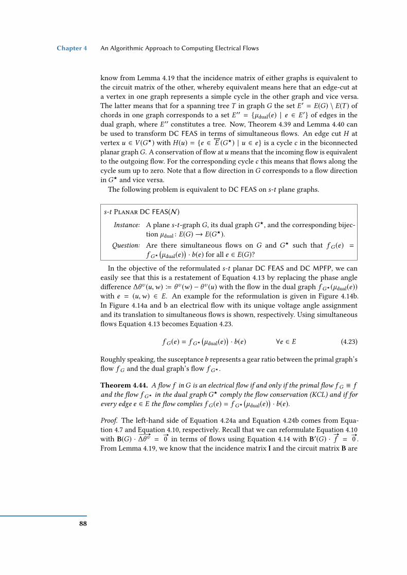
Chapter 4 An Algorithmic Approach to Computing Electrical Flows
know from Lemma 4.19 that the incidence matrix of either graphs is equivalent tothe circuit matrix of the other, whereby equivalent means here that an edge-cut ata vertex in one graph represents a simple cycle in the other graph and vice versa.The latter means that for a spanning tree T in graph G the set E ′ = E(G) \ E(T ) ofchords in one graph corresponds to a set E ′′ = µdual(e) | e ∈ E ′ of edges in thedual graph, where E ′′ constitutes a tree. Now, Theorem 4.39 and Lemma 4.40 canbe used to transform DC FEAS in terms of simultaneous ows. An edge cut H atvertex u ∈ V (G?) with H (u) = e ∈
←→E (G?) | u ∈ e is a cycle c in the biconnected
planar graphG . A conservation of ow atu means that the incoming ow is equivalentto the outgoing ow. For the corresponding cycle c this means that ows along thecycle sum up to zero. Note that a ow direction in G corresponds to a ow directionin G? and vice versa.
The following problem is equivalent to DC FEAS on s-t plane graphs.
s-t Planar DC FEAS(N )
Instance: A plane s-t-graph G, its dual graph G?, and the corresponding bijec-tion µdual : E(G) → E(G?).
Question: Are there simultaneous ows on G and G? such that f G (e) =f G?
(µdual(e)
)· b(e) for all e ∈ E(G)?
In the objective of the reformulated s-t planar DC FEAS and DC MPFP, we caneasily see that this is a restatement of Equation 4.13 by replacing the phase angledierence ∆θv (u,w) B θv (w) − θv (u) with the ow in the dual graph f G?(µdual(e))with e = (u,w) ∈ E. An example for the reformulation is given in Figure 4.14b.In Figure 4.14a and b an electrical ow with its unique voltage angle assignmentand its translation to simultaneous ows is shown, respectively. Using simultaneousows Equation 4.13 becomes Equation 4.23.
f G (e) = f G?
(µdual(e)
)· b(e) ∀e ∈ E (4.23)
Roughly speaking, the susceptanceb represents a gear ratio between the primal graph’sow f G and the dual graph’s ow f G? .
Theorem 4.44. A ow f inG is an electrical ow if and only if the primal ow f G ≡ fand the ow f G? in the dual graph G?
comply the ow conservation (KCL) and if for
every edge e ∈ E the ow complies f G (e) = f G?
(µdual(e)
)· b(e).
Proof. The left-hand side of Equation 4.24a and Equation 4.24b comes from Equa-tion 4.7 and Equation 4.10, respectively. Recall that we can reformulate Equation 4.10with B(G) ·
# »
∆θv =#»0 in terms of ows using Equation 4.14 with B′(G) ·
#»
f =#»0 .
From Lemma 4.19, we know that the incidence matrix I and the circuit matrix B are
88

Representations and Formulations of Electrical Flows Section 4.3
duals meaning I(G) = B′(G?) and B′(G) = I(G?). Using the duality, we get for Equa-tion 4.7 and Equation 4.10 the following.
I(G) ·# »
f G =#»0 ⇔ B(G?) ·
# »
∆θvG? =#»0 (4.24a)
B(G) ·# »
∆θvG =#»0 ⇔ I(G?) ·
# »
f G? =#»0 (4.24b)
From Equation 4.13 and Equation 4.24b we get Equation 4.25.
f G (e) = b(e) · ∆θvG (e) (4.25a)
f G (e) = b(e) · f G?(µdual(e)) (4.25b)
The illustration of the relationship is given in Figure 4.15.
Another equivalent representation is given in Figure 4.14c, which we describe inthe following.
4.3.3 Rectangular Representation
Another representation of simultaneous ows was given by Felsner [Fel13, p.18] and isshown in Figure 4.14c. We note that this is basically an adopted idea of Rosenstiehl andTarjan [RT86] that use a similar construction for rectilinear planar layouts but do notuse it for a squaring of an outer rectangle. This representation is in general denotedby rectangular dissection R. Within this representation a vertex is either a horizontalor vertical line segment dependent on whether the vertex is in the primal graph G ordual graph G?. In Figure 4.14c, a horizontal segment corresponds to a vertex in theprimal graph G and a vertical segment corresponds to a vertex in the dual graph G?.We illustrate the latter in Figure 4.14c for the primal graph by labeling the segmentswith the corresponding vertices s,u1,u2,u3,u4, t ∈ V . An edge represents a side of asquare. Dependent on the graph a ow on that edge aects either the horizontal orvertical side ratio (i. e., the width or height of a rectangle).
Felsner shows that a special case of simultaneous ow can be represented by squaringof an outer rectangle. The case in Figure 4.14c shows such a special case, where allinner partitions of an outer rectangle are squares. The reason for that is that thesusceptance b is b ≡ 1 and thus, Equation 4.23 becomes f G (e) = f G?
(µdual(e)
)for
all e ∈ E.However, a more general denition that is closer to power grids would be to allow
arbitrary susceptances b(←→e ) with ←→e ∈ ←→E . Than the representation is not a squaring
of an outer rectangle. Meaning that the inner partitions are not necessary squares,but can be rectangles with diering aspect ratio dependent on the susceptance b. Anexample is given in Figure 4.15.
Note that from Lemma 4.40 we know that a feasible ow in the primal graph Gmodels the actual (power) ow that is equivalent to a current ow i (see Section 3.3.2
89

Chapter 4 An Algorithmic Approach to Computing Electrical Flows
on Page 52) and that a feasible ow in the dual graph G? models the voltage angledierences ∆θv that is equivalent to the voltage drops v (see Section 3.3.2 on Page 52).Recall that a ow f G in the primal graph G represents one side of the rectangle(in Figure 4.15c this would be the width) and the f G? in the dual graph G? representsthe other side of the rectangle (in Figure 4.15c this would be the height). Thus, thesurface of a rectangle represents the powerp, which explains the quadratic relationship(see Lemma 4.45).
Lemma 4.45. The primal graphG and the dual graphG?model the quadratic relation-
ship between voltage v and current i meaning p = v · i (see Equation 3.5).
Felsner [Fel13, p.8] restricted R to the case, where there is no point where fourrectangles meet each other. However, in Figure 4.15c we can see that this is possibleand does not cause any problem. Such a representation can be also seen as a segmentcontact representation. We refer for the latter representation to Felsner [Fel13].
For a given graph the drawing of a squaring of rectangles is unique, which followsfrom Lemma 4.7. In Section 4.5.1, we will see that a bipolar orientation exists if thegraph is biconnected. The embedding of biconnected planar graph is not unique, sincewe can switch for example the order of parallel paths. However, from Lemma 4.7 weknow that the ows are unique.
Lemma 4.46 (Unique Partition of a Rectangular Representation). The rectangles of arectangular representation have unique minimum integral sizes. The embedding of these
rectangles can vary.
This concludes a very important property of simultaneous ows and a rectangularrepresentation. These representations separates the quadratic relationship and helpto understand important properties of electrical ows, which we will see in the nextsection. In the following, we will discuss the balancing property that will be used as acriteria for termination and basically describes the conict resolution in each graph.
4.4 The Balancing Property
Electrical ows have a property of balancing meaning the ows do not congest certainedges but spread the load over multiple paths from s to t . Note that this is the maindierence to graph-theoretical ows that try—while maximized—to congest all edgesas much as possible. The balancing property of electrical ows is equivalent to owsthat minimize the total losses (Equation 4.26).
min∑e ∈←→E
f (e)2/b(e), (4.26)
90

The Balancing Property Section 4.4
KCL conflictb scaling (c)(a) (b)
s
t
s? t?1
1 2
21
13 2
1
3
1
1
1
2
21
1
2
2
12
u1
u3
u2
u4
0
1
1
2
2
111
23t
s
1 2
5 63 4
2 3
u1
t
s
u3
u2
u4
1111
11
11
1 2
22
3
3
5
52
1
22
s
t
u4
u2u1
u3
Figure 4.15: We use the example graph of Felsner [Fel13, p.18] that is also used in Figure 4.14.The susceptances are b ≡ 1 and we neglect the capacities meaning cap ≡ ∞. We write theows f on the edges or on the rectangle’s side. (a) We apply some feasible ow f (i. e.,complying the KCL and capacity constraints only) on graph G. The feasible ow f is not afeasible electrical ow, since the voltage angles (distance labels)) θv at the vertices are notunique. The latter can be seen in the double assignments at u3,u4, t ∈ V . Thus, the KVL isviolated. (b) It is always possible to transform a feasible ow f into a feasible electrical ow f ′
by scaling the susceptances b at certain edges such that the ratio f/∆θv ≡ f G/f G? ≡ b changesthe ow f G? in such a way that it becomes feasible (i. e., complying KCL and thus, KVL) aslong as the susceptance b is not restricted meaning b ∈ [0,∞]. (c) In the geometric setting asusceptance scaling represents an aspect ratio scaling (indicated by the arrows ↑). The bottomright box would exceed the outer rectangle by one unit without the susceptance scaling of 2.Without the susceptance scaling of 1/2 there would be a gap of one unit in the right center.
which is a quadratic function [Chr+11, p.275, Section 2.2, Energy Equation]. In thissection, we describe this property in terms of simultaneous ows using algorithmicproperties that exploit the aforementioned structure (see Lemma 4.45)
Ford and Fulkerson [FF56, p.404, Section 3] introduced the duality between maxi-mum ows and shortest paths in which a minimum cut in G corresponds to a shortestpath in the dual graph G?. To use shortest paths, we rst introduce a distance metricfor power grids. The distance between two vertices is usually the length of an edge ortime to pass that edge. The distance in an electrical network, is given by the potentialdierence θv (w) − θv (u) that is the voltage angle dierence ∆θv (u,w).
For a given ow f the voltage angle dierence on any u-w-path π (u,w) is givenin Equation 4.27 and is derived from Equation 4.13. We now give a generalization ofthe voltage angle dierence ∆θv that is original dened on edges to the voltage angledierence on paths that is a distance function ∆θv : Π → F , where F is a eld (e. g.,R) and Π is a set of paths. Note that the equations that are build from Equation 4.27constitute a matrix and the generalization is a simple sum of the rows that resultin Equation 4.13.
∆θv (π (u,w)) B∑
(i , j)∈π (u ,w )
f (i, j)
b(i, j), (4.27)
91

Chapter 4 An Algorithmic Approach to Computing Electrical Flows
for a path π (u,w) ∈ Π with u,w ∈ V . For electrical ows the metric is f (e)/b(e)
deduced from Equation 4.27. The Shortest Path Problem (SPP) computes a pathwith minimum length π SP(s, t) Bminπ (s ,t )∈Π
∑e ∈π (s ,t ) f (e)/b(e). Contrary, the Longest
Path Problem (LPP) computes a path that has the longest distance between two vertexpairs π LP(s, t) B maxπ (s ,t )∈Π
∑e ∈π (s ,t ) f (e)/b(e).
From the previous section (see especially Equations 4.10 and 4.13) we know that thevoltage angle assignments are unique and thus, we get the following observation thatis illustrated in Figure 4.16.
The distance between to vertices u,w ∈ V with (u,w) ∈ E is given by the voltageangle dierence ∆θv (u,w) B θv (w) − θv (u) with voltage angles θv that can be inter-preted as distance labels. The voltage angle dierence (i. e., the electrical distance) for apath π (s, t) is given by ∆θv (π (s, t))=
∑(u ,w )∈π (s ,t )∆θ
v (u,w)=∑(u ,w )∈π (s ,t )f (u ,w )/b(u ,w ).
Lemma 4.47 (Balancing Flow Property). Given a primal graphG and its dual graphG?,
for which the shortest path π SP(s, t) ∈ Π(G) in G (respectively longest path π LP(s, t) ∈Π(G)) can dier to the shortest path π SP(s, t) ∈ Π(G?) in G?
(respectively longest
path π LP(s, t) ∈ Π(G?)). A ow f is an electrical ow if and only if the longest and
shortest path have the same length ∆θv (π SP(s, t)) = ∆θv (π LP(s, t)) inG with s, t ∈ V (G)and ∆θv (π SP(s
?, t?)) = ∆θv (π LP(s?, t?)) inG?
with s?, t? ∈ V (G?) (with respect to the
distance metric f/b).
Proof. ⇒ : First we show the one direction, where f is a feasible electrical ow, whichimplies that the length of all paths is equivalent ∆θv (π SP(s, t)) = ∆θv (π LP(s, t)).
Let f be a feasible electrical ow. If ∆θv (π SP(s, t)) , ∆θv (π LP(s, t)) in G with s, t ∈V (G) then there is no unique voltage angle assignment θv (u) for all u ∈ V (G). Thisimplies that f does not comply with the KVL (see Equation 4.13). If ∆θv (π SP(s
?, t?)) ,∆θv (π LP(s
?, t?)) in G? with s?, t? ∈ V (G?) then there is no unique voltage angleassignment in G? (see Equation 4.24), which means that f does not comply withthe KCL (see Equations 4.4–4.6). Any one of the two cases would be a contradictionto f being a feasible electrical ow (see Denition 4.5).⇐ : With the other direction, we show that if ∆θv (π SP(s, t)) = ∆θv (π LP(s, t)) then
this implies that f is a feasible electrical ow. Given two paths from s to t denotedby π 1(s, t), π 2(s, t) ∈ Π that merge at vertex x , meaning π 1(x, t) = π 2(x, t) C π . Inaddition, we have given the distance metric f (u ,w )/b(u ,w ) then from ∆θv
(π 1(s, t)
)=
∆θv(π 2(s, t)
)using the distance metric follows∑
(u ,w )∈π 1(s ,t )
f (u,w)
b(u,w)=
∑(u ,w )∈π 2(s ,t )
f (u,w)
b(u,w).
We dene the voltage angles on the source s and sink t to be θv (s) B 0, and θv (t) B∆θv
(π 1(s, t)
)= ∆θv
(π 2(s, t)
).
92

The Balancing Property Section 4.4
θv (s) +∑
(u ,w )∈π 1(s ,x )
f (u,w)
b(u,w)+ π = θv (t)
θv (s) +∑
(u ,w )∈π 2(s ,x )
f (u,w)
b(u,w)+ π = θv (t)
Sinceπ = π 1(x, t) = π 2(x, t), θv (s) = 0, and the voltage angleθv (t) = ∆θv(π 1(s, t)
)=
∆θv(π 2(s, t)
). It follows that∑
(u ,w )∈π 1(s ,x )
f (u,w)
b(u,w)=
∑(u ,w )∈π 2(s ,x )
f (u,w)
b(u,w)= θv (t) − θv (s) − π .
Thus, the distances from the source s to the vertexx are the same meaning∆θv(π 1(s, x)
)= ∆θv
(π 2(s, x)
)C θv (x). We can recursively proceed, which gives us the following
equality. ∑(u ,w )∈π 1(s ,x )
∆θv (u,w) =∑
(u ,w )∈π 2(s ,x )
∆θv (u,w)
This relationship is known from Equation 4.13 and restated by ∆θv (u,w) B(θv (w) −
θv (u))=
f (u ,w )b(u ,w ) . The phase angles on each side cancel each other out, but the source s
and the sink t .(θv (u1) − θ
v (s))+
(θv (u2) − θ
v (u1))
+(θv (u3) − θ
v (u2))+ . . .
. . . +(θv (un) − θ
v (un−1))+(θv (ut ) − θ
v (un))=
(θv (t) − θv (s)
)Since the source s and the sink t are for both paths π 1(s, t), π 2(s, t) ∈ Π the sameand both paths have the same distance ∆θv
(π 1(s, t)
)= ∆θv
(π 2(s, t)
)the voltage
angle assignments are unique. We get(θv (t) − θv (s)
)=
∑(u ,w )∈π 1(s ,t )
f (u ,w )b(u ,w ) =∑
(u ,w )∈π 2(s ,t )f (u ,w )b(u ,w ) =
f (s ,t )b(s ,t ) .
The intuition that electricity follows the path of the least resistance and tries tobalance itself leads us to a balanced ow, where all paths have the same length fromany vertex to any other vertex. First, we introduce shortest paths for power grids thatrepresent one part of the intuition namely the path with the least resistance. Note thatvertex label dierences always sum up to zero and thus, these labels, too. Recall thatthis is exactly the same behavior as in Equation 4.13 for the voltage angles. A vertex vthat violates Equations 4.4–4.6 has an excess fnet(v) , 0. The excess represents theamount of ow that has to be reduced or increased in v’s incoming or outgoing ow,respectively. From the duality of the Maximum Flow Problem and Shortest PathProblem [FF56, p.404, Section 3] and the aforementioned discussion on the duality ofthe KCL and KVL constraints, we get the following observation.
93
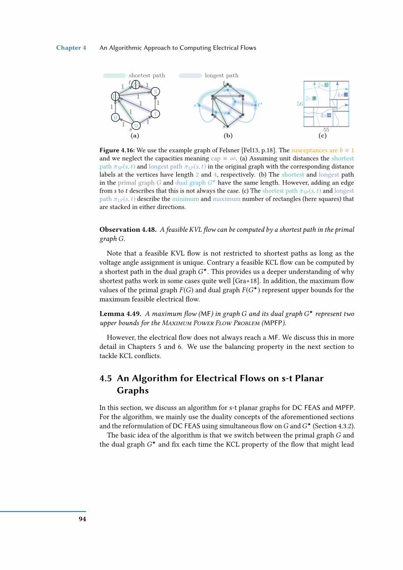
Chapter 4 An Algorithmic Approach to Computing Electrical Flows
(b) (c)(a)
shortest path
55
564×
4×
2×
2×
1
1
11
111
11 t
s
0 1
321
0
42
s
s? t?
tlongest path
Figure 4.16: We use the example graph of Felsner [Fel13, p.18]. The susceptances are b ≡ 1and we neglect the capacities meaning cap ≡ ∞. (a) Assuming unit distances the shortestpath π SP(s, t) and longest path π LP(s, t) in the original graph with the corresponding distancelabels at the vertices have length 2 and 4, respectively. (b) The shortest and longest pathin the primal graph G and dual graph G? have the same length. However, adding an edgefrom s to t describes that this is not always the case. (c) The shortest path π SP(s, t) and longestpath π LP(s, t) describe the minimum and maximum number of rectangles (here squares) thatare stacked in either directions.
Observation 4.48. A feasible KVL ow can be computed by a shortest path in the primal
graph G.
Note that a feasible KVL ow is not restricted to shortest paths as long as thevoltage angle assignment is unique. Contrary a feasible KCL ow can be computed bya shortest path in the dual graph G?. This provides us a deeper understanding of whyshortest paths work in some cases quite well [Gra+18]. In addition, the maximum owvalues of the primal graph F (G) and dual graph F (G?) represent upper bounds for themaximum feasible electrical ow.
Lemma 4.49. A maximum ow (MF) in graph G and its dual graph G?represent two
upper bounds for the Maximum Power Flow Problem (MPFP).
However, the electrical ow does not always reach a MF. We discuss this in moredetail in Chapters 5 and 6. We use the balancing property in the next section totackle KCL conicts.
4.5 An Algorithm for Electrical Flows on s-t PlanarGraphs
In this section, we discuss an algorithm for s-t planar graphs for DC FEAS and MPFP.For the algorithm, we mainly use the duality concepts of the aforementioned sectionsand the reformulation of DC FEAS using simultaneous ow onG andG? (Section 4.3.2).
The basic idea of the algorithm is that we switch between the primal graph G andthe dual graph G? and x each time the KCL property of the ow that might lead
94

An Algorithm for Electrical Flows on s-t Planar Graphs Section 4.5
Algorithm 2: s-t Planar DC FEAS(N ) & s-t Planar MPFP(N )Data: A network N = ( G, VG , VD , cap, b, pд , pд , pd , pd ) with |VG | = 1 (i. e.,
s = VG ), |VD | = 1 (i. e., t = VD ), cap ≡ 0, and cap ≡ ∞.Result: Flow f (u,w) for all (u,w) ∈ E, ow value F (f ,N), and voltage angles θv (u)
with u ∈ V .1 G = bipolarSubgraphOf(G, s, t); . see Section 4.5.12 E = planarEmbeddingOf(G); . PQ-Tree; see Section 4.5.23
(G?,b?, µdual : E(G) → E(G?)
)= constructDualGraphOf(G(E),b); . Section 4.5.2
. Augment ow along an incident edge at source s4 f ≡ 0; f (s,u) = 1 for some edge (s,u) ∈ E(G);5 (H ,b, s, t) = (G,b, s, t);6 X = u ∈ V (H ) | fnet(u) , 0;7 while X , ∅ do . Check KCL property in H8 f H = resolveKclConflict(H , X , b, s , t , f H);9 (H?,b?, s?, t?) = (H ,b, s, t); (H ,b, s, t) = dualGraphOf(H?,b?, s?, t?);
10 f H (e) = f H?(µdual(e)) · b(e);11 X = u ∈ V (H ) | fnet(u) , 0; . New KCL conicts in the dual graph12 end
to KCL conict in its dual graph. The property of balancing (see Section 4.4) is used todescribe how we x KCL conicts and that the algorithm terminates. In Algorithm 2,we show the algorithm to compute an electrical ow in an s-t biconnected planargraph. In the following, we will describe each part of the algorithm in more detail.
4.5.1 Bipolar Orientation
In this section, we focus on the function bipolarSubgraphOf(G, s, t) in Line 1 of Al-gorithm 2. Each simultaneous ow has a specic direction, which is naturally givenby an electrical ow that is in general a directed acyclic graph (DAG). Another in-terpretation can be given from the rectangular representation that has a DAG as avisibility graph [Fel13, pp.12f.]. The latter means that there is an edge between twovertices if there is a segment between them. See for example Figure 4.14c, where thehorizontal segments u3 and t are visible to each other, since there is a vertical segmentthat connects both segments directly. The visibility graph is given in Figure 4.14b,where we represent the visibility of u3 and t by an edge (u3, t). So if we dene avisibility direction, e. g., from bottom to top (horizontal segment visibility) and fromleft to right (vertical segment visibility), we get two directed acyclic visibility graphs asshown in Figure 4.14b. Note that the directed acyclic graphs (DAGs) are either calledbipolar orientation [FMR95] or s-t-numbering [ET76]. Such a numbering gives each
95

Chapter 4 An Algorithmic Approach to Computing Electrical Flows
vertex u ∈ V a number within the range of [s = 1, . . . , |V | = t], which represents atopological order of the vertices.
Observation 4.50 (Bipolar Duals [Fel13, p.13]). A bipolar orientation in the primal
graph G implies a bipolar orientation in the dual graph G?.
To see the latter, observation let us assume a directed edge (u1,u2) ∈ E(G). This edgeis incident to two faces c1, c2 ∈ V (G?). Looking in the direction of the edge (u1,u2),meaning that we look fromu1 tou2 then the face c1 is to the left of that edge and c2 is tothe right of that edge. Since we have a bijection of the edges there is an edge c1, c2 ∈←→E (G?). We dene that a direction from u1 to u2 implies a direction from c1 to c2 andthus, a direction from left to right. Thus, if there is a bipolar orientation for graph Gthis implies a bipolar orientation for its dual graph G? by denition. An illustration isgiven in Figures 4.14 and 4.15 b.
Observation 4.51 (Biconnectivity Assumption [Fel13, p.13]). If graphG has a bipolar
orientation then it is biconnected.
Calculating a bipolar orientation takes O(|V |) time [Fel13]. An overview of thegraph classes that fulll the latter property are given by Battista et al. [Bat+98, p.212,Theorem 6.19]. The most interesting classes to us are planar s-t-graphs, series-paralleldigraphs, and planar bipartite digraphs.
4.5.2 Planar Embedding and Dual Graph Construction
Recall that we assume that graph G is planar. To compute a planar embedding E, weuse in planarEmbeddingOf(G) (Algorithm 2 in Line 2) a linear-time planarity testingalgorithm [HT74][RT86, p.345]. These algorithms construct circular lists in O(|V |) thatrepresent for each vertex an ordered list of its incident edges in clock-wise order. Thelatter represents a set of rotations, which we will use to construct the dual graph G?.This can be done by selecting any edge u,w ∈ ←→E and traverse it in one direction suchas from u tow . Then select the next edge clockwise atw ∈ V . We proceed this methoduntil we reach u. The walk represents a traversal of a face, where (u,w) representsone boundary edge. We traverse the edge in the other direction meaning (w,u) thatgives us the boundary edges of the other face that is incident to edge u,w ∈ ←→E .We proceed with an edge that was not traversed in both direction and apply theaforementioned method. This extracts for each edge the left face c` and right face crwith c`, cr ∈ V (G
?) and within that, we construct implicitly the edge c`, cr ∈←→E (G?).
The dual graph G? of a graph G can be constructed in O(|V |).Since we use the same construction as Rosenstiehl and Tarjan [RT86, pp.344.,
Section 2], we assume that the graph is biconnected for the aforementioned construc-tion. Otherwise, we add—similar to Rosenstiehl and Tarjan [RT86, p.345]—dummyedges such that G stays planar and becomes biconnected, which is possible in O(|V |).
96
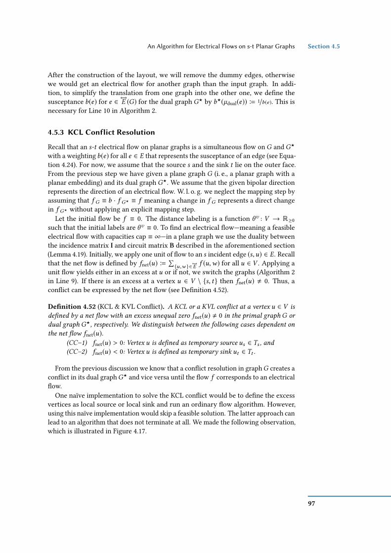
An Algorithm for Electrical Flows on s-t Planar Graphs Section 4.5
After the construction of the layout, we will remove the dummy edges, otherwisewe would get an electrical ow for another graph than the input graph. In addi-tion, to simplify the translation from one graph into the other one, we dene thesusceptance b(e) for e ∈ ←→E (G) for the dual graph G? by b?(µdual(e)) B 1/b(e). This isnecessary for Line 10 in Algorithm 2.
4.5.3 KCL Conflict Resolution
Recall that an s-t electrical ow on planar graphs is a simultaneous ow on G and G?
with a weighting b(e) for all e ∈ E that represents the susceptance of an edge (see Equa-tion 4.24). For now, we assume that the source s and the sink t lie on the outer face.From the previous step we have given a plane graph G (i. e., a planar graph with aplanar embedding) and its dual graph G?. We assume that the given bipolar directionrepresents the direction of an electrical ow. W. l. o. g. we neglect the mapping step byassuming that f G ≡ b · f G? ≡ f meaning a change in f G represents a direct changein f G? without applying an explicit mapping step.
Let the initial ow be f ≡ 0. The distance labeling is a function θv : V → R≥0such that the initial labels are θv ≡ 0. To nd an electrical ow—meaning a feasibleelectrical ow with capacities cap ≡ ∞—in a plane graph we use the duality betweenthe incidence matrix I and circuit matrix B described in the aforementioned section(Lemma 4.19). Initially, we apply one unit of ow to an s incident edge (s,u) ∈ E. Recallthat the net ow is dened by fnet(u) B
∑u ,w ∈
←→E f (u,w) for all u ∈ V . Applying a
unit ow yields either in an excess at u or if not, we switch the graphs (Algorithm 2in Line 9). If there is an excess at a vertex u ∈ V \ s, t then fnet(u) , 0. Thus, aconict can be expressed by the net ow (see Denition 4.52).
Denition 4.52 (KCL & KVL Conict). A KCL or a KVL conict at a vertex u ∈ V is
dened by a net ow with an excess unequal zero fnet(u) , 0 in the primal graph G or
dual graph G?, respectively. We distinguish between the following cases dependent on
the net ow fnet(u).
(CC–1) fnet(u) > 0: Vertex u is dened as temporary source us ∈ Ts , and(CC–2) fnet(u) < 0: Vertex u is dened as temporary sink ut ∈ Tt .
From the previous discussion we know that a conict resolution in graphG creates aconict in its dual graphG? and vice versa until the ow f corresponds to an electricalow.
One naïve implementation to solve the KCL conict would be to dene the excessvertices as local source or local sink and run an ordinary ow algorithm. However,using this naïve implementation would skip a feasible solution. The latter approach canlead to an algorithm that does not terminate at all. We made the following observation,which is illustrated in Figure 4.17.
97

Chapter 4 An Algorithmic Approach to Computing Electrical Flows
1616
1111
1212
66
55 77
1010
266
1615
1111
77
6666
10912
11 254
s
s? t?
c1c2
c3
u1 u2
u3 u4c46
10
1225
16 11
7
6
16
6
6
10
2
5
12
117
s
ts
(a) (b) (c)
(d) (e) (f)∆θv
orv
p or i
∆θv
orv
p or i
s
s? t?
c1c2
c3
u1 u2
u3 u4c4
16
6
6
10
72
5
12
11
6
9
1124
15 11
7
6s
s? t?
c1c2
c3
u1 u2
u3 u4c46
10
1225
16 11
7
6
16
6
6
10
2
5
12
117
s
s? t?
c1c2
c3
u1 u2
u3 u4c46
10
1235
16 12
7
6
16
6
6
10
5
12
117
2
t
t t
t
Figure 4.17: A primal graph G and its dual graph G? that have each six vertices, nine edges,one source and one sink are shown in (a), (c), (d), and (f). A geometrical representation ofboth graphs is given in (b) and (e). Each edge in either graphs represents a line segment inthe appropriate color and the ow on an edge denes the aspect ratio of a rectangle, e. g., theedges (c3, t?) and (u4, t) describe the height and width of the upper right rectangle, respectively.(a) A change in ow in the dual graph causes a mapping, which eect is shown in (b) and (c).(b) The mapping causes a rescaling of some rectangles sides, i. e., in this case the width of fourrectangles are changed. The outer hull changes from a rectangle to a non-rectangle (shown inthe background). (c) After the mapping step the one-to-one-correspondence is retained. (d) Inthis case the mapping result in a KCL conict (red) in the primal graph G . (e) Resizing the tworectangles resolves the conict. (f) The ow on the edges (u2,u3), (u4, t) ∈ E(G) resolves theconict.
Observation 4.53 (Resolve KCL Conicts). In each resolveConflict step, we have
to minimize the total resizing of the outer rectangle, since a too large increase might skip
a valid solution.
This observation leads us to the denition of a minimum conict resolution. Recallthat a KCL resolution means a KVL resolution in the dual graph. Resolving a KVLconict leads to an alignment of the length of the longest path π LP(s, t) and the shortestpath π SP(s, t) in the dual graph.
Denition 4.54 (Minimal Conict Resolution). The shortest path π SP and the longest
path π LP are dened by π SP(s, t) B argminπ (s ,t )∈Π∑
e ∈π (s ,t ) f (e)/b(e) with a length
of ∆θv (π SP(s, t)) and π LP(s, t) B argmaxπ (s ,t )∈Π∑
e ∈π (s ,t ) f (e)/b(e) with a length of
∆θv (π LP(s, t)), respectively. A conict resolution in one graph causes a ow change in
either graphs and thus, the minimum conict resolution is dened in G and G?by:
98

An Algorithm for Electrical Flows on s-t Planar Graphs Section 4.5
(CR–1) Let π SP(s?, t?), π LP(s
?, t?) ∈ Π(G?) then a conict resolution in G?is of
minimum size if and only if ∆θv (π SP(s?, t?)) = ∆θv (π LP(s
?, t?)).(CR–2) Let π LP(s, t) ∈ Π(G), and let ∆θv ′(π LP(s, t)) and ∆θv (π LP(s, t)) be the
longest path before and after the change. Then a conict resolution in Gis minimum if and only if the change of the longest path ∆LP(s, t) B∆θv ′(π LP(s, t)) − ∆θ
v (π LP(s, t)) is minimized min∆LP(s, t).We call a conict resolution minimum if and only if CR–1 and CR–2 holds.
The conict resolution CR–1 does not change the length of the longest path, butadjusts the length of the shortest path to the longest path resulting in a KVL feasibleow. The only conict resolution that changes the length of the longest path is CR–2.However, this represents the smallest possible change, since we chose the smallestchange of the longest path among all choices of changes.
This can be formulated as an LP, where CR–2 is an objective and CR–1 is a con-straint. CR–1 is illustrated in Figure 4.17d–f, where the width of the outer rectangledoes not change, which is equivalent to not changing longest path. CR–2 is shownin Figure 4.17a–c, where we solved a conict in the dual graph G?, which leads inthe mapping step to a change of the width (i. e., change in the longest path of theprimal graph G). We now use the aforementioned denition (see Denition 4.54)for a minimum conict resolution to formulate an algorithm for the conict resolu-tion step resolveKclConflict(H ,X , s, t, f H). The set of KCL conicts is givenby X B u ∈ V (H ) | fnet(u) , 0, where H is either G or G?. The conict resolutionCR–1 implies that the edges for the conict resolution should lie on path π (s?, t?)with π (s?, t?) < π LP(s
?, t?) of H? = dualGraphOf(H , s, t). Thus, a possibility is tocompute the shortest path graph inH?. We save all edges in a set of candidate edges E ′.We dene excesses accordingly by s,us ∈ Ts and t,ut ∈ Tt .
The conict resolution CR–2 corresponds to a minimum change of the longest pathin H . We have to evenly distribute the ow excess at each vertex u ∈ X ⊆ V alongall paths. Since we wish to minimize ∆LP(s, t) B ∆θv (π ′LP(s, t)) − ∆θ
v (π LP(s, t)), weincrease the ow only at edges on the shortest paths π SP(s
′, t ′) in the dual graph untileither s ′ or t ′ are saturated.
We augment iteratively one unit of ow along the shortest s-t-path from s ′ ∈ Ts \ sto t ′ ∈ Tt \ t using the metric f/b until all s ′ ∈ Ts , t ′ ∈ Tt have fnet(u) = 0 with u ∈(Ts ∪Tt ) \ s, t.
Conjecture 4.55. Algorithm 2 computes a correct s-t electrical ow of minimum integral
size.
We give an idea how we think the proof could work. Let f (e) be a minimal integralelectrical ow. Let f ′(e) be some ow with f ′(e) ≤ f (e) for all e ∈ E and the ow f ′
fullls the KVL. We claim that there is a f ′′(e) = f (e) for all e ∈ E. Assume thatthere is an edge f ′′(u, t) = f ′(u, t) + 1 > f (u, t) meaning the ow would skip a
99

Chapter 4 An Algorithmic Approach to Computing Electrical Flows
minimal integral solution. This would mean that there is another path from u to t
with f ′′′. Since minπ (u ,t )∈Π∑(u ,v)∈π (u ,t )
f (u ,v)b(u ,v) = minπ (u ,t )∈Π
∑(u ,v)∈π (u ,t ) ∆θ
v (u, t)this represents a contradiction.
We assume that the conjecture is correct for any s-t plane graph G as long as Gconstitutes an electrical ow. Assuming a graph with |←→E | = 1 then applying a owof f (s, t) = 1 along an edge incident to s (which is here the only edge (s, t)) results ina feasible ow f G in G and in a feasible ow f G? in G? accordingly.
Now, we assume an arbitrary s-t plane graph G. The construction of the graph iscorrect (see Section 4.5.2). Since we resolve each conict optimal meaning using theminimum number of changes in each conict resolution (see Denition 4.54) and wepush only ow in the predened direction, we get an order of increasing ows andusing the minimum conict resolution does not skip a solution. Since we know that Ghas an electrical ow the algorithm terminates.
4.6 Conclusion
This chapter provides a thorough analysis of electrical ows. In the beginning, weshowed dierent properties of electrical ows as well as methods that are essentialin the rst place to design an electrical ow algorithm for planar graphs and ma-troids. We give a rst algorithm for s-t electrical ows that uses electrical preservingtransformations and has a running time of O(|V |3). This is better than the knownexponential time algorithm mentioned in Lemma 4.6. Even though both algorithmsare constructive and exploit some structure, there is a comparable computation ofelectrical ows that needs polynomial time for arbitrary networks. To give electricalows more structure, we present dierent graph-theoretic representations. Theserepresentations help us to separate the quadratic relationship and lead to the balancingproperty, which will be used in an algorithmic approach that computes s-t electricalows by using two graphs that are dual (see Section 4.5).
There are still some open conjectures and research questions that we would like toinvestigate. One of the rst questions, we try to investigate is the running time andcorrectness of Algorithm 2 that depends on the unknown minimum integral generationand demand vector. For arbitrary susceptances b the resolution can have exponentialsize. However, if we restrict the resolution to some ratio, we might be able to restrictthe vector and the running time.
Recall that one assumption on our graphs is that they are planar. On general graphsthat cannot be embedded planar on a plane surface (i. e., surface with genus 0), wedo not have the concept of faces. However, if we chose a surface with higher genusthat allows a plane embedding of the graph, we can make use of the aforementionedalgorithms. Thus, we raise the following conjecture.
100

Conclusion Section 4.6
Conjecture 4.56. 3Algorithm 2 or the algorithm from Theorem 4.38 are FPT in the
genus.
We note that computing all s-t electrical ows, adding them, and scaling them leadsto a multi-source multi-sink electrical ow algorithm that is not very ecient. Thoughit might be in general inecient, it is worth investing these algorithms for dynamicpower grids that make use of the s-t-decompositions while starting with some initialelectrical ow.
3We thank Peter Sanders for the discussion on that topic. In addition, we like to thank Thomas WilliamBrown for mentioning and describing Cohomology to us.
101


5 Discrete Control Units1
Switching – A Temporary Removal of Links and Cables
Future power grids will change towards ecient and environmentally friendly energyoperation while handling increasing demands and renewable energy sources [ALH01].Renewable energy sources are often added to the medium and low voltage layer,leading to a bidirectional power ow which the power grid was not originally designedfor. The bidirectional ow dynamically causes new critical lines and instabilities in thepower grid and this eect is amplied by the increasing demand. Thus, the networkoperators have to adapt their power grid to the new challenges by either expanding it(i. e., adding lines) or operating it more eciently and exibly by adding control units.
This leads to the dynamic and static transmission design problem [BPG01a]. Dynamictransmission design [BPG01a, Cho+06, GMM92] is a long-term power grid congu-ration denoted by Transmission Network Expansion Planning (TNEP) that addsnew transmission lines and circuits to the existing power grid. Although adding linesto the power grid decreases the aggregated grid resistance [Cof+14, PH12], it maydecrease the operational limit (i. e., a state of power grid congestion is reached earlier).However, it is hard to determine the best power grid topology over a long time horizonfor dierent scenarios. Thus, a subproblem of the dynamic design problem—thoughless expensive—is the static design problem, which considers the placement of newelectrical devices and represents a short-term solution.
For the latter, devices such as circuit breakers (known as switches) or FACTS (Flexi-ble AC Transmission Systems) are able to manipulate the power ow by opening acircuit (switching a line o) or routing a certain fraction of power by changing the sus-ceptance at a transmission line, respectively. Switches and FACTS do not intrinsicallycause security and reliability problems [Li+13]. However, they are able to reduce thegeneration costs, while still satisfying the N − 1 criterion (i. e., power grid elementsremain in operation while one element is removed or has a failure) and extending theoperability [BPG01b, Lei+15a, Li+13]. While transmission system operators (TSOs)already use switching in certain cases of emergency to decouple parts of the grid,avoid abnormal voltage conditions or improve voltage proles [FOF08], it is not usedto extend the operability of the grid or reduce costs and losses, since TSOs wish tointerfere as little as possible with the power grid 2. However, these interventions aremainly done by rules of thumb, experience or ad-hoc reactions. Our approach tries tostructure and improve these interventions.
1This chapter is partly published in [Gra+18].2From a conversation with the TSO TransnetBW.
103

Chapter 5 Switching – A Temporary Removal of Links and Cables
Note that the reliability of the power grid is very important and one would intu-itively assume that only TNEP can maintain the power grid’s reliability and eciency.However, both switches and FACTS provide possible control methods for over- andunder-voltage situations, line overloads [Gra+06], loss and cost reductions [SG90],improving system security [SG88], and combinations of all [HOO11a]. In addition,in Chapter 6 we show that placing ideal FACTS such that the remaining graph is acactus or tree gives us a cost-equivalent power ow to the minimum cost ow repre-senting a global optimum. Furthermore, the results in Chapter 6 show that placingideal FACTS in the power grid often increases the operability while lowering the costs.Similar observations were made for switching [HOO11b]. Note that ideal FACTS aremore powerful than a combination of FACTS and switches as they can control thepower ow without limitations.
In contrast to FACTS and TNEP, transmission switching is a cost-eective wayto implement controllability [Xia+16] while using the existing power grid. Mosteciency gains arise while switching branches during peak periods [BB12] thougheciency is not part of the objective. Focusing on increasing the operability duringpeak periods leads towards the Maximum Flow Problem (MFP) and in terms of powergrids towards the Maximum Power Flow Problem (MPFP). Note that the gap betweenthe maximum power ow (MPF) and maximum ow (MF) can be large as Kirchho’sVoltage Law (KVL) restricts the ow on cycles. Adding switches decreases the gap andleads to the Maximum Transmission Switching Flow Problem (MTSFP). MTSFPtries to use switches to maximize the possible network capacity. Networks withmore available capacity are more reliable [HOO10]. Note that AC-feasibility (i. e.,deciding whether there is a generator dispatch such that the demand can be satised)is already NP-hard on trees [LGH16]. Thus, we use a linearization of the AC powerow, denoted by DC power ow (see Section 3.3.2), where the feasibility is easy todecide. However, MTSFP using DC is already NP-hard (see Section 5.2).
5.1 A Mathematical Model for thePlacement of Discrete Control Units
The general feasibility models were introduced in Chapter 3 and a deeper discussion ofthe DC feasibility problem was given in Chapter 4. The problem we introduce in thissection is a Combinatorial Optimization Problem. Note that an optimal solution forswitching problems is a subset of the edges E, where the set E of edges represents theset of transmission lines, transformers, phase shifters, and other line-based electricalequipment in a power grid. Every undirected graph can be represented by a directedgraph by replacing an undirected edge by two directed edges in either direction. Thelatter is called a bidirected graph. Let G = (V , E) be a bidirected graph with a setof vertices V (also called buses) representing generator vertices VG ⊆ V , consumer
104
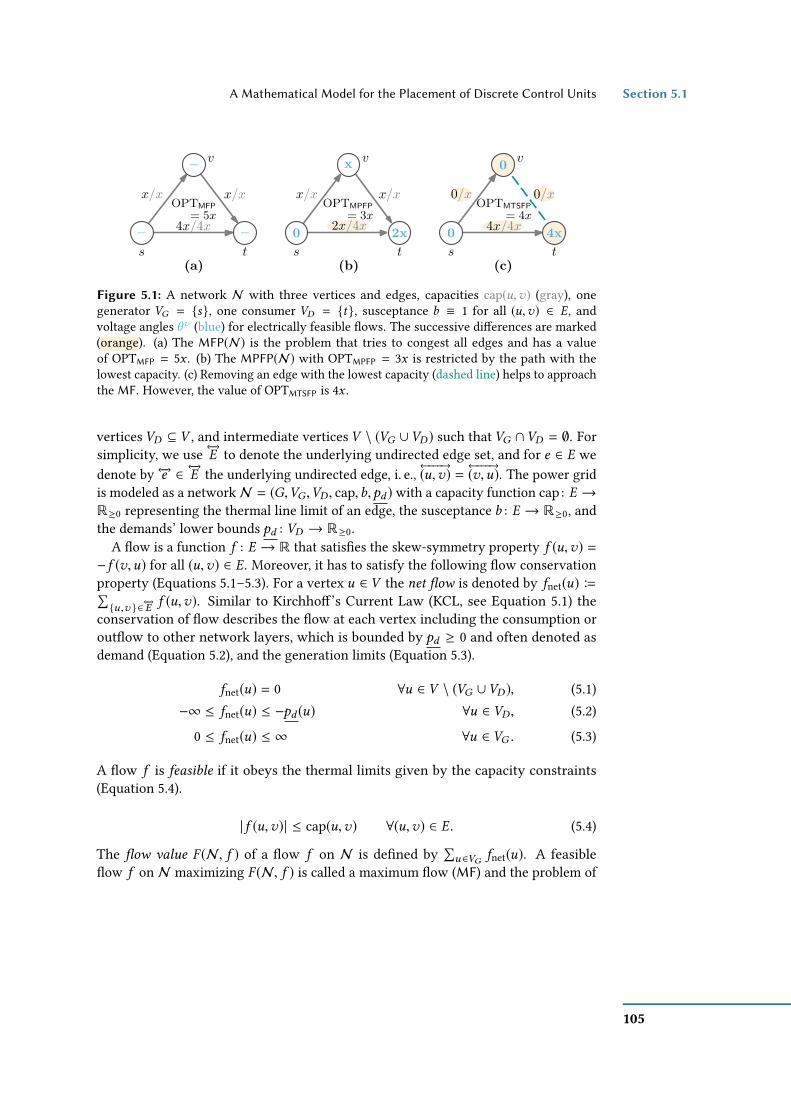
A Mathematical Model for the Placement of Discrete Control Units Section 5.1
2x/4x 4x/4x
(c)
0/x 0/xOPTMTSFP
= 4x
(a)
OPTMFP
4x/4x
x/x x/x
= 5x
(b)
OPTMPFP= 3x
x/x x/x
t
−s
−
v−
0s
2xt
x v
0s
4xt
0 v
Figure 5.1: A network N with three vertices and edges, capacities cap(u,v) (gray), onegenerator VG = s, one consumer VD = t, susceptance b ≡ 1 for all (u,v) ∈ E, andvoltage angles θv (blue) for electrically feasible ows. The successive dierences are marked(orange). (a) The MFP(N) is the problem that tries to congest all edges and has a valueof OPTMFP = 5x . (b) The MPFP(N) with OPTMPFP = 3x is restricted by the path with thelowest capacity. (c) Removing an edge with the lowest capacity (dashed line) helps to approachthe MF. However, the value of OPTMTSFP is 4x .
vertices VD ⊆ V , and intermediate vertices V \ (VG ∪VD ) such that VG ∩VD = ∅. Forsimplicity, we use ←→E to denote the underlying undirected edge set, and for e ∈ E wedenote by ←→e ∈ ←→E the underlying undirected edge, i. e.,
←−−−→(u,v) =
←−−−→(v,u). The power grid
is modeled as a networkN = (G,VG ,VD, cap,b,pd ) with a capacity function cap : E →R≥0 representing the thermal line limit of an edge, the susceptance b : E → R≥0, andthe demands’ lower bounds pd : VD → R≥0.
A ow is a function f : E → R that satises the skew-symmetry property f (u,v) =−f (v,u) for all (u,v) ∈ E. Moreover, it has to satisfy the following ow conservationproperty (Equations 5.1–5.3). For a vertex u ∈ V the net ow is denoted by fnet(u) B∑u ,v ∈
←→E f (u,v). Similar to Kirchho’s Current Law (KCL, see Equation 5.1) the
conservation of ow describes the ow at each vertex including the consumption oroutow to other network layers, which is bounded by pd ≥ 0 and often denoted asdemand (Equation 5.2), and the generation limits (Equation 5.3).
fnet(u) = 0 ∀u ∈ V \ (VG ∪VD ), (5.1)−∞ ≤ fnet(u) ≤ −pd (u) ∀u ∈ VD, (5.2)
0 ≤ fnet(u) ≤ ∞ ∀u ∈ VG . (5.3)
A ow f is feasible if it obeys the thermal limits given by the capacity constraints(Equation 5.4).
| f (u,v)| ≤ cap(u,v) ∀(u,v) ∈ E. (5.4)
The ow value F (N, f ) of a ow f on N is dened by∑u ∈VG fnet(u). A feasible
ow f on N maximizing F (N, f ) is called a maximum ow (MF) and the problem of
105
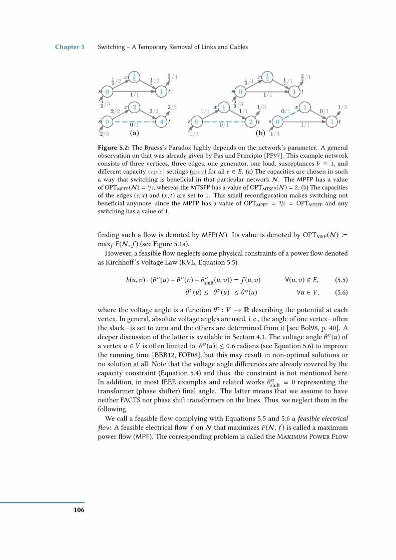
Chapter 5 Switching – A Temporary Removal of Links and Cables
(b)(a)
s t
x12 /2 1
2 /2
32 /3
32 /3
0
12
11/1
s t
x2/2 2/2
0/12/3
2/3
0
2
4
1/1s t0
12
1
x12 /1 1
2 /1
32 /3
32 /3
s t0
1
2
x1/1 1/1
1/3
1/3
0/1 s t0
1
1
x0/1 0/1
1/3
1/3
1/1
Figure 5.2: The Braess’s Paradox highly depends on the network’s parameter. A generalobservation on that was already given by Pas and Principio [PP97]. This example networkconsists of three vertices, three edges, one generator, one load, susceptances b ≡ 1, anddierent capacity cap(e) settings (gray) for all e ∈ E. (a) The capacities are chosen in sucha way that switching is benecial in that particular network N . The MPFP has a valueof OPTMPFP(N) = 3/2, whereas the MTSFP has a value of OPTMTSFP(N) = 2. (b) The capacitiesof the edges (s, x) and (x, t) are set to 1. This small reconguration makes switching notbenecial anymore, since the MPFP has a value of OPTMPFP = 3/2 = OPTMTSFP and anyswitching has a value of 1.
nding such a ow is denoted by MFP(N). Its value is denoted by OPTMFP(N) B
maxf F (N, f ) (see Figure 5.1a).However, a feasible ow neglects some physical constraints of a power ow denoted
as Kirchho’s Voltage Law (KVL, Equation 5.5).
b(u,v) · (θv (u) − θv (v) − θvshi(u,v)) = f (u,v) ∀(u,v) ∈ E, (5.5)θv (u) ≤ θv (u) ≤ θv (u) ∀u ∈ V , (5.6)
where the voltage angle is a function θv : V → R describing the potential at eachvertex. In general, absolute voltage angles are used, i. e., the angle of one vertex—oftenthe slack—is set to zero and the others are determined from it [see Bol98, p. 40]. Adeeper discussion of the latter is available in Section 4.1. The voltage angle θv (u) ofa vertex u ∈ V is often limited to |θv (u)| ≤ 0.6 radians (see Equation 5.6) to improvethe running time [BBB12, FOF08], but this may result in non-optimal solutions orno solution at all. Note that the voltage angle dierences are already covered by thecapacity constraint (Equation 5.4) and thus, the constraint is not mentioned here.In addition, in most IEEE examples and related works θvshi ≡ 0 representing thetransformer (phase shifter) nal angle. The latter means that we assume to haveneither FACTS nor phase shift transformers on the lines. Thus, we neglect them in thefollowing.
We call a feasible ow complying with Equations 5.5 and 5.6 a feasible electrical
ow. A feasible electrical ow f on N that maximizes F (N, f ) is called a maximumpower ow (MPF). The corresponding problem is called the Maximum Power Flow
106

A Mathematical Model for the Placement of Discrete Control Units Section 5.1
Problem (MPFP) and is denoted by MPFP(N). The value of MPFP(N) is denotedby OPTMPFP(N) and is dened by maxf F (N, f ) (see Figure 5.1b).
For a subset S ⊆ ←→E we consider the graphG−S and the corresponding networkN−Swhere the functions cap and b are restricted to E \S . We call S the set of switched edges(i. e., the switch is in OFF-state for these edges). Typically not all possible switchingsare feasible. Feasibility in this context means that there is an electrically feasible owin N − S . The problem of maximizing the ow value in N while allowing edges to beswitched is called Maximum Transmission Switching Flow Problem (MTSFP) andits value is denoted by OPTMTSFP(N) B maxS ⊆←→E OPTMPFP(N − S) (see Figure 5.1c).Such a ow obeys Equations 5.1–5.3 and 5.8–5.10. Note that switching is not alwaysbenecial as shown in Figure 5.2b.
Maximum Transmission Switching Flow Problem MTSFP(N)
Instance: A network N .Objective: Find a set S ⊆ ←→E of switched edges such that OPTMPFP(N − S) is
maximum among all choices of switched edges S .To model switching an edge we introduce a function z : E → 0, 1, which is 0 if an
edge is switched and 1 otherwise. To enforce the switching, the ow must be zero onthe switched edges. We therefore replace Equation 5.4 with Equation 5.8. This changeis not yet sucient, since the KVL (Equation 5.5) shall only apply to the non-switchededges. Hence, we modify this equation to Equation 5.7.
b(u,v)·z(u,v) · (θv (u) − θv (v)) = f (u,v) ∀(u,v) ∈ E, (5.7)| f (u,v)| ≤ z(u,v) · cap(u,v) ∀(u,v) ∈ E. (5.8)
Equation 5.7 can be linearized by either adding two big-M constraints (Equations 5.9and 5.10) or one indicator constraints (Equation 5.11), where M is a suitably largeconstant.
b(u,v) · (θv (u) − θv (v)) + (1 − z(u,v))M ≥ f (u,v) ∀(u,v) ∈ E, (5.9)b(u,v) · (θv (u) − θv (v)) − (1 − z(u,v))M ≤ f (u,v) ∀(u,v) ∈ E, (5.10)
z(u,v) = 1⇒ b(u,v) · (θv (v) − θv (u)) = f (u,v) ∀(u,v) ∈ E. (5.11)
The parameter M must be reasonably large to not impose any implicit voltage an-gle dierence limit at the edge (u,v) ∈ E. In general, one can choose M for eachedge (u,v) ∈ E by M(u,v) equal to max
∑e ∈π (u ,v) b(e)
−1cap(e), where the maxi-
mum ranges over all simple paths π (u,v) from u to v . It then suces to set M =max(u ,v)∈E M(u,v) [BPG01a]. However, it is NP-hard to calculate the longest path[KMR97]. It is simpler to set M(u,v) = b(u,v)·
∑e ∈E cap(e)/b(e). If we restrict the
voltage angle θv to 0.6 radians in Equation 5.6, which is common [BBB12, Hed+10],
107

Chapter 5 Switching – A Temporary Removal of Links and Cables
we can use M(u,v) = 1.2 · |b(u,v)|. Note that this decreases the solution spaceand possibly removes feasible and optimal solutions. Thus, this restriction can im-prove the running time, but might lead to other results and is thus debatable, froma physical point of view. In general, we have lower and upper bounds for genera-tors pд,pд : VG → R≥0 ∪ ∞, and demands pd ,pd : VD → R≥0 ∪ ∞ for u ∈ VDsuch that Equations 5.2 and 5.3 become Equations 5.12 and 5.13, respectively, andthe network is dened by N = (G,VG ,VD, cap,b,pд,pд,pd ,pd ). A network with theseadditional bounds is called bounded.
−pd (u) ≤ fnet(u) ≤ −pd (u) ∀u ∈ VD (5.12)
pд(u) ≤ fnet(u) ≤ pд(u) ∀u ∈ VG (5.13)
A MTSF obeying the latter constraints is a bounded MTSF. Note that xing the de-mands pd (u) = pd (u) = pd (u) and generations pд(u) = pд(u) = pд(u) leads to a DirectCurrent Feasibility Problem (DC FEAS) also known as Power Flow (PF) that is thesearch for a feasible electrical ow by given demands and generations. We discussedthe latter problem in more detail in Chapter 4.
Suppose every generator u ∈ VG has its own generation cost function γu : R→ R≥0representing the cost for generating the power fnet(u). The problem of minimizing thegeneration costs of all generators u ∈ VG while maintaining a feasible electrical owin a bounded network with pd (u) = pd (u) = pd (u) (i. e., Equations 5.1, 5.4–5.6, 5.12and 5.13) is called Optimal Power Flow Problem OPFP(N). The value of OPFP(N) isdenoted by OPTOPFP(N) = min
∑u ∈VG γu (fnet(u)). The problem of nding a ow with
value OPTOPFP(N) by allowing edges to be switched (i. e., Equations 5.1, 5.6, 5.8–5.9,5.12 and 5.13) is called Optimal Transmission Switching Problem OTSP(N) withvalue OPTOTSP(N) = minS ⊆←→E OPTOPFP(N−S) with S being the set of switched edges.
Optimal Transmission Switching Problem OTSP(N)
Instance: A network N .Objective: Find a set S ⊆ E and an electrically feasible ow f in N − S such that
the sum of the generation costs∑u ∈VG γu (fnet(u)) is minimized.
Note that neither the MTSFP nor the OTSP minimize the number of switches. Thiswould result in a min-max-problem that is harder to solve than the presented basicvariants (see Section 5.2 on Page 111). From Lehmann et al. [LGH15, Lemma 4] itfurther follows that the MTSFP and the Maximum FACTS Flow Problem (MFFP) arepolynomial-time solvable on trees. Thus, for trees we get the following relationship.
OPTMPFP(N) = OPTMTSFP(N) = OPTMFFP(N) = OPTMFP(N).
108

A Mathematical Model for the Placement of Discrete Control Units Section 5.1
If it is clear, which network is being referred to, we may omit the explicit refer-ence N and write P and OPTP instead of P(N) and OPTP(N), where P is a par-ticular problem (e. g., MTSFP). The common constraints of MTSFP and OTSP arethe base constraints for the Restoration Order Problem (ROP) [CH15, HCB11]and TNEP [HHK13].
109

Chapter
5Sw
itching–
ATem
poraryR
emovalofLinks
andC
ables
Table 5.1: Overview of known results on the complexity of the MTSFP and OTSP. The complexity increases from top to bottom as shownin the hardness column. Note that the major aspects that inuence the complexity of the problem are the graph structure of G , the numberof generators VG , the number of consumers VD , the susceptance b, and the capacity cap. If there are multiple results or if the results dierfor MTSFP and OTSP, we colored the relating entries in green.
Network Properties Complexity AlgorithmsProblem Graph Structure Example |VG | |VD | b cap Hardness Reference Name b cap
1 MTSFPand OTSP
tree graphs ∞ ∞ – – polynomial-timesolvable
Lemma 4.9,Theorem 6.5,
Section 3.2 p. 30MF ∞ ∞
2 MTSFPand OTSP
penrose-minor-free
graphs1 1 – – polynomial-time
solvableSections 5.4
and 5.5 DTP ∞ ∞
MTSFP series-parallel ∞ ∞ [Koc+16]3 and OTSP graphs 1 1∞ 1 NP-hard Section 5.2 – – –
4 MTSFPand OTSP
cacti withmaximum degree
of 3∞ ∞ 1 ∞ NP-hard [LGH14]
MaxST(see Sec-tion 5.6)
– –
5 MTSFPand OTSP
2-level trees 1 ∞ ∞ ∞ NP-hard [LGH14] – – –
6 MTSFPand OTSP
planar graphwith max degree
of 31 1 ∞ 1 strongly NP-hard [LGH14] – – –
MTSFP 2 2 [LGH14]7OTSP
arbitrary graphs 1 ∞∞ ∞ non-APX [LGH14] – – –
110

Complexity Considerations of using Discrete Control Units Section 5.2
5.2 Complexity Considerations of using Discrete ControlUnits
In Section 5.1, we showed that switching introduces a quadratic constraint (see Equa-tion 5.7). Note that models with quadratic constraints and linear objectives are ingeneral NP-hard [Sah74, page 278]. The proof uses a reduction from the SubsetSum Problem (SSP; see Garey and Johnson [GJ79, p.245, MP2] and Ausiello et al.[Aus+99, p.447, MP5] for more information). However, the quadratic constraint can bereplace by a big-M constraint (see Equations 5.9 and 5.10) or an indicator constraint(see Equation 5.11). Thus, we lose the bilinearity and the constraint becomes linear.
Problem Definitions. In Section 5.1, we already dened the optimization prob-lems MTSFP and OTSP. However, in this section we give a ner granularity of theproblem denitions concerning switching to increase the understanding of the dif-ferent problems that can be tackled. The rst problem considers switching witha xed number of preinstalled switches—meaning S ⊆
←→E is already given—and is
called MTSFP(N, S) and its value is dened by OPTMTSFP(N, S) B maxz(e)∈0,1 |e ∈S OPTMPFP(N −
⋃e | e ∈ S ∧ z(e) = 0). The problem is dened in the following.
MTSF Problem with Fixed Switches MTSFP(N, S)
Instance: A network N and a set S ⊆ ←→E .Objective: Find a switching z(e) ∈ 0, 1 for all e ∈ S such that OPTMPFP(N−e |
e ∈ S ∧ z(e) = 0) is maximum among all choices of z.The next problem denition will be the rst placement problem that relaxes the
denition in the sense that only the number of switches is xed by k ∈ N with |S | = k ,but the placement of the switches—meaning the set S ⊆ ←→E —is unknown. Thus, weare interested in a maximum possible ow for a network N and a xed numberof switches |S | = k . The problem is called MTSFP(N,k) and its value is denedby OPTMTSFP(N,k) B maxS ⊆←→E OPTMPFP(N − S) with |S | = k .
MTSF Problem with k-Switches MTSFP(N,k)
Instance: A network N and a parameter k ∈ N.Objective: Find a set S ⊆ ←→E of switches with |S | = k such that OPTMPFP(N − S)
is maximum among all choices of S .Assume that we have no limitation on the number of switches—meaning the number
of switches can be |S | = |←→E | = k . Thus, the problem to nd a maximum powerow in network N by allowing as many switches as possible (i. e., some k ∈ N) iscalled MTSFP(N) with value OPTMTSFP(N) B maxk OPTMTSFP(N,k).
111

Chapter 5 Switching – A Temporary Removal of Links and Cables
Maximum Transmission Switching Flow Problem MTSFP(N)
Instance: A network N .Objective: Find a set S ⊆ ←→E of switched edges such that OPTMPFP(N − S) is
maximum among all choices of switched edges S .
The latter problem allows as many switches as necessary to obtain a best possiblepower ow. However, when there is only one generator and one demand the maximumnumber of switches |S | is restricted by |V | − 1 that represents a tree. Removing moreedges would lead—independent on the generation limits—to an infeasible solution,since some demands are cut-o from any generator. If we have multiple generatorsand demands the maximum number would be restricted by a forest |V | − k , where krepresents the number of connected components. Note that the number of connectedcomponents can be still k = 1.
In general an desirable investigation is the minimum number of switches—meaningthe smallest k—such that we get the same value as OPTMTSFP(N). This problem iscalled OPTMNSP(N) B minOPTMTSFP(N,k )=OPTMTSFP(N) k with the value OPTMTSFP(N).
Minimum Number of Switches Problem under MTSF MNSP(N,k)
Instance: A network N and k ∈ N.Question: Is it possible to remove a set of edges S ⊆ E such that k = |S | is
minimum among all choices of OPTMTSFP(N)?
Note that similar denitions can be made for the OTSP. An overview of the switchingrelated problems is given in Appendix A.3.
Decision Problems. MTSFP is an optimization problem that involves searchingfor the best solution from some large set of solutions. Any optimization problem canbe transformed into a decision problem by asking whether the optimum value is atleast or at most k for some k ∈ R. We denote the corresponding decision problemfor MTSFP(N) by k-MTSFP.
k-Maximum Transmission Switching Flow Problem k-MTSFP(N,k)
Instance: A network N and k ∈ Q≥0.Question: Is it possible to remove a set of edges S such that there is an electrically
feasible ow f in N − S with ow value F (N − S, f ) ≥ k?
Note that decision problems are often used to show that a particular problem is NP-hard. We will use this problem in Section 5.2.2 to show that MTSFP(N) is NP-hard.An overview of the switching decision problems can be found in Appendix A.3.
112

Complexity Considerations of using Discrete Control Units Section 5.2
5.2.1 Literature Overview
We will see in Denition 5.14 (see also Section 5.4.4 and Figure 5.11) that for single-source single-sink penrose-minor-free graphs (see Table 6.1–1) the MTSFP(N) is poly-nomial-time solvable. We will look at this structure in Section 5.4.1. However, Kocuket al. [Koc+16] showed that for arbitrary susceptance b and capacity cap this problemis already NP-hard3. In Section 5.2.2, we will provide a dierent reduction that is alsoa generalization of the proof of Kocuk et al. [Koc+16]. Contrary to series-parallelgraphs, cactus graphs have the special property that the cycles in a cactus do not sharean edge. Thus, the dependencies on the voltage angles of a vertex decrease. Though,for single-source single-sink this problem is polynomial-time solvable, it becomesalready NP-hard for an arbitrary number of generators and consumers (see Table 6.1–3). Lehmann et al. [LGH14, pp.8., Section 5] motivated another non-standard graphstructure from the disaster management. The idea is that after a blackout a TSO willtry to recover the power grid by establishing a tree-like structure. The graph structureis denoted by N-level tree (see Table 6.1–4), which has a generator at the root andconsumers at the leaves. For each level there is a total order of the vertices that alsodenes the intra-level neighbors of a vertex. The tree allows intra-level connectionsto direct neighbors. Note that these intra-level connections cause cycles that shareedges with other cycles. Thus, this structure is more complex than a cactus. Thenext graph structure that is more complex are planar graphs (see Table 6.1–5) forwhich Lehmann et al. [LGH14, p.13, Section 7] show that the problem is stronglyNP-hard for planar graphs with maximum degree of 3, one generator, one consumer,and having unit capacities. Naturally this problems stays NP-hard for arbitrary graphs,but it is not possible for any ϵ > 0 to nd an approximation algorithm within a factorof 2O((logn)1−ϵ ) [LGH14, pp.10.] [KMR97, pp.95.].
5.2.2 NP-hardness of Source-Sink-MTSF on Series-Parallel-Graphs
First we prove that MTSFP is in NP by providing a polynomial time algorithm thatis denoted by valid(N, S). The polynomial algorithm species whether the set ofswitched edges S is a valid solution for an instance N . It is not hard to determinethat an instance N and a solution S are properly dened (Section 5.1). Checkingwhether a switching S provides an electrically feasible ow that is at least k can bedone by Linear Programming (LP) in polynomial time (see Section 5.1).
To show that k-MTSFP is also NP-hard we reduce the Subset Sum Problem to k-MTSFP.
3We found out about that proof after the publication of the later proof in [Gra+18] thanks to ThomasWilliam Brown.
113

Chapter 5 Switching – A Temporary Removal of Links and Cables
T1 Tn
v1
1k − 1
k+w1
2k+w1
v2
u1
2k+w1
s. . .
11
1+(n+1)k
vn
1k − 1
k+wn
2k+wn
un
2k+wn
t
Figure 5.3: A network N constructed from an instance of SSP having one source s ∈ VG (i. e.,|VG | ≡ 1) and one sink t ∈ VD (i. e., |VD | ≡ 1). All edges (u,v) ∈ E have a capacity of cap ≡ 1and the susceptances b are shown next to the edges.
Subset Sum Problem SSP(W ,k)
Instance: A nite set of numbers W = w1,w2, . . . ,wn with wi ∈ N anda k ∈ N.
Question: Is there a set of elements x1, . . . , xn ∈ 0, 1 such that∑n
j=1w jx j = k?
Lemma 5.1. k-MTSFP is NP-complete even if there is only one source and one sink in
the network and all edge capacities are 1.
Proof. We show the NP-hardness by reducing SSP to this restricted MTSFP-variant inpolynomial time. Since SSP is weakly NP-complete [GJ79], MTSFP is NP-hard, too.Given an SSP-instance (W ,k) we construct an instance of MTSFP that allows a owof 2 if and only if there is a solution of the SSP-instance. We may assume withoutloss of generality that no element ofW is larger than k as these elements are neverpart of any solution. In the constructed network N there is one source s C VG(i. e., |VG | ≡ 1) and one sink t C VD (i. e., |VD | ≡ 1; see Figure 5.3). All edges e ∈ Ehave capacity cap ≡ 1. There is one edge from s to t with susceptance 1/(1+(n+1)k ),where n = |W |. For each element wi ∈ W we build a triangle with vertices vi , ui ,andvi+1. We set b(vi ,ui ) B b(ui ,vi+1) B 2/(k+wi ) and b(vi ,vi+1) B 1/k − 1/(k+wi ). Notethat the triangles for wi and wi+1 have the vertex vi+1 in common. We set vn+1 = tand add the edge (s,v1) with susceptance b(s,v1) = 1. Note that the edge (s,v1) isnecessary when we do not switch any triangle, since this would exceed the ow ofone in the upper part.
To achieve a ow of 2 in the network both edges incident to s must be saturated.In particular, the ow through the chain of triangles is 1 and ∆θv (s, t) = 1 + (n + 1)k .Consider the triangle Ti for the element wi ∈W . In this triangle vi acts as a sourceandvi+1 as a sink. There are two paths fromvi tovi+1 inTi : The direct path consistingonly of the edge (vi ,vi+1) and the path viaui . In any solution toN at most one of these
114

Complexity Considerations of using Discrete Control Units Section 5.2
(a) (b) (c)∆θv(vi, vi+1)=k
wik+wi
/1
kk+wi
/1
vi vi+1
ui
Ti
∆θv(vi, vi+1)=k + wi
0/1
1/1
vi vi+1
ui
Ti
∆θv(vi, vi+1)>2k
1/1
0/1
vi vi+1
ui
Ti1/1 0/1
kk+wi
/1
Figure 5.4: Possible ways to switch the triangles Ti in a network N with correspondingangle dierences and ows. (a) If no edges are switched the angle dierence is k . (b) If theedge (vi ,vi+1) is switched, the angle dierence is k+wi . (c) If an edge incident toui is switched,the angle dierence is larger than 2k .
paths may be switched as otherwise the total ow inN is at most 1. If no edge inTi isswitched (Figure 5.4a), we obtain ∆θv (vi ,vi+1) ≡ k for one unit owing through Ti . Ifthe edge (vi ,vi+1) is switched (Figure 5.4b), we have ∆θv (vi ,vi+1) = k +wi . If an edgeincident to ui is switched (Figure 5.4c), the ow on (vi ,vi+1) must be equal to 1 andwe get
∆θv (vi ,vi+1) =1
1k −
1k+wi
=k(k +wi )
wi=
k2
wi+ k > 2k .
Note that in any case ∆θv (vi ,vi+1) ≥ k . If in any triangle Ti an edge incident to ui isswitched, we have
∆θv (s, t) = ∆θv (s,v1) +n∑i=1
∆θv (vi ,vi+1)
> 1 + (n − 1)k + 2k = 1 + (n + 1)k,
which contradicts ∆θv (s, t) = 1 + (n + 1)k . Hence, only the edges (vi ,vi+1) for i =1, . . . ,n may be switched.
If there is a set S of edges in N such that removing them from the network yields amaximum ow f in N − S with throughput F (N, f ) ≡ 2, we can construct a solutionto the corresponding SSP-instance as follows. Let xi = 1 if (vi ,vi+1) ∈ S and xi = 0otherwise. By the argumentation above we have ∆θv (vi ,vi+1) = k + wi if xi = 1
115

Chapter 5 Switching – A Temporary Removal of Links and Cables
and ∆θv (vi ,vi+1) = k otherwise. Hence, we have
1 + (n + 1)k = ∆θv (s, t)
= ∆θv (s,v1) +n∑i=1
∆θv (vi ,vi+1)
= 1 +n∑i=1(k + xiwi )
= 1 + nk +n∑i=1
xiwi .
and therefore∑n
i=1 xiwi = k as required by the SSP-instance.If the SSP-instance has a solution, i. e.,
∑ni=1 xiwi = k for a suitable assignment of
the xi , we dene S B (vi ,vi+1) | xi = 1. We claim that after switching these edgesthe remaining network N − S admits a power ow with value 2. Setting θv (s) = 0and θv (vi ) = 1 +
∑i−1j=1(k + xiwi ) induces a feasible electrical ow of 1 on the triangle
chain by the arguments above. We further note that
∆θv (s, t) = ∆θv (s,v1) +n∑i=1
∆θv (vi ,vi+1)
= 1 +n∑i=1(k + xiwi )
= 1 + nk +n∑i=1
xiwi
= 1 + (n + 1)k .
Hence, we have f (s, t) ≡ 1 and the total ow in N − S is 2.The size of the constructed network is linear in |W | and all parameters are polyno-
mial in k . Hence, the reduction from SSP to MTSFP runs in polynomial time. Since SSPis NP-complete [GJ79], this reduction implies that MTSFP is NP-hard even if we restrictourselves to networks with unit capacities and only one source and one sink.
5.3 Network Modeling
The model presented in Section 5.1 places no restriction on the network. Our algorithmsand proofs are often simpler if the underlying network has a specic form.
Without loss of generality we may assume that in the network N B (G, VG ,VD ,cap, b, pd ) all generators and consumers are degree-1 vertices. We achieve this byadding an edge with innite capacity and a susceptance of 1 between each generator
116

Network Modeling Section 5.3
(b)(a)
s∈VG
1/1
pg +2/pg +2 pg +1/pg +1
pg/pg
x/pg−pg
Npg+2
u s
pg+1
0 pg
pg+x
ts
s s t∈VC
pd+1/pd+1
pd+1/pd+1 1/1
pd/pd
x/pd − pd
Ntu
−x−2pd
−x−pd+1
−x
0
−x−pdt
st t
Figure 5.5: A bounded network can be transformed to an unbounded network by adding sub-structures to its generator and consumer vertices. (a) A generator s ∈ VG in a bounded MTSFPcan be transformed to a generator in an unbounded MTSFP by modifying the network Nat the source. Thereby, a generator with non-zero lower bound generation can be replacedby a construction of a cycle with generator s and consumer ts forcing a generation of pд onedge (u, s), and a generator s allowing a generation in total of up to pд at vertex s . (b) For con-sumers t to model the upper bound it suces to add an edge (t, t) and a minimum demandof pd to t . To model the lower bound, a triangle that congures the voltage angles in such afashion that there is a feasible power ow only if at least the lower demand is satised.
or consumer v ∈ (VG ∪VD ) and a new vertex uv . The new vertex uv then acts as agenerator or consumer and v becomes an intermediate vertex. We use this assumptionespecially in Section 5.4, where we restrict our network to certain graph classes.
We can shrink the networkN by contracting degree-2 vertices. For this we introducethe susceptance norm of a path π (u,v), which is dened as
‖π (u,v)‖b B∑
e ∈π (u ,v)
b(e)−1, (5.14)
and gives us a distance metric on power grids. The susceptance norm is a norm, sinceit fullls the axioms given by Banach [Ban22].
1. ‖ #»x ‖ ≡ 0 if and only if #»x ≡#»0 (neutral element),
2. ‖s · #»x ‖ ≡ |s | · ‖ #»x ‖ (absolute homogeneity),
3. ‖ #»x + #»y ‖ ≤ ‖ #»x ‖ + ‖ #»y ‖ (triangular inequality).
Applying the following lemma we can simplifyN by contracting paths to single edges.
Lemma 5.2. A simple path π in N whose internal vertices have degree 2 in N and are
neither generators nor consumers is equivalent to a single edge e with capacity cap(e) Bmin(u ,v)∈π cap(u,v) and susceptance b(e) B 1/‖π ‖b .
117

Chapter 5 Switching – A Temporary Removal of Links and Cables
(a) (b)
x+1/x+1
1/1
vtv
(x+2)·γv(1)/(x+2)·γv(1)
Nx/x+1
1/1
vtv
1
sv
1+1−1
−γv(1)
(x+1)·γv(1)/(x+2)·γv(1)
x+2
0
x+1
0
N10
sv
Figure 5.6: Transforming an OTSP-instance to an MTSFP-instance is possible by addingtriangles at consumer vertices. The edge e = (sv , tv ) and the other two edges have suscep-tances b(e) = γv (1) and 1, respectively. (a) The maximum ow in a triangle is obtained byinjecting no power to the network N from v . (b) Per injected unit of ow from v to N , thereis a decrease in ow value by γv (1) (red) in a triangle.
Note that if we assume that all generator and consumer vertices have degree 1, theyare never internal vertices of any simple path. Note that Lemma 5.2 is equivalent tothe transformation Reduction Rule 4.21 presented in Section 4.2.
Lehmann et al. [LGH14, LGH15] showed that the bounded MTSFP is NP-hard oncacti (i. e., a graph consisting of edge disjoint cycles). We can transform a bounded MTSFPwith network N = ( G, VG , VD , cap, b, pд , pд , pd , pd ) to an unbounded MTSFP. Wemodel the upper bounds by adding edges (u,v) with appropriate capacities at ver-tices u ∈ (VG ∪VD ). To model a non-zero lower generation bound pд at a generator,we replace it by the construction shown in Figure 5.5a, which is based on a struc-ture used by Lehmann et al. [LGH14]. The cycle with generator s and consumer tswith pd (ts ) = pд + 2 forces a ow of pд on the edge (u, s) and the generator s is able toadd the remaining generation capacity. Note that the cycle can be omitted if pд ≡ 0.For consumers we just add an edge (t, t) with a capacity of pd to model the upperbound. In addition, the minimum demand is modeled by a triangle for which thevoltage angle conguration enforces a minimum demand of pd (Figure 5.5b).
Lemma 5.3. Every bounded MTSFP can be transformed into an unbounded MTSFP on
a network with size linear in |V | and |E |.
Lehmann et al. [LGH14, Lemma 2] show that every MTSFP-instance can be trans-formed to an equivalent OTSP-instance while maintaining the network structure. Theidea is basically that we pay for each unit a consumer is not used to its maximumcapacity pd meaning pd (u) − fnet(u) , 0 and we pay |pd (u) − fnet(u)| units. Thistransformation is done by dening a generator cost function γ : VG ∪ VG ′ → R≥0with u ∈ VG
′ if u ∈ VD and γu (1) ≡ 1 with u ∈ VG′ and γu (1) ≡ 0 for all u ∈ VG . In
addition, the consumptions are xed meaning pd (u) = pd (u) = pd (u) for all u ∈ VD .
118

MTSF on Source-Sink-Networks Section 5.4
Thus, while maximizing the power ow a generator u ∈ VG ′ produces pd (u) − fnet(u)units of ow.
We present the reverse transformation for OTSP with linear cost functions. Let N =(G ,VG ,VD , cap, b, pд , pд , pd , pd ) be a bounded network, where each consumerv ∈ VDhas a xed demand pd (v) = pd (v) = pd (v). At each generator v ∈ VG with cost γv (1)per generated unit of power we add a triangle consisting of v , another generator svand a consumer tv as shown in Figure 5.6. The edge (sv , tv ) has susceptance γv (1)and the other two edges have susceptance 1. We denote the resulting network by N ′.If v injects no power into the original network (Figure 5.6a), all its generated powerows along (v, tv ) to tv . The ow in this triangle is then maximized by sending 1unit from sv via v to tv and (xv + 2) · γv (1) units directly on (sv , tv ). Per unit of owinjected by v into the original network, the angle dierence ∆θv (v, tv ) decreases by 1(Figure 5.6b). Therefore, ∆θv (sv , tv ) also decreases by 1 and the ow f (sv , tv ) by γv (1).Hence, a feasible ow in N with cost k can be transformed to a feasible ow in N ′with ow value M − k , where M =
∑v ∈VG
((pд(v) + 2) · γv (1) + pд(v) + 1
). This leads
to the following lemma.
Lemma5.4. For everyOTSP-instance N = (G ,VG ,VD , cap,b,pд ,pд ,pd ,pd ) with xeddemands pd (v) = pd (v) = pd (v) and linear cost functions γv for each consumer v ∈ VDthere is an MTSFP-instanceN ′ and a constantM ∈ R≥0 such that for every k ∈ R≥0 wehave OPTOTSP(N) ≤ k if and only if OPTMTSFP(N
′) ≥ M − k . Moreover, the size of N ′
is linear in the size of N .
The previous lemma and the result of Lehmann et al. [LGH14, Lemma 2] provide apossibility to interchangeably apply algorithms found for MTSFP to OTSP (and viceversa) by a simple graph transformation.
5.4 MTSF on Source-Sink-Networks
Fisher et al. [FOF08] found in their experiments that Wheatstone Bridges [Eke01](bridges or short-cut edges in a cycle with four edges) can be associated with Braess’s
Paradox [BNW05, Nag10, Pal+12], in which adding a line to a network (even with zerocost) can increase the cost of using that network (see Section 2.3). These structures areoften removed by switches in their results. In the following, we denote WheatstoneBridges by cycle chords [Gra99, Wes00, p. 225], since a bridge in a graph is an edgewhose removal disconnects the graph, which is not what we mean here. The structure—meaning cycle and chord together—is denoted by diamond graph. An observationof Fisher et al. [FOF08] is the following.
Observation 5.5. The OTSP and thus the MTSFP try to remove an edge set S in such a
way that the remaining graph is often chordless.
119

Chapter 5 Switching – A Temporary Removal of Links and Cables
We will show in this section that Observation 5.5 does not apply in general. How-ever, Fisher et al. [FOF08] empirically show on their test case that this is often thecase. Leibfried et al. [Lei+15a] prove that placing ideal FACTS in such a way thatthe remaining grid is a tree results in a MPF, which is equivalent to the MF. Thisobservation indicates that the power ow is equivalent to the graph theoretical ow ontrees as only determined by the conservation of ow (KCL, Equation 5.1) [see LGH15,Lemma 4]. However, power grids are meshed (i. e., they contain cycles) for reliabilityreasons. Each mesh in a power grid has to obey the KVL (Equation 5.5), meaning thesum of all voltage angle dierences is zero. These additional constraints are not onlythe dierence to a graph-theoretical ow, but make most of the problems hard to solveeven in the DC model. In addition, they lead to Braess’s Paradox and make switchingbenecial (see Section 2.3).
The idea is to reach a graph-theoretical ow by exploiting the network structureN .The upper and lower bound for MTSF are given by OPTMFP and OPTMPFP, respectively.
Lemma 5.6. OPTMPFP ≤ OPTMTSFP ≤ OPTMFP.
Transmission switching problems formulated as MILP models have highly coupledconstraints (see Section 5.1). Cycles add KVL constraints (Equation 5.5) to the problem,which are highly coupled with each other as the sum over the voltage angle dierencesin each cycle has to be zero (Figure 5.1). Thus, we get the following observation.
Observation 5.7. The relation OPTMPFP < OPTMFP can only be caused by cycles.
In this section we study MTSFP on networks that have only one generator vertex sand one consumer vertex t . We call such networks s-t-networks. Let Π(u,v) denotethe set of all paths between two vertices u and v . We denote the smallest capacity ofany edge on a path π ∈ Π(u,v) by
cap(π ) B min(u ,v)∈π
cap(u,v). (5.15)
From Equations 5.4 and 5.5 we get the following function to calculate the maximumvoltage angle dierence on any u-v-path π (u,v) ∈ Π(u,v).
∆θv (π (u,v)) B ‖π (u,v)‖b · cap(π (u,v)). (5.16)
Forπ 1(u,v), π 2(u,v) ∈ Π(u,v)we deneπ 1(u,v) ≤ π 2(u,v) if and only if∆θv (π 1(u,v))≤ ∆θv (π 2(u,v)).
5.4.1 The Dominating Theta Path (DTP)
The intuition that electricity follows the path of the least resistance leads us towardsshortest paths. However, in power grids the shortest path is not always the restricting
120

MTSF on Source-Sink-Networks Section 5.4
(a) (b)x/xx/x x/x
3x/3xOPTMTSFP
= 4x0/x
s tu v
3xx0 2x
x/x
x/x0
OPTMTSFP= 3x
0/x 0/x
2x/2x
s tu v
x 53 x0
x/x
OPTMPFP= 8
3 x
13 x/x 1
3 x/x
53 x/2x
L :
53 x2
3 x13 x0
23 x/x
s tu v
23 x/4x
x/x
OPTMPFP= 8
3 x
13 x/x 1
3 x/x
53 x/3x
L :
s tu v
13 x 2
3 x 53 x0
(0,∞) (1,x) (2,x)(2,x)(1,4x)(1,3x)
(3,x) 7 (0,∞) (1,x)(1,x)(2,x) 7
(1,2x)(2,x)
(2,2x)7(2,x)
Figure 5.7: A network N with four vertices and ve edges, one generator VG = s, oneconsumer VD = t, capacities cap(u,v) (gray), susceptance b(u,v) = 1 for all (u,v) ∈ E, andvoltage angles θv (u) (blue in the vertices) for all vertices u ∈ V . Note for the label calculationthat the underlying graph G is undirected. The algorithm computing the DTP saves a setof labels L for each vertex starting at vertex s with label (0,∞). The red edges representthe DTP from s to t . (a) The cross 7 means that the label (3, x) is dominated by the label (2, x) atvertex t . In addition, it is not sucient to compare only the voltage angle dierences ∆θv , sincewe would drop the DTP path [s, (s,v),v] at vertex v , which would lead to incorrect results.Switching edge (s,v) (green dashed edge) results in a solution of the MTSFP. (b) The DTPis not always unique. In addition, for general graphs the switched edge of the MTSFP is notalways on the DTP.
path. An s-t-network is often restricted (dominated) by the path with the smallestvoltage angle dierence. However, it does not seem feasible to give a general boundfor that. The smallest voltage angle dierence between a vertex u and a vertex v isdenoted by ∆θv (u,v) B min∆θv (π (u,v))with π (u,v) ∈ Π(u,v). We call the path thatminimizes ∆θv (π (u,v)) Dominating Theta Path (DTP) and denote it by πDTP(u,v).Its value is denoted by OPTDTP(u,v). We are mainly interested in s-t-paths, since thepower ows from generators s to consumers t .
Note that, unlike shortest paths, a DTP from s to t via another vertex v and a DTPfrom s to v may have no common edges. For example in the top part of Figure 5.7aa DTP to v goes via u, but not the DTP to t . To compute a DTP we therefore minimizeover two objectives ‖·‖b and cap(·). For this we perform a multi-objective search,where we search for Pareto-optimal solutions, i. e., we look for paths that are notdominated by other paths with regards to the objective functions (in our case thesusceptance norm ‖·‖b and minimum capacity cap(·)). Note that in general multi-
121
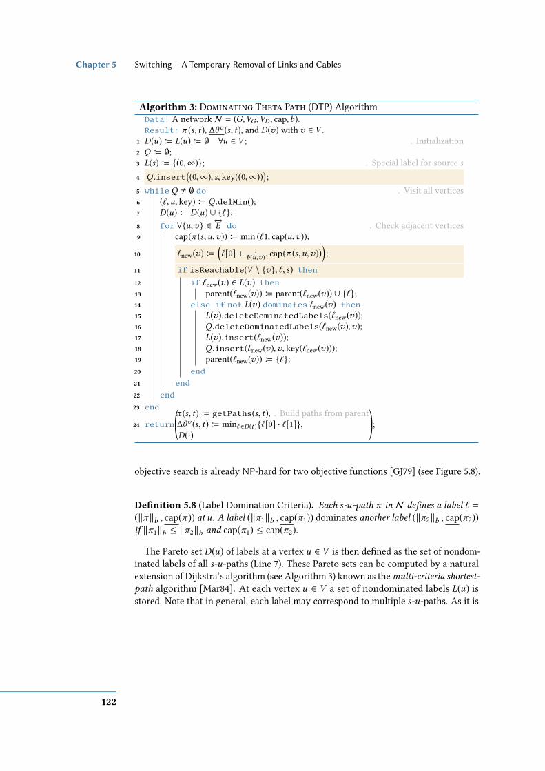
Chapter 5 Switching – A Temporary Removal of Links and Cables
Algorithm 3: Dominating Theta Path (DTP) AlgorithmData: A network N = (G,VG ,VD , cap,b).Result: π (s, t), ∆θv (s, t), and D(v) with v ∈ V .
1 D(u) B L(u) B ∅ ∀u ∈ V ; . Initialization2 Q B ∅;3 L(s) B (0,∞); . Special label for source s4 Q .insert
((0,∞), s, key((0,∞))
);
5 while Q , ∅ do . Visit all vertices6 (`,u, key) B Q .delMin();7 D(u) B D(u) ∪ `;8 for ∀u,v ∈
←→E do . Check adjacent vertices
9 cap(π (s,u,v)) B min (`1, cap(u,v));
10 `new(v) B(`[0] + 1
b(u ,v) , cap(π (s,u,v)));
11 if isReachable(V \ v, `, s) then
12 if `new(v) ∈ L(v) then13 parent(`new(v)) B parent(`new(v)) ∪ `;14 else if not L(v) dominates `new(v) then15 L(v).deleteDominatedLabels(`new(v));16 Q .deleteDominatedLabels(`new(v),v);17 L(v).insert(`new(v));18 Q .insert(`new(v),v, key(`new(v)));19 parent(`new(v)) B `;20 end21 end22 end23 end
24 return©«π (s, t) B getPaths(s, t), . Build paths from parent∆θv (s, t) B min`∈D(t )`[0] · `[1],D(·)
ª®¬;
objective search is already NP-hard for two objective functions [GJ79] (see Figure 5.8).
Denition 5.8 (Label Domination Criteria). Each s-u-path π in N denes a label ` =
(‖π ‖b , cap(π )) at u. A label (‖π1‖b , cap(π1)) dominates another label (‖π2‖b , cap(π2))if ‖π1‖b ≤ ‖π2‖b and cap(π1) ≤ cap(π2).
The Pareto set D(u) of labels at a vertex u ∈ V is then dened as the set of nondom-inated labels of all s-u-paths (Line 7). These Pareto sets can be computed by a naturalextension of Dijkstra’s algorithm (see Algorithm 3) known as the multi-criteria shortest-
path algorithm [Mar84]. At each vertex u ∈ V a set of nondominated labels L(u) isstored. Note that in general, each label may correspond to multiple s-u-paths. As it is
122

MTSF on Source-Sink-Networks Section 5.4
−/1 −/1 −/1
−/1 −/1 −/11
1 1
1 1
1
(0,∞)
(3, 1)(3, 1)
(3, 1)(3, 1)
(3, 1)(3, 1)(3, 1)(3, 1)
(2, 1)
(2, 1)
(2, 1)
(2, 1)(1, 1)
(1, 1)
s t. . .
...
Figure 5.8: An example, where the DTP produces exponential many labels. The edges aregiven with the susceptances b and capacities cap. The sets of labels are marked at the vertices.The number of labels increases from the source s for each vertex in the chain exponentially byeither choosing the upper or lower edge.
necessary to represent all these paths, we store for each label a set of parent-pointers.The latter point to labels that correspond to paths shortened by one vertex. Themerging of labels ensures the polynomial size of label sets.
The labels in the priority queue Q are compared by ‖·‖b . At the beginning of eachiteration a label with the minimum susceptance norm is extracted from Q . This labelbelongs to a vertex u. Then, new labels for all neighbors of u are computed (Line 10).First, it is checked whether there is a path π (s,u) that corresponds to ` and does notcontain the neighbor v (Line 11, Section 5.4.3). Extending this path to v then still givesa simple path. If the computed label already exists in L(v), the parent-pointers areupdated. Otherwise, if it is not dominated, it is added to L(v) and Q (Lines 17 and 18).Before that, all labels dominated by the new labels are removed. Here, only labelsat the same vertex are considered, i. e., in Line 16 only the dominated labels at v areremoved.
Lemma 5.9. Algorithm 3 computes a correct Dominating Theta Path (DTP).
Note that the proof for the next lemma is based on the proof for the multi-criteria
shortest-path algorithm by Martins [Mar84].
Proof. At any step of Algorithm 3 there is a set of labels L(u) associated with eachvertex u ∈ V . We rst show that at any step no label in L(u) is dominated by any otherlabel in the same set. After the initialization there is only one label. Hence, it is notdominated.
Suppose that there are no dominated labels in any label set before an iteration.We show that this property still holds after the iteration. First, a label (‖π (s,u)‖b ,cap(π (s,u))) with the minimum susceptance norm among all labels in Q is dequeued(Line 6). This label corresponds to a path π (s,u) from s to u. Then, the labels forneighbors of u are computed (Line 10 based on Equation 5.16). Since these labels areonly added if they are not dominated and labels dominated by them are removed
123

Chapter 5 Switching – A Temporary Removal of Links and Cables
(a) (b)
u222 2
2
2 2
1s
u1
u3
u4
u5
1, 2
0, ∞ 1, 24, 1
1, 24, 1
3, 12, 2
3, 1 2, 2
4, 11, 2
2, 24, 1E2 2s
u1 u51u4
0, ∞
3, 1
Figure 5.9: A networkN and the corresponding directed graph on the labels computed duringthe execution of the DTP-algorithm. All edges (u,v) ∈ E have susceptance b ≡ 1. Two labelshave the same color if and only if they belong to the same vertex inN . (a) To test whether thelabel (4, 1) at u3 shall be inserted into the graph, we search for a rainbow path from the labelat s to the new label (4, 1). The slightly colored labels produce no DTP from that particularvertex. (b) The rainbow path avoids cycles and ensures that the paths remain simple.
from L(v), the label sets still do not contain dominated labels. Moreover, the new labelsalso correspond to simple paths as it is tested whether v already lies on π (s,u). Notethat previously extracted labels from Q are not removed since their susceptance normis less than the one of `new(v). In particular, all labels extracted from Q will be presentin the nal label sets.
Secondly, we prove that in the end we have D(v) ⊆ L(v) for all v ∈ V . Assume thatthis was not the case. Then, there is a label ` ∈ D(v) that is not included in L(v) forsome v ∈ V . We pick such a label with the minimum susceptance norm. This labelcorresponds to a path π (s,v). Denote the vertex beforev byu. Since the subpath π (s,u)from s to u has ‖π (s,u)‖b < ‖π (s,v)‖b , the label for this subpath is present in L(u).But in the iteration in which this label was processed, all neighbors of u were explored.In particular, the label ` forv was computed and added to L(v). Moreover, it was neverremoved from L(v) later, since it is not dominated. This contradicts the existence of `.Since D(u) ⊆ L(u) and L(u) contains no dominated labels, we conclude D(u) = L(u).The DTP is then computed by minimizing over L(t).
A counterexample for monotone voltage angle paths is given in Figure 5.10 conrm-ing Lemma 5.10.
Lemma 5.10. The Dominating Theta Path (DTP) is not necessarily on a monotone
voltage angle path.
5.4.2 DTP without Merging the Labels
The Algorithm 3 for the DTP can be implemented using the merging of equivalentlabels or without merging. Neglecting the merging of labels would mean that weremove Line 11 that avoids cycles and Line 12 that merges the labels. Thus, the
124

MTSF on Source-Sink-Networks Section 5.4
(a) (b)
–/10–/1–/105 5
12/5, 11, 10
EE
E
s v
tts v1
2−3ε
13
23 −4ε
1+6ε
1 1 1−3ε
1
23−ε
3ε1−3ε
1 1 110 3+3ε2v2
v3
(4.5, 3ε)(5, 3ε)
0,∞
6/5, 11/5, 10
2/5, 107/5, 1
3/5, 1
Figure 5.10: The graphs represent two problematic cases. (a) An example that shows that itdoes not suce that the labels consist of (‖·‖b , cap(·)), but has to include the set of visitedverticesV ′. (b) Shows an example that the DTP is not necessarily on a monotone voltage anglepath. Let 0 < ϵ 2/3 then the green path represents the DTP from s to t .
reachability check is neglected, but we have to add cycle checks that are also doneby the reachability test (see Section 5.4.3). The implementation stores a set of visitedvertices V ′ for every label. Using a simple union operation on these set, we are able tocheck for cycles. In worst-case we have to save O(|V |) elements per vertex in that set.Thus, a label consists in that case of (‖·‖b , cap(·),V ′). Note that this method can leadto exponential many labels as exemplied in Figure 5.8. However, the reachability testleads to an exponential running time (see Section 5.4.3 and Equation 5.18).
5.4.3 Reachability Test
Algorithm 3 repeatedly tests whether the new labels correspond to simple paths inthe network (Line 11 of Algorithm 3). For this it is checked whether the label atvertex s is reachable fromu via parent-pointers from the label ` when all labels atv areignored. The labels and the pointers together form a directed acyclic graph, where thelabels have the same color if and only if they belong to the same vertex in network N(see Figure 5.9). We call a path whose vertices all have dierent colors a rainbow path.
Rainbow s-t-Path s-t-RP(G, c, s, t)
Instance: A directed acyclic graph G = (V , E), a coloring c : V → N, ands, t ∈ V .
Question: Is there an s-t-path π in G such that all vertices of π have dierentcolors?
An algorithm to test whether there is a Rainbow s-t-Path (s-t-RP) in undirectedgraphs was presented by Uchizawa et al. [Uch+13, Theorem 11]. It runs inO(k2k |E | |V |)time, where k is the number of colors, |E | the number of edges, and |V | the numberof vertices in G. We give a dierent algorithm for directed graphs, which can beimplemented to run in O(k2k |E |) time. The main work is done by Algorithm 4. It
125

Chapter 5 Switching – A Temporary Removal of Links and Cables
Algorithm 4: computeColorsData: A directed label network G = (G = (V , E), c, s), where c : V → N is the coloring
and s ∈ V is the xed source of the network, v ∈ V , and a set T ⊆ N offorbidden colors.
Result: The intersection of the colors of all rainbow s-v-paths, or N if there are nosuch paths.
1 if c(v) ∈ T then return N ; . Not a rainbow path?2 if s = v then return c(s) ; . Base case3 CT (v) B N;4 for (u,v) ∈ E do . All incoming edges into v5 C ′ B computeColors (G,u,T ∪ c(v)); . Incoming cut6 CT (v) B CT (v) ∩C
′;7 end8 CT (v) B CT (v) ∪ c(v);9 return CT (v);
additionally gets a set T of forbidden colors as input and ignores all vertices of thesecolors. To decide whether there is a rainbow path from a vertex s to a vertex t , weinitially set T to ∅. We compute for each vertex v a set of colors CT (v). A color c is inthe setCT (v) if and only if any rainbow s-v-path π (s,v) contains a vertex with color cwith the additional constraint that no vertex of π (s,v) is colored with a color in T(in Algorithm 4 Lines 5 and 6). For each vertex v and all its incoming edges (u,v) werecursively compute all necessary colors for the rainbow paths to u such that c(v) isforbidden. The set CT (v) is then equal to the intersection of these color sets togetherwith c(v). Throughout the algorithm we use N to indicate that there is no rainbowpath with the given restrictions.
During the execution Algorithm 4 may be called several times with the same param-eters. To speed up the computation one may store the results instead of recomputingthem every time. Further, we nd a relation between CT (v) and CT ′(v) for a vertex vand two sets of forbidden colorsT andT ′. If every color of a vertex beforev in the topo-logical order is either both in T and T ′ or neither in T nor T ′, we have CT (v) = CT ′(v).In particular, if no vertex before v is colored by any color inT , we haveCT (v) = C∅(v).This property can also be used to reduce the number of recursive calls.
Alternatively, the set of colors CT (v) at a vertex v can be computed by traversingall paths from s to v , checking if no two vertices are colored the same and nallytaking the common colors of all rainbow paths. This may be faster if there are onlyfew s-v-paths or if many of the paths can be eliminated quickly because they are notrainbow paths.
126
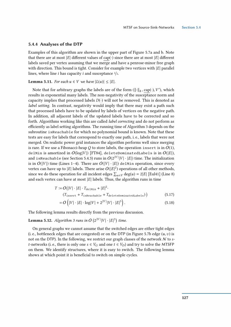
MTSF on Source-Sink-Networks Section 5.4
5.4.4 Analyses of the DTP
Examples of this algorithm are shown in the upper part of Figure 5.7a and b. Notethat there are at most |E | dierent values of cap(·) since there are at most |E | dierentlabels saved per vertex assuming that we merge and have a penrose-minor free graphwith direction. This bound is tight. Consider for example two vertices with |E | parallellines, where line i has capacity i and susceptance 1/i .
Lemma 5.11. For each u ∈ V we have |L(u)| ≤ |E |.
Note that for arbitrary graphs the labels are of the form (‖·‖b , cap(·),V ′), whichresults in exponential many labels. The non-negativity of the susceptance norm andcapacity implies that processed labels D(·) will not be removed. This is denoted aslabel setting. In contrast, negativity would imply that there may exist a path suchthat processed labels have to be updated by labels of vertices on the negative path.In addition, all adjacent labels of the updated labels have to be corrected and soforth. Algorithms working like this are called label correcting and do not perform aseciently as label setting algorithms. The running time of Algorithm 3 depends on thesubroutine isReachable for which no polynomial bound is known. Note that thesetests are easy for labels that correspond to exactly one path, i. e., labels that were notmerged. On realistic power grid instances the algorithm performs well since mergingis rare. If we use a Fibonacci-heap Q to store labels, the operation insert is in O(1),delMin is amortized in O(log|V |) [FT84], deleteDominatedLabels is in O(|E |),and isReachable (see Section 5.4.3) runs in O(2 |V | |V | · |E |) time. The initializationis in O(|V |) time (Lines 1–4). There are O(|V | · |E |) delMin operation, since everyvertex can have up to |E | labels. There arise O(|E |2) operations of all other methods,since we do these operation for all incident edges
∑u ∈V deg(u) = 2|E | [Eul41] (Line 8)
and each vertex can have at most |E | labels. Thus, the algorithm runs in time
T BO(|V | · |E | ·TdelMin + |E |
2·
(Tinsert +TisReachable +TdeleteDominatedLabels))
(5.17)
=O(|V | · |E | · log|V | + 2 |V | |V | · |E |3
). (5.18)
The following lemma results directly from the previous discussion.
Lemma 5.12. Algorithm 3 runs in O(2 |V | |V | · |E |3
)time.
On general graphs we cannot assume that the switched edges are either tight edges(i. e., bottleneck edges that are congested) or on the DTP (in Figure 5.7b edge (u,v) isnot on the DTP). In the following, we restrict our graph classes of the networkN to s-t-networks (i. e., there is only one s ∈ VG and one t ∈ VD ) and try to solve the MTSFPon them. We identify structures, where it is easy to switch. The following lemmashows at which point it is benecial to switch on simple cycles.
127

Chapter 5 Switching – A Temporary Removal of Links and Cables
girdle verticestip vertices
dart extensionkite extension
v
u
v
u
v v
u u
Figure 5.11: All cases show penrose-minors, whereu andv are either generators or consumers,but not both the same. They are a combination of a kite graph (i. e., diamond graph withan additional edge on one of the tip vertices) and a dart graph (i. e., diamond graph with anadditional edge on one of the girdle vertices).
Lemma 5.13. Let N be a simple cycle with one generator s and one consumer t , andletπ (s, t) ∈ Π(s, t)\πDTP(s, t). The Braess’s Paradox exists if and only if OPTMPFP(π (s, t))> OPTMPFP(N).
Proof. It suces to show that removing edge emin(πDTP(s, t)) B argmine ∈πDTP(s ,t ) cap(e)results in OPTMPFP(N − emin) > OPTMPFP(N) and thus, it holds OPTMTSFP(N) >
OPTMPFP(N). The ow on the path π (s, t) is dened by the ratio ∆θv (π (s ,t ))/‖π (s ,t ) ‖b(Equations 5.5 and 5.14). The smallest voltage angle dierence ∆θv (s, t) restricts theow on the other path π (s, t). Thus, the term ∆θv (s ,t )/‖π (s ,t ) ‖b is the maximum possibleow on path π (s, t). The value OPTMPFP(π (s, t)) > OPTMPFP(N) holds if and only if
∆θv (π (s, t))
‖π (s, t)‖b> ∆θv (s, t) ·
‖π (s, t)‖b + ‖πDTP(s, t)‖b‖π (s, t)‖b · ‖πDTP(s, t)‖b
.
Thus, switching an edge emin on πDTP(s, t) increases the total ow on the cycle andmakes switching benecial.
We now generalize this result to a more complex graph class. Following the construc-tion in Section 5.3, we assume that all generator and consumer vertices have degree 1.A diamond graph is a simple graph on four vertices and ve edges consisting of twotriangle facets identied along an edge. Moreover, we denote its degree-3 vertices asgirdle vertices and its degree-2 vertices as its tip vertices. Furthermore, we call thecombination of a kite and a dart graph representing both diamond graphs with anadditional edge on one of the tip and the girdle vertices, respectively, a penrose graph(Figure 5.11). These additional edges basically represent either a generator edge or aconsumer edge, but not both the same. We emphasize this by the following denition.
Denition 5.14 (Penrose Graph). A penrose graph is a kite graph with an additional
edge incident to one of the girdle vertices, or similarly, a dart graph with an additional
edge on one of the tip vertices.
128
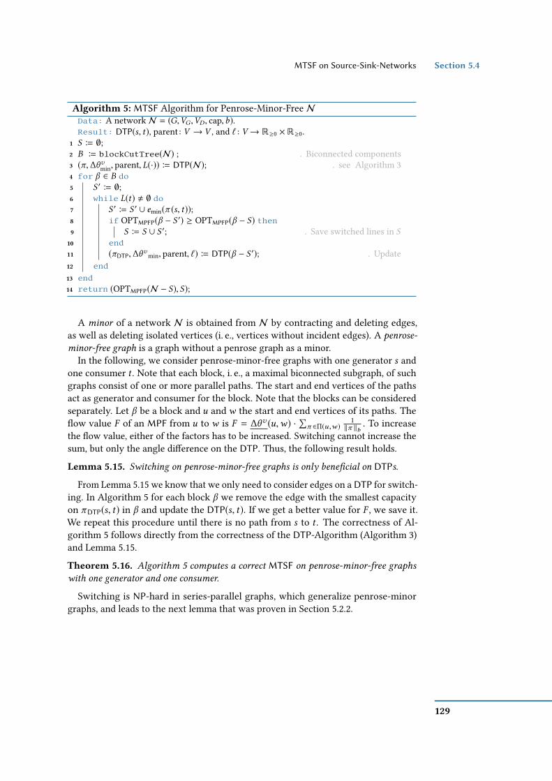
MTSF on Source-Sink-Networks Section 5.4
Algorithm 5: MTSF Algorithm for Penrose-Minor-Free NData: A network N = (G,VG ,VD , cap,b).Result: DTP(s, t), parent : V → V , and ` : V→ R≥0 ×R≥0.
1 S B ∅;2 B B blockCutTree(N) ; . Biconnected components3 (π,∆θvmin, parent, L(·)) B DTP(N); . see Algorithm 34 for β ∈ B do5 S ′ B ∅;6 while L(t) , ∅ do7 S ′ B S ′ ∪ emin(π (s, t));8 if OPTMPFP(β − S
′) ≥ OPTMPFP(β − S) then9 S B S ∪ S ′; . Save switched lines in S
10 end11 (πDTP,∆θ
vmin, parent, `) B DTP(β − S ′); . Update
12 end13 end14 return (OPTMPFP(N − S), S);
A minor of a network N is obtained from N by contracting and deleting edges,as well as deleting isolated vertices (i. e., vertices without incident edges). A penrose-
minor-free graph is a graph without a penrose graph as a minor.In the following, we consider penrose-minor-free graphs with one generator s and
one consumer t . Note that each block, i. e., a maximal biconnected subgraph, of suchgraphs consist of one or more parallel paths. The start and end vertices of the pathsact as generator and consumer for the block. Note that the blocks can be consideredseparately. Let β be a block and u and w the start and end vertices of its paths. Theow value F of an MPF from u to w is F = ∆θv (u,w) ·
∑π ∈Π(u ,w )
1‖π ‖b. To increase
the ow value, either of the factors has to be increased. Switching cannot increase thesum, but only the angle dierence on the DTP. Thus, the following result holds.
Lemma 5.15. Switching on penrose-minor-free graphs is only benecial on DTPs.
From Lemma 5.15 we know that we only need to consider edges on a DTP for switch-ing. In Algorithm 5 for each block β we remove the edge with the smallest capacityon πDTP(s, t) in β and update the DTP(s, t). If we get a better value for F , we save it.We repeat this procedure until there is no path from s to t . The correctness of Al-gorithm 5 follows directly from the correctness of the DTP-Algorithm (Algorithm 3)and Lemma 5.15.
Theorem 5.16. Algorithm 5 computes a correct MTSF on penrose-minor-free graphs
with one generator and one consumer.
Switching is NP-hard in series-parallel graphs, which generalize penrose-minorgraphs, and leads to the next lemma that was proven in Section 5.2.2.
129

Chapter 5 Switching – A Temporary Removal of Links and Cables
Lemma 5.17. MTSFP is NP-hard even if there is only one source and one sink in the
network and all edge capacities are 1.
A general observation in power grids is that shortest paths are somehow connectedto switching a line, since the betweenness centrality is negatively correlated to switch-ing lines [HB08]. Though switched edges on general graphs are not always on DTPs,Algorithm 3 gives us a new criterion focusing on switching by using DTPs insteadof the shortest paths. We dene the DTP centrality based on the number of DTPsthrough an edge.
Denition 5.18. Let N be a power grid. The DTP betweenness centrality cDTPB : E →R≥0 is dened by
cDTPB(e) B1mB
∑s ∈V
∑t ∈V \s
σDTP(s, t, e)
σDTP(s, t), (5.19)
where σDTP(s, t, e) is the number of DTPs between s and t that use e , σDTP(s, t) is the totalnumber of DTPs from s to t andmB = |V |(|V | − 1) is a normalizing constant.
For directed and undirected graphs, the normalization factor is the same, since thealgorithm operates on the directed label graph. However, we normalize the numberof DTPs already by the number of DTPs between s and t . Note that in power grids we donot necessarily check all pairs of vertices, but the paths between all generators s ∈ VGand consumers t ∈ VD . Thus, we dene the following centrality that diers in thebase—meaning generators and consumers instead of all vertices—and normalizationconstant.
Denition 5.19. Let N be a power grid. The switching centrality cS : E → R≥0 isdened by
cS(e) B1mB
∑s ∈VG
∑t ∈VD
σDTP(s, t, e)
σDTP(s, t), (5.20)
where σDTP(s, t, e) is the number of DTP-paths between s and t that use edge e , σDTP(s, t)is the total number of DTP-paths from s to t and mB = |VG | · |VD | is a normalizing
constant.
5.5 Computing one DTP in Polynomial Time
The previous algorithm computes all DTPs between two vertices u and v , but has anexponential running time or uses exponential space dependent on the implementa-tion. In this section, we present a polynomial time algorithm to calculate the DTP.However, instead of calculating all DTPs between two vertices u and v this algorithmcomputes only one DTP. Thus, it cannot be used for the centrality measurement.
130

Computing one DTP in Polynomial Time Section 5.5
(a) (b)
uout vin
uin vout
sout
sin
tin
tout
–/1
–/1
1/b(u,v)
1/b(u,v)
0–/1
0–/1
0–/1
0–/1
–/1
–/1
u v
u v
uout vin
uin vout
(c)
uoutvin
uin vout
sout
sin
tin
tout
1/1
1/1
01/1
uout vin
uin vout
sout
sin
tin
tout
–/1
–/1
1/b(u,v)
1/b(u,v)
–/1
–/1
01/1
01/1
1/1
1/1‖π(s, u)‖b
‖π(t, v)‖b
01/1
–/1
–/11/b(u,v)
1/1
1/1
0–/1
0–/1
0–/1
0–/1
1/b(u,v)
Figure 5.12: The necessary graph transformations to calculate a DTP in polynomial time.(a) The transformation from an undirected graph to a directed graph that is bidirected bytransforming edge u,v to two directed edges (u,v), (v,u). To have a vertex disjoint path,each vertex u is split into two vertices uin,uout with one additional edge (uin,uout). (b) Thetransformed network N ′′ with capacities cap ≡ 1 and edges costs γ (uout,vin) = 1/b(uout,vin) foran external edge and γ (uin,uout) = 0 for a vertex internal edge. (c) The resulting minimum-costow f for an edge emin = (u,v).
Recall from Section 5.4.1 that a label (‖π (s,u)‖b , cap(π (s,u))) consists of the suscep-tance norm—representing the electrical distance—and the minimum capacity alonga path π (s,u). Thus, xing the edge with the smallest capacity and calculating ashortest path from that particular edge to the source and sink vertex using the sus-ceptance norm ‖·‖b is equivalent to the bicriterial shortest path. Assume that oneknows an edge emin on the DTP from s to t with the minimum capacity. We thenneed to nd a shortest s-t-path π via emin, where all edges of π have capacity atleast cap(emin). Let N ′ be the network obtained from N when all edges with capacitysmaller than cap(emin) are removed. Searching for a shortest s-t-path via emin is thenequivalent to searching two disjoint paths π1 and π2 from s and t to the endpointsof emin in N ′ such that ‖π1‖b + ‖π2‖b is minimum.
These paths can be found by running a minimum-cost ow algorithm in a suitablegraph, which is obtained in the following way. First, we denote the endpoints of eminby u and v , and remove emin. We replace each undirected edge by directed edges inboth directions (bidirected graph). Finally, each vertex w is split into two vertices winandwout, which are joined by the directed edge (win,wout). We call these edges internal.The incoming and outgoing edges of w are then placed at win and wout, respectively.All edges of the resulting graph get a capacity of 1. The cost of the internal edges isset to 0. All other edges correspond to an edge e in the input network, and we settheir costs to 1/b(e). The vertices sout and tout produce one unit of ow each, while uinand vin consume one unit each. We call the resulting network N ′′.
Let f be a minimum-cost ow from u to v with ow value 2. We can decompose finto two unit ows from sin and tin, which correspond to disjoint paths π1 and π2from s and t to the endpoints u and v (i. e., endpoints of the removed edge emin).
131

Chapter 5 Switching – A Temporary Removal of Links and Cables
Algorithm 6: Factor 2-Approximation Algorithm for CactiData: A network N = (G,VG ,VD , cap,b).Result: OPTMPFP(N − S), and switched edges S .
1 S = ∅;2 C = dfs (N );3 for c ∈ C do4 S = S ∪ argmin∀e ∈c (cap(e));5 end6 return (OPTMFP(N − S), S);
Lemma 5.20. The shortest s-t-path π via emin inN cap(emin) has susceptance norm ‖π ‖b =cost(f ) + ‖emin‖b . If the edge on π with the minimum capacity is known, π can be
computed in polynomial time.
Proof. Constructing N ′′ as described above and computing the minimum-cost ow fis possible in polynomial time. The ow f can be decomposed into two unit ows, e. g.,by running a depth-rst search. The edge capacities of 1 ensure that these two owsfollow two edge-disjoint paths. Since each vertex ofN ′′ has only one incoming or oneoutgoing edge, these paths are vertex-disjoint as well. Further, they correspond to twopaths π1 and π2 inN ′, where π1 connects s with an endpoint of emin and π2 connects twith the other endpoint of emin. Together with emin we hence obtain an s-t-path Πvia emin with ‖π ‖b = cost(f ) + ‖emin‖b . The last property follows immediately fromthe denition of the costs in N ′′. As f has minimum cost, the constructed path πhas minimum susceptance norm among all s-t-paths via ‖π ‖b = cost(f ) + ‖emin‖bin N ′.
Since we assumed that emin was an edge with minimum capacity on a DTP between sand t , the path π is a DTP. However, emin is unknown. We therefore repeat thisprocedure for each edge in the network and pick the path with the smallest angledierence. Lemma 5.20 then guarantees that this results in a DTP.
5.6 Approximation Algorithm on Cacti
Lehmann et al. [LGH14] showed that the bounded MTSFP on cacti is NP-hard by usinga reduction from subset sum. Subset sum is weakly NP-hard and a fully polynomial-time approximation scheme (FPTAS) exists [Kel+03]. In this section, we present anapproximation algorithm for MTSFP on cacti with approximation factor 2. Recallfrom Section 5.3 that it is always possible to transform a bounded MTSFP into anunbounded MTSFP (Lemma 5.3).
In the following, we assume that our underlying graph G of N is a cactus. Unlikein Section 5.4 we allow multiple generators and consumers. The basic idea for our
132

Approximation Algorithm on Cacti Section 5.7
algorithm (Algorithm 6) is to remove from each cycle the edge with the smallestcapacity. Since we presume that N is a cactus, cycles are independent concerningthe voltage angle dierence, since they do not share an edge. Cycle detection can bedone via a depth-rst search (DFS) in O(|V |) time, where |V | is the number of vertices.Finding the edge with minimum capacity in each cycle is done during the DFS. Notethat the remaining structure is a tree that is equivalent to a Maximum Spanning Tree(MaxST). The running time of MaxST is in general O(|E | α(|E |, |V |)) [Cha00], where αis the inverse of the Ackermann function (i. e., α grows very slowly). Note that MaxSTon cacti runs also in O(|V |) time. The maximum ow on trees can be realized in O(|V |)time by using the pseudoow algorithm [Hoc08]. Thus, the algorithm runs in O(|V |)time.
Lemma5.21. LetN = (G,VG ,VD, cap,b) be a power grid and let S be the set argmin∀e ∈ccap(e) of switched edges for all cycles c ∈ C . Then there exist a feasible electrical ow f ′
on N − S such that F (f ′) = 1/2 OPTMF(N).
Proof. Let f ? be a MF with value OPTMFP on N . By reducing the ow on each edgeby one half (see Equation 5.21), we get a ow f on N with a value of 1/2 OPTMF.Applying Algorithm 6 returns a set of switched edges S =
⋃c ∈C argmin∀e ∈c cap(e).
We decompose each cycle c ∈ C into an edge emin having the smallest capacity on thecycle c (Equation 5.22) and into the remaining part denoted as path π . Since the owon emin is 1/2f ?(emin) it can be rerouted on the remaining part π of c (Equation 5.23).We denote the rerouted ow by f ′. For any e ∈ π we have
| f (e)| = |1/2 f ?(e)| ≤ 1/2 cap(e), (5.21)| f (emin)| ≤ 1/2 cap(emin) ≤ 1/2 cap(e), (5.22)| f ′(e)| = | f (emin) + f (e)| ≤ cap(e). (5.23)
Recall that OPTMFP is an upper bound for OPTMTSFP and that MFP and MTSFP areequal on trees. Thus, from Lemma 5.21 follows Theorem 5.22.
Theorem5.22. Algorithm 6 is a factor 2-approximation algorithm for theMFP andMTSFPproblem on cacti.
Note that an approximation ratio of 1/2 does not provide a good guarantee in theworst case. However, compared to other heuristics it gives guarantees and can be usedas an initial step for heuristics.
133

Chapter 5 Switching – A Temporary Removal of Links and Cables
0.00
0.05
0.10
0.15
0.20
0.25
nesta case189 edinMPF |S| = 1 Normalized cDTPBC
0
2817
2883
2950
2987.00
0 67 133 200Switched Edge
MPFin
MW
Normalized
c DTPBC
(a)
0.00
0.05
0.10
0.15
0.20
0.25
nesta case2746wop mpMPF |S| = 1 Normalized cDTPBC
0
23702
23713
23725
23737
23748
2376023759.50
0 600 1200 1800 2400 3000Switched Edge
MPFin
MW
Normalized
c DTPBC
(b)
Worse than OPTMTSF
2Better than OPTMTSF
2
0.00 0.25 0.50 0.75 1.00
Normalized flow value F (N , f) by OPTMTSF in MW
MaxST
(c)
High cDTPBC Low cDTPBC
0.00
0.25
0.50
0.75
1.00
0.00 0.25 0.50 0.75 1.00
Edges normalized by factor |E|Normalized
MPFin
MW
32% quantile 35% quantile 75% quantile
(d)
Figure 5.13: Simulation evaluation using the data from Table 5.2 for (c) and aggregat-ing the results from Figures C.1–C.3 into (d) including (a) and (b). (a) and (b) show thenesta_case189_edin and 2746wop_mp, respectively, with the gray dashed line being thecentrality of the edges (x-axis) and the green line the MPF (y-axis). (c) The 2-approximationon cacti using MaxST is tested on arbitrary graphs. The global optimum OPTMaxST is reachedat 1 and the proven factor for cacti is at 1/2. The green left (with range) and right point showthe mean and median, respectively. (d) The aggregated data are normalized with regards tothe edges and MPF using |E | and the MPF of each of the network. The edges are ranked fromhighest to lowest cDTPB. The quantiles show that 32 % of the test cases give worse results thanthe green line while switching an edge with low centrality.
5.7 Simulations
We simulated4 our DTP betweenness centrality and 2-approximation algorithms forpenrose-minor-free graphs and cacti, respectively, on arbitrary graphs. By arbitrarygraph we mean the NESTA benchmark sets [CGS14], which are based on the IEEEbenchmark sets [Alb+79, AS74, Bil70, Cro15, Dem+77, GJ03, Gri+99, Jos+16, LB10,Les+11, Mat13, Uni14, WWS13, ZMT11] and incorporate realistic data such as thermalline limits. Note that we run our simulations on arbitrary power grids, since thereare not a lot of benchmark sets presenting cacti namely nesta_case3_lmbd, 4_gs,
4https://i11www.iti.kit.edu/projects/mtsf/index
134

Simulations Section 5.7
and 9_wscc or s-t-networks available. Recall from Section 5.1 that we have a disjointset of generators and consumers. This theoretical assumption cannot be found in anybenchmark set and realistic power grid. Thus, we have to modify the data in such away that we still provide a realistic benchmark set and comply with the assumptionsto avoid innite generator production at buses having both generators and consumers(see Equations 5.2 and 5.3). In addition, we only allow to consume a real powerdemand pd at a real power generator (see bus data’s column three in the IEEE CommonData Format [Pie+73]). All other consumers have an innite maximum demand(Equation 5.12). The results for the problems in Section 5.1 are shown in Table 5.2.
For the 2-approximation, we use MaxST (Section 5.6) on dierent benchmark datasets and compare the results with the MILP from Section 5.1. The algorithm MaxSTgives very good results even though operating on arbitrary graphs (see Table 5.2).Nearly all—meaning 93 %—of the results are better than the approximation factorand 82 % are at most 7 % from the optimum value OPTMTSFP (see Figure 5.13c). Notethat 36 % of the results even reach the optimal value (cases equal to OPTMTSFP havegray markers in Table 5.2). Thus, the expected quality on arbitrary graphs is muchbetter than the proven approximation ratio of 2 on cacti (Section 5.6). There are twocases worse than the approximation factor, because there is no feasible power owfor the resulting networks N − SMaxST. There are three cases in which the number ofswitched lines in the 2-approximation is greater than OPTMTSFP.
The DTP is exact for s-t-penrose-minor-free graphs. There is no benchmark caseproviding this structure. However, since the DTP represents a distance measure, whichmarks interesting paths for switching, we introduced the DTP-betweenness centralityin Denition 5.18. To estimate the relation of the power ow and the dierent edgeshaving dierent centrality values cDTPB for the dierent benchmark cases with dierentassorted characteristics, we calculated the MPF for the network after removing a singleedge e with centrality cDTPB(e) from the network and decreasingly order the normal-ized edges by the centrality. Note that we normalized the MPF and edge index by thenetwork’s OPTMPFP value and |E |, respectively. The normalization is necessary to ag-gregate all cases from Figures C.1–C.3 into one plot. The 32 % and 35 % quantiles in Fig-ure 5.13d show cut points where the MPF decreases while switching an edge. Thesequantiles show that 32 % of the test cases at low centrality result in worse results thanthe plotted line. This eect happens mainly with edges having a small cDTPB (i. e., thenormalized edge index is close to 1). For the 35 % quantile there are only deections atedges with low centrality. Note, that the line at zero represents nesta_case57_ieee,nesta_case2383wp_mp, and nesta_case3012wp_mp, where switching of an edgeleads to a network with no feasible MPF. Note that deection at edges with low cen-trality motivates the algorithm also for ROP, since edges with low centrality are moreessential for the power grid to get into a stable operation and should be consideredrst.
135

Chapter
5Sw
itching–
ATem
poraryR
emovalofLinks
andC
ables
Table 5.2: The PF, MPF, MTSF and OTS models from Section 5.1 are evaluated on the NESTA benchmark sets [CGS14]. The parameters |V |,|E |, and |SP | represent the number of vertices, edges and switched edges for a problem P, respectively, and the optimal solutions are givenin OPTP . Since OTSP minimizes the cost, the ow value FOTSP is shown, too. The maximum possible generation is given in the last column(marked red if it is larger than the OPTMFP). The yellow rows mark the interesting cases where OPTMPFP is smaller than the OPTMTSFP.
NESTA Case |V | |E | |SMTSFP | |SOTSP | |SMaxST | OPTOTSP in $ FOTSP OPTPF OPTMPFP OPTMTSFP OPTMaxST OPTMFP max Gen
3_lmbd 3 3 1 1 1 5 638.97 315 315.00 353.53 4 000.00 4 000.00 4 000.00 4 000.004_gs 4 4 0 1 1 109.99 500 500.00 969.00 969.00 719.00 969.00 1 639.005_pjm 5 6 0 1 3 14 991.30 1000 1 000.00 1 448.39 1 448.39 1 356.00 1 530.00 1 530.006_c 6 7 4 1 4 22.77 107.5 107.50 370.00 370.00 248.00 370.00 1 002.006_ww 6 11 6 6 6 3 046.41 210 210.00 332.80 360.00 360.00 470.00 530.009_wscc 9 9 6 0 2 5 216.03 315 315.00 770.00 770.00 770.00 770.00 820.00
14_ieee 14 20 15 7 10 231.41 259 259.00 425.00 425.00 425.00 425.00 425.0024_ieee_rts 24 38 28 10 18 61 001.20 2850 2 850.00 3 405.00 3 405.00 3 405.00 3 405.00 3 405.0029_edin 29 99 55 54 79 29 669.40 56325.9 56 325.90 81 597.50 81 603.40 76 158.80 82 384.80 82 384.8030_as 30 41 32 10 15 767.60 283.4 283.40 435.00 435.00 435.00 435.00 435.0030_fsr 30 41 30 14 15 565.21 189.2 189.20 335.00 335.00 322.20 335.00 335.0030_ieee 30 41 34 12 19 152.67 283.4 283.40 390.00 390.00 252.00 390.00 884.0039_epri 39 46 35 7 17 95 578.30 6254.23 6 254.23 7 227.00 7 227.00 7 227.00 7 227.00 7 367.0057_ieee 57 80 75 25 40 1 125.14 1250.8 1 250.80 1 377.00 1 377.00 1 377.00 1 377.00 1 377.0073_ieee_rts 73 120 87 34 56 183 004.00 8550 8 550.00 10 215.00 10 215.00 10 215.00 10 215.00 10 215.0089_pegase 89 210 145 70 142 5 733.37 5733.37 5 733.37 9 921.23 9 921.23 9 718.23 9 921.23 9 921.23
118_ieee 118 186 150 — 92 — — 4 242.00 7 119.00 7 119.00 6 830.00 7 134.00 7 134.00162_ieee_dtc 162 284 269 77 154 3 904.81 7239.06 7 239.06 8 296.00 8 296.00 7 931.00 8 296.00 9 685.00189_edin 189 206 71 62 62 783.95 1367.83 1 367.83 2 987.00 2 987.00 2 987.00 2 987.00 3 012.00300_ieee 300 411 290 — 185 — — 23 527.20 31 568.00 31 568.00 30 504.00 31 735.00 32 492.00
2736sp_mp 2736 3269 2518 545 1307 991 228.00 18074.5 18 074.50 20 246.70 20 246.70 20 010.70 20 246.70 20 246.702737sop_mp 2737 3269 2536 630 1305 621 780.00 11267.2 11 267.20 14 677.90 14 677.90 14 537.20 14 677.90 14 677.902746wop_mp 2746 3307 2547 649 1349 861 568.00 18960 18 960.00 23 759.50 23 759.50 — 23 759.50 23 759.502746wp_mp 2746 3279 2487 594 1318 1 261 620.00 24873 24 873.00 27 618.70 27 618.70 — 27 618.70 27 618.703120sp_mp 3120 3693 2793 — 1513 — — 21 181.50 25 406.00 25 406.00 24 856.50 25 406.00 25 406.00
136
Conclusion Section 5.8
5.8 Conclusion
This paper is the rst to provide algorithms with provable guarantees for MTSFP oncertain graph structures and shrinks the gap between theory and practice. In addition,it provides an extensive theoretical analysis of the MTSFP, builds connections to relatedproblems and shows how to simplify the network including the transformations froma bounded to an unbounded MTSFP, and the equivalence of OTSP and MTSFP. Weintroduce an exact algorithm for networks with one generator and one consumerfor certain network structures and show when it becomes NP-hard on s-t-networks.On that base, we dene a new centrality measure based on Dominating ThetaPaths (DTPs) representing the s-t-path with the smallest voltage angle dierence. Formultiple generators and sinks in the network, we give a 2-approximation for cacti.At the end, the complementing evaluation rounds o the theoretical results. Thesimulations show very good results on the NESTA benchmark set with arbitrary graphstructures, i. e., the results are in nearly all cases either optimal or very close to theoptimum.
However, there are many open problems. It is unknown if the reachability test canbe done in polynomial time and, if not, if there is still a polynomial time algorithmfor DTP (see discussion in Section 5.4.3). Another open question is if there is a PTASon cacti. The current idea is a rounding based algorithm. There are many other openproblems such as the complexity and the existence of algorithms while xing a set ofedges as non-switchable (motivated by TNEP), as well as minimizing or constrainingthe number of switches. In addition, we used a linearization of the AC-model denotedby DC-model. Though, we could not easily transfer our results directly to AC-powergrids, the general idea can be applied as a heuristic since it is based on the fact that thepower ow uses the path with the smallest resistance, which makes sense also withthe AC-model. However, the evaluation of that will be part of our future research.
137

6 Continuous Control Units1
Ideal FACTS Placement – A Susceptance Scaling Approach
Future power grids will oer enhanced controllability due to the increased availabilityof power ow control units such as FACTS and switches. Contrary to switches thatoer a discrete decision, FACTS allow to manipulate the power ow continuously bychanging a line parameter in a certain range. As the installation of control units in thepower grid is an expensive investment, we are interested in using few controllers toachieve high controllability. In particular, two questions arise: How many ow controlunits are necessary to obtain globally optimal power ows? And if fewer ow controlunits are available, what can we achieve with them?
Using steady state IEEE benchmark data sets, we explore experimentally that a smallnumber of controllers placed at certain grid buses (i. e., vertices) or lines (i. e., edges)already suces to achieve globally optimal power ows. With globally optimal powerows, we mean power ows that have the same value as the minimum cost owsusing a graph-theoretical ow. We present a graph-theoretical explanation for thisbehavior. To answer the second question we perform a set of experiments that explorethe existence and costs of feasible power ow solutions at increased loads with respectto the number of ow control units in the grid. We observe that adding a small numberof ow control units reduces the ow costs and extends the existence of feasiblesolutions at increased load. The central task of any electrical power infrastructure isthe reliable and cost-ecient supply of electrical energy to industry and population ona national or even continental scale. Future power grids and their usage are subject tofundamental changes due to the shift towards renewable distributed energy productionand the installation of new power ow control units, which oer increased control, butmake the grid operation more demanding. Not only do these changes lead to a muchlarger number of independent power producers (IPP), which are highly distributed inthe network, but they also cause very dierent patterns of energy ow. For example,regions with o-shore wind farms may sometimes produce enough energy to supplyremote consumers, but at other times they are consumers themselves. In particular, thismay require long-distance energy transmission and frequent ow direction changes.Most of the existing power grids, however, were not designed for such transmissionpatterns. The current strategy to cope with these changes is to either extend the gridwith additional transmission lines, or to install advanced control units to facilitatebetter utilization of the existing infrastructure.
1This chapter is partly published in [Lei+15a, Lei+15b, Mch+15].
139

Chapter 6 Ideal FACTS Placement – A Susceptance Scaling Approach
(S1) Extending the grid with additional transmission lines.
(S2) Installing control units such as Flexible AC Transmission Systems (FACTS) [Hin93]to enhance the grid utilization.
In this chapter, we consider the latter option and study the advantageous eects ofmaking selected vertices or edges of a power grid controllable, both in terms of theminimum number of controllable units needed for achieving maximum ow controland in terms of the operation costs and the existence of feasible power ows at criticalline capacities. We discuss the placement of control units on vertices and edges, whichwe call ow control vertex (FCV) and ow control edge (FCE), respectively.
In abstract terms, we assume that a ow-control unit that is a FCV is able to exiblydistribute the entire power ow at the placed vertex among its incident edges, aslong as Kirchho’s current law—that is equivalent to the ow-conservation property
meaning the in-ow to the vertex equals its out-ow—is satised. In terms of FCE,we assume that a ow-control unit can only exibly control the power ow on oneedge by changing the voltage angle dierence for that particular edge (see Figure 6.1band c). These ow control units can be realized using power electronics devices knownas Flexible AC Transmission Systems (FACTS), which are a class of power systems thathave the capabilities to control various electrical parameters [GH99, Hin93]. Morespecically for FCV, since we are interested in controlling the real power ow on theedges incident to a particular vertex that has a FCV, we can realize our ow controlunits by installing on each (but one) incident edge a unied power ow controller
(UPFC), which is a FACTS that is able to control the voltage magnitude and angle andconsequently has control of the real and reactive power ow on the particular edge bychanging the voltage angle dierence [GH99, Nor+97]. In terms of FCEs, this would bea UPFC on that particular edge. Recall that in Chapter 4, we introduced the geometricalinterpretation of a feasible electrical ow. A FACTS is able to change the voltage angledierence, which can be modeled by a continuously changeable susceptance b. In thegeometrical setting this basically means that we are able to change the aspect ratioof a rectangle by resizing it in one dimension (e. g., in our examples it represents theheight; see Figure 6.1).
One of the most important tasks in operating a power grid is to control the energyproduction of each power generator such that supply and demand are balanced and theresulting power ow does not exceed the thermal line limits of the power lines. Amongall solutions we are interested in one that minimizes the total energy production andtransmission cost. This is called Economic Dispatch Problem (EDP). The OptimalPower Flow Problem (OPFP) solves EDP in power grids without FACTS [Car62]. Themethods to solve OPFP have subsequently been rened and generalized, see the recentsurveys by Frank et al. [FSR12a, FSR12b]. However, the standard OPFP does notincorporate ow control units and cannot exploit the extended ow control possibilities
140

Section 6.0
KCL conflictb scaling (c)(a) (b)
s
t
s? t?1
1 2
21
13 2
1
3
1
1
1
2
21
1
2
2
12
u1
u3
u2
u4
0
1
1
2
2
111
23t
s
1 2
5 63 4
2 3
u1
t
s
u3
u2
u4
1111
11
11
1 2
22
3
3
5
52
1
22
s
t
u4
u2u1
u3
Figure 6.1: We use the example graph of Felsner [Fel13, p.18] that was already used in Chapter 4to show the geometric analogies for the FACTS placement. A FACTS placement basicallyrepresents a susceptance scaling. (a) Shows a feasible ow that is not a feasible electricalow, since the voltage angles θv (u) at each vertex u ∈ V are not unique. This is illustratedat vertices u3,u4, t ∈ V , where for example vertex u3 has two voltage angle labels θv 1(u3) = 2and θv 2(u3) = 3. (b) The corresponding ows are shown in the primal graph G and the dualgraph G? (see Chapter 4 for more information). The ows on the two graphs do not mapon the associated edges. A mapping of the primal ow would result in KCL conicts inthe dual graph G?. Applying the shown susceptance scaling results in a feasible electricalow. (c) This is the geometric interpretation (see Section 4.3.3 for more information) of thesusceptance scaling, where each edge corresponds to a rectangle. A susceptance scaling isa scaling of a rectangle’s aspect ratio by resizing it in one dimension (here we dene it as aheight scaling). The scaling reduces the height of the bottom right square of size 2 × 2 to arectangle of size 1 × 2 and the center right square of size 1 × 1 to a rectangle of size 2 × 1. Thementioned susceptance scaling removes the conicts that are highlighted by the red areas.
to obtain globally optimal solutions. Recall from Section 3.3.1 that electrical elementssuch as FACTS can be modeled by the admittance matrix and incorporated into thestandard ow analysis. However, it usually models xed parameters for the electricalelements. In addition, the standard objective does not incorporate these componentsor ow control in general.
Hence, we propose in Section 6.2.2 a new hybrid DC-based model for power owsin power grids that combines traditional grid elements (i. e., vertices and edges) withsome ow-control units (meaning FCVs and FCEs). In order to answer our questions onthe eects of installing ow control units, we solve the EDP in our hybrid model usinga linear programming (LP) formulation. Our LP combines a standard graph-theoreticalnetwork ow model, which already satises Kirchho’s current law at all vertices,with additional constraints for Kirchho’s voltage law in those parts of the grid thatare not equipped with ow control units. Thus we are able to obtain feasible electricalows that minimize, similarly to OPFP, the overall ow costs in terms of generationand transmission costs.
Using the well-known IEEE power systems test cases, we performed simulationexperiments related to two key questions, which take into account that the FACTS
141

Chapter 6 Ideal FACTS Placement – A Susceptance Scaling Approach
(a) (b) (c)
(d) (e) (f)
13remaining graph G c-hitting set EF
3
1 98
12 11
13
6
5
2
47
14
10
3
1
5
9
78
1213
1411
106
2
4
3
1
5 4
9
78
1213
1411
10
2
6
3
1 98
12 11
13
6
5
2
4
14
107
3
1 9
78
1214
11
6
2
4
10
5
3
1
4
9
78
1214
1110
2
6
13
5
remaining graph G incident edges to VF c-hitting set VF
Figure 6.2: The IEEE 14 bus benchmark case is a graphG with 14 vertices and 20 edges [Uni14].The vertices (respectively edges) in the vertex hitting setVF c (respectively edge hitting set EF c )are marked red •. Edges that are aected by a vertex hitting set have a light gray color and theremaining graph that we call native power grid has a dark gray color. (a) The 1-pumpkin hittingset (i. e., vertex cover) has |VF c=1 | = 8 vertices and the remaining graph G is empty. (b) The2-pumpkin hitting set (i. e., feedback vertex set) has |VF c=2 | = 3 vertices and the remaininggraph is a forest. (c) The 3-pumpkin hitting set (i. e., diamond hitting set) has only |VF c=3 | = 2vertices and the remaining graph is a cactus graph. (d)–(f) Represent the same results as (a)–(c),but on edges and the set is denoted by EF
c . We get the following sizes for the hitting setsizes |EF c=1 | = 7, |EF c=2 | = 7, and |EF c=3 | = 3.
needed for realizing our ow control units in reality constitute a signicant andexpensive investment and hence their number should be as small as possible.
(Q1) How many ow control units are required and where do they have to be placedin order to obtain a lower bound for the operating costs?
(Q2) If the number of available ow control units is given, do we still see a positiveeect on the operating costs and on the operability of the grid during peakperiods of the grid?
In Section 6.5 we address the rst question. In our simulations we determine theminimum number of ow control vertices necessary to achieve the same solutionquality as in a power grid in which each vertex is controllable and which clearly admitsan upper bound on what can be achieved with the network topology. Interestingly, itturns out that a relatively small number of ow control units are sucient for this. Infact, we can prove a theorem stating a structural graph-theoretic property, which, if
142
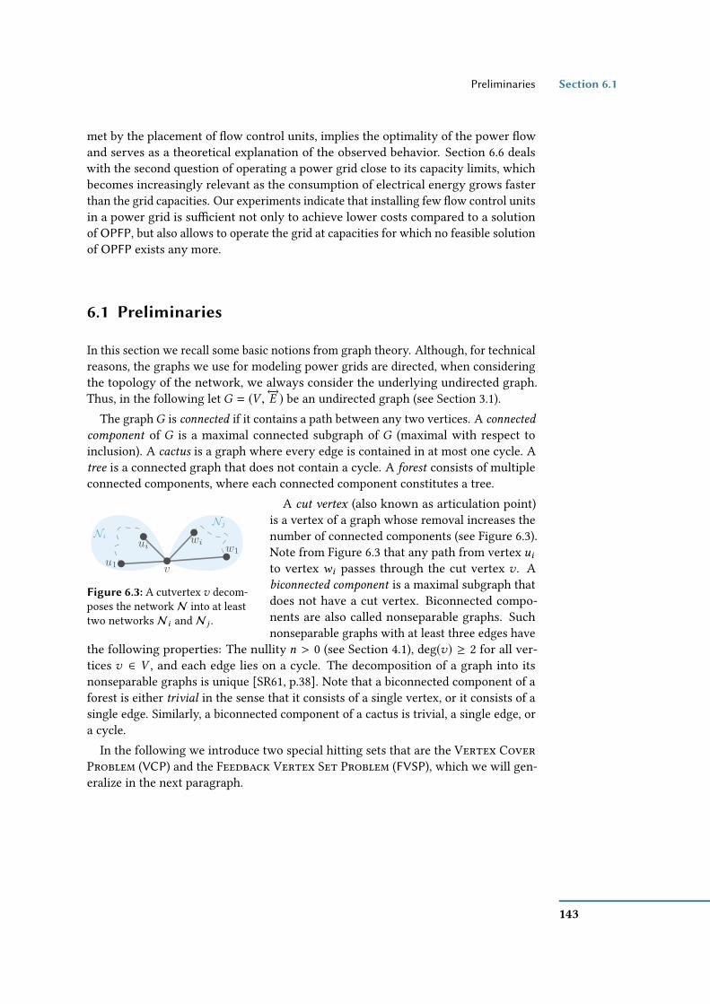
Preliminaries Section 6.1
met by the placement of ow control units, implies the optimality of the power owand serves as a theoretical explanation of the observed behavior. Section 6.6 dealswith the second question of operating a power grid close to its capacity limits, whichbecomes increasingly relevant as the consumption of electrical energy grows fasterthan the grid capacities. Our experiments indicate that installing few ow control unitsin a power grid is sucient not only to achieve lower costs compared to a solutionof OPFP, but also allows to operate the grid at capacities for which no feasible solutionof OPFP exists any more.
6.1 Preliminaries
In this section we recall some basic notions from graph theory. Although, for technicalreasons, the graphs we use for modeling power grids are directed, when consideringthe topology of the network, we always consider the underlying undirected graph.Thus, in the following let G = (V ,←→E ) be an undirected graph (see Section 3.1).
The graphG is connected if it contains a path between any two vertices. A connected
component of G is a maximal connected subgraph of G (maximal with respect toinclusion). A cactus is a graph where every edge is contained in at most one cycle. Atree is a connected graph that does not contain a cycle. A forest consists of multipleconnected components, where each connected component constitutes a tree.
v
Ni
u1
Nj
w1wiui
Figure 6.3: A cutvertex v decom-poses the networkN into at leasttwo networks N i and N j .
A cut vertex (also known as articulation point)is a vertex of a graph whose removal increases thenumber of connected components (see Figure 6.3).Note from Figure 6.3 that any path from vertex uito vertex wi passes through the cut vertex v . Abiconnected component is a maximal subgraph thatdoes not have a cut vertex. Biconnected compo-nents are also called nonseparable graphs. Suchnonseparable graphs with at least three edges have
the following properties: The nullity n > 0 (see Section 4.1), deg(v) ≥ 2 for all ver-tices v ∈ V , and each edge lies on a cycle. The decomposition of a graph into itsnonseparable graphs is unique [SR61, p.38]. Note that a biconnected component of aforest is either trivial in the sense that it consists of a single vertex, or it consists of asingle edge. Similarly, a biconnected component of a cactus is trivial, a single edge, ora cycle.
In the following we introduce two special hitting sets that are the Vertex CoverProblem (VCP) and the Feedback Vertex Set Problem (FVSP), which we will gen-eralize in the next paragraph.
143

Chapter 6 Ideal FACTS Placement – A Susceptance Scaling Approach
Vertex Cover Problem VCP(G,k)
Instance: A graph G = (V ,←→E ), and parameter k ∈ N.
Question: Is there a vertex cover VC(G) of size at mostk such that one endpoint ofeach edge u,w ∈ ←→E belongs to a subset ofVF c=1 ⊆ V with |VF c=1 | ≤k?
Feedback Vertex Set Problem FVSP(G,k)
Instance: A graph G = (V ,←→E ), and parameter k ∈ N.
Question: Is there a feedback vertex set FVS(G) of size at most k such that atleast one vertex of each cycle c ∈ C belongs to a subset of VF c=2 ⊆ Vwith |VF c=2 | ≤ k?
A vertex hitting set of G = (V , E) with respect to a class of graphs G is a set ofvertices VF ⊆ V such that G −VF ∈ G. We will only be interested in hitting sets withrespect to forests and cacti. The former is also called feedback vertex set. Naturally, oneis interested in nding a set VF that is as small as possible. A generalization of vertex
c = 3
c = 2
c = 1
c = i .....
.
c = 4
Figure 6.4: Forbidden c-pumpkinminors for dierent values of cwith c ∈ N>0.
cover and feedback vertex set is called c-pumpkinhitting set. A minor H of a graph G is a graphthat can be obtained from G by deletion of verticesand edges or by contraction of edges. A graphthat has no c-pumpkin minor for c = 1 is anempty graph (i. e., vertex cover; see Figure 6.2a),for c = 2 is a forest (i. e., feedback vertex set; see Fig-ure 6.2b), and for c = 3 is a cactus (i. e., diamondhitting set; see Figure 6.2c). We call a subset of ver-tices VF c c-pumpkin hitting set if there is a vertexsubset VF c ⊆ V (G) such that G − VF c consists ofno c-pumpkin minor (see Figure 6.4 for dierent c-minors). In addition, we try to minimize the sizeof the c-pumpkin hitting set. The general problemdenition is given below.
c-Pumkin Hitting Set Problem p-c-Hit(G, c,k) [Jor+11a, Jor+11b]
Instance: A graph G, parameter c ∈ N>0, and k ∈ N.Question: Is there a c-pumpkin hitting set VF c ⊆ V of size |VF c | ≤ k such
that G −VF c consists of no c-pumpkin minor?Note that the problem of nding a c-pumpkin hitting set is already NP-hard for
all c ≥ 1 [Jor+11a, Jor+11b]. Analogous to vertex hitting set, we dene the edge hitting
set EF ⊆ E such thatG−EF ∈ G and a c-pumpkin hitting set is denoted by EFc ⊆ E(G).
144

Preliminaries Section 6.2
An Exact Model for (Special) Hiing Sets. In general a set system (also knownas hypergraph or range space) is a tuple (V , S), where V is the set of elements such asvertices and S is the set of subsets ofV that is not necessarily a power set meaningP(V ).The latter would imply an exponential size of S with |S | = 2 |V | . A hitting set VF ⊆ V isa set that has at least one element in each subset of S meaningVF ∩Si , ∅ for all Si ∈ Swith i ∈ N (see Equation 6.1b) and thus, a hitting set highly depends on the denitionof the set S . One possibility to dene the set of subsets is S =
⋃ei ∈E Si ∩ V | Si =
ei , ei = u,v, which represent the set of subsets for vertex cover. The hitting setproblem is dened by Equation 6.1.
minimize∑v ∈V
z(v), (6.1a)
subject to ∑v ∈Si
z(v) ≥ 1 ∀Si ∈ S, (6.1b)
where z : V → 0, 1 is a decision variable that is z(v) = 1 if v is in the hittingset v ∈ VF and 0 otherwise. The latter represents basically the integrality constraintthat explains why this is an ILP. The solution to the above dened ILP dependent on Sis a hitting set VF c=1 that is a 1-pumpkin hitting set (i. e., vertex cover) [Cyg+15, p.60].
Now, we are interested in hitting sets such that the remaining graph has no c-pumpkin minor. Thus, we have to generalize the denition of S with subsets Si ∈ Ssuch that Si is a connected component (also known as block) that is not c-pumpkinminor free. We are looking for all such connected components. This is quite similar tothe Traveling Salesman Problem (TSP) approach that is generating subtour eliminationconstraints meaning if the tour does not have the correct length then the tour representsa subtour that is excluded from the solution set. However, we add a restriction to thestructure of Si that is a connected component that has at least one c-pumpkin minor.Thus, in each solver callback we add new sets Si with Si ⊆ V \
⋃v ∈V v | z(v) = 1.
For c-pumpkins with c = 2 or c = 3 we use block-cut trees to identify the set ofmaximum biconnected components and check by the ratio of the number of verticesto the number of edges whether each new connected component β is large enough.This means that for c = 2, we have |V (β)| − 1 < |E(β)| that excludes trees andfor c = 3 we have |V (β)| < |E(β)| that excludes simple cycles. This can be extend toany c ∈ N (see Figure 6.4). The substructure exclusion leads to exponentially manyconstraints. Thus, a common way to solve this ILP is by using techniques such ascolumn generation.
145

Chapter 6 Ideal FACTS Placement – A Susceptance Scaling Approach
6.2 A Hybrid Mathematical Model for thePlacement of Continuous Control Units
In this section we introduce three graph-theoretic ow models for optimal powerows. We propose a hybrid model that combines the ow model and the electricalow model in order to handle power grids with ow control units. Our models arebased on the DC power grid model [Ham07, SJA09, ZMT11], which is commonly usedas an approximation of AC grids [OCS04, Pur+05]. An overview of the simplicationsis given in Section 3.3.2. We model a power grid N as a graph G = (V , E), where Vis the set of vertices and E ⊆
(V2)
is the set of edges. The underlying power gridis an undirected graph. We model the undirected graph using a directed graph byreplacing the undirected edges u,v by two directed edges (u,v), (v,u) ∈ E that aredirected to either vertices of the original edge. However, in some cases we neglectfor the notational convenience the orientation and use the undirected edge that isdenoted by ←→e ∈ ←→E , where ←→e is the undirected edge of e . The vertices represent thebuses, some of which may be special generator and consumer vertices, and the edgesrepresent the branches, which may be transmission lines between the incident verticesor transformers. There is a subset VG ⊆ V of the vertices that represent generatorvertices. We dene the functions pд,pд : VG → R≥0 that represent the minimum andmaximum supply for each generator, respectively. In this chapter, we assume that thelower generation bound is zero meaning pд ≡ 0. Further, there is a subsetVD ⊆ V \VGof consumer vertices. We dene the functions pd ,pd : VD → R ∪ ∞ that representsthe minimum and maximum real power demand, respectively. We assume that thedemands are xed meaning pd (u) = pd (u) = pd (u) for each consumer u ∈ VD . Withoutloss of generality, we assume that VG ∩VD = ∅.
6.2.1 The Objective Function
Each generatoru ∈ VG is equipped with a convex cost functionγu : R→ R≥0 withγu >0 that is assumed to be piecewise linear (see Equation 6.2).
γu (x) = maxaix + ci | (ai , ci ) ∈ Fu , (6.2)
where Fu is the set of all piecewise linear functions of γu and ai ≤ ai+1 for i ∈ N.Each edge e ∈ E has a thermal line limit that is modeled by a capacity func-
tion cap : E → R restricting the real power. Further, each edge causes a certainloss of power depending on the physical edge parameters and the actual power owon that edge. These losses are again approximated as a convex, piecewise linearfunction `e : R→ R≥0 for each edge e ∈ E (see Equation 6.3).
`e (x) = maxaix + ci | (ai , ci ) ∈ Fe , (6.3)
146

A Hybrid Mathematical Model for the Placement of Continuous Control Units Section 6.2
where Fe is the set of all piecewise linear functions of `e and ai ≤ ai+1 for i ∈ N.A ow f in a power gridN is a function f : V ×V → R that complies with the skew
symmetry property f (u,v) = −f (v,u) for all u,v ∈ V . For every vertex u in V (G),we dene its net out-ow fnet(u) B
∑u ,v ∈
←→E f (u,v). For a ow f , we further dene
two types of cost functions. The total generator cost is a function cд : R→ R≥0 that isdened in Equation 6.4 and the total line loss is a function c` : R→ R≥0 that is denedin Equation 6.5.
cд(f ) =∑u ∈VG
γu (fnet(u)), (6.4)
c`(f ) =∑(u ,v)∈E
`(u ,v)(| f (u,v)|) . (6.5)
To obtain the overall cost for a ow f , we weight these two terms with λ ∈ [0, 1]such that the objective function represents a multi-criteria objective (see Equation 6.6)weighted with λ.
cλ(f ) = λ · cд(f ) + (1 − λ) · c`(f ). (6.6)
Our goal is to minimize this objective function cλ in dierent models.
6.2.2 Power Flow Models
The most basic model is the ow model, where f has to satisfy the constraints givenin the Equations 6.7–6.10. We call a ow satisfying these constraints feasible. Equa-tion 6.10 models the thermal line limits or real power capacities of all edges and iscalled capacity constraint. Equation 6.7 models the zero net out-ow for intermediatevertices, i. e., vertices that are neither generators nor consumers. Equation 6.8 mod-els that all consumer demands are satised and is called demand constraint. Finally,Equation 6.9 models that all generators respect their production limits and is calledgenerator constraint. The Equations 6.7–6.9 are called ow conservation constraints.
fnet(v) = 0 v ∈ V \ (VG ∪VD ), (6.7)fnet(v) = −pd (v) v ∈ VD, (6.8)
0 ≤ fnet(v) ≤ pд(v) v ∈ VG , (6.9)| f (u,v)| ≤ cap(u,v) ∀(u,v) ∈ E. (6.10)
The ow model (i. e., Equations 6.7–6.10) neglects some physical properties of electricalows, in particular Kirchho’s voltage law. Thus, the computed power ows canonly be applied to power grids where every vertex is a control vertex. In contrast,the electrical ow model, e. g., according to Zimmerman et al. [ZMT11], models thepower ow using the same set of constraints as the ow model, but additionallyrequires the existence of a suitable voltage angle assignment θv : V → R such that
147

Chapter 6 Ideal FACTS Placement – A Susceptance Scaling Approach
for each edge u,v ∈ ←→E the power ow specic constraint holds (see Equation 6.11).The power ow constraint basically represents Kirchho’s Voltage Law (KVL) that iscombined with Ohm’s law. More details can be found in Chapter 4.
f (u,v) = b(u,v)(θv (v) − θv (u)), (6.11)
where the susceptance b(u,v) is a function b : E → R. This is equivalent to restrict-ing the model to feasible ows that also satisfy the KVL, or, in other words, noow control units are used. This yields a model that matches the situation in thetraditional power grid existing today. We call a feasible ow f a feasible electrical
ow if there exists a voltage angle assignment θv satisfying Equation 6.11. We arenow able to give a complete denition of the power grid by the tuple N = (G =(V , E),VG ,VD, cap,b,γu ∈VG , `e ∈E,pд,pд,pd ).
Recall from the introduction that ow control vertices (FCVs) and ow controledges (FCEs) can be technically realized by UPFCs, which are FACTS. Ideal FACTS asintroduced by Grin et al. [GAG96] are often used to simplify the modeling of FACTSby using a linear model and assuming a complete and independent control of the realand reactive power. Our ow control units are ideal FACTS that control the powerow to all incident edges in terms of FCVs and the power ow on that particular edgein terms of FCEs. The ow model—in contrast to the electrical model—assumes owcontrol units at each vertex or each edge, whereas the electrical model assumes noimmediate control of the power ow. Instead, the grid is balanced by changing thegenerator outputs only. In the following, we propose a hybrid model that combinesthe ow model and the electrical ow model in order to handle power grids with owcontrol vertices (resp. edges) at a subset of selected vertices (resp. edges).
6.2.3 Flow Control Units on Vertices
In this section, we focus on continuous ow control units that are placed on vertices.As mentioned above, we call them ow control vertices (in short FCVs). Let VF ⊆ Vbe a subset of vertices of G . We denote by GVF the power network obtained from G byconsidering all vertices inVF as ow control vertices. We call any subgraphG ′ = G[V ′]induced by a subset V ′ ⊆ V \ VF of the vertices without controllers a native power
grid of G. A ow f on G is a feasible electrical ow for a native power grid G ′ ⊆ Gif there exists a voltage angle assignment θv : V → R such that every edge in G ′
satises Equation 6.11. In this case we call θv a feasible (voltage) angle assignment
for G ′.A feasible ow f is a feasible electrical ow for GVF if and only if f is a feasible
electrical ow for the maximal native power grid G −VF = G[V \VF ]. Intuitively, thismodels the fact that a power ow in GVF must be a feasible ow and that it satisesthe Kirchho’s voltage law in the maximum native power grid.
148
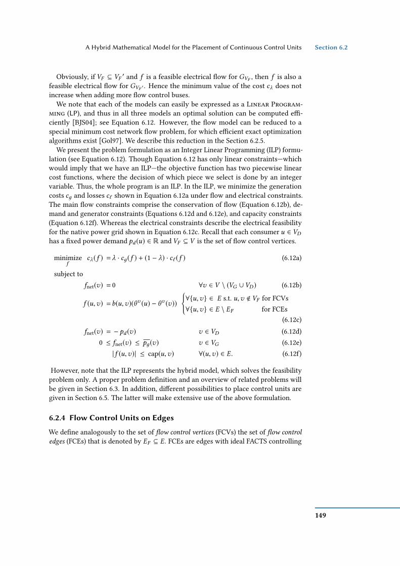
A Hybrid Mathematical Model for the Placement of Continuous Control Units Section 6.2
Obviously, if VF ⊆ VF′ and f is a feasible electrical ow for GVF , then f is also a
feasible electrical ow for GVF ′ . Hence the minimum value of the cost cλ does notincrease when adding more ow control buses.
We note that each of the models can easily be expressed as a Linear Program-ming (LP), and thus in all three models an optimal solution can be computed e-ciently [BJS04]; see Equation 6.12. However, the ow model can be reduced to aspecial minimum cost network ow problem, for which ecient exact optimizationalgorithms exist [Gol97]. We describe this reduction in the Section 6.2.5.
We present the problem formulation as an Integer Linear Programming (ILP) formu-lation (see Equation 6.12). Though Equation 6.12 has only linear constraints—whichwould imply that we have an ILP—the objective function has two piecewise linearcost functions, where the decision of which piece we select is done by an integervariable. Thus, the whole program is an ILP. In the ILP, we minimize the generationcosts cд and losses c` shown in Equation 6.12a under ow and electrical constraints.The main ow constraints comprise the conservation of ow (Equation 6.12b), de-mand and generator constraints (Equations 6.12d and 6.12e), and capacity constraints(Equation 6.12f). Whereas the electrical constraints describe the electrical feasibilityfor the native power grid shown in Equation 6.12c. Recall that each consumer u ∈ VDhas a xed power demand pd (u) ∈ R and VF ⊆ V is the set of ow control vertices.
minimizef
cλ(f ) = λ · cд(f ) + (1 − λ) · c`(f ) (6.12a)
subject tofnet(v) = 0 ∀v ∈ V \ (VG ∪VD ) (6.12b)
f (u,v) =b(u,v)(θv (u) − θv (v))
∀u,v ∈ E s.t. u,v < VF for FCVs∀u,v ∈ E \ EF for FCEs
(6.12c)fnet(v) = − pd (v) v ∈ VD (6.12d)
0 ≤ fnet(v) ≤ pд(v) v ∈ VG (6.12e)| f (u,v)| ≤ cap(u,v) ∀(u,v) ∈ E. (6.12f)
However, note that the ILP represents the hybrid model, which solves the feasibilityproblem only. A proper problem denition and an overview of related problems willbe given in Section 6.3. In addition, dierent possibilities to place control units aregiven in Section 6.5. The latter will make extensive use of the above formulation.
6.2.4 Flow Control Units on Edges
We dene analogously to the set of ow control vertices (FCVs) the set of ow control
edges (FCEs) that is denoted by EF ⊆ E. FCEs are edges with ideal FACTS controlling
149

Chapter 6 Ideal FACTS Placement – A Susceptance Scaling Approach
ow on them. We denote by GEF the subgraph of G that contains all edges of EF andtheir incident vertices.
In the standard ow model the ow on all edges can be manipulated, i. e., it is likehaving a FACTS on every edge in a power grid. In case of FCEs this means EF = E.The standard ow model asks to nd a ow, i. e., it neglects Equation 6.11. In theDC ow model [ZMT11] the ow on edges cannot be controlled, which translatesto EF = ∅ in case of FCEs. The DC ow model requires to nd a feasible electrical ow,i. e., Equation 6.11 satised for all edges e ∈ E \ EF . The hybrid model is formalizedin Equation 6.12 as an LP, the ow model and the DC ow model are combined and itis required to nd a ow on GVF such that Equation 6.11 holds only for edges that arenot in EF .
Since an ideal FACTS [GAG96] is technically realized on transmission lines, it ismore realistic to consider FCEs instead of FCVs. However, we can easily translate thedescribed models designed for FCVs to models on FCEs by simply replacing VF by EFand GVF by GEF and vice versa (see Equation 6.12c).
Recall that the EDP is the problem of generating the required amount of power whileobtaining minimum operation cost and meeting the constraints in Equations 6.7–6.9.The objective function cλ(f ) describing the operation cost is a weighted functionof generator costs cд(f ) and transmission line losses c`(f ), where λ ∈ [0, 1] is theweight factor (see Equations 6.6 and 6.12a). The overall optimization problem is givenin Equation 6.12 as an LP.
6.2.5 Reduction to MinCostFlow
Let N = (G = (V , E), s, t, cap,a) be a s-t ow network consisting of a directed (multi-)graph G, two dedicated source and sink vertices s, t ∈ V , edge capacities cap : E →R≥0, and edge costs a : E → R≥0. A ow f in N is a function f : E → R≥0 andit is called feasible if it satises the capacity constraint in Equation 6.10 and a owconservation constraint similar to Equation 6.7 that is given in Equation 6.13.∑
(u ,v)∈E
f (u,v) −∑(v ,u)∈E
f (v,u) = 0 ∀v ∈ V \ s, t. (6.13)
Theow value F (N) of a ow f is the total ow from s to t , i. e., F (N) =∑(u ,t )∈E f (u, t) =∑
(s ,u)∈E f (s,u). A feasible ow f with maximum value is called a maximum ow inNand denoted by MF(N). For a given ow value x the min-cost s-t ow problem is tond a feasible ow f of value F (N) = x such that the cost cN(f ) =
∑e ∈E a(e) · f (e) is
minimized.
150

A Hybrid Mathematical Model for the Placement of Continuous Control Units Section 6.2
b(e) ∈ [0.75; 1.25](b)(a)
2x/4x
3x/5x
3x/5xx/x x/x
MPFP
2x0ts
x u
4x/4x
5x/5x
5x/5xx/x x/x
MFP
−−ts
u−
83 x/4x
113 x/5x
113 x/5x
x/x x/x
83x0ts
u0.75 0.75
43x
1.25
52 x/4x
72 x/5x
72 x/5x
x/x x/x
2x0ts
x u
103 x/5x
103 x/5x
x/x x/x
73x0ts
u
73 x/4x
0.75
43x
133 x/5x
133 x/5xMFFP
1.25
103 x/4x
x/x x/x
83x0ts
u0.75 0.75
43x
Figure 6.5: A small example graph with three vertices, three edges, one source s , and onesink t . We label each vertex u ∈ V that is represented by a cycle with a voltage angle θv (u).On the edges, we write the ow f and the edge’s capacity cap in the form f /cap. Note thatthe susceptance on the black edges is xed to b ≡ 1 and when placing FACTS (red edges)the susceptance is in the range b(e) ∈ [0.75; 1.25] for all e ∈ EF . (a) The top graph showsan MPF(N)with a value of OPTMPFP(N) = 3x . The bottom graph shows a MF(N)with a valueof OPTMFP(N) = 5x . (b) Dierent placement of FACTS and their best susceptance scaling forthis situation result in dierent values for the resulting ow. However, the best placement isshown in the bottom right yielding a MFF(N) with a value of OPTMFFP(N) = 13/3 · x .
Min-cost s-t Flow Problem
Instance: A network N , parameter x ∈ R, and k ∈ R≥0.Question: Is there a feasible ow f of value F (N) = x such that cN(f ) ≤ k?
In Section 3.2, we discussed some approaches to tackle the problem. In order totransform the graph G = (V , E) of a power grid into an s-t ow network N , we rstadd a new source vertex s and a new sink vertex t to V . Each generator u ∈ VG isconnected by a directed edge (s,u)with capacity cap(s,u) = pд(u) to the source s . Eachconsumer u ∈ VD is connected by a directed edge (u, t) with capacity cap(u, t) = pd (u)to the sink t . Further, we replace each original undirected edge u,v ∈ E by twodirected edges (u,v) and (v,u), whose capacities cap(u,v) = cap(v,u) are given bytheir common thermal limit cap(u,v). Recall from the introduction of Section 6.2that this represents a bidirected graph.
Next, we dene the edge costs. It is well known that a convex, piecewise linear edgecost function h can easily be modeled in a ow network by replacing the respective
151

Chapter 6 Ideal FACTS Placement – A Susceptance Scaling Approach
edge (u,v) with as many copies as the linear pieces of the cost function. The edgecapacities are dened by the dierences between consecutive breakpoints of h andsum up to cap(u,v); the individual costs correspond to the costs as dened by thelinear pieces between the breakpoints. Thus for ease of presentation we refrain fromexplicitly modeling convex piecewise linear cost functions in N . We rather assumethat the ow cost zλ is given for each edge (u,v) ∈ E with u , s and v , t by theweighted loss function zλ((u,v), f ) B (1 − λ) · `u ,v (f (u,v)), where λ is the weightparameter of Equation 6.6. The edges (s,u) from the source s to a generator u ∈ VGhave cost zλ((s,u), f ) B λ · γu (f (s,u)) and the edges incident to the sink t have cost 0.Then the objective function to be minimized is zλ(f ) B
∑e ∈E zλ(e, f ). Finally, we
set the target ow value x to the total demand∑u ∈VD pd (u) of all consumers. By
construction, every feasible minimum-cost ow in N is a feasible minimum-cost owin the underlying power grid G and vice versa.
6.3 Complexity
In the above section we gave no restriction on the control unit’s ability. The lattermeans that a FACTS is able to adjust the ow arbitrarily. However, a realistic FACTSis only able to adjust the voltage angle dierence within a limited range. Since theproposed hybrid model does not incorporate a limitation of the power ow scaling, wecould instead use the DC-model and allow to adjust the susceptances b(u,v) arbitrarily,where either u or v is in VF for FCVs or (u,v) ∈ EF for FCEs. The limitation foradjusting the voltage angle dierence can be modeled by a real interval Ie ∈ I(R≥0)that depends on the edge e , where I(R≥0) is the set of all real intervals and I(R≥0)is a semiring (i. e., a ring without additive inverse) of sets. Thus, the interval Ie isa subset of R that is dened by the two elements x and y with x,y ∈ Ie and z ∈ R
such that x ≤ z ≤ y, which implies that z ∈ Ie . The dierence now is that eitheredges incident to a vertex VF for FCVs or all edges in e ∈ EF for FCEs have a variablesusceptance b : E → I(R≥0), (u,v) 7→ I(R≥0) with u or v in VF , or b : EF → I(R≥0),respectively. An example that shows dierent scalings for a triangle graph is givenin Figure 6.5. Figure 6.5 shows dierent susceptance scaling of the same graph thatlead to dierent power ows by either allowing more ow, but xing the voltageangles, changing the voltage angles and xing the ows, or both.
This modeling would change the linear program Equation 6.12 to a quadratic pro-gram, since Equation 6.12c is a quadratic constraint with variables f , θv , and b. Moreprecisely, it represents a bilinear constraint. In Equation 6.14 we use a bilinear form,where µbilin : V × V → R with (u,v) 7→ b(u,v) · (θv (v) − θv (u)). The latter bilinear
152

Complexity Section 6.3
form is skew-symmetric.
f (u,v) = b(u,v)(θv (v) − θv (u)) (6.14a)f (u,v) = b(u,v) · θv (v) − b(u,v) · θv (u) (6.14b)f (u,v) = µbilin(b(u,v), θ
v (v) − θv (u)) (6.14c)
Thus, we have one quadratic constraint (i. e., the KVL combined with Ohm’s law).However, the other constraints and—in terms of maximizing the throughput—also theobjective stays linear. In the rst problem, we assume a given placement of the FACTSand are just interested in the susceptance scaling, which is NP-hard under the conditionthat there are quadratic constraints and the objective is linear [Sahni,1974]. The proofuses a reduction from the Partition Problem. For more precise information aboutthe complexity of quadratic programming refer to Garey and Johnson [GJ79, p.245,MP2] and Ausiello et al. [Aus+99, p.447, MP5].
Maximum FACTS Flow Problem with EF MFFP(N, EF )
Instance: A network N , and a set EF ⊆ E.Objective: Find a susceptance setting b ∈ Ie for all e ∈ EF such that OPTMPFP(N)
is maximum among all choices of b.
Problem Definitions. We can now give dierent level of granularity for the prob-lem denition of the Maximum FACTS Flow Problem (MFFP). Recall from Chapter 4the Maximum Power Flow Problem MPFP(N) and its value OPTMPFP(N). For sim-plicity and for consistency reasons, we only consider FCEs. However, all formulationscan be translated to FCVs, too. The rst placement problem MFFP(N,k) consid-ers the problem with a xed number of FACTS—meaning |EF | = k—and is denedby OPTMFFP(N,k) B maxEF ⊆E ,b ∈Ib OPTMPFP(N) with |EF | = k . The optimizationproblem is dened as follows.
Maximum FACTS Flow Problem with k-FACTS MFFP(N,k)
Instance: A network N , and parameter k ∈ N.Objective: Find a set EF ⊆ E of FACTS with |EF | = k and a susceptance settingb ∈
Ie for all e ∈ EF such that OPTMPFP(N) is maximum among all choicesof EF and b.
Note that if |EF | = |E | = k and the susceptance is dened in b(e) ∈ [0,∞] for all e ∈EF the value of OPTMFFP(N,k) = OPTMFP(N). Assume, we have no limitation on thenumber of FACTS we can place. The problem to get the maximum possible ow for anetwork N by allowing as many FACTS as possible (i. e., some k) is called MFFP(N)
153

Chapter 6 Ideal FACTS Placement – A Susceptance Scaling Approach
and its value is denoted by OPTMFFP(N) B maxk OPTMFFP(N,k). The problem isdened as follows.
Maximum FACTS Flow Problem MFFP(N)
Instance: A network N .Objective: Find a set EF ⊆ E of FACTS with |EF | = k , 0 ≤ k ≤ |E |, and a
susceptance setting b ∈ Ie for all e ∈ EF such that OPTMPFP(N) ismaximum among all choices of EF , b, and k .
In the simulations, where we allow a susceptance range of b(e) ∈ [0,∞], we willsee that a small number of control units suces to get OPTMFP(N). However, depen-dent on the susceptance interval Ie and the network’s underlying graph structure,the OPTMFFP(N) does not necessarily have the same value as the OPTMFP(N) mean-ing OPTMFFP(N) ≤ OPTMFP(N).
In the simulations, we will be interested in the problem of nding the minimum num-ber of control units, which we call MNFP(N). Its value is denoted by OPTMNFP(N) B
minOPTMFFP(N,k )=OPTMFFP(N) k .
Minimum Number of FACTS Problem MNFP(N)
Instance: A network N , and a parameter k ∈ N.Objective: Find a set EF ⊆ E of FACTS and a susceptance setting b ∈ Ie with e ∈
EF such that k = |EF | is minimum among all choices of OPTMFFP(N).From Lemma 5.6, we know the bounds of MTSFP. A similar relationship holds for
the MFFP, which we describe in Lemma 6.1.
Lemma 6.1. OPTMPFP(N) ≤ OPTMFFP(N) ≤ OPTMFP(N).
In addition, we can give the following relationship between the aforementionedproblems that is given by the problem denition itself.
Lemma 6.2. MPFP(N) ⊆ MFFP(N,k) ⊆ MFFP(N) ⊆ MNFP(N).
Note that the KVL constraint is a bilinear constraint that can be reformulated asshown in Equations 6.14a–6.14c
Overview. For trees (see Table 6.1–1) any of the aforementioned problems is poly-nomial time solvable, since we reach OPTMFP(N) without any control units. We willdiscuss this in more detail in Section 6.5.2. While increasing the structural complexityof a graph by allowing cycles, Lehmann et al. [LGH15, pp.10., Theorem 4] showthat the problem is already NP-hard for cacti with maximum degree of 3 by reductionfrom Subset Sum Problem (SSP; see Section 5.2.2). In Table 6.1–3, we give a short
154

Complexity Section 6.3
overview. For the most general graph structure—meaning an arbitrary graph—theproblem is strongly NP-hard. The latter was shown by Lehmann et al. [LGH15, pp.7, Theorem 1] by reduction from exact cover by 3-set problem (i. e., given a set U anda set of subsets M ⊆ P(U ) with |M | = 3 the decision problem is whether there isa set M ′ ⊆ M such that
⋃X | X ∈ M ′ = U ) and an overview on that is given
in Table 6.1–5. Note that Lehmann et al. [LGH15] implemented this by a choicenetwork and focused on the problem MFFP(N, EF ), where the position of the FACTSis predened.
155
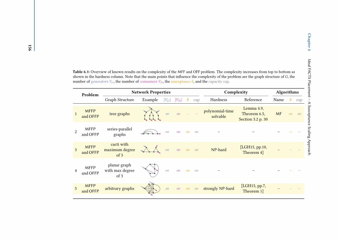
Chapter
6IdealFA
CTS
Placement
–A
SusceptanceScaling
Approach
Table 6.1: Overview of known results on the complexity of the MFF and OFF problem. The complexity increases from top to bottom asshown in the hardness column. Note that the main points that inuence the complexity of the problem are the graph structure of G, thenumber of generators VG , the number of consumers VD , the susceptance b, and the capacity cap.
Problem Network Properties Complexity Algorithms
Graph Structure Example |VG | |VD | b cap Hardness Reference Name b cap
1 MFFPand OFFP
tree graphs ∞ ∞ – – polynomial-timesolvable
Lemma 4.9,Theorem 6.5,
Section 3.2 p. 30MF ∞ ∞
2 MFFPand OFFP
series-parallelgraphs ∞ ∞ ∞ ∞ – – – – –
3 MFFPand OFFP
cacti withmaximum degree
of 3∞ ∞ ∞ ∞ NP-hard [LGH15, pp.10,
Theorem 4] – – –
4 MFFPand OFFP
planar graphwith max degree
of 3∞ ∞ ∞ ∞ – – – – –
5 MFFPand OFFP
arbitrary graphs ∞ ∞ ∞ ∞ strongly NP-hard [LGH15, pp.7,Theorem 1] – – –
156

Planar Problem Reinterpretation Section 6.4
(b)
(a)
1111
11
11
1 2
22
3
3
5
521
22
1
1
2
2
111
23t
s
1 1
0
35
2
s
s? t?1
1 2
21
13 2
1
3
1
1
1
22
1
1
2
2
12
s
t
s? t?1
1 2
21
13 2
1
3
1
1
2
21
1
1
2
t
1111
11
11
22
22
3
3
5
5
22 11
1
1
2
2
111
23t
s
1 2
0
3456
23
b scalingKVL conflict
Figure 6.6: The graph from Figure 6.1 [Fel13, p.18, Figure 18], where we split the KVL conictstep (a) that is a KCL conict in the dual graph G? from the susceptance scaling step (b).If not described otherwise, we have unit susceptances b with b ≡ 1. In (a) the KVL conictis visible in all three representations. Whether it is the left graph that shows the conictby non-unique voltage angle θv assignments, or in the middle representation with the KCLconicts in the dual graph G?, or the rectangle conicts in the geometric representation onthe right side. However, the susceptance scalings shown in (b) and indicated with the arrows ↑for the geometric interpretation in the right most gure in (a) x these conicts in all threerepresentations.
6.4 Planar Problem Reinterpretation
Recall from Section 5.3 that we dened a single source and single sink planar powerow in terms of simultaneous ows in the primal graph G and dual graph G?. Thedenition of simultaneous ows is given in Section 4.3.2. We adjust the problemformulation for FACTS in the following, while allowing a susceptance range of [0,∞]for all edges e ∈ E.
s-t-DC Feasibility Problem with FACTS s-t-DC-FEAS-FACTS(G,G?, µdual)
Instance: A plane s-t-graph G and its dual G?, subsets E1 ⊆ E(G) and E2 ⊆E(G?), and a bijection µdual : E1 → E2.
Objective: Find KCL-feasible ows f G and f G? in G and G? with F (G) , 0and F (G?) , 0 such that for every edge e ∈ E we have f G (e) =f G?(µdual(e)).
157

Chapter 6 Ideal FACTS Placement – A Susceptance Scaling Approach
Table 6.2: IEEE benchmark set with |V |, |E |, |VG |, and pd representing number of buses,number of transmission lines, number of generators and total power demand, respectively.
case |V | |E | |VG | pd
case6 6 11 3 210.00case9 9 9 3 315.00case14 14 20 5 259.00case30 30 41 6 189.20case39 39 46 10 6254.23case57 57 78 7 1250.80case118 118 179 54 4242.00
Instead of demanding that the bijection of the ows holds for all edges, we relaxthis property to edges in E \ EF . In Figure 6.6, we apply a feasible ow f on the primalgraph G and show that an adjustment of the susceptances transforms f into a feasiblepower ow. However, the assumption to [0,∞] is quite strong. Thus, restricting theheight scaling would lead to the same formulation as in Chapter 4.
6.5 Placing Flow Control Buses
In this section we seek to answer the question of how many ow control busesare necessary to obtain a globally optimal solution. Recall that the ow model isa relaxation of the physical model and uses fewer constraints. Therefore, optimalsolutions in the ow model are at least as good as in the physical model.
Given a power grid G = (V , E), we say that making the vertices in VF ow controlvertices achieves full control if the objective value of an optimal energy ow for thegridGVF is the same as the objective value of an optimal solution in the ow model (orequivalently in the hybrid network GV , where every vertex is a ow control vertex).Our experiments indicate that in the IEEE instances a small fraction of the vertices isoften sucient to achieve full control as was already indicated in Figure 6.1. Afterwardswe give a graph-theoretical explanation of this behavior.
6.5.1 Experiments
For our evaluation we use the IEEE benchmark data sets [Uni14, ZM11] shown in Ta-ble 6.2. There each case is named according to the number of buses |V |. The numberof generators and the number of edges are denoted by |VG | and |E |, respectively.
To obtain piecewise linear functions for generator costs γu for all u ∈ VG and linelosses `e for all e ∈ E, we simply sample the cost functions using a specied numberof sampling points. Note further that our approach requires convex cost functions,
158

Placing Flow Control Buses Section 6.5
λ = 1
λ = 0
50 100 150 200
560
580
600
620
640
660
680
700
Total Losses in MW
Tot
al G
ener
ator
Cos
ts in
$/M
Wh case30
Hybrid ModelOPF
(a) Total costs cд and losses c` for the IEEEbenchmark data with 30 buses, where the square
cross marks the solution computed by OPF.
0 20 40 60 80 100
50
60
70
80
90
100
Relative Losses in % of the Maximum Losses
Rel
ativ
e G
ener
ator
Cos
ts in
$/M
Wh
case6case9
case14case30
case39case57
case118
(b) Relative costs and losses for the IEEEbenchmark data sets.
Figure 6.7: Trade-o of generator costs cд and losses c` normalized to the maximum generatorcost (λ = 0) and the maximum loss (λ = 1) as λ varies from 0 to 1.
but this is ne in practice [WW96]; in particular the functions are convex for the IEEEbenchmark instances.
We performed our experiments on an AMD Opteron 6172 processor running open-SUSE 12.2. Our implementation is written in Python 2.7.3 and uses PYPOWER [Lin11],a Python port of MATPOWER [ZMT09, ZMT11], for computing solutions for the OPFP.For computing solutions and minimizing the number of control buses in our hybridmodel we use the (integer) linear programming solver Gurobi 6.0.0 [GUR13].
First, we observe that the value of λ, which controls the weighting of costs and lossesin the objective value, has a signicant eect on the objective values of generator costsand line losses. Figure 6.7a shows the trade-o for the IEEE instance case30 (the plotsfor the other instances can be found in Appendix D). The OPF solution, which ignoreslosses, is typically at the far end of the spectrum with high losses and is comparableto our solution with λ = 1. As can be seen in Figure 6.7b, where the costs and lossesare normalized to the maximum cost and the maximum loss per instance, the sametrade-o behavior is present in all instances. It thus makes sense to allow the operatorof a power grid to choose the value of λ in order to model the true operation costs.
On the other hand, it may then be the case that the number of ow control verticesto achieve full control of the network varies depending on the choice of λ. Figure 6.8shows for dierent values of λ the relative number of control vertices necessary toachieve full control in each of the instances. In most cases less than 15% of all verticesneed to be controllers to achieve full control. For the cases with 6 vertices and 14vertices this percentage is slightly bigger, which is mainly an artifact stemming fromthe small total size. As can be seen, the required number of units is relatively stable
159

Chapter 6 Ideal FACTS Placement – A Susceptance Scaling Approach
0 0.2 0.4 0.6 0.8 1
0
5
10
15
20
25
30
Weight λ
Rel
ativ
e N
umbe
r of
Con
trol
lers
in % case6
case9case14case30case39case57case118
Figure 6.8: Relative number of controllers for achieving full control in the IEEE instances as λvaries from 0 to 1.
but drops to zero for λ = 1, i. e., when only the generator costs are considered. This isdue to the fact that all IEEE instances have basically unlimited line capacities and thusdo not restrict the possible ows.
In order to make a useful prediction on the number of vertices required for fullcontrol that applies to all choices of λ, in the following we take for each instance themaximum of the smallest possible number of vertices to achieve full control over allvalues of λ and refer to this as the number of vertices for achieving full control of theinstance. This conservative choice ensures that the numbers we compute are certainlyan upper bound for achieving full control, independent of the actual choice of λ.
6.5.2 Structure of Optimal Solutions
As we have seen in our experimental evaluation, often a small number of ow controlvertices is sucient to ensure that solutions in the hybrid model are the same as inthe ow model. In the following we provide a theoretical explanation of this propertyand link it to structural properties of power grids. Farivar and Low [FL13] give similarstructural results on spanning trees, but using a dierent model.
A rst observation is that ow control vertices inuence all incident edges. Thus,if every edge is incident to a ow control vertex, i. e., the set VF c is a vertex cover
of G (i. e., c = 1), no edge in the network is aected by the constraint Equation 6.11).Then the ow model and the hybrid model are equivalent and full control is achieved.However, it is generally not true that power grids admit small vertex covers; as shownin Figure 6.9, all instances require more than 40% of their vertices for a vertex cover.In the following, we show a much stronger result, namely that it suces for becoming
160
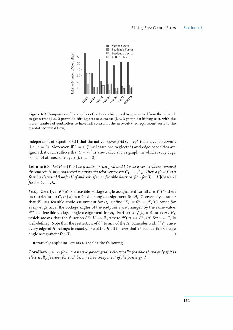
Placing Flow Control Buses Section 6.5
Vertex CoverFeedback ForestFeedback CactusFull Control
Rel
ativ
e N
umbe
r of
Con
trol
lers
0
10
20
30
40
50
60
case
6ca
se9
case
14
case
30
case
39
case
57
case
118
Figure 6.9: Comparison of the number of vertices which need to be removed from the networkto get a tree (i. e., 2-pumpkin hitting set) or a cactus (i. e., 3-pumpkin hitting set), with theworst number of controllers to have full control in the network (i. e., equivalent costs to thegraph-theoretical ow).
independent of Equation 6.11 that the native power grid G −VFc is an acyclic network
(i. e., c = 2). Moreover, if λ = 1, (line losses are neglected) and edge capacities areignored, it even suces that G −VF c is a so-called cactus graph, in which every edgeis part of at most one cycle (i. e., c = 3).
Lemma 6.3. Let H = (V , E) be a native power grid and let v be a vertex whose removal
disconnects H into connected components with vertex sets C1, . . . ,Ck . Then a ow f is a
feasible electrical ow forH if and only if it is a feasible electrical ow forHi = H [Ci∪v]for i = 1, . . . ,k .
Proof. Clearly, if θv (u) is a feasible voltage angle assignment for all u ∈ V (H ), thenits restriction to Ci ∪ v is a feasible angle assignment for Hi . Conversely, assumethat θv i is a feasible angle assignment for Hi . Dene θv i ′ = θv i − θv i (v). Since forevery edge in Hi the voltage angles of the endpoints are changed by the same value,θv ′ is a feasible voltage angle assignment for Hi . Further, θv i ′(v) = 0 for every Hi ,which means that the function θv : V → R, where θv (u) 7→ θv i
′(u) for u ∈ Ci iswell-dened. Note that the restriction of θv to any of the Hi coincides with θv i ′. Sinceevery edge of H belongs to exactly one of the Hi , it follows that θv is a feasible voltageangle assignment for H .
Iteratively applying Lemma 6.3 yields the following.
Corollary 6.4. A ow in a native power grid is electrically feasible if and only if it is
electrically feasible for each biconnected component of the power grid.
161
Chapter 6 Ideal FACTS Placement – A Susceptance Scaling Approach
We observe that ifG−VF c is a forest (i. e., c = 2), then each biconnected componentHconsists of a single edge u,v. Then θv (u) = f (u ,v)/b(u ,v) and θv (v) = 0 are feasiblevoltage angles for any ow f in G − VF
c=2. Thus, we conclude with the followingtheorem.
Theorem 6.5. Let H be a native power grid that is a forest. Then every ow f is a
feasible electrical ow on H .
Thus, whenVF is a feedback vertex set ofG , i. e.,G−VF c=2 is a forest, then every owon G is a feasible electrical ow for G −VF c=2, and thus any feasible ow for GVF c=2 iselectrically feasible for GVF c=2 . It follows that the ow model and the hybrid modelare equivalent in this case. In particular, whenever VF is a feedback vertex set, insteadof solving the LP for the hybrid model, we can rather assume the ow model andcompute an optimal solution using a, potentially more ecient, ow algorithm. Itfollows from Theorem 6.5 that this solution is optimal also in the hybrid model.
Figure 6.9 shows for each of our instances the relative number of vertices necessaryto obtain a vertex cover (i. e., c = 1), a feedback vertex set (i. e., c = 2) with respect toforests, and the number of vertices necessary to obtain full control. In all instances avertex cover is two to three times larger than a feedback vertex set (for forests) andthe vertex set necessary for full control. Comparing the relative number of controllersfor full control with the size of a feedback vertex sets shows that the number to getan optimal placement is in many cases smaller than the size of a feedback vertex set.Thus, in the optimal solutions, the native power grid does not always represent aforest, but can also include cycles. A closer inspection showed that this is in particularthe case for instances that are operated far from their capacity limits.
We now consider what happens when cycles exist in a native power grid. To thisend, we start with the simplest case of a power grid that consists of a single cycle C .We say that two ows f and f ′ on a network G = (V , E) are equivalent if for eachvertex v ∈ V we have fnet(v) = fnet
′(v).
Lemma 6.6. Let C be a native power grid that is a cycle. For every ow f there exists a
unique equivalent ow f ′ that is a feasible electrical ow for C .
Proof. Letv1, . . . ,vn be the vertices ofC as they occur along the cycle, i. e., f (vi ,vj ) = 0unless vi and vj are neighbors on the cycle. Assume we wish to change the amountof ow from v1 to v2 by a xed amount ∆ and obtain an equivalent ow. The netout-ow conservation at the vertices then uniquely determines the change of owalong the remaining edges. Hence, every ow f ′ equivalent to f is obtained from f bychoosing some amount ∆ and setting f ′(vi ,vi+1) = f (vi ,vi+1) + ∆ and f ′(vi+1,vi ) =f (vi+1,vi ) − ∆, where vn+1 = v1.
Now the existence of a suitable oset ∆ and the associated feasible voltage anglescan be expressed as a linear system of equations. Namely, for edge (vi ,vi+1) with i =
162
Placing Flow Control Buses Section 6.5
1, . . . ,n and vn+1 = v1, we have the following equation.
b(vi ,vi+1) · θv (vi ) − b(vi ,vi+1) · θ
v (vi+1) − ∆ = f (vi ,vi+1) .
It is readily seen that the n equations are linearly independent, and hence a solutionexists. Moreover, dividing each of the equations by b(vi ,vi+1) and summing them up
©«b(v1,v2) −b(v1,v2) 0 . . . −1
0 b(v2,v3) −b(v2,v3) . . . −1
0 . . .. . .
...
−b(vn,v1) . . . b(vn,v1) −1
ª®®®®¬©«
θv (u1)θv (u2)...
θv (un)∆
ª®®®®®®¬=
©«f (v1,v2)f (v2,v3)...
f (vn,v1)
ª®®®®¬yields −
∑ni=1 1/b(vi ,vi+1)∆ =
∑ni=1 f (vi ,vi+1)/b(vi ,vi+1), which shows that the value ∆ is
uniquely determined.
Note however, that the equivalent ow f ′ whose existence is guaranteed by Lemma6.6 does not necessarily satisfy the capacity constraints (see Equation 6.10). Also theevaluation of f ′ in terms of line losses may change. If neither of these is a limitingfactor, e.g., if λ = 1 and line capacities are suciently large, we can show a strongerversion of Theorem 6.5. Recall that a cactus is a graph where every edge belongs to atmost one cycle.
Theorem 6.7. Let GVF c be a power grid with ow control vertices at the vertices in VFc
such that the maximum native power gridG −VFcis a cactus (i. e., c = 3) and every edge
ofG −VFc=3
that lies on a cycle has innite capacity. For any feasible ow f there exists
an equivalent feasible ow f ′ that is a feasible electrical ow for GVF c=3 .
Proof. We rst construct an equivalent ow f ′ as follows. For each biconnectedcomponent C of G − VF c=3 that is a cycle, we consider the restriction f C of f to C .By Lemma 6.6, there exists a unique ow f ′C equivalent to f C that is electricallyfeasible for C . We now dene ow
f ′(u,v) =
f ′C (u,v) if u,v are on a cycle C,f (u,v) otherwise.
Note that changing the ow f along the edges of a cycle C to the values determinedby f ′C preserves the net out-ow at every vertex, and hence f ′ is a ow equivalentto f . We claim that f ′ is a feasible electrical ow. To see this, observe that each blockof G − VF c=3 is either a single edge or a cycle C . In the former case, f ′ is triviallyfeasible on the block. In the latter, we have that f ′ coincides on C with f ′C , which is afeasible electrical ow. By Corollary 6.4 f ′ is a feasible electrical ow.
163

Chapter 6 Ideal FACTS Placement – A Susceptance Scaling Approach
Let e1, . . . , ek be the edges of a cycle in GVF c=3 and f i be a ow on an edge ei incycleC . We abbreviate the susceptance b(ei ) on an edge in a cycle by bi . The maximumsusceptance is denoted by bmax with bmax = max1≤i≤k (bi ) for all i = 1, . . . ,k . The min-imum susceptance bmin is dened analogously. In practice, the requirement for innitecapacity in Theorem 6.7 is unnecessary. In fact, we can bound the suciently largecapacities of Theorem 6.7 by rearranging the equation of the proof of Lemma 6.6 suchthat the change of ow is bounded by the ratio of maximum to minimum susceptancetimes the average ow in the cycle C that is
∆ = −
∑ki=1
f ib i∑k
i=11b i
≤bmaxbmin
·
(∑ki=1 f i
)k
. (6.15)
We refer back to Figure 6.9, which in addition to the previously mentioned parametersalso shows the size of a minimum diamond hitting set (i. e., c = 3, where the nativepower grid represents a cactus). In all cases the number of vertices for full control isbetween the sizes of c-pumpkin hitting sets with c equal to 2 (i. e., forests) and 3 (i. e.,cacti). For the cases 14, 57 and 118, the minimum number of controllers for achievingfull control indeed results in a native power grid that forms a cactus (i. e., c = 3),although they do not necessarily achieve the smallest hitting number due to someinuence of line capacities.
6.6 Grid Operation Under Increasing Loads
In the previous section we have seen that typically selecting a small fraction of thevertices as ow control vertices suces to achieve full control in the network. In thissection we study what happens when even fewer ow control vertices are availableand whether few ow control vertices allow a better utilization of the existing infra-structure in the presence of increasing loads.
To measure the controllability in the presence of very few ow control vertices, wesimulate a load increase by a factor ρ in the power grid by decreasing all line capacitiesby the factor 1/ρ. This has the eect that the overall demand remains constant andthus any change of costs is due to ow redirections. It is then expected that, once theload increases, the network without ow control vertices will require signicantlyhigher operating costs, since the main criterion for determining the generator outputsbecomes the overall feasibility of the ow rather than the cost-ecient generation ofthe energy. At some point, the load increases to a level where, by means of changingonly the generator outputs, a feasible energy ow cannot be found. We compare theoperation costs to solutions in power grids with a small number of ow control vertices.Specically, our plots show two things. First, the operation costs for various smallnumbers of ow control vertices and, second, the operation costs and the number of
164

Grid Operation Under Increasing Loads Section 6.6
Ope
ratio
n C
osts
in $
/MW
h0
12
33.00
33.50
34.00
34.50
35.00
0
1
2
0 5 10 15 20 25Load Increase Factor
Num
ber o
f Con
trolle
rs
case57Hybrid k ControllersNumber of Controllers
OPF
Figure 6.10: Operation costs of case57 for OPF and the hybrid model with 1 and 2 controlvertices with respect to the load factor ρ.
ow control vertices necessary for achieving full control in the network with respectto the load increase factor ρ.
Of course these operation costs again vary depending on the value of λ. Since mostrelated work ignores line losses, we consider only the case λ = 1, i. e., only generationcosts are taken into account. Varying λ changes the objective value, but it does notinuence the existence of solutions with a certain number of ow control vertices.Recall from the plot in Figure 6.8 that, if the load increase ρ is small, full controlcan be achieved without ow control vertices for λ = 1. In the IEEE instances alllines have very large capacities, often much larger than even the total demand in thenetwork, e. g., the thermal line limit cap of each edge is 9 900MW, whereas the totaldemand is pd = 259MW in the case14 and pd = 1 250.8MW in the case57. To betterhighlight the interesting parts, similar to the work by Melo Lima et al. [Mel+03], werst scale all line capacities such that the smallest capacity is equal to the total demandof the consumers as given in Table 6.2. This changes neither the existence nor thecost of solutions. We increase the load until the ow model becomes infeasible; atthis point a feasible solution cannot be achieved by adding ow control vertices andadding additional lines to the network becomes unavoidable.
Figure 6.10 shows the results of our experiment for the power grid case57. Toimprove readability, all costs have been rescaled by the total demand in the network,and thus give the cost per MWh. The black curve shows the operation cost withsucient control vertices for full control. The dotted staircase curve shows the numberof ow control vertices that are necessary to achieve full control. Moreover, for eachnumber of ow control vertices from 1 up to the number required at the point whenfurther load increase makes the instance infeasible, we show the optimal operation
165

Chapter 6 Ideal FACTS Placement – A Susceptance Scaling Approach
1 9 8
12 11
13
4
14
7
3
2
5
6 10
s
t Flowsub-graph EF
SubgraphG − EF
(a)
0
20
40
60
80
100
RelativeNumber
ofControllers
case6
case9
case14
case30
case39
Feedback ForestFeedback CactusFull Control Cost
(b)
Figure 6.11: (a) IEEE benchmark case14 including the minimum numbers of controllers forλ = 0.5, where the bold normal lines represent G − EF and the bold dashed lines representFCEs EF . (b) Comparing of the minimum feedback set sizes for forests and cacti with thenecessary number of FCEs for full control. Cases 9 and 39 need zero FCEs, which is equivalentto Figure 6.9.
costs with this number of ow control vertices. Finally, the bold gray curve showsthe operation cost with OPF, i. e., without any control vertices. The plots for theother IEEE instances can be found in Appendix D.
As expected, increasing loads result in increasing operation costs. Interestingly, veryfew control vertices suce for increasing the maximal feasible operation point. Thisis emphasized by the curve for two control vertices in Figure 6.10, which continuesto a load increase of factor 23.09, whereas OPF works only for up to an increase ofroughly 17.27 and exhibits a signicant increase in operation costs at higher loads. Incontrast, when using ow control vertices, the costs start to increase much later andmore moderately. Interestingly, the solution with one control vertex remains roughlyequivalent to the solution with two control vertices until shortly before the end of itsfeasibility range. This example shows that control vertices indeed increase the feasibleoperation point and also decrease the corresponding operation costs even if there areonly very few controllers available.
6.7 Evaluation of Placing Flow Control Edges
In this section, we transfer our previous theoretical results from Section 6.5.2 to FCEs.Thereby, we answer Question 1: How many FCEs are necessary to achieve the lower
166

Eect of FCEs in Comparision to FCVs Section 6.8
bound for the operation cost, which happens in case each line is a FCE. We call thisoperation cost a full control cost.
In Figure 6.11a the graph of the IEEE case14 with the dierent subgrids is shownfor the placement of FCEs, that induces the operation cost equal to the full control cost.We observe that the subgrid G − EF
c (graph G where the edges of EF are removed)forms a cactus (i. e., c = 3; graph where each edge lies in at most one cycle). In otherexamples, we observed that G − EF c can be even simpler, forming a forest (i. e., c = 2;a graph without any cycle). If G − EF c is a cactus (resp. forest) and EF
c is the smallestsuch set, set EF c is called minimum diamond (resp. forest) hitting set.
In our experiments, summarized in Figure 6.11b, we compared the number of FCEsnecessary for achieving the full control cost to the size of minimum forest and diamondhitting sets. In case6-case30 the number of edges for the full control cost is betweenthe minimum size of a forest hitting set and that of a diamond hitting set. In addition,case6, case9 and case30 achieve full control cost with FCE size equal to the size ofa diamond hitting set. For case39, full control is achieved with fewer FCEs than thediamond hitting set size. Unfortunately computing the optimal number of FCEs forthe larger IEEE test cases is prohibitively expensive with our current integer linearprogramming formulation.
The following two theorems provide theoretical evidence for our empirical obser-vations. They explain why the number of FCEs to achieve full control cost and thesize of minimum diamond/forest hitting set are related. This relation and the fact thatpower grids are not dense networks, i. e., their forest hitting set is not large, suggeststhat the relatively small number of FCEs are enough to achieve the full control cost.Farivar and Low [FL13] give similar structural results on spanning trees, but using adierent model.
Theorem 6.8. Let G − EFcbe a forest (i. e., c = 2). Then every ow f is a feasible
electrical ow on GEF c=2 .
Theorem 6.9. LetGEF c be a power grid with FCEs at the edges in EFcsuch thatG −EF
c
is a cactus (i. e., c = 3) and every edge of G − EF c=3 that lies on a cycle has innite line
limits (or suitably bounded, see Equation 6.15). For any ow f there exists a ow f ′ withidentical cost that is electrically feasible for GEF .
The proofs for these theorems can be directly derived from Section 6.5.2 by replacingthe set of ow control vertices VF c with the set of ow control edges EF c .
6.8 Eect of FCEs in Comparision to FCVs
In this section we evaluate Question 2. For this reason, we increase the load by afactor ρ until the model becomes infeasible. For the hybrid model this happens whenadding more FCEs does not extend the operability.
167

Chapter 6 Ideal FACTS Placement – A Susceptance Scaling Approach
case6 with k = 3
14.50
14.52
14.54
14.56
14.58OperationCosts
in$/MWh
Load Increase Factor ρ
1 2 3 4 5 6 7 8
01
3...62
FCL BranchpointOPFHybrid k FCLs
case9 with k = 0
16.55
16.60
16.65
16.70
16.75
OperationCosts
in$/MWh
Load Increase Factor ρ
1 1.5 2 2.5 3 3.5 4
16.80
16.85
16.90
16.950...9
FCL BranchpointOPFHybrid k FCLs
case14 with k = 3
28.00
30.00
32.00
34.00
36.00
OperationCosts
in$/MWh
0 5 10 15
38.00
40.00
42.00
44.00
Load Increase Factor ρ
46.00
2 3...14
FCL BranchpointOPFHybrid k FCLs
1
0
case30 with k = 2
3.00
3.10
OperationCosts
in$/MWh
0 4 8 12
3.20
Load Increase Factor ρ
3.30
2 6 10
2...30
FCL BranchpointOPFHybrid k FCLs
1
0
case39 with k = 0
6.60
6.62
OperationCosts
in$/MWh
0 4 8
6.63
Load Increase Factor ρ
6.64
2 6 10
6.61
FCL BranchpointOPFHybrid k FCLs
0...39
case57 with k = 2
33.00
34.00
OperationCosts
in$/MWh
0 10 20
34.50
Load Increase Factor ρ
35.00
5 15 25
33.50
0
2...57
1
OPFHybrid k FCLs
FCL Branchpoint
Figure 6.12: Overview of operation costs for case6 to case57 for OPFP (0 FCEs) and thehybrid model with respect to load increase factor ρ, where k is the upper bound for FCEs. Thenumbers on the curves represent the number of FCEs for that specic curve. Cases 9 and 39need zero FCEs, equivalent to the results for FCVs.
168

Conclusion Section 6.9
Table 6.3: Comparison of the previous model using FCVs and the current model using FCEs.To compute the number of FACTS in case of FCVs, we compute the total number of edgesincident to the vertices holding FCVs.
Dependency of Con- case6 case9 case14 case30 case39trol Units Number
FCEsFeedback Edge Set 6 1 7 12 8Diamond Hitting Set 4 0 3 5 3Full Control 4 0 6 5 0
FCVs
Feedback Edge Set 2 1 3 5 4FACTS 9 2 11 21 15Diamond Hitting Set 1 0 2 2 2FACTS 5 0 8 10 5Full Control 2 1 2 5 4FACTS 9 3 8 23 15
Figure 6.12 show the experimental results for the IEEE power grids case6 to case57.The behavior is the same as for FCVs meaning that the operation cost and the rangeof operability increase when increasing the load factor ρ. Interestingly, the num-ber of FCEs does not increase substantially. For the case14 there is a maximum ofthree FCEs necessary instead of two FCVs and for the case57 the number of maxi-mum FCEs remains the same as for FCVs. Similar behavior can be observed for theremaining cases. Recall that FCVs control ow on all incident edges, which can berealized by placing FACTS on all of these edges. Thus, in case of FCVs the number ofnecessary FACTS actually depends on the degree of the vertices holding the FCVs andresults in large number of FACTS as indicated in Table 6.3.
6.9 Conclusion
Assuming the existence of special vertices that control the ow on all their incidenttransmission lines, we have presented a hybrid model for including some ow controlvertices. In this model, we have shown that relatively few control vertices suce forachieving full control. Further, we scaled the load of the network and showed thateven fewer ow control vertices improve the loadability and have a lower cost increasecompared to OPF.
A more realistic assumption is the placement of ow control units on edges, whichwe call FCEs. Here, we were able to transfer the results of FCVs and make some similarobservations.
169

Chapter 6 Ideal FACTS Placement – A Susceptance Scaling Approach
Our work shows the benets of augmenting power grids with ow control devices.Using our theoretical model, we were able to explain our empirical observations oncontroller placement with graph-theoretical means. While this also explains previousobservations of Gerbex et al. [GCG01], the main drawback is that the model is basedon several strong, simplifying assumptions such as neglecting line losses.
170

7Transmission Network Expansion Planning1
The Wind Farm Cabling Problem – A Greenfield Approach
Sustainability is an important aspect of the goal of improving and preserving theexistence of human society. Accordingly, renewable energy sources play an importantrole. The renewable energy act EEG 2017 aims for 40% to 45% of electricity to beproduced from renewable energy producers to gross electricity consumption until 2025and 55% to 60% until 2035 [Jus16]. Thus, it is expected that the current trend of addingrenewable energy producers, will continue [ALH01, IWR16, Jus14].
Wind farms transform wind energy into electrical energy and present an importantand one of the most promising renewable energy producers (Chapter 1) for today’sand future power grid. In contrast to traditional power plants, which produce thepower in a centralized way (see Figure 1.1 on Page 2), wind farms aggregate thepower of multiple wind turbines, each injecting power at around 33 kV (mediumvoltage level), e. g., the Hornsea Project One oshore wind farm is planned to haveup to 240 turbines [Ltd16f]. As the number of wind turbines increases, algorithmsfor planning a wind farm cabling have to handle this amount of wind turbines. If weconsider for instance a wind turbine of 3.6 MW then the number of wind turbinesincreases worldwide from 2014 to 2015 by 38% (see Table 7.1). The biggest plannedoshore wind farm so far with approximately 300 turbines is the Hornsea ProjectThree [Ltd16g]. In total, the European grid has 3 344 connected turbines on 82 oshorewind farms [asb16]. The onshore wind farms Terra-Gen with 617 turbines and Gansuwith more than 3 500 turbines represent two of the largest onshore wind farm projectsin North America and China, respectively. Table 7.1 shows that the annual potentialof oshore power production compared to the current annual electricity consumptionworldwide is about 80% larger [ALH01]. Thus, satisfying a reasonable portion of theannual consumption of electricity with wind energy seems to be possible and reducingthe cabling costs is important to reduce the trade-o between usage and expenses forwind farms [LHF08]. Since it is expected that the trend of adding renewable energysources, such as wind turbines, will continue and accelerate [ALH01, IWR16, Jus14],the number of wind turbines and wind farms will increase. This gives an indicator forrealistic instance sizes.
In this chapter, we focus on network planning for wind farms due to a high potentialof cost savings [Fra+05] and a rapidly increasing number of planned projects [IWR16,Ltd16c]. The design process of a wind farm includes a variety of decisions that inuencethe construction and operation costs [Lun06]. Typical layout and design factors arepresented in [Cam+09] such as the turbine locations, terrain, landowner requirements,
1This chapter is partly published in [Leh+17, Weg17].
171

Chapter 7 The Wind Farm Cabling Problem – A Greenfield Approach
Table 7.1: The roughly installed oshore wind power (status February 2016)[Gmb16, IWR16]increases signicantly from 2014 to 2015. The number of turbines |VG | is based on the totalpower and assumes that all wind turbines have a power rating of 3.6MW, which matches to-day’s dominating Siemens SWT-3.6 turbines. In the last three columns the annual consumptionof electricity (El. Cons.) and total energy consumption (Tot. E.) is compared to the potentialoshore wind energy (Max. Pot.), respectively [Ene16, GM93].
2015 2014 2015 —El. Cons. Tot. E. Max. Pot.
in MW |VG | in MW |VG | in TWh/a in TWh/a in TWh/a
World 12 100 3 362 8 800 2 444 20 568 160 240 36 990Europe 11 000 3 056 8 050 2 237 3 291 20 930 8 480
UK 5 100 1 417 4 500 1 250 312 2 080 986Germany 3 300 917 1 050 292 521 3 550 237Denmark 1 300 362 1 300 362 — — 550
NorthAmerica 0 — 0 — 4 342 28 450 9 860
SouthAmerica 0 — 0 — 1 279 9 850 5 660
Asia 1 100 306 710 198 8 608 65 420 7 210Australia 0 — 0 — 220 1 470 4 110
and wind proles, to name a few. A large fraction of the investment is needed forthe cables, cable laying and substations [Fra+05]. Thus, reducing the cabling costsreduces the trade-o between usage and expenses of wind farms [LHF08]. We focuson network planning for wind farms due to a high potential of cost savings [Fra+05]and an increasing number of planned projects [IWR16, Ltd16c].
Wind farms are organized in a hierarchical fashion; compare Figures 2.2 and 7.1.Turbines in a wind farm are usually grouped into circuits representing connectedcomponents attached to a collector point, which represents a substation. Circuits arecombined at a substation to a local wind turbine grid known as collector system. Eachcollector system is connected to a collector point and from there using a transmissionsystem, possibly via multiple substations [Ltd16a], to a unique substation representingthe grid access point of the wind farm. The grid access point is connected to thegrid itself via the point of common connection (PCC). The wind farm network usuallyforms a tree network (i. e., it is acyclic) [Ltd16b], sometimes a cactus network (i. e.,each edge is contained in at most one cycle) [Ltd16e] or less commonly a meshednetwork [Ltd16d]. During the construction of on- or oshore wind farms the cabling ofturbines and substations represents one important design question, while the locationof the wind turbines is already xed. Within this design question, typical cabling
172

Section 7.0
Circuit
Collector System
Full Wind Farm
Grid Point
Transport Cable (34 kV)Transmission Cable (155 kV)Collection Point / SubstationWind Turbine (4-5 MW)
(380 kV)PCC
Figure 7.1: The wind farm topology typically consists of wind turbines ⊗ and substations .The latter are connected with consecutive substations using the transmission system . Thelast substation represents the grid point —building the access to the (usually) high-voltage ACpower grid—building the interface to the PCC . Wind turbines forming a connected com-ponent are called circuit. Multiple circuits connected to a substation constitute a collectorsystem. Cables interconnecting turbines and connecting turbines with substations are calledtransport cables . Both shown collector systems are the Alpha Ventus (left) and BorkumRigrund I (right) with 12 (60MW) and 78 turbines (312MW), respectively.
problem layers are the cabling of turbines within a circuit with one or multiple cabletypes known as Circuit Problem (CP), the cabling of multiple independent circuitswith one substation to a collector system, known as Substation Problem (SP), andthe cabling during the consideration of multiple—not necessarily xed—substationsknown as Full Farm Problem (FFP). A simple example that describes dierent cablingfor SP with their costs is given in Figure 7.2. It also shows that a redundant cablingdesign has a signicant impact on the overall costs and that—when allowing multiplecable types—the minimum spanning tree does not necessarily present an optimalsolution to the wind farm cabling problem (see Figure 2.2).
We study the problem of computing a cabling in a wind farm with minimum costsallowing dierent cable types and provide a model formulation using three dierentlevels of granularity, where the highest level represents the whole wind farm. This is agreeneld approach for Transmission Network Expansion Planning (TNEP). Thealgorithmic issues for wind farm planning with multiple cable types are in general NP-hard (see Section 2). To solve this NP-hard problem, we propose to use simulatedannealing (SA), a well-known heuristic approach [OL96, pp.532., Section 5]. We
173

Chapter 7 The Wind Farm Cabling Problem – A Greenfield Approach
(a)
(d)(c)
(b)
Circuit
1 1
1
11
√5
√2
√2 √
2
√2
1 1
1 1
11
2
2
√5
1
1 1
1 1
11√
21
1 1
1
5 Wind Turbines 600e/m3 Wind Turbines 300e/m2 Wind Turbines 150e/m1 Wind Turbine 100e/m
Capacity CableCosts per Unit(e.g., m for Meter)
CircuitCircuit
Circuit
Collection Point (e. g., Substation)Wind Turbine
Transport Cable
Figure 7.2: The circuit of a wind farm in this small example has ve wind turbines ⊗, onesubstation , and four possible cable types and one additional option to lay no cable typeat all. Each cable type has a maximum capacity of power it is able to carry, which is shownin the table on the upper right corner. Since we assume that each turbine produces the sameamount of power, we dene the capacity in terms of connected turbines to a particular cable.(a) The circuit with its 15 possible cabling connections that represent a complete graph. Everypossible connection has a certain length that is shown at each connection. (b) A MinimumSpanning Tree (MST) of this circuit has costs of about 800e. (c) A circuit that is cabled usinga simple cycle has costs of about 3 000e. (d) One best possible cabling costs about 662e andconstitutes a star-shaped cabling.
introduce a rst formal hierarchical structure denition of the wind farm problem.To evaluate our algorithm, we demonstrate on a large variety of benchmark setsthe performance of our simulated annealing algorithm. In the following section weformalize the problem structure.
7.1 A Mathematical Model for theWind Farm Cabling Problem
The cable layout problem for a wind farm considers multiple—not necessarily xed—substations and dierent cable types. A cable layout of a wind farm determines whichentities are connected by cables, and for each of them a cable type. A valid cablelayout for a wind farm interconnects turbines and turbines with substations in sucha way that, in the end, all turbines are connected through a path to a substation.Further, a valid cable layout has to support a power ow from the turbines to the
174

A Mathematical Model for the Wind Farm Cabling Problem Section 7.1
collector point in such a way that (i) the thermal limits of the cables are respected, and(ii) the substation capacities are satised. Our goal is to nd a valid cable layout thatminimizes the construction costs, which depend on the lengths and the chosen cabletypes.
Cable Specific Definitions. Before we model the wind farm cabling problem, weneed some preliminaries. Let K denote a set of cable types and let cap,γ : K →R≥0 ∪ ∞ denote two functions that assign to each cable type κ ∈ K a maximumcapacity cap(κ) and a cost γ (κ) per unit of length. For κ1,κ2 ∈ K we dene κ1 < κ2 ifand only if cap(κ1) < cap(κ2) andγ (κ1) < γ (κ2). Without loss of generality, we assumethat < is a strict total ordering on K (it never makes sense to use a more expensivecable with same or lower capacity). We further assume that there exist two specialcable types κ0,κ∞ ∈ K with cap(κ0) = γ (κ0) = 0 and cap(κ∞) = γ (κ∞) = ∞, wherethe former allows to easily model connections that are not used and the latter is usedto make every instance feasible, though possibly with innite costs.
Topology and Flows. A bidirected graph is a graph G = (V , E) with vertex set Vand edge set E that contains each edge in both directions. We use ←→E to denote theunderlying undirected edge set, and for e ∈ E we denote by ←→e ∈ ←→E the underlyingundirected edge, i.e.,
←−−−→(u,v) =
←−−−→(v,u) = u,v. A ow on a bidirected graph G =
(V , E) is a function f : E → R satisfying the skew-symmetry property f (u,v) =−f (v,u) for all (u,v) ∈ E. We denote the net out-ow of each vertex u inV as fnet(u) =∑(u ,v)∈E f (u,v).
Wind Farm Cabling Model. We are now ready to present our model of the generalwind farm cabling problem called Full Farm Problem (FFP). An instance of thisproblem is given by a weighted, bidirected graph G = (V , E, len), where the vertexsetV = VD ∪VG is the union of the setVD of substations and the setVG of turbines, theset E of edges models the possible connections in the wind farm, and len : ←→E → R≥0denes the lengths of the connections. Further, we are given a set K of cable typesand for each turbine u ∈ VG the amount pд(u) ∈ R≥0 of power it supplies with xedminimum, maximum, and current power generation with pд(u) = pд(u) = pд(u),respectively. In addition, there is for eachw ∈ VD its minimum, maximum, and currentcapacity pd (w),pd (w),pd (w) ∈ R≥0. We assume that the minimum substation capacityis zero meaning pd ≡ 0.
A solution to such an instance is a pair (κ, f )where κ : ←→E → K is a cable assignmentand f is a ow onG satisfying the conservation of ow and the edge capacity constraints.The conservation of ow (Equations 7.1–7.3) describes the ow at each vertex includingthe production of wind turbines (Equation 7.2) and capacity restrictions at substations(Equation 7.3). The capacity restrictions of substations should be in general described
175
Chapter 7 The Wind Farm Cabling Problem – A Greenfield Approach
by∑(u ,v)∈E max
(0, f (u,v)
)≤ pd (v) for all v ∈ VD . However, we assume that there is
no positive ow leaving any substation (Equation 7.3). The edge capacity constraints(Equation 7.4) require that the ow on each edge respects the thermal limits of thechosen cable type.∑
u ∈V
fnet(u) = 0, (7.1)
fnet(u) = − pд(u) u ∈ VG , (7.2)fnet(u) ≤ pd (u) u ∈ VD, (7.3)| f (e)| ≤ cap(κ(←→e )) e ∈ E. (7.4)
We call a pair (κ, f ) satisfying these properties valid. The total cost c(κ, f ) is givenin Equation 7.5.
c(κ, f ) =∑←→e ∈
←→E
(γ (κ(←→e )) · len(←→e )
). (7.5)
Our goal is to nd a valid pair (κ?, f ?) of minimum total cost for FFP with inputN =(G,K, cap,γ ,pд,pd ). We denote the optimum cost of such a solution by OPTFFP(N) B
min c(κ, f ).
Full Farm Problem FFP(N)
Instance: A network corresponding to the whole wind farm N =
(G,K, cap,γ ,pд,pd ).Objective: Find a valid pair (κ, f ) that minimizes the total cost c(κ, f ) while
complying with Equations 7.1–7.4.We note that our model only requires f to be a combinatorial ow, i. e., it satises
Kirchho’s current law (KCL), and not necessarily an electrical ow (power ow)satisfying also Kirchho’s voltage law (KVL). However, this is not a restriction inour setting. First of all, our heuristics mainly produce tree networks, and it is knownthat in this setting every combinatorial ow is also a power ow (see Theorem 6.5on Page 162). While our mixed-integer linear program can also produce networktopologies that are not trees, this happens only rarely.
Transformation to a Minimum Cost Flow Problem. In the following we trans-form this problem into a minimum cost ow problem on the input graph G, but withnon-convex staircase cost functions (see Figure 7.3b). For this, we rst observe that,given a ow f on G satisfying Equations 7.1–7.3, it is easy to construct a cable as-signment κ of minimum cost such that (κ, f ) is valid. Namely, for each edge ←→e ∈ ←→E ,we dene κf (←→e ) = minκ ∈ K | | f (e)| ≤ cap(κ), i. e., κf (←→e ) is the cable type withthe smallest capacity (and by our assumption on K also with the smallest cost) whose
176

A Mathematical Model for the Wind Farm Cabling Problem Section 7.1
Cable type Capacity cap Cost per unit γ1 5 202 8 253 12 274 15 41
(a)
202527
41
5 8 12 15
cost in e/m
cap in W≈
≈
(b)
Figure 7.3: The cable types for our experiments are based on Berzan et al. [Ber+]. The costfor a cable on an edge is the product of the cost per lengthγ (e. g., in Euro e/m) and the euclideandistance (e. g., in meter m). Note that each cable has a certain capacity cap (e. g., using realpower in Watt W). (a) The cable types in tabular form. (b) The diagram’s x-axis represents thecable capacity (e. g., in terms of real power in W) and its y-axis represents the costs γ (e. g.,in e/m). The cable types in a diagram illustrate the non-convex staircase cost function. If theline ends with a dark lled cycle the value is included and otherwise it is not.
capacity is large enough so that Equation 7.4 is satised for f . Note that the costassociated with edge ←→e = u,v then is γ (κf (←→e )) · len(←→e ). Thus, by using for eachedge e ∈ E the cost function γ e : R→ R≥0 as
γ e (x) = minγ (κ) | κ ∈ K, |x | ≤ cap(κ) · len(e), (7.6)
the problem becomes equivalent to a minimum-cost ow problem N = (G,γ e ,pд,pd )on the bidirected graph G = (V , E) where the cost of x units of ow along an edgeis γ e (x). An optimal solution is a ow f ? minimizing
∑e ∈E γ e (f
?(e)). As above, wedenote the optimal cost by OPTFFP(N).
Minimum Cost Flow Problem MCFPFFP(N)
Instance: A ow network N = (G,γ e ,pд,pd ).Objective: Find a feasible ow f such that the sum of the cost over all
edges∑
e ∈E γ e (f (e)) is minimized.We note that, generally, γ e forms a stair-case function, and thus this problem is NP-
hard [YK12] and that this transformation generalizes to the case where an individualset of cable types K←→e is specied for each edge ←→e ∈ ←→E . In our simulations we usethe same set of cable types for all edges. Further, factors such as wind strength andturbulences aect all turbines with the same maximum power rating in the windfarm equally [Ltd16c]. Thus, a nominal power can be used to dimension the cablingand pд(u) = 1 can be set for all u ∈ VG .
The optimization of the transmission system’s export cables is not considered forthe FFP, since it is separately improvable. However, if the substations are exible,
177

Chapter 7 The Wind Farm Cabling Problem – A Greenfield Approach
Table 7.2: The generated benchmark sets for our simulations. The sets N 1 . . .N 4 are thesets with a restricted edge set E resembling realistic wind farms in the sense of allowedcabling. The benchmark set N 5 represents a complete graph vertex-equivalent to N 3. Theparameters β,VG ,VD , ξ , δ ,k , and ϵ represent the shape aspect ratio, set of turbines, set ofsubstations, substation capacity tightness, substation capacity variance, k-nearest neighbor,and value for the inclusion of shortcut edges E ′, respectively.
Benchmark Set β |VG | |VD | |VG |/|VD | ξδ k ϵ |N i |
runT 0min max min max min max min max min max
[minNi
]N1 small/single 0.7 1 10 80 1 1 – – – – – 6 1.1 500 2 0.01N2 small 0.7 1 10 80 2 7 10 20 0.83 1 0 6 1.1 500 2 0.01N3 medium 0.5 1 80 200 4 10 10 20 0.83 1 0 6 1.1 1 000 30 0.01N4 large 0.4 1 200 1 000 10 40 10 50 0.83 1 0 6 1.1 1 000 30 0.01N5 medium/com-plete 0.5 1 80 200 4 10 10 20 0.83 1 0 (|V | − 1) – 1 000 30 0.01
export cables have to be considered. We call that problem exible FFP (fFFP) and itsoptimum value is denoted by OPTfFFP(N(k)). Hierarchical-wise we consider two spe-cial cases: the Substation Problem (SP) and the Circuit Problem (CP) regarding thecabling layout of a single collector system with OPTSP(N) and circuit with OPTCP(N),respectively. Note that the problem is the same, but the network changes. For thewind farm cabling problem hierarchy holds that
OPTFFP(N) ≤∑j ∈VD
OPTSP(N(j)) ≤∑j ∈VD
∑i ∈N
OPTCP(N(j, i)).
Note that the CP is already NP-hard [YK12]. In order to provide a good solution, weneed a heuristic which is described in the following section.
7.2 Simulated Annealing-based Approach
The layout problem for multiple cable types is NP-hard [YK12]. Thus, this optimizationproblem becomes impracticable using combinatorial methods as the problem sizegrows. However, meta-heuristics such as simulated annealing (SA) [Čer85, KGV83] arepromising probabilistic approaches—especially for large search spaces—even thoughthey do not necessarily nd an optimum, but often a very good solution. SA is oftenused for optimization problems where the search space is discrete such as the cablingproblem. The Metropolis algorithm [Met+53] and the cooling schedule represent twocharacteristic methods of the SA algorithm. The SA approach calculates a nite set ofsolutions S (since the number of iteration is nite). A solution at time t ∈ N is denotedby st ∈ S , where each solution is a tuple st = (N
t , f t ) with a ow network N attime t , where the underlying graphG changes dependent on t denoted byGt = (V , Et )with Et ⊆ E. By using Equation 7.6, we have a real-valued cost function for our SA
178

Simulated Annealing-based Approach Section 7.2
approach, which is dened in Equation 7.7.
c(st ) =∑e ∈Et
γ e (f (e)). (7.7)
We call a solution feasible if the ow f is feasible and the graph Gt is connected. Theglobal optimum for problem P (see Section 7.1) minimizing the total cost c(s?) is afeasible solution s? = (N?, f ?) with s? ∈ S and cost OPT(s?). For each edge ←→e ∈ ←→E ,we denote the neighborhood NG (
←→e ) as the set of adjacent edges that are connected toeither endpoints u,v of ←→e = u,v with NG (
←→e ) (←→E − ←→e (an edge ←→e1 ∈ NG (
←→e2 ) ifand only if ←→e2 ∈ NG (
←→e1 )). We write N (←→e ) instead of NG (←→e ) if the underlying graphG
is unambiguous. In a similar fashion, we dene the neighborhood of solutions, wherewe denote that solution s1 ∈ S is neighbor of solution s2 ∈ S by s1 ∈ S(s2). The cooling
schedule is a non-increasing monotone function T : N → (0,∞), where T (t) is thetemperature at time t . The cooling of an object at time t ∈ N (Equation 7.8) is alsoinuenced by the thermal conductivity and capacity represented by the factor τ .
T (t + 1) = (1 − τ ) ·T (t) (7.8)
It inuences the probabilityWs1s2 ∈ R≥0 of accepting a worse solution s2 from s1. Allpossible probabilities are assumed to be
∑s2∈S (s1)Ws1s2 = 1. We introduce a dynamic
cooling schedule in the following. In Equation 7.9, we dene the activity µt .
µt+1 = αsmoothWNorm + (1 − αsmooth)µt , (7.9)
where the initial activity µt=0 = 1, the impact of the current probability uctuationsand the normalized probability are denoted by αsmooth and
WNorm[st+1 | st+1 ∈ S(st )] ≈ exp(−∆c/T (t )c(s t )),
respectively, where ∆c = c(st+1) − c(st ) represents the cost dierence between thepresent and the next cost value (often considered as energy). Thus, we adjust thecooling schedule in Equation 7.8 to a dynamic cooling scheduleT (t +1) = (1−µτ ) ·T (t).
An SA algorithm always starts with an initial solution st=0 ∈ S . The set of instancesis denoted byI. Further, we denote as an instance I ∈ I a sequence of solutions startingwith an arbitrary but xed solution st=0, where I = (st , s,T ), with s representing thebest feasible solution found so far. Note that the standard SA approach holds onlyone instance. The encoding is a representation of a solution candidate st ∈ S . Ourrepresentation R = (θ,H ) is a tuple representing a potential eld θ : V → N, u 7→ xwith x ∈ 1, . . . , |V | representing a strict order on the set of turbines using thedistance function len(u, j), and edge cuts H ( E with G = G − H representing theedges that are not considered as possible cable routes (see Figure 7.4a). The potentialeld avoids to lay cables to vertices having a smaller potential.
179

Chapter 7 The Wind Farm Cabling Problem – A Greenfield Approach
(c)
1 1
3
42
11
21
(b)(a)
38
29
4
67
10
5
1
(d)
Figure 7.4: Given an example graph G = (V , E) with vertex set V = 1, . . . , 10, with asubstation j ∈ VD represented by squares , set of turbines VG represented by cycles ⊗ andset of edges E represented by gray lines. (a) The encoded graph G is shown in the initialrepresentation, where the cut set H is represented by the green dashed lines and the potentialeld θ is represented by the indices in the vertices. (b) The intermediate path representationused by the evaluation, where for each turbine u ∈ VG the path to the substation w ∈ VDis shown with π (u,w) =
(v0 = u,v1, . . . ,v` = w
), where vi ,vi+1 ∈
←→E for i = 0, 1, . . . , `.
(c) The cables are labeled with the maximum cable ow, which depends on the number ofattached turbines. (d) The dierent cable types are represented by dierent diameters andcolors presenting dierent cable types for the transport cables . Note that this is an adoptionfrom Lehmann [Leh16].
The set of turbines closest to substation j is denoted by VGj . The turbines u ∈ VG j
are ordered by distance len(u, j) for each j ∈ VD separately and their rank representsthe initial potential θ (u) and H is empty. To evaluate the result, the total cost c(s) ofa solution candidate s is calculated. However, the representation R does not providea solution in the from s = (N, f ). Therefore, we decode R to a path representation(see Figure 7.4b), in which we dene for each turbine u ∈ VG j a simple path π (u, j) =(v0 = u,v1, . . . ,v` = j
), where vi ,vi+1 ∈
←→E for i = 0, 1, . . . , `. The result is used
to calculate the ow by f (vi ,vi+1) = −∑vi ∈π (u , j) pд(u) for all u ∈ VG and j ∈ VD
(see Figure 7.4c). If the ow f is valid, a solution s = (N, f ) exists (see Figure 7.4d).For the wind farm planning we introduce new methods to the diversication—
increasing the SA search space exploration—and intensication—improving a solution—phase to improve the solution quality. In the diversication, the standard SA algo-rithm iteratively mutates and evaluates one solution at a time. To increase the diver-sity of the search space exploration, we allow multiple independent instances Ik =(skt , s
k ,T k , τ k , µk ) of SA computations with Ik ∈ I each starting with a dierent ran-dom seed k . An activity threshold µ stops a sequence of solutions once it stagnatesand falls below that activity. Further, we introduce a counter tracking the number ofiterations and resetting the instance to the best feasible solution s k or apply branching
at s k . Further, we restrict |I | to stabilize the computation time per instance andcall instances mature for removal, when they reach a minimum number of muta-tions. Due to the fact that dierent solutions with similar good energy levels provide
180

Benchmark Generation Section 7.3
good partial solutions, we use crossings to generate new solutions based on the bestparts of two solutions. From the biological evolution, crossing provides a techniqueknown from evolutionary computing. We use only solutions s1, s2 ∈ S that have ahigh compatibility, i. e., small minimum cuts F (s1, s2) among all solutions in S . Tocompute such a minimum cut, we use a complete graph Gs1,s2 = (VD,
(|VD |2
)) with
edge capacities cap : E → N, (u,v) 7→ |VGu (s1) ∩VGv (s2)|, with u,v ∈ VD , andVGx (si )
being the set of all turbines connected to substation x ∈ VD of solution si ∈ S . Theassignment of the potential function θ of two solutions becomes fuzzy within the cutregion of the two partitions. Thus, we assign θ (v) = d(θ s1 (v)+θ s2 (v))/2e, sort the vectorof potentials, and use the indices of the vector as new potentials. For an edge e : (u,v)with u,v ∈ VG
x (s1) ∩VGx (s2) and x ∈ VD , i. e. both vertices are assigned to the same
substation in both solutions, we have e ∈ H if e ∈ H s1 ∪Hs2 . With the symmetric case,we get two new representation.
The intensication method mutates a representation R by modifying either thepotential eld θ or the set of cuts H . We use swapping techniques to change thepotential eld. Either we swap the potential of two distinct verticesu,v ∈ VG randomlyor we change the potential eld with regard to a potential change of a vertex u. Thecut-based modication is another method using random edges. Whether we add orremove an edge to the set of cuts H depends on the cardinality of H set to O(
√|V |).
7.3 Benchmark Generation
For our thorough evaluation, we have to generate wind farms of dierent sizes asthere are no published benchmark sets or generators for wind farms so far. In addition,current wind farms provide only a limited size and complexity.
We introduce numerical parameters which characterize a typical wind farm. Wedene the shape of a wind farm to be an ellipse described by the aspect ratio β ∈ (0, 1].The size of the shape is set such that its area is equal to |VG |. Placing the turbines withinthis shape is done using poisson disc sampling [Bri07], a random point placementstrategy in which all points are tightly placed within a minimum distance to each other(in our case 1). If the new randomly generated point violates the minimum pairwisedistance, the whole farm is scaled up by an ϵ > 0. The substations are placed in thesame way with a minimum pairwise distance of
√|VG |/|VD |.
The substation capacities are characterized by the substation capacity tightness ξ(see Equation 7.10), which roughly states how exible turbines can be shifted todierent substations without violating the substation capacity pd . If the substationcapacity is tight meaning ξ = 1 then there is no exibility at all and our assumption isthat it is hard to nd any feasible solution.∑
u ∈VD
fnet(u) =
∑v ∈VG pд(v)
ξ(7.10)
181

Chapter 7 The Wind Farm Cabling Problem – A Greenfield Approach
The substation capacity variance δ restricts the net ow at each substation and thus,denes pd and pd (see Equation 7.11).
fnet(u) ∈
[(1 − δ ) |VG |
ξ |VD |, δ|VG |
ξ |VD |
]∀u ∈ VD (7.11)
We call the substation capacity tight if ξ = 1 as the supply meets the substationcapacity. However, the individual substation capacities are chosen randomly in thisinterval while making sure that their sum is equal to ∑
v∈VG pд (v)/ξ . SinceG is a completegraph our generator has the ability to connect all pairs of vertices (except for exportcable in the transmission system). However, we apply a preprocessing in which weassume that direct connections over long distances (dependent on the cable types K )are uncommon, which is a valid assumption for real world instances. Given a setof vertices we add for each vertex u ∈ V edges to the k-nearest neighbors (k-NN)based on the euclidean distance. In addition, we add shortcut edges between anyvertex pair having no edge in ←→E but are fairly near to each other, which is describedby Equation 7.12.
←→E ′ B u,w <
←→E : len(u,v) + len(v,w) > ϵ · len(u,w), (7.12)
where u,v, v,w ∈ ←→E . We denoted the set of edges by ←→E = ←→E ∪←→E ′.Even thought the generator is able to handle distinct sets of cable types for each
edge, we generate graphs using the same set of cables for all edges, which is standardin practice. Throughout our experiments, we use the cables from Berzan et al. [Ber+]obtaining their data from domain experts (see Figure 7.3).
7.4 Simulations
In this section we run simulations of our SA approach and compare instances withsimilar turbine to substation ratio. In an analysis we compare the performanceinuence of the benchmark data on our SA heuristic and Mixed-integer LinearProgram (MILP) based on Section 7.1 subject to dierent criteria such as instancesize |V |, number of substations |VD | and the substation capacity tightness measuringthe ratio of maximum supply and demand. Our code is written in C++14, based onOGDF 2015.05 [Chi+13], Gurobi 6.5 [Gur16], Qt 5.5; compiled with the GCC 4.8.3 with-O3 -march=native. The experiment runs on a 64-bit with four 12-core CPU ofAMD 6172, clocked at 2.1GHz, with 256GB RAM running OpenSUSE 13.2.
In order to ensure comparability, all simulations are evaluated in single-threadmode. The upper bound of the MILP after 1 hour serves as our reference solution. Forour experiments, we use the benchmark sets N ` with ` = 1, . . . , 5 (see Table 7.2)generated by benchmark generator for wind farms; see Section 7.3. In general we
182

Simulations Section 7.4
-10123456
200 250 300 350 400 450 500Rela
tive
tota
lcos
t(%)
Number of turbines |VG |
τ = 1 · 10−5τ = 2 · 10−5τ = 4 · 10−5τ = 8 · 10−5τ = 16 · 10−5
(a)
-1.5-1
-0.50
0.51
1.52
0.85 0.9 0.95 1Rela
tive
tota
lcos
t(%)
Substation capacity tightness γ
(b)
-0.6-0.4-0.2
00.20.40.6
50 100 150 200 250 300 350 400Rela
tive
tota
lcos
t(%)
Number of turbines |VG |
dynamic cooling schedulestandard cooling schedule
(c)
-0.6-0.4-0.2
00.20.40.60.8
11.21.4
50 100 150 200 250 300 350 400 450 500Rela
tive
tota
lcos
t(%)
Number of turbines |VG |
|I | = 1|I | = 2|I | = 4
(d)
Figure 7.5: Comparison of our SA algorithm with the MILP. (a) The value of τ has to be chosenin relation to the network size. (b) A tighter substation capacity decreases the performance ofour SA approach, where for ξ < 0.83 it is better. (c) Dierent cooling schedules have dierentinuence on the quality. (d) Multi-instance SA performs better for networks ≤ 450.
use the benchmark sets N 1 to N 4, since they work on a restricted set of edges. Notethat this is already a heuristic restriction of the solution space and thus improvesthe running time for both the MILP and the SA algorithm. For the small benchmarksets N 1 and N 2 with shorter running times the parameter τ = 10−5 represents a goodvalue for the cooling schedule. Whereas for the longer running times τ = 10−6 resultsin better solutions as the temperature is reduced more slowly. By default, the SAalgorithm uses a single SA instance, a dynamic cooling schedule and no crossings.
For the MILP we observe dierent gaps after one hour running time dependent onthe wind farm size. For small networks N 1 and N 2, the average gap was about 22 %,for networks N 3 it was 30 − 31 %, and for N 4 it reaches 32 %. Benchmark instanceswith up to 13 turbines are solvable to optimality in less than an hour.
Note that the parameter τ inuences the cooling schedule and is relevant to achievegood results (see Figure 7.5a). However, our SA algorithm performs for N 1 with onesubstation better than the MILP for 48.2 % of all benchmarks with a better averagerelative cost of 0.44 %. In all other cases it performs 1.77 % worse than the MILP. Notethat our SA algorithm takes only 2min for small networks (see Table 7.2). However,for multiple substations our algorithm outperforms the MILP in about half of allbenchmarks with a better average relative cost of 0.29 %. For the other cases it
183

Chapter 7 The Wind Farm Cabling Problem – A Greenfield Approach
performs 0.41 % worse. The network size inuences the time each iteration of the SAalgorithm takes, i. e. an increasing network size results in a decreasing number ofiterations for the same amount of time. For the medium and large benchmark sets N 3with up to 200 and N 4 with up to 500 turbines, both evaluated with value τ = 10−6,our SA outperforms the MILP in 7.9 % of the cases due to a too short intensicationtime. Thus, we increase τ to at least 10−5 (see Figure 7.5a).
The complexity of the problem can be increased by the substation capacity tight-ness ξ (see Figure 7.5b). For ξ = 0.83 the capacities can be up to 20 % more than theturbine supply and for ξ = 1 there is no variability in the number of turbines percollector system. For medium benchmark networks and parameter value τ = 8 · 10−5the simulations show that the instances are more dicult to solve for ξ = 1, whereasmore exibility (ξ = 0.83) improves the results. Our algorithm nds better solutionfor instances with ξ < 0.85 than the MILP, where for ξ > 0.95 the MILP is betteron average. For the dynamic cooling schedule a larger value for τ is better, sincethe factor µ drastically decreases the resulting temperature dierence. By comparingthe dynamic with the standard static cooling schedule, we use 2k · 10−5 and 2k · 10−7with k ∈ 0, 1, . . . , 7, respectively. In addition, we use for each group |VG | the value τminimizing the average relative performance of our algorithm. The results are shownin Figure 7.5c. However, the dierence between the standard and dynamic coolingschedule is never larger than 0.1 %. In Figure 7.5c the dynamic cooling schedule ismore applicable for networks with up to 200 turbines, while the standard coolingschedule is slightly better for larger networks. The dynamic cooling schedule has aslight advantage when not optimizing τ .
For all previous simulations, our SA algorithm runs one instance. Multiple instances(see Figure 7.5d) increase the diversication, but the total running time is distributedamong all SA instances in I resulting in a shorter intensication phase. The results ofthe experiments are aggregated using τ = 8 · 10−5 for small and τ = 16 · 10−5 for largeinstances. For small networks multiple SA instances are better, but for larger instancesfew SA instances should be used. The reason is that the diversication phase exploresmore of the search space with multiple SA instances, but the intensication phase forlarge networks is too short to nd or improve good solutions.
7.5 Conclusion
In this chapter, we introduced the wind farm cabling problem and provided modelformulations for the four hierarchical layers. Since the cabling problem is already NP-hard for the smallest problem layer, we introduced a novel simulated annealing (SA)to cope with the wind farms cabling problem. In this context, we introduce dierentcriteria and strategies to adapt the standard SA algorithm to the cabling problem.In an extensive experimental study, we compared our SA algorithm, induced by
184

Conclusion Section 7.5
dierent criteria and strategies, with the Mixed-integer Linear Program (MILP)by using various benchmark data sets, which we generated to enable comparabilityand to overcome the shortcomings of the current literature. The latter used a smallset of small-sized networks, which can lead to falsications of the results, since theconguration of the algorithm is improved with regards to one specic data set. Weare the rst that work on a great variety of benchmark data sets. In our simulationswe studied the inuence of dierent wind farm properties on our algorithm and MILP.Our SA algorithm demonstrates excellent performance on a variety of benchmarksets and outperforms the MILP in benchmark instances with up to 450 turbines in asmaller fraction of time. It is worth noting that we will do some future endeavors inimproving our tuning parameters and adapting the SA algorithm by improving andadding strategies and tuning parameters.
185

8 Conclusion
In this thesis, we identied a bunch of problems in energy networks. We analyzed theproblems and networks such that we were able to design algorithms that give certainguarantees or bounds. In addition, we evaluated the algorithms on the IEEE benchmarkdata set or on self-generated instances. In this chapter, we briey recapitulate themain results of this thesis in Section 8.1. There are still many ideas and open questions,which we were not able to tackle during that time. Thus, we give an outlook of whatcan be done in the future by outlining a few of the remaining ideas and open problemsin Section 8.2.
8.1 Summary
One of the most fundamental problems that is part of nearly all problems that in-corporate the power grid is the feasibility problem for electrical ows. We gave arst comprehensive analysis of electrical ows. We showed the duality of the twoKirchho’s laws known as Kirchho’s Current Law and Kirchho’s Voltage Law thatseparates the relationship between current and voltage by using two graphs. We alsoshow dierent possible representations that increase the understanding of electricalows leading to dierent properties in electrical networks. We think that one of themost interesting properties is the balancing property that basically shows that all pathsfrom one vertex to another vertex have the same length. We developed rst algorithmsfor the feasibility problem on s-t-planar biconnected graphs that can be seen as a s-telectrical ow decomposition. Using the superposition principle, we can computeall s-t electrical ows and combine them into one electrical ow. The algorithmicidea that uses the duality has the potential to be used in dynamic scenarios, since atopology change does not need a full new recomputation of the ow, but can startfrom an already existing solution.
The second content chapter is about Maximum Transmission Switching Flow(MTSF) that can be seen as a discrete manipulation of the electrical network topology.We are the rst that develop algorithms with provable guarantees on certain graphstructures and shrink the gap between theory and practice. With the theoreticalanalysis of this problem, we are able to build connections to related problems. Weshowed network simplications including transformations from the bounded to theunbounded MTSF and the equivalence between Optimal Transmission Switching(OTS) and MTSF. We introduced exact algorithms for networks with one generator andone demand for certain graph structures. We also show when the problem becomes
187

Chapter 8 Conclusion
already NP-hard on s-t networks. Though the algorithms are only designed for specialgraph structures, we evaluate them on general power grids. For the s-t algorithm,which we called Dominating Theta Path (DTP), we dened a new centrality. Theresults of the centrality seem to give a hint on which edges are critical, since there areedges where the electrical network degenerates and we realized that these edges arethe ones with a low centrality.
The third chapter is about the continuous manipulation of the electrical networktopology. We motivate this by placing FACTS either at vertices or at edges. For thatproblem, we present a hybrid model for including ow control vertices or edges. Wewere able to show that it suces to place a relatively small number of ow control unitsto reach the same solution as the graph-theoretical ow solution that is equivalentto placing these units everywhere. In addition to that, we even saw that fewer owcontrol buses improve the loadability and even have lower cost increase comparedto Optimal Power Flow (OPF). We were able to explain our empirical observationson controller placement with graph-theoretical means.
We focused in the last part of this work on transmission network expansion planningon the green eld. This particular problem represents a layout problem and wasmotivated by the wind farm cabling problem. We assumed that the turbines havexed positions and that there are multiple cables types. We want to nd a cabling ofthe wind farm such that the overall cabling costs are minimized. This is in generalan NP-hard problem. We give a rst proper model and decompose the wind farmcabling problem into multiple subproblems, each remaining NP-hard for multiple cabletypes. We developed a meta-heuristic known as simulated annealing algorithm, whichwe compare to the MILP by using various benchmark sets that we generated to enablecomparability and to overcome the shortcoming of the current literature. We couldsee good results in the simulations for medium to large wind farms.
8.2 Outlook
For the electrical ow feasibility problem there remain several further investigationsand proofs to explain the properties of such an electrical ow in depth. Furthermore,it would be interesting to evaluate whether the assumptions we make—meaningbiconnectivity and planarity—are reasonable assumptions for the problem. We thinkthat planarity should be a reasonable assumption following the statement of Cain et al.[COC12, p.13] and even the biconnectivity assumption for an s-t subgraph should bereasonable, since the electrical ow takes a path with the least resistance. However, itmight lead to some error, which will be interesting to evaluate in simulations.
For Maximum Transmission Switching Flow (MTSF), which is a discrete ma-nipulation of the power grid topology, it is unknown to us whether the reachabilitytest can be done in polynomial time and if not, whether there is a polynomial time
188

Outlook Section 8.2
algorithm that nds all Dominating Theta Paths (DTPs) from one source s to onesink t . Another open question to us is whether there is a Polynomial Time Approx-imation Scheme (PTAS) on cacti. It would be also interesting to see whether thecomplexity changes and whether there are algorithms when we dene a set of edges asnon-switchable (motivated by TNEP). Other interesting problems are the minimizationand the constraining of the number of switches.
For the manipulation of the power grid topology using control units a complexityanalysis would give the problem more structure and would increase the understandingof the problem. It would be even interesting if we can adopt the methods and algorithmfrom MTSF such that they work for the susceptance scaling, too. It is also unknownto us if the bilinearity will help us to some extent.
For both problems it would be interesting if the recent ndings in the electrical owfeasibility also help in developing better algorithms for the discrete and continuousmanipulation in power grids. In addition, a comparison to more realistic networkmodels such as AC model is another main evaluation.
For the wind farm cabling there are many open questions concerning complexityand algorithms that give certain guarantees. In addition, so far we completely omitelectrical ows in the wind farm cabling, since we more or less assume that the resultingnetworks are tree-like and thus, a graph-theoretical ow is a reasonable assumption.It would be worth investigating whether the results are electrically feasible and toincorporate electrical ows in general.
189


8Bibliography
[AF09] Joes M. Arroyo and Federico J. Fernández. A Genetic Algorithm Approachfor the Analysis of Electric Grid Interdiction with Line Switching. In15th International Conference on Intelligent System Applications to Power Systems,pages 1–6, 2009. doi: 10.1109/ISAP.2009.5352849.Cited on page 19.
[Ake60] Sheldon B. Akers.TheUse ofWye-Delta Transformations inNetwork Sim-plication. Operations Research 8:3, pages 311–323, 1960. doi: 10.1287/opre.8.3.311.Cited on pages 14, 15, 77, 79.
[Alb+79] Paul F. Albrecht, Murty P. Bhavaraju, Billie E. Biggersta, Roy Billinton, Gun-nar E. Jorgensen, Norbjorn D. Reppen, and Paul B. Shortley. IEEE Reliabil-ity Test System. IEEE Transactions on Power Apparatus and Systems PAS-98:6,pages 2047–2054, 1979. issn: 0018-9510. doi: 10.1109/TPAS.1979.319398.Cited on pages 6, 134.
[ALH01] Thomas Ackermann, Ralf Leutz, and Jens Hobohm.World-wide oshorewindpotential and European projects. In Power Engineering Society Summer Meet-
ing. Volume 1 of, pages 4–9, 2001. isbn: 0-7803-7173-9. doi: 10.1109/PESS.2001.969970.Cited on pages 103, 171.
[AMO93] Ravindra K. Ahuja, Thomas L. Magnanti, and James B. Orlin. NetworkFlows: Theory, Algorithms, and Applications. Upper Saddle River, NJ,USA: Prentice-Hall, Inc., 1993, Upper Saddle River, NJ, USA. isbn: 0-13-617549-X.Cited on page 30.
[AO89] R. K. Ahuja and James B. Orlin. A Fast and Simple Algorithm for the Max-imum Flow Problem. Oper. Res. 37:5, pages 748–759, 1989. issn: 0030-364X.doi: 10.1287/opre.37.5.748.Cited on page 71.
[APC90] Stefan Arnborg, Andrzej Proskurowski, and Derek G. Corneil. Forbidden mi-nors characterization of partial 3-trees. Discrete Mathematics 80:1, pages 1–19, 1990. issn: 0012-365X. doi: 10.1016/0012-365X(90)90292-P.Cited on page 15.
[Arc+00] Dan Archdeacon, Charles J. Colbourn, Isidoro Gitler, and J. Scott Provan. Four-terminal reducibility and projective-planar wye-delta-wye-reduciblegraphs. Journal of Graph Theory 33:2, pages 83–93, 2000. issn: 0364-9024.Cited on page 16.
191

[Ari+09] Sergio Arianos, Ettore Bompard, Anna Carbone, and Fei Xue. Power grid vul-nerability: A complex network approach. Chaos: An Interdisciplinary Jour-
nal of Nonlinear Science 19:1, pages 013119-1–013119-6, 2009. doi: 10.1063/1.3077229.Cited on page 19.
[AS74] Ongun Alsacc and Brian Stott. Optimal Load Flow with Steady-State Secu-rity. IEEE Transactions on Power Apparatus and Systems PAS-93:3, pages 745–751,1974. issn: 0018-9510. doi: 10.1109/TPAS.1974.293972.Cited on pages 6, 134.
[AS84] Avinash Agrawal and Appaajosyula Satyanarayana. An O(|E |) Time Algo-rithm for Computing the Reliability of a Class of Directed Networks.Operations Research 32:3, pages 493–515, 1984. doi: 10.1287/opre.32.3.493.Cited on page 16.
[AS85] Avinash Agrawal and Appaajosyula Satyanarayana. Network reliability anal-ysis using 2-connected digraph reductions. Networks 15:2, pages 239–256,1985. doi: 10.1002/net.3230150209.Cited on page 16.
[asb16] WindEurope asbl/vzw. The european oshore wind industry – Key trendsand statistics 1st half 2016. https://windeurope.org/wp-content/uploads/files/about-wind/statistics/WindEurope-mid-year-offshore-statistics-2016.pdf, Accessed: 2016-10-24. @ONLINE. 2016.Cited on page 171.
[Aus+99] Giorgio Ausiello, Marco Protasi, Alberto Marchetti-Spaccamela, Giorgio Gam-bosi, Pierluigi Crescenzi, and Viggo Kann. Complexity and Approxima-tion: Combinatorial Optimization Problems and Their ApproximabilityProperties. 1st. Berlin, Heidelberg: Springer-Verlag, 1999, Berlin, Heidelberg.isbn: 3-54065431-3.Cited on pages 25, 111, 153.
[Bai+15] Yang Bai, Haiwang Zhong, Qing Xia, and Yang Wang. A conic programmingapproach to optimal transmission switching considering reactive powerand voltage security. In IEEE Power Energy Society General Meeting, pages 1–5,2015. doi: 10.1109/PESGM.2015.7285833.Cited on page 18.
[Bai+17] Yang Bai, Haiwang Zhong, Qing Xia, and Chongqing Kang. A Two-Level Ap-proach to AC Optimal Transmission Switching With an AcceleratingTechnique. IEEE Transactions on Power Systems 32:2, pages 1616–1625, 2017.issn: 0885-8950. doi: 10.1109/TPWRS.2016.2582214.Cited on page 19.
[Ban22] Stefan Banach. Sur les opérations dans les ensembles abstraits et leurapplication aux équations intégrales. fre. Fundamenta Mathematicae 3:1,pages 133–181, 1922. url: http://eudml.org/doc/213289.Cited on page 117.
192

[Bat+98] Giuseppe Di Battista, Peter Eades, Roberto Tamassia, and Ioannis G. Tollis.Graph Drawing: Algorithms for the Visualization of Graphs. 1st. UpperSaddle River, NJ, USA: Prentice Hall PTR, 1998, Upper Saddle River, NJ, USA.isbn: 0133016153.Cited on page 96.
[Bax16] Rodney J. Baxter. Exactly solved models in statistical mechanics. Elsevier,2016.Cited on page 14.
[BB11] Clayton Barrows and Seth Blumsack.Optimal transmission switching analy-sis andmarginal switching results. In IEEE Power and Energy Society General
Meeting. PESGM, pages 1–3, 2011. doi: 10.1109/PES.2011.6039669.Cited on page 19.
[BB12] Clayton Barrows and Seth Blumsack. Transmission Switching in the RTS-96Test System. IEEE Transactions on Power Systems 27:2, pages 1134–1135, 2012.issn: 0885-8950. doi: 10.1109/TPWRS.2011.2170771.Cited on pages 19, 104.
[BBB12] Clayton Barrows, Seth Blumsack, and Russell Bent. Computationally ecientoptimal Transmission Switching: Solution space reduction. In IEEE Power
and Energy Society General Meeting. PESGM, pages 1–8, 2012. doi: 10.1109/PESGM.2012.6345550.Cited on pages 106, 107.
[BBB13] Clayton Barrows, Seth Blumsack, and Russell Bent. Using Network Metricsto Achieve Computationally Ecient Optimal Transmission Switching.In Proceedings of the 46th Hawaii International Conference on System Sciences.HICSS, pages 2187–2196, 2013. doi: 10.1109/HICSS.2013.590.Cited on page 19.
[BC75] J. Wesley Barnes and Robert M. Crisp Jr. Linear Programming: A Surveyof General Purpose Algorithms. American Institute of Industrial Engineers
Transactions 8:1, pages 212–221, 1975. doi: 10.1080/05695557508975428.Cited on pages 51, 58.
[BDD89] Timothy J. Bertram, Kendall D. Demaree, and Lisa C. Dangelmaier. An in-tegrated package for real-time security enhancement. In Conference Pa-
pers Power Industry Computer Application Conference, pages 18–24, 1989. doi:10.1109/PICA.1989.38969.Cited on page 18.
[Bed61] S. Bedrosian. Converse of the star-mesh transformation. IRE Transactions
on Circuit Theory 8:4, pages 491–493, 1961. issn: 0096-2007, 2331-3854. doi:10.1109/TCT.1961.1086832.Cited on page 14.
193

[Ber+] Constantin Berzan, Kalyan Veeramachaneni, James McDermott, and Una-MayO’Reilly. Algorithms for cable network design on large-scale wind farms.http://thirld.com/files/msrp_techreport.pdf, Accessed: 2016-01-04.Cited on pages 22, 177, 182.
[BG88] Rainer Bacher and Hans Glavitsch. Loss reduction by network switching.IEEE Transactions on Power Systems 3:2, pages 447–454, 1988. issn: 0885-8950.doi: 10.1109/59.192895.Cited on page 18.
[Bil70] Glenn W. Bills. On-line stability analysis study, RP 90-1. Tech. rep. NorthAmerican Rockwell Information Systems Co., Anaheim, CA (USA), 1970.Cited on pages 6, 134.
[BJS04] Mokhtar S. Bazaraa, John J. Jarvis, and Hanif D. Sherali. Linear Programmingand Network Flows. Wiley-Interscience, 2004. isbn: 0-47148599-3.Cited on page 149.
[BK98] Therese Biedl and Goos Kant. A better heuristic for orthogonal graph draw-ings. Computational Geometry 9:3, pages 159–180, 1998. issn: 0925-7721. doi:10.1016/S0925-7721(97)00026-6.Cited on page 83.
[Bla+11] Gerardo Blanco, Fernando Olsina, Francisco Garcés, and Christian Rehtanz.Real Option Valuation of FACTS Investments Based on the Least SquareMonte Carlo Method. IEEE Transactions on Power Systems 26:3, pages 1389–1398, 2011. doi: 10.1109/TPWRS.2010.2094211.Cited on page 20.
[BM87] Anastasios G. Bakirtzis and Athanasios P. Sakis Meliopoulos. Incorporationof Switching Operations in Power System Corrective Control Compu-tations. IEEE Transactions on Power Systems 2:3, pages 669–675, 1987. issn:0885-8950. doi: 10.1109/TPWRS.1987.4335192.Cited on page 18.
[BNW05] Dietrich Braess, Anna Nagurney, and Tina Wakolbinger. On a Paradox ofTrac Planning. Transportation Science 39:4, pages 446–450, 2005. issn: 1526-5447. doi: 10.1287/trsc.1050.0127.Cited on pages 4, 17, 119.
[BNX09] Ettore Bompard, Roberto Napoli, and Fei Xue. Analysis of structural vul-nerabilities in power transmission grids. International Journal of CriticalInfrastructure Protection 2:1, pages 5–12, 2009. issn: 1874-5482. doi: 10.1016/j.ijcip.2009.02.002.Cited on page 19.
[Bol98] Béla Bollobás. Modern Graph Theory. Springer New York, 1998. isbn: 978-0-38798488-9.Cited on page 106.
194

[BPG01a] Silvio Binato, Mário V. F. Pereira, and Sérgio Granville. A new Benders decom-position approach to solve power transmission network design prob-lems. IEEE Transactions on Power Systems 16:2, pages 235–240, 2001. issn: 0885-8950. doi: 10.1109/59.918292.Cited on pages 2, 103, 107.
[BPG01b] Silvio Binato, Mário Veiga F. Pereira, and Sérgio Granville. A New BendersDecompositionApproach to Solve Power TransmissionNetworkDesignProblems. IEEE Power Engineering Review 21:5, pages 62–62, 2001. issn: 0272-1724. doi: 10.1109/MPER.2001.4311380.Cited on page 103.
[Bra68] Dietrich Braess. Über ein Paradoxon aus der Verkehrsplanung (engl. Overa paradox in the trac planning). Unternehmensforschung 12:1, pages 258–268, 1968. issn: 1432-5217. doi: 10.1007/BF01918335.Cited on pages 4, 17.
[Bri07] Robert Bridson. Fast poisson disk sampling in arbitrary dimensions. InACM SIGGRAPH Sketches. SIGGRAPH, page 22. San Diego, California: ACM,2007. isbn: 978-1-4503-4726-6. doi: 10.1145/1278780.1278807.Cited on page 181.
[But21] Stephen Butterworth. Notes on Earth Capacity Eects in Alternating-Current Bridges. Proceedings of the Physical Society of London 34:1, pages 8–16,1921. doi: 10.1088/1478-7814/34/1/302.Cited on pages 77, 81.
[BV19] Daniel Bienstock and Abhinav Verma. Strong NP-hardness of AC powerows feasibility. CoRR abs/1512.07315, 2019. arXiv: 1512.07315. url: https://arxiv.org/abs/1512.07315.Cited on pages 25, 54, 55.
[Cam+09] Ernst H. Camm, Michael R. Behnke, Oscar Bolado, Math H. J. Bollen, MitchBradt, C. Brooks, Wayne A. Dilling, Mike Edds, W. J. Hejdak, D. Houseman,Stanley A. Klein, F. Li, J. Li, Philippe Maibach, T. Nicolai, J. Patino, Subbaiah V.Pasupulati, Nader Samaan, Steven W. Saylors, T. Siebert, Travis M. Smith, MichaelStarke, and Reigh A. Walling. Wind power plant collector system designconsiderations: IEEE PES wind plant collector system design workinggroup. In IEEE Power Energy Society General Meeting. PESGM, pages 1–7, 2009.isbn: 978-1-4244-4241-6. doi: 10.1109/PES.2009.5275322.Cited on page 171.
[Can+17] José M. Cano, Md. Rejwanur R. Mojumdar, Joaquín G. Norniella, and GonzaloA. Orcajo. Phase shifting transformer model for direct approach powerow studies. International Journal of Electrical Power & Energy Systems 91,pages 71–79, 2017. issn: 0142-0615. doi: 10.1016/j.ijepes.2017.03.007.Cited on page 47.
[Car62] J. Carpentier. Contribution to the Economic Dispatch Problem. Bulletin de
la Société Franccoise des Électriciens 3:8, pages 431–437, 1962.Cited on pages 13, 140.
195

[Car79] J. L. Carpentier. Optimal power ows. International Journal of Electrical Power& Energy Systems 1:1, pages 3–15, 1979. issn: 0142-0615. doi: 10.1016/0142-0615(79)90026-7.Cited on page 13.
[CE17] Hsien-Chih Chang and Je Erickson. Untangling Planar Curves. Discrete& Computational Geometry 58:4, pages 889–920, 2017. issn: 1432-0444. doi:10.1007/s00454-017-9907-6.Cited on pages 14, 15.
[Ced55] I. Cederbaum. Invariance andMutual Relations of Electrical Network De-terminants. Journal of Mathematics and Physics 34:1-4, pages 236–244, 1955.doi: 10.1002/sapm1955341236.Cited on page 64.
[Čer85] V. Černý. Thermodynamical approach to the traveling salesman prob-lem: An ecient simulation algorithm. Journal of Optimization Theory
and Applications 45:1, pages 41–51, 1985. issn: 1573-2878. doi: 10 . 1007 /BF00940812.Cited on page 178.
[CES04] Li-Jun Cai, István Erlich, and Georgios C. Stamtsis. Optimal Choice and Al-location of FACTS Devices in Deregulated Electricity Market using Ge-netic Algorithms. In IEEE Power Systems Conference and Exposition. Volume 1of PES, pages 201–207, 2004. isbn: 0-7803-8718-X. doi: 10.1109/PSCE.2004.1397562.Cited on page 20.
[CGS14] Carleton Corin, Dan Gordon, and Paul Scott. NESTA, The NICTA EnergySystem Test Case Archive. CoRR abs/1411.0359, 2014. arXiv: 1411.0359. url:http://arxiv.org/abs/1411.0359.Cited on pages 134, 136.
[CH15] Carleton Corin and Pascal Van Hentenryck. Transmission system restora-tion with co-optimization of repairs, load pickups, and generation dis-patch. International Journal of Electrical Power & Energy Systems 72:Supple-ment C. The Special Issue for 18th Power Systems Computation Conference,pages 144–154, 2015. issn: 0142-0615. doi: 10.1016/j.ijepes.2015.02.027.Cited on page 109.
[CH91] Joel E. Cohen and Paul Horowitz. Paradoxical behaviour of mechanical andelectrical networks. Nature 352:6337, pages 699–701, 1991. issn: 1476-4687.doi: 10.1038/352699a0.Cited on page 17.
[Cha00] Bernard Chazelle. A Minimum Spanning Tree Algorithm with inverse-Ackermann Type Complexity. J. ACM 47:6, pages 1028–1047, 2000. issn:0004-5411. doi: 10.1145/355541.355562.Cited on page 133.
196

[Chi+13] Markus Chimani, Carsten Gutwenger, Michael Jünger, Gunnar W. Klau, KarstenKlein, and Petra Mutzel. “The open graph drawing framework (OGDF).” InHandbook of Graph Drawing and Visualization. Ed. by Roberto Tamassia. CRCPress, 2013. Chap. 17, pages 543–569.Cited on page 182.
[Cho+06] Jaeseok Choi, Timothy D. Mount, Robert J. Thomas, and Roy Billinton. Proba-bilistic reliability criterion for planning transmission system expan-sions. IEE Proceedings - Generation, Transmission and Distribution 153:6,pages 719–727, 2006. issn: 1350-2360. doi: 10.1049/ip-gtd:20050205.Cited on pages 2, 18, 103.
[Chr+11] Paul Christiano, Jonathan A. Kelner, Aleksander Madry, Daniel A. Spielman, andShang-Hua Teng. Electrical Flows, Laplacian Systems, and Faster Approx-imation of Maximum Flow in Undirected Graphs. In Proceedings of the
Forty-third Annual ACM Symposium on Theory of Computing. STOC, pages 273–282. San Jose, California, USA: ACM, 2011. isbn: 978-1-4503-0691-1. doi: 10.1145/1993636.1993674.Cited on page 91.
[COC12] Mary B. Cain, Richard P. O’Neill, and Anya Castillo.History ofOptimal PowerFlow and Formulations – Optimal Power Flow Paper 1. Tech. rep. FERC,2012, pages 1–36. url: https://www.ferc.gov/industries/electric/indus - act / market - planning / opf - papers / acopf - 1 - history -formulation-testing.pdf.Cited on pages 13, 26, 33, 46, 48, 49, 58, 74, 85, 188, 274.
[Cof+14] Carleton Corin, Hassan L. Hijazi, Karsten Lehmann, and Pascal Van Henten-ryck. Primal and dual bounds for Optimal Transmission Switching. InProceedings of the 18th Power Systems Computation Conference. PSCC, pages 1–8,2014. doi: 10.1109/PSCC.2014.7038446.Cited on pages 3, 103.
[Cro15] Mariesa L. Crow. Computational Methods for Electric Power Systems.Third Edition. CRC Press, 2015. isbn: 978-1-49871160-9.Cited on pages 6, 134.
[CW14] Florin Capitanescu and Louis Wehenkel. An AC OPF-based heuristic algo-rithm for optimal transmission switching. In Proceedings of the 18th Power
Systems Computation Conference. PSCC, pages 1–6, 2014. doi: 10.1109/PSCC.2014.7038445.Cited on page 18.
[Cyg+15] Marek Cygan, Fedor V. Fomin, Lukasz Kowalik, Daniel Lokshtanov, DanielMarx, Marcin Pilipczuk, Michal Pilipczuk, and Saket Saurabh. Parameter-ized Algorithms. 1st. Springer Publishing Company, Incorporated, 2015. isbn:3319212745.Cited on page 145.
197

[Dem+77] Benjamin Dembart, Albert M. Erisman, Esko G. Cate, Michael A. Epton, andHerman Dommel. Power system dynamic analysis: Phase I. Final report.Tech. rep. Boeing Computer Services, Inc., Seattle, Wash.(USA). Energy Technol-ogy Applications Div., 1977.Cited on pages 6, 134.
[DF57] George B. Dantzig and Delbert R. Fulkerson. On the Max-FlowMin-Cut The-orem of Networks. In Linear Inequalities and Related Systems. Ed. by HaroldWilliam Kuhn and Albert William Tucker. Volume 38 of, pages 215–222. Prince-ton: Princeton University Press, 1957. isbn: 978-1-40088198-7. doi: 10.1515/9781400881987-013.Cited on page 30.
[DK15] Payman Dehghanian and Mladen Kezunovic. Impact assessment of trans-mission line switching on system reliability performance. In 18th Inter-
national Conference on Intelligent System Application to Power Systems. ISAP,pages 1–6, 2015. doi: 10.1109/ISAP.2015.7325581.Cited on page 18.
[DK67] Eugene P. Durbin and David M. Kroenke. The Out-of-kilter algorithm: APrimer. Tech. rep. https://apps.dtic.mil/docs/citations/AD0663370. Santa Mon-ica, CA: RAND Corporation, 1967. url: https://www.rand.org/content/dam/rand/pubs/research_memoranda/2008/RM5472.pdf.Cited on page 31.
[DM15] Lino Demasi and Bojan Mohar. Four Terminal Planar Delta-Wye Reducibil-ity via Rooted K2,4 Minors. In Proceedings of the Twenty-sixth Annual ACM-
SIAM Symposium on Discrete Algorithms. SODA ’15, pages 1728–1742. San Diego,California: Society for Industrial and Applied Mathematics, 2015. url: http://dl.acm.org/citation.cfm?id=2722129.2722244.Cited on page 16.
[dMP99] Vander M. da Costa, Nelson Martins, and José L. R. Pereira. Developmentsin the Newton Raphson power ow formulation based on current injec-tions. IEEE Transactions on Power Systems 14:4, pages 1320–1326, 1999. issn:0885-8950. doi: 10.1109/59.801891.Cited on page 13.
[DO11] Sudipta Dutta and Thomas J. Overbye. A clustering based wind farm col-lector system cable layout design. In IEEE Power and Energy Conference at
Illinois. PECI, pages 1–6, 2011. isbn: 978-1-4244-8052-4. doi: 10.1109/PECI.2011.5740480.Cited on page 22.
[Don+05] Vaibhav Donde, Vanessa López, Bernard Lesieutre, Ali Pinar, Chao Yang, andJuan Meza. Identication of severe multiple contingencies in electricpower networks. In Proceedings of the 37th Annual North American Power
Symposium, pages 59–66, 2005. isbn: 0-7803-9255-8. doi: 10.1109/NAPS.2005.1560502.Cited on page 52.
198

[Dor01] Marco Dorigo. Advances in articial life: 6th european conference, ECALPrague, Czech Republic. In. Ed. by Jozef Kelemen and Petr Sosík, pages 11–22.Berlin, Heidelberg: Springer Berlin Heidelberg, 2001. isbn: 978-3-540-44811-2.doi: 10.1007/3-540-44811-X_2.Cited on page 22.
[Dör17] Maximilian Dörrbecker. Map of the oshore wind power farms in the Ger-man Bight. https://en.wikipedia.org/wiki/File:Map_of_the_offshore_wind_power_farms_in_the_German_Bight.png#/media/File:Map_of_the_offshore_wind_power_farms_in_the_German_Bight.png, Accessed: 2017-05-17. @ONLINE. 2017.Cited on page 3.
[dR08] Vander M. da Costa and Arlei L. S. Rosa. A comparative analysis of dier-ent power ow methodologies. In IEEE/PES Transmission and Distribution
Conference and Exposition: Latin America, pages 1–7, 2008. doi: 10.1109/TDC-LA.2008.4641868.Cited on page 13.
[Dub86] Pradeep Dubey. Ineciency of Nash Equilibria. Mathematics of Operations
Research 11:1, pages 1–8, 1986. doi: 10.1287/moor.11.1.1.Cited on page 17.
[DV01] Markus Doll and Johannes F. Verstege. Congestion management in a dereg-ulated environment using corrective measures. In Conference Proceedings
(Cat. No.01CH37194) – IEEE Power Engineering Society Winter Meeting. Volume 2of, pages 393–398, 2001. doi: 10.1109/PESW.2001.916873.Cited on page 19.
[EK72] Jack Edmonds and Richard M. Karp. Theoretical Improvements in Algorith-mic Eciency for Network Flow Problems. J. ACM 19:2, pages 248–264,1972. issn: 0004-5411. doi: 10.1145/321694.321699.Cited on pages 12, 31, 71.
[Eke01] Stig Ekelöf. The genesis of the Wheatstone bridge. Engineering Science andEducation Journal 10:1, pages 37–40, 2001. issn: 0963-7346. doi: 10.1049/esej:20010106.Cited on page 119.
[Els17] Marc Elsberg. Blackout. Thorndike Press, 2017. isbn: 978-1-43284242-0.Cited on page 1.
[Ene16] Enerdata. Global energy statistical yearbook 2016. https://yearbook.enerdata.net, Accessed: 2016-11-17. @ONLINE. 2016.Cited on page 172.
[ent18] entsoe. TYNDP 2018 Projects Sheets (166). https://tyndp.entsoe.eu/tyndp2018/projects/projects, Accessed: 2019-06-05. @ONLINE. 2018.Cited on pages 2, 3.
199
[ent19a] entsoe. North-South interconnections inWestern Europe–regional plan-ning. https://tyndp.entsoe.eu/2016/insight-reports/north-south - interconnection - western/, Accessed: 2019-06-05. @ONLINE.2019.Cited on page 2.
[ent19b] entsoe. Project 132 – HVDC Line A-North. https://tyndp.entsoe.eu/tyndp2018/projects/projects/132, Accessed: 2019-06-05. @ONLINE.2019.Cited on page 2.
[ent19c] entsoe. Project 235 - HVDC SuedLink Brunsbüttel/Wilster to Groß-gartach/Grafenrheinfeld. https : / / tyndp . entsoe . eu / tyndp2018 /projects/projects/235, Accessed: 2019-06-05. @ONLINE. 2019.Cited on page 2.
[Epi66] G. V. Epifanov. Reduction of a plane graph to an edge by star-triangletransformations. Doklady Akademii Nauk SSSR 166:1, pages 19–22, 1966. url:http://mi.mathnet.ru/dan31994.Cited on pages 14, 81.
[ET76] Shimon Even and Robert Endre Tarjan. Computing an st-numbering. The-oretical Computer Science 2:3, pages 339–344, 1976. issn: 0304-3975. doi: 10.1016/0304-3975(76)90086-4.Cited on page 95.
[Eul41] Leonhard Euler. Solutio problematis ad geometriam situs pertinentis.Commentarii academiae scientiarum Petropolitanae 8, pages 128–140, 1741. url:http://eulerarchive.maa.org//pages/E053.html.Cited on page 127.
[EW66] L. R. Esau and K. C. Williams. On teleprocessing system design, Part II: Amethod for approximating the optimal network. IBM Systems Journal 5:3,pages 142–147, 1966. issn: 0018-8670. doi: 10.1147/sj.53.0142.Cited on page 22.
[Fel13] Stefan Felsner. Rectangle and Square Representations of Planar Graphs.In Thirty Essays on Geometric Graph Theory. Ed. by János Pach, pages 213–248.New York, NY: Springer, 2013. isbn: 978-1-4614-0110-0. doi: 10.1007/978-1-4614-0110-0_12.Cited on pages 57, 71, 87, 89, 90, 91, 94, 95, 96, 141, 157.
[Feo85] Thomas A. Feo. Ecient reduction of planar networks for solving certaincombinatorial problems. University of California, Berkeley. Working Paper,1985.Cited on page 14.
[FF56] Lester R. Ford and Delbert R. Fulkerson. Maximal Flow through a Network.Canadian Journal of Mathematics 8:0, pages 399–404, 1956. issn: 1496-4279. doi:10.4153/cjm-1956-045-5.Cited on pages 91, 93.
200
[FL13] Masoud Farivar and Steven H. Low. Branch Flow Model: Relaxations andConvexication –Part II. IEEE Transactions on Power Systems 28:3, pages 2565–2572, 2013. issn: 0885-8950. doi: 10.1109/TPWRS.2013.2255318.Cited on pages 21, 160, 167.
[FMR95] Hubert de Fraysseix, Patrice Ossona de Mendez, and Pierre Rosenstiehl. Bipo-lar orientations revisited. Discrete Applied Mathematics 56:2. Fifth Franco-Japanese Days, pages 157–179, 1995. issn: 0166-218X. doi: 10.1016/0166-218X(94)00085-R.Cited on page 95.
[FOF08] Emily B. Fisher, Richard P. O’Neill, and Michael C. Ferris. Optimal Transmis-sion Switching. IEEE Transactions on Power Systems 23:3, pages 1346–1355,2008. issn: 0885-8950. doi: 10.1109/TPWRS.2008.922256.Cited on pages 4, 5, 18, 103, 106, 119, 120.
[Fou96] Robert Fourer. AMPL:A modeling language for mathematical program-ming. 2nd ed. San Francisco, California: San Francisco, California : ScienticPr., 1996, San Francisco, California.Cited on page 33.
[Fra+05] Bengt Frankén, Henrik Breder, Mikael Dahlgren, and Erik K. Nielsen.Collectiongrid topologies for o-shore wind parks. In 18th International Conference
and Exhibition on Electricity Distribution. CIRED, pages 1–5, 2005. isbn: 978-0-86341-534-0. doi: 10.1049/cp:20051326.Cited on pages 171, 172.
[FRC12] J. David Fuller, Raynier Ramasra, and Amanda Cha. Fast Heuristics forTransmission-Line Switching. IEEE Transactions on Power Systems 27:3,pages 1377–1386, 2012. issn: 0885-8950. doi: 10.1109/TPWRS.2012.2186155.Cited on page 18.
[FSR12a] Stephen Frank, Ingrida Steponavice, and Steen Rebennack. Optimal PowerFlow: A Bibliographic Survey I. Energy Systems 3:3, pages 221–258, 2012. issn:1868-3967. doi: 10.1007/s12667-012-0056-y.Cited on pages 13, 140.
[FSR12b] Stephen Frank, Ingrida Steponavice, and Steen Rebennack. Optimal PowerFlow: A Bibliographic Survey II. Energy Systems 3:3, pages 259–289, 2012.issn: 1868-3967. doi: 10.1007/s12667-012-0057-x.Cited on pages 13, 140.
[FT84] Michael L. Fredman and Robert E. Tarjan. FibonacciHeapsAndTheir Uses InImproved Network Optimization Algorithms. In 25th Annual Symposium
on Foundations of Computer Science, pages 338–346, 1984. doi: 10.1109/SFCS.1984.715934.Cited on page 127.
[Ful61] Delbert R. Fulkerson. An out-of-kiltermethod forminimal-cost ow prob-lems. Journal of the Society for Industrial and Applied Mathematics 9:1, pages 18–27, 1961. issn: 0368-4245, 2168-3484. doi: 10.1137/0109002.Cited on page 31.
201

[Gab+86] Harold N. Gabow, Zvi Galil, Thomas Spencer, and Robert E. Tarjan. Ecientalgorithms for nding minimum spanning trees in undirected and di-rected graphs. Combinatorica 6:2, pages 109–122, 1986. issn: 1439-6912. doi:10.1007/BF02579168.Cited on page 22.
[GAG96] Julie Grin, Djordje R. Atanackovic, and Francisco D. Galiana. A study ofthe impact of exible AC transmission system devices on the economic-secure operation of power systems. In Proceedings of the 12th Power Systems
Computation Conference. PSCC, pages 1077–1082, 1996.Cited on pages 6, 148, 150.
[Gao+18] Shilin Gao, Hua Ye, Yanling Du, and Haitao Liu. A general decoupled AC/DCpowerowalgorithmwithVSC-MTDC. In 13th IEEE Conference on Industrial
Electronics and Applications (ICIEA), pages 1779–1784, 2018. doi: 10.1109/ICIEA.2018.8397997.Cited on page 41.
[GCG01] Stéphane Gerbex, Rachid Cherkaoui, and Alain J. Germond. Optimal locationof multi-type FACTS devices in a power system by means of genetic al-gorithms. IEEE Transactions on Power Systems 16:3, pages 537–544, 2001. doi:10.1109/59.932292.Cited on pages 20, 170.
[GH99] Laszlo Gyugyi and Narain G. Hingorani. Understanding FACTS. Conceptsand Technology of Flexible AC Transmission Systems. Wiley-IEEE Press,1999.Cited on page 140.
[Git91] Isidoro Gitler. Delta-wye-delta Transformations: Algorithms and Appli-cations. AAINN68979. PhD dissertation. Waterloo, Ont., Canada: University ofWaterloo, 1991. isbn: 0-315-68979-X.Cited on pages 16, 17.
[GJ03] John J. Grainger and William D. Stevenson Jr. Power System Analysis.McGraw-Hill, 2003. isbn: 978-0-07058515-7.Cited on pages 6, 134.
[GJ79] Michael R. Garey and David S. Johnson. Computers and Intractability: AGuide to the Theory of NP-Completeness. New York, NY, USA: W. H. Free-man & Co., 1979, New York, NY, USA. isbn: 0-71671044-7.Cited on pages 25, 57, 71, 111, 114, 116, 122, 153.
[GK03] Branko Grünbaum and Volker Kaibel. Convex polytopes. 2. ed. / preparedby Volker Kaibel. Includes bibliographical references and index. - Previous ed.:s.l.: Wiley, 1967. New York: Springer, 2003, New York, XVI, 466 S. isbn: 978-0-38700424-2. doi: 10.1007/978-1-4613-0019-9.Cited on page 14.
202

[GL99] Fred W. Glover and Manuel Laguna. Handbook of combinatorial optimiza-tion: Volume 1–3. In. Ed. by Ding-Zhu Du and Panos M. Pardalos, pages 2093–2229. Boston, MA: Springer US, 1999. isbn: 978-1-46130303-9. doi: 10.1007/978-1-4613-0303-9_33.Cited on page 22.
[Gla85] Hans Glavitsch. Switching as means of control in the power system. Inter-national Journal of Electrical Power & Energy Systems 7:2, pages 92–100, 1985.issn: 0142-0615. doi: 10.1016/0142-0615(85)90014-6.Cited on pages 18, 19.
[GM93] Andrew D. Garrad and Hermann G. Matthies. Study of oshore wind energyin the European Community (EC). JOULE I (JOUR 0072). Executive sum-mary. Oshore wind turbines. 1993. url: https://books.google.de/books?id=SximQwAACAAJ.Cited on page 172.
[Gmb16] Internationales Wirtschaftsforum Regenerative Energien (IWR) / IWR.de GmbH.Windparks. http://www.offshore-windindustrie.de/windparks,Accessed: 2016-10-25. @ONLINE. 2016.Cited on page 172.
[GMM92] Francisco D. Galiana, Donald T. McGillis, and Miguel A. Marin. Expert systemsin transmission planning. Proceedings of the IEEE 80:5, pages 712–726, 1992.issn: 0018-9219. doi: 10.1109/5.137226.Cited on pages 2, 103.
[Gol97] Andrew V. Goldberg. An Ecient Implementation of a Scaling Minimum-Cost Flow Algorithm. Journal of Algorithms 22:1, pages 1–29, 1997. issn: 0196-6774. doi: 10.1006/jagm.1995.0805.Cited on page 149.
[Gon+12] Francisco M. González-Longatt, Peter Wall, Pawel Regulski, and Vladimir Terzija.Optimal electric network design for a large oshorewind farmbased onamodied genetic algorithm approach. IEEE Systems Journal 6:1, pages 164–172, 2012. issn: 1932-8184. doi: 10.1109/JSYST.2011.2163027.Cited on page 22.
[Gor19] Alice Gordenker. Japan’s incompatible power grids. https : / / www .japantimes . co . jp / news / 2011 / 07 / 19 / reference / japans -incompatible- power- grids/#.XtZpBC- w01I, Accessed: 2019-08-28.@ONLINE. 2019.Cited on page 31.
[Gra+06] Gianpietro Granelli, Mario Montagna, Fabio Zanellini, Paola Bresesti, RiccardoVailati, and Mario Innorta. Optimal Network Reconguration for Con-gestion Management by Deterministic and Genetic Algorithms. ElectricPower Systems Research 76:6–7, pages 549–556, 2006. issn: 0378-7796. doi: 10.1016/j.epsr.2005.09.014.Cited on page 104.
203
https://www.japantimes.co.jp/news/2011/07/19/reference/japans-incompatible-power-grids/#.XtZpBC-w01I
https://www.japantimes.co.jp/news/2011/07/19/reference/japans-incompatible-power-grids/#.XtZpBC-w01I

[Gra+18] Alban Grastien, Ignaz Rutter, Dorothea Wagner, Franziska Wegner, and MatthiasWolf. The Maximum Transmission Switching Flow Problem. In Proceed-
ings of the Ninth International Conference on Future Energy Systems. e-Energy,pages 340–360. Karlsruhe, Germany: ACM, 2018. isbn: 978-1-4503-5767-8. doi:10.1145/3208903.3208910.Cited on pages 6, 7, 8, 94, 103, 113, 275.
[Gra99] ISGCI: Information System on Graph Class Inclusions. List of Small Graphs.http://www.graphclasses.org/smallgraphs.html, Verion: 2.0, Ac-cessed: 2017-12-03. @ONLINE. 1999.Cited on page 119.
[Gri+99] Cli Grigg, Peter Wong, Paul Albrecht, Ron Allan, Murty Bhavaraju, RoyBillinton, Quan Chen, Clement Fong, Suheil Haddad, Sastry Kuruganty,Wenyuan Li, Rana Mukerji, Dee Patton, Narayan Rau, Dag Reppen, AlexSchneider, Mohammed Shahidehpour, and Chanan Singh. The IEEE Reliabil-ity Test System-1996. A report prepared by the Reliability Test SystemTask Force of the Application of Probability Methods Subcommittee.IEEE Transactions on Power Systems 14:3, pages 1010–1020, 1999. issn: 0885-8950.doi: 10.1109/59.780914.Cited on pages 6, 134.
[Gro+19] Martin Gross, Marc E. Pfetsch, Lars Schewe, Martin Schmidt, and Martin Skutella.Algorithmic results for potential-based ows: Easy and hard cases. Net-works 73:3, pages 306–324, 2019. doi: 10.1002/net.21865.Cited on pages vii, 273.
[GS] Isidoro Gitler and Feliú Sagols.On terminal delta-wye reducibility of planargraphs. Networks 57:2, pages 174–186. doi: 10.1002/net.20399.Cited on page 17.
[GT01] Jonathan L. Gross and Thomas W. Tucker. Topological graph theory. CourierCorporation, 2001.Cited on pages 26, 74.
[GT14] Andrew V. Goldberg and Robert E. Tarjan. Ecient Maximum Flow Algo-rithms. Commun. ACM 57:8, pages 82–89, 2014. issn: 0001-0782. doi: 10.1145/2628036.Cited on page 12.
[GT89] Andrew V. Goldberg and Robert E. Tarjan. Finding Minimum-cost Circula-tions by Canceling Negative Cycles. J. ACM 36:4, pages 873–886, 1989. issn:0004-5411. doi: 10.1145/76359.76368.Cited on pages 12, 31, 71.
[GT90] Andrew V. Goldberg and Robert E. Tarjan. Finding Minimum-Cost Circula-tions by Successive Approximation. Mathematics of Operations Research 15:3,pages 430–466, 1990. doi: 10.1287/moor.15.3.430.Cited on pages 12, 31.
204

[GTT89] Andrew V. Goldberg, Éva Tardos, and Robert E. Tarjan. Network Flow Algo-rithms. Tech. rep. Princeton University NJ Department of Computer Science,1989. url: https://www.researchgate.net/publication/235021228_Network_Flow_Algorithms.Cited on pages 30, 31.
[GUR13] Inc. GUROBI Optimization. GUROBI OPTIMIZER – State of the Art Math-ematical Programming Solver. http://www.gurobi.com/products/gurobi-optimizer/gurobi-overview, Accessed 2013-08-06. @ONLINE.2013.Cited on pages 13, 159.
[Gur16] Inc. Gurobi Optimization. Gurobi optimizer reference manual. http://www.gurobi.com, Accessed: 2017-01-14. @ONLINE. 2016.Cited on pages 8, 13, 66, 182.
[Hag15] Hossein Haghighat. Loading margin calculation with line switching: Adecomposition method. International Journal of Electrical Power & Energy
Systems 64:Supplement C, pages 104–111, 2015. issn: 0142-0615. doi: 10.1016/j.ijepes.2014.07.019.Cited on page 5.
[Ham07] Donald J. Hammerstrom. ACVersus DCDistribution Systems – DidWeGetit Right? In IEEE Power Engineering Society General Meeting, pages 1–5. IEEE,2007. isbn: 1-4244-1296-X. doi: 10.1109/PES.2007.386130.Cited on pages 54, 146.
[HB08] Paul Hines and Seth Blumsack. A Centrality Measure for Electrical Net-works. In Proceedings of the 41st Annual Hawaii International Conference on
System Sciences. HICSS, pages 185–185, 2008. doi: 10.1109/HICSS.2008.5.Cited on pages 19, 130.
[HCB11] Pascal Van Hentenryck, Carleton Corin, and Russell Bent. Vehicle routingfor the last mile of power system restoration. In Proceedings of the 17th
Power Systems Computation Conference. PSCC, 2011.Cited on page 109.
[Hed+08] Kory W. Hedman, Richard P. O’Neill, Emily B. Fisher, and Shmuel S. Oren.Optimal Transmission Switching: Sensitivity Analysis and Extensions.IEEE Transactions on Power Systems 23:3, pages 1469–1479, 2008. issn: 0885-8950.doi: 10.1109/TPWRS.2008.926411.Cited on page 18.
[Hed+09] Kory W. Hedman, Richard P. O’Neill, Emily B. Fisher, and Shmuel S. Oren. Op-timal Transmission Switching With Contingency Analysis. IEEE Trans-
actions on Power Systems 24:3, pages 1577–1586, 2009. issn: 0885-8950. doi:10.1109/TPWRS.2009.2020530.Cited on page 18.
205

[Hed+10] Kory W. Hedman, Michael C. Ferris, Richard P. O’Neill, Emily B. Fisher, andShmuel S. Oren. Co-Optimization of Generation Unit Commitment andTransmission SwitchingWith N − 1 Reliability. IEEE Transactions on Power
Systems 25:2, pages 1052–1063, 2010. issn: 0885-8950. doi: 10.1109/TPWRS.2009.2037232.Cited on page 107.
[Hed+11] Kory W. Hedman, Richard P. O’Neill, Emily B. Fisher, and Shmuel S. Oren.Smart Flexible Just-in-Time Transmission and Flowgate Bidding. IEEETransactions on Power Systems 26:1, pages 93–102, 2011. issn: 0885-8950. doi:10.1109/TPWRS.2010.2047660.Cited on page 18.
[Her+12] Alain Hertz, Odile Marcotte, Asma Mdimagh, Michel Carreau, and FranccoisWelt. Optimizing the design of a wind farm collection network. INFOR:Information Systems and Operational Research 50:2, pages 95–104, 2012. doi:10.3138/infor.50.2.095.Cited on page 22.
[HG91] Maurice Huneault and Francisco D. Galiana. A survey of the optimal powerow literature. IEEE Transactions on Power Systems 6:2, pages 762–770, 1991.issn: 08858950. doi: 10.1109/59.76723.Cited on page 13.
[HHK13] Reza Hemmati, Rahmat-Allah Hooshmand, and Amin Khodabakhshian. State-of-the-art of transmission expansion planning: Comprehensive review.Renewable and Sustainable Energy Reviews 23, pages 312–319, 2013. issn: 1364-0321. doi: 10.1016/j.rser.2013.03.015.Cited on pages 2, 109.
[Hin93] Narain G. Hingorani. Flexible AC transmission. IEEE Spectrum 30:4, pages 40–45, 1993. issn: 0018-9235. doi: 10.1109/6.206621.Cited on page 140.
[HK71] Michael Held and Richard M. Karp. The traveling-salesman problem andminimum spanning trees: Part II. Mathematical Programming 1:1, pages 6–25, 1971. issn: 1436-4646. doi: 10.1007/BF01584070.Cited on page 22.
[Hoc08] Dorit S. Hochbaum. The Pseudoow Algorithm: A New Algorithm for theMaximum-Flow Problem. Operations Research 56:4, pages 992–1009, 2008.doi: 10.1287/opre.1080.0524.Cited on page 133.
[Hof19] Remco van der Hofstad. Random Graphs and Complex Networks. https://www.win.tue.nl/~rhofstad/NotesRGCN.pdf, Accessed: 2019-09-13.@ONLINE. 2019.Cited on page 18.
206
[HOO10] Kory W. Hedman, Shmuel S. Oren, and Richard P. O’Neill. Optimal transmis-sion switching: When economic eciency and nancial transmissionrights markets collide. In Proceedings of the 6th Conference on Economics of
Energy Markets Conference, 2010.Cited on page 104.
[HOO11a] Kory W. Hedman, Shmuel S. Oren, and Richard P. O’Neill. A review of trans-mission switching and network topology optimization. In IEEE Power and
Energy Society General Meeting. PESGM, pages 1–7, 2011. doi: 10.1109/PES.2011.6039857.Cited on pages 4, 18, 104.
[HOO11b] Kory W. Hedman, Shmuel S. Oren, and Richard P. O’Neill. Optimal transmis-sion switching: Economic eciency and market implications. Journal ofRegulatory Economics 40:2, page 111, 2011. issn: 1573-0468. doi: 10.1007/s11149-011-9158-z.Cited on page 104.
[HT74] John Hopcroft and Robert Tarjan. Ecient Planarity Testing. Journal of theACM 21:4, pages 549–568, 1974. issn: 0004-5411. doi: 10 . 1145 / 321850 .321852.Cited on page 96.
[IS04] Lucio Ippolito and Pierluigi Siano. Selection of optimal number and locationof thyristor-controlled phase shifters using genetic based algorithms.IEE Proceedings – Generation, Transmission and Distribution 151:5, pages 630–637, 2004. doi: 10.1049/ip-gtd:20040800.Cited on page 21.
[IWR16] Internationales Wirtschaftsforum Regenerative Energien (IWR) / IWR.de GmbH.Oshore-windparks europa. http://www.offshore-windindustrie.de/windparks/europa, Accessed: 2016-10-25. @ONLINE. 2016.Cited on pages 171, 172.
[Jas19] Markus Jaschinsky. Netzfrequenz (engl. grid frequency). https://www.netzfrequenz.info/aktuelle-netzfrequenz-full, Accessed: 2019-05-12. @ONLINE. 2019.Cited on pages 31, 32.
[Jor+11a] Gwenaël Joret, Christophe Paul, Ignasi Sau, Saket Saurabh, and StéphanThomassé. Hitting and Harvesting Pumpkins. In Algorithms – ESA 2011.Ed. by Camil Demetrescu and Magnús M. Halldórsson, pages 394–407. Berlin,Heidelberg: Springer Berlin Heidelberg, 2011. isbn: 978-3-642-23719-5. doi:10.1007/978-3-642-23719-5_34.Cited on pages 144, 246.
[Jor+11b] Gwenaël Joret, Christophe Paul, Ignasi Sau, Saket Saurabh, and StéphanThomassé. Hitting and Harvesting Pumpkins. CoRR abs/1105.2704, 2011.arXiv: 1105.2704. url: http://arxiv.org/abs/1105.2704.Cited on pages 144, 246.
207
[Jos+16] Cédric Josz, Stéphane Fliscounakis, Jean Maeght, and Patrick Panciatici. ACpower ow data in MATPOWER and QCQP format: iTesla, RTE snap-shots, and PEGASE. CoRR abs/1603.01533, 2016. arXiv: 1603.01533. url:http://arxiv.org/abs/1603.01533.Cited on pages 6, 134.
[Jün+10] Michael Jünger, Thomas M. Liebling, Denis Naddef, George L. Nemhauser,William R. Pulleyblank, Gerhard Reinelt, Giovanni Rinaldi, and Laurence A.Wolsey (editors). 50 Years of Integer Programming 1958-2008 – From theEarly Years to the State-of-the-Art. Springer, 2010. isbn: 978-3-54068274-5.doi: 10.1007/978-3-540-68279-0.Cited on page 19.
[Jus14] Bundesministerium der Justiz und für Verbraucherschutz. Gesetz für den Aus-bau erneuerbarer Energien (Erneuerbare-Energien-Gesetz – EEG 2014)S 1 Zweck und Ziel des Gesetzes (engl. Act for the expansion of the re-newable energy (German renewable energy sources act – EEG 2014) S 1aim and goal of the act). http://www.gesetze-im-internet.de/eeg_2014/__1.html, Accessed: 2016-10-24. @ONLINE. 2014.Cited on pages 1, 3, 171.
[Jus16] Bundesministerium der Justiz und für Verbraucherschutz. Gesetz für den Aus-bau erneuerbarer Energien (Erneuerbare-Energien-Gesetz – EEG 2017).http://www.gesetze-im-internet.de/eeg_2014/__1.html, Ac-cessed: 2016-11-03. @ONLINE. 2016.Cited on page 171.
[JWV15] Masood Jabarnejad, Jianhui Wang, and Jorge Valenzuela. A DecompositionApproach for Solving Seasonal Transmission Switching. IEEE Transactionson Power Systems 30:3, pages 1203–1211, 2015. issn: 0885-8950. doi: 10.1109/TPWRS.2014.2343944.Cited on page 18.
[Kal59] R. E. Kalman. On the general theory of control systems. IRE Transactions
on Automatic Control 4:3, pages 110–110, 1959. issn: 0096-199X. doi: 10.1109/TAC.1959.1104873.Cited on page 68.
[Kan+02] Tapas Kanungo, David M. Mount, Nathan S. Netanyahu, Christine D. Piatko, RuthSilverman, and Angela Y. Wu. An ecient k-means clustering algorithm:Analysis and implementation. IEEE Transactions on Pattern Analysis and
Machine Intelligence 24:7, pages 881–892, 2002. issn: 0162-8828. doi: 10.1109/TPAMI.2002.1017616.Cited on page 22.
[Kav+09] Telikepalli Kavitha, Christian Liebchen, Kurt Mehlhorn, Dimitrios Michail,Romeo Rizzi, Torsten Ueckerdt, and Katharina A. Zweig. Survey: Cycle Basesin Graphs Characterization, Algorithms, Complexity, and Applications.Comput. Sci. Rev. 3:4, pages 199–243, 2009. issn: 1574-0137. doi: 10.1016/j.cosrev.2009.08.001.Cited on page 63.
208

[Kel+03] Hans Kellerer, Renata Mansini, Ulrich Pferschy, and Maria G. Speranza. Anecient fully polynomial approximation scheme for the Subset-SumProblem. Journal of Computer and System Sciences 66:2, pages 349–370, 2003.issn: 0022-0000. doi: 10.1016/S0022-0000(03)00006-0.Cited on page 132.
[Ken99] Arthur E. Kennelly. The Equivalence of Triangles and Three-Pointed Starsin Conducting Networks. Electrical World and Engineer 34:12, pages 413–414,1899.Cited on page 79.
[KGD13] Mojtaba Khanabadi, Hassan Ghasemi, and Meysam Doostizadeh. OptimalTransmission Switching Considering Voltage Security and N − 1 Con-tingency Analysis. IEEE Transactions on Power Systems 28:1, pages 542–550,2013. issn: 0885-8950. doi: 10.1109/TPWRS.2012.2207464.Cited on page 5.
[KGV83] Scott Kirkpatrick, C. Daniel Gelatt, and Mario P. Vecchi. Optimization bysimulated annealing. Science 220:4598, pages 671–680, 1983. issn: 1095-9203.doi: 10.1126/science.220.4598.671.Cited on page 178.
[Kir47] Gustav Robert Kirchho. Über die Auösung der Gleichungen, auf welcheman bei der Untersuchung der linearen Vertheilung galvanischerStröme geführt wird. Annalen der Physik 148:12, pages 497–508, 1847. doi:10.1002/andp.18471481202.Cited on pages 12, 18, 57, 59, 63.
[Kle67] Morton Klein. A Primal Method for Minimal Cost Flows with Applica-tions to the Assignment and Transportation Problems. Management Sci-
ence 14:3, pages 205–220, 1967. doi: 10.1287/mnsc.14.3.205.Cited on pages 12, 31.
[KM80] Hans-Jürgen Koglin and Hermann Müller. Overload reduction through cor-rective switching actions. In International Conference on Power System Moni-
toring and Control. Volume 24 of, pages 159–164, 1980.Cited on page 18.
[KMR97] David R. Karger, Rajeev Motwani, and Gurumurthy D. S. Ramkumar. On ap-proximating the longest path in a graph. Algorithmica 18:1, pages 82–98,1997. issn: 1432-0541. doi: 10.1007/BF02523689.Cited on pages 107, 113.
[Koc+16] Burak Kocuk, Hyemin Jeon, Santanu S. Dey, Je Linderoth, James Luedtke, andXu Andy Sun. A Cycle-Based Formulation and Valid Inequalities for DCPower Transmission Problems with Switching. Operations Research 64:4,pages 922–938, 2016. doi: 10.1287/opre.2015.1471.Cited on pages 6, 110, 113.
209
[KSK10] Amin Khodaei, Mohammad Shahidehpour, and Saeed Kamalinia. TransmissionSwitching in Expansion Planning. IEEE Transactions on Power Systems 25:3,pages 1722–1733, 2010. issn: 0885-8950. doi: 10.1109/TPWRS.2009.2039946.Cited on page 18.
[KV00] Bernhard Korte and Jens Vygen. Combinatorial Optimization: Theory andAlgorithms. 1th. Springer Publishing Company, Incorporated, 2000. isbn: 3-540-67226-5.Cited on page 75.
[LB10] Fangxing Li and Rui Bo. Small test systems for power system economicstudies. In IEEE Power and Energy Society General Meeting. PESGM, pages 1–4,2010. doi: 10.1109/PES.2010.5589973.Cited on pages 6, 134.
[Leh+17] Sebastian Lehmann, Ignaz Rutter, Dorothea Wagner, and Franziska Wegner.A Simulated-Annealing-Based Approach forWind Farm Cabling. In Pro-
ceedings of the Eighth International Conference on Future Energy Systems. e-Energy’17, pages 203–215. Shatin, Hong Kong: ACM, 2017. isbn: 978-1-4503-5036-5.doi: 10.1145/3077839.3077843.Cited on pages 7, 9, 171, 275.
[Leh16] Sebastian Lehmann. Simulated Annealing-Based Heuristics for WindFarm Cabling Problems. Master’s thesis. Karlsruhe Institute of Technology,Germany, 2016.Cited on page 180.
[Leh63] Alfred Lehman. Wye-Delta Transformation in Probabilistic Networks.Journal of the Society for Industrial and Applied Mathematics 11:3, pages 773–805,1963. issn: 03684245.Cited on pages 14, 15, 16.
[Lei+15a] Thomas Leibfried, Tamara Mchedlidze, Nico Meyer-Hübner, Martin Nöllenburg,Ignaz Rutter, Peter Sanders, Dorothea Wagner, and Franziska Wegner. Operat-ing Power Grids with Few Flow Control Buses. In Proceedings of the ACM
Sixth International Conference on Future Energy Systems. e-Energy, pages 289–294. ACM, 2015. isbn: 978-1-4503-3609-3. doi: 10.1145/2768510.2768521.Cited on pages 7, 8, 76, 86, 103, 120, 139.
[Lei+15b] Thomas Leibfried, Tamara Mchedlidze, Nico Meyer-Hübner, Martin Nöllenburg,Ignaz Rutter, Peter Sanders, Dorothea Wagner, and Franziska Wegner. Operat-ing Power Grids with Few Flow Control Buses. CoRR abs/1505.05747, 2015.arXiv: 1505.05747. url: http://arxiv.org/abs/1505.05747.Cited on pages 7, 8, 139.
[Les+11] Bernard C. Lesieutre, Daniel K. Molzahn, Alex R. Borden, and Christopher L.DeMarco. Examining the limits of the application of semidenite pro-gramming to power ow problems. In 49th Annual Allerton Conference on
Communication, Control, and Computing (Allerton), pages 1492–1499, 2011. doi:10.1109/Allerton.2011.6120344.Cited on pages 6, 134.
210

[LGH14] Karsten Lehmann, Alban Grastien, and Pascal Van Hentenryck. The Complex-ity of DC-Switching Problems. CoRR abs/1411.4369, 2014. arXiv: 1411.4369.url: http://arxiv.org/abs/1411.4369.Cited on pages 5, 18, 110, 113, 118, 119, 132, 275.
[LGH15] Karsten Lehmann, Alban Grastien, and Pascal Van Hentenryck. The Com-plexity of Switching and FACTS Maximum-Potential-Flow Problems.CoRR abs/1507.04820, 2015. arXiv: 1507.04820. url: http://arxiv.org/abs/1507.04820.Cited on pages 18, 76, 86, 108, 118, 120, 154, 155, 156.
[LGH16] Karsten Lehmann, Alban Grastien, and Pascal Van Hentenryck. AC-Feasibilityon Tree Networks is NP-Hard. IEEE Transactions on Power Systems 31:1,pages 798–801, 2016. issn: 0885-8950. doi: 10.1109/TPWRS.2015.2407363.Cited on pages 6, 25, 33, 45, 49, 104.
[LHF08] Dong D. Li, Chao He, and Yang Fu. Optimization of internal electric con-nection system of large oshore wind farm with hybrid genetic and im-mune algorithm. In Third International Conference on Electric Utility Deregu-
lation and Restructuring and Power Technologies. DRPT, pages 2476–2481, 2008.isbn: 978-7-900714-13-8. doi: 10.1109/DRPT.2008.4523827.Cited on pages 171, 172.
[Li+13] W. Q. Li, W. M. Guo, G. J. Liu, M. Yang, X. S. Han, and X. K. Zhang. A bilevelapproach to transmission switching. In IEEE International Conference of IEEE
Region 10 (TENCON). TENCON, pages 1–4, 2013. doi: 10.1109/TENCON.2013.6718479.Cited on pages 4, 19, 103.
[Lin11] R. Lincoln.PYPOWER4.0.0. https://pypi.python.org/pypi/PYPOWER/4.0.0, accessed 2015-01-01. @ONLINE. 2011.Cited on pages 47, 159.
[LL12] Javad Lavaei and Steven H. Low. Zero Duality Gap in Optimal Power FlowProblem. IEEE Transactions on Power Systems 27:1, pages 92–107, 2012. issn:0885-8950. doi: 10.1109/TPWRS.2011.2160974.Cited on page 45.
[LO73] Marinus C. van Lier and Ralph H. J. M. Otten. Planarization by Transfor-mation. IEEE Transactions on Circuit Theory 20:2, pages 169–171, 1973. issn:0018-9324. doi: 10.1109/TCT.1973.1083633.Cited on page 14.
[Ltd16a] 4C Oshore Ltd. BARD 1 substation. http://www.4coffshore.com/windfarms / substation - bard - 1 - substation -- sid101 . html, Ac-cessed: 2016-11-04. @ONLINE. 2016.Cited on page 172.
[Ltd16b] 4C Oshore Ltd. BARD oshore 1 oshore wind farm. http : / / www .4coffshore.com/windfarms/bard-offshore-1-germany-de23.html,Accessed: 2017-04-19. @ONLINE. 2016.Cited on page 172.
211
[Ltd16c] 4C Oshore Ltd. Global oshore wind farms database. http : / / www .4coffshore.com/offshorewind/, Accessed: 2016-10-24. @ONLINE. 2016.Cited on pages 171, 172, 177.
[Ltd16d] 4C Oshore Ltd.Global tech I oshorewind farm. http://www.4coffshore.com/windfarms/global-tech-i-germany-de09.html, Accessed: 2017-04-19. @ONLINE. 2016.Cited on page 172.
[Ltd16e] 4C Oshore Ltd. Trianel windpark Borkum I oshore wind farm. http://www.4coffshore.com/windfarms/trianel-windpark-borkum-i-germany-de27.html, Accessed: 2017-04-19. @ONLINE. 2016.Cited on page 172.
[Ltd16f] DONG Energy Hornsea Project One (UK) Ltd. Hornsea project one. https://assets.dongenergy.com/DONGEnergyDocuments/horns/Hornsea%20Project%20One%20project%20summary.pdf, Accessed: 2016-10-24.@ONLINE. 2016.Cited on page 171.
[Ltd16g] DONG Energy Hornsea Project One (UK) Ltd. Hornsea project three. http://www.dongenergy.co.uk/uk-business-activities/wind-power/offshore - wind - farms - in - the - uk / hornsea - project - three -development, Accessed: 2016-10-24. @ONLINE. 2016.Cited on page 171.
[Lun06] Stefan Lundberg. Evaluation of wind farm layouts. European Power Electron-
ics and Drives Journal 16:1, pages 14–21, 2006. doi: 10.1080/09398368.2006.11463608.Cited on page 171.
[LWO12] Cong Liu, Jianhui Wang, and James Ostrowski. Heuristic PrescreeningSwitchable Branches in Optimal Transmission Switching. IEEE Trans-
actions on Power Systems 27:4, pages 2289–2290, 2012. issn: 0885-8950. doi:10.1109/TPWRS.2012.2193489.Cited on page 19.
[LYX09] Huang Lingling, Fu Yang, and Guo Xiaoming. Optimization of electricalconnection scheme for large oshorewind farmwith genetic algorithm.In International Conference on Sustainable Power Generation and Supply, pages 1–4, 2009. doi: 10.1109/SUPERGEN.2009.5348118.Cited on page 22.
[Mäk+14] Olli Mäkelä, Joseph Warrington, Manfred Morari, and Göran Andersson. Op-timal transmission line switching for large-scale power systems usingthe Alternating Direction Method of Multipliers. In Proceedings of the 18th
Power Systems Computation Conference. PSCC, pages 1–6, 2014. doi: 10.1109/PSCC.2014.7038447.Cited on page 19.
[Mar67] James Martin. Design of real-time computer systems. Prentice-Hall, 1967.Cited on page 22.
212
[Mar84] Ernesto Q. V. Martins. On a multicriteria shortest path problem. EuropeanJournal of Operational Research 16:2, pages 236–245, 1984. issn: 0377-2217. doi:10.1016/0377-2217(84)90077-8.Cited on pages 122, 123.
[Mat13] The University Of Edinburgh – School of Mathematics. Power SystemTest Case Archive. http : / / www . maths . ed . ac . uk / optenergy /NetworkData/, Verion: March 31, 2013, Accessed: 2018-01-11. @ONLINE. 2013.Cited on pages 6, 134.
[Max65] James Clerk Maxwell. VIII. A dynamical theory of the electromagneticeld. Philosophical Transactions of the Royal Society of London 155, pages 459–512, 1865. doi: 10.1098/rstl.1865.0008.Cited on page 12.
[Mch+15] Tamara Mchedlidze, Martin Nöllenburg, Ignaz Rutter, Dorothea Wagner, andFranziska Wegner. Towards Realistic Flow Control in Power Grid Opera-tion. In Energy Informatics. Ed. by Sebastian Gottwalt, Lukas König, and HartmutSchmeck, pages 192–199. Cham: Springer International Publishing, 2015. isbn:978-3-319-25876-8.Cited on pages 7, 8, 139.
[MEA99] J.A. Momoh, M.E. El-Hawary, and R. Adapa. A review of selected optimalpower ow literature to 1993. II. Newton, linear programming and inte-rior point methods. IEEE Transactions on Power Systems 14:1, pages 105–111,1999. issn: 0885-8950. doi: 10.1109/59.744495.Cited on page 20.
[Mel+03] Flavio Guilherme de Melo Lima, Francisco D. Galiana, Ivana Kockar, and JorgeMunoz. Phase shifter placement in large-scale systems viamixed integerlinear programming. IEEE Transactions on Power Systems 18:3, pages 1029–1034, 2003. doi: 10.1109/TPWRS.2003.814858.Cited on pages 20, 165.
[Met+53] Nicholas Metropolis, Arianna W. Rosenbluth, Marshall N. Rosenbluth, Augusta H.Teller, and Edward Teller. Equation of state calculations by fast computingmachines. The Journal of Chemical Physics 21:6, pages 1087–1092, 1953. doi:10.1063/1.1699114.Cited on page 178.
[MH19] Daniel K. Molzahn and Ian A. Hiskens. A Survey of Relaxations and Ap-proximations of the Power Flow Equations. Volume 4 of. 2019, pages 1–221.isbn: 978-1-68083540-3. doi: 10.1561/3100000012.Cited on page 13.
[MTB89] Elham B. Makram, Katherine P. Thorton, and Homer E. Brown. Selectionof lines to be switched to eliminate overloaded lines using a Z-matrixmethod. IEEE Transactions on Power Systems 4:2, pages 653–661, 1989. issn:0885-8950. doi: 10.1109/59.193839.Cited on page 18.
213

[MWH86] Abdulhalem A. Mazi, Bruce F. Wollenberg, and Morten H. Hesse. CorrectiveControl of Power System Flows by Line and Bus-Bar Switching. IEEETransactions on Power Systems 1:3, pages 258–264, 1986. issn: 0885-8950. doi:10.1109/TPWRS.1986.4334990.Cited on pages 18, 19.
[Nag10] Anna Nagurney. The Negation of the Braess Paradox as Demand In-creases: The Wisdom of Crowds in Transportation Networks. EPL (Euro-
physics Letters), 2010. issn: 0295-5075. doi: 10.1209/0295-5075/91/48002.Cited on page 119.
[Nor+97] Mojtaba Noroozian, Lennart Ängquist, Mehrdad Ghandhari, and Göran Ander-sson. Use of UPFC for optimal power ow control. IEEE Transactions on
Power Delivery 12:4, pages 1629–1634, 1997. issn: 0885-8977. doi: 10.1109/61.634183.Cited on page 140.
[Nov+12] Alexander Novitskiy, Dorothee Arlt, Jens Wolling, and Dirk Westermann.Freileitungen oder Erdkabelleitungen? – Eine Metastudie über die Kri-terien und Ergebnisse von Untersuchungen zum Netzausbau. Univer-sitätsverlag Ilmenau, 2012, page 150. isbn: 978-3-86360-029-7.Cited on page 48.
[OCS04] Thomas J. Overbye, Xu Cheng, and Yan Sun. A comparison of the AC and DCpower ow models for LMP calculations. In Proceedings of the 37th Annual
Hawaii International Conference on System Sciences. HICSS, pages 1–9. IEEE,2004. isbn: 0-7695-2056-1. doi: 10.1109/HICSS.2004.1265164.Cited on page 146.
[OJ05] Weerakorn Ongsakul and Peerapol Jirapong. Optimal Allocation of FACTSDevices to Enhance Total Transfer Capability using Evolutionary Pro-gramming. In IEEE International Symposium on Circuits and Systems. Volume 5of ISCAS, pages 4175–4178, 2005. doi: 10.1109/ISCAS.2005.1465551.Cited on page 20.
[Oka55] S. Okada. Topologic and Algebraic Foundations of Network Synthesis.Proceedings of Symposim on Modern Network Synthesis 5, pages 283–322, 1955.Cited on page 63.
[OL96] Ibrahim H. Osman and Gilbert Laporte. Metaheuristics: A bibliography. An-nals of Operations Research 63:5, pages 511–623, 1996. issn: 1572-9338. doi:10.1007/BF02125421.Cited on pages 22, 173.
[ONe+05] Richard P. O’Neill, Ross Baldick, Udi Helman, Michael H. Rothkopf, and WilliamStewart. Dispatchable transmission in RTO markets. IEEE Transactions on
Power Systems 20:1, pages 171–179, 2005. issn: 0885-8950. doi: 10.1109/TPWRS.2004.841168.Cited on page 18.
214

[ONe+10] Richard P. O’Neill, Kory W. Hedman, Eric A. Krall, Anthony Papavasiliou, andShmuel S. Oren. Economic analysis of the N −1 reliable unit commitmentand transmission switching problem using duality concepts. Energy Sys-
tems 1:2, pages 165–195, 2010. issn: 1868-3975. doi: 10.1007/s12667-009-0005-6.Cited on page 18.
[OPT93] James B. Orlin, Serge A. Plotkin, and Éva Tardos. Polynomial dual networksimplex algorithms. Mathematical Programming 60:1, pages 255–276, 1993.issn: 1436-4646. doi: 10.1007/BF01580615.Cited on page 31.
[Orl97] James B. Orlin. A polynomial time primal network simplex algorithm forminimum cost ows. Mathematical Programming 78:2, pages 109–129, 1997.issn: 1436-4646. doi: 10.1007/BF02614365.Cited on pages 12, 31.
[OWL12] James Ostrowski, Jianhui Wang, and Cong Liu. Exploiting Symmetry inTransmission Lines for Transmission Switching. IEEE Transactions on
Power Systems 27:3, pages 1708–1709, 2012. issn: 0885-8950. doi: 10.1109/TPWRS.2012.2187121.Cited on page 19.
[OWL14] James Ostrowski, Jianhui Wang, and Cong Liu. Transmission SwitchingWithConnectivity-EnsuringConstraints. IEEE Transactions on Power Systems 29:6,pages 2621–2627, 2014. issn: 0885-8950. doi: 10.1109/TPWRS.2014.2315434.Cited on page 19.
[Pal+12] Marco G. Pala, Samuel Baltazar, Peng Liu, Hermann Sellier, Benoît Hackens, Fred-erico R. Martins, Vincent Bayot, Xavier Wallart, Ludovic Desplanque, and SergeHuant. Transport Ineciency in Branched-Out Mesoscopic Networks:An Analog of the Braess Paradox. Physical Review Letters 108, page 076802,2012. doi: 10.1103/PhysRevLett.108.076802.Cited on pages 17, 119.
[PB83] J. Scott Provan and Michael O. Ball. The Complexity of Counting Cuts andof Computing the Probability that a Graph is Connected. SIAM Journal
on Computing 12:4, pages 777–788, 1983. doi: 10.1137/0212053.Cited on page 15.
[Pes+68] John Peschon, Dean S. Piercy, William F. Tinney, Odd J. Tveit, and MichaelCuenod. Optimum Control of Reactive Power Flow. IEEE Transactions on
Power Apparatus and Systems PAS-87:1, pages 40–48, 1968. issn: 0018-9510. doi:10.1109/TPAS.1968.292254.Cited on page 13.
[PH12] Tanvi Potluri and Kory W. Hedman. Impacts of topology control on theACOPF. In IEEE Power and Energy Society General Meeting. PESGM, pages 1–7,2012. doi: 10.1109/PESGM.2012.6345676.Cited on page 103.
215
[Pie+73] H. E. Pierce, Harry W. Colborn, D. W. Coleman, E. A. Marriage, J. C. Richard,L. J. Rindt, L. J. Rubino, G. W. Stagg, T. P. Traub, J. Vandergrift, C. E. Winn, andC. C. Young. Common Format For Exchange of Solved Load Flow Data.IEEE Transactions on Power Apparatus and Systems PAS-92:6, pages 1916–1925,1973. issn: 0018-9510. doi: 10.1109/TPAS.1973.293571.Cited on page 135.
[Pin+10] Ali Pinar, Juan Meza, Vaibhav Donde, and Bernard Lesieutre. OptimizationStrategies for the Vulnerability Analysis of the Electric Power Grid.SIAM Journal on Optimization 20:4, pages 1786–1810, 2010. doi: 10.1137/070708275.Cited on page 52.
[PJH16] Farzaneh Pourahmadi, Mohammad Jooshaki, and Seyed H. Hosseini. A dy-namic programming-based heuristic approach for optimal transmis-sion switching problem with N − 1 reliability criterion. In International
Conference on Probabilistic Methods Applied to Power Systems. PMAPS, pages 1–7,2016. doi: 10.1109/PMAPS.2016.7764208.Cited on page 18.
[Pol83] Themistocles Politof. A Characterization and Ecient Reliability Compu-tation of Delta-Y Reducible Networks. AAI8413557. PhD dissertation. Uni-versity of California, Berkeley, 1983.Cited on page 15.
[PP03] Claude M. Penchina and Leora J. Penchina. The Braess paradox in mechani-cal, trac, and other networks. American Journal of Physics 71:5, pages 479–482, 2003. doi: 10.1119/1.1538553.Cited on page 17.
[PP97] Eric I. Pas and Shari L. Principio. Braess’ paradox: Some new insights. Trans-portation Research Part B: Methodological 31:3, pages 265–276, 1997. issn: 0191-2615. doi: 10.1016/S0191-2615(96)00024-0.Cited on pages 17, 18, 19, 106.
[PS86] Themistocles Politof and Appaajosyula Satyanarayana. Ecient algorithmsfor reliability analysis of planar networks - a survey. IEEE Transactions on
Reliability 35:3, pages 252–259, 1986. issn: 0018-9529. doi: 10.1109/TR.1986.4335427.Cited on page 16.
[PS90] Themistocles Politof and Appaajosyula Satyanarayana. A linear-time al-gorithm to compute the reliability of planar cube-free networks. IEEETransactions on Reliability 39:5, pages 557–563, 1990.Cited on page 16.
[PST92] Themistocles Politof, Appaajosyula Satyanarayana, and L. Tung. An O(n ·log(n))Algorithm to Compute the All-Terminal Reliability of (K5,K2,2,2) FreeNetworks. IEEE Transactions on Reliability 41:4, pages 512–517, 1992. issn:0018-9529. doi: 10.1109/24.249577.Cited on page 16.
216
[Pur+05] Konrad Purchala, Leonardo Meeus, Daniel Van Dommelen, and Ronnie Belmans.Usefulness ofDCpowerow for active powerowanalysis. In IEEE Power
Engineering Society General Meeting, pages 2457–2462. IEEE, 2005. isbn: 0-7803-9157-8. doi: 10.1109/PES.2005.1489581.Cited on pages 50, 51, 54, 55, 146.
[PV12] Sarah Peters and Mark Vondracek. Counterintuitive Behavior in Mechani-cal Networks. The Physics Teacher 50:6, pages 359–362, 2012. doi: 10.1119/1.4745689.Cited on page 17.
[Rei83] Kurt Reidemeister. Knot theory. BCS Associates Moscow, Idaho, 1983.Cited on page 14.
[RIM95] Jacqueline G. Rolim, Malcolm R. Irving, and Luiz Jairo B. Machado. SECTE –An Expert System For Voltage Control, Including Topological Changes.IFAC Symposium on Control of Power Plants and Power Systems 28:26, pages 177–182, 1995. issn: 1474-6670. doi: 10.1016/S1474-6670(17)44753-7.Cited on page 18.
[RM12] Allan H. Robbins and Wilhelm C. Miller. Circuit Analysis: Theory and Prac-tice. Fifth Edition. Cengage Learning, 2012. isbn: 1-28540192-1.Cited on page 34.
[RM99] Jacqueline G. Rolim and Luiz J. B. Machado. A study of the use of correctiveswitching in transmission systems. IEEE Transactions on Power Systems 14:1,pages 336–341, 1999. issn: 0885-8950. doi: 10.1109/59.744552.Cited on page 18.
[Roc84] R. Tyrrell Rockafellar.Network Flows andMonotropicOptimization. Wiley-Interscience, 1984. isbn: 1-886529-06-X.Cited on page 68.
[Roh+12] Martin Rohden, Andreas Sorge, Marc Timme, and Dirk Witthaut. Self-Organized Synchronization in Decentralized Power Grids. Physical Re-view Letters 109, page 064101, 2012. doi: 10 . 1103 / PhysRevLett . 109 .064101.Cited on page 35.
[Ros24] A. Rosen. A new network theorem. Journal of the Institution of Electrical
Engineers 62:335, pages 916–918, 1924. doi: 10.1049/jiee-1.1924.0120.Cited on pages 77, 81.
[RT86] Pierre Rosenstiehl and Robert E. Tarjan. Rectilinear planar layouts and bipo-lar orientations of planar graphs. Discrete & Computational Geometry 1:4,pages 343–353, 1986. issn: 1432-0444. doi: 10.1007/BF02187706.Cited on pages 89, 96.
[Sah74] Sartaj Sahni. Computationally Related Problems. SIAM Journal on Comput-
ing 3:4, pages 262–279, 1974. doi: 10.1137/0203021.Cited on page 111.
217
[Sch03] Alexander Schrijver. Combinatorial Optimization: Polyhedra and E-ciency. Springer, 2003. isbn: 3-540-44389-4.Cited on page 73.
[SF14] Milad Soroush and J. David Fuller. Accuracies of Optimal TransmissionSwitching Heuristics Based on DCOPF and ACOPF. IEEE Transactions on
Power Systems 29:2, pages 924–932, 2014. issn: 0885-8950. doi: 10.1109/TPWRS.2013.2283542.Cited on page 18.
[SG88] Gilbert Schnyder and Hans Glavitsch. Integrated security control using anoptimal power ow and switching concepts. IEEE Transactions on Power
Systems 3:2, pages 782–790, 1988. issn: 0885-8950. doi: 10.1109/59.192935.Cited on pages 4, 104.
[SG90] Gilbert Schnyder and Hans Glavitsch. Security enhancement using an opti-mal switching power ow. IEEE Transactions on Power Systems 5:2, pages 674–681, 1990. issn: 0885-8950. doi: 10.1109/59.54580.Cited on pages 4, 18, 104.
[SGV03] Nikhlesh K. Sharma, Arindam Ghosh, and Rajiv K. Varma. A novel placementstrategy for FACTS controllers. IEEE Transactions on Power Delivery 18:3,pages 982–987, 2003. doi: 10.1109/TPWRD.2003.813874.Cited on page 21.
[Sha87] Louis W. Shapiro. AnElectrical Lemma. Mathematics Magazine 60:1, pages 36–38, 1987. issn: 0025570X, 19300980. url: http://www.jstor.org/stable/2690136.Cited on pages 11, 13, 57, 66.
[SJ67] Albert M. Sasson and Fernando J. Jaimes. Digital Methods Applied to PowerFlow Studies. IEEE Transactions on Power Apparatus and Systems PAS-86:7,pages 860–867, 1967. issn: 0018-9510. doi: 10.1109/TPAS.1967.291753.Cited on page 12.
[SJA09] Brian Stott, Jorge Jardim, and Ongun Alsacc. DC Power Flow Revisited. IEEETransactions on Power Systems 24:3, pages 1290–1300, 2009. doi: 10.1109/TPWRS.2009.2021235.Cited on page 146.
[SR61] Sundaram Seshu and Myril B. Reed. Linear graphs and electrical networks.Addison-Wesley Publishing Company, 1961.Cited on pages 11, 13, 27, 28, 47, 57, 59, 61, 63, 64, 65, 66, 69, 75, 76, 143.
[ST90] Appaajosyula Satyanarayana and L. Tung. A characterization of partial 3-trees. Networks 20:3, pages 299–322, 1990. doi: 10.1002/net.3230200304.Cited on page 15.
[ST93] Appaajosyula Satyanarayana and Ralph Tindell. Ecient Algorithms for theEvaluation of Planar Network Reliability. Tech. rep. Stevens Institute ofTechnology, Hoboken NJ, Department of Electrical Engineering and ComputerScience, 1993.Cited on pages 14, 16, 81.
218

[Sto74] Brian Stott. Review of load-ow calculation methods. Proceedings of theIEEE 62:7, pages 916–929, 1974. issn: 0018-9219. doi: 10.1109/PROC.1974.9544.Cited on page 13.
[Str18] Steven H. Strogatz. Nonlinear Dynamics and Chaos: With Applicationsto Physics, Biology, Chemistry, and Engineering. CRC Press, 2018. isbn:9780429961113.Cited on page 35.
[SV05] Wei Shao and Vijay Vittal. Corrective Switching Algorithm for RelievingOverloads and Voltage Violations. IEEE Transactions on Power Systems 20:4,pages 1877–1885, 2005. issn: 0885-8950. doi: 10.1109/TPWRS.2005.857931.Cited on page 18.
[Sve13] Harald G. Svendsen. Planning tool for clustering and optimised grid con-nection of oshore wind farms. Energy Procedia 35, pages 297–306, 2013.issn: 1876-6102. doi: 10.1016/j.egypro.2013.07.182.Cited on page 22.
[SW73] Huntington S. Swanson and Robert E. D. Woolsey. An "Out-of-Kilter" Net-work Tutorial. SIGMAP Bull. 13, pages 34–40, 1973. issn: 0163-5786. doi: 10.1145/1216978.1216980.Cited on page 31.
[SW85] Appaajosyula Satyanarayana and R. Kevin Wood. A Linear-Time AlgorithmforComputingK-TerminalReliability in Series-Parallel Networks. SIAMJournal on Computing 14:4, pages 818–832, 1985. doi: 10.1137/0214057.Cited on pages 16, 81.
[Tar97] Robert E. Tarjan. Dynamic trees as search trees via euler tours, applied tothe network simplex algorithm. Mathematical Programming 78:2, pages 169–177, 1997. issn: 1436-4646. doi: 10.1007/BF02614369.Cited on page 31.
[TC14a] Marc Timme and Jose Casadiego. Revealing networks from dynamics:An introduction. Journal of Physics A: Mathematical and Theoretical 47:34,page 343001, 2014. doi: 10.1088/1751-8113/47/34/343001.Cited on page 35.
[TC14b] Santiago P. Torres and Carlos A. Castro.Practical heuristic approach to solvethe Optimal Transmission Switching problem for Smart Grids. In IEEE
PES Transmission Distribution Conference and Exposition - Latin America. PES TD-LA, pages 1–6, 2014. doi: 10.1109/TDC-LA.2014.6955256.Cited on page 19.
[TI12] Chin Yen Tee and Marija D. Ilić. Optimal investment decisions in transmis-sion expansion. In North American Power Symposium. NAPS, pages 1–6, 2012.isbn: 978-1-4673-2308-6. doi: 10.1109/NAPS.2012.6336421.Cited on page 20.
219

[Tim18] Marc Timme. Collective Dynamics of Power Grids –Paradoxes and Chal-lenges for Data Analysis and Modeling. In Modern Computational Science –
Energy of the Future. Ed. by Stefan Harfst and Alexander K. Hartmann, pages 231–260. Oldenburg: BIS-Verlag der Carl von Ossietzky Universität Oldenburg, 2018.isbn: 978-3-81422370-4.Cited on page 35.
[Tra02] Lorenzo Traldi.Anote on delta-wye-delta reductions of plane graphs.Con-gressus Numerantium 158, pages 213–220, 2002.Cited on page 14.
[Tru89] Klaus Truemper. On the delta-wye reduction for planar graphs. Journal ofGraph Theory 13:2, pages 141–148, 1989. doi: 10.1002/jgt.3190130202.Cited on pages 14, 82, 83, 84, 85.
[Uch+13] Kei Uchizawa, Takanori Aoki, Takehiro Ito, Akira Suzuki, and Xiao Zhou. Onthe Rainbow Connectivity of Graphs: Complexity and FPT Algorithms.Algorithmica 67:2, pages 161–179, 2013. issn: 1432-0541. doi: 10.1007/s00453-012-9689-4.Cited on page 125.
[Uni14] Department of Electrical Engineering University of Washington. Power Sys-tems Test Case Archive. http://www.ee.washington.edu/research/pstca/, accessed 2014-12-2. @ONLINE. 2014.Cited on pages 6, 134, 142, 158.
[Vai89] Pravin M. Vaidya. Speeding-up linear programming using fast matrixmultiplication. In 30th Annual Symposium on Foundations of Computer Science,pages 332–337, 1989. doi: 10.1109/SFCS.1989.63499.Cited on pages 51, 58.
[Val79] Leslie G. Valiant. The Complexity of Enumeration and Reliability Prob-lems. SIAM Journal on Computing 8:3, pages 410–421, 1979. doi: 10.1137/0208032.Cited on page 15.
[Ver05] Dirk Vertigan. The Computational Complexity of Tutte Invariants forPlanar Graphs. SIAM Journal on Computing 35:3, pages 690–712, 2005. doi:10.1137/S0097539704446797.Cited on page 15.
[Ver10] Abhinav Verma. Power Grid Security Analysis: An Optimization Ap-proach. PhD dissertation. Columbia University, 2010. isbn: 978-1-124-17436-5.url: http://www.columbia.edu/~dano/theses/verma.pdf.Cited on pages 25, 53, 68.
[Voß09] Stefan Voß. Capacitated minimum spanning trees. In Encyclopedia of Opti-
mization. Ed. by Christodoulos A. Floudas and Panos M. Pardalos, pages 347–357.Boston, MA: Springer US, 2009. isbn: 978-0-38774759-0. doi: 10.1007/978-0-387-74759-0_62.Cited on page 22.
220

[VP12] Jonas C. Villumsen and Andrew B. Philpott. Investment in electricity net-works with transmission switching. European Journal of Operational Re-
search 222:2, pages 377–385, 2012. issn: 0377-2217. doi: 10.1016/j.ejor.2012.05.002.Cited on page 18.
[VR06] Greg Valiant and Tim Roughgarden. Braess’s Paradox in Large RandomGraphs. In Proceedings of the 7th ACM Conference on Electronic Commerce. EC’06, pages 296–305. Ann Arbor, Michigan, USA: ACM, 2006. isbn: 1-59593-236-4.doi: 10.1145/1134707.1134740.Cited on page 18.
[VTL79] Jacobo Valdes, Robert E. Tarjan, and Eugene L. Lawler. The Recognition ofSeries Parallel Digraphs. In Proceedings of the Eleventh Annual ACM Sympo-
sium on Theory of Computing. STOC, pages 1–12. Atlanta, Georgia, USA: ACM,1979. doi: 10.1145/800135.804393.Cited on page 15.
[Wag15] Donald K. Wagner. Delta–wye reduction of almost-planar graphs. DiscreteApplied Mathematics 180, pages 158–167, 2015. issn: 0166-218X. doi: 10.1016/j.dam.2014.07.014.Cited on page 16.
[Weg17] Franziska Wegner. Netzwerkplanung inWindparks – Die Lücke zwischenAufwand und Nutzen schließen. Karlsruher Transfer (KT): Ausgabe 53, Ok-tober 2017. Magazine. 2017.Cited on page 171.
[Wes00] Douglas B. West. Introduction to Graph Theory. 2nd ed. Prentice Hall, 2000.isbn: 0-13014400-2.Cited on page 119.
[WH56] J. B. Ward and H. W. Hale. Digital Computer Solution of Power-Flow Prob-lems [includes discussion]. Transactions of the American Institute of Electrical
Engineers. Part III: Power Apparatus and Systems 75:3, pages 398–404, 1956. issn:0097-2460. doi: 10.1109/AIEEPAS.1956.4499318.Cited on page 13.
[Whi31] Hassler Whitney. Non-Separable and Planar Graphs. Proceedings of the Na-tional Academy of Sciences of the United States of America 17:2, pages 125–127,1931. issn: 00278424.Cited on page 75.
[Whi32] Hassler Whitney. Congruent Graphs and the Connectivity of Graphs.American Journal of Mathematics 54:1, pages 150–168, 1932. issn: 00029327,10806377. doi: 10.2307/2371086.Cited on page 27.
[Whi35] Hassler Whitney. On the abstract properties of linear dependence. Ameri-
can Journal of Mathematics 57:3, pages 509–533, 1935. doi: 10.2307/2371182.Cited on pages 63, 75, 76, 85.
221
[Wit+16] Dirk Witthaut, Martin Rohden, Xiaozhu Zhang, Sarah Hallerberg, and MarcTimme. Critical Links and Nonlocal Rerouting in Complex Supply Net-works. Phys. Rev. Lett. 116, page 138701, 2016. doi: 10.1103/PhysRevLett.116.138701.Cited on page 2.
[Wru+96] Joseph N. Wrubel, Paul S. Rapcienski, Kuang-Li Lee, Boris S. Gisin, and George W.Woodzell. Practical experience with corrective switching algorithm foron-line applications. IEEE Transactions on Power Systems 11:1, pages 415–421,1996. issn: 0885-8950. doi: 10.1109/59.486127.Cited on pages 18, 19.
[WT12] Dirk Witthaut and Marc Timme. Braess’s paradox in oscillator networks,desynchronization andpower outage.New Journal of Physics 14:8, page 083036,2012.Cited on page 17.
[WW96] Allen J. Wood and Bruce F. Wollenberg. Power Generation, Operation, andControl. Wiley, 1996. isbn: 978-0-47158699-9.Cited on pages 42, 43, 47, 159.
[WWS13] Allen J. Wood, Bruce F. Wollenberg, and Gerald B. Sheblé. Power Generation,Operation, and Control. Third. Wiley, 2013. isbn: 978-1-11873391-2.Cited on pages 6, 134.
[Xia+16] Ruosong Xiao, Yingmeng Xiang, Lingfeng Wang, and Kaigui Xie. Bulk powersystem reliability evaluation considering optimal transmission switch-ing and dynamic line thermal rating. In International Conference on Prob-
abilistic Methods Applied to Power Systems. PMAPS, pages 1–5, 2016. doi: 10.1109/PMAPS.2016.7764210.Cited on page 104.
[YGJ08] Hyejin Youn, Michael T. Gastner, and Hawoong Jeong. Price of Anarchy inTransportation Networks: Eciency and Optimality Control. Phys. Rev.Lett. 101, page 128701, 2008. doi: 10.1103/PhysRevLett.101.128701.Cited on page 17.
[YK12] Masoud Yaghini and Mohammad R. Akhavan Kazemzadeh. A simulated an-nealing algorithm for unsplittable capacitated network design. Interna-tional Journal of Industiral Engineering & Producion Research 23, pages 91–100,2012. issn: 2008-4889.Cited on pages 22, 177, 178.
[YL08] Won Y. Yang and Seung C. Lee. Circuit Systems with MATLAB and PSpice.In, pages 256–261. John Wiley & Sons, 2008. isbn: 978-0-47082240-1.Cited on page 34.
[Yu04] Yaming Yu. Forbidden minors for wye-delta-wye reducibility. Journal ofGraph Theory 47:4, pages 317–321, 2004. doi: 10.1002/jgt.20039.Cited on page 16.
222
[Yu06] Yaming Yu.More ForbiddenMinors forWye-Delta-WyeReducibility. Elec-tronic Journal of Combinatorics 13:1, 2006. issn: 1077-8926. url: https://www.combinatorics.org/ojs/index.php/eljc/article/download/v13i1r7/pdf.Cited on page 16.
[YZX14] Zhifang Yang, Haiwang Zhong, and Qing Xia. Optimal transmission switch-ing based on auxiliary induce function. In IEEE Power and Energy Society
General Meeting | Conference Exposition. PESGM, pages 1–5, 2014. doi: 10.1109/PESGM.2014.6938949.Cited on page 19.
[ZCB04] Menghua Zhao, Zhe Chen, and Frede Blaabjerg. Optimization of electricalsystem for a large DC oshore wind farm by genetic algorithm. In Nordic
Workshop on Power and Industrial Electronics, 2004.Cited on page 22.
[ZCB09] Menghua Zhao, Zhe Chen, and Frede Blaabjerg. Optimisation of electri-cal system for oshore wind farms via genetic algorithm. IET Renewable
Power Generation 3:2, pages 205–216, 2009. issn: 1752-1416. doi: 10.1049/iet-rpg:20070112.Cited on page 22.
[ZCH06] Menghua Zhao, Zhe Chen, and Jesper Hjerrild. Analysis of the behaviourof genetic algorithm applied in optimization of electrical system designfor oshorewind farms. In IECON - 32nd Annual Conference on IEEE Industrial
Electronics, pages 2335–2340, 2006. doi: 10.1109/IECON.2006.347333.Cited on page 22.
[ZM11] Ray D. Zimmerman and Carlos E. Murillo-Sanchez. MATPOWER User’s Man-ual. http://www.pserc.cornell.edu/matpower/. 2011.Cited on pages 43, 47, 50, 158.
[ZMT09] Ray D. Zimmerman, Carlos E. Murillo-Sanchez, and Robert J. Thomas. MAT-POWER’s Extensible Optimal Power Flow Architecture. In IEEE Power &
Energy Society General Meeting, pages 1–7. IEEE, 2009. isbn: 978-1-4244-4241-6.doi: 10.1109/PES.2009.5275967.Cited on page 159.
[ZMT11] Ray D. Zimmerman, Carlos E. Murillo-Sanchez, and Robert J. Thomas. MAT-POWER: Steady-State Operations, Planning, and Analysis Tools forPower Systems Research and Education. IEEE Transactions on Power Sys-
tems 26:1, pages 12–19, 2011. issn: 0885-8950. doi: 10.1109/TPWRS.2010.2051168.Cited on pages 6, 134, 146, 147, 150, 159.
[ZS17] Shijia Zhao and Chanan Singh. Studying the Reliability Implicationsof Line Switching Operations. IEEE Transactions on Power Systems 32:6,pages 4614–4625, 2017. issn: 0885-8950. doi: 10.1109/TPWRS.2017.2679541.Cited on page 18.
223

[ZW14] Chi Zhang and Jianhui Wang. Optimal Transmission Switching Consid-ering Probabilistic Reliability. IEEE Transactions on Power Systems 29:2,pages 974–975, 2014. issn: 0885-8950. doi: 10.1109/TPWRS.2013.2287999.Cited on page 18.
224

8List of Figures
1.1 Change of the power grid hierarchical structure. . . . . . . . . . . . . 21.2 The oshore wind farms of the German Bight in the north sea. . . . . 3
2.1 Common network reduction rules. . . . . . . . . . . . . . . . . . . . . 142.2 The complexity of wind farm cabling problems. . . . . . . . . . . . . 21
3.1 Simple description of the feasibility problem. . . . . . . . . . . . . . . 323.2 The relationship between voltage and current. . . . . . . . . . . . . . 343.3 Time varying AC sinusoid curves with dierent voltage angle dierences. 363.4 Relationship between conductivity and the material’s atomic structure. 383.5 The Pi-equivalent circuit model for a transmission line . . . . . . . . 473.6 Dierence between the AC and DC model . . . . . . . . . . . . . . . 54
4.1 The image and kernel of the incidence matrix I. . . . . . . . . . . . . 614.2 Linear maps of the incidence matrix I. . . . . . . . . . . . . . . . . . . 624.3 The image and kernel of the circuit matrix B. . . . . . . . . . . . . . . 644.4 A simple polytope example. . . . . . . . . . . . . . . . . . . . . . . . 674.5 TUM counter example. . . . . . . . . . . . . . . . . . . . . . . . . . . 684.6 The combined incidence and circuit matrix structure. . . . . . . . . . 694.7 Combinatorial dual graphs. . . . . . . . . . . . . . . . . . . . . . . . . 744.8 The series-parallel-contraction and contraction of superuous edges. 774.9 The delta-wye- and wye-delta-transformations. . . . . . . . . . . . . 804.10 A grid graph. . . . . . . . . . . . . . . . . . . . . . . . . . . . . . . . . 814.11 An extended grid graph. . . . . . . . . . . . . . . . . . . . . . . . . . 824.12 The delta-wye-reducibility of the smallest extended grid graph. . . . 834.13 The delta-wye-reducibility of a general extended grid graph. . . . . . 854.14 Dierent representation for the power ow feasibility problem. . . . 874.15 The geometric interpretation of a susceptance scaling. . . . . . . . . . 914.16 The property of balancing. . . . . . . . . . . . . . . . . . . . . . . . . 944.17 KCL Conict Resolution. . . . . . . . . . . . . . . . . . . . . . . . . . 98
5.1 A simple switching example that compares MF, MPF, and MTSF. . . 1055.2 The Braess’s Paradox highly depends on the network’s parameters. . 1065.3 A network constructed from SSP. . . . . . . . . . . . . . . . . . . . . 1145.4 Possible ways to switch in a triangle in a network constructed from SSP 115
225

5.5 The transformation of an unbounded into a bounded network. . . . . 1175.6 Transformation from an OTSP- to an MTSFP-instance. . . . . . . . . 1185.7 An example and counterexample for the DTP calculation. . . . . . . . 1215.8 An example, where the DTP produces exponential many labels. . . . 1235.9 The directed label graph after an DTP-algorithm execution. . . . . . . 1245.10 DTP problematic cases. . . . . . . . . . . . . . . . . . . . . . . . . . . 1255.11 A description of penrose-minors. . . . . . . . . . . . . . . . . . . . . . 1285.12 Necessary graph transformation to calculate a polynomial algorithm. 1315.13 Simulation results for switching. . . . . . . . . . . . . . . . . . . . . . 134
6.1 Geometric interpretation of the susceptance scaling. . . . . . . . . . . 1416.2 Dierent vertex and edge hitting sets for the IEEE 14 system. . . . . . 1426.3 A cutvertex decomposes the network. . . . . . . . . . . . . . . . . . . 1436.4 Forbidden c-pumpkin minors for dierent values of c with c ∈ N>0. . 1446.5 The inuence of susceptance scaling. . . . . . . . . . . . . . . . . . . 1516.6 Dierent interpretations for the KVL conict and resolution. . . . . . 1576.7 Trade-o of generator costs cд and losses c` . . . . . . . . . . . . . . 1596.8 Comparison of the relative number of controller. . . . . . . . . . . . . 1606.9 Comparison of the size of dierent c-pumpkin hitting sets. . . . . . . 1616.10 Operation costs of case57. . . . . . . . . . . . . . . . . . . . . . . . . 1656.11 Minimum number of controllers to reach full control. . . . . . . . . . 1666.12 Overview of operation costs while placing FACTS. . . . . . . . . . . . 168
7.1 The description of the wind farm topology. . . . . . . . . . . . . . . . 1737.2 A circuit cabling example showing dierent cabling. . . . . . . . . . . 1747.3 An example set of cable types. . . . . . . . . . . . . . . . . . . . . . . 1777.4 The simulated annealing representation used within this work. . . . . 1807.5 Comparison of our SA algorithm with the MILP. . . . . . . . . . . . . 183
C.1 Results of the simulations for the DTP betweenness centrality onnesta_case3_lmbd to nesta_case24_ieee_rts. . . . . . . . . . 260
C.2 Results of the simulations for the DTP betweenness centrality on casesnesta_case30_as to nesta_case118_ieee. . . . . . . . . . . . . 261
C.3 Results of the simulations for the DTP betweenness centrality oncases nesta_case162_ieee to nesta_case3012wp_mp. . . . . . . 262
D.1 Trade-o of generator costs and costs of the losses depending as λvaries from 0 to 1. The square cross marks the solution computedby OPF. . . . . . . . . . . . . . . . . . . . . . . . . . . . . . . . . . . . 264
D.2 Operation costs of case6 to case118 for OPF and the hybrid modelwith their control buses with respect to the load factor ρ. . . . . . . . 265
226

8List of Tables
3.1 Specication of the dierent power grid vertex types. . . . . . . . . . 423.2 Comparison of the dierent AC models. . . . . . . . . . . . . . . . . . 46
5.1 Overview of results on the complexity of switching. . . . . . . . . . . 1105.2 Switching Results using the NESTA Benchmark Sets. . . . . . . . . . 136
6.1 Overview of results on the complexity of FACTS placement. . . . . . 1566.2 IEEE Benchmark Set Structure. . . . . . . . . . . . . . . . . . . . . . . 1586.3 Comparison of the FCV and FCE Model. . . . . . . . . . . . . . . . . 169
7.1 Installed oshore wind farm power . . . . . . . . . . . . . . . . . . . 1727.2 Values of the generated benchmark data set. . . . . . . . . . . . . . . 178
227


8Glossary
Acronyms and Abbreviations
AC Alternating Current 10, 11, 33CMST Capacitated Minimum Spanning Tree 11DC Direct Current 8, 10, 33–35,
37DCOPF Direct Current Optimal Power Flow 8DCOTS Direct Current Optimal Transmission
Switching8
EDP Economic Dispatch Problem 3, 8FACTS Flexible AC Transmission Systems 1, 8–11, 37FEAS Feasibility Problem 2, 33, 34, 37FVSP Feedback Vertex Set Problem 38KCL Kirchho’s Current Law 2, 9, 34, 37KVL Kirchho’s Voltage Law 2MCFP Minimum Cost Flow Problem 2, 35, 39MCND Multicommodity Capacitated Network De-
sign12
MFF Maximum FACTS Flow 37MFP Maximum Flow Problem 2, 5, 34MILP Mixed-integer Linear Program 12MNSP Minimum Number of Switches Problem 36MPF maximum power ow 35–37MPFP Maximum Power Flow Problem 35, 36MST Minimum Spanning Tree 11, 12MTSF Maximum Transmission Switching Flow 35, 36MTSFP Maximum Transmission Switching Flow Prob-
lem35, 36
OPF Optimal Power Flow 11
229

OPFP Optimal Power Flow Problem 2, 3OTS Optimal Transmission Switching 9OTSP Optimal Transmission Switching Problem 8, 35SFP Simultaneous Flow Problem 34VNLP Voltage Normalized Lossless Real Power Flow 34SPP Shortest Path Problem 5SSP Subset Sum Problem 38s-t-RP Rainbow s-t-Path 38TNEP Transmission Network Expansion Planning 7, 8VCP Vertex Cover Problem 38
fFFP The exible full farm problem represents the ca-bling of multiple collector systems with substationlocations. In this problem layer the location of thesubstation is not x and has to be computed, too.Note that the assignment of turbines is neitherxed to a circuit nor to a substation. The Substa-tion Problem and Circuit Problem are subprob-lems. See Figure 7.1 for more information.
FFP The Full Farm Problem represents the cablingof multiple collector systems with x substationlocations. Note that the assignment of turbinesis neither xed to a circuit nor to a substation.The Substation Problem and Circuit Problemare subproblems. See Figure 7.1 for more informa-tion.
11, 39
SP The Substation Problem is a cabling of multipleindependent circuits with one preassigned substa-tion. This represents the cable layout of a singlecollector system of a substation in the wind farm.Note that the turbines are not assigned to a circuit.Thus, the Circuit Problem can be seen as a sub-problem if the turbine to substation assignment iscomputed. See Figure 7.1 for more information.
11
230

CP Circuit Problem (CP) is the smallest problemlayer in the wind farm layout problem hierarchy.In this problem layer only the cable layout of acircuit—a connected component connected to asubstation—is considered, where turbines are ei-ther connected to other turbines or to a preas-signed substation. See Figure 7.1 for more infor-mation.
11, 12
GA Genetic Algorithm 12, 13GurobiOp-ti-mizer Gurobi is a solver that can solve optimization prob-
lems formulated as an Linear Programming (LP)or an MILP (MILP).
3
ILP Integer Linear Programming 8
QT Quality Threshold is a clustering algorithm. 12
RTS reliability test system 9
SA Simulated Annealing 12
231

Model
ω The velocity of the angle (here voltage angle θvand current angle θ i ) rotation is dened by theangular frequency ω B dθ/dt . Thus, it describeshow the phase changes of a sinusoid function. Ina time-invariant setting, we have a constant ro-tation velocity meaning ω B dθ/dt = 2 · π s. Inthe Argand diagram (see Figure 3.2) the rotationspeed of the voltage vector v and current vector i(counter-clock-wise) is meant.
41, 42, 45
s The complex power function s : V → C is the sumof the real and reactive power. For time varyingmodels, the function is called instantaneous elec-tric power, which is a function s : V ×R→ C rep-resenting the instantaneous power at vertex u ∈ Vfor timestamp t ∈ R. It is usually denoted by p, butthe additional parameter separates the constantterm s(u) clearly from the time varying term s(u, t).
41–43, 46
s The apparent power maximum s is a total thermalline limitation in terms of power.
46
i The current is a function i : V → R that representsthe electrons that move through an element persecond an thus, is measured in AmpereA. The timevarying function (in a dynamic network setting) ofcurrent is dened by i : V ×R→ R that representsthe instantaneous current i(u, t) at vertex u ∈ Vfor timestamp t ∈ R.
41–44, 46–48
θ i The current angle is a function θ i : V → R at avertex u ∈ V that represents an initial potential ata vertex u. The current angle θ i is the initial anglebetween the current vector and the x-axis in theArgand diagram (see Figure 3.2).
41, 42, 47
i The current power maximum i is a total thermalline limitation in terms of current i .
48
232

IRMS The root-mean-squared (RMS) value of a cur-rent magnitude |i(u)| at vertex u ∈ V is denedby |i(u) |/√2. It represents the eective value of a si-nusoid current waveform. Note that the RMS valueis only used for time varying sinusoid functionsand not for DC or AC models, where we assumetime invariance and thus, the functions becomeconstant over time.
41
C The set C is called the set of cycles for a graph G. 38c A cycle is a path π (s, t) ∈ Π(s, t), where the rst
and the last vertex are identical meaning s = t . Acycle is called simple if no vertex is visited twicewith the exception of s and t .
38
∆-Y The delta-wye transformation transforms a trian-gle to a star by adding one vertex into the centerand adding edges from the center to the alreadyexisting vertices.
3–5
EF The set of facts buses. 36, 37VF The set of facts buses. A vertex hitting set of G =
(V , E) with respect to a class of graphs G is a setof verticesVF ⊆ V such thatG −VF ∈ G. We call asubset of verticesVF c c-pumpkin hitting set if thereis a vertex subset VF c ⊆ V (G) such that G − VF cconsists of no c-pumpkin minor.
38
f The ow f is a function f : E → R satisfying theskew-symmetry property.
33–37, 39
F The ow value F (N, f ) of a network N and someow f is dened by F (N, f ) B
∑u ∈VG fnet(u).
34–37
fnet The net ow fnet(u) at a vertex u ∈ V is de-ned by the sum of all incident edges fnet(u) B∑u ,v ∈
←→E f (u,v).
35
G The topological structure of a power grid is agraph G = (V , E), where the set V is the set ofvertices and the set E is the set of edges.
6, 33–35, 37–39
cubicgraph A cubic graph (also known as trivalent graph) is a
3-regular graph, where all vertices have a degreeof three.
6
233
G? A dual graph G? of a planar graph G with a xedplanar embedding E is a graph that has for eachface of G a vertex and whenever two faces areincident to each other in graph G these two ver-tices representing the faces are connected by anedge in the dual graph G?. There is a one-to-onecorrespondence between the edges of the primalgraph G and the edges of the dual graph G?.
34, 37
E The set E of edges (in the power grid denoted asbranches) represents curves that interconnect topoints such as transmission lines or cables.
6, 12, 33–39
←→E The set ←→E of undirected edges that is represented
by unordered pairs of vertices u,w ∈ ←→E (G).35, 36, 38
Y -∆graph The Y -∆ graph is a topological structure of the
power grid that can be reduced to a vertex by thefollowing reduction rules: degree 1 and self-loopdeletion, series and parallel contraction, and Y -∆transformations.
5, 6
tri-sub-graph Is a minimal non-trivial 3-attached subgraph. 6V The setV of vertices (in the power grid denoted as
buses) represent points such as transmission linejunctions.
4–6, 33, 38, 48
N A network N represents a power gridwith electrical parameters such as N =
(G,VG ,VD, cap,b,pд,pд,pd ,pd ) for the DC-network. See Chapter 3 for other examplenetworks.
33–37, 39
cap The capacity is in general a function cap : ←→E →R≥0 representing the (thermal line) limits of anedge. For the wind farm cabling problem the capa-city is a function cap : K → R≥0 ∪ ∞.
33–35, 39
VD The set VD of consumer vertices is a subset of theset V of vertices. It represents the set of sinks.
33–35
234

y The admittance is a function y : ←→E → C (Equa-tion 3.9), where y(u,v) (Equation 3.9) is denedby the conductance д(u,v) (Equation 3.11) and thesusceptanceb(u,v) (Equation 3.12) that dene howeasy the current is able to ow through an elementsuch as a transmission line u,v ∈ ←→E .
43, 46
д The conductanceд is a functionд : ←→E → R denedby д(u,w) B r (u ,w )/(r (u ,w )2+x (u ,w )2) for all u,w ∈←→E . Note that for DC models it is simply the re-ciprocal of the resistance r . Roughly speaking itrepresents how easy an electron is able to pass amaterial.
33, 43–48
x The reactance is a function x : ←→E → R≥0 ∪ ∞representing the imaginary part of the impedance.Note that for DC models it is simply the reciprocalof the b. Roughly speaking it represents how easyan electron is able to pass a material.
33
r The resistance is a function r : ←→E → R≥0 ∪ ∞representing the real part of the impedance. Notethat for DC models it is simply the reciprocal ofthe д. Roughly speaking it represents how easy anelectron is able to pass a material.
33
b The susceptance is a function b : ←→E → R≥0 de-ned by b(u,w) B −x (u ,w )/(r (u ,w )2+x (u ,w )2) forall u,w ∈ ←→E . Note that for DC models it issimply the reciprocal of the reactance x . Roughlyspeaking it represents how easy an electron is ableto pass a material.
33–37, 43–48
VG The set VG of generator vertices is a subset of theset V of vertices. It represents the set of sources.
33–35
qd The demands’ reactive power upper bound at ver-tex u ∈ VD .
33
qd The demands’ reactive power lower bound at ver-tex u ∈ VD .
33
qд The generators’ reactive power upper bound atvertex u ∈ VG .
33
qд The generators’ reactive power lower bound atvertex u ∈ VG .
33
q The reactive power maximum q is the imaginarypart of the thermal line limitation.
46–48
q The reactive power minimum q is the imaginarypart of the thermal line limitation.
47, 48
235

pd The demands’ real power upper bound at ver-tex u ∈ VD .
33–35
pd The demands’ lower real power bound at ver-tex u ∈ VD .
33–35
pд The generators’ real power output at vertex u ∈VG .
33, 39
pд The generators’ real power upper bound at ver-tex u ∈ VG .
33–35
pд The generators’ real power lower bound at ver-tex u ∈ VG .
33–35
Π(u,w) The set of all paths between two vertices u and wwith u,w ∈ V is denoted by Π(u,w).
π (u,w)A path starting at u and ending atw with u,w ∈ Vis denoted by π (u,w).
6
q The reactive power q is also called phantom powerand represents the imaginary part of the complexpower s .
41–43, 45–48
p The real power p is also called active power andrepresents the real part of the complex power s .
41, 42, 45–48
pd The demands’ real power at vertex u ∈ VD . 33, 39p The real power maximum p is the real part of the
thermal line limitation in terms of power.46–48
p The real power minimum p is the real part of thethermal line limitation in terms of power.
47, 48
S Set of switched edges S with S ⊆←→E . Note that for
a static analysis with one timestamp the switchis in OFF-state for these edges. Roughly speakingthe transmission line is temporary removed fromthe topology.
35, 36
z(u,v) The function z : ←→E → 0, 1 is z(u,v) = 0 if anedge is switched and z(u,v) = 1 otherwise.
36
t A timestamp represents a point in time. 41, 42, 45
236

v The voltage is a function v : V → R that repre-sents the push of current i and is measured in Volt.Note that we will talk some times of a voltagedrop at an element (u,w) ∈ E. Then voltage is afunctionv : E → R. If we use the vertex based def-inition, we just neglect the reference point, whichis ground 0.
41–48
θv The voltage angle (also called phase angle or thetaangle) is a function θv : V → R at a vertex u thatrepresents a potential at a vertex u. The voltageangle is the angle between the voltage vector andthe x-axis in the Argand diagram (see Figure 3.2).
41, 42, 45, 47
∆θv The voltage angle dierence’s upper bound ∆θv
restricts the ow.33, 45–48
∆θv The voltage angle dierence’s lower bound ∆θv
restricts the ow.33, 45–48
v The voltage magnitude’s |v(u)| upper bound is de-noted by v .
33, 45–48
v The voltage magnitude’s |v(u)| lower bound is de-noted by v .
33, 45–48
VRMS The root-mean-squared (RMS) value of a volt-age magnitude |v(u)| is dened by |v(u) |/√2 at ver-tex u ∈ V . It represents the eective value of thevoltage. Note that the RMS value is only used fortime varying sinusoid functions.
41
K The set of cable types is denoted by K . See cable-type κ for a detailed specication of a cable typeand for an example set of cable types see Figure 7.3.
39
κ A cabletype is denoted by κ. Each cable type has athermal limit cap and a cost per unit γ , where theunit can be meter m. See for example Figure 7.3.
39
c The total cost c is dened by the costs of the trans-port and export cables and is dened in Equa-tion 7.5.
39
γ A cable type is among other things dened by itscost. The cost function is dened by γ : K → R≥0and is non-convex.
39
237
Y -∆ The wye-delta transformation transforms a starwith three edges to a triangle by removing thestar’s center and its incident edges, and addingedges such that the remaining vertices build a com-plete graph that is a triangle.
3–5
Units
A The unit of electrical current is called Ampere (in short C). It is one ofthe seven SI base units and describes how much coulomb of currentows through a point per second (C/s).
C The Coulomb corresponds to 6.24 × 10¹⁸ electrons and was introducedsince the amount of one electron is simply to small. It is equal to theunit As and represents a SI derived unit of electric charge.
Hz One Hz corresponds to one s−1. It is used in terms of frequencies.
J The unit of energy and thus, work is measured in Joule. From anelectrical point of view it represents the electrical current density. Itis a SI derived unit measuring the (electrical) energy or work that isdone Nm = VA s =Ws = kg m2/s2.
Ω The unit of electrical impedance z, resistance r , and reactance x iscalled Ohm. It is a derived SI unit from V/A = kg m2/A2s3.
Ωm The unit of resistivity ρ is Ωm. It represents the property how well amaterial resists electric current. It is reciprocal to the electrical con-ductivity σ and is a derived SI unit from kgm3/A2s3. Note that anotherdenition is ρ := r A` , whereA is the area (wired gauge) and ` the lengthof the material.
π The ratio of a circle’s circumference to its diameter.2 · π A full period T that corresponds to a full cycle rotation of a vector in
the Argand diagram that corresponds to 2π (see Figure 3.2).
SI The International System of Units (SI) is a metric system that helps toprevent conversion problems as it specify the seven base units that areampere A, candela cd, kelvin K, kilogram kg, metre m, mole mol, andseconds s.
238
S The unit of electrical admittance y, conductance д, and susceptance bis Siemens S. It is a derived SI unit from 1/Ω = A/V = A2s3/kg m2. It alsoshows that Siemens is reciprocal to Ohm.
S/m The unit of conductivity σ is S/m. It represents the property how well amaterial (conductor) conducts electric current. It is reciprocal to theelectrical resistivity ρ and is a derived SI unit from A2s3/kg m3.
VA The unit of the complex and apparent power is Volt Ampere VA. Formore information see Watt W.
VAr The unit of the reactive power is Volt Ampere reactive VAr. For moreinformation see Watt W.
V The unit of voltage v is called Volt representing a potential dierenceand a electromotive force in electrical circuits. It is a SI derived unitmeasuring either the work that is done on one ampere or an alternativeformulation the force that take eect on an electrical charge W/A = J/C =
Nm/As.
W The unit of power such as real power p is measured in Watt. It is a SIderived unit measuring the (electrical) energy conversion per second(representing a degree of eciency) that is done J/s = kg m2/s3. Note thatit is used for the real power. For the complex power and reactive powerthe units VA and VAr are used, respectively.
kV One kV corresponds to 1 000 V.kW One kW corresponds to 1 000 W.kWh One kWh corresponds to 3.6 MJ. It basically describes that one kW is
in average used over one hour of time. Note that this is a non-SI unitand mainly used for electricity bills.
mWh One mW corresponds to 10−3 W and thus, a mWh corresponds to 3.6 J.MW One MW corresponds to 1 000 000 W.MWh One MW corresponds to 106 W.
239


A Problem Definitions
A.1 Flow Feasibility Problems
All feasibility problems check if there is a feasible electrical ow such that the demandcan be satised. From the combinatorial nature of the problems it makes more senseto formulate the problems as decision problems.
The next problem denition is introduced in Section 3.2 on Page 30.
Flow Feasibility Problem FEAS(N)
Instance: A ow network N = (G, s, t, cap,pд,pд,pd ,pd ).Question: Is there a feasible ow f complying with the constraints in Equa-
tions 3.1–3.4?
The next problem denition is introduced in Section 3.3.1 on Page 45.
Alternating Current Feasibility Problem AC FEAS(N)
Instance: An AC network N = (G = (V , E), VG ,VD , cap, r , x , b, д, ∆θv , ∆θv , v ,v , pд , pд , qд , qд , pd , pd , qd , qd ) .
Question: Is there a feasible electrical ow complying with one of these modelconstraints in Table 3.2?
The next problem denition is introduced in Section 3.3.2 on Page 51.
Direct Current Feasibility Problem DC FEAS(N)
Instance: A DC network N = ( G, VG , VD , cap, b, pд , pд , pd , pd ) .Question: Is there a feasible electrical ow complying with the Equations 3.33–
3.38?
The next problem denition is introduced in Section 4.1 on Page 66.
241

Direct Current Feasibility Problem DC-FEAS(N)
Instance: An exact bounded network N = ( G, VG , VD , cap, b, pд , pд , pd , pd ) ,i. e., pд ≡ pд ≡ pд and pd ≡ pd ≡ pd .
Question: Is there a feasible electrical ow f (see Equations 4.7, 4.9 and 4.10)?
The next problem denition is introduced in Section 3.3.3 on Page 53.
Voltage Normalized Lossless Real Power Flow Feasibility Problem
Instance: A VNLP network N = ( G, VG , VD , cap, b, pд , pд , pd , pd ) .Question: Is there a feasible electrical ow complying with Equations 3.43a–
3.43f?
The next problem denition is introduced in Section 4.3.2 on Page 87.
Simultaneous Flow Problem 1 SFP(N)
Instance: Two graphs G1 and G2, subsets E1 ⊆ E(G1) and E2 ⊆ E(G2), and abijection µSFP : E1 → E2.
Question: Are there nonzero KCL-feasible ows f G1 and f G2 in G1 and G2 suchthat for every edge e ∈ E1 we have f G1(e) = f G2(µSFP(e))?
The next problem denition is introduced in Section 4.3.2 on Page 88.
s-t Planar DC FEAS(N )
Instance: A plane s-t-graph G, its dual graph G?, and the corresponding bijec-tion µdual : E(G) → E(G?).
Question: Are there simultaneous ows on G and G? such that f G (e) =f G?
(µdual(e)
)· b(e) for all e ∈ E(G)?
A.2 Flow Optimization Problems
The next problem denition is introduced in Section 3.2 on Page 30.
1After showing our results to Guido Brückner, he mentioned the SFP generalization to us. We wouldlike to thank him for that generalization of the biconnected planar s-t-DC FEAS-problem.
242

Maximum Flow Problem MFP(N)
Instance: A ow network N = ( G, s , t , cap, pд , pд , pd , pd ) .Objective: Is there a feasible ow f that maximizes the ow value F (N, f ).
The next problem denition is introduced in Section 3.2 on Page 31.
Minimum Cost Flow Problem MCFP(N)
Instance: A ow networkN = (G, s, t, cap,pд,pд,pd ,pd ) and a cost function γe .Objective: Find a feasible ow f such that the sum of the cost over all
edges∑
e ∈E γe (f (e)) is minimized.
The next problem denition is introduced in Section 4.1 on Page 66.
Direct Current Maximum Power Flow Problem DC-MPFP(N)
Instance: A network N = ( G, VG , VD , cap, b, pд , pд , pd , pd ) .Objective: Find a feasible electrical ow f (see Equations 4.7, 4.9 and 4.10) such
that the ow value F (N) is maximum among all choices of f .
A.3 Discrete Placement Problems
The next problem denition is introduced in Section 5.1 on Page 107.
Maximum Transmission Switching Flow Problem MTSFP(N)
Instance: A network N .Objective: Find a set S ⊆ ←→E of switched edges such that OPTMPFP(N − S) is
maximum among all choices of switched edges S .
The next problem denition is introduced in Section 5.2 on Page 112.
k-Maximum Transmission Switching Flow Problem k-MTSFP(N,k)
Instance: A network N and k ∈ Q≥0.Question: Is it possible to remove a set of edges S such that there is an electrically
feasible ow f in N − S with ow value F (N − S, f ) ≥ k?
243

The next problem denition is introduced in Section 5.1 on Page 108.
Optimal Transmission Switching Problem OTSP(N)
Instance: A network N .Objective: Find a set S ⊆ E and an electrically feasible ow f in N − S such that
the sum of the generation costs∑u ∈VG γu (fnet(u)) is minimized.
The next problem denition is introduced in Section 5.2 on Page 111.
MTSF Problem with Fixed Switches MTSFP(N, S)
Instance: A network N and a set S ⊆ ←→E .Objective: Find a switching z(e) ∈ 0, 1 for all e ∈ S such that OPTMPFP(N−e |
e ∈ S ∧ z(e) = 0) is maximum among all choices of z.
The next problem denition is introduced in Section 5.2 on Page 111.
MTSF Problem with k-Switches MTSFP(N,k)
Instance: A network N and a parameter k ∈ N.Objective: Find a set S ⊆ ←→E of switches with |S | = k such that OPTMPFP(N − S)
is maximum among all choices of S .
The next problem denition is introduced in Section 5.2 on Page 112.
Minimum Number of Switches Problem under MTSF MNSP(N,k)
Instance: A network N and k ∈ N.Question: Is it possible to remove a set of edges S ⊆ E such that k = |S | is
minimum among all choices of OPTMTSFP(N)?
A.4 Continuous Placement Problems
The next problem denition is introduced in Section 6.2.5 on Page 151.
Min-cost s-t Flow Problem
Instance: A network N , parameter x ∈ R, and k ∈ R≥0.Question: Is there a feasible ow f of value F (N) = x such that cN(f ) ≤ k?
244

The next problem denition is introduced in Section 6.3 on Page 153.
Maximum FACTS Flow Problem with EF MFFP(N, EF )
Instance: A network N , and a set EF ⊆ E.Objective: Find a susceptance setting b ∈ Ie for all e ∈ EF such that OPTMPFP(N)
is maximum among all choices of b.
The next problem denition is introduced in Section 6.3 on Page 153.
Maximum FACTS Flow Problem with k-FACTS MFFP(N,k)
Instance: A network N , and parameter k ∈ N.Objective: Find a set EF ⊆ E of FACTS with |EF | = k and a susceptance settingb ∈
Ie for all e ∈ EF such that OPTMPFP(N) is maximum among all choicesof EF and b.
The next problem denition is introduced in Section 6.3 on Page 154.
Maximum FACTS Flow Problem MFFP(N)
Instance: A network N .Objective: Find a set EF ⊆ E of FACTS with |EF | = k , 0 ≤ k ≤ |E |, and a
susceptance setting b ∈ Ie for all e ∈ EF such that OPTMPFP(N) ismaximum among all choices of EF , b, and k .
The next problem denition is introduced in Section 6.3 on Page 154.
Minimum Number of FACTS Problem MNFP(N)
Instance: A network N , and a parameter k ∈ N.Objective: Find a set EF ⊆ E of FACTS and a susceptance setting b ∈ Ie with e ∈
EF such that k = |EF | is minimum among all choices of OPTMFFP(N).
The next problem denition is introduced in Section 6.4 on Page 157.
245
s-t-DC Feasibility Problem with FACTS s-t-DC-FEAS-FACTS(G,G?, µdual)
Instance: A plane s-t-graph G and its dual G?, subsets E1 ⊆ E(G) and E2 ⊆E(G?), and a bijection µdual : E1 → E2.
Objective: Find KCL-feasible ows f G and f G? in G and G? with F (G) , 0and F (G?) , 0 such that for every edge e ∈ E we have f G (e) =f G?(µdual(e)).
A.5 Others
The next problem denition is introduced in Section 5.2.2 on Page 114.
Subset Sum Problem SSP(W ,k)
Instance: A nite set of numbers W = w1,w2, . . . ,wn with wi ∈ N anda k ∈ N.
Question: Is there a set of elements x1, . . . , xn ∈ 0, 1 such that∑n
j=1w jx j = k?
The next problem denition is introduced in Section 5.4.3 on Page 125.
Rainbow s-t-Path s-t-RP(G, c, s, t)
Instance: A directed acyclic graph G = (V , E), a coloring c : V → N, ands, t ∈ V .
Question: Is there an s-t-path π in G such that all vertices of π have dierentcolors?
The next problem denition is introduced in Section 6.1 on Page 144.
c-Pumkin Hitting Set Problem p-c-Hit(G, c,k) [Jor+11a, Jor+11b]
Instance: A graph G, parameter c ∈ N>0, and k ∈ N.Question: Is there a c-pumpkin hitting set VF c ⊆ V of size |VF c | ≤ k such
that G −VF c consists of no c-pumpkin minor?
The next problem denition is introduced in Section 6.1 on Page 144.
246
Vertex Cover Problem VCP(G,k)
Instance: A graph G = (V ,←→E ), and parameter k ∈ N.
Question: Is there a vertex cover VC(G) of size at mostk such that one endpoint ofeach edge u,w ∈ ←→E belongs to a subset ofVF c=1 ⊆ V with |VF c=1 | ≤k?
The next problem denition is introduced in Section 6.1 on Page 144.
Feedback Vertex Set Problem FVSP(G,k)
Instance: A graph G = (V ,←→E ), and parameter k ∈ N.
Question: Is there a feedback vertex set FVS(G) of size at most k such that atleast one vertex of each cycle c ∈ C belongs to a subset of VF c=2 ⊆ Vwith |VF c=2 | ≤ k?
The next problem denition is introduced in Section 7.1 on Page 176.
Full Farm Problem FFP(N)
Instance: A network corresponding to the whole wind farm N =
(G,K, cap,γ ,pд,pd ).Objective: Find a valid pair (κ, f ) that minimizes the total cost c(κ, f ) while
complying with Equations 7.1–7.4.
The next problem denition is introduced in Section 7.1 on Page 177.
Minimum Cost Flow Problem MCFPFFP(N)
Instance: A ow network N = (G,γ e ,pд,pd ).Objective: Find a feasible ow f such that the sum of the cost over all
edges∑
e ∈E γ e (f (e)) is minimized.
247


B Fundamentals
B.1 Instantaneous Curves
IRMS(u) = |i(u)| ·1√2
(B.1a)
VRMS(u) = |v(u)| ·1√2
(B.1b)
i(u, t) = |i(u)| · sin(ωt − θ i (u)) (B.1c)v(u, t) = |v(u)| · sin(ωt − θv (u)) (B.1d)p(u) = IRMS(u) ·VRMS(u) · cos(θv (u) − θ i (u))
=12 |v(u)| |i(u)| · cos(θ
v (u) − θ i (u))(B.1e)
q(u) = IRMS(u)VRMS(u) · sin(θv (u) − θ i (u))
=12 |v(u)| |i(u)| · sin(θ
v (u) − θ i (u))(B.1f)
q(u, t) = −q(u) · sin(2 · (ωt − (θv (u) − θ i (u)))) (B.1g)p(u, t) = p(u) · (1 + cos(2 · (ωt − (θv (u) − θ i (u))))) (B.1h)s(u, t) = v(u, t) · i(u, t) (B.1i)s(u, t) = p(u, t) + q(u, t) (B.1j)
249

B.2 Complex Power Injection
The complete derivation of the trigonometric relationship from Equation 3.7 on Page 35is given in Equation B.2. We emphasize the decoupled parts of the real power p andreactive power q.
s(u, t) = v(u, t) · i(u, t)? (B.2a)=
(Re(v(u, t)) + jIm(v(u, t))
)·(Re(i(u, t)) − j · Im(i(u, t))
)(B.2b)
= Re(v(u, t)) · Re(i(u, t)) + Im(v(u, t)) · Im(i(u, t))︸ ︷︷ ︸Cp(u)
− j ·(Re(v(u, t)) · Im(i(u, t)) − Im(v(u, t)) · Re(i(u, t))
)︸ ︷︷ ︸Cq(u)
(B.2c)
= |v(u)| |i(u)| cos(θv (u) + ωt
)cos
(θ i (u) + ωt
)+ |v(u)| |i(u)| sin
(θv (u) + ωt
)sin
(θ i (u) + ωt
)− j · |v(u)| |i(u)| cos
(θv (u) + ωt
)sin
(θ i (u) + ωt
)+ j · |v(u)| |i(u)| sin
(θv (u) + ωt
)cos
(θ i (u) + ωt
) (B.2d)
= |v(u)| |i(u)|(cos
(θv (u) + ωt − θ i (u) − ωt
)+ j · sin
(θv (u) + ωt − θ i (u) − ωt
) )(B.2e)
= |v(u)| |i(u)| cos(θv (u) − θ i (u)
)︸ ︷︷ ︸=p(u)
+ j · |v(u)| |i(u)| sin(θv (u) − θ i (u)
)︸ ︷︷ ︸=q(u)
(B.2f)
250
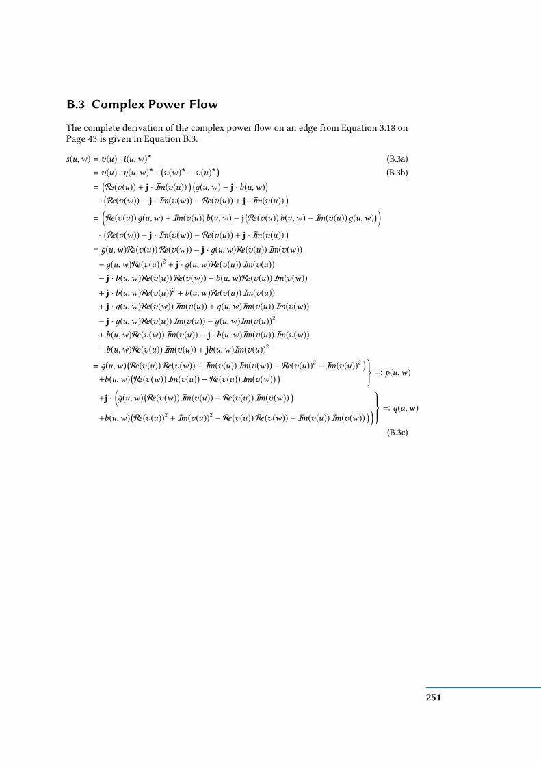
B.3 Complex Power Flow
The complete derivation of the complex power ow on an edge from Equation 3.18 onPage 43 is given in Equation B.3.
s(u,w) = v(u) · i(u,w)? (B.3a)= v(u) · y(u,w)? ·
(v(w)? −v(u)?
)(B.3b)
=(Re(v(u)) + j · Im(v(u))
) (д(u,w) − j · b(u,w)
)·(Re(v(w)) − j · Im(v(w)) − Re(v(u)) + j · Im(v(u))
)=
(Re(v(u))д(u,w) + Im(v(u))b(u,w) − j
(Re(v(u))b(u,w) − Im(v(u))д(u,w)
) )·(Re(v(w)) − j · Im(v(w)) − Re(v(u)) + j · Im(v(u))
)= д(u,w)Re(v(u)) Re(v(w)) − j · д(u,w)Re(v(u)) Im(v(w))
− д(u,w)Re(v(u))2 + j · д(u,w)Re(v(u)) Im(v(u))− j · b(u,w)Re(v(u)) Re(v(w)) − b(u,w)Re(v(u)) Im(v(w))
+ j · b(u,w)Re(v(u))2 + b(u,w)Re(v(u)) Im(v(u))+ j · д(u,w)Re(v(w)) Im(v(u)) + д(u,w)Im(v(u)) Im(v(w))
− j · д(u,w)Re(v(u)) Im(v(u)) − д(u,w)Im(v(u))2
+ b(u,w)Re(v(w)) Im(v(u)) − j · b(u,w)Im(v(u)) Im(v(w))
− b(u,w)Re(v(u)) Im(v(u)) + jb(u,w)Im(v(u))2
= д(u,w)(Re(v(u)) Re(v(w)) + Im(v(u)) Im(v(w)) − Re(v(u))2 − Im(v(u))2
)+b(u,w)
(Re(v(w)) Im(v(u)) − Re(v(u)) Im(v(w))
) C p(u,w)
+j ·(д(u,w)
(Re(v(w)) Im(v(u)) − Re(v(u)) Im(v(w))
)+b(u,w)
(Re(v(u))2 + Im(v(u))2 − Re(v(u)) Re(v(w)) − Im(v(u)) Im(v(w))
) ) C q(u,w)
(B.3c)
251

B.4 Complex Current Flow
The complete derivation of the complex current ow on an edge from Equation 3.23on Page 44 is given in Equation B.4.
i(u,w) =(д(u,w) + j · b(u,w)
) (v(w) −v(u)
)=
(д(u,w) + j · b(u,w)
) (Re(v(w)) + j · Im(v(w)) − Re(v(u)) − j · Im(v(u))
)= д(u,w) · Re(v(w))+ j·д(u,w) · Im(v(w)) −
д(u,w) · Re(v(u) )− j·д(u,w) · Im(v(u) ) +j· b(u,w) · Re(v(w))+ j2·b(u,w) · Im(v(w)) −j· b(u,w) · Re(v(u) )− j2·b(u,w) · Im(v(u) )= д(u,w)
(Re(v(w)) − Re(v(u))
)+ b(u,w)
(Im(v(u)) − Im(v(w))
)︸ ︷︷ ︸CRe(i(u ,w ))
+
j ·(
д(u,w)(Im(v(w)) − Im(v(u))
)+ b(u,w)
(Re(v(w)) − Re(v(u))
)︸ ︷︷ ︸CIm(i(u ,w ))
)(B.4)
252
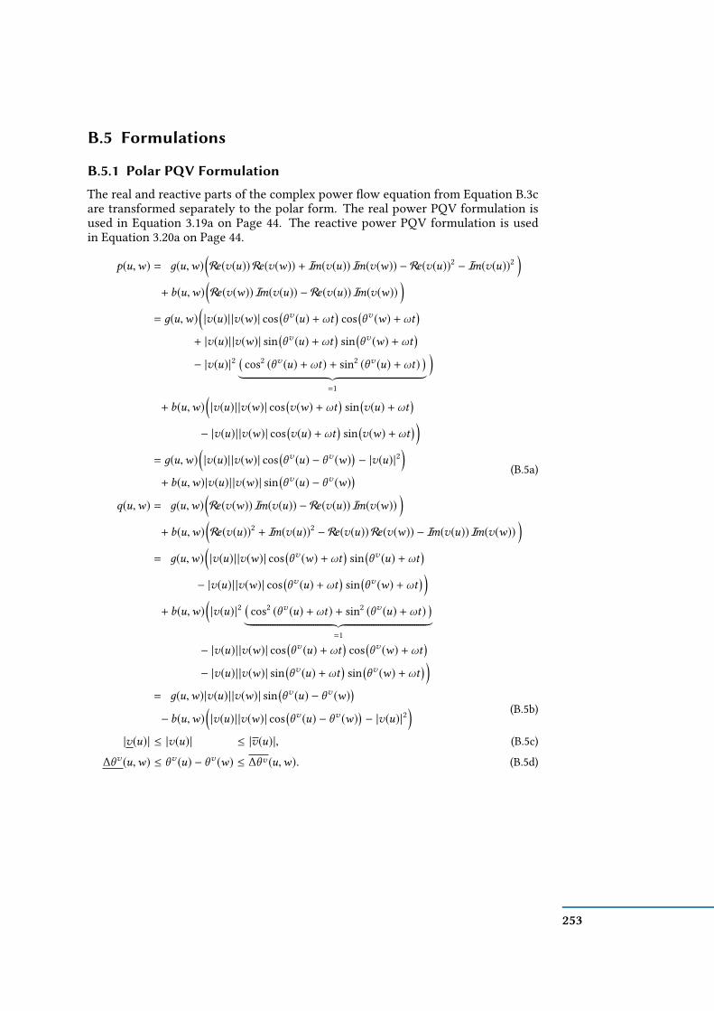
B.5 Formulations
B.5.1 Polar PQV FormulationThe real and reactive parts of the complex power ow equation from Equation B.3care transformed separately to the polar form. The real power PQV formulation isused in Equation 3.19a on Page 44. The reactive power PQV formulation is usedin Equation 3.20a on Page 44.
p(u,w) = д(u,w)(Re(v(u)) Re(v(w)) + Im(v(u)) Im(v(w)) − Re(v(u))2 − Im(v(u))2
)+ b(u,w)
(Re(v(w)) Im(v(u)) − Re(v(u)) Im(v(w))
)= д(u,w)
(|v(u)| |v(w)| cos
(θv (u) + ωt
)cos
(θv (w) + ωt
)+ |v(u)| |v(w)| sin
(θv (u) + ωt
)sin
(θv (w) + ωt
)− |v(u)|2
(cos2 (θv (u) + ωt) + sin2 (θv (u) + ωt)
)︸ ︷︷ ︸=1
)+ b(u,w)
(|v(u)| |v(w)| cos
(v(w) + ωt
)sin
(v(u) + ωt
)− |v(u)| |v(w)| cos
(v(u) + ωt
)sin
(v(w) + ωt
) )= д(u,w)
(|v(u)| |v(w)| cos
(θv (u) − θv (w)
)− |v(u)|2
)+ b(u,w)|v(u)| |v(w)| sin
(θv (u) − θv (w)
) (B.5a)
q(u,w) = д(u,w)(Re(v(w)) Im(v(u)) − Re(v(u)) Im(v(w))
)+ b(u,w)
(Re(v(u))2 + Im(v(u))2 − Re(v(u)) Re(v(w)) − Im(v(u)) Im(v(w))
)= д(u,w)
(|v(u)| |v(w)| cos
(θv (w) + ωt
)sin
(θv (u) + ωt
)− |v(u)| |v(w)| cos
(θv (u) + ωt
)sin
(θv (w) + ωt
) )+ b(u,w)
(|v(u)|2
(cos2 (θv (u) + ωt) + sin2 (θv (u) + ωt)
)︸ ︷︷ ︸=1
− |v(u)| |v(w)| cos(θv (u) + ωt
)cos
(θv (w) + ωt
)− |v(u)| |v(w)| sin
(θv (u) + ωt
)sin
(θv (w) + ωt
) )= д(u,w)|v(u)| |v(w)| sin
(θv (u) − θv (w)
)− b(u,w)
(|v(u)| |v(w)| cos
(θv (u) − θv (w)
)− |v(u)|2
) (B.5b)
|v(u)| ≤ |v(u)| ≤ |v(u)|, (B.5c)
∆θv (u,w) ≤ θv (u) − θv (w) ≤ ∆θv (u,w). (B.5d)
253

B.5.2 Rectangular PQV FormulationThe real part in Equation B.6b and the reactive part in Equation B.6c are comefrom Equation B.3c.
p(u,w) + j · q(u,w)v(u) · i(u,w)?
v(u) · (v(w)? · y(u,w)?)
= s(u,w) (B.6a)
д(u,w)©«
Re(v(u)) Re(v(w))
+Im(v(u)) Im(v(w))
−Re(v(u))2 − Im(v(u))2
ª®®¬ − b(u,w)(Re(v(u)) Im(v(w))
−Re(v(w)) Im(v(u))
)= p(u,w) (B.6b)
−д(u,w)
(Re(v(u)) Im(v(w))
−Re(v(w)) Im(v(u))
)− b(u,w)
©«Re(v(u)) Re(v(w))
+Im(v(u)) Im(v(w))
−Re(v(u))2 − Im(v(u))2
ª®®¬ = q(u,w) (B.6c)
|p(u,w)| ≤ p(u,w) (B.6d)|q(u,w)| ≤ q(u,w) (B.6e)|s(u,w)| ≤ s(u,w) (B.6f)
Re(v(u))2 + Im(v(u))2 ≤ v(u)2 (B.6g)v(u)2 ≤ Re(v(u))2 + Im(v(u))2 (B.6h)
∆θv (u,w) ≤ arctan(Re(v(u))
Im(v(u))
)− arctan
(Re(v(w))
Im(v(w))
)≤ ∆θv (u,w), (B.6i)
254

B.5.3 Polar IV FormulationThe Equation B.7 comes from Equations 3.22 and 3.23.
i(u) = д(u, 0)|v(u)| cos(θv (u)
)+
∑u ,w ∈
←→E
д(u,w)(|v(w)| cos
(θv (w)
)− |v(u)| cos
(θv (u)
) )− b(u, 0)|v(u)| sin
(θv (u)
)−
∑u ,w ∈
←→E
b(u,w)(|v(w)| sin
(θv (w)
)− |v(u)| sin
(θv (u)
) )+ j
(д(u, 0)|v(u)| sin
(θv (u)
)+
∑u ,w ∈
←→E
д(u,w)(|v(w)| sin
(θv (w)
)− |v(u)| sin
(θv (u)
) )+ b(u, 0)|v(u)| cos
(θv (u)
)+
∑u ,w ∈
←→E
b(u,w)(|v(w)| cos
(θv (w)
)− |v(u)| cos
(θv (u)
) ) ),
(B.7a)
|v(u)| |i(u)| cos(θv (u) − θ i (u)
)︸ ︷︷ ︸Cp(u)
≤ p(u),
(B.7b)p(u) ≤ |v(u)| |i(u)| cos
(θv (u) − θ i (u)
),︸ ︷︷ ︸
Cp(u)
(B.7c)
|v(u)| |i(u)| sin(θv (u) − θ i (u)
)︸ ︷︷ ︸Cq(u)
≤ q(u),
(B.7d)q(u) ≤ |v(u)| |i(u)| sin
(θv (u) − θ i (u)
),︸ ︷︷ ︸
Cq(u)
(B.7e)
|v(u)| ≤ |v(u)| ≤ |v(u)|,(B.7f)
∆θv (u,w) ≤ θv (u) − θv (w) ≤ ∆θv (u,w).(B.7g)
255

B.5.4 Rectangular IV Formulation
i(u) = д(u, 0)Re(v(u)) +∑
u ,w ∈←→E
д(u,w)(Re(v(w)) − Re(v(u))
)− b(u, 0)Im(v(u)) −
∑u ,w ∈
←→E
b(u,w)(Im(v(w)) − Im(v(u))
)+ j ·
(д(u, 0)Im(v(u)) +
∑u ,w ∈
←→E
д(u,w)(Im(v(w)) − Im(v(u))
)+ b(u, 0)Re(v(u)) +
∑u ,w ∈
←→E
b(u,w)(Re(v(w)) − Re(v(u))
) )(B.8a)
Re(v(u)) · Re(i(u)) + Im(v(u)) · Im(i(u))︸ ︷︷ ︸Cp(u)
≤ p(u) (B.8b)
p(u) ≤ Re(v(u)) · Re(i(u)) + Im(v(u)) · Im(i(u))︸ ︷︷ ︸=p(u)
(B.8c)
Im(v(u)) · Re(i(u)) − Re(v(u)) · Im(i(u))︸ ︷︷ ︸Cq(u)
≤ q(u) (B.8d)
q(u) ≤ Im(v(u)) · Re(i(u)) − Re(v(u)) · Im(i(u))︸ ︷︷ ︸=q(u)
(B.8e)
Re(v(u))2 + Im(v(u))2 ≤ v(u)2 (B.8f)v(u)2 ≤ Re(v(u))2 + Im(v(u))2 (B.8g)
|i(u,w)| ≤ i(u,w) (B.8h)
∆θv (u,w) ≤ arctan(Re(v(u))
Im(v(u))
)− arctan
(Re(v(w))
Im(v(w))
)≤ ∆θv (u,w), (B.8i)
256
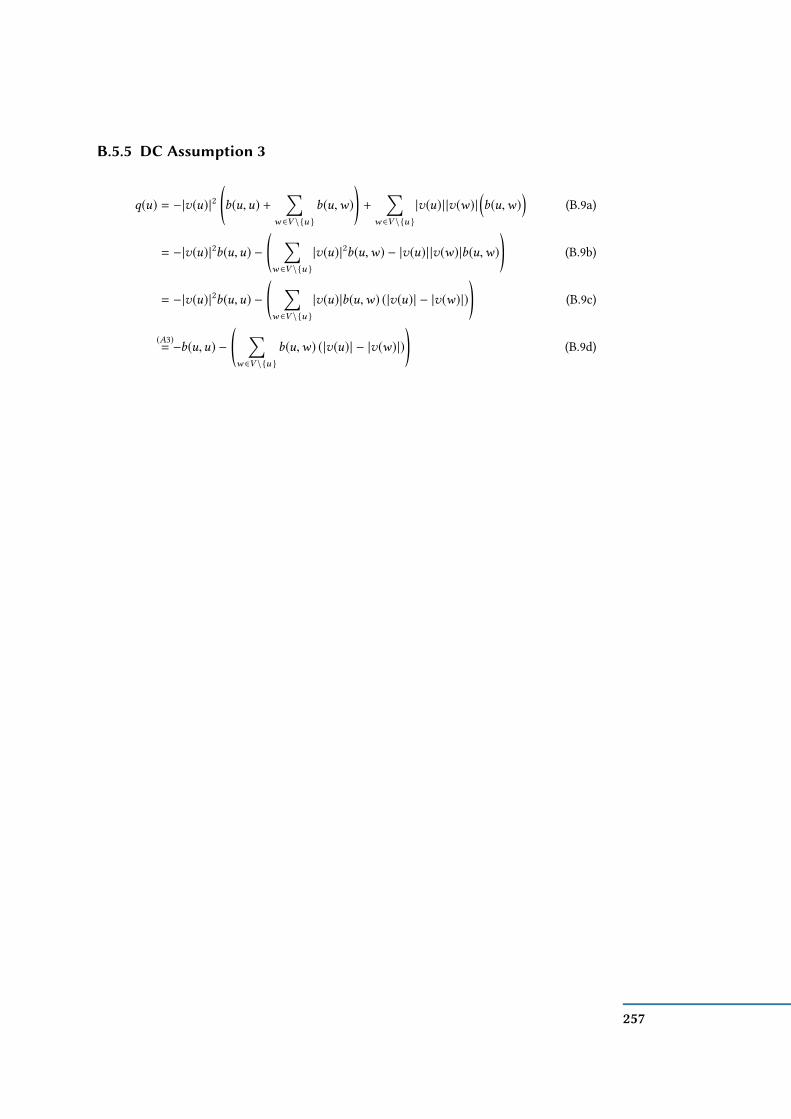
B.5.5 DC Assumption 3
q(u) = −|v(u)|2
(b(u,u) +
∑w ∈V \u
b(u,w)
)+
∑w ∈V \u
|v(u)| |v(w)|(b(u,w)
)(B.9a)
= −|v(u)|2b(u,u) −
( ∑w ∈V \u
|v(u)|2b(u,w) − |v(u)| |v(w)|b(u,w)
)(B.9b)
= −|v(u)|2b(u,u) −
( ∑w ∈V \u
|v(u)|b(u,w) (|v(u)| − |v(w)|)
)(B.9c)
(A3)= −b(u,u) −
( ∑w ∈V \u
b(u,w) (|v(u)| − |v(w)|)
)(B.9d)
257


C Discrete Changes to the Power Grid
This section is an extension of the Chapter 5 in which we consider discrete changes tothe power grid topology with the focus on transmission switching. In Section 5.7, weevaluate two dierent algorithms and present for the DTP betweenness centralitiestwo networks in Figure 5.13a&b. In this section, we extend this to other power gridsizes and structures such that we have a broader evaluation. Figure 5.13d illustratesthe compressed representation.
In this section, we test the inuence of switching edges one by one with dier-ent Dominating Theta Path (DTP) betweenness centralities and their inuence onthe maximum power ow (MPF). For each test case, we compute the DTP between-ness centrality for each edge and the MPF when only this edge is switched. Theresults of these simulations are shown in Figures C.1–C.3. We sort the edges fromhighest to lowest centrality. The centrality of the edges is shown as a dashed curve.The solid curve represents the value of the MPF if the edge is switched. We can seethat for many edges switching them does not inuence the value of the MPF. Theedges where switching them decreases the value are often those with medium to lowcentrality values (see in particular nesta_case14_ieee, nesta_case30_ieee andnesta_case300_ieee). Switching edges with high centrality (relative to the otheredges in the network) still keeps a large ow value. For a combination of all the resultsrefer to Figure 5.13d.
259

0.40.50.60.70.80.91.0
nesta_case3_lmbdMPF |S | = 1 Normalized cDTPBC
270
282
294
306
318
330 329.89
1 2 2 3Switched Edge
MPF
inMW
Nor
mal
ized
c DTP
BC
0.200.250.300.350.400.450.50
nesta_case4_gsMPF |S | = 1 Normalized cDTPBC
600
700 719.00
1 2 2 3 3 4Switched Edge
MPF
inMW
Nor
mal
ized
c DTP
BC
0.0
0.1
0.2
0.3
0.4nesta_case5_pjm
MPF |S | = 1 Normalized cDTPBC
900
1050
12001263.14
1 2 4 5 6Switched Edge
MPF
inMW
Nor
mal
ized
c DTP
BC
0.150.200.250.300.350.40
nesta_case6_cMPF |S | = 1 Normalized cDTPBC
100
162
225
288
350 370.00
1 2 3 5 6 7Switched Edge
MPF
inMW
Nor
mal
ized
c DTP
BC
0.000.050.100.150.200.25
nesta_case6_wwMPF |S | = 1 Normalized cDTPBC
0
267
293
320 330.97
2 5 7 10Switched Edge
MPF
inMW
Nor
mal
ized
c DTP
BC
0.100.150.200.250.300.350.400.45
nesta_case9_wsccMPF |S | = 1 Normalized cDTPBC
0
620
740
860
980
1100
770.00
2 5 8Switched Edge
MPF
inMW
Nor
mal
ized
c DTP
BC
0.1
0.2
0.3
0.4
0.5nesta_case14_ieeeMPF |S | = 1 Normalized cDTPBC
100
250
400 425.00
5 12 20Switched Edge
MPF
inMW
Nor
mal
ized
c DTP
BC
0.00
0.05
0.10
0.15
0.20
0.25
nesta_case24_ieeeMPF |S | = 1 Normalized cDTPBC
0
3212
3275
3338
3400 3405.00
0 15 30Switched Edge
MPF
inMW
Nor
mal
ized
c DTP
BC
Figure C.1: Results of the simulations for the DTP betweenness centrality onnesta_case3_lmbd to nesta_case24_ieee_rts.
260
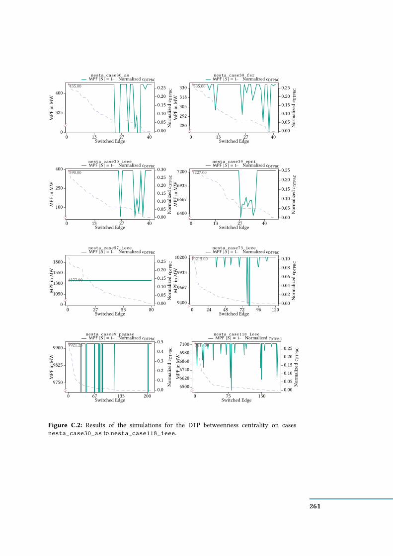
0.000.050.100.150.200.25
nesta_case30_asMPF |S | = 1 Normalized cDTPBC
0
325
400435.00
0 13 27 40Switched Edge
MPF
inMW
Nor
mal
ized
c DTP
BC
0.000.050.100.150.200.25
nesta_case30_fsrMPF |S | = 1 Normalized cDTPBC
280
292
305
318
330 335.00
0 13 27 40Switched Edge
MPF
inMW
Nor
mal
ized
c DTP
BC
0.000.050.100.150.200.250.30
nesta_case30_ieeeMPF |S | = 1 Normalized cDTPBC
100
250
400390.00
0 13 27 40Switched Edge
MPF
inMW
Nor
mal
ized
c DTP
BC
0.00
0.05
0.10
0.15
0.20
0.25nesta_case39_epriMPF |S | = 1 Normalized cDTPBC
6400
6667
6933
7200 7227.00
0 13 27 40Switched Edge
MPF
inMW
Nor
mal
ized
c DTP
BC
0.000.050.100.150.200.25
nesta_case57_ieeeMPF |S | = 1 Normalized cDTPBC
0
1050
1300
1550
1800
1377.00
0 27 53 80Switched Edge
MPF
inMW
Nor
mal
ized
c DTP
BC
0.000.020.040.060.080.10
nesta_case73_ieeeMPF |S | = 1 Normalized cDTPBC
9400
9667
9933
10200 10215.00
0 24 48 72 96 120Switched Edge
MPF
inMW
Nor
mal
ized
c DTP
BC
0.0
0.1
0.2
0.3
0.4
0.5nesta_case89_pegase
MPF |S | = 1 Normalized cDTPBC
9750
9825
9900 9921.23
0 67 133 200Switched Edge
MPF
inMW
Nor
mal
ized
c DTP
BC
0.000.050.100.150.200.25
nesta_case118_ieeeMPF |S | = 1 Normalized cDTPBC
650066206740686069807100 7119.00
0 75 150Switched Edge
MPF
inMW
Nor
mal
ized
c DTP
BC
Figure C.2: Results of the simulations for the DTP betweenness centrality on casesnesta_case30_as to nesta_case118_ieee.
261

0.0
0.1
0.2
0.3
0.4
nesta_case162_ieeeMPF |S | = 1 Normalized cDTPBC
072407480772079608200 8296.00
0 62 125 188 250Switched Edge
MPF
inMW
Nor
mal
ized
c DTP
BC
0.000.050.100.150.200.25
nesta_case189_edinMPF |S | = 1 Normalized cDTPBC
0
2817
2883
29502987.00
0 67 133 200Switched Edge
MPF
inMW
Nor
mal
ized
c DTP
BC
0.000.050.100.150.200.250.300.35
nesta_case300_ieeeMPF |S | = 1 Normalized cDTPBC
30000
30750
31500 31568.00
0 133 267 400Switched Edge
MPF
inMW
Nor
mal
ized
c DTP
BC
-1.0
-0.5
0.0
0.5
1.0nesta_case2383wp_mp
MPF |S | = 1 Normalized cDTPBC
-1
0
1
0.00
0 600 1200 1800 2400 3000Switched Edge
MPF
inMW
Nor
mal
ized
c DTP
BC
0.000.050.100.150.200.25
nesta_case2736sp_mpMPF |S | = 1 Normalized cDTPBC
02014420168
20192
20216
20240 20246.70
0 600 1200 1800 2400 3000Switched Edge
MPF
inMW
Nor
mal
ized
c DTP
BC
0.000.050.100.150.200.25
nesta_case2737sop_mpMPF |S | = 1 Normalized cDTPBC
14610146221463314645146571466814680
14677.90
0 600 1200 1800 2400 3000Switched Edge
MPF
inMW
Nor
mal
ized
c DTP
BC
0.000.050.100.150.200.25
nesta_case2746wop_mpMPF |S | = 1 Normalized cDTPBC
0237022371323725237372374823760 23759.50
0 600 1200 1800 2400 3000Switched Edge
MPF
inMW
Nor
mal
ized
c DTP
BC
-1.0
-0.5
0.0
0.5
1.0nesta_case3012wp_mp
MPF |S | = 1 Normalized cDTPBC
-1
0
1
0.00
0 583 1167 1750 2333 2917 3500Switched Edge
MPF
inMW
Nor
mal
ized
c DTP
BC
Figure C.3: Results of the simulations for the DTP betweenness centrality oncases nesta_case162_ieee to nesta_case3012wp_mp.
262

DContinuous Changes in the Power Grid
This section is an extension of the Chapter 6 in which we consider continuous changesto the power grid topology with the focus on the placement of Flexible AC TransmissionSystems (FACTS). In Figure D.1, we investigate the trade-o between costs and lossesof the multi-objective function (Equation 6.6) that we optimize in our hybrid model(Equation 6.12). In all our simulations, we see a Pareto front that shows for dierent λ ∈[0, 1] an optimal solution in Figure D.1.
If we concentrate on the placement problem, we can evaluate for dierent numbersof control vertices VF the operation costs for dierent load increase factors. This isshown for dierent power grids in Figure D.2.
263

λ = 1
λ = 0
320 340 360 380 400
3045
3050
3055
3060
3065
Total Losses in MW
Tot
al G
ener
ator
Cos
ts in
$/M
Wh case6
Hybrid ModelOPF
λ = 1
λ = 0
0 40 80 120 160 200
5200
5250
5300
5350
5400
5450
5500
Total Losses in MW
Tot
al G
ener
ator
Cos
ts in
$/M
Wh case9
Hybrid ModelOPF
λ = 1
λ = 0
0 500 1000
8000
9000
10000
11000
Total Losses in MW
Tot
al G
ener
ator
Cos
ts in
$/M
Wh case14
Hybrid ModelOPF
λ = 1
λ = 0
500 1000 1500
41000
42000
43000
44000
45000
46000
Total Losses in MW
Tot
al G
ener
ator
Cos
ts in
$/M
Wh case39
Hybrid ModelOPF
λ = 1
λ = 0
500 1000
41000
42000
43000
44000
45000
46000
47000
Total Losses in MW
Tot
al G
ener
ator
Cos
ts in
$/M
Wh case57
Hybrid ModelOPF
λ = 1
λ = 0
0 5000 10000
140000
160000
180000
2e+05
220000
240000
260000
Total Losses in MW
Tot
al G
ener
ator
Cos
ts in
$/M
Wh case118
Hybrid ModelOPF
Figure D.1: Trade-o of generator costs and costs of the losses depending as λ varies from 0to 1. The square cross marks the solution computed by OPF.
264
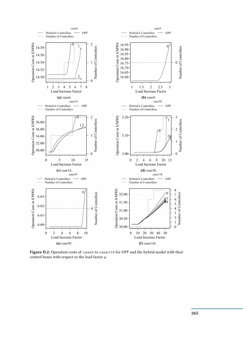
Ope
ratio
n C
osts
in $
/MW
h 0 1
214.50
14.52
14.54
14.56
14.58
0
1
2
1 2 3 4 5 6 7 8Load Increase Factor
Num
ber o
f Con
trolle
rs
case6Hybrid k ControllersNumber of Controllers
OPF
(a) case6.
Ope
ratio
n C
osts
in $
/MW
h
0
16.6016.6516.7016.7516.8016.8516.9016.95
0
1 1.5 2 2.5 3Load Increase Factor
Num
ber o
f Con
trolle
rs
case9Hybrid k ControllersNumber of Controllers
OPF
(b) case9.
Ope
ratio
n C
osts
in $
/MW
h 0
1 2
30.00
32.00
34.00
36.00
38.00
0
1
2
0 5 10 15Load Increase Factor
Num
ber o
f Con
trolle
rs
case14Hybrid k ControllersNumber of Controllers
OPF
(c) case14.
Ope
ratio
n C
osts
in $
/MW
h
0
1
23
3.00
3.10
3.20
0
1
2
3
0 2 4 6 8 10 12Load Increase Factor
Num
ber o
f Con
trolle
rs
case30Hybrid k ControllersNumber of Controllers
OPF
(d) case30.
Ope
ratio
n C
osts
in $
/MW
h
0
6.60
6.61
6.62
6.63
0
0 2 4 6 8 10Load Increase Factor
Num
ber o
f Con
trolle
rs
case39Hybrid k ControllersNumber of Controllers
OPF
(e) case39.
Ope
ratio
n C
osts
in $
/MW
h
018
30.00
30.50
31.00
31.50
32.00
012345678
0 10 20 30 40 50Load Increase Factor
Num
ber o
f Con
trolle
rscase118
Hybrid k ControllersNumber of Controllers
OPF
(f) case118.
Figure D.2: Operation costs of case6 to case118 for OPF and the hybrid model with theircontrol buses with respect to the load factor ρ.
265


E Curriculum Vitæ
Name Franziska Wegner
Place of Birth Potsdam, Germany
Nationality German
Education and Professional Experience
12/2019–07/2020 Research assistant at the Institute of Theoretical Informatics,Karlsruhe Institute of Technology (KIT)
04/2014–12/2019 PhD student at the Institute of Theoretical Informatics,Karlsruhe Institute of Technology (KIT)Advisors: Prof. Dr. Dorothea Wagner, Prof. Dr. Sylvie Thiébaux
01/2016–04/2016 Research stay at Australia’s National Information and Commu-nications Technology (NICTA), Canberra, Australia
10/2010–03/2014 Master of Science in Computer ScienceKarlsruhe Institute of Technology (KIT)
09/2007–04/2012 Employee at SAP SEWalldorf, Germany
10/2007–10/2010 Bachelor of Engineering in Information TechnologyUniversity of Cooperative Education, Karlsruhe (SAP SE)
Teaching Experience
10/2019–03/2020 Seminar “Energy Informatics”
04/2019–07/2019 Lecture “Energy Informatics 2”
10/2018–03/2019 Seminar “Energy Informatics”
267

04/2018–07/2018 Lecture “Energy Informatics 2”
04/2018–07/2018 Seminar “Algorithms for NP-hard Problems”
10/2017–03/2018 Seminar “Energy Informatics”
04/2017–07/2017 Practical course “Visualization of Energy-Schedules”
04/2017–07/2017 Seminar “Classics in Theoretical Computer Science”
04/2017–07/2017 Lecture “Energy Informatics 2”
10/2016–03/2017 Seminar “Energy Informatics”
04/2016–07/2016 Seminar “Techniques in Algorithmic – Selected Topics in theAlgorithmic Graph Theory”
10/2015–03/2016 Seminar “Modeling and Simulation of Smart Grids”
04/2015–07/2015 Practical course “Development of a Campus Route Planner”
04/2015–07/2015 Seminar “Methods and Algorithm for Evaluating and OptimizingPower Grids”
04/2015–07/2015 Seminar “The P unequal NP Hypothesis”
10/2014–03/2015 Seminar “Techniques in Algorithmic”
10/2014–03/2015 Lecture “Fundamentals of Theoretical Computer Science”
04/2014–07/2014 Practical course “Development of a Campus Route Planner”
Supervised Master’s Theses
07/2019–04/2020 Adrian Grupp, A Comparative Analysis of Switchings in Staticand Dynamic Power Grids
11/2018–05/2019 Lena Winter, Transmission Network Expansion Planning forCuring Critical Edges
11/2017–05/2018 Chao Wang, Transmission Network Expansion Planning usingthe Railway Network
08/2017–04/2018 Larisa Duczek, Beobachtungen des Maximalen Flexiblen Dreh-stromübertragungssystem Flusses (Diploma thesis)
11/2016–06/2017 Carina Mieth, Observability of Multi-Carrier Energy DistributionNetworks and Optimal Sensor Placement
12/2015–05/2016 Sebastian Lehmann, Simulated Annealing-Based Heuristics forWind Farm Cabling Problems
268

Supervised Bachelor’s Theses
11/2018–03/2019 Robert Mumper, Erweiterungsplanung in elektrischen Netzenmittels dynamischer Programmierung
07/2018–11/2018 Florian Krüger, A Block-Cut-Tree-based Switching Algorithmfor Cacti
04/2018–08/2018 Niklas Fuhrberg, Wind Farm Cabling using Spectral Clustering
02/2017–06/2017 Hannah Wenk, Clusteringansätze von Windfarmen
01/2017–05/2017 Ivo Baar, Entwicklung eines genetischen Algorithmus zur ef-zienten Verkabelung von Windfarmen
01/2017–05/2017 Jakob Nedlin, Ant-based Algorithms for the Wind Farm CableLayout Problem
269


F List of Publications
Journal Articles
[1] Scalable Exact Visualization of Isocontours in Road Networks via Minimum-Link Paths. Journal of Computational Geometry 9:1, pages 24–70, 2018. url: http://jocg.org/index.php/jocg/article/view/313.Cited on page 272. Joint work with Moritz Baum, Thomas Bläsius, Andreas Gemsa, and IgnazRutter.
[2] Poster Abstract: Graph-theoretic Model for Observability in Multi-carrierEnergy Distribution Networks. Computer Science - Research and Development, 2017.url: https://doi.org/10.1007/s00450-017-0366-3.Cited on page 272. Joint work with Sören Hohmann, Heiko Maaß, Carina Mieth, Martin Pfeifer,and Dorothea Wagner.
Articles in Conference Proceedings
[3] Scalable Exact Visualization of Isocontours in Road Networks via Minimum-Link Paths. In Proceedings of the 24th Annual European Symposium on Algorithms
(ESA’16). Volume 57 of Leibniz International Proceedings in Informatics, pages 7:1–7:18. Schloss Dagstuhl - Leibniz-Zentrum für Informatik, 2016. url: http://drops.dagstuhl.de/opus/frontdoor.php?source_opus=6349.Cited on page 272. Joint work with Moritz Baum, Thomas Bläsius, Andreas Gemsa, and IgnazRutter.
[4] Computing Minimum-Link Separating Polygons in Practice. In Proceedings of
the 32nd European Workshop on Computational Geometry (EuroCG’16), 2016.Cited on page 272. Joint work with Moritz Baum, Thomas Bläsius, Andreas Gemsa, and IgnazRutter.
[5] TheMaximum Transmission Switching Flow Problem. In Proceedings of the 9th
ACM e-Energy International Conference on Future Energy Systems (ACM e-Energy’18),pages 340–360. ACM Press, 2018. url: https://doi.org/10.1145/3208903.3208910. Joint work with Alban Grastien, Ignaz Rutter, Dorothea Wagner, andMatthias Wolf.
[6] TowardsNegativeCycle Canceling inWind FarmCable LayoutOptimization.In Proceedings of the 7th DACH+ Conference on Energy Informatics. Volume 1 (Suppl1) of. Springer, 2018. url: https://energyinformatics.springeropen.com/articles/10.1186/s42162-018-0030-6.Cited on page 272. Joint work with Sascha Gritzbach, Torsten Ueckerdt, Dorothea Wagner, andMatthias Wolf.
271

[7] Operating Power Grids with few Flow Control Buses. In Proceedings of the 6th
ACM e-Energy International Conference on Future Energy Systems, pages 289–294. ACMPress, 2015. url: http://doi.acm.org/10.1145/2768510.2768521. Joint workwith Thomas Leibfried, Tamara Mchedlidze, Nico Meyer-Hübner, Martin Nöllenburg,Ignaz Rutter, Peter Sanders, and Dorothea Wagner.
[8] A Simulated-Annealing-Based Approach for Wind Farm Cabling. In Proceed-
ings of the 8th ACM e-Energy International Conference on Future Energy Systems (ACM
eEnergy’17), pages 203–215. ACM Press, 2017. url: https://doi.org/10.1145/3077839.3077843. Joint work with Sebastian Lehmann, Ignaz Rutter, and DorotheaWagner.
[9] Towards Realistic Flow Control in Power Grid Operation. In Proceedings of
the 4th D-A-CH Conference on Energy Informatics. Volume 9424 of Lecture Notes inComputer Science, pages 192–199. Springer, 2015. url: http://dx.doi.org/10.1007/978-3-319-25876-8_16. Joint work with Tamara Mchedlidze, MartinNöllenburg, Ignaz Rutter, and Dorothea Wagner.
[10] Analysis of Redispatch and Transmission Capacity Pricing on a Local Elec-tricityMarket Setup. In 14th International Conference on the European EnergyMarket,pages 1–6. IEEE, 2017. url: http://doi.org/10.1109/EEM.2017.7981959.Cited on page 272. Joint work with Philipp Staudt, Johannes Garttner, and Christof Weinhardt.
Technical Reports
[11] Engineering Negative Cycle Canceling for Wind Farm Cabling. 2019. arXiv:1908.02129 [cs.DS].Cited on page 272. Joint work with Sascha Gritzbach, Torsten Ueckerdt, Dorothea Wagner,Franziska Wegner, and Matthias Wolf.
The papers [Gri+19], [Bau+18], [Hoh+17], [Bau+16b], [Bau+16c], [Gri+18], and [SGW17] [Bau+16a]are omitted in this thesis because of missing thematically closeness and since the main author issomeone else.
272
G Deutsche Zusammenfassung
Energienetze bilden das Rückgrat unserer Gesellschaft, die unter anderem unsereNahrungskette und andere wichtige Infrastrukturen, wie die Wasser- und Wärmever-sorgung, bestimmen. Um die grundlegenden menschlichen Bedürfnisse zu befriedigen,müssen wir ein nachhaltigeres und umweltfreundlicheres Verhalten im Allgemeinenund in Energienetzen im Speziellen an den Tag legen. In dieser Arbeit geht es umEnergienetze, wobei wir uns auf Stromnetze spezialisieren und uns darauf fokussieren,wie wir die vorhandene Infrastruktur besser ausnutzen können. Wir merken an, dassdie Ergebnisse aus dieser Arbeit auch auf andere Energienetze übertragen werdenkönnen [Gro+19] und bestimmte auftretende Phänomene legen es nahe, dass sicheinige Ergebnisse eventuell auch auf Verkehrsnetze übertragen lassen. Diese Arbeitbesteht aus vier inhaltlichen Teilen. Der erste Teil beschäftigt sich mit der Funktions-weise und Struktur von elektrischen Flüssen. Der zweite und dritte inhaltliche Teil derArbeit beschäftigt sich jeweils mit der ezienten Ausnutzung der vorhandenen Ener-gienetzinfrastruktur. Dabei verstehen wir hier unter ezienter Ausnutzung entwederdie Maximierung der Gesamterzeugung und die damit verbundene Erweiterung desBetriebspunktes oder die Minimierung der Erzeugungskosten verstehen.
Das elektrische Netz besteht aus drei Spannungsebenen, die wir als Hoch-, Mittel-,und Niederspannungsebene bezeichnen. Das traditionelle elektrische Netz ist auf einezentrale Energieversorgung ausgelegt, bei der die Erzeuger sich in der Hochspan-nungsebene benden. Der elektrische Fluss im klassischen Sinne ießt von der Hoch-in die Mittel- und Niederspannungsebene. Die industriellen Verbraucher benden sichzumeist auf der Mittelspannungsebene, während sich die Haushalte und kleinerenIndustrien in der Niederspannungsebene benden. Durch nachhaltige Erzeuger, dieihre Energie aus erneuerbaren Energien wie beispielsweise Wind gewinnen, ndetnun ein Paradigmenwechsel im elektrischen Netz statt. Diese nachhaltigen Erzeugerbenden sich zumeist im Nieder- und Mittelspannungsnetz und der elektrische Flusskönnte nun bidirektional ießen. Dieser Paradigmenwechsel kann zu Engpäßen undanderen Problemen führen, da das elektrische Netz für ein solches Szenario nichtkonzipiert ist.
Eine Hauptaufgabe dieser Arbeit war die Identizierung von Problemstellungen inelektrischen Netzen. Die extrahierten Problemstellungen haben wir dann in graphen-theoretische Modelle übersetzt und Algorithmen entwickelt, die oftmals Gütegarantienbesitzen. Wir haben uns dabei zunächst auf die Modellierung von elektrischen Net-zen und das Verhalten von Flüssen in diesen Netzen mit Hilfe von Graphentheoriekonzentriert. Zur Modellierung des elektrischen Flusses nutzen wir eine linearisierte
273

Modellierung, die mehrere vereinfachende Annahmen trit. Diese linearisierte Mo-dellierung ist für Hochspannungsnetze im Allgemeinen eine gute Annäherung undmacht das Entscheidungsproblem für elektrische Flüsse, das heißt, ob ein gültiger elek-trischer Fluss für eine bestimmte Konguration des Netzes und für einen bestimmtenVerbrauch und eine bestimmte Erzeugung existiert, in Polynomialzeit lösbar.
Leistungsuss. Fokusiert man sich auf das vereinfachte Zulässigkeitsproblem vonelektrischen Flüssen und den Maximalen Leistungsüssen, so existieren verschiedenemathematische Formulierungen, die den Leistungsuss beschreiben. Auf allgemeinenGraphen ist es oftmals der Fall, dass graphentheoretischen Flüsse keine zulässigen Leis-tungsüsse darstellen. Im Gegensatz zu graphentheoretischen Flüssen balancieren sichLeistungsüsse. Wir diskutieren diese Eigenschaft aus graphentheoretischer Sicht. Dieverschiedenen mathematischen Formulierungen geben uns strukturelle Einblicke indas Leistungsussproblem. Sie zeigen uns die Dualität der zwei Kirchhoschen Regeln.Diese nutzen wir um einen algorithmischen Ansatz zur Berechnung von Leistungs-üssen zu formulieren, der zu einem Algorithmus für Leistungsüsse auf planarenGraphen führen könnte. Die Einschränkung auf planare zweifachzusammenhängendeGraphen ist vertretbar, da elektrische Netze im Allgemeinen planar sind [COC12, S. 13].Zudem hilft uns diese Sichtweise, um Analogien zu anderen geometrischen Problemenherzustellen.Kontinuierliche Änderungen. Da graphentheoretische Flüsse sich in vielen Fäl-
len anders als elektrische Flüsse verhalten, haben wir versucht, das Stromnetz mittelsKontrolleinheiten so auszustatten, dass der elektrische Fluss den gleichen Wert hatwie der graphentheoretische Fluss. Um dieses Ziel zu erreichen, platzieren wir dieKontrolleinheiten entweder an den Knoten oder an den Kanten. Durch eine Suszeptanz-Skalierung, die durch die Kontrolleinheiten ermöglicht wird, ist es nun prinzipiellmöglich jeden graphentheoretischen Fluss elektrisch zulässig zu machen. Dabei konn-ten wir zeigen, dass das gezielte Platzieren von Kontrolleinheiten die Kosten derErzeugung von elektrischer Leistung durch Generatoren im elektrischen Netz senkenkann und den Betriebspunkt des Netzes in vielen Fällen auch erweitert. Platziert manKontrolleinheiten so, dass der verbleibende Teil (d. h. das Netz ohne die Kontrollein-heiten) ein Baum oder Kaktus unter geeigneter Begrenzung der Kapazitäten ist, soist es möglich, jeden graphentheoretischen Fluss als elektrisch zulässigen Fluss mitgleichwertigen Kosten zu realisieren. Die Kostensenkung und die Erweiterung desBetriebspunktes konnten wir experimentell auf IEEE-Benchmark-Daten bestätigen.Diskrete Änderungen. Die oben beschriebenen Kontrolleinheiten sind eine idea-
lisierte, aktuell nicht realisierbare Steuereinheit, da sie den elektrischen Fluss imgesamten Leistungsspektrum einstellen können. Damit ist vor allem gemeint, dasssie den elektrischen Fluss auf einer Leitung von „Die Leitung ist abgeschaltet.“ biszur maximalen Kapazität stufenlos einstellen können. Diese Idealisierung ist auch eingroßer Kritikpunkt an der Modellierung. Aus diesem Grund haben wir versucht, unser
274

Modell realistischer zu gestalten. Wir haben zwei mögliche Modellierungen identi-ziert. In der ersten Modellierung können Leitungen ein- und ausgeschaltet werden.Dieser Prozess wird als Switching bezeichnet und kann in realen Netzen mittels CircuitBreakers (dt. Leistungsschaltern) realisiert werden. Die zweite Modellierung kommtder Kontrolleinheiten-Modellierung sehr nahe und beschäftigt sich mit der Platzie-rung von Kontrolleinheiten, die die Suszeptanz innerhalb eines gewissen Intervallseinstellen können. Diese wirkt im ersten Moment wie eine Verallgemeinerung derSchaltungsussmodellierung. Nutzt man jedoch eine realistischere Modellierung derKontrolleinheiten, so ist das Einstellen der Suszeptanz durch ein Intervall begrenzt, dasdas Ausschalten einer Leitung nicht mit beinhaltet. Sowohl ein optimales (im Sinne derMinimierung der Gesamterzeugungskosten oder der Maximierung des Durchsatzes)Platzieren von Switches als auch ein optimales Platzieren von Kontrolleinheiten istim Allgemeinen NP-schwer [LGH14]. Diese beiden Probleme ergänzen sich dahinge-hend, dass man den maximalen graphentheoretischen Fluss, mit den zuvor genanntenPlatzierungen annähern kann.
Für Switching konnten wir zeigen, dass das Problem bereits schwer ist, wenn derGraph serien-parallel ist und das Netzwerk nur einen Erzeuger und einen Verbraucherbesitzt [Gra+18]. Wir haben sowohl für den Maximalen Übertragungsschaltungs-uss (engl. Maximum Transmission Switching Flow; kurz MTSF) als auch für denoptimalen Übertragungsschaltungsuss (engl. Optimal Switching Flow; kurz OSF)erste algorithmische Ansätze vorgeschlagen und gezeigt, dass sie auf bestimmtengraphentheoretischen Strukturen exakt sind, und dass auf anderen graphentheoreti-schen Strukturen Gütegarantien möglich sind [Gra+18]. Die Algorithmen haben wirdann auf allgemeinen Netzen evaluiert. Simulationen führen zu guten Ergebnissen aufden NESTA-Benchmark-Daten.
Erweiterungsplanung auf der Grünen Wiese. Eine vom Rest der Arbeit eherlosgelöste Fragestellung war die Verkabelung von Windturbinen. Unter Verwendungeiner Metaheuristik haben wir gute Ergebnisse im Vergleich zu einem „Mixed Inte-ger Linear Program“ (MILP; dt. gemischt-ganzzahliges lineares Programm) erzielt,das wir nach einer Stunde abgebrochen haben. Die Modellierung der Problemstel-lung und die Evaluation des Algorithmus haben wir auf der ACM e-Energy 2017veröentlicht [Leh+17].
Schlusswort. Abschließend kann man sagen, dass mit dieser Arbeit allgemeine,tieiegende Aussagen über elektrische Netze getroen wurden, unter der Berücksichti-gung struktureller Eigenschaften unterschiedlicher Netzklassen. Diese Arbeit zeigt wiedas Netz ausgestaltet sein muss, um bestimmte Eigenschaften garantieren zu könnenund zeigt verschiedene Lösungsansätze mit oft beweisbaren Gütegarantien auf.
275
Related Documents