Combinatorial Auctions: A Survey Sven de Vries * & Rakesh Vohra † December 1, 2000 Abstract Many auctions involve the sale of a variety of distinct assets. Ex- amples are airport time slots, delivery routes and furniture. Because of complementarities (or substitution effects) between the different as- sets, bidders have preferences not just for particular items but for sets or bundles of items. For this reason, economic efficiency is enhanced if bidders are allowed to bid on bundles or combinations of different assets. This paper surveys the state of knowledge about the design of combinatorial auctions. Second, it uses this subject as a vehicle to convey the aspects of integer programming that are relevant for the design of such auctions and combinatorial markets in general. (Auctions; Combinatorial Optimization ) * Zentrum Mathematik, TU M¨ unchen, D-80290 M¨ unchen, Germany. e-mail: [email protected] † Department of Managerial Economics and Decision Sciences, Kellogg School of Man- agement, Northwestern University, Evanston IL 60208. e-mail: [email protected] 1

Welcome message from author
This document is posted to help you gain knowledge. Please leave a comment to let me know what you think about it! Share it to your friends and learn new things together.
Transcript
Combinatorial Auctions: A Survey
Sven de Vries∗ & Rakesh Vohra†
December 1, 2000
Abstract
Many auctions involve the sale of a variety of distinct assets. Ex-
amples are airport time slots, delivery routes and furniture. Because
of complementarities (or substitution effects) between the different as-
sets, bidders have preferences not just for particular items but for sets
or bundles of items. For this reason, economic efficiency is enhanced
if bidders are allowed to bid on bundles or combinations of different
assets. This paper surveys the state of knowledge about the design
of combinatorial auctions. Second, it uses this subject as a vehicle to
convey the aspects of integer programming that are relevant for the
design of such auctions and combinatorial markets in general.
(Auctions; Combinatorial Optimization )
∗Zentrum Mathematik, TU Munchen, D-80290 Munchen, Germany.
e-mail: [email protected]†Department of Managerial Economics and Decision Sciences, Kellogg School of Man-
agement, Northwestern University, Evanston IL 60208. e-mail: [email protected]
1
Contents
1 Introduction 4
2 The CAP 5
2.1 The Set Packing Problem . . . . . . . . . . . . . . . . . . . . 8
2.2 Complexity of the SPP . . . . . . . . . . . . . . . . . . . . . . 10
2.3 Solvable Instances of the SPP . . . . . . . . . . . . . . . . . . 12
2.3.1 Total Unimodularity . . . . . . . . . . . . . . . . . . . 13
2.3.2 Balanced Matrices . . . . . . . . . . . . . . . . . . . . 15
2.3.3 Perfect Matrices . . . . . . . . . . . . . . . . . . . . . 16
2.3.4 Graph Theoretic Methods . . . . . . . . . . . . . . . . 16
2.3.5 Using Preferences . . . . . . . . . . . . . . . . . . . . . 18
2.4 Exact Methods . . . . . . . . . . . . . . . . . . . . . . . . . . 19
2.5 Approximate Methods . . . . . . . . . . . . . . . . . . . . . . 23
2.5.1 Worst-Case Analysis . . . . . . . . . . . . . . . . . . . 25
2.5.2 Probabilistic Analysis . . . . . . . . . . . . . . . . . . 26
2.5.3 Empirical Testing . . . . . . . . . . . . . . . . . . . . . 26
3 Decentralized Methods 27
3.1 Duality in Integer Programming . . . . . . . . . . . . . . . . 28
3.2 Lagrangean Relaxation . . . . . . . . . . . . . . . . . . . . . . 30
3.3 Variations . . . . . . . . . . . . . . . . . . . . . . . . . . . . . 35
3.4 Column Generation . . . . . . . . . . . . . . . . . . . . . . . . 36
3.5 Cuts, Extended Formulations and Non-linear Prices . . . . . 38
4 Incentive Issues 45
2
5 Computational Experiments and Test Problems 53
5.1 Test Problems . . . . . . . . . . . . . . . . . . . . . . . . . . . 58
5.2 FCC Data . . . . . . . . . . . . . . . . . . . . . . . . . . . . . 61
3
1. Introduction
Many auctions involve the sale of a variety of distinct assets. Examples
are the FCC spectrum auction and auctions for airport time slots, railroad
segments (Brewer (1999)) and delivery routes (Caplice (1996)). Because of
complementarities (or substitution effects) between different assets, bidders
have preferences not just for particular items but for sets or bundles of items.
For this reason, economic efficiency is enhanced if bidders are allowed to bid
on combinations of different assets.
Auctions where bidders submit bids on combinations have recently re-
ceived much attention. See for example Caplice (1996), Rothkopf et. al.
(1998), Fujishima et. al. (1999), and Sandholm (1999). However such auc-
tions were proposed as early as 1976 (Jackson (1976) for radio spectrum
rights.1 Increases in computing power have made them more attractive to
implement. In fact a number of logistics consulting firms tout software to
implement combinatorial auctions. SAITECH-INC, for example, offers a
software product called SBIDS that allows trucking companies to bid on
”bundles” of lanes. Logistics.com’s system is called OptiBidTM. Logis-
tics.com claims that more than $5 billion in transportation contracts have
been bid to date (January 2000) using OptiBidTM by Ford Motor Company,
Wal-Mart and K-Mart.2
1In earlier versions of this paper we had listed Rassenti et. al. (1982) as the earliest. In
that paper the focus is to allocate airport time slots. We thank Dr. Jackson for bringing
the reference to our attention.2Yet another firm called InterTrans Logistics Solutions, offers a software product called
Carrier Bid Optimizer that allows trucking companies to bid on ”bundles” of lanes over
several bidding rounds. They appear to have been acquired by i2 and we have not been
able to find anything more about them.
4
The most obvious problem that bids on combinations of items impose
is in selecting the winning set of bids. Call this the Combinatorial Auc-
tion Problem (CAP).3 CAP can be formulated as an Integer Program. This
paper will survey what is known about the CAP. It assumes a knowledge
of linear programming and familiarity with basic graph theoretic terminol-
ogy. The penultimate section is devoted to incentive issues in the design of
combinatorial auctions.
2. The CAP
The first and most obvious difficulty an auction which allows bidders to bid
on combinations faces is that each bidder must submit a bid for every subset
of objects he is interested in. The second problem is how to transmit this
bidding function in a succinct way to the auctioneer. The only resolution
of these two problems is to restrict the kinds of combinations that bidders
may bid on.
A discussion of various ways in which bids can be restricted and their
consequences can be found in Nisan (1999). In that paper Nisan asks, given
a language for expressing bids, what preferences over subsets of objects can
be correctly represented by the language. An alternative approach, not
much explored, is to rely on an ‘oracle’. An oracle is a program (black box)
that, for example, given a bidder and a subset computes the bid for it. Thus
bidders submit oracles rather than bids. The auctioneer can simply invoke
the relevant oracle at any stage to determine the bid for a particular subset.4
3We assume that the auctioneer is a seller and bidders are buyers.4Sandholm (1999) points out that another advantage of oracles is that bidders need
not be present. Their application does rely on the probity of the auctioneer.
5
Even if this problem is resolved (in a non-trivial way) to the satisfaction
of the parties involved, it still leaves open the problem of deciding which
collection of bids to accept. This is the problem we consider.
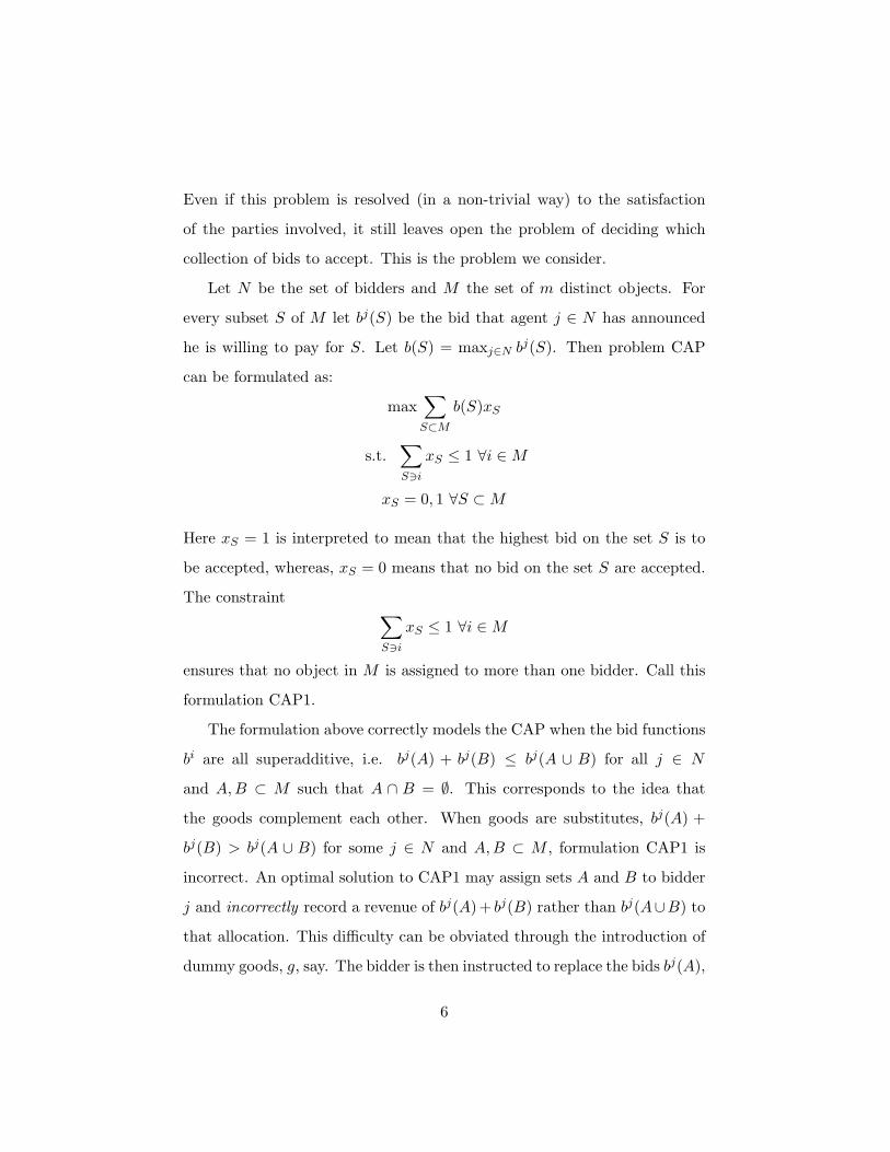
Let N be the set of bidders and M the set of m distinct objects. For
every subset S of M let bj(S) be the bid that agent j ∈ N has announced
he is willing to pay for S. Let b(S) = maxj∈N bj(S). Then problem CAP
can be formulated as:
max∑
S⊂Mb(S)xS
s.t.∑
S3ixS ≤ 1 ∀i ∈M
xS = 0, 1 ∀S ⊂M
Here xS = 1 is interpreted to mean that the highest bid on the set S is to
be accepted, whereas, xS = 0 means that no bid on the set S are accepted.
The constraint∑
S3ixS ≤ 1 ∀i ∈M
ensures that no object in M is assigned to more than one bidder. Call this
formulation CAP1.
The formulation above correctly models the CAP when the bid functions
bi are all superadditive, i.e. bj(A) + bj(B) ≤ bj(A ∪ B) for all j ∈ N
and A,B ⊂ M such that A ∩ B = ∅. This corresponds to the idea that
the goods complement each other. When goods are substitutes, bj(A) +
bj(B) > bj(A ∪ B) for some j ∈ N and A,B ⊂ M , formulation CAP1 is
incorrect. An optimal solution to CAP1 may assign sets A and B to bidder
j and incorrectly record a revenue of bj(A) + bj(B) rather than bj(A∪B) to
that allocation. This difficulty can be obviated through the introduction of
dummy goods, g, say. The bidder is then instructed to replace the bids bj(A),
6
bj(B) and bj(A∪B) with bj(A∪ g), bj(B ∪ g) and bj(A∪B) and to replace
M by M ∪ g. Notice that by the constraints of the integer programming
formulation, if the set A is assigned to j then so is g and thus B cannot be
assigned to j.
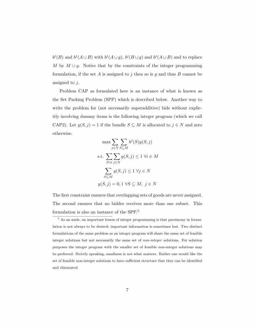
Problem CAP as formulated here is an instance of what is known as
the Set Packing Problem (SPP) which is described below. Another way to
write the problem for (not necessarily superadditive) bids without explic-
itly involving dummy items is the following integer program (which we call
CAP2). Let y(S, j) = 1 if the bundle S ⊆M is allocated to j ∈ N and zero
otherwise.
max∑
j∈N
∑
S⊆Mbj(S)y(S, j)
s.t.∑
S3i
∑
j∈Ny(S, j) ≤ 1 ∀i ∈M
∑
S⊆My(S, j) ≤ 1 ∀j ∈ N
y(S, j) = 0, 1 ∀S ⊆M, j ∈ N
The first constraint ensures that overlapping sets of goods are never assigned.
The second ensures that no bidder receives more than one subset. This
formulation is also an instance of the SPP.5
5 As an aside, an important lesson of integer programming is that parsimony in formu-
lation is not always to be desired; important information is sometimes lost. Two distinct
formulations of the same problem as an integer program will share the same set of feasible
integer solutions but not necessarily the same set of non-integer solutions. For solution
purposes the integer program with the smaller set of feasible non-integer solutions may
be preferred. Strictly speaking, smallness is not what matters. Rather one would like the
set of feasible non-integer solutions to have sufficient structure that they can be identified
and eliminated.
7
There is another interpretation of the CAP possible. If we interpret the
bids submitted as the true values that bidders have for various combinations,
then the solution to the CAP is the efficient allocation of indivisible objects
in an exchange economy.
We have formulated CAP1 under the assumption that there is at most
one copy of each object. It is an easy matter to extend the formulation to
the case when there are multiple copies of the same object and each bidder
wants at most one copy of each object. All that happens is that the right
hand side of the constraints in CAP1 take on values larger than 1.
In the case when there are multiple units and bidders may want more
than one copy of the same unit, bids are column vectors of the form {ajk}k≥1
where ajk is the number of items of object k requested by bidder j. Again
it is easy to see that the problem of determining the winning set of bids can
be formulated as an integer program. Multi-unit combinatorial auctions are
investigated in Leyton-Brown et. al. (2000).6
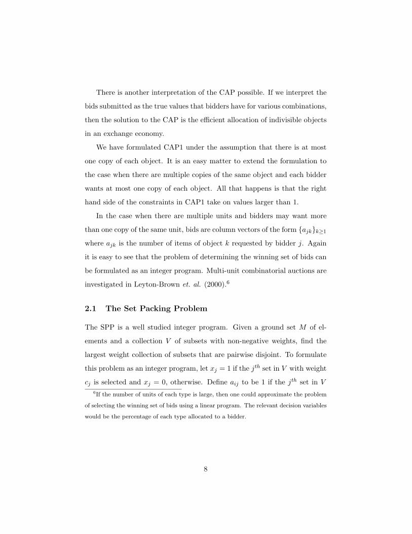
2.1 The Set Packing Problem
The SPP is a well studied integer program. Given a ground set M of el-
ements and a collection V of subsets with non-negative weights, find the
largest weight collection of subsets that are pairwise disjoint. To formulate
this problem as an integer program, let xj = 1 if the jth set in V with weight
cj is selected and xj = 0, otherwise. Define aij to be 1 if the jth set in V6If the number of units of each type is large, then one could approximate the problem
of selecting the winning set of bids using a linear program. The relevant decision variables
would be the percentage of each type allocated to a bidder.
8
contains element i ∈M . Given this, the SPP can be formulated as:
max∑
j∈Vcjxj
s.t.∑
j∈Vaijxj ≤ 1 ∀i ∈M
xj = 0, 1 ∀j ∈ V
It is easy to see that the CAP is an instance of the SPP. Just take M to be
the set of objects and V the set of all subsets of M .
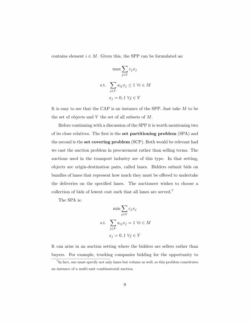
Before continuing with a discussion of the SPP it is worth mentioning two
of its close relatives. The first is the set partitioning problem (SPA) and
the second is the set covering problem (SCP). Both would be relevant had
we cast the auction problem in procurement rather than selling terms. The
auctions used in the transport industry are of this type. In that setting,
objects are origin-destination pairs, called lanes. Bidders submit bids on
bundles of lanes that represent how much they must be offered to undertake
the deliveries on the specified lanes. The auctioneer wishes to choose a
collection of bids of lowest cost such that all lanes are served.7
The SPA is:
min∑
j∈Vcjxj
s.t.∑
j∈Vaijxj = 1 ∀i ∈M
xj = 0, 1 ∀j ∈ V
It can arise in an auction setting where the bidders are sellers rather than
buyers. For example, trucking companies bidding for the opportunity to7In fact, one must specify not only lanes but volume as well, so this problem constitutes
an instance of a multi-unit combinatorial auction.
9
ship goods from a particular warehouse to retail outlet. Any instance of
SPP can be rewritten as an instance of SPA by using slack variables and
negating the objective function coefficients.
The SCP is:
min∑
j∈Vcjxj
s.t.∑
j∈Vaijxj ≥ 1 ∀i ∈M
xj = 0, 1 ∀j ∈ V
A prominent application of the SCP is the scheduling of crews for railways.
Both the SPA and SCP have been extensively investigated.
Other applications of the SPP include switching theory, the testing of
VLSI circuits, line balancing and scheduling problems where one wishes to
satisfy as much demand as possible, without creating conflicts. The survey
by Balas and Padberg [1976] contains a bibliography on applications of the
SPP, SCP and SPA. The instances of SPP that have received the most
attention are those that that stem from relaxations of SPAs.
2.2 Complexity of the SPP
How hard is the SPP to solve? By enumerating all possible 0-1 solutions
we can find an optimal solution in a finite number of steps. If |V | is the
number of variables, then the number of solutions to check would be 2|V |,
clearly impractical for all but small values of |V |. For the instances of SPP
that arise in the CAP, the cardinality of V is the number of subsets of M ;
a large number.
Is there an efficient algorithm for solving SPP? The answer depends on
the definition of efficiency. In complexity theory, efficiency is measured by
10
the number of elementary operations (addition, subtraction, multiplication
and rounding) needed to determine the solution. An algorithm for a prob-
lem is said to be efficient or polynomial if for all instances of the input
problem the number of elementary operations needed grows as a polyno-
mial function of the size of the instance. Of course the definition allows the
number of operations executed to grow with the size of the problem. To
ensure that the number of instructions grows only modestly in the size of
the problem, usually polynomiality is required. By focusing on the number
of operations rather than time, the definition is machine independent. Effi-
ciency should not hinge on the particular technology being used. The size
of a problem instance is measured by the number of binary bits needed to
encode the instance. In the case of the SPP the proxy for size of an instance
is max{|M |, |V |, ln cmax} where cmax = maxj∈V cj .
Returning to the efficiency question, no polynomial time algorithm for
the SPP is known and there are strong reasons for believing none exists.
The SPP belongs to an equivalence class of problems called NP-hard.8 No
problem in this class is currently known to admit a polynomial time solution
method. It is conjectured that no member in this class admits a polynomial
time solution algorithm. The conjecture is sometimes called the P6=NP
conjecture and its resolution is the holy grail of theoretical computer science.
Two points about this notion of efficiency are in order. First, polyno-
mial time algorithms while theoretically efficient may still be impractical.
For example, an algorithm whose complexity is a 23rd order polynomial of
problem size would still take a long time to run on even the fastest known
machines. Generally, a third order polynomial seems to be the upper limit8More precisely, the recognition version of SPP is NP-complete.
11
of what is viewed as practical to implement. Second, the fact that a problem
is NP-hard in general does not mean there is no hope for solving it rapidly.
NP-hard does not mean ‘hard all the time’, just ‘hard some times’. An al-
gorithm that is polynomial on some rather than all instances may be good
enough for the purpose at hand.
For the CAP, this discussion of complexity may have little relevance.
Any algorithm for the CAP, that uses directly the bids for the sets, must
scan, in the worst case, the bids and the number of such bids could be
exponential in |M |. Thus effective solution procedures for the CAP must
rely on two things. The first is that the number of distinct bids is not large
or is structured in computationally useful ways. The second is that the
underlying SPP can be solved reasonably quickly.
2.3 Solvable Instances of the SPP
The usual way in which instances of the SPP can be solved by a polyno-
mial algorithm is when the extreme points of the polyhedron P (A) = {x :∑
j∈V aijxj ≤ 1 ∀i ∈ M ; xj ≥ 0 ∀j ∈ V } are all integral, i.e. 0-1. In these
cases we can simply drop the integrality requirement from the SPP and solve
it as a linear program. Linear programs can be solved in polynomial time.
It turns out that in most of these cases, because of the special structure
of these problems, algorithms more efficient than linear programming ones
exist. Nevertheless, the connection to linear programming is important be-
cause it allows one to interpret dual variables as prices for the objects being
auctioned. We will say more about this later in the paper.
A polyhedron with all integral extreme points is called integral. Iden-
tifying sufficient conditions for when a polyhedron is integral has been a
12
cottage industry in integer programming. These sufficient conditions in-
volve restrictions on the constraint matrix, which in this case amount to
restrictions on the kinds of subsets for which bids are submitted. We list
the most important ones here.
Rothkopf et. al. (1998) covers the same ground but organizes the solvable
instances differently as well as suggesting auction contexts in which they may
be salient. An example of one such context is given below.
2.3.1 Total Unimodularity
The most well known of these sufficient conditions is total unimodularity,
sometimes abbreviated to ‘TU’. A matrix is said to be TU if the determinant
of every square submatrix is 0, 1 or -1. Notice also that if a matrix is TU
so is its transpose.
If the matrix A = {aij}i∈M,j∈V is TU then all extreme points of the
polyhedron P (A) are integral. It is easy to see why. Every extreme point of
P (A) corresponds to a basis or square submatrix of A. Now apply Cramer’s
rule to the system of equations associated with the basis.
The problem of characterizing the class of TU matrices was solved in 1981
by Paul Seymour who gave a polynomial (in the number of rows and columns
of the matrix) time algorithm to decide whether a matrix was TU. A nice
description of the algorithm can be found in Chapter 20 of Schrijver (1986).
However, for most applications, in particular for the CAP, the following
characterization of TU for restricted classes of matrices due to Ghouila-
Houri seems to be the tool of choice:
Theorem 2.1 Let B be a matrix each of whose entries is 0, 1 or -1. Suppose
each subset S of columns of B can be divided into two sets L and R such
13
that ∣
∣
∣
∣
∣
∣
∑
j∈S∩Lbij −
∑
j∈S∩Rbij
∣
∣
∣
∣
∣
∣
= 0, 1 ∀i
then B is TU. The converse is also true.
Other characterizations for matrices each of whose entries are 0, 1 or -1 can
be found in Chapter 19 of Schrijver (1986).
The most important class of TU matrices are called network matrices.
A matrix is a network matrix if each column contains at most two non-
zero entries of opposite sign and absolute value 1. One of the usual tricks
for establishing that a matrix is TU is to use a restricted set of row and
column operations to convert it into a network matrix. These operations
are negating a row (or column) or adding one row (column) to another.
Notice that if a matrix is TU before the operation it must be TU after the
operation.
A 0-1 matrix has the consecutive ones property if the non-zero entries in
each column occur consecutively.
Theorem 2.2 All 0-1 matrices with the consecutive ones property are TU.
Whether any of the results identified above apply to the CAP depends
upon the context. Rothkopf et. al. (1998) offer the following to motivate
the consecutive ones property. Suppose the objects to be auctioned are
parcels of land along a shore line. The shore line is important as it imposes
a linear order on the parcels. In this case it is easy to imagine that the most
interesting combinations (in the bidders eyes) would be contiguous. If this
were true it would have two computational consequences. The first is that
the number of distinct bids would be limited (to intervals of various length)
14
by a polynomial in the number of objects. Second, the constraint matrix A
of the CAP would have the consecutive ones property in the columns.9
2.3.2 Balanced Matrices
A 0-1 matrix B is balanced if it has no square submatrix of odd order with
exactly two 1’s in each row and column. The usefulness of the balanced
condition comes from:
Theorem 2.3 Let B be a balanced 0-1 matrix. Then the following linear
program:
max
∑
j
cjxj :∑
j
bijxj ≤ 1 ∀i, xj ≥ 0 ∀j
has an integral optimal solution whenever the the cj’s are integral.
Notice that balancedness does not guarantee integrality of the polyhedron,
but only that there will be an integral optimal solution to the linear pro-
gram. However, it is true that when B is balanced then the polyhedron
{x :∑
j bijxj = 1 ∀i, xj ≥ 0 ∀j} is integral.
We now describe one instance of balancedness that may be relevant to
the CAP. Consider a tree T with a distance function d. For each vertex v
in T let N(v, r) denote the set of all vertices in T that are within distance
r of v. If you like, the vertices represent parcels of land connected by a
road network with no cycles. Bidders can bid for subsets of parcels but the
subsets are constrained to be of the form N(v, r) for some vertex v and some
number r. Now the constraint matrix of the corresponding SPP will have9If the intervals are substitutes for each other, then the introduction of dummy goods
into the formulation destroys the consecutive ones property. Nevertheless the underlying
optimization problem can still be solved efficiently. See van Hoesel and Muller (2000) for
details.
15
one column for each set of the form N(v, r) and one row for each vertex of
T . This constraint matrix is balanced. See Nemhauser and Wolsey (1988)
for a proof as well as efficient algorithms. In the case when the underlying
tree T is a path the constraint matrix reduces to having the consecutive ones
property. If the underlying network were not a tree then the corresponding
version of SPP becomes NP-hard.
Characterizing the class of balanced matrices is an outstanding open
problem.
2.3.3 Perfect Matrices
More generally, if the constraint matrix A can be identified with the vertex-
clique adjacency matrix of what is known as a perfect graph, then SPP
can be solved in polynomial time. The interested reader should consult
Chapter 9 of Grotschel et. al. (1988) for more details. The algorithm, while
polynomial, is impractical.
We now describe one instance of perfection that may be relevant to the
CAP. It is related to the example on balancedness. Consider a tree T .
As before imagine the vertices represent parcels of land connected by a road
network with no cycles. Bidders can bid for any connected subset of parcels.
Now the constraint matrix of the corresponding SPP will have one column
for each connected subset of T and one row for each vertex of T . This
constraint matrix is perfect.
2.3.4 Graph Theoretic Methods
There are situations where P (A) is not integral yet the SPP can be solved in
polynomial time because the constraint matrix of A admits a graph theoretic
16
interpretation in terms of an easy problem. The most well known instance
of this is when each column of the matrix A contains at most two 1’s. In
this case the SPP becomes an instance of the maximum weight matching
problem in a graph which can be solved in polynomial time.
Each row (object) corresponds to a vertex in a graph. Each column
(bid) corresponds to an edge. The identification of columns of A with edges
comes from the fact that each column contains two non-zero entries. It is well
known that P (A) contains fractional extreme points. Consider for example
a graph which is a cycle on three vertices. A comprehensive discussion of
the matching problem can be found in the book by Lovasz and Plummer
(1986). Instances of SPP where each column has at most K ≥ 3 non-zero
entries are NP-hard.
It is natural to ask what happens if one restricts the number of 1’s in
each row rather than column. Instances of SPP with at most two non-zero
entries per row of A are NP-hard. These instances correspond to what is
called the stable set problem in graphs, a notoriously difficult problem.10
Another case is when the matrix A has the circular ones property. A
0-1 matrix has the circular ones property if the non-zero entries in each
column (row) are consecutive; first and last entries in each column (row)
are treated consecutively. Notice the resemblance to the consecutive ones
property. In this case the constraint matrix can be identified with what
is known as the vertex-clique adjacency matrix of a circular arc graph.11
10The intstance of CAP produced by the radio spectrum auction in Jackson (1976)
reduces to just such a problem.11Take a circle and a collection of arcs of the circle. To each arc associate a vertex. Two
vertices will be adjacent if the corresponding arcs overlap. The consecutive ones property
also bears a graph theoretic interpretation. Take intervals of the real line and associate
them with vertices. Two vertices are adjacent if the corresponding intervals overlap. Such
17
The SPP then becomes the maximum weight independent set problem for
a circular arc graph. This problem can also be solved in polynomial time,
see Golumbic et. al. (1988). Following the parcels of land on the seashore
example, the circular ones structure makes sense when the land parcels lie
on the shores of an island or lake.
2.3.5 Using Preferences
The solvable instances above work by restricting the sets of objects over
which preferences can expressed. Another approach would be to study the
implications of restrictions in the preference orderings of the bidders them-
selves. This can be accomplished using formulation CAP1 but is more trans-
parent with formulation CAP2. Recall CAP2:
max∑
j∈N
∑
S⊆Mbj(S)y(S, j)
s.t.∑
S3i
∑
j∈Ny(S, j) ≤ 1 ∀i ∈M
∑
S⊆My(S, j) ≤ 1 ∀j ∈ N
y(S, j) = 0, 1 ∀S ⊆M, j ∈ N
One common restriction that is placed on bj(·) is that it be non-decreasing
and supermodular. Suppose now that bidders come in two types. The type
one bidders have bj(·) = g1(·) and those of type two have bj(·) = g2(·) where
gr(·) are non-decreasing, integer valued supermodular functions. Let N r be
the set of type r bidders. Now the dual to the linear programming relaxation
of CAP2 is:
min∑
i∈Mpi +
∑
j∈Nqj
graphs are called interval graphs.
18
s.t.∑
i∈Spi + qj ≥ g1(S) ∀S ⊆M, j ∈ N1
∑
i∈Spi + qj ≥ g2(S) ∀S ⊆M, j ∈ N2
pi, qj ≥ 0 ∀i ∈M, j ∈ N
This problem is an instance of the polymatroid intersection problem and
is polynomially solvable; see Theorem 10.1.13 in Grotschel et. al. (1988).
More importantly it has the property of being totally dual integral, which
means that its linear programming dual, the linear relaxation of the original
primal problem, has an integer optimal solution. This last observation is
used in Bikhchandani and Mamer (1997) to establish the existence of com-
petitive equilibria in exchange economies with indivisibilities. Utilizing the
method to solve problems with three or more types of bidders is not possi-
ble because it is known in those cases that the dual problem above admits
fractional extreme points. In fact the problem of finding an integer optimal
solution for the intersection of three or more polymatroids is NP-hard.
In the case when each of the bj(·) have the gross substitutes property
(Kelso and Crawford (1982)), CAP2 reduces to a sequence of matroid par-
tition problems (see Nemhauser and Wolsey (1988)), each of which can be
solved in polynomial time. Gul and Stachetti (1997) describe the reduction
as well as provide a ‘Walrasian’ auctioneer interpretation of it.
2.4 Exact Methods
Exact approaches to solving the SPP require algorithms that generate both
good lower and upper bounds on the maximum objective function value of
the instance. In general, the upper bound on the optimal solution value is
obtained by solving a relaxation of the optimization problem. That is, one
19
solves a related optimization problem whose set of feasible solutions properly
contains all feasible solutions of the original problem and whose objective
function value is at least as large as the true objective function value for
points feasible to the original problem. Thus, we replace the “true” problem
by one with a larger feasible region that is more easily solved. There are
two standard relaxations for SPP: Lagrangean relaxation (where the feasible
set is usually required to maintain 0-1 feasibility, but many if not all of the
constraints are moved to the objective function with a penalty term) and
the linear programming relaxation (where only the integrality constraints are
relaxed—the objective function remains the original function). Lagrangean
relaxation will be discussed in greater detail in Section 3 on decentralization.
Exact methods come in three varieties: branch and bound, cutting planes
and a hybrid called branch and cut. The basic idea of branch and bound
can be described as intelligent enumeration. At each stage, after solving
the LP, a fractional variable, xj , is selected and two subproblems are set up
(this is the branching phase) one where xj is set to 1 and the other where xj
is set to 0. The linear programming relaxation of the two subproblems are
solved to identify an upper bound on the objective function value for each
subproblem. From each subproblem with a nonintegral solution we branch
again to generate two subproblems and so on. In the worst case we generate
a binary tree that includes all feasible solutions. However by comparing the
linear programming bound across nodes in different branches of the tree,
one can prune some branches in advance without the need to explore them
further. That is solutions with some variable xk, say, set to 1 (or zero) can
never be optimal. This is the ‘bound’ in the name of the method.
Cutting plane methods find linear inequalities that are violated by a so-
lution of a given relaxation but are satisfied by all feasible zero-one solutions.
20
These inequalities are called cuts. If one adds enough cuts, one is left with
integral extreme points. Later in this paper (see Subsection 3.5) we show
how cuts can be used to develop prices for various subsets of objects. The
most successful cutting plane approaches are based on polyhedral theory,
that is they replace the constraint set of an integer programming problem
by a convexification of the feasible zero-one points and extreme rays of the
problem. For details on polyhedral structure of the SPP and its relatives see
Padberg (1973, 1975 and 1979), Cornuejols and Sassano (1989) and Sassano
(1989). Given that the problems are NP-hard a full polyhedral description
of these problems is unlikely.
Branch and cut works likes branch and bound but tightens the bounds
in every node of the tree by adding cuts. For a complete description of how
such cuts are embedded into a tree search structure along with other tricks
of the trade, see Hoffman and Padberg (1993).
Because even small instances of the CAP1 may involve a huge number of
columns (bids) the techniques described above need to be augmented with
another method known as column generation. Introduced by Gilmore and
Gomory (1961) it works by generating a column when needed rather than
all at once. An overview of such methods can be found in Barnhart et. al.
(1994). Later in this paper we illustrate how this idea could be implemented
in an auction.
One sign of how successful exact approaches are can be found in Hoffman
and Padberg (1993). They report being able to find an optimal solution to
an instance of SPA with 1,053,137 variables and 145 constraints in under 25
minutes. In auction terms this corresponds to a problem with 145 items and
1,053,137 bids. A major impetus behind the desire to solve large instances
of SPA (and SPC) quickly has been the airline industry. The problem of
21
assigning crews to routes can be formulated as an SPA. The rows of the SPA
correspond to flight legs and the columns to a sequence of flight legs that
would be assigned to a crew. Like the CAP, in this problem the number of
columns grows exponentially with the number of rows.12 For the SPP, the
large instances that have been studied have usually arisen from relaxations
of SPA’s. Given the above we believe that established integer programming
methods will prove quite successful when applied to the solution of CAP.
Logistics.com’s OptiBidTM software has been used in situations where
the number of bidders is between 12 to 350 with the average being around
120. The number of lanes (objects) has ranged between 500 and 10,000.
Additionally, each lane bid can contain a capacity constraint as well as a
budget capacity constraint covering multiple lanes. The typical number of
lanes is 3000. OptiBidTM does not limit the number of distinct subsets that
bidders bid on or the number of items allowed within a package. OptiBidTM
is based on a integer program with a series of proprietary formulations and
starting heuristic algorithms.13
SAITECH-INC’s bidding software, SBID, is also based on integer pro-
gramming. They report being able to handle problems of similar size as
OptiBidTM.14
Exact methods for CAP1 have been proposed by Fujishima et. al. (1999)
as well as Sandholm (1999) and Andersson et. al. (2000). The first two use
variations of dynamic programming and the third uses integer programming.
In the first, the method is tested on randomly generated instances the largest12However, these crew scheduling problems give rise to instances of SPA that have a
large number of duplicate columns in the constraint matrix. In some cases as many as
60% of them. We thank Dr. Marta Eso for alerting us to this.13We thank Dr. Christopher Caplice of Logistics.com for providing this information.14We thank Dr. Yoshiro Ikura of SAITECH-INC for providing us with this information.
22
of which involved 500 objects (rows) and 20,000 bids (variables). The second
also tests the method on randomly generated instances, the largest of which
involved 400 objects (rows) and 2000 bids (variables). In these tests the
number of bids examined is far less than the number of subsets of objects.
The third uses integer programming methods on the test problems generated
by the first two.
By comparison, a straightforward implementation on a commercially
available code for solving linear integer programs (called CPLEX) runs into
difficulties for instances of CAP involving more than 19 objects if one lists
all the bids for the various subsets. There will be 219 variables. This al-
ready requires one giga-byte of memory to store. CPLEX can handle in this
straight forward approach on the order of 219 variables and 19 constraints
before running out of resident memory. Notice that this is large enough
to handle the test problems considered in Sandholm (1999) and Fujishima
et. al. (1999). We report on this in a later section where we also discuss
schemes for generating test problems.15
The reader should note that size of an instance is not by itself an indicator
of problem difficulty. Structure of the problem plays an important role. In a
later section we will discuss some of the structure inherent in the generation
schemes used by Sandholm and others.
2.5 Approximate Methods
One way of dealing with hard integer programs is to give up on finding the
optimal solution. Rather one seeks a feasible solution fast and hopes that it
is near optimal. This raises the obvious question of how close to optimal the15Since our findings duplicate those of Andersson et. al. (2000) we will comment on this
paper in a later section.
23
solution is. There have traditionally been three ways to assess the accuracy
of an approximate solution. The first is by worst-case analysis, the second
by probabilistic analysis and the third empirically.
Before describing these approaches it is important to say that proba-
bly every heuristic approach for solving general integer programming prob-
lems has been applied to the SPP. The first one that almost everyone
thinks off, called Greedy, is to iteratively select the column j that maxi-
mizes cj/∑
i aij , the weight to column sum ratio (see Fisher and Wolsey
(1982) for example). Interchange/steepest ascent approaches have also been
used; a swap of one or more columns is executed whenever such a swap
improves the objective function value (see Hurkens and Schrijver (1989) for
the case of maximum cardinality packing and Arkin and Hassin (1998) for
weighted packing problems). More fashionable approaches such as genetic
algorithms Huang et. al. (1994), probabilistic search (Feo et. al., 1989),
simulated annealing (Johnson, et. al., 1989), and neural networks (Aourid
and Kaminska, 1994) have also been tried. Unfortunately, there has not
been a comparative testing across such methods to determine under what
circumstances a specific method might perform best. Beasley (1990) main-
tains (at http://mscmga.ms.ic.ac.uk/info.html) an extensive test set of
covering and partitioning problem instances for those who would like to try
their hand. We think it safe to say that anything one can think of for ap-
proximating the SPP has probably been thought of. In addition, one can
embed approximation algorithms within exact algorithms so that one is at-
tempting to get a sharp approximation to the lower bound for the problem
at the same time that one iteratively tightens the upper bound.
24
2.5.1 Worst-Case Analysis
Let I denote an instance of the integer program one wishes to solve and Z(I)
its optimal objective function value. Assume the goal is to maximize the
objective function as in the SPP. Let ZH(I) denote the value of the solution
returned on the instance I by the polynomial time approximation algorithm
(also called heuristic) H. The worst-case ratio for the performance of H
is inf ZH(I)/Z(I). Here the infimum is over all instances in the problem
class. For a problem with a maximization objective, ZH(I) ≤ Z(I) and so
the worst-case ratio will always be less than 1. The objective is to bound it
from below.
The SPP is difficult to approximate. It is proved by Hastad (1999) that
unless P = NP, there is no polynomial time algorithm for the SPP that can
deliver a worst case ratio larger than nε−1 for any ε > 0. On the positive
side polynomial algorithms that have a worst case ratio of O(n/(log n)2)
are known. Bounds that are a function of the data of the underlying input
problem are also known. A recent example of this motivated by CAP1 can
be found in Akcoglu et. al. (2000). In general restricting the instances of
SPP does not help things very much. The reader interested in a full account
of what is known about approximating the SPP should consult Crescenzi
et. al. (1998) where an updated list of what is known about the worst-case
approximation ratio of a whole range of optimization problems is given.
When interpreting these worst case results, two things should be kept in
mind. The first is that they are worst-case results and so shed little light
on the ‘typical’ accuracy of an approximation algorithm. The second is that
these results are lower bounds on ZH(I) as a linear function of Z(I). It is
very possible that bounds on ZH(I) that are non-linear functions of Z(I)
25
might not be so pessimistic.
2.5.2 Probabilistic Analysis
Probabilistic analysis is an attempt to characterize the typical behavior of an
approximation algorithm. A probability distribution over problem instances
is specified in which case Z(I) and ZH(I) become random variables. The
goal is to understand the behavior of the difference or ratio of the two
variables as the size of the instances increase. For example, what is the
mean difference, the variance etc. Since the results are asymptotic in nature,
attention must be paid to the convergence results when interpreting the
results. A problematic feature is that the distributions over instances that
are chosen (because of ease of analysis) do not necessarily coincide with the
distributions that actual instances will be drawn from. This issue arises also
in the empirical testing of approximation algorithms.
2.5.3 Empirical Testing
Many approximation algorithms will be elaborate enough to defy theoretical
analysis. For this reason it is common to resort to empirical testing. Further
empirical testing allows one to consider issues not easily treated analytically.
A good guide to the consumption of an empirical study of approximation
algorithms is given by Ball and Magazine (1981). They list the following
evaluation criteria:
1. Proximity to the optimal solution.
2. Ease of implementation (coding and data requirements).
3. Flexibility; ability to handle changes in the model.
26
4. Robustness; ability to provide sensitivity analysis and bounds.
This is not the forum for an extensive discussion of the issues associated
with the empirical testing of heuristics. However, some points are worth
highlighting.
The most obvious is the choice of test problems. Are they realistic? Do
they exhibit the features that one thinks one will find in the environment?
Interestingly, probabilistic analysis has a role to play here in eliminating
some schemes for randomly generating test problems. For example it is
known that certain generation schemes give rise to problems that are easy
to solve; for example, a randomly generated solution is with high probability
close to optimal. Success on a collection of problems generated in this way
conveys no information. Is the accuracy due to the approximation algorithm
or the structure of the test problems?
Some approximation algorithms involve a number of parameters that
need to be fine tuned. Comparing their performance with heuristics whose
parameters are not fine tuned becomes difficult because it is not clear wheth-
er one should include the overhead in the tuning stage in the comparison.
3. Decentralized Methods
One way of reducing some of the computational burden in solving the CAP is
to set up a ‘fictitious’ market that will determine an allocation and prices in
a decentralized way. The traditional auctioneer is replaced with a Walrasian
one who sets prices for the objects. Agents announce which sets of objects
they will purchase at the posted prices. If two or more agents compete for the
same object, the Walrasian auctioneer adjusts the price vector. This saves
bidders from specifying their bids for every possible combination and the
27
auctioneer from having to process each bid function. Such methods also have
the advantage that they can be adapted to dynamic environments where
bidders and objects arrive and depart at different times. While such methods
reduce the computational burden they cannot eliminate them altogether. A
more compelling argument for decentralized methods is that the relevant
information for choosing an allocation is itself decentralized.
Examples of decentralized approaches for solving the CAP can be found
in Fujishima et. al. (1999) and Rassenti et. al. (1982). In the same spirit,
Brewer (1999) and Wellman et. al. (1998) propose decentralized scheduling
procedures in different contexts. In their set up the auctioneer chooses a
feasible solution and ‘bidders’ are asked to submit improvements to the so-
lution. In return for these improvements, the auctioneer agrees to share a
portion of the revenue gain with the bidder. These methods can be viewed
as instances of dual based procedures for solving an integer program. Auc-
tion or market interpretations of dual based procedures for optimization
problems are not new. They appear, for example in Dantzig (1963). The
updates on the dual variables that are executed in these algorithms can be
interpreted as a form of myopic best response on the part of bidders. More
recently, Bertsekas (1991) has proposed a collection of dual based algorithms
for the class of linear network optimization problems. These algorithms he
dubs auctions algorithms. The incentive issues associated with such methods
are discussed later.
3.1 Duality in Integer Programming
To describe the dual to SPP let 1 denote the m-vector of all 1’s and aj the jth
column of the constraint matrix A. The (superadditive) dual to SPP is the
28
problem of finding a superadditive, non-decreasing function F : Rm → R1
that
minF (1)
s.t. F (aj) ≥ cj ∀j ∈ V
F (0) = 0
We can think of F as being a non-linear price function that assigns a price
to each bundle of goods (see Wolsey (1981)).
If the primal integer program has the integrality property, there is an
optimal integer solution to its linear programming relaxation, the dual func-
tion F will be linear i.e. F (u) =∑
i yiui for some y and all u ∈ Rm. The
dual becomes:
min∑
i
yi
s.t.∑
i
aijyi ≥ cj ∀j ∈ V
yi ≥ 0 ∀i ∈M
That is, the superadditive dual reduces to the dual of the linear programming
relaxation of SPP. In this case we can interpret each yi to be the price of
object i. Thus an optimal allocation given by a solution to the CAP can be
supported by prices on individual objects.
Optimal objective function values of SPP and its dual coincide (when
both are well defined). There is also a complementary slackness condition:
Theorem 3.1 If x is an optimal solution to SPP and F an optimal solution
to the superadditive dual then
(F (aj)− cj)xj = 0 ∀j.
29
Solving the superadditive dual problem is as hard as solving the original
primal problem. It is possible to reformulate the superadditive dual problem
as a linear program (the number of variables in the formulation is exponen-
tial in the size of the original problem). For small or specially structured
problems this can provide some insight. The interested reader is referred
to Nemhauser and Wolsey (1988) for more details. In general one relies on
the solution to the linear programming dual and uses its optimal value to
guide the search for an optimal solution to the original primal integer pro-
gram. The way this is done is through a technique known as Lagrangean
Relaxation.
3.2 Lagrangean Relaxation
The basic idea is to ‘relax’ some of the constraints of the original problem
by moving them into the objective function with a penalty term. That is in-
feasible solutions to the original problem are allowed, but they are penalized
in the objective function in proportion to the amount of infeasibility. The
constraints that are chosen to be relaxed, are selected so that the optimiza-
tion problem over the remaining set of constraints is in some sense easy.
We describe the bare bones of the method first and then give a ‘market’
interpretation of it.
Recall the SPP:
Z = max∑
j∈Vcjxj
s.t.∑
j∈Vaijxj ≤ 1 ∀i ∈M
xj = 0, 1 ∀j ∈ V
30
Let ZLP denote the optimal objective function value to the linear program-
ming relaxation of SPP. Note that Z ≤ ZLP . Consider now the following
relaxed problem:
Z(λ) = max∑
j∈Vcjxj +
∑
i∈Mλi(1−
∑
j∈Vaijxj)
s.t. 1 ≥ xj ≥ 0 ∀j ∈ V
For a given λ, computing Z(λ) is easy. To see why note that
∑
j∈Vcjxj +
∑
i∈Mλi(1−
∑
j∈Vaijxj) =
∑
j∈V(cj −
∑
i∈Mλiaij)xj +
∑
i∈Mλi.
Thus, to find Z(λ), simply set xj = 1 if (cj −∑
i∈M λiaij) > 0 and zero
otherwise. It is also easy to see that Z(λ) is piecewise linear and convex. A
basic result that is easy to prove is:
Theorem 3.2
ZLP = minλ≥0
Z(λ).
Why might this be useful? Since evaluating Z(λ) for each λ is a snap, if we
can find a fast way to determine the λ that solves minλ≥0 Z(λ) we would
have fast procedure to find ZLP . The resulting solution (values of the x
variables) while integral need not be feasible. However it may not be ‘too
infeasible’ and so could be fudged into a feasible solution without a great
reduction in objective function value.
Finding the λ that solves minλ≥0 Z(λ) can be accomplished using the
subgradient algorithm. Suppose the value of the lagrange multiplier λ at
iteration t is λt. Choose any subgradient of Z(λt) and call it st. Choose the
lagrange multiplier for iteration t+ 1 to be λt + θtst, where θt is a positive
31
number called the step size. In fact if xt is the optimal solution associated
with Z(λt),
λt+1 = λt + θt(Axt − 1).
Notice that λt+1i > λti for any i such that
∑
j aijxtj > 1. The penalty term
is increased on any constraint currently being violated.
The algorithm is a natural adaptation of the steepest descent algorithm
to non-differentiable functions. At each stage it adjusts the multiplier so as
to produce a decrease in the function value. Since the function Z(λ) is not
differentiable, we must choose a subgradient rather than gradient. For an
appropriate choice of step size at each iteration, this procedure can be shown
to converge to the optimal solution. Specifically, θt → 0 as t→∞ but∑
t θt
diverges. The first condition ensures that as we get closer to the optimal
solution, our step sizes go down, i.e. we won’t leave the optimum once it
is found. The second ensures that we don’t stop prematurely, i.e., before
finding the optimal solution. The subgradient algorithm is not guaranteed
to converge to the optimal solution in a finite number of steps. Hence, when
implemented, the user will incorporate a stopping rule, e.g., stop once an
improvement in objective function value that does not exceed some threshold
is observed and experiment with step sizes to ensure rapid convergence.
It should be emphasized that Lagrangean relaxation is not guaranteed
to find the optimal solution to the underlying problem. Rather, it finds an
optimal solution to a relaxation of it.
Here is the market interpretation. The Walrasian auctioneer chooses a
price vector λ for the individual objects and bidders submit bids. If the high-
est bid, cj , for the jth bundle exceeds∑
i∈M aijλi, this bundle is tentatively
assigned to that bidder. Notice that the auctioneer need not know what
32
cj is ahead of time. This is supplied by the bidders after λ is announced.
In fact, the bidders need not announce bids, they could simply state which
individual objects are acceptable to them at the announced prices. The
auctioneer can randomly assign objects to bidders in case of ties. If there is
a conflict in the assignments, the auctioneer uses the subgradient algorithm
to adjust prices and repeats the process.
Now let us compare this market interpretation of Lagrangean relaxation
with the simultaneous ascending auction (SAA) proposed by P. Milgrom,
R. Wilson and P. McAfee (see Milgrom (1995)). In the SAA, bidders bid
on individual items simultaneously in rounds. To stay in the auction for an
item, bids must be increased by a specified minimum from one round to the
next just like the step size. Winning bidders pay their bids. The only dif-
ference between this and Lagrangean relaxation, is that the bidders through
their bids adjust their prices rather than the auctioneer. The adjustment is
along a subgradient. Bids increase on those items for which there are two
or more bidders competing.
One byproduct of the SAA is called the exposure problem. Bidders pay
too much for individual items or bidders with preferences for certain bun-
dles drop out early to limit losses. As an illustration consider an extreme
example of a bidder who values the bundle of goods i and j at $100 but
each separately at $0. In the SAA, this bidder may have to submit high
bids on i and j to be able to secure them. Suppose that it loses the bidding
on i. Then it is left standing with a high bid j which it values at zero. The
presence of such a problem is easily seen within the Lagrangean relaxation
framework. While Lagrangean relaxation will yield the optimal objective
function value for the linear relaxation of the underlying integer program,
it is not guaranteed to produce a feasible solution. Thus the solution gener-
33
ated may not satisfy the complementary slackness conditions. The violation
of complementary slackness is the exposure problem associated with this
auction scheme. Notice that any auction scheme that relies on prices for
individual items will face this problem.
In contrast to the SAA outlined above is the Adaptive User Selection
Mechanism (AUSM) proposed by Banks et. al. (1989). AUSM is asyn-
chronous in that bids on subsets can be submitted at any time and so is
difficult to connect to the Lagrangean ideas just described. An important
feature of AUSM is an arena which allows bidders to aggregate bids to ex-
ploit synergies. DeMartini et. al. (1999) propose an iterative auction scheme
that is a hybrid of the SAA and AUSM that is easier to connect to the La-
grangean framework. In this scheme, bidders submit bids on packages rather
than on individual items. Like the SAA, bids on packages must be increased
by a specified amount from one round to the next. This minimum incre-
ment is a function of the bids submitted in the previous round. In addition,
the number of items that a bidder may bid on in each round is limited by
the number of items s/he bid on in previous rounds. The particular im-
plementation of this scheme advanced by DeMartini et. al. (1999) can also
be given a Lagrangean interpretation. They choose the multipliers (which
can be interpreted as prices on individual items) so as to try and satisfy the
complementary slackness conditions of linear programming. Given the bids
in each round, they allocate the objects so as to maximize revenue. Then
they solve a linear program (that is essentially the dual to CAP2) that finds
a set of prices/multipliers that approximately satisfy the complementary
slackness conditions associated with the allocation.
Kelly and Steinberg (2000) also propose an iterative scheme for combi-
34
natorial auctions.16 The auction has two phases. The first phase is an SAA
where bidders bid on individual items. In the second phase an AUSM like
mechanism is used. The important difference is that each bidder submits
a temporary assignment of all the items in the auction. Here a temporary
assignment is comprised of previous bids of other players plus new bids of
his own.17
In Parkes (1999) an ascending auction, called iBundle, that allows bid-
ders to bid on combinations of items and uses non-linear prices is proposed.
Bidders submit bids for subsets of items. At each iteration the auctioneer
announces prices for those subsets of items that receive unsuccessful bids
from agents. For a bid on a subset to be ‘legal’ it must exceed the price
posted by the auctioneer. Given the bids, the auctioneer solves an instance
of CAP2 and tentatively assigns the objects. For the next iteration, the
prices on each subset are either kept the same or adjusted upwards. The
upward adjustment is determined by the highest losing bid for the subset in
question plus a user specified increment. The auction terminates when the
bids from one round to the next do not show sufficient change. The scheme
can be given a Lagrangian interpretation as well, however the underlying
formulation is different from CAP1 or CAP2. We discuss it in Section 3.5.
3.3 Variations
By relaxing on a subset of the constraints as opposed to all of them we get
different relaxations, some of which give upper bounds on Z that are smaller16The description is tailored to the auction for assigning carrier of last resort rights in
telecommunications.17We thank Professor Steinberg for alerting us to an earlier inaccuracy in the description
of the procedure.
35
than ZLP . Details can be found in Nemhauser and Wolsey (1988). Needless
to say there have been many applications of Lagrangean relaxation to SPP,
SPA and SPC and hybrids with exact methods have also been investigated.
See Balas and Carrera (1996) and Beasley (1990) for recent examples.
3.4 Column Generation
Column generation is a technique for solving linear programs with an ex-
ceedingly large number of variables. Each variable gives rise to a column in
the constraint matrix, hence the name column generation. A naive imple-
mentation of a simplex type algorithm for linear programming would require
recording and storing every column of the constraint matrix. However, only
a small fraction of those columns would ever make it into an optimal basic
feasible solution to the linear program. Further, of those columns not in
the current basis, one only cares about the ones whose reduced cost will
be of the appropriate sign. Column generation exploits this observation
in the following way. First an optimal solution is found using a subset of
the columns/variables. Next, given the dual variable implied by this pre-
liminary solution, an optimization problem is solved to find a non-basic
column/variable that has a reduced cost of appropriate sign. The trick is
to design an optimization problem to find this non-basic column without
listing all non-basic columns.
The column generation idea can be implemented in an auction setting
as follows. In the first step the auctioneer chooses an extreme point solution
to the CAP. It does not matter which one, any one will do. Note that this
initial solution could involve fractional allocations of objects.
This extreme point solution is reported to all bidders. Each bidder, look-
36
ing only at how they value the allocation proposes a column/variable/subset
to enter the basis (along with its value to the bidder). The proposed col-
umn and its valuation must satisfy the appropriate reduced cost criterion
for inclusion in the basis. In effect each bidder is being used as a subroutine
to execute the column generation step.
The auctioneer now gathers up the proposed columns (along with their
valuations) and using these columns and the columns from the initial basis
only (and possibly previously generated nonbasic columns), solves a linear
program to find a revenue maximizing (possibly fractional) allocation. The
new extreme point solution generated is handed out to the bidders who are
asked to each identify a new column (if any) to be added to the new basis
that meets the reduced cost criterion for inclusion. The process is then
repeated until an extreme point solution is identified that no bidder wishes
to modify. To avoid cycling, the auctioneer can always implement one of
the standard anti-cycling rules for linear programming.
This auction procedure eliminates the need to transmit and process long
lists of subsets and their bids. Bids and subsets are generated only as needed.
Second, the bidders are provided an opportunity to challenge an allocation
provided they propose an alternative that increases the revenue to the seller.
If the bids might lead to a nonintegral allocation, then this column genera-
tion has to be imbedded into a branch and cut/price scheme to produce an
integer solution.18
Notice that the ellipsoid method provides a way to solve the fractional
CAP to optimality while generating only a polynomially bounded number
of columns.18We thank Dr. Marta Eso for suggesting this last refinement. See Eso (1999) for an
example of such a branch and cut scheme.
37
3.5 Cuts, Extended Formulations and Non-linear Prices
The decentralized methods described above work by conveying ‘price’ in-
formation to the bidders. Given a set of bids and an allocation, prices for
individual items that ‘support’ or are ‘consistent’ with the bids and alloca-
tions are derived and communicated to the bidders. Such prices, because
they are linear cannot hope to fully capture the interactions between the
parties. Here we show, with an example, how cutting plane methods can
be used to generate prices that more closely reflect the interactions between
bids on different sets of objects.
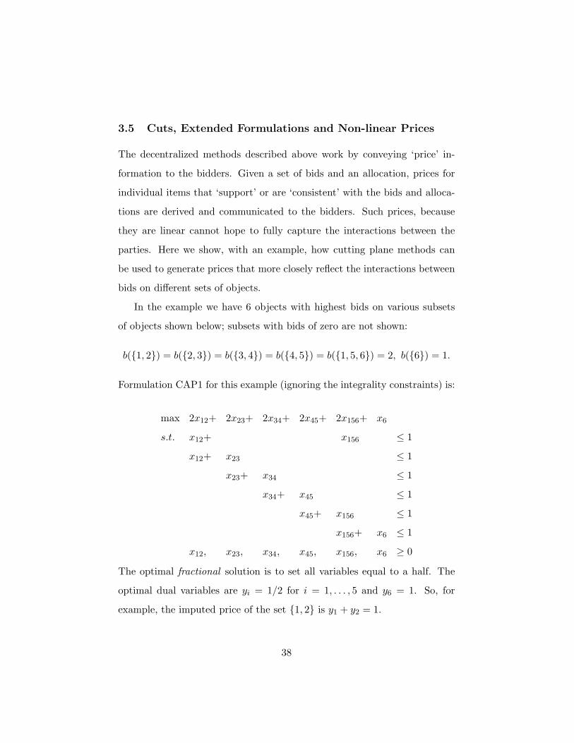
In the example we have 6 objects with highest bids on various subsets
of objects shown below; subsets with bids of zero are not shown:
b({1, 2}) = b({2, 3}) = b({3, 4}) = b({4, 5}) = b({1, 5, 6}) = 2, b({6}) = 1.
Formulation CAP1 for this example (ignoring the integrality constraints) is:
max 2x12+ 2x23+ 2x34+ 2x45+ 2x156+ x6
s.t. x12+ x156 ≤ 1
x12+ x23 ≤ 1
x23+ x34 ≤ 1
x34+ x45 ≤ 1
x45+ x156 ≤ 1
x156+ x6 ≤ 1
x12, x23, x34, x45, x156, x6 ≥ 0
The optimal fractional solution is to set all variables equal to a half. The
optimal dual variables are yi = 1/2 for i = 1, . . . , 5 and y6 = 1. So, for
example, the imputed price of the set {1, 2} is y1 + y2 = 1.
38
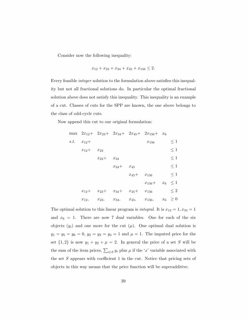
Consider now the following inequality:
x12 + x23 + x34 + x45 + x156 ≤ 2.
Every feasible integer solution to the formulation above satisfies this inequal-
ity but not all fractional solutions do. In particular the optimal fractional
solution above does not satisfy this inequality. This inequality is an example
of a cut. Classes of cuts for the SPP are known, the one above belongs to
the class of odd-cycle cuts.
Now append this cut to our original formulation:
max 2x12+ 2x23+ 2x34+ 2x45+ 2x156+ x6
s.t. x12+ x156 ≤ 1
x12+ x23 ≤ 1
x23+ x34 ≤ 1
x34+ x45 ≤ 1
x45+ x156 ≤ 1
x156+ x6 ≤ 1
x12+ x23+ x34+ x45+ x156 ≤ 2
x12, x23, x34, x45, x156, x6 ≥ 0
The optimal solution to this linear program is integral. It is x12 = 1, x34 = 1
and x6 = 1. There are now 7 dual variables. One for each of the six
objects (yi) and one more for the cut (µ). One optimal dual solution is
y1 = y5 = y6 = 0, y2 = y3 = y4 = 1 and µ = 1. The imputed price for the
set {1, 2} is now y1 + y2 + µ = 2. In general the price of a set S will be
the sum of the item prices,∑
i∈S yi plus µ if the ‘x’ variable associated with
the set S appears with coefficient 1 in the cut. Notice that pricing sets of
objects in this way means that the price function will be superadditive.
39
It is instructive to compare the imputed price of the set {1, 2} in the
two formulations. The first formulation assigns a price of one to the set.
The second a higher price. The first formulation ignores the fact that if
the set {1, 2} is assigned to a bidder, the sets {1, 5, 6} and {2, 3} cannot be
assigned to anyone else. This fact is captured by the cut. The dual variable
associated with the cut can be interpreted as the associated opportunity
cost of assigning the set {1, 2} to a bidder. Thus the actual price of the set
{1, 2} is the sum of the prices of the objects in it plus the opportunity cost
associated with its sale.
Cuts can be derived in one of two ways. The first is by purely combina-
torial reasoning and the other through an algebraic technique first proposed
by Ralph Gomory (see Nemhauser and Wolsey (1988) for the details). For
CAP1, given a fractional extreme point, one can use the Gomory method
to generate a cut involving only the variables that are basic in the current
extreme point. This is useful for computational purposes as one does not
have to lug all variables around to identify a cut. Second, the new inequality
will be a non-negative linear combination of the current basic rows less equal
than a non-negative number. Thus the dual variable associated with this
new constraint will have an additive effect on the prices of various subsets
as in the example.
The reader will notice that by picking an extreme point dual solution,
the imputed prices for some sets are zero. Since there is some flexibility
in the choice of dual variables, one can choose an interior (to the feasible
region) dual solution.
Yet another way to get non-linear prices is by starting with a stronger
formulation of the underlying optimization problem. One formulation is
stronger than another if its set of feasible (fractional) solutions is strictly
40
contained in the other. In the example above, the second formulation is
stronger than the first. Both formulations share the same set of integer
solutions, but not fractional solutions. The set of fractional solutions to the
second formulation is a strict subset of the fractional solutions to the first
one.
Stronger formulations can be obtained, as shown above, by the addition
of inequalities. Yet another, standard way, of obtaining stronger formu-
lations is through the use of additional or auxiliary variables, typically a
large number of them. Geometrically, one is treating the problem formu-
lated in the original set of variables as the projection of a higher dimensional
but structurally simpler polyhedron. Formulations involving such additional
variables are called extended formulations and developing these extended
formulations is called lifting. Using lifting one can develop a hierarchy of
successively stronger formulations of the underlying integer program.
There is a close connection between lifting and cutting plane approaches.
When one projects out the auxiliary variables one obtains a formulation
involving the original variables but with additional constraints which are
cuts.
Extended formulations can be generated by the study of the problem at
hand or algorithmically. Perhaps the most accessible introduction to these
matters is Balas et. al. (1993) which also discusses the connection to cutting
planes.
In the auction context, Bikchandani and Ostroy (1998), propose an ex-
tended formulation for the problem of selecting the winning set of bids. To
describe this formulation let Π be the set of all possible partitions of the
objects in the set M . If π is an element of Π, we write S ∈ π to mean that
the set S ⊂ M is a part of the partition π. Let zπ = 1 if the partition π is
41
selected and zero otherwise. These are the auxiliary variables. Using them
we can reformulate CAP2 as follows:
max∑
j∈N
∑
S⊆Mbj(S)y(S, j)
s.t.∑
S⊆My(S, j) ≤ 1 ∀j ∈ N
∑
j∈Ny(S, j) ≤
∑
π3Szπ ∀S ⊂M
∑
π∈Π
zπ ≤ 1
y(S, j) = 0, 1 ∀S ⊆M, j ∈ N
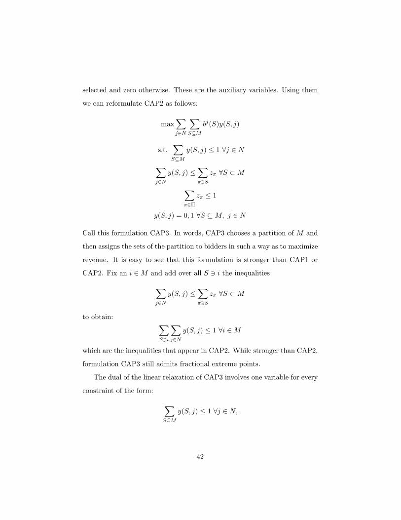
Call this formulation CAP3. In words, CAP3 chooses a partition of M and
then assigns the sets of the partition to bidders in such a way as to maximize
revenue. It is easy to see that this formulation is stronger than CAP1 or
CAP2. Fix an i ∈M and add over all S 3 i the inequalities
∑
j∈Ny(S, j) ≤
∑
π3Szπ ∀S ⊂M
to obtain:∑
S3i
∑
j∈Ny(S, j) ≤ 1 ∀i ∈M
which are the inequalities that appear in CAP2. While stronger than CAP2,
formulation CAP3 still admits fractional extreme points.
The dual of the linear relaxation of CAP3 involves one variable for every
constraint of the form:
∑
S⊆My(S, j) ≤ 1 ∀j ∈ N,
42
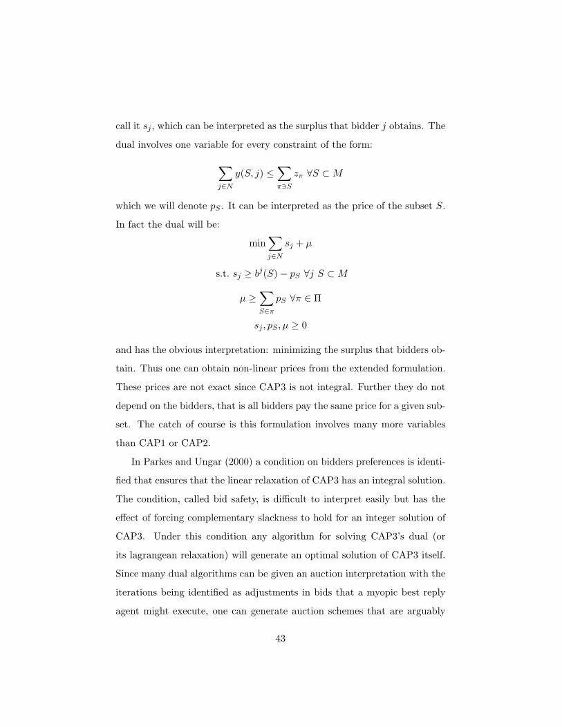
call it sj , which can be interpreted as the surplus that bidder j obtains. The
dual involves one variable for every constraint of the form:
∑
j∈Ny(S, j) ≤
∑
π3Szπ ∀S ⊂M
which we will denote pS . It can be interpreted as the price of the subset S.
In fact the dual will be:
min∑
j∈Nsj + µ
s.t. sj ≥ bj(S)− pS ∀j S ⊂M
µ ≥∑
S∈πpS ∀π ∈ Π
sj , pS , µ ≥ 0
and has the obvious interpretation: minimizing the surplus that bidders ob-
tain. Thus one can obtain non-linear prices from the extended formulation.
These prices are not exact since CAP3 is not integral. Further they do not
depend on the bidders, that is all bidders pay the same price for a given sub-
set. The catch of course is this formulation involves many more variables
than CAP1 or CAP2.
In Parkes and Ungar (2000) a condition on bidders preferences is identi-
fied that ensures that the linear relaxation of CAP3 has an integral solution.
The condition, called bid safety, is difficult to interpret easily but has the
effect of forcing complementary slackness to hold for an integer solution of
CAP3. Under this condition any algorithm for solving CAP3’s dual (or
its lagrangean relaxation) will generate an optimal solution of CAP3 itself.
Since many dual algorithms can be given an auction interpretation with the
iterations being identified as adjustments in bids that a myopic best reply
agent might execute, one can generate auction schemes that are arguably
43
optimal. This is precisely the tack taken in Parkes and Ungar (2000) to
support the adoption of the iBundle auction scheme of Parkes (1999).
Bikchandani and Ostroy (1998) introduce yet another formulation stronger
than CAP3 which is integral. The idea is to use a variable that represents
both a partition of the objects and an allocation. The dual to this for-
mulation gives rise to non-linear prices with the twist that they are bidder
specific. Different bidders pay different prices for the same subset.
A warning about extended formulations is in order. One must be careful
in invoking an extended formulation that simply formulates the problem
away. As an example, consider the auxiliary variables introduced in CAP3,
the zπ’s. For each zr, let yr be an optimal extreme point solution to the
following :
max∑
j∈N
∑
S⊆Mbj(S)y(S, j)
s.t.∑
S⊆My(S, j) ≤ 1 ∀j ∈ N
∑
j∈Ny(S, j) ≤
∑
π3Szrπ ∀S ⊂M
y(S, j) ≥ 0 ∀S ⊆M, j ∈ N
Notice that yr is integral because the constraint matrix is totally unimodu-
lar. Given this we can formulate the problem of finding the winning set of
bids as:
max∑
r≥1
[∑
j∈N
∑
S⊆Mbj(S)yr(S, j)]νr
∑
r≥1
νr = 1
νr ≥ 0
44
It is trivial to see that this linear program has the integrality property.
It should also be clear that the formulation sheds no light on the original
problem.
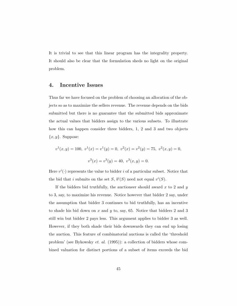
4. Incentive Issues
Thus far we have focused on the problem of choosing an allocation of the ob-
jects so as to maximize the sellers revenue. The revenue depends on the bids
submitted but there is no guarantee that the submitted bids approximate
the actual values that bidders assign to the various subsets. To illustrate
how this can happen consider three bidders, 1, 2 and 3 and two objects
{x, y}. Suppose:
v1(x, y) = 100, v1(x) = v1(y) = 0, v2(x) = v2(y) = 75, v2(x, y) = 0,
v3(x) = v3(y) = 40, v3(x, y) = 0.
Here vi(·) represents the value to bidder i of a particular subset. Notice that
the bid that i submits on the set S, bi(S) need not equal vi(S).
If the bidders bid truthfully, the auctioneer should award x to 2 and y
to 3, say, to maximize his revenue. Notice however that bidder 2 say, under
the assumption that bidder 3 continues to bid truthfully, has an incentive
to shade his bid down on x and y to, say, 65. Notice that bidders 2 and 3
still win but bidder 2 pays less. This argument applies to bidder 3 as well.
However, if they both shade their bids downwards they can end up losing
the auction. This feature of combinatorial auctions is called the ‘threshold
problem’ (see Bykowsky et. al. (1995)): a collection of bidders whose com-
bined valuation for distinct portions of a subset of items exceeds the bid
45
submitted on that subset by some other bidder. It may be difficult for them
to coordinate their bids to outbid the large bidder on that subset.
In this section we describe what is known about auction mechanisms
that give bidders the incentive to truthfully reveal their valuations.
To discuss incentive issues we need a model of bidders preferences. The
simplest conceptual model endows bidder j ∈ N with a list {vj(S)}S⊆M ,
abbreviated to vj , that specifies how she values (monetarily) each subset of
objects. Thus vj(S) represents how much bidder j values the subset S of
objects.19
The auction scheme chosen and the bids submitted will be a function
of the beliefs that seller and bidders have about each other. The simplest
model of beliefs is the independent private values model. Each bidder’s
vj is assumed by seller and all bidders to be an independent draw from a
commonly known distribution over a compact, convex set.20 Bidder j knows
her vj but not the valuations of the other bidders. Last, bidders and seller
are assumed to be risk neutral.
The seller is interested in choosing an auction design that will do three
things:
1. Induce bidders to reveal their actual valuations (incentive compati-
bility).footnoteOne might argue that a seller cares only about revenue
and not whether the bidders truthfully reveal their valuations. The
requirement here is a consequence of using the revelation principle.
2. No bidder is made worse off (in expectation) by participating in the
auction.19In the language of mechanism design, this list of valuations becomes the bidders type.
In this case, since the type is not a single number it is called multi-dimensional.20Williams (1999) obtains similar results under slightly different assumptions.
46
3. Subject to the two conditions above the seller maximizes expected
revenue.
Call the auction design that satisfies these conditions optimal. Finding
the optimal auction appears daunting given the cornucopia of elaborate
schemes with multiple rounds that one can imagine. However the revelation
principle (see Myerson (1981) for an explanation) allows one to concentrate
on auctions with a single round where bidders submit bids and the seller
decides, as a function of the reported bids, who gets what and for how much.
The optimal auction in this general setting is still not known. In Jehiel
et. al. (1999) and Jehiel and Moldovanu (2000) it is shown that the optimal
auction must satisfy conditions involving elaborate partial differential equa-
tions. Levin (1997) identifies the optimal auction under a more restrictive
setting. Specifically, all objects, for all bidders, complement each other and
bidders are perfectly symmetric. In this case, the revenue maximizing auc-
tion is to simply bundle all the objects together and auction the bundle off
using an optimal single item auction.
Krishna and Rosenthal (1996), again with a simplified model of pref-
erences, attempt to make revenue comparisions between different auction
schemes. They consider auctions involving two items where bidders are of
two kinds. One kind, they call local, are interested in receiving a single item.
The other, global, have valuations for the entire set that are superadditive.
In this paper they identify equilibria for two item sequential second-price
auctions, (a particular) simultaneous second-price auctions, and a combi-
natorial second-price auction. The revenues obtained from each auction
(under the identified equilibria) are compared numerically. They observe
that if the synergy is small then the sequential second-price auction gener-
47
ates the largest revenue. For larger synergies the simultaneous second-price
auction generates the largest revenue. In their simulations the combinato-
rial second-price auction always generates the smallest revenue. It is not
not known whether the comparision is a function of the equilibrium found
or the specification of the simultaneous auction.
Cybernomics, Inc. (2000) went a step farther by comparing a simultane-
ous multi-round auction with an multi-round combinatorial auction. They
performed experiments for additive values, and for valuations with syner-
gies of small, medium or high intensity. Their experiments indicate, that
the combinatorial multi-round auction was always superior with respect to
efficency but the revenue was smaller and it took more rounds of longer
duration to finish the auction.
If one is willing to accept an additional restriction, efficiency, then the
optimal auction is known. An auction is efficient if the allocation of objects
to bidders chosen by the seller solves the following:
max∑
j∈N
∑
S⊆Mvj(S)y(S, j)
s.t.∑
S3i
∑
j∈Ny(S, j) ≤ 1 ∀i ∈M
∑
S⊆My(S, j) ≤ 1 ∀j ∈ N
y(S, j) = 0, 1 ∀S ⊆M, j ∈ N
Notice that this is just CAP2 with bi replaced by vi. The optimal objective
function value of this integer program is an upper bound on the revenue
that the seller can achieve. The fact the seller uses an auction that selects
an allocation that solves this integer program does not imply that the seller
48
achieves this revenue.21
It is proved in Krishna and Perry (1997) (see also Williams (1999) for
the same result under slightly different assumptions) that (in the model
described) the optimal auction that is also efficient is what is sometimes
known as as Vickrey-Clarke-Groves (VCG) scheme. It works as follows:
1. Agent j reports vj . There is nothing to prevent agent j from misrep-
resenting themselves. Since the VCG scheme is incentive compatible
this does not happen.
2. The seller chooses the allocation that solves:
V = max∑
j∈N
∑
S⊆Mvj(S)y(S, j)
s.t.∑
S3i
∑
j∈Ny(S, j) ≤ 1 ∀i ∈M
∑
S⊆My(S, j) ≤ 1 ∀j ∈ N
y(S, j) = 0, 1 ∀S ⊆M, j ∈ N
Call this optimal allocation y∗
3. To compute the payment that each bidder must make let, for each
k ∈ N ,
V −k = max∑
j∈N\k
∑
S⊆Mvj(S)y(S, j)
s.t.∑
S3i
∑
j∈N\k
y(S, j) ≤ 1 ∀i ∈M
21In Myerson (1981) it is shown that optimal auction for a single good is not guaranteed
to be efficient. See Jehiel and Moldovanu (1999) for a more pronounced version of the
same.
49
∑
S⊆My(S, j) ≤ 1 ∀j ∈ N \ k
y(S, j) = 0, 1 ∀S ⊆M, j ∈ N \ k
Denote by yk the optimal solution to this integer program. Thus yk is
the efficient allocation when bidder k is excluded.
4. The payment that bidder k makes is equal to
V −k − [V −∑
S⊆Mvk(S)y∗(S, k)].
Thus bidder k’s payment is the difference in ‘welfare’ of the other bid-
ders without him and the welfare of others when he is included in the
allocation. Notice that the payment made by each bidder to the auc-
tioneer is non-negative. This is not true in all economic environments.
If a seller were to adopt the VCG scheme her total revenue would be
∑
k∈NV −k −
∑
k∈N[V −
∑
S⊆Mvk(S)y∗(S, k)]
=∑
k∈N
∑
S⊆Nvk(S)y∗(S, k) +
∑
k∈N(V −k − V )
= V +∑
k∈N(V −k − V ).
If there were a large number of agents then no single agent can have a
significant effect, i.e., one would expect that, on average, V is very close in
value to V −k. Thus the revenue to the seller would be close to V , the largest
possible revenue that any auction could extract. To solidify this intuition
we need that for all agents k that their valuation vk is superadditive, i.e.
vk(A) + vk(B) ≤ vk(A∪B) for all k ∈ N and A,B ⊂M such that A∩B =
50
∅. With this assumption we can find the efficient allocation using CAP1
without the need to introduce dummy goods. Thus:
V = max∑
S⊂M{maxj∈N
vj(S)}xS
s.t.∑
S3ixS ≤ 1 ∀i ∈M
xS = 0, 1 ∀S ⊂M
and
V −k = max∑
S⊂M{ maxj∈N\k
vj(S)}xS
s.t.∑
S3ixS ≤ 1 ∀i ∈M
xS = 0, 1 ∀S ⊂M
Notice now that if the number |N | of bidders is large and given that the vj ’s
live in a compact set, the random variable maxj∈N vj(S) is very close on
average to maxj∈N\k vj(S).22 Hence the objective function of the program
that defines V is essentially the same as the objective function of the integer
program that defines V −k. This argument is made precise in Monderer and
Tennenholtz (1999), where it is shown in the model used here that the VCG
scheme generates a revenue for the seller that is asymptotically close to the
revenue from the optimal auction.
The VCG scheme is clearly impractical to implement, if the number of
bidders is very large. To overcome the computational difficulties one might
replace y∗ and yk for all k ∈ N with approximately optimal solutions. Such
a modification in the scheme need not preserve incentive compatibility. In22In fact the difference of the two is essentially the difference between the first and second
order statistic of a large collection of independent random numbers from a compact set.
51
Lehmann et. al. (1999) such a direction is taken. They solve the embedded
optimization problems using a greedy type algorithm and show that the
resulting scheme is not incentive compatible. However if one is willing to
restrict bidders valuations (drastically) it is possible to generate schemes
based on the greedy algorithm that are incentive compatible. In Lehmann
et. al. (1999) this restriction is called single mindedness. Each bidder values
only one subset and no other.23
Even if one is willing to relax incentive compatibility, an approximate
solution to the underlying optimization problems in the VCG can lead to
other problems. There can be many different solutions to an optimization
problem whose objective function values are within a specified tolerance of
the optimal objective function value. The payments specified by the VCG
scheme are very sensitive to the choice of solution. Thus the choice of ap-
proximate solution can have a significant impact on the payments made by
bidders. This issue is discussed in Johnson et. al. (1997) in the context of
an electricity auction used to decide the scheduling of short term electric-
ity needs. Through simulations they show that variations in near-optimal
schedules that have negligible effect on total system cost can have significant
consequences on the total payments by bidders.
Yet another way in which the computational difficulties can be side
stepped is to ask for auction schemes that give computationally bounded
bidders the incentive to truthfully reveal their valuations. Parkes and Ungar
(2000b), for example attempts to do just this. They propose a method to23 Another restriction that might be fruitful to explore is introduced in Eso and Maskin
(1999) which they call partition preferences. The collection of subsets that a bidder assigns
positive value to form a partition of the set of objects. Note that problem CAP is still
NP-hard under this restriction.
52
adjust the final prices in iBundle towards VCG prices. Under appropriate
conditions on bidder behavior, the method allows iBundle to inherit the
strategy-proofness of the VCG scheme.
Experience with the VCG scheme in field settings is limited. Isaac and
James (1998) report on an experiment using the VCG scheme for a combi-
natorial auction involving three bidders and two objects. On the basis of
their results they argue that the VCG scheme can be operationalized and, in
their words, ‘achieve high allocative efficiency’. In Hobbs et. al. (2000) the
possibility that the VCG scheme is vulnerable to collusion is explored. It
is pointed out by these authors in environments with repeated interactions
that not only are there many opportunities for collusion amongst bidders
but incentive compatibility of the VCG scheme cannot be guaranteed.
5. Computational Experiments and Test Problems
To evaluate the strength of standard methods of combinatorial optimization
we implemented a solver using the branch and bound solver 24 of the CPLEX
6.5 callable library (see ILOG (1997)). We wrote the (straight forward)
program in C++. The running-times we report were obtained on an SGI O2
computer with one MIPS R10000 processor at 175MHz with 192MB of main
memory running IRIX 6.5.5m. This machine is is slightly inferior to the one
used in Sandholm (1999). As test cases25 we considered the same problems
as studied in Sandholm (1999). They belong to four different classes of
distributions:24In fact at all nodes, clique-cuts might be added.25Our problem data are available from http://www-m9.ma.tum.de/~devries/comb_
auction_supplement/.
53
Random: For each bid, pick the number of items randomly from 1, . . . ,m.
Randomly choose that many items without replacement. Pick the
prices randomly from [0, 1].
Weighted Random: As above, but pick the price as a real number be-
tween 0 and the number of items in the bid.
Uniform: Draw the same number of randomly chosen items for each bid.
Pick the prices from [0, 1].
Decay: Give the bid one random item. Then repeatedly add a new random
item with probability α until an item is not added or the bid includes
all m items. Pick the price as a real number between 0 and the number
of items in the bid.
For these experiments we did not throw out duplicate sets. However
for the given parameters duplicate sets occur with very small probability.
No fine tuning of the parameters of libcplex.a was attempted. We used
standard settings only. Our Figures 1, 2, and 3 show the runtimes for CAP1
instances from the same distribution as Sandholm (1999). In fact we use
the same convention as Sandholm (1999) to summarize the data so that
comparisons will be easier.
In Figure 1 we show the logarithm of the runtimes our program needed
to solve instances from the random (left) and weighted random (right) dis-
tribution for different numbers of items and bids. In Figure 2 we show the
logarithm of the runtimes our program needed to solve instances from the
uniform distribution and Figure 3 shows the logarithms of runtimes for the
decay distribution. A comparison with Sandholm’s (1999) result graphs re-
veals that the runtimes with the CPLEX solver (on these instances) are
54
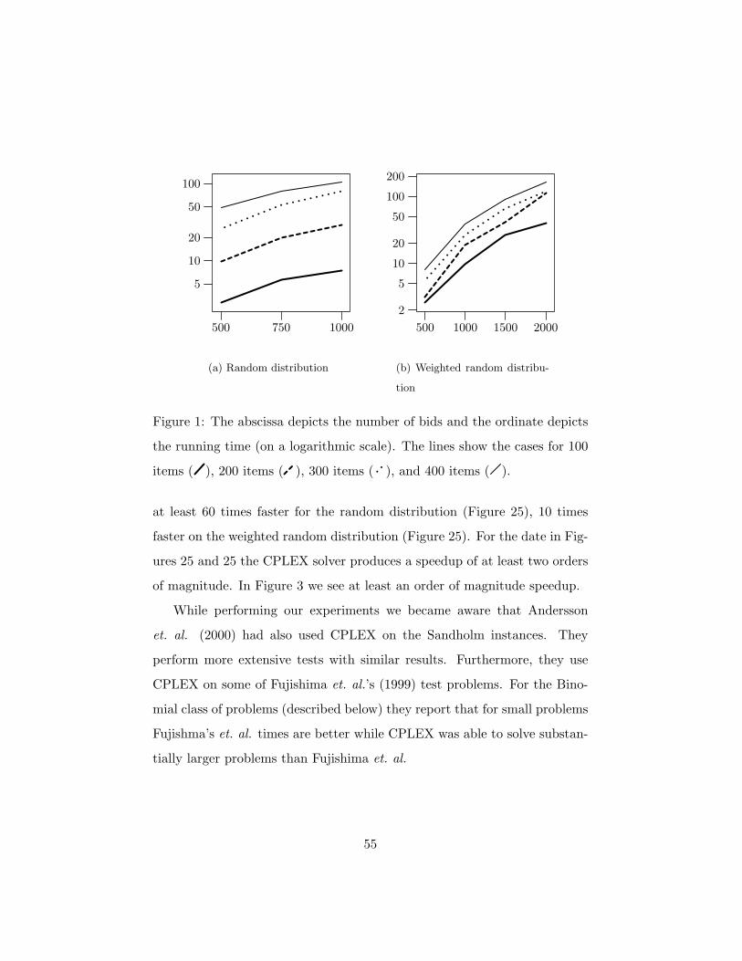
5
10
20
50
100
500 750 1000
(a) Random distribution
2
5
10
20
50
100
200
500 1000 1500 2000
(b) Weighted random distribu-
tion
Figure 1: The abscissa depicts the number of bids and the ordinate depicts
the running time (on a logarithmic scale). The lines show the cases for 100
items ( ), 200 items ( ), 300 items ( ), and 400 items ( ).
at least 60 times faster for the random distribution (Figure 25), 10 times
faster on the weighted random distribution (Figure 25). For the date in Fig-
ures 25 and 25 the CPLEX solver produces a speedup of at least two orders
of magnitude. In Figure 3 we see at least an order of magnitude speedup.
While performing our experiments we became aware that Andersson
et. al. (2000) had also used CPLEX on the Sandholm instances. They
perform more extensive tests with similar results. Furthermore, they use
CPLEX on some of Fujishima et. al.’s (1999) test problems. For the Bino-
mial class of problems (described below) they report that for small problems
Fujishma’s et. al. times are better while CPLEX was able to solve substan-
tially larger problems than Fujishima et. al.
55
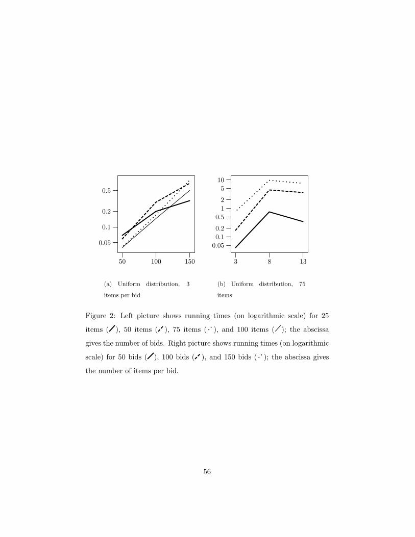
0.05
0.1
0.2
0.5
50 100 150
(a) Uniform distribution, 3
items per bid
0.050.10.2
0.512
510
3 8 13
(b) Uniform distribution, 75
items
Figure 2: Left picture shows running times (on logarithmic scale) for 25
items ( ), 50 items ( ), 75 items ( ), and 100 items ( ); the abscissa
gives the number of bids. Right picture shows running times (on logarithmic
scale) for 50 bids ( ), 100 bids ( ), and 150 bids ( ); the abscissa gives
the number of items per bid.
56
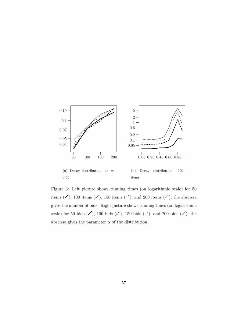
0.040.05
0.07
0.1
0.15
50 100 150 200
(a) Decay distribution, α =
0.55
0.050.10.2
0.512
5
0.05 0.25 0.45 0.65 0.85
(b) Decay distribution, 100
items
Figure 3: Left picture shows running times (on logarithmic scale) for 50
items ( ), 100 items ( ), 150 items ( ), and 200 items ( ); the abscissa
gives the number of bids. Right picture shows running times (on logarithmic
scale) for 50 bids ( ), 100 bids ( ), 150 bids ( ), and 200 bids ( ); the
abscissa gives the parameter α of the distribution.
57
5.1 Test Problems
Performance of an algorithm for CAP1 will depend on the class of test
problems chosen. Thus it is important to know whether good performance
is a function of algorithm design or ‘easy’ problems.
As is pointed out in Andersson et. al. (2000), the random model in
Sandholm (1999) is ‘easy’ when the problems become large. This is because
the bid values assigned to each set are independent draws from the same
distribution. Thus many small sets, in fact singletons, when combined are
likely to generate a higher total revenue than a large set that contains the
same elements.
The weighted random model suffers from the fact that on average the
bid to column sum ratio is constant across columns. This implies that the
model does not capture synergies among the items in a bidset. Further,
for large enough problems, the optimal linear programming solution to the
problem may be integral. In the uniform model bids have no relation to the
size of subsets.
The binomial model of Fujishima et. al. (1999) can be described by
saying that each entry of the constraint matrix of CAP1 is set to one with
a given probability p independently of the others. The bid value of a sub-
set/column is a uniform draw from a distribution whose mean depends on
the size of the corresponding subset. Given the report of Andersson et. al.
this class of problems may be of interest.
None of these schemes is based on a model of how bidders might value
different subsets of objects. For example, each assumes that b(S), the highest
bid on the subset S, is a random draw from a uniform distribution. But,
b(S) = maxj∈N bj(S), i.e. it is the maximum of a collection of numbers.
58
If we assume that each bidder’s bid on S is an independent draw from
some distribution then it is hard to imagine that b(S) will be uniformly
distributed.
Out of curiosity we generated some test problems involving 3 bidders.
Each bidder’s value for a single item was an independent uniform draw from
[0, 1]. Let vjk be the value that bidder j assigns to object k. To capture
complementarities, we assumed the value that bidder j assigns to a subset
S is∑
k∈S vjk +
∑
k 6=q and k,q∈S vjkvjq . Hence, assuming truthful bidding, the
highest bid on subset S is
max1≤j≤3
∑
k∈Svjk +
12
∑
k 6=q and k,q∈Svjkv
jq .
In this experiment we allowed only subsets of size 3 to be bid upon. Fig-
ure 4 reports on the solution times for various numbers of bids on instances
involving 100 objects and uniform sets of size 3. There, the times for prices
according to Sandholms uniform model and our just outlined model (for
three bidders) are compared.
It is not clear from the data that the quadratic prices model is easier or
harder to solve than the uniform model. To see how large a problem one
could solve in the quadratic price model we solved an instance involving 100
items, 3000 bids (each on subsets of size 10) and 3 bidders. On an SGI
Origin 200 computer26 it took 410 minutes.
Motivated by the FCC spectrum auctions (see Ausubel et. al. (1997))
we outline a model, called the Quadratic Model (QM), of how bidders value
different combinations of objects. In the spectrum auctions it was gener-
ally believed that the stand-alone value of a spectrum licence/object was26That has four MIPS R10000 processor at 225MHz, 1GB of main memory running
parallel CPLEX6.5.2.
59
50
100
200
500
1000
500 700 900 1100
Figure 4: The abscissa depicts the number of bids and the ordinate depicts
the mean running time (for 20 examples) (on a logarithmic scale) for 100
objects and uniform bidsets of three items. The lines show the cases for
Sandholm’s prices in the uniform case ( ) and for our quadratic prices for
three bidders and prices drawn uniformly from [0, 1] ( ).
proportional to the population covered by that spectrum licence. To model
this we assign to each object k a value vk which will be an iid draw from a
distribution. This is the stand alone value of object k, which is common to
all bidders.27
Second, as suggested in Ausubel et. al. (1997) if a bidder was interested
in owning two spectrum licenses, the value of owning the two spectrum
licences was proportional to the sum of the populations plus the products
of the populations covered. The product term captures the synergies to be
had from owning a pair of licences. However, these synergies were bidder
specific. We model this feature in two steps.
First for each bidder j we choose a subset M j of objects at random.27In a more elaborate version we could allow each bidders value of object k to be drawn
from a distribution centered at vk.
60
The set M j represents the set of objects that in bidder j’s eyes complement
each other. There are many ways to specify how the M j can be selected.
In some schemes the resulting sets may not overlap very much. In others
they may be small, or mostly large or run the gamut from large to small.
Second, the value to bidder j of the subset S of objects will be∑
k∈S vk +
µj∑
k,q∈S∩Mj vkvq. Here µj is a bidder specific parameter that allows one
to vary the strength of the complementarities.28 In this model, the largest
bid (assuming truthful bidding) on subset S would be
maxj∈N
∑
k∈Svk + µj
∑
k,q∈S∩Mj
vkvq.
The QM model is by no means universally appropriate. In the trans-
portation setting for example, it would make no sense whatsoever. The
value of a set of lanes would depend on the transportation costs incurred to
service those lanes. Complementarities come from combining different lanes
together to reduce travel costs. These complementarities will be bidder spe-
cific in that they may already be servicing some collection of lanes. It is not
hard to propose an alternative model for this set up as well. We do not do
so here. Our goal is only to suggest that the specific application should be
used to guide the model for generating test problems.
5.2 FCC Data
Perhaps the most well known combinatorial auction to be run to date is the
FCC spectrum auction. Data from this auction is available from ftp://ftp.
fcc.gov/pub/Auctions/PCS/Broadband/MTA/Programs/. Since the auc-
tion was run in rounds we have information on the bids submitted by each28The parameters µk should not be set too large since this will bias a solution in favor
of bids on large sets.
61
bidder on each licence. From this we can infer something about the subsets
that each bidder had an interest in. However one can deduce very little
about what bids they might have submitted on a package. In fact in some
preliminary stabs we assigned bids to subsets in various ways (using the
recorded bids as a a starting point) to generate instances of CAP1. All
of these instances solved immediately using CPLEX but this is probably a
function of how we assigned bid values.
Acknowledgements
We thank David Parkes, Sunil Chopra, Michael Rothkopf and John Ledyard
for useful comments.
REFERENCES
A. Andersson, M. Tenhunen and F. Ygge, “Integer Programming for Com-
binatorial Auction Winner Determination”, Proceedings of the Fourth
International Conference on Multi-Agent Systems (ICMAS00), 39–46,
2000.
M. Aourid and B. Kaminska, “Neural Networks for the Set Covering Prob-
lem: An Application to the Test Vector Compaction”, IEEE Interna-
tional Conference on Neural Networks Conference Proceedings, 7, 4645–
4649, 1994.
E. M. Arkin and R. Hassin, “On Local Search for Weighted k-Set Packing”,
Mathematics of Operations Research, 23, 640–648, 1998.
K. Akcoglu, J. Aspnes, B. DasGupta and M. Kao, “An Opportunity-Cost
Algorithm for Combinatorial Auctions”, 2000.
62
L. M. Ausubel, P. Cramton, R. Preston McAfee and J. McMillan, “Synergies
in Wireless Telephony: Evidence from the Broadband PCS Auction”,
Journal of Economics and Management Strategy, 6, 3, 497-527, 1997.
E. Balas, S. Ceria and G. Cornuejols, “A Lift-and-Project Cutting Plane
Algorithm for mixed 0-1 Programs”, Mathematical Programming, 58,
295-324, 1993.
E. Balas and M. C. Carrera, “A Dynamic Subgradient-based Branch-and-
Bound Procedure for Set Covering”, Operations Research, 44, 875–890,
1996.
E. Balas and A. Ho, “Set Covering Algorithms Using Cutting Planes, Heuris-
tics, and Subgradient Optimization: A Computational Study”, Mathe-
matical Programming, 12, 37–60, 1980.
E. Balas and M. W. Padberg, ”Set Partitioning: A Survey”, SIAM Review,
18, 710–760, 1976.
M. O. Ball and M. Magazine, 1981, “The Design and Analysis of Heuristics”,
Networks, 11, 215-219, 1981.
J. S. Banks, J. O. Ledyard and D. P. Porter “Allocating Uncertain and
Unresponsive Resources: An experimental approach”, Rand Journal of
Economics, vol. 20, 1, 1-25, 1989.
C. Barnhart, E. D. Johnson, G. L. Nemhauser, M. W. P. Savelsbergh and
P. H. Vance “Branch and Price: Column Generation for Solving Huge
Integer Programs”, Operations Research, 46, 316–329, 1998.
J. E. Beasley, “A Lagrangian Heuristic for Set-Covering Problems”, Naval
Research Logistics, 37, 151–164, 1990.
D. P. Bertsekas, Linear Network Optimization: Algorithms and Codes, MIT
63
press, Cambridge, MA, 1991.
S. Bikchandani and J. M. Ostroy, “The Package Assignment Model”, manuscript,
1998.
S. Bikchandani and J. Mamer, “Competitive Equilibrium in an Exchange
Economy with Indivisibilities”, Journal of Economic Theory, vol. 74,
no. 2, 385–413, 1997.
P. J. Brewer, “Decentralized Computation Procurement and Computational
Robustness in a Smart Market”, Economic Theory, 13, 41–92, 1999.
M. M. Bykowsky, R. J. Cull and J. O. Ledyard, “Mutually Destructive
Bidding: The FCC Auction Design Problem”, Journal of Regulatory
Economics, 17, 205–228, 2000.
C. G. Caplice, “An Optimization Based Bidding Process: A New Framework
for Shipper-Carrier Relationships”, Thesis in the field of Transportation
and Logistics Systems submitted to the Department of Civil and Envi-
ronmental Engineering, School of Engineering, MIT, June 1996.
Cybernomics, Inc., “An Experimental Comparison of the Simultaneous Mlti-
Round Auction and the CRA Combinatorial Auction”, http://combin.
fcc.gov/98540193.pdf, 2000
G. Cornuejols and A. Sassano, “On the 0-1 Facets of the Set Covering Poly-
tope”, Mathematical Programming, 43, 45–56, 1989.
P. Crescenzi and V. Kann, “A compendium of NP optimization problems”,
http://www.nada.kth.se/theory/compendium/, manuscript, 1998.
G. B. Dantzig, Linear Programming and Extensions, Princeton University
Press, New Jersey, 1963.
C. DeMartini, A. Kwasnica, J. Ledyard and D. Porter, “A New and Im-
64
proved design for Multi-Object Iterative Auctions”, manuscript, 1999.
M. Eso, “Parallel Branch and Cut for Set Partitioning”, Ph.D. thesis, School
of Operations Research and Industrial Engineering, Cornell University,
1999.
P. Eso and E. Maskin, “Multi-Good Efficient Auctions with Multi-Dimensional
Information”, manuscript, 1999.
A. Feo, G. C. Mauricio and A. Resende, “A Probabilistic Heuristic for a
Computationally Difficult Set Covering Problem”, Operations Research
Letters, 8, 67–71, 1989.
M. Fisher and L. Wolsey “On the Greedy Heuristic for Continuous Cover-
ing and Packing Problems”, SIAM Journal on Algebraic and Discrete
Methods, 3, 584–591, 1982.
Y. Fujishima, K. Leyton-Brown and Y. Shoham, “Taming the Computa-
tional Complexity of Combinatorial Auctions: Optimal and Approxi-
mate Approaches”, Proceedings of IJCAI-99, Stockholm, 1999.
M. Grotschel, L. Lovasz and A. Schrijver, Geometric Algorithms and Com-
binatorial Optimization, Springer-Verlag, 1988.
P. C. Gilmore and R. E. Gomory, “A Linear Programming Approach to the
Cutting Stock Problem”, Operations Research, 9, 849–859, 1961.
M. C. Golumbic and P. L. Hammer, “Stability in circular arc graphs”, J.
Algorithms, 9, 314–320, 1988.
F. Gul and E. Stachetti, “English and Double Auctions with Differentiated
Commodities”, Journal of Economic theory, 92, 66–95, 2000.
J. Hastad, “Clique is hard to approximate within n1−ε”, Acta Mathematica,
to appear.
65
B. F. Hobbs, M. Rothkopf, L. Hyde and R. P. O’Neill, “Evaluation of a
Truthful Revelation Auction in the Context of Energy markets with Non-
concave Benefits”, Journal of Regulatory Economics, 18, 5–32, 2000.
S. van Hoesel and R. Muller, “Optimization in Electronic Markets: Exam-
ples in Combinatorial Auctions”, Netnomics, forthcoming, 2000.
K. Hoffman and M. W. Padberg, “Solving Airline Crew Scheduling Problems
by Branch and Cut”, Management Science, 39, 657–682, 1993.
W. C. Huang, C. Y. Kao, and J. T. Hong, “A genetic algorithm for set cov-
ering problems”, IEEE International Conference on Genetic Algorithms:
Proceedings, 569–574, 1994.
C. A. J. Hurkens and A. Schrijver, “On the size of systems of sets every t
of which have an SDR, with an application to the worst–case ratio of
heuristic problems”, SIAM Journal on Discrete Math., 2, 68–72, 1989.
ILOG Inc. CPLEX Division, 930 Tahoe Blvd. # 802-279, Incline Village,
NV 89451-9436, USA, “Using the CPLEX Callable Library” (informa-
tion available at URL http://www.cplex.com) 1997.
R. Mark Isaac and D. James, “Robustness of the Incentive Compatible Com-
binatorial Auction”, manuscript, 1998.
C. Jackson, “Technology for Spectrum Markets”, Ph. D. Thesis submit-
ted to the Department of Electrical Engineering, School of Engineering,
MIT, June 1976.
P. Jehiel, B. Moldovanu and E. Stacchetti, “Multidimensional Mechanism
Design for Auctions with Externalities”, Journal of Economic Theory
85(2), 258-294, 1999.
P. Jehiel, B. Moldovanu, “Efficient Design with Inderdependent Valuations”,
66
discussion paper, University of Mannheim, 2000.
P, Jehiel and B. Moldovanu, “A Note on Revenue Maximization and Effi-
ciency in Multi-Object Auctions”, discussion paper, University College
London, 1999.
R. B. Johnson, S. S. Oren, and A. J. Svoboda, “Equity and Efficiency of
Unit Commitment in Competitive Electricity Markets”, Utilities Policy,
6(1), 9-20, 1997.
A. S. Kelso and V. P. Crawford, “Job matching, Coalition Formation and
Gross Substitutes”, Econometrica, 50, 1483–1504, 1982.
F. Kelly and R. Steinberg, “A Combinatorial Auction with Multiple Winners
for Universal Service”, Management Science, 46(4), 586–596, 2000.
V. Krishna and M. Perry, “Efficient Mechanism Design”, manuscript, 1998.
V. Krishna and R. W. Rosenthal, “Simultaneous Auctions with Synergies”,
Games and Economic Behavior, 17, 1–31, 1996.
D. Lehmann, L. O’Callaghan and Y. Shoham, “Truth Revelation in Rapid,
Approximately Efficient Combinatorial Auctions”, manuscript, 1999.
J. Levin, “An Optimal Auction for Complements”, Games and Economic
Behavior, 18, 176-192, 1997.
K. Leyton-Brown, Y. Shoham and M. Tennenholtz, “An Algorithm for
Multi-Unit Combinatorial Auctions”, Proceedings of the Seventeenth Na-
tional Conference on Artificial Intelligence and Twelfth Conference on
Innovative Applications of Artificial Intelligence, 2000.
P. Milgrom, “Auctioning the Radio Spectrum” in Auction Theory for Pri-
vatization, Cambridge University Press, 1995.
67
D. Monderer and M. Tennenholtz, “Asymptotically Optimal Multi-Object
Auctions for Risk-Averse Agents”, manuscript, 2000.
R. Myerson, “Optimal Auction Design”, Mathematics of Operations Re-
search, 6, 58-73, 1981.
G. L. Nemhauser and L. A. Wolsey, Integer and Combinatorial Optimiza-
tion, John Wiley, New York, 1998.
N. Nisan, “Bidding and Allocation in Combinatorial Auctions”, to appear
in EC2000, 2000.
M. W. Padberg, “On the facial structure of set packing polyhedra”, Math-
ematical Programming, 5, 199–215, 1973.
M. W. Padberg, “Perfect zero-one matrices”, Mathematical Programming,
6, 180–196, 1974.
M. W. Padberg “On the complexity of the set packing polyhedra”, Annals
of Discrete Mathematics 1, 421–434, 1975.
M. W. Padberg, “Covering, Packing and Knapsack Problems”, Annals of
Discrete Mathematics, 4, 265-287, 1979.
M. Parker and J. Ryan “A column generation algorithm for bandwidth pack-
ing”, Telecommunications Systems, 2, 185–196, 1994.
D. C. Parkes, “iBundle: An Efficient Ascending Price Bundle Auction”,
Proceedings ACM Conference on Electronic Commerce (EC-99), Denver,
148–157, November 1999.
D. C. Parkes and L. Ungar, “Iterative Combinatorial Auctions: Theory and
Practice”, Proceedings 17th Nat. Conf. on Artificial Intelligence, 74–81,
2000(a).
68
D. C. Parkes and L. Ungar, “Preventing Strategic Manipulation in Iterative
Auctions: proxy Agents and Price Adjustment”, Proceedings 17th Nat.
Conf. on Artificial Intelligence, 82–89, 2000 (b).
A. Sassano, “On the Facial Structure of the Set Covering Polytope”, Math-
ematical Programming, 44, 181–202, 1973.
S. J. Rassenti, V. L. Smith and R. L. Bulfin, “A Combinatorial Auction
Mechanism for Airport Time Slot Allocation”, Bell Journal of Eco-
nomics, vol. 13, No. 2, 402–417, 1982.
M. H. Rothkopf, A. Pekec and R. M. Harstad, “Computationally Manage-
able Combinatorial Auctions”, Management Science, vol. 44, No. 8,
1131–1147, 1998.
T. Sandholm, “An Algorithm for Optimal Winner Determination in Com-
binatorial Auctions”, Proceedings of IJCAI-99, Stockholm, 1999.
A. Schrijver, Theory of Linear and Integer Programming, John Wiley, New
York, 1986.
M. P. Wellman, W. E. Walsh, P. R. Wurman and J. K. MacKie-Mason,
“Auction Protocols for Decentralized Scheduling”, manuscript, 1998.
S. R. Williams, “A Characterization of Efficient, Bayesian Incentive Com-
patible Mechanisms”, Economic Theory, vol. 14, 155–180, 1999.
L. Wolsey, “Integer Programming Duality: Price Functions and Sensitivity
Analysis”, Mathematical Programming, vol. 20, 173–195, 1981.
69
Related Documents