Color Constancy Beyond Bags of Pixels - Harvard University

Color Constancy Beyond Bags of Pixels

Ayan Chakrabarti Keigo Hirakawa Todd ZicklerHarvard School of Engineering and Applied Sciences

[email protected] [email protected] [email protected]

Abstract

Estimating the color of a scene illuminant often plays acentral role in computational color constancy. While thisproblem has received significant attention, the methods thatexist do not maximally leverage spatial dependencies be-tween pixels. Indeed, most methods treat the observed color(or its spatial derivative) at each pixel independently ofits neighbors. We propose an alternative approach to illu-minant estimation—one that employs an explicit statisticalmodel to capture the spatial dependencies between pixelsinduced by the surfaces they observe. The parameters ofthis model are estimated from a training set of natural im-ages captured under canonical illumination, and for a newimage, an appropriate transform is found such that the cor-rected image best fits our model.

1. IntroductionColor is useful for characterizing objects only if we have

a representation that is unaffected by changes in scene illu-mination. As the spectral content of an illuminant changes,so does the spectral radiance emitted by surfaces in a scene,and so do the spectral observations collected by a tri-chromatic sensor. For color to be of practical value, werequire the ability to compute color descriptors that are in-variant to these changes.

As a first step, we often consider the case in whichthe spectrum of the illumination is uniform across a scene.Here, the task is to compute a mapping from an input colorimage y(n) to an illuminant-invariant representation x(n).What makes the task difficult is that we do not know theinput illuminant a priori.

The task of computing invariant color representationshas received significant attention under a variety of titles,including color constancy, illuminant estimation, chromaticadaptation, and white balance. Many methods exist, andalmost all of them leverage the assumed independence ofeach pixel. According to this paradigm, spatial informationis discarded, and each pixel in a natural image is modeled asan independent draw. The well-known grey world hypoth-

(a) (b)

0 0.05 0.1 0.15 0.2 0.25 0.3 0.350

0.05

0.1

0.15

0.2

0.25

0.3

0.35

Red

Gre

en

0 0.05 0.1 0.15 0.2 0.25 0.3 0.35 0.40

0.05

0.1

0.15

0.2

0.25

0.3

0.35

0.4

Red

Gre

en

(c) (d)

−0.25 −0.2 −0.15 −0.1 −0.05 0 0.05 0.1 0.15 0.2 0.25

−0.25

−0.2

−0.15

−0.1

−0.05

0

0.05

0.1

0.15

0.2

0.25

Red

Gre

en

−0.2 −0.15 −0.1 −0.05 0 0.05 0.1 0.15 0.2

−0.2

−0.15

−0.1

−0.05

0

0.05

0.1

0.15

0.2

Red

Gre

en

(e) (f)Figure 1. Color distributions under changing illumination. Im-ages (a,b) were generated synthetically from a hyper-spectral re-flectance image[12], standard color filters and two different illumi-nant spectra. Above are scatter plots for the red and green values of(c,d) individual pixels; and (e,f) 8×8 image patches projected ontoa particular spatial basis vector. Black lines in (c-f) correspond tothe illuminant direction. The distribution of individual pixels doesnot disambiguate between dominant colors in the image and thecolor of the illuminant.

esis is a good example; it simply states that the expectedreflectance in an image is achromatic [14]. A wide vari-ety of more sophisticated techniques take this approach aswell. Methods based on the dichromatic model [10], gamutmapping [8, 11], color by correlation [9], Bayesian infer-ence [1], neural networks [3], and the grey edge hypothe-

sis [18] are distinct in terms of the computational techniquesthey employ, but they all discard spatial information and ef-fectively treat images as “bags of pixels.”

Bag-of-pixels methods depend on the statistical distribu-tions of individual pixels and ignore their spatial contexts.Such distributions convey only meager illuminant informa-tion, however, because the expected behavior of the mod-els is counterbalanced by the strong dependencies betweennearby pixels. This is demonstrated in Figure 1(c,d), forexample, where it is clearly difficult to infer the illuminantdirection with high precision.

In this paper, we break from the bag-of-pixels paradigmby building an explicit statistical model of the spatial depen-dencies between nearby image points. These image depen-dencies echo those of the spatially-varying reflectance[17]of an observed scene, and we show that they can be ex-ploited to distinguish the illuminant from the natural vari-ability of the scene (Figure 1(e,f)).

We describe an efficient method for inferring scene il-lumination by examining the statistics of natural color im-ages in the spatio-spectral sense. These statistics are learnedfrom images collected under a known illuminant. Then,given an input image captured under a unknown illuminant,we can map it to its invariant (canonical) representation byfitting it to the learned model. Our results suggest that ex-ploiting spatial information in this way can significantly im-prove our ability to achieve chromatic adaptation.

The rest of this paper is organized as follows. We be-gin with a brief review of a standard color image formationmodel in Section 2. A statistical model for a single color im-age patch is introduced in Section 3, and the optimal correc-tive transform for the illuminant is found via model-fittingin Section 4. The proposed model is empirically verifiedusing available training data in Section 5.

2. Background: Image FormationWe assume a Lambertian model where x : R × Z

2 →[0, 1] is the diffuse reflectivity of a surface correspondingto the image pixel location n ∈ Z

2 as a function of theelectromagnetic wavelength λ ∈ R in the visible range. Thetri-stimulus value recorded by a color imaging device is

y(n) =

∫

f(λ)`(λ)x(λ, n) dλ, (1)

where y(n) = [y{1}(n), y{2}(n), y{3}(n)]T is the tri-stimulus (e.g. RGB) value at pixel location n cor-responding to the color matching functions f(λ) =[f{1}(λ), f{2}(λ), f{3}(λ)]T , f{1}, f{2}, f{3} : R →[0, 1], and ` : R → R is the spectrum of the illuminant.

Our task is to map a color image y(n) taken under anunknown illuminant to an illuminant-invariant representa-

tion x(n)1. In general, this computational chromatic adap-tation problem is ill-posed. To make it tractable, we makethe standard assumption that the mapping from y to x isalgebraic/linear; and furthermore, that it is a diagonal trans-form (in RGB or some other linear color space[7]). This as-sumption effectively imposes joint restrictions on the colormatching functions, the scene reflectivities, and the illumi-nant spectra[5, 19]. Under this assumption of (generalized)diagonal transforms, we can write:

y(n) = Lx(n), (2)

where L = diag(`), ` ∈ R3, x(n) =

[x{1}(n) x{2}(n) x{3}(n)]T ∈ [0, 1]3, and f is im-plicit in the algebraic constraints imposed.

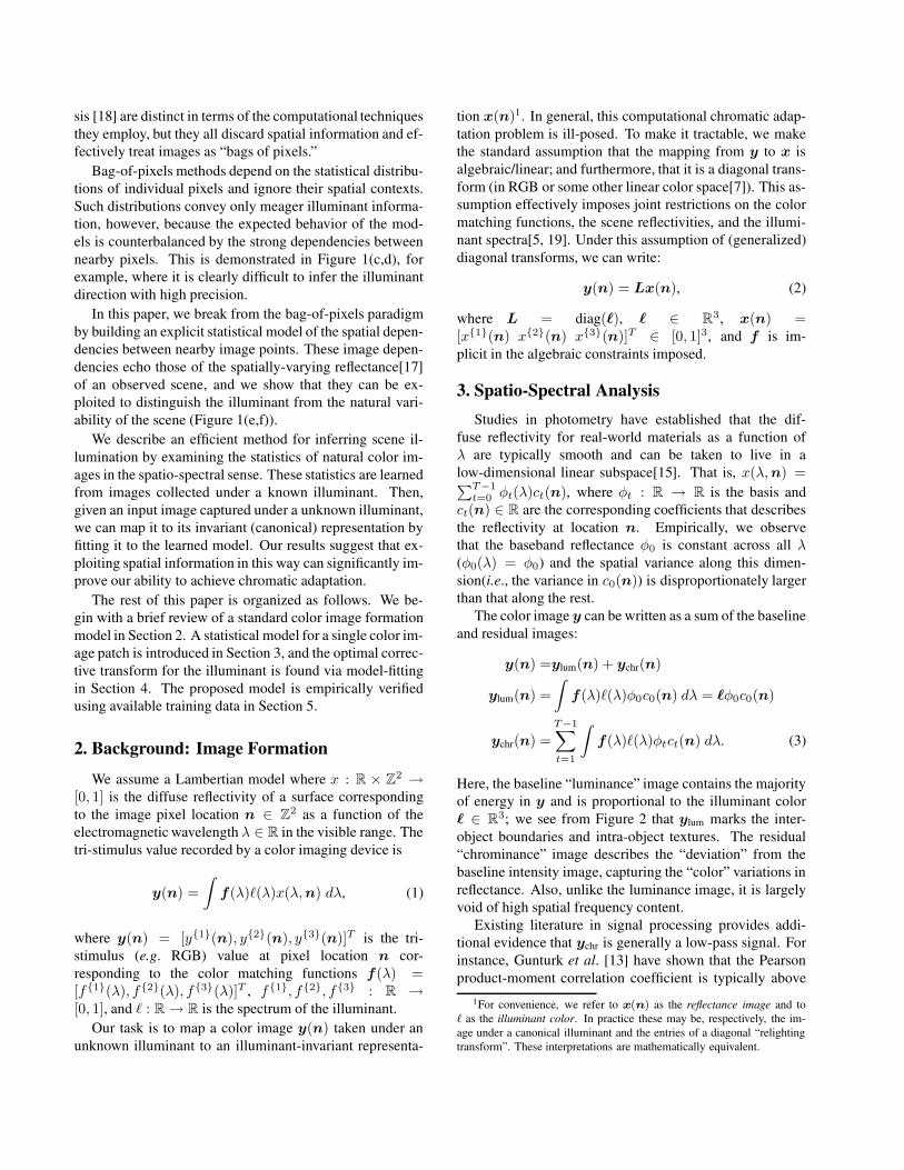
3. Spatio-Spectral AnalysisStudies in photometry have established that the dif-

fuse reflectivity for real-world materials as a function ofλ are typically smooth and can be taken to live in alow-dimensional linear subspace[15]. That is, x(λ, n) =∑T−1

t=0 φt(λ)ct(n), where φt : R → R is the basis andct(n) ∈ R are the corresponding coefficients that describesthe reflectivity at location n. Empirically, we observethat the baseband reflectance φ0 is constant across all λ(φ0(λ) = φ0) and the spatial variance along this dimen-sion(i.e., the variance in c0(n)) is disproportionately largerthan that along the rest.

The color image y can be written as a sum of the baselineand residual images:

y(n) =ylum(n) + ychr(n)

ylum(n) =

∫

f(λ)`(λ)φ0c0(n) dλ = `φ0c0(n)

ychr(n) =T−1∑

t=1

∫

f(λ)`(λ)φtct(n) dλ. (3)

Here, the baseline “luminance” image contains the majorityof energy in y and is proportional to the illuminant color` ∈ R

3; we see from Figure 2 that ylum marks the inter-object boundaries and intra-object textures. The residual“chrominance” image describes the “deviation” from thebaseline intensity image, capturing the “color” variations inreflectance. Also, unlike the luminance image, it is largelyvoid of high spatial frequency content.

Existing literature in signal processing provides addi-tional evidence that ychr is generally a low-pass signal. Forinstance, Gunturk et al. [13] have shown that the Pearsonproduct-moment correlation coefficient is typically above

1For convenience, we refer to x(n) as the reflectance image and to` as the illuminant color. In practice these may be, respectively, the im-age under a canonical illuminant and the entries of a diagonal “relightingtransform”. These interpretations are mathematically equivalent.

Figure 2. Decomposition of (left column) a color image y into(middle column) luminance ylum and (right column) chrominanceychr components. Log-magnitude of the Fourier coefficients in(bottom row) correspond to the images in (top row), respectively.Owing to the edge and texture information that comprise lumi-nance image, luminance dominates chrominance in the high-passcomponents of y.

0.9 for high-pass components of y{1}, y{2}, and y{3}—suggesting that ylum dominates high-pass components of y.Figure 2 also illustrates Fourier support of a typical colorimage taken under a canonical illuminant, clearly confirm-ing the band-limitedness of ychr. These observations areconsistent with the contrast sensitivity function of humanvision[14] (but see [16]) as well as the notion that the scenereflectivity x(λ, n) is spatially coherent, with a high con-centration of energy at low spatial frequencies.

All of this suggests that decomposing images by spa-tial frequency can aid in illuminant estimation. High-passcoefficients of an image y will be dominated by contribu-tions from the luminance image ylum, and the contributionof ychr (and thus the scene chrominance xlum) will be lim-ited. Since the luminance image ylum provides direct infor-mation about the illuminant color (equation (3)), so too willthe high-pass image coefficients. This is demonstrated inFigure 1(e,f), which shows the color of 8× 8 image patchesprojected onto a high-pass spatial basis function.

In subsequent sections, we develop a method to exploitthe ‘extra information’ available in (high-pass coefficientsof) spatial image patches.

3.1. Statistical ModelWe seek to develop a statistical model for a

√K ×

√K

patch where X{1}, X{2} and X{3} ∈ RK are cropped

from x{1}(n), x{2}(n) and x{3}(n) respectively. Ratherthan using a general model for patches of size

√K×

√K×

3, we employ a spatial decorrelating basis and representsuch patches using a mutually independent collection of Kthree-vectors in terms of this basis. We use the discrete co-sine transform(DCT) here, but the discrete wavelet trans-form(DWT), steerable pyramids, curvelets, etc. are othercommon transform domains that could also be used. Thisgives us a set of basis vectors {Dk}k=0...(K−1) ∈ R

K

where without loss of generality, D0 can be taken to cor-

k = 1

k = 9

k = 59

Figure 3. Eigen-vectors of the covariance matrices Λk. The pat-tern in each patch corresponds to a basis vector used for spatialdecorrelation (in this case a DCT filter) and the colors representthe eigen-vectors of the corresponding Λk. The right-most col-umn contains the most significant eigen-vectors that are found tobe achromatic.

respond to the lowest frequency component or DC.By using this decorrelating basis, modeling the distri-

bution of color image patches X reduces to modeling thedistribution of three-vectors D

Tk X ∈ R

3, ∀k, where Dk

computes the response of each of X{1}, X{2} and X{3} toDk such that

DTk X =

DTk

DTk

DTk

X{1}

X{2}

X{3}

=

DTk X{1}

DTk X{2}

DTk X{3}

. (4)

The DC component for natural images is known to havenear uniform distributions[4]. The remaining componentsare modeled as Gaussian. Formally,

DT0 X

i.i.d.∼ U(νmin × νmax)

DTk X

i.i.d.∼ N (0,Λk), k > 0, (5)

where Λk = E[DTk XXT Dk], and [νmin, νmax] is the range

of the DC coefficients. The probability of the entire re-flectance image patch is then given by

P (X) ∝∏

k>0

1

det(Λk)1/2exp

(

−1

2(DT

k X)TΛ

−1k D

Tk X

)

.

(6)We can gain further insight from looking at the sam-

ple covariance matrices {Λk} computed from a set of nat-ural images taken under a single (canonical) illuminant.The eigenvectors of Λk represent directions in tri-stimulusspace, and Figure 3 visualizes these directions for threechoices of k. For all K > 0 we find that the most signif-icant eigenvector is achromatic, and that the correspondingeigenvalue is significantly larger than the other two. Thisis consistent with the scatter plots in Figure 1, where thedistributions have a highly eccentric elliptical shape that isaligned with the illuminant direction.

4. Estimation AlgorithmIn the previous section, a statistical model for a single

color patch was proposed. The parameters of this modelcan be learned, for example, from a training set of naturalimages with a canonical illumination. In this section, wedevelop a method for color constancy that breaks an imageinto a “bag of patches” and then attempts to fit these patchesto such a learned model.

Let diag(w), w = [1/`{1} 1/`{2} 1/`{3}] represent thediagonal transform that maps the observed image to thereflectance image (or image under a canonical illumina-tion). Dividing the observed image into a set of overlappingpatches {Yj}, we wish to find the set of patches {X̂j(w)}that best fit the learned model from the previous section (interms of log-likelihood) such that ∀j, X̂j is related to Yj as

X̂j(w) =

[

w{1}Y{1}

j

Tw{2}Y

{2}j

Tw{3}Y

{3}j

T]T

. (7)

We choose to estimate w by model-fitting as follows:

w = arg maxw′

∑

j

log P(

X̂j (w′))

. (8)

It is clear that (8) always admits the solution w = 0. Wetherefore add the constraint that wT w = 3 (so that w =[1 1 1]T when Y is taken under canonical illumination).

This constrained optimization problem admits a closedform solution. To see this, let the eigen-vectorsand eigen-values for Λk be given by {Vkh =

[V{1}kh V{2}

kh V{3}kh ]}h={1,2,3} and {σ2

kh}h={1,2,3} respec-tively. Then equation (8) simplifies as

w = argminw′

∑

j,k>0,h

1

2σ2kh

(

w′{1}V{1}kh DT

k Y{1}

j

+w′{2}V{2}kh DT

k Y{2}

j + w′{3}V{3}kh DT

k Y{3}

j

)2

= argminw′

∑

j,k>0,h

1

2σ2kh

w′T ajkhaTjkhw′

= argminw′

w′T Aw′, (9)

subject to wT w = 3, where

ajkh =[

V{1}kh DT

k Y{1}

j V{2}kh DT

k Y{2}

j V{3}kh DT

k Y{3}

j

]T

A =∑

j,k>0,h

ajkhaTjkh

2σ2kh

. (10)

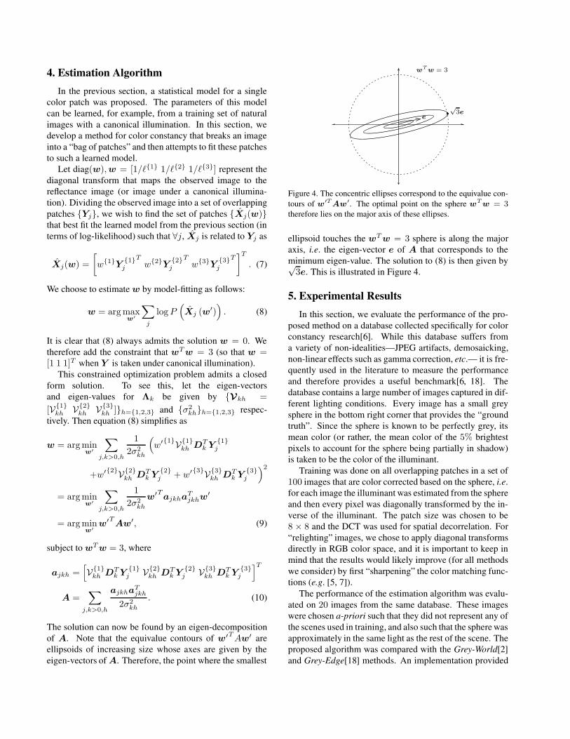
The solution can now be found by an eigen-decompositionof A. Note that the equivalue contours of w′T Aw′ areellipsoids of increasing size whose axes are given by theeigen-vectors of A. Therefore, the point where the smallest

��√

3e

wT

w = 3

e

Figure 4. The concentric ellipses correspond to the equivalue con-tours of w′T Aw′. The optimal point on the sphere wT w = 3

therefore lies on the major axis of these ellipses.

ellipsoid touches the wT w = 3 sphere is along the majoraxis, i.e. the eigen-vector e of A that corresponds to theminimum eigen-value. The solution to (8) is then given by√

3e. This is illustrated in Figure 4.

5. Experimental ResultsIn this section, we evaluate the performance of the pro-

posed method on a database collected specifically for colorconstancy research[6]. While this database suffers froma variety of non-idealities—JPEG artifacts, demosaicking,non-linear effects such as gamma correction, etc.— it is fre-quently used in the literature to measure the performanceand therefore provides a useful benchmark[6, 18]. Thedatabase contains a large number of images captured in dif-ferent lighting conditions. Every image has a small greysphere in the bottom right corner that provides the “groundtruth”. Since the sphere is known to be perfectly grey, itsmean color (or rather, the mean color of the 5% brightestpixels to account for the sphere being partially in shadow)is taken to be the color of the illuminant.

Training was done on all overlapping patches in a set of100 images that are color corrected based on the sphere, i.e.for each image the illuminant was estimated from the sphereand then every pixel was diagonally transformed by the in-verse of the illuminant. The patch size was chosen to be8 × 8 and the DCT was used for spatial decorrelation. For“relighting” images, we chose to apply diagonal transformsdirectly in RGB color space, and it is important to keep inmind that the results would likely improve (for all methodswe consider) by first “sharpening” the color matching func-tions (e.g. [5, 7]).

The performance of the estimation algorithm was evalu-ated on 20 images from the same database. These imageswere chosen a-priori such that they did not represent any ofthe scenes used in training, and also such that the sphere wasapproximately in the same light as the rest of the scene. Theproposed algorithm was compared with the Grey-World[2]and Grey-Edge[18] methods. An implementation provided

(a)10.4◦ 3.3◦ 0.98◦

(b)3.1◦ 8.1◦ 1.5◦

(c)4.1◦ 5.5◦ 1.2◦

(d)0.55◦ 0.48◦ 1.7◦

Un-processed Image Grey World Grey Edge Proposed MethodFigure 5. A selection of images from the test set corrected by different methods with the corresponding angular errors.

# Grey-World[2] Grey-Edge[18] Proposed1 7.4◦ 5.9◦

2.5◦

2 4.1◦ 5.5◦1.2◦

3 10.4◦ 3.3◦0.98

◦

4 3.1◦ 8.1◦1.5◦

5 11.3◦ 1.8◦0.31

◦

6 4.3◦ 1.8◦0.90

◦

7 2.2◦ 4.2◦1.4◦

8 4.4◦ 1.9◦1.2◦

9 3.3◦ 1.7◦1.1◦

10 2.6◦ 0.91◦0.42

◦

11 4.4◦ 1.9◦1.7◦

12 2.5◦ 3.6◦ 2.6◦

13 2.4◦2.1◦ 2.6◦

14 4.6◦0.80

◦ 1.4◦

15 14.7◦6.8◦ 7.7◦

16 7.2◦2.2◦ 3.1◦

17 13.7◦0.96

◦ 1.9◦

18 6.9◦3.1◦ 4.3◦

19 0.55◦0.48

◦ 1.7◦

20 3.9◦0.08

◦ 2.2◦

Mean 5.7◦ 2.9◦2.0◦

Table 1. Angular errors for different color constancy algorithms.

by the authors of [18] was used for both these methods,and for Grey-Edge the parameters that were described in[18] to perform best were chosen (i.e. second-order edges,a Minkowski norm of 7 and a smoothing standard devia-

tion of 5). For all algorithms, the right portion of the imagewas masked out so that the sphere would not be included inthe estimation process. The angular deviation of the spherecolor in the corrected image from [1 1 1]T was chosen asthe error metric.

Table 1 shows the angular errors for each of the threealgorithms for all images . The proposed method does bet-ter than Grey-World in 17 and better than Grey-Edge in 12of the 20 images. Some of the actual color corrected im-ages are shown in Figure 5. In Figure 5(a-c), the proposedmethod outperforms both Grey-World and Grey-Edge. Inthe first case, we see that since the image has green as a verydominant color, Grey-World performs poorly and infers theilluminant to be green. For images (b) and (c), there aremany edges (e.g. the roof in (c)) with the same color distri-bution across them, and this causes the Grey-Edge methodto perform poorly. In both cases, the proposed method ben-efits from spatial correlations and cues from complex imagefeatures. In Figure 5(d), both Grey-World and Grey-Edge dobetter than the proposed method. This is because most of

k=1 k=9 k=59 GW GE Proposed0

5

10

15An

gula

r Erro

r in

Degr

ees

Figure 6. This box-plot summarizes the performance of three in-dividual spatial components (Dk), showing the median and quan-tiles of angular errors across the test set. These are also comparedto the Grey World(GW) and Grey Edge(GE) algorithms, and theproposed method that combines cues from all spatial components.The proposed method performs best—having the lowest averageerror as well as the smallest variance.

the objects in the scene are truly achromatic (i.e. their truecolor is grey/white/black) and therefore the image closelysatisfies the underlying hypothesis for those algorithms.

Finally, the performance of each individual spatial sub-band component was evaluated. That is, we observed howwell the proposed method performed when estimating w

using the statistics of each DkY j alone, for every k. Figure6 shows a box-plot summarizing the angular errors acrossthe test set for three representative values of k and comparesthem with the Grey-World and Grey-Edge algorithm as wellas the proposed method which combines all components.Each single component outperforms Grey-World and someare comparable to Grey-Edge. The proposed method, whichuses a statistical model to weight and combine cues from allcomponents, performs best.

6. Conclusion and Future WorkIn this paper, we presented a novel solution to the com-

putational chromatic adaptation task through an explicit sta-tistical modeling of the spatial dependencies between pix-els. Local image features are modeled using a combina-tion of spatially decorrelating transforms and an evalua-tion of the spectral correlation in this transform domain.The experimental verifications suggest that this joint spatio-spectral modeling strategy is effective.

The ideas explored in this paper underscores the benefitsto exploiting spatio-spectral statistics for color constancy.We expect further improvements from a model based onheavy-tailed probability distribution functions for the trans-form coefficients. Also, many bag-of-pixel approaches tocolor constancy can be adapted to use bags of patches in-stead, especially Bayesian methods [1] that fit naturally intoour statistical framework. Examining spatially-varying illu-

mination is also within the scope of our future work.

AcknowledgmentsThe authors thank Dr. H.-C. Lee for useful discussions, and the

authors of [6, 12, 18] for access to their databases and code.

References[1] D. Brainard and W. Freeman. Bayesian color constancy. J.

of the Optical Soc. of Am. A, 14(7):1393–1411, 1993.[2] G. Buchsbaum. A spatial processor model for object colour

perception. J. Franklin Inst., 310(1):1–26, 1980.[3] V. Cardei, B. Funt, and K. Barnard. Estimating the scene

illumination chromaticity using a neural network. J. of theOptical Soc. of Am. A, 19(12):2374–2386, 2002.

[4] A. Chakrabarti and K. Hirakawa. Effective Separation ofSparse and Non-Sparse Image Features for Denoising. InProc. ICASSP, 2008.

[5] H. Chong, S. Gortler, and T. Zickler. The von Kries hypoth-esis and a basis for color constancy. In Proc. ICCV, 2007.

[6] F. Ciurea and B. Funt. A Large Image Database for ColorConstancy Research. In Proc. IS&T/SID Color ImagingConf., pages 160–164, 2003.

[7] G. Finlayson, M. Drew, and B. Funt. Diagonal transformssuffice for color constancy. In Proc. ICCV, 1993.

[8] G. Finlayson and S. Hordley. Gamut constrained illumina-tion estimation. Intl. J. of Comp. Vis., 67(1):93–109, 2006.

[9] G. Finlayson, S. Hordley, and P. M. Hubel. Color by cor-relation: A simple, unifying framework for color constancy.IEEE Trans. PAMI, 23(11):1209–1221, 2001.

[10] G. Finlayson and G. Schaefer. Convex and non-convex il-luminant constraints for dichromatic colour constancy. InProc. CVPR, 2001.

[11] D. Forsyth. A novel algorithm for color constancy. Intl. J. ofComp. Vis., 5(1), 1990.

[12] D. Foster, S. Nascimento, and K. Amano. Information limitson neural identification of colored surfaces in natural scenes.Visual Neuroscience, 21(03):331–336, 2005.

[13] B. K. Gunturk, Y. Altunbasak, and R. M. Mersereau. Colorplane interpolation using alternating projections. IEEETrans. Image Processing, 11(9):997–1013, 2002.

[14] E. Land. The retinex theory of colour vision. In Proc. R.Instn. Gr. Br., volume 47, pages 23–58, 1974.

[15] H.-C. Lee. Introduction to Color Imaging Science. Camb.Univ. Press, 2005.

[16] C. Parraga, G. Brelstaff, T. Troscianko, and I. Moorehead.Color and luminance information in natural scenes. J. of theOptical Soc. of Am. A, 15(3):563–569, 1998.

[17] B. Singh, W. Freeman, and D. Brainard. Exploiting Spatialand Spectral Image Regularities for Color Constancy. Work-shop on Stat. and Comp. Theories of Vis., 2003.

[18] J. van de Weijer, T. Gevers, and A. Gijsenij. Edge-Based Color Constancy. IEEE Trans. on Image Processing,16(9):2207–2214, 2007.

[19] G. West and M. H. Brill. Necessary and sufficient conditionsfor von kries chromatic adaptation to give color constancy. J.of Math. Bio., 15(2):249–258, 1982.