Color Appearance Models Second Edition Mark D. Fairchild Munsell Color Science Laboratory Rochester Institute of Technology, USA

Welcome message from author
This document is posted to help you gain knowledge. Please leave a comment to let me know what you think about it! Share it to your friends and learn new things together.
Transcript

Color AppearanceModelsSecond Edition
Mark D. Fairchild
Munsell Color Science LaboratoryRochester Institute of Technology, USA


Color Appearance Models
Wiley–IS&T Series in Imaging Science and Technology
Series Editor: Michael A. KrissFormerly of the Eastman Kodak Research Laboratories and the University of Rochester
The Reproduction of Colour (6th Edition)R. W. G. Hunt
Color Appearance Models (2nd Edition)Mark D. Fairchild
Published in Association with the Society for Imaging Science and Technology
Color AppearanceModelsSecond Edition
Mark D. Fairchild
Munsell Color Science LaboratoryRochester Institute of Technology, USA

Copyright © 2005 John Wiley & Sons Ltd, The Atrium, Southern Gate, Chichester,West Sussex PO19 8SQ, England
Telephone (+44) 1243 779777
This book was previously publisher by Pearson Education, Inc
Email (for orders and customer service enquiries): [email protected] our Home Page on www.wileyeurope.com or www.wiley.com
All Rights Reserved. No part of this publication may be reproduced, stored in a retrieval systemor transmitted in any form or by any means, electronic, mechanical, photocopying, recording,scanning or otherwise, except under the terms of the Copyright, Designs and Patents Act 1988or under the terms of a licence issued by the Copyright Licensing Agency Ltd, 90 TottenhamCourt Road, London W1T 4LP, UK, without the permission in writing of the Publisher.Requests to the Publisher should be addressed to the Permissions Department, John Wiley &Sons Ltd, The Atrium, Southern Gate, Chichester, West Sussex PO19 8SQ, England, oremailed to [email protected], or faxed to (+44) 1243 770571.
This publication is designed to offer Authors the opportunity to publish accurate andauthoritative information in regard to the subject matter covered. Neither the Publisher nor the Society for Imaging Science and Technology is engaged in rendering professional services.If professional advice or other expert assistance is required, the services of a competentprofessional should be sought.
Other Wiley Editorial Offices
John Wiley & Sons Inc., 111 River Street, Hoboken, NJ 07030, USA
Jossey-Bass, 989 Market Street, San Francisco, CA 94103-1741, USA
Wiley-VCH Verlag GmbH, Boschstr. 12, D-69469 Weinheim, Germany
John Wiley & Sons Australia Ltd, 33 Park Road, Milton, Queensland 4064, Australia
John Wiley & Sons (Asia) Pte Ltd, 2 Clementi Loop #02-01, Jin Xing Distripark, Singapore129809
John Wiley & Sons Canada Ltd, 22 Worcester Road, Etobicoke, Ontario, Canada M9W 1L1
British Library Cataloguing in Publication Data
A catalogue record for this book is available from the British Library
ISBN 0-470-01216-1
Typeset in 10/12pt Bookman by Graphicraft Limited, Hong KongPrinted and bound by Grafos S. A., Barcelona, SpainThis book is printed on acid-free paper responsibly manufactured from sustainable forestryin which at least two trees are planted for each one used for paper production.

To those that don’t let me forget to be the ball, Lisa, Acadia, Elizabeth, Sierra, and Cirrus
How much of beauty — of coloras well as form — on which our eyes daily rest
goes unperceived by us?
Henry David Thoreau

Contents
Series Preface xiiiPreface xvIntroduction xix
1 Human Color Vision 11.1 Optics of the Eye 11.2 The Retina 61.3 Visual Signal Processing 121.4 Mechanisms of Color Vision 171.5 Spatial and Temporal Properties of Color Vision 261.6 Color Vision Deficiencies 301.7 Key Features for Color Appearance Modeling 34
2 Psychophysics 352.1 Psychophysics Defined 362.2 Historical Context 372.3 Hierarchy of Scales 402.4 Threshold Techniques 422.5 Matching Techniques 452.6 One-Dimensional Scaling 462.7 Multidimensional Scaling 492.8 Design of Psychophysical Experiments 502.9 Importance in Color Appearance Modeling 52
3 Colorimetry 533.1 Basic and Advanced Colorimetry 533.2 Why is Color? 543.3 Light Sources and Illuminants 553.4 Colored Materials 593.5 The Human Visual Response 663.6 Tristimulus Values and Color Matching Functions 703.7 Chromaticity Diagrams 773.8 CIE Color Spaces 783.9 Color Difference Specification 803.10 The Next Step 82
CONTENTSviii
4 Color Appearance Terminology 834.1 Importance of Definitions 834.2 Color 844.3 Hue 854.4 Brightness and Lightness 864.5 Colorfulness and Chroma 874.6 Saturation 884.7 Unrelated and Related Colors 884.8 Definitions in Equations 904.9 Brightness–Colorfulness vs Lightness–Chroma 91
5 Color Order Systems 945.1 Overview and Requirements 945.2 The Munsell Book of Color 965.3 The Swedish Natural Color System (NCS) 995.4 The Colorcurve System 1025.5 Other Color Order Systems 1035.6 Uses of Color Order Systems 1065.7 Color Naming Systems 109
6 Color Appearance Phenomena 1116.1 What Are Color Appearance Phenomena? 1116.2 Simultaneous Contrast, Crispening, and Spreading 1136.3 Bezold–Brücke Hue Shift (Hue Changes with Luminance) 1166.4 Abney Effect (Hue Changes with Colorimetric Purity) 1176.5 Helmholtz–Kohlrausch Effect (Brightness Depends on
Luminance and Chromaticity) 1196.6 Hunt Effect (Colorfulness Increases with Luminance) 1206.7 Stevens Effect (Contrast Increases with Luminance) 1226.8 Helson–Judd Effect (Hue of Nonselective Samples) 1236.9 Bartleson–Breneman Equations (Image Contrast
Changes with Surround) 1256.10 Discounting the Illuminant 1276.11 Other Context and Structural Effects 1276.12 Color Constancy? 132
7 Viewing Conditions 1347.1 Configuration of the Viewing Field 1347.2 Colorimetric Specification of the Viewing Field 1387.3 Modes of Viewing 1417.4 Unrelated and Related Colors Revisited 144
8 Chromatic Adaptation 1468.1 Light, Dark, and Chromatic Adaptation 1478.2 Physiology 1498.3 Sensory and Cognitive Mechanisms 157
CONTENTS ix
8.4 Corresponding-colors Data 1598.5 Models 1628.6 Computational Color Constancy 164
9 Chromatic Adaptation Models 1669.1 von Kries Model 1689.2 Retinex Theory 1719.3 Nayatani et al. Model 1729.4 Guth’s Model 1749.5 Fairchild’s Model 1779.6 Herding CATs 1799.7 CAT02 181
10 Color Appearance Models 18310.1 Definition of Color Appearance Models 18310.2 Construction of Color Appearance Models 18410.3 CIELAB 18510.4 Why Not Use Just CIELAB? 19310.5 What About CIELUV? 194
11 The Nayatani et al. Model 19611.1 Objectives and Approach 19611.2 Input Data 19711.3 Adaptation Model 19811.4 Opponent Color Dimensions 20011.5 Brightness 20111.6 Lightness 20211.7 Hue 20211.8 Saturation 20311.9 Chroma 20311.10 Colorfulness 20411.11 Inverse Model 20411.12 Phenomena Predicted 20511.13 Why Not Use Just the Nayatani et al. Model? 205
12 The Hunt Model 20812.1 Objectives and Approach 20812.2 Input Data 20912.3 Adaptation Model 21112.4 Opponent Color Dimensions 21512.5 Hue 21612.6 Saturation 21712.7 Brightness 21812.8 Lightness 22012.9 Chroma 22012.10 Colorfulness 220
CONTENTSx
12.11 Inverse Model 22112.12 Phenomena Predicted 22212.13 Why Not Use Just the Hunt Model? 224
13 The RLAB Model 22513.1 Objectives and Approach 22513.2 Input Data 22713.3 Adaptation Model 22813.4 Opponent Color Dimensions 23013.5 Lightness 23213.6 Hue 23213.7 Chroma 23413.8 Saturation 23413.9 Inverse Model 23413.10 Phenomena Predicted 23613.11 Why Not Use Just the RLAB Model? 236
14 Other Models 23814.1 Overview 23814.2 ATD Model 23914.3 LLAB Model 245
15 The CIE Color Appearance Model (1997), CIECAM97s 25215.1 Historical Development, Objectives, and Approach 25215.2 Input Data 25515.3 Adaptation Model 25515.4 Appearance Correlates 25715.5 Inverse Model 25915.6 Phenomena Predicted 25915.7 The ZLAB Color Appearance Model 26015.8 Why Not Use Just CIECAM97s? 264
16 CIECAM02 26516.1 Objectives and Approach 26516.2 Input Data 26616.3 Adaptation Model 26716.4 Opponent Color Dimensions 27116.5 Hue 27116.6 Lightness 27216.7 Brightness 27216.8 Chroma 27316.9 Colorfulness 27316.10 Saturation 27316.11 Cartesian Coordinates 27316.12 Inverse Model 27416.13 Implementation Guidelines 274
CONTENTS xi
16.14 Phenomena Predicted 27516.15 Why Not Use Just CIECAM02? 27516.16 Outlook 277
17 Testing Color Appearance Models 27817.1 Overview 27817.2 Qualitative Tests 27917.3 Corresponding Colors Data 28317.4 Magnitude Estimation Experiments 28517.5 Direct Model Tests 28717.6 CIE Activities 29117.7 A Pictorial Review of Color Appearance Models 295
18 Traditional Colorimetric Applications 29918.1 Color Rendering 29918.2 Color Differences 30118.3 Indices of Metamerism 30418.4 A General System of Colorimetry? 306
19 Device-independent Color Imaging 30819.1 The Problem 30919.2 Levels of Color Reproduction 31019.3 A Revised Set of Objectives 31219.4 General Solution 31519.5 Device Calibration and Characterization 31619.6 The Need for Color Appearance Models 32119.7 Definition of Viewing Conditions 32119.8 Viewing-conditions-independent Color Space 32319.9 Gamut Mapping 32419.10 Color Preferences 32719.11 Inverse Process 32819.12 Example System 32819.13 ICC Implementation 330
20 Image Appearance Modeling and The Future 33420.1 From Color Appearance to Image Appearance 33520.2 The iCAM Framework 34020.3 A Modular Image-difference Model 34620.4 Image Appearance and Rendering Applications 35020.5 Image Difference and Quality Applications 35520.6 Future Directions 357
References 361Index 378

Series Preface
There is more to colour than meets the eye! This may be taken as a shopworncomment for a serious text entitled Color Appearance Models, but nothingcould be more to the point about colour. Since the Commission Interna-tionale de l’Eclairage (CIE) established the basis for modern colorimetry,researchers have been developing theories and testing them experimentallyin the hope of finding a unified model to explain how people ‘see’ colours(given spectral reflection curves under given illuminants within given view-ing conditions). As with the unified field theory in physics, no final, all-inclu-sive colour appearance model has been established and tested, althoughconsiderable progress has been made over the last fifteen years. The secondoffering in the Wiley-IS&T Series in Imaging Science and Technology isthe Second Edition of Color Appearance Models by Mark D. Fairchild. Thisoutstanding text provides an expansive, detailed and clear exposition of theprogress made since 1998 along with a thorough development of the funda-mental aspects of colour science required to fully understand the currenttheories and results. Color Appearance Models is an absolute requirementfor any colour science researcher or engineer, be they in industry or academia.
Consider the following ‘real life’ problems, which will find solutions in afuller understanding of Color Appearance Models. Digital still cameras havewell understood means of automatically balancing the red-green-blue expos-ures to compensate for an obvious shift in taking illuminant (for example,from daylight to tungsten). However, these ‘global’ shifts in exposure do notreflect the ability of the human visual system to adjust in a local manner to a complexly illuminated scene like a sunrise or sunset in the desert ormountains. Using the results of advanced colour appearance models it willbe possible to construct digital image processing algorithms that automati-cally analyse the entire image, segment the image into areas of ‘different’illuminants and apply local corrections that match the adjustments madeby the human visual system at the time the image was recorded. A secondpractical problem is: how does an inkjet manufacturer develop the propercombination of inks and halftone algorithms, which will minimize the colourshifts in the hardcopy as it is viewed under a variety of illuminants (daylight,shaded daylight, tungsten, fluorescent, etc)? These are just two of the import-ant, practical problems that will only be solved as progress is made toward aunified colour appearance model.
Mark Fairchild received his B.S. and M.S. degrees in Imaging Science fromthe Rochester Institute of Technology and his Ph.D. in Vision Science from
SERIES PREFACExiv
the University of Rochester. Upon receiving his doctorate Mark returned to the Rochester Institute of Technology where he has conducted research in colour science for over fourteen years in the Munsell Color Science Lab-oratory, which is part of the Chester F. Carlson Center for Imaging Science.Mark is currently the Director of the Munsell Color Science Laboratory. Markis leader among a new breed of colour scientists who have expanded andextended the ‘classical’ colour research of J. von Kreis, W.D. Wright, D.L.MacAdam, G. Wyszecki, W.S. Stiles, R.W.G. Hunt, and many others who laidthe foundations of colour science. This new breed, which also includesresearchers like B.W. Wandell, B.V. Funt, G.D. Finlayson and D.R. Williams,are combining the results of vision research and basic colour measurementsto form the genesis of a unified colour appearance theory. It is with greatexpectations that we start to follow and chronicle the results and applica-tions of Mark’s research and those of his colleagues.
MICHAEL A. KRISSFormerly of the Eastman Kodak Research Laboratories
and the University of Rochester
Preface
The law of proportion according to which the several colors are formed, even ifa man knew he would be foolish in telling, for he could not give any necessaryreason, nor indeed any tolerable or probable explanation of them.
Plato
Despite Plato’s warning, this book is about one of the major unresolvedissues in the field of color science, the efforts that have been made toward itsresolution, and the techniques that can be used to address current techno-logical problems. The issue is the prediction of the color appearance experi-enced by an observer when viewing stimuli in natural, complex settings.Useful solutions to this problem have impacts in a number of industriessuch as lighting, materials, and imaging. In lighting, color appearance models can be used to predict the color rendering properties of various light sources, allowing specification of quality rather than just efficiency. Inmaterials fields (coatings, plastics, textiles, etc.), color appearance modelscan be used to specify tolerances across a wider variety of viewing conditionsthan is currently possible and to more accurately evaluate metamerism. The imaging industries have produced the biggest demand for accurate and practical color appearance models. The rapid growth in color imagingtechnology, particularly the desktop publishing market, has led to the emer-gence of color management systems. It is widely acknowledged that such systems require color appearance models to allow images originating in onemedium and viewed in a particular environment to be acceptably repro-duced in a second medium and viewed under different conditions. While theneed for color appearance models is recognized, their development has beenat the forefront of color science and largely confined to the discourse of aca-demic journals and conferences. This book brings the fundamental issuesand current solutions in the area of color appearance modeling together in a single place for those needing to solve practical problems or looking forbackground for ongoing research projects.
Everyone knows what color is, but the accurate description and specifica-tion of colors is quite another story. In 1931, the Commission Internationalede l’Éclairage (CIE) recommended a system for color measurement estab-lishing the basis for modern colorimetry. That system allows the specificationof color matches through CIE XYZ tristimulus values. It was immediatelyrecognized that more advanced techniques were required. The CIE recom-mended the CIELAB and CIELUV color spaces in 1976 to enable uniform
PREFACExvi
international practice for the measurement of color differences and estab-lishment of color tolerances. While the CIE system of colorimetry has beenapplied successfully for nearly 70 years, it is limited to the comparison ofstimuli that are identical in every spatial and temporal respect and viewedunder matched viewing conditions. CIE XYZ values describe whether or nottwo stimuli match. CIELAB values can be used to describe the perceived dif-ferences between stimuli in a single set of viewing conditions. Color appear-ance models extend the current CIE systems to allow the description of whatcolor stimuli look like under a variety of viewing conditions. The applicationof such models opens up a world of possibilities for the accurate specifica-tion, control, and reproduction of color.
Understanding color appearance phenomena and developing models topredict them have been the topics of a great deal of research — particularlyin the last 15 to 20 years. Color appearance remains a topic of much activeresearch that is often being driven by technological requirements. Despitethe fact that the CIE is not yet able to recommend a single color appearancemodel as the best available for all applications, there are many who need toimplement some form of a model to solve their research, development, andengineering needs. One such application is the development of color man-agement systems based on the ICC Profile Format that is being developed bythe International Color Consortium and incorporated into essentially allmodern computer operating systems. Implementation of color managementusing ICC profiles requires the application of color appearance models withno specific instructions on how to do so. Unfortunately, the fundamentalconcepts, phenomena, and models of color appearance are not recorded in a single source. Generally, one interested in the field must search out theprimary references across a century of scientific journals and conferenceproceedings. This is due to the large amount of active research in the area.While searching for and keeping track of primary references is fine for thosedoing research on color appearance models, it should not be necessary forevery scientist, engineer, and software developer interested in the field. Theaim of this book is to provide the relevant information for an overview of colorappearance and details of many of the most widely used models in a singlesource. The general approach has been to first provide an overview of thefundamentals of color measurement and the phenomena that necessitatethe development of color appearance models. This eases the transition intothe formulation of the various models and their applications that appearlater in the book. This approach has proven quite useful in various univer-sity courses, short courses, and seminars in which the full range of materialmust be presented in a limited time.
Chapters 1 through 3 provide a review of the fundamental concepts ofhuman color vision, psychophysics, and the CIE system of colorimetry thatare prerequisite to understanding the development and implementation ofcolor appearance models. Chapters 4 through 7 present the fundamental def-initions, descriptions, and phenomena of color appearance. These chapters
PREFACE xvii
provide a review of the historical literature that has led to modern researchand development of color appearance models. Chapters 8 and 9 concentrateon one of the most important component mechanisms of color appearance,chromatic adaptation. The models of chromatic adaptation described inChapter 9 are the foundation of the color appearance models described in later chapters. Chapter 10 presents the definition of color appearancemodels and outlines their construction using the CIELAB color space as an example. Chapters 11 through 13 provide detailed descriptions of theNayatani et al., Hunt, and RLAB color appearance models along with theadvantages and disadvantages of each. Chapter 14 reviews the ATD andLLAB appearance models that are of increasing interest for some applica-tions. Chapter 15 presents the CIECAM97s model established as a recom-mendation by the CIE just as the first edition of this book went to press (andincluded as an appendix in that edition). Also included is a description of the ZLAB simplification of CIECAM97s. Chapter 16 describes the recentlyformulated CIECAM02 model that represents a significant improvement ofCIECAM97s and is the best possible model based on current knowledge.Chapters 17 and 18 describe tests of the various models through a variety ofvisual experiments and colorimetric applications of the models. Chapter 19presents an overview of device-independent color imaging, the applicationthat has provided the greatest technological push for the development ofcolor appearance models. Finally, Chapter 20 introduces the concept ofimage appearance modeling as a potential future direction for color appear-ance modeling research and provides an overview of iCAM as one example ofan image appearance model.
While the field of color appearance modeling remains young and likely tocontinue developing in the near future, this book includes extensive mater-ial that will not change. Chapters 1 through 10 provide overviews of funda-mental concepts, phenomena, and techniques that will change little, if at all,in the coming years. Thus, these chapters should serve as a steady refer-ence. The models, tests, and applications described in the later chapters willcontinue to be subject to evolutionary changes as research progresses.However, these chapters do provide a useful snapshot of the current state ofaffairs and provide a basis from which it should be much easier to keep trackof future developments. To assist readers in this task, a worldwide web pagehas been set up <www.cis.rit.edu/Fairchild/CAM.html> that lists import-ant developments and publications related to the material in this book. Aspreadsheet with example calculations can also be found there.
‘Yes,’ I answered her last night;‘No,’ this morning sir, I say,Colours seen by candle-lightWill not look the same by day.
Elizabeth Barrett Browning
ACKNOWLEDGEMENTS
A project like this book is never really completed by a single author. I particu-larly thank my family for the undying support that encouraged completion of this work. The research and learning that led to this book is directlyattributable to my students. Much of the research would not have been com-pleted without their tireless work and I would not have learned about colorappearance models were it not for their keen desire to learn more and moreabout them from me. I am deeply indebted to all of my students and friends— those that have done research with me, those working at various times in the Munsell Color Science Laboratory, and those that have participated in my university and short courses at all levels. There is no way to list all ofthem without making an omission, so I will take the easy way out and thankthem as a group. I am indebted to those that reviewed various chapters whilethe first edition of this book was being prepared and provided useful insights,suggestions, and criticisms. These reviewers include: Paula J. Alessi, EdwinBreneman, Ken Davidson, Ron Gentile, Robert W.G. Hunt, LindsayMacDonald, Mike Pointer, Michael Stokes, Jeffrey Wang, Eric Zeise, andValerie Zelenty. Thank you to Addison-Wesley for convincing me to write thefirst edition and then publishing it and to IS&T, the Society for ImagingScience and Technology, (particularly Calva Leonard) and John Wiley &Sons, Ltd for having the vision to publish this second edition. It has been ajoy to work with all of the IS&T staff throughout my color imaging career.Thanks to all of the industrial and government sponsors of our research andeducation in the Munsell Color Science Laboratory at R.I.T., particularlyThor Olson of Management Graphics for the donation of the Opal imagerecorder and loan of the 120-camera back used to output the color imagesfor the first edition. (It is a reflection of technological advancement in colorimaging that no hard-copy versions of the images were required for the second edition!). Valerie Hemink has provided unwavering, excellent, and attimes seemingly psychic, support of my activities in her role as the MunsellColor Science Laboratory administrative assistant. Last, but not least, I thankColleen Desimone for her support, friendship, and excellent work as theMCSL outreach coordinator, particularly in her help with the second editionof this book. I couldn’t possible function coherently without the outstandingsupport of Val and Colleen that makes going to the office so much easier.This edition would not have been possible without them.
M.D.F.Honeoye Falls, N.Y.
Ye’ll come away from the linkswith a new hold on life, that is certainif ye play the game with all yer heart.
Michael Murphy, Golf in the Kingdom
PREFACExviii

Introduction
Standing before it, it has no beginning; even when followed, it has no end. In the now, it exists; to the present apply it, follow it well, and reach its beginning.
Tao Te Ching, 300–600 BCE
Like beauty, color is in the eye of the beholder. For as long as human sci-entific inquiry has been recorded, the nature of color perception has been atopic of great interest. Despite tremendous evolution of technology, funda-mental issues of color perception remain unanswered. Many scientificattempts to explain color rely purely on the physical nature of light andobjects. However, without the human observer there is no color. It is oftenasked whether a tree falling in the forest makes a sound if no one is there toobserve it. Perhaps equal philosophical energy should be spent wonderingwhat color its leaves are.
WHAT IS A COLOR APPEARANCE MODEL?
It is common to say that certain wavelengths of light, or certain objects, are a given color. This is an attempt to relegate color to the purely physicaldomain. It is more correct to state that those stimuli are perceived to be of acertain color when viewed under specified conditions. Attempts to specifycolor as a purely physical phenomenon fall within the domain of spectropho-tometry and spectroradiometry. When the lowest level sensory responses ofan average human observer are factored in, the domain of colorimetry hasbeen entered. When the many other variables that influence color perceptionare considered, in order to better describe our perceptions of stimuli, one iswithin the domain of color appearance modeling — the subject of this book.
Consider the following observations.
• The headlights of an oncoming automobile are nearly blinding at night,but barely noticeable during the day.
• As light grows dim, colors fade from view while objects remain readilyapparent.
• Stars disappear from sight during the daytime.• The walls of a freshly painted room appear significantly different from the
color of the sample that was used to select the paint in a hardware store.
INTRODUCTIONxx
• Artwork displayed in different color mat board takes on a significantly dif-ferent appearance.
• Printouts of images do not match the originals displayed on a computermonitor.
• Scenes appear more colorful and of higher contrast on a sunny day.• Blue and green objects (e.g., game pieces) become indistinguishable under
dim incandescent illumination.• It is nearly impossible to select appropriate socks (e.g., black, brown, or
blue) in the early morning light.• There is no such thing as a gray, or brown, light bulb.• There are no colors described as reddish-green, or yellowish-blue.
None of the above observations can be explained by physical measure-ments of materials and/or illumination alone. Rather, such physical meas-urements must be combined with other measurements of the prevailingviewing conditions and models of human visual perception in order to makereasonable predictions of these effects. This aggregate is precisely the taskthat color appearance models are designed to embrace. Each of the observa-tions outlined above, and many more like them, can be explained by variouscolor appearance phenomena and models. They cannot be explained by theestablished techniques of color measurement, sometimes referred to asbasic colorimetry. This book details the differences between basic colori-metry and color appearance models, provides fundamental background onhuman visual perception and color appearance phenomena, and describesthe application of color appearance models to current technological prob-lems such as digital color reproduction. Upon completion of this book, areader should be able to fairly easily explain each of the appearance phe-nomena listed above.
Basic colorimetry provides the fundamental color measurement tech-niques that are used to specify stimuli in terms of their sensory potential foran average human observer. These techniques are absolutely necessary asthe foundation for color appearance models. However, on their own, thetechniques of basic colorimetry can only be used to specify whether or nottwo stimuli, viewed under identical conditions, match in color for an averageobserver. Advanced colorimetry aims to extend the techniques of basic col-orimetry to enable the specification of color difference perceptions and, ulti-mately, color appearance. There are several established techniques for colordifference specification that have been formulated and refined over the pastfew decades. These techniques have also reached the point that a few,agreed upon, standards are used throughout the world. Color appearancemodels aim to go the final step. This would allow the mathematical descrip-tion of the appearance of stimuli in a wide variety of viewing conditions.Such models have been the subject of much research over the past twodecades and more recently become required for practical applications. Thereare a variety of models that have been proposed. These models are beginningto find their way into color imaging systems through the refinement of color
INTRODUCTION xxi
management techniques. This requires an ever-broadening array of scient-ists, engineers, programmers, imaging specialists, and others to understandthe fundamental philosophy, construction, and capabilities of color appear-ance models as described in the ensuing chapters.
So as not to make the learning process too difficult, here are some clues tothe explanation of the color appearance observations listed near the begin-ning of this introduction.
• The change of appearance of oncoming headlights can be largely explainedby the processes of light adaptation and described by Weber’s law.
• The fading of color in dim light while objects remain clearly visible isexplained by the transition from trichromatic cone vision to monochro-matic rod vision.
• The incremental illumination of a star on the daytime sky is not largeenough to be detected, while the same physical increment on the darkernighttime sky is easily perceived, because the visual threshold to lumin-ance increments has changed between the two viewing conditions.
• The paint chip doesn’t match the wall due to changes in the size, sur-round, and illumination of the stimulus.
• Changes in the color of a surround or background profoundly influencethe appearance of stimuli. This can be particularly striking for photo-graphs and other artwork.
• Assuming the computer monitor and printer are accurately calibrated andcharacterized, differences in media, white point, luminance level, and sur-round can still force the printed image to look significantly different fromthe original.
• The Hunt effect and Stevens effect describe the apparent increase in color-fulness and contrast of scenes with increases in illumination level.
• Low levels of incandescent illumination do not provide the energy requiredby the short-wavelength sensitive mechanisms of the human visual sys-tem (the least sensitive of the color mechanisms) to distinguish greenobjects from blue objects.
• In the early morning light, the ability to distinguish dark colors is diminished.
• The perceptions of gray and brown only occur as related colors, thus theycannot be observed as light sources that are the brightest element of ascene.
• The hue perceptions red and green (or yellow and blue) are encoded in abipolar fashion by our visual system and thus cannot exist together.
Given those clues, it is time to read on and further unlock the mysteries ofcolor appearance.

Color Appearance Models Second Edition M. D. Fairchild © 2005 John Wiley & Sons, LtdISBN: 0-470-01216-1 (HB)
1Human Color Vision
Color appearance models aim to extend basic colorimetry to the level of speci-fying the perceived color of stimuli in a wide variety of viewing conditions. Tofully appreciate the formulation, implementation, and application of colorappearance models, several fundamental topics in color science must firstbe understood. These are the topics of the first few chapters of this book.Since color appearance represents several of the dimensions of our visualexperience, any system designed to predict correlates to these experiencesmust be based, to some degree, on the form and function of the humanvisual system. All of the color appearance models described in this book arederived with human visual function in mind. It becomes much simpler tounderstand the formulations of the various models if the basic anatomy,physiology, and performance of the visual system is understood. Thus, thisbook begins with a treatment of the human visual system.
As necessitated by the limited scope available in a single chapter, thistreatment of the visual system is an overview of the topics most importantfor an appreciation of color appearance modeling. The field of vision scienceis immense and fascinating. Readers are encouraged to explore the liter-ature and the many useful texts on human vision in order to gain furtherinsight and details. Of particular note are the review paper on the mechan-isms of color vision by Lennie and D’Zmura (1988), the text on human colorvision by Kaiser and Boynton (1996), the more general text on the founda-tions of vision by Wandell (1995), the comprehensive treatment by Palmer(1999), and edited collections on color vision by Backhaus et al. (1998) andGegenfurtner and Sharpe (1999). Much of the material covered in this chap-ter is treated in more detail in those references.
1.1 OPTICS OF THE EYE
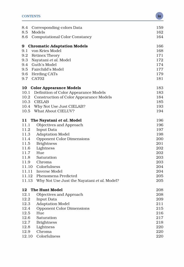
Our visual perceptions are initiated and strongly influenced by the anatom-ical structure of the eye. Figure 1.1 shows a schematic representation of
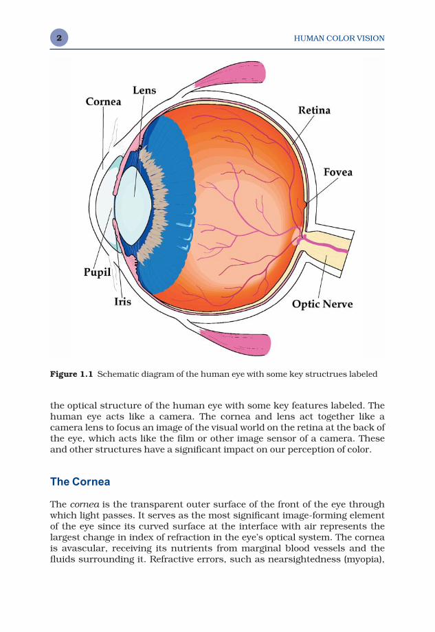
HUMAN COLOR VISION2
the optical structure of the human eye with some key features labeled. Thehuman eye acts like a camera. The cornea and lens act together like a camera lens to focus an image of the visual world on the retina at the back ofthe eye, which acts like the film or other image sensor of a camera. Theseand other structures have a significant impact on our perception of color.
The Cornea
The cornea is the transparent outer surface of the front of the eye throughwhich light passes. It serves as the most significant image-forming elementof the eye since its curved surface at the interface with air represents thelargest change in index of refraction in the eye’s optical system. The corneais avascular, receiving its nutrients from marginal blood vessels and thefluids surrounding it. Refractive errors, such as nearsightedness (myopia),
Figure 1.1 Schematic diagram of the human eye with some key structrues labeled
HUMAN COLOR VISION 3
farsightedness (hyperopia), or astigmatism, can be attributed to variationsin the shape of the cornea and are sometimes corrected with laser surgerythat reshapes the cornea.
The Lens
The lens serves the function of accommodation. It is a layered, flexible struc-ture that varies in index of refraction. It is a naturally occurring gradient-index optical element with the index of refraction higher in the center of thelens than at the edges. This feature serves to reduce some of the aberrationsthat might normally be present in a simple optical system.
The shape of the lens is controlled by the ciliary muscles. When we gaze ata nearby object, the lens becomes ‘fatter’ and thus has increased opticalpower to allow us to focus on the near object. When we gaze at a distantobject, the lens becomes ‘flatter’ resulting in the decreased optical powerrequired to bring far away objects into sharp focus. As we age, the internalstructure of the lens changes resulting in a loss of flexibility. Generally,when an age of about 50 years is reached the lens has completely lost itsflexibility and observers can no longer focus on near objects (this is calledpresbyopia, or ‘old eye’). It is at this point that most people need readingglasses or bifocals.
Concurrent with the hardening of the lens is an increase in its optical density. The lens absorbs and scatters short-wavelength (blue and violet)energy. As it hardens, the level of this absorption and scattering increases.In other words, the lens becomes more and more yellow with age. Variousmechanisms of chromatic adaptation generally make us unaware of thesegradual changes. However, we are all looking at the world through a yellowfilter that not only changes with age, but is significantly different fromobserver to observer. The effects are most noticeable when performing crit-ical color matching or comparing color matches with other observers. Theeffect is particularly apparent with purple objects. Since an older lensabsorbs most of the blue energy reflected from a purple object, but does notaffect the reflected red energy, older observers will tend to report that theobject is significantly more red than reported by younger observers. Import-ant issues regarding the characteristics of lens aging and its influence onvisual performance are discussed by Pokorny et al. (1987), Werner andSchefrin (1993), and Schefrin and Werner (1993).
The Humors
The volume between the cornea and lens is filled with the aqueous humor,which is essentially water. The region between the lens and retina is filledwith vitreous humor, which is also a fluid, but with a higher viscosity, similarto that of gelatin. Both humors exist in a state of slightly elevated pressure
HUMAN COLOR VISION4
(relative to air pressure) to assure that the flexible eyeball retains its shapeand dimensions in order to avoid the deleterious effects of wavering retinalimages. The flexibility of the entire eyeball serves to increase its resistance toinjury. It is much more difficult to break a structure that gives way underimpact than one of equal ‘strength’ that attempts to remain rigid. Since theindices of refraction of the humors are roughly equal to that of water, andthose of the cornea and lens are only slightly higher, the rear surface of thecornea and the entire lens have relatively little optical power.
The Iris
The iris is the sphincter muscle that controls pupil size. The iris is pig-mented, giving each of us our specific eye color. Eye color is determined bythe concentration and distribution of melanin within the iris. The pupil,which is the hole in the middle of the iris through which light passes, definesthe level of illumination on the retina. Pupil size is largely determined by theoverall level of illumination, but it is important to note that it can also varywith non-visual phenomena such as arousal. (This effect can be observed byenticingly shaking a toy in front of a cat and paying attention to its pupils.)Thus it is difficult to accurately predict pupil size from the prevailing illum-ination. In practical situations, pupil diameter varies from about 3 mm toabout 7 mm. This change in pupil diameter results in approximately a five-fold change in pupil area, and therefore retinal illuminance. The visual sens-itivity change with pupil area is further limited by the fact that marginal raysare less effective at stimulating visual response in the cones than centralrays (the Stiles–Crawford effect). The change in pupil diameter alone is notsufficient to explain excellent human visual function over prevailing illumin-ance levels that can vary over 10 orders of magnitude.
The Retina
The optical image formed by the eye is projected onto the retina. The retina isa thin layer of cells, approximately the thickness of tissue paper, located atthe back of the eye and incorporating the visual system’s photosensitive cells and initial signal processing and transmission ‘circuitry.’ These cellsare neurons, part of the central nervous system, and can appropriately beconsidered a part of the brain. The photoreceptors, rods and cones, serve totransduce the information present in the optical image into chemical andelectrical signals that can be transmitted to the later stages of the visual sys-tem. These signals are then processed by a network of cells and transmittedto the brain through the optic nerve. More detail on the retina is presented inthe next section.
Behind the retina is a layer known as the pigmented epithelium. This darkpigment layer serves to absorb any light that happens to pass through the
HUMAN COLOR VISION 5
retina without being absorbed by the photoreceptors. The function of thepigmented epithelium is to prevent light from being scattered back throughthe retina, thus reducing the sharpness and contrast of the perceived image.Nocturnal animals give up this improved image quality in exchange for ahighly reflective tapetum that reflects the light back in order to provide a second chance for the photoreceptors to absorb the energy. This is why theeyes of a deer, or other nocturnal animal, caught in the headlights of anoncoming automobile, appear to glow.
The Fovea
Perhaps the most important structural area on the retina is the fovea. Thefovea is the area on the retina where we have the best spatial and colorvision. When we look at, or fixate, an object in our visual field, we move ourhead and eyes such that the image of the object falls on the fovea. As you arereading this text, you are moving your eyes to make the various words fall onyour fovea as you read them. To illustrate how drastically spatial acuity fallsoff as the stimulus moves away from the fovea, try to read preceding text inthis paragraph while fixating on the period at the end of this sentence. It isprobably difficult, if not impossible, to read text that is only a few lines awayfrom the point of fixation. The fovea covers an area that subtends about twodegrees of visual angle in the central field of vision. To visualize two degreesof visual angle, a general rule is that the width of your thumbnail, held atarm’s length, is approximately one degree of visual angle.
The Macula
The fovea is also protected by a yellow filter known as the macula. The mac-ula serves to protect this critical area of the retina from intense exposures toshort-wavelength energy. It might also serve to reduce the effects of chro-matic aberration that cause the short-wavelength image to be rather severelyout of focus most of the time. Unlike the lens, the macula does not becomemore yellow with age. However, there are significant differences in the opticaldensity of the macular pigment from observer to observer and in some casesbetween a single observer’s left and right eyes. The yellow filters of the lensand macula, through which we all view the world, are the major source ofvariability in color vision between observers with normal color vision.
The Optic Nerve
A last key structure of the eye is the optic nerve. The optic nerve is made up of the axons (outputs) of the ganglion cells, the last level of neural processingin the retina. It is interesting to note that the optic nerve is made up of

HUMAN COLOR VISION6
approximately one million fibers, carrying information generated by approx-imately 130 million photoreceptors. Thus there is a clear compression of thevisual signal prior to transmission to higher levels of the visual system. Aone-to-one ‘pixel map’ of the visual stimulus is never available for processingby the brain’s higher visual mechanisms. This processing is explored ingreater detail below. Since the optic nerve takes up all of the space that would normally be populated by photoreceptors, there is a small area in each eye inwhich no visual stimulation can occur. This area is known as the blind spot.
The structures described above have a clear impact in shaping anddefining the information available to the visual system that ultimatelyresults in the perception of color appearance. The action of the pupil servesto define retinal illuminance levels that, in turn, have a dramatic impact oncolor appearance. The yellow-filtering effects of the lens and macula modu-late the spectral responsivity of our visual system and introduce significantinter-observer variability. The spatial structure of the retina serves to helpdefine the extent and nature of various visual fields that are critical fordefining color appearance. The neural networks in the retina reiterate thatvisual perception in general, and specifically color appearance, cannot betreated as simple point-wise image processing problems. Several of theseimportant features are discussed in more detail in the following sections onthe retina, visual physiology, and visual performance.
1.2 THE RETINA
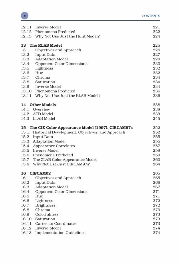
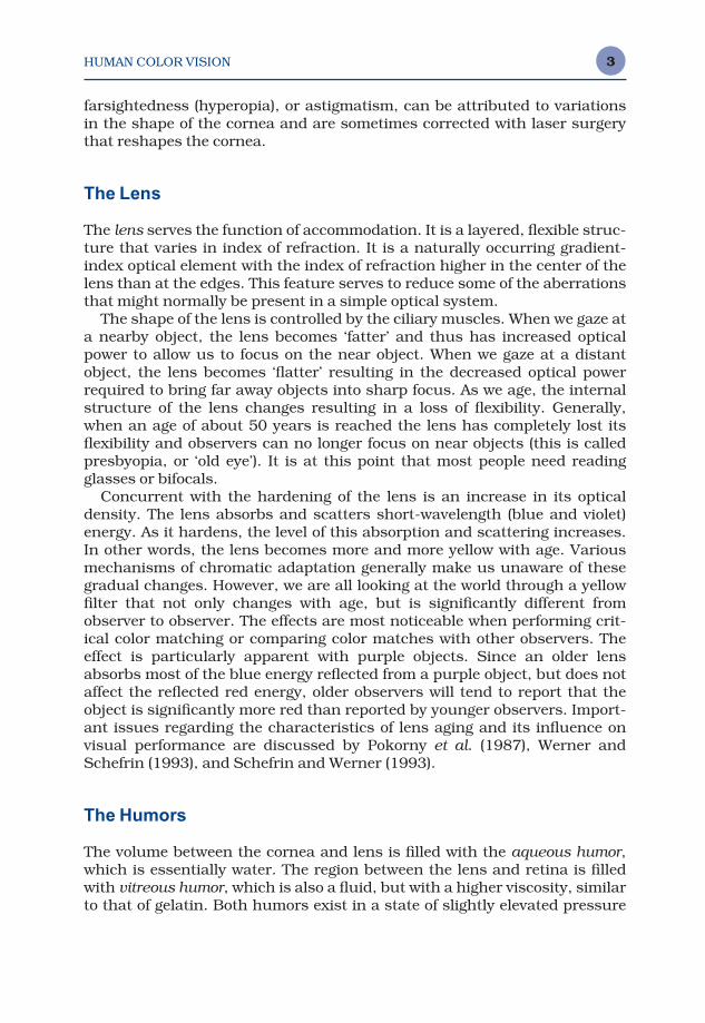
Figure 1.2 illustrates a cross-sectional representation of the retina. Theretina includes several layers of neural cells, beginning with the photorecep-tors, the rods and cones. A vertical signal processing chain through theretina can be constructed by examining the connections of photoreceptors tobipolar cells, which are in turn connected to ganglion cells, which form theoptic nerve. Even this simple pathway results in the signals from multiplephotoreceptors being compared and combined. This is because multiplephotoreceptors provide input to many of the bipolar cells and multiple bipo-lar cells provide input to many of the ganglion cells. More importantly, thissimple concept of retinal signal processing ignores two other significanttypes of cells. These are the horizontal cells, that connect photoreceptors andbipolar cells laterally to one another, and the amacrine cells, that connectbipolar cells and ganglion cells laterally to one another. Figure 1.2 providesonly a slight indication of the extent of these various interconnections.
The specific processing that occurs in each type of cell is not completelyunderstood and is beyond the scope of this chapter. However, it is importantto realize that the signals transmitted from the retina to the higher levels of the brain via the ganglion cells are not simple point-wise representationsof the receptor signals, but rather consist of sophisticated combinations ofthe receptor signals. To envision the complexity of the retinal processing,keep in mind that each synapse between neural cells can effectively perform

HUMAN COLOR VISION 7
a mathematical operation (add, subtract, multiply, divide) in addition to the amplification, gain control, and nonlinearities that can occur within the neural cells. Thus the network of cells within the retina can serve as asophisticated image computer. This is how the information from 130 millionphotoreceptors can be reduced to signals in approximately one million gan-glion cells without loss of visually meaningful data.
It is interesting to note that light passes through all of the neural machin-ery of the retina prior to reaching the photoreceptors. This has little impacton visual performance since these cells are transparent and in fixed posi-tion, thus not perceived. It also allows the significant amounts of nutrients
Figure 1.2 Schematic diagram of the ‘wiring’ of cells in the human retina
HUMAN COLOR VISION8
required and waste produced by the photoreceptors to be processed throughthe back of the eye.
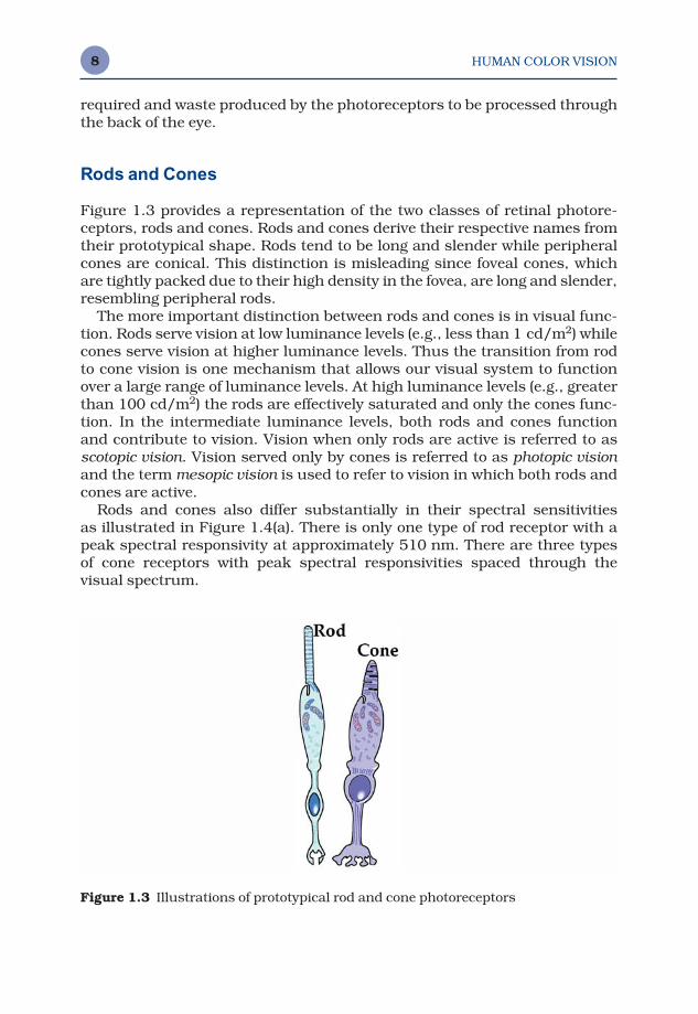
Rods and Cones
Figure 1.3 provides a representation of the two classes of retinal photore-ceptors, rods and cones. Rods and cones derive their respective names fromtheir prototypical shape. Rods tend to be long and slender while peripheralcones are conical. This distinction is misleading since foveal cones, whichare tightly packed due to their high density in the fovea, are long and slender,resembling peripheral rods.
The more important distinction between rods and cones is in visual func-tion. Rods serve vision at low luminance levels (e.g., less than 1 cd/m2) whilecones serve vision at higher luminance levels. Thus the transition from rodto cone vision is one mechanism that allows our visual system to functionover a large range of luminance levels. At high luminance levels (e.g., greaterthan 100 cd/m2) the rods are effectively saturated and only the cones func-tion. In the intermediate luminance levels, both rods and cones function and contribute to vision. Vision when only rods are active is referred to asscotopic vision. Vision served only by cones is referred to as photopic visionand the term mesopic vision is used to refer to vision in which both rods andcones are active.
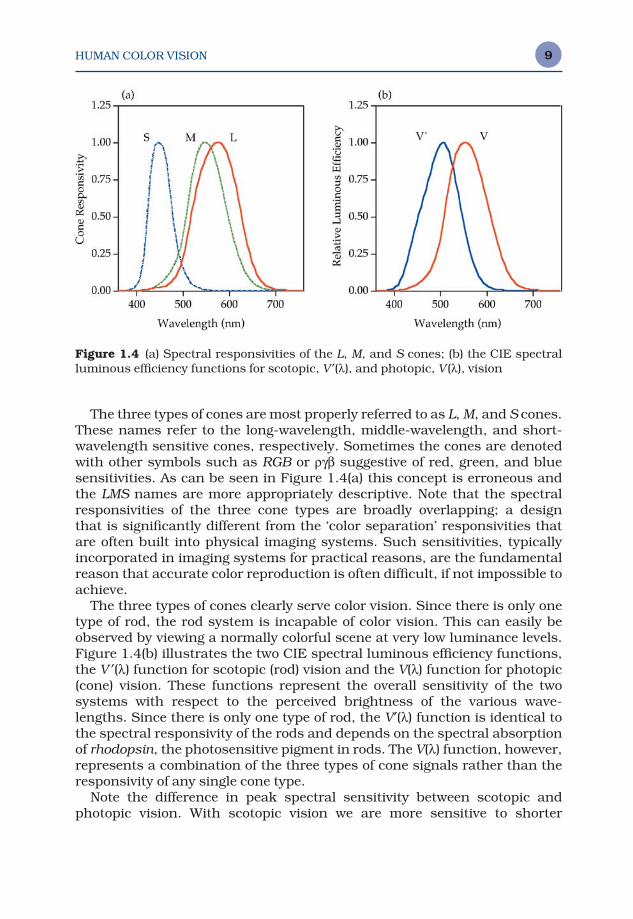
Rods and cones also differ substantially in their spectral sensitivities as illustrated in Figure 1.4(a). There is only one type of rod receptor with apeak spectral responsivity at approximately 510 nm. There are three typesof cone receptors with peak spectral responsivities spaced through thevisual spectrum.
Figure 1.3 Illustrations of prototypical rod and cone photoreceptors
HUMAN COLOR VISION 9
The three types of cones are most properly referred to as L, M, and S cones.These names refer to the long-wavelength, middle-wavelength, and short-wavelength sensitive cones, respectively. Sometimes the cones are denotedwith other symbols such as RGB or ργβ suggestive of red, green, and bluesensitivities. As can be seen in Figure 1.4(a) this concept is erroneous andthe LMS names are more appropriately descriptive. Note that the spectralresponsivities of the three cone types are broadly overlapping; a design that is significantly different from the ‘color separation’ responsivities thatare often built into physical imaging systems. Such sensitivities, typically incorporated in imaging systems for practical reasons, are the fundamentalreason that accurate color reproduction is often difficult, if not impossible toachieve.
The three types of cones clearly serve color vision. Since there is only onetype of rod, the rod system is incapable of color vision. This can easily beobserved by viewing a normally colorful scene at very low luminance levels.Figure 1.4(b) illustrates the two CIE spectral luminous efficiency functions,the V ′(λ) function for scotopic (rod) vision and the V(λ) function for photopic(cone) vision. These functions represent the overall sensitivity of the two systems with respect to the perceived brightness of the various wave-lengths. Since there is only one type of rod, the V′(λ) function is identical tothe spectral responsivity of the rods and depends on the spectral absorptionof rhodopsin, the photosensitive pigment in rods. The V(λ) function, however,represents a combination of the three types of cone signals rather than theresponsivity of any single cone type.
Note the difference in peak spectral sensitivity between scotopic and photopic vision. With scotopic vision we are more sensitive to shorter
Figure 1.4 (a) Spectral responsivities of the L, M, and S cones; (b) the CIE spectralluminous efficiency functions for scotopic, V ′(λ), and photopic, V (λ), vision
HUMAN COLOR VISION10
wavelengths. This effect, known as the Purkinje shift, can be observed byfinding two objects, one blue and the other red, that appear the same light-ness when viewed in daylight. When the same two objects are viewed undervery low luminance levels, the blue object will appear quite light while thered object will appear nearly black because of the scotopic spectral sensitiv-ity function.
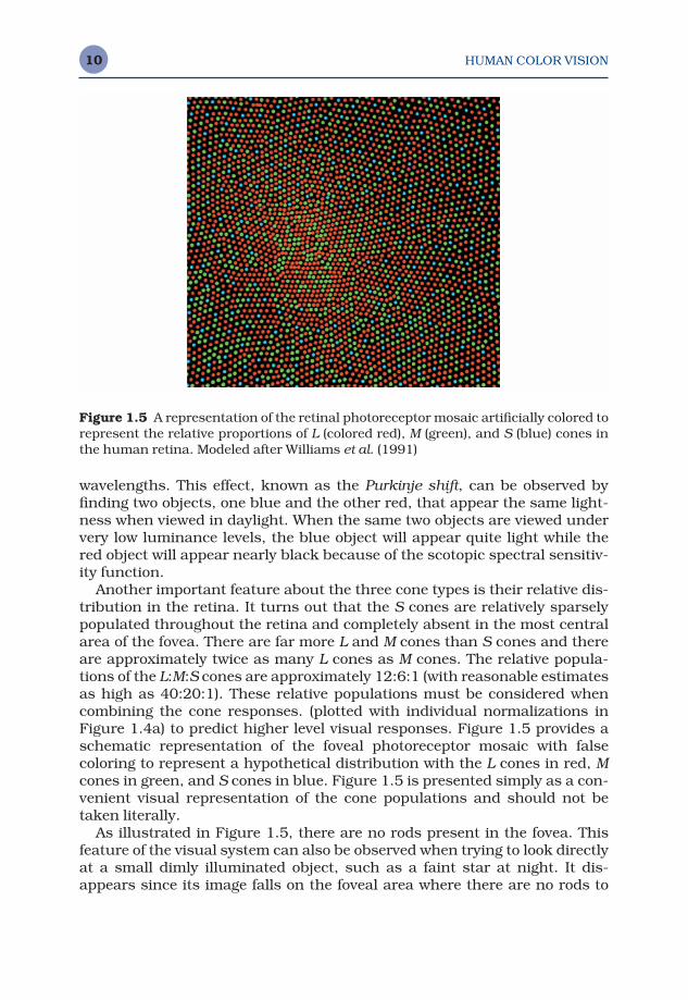
Another important feature about the three cone types is their relative dis-tribution in the retina. It turns out that the S cones are relatively sparselypopulated throughout the retina and completely absent in the most centralarea of the fovea. There are far more L and M cones than S cones and thereare approximately twice as many L cones as M cones. The relative popula-tions of the L:M:S cones are approximately 12:6:1 (with reasonable estimatesas high as 40:20:1). These relative populations must be considered whencombining the cone responses. (plotted with individual normalizations inFigure 1.4a) to predict higher level visual responses. Figure 1.5 provides aschematic representation of the foveal photoreceptor mosaic with false coloring to represent a hypothetical distribution with the L cones in red, Mcones in green, and S cones in blue. Figure 1.5 is presented simply as a con-venient visual representation of the cone populations and should not betaken literally.
As illustrated in Figure 1.5, there are no rods present in the fovea. Thisfeature of the visual system can also be observed when trying to look directlyat a small dimly illuminated object, such as a faint star at night. It dis-appears since its image falls on the foveal area where there are no rods to
Figure 1.5 A representation of the retinal photoreceptor mosaic artificially colored torepresent the relative proportions of L (colored red), M (green), and S (blue) cones inthe human retina. Modeled after Williams et al. (1991)
HUMAN COLOR VISION 11
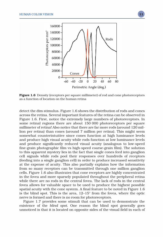
detect the dim stimulus. Figure 1.6 shows the distribution of rods and conesacross the retina. Several important features of the retina can be observed inFigure 1.6. First, notice the extremely large numbers of photoreceptors. Insome retinal regions there are about 150 000 photoreceptors per square millimeter of retina! Also notice that there are far more rods (around 120 mil-lion per retina) than cones (around 7 million per retina). This might seemsomewhat counterintuitive since cones function at high luminance levelsand produce high visual acuity while rods function at low luminance levelsand produce significantly reduced visual acuity (analogous to low-speedfine-grain photographic film vs high-speed coarse-grain film). The solutionto this apparent mystery lies in the fact that single cones feed into ganglioncell signals while rods pool their responses over hundreds of receptors (feeding into a single ganglion cell) in order to produce increased sensitivityat the expense of acuity. This also partially explains how the informationfrom so many receptors can be transmitted through one million ganglioncells. Figure 1.6 also illustrates that cone receptors are highly concentratedin the fovea and more sparsely populated throughout the peripheral retinawhile there are no rods in the central fovea. The lack of rods in the centralfovea allows for valuable space to be used to produce the highest possiblespatial acuity with the cone system. A final feature to be noted in Figure 1.6is the blind spot. This is the area, 12–15° from the fovea, where the opticnerve is formed and there is no room for photoreceptors.
Figure 1.7 provides some stimuli that can be used to demonstrate theexistence of the blind spot. One reason the blind spot generally goes unnoticed is that it is located on opposite sides of the visual field in each of
Figure 1.6 Density (receptors per square millimeter) of rod and cone photoreceptorsas a function of location on the human retina
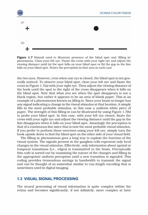
HUMAN COLOR VISION12
the two eyes. However, even when one eye is closed, the blind spot is not gen-erally noticed. To observe your blind spot, close your left eye and fixate thecross in Figure 1.7(a) with your right eye. Then adjust the viewing distance ofthe book until the spot to the right of the cross disappears when it falls onthe blind spot. Note that what you see when the spot disappears is not ablack region, but rather it appears to be an area of blank paper. This is anexample of a phenomenon known as filling in. Since your brain no longer hasany signal indicating a change in the visual stimulus at that location, it simplyfills in the most probable stimulus, in this case a uniform white piece ofpaper. The strength of this filling in can be illustrated by using Figure 1.7(b)to probe your blind spot. In this case, with your left eye closed, fixate thecross with your right eye and adjust the viewing distance until the gap in theline disappears when it falls on your blind spot. Amazingly the perception isthat of a continuous line since that is now the most probable visual stimulus.If you prefer to perform these exercises using your left eye, simply turn thebook upside down to find the blind spot on the other side of your visual field.
The filling in phenomenon goes a long way to explain the function of thevisual system. The signals present in the ganglion cells represent only localchanges in the visual stimulus. Effectively, only information about spatial ortemporal transitions (i.e., edges) is transmitted to the brain. Perceptuallythis code is sorted out by examining the nature of the changes and filling inthe appropriate uniform perception until a new transition is signaled. Thiscoding provides tremendous savings in bandwidth to transmit the signaland can be thought of as somewhat similar to run-length encoding that issometimes used in digital imaging.
1.3 VISUAL SIGNAL PROCESSING
The neural processing of visual information is quite complex within theretina and becomes significantly, if not infinitely, more complex at later
Figure 1.7 Stimuli used to illustrate presence of the blind spot and ‘filling in’ phenomena. Close your left eye. Fixate the cross with your right eye and adjust theviewing distance until (a) the spot falls on your blind spot or (b) the gap in the linefalls on your blind spot. Notice the perception in that area in each case
HUMAN COLOR VISION 13
stages. This section provides a brief overview of the paths that some of thisinformation takes. It is helpful to begin with a general map of the steps alongthe way. The optical image on the retina is first transduced into chemicaland electrical signals in the photoreceptors. These signals are then pro-cessed through the network of retinal neurons (horizontal, bipolar, amacrine,and ganglion cells) described above. The ganglion cell axons gather to formthe optic nerve, which projects to the lateral geniculate nucleus (LGN) in thethalamus. The LGN cells, after gathering input from the ganglion cells, pro-ject to visual area one (V1) in the occipital lobe of the cortex. At this point, theinformation processing begins to become amazingly complex. Approximately30 visual areas have been defined in the cortex with names such as V2, V3,V4, MT, etc. Signals from these areas project to several other areas and viceversa. The cortical processing includes many instances of feed-forward,feed-back, and lateral processing. Somewhere in this network of informationour ultimate perceptions are formed. A few more details of these processesare described in the following paragraphs.
Light incident on the retina is absorbed by photopigments in the variousphotoreceptors. In rods, the photopigment is rhodopsin. Upon absorbing aphoton, rhodopsin changes in structure, setting off a chemical chain reac-tion that ultimately results in the closing of ion channels in its cell wallswhich produce an electrical signal based on the relative concentrations ofvarious ions (e.g., sodium and potassium) inside and outside the cell wall. A similar process takes place in cones. Rhodopsin is made up of opsin andretinal. Cones have similar photopigment structures. However, in cones the‘cone-opsins’ have slightly different molecular structures resulting in thevarious spectral responsivities observed in the cones. Each type of cone (L,M, or S) contains a different form of ‘cone-opsin.’ Figure 1.8 illustrates therelative responses of the photoreceptors as a function of retinal exposure.
It is interesting to note that these functions show characteristics similarto those found in all imaging systems. At the low end of the receptor res-ponses there is a threshold, below which the receptors do not respond. Thereis then a fairly linear portion of the curves, followed by response saturationat the high end. Such curves are representations of the photocurrent at the receptors and represent the very first stage of visual processing. Thesesignals are then processed through the retinal neurons and synapses until a transformed representation is generated in the ganglion cells for trans-mission through the optic nerve.
Receptive Fields
For various reasons, including noise suppression and transmission speed,the amplitude-modulated signals in the photoreceptors are converted intofrequency-modulated representations at the ganglion-cell and higher levels.In these, and indeed most, neural cells the magnitude of the signal is repres-ented in terms of the number of spikes of voltage per second fired by the

HUMAN COLOR VISION14
cell rather than by the voltage difference across the cell wall. To representthe physiological properties of these cells, the concept of receptive fieldsbecomes useful.
A receptive field is a graphical representation of the area in the visual fieldto which a given cell responds. In addition, the nature of the response (e.g.,positive, negative, spectral bias) is typically indicated for various regions inthe receptive field. As a simple example, the receptive field of a photoreceptoris a small circular area representing the size and location of that particularreceptor’s sensitivity in the visual field. Figure 1.9 represents some prototyp-ical receptive fields for ganglion cells. They illustrate center-surround antag-onism, which is characteristic at this level of visual processing. The receptivefield in Figure 1.9(a) illustrates a positive central response, typically gener-ated by a positive input from a single cone, surrounded by a negative sur-round response, typically driven by negative inputs from several neighboringcones. Thus the response of this ganglion cell is made up of inputs from a number of cones with both positive and negative signs. The result is that
Figure 1.8 Relative energy responses for the rod and cone photoreceptors
Figure 1.9 Typical center-surround antagonistic receptive fields: (a) on-center, (b) off-center
HUMAN COLOR VISION 15
the ganglion cell does not simply respond to points of light, but serves as anedge detector (actually a ‘spot’ detector). Readers familiar with digital imageprocessing can think of the ganglion cell responses as similar to the outputof a convolution kernel designed for edge detection.
Figure 1.9(b) illustrates that a ganglion cell response of opposite polarityis equally likely. The response in Figure 1.9(a) is considered an on-centerganglion cell while that in Figure 1.9(b) is called an off-center ganglion cell.Often on-center and off-center cells will occur at the same spatial location,fed by the same photoreceptors, resulting in an enhancement of the system’sdynamic range.
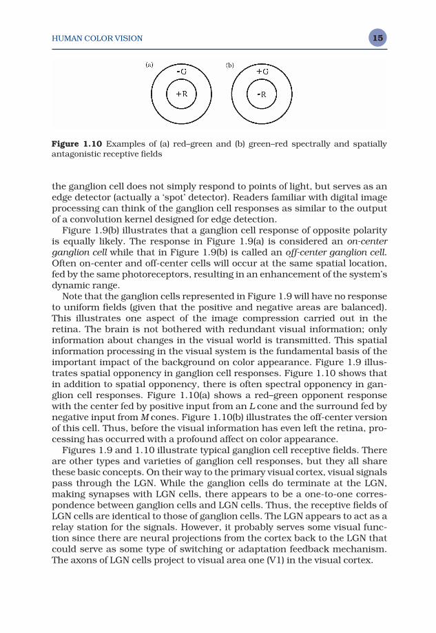
Note that the ganglion cells represented in Figure 1.9 will have no responseto uniform fields (given that the positive and negative areas are balanced).This illustrates one aspect of the image compression carried out in theretina. The brain is not bothered with redundant visual information; onlyinformation about changes in the visual world is transmitted. This spatialinformation processing in the visual system is the fundamental basis of theimportant impact of the background on color appearance. Figure 1.9 illus-trates spatial opponency in ganglion cell responses. Figure 1.10 shows thatin addition to spatial opponency, there is often spectral opponency in gan-glion cell responses. Figure 1.10(a) shows a red–green opponent responsewith the center fed by positive input from an L cone and the surround fed bynegative input from M cones. Figure 1.10(b) illustrates the off-center versionof this cell. Thus, before the visual information has even left the retina, pro-cessing has occurred with a profound affect on color appearance.
Figures 1.9 and 1.10 illustrate typical ganglion cell receptive fields. Thereare other types and varieties of ganglion cell responses, but they all sharethese basic concepts. On their way to the primary visual cortex, visual signalspass through the LGN. While the ganglion cells do terminate at the LGN,making synapses with LGN cells, there appears to be a one-to-one corres-pondence between ganglion cells and LGN cells. Thus, the receptive fields ofLGN cells are identical to those of ganglion cells. The LGN appears to act as arelay station for the signals. However, it probably serves some visual func-tion since there are neural projections from the cortex back to the LGN thatcould serve as some type of switching or adaptation feedback mechanism.The axons of LGN cells project to visual area one (V1) in the visual cortex.
Figure 1.10 Examples of (a) red–green and (b) green–red spectrally and spatiallyantagonistic receptive fields
HUMAN COLOR VISION16
Processing in Area V1
In area V1 of the cortex, the encoding of visual information becomes sig-nificantly more complex. Much as the outputs of various photoreceptors arecombined and compared to produce ganglion cell responses, the outputs ofvarious LGN cells are compared and combined to produce cortical responses.As the signals move further up in the cortical processing chain, this processrepeats itself with the level of complexity increasing very rapidly to the pointthat receptive fields begin to lose meaning. In V1, cells can be found thatselectively respond to various types of stimuli, including
• Oriented edges or bars• Input from one eye, the other, or both• Various spatial frequencies• Various temporal frequencies• Particular spatial locations• Various combinations of these features
In addition, cells can be found that seem to linearly combine inputs fromLGN cells and others with nonlinear summation. All of these various res-ponses are necessary to support visual capabilities such as the perceptionsof size, shape, location, motion, depth, and color. Given the complexity of cor-tical responses in V1 cells, it is not difficult to imagine how complex visualresponses can become in an interwoven network of approximately 30 visualareas.
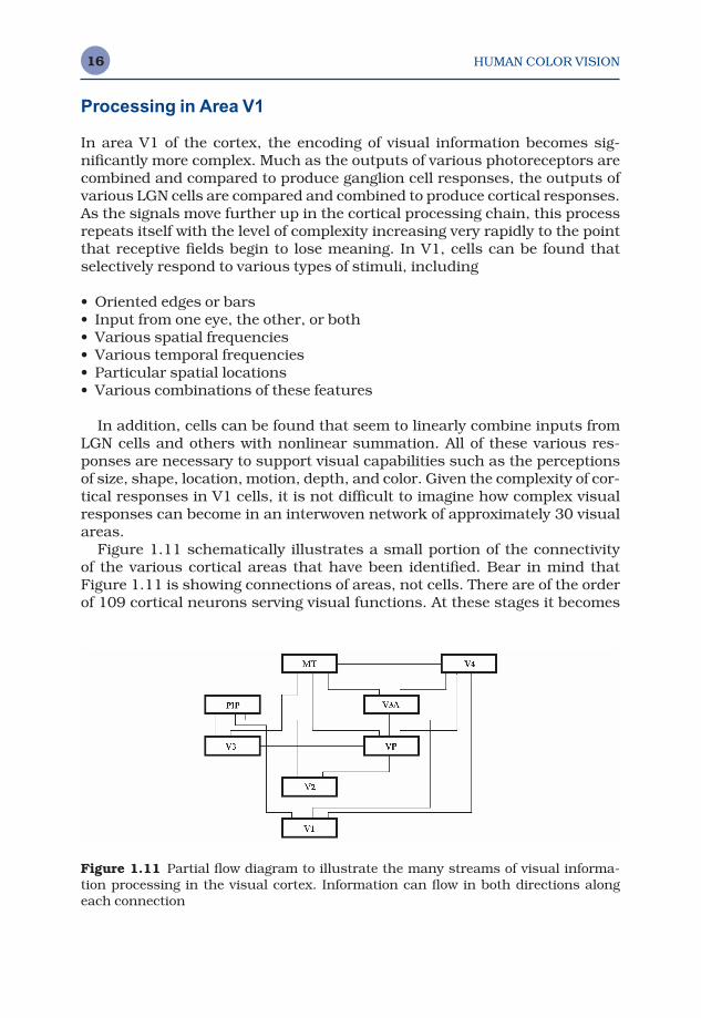
Figure 1.11 schematically illustrates a small portion of the connectivity of the various cortical areas that have been identified. Bear in mind thatFigure 1.11 is showing connections of areas, not cells. There are of the orderof 109 cortical neurons serving visual functions. At these stages it becomes
Figure 1.11 Partial flow diagram to illustrate the many streams of visual informa-tion processing in the visual cortex. Information can flow in both directions alongeach connection
HUMAN COLOR VISION 17
exceedingly difficult to explain the function of single cortical cells in simpleterms. In fact, the function of a single cell might not have meaning since therepresentation of various perceptions must be distributed across collectionsof cells throughout the cortex. Rather than attempting to explore the physi-ology further, the following sections will describe some of the overall percep-tual and psychophysical properties of the visual system that help to specifyits performance.
1.4 MECHANISMS OF COLOR VISION
Historically, there have been many theories that attempt to explain the function of color vision. A brief look at some of the more modern conceptsprovides useful insight into current concepts.
Trichhromatic Theory
In the later half of the 19th century, the trichromatic theory of color vision wasdeveloped, based on the work of Maxwell, Young, and Helmholtz. They recog-nized that there must be three types of receptors, approximately sensitive tothe red, green, and blue regions of the spectrum, respectively. The trichro-matic theory simply assumed that three images of the world were formed bythese three sets of receptors and then transmitted to the brain where theratios of the signals in each of the images was compared in order to sort outcolor appearances. The trichromatic (three-receptor) nature of color visionwas not in doubt, but the idea of three images being transmitted to the brainis both inefficient and fails to explain several visually observed phenomena.
Hering’s Opponent-Colors Theory
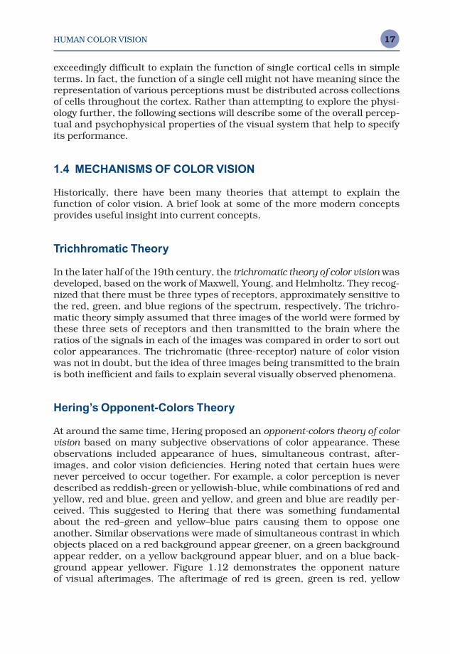
At around the same time, Hering proposed an opponent-colors theory of colorvision based on many subjective observations of color appearance. Theseobservations included appearance of hues, simultaneous contrast, after-images, and color vision deficiencies. Hering noted that certain hues werenever perceived to occur together. For example, a color perception is neverdescribed as reddish-green or yellowish-blue, while combinations of red andyellow, red and blue, green and yellow, and green and blue are readily per-ceived. This suggested to Hering that there was something fundamentalabout the red–green and yellow–blue pairs causing them to oppose oneanother. Similar observations were made of simultaneous contrast in whichobjects placed on a red background appear greener, on a green backgroundappear redder, on a yellow background appear bluer, and on a blue back-ground appear yellower. Figure 1.12 demonstrates the opponent nature of visual afterimages. The afterimage of red is green, green is red, yellow
HUMAN COLOR VISION18
is blue, and blue is yellow. (It is worth noting that afterimages can also beeasily explained in terms of complementary colors due to adaptation in atrichromatic system. Hering only referred to light-dark afterimages in sup-port of opponent theory, not chromatic afterimages.) Lastly, Hering observedthat those with color vision deficiencies lose the ability to distinguish hues inred–green or yellow–blue pairs.
All of these observations provide clues regarding the processing of color in-formation in the visual system. Hering proposed that there were three typesof receptors, but Hering’s receptors had bipolar responses to light–dark,red–green, and yellow–blue. At the time, this was thought to be physiologic-ally implausible and Hering’s opponent theory did not receive appropriateacceptance.
Modern Opponent-Colors Theory
In the middle of the 20th century, Hering’s opponent theory enjoyed a revivalof sorts when quantitative data supporting it began to appear. For example,Svaetichin (1956) found opponent signals in electrophysiological measure-ments of responses in the retinas of goldfish (which happen to be trichro-matic!). DeValois et al. (1958), found similar opponent physiological responsesin the LGN cells of the macaque monkey. Jameson and Hurvich (1955) alsoadded quantitative psychophysical data through their hue-cancellationexperiments with human observers that allowed measurement of the relat-ive spectral sensitivities of opponent pathways. These data, combined with
Figure 1.12 Stimulus for the demonstration of opponent afterimages. Fixate uponthe black spot in the center of the four colored squares for about 30 seconds thenmove your gaze to fixate the black spot in the uniform white area. Note the colors ofthe afterimages relative to the colors of the original stimuli
HUMAN COLOR VISION 19
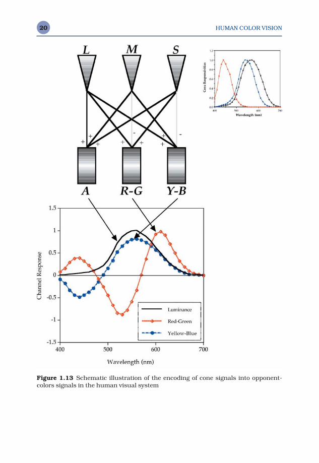
the overwhelming support of much additional research since that time, haveled to the development of the modern opponent theory of color vision (some-times called a stage theory) as illustrated in Figure 1.13.
Figure 1.13 illustrates that the first stage of color vision, the receptors, isindeed trichromatic as hypothesized by Maxwell, Young, and Helmholtz.However, contrary to simple trichromatic theory, the three ‘color-separation’images are not transmitted directly to the brain. Instead the neurons of theretina (and perhaps higher levels) encode the color into opponent signals.The outputs of all three cone types are summed (L + M + S) to produce anachromatic response that matches the CIE V(λ) curve as long as the summa-tion is taken in proportion to the relative populations of the three cone types.Differencing of the cone signals allows construction of red-green (L − M + S)and yellow-blue (L + M − S) opponent signals. The transformation from LMSsignals to the opponent signals serves to decorrelate the color informationcarried in the three channels, thus allowing more efficient signal transmis-sion and reducing difficulties with noise. The three opponent pathways alsohave distinct spatial and temporal characteristics that are important for pre-dicting color appearance. They are discussed further in Section 1.5.
The importance of the transformation from trichromatic to opponent sig-nals for color appearance is reflected in the prominent place that it findswithin the formulation of all color appearance models. Figure 1.13 includesnot only a schematic diagram of the neural ‘wiring’ that produces opponentresponses, but also the relative spectral responsivities of these mechanismsboth before and after opponent encoding.
Adaptation Mechanisms
However, it is not enough to consider the processing of color signals in thehuman visual system as a static ‘wiring diagram.’ The dynamic mechanismsof adaptation that serve to optimize the visual response to the particularviewing environment at hand must also be considered. Thus an overview ofthe various types of adaptation is in order. Of particular relevance to thestudy of color appearance are the mechanisms of dark, light, and chromaticadaptation.
Dark Adaptation
Dark adaptation refers to the change in visual sensitivity that occurs whenthe prevailing level of illumination is decreased, such as when walking into adarkened theater on a sunny afternoon. At first the entire theater appearscompletely dark, but after a few minutes one is able to clearly see objects in the theater such as the aisles, seats, and other people. This happensbecause the visual system is responding to the lack of illumination bybecoming more sensitive and therefore capable of producing a meaningfulvisual response at the lower illumination level.
HUMAN COLOR VISION20
Figure 1.13 Schematic illustration of the encoding of cone signals into opponent-colors signals in the human visual system
HUMAN COLOR VISION 21
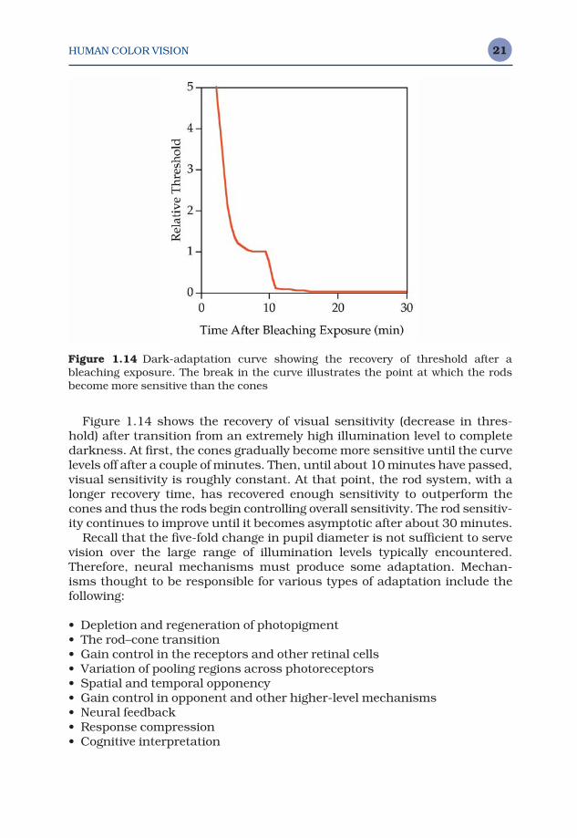
Figure 1.14 shows the recovery of visual sensitivity (decrease in thres-hold) after transition from an extremely high illumination level to completedarkness. At first, the cones gradually become more sensitive until the curve levels off after a couple of minutes. Then, until about 10 minutes have passed,visual sensitivity is roughly constant. At that point, the rod system, with alonger recovery time, has recovered enough sensitivity to outperform thecones and thus the rods begin controlling overall sensitivity. The rod sensitiv-ity continues to improve until it becomes asymptotic after about 30 minutes.
Recall that the five-fold change in pupil diameter is not sufficient to servevision over the large range of illumination levels typically encountered.Therefore, neural mechanisms must produce some adaptation. Mechan-isms thought to be responsible for various types of adaptation include thefollowing:
• Depletion and regeneration of photopigment• The rod–cone transition• Gain control in the receptors and other retinal cells• Variation of pooling regions across photoreceptors• Spatial and temporal opponency• Gain control in opponent and other higher-level mechanisms• Neural feedback• Response compression• Cognitive interpretation
Figure 1.14 Dark-adaptation curve showing the recovery of threshold after ableaching exposure. The break in the curve illustrates the point at which the rodsbecome more sensitive than the cones
HUMAN COLOR VISION22
Light Adaptation
Light adaptation is essentially the inverse process of dark adaptation. How-ever, it is important to consider it separately since its visual properties differ.Light adaptation occurs when leaving the darkened theater and returningoutdoors on a sunny afternoon. In this case, the visual system must becomeless sensitive in order to produce useful perceptions since there is signific-antly more visible energy available.
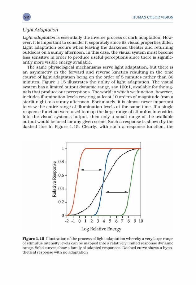
The same physiological mechanisms serve light adaptation, but there isan asymmetry in the forward and reverse kinetics resulting in the timecourse of light adaptation being on the order of 5 minutes rather than 30minutes. Figure 1.15 illustrates the utility of light adaptation. The visualsystem has a limited output dynamic range, say 100:1, available for the sig-nals that produce our perceptions. The world in which we function, however,includes illumination levels covering at least 10 orders of magnitude from astarlit night to a sunny afternoon. Fortunately, it is almost never importantto view the entire range of illumination levels at the same time. If a singleresponse function were used to map the large range of stimulus intensitiesinto the visual system’s output, then only a small range of the available output would be used for any given scene. Such a response is shown by thedashed line in Figure 1.15. Clearly, with such a response function, the
Figure 1.15 Illustration of the process of light adaptation whereby a very large rangeof stimulus intensity levels can be mapped into a relatively limited response dynamicrange. Solid curves show a family of adapted responses. Dashed curve shows a hypo-thetical response with no adaptation
HUMAN COLOR VISION 23
perceived contrast of any given scene would be limited and visual sensitivityto changes would be severely degraded due to signal-to-noise issues.
On the other hand, light adaptation serves to produce a family of visualresponse curves as illustrated by the solid lines in Figure 1.15. These curvesmap the useful illumination range in any given scene into the full dynamicrange of the visual output, thus resulting in the best possible visual percep-tion for each situation. Light adaptation can be thought of as the process ofsliding the visual response curve along the illumination level axis in Figure1.15 until the optimum level for the given viewing conditions is reached.Light and dark adaptation can be thought of as analogous to an automaticexposure control in a photographic system.
Chromatic Adaptation
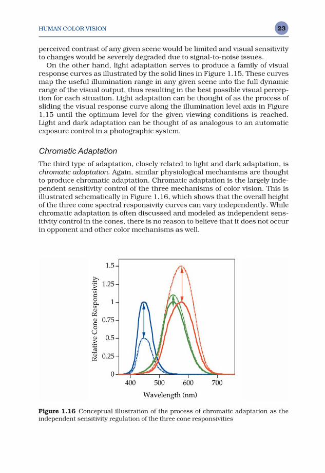
The third type of adaptation, closely related to light and dark adaptation, ischromatic adaptation. Again, similar physiological mechanisms are thoughtto produce chromatic adaptation. Chromatic adaptation is the largely inde-pendent sensitivity control of the three mechanisms of color vision. This isillustrated schematically in Figure 1.16, which shows that the overall heightof the three cone spectral responsivity curves can vary independently. Whilechromatic adaptation is often discussed and modeled as independent sens-itivity control in the cones, there is no reason to believe that it does not occurin opponent and other color mechanisms as well.
Figure 1.16 Conceptual illustration of the process of chromatic adaptation as theindependent sensitivity regulation of the three cone responsivities

HUMAN COLOR VISION24
Chromatic adaptation can be observed by examining a white object, suchas a piece of paper, under various types of illumination (e.g., daylight, fluore-scent, and incandescent). Daylight contains relatively far more short-wave-length energy than fluorescent light, and incandescent illumination containsrelatively far more long-wavelength energy than fluorescent light. However,the paper approximately retains its white appearance under all three lightsources. This is because the S-cone system becomes relatively less sensitiveunder daylight to compensate for the additional short-wavelength energyand the L-cone system becomes relatively less sensitive under incandescentillumination to compensate for the additional long-wavelength energy.
Chromatic adaptation can be thought of as analogous to an automaticwhite-balance in video cameras. Figure 1.17 provides a visual demonstra-tion of chromatic adaptation in which the two halves of the visual field areconditioned to produce disparate levels of chromatic adaptation. Given itsfundamental importance in color appearance modeling, chromatic adapta-tion is covered in more detail in Chapter 8.
Visual Mechanisms Impacting Color Appearance
There are many important cognitive visual mechanisms that impact colorappearance. These are described in further detail in Chapters 6–8. They in-clude memory color, color constancy, discounting the illuminant, and objectrecognition.
• Memory color refers to the phenomenon that recognizable objects oftenhave a prototypical color that is associated with them. For example, mostpeople have a memory for the typical color of green grass and can producea stimulus of this color if requested to do so in an experiment. Inter-estingly, the memory color often is not found in the actual objects. Forexample, green grass and blue sky are typically remembered as beingmore saturated than the actual stimuli.
• Color constancy refers to the everyday perception that the colors of objectsremain unchanged across significant changes in illumination color andluminance level. Color constancy is served by the mechanisms of chro-matic adaptation and memory color and can easily be shown to be verypoor when careful observations are made.
• Discounting the illuminant refers to an observer’s ability to automaticallyinterpret the illumination conditions and perceive the colors of objectsafter discounting the influences of illumination color.
• Object recognition is generally driven by the spatial, temporal, and light–dark properties of the objects rather than by chromatic properties(Davidoff 1991).
Thus once the objects are recognized, the mechanisms of memory color anddiscounting the illuminant can fill in the appropriate color. Such mechanisms

HUMAN COLOR VISION 25
have fascinating impacts on color appearance and become of critical import-ance when performing color comparisons across different media.
Clearly, visual information processing is extremely complex and not yetfully understood (perhaps it never will be). It is of interest to consider theincreasing complexity of cortical visual responses as the signal movesthrough the visual system. Single-cell electrophysiological studies havefound cortical cells with extremely complex driving stimuli. For example,cells in monkeys that respond only to images of monkey paws or faces havebeen occasionally found in physiological experiments. The existence of suchcells raises the question of how complex a single-cell response can become.
Figure 1.17 A demonstration of retinally localized chromatic adaptation. Fixate theblack spot in between the uniform blue and yellow areas for about 30 seconds thenshift your gaze to the white spot in the center of the barn image. Note that the barnimage appears approximately uniform after this adaptation. Original barn imagefrom Kodak Photo Sampler PhotoCD
HUMAN COLOR VISION26
Clearly it is not possible for every perception to have its own cortical cell.Thus, at some point in the visual system, the representation of perceptionsmust be distributed with combinations of various signals producing variousperceptions. Such distributed representations open up the possibilities fornumerous permutations on a given perception, such as color appearance. It is clear from the large number of stimulus variables that impact colorappearance that our visual system is often experimenting with these permutations.
1.5 SPATIAL AND TEMPORAL PROPERTIES OF COLOR VISION
No dimension of visual experience can be considered in isolation. The colorappearance of a stimulus is not independent of its spatial and temporalcharacteristics. For example, a black and white stimulus flickering at anappropriate temporal frequency can be perceived as quite colorful. The spa-tial and temporal characteristics of the human visual system are typicallyexplored through measurement of contrast sensitivity functions. Contrastsensitivity functions (CSFs) in vision science are analogous to modulationtransfer functions (MTFs) in imaging science. However, CSFs cannot legitim-ately be considered MTFs since the human visual system is highly non-linear and CSFs represent threshold sensitivity and not suprathresholdmodulation. A contrast sensitivity function is defined by the thresholdresponse to contrast (sensitivity is the inverse of threshold) as a function ofspatial or temporal frequency. Contrast is typically defined as the differencebetween maximum and minimum luminance in a stimulus divided by thesum of the maximum and minimum luminances, and CSFs are typicallymeasured with stimuli that vary sinusoidally across space or time. Thus auniform pattern has a contrast of zero and sinusoidal patterns with troughsthat reach a luminance of zero have a contrast of 1.0, no matter what theirmean luminance is.
Figure 1.18 conceptually illustrates typical spatial contrast sensitivityfunctions for luminance (black–white) and chromatic (red–green and yellow–blue at constant luminance) contrast. The luminance contrast sensitivityfunction is band-pass in nature, with peak sensitivity around 5 cycles perdegree. This function approaches zero at zero cycles per degree, illustratingthe tendency for the visual system to be insensitive to uniform fields. It alsoapproaches zero at about 60 cycles per degree, the point at which detail canno longer be resolved by the optics of the eye or the photoreceptor mosaic.The band-pass contrast sensitivity function correlates with the concept ofcenter-surround antagonistic receptive fields that would be most sensitiveto an intermediate range of spatial frequency. The chromatic mechanismsare of a low-pass nature and have significantly lower cutoff frequencies. Thisindicates the reduced availability of chromatic information for fine details(high spatial frequencies) that is often taken advantage of in image codingand compression schemes (e.g., NTSC or JPEG).
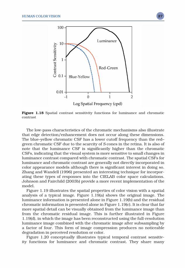
HUMAN COLOR VISION 27
The low-pass characteristics of the chromatic mechanisms also illustratethat edge detection/enhancement does not occur along these dimensions.The blue–yellow chromatic CSF has a lower cutoff frequency than the red–green chromatic CSF due to the scarcity of S cones in the retina. It is also ofnote that the luminance CSF is significantly higher than the chromaticCSFs, indicating that the visual system is more sensitive to small changes inluminance contrast compared with chromatic contrast. The spatial CSFs forluminance and chromatic contrast are generally not directly incorporated incolor appearance models although there is significant interest in doing so.Zhang and Wandell (1996) presented an interesting technique for incorpor-ating these types of responses into the CIELAB color space calculations.Johnson and Fairchild (2003b) provide a more recent implementation of themodel.
Figure 1.19 illustrates the spatial properties of color vision with a spatialanalysis of a typical image. Figure 1.19(a) shows the original image. Theluminance information is presented alone in Figure 1.19(b) and the residualchromatic information is presented alone in Figure 1.19(c). It is clear that farmore spatial detail can be visually obtained from the luminance image thanfrom the chromatic residual image. This is further illustrated in Figure1.19(d), in which the image has been reconstructed using the full-resolutionluminance image combined with the chromatic image after subsampling bya factor of four. This form of image compression produces no noticeabledegradation in perceived resolution or color.
Figure 1.20 conceptually illustrates typical temporal contrast sensitiv-ity functions for luminance and chromatic contrast. They share many
Figure 1.18 Spatial contrast sensitivity functions for luminance and chromatic contrast
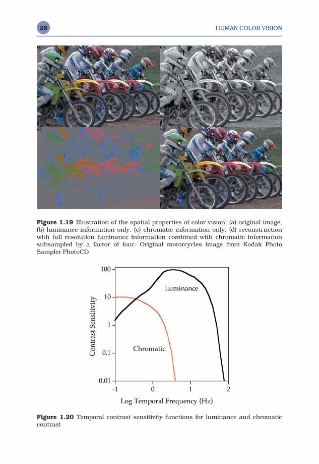
HUMAN COLOR VISION28
Figure 1.20 Temporal contrast sensitivity functions for luminance and chromaticcontrast
Figure 1.19 Illustration of the spatial properties of color vision: (a) original image, (b) luminance information only, (c) chromatic information only, (d) reconstructionwith full resolution luminance information combined with chromatic informationsubsampled by a factor of four. Original motorcycles image from Kodak PhotoSampler PhotoCD
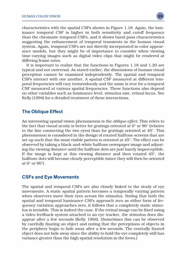
HUMAN COLOR VISION 29
characteristics with the spatial CSFs shown in Figure 1.18. Again, the lum-inance temporal CSF is higher in both sensitivity and cutoff frequency than the chromatic temporal CSFs, and it shows band-pass characteristics suggesting the enhancement of temporal transients in the human visualsystem. Again, temporal CSFs are not directly incorporated in color appear-ance models, but they might be of importance to consider when viewingtime-varying images such as digital video clips that might be rendered at differing frame rates.
It is important to realize that the functions in Figures 1.18 and 1.20 aretypical and not universal. As stated earlier, the dimensions of human visualperception cannot be examined independently. The spatial and temporalCSFs interact with one another. A spatial CSF measured at different tem-poral frequencies will vary tremendously and the same is true for a temporalCSF measured at various spatial frequencies. These functions also dependon other variables such as luminance level, stimulus size, retinal locus. SeeKelly (1994) for a detailed treatment of these interactions.
The Oblique Effect
An interesting spatial vision phenomenon is the oblique effect. This refers tothe fact that visual acuity is better for gratings oriented at 0° or 90° (relativeto the line connecting the two eyes) than for gratings oriented at 45°. Thisphenomenon is considered in the design of rotated halftone screens that areset up such that the most visible pattern is oriented at 45°. The effect can beobserved by taking a black-and-white halftone newspaper image and adjust-ing the viewing distance until the halftone dots are just barely imperceptible.If the image is kept at this viewing distance and then rotated 45°, thehalftone dots will become clearly perceptible (since they will then be orientedat 0° or 90°).
CSFs and Eye Movements
The spatial and temporal CSFs are also closely linked to the study of eyemovements. A static spatial pattern becomes a temporally varying patternwhen observers move their eyes across the stimulus. Noting that both thespatial and temporal luminance CSFs approach zero as either form of fre-quency variation approaches zero, it follows that a completely static stimu-lus is invisible. This is indeed the case. If the retinal image can be fixed usinga video feedback system attached to an eye tracker, the stimulus does dis-appear after a few seconds (Kelly 1994). (Sometimes this can be observed by carefully fixating an object and noting that the perceptions of objects inthe periphery begin to fade away after a few seconds. The centrally fixatedobject does not fade away since the ability to hold the eye completely still hasvariance greater than the high spatial resolution in the fovea.)
HUMAN COLOR VISION30
To avoid this rather unpleasant phenomenon in typical viewing, our eyesare constantly moving. Large eye movements take place to allow viewing ofdifferent areas of the visual field with the high-resolution fovea. Also, thereare small constant eye movements that serve to keep the visual world nicelyvisible. This also explains why the shadows of retinal cells and blood vesselsare generally not visible since they do not move on the retina, but rathermove with the retina. The history of eye movements has significant impacton adaptation and appearance through integrated exposure of various ret-inal areas and the need for movements to preserve apparent contrast. Recenttechnological advances have allowed psychophysical investigation of theseeffects (e.g., Babcock et al. 2003).
1.6 COLOR VISION DEFICIENCIES
There are various types of inherited and acquired color vision deficiencies.Kaiser and Boynton (1996) provide a current and comprehensive overview of the topic. This section concentrates on the most common inheriteddeficiencies.
Protanopia, Deuteranopia, and Tritanopia
Some color vision deficiencies are caused by the lack of a particular type ofcone photopigment. Since there are three types of cone photopigments,there are three general classes of these color vision deficiencies, namely pro-tanopia, deuteranopia, and tritanopia. An observer with protanopia, knownas a protanope, is missing the L-cone photopigment and therefore is unableto discriminate reddish and greenish hues since the red–green opponentmechanism cannot be constructed. A deuteranope is missing the M-conephotopigment and therefore also cannot distinguish reddish and greenishhues due to the lack of a viable red–green opponent mechanism. Protanopesand deuteranopes can be distinguished by their relative luminous sensitiv-ity since it is constructed from the summation of different cone types. Theprotanopic luminous sensitivity function is shifted toward shorter wave-lengths. A tritanope is missing the S-cone photopigment and therefore cannotdiscriminate yellowish and bluish hues due to the lack of a yellow–blueopponent mechanism.
Anomalous Trichromacy
There are also anomalous trichromats who have trichromatic vision, but the ability to discriminate particular hues is reduced either due to shifts in the spectral sensitivities of the photopigments or contamination of photo-pigments (e.g., some L-cone photopigment in the M-cones). Among theanomalous trichromats are those with any of the following:
HUMAN COLOR VISION 31
• Protanomaly (weak in L-cone photopigment or L-cone absorption shiftedtoward shorter wavelengths)
• Deuteranomaly (weak in M-cone photopigment or M-cone absorptionshifted toward longer wavelengths)
• Tritanomaly (weak in S-cone photopigment or S-cone absorption shiftedtoward longer wavelengths).
There are also some cases of cone monochromatism (effectively only onecone type) and rod monochromatism (no cone responses).
While it is impossible for a person with normal color vision to experiencewhat the visual world looks like to a person with a color vision deficiency, itis possible to illustrate the hues that become indistinguishable. Figure 1.21provides such a demonstration. To produce Figure 1.21, the two color-normalimages (Figure 1.21a) processed according to a simulation algorithm pub-lished by Brettel et al. (1997) as implemented at <www.vischeck.com> togenerate the images. This allows an illustration of the various colors thatwould be confused by protanopes, deuteranopes, and tritanopes. The studyof color vision deficiencies is of more than academic interest in the field ofcolor appearance modeling and color reproduction. This is illustrated inTable 1.1 showing the approximate percentages of the population with vari-ous types of color vision deficiencies.
It is clear from Table 1.1 that color deficiencies are not extremely rare, par-ticularly in the male population (about 8%) and that it might be important toaccount for the possibility of color deficient observers in many applications.
Color Vision Deficiencies and Gender
Why the disparity between the occurrence of color vision deficiencies inmales and females? This can be traced back to the genetic basis of colorvision deficiencies. It turns out that the most common forms of color visiondeficiencies are sex-linked genetic traits.
The genes for photopigments are present on the X chromosome. Femalesinherit one X chromosome from their mother and one from their father. Onlyone of these need have the genes for the normal photopigments in order toproduce normal color vision. On the other hand, males inherit an X chromo-some from their mother and a Y chromosome from their father. If the single Xchromosome does not include the genes for the photopigments, the son willhave a color vision deficiency. If a female is color deficient, it means she hastwo deficient X chromosomes and all male children are destined to have acolor vision deficiency. It is clear that the genetic ‘deck of cards’ is stackedagainst males when it comes to inheriting deficient color vision.
Knowledge regarding the genetic basis of color vision has grown tremend-ously in recent years. John Dalton was an early investigator of deficient colorvision. He studied his own vision, which to was formerly thought to havebeen protanopic based on his observations, and came up with a theory as to

HUMAN COLOR VISION32
the cause of his deficiencies. Dalton hypothesized that his color visiondeficiency was caused by a coloration of his vitreous humor causing it to actlike a filter. Upon his death, he donated his eyes to have them dissected toexperimentally confirm his theory. Unfortunately Dalton’s theory was incor-rect. However, Dalton’s eyes have been preserved to this day in a museum inManchester, UK. D.M. Hunt et al. (1995) performed DNA tests on Dalton’spreserved eyes and were able to show that Dalton was a deuteranope ratherthan a protanope, but with an L-cone photopigment having a spectralresponsivity shifted toward the shorter wavelengths. They were also able to
Figure 1.21 Images illustrating the color discrimination capabilities that are miss-ing from observers with various color vision deficiencies: (a) original images, (b)protanope, (c) deuteranope, (d) tritanope. Original birds image from Kodak PhotoSampler PhotoCD. Original girls image from the author. Images were processed at<www.vischeck.com>
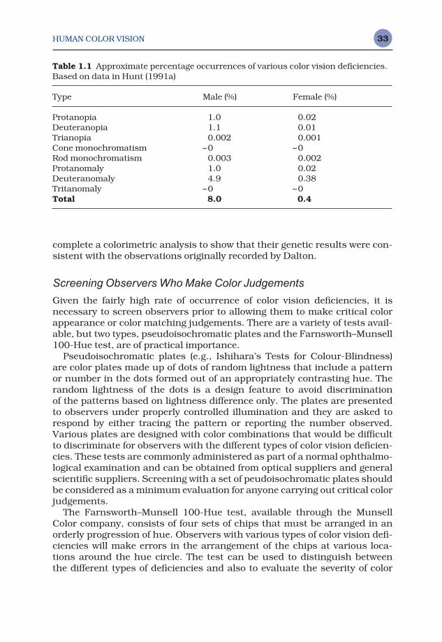
HUMAN COLOR VISION 33
complete a colorimetric analysis to show that their genetic results were con-sistent with the observations originally recorded by Dalton.
Screening Observers Who Make Color Judgements
Given the fairly high rate of occurrence of color vision deficiencies, it is necessary to screen observers prior to allowing them to make critical colorappearance or color matching judgements. There are a variety of tests avail-able, but two types, pseudoisochromatic plates and the Farnsworth–Munsell100-Hue test, are of practical importance.
Pseudoisochromatic plates (e.g., Ishihara’s Tests for Colour-Blindness)are color plates made up of dots of random lightness that include a patternor number in the dots formed out of an appropriately contrasting hue. Therandom lightness of the dots is a design feature to avoid discrimination of the patterns based on lightness difference only. The plates are presentedto observers under properly controlled illumination and they are asked torespond by either tracing the pattern or reporting the number observed.Various plates are designed with color combinations that would be difficultto discriminate for observers with the different types of color vision deficien-cies. These tests are commonly administered as part of a normal ophthalmo-logical examination and can be obtained from optical suppliers and generalscientific suppliers. Screening with a set of peudoisochromatic plates shouldbe considered as a minimum evaluation for anyone carrying out critical colorjudgements.
The Farnsworth–Munsell 100-Hue test, available through the MunsellColor company, consists of four sets of chips that must be arranged in anorderly progression of hue. Observers with various types of color vision defi-ciencies will make errors in the arrangement of the chips at various loca-tions around the hue circle. The test can be used to distinguish between the different types of deficiencies and also to evaluate the severity of color
Table 1.1 Approximate percentage occurrences of various color vision deficiencies.Based on data in Hunt (1991a)
Type Male (%) Female (%)
Protanopia 1.0 0.02Deuteranopia 1.1 0.01Trianopia 0.002 0.001Cone monochromatism ~0 ~0Rod monochromatism 0.003 0.002Protanomaly 1.0 0.02Deuteranomaly 4.9 0.38Tritanomaly ~0 ~0Total 8.0 0.4
HUMAN COLOR VISION34
discrimination problems. This test can also be used to identify observerswith normal color vision, but poor color discrimination for all colors.
1.7 KEY FEATURES FOR COLOR APPEARANCE MODELING
This chapter provides a necessarily brief overview of the form and function ofthe human visual system, concentrating on the features that are importantin the study, modeling, and prediction of color appearance phenomena.What follows is a short review of the key features.
Important features in the optics of the eye include the lens, macula, andcone photoreceptors. The lens and macula impact color matching throughtheir action as yellow filters. They impact inter-observer variability sincetheir optical density varies significantly from person to person. The conesserve as the first stage of color vision, transforming the spectral power distri-bution on the retina into a three-dimensional signal that defines what isavailable for processing at higher levels in the visual system. This is thebasis of metamerism, the fundamental governing principle of colorimetry.
The numerical distribution of the cones (L:M:S of about 12:6:1) is import-ant in constructing the opponent signals present in the visual system.Proper modeling of these steps requires the ratios to be accounted for appro-priately. The spatial distribution of rods and cones and their lateral inter-actions are critical in the specification of stimulus size and retinal locus. Acolor appearance model for stimuli viewed in the fovea would be differentfrom one for peripheral stimuli. The spatial interaction in the retina, repres-ented by horizontal and amacrine cells, is critical for mechanisms that pro-duce color appearance effects due to changes in background, surround, andlevel of adaptation.
The encoding of color information through the opponent channels alongwith the adaptation mechanisms before, during, and after this stage are per-haps the most important feature of the human visual system that must beincorporated into color appearance models. Each such model incorporates achromatic adaptation stage, an opponent processing stage, and nonlinearresponse functions. Some models also incorporate light and dark adaptationeffects and interactions between the rod and cone systems.
Lastly, the cognitive mechanisms of vision such as memory color and dis-counting the illuminant have a profound impact on color appearance. Theseand other color appearance phenomena are described in greater detail inChapters 6–8.
Color Appearance Models Second Edition M. D. Fairchild © 2005 John Wiley & Sons, LtdISBN: 0-470-01216-1 (HB)
2Psychophysics
Clearly, an understanding of the basic function of the human visual systemis necessary for appreciation of the formulation, implementation, and appli-cation of color appearance models. The need for a basic understanding of the principles of psychophysics might not seem so clear. Psychophysicaltechniques have produced most of our knowledge of human color vision andcolor appearance phenoma. These are the underpinnings of colorimetry andits extension through color appearance models. Also, psychophysical tech-niques are used to test, compare, and generate data for improving colorappearance models. Thus to fully understand the use and evaluation of colorappearance models, a basic appreciation of the field of psychophysics isessential. As an added bonus, psychophysical techniques such as thosedescribed in this chapter can help to prove that the implementation of acolor appearance model truly improves a system.
This chapter provides an overview of experimental design and data ana-lysis techniques for visual experiments. Carefully conducted visual experi-ments allow accurate quantitative evaluation of perceptual phenomena thatare often thought of as being completely subjective. Such results can be of immense value in a wide variety of fields, including color measurementand the evaluation of perceived image quality. Issues regarding the choiceand design of viewing environments, an overview of various classes of visual experiments, and a review of experimental techniques for threshold,matching, and scaling experiments are also described. Data reduction andanalysis procedures are also briefly discussed. The treatment of psycho-physics presented in this chapter is based on the ASTM Standard Guide forDesigning and Conducting Visual Experiments (ASTM 1996), which wasbased on materials from the RIT course work of this book’s author. There areseveral excellent texts on psychophysics that provide additional details onthe topics covered in this chapter. Of particular note are those of Gescheider(1985), Bartleson and Grum (1984), Torgerson (1958), and Thurstone (1959).Unfortuantely, the last three references are out of print and can only be foundin libraries. An interesting overview of the application of psychophysics

PSYCHOPHYSICS36
to image quality has been presented by Engeldrum (1995). The text byEngeldrum (2000) on psychometric scaling provides an excellent, modernreview of psychophysical techniques and their application.
2.1 PSYCHOPHYSICS DEFINED
Psychophysics is the scientific study of the relationships between the physical measurements of stimuli and the sensations and perceptions thatthose stimuli evoke. Psychophysics can be considered a discipline of sciencesimilar to the more traditional disciplines such as physics, chemistry, andbiology.
The tools of psychophysics are used to derive quantitative measures ofperceptual phenomena that are often considered subjective. It is importantto note that the results of properly designed psychophysical experiments are just as objective and quantitative as the measurement of length with aruler (or any other physical measurement). One important difference is that the uncertainties associated with psychophysical measurements tendto be significantly larger than those of physical measurements. However, theresults are equally useful and meaningful as long as those uncertainties areconsidered (as they always should be for physical measurements as well).Psychophysics is used to study all dimensions of human perception. Sincethe topic of this book is color appearance, visual psychophysics is specific-ally discussed.
Two Classes of Visual Experiments
Visual experiments tend to fall into two broad classes:
1. Threshold and matching experiments, designed to measure visual sensit-ivity to small changes in stimuli (or perceptual equality)
2. Scaling experiments, intended to generate a relationship between thephysical and perceptual magnitudes of a stimulus
It is critical to first determine which class of experiment is appropriate fora given application. Threshold experiments are appropriate for measuringsensitivity to changes and the detectability of stimuli. For example, thresh-old experiments could be used to determine whether an image compressionalgorithm was truly visually lossless or if the performance of two colorappearance models is perceptibly different in some practical application.
Scaling experiments are appropriate when it is necessary to specify therelationships between stimuli. For example, a scaling experiment might be used to develop a quantitative relationship between the perceived qualityof a printed image and the spatial addressability of the printer. In color
PSYCHOPHYSICS 37
appearance modeling, the results of scaling experiments are used to deriverelationships between physically measurable colorimetric quantities (e.g.,CIE XYZ tristimulus values) and perceptual attributes such as lightness,chroma, and hue.
2.2 HISTORICAL CONTEXT
As with any scientific discipline, a better appreciation of psychophysics canbe obtained with a brief look at the historical development of the field. Whilescientists have been making and recording careful observations of their perceptions for centuries, the formal discipline of psychophysics is less than150 years old. Important milestones in the history of psychophysics can berepresented in the work of Weber, Fechner, and Stevens.
Weber’s Work
In the early part of the 19th century, E.H. Weber investigated the perceptionof the heaviness of lifted weights. Weber asked observers to lift a given weightand then he added to the weight (with all of the necessary experimental controls) until the observers could just distinguish the new weight from theoriginal. This is a measurement of the threshold for change in weight. Webernoted that as the initial weight increased, the change in weight required to reach a threshold increased proportionally. If the initial magnitude of the stimulus (weight in this case) is denoted I, and the change required toachieve a threshold is denoted ∆ I, Weber’s results can be expressed by stating that the ratio ∆ I/I is constant. In fact, this general relationship holdsapproximately true for many perceptual stimuli and has come to be knownas Weber’s law.
Weber’s result is quite intuitive. For example, imagine carrying a fewsheets of paper and then adding a 20-page document to the load. Clearly thedifference between the two weights would be perceived. Now imagine carry-ing a briefcase full of books and papers and then adding another 20-pagedocument to the case. Most likely the added weight of 20 more pages wouldgo unnoticed. That is because a greater change is required to reach a percep-tual threshold when the initial stimulus intensity is higher. Weber’s law can also be used to explain why stars cannot be seen during the daytime. At night, the stars represent a certain increment in intensity ∆ I over thebackground illumination of the sky I, that exceeds the visual threshold andtherefore they can be seen. During the day, the stars still produce the sameincrement in intensity ∆ I over the background illumination. However, thebackground intensity of the daytime sky I is much larger than at night.Therefore the ratio ∆ I/I is far lower during the day than at night. So low, infact, that the stars cannot be perceived during the day.
PSYCHOPHYSICS38
Fechner’s Work
The next milestone is the work of Fechner. Fechner built on the work ofWeber to derive a mathematical relationship between stimulus intensity andperceived magnitude. While Fechner’s motivation was to solve the mind–body problem by proving that functions of the mind could be physically measured, he inadvertently became known as the father of psychophysicsthrough his publication of Elements of Psychophysics in 1860 (Fechner1966).
Fechner started with two basic assumptions:
1. Weber’s law was indeed valid.2. A just-noticeable difference (JND) can be considered a unit of perception.
Weber’s results showed that the JNDs measured on the physical scalewere not equal as the stimulus intensity increased, but rather increased inproportion to the stimulus intensity. Fechner strived to derive a transforma-tion of the physical stimulus intensity scale to a perceptual magnitude scaleon which the JNDs were of equal size for all perceptual magnitudes. Thisproblem essentially becomes one of solving the differential equation posedby Weber’s law. Since JNDs followed a geometric series on the stimulusintensity scale, the solution is straightforward, that a logarithmic transforma-tion will produce JNDs of equal incremental size on a perceptual scale. Thusthe JNDs represented by equal ratios on the physical scale become trans-formed into equal increments on a perceptual scale according to what hascome to be known as Fechner’s law.
Simply put, Fechner’s law states that the perceived magnitude of a stimu-lus is proportional to the logarithm of the physical stimulus intensity. Thisrelationship is illustrated in Figure 2.1. Fechner’s law results in a compress-ive nonlinear relationship between the physical measurement and perceivedmagnitude that illustrates a decreasing sensitivity (i.e., slope of the curve inFigure 2.1) with increasing stimulus intensity. If Fechner’s law were strictlyvalid, then the relationship would follow the same nonlinear form for all per-ceptions. While the general trend of a compressive nonlinearity is valid formost perceptions, various perceptions take on relationships with differentlyshaped functions. This means that Fechner’s law is not completely accurate.However, there are numerous examples in the vision science literature ofinstances in which Fechner’s law (or at least Weber’s law) is obeyed.
Stevens’ Work
Addressing the lack of generality in Fechner’s result, Stevens (1961) pub-lished an intriguing paper entitled ‘To honor Fechner and repeal his law.’Stevens studied the relationship between physical stimulus intensity andperceptual magnitude for over 30 different types of perceptions using a mag-
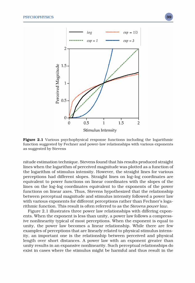
PSYCHOPHYSICS 39
nitude estimation technique. Stevens found that his results produced straightlines when the logarithm of perceived magnitude was plotted as a function ofthe logarithm of stimulus intensity. However, the straight lines for variousperceptions had different slopes. Straight lines on log–log coordinates areequivalent to power functions on linear coordinates with the slopes of thelines on the log–log coordinates equivalent to the exponents of the powerfunctions on linear axes. Thus, Stevens hypothesized that the relationshipbetween perceptual magnitude and stimulus intensity followed a power lawwith various exponents for different perceptions rather than Fechner’s loga-rithmic function. This result is often referred to as the Stevens power law.
Figure 2.1 illustrates three power law relationships with differing expon-ents. When the exponent is less than unity, a power law follows a compress-ive nonlinearity typical of most perceptions. When the exponent is equal tounity, the power law becomes a linear relationship. While there are fewexamples of perceptions that are linearly related to physical stimulus intens-ity, an important one is the relationship between perceived and physicallength over short distances. A power law with an exponent greater thanunity results in an expansive nonlinearity. Such perceptual relationships doexist in cases where the stimulus might be harmful and thus result in the
Figure 2.1 Various psychophysical response functions including the logarithmicfunction suggested by Fechner and power-law relationships with various exponentsas suggested by Stevens
PSYCHOPHYSICS40
perception of pain. A compressive function for the pain perception could bequite dangerous since the observer would become less and less sensitive tothe stimulus as it became more and more dangerous.
The Stevens power law can be used to model many perceptual phenom-ena, and can be found in fundamental aspects of color measurement suchas the relationship between CIE XYZ tristimulus values and the predictors oflightness and chroma in the CIELAB color space that are based on a cube-root compressive power-law nonlinearity.
2.3 HIERARCHY OF SCALES
When deriving perceived magnitude scales, it is critical to understand theproperties of the resulting scales. Often a psychophysical technique will pro-duce a scale with only limited mathematical utility. In such cases it is criticalthat inappropriate mathematical manipulations are not applied to the scale.Four key types of scales have been defined. In order of increasing mathem-atical power and complexity, they are nominal, ordinal, interval, and ratioscales.
Nominal Scales
Nominal scales are relatively trivial in that they scale items simply by name;for color a nominal scale could consist of reds, yellows, greens, blues, andneutrals. Scaling in this case would simply require deciding which colorbelonged in which category. Only naming can be performed with nominaldata.
Ordinal Scales
Ordinal scales are scales in which elements are sorted in ascending ordescending order based on greater or lesser amount of a particular attribute.A set of color swatches could be sorted by hue and then in each hue rangethe colors could be sorted from the lightest to the darkest. Since the swatchcolors are not evenly spaced, there might be three dark, one medium, andtwo light green swatches. If these were numbered from one to six in order ofincreasing lightness, an ordinal scale would be created. There is no informa-tion on such a scale as to how much lighter one of the green swatches is thananother and it is clear that they are not evenly spaced. For an ordinal scaleall that matters is that the samples be arranged in increasing or decreasingamounts of an attribute. The spacing between samples can be large or smalland can change up and down the scale. Logical operations such as greater-than, less-than, or equal-to can be performed with ordinal scales.
PSYCHOPHYSICS 41
Interval Scales
Interval scales have equal intervals. On an interval scale if a pair of sampleswas separated by two units and a second pair at some other point on thescale was also separated by two units, the differences between the pairswould be perceptually equal. However, there is no meaningful zero point onan interval scale. In addition to the mathematical operations listed for theabove scales, addition and subtraction can be performed with interval data.The Celsius and Fahrenheit temperature scales are interval scales.
Ratio Scales
Ratio scales have all the properties of the above scales plus a meaningfullydefined zero point. Thus it is possible to properly equate ratios of numberson a ratio scale. Ratio scales in visual work are often difficult and sometimesimpossible to obtain. This is sometimes the case since a meaningful zeropoint does not exist. For example, an interval scale of image quality is relat-ively easy to derive, but try to imagine an image with zero quality. Similarly it is relatively straightforward to derive interval scales of hue, but there is nophysically meaningful zero hue. All of the mathematical operations that canbe performed on an interval scale can also be performed on a ratio scale. Inaddition, multiplication and division can be performed.
Example of the Use of Scales
It is helpful to reinforce the concepts of the hierarchy of scales by example.Imagine that it is necessary to measure the heights of all the people in aroom. If only a nominal scale were available, you could choose a first subjectand assign a name to his or her height, say Joe. Then you could examine theheight of each additional subject relative to the height of Joe. If another per-son had the same height as Joe (assuming some reasonable tolerance), theirheight would also be assigned the name Joe. If their height differed from Joe,they would be given a different name. This process could be completed bycomparing the heights of everyone in the room until each unique height wasassigned a unique name. Note that there is no information regarding who istaller or shorter than anyone else. The only information available is whethersubjects share the same height (and therefore name) or not.
If, instead, an ordinal scale was used to measure height. Joe could arbit-rarily be assigned a height of zero. If the next subject was taller than Joe, heor she would be assigned any number larger than Joe’s, say 10. If a thirdsubject was found to be taller than Joe, but shorter than the second subject,they would be assigned a number between zero and 10. This would continueuntil everyone in the room was assigned a number to represent their height.Since the magnitude of the numbers was assigned arbitrarily, nothing can

PSYCHOPHYSICS42
be said about how much shorter or taller one subject is than another.However they could be put in order from shortest to tallest.
If an interval scale was available for measurement of height, Joe couldagain be arbitrarily assigned a height of zero. However, other subjects couldthen be assigned heights relative to Joe’s in terms of meaningful incrementssuch as +3 cm (taller than Joe) or −2 cm (shorter than Joe). If subjects A andB had heights of +3 cm and −2 cm, respectively on this interval scale, it can be determined that subject A is 5 cm taller than subject B. Note howeverthat there is still no information to indicate how tall either of the subjects is. The only information available with the interval scale are differencesbetween subjects.
Finally, if a ratio scale is available to measure height (the normal situ-ation), Joe might be measured and found to be 182 cm tall. Then subjects Aand B would have heights of 185 cm and 180 cm, respectively. If anothersubject came along who was 91 cm tall, it could be concluded that Joe istwice as tall as this subject. Since zero cm tall is a physically meaningful zeropoint, a true ratio scale is available for the measurement of height and thusmultiplications and divisions of scale values can be performed.
2.4 THRESHOLD TECHNIQUES
Threshold experiments are designed to determine the just-perceptiblechange in a stimulus, sometimes referred to as a just-noticeable difference(JND). Threshold techniques are used to measure the observers’ sensitivityto changes in a given stimulus. Absolute thresholds are defined as the just-perceptible difference for a change from no stimulus, while differencethresholds represent the just-perceptible difference from a particular stimu-lus level greater than zero. Thresholds are reported in terms of the physicalunits used to measure the stimulus. For example, a brightness thresholdmight be measured in luminance units of cd/m2. Sensitivity is defined as the inverse of the threshold since a low threshold implies high sensitivity.Threshold techniques are useful for defining visual tolerances such as thosefor perceived color differences.
Types of Threshold Experiments
There are several basic types of threshold experiments presented below inorder of increasing complexity of experimental design and utility of the datagenerated. Many modifications of these techniques have been developed forparticular applications. Experimenters strive to design experiments thatremove as much control of the results from the observers as possible, thusminimizing the influence of variable observer judgement criteria. Generally
PSYCHOPHYSICS 43
this comes at the cost of implementing more complicated experimental pro-cedures. Threshold techniques include the following:
• Method of adjustment• Method of limits• Method of constant stimuli
Method of Adjustment
The method of adjustment is the simplest and most straightforward tech-nique for deriving threshold data. In it, the observer controls the stimulusmagnitude and adjusts it to a point that is just perceptible (absolute thresh-old), or just perceptibly different (difference threshold) from a starting level.The threshold is taken to be the average setting across a number of trials by one or more observers. The method of adjustment has the advantage that it is quick and easy to implement. However, a major disadvantage isthat the observer is in control of the stimulus. This can bias the results due to variability in observers’ criteria and adaptation effects. If an observerapproaches the threshold from above, adaptation might result in a higherthreshold than if it were approached from below. Often the method of adjust-ment is used to obtain a first estimate of the threshold to be used in thedesign of more sophisticated experiments. The method of adjustment is alsocommonly used in matching experiments, including asymmetric matchingexperiments used in color appearance studies.
Method of Limits
The method of limits is only slightly more complex than the method ofadjustment. In the method of limits, the experimenter presents the stimuliat predefined discrete intensity levels in either ascending or descendingseries. For an ascending series, the experimenter presents a stimulus, begin-ning with one that is certain to be imperceptible, and asks the observers torespond ‘yes’ if they perceive it and ‘no’ if they do not. If they respond ‘no’, theexperimenter increases the stimulus intensity and presents another trial.This continues until the observer responds ‘yes’. A descending series beginswith a stimulus intensity that is clearly perceptible and continues until theobservers respond ‘no’ — that is, they cannot perceive the stimulus. Thethreshold is taken to be the average stimulus intensity at which the transi-tion from ‘no’ to ‘yes’ (or ‘yes’ to ‘no’) responses occurs for a number ofascending and descending series. Averaging over both types of series min-imizes adaptation effects. However, the observers are still in control of theircriteria since they can respond ‘yes’ or ‘no’ at their own discretion.

PSYCHOPHYSICS44
Method of Constant Stimuli
In the method of constant stimuli, the experimenter chooses several stimu-lus intensity levels (typically about 5 or 7) around the level of the threshold.Then each of these stimuli is presented multiple times in random order. Over the trials, the frequency with which each stimulus level is perceived isdetermined. From such data, a frequency-of-seeing curve, or psychometricfunction, can be derived that allows determination of the threshold and itsuncertainty. The threshold is generally taken to be the intensity at which thestimulus is perceived on 50% of the trials. Psychometric functions can bederived either for a single observer (through multiple trials) or for a popula-tion of observers (one or more trials per observer). Two types of response canbe obtained:
• Yes–no (or pass–fail)• Forced choice
Yes–No Method
In a yes–no method of constant stimuli procedure, the observers are asked torespond ‘yes’ if they detect the stimulus (or stimulus change) and ‘no’ if theydo not. The psychometric function is then simply the percentage of ‘yes’responses as a function of stimulus intensity; 50% ‘yes’ responses would betaken as the threshold level. Alternatively, this procedure can be used tomeasure visual tolerances above threshold by providing a reference stimu-lus intensity (e.g., a color difference anchor pair) and asking observers topass stimuli that fall below the intensity of the reference (e.g., a smaller colordifference) and fail those that fall above it (e.g., a larger color difference). Thepsychometric function is then taken to be the percent of fail responses as afunction of stimulus intensity and the 50% fail level is deemed to be thepoint of visual equality.
Forced Choice Procedures
A forced-choice procedure eliminates the influence of varying observer criteria on the results. This is accomplished by presenting the stimulus inone of two intervals defined by either a spatial or temporal separation. Theobservers are then asked to indicate in which of the two intervals the stimu-lus was presented. The observers are not allowed to respond that the stimu-lus was not present and are forced to guess one of the two intervals if theyare unsure (hence the name forced choice). The psychometric function isthen plotted as the percentage of correct responses as a function of stimulusintensity. The function ranges from 50% correct when the observers are simply guessing to 100% correct for stimulus intensities at which they can

PSYCHOPHYSICS 45
always detect the stimulus. Thus the threshold is defined as the stimulusintensity at which the observers are correct 75% of the time and thereforedetecting the stimulus 50% of the time. As long as the observers respondhonestly, their criteria, whether liberal or conservative, cannot influence theresults.
Staircase Procedures
Staircase procedures are a modification of the forced-choice proceduredesigned to measure only the threshold point on the psychometric function.Staircase procedures are particularly applicable to situations in which thestimulus presentations can be fully automated. A stimulus is presented andthe observer is asked to respond. If the response is correct, the same stimu-lus intensity is presented again. If the response is incorrect, the stimulusintensity is increased for the next trial. Generally, if the observer respondscorrectly on three consecutive trials, the stimulus intensity is decreased.The stimulus intensity steps are decreased until some desired precision inthe threshold is reached. The sequence of three correct or one incorrectresponse prior to changing the stimulus intensity will result in a conver-gence to a stimulus intensity that is correctly identified on 79% of the trials(0.793 = 0.5), very close to the nominal threshold level of 75%. Often severalindependent staircase procedures are run simultaneously to further ran-domize the experiment. A staircase procedure could also be run with yes–noresponses.
Probit Analysis of Threshold Data
Threshold data that generate a psychometric function can be most usefullyanalyzed using Probit analysis. Probit analysis is used to fit a cumulativenormal distribution to the data (psychometric function). The threshold pointand its uncertainty can then be easily determined from the fitted distribu-tion. There are also several significance tests that can be performed to verifythe suitability of the analyses. Finney (1971) provides details on the theoryand application of Probit analysis. Several commercially available statisticalsoftware packages can be used to perform Probit analyses.
2.5 MATCHING TECHNIQUES
Matching techniques are similar to threshold techniques except that thegoal is to determine when two stimuli are not perceptibly different. Measuresof the variability in matching are sometimes used to estimate thresholds.Matching experiments provided the basis for CIE colorimetry through themetameric matches used to derive color matching functions. For example, if
PSYCHOPHYSICS46
a given color is perceptually matched by an additive mixture of red, green,and blue primary lights that do not mix to produce a spectral energy distri-bution that is identical to the test color, then the match is considered meta-meric. The physical properties of such matches can be used to derive thefundamental responsivities of the human visual system and ultimately beused to derive a system of tristimulus colorimetry as outlined in Chapter 3.
Asymmetric Matching
Matching experiments are often used in the study of chromatic adaptationand color appearance as well. In such cases, asymmetric matches are made.An asymmetric match is a color match made across some change in viewingconditions. For example, a stimulus viewed in daylight illumination might bematched to another stimulus viewed under incandescent illumination toderive a pair of corresponding colors for this change in viewing conditions.Such data can then be used to formulate and test color appearance modelsdesigned to account for such changes in viewing condition. One special caseof an asymmetric matching experiment is the haploscopic experiment inwhich one eye views a test stimulus in one set of viewing conditions and theother eye simultaneously views a matching stimulus in a different set ofviewing conditions. The observer simultaneously views both stimuli andproduces a match.
Memory Matching
Another type of matching experiment that is sometimes used in the study ofcolor appearance is called memory matching. In such experiments observersproduce a match to a previously memorized color. Typically such matchesare asymmetric to study viewing conditions dependencies. Occasionallymemory matches are made to mental stimuli such as an ideal achromatic(gray) color or a unique hue (e.g., a unique red with no blue or yellow content).
2.6 ONE-DIMENSIONAL SCALING
Scaling experiments are intended to derive relationships between perceptualmagnitudes and physical measures of stimulus intensity. Depending on thetype and dimensionality of the scale required, several approaches are pos-sible. Normally the type of scale required and the scaling method to be usedare decided upon before any visual data are collected. One-dimensional scaling requires the assumption that both the attribute to be scaled and thephysical variation of the stimulus are one dimensional. Observers are askedto make their judgements on a single perceptual attribute (e.g., how light is
PSYCHOPHYSICS 47
one sample compared with another, what is the quality of the differencebetween a pair of images). A variety of scaling techniques have been devisedfor the measurement of one-dimensional psychophysical scales, which aredescribed in the following paragraphs:
• Rank order• Graphical rating• Category scaling• Paired comparisons• Partition scaling• Magnitude estimation or production• Ratio estimation or production
In a rank order experiment, the observer is asked to arrange a given set ofsamples according to increasing or decreasing magnitudes of a particularperceptual attribute. With a large number of observers the data may be aver-aged and reranked to obtain an ordinal scale. To obtain an interval scale.certain assumptions about the data need to be made and additional ana-lyses need to be performed. In general it is somewhat dubious to attempt toderive interval scales from rank order data. One of the more reasonableassumptions is to treat the data as if each pair of stimuli were compared,thereby deriving paired comparison data from the rank results.
Graphical rating allows direct determination of an interval scale. Observersare presented stimuli and asked to indicate the magnitude of their percep-tion on a one-dimensional scale with defined endpoints. For example, in alightness scaling experiment a line might be drawn with one end labeledwhite and the other end labeled black. When the observers are presentedwith a medium gray that is perceptually halfway between white and black,they would make a mark on the line at the midpoint. If the sample was closerto white than black, they would make a mark at the appropriate physicallocation along the line, closer to the end labeled white. The interval scale is taken to be the mean location on the graphical scale for each stimulus.This technique relies on the well-established fact that the perception oflength over short distances is linear with respect to physically measuredlength.
Category scaling is a popular technique for deriving ordinal or intervalscales for large numbers of stimuli. An observer is asked to separate a largenumber of samples into various categories. With several observers, the number of times each particular sample is placed in a category is recorded.For this to be an effective scaling method the samples need to be similarenough that they are not always placed in the distinct categories by differentobservers or by the same observer on different occasions. Interval scalesmay be obtained by this method by assuming that the perceptual magni-tudes are normally distributed and by making use of the standard normaldistribution according to the law of categorical judgements (Torgerson1954).
PSYCHOPHYSICS48
When the number of different stimuli is smaller, a paired comparisonexperiment can be performed. In this method, all samples are presented tothe observer in all the possible pairwise combinations, usually one pair at a time (sometimes with a third stimulus as a reference). The proportion oftimes a particular sample is judged greater in some attribute than eachother sample is calculated and recorded. Interval scales can be obtainedfrom such data by applying the law of comparative judgements (Thurstone,1927). Thurstone’s law of comparative judgements and its extensions can beusefully applied to ordinal data (such as paired comparisons and categoryscaling) to derive meaningful interval scales. The perceptual magnitudes of the stimuli are normally distributed on the resulting scales. Thus, if it issafe to assume that the perceptual magnitudes are normally distributed onthe true perceptual scale; these analyses derive the desired scale. They alsoallow useful evaluation of the statistical significance of differences betweenstimuli since the power of the normal distribution can be utilized. Torgerson(1958), Bartleson and Grum (1984), and Engeldrum (2000) describe theseand other related analyses in detail. ASTM (1996) describes a simple methodfor deriving confidence limits on Thurstonian interval scales. That tech-nique, while conservative, might be less than optimal and is difficult toderive with statistical rigor. Montag et al. (2004) describe a Monte Carlo simulation of the problem and recommends a more appropriate method forderiving confidence intervals. Handley (2001) also describes some relatedtechniques.
A rather direct method for deriving interval scales is through partitionscaling. A common method is by equating intervals through bisection. Theobserver is given two different samples (A and B) and asked to select a thirdsuch that the difference between it and A appears equal to the differencebetween it and B. A full interval scale may be obtained by successive bisections.
Ratio scales can be directly obtained through the methods of magnitudeestimation or production. In such experiments, the observer is asked toassign numbers to the stimuli according to the magnitude of the perception.Alternatively, observers are given a number and asked to produce a stimuluswith that perceptual magnitude. This is one of the few techniques that can be used to generate a ratio scale. It can also be used to generate data for multidimensional scaling by asking observers to scale the differencesbetween pairs of stimuli.
A slightly more complicated technique involves ratio estimation or pro-duction. The observer is asked for judgements in one of two ways: (1) selector produce a sample that bears some prescribed ratio to a standard; or (2)given two or more samples, to state the apparent ratios among them. A typical experiment is to give the observers a sample and ask them to find,select, or produce a test sample that is one-half or twice the standard insome attribute. For most practical visual work this method is too difficult touse, either because of the sample preparation or the judgement by theobservers. However, it can be also used to generate a ratio scale.
PSYCHOPHYSICS 49
2.7 MULTIDIMENSIONAL SCALING
Multidimensional scaling (MDS) is a method similar to one-dimensionalscaling, but it does not require the assumption that the attribute to bescaled is one-dimensional. The dimensionality is found as part of the ana-lysis. In multidimensional scaling, the data are interval or ordinal scales ofthe similarities or dissimilarities between each of the stimuli, and the result-ing output is a multidimensional geometric configuration of the perceptualrelationships between the stimuli, as on a map.
The dissimilarity data required for MDS can conveniently be obtainedusing paired comparison and triadic combination experiments. In a pairedcomparison experiment, all samples in all possible pairs are presented andthe observer is asked to make a magnitude estimation of the perceived dif-ference between each pair. The resulting estimates for each pairwise com-bination can then be subjected to MDS analyses. In the method of triadiccombinations, observers are presented with each possible combination ofthe stimuli taken three at a time. They are then asked to judge which two ofthe stimuli in each triad are most similar to one another and which two aremost different. The data can then be converted into frequencies of times eachpair is judged most similar or most different. These frequency data can thenbe combined into either a similarity or dissimilarity matrix for use in MDSanalyses.
MDS analysis techniques take such similarity or dissimilarity data asinput and produce a multidimensional configuration of points representingthe relationships and dimensionality of the data. It is necessary to use suchtechniques when either the perception in question is multidimensional (suchas color — hue, lightness, and chroma) or the physical variation in the stimuliis multidimensional. Kruskal and Wish (1978) provide details of these tech-niques. There are several issues with respect to MDS analyses. There are twoclasses of MDS: metric, which requires interval data, and non-metric, whichonly requires ordinal data. Both classes of MDS techniques result in interval-scale output. Various MDS software packages process input dataaccording to specific assumptions regarding the input data, treatment ofindividual cases, goodness-of-fit metrics (stress), distance metrics (e.g.,Euclidean or cityblock), etc. Several commercial statistical software pack-ages provide MDS capabilities.
A classic example of MDS analysis is the construction of a map from datarepresenting the distances between cities (Kruskal and Wish 1978). In thisexample, a map of the USA is constructed from the dissimilarity matrix ofdistances between eight cities gathered from a road atlas, as illustrated inTable 2.1.
The dissimilarity data are then analyzed via MDS. Stress (RMS error) isused as a measure of goodness-of-fit in order to determine the dimensional-ity of the data. In this example, the stress of a one-dimensional fit is about0.12, while the stress in two or more dimensions is essentially zero. Thisindicates that a two-dimensional fit, as expected, is appropriate. The results

PSYCHOPHYSICS50
output include the coordinates in each of the two dimensions for each of thecities as listed in Table 2.2.
Plotting the coordinates of each city in the two output dimensions willresult in a familiar map of the USA, as shown in Figure 2.2. However, itshould be noted that dimension 1 goes from east to west and dimension 2goes from north to south, resulting in a map that has the axes reversed froma traditional map. This illustrates a feature of MDS, namely that thedefinition of the output dimensions requires post hoc analysis by the experi-menter. MDS experiments can be used to explore the dimensionality andstructure of color appearance spaces (e.g., Indow 1988).
2.8 DESIGN OF PSYCHOPHYSICAL EXPERIMENTS
The previous sections provide an overview of some of the techniques used toderive psychophysical thresholds and scales. However there are many moreissues that arise in the design of psychophysical experiments that have asignificant impact on the experimental results, particularly when colorappearance is concerned. Many of these experimental factors are the key
Table 2.1 Dissimilarity matrix consisting of distances between cities in the USA
ATL BOS CHI DAL DEN LA SEA NYC
ATLBOS 1037CHI 674 963DAL 795 1748 917DEN 1398 1949 996 781LA 2182 2979 2054 1387 1059SEA 2618 2976 2013 2078 1307 1131NYC 841 206 802 1552 1771 2786 2815
Table 2.2 Output two-dimensional coordinates for each city in the USA. MDS example
City Dimension 1 Dimension 2
Atlanta −0.63 0.40Boston −1.19 −0.31Chicago −0.36 −0.15Dallas 0.07 0.55Denver 0.48 0.00Los Angeles 1.30 0.36Seattle 1.37 −0.66New York City −1.04 −0.21

PSYCHOPHYSICS 51
variables that have illustrated the need to extend basic colorimetry with thedevelopment of color appearance models. A complete description of all of thevariables involved in visual experiments could easily fill several books andmany of the critical issues for color appearance phenomena are described inmore detail in later chapters. At this point a simple listing of some of theissues that require consideration should be sufficient to bring these issuesto light. Important factors in visual experiments include (in no particularorder):
Observer age Control and history of eye movementsObserver experience Adaptation stateNumber of observers Complexity of observer taskScreening for color vision deficiencies ControlsObserver acuity Repetition rateInstructions Range effectsContext Regression effectsFeedback Image contentRewards Number of imagesIllumination level Duration of observation sessionsIllumination color Number of observation sessionsIllumination geometry Observer motivationBackground conditions Cognitive factorsSurround conditions Statistical significance of results
Figure 2.2 The output of a multidimensional scaling (MDS) program used to gener-ate a map of the USA from input data on the proximities of cities
PSYCHOPHYSICS52
All these items, and probably many more, can have a profound effect onpsychophysical results and should be carefully specified and/or controlled.Such issues need to be addressed both by those performing experiments andby those trying to interpret and utilize the results for various applications.
2.9 IMPORTANCE IN COLOR APPEARANCE MODELING
A fundamental understanding of the processes involved in psychophysicalexperiments provides useful insight for understanding the need for anddevelopment and evaluation of color appearance models. Psychophysicalexperiments provided much of the information reviewed in Chapter 1 on thehuman visual system. Psychophysics is the basis of colorimetry presented inChapter 3. The results of psychophysical experiments are also presented inChapters 6, 8, and 17 on color appearance phenomena, chromatic adapta-tion, and testing color appearance models. Simply put, without extensivepsychophysical experimentation, none of the information required to createand use color appearance models would exist.

Color Appearance Models Second Edition M. D. Fairchild © 2005 John Wiley & Sons, LtdISBN: 0-470-01216-1 (HB)
3Colorimetry
Colorimetry serves as the fundamental underpinning of color appearancespecification. This chapter reviews the well-established practice of colori-metry according to the CIE (International Commission on Illumination) sys-tem first established in 1931. This system allows the specification of colormatches for an average observer and has amazingly withstood an onslaughtof technological pressures and remained a useful international standard forover 65 years (Wright 1981b, Fairchild 1993b). However, CIE colorimetryprovides only the starting point. Color appearance models enhance this system in an effort to predict the actual appearances of stimuli in variousviewing conditions rather than simply whether or not two stimuli will match.This chapter provides a general review of the concepts of colorimetry to setthe stage for development of various color appearance models. It is notintended to be a complete reference on colorimetry since there are a numberof excellent texts on the subject available. For introductions to colorimetry,readers are referred to the texts of Berns (2000), Hunt (1991a), Berger-Schunn (1994), and Hunter and Harold (1987). The precise definition of colorimetry can be found in the primary reference, CIE Publication 15.2 (CIE1986), which is currently being updated to Publication 15.3. For completedetails in an encyclopedic reference volume, the classic book by Wyszeckiand Stiles (1982), Color Science, should be consulted. Fundamental insightinto the mathematics and theory of visual color matching can be found inthe work of Cohen (2001).
3.1 BASIC AND ADVANCED COLORIMETRY
Colorimetry refers to the measurement of color. Wyszecki (1973) describedan important distinction between basic and advanced colorimetry (see alsoWyszecki 1986). This distinction is the basis of this book and warrantsattention. It is perhaps most enlightening to quote Wyszecki’s exact words in
COLORIMETRY54
making the distinction. Wyszecki’s (1973) description of basic colorimetry isas follows.
Colorimetry, in its strict sense, is a tool used to making a prediction onwhether two lights (visual stimuli) of different spectral power distributions willmatch in colour for certain given conditions of observation. The prediction ismade by determining the tristimulus values of the two visual stimuli. If thetristimulus values of a stimulus are identical to those of the other stimulus, acolour match will be observed by an average observer with normal colourvision.
Wyszecki (1973) went on to describe the realm of advanced colorimetry.
Colorimetry in its broader sense includes methods of assessing the appear-ance of colour stimuli presented to the observer in complicated surroundingsas they may occur in everyday life. This is considered the ultimate goal of colorimetry, but because of its enormous complexity, this goal is far from beingreached. On the other hand, certain more restricted aspects of the overallproblem of predicting colour appearance of stimuli seem somewhat less elus-ive. The outstanding examples are the measurement of colour differences,whiteness, and chromatic adaptation. Though these problems are still essen-tially unresolved, the developments in these areas are of considerable interestand practical importance.
This chapter describes the well-established techniques of basic colorimetrythat form the foundation for color appearance modeling. It also describessome of the widely used methods for color difference measurement, one ofthe first objectives of advanced colorimetry. Wyszecki’s distinction betweenbasic and advanced colorimetry serves to highlight the purpose of this book,an account of the research and modeling aimed at the extension of basic col-orimetry toward the ultimate goals of advanced colorimetry.
3.2 WHY IS COLOR?
To begin a discussion of the measurement of color, one must first considerthe nature of color. Figure 3.1 illustrates the answer to the question — ‘whyis color?’ ‘Why’ is a more appropriate question than the more typical ‘what’since color is not a simple thing that can be easily described to someone whohas never experienced it. Color cannot even be defined without resort toexamples (see Chapter 4). Color is an attribute of visual sensation and thecolor appearance of objects depends on the three components making up thetriangle in Figure 3.1. The first requirement is a source of visible electromag-netic energy necessary to initiate the sensory process of vision. This energyis then modulated by the physical and chemical properties of an object. Themodulated energy is then imaged by the eye, detected by photoreceptors,
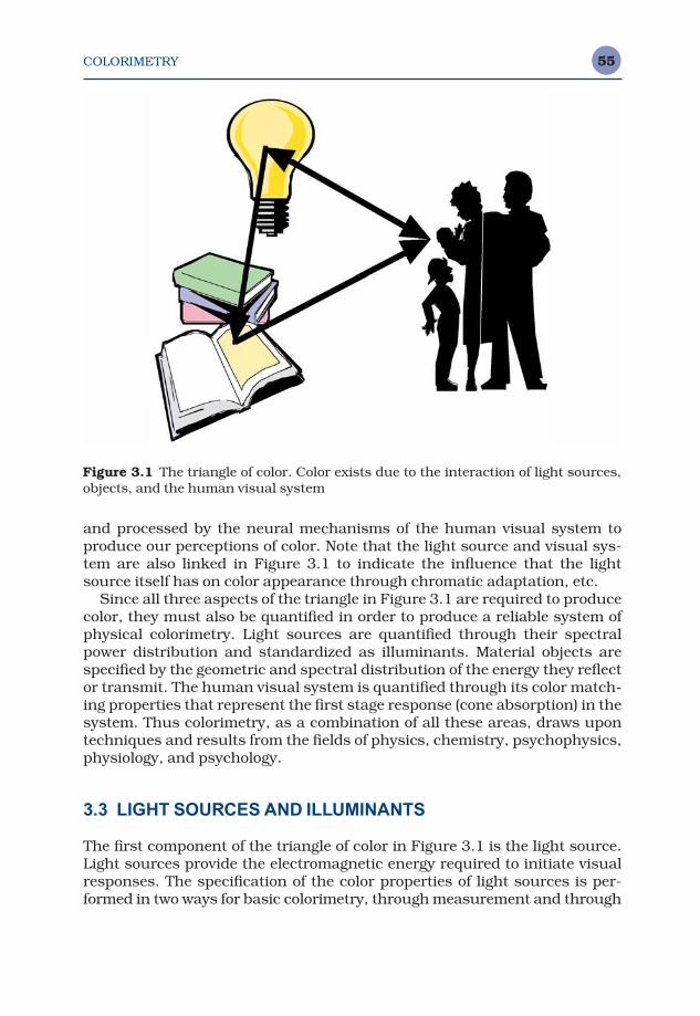
COLORIMETRY 55
and processed by the neural mechanisms of the human visual system toproduce our perceptions of color. Note that the light source and visual sys-tem are also linked in Figure 3.1 to indicate the influence that the lightsource itself has on color appearance through chromatic adaptation, etc.
Since all three aspects of the triangle in Figure 3.1 are required to producecolor, they must also be quantified in order to produce a reliable system ofphysical colorimetry. Light sources are quantified through their spectralpower distribution and standardized as illuminants. Material objects arespecified by the geometric and spectral distribution of the energy they reflector transmit. The human visual system is quantified through its color match-ing properties that represent the first stage response (cone absorption) in thesystem. Thus colorimetry, as a combination of all these areas, draws upontechniques and results from the fields of physics, chemistry, psychophysics,physiology, and psychology.
3.3 LIGHT SOURCES AND ILLUMINANTS
The first component of the triangle of color in Figure 3.1 is the light source.Light sources provide the electromagnetic energy required to initiate visualresponses. The specification of the color properties of light sources is per-formed in two ways for basic colorimetry, through measurement and through
Figure 3.1 The triangle of color. Color exists due to the interaction of light sources,objects, and the human visual system
COLORIMETRY56
standardization. The distinction between these two techniques is clarified in the definition of light sources and illuminants. Light sources are actualphysical emitters of visible energy. Incandescent light bulbs, the sky at anygiven moment, and fluorescent tubes represent examples of light sources.Illuminants, on the other hand, are simply standardized tables of values thatrepresent a spectral power distribution typical of some particular lightsource. CIE illuminants A, D65, and F2 are standardized representations oftypical incandescent, daylight, and fluorescent sources. Some illuminantshave corresponding sources that are physical embodiments of the standard-ized spectral power distributions. For example, CIE source A is a particulartype of tungsten source that produces the relative spectral power distribu-tion of CIE illuminant A. Other illuminants do not have correspondingsources. For example, CIE illuminant D65 is a statistical representation ofan average daylight with a correlated color temperature of approximately6500 K and thus there is no CIE source D65 capable of producing the illum-inant D65 spectral power distribution. The importance of distinguishingbetween light sources and illuminants in color appearance specification isdiscussed in Chapter 7 (see Table 7.1). Since there are likely to be significantdifferences between the spectral power distributions of a CIE illuminant anda light source designed to simulate it, the actual spectral power distributionof the light source must be used in colorimetric calculations of stimuli usedin color appearance specification.
Spectroradiometry
The measurement of the spectral power distributions of light sources is the realm of spectroradiometry. Spectroradiometry is the measurement ofradiometric quantities as a function of wavelength. In color measurement,the wavelength region of interest encompasses electromagnetic energy ofwavelengths from approximately 400 nm (violet) to 700 nm (red). There are a variety of radiometric quantities that can be used to specify the propertiesof a light source. Of particular interest in color appearance measurement are irradiance and radiance. Both are measurements of the power of lightsources with basic units of watts.
Irradiance is the radiant power per unit area incident onto a surface andhas units of watts per square meter (W/m2). Spectral irradiance adds thewavelength dependency and has units of W/m2 nm, sometimes expressed asW/m3. Radiance differs from irradiance in that it is a measure of the poweremitted from a source (or surface), rather than incident upon a surface, per unit area per unit solid angle with units of watts per square meter persteradian (W/m2 sr). Spectral radiance includes the wavelength dependencyhaving units of W/m2 sr nm or W/m3 sr.
Radiance has the interesting properties that it is preserved through opticalsystems (neglecting absorption) and is independent of distance. Thus, thehuman visual system responds commensurably to radiance, making it a key
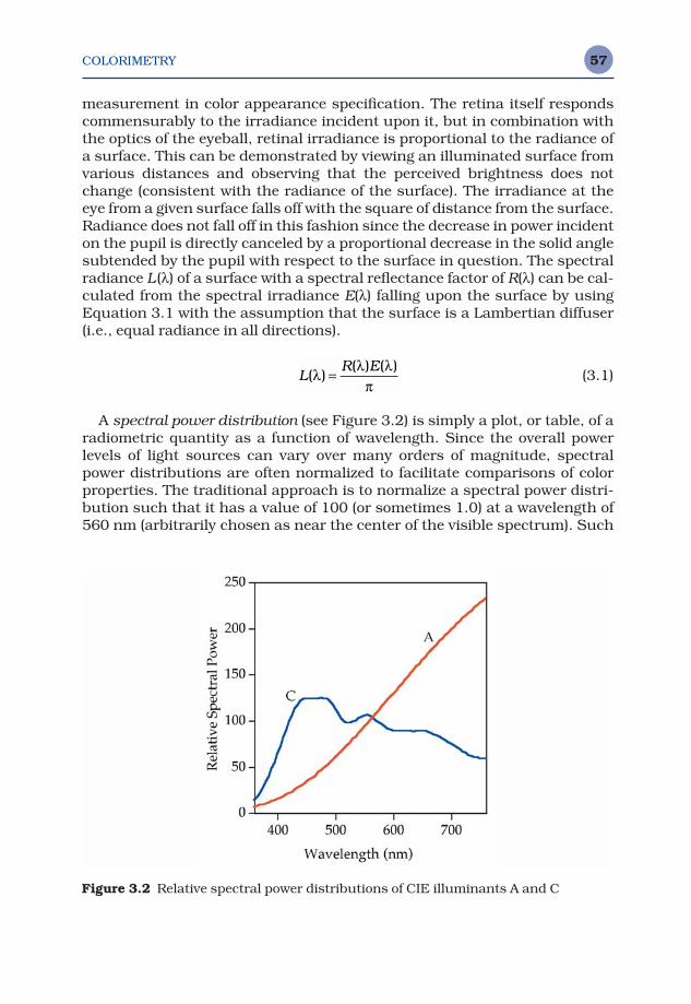
COLORIMETRY 57
measurement in color appearance specification. The retina itself respondscommensurably to the irradiance incident upon it, but in combination withthe optics of the eyeball, retinal irradiance is proportional to the radiance ofa surface. This can be demonstrated by viewing an illuminated surface fromvarious distances and observing that the perceived brightness does notchange (consistent with the radiance of the surface). The irradiance at theeye from a given surface falls off with the square of distance from the surface.Radiance does not fall off in this fashion since the decrease in power incidenton the pupil is directly canceled by a proportional decrease in the solid anglesubtended by the pupil with respect to the surface in question. The spectralradiance L (λ) of a surface with a spectral reflectance factor of R(λ) can be cal-culated from the spectral irradiance E(λ) falling upon the surface by usingEquation 3.1 with the assumption that the surface is a Lambertian diffuser(i.e., equal radiance in all directions).
(3.1)
A spectral power distribution (see Figure 3.2) is simply a plot, or table, of aradiometric quantity as a function of wavelength. Since the overall powerlevels of light sources can vary over many orders of magnitude, spectralpower distributions are often normalized to facilitate comparisons of colorproperties. The traditional approach is to normalize a spectral power distri-bution such that it has a value of 100 (or sometimes 1.0) at a wavelength of560 nm (arbitrarily chosen as near the center of the visible spectrum). Such
LR E
( )( ) ( )
λλ λ
π=
Figure 3.2 Relative spectral power distributions of CIE illuminants A and C
COLORIMETRY58
normalized spectral power distributions are referred to as relative spectralpower distributions and are dimensionless.
Black-body Radiators
Another important radiometric quantity is the color temperature of a lightsource. A special type of theoretical light source, known as a black-bodyradiator, or Planckian radiator, emits energy due only to thermal excitationand is a perfect emitter of energy. The energy emitted by a black bodyincreases in quantity and shifts toward shorter wavelengths as the temper-ature of the black body increases. The spectral power distribution of a black-body radiator can be specified using Planck’s equation as a function of asingle variable, absolute temperature (in Kelvin). Thus, if the absolute tem-perature of a black body is known, so is its spectral power distribution. Thetemperature of a black body is referred to as its color temperature since ituniquely specifies the color of the source. Since black-body radiators seldomexist outside specialized laboratories, color temperature is not a generallyuseful quantity. A second quantity, correlated color temperature, is moregenerally useful. A light source need not be a black-body radiator in order tobe assigned a correlated color temperature. The correlated color temper-ature (CCT) of a light source is simply the color temperature of a black-bodyradiator that has most nearly the same color as the source in question. Asexamples, an incandescent source might have a CCT of 2800 K, a typicalfluorescent tube 4000 K, an average daylight 6500 K, and the white-point ofa computer graphics display 9300 K. As the correlated color temperature ofa source increases, it becomes more blue, or less red.
CIE Illuminants
The CIE has established a number of spectral power distributions as CIEilluminants for colorimetry. These include CIE illuminants A, C, D65, D50,F2, F8, and F11:
• CIE illuminant A represents a Planckian radiator with a color temperatureof 2856 K and is used for colorimetric calculations when incandescentillumination is of interest.
• CIE illuminant C is the spectral power distribution of illuminant A asmodified by particular liquid filters defined by the CIE and represents adaylight simulator with a CCT of 6774 K.
• CIE Illuminants D65 and D50 are part of the CIE D-series of illuminantsthat have been statistically defined based upon a large number of meas-urements of real daylight. Illuminant D65 represents an average daylightwith a CCT of 6504 K and D50 represents an average daylight with a CCTof 5003 K. D65 is commonly used in colorimetric applications, while D50
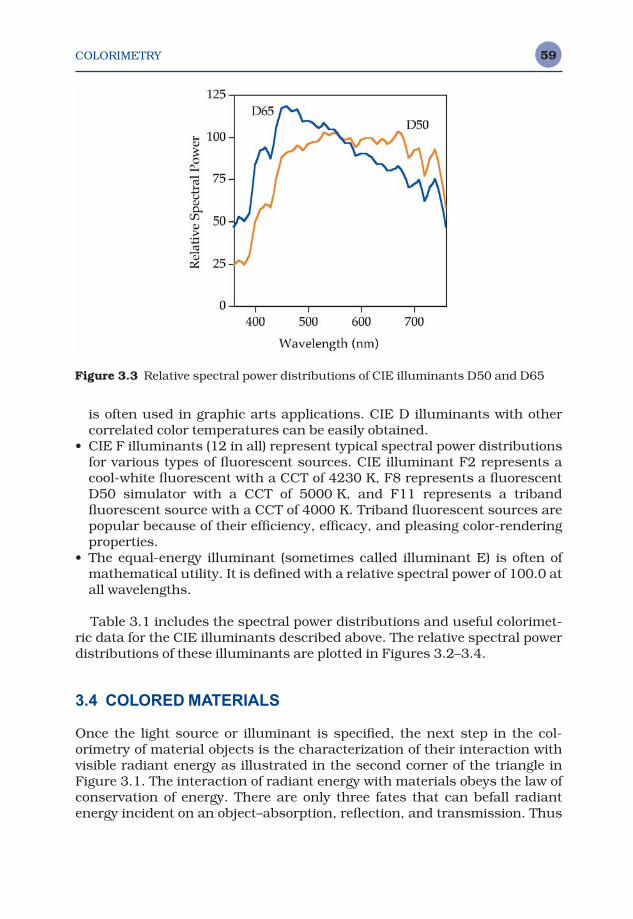
COLORIMETRY 59
is often used in graphic arts applications. CIE D illuminants with othercorrelated color temperatures can be easily obtained.
• CIE F illuminants (12 in all) represent typical spectral power distributionsfor various types of fluorescent sources. CIE illuminant F2 represents acool-white fluorescent with a CCT of 4230 K, F8 represents a fluorescentD50 simulator with a CCT of 5000 K, and F11 represents a tribandfluorescent source with a CCT of 4000 K. Triband fluorescent sources arepopular because of their efficiency, efficacy, and pleasing color-renderingproperties.
• The equal-energy illuminant (sometimes called illuminant E) is often ofmathematical utility. It is defined with a relative spectral power of 100.0 atall wavelengths.
Table 3.1 includes the spectral power distributions and useful colorimet-ric data for the CIE illuminants described above. The relative spectral powerdistributions of these illuminants are plotted in Figures 3.2–3.4.
3.4 COLORED MATERIALS
Once the light source or illuminant is specified, the next step in the col-orimetry of material objects is the characterization of their interaction withvisible radiant energy as illustrated in the second corner of the triangle inFigure 3.1. The interaction of radiant energy with materials obeys the law ofconservation of energy. There are only three fates that can befall radiantenergy incident on an object–absorption, reflection, and transmission. Thus
Figure 3.3 Relative spectral power distributions of CIE illuminants D50 and D65
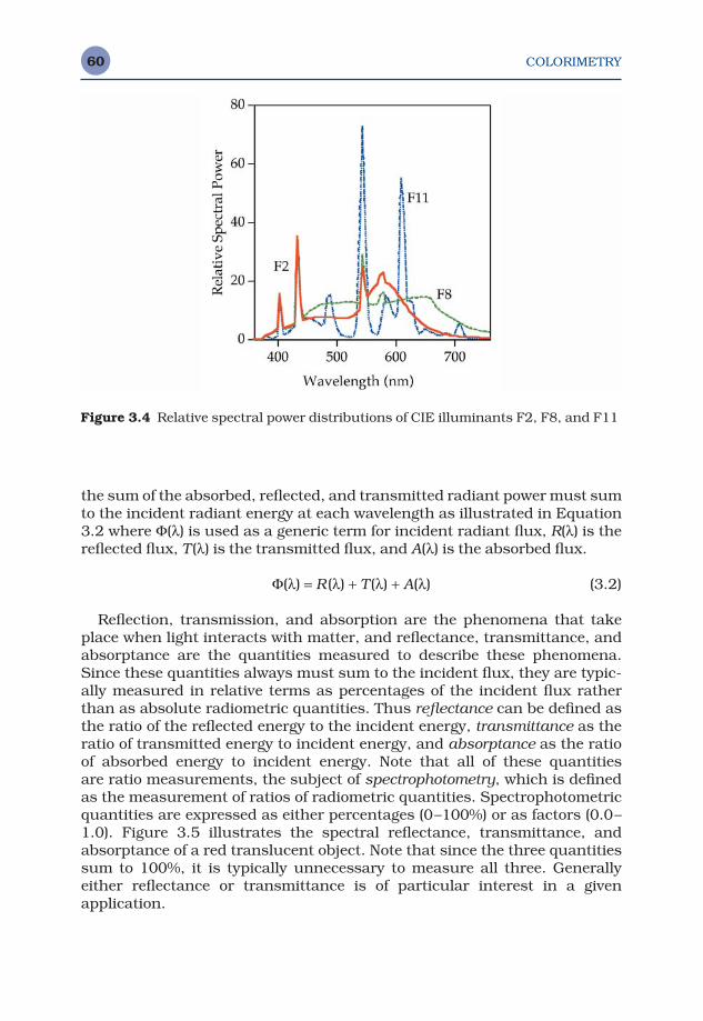
COLORIMETRY60
the sum of the absorbed, reflected, and transmitted radiant power must sumto the incident radiant energy at each wavelength as illustrated in Equation3.2 where Φ(λ) is used as a generic term for incident radiant flux, R(λ) is thereflected flux, T (λ) is the transmitted flux, and A(λ) is the absorbed flux.
Φ(λ) = R (λ) + T (λ) + A(λ) (3.2)
Reflection, transmission, and absorption are the phenomena that takeplace when light interacts with matter, and reflectance, transmittance, andabsorptance are the quantities measured to describe these phenomena.Since these quantities always must sum to the incident flux, they are typic-ally measured in relative terms as percentages of the incident flux ratherthan as absolute radiometric quantities. Thus reflectance can be defined asthe ratio of the reflected energy to the incident energy, transmittance as theratio of transmitted energy to incident energy, and absorptance as the ratioof absorbed energy to incident energy. Note that all of these quantities are ratio measurements, the subject of spectrophotometry, which is definedas the measurement of ratios of radiometric quantities. Spectrophotometricquantities are expressed as either percentages (0–100%) or as factors (0.0–1.0). Figure 3.5 illustrates the spectral reflectance, transmittance, andabsorptance of a red translucent object. Note that since the three quantitiessum to 100%, it is typically unnecessary to measure all three. Generallyeither reflectance or transmittance is of particular interest in a given application.
Figure 3.4 Relative spectral power distributions of CIE illuminants F2, F8, and F11
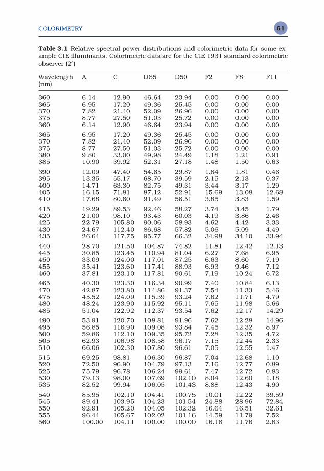
COLORIMETRY 61
Table 3.1 Relative spectral power distributions and colorimetric data for some ex-ample CIE illuminants. Colorimetric data are for the CIE 1931 standard colorimetricobserver (2°)
Wavelength A C D65 D50 F2 F8 F11(nm)
360 6.14 12.90 46.64 23.94 0.00 0.00 0.00365 6.95 17.20 49.36 25.45 0.00 0.00 0.00370 7.82 21.40 52.09 26.96 0.00 0.00 0.00375 8.77 27.50 51.03 25.72 0.00 0.00 0.00360 6.14 12.90 46.64 23.94 0.00 0.00 0.00
365 6.95 17.20 49.36 25.45 0.00 0.00 0.00370 7.82 21.40 52.09 26.96 0.00 0.00 0.00375 8.77 27.50 51.03 25.72 0.00 0.00 0.00380 9.80 33.00 49.98 24.49 1.18 1.21 0.91385 10.90 39.92 52.31 27.18 1.48 1.50 0.63
390 12.09 47.40 54.65 29.87 1.84 1.81 0.46395 13.35 55.17 68.70 39.59 2.15 2.13 0.37400 14.71 63.30 82.75 49.31 3.44 3.17 1.29405 16.15 71.81 87.12 52.91 15.69 13.08 12.68410 17.68 80.60 91.49 56.51 3.85 3.83 1.59
415 19.29 89.53 92.46 58.27 3.74 3.45 1.79420 21.00 98.10 93.43 60.03 4.19 3.86 2.46425 22.79 105.80 90.06 58.93 4.62 4.42 3.33430 24.67 112.40 86.68 57.82 5.06 5.09 4.49435 26.64 117.75 95.77 66.32 34.98 34.10 33.94
440 28.70 121.50 104.87 74.82 11.81 12.42 12.13445 30.85 123.45 110.94 81.04 6.27 7.68 6.95450 33.09 124.00 117.01 87.25 6.63 8.60 7.19455 35.41 123.60 117.41 88.93 6.93 9.46 7.12460 37.81 123.10 117.81 90.61 7.19 10.24 6.72
465 40.30 123.30 116.34 90.99 7.40 10.84 6.13470 42.87 123.80 114.86 91.37 7.54 11.33 5.46475 45.52 124.09 115.39 93.24 7.62 11.71 4.79480 48.24 123.90 115.92 95.11 7.65 11.98 5.66485 51.04 122.92 112.37 93.54 7.62 12.17 14.29
490 53.91 120.70 108.81 91.96 7.62 12.28 14.96495 56.85 116.90 109.08 93.84 7.45 12.32 8.97500 59.86 112.10 109.35 95.72 7.28 12.35 4.72505 62.93 106.98 108.58 96.17 7.15 12.44 2.33510 66.06 102.30 107.80 96.61 7.05 12.55 1.47
515 69.25 98.81 106.30 96.87 7.04 12.68 1.10520 72.50 96.90 104.79 97.13 7.16 12.77 0.89525 75.79 96.78 106.24 99.61 7.47 12.72 0.83530 79.13 98.00 107.69 102.10 8.04 12.60 1.18535 82.52 99.94 106.05 101.43 8.88 12.43 4.90
540 85.95 102.10 104.41 100.75 10.01 12.22 39.59545 89.41 103.95 104.23 101.54 24.88 28.96 72.84550 92.91 105.20 104.05 102.32 16.64 16.51 32.61555 96.44 105.67 102.02 101.16 14.59 11.79 7.52560 100.00 104.11 100.00 100.00 16.16 11.76 2.83
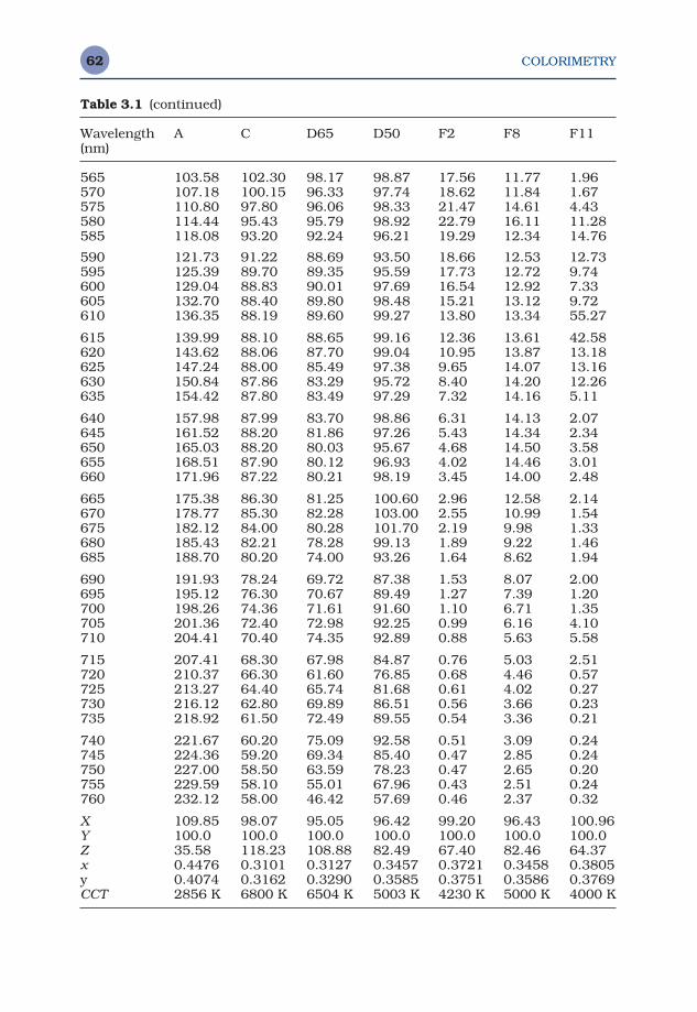
COLORIMETRY62
Table 3.1 (continued)
Wavelength A C D65 D50 F2 F8 F11(nm)
565 103.58 102.30 98.17 98.87 17.56 11.77 1.96570 107.18 100.15 96.33 97.74 18.62 11.84 1.67575 110.80 97.80 96.06 98.33 21.47 14.61 4.43580 114.44 95.43 95.79 98.92 22.79 16.11 11.28585 118.08 93.20 92.24 96.21 19.29 12.34 14.76
590 121.73 91.22 88.69 93.50 18.66 12.53 12.73595 125.39 89.70 89.35 95.59 17.73 12.72 9.74600 129.04 88.83 90.01 97.69 16.54 12.92 7.33605 132.70 88.40 89.80 98.48 15.21 13.12 9.72610 136.35 88.19 89.60 99.27 13.80 13.34 55.27
615 139.99 88.10 88.65 99.16 12.36 13.61 42.58620 143.62 88.06 87.70 99.04 10.95 13.87 13.18625 147.24 88.00 85.49 97.38 9.65 14.07 13.16630 150.84 87.86 83.29 95.72 8.40 14.20 12.26635 154.42 87.80 83.49 97.29 7.32 14.16 5.11
640 157.98 87.99 83.70 98.86 6.31 14.13 2.07645 161.52 88.20 81.86 97.26 5.43 14.34 2.34650 165.03 88.20 80.03 95.67 4.68 14.50 3.58655 168.51 87.90 80.12 96.93 4.02 14.46 3.01660 171.96 87.22 80.21 98.19 3.45 14.00 2.48
665 175.38 86.30 81.25 100.60 2.96 12.58 2.14670 178.77 85.30 82.28 103.00 2.55 10.99 1.54675 182.12 84.00 80.28 101.70 2.19 9.98 1.33680 185.43 82.21 78.28 99.13 1.89 9.22 1.46685 188.70 80.20 74.00 93.26 1.64 8.62 1.94
690 191.93 78.24 69.72 87.38 1.53 8.07 2.00695 195.12 76.30 70.67 89.49 1.27 7.39 1.20700 198.26 74.36 71.61 91.60 1.10 6.71 1.35705 201.36 72.40 72.98 92.25 0.99 6.16 4.10710 204.41 70.40 74.35 92.89 0.88 5.63 5.58
715 207.41 68.30 67.98 84.87 0.76 5.03 2.51720 210.37 66.30 61.60 76.85 0.68 4.46 0.57725 213.27 64.40 65.74 81.68 0.61 4.02 0.27730 216.12 62.80 69.89 86.51 0.56 3.66 0.23735 218.92 61.50 72.49 89.55 0.54 3.36 0.21
740 221.67 60.20 75.09 92.58 0.51 3.09 0.24745 224.36 59.20 69.34 85.40 0.47 2.85 0.24750 227.00 58.50 63.59 78.23 0.47 2.65 0.20755 229.59 58.10 55.01 67.96 0.43 2.51 0.24760 232.12 58.00 46.42 57.69 0.46 2.37 0.32
X 109.85 98.07 95.05 96.42 99.20 96.43 100.96Y 100.0 100.0 100.0 100.0 100.0 100.0 100.0Z 35.58 118.23 108.88 82.49 67.40 82.46 64.37x 0.4476 0.3101 0.3127 0.3457 0.3721 0.3458 0.3805y 0.4074 0.3162 0.3290 0.3585 0.3751 0.3586 0.3769CCT 2856 K 6800 K 6504 K 5003 K 4230 K 5000 K 4000 K
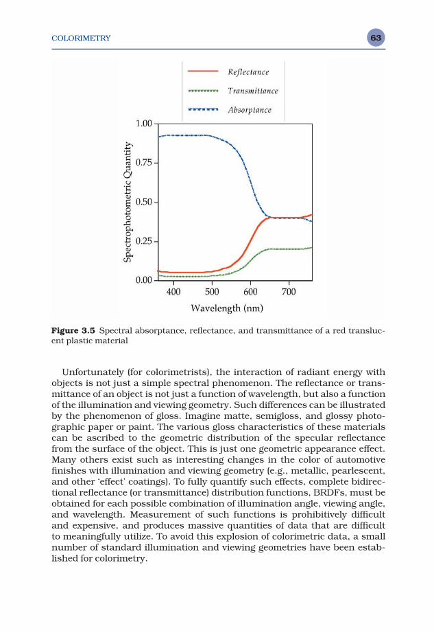
COLORIMETRY 63
Unfortunately (for colorimetrists), the interaction of radiant energy withobjects is not just a simple spectral phenomenon. The reflectance or trans-mittance of an object is not just a function of wavelength, but also a functionof the illumination and viewing geometry. Such differences can be illustratedby the phenomenon of gloss. Imagine matte, semigloss, and glossy photo-graphic paper or paint. The various gloss characteristics of these materialscan be ascribed to the geometric distribution of the specular reflectancefrom the surface of the object. This is just one geometric appearance effect.Many others exist such as interesting changes in the color of automotivefinishes with illumination and viewing geometry (e.g., metallic, pearlescent,and other ‘effect’ coatings). To fully quantify such effects, complete bidirec-tional reflectance (or transmittance) distribution functions, BRDFs, must beobtained for each possible combination of illumination angle, viewing angle,and wavelength. Measurement of such functions is prohibitively difficultand expensive, and produces massive quantities of data that are difficult to meaningfully utilize. To avoid this explosion of colorimetric data, a smallnumber of standard illumination and viewing geometries have been estab-lished for colorimetry.
Figure 3.5 Spectral absorptance, reflectance, and transmittance of a red transluc-ent plastic material
COLORIMETRY64
CIE Illumination and Viewing Geometries
The CIE has historically defined four standard illumination and viewing geo-metries for spectrophotometric reflectance measurements. (More detaileddesignations and specifications will be part of the forthcoming CIE Publica-tion 15.3 on colorimetry.) These come as two pairs of optically reversiblegeometries:
1. Diffuse/normal (d/0) and normal/diffuse (0/d)2. 45/normal (45/0) and normal/45 (0/45)
The designations indicate first the illumination geometry and then theviewing geometry following the slash (/).
Diffuse/Normal and Normal/Diffuse
In the diffuse/normal geometry, the sample is illuminated from all anglesusing an integrating sphere and viewed at an angle near the normal to thesurface. In the normal/diffuse geometry, the sample is illuminated from anangle near to its normal and the reflected energy is collected from all anglesusing an integrating sphere. These two geometries are optical reverses of oneanother and therefore produce the same measurement results (assuming allother instrumental variables are constant). The measurements made are oftotal reflectance. In many instruments, an area of the integrating sphere,corresponding to the angle of specular (regular) reflection of the illumina-tion in a 0/d geometry or the angle from which specular reflection would bedetected in a d/0 geometry, can be replaced with a black trap such that thespecular component of reflection is excluded and only diffuse reflectance ismeasured. Such measurements are referred to as ‘specular componentexcluded’ measurements as opposed to ‘specular component included’ meas-urements made when the entire sphere is intact.
45/Normal and Normal/45
The second pair of geometries is the 45/normal (45/0) and normal/45 (0/45)measurement configurations. In a 45/0 geometry, the sample is illuminatedwith one or more beams of light incident at an angle of 45° from the normaland measurements are made along the normal. In the 0/45 geometry, thesample is illuminated normal to its surface and measurements are madeusing one or more beams at a 45° angle to the normal. Again, these twogeometries are optical reverses of one another and produce identical resultsgiven equality of all other instrumental variables. Use of the 45/0 and 0/45measurement geometries ensures that all components of gloss are excludedfrom the measurements. Thus these geometries are typically used in
COLORIMETRY 65
applications where it is necessary to compare the colors of materials havingvarious levels of gloss (e.g., graphic arts and photography). It is critical tonote the instrumental geometry used whenever reporting colorimetric datafor materials.
The definition of reflectance as the ratio of reflected energy to incidentenergy is perfectly appropriate for measurements of total reflectance (d/0 or0/d). However, for bidirectional reflectance measurements (45/0 and 0/45),the ratio of reflected energy to incident energy is exceedingly small since onlya small range of angles of the distribution of reflected energy is detected.Thus, to produce more practically useful values for any type of measurementgeometry, reflectance factor measurements are made relative to a perfectreflecting diffuser. A perfect reflecting diffuser (PRD) is a theoretical materialthat is both a perfect reflector (100% reflectance) and perfectly Lambertian(radiance equal in all directions). Thus, measurements of reflectance factorare defined as the ratio of the energy reflected by the sample to the energythat would be reflected by a PRD illuminated and viewed in the identicalgeometry. For the integrating sphere geometries, measuring total reflect-ance, this definition of reflectance factor is identical to the definition ofreflectance. For the bidirectional geometries, measurement of reflectancefactor relative to the PRD results in a zero-to-one scale similar to thatobtained for total reflectance measurements. Since PRDs are not physicallyavailable, reference standards that are calibrated relative to the theoreticalaim are provided by national standardizing laboratories (such as NIST, theNational Institute for Standards and Technology, in the USA) and instru-ment manufacturers.
Fluorescence
One last topic of importance in the colorimetric analysis of materials isfluorescence. Fluorescent materials absorb energy in a region of wave-lengths and then emit this energy in a region of longer wavelengths. Forexample, a fluorescent orange material might absorb blue energy and emit itas orange energy. Fluorescent materials obey the law of conservation ofenergy as stated in Equation 3.2. However, their behavior is different in thatsome of the absorbed energy is emitted at (normally) longer wavelengths. Afull treatment of the color measurement of fluorescent materials is complexand beyond the scope of this book. In general; a fluorescent material is characterized by its total radiance factor, which is the sum of the reflectedand emitted energy at each wavelength relative to the energy that would bereflected by a PRD. This definition allows total radiance factors greater than1.0, which is often the case. It is important to note that the total radiancefactor will depend on the light source used in the measuring instrumentsince the amount of emitted energy is directly proportional to the amount ofabsorbed energy in the excitation wavelengths. Spectrophotometric meas-urements of reflectance or transmittance of nonfluorescent materials are
COLORIMETRY66
insensitive to the light source in the instrument since its characteristics arenormalized in the ratio calculations. This important difference highlights themajor difficulty in measuring fluorescent materials. Unfortunately, manyartificial materials (such as paper and inks) are fluorescent and thussignificantly more difficult to measure accurately.
3.5 THE HUMAN VISUAL RESPONSE
Measurement or standardization of light sources and materials provides thenecessary physical information for colorimetry. What remains is a quantitat-ive technique to predict the response of the human visual system as illus-trated by the third corner of the triangle in Figure 3.1. Following Wyszecki’s(1973) definition of basic colorimetry, quantification of the human visualresponse focuses on the earliest level of vision, absorption of energy in thecone photoreceptors, through the psychophysics of color matching. Theability to predict when two stimuli match for an average observer, the basisof colorimetry, provides great utility in a variety of applications. While such asystem does not specify color appearance, it provides the basis of colorappearance specification and allows the prediction of matches for variousapplications and the tools required to set up tolerances on matches neces-sary for industry. The properties of human color matching are defined by thespectral responsivities of the three cone types. This is because, once theenergy is absorbed by the three cone types, the spectral origin of the signalsis lost and, if the signals from the three cone types are equal for two stimuli,they must match in color when seen in the same conditions since there is no further information introduced within the visual system to distinguishthem.
Thus, if the spectral responsivities of the three cone types are known, twostimuli, denoted by their spectral power distributions Φ1(λ) and Φ2(λ), willmatch in color if the product of their spectral power distributions and eachof the three cone responsivities, L (λ), M(λ), and S(λ), integrated over wave-length, are equal. This equality for a visual match is illustrated in Equations3.3–3.5. Two stimuli match if all three of the equalities in Equations 3.3–3.5hold true.
(3.3)
(3.4)
(3.5)� �λ λ
λ λ λ λ λ λΦ Φ1 2( ) ( ) ( ) ( ) S Sd d=
� �λ λ
λ λ λ λ λ λΦ Φ1 2( ) ( ) ( ) ( ) M Md d=
� �λ λ
λ λ λ λ λ λΦ Φ1 2( ) ( ) ( ) ( ) L Ld d=
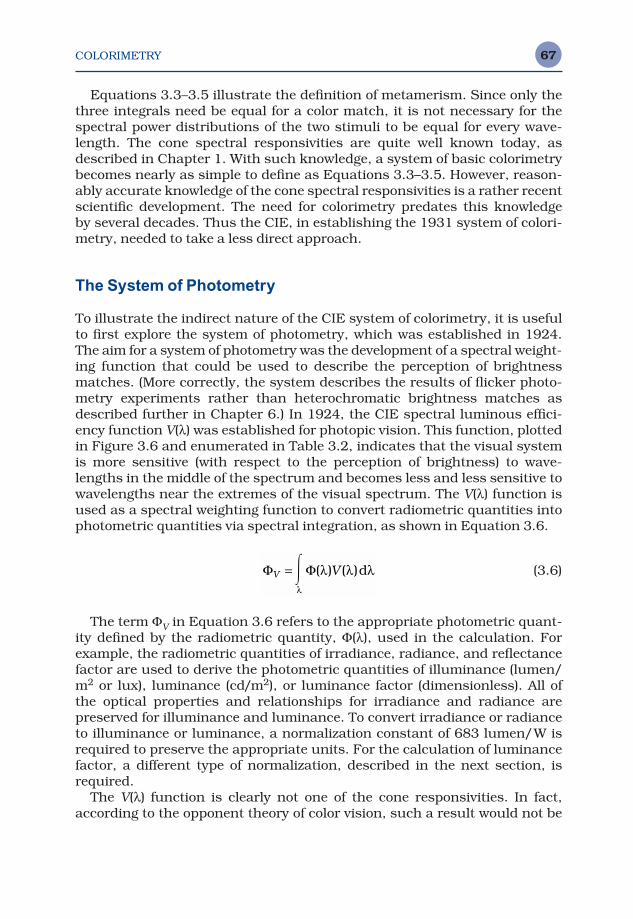
COLORIMETRY 67
Equations 3.3–3.5 illustrate the definition of metamerism. Since only thethree integrals need be equal for a color match, it is not necessary for thespectral power distributions of the two stimuli to be equal for every wave-length. The cone spectral responsivities are quite well known today, asdescribed in Chapter 1. With such knowledge, a system of basic colorimetrybecomes nearly as simple to define as Equations 3.3–3.5. However, reason-ably accurate knowledge of the cone spectral responsivities is a rather recentscientific development. The need for colorimetry predates this knowledge by several decades. Thus the CIE, in establishing the 1931 system of colori-metry, needed to take a less direct approach.
The System of Photometry
To illustrate the indirect nature of the CIE system of colorimetry, it is usefulto first explore the system of photometry, which was established in 1924.The aim for a system of photometry was the development of a spectral weight-ing function that could be used to describe the perception of brightnessmatches. (More correctly, the system describes the results of flicker photo-metry experiments rather than heterochromatic brightness matches asdescribed further in Chapter 6.) In 1924, the CIE spectral luminous effici-ency function V(λ) was established for photopic vision. This function, plottedin Figure 3.6 and enumerated in Table 3.2, indicates that the visual systemis more sensitive (with respect to the perception of brightness) to wave-lengths in the middle of the spectrum and becomes less and less sensitive towavelengths near the extremes of the visual spectrum. The V(λ) function isused as a spectral weighting function to convert radiometric quantities intophotometric quantities via spectral integration, as shown in Equation 3.6.
(3.6)
The term ΦV in Equation 3.6 refers to the appropriate photometric quant-ity defined by the radiometric quantity, Φ(λ), used in the calculation. Forexample, the radiometric quantities of irradiance, radiance, and reflectancefactor are used to derive the photometric quantities of illuminance (lumen/m2 or lux), luminance (cd/m2), or luminance factor (dimensionless). All of the optical properties and relationships for irradiance and radiance are preserved for illuminance and luminance. To convert irradiance or radianceto illuminance or luminance, a normalization constant of 683 lumen/W isrequired to preserve the appropriate units. For the calculation of luminancefactor, a different type of normalization, described in the next section, isrequired.
The V(λ) function is clearly not one of the cone responsivities. In fact,according to the opponent theory of color vision, such a result would not be
Φ ΦV V= �
λ
λ λ λ( ) ( )d
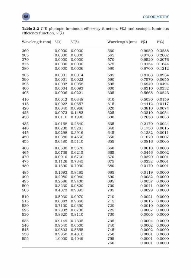
COLORIMETRY68
Table 3.2 CIE photopic luminous efficiency function, V(λ) and scotopic luminousefficiency function, V ′(λ)
Wavelength (nm) V(λ) V ′(λ)
360 0.0000 0.0000365 0.0000 0.0000370 0.0000 0.0000375 0.0000 0.0000380 0.0000 0.0006
385 0.0001 0.0014390 0.0001 0.0022395 0.0002 0.0058400 0.0004 0.0093405 0.0006 0.0221
410 0.0012 0.0348415 0.0022 0.0657420 0.0040 0.0966425 0.0073 0.1482430 0.0116 0.1998
435 0.0168 0.2640440 0.0230 0.3281445 0.0298 0.3916450 0.0380 0.4550455 0.0480 0.5110
460 0.0600 0.5670465 0.0739 0.6215470 0.0910 0.6760475 0.1126 0.7345480 0.1390 0.7930
485 0.1693 0.8485490 0.2080 0.9040495 0.2586 0.9430500 0.3230 0.9820505 0.4073 0.9895
510 0.5030 0.9970515 0.6082 0.9660520 0.7100 0.9350525 0.7932 0.8730530 0.8620 0.8110
535 0.9149 0.7305540 0.9540 0.6500545 0.9803 0.5655550 0.9950 0.4810555 1.0000 0.4049
Wavelength (nm) V(λ) V ′(λ)
560 0.9950 0.3288565 0.9786 0.2682570 0.9520 0.2076575 0.9154 0.1644580 0.8700 0.1212
585 0.8163 0.0934590 0.7570 0.0655595 0.6949 0.0494600 0.6310 0.0332605 0.5668 0.0246
610 0.5030 0.0159615 0.4412 0.0117620 0.3810 0.0074625 0.3210 0.0054630 0.2650 0.0033
635 0.2170 0.0024640 0.1750 0.0015645 0.1382 0.0011650 0.1070 0.0007655 0.0816 0.0005
660 0.0610 0.0003665 0.0446 0.0002670 0.0320 0.0001675 0.0232 0.0001680 0.0170 0.0001
685 0.0119 0.0000690 0.0082 0.0000695 0.0057 0.0000700 0.0041 0.0000705 0.0029 0.0000
710 0.0021 0.0000715 0.0015 0.0000720 0.0010 0.0000725 0.0007 0.0000730 0.0005 0.0000
735 0.0004 0.0000740 0.0002 0.0000745 0.0002 0.0000750 0.0001 0.0000755 0.0001 0.0000760 0.0001 0.0000
COLORIMETRY 69
expected. Instead, as suggested by the opponent theory of color vision, theV(λ) function corresponds to a weighted sum of the three cone responsivityfunctions. When the cone functions are weighted according to their relativepopulation in the retina and summed, the overall responsivity matches theCIE 1924 V(λ) function. Thus the photopic luminous response represents acombination of cone signals. This sort of combination is present in the entiresystem of colorimetry. The use of a spectral weighting function to predictluminance matches is the first step toward a system of colorimetry.
There is also a luminous efficiency function for scotopic vision (rods)known as the V ′(λ) function. This function, used for photometry at very lowluminance levels is plotted in Figure 3.6 and presented in Table 3.2 alongwith the V(λ) function. Since there is only one type of rod photoreceptor, theV ′(λ) function corresponds exactly to the spectral responsivity of the rodsafter transmission through the ocular media. Figure 3.6 illustrates the shiftin peak spectral sensitivity toward shorter wavelengths during the transitionfrom photopic to scotopic vision. This shift, known as the Purkinje shift,explains why blue objects tend to look lighter than red objects at very lowluminance levels. The V ′(λ) function is used in a way similar to the V(λ)function.
It has long been recognized in vision research that the V(λ) function mightunderpredict observed responsivity in the short-wavelength region of thespectrum. To address this issue and standard practice in the vision com-munity, an additional function, the CIE 1988 spectral luminous efficiencyfunction, VM (λ), was established (CIE 1990).
Figure 3.6 CIE scotopic, V ′(λ), and photopic, V (λ), luminous efficiency functions
COLORIMETRY70
3.6 TRISTIMULUS VALUES AND COLOR MATCHING FUNCTIONS
Following the establishment of the CIE 1924 luminous efficiency functionV(λ), attention was turned to development of a system of colorimetry thatcould be used to specify when two metameric stimuli match in color for anaverage observer. Since the cone responsivities were unavailable at thattime, a system of colorimetry was constructed based on the principles oftrichromacy and Grassmann’s laws of additive color mixture. The concept ofthis system is that color matches can be specified in terms of the amounts of three additive primaries required to visually match a stimulus. This isillustrated in the equivalence statement of Equation 3.7.
C ≡ R (R ) + G (G ) + B(B ) (3.7)
The way Equation 3.7 reads is that a color C is matched by R units of the R primary, G units of the G primary, and B units of the B primary. Theterms, RGB, define the particular set of primaries and indicate that for differ-ent primary sets, different amounts of the primaries will be required to makea match. The terms RGB indicate the amounts of the primaries required tomatch the color and are known as tristimulus values. Since any color can bematched by certain amounts of three primaries, those amounts (tristimulusvalues), along with a definition of the primary set, allow the specification of acolor. If two stimuli can be matched using the same amounts of the prim-aries, (i.e., they have equal tristimulus values) then they will also matcheach other when viewed in the same conditions.
Tristimulus Values for Any Stimulus
The next step in the derivation of colorimetry is the extension of tristimulusvalues such that they can be obtained for any given stimulus, defined by aspectral power distribution. To accomplish this, two steps are required. Thefirst is to obtain tristimulus values for matches to spectral colors. The sec-ond is to take advantage of Grassmann’s laws of additivity and proportional-ity to sum tristimulus values for each spectral component of a stimulusspectral power distribution in order to obtain the integrated tristimulus val-ues for the stimulus. Conceptually, the tristimulus values of the spectrum(i.e., spectral tristimulus values) are obtained by matching a unit amount of power at each wavelength with an additive mixture of three primaries.Figure 3.7 illustrates a set of spectral tristimulus values for monochromaticprimaries at 435.6 (B), 546.1 (G), and 700.0 nm (R). Spectral tristimulus values for the complete spectrum are also known as color matching func-tions, or sometimes color mixture functions. Notice that some of the spectraltristimulus values plotted in Figure 3.7 are negative. This implies the addi-tion of a negative amount of power into the match. For example, a negativeamount of the R primary is required to match a monochromatic 500 nm
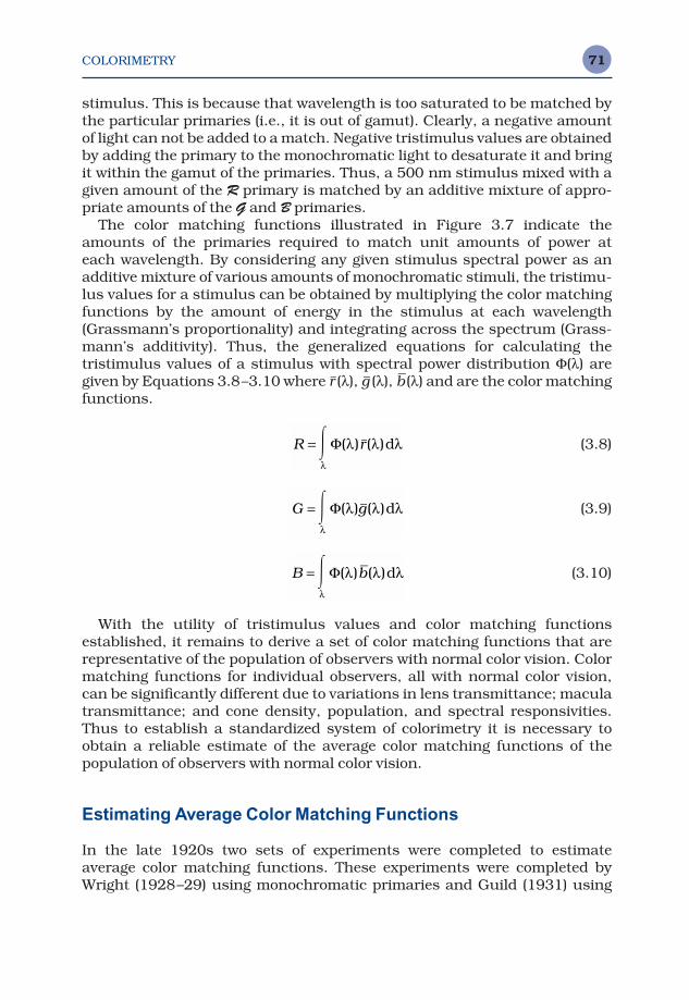
COLORIMETRY 71
stimulus. This is because that wavelength is too saturated to be matched bythe particular primaries (i.e., it is out of gamut). Clearly, a negative amountof light can not be added to a match. Negative tristimulus values are obtainedby adding the primary to the monochromatic light to desaturate it and bringit within the gamut of the primaries. Thus, a 500 nm stimulus mixed with agiven amount of the R primary is matched by an additive mixture of appro-priate amounts of the G and B primaries.
The color matching functions illustrated in Figure 3.7 indicate theamounts of the primaries required to match unit amounts of power at each wavelength. By considering any given stimulus spectral power as anadditive mixture of various amounts of monochromatic stimuli, the tristimu-lus values for a stimulus can be obtained by multiplying the color matchingfunctions by the amount of energy in the stimulus at each wavelength(Grassmann’s proportionality) and integrating across the spectrum (Grass-mann’s additivity). Thus, the generalized equations for calculating the tristimulus values of a stimulus with spectral power distribution Φ(λ) aregiven by Equations 3.8–3.10 where R (λ), G (λ), B (λ) and are the color matchingfunctions.
(3.8)
(3.9)
(3.10)
With the utility of tristimulus values and color matching functions established, it remains to derive a set of color matching functions that arerepresentative of the population of observers with normal color vision. Colormatching functions for individual observers, all with normal color vision,can be significantly different due to variations in lens transmittance; maculatransmittance; and cone density, population, and spectral responsivities.Thus to establish a standardized system of colorimetry it is necessary toobtain a reliable estimate of the average color matching functions of the population of observers with normal color vision.
Estimating Average Color Matching Functions
In the late 1920s two sets of experiments were completed to estimate average color matching functions. These experiments were completed byWright (1928–29) using monochromatic primaries and Guild (1931) using
B = �
λ
λ λ λΦ( ) ( )B d
G = �
λ
λ λ λΦ( ) ( )G d
R = �
λ
λ λ λΦ( ) ( )R d
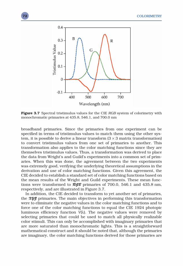
COLORIMETRY72
broadband primaries. Since the primaries from one experiment can bespecified in terms of tristimulus values to match them using the other sys-tem, it is possible to derive a linear transform (3 × 3 matrix transformation)to convert tristimulus values from one set of primaries to another. Thistransformation also applies to the color matching functions since they arethemselves tristimulus values. Thus, a transformation was derived to placethe data from Wright’s and Guild’s experiments into a common set of prim-aries. When this was done, the agreement between the two experiments was extremely good, verifying the underlying theoretical assumptions in thederivation and use of color matching functions. Given this agreement, theCIE decided to establish a standard set of color matching functions based onthe mean results of the Wright and Guild experiments. These mean func-tions were transformed to RGB primaries of 700.0, 546.1 and 435.8 nm,respectively, and are illustrated in Figure 3.7.
In addition, the CIE decided to transform to yet another set of primaries,the XYZ primaries. The main objectives in performing this transformationwere to eliminate the negative values in the color matching functions and toforce one of the color matching functions to equal the CIE 1924 photopicluminous efficiency function V(λ). The negative values were removed byselecting primaries that could be used to match all physically realizablecolor stimuli. This can only be accomplished with imaginary primaries thatare more saturated than monochromatic lights. This is a straightforwardmathematical construct and it should be noted that, although the primariesare imaginary, the color matching functions derived for those primaries are
Figure 3.7 Spectral tristimulus values for the CIE RGB system of colorimetry withmonochromatic primaries at 435.8, 546.1, and 700.0 nm
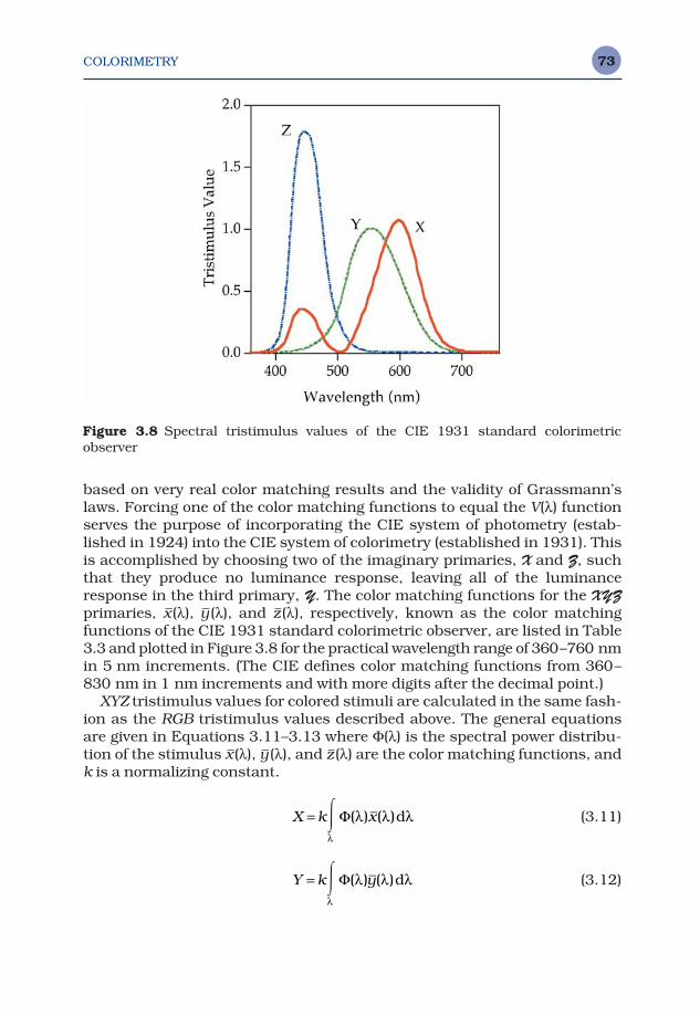
COLORIMETRY 73
based on very real color matching results and the validity of Grassmann’slaws. Forcing one of the color matching functions to equal the V(λ) functionserves the purpose of incorporating the CIE system of photometry (estab-lished in 1924) into the CIE system of colorimetry (established in 1931). Thisis accomplished by choosing two of the imaginary primaries, X and Z, suchthat they produce no luminance response, leaving all of the luminanceresponse in the third primary, Y. The color matching functions for the XYZ
primaries, X (λ), Y (λ), and Z (λ), respectively, known as the color matchingfunctions of the CIE 1931 standard colorimetric observer, are listed in Table3.3 and plotted in Figure 3.8 for the practical wavelength range of 360–760 nmin 5 nm increments. (The CIE defines color matching functions from 360–830 nm in 1 nm increments and with more digits after the decimal point.)
XYZ tristimulus values for colored stimuli are calculated in the same fash-ion as the RGB tristimulus values described above. The general equationsare given in Equations 3.11–3.13 where Φ(λ) is the spectral power distribu-tion of the stimulus X (λ), Y (λ), and Z (λ) are the color matching functions, andk is a normalizing constant.
(3.11)
(3.12)
Y k= �
λ
λ λ λΦ( ) ( )Y d
X k= �
λ
λ λ λΦ( ) ( )X d
Figure 3.8 Spectral tristimulus values of the CIE 1931 standard colorimetricobserver
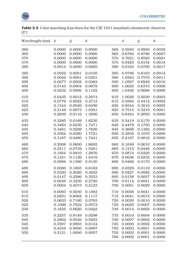
COLORIMETRY74
Table 3.3 Color matching functions for the CIE 1931 standard colorimetric observer(2°)
Wavelength (nm) X Y Z
360 0.0000 0.0000 0.0000365 0.0000 0.0000 0.0000370 0.0000 0.0000 0.0000375 0.0000 0.0000 0.0000380 0.0014 0.0000 0.0065
385 0.0022 0.0001 0.0105390 0.0042 0.0001 0.0201395 0.0077 0.0002 0.0362400 0.0143 0.0004 0.0679405 0.0232 0.0006 0.1102
410 0.0435 0.0012 0.2074415 0.0776 0.0022 0.3713420 0.1344 0.0040 0.6456425 0.2148 0.0073 1.0391430 0.2839 0.0116 1.3856
435 0.3285 0.0168 1.6230440 0.3483 0.0230 1.7471445 0.3481 0.0298 1.7826450 0.3362 0.0380 1.7721455 0.3187 0.0480 1.7441
460 0.2908 0.0600 1.6692465 0.2511 0.0739 1.5281470 0.1954 0.0910 1.2876475 0.1421 0.1126 1.0419480 0.0956 0.1390 0.8130
485 0.0580 0.1693 0.6162490 0.0320 0.2080 0.4652495 0.0147 0.2586 0.3533500 0.0049 0.3230 0.2720505 0.0024 0.4073 0.2123
510 0.0093 0.5030 0.1582515 0.0291 0.6082 0.1117520 0.0633 0.7100 0.0782525 0.1096 0.7932 0.0573530 0.1655 0.8620 0.0422
535 0.2257 0.9149 0.0298540 0.2904 0.9540 0.0203545 0.3597 0.9803 0.0134550 0.4334 0.9950 0.0087555 0.5121 1.0000 0.0057
X Y Z
560 0.5945 0.9950 0.0039565 0.6784 0.9786 0.0027570 0.7621 0.9520 0.0021575 0.8425 0.9154 0.0018580 0.9163 0.8700 0.0017
585 0.9786 0.8163 0.0014590 1.0263 0.7570 0.0011595 1.0567 0.6949 0.0010600 1.0622 0.6310 0.0008605 1.0456 0.5668 0.0006
610 1.0026 0.5030 0.0003615 0.9384 0.4412 0.0002620 0.8544 0.3810 0.0002625 0.7514 0.3210 0.0001630 0.6424 0.2650 0.0000
635 0.5419 0.2170 0.0000640 0.4479 0.1750 0.0000645 0.3608 0.1382 0.0000650 0.2835 0.1070 0.0000655 0.2187 0.0816 0.0000
660 0.1649 0.0610 0.0000665 0.1212 0.0446 0.0000670 0.0874 0.0320 0.0000675 0.0636 0.0232 0.0000680 0.0468 0.0170 0.0000
685 0.0329 0.0119 0.0000690 0.0227 0.0082 0.0000695 0.0158 0.0057 0.0000700 0.0114 0.0041 0.0000705 0.0081 0.0029 0.0000
710 0.0058 0.0021 0.0000715 0.0041 0.0015 0.0000720 0.0029 0.0010 0.0000725 0.0020 0.0007 0.0000730 0.0014 0.0005 0.0000
735 0.0010 0.0004 0.0000740 0.0007 0.0002 0.0000745 0.0005 0.0002 0.0000750 0.0003 0.0001 0.0000755 0.0002 0.0001 0.0000760 0.0002 0.0001 0.0000
COLORIMETRY 75
(3.13)
The spectral power distribution of the stimulus is defined in different waysfor various types of stimuli. For self-luminous stimuli (e.g., light sources andCRT displays), Φ(λ) is typically spectral radiance or a relative spectral powerdistribution. For reflective materials, Φ(λ) is defined as the product of thespectral reflectance factor of the material, R(λ), and the relative spectralpower distribution of the light source or illuminant of interest, S(λ), that isR(λ)S(λ). For transmitting materials, Φ(λ) is defined as the product of thespectral transmittance of the material, T (λ), and the relative spectral powerdistribution of the light source or illuminant of interest, S(λ), that is T (λ)S(λ).
The normalization constant k in Equations 3.11–3.13, is defined differ-ently for relative and absolute colorimetry. In absolute colorimetry, k is setequal to 683 lumen/W, making the system of colorimetry compatible withthe system of photometry. For relative colorimetry, k is defined by Equa-tion 3.14.
(3.14)
The normalization for relative colorimetry in Equation 3.14 results in tristimulus values that are scaled from zero to approximately 100 for variousmaterials. It is useful to note that if relative colorimetry is used to calculatethe tristimulus values of a light source, the Y tristimulus value is alwaysequal to 100.
There is another, completely inappropriate, use of the term relative col-orimetry in the graphic arts and other color reproduction industries. In somecases tristimulus values are normalized to the paper white rather than aperfect reflecting diffuser. This results in a Y tristimulus value for the paperof 100 rather than its more typical value of about 85. The advantage of this isthat it allows transformation between different paper types, preserving thepaper white as the lightest color in an image, without having to keep track ofthe paper color. Such a practice might be useful, but it is actually a gamutmapping issue rather than a color measurement issue. A more appropriateterminology for this practice might be normalized colorimetry to avoid con-fusion with the long-established practice of relative colorimetry. It is alsoworth noting that the practice of normalized colorimetry is not always con-sistent. In some cases, reflectance measurements are made relative to thepaper white. This ensures that the Y tristimulus value is normalizedbetween zero for a perfect black and 1.0 (or 100.0) for the paper white, how-ever, the X and Z tristimulus values might still range above 1.0 (or 100.0)depending on the particular illuminant used in the colorimetric calculations.
k
S
=100
�λ
λ λ λ( ) ( )Y d
Z k= ( ) ( )�
λ
λ λ λΦ Z d
COLORIMETRY76
Another approach is to normalize the tristimulus values for each stimuluscolor XYZ by the tristimulus values of the paper XpYpZp individually (X/Xp,Y/Yp, and Z/Zp). This is analogous to the white point normalization inCIELAB and is often used to adjust for white point changes and limiteddynamic range in imaging systems. It is important to know which type ofnormalized colorimetry one is dealing with in various applications.
The relationship between CIE XYZ tristimlus values and cone responses(sometimes referred to as fundamental tristimulus values) is of great import-ance and interest in color appearance modeling. Like the V(λ) function, theCIE XYZ color matching functions each represent a linear combination ofcone responsivities. Thus the relationship between the two is defined by a 3 × 3 linear matrix transformation as described more fully in Chapter 9 (see Figure 9.1). Cone spectral responsivities can be thought of as the colormatching functions for a set of primaries that are constructed such thateach primary stimulates only one cone type. It is possible to produce a realprimary that stimulates only the S cones. However, no real primaries can beproduced that stimulate only the M or L cones since their spectral respons-ivities overlap across the visible spectrum. Thus, the required primaries are also imaginary and produce all-positive color matching functions, but donot incorporate the V(λ) function as a color matching function (since thatrequires a primary that stimulates all three cone types). The historical devel-opment of and recent progress in the development of colorimetric systemsbased on physiological cone responsivities has been reviewed by Boynton(1996).
Two Sets of Color Matching Functions
It is important to be aware that there are two sets of color matching func-tions that have been established by the CIE. The CIE 1931 standard colori-metric observer was determined from experiments using a visual field thatsubtended 2°. Thus the matching stimuli were imaged onto the retina com-pletely within the fovea. These color matching functions are used, almostexclusively, in color appearance modeling. Often they are referred to as the2° color matching functions or the 2° observer. It is of historical interest tonote that the 1931 standard colorimetric observer is based on data collectedfrom fewer than 20 observers. In the 1950s, experiments were completed(Stiles and Burch 1959) to collect 2° color matching functions for moreobservers using more precise and accurate instrumentation. The resultsshowed slight systematic discrepancies, but not of sufficient magnitude towarrant a change in the standard colorimetric observer. At the same time,experiments were completed (Stiles and Burch 1959) to collect color match-ing function data for large visual fields. This was prompted by discrepanciesbetween colorimetric and visual determination of the whiteness of paper.These experiments were completed using a 10° visual field that excluded thecentral fovea. Thus the color matching functions include no influence of the
COLORIMETRY 77
macular absorption. The results for large fields were deemed significantlydifferent from the 2° standard to warrant the establishment of the CIE 1964supplementary standard colorimetric observer, sometimes called the 10°observer. The difference between the two standard observers is significant,so care should be taken to report which observer is used with any colori-metric data. The differences are computationally significant, but certainlywithin the variability of color matching functions found for either 2° or 10°visual fields. Thus the two standard colorimetric observers can be thought ofas representing the color matching functions of two individuals.
3.7 CHROMATICITY DIAGRAMS
The color of a stimulus can be specified by a triplet of tristimulus values. Toprovide a convenient two-dimensional representation of colors, chromatic-ity diagrams were developed. The transformation from tristimulus values to chromaticity coordinates is accomplished through a normalization thatremoves luminance information. This transformation is a one-point per-spective projection of data points in the three-dimensional tristimulus spaceonto the unit plane of that space (with a center of projection at the origin) asdefined by Equations 3.15–3.17.
(3.15)
(3.16)
(3.17)
Since there are only two-dimensions of information in chromaticity co-ordinates, the third chromaticity coordinate can always be obtained fromthe other two by noting that the three always sum to unity. Thus z can becalculated from x and y using Equation 3.18.
z = 1.0 − x − y (3.18)
Chromaticity coordinates should be used with great care since theyattempt to represent a three-dimensional phenomenon with just two vari-ables. To fully specify a colored stimulus, one of the tristimulus values mustbe reported in addition to two (or three) chromaticity coordinates. Usuallythe Y tristimulus value is reported since it represents the luminance infor-mation. The equations for obtaining the other two tristimulus values fromchromaticity coordinates and the Y tristimulus value are often useful andtherefore given in Equations 3.19 and 3.20.
zZ
X Y Z=
+ +
yY
X Y Z=
+ +
xX
X Y Z=
+ +

COLORIMETRY78
(3.19)
(3.20)
Chromaticity coordinates, alone, provide no information about the colorappearance of stimuli since they include no luminance (or therefore light-ness) information and do not account for chromatic adaptation. As anobserver’s state of adaptation changes, the color corresponding to a given setof chromaticity coordinates can change in appearance dramatically (e.g., achange from yellow to blue could occur with a change from daylight to incan-descent light adaptation).
Much effort has been expended in attempts to make chromaticity dia-grams more perceptually uniform. While this is an intrinsically doomedeffort (i.e., an attempt to convert a nominal scale into an interval scale), it isworth mentioning one of the results, which is actually the chromaticity dia-gram currently recommended by the CIE for general use. It is the CIE 1976Uniform Chromaticity Scales (UCS) diagram defined by Equations 3.21 and3.22.
(3.21)
(3.22)
The use of chromaticity diagrams should be avoided in most circum-stances, particularly when the phenomena being investigated are highlydependent on the three-dimensional nature of color. For example, the dis-play and comparison of the color gamuts of imaging devices in chromaticitydiagrams is misleading to the point of being almost completely erroneous.
3.8 CIE COLOR SPACES
The general use of chromaticity diagrams has been made largely obsolete by the advent of the CIE color spaces, CIELAB and CIELUV. These spacesextend tristimulus colorimetry to three-dimensional spaces with dimensionsthat approximately correlate with the perceived lightness, chroma, and hueof a stimulus. This is accomplished by incorporating features to account for chromatic adaptation and nonlinear visual responses. The main aim inthe development of these spaces was to provide uniform practices for themeasurement of color differences, something that cannot be done reliably intristimulus or chromaticity spaces. In 1976, two spaces were recommended
′ =+ +
vY
X Y Z
915 3
′ =+ +
uX
X Y Z
415 3
Zx y Y
y=
− −( . )1 0
XxY
y=
COLORIMETRY 79
for use since there was no clear evidence to support one over the other atthat time. The CIELAB and CIELUV color spaces are described in more detailin Chapter 10. Their equations are briefly summarized in this section.Wyszecki (1986) provides an overview of the development of the CIE colorspaces.
CIELAB
The CIE 1976 (L* a* b*) color space, abbreviated CIELAB, is defined byEquations 3.23–3.27 for tristimulus values normalized to the white that aregreater than 0.008856.
L* = 116(Y/Yn)1/3 − 16 (3.23)
a* = 500[(X/Xn)1/3 − (Y/Yn)1/3] (3.24)
b* = 200[(Y/Yn)1/3 − (Z/Zn)1/3] (3.25)
(3.26)
hab = tan−1(b*/a*) (3.27)
In these equations X, Y, and Z are the tristimulus values of the stimulusand Xn, Yn, and Zn are the tristimulus values of the reference white. L*represents lightness, a* approximate redness–greenness, b* approximateyellowness–blueness, C*ab chroma, and hab hue. The L*, a*, and b* coordin-ates are used to construct a Cartesian color space as illustrated in Fig-ure 3.9. The L*, C*ab, and hab coordinates are the cylindrical representation ofthe same space. The CIELAB space, including the full set of equations fordark colors, is described in greater detail in Chapter 10.
CIELUV
The CIE 1976 (L* u* v*) color space, abbreviated CIELUV, is defined byEquations 3.28–3.32. Equation 3.28 is also restricted to tristimulus valuesnormalized to the white that are greater than 0.008856.
L* = 116(Y/Yn)1/3 − 16 (3.28)
u* = 13L*(u′ − u′n) (3.29)
v* = 13L*(v′ − v′n) (3.30)
(3.31)C u vuv* ( * * )= +2 2
C a bab* ( * * )= +2 2
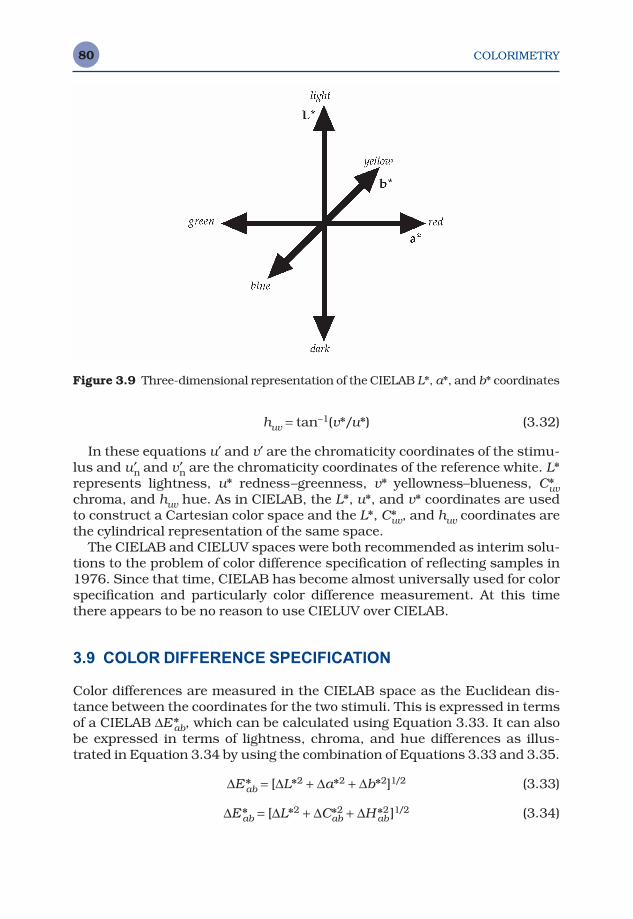
COLORIMETRY80
huv = tan−1(v*/u*) (3.32)
In these equations u′ and v′ are the chromaticity coordinates of the stimu-lus and u′n and v′n are the chromaticity coordinates of the reference white. L*represents lightness, u* redness–greenness, v* yellowness–blueness, C*uvchroma, and huv hue. As in CIELAB, the L*, u*, and v* coordinates are usedto construct a Cartesian color space and the L*, C*uv, and huv coordinates arethe cylindrical representation of the same space.
The CIELAB and CIELUV spaces were both recommended as interim solu-tions to the problem of color difference specification of reflecting samples in1976. Since that time, CIELAB has become almost universally used for colorspecification and particularly color difference measurement. At this timethere appears to be no reason to use CIELUV over CIELAB.
3.9 COLOR DIFFERENCE SPECIFICATION
Color differences are measured in the CIELAB space as the Euclidean dis-tance between the coordinates for the two stimuli. This is expressed in termsof a CIELAB ∆E*ab, which can be calculated using Equation 3.33. It can alsobe expressed in terms of lightness, chroma, and hue differences as illus-trated in Equation 3.34 by using the combination of Equations 3.33 and 3.35.
∆E*ab = [∆L*2 + ∆a*2 + ∆b*2]1/2 (3.33)
∆E*ab = [∆L*2 + ∆C*2ab + ∆H*2
ab ]1/2 (3.34)
Figure 3.9 Three-dimensional representation of the CIELAB L*, a*, and b* coordinates
COLORIMETRY 81
∆H*ab = [∆E*2ab − ∆L*2 − ∆C*2
ab ]1/2 (3.35)
While the CIELAB color space was designed with the goal of having colordifferences be perceptually uniform throughout the space (i.e., a ∆E*ab of 1.0for a pair of red stimuli is perceived to be equal in magnitude to a ∆E*ab of 1.0for a pair of gray stimuli), this goal was not strictly achieved.
To improve the uniformity of color difference measurements, modifica-tions to the CIELAB ∆E*ab equation have been made based upon variousempirical data. One of the most widely used modifications is the CMC colordifference equation (Clarke et al. 1984), which is based on a visual experi-ment on color difference perception in textiles. The CIE (1995b) has recentlyevaluated such equations, and the available visual data, recommending anew color difference equation for industrial use. This system for color differ-ence measurement is called the CIE 1994 (∆L* ∆C*ab ∆H*ab) color differencemodel with the symbol ∆E*94 and abbreviation CIE94. Use of the CIE94 equa-tion is preferred over a simple CIELAB ∆E*ab. CIE94 color differences are calculated using Equations 3.36–3.39.
(3.36)
SL = 1 (3.37)
SC = 1 + 0.045C*ab (3.38)
SH = 1 + 0.015C*ab (3.39)
The parametric factors, kL, kC, and kH are used to adjust the relativeweighting of the lightness, chroma, and hue components, respectively, ofcolor difference for various viewing conditions and applications that departfrom the CIE94 reference conditions. It is also worth noting that, when aver-aged across the color space, CIE94 color differences are significantly smallerin magnitude than CIELAB color differences for the same stimuli pairs.Thus, use of CIE94 color differences to report overall performance in applica-tions such as the colorimetric characterization of imaging devices results in the appearance of significantly improved performance if the numbers aremistakenly considered equivalent to CIELAB color differences. The same istrue for CMC color differences.
The CIE (1995) established a set of reference conditions for use of theCIE94 color difference equations. These are:
• Illumination: CIE illuminant D65 simulator• Illuminance: 1000 lux• Observer: normal color vision• Background: uniform, achromatic, L* = 50
∆∆ ∆ ∆
EL
k S
C
k S
H
k SL L
ab
C C
ab
H H
** * *
/
94
2 2 2 1 2
=
+
+
COLORIMETRY82
• Viewing mode: object• Sample size: greater than 4° visual angle• Sample Separation: direct edge contact• Sample Color-Difference Magnitude: 0–5 CIELAB units• Sample Structure: no visually apparent pattern or nonuniformity
The tight specification of reference conditions for the CIE94 equationshighlights the vast amount of research that remains to be performed in orderto generate a universally useful process for color difference specification.These issues are some of the same problems that must be tackled in thedevelopment of color appearance models. It should also be noted that forsample sizes greater than 4°, use of the CIE 1964 supplementary standardcolorimetric observer is recommended.
More recently, the CIE has established the CIE DE2000 color differenceequation (see Johnson and Fairchild 2003b, CIE 2001) that extends the con-cept of CIE94 with further complexity. While the DE2000 equation certainlyperforms better than CIE94 for some data sets, its added complexity is prob-ably not justified for most practical applications.
3.10 THE NEXT STEP
This chapter has reviewed the fundamentals of basic colorimetry (and begunto touch on advanced colorimetry) as illustrated conceptually in Figure 3.1.While these techniques are well established and have been successfullyused for decades, much more information needs to be added to the triangleof color in Figure 3.1 in order to extend basic colorimetry toward the spe-cification of the color appearance of stimuli under a wide variety of viewingconditions. Some of the additional information that must be consideredincludes:
• chromatic adaptation,• light adaptation,• luminance level,• background color,• surround color, • etc.
These issues are explored further along the road to the development anduse of color appearance models presented in the remaining chapters of thisbook.
Color Appearance Models Second Edition M. D. Fairchild © 2005 John Wiley & Sons, LtdISBN: 0-470-01216-1 (HB)
4Color Appearance
Terminology
In any scientific field a large portion of the knowledge is contained in thedefinitions of terms used by its practitioners. Newcomers to a field often real-ize that they understand the fundamental scientific concepts, but must firstlearn the language in order to communicate accurately, precisely, and effect-ively in the new discipline. Nowhere is this more true, or more important,than in the study of color appearance. Hunt (1978) showed concern thatcolor scientists and technologist might be taking an attitude like HumptyDumpty from Alice Through the Looking Glass who is quoted as saying ‘WhenI use a word it means just what I choose it to mean — neither more nor less.’We all know what happened to Humpty Dumpty. The careful definition ofcolor appearance terms presented in this chapter is intended to put every-one on a level playing field and help ensure that the concepts, data, andmodels discussed in this book are presented and interpreted in a consistentmatter. As can be seen throughout this book, consistent use of terminologyhas not been the historical norm and continues to be one of the challenges ofcolor appearance research and application.
4.1 IMPORTANCE OF DEFINITIONS
Why should it be particularly difficult to agree upon consistent terminologyin the field of color appearance? Perhaps the answer lies in the very nature ofthe subject. Almost everyone knows what color is. After all, they have hadfirst-hand experience of it since shortly after birth. However, very few canprecisely describe their color experiences or even precisely define color. Thisinnate knowledge, along with the imprecise use of color terms (e.g., warmer,cooler, brighter, cleaner, fresher), leads to a subject that everyone knowsabout, but few can discuss precisely. Clearly, if color appearance is to be
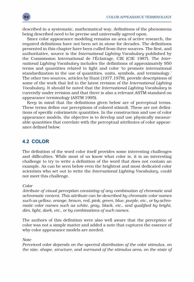
COLOR APPEARANCE TERMINOLOGY84
described in a systematic, mathematical way, definitions of the phenomenabeing described need to be precise and universally agreed upon.
Since color appearance modeling remains an area of active research, therequired definitions have not been set in stone for decades. The definitionspresented in this chapter have been culled from three sources. The first, andauthoritative, source is the International Lighting Vocabulary published bythe Commission International de l’Éclairage, CIE (CIE 1987). The Inter-national Lighting Vocabulary includes the definitions of approximately 950terms and quantities related to light and color ‘to promote internationalstandardization in the use of quantities, units, symbols, and terminology.’The other two sources, articles by Hunt (1977,1978), provide descriptions ofsome of the work that led to the latest revision of the International LightingVocabulary. It should be noted that the International Lighting Vocabulary iscurrently under revision and that there is also a relevant ASTM standard onappearance terminology (ASTM 1995).
Keep in mind that the definitions given below are of perceptual terms.These terms define our perceptions of colored stimuli. These are not defini-tions of specific colorimetric quantities. In the construction and use of colorappearance models, the objective is to develop and use physically measur-able quantities that correlate with the perceptual attributes of color appear-ance defined below.
4.2 COLOR
The definition of the word color itself provides some interesting challengesand difficulties. While most of us know what color is, it is an interesting challenge to try to write a definition of the word that does not contain anexample. As can be seen below even the brightest and most dedicated colorscientists who set out to write the International Lighting Vocabulary, couldnot meet this challenge.
ColorAttribute of visual perception consisting of any combination of chromatic andachromatic content. This attribute can be described by chromatic color namessuch as yellow, orange, brown, red, pink, green, blue, purple, etc., or by achro-matic color names such as white, gray, black, etc., and qualified by bright,dim, light, dark, etc., or by combinations of such names.
The authors of this definition were also well aware that the perception ofcolor was not a simple matter and added a note that captures the essence ofwhy color appearance models are needed.
NotePerceived color depends on the spectral distribution of the color stimulus, onthe size, shape, structure, and surround of the stimulus area, on the state of
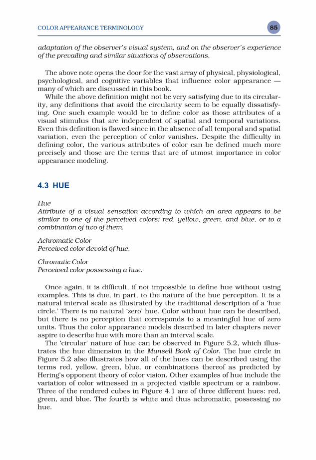
COLOR APPEARANCE TERMINOLOGY 85
adaptation of the observer’s visual system, and on the observer’s experienceof the prevailing and similar situations of observations.
The above note opens the door for the vast array of physical, physiological,psychological, and cognitive variables that influence color appearance —many of which are discussed in this book.
While the above definition might not be very satisfying due to its circular-ity, any definitions that avoid the circularity seem to be equally dissatisfy-ing. One such example would be to define color as those attributes of a visual stimulus that are independent of spatial and temporal variations.Even this definition is flawed since in the absence of all temporal and spatialvariation, even the perception of color vanishes. Despite the difficulty indefining color, the various attributes of color can be defined much more precisely and those are the terms that are of utmost importance in colorappearance modeling.
4.3 HUE
HueAttribute of a visual sensation according to which an area appears to be similar to one of the perceived colors: red, yellow, green, and blue, or to a combination of two of them.
Achromatic ColorPerceived color devoid of hue.
Chromatic ColorPerceived color possessing a hue.
Once again, it is difficult, if not impossible to define hue without usingexamples. This is due, in part, to the nature of the hue perception. It is a natural interval scale as illustrated by the traditional description of a ‘huecircle.’ There is no natural ‘zero’ hue. Color without hue can be described,but there is no perception that corresponds to a meaningful hue of zerounits. Thus the color appearance models described in later chapters neveraspire to describe hue with more than an interval scale.
The ‘circular’ nature of hue can be observed in Figure 5.2, which illus-trates the hue dimension in the Munsell Book of Color. The hue circle inFigure 5.2 also illustrates how all of the hues can be described using theterms red, yellow, green, blue, or combinations thereof as predicted byHering’s opponent theory of color vision. Other examples of hue include thevariation of color witnessed in a projected visible spectrum or a rainbow.Three of the rendered cubes in Figure 4.1 are of three different hues: red,green, and blue. The fourth is white and thus achromatic, possessing nohue.

COLOR APPEARANCE TERMINOLOGY86
4.4 BRIGHTNESS AND LIGHTNESS
BrightnessAttribute of a visual sensation according to which an area appears to emitmore or less light.
LightnessThe brightness of an area judged relative to the brightness of a similarly illuminated area that appears to be white or highly transmitting.
NoteOnly related colors [see Section 4.7] exhibit lightness.
The definitions of brightness and lightness are straightforward and ratherintuitive. The important distinction is that brightness refers to the absolutelevel of the perception while lightness can be thought of as relative bright-ness — normalized for changes in the illumination and viewing conditions.
A classic example is to think about a piece of paper, such as this bookpage. If this page was viewed in a typical office environment, the paper wouldhave some brightness and a fairly high lightness (perhaps it is the lighteststimulus in the field of vision and therefore white). If the book was viewedoutside on a sunny summer day, there would be significantly more energyreflected from the page and the paper would appear brighter. However, thepage would still likely be the lightest stimulus in the field of vision and retain
Figure 4.1 A computer graphics rendering of four solid blocks illuminated by twolight sources of differing intensities and angle of illumination to be used for demon-stration of various color appearance attributes
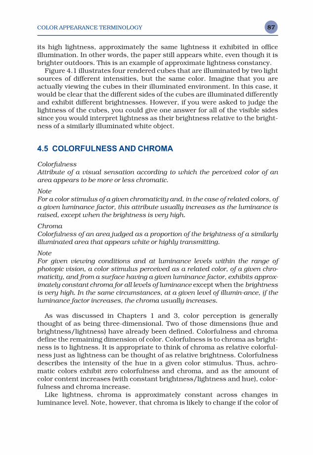
COLOR APPEARANCE TERMINOLOGY 87
its high lightness, approximately the same lightness it exhibited in officeillumination. In other words, the paper still appears white, even though it isbrighter outdoors. This is an example of approximate lightness constancy.
Figure 4.1 illustrates four rendered cubes that are illuminated by two lightsources of different intensities, but the same color. Imagine that you areactually viewing the cubes in their illuminated environment. In this case, itwould be clear that the different sides of the cubes are illuminated differentlyand exhibit different brightnesses. However, if you were asked to judge thelightness of the cubes, you could give one answer for all of the visible sidessince you would interpret lightness as their brightness relative to the bright-ness of a similarly illuminated white object.
4.5 COLORFULNESS AND CHROMA
ColorfulnessAttribute of a visual sensation according to which the perceived color of anarea appears to be more or less chromatic.
NoteFor a color stimulus of a given chromaticity and, in the case of related colors, ofa given luminance factor, this attribute usually increases as the luminance israised, except when the brightness is very high.
ChromaColorfulness of an area judged as a proportion of the brightness of a similarlyilluminated area that appears white or highly transmitting.
NoteFor given viewing conditions and at luminance levels within the range of photopic vision, a color stimulus perceived as a related color, of a given chro-maticity, and from a surface having a given luminance factor, exhibits approx-imately constant chroma for all levels of luminance except when the brightnessis very high. In the same circumstances, at a given level of illumin-ance, if theluminance factor increases, the chroma usually increases.
As was discussed in Chapters 1 and 3, color perception is generallythought of as being three-dimensional. Two of those dimensions (hue andbrightness/lightness) have already been defined. Colorfulness and chromadefine the remaining dimension of color. Colorfulness is to chroma as bright-ness is to lightness. It is appropriate to think of chroma as relative colorful-ness just as lightness can be thought of as relative brightness. Colorfulnessdescribes the intensity of the hue in a given color stimulus. Thus, achro-matic colors exhibit zero colorfulness and chroma, and as the amount ofcolor content increases (with constant brightness/lightness and hue), color-fulness and chroma increase.
Like lightness, chroma is approximately constant across changes in luminance level. Note, however, that chroma is likely to change if the color of
COLOR APPEARANCE TERMINOLOGY88
the illumination is varied. Colorfulness, on the other hand, increases for agiven object as the luminance level increases since it is an absolute percep-tual quantity. Figure 4.1 illustrates the difference between colorfulness andchroma. Again, imagine you are in the illuminated environment with thecubes in Figure 4.1. Since different sides of each cube are illuminated withdiffering amounts of the same color energy, they vary in colorfulness. On theother hand, if you were to judge the chroma of the cubes, you could provideone answer for each of the cubes. This is because you would be judging eachside relative to a similarly illuminated white object. The sides of the cubeswith greater illumination exhibit greater colorfulness, but the chroma isroughly constant within each cube.
4.6 SATURATION
SaturationColorfulness of an area judged in proportion to its brightness.
NoteFor given viewing conditions and at luminance levels within the range of pho-topic vision, a color stimulus of a given chromaticity exhibits approximatelyconstant saturation for all luminance levels, except when brightness is veryhigh.
Saturation is a unique perceptual experience separate from chroma. Likechroma, saturation can be thought of as relative colorfulness. However, sat-uration is the colorfulness of a stimulus relative to its own brightness, whilechroma is colorfulness relative to the brightness of a similarly illuminatedarea that appears white. In order for a stimulus to have chroma, it must bejudged in relation to other colors, while a stimulus seen completely in isola-tion can have saturation. An example of a stimulus that exhibits saturation,but not chroma, is a traffic signal light viewed in isolation on a dark night.The lights, typically red, yellow, or green, are quite saturated and can becompared with the color appearance of oncoming headlights whose satura-tion is very nearly zero (since they typically appear white).
Saturation is sometimes described as a shadow series. This refers to therange of colors observed when a single object has a shadow cast upon it. Asthe object falls into deeper shadow, it becomes darker, but saturationremains constant. This can be observed in Figure 4.1 by assuming that therendered environment is illuminated by a single light source. The varioussides of the cubes will all be of approximately constant saturation.
4.7 UNRELATED AND RELATED COLORS
Unrelated ColorColor perceived to belong to an area or object seen in isolation from other colors.
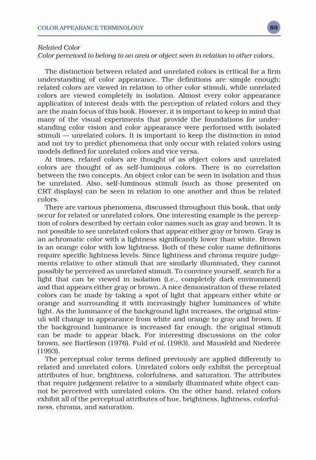
COLOR APPEARANCE TERMINOLOGY 89
Related ColorColor perceived to belong to an area or object seen in relation to other colors.
The distinction between related and unrelated colors is critical for a firmunderstanding of color appearance. The definitions are simple enough;related colors are viewed in relation to other color stimuli, while unrelatedcolors are viewed completely in isolation. Almost every color appearanceapplication of interest deals with the perception of related colors and theyare the main focus of this book. However, it is important to keep in mind thatmany of the visual experiments that provide the foundations for under-standing color vision and color appearance were performed with isolatedstimuli — unrelated colors. It is important to keep the distinction in mindand not try to predict phenomena that only occur with related colors usingmodels defined for unrelated colors and vice versa.
At times, related colors are thought of as object colors and unrelated colors are thought of as self-luminous colors. There is no correlationbetween the two concepts. An object color can be seen in isolation and thusbe unrelated. Also, self-luminous stimuli (such as those presented on CRT displays) can be seen in relation to one another and thus be related colors.
There are various phenomena, discussed throughout this book, that onlyoccur for related or unrelated colors. One interesting example is the percep-tion of colors described by certain color names such as gray and brown. It isnot possible to see unrelated colors that appear either gray or brown. Gray isan achromatic color with a lightness significantly lower than white. Brown is an orange color with low lightness. Both of these color name definitionsrequire specific lightness levels. Since lightness and chroma require judge-ments relative to other stimuli that are similarly illuminated, they cannotpossibly be perceived as unrelated stimuli. To convince yourself, search for alight that can be viewed in isolation (i.e., completely dark environment) and that appears either gray or brown. A nice demonstration of these relatedcolors can be made by taking a spot of light that appears either white ororange and surrounding it with increasingly higher luminances of whitelight. As the luminance of the background light increases, the original stim-uli will change in appearance from white and orange to gray and brown. Ifthe background luminance is increased far enough, the original stimuli can be made to appear black. For interesting discussions on the colorbrown, see Bartleson (1976), Fuld et al. (1983), and Mausfeld and Niederée(1993).
The perceptual color terms defined previously are applied differently torelated and unrelated colors. Unrelated colors only exhibit the perceptualattributes of hue, brightness, colorfulness, and saturation. The attributesthat require judgement relative to a similarly illuminated white object can-not be perceived with unrelated colors. On the other hand, related colorsexhibit all of the perceptual attributes of hue, brightness, lightness, colorful-ness, chroma, and saturation.

COLOR APPEARANCE TERMINOLOGY90
4.8 DEFINITIONS IN EQUATIONS
The various terms used to carefully describe color appearance can be con-fusing at times. To keep the definitions straight, it is often helpful to think ofthem in terms of simple equations. These equations, while not strictly true ina mathematical sense, provide a first-order description of the relationshipsbetween the various color percepts. In fact, an understanding of the defini-tions in terms of the following equations provides the first building blocktoward understanding the construction of the various color appearancemodels.
Chroma can be thought of as colorfulness relative to the brightness of asimilarly illuminated white as shown in Equation 4.1.
(4.1)
Saturation can be described as the colorfulness of a stimulus relative toits own brightness as illustrated in Equation 4.2.
(4.2)
Finally, lightness can be expressed as the ratio of the brightness of a stimu-lus to the brightness of a similarly illuminated white stimulus as given inEquation 4.3.
(4.3)
The utility of these simple definitions in terms of equations is illustratedby a derivation of the fact that an alternative definition of saturation (used insome appearance models) is given by the ratio of chroma and lightness inEquation 4.4.
(4.4)
This can be proven by first substituting the definitions of chroma andlightness from Equations 4.1 and 4.3 into Equation 4.4, arriving at Equation4.5.
(4.5)
Completing the algebraic exercise by canceling out the brightness of thewhite terms in Equation 4.5 results in saturation being expressed as the
SaturationColorfu ess
Brightness White
Brightness White
Brightness= ⋅
ln
( )( )
SaturationChroma
Lightness=
LightnessBrightness
Brightness White=
( )
SaturationColorfu ess
Brightness=
ln
ChromaColorfu ess
Brightness White=
ln
( )
COLOR APPEARANCE TERMINOLOGY 91
ratio of colorfulness to brightness as shown in Equation 4.6, which is ident-ical to the original definition in Equation 4.2.
(4.6)
4.9 BRIGHTNESS–COLORFULNESS VS LIGHTNESS–CHROMA
While color is typically thought of as three-dimensional and color matchescan be specified by just three numbers, it turns out that three dimensionsare not enough to completely specify color appearance. In fact, five percep-tual dimensions are required for a complete specification of color appearance:
• Brightness• Lightness• Colorfulness• Chroma• Hue
Saturation is redundant since it is known if the five attributes above areknown. However, in many practical color appearance applications it is notnecessary to know all five attributes. Typically, related colors are of mostinterest and only the relative appearance attributes are of significant import-ance. Thus it is often sufficient to be concerned with only the relative appear-ance attributes of lightness, chroma, and hue.
There might seem to be some redundancy in using all five appearanceattributes to describe a color appearance. However, this is not the case, aswas elegantly described by Nayatani et al. (1990a). In that article, Nayataniet al. illustrated both theoretically and experimentally the distinction betweenbrightness–colorfulness appearance matches and lightness–chroma appear-ance matches and showed that in most viewing conditions the two types of matches are distinct. Imagine viewing a yellow school bus outside on asunny day. The yellow bus will exhibit its typical appearance attributes ofhue (yellow), brightness (high), lightness (high), colorfulness (high), andchroma (high). Now imagine viewing a printed photographic reproduction ofthe school bus in the relatively subdued lighting of an office or home. Theimage of the bus could be a perfect match to the original object in hue (yellow), lightness (high), and chroma (high). However, the brightness andcolorfulness of the print viewed in subdued lighting could never equal that ofthe original school bus viewed in bright sunlight. This is simply because ofthe lack of energy reflecting off the print relative to the original object. If thatsame print were carried outside into the bright sunlight that the original buswas viewed under, it is then possible that the reproduction could match theoriginal object in all five appearance attributes.
So which is more important, the matching (i.e., reproduction) of bright-ness and colorfulness or the matching of lightness and chroma? (Note that
SaturationColorfu ess
Brightness=
ln

COLOR APPEARANCE TERMINOLOGY92
hue is defined the same way in either circumstance.) The answer depends onthe application, but it is safe to say that much more often it is lightness andchroma that are of greater importance. As illustrated by the above example,in color reproduction applications it is typically possible and desirable toaspire to lightness–chroma matching. Imagine trying to make reproductionswith a brightness–colorfulness matching objective. To reproduce the sun-light-illuminated school bus in office lighting, one would have to make aprint that was literally glowing in order to reproduce brightness and colorful-ness. This is not physically possible. Going in the other direction (subduedlighting to bright lighting) is possible, but is it desirable? Imagine taking aphotograph of a person at a candlelight dinner and making a reproduction tobe viewed under bright sunlight. It would be easy to reproduce the bright-ness and colorfulness of the original scene, but the print would be extremelydark (essentially black everywhere) and it would be considered a very poorprint. Customers of such color reproductions expect lightness–chromareproduction. Attempts to make such reproductions using a color appear-ance model across changes in luminance are given in Figures 4.2 and 4.3.
Figure 4.2 Comparison of lightness–chroma reproduction with brightness–colorful-ness reproduction when the original is at a lower luminance than the reproduction.Brightness–chroma reproduction results in an image that is very dark to compensatefor the increased level of illumination. Lightness–chroma reproduction representsmore complete adaptation since they are relative appearance attributes
COLOR APPEARANCE TERMINOLOGY 93
There are a few situations in which brightness and colorfulness might bemore important than lightness and colorfulness. Nayatani et al. (1990a) sug-gest a few such situations. One of those is in the specification of the colorrendering properties of light sources. In such an application it might be moreimportant to know how bright and colorful objects appear under a given lightsource, rather than just lightness and chroma. Another situation might bein the judgement of image quality for certain types of reproductions. Forexample, in comparing the quality of projected transparencies in a darkened(or not so darkened) room, observers might be more interested in the bright-ness and colorfulness of an image than in the lightness and chroma. In fact,the lightness and chroma of image elements might remain nearly constantas the luminance of the projector is decreased, while it is fairly intuitive thatthe perceived image quality would be decreasing. It is very rare for observersto comment that they wish the image from a slide or overhead projector wasnot so bright unless a bright overhead projector image is displayed adjacentto a dim 35 mm projector image!
Figure 4.3 Comparison of lightness–chroma reproduction with brightness–colorful-ness reproduction when the original is at a higher luminance than the reproduction.Brightness–chroma reproduction results in an image that is very bright to compens-ate for the decreased level of illumination. Lightness–chroma reproduction representsmore complete adaptation since they are relative appearance attributes
Color Appearance Models Second Edition M. D. Fairchild © 2005 John Wiley & Sons, LtdISBN: 0-470-01216-1 (HB)
5Color Order Systems
Since color appearance is a basic perception, the most direct method to meas-ure it is through psychophysical techniques designed to elucidate perceptu-ally uniform scales of the various color appearance attributes defined inChapter 4. When such experiments are performed, it is possible to specifystimuli using basic colorimetry that embody the perceptual color appearanceattributes. A collection of such stimuli, appropriately specified and denoted,forms a color order system. Such a color order system does allow a fairlyunambiguous specification of color appearance. However, there is no reasonto expect that the specified appearances will generalize to other viewing con-ditions or be mathematically related to physical measurements in any straight-forward way. Thus, color order systems provide data and a technique forspecifying color appearance, but do not provide a mathematical frameworkto allow extension of that data to novel viewing conditions. Therefore colororder systems are of significant interest in the development and testing ofcolor appearance models, but cannot serve as a replacement for them.
This chapter provides an overview of some color order systems that are ofparticular interest in color appearance modeling and device-independentcolor imaging. Their importance and application will become self-evident in this and later chapters. Additional details on color order systems can befound in Berns’ colorimetry text (Berns 2000), Hunt’s text on color measure-ment (Hunt 1991a, 1998), Wyszecki and Stiles’ reference volume on colorscience (Wyszecki and Stiles 1982), Wyszecki’s review chapter on colorappearance (Wyszecki 1986), Derefeldt’s review on color appearance sys-tems (Derefeldt 1991), and Kuehni’s detailed historical review of color spaces(Kuehni 2003).
5.1 OVERVIEW AND REQUIREMENTS
Many definitions of color order systems have been suggested and it is prob-ably most useful to adopt some combination of them. Wyszecki (1986) pointsout that color order systems fall into three broad groups:
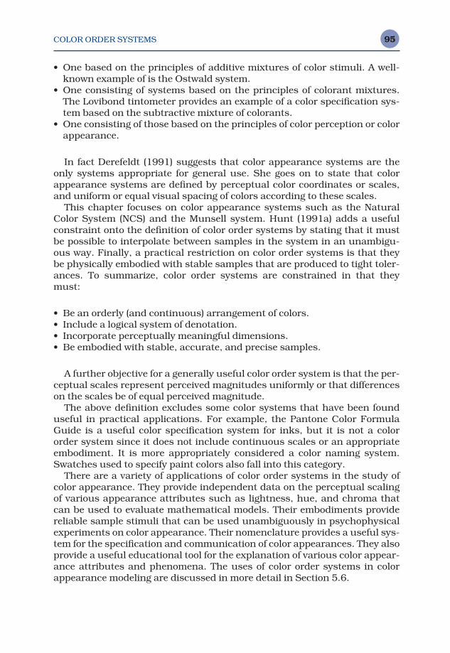
COLOR ORDER SYSTEMS 95
• One based on the principles of additive mixtures of color stimuli. A well-known example of is the Ostwald system.
• One consisting of systems based on the principles of colorant mixtures.The Lovibond tintometer provides an example of a color specification sys-tem based on the subtractive mixture of colorants.
• One consisting of those based on the principles of color perception or colorappearance.
In fact Derefeldt (1991) suggests that color appearance systems are theonly systems appropriate for general use. She goes on to state that colorappearance systems are defined by perceptual color coordinates or scales,and uniform or equal visual spacing of colors according to these scales.
This chapter focuses on color appearance systems such as the NaturalColor System (NCS) and the Munsell system. Hunt (1991a) adds a usefulconstraint onto the definition of color order systems by stating that it mustbe possible to interpolate between samples in the system in an unambigu-ous way. Finally, a practical restriction on color order systems is that they be physically embodied with stable samples that are produced to tight toler-ances. To summarize, color order systems are constrained in that they must:
• Be an orderly (and continuous) arrangement of colors.• Include a logical system of denotation.• Incorporate perceptually meaningful dimensions.• Be embodied with stable, accurate, and precise samples.
A further objective for a generally useful color order system is that the per-ceptual scales represent perceived magnitudes uniformly or that differenceson the scales be of equal perceived magnitude.
The above definition excludes some color systems that have been founduseful in practical applications. For example, the Pantone Color FormulaGuide is a useful color specification system for inks, but it is not a colororder system since it does not include continuous scales or an appropriateembodiment. It is more appropriately considered a color naming system.Swatches used to specify paint colors also fall into this category.
There are a variety of applications of color order systems in the study ofcolor appearance. They provide independent data on the perceptual scalingof various appearance attributes such as lightness, hue, and chroma thatcan be used to evaluate mathematical models. Their embodiments providereliable sample stimuli that can be used unambiguously in psychophysicalexperiments on color appearance. Their nomenclature provides a useful sys-tem for the specification and communication of color appearances. They alsoprovide a useful educational tool for the explanation of various color appear-ance attributes and phenomena. The uses of color order systems in colorappearance modeling are discussed in more detail in Section 5.6.
COLOR ORDER SYSTEMS96
5.2 THE MUNSELL BOOK OF COLOR
One of the most widely used color order systems, particularly in the UnitedStates, is the Munsell system, embodied in the Munsell Book of Color. Thehistory of the Munsell system has been reviewed by Nickerson (1940,1976a,b,c), and interesting insight can be obtained by reviewing the visualexperiments leading to the renotation of the Munsell colors in the 1940s(Newhall 1940). The system was developed by an artist, Albert H. Munsell, inthe early part of the 20th century. Munsell was particularly interested indeveloping a system that would aid in the education of children. The basicpremise of the system is to specify color appearance according to threeattributes:
• Hue (H )• Value (V )• Chroma (C )
The definitions of the three Munsell dimensions match the currentdefinitions of the corresponding appearance attributes, with Munsell Valuereferring to lightness. Munsell’s objective was to specify colors (both psy-chophysically and physically) with equal visual increments along each of thethree perceptual dimensions.
Munsell Value
The Munsell value scale is the anchor of the system. There are ten mainsteps in the Munsell value scale with white given a notation of 10, blackdenoted zero, and intermediate grays given notations ranging between zeroand 10. The design of the Munsell value scale is such that an intermediategray with a Munsell value of 5 (denoted N5 for a neutral sample with value 5)is perceptually halfway between an ideal white (N10) and an ideal black (N0).Also, the perceived lightness difference between N3 and N4 samples is equi-valent to the lightness difference between N6 and N7 samples, or any othersamples varying by one step in Munsell value. Lightness perceptions fallingin between two Munsell value steps are denoted with decimals. For example,Munsell value 4.5 falls perceptually halfway between Munsell value 4 and 5. It is important to note that the relationship between Munsell value V andrelative luminance Y is nonlinear. In fact, it is specified by the fifth-orderpolynomial given in Equation 5.1 and plotted in Figure 5.1.
Y = 1.2219V − 0.23111V2 + 0.23951V3 − 0.021009V4
+ 0.0008404V5 (5.1)
As can be seen in Figure 5.1, a sample that is perceived to be a middle gray(N5) has a relative luminance (or luminous reflectance factor) of about 20%.
COLOR ORDER SYSTEMS 97
The Munsell value of any color (independent of hue or chroma) is defined bythe same univariate relationship with relative luminance. Thus, if theMunsell value of a sample is known, so is its relative luminance, CIE Y, andvice versa. Unfortunately, the fifth-order polynomial in Equation 5.1 cannotbe analytically inverted for practical application. Since the CIE lightnessscale L* was designed to model the Munsell system, it provides a very goodcomputational approximation to Munsell value. As a very useful and accur-ate general rule, the Munsell value of a stimulus can be obtained from itsCIE L* (Ill. C, 2° Obs.) by simply dividing by 10.
Munsell Hue
The next dimension of the Munsell system is hue. The hue circle in theMunsell system is divided into five principle hues (purple, blue, green, yel-low, and red, denoted 5P, 5B, 5G, 5Y, and 5R, respectively) and is designedto divide the complete hue circle into equal perceptual intervals. Five inter-mediate hues are also designated in the Munsell system as 5PB, 5BG, 5GY,5YR, and 5RP for a total of 10 hue names. For each of the ten hues there areten integral hues with notations as illustrated by the range between 5PB and5P, which is 6PB, 7PB, 8PB, 9PB, 10PB, 1P, 2P, 3P, and 4P. This type ofsequence continues around the entire hue circle, resulting in 100 integerhue designations that are intended to be equal perceived hue intervals. Huesintermediate to the integer designations are denoted with decimal values(e.g., 7.5PB).
Figure 5.1 Munsell value as a function of relative luminance
COLOR ORDER SYSTEMS98
Munsell Chroma
The third dimension of the Munsell system is chroma. The chroma scale isdesigned to have equal visual increments from a chroma of zero for neutralsamples to increasing chromas for samples with stronger hue content. Thereis no set maximum for the chroma scale. The highest chromas achieveddepend on the hue and value of the samples and the colorants used to pro-duce them. For example, there are no high chroma samples with a yellowhue and low value, or a purple hue and high value. Such stimuli cannot bephysically produced due to the nature of the human visual response. Figure5.2 illustrates the three-dimensional arrangement of the Munsell system interms of a constant value plane (Figure 5.2a) and a constant hue plane(Figure 5.2b). Figure 5.3 illustrates similar planes and a three-dimensionalperspective of the Munsell system generated using a computer graphicsmodel of the system. The Munsell system is used to denote a specific coloredstimulus using its Munsell hue, value, and chroma designations in a tripletarranged with the hue designation followed by the value, a forward slash (/),and then the chroma. For example, a red stimulus of medium lightness andfairly high chroma would be designated 7.5R5/10 (hue value/chroma).
Munsell Book of Color
The Munsell system is embodied in the Munsell Book of Color. The MunsellBook of Color consists of about 1500 samples arranged on 40 pages of con-stant hue. Each hue page is arranged in order of increasing lightness (bottom to top) and chroma (center of book to edge). The samples consist ofpainted paper and are available in both glossy and matte surfaces. Largersized Munsell samples can also be purchased for special applications suchas visual experiments or construction of test targets for imaging systems.Munsell samples are produced to colorimetric aim points that were specifiedby the experiments leading up to the Munsell renotation (Newhall, 1940).The chromaticity coordinates and luminance factors for each Munsell sample (including many that cannot be easily produced) can be found inWyszecki and Stiles (1982). The colorimetric specifications utilize CIE illum-inant C and the CIE 1931 Standard Colorimetric Observer (2°). Thesespecifications should be kept in mind when viewing any embodiment of theMunsell system. The perceptual uniformity of the system is only valid undersource C, on a uniform middle gray (N5) background, with a sufficiently highilluminance level (e.g., greater than 500 lux). Viewing the samples in theMunsell Book of Color under any other viewing conditions does not representan embodiment of the Munsell system.
It is worth noting that the Munsell system was scaled as three one-dimensional scales of color appearance and the relationship betweenMunsell step size and perceived color difference is not constant across thethree dimensions. It is generally accepted, see discussion of Nickerson Index
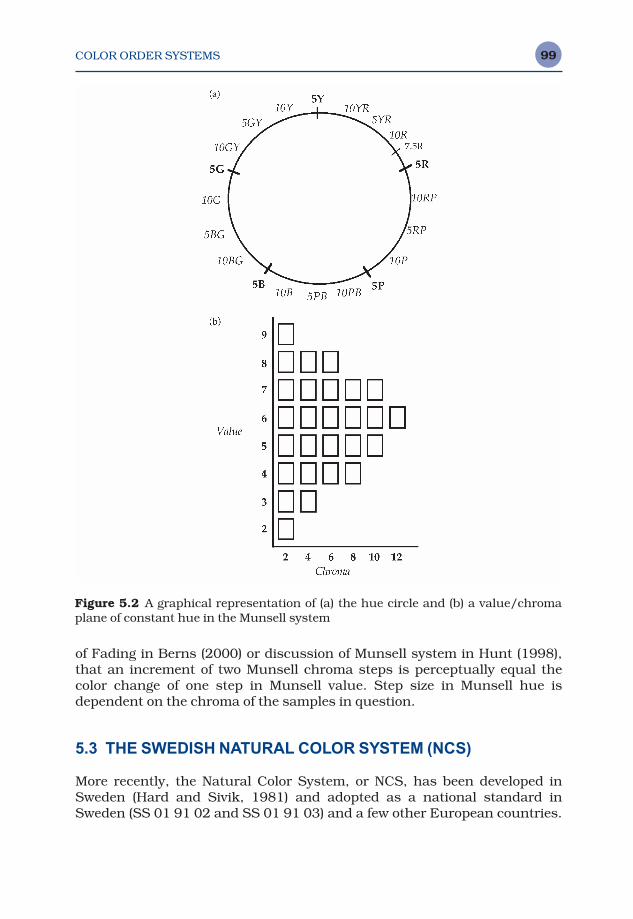
COLOR ORDER SYSTEMS 99
of Fading in Berns (2000) or discussion of Munsell system in Hunt (1998),that an increment of two Munsell chroma steps is perceptually equal thecolor change of one step in Munsell value. Step size in Munsell hue is dependent on the chroma of the samples in question.
5.3 THE SWEDISH NATURAL COLOR SYSTEM (NCS)
More recently, the Natural Color System, or NCS, has been developed inSweden (Hard and Sivik, 1981) and adopted as a national standard inSweden (SS 01 91 02 and SS 01 91 03) and a few other European countries.
Figure 5.2 A graphical representation of (a) the hue circle and (b) a value/chromaplane of constant hue in the Munsell system
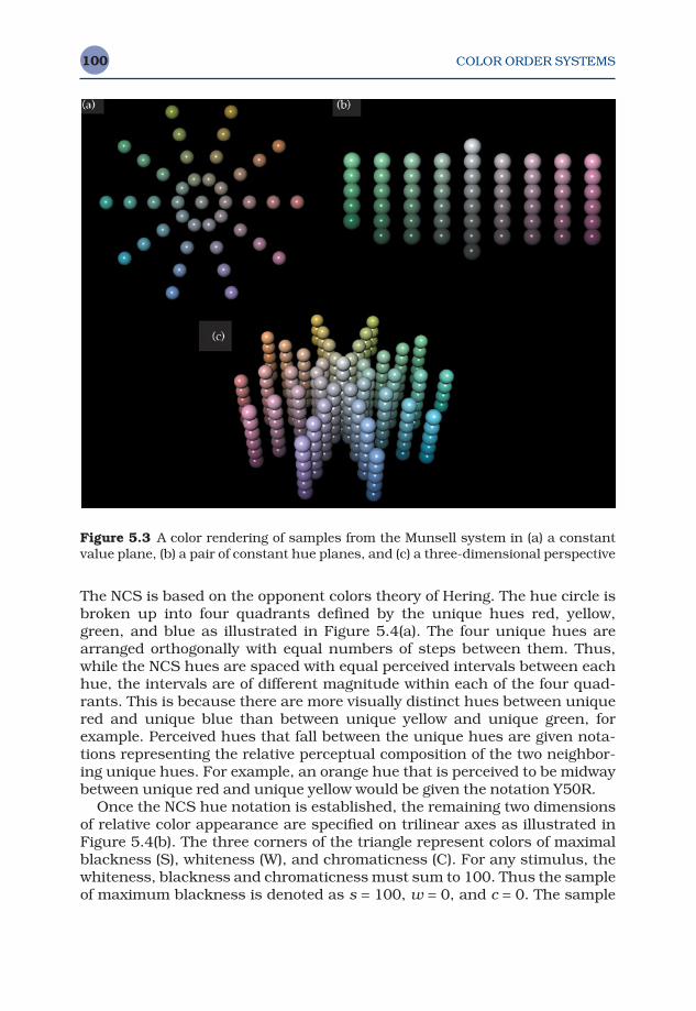
COLOR ORDER SYSTEMS100
The NCS is based on the opponent colors theory of Hering. The hue circle isbroken up into four quadrants defined by the unique hues red, yellow,green, and blue as illustrated in Figure 5.4(a). The four unique hues arearranged orthogonally with equal numbers of steps between them. Thus,while the NCS hues are spaced with equal perceived intervals between eachhue, the intervals are of different magnitude within each of the four quad-rants. This is because there are more visually distinct hues between uniquered and unique blue than between unique yellow and unique green, forexample. Perceived hues that fall between the unique hues are given nota-tions representing the relative perceptual composition of the two neighbor-ing unique hues. For example, an orange hue that is perceived to be midwaybetween unique red and unique yellow would be given the notation Y50R.
Once the NCS hue notation is established, the remaining two dimensionsof relative color appearance are specified on trilinear axes as illustrated inFigure 5.4(b). The three corners of the triangle represent colors of maximalblackness (S), whiteness (W), and chromaticness (C). For any stimulus, thewhiteness, blackness and chromaticness must sum to 100. Thus the sampleof maximum blackness is denoted as s = 100, w = 0, and c = 0. The sample
Figure 5.3 A color rendering of samples from the Munsell system in (a) a constantvalue plane, (b) a pair of constant hue planes, and (c) a three-dimensional perspective
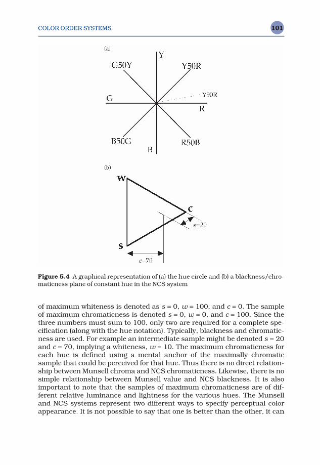
COLOR ORDER SYSTEMS 101
of maximum whiteness is denoted as s = 0, w = 100, and c = 0. The sampleof maximum chromaticness is denoted s = 0, w = 0, and c = 100. Since thethree numbers must sum to 100, only two are required for a complete spe-cification (along with the hue notation). Typically, blackness and chromatic-ness are used. For example an intermediate sample might be denoted s = 20and c = 70, implying a whiteness, w = 10. The maximum chromaticness foreach hue is defined using a mental anchor of the maximally chromatic sample that could be perceived for that hue. Thus there is no direct relation-ship between Munsell chroma and NCS chromaticness. Likewise, there is no simple relationship between Munsell value and NCS blackness. It is alsoimportant to note that the samples of maximum chromaticness are of dif-ferent relative luminance and lightness for the various hues. The Munselland NCS systems represent two different ways to specify perceptual colorappearance. It is not possible to say that one is better than the other, it can
Figure 5.4 A graphical representation of (a) the hue circle and (b) a blackness/chro-maticness plane of constant hue in the NCS system
COLOR ORDER SYSTEMS102
only be stated that the two are different. This was recently reaffirmed in thereport of CIE TC1-31 (CIE, 1996a), which was requested by ISO to recom-mend a single color order system as an international standard along withtechniques to convert from one to another. This international committee ofexperts concluded that such a task is impossible.
A color is denoted in the NCS by its blackness s, chromaticness c, andhue. For example, the stimulus described in the previous section with aMunsell designation of 7.5YR 5/10 has an NCS designation of 20, 70, Y90R.This suggests that the sample is nearly a unique red, with only 10% yellowcontent. It is further described as being highly chromatic (70%) with only asmall amount of blackness (20%). Note that even though this sample is ofmedium Munsell value, it is of substantially lower blackness (or higherwhiteness) in the NCS. This illustrates the fundamental difference betweenthe Munsell value scale and the NCS whiteness–blackness–chromaticnessscale.
Like the Munsell system, the NCS is embodied in an atlas and specified byCIE tristimulus values based on extensive visual observations. The NCSatlas includes 40 different hues and samples in steps of 10 along the black-ness and chromaticness scales. Since it is not possible to produce all of thepossible samples, due to limitations in pigments, there are approximately1500 samples in the atlas. The NCS atlas should also be viewed under day-light illumination with appropriate luminance levels and background. NCSsamples are also available in various sizes for different specialized applica-tions. As a Swedish national standard, the NCS is taught at a young age andused widely in color communication in Sweden, providing an enviable levelof precision in everyday color communication.
5.4 THE COLORCURVE SYSTEM
A recently developed color order system is the Colorcurve system (Stanziola1992), designed as a color communication system representing a combina-tion of a color appearance system and a color mixture system. The system is designed such that colors can be specified within the system and then spectral reflectance data for each sample can be used to formulate matchingsamples in various materials or media. Thus each sample in the system isspecified not only by its colorimetric coordinates, but also by its spectralreflectance properties.
The Colorcurve system uses the CIELAB color space as a starting point.Eighteen different L* levels were chosen at which to construct constant light-ness planes in the system. The L* levels range from 30 to 95 in steps of fiveunits with a few extra levels incorporated at the higher lightness levels thatare particularly important in design (e.g., light colors are popular for wallpaint). At each lightness level, nine starting points were selected. These con-sisted of one gray (a* = 0, b* = 0) and eight chromatic colors with chroma C* of 60. The chromatic starting points were red (60,0), orange (42.5, 42.5),yellow (0,60), yellow/green (−42.5, 42.5), green (−60,0), blue/green (−42.5,
COLOR ORDER SYSTEMS 103
−42.5), blue (0,−60), and purple (42.5,−42.5). Thus the starting points weredefined using principles of a color appearance space.
The remainder of the system was constructed using additive color mixing.Each quadrant of the CIELAB a*b* plane was filled with a rectangular sam-pling of additive mixtures of the gray and three chromatic starting points inthat quadrant. Equal steps in the Colorcurve designations represent equaladditive mixtures between the four starting points. These principles wereused to define all of the aim points for the Colorcurve system. The sampleswere then formulated with real pigments such that the system could beembodied along with the desired spectral reflectance curve specifications.The system is embodied in two atlases made up of samples of nitrocelluloselacquer coated on paper. The Master Atlas is made up of about 1200 samplesat the 18 different lightness levels. There is also a Gray and Pastel Atlasmade up of 956 additional samples that more finely sample the regions of color space that are near grays or pastels. Since the Colorcurve system isspecified by the spectral reflectance characteristics of the samples, the viewing illumination is not critical as long as a spectral match is made to thecolor curve sample. If a spectral match is made, the sample produced willmatch the Colorcurve sample under all light sources. This is not possiblewith other color order systems. Like the other color order systems, Color-curve samples can be obtained in a variety of forms and sizes for differentapplications.
One unique attribute of the Colorcurve system is of particular interest.The samples in the atlases are circular rather than square as found in mostsystems. The circular samples avoid two difficulties with color atlases. Thefirst is the contrast illusion of dark spots that appear at the corners betweensquare samples (the Hermann grid illusion). The second is that it is imposs-ible to mount a circular sample crooked!
5.5 OTHER COLOR ORDER SYSTEMS
The Munsell and NCS systems described above are the most important color order systems in the study of color appearance models. The Colorcurvesystem provides an interesting combination of color appearance and colormixture systems that could provide a useful source of samples for color ap-pearance and reproduction research. However, there are many other colororder systems that have been created for a variety of purposes. Derefeldt(1991) and Wyszecki and Stiles (1982) provide more details, but there are afew systems that warrant mention here. These include the OSA UniformColor Scales, the DIN system, and the Ostwald system.
OSA Uniform Color Scales
The Optical Society of America (OSA) set up a committee on Uniform ColorScales in 1947. The ultimate results of this committee’s work were described
COLOR ORDER SYSTEMS104
by MacAdam (1974,1978) as the OSA Uniform Color Scales system, or OSAUCS. The OSA system is a color appearance system, but it is significantlydifferent in nature from either the Munsell or NCS systems. The OSA systemis designed such that a given sample is equal in perceptual color differencefrom each of its neighbors in three-dimensional color space (not simply onedimension at a time as in the Munsell system). The OSA space is designed ina three-dimensional Euclidean geometry with L, j, and g axes representinglightness, yellowness–blueness, and redness–greenness, respectively. Inorder to make each sample equally spaced from each of its neighbors, a regular rhombohedral sampling of the three-dimensional space is requiredin which each sample has 12 nearest neighbors, all at an equal distance. Ifthe 12 points of the nearest neighbors to a sample are connected, they forma polyhedron known as a cubo-octohedron. Such sampling allows rectan-gularly sampled planes of the color space to be viewed from a variety of directions. Figure 5.5(a) shows a computer graphics representation of two adjacent constant lightness planes in the OSA system illustrating the sampling scheme. Figure 5.5(b) illustrates a three-dimensional representa-tion of the OSA system. It is clear that the objective of equal color differencesin all directions results in a very different type of color order system. Perhapsdue to its complex geometry (and the lack of a useful embodiment), the OSAsystem is not very popular. It does provide another set of data that could be used in the evaluation of color appearance and color difference models.The OSA space was also specified in terms of equations to transform fromCIE coordinates to the OSA system’s L, j, and g coordinates. Unfortunatelythe equations are not invertible, limiting their practical utility. The equa-tions and sample point specifications for the OSA system can be found inWyszecki and Stiles (1982).
DIN System
The DIN (Deusches Institut für Normung) system was developed in Germanywith the perceptual variables of hue, saturation, and darkness. An historicaloverview of the DIN system was presented by Richter and Witt (1986). Thespecification of colors in the DIN system is closely related to colorimetricspecification on a chromaticity diagram. Colors of equal hue in the DIN system fall on lines of constant dominant (or complementary) wavelength onthe chromaticity diagram (i.e., straight lines radiating from the white point).Colors of constant DIN saturation represent constant chromaticities. Thesampling of DIN hue and saturation is designed to be perceptually uniform.DIN darkness is related to the luminous reflectance of the sample relative toan ideal sample (a sample that either reflects all, or none, of the incidentenergy at each wavelength) of the same chromaticity resulting in a darknessscale that is similar to NCS blackness rather than Munsell value. The DINsystem is embodied in the DIN Color Chart that includes constant hue pageswith a rectangular sampling of darkness and saturation. Thus columns on a

COLOR ORDER SYSTEMS 105
DIN page represent constant chromaticity (DIN saturation) and appear as a shadow series (a single object illuminated at various levels of the same illuminant). The DIN charts also illustrate that chromaticity differencesbecome less distinguishable as darkness increases. The bottom row of anygiven DIN page appears uniformly black.
Ostwald System
The Ostwald system has been widely used in art and design and is thereforeof substantial historical interest (Derefeldt 1991). Like the NCS system, the
Figure 5.5 A color rendering of samples from the OSA UCS system in (a) a pair ofadjacent constant lightness planes and (b) a three-dimensional projection
COLOR ORDER SYSTEMS106
Ostwald system is based on Hering’s opponent colors theory. However, theOstwald system, much like the Colorcurve system, represents a combina-tion of a color appearance system and a color mixture system. Ostwald usedHering’s four unique hues to set up a hue circle, but rather than placing theperceptually opponent hues opposite one another, he used colorimetriccomplements (chromaticities connected by a straight line through the whitepoint on a chromaticity diagram) in the opposite positions on the hue circle.The Ostwald system also includes a trilinear representation of white con-tent, black content, and full-color content on each constant hue plane. Inthe NCS system, these planes are defined according to perceptual colorscales. However, in the Ostwald system, these planes were defined by addit-ive color mixtures of the three maxima located at the corners of the triangles.Thus the Ostwald system was set up with color appearance in mind, but thesamples were filled in using additive color mixing. (This is exactly analogousto the much more recent formulation of the Colorcurve system based onCIELAB.)
5.6 USES OF COLOR ORDER SYSTEMS
Color order systems have a variety of applications in the study of colorappearance and related areas. These include use as samples in experiments,color design, communication, education, model testing, test targets, andother applications where physical samples are helpful.
Color Order Systems in Visual Experiments
Often in visual experiments aimed at studying color appearance it is neces-sary to view and/or match a variety of colored stimuli under different viewingconditions. Color order systems provide a useful source of samples for suchexperiments. For example, an experimenter might select a collection ofMunsell, NCS, or Colorcurve samples to scale in a color appearance experi-ment. These samples will have well-known characteristics and in publishingthe notations of the samples used, the researchers provide a useful defini-tion of the stimuli that can be used by others to replicate the experiments.Note that actually using samples from the color order systems, and not justtheir designations on arbitrary samples, has the advantage that the reflect-ance characteristics of the samples are also defined. A related use of colororder systems in appearance experiments involves teaching the system toobservers and then asking them to assign designations (Munsell and NCSare particularly useful in this type of experiment) to samples viewed under avariety of conditions. This allows a specification of the change in appearancecaused by various changes in viewing conditions which can be used, togetherwith the colorimetric specifications of each sample in each viewing condi-tion, to formulate and test color appearance models.
COLOR ORDER SYSTEMS 107
Color Order Systems in Art and Design
Color order systems are often used in art and design. Their very nature as an orderly arrangement of colors allows designers to easily select sampleswith various color relationships. For example, with the Munsell system it issimple to select a range of colors of constant lightness or hue, or to selecthues that complement one another in various ways. Color mixing systemsprovide this utility in addition to providing some insight for artists to helpthem actually produce the colors in various media. The color order systemsnot only provide a design tool, but also incorporate a communication tool intheir designations, allowing the chosen colors to be communicated to thoseproducing the materials to be incorporated into a design.
Color Order Systems in Communication
Clearly, precise communication of color appearance is an application forcolor order systems. This is effective as long as those on both ends of thecommunication link are viewing the systems in properly controlled environ-ments. While colorimetric coordinates have the potential to provide muchmore precise, accurate, and useful specifications of colors, the perceptualmeaning is not so readily apparent to various users. A color order systemcan provide a more readily accessible communication tool. It can also beused to describe a color appearance to someone familiar with the system,but not necessarily in possession of an atlas. An interesting example of thistype of communication can be found in the ANSI specifications for viewing ofcolor images (ANSI 1989) in which the backgrounds are specified in terms ofMunsell value when a reflectance factor alone is sufficient and potentiallymore precise.
Color Order Systems in Education
Color order systems are immensely useful in education regarding colorappearance (as well as many other aspects of color). For example, examina-tion of the Munsell system allows a visual definition of the color appearanceattributes of lightness, chroma, and hue. Moving pages from the MunsellBook of Color from a low luminance level to a high luminance level allows fora nice demonstration of how brightness and colorfulness increase substan-tially while lightness and chroma remain nearly constant. The DIN system isuseful to illustrate the difference between chroma and saturation and howsaturation is related to a shadow series (a single object illuminated bydecreasing illuminance levels of the same spectral power distribution). Colororder systems can also be educational in their limitations. For example, inthe Munsell system, constant value is defined as constant relative lumin-ance. However, it is well known (Helmholtz–Kohlrausch effect described in
COLOR ORDER SYSTEMS108
Chapter 6) that as samples increase in chroma at constant relative lumin-ance they appear lighter. One need only examine a series of Munsell samplesof constant value and varying chroma to see that indeed there is a large andsystematic variation in lightness. Lastly, systems like the NCS systems canbe a great aid in education regarding the opponent theory of color vision,particularly in their hue designations which closely follow the physiologicalencoding of color.
Color Order Systems to Evaluate Mathematical ColorAppearance Models
Since color order systems such as Munsell and NCS are based on perceptualscaling of color appearance, they provide readily available data that can beused to evaluate mathematical color appearance models. For example, theMunsell system includes planes of constant lightness and hue, and cylin-drical surfaces of constant chroma. The tristimulus specifications of theMunsell system can be converted into the appropriate color appearance pre-dictors for a given color appearance model in order to see how well it predictsthe constant hue, lightness, and chroma contours. Such an evaluation provides a useful, widely understood technique for the intercomparison ofvarious color appearance models. Intercomparison of the predictions ofMunsell and NCS contours in various models also allows further study tounderstand the fundamental differences between the two systems.
Color Order Systems and Imaging Systems
Color order systems can also be used as sources for test targets for imagingsystems or other measurement devices. For example, the Macbeth ColorChecker Chart (McCamy et al. 1976) is a commonly used test target forimaging systems that is partially based on samples from the Munsell sys-tem. Despite its common use, the Macbeth Color Checker Chart incorpor-ates only a small sample of colors (24) and an incomplete sampling of colorspace. Targets of greater practical utility could fairly easily be constructed.Samples from various color order systems can be used to develop customtest targets that can be reliably specified and replicated elsewhere.
Limitations of Color Order Systems
While color order systems have a variety of useful applications in colorappearance, they are not a substitute for a color appearance model. In gen-eral they suffer from two significant limitations in this regard. First, they are not specified mathematically in relationship to physically measurablevalues. While both the Munsell and NCS systems have colorimetric spe-cifications for each sample in the system, there are no equations to relate the
COLOR ORDER SYSTEMS 109
colorimetric coordinates to the perceptual coordinates of the color order sys-tems. Approximate equations have been derived by statistical fitting andneural network modeling, but the only reliable technique for transformationfrom CIE colorimetry to color order system coordinates remains look-uptable interpolation. Clearly, the lack of mathematical definitions in the for-ward direction precludes the possibility of the analytical inverse models forthe required reverse direction. Second, these color order systems have beenestablished as perceptual scales of color appearance for a single viewingcondition. They provide no data with respect to the changes in color appear-ance induced by changes in viewing conditions.
5.7 COLOR NAMING SYSTEMS
There are a variety of color specification systems available that do not meetthe requirements for consideration as true color order systems, but are useful for some practical applications. Generally such systems, more pro-perly considered color naming systems, are not arranged in a perceptuallyordered manner (although some are arranged in order according to someimaging process), and are not presented or specified for controlled viewingconditions. In addition, the physical embodiments of these systems are notcontrolled with the colorimetric accuracy required for precise color commun-ication. Examples of such systems include the Pantone, Toyo, Focoltone,and Trumatch systems.
The Pantone System
The main component of the Pantone system is the Pantone Color FormulaGuide. This guide is a swatch book containing 1012 Pantone spot color inkmixtures on coated and uncoated stock. Each swatch has a numericalidentifier that can be used to communicate the desired color to a printer. Theprinter will then mix the spot color ink using the prescribed Pantone formulaand the resulting printed color should be a reasonable approximation to thecolor in the swatch book. This system is the prevalent tool for the specifica-tion of spot color in the USA.
The Pantone Process Color Imaging Guide includes 942 color swatchesillustrating the Pantone spot colors that can be reasonably well simulatedwith a four-color (CMYK) printing process. The swatch book includes a patchof the Pantone spot color adjacent to the process-color simulation to indicatethe variance that can be expected.
The Trumatch System
The Trumatch Colorfinder is a swatch book including over 2000 process colorsamples. These samples are arranged in an order that is slightly more
COLOR ORDER SYSTEMS110
perceptually based than the Pantone system. Such a system allows com-puter users to select CMYK color specifications according to the appearanceof printed swatches rather than relying on the approximate color repres-ented on a CRT display for a given CMYK specification. The user finds the de-sired color in the swatch book, sets the particular area in an image to thoseCMYK values, and then proceeds to ignore the often inappropriate appear-ance of the computer display, with confidence that the final printed color willbe a fairly close approximation to the color selected in the swatch book.
Other Systems
In addition to the Pantone and Trumatch process color guides that can beused as shortcuts to specification of colors that are ultimately to be printed,there is the PostScript Process Color Guide published by Agfa that includesover 16 000 examples of process colors representing a complete sampling ofCMY combinations from 0% to 100% (dot coverage) in 5% increments withadditional samples incorporating four different levels of black ink coverage.The samples are presented on both coated and uncoated stock.
Given the variability in printing inks, papers, and processes, these sys-tems can only be considered as approximate guides. They are known to notbe very stable and it is often recommended that swatch books be replacedevery six months or so. However, their performance is far superior thanworking with no guides and uncalibrated/uncharacterized imaging systems.However, a system in which all of the imaging devices have been carefullycalibrated and characterized, and in which viewing conditions are carefullycontrolled, will be capable of easily producing superior color accuracy andprecision for within-gamut colors. For out-of-gamut colors (such as metallicinks which cannot be simulated on a two-dimensional computer graphicsdisplay) a swatch-book system might still prove invaluable.

Color Appearance Models Second Edition M. D. Fairchild © 2005 John Wiley & Sons, LtdISBN: 0-470-01216-1 (HB)
6Color Appearance
Phenomena
Chapter 3 describes the fundamental concepts of basic colorimetry. Whilethe CIE system of colorimetry has proven to be extremely useful, it is import-ant to remember that it has limitations. Most of its limitations are inherentin the design of a system of tristimulus values based on color matching.Such a system can accurately predict color matches for an average observer,but it incorporates none of the information necessary for specifying the colorappearance of those matching stimuli. Such is the realm of color appearancemodels. Tristimulus values can be considered as a nominal (or at best ordinal) scale of color. They can be used to state whether two stimuli matchor not. The specification of color differences requires interval scales and thedescription of color appearance requires interval scales (for hue) and ratioscales (for brightness, lightness, colorfulness, and chroma). Additionalinformation is needed, in conjunction with tristimulus values, to derivethese more sophisticated scales.
Where is this additional information found? Why is it necessary? Whatcauses tristimulus colorimetry to ‘fail’? These questions can be answeredthrough examination of various color appearance phenomena, several ofwhich are described in this chapter. These phenomena represent instancesin which one of the necessary requirements for the success of tristimuluscolorimetry is violated. Understanding what causes these violations and thenature of the discrepancies is what allows the construction of color appear-ance models.
6.1 WHAT ARE COLOR APPEARANCE PHENOMENA?
Given two stimuli with identical CIE XYZ tristimulus values, they will matchin color for an average observer as long as certain constraints are followed.
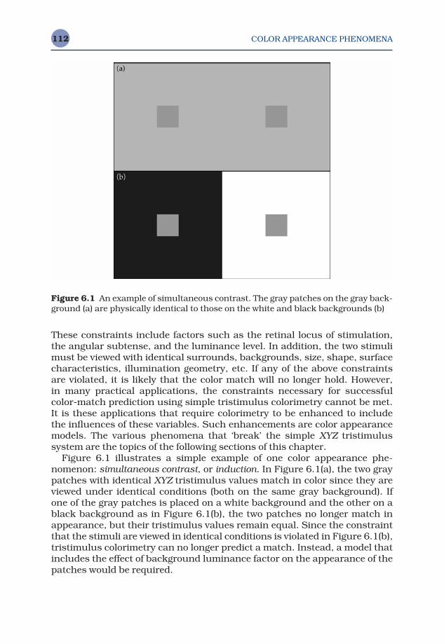
COLOR APPEARANCE PHENOMENA112
These constraints include factors such as the retinal locus of stimulation,the angular subtense, and the luminance level. In addition, the two stimulimust be viewed with identical surrounds, backgrounds, size, shape, surfacecharacteristics, illumination geometry, etc. If any of the above constraintsare violated, it is likely that the color match will no longer hold. However, in many practical applications, the constraints necessary for successfulcolor-match prediction using simple tristimulus colorimetry cannot be met.It is these applications that require colorimetry to be enhanced to includethe influences of these variables. Such enhancements are color appearancemodels. The various phenomena that ‘break’ the simple XYZ tristimulussystem are the topics of the following sections of this chapter.
Figure 6.1 illustrates a simple example of one color appearance phe-nomenon: simultaneous contrast, or induction. In Figure 6.1(a), the two graypatches with identical XYZ tristimulus values match in color since they areviewed under identical conditions (both on the same gray background). Ifone of the gray patches is placed on a white background and the other on ablack background as in Figure 6.1(b), the two patches no longer match inappearance, but their tristimulus values remain equal. Since the constraintthat the stimuli are viewed in identical conditions is violated in Figure 6.1(b),tristimulus colorimetry can no longer predict a match. Instead, a model thatincludes the effect of background luminance factor on the appearance of thepatches would be required.
Figure 6.1 An example of simultaneous contrast. The gray patches on the gray back-ground (a) are physically identical to those on the white and black backgrounds (b)
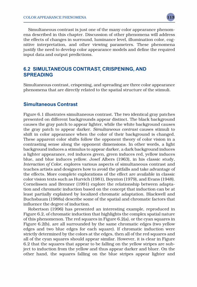
COLOR APPEARANCE PHENOMENA 113
Simultaneous contrast is just one of the many color appearance phenom-ena described in this chapter. Discussion of other phenomena will addressthe effects of changes in surround, luminance level, illumination color, cog-nitive interpretation, and other viewing parameters. These phenomena justify the need to develop color appearance models and define the requiredinput data and output predictions.
6.2 SIMULTANEOUS CONTRAST, CRISPENING, ANDSPREADING
Simultaneous contrast, crispening, and spreading are three color appearancephenomena that are directly related to the spatial structure of the stimuli.
Simultaneous Contrast
Figure 6.1 illustrates simultaneous contrast. The two identical gray patchespresented on different backgrounds appear distinct. The black backgroundcauses the gray patch to appear lighter, while the white background causesthe gray patch to appear darker. Simultaneous contrast causes stimuli toshift in color appearance when the color of their background is changed.These apparent color shifts follow the opponent theory of color vision in acontrasting sense along the opponent dimensions. In other words, a lightbackground induces a stimulus to appear darker, a dark background inducesa lighter appearance, red induces green, green induces red, yellow inducesblue, and blue induces yellow. Josef Albers (1963), in his classic study,Interaction of Color, explores various aspects of simultaneous contrast andteaches artists and designers how to avoid the pitfalls and take advantage ofthe effects. More complete explorations of the effect are available in classiccolor vision texts such as Hurvich (1981), Boynton (1979), and Evans (1948).Cornelissen and Brenner (1991) explore the relationship between adapta-tion and chromatic induction based on the concept that induction can be atleast partially explained by localized chromatic adaptation. Blackwell andBuchsbaum (1988a) describe some of the spatial and chromatic factors thatinfluence the degree of induction.
Robertson (1996) has presented an interesting example, reproduced inFigure 6.2, of chromatic induction that highlights the complex spatial natureof this phenomenon. The red squares in Figure 6.2(a), or the cyan squares inFigure 6.2(b), are all surrounded by the same chromatic edges (two yellowedges and two blue edges for each square). If chromatic induction werestrictly determined by the colors at the edges, then all of the red squares andall of the cyan squares should appear similar. However, it is clear in Figure6.2 that the squares that appear to be falling on the yellow stripes are sub-ject to induction from the yellow and thus appear darker and bluer. On theother hand, the squares falling on the blue stripes appear lighter and
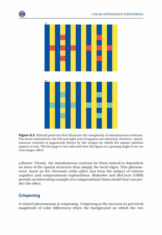
COLOR APPEARANCE PHENOMENA114
yellower. Clearly, the simultaneous contrast for these stimuli is dependenton more of the spatial structure than simply the local edges. This phenom-enon, know as the chromatic white effect, has been the subject of variouscognitive and computational explanations. Blakeslee and McCourt (1999)provide an interesting example of a computational vision model that can pre-dict the effect.
Crispening
A related phenomenon is crispening. Crispening is the increase in perceivedmagnitude of color differences when the background on which the two
Figure 6.2 Stimuli patterns that illustrate the complexity of simultaneous contrast.The local contrasts for the left and right sets of squares are identical. However, simul-taneous contrast is apparently driven by the stripes on which the square patchesappear to rest. Tilt the page to one side and view the figure at a grazing angle to see aneven larger effect
COLOR APPEARANCE PHENOMENA 115
stimuli are compared is similar in color to the stimuli themselves. Figure 6.3illustrates crispening for a pair of gray samples. The two gray stimuli appearto be of greater lightness difference on the gray background than on eitherthe white or black backgrounds. Similar effects occur for color differences.Semmelroth (1970) published a comprehensive study on the crispeningeffect along with a model for its prediction.
Spreading
When the stimuli increase in spatial frequency, or become smaller, thesimultaneous contrast effect disappears and is replaced with a spreadingeffect. Spreading refers to the apparent mixture of a color stimulus with itssurround. This effect is complete at the point of spatial fusion when thestimuli are no longer viewed as discrete, but fuse into a single stimulus(such as when a halftone image is viewed at a sufficient distance such thatthe individual dots cannot be resolved). Spreading, however, occurs at spatial frequencies below those at which fusion occurs. Thus, the stimuli arestill observed as distinct from the background, but their colors begin toblend.
Classic studies by Chevreul (1839) explored the importance of spreadingand contrast in the design of tapestries where it was often desired to pre-serve the color appearance of design elements despite changes in spatialconfiguration and background color. Thus the tapestry designers wererequired to physically change the colors used throughout the tapestry inorder to preserve color appearance. A related, although more complex, phe-nomenon known as neon spreading is discussed by Bressan (1993). Neonspreading is an interesting combination of perceptions of spreading andtransparency.
Figure 6.3 An example of crispening. The pairs of gray patches are physically ident-ical on all three backgrounds

COLOR APPEARANCE PHENOMENA116
Figure 6.4 illustrates both simultaneous contrast and spreading along a color dimension. Colorimetrically achromatic stimuli patches of variousspatial frequency are presented on a red background. For the low-frequency(large) patches, simultaneous contrast takes place and the patches appearslightly greenish. However, at higher spatial frequencies (small patches),spreading occurs and the patches appear pinkish. The dependency on spa-tial frequency can be explored by examining Figure 6.4 from various viewingdistances. Simultaneous contrast and spreading point to lateral interactionsand adaptation effects in the human visual system.
6.3 BEZOLD–BRÜCKE HUE SHIFT (HUE CHANGES WITHLUMINANCE)
It is often assumed that hue can be specified by the wavelength of amonochromatic light. Unfortunately, this is not the case as illustrated byphenomena such as the Bezold–Brücke hue shift. This hue shift occurswhen one observes the hue of a monochromatic stimulus while changing itsluminance. The hue will not remain constant.
Some typical experimental results on the Bezold–Brücke hue shift havebeen reported by Purdy (1931). Figure 6.5 represents some of the resultsfrom the Purdy (1931) research. The data in Figure 6.5 indicate the changein wavelength required to preserve a constant hue appearance across areduction in luminance by a factor of 10. For example, to match the hue of650 nm light at a given luminance would require a light of 620 nm at one-tenth the luminance level (−30 nm shift). Recall that a given monochromaticlight will have the same relative tristimulus values no matter what the luminance level (since absolute luminance level is usually not considered in tristimulus colorimetry). Thus, tristimulus values alone would predictthat the color of a monochromatic light should remain constant at all lumin-ance levels. Purdy’s results clearly disprove that hypothesis and point to the
Figure 6.4 A demonstration of the difference between simultaneous contrast andspreading. The gray areas are physically identical, but appear different depending ontheir spatial scale with respect to the red background
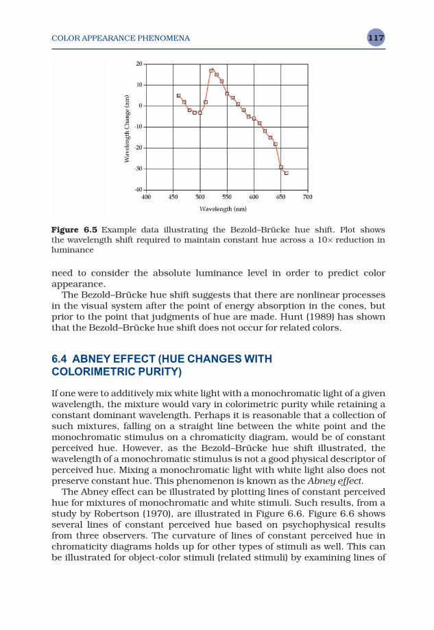
COLOR APPEARANCE PHENOMENA 117
need to consider the absolute luminance level in order to predict colorappearance.
The Bezold–Brücke hue shift suggests that there are nonlinear processesin the visual system after the point of energy absorption in the cones, butprior to the point that judgments of hue are made. Hunt (1989) has shownthat the Bezold–Brücke hue shift does not occur for related colors.
6.4 ABNEY EFFECT (HUE CHANGES WITH COLORIMETRIC PURITY)
If one were to additively mix white light with a monochromatic light of a givenwavelength, the mixture would vary in colorimetric purity while retaining aconstant dominant wavelength. Perhaps it is reasonable that a collection ofsuch mixtures, falling on a straight line between the white point and themonochromatic stimulus on a chromaticity diagram, would be of constantperceived hue. However, as the Bezold–Brücke hue shift illustrated, thewavelength of a monochromatic stimulus is not a good physical descriptor ofperceived hue. Mixing a monochromatic light with white light also does notpreserve constant hue. This phenomenon is known as the Abney effect.
The Abney effect can be illustrated by plotting lines of constant perceivedhue for mixtures of monochromatic and white stimuli. Such results, from astudy by Robertson (1970), are illustrated in Figure 6.6. Figure 6.6 showsseveral lines of constant perceived hue based on psychophysical resultsfrom three observers. The curvature of lines of constant perceived hue inchromaticity diagrams holds up for other types of stimuli as well. This can be illustrated for object-color stimuli (related stimuli) by examining lines of
Figure 6.5 Example data illustrating the Bezold–Brücke hue shift. Plot shows the wavelength shift required to maintain constant hue across a 10× reduction in luminance
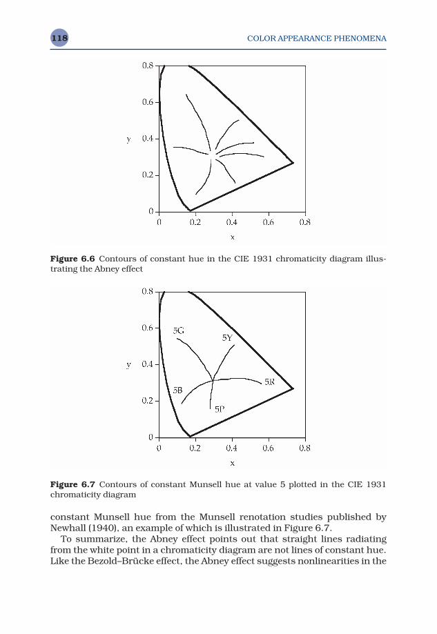
COLOR APPEARANCE PHENOMENA118
constant Munsell hue from the Munsell renotation studies published byNewhall (1940), an example of which is illustrated in Figure 6.7.
To summarize, the Abney effect points out that straight lines radiatingfrom the white point in a chromaticity diagram are not lines of constant hue.Like the Bezold–Brücke effect, the Abney effect suggests nonlinearities in the
Figure 6.6 Contours of constant hue in the CIE 1931 chromaticity diagram illus-trating the Abney effect
Figure 6.7 Contours of constant Munsell hue at value 5 plotted in the CIE 1931chromaticity diagram
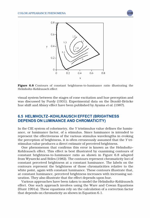
COLOR APPEARANCE PHENOMENA 119
visual system between the stages of cone excitation and hue perception andwas discussed by Purdy (1931). Experimental data on the Bezold–Brückehue shift and Abney effect have been published by Ayama et al. (1987).
6.5 HELMHOLTZ–KOHLRAUSCH EFFECT (BRIGHTNESSDEPENDS ON LUMINANCE AND CHROMATICITY)
In the CIE system of colorimetry, the Y tristimulus value defines the lumin-ance, or luminance factor, of a stimulus. Since luminance is intended to represent the effectiveness of the various stimulus wavelengths in evokingthe perception of brightness, it is often erroneously assumed that the Y tri-stimulus value produces a direct estimate of perceived brightness.
One phenomenon that confirms this error is known as the Helmholtz–Kohlrausch effect. This effect is best illustrated by examining contours ofconstant brightness-to-luminance ratio as shown in Figure 6.8 adaptedfrom Wyszecki and Stiles (1982). The contours represent chromaticity loci ofconstant perceived brightness at a constant luminance. The labels on thecontours represent the brightness of those chromaticities relative to thewhite point, again with constant luminance. These contours illustrate that,at constant luminance, perceived brightness increases with increasing sat-uration. They also illustrate that the effect depends upon hue.
Various approaches have been taken to model the Helmholtz–Kohlrauscheffect. One such approach involves using the Ware and Cowan Equations(Hunt 1991a). These equations rely on the calculation of a correction factorthat depends on chromaticity as shown in Equation 6.1.
Figure 6.8 Contours of constant brightness-to-luminance ratio illustrating theHelmholtz–Kohlrausch effect
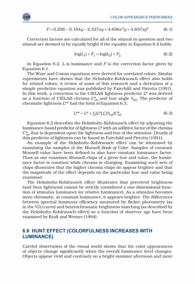
COLOR APPEARANCE PHENOMENA120
F = 0.256 − 0.184y − 2.527xy + 4.656x3y + 4.657xy4 (6.1)
Correction factors are calculated for all of the stimuli in question and twostimuli are deemed to be equally bright if the equality in Equation 6.2 holds.
log(L1) + F1 = log(L2) + F2 (6.2)
In Equation 6.2, L is luminance and F is the correction factor given byEquation 6.1.
The Ware and Cowan equations were derived for unrelated colors. Similarexperiments have shown that the Helmholtz–Kohlrausch effect also holdsfor related colors. A review of some of this research and a derivation of a simple predictive equation was published by Fairchild and Pirrotta (1991).In this work, a correction to the CIELAB lightness predictor L* was derivedas a function of CIELAB chroma C*ab and hue angle hab. The predictor ofchromatic lightness L** had the form of Equation 6.3.
L** = L* + f2(L*)f1(hab)C*ab (6.3)
Equation 6.3 describes the Helmholtz–Kohlrausch effect by adjusting theluminance-based predictor of lightness L* with an additive factor of the chromaC*ab that is dependent upon the lightness and hue of the stimulus. Details ofthis predictor of lightness can be found in Fairchild and Pirrotta (1991).
An example of the Helmholtz–Kohlrausch effect can be witnessed byexamining the samples of the Munsell Book of Color. Samples of constantMunsell value have been defined to also have constant luminance factor.Thus as one examines Munsell chips of a given hue and value, the lumin-ance factor is constant while chroma is changing. Examining such sets ofchips illustrates that the higher chroma chips do appear brighter and thatthe magnitude of the effect depends on the particular hue and value beingexamined.
The Helmholtz–Kohlrausch effect illustrates that perceived brightness(and thus lightness) cannot be strictly considered a one-dimensional func-tion of stimulus luminance (or relative luminance). As a stimulus becomesmore chromatic, at constant luminance, it appears brighter. The differencesbetween spectral luminous efficiency measured by flicker photometry (as in the V(λ) curve) and heterochromatic brightness matching (as described bythe Helmholtz–Kohlrausch effect) as a function of observer age have beenexamined by Kraft and Werner (1994).
6.6 HUNT EFFECT (COLORFULNESS INCREASES WITHLUMINANCE)
Careful observation of the visual world shows that the color appearances of objects change significantly when the overall luminance level changes.Objects appear vivid and contrasty on a bright summer afternoon and more
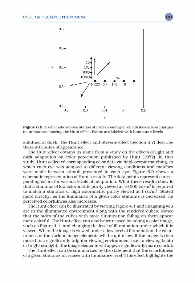
COLOR APPEARANCE PHENOMENA 121
subdued at dusk. The Hunt effect and Stevens effect (Section 6.7) describethese attributes of appearance.
The Hunt effect obtains its name from a study on the effects of light anddark adaptation on color perception published by Hunt (1952). In thatstudy, Hunt collected corresponding color data via haploscopic matching, inwhich each eye was adapted to different viewing conditions and matcheswere made between stimuli presented in each eye. Figure 6.9 shows aschematic representation of Hunt’s results. The data points represent corres-ponding colors for various levels of adaptation. What these results show isthat a stimulus of low colorimetric purity viewed at 10 000 cd/m2 is requiredto match a stimulus of high colorimetric purity viewed at 1 cd/m2. Statedmore directly, as the luminance of a given color stimulus is increased, itsperceived colorfulness also increases.
The Hunt effect can be illustrated by viewing Figure 4.1 and imagining youare in the illuminated environment along with the rendered cubes. Noticethat the sides of the cubes with more illumination falling on them appearmore colorful. The Hunt effect can also be witnessed by taking a color image,such as Figure 4.1, and changing the level of illumination under which it isviewed. When the image is viewed under a low level of illumination the color-fulness of the various image elements will be quite low. If the image is thenmoved to a significantly brighter viewing environment (e.g., a viewing boothor bright sunlight), the image elements will appear significantly more colorful.
The Hunt effect can be summarized by the statement that the colorfulnessof a given stimulus increases with luminance level. This effect highlights the
Figure 6.9 A schematic representation of corresponding chromaticities across changesin luminance showing the Hunt effect. Points are labeled with luminance levels

COLOR APPEARANCE PHENOMENA122
importance of considering the absolute luminance level in color appearancemodels — something that traditional colorimetry does not do.
6.7 STEVENS EFFECT (CONTRAST INCREASES WITH LUMINANCE)
The Stevens effect is a close relative of the Hunt effect. While the Hunt effectrefers to an increase in chromatic contrast (colorfulness) with luminance,the Stevens effect refers to an increase in brightness (or lightness) contrastwith increasing luminance. For the purposes of understanding these effects,contrast should be thought of as the rate of change of perceived brightness(or lightness) with respect to luminance. For a more complete discussion oncontrast, refer to Fairchild (1995b).
Like the Hunt effect, the Stevens effect draws its name from a classic psy-chophysical study (Stevens and Stevens 1963). In this study, observers wereasked to perform magnitude estimations on the brightness of stimuli acrossvarious adapting conditions. The results illustrated that the relationshipbetween perceived brightness and measured luminance tended to follow apower function. This power function is sometimes referred to as Stevenspower iaw in psychophysics. A relationship that follows a power functionwhen plotted on linear coordinates becomes a straight line (with slope equalto the exponent of the power function) on log–log coordinates. Typical resultsfrom the experiments of Stevens and Stevens (1963) are plotted on logarith-mic axes in Figure 6.10, which shows average relative brightness magnitudeestimations as a function of relative luminance for four different adaptationlevels. Figure 6.10 shows that the slope of this relationship (and thus the exponent of the power function) increases with increasing adaptingluminance.
The Stevens effect indicates that, as the luminance level increases, darkcolors will appear darker and light colors will appear lighter. While this prediction might seem somewhat counterintuitive, it is indeed the case. TheStevens effect can be demonstrated by viewing an image at high and lowluminance levels. A black-and-white image is particularly effective for thisdemonstration. At a low luminance level, the image will appear of rather lowcontrast. White areas will not appear very bright and, perhaps surprisingly,dark areas will not appear very dark. If the image is then moved to a signific-antly higher level of illumination, white areas appear substantially brighterand dark areas darker — the perceived contrast has increased.
6.8 HELSON–JUDD EFFECT (HUE OF NONSELECTIVE SAMPLES)
The Helson–Judd effect is elusive and perhaps cannot even be observed innormal viewing conditions. It is probably unimportant in practical situations.

COLOR APPEARANCE PHENOMENA 123
However, its description is included here since two color appearance models(Hunt and Nayatani et al.) make rather strong predictions of this effect. Thusit is important to understand its definition and consider its importance whenimplementing those models. The experimental data first describing theHelson–Judd effect were presented by Helson (1938).
In Helson’s experiment, observers were placed in a light booth (effectivelya closet) that was illuminated with nearly monochromatic light. They werethen asked to assign Munsell designations (after a training period) to variousnonselective (neutral Munsell patches) samples. Typical results are illus-trated in Figure 6.11 for a background of Munsell value 5/. Similar trendswere observed on black-and-white backgrounds. Figure 6.11 shows the perceived chroma (in Munsell units) for nonselective samples of variousMunsell values. The results indicate that these nonselective samples did notappear neutral under strongly chromatic illumination. Samples lighter thanthe background exhibited chroma of the same hue as the source while samples darker than the background exhibited chroma of the hue of thesource’s complement. It is important to note that this effect only occurred fornearly monochromatic illumination. Helson (1938) stated that the effect com-pletely disappeared if as little as 5% white light was added to the mono-chromatic light. Thus, the effect is of little practical importance since coloredstimuli should never be evaluated under monochromatic illumination.
However, the effect is predicted by some color appearance models and hasbeen observed in one recent experiment (Mori et al. 1991). The Mori et al.
Figure 6.10 Changes in lightness contrast as a function of adapting luminanceaccording to the Stevens effect
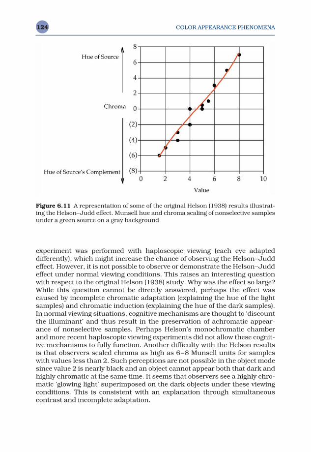
COLOR APPEARANCE PHENOMENA124
experiment was performed with haploscopic viewing (each eye adapted differently), which might increase the chance of observing the Helson–Juddeffect. However, it is not possible to observe or demonstrate the Helson–Juddeffect under normal viewing conditions. This raises an interesting questionwith respect to the original Helson (1938) study. Why was the effect so large?While this question cannot be directly answered, perhaps the effect wascaused by incomplete chromatic adaptation (explaining the hue of the lightsamples) and chromatic induction (explaining the hue of the dark samples).In normal viewing situations, cognitive mechanisms are thought to ‘discountthe illuminant’ and thus result in the preservation of achromatic appear-ance of nonselective samples. Perhaps Helson’s monochromatic chamberand more recent haploscopic viewing experiments did not allow these cognit-ive mechanisms to fully function. Another difficulty with the Helson resultsis that observers scaled chroma as high as 6–8 Munsell units for sampleswith values less than 2. Such perceptions are not possible in the object modesince value 2 is nearly black and an object cannot appear both that dark andhighly chromatic at the same time. It seems that observers see a highly chro-matic ‘glowing light’ superimposed on the dark objects under these viewingconditions. This is consistent with an explanation through simultaneouscontrast and incomplete adaptation.
Figure 6.11 A representation of some of the original Helson (1938) results illustrat-ing the Helson–Judd effect. Munsell hue and chroma scaling of nonselective samplesunder a green source on a gray background
COLOR APPEARANCE PHENOMENA 125
Recent attempts to demonstrate the Helson–Judd effect in the MunsellColor Science Laboratory have verified the unique nature of the percept. Theeffect cannot be observed with complex stimuli. It is only observed whenindividual nonselective patches are viewed on a uniform background. (Evena step tablet of nonselective stimuli of various reflectances is too complex toproduce the effect.) Also, nearly monochromatic light is required, as origin-ally reported by Helson (1938). Under these conditions, observers do report a‘glowing light’ of the hue complementary to the light source superimposed onthe samples darker than the background. Interestingly, only about 50% ofobservers report seeing any effect at all.
While the practical importance of the Helson–Judd effect might be ques-tionable, it does raise some interesting questions and warrants considera-tion since it influences the predictions of some color appearance models. Toreview, the Helson–Judd effect suggests that nonselective samples, viewedunder highly chromatic illumination, take on the hue of the light source ifthey are lighter than the background and take on the complementary hue ifthey are darker than the background.
6.9 BARTLESON–BRENEMAN EQUATIONS (IMAGE CONTRASTCHANGES WITH SURROUND)
While Stevens and Stevens (1963) showed that perceived contrast increasedwith increasing luminance level, Bartleson and Breneman (1967) were inter-ested in the perceived contrast of elements in complex stimuli (images) andhow it varied with luminance level and surround. They observed results similar to those described by the Stevens effect with respect to luminancechanges, but they also observed some interesting results with respect tochanges in the relative luminance of an image’s surround.
Their experimental results, obtained through matching and scaling experi-ments, showed that the perceived contrast of images increased when theimage surround was changed from dark to dim to light. This effect occursbecause the dark surround of an image causes dark areas to appear lighterwhile having little effect on light areas (white areas still appear white despitechanges in surround). Thus since there is more of a perceived change in thedark areas of an image than in the light areas, there is a resultant change inperceived contrast.
These results are consistent with the historical requirements for optimumimage tone reproduction. Photographic prints viewed in an average surroundare reproduced with a one-to-one relationship between relative luminancesin the original scene and the print. Photographic transparencies intendedfor projection in a dark surround are reproduced with a system transferfunction that is a power function with an exponent of approximately 1.5(roughly that is a photographic gamma of 1.5 for the complete system). Thisis one reason transparencies are produced with a physically higher contrastin order to counteract the reduction in perceived contrast caused by the

COLOR APPEARANCE PHENOMENA126
dark surround. Similarly, television images, typically viewed in a dim sur-round, are reproduced using a power function with an exponent of about1.25 (roughly the gamma for the complete television system). More detailsregarding the history and importance of surround compensation in imagereproduction can be found in Hunt (1995) and Fairchild (1995a).
Bartleson and Breneman (1967) published equations that predict theirexperimental results quite well. Bartleson (1975), in a paper on optimumimage tone reproduction, published a simplified set of equations that are ofmore practical value. Figure 6.12 illustrates predictions of perceived light-ness as a function of relative luminance for various surround conditionsaccording to results of the type described by Bartleson and Breneman. Thisplot is virtually identical to the results of Stevens and Stevens given in Figure6.10 on logarithmic axes. The straight lines of various slopes on logarithmicaxes transform into power functions with various exponents on linear axessuch as those in Figure 6.12. Color appearance models such as Hunt’s,RLAB, and the CIE models include predictions of the surround effects onperceived contrast of images.
Often, when working at a computer workstation, users turn off the roomlights in order to make the CRT display appear of higher contrast. This pro-duces a darker surround that should perceptually lower the contrast of thedisplay. The predictions of Bartleson and Breneman are counter to everydayexperience in this situation. The reason for this is that the room lights areusually introducing a significant amount of reflection off the face of the mon-itor and thus reducing the physical contrast of the displayed images. If thesurround of the display can be illuminated without introducing reflection off
Figure 6.12 Changes in lightness contrast as a function of surround relative lumin-ance according to the results of Bartleson and Breneman (Bartleson 1975)
COLOR APPEARANCE PHENOMENA 127
the face of the display (e.g., by placing a light source behind the monitor thatilluminates the surrounding area), the perceived contrast of the display willactually be higher than when it is viewed in a completely darkened room.
6.10 DISCOUNTING THE ILLUMINANT
Mechanisms of chromatic adaptation can be classified as sensory or cognit-ive. It is well established (Hunt and Winter 1975, Fairchild 1992b, 1993a)that sensory mechanisms are not capable of complete chromatic adaptation.However, under most typical viewing conditions, observers perceive coloredobjects as if adaptation to the color of the illumination were complete (i.e., awhite object appears white under tungsten light, fluorescent light, or day-light). Since the sensory mechanisms are incapable of mediating such per-ceptions, it can be shown that cognitive mechanisms (based on knowledgeabout objects, illumination, and the viewing environment) take over to com-plete the job. Further details of these different mechanisms of adaptation arepresented in Chapter 8.
‘Discounting the illuminant’ refers to the cognitive ability of observers tointerpret the colors of objects based on the illuminated environment inwhich they are viewed. This allows observers to perceive the colors of objectsmore independent of changes in the illumination and is consistent with the typical notion that color somehow ‘belongs’ to an object. Discounting the illuminant is important to understand and has been allowed for in some color appearance models (e.g., Hunt and RLAB). It is of importance inimaging applications where comparisons are made across various media.For example, when viewing prints, observers will be able to discount the illumination color. However, when viewing a computer display, there are noilluminated objects and discounting the illuminant does not occur. Thus insome situations it might be necessary to model this change in viewing mode.
There is a significant amount of recent research that addresses issuesrelated to changes in color appearance induced by complex stimulus struc-ture and observer interpretation. Examples of relevant references includeGilchrist (1980), Arend and Reeves (1986), Arend and Goldstein (1987,1990), Schirillo et al. (1990), Arend et al. (1991), Arend (1993), Schirillo andShevell (1993, 1996), Schirillo and Arend (1995), and Cornelissen andBrenner (1995). Work by Craven and Foster (1992) and Speigle and Brainard(1996) addresses the ability of observers to detect changes in illuminationseparate from changes in object colors. Lotto and Purves (2002) and Purveset al. (2002) have brought these concepts together nicely in an empirical theory of color perception.
6.11 OTHER CONTEXT AND STRUCTURAL EFFECTS
There are a wide variety of color appearance effects that depend on the struc-ture and/or context of the stimuli. Some of them fall into the category of
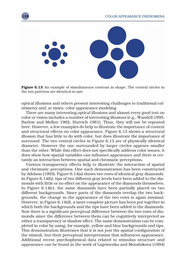
COLOR APPEARANCE PHENOMENA128
optical illusions and others present interesting challenges to traditional col-orimetry and, at times, color appearance modeling.
There are many interesting optical illusions and almost every good text oncolor or vision includes a number of interesting illusions (e.g., Wandell 1995,Barlow and Mollon 1982, Hurvich 1981). Thus, they will not be repeatedhere. However, a few examples do help to illustrate the importance of contextand structural effects on color appearance. Figure 6.13 shows a structuralillusion that has little to do with color, but does illustrate the importance ofsurround. The two central circles in Figure 6.13 are of physically identicaldiameter. However the one surrounded by larger circles appears smallerthan the other. While this effect does not specifically address color issues, itdoes show how spatial variables can influence appearance and there is cer-tainly an interaction between spatial and chromatic perceptions.
Various transparency effects help to illustrate the interaction of spatialand chromatic perceptions. One such demonstration has been constructedby Adelson (1993). Figure 6.14(a) shows two rows of identical gray diamonds.In Figure 6.14(b), tips of two different gray levels have been added to the dia-monds with little or no effect on the appearance of the diamonds themselves.In Figure 6.14(c), the same diamonds have been partially placed on two different backgrounds. Since parts of the diamonds overlap the two back-grounds, the change in the appearance of the two rows is again minimal.However, in Figure 6.14(d), a more complete picture has been put together inwhich both the backgrounds and the tips have been added to the diamonds.Now there is a significant perceptual difference between the two rows of dia-monds since the difference between them can be cognitively interpreted aseither a transparency or shadow effect. The same demonstration can be com-pleted in color by using, for example, yellow and blue backgrounds and tips.This demonstration illustrates that it is not just the spatial configuration ofthe stimuli, but their perceptual interpretation that influences appearance.Additional recent psychophysical data related to stimulus structure andappearance can be found in the work of Logvinenko and Menshikova (1994)
Figure 6.13 An example of simultaneous contrast in shape. The central circles inthe two patterns are identical in size
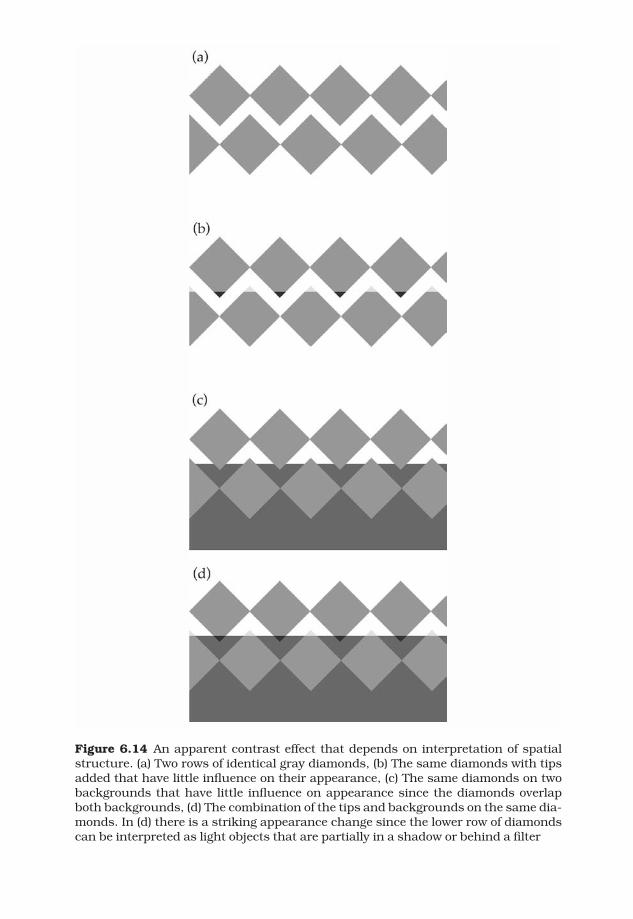
Figure 6.14 An apparent contrast effect that depends on interpretation of spatialstructure. (a) Two rows of identical gray diamonds, (b) The same diamonds with tipsadded that have little influence on their appearance, (c) The same diamonds on twobackgrounds that have little influence on appearance since the diamonds overlapboth backgrounds, (d) The combination of the tips and backgrounds on the same dia-monds. In (d) there is a striking appearance change since the lower row of diamondscan be interpreted as light objects that are partially in a shadow or behind a filter
COLOR APPEARANCE PHENOMENA130
and Taya et al. (1995). Not completely unrelated are the various perceptualphenomena of ‘filling in,’ which are discussed in recent work by De Weerd et al. (1998).
Other evidence of important structural effects on color appearance hasbeen reported by Shevell (1993). In these experiments, simple spatial struc-tures were added to the surrounds of colored stimuli with profound effectsthat could not be explained by the usual theories of simultaneous contrastand adaptation. Such results highlight the importance of considering spatialand color variables in conjunction with one another, not as separate entities.While various color appearance models do include spatial variables in a simple way, more complex approaches along the lines of those suggested byPoirson and Wandell (1993) need to be explored further.
Other interesting color demonstrations and effects rely to some degree oncognitive interpretation of the structure and context of the stimuli. Classicexperiments on memory color that are often described in sensation and per-ception textbooks fall into this category. Memory color refers to the idea thatobservers remember prototypical colors for familiar objects. In image repro-duction, objects such as sky, skin, and foliage are often mentioned (Hunt1995, Bartleson 1960, Hunt et al. 1974). Other examples include simpleexperiments (which are quite repeatable!) in which, for example, cutouts inthe shape of a tomato and a banana are made from orange constructionpaper and observers are asked to scale the color appearance of the twoobjects. The orange cutout in the shape of the banana will typically be per-ceived as slightly more yellow than an arbitrary shape cut out of the samepaper and the cutout in the shape of a tomato will be perceived as more red.These effects are small, but consistent, and reiterate the importance ofobservers’ interpretations of stimuli. Additional experimental results on thecharacteristics of color memory have been published by Nilsson and Nelson(1981) and Jin and Shevell (1996).
Two-Color Projections
Partially related to memory color are the somewhat famous two-color projec-tions that were demonstrated by Land (1959) and apparently included a fullrange of color appearances despite not having the three primaries requiredby conventional colorimetric theory. Figure 6.15 illustrates the process ofthe two-color projection. The original color image (Figure 6.15a) is separatedinto three black-and-white positive transparencies (Figure 6.15b), repres-enting the red, green, and blue information, as done in Maxwell’s (1858–62) original color photographic process. Normally, the three transparencieswould be projected through red, green, and blue filters and superimposed toproduce an accurate reproduction of the original (as in Figure 6.15a). In theLand two-color projection, however, the red separation is projected througha red filter, the green separation is projected with white light, and the blueseparation is not projected at all (Figure 6.15c). While one might expect such

COLOR APPEARANCE PHENOMENA 131
Figure 6.15 Example of a two-color image reproduction. (a) Original full-color image,(b) red, green, and blue separations of the image, (c) combination of the red separa-tion ‘projected’ through a red filter and the green separation ‘projected’ with whitelight
COLOR APPEARANCE PHENOMENA132
a projection could only produce a pinkish image, the result does indeedappear to be fairly colorful (although not nearly as colorful as a three-colorprojection to which Land apparently never made a direct comparison!). Thequality of the two-color projection depends on the subject matter since theeffect is strengthened if memory color can be applied. The remainder of the colors appearing in the two-color projection can be quite easily explainedby simultaneous contrast and chromatic adaptation (Judd 1960, Valbergand Lange-Malecki 1990).
Cognitive aspects of color appearance and recognition are of significantinterest, but largely outside the scope of this book. An interesting mono-graph on the subject has been published by Davidoff (1991). It is noteworthythat the cognitive model proposed by Davidoff is consistent with the variousinterpretations of color appearance necessary to explain the phenomenaand models described in this book. The topic of cognitive aspects of colorappearance cannot be fully considered without reference to the classic workof Katz (1935) that provides fascinating insight into the topic.
6.12 COLOR CONSTANCY?
Color constancy is another phenomenon that is often discussed. Typicallycolor constancy is defined as the apparent invariance in the color appear-ance of objects upon changes in illumination. This definition is somewhatmisleading. The main reason for this is because color constancy does notexist in humans! The data presented in the previous sections of this chapterand the discussion of chromatic adaptation in Chapter 8 should make thispoint abundantly clear.
An interesting thought experiment also points out the difficulty with theterm color constancy. If the colors of objects were indeed constant, then onewould not have to include the light source in colorimetric calculations inorder to predict color matches. In fact, color appearance models would notbe necessary as CIE XYZ colorimetry would define color appearance for allviewing conditions. Clearly, this is not the case as demonstrated, sometimespainfully, by metameric object color matches. Such objects match in colorunder one light source, but mismatch under others. Clearly both objects in ametameric pair cannot be color constant.
Then why does the term color constancy exist? Perhaps a quote fromEvans (1943) answers that question best; ‘. . . in everyday life we are accus-tomed to thinking of most colors as not changing at all. This is due to thetendency to remember colors rather than to look at them closely.’ When colors are closely examined, the lack of color constancy becomes extremelyclear. The study of color appearance and the derivation of color appearancemodels are, in fact, aiming to quantify and predict the failure of color con-stancy. Examples of more recent data are presented in the research ofBlackwell and Buchsbaum (1988b), Foster and Nascimento (1994), Kurikiand Uchikawa (1996), and Bäuml (1999).
COLOR APPEARANCE PHENOMENA 133
There still remains a great deal of interest in the concept of color con-stancy. At first this might seem strange, since it is known not to exist inhuman observers. However, the study of color constancy can potentiallylead to theories describing how the human visual system might strive forapproximate color constancy and the fundamental limitations preventingcolor constancy in the real world. Such studies take place in the arena ofcomputational color constancy with applications in machine vision (e.g.,Maloney and Wandell 1986, Drew and Finlayson 1994, Finlayson et al.1994a,b).
Jameson and Hurvich (1989) discussed some interesting concepts inregard to color constancy, the lack thereof in humans, and the utility in not being color constant that are suitable to end this chapter. They pointedout the value of having multiple mechanisms of chromatic adaptation, thusproducing imperfect color constancy and retaining information about theillumination, to provide important information about changes, such as wea-ther, light, and time of day, and the constant physical properties of objects inthe scene.
Color Appearance Models Second Edition M. D. Fairchild © 2005 John Wiley & Sons, LtdISBN: 0-470-01216-1 (HB)
7Viewing Conditions
Some of the various color appearance phenomena that produce the need forextensions to basic colorimetry were presented in Chapter 6. It is clear fromthese phenomena that various aspects of the visual field impact the colorappearance of a stimulus. In this chapter, practical definitions and descrip-tions of the components of the viewing field that allow the development of reasonable color appearance models are given along with the required colorimetric measurements for these components. Accurate use of colorappearance models requires accurate definition and measurement of thevarious components of the viewing field.
Different configurations of the viewing field will result in different cognit-ive interpretations of a stimulus and, in turn, different color perceptions.The last part of this chapter includes explanations of some of these phe-nomena and definitions of the various modes of viewing that can be observedfor colored stimuli. Understanding these modes of viewing can help explainwhy seemingly physically identical stimuli can appear significantly differentin color.
Related to the specification of viewing fields for color appearance modelsare the various definitions of standard viewing conditions used in differentindustries. These attempt to minimize difficulties with color appearance bydefining appropriate viewing field configurations. One example of such astandard is the ANSI (1989) standard defining viewing conditions for printsand transparencies.
7.1 CONFIGURATION OF THE VIEWING FIELD
The color appearance of a stimulus depends on the stimulus itself as well asother stimuli that are nearby in either space or time. Temporal effects, whileimportant, are generally not encountered in typical color appearance applica-tions. They are dealt with by ensuring that observers have had adequatetime to adapt to the viewing environment and presenting stimuli that do not
VIEWING CONDITIONS 135
vary in time. (Of course, there are several recent applications, such as digitalvideo, that will push color appearance studies toward the domain of tem-poral variation.) The spatial configuration of the viewing field is always of critical importance. (Since the eyes are constantly in motion it is impossible,in practical situations, to separate spatial and temporal effects.) The idealspatial representation of the visual field would be to have a fully specifiedimage of the scene. Such an image would have to have a spatial resolutiongreater than the visual acuity of the fovea and each pixel would be repres-ented by a complete spectral power distribution. With such a representationof the entire visual field, one would have almost all of the information neces-sary to specify the color appearance of any element of the scene; however,cognitive experience of the observer and temporal information would still bemissing. Some interesting data on the impact of the spatial configuration ofstimulus and surround were published by Abramov et al. (1992).
Such a specification of the viewing field is not practical for several reasons.First, the extensive data required are difficult to obtain accurately, even in a laboratory setting. It is not plausible to require such data in practicalapplications. Second, even if the data could be obtained, the sheer volumewould make its use quite difficult. Third, assuming these technical issueswere overcome, one would then require a color appearance model capable ofutilizing all of that data. Such a model does not exist and is not likely to bedeveloped in the foreseeable future. When the inter-observer variability incolor appearance judgements is considered, such a detailed model wouldcertainly be unnecessarily complex.
Given all the above limitations, the situation is simplified by defining aminimum number of important components of the viewing field. The variouscolor appearance models use different subsets of these viewing field com-ponents. The most extensive set is the one presented by Hunt (1991b, 1995)for use with his color appearance model. Since Hunt’s definition of the view-ing field includes a superset of the components required by all other models,his definitions are presented below. The viewing field is divided into fourcomponents:
1. Stimulus2. Proximal field3. Background4. Surround.
Figure 7.1 schematically represents these components of the visual field.
Stimulus
The stimulus is defined as the color element for which a measure of colorappearance is desired. Typically the stimulus is taken to be a uniform patchof about 2° angular subtense. Figure 7.1 illustrates a 2° stimulus when
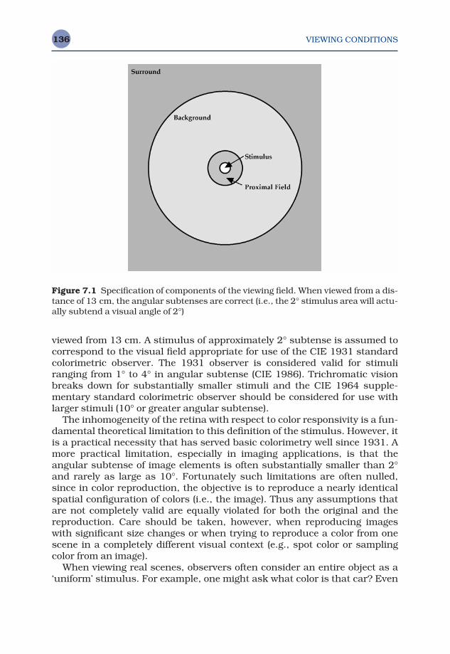
VIEWING CONDITIONS136
viewed from 13 cm. A stimulus of approximately 2° subtense is assumed tocorrespond to the visual field appropriate for use of the CIE 1931 standardcolorimetric observer. The 1931 observer is considered valid for stimuliranging from 1° to 4° in angular subtense (CIE 1986). Trichromatic visionbreaks down for substantially smaller stimuli and the CIE 1964 supple-mentary standard colorimetric observer should be considered for use withlarger stimuli (10° or greater angular subtense).
The inhomogeneity of the retina with respect to color responsivity is a fun-damental theoretical limitation to this definition of the stimulus. However, itis a practical necessity that has served basic colorimetry well since 1931. Amore practical limitation, especially in imaging applications, is that theangular subtense of image elements is often substantially smaller than 2°and rarely as large as 10°. Fortunately such limitations are often nulled,since in color reproduction, the objective is to reproduce a nearly identicalspatial configuration of colors (i.e., the image). Thus any assumptions thatare not completely valid are equally violated for both the original and thereproduction. Care should be taken, however, when reproducing imageswith significant size changes or when trying to reproduce a color from onescene in a completely different visual context (e.g., spot color or samplingcolor from an image).
When viewing real scenes, observers often consider an entire object as a‘uniform’ stimulus. For example, one might ask what color is that car? Even
Figure 7.1 Specification of components of the viewing field. When viewed from a dis-tance of 13 cm, the angular subtenses are correct (i.e., the 2° stimulus area will actu-ally subtend a visual angle of 2°)
VIEWING CONDITIONS 137
though different areas of the car will produce widely different color appear-ances, most observers would reply with a single answer. Thus, the stimulusis not a 2° field, but the entire object. This occurs to a limited extent inimages, but it is more conceivable for observers to break an image apart intosmaller image elements.
Proximal Field
The proximal field is defined as the immediate environment of the stimulus,extending for about 2° from the edge of the stimulus in all, or most, direc-tions. Definition of the proximal field is useful for modeling local contrasteffects such as lightness or chromatic induction, crispening, or spreading.Of current models, only that of Hunt (1991b) distinguishes the proximal fieldfrom the background.
While knowledge of the proximal field is necessary for detailed appearancemodeling, it is often impractical to specify it precisely. For example, in animage, the proximal field for any given element would be defined by its surrounding pixels. While these data are available (at least in digital imagingapplications), utilizing them should require the parameters of the colorappearance model to be recalculated for each spatial location within theimage. Often, such computations are prohibitive, and probably of little prac-tical value. In cases where the proximal field is not known, it is normallyspecified to be equal to the background.
Background
The background is defined as the environment of the stimulus, extending forabout 10° from the edge of the stimulus (or proximal field, if defined) in all, ormost, directions. Specification of the background is absolutely necessary for modeling simultaneous contrast. If the proximal field is different, itsspecification can be used for more complex modeling.
Like the proximal field, it becomes difficult to define the background inimaging applications. When considering a given image element, the back-ground is usually made up of the surrounding image areas, the exactspecification of which will change with image content and from location tolocation in the image. Thus, precise specification of the background inimages would require point-wise recalculation of appearance model para-meters. Since this is impractical in any typical applications, it is usuallyassumed that the background is constant and of some medium chromaticityand luminance factor (e.g., a neutral gray with 20% luminance factor).Alternatively, the background can be defined as the area immediately adjac-ent to the image. However, such a definition tends to attribute more import-ance to this area than is warranted. The difficulty of such definitions ofbackground and the impact on image reproduction are discussed by Braun
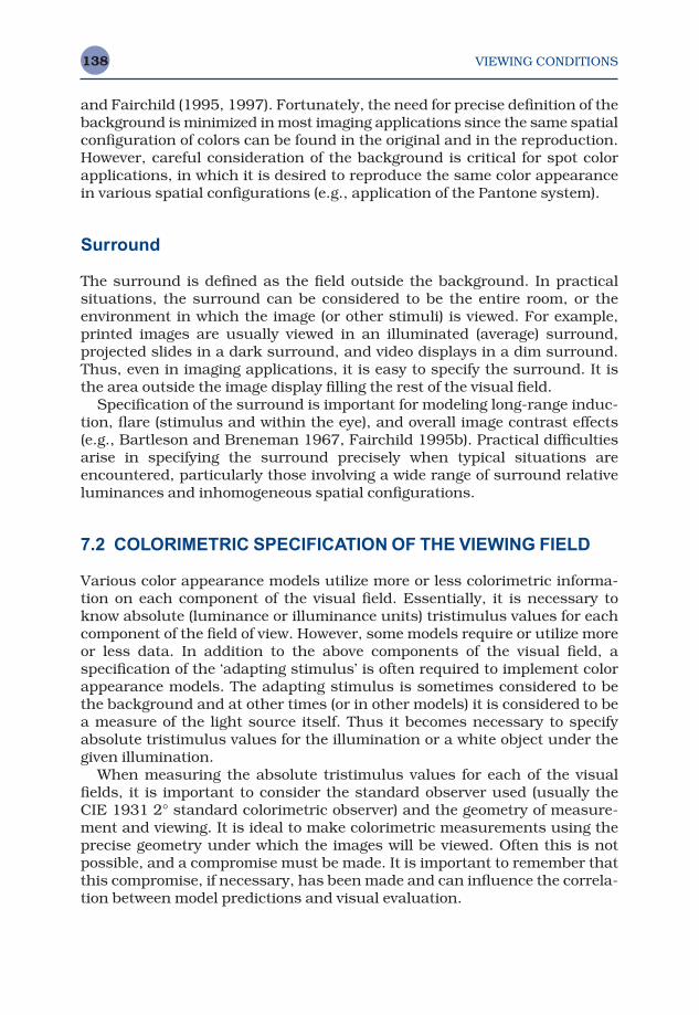
VIEWING CONDITIONS138
and Fairchild (1995, 1997). Fortunately, the need for precise definition of thebackground is minimized in most imaging applications since the same spatialconfiguration of colors can be found in the original and in the reproduction.However, careful consideration of the background is critical for spot colorapplications, in which it is desired to reproduce the same color appearancein various spatial configurations (e.g., application of the Pantone system).
Surround
The surround is defined as the field outside the background. In practical situations, the surround can be considered to be the entire room, or theenvironment in which the image (or other stimuli) is viewed. For example,printed images are usually viewed in an illuminated (average) surround, projected slides in a dark surround, and video displays in a dim surround.Thus, even in imaging applications, it is easy to specify the surround. It isthe area outside the image display filling the rest of the visual field.
Specification of the surround is important for modeling long-range induc-tion, flare (stimulus and within the eye), and overall image contrast effects(e.g., Bartleson and Breneman 1967, Fairchild 1995b). Practical difficultiesarise in specifying the surround precisely when typical situations areencountered, particularly those involving a wide range of surround relativeluminances and inhomogeneous spatial configurations.
7.2 COLORIMETRIC SPECIFICATION OF THE VIEWING FIELD
Various color appearance models utilize more or less colorimetric informa-tion on each component of the visual field. Essentially, it is necessary toknow absolute (luminance or illuminance units) tristimulus values for eachcomponent of the field of view. However, some models require or utilize moreor less data. In addition to the above components of the visual field, aspecification of the ‘adapting stimulus’ is often required to implement colorappearance models. The adapting stimulus is sometimes considered to bethe background and at other times (or in other models) it is considered to bea measure of the light source itself. Thus it becomes necessary to specifyabsolute tristimulus values for the illumination or a white object under thegiven illumination.
When measuring the absolute tristimulus values for each of the visualfields, it is important to consider the standard observer used (usually theCIE 1931 2° standard colorimetric observer) and the geometry of measure-ment and viewing. It is ideal to make colorimetric measurements using theprecise geometry under which the images will be viewed. Often this is notpossible, and a compromise must be made. It is important to remember thatthis compromise, if necessary, has been made and can influence the correla-tion between model predictions and visual evaluation.
VIEWING CONDITIONS 139
When dealing with self-luminous displays (such as CRT and LCD mon-itors), the determination of absolute tristimulus values can be accomplishedin a straightforward manner by measuring the display with a colorimeter orspectroradiometer. However, when dealing with reflective or transmissivemedia, the situation becomes more complex. Normally, such materials arecharacterized by their spectral reflectance, or transmittance, distributionsas measured with a spectrophotometer. Colorimetric coordinates (such asCIE tristimulus values) are then calculated using a standard colorimetricobserver and, normally, one of the defined illuminants (e.g., CIE illuminantD65, D50, A, F2). Such measurements and calculations are usually adequatein basic colorimetric applications. However, it is an extremely rare case inwhich images, or other colored objects, are actually viewed under lightsources that closely approximate one of the CIE illuminants (Hunt 1992).The difference in color between that calculated using a CIE illuminant andthat observed under a real source intended to simulate such an illuminantcan be quite significant. A conservative example of the differences encoun-tered is given in Table 7.1. The spectral reflectances for seven different colorsproduced on a digital photographic printer were measured and used to cal-culate CIELAB coordinates using CIE illuminants D50 and F8. IlluminantF8 is specified as a typical fluorescent illuminant with a correlated colortemperature of 5000 K and can be thought of as an extremely high-qualityilluminant D50 simulator. A real fluorescent lamp, intended to simulate illuminant D50 as found in typical viewing booths, would most likely have aspectral power distribution that deviates more from illuminant D50 than F8.The spectral power distributions of illuminants D50 and F8 are illustrated(for 10 nm increments) in Figure 7.2.
The color differences in Table 7.1 are as large as 2.5, a magnitude thatwould be perceptible in an image and easily perceptible in simple patches.While perceptible, the differences in this example are probably small enough
Table 7.1 CIELAB coordinates and ∆E*ab values for photographic samples evaluatedusing CIE Illuminants D50 and F8
Sample D50 F8L* a* b* L* a* b* ∆E*ab
Gray 53.7 −2.6 −9.7 53.6 −3.2 −9.8 0.6Red 39.1 41.0 20.4 39.4 41.5 21.0 0.8Green 43.2 −41.4 22.8 42.9 −40.6 22.0 1.2Blue 26.5 11.2 −28.8 26.4 9.2 −28.5 2.0Cyan 64.2 −38.7 −29.4 63.7 −40.8 −30.6 2.5Magenta 54.7 57.3 −24.8 55.0 56.3 −23.6 1.6Yellow 85.3 0.5 63.2 85.5 2.2 63.0 1.7
Average 1.49
VIEWING CONDITIONS140
to not be of significant concern. However, more typical light sources will pro-duce substantially larger errors.
A common example is encountered when colorimetric values (e.g., CIELABcoordinates) are used to color balance an imaging system. When the colori-metric coordinates indicate that printed samples should be neutral (i.e., a* = b* = 0.0), significant chromatic content is often observed. This result canbe traced to two causes. The first cause is differences between the standardilluminant used in the calculation and the light source used for observation,and the second cause is differences between the CIE standard observer andthe particular human observer making the evaluation. Differences betweenindividual observers can be siginficant. For color reproduction stimuli, theaverage CIELAB DE*ab between colors deemed to be matches by an indi-vidual observer is approximately 2.5 with maxima ranging up to 20 units(Fairchild and Alfvin 1995, Alfvin and Fairchild 1997). The former cause canbe corrected by using the actual spectral power distribution of the observingcondition in the colorimetric calculation. The latter is a fundamental limita-tion of colorimetry (indeed a limitation of any mean value) that cannot becorrected, but can only be understood.
To summarize, it is critical to use the actual spectral power distribution ofilluminating sources, rather than CIE standard illuminants, when preciseestimates of color appearance are required. When this is not feasible, view-ing booths with light sources that are close approximations of the CIE illumin-ants should be used.
While it would be ideal to have absolute spectral power distributions (andthus absolute tristimulus values) for each component of the viewing field, it
Figure 7.2 The relative spectral power distributions of CIE Illuminants D50 and F8(each normalized to 100.0 at 560 nm)
VIEWING CONDITIONS 141
is not necessary to have such detailed information for each model. The minimum data required for each subfield are described below. Some modelsrequire even less data as they do not consider each of the components of the visual field. The adapting field must be specified by at least its absolutetristimulus values (an alternative and equivalent specification is to have relative tristimulus values and the absolute luminance or illuminance). Thestimulus must also be specified by absolute tristimulus values (preferablycalculated with the actual light source). Similar data are also required for the proximal field and the background, although often the background isassumed to be achromatic and can then be specified using only its lumin-ance factor.
The color of the surround is not considered in any appearance model; it issufficient to know the relative luminance of the surround with respect to theimage (or stimulus) areas. Often, this is even more detail on the surroundthan is necessary and the surround can be specified sufficiently with anadjective such as dark, dim, and average. As a practical definition of sur-round relative luminance, dark can be taken to be 0%, dim between 0% and20%, and average between 20% and 100% of the luminance of the scene, orimage, white.
7.3 MODES OF VIEWING
While it is often hard to accept, especially by those with an affinity for physicalsciences and engineering, it has been clearly shown that the mode of appear-ance, and thus apparent color, depends upon the stimulus configurationand cognitive interpretation. This is most clearly illustrated by example andmost clearly understood (and believed!) upon personal experience.
One example has been observed by the author (and others) when viewinga familiar house that was painted a light yellow color and had a front door ofthe same yellow color. On one occasion in the late evening it appeared thatthe door of this yellow house had been painted blue. A blue door on a yellowhouse is a noteworthy perception! However, upon closer examination, it wasdetermined that the door was still its normal yellow color. The illuminationwas such that the house was illuminated directly by the sunlight from thesetting sun (quite yellow), while a small brick wall (at first unnoticed) cast ashadow that just covered the door. Thus the door was illuminated only byskylight (and no direct sunlight) and therefore appeared substantially moreblue than the rest of the house. On first sight, the scene was interpreted as ayellow house and blue door under uniform illumination. However, once itwas understood that the illumination was not uniform (and the door wasactually illuminated with blue light), the door actually changed in appear-ance from blue to yellow. The change in color appearance of the door wasbased completely on cognitive information about the illumination and couldnot be reversed once the illumination was known. A simulation of this effectis illustrated in Figure 7.3, which is an ambiguous figure that can be
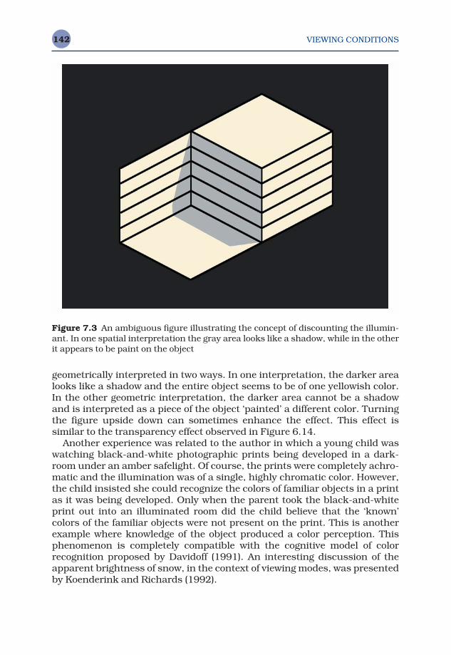
VIEWING CONDITIONS142
geometrically interpreted in two ways. In one interpretation, the darker arealooks like a shadow and the entire object seems to be of one yellowish color.In the other geometric interpretation, the darker area cannot be a shadowand is interpreted as a piece of the object ‘painted’ a different color. Turningthe figure upside down can sometimes enhance the effect. This effect is similar to the transparency effect observed in Figure 6.14.
Another experience was related to the author in which a young child waswatching black-and-white photographic prints being developed in a dark-room under an amber safelight. Of course, the prints were completely achro-matic and the illumination was of a single, highly chromatic color. However,the child insisted she could recognize the colors of familiar objects in a printas it was being developed. Only when the parent took the black-and-whiteprint out into an illuminated room did the child believe that the ‘known’ colors of the familiar objects were not present on the print. This is anotherexample where knowledge of the object produced a color perception. Thisphenomenon is completely compatible with the cognitive model of colorrecognition proposed by Davidoff (1991). An interesting discussion of theapparent brightness of snow, in the context of viewing modes, was presentedby Koenderink and Richards (1992).
Figure 7.3 An ambiguous figure illustrating the concept of discounting the illumin-ant. In one spatial interpretation the gray area looks like a shadow, while in the otherit appears to be paint on the object
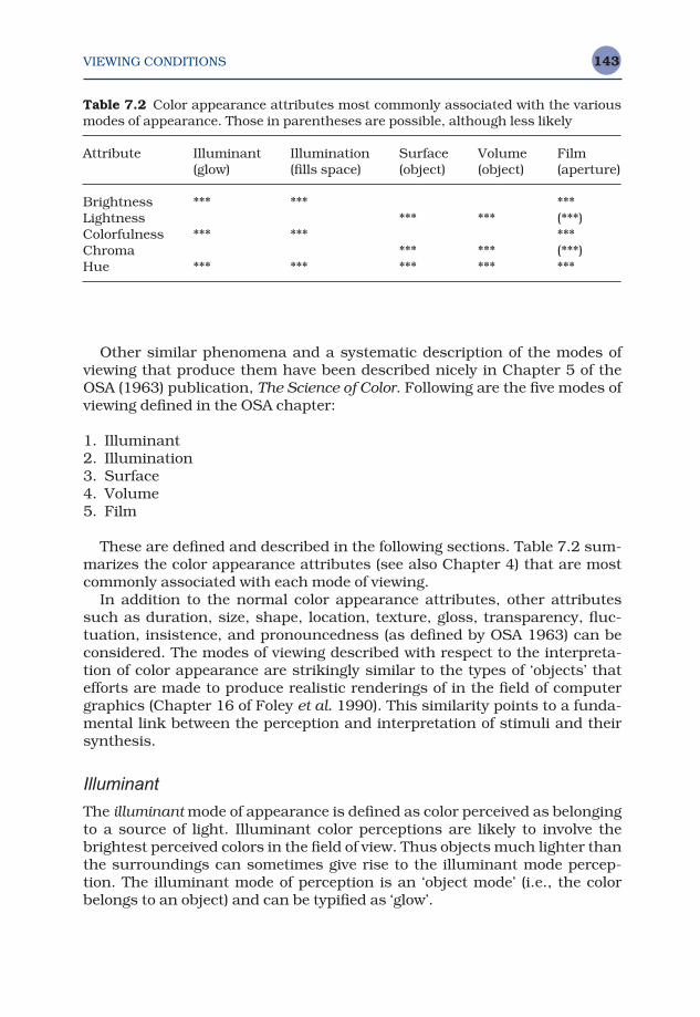
VIEWING CONDITIONS 143
Other similar phenomena and a systematic description of the modes ofviewing that produce them have been described nicely in Chapter 5 of theOSA (1963) publication, The Science of Color. Following are the five modes ofviewing defined in the OSA chapter:
1. Illuminant2. Illumination3. Surface4. Volume5. Film
These are defined and described in the following sections. Table 7.2 sum-marizes the color appearance attributes (see also Chapter 4) that are mostcommonly associated with each mode of viewing.
In addition to the normal color appearance attributes, other attributessuch as duration, size, shape, location, texture, gloss, transparency, fluc-tuation, insistence, and pronouncedness (as defined by OSA 1963) can be considered. The modes of viewing described with respect to the interpreta-tion of color appearance are strikingly similar to the types of ‘objects’ thatefforts are made to produce realistic renderings of in the field of computergraphics (Chapter 16 of Foley et al. 1990). This similarity points to a funda-mental link between the perception and interpretation of stimuli and theirsynthesis.
Illuminant
The illuminant mode of appearance is defined as color perceived as belongingto a source of light. Illuminant color perceptions are likely to involve thebrightest perceived colors in the field of view. Thus objects much lighter thanthe surroundings can sometimes give rise to the illuminant mode percep-tion. The illuminant mode of perception is an ‘object mode’ (i.e., the colorbelongs to an object) and can be typified as ‘glow’.
Table 7.2 Color appearance attributes most commonly associated with the variousmodes of appearance. Those in parentheses are possible, although less likely
Attribute Illuminant Illumination Surface Volume Film(glow) (fills space) (object) (object) (aperture)
Brightness *** *** ***Lightness *** *** (***)Colorfulness *** *** ***Chroma *** *** (***)Hue *** *** *** *** ***

VIEWING CONDITIONS144
Illumination
The illumination mode of appearance is defined as color attributed to pro-perties of the prevailing illumination rather than to objects. The ‘blue door’example described earlier is an example of a mode change between illumin-ant and surface. OSA (1963) gave an example of a perception of irregularsplotches of highly chromatic yellow paint (surface mode) on the dark shad-owed side of a railroad coach. When the observer came closer, noticed theangle of the setting sun, and could see penumbral gradations, he realizedthat the yellow patches were due to sunlight masked off by obstructions(illumination mode). The illumination mode of perception is a ‘non-object’mode and is mediated by the presence of illuminated objects that reflect lightand cast shadows (sometimes particles in the atmosphere).
Surface
The surface mode of appearance is defined as color perceived as belonging toa surface. Any recognizable, illuminated object provides an example of thesurface mode. This mode requires the presence of a physical surface andlight being reflected from the surface. It is an ‘object mode.’
Volume
The volume mode of appearance is defined as color perceived as belonging tothe bulk of a more or less uniform and transparent substance. For example,as the number of air bubbles in a block of ice increases, the lightness of the block increases toward white, while the transparency decreases towardzero. Thus a volume color transforms into a surface color. The volume modeof perception is an ‘object mode’ and requires transparency and a three-dimensional structure.
Film
The film mode of appearance (also referred to as aperture mode) is defined ascolor perceived in an aperture with no connection to an object. For example,failure to focus on a surface can cause a mode shift from surface to film. Anaperture screen accomplishes this since the observer tends to focus on theplane of the aperture. The film mode of perception is a ‘non-object’ mode. Allother modes of appearance can be reduced to film mode.
7.4 UNRELATED AND RELATED COLORS REVISITED
Unrelated and related colors were defined in Chapter 4. However, their fundamental importance in color appearance specification, their simplify-ing and unifying theme with respect to modes of appearance, and their
VIEWING CONDITIONS 145
important relation to the specification of brightness-colorfulness or lightness-chroma appearance matches warrant a revisit. The distinction betweenrelated and unrelated colors is the single most important viewing-mode con-cept to understand.
Unrelated ColorColor perceived to belong to an area or object seen in isolation from other colors.
Related ColorColor perceived to belong to an area or object seen in relation to other colors.
Unrelated colors only exhibit the perceptual attributes of hue, brightness,colorfulness, and saturation. The attributes that require judgement relativeto a similarly illuminated white object cannot be perceived with unrelatedcolors. On the other hand, related colors exhibit all of the perceptual attri-butes of hue, brightness, lightness, colorfulness, chroma, and saturation.
Recall that five perceptual dimensions are required for a complete spe-cification of the color appearance of related colors. These are brightness,lightness, colorfulness, chroma, and hue. However, in most practical colorappearance applications it is not necessary to know all five of these attributes.Typically, for related colors, only the three relative appearance attributes are of significant importance. Thus it is often sufficient to be concerned with only the relative appearance attributes of lightness, chroma, and hue.See Chapter 4 for a discussion of the distinction between brightness–colorfulness matching and lightness–chroma matching and their relativeimportance.
Color Appearance Models Second Edition M. D. Fairchild © 2005 John Wiley & Sons, LtdISBN: 0-470-01216-1 (HB)
8Chromatic
Adaptation
Various color appearance phenomena were discussed in Chapter 6. Thesephenomena illustrated cases in which simple tristimulus colorimetry wasnot capable of adequately describing appearance. Many of those phenomenacould be considered second-order effects. The topic of this chapter, chro-matic adaptation, is clearly the most important first-order color appearancephenomenon. Tristimulus colorimetry tells us when two stimuli match foran average observer when viewed under identical conditions. Interestinglyenough, such visual matches persist when the stimuli are viewed (as a pair)under an extremely wide range of viewing conditions. While the match per-sists, the color appearance of the two stimuli might be changing drastically.Changes in chromatic adaptation are one instance in which matches per-sist, but appearance changes. It is this change in appearance that must beunderstood to construct a color appearance model.
The term chromatic adaptation refers to the human visual system’s capab-ility to adjust to widely varying colors of illumination in order to approxim-ately preserve the appearance of object colors. Perhaps it is best illustratedby considering a system that does not have the capacity for chromatic adap-tation — photographic transparency film. Most transparency film is designedfor exposure under daylight sources. If such film is used to make photo-graphs of objects under incandescent illumination, the resulting trans-parencies have an unacceptable yellow–orange cast. This is because the filmcannot adjust the relative responsivities of its red, green, and blue imaginglayers in the way the human visual system adjusts the responsivities of itscolor mechanisms. Humans perceive relatively little change in the colors ofobjects when the illumination is changed from daylight to incandescent.
This chapter reviews some of the basic concepts of chromatic adapta-tion. Issues related to chromatic adaptation have been studied for much ofmodern history. The topic is even discussed by Aristotle (Wandell 1995).
CHROMATIC ADAPTATION 147
In woven and embroidered stuffs the appearance of colors is profoundlyaffected by their juxtaposition with one another (purple, for instance, appearsdifferent on white than on black wool), and also by differences of illumination.Thus embroiderers say that they often make mistakes in their colors whenthey work by lamplight, and use the wrong ones.
There are many excellent discussions of chromatic adaptation available inbooks (e.g., Barlow and Mollon 1982, Wyszecki and Stiles 1982, Spillmanand Werner 1990, Wandell 1995) and journals (e.g., Terstiege 1972, Hunt1976, Bartleson 1978, Wright 1981a, Lennie and D’Zmura 1988). The inter-ested reader is encouraged to explore this extensive and fascinating literature.
8.1 LIGHT, DARK, AND CHROMATIC ADAPTATION
Adaptation is the ability of an organism to change its sensitivity to a stimulusin response to changes in the conditions of stimulation. The general conceptof adaptation applies to all domains of perception. The various mechanismsof adaptation can act over extremely short durations (of the order of milli-seconds) or very long durations (weeks, months, or years!). In general, themechanisms of adaptation serve to make the observer less sensitive to astimulus when the physical intensity of the stimulus is greater. For example,one might be keenly aware of the ticking of a clock in the middle of a quietnight, but completely unable to perceive the same ticking during a busycocktail party. In the realm of vision, three types of adaptation becomeimportant — light, dark, and chromatic.
Light Adaptation
Light adaptation is the decrease in visual sensitivity upon increases in theoverall level of illumination. For example, it is easy to see millions of stars ona clear night. An equivalent number and variety of stars are present in thesky on a clear day; however, we are unable to perceive them. This is becausethe overall luminance level of the sky is several orders of magnitude higherin the daytime than at night. This causes visual sensitivity to changes inluminance to be reduced in the daytime relative to night. Thus the lumin-ance change that served to produce the perception of millions of stars atnight is inadequate to allow their perception during the day.
As another example, imagine waking up in the middle of the night andswitching on a bright room light. At first your visual system is dazzled, youare unable to see much of anything, and you might even feel a little pain.Then, after tens of seconds, you begin to be able to view objects normally inthe illuminated room. What has happened is that the mechanisms of visionwere at their most sensitive in the dark room. When the light was firstswitched on, they were overloaded due to their high sensitivity. After a short
CHROMATIC ADAPTATION148
period, they light adapted, thus decreasing their sensitivity and allowingnormal vision.
Dark Adaptation
Dark adaptation is similar to light adaptation, with the exception that darkadaptation refers to changes in the opposite direction. Thus dark adaptationis the increase in visual sensitivity experienced upon decreases in lumin-ance level. While the phenomena associated with light and dark adaptationare similar, it is useful to distinguish the two since they are mediated by dif-ferent mechanisms and exhibit different visual performance.
For example, light adaptation takes place much more quickly than darkadaptation. One can experience dark adaptation when entering a dark movietheater after being outdoors in bright sunlight. At first the theater will seemcompletely dark. Often people stop walking immediately upon entering adarkened room because they cannot see anything. However, after a shortperiod objects in the room (theater seats, other people, etc.) begin to becomevisible. After several minutes, objects will become quite visible and there islittle difficulty identifying other people, finding better seats, etc. All of thishappens because the mechanisms of dark adaptation are gradually increas-ing the overall sensitivity of the visual system. Light and dark adaptation inthe visual system can be thought of as analogous to automatic exposurecontrols in cameras.
Chromatic Adaptation
The processes of light and dark adaptation do have profound impacts on thecolor appearance of stimuli. Thus they will be considered in various colorappearance models. However, a third type of visual adaptation, chromaticadaptation, is far more important and must be included in all color appear-ance models. Chromatic adaptation is the largely independent sensitivityregulation of the mechanisms of color vision. Often it is considered to be onlythe independent changes in responsivity of the three types of cone photore-ceptors (while light and dark adaptation refer to overall responsivity changesin all of the receptors). However, it is important to keep in mind that thereare other mechanisms of color vision (e.g., at the opponent level and even atthe object recognition level) that are capable of changes in sensitivity thatcan be considered mechanisms of chromatic adaptation.
As an example of chromatic adaptation, consider a piece of white paperilluminated by daylight. When such a piece of paper is moved to a room withincandescent light, it still appears white despite the fact that the energyreflected from the paper has changed from predominantly blue to predomin-antly yellow (this is the change in illumination that the transparency filmdiscussed in the introduction to this chapter couldn’t adjust to). Figure 8.1
CHROMATIC ADAPTATION 149
illustrates such a change in illumination. Figure 8.1(a) illustrates a typicalscene under daylight illumination. Figure 8.1(b) shows what the scenewould look like under incandescent illumination when viewed by a visualsystem that is incapable of chromatic adaptation. Figure 8.1(c) illustratesthe same scene viewed under incandescent illumination by a visual systemcapable of adaptation similar to that observed in the human visual system.
Afterimages provide a second illustrative example of chromatic adapta-tion. These can be observed by viewing Figure 8.2. Stare at the black dot inthe center of Figure 8.2 and memorize the positions of the various colors.After approximately 30 seconds, move your gaze to an illuminated whitearea such as a wall or blank piece of paper. Notice the various colors andtheir locations. These afterimages are the result of independent sensitivitychanges of the color mechanisms. For example, the retinal areas exposed tothe red area in Figure 8.2 became less sensitive to red energy during theadapting exposure, resulting in the cyan appearance of the afterimage whenviewing a white area. This is caused by the lack of red response in this areathat would normally be expected when viewing a white stimulus. Similarexplanations hold for the other colors observed in the afterimage. While lightadaptation can be thought of as analogous to an automatic exposure con-trol, chromatic adaptation can be thought of as analogous to an automaticwhite-balance feature on a video camera or digital still camera.
8.2 PHYSIOLOGY
While the various phenomena of adaptation are interesting in their ownright, it becomes necessary to understand something of the physiologicalmechanisms of adaptation in order to model them properly. There are a variety of mechanisms of adaptation ranging from strictly sensory, reflex-like responses, to purely cognitive. While all of these mechanisms are notfully understood, it is instructive to examine their variety in order to laterunderstand how they are incorporated into various models. The mechan-isms discussed here are the following:
• Pupil dilation/constriction• Rod-cone transition• Receptor gain control• Subtractive mechanisms• High-level adaptation
Pupil Dilation/Constriction
The most apparent mechanism of light and dark adaptation is dilation andconstriction of the pupil. In ordinary viewing situations, the pupil diametercan range from about 3 to 7 mm. This represents a change in pupil area of
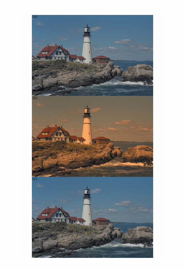
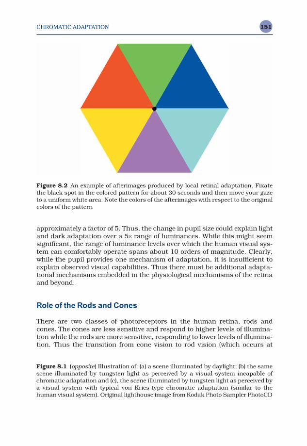
CHROMATIC ADAPTATION 151
approximately a factor of 5. Thus, the change in pupil size could explain lightand dark adaptation over a 5× range of luminances. While this might seemsignificant, the range of luminance levels over which the human visual sys-tem can comfortably operate spans about 10 orders of magnitude. Clearly,while the pupil provides one mechanism of adaptation, it is insufficient toexplain observed visual capabilities. Thus there must be additional adapta-tional mechanisms embedded in the physiological mechanisms of the retinaand beyond.
Role of the Rods and Cones
There are two classes of photoreceptors in the human retina, rods andcones. The cones are less sensitive and respond to higher levels of illumina-tion while the rods are more sensitive, responding to lower levels of illumina-tion. Thus the transition from cone vision to rod vision (which occurs at
Figure 8.1 (opposite) Illustration of: (a) a scene illuminated by daylight; (b) the samescene illuminated by tungsten light as perceived by a visual system incapable ofchromatic adaptation and (c), the scene illuminated by tungsten light as perceived bya visual system with typical von Kries-type chromatic adaptation (similar to thehuman visual system). Original lighthouse image from Kodak Photo Sampler PhotoCD
Figure 8.2 An example of afterimages produced by local retinal adaptation. Fixatethe black spot in the colored pattern for about 30 seconds and then move your gazeto a uniform white area. Note the colors of the afterimages with respect to the originalcolors of the pattern

CHROMATIC ADAPTATION152
luminances of the order of 0.1–1.0 cd/m2) provides an additional mechan-ism for light and dark adaptation.
The decrease in responsivity of the cones upon exposure to increasedluminance levels (light adaptation) takes place fairly rapidly, requiring a fewminutes at most, the increase in sensitivity of the rods upon exposure todecreased luminance levels requires more time. This can be illustrated witha classic dark adaptation curve showing the recovery of threshold after expos-ure to an extremely bright adapting stimulus as illustrated in Figure 8.3.The first phase of the curve shows the recovery of sensitivity of the cones,which levels off after a couple of minutes. Then, after about 10 minutes, therods have recovered enough sensitivity to become more sensitive than thecones and the curve takes another drop. After about 20 minutes, the rodshave reached their maximal sensitivity and the dark adaptation curve levelsoff. This curve explains the perceptions observed over time after entering adarkened movie theater.
In addition to providing a mechanism for light and dark adaptation, therod–cone transition has a profound impact on color appearance. Recall thatthere are three types of cones to serve the requirements of color vision, butonly one type of rod. Thus when luminance is reduced to levels at which onlythe rods are active, humans become effectively color blind, seeing the worldonly in shades of gray. Thus the rod–cone transition is of limited interest incolor appearance and chromatic adaptation models, and other mechanismsmust be considered. (Note: the influence of rods on color appearance can beimportant at low luminance levels and it is incorporated in Hunt’s colorappearance model.)
Figure 8.3 A typical dark adaptation curve showing the recovery of threshold after astrong exposure
CHROMATIC ADAPTATION 153
Receptor Gain Control
Perhaps the most important mechanism of chromatic adaptation is inde-pendent sensitivity changes in the photoreceptors, sometimes referred to as receptor gain control. It is possible imagine a gain control that varies therelationship between the number of photons incident on a photoreceptorand the electrochemical signal it produces in response to those photons.Chromatic adaptation would be served by turning down the gain when thereare many photons (high levels of excitation for the particular cone type) andturning up the gain when photons are less readily available. The key to chro-matic adaptation is that these gain controls are independent in each of thethree cone types. (Gain control is certainly a mechanism of light adaptationas well, but light adaptation could be served by a single gain control for allthree cone types. It is overly well served by independent mechanisms ofchromatic adaptation.)
Physiologically, changes in photoreceptor gain can be explained by pig-ment depletion at higher luminance levels. Light breaks down molecules ofvisual pigment (part of the process of phototransduction) and thus decreasesthe number of molecules available to produce further visual response.Therefore, at higher stimulus intensities there is less photopigment avail-able and the photoreceptors exhibit a decreased responsivity. While pig-ment depletion provides a nice explanation, there is evidence that the visual system adapts in a similar way at luminance levels for which there isinsignificant pigment depletion. This adaptation is thought to be caused bygain-control mechanisms at the level of the horizontal, bipolar, and ganglioncells in the retina. Gain control in retinal cells beyond the photoreceptorshelps to explain some of the spatially low-pass characteristics of chromaticadaptation. Delahunt and Brainard (2000) also discuss the interaction ofvarious cone types in the control of chromatic adapatation.
Subtractive Mechanisms
There is also psychophysical evidence for subtractive mechanisms of chro-matic adaptation in addition to gain control mechanisms (e.g., Walraven1976, Shevell 1978). Physiological mechanisms for such subtractive adapta-tion can be found by examining the temporal impulse response of the conephotoreceptors, which is biphasic and thus enhances transients and sup-presses steady signals. Similar processes are found in lateral inhibitorymechanisms in the retina that produce its spatially antagonistic impulseresponse that enhances spatial transients and suppresses spatially uniformstimuli. Physiological models of adaptation that require both multiplicative(gain) and subtractive mechanisms (e.g., Hayhoe et al. 1987, Hayhoe andSmith1989) can be made completely compatible with models typically pro-posed in the field of color appearance (see Chapter 9) that include only gaincontrols by assuming that the subtractive mechanism takes place after a
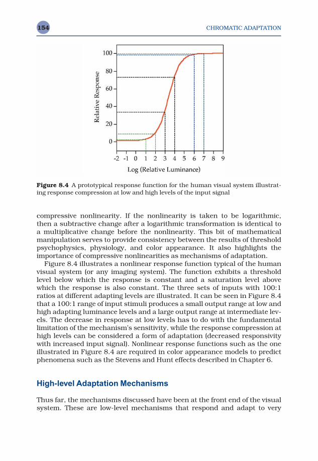
CHROMATIC ADAPTATION154
compressive nonlinearity. If the nonlinearity is taken to be logarithmic, then a subtractive change after a logarithmic transformation is identical to a multiplicative change before the nonlinearity. This bit of mathematicalmanipulation serves to provide consistency between the results of thresholdpsychophysics, physiology, and color appearance. It also highlights theimportance of compressive nonlinearities as mechanisms of adaptation.
Figure 8.4 illustrates a nonlinear response function typical of the humanvisual system (or any imaging system). The function exhibits a thresholdlevel below which the response is constant and a saturation level abovewhich the response is also constant. The three sets of inputs with 100:1ratios at different adapting levels are illustrated. It can be seen in Figure 8.4that a 100:1 range of input stimuli produces a small output range at low andhigh adapting luminance levels and a large output range at intermediate lev-els. The decrease in response at low levels has to do with the fundamentallimitation of the mechanism’s sensitivity, while the response compression athigh levels can be considered a form of adaptation (decreased responsivitywith increased input signal). Nonlinear response functions such as the oneillustrated in Figure 8.4 are required in color appearance models to predictphenomena such as the Stevens and Hunt effects described in Chapter 6.
High-level Adaptation Mechanisms
Thus far, the mechanisms discussed have been at the front end of the visualsystem. These are low-level mechanisms that respond and adapt to very
Figure 8.4 A prototypical response function for the human visual system illustrat-ing response compression at low and high levels of the input signal
CHROMATIC ADAPTATION 155
simple stimulus configurations. Webster and Mollon (1994) present inter-esting results that illustrate the relationship between spatial contrast, colorappearance, and higher-level visual mechanisms. There are also numerousexamples of visual adaptation that must take place at higher levels in thesystem (i.e., in the visual cortex). Examples of such cortical adaptationinclude
• The McCollough effect• Spatial frequency adaptation• Motion adaptation.
It is useful to consider these examples as illustrations of the potential forother types of high-level adaptation not yet considered.
A nice example of the McCollough effect can be found in Barlow andMollon (1982). To experience the McCollough effect, one must intermittentlyview a pattern of red and black strips in one orientation, say horizontal, andanother pattern of green and black strips of a second orientation, say ver-tical. By viewing each pattern for several seconds and then switching to theother, it is ensured that no simple afterimages are formed. After continuingthis adaptation process for about four minutes, the observers can then turntheir attention to patterns of black and white strips of spatial frequency similar to the adapting patterns. What will be observed is that black andwhite patterns of a vertical orientation will appear black and pink and blackand white patterns in a horizontal pattern will appear black and pale green.The effect is contingent upon the color and orientation of the adapting stim-uli and cannot be explained as a simple afterimage. It suggests adaptation ata cortical level in the visual system, where neurons that respond to particu-lar orientations and spatial frequencies are first observed. The effect is alsovery persistent, sometimes lasting for several days or longer!
Spatial frequency adaptation can be observed by examining Figure 8.5.Adapt to Figure 8.5(a) by gazing at the black bar in the center for one to twominutes. In order to avoid producing simple afterimages, do not fixate a single point, but rather let your gaze move back and forth along the blackbar. After the adaptation period, fixate on the black dot in the middle ofFigure 8.5(b). The pattern on the left in Figure 8.5(b) should look as if it is ofa higher spatial frequency than the pattern on the right. The two patterns in Figure 8.5(b) are identical. The difference in appearance after adaptationto Figure 8.5(a) is caused by the adaptation of mechanisms sensitive to vari-ous spatial frequencies. When adapting to a high spatial frequency, otherpatterns appear to be of lower spatial frequency and vice versa. Once again,this adaptation is attributed to cortical cells that selectively respond to various spatial frequencies.
Motion adaptation provides similar evidence in the temporal domain. Anexample of motion adaptation can be observed when viewing the credits atthe end of a motion picture (or text scrolling up a computer terminal). If thecredits are scrolling up the screen (and being observed) for several minutes,
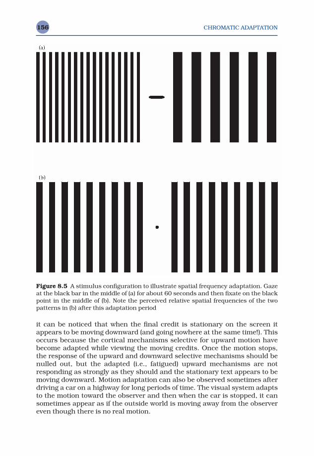
CHROMATIC ADAPTATION156
it can be noticed that when the final credit is stationary on the screen itappears to be moving downward (and going nowhere at the same time!). Thisoccurs because the cortical mechanisms selective for upward motion havebecome adapted while viewing the moving credits. Once the motion stops,the response of the upward and downward selective mechanisms should benulled out, but the adapted (i.e., fatigued) upward mechanisms are notresponding as strongly as they should and the stationary text appears to bemoving downward. Motion adaptation can also be observed sometimes afterdriving a car on a highway for long periods of time. The visual system adaptsto the motion toward the observer and then when the car is stopped, it cansometimes appear as if the outside world is moving away from the observereven though there is no real motion.
Figure 8.5 A stimulus configuration to illustrate spatial frequency adaptation. Gazeat the black bar in the middle of (a) for about 60 seconds and then fixate on the blackpoint in the middle of (b). Note the perceived relative spatial frequencies of the twopatterns in (b) after this adaptation period
CHROMATIC ADAPTATION 157
The examples of cortical adaptation discussed above lead to the next log-ical step. If there are adaptive mechanisms at such a high level in the visualsystem, is it possible that there are also cognitive mechanisms of adapta-tion? This issue is discussed in the following section.
8.3 SENSORY AND COGNITIVE MECHANISMS
It is tempting to assume that chromatic adaptation can be considered a sens-ory mechanism that is some sort of automatic response to changes in thestimulus configuration. However, there is clear evidence for mechanisms of chromatic adaptation that depend on knowledge of the objects and theirilluminated environment (Fairchild 1992a,b, 1993a). These are cognitivemechanisms of adaptation.
Chromatic adaptation mechanisms can be classified into two groups:
• Sensory — those that respond automatically to the stimulus energy• Cognitive — those that respond based upon observers’ knowledge of scene
content
Sensory Mechanisms
Sensory chromatic adaptation mechanisms are well known and have beenwidely discussed in the vision and color science literature. The physiologicallocus of such mechanisms is generally believed to be sensitivity control inthe photoreceptors and neurons in the first few stages of the visual system,as discussed previously. Most modern theories and models of sensory chro-matic adaptation trace their roots to the work of von Kries (1902) who wrote:
. . . the individual components present in the organ of vision are completelyindependent of one another and each is fatigued or adapted exclusivelyaccording to its own function.
These words of von Kries are known to be not precisely correct today, but theconcept is accurate and provides useful insight. To this day, the idea thatchromatic adaptation takes place through normalization of cone signals isknown as the von Kries coefficient law and serves as the basis of all modernmodels of chromatic adaptation and color appearance.
Cognitive Mechanims
Cognitive mechanisms have also been long recognized in the literature. How-ever, perhaps because of the difficulty of quantifying cognitive effects, theyare usually discussed briefly and are not as widely recognized or understood.To help understand the idea of cognitive chromatic adaptation mechanisms
CHROMATIC ADAPTATION158
it might be best to quote some of those that have mentioned them in the pasttwo centuries. Helmholtz (1866) in his treatise on physiological optics dis-cussed object color appearance:
We learn to judge how such an object would look in white light, and since ourinterest lies entirely in the object color, we become unconscious of the sensa-tions on which the judgement rests. [Translation Woodworth 1938]
Hering (1920), who is known for hypothesizing the opponent-colors theory ofcolor vision, discussed the concept of memory color:
All objects that are already known to us from experience, or that we regard as familiar by their color, we see through the spectacles of memory color.[Translation Hurvich and Jameson 1964]
Judd (1940) who made innumerable contributions to the field of color sci-ence referred to two types of chromatic adaptation mechanisms:
The processes by means of which the observer adapts to the illuminant or dis-counts most of the effect of a nondaylight illuminant are complicated; they areknown to be partly retinal and partly cortical.
Lastly, Evans (1943) who wrote and lectured on many aspects of color photo-graphy and color perception discussed reasons why the colors in photo-graphs look acceptable:
. . . in everyday life we are accustomed to thinking of most colors as notchanging at all. This is in large part due to the tendency to remember colorsrather than to look at them closely.
Jameson and Hurvich (1989) discussed the value of having multiple mech-anisms of chromatic adaptation to provide important information bothabout changes such as weather, light, and time of day and constant physicalproperties of objects in the scene. Finally, Davidoff (1991) published a mono-graph on the cognitive aspects of color and object recognition.
Hard-copy Versus Soft-copy Output
While it is clear that chromatic adaptation is complicated and relies on bothsensory and cognitive mechanisms, it is less clear how important it is to dis-tinguish between the two types of mechanisms when viewing image dis-plays. If an image is being reproduced in the same medium as the originaland is viewed under similar conditions, it is safe to assume that the samechromatic adaptation mechanisms are active when viewing both the originaland the reproduction. But, what happens when the original is presented in
CHROMATIC ADAPTATION 159
one medium, such as a soft-copy display, and the reproduction is viewed in a second medium, such as a hard-copy output? A series of experiments have been described (Fairchild 1992b, 1993a) that quantify some of thecharacteristics of chromatic-adaptation mechanisms and indicate that thesame mechanisms are not active when soft-copy displays are viewed as areactive when hard-copy displays or original scenes are viewed.
When hard-copy images are being viewed, an image is perceived as anobject that is illuminated by the prevailing illumination. Thus both sensorymechanisms, that respond to the spectral energy distribution of the stimu-lus, and cognitive mechanisms, that discount the ‘known’ color of the lightsource, are active. When a soft-copy display is being viewed, it cannot easilybe interpreted as an illuminated object. Therefore there is no ‘known’ illumin-ant color and only sensory mechanisms are active. This can be demon-strated by viewing a white piece of paper under incandescent illuminationand comparing the appearance to that of a CRT (or LCD) display of a uniformfield with exactly the same chromaticity and luminance viewed in a dark-ened room. The paper will appear white or just slightly yellowish. The displaywill appear relatively high-chroma yellow. In fact, a white piece of paper illuminated by that display will appear white while the display itself retains a yellow appearance! Color appearance models such as RLAB, the Huntmodel, and CIECAM02 include provisions for various degrees of cognitive‘discounting-the-illuminant.’
The Time-course of Adaptation
Another important feature of chromatic adaptation mechanisms is theirtime-course. The time-course of chromatic adaptation for color appear-ance judgements has been explored in detail (Fairchild and Lennie 1992,Fairchild and Reniff 1995). The results of these studies suggest that the sens-ory mechanisms of chromatic adaptation are about 90% complete after 60seconds for changes in adapting chromaticity at constant luminance. Sixtyseconds can be considered a good general rule for the minimum durationobservers should adapt to a given viewing environment prior to making crit-ical judgments. Adaptation is slightly slower when significant luminancechanges are also involved (Hunt 1950). Cognitive mechanisms of adaptationrely on knowledge and interpretation of the stimulus configuration. Thusthey can be thought of as effectively instantaneous once such knowledge isobtained. However, in some unusual viewing situations, the time required tointerpret the scene can be quite lengthy, if not indefinite.
8.4 CORRESPONDING-COLORS DATA
The most extensively available visual data on chromatic adaptation are corresponding-colors data. Corresponding colors are defined as two stimuli,
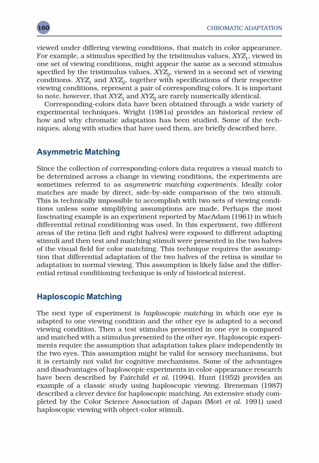
CHROMATIC ADAPTATION160
viewed under differing viewing conditions, that match in color appearance.For example, a stimulus specified by the tristimulus values, XYZ1, viewed inone set of viewing conditions, might appear the same as a second stimulusspecified by the tristimulus values, XYZ2, viewed in a second set of viewingconditions. XYZ1 and XYZ2, together with specifications of their respectiveviewing conditions, represent a pair of corresponding colors. It is importantto note, however, that XYZ1 and XYZ2 are rarely numerically identical.
Corresponding-colors data have been obtained through a wide variety ofexperimental techniques. Wright (1981a) provides an historical review ofhow and why chromatic adaptation has been studied. Some of the tech-niques, along with studies that have used them, are briefly described here.
Asymmetric Matching
Since the collection of corresponding-colors data requires a visual match tobe determined across a change in viewing conditions, the experiments aresometimes referred to as asymmetric matching experiments. Ideally colormatches are made by direct, side-by-side comparison of the two stimuli.This is technically impossible to accomplish with two sets of viewing condi-tions unless some simplifying assumptions are made. Perhaps the most fascinating example is an experiment reported by MacAdam (1961) in whichdifferential retinal conditioning was used. In this experiment, two differentareas of the retina (left and right halves) were exposed to different adaptingstimuli and then test and matching stimuli were presented in the two halvesof the visual field for color matching. This technique requires the assump-tion that differential adaptation of the two halves of the retina is similar toadaptation in normal viewing. This assumption is likely false and the differ-ential retinal conditioning technique is only of historical interest.
Haploscopic Matching
The next type of experiment is haploscopic matching in which one eye isadapted to one viewing condition and the other eye is adapted to a secondviewing condition. Then a test stimulus presented in one eye is comparedand matched with a stimulus presented to the other eye. Haploscopic experi-ments require the assumption that adaptation takes place independently inthe two eyes. This assumption might be valid for sensory mechanisms, but it is certainly not valid for cognitive mechanisms. Some of the advantagesand disadvantages of haploscopic experiments in color-appearance researchhave been described by Fairchild et al. (1994). Hunt (1952) provides anexample of a classic study using haploscopic viewing. Breneman (1987)described a clever device for haploscopic matching. An extensive study com-pleted by the Color Science Association of Japan (Mori et al. 1991) used haploscopic viewing with object-color stimuli.
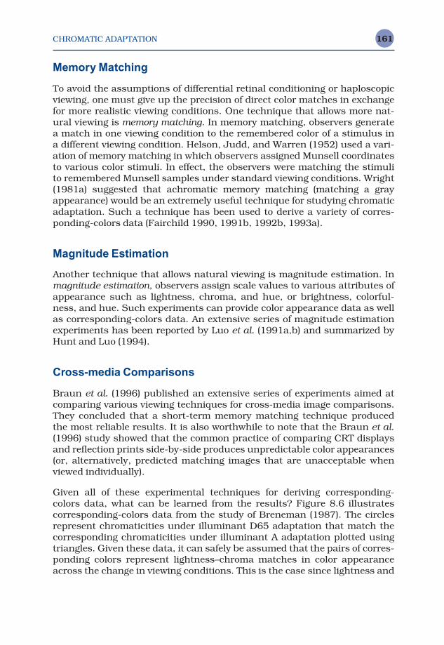
CHROMATIC ADAPTATION 161
Memory Matching
To avoid the assumptions of differential retinal conditioning or haploscopicviewing, one must give up the precision of direct color matches in exchangefor more realistic viewing conditions. One technique that allows more nat-ural viewing is memory matching. In memory matching, observers generate a match in one viewing condition to the remembered color of a stimulus in a different viewing condition. Helson, Judd, and Warren (1952) used a vari-ation of memory matching in which observers assigned Munsell coordinatesto various color stimuli. In effect, the observers were matching the stimuli to remembered Munsell samples under standard viewing conditions. Wright(1981a) suggested that achromatic memory matching (matching a grayappearance) would be an extremely useful technique for studying chromaticadaptation. Such a technique has been used to derive a variety of corres-ponding-colors data (Fairchild 1990, 1991b, 1992b, 1993a).
Magnitude Estimation
Another technique that allows natural viewing is magnitude estimation. Inmagnitude estimation, observers assign scale values to various attributes ofappearance such as lightness, chroma, and hue, or brightness, colorful-ness, and hue. Such experiments can provide color appearance data as wellas corresponding-colors data. An extensive series of magnitude estimationexperiments has been reported by Luo et al. (1991a,b) and summarized byHunt and Luo (1994).
Cross-media Comparisons
Braun et al. (1996) published an extensive series of experiments aimed atcomparing various viewing techniques for cross-media image comparisons.They concluded that a short-term memory matching technique producedthe most reliable results. It is also worthwhile to note that the Braun et al.(1996) study showed that the common practice of comparing CRT displaysand reflection prints side-by-side produces unpredictable color appearances(or, alternatively, predicted matching images that are unacceptable whenviewed individually).
Given all of these experimental techniques for deriving corresponding-colors data, what can be learned from the results? Figure 8.6 illustrates corresponding-colors data from the study of Breneman (1987). The circlesrepresent chromaticities under illuminant D65 adaptation that match thecorresponding chromaticities under illuminant A adaptation plotted usingtriangles. Given these data, it can safely be assumed that the pairs of corres-ponding colors represent lightness–chroma matches in color appearanceacross the change in viewing conditions. This is the case since lightness and
CHROMATIC ADAPTATION162
chroma are the appearance parameters most intuitively judged for relatedcolors. With this assumption, the corresponding-colors data can be used totest a color appearance model by taking the set of values for the first viewingcondition, using the model to predict lightness–chroma matches for the sec-ond viewing condition, and comparing the predictions with the visual results.
This same sort of test can be completed with a simpler form of model,known as a chromatic adaptation transform (or chromatic adaptation model).A chromatic adaptation model does not include correlates of appearanceattributes such as lightness, chroma, and hue. Instead, a chromatic adapta-tion model simply provides a transformation from tristimulus values in oneviewing condition to matching tristimulus values in a second set of viewingconditions.
8.5 MODELS
As described in the previous section, a chromatic adaptation model allowsprediction of corresponding-colors data. A general form of a chromatic adapta-tion model can be expressed as shown in Equations 8.1–8.3.
La = f (L,Lwhite, . . . ) (8.1)
Figure 8.6 An example of corresponding-colors data for a change in chromatic adap-tation from the chromaticity of illuminant D65 to that of illuminant A plotted in theu′v′ chromaticity diagram
CHROMATIC ADAPTATION 163
Ma = f (M,Mwhite, . . . ) (8.2)
Sa = f (S,Swhite, . . . ) (8.3)
This generic chromatic adaptation model is designed to predict three conesignals, La, Ma, and Sa, after all of the effects of adaptation have acted uponthe initial cone signals, L, M, and S. Such a model requires, as a minimum,the cone excitations for the adapting stimulus, Lwhite, Mwhite, and Swhite. It isquite likely that an accurate model would require additional information aswell (represented by the ellipses). A chromatic adaptation model can be con-verted into a chromatic adaptation transform by combining the forwardmodel for one set of viewing conditions with the inverse model for a secondset. Often such a transform is expressed in terms of CIE tristimulus valuesas shown in Equation 8.4.
XYZ2 = f (XYZ1,XYZwhite1,XYZwhite2, . . . ) (8.4)
In order to accurately model the physiological mechanisms of chromaticadaptation, it is necessary to express stimuli in terms of cone excitationsLMS rather than CIE tristimulus values, XYZ. Fortunately, cone excitationscan be reasonably approximated by a linear transformation (3 × 3 matrix) ofCIE tristimulus values. Thus a generic chromatic adaptation transform canbe described as shown in the flow chart in Figure 8.7. The complete processis as follows:
Figure 8.7 A flow chart of the application of a chromatic adaptation model to the cal-culation of corresponding colors
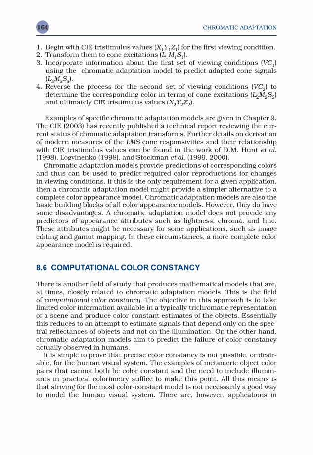
CHROMATIC ADAPTATION164
1. Begin with CIE tristimulus values (X1Y1Z1) for the first viewing condition. 2. Transform them to cone excitations (L1M1S1).3. Incorporate information about the first set of viewing conditions (VC1)
using the chromatic adaptation model to predict adapted cone signals(LaMaSa).
4. Reverse the process for the second set of viewing conditions (VC2) todetermine the corresponding color in terms of cone excitations (L2M2S2)and ultimately CIE tristimulus values (X2Y2Z2).
Examples of specific chromatic adaptation models are given in Chapter 9.The CIE (2003) has recently published a technical report reviewing the cur-rent status of chromatic adaptation transforms. Further details on derivationof modern measures of the LMS cone responsivities and their relationshipwith CIE tristimulus values can be found in the work of D.M. Hunt et al.(1998), Logvinenko (1998), and Stockman et al. (1999, 2000).
Chromatic adaptation models provide predictions of corresponding colorsand thus can be used to predict required color reproductions for changes in viewing conditions. If this is the only requirement for a given application,then a chromatic adaptation model might provide a simpler alternative to acomplete color appearance model. Chromatic adaptation models are also thebasic building blocks of all color appearance models. However, they do havesome disadvantages. A chromatic adaptation model does not provide anypredictors of appearance attributes such as lightness, chroma, and hue.These attributes might be necessary for some applications, such as imageediting and gamut mapping. In these circumstances, a more complete colorappearance model is required.
8.6 COMPUTATIONAL COLOR CONSTANCY
There is another field of study that produces mathematical models that are,at times, closely related to chromatic adaptation models. This is the field of computational color constancy. The objective in this approach is to takelimited color information available in a typically trichromatic representationof a scene and produce color-constant estimates of the objects. Essentiallythis reduces to an attempt to estimate signals that depend only on the spec-tral reflectances of objects and not on the illumination. On the other hand,chromatic adaptation models aim to predict the failure of color constancyactually observed in humans.
It is simple to prove that precise color constancy is not possible, or desir-able, for the human visual system. The examples of metameric object colorpairs that cannot both be color constant and the need to include illumin-ants in practical colorimetry suffice to make this point. All this means is that striving for the most color-constant model is not necessarily a good wayto model the human visual system. There are, however, applications in
CHROMATIC ADAPTATION 165
machine vision that could benefit greatly from having the most color-con-stant sensors possible.
The results in the field of computational color constancy provide someinteresting constraints and techniques that could help in modeling humanperformance. For example, the results of Maloney and Wandell (1986) illus-trate limits to the accuracy with which a trichromatic system could possiblyestimate surface reflectances in a natural scene. D’Zmura and Lennie (1986)show how a trichromatic visual system can provide color-constant responsesfor one dimension of color appearance, hue, while sacrificing constancy forthe other dimensions. The work of Finlayson et al. (1994a, b) illustrates howoptimum sensory spectral responsivities can be derived to utilize the vonKries coefficient rule to obtain near color constancy.
These studies, and many more in the field, provide interesting insightsinto what the visual system could possibly do at the limits. Such insightscan help in the construction, implementation, and testing of color appear-ance models. The techniques also provide definitive answers to questionspertaining to requirements for the collection of color images (digital stillcameras, computer vision systems, and other image scanners), the synthe-sis of realistic images (computer graphics), and the design of colorimetricinstrumentation (imaging colorimeters). Brill and West (1986) provide a useful review of the similarities and differences in the studies of chromaticadaptation and color constancy.
Color Appearance Models Second Edition M. D. Fairchild © 2005 John Wiley & Sons, LtdISBN: 0-470-01216-1 (HB)
9Chromatic
Adaptation Models
Chromatic adaptation is the single most important property of the humanvisual system with respect to understanding and modeling color appear-ance. Given this importance in vision science, there is significant literatureavailable on various aspects of the topic. Chapter 8 reviewed some of theimportant properties of adaptation phenomena and mechanisms. It alsoprovided the generic outline of a chromatic adaptation model for predict-ing corresponding colors. This chapter builds upon that information by including more detailed descriptions of a few specific chromatic adaptationtransformations. It is impossible to cover all of the models that have beenpublished. An attempt has been made to cover a variety of models and showtheir fundamental relationships to each other. Readers interested in moredetail on the models or historical developments should delve into the avail-able literature.
There are several good places to start, including the review papers cited in Chapter 8 (Bartleson 1978, Terstiege 1972, Wright 1981a, Lennie andD’Zmura 1988). Further details on the early history of chromatic adaptationmodels can be found in an interesting overview in a study by Helson, Judd,and Warren (1952). Another excellent review of the entire field of colorappearance with significant treatment of chromatic adaptation was writtenby Wyszecki (1986). Many of the classic papers in the field can be found inthe collection edited by MacAdam (1993).
The models described in this chapter do allow the computation of corres-ponding colors, but they are not color appearance models. They include nopredictors of appearance attributes such as lightness, chroma, and hue.They are, however, quite useful in predicting color matches across changesin viewing conditions. This is a significant extension of tristimulus colori-metry, all that is necessary in some applications, and the fundamental basisupon which all color appearance models are constructed.
CHROMATIC ADAPTATION MODELS 167
Any physiologically plausible model of chromatic adaptation must act onsignals representing the cone responses (or at least relative cone responses).Thus, in applications for which the use of CIE colorimetry is important, it isnecessary to first transform from CIE tristimulus values (XYZ) to cone res-ponses (denoted LMS, RGB, or rgb, depending on the model). Fortunately,cone responsivities can be accurately represented using a linear transforma-tion of CIE tristimulus values. An example of such a transformation isgraphically illustrated in Figure 9.1. This transformation, or a similar one, iscommon to all chromatic adaptation and color appearance models that are
Figure 9.1 The process of transformation from XYZ tristimulus values to LMS coneresponsivities using an example linear matrix multiplication
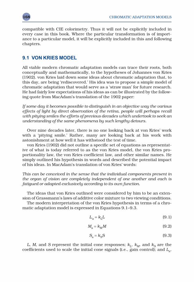
CHROMATIC ADAPTATION MODELS168
compatible with CIE colorimetry. Thus it will not be explicitly included inevery case in this book. Where the particular transformation is of import-ance to a particular model, it will be explicitly included in this and followingchapters.
9.1 VON KRIES MODEL
All viable modern chromatic adaptation models can trace their roots, bothconceptually and mathematically, to the hypotheses of Johannes von Kries(1902). von Kries laid down some ideas about chromatic adaptation that, tothis day, are being ‘rediscovered.’ His idea was to propose a simple model ofchromatic adaptation that would serve as a ‘straw man’ for future research.He had fairly low expectations of his ideas as can be illustrated by the follow-ing quote from MacAdam’s translation of the 1902 paper:
If some day it becomes possible to distinguish in an objective way the variouseffects of light by direct observation of the retina, people will perhaps recallwith pitying smiles the efforts of previous decades which undertook to seek anunderstanding of the same phenomena by such lengthy detours.
Over nine decades later, there is no one looking back at von Kries’ workwith a ‘pitying smile.’ Rather, many are looking back at his work with astonishment at how well it has withstood the test of time.
von Kries (1902) did not outline a specific set of equations as representat-ive of what is today referred to as the von Kries model, the von Kries pro-portionality law, the von Kries coefficient law, and other similar names. Hesimply outlined his hypothesis in words and described the potential impactof his ideas. In MacAdam’s translation of von Kries’ words:
This can be conceived in the sense that the individual components present inthe organ of vision are completely independent of one another and each isfatigued or adapted exclusively according to its own function.
The ideas that von Kries outlined were considered by him to be an exten-sion of Grassmann’s laws of additive color mixture to two viewing conditions.
The modern interpretation of the von Kries hypothesis in terms of a chro-matic adaptation model is expressed in Equations 9.1–9.3.
La = kLL (9.1)
Ma = kMM (9.2)
Sa = kSS (9.3)
L, M, and S represent the initial cone responses; kL, kM, and kS are thecoefficients used to scale the initial cone signals (i.e., gain control); and La,
CHROMATIC ADAPTATION MODELS 169
Ma, and Sa are the post-adaptation cone signals. Equations 9.1–9.3 repres-ent a simple gain-control model of chromatic adaptation in which each of thethree cone types has a separate gain coefficient. A key aspect of any model ishow the particular values of kL, kM, and kS are obtained. In most moderninstantiations of the von Kries model, the coefficients are taken to be theinverse of the L, M, and S cone responses for the scene white or maximumstimulus as illustrated in Equations 9.4–9.6.
kL = 1/Lmax or kL = 1/Lwhite (9.4)
kM = 1/Mmax or kM = 1/Mwhite (9.5)
kS = 1/Smax or kS = 1/Swhite (9.6)
Equations 9.4–9.6 are a mathematical representation of von Kries’ state-ment that ‘each is fatigued or adapted exclusively according to its own func-tion.’ Given the above interpretations of the gain coefficients, the von Kriesmodel can be used to calculate corresponding colors between two viewingconditions by calculating the post-adaptation signals for the first condition,setting them equal to the post-adaptation signals for the second condition,and then reversing the model for the second condition. Performing thesesteps and completing the algebra results in the transformations given inEquations 9.7–9.9 that can be used to calculate corresponding colors.
L2 = (L1/Lmax1)Lmax2 (9.7)
M2 = (M1/Mmax1)Mmax2 (9.8)
S2 = (S1/Smax1)Smax2 (9.9)
In some cases it becomes more convenient to express chromatic adapta-tion models in terms of matrix transformations. The interpretation of the von Kries model as described above is expressed in matrix notation in Equ-ation 9.10.
(9.10)
The matrix notation can be extended to the calculation of correspondingcolors across two viewing conditions and to explicitly include the trans-formation (matrix M) from CIE tristimulus values (XYZ) to relative coneresponses (LMS). This is illustrated in Equation 9.11.
(9.11)
XYZ
LM
S
LM
S
XYZ
2
2
2
12
2
2
1
1
1
1
1
1
0 0 0 00 0 0 00 0 0 0
1 0 0 0 00 0 1 0 00 0 0 0 1
= −M Mmax
max
max
max
max
max
. .. .. .
/ . .. / .. . /
LMS
LM
S
LMS
a
a
a
=1 0 0 0 0
0 0 1 0 00 0 0 0 1
/ . .. / .. . /
max
max
max
CHROMATIC ADAPTATION MODELS170
The von Kries transformation was used to predict the visual data ofBreneman (1987) that were described in Chapter 8. The results are illus-trated in a u ′v ′ chromaticity diagram in Figure 9.2. The open symbols repres-ent Breneman’s corresponding colors data and the filled symbols representthe predictions using a von Kries model. Perfect model predictions wouldresult in the filled triangles completely coinciding with the open triangles. Inthis calculation, the chromaticities under daylight adaptation (open circlesin Figure 9.2) were used to predict the corresponding chromaticities underincandescent adaptation (triangles in Figure 9.2). It is clear in Figure 9.2that the von Kries hypothesis was indeed a good one and that the moderninterpretation as a chromatic adaptation transformation predicts the datasurprisingly well.
Helson, Judd, and Warren (1952) presented an early study in which cor-responding colors were derived by memory matching and the von Krieshypothesis was tested and performed quite well. Examples of recent experi-mental data and analyses that address the utility and limitations of the vonKries hypothesis can be found in the work of Brainard and Wandell (1992)and Chichilnisky and Wandell (1995). There are some discrepanciesbetween these, and other, visual data and the predictions of the von Kriesmodel. Such discrepancies have led investigators down many paths that aredescribed in the remaining sections of this chapter and throughout this
Figure 9.2 Prediction of some example corresponding colors data using the von Kriesmodel. Open triangles represent visual data and filled triangles represent model predictions
CHROMATIC ADAPTATION MODELS 171
book. Perhaps it shouldn’t be too surprising to realize that von Kries (1902)himself foresaw this. The next line after his description of what is nowreferred to as the von Kries model reads:
But if the real physiological equipment is considered, on which the processesare based, it is permissible to doubt whether things are so simple.
Indeed things are not so simple, but it is amazing how close such a simplehypothesis comes to explaining the majority of the chromatic adaptationphenomenon.
9.2 RETINEX THEORY
An often discussed account of the mechanisms of chromatic adaptationunder the rubric of color constancy is the retinex theory developed by EdwinLand and his colleagues (e.g., Land and McCann 1971, Land 1977, 1986)The retinex theory can be considered an enhanced version of the von Kriesmodel. Various enhancements have been proposed, but the key feature isthat the retinex algorithm explicitly treats the spatial distribution of colors ina scene in order to better model the visual perceptions that can be observedin complex scenes.
Land’s theory was formulated to explain demonstrations of the independ-ence of color appearance on the spectral distribution of reflected light (tristimulus values). Land suggested that color appearance is controlled bysurface reflectances rather than the distribution of reflected light. Theretinex algorithm, in its most recent form (Land 1986), is quite simple. Landproposed three color mechanisms with the spectral responsivities of thecone photoreceptors. He called these mechanisms retinexes since they arethought to be some combination of retinal and cortical mechanisms. Landhypothesized a three-dimensional color appearance space with the output ofthe long-, middle-, and short-wavelength-sensitive retinexes as the dimen-sions. The output of a retinex is determined by taking the ratio of the signalat any given point in the scene and normalizing it with an average of the signals in that retinex throughout the scene. The most interesting feature of this algorithm is that it acknowledges variations in color due to changes in the background of the stimulus. The influence of the background can bevaried by changing the spatial distribution of the retinex signals that areused to normalize a given point in the scene. If one takes the normalizing signal to be the scene average for a given retinex, then the retinex algorithmreduces to a typical instantiation of a von Kries-type transformation. Thereare some flaws in the physiological implementation of the retinex model(Brainard and Wandell 1986; Lennie and D’Zmura 1988), but if one is moreinterested in the algorithm output than having a strict physiological modelof the visual system (which is also the case for most color appearance models),then the concepts in the retinex theory might prove useful. For example, the

CHROMATIC ADAPTATION MODELS172
retinex algorithm has recently been applied in the development of a digitalimage processing algorithm for dynamic range compression and color cor-rection (Jobson et al. 1997). Other applications, challenges, and successesfor such a theory have been reviewed by McCann (1993).
The need to consider spatial as well as spectral dimensions in high-levelcolor appearance models is undeniable. Concepts embedded in the retinextheory provide some insight on how this might be accomplished. Otherapproaches are also under development (e.g., Poirson and Wandell 1993,Zhang and Wandell 1996). The retinex theory sets the stage for other devel-opments in chromatic adaptation models. The general theme is that the vonKries model provides a good foundation, but needs enhancement to addresscertain adaptation phenomena. Spatial models of chromatic adaptation andimage appearance are discussed more fully in Chapter 20.
9.3 NAYATANI et al. MODEL
One important enhancement to the von Kries hypothesis is the nonlinearchromatic adaptation model developed by Nayatani and coworkers. Thisnonlinear model was developed from a colorimetric background (enhance-ment to CIE tristimulus colorimetry) within the field of illumination engin-eering. The early roots of this model can be traced to the work of MacAdam(1961).
MacAdam’s Model
MacAdam (1961) described a nonlinear model of chromatic adaptation inwhich the output of the cones was expressed as a constant plus a multi-plicative factor of the cone excitation raised to some power. This nonlinearmodel represented an empirical fit to MacAdam’s (1956) earlier chromaticadaptation data. Interestingly enough, MacAdam required a visual systemwith five types of cones in order to explain his data with a linear model! (Thisis probably because MacAdam used a rather unusual experimental tech-nique in which two halves of the same retina were differentially adapted.)MacAdam’s nonlinear model provided a good fit to the data and was the pre-cursor of later nonlinear models.
Nayatani’s Model
The nonlinear model of Nayatani et al. (1980, 1981) begins with a gainadjustment followed by a power function with a variable exponent. In thismodel, the von Kries coefficients are proportional to the maximum long-,middle-, and short-wavelength cone responses and the exponents of thepower functions depend on the luminance of the adapting field. The power
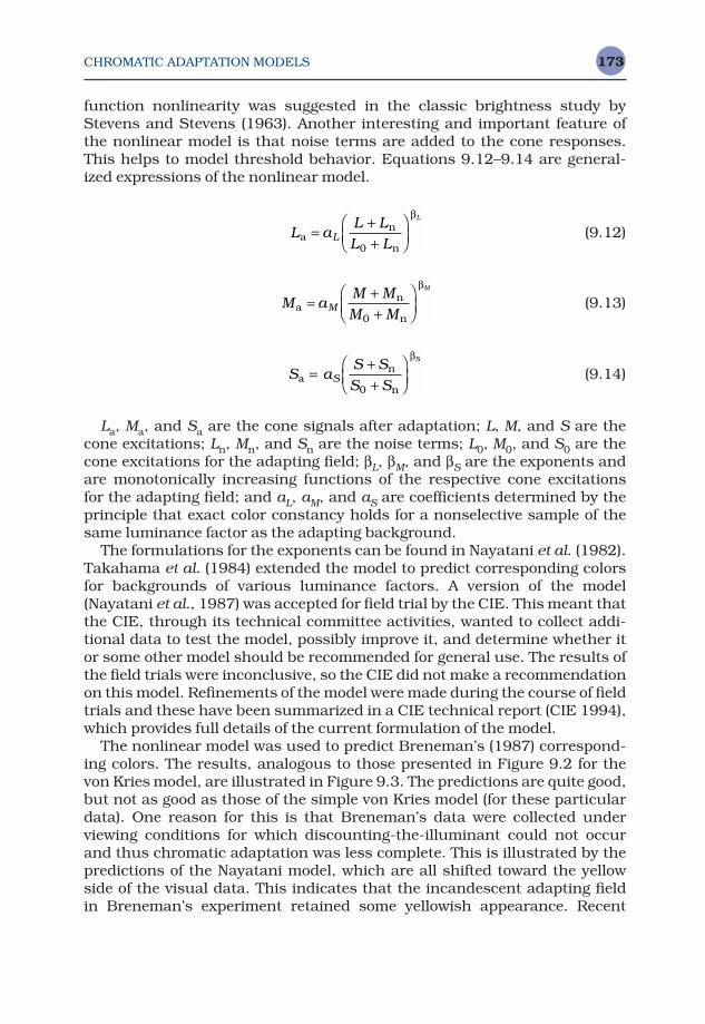
CHROMATIC ADAPTATION MODELS 173
function nonlinearity was suggested in the classic brightness study byStevens and Stevens (1963). Another interesting and important feature ofthe nonlinear model is that noise terms are added to the cone responses.This helps to model threshold behavior. Equations 9.12–9.14 are general-ized expressions of the nonlinear model.
(9.12)
(9.13)
(9.14)
La, Ma, and Sa are the cone signals after adaptation; L, M, and S are thecone excitations; Ln, Mn, and Sn are the noise terms; L0, M0, and S0 are thecone excitations for the adapting field; βL, βM, and βS are the exponents andare monotonically increasing functions of the respective cone excitations for the adapting field; and aL, aM, and aS are coefficients determined by theprinciple that exact color constancy holds for a nonselective sample of thesame luminance factor as the adapting background.
The formulations for the exponents can be found in Nayatani et al. (1982).Takahama et al. (1984) extended the model to predict corresponding colorsfor backgrounds of various luminance factors. A version of the model(Nayatani et al., 1987) was accepted for field trial by the CIE. This meant thatthe CIE, through its technical committee activities, wanted to collect addi-tional data to test the model, possibly improve it, and determine whether itor some other model should be recommended for general use. The results ofthe field trials were inconclusive, so the CIE did not make a recommendationon this model. Refinements of the model were made during the course of fieldtrials and these have been summarized in a CIE technical report (CIE 1994),which provides full details of the current formulation of the model.
The nonlinear model was used to predict Breneman’s (1987) correspond-ing colors. The results, analogous to those presented in Figure 9.2 for thevon Kries model, are illustrated in Figure 9.3. The predictions are quite good,but not as good as those of the simple von Kries model (for these particulardata). One reason for this is that Breneman’s data were collected underviewing conditions for which discounting-the-illuminant could not occurand thus chromatic adaptation was less complete. This is illustrated by thepredictions of the Nayatani model, which are all shifted toward the yellowside of the visual data. This indicates that the incandescent adapting field in Breneman’s experiment retained some yellowish appearance. Recent
S aS S
S SS
S
an
n=
++
0
β
M aM M
M MM
M
an
n=
++
0
β
L aL L
L LL
L
an
n=
++
0
β
CHROMATIC ADAPTATION MODELS174
enhancements (Nayatani 1997) have provided techniques to estimate andaccount for the degree of chromatic adaptation in various experiments.
This nonlinear model is capable of predicting the Hunt (1952) effect(increase in colorfulness with adapting luminance), the Stevens effect (in-crease in lightness contrast with luminance), and the Helson–Judd effect (hueof nonselective samples under chromatic illumination). It is worth notingthat the von Kries adaptation transform is luminance independent and there-fore cannot be used to predict appearance phenomena that are functions ofluminance. Also, the linear nature of the simple von Kries transform pre-cludes it from predicting the Helson–Judd effect.
Nayatani’s nonlinear model is important for several reasons. It provides arelatively simple extension of the von Kries hypothesis that is capable of pre-dicting several additional effects, it has had a significant historical impact onthe CIE work in chromatic adaptation and color appearance modeling, and itprovides the basis for one of just two comprehensive color appearance mod-els. The full Nayatani color appearance model is described in Chapter 11.
9.4 GUTH’S MODEL
There are many variations of the von Kries hypothesis. One significant vari-ation that is in some ways similar to the Nayatani model, from the field of
Figure 9.3 Prediction of some example corresponding colors data using the nonlin-ear model of Nayatani et al. Open triangles represent visual data and filled trianglesrepresent model predictions
CHROMATIC ADAPTATION MODELS 175
vision science (rather than colorimetry), is the model described by Guth(1991, 1995). Guth’s model is not directly related to CIE tristimulus col-orimetry since the cone responsivities used are not linear transformations ofthe CIE color matching functions. This produces some practical difficultiesin implementing the model, but for practical situations it is advisable andcertainly not harmful to the predictions to use a set of cone responsivitiesthat can be derived directly from CIE tristimulus values, along with theremainder of Guth’s formulation. This model, part of the ATD vision modeldescribed in Chapter 14, has been developed over many years to predict theresults of various vision experiments. Most of these experiments involveclassical threshold psychophysics rather than scaling of the various dimen-sions of color appearance as defined in Chapter 4.
The general form of Guth’s chromatic adaptation model is given inEquations 9.15–9.20.
La = Lr [1 − (Lr0/(σ + Lr0))] (9.15)
Lr = 0.66L0.7 + 0.002 (9.16)
Ma = Mr [1 − (Mr0/(σ + Mr0))] (9.17)
Mr = 1.0M0.7 + 0.003 (9.18)
Sa = Sr [1 − (Sr0/(σ + Sr0))] (9.19)
Sr = 0.45S0.7 + 0.00135 (9.20)
La, Ma, and Sa are the cone signals after adaptation; L, M, and S, are thecone excitations; Lr0, Mr0, and Sr0 are the cone excitations for the adaptingfield after the nonlinear function; and σ is a constant (nominally 300) thatcan be thought of as representing a noise term. It is also important to notethat the cone responses in this model must be expressed in absolute unitssince the luminance level does not enter the model elsewhere.
Some algebraic manipulation of the adaptation model as expressed abovehelps to illustrate its relationship with the von Kries model. Ignoring the ini-tial nonlinearity, a von Kries-type gain control coefficient for the Guth modelcan be pulled out of Equation 9.15 as shown in Equation 9.21.
kL = 1 − (Lr0/(σ + Lr0)) (9.21)
Using the algebraic substitutions illustrated in Equations 9.22–9.24, the relationship to the traditional von Kries coefficient becomes clear. Thedifference lies in the s term, which can be thought of as a noise factor that ismore important at low stimulus intensities than at high intensities. Thus, asluminance level increases, the Guth model becomes more and more similarto the nominal von Kries model.
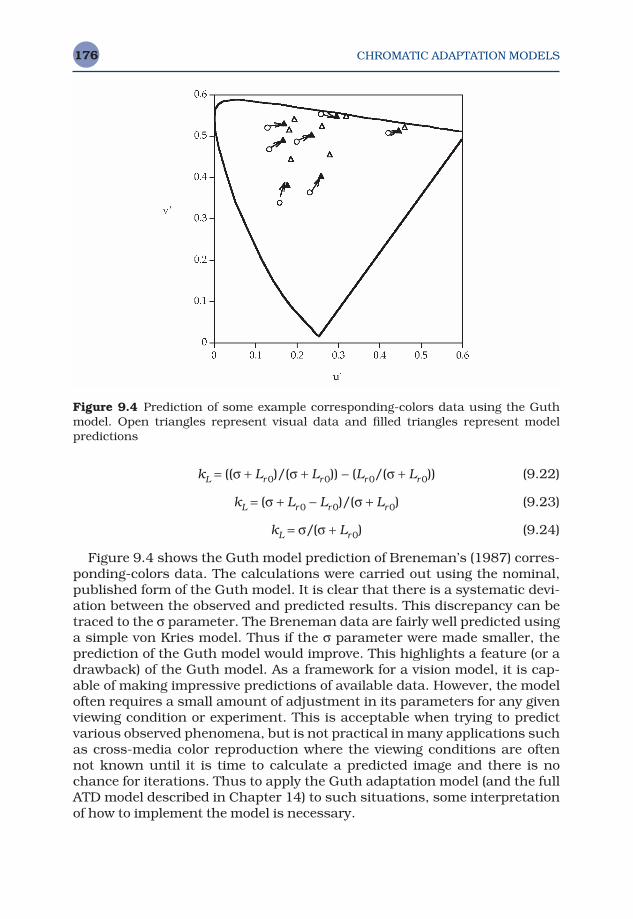
CHROMATIC ADAPTATION MODELS176
kL = ((σ + Lr0)/(σ + Lr0)) − (Lr0/(σ + Lr0)) (9.22)
kL = (σ + Lr0 − Lr0)/(σ + Lr0) (9.23)
kL = σ/(σ + Lr0) (9.24)
Figure 9.4 shows the Guth model prediction of Breneman’s (1987) corres-ponding-colors data. The calculations were carried out using the nominal,published form of the Guth model. It is clear that there is a systematic devi-ation between the observed and predicted results. This discrepancy can betraced to the σ parameter. The Breneman data are fairly well predicted usinga simple von Kries model. Thus if the σ parameter were made smaller, theprediction of the Guth model would improve. This highlights a feature (or adrawback) of the Guth model. As a framework for a vision model, it is cap-able of making impressive predictions of available data. However, the modeloften requires a small amount of adjustment in its parameters for any givenviewing condition or experiment. This is acceptable when trying to predictvarious observed phenomena, but is not practical in many applications suchas cross-media color reproduction where the viewing conditions are oftennot known until it is time to calculate a predicted image and there is nochance for iterations. Thus to apply the Guth adaptation model (and the fullATD model described in Chapter 14) to such situations, some interpretationof how to implement the model is necessary.
Figure 9.4 Prediction of some example corresponding-colors data using the Guthmodel. Open triangles represent visual data and filled triangles represent model predictions
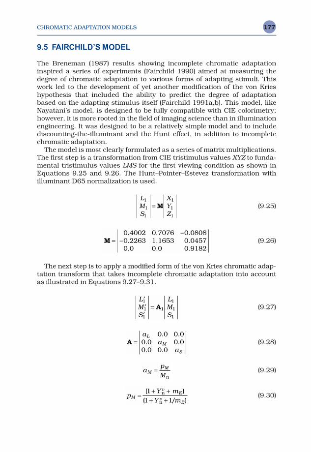
CHROMATIC ADAPTATION MODELS 177
9.5 FAIRCHILD’S MODEL
The Breneman (1987) results showing incomplete chromatic adaptationinspired a series of experiments (Fairchild 1990) aimed at measuring thedegree of chromatic adaptation to various forms of adapting stimuli. Thiswork led to the development of yet another modification of the von Krieshypothesis that included the ability to predict the degree of adaptation based on the adapting stimulus itself (Fairchild 1991a,b). This model, likeNayatani’s model, is designed to be fully compatible with CIE colorimetry;however, it is more rooted in the field of imaging science than in illuminationengineering. It was designed to be a relatively simple model and to includediscounting-the-illuminant and the Hunt effect, in addition to incompletechromatic adaptation.
The model is most clearly formulated as a series of matrix multiplications.The first step is a transformation from CIE tristimulus values XYZ to funda-mental tristimulus values LMS for the first viewing condition as shown inEquations 9.25 and 9.26. The Hunt–Pointer–Estevez transformation withilluminant D65 normalization is used.
(9.25)
(9.26)
The next step is to apply a modified form of the von Kries chromatic adap-tation transform that takes incomplete chromatic adaptation into accountas illustrated in Equations 9.27–9.31.
(9.27)
(9.28)
(9.29)
(9.30)pY m
Y mM
vE
vE
=+ +
+ +( )
( / )1
1 1n
n
ap
MMM=n
A =a
aa
L
M
S
0 0 0 00 0 0 00 0 0 0
. .. .. .
′′′
=LMS
LMS
1
1
1
1
1
1
1
A
M =−
−0 4002 0 7076 0 08080 2263 1 1653 0 04570 0 0 0 0 9182
. . .
. . .
. . .
LMS
XYZ
1
1
1
1
1
1
= M
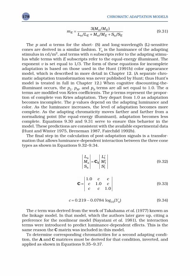
CHROMATIC ADAPTATION MODELS178
(9.31)
The p and a terms for the short- (S) and long-wavelength (L)-sensitivecones are derived in a similar fashion. Yn is the luminance of the adaptingstimulus in cd/m2, and terms with n subscripts refer to the adapting stimu-lus while terms with E subscripts refer to the equal-energy illuminant. Theexponent v is set equal to 1/3. The form of these equations for incompleteadaptation is based on those used in the Hunt (1991b) color appearancemodel, which is described in more detail in Chapter 12. (A separate chro-matic adaptation transformation was never published by Hunt; thus Hunt’smodel is treated in full in Chapter 12.) When cognitive discounting-the-illuminant occurs, the pL, pM, and pS terms are all set equal to 1.0. The aterms are modified von Kries coefficients. The p terms represent the propor-tion of complete von Kries adaptation. They depart from 1.0 as adaptationbecomes incomplete. The p values depend on the adapting luminance andcolor. As the luminance increases, the level of adaptation becomes morecomplete. As the adapting chromaticity moves farther and farther from anormalizing point (the equal-energy illuminant), adaptation becomes lesscomplete. Equations 9.30 and 9.31 serve to ensure this behavior in themodel. These predictions are consistent with the available experimental data(Hunt and Winter 1975, Breneman 1987, Fairchild 1992b).
The final step in the calculation of post-adaptation signals is a transfor-mation that allows luminance-dependent interaction between the three conetypes as shown in Equations 9.32–9.34.
(9.32)
(9.33)
c = 0.219 − 0.0784 log10(Yn) (9.34)
The c term was derived from the work of Takahama et al. (1977) known asthe linkage model. In that model, which the authors later gave up, citing apreference for the nonlinear model (Nayatani et al. 1981), the interactionterms were introduced to predict luminance-dependent effects. This is thesame reason the C matrix was included in this model.
To determine corresponding chromaticities for a second adapting condi-tion, the A and C matrices must be derived for that condition, inverted, andapplied as shown in Equations 9.35–9.37.
C =1 0
1 01 0
..
.
c cc cc c
LMS
LMS
a
a
a
=′′′
C1
1
1
1
mM M
L L M M S SEE
E E E=
+ +3( / )
/ / /n
n n n
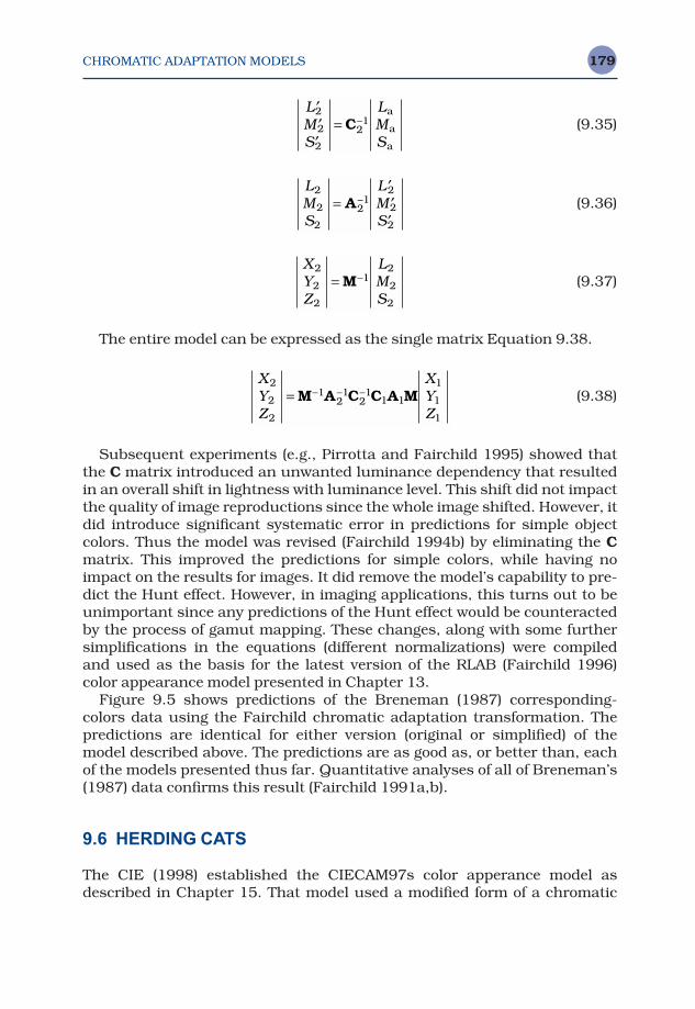
CHROMATIC ADAPTATION MODELS 179
(9.35)
(9.36)
(9.37)
The entire model can be expressed as the single matrix Equation 9.38.
(9.38)
Subsequent experiments (e.g., Pirrotta and Fairchild 1995) showed thatthe C matrix introduced an unwanted luminance dependency that resultedin an overall shift in lightness with luminance level. This shift did not impactthe quality of image reproductions since the whole image shifted. However, itdid introduce significant systematic error in predictions for simple objectcolors. Thus the model was revised (Fairchild 1994b) by eliminating the Cmatrix. This improved the predictions for simple colors, while having noimpact on the results for images. It did remove the model’s capability to pre-dict the Hunt effect. However, in imaging applications, this turns out to beunimportant since any predictions of the Hunt effect would be counteractedby the process of gamut mapping. These changes, along with some furthersimplifications in the equations (different normalizations) were compiledand used as the basis for the latest version of the RLAB (Fairchild 1996)color appearance model presented in Chapter 13.
Figure 9.5 shows predictions of the Breneman (1987) corresponding-colors data using the Fairchild chromatic adaptation transformation. Thepredictions are identical for either version (original or simplified) of themodel described above. The predictions are as good as, or better than, eachof the models presented thus far. Quantitative analyses of all of Breneman’s(1987) data confirms this result (Fairchild 1991a,b).
9.6 HERDING CATS
The CIE (1998) established the CIECAM97s color apperance model asdescribed in Chapter 15. That model used a modified form of a chromatic
XYZ
XYZ
2
2
2
1
1
1
= − − −M A C C A M121
21
1 1
XYZ
LMS
2
2
2
= −M 12
2
2
LMS
LMS
2
2
2
21
2
2
2
=′′′
−A
′′′
= −LMS
LMS
2
2
2
21C
a
a
a
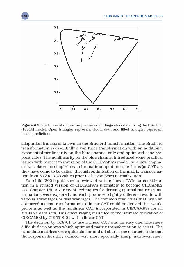
CHROMATIC ADAPTATION MODELS180
adaptation transform known as the Bradford transformation. The Bradfordtransformation is essentially a von Kries transformation with an additionalexponential nonlinearity on the blue channel only and optimized cone res-ponsivities. The nonlinearity on the blue channel introduced some practicalissues with respect to inversion of the CIECAM97s model, so a new empha-sis was placed on simple linear chromatic adaptation transforms (or CATs asthey have come to be called) through optimization of the matrix transforma-tion from XYZ to RGB values prior to the von Kries normalization.
Fairchild (2001) published a review of various linear CATs for considera-tion in a revised version of CIECAM97s ultimately to become CIECAM02 (see Chapter 16). A variety of techniques for deriving optimal matrix trans-formations were explored and each produced slightly different results withvarious advantages or disadvantages. The common result was that, with anoptimized matrix transformation, a linear CAT could be derived that wouldperform as well as the nonlinear CAT incorporated in CIECAM97s for allavailable data sets. This encouraging result led to the ultimate derivation ofCIECAM02 by CIE TC8-01 with a linear CAT.
The decision by TC8-01 to use a linear CAT was an easy one. The moredifficult decision was which optimized matrix transformation to select. Thecandidate matrices were quite similar and all shared the characteristic thatthe responsivities they defined were more spectrally sharp (narrower, more
Figure 9.5 Prediction of some example corresponding-colors data using the Fairchild(1991b) model. Open triangles represent visual data and filled triangles representmodel predictions
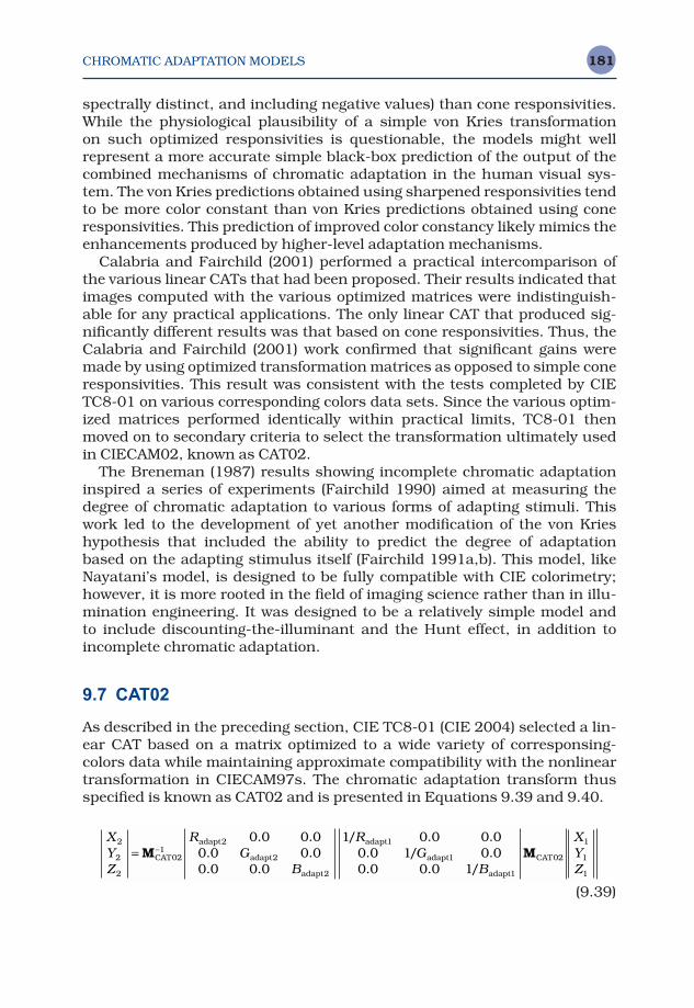
CHROMATIC ADAPTATION MODELS 181
spectrally distinct, and including negative values) than cone responsivities.While the physiological plausibility of a simple von Kries transformation on such optimized responsivities is questionable, the models might well represent a more accurate simple black-box prediction of the output of thecombined mechanisms of chromatic adaptation in the human visual sys-tem. The von Kries predictions obtained using sharpened responsivities tendto be more color constant than von Kries predictions obtained using coneresponsivities. This prediction of improved color constancy likely mimics theenhancements produced by higher-level adaptation mechanisms.
Calabria and Fairchild (2001) performed a practical intercomparison ofthe various linear CATs that had been proposed. Their results indicated thatimages computed with the various optimized matrices were indistinguish-able for any practical applications. The only linear CAT that produced sig-nificantly different results was that based on cone responsivities. Thus, theCalabria and Fairchild (2001) work confirmed that significant gains weremade by using optimized transformation matrices as opposed to simple coneresponsivities. This result was consistent with the tests completed by CIETC8-01 on various corresponding colors data sets. Since the various optim-ized matrices performed identically within practical limits, TC8-01 thenmoved on to secondary criteria to select the transformation ultimately usedin CIECAM02, known as CAT02.
The Breneman (1987) results showing incomplete chromatic adaptationinspired a series of experiments (Fairchild 1990) aimed at measuring thedegree of chromatic adaptation to various forms of adapting stimuli. Thiswork led to the development of yet another modification of the von Krieshypothesis that included the ability to predict the degree of adaptation based on the adapting stimulus itself (Fairchild 1991a,b). This model, likeNayatani’s model, is designed to be fully compatible with CIE colorimetry;however, it is more rooted in the field of imaging science rather than in illu-mination engineering. It was designed to be a relatively simple model and to include discounting-the-illuminant and the Hunt effect, in addition toincomplete chromatic adaptation.
9.7 CAT02
As described in the preceding section, CIE TC8-01 (CIE 2004) selected a lin-ear CAT based on a matrix optimized to a wide variety of corresponsing-colors data while maintaining approximate compatibility with the nonlineartransformation in CIECAM97s. The chromatic adaptation transform thusspecified is known as CAT02 and is presented in Equations 9.39 and 9.40.
(9.39)
XYZ
RG
B
RG
B
XYZ
2
2
2
CAT
adapt
adapt
adapt
adapt
adapt
adapt
CAT
1
1
1
= −M M021
2
2
2
1
1
1
02
0 0 0 00 0 0 00 0 0 0
1 0 0 0 00 0 1 0 00 0 0 0 1
. .. .. .
/ . .. / .. . /
CHROMATIC ADAPTATION MODELS182
(9.40)
The process follows the normal von Kries transformation with a conversionfrom CIE tristimulus values (XYZ) to sharpened cone responsivities (RGB)using the MCAT02 matrix transformation. The RGB values are then divided bythe adapting RGB values for the first viewing condition and multiplied by the adapting RGB values for the second viewing condition prior to a lineartransformation back to corresponding CIE tristimulus values. In Figure 9.6,the spectral responsivities represented by MCAT02 are contrasted with theHunt–Pointer–Estevez cone responsivities used in many chromatic adapta-tion transformations and color appearance models.
It should also be noted that Equations 9.39 and 9.40 represent CAT02 inits simplest form under the assumption of complete chromatic adaptation.Simple enhancements to the transformation to allow for the prediction ofincomplete chromatic adaptation and discounting the illuminant are pre-sented in the full description of CIECAM02 in Chapter 16.
MCAT02
0 4002 0 7076 0 08080 2263 1 1653 0 04570 0 0 0 0 9182
=−
−. . .. . .. . .
Figure 9.6 Comparison of the Hunt–Pointer–Estevez cone responsivities (thin lines,labeled HPE) with the ‘sharpened’ responsivities used in the CAT02 chromatic adapta-tion transform (thick lines, labeled CAT02). Note how the ‘sharpened’ responsivitiesare more spectrally distinct, narrower, and include some negative values. All respons-ivities have been normalized to set their maximum value to 1.0
Color Appearance Models Second Edition M. D. Fairchild © 2005 John Wiley & Sons, LtdISBN: 0-470-01216-1 (HB)
10Color Appearance
Models
The chromatic adaptation transforms discussed in Chapter 9 go a long waytoward extending tristimulus colorimetry toward the prediction of colorappearance. However, they are still limited in that they can only predictmatches across disparate viewing conditions (i.e., corresponding colors). Achromatic adaptation transform alone cannot be used to describe the actualcolor appearance of stimuli. To do this, one must use the appearance para-meters defined in Chapter 4 — the absolute color appearance attributes ofbrightness, colorfulness, and hue and the relative color appearance attri-butes of lightness, chroma, saturation, and, again, hue. These terms areused to describe the color appearance of stimuli. Chromatic adaptationtransforms provide no measure of correlates to these perceptual attributes.This is the domain of color appearance models.
10.1 DEFINITION OF COLOR APPEARANCE MODELS
The world of color measurement is full of various descriptors of color such astristimulus values, chromaticity coordinates, uniform chromaticity scales,uniform color spaces, and ‘just plain-old’ color spaces. Sometimes it is diffi-cult to keep all the names and distinctions straight. So just what is it thatsets a color appearance model apart from all of these other types of colorspecification? CIE Technical Committee 1-34, Testing Color AppearanceModels, was given the task of evaluating the performance of various colorappearance models and recommending a model for general use. Thus, one ofthe first tasks of this committee became the definition of just what consti-tutes a color appearance model in order to be included in the tests (Fairchild1995a).
COLOR APPEARANCE MODELS184
TC1-34 agreed on the following definition: a color appearance model isany model that includes predictors of at least the relative color appearanceattributes of lightness, chroma, and hue. For a model to include reason-able predictors of these attributes, it must include at least some form of achromatic adaptation transform. Models must be more complex to includepredictors of brightness and colorfulness or to model other luminance-dependent effects such as the Stevens effect or the Hunt effect.
Given the above definition, some fairly simple uniform color spaces, suchas the CIE 1976 L*a*b* color space (CIELAB) and the CIE 1976 L*u*v* colorspace (CIELUV), can be considered color appearance models. These colorspaces include simple chromatic adaptation transforms and predictors oflightness, chroma, and hue. The general construction of a color appearancemodel and then a discussion of CIELAB as a specific example are presentedin the following sections.
10.2 CONSTRUCTION OF COLOR APPEARANCE MODELS
Some general concepts that apply to the construction of all color appear-ance models are described in this section. All color appearance models forpractical applications begin with the specification of the stimulus and view-ing conditions in terms of CIE XYZ tristimulus values (along with certainabsolute luminances for some models). The first process applied to thesedata is generally a linear transformation from XYZ tristimulus values to coneresponses in order to more accurately model the physiological processes inthe human visual system. The importance of beginning with CIE tristimulusvalues is a matter of practicality. There is a great deal of color measurementinstrumentation that is available to quickly and accurately measure stimuliin terms of CIE tristimulus values. The CIE system is also a well-established,international standard for color specification and communication.
Occasionally, vision-science-based models of color vision and appearanceare based upon cone responsivities that are not linear transformations of CIE color matching functions (e.g., Guth 1995). The small advantage inperformance that such an approach provides is far outweighed by the incon-venience in practical applications.
Given tristimulus values for the stimulus, other data regarding the view-ing environment must also be considered in order to predict color appear-ance. This is illustrated by all of the color appearance phenomena describedin Chapters 6 and 7. As a minimum, the tristimulus values of the adaptingstimulus (usually taken to be the light source) are also required. Additionaldata that might be utilized include the absolute luminance level, colorimetricdata on the proximal field, background, and surround, and perhaps otherspatial or temporal information.
Given some or all of the above data, the first step in a color appearancemodel is generally a chromatic adaptation transform such as those describedin Chapter 9. The post-adaptation signals are then combined into higher-
COLOR APPEARANCE MODELS 185
level signals, usually modeled after the opponent theory of color vision andincluding threshold and/or compressive nonlinearities. These signals arethen combined in various ways to produce predictors of the various appear-ance attributes. Data on the adapting stimulus, background, surround, etc.are incorporated into the model at the chromatic adaptation stage and laterstages as necessary.
This general process can be witnessed within all of the color appearancemodels described in this book. However, each model has been derived with adifferent approach and various of the previously given aspects are stressedto a greater or lesser degree. A simple example of a color appearance modelthat follows most of the construction steps outlined above is CIELAB. Theinterpretation of the CIELAB color space as a color appearance model isdescribed in the next section.
10.3 CIELAB
Those trained in traditional colorimetry usually have a negative reactionwhen they hear CIELAB described as a color appearance model. This isbecause the CIE (1986) went to great lengths to make sure that it was calleda uniform color space and not an appearance space. CIELAB was developedas a color space to be used for the specification of color differences. In theearly 1970s, there were as many as 20 different formulas being used to calculate color differences. To promote uniformity of practice pending thedevelopment of a better formula, the CIE recommended two color spaces,CIELAB and CIELUV, for use in 1976 (Robertson 1977, 1990). The Euclideandistance between two points in these spaces is taken to be a measure of theircolor difference (∆E*ab or ∆E*uv). As an historical note, in 1994 the CIE recom-mended a single better formula for color difference measurement, based onthe CIELAB space, known as ∆E*94 (Berns 1993a, CIE 1995b). In the processof creating a color difference formula, the CIE happened to construct a colorspace with some predictors of color appearance attributes. Perhaps it is notsurprising that the best way to describe the difference in color of two stimuliis to first describe the appearance of each. Thus, with appropriate care,CIELAB can be considered a color appearance model.
Calculating CIELAB Coordinates
To calculate CIELAB coordinates, one must begin with two sets of CIE XYZtristimulus values, those of the stimulus, XYZ, and those of the referencewhite, XnYnZn. These data are utilized in a modified form of the von Krieschromatic adaptation transform by normalizing the stimulus tristimulusvalues by those of the white (i.e., X/Xn, Y/Yn, and Z/Zn). Note that the CIEtristimulus values are not first transformed to cone responses as would benecessary for a true von Kries adaptation model. These adapted signals are
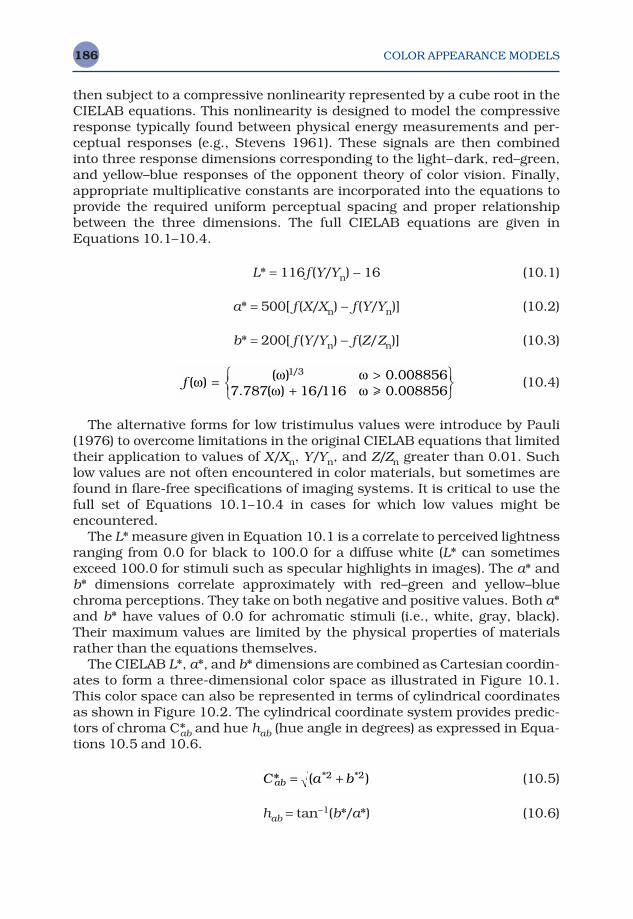
COLOR APPEARANCE MODELS186
then subject to a compressive nonlinearity represented by a cube root in theCIELAB equations. This nonlinearity is designed to model the compressiveresponse typically found between physical energy measurements and per-ceptual responses (e.g., Stevens 1961). These signals are then combined into three response dimensions corresponding to the light–dark, red–green,and yellow–blue responses of the opponent theory of color vision. Finally,appropriate multiplicative constants are incorporated into the equations toprovide the required uniform perceptual spacing and proper relationshipbetween the three dimensions. The full CIELAB equations are given inEquations 10.1–10.4.
L* = 116f (Y/Yn) − 16 (10.1)
a* = 500[ f (X/Xn) − f (Y/Yn)] (10.2)
b* = 200[ f (Y/Yn) − f (Z/Zn)] (10.3)
(10.4)
The alternative forms for low tristimulus values were introduce by Pauli(1976) to overcome limitations in the original CIELAB equations that limitedtheir application to values of X/Xn, Y/Yn, and Z/Zn greater than 0.01. Suchlow values are not often encountered in color materials, but sometimes arefound in flare-free specifications of imaging systems. It is critical to use thefull set of Equations 10.1–10.4 in cases for which low values might beencountered.
The L* measure given in Equation 10.1 is a correlate to perceived lightnessranging from 0.0 for black to 100.0 for a diffuse white (L* can sometimesexceed 100.0 for stimuli such as specular highlights in images). The a* andb* dimensions correlate approximately with red–green and yellow–bluechroma perceptions. They take on both negative and positive values. Both a*and b* have values of 0.0 for achromatic stimuli (i.e., white, gray, black).Their maximum values are limited by the physical properties of materialsrather than the equations themselves.
The CIELAB L*, a*, and b* dimensions are combined as Cartesian coordin-ates to form a three-dimensional color space as illustrated in Figure 10.1.This color space can also be represented in terms of cylindrical coordinatesas shown in Figure 10.2. The cylindrical coordinate system provides predic-tors of chroma C*ab and hue hab (hue angle in degrees) as expressed in Equa-tions 10.5 and 10.6.
(10.5)
hab = tan−1(b*/a*) (10.6)
C a bab* ( )* *= +2 2
f ( ) ( ) .
. ( ) / .
/ω ω ω
ω ω= >
+
1 3 0 0088567 787 16 116 0 008856>
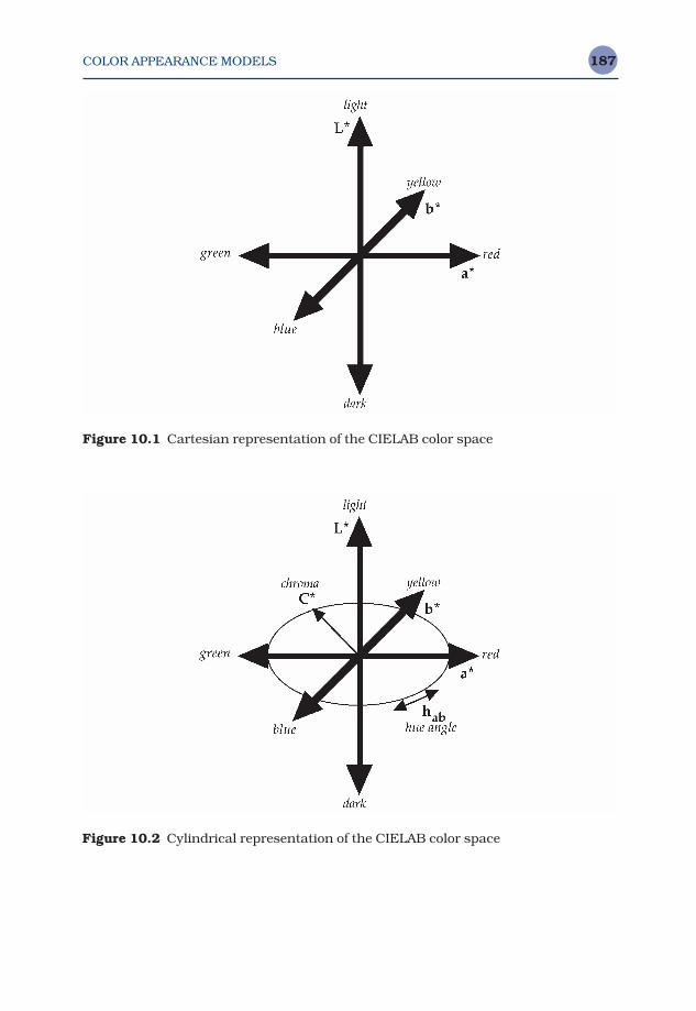
COLOR APPEARANCE MODELS 187
Figure 10.1 Cartesian representation of the CIELAB color space
Figure 10.2 Cylindrical representation of the CIELAB color space
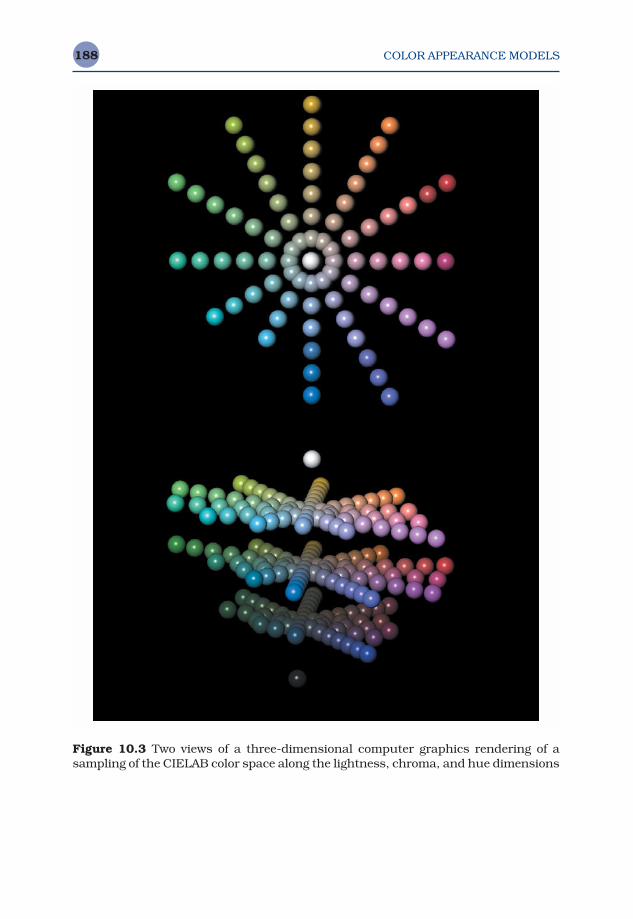
COLOR APPEARANCE MODELS188
Figure 10.3 Two views of a three-dimensional computer graphics rendering of asampling of the CIELAB color space along the lightness, chroma, and hue dimensions
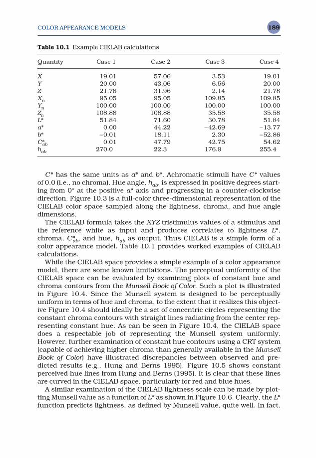
COLOR APPEARANCE MODELS 189
C* has the same units as a* and b*. Achromatic stimuli have C* values of 0.0 (i.e., no chroma). Hue angle, hab, is expressed in positive degrees start-ing from 0° at the positive a* axis and progressing in a counter-clockwisedirection. Figure 10.3 is a full-color three-dimensional representation of theCIELAB color space sampled along the lightness, chroma, and hue angledimensions.
The CIELAB formula takes the XYZ tristimulus values of a stimulus andthe reference white as input and produces correlates to lightness L*,chroma, C*ab, and hue, hab as output. Thus CIELAB is a simple form of acolor appearance model. Table 10.1 provides worked examples of CIELABcalculations.
While the CIELAB space provides a simple example of a color appearancemodel, there are some known limitations. The perceptual uniformity of theCIELAB space can be evaluated by examining plots of constant hue andchroma contours from the Munsell Book of Color. Such a plot is illustrated in Figure 10.4. Since the Munsell system is designed to be perceptually uniform in terms of hue and chroma, to the extent that it realizes this object-ive Figure 10.4 should ideally be a set of concentric circles representing theconstant chroma contours with straight lines radiating from the center rep-resenting constant hue. As can be seen in Figure 10.4, the CIELAB spacedoes a respectable job of representing the Munsell system uniformly.However, further examination of constant hue contours using a CRT system(capable of achieving higher chroma than generally available in the MunsellBook of Color) have illustrated discrepancies between observed and pre-dicted results (e.g., Hung and Berns 1995). Figure 10.5 shows constant perceived hue lines from Hung and Berns (1995). It is clear that these linesare curved in the CIELAB space, particularly for red and blue hues.
A similar examination of the CIELAB lightness scale can be made by plot-ting Munsell value as a function of L* as shown in Figure 10.6. Clearly, the L*function predicts lightness, as defined by Munsell value, quite well. In fact,
Table 10.1 Example CIELAB calculations
Quantity Case 1 Case 2 Case 3 Case 4
X 19.01 57.06 3.53 19.01Y 20.00 43.06 6.56 20.00Z 21.78 31.96 2.14 21.78Xn 95.05 95.05 109.85 109.85Yn 100.00 100.00 100.00 100.00Zn 108.88 108.88 35.58 35.58L* 51.84 71.60 30.78 51.84a* 0.00 44.22 −42.69 −13.77b* −0.01 18.11 2.30 −52.86C*ab 0.01 47.79 42.75 54.62hab 270.0 22.3 176.9 255.4

COLOR APPEARANCE MODELS190
the L* function predicts the original Munsell lightness scaling data betterthan the fifth-order polynomial used to define Munsell value (Fairchild1995b). The result in Figure 10.6 is not surprising given the historicalderivation of the L* scale to be a close approximation to the Munsell valuescale (Robertson 1990).
Figure 10.4 Contours of constant Munsell chroma and hue at value 5 plotted in theCIELAB a*b* plane
Figure 10.5 Contours of constant perceived hue from Hung and Berns (1995) plot-ted in the CIELAB a*b* plane
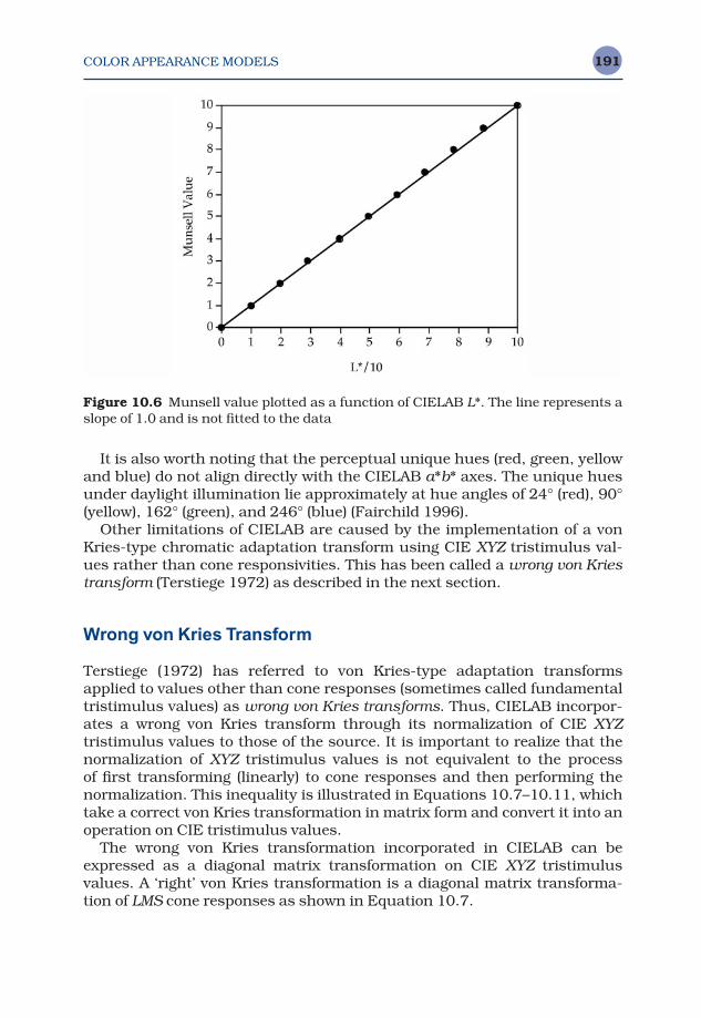
COLOR APPEARANCE MODELS 191
It is also worth noting that the perceptual unique hues (red, green, yellowand blue) do not align directly with the CIELAB a*b* axes. The unique huesunder daylight illumination lie approximately at hue angles of 24° (red), 90°(yellow), 162° (green), and 246° (blue) (Fairchild 1996).
Other limitations of CIELAB are caused by the implementation of a vonKries-type chromatic adaptation transform using CIE XYZ tristimulus val-ues rather than cone responsivities. This has been called a wrong von Kriestransform (Terstiege 1972) as described in the next section.
Wrong von Kries Transform
Terstiege (1972) has referred to von Kries-type adaptation transformsapplied to values other than cone responses (sometimes called fundamentaltristimulus values) as wrong von Kries transforms. Thus, CIELAB incorpor-ates a wrong von Kries transform through its normalization of CIE XYZtristimulus values to those of the source. It is important to realize that thenormalization of XYZ tristimulus values is not equivalent to the process of first transforming (linearly) to cone responses and then performing thenormalization. This inequality is illustrated in Equations 10.7–10.11, whichtake a correct von Kries transformation in matrix form and convert it into anoperation on CIE tristimulus values.
The wrong von Kries transformation incorporated in CIELAB can beexpressed as a diagonal matrix transformation on CIE XYZ tristimulusvalues. A ‘right’ von Kries transformation is a diagonal matrix transforma-tion of LMS cone responses as shown in Equation 10.7.
Figure 10.6 Munsell value plotted as a function of CIELAB L*. The line represents aslope of 1.0 and is not fitted to the data
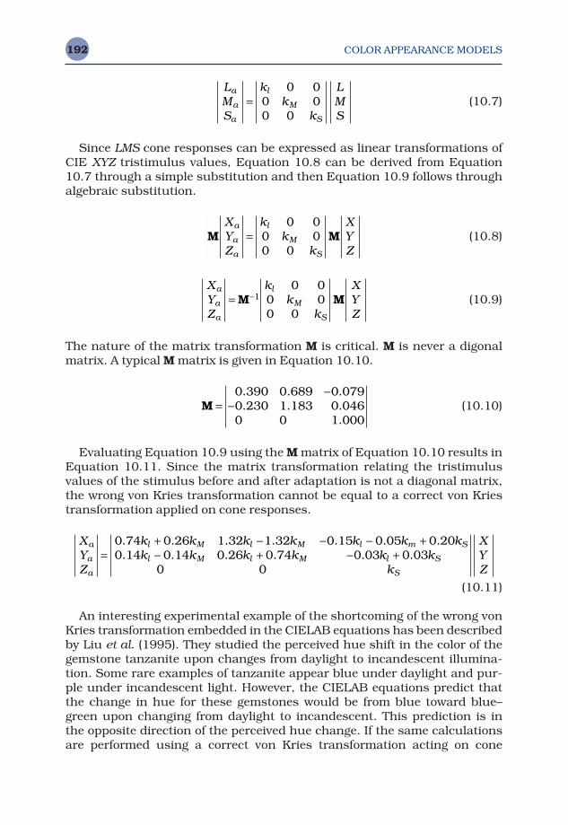
COLOR APPEARANCE MODELS192
(10.7)
Since LMS cone responses can be expressed as linear transformations ofCIE XYZ tristimulus values, Equation 10.8 can be derived from Equation10.7 through a simple substitution and then Equation 10.9 follows throughalgebraic substitution.
(10.8)
(10.9)
The nature of the matrix transformation M is critical. M is never a digonalmatrix. A typical M matrix is given in Equation 10.10.
(10.10)
Evaluating Equation 10.9 using the M matrix of Equation 10.10 results inEquation 10.11. Since the matrix transformation relating the tristimulusvalues of the stimulus before and after adaptation is not a diagonal matrix,the wrong von Kries transformation cannot be equal to a correct von Kriestransformation applied on cone responses.
(10.11)
An interesting experimental example of the shortcoming of the wrong vonKries transformation embedded in the CIELAB equations has been describedby Liu et al. (1995). They studied the perceived hue shift in the color of thegemstone tanzanite upon changes from daylight to incandescent illumina-tion. Some rare examples of tanzanite appear blue under daylight and pur-ple under incandescent light. However, the CIELAB equations predict thatthe change in hue for these gemstones would be from blue toward blue–green upon changing from daylight to incandescent. This prediction is in the opposite direction of the perceived hue change. If the same calculationsare performed using a correct von Kries transformation acting on cone
XYZ
k k k k k k kk k k k k k
k
XYZ
a
a
a
l M l M l m S
l M l M l S
S
=+ − − − +− + − +
0 74 0 26 1 32 1 32 0 15 0 05 0 200 14 0 14 0 26 0 74 0 03 0 03
0 0
. . . . . . .
. . . . . .
M =−
−0 390 0 689 0 0790 230 1 183 0 0460 0 1 000
. . .
. . ..
XYZ
kk
k
XYZ
a
a
a
l
M
S
= −M M10 0
0 00 0
M MXYZ
kk
k
XYZ
a
a
a
l
M
S
=0 0
0 00 0
LMS
kk
k
LMS
a
a
a
l
M
S
=0 0
0 00 0
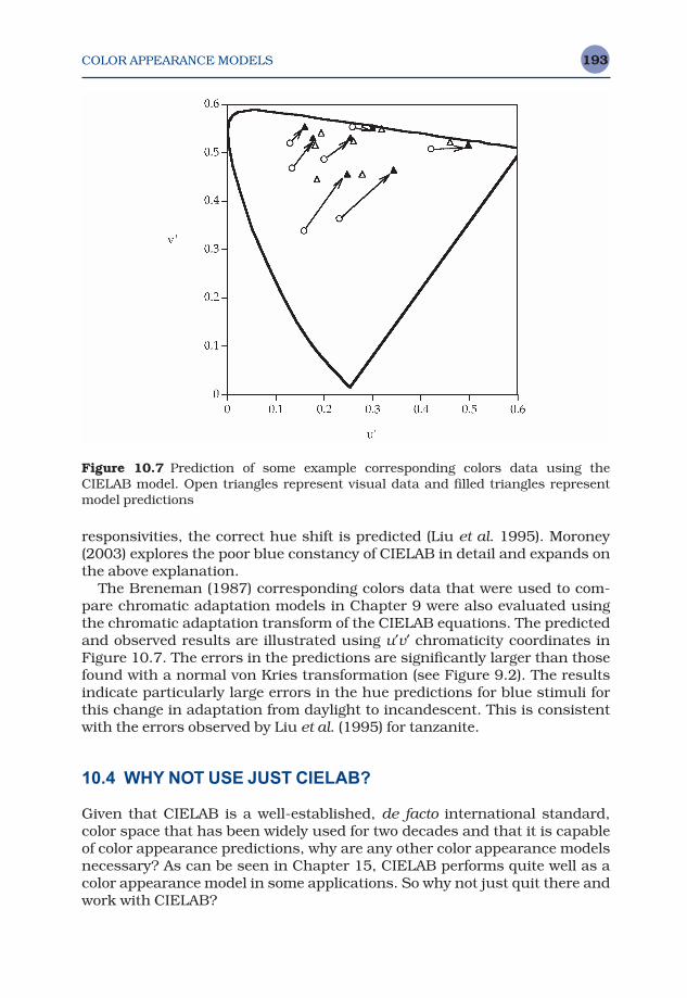
COLOR APPEARANCE MODELS 193
responsivities, the correct hue shift is predicted (Liu et al. 1995). Moroney(2003) explores the poor blue constancy of CIELAB in detail and expands onthe above explanation.
The Breneman (1987) corresponding colors data that were used to com-pare chromatic adaptation models in Chapter 9 were also evaluated usingthe chromatic adaptation transform of the CIELAB equations. The predictedand observed results are illustrated using u′v′ chromaticity coordinates inFigure 10.7. The errors in the predictions are significantly larger than thosefound with a normal von Kries transformation (see Figure 9.2). The resultsindicate particularly large errors in the hue predictions for blue stimuli forthis change in adaptation from daylight to incandescent. This is consistentwith the errors observed by Liu et al. (1995) for tanzanite.
10.4 WHY NOT USE JUST CIELAB?
Given that CIELAB is a well-established, de facto international standard,color space that has been widely used for two decades and that it is capableof color appearance predictions, why are any other color appearance modelsnecessary? As can be seen in Chapter 15, CIELAB performs quite well as acolor appearance model in some applications. So why not just quit there andwork with CIELAB?
Figure 10.7 Prediction of some example corresponding colors data using theCIELAB model. Open triangles represent visual data and filled triangles representmodel predictions
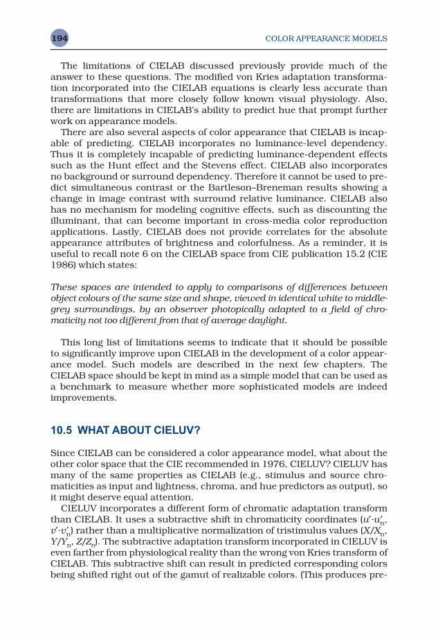
COLOR APPEARANCE MODELS194
The limitations of CIELAB discussed previously provide much of theanswer to these questions. The modified von Kries adaptation transforma-tion incorporated into the CIELAB equations is clearly less accurate thantransformations that more closely follow known visual physiology. Also,there are limitations in CIELAB’s ability to predict hue that prompt furtherwork on appearance models.
There are also several aspects of color appearance that CIELAB is incap-able of predicting. CIELAB incorporates no luminance-level dependency.Thus it is completely incapable of predicting luminance-dependent effectssuch as the Hunt effect and the Stevens effect. CIELAB also incorporates no background or surround dependency. Therefore it cannot be used to pre-dict simultaneous contrast or the Bartleson–Breneman results showing achange in image contrast with surround relative luminance. CIELAB alsohas no mechanism for modeling cognitive effects, such as discounting theilluminant, that can become important in cross-media color reproductionapplications. Lastly, CIELAB does not provide correlates for the absoluteappearance attributes of brightness and colorfulness. As a reminder, it isuseful to recall note 6 on the CIELAB space from CIE publication 15.2 (CIE1986) which states:
These spaces are intended to apply to comparisons of differences betweenobject colours of the same size and shape, viewed in identical white to middle-grey surroundings, by an observer photopically adapted to a field of chro-maticity not too different from that of average daylight.
This long list of limitations seems to indicate that it should be possible to significantly improve upon CIELAB in the development of a color appear-ance model. Such models are described in the next few chapters. TheCIELAB space should be kept in mind as a simple model that can be used asa benchmark to measure whether more sophisticated models are indeedimprovements.
10.5 WHAT ABOUT CIELUV?
Since CIELAB can be considered a color appearance model, what about theother color space that the CIE recommended in 1976, CIELUV? CIELUV hasmany of the same properties as CIELAB (e.g., stimulus and source chro-maticities as input and lightness, chroma, and hue predictors as output), soit might deserve equal attention.
CIELUV incorporates a different form of chromatic adaptation transformthan CIELAB. It uses a subtractive shift in chromaticity coordinates (u′-u′n,v′-v′n) rather than a multiplicative normalization of tristimulus values (X/Xn,Y/Yn, Z/Zn). The subtractive adaptation transform incorporated in CIELUV iseven farther from physiological reality than the wrong von Kries transform ofCIELAB. This subtractive shift can result in predicted corresponding colorsbeing shifted right out of the gamut of realizable colors. (This produces pre-
COLOR APPEARANCE MODELS 195
dicted tristimulus values less than zero, which cannot happen with theCIELAB transformation.) Even if this does not occur, the transform is likelyto shift predicted colors outside the gamut of colors producible by any givendevice. In addition to this problem, the CIELUV adaptation transform isextremely inaccurate with respect to predicting visual data. This is illus-trated nicely in Figure 10.8, which shows the CIELUV predictions of theBreneman (1987) corresponding colors data. Figure 10.8 illustrates howsome colors are shifted outside the gamut of realizable colors (outside thespectrum locus on the u ′v ′ chromaticity diagram) and the inaccuracy of allthe predictions.
The difficulties with the CIELUV adaptation transform are reason enoughto eliminate it from serious consideration as an appearance model. However,additional evidence is provided by its poor performance for predicting colordifferences. The current CIE recommendation for color difference specifica-tion, CIE94 (CIE 1995b), is based on the CIELAB color space. So are themore recent CIE DE2000 (CIE 2001) color difference equations. While theDE2000 equations are more recent, their added complexity over the CIE94specification is probably unwarranted in most applications. Alman et al.(1989) provide experimental evidence for the poor performance of CIELUV asa color difference equation. Additional comparisons between CIELUV andCIELAB have been made by Robertson (1990).
Figure 10.8 Prediction of some example corresponding colors data using the CIELUVmodel. Open triangles represent visual data and filled triangles represent model predictions
Color Appearance Models Second Edition M. D. Fairchild © 2005 John Wiley & Sons, LtdISBN: 0-470-01216-1 (HB)
11The Nayatani
et al. Model
The next few chapters describe details of the most widely discussed andused color appearance models. This chapter discusses the color appearancemodel developed by Nayatani and his co-workers that has evolved as one of the more important early colorimetry-based models. This model, alongwith Hunt’s model (described in Chapter 12), is a complete color appearancemodel capable of predicting the full array of color appearance parametersdefined in Chapter 4 for a fairly wide range of viewing conditions.
11.1 OBJECTIVES AND APPROACH
The Nayatani et al. color appearance model evolved as a natural extension oftheir chromatic adaptation model described in Chapter 9 (Nayatani et al.1981) in conjunction with the attributes of a color appearance model firstoutlined by Hunt (1982, 1985). The Nayatani et al. color appearance modelwas first described in Nayatani et al. (1986, 1987) and most recently revisedand summarized in Nayatani et al. (1995). The latter version of the model isdescribed in this chapter.
As with any color appearance model, it is important to note the context inwhich the Nayatani et al. model was formulated. The researchers who devel-oped this model come from the field of illumination engineering, in which the critical application of color appearance models is the specification of the color rendering properties of light sources. This application provides significantly different challenges from those encountered in the field ofimage reproduction. Thus, those interested in image reproduction mightfind some aspects of the Nayatani et al. model inappropriate for their needs.The reverse is also true. Models derived strictly for imaging applicationsmight not fulfill the requirements for illumination engineering applications.
THE NAYATANI et al. MODEL 197
Despite the different pedigrees of the various models, it is worthwhile to stretch them to applications for which they were not designed. The bestpossible result will be that they work well (indicating good generality) andthe worst outcome is that something more is learned about the importantdifferences in applications. Thus, while the Nayatani et al. model was notdesigned for imaging applications, it is certainly worthy of evaluation in anyapplication that might require a color appearance model.
The model attempts to predict a wide range of color appearance phenom-ena including the Stevens effect, the Hunt effect, and the Helson–Judd effectin addition to the effects of chromatic adaptation. It is designed to predict the color appearance of simple patches on uniform mid-to-light-gray back-grounds. It is not designed for complex stimuli or changes in background orsurround. The model includes output values designed to correlate with all ofthe important color appearance attributes including brightness, lightness,colorfulness, chroma, and hue. The model’s design for simple stimuli on uni-form backgrounds highlights the distinction between it and models such as Hunt’s, RLAB, and CIECAM02 that were designed with specific attributesfor imaging applications. These apparent limitations of the model are notlimitations at all for lighting and illumination color-rendering applications.
11.2 INPUT DATA
The input data for the model include the colorimetric and photometric spe-cification of the stimulus, the adapting illuminant, and the luminance factorof the background. Specifically, the required data include the following:
• The luminance factor of the achromatic background is expressed as a per-centage Yo, limited to values equal to or greater than 18%.
• The color of the illumination xo, yo is expressed in terms of its chromaticitycoordinates for the CIE 1931 standard colorimetric observer.
• The test stimulus is specified in terms of its chromaticity coordinates x, yand its luminance factor Y.
• The absolute luminance of the stimulus and adapting field is defined bythe illuminance of the viewing field Eo expressed in lux.
In addition, two other parameters must also be specified to define themodel’s required input:
• The normalizing illuminance Eor which is expressed in lux and usually inthe range of 1000–3000 lux.
• The noise term n used in the nonlinear chromatic adaptation model whichis usually taken to be 1.
From these input data, a variety of intermediate and final output valuesare calculated according to the model. The equations necessary for
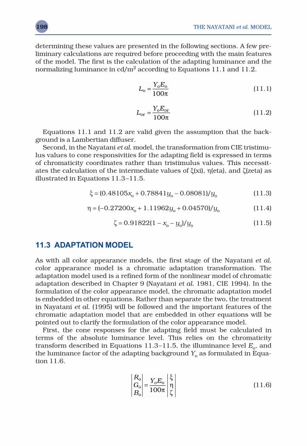
THE NAYATANI et al. MODEL198
determining these values are presented in the following sections. A few pre-liminary calculations are required before proceeding with the main featuresof the model. The first is the calculation of the adapting luminance and thenormalizing luminance in cd/m2 according to Equations 11.1 and 11.2.
(11.1)
(11.2)
Equations 11.1 and 11.2 are valid given the assumption that the back-ground is a Lambertian diffuser.
Second, in the Nayatani et al. model, the transformation from CIE tristimu-lus values to cone responsivities for the adapting field is expressed in termsof chromaticity coordinates rather than tristimulus values. This necessit-ates the calculation of the intermediate values of ξ(xi), η(eta), and ζ(zeta) asillustrated in Equations 11.3–11.5.
ξ = (0.48105xo + 0.78841yo − 0.08081)/yo (11.3)
η = (−0.27200xo + 1.11962yo + 0.04570)/yo (11.4)
ζ = 0.91822(1 − xo − yo)/yo (11.5)
11.3 ADAPTATION MODEL
As with all color appearance models, the first stage of the Nayatani et al.color appearance model is a chromatic adaptation transformation. Theadaptation model used is a refined form of the nonlinear model of chromaticadaptation described in Chapter 9 (Nayatani et al. 1981, CIE 1994). In theformulation of the color appearance model, the chromatic adaptation modelis embedded in other equations. Rather than separate the two, the treatmentin Nayatani et al. (1995) will be followed and the important features of thechromatic adaptation model that are embedded in other equations will bepointed out to clarify the formulation of the color appearance model.
First, the cone responses for the adapting field must be calculated interms of the absolute luminance level. This relies on the chromaticity transform described in Equations 11.3–11.5, the illuminance level Eo, andthe luminance factor of the adapting background Yo as formulated in Equa-tion 11.6.
(11.6)RGB
Y Eo
o
o
o o=100π
ξηζ
LY E
oro or=
100π
LY E
oo o=
100π
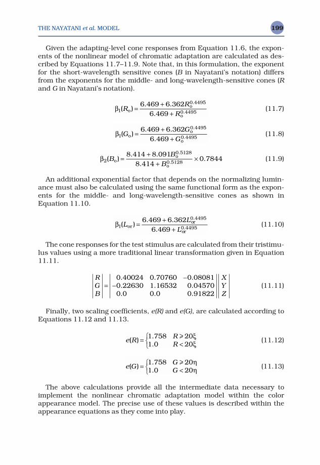
THE NAYATANI et al. MODEL 199
Given the adapting-level cone responses from Equation 11.6, the expon-ents of the nonlinear model of chromatic adaptation are calculated as des-cribed by Equations 11.7–11.9. Note that, in this formulation, the exponentfor the short-wavelength sensitive cones (B in Nayatani’s notation) differsfrom the exponents for the middle- and long-wavelength-sensitive cones (Rand G in Nayatani’s notation).
(11.7)
(11.8)
(11.9)
An additional exponential factor that depends on the normalizing lumin-ance must also be calculated using the same functional form as the expon-ents for the middle- and long-wavelength-sensitive cones as shown inEquation 11.10.
(11.10)
The cone responses for the test stimulus are calculated from their tristimu-lus values using a more traditional linear transformation given in Equation11.11.
(11.11)
Finally, two scaling coefficients, e(R) and e(G), are calculated according toEquations 11.12 and 11.13.
(11.12)
(11.13)
The above calculations provide all the intermediate data necessary toimplement the nonlinear chromatic adaptation model within the colorappearance model. The precise use of these values is described within theappearance equations as they come into play.
e GGG
( )..
= <1 758 201 0 20
> ηη
e RRR
( )..
= <1 758 201 0 20
> ξξ
RGB
XYZ
=−
−0 40024 0 70760 0 080810 22630 1 16532 0 045700 0 0 0 0 91822
. . .
. . .
. . .
β16 469 6 362
( ). .
LL
Loror0.4495
or0.44956.469
=+
+
β28 414 8 091
0 7844( ). .
.BB
Boo0.5128
o0.51288.414
=+
+×
β16 469 6 362
( ). .
GG
Goo0.4495
o0.44956.469
=+
+
β16 469 6 362
( ). .
RR
Roo0.4495
o0.44956.469
=+
+

THE NAYATANI et al. MODEL200
11.4 OPPONENT COLOR DIMENSIONS
The cone responses are transformed directly into intermediate values repres-enting classical opponent dimensions of visual response: an achromaticchannel and two chromatic channels. These equations, used to model theseopponent processes, also incorporate the nonlinear chromatic adaptationmodel.
First, the achromatic response Q is calculated using Equation 11.14.
(11.14)
At first, Equation 11.14 looks fairly complex, but its components can bereadily teased apart and understood. First, the general structure of Equa-tion 11.14 is such that the achromatic response is calculated as a weightedsum of the outputs of the long- and middle-wavelength cone responses (Rand G) as is often postulated in color vision theory. The outputs are summedwith relative weights of 2/3 and 1/3, which correspond to their relative population in the human retina. They are first normalized after addition ofnoise n, by the cone responses for the adapting stimulus represented by ξand η according to a von Kries-type transformation. The value of n is typicallytaken to be 1.0 although it can vary. A logarithmic transform is then taken tomodel the compressive nonlinearity that is known to occur in the humanvisual system. Given the logarithmic transformation, the exponents (β terms)of the nonlinear chromatic adaptation model become multiplicative factorsalong with the scaling factors e(R ) and e(G ), as shown in Equation 11.14. Allthat remains is one more scaling factor 41.69, and the luminance-depend-ent, exponential adjustment, β1(Lor), to complete the equation. Thus theachromatic response can be simply expressed as a weighted sum of the post-adaptation signals from the long- and middle-wavelength-sensitive cones.
Next, preliminary chromatic channel responses t (red–green) and p (yellow–blue), are calculated in a similar manner using Equations 11.15 and 11.16.
(11.15)
(11.16)
The explanation of Equations 11.15 and 11.16 follows the same logic asthat for the achromatic response, Equation 11.14. Beginning with the tresponse; it is a weighted combination of the post-adaptation signals fromeach of the three cone types. The combination is the difference between thelong- and middle-wavelength-sensitive cones with a small input from theshort-wavelength-sensitive cones that adds with the long-wavelength
p RR n
nG
G n
nB
B n
n=
++
++
+−
++
19 20
19 20
29 201 1 2β
ξβ
ηβ
ζ( ) log ( ) log ( ) logo o o
t RR n
nG
G n
nB
B n
n=
++
−+
++
++
βξ
βη
βζ1 1 220
1211 20
111 20
( ) log ( ) log ( ) logo o o
QL
R e RR n
nG e G
G n
n=
++
++
+
41 69 23 20
13 201
1 1.
( )( ) ( ) log ( ) ( ) log
ββ
ξβ
ηoro o
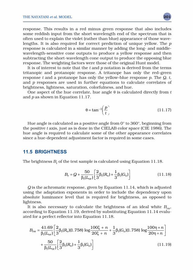
THE NAYATANI et al. MODEL 201
response. This results in a red minus green response that also includessome reddish input from the short wavelength end of the spectrum that isoften used to explain the violet (rather than blue) appearance of those wave-lengths. It is also required for correct prediction of unique yellow. The presponse is calculated in a similar manner by adding the long- and middle-wavelength-sensitive cone outputs to produce a yellow response and thensubtracting the short-wavelength cone output to produce the opposing blueresponse. The weighting factors were those of the original Hunt model.
It is of interest to note that the t and p notation is derived from the termstritanopic and protanopic response. A tritanope has only the red–greenresponse t and a protanope has only the yellow–blue response p. The Q, t,and p responses are used in further equations to calculate correlates ofbrightness, lightness, saturation, colorfulness, and hue.
One aspect of the hue correlate, hue angle θ is calculated directly from tand p as shown in Equation 11.17.
(11.17)
Hue angle is calculated as a positive angle from 0° to 360°, beginning fromthe positive t axis, just as is done in the CIELAB color space (CIE 1986). Thehue angle is required to calculate some of the other appearance correlatessince a hue-dependent adjustment factor is required in some cases.
11.5 BRIGHTNESS
The brightness Br of the test sample is calculated using Equation 11.18.
(11.18)
Q is the achromatic response, given by Equation 11.14, which is adjustedusing the adaptation exponents in order to include the dependency uponabsolute luminance level that is required for brightness, as opposed to lightness.
It is also necessary to calculate the brightness of an ideal white Brw,according to Equation 11.19, derived by substituting Equation 11.14 evalu-ated for a perfect reflector into Equation 11.18.
(11.19)+ +
50 23
131
1 1ββ β
( )( ) ( )
LR G
oro o
BL
Rn
nG
n
nrwor
o o=++
+++
41 69 23
1 75810020
13
1 758100201
1 1.
( )( )( . ) log ( )( . ) log
ββ
ξξ
βηη
B QL
R Gror
o o= + +
50 23
131
1 1ββ β
( )( ) ( )
θ =
−tan 1 p
t
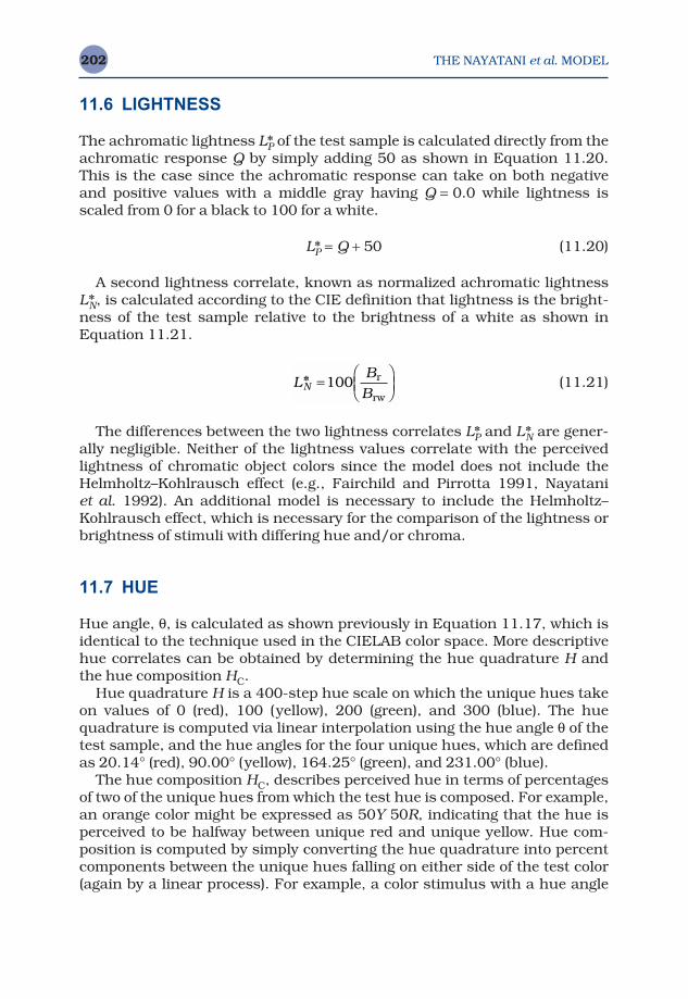
THE NAYATANI et al. MODEL202
11.6 LIGHTNESS
The achromatic lightness L*P of the test sample is calculated directly from theachromatic response Q by simply adding 50 as shown in Equation 11.20.This is the case since the achromatic response can take on both negativeand positive values with a middle gray having Q = 0.0 while lightness isscaled from 0 for a black to 100 for a white.
L*P = Q + 50 (11.20)
A second lightness correlate, known as normalized achromatic lightnessL*N, is calculated according to the CIE definition that lightness is the bright-ness of the test sample relative to the brightness of a white as shown inEquation 11.21.
(11.21)
The differences between the two lightness correlates L*P and L*N are gener-ally negligible. Neither of the lightness values correlate with the perceivedlightness of chromatic object colors since the model does not include theHelmholtz–Kohlrausch effect (e.g., Fairchild and Pirrotta 1991, Nayatani et al. 1992). An additional model is necessary to include the Helmholtz–Kohlrausch effect, which is necessary for the comparison of the lightness orbrightness of stimuli with differing hue and/or chroma.
11.7 HUE
Hue angle, θ, is calculated as shown previously in Equation 11.17, which isidentical to the technique used in the CIELAB color space. More descriptivehue correlates can be obtained by determining the hue quadrature H andthe hue composition HC.
Hue quadrature H is a 400-step hue scale on which the unique hues takeon values of 0 (red), 100 (yellow), 200 (green), and 300 (blue). The huequadrature is computed via linear interpolation using the hue angle θ of thetest sample, and the hue angles for the four unique hues, which are definedas 20.14° (red), 90.00° (yellow), 164.25° (green), and 231.00° (blue).
The hue composition HC, describes perceived hue in terms of percentagesof two of the unique hues from which the test hue is composed. For example,an orange color might be expressed as 50Y 50R, indicating that the hue isperceived to be halfway between unique red and unique yellow. Hue com-position is computed by simply converting the hue quadrature into percentcomponents between the unique hues falling on either side of the test color(again by a linear process). For example, a color stimulus with a hue angle
LB
BN* =
100 r
rw
THE NAYATANI et al. MODEL 203
of 44.99° will have a hue quadrature of 32.98 and a hue composition of 33Y 67R.
11.8 SATURATION
In the Nayatani et al. color appearance model, saturation is derived mostdirectly and then the measures of colorfulness and chroma are derived fromit. Saturation is expressed in terms of a red–green component, SRG, derivedfrom the t response as shown in Equation 11.22 and a yellow–blue compon-ent SYB derived from the p response as shown in Equation 11.23.
(11.22)
(11.23)
The saturation predictors include a scaling factor 488.93 for convenience;the luminance-dependent b terms required to predict the Hunt effect; and a chromatic strength function, Es(θ), that was introduced to correct the saturation scale as a function of hue angle (Nayatani 1995). It takes on theempirically derived form expressed in Equation 11.24.
Es(θ) = 0.9394 − 0.2478 sin θ − 0.0743 sin 2θ + 0.0666 sin 3θ
− 0.0186 sin 4θ − 0.0055 cos θ − 0.0521 cos 2θ
− 0.0573 cos 3θ − 0.0061 cos 4θ (11.24)
Finally, an overall saturation correlate S is calculated using Equation11.25. This is precisely the same functional form as the chroma calculationin CIELAB (Euclidean distance from the origin).
S = (S2RG + S2
YB)1/2 (11.25)
11.9 CHROMA
Given the correlates for saturation described above, correlates of chromacan be easily derived by considering their definitions. As was illustrated inChapter 4, saturation can be expressed as chroma divided by lightness.Thus chroma can be described as saturation multiplied by lightness. This isalmost exactly the functional form for chroma in the Nayatani et al. model.The correlates for the red–green, yellow–blue, and overall chroma of the testsample are given in Equations 11.26–11.28.
SL
E pYB =488 93
1
.( )
( )β
θor
s
SL
E tRG =488 93
1
.( )
( )β
θor
s
THE NAYATANI et al. MODEL204
(11.26)
(11.27)
(11.28)
The only differences between the nominal definition of chroma and Equa-tions 11.26–11.28 are the scaling factor of 50 and the slight nonlinearityintroduced by the power function of lightness with an exponent of 0.7. Thisnonlinearity was introduced to better model constant chroma contours fromthe Munsell Book of Color (Nayatani et al. 1995).
11.10 COLORFULNESS
The predictors of colorfulness in the Nayatani et al. model can also be de-rived directly from the CIE definitions of the appearance attributes. Recall thatchroma is defined as colorfulness of the sample relative to the brightness of a white object under similar illumination. Thus colorfulness is simply thechroma of the sample multiplied by the brightness of an ideal white as illustrated in Equations 11.29–11.31.
(11.29)
(11.30)
(11.31)
The normalizing value of 100 is derived as the brightness of an ideal whiteunder illuminant D65 at the normalizing illuminance. It provides a conveni-ent place to tie down the scale.
11.11 INVERSE MODEL
In many applications, and particularly image reproduction, it is necessary touse a color appearance model in both forward and reverse directions. Thus it
M CB
= rw
100
M CB
YB YB= rw
100
M CB
RG RG= rw
100
CL
SP=
* .
50
0 7
CL
SYBP
YB=
* .
50
0 7
CL
SRGP
RG=
* .
50
0 7
THE NAYATANI et al. MODEL 205
is important, or at least highly convenient, that the equations can be analyt-ically inverted. Fortunately, the Nayatani et al. color appearance model canbe inverted analytically. Nayatani et al. (1990a) published a paper that intro-duces the process for inverting the model for both brightness–colorfulnessand lightness–chroma matches. While the model has changed slightly, thesame general procedure can be followed.
In applying the model, it is often useful to consider its implementation as asimple step-by-step process. Thus the steps required to implement themodel (and in reverse order to invert it) are given below.
1. Obtain physical data.2. Calculate Q, t, and p.3. Calculate θ, Es(θ), H, and HC.4. Calculate Br, Brw, L*P, L*N, and S.5. Calculate C.6. Calculate M.
11.12 PHENOMENA PREDICTED
The Nayatani et al. color appearance model accounts for changes in colorappearance due to chromatic adaptation and luminance level (Steven effectand Hunt effect). It also predicts the Helson–Judd effect. The model can beused for different background luminance factors (greater than 18%), but themodel’s authors caution against using it for comparisons between differentluminance levels (Nayatani et al. 1990a). It cannot be used to predict theeffects of changes in background color (simultaneous contrast) or surroundrelative luminance (e.g., Bartleson–Breneman equations.).
The Nayatani et al. color appearance model also does not incorporatemechanisms for predicting incomplete chromatic adaptation or cognitivediscounting-the-illuminant. Nayatani (1997) has outlined a procedure toestimate the level of chromatic adaptation from experimental data. This isuseful to allow the model to be used to predict the results of visual experi-ments in which chromatic adaptation is incomplete. However, this tech-nique is of little value in practical applications in which a prediction of thelevel of chromatic adaptation must be made for a set of viewing conditionsfor which prior visual data are not available.
Example calculations using the Nayatani et al. color appearance model asdescribed in this chapter are given for four samples in Table 11.1.
11.13 WHY NOT USE JUST THE NAYATANI et al. MODEL?
Given the extensive nature of the Nayatani et al. color appearance model andits inclusion of correlates for all of the important color appearance attri-butes, it is reasonable to wonder why the CIE hasn’t simply adopted this
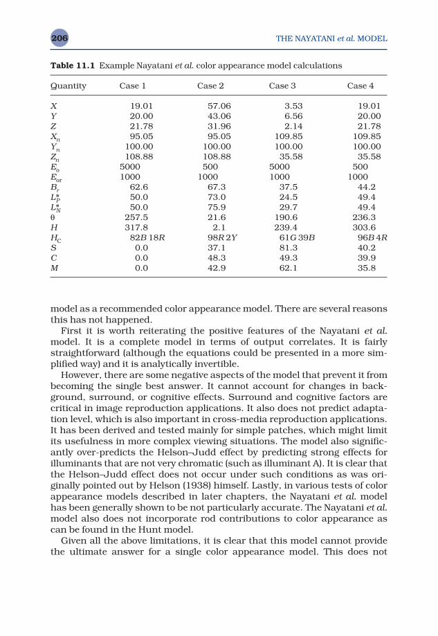
THE NAYATANI et al. MODEL206
model as a recommended color appearance model. There are several reasonsthis has not happened.
First it is worth reiterating the positive features of the Nayatani et al.model. It is a complete model in terms of output correlates. It is fairlystraightforward (although the equations could be presented in a more sim-plified way) and it is analytically invertible.
However, there are some negative aspects of the model that prevent it frombecoming the single best answer. It cannot account for changes in back-ground, surround, or cognitive effects. Surround and cognitive factors arecritical in image reproduction applications. It also does not predict adapta-tion level, which is also important in cross-media reproduction applications.It has been derived and tested mainly for simple patches, which might limitits usefulness in more complex viewing situations. The model also signific-antly over-predicts the Helson–Judd effect by predicting strong effects forilluminants that are not very chromatic (such as illuminant A). It is clear thatthe Helson–Judd effect does not occur under such conditions as was ori-ginally pointed out by Helson (1938) himself. Lastly, in various tests of colorappearance models described in later chapters, the Nayatani et al. modelhas been generally shown to be not particularly accurate. The Nayatani et al.model also does not incorporate rod contributions to color appearance ascan be found in the Hunt model.
Given all the above limitations, it is clear that this model cannot providethe ultimate answer for a single color appearance model. This does not
Table 11.1 Example Nayatani et al. color appearance model calculations
Quantity Case 1 Case 2 Case 3 Case 4
X 19.01 57.06 3.53 19.01Y 20.00 43.06 6.56 20.00Z 21.78 31.96 2.14 21.78Xn 95.05 95.05 109.85 109.85Yn 100.00 100.00 100.00 100.00Zn 108.88 108.88 35.58 35.58Eo 5000 500 5000 500Eor 1000 1000 1000 1000Br 62.6 67.3 37.5 44.2L*P 50.0 73.0 24.5 49.4L*N 50.0 75.9 29.7 49.4θ 257.5 21.6 190.6 236.3H 317.8 2.1 239.4 303.6HC 82B 18R 98R 2Y 61G 39B 96B 4RS 0.0 37.1 81.3 40.2C 0.0 48.3 49.3 39.9M 0.0 42.9 62.1 35.8

THE NAYATANI et al. MODEL 207
lessen its significance and contributions to the development of color appear-ance models. It is almost certain that some aspects of the Nayatani et al.model will find their way into whatever model is agreed upon for general usein the future as illustrated by the evolution of CIECAM97s and CIECAM02.
Color Appearance Models Second Edition M. D. Fairchild © 2005 John Wiley & Sons, LtdISBN: 0-470-01216-1 (HB)
12The Hunt Model
This chapter continues the review of some of the most widely discussed andused color appearance models with a description of the model developed byRobert William Gainer Hunt. This model is the most extensive, complete,and complex color appearance model that has been developed. Its roots canbe traced to some of Hunt’s early chromatic adaptation studies (Hunt 1952)up through its rigorous development in the 1980s and 1990s (Hunt 1982,1985, 1987, 1991b, 1994, 1995).
The Hunt color appearance model is not simple, but it is designed to pre-dict a wide range of visual phenomena and, as Hunt himself has stated, thehuman visual system is not simple either. While there are applications in which simpler models such as those described in later chapters are ade-quate, it is certainly of great value to have a complete model that can beadapted to a wider range of viewing conditions for more well defined orunusual circumstances. The Hunt model serves this purpose well and manyof the other color appearance models discussed in this book can trace manyof their features back to ideas that originally appeared in Hunt’s model.
12.1 OBJECTIVES AND APPROACH
Hunt spent 36 years of his career in the Kodak Research Laboratories. Thus,the Hunt model has been developed in the context of the requirements forcolor image reproduction. This is a significantly different point of view thanfound in the field of illumination engineering from which the Nayatani et al.model discussed in Chapter 11 was developed. The imaging science influ-ence on the Hunt model can be easily witnessed by examining its inputparameters. For example, the surround relative luminance is an importantfactor that is not present in the Nayatani et al. model. Other examples can be found in parameters that are set to certain values for ‘transparencies
THE HUNT MODEL 209
projected in a dark room’ or ‘television displays in a dim surround’ or ‘normalscenes.’ Such capabilities clearly indicate that the model was intended to beapplied to imaging situations. However, this is not the limit of the model’sapplicability. For example, it has also been extended for unrelated colorssuch as those found in traditional vision science experiments.
The Hunt model is designed to predict a wide range of visual phenomenaincluding the appearance of related and unrelated colors in various back-grounds, surrounds, illumination colors, and luminance levels ranging fromlow scotopic to bleaching levels. In this sense it is a complete model of colorappearance for static stimuli. Hunt’s model, like most of the others describedin this book, does not attempt to incorporate complex spatial or temporalcharacteristics of appearance.
To make reasonable predictions of appearance over such a wide range ofconditions, the Hunt model requires more rigorous definition of the viewingfield. Thus, Hunt (1991b) defined the components of the viewing field asdescribed in Chapter 7. These components include the stimulus, the prox-imal field, the background, and the surround. The Hunt model is the onlyavailable model that treats each of these components of the viewing fieldseparately.
While Hunt’s model has been continuously evolving over the past twodecades (see Hunt 1982, 1985, 1987, 1991b, and 1994 for major mile-stones), a comprehensive review of the model’s current formulation can befound in Chapter 31 of the 5th Edition of Hunt’s book, The Reproduction ofColour (Hunt 1995). The treatment that follows is adapted from that chapter.Those desiring more detail on Hunt’s model should refer to Chapter 31 ofHunt’s book.
12.2 INPUT DATA
The Hunt model requires an extensive list of input data. All colorimetriccoordinates are typically calculated using the CIE 1931 standard colorimet-ric observer (2°). The chromaticity coordinates (x,y) of the illuminant and theadapting field are required. Typically, the adapting field is taken to be theintegrated chromaticity of the scene, which is assumed to be identical to thatof the illuminant (or source). Next, the chromaticities (x,y) and luminancefactors Y of the background, proximal field, reference white, and test sampleare required. If separate data are not available for the proximal field, it isgenerally assumed to be identical to the background. Also, the referencewhite is often taken to have the same chromaticities as the illuminant with aluminance factor of 100 if specific data are not available.
All of these data are relative colorimetric values. Absolute luminance levels are required to predict several luminance-dependent appearance phenomena. Thus the absolute luminance levels, in cd/m2, are required forthe reference white and the adapting field. If the specific luminance of the
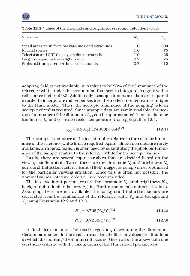
THE HUNT MODEL210
adapting field is not available, it is taken to be 20% of the luminance of thereference white under the assumption that scenes integrate to a gray with areflectance factor of 0.2. Additionally, scotopic luminance data are requiredin order to incorporate rod responses into the model (another feature uniqueto the Hunt model). Thus, the scotopic luminance of the adapting field inscotopic cd/m2 is required. Since scotopic data are rarely available, the sco-topic luminance of the illuminant LAS can be approximated from its photopicluminance LA and correlated color temperature T using Equation 12.1.
LAS = 2.26LA[(T/4000) − 0.4]1/3 (12.1)
The scotopic luminance of the test stimulus relative to the scotopic lumin-ance of the reference white is also required. Again, since such data are rarelyavailable, an approximation is often used by substituting the photopic lumin-ance of the sample relative to the reference white for the scotopic values.
Lastly, there are several input variables that are decided based on theviewing configuration. Two of these are the chromatic Nc and brightness Nbsurround induction factors. Hunt (1995) suggests using values optimizedfor the particular viewing situation. Since this is often not possible, the nominal values listed in Table 12.1 are recommended.
The last two input parameters are the chromatic Ncb and brightness Nbbbackground induction factors. Again, Hunt recommends optimized values.Assuming these are not available, the background induction factors are calculated from the luminances of the reference white YW and backgroundYb using Equations 12.2 and 12.3.
Ncb = 0.725(YW/Yb)0.2 (12.2)
Nbb = 0.725(YW/Yb)0.2 (12.3)
A final decision must be made regarding discounting-the-illuminant.Certain parameters in the model are assigned different values for situationsin which discounting-the-illuminant occurs. Given all of the above data onecan then continue with the calculations of the Hunt model parameters.
Table 12.1 Values of the chromatic and brightness surround induction factors
Situation Nc Nb
Small areas in uniform backgrounds and surrounds 1.0 300Normal scenes 1.0 75Television and CRT displays in dim surrounds 1.0 25Large transparencies on light boxes 0.7 25Projected transparencies in dark surrounds 0.7 10
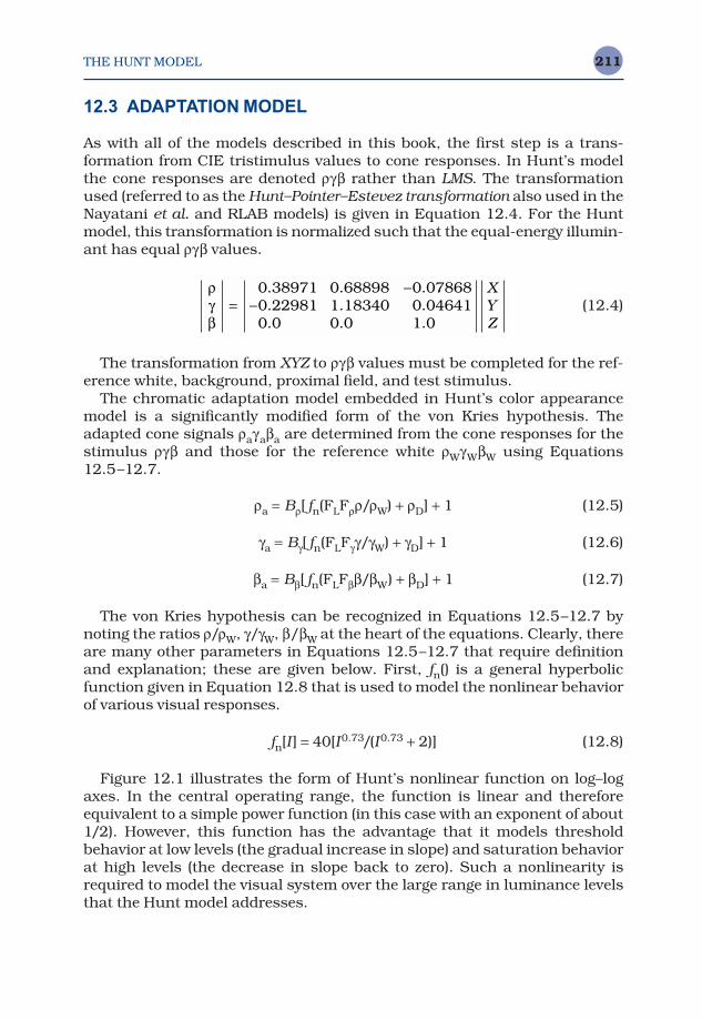
THE HUNT MODEL 211
12.3 ADAPTATION MODEL
As with all of the models described in this book, the first step is a trans-formation from CIE tristimulus values to cone responses. In Hunt’s modelthe cone responses are denoted ργβ rather than LMS. The transformationused (referred to as the Hunt–Pointer–Estevez transformation also used in theNayatani et al. and RLAB models) is given in Equation 12.4. For the Huntmodel, this transformation is normalized such that the equal-energy illumin-ant has equal ργβ values.
(12.4)
The transformation from XYZ to ργβ values must be completed for the ref-erence white, background, proximal field, and test stimulus.
The chromatic adaptation model embedded in Hunt’s color appearancemodel is a significantly modified form of the von Kries hypothesis. Theadapted cone signals ρaγaβa are determined from the cone responses for thestimulus ργβ and those for the reference white ρWγWβW using Equations12.5–12.7.
ρa = Bρ[ fn(FLFρρ/ρW) + ρD] + 1 (12.5)
γa = Bγ[ fn(FLFγγ/γW) + γD] + 1 (12.6)
βa = Bβ[ fn(FLFββ/βW) + βD] + 1 (12.7)
The von Kries hypothesis can be recognized in Equations 12.5–12.7 bynoting the ratios ρ/ρW, γ/γW, β/βW at the heart of the equations. Clearly, thereare many other parameters in Equations 12.5–12.7 that require definitionand explanation; these are given below. First, fn() is a general hyperbolicfunction given in Equation 12.8 that is used to model the nonlinear behaviorof various visual responses.
fn[I ] = 40[I0.73/(I0.73 + 2)] (12.8)
Figure 12.1 illustrates the form of Hunt’s nonlinear function on log–logaxes. In the central operating range, the function is linear and thereforeequivalent to a simple power function (in this case with an exponent of about1/2). However, this function has the advantage that it models thresholdbehavior at low levels (the gradual increase in slope) and saturation behaviorat high levels (the decrease in slope back to zero). Such a nonlinearity isrequired to model the visual system over the large range in luminance levelsthat the Hunt model addresses.
ργβ
. . .
. . .
. . .=
−−0 38971 0 68898 0 078680 22981 1 18340 0 046410 0 0 0 1 0
XYZ
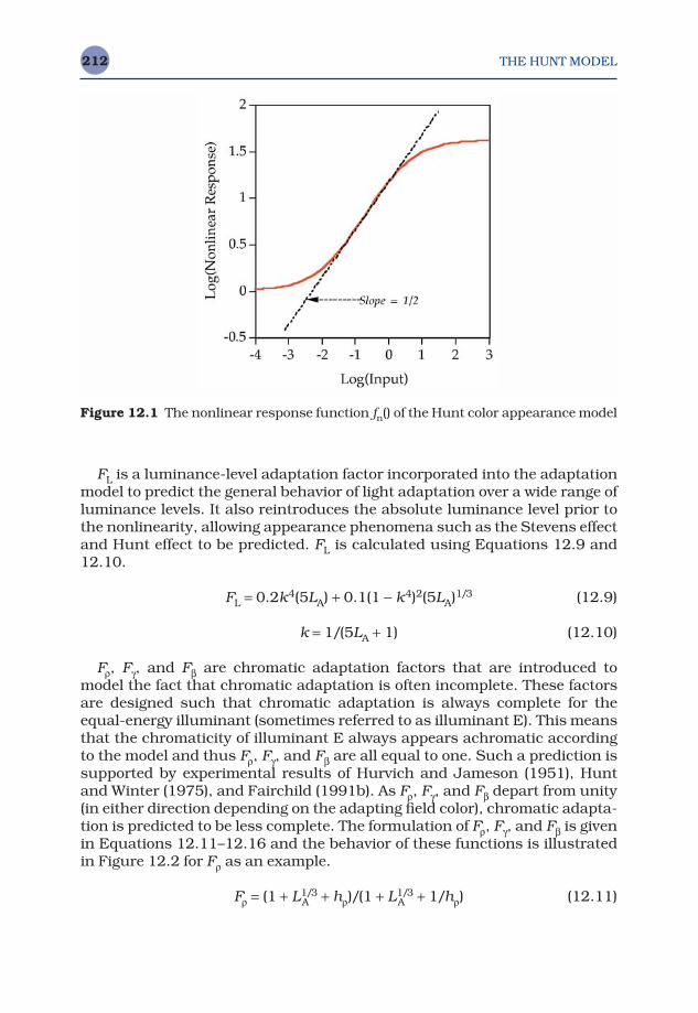
THE HUNT MODEL212
FL is a luminance-level adaptation factor incorporated into the adaptationmodel to predict the general behavior of light adaptation over a wide range ofluminance levels. It also reintroduces the absolute luminance level prior tothe nonlinearity, allowing appearance phenomena such as the Stevens effectand Hunt effect to be predicted. FL is calculated using Equations 12.9 and12.10.
FL = 0.2k4(5LA) + 0.1(1 − k4)2(5LA)1/3 (12.9)
k = 1/(5LA + 1) (12.10)
Fρ, Fγ, and Fβ are chromatic adaptation factors that are introduced tomodel the fact that chromatic adaptation is often incomplete. These factorsare designed such that chromatic adaptation is always complete for theequal-energy illuminant (sometimes referred to as illuminant E). This meansthat the chromaticity of illuminant E always appears achromatic accordingto the model and thus Fρ, Fγ, and Fβ are all equal to one. Such a prediction issupported by experimental results of Hurvich and Jameson (1951), Huntand Winter (1975), and Fairchild (1991b). As Fρ, Fγ, and Fβ depart from unity(in either direction depending on the adapting field color), chromatic adapta-tion is predicted to be less complete. The formulation of Fρ, Fγ, and Fβ is givenin Equations 12.11–12.16 and the behavior of these functions is illustratedin Figure 12.2 for Fρ as an example.
Fρ = (1 + LA1/3 + hρ)/(1 + LA
1/3 + 1/hρ) (12.11)
Figure 12.1 The nonlinear response function fn() of the Hunt color appearance model
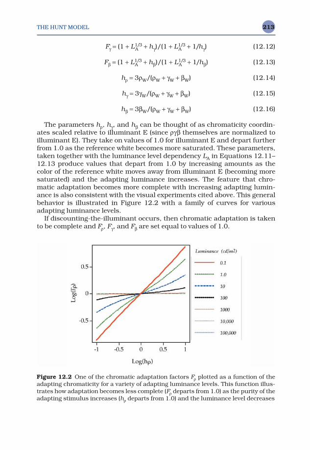
THE HUNT MODEL 213
Fγ = (1 + LA1/3 + hγ)/(1 + LA
1/3 + 1/hγ) (12.12)
Fβ = (1 + LA1/3 + hβ)/(1 + LA
1/3 + 1/hβ) (12.13)
hρ = 3ρW/(ρW + γW + βW) (12.14)
hγ = 3γW/(ρW + γW + βW) (12.15)
hβ = 3βW/(ρW + γW + βW) (12.16)
The parameters hρ, hγ, and hβ can be thought of as chromaticity coordin-ates scaled relative to illuminant E (since ργβ themselves are normalized toilluminant E). They take on values of 1.0 for illuminant E and depart furtherfrom 1.0 as the reference white becomes more saturated. These parameters,taken together with the luminance level dependency LA in Equations 12.11–12.13 produce values that depart from 1.0 by increasing amounts as thecolor of the reference white moves away from illuminant E (becoming moresaturated) and the adapting luminance increases. The feature that chro-matic adaptation becomes more complete with increasing adapting lumin-ance is also consistent with the visual experiments cited above. This generalbehavior is illustrated in Figure 12.2 with a family of curves for variousadapting luminance levels.
If discounting-the-illuminant occurs, then chromatic adaptation is takento be complete and Fρ, Fγ, and Fβ are set equal to values of 1.0.
Figure 12.2 One of the chromatic adaptation factors Fρ plotted as a function of theadapting chromaticity for a variety of adapting luminance levels. This function illus-trates how adaptation becomes less complete (Fρ departs from 1.0) as the purity of theadapting stimulus increases (hρ departs from 1.0) and the luminance level decreases
THE HUNT MODEL214
The parameters ρD, γD, and βD are included to allow prediction of theHelson–Judd effect. This is accomplished by additive adjustments to thecone signals that are dependent upon the relationship between the lumin-ance of the background Yb, the reference white YW, and the test stimulus asgiven in Equations 12.17–12.19.
ρD = fn[(Yb/YW)FLFγ] − fn[(Yb/YW)FLFρ] (12.17)
γD = 0.0 (12.18)
βD = fn[(Yb/YW)FLFγ] − fn[(Yb/YW)FLFβ] (12.19)
The Helson–Judd effect does not occur in most typical viewing situations(Helson 1938). In such cases ρD, γD, and βD should be set equal to 0.0. Incases for which discounting-the-illuminant occurs, there is no Helson–Juddeffect and ρD, γD, and βD are forced to 0.0 since Fρ, Fγ, and Fβ are set equal to1.0. There are some situations in which it is desirable to have Fρ, Fγ, and Fβtake on their normal values while ρD, γD, and βD are set to 0.0. These includethe viewing of images projected in a darkened surround or viewed on CRTdisplays.
The last factors in the chromatic adaptation formulas (Equations 12.5–12.7) are the cone bleach factors Bρ, Bγ, and Bβ. Once again, these factors are only necessary to model visual responses over extremely large ranges in luminance level. They are formulated to model photopigment depletion(i.e., bleaching) that occurs at high luminance levels resulting in decreasedphotoreceptor output, as shown in Equations 12.20–12.22.
Bρ = 107/[107 + 5LA(ρW/100)] (12.20)
Bγ = 107/[107 + 5LA(γW/100)] (12.21)
Bβ = 107/[107 + 5LA(βW/100)] (12.22)
The cone bleaching factors are essentially 1.0 for most normal luminancelevels. As the adapting luminance LA reaches extremely high levels, thebleaching factors begin to decrease, resulting in decreased adapted coneoutput. In the limit, the bleaching factors will approach zero as the adaptingluminance approaches infinity. This would result in no cone output whenthe receptors are fully bleached (sometimes referred to as a retinal burn).Such adapting levels are truly dangerous to the observer and would causepermanent damage. However, the influence of the cone bleaching factorsdoes begin to take effect at high luminance levels that are below the thresh-old for retinal damage such as outdoors on a sunny day. In such situations,one can observe the decreased range of visual response due to ‘too muchlight’ and a typical response is to put on sunglasses. These high luminancelevels are not found in typical image reproduction applications (except, per-haps, in some original scenes).
THE HUNT MODEL 215
The adaptation formulas (Equations 12.5–12.7) are completed with theaddition of 1.0 designed to represent noise in the visual system.
If the proximal field and background differ from a gray, chromatic induc-tion is modeled by adjusting the cone signals for the reference white used inthe adaptation equations. This suggests that the state of adaptation is beinginfluenced by the local color of the proximal field and background in addi-tion to the color of the reference white. This type of modeling is completelyconsistent with observed visual phenomena. Hunt (1991b) has suggestedone algorithm for calculating adjusted reference white signals ρ′W, γ ′W, and β′Wfrom the cone responses for the background ρb, γb, and βb, and proximal fieldρp, γp, and βp, given in Equations 12.23–12.28.
(12.23)
(12.24)
(12.25)
pρ = (ρp/ρb) (12.26)
pγ = (γp/γb) (12.27)
pγ = (γp/γb) (12.28)
Values of p in Equations 12.23–12.25 are taken to be between 0 and −1when simultaneous contrast occurs and between 0 and +1 when assimila-tion occurs. In most practical applications, the background and proximalfield are assumed to be achromatic and adjustments such as those given inEquations 12.23–12.25 are not used.
Now that the adapted cone signals ρa, γa, and βa are available, it is possibleto move onward to the opponent responses and color appearance correlates.The rod signals and their adaptation will be treated at the point they areincorporated in the achromatic response.
12.4 OPPONENT COLOR DIMENSIONS
Given the adapted cone signals ρa, γa, and βa, opponent-type visual responsesare calculated in a very simple manner as shown in Equations 12.29–12.32.
Aa = 2ρa + γa + (1/20)βa − 3.05 + 1 (12.29)
C1 = ρa − γa (12.30)
′ =− + +
+ + −β
β β β
β βW
W[( ) ( )/ ]
[( ) ( )/ ]
/
/
1 1
1 1
1 2
1 2
p p p p
p p p p
′ =− + +
+ + −γ
γ γ γ
γ γW
W[( ) ( )/ ]
[( ) ( )/ ]
/
/
1 1
1 1
1 2
1 2
p p p p
p p p p
′ =− + +
+ + −ρ
ρ ρ ρ
ρ ρW
W[( ) ( )/ ]
[( ) ( )/ ]
/
/
1 1
1 1
1 2
1 2
p p p p
p p p p
THE HUNT MODEL216
C2 = γa − βa (12.31)
C3 = βa − ρa (12.32)
The achromatic post-adaptation signal Aa is calculated by summing thecone responses with weights that represent their relative population in theretina. The subtraction of 3.05 and the addition of 1.0 represent removal ofthe earlier noise components followed by the addition of new noise. The threecolor difference signals C1, C2, and C3, represent all of the possible chromaticopponent signals that could be produced in the retina. These may or may nothave direct physiological correlates, but they are convenient formulationsand used to construct more traditional opponent responses as describedbelow.
12.5 HUE
Hue angle in the Hunt color appearance model is calculated just as it is inother models once red–green and yellow–blue opponent dimensions arespecified as appropriate combinations of the color difference signals des-cribed in Equations 12.30–12.32. Hue angle hs is calculated using Equation12.33.
(12.33)
Given the hue angle hs, a hue quadrature value H, is calculated by inter-polation between specified hue angles for the unique hues with adjustmentof an eccentricity factor es. The interpolating function is given by Equa-tion 12.34.
(12.34)
H1 is defined as 0, 100, 200, or 300 based on whether red, yellow, green, or blue, respectively, is the unique hue with the hue angle nearest to andless than that of the test sample. The values of h1 and e1 are taken fromTable 12.2 as the values for the unique hue having the nearest lower value ofhs while h2 and e2 are taken as the values of the unique hue with the nearesthigher value of hs.
Hue composition HC is calculated directly from the hue quadrature just asit was in the Nayatani et al. model described in Chapter 11. Hue compositionis expressed as percentages of two unique hues that describe the composi-tion of the test stimulus hue.
Finally, an eccentricity factor es must be calculated for the test stimulus tobe used in further calculations of appearance correlates. This is accomplished
H Hh h e
h h e h h es
s s= +
−− + −1
1 1
1 1 2 2
100[( )/ ][( )/ ( )/ ]
hC C
C Cs =−
−
−tan
( / )( )/ .( / )
1 2 3
1 2
1 2 4 511
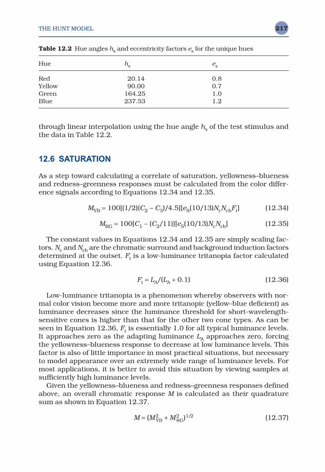
THE HUNT MODEL 217
through linear interpolation using the hue angle hs of the test stimulus andthe data in Table 12.2.
12.6 SATURATION
As a step toward calculating a correlate of saturation, yellowness–bluenessand redness–greenness responses must be calculated from the color differ-ence signals according to Equations 12.34 and 12.35.
MYB = 100[(1/2)(C2 − C3)/4.5][eS(10/13)NcNcbFt] (12.34)
MRG = 100[C1 − (C2/11)][eS(10/13)NcNcb] (12.35)
The constant values in Equations 12.34 and 12.35 are simply scaling fac-tors. Nc and Ncb are the chromatic surround and background induction factorsdetermined at the outset. Ft is a low-luminance tritanopia factor calculatedusing Equation 12.36.
Ft = LA/(LA + 0.1) (12.36)
Low-luminance tritanopia is a phenomenon whereby observers with nor-mal color vision become more and more tritanopic (yellow–blue deficient) asluminance decreases since the luminance threshold for short-wavelength-sensitive cones is higher than that for the other two cone types. As can beseen in Equation 12.36, Ft is essentially 1.0 for all typical luminance levels.It approaches zero as the adapting luminance LA approaches zero, forcingthe yellowness–blueness response to decrease at low luminance levels. Thisfactor is also of little importance in most practical situations, but necessaryto model appearance over an extremely wide range of luminance levels. Formost applications, it is better to avoid this situation by viewing samples atsufficiently high luminance levels.
Given the yellowness–blueness and redness–greenness responses definedabove, an overall chromatic response M is calculated as their quadraturesum as shown in Equation 12.37.
M = (M2YB + M2
RG)1/2 (12.37)
Table 12.2 Hue angles hs and eccentricity factors es for the unique hues
Hue hs es
Red 20.14 0.8Yellow 90.00 0.7Green 164.25 1.0Blue 237.53 1.2
THE HUNT MODEL218
Finally, saturation s is calculated from M and the adapted cone signalsusing Equation 12.38. This calculation follows the definition of saturation(colorfulness of stimulus relative to its own brightness) if one takes the over-all chromatic response M to approximate colorfulness, and the sum of theadapted cone signals in the denominator of Equation 12.38 to approximatethe stimulus brightness.
s = 50M/(ρa + γa + βa) (12.38)
12.7 BRIGHTNESS
Further development of the achromatic signals is required to derive corre-lates of brightness and lightness. Recall that the Hunt color appearancemodel is designed to function over the full range of luminance levels. In sodoing, it must also incorporate the response of the rod photoreceptors,which are active at low luminance levels. The rod response is incorporatedinto the achromatic signal (which in turn impacts the predictors of chromaand colorfulness). The rod response after adaptation AS is given by Equation12.39. The subscript S is derived from the word scotopic, which is used to describe vision at the low luminance levels for which the rod responsedominates.
AS = 3.05BS[ fn(FLSS/SW)] + 0.3 (12.39)
The formulation of the adapted rod signal is analogous to the formulationof the adapted cone signals described previously (Equations 12.5–12.7). Atits heart is a von Kries-type scaling of the scotopic response for the stimulusS, by that for the reference white SW. FLS is a scotopic luminance level adapta-tion factor given by Equations 12.40 and 12.41 that is similar to the coneluminance adaptation factor.
FLS = 3800j2(5LAS/2.26) + 0.2(1 − j2)4(5LAS/2.26)1/6 (12.40)
j = 0.00001/[(5LAS/2.26) + 0.00001] (12.41)
The same nonlinear photoreceptor response function fn(), is also used forthe scotopic response (see Equation 12.8). The value 3.05 is simply a scalingfactor and the noise level of 0.3 (rather than 1.0) is chosen since the rods aremore sensitive than cones. Finally, a rod bleaching factor BS is added toreduce the rod contribution to the overall color appearance as luminancelevel increases and the rods become less active. This factor is calculatedusing Equation 12.42. Examination of the rod bleaching factor in com-parison with the cone bleaching factors given in Equations 12.20–12.22shows that the rods will become saturated and their response will becomesignificantly decreased at much lower luminance levels.
THE HUNT MODEL 219
BS = 0.5/{1 + 0.3[(5LAS/2.26)(S/SW)]0.3} + 0.5/{1 + 5[5LAS/2.26]}(12.42)
Given the achromatic cone signal Aa (Equation 12.29), the adapted sco-topic signal AS (Equation 12.39), and the brightness background inductionfactor determined at the outset, an overall achromatic signal A is calculatedusing Equation 12.43.
A = Nbb[Aa − 1 + AS − 0.3 + (12 + 0.32)1/2] (12.43)
All the constant values in Equation 12.43 represent removal of the earliernoise terms and then their reintroduction through quadrature summation.
The achromatic signal A is then combined with the overall chromatic signal M to calculate a correlate of brightness Q using Equation 12.44.
Q = {7[A + (M/100)] }0.6N1 − N2 (12.44)
The correlate of brightness Q depends on both the achromatic A and chro-matic M responses in order to appropriately model the Helmholtz–Kohlrausch effect. Equation 12.44 also includes two terms N1 and N2 thataccount for the effects of surround on perceived brightness (e.g., Stevenseffect and Bartleson–Breneman results discussed in Chapter 6). Theseterms are calculated from the achromatic signal for the reference white AWand the brightness surround induction factor Nb (also determined at the out-set), through Equations 12.45 and 12.46.
N1 = (7AW)0.5/(5.33Nb0.13) (12.45)
N2 = 7AWNb0.362/200 (12.46)
Note that since the achromatic signal for the reference white AW isrequired, it is necessary to carry through all of the model calculationsdescribed above for the reference white in addition to the test stimulus. Thebrightness of the reference white QW, must also be calculated for use in laterequations.
Another form of brightness, referred to as whiteness–blackness QWB, canbe calculated in the Hunt model. This is a bipolar value similar to the Q valuein the Nayatani et al. model that illustrates that black objects look darkerand white objects look brighter as the adapting luminance level increases(another way to state the Stevens effect). QWB is calculated according toEquation 12.47 using the brightness of the background (which also must becalculated through the model).
QWB = 20(Q0.7 − Qb0.7) (12.47)
THE HUNT MODEL220
12.8 LIGHTNESS
Given the brightness of the test stimulus Q and the brightness of the refer-ence white QW the Hunt color appearance model correlate of lightness J iscalculated as shown in Equation 12.48.
J = 100(Q/QW)z (12.48)
This formulation for lightness follows the CIE definition that lightness isthe brightness of the test stimulus relative to the brightness of a white. Thisratio is raised to a power z that models the influence of the background relative luminance on perceived lightness according to Equation 12.49. Theexponent z increases as the background becomes lighter, indicating thatdark test stimuli will appear relatively more dark on a light background than they would on a dark background. This follows the commonly observedphenomenon of simultaneous lightness contrast.
z = 1 + (Yb/YW)1/2 (12.49)
12.9 CHROMA
The Hunt color appearance model correlate of chroma C94 is determinedfrom saturation s and the relative brightness (approximately lightness) fol-lowing the general definitions given in Chapter 4 that indicate chroma can berepresented as saturation multiplied by lightness. The precise formulation isgiven in Equation 12.50.
(12.50)
Equation 12.50 illustrates that chroma depends on the relative brightnessof the stimulus Q/QW and on the relative luminance of the backgroundYb/YW. The formulation for chroma given by Equation 12.50 was derivedempirically based upon the results of a series of appearance scaling experi-ments (Hunt 1994, Hunt and Luo 1994).
12.10 COLORFULNESS
Given chroma, colorfulness can be determined by factoring in the brightness(or at least the luminance level). This is accomplished in the Hunt colorappearance model by multiplying chroma C94 by the luminance level adapta-tion factor FL (Equation 12.9) raised to a power of 0.15 as shown in Equa-tion 12.51.
M94 = FL0.15C94 (12.51)
C s Q QWY Y Y Yb W b W
940 692 44 1 64 0 29= = −. ( / ) ( . . ). / /
THE HUNT MODEL 221
Thus M94 is the colorfulness correlate for the Hunt color appearance model.It was also derived empirically through analysis of visual scaling results.
12.11 INVERSE MODEL
Unfortunately, because of its complexity, the complete Hunt color appear-ance model cannot be analytically inverted. It is an even more severe prob-lem if one has only lightness, chroma, and hue correlates to start from,which is often the case. Many applications, particularly image reproduction,require a color appearance model to be used in both forward and reversedirections. Thus the lack of an analytical inverse introduces some difficultyin using the Hunt model for these applications. Hunt (1995) provides somesuggestions for how to deal with this difficulty.
In all cases, it is easier to reverse the model if all the appearance correlatesare available rather than just three. One alternative is to use the model with-out the scotopic response. This simplifies the inversion process since theintroduction of the scotopic terms into higher-level equations is one featurethat prevents analytical inversion. The predictions of the model are slightlychanged when the scotopic response is ignored, but this difference might benegligible for many applications. Hunt (1995) suggests that this technique is appropriate for reference white luminances greater than 10 cd/m2. Mostsituations in which careful judgements of color reproduction are made are atluminance levels above 10 cd/m2.
Other techniques suggested by Hunt (1995) require successive approx-imation for some parts of the reverse model. In most applications, it is simpler to use successive approximation for the whole model, iterating until appropriate output tristimulus values are obtained that produce theappearance correlates that are available at the outset. This technique can beaccomplished with a technique such as a Newton–Raphson optimization,and it can be applied when only lightness, chroma, and hue are available (in fact it is the only option). While a successive approximation techniquecan be very time consuming for large data sets, such as images, this drawback is overcome by using the forward and reverse models to buildthree-dimensional look-up tables, which are then used with an interpolationtechnique to convert image data. Then, the time-consuming model inver-sion process need only be performed once for each viewing condition in order to build the look-up table. This approach helps, but if users want tovary the viewing conditions, they must wait a long time for the look-up table to be recalculated before an image can be processed. The delay might be significant enough to render the full Hunt model impractical for someapplications.
In applying the model, it is often useful to consider its implementation as asimple step-by-step process. Thus the steps required to implement themodel (and in reverse, as possible, to invert it) are given below.
THE HUNT MODEL222
1. Obtain physical data and decide on other parameters.2. Calculate cone excitations ργβ for the various stimulus fields.3. Calculate relative cone excitations.4. Calculate the luminance-level adaptation factor FL.5. Calculate chromatic adaptation factors Fρ, Fγ, Fβ.6. Calculate Helson–Judd effect parameters ρD, γD, βD.7. Calculate adapted cone signals ρa, γa, βa.8. Calculate achromatic Aa and color difference C1, C2, C3 signals.9. Calculate hue angle hS.
10. Calculate hue quadrature H.11. Calculate hue composition HC.12. Calculate eccentricity factor eS.13. Calculate low-luminance tritanopia factor Ft.14. Calculate chromatic responses M and saturation s.15. Calculate scotopic luminance adaptation factor FLS.16. Calculate scotopic response AS.17. Calculate complete achromatic response A.18. Calculate brightness Q.19. Calculate lightness J.20. Calculate chroma C94.21. Calculate colorfulness M94.22. Calculate whiteness–blackness QWB.
The Hunt color appearance model is the most complex to implement of the traditional color appearance models described in this book. There are acouple of implementation techniques that can simplify program develop-ment and greatly improve computational speed. One is to go through themodel and calculate all the parameters that are constant for a given set ofviewing conditions first in a precalculation routine. This can be applied to allof the adaptation factors, correlates for the reference white, etc. Then, theseprecalculated data can be used for the remaining data calculations ratherthan recalculating the values for each stimulus (or pixel in an image). Thiscan be particularly useful when transforming image data (or look-up tables)that might require the model calculations to be completed millions of times.Secondly, many of the equations, for example the achromatic response A (Equation 12.43), include operations on constants. The number of com-putations can be reduced by combining all of these constants into a singlenumber first (some compilers will do this for you). For example, the −1 − 0.3+ (12 + 0.32)1/2 can be converted into simply 1.044.
12.12 PHENOMENA PREDICTED
As stated previously, the Hunt color appearance model is the most extens-ive and complete color appearance model available. It has the following features:
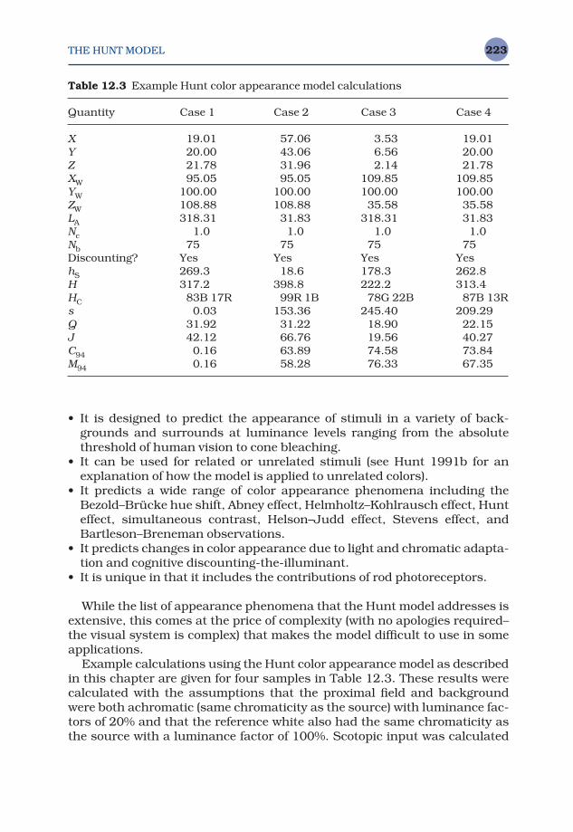
THE HUNT MODEL 223
• It is designed to predict the appearance of stimuli in a variety of back-grounds and surrounds at luminance levels ranging from the absolutethreshold of human vision to cone bleaching.
• It can be used for related or unrelated stimuli (see Hunt 1991b for anexplanation of how the model is applied to unrelated colors).
• It predicts a wide range of color appearance phenomena including theBezold–Brücke hue shift, Abney effect, Helmholtz–Kohlrausch effect, Hunteffect, simultaneous contrast, Helson–Judd effect, Stevens effect, andBartleson–Breneman observations.
• It predicts changes in color appearance due to light and chromatic adapta-tion and cognitive discounting-the-illuminant.
• It is unique in that it includes the contributions of rod photoreceptors.
While the list of appearance phenomena that the Hunt model addresses isextensive, this comes at the price of complexity (with no apologies required–the visual system is complex) that makes the model difficult to use in someapplications.
Example calculations using the Hunt color appearance model as describedin this chapter are given for four samples in Table 12.3. These results werecalculated with the assumptions that the proximal field and backgroundwere both achromatic (same chromaticity as the source) with luminance fac-tors of 20% and that the reference white also had the same chromaticity asthe source with a luminance factor of 100%. Scotopic input was calculated
Table 12.3 Example Hunt color appearance model calculations
Quantity Case 1 Case 2 Case 3 Case 4
X 19.01 57.06 3.53 19.01Y 20.00 43.06 6.56 20.00Z 21.78 31.96 2.14 21.78XW 95.05 95.05 109.85 109.85YW 100.00 100.00 100.00 100.00ZW 108.88 108.88 35.58 35.58LA 318.31 31.83 318.31 31.83Nc 1.0 1.0 1.0 1.0Nb 75 75 75 75Discounting? Yes Yes Yes YeshS 269.3 18.6 178.3 262.8H 317.2 398.8 222.2 313.4HC 83B 17R 99R 1B 78G 22B 87B 13Rs 0.03 153.36 245.40 209.29Q 31.92 31.22 18.90 22.15J 42.12 66.76 19.56 40.27C94 0.16 63.89 74.58 73.84M94 0.16 58.28 76.33 67.35
THE HUNT MODEL224
using the approximate equations described in this chapter. The Helson–Judd parameters were always set to 0.0.
12.13 WHY NOT USE JUST THE HUNT MODEL?
Given that the Hunt color appearance model seems to be able to do every-thing that anyone could ever want a color appearance model to do, why isn’tit adopted as the single standard color appearance model for all applica-tions? The main reason could be the very fact that it is so complete. In itscompleteness also lies its complexity. Its complexity makes application ofthe Hunt model to practical situations range from difficult to impossible.However, the complexity of the Hunt model also allows it to be extremelyflexible. As will be seen in Chapter 15, the Hunt model is generally capable ofmaking accurate predictions for a wide range of visual experiments. This isbecause the model is flexible enough to be adjusted to the required situ-ations. Clearly, this flexibility and general accuracy are great features of theHunt model. However, often it is not possible to know just how to apply theHunt model (i.e., to decide on the appropriate parameter values) until afterthe visual data have been obtained. In other cases, the parameters actuallyneed to be optimized, not just chosen, for the particular viewing situation.This is not a problem if the resources are available to derive the optimizedparameters. However, when such resources are not available and the Huntmodel must be used ‘as is’ with the recommended parameters, the modelcan perform extremely poorly (see Chapter 15). This is because the nominalparameters used for a given viewing condition are being used to makespecific predictions of phenomena that may or may not be important in thatsituation. After the fact, adjustments can be made, but that might be toolate. Thus, if it is not possible to optimize (or optimally choose) the imple-mentation of the Hunt model, its precision might result in predictions thatare worse than much simpler models for some applications.
Other negative aspects that counteract the positive features of the Huntcolor appearance model are that it cannot be easily inverted and that it iscomputationally expensive, difficult to implement, and requires significantuser knowledge to use consistently. The Hunt model also uses functionswith additive offsets to predict contrast changes due to variation in surroundrelative luminance. These functions can result in predicted correspondingcolors with negative tristimulus values for some changes in surround.
Color Appearance Models Second Edition M. D. Fairchild © 2005 John Wiley & Sons, LtdISBN: 0-470-01216-1 (HB)
13The RLAB Model
This chapter completes the discussion of some of the most widely used his-torical (pre-CIE models) color appearance models with a description of theRLAB model. While the Hunt and Nayatani et al. models discussed in thepreceding chapters are designed to predict all of the perceptual attributes ofcolor appearance for a wide range of viewing conditions, the RLAB model wasdesigned with other considerations. RLAB was developed with the intent ofproducing a simple color appearance model capable of predicting the mostsignificant appearance phenomena in practical applications. RLAB wasdeveloped with cross-media image reproduction as its target application andit has been effectively applied to such situations.
13.1 OBJECTIVES AND APPROACH
The RLAB color appearance model evolved from studies of chromatic adapta-tion (Fairchild 1990), chromatic adaptation modeling (Fairchild 1991a,b),fundamental CIE colorimetry (CIE 1986), and practical implications in cross-media image reproduction (Fairchild and Berns 1993, Fairchild 1994b). Thestarting point for RLAB is the CIELAB color space. While CIELAB can be usedas an approximate color appearance model, it does have significant limita-tions. These include an inaccurate chromatic adaptation transform, noluminance-level dependency, no surround dependency, and no distinctionfor when discounting-the-illuminant occurs. While CIELAB has other limita-tions as a color appearance model, these are the most important for manypractical applications. Thus, RLAB was designed to build on the positiveaspects of CIELAB, and, by making additions, to address its limitations.
CIELAB provides good perceptual uniformity with respect to color appear-ance for average daylight illuminants. This is illustrated by the spacing ofconstant hue and chroma contours from the Munsell Book of Color shown inFigure 13.1. The contours plotted in Figure 13.1 are as good as, and in some

THE RLAB MODEL226
Figure 13.1 Contours of constant Munsell hue and chroma plotted in the CIELAB/RLAB color space at (a) value 3, (b) value 5, and (c) value 7

THE RLAB MODEL 227
cases better, than those produced using any other color appearance model.However, due to CIELAB’s ‘wrong von Kries’ chromatic adaptation trans-form, the good perceptual spacing of CIELAB quickly degrades as the illum-inant moves away from average daylight. The concept of RLAB is to takeadvantage of the good spacing under daylight and familiarity of the CIELABspace while improving its applicability to non-daylight illuminants. This wasaccomplished by defining a reference set of viewing conditions (IlluminantD65, 318 cd/m2, average surround, discounting the illuminant) for whichthe CIELAB space is used, and then using a more accurate chromatic adapta-tion transform (Fairchild 1991b, 1994b, 1996) to determine correspondingcolors between the test viewing conditions and the reference viewing condi-tions. Thus, test tristimulus values are first transformed into correspondingcolors under the reference viewing condition, and then a modified CIELABspace is used to describe appearance correlates.
In addition, the compressive nonlinearity (cube root) of the CIELAB space is adapted to become a function of the surround relative luminance.This allows the prediction of decreases in perceived image contrast as the surround becomes darker as suggested in the work of Bartleson (1975).The improved chromatic adaptation transform and the surround depend-ence enhance CIELAB in the two areas that are most critical in image reproduction.
RLAB was designed to include predictors of only relative color appearanceattributes. Thus it can be used to calculate correlates of lightness, chroma,saturation, and hue, but it cannot be used to predict brightness or colorful-ness. This limitation was imposed to keep the model as simple as possibleand because the prediction of brightness and colorfulnes have little import-ance in most image reproduction applications.
The fact that RLAB is based on the CIELAB space has benefit in additionto familiarity. Since the RLAB spacing is essentially identical to CIELABspacing, color difference formulas such as CIELAB ∆E*ab (CIE 1986), CMC(Clarke et al. 1984), and CIE94 (CIE 1995b) can be used with results that aresimilar to those obtained when using CIELAB alone under average daylightilluminants.
A more detailed description of the RLAB model, as presented in this chap-ter, can be found in Fairchild (1996).
13.2 INPUT DATA
Input data for the RLAB model include the relative tristimulus values of thetest stimulus (XYZ ) and the white point (XnYnZn), the absolute luminance ofa white object in the scene in cd/m2, the relative luminance of the surround(dark, dim, average), and a decision on whether discounting-the-illuminantis taking place. The surround relative luminance is generally taken to beaverage for reflection prints, dim for CRT displays or televisions, and dark forprojected transparencies under the assumption that these media are being
THE RLAB MODEL228
viewed in their typical environments. The surround is not directly tied to themedium. Thus it is certainly possible to have reflection prints viewed in adark surround and projected transparencies viewed in an average surround.Discounting-the-illuminant is assumed to occur for object color stimulisuch as prints and not to occur for emissive displays such as CRTs. Inter-mediate levels of discounting-the-illuminant are likely to occur in some situations such as the viewing of projected transparencies.
13.3 ADAPTATION MODEL
The following equations describe the chromatic adaptation model built into RLAB. It is based on the model of incomplete chromatic adaptationdescribed by Fairchild (1991b) and later modified (Fairchild 1994b, 1996).This transformation is also discussed in Chapter 9. One begins with a con-version from CIE tristimulus values (Y = 100 for white) to fundamental tri-stimulus values as illustrated in Equations 13.1 and 13.2. All CIE tristimulusvalues are normally calculated using the CIE 1931 Standard ColorimetricObserver (2°). The transformation must also be completed for the tristimulusvalues of the adapting stimulus.
(13.1)
(13.2)
The transformation to cone responses is the same as that used in theHunt model. Matrix M is normalized such that the tristimulus values for the equal-energy illuminant (X = Y = Z = 100) produce equal cone responses(L = M = S = 100). The next step is calculation of the A matrix that is used tomodel the chromatic adaptation transformation.
(13.3)
The A matrix represents von Kries adaptation coefficients that are appliedto the cone responses for the test stimulus (LMS). The von Kries-type coef-ficients are calculated using Equations 13.4–13.12.
(13.4)ap D p
LLL L=
+ −( . )1 0
n
A =a
aa
L
M
S
0 0 0 00 0 0 00 0 0 0
. .. .. .
M =−
−0 3897 0 6890 0 07870 2298 1 1834 0 04640 0 0 0 1 0000
. . .
. . .
. . .
LMS
XYZ
= M
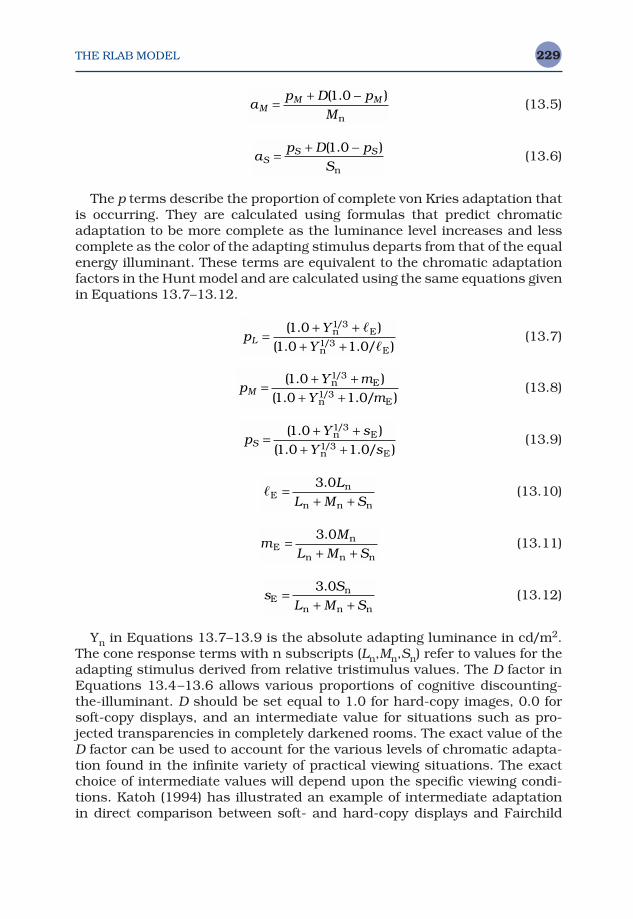
THE RLAB MODEL 229
(13.5)
(13.6)
The p terms describe the proportion of complete von Kries adaptation thatis occurring. They are calculated using formulas that predict chromaticadaptation to be more complete as the luminance level increases and lesscomplete as the color of the adapting stimulus departs from that of the equalenergy illuminant. These terms are equivalent to the chromatic adaptationfactors in the Hunt model and are calculated using the same equations givenin Equations 13.7–13.12.
(13.7)
(13.8)
(13.9)
(13.10)
(13.11)
(13.12)
Yn in Equations 13.7–13.9 is the absolute adapting luminance in cd/m2.The cone response terms with n subscripts (Ln,Mn,Sn) refer to values for theadapting stimulus derived from relative tristimulus values. The D factor inEquations 13.4–13.6 allows various proportions of cognitive discounting-the-illuminant. D should be set equal to 1.0 for hard-copy images, 0.0 forsoft-copy displays, and an intermediate value for situations such as pro-jected transparencies in completely darkened rooms. The exact value of theD factor can be used to account for the various levels of chromatic adapta-tion found in the infinite variety of practical viewing situations. The exactchoice of intermediate values will depend upon the specific viewing condi-tions. Katoh (1994) has illustrated an example of intermediate adaptation in direct comparison between soft- and hard-copy displays and Fairchild
sS
L M SEn
n n n=
+ +3 0.
mM
L M SEn
n n n=
+ +3 0.
�E
n
n n n=
+ +3 0. L
L M S
pY s
Y sS =+ +
+ +( . )
( . . / )
/
/
1 01 0 1 0
1 3
1 3n E
n E
pY m
Y mM =+ +
+ +( . )
( . . / )
/
/
1 01 0 1 0
1 3
1 3n E
n E
pY
YL =+ +
+ +( . )
( . . / )
/
/
1 01 0 1 0
1 3
1 3n E
n E
�
�
ap D p
SSS S=
+ −( . )1 0
n
ap D p
MMM M=
+ −( . )1 0
n
THE RLAB MODEL230
(1992a) has reported a case of intermediate discounting-the-illuminant for a soft-copy display. When no visual data are available and an intermedi-ate value is necessary, a value of 0.5 should be chosen and refined withexperience.
Note that if discounting-the-illuminant occurs and D is set equal to 1.0,then the adaptation coefficients described in Equations 13.4–13.6 reduce tothe reciprocals of the adapting cone excitations exactly as would be imple-mented in a simple von Kries model.
After the A matrix is calculated, the tristimulus values for a stimulus color are converted to corresponding tristimulus values under the referenceviewing conditions using Equations 13.13 and 13.14.
(13.13)
(13.14)
The R matrix represents the inverse of the M and A matrices for the refer-ence viewing conditions (M−1A−1) plus a normalization, discussed below, thatare always constant and can therefore be precalculated. Thus Equation13.13 represents a modified von Kries chromatic adaptation transform thatconverts test stimulus tristimulus values to corresponding colors under theRLAB reference viewing conditions (Illuminant D65, 318 cd/m2, discounting-the-illuminant). The next step is to use these reference tristimulus values tocalculate modified CIELAB appearance correlates as shown in the followingsections.
13.4 OPPONENT COLOR DIMENSIONS
Opponent-type responses in RLAB are calculated using Equations 13.15–13.17.
LR = 100(Yref)σ (13.15)
aR = 430[(Xref)σ − (Yref)
σ] (13.16)
bR = 170[(Yref)σ − (Zref)
σ] (13.17)
LR represents an achromatic response analogous to CIELAB L*. The red-green chromatic response is given by aR (analogous to CIELAB a*) and theyellow–blue chromatic response is given by bR (analogous to CIELAB b*).
R =−1 9569 1 1882 0 2313
0 3612 0 6388 0 00 0 0 0 1 0000
. . .
. . .
. . .
XYZ
XYZ
ref
ref
ref
= RAM
THE RLAB MODEL 231
Recall that, for the reference viewing conditions, the RLAB coordinates arenearly identical to CIELAB coordinates. They are not identical becauseEquations 13.15–13.17 have been simplified from the CIELAB equations forcomputational efficiency. The conditional compressive nonlinearities (i.e.,different functions for low tristimulus values) of CIELAB have been replacedwith simple power functions. This results in the exponents and the scalingfactors being slightly different than the CIELAB equations. Fairchild (1996)provides more details on these differences. It is also worth noting that thedivisions by the tristimulus values of the white point that are incorporated inthe CIELAB equations are missing from Equations 13.15–13.17. This isbecause these normalizations are constant in the RLAB model and they havebeen built into the R matrix given in Equation 13.14.
The exponents in Equations 13.15–13.17 vary, depending on the relativeluminance of the surround. For an average surround σ = 1/2.3, for a dimsurround σ = 1/2.9, and for a dark surround σ = 1/3.5. The ratios of theseexponents are precisely in line with the contrast changes suggested byBartleson (1975) and Hunt (1995) for image reproduction. More detail on theexponents can be found in Fairchild (1995b). As a nominal definition, a darksurround is considered essentially zero luminance, a dim surround is con-sidered a relative luminance less than 20% of white in the image, and anaverage surround is considered a relative luminance equal to or greater than20% of the image white. The precise nature and magnitude of the contrastchanges required for various changes in image viewing conditions is still atopic of research and debate. Thus it is best to use these parameters withsome flexibility. In some applications, it might be desired to use intermediatevalues for the exponents in order to model less severe changes in surroundrelative luminance. This requires no more than a substitution in the RLABequations since they do not include the conditional functions that are foundin the CIELAB equations. In addition, it might be desirable to use differentexponents on the lightness LR dimension than on the chromatic aR and bR
dimensions. This can also be easily accommodated. The equations havebeen formulated as simple power functions to encourage the use of differentexponents, which might be more appropriate than the nominal exponentsfor particular, practical viewing conditions.
Figure 13.2 illustrates the effect of changing the exponents. The left image(a) is a typical printed reproduction. The other two images (b and c) show thechange in contrast necessary to reproduce the same appearance if the imagewere viewed in a dark surround. Note the increase in contrast required forviewing in a dark surround. In the middle image (b), the adjustment hasbeen made on lightness contrast only. In the right image (c), the surroundcompensation has been applied to the chromatic dimensions, as well as tolightness. The right image (c) is similar to the reproduction that would beproduced in a simple photographic system (since the contrast of all threefilm layers must be changed together) and is generally preferable. Note, how-ever, that inter-image effects in real film could be used to compensate forsome of the increase in saturation with contrast. The images in Figure 13.2
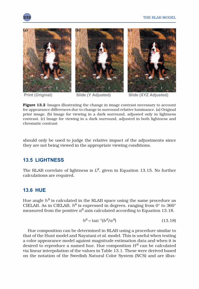
THE RLAB MODEL232
should only be used to judge the relative impact of the adjustments sincethey are not being viewed in the appropriate viewing conditions.
13.5 LIGHTNESS
The RLAB correlate of lightness is LR, given in Equation 13.15. No furthercalculations are required.
13.6 HUE
Hue angle hR is calculated in the RLAB space using the same procedure asCIELAB. As in CIELAB, hR is expressed in degrees, ranging from 0° to 360°measured from the positive aR axis calculated according to Equation 13.18.
hR = tan−1(bR/aR) (13.18)
Hue composition can be determined in RLAB using a procedure similar tothat of the Hunt model and Nayatani et al. model. This is useful when testinga color appearance model against magnitude estimation data and when it isdesired to reproduce a named hue. Hue composition HR can be calculatedvia linear interpolation of the values in Table 13.1. These were derived basedon the notation of the Swedish Natural Color System (NCS) and are illus-
Figure 13.2 Images illustrating the change in image contrast necessary to accountfor appearance differences due to change in surround relative luminance. (a) Originalprint image. (b) Image for viewing in a dark surround, adjusted only in lightness contrast. (c) Image for viewing in a dark surround, adjusted in both lightness andchromatic contrast

THE RLAB MODEL 233
trated in Figure 13.3, which is a useful visualization of the loci of the uniquehues since they do not correspond to the principal axes of the color space.The unique hue locations are the same as those in the CIELAB space underonly the reference conditions. Example hue composition values are listed inTable 13.1 in italics.
Table 13.1 Data for conversion from hue angle to hue composition
hR R B G Y HR
24 100 0 0 0 R90 0 0 0 100 Y
162 0 0 100 0 G180 0 21.4 78.6 0 B79G246 0 100 0 0 B270 17.4 82.6 0 0 R83B
0 82.6 17.4 0 0 R17B24 100 0 0 0 R
Figure 13.3 Illustration of the hue angles of the perceptually unique hues in theRLAB color space
THE RLAB MODEL234
13.7 CHROMA
RLAB chroma CR is calculated in the same way as CIELAB chroma, asshown in Equation 13.19.
(13.19)
13.8 SATURATION
In some applications, such as the image color manipulation required forgamut mapping, it might be desirable to change colors along lines of con-stant saturation rather than constant chroma. Wolski, Allebach, and Bouman(1994) have proposed such a technique and Montag and Fairchild (1996,1997) also describe such situations. Saturation is defined as colorfulnessrelative to brightness, chroma is defined as colorfulness relative to the bright-ness of a white, and lightness is defined as brightness relative to the bright-ness of a white. Therefore, saturation can be defined as chroma relative tolightness. Chroma CR and lightness LR are already defined in RLAB; thussaturation sR is defined as shown in Equation 13.20.
sR = CR/LR (13.20)
It is of interest to note that a progression along a line of constant satura-tion is the series of colors that can be observed when an object is viewed inever deepening shadows. This could be why transformations along lines ofconstant saturation, rather than chroma, are sometimes useful in gamutmapping applications.
13.9 INVERSE MODEL
Since the RLAB model was designed with image reproduction applications inmind, computational efficiency and simple inversion were considered ofsignificant importance. Thus the RLAB model is very easy to invert andrequires a minimum of calculations. A step-by-step procedure for imple-menting the RLAB model is given below.
Step 1. Obtain the colorimetric data for the test and adapting stimuli and theabsolute luminance of the adapting stimulus. Decide on the discounting-the-illuminant factor and the exponent (based on surround relative luminance).Step 2. Calculate the chromatic adaptation matrix A.Step 3. Calculate the reference tristimulus values.Step 4. Calculate the RLAB parameters LR, aR, and bR.
C a bR R R= +( ) ( )2 2
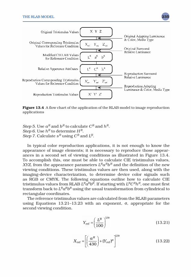
THE RLAB MODEL 235
Step 5. Use aR and bR to calculate CR and hR.Step 6. Use hR to determine H R.Step 7. Calculate sR using CR and LR.
In typical color reproduction applications, it is not enough to know theappearance of image elements; it is necessary to reproduce those appear-ances in a second set of viewing conditions as illustrated in Figure 13.4. To accomplish this, one must be able to calculate CIE tristimulus values,XYZ, from the appearance parameters LRaRbR and the definition of the new viewing conditions. These tristimulus values are then used, along with theimaging-device characterization, to determine device color signals such as RGB or CMYK. The following equations outline how to calculate CIE tristimulus values from RLAB LRaRbR. If starting with LRCRhR, one must firsttransform back to LRaRbR using the usual transformation from cylindrical torectangular coordinates.
The reference tristimulus values are calculated from the RLAB parametersusing Equations 13.21–13.23 with an exponent, σ, appropriate for the second viewing condition.
(13.21)
(13.22)Xa
YR
ref ref=
+
430
1
( )/
σσ
YLR
ref =
100
1/σ
Figure 13.4 A flow chart of the application of the RLAB model to image reproductionapplications

THE RLAB MODEL236
(13.23)
The reference tristimulus values are then transformed to tristimulus val-ues for the second viewing condition using Equation 13.24 with an A matrixcalculated for the second viewing conditions.
(13.24)
13.10 PHENOMENA PREDICTED
The RLAB model provides correlates for relative color appearance attributesonly (lightness, chroma, saturation, and hue). It cannot be used to predictbrightness and colorfulness. This limitation is of little practical importancefor image reproduction since there are few applications in which brightnessand colorfulness are required. RLAB includes a chromatic adaptation trans-form with a parameter for discounting-the-illuminant, and predicts incom-plete chromatic adaptation to certain stimuli (e.g., RLAB correctly predictsthat a CRT display with a D50 white point will retain a yellowish appear-ance). It also includes variable exponents, σ, that modulate image contrastas a function of the surround relative luminance. These are the most import-ant color appearance phenomena for cross-media image reproduction applications. If it is necessary to predict absolute appearance attributes (i.e.,brightness and colorfulness) or more unusual appearance phenomena, thenmore extensive appearance models such as the Nayatani et al. and Huntmodels described in preceding chapters should be considered.
Example calculations for the RLAB color appearance model are given inTable 13.2.
13.11 WHY NOT USE JUST THE RLAB MODEL?
The RLAB model is simple, straightforward, easily invertible, and has beenfound to be as accurate as, or better than, more complicated color appear-ance models for many practical applications. Given all of these features, whywouldn’t RLAB be considered as a recommendation for a single, universalcolor appearance model?
RLAB’s weaknesses are the same as its strengths. Since it is such a simplemodel, it is not exhaustive in its prediction of color appearance phenomena.It does not include correlates of brightness and colorfulness. It cannot beapplied over a wide range of luminance levels. It does not predict some color
XYZ
XYZ
= −( )RAM 1ref
ref
ref
Z YbR
ref ref= −
( )
/
σσ
170
1
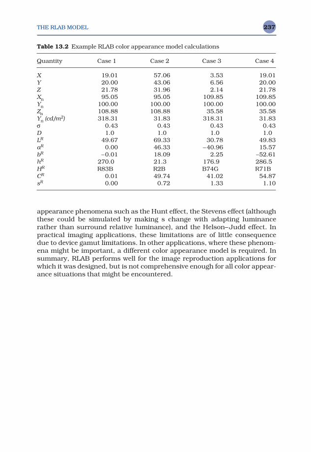
THE RLAB MODEL 237
appearance phenomena such as the Hunt effect, the Stevens effect (althoughthese could be simulated by making s change with adapting luminancerather than surround relative luminance), and the Helson–Judd effect. Inpractical imaging applications, these limitations are of little consequencedue to device gamut limitations. In other applications, where these phenom-ena might be important, a different color appearance model is required. Insummary, RLAB performs well for the image reproduction applications forwhich it was designed, but is not comprehensive enough for all color appear-ance situations that might be encountered.
Table 13.2 Example RLAB color appearance model calculations
Quantity Case 1 Case 2 Case 3 Case 4
X 19.01 57.06 3.53 19.01Y 20.00 43.06 6.56 20.00Z 21.78 31.96 2.14 21.78Xn 95.05 95.05 109.85 109.85Yn 100.00 100.00 100.00 100.00Zn 108.88 108.88 35.58 35.58Yn (cd/m2) 318.31 31.83 318.31 31.83σ 0.43 0.43 0.43 0.43D 1.0 1.0 1.0 1.0LR 49.67 69.33 30.78 49.83aR 0.00 46.33 −40.96 15.57bR −0.01 18.09 2.25 −52.61hR 270.0 21.3 176.9 286.5HR R83B R2B B74G R71BCR 0.01 49.74 41.02 54.87sR 0.00 0.72 1.33 1.10
Color Appearance Models Second Edition M. D. Fairchild © 2005 John Wiley & Sons, LtdISBN: 0-470-01216-1 (HB)
14Other Models
The preceding chapters have reviewed four of the most widely used and gen-eral color appearance models representing the evolution toward the CIECAMmodels presented in the following chapters. These and other models are con-tinually being modified and introduced. This chapter provides overviews oftwo more color appearance models — one that has been evolving for manyyears and a second that is relatively new. For various reasons discussedherein, these models are not as well suited for general application as thosedescribed in earlier chapters or the more refined CIECAM models. However,various aspects of their formulation are of interest both historically and fordevelopment of future models or applications. Thus they have been includedto appropriately cover their potential impact on the field.
14.1 OVERVIEW
The formulation of color appearance models remains an area of active, ongo-ing research. That explains why this book can only provide an overview ofthe associated problems and several approaches to solving them. It is notpossible to present a single model of color appearance that will solve allproblems if followed in a ‘cookbook’ manner. This is the ‘Holy Grail’ forresearchers in the field, but not likely to be achieved in short order. Chapters10–13 presented some of the best historically available approaches to prob-lems of color appearance specification and reproduction. Chapters 15 and16 present more recent CIE color appearance models, CIECAM97s andCIECAM02. One of those models is likely to be the most appropriate solutionfor any given application. However, one model is not likely to be the bestsolution for all applications. Since the development of color appearancemodels is an ongoing endeavor, it is important to describe other models thathave had, or are likely to have, significant impact on the field.
Two such models are described in this chapter:
OTHER MODELS 239
1. The ATD model formulated by Guth (1995), which has a history of devel-opment dating back over 20 years (Guth 1994a).
2. A more recent model derived by Luo et al. (1996) known as LLAB.
A third model was under development by CIE Technical Committee 1-34as an attempt to promote uniformity of practice in color appearance spe-cification for industry when the first edition of this book was published. Thethen current status of this CIE color appearance model was described in anappendix. In the intervening years that model, CIECAM97s, was publishedand widely used and revised. It is discussed in Chapter 15. The results offurther research on CIECAM97s (within CIE TC8-01) resulted in furtherimprovements being adopted by the CIE in the CIECAM02 model, describedin Chapter 16.
14.2 ATD MODEL
The ATD model, developed by Guth, is a different type of model from thosedescribed in earlier (and later) chapters. In fact, according to the CIE TC1-34definition of what makes a color appearance model, it cannot be considereda color appearance model. This is because the model was developed with dif-ferent aims. It is described as a model of color vision, or more appropriatelythe first few stages of color vision.
Guth (1994a,b) has given a good overview of the development and perform-ance of the model. The model’s history dates back as far as 1972. The ATDmodel was developed to predict a wide range of vision science data on phe-nomena such as chromatic discrimination, absolute thresholds, the Bezold–Brücke hue shift, the Abney effect, heterochromatic brightness matching,light adaptation, and chromatic adaptation. The ATD model is capable ofmaking remarkable predictions of vision data for these phenomena. How-ever, most such experiments have been performed using unrelated stimuli.Thus the model is designed for unrelated stimuli and only by somewhat arbitrary modification of the model can it be applied to related colors. Thisbackground explains why the model incorporates measures of color dis-crimination, brightness, saturation, and hue, but does not distinguish otherimportant appearance attributes such as lightness, colorfulness, and chroma.This limits the model’s applicability somewhat, but its general structure andchromatic adaptation transformation are certainly worthy of further studyand attention.
The ATD model has been modified and used in practical imaging applica-tions. Such applications have been described by Granger (1994, 1995).Granger took advantage of the opponent colors encoding of the ATD model todevelop a space that is useful for describing color appearance and doingcolor manipulations in desktop publishing. However, Granger did not incor-porate any chromatic adaptation transformation in his modified ATD model;thus the utility of the model is limited to a single illumination white point
OTHER MODELS240
unless a user is willing to make the erroneous assumption that printed colorimages represent color-constant stimuli.
Objectives and Approach
As stated above, the ATD model has a long history of development aimed at the prediction of various color vision data. Guth (1995) refers to it as a‘model for color perception and visual adaptation,’ and that is certainly anappropriate description. Regarding what the model is intended for, Guth(1995) states that it ‘should now be seriously considered by the vision com-munity as a replacement for all models that are currently used to make pre-dictions (or to establish standards) that concern human color perception.’This is an ambitious goal that clearly overlaps the objectives of some of theother models described in this book. As discussed below it is also an extremeoverstatement of the capabilities of the model.
One of the latest revisions of the ATD model referred to as ATD95 isdescribed in the following sections. The treatment in Guth (1995) has beenfollowed. Earlier papers such as Guth (1991) should also be referred to inorder to obtain a more global understanding of the model’s derivation andcapabilities. Interested readers are encouraged to look for more recent liter-ature on modifications of the model.
The model begins with nonlinear cone responses followed by a nonlinearvon Kries-type receptor gain control and two stages of opponent responsesnecessary for the prediction of various discrimination and appearance phe-nomena. Finally the model includes a neural compression of the opponentsignals. The letters A, T, and D are abbreviations for achromatic, tritanopic,and deuteranopic mechanisms. The A system signals brightness, the T sys-tem redness–greenness, and the D system yellowness–blueness.
Input Data
The input data for the ATD model operating on unrelated colors are theX ′Y ′Z ′ tristimulus values (Judd’s modified tristimulus values, not CIE XYZtristimulus values) expressed in absolute luminance units. The X ′Y ′Z ′ tri-stimulus values are scaled such that Y ′ is set equal to Y (photopic luminance)expressed in trolands. Trolands are a measure of retinal illuminance thatfactors in the eye’s pupil diameter. Since the pupil diameter is controlled bythe scene luminance (to some degree), Guth (1995) suggests converting fromluminance in cd/m2 to retinal illuminance in trolands by raising the lumin-ance to the power of 0.8 and multiplying by 18 as a reasonable approxima-tion. Strictly, the ATD model is incompatible with CIE colorimetry since it is based on Judd-modified X ′Y ′Z ′ tristimulus values rather than CIE XYZtristimulus values. However, Guth (1995) states that ‘it is probably true thatXYZs rather than X ′Y ′Z ′s can be used in most situations.’ For the remainder
OTHER MODELS 241
of this chapter, it will be assumed that CIE XYZ tristimulus values are used.
For predictions involving related colors, the absolute tristimulus valuesexpressed in trolands must also be available for the adapting stimulus,X0Y0Z0. Guth (1995) is equivocal on how to obtain these values, so it will beassumed that they are the tristimulus values for a perfect white under illum-ination similar to the test stimulus.
No other input data are required, or used, in the ATD model. Thus it isclear that it cannot be used to account for background, surround, or cognit-ive effects.
Adaptation Model
As with all of the models presented in this book, the first step of the ATDmodel is a transformation from CIE (or Judd) tristimulus values to coneresponses. However, a significant difference in the ATD model is that thecone responses are nonlinear and additive noise signals are incorporated atthis stage. The transformations are given in Equations 14.1–14.3.
L = [0.66(0.2435X + 0.8524Y − 0.0516Z)]0.70 + 0.024 (14.1)
M = [1.0(−0.3954X + 1.1642Y + 0.0837Z)]0.70 + 0.036 (14.2)
S = [0.43(0.04Y + 0.6225Z)]0.70 + 0.31 (14.3)
Chromatic adaptation is then modeled using a modified form of the vonKries transformation as illustrated in Equations 14.4–14.6.
Lg = L [σ/(σ + La)] (14.4)
Mg = M [σ/(σ + Ma)] (14.5)
Sg = S [σ/(σ + Sa)] (14.6)
Lg, Mg, and Sg are the post-adaptation cone signals. The constant σ isvaried to predict different types of data, but is nominally set equal to 300.The cone signals for the adapting light La, Ma, and Sa are determined from aweighted sum of the tristimulus values for the stimulus itself and for a per-fect white (or other adapting stimulus), as shown in Equations 14.7–14.9,which are then transformed to cone signals using Equations 14.1–14.3.
Xa = k1X + k2X0 (14.7)
Ya = k1Y + k2Y0 (14.8)
Za = k1Z + k2Z0 (14.9)

OTHER MODELS242
For unrelated colors, there is only self-adaptation and k1 is set to 1.0 whilek2 is set to 0.0. For related colors such as typical colorimetric applications,k1 is set to 0.0 and k2 is set to a value between 15 and 50 (Guth 1995). Insome cases, the observer might adapt to both the test stimulus and thewhite point to some degree, and some other combination of values, such ask1 = 1.0 and k2 = 5.0, would be used (Guth 1995). Guth (1995) makes nospecific recommendation on how to calculate cone signals for the adaptinglight. It is left open for interpretation. However, it is worth noting that as thevalue of k2 increases, the adaptation transform of Equations 14.4–14.6becomes more and more like the nominal von Kries transformation. This isalso true as s is decreased. Thus it is not difficult to make the ATD modelperform almost the same as a simple von Kries model for color reproductionapplications. It is therefore recommended that Guth’s maximum value of k2equal to 50 be used with k1 set to 0.0.
Opponent Color Dimensions
The adapted cone signals are then transformed into two sets of initial oppon-ent signals. The first stage initial signals are denoted A1i, T1i, and D1i and cal-culated according to Equations 14.10–14.12. The second stage initial signals,calculated using Equations 14.13–14.15 are denoted A2i, T2i, and D2i.
A1i = 3.57Lg + 2.64Mg (14.10)
T1i = 7.18Lg − 6.21Mg (14.11)
D1i = −0.70Lg + 0.085Mg + 1.00Sg (14.12)
A2i = 0.09A1i (14.13)
T2i = 0.43T1i + 0.76D1i (14.14)
D2i = D1i (14.15)
The final ATD responses after compression are calculated for both the firstand second stages according to Equations 14.16–14.21.
A1 = A1i/(200 + | A1i |) (14.16)
T1 = T1i/(200 + | T1i |) (14.17)
D1 = D1i/(200 + | D1i |) (14.18)
A2 = A2i/(200 + | A2i |) (14.19)
OTHER MODELS 243
T2 = T2i/(200 + | T2i |) (14.20)
D2 = D2i/(200 + | D2i |) (14.21)
The first-stage opponent responses are used to model apparent bright-ness and discriminations (absolute and difference thresholds). Discrimina-tions are modeled using Euclidean distance in the A1T1D1 three-dimeusionalspace with a visual threshold set to approximately 0.005 units. The second-stage mechanisms are used to model large color differences, hue, and saturation.
Perceptual Correlates
The ATD model incorporates measures to predict brightness, saturation,and hue. The brightness correlate is the quadrature summation of the A1,T1, and D1 responses as illustrated in Equation 14.22.
A1 = A1i/(200 + | A1i |) (14.22)
Saturation is calculated as the quadrature sum of the second-stage chro-matic responses T2 and D2, divided by the achromatic response A2, as shownin Equation 14.23.
A1 = A1i/(200 + | A1i |) (14.23)
Guth (1995) incorrectly uses the terms saturation and chroma inter-changeably. However, it is clear that the formulation of Equation 14.23 is ameasure of saturation rather than chroma since it is measured relative tothe achromatic response for the stimulus rather than that of a similarly illum-inated white.
Guth (1995) indicates that hue is directly related to H as defined in Equa-tion 14.24. However, the ratio in Equation 14.24 is equivocal (giving equalvalues for complementary hues, infinite values for some, and undefined values for others) and it is therefore necessary to add an inverse tangentfunction as is typical practice.
H = T2/D2 (14.24)
There are no correlates of lightness, colorfulness, chroma, or hue com-position in the ATD model.
Phenomena Predicted
The ATD model accounts for chromatic adaptation, heterochromatic bright-ness matching (Helmholtz–Kohlrausch effect), the Bezold–Brücke hue shift,
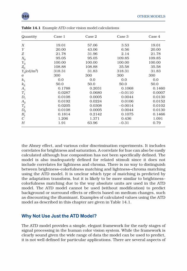
OTHER MODELS244
the Abney effect, and various color discrimination experiments. It includescorrelates for brightness and saturation. A correlate for hue can also be easilycalculated although hue composition has not been specifically defined. Themodel is also inadequately defined for related stimuli since it does notinclude correlates for lightness and chroma. There is no way to distinguishbetween brightness–colorfulness matching and lightness–chroma matchingusing the ATD model. It is unclear which type of matching is predicted by the adaptation transform, but it is likely to be more similar to brightness–colorfulness matching due to the way absolute units are used in the ATDmodel. The ATD model cannot be used (without modification) to predictbackground or surround effects or effects based on medium changes, suchas discounting the illuminant. Examples of calculated values using the ATDmodel as described in this chapter are given in Table 14.1.
Why Not Use Just the ATD Model?
The ATD model provides a simple, elegant framework for the early stages ofsignal processing in the human color vision system. While the framework isclearly sound given the wide range of data the model can be used to predict,it is not well defined for particular applications. There are several aspects of
Table 14.1 Example ATD color vision model calculations
Quantity Case 1 Case 2 Case 3 Case 4
X 19.01 57.06 3.53 19.01Y 20.00 43.06 6.56 20.00Z 21.78 31.96 2.14 21.78X0 95.05 95.05 109.85 109.85Y0 100.00 100.00 100.00 100.00Z0 108.88 108.88 35.58 35.58Y0(cd/m2) 318.31 31.83 318.31 31.83σ 300 300 300 300k1 0.0 0.0 0.0 0.0k2 50.0 50.0 50.0 50.0A1 0.1788 0.2031 0.1068 0.1460T1 0.0287 0.0680 −0.0110 0.0007D1 0.0108 0.0005 0.0044 0.0130A2 0.0192 0.0224 0.0106 0.0152T2 0.0205 0.0308 −0.0014 0.0102D2 0.0108 0.0005 0.0044 0.0130Br 0.1814 0.2142 0.1075 0.1466C 1.206 1.371 0.436 1.091H 1.91 63.96 −0.31 0.79
OTHER MODELS 245
the model that require further definition or specification for practical applica-tion. Thus, the flexibility of the ATD model that allows it to predict a widerange of data also precludes it from being practically useful. The model canbe applied to practical applications with some modification as has been doneby Granger (1994, 1995). However, even this formulation is incomplete as acolor appearance model since it neglects chromatic adaptation.
The ATD model has the advantages that it is fairly simply and generallyeasily invertible (for k1 = 0.0). Its disadvantages include the lack of a strictdefinition of its implementation, inadequate treatment of related colors (neces-sary for most applications), and lack of cognitive factors. Strictly speaking,the ATD model is also not directly relatable to CIE tristimulus values. Sinceit does not incorporate distinct predictors for lightness and chroma, it actu-ally cannot be considered a color appearance model. However, as a frame-work for visual processing and discrimination, it certainly warrants someattention.
14.3 LLAB MODEL
The LLAB model is a more recent entry into the field of color appearancemodels. It is similar in structure to the RLAB model described in Chapter 13.However, the LLAB model does incorporate a different range of effects thanthe RLAB model. The LLAB color appearance model was developed by Luo,Lo and Kuo (1996). However, prior to their publication, the LLAB model wasrevised by Luo and Morovic (1996) in a conference proceedings. The treat-ment in this chapter follows the revised model, but includes some commentson the original formulation presented in Luo, Lo, and Kuo (1996). LLAB isdesigned as a colorimetric model and is clearly an extension of CIE colori-metry (as opposed to a vision model). It was synthesized from the results of a series of experiments on color appearance and color difference scaling.
The LLAB model is designed to be a universal model for color matching,color appearance specification, and color difference measurement. It there-fore incorporates features from previous work in both areas of study. LikeRLAB, it is designed to be relatively simple and not inclusive of all visualphenomena. It is not as simple as the RLAB model. It does, however, predictsome effects that RLAB cannot (the converse is also true).
Objectives and Approach
The LLAB model, as described by Luo et al. (1996), is derived from an extens-ive series of data derived by Luo and his co-workers on color appearancescaling and color discrimination. This work has resulted in tests of colorappearance models and the development of color difference equations assummarized by Luo et al. (1996). The LLAB model is an attempt to synthes-ize this work into a single coherent model.
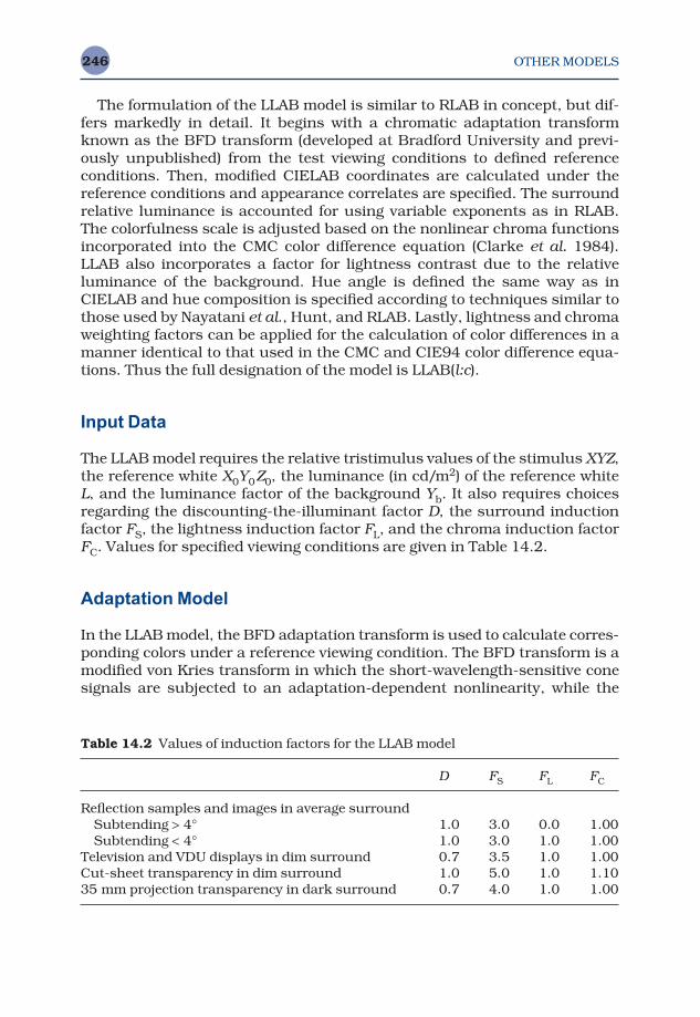
OTHER MODELS246
The formulation of the LLAB model is similar to RLAB in concept, but dif-fers markedly in detail. It begins with a chromatic adaptation transformknown as the BFD transform (developed at Bradford University and previ-ously unpublished) from the test viewing conditions to defined referenceconditions. Then, modified CIELAB coordinates are calculated under the reference conditions and appearance correlates are specified. The surroundrelative luminance is accounted for using variable exponents as in RLAB.The colorfulness scale is adjusted based on the nonlinear chroma functionsincorporated into the CMC color difference equation (Clarke et al. 1984).LLAB also incorporates a factor for lightness contrast due to the relativeluminance of the background. Hue angle is defined the same way as inCIELAB and hue composition is specified according to techniques similar tothose used by Nayatani et al., Hunt, and RLAB. Lastly, lightness and chromaweighting factors can be applied for the calculation of color differences in amanner identical to that used in the CMC and CIE94 color difference equa-tions. Thus the full designation of the model is LLAB(l:c).
Input Data
The LLAB model requires the relative tristimulus values of the stimulus XYZ,the reference white X0Y0Z0, the luminance (in cd/m2) of the reference whiteL, and the luminance factor of the background Yb. It also requires choicesregarding the discounting-the-illuminant factor D, the surround inductionfactor FS, the lightness induction factor FL, and the chroma induction factorFC. Values for specified viewing conditions are given in Table 14.2.
Adaptation Model
In the LLAB model, the BFD adaptation transform is used to calculate corres-ponding colors under a reference viewing condition. The BFD transform is amodified von Kries transform in which the short-wavelength-sensitive conesignals are subjected to an adaptation-dependent nonlinearity, while the
Table 14.2 Values of induction factors for the LLAB model
D FS FL FC
Reflection samples and images in average surroundSubtending > 4° 1.0 3.0 0.0 1.00Subtending < 4° 1.0 3.0 1.0 1.00
Television and VDU displays in dim surround 0.7 3.5 1.0 1.00Cut-sheet transparency in dim surround 1.0 5.0 1.0 1.1035 mm projection transparency in dark surround 0.7 4.0 1.0 1.00
OTHER MODELS 247
middle- and long-wavelength-sensitive cone signals are subject to a simplevon Kries transform. The first step is a transform from CIE XYZ tristimulusvalues to normalized cone responses, denoted RGB, as shown in Equations14.25 and 14.26.
(14.25)
(14.26)
It should be noted that the transform in Equations 14.25 and 14.26 isatypical in two ways. First, the CIE tristimulus values are always normalizedto Y prior to the transform. This results in all stimuli with identical chro-maticity coordinates having the same cone signals (a luminance normaliza-tion). This normalization is required to preserve achromatic scales throughthe nonlinear chromatic adaptation transform described below. Second, thetransform itself does not represent plausible cone responses, but rather‘spectrally sharpened’ cone responses with negative responsivity at somewavelengths. These responsvities tend to preserve saturation across changesin adaptation and impact predicted hue changes across adaptation. Despitethe fact that the BFD transformation results in RGB signals that cannot beconsidered physiologically plausible cone responses, they will be referred toas cone responses for simplicity. The cone responses are then transformedto the corresponding cone responses for adaptation to the reference illumin-ant. The reference illuminant is defined to be CIE illuminant D65 using the1931 standard colorimetric observer (X0r = 95.05, Y0r = 100.0, Z0r = 108.88).The transformation is performed using Equations 14.27–14.30.
Rr = [D(R0r/R0) + 1 − D]R (14.27)
Gr = [D(G0r/G0) + 1 − D]G (14.28)
Br = [D(B0r/B0β ) + 1 − D]Bβ (14.29)
β = (B0/B0r)0.0834 (14.30)
In the event that the B response is negative, Equations 14.29 is replacedwith Equations 14.31 to avoid taking a root of a negative number.
Br = −[D (B0r/B0β ) + 1 − D]| B |β (14.31)
The D factors in Equations 14.27–14.31 allow for discounting the illuminant.When discounting occurs, D = 1.0 and observers completely adapt to the
M =−
−−
0 8951 0 2664 0 16140 7502 1 7135 0 03670 0389 0 0685 1 0296
. . .
. . .
. . .
RGB
X YY YZ Y
///
= M
OTHER MODELS248
color of the light source. If there is no adaptation, D = 0.0 and observers arealways adapted to the reference illuminant. For intermediate values of D,observers are adapted to chromaticities intermediate to the light source andthe reference illuminant (with D specifying the proportional level of adaptionto the source). This is different from the D value in RLAB, which allows forvarious levels of incomplete adaptation that depend on the color and lumin-ance of the source. (D = 0.0 in RLAB does not mean no adaptation, rather itmeans incomplete adaptation to that particular source.)
The final step of the chromatic adaptation transformation is the conver-sion from the cone signals for the reference viewing condition to CIE tristimu-lus values XrYrZr using Equation 14.32.
(14.32)
Opponent Color Dimensions
The corresponding tristimulus values under the reference illuminant (D65)are then transformed to preliminary opponent dimensions using modifiedCIELAB formulae as illustrated in Equations 14.33–14.36.
LL = 116f (Yr/100)z − 16 (14.33)
z = 1 + FL(Yb/100)1/2 (14.34)
A = 500[ f (Xr/95.05) − f (Yr/100)] (14.35)
B = 200[ f (Yr/100) − f (Zr/108.88)] (14.36)
The z exponent is incorporated to account for lightness contrast from thebackground. It is similar to the form used in the Hunt model. Since the LL, A,and B dimensions follow the definitions of the CIELAB equations, the non-linearity is dependent on the relative tristimulus values as shown in Equa-tions 14.37 and 14.38. For values of ω > 0.008856, Equation 14.37 is used.
(14.37)
For values of w < 0.008856, Equations 14.38 is used.
(14.38)
The value of FS depends on the surround relative luminance as specifiedin Table 14.2. This is the similar to the surround dependency incorporatedin the RLAB model.
f FS( ) [( . / )/ . ] //ω ω= − +0 008856 16 116 0 008856 16 1161
f FS( ) ( ) /ω ω= 1
XYZ
R YG YB Y
r
r
r
r
r
r
= −M 1
OTHER MODELS 249
Perceptual Correlates
The LLAB model includes predictors for lightness, chroma, colorfulness, saturation, hue angle, and hue composition. The lightness predictor LL isdefined in Equation 14.33. The chroma predictor ChL, and colorfulness pre-dictor CL, are derived using a nonlinear function similar to that incorporatedin the CMC color difference equation as a chroma weighting function. Thisincorporates the behavior of the CMC color difference equation into theLLAB color space as shown in Equations 14.39–14.43.
C = (A2 + B2)1/2 (14.39)
ChL + 25 ln(1 + 0.05C ) (14.40)
CL = ChLSMSCFC (14.41)
SC = 1.0 + 0.47 log(L) − 0.057[log(L)]2 (14.42)
SM = 0.7 + 0.02LL − 0.0002LL2 (14.43)
FC is the chroma induction factor defined in Table 14.2. SC provides theluminance dependency necessary to predict an increase in colorfulness withluminance. Thus CL is truly a colorfulness predictor. SM provides a similarlightness dependency.
Saturation is defined in LLAB as the ratio of chroma to lightness as shownin Equation 14.44.
sL = ChL/LL (14.44)
LLAB hue angle hL, is calculated in the usual way according to Equa-tion 14.45.
hL = tan−1(B/A) (14.45)
Hue composition in NCS notation is calculated via linear interpolationbetween the hue angles for the unique hues, which are defined as 25° (red),93° (yellow), 165° (green), and 254° (blue).
The final opponent signals are calculated using the colorfulness scale CL,and the hue angle hL, as shown in Equations 14.46 and 14.47.
AL = CL cos(hL) (14.46)
BL = CL sin(hL) (14.47)
There were no predictors of brightness, chroma, or saturation defined inthe LLAB model as initially published by Luo, Lo and Kuo (1996). In the
OTHER MODELS250
revised version (Luo and Morovic 1996), the predictors of chroma and satura-tion were added.
Color Differences
The LLAB model incorporates the chroma weighting function from the CMCcolor difference equation. This chroma dependency is the most importantfactor that produces the improved performance of the CMC color differenceequation over the simple CIELAB ∆E*ab equation. Thus LLAB(l:c) color differ-ences are defined by Equation 14.48.
∆EL = [(∆LL/l )2 + ∆AL2 + ∆BL
2] (14.48)
The lightness weight l is defined to be 1.0, 1.5, and 0.67 for perceptibility,acceptability, and large color differences, respectively. The chroma weight c(not present in this formulation) is always set equal to 1.0.
Phenomena Predicted
The revised LLAB model accounts for chromatic adaptation, lightnessinduction, surround relative luminance, discounting-the-illuminant, andthe Hunt effect. It cannot predict the Stevens effect, incomplete chromaticadaptation, or the Helmholtz–Kohlrausch effect. It also cannot predict theHelson–Judd effect.
LLAB includes predictors for lightness, chroma, saturation, colorfulness,and hue in its latest revision (Luo and Morivic 1996). This corrected theunnatural combination of appearance attributes (lightness, colorfulness,hue) in the original version (Luo, Lo, and Kuo 1996). The natural sets arelightness, chroma, and hue or brightness, colorfulness, and hue. The ori-ginal LLAB formulation could not be used to calculate either brightness–colorfulness matches or lightness–chroma matches. It could be used to predict lightness–colorfulness matches, which probably have little practicalutility. If corresponding colors are predicted at constant luminance, then thelightness–colorfulness matches become equivalent to lightness–chromamatches. Interestingly, the original LLAB formulation did not meet the CIETC1-34 requirements of a color appearance model that it include predictorsof at least lightness, chroma, and hue. These limitations were corrected inthe Luo and Morivic (1996) formulation presented in this chapter.
Table 14.3 includes example calculations of LLAB appearance attributesfor a few stimuli.
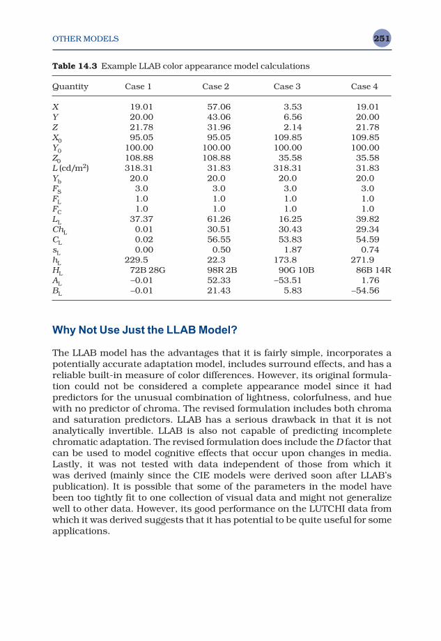
OTHER MODELS 251
Why Not Use Just the LLAB Model?
The LLAB model has the advantages that it is fairly simple, incorporates apotentially accurate adaptation model, includes surround effects, and has areliable built-in measure of color differences. However, its original formula-tion could not be considered a complete appearance model since it had predictors for the unusual combination of lightness, colorfulness, and huewith no predictor of chroma. The revised formulation includes both chromaand saturation predictors. LLAB has a serious drawback in that it is notanalytically invertible. LLAB is also not capable of predicting incompletechromatic adaptation. The revised formulation does include the D factor thatcan be used to model cognitive effects that occur upon changes in media.Lastly, it was not tested with data independent of those from which it was derived (mainly since the CIE models were derived soon after LLAB’spublication). It is possible that some of the parameters in the model havebeen too tightly fit to one collection of visual data and might not generalizewell to other data. However, its good performance on the LUTCHI data fromwhich it was derived suggests that it has potential to be quite useful for someapplications.
Table 14.3 Example LLAB color appearance model calculations
Quantity Case 1 Case 2 Case 3 Case 4
X 19.01 57.06 3.53 19.01Y 20.00 43.06 6.56 20.00Z 21.78 31.96 2.14 21.78X0 95.05 95.05 109.85 109.85Y0 100.00 100.00 100.00 100.00Z0 108.88 108.88 35.58 35.58L (cd/m2) 318.31 31.83 318.31 31.83Yb 20.0 20.0 20.0 20.0FS 3.0 3.0 3.0 3.0FL 1.0 1.0 1.0 1.0FC 1.0 1.0 1.0 1.0LL 37.37 61.26 16.25 39.82ChL 0.01 30.51 30.43 29.34CL 0.02 56.55 53.83 54.59sL 0.00 0.50 1.87 0.74hL 229.5 22.3 173.8 271.9HL 72B 28G 98R 2B 90G 10B 86B 14RAL −0.01 52.33 −53.51 1.76BL −0.01 21.43 5.83 −54.56
Color Appearance Models Second Edition M. D. Fairchild © 2005 John Wiley & Sons, LtdISBN: 0-470-01216-1 (HB)
15The CIE Color
Appearance Model(1997), CIECAM97s
Publication of the first edition of this book coincided with the creation andpublication of the first CIE color appearance model, CIECAM97s. At thattime it was clear there was a significant amount of interest in the establish-ment and use of a single, standardized, color appearance model, but it wasuncertain how effective a single CIE model could be. The industrial demandfor such a model led the CIE to step up its efforts to establish a model to be put into use, tested, and perhaps recommended as a standard later on. CIECAM97s represents such a model and also represents a significantaccomplishment in the field of color appearance modeling. This chapter pro-vides an overview of the development and formulation of CIECAM97s. It isnot an extensive treatment, since an improved model, the subject of Chapter16, has been developed by the CIE. As will be seen in this chapter, the CIEexperiment of CIECAM97s was a great success and led to real progress incolor appearance models.
15.1 HISTORICAL DEVELOPMENT, OBJECTIVES, AND APPROACH
In March of 1996 the CIE held an expert symposium on Colour Standards for Image Technology in Vienna (CIE 1996b). While the symposium coveredmany aspects of image technology for which the CIE could provide guidanceor standards to assist industry, one of the most critical issues was the estab-lishment of a color appearance model for general use. Industrial participants

THE CIE COLOR APPEARANCE MODEL (1997), CIECAM97S 253
in the symposium recognized the need to apply a color appearance model,but requested guidance from the CIE in establishing a single model that couldbe used throughout the industry to promote uniformity of practice and com-patibility between various components in modern open imaging systems.
The push toward a single model was highlighted and summarized in a presentation by Hunt made at that symposium (CIE 1996b) entitled ‘TheFunction, Evolution, and Future of Colour Appearance Models.’ In that pre-sentation, Hunt reviewed the current status and historical development of various models and presented 12 principles for consideration in establish-ing a single model. These principles are reproduced here verbatim (CIE1996b).
1. The model should be as comprehensive as possible, so that it can be usedin a variety of applications; but at this stage, only static states of adapta-tion should be included, because of the great complexity of dynamiceffects.
2. The model should cover a wide range of stimulus intensities, from verydark object colours to very bright self-luminous colour. This means thatthe dynamic response function must have a maximum, and cannot be asimple logarithmic or power function.
3. The model should cover a wide range of adapting intensities, from verylow scotopic levels, such as occur in starlight, to very high photopic levels, such as occur in sunlight. This means that rod vision should beincluded in the model; but because many applications will be such thatrod vision is negligible, the model should be usable in a mode that doesnot include rod vision.
4. The model should cover a wide range of viewing conditions, includingbackgrounds of different luminance factors, and dark, dim, and averagesurrounds. It is necessary to cover the different surrounds because oftheir widespread use in projected and self-luminous displays.
5. For ease of use, the spectral sensitivities of the cones should be a lineartransformation of the CIE x, y, z or x10, y10, z10 functions, and the V′(λ)function should be used for the spectral sensitivity of the rods. Becausescotopic photometric data is often unknown, methods of providing approx-imate scotopic values should be provided.
6. The model should be able to provide for any degree of adaptation betweencomplete and none, for cognitive factors, and for the Helson–Judd effect,as options.
7. The model should give predictions of hue (both as hue-angle, and as hue-quadrature), brightness, lightness, saturation, chroma, and colourfulness.
8. The model should be capable of being operated in a reverse mode.9. The model should be no more complicated than is necessary to meet the
above requirements.10. Any simplified version of the model, intended for particular applications,
should give the same predictions as the complete model for some specifiedset of conditions.
THE CIE COLOR APPEARANCE MODEL (1997), CIECAM97S254
11. The model should give predictions of colour appearance that are notappreciably worse than those given by the model that is best in eachapplication.
12. A version of the model should be available for application to unrelatedcolours (those seen in dark surrounds in isolation from other colours).
The conclusion drawn at the symposium was that the CIE should immedi-ately begin work on the formulation of such a model with the goal that it becompleted prior to the AIC (International Colour Association) quadrennialmeeting to be held in Kyoto in May, 1997. The CIE decided that TC1-34 wasthe most appropriate committee to complete this work and expanded itsterms of reference at the 1996 meeting of CIE Division 1 in Gothenburg toinclude:
To recommend one colour appearance model. This model should give due con-sideration to the findings of other relevant Technical Committees.
TC1-34 immediately began work on the formulation of a CIE model (bothsimple and comprehensive versions). A technical report on the simple ver-sion, CIECAM97s, was published (CIE 1998). The comprehensive versionwas never formulated due to an apparent lack of interest and demand.
TC1-34 members R.W.G. Hunt and M.R. Luo agreed to develop the firstset of equations for consideration of the committee. The working philosophyof TC1-34 was to essentially follow the 12 principles outlined by Hunt in the development of a comprehensive CIE model and a simplified version forpractical applications. The general concept was to develop a comprehensivemodel (like the Hunt model) that can be applied to a wide range of colorappearance phenomena and a simplified version (like the RLAB model) thatis sufficient for applications such as device-independent color imaging withthe additional constraint that the two versions of the model be compatiblefor some defined set of conditions.
In preparing these models, revised versions of the Hunt color appearancemodel were developed. These are referred to as the Bradford–Hunt 96S (simple) model and the Bradford–Hunt 96C (comprehensive) model. Thesemodels represented one intermediate step in the formulation of CIECAM97sand were included in the first edition of this book (Fairchild 1998a) courtesyof the authors (Hunt 1996). These models were not approved by TC1-34 asthe CIE model; however, they served as the starting point for the committeeand provide good illustrations of how the twelve principles above could befulfilled. As expected these models underwent some significant revision priorto consideration of the full committee. R.W.G. Hunt and M.R. Luo providedtwo revised models for TC1-34 consideration prior to the Kyoto meeting. Inaddition M. Fairchild provided a third alternative and K. Richter provided afourth. These four alternatives were considered at the May 1997 meeting ofTC1-34 in Kyoto and an agreement was reached to adopt one of the Huntand Luo alternatives as the simple form of the CIE Color Appearance Model
THE CIE COLOR APPEARANCE MODEL (1997), CIECAM97S 255
(1997), designated CIECAM97s. This model is presented in the following sections. The model was formally approved and published by the CIE (1998).A comprehensive version of the model that extends upon CIECAM97s, to be designated CIECAM97c, was never formulated. A significantly simpleralternative with similar performance over a limited range of viewing condi-tions was prepared by Fairchild, but not recommended by the committeesince it was not as extensible to a comprehensive form as the model selectedto become CIECAM97s. (In hindsight, this shouldn’t have been a concern.)This model has been designated as the ZLAB color appearance model and ispresented in Section 15.7 since it has proven useful in some simple imagereproduction applications.
15.2 INPUT DATA
Some slight, but important, revisions were made to the Bradford–Hunt 96Smodel to derive the model agreed upon by TC1-34 to become the CIECAM97smodel, i.e., the simple version of the CIE Color Appearance Model (1997).These include a reformulation of the surround compensation to use powerfunctions in order to avoid predictions of corresponding colors with negativeCIE tristimulus values and a clear definition of the adaptation level factor D. It is important to note that the formulation of CIECAM97s builds uponthe work of many researchers in the field of color appearance. This was a key issue in TC1-34’s establishment of this model as the best of what is currently available. Various aspects of the model can be traced to work of (inalphabetical order) Bartleson, Breneman, Fairchild, Estevez, Hunt, Lam,Luo, Nayatani, Rigg, Seim, and Valberg among others. Since a comprehens-ive model was never formulated, those interested in color appearance pre-dictions for more extreme viewing conditions (such as high luminance levelswhen bleaching occurs or low luminance levels when the rods becomeactive) or more esoteric appearance phenomena (such as the Helson–Juddeffect) should explore use of the Hunt model described in Chapter 12.
The input data to the model are the luminance of the adapting field (norm-ally taken to be 20% of the luminance of white in the adapting field) LA, thetristimulus values of the sample in the source conditions, XYZ, the tristimu-lus values of the source white in the source conditions, XwYwZw, the relativeluminance of the source background in the source conditions Yb. Addition-ally, the constants c for the impact of surround, Nc a chromatic induction factor, FLL a lightness contrast factor, and F a factor for degree of adaptation,must be selected according to the guidelines in Table 15.1.
15.3 ADAPTATION MODEL
An initial chromatic adaptation transform is used to go from the source view-ing conditions to the equal-energy-illuminant reference viewing conditions

THE CIE COLOR APPEARANCE MODEL (1997), CIECAM97S256
(although tristimulus values need never be expressed in the reference condi-tions). First, tristimulus values for both the sample and white are normalizedand transformed to spectrally sharpened cone responses using the trans-formation given in Equations 15.1 and 15.2.
(15.1)
(15.2)
The chromatic adaptation transform is a modified von Kries transforma-tion (performed on a type of chromaticity coordinates) with an exponentialnonlinearity added to the short-wavelength-sensitive channel as given inEquations 15.3–15.6. In addition, the variable D is used to specify the degreeof adaptation. D is set to 1.0 for complete adaptation or discounting the illum-inant. D is set to 0.0 for no adaptation. D takes on intermediate values forvarious degrees of incomplete chromatic adaptation. Equation 15.7 allowscalculation of D for various luminance levels and surround conditions.
Rc = [D(1.0/Rw) + 1 − D]R (15.3)
Gc = [D(1.0/Gw) + 1 − D]G (15.4)
Bc = [D(1.0/Bpw) + 1 − D]| B |p (15.5)
p = (Bw/1.0)0.0834 (15.6)
D = F − F/[1 + 2(LA1/4) + (LA
2/300)] (15.7)
If B happens to be negative, then Bc is also set to be negative. Similartransformations are also made for the source white since they are requiredin later calculations. Various factors must be calculated prior to further
MB =−
−−
0 8951 0 2664 0 16140 7502 1 7135 0 03670 0389 0 0685 1 0296
. . .
. . .
. . .
RGB
X YY YZ Y
=
MB
///
Table 15.1 Input parameters for the CIECAM97s model
Viewing condition c Nc FLL F
Average surround, samples subtending > 4° 0.69 1.0 0.0 1.0Average surround 0.69 1.0 1.0 1.0Dim surround 0.59 1.1 1.0 0.9Dark surround 0.525 0.8 1.0 0.9Cut-sheet transparencies 0.41 0.8 1.0 0.9
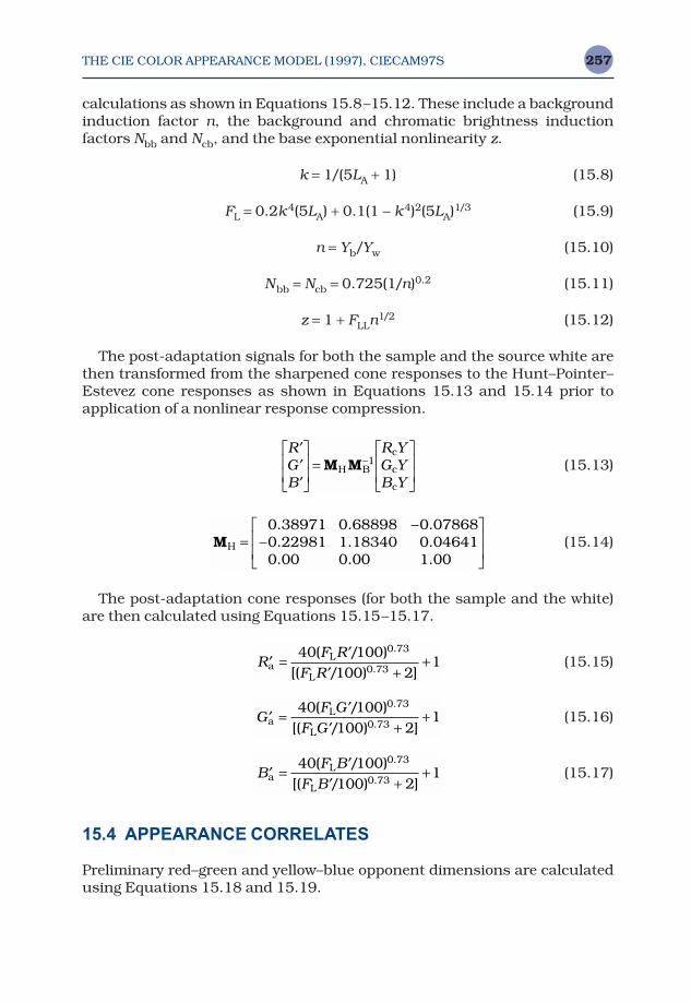
THE CIE COLOR APPEARANCE MODEL (1997), CIECAM97S 257
calculations as shown in Equations 15.8–15.12. These include a backgroundinduction factor n, the background and chromatic brightness induction factors Nbb and Ncb, and the base exponential nonlinearity z.
k = 1/(5LA + 1) (15.8)
FL = 0.2k4(5LA) + 0.1(1 − k4)2(5LA)1/3 (15.9)
n = Yb/Yw (15.10)
Nbb = Ncb = 0.725(1/n)0.2 (15.11)
z = 1 + FLLn1/2 (15.12)
The post-adaptation signals for both the sample and the source white arethen transformed from the sharpened cone responses to the Hunt–Pointer–Estevez cone responses as shown in Equations 15.13 and 15.14 prior toapplication of a nonlinear response compression.
(15.13)
(15.14)
The post-adaptation cone responses (for both the sample and the white)are then calculated using Equations 15.15–15.17.
(15.15)
(15.16)
(15.17)
15.4 APPEARANCE CORRELATES
Preliminary red–green and yellow–blue opponent dimensions are calculatedusing Equations 15.18 and 15.19.
′ = ′′ +
+BF B
F BaL
L
40 100100 2
10 73
0 73
( / )[( / ) ]
.
.
′ = ′′ +
+GF G
F GaL
L
40 100100 2
10 73
0 73
( / )[( / ) ]
.
.
′ = ′′ +
+RF R
F RaL
L
40 100100 2
10 73
0 73
( / )[( / ) ]
.
.
MH =−
−
0 38971 0 68898 0 078680 22981 1 18340 0 046410 00 0 00 1 00
. . .
. . .
. . .
′′′
=
−RGB
R YG YB Y
M MH B
c
c
c
1
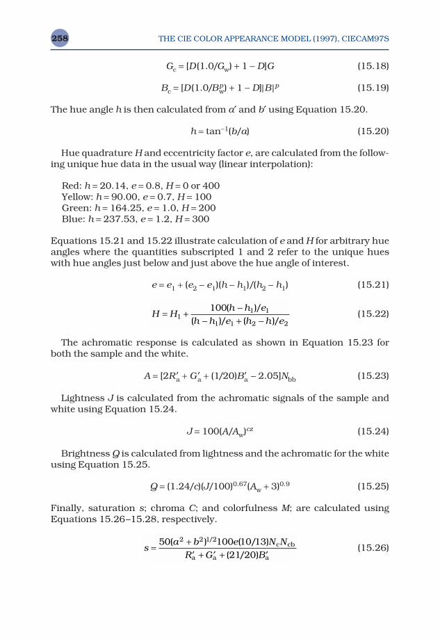
THE CIE COLOR APPEARANCE MODEL (1997), CIECAM97S258
Gc = [D (1.0/Gw) + 1 − D]G (15.18)
Bc = [D (1.0/Bpw) + 1 − D]|B |p (15.19)
The hue angle h is then calculated from a′ and b′ using Equation 15.20.
h = tan−1(b/a) (15.20)
Hue quadrature H and eccentricity factor e, are calculated from the follow-ing unique hue data in the usual way (linear interpolation):
Red: h = 20.14, e = 0.8, H = 0 or 400Yellow: h = 90.00, e = 0.7, H = 100Green: h = 164.25, e = 1.0, H = 200Blue: h = 237.53, e = 1.2, H = 300
Equations 15.21 and 15.22 illustrate calculation of e and H for arbitrary hueangles where the quantities subscripted 1 and 2 refer to the unique hueswith hue angles just below and just above the hue angle of interest.
e = e1 + (e2 − e1)(h − h1)/(h2 − h1) (15.21)
(15.22)
The achromatic response is calculated as shown in Equation 15.23 forboth the sample and the white.
A = [2R ′a + G ′a + (1/20)B′a − 2.05]Nbb (15.23)
Lightness J is calculated from the achromatic signals of the sample andwhite using Equation 15.24.
J = 100(A/Aw)cz (15.24)
Brightness Q is calculated from lightness and the achromatic for the whiteusing Equation 15.25.
Q = (1.24/c)(J/100)0.67(Aw + 3)0.9 (15.25)
Finally, saturation s; chroma C; and colorfulness M; are calculated usingEquations 15.26–15.28, respectively.
(15.26)sa b e N N
R G B=
+′ + ′ + ′
50 100 10 1321 20
2 2 1 2( ) ( / )( / )
/c cb
a a a
H Hh h e
h h e h h e= +
−− + −1
1 1
1 1 2 2
100( )/( )/ ( )/
THE CIE COLOR APPEARANCE MODEL (1997), CIECAM97S 259
C = 2.44s0.69(J/100)0.67n(1.64 − 0.29n) (15.27)
M = CF L0.15 (15.28)
15.5 INVERSE MODEL
The CIECAM97s Model can be nearly analytically inverted, but requires oneapproximation since the Y value on inversion is not easily computed (step 8).Beginning with lightness J, chroma C, and hue angle h, the process is as follows:
1. From J obtain A.2. From h obtain e.3. Calculate s using C and J.4. Calculate a and b using s, h, and e.5. Calculate R ′a, G′a, and B′a from A, a, and b.6. Calculate R ′, G′, and B′ from R′a, G′a, and B′a.7. Calculate RcY, GcY, and BcY from R’, G′, and B′.8. Calculate Y from RcY, GcY, and BcY using MB
−1 (approximation).9. Calculate Rc, Gc, and Bc from RcY, GcY, and BcY and Y.
10. Calculate R, G, and B from Rc, Gc, and Bc.11. Calculate X, Y, and Z, from R, G, B, and Y.
While CIECAM97s cannot be simply inverted in an analytical form, itsinversion is far simpler and more accurate than some previous models. ThusCIECAM97s has been of far more practical utility. A detailed explanation of the inversion process can be found at <www.cis.rit.edu/Fairchild/CAM.html>.
15.6 PHENOMENA PREDICTED
Although CIECAM97s is a fairly simply model it is also quite complete in thevariety of phenomena predicted. It includes correlates of all the importantappearance dimensions (lightness, brightness, chroma, colorfulness, satura-tion, and hue) and it can predict a wide range of adaptation-, surround-, andluminance-dependent effects. It is not applicable to extremely high or lowluminance levels, which are atypical of careful color judgements. Examplecalculations using the CIECAM97s color appearance model as described inthis chapter are given for four samples in Table 15.2. A spreadsheet withthese example calculations can be found at <www.cis.rit.edu/fairchild/CAM.html>.
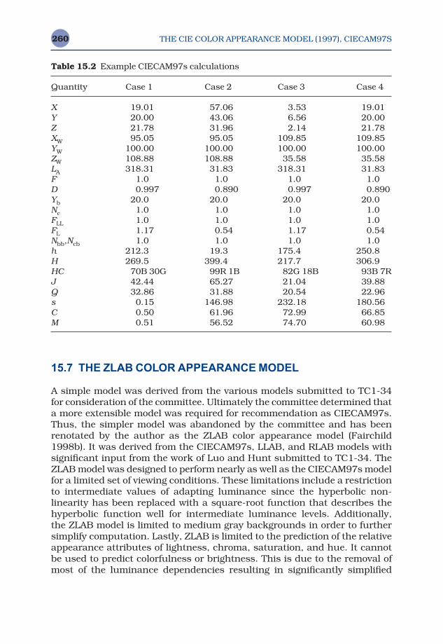
THE CIE COLOR APPEARANCE MODEL (1997), CIECAM97S260
15.7 THE ZLAB COLOR APPEARANCE MODEL
A simple model was derived from the various models submitted to TC1-34for consideration of the committee. Ultimately the committee determined thata more extensible model was required for recommendation as CIECAM97s.Thus, the simpler model was abandoned by the committee and has beenrenotated by the author as the ZLAB color appearance model (Fairchild1998b). It was derived from the CIECAM97s, LLAB, and RLAB models withsignificant input from the work of Luo and Hunt submitted to TC1-34. TheZLAB model was designed to perform nearly as well as the CIECAM97s modelfor a limited set of viewing conditions. These limitations include a restrictionto intermediate values of adapting luminance since the hyperbolic non-linearity has been replaced with a square-root function that describes thehyperbolic function well for intermediate luminance levels. Additionally, the ZLAB model is limited to medium gray backgrounds in order to furthersimplify computation. Lastly, ZLAB is limited to the prediction of the relativeappearance attributes of lightness, chroma, saturation, and hue. It cannotbe used to predict colorfulness or brightness. This is due to the removal ofmost of the luminance dependencies resulting in significantly simplified
Table 15.2 Example CIECAM97s calculations
Quantity Case 1 Case 2 Case 3 Case 4
X 19.01 57.06 3.53 19.01Y 20.00 43.06 6.56 20.00Z 21.78 31.96 2.14 21.78XW 95.05 95.05 109.85 109.85YW 100.00 100.00 100.00 100.00ZW 108.88 108.88 35.58 35.58LA 318.31 31.83 318.31 31.83F 1.0 1.0 1.0 1.0D 0.997 0.890 0.997 0.890Yb 20.0 20.0 20.0 20.0Nc 1.0 1.0 1.0 1.0FLL 1.0 1.0 1.0 1.0FL 1.17 0.54 1.17 0.54Nbb,Ncb 1.0 1.0 1.0 1.0h 212.3 19.3 175.4 250.8H 269.5 399.4 217.7 306.9HC 70B 30G 99R 1B 82G 18B 93B 7RJ 42.44 65.27 21.04 39.88Q 32.86 31.88 20.54 22.96s 0.15 146.98 232.18 180.56C 0.50 61.96 72.99 66.85M 0.51 56.52 74.70 60.98

THE CIE COLOR APPEARANCE MODEL (1997), CIECAM97S 261
equations. The ZLAB model performs identically to CIECAM97s for most corresponding colors calculations since it utilizes the same chromatic adapta-tion transform. It also performs very nearly as well for the prediction ofappearance scaling data. The ZLAB model has found some useful applica-tion in image reproduction where gamut mapping and lack of viewing con-ditions control are major limiting factors obviating the need for a more com-plex model.
Input Data
The input data to the model are the luminance of the adapting field, LA(taken to be 0.2 times the luminance of a reference white), the tristimulusvalues of the sample in the source conditions, XYZ, the tristimulus values ofthe source white in the source conditions XwYwZw.
Chromatic Adaptation
As with CIECAM97s the Bradford chromatic adaptation transform is used to go from the source viewing conditions to corresponding colors under thereference (equal-energy illuminant) viewing conditions. First, all three sets of tristimulus values are normalized and transformed to sharpened coneresponses using the Bradford transformation as given in Equations 15.29and 15.30.
(15.29)
(15.30)
The chromatic–adaptation transform is a modified von Kries transforma-tion (performed on a type of chromaticity coordinates) with an exponentialnonlinearity added to the short-wavelength-sensitive channel as given inEquations 15.31–15.34. In addition, the variable D is used to specify thedegree of adaptation. D is set to 1.0 for complete adaptation or discountingthe illuminant. D is set to 0.0 for no adaptation. D is set to intermediate val-ues for various degrees of incomplete chromatic adaptation. The D variablecould be left as an empirical parameter, or calculated using Equation 15.35,as in CIECAM97s, with F = 1.0 for average surrounds and F = 0.9 for dim or dark surrounds. If Equation 15.35 is used, it is the only place absoluteluminance is required in the ZLAB model.
M =−
−−
0 8951 0 2664 0 16140 7502 1 7135 0 03670 0389 0 0685 1 0296
. . .
. . .
. . .
RGB
X YY YZ Y
=
M///
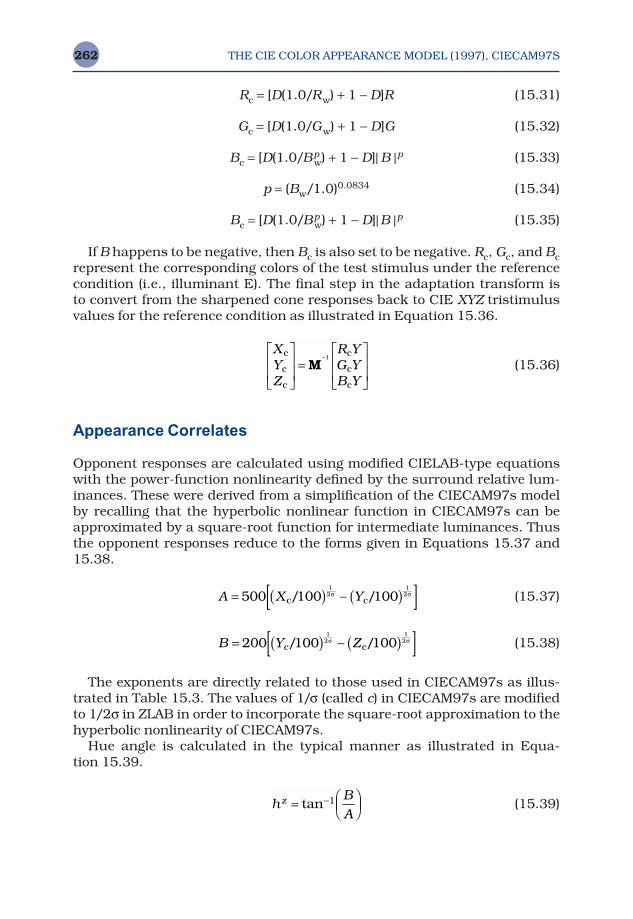
THE CIE COLOR APPEARANCE MODEL (1997), CIECAM97S262
Rc = [D(1.0/Rw) + 1 − D]R (15.31)
Gc = [D(1.0/Gw) + 1 − D]G (15.32)
Bc = [D(1.0/Bpw) + 1 − D]| B |p (15.33)
p = (Bw/1.0)0.0834 (15.34)
Bc = [D(1.0/Bpw) + 1 − D]| B |p (15.35)
If B happens to be negative, then Bc is also set to be negative. Rc, Gc, and Bcrepresent the corresponding colors of the test stimulus under the referencecondition (i.e., illuminant E). The final step in the adaptation transform is to convert from the sharpened cone responses back to CIE XYZ tristimulusvalues for the reference condition as illustrated in Equation 15.36.
(15.36)
Appearance Correlates
Opponent responses are calculated using modified CIELAB-type equationswith the power-function nonlinearity defined by the surround relative lum-inances. These were derived from a simplification of the CIECAM97s modelby recalling that the hyperbolic nonlinear function in CIECAM97s can beapproximated by a square-root function for intermediate luminances. Thusthe opponent responses reduce to the forms given in Equations 15.37 and15.38.
(15.37)
(15.38)
The exponents are directly related to those used in CIECAM97s as illus-trated in Table 15.3. The values of 1/σ (called c) in CIECAM97s are modifiedto 1/2σ in ZLAB in order to incorporate the square-root approximation to thehyperbolic nonlinearity of CIECAM97s.
Hue angle is calculated in the typical manner as illustrated in Equa-tion 15.39.
(15.39)hB
Az =
−tan 1
B Y Z= ( ) − ( )[ ]200 100 1001
21
2c c/ /σ σ
A X Y= ( ) − ( )[ ]500 100 1001
21
2c c/ /σ σ
XYZ
R YG YB Y
c
c
c
c
c
c
=
−
M1
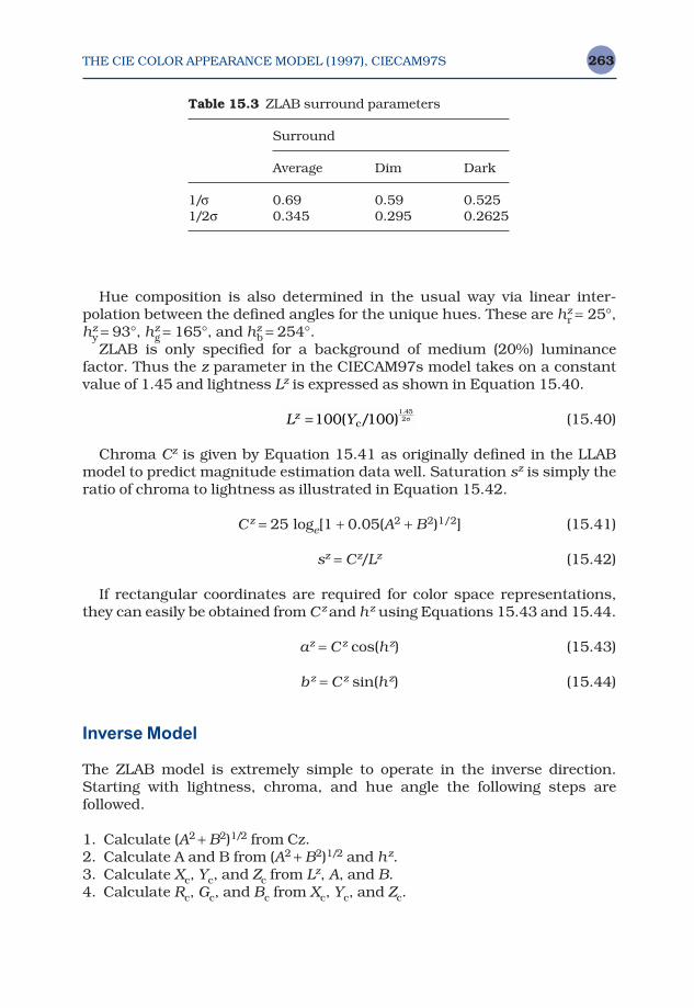
THE CIE COLOR APPEARANCE MODEL (1997), CIECAM97S 263
Hue composition is also determined in the usual way via linear inter-polation between the defined angles for the unique hues. These are hz
r = 25°,hz
y = 93°, hzg = 165°, and hz
b = 254°.ZLAB is only specified for a background of medium (20%) luminance
factor. Thus the z parameter in the CIECAM97s model takes on a constantvalue of 1.45 and lightness Lz is expressed as shown in Equation 15.40.
(15.40)
Chroma Cz is given by Equation 15.41 as originally defined in the LLABmodel to predict magnitude estimation data well. Saturation sz is simply theratio of chroma to lightness as illustrated in Equation 15.42.
Cz = 25 loge[1 + 0.05(A2 + B2)1/2] (15.41)
sz = Cz/Lz (15.42)
If rectangular coordinates are required for color space representations,they can easily be obtained from Cz and hz using Equations 15.43 and 15.44.
az = Cz cos(hz) (15.43)
bz = Cz sin(hz) (15.44)
Inverse Model
The ZLAB model is extremely simple to operate in the inverse direction.Starting with lightness, chroma, and hue angle the following steps are followed.
1. Calculate (A2 + B2)1/2 from Cz.2. Calculate A and B from (A2 + B2)1/2 and hz.3. Calculate Xc, Yc, and Zc from Lz, A, and B.4. Calculate Rc, Gc, and Bc from Xc, Yc, and Zc.
L Yz =100 1001 452( / ).
c σ
Table 15.3 ZLAB surround parameters
Surround
Average Dim Dark
1/σ 0.69 0.59 0.5251/2σ 0.345 0.295 0.2625
THE CIE COLOR APPEARANCE MODEL (1997), CIECAM97S264
5. Calculate R, G, and B from Rc, Gc, and Bc.6. Calculate X, Y, and Z from R, G, and B.
15.8 WHY NOT USE JUST CIECAM97S?
It was a truly unprecedented event that CIE TC1-34 was able to agree uponthe derivation of the CIECAM97s model within a one-year time frame, as was its goal. As anticipated in the first edition of this book, the CIE approvalprocedures did not introduce any changes of significance to the model. It isimportant to note that CIECAM97s was considered an interim model withthe expectation that it would be revised as more data and theoretical under-standing became available. Industrial response to the CIECAM97s modelwas strong and it was quickly brought to bear on commercial applications,particularly in the imaging industry. Application of CIECAM97s, and furtherscientific research, quickly led to understanding of limitations in its for-mulation and performance as well as the creation of additional data forimprovements. The great success of CIECAM97s was in the focus it providedto researchers and engineers in the field. With everyone focusing on a singlemodel for testing and improvement, it became possible to make rapid,significant improvement. The fruits of that work are the recently publishedCIECAM02 color appearance model that is the topic of Chapter 16.
The existence of CIECAM97s is one reason to not use just CIECAM97s.CIECAM02 is a simpler formulation with better performance. Also,CIECAM97s might be too complex for some applications. In such cases,models like ZLAB, RLAB, or the combination of a chromatic adaptationtransform with CIELAB might be adequate.
Color Appearance Models Second Edition M. D. Fairchild © 2005 John Wiley & Sons, LtdISBN: 0-470-01216-1 (HB)
16CIECAM02
CIECAM97s was a great success. If that’s so, then why is there a CIECAM02model? The answer is that the natural evolution or color appearance modelswas anticipated and encouraged with the publication of CIECAM97s. That isexactly why the year (97) is in the name. The success of CIECAM97s is that itallowed a variety of researchers and practitioners in color appearance to focustheir efforts on a single model. This focus quickly led to suggested improve-ments in CIECAM97s that ultimately led to the formulation of a simpler andmore effective model called CIECAM02. This chapter discusses the deriva-tion and formulation of CIECAM02, the current CIE color appearance model,a model likely to remain the current CIE recommendation for some time.
16.1 OBJECTIVES AND APPROACH
As soon as CIECAM97s was published, the intense scrutiny it was subjectedto resulted in suggestions for its improvement and in some cases for simplecorrections to certain elements. With the creation of CIE Division 8, ImageTechnology, came the formation of its first technical committee. This wasCIE TC8-01, Colour Appearance Modeling for Colour Management Systems,chaired by Nathan Moroney and charged with suggesting revisions toCIECAM97s and perhaps a new CIE model. The ultimate result of TC8-01’swork to collect and test suggested revisions of CIECAM97s has been the for-mulation and publication of a revised color appearance model, CIECAM02(CIE 2004, Moroney et al. 2002). Note that CIECAM02 has no ‘s’ notation atthe end of its name. This is because there is no intention to create a com-prehensive version (especially since CIECAM97c was never created) andeven if one were created, a ‘c’ could be added at the end of its name.
A number of potential improvements to CIECAM97s were suggested andthese were compiled into a single publication on behalf of TC8-01 byFairchild (2001). The adjustments considered and ultimately included inCIECAM02 in some form included:
CIECAM02266
• Linearization of the chromatic adaptation transform to simplify the modeland facilitate analytical inversion (Finlayson and Drew 1999, Finlaysonand Süsstrunk 2000, Li et al. 2000a,b)
• Correction of anomalous surround compensation (Moroney 2002, Li et al.1999), Li et al. 2000a,b)
• Correction of the lightness scale for perfect black stimuli (Moroney 2002, Li et al. 1999, Li et al. 2000a,b)
• Correction of chroma scale expansion for color of low chroma (Wyble andFairchild 2000, Newman and Pirrotta 2000)
• Inclusion of a continuously variable surround compensation (Fairchild1995b, 1996)
• Improved response compression function to facilitate an improved satura-tion correlate (Hunt et al. 2003)
After significant consideration of all the suggested revisions, TC8-01 con-verged on a single set of new equations and formulated a revised model designated CIECAM02 (CIE 2004, Moroney et al. 2002). The year remains inthe name as aknowledgement that much remains to be learned about colorappearance psychophysics and modeling. Simply put, CIECAM02 is simplerin formulation, easier to invert, and performs as well as, if not better, thanCIECAM97s for all available data sets. CIECAM02 should be considered forany applications that were previously served well by CIECAM97s. The fol-lowing sections describe the formulation and use of CIECAM02.
16.2 INPUT DATA
Input data for the CIECAM02 include the relative tristimulus values of thetest stimulus (XYZ ) and the white point (XwYwZw), the adapting luminance(often taken to be 20% of the luminance a white object in the scene) LA,in cd/m2, the relative luminance of the surround (dark, dim, average), and a decision on whether discounting-the-illuminant is taking place. The sur-round relative luminance is generally taken to be average for reflectionprints, dim for CRT displays or televisions, and dark for projected trans-parencies under the assumption that these media are being viewed in theirtypical environments. The surround is not directly tied to the medium. Thusit is certainly possible to have reflection prints viewed in a dark surroundand projected transparencies viewed in an average surround. Discounting-the-illuminant is generally assumed to occur for object color stimuli such asprints and not to occur for emissive displays such as CRTs. When discount-ing the illuminant occurs, the D factor in the chromatic adaptation model isset to 1.0. Otherwise it is computed as described in Section 16.3.
Once the surround relative luminance is established, Table 16.1 is used toset the values of c an exponential nonlinearity, Nc the chromatic inductionfactor, and F the maximum degree of adaptation. In CIECAM02, interme-diate values for these parameters are allowed. If intermediate values are

CIECAM02 267
desired, the proper procedure is to choose the intermediate value for c andthen compute the corresponding intermediate values for Nc and F via linearinterpolation as shown in the relationship plotted in Figure 16.1. These val-ues have been corrected slightly from those in CIECAM97s and the numberof conditions has been reduced to a more meaningful, and simpler, set.
16.3 ADAPTATION MODEL
One of the most important changes in CIECAM02 is the use of a linear, vonKries-type chromatic adaptation transform (as described in more detail inChapter 9). This results in a simpler model with equivalent performance(Calabria and Fairchild 2001) and allows for a simple analytical inversion of CIECAM02 (another significant improvement over CIECAM97s). One be-gins with a conversion from CIE tristimulus values (scaled approximately
Figure 16.1 Linear relationship between surround parameters used for the com-putation of intermediate, continuously variable, surround settings in CIECAM02
Table 16.1 Input parameters for the CIECAM02 model
Viewing condition c Nc F
Average surround 0.69 1.0 1.0Dim surround 0.59 0.9 0.9Dark surround 0.525 0.8 0.8
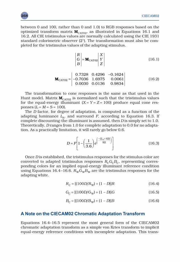
CIECAM02268
between 0 and 100, rather than 0 and 1.0) to RGB responses based on theoptimized transform matrix MCAT02, as illustrated in Equations 16.1 and16.2. All CIE tristimulus values are normally calculated using the CIE 1931standard colorimetric observer (2°). The transformation must also be com-pleted for the tristimulus values of the adapting stimulus.
(16.1)
(16.2)
The transformation to cone responses is the same as that used in theHunt model. Matrix MCAT02 is normalized such that the tristimulus valuesfor the equal-energy illuminant (X = Y = Z = 100) produce equal cone res-ponses (L = M = S = 100).
The D factor, for degree of adaptation, is computed as a function of theadapting luminance LA, and surround F, according to Equation 16.3. If complete discounting-the-illuminant is assumed, then D is simply set to 1.0.Theoretically, D ranges from 1.0 for complete adaptation to 0.0 for no adapta-tion. As a practically limitation, it will rarely go below 0.6.
(16.3)
Once D is established, the tristimulus responses for the stimulus color areconverted to adapted tristimulus responses RCGCBC, representing corres-ponding colors for an implied equal-energy illuminant reference conditionusing Equations 16.4–16.6. RWGWBW are the tristimulus responses for theadapting white.
RC = [(100D/RW) + (1 − D)]R (16.4)
GC = [(100D/GW) + (1 − D)]G (16.5)
BC = [(100D/BW) + (1 − D)]B (16.6)
A Note on the CIECAM02 Chromatic Adaptation Transform
Equations 16.4–16.5 represent the most general form of the CIECAM02chromatic adaptation transform as a simple von Kries transform to implicitequal-energy reference conditions with incomplete adaptation. This trans-
D F eL
= −
− +
1
13 6
4292
.
( )A
MCAT02
0 7328 0 4296 0 16240 7036 1 6975 0 00610 0030 0 0136 0 9834
=−
−. . .. . .. . .
RGB
XYZ
= MCAT02

CIECAM02 269
formation can be used consistently, independent of the remainder of theCIECAM02 model. It can also be applied regardless of the scaling of initialtristimulus values (0 to approximately 100 as normal in CIECAM02, or 0 toapproximately 1.0 as sometimes used). It is recommended that Equations16.4–16.6 be used in all applications of CIECAM02 to maximize generalityand minimize confusion in the function of the adaptation transform. How-ever, the CIE (2004) technical report on CIECAM02 provides slightly differentdefault equations as given in Equations 16.4a–16.6a.
RC = [(YWD/RW) + (1 − D)]R (16.4a)
GC = [(YWD/GW) + (1 − D)]G (16.5a)
BC = [(YWD/BW) + (1 − D)]B (16.6a)
Since YW, the Y tristimulus value of white, is normally 100, the two sets of equations are normally indistinguishable. However, there are times whenYW values different from 100 are used, such as when one considers paper,rather than the perfect reflecting diffuser, to be white in a printing applica-tion. While it appears that the YW factor in Equations 16.4a–16.6a mightaccount for the change in adopted white, it does not. Such normalization isalready built into the equations with RW, GW, and BW. The YW terms serves nomeaningful purpose and is a remnant of an earlier model formulation (sim-ilar to that in CIECAM97s) that was not corrected prior to publication of theCIE technical report. There will be little effect of the difference in equationson final computed appearance correlates since the scaling of appearance relative to the white point is accomplished in later equations (such as thatfor lightness J) in CIECAM02. However, the transform in Equations 16.4a–16.6a cannot be used without the remainder of the CIECAM02 model. Doingso will produce inconsistent results (e.g., white from one viewing conditionmight not map to white in a second viewing condition). If the adaptationtransform is to be used separately from the full CIECAM02 model, the formin Equations 16.4–16.6 must be used for consistent predictions. Also, itshould be noted that the YW factor in Equations 16.4a–16.6a does not norm-alize the scaling of tristimulus values (it actually has the opposite effect) and values scaled from 0 to approximately 100 should be used as input toCIECAM02.
Remainder of CIECAM02 Adaptation Model
Next a number of viewing-condition-dependent components are computedas intermediate values required for further computations. These include aluminance-level adaptation factor FL, and induction factors Nbb and Ncb, andthe base exponential nonlinearity z that each depend on the background relat-ive luminance Yb. These factors are computed using Equations 16.7–16.11.
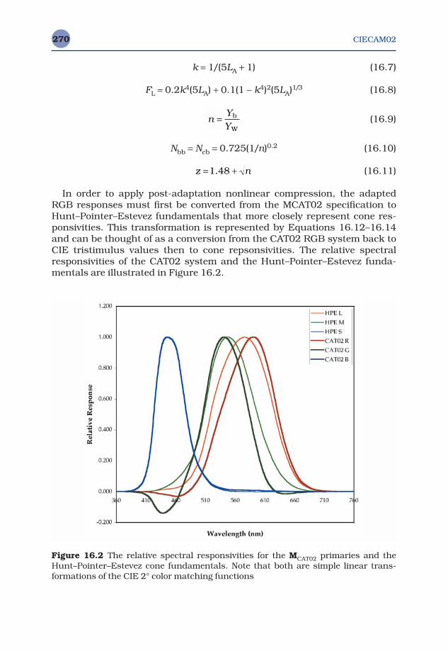
CIECAM02270
k = 1/(5LA + 1) (16.7)
FL = 0.2k4(5LA) + 0.1(1 − k4)2(5LA)1/3 (16.8)
(16.9)
Nbb = Ncb = 0.725(1/n)0.2 (16.10)
(16.11)
In order to apply post-adaptation nonlinear compression, the adaptedRGB responses must first be converted from the MCAT02 specification toHunt–Pointer–Estevez fundamentals that more closely represent cone res-ponsivities. This transformation is represented by Equations 16.12–16.14and can be thought of as a conversion from the CAT02 RGB system back toCIE tristimulus values then to cone repsonsivities. The relative spectralresponsivities of the CAT02 system and the Hunt–Pointer–Estevez funda-mentals are illustrated in Figure 16.2.
z n= +1 48.
nY
Y= b
W
Figure 16.2 The relative spectral responsivities for the MCAT02 primaries and theHunt–Pointer–Estevez cone fundamentals. Note that both are simple linear trans-formations of the CIE 2° color matching functions
CIECAM02 271
(16.12)
(16.13)
(16.14)
The post-adaptation nonlinearities are similar in form to those inCIECAM97s, but slightly modified to produce a simple power-functionresponse over a larger dynamic range. This facilitates a simple definition ofsaturation later in the model. For much of the normal operating range ofthese functions, the are similar to simple square-root functions. These non-linearities are given in Equations 16.15–16.17.
(16.15)
(16.16)
(16.17)
These values are then used to create opponent color responses and formu-late correlates of color appearance.
16.4 OPPONENT COLOR DIMENSIONS
Initial opponent-type responses in CIECAM02 are calculated using Equa-tions 16.18 and 16.19.
a = R ′a − 12G ′a/11 + B′a/11 (16.18)
b = (1/9)(R ′a + G ′a − 2B′a) (16.19)
16.5 HUE
Hue angle h is calculated in CIECAM02 space using the same procedure asCIELAB. As in CIELAB, h is expressed in degrees ranging from 0° to 360°,measured from the positive a axis calculated according to Equation. 16.20.
′ = ′+ ′
+BF B
F BaL
L
400 10027 13 100
0 10 42
0 42
( / ). ( / )
..
.
′ = ′+ ′
+GF G
F GaL
L
400 10027 13 100
0 10 42
0 42
( / ). ( / )
..
.
′ = ′+ ′
+RF R
F RaL
L
400 10027 13 100
0 10 42
0 42
( / ). ( / )
..
.
MCAT021
1 096124 0 278869 0 1827450 454369 0 473533 0 0720980 009628 0 005698 1 015326
− =−
− −
. . .
. . .
. . .
MHPE =−
−0 38971 0 68898 0 078680 22981 1 18340 0 046410 00000 0 00000 1 00000
. . .
. . .. . .
′′′
= −RGB
RGB
M MHPE CAT
C
C
C
021
CIECAM02272
h = tan−1(b/a) (16.20)
Next an eccentricity factor et is computed. This factor is similar to that inCIECAM97s, but has been formulated analytically as given in Equation 16.21.
(16.21)
Hue quadrature and hue composition can be determined through linearinterpolation of the data given in Table 16.2 using Equation 16.22.
(16.22)
16.6 LIGHTNESS
An initial achromatic response is computed by weighted summation of the nonlinear adapted cone responses modified with the brightness induc-tion factor as illustrated in Equation 16.23. A similar quantity must also becomputed for the white in order to facilitate computation of lightness andbrightness.
A = [2R ′a + G′a + (1/20)B′a − 0.305]Nbb (16.23)
Lightness J is then simply computed from the achromatic response, A,achromatic response for white AW, the surround factor c, and the base expo-nent z, according to Equation 16.24.
J = 100(A/AW)cz (16.24)
16.7 BRIGHTNESS
The CIECAM02 correlate to brightness Q is computed from lightness J, theachromatic response for white AW, the surround factor c, and the luminance-level adaptation factor FL, as shown in Equation 16.25.
H Hh h e
h h e h h eii i
i i i i= +
−− + −+ +
100
1 1
( )/( )/ ( )/
e ht = +
+
1 4
1802 3 8/ cos .
π
Table 16.2 Data for conversion from hue angle to hue quadrature
Red Yellow Green Blue Red
i 1 2 3 4 5hi 20.14 90.00 164.25 237.53 380.14ei 0.8 0.7 1.0 1.2 0.8Hi 0 100 200 300 400
CIECAM02 273
(16.25)
16.8 CHROMA
A temporary quantity t, that is related to saturation and incorporates thechromatic induction factors for surround and background (Nc and Ncb) aswell as the eccentricity adjustment et, is computed as the basis for chroma,colorfulness, and saturation correlates. The formula for t is given in Equa-tion 16.26.
(16.26)
CIECAM02 chroma C, is then computed by multiplying a slightly nonlinearform of t by the square root of lightness J, with some adjustment for back-ground n, as shown in Equation 16.27. This formulation, as with most of themodel, is based on empirical fitting to various color appearance scaling data.
(16.27)
16.9 COLORFULNESS
The colorfulness correlate in CIECAM02 is calculated by scaling the chromapredictor C, by the fourth root of the luminance-level adaptation factor FL,as illustrated in Equation 16.28. This makes sense since colorfulness isrelated to chroma, but increases with adapting luminance while chroma isrelatively constant across changes in luminance.
M = CF L0.25 (16.28)
16.10 SATURATION
Lastly, a simple and logically defined predictor of saturation s is defined inCIECAM02 as the square root of colorfulness relative to brightness inEquation 16.29. This is analogous to the CIE definition of saturation as thecolorfulness of a stimulus relative to its brightness.
(16.29)
16.11 CARTESIAN COORDINATES
Color spaces related to appearance models are normally specified in terms ofcylindrical coordinates of lightness, chroma, and hue (JCh) or brightness,
s M Q=100 /
C t J n= −0 9 0 73100 1 64 0 29. ./ ( . . )
tN N e a b
R G B=
+′ + ′ + ′
( / )
( / )
50 000 13
21 20
2 2c cb t
a a a
Q c J A F= +( / ) / ( )4 100 4W L0.25
CIECAM02274
colorfulness, and hue (QMh). However in some applications it is useful tohave the equivalent Cartesian coordinates. While this computation is a sim-ple coordinate transformation, it was never explicitly defined in CEICAM97s.Thus Cartesian coordinates for chroma, colorfulness, and saturation dimen-sions are defined in Equations 16.30–16.35.
aC = C cos(h) (16.30)
bC = C sin(h) (16.31)
aM = M cos(h) (16.32)
bM = M sin(h) (16.33)
as = s cos(h) (16.34)
bs = s sin(h) (16.35)
16.12 INVERSE MODEL
Particularly for color reproduction applications, an inverse color appearancemodel is of practical importance. CIECAM02 is a significant improvementover CIECAM97s in terms of simplicity of inversion. This is largely due to the adoption of a simple linear chromatic adaptation transform. In addition,the CIE technical report on CIECAM02 includes a detailed explanation of themodel inversion and worked examples (CIE 2004). A step-by-step procedurefor implementing the CIECAM02 model in reverse is given below (startingfrom JCh).
Step 1. Calculate t from C and J.Step 2. Calculate et from h.Step 3. Calculate A from AW and J.Step 4. Calculate a and b from t, et, h, and A.Step 5. Calculate R ′a, G ′a, and B′a from A, a and b.Step 6. Use the inverse nonlinearity to compute R′, G′, and B′.Step 7. Convert to RC, GC, and BC, via linear transform.Step 8. Invert the chromatic adaptation transform to compute R, G, and B
and then X, Y, and Z.
16.13 IMPLEMENTATION GUIDELINES
Another improved feature of the CIECAM02 technical report (CIE 2004) aremore detailed guidelines for implementation of the model. Several workedexamples are provide along with examples of parameter settings. This
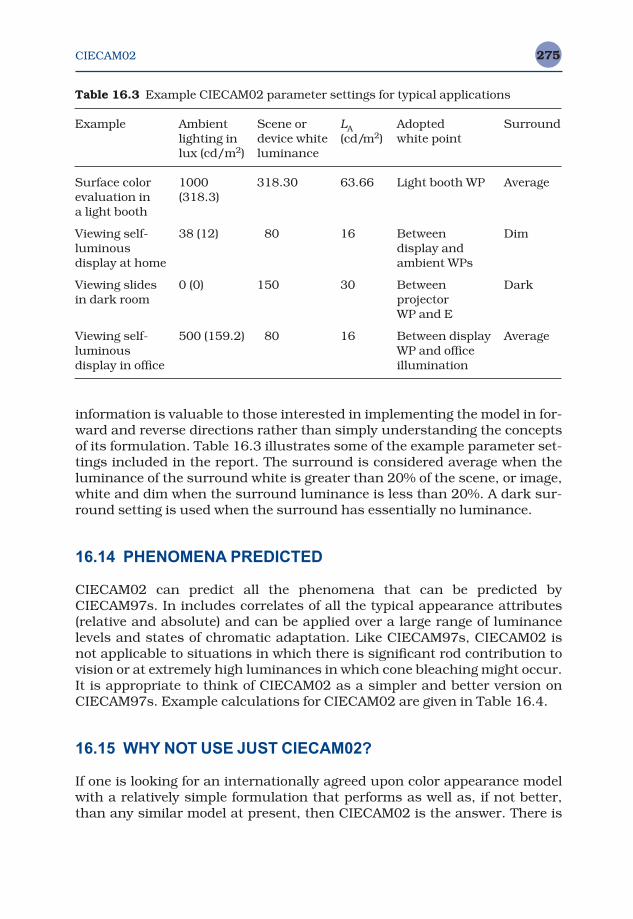
CIECAM02 275
information is valuable to those interested in implementing the model in for-ward and reverse directions rather than simply understanding the conceptsof its formulation. Table 16.3 illustrates some of the example parameter set-tings included in the report. The surround is considered average when theluminance of the surround white is greater than 20% of the scene, or image,white and dim when the surround luminance is less than 20%. A dark sur-round setting is used when the surround has essentially no luminance.
16.14 PHENOMENA PREDICTED
CIECAM02 can predict all the phenomena that can be predicted byCIECAM97s. In includes correlates of all the typical appearance attributes(relative and absolute) and can be applied over a large range of luminancelevels and states of chromatic adaptation. Like CIECAM97s, CIECAM02 isnot applicable to situations in which there is significant rod contribution tovision or at extremely high luminances in which cone bleaching might occur.It is appropriate to think of CIECAM02 as a simpler and better version onCIECAM97s. Example calculations for CIECAM02 are given in Table 16.4.
16.15 WHY NOT USE JUST CIECAM02?
If one is looking for an internationally agreed upon color appearance modelwith a relatively simple formulation that performs as well as, if not better,than any similar model at present, then CIECAM02 is the answer. There is
Table 16.3 Example CIECAM02 parameter settings for typical applications
Example Ambient Scene or LA Adopted Surroundlighting in device white (cd/m2) white pointlux (cd/m2) luminance
Surface color 1000 318.30 63.66 Light booth WP Averageevaluation in (318.3)a light booth
Viewing self- 38 (12) 80 16 Between Dim luminous display and display at home ambient WPs
Viewing slides 0 (0) 150 30 Between Darkin dark room projector
WP and E
Viewing self- 500 (159.2) 80 16 Between display Averageluminous WP and office display in office illumination
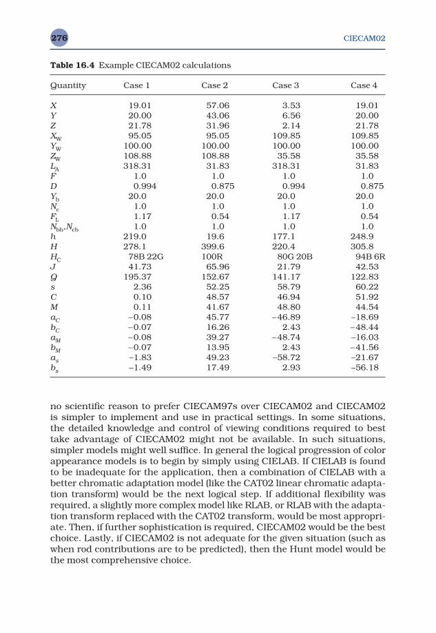
CIECAM02276
no scientific reason to prefer CIECAM97s over CIECAM02 and CIECAM02 is simpler to implement and use in practical settings. In some situations, the detailed knowledge and control of viewing conditions required to besttake advantage of CIECAM02 might not be available. In such situations,simpler models might well suffice. In general the logical progression of colorappearance models is to begin by simply using CIELAB. If CIELAB is foundto be inadequate for the application, then a combination of CIELAB with abetter chromatic adaptation model (like the CAT02 linear chromatic adapta-tion transform) would be the next logical step. If additional flexibility wasrequired, a slightly more complex model like RLAB, or RLAB with the adapta-tion transform replaced with the CAT02 transform, would be most appropri-ate. Then, if further sophistication is required, CIECAM02 would be the bestchoice. Lastly, if CIECAM02 is not adequate for the given situation (such aswhen rod contributions are to be predicted), then the Hunt model would bethe most comprehensive choice.
Table 16.4 Example CIECAM02 calculations
Quantity Case 1 Case 2 Case 3 Case 4
X 19.01 57.06 3.53 19.01Y 20.00 43.06 6.56 20.00Z 21.78 31.96 2.14 21.78XW 95.05 95.05 109.85 109.85YW 100.00 100.00 100.00 100.00ZW 108.88 108.88 35.58 35.58LA 318.31 31.83 318.31 31.83F 1.0 1.0 1.0 1.0D 0.994 0.875 0.994 0.875Yb 20.0 20.0 20.0 20.0Nc 1.0 1.0 1.0 1.0FL 1.17 0.54 1.17 0.54Nbb,Ncb 1.0 1.0 1.0 1.0h 219.0 19.6 177.1 248.9H 278.1 399.6 220.4 305.8HC 78B 22G 100R 80G 20B 94B 6RJ 41.73 65.96 21.79 42.53Q 195.37 152.67 141.17 122.83s 2.36 52.25 58.79 60.22C 0.10 48.57 46.94 51.92M 0.11 41.67 48.80 44.54aC −0.08 45.77 −46.89 −18.69bC −0.07 16.26 2.43 −48.44aM −0.08 39.27 −48.74 −16.03bM −0.07 13.95 2.43 −41.56as −1.83 49.23 −58.72 −21.67bs −1.49 17.49 2.93 −56.18

CIECAM02 277
16.16 OUTLOOK
CIECAM02 represents a significant advance in color appearance modelsover the six years between its publication and the initial formulation ofCIECAM97s. Immediately upon the publication of CIECAM97s, limitationswere noted, suggestions for improvements were made, and a new CIE com-mittee was formed to suggest improvements. Currently, no similar situ-ations are arising with respect to CIECAM02. It appears that the time betweenCIECAM02 and the next CIE color appearance model will be significantlylonger than six years. One reason for this is that this type of model seems tobe predicting the available visual data to within experimental uncertainty.Thus there is no room for significant improvement until more precise (andaccurate) experimental data become available or until vastly larger volumesof data are produced to allow improved prediction of the mean response. Thecost and difficulty of collecting such data as well as inherent inter-observervariability make it unlikely that significant improvements in the availabledata will be obtained in the foreseeable future.
Instead, many researchers in the field of color appearance are turning tomore complex viewing situations and deriving models with new and differentcapabilities. Such capabilities include computational prediction of spatialand temporal effects. These types of models were only just being consideredwhen the first edition of this book was published, but are becoming more of apractical reality as the second edition is being produced. The concepts ofsuch models and one example are described in Chapter 20. Perhaps suchmodels are the direction color appearance modeling will move in the future.Meanwhile, it is likely that CIECAM02 will see significant practical adoptionand use. It will be interesting to see the degree to which it is considered apractical success.
Color Appearance Models Second Edition M. D. Fairchild © 2005 John Wiley & Sons, LtdISBN: 0-470-01216-1 (HB)
17Testing Color
Appearance Models
Chapters 10–16 described several color appearance models with little refer-ence to data on the visual phenomena they are intended to predict. In con-templating the existence of this variety of color appearance models, it islogical to wonder just how well they work. Quantitative tests of the modelsare certainly required (as with any scientific theory, they must be supportedby data); unfortunately far more has been published on the formulation ofthe models than their actual performance. There are several reasons for this.The first is the paucity of reliable data measuring observers’ perceptions of color appearance. The second is that the models themselves have evolvedat a rate that outpaced researchers’ abilities to evaluate their perform-ance. Fortunately, both of these situations continue to change. This chapterreviews some of the experimental work to test color appearance models and collect additional color appearance data for future model testing. Thisremains an active area of research and it is to be expected that additionaltests (and model revisions) will continue to be published.
17.1 OVERVIEW
One might expect that the derivation of color appearance models of thesophistication presented in Chapters 10–16 would require extensive data.This is true; however, the data used to derive the models come from a longhistory of vision experiments, each aimed at one particular aspect of colorappearance. These include the experiments described in Chapter 6 on colorappearance phenomena. The models were then formulated to simultan-eously predict a wide variety of these phenomena. In so doing, quite sophist-icated models can be derived with little or no data that test the wide variety of predictions. To truly test the models, visual data scaling the appearance
TESTING COLOR APPEARANCE MODELS 279
attributes of brightness, lightness, colorfulness, chroma, and hue are re-quired. Alternately, visual evaluations of the performance can be made forexistent models.
A variety of tests of color appearance models have been performed.Unfortunately, none of these tests is completely satisfactory and the questionof which model is best cannot be unequivocally answered for all situations.The various tests that have been performed can be classified into four gen-eral groups as described in the following sections:
• Qualitative tests of various phenomena• Prediction of corresponding colors data• Magnitude estimation of appearance attributes• Direct psychophysical comparison of the predictions of various models.
Each of these types of tests contributes to the evaluation of models in aunique way and none is adequate, on its own, to completely specify the bestcolor appearance model. There are also organized activities within the CIEtechnical committee structure aimed at the evaluation of color appearancemodels. These activities draw upon evaluations in each of the four groupsdescribed above with the ultimate aim to recommend models and proced-ures for color appearance specification.
17.2 QUALITATIVE TESTS
There are a variety of model tests that can be considered qualitative for onereason or another. A test is qualitative if the results show general trends inthe predictions rather than providing numerical comparisons of variousmodels. Such tests include
• Calculations showing that a particular appearance phenomenon can bepredicted (e.g., colorfulness increases with luminance)
• Prediction of trends from historical data• Comparisons with color order systems• Abridged visual experiments on model features.
Nayatani et al. (1988) published an early example of qualitative evaluation oftheir color appearance model. They looked at two sets of data. The first wasthe predicted color appearance of Munsell samples under CIE illuminant Aand the second was the evaluation of results from a color rendering experi-ment of Mori and Fuchida (1982). Their predictions for the Munsell samplesshowed that their model predicted the Helson–Judd effect under illumin-ant A while a von Kries transformation would not. Nayatani et al. followedthis up with a brief visual experiment in which three observers (including the authors) observed a small Helson–Judd effect for samples viewed underan incandescent lamp. They also examined some color discrimination

TESTING COLOR APPEARANCE MODELS280
observations that correlated better with results from their model than pre-dictions made using a von Kries transformation. They also showed that theNayatani et al. color appearance model made reasonable predictions of theMori and Fuchida corresponding colors data. However, they did not comparethese results with other models.
As illustrated in the Nayatani et al. (1988) study cited above, color ordersystems are often used to evaluate the performance of appearance models.The systems used are those based on color appearance (Munsell and NCS)as described in Chapter 5. In many cases when formulating a model, itsauthors will plot contours of Munsell hue, value, and chroma in order toevaluate the perceptual uniformity of the model.
Alternatively, contours of constant NCS hue, whiteness–blackness, andchromaticness can be examined. The assumption is that the color order systems have been constructed with accurate appearance scales. Thus, forexample, a model should be able to predict that samples with constantMunsell hue have the same predicted hue and make analogous predictionsfor Value (lightness) and chroma. Many authors have included plots ofMunsell or NCS contours along with the formulation of their models.Examples include Nayatani et al. (1987, 1990b), Guth (1991), Hunt (1995),and Fairchild and Berns (1993). In fact, the latest revision of the Nayatani etal. (1995) model was formulated to correct discrepancies in plots of Munsellhue and chroma contours at various value levels. Seim and Valberg (1986)provide a more quantitive analysis of the Munsell system in the CIELABcolor space and propose alternative equations similar to those found in theHunt model. Wyble and Fairchild (2000) performed quantitative analyses ofthe Munsell system in various color appearance models that helped lead tosome of the improvements in CIECAM02.
Nayatani et al. (1990b) published an interesting comparison of the Huntand Nayatani et al. models. This included plots of Munsell contours in thecolor spaces of each model as well as flow charts comparing the computa-tional procedure for each model. While this work is interesting, at this pointit is largely historical since both models have been revised significantly sinceit was published. Plots of Munsell and NCS contours do provide some insightinto the performance and properties of various color appearance models;however, none of the published results include a quantitative comparisonbetween the color order systems and color appearance models. For example,constant hue contours should plot as straight radial lines and constantchroma contours as concentric, evenly spaced circles. It would be possible toderive measures of how close the models come to producing these results;see Wyble and Fairchild (2000) for an example. Perhaps this has not oftenbeen done because the results would not be terribly impressive. Another reason is that the perceptual uncertainty of the color order systems is notwell defined, making it difficult to know how good the predictions should be.Examination of the published results suggests that the models performabout equally well in these qualitative comparisons. This conclusion is con-firmed by a study of constant-hue contours completed by Hung and Berns
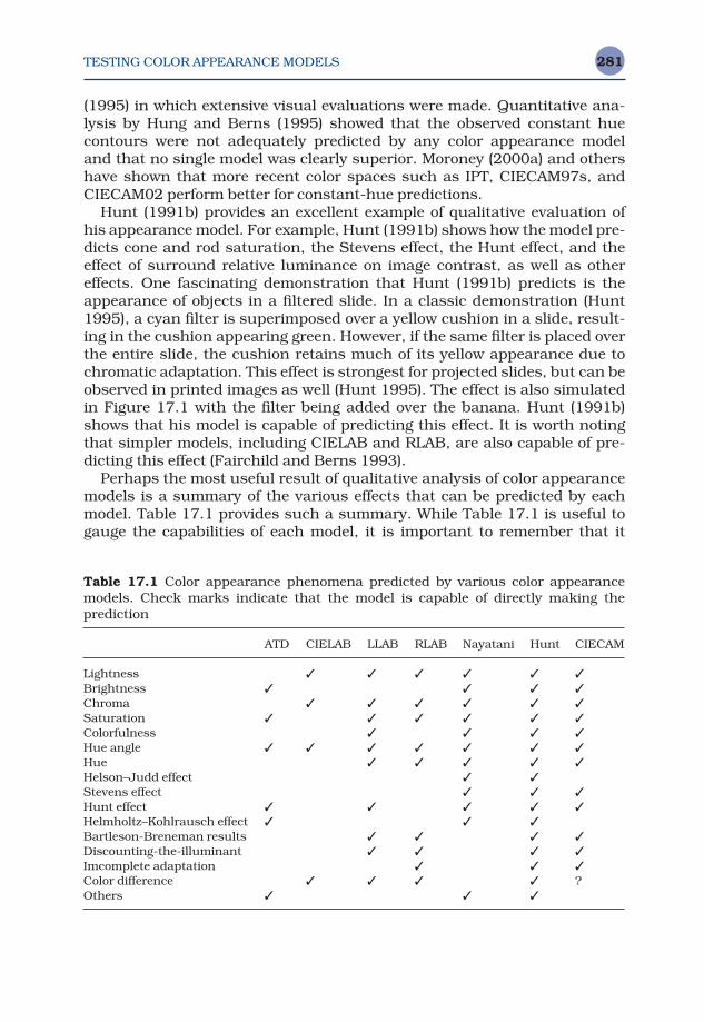
TESTING COLOR APPEARANCE MODELS 281
(1995) in which extensive visual evaluations were made. Quantitative ana-lysis by Hung and Berns (1995) showed that the observed constant hue contours were not adequately predicted by any color appearance model and that no single model was clearly superior. Moroney (2000a) and othershave shown that more recent color spaces such as IPT, CIECAM97s, andCIECAM02 perform better for constant-hue predictions.
Hunt (1991b) provides an excellent example of qualitative evaluation ofhis appearance model. For example, Hunt (1991b) shows how the model pre-dicts cone and rod saturation, the Stevens effect, the Hunt effect, and theeffect of surround relative luminance on image contrast, as well as othereffects. One fascinating demonstration that Hunt (1991b) predicts is theappearance of objects in a filtered slide. In a classic demonstration (Hunt1995), a cyan filter is superimposed over a yellow cushion in a slide, result-ing in the cushion appearing green. However, if the same filter is placed overthe entire slide, the cushion retains much of its yellow appearance due tochromatic adaptation. This effect is strongest for projected slides, but can beobserved in printed images as well (Hunt 1995). The effect is also simulatedin Figure 17.1 with the filter being added over the banana. Hunt (1991b)shows that his model is capable of predicting this effect. It is worth notingthat simpler models, including CIELAB and RLAB, are also capable of pre-dicting this effect (Fairchild and Berns 1993).
Perhaps the most useful result of qualitative analysis of color appearancemodels is a summary of the various effects that can be predicted by eachmodel. Table 17.1 provides such a summary. While Table 17.1 is useful togauge the capabilities of each model, it is important to remember that it
Table 17.1 Color appearance phenomena predicted by various color appearancemodels. Check marks indicate that the model is capable of directly making the prediction
ATD CIELAB LLAB RLAB Nayatani Hunt CIECAM
Lightness 3 3 3 3 3 3Brightness 3 3 3 3Chroma 3 3 3 3 3 3Saturation 3 3 3 3 3 3Colorfulness 3 3 3 3Hue angle 3 3 3 3 3 3 3Hue 3 3 3 3 3Helson–Judd effect 3 3Stevens effect 3 3 3Hunt effect 3 3 3 3 3Helmholtz–Kohlrausch effect 3 3 3Bartleson-Breneman results 3 3 3 3Discounting-the-illuminant 3 3 3 3Imcomplete adaptation 3 3 3Color difference 3 3 3 3 ?Others 3 3 3
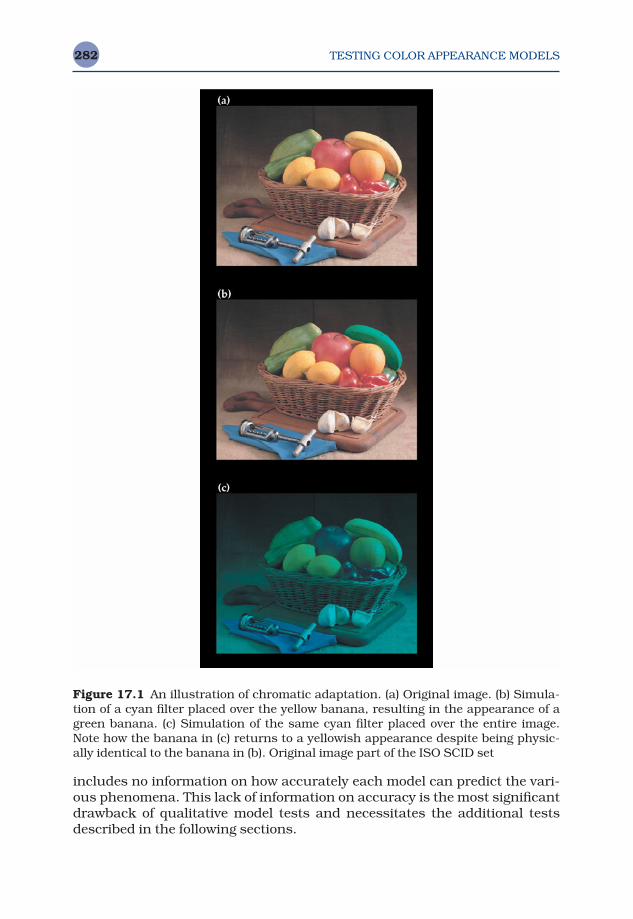
TESTING COLOR APPEARANCE MODELS282
includes no information on how accurately each model can predict the vari-ous phenomena. This lack of information on accuracy is the most significantdrawback of qualitative model tests and necessitates the additional testsdescribed in the following sections.
Figure 17.1 An illustration of chromatic adaptation. (a) Original image. (b) Simula-tion of a cyan filter placed over the yellow banana, resulting in the appearance of agreen banana. (c) Simulation of the same cyan filter placed over the entire image.Note how the banana in (c) returns to a yellowish appearance despite being physic-ally identical to the banana in (b). Original image part of the ISO SCID set
TESTING COLOR APPEARANCE MODELS 283
17.3 CORRESPONDING COLORS DATA
Corresponding colors data were described in Chapter 8 with respect to thestudy of chromatic adaptation. In addition, corresponding colors data can becollected and analyzed for a wide range of color appearance phenomena inaddition to simple chromatic adaptation. Corresponding colors are definedby two sets of tristimulus values specifying stimuli that match in colorappearance for two disparate sets of viewing conditions. Recall that if thechange in viewing conditions has an impact on color appearance, then thecorresponding tristimulus values of the stimuli will be different in absolutevalue.
Corresponding colors data are used to test color appearance models bytaking the tristimulus values for the first viewing condition and trans-forming them to the matching tristimulus values under the second viewingcondition. The predicted corresponding colors can then be compared withvisually observed corresponding colors to determine how well the model per-forms. The results are often analyzed in terms of RMS deviations betweenpredicted and observed colors in either a uniform chromaticity space (e.g.,u′v′) or a uniform color space, (e.g., CIELAB). Recall that Nayatani et al.(1990a) illustrated the important distinction between lightness–chroma andbrightness–colorfulness matches. Complete color appearance models can beused to predict either type of match. The two types of matches will be differ-ent if there is a change in luminance level between the two viewing condi-tions in question.
One of the most extensive series of experiments measuring correspondingcolors data for color appearance analysis was completed by the Color ScienceAssociation of Japan (CSAJ) and reported by Mori et al. (1991). Data fromfour experiments performed by CSAJ were summarized by Mori et al. (1991).
1. An experiment on chromatic adaptation from illuminant D65 to illumin-ant A simulators at an illuminance of 1000 lux. Judgements were madeby 104 observers on 87 samples using a modified haploscopic matchingtechnique.
2. An experiment that collected data consisting of measurements of theHunt effect using five colored samples judged under illuminant D65 simulators at five different illuminance levels by 40 observers.
3. An experiment that collected data representing measurements of theStevens effect using five neutral samples viewed under five different illum-inance levels by 31 observers.
4. An experiment that examined the Helson–Judd effect for achromaticsamples viewed under highly chromatic fluorescent light sources. Thesedata represent one of the most extensive studies, with the largest numbersof observers, completed in the area of color appearance to date.
Unfortunately, Mori et al. (1991) reported only qualitative analyses of theexperimental results. They showed plots of predicted and observed corres-ponding colors for the chromatic adaptation experiment and the Nayatani,

TESTING COLOR APPEARANCE MODELS284
von Kries, and Hunt models. Mori et al. (1991) concluded that the Nayatanimodel made the best predictions. However, examination of their plots sug-gests that Hunt’s model provides similar performance to it and the von Kriestransform perhaps works better than both of them. They illustrated that theNayatani et al. model could predict the Hunt effect data well, but they did notcompare the results with predictions of the Hunt model. Similar analyseswere performed for the Stevens effect and Helson–Judd effect data. Theresults showed a fairly small Stevens effect that was over-predicted by theNayatani et al. model. The Helson–Judd effect, while observed in this experi-ment, was also over-predicted by the Nayatani et al. model. Further, quantit-ative analyses of these data have been carried out through CIE TC1-34 andare described later in the chapter.
Breneman (1987) collected a fairly extensive set of corresponding colorsdata for changes in chromatic adaptation and luminance level. These datawere used to evaluate various chromatic adaptation transforms and colorappearance models by Fairchild (1991a,b). The models were compared interms of RMS deviations between observed and predicted results in the CIE1976 u′v′ chromaticity diagram. The chromatic adaptation data were bestpredicted by the Hunt and RLAB models followed by the Nayatani and vonKries models. The CIELAB and CIELUV models performed the worst forthese data. Breneman’s data showed a small Hunt effect that was over-predicted by the Hunt and Nayatani et al. models and not predicted at all bythe other models. The RMS deviations produced by of both sets of models aresimilar in magnitude, suggesting that making no prediction is as accurate asan over-prediction for these particular data.
Luo et al. (1991b) converted some of their magnitude scaling data (des-cribed in Section 17.4) to sets of corresponding colors for various changes inviewing conditions. They generated three sets of corresponding colors datafor changes in chromatic adaptation from CIE illuminant D65 to D50, D65 toA, and D65 to white fluorescent, and then evaluated six different chromaticadaptation transforms using mean and RMS color differences in the CIELABspace. The results showed that the Bradford model, the basis of LLAB andCIECAM97s, performed best. The Hunt, Nayatani et al., and CIELAB modelsperformed similarly and almost as well. These were followed by the simplevon Kries transformation and a transformation proposed by Bartleson. Addi-tional results can be found in Kuo et al. (1995).
Braun and Fairchild (1997) performed an experiment in which observerswere asked to adjust CRT-displayed images to match printed images viewed under a different white point. Matching images were obtained for fiveobservers using two different images for white point changes from 3000 K to6500 K and 9300 K to 6500 K. The data were analyzed by segmenting theimages into meaningful object regions to avoid overly weighting large imageareas. The corresponding colors were analyzed in terms of average and RMSCIELAB color differences. The results showed that RLAB, LLAB, and CIELABbest predicted the observed corresponding colors. The Hunt and Nayatani et al. models did not perform as well.
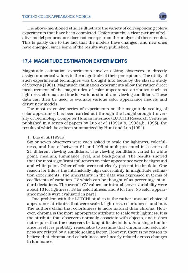
TESTING COLOR APPEARANCE MODELS 285
The above-mentioned studies illustrate the variety of corresponding colorsexperiments that have been completed. Unfortunately, a clear picture of rel-ative model performance does not emerge from the analysis of these results.This is partly due to the fact that the models have changed, and new oneshave emerged, since some of the results were published.
17.4 MAGNITUDE ESTIMATION EXPERIMENTS
Magnitude estimation experiments involve asking observers to directlyassign numerical values to the magnitude of their perceptions. The utility ofsuch experimental techniques was brought into focus by the classic study of Stevens (1961). Magnitude estimation experiments allow the rather directmeasurement of the magnitudes of color appearance attributes such aslightness, chroma, and hue for various stimuli and viewing conditions. Thesedata can then be used to evaluate various color appearance models andderive new models.
The most extensive series of experiments on the magnitude scaling ofcolor appearance has been carried out through the Loughborough Univer-sity of Technology Computer Human Interface (LUTCHI) Research Centre aspublished in a series of papers by Luo et al. (1991a,b, 1993a,b, 1995), theresults of which have been summarized by Hunt and Luo (1994).
1. Luo et al. (1991a)Six or seven observers were each asked to scale the lightness, colorful-ness, and hue of between 61 and 105 stimuli presented in a series of 21 different viewing conditions. The viewing conditions varied in whitepoint, medium, luminance level, and background. The results showedthat the most significant influences on color appearance were backgroundand white point. Other effects were not clearly present in the data. Onereason for this is the intrinsically high uncertainty in magnitude estima-tion experiments. The uncertainty in the data was expressed in terms ofcoefficients of variation CV which can be thought of as percentage stan-dard deviations. The overall CV values for intra-observer variability wereabout 13 for lightness, 18 for colorfulness, and 9 for hue. No color appear-ance models were evaluated in part I.
One problem with the LUTCHI studies is the rather unusual choice ofappearance attributes that were scaled, lightness, colorfulness, and hue.The authors claim that colorfulness is more natural than chroma. How-ever, chroma is the more appropriate attribute to scale with lightness. It isthe attribute that observers normally associate with objects, and it doesnot require that the observers be taught its definition. At a single lumin-ance level it is probably reasonable to assume that chroma and colorful-ness are related by a simple scaling factor. However, there is no reason tobelieve that chroma and colorfulness are linearly related across changesin luminance.
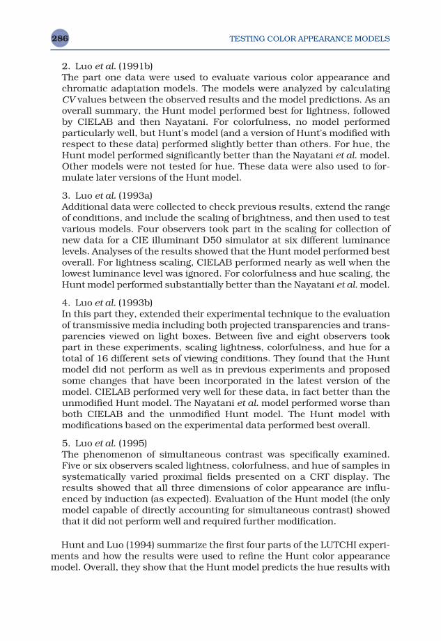
TESTING COLOR APPEARANCE MODELS286
2. Luo et al. (1991b)The part one data were used to evaluate various color appearance andchromatic adaptation models. The models were analyzed by calculatingCV values between the observed results and the model predictions. As anoverall summary, the Hunt model performed best for lightness, followedby CIELAB and then Nayatani. For colorfulness, no model performed particularly well, but Hunt’s model (and a version of Hunt’s modified withrespect to these data) performed slightly better than others. For hue, theHunt model performed significantly better than the Nayatani et al. model.Other models were not tested for hue. These data were also used to for-mulate later versions of the Hunt model.
3. Luo et al. (1993a)Additional data were collected to check previous results, extend the rangeof conditions, and include the scaling of brightness, and then used to testvarious models. Four observers took part in the scaling for collection ofnew data for a CIE illuminant D50 simulator at six different luminancelevels. Analyses of the results showed that the Hunt model performed bestoverall. For lightness scaling, CIELAB performed nearly as well when thelowest luminance level was ignored. For colorfulness and hue scaling, theHunt model performed substantially better than the Nayatani et al. model.
4. Luo et al. (1993b)In this part they, extended their experimental technique to the evaluationof transmissive media including both projected transparencies and trans-parencies viewed on light boxes. Between five and eight observers tookpart in these experiments, scaling lightness, colorfulness, and hue for atotal of 16 different sets of viewing conditions. They found that the Huntmodel did not perform as well as in previous experiments and proposedsome changes that have been incorporated in the latest version of themodel. CIELAB performed very well for these data, in fact better than theunmodified Hunt model. The Nayatani et al. model performed worse thanboth CIELAB and the unmodified Hunt model. The Hunt model withmodifications based on the experimental data performed best overall.
5. Luo et al. (1995)The phenomenon of simultaneous contrast was specifically examined.Five or six observers scaled lightness, colorfulness, and hue of samples insystematically varied proximal fields presented on a CRT display. Theresults showed that all three dimensions of color appearance are influ-enced by induction (as expected). Evaluation of the Hunt model (the onlymodel capable of directly accounting for simultaneous contrast) showedthat it did not perform well and required further modification.
Hunt and Luo (1994) summarize the first four parts of the LUTCHI experi-ments and how the results were used to refine the Hunt color appearancemodel. Overall, they show that the Hunt model predicts the hue results with

TESTING COLOR APPEARANCE MODELS 287
CVs between 7 and 8 while the inter-observer variability CV is 8. For light-ness, the model CVs range from 10 to 14 with the inter-observer variability of 13. For colorfulness, the model CVs are around 18 with inter-observervariability of 17. Thus they conclude that the Hunt model is capable of pre-dicting the experimental results as well as the results from one observerwould predict the mean. This is impressive, and certainly a good result, butit should be kept in mind that these data are not independent of the modelformulation.
Many of the results of the LUTCHI experiments were also contributed tothe efforts of CIE TC1-34 in order to allow the evaluation of more recent colorappearance models and the formulation of CIECAM97s. The results of theseanalyses are described in Section 17.6. Unfortunately, the data themselveshave were deemed proprietary by the research sponsors and were not beenreleased for a number of years. Ultimately these data were made publiclyavailable and used as one of the data sets for development of CIECAM02.
17.5 DIRECT MODEL TESTS
One way to overcome the limited precision of magnitude estimation experi-ments is to take advantage of more refined psychophysical techniques toevaluate model performance. One such technique involves paired compar-ison experiments in which observers view two stimuli at a time and simplychoose which is better. The results are then analyzed using the law of com-parative judgements to derive an interval scale and associated uncertain-ties. To evaluate color appearance models in this fashion, one must beginwith an original stimulus (or image) in one set of viewing conditions and thencalculate the corresponding stimulus (or image) for the second set of viewingconditions using each model to be tested. The observers then look at eachpossible pair of stimuli and choose which is a better reproduction of the original in its viewing condition. The interval scale results are then used tomeasure the relative performance of each model. The significant drawbackof this approach is that the results cannot be used to derive new models andare limited to the models available and included at the time of the experi-ment. An extensive series of these experiments has been conducted at theMunsell Color Science Laboratory at Rochester Institute of Technology andsummarized by Fairchild (1996). The results of these and other experimentsare described below.
Fairchild and Berns (1993) described an early and simplified form of theseexperiments to confirm the utility of color appearance models in cross-mediaimage reproduction applications. They examined the transformation fromprints viewed under either illuminant A or D50 simulators to CRT displayswith a D65 white point and various backgrounds using a simple successivebinocular viewing technique. Six different images were used and 14 observerstook part in the experiment. Comparisons were made between no model (CIEXYZ reproduction), CIELAB, and RLAB. The results indicated that observers
TESTING COLOR APPEARANCE MODELS288
chose the RLAB reproduction as the best nearly 70% of the time, the CIELABimage about 30% of the time, and the XYZ image almost never. This resultshowed that a color appearance transformation was indeed required forthese viewing conditions and that the RLAB model outperformed CIELAB.
Kim et al. (1993) examined the performance of eight color appearancetransformations for printed images viewed under different viewing condi-tions. Original prints were viewed under a CIE illuminant A simulator andreproductions calculated using the various appearance transformationswere viewed under CIE illuminant D65 simulators at three different lumin-ance levels. A paired-comparison experiment was completed and an intervalscale was derived using the law of comparative judgements. A sucessive-Ganzfeld haploscopic viewing technique (Fairchild, Pirrotta, and Kim 1994)was used with 30 observers. The results showed that the Hunt, RLAB,CIELAB, and von Kries models performed similarly to one another and sig-nificantly better than the other models. The Nayatani et al. model performedworse than each of the above models. Three models performed significantlyworse and were not included in further experiments. These includedCIELUV, LABHNU2, and a proprietary model. The Nayatani et al. model per-formed poorly due to its prediction of the Helson–Judd effect resulting in yellowish highlights and bluish shadows in the reproductions. The Helson–Judd effect cannot be observed for complex stimuli under these viewing con-ditions. CIELUV and the others performed poorly due to their intrinsicallyflawed chromatic adaptation transformations.
Pirrotta and Fairchild (1995) performed a similar experiment using simplestimuli on gray backgrounds rather than images. The first phase of thisstudy was a computational comparison of the various models in order to findthe stimuli and viewing conditions for which the models differed the mostsuch that the visual experiments could concentrate on these differences. Itis useful to examine a few of these results. Figure 17.2 shows the CIELABcoordinates of corresponding colors under CIE illuminant A at 1000 lux forneutral Munsell samples of values 3, 5, and 7 viewed under CIE illuminantD65 at either 1000 or 10 000 lux. The points labeled F illustrate the incom-plete adaptation predicted by the Fairchild (1991b) model used in RLAB. Thepoints labeled N show the prediction of the Helson–Judd and Stevens effectsincorporated in the Nayatani et al. model. The points labeled H show the prediction of the Stevens effect for the condition with a luminance changeaccording to the Hunt model. Figure 17.2 illustrates the extreme predictionof the Helson–Judd effect for illuminant A according to the Nayatani et al.model.
Figure 17.3 illustrates the wide range of corresponding color predictionsfor a 5PB 5/12 Munsell sample under the same viewing conditions. Oneshould note the extreme differences in the predictions of the various modelsas the scales of the plots in Figure 15.3 encompass 50 CIELAB units. ThePirrotta and Fairchild (1995) visual experiment used a paired-comparisontechnique with 26 observers, 10 stimulus colors, and a change in viewingconditions from an illuminant A simulator at 76 cd/m2 to an illuminant D65
TESTING COLOR APPEARANCE MODELS 289
simulator at 763 cd/m2. The results showed that the Hunt model performedbest. Von Kries, CIELAB, and the Nayatani et al. model performed similarlyto one another, but not as well as the Hunt model. CIELUV and the Fairchild(1991b) model performed significantly worse. These results led to the revi-sion of the adaptation model incorporated in RLAB (Fairchild 1996).
Braun et al. (1996) investigated viewing techniques and the perform-ance of color appearance models for changes in image medium and viewing
Figure 17.2 Illustration of differences between predictions of various appearancemodels represented in the CIELAB L*–b* plane. Neutrals at (a) 1000 lux and (b) 10 000 lux
Figure 17.3 Illustration of differences between predictions of various appearancemodels represented in the CIELAB a*–b* plane. 5PB 5/12 at (a) 1000 lux and (b) 10 000 lux
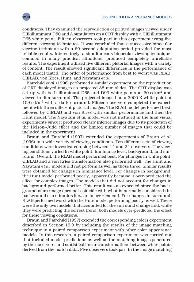
TESTING COLOR APPEARANCE MODELS290
conditions. They examined the reproduction of printed images viewed underCIE illuminant D50 and A simulators on a CRT display with a CIE illuminantD65 white point. Fifteen observers took part in this experiment using fivedifferent viewing techniques. It was concluded that a successive binocularviewing technique with a 60 second adaptation period provided the mostreliable results. Interestingly, a simultaneous binocular viewing technique,common in many practical situations, produced completely unreliableresults. The experiment utilized five different pictorial images with a varietyof content. The result showed significant differences in the performance ofeach model tested. The order of performance from best to worst was RLAB,CIELAB, von Kries, Hunt, and Nayatani et al.
Fairchild et al. (1996) performed a similar experiment on the reproductionof CRT displayed images as projected 35 mm slides. The CRT display was set up with both illuminant D65 and D93 white points at 60 cd/m2 andviewed in dim surround. The projected image had a 3900 K white point at109 cd/m2 with a dark surround. Fifteen observers completed the experi-ment with three different pictorial images. The RLAB model performed best,followed by CIELAB and von Kries with similar performance and then theHunt model. The Nayatani et al. model was not included in the final visualexperiments since it produced clearly inferior images due to its prediction ofthe Helson–Judd effect and the limited number of images that could beincluded in the experiment.
Braun and Fairchild (1997) extended the experiments of Braun et al.(1996) to a wide variety of viewing conditions. Ten different sets of viewingconditions were investigated using between 14 and 24 observers. The view-ing conditions varied in white point, luminance level, background, and sur-round. Overall, the RLAB model performed best. For changes in white point,CIELAB and a von Kries transformation also performed well. The Hunt andNayatani et al. models did not perform as well as those three. Similar resultswere obtained for changes in luminance level. For changes in background,the Hunt model performed poorly, apparently because it over-predicted theeffect for complex images. The models that did not account for changes inbackground performed better. This result was as expected since the back-ground of an image does not coincide with what is normally considered thebackground of a stimulus (i.e., an image element). For changes in surround,RLAB performed worst with the Hunt model performing poorly as well. Thesewere the only two models that accounted for the surround change and, whilethey were predicting the correct trend, both models over-predicted the effectfor these viewing conditions.
Braun and Fairchild (1997) extended the corresponding colors experimentdescribed in Section 15.3 by including the results of the image matchingtechnique in a paired comparison experiment with other color appearancemodels. In this research, a paired comparison experiment was carried outthat included model predictions as well as the matching images generatedby the observers, and statistical linear transformations between white pointsderived from the match data. Five observers took part in the image matching
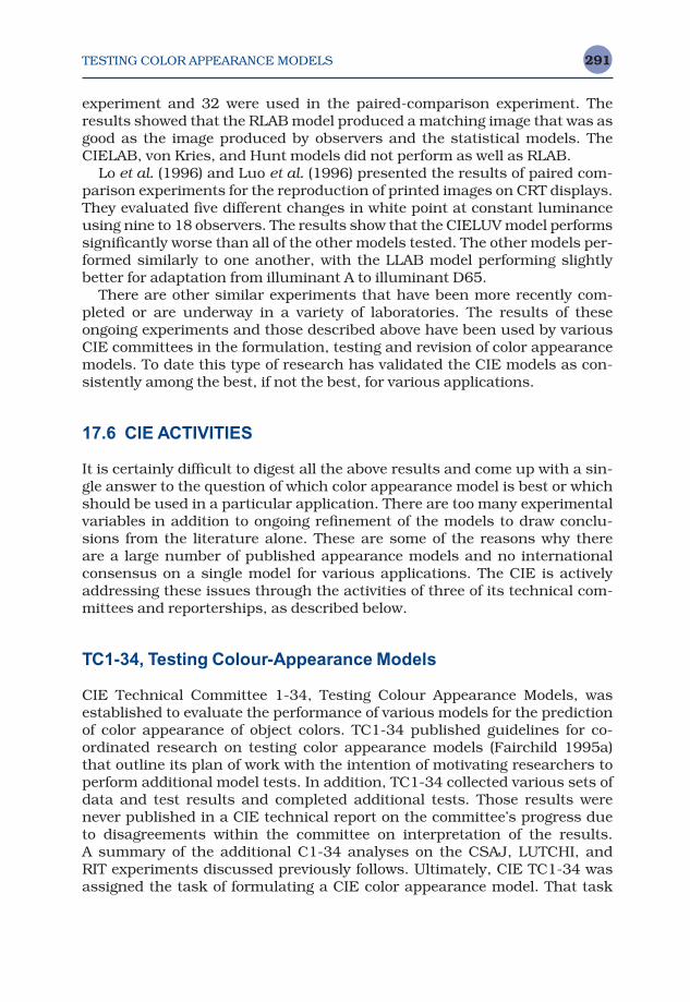
TESTING COLOR APPEARANCE MODELS 291
experiment and 32 were used in the paired-comparison experiment. Theresults showed that the RLAB model produced a matching image that was asgood as the image produced by observers and the statistical models. TheCIELAB, von Kries, and Hunt models did not perform as well as RLAB.
Lo et al. (1996) and Luo et al. (1996) presented the results of paired com-parison experiments for the reproduction of printed images on CRT displays.They evaluated five different changes in white point at constant luminanceusing nine to 18 observers. The results show that the CIELUV model performssignificantly worse than all of the other models tested. The other models per-formed similarly to one another, with the LLAB model performing slightlybetter for adaptation from illuminant A to illuminant D65.
There are other similar experiments that have been more recently com-pleted or are underway in a variety of laboratories. The results of these ongoing experiments and those described above have been used by variousCIE committees in the formulation, testing and revision of color appearancemodels. To date this type of research has validated the CIE models as con-sistently among the best, if not the best, for various applications.
17.6 CIE ACTIVITIES
It is certainly difficult to digest all the above results and come up with a sin-gle answer to the question of which color appearance model is best or whichshould be used in a particular application. There are too many experimentalvariables in addition to ongoing refinement of the models to draw conclu-sions from the literature alone. These are some of the reasons why there are a large number of published appearance models and no internationalconsensus on a single model for various applications. The CIE is activelyaddressing these issues through the activities of three of its technical com-mittees and reporterships, as described below.
TC1-34, Testing Colour-Appearance Models
CIE Technical Committee 1-34, Testing Colour Appearance Models, wasestablished to evaluate the performance of various models for the predictionof color appearance of object colors. TC1-34 published guidelines for co-ordinated research on testing color appearance models (Fairchild 1995a)that outline its plan of work with the intention of motivating researchers toperform additional model tests. In addition, TC1-34 collected various sets ofdata and test results and completed additional tests. Those results werenever published in a CIE technical report on the committee’s progress due to disagreements within the committee on interpretation of the results. A summary of the additional C1-34 analyses on the CSAJ, LUTCHI, and RIT experiments discussed previously follows. Ultimately, CIE TC1-34 wasassigned the task of formulating a CIE color appearance model. That task
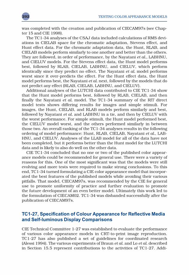
TESTING COLOR APPEARANCE MODELS292
was completed with the creation and publication of CIECAM97s (see Chap-ter 15 and CIE 1998).
The TC1-34 analyses of the CSAJ data included calculations of RMS devi-ations in CIELAB space for the chromatic adaptation, Stevens effect, andHunt effect data. For the chromatic adaptation data, the Hunt, RLAB, andCIELAB models perform similarly to one another and better than the others.They are followed, in order of performance, by the Nayatani et al., LABHNU,and CIELUV models. For the Stevens effect data, the Hunt model performsbest, followed by RLAB, CIELAB, LABHNU, and CIELUV, which performidentically since they predict no effect. The Nayatani et al. model performsworst since it over-predicts the effect. For the Hunt effect data, the Huntmodel performs best, the Nayatani et al. next, followed by the models that donot predict any effect (RLAB, CIELAB, LABHNU, and CIELUV).
Additional analyses of the LUTCHI data contributed to CIE TC1-34 showthat the Hunt model performs best, followed by RLAB, CIELAB, and thenfinally the Nayatani et al. model. The TC1-34 summary of the RIT directmodel tests shows differing results for images and simple stimuli. Forimages, the Hunt, CIELAB, and RLAB models perform similarly and best,followed by Nayatani et al. and LABHNU in a tie, and then by CIELUV withthe worst performance. For simple stimuli, the Hunt model performed best,the CIELUV model worst, and the others performed similarly in betweenthose two. An overall ranking of the TC1-34 analyses results in the followingordering of model performance: Hunt, RLAB, CIELAB, Nayatani et al., LAB-HNU, and CIELUV. Analyses of the LLAB model for all of the data have notbeen completed, but it performs better than the Hunt model for the LUTCHIdata and is likely to also do well on the other data.
CIE TC1-34 concluded that no one or two of the published color appear-ance models could be recommended for general use. There were a variety ofreasons for this. One of the most significant was that the models were stillevolving and more tests were required to make strong conclusions. To thisend, TC1-34 turned formulating a CIE color appearance model that incorpor-ated the best features of the published models while avoiding their variouspitfalls. That model, CIECAM97s, was recommended by the CIE for generaluse to promote uniformity of practice and further evaluation to promote the future development of an even better model. Ultimately this work led tothe formulation of CIECAM02. TC1-34 was disbanded successfully after thepublication of CIECAM97s.
TC1-27, Specification of Colour Appearance for Reflective Mediaand Self-luminous Display Comparisons
CIE Technical Committee 1-27 was established to evaluate the performanceof various color appearance models in CRT-to-print image reproduction.TC1-27 has also published a set of guidelines for coordinated research(Alessi 1994). The various experiments of Braun et al. and Lo et al. describedin Section 15.5 represent contributions to the activities of TC1-27. Addi-
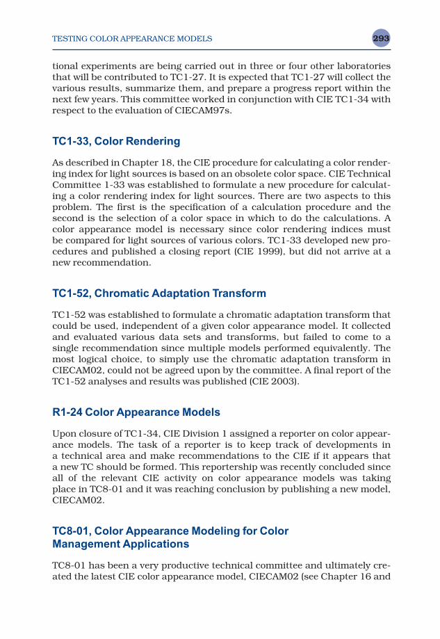
TESTING COLOR APPEARANCE MODELS 293
tional experiments are being carried out in three or four other laboratoriesthat will be contributed to TC1-27. It is expected that TC1-27 will collect thevarious results, summarize them, and prepare a progress report within thenext few years. This committee worked in conjunction with CIE TC1-34 withrespect to the evaluation of CIECAM97s.
TC1-33, Color Rendering
As described in Chapter 18, the CIE procedure for calculating a color render-ing index for light sources is based on an obsolete color space. CIE TechnicalCommittee 1-33 was established to formulate a new procedure for calculat-ing a color rendering index for light sources. There are two aspects to thisproblem. The first is the specification of a calculation procedure and the second is the selection of a color space in which to do the calculations. Acolor appearance model is necessary since color rendering indices must be compared for light sources of various colors. TC1-33 developed new pro-cedures and published a closing report (CIE 1999), but did not arrive at anew recommendation.
TC1-52, Chromatic Adaptation Transform
TC1-52 was established to formulate a chromatic adaptation transform thatcould be used, independent of a given color appearance model. It collectedand evaluated various data sets and transforms, but failed to come to a single recommendation since multiple models performed equivalently. Themost logical choice, to simply use the chromatic adaptation transform inCIECAM02, could not be agreed upon by the committee. A final report of theTC1-52 analyses and results was published (CIE 2003).
R1-24 Color Appearance Models
Upon closure of TC1-34, CIE Division 1 assigned a reporter on color appear-ance models. The task of a reporter is to keep track of developments in a technical area and make recommendations to the CIE if it appears that a new TC should be formed. This reportership was recently concluded sinceall of the relevant CIE activity on color appearance models was taking place in TC8-01 and it was reaching conclusion by publishing a new model,CIECAM02.
TC8-01, Color Appearance Modeling for Color Management Applications
TC8-01 has been a very productive technical committee and ultimately cre-ated the latest CIE color appearance model, CIECAM02 (see Chapter 16 and
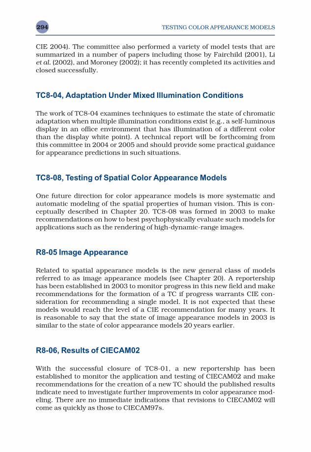
TESTING COLOR APPEARANCE MODELS294
CIE 2004). The committee also performed a variety of model tests that aresummarized in a number of papers including those by Fairchild (2001), Li et al. (2002), and Moroney (2002); it has recently completed its activities andclosed successfully.
TC8-04, Adaptation Under Mixed Illumination Conditions
The work of TC8-04 examines techniques to estimate the state of chromaticadaptation when multiple illumination conditions exist (e.g., a self-luminousdisplay in an office environment that has illumination of a different colorthan the display white point). A technical report will be forthcoming fromthis committee in 2004 or 2005 and should provide some practical guidancefor appearance predictions in such situations.
TC8-08, Testing of Spatial Color Appearance Models
One future direction for color appearance models is more systematic andautomatic modeling of the spatial properties of human vision. This is con-ceptually described in Chapter 20. TC8-08 was formed in 2003 to make recommendations on how to best psychophysically evaluate such models forapplications such as the rendering of high-dynamic-range images.
R8-05 Image Appearance
Related to spatial appearance models is the new general class of modelsreferred to as image appearance models (see Chapter 20). A reportership has been established in 2003 to monitor progress in this new field and makerecommendations for the formation of a TC if progress warrants CIE con-sideration for recommending a single model. It is not expected that thesemodels would reach the level of a CIE recommendation for many years. It is reasonable to say that the state of image appearance models in 2003 issimilar to the state of color appearance models 20 years earlier.
R8-06, Results of CIECAM02
With the successful closure of TC8-01, a new reportership has been established to monitor the application and testing of CIECAM02 and makerecommendations for the creation of a new TC should the published resultsindicate need to investigate further improvements in color appearance mod-eling. There are no immediate indications that revisions to CIECAM02 willcome as quickly as those to CIECAM97s.
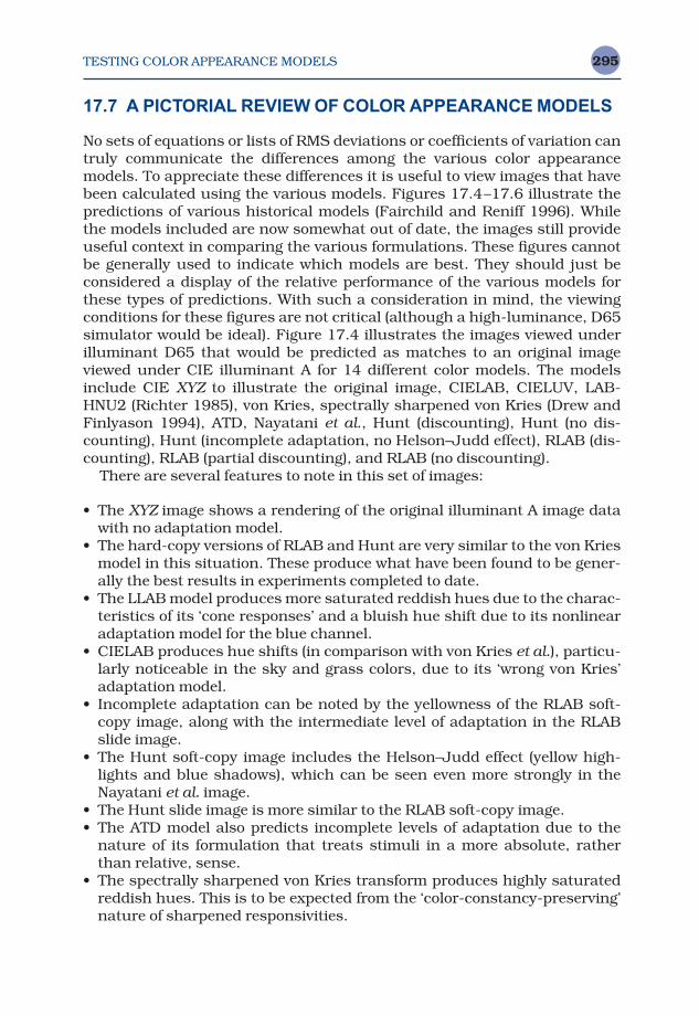
TESTING COLOR APPEARANCE MODELS 295
17.7 A PICTORIAL REVIEW OF COLOR APPEARANCE MODELS
No sets of equations or lists of RMS deviations or coefficients of variation cantruly communicate the differences among the various color appearancemodels. To appreciate these differences it is useful to view images that havebeen calculated using the various models. Figures 17.4–17.6 illustrate thepredictions of various historical models (Fairchild and Reniff 1996). Whilethe models included are now somewhat out of date, the images still provideuseful context in comparing the various formulations. These figures cannotbe generally used to indicate which models are best. They should just beconsidered a display of the relative performance of the various models forthese types of predictions. With such a consideration in mind, the viewingconditions for these figures are not critical (although a high-luminance, D65simulator would be ideal). Figure 17.4 illustrates the images viewed underilluminant D65 that would be predicted as matches to an original imageviewed under CIE illuminant A for 14 different color models. The modelsinclude CIE XYZ to illustrate the original image, CIELAB, CIELUV, LAB-HNU2 (Richter 1985), von Kries, spectrally sharpened von Kries (Drew andFinlyason 1994), ATD, Nayatani et al., Hunt (discounting), Hunt (no dis-counting), Hunt (incomplete adaptation, no Helson–Judd effect), RLAB (dis-counting), RLAB (partial discounting), and RLAB (no discounting).
There are several features to note in this set of images:
• The XYZ image shows a rendering of the original illuminant A image datawith no adaptation model.
• The hard-copy versions of RLAB and Hunt are very similar to the von Kriesmodel in this situation. These produce what have been found to be gener-ally the best results in experiments completed to date.
• The LLAB model produces more saturated reddish hues due to the charac-teristics of its ‘cone responses’ and a bluish hue shift due to its nonlinearadaptation model for the blue channel.
• CIELAB produces hue shifts (in comparison with von Kries et al.), particu-larly noticeable in the sky and grass colors, due to its ‘wrong von Kries’adaptation model.
• Incomplete adaptation can be noted by the yellowness of the RLAB soft-copy image, along with the intermediate level of adaptation in the RLABslide image.
• The Hunt soft-copy image includes the Helson–Judd effect (yellow high-lights and blue shadows), which can be seen even more strongly in theNayatani et al. image.
• The Hunt slide image is more similar to the RLAB soft-copy image.• The ATD model also predicts incomplete levels of adaptation due to the
nature of its formulation that treats stimuli in a more absolute, ratherthan relative, sense.
• The spectrally sharpened von Kries transform produces highly saturatedreddish hues. This is to be expected from the ‘color-constancy-preserving’nature of sharpened responsivities.
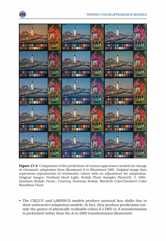
TESTING COLOR APPEARANCE MODELS296
• The CIELUV and LABHNU2 models produce unusual hue shifts due totheir subtractive adaptation models. In fact, they produce predictions out-side the gamut of physically realizable colors if a D65-to-A transformationis performed rather than the A-to-D65 transformation illustrated.
Figure 17.4 Comparison of the predictions of various appearance models for changein chromatic adaptation from Illuminant A to Illuminant D65. Original image datarepresents reproduction of tristimulus values with no adjustment for adaptation.Original images: Portland Head Light, Kodak Photo Sampler PhotoCD, © 1991,Eastman Kodak; Picnic, Courtesy Eastman Kodak; Macbeth ColorChecker® ColorRendition Chart
TESTING COLOR APPEARANCE MODELS 297
Figure 17.5 illustrates the changes predicted for changes in adapting lum-inance from 100 cd/m2 to 10 000 cd/m2 with a constant D65 white point.These predictions are presented for the models with luminance depend-encies (ATD, LLAB, Nayatani et al., Hunt, and RLAB) in addition to a singleimage representing all of the other models. The original image was ‘gamutcompressed’ to allow all of the model predictions to remain within gamut.The RLAB model has very little luminance dependency and therefore pro-duces an image very similar to the original. The Hunt and Nayatani et al.models produce images of lower contrast. This is to be expected according to the Hunt and Stevens effects. These low-contrast images would appear tobe of higher contrast when viewed at a high luminance level. The Nayatani et al. model predicts a larger luminance-dependent effect than the Huntmodel. The ATD model makes the opposite prediction. Since it is based onabsolute rather than relative signals, the ATD model predicts that a brighter,higher-contrast image will be required at the higher luminance levels. Thisprediction is incorrect.
Figure 17.5 Comparison of the predictions of various appearance models for changein luminance from illuminant D65 at 100 cd/m2 to illuminant D65 at 10 000 cd/m2.Original image data represents reproduction of tristimulus values with no adjust-ment for luminance and therefore the predictions of all models that do not accountfor luminance level changes. See Figure 17.4 caption for image credits
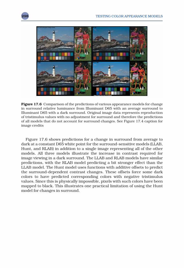
TESTING COLOR APPEARANCE MODELS298
Figure 17.6 shows predictions for a change in surround from average todark at a constant D65 white point for the surround-sensitive models (LLAB,Hunt, and RLAB) in addition to a single image representing all of the othermodels. All three models illustrate the increase in contrast required forimage viewing in a dark surround. The LLAB and RLAB models have similarpredictions, with the RLAB model predicting a bit stronger effect than theLLAB model. The Hunt model uses functions with additive offsets to predictthe surround-dependent contrast changes. These offsets force some darkcolors to have predicted corresponding colors with negative tristimulus values. Since this is physically impossible, pixels with such colors have beenmapped to black. This illustrates one practical limitation of using the Huntmodel for changes in surround.
Figure 17.6 Comparison of the predictions of various appearance models for changein surround relative luminance from Illuminant D65 with an average surround toIlluminant D65 with a dark surround. Original image data represents reproductionof tristimulus values with no adjustment for surround and therefore the predictionsof all models that do not account for surround changes. See Figure 17.4 caption forimage credits
Color Appearance Models Second Edition M. D. Fairchild © 2005 John Wiley & Sons, LtdISBN: 0-470-01216-1 (HB)
18Traditional
ColorimetricApplications
Given all the effort put into the formulation, evaluation, and refinement ofcolor appearance models, it is natural to wonder if they have practical applica-tion beyond the natural scientific curiosity that has driven much of the his-torical research on color appearance phenomena. In recent years, it has beenthe development of technology, and thus applications, that has really pushedthe scientific investigation of color appearance and development of models.These applications can be divided into two general categories:
1. Image reproduction, which is the subject of Chapter 19. 2. The area of color measurement and specification, the subject of this
chapter.
Colorimetry has steadily evolved over the past century. For many applica-tions, simple tristimulus (XYZ) colorimetry or CIELAB-type color differencespecifications are sufficient. However, there are some applications in the traditional fields of colorimetry that require further evolution. A few of theseare discussed in this chapter.
18.1 COLOR RENDERING
Color rendering refers to the way in which various light sources influence, or‘render,’ the color appearance of objects. For example, it is possible for twolight sources to be of the same color while one is a natural daylight and theother is a fluorescent source made up of two narrow-band phosphors that

TRADITIONAL COLORIMETRIC APPLICATIONS300
happen to add together to make the same white. While the color of the twosources will match, the appearances of objects illuminated by these twosources will differ tremendously. This phenomenon is obviously importantin the engineering of artificial illumination and the choice of light sources forvarious installations. If illumination was specified strictly on its efficiency, orits efficacy, the appearance of objects in our environment would be quite disturbing. To aid in this application, the CIE has defined a color renderingindex as a measure of the quality with which a light source renders the colors of objects.
Current Techniques and Recommendations
The current CIE recommended techniques for calculation of color renderingindices are described in CIE Publication 13.3 (CIE 1995a). Light sources areevaluated relative to reference illuminants, which are defined to be the CIED-series of illuminants for correlated color temperatures greater than orequal to 5000 K and Planckian radiators for correlated color temperaturesless than 5000 K. The reference illuminant is chosen such that it has thesame correlated color temperature as the test source. Differences in colorbetween the test source and reference illuminant are accounted for using avon Kries-type chromatic adaptation transform. The CIE technique defines aspecial color rendering index according to Equation 18.1.
Ri = 100 − ∆Ei (18.1)
The color difference calculation ∆Ei is based on the Euclidean distancebetween the color of the sample under the test and reference sources in thenow obsolete CIE U*V*W* space. A general color rendering index Ra is de-fined as the average of the special color rendering indices for eight specifiedMunsell samples. Examples of general color rendering indices for variouslight sources are given in Table 18.1.
Table 18.1 Example values of color rendering indices
Source Ra
Tungsten halogen 100Illuminant D65 100Xenon 93Daylight fluorescent 92Cool white fluorescent 58Tri-band fluorescent 85High pressure sodium 25Mercury 45Metal halide 80
TRADITIONAL COLORIMETRIC APPLICATIONS 301
Application of Color Appearance Models
The fundamental question in the specification of color rendering propertiesof light sources is the specification of the appearance of colored objectsunder different light sources. In some cases, it is necessary to compare theappearance of objects under sources of different colors. It might also be ofinterest to compare the rendering properties of sources at different lumin-ance levels. To make comparisons of color appearance across changes inillumination color and luminance level, an accurate color appearance modelis required. Thus, given appropriate standard references, one would be ableto compare the quality of color rendering of a tungsten source with that of adaylight source and have meaningful results.
Future Directions
While there is certainly room for improved measures of color renderingbased on an accurate color appearance model, the current status of colorappearance models precludes a large change in the capabilities of an index.Currently, CIE Technical Committee 1-33, Colour Rendering, proposed somerevised procedures for the specification of color rendering. The first step wasto define a new procedure for calculation, independent of the color spaceused.
That procedure, using the CIELAB color space combined with an improvedchromatic adaptation transform (originally the Nayatani et al. nonlineartransform was considered, but the CAT02 transform would be a better cur-rent solution), would be an improvement over the current color renderingindex.
With the current type of color rendering index, in which sources are onlycompared with a standard illuminant of the same correlated color tempera-ture, the color appearance model is not being used for a large change inchromatic adaptation. Thus it is doubtful whether any color appearancemodel would be significantly better than any other, including CIELAB, forthis calculation. Only when a more sophisticated technique for specifyingcolor rendering across large changes in light source color and/or luminancelevel is formulated will a more complicated color appearance model berequired.
18.2 COLOR DIFFERENCES
The measurement of color differences has wide application in a variety ofindustries. Such measurements are required to set and maintain color toler-ances for the production and sale of all colored materials. Ideally, one wouldbe able to take a metric of color difference, such as CIELAB ∆E*ab, and con-sider it as a ratio scale of perceived color differences. This would require that
TRADITIONAL COLORIMETRIC APPLICATIONS302
color differences of the same perceived magnitude have the same ∆E*ab forall areas of color space. Another requirement would be for the perceptions of color differences to scale linearly with measured ∆E*ab. A third desirablefeature would be for ∆E*ab values measured under one illuminant to be per-ceptually equal to ∆E*ab values measured under any other illuminant suchthat color differences could be directly compared across different lightsources. It has been well established that the CIELAB color space is not uniform for the measurement of color differences and does not meet any ofthe above requirements. In fact, this might not be possible in any Euclideancolor space.
Current Techniques and Recommendations
The weaknesses of the simple CIELAB ∆E*ab formula have been addressedboth within and outside CIE activities. For example, the CMC color differ-ence formula is designed to address some of the nonuniformities in theCIELAB space in order to make color difference measurements in one regionof color space equivalent to measurements in other regions of color space.CIE Technical Committee 1-29 investigated the CMC and other equations as possible refinements of the CIELAB ∆E*ab formula. They concluded thatthe CMC color difference equation was more complex than warranted by theavailable visual data, and they created a simplified formula known as CIE∆E*94 (CIE, 1995). The ∆E*94 equations are specified in Equations 18.2–18.5.
(18.2)
SL = 1 (18.3)
SC = 1 + 0.045C*ab (18.4)
SH = 1 + 0.015C*ab (18.5)
C*ab in Equations 18.4 and 18.5 refers to the CIELAB chroma of the standardsample of the color difference pair or, alternatively, to the geometric mean ofthe two chroma values. Parametric factors, kL, kC, and kH, are introduced tocorrect for variation in perceived color difference caused by certain experi-mental variables such as sample size, texture, separation, etc. Under refer-ence conditions the parametric factors are all set to 1.0. Reference conditionsare defined as follows:
Illuminantion: CIE illuminant D65 simulatorIlluminance: 1000 luxObserver: normal color vision
∆∆ ∆ ∆
EL
k S
C
k S
H
k SL L
ab
C C
ab
H H
** * *
/
94
2 2 2 1 2
=
+
+
TRADITIONAL COLORIMETRIC APPLICATIONS 303
Viewing mode: objectSample size: greater than 4° visual angleSample separation: minimal, direct edge contactColor difference magnitude: 0–5 CIELAB unitsStructure: visually homogeneous.
The reference conditions of the ∆E*94 equations illustrate the limitations ofthe CIELAB space for the specification of color appearance. These are theareas in which it might be possible for a color appearance model to make acontribution to the specification of color differences. More recently (CIE2001) the CIE has recommended a substantially more complex, empiricalcolor difference equation based upon the CIELAB color space, referred to asDE2000. The DE2000 equation could legitimately be considered to complex,with unreasonable implied precision, for the available perceptual data.Thus, the ∆E*94 equations, are often a more practical and reasonable choice.
Application of Color Appearance Models
In the area of color difference specification, color appearance models couldbe used to incorporate some of the parametric effects directly into the equa-tion. For example, an accurate color appearance model could incorporatethe effects of the background and luminance level on color difference percep-tion. A color appearance model would also make it possible to directly com-pare color differences measured for different viewing conditions. This hasapplications in the calculation of indices of metamerism, as described below.Color appearance models would also make it possible to calculate color dif-ferences between a sample viewed in one condition and a second sampleviewed in another different conditions. This could be useful for critical colorssuch as those on warning signs or corporate trademarks.
It is reasonable to expect that a color difference equation could be optim-ized in a color appearance space, like CIECAM02, with performance equalto, or better than, equations like ∆E*94 and DE2000. Recently, Li et al. (2003)have shown this to be the case.
Future Directions
Currently there is little activity aimed at incorporating color appearancemodels beyond CIELAB into practical color difference specification. Perhapsthis is because of the effort already invested in fine-tuning CIELAB withinvarious industries. Instead, research activity (which is not abundant) isaimed at further refining equations within CIELAB, such as DE2000 and∆E*94, and defining the influence of parametric effects such as gloss, texture,sample separation, sample size, etc. Also, the majority of effort in the for-mulation of color appearance models has been in the area of chromatic
TRADITIONAL COLORIMETRIC APPLICATIONS304
adaptation transforms, and little attention has been paid to color differencespecification within the color appearance spaces. The notable historicalexception is the formulation of the LLAB space (Luo et al. 1996) in whichcolor appearance and color difference were treated simultaneously and therecent efforts by Li et al. (2003) to derive similar equations in CIECAM02.Also, the RLAB space (Fairchild 1996) has been formulated to preserve theCIELAB spacing such that CIE color difference formulas such as ∆E*94 couldstill be used.
Another interesting future direction for color difference specification is theincorporation of the spatial characteristics of human visual performanceinto the difference metric such that the relative sensitivity to color variationsof various spatial frequencies is appropriately treated. Examples of this typeof metric can be found in the work of Maximus et al. (1994), Zhang andWandell (1996), and Johnson and Fairchild (2003a,b). Chapter 20 discussesfuture directions for these ideas.
18.3 INDICES OF METAMERISM
Metamerism, the fact that two stimuli can match in color while having disparate spectral power distributions, is both a great benefit and severedetriment to a variety of industries. Techniques to quantify the degree ofmetamerism for various stimuli are of significant value. There are two typesof metamerism to be measured:
1. Illuminant metamerism2. Observer metamerism
Measures of the degree of metamerism for specific stimuli are called in-dices of metamerism.
Illuminant metamerism is generally of most concern. It occurs when two objects match in color for one illuminant, but mismatch for a secondilluminant. This happens when the spectral reflectance functions of the twostimuli differ, but those differences are unimportant with respect to thevisual response functions (color matching functions) when integrated withthe spectral power distribution of the first illuminant. When the illuminantis changed, these differences might become apparent to an observer. Illum-inant metamerism is often a problem in industries that produce coloredmaterials. If they produce two materials that are a metameric match to oneanother, they might mismatch under some practical viewing conditions. Ifthe two materials are an identical match, meaning their spectral reflectancefunctions are identical, then they are not metameric and will match for anyilluminant.
Observer metamerism is more difficult to quantify, but perhaps equallyimportant. It is caused by the normal variations in the color responsivities of various observers. Observer metamerism is defined by two stimuli with
TRADITIONAL COLORIMETRIC APPLICATIONS 305
differing spectral power distributions that match for a given observer. Whenthese stimuli are examined by a second observer, they might no longermatch. Again, stimuli that are identical spectral matches will match for any observer. Thus, illuminant metamerism becomes apparent when theilluminant is changed and observer metamerism becomes apparent whenthe observer is changed.
Current Techniques and Recommendations
CIE Publication 15.2 (CIE 1986) describes a technique to calculate an indexof metamerism for change in illuminant. Essentially the recommendation is to calculate a CIELAB ∆E*ab, or any other color difference metric, for theilluminant under which the two stimuli do not match. This could be any illum-inant of interest as long as the two stimuli match under the illuminant of primary interest. There is no clear recommendation on how to calculate thisindex of metamerism when the two stimuli are not perfect matches underthe primary illuminant. In such a case, technically, there is no metamerism,but simply a pair of stimuli with an unstable color difference. Techniques forovercoming this limitation have been discussed by Fairman (1987).
CIE Publication 80 (CIE 1989) describes a technique for calculation of an index of metamerism for change in observer. Essentially, the standardcolorimetric observer is replaced with a standard deviate observer and thecolor difference between the two stimuli is calculated for this new observer.The concept is sound, but the data on which the standard deviate observerwere based had been normalized resulting in an under-prediction of thedegree of observer metamerism (Alfvin and Fairchild 1997). Nimeroff et al.(1961) described a technique whereby a complete standard observer system,including mean and covariance color matching functions, could be spe-cified. This concept is similar to the idea of the CIE (1989) technique, but ithas never been fully implemented due to a lack of data.
Application of Color Appearance Models
Color appearance models could be of some utility in the quantification ofilluminant metamerism since it involves the comparison of stimuli acrosschanges in illumination. Essentially the contribution to an index of illumin-ant metamerism would be the availability of a color difference metric that isconsistent across a variety of illuminants. Also, an accurate color appear-ance model would allow the creation of a new type of metric for single stim-uli. A single sample cannot be considered metameric since it does not matchanything. However, it is common to talk of a single sample being metamericwhen its apparent color changes significantly with a change in illuminant.This is really a lack of color constancy. A good color appearance model wouldallow one to calculate a color difference metric between a sample under one

TRADITIONAL COLORIMETRIC APPLICATIONS306
illuminant and the same sample under a second illuminant, thus allowingthe creation of an index of color constancy. This could be useful for objectsthat are intended to look the same color under various illumination condi-tions, such as those containing safety colors.
There really is little use for a color appearance model in the specification of observer metamerism beyond the potential for a better color differencemetric. The measurement of observer metamerism is an excellent example of a situation in which the problem needs to first be completely addressed at the level of basic colorimetry. In other words, the observer variability intristimulus values must first be adequately specified before it is necessary tobe concerned about the improvements that a color appearance model couldmake. This path should be taken as a model for all potential applications ofcolor appearance models.
Future Directions
There is little activity aimed at the improvement of indices of metamerism.For illuminant metamerism, effort is concentrated on the improvement ofcolor difference metrics. For observer metamerism, there seems to be littlecall for a better metric, despite the flaws in the current metric (which is notwidely used). This situation could be because it is difficult enough to addressproblems of illuminant metamerism to cause the difficulties associated withobserver metamerism to be considered of second order at this time.
18.4 A GENERAL SYSTEM OF COLORIMETRY?
Consideration of some of the problems of traditional colorimetry described inthis chapter leads one to wonder whether it might be possible to create ageneral system of colorimetry that could be used to address all the problemsof interest. Currently, colorimetry has taken a very evolutionary form ofdevelopment moving from CIE XYZ tristimulus values to the CIELAB colorspace, to enhancements of CIELAB for measuring color difference and colorappearance. This development is useful to ensure compatibility with indus-trial practices that are based on previous standard procedures. However, the level of complexity is getting to the point where there might be multiplecolor models, each more appropriate for a different application. CIELAB andCIELUV were recommended by the CIE in 1976 to limit the number of colordifference formulae being used internationally to two, rather than the everincreasing number that were being used prior to that time. That recommenda-tion was quite successful and has resulted in CIELAB becoming essentiallythe only color space in use (along with a few color difference equations basedon it). Perhaps a similar state of affairs is currently developing in the area ofcolor appearance models and recent recommendations from the CIE willbring about some order. However, it is still likely that systems for color

TRADITIONAL COLORIMETRIC APPLICATIONS 307
appearance and for color difference will be separate in practice. The LLABmodel (Luo et al. 1996) represents one interesting attempt to bring colori-metry together with one general model. Li et al. (2003) have begun to carrythis work forward with respect to CIECAM02. Perhaps this approach shouldbe pursued.
An alternate approach is to start over from scratch, taking advantage ofthe progress in visual science and colorimetry over the last century, to createa new system of colorimetry that is superior for all steps in the process andcan find a wide range of applications in science, technology, and industry.Color appearance models take a step in this direction by first transformingfrom CIE tristimulus values to cone responses and then building up colorappearance correlates from there. There is also activity within the CIE (e.g.,TC1-36, Fundamental Chromaticity Diagram with Physiologically Signific-ant Axes) to develop a system of colorimetry based on more accurate coneresponsivities that are not necessarily tied to a CIE Standard ColorimetricObserver. It is thought that such a system would find wide use in color visionresearch. Boynton (1996) has reviewed the history and status of such work.Perhaps some convergence between the two activities is needed to develop a better, general system of colorimetry that could be used by everyone.Unfortunately, this paragraph is just as true for the second edition of thisbook in 2004 as it was when written for the first edition in 1997!
Color Appearance Models Second Edition M. D. Fairchild © 2005 John Wiley & Sons, LtdISBN: 0-470-01216-1 (HB)
19Device-independent
Color Imaging
A computer user takes a photograph, has it processed and printed, scansthe print into the system, displays it on the monitor, and finally prints it on adigital printer. This user has completed at least three input–process–displaycycles on this image. Despite spending large sums of money on variousimaging hardware, it is extremely unlikely that the colors in the final printlook anything like the original object or are even satisfactory. There are also intermediate images that might be compared with one another and theoriginal object.
The system described above is an ‘open system’. This means that the userchose each of the components and put them together. Each of the imagingdevices has its own intrinsic physical process for image input, processing,and/or display and they are not necessarily designed to function with eachother. If each component functions in its native mode, then the results pro-duced with an open system are nearly unpredictable. One reason for this isthe open nature of the systems; there are too many possible combinations ofdevices to make them all work well with one another.
Allowing the devices to function in their own intrinsic color dimensions iswhat is known as device-dependent color imaging. The difficulty with device-dependent coordinates is that the RGB coordinates from a scanner mightnot mean the same thing as the RGB signals used to drive a monitor orprinter. To solve these problems and produce reliable results with open sys-tems, device-independent color imaging processes must be used. The con-cept of device-independent color imaging is to provide enough informationalong with the image color data such that the image data could, if necessary,be described in coordinates that are not necessarily related to any particulardevice. Transformations are then performed to represent those colors on anyparticular device.
DEVICE-INDEPENDENT COLOR IMAGING 309
The strong technological push for reliable device-independent color imag-ing over the last decade has stressed the scientific capabilities in the area ofcolor appearance modeling since the various images are typically viewed in awide variety of viewing conditions. While it has been recognized for some timethat a color appearance model is necessary for successful device-independentcolor imaging, there has not been a simple solution to that problem available.The first 17 chapters of this book present some of the issues and problemsthat must be addressed while this chapter provides an overview of the basicconcepts required to put the pieces together and build systems.
Device-independent color imaging has become the focus of many scient-ists and engineers over recent years. It is impossible to cover the scope ofissues involved in a single chapter. Entire books dedicated to this topic havebecome available (Giorgianni and Madden 1997, Kang 1997, Sharma 2003).In recent years, color management systems have become more common-place and many books aimed at advanced end-users have been published(e.g., Fraser et al. 2003, Stone 2003) Also, Hunt’s text on color reproduction(Hunt 1995) provides much necessary insight into the fundamentals of traditional and digital color reproduction. Sharma and Trussel (1997) havepublished a review paper on the field of digital color imaging that includeshundreds of references. The treatment in this chapter is culled from a seriesof earlier works (Fairchild 1994a, 1995b, 1996).
19.1 THE PROBLEM
The application of basic colorimetry produces significant improvement inthe construction of open color imaging systems by defining the relationshipsbetween device coordinates (e.g., RGB, CMYK) and the colors detected orproduced by the imaging systems. However, it is important to recall thatmatching CIE tristimulus values across various imaging devices is only partof the story. If an image is reproduced such that it has CIE tristimulus values identical to the original, then it will match the original in appearanceas long as the two are viewed under identical viewing conditions (matchingthose for which the tristimulus values were calculated). Since originals,reproductions, and intermediate images are rarely viewed under identicalconditions, it becomes necessary to introduce color appearance models tothe system in order to represent the appearance of the image at each stage ofthe process.
Issues in device-independent color imaging that color appearance modelscan be used to address include changes in white point, luminance level, sur-round, medium (viewing mode), etc. Since these parameters normally varyfor different imaging modalities, the necessity for color appearance models isclear. The introduction of color appearance models allows the systems to beset up and used to preserve, or purposefully manipulate, the appearances of image elements in a controlled manner at each step. Thus, users can viewan image on an LCD display, manipulate it as they choose, and then make

DEVICE-INDEPENDENT COLOR IMAGING310
prints that accurately reproduce the appearance of the image on the LCDwith the aid of color appearance models.
Of course, it is not always possible, or desirable, to exactly reproduce theappearance of an original image. Color appearance models can be useful inthese situations as well. One problem is that different imaging devices arecapable of producing different ranges of colors, known as their color gamut.A given stimulus on an LCD display produces a certain appearance. It mightnot be possible to produce a stimulus on a given printer that can replicatethat appearance. In such cases, a color appearance model can be used toadjust the image in a perceptually meaningful way to produce the best pos-sible result. In other cases, the viewing conditions might limit the gamut of areproduction. For example, photographic prints of outdoor scenes are oftenviewed under artificial illumination at significantly lower luminance levelsthan the original scene. At the lower luminance level it is impossible to pro-duce the range of luminance and chromatic contrast that is witnessed in theoriginal scene. Thus it is common for consumer photographic prints to beproduced with increased physical contrast to overcome this change in view-ing conditions. Color appearance models can be used to predict such effectsand guide the design of systems to address them.
Another advantage of color appearance models in device-independentcolor imaging is in the area of image editing. It is more intuitive for untrainedusers to manipulate the colors in images along perceptual dimensions suchas lightness, hue, and chroma, rather than through device coordinates such as CMYK. A good color appearance model can improve the correlationbetween tools intended to manipulate these dimensions and the changesthat users implement on their images.
19.2 LEVELS OF COLOR REPRODUCTION
Hunt (1970, 1995) has defined six different objectives for color reproduction:
1. Spectral Color Reproduction
Spectral color reproduction involves identical reproduction of the spectralreflectance curves of the original image or objects. Two techniques that areso impractical as to be of only historical interest, the Lippman and microdis-persion methods (see Hunt 1995), managed to fulfill this difficult objective.Modern color reproduction techniques take advantage of metamerism byusing RGB additive primaries or CMY subtractive primaries, thus eliminat-ing the possibility of spectral reproduction except in cases in which the original is comprised of the same imaging materials. Recently developed,and currently developing, printing techniques that utilize six or more inksprovide an opportunity for better approximations to spectral color reproduc-tion that might be useful in applications such as mail-order catalogs or fine-art reproductions (in addition to expanding the output gamut).

DEVICE-INDEPENDENT COLOR IMAGING 311
2. Colorimetric Color Reproduction
Colorimetric color reproduction is defined via metameric matches betweenthe original and the reproduction such that they both have the same CIEXYZ tristimulus values. This will result in the reproduction of color appear-ances in cases for which the original and reproduction of the same size areviewed under illuminants with the same relative spectral power distribution,luminance, and surround. Hunt, however, does not make equality of lumin-ance level a requirement for colorimetric color reproduction.
3. Exact Color Reproduction
Exact color reproduction is defined as colorimetric color reproduction withthe additional constraint that the luminance levels be equal for the originaland the reproduction.
4. Equivalent Color Reproduction
Equivalent color reproduction is defined to acknowledge situations in whichthe color of illumination for the original and the reproduction differ. In suchcases, precise reproduction of CIE tristimulus values would result in imagesthat were clearly incorrect since nothing has been done to account for chro-matic adaptation. Equivalent color reproduction thus requires the tristimu-lus values and the luminances of the reproduction to be adjusted such thatthey produce the same appearances as found in the original. This requiresthe differences between the original and the reproduction viewing conditionsto be incorporated using some form of color appearance or chromatic adapta-tion model. When there are large changes in luminance level between theoriginal and the reproduction, it might be impossible to produce appearancematches, especially if the objective is brightness–colorfulness matchingrather than lightness–chroma matching.
5. Corresponding Color Reproduction
Corresponding color reproduction addresses the luminance issue byneglecting it to a degree. A corresponding color reproduction is one that isadjusted such that its tristimulus values are those required to produceappearance matches if the original and the reproduction were viewed atequal luminance levels. This eliminates the problems that arise when tryingto reproduce brightly illuminated originals in dim viewing conditions andvice versa. It can be thought of as an approximation to lightness–chromamatching if one were willing to assume (incorrectly) that lightness andchroma are constant across changes in luminance level. Since lightness and
DEVICE-INDEPENDENT COLOR IMAGING312
chroma are far more constant across luminance changes than brightnessand colorfulness, this assumption might not be too bad, especially givenpractical gamut-mapping constraints.
6. Preferred Color Reproduction
Preferred color reproduction is defined as reproduction in which the colorsdepart from equality of appearance to those in the original in order to give a more pleasing result. This might be applicable in situations such as con-sumer photography in which consumers prefer to have prints that repro-duce colors closer to their memory colors for objects such as skin tones,vegetation, sky, bodies of water, etc. However, as Hunt (1970) points out,‘the concepts of spectral, colorimetric, exact, equivalent, and correspondingcolor reproduction provide a framework which is a necessary preliminary toany discussion of deliberate distortions of colour reproduction.’
19.3 A REVISED SET OF OBJECTIVES
Hunt’s objectives for color reproduction provide a good summary of theproblems encountered in color reproduction and how they can be addressedusing concepts of basic and advanced colorimetry. It is interesting to notethat these objectives were originally published long before issues in device-independent color imaging were commonly discussed (Hunt 1970). A slightrearrangement and simplification of Hunt’s objectives can be used to definefive levels of color reproduction that provide a framework for modern colorimaging systems.
1. Color Reproduction
Color reproduction refers to simple availability devices capable of producingcolor graphics and images. There is usually great excitement surroundingthe initial commercial availability of color devices of any given type. Whilethis might not seem like much of an accomplishment, it is worth remember-ing that personal computers with reasonable color capabilities have beenavailable for less than 20 years. The plethora of high-quality input and out-put devices is very recent. When these technologies are first introduced,users are excited simply by the fact that they now have color available wherepreviously it was not. However, this ‘honeymoon period’ quickly wears offand users begin to demand more from their color imaging devices — theywant to have devices that produce and reproduce colors with some sem-blance of control and accuracy. This pushes open-systems technology towardthe next levels of color reproduction.

DEVICE-INDEPENDENT COLOR IMAGING 313
2. Pleasing Color Reproduction
Pleasing color reproduction refers to efforts to adjust imaging devices andalgorithms such that consumers find the resulting images acceptable. Suchimages might not be accurate reproductions and they are probably not thepreferred reproductions, but they look pleasing and are found acceptable tomost consumers of the images. This level of reproduction can often beachieved through trial and error without requiring any of the concepts ofdevice-independent color imaging. The approach to obtaining pleasing colorreproduction in open systems would be similar to the approaches historic-ally taken in closed imaging systems to achieve similar goals or, in somecases, preferred color reproduction. Pleasing color reproduction can be areasonable final goal for a color reproduction system in which observershave no knowledge of the original scene or image and, therefore, no expecta-tions beyond desiring a pleasing image.
3. Colorimetric Color Reproduction
Colorimetric color reproduction includes calibration and characterization ofimaging devices. This means that for a given device signal, the colorimetriccoordinates of the image element produced (or scanned) are known with areasonable degree of accuracy and precision. With colorimetric color repro-duction, a user can put together a system in which an image is scanned, thedata are converted to colorimetric coordinates (e.g., CIE XYZ ), and thenthese coordinates are transformed into appropriate RGB signals to displayon an LCD, or into CMYK signals for output to a printer. Of course, it is notnecessary for the image data to actually be transformed through the device-indpendent color space. Instead, the full transform from one device, throughthe device-independent space, to the second device can be constructed andimplemented for enhanced compuatational efficiency and minimization ofquantization errors. Such a system allows the CIE tristimulus values of theoriginal image to be accurately reproduced on any given output device. Thisis similar to Hunt’s definition of colorimetric color reproduction. To achievecolorimetric color reproduction, devices and techniques for the colorimetriccharacterization and calibration of input and output devices must be readilyavailable. A variety of such techniques and devices is available commer-cially, but the degree to which colorimetric color reproduction can actuallybe achieved by typical users is dubious. Unfortunately, the state of the artfor most users is just color reproduction; colorimetric color reproduction hasyet to be reliably achieved. Colorimetric color reproduction is useful onlywhen the viewing conditions for the original and reproduced images areidentical since this is the only time that tristimulus matches representappearance matches. When the viewing conditions differ, as they usually do,one must move from colorimetric color reproduction to the next level.
DEVICE-INDEPENDENT COLOR IMAGING314
4. Color Appearance Reproduction
Color appearance reproduction requires a color appearance model, informa-tion about the viewing conditions of the original and reproduced images, andaccurate colorimetric calibration and characterization of all the devices. Forcolor appearance reproduction, the tristimulus values of the original imageare transformed to appearance correlates, such as lightness, chroma, andhue, using information about the viewing conditions such as white point,luminance, surround, etc. Information about the viewing conditions for theimage to be reproduced is then used to transform these appearance corre-lates into the tristimulus values necessary to produce them on the outputdevice. Color appearance reproduction is necessary to account for the widerange of media and viewing conditions found in different imaging devices.This is similar to Hunt’s equivalent color reproduction applied to lightness–chroma matches. Color appearance reproduction has yet to become a com-mercial reality and perhaps it cannot for typical users. However, even whenreasonable color appearance reproduction does become available, there willbe cases when users will desire reproductions that are not accurate appear-ance matches to the originals. Such cases enter the domain of color prefer-ence reproduction.
5. Color Preference Reproduction
Color preference reproduction involves purposefully manipulating the colorsin a reproduction such that the result is preferable to the users over anaccurate appearance reproduction. The objective is to produce the best pos-sible reproduction for a given medium and subject. This is similar to Hunt’sdefinition of preferred color reproduction.
Note that to achieve each level of reproduction in open systems it is neces-sary to have first achieved the lower levels. To summarize, the five levelsinvolve simply reproducing colors, reproducing pleasing colors, equality oftristimulus values, equality of appearance attributes, and manipulation ofappearance attributes to ‘improve’ the result. In closed systems it is not necessary for technology to progress through each of the five levels. This is because the path of image data is defined and controlled throughout the whole process. For example, in color photography, the film sensitivities,dyes, processing procedures, and printing techniques are all well defined.Thus it is possible to design a photographic negative film to produce pleasingor preferred color reproduction without having the capability for colorimetricor color appearance reproduction since the processing and printing stepsare well defined. A similar system exists in color television with standardcamera sensitivities, signal processing, and output device setup. In opensystems, an intractable number of combinations of input, processing, dis-play, and output devices can be constructed and used together. The manu-facturer of each subsystem cannot possibly anticipate all of the possible
DEVICE-INDEPENDENT COLOR IMAGING 315
combinations of devices that might be used with it. Thus the only feasiblesolution is to have each device in the system develop through the five levelsdescribed above such that colorimetric, or color appearance, data (or theinformation necessary for obtaining it) can be handed off from one device tothe next in the process known as device-independent color imaging.
19.4 GENERAL SOLUTION
Figure 19.1 is a flow chart of the general process of device-independent colorimaging. At the top of the diagram is the original image as represented bysome input device. (Note that this ‘input’ could come from a display devicesuch as a CRT.) The colorimetric characterization of the input device is thenused to transform the device coordinates (e.g., RGB) to colorimetric coordin-ates such as CIE XYZ or CIELAB, which are referred to as device-independ-ent color spaces since the colorimetric coordinates do not depend on anyspecific imaging device.
The second step is to apply a chromatic adaptation and/or color appear-ance model to the colorimetric data with additional information on the viewing conditions of the original image in order to transform the image datainto dimensions that correlate with appearance such as lightness, hue, andchroma. These coordinates, that have accounted for the influences of theparticular device and the viewing conditions, are referred to as viewing-conditions-independent space. At this point, the image is represented purelyby its original appearance. This is the point where it is most appropriate toperform manipulations on the image colors. These manipulations mightinclude gamut mapping, preference editing, tone reproduction adjustments,spatial scaling operations, certain forms of error diffusion, etc. At this point,the image is in its final form with respect to the appearances that are to bereproduced. Now the process must be reversed.
This highlights the utility of an analytically invertible color appearancemodel. The viewing conditions for the output image, along with the finalimage appearance data, are used in an inverted color appearance model totransform back from the viewing conditions independent space to a device-independent color space such as CIE XYZ tristimulus values. These values,together with the colorimetric characterization of the output device, are usedto transform to the device coordinates (e.g., CMYK) necessary to produce thedesired output image. The following sections provide some additional detailon each step of this process.
Note that the literal implementation of the processes of device-independentcolor imaging as described above requires substantial computational re-sources. For example, to avoid severe quantization errors, image processingis usually performed on floating-point image data with floating-point com-putational precision when working within the intermediate color appearancespaces. While this is acceptable for color imaging research, it is not prac-tical in most commercial color imaging systems, particularly those that are
DEVICE-INDEPENDENT COLOR IMAGING316
limited to 24-bits-per-pixel color data. In such cases, the processes describedabove are used to construct the systems and algorithms, while implementa-tion is left to multidimensional interpolation within eight-bits-per-channellook-up tables (LUTs). It is interesting to note that the computer graphicsindustry, as opposed to the color imaging/publishing industry, typicallyworks with floating-point, and higher-precision integer, image data. Perhapsthe confluence of the two fields will solve some historical computationalissues and limitations.
19.5 DEVICE CALIBRATION AND CHARACTERIZATION
Device calibration refers to setting the imaging device to a known state. Thismight represent a certain white point, gain, and offset for a CRT or certainrelationships between density and drive signal for a printer. Calibrationensures that the device is producing consistent results, both from day to dayand from device to device. However, device calibration can be completed withabsolutely no information about the relationship between device coordinatesand the colorimetric coordinates of the input or output image. Colorimetriccharacterization of the device is required to obtain this information. Charac-terization refers to the creation of a relationship between device coordinatesand a device-independent color space — the first step in Figure 19.1.
Device calibration is usually an issue for the manufacturer, rather thanthe user, and the techniques depend heavily on the technology. Thus calib-ration will not be discussed further except to stress its importance. If con-sistent results are necessary from day to day or from device to device, thencareful and frequent device calibration is necessary. There are tradeoffs thatcan be made between calibration and characterization. If careful calibrationis not possible, then accuracy can be achieved through frequent character-ization. If an extremely good calibration procedure is available, it might bepossible to perform the colorimetric characterization just once, as long asthe device is frequently calibrated.
Three Approaches to Device Characterization
There are three main approaches to device characterization:
1. Physical modeling2. Empirical modeling3. Exhaustive measurement.
Of course, there are also procedures that combine aspects of one or moreof these techniques. In all cases, it is typical to use the characterization tobuild a three-dimensional look-up table (LUT) that is used in conjunctionwith an interpolation procedure to process the vast amounts of image datathat are encountered.

DEVICE-INDEPENDENT COLOR IMAGING 317
Physical Modeling
Physical modeling of imaging devices involves building mathematical modelsthat relate the colorimetric coordinates of the input or output image ele-ments to the signals used to drive an output device or the signals originatingfrom an input device. Such models can be derived for all types of imagingdevices with varying degrees of difficulty. A physical model for a scannerwould involve a step to first linearize the signals with respect to luminance,or perhaps absorbance, and then a second step to transform the signals toCIE tristimulus values. Depending on the scanner design, knowledge of thephysical properties of the material being scanned might be required. Thiscould be avoided if the scanner were designed as a colorimeter rather thanwith arbitrary RGB responsivities.
A physical model for a CRT display involves a nonlinear transform to con-vert drive voltages to the corresponding RGB phosphor luminances, followedby a linear transformation to CIE XYZ tristimulus values. A physical modelfor a hard-copy output device requires a transformation from drive signals to
Figure 19.1 A flow chart of the conceptual process of device-independent colorimaging
DEVICE-INDEPENDENT COLOR IMAGING318
concentrations of dyes, pigments, or inks and then a color mixing model topredict spectral reflectances or transmittances that can then be used to cal-culate CIE XYZ tristimulus values. The advantage of physical device modelsis that they are robust, typically require few colorimetric measurements inorder to characterize the device, and allow for easy recharacterization ifsome component of the imaging system is modified. The disadvantage is thatthe models are often quite complex to derive and can be complicated toimplement. Physical models are often used for CRT display characterization.
Empirical Modeling
Empirical modeling of imaging devices involves collecting a fairly large set ofdata and then statistically fitting a relationship between device coordinatesand colorimetric coordinates. Such models are often implemented to trans-form directly to CIELAB coordinates to avoid quantization difficulties in CIEXYZ tristimulus values.
Empirical models are often high-order multidimensional polynomials or,alternatively, neural network models of significant complexity. Empiricalmodels require fewer measurements than look-up table techniques, but morethan physical models. Empirical models are also often poorly behaved nearthe edge of the device gamut, producing very large systematic errors. Sinceempirical models have no relationship to the physics of the imaging devices,they must be recreated each time a change is made in any component of thesystem. Empirical models are often used for scanner characterization.
Exhaustive Measurement
The final class of characterization techniques involves exhaustive measure-ment of the output for a complete sampling of the device’s gamut. (Signalsfor a large sampling of known input colors can be collected for scanner char-acterization.) Typically, something like a 9 × 9 × 9 sampling of the devicedrive signals is output and colorimetrically measured. This results in a totalof 729 measurements. Many more measurements might be used for deviceswith poor image-to-image or device-to-device repeatability. The array of colorimetric data must then be nonlinearly interpolated to populate a higherdensity (e.g., 33 × 33 × 33) look-up table (LUT) that can be used to processimage data via multidimensional interpolation. Disadvantages of such tech-niques include the large number of measurements that must be made, diffi-culties in interpolating the highly nonlinear data, the need to redo the entireprocess if any aspect of the device changes, and difficulty in creating theinverse solutions that are typically required. The advantage of exhaustivemeasurement techniques that make them popular is that they require noknowledge of the device physics. Exhaustive measurement and LUT inter-polation techniques are often used for printer characterization.
DEVICE-INDEPENDENT COLOR IMAGING 319
Types of Colorimetric Measurements
Different types of colorimetric measurements are required for characteriza-tion of various imaging devices.
CRT or LCD display characterization requires spectroradiometric or col-orimetric measurements of the phosphor chromaticities in order to derive theRGB-to-XYZ transformation and relative radiometric or photometric meas-urements to derive the nonlinear transfer functions for each channel. Berns(1996) reviews a practical procedure for the calibration and characterizationof CRT displays. Berns et al. (1993a,b) provide further details on the meas-urement and characterization of CRT displays. Berns et al. (2003) also pro-vide details on the measurements and techniques for LCD characterization.
Printers and other output devices require spectrophotometric measure-ments (spectral reflectance or transmittance) to characterize the device col-orants or derive colorimetric coordinates for various illuminants or sources.Additional, densitometric measurements might be of value to characterizetone-transfer functions. Issues in the colorimetric characterization of binaryand multilevel display devices have been discussed by a variety of authorsincluding Jarvis et al. (1976), Engeldrum (1986), Gentile et al. (1990a),Rolleston and Balasubramanian (1993), Berns (1993b), and Haneishi et al.(1996).
Scanners and digital cameras require spectroradiometric evaluation oftheir channel spectral responsivities or empirical estimates of them. Spec-troradiometric data on the illumination system is also required. Additionally,spectroradiometric linearity evaluation and characterization is required forthe detector systems. Often, scanner data for well-characterized input tar-gets are collected to derive relationships between scanner signals and colori-metric coordinates. The colorimetric calibration and characterization ofinput devices has been described by Hung (1991), Kang (1992), Engeldrum(1993), Rodriguez and Stockham (1993), and Berns and Shyu (1995).
Flare, Metamerism, and Fluorescence
There are three additional issues regarding colorimetric measurements thatare often overlooked in device characterization, but require attention: flare,metamerism, and fluorescence.
Flare
Typically, the spectrophotometric or colorimetric measurements made tocharacterize a device are performed with specialized instrumentation andspecially prepared samples. Such measurements are not made in the actualviewing situation for the device. Any real viewing situation includes flare.The spectral energy distribution and level of the flare must be measured andadded to any real colorimetric characterization of an imaging device. Since
DEVICE-INDEPENDENT COLOR IMAGING320
flare is an additive mixture of light with the image, it can be treated as a simple addition of the tristimulus values of the flare to the tristimulus valuesof the image data. This addition might result in the need to recalculate theimage white point and renormalize data appropriately. In some cases, flaremight be image dependent and require a more sophisticated treatment.Alternatively, meaasurements of image color must be made in situ, using atelespectroradiometer that will include the flare of the viewing environmentin the measurement.
Metamerism
Metamerism causes difficulties in both input and output devices. For inputdevices, metamerism combined with non-colorimetric sensor responsivitiescan defeat all hope of obtaining reliable color reproduction. At the outputend, it is necessary to characterize devices using spectral reflectance ortransmittance functions integrated with the actually viewing spectral powerdistributions in order to derive colorimetric coordinates. This is necessaryfor reasonable accuracy, even when using standardized viewing sources. Forexample, the colors observed under a fluorescent D50 simulator can differdramatically from those calculated using CIE illuminant D50.
Fluorescence
The colorimetry of fluoresecent materials is a significant challenge since theenregy emitted by the material is a function of the incident energy from theilluminating source. Since this is not the case for non-fluorescent materials,the light source used for spectrophotometric measurement has no impact onthe colorimetric coordinates calculated for any particular illuminant. Fluo-rescent materials must be measured using illumination that closely simu-lates the illuminant to be used in colorimetric calculations in order to obtainreasonable accuracy. The best practical solution is to measure fluorescentmaterials in their final viewing conditions using a telespectroradiometer.
Fluoresence is an important issue in imaging applications since manysubstrates (i.e., most paper) and many inks and dyes are fluorescent. Grumand Bartleson (1980) provide an excellent overview of the colorimetry offluorescent materials. Gonzalez and Fairchild (2000) examined the signific-ance of fluorescence in the colorimetry of typical printing materials.
Multidimensional LUT Interpolation
No matter what approach is taken to characterize an imaging device, the endresult is typically used to construct a multidimensional LUT for practicalimplementations. This is because it is necessary to complete the many layers of nonlinear transformations and color space conversions requiredwith computational precision significantly greater than the eight bits perchannel found in most imaging devices. Such computations take prohibitive

DEVICE-INDEPENDENT COLOR IMAGING 321
amounts of time on typical desktop imaging systems. Thus multidimen-sional LUT interpolation is implemented for the end-to-end transform forconvenience and efficiency. The construction of multidimensional LUTs andtheir use through interpolation has been described by Hung (1993) andKasson et al. (1993, 1995).
Multidimensional LUT interpolation is implemented in a variety of waysincluding proprietary software such as Adobe Photoshop® and other ‘colormanagement’ software that use these techniques for color space transforma-tions. Multidimensional LUTs are also implemented in the PostScript® Level2 (Adobe Systems Incorporated, 1990) page-description language in theform of color rendering dictionaries. Another well-known open system thatprovides the framework for the implementation of multidimensional LUTsfor device characterization is the ICC profile format (International ColorConsortium, 1995; www.color.org) that serves as a cross-platform standardfor a wide variety of system-level color management systems.
19.6 THE NEED FOR COLOR APPEARANCE MODELS
The process of device-independent color imaging described by Figure 19.1illustrates the necessity of color appearance models. There are two mainneeds for these models–image editing and viewing-condition transformations.Image manipulations such as color preference reproduction and gamutmapping are best performed in the perceptually significant dimensions (e.g.,lightness, chroma, and hue) of a color appearance model. Clearly the trans-formation of colorimetric coordinates from one set of viewing conditions(white point, luminance, surround, medium, etc.) to a second set of viewingconditions requires a color appearance model.
The only way to avoid the use of a color appearance model in device-independent color imaging is to specify a rather strong set of constraints. Theoriginal and the reproduction must be viewed in the same medium, underidentical viewing conditions, with identical gamuts, and with the objective ofcolorimetric color reproduction. In such a constrained world, colorimetric andcolor appearance reproduction are identical. Clearly, the above constraintsare far too severe for all but the most specialized applications. Thus the useof color appearance models in device-independent color imaging is unavoid-able if high-quality, reliable results are to be obtained in open systems.
19.7 DEFINITION OF VIEWING CONDITIONS
One key unresolved issue in the implementation of color appearance modelsin device-independent color imaging is the definition and control of viewingconditions. Even a perfect color appearance model is of little utility if theactual viewing conditions are not the same as those used in the model cal-culations. (The metamerism problems between CIE illuminants and theirphysical simulators is one straightforward example of this difficulty.)
DEVICE-INDEPENDENT COLOR IMAGING322
Part of the difficulty in controlling the viewing conditions is definition of thefields. Hunt (1991b) has done the most extensive job of defining the variouscomponents of the viewing field. However, even with Hunt’s extended defini-tions, it is difficult to decide which portions of the field should be consideredthe proximal field, the background, and the surround when viewing compleximage displays in typical viewing conditions. For example, is the backgroundof an image the area immediately adjacent to the image borders or should itbe considered to be the areas adjacent to individual elements within theimage? The latter definition might be more appropriate; however, it requiressubstantially more complex image-wise computations that are often com-pletely impractical. However the particular aspects of the viewing conditionsare defined, it is important that the treatment is consistent across all imagetransformations to avoid the introduction of bias simply due to the use ofcolor appearance models. As a practical definition, the background forimages should be defined as the area immediately around the image borderwith the surround defined as the remainder of the viewing environment; thisdefinition of background, however, is different from that used by Hunt asdescribed in Chapter 7. The definition of proximal field is unnecessary inimage reproduction since the spatial relationships of the various image ele-ments is constant in the original and the reproduction. The proximal fieldbecomes important when it is desired to reproduce the color appearance ofan image element in a completely different context (e.g., logo colors, trade-mark colors).
Even with strict definitions of the various components of the viewing field,it is of paramount importance that the viewing conditions be carefully con-trolled for successful device-independent color imaging. If users are unwill-ing to control the viewing conditions carefully, they should expect nothingless than unpredictable color reproduction. Viewing condition parametersthat must be carefully controlled for successful color appearance reproduc-tion include:
• The spectral power distribution of the light source• Luminance level• Surround color and relative luminance• Background color and relative luminance• Image flare (if not already incorporated in the device characterization)• Image size and viewing distance (i.e., solid angle)• Viewing geometry.
Also, observers must make critical judgements of the various images onlyafter sufficient time has passed to allow full adaptation to the respectiveviewing conditions.
Braun et al. (1996) illustrated the importance of controlling the viewingconditions for cross-media image comparisons. They concluded that thebest technique for critical judgements was successive binocular viewing inwhich the observer viewed first one image display with both eyes and thenswitched to the other display, allowing approximately one minute to adapt to
DEVICE-INDEPENDENT COLOR IMAGING 323
the new viewing conditions. The arrangement was such that only one imagedisplay could be viewed at a time and the one-minute adaptation wasrequired each time the observer changed from one display to the other.Unfortunately, the most common technique, simultaneous binocular view-ing, in which the original and the reproduction (in a different medium andwhite point) are viewed simultaneously side-by-side produces unacceptableresults. In such cases, the observer’s state of chromatic adaptation cannotbe reliably predicted since it depends on the relative amount of time spentviewing each image. In general, the best results will be obtained if a single,intermediate adaptation point is assumed. However, the result of such achoice will be a reproduction that matches the original when viewed side-by-side, but that looks quite strange when viewed by itself.
For example, if a CRT has a 9300 K white point and a reproduced print isviewed under a D50 simulator, the required print to produce a simultane-ously viewed match will have an overall blue cast. When this print is viewedin isolation, still under a D50 simulator, it will appear unacceptably bluishand be considered a poor match. Katoh (1995) has investigated the problemswith simultaneous viewing of images in different media. However, if a suc-cessive viewing technique with sufficient adaptation time is used, an excel-lent neutrally balanced 9300 K CRT image will be matched by a neutrallybalanced print viewed under a D50 simulator. Thus both color appearancematching and high individual image quality can be obtained with appropri-ate viewing procedures.
Once the viewing conditions are appropriately defined and controlled,some computational advantage can be obtained through judicious precal-culation procedures. Such procedures rely on parsing the implementation ofthe color appearance models into parts that need only be calculated once for each viewing condition and those that require calculation for each imageelement. The most efficient implementation procedure is then to precal-culate the model parameters that are viewing-condition dependent and thenuse this array of data for the individual appearance model calculations performed on each pixel or element of a LUT. For example, when using RLABfor a change in white point and luminance with a constant surround, thechange in viewing conditions can be precalculated down to a single 3 × 3matrix transform that is applied to the CIE XYZ tristimulus values of theoriginal in order to determine the tristimulus values of the reproduction.This is a significant computational simplification that makes it possible toallow users to interactively change the settings in a color appearance modelsuch that they can choose the illuminant under which a given image will beviewed.
19.8 VIEWING-CONDITIONS-INDEPENDENT COLOR SPACE
Device-independent color spaces are well understood as representations of color based on CIE colorimetry that are not specified in terms of any par-ticular imaging device. (Alternatively, a device-independent color space can
DEVICE-INDEPENDENT COLOR IMAGING324
be defined as a transform from CIE coordinates to those of some standard-ized device (e.g., Anderson et al. 1996) The introduction of color appearance models to the process, as illustrated in Figure 19.1, creates the additionalconcept of a viewing-conditions-independent color space. The viewing-conditions-independent coordinates extend CIE colorimetry to specify thecolor appearance of image elements at a level that does not rely on outsideconstraints. Such a representation encodes the perceptual correlates (e.g.,lightness, chroma, and hue) of the image elements. This representationfacilitates editorial adjustments to the image colors necessary for color pref-erence reproduction and gamut mapping.
It is also worth noting that the viewing conditions themselves might intro-duce ‘perceptual gamut limits.’ For example, the lightness, chroma, and hueof certain image elements viewed under a high luminance level cannot be reproduced in an image viewed at a low luminance level. In other words,certain color perceptions simply cannot be produced in certain viewing conditions.
The limitations of ‘perceptual gamut limits’ do not in any way reduce theutility of color appearance models. In fact, they can only be reliably definedusing color appearance models. It is interesting to note that the concept ofviewing-conditions-independent color space has a correlate in the field ofcognitive science. Davidoff (1991) presents a model of object color representa-tion that ultimately encodes color in terms of an output lexicon, the wordswe use to describe color appearance. Such a representation can be thoughtof as a high-level color appearance model in which colors are specified byname, as people do, rather than with the mathematically necessary reduc-tion to scales of the five requisite color appearance attributes.
19.9 GAMUT MAPPING
It would be misleading to suggest that all the problems of device-independentcolor imaging would be solved by use of a reliable, accurate color appearancemodel. Even with a perfect color appearance model, the critical question ofcolor gamut mapping would remain. The development of robust algorithmsfor automated gamut specification and color mappings for various devicesand intents remains as perhaps the most important unresolved issue incross-media color reproduction (Fairchild 1994a).
The gamut of a color imaging device is defined as the range of colors thatcan be produced by the device as specified in some appropriate three, ormore, dimensional color space. (It is important to reiterate that color gamutsmust be expressed in a three-dimensional color space, since two-dimensionalrepresentations such as those often plotted on chromaticity diagrams aremisleading.) The most appropriate space for the specification of a devicegamut is within the coordinates of a color appearance model since theimpact of viewing conditions on the perceived color gamut can be properlyrepresented. For example, only a complete color appearance model will show
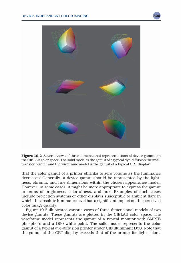
DEVICE-INDEPENDENT COLOR IMAGING 325
that the color gamut of a printer shrinks to zero volume as the luminancedecreases! Generally, a device gamut should be represented by the light-ness, chroma, and hue dimensions within the chosen appearance model.However, in some cases, it might be more appropriate to express the gamutin terms of brightness, colorfulness, and hue. Examples of such casesinclude projection systems or other displays susceptible to ambient flare inwhich the absolute luminance level has a significant impact on the perceivedcolor image quality.
Figure 19.2 illustrates various views of three-dimensional models of twodevice gamuts. These gamuts are plotted in the CIELAB color space. Thewireframe model represents the gamut of a typical monitor with SMPTEphosphors and a D50 white point. The solid model represents the colorgamut of a typical dye-diffusion printer under CIE illuminant D50. Note thatthe gamut of the CRT display exceeds that of the printer for light colors,
Figure 19.2 Several views of three-dimensional representations of device gamuts inthe CIELAB color space. The solid model is the gamut of a typical dye-diffusion thermal-transfer printer and the wireframe model is the gamut of a typical CRT display
DEVICE-INDEPENDENT COLOR IMAGING326
while the gamut of the printer exceeds that of the CRT for some darker col-ors. This three-dimensional gamut representation should clear up somemisconceptions about color gamuts. For example, Figure 19.2 illustrates the large extent to which color gamuts are not coincident and the fact thatprinter gamuts often extend outside the range of CRT gamuts. Typically, it isassumed that CRT gamuts are significantly larger than most printer gamuts.This is a result of examination of two-dimensional gamut boundaries inchromaticity diagrams while neglecting the third dimension of color space.
Gamut mapping is the process of adjusting the colors in an image suchthat it can be represented on a given device. For example, it might be desiredto use a CRT display to reproduce a dark, saturated cyan that is present on aprint. If the CRT cannot produce the desired color, the image element mustbe shifted to an appropriate color that is within the CRT gamut. The oppositeproblem might also arise in which a device is capable of producing more saturated colors than present in the original image. If the full gamut of theoutput device is not utilized, users might be displeased with the resultssince they know that the device is capable of producing a wider range of colors. Thus, image colors might also be adjusted to fill color gamuts as well.Therefore the problem of gamut mapping can be described as gamut com-pression in regions where the desired color falls outside the device gamutand gamut expansion in regions where the gamut of image colors does notfully utilize the device gamut. Proper gamut expansion requires full know-ledge of the source image’s gamut and computationally expensive image-dependent processing. Thus it might not be fully implemented withinpractical systems for some time. This is somewhat counter to the commonperception that gamut mapping is only a problem of gamut compression.Color adjustments in the opposite direction represent an equally important,and perhaps more challenging, problem. Clearly, a color appearance modelis the best place to specify gamuts and perform mapping transformationssince the manipulations can be carried out on perceptually meaningfuldimensions.
A variety of gamut mapping techniques have been suggested, but a gener-alized, automated algorithm that can be used for a variety of applicationshas yet to be developed. Perhaps some lessons can be learned from the fieldof color photography (Evans et al. 1953, Hunt 1995) in which optimumreproductions are thought to be those that preserve the hue of the original,map lightness to preserve its relative reproduction and the mean level, andmap chroma such that the relationships between the relative chromas ofvarious image elements are retained. Of course, such guidelines would beoverruled by specific color preferences. Beginning with such approaches andconsidering other practical constraints, issues of color gamut mapping havebeen discussed by Stone et al. (1988), Gentile et al. (1990b), Hoshino andBerns (1993), Wolski et al. (1994), and Montag et al. (1996, 1997).
While a general solution to the gamut-mapping problem has not beenderived, some fundamental concepts can be suggested. For pictorial images,a reasonable gamut-mapping solution can be obtained by first linearly scaling the lightnesses such that the white and black points match and the
DEVICE-INDEPENDENT COLOR IMAGING 327
middle gray (L* = 50) is kept constant. Next, hue is preserved as chroma isclipped to the gamut boundary for compression or linearly scaled for expan-sion. An alternative approach is to clip the out-of-gamut colors to the gamutboundary at a minimum distance in a uniform color space while eliminatingthe constant-hue constraint. Such approaches are likely to be too simplisticand do not produce the optimum results (e.g., Wolski et al. 1994, Montag et al. 1996, 1997, Braun and Fairchild 1999a,b).
For other image types, such as business graphics, other gamut mappingstrategies might be more appropriate. One such approach is to preserve thechroma of image elements while changing hue if necessary in order to retainthe impact and intent of business graphic images. These differences high-light the importance of understanding the intent for an image when makinga reproduction. Depending on the intended application for a given image, theoptimum gamut-mapping strategy will vary. The difference between pictorialimages and business graphics is readily apparent. However, even amongpictorial images, different gamut-mapping strategies might be more appro-priate for various applications. For example, the best strategy for a scientificor medical image will be different than that for a fine-art reproduction, whichwill in turn be different from that for a consumer snapshot.
19.10 COLOR PREFERENCES
Once the problems of color appearance and gamut mapping are solved, therewill remain one last color operation, the mapping of colors to those that arepreferred by observers for a given application. Thus accurate color reproduc-tion might not be the ultimate goal, but rather a required step along the way.Color mapping for preference reproduction should be addressed simultan-eously with gamut mapping since the two processes deliberately force inac-curate color reproduction and will certainly impact each other. Like gamutmapping, color preference mapping is intent-, or application-dependent. Insome applications, such as scientific and medical imaging, accurate colorreproduction might be an objective that cannot be compromised. In pictorialimaging, preferred reproduction of certain object colors (e.g., sky, skin,foliage) might be biased toward the idealized memory color of these objects.In abstract images, such as business graphics, preferred color reproductionmight depend more upon the device capabilities or intended message thanon the colors of the original image.
An additional factor in color preference reproduction is the culturaldependency of color preferences. It is well established in the color reproduc-tion industry that preferred color reproduction systems sold into differentcultures have different color capabilities and cannot be substituted betweencultures without a loss in sales. While it seems certain that such culturalbiases exist, they are not well documented (publicly) and their cause is notwell understood. Many such effects have achieved the level of folklore andmight only exist for historical reasons. For example, certain customersmight have a strong preference for certain color reproduction capabilities
DEVICE-INDEPENDENT COLOR IMAGING328
because they have grown accustomed to those properties and consider anychange to be negative. Such biases are certainly cultural, but they arelearned responses. This illustrates the point that most, if not all, culturalbiases in color preference reproduction are learned in some way (this is thefundamental definition of culture). The topic of cultural biases is certainlyan interesting one and worthy of additional research and exploration.Fernandez et al. (2002) failed to find any significant cultural biases in imagepreference in one recent study. They showed that individual variation inpreferences were larger than any changes in the cultural averages. It wouldbe particularly interesting to see if biases, if indeed they exist at all, could betraced historically to see if they change with advances in communicationand interchange of image information.
The concept of cultural dependency in color preference reproductionsparks several interesting possibilities. However, there are also significantindividual differences in color preference reproduction as well. In fact, whilethere might be significant differences in color preference between cultures, itis almost certainly true that the range of color preferences of individualswithin any given culture exceeds the differences between the mean levels(confirmed by Fernandez et al. 2002). One need only attempt to produce asingle ideal image for two observers to understand the magnitude of suchdifferences in preference.
19.11 INVERSE PROCESS
Thus far, the process of moving image data into the middle of the flow chartin Figure 19.1 has been described. Once all of the processing at this level iscomplete, the image data is conceptually in an abstract space that repres-ents the appearances to be reproduced on the output image. At this point,the entire process must be reversed to move from the viewing-conditionsindependent color space, to a traditional device-independent color space, todevice coordinates, and then ultimately to the reproduced image. This pro-cess highlights the importance of working in both the forward and reversedirections in order to successfully create reproductions. Clearly, the entireprocess is facilitated by the use of analytically invertible color appearancemodels and device characterizations. The main advantage is that such models allow the user to manipulate a setting on the imaging device, orchange the viewing conditions, and still be able to recreate the process and produce an image in a reasonable amount of time. If the models must beiteratively inverted or recreated through exhaustive measurements, it mightbe completely impractical for a user to adjust any settings in order to obtaina desired result.
19.12 EXAMPLE SYSTEM
The previous discussions provide an overview of the process of device-independent color imaging. It is useful to examine an illustrative example of
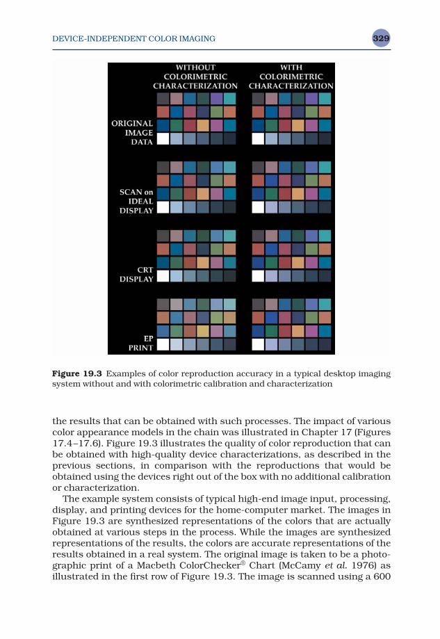
DEVICE-INDEPENDENT COLOR IMAGING 329
the results that can be obtained with such processes. The impact of variouscolor appearance models in the chain was illustrated in Chapter 17 (Figures17.4–17.6). Figure 19.3 illustrates the quality of color reproduction that canbe obtained with high-quality device characterizations, as described in theprevious sections, in comparison with the reproductions that would beobtained using the devices right out of the box with no additional calibrationor characterization.
The example system consists of typical high-end image input, processing,display, and printing devices for the home-computer market. The images inFigure 19.3 are synthesized representations of the colors that are actuallyobtained at various steps in the process. While the images are synthesizedrepresentations of the results, the colors are accurate representations of theresults obtained in a real system. The original image is taken to be a photo-graphic print of a Macbeth ColorChecker® Chart (McCamy et al. 1976) asillustrated in the first row of Figure 19.3. The image is scanned using a 600
Figure 19.3 Examples of color reproduction accuracy in a typical desktop imagingsystem without and with colorimetric calibration and characterization
DEVICE-INDEPENDENT COLOR IMAGING330
dpi flat-bed scanner with 10-bits-per-channel quantization. The second rowof Figure 19.3 illustrates the accuracy of the scanned image as representedon a theoretically ideal display (i.e., the display introduces no additionalerror). The image on the left illustrates the result obtained with no colorimetriccharacterization ( just gamma correction), while the image on the right illus-trates the accuracy obtained with a characterization technique such as thatoutlined by Berns and Shyu (1995).
The next step involves display on a high-resolution CRT as illustrated inthe third row of Figure 19.3. The left image illustrates the result of assumingthe monitor and video driver are set up to the nominally defined systemgamma (e.g., 1.8 for a Macintosh® system, 1.3–1.5 for a Silicon Graphicssystem, 2.2–2.5 for a Windows® system). It is assumed that any deviationfrom the nominal white point goes unnoticed due to chromatic adaptation.The image on the right illustrates the accuracy obtained with a specific char-acterization of the display systems using the techniques described by Berns(1996). Note that these images include both the scanner errors and the monitor errors as the full system is being constructed.
The final step is to print the image on a 600 dpi color laser printer. Theimage on the left illustrates the result obtained when using the defaultprinter driver and PostScript® Printer Description (PPD) file. The image on the right illustrates the results obtained when a three-dimensional LUT isconstructed using a measurement technique with a 9 × 9 × 9 sampling ofthe gamut. Again, these final images illustrate errors that have been pro-pagated through the entire imaging system. Clearly careful colorimetriccharacterization of the three devices making up this system can result insignificantly improved results. Unfortunately, the current state of techno-logy does not allow typical users to achieve this level of colorimetric accur-acy. However, the potential does exist. The ICC implementation described inthe next section provides a framework. What remains to be implemented isthe production of devices that can be accurately calibrated and characterizedin the factory (and remain stable) such that typical users will not have to beconcerned about calibrating and characterizing the devices themselves.
19.13 ICC IMPLEMENTATION
The International Color Consortium (1995) has provided a framework for amore universally implemented system to implement the process of device-independent color imaging as illustrated in Figure 19.1 through their speci-fication of the ICC Profile Format. The consortium consists of approximately50 corporations and organizations involved in color reproduction software,hardware, computer systems, and operating systems. The profile format is aspecification of a data structure that can be used to describe device charac-terizations (both models and LUTs), viewing conditions, and rendering intent.Such profiles can be used in conjunction with various imaging devices orconnected with images to facilitate communication of the colorimetric his-
DEVICE-INDEPENDENT COLOR IMAGING 331
tory of image data. The profile format provides a structure for communicationof the required data such that the profiles can be easily interchanged amongdifferent computers, operating systems, and/or software applications. Whilethe ICC profile provides the data necessary to implement device-independentcolor imaging, it is up to the software and hardware developers to build soft-ware to utilize this information to complete the system. Such software isreferred to as a color management system and is quickly becoming more andmore integrated into operating systems. There is also a significant require-ment for the development of profiles to accurately characterize variousdevices, appearance transformations, gamut-mapping transformations, andcolor preference mappings. The quality of a system based on ICC profiles willdepend on the capabilities of the color management software and the qualityof the profiles. With high-quality implementations, the ICC profile specifica-tion provides the framework and potential for excellent results.
The construction and implementation of the ICC profile format and colormanagement systems and other compatible software is an evolving process.The current status and profile format documentation can be found at theICC world-wide web site, www.color.org. The ICC documents also containinformation on other ongoing international standardization activities relev-ant to device-independent color imaging applications.
Profile Connection Space
One important concept of the ICC specification is the profile connectionspace. It is often misunderstood because the exact definition and implementa-tion of the profile connection space is remains an issue of discussion anddebate within ICC. The most recent ICC documentation should be referred tofor an up-to-date discussion of this topic.
Essentially, the profile connection space is defined by a particular set ofviewing condition parameters that are used to establish reference viewingconditions. The concept of the profile connection space is that a given inputdevice profile will provide the information necessary to transform devicecoordinates to a device-independent color specification (CIE XYZ or CIELAB)of the image data that represents the appearances of the original image datain the viewing conditions of the profile connection space (or from CIE spe-cifications in profile connection space to device coordinates for an outputdevice profile). The technique for obtaining this transformation is not yetagreed upon. As an example, the original definition of the ICC profile connec-tion space reference viewing conditions are as follows:
Reference reproduction medium: idealized print with Dmin = 0.0Reference viewing environment: ANSI PH2.30 standard booth
Surround: normalIllumination color: that of CIE illuminant D50Illuminance: 2200 ± 470 lux
DEVICE-INDEPENDENT COLOR IMAGING332
Colorimetry: ideal, flareless measurementObserver: CIE 1931 standard colorimetric observer (implied)Measurement geometry: unspecified
As an example of using ICC profiles with the profile connection space,imagine a system with a digital camera calibrated for D65 illumination, aCRT display with a 9300 K white point, and a printer with output viewedunder D50 illumination. An input profile for the digital camera would have toprovide the information necessary to first transform from the camera devicecoordinates, say RGB, to CIE tristimulus values for illuminant D65 usingtypical device calibration and characterization techniques. The tristimulusvalues for illuminant D65 and the viewing conditions of image capture wouldthen need to be transformed to corresponding tristimulus values for theprofile connection space (illuminant D50, etc.) using some color appearancemodel. All the information necessary to perform the transformation fromdevice coordinates to corresponding tristimulus values in the profile connec-tion space would have to be incorporated into the input device profile.
The CRT display would have an output device profile that would includethe information necessary to transform from the profile connection space tocorresponding tristimulus values for the CRT viewing conditions (9300 Kwhite point, dim surround, etc.) and then through a device characterizationto the RGB values required to display the desired colors. When implementedwithin a color management system, the two device profiles would be con-catenated such that the RGB data from the camera is transformed directly tothe RGB data for the display without ever existing in any of the several inter-mediate spaces or, indeed, even in the profile connection space.
Assuming the printer is set up and characterized for viewing conditionsthat match the profile connection space, the output device profile for theprinter only needs to include information for the transform from illuminantD50 CIE coordinates to the device coordinates.
An interesting ‘feature’ of this process is that a device profile is required toprovide the transformation from device coordinates to the profile connectionspace, even for situations in which a color appearance model would norm-ally not be required. For example, if the camera is set up for D65 illumina-tion and the monitor is set up with a D65 white point, then it makes no senseto first transform through the appearance models to get to the D50 profileconnection space and then come back out to a D65 display. Since profilesare concatenated by color management systems, this is not a problem aslong as a single color appearance model is agreed upon. The ICC is workingtoward this objective, but at the present time, there is no single recom-mended color appearance model for the construction of ICC profiles. Thusan input device profile builder might implement the Hunt model to get intothe profile connection space, while an output device profile builder mightimplement the RLAB model to come out of the profile connection space.Since there are significant differences between the various appearance models, processed images might change dramatically in situations for whicha color appearance model was not even required. The existence of CIE color
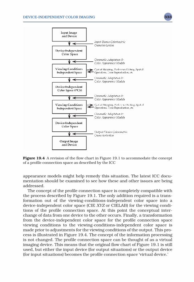
DEVICE-INDEPENDENT COLOR IMAGING 333
appearance models might help remedy this situation. The latest ICC docu-mentation should be examined to see how these and other issues are beingaddressed.
The concept of the profile connection space is completely compatible withthe process described by Figure 19.1. The only addition required is a trans-formation out of the viewing-conditions-independent color space into adevice-independent color space (CIE XYZ or CIELAB) for the viewing condi-tions of the profile connection space. At this point the conceptual inter-change of data from one device to the other occurs. Finally, a transformationfrom the device-independent color space for the profile connection spaceviewing conditions to the viewing-conditions-independent color space ismade prior to adjustments for the viewing conditions of the output. This pro-cess is illustrated in Figure 19.4. The concept of the information processingis not changed. The profile connection space can be thought of as a virtualimaging device. This means that the original flow chart of Figure 19.1 is stillused, but either the input device (for output situations) or the output device(for input situations) becomes the profile connection space ‘virtual device.’
Figure 19.4 A revision of the flow chart in Figure 19.1 to accommodate the conceptof a profile connection space as described by the ICC
Color Appearance Models Second Edition M. D. Fairchild © 2005 John Wiley & Sons, LtdISBN: 0-470-01216-1 (HB)
20Image Appearance
Modeling and the Future
Color appearance modeling has made some significant advances in the six years between editions of this book. The general approach of the modelspresented in this book is to isolate color from other dimensions of visual performance as much as possible. It is possible, and perhaps likely, thatsuch models have progressed about as far as they can and that furtheradvances will require different types of models. Recently, Fairchild andJohnson (2002, 2003, 2004) have proposed a different sort of model referredto as an image appearance model. An image appearance model extends colorappearance models to incorporate properties of spatial and temporal visionallowing prediction of appearance in complex stimuli and the measurementof image differences (the first step toward an image quality metric). Thischapter reviews the concept of image appearance modeling and presents onesuch model, known as iCAM. The treatment is largely based on the Fairchildand Johnson (2004) review article. Finally, this chapter ends with somespeculation on what might happen in the near future in the areas of colorappearance modeling and image appearance modeling. For updates on thecurrent status of various models and key references that appeared afterpublication of this book, refer to the associated website, <www.cis.rit.edu/fairchild/CAM.html>. For updates on iCAM and related source code, refer to<www.cis.rit.edu/mcsl/iCAM>.
IMAGE APPEARANCE MODELING AND THE FUTURE 335
20.1 FROM COLOR APPEARANCE TO IMAGE APPEARANCE
The history of image measurement helps set the context for the formulationand application of image appearance models, a somewhat natural evolutionof color appearance, spatial vision, and temporal vision models when theyare considered in a holistic sense, rather than as individual research fields.Early imaging systems were either not scientifically measured at all, or measured with systems designed to specify the variables of the imaging sys-tem itself. For example, densitometers were developed for measuring photo-graphic materials with the intent of specifying the amounts of dye or silverproduced in the film. In printing, similar measurements would be made forthe inks as well as measures of the dot area coverage for halftone systems. In electronic systems like television, system measurements such as signalvoltages were used to colorimetrically quantify the imaging system (Hunt1995). Vision-based measurements of imaging systems for image-quality dohave a long history as illustrated by the example of Schade’s (1956) pioneer-ing work. However, as imaging systems evolved in complexity and openness,the need for device-independent image measures became self-evident.
Image Colorimetry
Electronic imaging systems, specifically the development of color television,prompted the first application of device-independent color measurements of images. Wright (1981b), in fact, points out that color television could not have been invented without colorimetry. The CIE system was used verysuccessfully in the design and standardization of color television systems(including recent digital television systems).
Application of CIE colorimetry to imaging systems became much moreprevalent with the advent of digital imaging systems and the use of computersystems to generate and proof content ultimately destined for other media.The use of CIE colorimetry to specify images across the various devicespromised to solve some of the new color reproduction problems created byopen, digital systems. The flexibility of digital systems also made it possibleand practical to perform colorimetric transformations on image data inattempts to match the colors across disparate devices and media.
Research on imaging device calibration and characterization has spannedthe range from fundamental color measurement techniques to the specifica-tion of a variety of devices including CRT, LCD, and projection displays,scanners and digital cameras, and various film recording and print media.Some of the concepts and results of this research have been summarized byBerns (1997). Such capabilities are a fundamental requirement for researchand development in color and image appearance. Research on device char-acterization and calibration provides a means to tackle more fundamentalproblems in device-independent color imaging. For example, conceptualresearch on design and implementation of device-independent color imaging
(Fairchild 1994a), gamut mapping algorithms to deal with the reproductionof desired colors that fall outside the range that can be obtained with a givenimaging device (Braun and Fairchild 2000), and computer graphics render-ing of high-quality spectral images that significantly improve the potentialfor accurate color in rendered scenes (Johnson and Fairchild 1999). This typeof research built upon, and contributed to, research on the development andtesting of color appearance models for cross-media image reproduction.
Color Difference Equations
Color difference research has culminated with the recently publishedCIEDE2000 color difference formula (Luo et al. 2001). At the heart of suchcolor difference equations lies some form of uniform color space. The CIE initially recommended two such color spaces in 1976, CIELAB and CIELUV.Both spaces were initially described as interim color spaces, with the know-ledge that they were far from complete. With a truly uniform color space,color differences can then be taken to be a simple measure of distancebetween two colors in the space, such as CIE ∆E*ab. The CIE recognized thenonuniformity of the CIELAB color space, and formulated more advancedcolor difference equations such as CIE DE94 and CIEDE2000. These morecomplicated equations are very capable of predicting perceived color differ-ences of simple color patches.
Image Difference
The CIE color difference formulae were developed using simple color patchesin controlled viewing conditions. There is no reason to believe that they areadequate for predicting color difference for spatially complex image stimuli.The S-CIELAB model (Zhang and Wandell 1996) was designed as a spatialpre-processor to the standard CIE color difference equations, to account forcomplex color stimuli such as halftone patterns. The spatial preprocessinguses separable convolution kernels to approximate the contrast sensitivityfunctions (CSF) of the human visual system. The CSF serves to remove information that is imperceptible to the visual system. For instance, whenviewing halftone dots at a certain distance the dots tend to blur, and integ-rate into a single color. A pixel-by-pixel color difference calculation betweena continuous image and a halftone image would result in very large errors,while the perceived difference might in fact be small. The spatial pre-processing would blur the halftone image so that it more closely resemblesthe continuous tone image.
S-CIELAB represents the first incarnation of an image difference modelbased upon the CIELAB color space and color difference equations. Recentlythis model has been refined and extended into a modular framework forimage color difference calculations (Johnson and Fairchild 2001a, 2003a,b).
IMAGE APPEARANCE MODELING AND THE FUTURE336
IMAGE APPEARANCE MODELING AND THE FUTURE 337
This framework, discussed in Section 20.3, refines the CSF equations fromthe S-CIELAB model, and adds modules for spatial frequency adaptation,spatial localization, and local and global contrast detection.
Color Appearance
Unfortunately, fundamental CIE colorimetry does not provide a completesolution for image specification. By their very nature, the images producedor captured by various digital systems are examined in widely disparateviewing conditions, from the original captured scene, to a computer displayin a dim room, to printed media under a variety of light sources to projectiondisplays in dark rooms. Thus color appearance models were developed toextend CIE colorimetry to the prediction of color appearance (not just colormatches) across changes in media and viewing conditions (not just within asingle condition). Color appearance modeling research applied to digitalimaging systems was very active throughout the 1990s, culminating withthe recommendation of the CIECAM97s model in 1997 (Chapter 15) and itsrevision, CIECAM02, in 2002 (Chapter 16). The development of these modelswas also enabled by visual experiments performed to test the performance ofpublished color appearance models in realistic image reproduction situ-ations (e.g., Braun and Fairchild 1997). Such research on color appearancemodeling in imaging applications naturally highlighted the areas that arenot adequately addressed for spatially complex image appearance and imagequality problems.
Image Appearance and Image Quality
Color appearance models account for many changes in viewing conditions, butare mainly focused on changes in the color of the illumination (white point),the illumination level (luminance), and surround relative luminance. Suchmodels do not directly incorporate any of the spatial or temporal propertiesof human vision and the perception of images. They essentially treat each pixelof an image (and each frame of a video) as completely independent stimuli.
Visual adaptation to scenes and images is not only spatially localizedaccording to some low-pass characteristics, but also temporally localized in a similar manner. To predict the appearance of digital video sequences,particularly those of high dynamic range, the temporal properties of lightand chromatic adaptation must be considered. To predict the quality (orimage differences) of video sequences, temporal filtering to remove imper-ceptible high-frequency temporal modulations (imperceptible ‘flicker’) mustbe added to the spatial filtering that removes imperceptible spatial artifacts(e.g., noise or compression artifacts).
It is easy to illustrate that adaptation has a significant temporal low-passcharacteristic. For example, if one suddenly turns on the lights in a darkened
room (as upon first awakening in the morning), the increased illuminationlevel is at first dazzling to the visual system, essentially overexposing it. Aftera short period of time, the visual system adapts to the new, higher level ofillumination and normal visual perception becomes possible. The same is true when going from high levels of illumination to low levels (imagine driving into a tunnel in the daytime). Fairchild and Reniff (1995) and Rinnerand Gegenfurtner (2000) have made detailed measurements of the time-course of chromatic adaptation. These results suggest temporal integrationfunctions that could be used in models of moving image appearance and alsoillustrate one of the mechanisms for spatially low-pass adaptation stimulidue to the influence of ever-present eye movements.
There has been significant research on video quality and video qualitymetrics, often aimed at the creation and optimization of encoding/compres-sion/decoding algorithms such as MPEG2 and MPEG4. By analogy, the still-image visible differences predictor of Daly (1993) is quite applicable tothe prediction of the visibility of artifacts introduced into still images byJPEG image compression. The Daly model was designed to predict the prob-ability of detecting an artifact. Instead of focusing on threshold differences in quality, the focus in developing iCAM has been on the prediction of imagequality scales (e.g., scales of sharpness, contrast, graininess) for imageswith changes well above threshold. Such suprathreshold image differencesare a different domain of image quality research based on image appearance.
Likewise, a similar situation exists in the area of video quality metrics.Metrics have been published to examine the probability of detection of arti-facts in video, but there appear to be no models of video image appearancedesigned for rendering video and predicting the magnitudes of perceived differences in video sequences. Two well-known video image quality models,the Sarnoff JND model and the NASA DVQ model, are briefly describedbelow to contrast their capabilities with the objectives of the iCAM model.
The Sarnoff JND model is the basis of the JNDmetrix software package<www.jndmetrix.com> and related video quality hardware. The model isbriefly described in a technical report published by Sarnoff (2001) and morefully disclosed in other publications (ATIS 2001). It is based on the multi-scale model of spatial vision published by Lubin (1993, 1995) with someextensions for color processing and temporal variation. The Lubin model issimilar in nature to the Daly model in that it is designed to predict the prob-ability of detection of artifacts in images. These are threshold changes inimages, often referred to as just-noticeable differences, or JNDs. The SarnoffJND model has no mechanisms of chromatic and luminance adaptation, as are included in the iCAM model. The input to the Sarnoff model must first be normalized (which can be considered a very rudimentary form ofadaptation). The temporal aspects of the Sarnoff model are also not aimed atpredicting the appearance of video sequences, but rather at predicting thedetectability of temporal artifacts. As such, the model only uses two frames(four fields) in its temporal processing. Thus, while it is capable of predictingthe perceptibility of relatively high-frequency temporal variation in the video
IMAGE APPEARANCE MODELING AND THE FUTURE338

IMAGE APPEARANCE MODELING AND THE FUTURE 339
(flicker) it cannot predict the visibility of low frequency variations that wouldrequire an appearance-oriented, rather than JND-oriented, model. TheSarnoff model also is not designed for rendering video. This is not a criticismof the model formulation, but an illustration of how the objective of theSarnoff JND model is significantly different from that of the iCAM model.While it is well accepted in the vision science literature that JND predictionsare not linearly related to suprathreshold appearance differences, it is cer-tainly possible to use a JND model to try to predict suprathreshold imagedifferences and the Sarnoff JND model has been applied with some successto such data.
A similar model, the DVQ (Digital Video Quality) metric has been pub-lished by Watson (1998) and Watson et al. (2001) of NASA. The DVQ metric issimilar in concept to the Sarnoff JND model, but significantly different inimplementation. Its spatial decomposition is based on the coefficients of a discrete cosine transformation (DCT) making it amenable to hardwareimplementation and likely making it particularly good at detecting artifactsintroduced by DCT-based video compression algorithms. It also has a morerobust temporal filter that should be capable of predicting a wider array oftemporal artifacts. Like the Sarnoff model, the DVQ metric is aimed at pre-dicting the probability of detection of threshold image differences. The DVQmodel also includes no explicit appearance processing through spatial ortemporal adaptation, or correlates of appearance attributes and thereforealso cannot be used for video rendering. Again, this is not a shortcoming, butrather a property of the design objectives for the DVQ model.
While color appearance modeling has been successful in facilitatingdevice-independent color imaging and is incorporated into modern colormanagement systems, there remains significant room for improvement andextension of capabilities. To address these issues with respect to spatialproperties of vision and image perception and image quality, the concept ofimage appearance models has been recently introduced and implemented(Fairchild and Johnson 2002, Fairchild 2002a,b). These models combineattributes of color appearance models with attributes of spatial vision mod-els that have been previously used for image quality metrics in an attempt to further extend the capabilities of color appearance models. Historicallycolor appearance models largely ignored spatial vision (e.g., CIECAM97s,CIECAM02) while spatial vision models for image quality largely ignoredcolor (Daly 1993, Lubin 1993). Some exceptions include the retinex model(Land 1986, 1964, Land and McCann 1971, McCann et al. 1976) and its various derivatives (Funt et al. 2000, Barnard and Funt 1997, Brainard andWandell 1986). The spatial ATD model (Granger 1993) and the S-CIELABmodel (Zhang and Wandell 1996) also address some of these issues to various extents. While the retinex model was never designed as a completemodel of image appearance and quality, its spatially variable mechanisms ofchromatic adaptation and color constancy serve some of the same purposesin image rendering and provide some of the critical groundwork for imageappearance modeling.
The goal in developing an image appearance model has been to bring theseresearch areas together to create a single model applicable to image appear-ance, image rendering, and image quality specifications and evaluations.One such model for still images, referred to as iCAM, is detailed in this chap-ter. This model was built upon previous research in uniform color spaces(Ebner and Fairchild 1998), the importance of image surround (Fairchild1995b), algorithms for image difference and image quality measurement(Johnson and Fairchild 2003a, Fairchild 2002a,b), insights into observerseye movements while performing various visual imaging tasks and adapta-tion to natural scenes (Babcock et al. 2003, Webster and Mollon 1997), andan earlier model of spatial and color vision applied to color appearance prob-lems and high-dynamic-range (HDR) imaging (Pattanaik et al. 1998).
Color and Image Appearance Models
A model capable of predicting perceived color difference between compleximage stimuli is a useful tool, but has some limitations. Just as a colorappearance model is necessary to fully describe the appearance of colorstimuli, an image appearance model is necessary to describe spatially com-plex color stimuli. Color appearance models allow for the description ofattributes such as lightness, brightness, colorfulness, chroma, and hue.Image appearance models extend upon this to also predict such attributesas sharpness, graininess, contrast, and resolution.
A uniform color space also lies at the heart of the of an image appearancemodel. The modular image difference framework allows for great flexibility inthe choice of color spaces. Examples are the CIELAB color space, similar toS-CIELAB, the CIECAM02 color appearance model, or the IPT color space(Ebner and Fairchild 1998). Thus, the modular image difference frameworkcan be implemented within the iCAM model as described in this chapter tocreate a full image appearance and image difference model. It could also beimplemented in other color spaces if desired.
Models of image appearance can be used to formulate multi-dimensionalmodels of image quality. For example it is possible to take weighted sums ofvarious appearance attributes to determine a metric of overall image quality,as described by Keelan (2002) and Engledrum (2002). Essentially thesemodels can augment or replace human observations to weight image attri-butes with overall appearances of quality. For instance a model of qualitymight involve weighted sums of tonal balance, contrast, and sharpness. Astep towards this type of model is illustrated in the following sections.
20.2 THE ICAM FRAMEWORK
Figure 20.1 presents a flowchart of the general framework for the iCAMimage appearance model as applied to still images. For input, the model
IMAGE APPEARANCE MODELING AND THE FUTURE340
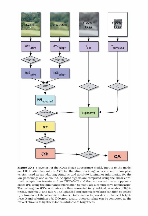
Figure 20.1 Flowchart of the iCAM image appearance model. Inputs to the modelare CIE tristimulus values, XYZ, for the stimulus image or scene and a low-pass version used as an adapting stimulus and absolute luminance information for thelow-pass image and surround. Adapted signals are computed using the linear chro-matic adaptation transform from CIECAM02 and then converted into an opponentspace IPT, using the luminance information to modulate a compressive nonlinearity.The rectangular IPT coordinates are then converted to cylindrical correlates of light-ness J, chroma C, and hue h. The lightness and chroma correlates can then be scaledby a function of the absolute luminance information to provide correlates of bright-ness Q and colorfulness M. If desired, a saturation correlate can be computed as theratio of chroma to lightness (or colorfulness to brightness)
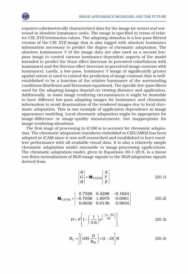
IMAGE APPEARANCE MODELING AND THE FUTURE342
requires colorimetrically characterized data for the image (or scene) and sur-round in absolute luminance units. The image is specified in terms of relat-ive CIE XYZ tristimulus values. The adapting stimulus is a low-pass filteredversion of the CIE XYZ image that is also tagged with absolute luminanceinformation necessary to predict the degree of chromatic adaptation. Theabsolute luminances Y of the image data are also used as a second low-pass image to control various luminance-dependent aspects of the modelintended to predict the Hunt effect (increase in perceived colorfulness withluminance) and the Stevens effect (increase in perceived image contrast withluminance). Lastly, a low-pass, luminance Y image of significantly greaterspatial extent is used to control the prediction of image contrast that is well-established to be a function of the relative luminance of the surroundingconditions (Bartleson and Breneman equations). The specific low-pass filtersused for the adapting images depend on viewing distance and application.Additionally, in some image rendering circumstances it might be desirable to have different low-pass adapting images for luminance and chromaticinformation to avoid desaturation of the rendered images due to local chro-matic adaptation. This is one example of application dependence in imageappearance modeling. Local chromatic adaptation might be appropriate forimage-difference or image-quality measurements, but inappropriate forimage-rendering situations.
The first stage of processing in iCAM is to account for chromatic adapta-tion. The chromatic adaptation transform embedded in CIECAM02 has beenadopted in iCAM since it was well researched and established to have excel-lent performance with all available visual data. It is also a relatively simplechromatic adaptation model amenable to image-processing applications.The chromatic adaptation model, given in Equations 20.1–20.6, is a linearvon Kries normalization of RGB image signals to the RGB adaptation signalsderived from
(20.1)
(20.2)
(20.3)
(20.4)RD
RD RC
W=
+ −
100 1( )
D F eL
= −
− −
1
13 6
4292
.
A
MCAT02
0 7328 0 4296 0 16240 7036 1 6975 0 00610 0030 0 0136 0 9834
=−
−. . .. . .. . .
RGB
XYZ
= MCAT02

IMAGE APPEARANCE MODELING AND THE FUTURE 343
(20.5)
(20.6)
the low-pass adaptation image at each pixel location (RWGWBW). The RGBsignals are computed using a linear transformation from XYZ to RGB derivedby CIE TC8-01 in the formulation of CIECAM02. The von Kries normal-ization is further modulated with a degree-of-adaptation factor D that canvary from 0.0 for no adaptation to 1.0 for complete chromatic adaptation.Equation 20.3 is provided in the CIECAM02 formulation, and used in iCAM,for computation of D as a function of adapting luminance LA, for variousviewing conditions. Alternatively the D factor can be established manually.The chromatic adaptation model is used to compute corresponding colorsfor CIE Illuminant D65 that are then used in the later stages of the iCAMmodel. This is accomplished by taking the adapted signals for the viewingcondition, RCGCBC, and then inverting Equations 20.1–20.6 for an illumin-ant D65 adapting white point and with D = 1.0. It should be noted that, whilethe adaptation transformation is identical to that in CIECAM02, the iCAMmodel is already significantly different since it uses spatially modulatedimage data as input rather than single color stimuli and adaptation points.One example of this is the modulation of the absolute luminance image andsurround luminance image using the FL function from CIECAM02 given inEquation 20.7. This function, slowly varying with luminance, has been
(20.7)
established to predict a variety of luminance-dependent appearance effectsin CIECAM02 and earlier models. Since the function has been establishedand understood, it was also adopted for the early stages of iCAM. However,the manner in which the FL factor is used in CIECAM02 and iCAM are quitedifferent.
The next stage of the model is to convert from RGB signals (roughly analog-ous to cone signals in the human visual system) to opponent-color signals(light–dark, red–green, and yellow–blue; analogous to higher-level encodingin the human visual system) that are necessary for constructing a uniformperceptual color space and correlates of various appearance attributes. In choosing this transformation, simplicity, accuracy, and applicability toimage processing were the main considerations. The color space chosen wasthe IPT space previously published by Ebner and Fairchild (1998). The IPTspace was derived specifically for image processing applications to have arelatively simple formulation and specifically to have a hue angle component
FL
LL
LLA
AA
A=+
+ −+
0 2
15 1
5 0 1 11
5 15
4 4 2
1 3.( )
( ) .( )
( ) /
BD
BD BC
W=
+ −
100 1( )
GD
GD GC
W=
+ −
100 1( )
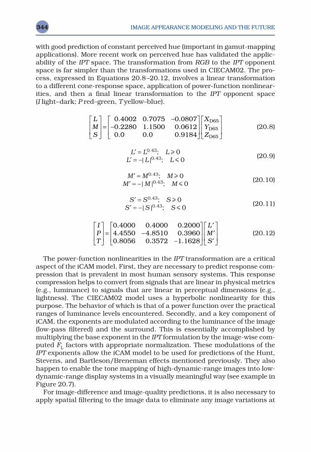
with good prediction of constant perceived hue (important in gamut-mappingapplications). More recent work on perceived hue has validated the applic-ability of the IPT space. The transformation from RGB to the IPT opponentspace is far simpler than the transformations used in CIECAM02. The pro-cess, expressed in Equations 20.8–20.12, involves a linear transformation to a different cone-response space, application of power-function nonlinear-ities, and then a final linear transformation to the IPT opponent space (I light–dark; P red–green, T yellow–blue).
(20.8)
L′ = L0.43; L > 0L′ = −| L |0.43; L < 0
(20.9)
M ′ = M0.43; M > 0M ′ = −| M |0.43; M < 0
(20.10)
S ′ = S0.43; S > 0S ′ = −| S |0.43; S < 0
(20.11)
(20.12)
The power-function nonlinearities in the IPT transformation are a criticalaspect of the iCAM model. First, they are necessary to predict response com-pression that is prevalent in most human sensory systems. This responsecompression helps to convert from signals that are linear in physical metrics(e.g., luminance) to signals that are linear in perceptual dimensions (e.g.,lightness). The CIECAM02 model uses a hyperbolic nonlinearity for this purpose. The behavior of which is that of a power function over the practicalranges of luminance levels encountered. Secondly, and a key component ofiCAM, the exponents are modulated according to the luminance of the image(low-pass filtered) and the surround. This is essentially accomplished bymultiplying the base exponent in the IPT formulation by the image-wise com-puted FL factors with appropriate normalization. These modulations of theIPT exponents allow the iCAM model to be used for predictions of the Hunt,Stevens, and Bartleson/Breneman effects mentioned previously. They alsohappen to enable the tone mapping of high-dynamic-range images into low-dynamic-range display systems in a visually meaningful way (see example inFigure 20.7).
For image-difference and image-quality predictions, it is also necessary toapply spatial filtering to the image data to eliminate any image variations at
IPT
LMS
= −−
′′′
0 4000 0 4000 0 20004 4550 4 8510 0 39600 8056 0 3572 1 1628
. . .
. . .
. . .
LMS
XYZ
=−
−
0 4002 0 7075 0 08070 2280 1 1500 0 06120 0 0 0 0 9184
65
65
65
. . .
. . .
. . .
D
D
D
IMAGE APPEARANCE MODELING AND THE FUTURE344
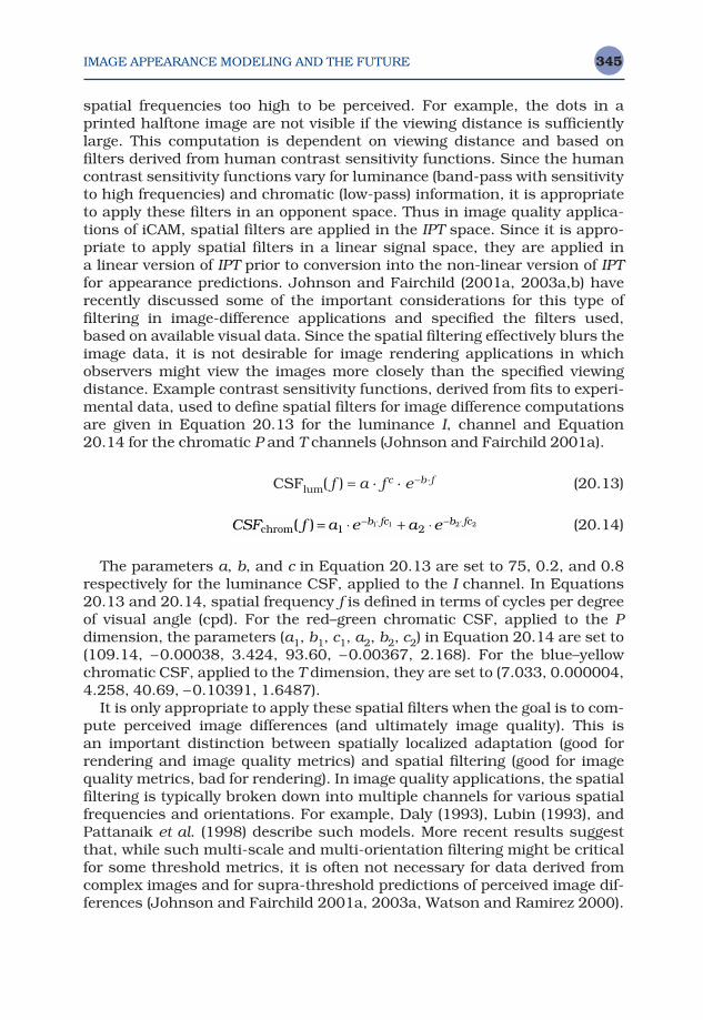
IMAGE APPEARANCE MODELING AND THE FUTURE 345
spatial frequencies too high to be perceived. For example, the dots in aprinted halftone image are not visible if the viewing distance is sufficientlylarge. This computation is dependent on viewing distance and based onfilters derived from human contrast sensitivity functions. Since the humancontrast sensitivity functions vary for luminance (band-pass with sensitivityto high frequencies) and chromatic (low-pass) information, it is appropriateto apply these filters in an opponent space. Thus in image quality applica-tions of iCAM, spatial filters are applied in the IPT space. Since it is appro-priate to apply spatial filters in a linear signal space, they are applied in a linear version of IPT prior to conversion into the non-linear version of IPTfor appearance predictions. Johnson and Fairchild (2001a, 2003a,b) haverecently discussed some of the important considerations for this type offiltering in image-difference applications and specified the filters used,based on available visual data. Since the spatial filtering effectively blurs theimage data, it is not desirable for image rendering applications in whichobservers might view the images more closely than the specified viewing distance. Example contrast sensitivity functions, derived from fits to experi-mental data, used to define spatial filters for image difference computationsare given in Equation 20.13 for the luminance I, channel and Equation20.14 for the chromatic P and T channels (Johnson and Fairchild 2001a).
CSFlum( f ) = a · f c · e−b·f (20.13)
(20.14)
The parameters a, b, and c in Equation 20.13 are set to 75, 0.2, and 0.8respectively for the luminance CSF, applied to the I channel. In Equations20.13 and 20.14, spatial frequency f is defined in terms of cycles per degreeof visual angle (cpd). For the red–green chromatic CSF, applied to the Pdimension, the parameters (a1, b1, c1, a2, b2, c2) in Equation 20.14 are set to(109.14, −0.00038, 3.424, 93.60, −0.00367, 2.168). For the blue–yellowchromatic CSF, applied to the T dimension, they are set to (7.033, 0.000004,4.258, 40.69, −0.10391, 1.6487).
It is only appropriate to apply these spatial filters when the goal is to com-pute perceived image differences (and ultimately image quality). This is an important distinction between spatially localized adaptation (good forrendering and image quality metrics) and spatial filtering (good for imagequality metrics, bad for rendering). In image quality applications, the spatialfiltering is typically broken down into multiple channels for various spatialfrequencies and orientations. For example, Daly (1993), Lubin (1993), andPattanaik et al. (1998) describe such models. More recent results suggestthat, while such multi-scale and multi-orientation filtering might be criticalfor some threshold metrics, it is often not necessary for data derived fromcomplex images and for supra-threshold predictions of perceived image dif-ferences (Johnson and Fairchild 2001a, 2003a, Watson and Ramirez 2000).
CSF f a e a eb fc b fcchrom( ) = ⋅ + ⋅− ⋅ − ⋅
1 21 1 2 2
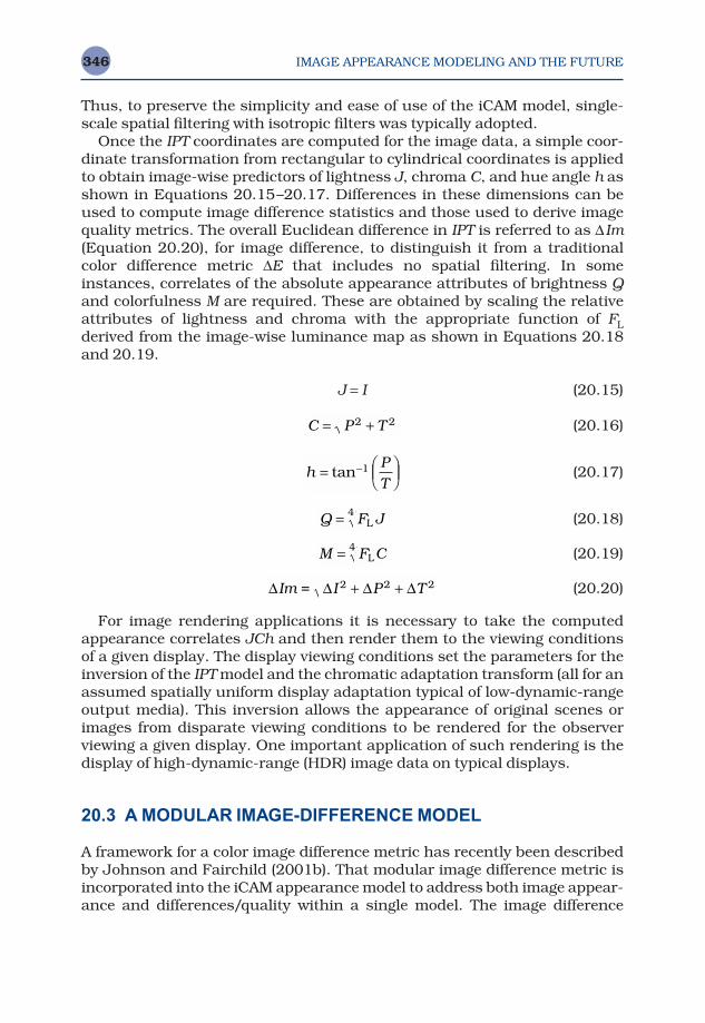
Thus, to preserve the simplicity and ease of use of the iCAM model, single-scale spatial filtering with isotropic filters was typically adopted.
Once the IPT coordinates are computed for the image data, a simple coor-dinate transformation from rectangular to cylindrical coordinates is appliedto obtain image-wise predictors of lightness J, chroma C, and hue angle h asshown in Equations 20.15–20.17. Differences in these dimensions can beused to compute image difference statistics and those used to derive imagequality metrics. The overall Euclidean difference in IPT is referred to as ∆ Im(Equation 20.20), for image difference, to distinguish it from a traditionalcolor difference metric ∆E that includes no spatial filtering. In someinstances, correlates of the absolute appearance attributes of brightness Qand colorfulness M are required. These are obtained by scaling the relativeattributes of lightness and chroma with the appropriate function of FLderived from the image-wise luminance map as shown in Equations 20.18and 20.19.
J = I (20.15)
(20.16)
(20.17)
(20.18)
(20.19)
(20.20)
For image rendering applications it is necessary to take the computedappearance correlates JCh and then render them to the viewing conditionsof a given display. The display viewing conditions set the parameters for theinversion of the IPT model and the chromatic adaptation transform (all for anassumed spatially uniform display adaptation typical of low-dynamic-rangeoutput media). This inversion allows the appearance of original scenes orimages from disparate viewing conditions to be rendered for the observerviewing a given display. One important application of such rendering is thedisplay of high-dynamic-range (HDR) image data on typical displays.
20.3 A MODULAR IMAGE-DIFFERENCE MODEL
A framework for a color image difference metric has recently been describedby Johnson and Fairchild (2001b). That modular image difference metric isincorporated into the iCAM appearance model to address both image appear-ance and differences/quality within a single model. The image difference
∆ ∆ ∆ ∆Im = I P T2 2 2+ +
M F C= L4
Q F J= L4
hP
T=
−tan 1
C P T= +2 2
IMAGE APPEARANCE MODELING AND THE FUTURE346
IMAGE APPEARANCE MODELING AND THE FUTURE 347
framework was designed to be modular in nature, to allow for flexibility andadaptation. The framework itself is based upon the S-CIELAB spatial exten-sion to the CIELAB color space. S-CIELAB merges traditional color differ-ence equations with spatial properties of the human visual system. This wasaccomplished as a spatial filtering pre-processing, before a pixel-by-pixelcolor difference calculation.
The modular framework further extends this idea by adding several pro-cessing steps, in addition to the spatial filtering. These processing steps arecontained in independent modules, so they can be tested and refined. Severalmodules have been defined (Johnson and Fairchild 2003a) and include spatialfiltering, adaptation, and localization, as well as local and global contrastdetection. Figure 20.2 shows a general flowchart with several distinct mod-ules. These modules and their origins are described briefly below.
Spatial Filtering
The behavior of the human visual system in regards to spatially complexstimuli has been well studied over the years dating back to the seminal workof Campbell and Robson (1968) and Mullen (1985). Summaries of currentknowledge and techniques for quantifying spatial vision can be found in several books (e.g., DeValois and DeValois 1988, Kelly 1994, Wandell 1995).The contrast sensitivity function describes this behavior in relation to spa-tial frequency. Essentially the CSF is described in a post-retinal opponentcolor space, with a band-pass nature for the luminance channel and low-pass nature for the chrominance channels. S-CIELAB uses separable con-volution kernels to approximate the CSF, and modulate image details that areimperceptible. More complicated contrast sensitivity functions that includeboth modulation and frequency enhancement were discussed in detail byJohnson and Fairchild (2001a). Other models with similar features includethe previously mentioned Lubin (1993), Daly (1993), MOM,(Pattanaik et al.1998) S-CIELAB,(Zhang and Wandell 1996) and spatial ATD (Granger 1993)models. Other relevant discussions and models can be found in the work ofLi et al. (1998), Taylor et al. (1997, 1998), and Brill’s (1997) extension of theLubin/Sarnoff model.
Spatial Frequency Adaptation
The contrast sensitivity function in this framework serves to modulate spa-tial frequencies that are not perceptible, and enhance certain frequenciesthat are most perceptible. Generally CSFs are measured using simple grat-ing stimuli with care taken to avoid spatial frequency adaptation. Spatial frequency adaptation essentially decreases sensitivity to certain frequenciesbased upon information present in the visual field. An early and classic des-cription of spatial frequency adaptation was published by Blakemore and
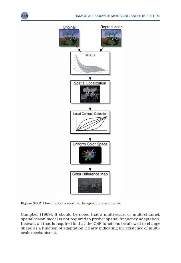
Campbell (1969). It should be noted that a multi-scale, or multi-channel,spatial vision model is not required to predict spatial frequency adaptation.Instead, all that is required is that the CSF functions be allowed to changeshape as a function of adaptation (clearly indicating the existence of multi-scale mechanisms).
IMAGE APPEARANCE MODELING AND THE FUTURE348
Figure 20.2 Flowchart of a modular image-difference metric
IMAGE APPEARANCE MODELING AND THE FUTURE 349
Since spatial frequency adaptation cannot be avoided in real world view-ing conditions, several models of spatial frequency adaptation have beendescribed for practical applications (Johnson and Fairchild 2001b). Thesemodels alter the nature of the CSF based upon either assumptions of theviewing conditions, or based upon the information contained in the imagesthemselves.
Spatial Localization
The band-pass and low-pass contrast sensitivity serve to modulate high-frequency information, including high-frequency edges. The human visualsystem is generally acknowledged to be very adept at detecting edges. Toaccommodate this behavior, a module of spatial localization has been devel-oped. This module can be as simple as an image processing edge-enhancingkernel, although that kernel must change as a function of viewing distance.Alternatively, the CSF can be modified to boost certain high-frequency infor-mation. The formulation and utility of edge-detection algorithms in visionapplications has been well described by Marr (1982).
Local Contrast Detection
This module serves to detect local and global contrast changes betweenimages. The utility of such processing in real visual systems has been des-cribed by Tolhurst and Heeger (1997). The current implementation is basedupon the nonlinear mask based local contrast enhancement described byMoroney (2000b). Essentially a low-pass image mask is used to generate aseries of tone-reproduction curves. These curves are based upon the globalcontrast of the image, as well as the relationship between a single pixel andits local neighborhood.
Color Difference Map
The output of the modular framework is a map of color differences ∆ Im cor-responding to the perceived magnitude of error at each pixel location. Thismap can be very useful for determining specific causes of error, or for detect-ing systematic errors in a color imaging system. Often it is useful to reducethe error map into a more manageable dataset. This can be accomplishedusing image statistics, so long as care is taken. Such statistics can be imagemean, maximum median, or standard deviation. Different statistics mightbe more valuable than others depending on the application, as perhaps themean error better describes overall difference, while the max might betterdescribe threshold differences.
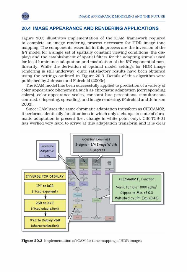
20.4 IMAGE APPEARANCE AND RENDERING APPLICATIONS
Figure 20.3 illustrates implementation of the iCAM framework required to complete an image rendering process necessary for HDR image tone mapping. The components essential in this process are the inversion of theIPT model for a single set of spatially constant viewing conditions (the dis-play) and the establishment of spatial filters for the adapting stimuli used for local luminance adaptation and modulation of the IPT exponential non-linearity. While the derivation of optimal model settings for HDR image rendering is still underway, quite satisfactory results have been obtainedusing the settings outlined in Figure 20.3. Details of this algorithm werepublished by Johnson and Fairchild (2003c).
The iCAM model has been successfully applied to prediction of a variety ofcolor appearance phenomena such as chromatic adaptation (correspondingcolors), color appearance scales, constant hue perceptions, simultaneouscontrast, crispening, spreading, and image rendering. (Fairchild and Johnson2002).
Since iCAM uses the same chromatic adaptation transform as CIECAM02,it performs identically for situations in which only a change in state of chro-matic adaptation is present (i.e., change in white point only). CIE TC8-01has worked very hard to arrive at this adaptation transform and it is clear
IMAGE APPEARANCE MODELING AND THE FUTURE350
Figure 20.3 Implementation of iCAM for tone mapping of HDR images
IMAGE APPEARANCE MODELING AND THE FUTURE 351
that no other model currently exists with better performance (although thereare several with equivalent performance). Thus the chromatic adaptationperformance of iCAM is as good as possible at this juncture.
The appearance scales of iCAM are identical to the IPT scales for the refer-ence viewing conditions. The IPT space has the best available performancefor constant hue contours and thus this feature is retained in iCAM. Thisfeature makes accurate implementation of gamut-mapping algorithms fareasier in iCAM than in other appearance spaces. In addition, the predictionsof lightness and chroma in iCAM are very good and comparable to the bestcolor appearance models in typical viewing conditions. The brightness andcolorfulness scales will also perform as well as any other model for typicalconditions. In more extreme viewing conditions, the performance of iCAMand other models will begin to deviate. It is in these conditions that thepotential strengths of iCAM will become evident. Further visual data must becollected to evaluate the model’s relative performance in such situations.
The color difference performance of iCAM will be similar to that of CIELABsince the space is very similar under the reference viewing conditions. Thus,color difference computations will be similar to those already commonly usedand the space can be easily extended to have a more accurate differenceequation following the successful format of the CIE94 equations. (Followingthe CIEDE2000 equations in iCAM is not recommended since they are ex-tremely complex and fitted to particular discrepancies of the CIELAB spacesuch as poor constant-hue contours.)
Simultaneous contrast (or induction) causes a stimulus to shift in appear-ance away from the color of the background in terms of opponent dimen-sions. Figure 20.4 illustrates a stimulus that exhibits simultaneous contrastin lightness (the gray square is physically identical on all three backgrounds)and its prediction by iCAM as represented by the iCAM lightness predictor.This prediction is facilitated by the local adaptation features of iCAM.
Crispening is the phenomenon whereby the color differences between twostimuli are perceptually larger when viewed on a background that is similarto the stimuli. Figure 20.5 illustrates a stimulus that exhibits chromacrispening and its prediction by the iCAM chroma predictor. This predictionis also facilitated by the local adaptation features of iCAM.
Spreading is a spatial color appearance phenomenon in which the appar-ent hue of spatially complex image areas appears to fill various spatiallycoherent regions. Figure 20.6 provides an example of spreading in which thered hue of the annular region spreads significantly from the lines to the fullannulus. The iCAM prediction of spreading is illustrated through reproduc-tion of the hue prediction. The prediction of spreading in iCAM is facilitatedby spatial filtering of the stimulus image.
One of the most interesting and promising applications of iCAM is to the rendering of high-dynamic-range (HDR) images to low-dynamic-rangedisplay systems. HDR image data are quickly becoming more prevalent.Historically HDR images were obtained through computer graphics simula-tions computed with global illumination algorithms (e.g., ray tracing or
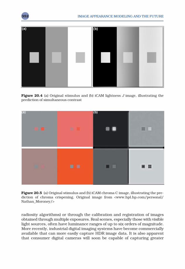
radiosity algorithms) or through the calibration and registration of imagesobtained through multiple exposures. Real scenes, especially those with visiblelight sources, often have luminance ranges of up to six orders of magnitude.More recently, industrial digital imaging systems have become commerciallyavailable that can more easily capture HDR image data. It is also apparentthat consumer digital cameras will soon be capable of capturing greater
IMAGE APPEARANCE MODELING AND THE FUTURE352
Figure 20.4 (a) Original stimulus and (b) iCAM lightness J image, illustrating theprediction of simultaneous contrast
Figure 20.5 (a) Original stimulus and (b) iCAM chroma C image, illustrating the pre-diction of chroma crispening. Original image from <www.hpl.hp.com/personal/Nathan_Moroney/>
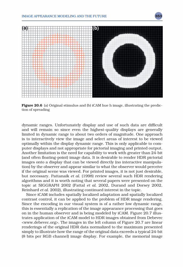
IMAGE APPEARANCE MODELING AND THE FUTURE 353
dynamic ranges. Unfortunately display and use of such data are difficultand will remain so since even the highest-quality displays are generally limited in dynamic range to about two orders of magnitude. One approach is to interactively view the image and select areas of interest to be viewedoptimally within the display dynamic range. This is only applicable to com-puter displays and not appropriate for pictorial imaging and printed output.Another limitation is the need for capability to work with greater than 24-bit(and often floating-point) image data. It is desirable to render HDR pictorialimages onto a display that can be viewed directly (no interactive manipula-tion) by the observer and appear similar to what the observer would perceiveif the original scene was viewed. For printed images, it is not just desirable,but necessary. Pattanaik et al. (1998) review several such HDR renderingalgorithms and it is worth noting that several papers were presented on thetopic at SIGGRAPH 2002 (Fattal et al. 2002, Durand and Dorsey 2002,Reinhard et al. 2002), illustrating continued interest in the topic.
Since iCAM includes spatially localized adaptation and spatially localizedcontrast control, it can be applied to the problem of HDR image rendering.Since the encoding in our visual system is of a rather low dynamic range,this is essentially a replication of the image appearance processing that goeson in the human observer and is being modeled by iCAM. Figure 20.7 illus-trates application of the iCAM model to HDR images obtained from Debevec<www.debevec.org>. The images in the left column of Figure 20.7 are linearrenderings of the original HDR data normalized to the maximum presentedsimply to illustrate how the range of the original data exceeds a typical 24-bit(8 bits per RGB channel) image display. For example, the memorial image
Figure 20.6 (a) Original stimulus and (b) iCAM hue h image, illustrating the predic-tion of spreading
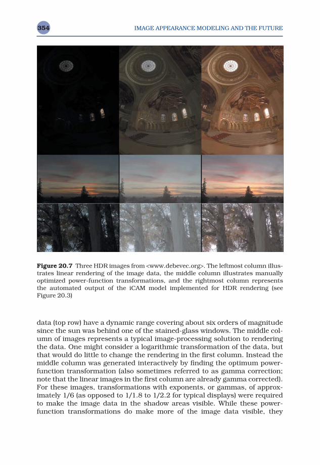
data (top row) have a dynamic range covering about six orders of magnitudesince the sun was behind one of the stained-glass windows. The middle col-umn of images represents a typical image-processing solution to renderingthe data. One might consider a logarithmic transformation of the data, butthat would do little to change the rendering in the first column. Instead themiddle column was generated interactively by finding the optimum power-function transformation (also sometimes referred to as gamma correction;note that the linear images in the first column are already gamma corrected).For these images, transformations with exponents, or gammas, of approx-imately 1/6 (as opposed to 1/1.8 to 1/2.2 for typical displays) were required to make the image data in the shadow areas visible. While these power-function transformations do make more of the image data visible, they
IMAGE APPEARANCE MODELING AND THE FUTURE354
Figure 20.7 Three HDR images from <www.debevec.org>. The leftmost column illus-trates linear rendering of the image data, the middle column illustrates manuallyoptimized power-function transformations, and the rightmost column represents the automated output of the iCAM model implemented for HDR rendering (see Figure 20.3)
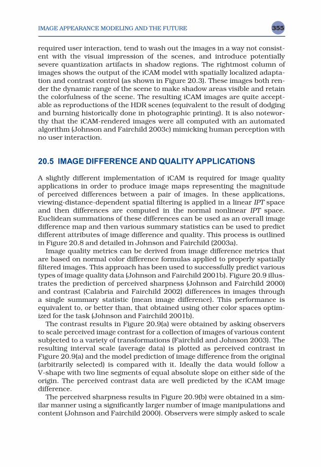
IMAGE APPEARANCE MODELING AND THE FUTURE 355
required user interaction, tend to wash out the images in a way not consist-ent with the visual impression of the scenes, and introduce potentiallysevere quantization artifacts in shadow regions. The rightmost column ofimages shows the output of the iCAM model with spatially localized adapta-tion and contrast control (as shown in Figure 20.3). These images both ren-der the dynamic range of the scene to make shadow areas visible and retainthe colorfulness of the scene. The resulting iCAM images are quite accept-able as reproductions of the HDR scenes (equivalent to the result of dodgingand burning historically done in photographic printing). It is also notewor-thy that the iCAM-rendered images were all computed with an automatedalgorithm (Johnson and Fairchild 2003c) mimicking human perception withno user interaction.
20.5 IMAGE DIFFERENCE AND QUALITY APPLICATIONS
A slightly different implementation of iCAM is required for image qualityapplications in order to produce image maps representing the magnitude of perceived differences between a pair of images. In these applications,viewing-distance-dependent spatial filtering is applied in a linear IPT spaceand then differences are computed in the normal nonlinear IPT space.Euclidean summations of these differences can be used as an overall imagedifference map and then various summary statistics can be used to predictdifferent attributes of image difference and quality. This process is outlinedin Figure 20.8 and detailed in Johnson and Fairchild (2003a).
Image quality metrics can be derived from image difference metrics thatare based on normal color difference formulas applied to properly spatiallyfiltered images. This approach has been used to successfully predict varioustypes of image quality data (Johnson and Fairchild 2001b). Figure 20.9 illus-trates the prediction of perceived sharpness (Johnson and Fairchild 2000)and contrast (Calabria and Fairchild 2002) differences in images through a single summary statistic (mean image difference). This performance isequivalent to, or better than, that obtained using other color spaces optim-ized for the task (Johnson and Fairchild 2001b).
The contrast results in Figure 20.9(a) were obtained by asking observersto scale perceived image contrast for a collection of images of various contentsubjected to a variety of transformations (Fairchild and Johnson 2003). Theresulting interval scale (average data) is plotted as perceived contrast inFigure 20.9(a) and the model prediction of image difference from the original(arbitrarily selected) is compared with it. Ideally the data would follow a V-shape with two line segments of equal absolute slope on either side of theorigin. The perceived contrast data are well predicted by the iCAM image difference.
The perceived sharpness results in Figure 20.9(b) were obtained in a sim-ilar manner using a significantly larger number of image manipulations andcontent (Johnson and Fairchild 2000). Observers were simply asked to scale
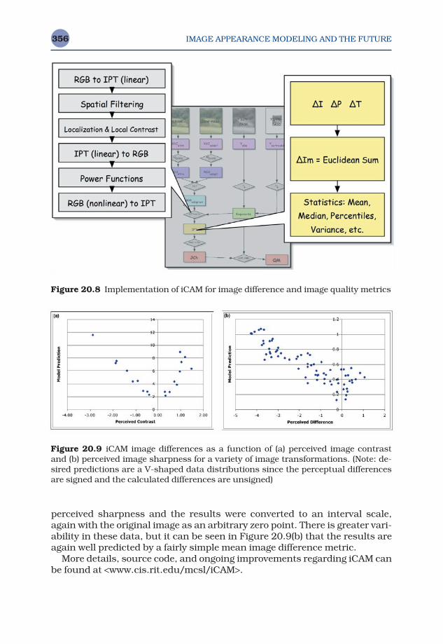
perceived sharpness and the results were converted to an interval scale,again with the original image as an arbitrary zero point. There is greater vari-ability in these data, but it can be seen in Figure 20.9(b) that the results areagain well predicted by a fairly simple mean image difference metric.
More details, source code, and ongoing improvements regarding iCAM canbe found at <www.cis.rit.edu/mcsl/iCAM>.
IMAGE APPEARANCE MODELING AND THE FUTURE356
Figure 20.8 Implementation of iCAM for image difference and image quality metrics
Figure 20.9 iCAM image differences as a function of (a) perceived image contrastand (b) perceived image sharpness for a variety of image transformations. (Note: de-sired predictions are a V-shaped data distributions since the perceptual differencesare signed and the calculated differences are unsigned)
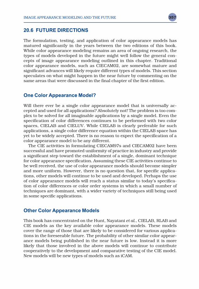
IMAGE APPEARANCE MODELING AND THE FUTURE 357
20.6 FUTURE DIRECTIONS
The formulation, testing, and application of color appearance models hasmatured significantly in the years between the two editions of this book.While color appearance modeling remains an area of ongoing research, thetypes of models developed in the future might well follow the general con-cepts of image appearance modeling outlined in this chapter. Traditionalcolor appearance models, such as CIECAM02, are somewhat mature andsignificant advances will likely require different types of models. This sectionspeculates on what might happen in the near future by commenting on thesame areas that were discussed in the final chapter of the first edition.
One Color Appearance Model?
Will there ever be a single color appearance model that is universally ac-cepted and used for all applications? Absolutely not! The problem is too com-plex to be solved for all imaginable applications by a single model. Even thespecification of color differences continues to be performed with two colorspaces, CIELAB and CIELUV. While CIELAB is clearly preferable for suchapplications, a single color difference equation within the CIELAB space hasyet to be widely accepted. There is no reason to expect the specification of acolor appearance model to be any different.
The CIE activities in formulating CIECAM97s and CIECAM02 have beensuccessful and have promoted uniformity of practice in industry and providea significant step toward the establishment of a single, dominant techniquefor color appearance specification. Assuming these CIE activities continue tobe well received, the use of color appearance models should become simplerand more uniform. However, there is no question that, for specific applica-tions, other models will continue to be used and developed. Perhaps the useof color appearance models will reach a status similar to today’s specifica-tion of color differences or color order systems in which a small number oftechniques are dominant, with a wider variety of techniques still being usedin some specific applications.
Other Color Appearance Models
This book has concentrated on the Hunt, Nayatani et al., CIELAB, RLAB andCIE models as the key available color appearance models. These modelscover the range of those that are likely to be considered for various applica-tions in the foreseeable future. The probability of other similar color appear-ance models being published in the near future is low. Instead it is morelikely that those involved in the above models will continue to contributecooperatively to the development and comparative testing of the CIE model.New models will be new types of models such as iCAM.
Ongoing Research to Test Models
Given the recent increase in interest in color appearance models and theirapplication to practical problems, the amount of research dedicated to theevaluation of model performance has also grown. This research is being carried out by a variety of scientists in industry and academia through indi-vidual programs, product development, and the activities of various CIETechnical Committees described in Chapter 17.
Of interest in the coming years will be an evaluation of the success of colorappearance models in real applications, such as device-independent colorimaging through the ICC profile framework. The results of these ‘real world’tests will set a practical standard for color appearance modeling. It isentirely possible that a very simple level of modeling, such as a von Kriestransform, will suffice if the control and specification of viewing conditionsand the accuracy of device characterizations are not first improved. Theseare necessary prerequisites to the application of color appearance models.
An analog for the future development of color appearance models can befound in the specification of the color matching functions of the CIE 1931Standard Colorimetric Observer. These functions were established over 70 years ago and have been successfully used in industry since that time.However, research on the measurement of more accurate color matchingfunctions and the variability in those functions has continued since thattime and is still ongoing. Such research has uncovered systematic errors inthe CIE functions that are critical for some applications. In such applica-tions, alternative color matching functions are often used. However, none ofthe discrepancies found through this research to date has been significantenough to warrant the abandonment of the 1931 recommendation that is firmly, and successfully, entrenched in a variety of industries. Perhaps a similar path will be followed in the area of color appearance models. IfCIECAM02 finds wide acceptance and application, research on it and theother models presented in this book will continue. If an improvement that istruly significant for practical applications is found, it will be quickly adopted.However, this might not happen until well after the other fundamentalissues (e.g., characterization accuracy, viewing condition control) are ade-quately addressed.
Ongoing Model Development
The first edition of this book stated:
An interesting direction that is likely to be pursued in the future is the incor-poration of spatial and temporal effects into color appearance models. Some ofthe issues to be addressed have been discussed by Wandell (1993), Poirsonand Wandell (1993, 1996), and Bäuml and Wandell (1996).
IMAGE APPEARANCE MODELING AND THE FUTURE358
IMAGE APPEARANCE MODELING AND THE FUTURE 359
It is clear that this is coming to pass as described in the preceding sectionsof this chapter. Research along these lines will continue, with models beingfurther refined, for the foreseeable future.
The first edition also spectulated on the use of neural networks.
Another approach that is being investigated for the prediction of color appear-ance phenomena is the use of neural network models. Courtney et al.(1995a,b) presented interesting examples of such an approach.
This approach has seemed to fall out of favor in color appearance modeling.
What To Do Now
Given the current status of color appearance specification, it is perfectly reasonable to ask the question: ‘What should I do now?’ Some recommenda-tions can be made based on the status of the models and tests as describedin this book. The first point to remember is that a color appearance modelshould only be used if absolutely necessary. If the viewing conditions can bearranged to eliminate the need for an appearance transform, that is the bestcourse of action. If a complete color appearance model is required, the Huntmodel is probably the best choice. If that level of complexity is not required,CIECAM02 might be a good choice. It is even possible that CIELAB might beadequate as a color appearance model in some applications. The best recom-mendation is to work up this chain from the simplest solution to the higherlevels of complexity until the problem is solved. It is also worth noting thatmodels should not be ‘mixed-and-matched’ due to the significant differencesbetween them. A single model should be used throughout a given system orprocess. The following listing summarizes this recommendation in order ofincreasing complexity and it should be noted that increasingly careful con-trol of the viewing conditions is also required.
1. If possible, it is preferable to equate the viewing conditions such that simple tristimulus matches are also appearance matches.
2. If a white point change is necessary, CIELAB can be used as a reasonablefirst-order approximation of an appearance model.
3. If CIELAB is found to be inadequate, it can be enhanced by using a vonKries chromatic adaptation transform (on cone responses) to a referenceviewing condition. An even better choice of adaptation transform wouldbe a von Kries transform based on the CIECAM02 MCAT02 matrix.
4. If a more flexible adaptation model is required (e.g., hard-copy to soft-copy changes) and/or there are surround changes, then the RLAB modelcan be used without too much added complexity. Again, the adaptationtransform in RLAB could be improved by substituting the CIECAM02adaptation transform.

5. If control of the viewing conditions and stimulus warrant a complete colorappearance model, or if predictions of brightness and colorfulness arerequired, then the CIECAM02 model should be used.
6. Lastly, if a full range of appearance phenomena and wide range of viewingconditions (e.g., very high or low luminances, rod responses) must beaddressed, then the Hunt model should be used.
IMAGE APPEARANCE MODELING AND THE FUTURE360
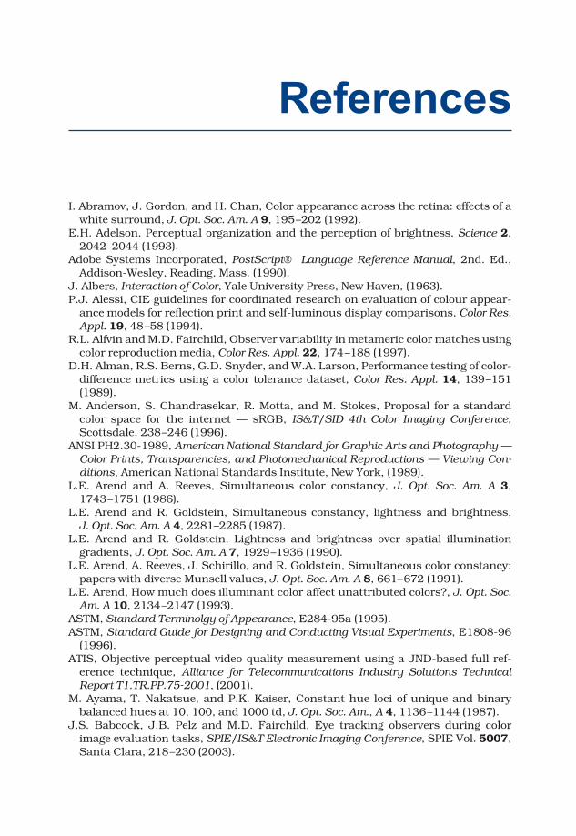
References
I. Abramov, J. Gordon, and H. Chan, Color appearance across the retina: effects of awhite surround, J. Opt. Soc. Am. A 9, 195–202 (1992).
E.H. Adelson, Perceptual organization and the perception of brightness, Science 2,2042–2044 (1993).
Adobe Systems Incorporated, PostScript® Language Reference Manual, 2nd. Ed.,Addison-Wesley, Reading, Mass. (1990).
J. Albers, Interaction of Color, Yale University Press, New Haven, (1963).P.J. Alessi, CIE guidelines for coordinated research on evaluation of colour appear-
ance models for reflection print and self-luminous display comparisons, Color Res.Appl. 19, 48–58 (1994).
R.L. Alfvin and M.D. Fairchild, Observer variability in metameric color matches usingcolor reproduction media, Color Res. Appl. 22, 174–188 (1997).
D.H. Alman, R.S. Berns, G.D. Snyder, and W.A. Larson, Performance testing of color-difference metrics using a color tolerance dataset, Color Res. Appl. 14, 139–151(1989).
M. Anderson, S. Chandrasekar, R. Motta, and M. Stokes, Proposal for a standardcolor space for the internet — sRGB, IS&T/SID 4th Color Imaging Conference,Scottsdale, 238–246 (1996).
ANSI PH2.30-1989, American National Standard for Graphic Arts and Photography —Color Prints, Transparencies, and Photomechanical Reproductions — Viewing Con-ditions, American National Standards Institute, New York, (1989).
L.E. Arend and A. Reeves, Simultaneous color constancy, J. Opt. Soc. Am. A 3,1743–1751 (1986).
L.E. Arend and R. Goldstein, Simultaneous constancy, lightness and brightness, J. Opt. Soc. Am. A 4, 2281–2285 (1987).
L.E. Arend and R. Goldstein, Lightness and brightness over spatial illumination gradients, J. Opt. Soc. Am. A 7, 1929–1936 (1990).
L.E. Arend, A. Reeves, J. Schirillo, and R. Goldstein, Simultaneous color constancy:papers with diverse Munsell values, J. Opt. Soc. Am. A 8, 661–672 (1991).
L.E. Arend, How much does illuminant color affect unattributed colors?, J. Opt. Soc.Am. A 10, 2134–2147 (1993).
ASTM, Standard Terminolgy of Appearance, E284-95a (1995).ASTM, Standard Guide for Designing and Conducting Visual Experiments, E1808-96
(1996).ATIS, Objective perceptual video quality measurement using a JND-based full ref-
erence technique, Alliance for Telecommunications Industry Solutions TechnicalReport T1.TR.PP.75-2001, (2001).
M. Ayama, T. Nakatsue, and P.K. Kaiser, Constant hue loci of unique and binary balanced hues at 10, 100, and 1000 td, J. Opt. Soc. Am., A 4, 1136–1144 (1987).
J.S. Babcock, J.B. Pelz and M.D. Fairchild, Eye tracking observers during colorimage evaluation tasks, SPIE/IS&T Electronic Imaging Conference, SPIE Vol. 5007,Santa Clara, 218–230 (2003).

REFERENCES362
W.G.K. Backhaus, R. Kliegl, and J.S. Werner, Eds., Color Vision: Perspectives fromDifferent Disciplines, Walter de Gruyter, Berlin, (1998).
H.B. Barlow and J.D. Mollon, The Senses, Cambridge Universtiy Press, Cambridge,(1982).
K. Barnard and B. Funt, Analysis and improvement of multi-scale retinex, Proceed-ings of the 5th IS&T/SID Color Imaging Conference, Scottsdale, 221–226 (1997).
C.J. Bartleson, Memory colors of familiar objects, J. Opt. Soc. Am., 50, 73–77 (1960).C.J. Bartleson and E.J. Breneman, Brightness perception in complex fields, J. Opt.
Soc. Am., 57, 953–957 (1967).C.J. Bartleson, Optimum image tone reproduction, J. SMPTE 84, 613–618 (1975).C.J. Bartleson, Brown, Color Res. Appl. 1, 181–191 (1976).C.J. Bartleson, A review of chromatic adaptation, AIC Proceedings, Color 77, 63–96
(1978).C.J. Bartleson and F. Grum, Optical Radiation Measurements Vol 5: Visual Measure-
ments, Academic, Orlando (1984).K.-H. Bäuml and B.A. Wandell, Color appearance of mixture gratings, Vision Res. 36,
2894–2864 (1996).K.H. Bäuml, Simultaneous color constancy: how surface color perception varies with
the illuminant, Vision Res. 39, 1531–1550 (1999).A. Berger-Schunn, Practical Color Measurement, Wiley, New York (1994).R.S. Berns, The mathematical development of CIE TC1-29 proposed color difference
equation: CIELCH, AIC Proceedings, Color 93, C19-1 (1993a).R.S. Berns, Spectral modeling of a dye diffusion thermal transfer printer, J. Electronic
Imaging 2, 359–370 (1993b).R.S. Berns, R.J. Motta, and M.E. Gorzynski, CRT colorimetry, part I: Theory and
practice, Color Res. Appl. 18, 299–314 (1993a).R.S. Berns, M.E. Gorzynski, and R.J. Motta, CRT colorimetry, part II: Metrology,
Color Res. Appl. 18, 315–325 (1993b).R.S. Berns and M.J. Shyu, Colorimetric characterization of a desktop drum scanner
using a spectral model, J. Electronic Imaging 4, 360–372 (1995).R.S. Berns, Methods for characterizing CRT displays, Displays 16, 173–182 (1996).R.S. Berns, A generic approach to color modeling, Color Res. Appl. 22, 318–325
(1997).R.S. Berns, Billmeyer and Saltzman’s Principles of Color Technology, 3rd. Ed., John
Wiley & Sons, New York (2000).R.S. Berns, S.R. Fernandez, and L. Taplin, Estimating black-level emissions of
computer-controlled displays, Color Res. Appl. 28, 379–383 (2003).K.T. Blackwell and G. Buchsbaum, The effect of spatial and chromatic parameters on
chromatic induction, Color Res. Appl. 13, 166–173 (1988a).K.T. Blackwell and G. Buchsbaum, Quantitative studies in color constancy, J. Opt.
Soc. Am. A 5, 1772–1780 (1988b).C. Blakemore and F.W. Campbell, On the existence of neurons in the human visual
system selectively sensitive to the orientation and size of retinal images, J. ofPhysiology 203, 237–260 (1969).
B. Blakeslee and M.E. McCourt, A multiscale spatial filtering account of the Whiteeffect, simultaneous brightness contrast and grating induction, Vision Res. 39,4361–4377 (1999).
R.M. Boynton, Human Color Vision, Optical Society of America, Washington, (1979).R.M. Boynton, History and current status of a physiologically based system of photo-
metry and colorimetry, J. Opt. Soc. Am. A 13, 1609–1621 (1996).
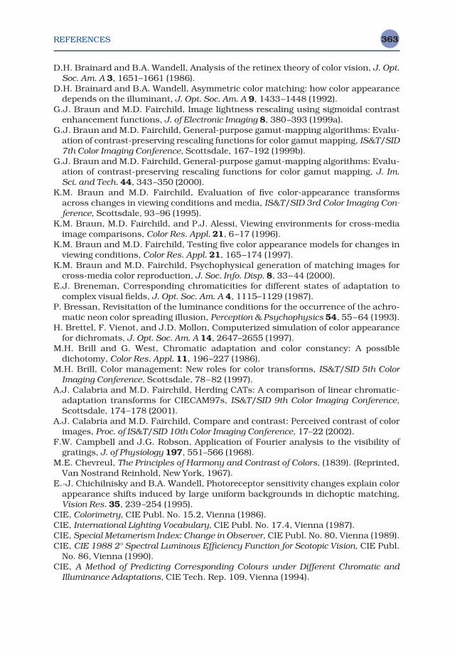
REFERENCES 363
D.H. Brainard and B.A. Wandell, Analysis of the retinex theory of color vision, J. Opt.Soc. Am. A 3, 1651–1661 (1986).
D.H. Brainard and B.A. Wandell, Asymmetric color matching: how color appearancedepends on the illuminant, J. Opt. Soc. Am. A 9, 1433–1448 (1992).
G.J. Braun and M.D. Fairchild, Image lightness rescaling using sigmoidal contrastenhancement functions, J. of Electronic Imaging 8, 380–393 (1999a).
G.J. Braun and M.D. Fairchild, General-purpose gamut-mapping algorithms: Evalu-ation of contrast-preserving rescaling functions for color gamut mapping, IS&T/SID7th Color Imaging Conference, Scottsdale, 167–192 (1999b).
G.J. Braun and M.D. Fairchild, General-purpose gamut-mapping algorithms: Evalu-ation of contrast-preserving rescaling functions for color gamut mapping, J. Im.Sci. and Tech. 44, 343–350 (2000).
K.M. Braun and M.D. Fairchild, Evaluation of five color-appearance transformsacross changes in viewing conditions and media, IS&T/SID 3rd Color Imaging Con-ference, Scottsdale, 93–96 (1995).
K.M. Braun, M.D. Fairchild, and P.J. Alessi, Viewing environments for cross-mediaimage comparisons, Color Res. Appl. 21, 6–17 (1996).
K.M. Braun and M.D. Fairchild, Testing five color appearance models for changes inviewing conditions, Color Res. Appl. 21, 165–174 (1997).
K.M. Braun and M.D. Fairchild, Psychophysical generation of matching images forcross-media color reproduction, J. Soc. Info. Disp. 8, 33–44 (2000).
E.J. Breneman, Corresponding chromaticities for different states of adaptation tocomplex visual fields, J. Opt. Soc. Am. A 4, 1115–1129 (1987).
P. Bressan, Revisitation of the luminance conditions for the occurrence of the achro-matic neon color spreading illusion, Perception & Psychophysics 54, 55–64 (1993).
H. Brettel, F. Vienot, and J.D. Mollon, Computerized simulation of color appearancefor dichromats, J. Opt. Soc. Am. A 14, 2647–2655 (1997).
M.H. Brill and G. West, Chromatic adaptation and color constancy: A possibledichotomy, Color Res. Appl. 11, 196–227 (1986).
M.H. Brill, Color management: New roles for color transforms, IS&T/SID 5th ColorImaging Conference, Scottsdale, 78–82 (1997).
A.J. Calabria and M.D. Fairchild, Herding CATs: A comparison of linear chromatic-adaptation transforms for CIECAM97s, IS&T/SID 9th Color Imaging Conference,Scottsdale, 174–178 (2001).
A.J. Calabria and M.D. Fairchild, Compare and contrast: Perceived contrast of colorimages, Proc. of IS&T/SID 10th Color Imaging Conference, 17–22 (2002).
F.W. Campbell and J.G. Robson, Application of Fourier analysis to the visibility ofgratings, J. of Physiology 197, 551–566 (1968).
M.E. Chevreul, The Principles of Harmony and Contrast of Colors, (1839). (Reprinted,Van Nostrand Reinhold, New York, 1967).
E.-J. Chichilnisky and B.A. Wandell, Photoreceptor sensitivity changes explain colorappearance shifts induced by large uniform backgrounds in dichoptic matching,Vision Res. 35, 239–254 (1995).
CIE, Colorimetry, CIE Publ. No. 15.2, Vienna (1986).CIE, International Lighting Vocabulary, CIE Publ. No. 17.4, Vienna (1987).CIE, Special Metamerism Index: Change in Observer, CIE Publ. No. 80, Vienna (1989).CIE, CIE 1988 2° Spectral Luminous Efficiency Function for Scotopic Vision, CIE Publ.
No. 86, Vienna (1990).CIE, A Method of Predicting Corresponding Colours under Different Chromatic and
Illuminance Adaptations, CIE Tech. Rep. 109, Vienna (1994).
REFERENCES364
CIE, Method of Measuring and Specifying Colour Rendering Properties of LightSources, CIE Publ. No. 13.3, Vienna (1995a).
CIE, Industrial Colour-Difference Evaluation, CIE Tech. Rep. 116, Vienna (1995b).CIE, Report to CIE Division 1 from TC1-31 Colour Notations and Colour-Order Sys-
tems, (1996a).CIE, CIE Expert Symposium ’96 Color Standards for Image Technology, CIE Pub.
x010, Vienna (1996b).CIE, The CIE 1997 Interim Colour Appearance Model (Simple Version), CIECAM97s,
CIE Pub. 131 (1998).CIE, CIE Collection/Colour Rendering (TC1-33 Closing Remarks), CIE Pub. 135/2
rendering (1999).CIE, Improvement to Industrial Colour difference Evaluation, CIE Pub 142 (2001).CIE, CIE TC1-52 Technical Report, A Review of Chromatic Adaptation Transforms
(2003).CIE, CIE TC8-01 Technical Report, A Colour Appearance Model for Color Management
Systems: CIECAM02, CIE Pub. 159 (2004).F.J.J. Clarke, R. McDonald, and B. Rigg, Modification to the JPC 79 colour-difference
formula, J. Soc. Dyers Colourists 100, 128–132 (1984).J.B. Cohen, Visual Color and Color Mixture: The Fundamental Color Space, University
of Illinois Press, Urbana (2001).F.W. Cornelissen and E. Brenner, On the role and nature of adaptation in chromatic
induction, Channels in the Visual Nervous System: Neurophysiology, Psychophys-ics and Models, B. Blum, Ed., Freund Publishing, London, 109–123 (1991).
F.W. Cornelissen and E. Brenner, Simultaneous colour constancy revisted: An ana-lysis of viewing strategies, Vision Res. 35, 2431–2448 (1995).
S.M. Courtney, L.H. Finkel, and G. Buchsbaum, A multistage neural network for colorconstancy and color induction, IEEE Trans. on Neural Networks 6, 972–985 (1995a).
S.M. Courtney, L.H. Finkel, and G. Buchsbaum, Network simulations of retinal andcortical contributions to color constancy, Vision Res. 35, 413–434 (1995b).
B.J. Craven and D.H. Foster, An operational approach to color constancy, Vision Res.32, 1359–1366 (1992).
S. Daly, The Visible Differences Predictor: An algorithm for the assessment of imagefidelity, in Digital Images and Human Vision, A. Watson, Ed., MIT, Cambridge, 179–206 (1993).
J. Davidoff, Cognition Through Color, MIT Press, Cambridge, (1991).P.B. Delahunt and D.H. Brainard, Control of chromatic adaptation: Signals from
separate cone classes interact, Vision Res. 40, 2885–2903 (2000).G. Derefeldt, Colour appearance systems, Chapter 13 in The Pereception of Colour,
P. Gouras, Ed., CRC Press, Boca Raton, 218–261 (1991).R.L. DeValois, C.J. Smith, S.T. Kitai, and S.J. Karoly, Responses of single cells in dif-
ferent layers of the primate lateral geniculate nucleus to monochromatic light,Science 127, 238–239 (1958).
R.L. DeValois and K.K. DeValois, Spatial Vision, Oxford University Press, Oxford(1988).
P. De Weerd, R. Desimone, and L.G. Ungerleider, Perceptual filling-in: a parametricstudy, Vision Res. 38, 2721–2734 (1998).
M.S. Drew and G.D. Finlayson, Device-independent color via spectral sharpening,IS&T/SID 2nd Color Imaging Conference, Scottsdale, 121–126 (1994).
F. Durand and J. Dorsey, Fast bilateral filtering for the display of high-dynamic-range images, Proceedings of SIGGRAPH 2002, San Antonio, 257–266 (2002).
REFERENCES 365
M. D’Zmura and P. Lennie, Mechanisms of color constancy, J. Opt. Soc. Am. A 3,1662–1672 (1986).
F. Ebner, and M.D. Fairchild, Development and testing of a color space (IPT) withimproved hue uniformity, IS&T/SID 6th Color Imaging Conference, Scottsdale,8–13 (1998).
P.G. Engeldrum, Four color reproduction theory for dot formed imaging systems, J. Imag. Tech. 12, 126–131 (1986).
P.G. Engeldrum, Color scanner colorimetric design requirements, Proc. SPIE 1909,75–83 (1993).
P.G. Engeldrum, A framework for image quality models, J. Imag. Sci. Tech. 39,312–318 (1995).
P.G. Engeldrum, Psychometric Scaling: A Toolkit for Imaging Systems Development,Imcotek Press, Winchester (2000).
P.G. Engledrum, Extending image quality models, Proc IS&T PICS Conference, 65–69(2002).
R.M. Evans, Visual processes and color photography, J. Opt. Soc. Am. 33, 579–614(1943).
R.M. Evans, An Introduction to Color, John Wiley & Sons, New York, (1948).R.M. Evans, W.T. Hanson, and W.L. Brewer, Principles of Color Photography, John
Wiley & Sons, New York, (1953).M.D. Fairchild, Chromatic Adaptation and Color Appearance, Ph.D. Dissertation,
University of Rochester (1990).M.D. Fairchild, A model of incomplete chromatic adaptation, Proceedings of the 22nd
Session of the CIE (Melbourne) 33–34 (1991a). M.D. Fairchild, Formulation and testing of an incomplete-chromatic-adaptation
model, Color Res. Appl. 16, 243–250 (1991b).M.D. Fairchild and E. Pirrotta, Predicting the lightness of chromatic object colors
using CIELAB, Color Res. Appl. 16, 385–393 (1991).M.D. Fairchild, Chromatic adaptation and color constancy, in Advances in Color
Vision Technical Digest, Vol. 4 of the OSA Technical Digest Series (Optical Society ofAmerica, Washington, D.C.), 112–114 (1992a).
M.D. Fairchild, Chromatic adaptation to image displays, TAGA 2, 803–824 (1992b).M.D. Fairchild and P. Lennie, Chromatic adaptation to natural and artificial illumin-
ants, Vision Res. 32, 2077–2085 (1992).M.D. Fairchild, Chromatic adaptation in hard-copy/soft-copy comparisons, Color
Hard Copy and Graphic Arts II, Proc. SPIE 1912, 47–61 (1993a).M.D. Fairchild, Color Forum: The CIE 1931 Standard Colorimetric Observer:
Mandatory retirement at age 65?, Color Res. Appl. 18, 129–134 (1993b).M.D. Fairchild and R.S. Berns, Image color appearance specification through exten-
sion of CIELAB, Color Res. Appl. 18, 178–190 (1993).M.D. Fairchild, E. Pirrotta, and T.G. Kim, Successive-Ganzfeld haploscopic viewing
technique for color-appearance research, Color Res. Appl. 19, 214–221 (1994).M.D. Fairchild, Some hidden requirements for device-independent color imaging,
SID International Symposium, San Jose, 865–868 (1994a).M.D. Fairchild, Visual evaluation and evolution of the RLAB color space, IS&T/SID
2nd Color Imaging Conference, Scottsdale, 9–13 (1994b).M.D. Fairchild, Testing colour-appearance models: Guidelines for coordinated
research, Color Res. Appl. 20, 262–267 (1995a). M.D. Fairchild, Considering the surround in device-independent color imaging, Color
Res. Appl. 20 352–363 (1995b).
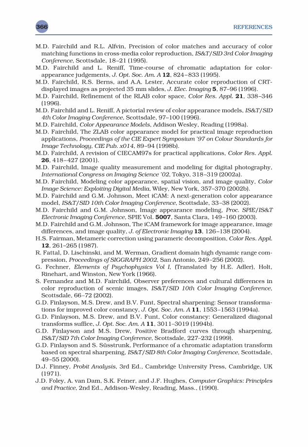
REFERENCES366
M.D. Fairchild and R.L. Alfvin, Precision of color matches and accuracy of colormatching functions in cross-media color reproduction, IS&T/SID 3rd Color ImagingConference, Scottsdale, 18–21 (1995).
M.D. Fairchild and L. Reniff, Time-course of chromatic adaptation for color-appearance judgements, J. Opt. Soc. Am. A 12, 824–833 (1995).
M.D. Fairchild, R.S. Berns, and A.A. Lester, Accurate color reproduction of CRT-displayed images as projected 35 mm slides, J. Elec. Imaging 5, 87–96 (1996).
M.D. Fairchild, Refinement of the RLAB color space, Color Res. Appl. 21, 338–346(1996).
M.D. Fairchild and L. Reniff, A pictorial review of color appearance models, IS&T/SID4th Color Imaging Conference, Scottsdale, 97–100 (1996).
M.D. Fairchild, Color Appearance Models, Addison Wesley, Reading (1998a).M.D. Fairchild, The ZLAB color appearance model for practical image reproduction
applications, Proceedings of the CIE Expert Symposium ’97 on Colour Standards forImage Technology, CIE Pub. x014, 89–94 (1998b).
M.D. Fairchild, A revision of CIECAM97s for practical applications, Color Res. Appl.26, 418–427 (2001).
M.D. Fairchild, Image quality measurement and modeling for digital photography,International Congress on Imaging Science ’02, Tokyo, 318–319 (2002a).
M.D. Fairchild, Modeling color appearance, spatial vision, and image quality, ColorImage Science: Exploiting Digital Media, Wiley, New York, 357–370 (2002b).
M.D. Fairchild and G.M. Johnson, Meet iCAM: A next-generation color appearancemodel, IS&T/SID 10th Color Imaging Conference, Scottsdale, 33–38 (2002).
M.D. Fairchild and G.M. Johnson, Image appearance modeling, Proc. SPIE/IS&TElectronic Imaging Conference, SPIE Vol. 5007, Santa Clara, 149–160 (2003).
M.D. Fairchild and G.M. Johnson, The iCAM framework for image appearance, imagedifferences, and image quality, J. of Electronic Imaging 13, 126–138 (2004).
H.S. Fairman, Metameric correction using parameric decomposition, Color Res. Appl.12, 261–265 (1987).
R. Fattal, D. Lischinski, and M. Werman, Gradient domain high dynamic range com-pression, Proceedings of SIGGRAPH 2002, San Antonio, 249–256 (2002).
G. Fechner, Elements of Psychophysics Vol I, (Translated by H.E. Adler), Holt,Rinehart, and Winston, New York (1966).
S. Fernandez and M.D. Fairchild, Observer preferences and cultural differences incolor reproduction of scenic images, IS&T/SID 10th Color Imaging Conference,Scottsdale, 66–72 (2002).
G.D. Finlayson, M.S. Drew, and B.V. Funt, Spectral sharpening: Sensor transforma-tions for improved color constancy, J. Opt. Soc. Am. A 11, 1553–1563 (1994a).
G.D. Finlayson, M.S. Drew, and B.V. Funt, Color constancy: Generalized diagonaltransforms suffice, J. Opt. Soc. Am. A 11, 3011–3019 (1994b).
G.D. Finlayson and M.S. Drew, Positive Bradford curves through sharpening,IS&T/SID 7th Color Imaging Conference, Scottsdale, 227–232 (1999).
G.D. Finlayson and S. Süsstrunk, Performance of a chromatic adaptation transformbased on spectral sharpening, IS&T/SID 8th Color Imaging Conference, Scottsdale,49–55 (2000).
D.J. Finney, Probit Analysis, 3rd Ed., Cambridge University Press, Cambridge, UK(1971).
J.D. Foley, A. van Dam, S.K. Feiner, and J.F. Hughes, Computer Graphics: Principlesand Practice, 2nd Ed., Addison-Wesley, Reading, Mass., (1990).
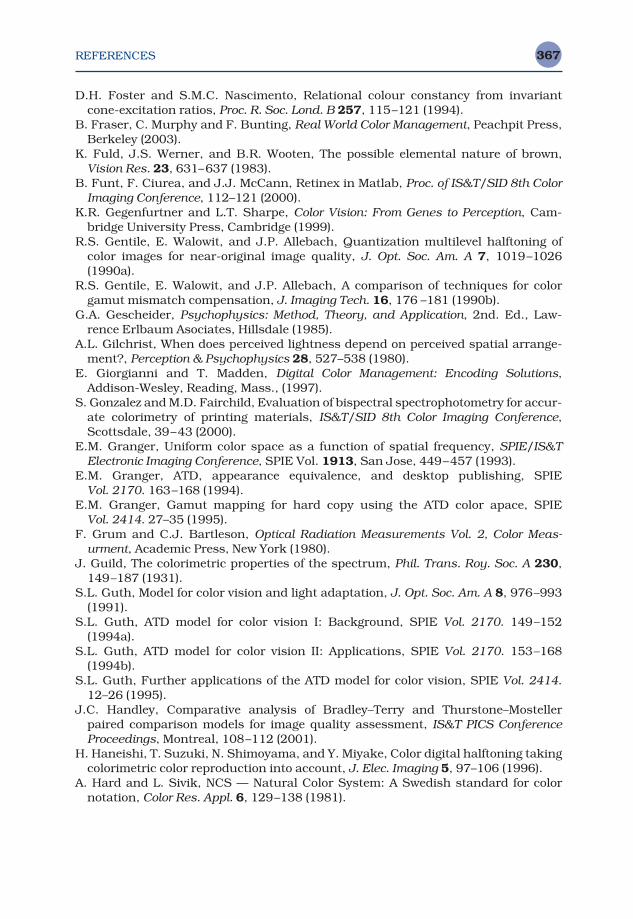
REFERENCES 367
D.H. Foster and S.M.C. Nascimento, Relational colour constancy from invariantcone-excitation ratios, Proc. R. Soc. Lond. B 257, 115–121 (1994).
B. Fraser, C. Murphy and F. Bunting, Real World Color Management, Peachpit Press,Berkeley (2003).
K. Fuld, J.S. Werner, and B.R. Wooten, The possible elemental nature of brown,Vision Res. 23, 631–637 (1983).
B. Funt, F. Ciurea, and J.J. McCann, Retinex in Matlab, Proc. of IS&T/SID 8th ColorImaging Conference, 112–121 (2000).
K.R. Gegenfurtner and L.T. Sharpe, Color Vision: From Genes to Perception, Cam-bridge University Press, Cambridge (1999).
R.S. Gentile, E. Walowit, and J.P. Allebach, Quantization multilevel halftoning ofcolor images for near-original image quality, J. Opt. Soc. Am. A 7, 1019–1026(1990a).
R.S. Gentile, E. Walowit, and J.P. Allebach, A comparison of techniques for colorgamut mismatch compensation, J. Imaging Tech. 16, 176 –181 (1990b).
G.A. Gescheider, Psychophysics: Method, Theory, and Application, 2nd. Ed., Law-rence Erlbaum Asociates, Hillsdale (1985).
A.L. Gilchrist, When does perceived lightness depend on perceived spatial arrange-ment?, Perception & Psychophysics 28, 527–538 (1980).
E. Giorgianni and T. Madden, Digital Color Management: Encoding Solutions,Addison-Wesley, Reading, Mass., (1997).
S. Gonzalez and M.D. Fairchild, Evaluation of bispectral spectrophotometry for accur-ate colorimetry of printing materials, IS&T/SID 8th Color Imaging Conference,Scottsdale, 39–43 (2000).
E.M. Granger, Uniform color space as a function of spatial frequency, SPIE/IS&TElectronic Imaging Conference, SPIE Vol. 1913, San Jose, 449–457 (1993).
E.M. Granger, ATD, appearance equivalence, and desktop publishing, SPIEVol. 2170. 163–168 (1994).
E.M. Granger, Gamut mapping for hard copy using the ATD color apace, SPIEVol. 2414. 27–35 (1995).
F. Grum and C.J. Bartleson, Optical Radiation Measurements Vol. 2, Color Meas-urment, Academic Press, New York (1980).
J. Guild, The colorimetric properties of the spectrum, Phil. Trans. Roy. Soc. A 230,149–187 (1931).
S.L. Guth, Model for color vision and light adaptation, J. Opt. Soc. Am. A 8, 976–993(1991).
S.L. Guth, ATD model for color vision I: Background, SPIE Vol. 2170. 149–152(1994a).
S.L. Guth, ATD model for color vision II: Applications, SPIE Vol. 2170. 153–168(1994b).
S.L. Guth, Further applications of the ATD model for color vision, SPIE Vol. 2414.12–26 (1995).
J.C. Handley, Comparative analysis of Bradley–Terry and Thurstone–Mostellerpaired comparison models for image quality assessment, IS&T PICS ConferenceProceedings, Montreal, 108–112 (2001).
H. Haneishi, T. Suzuki, N. Shimoyama, and Y. Miyake, Color digital halftoning takingcolorimetric color reproduction into account, J. Elec. Imaging 5, 97–106 (1996).
A. Hard and L. Sivik, NCS — Natural Color System: A Swedish standard for colornotation, Color Res. Appl. 6, 129–138 (1981).

REFERENCES368
M.M. Hayhoe, N.I. Benimoff, and D.C. Hood, The time-course of multiplicative andsubtractive adaptation processes, Vision Res. 27, 1981–1996 (1987).
M.M. Hayhoe, and M.V. Smith, The role of spatial filtering in sensitivity regulation,Vision Res. 29, 457–469 (1989).
H. v. Helmholtz, Handbuch der physiologischen Optick, 1st Ed. Voss, Hamburg(1866).
H. Helson, Fundamental problems in color vision. I. The principle governing changesin hue, saturation, and lightness of non-selective samples in chromatic illumina-tion, J. Exp. Psych. 23, 439–477 (1938).
H. Helson, D.B. Judd, and M.H. Warren, Object color changes from daylight to incan-descent filament illumination, Illum. Eng. 47, 221–233 (1952).
E. Hering, Outlines of a theory of the light sense, Harvard Univ. Press, Cambridge(1920). (trans. by L.M. Hurvich and D. Jameson, 1964.).
T. Hoshino and R.S. Berns, Color gamut mapping techniques for color hard copyimages, Proc. SPIE, 1909, 152–165 (1993).
P.-C. Hung, Colorimetric calibration for scanners and media, Proc. SPIE 1448,164–174 (1991).
P.-C. Hung, Colorimetric calibration in electronic imaging devices using a look-up-table model and interpolations, J. Electronic Imaging 2, 53–61 (1993).
P.-C. Hung and R.S. Berns, Determination of constant hue loci for a CRT gamut andtheir predictions using color apppearance spaces, Color Res. Appl. 20, 285–295(1995).
D.M. Hunt, S.D. Kanwaljit, J.K. Bowmaker, and J.D. Mollon, The chemistry of JohnDalton’s color blindness, Science 267, 984–988 (1995).
D.M. Hunt, K.S. Dulai, J.A. Cowing, C. Julliot, J.D. Mollon, J.K. Bowmaker, W.-H. Li,D. Hewett-Emmett, Molecular evolution of trichromacy in primates, Vision Res. 38,3299–3306 (1998).
R.W.G. Hunt, The effects of daylight and tungsten light-adaptation on color percep-tion, J. Opt. Soc. Am. 40, 362–371 (1950).
R.W.G. Hunt, Light and dark adaptation and the perception of color, J. Opt. Soc. Am.42, 190–199 (1952).
R.W.G. Hunt, Objectives in colour reproduction, J. Phot. Sci. 18, 205–215 (1970).R.W.G. Hunt, I.T. Pitt, and L.M. Winter, The preferred reproduction of blue sky,
green grass and caucasian skin in colour photography, J. Phot. Sci. 22, 144–150(1974).
R.W.G. Hunt and L.M. Winter, Colour adaptation in picture-viewing situations, J.Phot. Sci. 23, 112–115 (1975).
R.W.G. Hunt, Sky-blue pink, Color Res. Appl. 1, 11–16 (1976).R.W.G. Hunt, The specification of colour appearance. I. Concepts and terms, Color
Res. Appl. 2, 55–68 (1977).R.W.G. Hunt, Colour terminology, Color Res. Appl. 3, 79–87 (1978).R.W.G. Hunt, A model of colour vision for predicting colour appearance, Color Res.
Appl. 7, 95–112 (1982).R.W.G. Hunt and M.R. Pointer, A colour-appearance transform for the CIE 1931
standard colorimetric observer, Color Res. Appl. 10, 165–179 (1985).R.W.G. Hunt, A model of colour vision for predicting colour appearance in various
viewing conditions, Color Res. Appl. 12, 297–314 (1987).R.W.G. Hunt, Hue shifts in unrelated and related colours, Color Res. Appl. 14,
235–239 (1989).R.W.G. Hunt, Measuring Colour, 2nd Ed., Ellis Horwood, New York, (1991a).
REFERENCES 369
R.W.G. Hunt, Revised colour-appearance model for related and unrelated colours,Color Res. Appl. 16, 146–165 (1991b).
R.W.G. Hunt, Standard sources to represent daylight, Color Res. Appl. 17, 293–294(1992).
R.W.G. Hunt, An improved predictor of colourfulness in a model of colour vision,Color Res. Appl. 19, 23–26 (1994).
R.W.G. Hunt and M.R. Luo, Evaluation of a model of colour vision by magnitude scal-ings: Discussion of collected results, Color Res. Appl. 19, 27–33 (1994).
R.W.G. Hunt, The Reproduction of Colour, 5th Ed., Fountain Press, England, (1995).R.W.G. Hunt, Personal Communication, October 14, (1996).R.W.G. Hunt, Measuring Color, 3rd Ed., Fountain Press, England (1998).R.W.G. Hunt, C.J. Li, and M.R. Luo, Dynamic cone response function for models of
colour appearance, Color Res. Appl. 28, 82–88 (2003).R.S. Hunter and R.W. Harold, The Measurement of Appearance, 2nd Ed., Wiley, New
York (1987).L.M. Hurvich and D. Jameson, A psychophysical study of white. III. Adaptation as a
variant, J. Opt. Soc. Am. 41, 787–801 (1951).L.M. Hurvich, Color Vision, Sinauer Associates, Sunderland, Mass., (1981).T. Indow, Multidimensional studies of Munsell color solid, Psych. Rev. 95, 456–470
(1988).International Color Consortium, ICC Profile Format Specification, Version 3.3 (1996).
(http://www.color.org)D. Jameson and L.M. Hurvich, Some quantitative aspects of an opponent-colors
theory: I. Chromatic responses and spectral saturation, J. Opt. Soc. Am. 45,546–552 (1955).
D. Jameson and L.M. Hurvich, Essay concerning color constancy, Ann. Rev. Psychol.40, 1–22 (1989).
J.F. Jarvis, C.N. Judice, and W.H. Ninke, A survey of techniques for the display ofcontinuous tone images on bilevel displays, Comp. Graphics Image Proc. 5, 13–40(1976).
E.W. Jin and S.K. Shevell, Color memory and color constancy, J. Opt. Soc. Am. A 13,1981–1991 (1996).
D.J. Jobson, Z. Rahman, and G.A. Woodell, A multi-scale retinex for bridging the gapbetween color images and the human observation of scenes, IEEE Trans. Im. Proc.6, 956–976 (1997).
G.M. Johnson and M.D. Fairchild, Full-spectral color calculations in realistic imagesynthesis, IEEE Computer Graphics & Applications 19:4, 47–53 (1999).
G.M. Johnson and M.D. Fairchild, Sharpness rules, Proc of IS&T/SID 8th ColorImaging Conference, 24–30 (2000).
G.M. Johnson and M.D. Fairchild, On contrast sensitivity in an image differencemodel, Proc. of IS&T PICS Conference, 18–23 (2001a).
G.M. Johnson and M.D. Fairchild, Darwinism of color image difference models, Proc.of IS&T/SID 9th Color Imaging Conference, 108–112 (2001b).
G.M. Johnson and M.D. Fairchild, Measuring images: Differences, quality, andappearance, SPIE/IS&T Electronic Imaging Conference, SPIE Vol. 5007, SantaClara, 51–60 (2003a).
G.M. Johnson and M.D. Fairchild, A top down description of S-CIELAB andCIEDE2000, Color Res. Appl. 28, 425–435 (2003b).
G.M. Johnson and M.D. Fairchild, Rendering HDR images, IS&T/SID 11th ColorImaging Conference, Scottsdale, 36–41 (2003c).
REFERENCES370
D.B. Judd, Hue, saturation, and lightness of surface colors with chromatic illumina-tion, J. Opt. Soc. Am. 30, 2–32 (1940).
D.B. Judd, Appraisal of Land’s work on two-primary color projections, J. Opt. Soc.Am. 50, 254–268 (1960).
P.K. Kaiser and R.M. Boynton, Human Color Vision, 2nd Ed., Optical Society ofAmerica, Washington, (1996).
H. Kang, Color scanner calibration, J. Imaging Sci. Tech. 36, 162–170 (1992).H. Kang, Color Technology for Electronic Imaging Devices, SPIE, Bellingham, Wash.
(1997).J.M. Kasson, W. Plouffe, and S.I. Nin, A tetrahedral interpolation technique for color
space conversion, Proc. SPIE 1909, 127–138 (1993).J.M. Kasson, S.I. Nin, W. Plouffe, and J.L. Hafner, Performing color space conver-
sions with three-dimensional linear interpolation, J. Elec. Imaging 4, 226–250(1995).
N. Katoh, Practical method for appearance match between soft copy and hard copy,in Device-Independent Color Imaging, SPIE Vol. 2170, 170–181 (1994).
N. Katoh, Appearance match between soft copy and hard copy under mixed chro-matic adaptation, IS&T/SID 3rd Color Imaging Conference, Scottsdale 22–25(1995).
D. Katz, The World of Colour, Trubner & Co., London (1935).B.W. Keelan, Handbook of Image Quality: Characterization and Prediction, Marcel
Dekker, New York, NY (2002).D.H. Kelly, Ed., Visual Science and Engineering: Models and Applications, Marcel
Dekker, New York (1994).T.G. Kim, R.S. Berns, and M.D. Fairchild, Comparing appearance models using
pictorial images, IS&T/SID 1st Color Imaging Conference, Scottsdale, Ariz. 72–77(1993).
J.J. Koenderink and W.A. Richards, Why is snow so bright?, J. Opt. Soc. Am. A 9,643–648 (1992).
J.M. Kraft and J.S. Werner, Spectral efficiency across the life span: flicker photo-metry and brightness matching, J. Opt. Soc. Am. A 11, 1213–1221 (1994).
J.B. Kruskal and M. Wish, Multidimensional Scaling, Sage Publications, ThousandOaks, CA, (1978).
R.G. Kuehni, Color Space and Its Divisions: Color Order from Antiquity to the Present,John Wiley & Sons, Hoboken (2003).
W.-G. Kuo, M.R. Luo, and H.E. Bez, Various chromatic-adaptation transformationstested using new colour appearance data in textiles, Color Res. Appl. 20, 313–327(1995).
I. Kuriki and K. Uchikawa, Limitations of surface-color and apparent-color con-stancy, J. Opt. Soc. Am. A 13, 1622–1636 (1996).
E.H. Land, Color vision and the natural image part II, Proc. Nat. Acad. Sci., 45,636–644 (1959).
E.H. Land, The retinex, American Scientist 52, 247–264 (1964).E.H. Land and J.J. McCann, Lightness and the retinex theory, J. Opt. Soc. Am. 61,
1–11 (1971).E.H. Land, The retinex theory of color vision, Scientific American 237, 108–128
(1977).E.H. Land, Recent advances in retinex theory, Vision Res. 26, 7–21 (1986).P. Lennie and M. D’Zmura, Mechanisms of color vision, CRC Critical Reviews in
Neurobiology 3, 333–400 (1988).
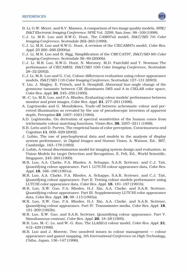
REFERENCES 371
B. Li, G.W. Meyer, and R.V. Klassen, A comparison of two image quality models, SPIE/IS&T Electronic Imaging Conference, SPIE Vol. 3299, San Jose, 98–109 (1998).
C.J. Li, M.R. Luo and R.W.G. Hunt, The CAM97s2 model, IS&T/SID 7th ColorImaging Conference, Scottsdale 262–263 (1999).
C.J. Li, M.R. Luo and R.W.G. Hunt, A revision of the CIECAM97s model, Color Res.Appl. 25 260–266 (2000a).
C.J. Li, M.R. Luo and B. Rigg, Simplification of the CMCCAT97, IS&T/SID 8th ColorImaging Conference, Scottsdale 56–60 (2000b).
C.J. Li, M.R. Luo, R.W.G. Hunt, N. Moroney, M.D. Fairchild and T. Newman The performance of CIECAM02, IS&T/SID 10th Color Imaging Conference, Scottsdale28–32 (2002).
C.J. Li, M.R. Luo and G. Cui, Colour-differences evaluation using colour appearancemodels, IS&T/SID 11th Color Imaging Conference, Scottsdale 127–131 (2003).
Y. Liu, J. Shigley, E. Fritsch, and S. Hemphill, Abnormal hue-angle change of thegemstone tanzanite between CIE illuminants D65 nad A in CIELAB color space,Color Res. Appl. 20, 245–250 (1995).
M.-C. Lo, M.R. Luo, and P.A. Rhodes, Evaluating colour models’ performance betweenmonitor and print images, Color Res. Appl. 21, 277–291 (1996).
A. Logvinenko and G. Menshikova, Trade-off between achromatic colour and per-ceived illumination as revealed by the use of pseudoscopic inversion of apparentdepth, Perception 23, 1007–1023 (1994).
A.D. Logvinenko, On derivation of spectral sensitivities of the human cones fromtrichromatic colour matching functions, Vision Res. 38, 3207–3211 (1998).
R.B. Lotto and D. Purves, The empricial basis of color perception, Consciousness andCognition 11, 609–629 (2002).
J. Lubin, The use of psychophysical data and models in the analysis of display system performance, in Digital Images and Human Vision, A. Watson, Ed., MIT,Cambridge, 163–178 (1993).
J. Lubin, A visual discrimination model for imaging system design and evaluation, inVision Models for target Detection and Recognition, E. Peli, Ed., World Scientific,Singapore, 245–283 (1995).
M.R. Luo, A.A. Clarke, P.A. Rhodes, A. Schappo, S.A.R. Scrivner, and C.J. Tait,Quantifying colour appearance. Part I. LUTCHI colour appearance data, Color Res.Appl. 16, 166–180 (1991a).
M.R. Luo, A.A. Clarke, P.A. Rhodes, A. Schappo, S.A.R. Scrivner, and C.J. Tait,Quantifying colour appearance. Part II. Testing colour models performance usingLUTCHI color appearance data, Color Res. Appl. 16, 181–197 (1991b).
M.R. Luo, X.W. Gao, P.A. Rhodes, H.J. Xin, A.A. Clarke, and S.A.R. Scrivner,Quantifying colour appearance. Part III. Supplementary LUTCHI color appearancedata, Color Res. Appl. 18, 98–113 (1993a).
M.R. Luo, X.W. Gao, P.A. Rhodes, H.J. Xin, A.A. Clarke, and S.A.R. Scrivner,Quantifying colour appearance. Part IV. Transmissive media, Color Res. Appl. 18,191–209 (1993b).
M.R. Luo, X.W. Gao, and S.A.R. Scrivner, Quantifying colour appearance. Part V.Simultaneous contrast, Color Res. Appl. 20, 18–28 (1995).
M.R. Luo, M.-C. Lo, and W.-G. Kuo, The LLAB(l:c) colour model, Color Res. Appl. 21,412–429 (1996).
M.R. Luo and J. Morovic, Two unsolved issues in colour management — colourappearance and gamut mapping, 5th International Conference on High Technology,Chiba, Japan, 136–147 (1996).

REFERENCES372
M.R. Luo, G. Cui, and B. Rigg, The development of the CIE 2000 Colour DifferenceFormula, Color Res. Appl. 26, 340–350 (2001).
D.L. MacAdam, Chromatic adaptation, J. Opt. Soc. Am. 46, 500–513 (1956).D.L. MacAdam, A nonlinear hypothesis for chromatic adaptation, Vis. Res. 1, 9–41
(1961).D.L. MacAdam, Uniform color scales, J. Opt. Soc. Am. 64, 1691–1702 (1974).D.L. MacAdam, Colorimetric data for samples of the OSA uniform color scales, J. Opt.
Soc. Am. 68, 121–130 (1978).D.L. MacAdam, Ed., Selected Papers on Colorimetry — Fundamentals, SPIE Milestone
Series, Vol. MS 77, SPIE, Bellingham, Wash. (1993).L.T. Maloney and B.A. Wandell, Color constancy: A method for recovering surface
spectral reflectance, J. Opt. Soc. Am. A 3, 29–33 (1986).D. Marr, Vision, Freeman, New York (1982).R. Mausfeld and R. Niederée, An inquiry into relational concepts of colour, based on
incremental principles of colour coding for minimal relational stimuli, Perception22, 427–462 (1993).
B. Maximus, A. De Metere, and J.P. Poels, Influence of thickness variations in LCDson color uniformity, SID 94 Digest, 341–344 (1994).
J.C. Maxwell, On the theory of three primary colors, Proc. Roy. Inst., 3, 370–375(1858–62).
C.S. McCamy, H. Marcus, and J.G. Davidson, A color rendition chart, J. App. Phot.Eng. 11, 95–99 (1976).
J.J. McCann, S. McKee, and T. Taylor, Quantitative studies in retinex theory: A com-parison between theoretical predictions and observer responses to ‘Color Mondrian’experiments, Vision Res. 16, 445–458 (1976).
J. McCann, Color Sensations in Complex Images, IS&T/SID 1st Color Imaging Con-ference, Scottsdale, 16–23 (1993).
E.D. Montag and M.D. Fairchild, Simulated color gamut mapping using simple ren-dered images, Proc. SPIE 2658, 316–325 (1996).
E.D. Montag and M.D. Fairchild, Evaluation of gamut mapping techniques usingsimple rendered images and artificial gamut boundaries, IEEE Transactions onImage Processing 6, 977–989 (1997).
E.D. Montag, Louis Leon Thurstone in Monte Carlo: Creating error bars for themethod of paired comparison, Proceedings of the SPIE/IS&T Electronic ImagingConference, in press (2004).
L. Mori and T. Fuchida, Subjective evaluation of uniform color spaces used for color-rendering specification, Color Res. Appl. 7, 285–293 (1982).
L. Mori, H. Sobagaki, H. Komatsubara, and K. Ikeda, Field trials on CIE chromaticadaptation formula, Proceedings of the CIE 22nd Session, Melbourne, 55–58 (1991).
N. Moroney, Assessing hue constancy using gradients, Proceedings of the SPIE/IS&TElectronic Imaging Conference 3963, 294–300 (2000a).
N. Moroney, Local color correction using non-linear masking, Proc. of IS&T/SID 8thColor Imaging Conference, 108–111 (2000b).
N. Moroney, M.D. Fairchild, R.W.G. Hunt, C.J Li, M.R. Luo, and T. Newman, TheCIECAM02 color appearance model, IS&T/SID 10th Color Imaging Conference,Scottsdale, 23–27 (2002).
N. Moroney, A hypothesis regarding the poor blue constancy of CIELAB, Color Res.App. 28, 371–378 (2003).
K.T. Mullen, The contrast sensitivity of human color vision to red-green and blue-yellow chromatic gratings, J. of Physiology 359, 381–400 (1985).
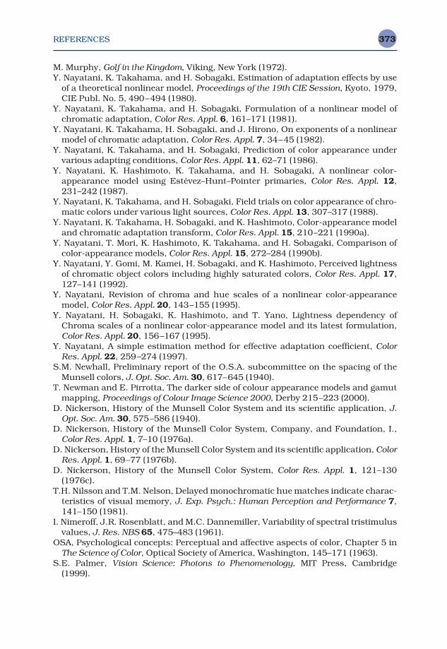
REFERENCES 373
M. Murphy, Golf in the Kingdom, Viking, New York (1972).Y. Nayatani, K. Takahama, and H. Sobagaki, Estimation of adaptation effects by use
of a theoretical nonlinear model, Proceedings of the 19th CIE Session, Kyoto, 1979,CIE Publ. No. 5, 490–494 (1980).
Y. Nayatani, K. Takahama, and H. Sobagaki, Formulation of a nonlinear model ofchromatic adaptation, Color Res. Appl. 6, 161–171 (1981).
Y. Nayatani, K. Takahama, H. Sobagaki, and J. Hirono, On exponents of a nonlinearmodel of chromatic adaptation, Color Res. Appl. 7, 34–45 (1982).
Y. Nayatani, K. Takahama, and H. Sobagaki, Prediction of color appearance undervarious adapting conditions, Color Res. Appl. 11, 62–71 (1986).
Y. Nayatani, K. Hashimoto, K. Takahama, and H. Sobagaki, A nonlinear color-appearance model using Estévez–Hunt–Pointer primaries, Color Res. Appl. 12,231–242 (1987).
Y. Nayatani, K. Takahama, and H. Sobagaki, Field trials on color appearance of chro-matic colors under various light sources, Color Res. Appl. 13, 307–317 (1988).
Y. Nayatani, K. Takahama, H. Sobagaki, and K. Hashimoto, Color-appearance modeland chromatic adaptation transform, Color Res. Appl. 15, 210–221 (1990a).
Y. Nayatani, T. Mori, K. Hashimoto, K. Takahama, and H. Sobagaki, Comparison ofcolor-appearance models, Color Res. Appl. 15, 272–284 (1990b).
Y. Nayatani, Y. Gomi, M. Kamei, H. Sobagaki, and K. Hashimoto, Perceived lightnessof chromatic object colors including highly saturated colors, Color Res. Appl. 17,127–141 (1992).
Y. Nayatani, Revision of chroma and hue scales of a nonlinear color-appearancemodel, Color Res. Appl. 20, 143–155 (1995).
Y. Nayatani, H. Sobagaki, K. Hashimoto, and T. Yano, Lightness dependency ofChroma scales of a nonlinear color-appearance model and its latest formulation,Color Res. Appl. 20, 156–167 (1995).
Y. Nayatani, A simple estimation method for effective adaptation coefficient, ColorRes. Appl. 22, 259–274 (1997).
S.M. Newhall, Preliminary report of the O.S.A. subcommittee on the spacing of theMunsell colors, J. Opt. Soc. Am. 30, 617–645 (1940).
T. Newman and E. Pirrotta, The darker side of colour appearance models and gamutmapping, Proceedings of Colour Image Science 2000, Derby 215–223 (2000).
D. Nickerson, History of the Munsell Color System and its scientific application, J.Opt. Soc. Am. 30, 575–586 (1940).
D. Nickerson, History of the Munsell Color System, Company, and Foundation, I.,Color Res. Appl. 1, 7–10 (1976a).
D. Nickerson, History of the Munsell Color System and its scientific application, ColorRes. Appl. 1, 69–77 (1976b).
D. Nickerson, History of the Munsell Color System, Color Res. Appl. 1, 121–130(1976c).
T.H. Nilsson and T.M. Nelson, Delayed monochromatic hue matches indicate charac-teristics of visual memory, J. Exp. Psych.: Human Perception and Performance 7,141–150 (1981).
I. Nimeroff, J.R. Rosenblatt, and M.C. Dannemiller, Variability of spectral tristimulusvalues, J. Res. NBS 65, 475–483 (1961).
OSA, Psychological concepts: Perceptual and affective aspects of color, Chapter 5 inThe Science of Color, Optical Society of America, Washington, 145–171 (1963).
S.E. Palmer, Vision Science: Photons to Phenomenology, MIT Press, Cambridge(1999).
REFERENCES374
S.N. Pattanaik, J.A. Ferwerda, M.D. Fairchild, and D.P. Greenberg, A multiscalemodel of adaptation and spatial vision for image display, Proceedings of SIGGRAPH98, 287–298 (1998).
H. Pauli, Proposed extnsion of the CIE recommendation on Uniform color spaces,color difference equations, and metric color terms, J. Opt. Soc. Am. 36, 866–867(1976).
E. Pirrotta and M.D. Fairchild, Directly testing chromatic-adaptation models usingobject colors, Proceedings of the 23rd Session of the CIE (New Delhi) Vol. 1, 77–78(1995).
A.B. Poirson and B.A. Wandell, Appearance of colored patterns: Pattern-color separ-ability, J. Opt. Soc. Am. A 10, 2458–2470 (1993).
A.B. Poirson and B.A. Wandell, Pattern-color separable pathways predict sensitivityto simple colored patterns, Vision Res. 36, 515–526 (1996).
J. Pokorny, V.C. Smith, and M. Lutze, Aging of the human lens, Appl. Opt. 26,1437–1440 (1987).
D.M. Purdy, Spectral hue as a function of intensity, Am. J. Psych, 43, 541–559(1931).
D. Purves, R.B. Lotto, and S. Nundy, Why we see what we do, American Scientist 90,236–243 (2002).
E. Reinhard, M. Stark, P. Shirley, and J. Ferwerda, Gradient domain high dynamicrange compression, Proceedings of SIGGRAPH 2002, San Antonio, 267–276 (2002).
K. Richter, Cube-root color spaces and chromatic adaptation,Color Res. Appl. 5, 7–11(1980).
K. Richter, Farbempfindungsmerkmal Elementarbuntton und Buntheitsabstände alsFunktion von Farbart und Leuchtdichte von In- und Umfeld, Bundesanstalt fürMaterialprüfung (BAM) Forschungsbericht 115, Berlin, (1985).
M. Richter and K. Witt, The story of the DIN color system, Color Res. Appl. 11, 138–145 (1986).
O. Rinner and K.R. Gegenfurtner, Time course of chromatic adaptation for colorappearance discrimination, Vision Res. 40, 1813–1826 (2000).
A.R. Robertson, A new determination of lines of constant hue, AIC Color 69,Stockholm, 395–402 (1970).
A.R. Robertson, The CIE 1976 color-difference formulae, Color Res. Appl. 2, 7–11(1977).
A.R. Robertson, Historical development of CIE recommended color difference equa-tions, Color Res. Appl. 15, 167–170 (1990).
A.R. Robertson, Figure 6–2 Presented at the 1996 ISCC Annual Meeting, Orlando,Fla. (1996).
M.A. Rodriguez and T. G. Stockham, ‘Producing colorimetric data from densitometricscans,’ Proc. SPIE 1913, 413–418 (1993).
R. Rolleston and R. Balasubramanian, ‘Accuracy of various types of NeugebauerModel,’ Proceedings IS&T/SID Color Imaging Conference, Scottsdale, Ariz., 32–37(1993).
Sarnoff Corporation, JND: A human vision system model for objective picture qualitymeasurement, Sarnoff Technical Report from www.jndmetrix.com, (2001).
O.H. Schade, Optical and photoelectric analog of the eye, J. Opt. Soc. Am. 46,721–739 (1956).
B.E. Schefrin and J.S. Werner, Age-related changes in the color appearance of broad-band surfaces, Color Res. Appl. 18, 380–389 (1993).
REFERENCES 375
J. Schirillo, A. Reeves, and L. Arend, Perceived lightness, but not brightness, ofachromatic surfaces depends on perceived depth information, Perception & Psy-chophysics 48, 82–90 (1990).
J. Schirillo and S.K. Shevell, Lightness and brightness judgments of coplanar retin-ally noncontiguous surfaces, J. Opt. Soc. Am. A 10, 2442–2452 (1993).
J. Schirillo and L. Arend, Illumination changes at a depth edge can reduce lightnessconstancy, Perception & Psychophysics 57, 225–230 (1995).
J. Schirillo and S.K. Shevell, Brightness contrast from inhomogeneous surrounds,Vision Res. 36, 1783–1796 (1996).
T, Seim and A. Valberg, Towards a uniform colorspace: A better formula to describethe Munsell and OSA Color Scales, Color Res. Appl. 11, 11–24 (1986).
C.C. Semmelroth, Prediction of lightness and brightness on different backgrounds, J. Opt. Soc. Am., 60, 1685–1689 (1970).
G. Sharma and H.J. Trussel, Digital color imaging, IEEE Trans. Im. Proc. 6, 901–932(1997).
G. Sharma, Ed., Digital Color Imaging Handbook, CRC Press, Boca Raton (2003).S.K. Shevell, The dual role of chromatic backgrounds in color perception, Vision Res.
18, 1649–1661 (1978).S.K. Shevell, Color and brightness: Contrast and context, IS&T/SID 1st Color Imaging
Conference, Scottsdale, 11–15 (1993).J.M. Speigle and D.H. Brainard, Is color constancy task independent?, IS&T/SID 4th
Color Imaging Conference, Scottsdale, 167–172 (1996).L. Spillman and J.S. Werner, Visual Perception: The Neurophysiological Foundations,
Academic Press, San Diego, (1990).R. Stanziola, The Colorcurve System®, Color Res. Appl. 17, 263–272 (1992).S.S. Stevens, To honor Fechner and repeal his law, Science 133, 80–86 (1961).J.C. Stevens and S.S. Stevens, Brightness functions: Effects of adaptation, J. Opt.
Soc. Am. 53, 375–385 (1963).W.S. Stiles and J.M. Burch, N.P.L. colour-matching investigation: Final report
(1958), Optica Acta 6, 1–26 (1959).A. Stockman, L.T. Sharpe, and C. Fach, The spectral sensitivity of the human short-
wavelength sensitive cones derived from threshold and color matches, Vision Res.39, 2901–2927 (1999).
A. Stockman and L.T. Sharpe, The spectral sensitivities of the middle- and long-wavelength-sensitive cones derived from measurements in observers of knowngenotype, Vision Res. 40, 1711–1737 (2000).
M. Stokes, M. Fairchild, and R.S. Berns, Precision requirements for digital colorreproduction, ACM Trans. Graphics 11, 406–422 (1992).
M.C. Stone, W.B. Cowan, and J.C. Beatty, Color gamut mapping and the printing ofdigital images, ACM Trans. Graphics 7, 249–292 (1988).
M.C. Stone, A Field Guide to Digital Color, A.K. Peters, Natick (2003).G. Svaetichin, Spectral response curves from single cones, Acta Physiologica Scan-
dinavica 39 (Suppl. 134), 17–46 (1956).K. Takahama, H. Sobagaki, and Y. Nayatani, Analysis of chromatic adaptation effect
by a linkage model, J. Opt. Soc. Am. 67, 651–656 (1977).K. Takahama, H. Sobagaki, and Y. Nayatani, Formulation of a nonlinear model of
chromatic adaptation for a light-gray background, Color Res. Appl. 9, 106–115(1984).
R. Taya, W.H. Ehrenstein, and C.R. Cavonius, Varying the strength of the Munker–White effect by stereoscopic viewing, Perception 24, 685–694 (1995).
REFERENCES376
C.C. Taylor, Z. Pizlo, J.P. Allebach, and C.A. Bouman, Image quality assessment witha Gabor pysamid model of the human visual system, IS&T/SPIE Electronic ImagingConference, SPIE Vol. 3016, San Jose, 58–69 (1997).
C.C. Taylor, Z. Pizlo, and J.P. Allebach, Perceptually relevant image fidelity, IS&T/SPIE Electronic Imaging Conference, SPIE Vol. 3299, San Jose, 110–118 (1998).
H. Terstiege, Chromatic adaptation: A state-of-the-art report, J. Col. & Appear. 1, 19–23 (1972).
L.L. Thurstone, A law of comparative judgment, Psych. Review 34, 273–286, (1927).
L.L. Thurstone, The Measurment of Values, University of Chicago Press, Chicago(1959).
D.J. Tolhurst and D.J. Heeger, Comparison of contrast-normalization and thresholdmodels of the responses of simple cells in cat striate cortex, Visual Neuroscience14, 293–309 (1997).
W.S. Torgerson, A law of categrocial judgment, in Consumer Behavior, L.H. Clark,Ed., New York University Press, New York, 92–93 (1954).
W.S. Torgerson, Theory and Methods of Scaling, Wiley, New York (1958).A. Valberg and B. Lange-Malecki, ‘Colour constancy’ in Mondrian patterns: A partial
cancellation of physical chromaticity shifts by simultaneous contrast, Vision Res.30, 371–380 (1990).
J. von Kries, Chromatic adaptation, Festschrift der Albrecht-Ludwig-Universität,(Fribourg) (1902) [Translation: D.L. MacAdam, Sources of Color Science, MIT Press,Cambridge, (1970)].
J. Walraven, Discounting the background — the missing link in the explanation ofchromatic induction, Vision Res. 16, 289–295 (1976).
B.A. Wandell, Color appearance: The effects of illumination and spatial pattern, Proc.Natl. Acad. Sci. USA 90, 9778–9784 (1993).
B.A. Wandell, Foundations of Vision, Sinauer, Sunderland, Mass., (1995).A.B. Watson, Toward a perceptual video quality metric, Human Vision and Electronic
Imaging III, SPIE Vol. 3299, 139–147 (1998).A.B. Watson and C.V. Ramirez, A standard observer for spatial vision, Investigative
Ophthalmology and Visual Science 41, S713 (2000).A.B. Watson, J. Hu, and J.F. McGowan, DVQ: A digital video quality metric based on
human vision, J. of Electronic Imaging 10, 20–29 (2001).M.A. Webster and J.D. Mollon, The influence of contrast adaptation on color appear-
ance, Vision Res. 34, 1993–2020 (1994).M.A. Webster and J.D. Mollon, Adaptation and the color statistics of natural images,
Vision Res. 37, 3283–3298 (1997).J.S. Werner and B.E. Schefrin, Loci of achromatic points throughout the life span,
J. Opt. Soc. Am. A 10, 1509–1516 (1993).D.R. Williams, N. Sekiguchi, W. Haake, D. Brainard, and O. Packer, The cost of
trichromacy for spatial vision, in From Pigments to Perception (A. Valberg and B.B. Lee, Eds.), Plenum Press, New York 11–22 (1991).
M. Wolski, J.P. Allebach, and C.A. Bouman, Gamut mapping: Squeezing the mostout of your color system, IS&T/SID 2nd Color Imaging Conference, Scottsdale,89–92 (1994).
W.D. Wright, A re-determination of the trichromatic coefficients of the spectralcolours, Trans. Opt. Soc. 30, 141–161 (1928–29).
W.D. Wright, Why and how chromatic adaptation has been studied, Color Res. Appl.6, 147–152 (1981a).

REFERENCES 377
W.D. Wright, 50 years of the 1931 CIE standard observer for colorimetry, AIC Color81, Paper A3 (1981b).
D.R. Wyble and M.D. Fairchild, Prediction of Munsell appearance scales using vari-ous color appearance models, Color Res. Appl. 25, 132–144 (2000).
G. Wyszecki, Current developments in colorimetry, AIC Color 73, 21–51 (1973).G. Wyszecki and W.S. Stiles, Color Science: Concepts and Methods, Quantitative Data
and Formulae, Wiley, New York, (1982).G. Wyszecki, Color appearance, Chapter 9 in Handbook of Perception and Human
Performance, Wiley, New York, (1986).X. Zhang and B.A. Wandell, A spatial extension of CIELAB for digital color image
reproduction, SID 96 Digest, (1996).
Index
Abney effect, 117–119absorptance, 60achromatic color, defined, 84adaptation
chromatic. See chromatic adaptationand chromatic induction, 113, 124dark, 22–23, 34, 148, 151–152, 159light, 22–23, 148–149, 152mechanisms of, 21motion, 155–156spatial frequency, 155
additive mixtures, 95, 103additivity, Grassmann’s law of, 70adjustment, method of, 43advanced colorimetry, 34afterimages, 149, 155Albers, Josef, 113amacrine cells, of retina, 4aqueous humor, 3art, color-order systems in, 95, 102, 106ASTM Standard Guide for Designing and
Conducting Visual Experiments, 35asymmetric matching, 43, 46, 160ATD color appearance model
adaptation model for, 220, 224brightness equation in, 210, 218–220chroma equation in, 220data for, 208, 210, 216example of, 279, 281hue equation in, 216–217, 221limitations of, 197objectives and approach of, 196opponent-color dimensions in, 200perceptual correlates in, 201predictions of, 201, 205saturation equation in, 201–202
axons, defined, 5
background, defined, 137Bartleson–Breneman equations, 126, 130basic colorimetry, 51Bezold–Brücke hue shift, 116, 118–119bidirectional reflectance distribution
functions (BRDF), 63bidirectional transmittance distributions
functions, 63black-body radiator, 58blackness, NCS value, 95
blind spot, 6, 10–12Bradford–Hunt 96c color appearance model,
208Bradford–Hunt 96s color appearance model,
208brain
visual area 1 of, 13, 15and visual signal processing, 12, 15
brightness, 86chromaticity and, 117–119–colorfulness reproduction, 92in color appearance, 85defined, 79luminance and, 100
cameras, digital, 319category scaling, 47–48characterization
approaches to, 238defined, 243–244, 248, 250goals of, 54
chroma, 87, 92in color appearance, 85defined, 84–85, 87–88, 90equation for, 90Munsell, 85
chromatic adaptation, 19, 21, 23–25cognitive mechanisms of, 127defined, 120example of, 112, 114, 118, 120, 128high-level, 149, 154mechanics of, 124models of, 148–149, 152–154, 157, 159,
162, 164–165photoreceptors in, 148, 151, 153, 157physiology of, 149, 154receptor gain control in, 151, 153sensory mechanisms of, 157, 159–160subtractive mechanisms of, 149, 153time course of, 159treatises on, 158
chromatic adaptation models, 146–149,152–153, 157–160, 162–165
applications of, 164–165CAT02 transform, 183–184, 191–195
concerns of, 166equations for, 162–163Fairchild’s model, 183, 190–191
INDEX 379
MacAdam’s model, 166, 172Nayatani’s model, 172–174, 177–178, 181retinex theory, 171–172treatises on, 158von Kries model, 151, 157, 165
chromatic adaptation transforms, 163–164chromatic color, defined, 84chromatic contrast, 34, 28f
contrast sensitivity functions for, 33–34,27f
chromatic induction, 113, 124chromaticity and brightness, 119
diagrams of, 77–78chromaticness, NCS value, 100–102CIE illuminants, 56, 58–59
characteristics of, 63, 66, 130CIE 1931 Standard Colorimetric Observer,
73, 76, 61t, 74t, 307CIE 1964 Supplementary Standard
Colorimetric Observer, 77, 82CIE 1976 Uniform Chromaticity Scales,
78–79CIECAM02 color appearance model,
238–239adaptation model in, 241, 246, 251brightness, 239–240Cartesian coordinates, 246–247chroma, 243–244colorfulness, 239, 243–244, 246hue, 239, 243input data, 240–241, 246inverse model, 243implementation guidelines, 245lightness, 239, 243objectives, 240, 245opponent dimensions, 248phenomena predicted, 243saturation, 239
CIECAM97s color appearance model, 238appearance correlates in, 246chromatic adaptation in, 239, 241, 243,
245–248, 250–251data for, 239–240historical background for, 239, 241, 244,
246, 248invertibility, 259–260
CIELAB color space, xv, 81color differences in, 78, 80–81coordinates of, 161described, 154, 159–160, 162–163example of, 229lightness scale of, 161limitations of, 170mapping of, 164, 179recommended usage of, 300, 303, 306testing of, 264uniformity of, 185, 189utility of, 305
wrong von Kries transforms in, 191–192,194
CIELAB ∆E*ab, 80–81CIELUV color space, 81, 194–195
example of, 279, 281testing of, 264
CIE94 color difference model, 81CMC color difference equation, 81CMYK, device coordinates, 315color(s)
adaptation to, 19characteristics of, 63, 66constancy of, 24, 132–133, 164–165corresponding, 159–162, 164, 162f–163f,
255, 261–262defined, 47, 159memory, 24, 130, 132related, 84, 146, 162, 164triangle of, 54–55, 66, 82, 55ftristimulus values and, 70–71unrelated, 88–89, 120, 130
color appearancecognitive aspects of, 132spatial influences on, 112, 125, 128
color appearance models, applications of,238
ATD, 239Bradford–Hunt models, 246
CIECAM02, 238–239CIECAM97s, 238–239CIELAB, 184–186, 189, 191–195CIELUV, 184, 194–195
color attributes and, 84–85, 89, 91construction of, 184–185corresponding-colors data and, 255,
261–262current cutting edge, 300defined, 183, 189developments for the future, 299, 306and device independent color imaging,
309–310, 312–313, 315, 321–322, 324,330–331
direct-model testing of, 264Hunt’s, 196–197, 201, 203, 205–206LLAB, 239, 245–246, 249–251magnitude-estimation experiments and,
263Nayatani’s, 196–199, 202–207pictorial review of, 253psychophysics and, 53, 66qualitative testing of, 264research on, 299RLAB, 225, 227–228, 230–232, 234–237testing of, 94, 165, 264utility of, 90variety of, 301, 304–305visual system and, 35, 46, 52ZLAB, 255, 260–263
INDEX380
color appearance phenomena, 108color appearance reproduction, 255, 261color constancy, 24, 132–133
computational, 164–165color differences specifications, 64color differences measurement, 245
application of color appearance models to,254
future directions for, 253recommendations for, 260techniques of, 246
color gamut, 261color measurement, 285
based on ICC Profile Format, xivcolor matching, 70–73, 76–77, 74tcolor matching functions, 70–72, 76–77
average, 71, 81color naming systems, 109
types of, 97, 104, 106–107color order systems, 94–96, 103, 106–109
applications of, 94–95, 97–98, 102–103,106–109
in art and design, 105, 107in communication, 107in education, 107–108in evaluation of color appearance models,
104and imaging systems, 98, 108, 110limitations of, 102, 107–108in visual experiments, 106
color preference reproduction, 287color preferences, 314, 324, 327–328, 331color rendering, 279, 293–295
application of color appearance models to,278–281, 283–287, 289–295
CIE technical committee on, 279, 291–293future directions for, 294indices for, 293recommendations for, 293–294techniques of, 285, 287, 289, 294
color reproductiondefined, 273–274enhancing accuracy of, 282levels of, 275
color spaces(s)CIE, xiii, 78–79color differences in, 78, 80–81viewing-conditions-independent, 283
color temperature, 56–58color vision
deficiencies of, 31historic theories of, 17spatial properties of, 27, 28ftemporal properties of, 26
color vision deficiencies, 17–18, 30–33gender and, 31screening for, 33
colorcurve system, 102–103, 106
colorfulness, 87–93in color appearance, 85defined, 84varying directly with luminance, 113, 121,
124colorimetric color reproduction, 274colorimetry
absolute, 58, 60, 75advanced, 53–54, 82basic, xviii, 53–56, 66–67, 82defined, 54future directions in, 263normalized, 75origin of, 66relative, 75
colour standards for image technology, 240Commission Internationale de l’Eclairage
(CIE), xiiiactivities of, 279, 291–292, 294See also CIE entries
communication, color-order systems in, 107computational color constancy, 164–165cone monochromatism, 31, 33tincidence of, 33tcone responses
transformation of tristimulus values to,191
cones, 4, 6, 8–11, 13–15, 21, 23, 27, 30, 34distinguished from rods, 30function of, 8–11relative abundance of, 29role in light and dark adaptation, 151spectral responsivities of, 66–67, 71, 76types of, 6, 8–9, 16–19, 21, 24, 27, 30–31,
33constant stimuli, method of, 30contrast
varying directly with luminance, 116–117varying directly with surround, 125
contrast sensitivity functions (CSFs), 26–27,27f, 28f
and eye movements, 29–30spatial, 26 –27, 29, 34, 15f, 27f , 28ftemporal, 26 –27, 29, 28f
cool white fluorescent lamp, and colorrendering, 293–295
corneadescribed, 1function of, 1
correlated color temperature (CCT), 56, 58–59corresponding color reproduction, 283corresponding colors, 159–160, 164, 163f
color appearance models and, 252Cowan equation, 119–120crispening, 113–115, 115fCRT display, 139
characterization of, 295cubo-octahedron, 104
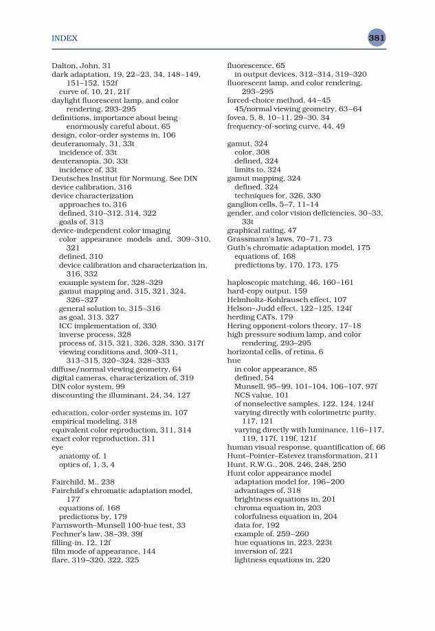
INDEX 381
Dalton, John, 31dark adaptation, 19, 22–23, 34, 148–149,
151–152, 152fcurve of, 10, 21, 21f
daylight fluorescent lamp, and colorrendering, 293–295
definitions, importance about beingenormously careful about, 65
design, color-order systems in, 106deuteranomaly, 31, 33t
incidence of, 33tdeuteranopia, 30, 33t
incidence of, 33tDeutsches Institut für Normung. See DINdevice calibration, 316device characterization
approaches to, 316defined, 310–312, 314, 322goals of, 313
device-independent color imagingcolor appearance models and, 309–310,
321defined, 310device calibration and characterization in,
316, 332example system for, 328–329gamut mapping and, 315, 321, 324,
326–327general solution to, 315–316as goal, 313, 327ICC implementation of, 330inverse process, 328process of, 315, 321, 326, 328, 330, 317fviewing conditions and, 309–311,
313–315, 320–324, 328–333diffuse/normal viewing geometry, 64digital cameras, characterization of, 319DIN color system, 99discounting the illuminant, 24, 34, 127
education, color-order systems in, 107empirical modeling, 318equivalent color reproduction, 311, 314exact color reproduction, 311eye
anatomy of, 1optics of, 1, 3, 4
Fairchild, M., 238Fairchild’s chromatic adaptation model,
177equations of, 168predictions by, 179
Farnsworth–Munsell 100-hue test, 33Fechner’s law, 38–39, 39ffilling-in, 12, 12ffilm mode of appearance, 144flare, 319–320, 322, 325
fluorescence, 65in output devices, 312–314, 319–320
fluorescent lamp, and color rendering,293–295
forced-choice method, 44–4545/normal viewing geometry, 63–64
fovea, 5, 8, 10–11, 29–30, 34frequency-of-seeing curve, 44, 49
gamut, 324color, 308defined, 324limits to, 324
gamut mapping, 324defined, 324techniques for, 326, 330
ganglion cells, 5–7, 11–14gender, and color vision deficiencies, 30–33,
33tgraphical rating, 47Grassmann’s laws, 70–71, 73Guth’s chromatic adaptation model, 175
equations of, 168predictions by, 170, 173, 175
haploscopic matching, 46, 160–161hard-copy output, 159Helmholtz–Kohlrausch effect, 107Helson–Judd effect, 122–125, 124fherding CATs, 179Hering opponent-colors theory, 17–18high pressure sodium lamp, and color
rendering, 293–295horizontal cells, of retina, 6hue
in color appearance, 85defined, 54Munsell, 95–99, 101–104, 106–107, 97fNCS value, 101of nonselective samples, 122, 124, 124fvarying directly with colorimetric purity,
117, 121varying directly with luminance, 116–117,
119, 117f, 119f, 121fhuman visual response, quantification of, 66Hunt–Pointer–Estevez transformation, 211Hunt, R.W.G., 208, 246, 248, 250Hunt color appearance model
adaptation model for, 196–200advantages of, 318brightness equations in, 201chroma equation in, 203colorfulness equation in, 204data for, 192example of, 259–260hue equations in, 223, 223tinversion of, 221lightness equations in, 220
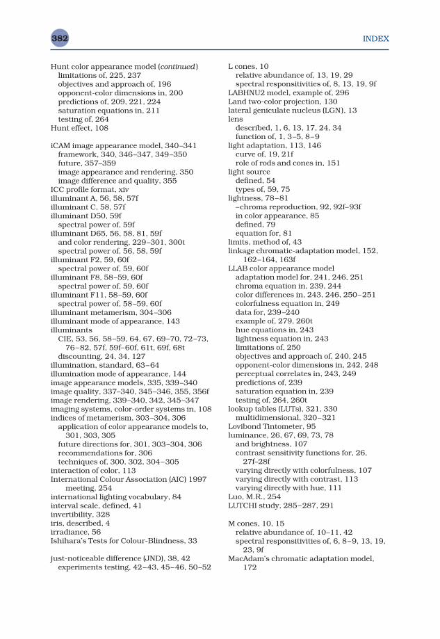
INDEX382
Hunt color appearance model (continued )limitations of, 225, 237objectives and approach of, 196opponent-color dimensions in, 200predictions of, 209, 221, 224saturation equations in, 211testing of, 264
Hunt effect, 108
iCAM image appearance model, 340–341framework, 340, 346–347, 349–350future, 357–359image appearance and rendering, 350image difference and quality, 355
ICC profile format, xivilluminant A, 56, 58, 57filluminant C, 58, 57filluminant D50, 59f
spectral power of, 59filluminant D65, 56, 58, 81, 59f
and color rendering, 229–301, 300tspectral power of, 56, 58, 59f
illuminant F2, 59, 60fspectral power of, 59, 60f
illuminant F8, 58–59, 60fspectral power of, 59, 60f
illuminant F11, 58–59, 60fspectral power of, 58–59, 60f
illuminant metamerism, 304–306illuminant mode of appearance, 143illuminants
CIE, 53, 56, 58–59, 64, 67, 69–70, 72–73,76–82, 57f, 59f–60f, 61t, 69f, 68t
discounting, 24, 34, 127illumination, standard, 63–64illumination mode of appearance, 144image appearance models, 335, 339–340image quality, 337–340, 345–346, 355, 356fimage rendering, 339–340, 342, 345–347imaging systems, color-order systems in, 108indices of metamerism, 303–304, 306
application of color appearance models to,301, 303, 305
future directions for, 301, 303–304, 306recommendations for, 306techniques of, 300, 302, 304–305
interaction of color, 113International Colour Association (AIC) 1997
meeting, 254international lighting vocabulary, 84interval scale, defined, 41invertibility, 328iris, described, 4irradiance, 56Ishihara’s Tests for Colour-Blindness, 33
just-noticeable difference (JND), 38, 42experiments testing, 42–43, 45–46, 50–52
L cones, 10relative abundance of, 13, 19, 29spectral responsitivities of, 8, 13, 19, 9f
LABHNU2 model, example of, 296Land two-color projection, 130lateral geniculate nucleus (LGN), 13lens
described, 1, 6, 13, 17, 24, 34function of, 1, 3–5, 8–9
light adaptation, 113, 146curve of, 19, 21frole of rods and cones in, 151
light sourcedefined, 54types of, 59, 75
lightness, 78–81–chroma reproduction, 92, 92f–93fin color appearance, 85defined, 79equation for, 81
limits, method of, 43linkage chromatic-adaptation model, 152,
162–164, 163fLLAB color appearance model
adaptation model for, 241, 246, 251chroma equation in, 239, 244color differences in, 243, 246, 250–251colorfulness equation in, 249data for, 239–240example of, 279, 260thue equations in, 243lightness equation in, 243limitations of, 250objectives and approach of, 240, 245opponent-color dimensions in, 242, 248perceptual correlates in, 243, 249predictions of, 239saturation equation in, 239testing of, 264, 260t
lookup tables (LUTs), 321, 330multidimensional, 320–321
Lovibond Tintometer, 95luminance, 26, 67, 69, 73, 78
and brightness, 107contrast sensitivity functions for, 26,
27f–28fvarying directly with colorfulness, 107varying directly with contrast, 113varying directly with hue, 111
Luo, M.R., 254LUTCHI study, 285–287, 291
M cones, 10, 15relative abundance of, 10–11, 42spectral responsitivities of, 6, 8–9, 13, 19,
23, 9fMacAdam’s chromatic adaptation model,
172
INDEX 383
Macbeth Color Checker Chart, 108macula, 5–6, 34magnitude estimation, 47–49matching techniques, 45Maxwell’s color process, 130McCollough effect, 155measurement
colorimetric, 311–321, 330, 332, 329fexhaustive, 316, 318, 328
memory color, 24, 34, 130, 132memory matching, 46, 161mercury lamp, and color rendering, 300tmesopic vision, 8metal halide lamp, and color rendering, 300tmetamerism, 67
indices of, 303–304, 306in input and output devices, 312–313, 320
metameric, defined, 70method of adjustment, 43method of constant stimuli, 43–44method of limits, 43modeling
empirical, 316, 318physical, 316–317
modular image difference model, 340modulation transfer functions, 26monochromatism, 31, 33t
incidence of, 33tMori experiment, 123motion adaptation, 155–156multidimensional scaling (MDS), 48–49, 51fMunsell Book of Color, 85Munsell value scale, 85
Natural Color System (NCS), 95, 99chromaticness in, 100–102, 101fhue in, 104
Nayatani’s chromatic-adaptation model asbasis for color appearance model, 199
equations of, 173forebears of, 173predictions by, 162, 164
Nayatani’s color appearance modeladaptation model for, 205brightness equations in, 204chroma equations in, 204data for, 197example of, 279, 281hue equations in, 216–217, 222–223inversion of, 221lightness equations in, 220, 222limitations of, 225objectives and approach of, 208opponent-color dimensions in, 215–216predictions of, 209, 221, 224saturation equations in, 217–218, 220,
222testing of, 264
nominal scale, defined, 40–41normal/diffuse viewing geometry, 64normal/45 viewing geometry, 64normalization constant, in colorimetry, 67,
75–77normalized colorimetry, 67, 75
objects, recognition of, 24oblique effect, 29observer metamerism, 304–306off-center ganglion cells, 15on-center ganglion cells, 15one-dimensional scaling, 46, 49opponent-colors theory
Hering’s, 17–18modern, 17–19
opsin, 13optic nerve, 4–6, 11, 13optical illusions, 128Optical Society of America Uniform Color
Scales (OSA UCS), 103ordinal scale, defined, 40–41, 47, 49Ostwald system, 95, 103, 105–106output lexicon, defined, 324
paired comparison experiment, 48–49Pantone Process Color Formula Guide, 95,
109partition scaling, 47–48pass-fail method, 44perceptual threshold, 37perfect reflecting diffuser (PRD), 65, 75photometry, 67, 69, 73, 75photopic luminous efficiency function, 72photopic vision, 8–9photoreceptors, 4–8, 11, 13, 15, 21, 34
energy responses of, 10–11, 13, 15–16, 18,25, 27, 31
gain control of, 149, 153see also cones; rods
physical modeling, 316–317pigmented epithelium, 4–5Planckian radiator, 58pleasing color reproduction, 313PostScript Process Color Guide, 110power law, 39–40preferred color reproduction, 312–314, 327presbyopia, 3printers, characterization of, 319probit analysis, 45profile connection space, 331–332proportionality, Grassmann’s law of, 73protanomaly, 31
incidence of, 33tprotanopia, 30
incidence of, 33tproximal field, defined, 137pseudoisochromatic plates, 33
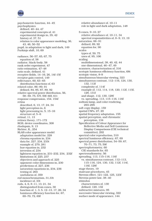
INDEX384
psychometric function, 44–45psychophysics
defined, 40–44, 47experimental concepts of, 41experimental design in, 35, 42history of, 37, 51relation to color appearance modeling, 36,
43, 46, 50–52pupil, in adaptation to light and dark, 149Purkinje shift, 10, 69
radiance, 56–57, 65, 67, 75equation of, 58
radiator, black-body, 58rank order experiment, 47ratio estimation, 47–48ratio scale, defined, 41receptive fields, 14–16, 26, 14f–15freceptor gain control, 149reflectance, 60, 63–65
distribution functions of, 63related color, 86–89, 91
defined, 84, 85, 87, 89, 92relative spectral power distribution, 56,
58–59, 75, 57f, 59f–60f, 61tresponse compression, 154, 154fretina
described, 6, 13, 17, 24, 34light perception in, 6light processing in, 5, 15–16structure of, 5–6
retinal, 11, 13retinex theory, 171–172RGB, device coordinates, 308rhodopsin, 9, 13Richter, K., 254RLAB color appearance model
adaptation model for, 228chroma equation in, 234data for, 227, 234, 233texample of, 279, 281hue equation in, 232inversion of, 234lightness equation in, 231–232, 234, 232flimitations of, 225, 237objectives and approach of, 225opponent-color dimensions in, 230predictions of, 227, 236saturation equations in, 234, 236testing of, 264usefulness of, 359
rod monochromatism, 31,33tincidence of, 33t
rods, 4, 6, 8–11, 13, 21, 34distinguished from cones, 30function of, 1, 3, 5, 12–13, 17, 26, 34luminous efficiency function for, 67,
69–70, 72, 69f
relative abundance of, 10–11role in light and dark adaptation, 148
S cones, 9–10, 27relative abundance of, 10–11, 34spectral responsitivities of, 8–9, 13, 19
saturation, 88–91defined, 89, 92equation for, 90
scalestypes of, 59, 75uses of, 95, 106
scalingmultidimensional, 38, 40, 42, 44one-dimensional, 46–47, 49
scanners, characterization of, 316scotopic luminous efficiency function, 68tscotopic vision, 8–9simultaneous binocular viewing, 323simultaneous contrast, 112–116, 124, 130,
132, 112fcomplexity of, 114fexample of, 112, 114, 118, 120, 112f, 115f,
128, 131fand shape, 112, 130, 128fvs. spreading, 113, 115–116, 116f
sodium lamp, and color rendering, 293–295
soft-copy display, 159spatial CSFs, 27, 29spatial frequency adaptation, 155spatial perception, and chromatic
perception, 134Specification of Colour Appearance for
Reflective Media and Self-LuminousDisplay Comparisons (CIE technicalcommittee), 292
spectral color reproduction, 310spectral luminous efficiency, 67, 69spectral power distribution, 54–59, 67,
70–71, 73, 75, 59fspectrophotometry, 60
CIE standards for, 65spectroradiometry, 56spreading, 113, 115–116, 116f
vs. simultaneous contrast, 112–113,115–116, 124, 130, 132, 112f, 114f,116f, 128f
stage theory, 19staircase procedures, 45Stevens effect, 121–122, 125, 123fStevens power law, 38–40stimulus
characteristics of, 130defined, 120, 132
subtractive mixtures, 95successive binocular viewing, 322surface mode of appearance, 144
INDEX 385
surroundcontrast and, 113, 116, 124, 130, 132,
116fdefined, 120, 132
tapetum, 5TC1-27, Specification of Color Appearance
for Reflective Media and Self-LuminousDisplay Comparisons, 292
TC1-33, Color Rendering, 293TC1-34, Testing Colour Appearance Models,
291model preparation by, 254
temporal CSFs, 2910∞ observer, 76
testing color appearance models, 183Testing Colour Appearance Models
(CIE technical committee), 291model preparation by, 254
threshold experiments, 36, 42types of, 38, 40, 42–44
Thurstone’s law, 48tintometer, 95transmittance, 60, 63, 71, 75, 63f
distribution functions of, 63tri-band fluorescent lamp, and color
rendering, 293–295trichromatic theory, 17, 19tristimulus values, 54, 70–73, 75–77, 79,
73fmeasurement of, 134transformation to cone responses,
167–169, 172–173, 175XYZ, xiii-xiv, 72–73, 76
tritanomaly, 31incidence of, 33t
tritanopia, 30incidence of, 33t
Troland, defined, 240Trumatch Colorfinder, 109tungsten halogen, lamp, and color
rendering, 293–295two-color projections, 130
2° color-matching functions, 76
unrelated color, 88–89defined, 89, 143
viewinganomolies of, 141–145modes of, 134, 141, 143–144, 144t
viewing conditions, definition of, 303–304viewing-conditions-independent space, 301viewing field
colorimetric specifications of, 138components of, 134–135, 138, 141, 136fconfiguration of, 135–136, 138
viewing geometries, 63–64vision
experiments on, 35–38, 42–43, 45–47,50–52
human, 55–56, 66, 55fvisual area 13, 16visual experiments, 106
types of, 38, 40, 42–44visual threshold, 37vitreous humor, 3, 32volume mode of appearance, 144von Kries chromatic-adaptation model
equations of, 178–179history of, 166predictions by, 178–179, 181testing of, 264
Ware equation, 119–120Weber. E.H., 37Weber’s law, 37–38whiteness, NCS value, 99–104, 106, 108,
101fwrong von Kries transforms, 191–192, 194,
180f
xenon lamp, and color rendering, 293–295XYZ tristimulus values, xiii, 73
yes-no method, 44
ZLAB color appearance model, 255, 260appearance correlates in, 257, 262chromatic adaptation in, 255–256, 261,
264data for, 264invertibility of, 263similarities of CIECAM97s, 252, 254–255,
259–264
Related Documents