collocation methods for cauchy problems of elliptic operators ...

COLLOCATION METHODS FOR CAUCHY PROBLEMS OFELLIPTIC OPERATORS VIA CONDITIONAL STABILITIES

SIQING LI∗ AND LEEVAN LING†

Abstract. Ill-posed Cauchy problems for elliptic partial differential equations appear in manyengineering fields. In this paper, we focus on stable reconstruction methods for this kind of inverseproblems. Using kernels that reproduce Hilbert spacesHm(Ω), numerical approximations to solutionsof elliptic Cauchy problems are formulated as solutions of nonlinear least-squares problems withquadratic inequality constraints (LSQI). A convergence analysis with respect to noise levels and filldistances of data points is provided, from which a Tikhonov regularization strategy is obtained.A nonlinear algorithm using generalized singular value decomposition of matrices and Lagrangemultipliers is proposed to solve the LSQI problem. Numerical experiments of two-dimensional casesverify our proved convergence results. By comparing with solutions of MFS and FEM with thediscrete Tikhonov regularization by RKHS under same Cauchy data, we demonstrate that our methodcan reconstruct stable and high accuracy solutions for noisy Cauchy data.

Key words. Cauchy problems, Meshfree, Kansa method, Error analysis, LSQI problem,Tikhonov regularization.

AMS subject classifications. 65D15, 65N35, 65N21.

1. Introduction. It is well known that Cauchy problems are ill-posed in thesense that their solutions do not continuously depend on data. However, Tikhonov[36] proposed that conditional stabilities of solutions for Cauchy problems can beconstructed with an a priori bound to the exact solution. In [21], an interior stabilityfor elliptic Cauchy problems was proved. A global stability was proved based on theCarleman estimate in [34] by Takeuchi and Yamamoto. There are many other interiorand global conditional stability results for Cauchy problems, and for more detail, onecan refer to [1, 5, 15].

Based on these conditional stabilities, efforts were made to look for stable numer-ical methods. The quasi-reversibility method [24] as regularization was proposed forsolving Cauchy problems of Laplace equations by Klibanov in 1990 and convergenceanalysis for a discrete finite difference scheme was also given. In [3], a similar methodwith an adaptive regularization parameter selective strategy was proposed for inverseCauchy problems. In [34], the discretized Tikhonov regularization was proposed byTakeuchi and Yamamoto. Their regularization was built on the theory of reproducingkernel Hilbert spaces (RKHS). A finite element scheme for Cauchy problems was usedand convergence results of the method were also proved in the same paper. Othernumerical methods with convergent analysis are found in the works [6, 19,33].

Meshless methods are another popular numerical method for solving Cauchy prob-lems. Generally speaking, these methods can be applied to complicated geometry andto solving high dimensional problems. The method of fundamental solution (MFS)with different regularization strategies was used to solve homogenous Cauchy prob-lems in [16, 20, 40]. MFS combined with the method of particular solution (MPS)was used to solve nonhomogeneous cases by Li, Xiong, and Chen in [27,38]. A mesh-less method called the general finite difference method (GFDM) was proposed by Fan

∗College of Mathematics, Taiyuan University of Technology, Shanxi, China. & De-partment of Mathematics, Hong Kong Baptist University, Kowloon Tong, Hong Kong.([email protected])

†Department of Mathematics, Hong Kong Baptist University, Kowloon Tong, Hong Kong.([email protected])

1

in [9] to solve inverse Cauchy problems. These meshless approaches usually have goodnumerical performance. However, most , if not all, are ad hoc and do not have robusttheoretical support.

Recently, some progress has been made in the theoretical aspects of meshlesscollocation methods for PDEs. The Kansa method, proposed by E. J. Kansa in1990 [22,23], is a typical meshless method used to solve partial differential equations(PDEs) by imposing strong form collocation conditions to PDEs. To overcome thesingular problem of matrix systems by the Kansa method appearing in some cases[18], the overdetermined Kansa method was applied to solve PDEs in [29]. Partialconvergence results of the overdetermined Kansa method were proved by Ling andSchaback in [30]. Recently, convergence theorems for overdetermined Kansa methodsfor elliptic PDEs were proved by Cheung, Ling, and Schaback in [7].

Motivated by these improvements, in this paper, we apply an overdeterminedkernel-based collocation formulation to solve inverse Cauchy problems. In Section 2,we first introduce Cauchy problems considered in this paper and make some assump-tions. We define discrete solutions for Cauchy problems with exact Cauchy data insome trial spaces of the symmetric positive definite kernel. The discrete solutions weredefined as solutions of nonlinear optimization problems with quadratic inequality con-straints. In the definition, the Tikhonov regularization strategy is used. Convergenceresults of discrete solutions with respect to data densities and noise levels are alsoproved based upon the scattered data approximation theory in RKHS [10, 37]. Thevalue of the regularization parameter can also be fixed in the proof. After consideringexact Cauchy data, we also define discrete solutions with noisy Cauchy data as solu-tions of nonlinear least-squares problems with quadratic constraints. The convergencetheorem of the discrete solution with noisy Cauchy data is proved based on the resultsof the discrete solution with exact Cauchy data. In Section 3, a solver for least-squaresproblems with quadratic constraints is introduced based on generalized singular valuedecomposition (GSVD) and the Lagrange multiplier method. In Section 4, we com-pare the results by the least-quares optimization problem with quadratic inequalityconstraints (LSQI) solver we introduced with those of other nonlinear solvers andshow numerically that the proposed solver can obtain high accuracy and stable solu-tions. Numerical experiments for two-dimensional examples are computed to verifythe convergence results we proved in Section 2. The high accuracy of the numericalresults can also be seen by comparing them with the numerical solutions by MFS [31]and RKHS [34].

2. Reconstruction methods and error analysis.

2.1. Cauchy problems. In this paper, we consider the following Cauchy prob-lem for elliptic PDEs: given f, g∗0 and g∗1 , find u insider Ω or on ∂Ω \ Γ where

Lu = f in Ω,

u = g∗0 on Γ,

∂Lu = g∗1 on Γ.

(2.1)

In Eq. (2.1), domain Ω ⊆ Rd is a bounded domain with sufficiently smooth boundary∂Ω and Γ is a nonempty open subset of ∂Ω. The elliptic operator L and the conormalderivative operator ∂L associated with L can be denoted as

Lu(x) :=d∑

i,j=1

∂j(aij(x)∂iu(x)

)+ c(x)u(x) for x ∈ Ω, (2.2)

2

and

∂Lu(x) :=d∑

i,j=1

aij(x)νj∂iu(x) for x ∈ Γ,

where ν = ν(x) is the unit outer normal vector of ∂Ω at x.We make assumptions for the domain and operator coefficients for further use.Assumption 2.1 (Smoothness of coefficients and domain). We assume Ω ⊆ Rd is

an open bounded domain with Lipschitz continuous boundary and satisfies an interiorcone condition. Coefficients in Eq. (2.2) satisfy c(x) ≤ 0 almost everywhere in Ω,aijdi,j=1 and c(x) ∈ Wm−1

∞ (Ω) for m ≥ 2. We also assume aijdi,j=1 are symmetricpositive definite, that is there exists a constant α > 0 such that

d∑i,j=1

aijξiξj ≥ α

d∑i=1

ξ2i for all x ∈ Ω, ξidi=1 ∈ Rd.

We assume g∗0 and g∗1 are smooth enough to admit a uniquely defined exactsolution u∗ ∈ Hm(Ω) for the Cauchy problem (2.1) [21, Thm.3.3.1]. By the tracetheorem, g∗0 ∈ Hm−1/2(Γ) and g∗1 ∈ Hm−3/2(Γ). Conditional stabilities for Cauchyproblems (2.1) can be proved under an a priori bound for u∗, based on which weconstruct numerical algorithms. We state the recent global conditional stability resultproved by Takeuchi and Yamamoto in [34].

Proposition 2.2 (Global Conditional Stability). Let u∗ be the exact solutionof the Cauchy problem (2.1) and u∗ ∈ Hm(Ω) with m > d+2

2 . For 0 < κ < 1, thereexists a constant C > 0 such that

∥u∥L∞(∂Ω\Γ) ≤ C∥u∥Hm(Ω)

(log

1

E(u)+ log

1

∥u∥Hm(Ω)

)−κ

, (2.3)

with E(u) := ∥u∥L2(Γ) + ∥∂Lu∥L2(Γ) + ∥Lu∥L2(Ω).

From the above result, we can easily see that ∥u∥L∞(∂Ω\Γ) converges to zerowhenever ∥u∗∥Hm(Ω) ≤ M and E(u) converges to 0. The latter suggests that kernelcollocation methods similar to those for solving direct problems can be developed tominimize E(u).

2.2. Kernels and native space. We consider symmetric positive definite ker-nels Φ : Rd × Rd → R and further assume that their Fourier transforms Φ of kernelΦ decay algebraically as

c1(1 + ∥ω∥22)−m ≤ Φ(ω) ≤ c2(1 + ∥ω∥22)−m for m > d/2. (2.4)

Matern functions and Wendland’s compactly supported functions are two commonlyused kernels satisfying (2.4). The native space NRd,Φ of a kernel Φ is defined as

NRd,Φ :=f ∈ L2(Rd) ∩ C(Rd) : f/

√Φ ∈ L2(Rd)

associated with norms

∥f∥2NRd,Φ:= (2π)−

d2

∫Rd

f2(ω)

Φdω.

3

It was shown in [37] that native spaces NRd,Φ of kernels Φ satisfying (2.4) coincidewith Sobolev spaces Hm(Rd). Native space norms ∥ · ∥NRd,Φ

and Sobolev norms ∥ · ∥mare equivalent. From [37, Cor.10.48], if Ω has a Lipschitz boundary, we also havenative spaces NΩ,Φ being norm equivalent to Sobolev spaces Hm(Ω).

Let Z = z1, z2, . . . , znZ be a discrete set of trial centers in the domain Ω. We

define the finite dimensional trial space based on the trial set Z.Definition 2.3. Let Z be the trial set and kernel Φ satisfy (2.4), the finite

dimensional trial space UZ is defined as:

UZ,Φm := spanΦ(., zi), zi ∈ Z ⊂ NΩ,Φ.

We propose a numerical method to seek numerical approximations of the Cauchyproblem (2.1) from these trial spaces. We do so by imposing collocation conditions.Let X = x1, x2, . . . , xnX, Y0 = y01 , y02 , . . . , y0nY0

and Y1 = y11 , y12 , . . . , y1nY1 be sets

of discrete collocation points in Ω and on the Dirichlet and Neumann boundary.To describe the point density of Z, we define the following quantities

hZ := supz∈Ω

minzi∈Z

∥z − zi∥ℓ2(Rd), qZ :=1

2min

zi, zj ∈ Zzi = zj

∥zi − zj∥ℓ2(Rd) and ρZ :=hZ

qZ,

which are normally called fill distance, separation distance, and mesh ratio of Z re-spectively. We further assume the trial set Z and collocation sets X, Y0 and Y1 areall quasi-uniform, that is, the mesh ratio ρχ > 1 satisfies

qχ ≤ hχ ≤ ρχqχ and χ = X, Y0, Y1, Z. (2.5)

2.3. The discrete solution with exact Cauchy data and error analysis.For easy understanding, we begin by introducing a discrete approximation with exactCauchy data in the trial space to the solution of the Cauchy problem. We aim todevelop a simple least-squares approach. Let u be a function in Hm(Ω), and v be ageneral notation for functions in the trial space UZ,Φm ⊆ NΩ,Φm = Hm(Ω). We firstintroduce some preliminaries. For any u ∈ C(Ω), we define a discrete norm of u oncollocation set X as

∥u∥X =

(∑xi∈X

u(xi)2

)1/2

.

From [11], for any u ∈ Hm(Ω), when Assumption 2.1 holds for coefficients of anelliptic operator, one has

∥Lu∥Hm−2(Ω) ≤ CΩ,L∥u∥Hm(Ω), (2.6)

and

∥∂Lu∥Hm−1(Ω) ≤ CΩ,∂L∥u∥Hm(Ω).

To define a computable scheme for the Cauchy problem, we need to discretize thecontinuous norms by discrete point sets in both the domain and the Cauchy boundary.To do this, we introduce sampling inequalities in the following proposition.

4

Proposition 2.4 (Sampling inequality of fractional order [7]). Suppose Ω ⊂Rd is a bounded Lipschitz domain with a piecewise Cm–boundary. Then there is aconstant CΩ,m,s depending only on Ω, m and s such that following inequalities hold:

∥u∥s,Ω ≤ CΩ,m,s

(hm−sX ∥u∥m,Ω + h

d/2−sX ∥u∥X

)for 0 ≤ s ≤ m,

and

∥u∥s−1/2,Γ ≤ CΓ,m,s

(hm−sY ∥u∥m,Ω + h

d/2−sY ∥u∥Y

)for 1/2 ≤ s ≤ m,

for any u ∈ Hm(Ω) with m > d/2 and any discrete sets X ⊂ Ω and Y ⊂ Γ withsufficiently small mesh norm hX and hY .

For the ill-posed property of the problems being solved, different regulariza-tion strategies were proposed to stabilizing the numerical solutions, for instance,the Tikhonov regularization method [26, 35], the damped singular value decompo-sition [8, 20], and the truncated singular value decomposition [17]. Recently, a novelregularization method for ill-posed problems called mixed regularization method wasput forward by Zheng, Zhang in [41]. In this paper, we use the Tikhonov regulariza-tion method. Combining discrete norms on collocation sets X, Y0 and Y1, we definethe discrete solution in trial space UZ,Φm of Cauchy problems with exact data as:

Definition 2.5. The solution uX,Y0,Y1,σ ∈ UZ,Φm with exact Cauchy data de-fined as the solution of the following least-squares problems with quadratic inequalityconstraints (LSQI) problem:

uX,Y0,Y1,σ := arg infv∈UZ,Φm

σ2∥v∥2Hm(Ω) + ∥Lv − f∥2X

s.t. hd−1Y0

∥v − g∗0∥2Y0+ hd−1

Y1∥∂Lv − g∗1∥2Y1

≤ (h2m−d−2Z + h2m−d

Z )M2.

(2.7)

with σ being a regularization parameter and M being a constant.To decide the value of regularization parameter, one can choose different ex-

perimental methods, like discrepancy principal, L-curve method, generalized cross-validation, and quasi-optimality criterion [20,39]. In our work, both the regularization

parameter σ and the constant M in (2.7) will be chosen during the convergence proof.Let su denote the interpolant of the exact solution u∗ ∈ Hm(Ω) on Z from the trialspace UZ,Φm . It is known that su can be uniquely defined for positive definite kernels.Convergence analysis of su to u∗ in native space was well studied in [10, 32, 37]. Tomake use of these results in proving convergence of uX,Y0,Y1,σ, we first show that suis feasible for the problem (2.7).

Lemma 2.6. Suppose domain Ω and elliptic operator satisfy the Assumption 2.1.Let uX,Y0,Y1,σ be the discrete solution with exact Cauchy data and u∗ ∈ Hm(Ω) be theexact solution. When kernel smoothness m > 1+d/2, the unique interpolant su of u∗

in UZ,Φm is a feasible solution for the problem (2.7).Proof : As su is the interpolant function of u∗ in trial space UZ,Φm , we need only to

prove that it satisfies quadratic inequality constraints in (2.7). First, on the Dirichletboundary, one has for m > d/2

h(d−1)/2Y0

∥su − g∗0∥Y0 ≤ h(d−1)/2Y0

n1/2Y0

∥su − g∗0∥L∞(Γ)

≤ CρY0 ,Γ,Ω∥su − u∗∥L∞(Ω)

≤ CΩ,ρY0 ,Φm,Γhm−d/2Z ∥u∗∥Hm(Ω),

5

with the second inequality from nY0 ≤ CΓq−(d−1)Y0

≤ CΓ,ρY0h−(d−1)Y0

and the last in-equality from [10, Sec.15.1.2]. On the Neumann boundary, for m > 1 + d/2

h(d−1)/2Y1

∥∂Lsu − g∗1∥Y1 ≤ h(d−1)/2Y1

n1/2Y1

∥∂Lsu − ∂Lu∗∥L∞(Γ)

≤ CΩ,ρY1,Γ∥∂Lsu − ∂Lu

∗∥L∞(Ω)

≤ CΩ,ρY1,Φm,∂L,Γh

m−1−d/2Z ∥u∗∥Hm(Ω),

by [10, Sec.15.1.2] and inequality nY1 ≤ CΓq−(d−1)Y1

≤ CΓ,ρY1h−(d−1)Y1

. Squaring bothsides of these two inequalities and applying ∥u∗∥Hm(Ω) ≤ M , the lemma was proved.

From the proof of Lemma 2.6, besides the fill distance of trial center Z and upperbound M of ∥u∗∥Hm(Ω), the right hand side value of the inequality constraints inproblem (2.7) also affected by constant C depends on domain Ω, Cauchy boundaryΓ, and the mesh ratio ρY0 , ρY1 of boundary collocation sets Y0, Y1 and kernel Φm.

As the constant cannot be evaluated exactly, we write M = CΩ,ρY0,ρY1

,Φm,ΓM .With Lemma 2.6, we can prove the error of objective functions in LSQI problem

(2.7). Let functional Jσ : Hm → R be defined as

Jσ(v) :=(σ2∥v∥2Hm(Ω) + ∥Lv − f∥2X

)1/2. (2.8)

The discrete solution uX,Y0,Y1,σ satisfies Jσ(uX,Y0,Y1,σ) ≤ Jσ(su) for its optimal prop-erty, and for Jσ(su), we have

Jσ(su) ≤ ∥Lsu − f∥X + σ∥su∥Hm(Ω)

≤ ∥Lsu − Lu∗∥X + σ(∥su − u∗∥Hm(Ω) + ∥u∗∥Hm(Ω)).

For the interpolant su, by [10, Cor. 18.1], we have in native space NΩ,Φm

∥su − u∗∥2NΩ,Φm≤ ∥su − u∗∥2NΩ,Φm

+ ∥su∥2NΩ,Φm= ∥u∗∥2NΩ,Φm

.

Then by the norm equivalent property of NΩ,Φm and Hm(Ω) for kernel Φm, we obtain∥su−u∗∥Hm(Ω) ≤ CΩ,Φm∥u∗∥Hm(Ω). Error estimation of su to u∗ in [25, theorem 2.3]suggests that for kernel smoothness m ≥ 2 + d/2

∥Lsu − f∥X ≤ CΩ,Φm,Lρd/2X n

1/2X hm−2

Z ∥u∗∥Hm(Ω).

By inequality nX ≤ CΩq−dX ≤ CΩ,ρXh−d

X , we can obtain the error estimation forJσ(uX,Y0,Y1,σ) as

Jσ(uX,Y0,Y1,σ) ≤ CΩ,Φm,L,ρX(σ + h

−d/2X hm−2

Z )∥u∗∥Hm(Ω). (2.9)

This observation combined with sampling inequalities and Lemma 2.6 allows us tostudy the convergence of uX,Y0,Y1,σ.

Theorem 2.7. (Convergence of uX,Y0,Y1,σ) Suppose the domain and elliptic oper-ators satisfy the Assumption 2.1 and conditional stability in the Proposition 2.3 holdsfor the Cauchy problem. Let kernel Φ have smoothness order m ≥ 2 + d

2 . The exactsolution is denoted as u∗ ∈ Hm(Ω). When the regularization parameter is taken as

σ∗ = h− d

2

X hm−2Z , (2.10)

6

convergence results for uX,Y0,Y1,σ defined in (2.7) hold as:

∥uX,Y0,Y1,σ − u∗∥L∞(∂Ω\Γ) ≤ CM

(log

1(hm−2Z + h

m−1−d/2Z + h

m−1/2Y0

+ hm−3/2Y1

)M2

)−κ

,

(2.11)

with the constant C depending on L, ∂L, Φm, Ω, Γ, ρX , ρY0, and ρY1

.Proof : Tikhonov regularization parameter σ is chosen to ensure the bound-

ness of ∥uσ,X,Y0,Y1∥Hm(Ω) which is necessary for its convergence. Because the reg-

ularization term is contained in the definition of functional Jσ(uσ,X,Y0,Y1), we have∥uσ,X,Y0,Y1

∥Hm(Ω) ≤ Jσ(uσ,X,Y0,Y1)/σ. From error estimation of Jσ(uσ,X,Y0,Y1

), wehave

∥uσ,X,Y0,Y1∥Hm(Ω) ≤ CL,Φm,Ω,ρX

1

σ

(h−d/2X h

m−2−d/2Z + σ

)M

≤ CL,Φm,Ω,ρXM,(2.12)

with σ taken as in Eq. (2.10). Then, we consider the convergence of E(uσ,X,Y0,Y1−u∗).It contains three terms that represent the L2 norm of the difference between uσ,X,Y0,Y1

and u∗ in the domain, on the Dirichlet Cauchy boundary, and on the Neumann Cauchyboundary. For simplicity, we consider terms in the domain and on the Cauchy bound-ary separately. For boundary terms, using sampling inequalities on the boundary inProposition 2.4 and inequality a+ b ≤ C(a2 + b2)1/2, we have

∥uσ,X,Y0,Y1 − g∗0∥L2(Γ) + ∥∂Luσ,X,Y0,Y1 − g∗1∥L2(Γ)

≤ CΩ,Γ,∂L

((hd−1Y0

∥uσ,X,Y0,Y1− g∗0∥2Y0

+ hd−1Y1

∥∂Luσ,X,Y0,Y1− g∗1∥2Y1

)1/2+(hm−1/2Y0

+ hm−3/2Y1

)∥uσ,X,Y0,Y1 − u∗∥Hm(Ω)

).

Because uσ,X,Y0,Y1 satisfy constraint inequalities in (2.7) and ∥uσ,X,Y0,Y1∥Hm(Ω) isbounded, we obtain

∥uσ,X,Y0,Y1 − g∗0∥L2(Γ) + ∥∂Luσ,X,Y0,Y1 − g∗1∥L2(Γ)

≤ C(hm−1−d/2Z + h

m−1/2Y0

+ hm−3/2Y1

)M,

with C depending on Ω, Γ, ρY0 , ρY0 , Φm and ∂L. By sampling inequality in thedomain, we can get

∥Luσ,X,Y0,Y1 − f∥L2(Ω) ≤ CΩhd/2X

(∥Luσ,X,Y0,Y1 − f∥X + σ∥uσ,X,Y0,Y1 − u∗∥m,Ω

+(hm−2−d/2X − σ

)+∥uσ,X,Y0,Y1 − u∗∥m,Ω

),

with (x)+ = max0, x. When σ takes as in Eq. (2.10), we have (hm−2−d/2X −σ)+ = 0

under the condition hX ≤ hZ . Applying the boundness property of ∥u∗σ,X,Y0,Y1

∥Hm(Ω)

in Eq. (2.12), for m ≥ 2 + d/2, we have

∥Luσ,X,Y0,Y1 − f∥L2(Ω) ≤ CΩhd/2X

(Jσ(uσ,X,Y0,Y1) + σ∥u∗∥Hm(Ω)

)≤ CΩ,Φm,L,ρXhm−2

Z M.

7

Then, the convergence of E(uσ,X,Y0,Y1 − u∗) becomes

E(uσ,X,Y0,Y1 − u∗) ≤ C(hm−2Z + h

m−1−d/2Z + h

m−1/2Y0

+ hm−3/2Y1

)M, (2.13)

with C depending on Ω, Φm, L, ρX , Γ, ρY0 , ρY0 , and ∂L.Substituting estimation for E(uσ,X,Y0,Y1 − u∗) in Eq. (2.13), boundness of Hm

norm of uσ,X,Y0,Y1 to the conditional stability of the Cauchy problem in Eq. (2.3)results in the convergence of uσ,X,Y0,Y1 obtained as in Eq. (2.11).

From convergence results of the discrete solution with exact Cauchy data in Eq.(2.11), we can see uσ,X,Y0,Y1 converge to u∗ at log rate with respect to fill distance

of the trial centers hm−1−d/2Z , boundary collocation sets h

m−1/2Y0

and hm−3/2Y1

. Afterknowing that there is a good approximation in Hm(Ω) with exact Cauchy data, wecan now seek a good comparison function in trial spaces with noisy Cauchy data.

2.4. Discrete solution with noisy Cauchy data and error analysis. Whenconsidering Cauchy data with noise, we need only to consider boundary terms. Wedenote noisy Cauchy data as gδ0 and gδ1 for the Dirichlet and Neumann boundaries,respectively, and assume noise level ∆ > 0 such that(

hd−1Y0

∥gδ0 − g∗0∥2Y0+ hd−1

Y1∥gδ1 − g∗1∥2Y1

)1/2 ≤ ∆.

With noisy Cauchy data with noise level ∆ contained in the definition of thesolution, similar to the discrete solution in the noise-free case in Definition 2.5, wecan define the solutions with noisy Cauchy data as:

Definition 2.8. The discrete solution uδX,Y0,Y1,σ

∈ Hm(Ω) with noisy data de-fined as solutions of the following LSQI problem:

uδX,Y0,Y1,σ := arg inf

v∈UZ,Φm

σ2∥v∥2Hm(Ω) + ∥Lv − f∥2ℓ2(X),

s.t. hd−1Y0

∥v − gδ0∥2Y0+ hd−1

Y1∥∂Lv − gδ1∥2Y1

≤(h2m−d−2Z + h2m−d

Z

)M2 +∆2.

(2.14)

Unlike the definition in the noise-free case, noise Cauchy data gδ0 and gδ1 are used inthe left side of the inequality constraint, and an additional noise level term is added tothe right side of the inequality constraint. It is easy to show that the discrete solutionin the noise-free case uX,Y0,Y1,σ is a feasible solution of problem (2.14). By triangleinequalities, we have

∥uX,Y0,Y1,σ − gδ0∥2Y0≤ ∥uX,Y0,Y1,σ − g∗0∥2Y0

+ ∥gδ0 − g∗0∥2Y0,

and

∥∂LuX,Y0,Y1,σ − gδ1∥2Y1≤ ∥∂LuX,Y0,Y1,σ − g∗1∥2Y1

+ ∥gδ1 − g∗1∥2Y1.

Since uX,Y0,Y1,σ satisfies quadratic constraints in definition 2.5, we have proved it tobe a feasible solution of problem (2.14). By the optimal property of uδ

X,Y0,Y1,σand

the convergence results of Jσ(uX,Y0,Y1,σ) in Eq. (2.9), we get

J(uδX,Y0,Y1,σ) ≤ J(uX,Y0,Y1,σ) ≤ CΩ,Φm,L,ρX

(h−d/2X hm−2

Z + σ)M.

8

Then, we are ready to prove the convergence of the discrete solution with noisy Cauchydata.

Theorem 2.9. Suppose the domain and elliptic operators satisfy the Assumption2.1 and conditional stability in the Proposition 2.3 holds for the Cauchy problem. Letkernel Φ have smoothness order m ≥ 2 + d

2 with Theorem 2.7 for u∗X,Y0,Y1,σ

holding.The exact solution is denoted as u∗ ∈ Hm(Ω). When the regularization parametertakes the value

σ = h−d/2X hm−2

Z , (2.15)

the convergence result for discrete solution uδX,Y0,Y1,σ

with noisy Cauchy data is

∥uδX,Y0,Y1,σ − u∗∥L∞(∂Ω\Γ)

≤ CM

(log

1((hm−2

Z + hm−1−d/2Z + h

m−1/2Y0

+ hm−3/2Y1

)M +∆)M

)−κ

,

(2.16)

with the constant C depending on L, ∂L, Φm, Ω, Γ, ρX , ρY0 , and ρY1 .Proof : For convergence of uδ

σ,X,Y0,Y1, we need to prove the convergence of func-

tional E(uδσ,X,Y0,Y1

− u∗) and the boundness of ∥uδσ,X,Y0,Y1

∥m,Ω. We first consider theboundness condition. From the definition of functional Jσ in Eq. (2.8), we have

∥uδX,Y0,Y1,σ∥m,Ω ≤

Jσ(uδX,Y0,Y1,σ

)

σ≤ CΩ,Φm,L,ρX

M,

with σ as in Eq. (2.15). Next, we analyze the convergence of E(uδσ,X,Y0,Y1

− u∗). Byapplying sampling inequalities on boundary terms and then inserting noisy Cauchydata gδ0 and gδ1, we get

∥uδX,Y0,Y1,σ − g∗0∥L2(Γ) ≤ CΩ,Γ,Φm,L,ρX

(h

d−12

Y0∥uδ

X,Y0,Y1,σ − g∗0∥Y0 + hm− 1

2

Y0M)

≤ C(h

d−12

Y0

(∥uδ

X,Y0,Y1,σ − gδ0∥Y0 + ∥gδ0 − g∗0∥Y0

)+ h

m− 12

Y0M),

with C depending on Ω, Γ, Φm, L, ρX , and

∥∂Luδσ,X,Y0,Y1

− g∗1∥L2(Γ) ≤ C(h

d−12

Y1∥∂Luδ

σ,X,Y0,Y1− g∗1∥Y1 + h

m− 32

Y1M)

≤ C(h

d−12

Y1(∥∂Luδ

σ,X,Y0,Y1− gδ1∥Y1

+ ∥gδ1 − g∗1∥Y1)

+hm− 3

2

Y1M),

with C depending on Ω, Γ, Φm, L, ρX , and ∂L. Combining these two inequalitiesand using constraint conditions for uδ

σ,X,Y0,Y1in definition 2.8, we obtain

∥uδX,Y0,Y1,σ − g∗0∥L2(Γ) + ∥∂Luδ

X,Y0,Y1,σ − g∗1∥L2(Γ)

≤ CΩ,Γ,Φm,L,ρX ,ρY0,ρY1

∂L

((h

m−1−d/2Z + h

m−1/2Y0

+ hm−3/2Y1

)M +∆).

In the domain, when σ takes values as in Eq. (2.15), by the same argument used inthe proof of the theorem 2.7, the residual has an error estimation as

∥Luδσ,X,Y0,Y1

− f∥L2(Ω) ≤ CΩhd/2X (Jσ(u

δσ,X,Y0,Y1

) + σ∥u∗∥Hm(Ω))

≤ CΩ,Φm,L,ρXhm−2Z M.

9

By combining the error in the domain with that on the Cauchy boundary, the errorestimation for E(uδ

σ,X,Y0,Y1− u∗) becomes

E(uδσ,X,Y0,Y1

− u∗) ≤ C((hm−2

Z + hm−1−d/2Z + h

m−1/2Y0

+ hm−3/2Y1

)M +∆). (2.17)

with C depending Ω, Γ, Φm, L, ρX , ρY0 , ρY1 , and ∂L. Substituting estimation inEq. (2.17) and the boundness of ∥uδ

σ,X,Y0,Y1∥Hm(Ω) to the conditional stability of the

Cauchy problem in Eq. (2.3), the convergence of uδσ,X,Y0,Y1

holds as Eq. (2.16).

From Theorem 2.9, with an a prior bound to the Hm norm of exact solutionu∗, the discrete solution with noisy Cauchy data uδ

σ,X,Y0,Y1converges at log-rate with

respect to noise levels ∆, the fill distance of trial centers hm−2Z , and collocation set

hm−1/2Y0

and hm−3/2Y1

. After defining the solution for the Cauchy problem (2.1) andproving its convergence with respect to the exact solution, we can find numericalmethods to solve problem (2.14) in Definition 2.8.

3. Numerical algorithms. In this section, the LSQI problem will first be writ-ten in matrix form by RBF collocation methods. A numerical solver by combiningGSVD and the Lagrange multiplier method is introduced for the LSQI problem. Theapproximated solution uδ

σ,X,Y0,Y1can be represented by the radial basis function ex-

pansion analogous to that used for scattered data interpolation as

uδσ,X,Y0,Y1

=

nZ∑j=1

λjΦ(·, zj) for zj ∈ Z.

By overdetermined Kansa methods, collocation conditions in the domain Ω are im-posed at set X with elliptic operator L acting on the collocation matrix as

Luδσ,X,Y0,Y1

=

nX∑i=1

nZ∑j=1

λjLΦ(xi, zj) := LK(X,Z)λ for xi ∈ X, zj ∈ Z,

with λ = [λ1, . . . , λnZ]T ∈ RnZ . By the same argument, we impose collocation

conditions on the Dirichlet and Neumann boundaries at sets Y0 and Y1 as

uδσ,X,Y0,Y1

=

nY∑i=1

nZ∑j=1

λjΦ(yi, zj) := K(Y,Z)λ for yi ∈ Y0, zj ∈ Z,

and

∂Luδσ,X,Y0,Y1

=

nY∑i=1

nZ∑j=1

λj∂LΦ(yi, zj) := ∂LK(Y, Z)λ for yi ∈ Y1, zj ∈ Z.

Furthermore, by the norm equivalence property with native space norm from [37,Sec.10.1], norm ∥uδ

σ,X,Y0,Y1∥m in the Tikhonov regularization term can be expressed

as

∥uδσ,X,Y0,Y1

∥2m =

nZ∑i=1

nZ∑j=1

λjλiΦ(zi, zj) := λTK(Z,Z)λ for zi, zj ∈ Z.

10

Combining the above representations, the problem (2.14) with quadratic constraintscan be written in matrix form as:

arg infλ∈RnZ

∥Aλ− b∥2 s.t. ∥Bλ− d∥2 ≤ E, (3.1)

with expressions and sizes for matrices and vectors are

A =

[LK(X,Z)

σ(K(Z,Z))1/2

]∈ R(nX+nZ)×nZ , b =

[f(X)0

]∈ R(nX+nZ),

B =

[h(d−1)/2Y0

K(Y0, Z)

h(d−1)/2Y1

∂LK(Y1, Z)

]∈ R(nY0+nY1 )×nZ , d =

[h(d−1)/2Y0

gδ0|Y0

h(d−1)/2Y1

gδ1|Y1

]∈ RnY0+nY1 ,

E =((h2m−d−2

Z + h2m−dZ )M2 +∆2

)1/2 ∈ R.

Nonlinear optimization solvers such as SDPT3 solver in Matlab CVX toolbox[13,14], and Mosek solver [2] can be used to solve the quadratic constraints quadraticproblem (3.1). Furthermore, a faster algorithm presented in [12] can be modified tosolve problem (3.1) and we introduce it here. First, the problem is simplified usingthe GSVD of matrix A and B in problem (3.1). The full GSVD of A and B are

UTAX = DA, V TBX = DB , UTU = InX+nZ, and V TV = InY0+nY1

, (3.2)

with the size of each matrix being U ∈ R(nX+nZ)×(nX+nZ), X ∈ RnZ×nZ , DA ∈R(nX+nZ)×nZ , DB ∈ R(nY0

+nY1)×nZ , and V ∈ R(nY0

+nY1)×(nY0

+nY1). Matrices DA

and DB have representations as:

DA =

α1 0 · · · 00 α2 · · · 0...

.... . .

...0 0 · · · αnZ

......

. . ....

0 0 · · · 0

, DB =

β1 0 · · · 0 · · · 00 β2 · · · 0 · · · 0...

.... . .

... · · · 00 0 · · · βnY0+nY1

· · · 0

.

After computing the GSVD of matrices A and B in Eq. (3.2), we can convert theLSQI problem to

arg infΛZ∈RnZ

∥DAΛZ − b∥2 s.t. ∥DBΛZ − d∥2 ≤ E, (3.3)

with ΛZ = X−1ΛZ ∈ RnZ , b = UT b ∈ RnX+nZ and d = V T d ∈ RnY0+nY1 . We can

write the problem (3.3) in scaler form as

arg infΛZ∈RnZ

nZ∑i=1

(αiλi − bi)2 +

nX+nZ∑i=nZ+1

b2i s.t.

nY0+nY1∑

j=1

(βj λj − dj)2 ≤ E2,

with ΛZ = λ1, . . . , λnZ. The minimization without regards to constraints given as

λi =

bi/αi, αi = 0,

di/βi, αi = 0.

11

If the above unconstrained solution does not satisfy the constraint, the solution of theLSQI problem occurs on the boundary of the feasible set. Therefore, we need onlyfind the solution of the least-squares problem with the equality constraint condition

arg infΛZ∈RnZ

∥DAΛZ − b∥2 s.t. ∥DBΛZ − d∥2 = E.

To solve the above optimization problem, we use the method of Lagrange multipliers.The Lagrange function is defined as:

h(η, Λ) = ∥DAΛZ − b∥22 + η(∥DBΛZ − d∥22 − E2).

By making derivatives of h with respect to λi, i = 1, . . . , nZ equal zero, we obtainthe following equation system:

(DTADA + ηDT

BDB)ΛZ = DTAb+DT

B d.

The solution of λ can obtained with respect to Lagrange parameter η by solving theabove equations system

λi(η) =

αibi + ηβidiα2i + ηβ2

i

, 1 ≤ i ≤ nY0 + nY1 ,

biαi

, nY0 + nY1 + 1 ≤ i ≤ nZ .

We are left to evaluate the Lagrange parameter η, which can be obtained by solvingthe scaler secular equation:

ϕ(η) = ∥DB(ΛZ(η)− (DB)−1d)∥22 = E2.

It was shown in [12] that the above scaler secular equation has a unique solution η∗

and that it can be obtained by, say, Newton iteration with a Hebden model as in [4].Finally, the coefficients ΛZ for the LSQI problem (3.1) can evaluated by the relation

ΛZ = XΛZ .

4. Numerical experiments. In this section, we test the accuracy and efficiencyof the proposed method in Section 3 for solving Cauchy problems by comparing themwith other nonlinear solvers. We study convergence behavior of numerical resultswith respect to noise levels and the fill distance of trial centers. By comparing ournumerical results with the MFS and the finite element method (FEM), we furthershow the effectiveness of our method.

Noisy Cauchy data are utilized to test the robustness of the algorithm proposedin Section 3. Cauchy data with noise are generated by the same method as in [31]and [34]

gδi = g∗i + δmaxy∈Γ

|g∗i |rand(ξ) for i = 0, 1,

where rand(ξ) is a uniformly random number in [−1, 1] for each component and δ isthe level of noise. In all numerical experiments, we compute relative errors over thedomain as

Er(uδσ,X,Y0,Y1

) =∥u∗ − uδ

σ,X,Y0,Y1∥L2(Ω)

∥u∗∥L2(Ω)

12

and pointwise relative errors on evaluation points as:

E(uδσ,X,Y0,Y1

)(i) =|u∗(i)− uδ

σ,X,Y0,Y1(i)|

max|u∗|

as in [31] and [34] for the sake of comparison. The unscaled Whittle-Matern-Sobolevkernel

Φm(x) := ∥x∥m−d/22 Km−d/2(∥x∥2) for all x ∈ Rd,

satisfying (2.4) is used in all numerical examples, and Kν is the Bessel function of thesecond kind.

When solving the LSQI problem (2.14) numerically, the value of M , which appearsin the upper bound of the inequality constraint, is required. As its value cannot beevaluated exactly from Lemma 2.6, we take M = 1 in all numerical tests. Boundarycollocation sets Y0 and Y1 are given as hY0 = hY1 and we use hY as a simple notation.The elliptic operator is chosen to be the Laplacian operator in all examples.

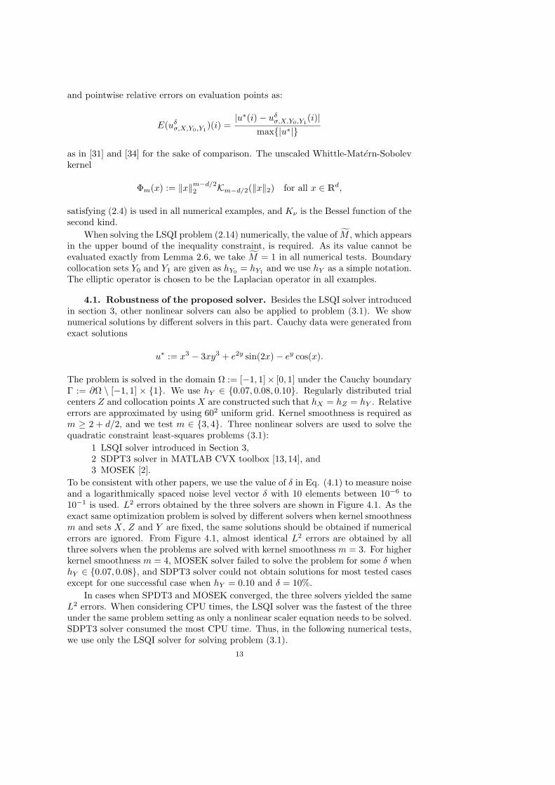
4.1. Robustness of the proposed solver. Besides the LSQI solver introducedin section 3, other nonlinear solvers can also be applied to problem (3.1). We shownumerical solutions by different solvers in this part. Cauchy data were generated fromexact solutions

u∗ := x3 − 3xy3 + e2y sin(2x)− ey cos(x).

The problem is solved in the domain Ω := [−1, 1]× [0, 1] under the Cauchy boundaryΓ := ∂Ω \ [−1, 1] × 1. We use hY ∈ 0.07, 0.08, 0.10. Regularly distributed trialcenters Z and collocation pointsX are constructed such that hX = hZ = hY . Relativeerrors are approximated by using 602 uniform grid. Kernel smoothness is required asm ≥ 2 + d/2, and we test m ∈ 3, 4. Three nonlinear solvers are used to solve thequadratic constraint least-squares problems (3.1):

1 LSQI solver introduced in Section 3,2 SDPT3 solver in MATLAB CVX toolbox [13,14], and3 MOSEK [2].

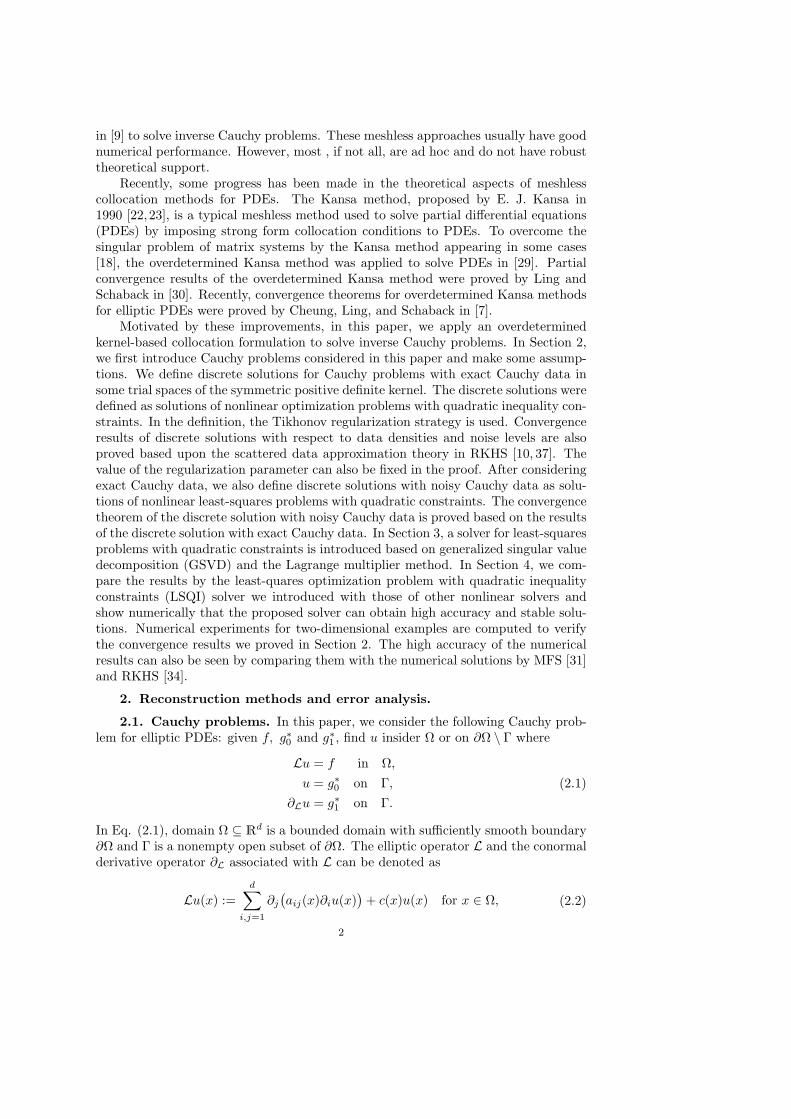
To be consistent with other papers, we use the value of δ in Eq. (4.1) to measure noiseand a logarithmically spaced noise level vector δ with 10 elements between 10−6 to10−1 is used. L2 errors obtained by the three solvers are shown in Figure 4.1. As theexact same optimization problem is solved by different solvers when kernel smoothnessm and sets X, Z and Y are fixed, the same solutions should be obtained if numericalerrors are ignored. From Figure 4.1, almost identical L2 errors are obtained by allthree solvers when the problems are solved with kernel smoothness m = 3. For higherkernel smoothness m = 4, MOSEK solver failed to solve the problem for some δ whenhY ∈ 0.07, 0.08, and SDPT3 solver could not obtain solutions for most tested casesexcept for one successful case when hY = 0.10 and δ = 10%.

In cases when SPDT3 and MOSEK converged, the three solvers yielded the sameL2 errors. When considering CPU times, the LSQI solver was the fastest of the threeunder the same problem setting as only a nonlinear scaler equation needs to be solved.SDPT3 solver consumed the most CPU time. Thus, in the following numerical tests,we use only the LSQI solver for solving problem (3.1).

13

10-6 10-4 10-210-3

10-2

10-1

100

m=3,hY=0.07m=3,hY=0.08m=3,hY=0.10m=4,hY=0.07m=4,hY=0.08m=4,hY=0.10

L2Error

LSQI

δ

10-6 10-4 10-210-3

10-2

10-1

100m=3,hY=0.07m=3,hY=0.08m=3,hY=0.10m=4,hY=0.07m=4,hY=0.08m=4,hY=0.10

SDPT3

δ

10-6 10-4 10-210-3

10-2

10-1

100

m=3,hY=0.07m=3,hY=0.08m=3,hY=0.10m=4,hY=0.07m=4,hY=0.08m=4,hY=0.10

MOSEK

δ

Fig. 4.1: L2 errors by three nonlinear solvers for example u∗ = x3 − 3xy3 + e2y sin(2x) −ey cos(x) with Cauchy boundary ∂Ω\[−1, 1]× 1, hY ∈ 0.07, 0.08, 0.10 and m ∈ 3, 4

4.2. Convergence with respect to δ and hZ . From Theorem 2.9, numericalsolutions converge to exact solutions with respect to a log-rate of noise levels δ, fill

distances hm−2Z and h

m−3/2Y . For convergence tests, we use an example with exact

solutions u∗ := x3−3xy3+e2y sin(2x)−ey cos(x) in domain Ω := [−1, 1]× [0, 1] undertwo kinds of Cauchy boundaries

Γ1 : ∂Ω \ [−1, 1]× 1,

and

Γ2 : [−1, 1]× 0.

Regularly distributed collocation points and trial centers satisfying hX = hZ = hY

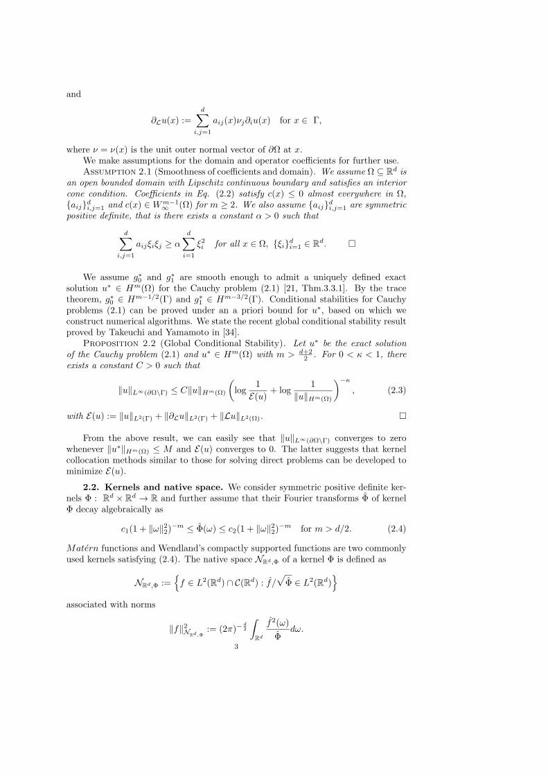
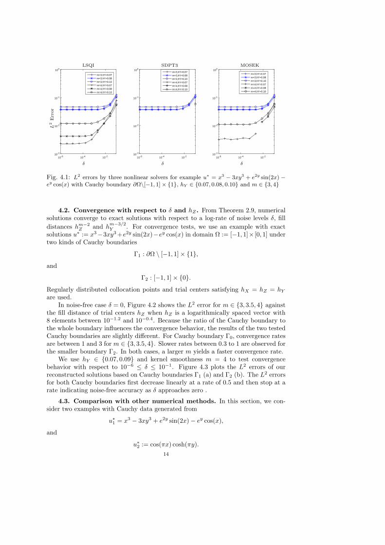
are used.In noise-free case δ = 0, Figure 4.2 shows the L2 error for m ∈ 3, 3.5, 4 against

the fill distance of trial centers hZ when hZ is a logarithmically spaced vector with8 elements between 10−1.2 and 10−0.4. Because the ratio of the Cauchy boundary tothe whole boundary influences the convergence behavior, the results of the two testedCauchy boundaries are slightly different. For Cauchy boundary Γ0, convergence ratesare between 1 and 3 for m ∈ 3, 3.5, 4. Slower rates between 0.3 to 1 are observed forthe smaller boundary Γ2. In both cases, a larger m yields a faster convergence rate.

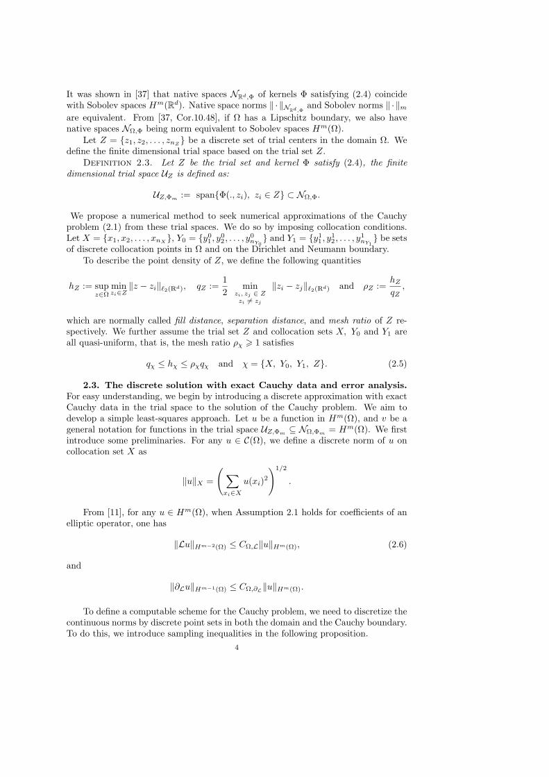
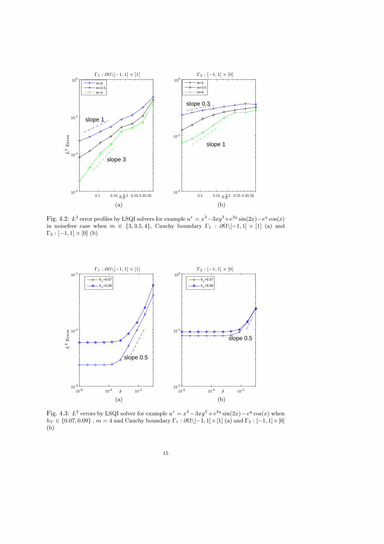
We use hY ∈ 0.07, 0.09 and kernel smoothness m = 4 to test convergencebehavior with respect to 10−6 ≤ δ ≤ 10−1. Figure 4.3 plots the L2 errors of ourreconstructed solutions based on Cauchy boundaries Γ1 (a) and Γ2 (b). The L2 errorsfor both Cauchy boundaries first decrease linearly at a rate of 0.5 and then stop at arate indicating noise-free accuracy as δ approaches zero .

4.3. Comparison with other numerical methods. In this section, we con-sider two examples with Cauchy data generated from

u∗1 = x3 − 3xy3 + e2y sin(2x)− ey cos(x),

and

u∗2 := cos(πx) cosh(πy).

14

0.1 0.15 0.2 0.25 0.30.3510-3

10-2

10-1

100

slope 3

slope 1

m=3m=3.5m=4

L2Error

Γ1 : ∂Ω\[−1, 1] × [1]

hZ

(a)

0.1 0.15 0.2 0.25 0.30.3510-2

10-1

100

slope 1

slope 0.3

m=3m=3.5m=4

Γ2 : [−1, 1] × [0]

hZ

(b)

Fig. 4.2: L2 error profiles by LSQI solvers for example u∗ = x3−3xy3+e2y sin(2x)−ey cos(x)in noisefree case when m ∈ 3, 3.5, 4, Cauchy boundary Γ1 : ∂Ω\[−1, 1] × [1] (a) andΓ2 : [−1, 1]× [0] (b)

10-6 10-4 10-210-3

10-2

10-1

slope 0.5

hY

=0.07

hY

=0.09

L2Error

Γ1 : ∂Ω\[−1, 1] × [1]

δ

(a)

10-6 10-4 10-210-2

10-1

100

slope 0.5

hY

=0.07

hY

=0.09

Γ2 : [−1, 1] × [0]

δ

(b)

Fig. 4.3: L2 errors by LSQI solver for example u∗ = x3−3xy3+e2y sin(2x)−ey cos(x) whenhY ∈ 0.07, 0.09 , m = 4 and Cauchy boundary Γ1 : ∂Ω\[−1, 1]× [1] (a) and Γ2 : [−1, 1]× [0](b)

15

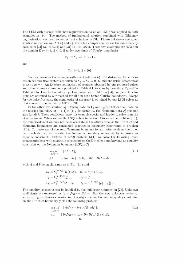
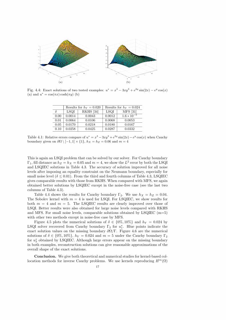
The FEM with discrete Tikhonov regularization based on RKHS was applied to bothexamples in [34]. The method of fundamental solution combined with Tikhonovregularization was used to reconstruct solutions in [31]. Figure 4.4 shows the exactsolution in the domain Ω of u∗

1 and u∗2. For a fair comparison, we use the same Cauchy

data as in [34] (hY = 0.02) and [31] (hY = 0.024). These two examples are solved inthe domain Ω := [−1, 1]× [0, 1] under two kinds of Cauchy boundaries

Γ1 : ∂Ω \ [−1, 1]× 1,

and

Γ2 : [−1, 1]× 0.

We first consider the example with exact solution u∗1. Fill distances of the collo-

cation set and trial centers are taken as hZ = hX = 0.06, and the kernel smoothnessis set to m = 4. An L2 error comparison of accuracy obtained by our proposed solverand other numerical methods provided in Table 4.1 for Cauchy boundary Γ1 and inTable 4.2 for Cauchy boundary Γ2. Compared with RKHS in [34], comparable solu-tions are obtained by our method for all δ in both tested Cauchy boundaries. Exceptfor the noise-free case, the same order of accuracy is obtained by our LSQI solver asthat shown in the results by MFS in [31].

In the other test solution u∗2, Cauchy data on Γ1 and Γ2 are flatter than data on

the missing boundary at [−1, 1] × 1. Importantly, the Neumann data gδ1 remainszero for all δ. These conditions make this example special and harder to solve than theother example. When we use the LSQI solver in Section 3 to solve the problem (3.1),the numerical solution may not be as accurate as the others because the Dirichlet andNeumann boundaries are considered together in inequality constraints in problem(3.1). To make use of the zero Neumann boundary for all noise levels as the othertwo methods did, we consider the Neumann boundary separately by imposing anequality constraint. Instead of LSQI problem (3.1), we solve the following least-squares problems with quadratic constraints on the Dirichlet boundary and an equalityconstraint on the Neumann boundary (LSQIEC)

arg infλ∈RnZ

∥Aλ− b∥2 (4.1)

s.t. ∥B0λ− d0∥2 ≤ E0 and B1λ = d1,

with A and b being the same as in Eq. (3.1) and

B0 = h(d−1)/2Y K(Y,Z), B1 = ∂LK(Y,Z),

d0 = h(d−1)/2Y gδ0|Y , d1 = gδ1|Y ,

E0 = hm−d/2Z M + δ0, δ0 = h

(d−1)/2Y ∥g∗0 − gδ0∥Y .

The equality constraint can be handled by the null space approach in [28]. Unknowncoefficients are expressed as λ = NBγ + B1\d1. For the new unknown vector γ,substituting the above expression into the objective function and inequality constrainton the Dirichlet boundary yields the following problem:

arg infλ∈RnZ

∥ANBγ − b+A(B1\d1)∥2 (4.2)

s.t. ∥B0NBγ − d0 +B0(B1\d1)∥2 ≤ E0.

16

(a) (b)

Fig. 4.4: Exact solutions of two tested examples: u∗ = x3 − 3xy3 + e2y sin(2x) − ey cos(x)(a) and u∗ = cos(πx) cosh(πy) (b)

Results for hY = 0.020 Results for hY = 0.024

δ LSQI RKHS [34] LSQI MFS [31]

0.00 0.0014 0.0043 0.0012 1.6 ∗ 10−5

0.01 0.0064 0.0106 0.0068 0.0053

0.05 0.0170 0.0218 0.0180 0.0167

0.10 0.0258 0.0425 0.0287 0.0332

Table 4.1: Relative errors compare of u∗ = x3 − 3xy3 + e2y sin(2x)− ey cos(x) when Cauchyboundary given on ∂Ω \ [−1, 1]× 1, hX = hZ = 0.06 and m = 4

This is again an LSQI problem that can be solved by our solver. For Cauchy boundaryΓ1, fill distance as hZ = hX = 0.05 and m = 4, we show the L2 error by both the LSQIand LSQIEC solutions in Table 4.3. The accuracy of solution improved for all noiselevels after imposing an equality constraint on the Neumann boundary, especially forsmall noise level (δ ≤ 0.01). From the third and fourth columns of Table 4.3, LSQIECgives comparable results with those from RKHS. When compared with MFS, we againobtained better solutions by LSQIEC except in the noise-free case (see the last twocolumns of Table 4.3).

Table 4.4 shows the results for Cauchy boundary Γ2. We use hX = hZ = 0.04.The Sobolev kernel with m = 4 is used for LSQI. For LSQIEC, we show results forboth m = 4 and m = 5. The LSQIEC results are clearly improved over those ofLSQI. Better results were also obtained for large noise levels compared with RKHSand MFS. For small noise levels, comparable solutions obtained by LSQIEC (m=5)with other two methods except in noise-free case by MFS.

Figure 4.5 plots the numerical solutions of δ ∈ 0%, 10% and hY = 0.024 byLSQI solver recovered from Cauchy boundary Γ2 for u∗

1. Blue points indicate theexact solution values on the missing boundary ∂Ω/Γ. Figure 4.6 are the numericalsolutions of δ ∈ 0%, 10%, hY = 0.024 and m = 5 under the Cauchy boundary Γ2

for u∗2 obtained by LSQIEC. Although large errors appear on the missing boundary

in both examples, reconstruction solutions can give reasonable approximations of theoverall shape of the exact solutions.

Conclusion. We give both theoretical and numerical studies for kernel-based col-location methods for inverse Cauchy problems. We use kernels reproducing Hm(Ω)

17

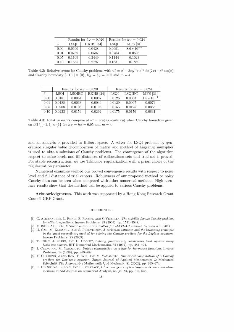
Results for hY = 0.020 Results for hY = 0.024

δ LSQI RKHS [34] LSQI MFS [31]

0.00 0.0690 0.0428 0.0691 8.6 ∗ 10−4

0.01 0.0769 0.0507 0.0784 0.0696

0.05 0.1109 0.2449 0.1144 0.1023

0.10 0.1555 0.2797 0.1631 0.1869

Table 4.2: Relative errors for Cauchy problems with u∗1 = x3−3xy3+e2y sin(2x)−ey cos(x)

and Cauchy boundary [−1, 1]× 0, hX = hZ = 0.06 and m = 4

Results for hY = 0.020 Results for hY = 0.024

δ LSQI LSQIEC RKHS [34] LSQI LSQIEC MFS [31]

0.00 0.0181 0.0064 0.0037 0.0126 0.0063 1.5 ∗ 10−4

0.01 0.0188 0.0063 0.0046 0.0129 0.0067 0.0074

0.05 0.0208 0.0106 0.0198 0.0155 0.0125 0.0365

0.10 0.0223 0.0159 0.0292 0.0175 0.0176 0.0831

Table 4.3: Relative errors compare of u∗ = cos(πx) cosh(πy) when Cauchy boundary givenon ∂Ω \ [−1, 1]× 1 for hX = hZ = 0.05 and m = 4

and all analysis is provided in Hilbert space. A solver for LSQI problem by gen-eralized singular value decomposition of matric and method of Lagrange multiplieris used to obtain solutions of Cauchy problems. The convergence of the algorithmrespect to noise levels and fill distances of collocations sets and trial set is proved.For stable reconstruction, we use Tikhonov regularization with a priori choice of theregularization parameter.

Numerical examples verified our proved convergence results with respect to noiselevel and fill distance of trial centers. Robustness of our proposed method to noisyCauchy data can be seen when compared with other numerical methods. High accu-racy results show that the method can be applied to various Cauchy problems.

Acknowledgments. This work was supported by a Hong Kong Research GrantCouncil GRF Grant.

REFERENCES

[1] G. Alessandrini, L. Rondi, E. Rosset, and S. Vessella, The stability for the Cauchy problemfor elliptic equations, Inverse Problems, 25 (2009), pp. 1541–1548.

[2] MOSEK ApS, The MOSEK optimization toolbox for MATLAB manual. Version 8.1., 2017.[3] H. Cao, M. Klibanov, and S. Pereverzev, A carleman estimate and the balancing principle

in the quasi-reversibility method for solving the Cauchy problem for the Laplace equation,Inverse Problems, 25 (2009).

[4] T. Chan, J. Olkin, and D. Cooley, Solving quadratically constrained least squares usingblack box solvers, BIT Numerical Mathematics, 32 (1992), pp. 481–494.

[5] J. Cheng and M. Yamamoto, Unique continuation on a line for harmonic functions, InverseProblems, 14 (1998), pp. 869–882.

[6] Y. C. Cheng, J.and Hon, T. Wei, and M. Yamamoto, Numerical computation of a Cauchyproblem for Laplace’s equation, Zamm Journal of Applied Mathematics & MechanicsZeitschrift Fur Angewandte Mathematik Und Mechanik, 81 (2002), pp. 665–674.

[7] K. C. Cheung, L. Ling, and R. Schaback, H2–convergence of least-squares kernel collocationmethods, SIAM Journal on Numerical Analysis, 56 (2018), pp. 614–633.

18

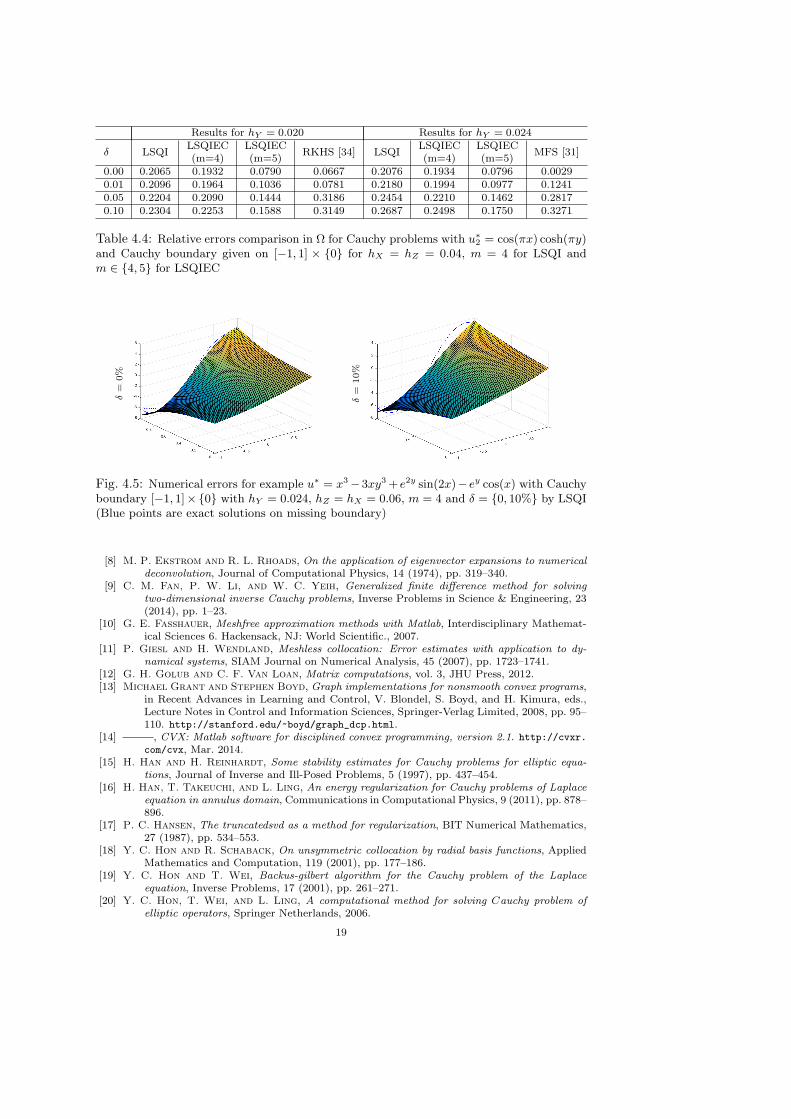
Results for hY = 0.020 Results for hY = 0.024

δ LSQILSQIEC(m=4)

LSQIEC(m=5)

RKHS [34] LSQILSQIEC(m=4)

LSQIEC(m=5)

MFS [31]

0.00 0.2065 0.1932 0.0790 0.0667 0.2076 0.1934 0.0796 0.00290.01 0.2096 0.1964 0.1036 0.0781 0.2180 0.1994 0.0977 0.12410.05 0.2204 0.2090 0.1444 0.3186 0.2454 0.2210 0.1462 0.28170.10 0.2304 0.2253 0.1588 0.3149 0.2687 0.2498 0.1750 0.3271

Table 4.4: Relative errors comparison in Ω for Cauchy problems with u∗2 = cos(πx) cosh(πy)

and Cauchy boundary given on [−1, 1] × 0 for hX = hZ = 0.04, m = 4 for LSQI andm ∈ 4, 5 for LSQIEC

δ=

0%

δ=

10%

Fig. 4.5: Numerical errors for example u∗ = x3−3xy3+ e2y sin(2x)− ey cos(x) with Cauchyboundary [−1, 1]×0 with hY = 0.024, hZ = hX = 0.06, m = 4 and δ = 0, 10% by LSQI(Blue points are exact solutions on missing boundary)

[8] M. P. Ekstrom and R. L. Rhoads, On the application of eigenvector expansions to numericaldeconvolution, Journal of Computational Physics, 14 (1974), pp. 319–340.

[9] C. M. Fan, P. W. Li, and W. C. Yeih, Generalized finite difference method for solvingtwo-dimensional inverse Cauchy problems, Inverse Problems in Science & Engineering, 23(2014), pp. 1–23.

[10] G. E. Fasshauer, Meshfree approximation methods with Matlab, Interdisciplinary Mathemat-ical Sciences 6. Hackensack, NJ: World Scientific., 2007.

[11] P. Giesl and H. Wendland, Meshless collocation: Error estimates with application to dy-namical systems, SIAM Journal on Numerical Analysis, 45 (2007), pp. 1723–1741.

[12] G. H. Golub and C. F. Van Loan, Matrix computations, vol. 3, JHU Press, 2012.[13] Michael Grant and Stephen Boyd, Graph implementations for nonsmooth convex programs,

in Recent Advances in Learning and Control, V. Blondel, S. Boyd, and H. Kimura, eds.,Lecture Notes in Control and Information Sciences, Springer-Verlag Limited, 2008, pp. 95–110. http://stanford.edu/~boyd/graph_dcp.html.

[14] , CVX: Matlab software for disciplined convex programming, version 2.1. http://cvxr.com/cvx, Mar. 2014.

[15] H. Han and H. Reinhardt, Some stability estimates for Cauchy problems for elliptic equa-tions, Journal of Inverse and Ill-Posed Problems, 5 (1997), pp. 437–454.

[16] H. Han, T. Takeuchi, and L. Ling, An energy regularization for Cauchy problems of Laplaceequation in annulus domain, Communications in Computational Physics, 9 (2011), pp. 878–896.

[17] P. C. Hansen, The truncatedsvd as a method for regularization, BIT Numerical Mathematics,27 (1987), pp. 534–553.

[18] Y. C. Hon and R. Schaback, On unsymmetric collocation by radial basis functions, AppliedMathematics and Computation, 119 (2001), pp. 177–186.

[19] Y. C. Hon and T. Wei, Backus-gilbert algorithm for the Cauchy problem of the Laplaceequation, Inverse Problems, 17 (2001), pp. 261–271.

[20] Y. C. Hon, T. Wei, and L. Ling, A computational method for solving Cauchy problem ofelliptic operators, Springer Netherlands, 2006.

19

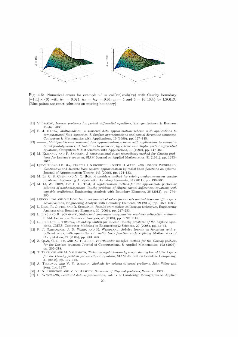
δ=

0%

δ=

10%

Fig. 4.6: Numerical errors for example u∗ = cos(πx) cosh(πy) with Cauchy boundary[−1, 1] × 0 with hY = 0.024, hZ = hX = 0.04, m = 5 and δ = 0, 10% by LSQIEC(Blue points are exact solutions on missing boundary)

[21] V. Isakov, Inverse problems for partial differential equations, Springer Science & BusinessMedia, 2006.

[22] E. J. Kansa, Multiquadrics—a scattered data approximation scheme with applications tocomputational fluid-dynamics. I. Surface approximations and partial derivative estimates,Computers & Mathematics with Applications, 19 (1990), pp. 127–145.

[23] , Multiquadrics—a scattered data approximation scheme with applications to computa-tional fluid-dynamics. II. Solutions to parabolic, hyperbolic and elliptic partial differentialequations, Computers & Mathematics with Applications, 19 (1990), pp. 147–161.

[24] M. Klibanov and F. Santosa, A computational quasi-reversibility method for Cauchy prob-lems for Laplace’s equation, SIAM Journal on Applied Mathematics, 51 (1991), pp. 1653–1675.

[25] Quoc Thong Le Gia, Francis J Narcowich, Joseph D Ward, and Holger Wendland,Continuous and discrete least-squares approximation by radial basis functions on spheres,Journal of Approximation Theory, 143 (2006), pp. 124–133.

[26] M. Li, C. S. Chen, and Y. C. Hon, A meshless method for solving nonhomogeneous cauchyproblems, Engineering Analysis with Boundary Elements, 35 (2011), pp. 499–506.

[27] M. Li, W. Chen, and C. H. Tsai, A regularization method for the approximate particularsolution of nonhomogeneous Cauchy problems of elliptic partial differential equations withvariable coefficients, Engineering Analysis with Boundary Elements, 36 (2012), pp. 274–280.

[28] Leevan Ling and YC Hon, Improved numerical solver for kansa’s method based on affine spacedecomposition, Engineering Analysis with Boundary Elements, 29 (2005), pp. 1077–1085.

[29] L. Ling, R. Opfer, and R. Schaback, Results on meshless collocation techniques, EngineeringAnalysis with Boundary Elements, 30 (2006), pp. 247–253.

[30] L. Ling and R. Schaback, Stable and convergent unsymmetric meshless collocation methods,SIAM Journal on Numerical Analysis, 46 (2008), pp. 1097–1115.

[31] L. Ling and T. Tomoya, Boundary control for inverse Cauchy problems of the Laplace equa-tions, CMES: Computer Modeling in Engineering & Sciences, 29 (2008), pp. 45–54.

[32] F. J. Narcowich, J. D. Ward, and H. Wendland, Sobolev bounds on functions with s-cattered zeros, with applications to radial basis function surface fitting, Mathematics ofComputation, 74 (2005), pp. 743–763.

[33] Z. Qian, C. L. Fu, and X. T. Xiong, Fourth-order modified method for the Cauchy problemfor the Laplace equation, Journal of Computational & Applied Mathematics, 192 (2006),pp. 205–218.

[34] T. Takeuchi and M. Yamamoto, Tikhonov regularization by a reproducing kernel hilbert spacefor the Cauchy problem for an elliptic equation, SIAM Journal on Scientific Computing,31 (2008), pp. 112–142.

[35] A. Tikhonov and V. Y. Arsenin, Methods for solving ill-posed problems, John Wiley andSons, Inc, 1977.

[36] A. N. Tikhonov and V. Y. Arsenin, Solutions of ill-posed problems, Winston, 1977.[37] H. Wendland, Scattered data approximation, vol. 17 of Cambridge Monographs on Applied

20

and Computational Mathematics, Cambridge University Press, Cambridge, 2005.[38] X. T. Xiong, M. Li, and M. Q. Wang, A one-stage meshless method for nonhomogeneous

Cauchy problems of elliptic partial differential equations with variable coefficients, Journalof Engineering Mathematics, 80 (2013), pp. 189–200.

[39] F. L. Yang and L. Ling, On numerical experiments for cauchy problems of elliptic operators,Engineering Analysis with Boundary Elements, 35 (2011), pp. 879–882.

[40] D. L. Young, C. C. Tsai, C. W. Chena, and C. M. Fana, The method of fundamental solu-tions and condition number analysis for inverse problems of Laplace equation, Computers& Mathematics with Applications, 55 (2008), pp. 1189–1200.

[41] H. Zheng and W. S. Zhang, A mixed regularization method for ill-posed problems, NumericalMathematics Theory Methods and Applications, 12 (2019), pp. 212–232.

21