TE 176 . D67 1997 FINAL REPORT An Evaluation of the MICHIGAN URBAN DIAMOND INTERCHANGE with respect to the SINGLE-POINT URBAN INTERCHANGE by Paul B. W. Dorothy and Thomas L. Maleck, Ph.D., P.E. December, 1997 COLLEGE OF ENGINEERING MICHIGAN STATE UNIVERSITY EAST LANSING, MICHIGAN 48824 MSU IS AN AFFIRMATIVE ACTION/EQUAL OPPORTUNITY INSTITUTION

Welcome message from author
This document is posted to help you gain knowledge. Please leave a comment to let me know what you think about it! Share it to your friends and learn new things together.
Transcript

TE 176
. D67 1997
FINAL REPORT
An Evaluation of the MICHIGAN URBAN DIAMOND INTERCHANGE
with respect to the SINGLE-POINT URBAN INTERCHANGE
by
Paul B. W. Dorothy
and
Thomas L. Maleck, Ph.D., P.E.
December, 1997
COLLEGE OF ENGINEERING MICHIGAN STATE UNIVERSITY
EAST LANSING, MICHIGAN 48824 MSU IS AN AFFIRMATIVE ACTION/EQUAL OPPORTUNITY INSTITUTION

Technical Report Documentation Page 1. Report No. 12. Government Accession No. 3. Reciepient's Catalog No.
4. Title and Subtitle 5. Report Date
An Evaluation of the Michigan Urban Diamond December 1997 Interchange with Respect to the Single Point 6. Performing Organization Code
Urban Interchange. 8. Performing Organization Report No,
7. Author(s)
Dorothy, Paul & Maleck, Thomas L. 9. Performing Organization Name and Address 10. Work Unit No.
Michigan State University Civil & Envir Engineering 11, Contract or Grant No.
3546 Engineering Building Easr Lansin". MT 4R824 13. Type of Report and Period Covered
12. Sponsoring Agency Name and Address
Michigan Department of Transportation Final Report Traffic & Safety Division
425 West Ottawa 14. Sponsoring Agency Code
Lansing, MI 48909 IIDoT 94-1521A 15. Supplementary Notes
16. Abstract
The Michigan Department of Transportation (MDOT) is considering the much needed rehabilitation and upgrading of many interchanges found in urban environments. Thus, MDOT and Michigan State University (MSU) undertook a joint effort to evaluate the appropriateness of an urban interchange geometric configuration, the Single Point Urban Interchange (SPUI), as an alternative design to those presently used by MDOT. In particular, the Michigan Urban Diamond Interchange (MUD!) and the traditional diamond were investigated. A field review was conducted to collect information about the geometric design, signal operation, pedestrian control and pavement markings of SPUis, as none cmrently exist in Michigan. The field review showed that the design and operation of SPUis vary greatly from state to state. Thus, the SPUI and MUDI designs were computer modeled to facilitate a comparison of their respective operational characteristics. A traditional diamond was also modeled to generate a frame of reference. The results showed that the SPUI operation is adversely affected with the addition of frontage roads. MUDI operation, in most situations, is superior to that of either a SPUI and diamond interchange configuration. Also, there was less migration of delay to downstream intersections with a MUDI configurariou than with either a SPUI or diamond. Finally, MUD! operation, in most situations, is insensitive to the proximity of the closest downstream node, while the SPUI operation is sensitive. 1 7. Key Words 18. Distribution Statement
interchange design geometric design simulation modeling
19. Security Classif. (of this report) 20. Security Classif (of this page) 21. No. of Pages 22. Price
138
NOTICE
This document is disseminated under the sponsorship of the Michigan Department of Transportation and the United States Department of Transportation in the interest of information exchange. The sponsors assume no liability for its contents or use thereof.
The contents of this report reflect the views of the authors who are solely responsible for the facts and accuracy of the material presented. The contents do not necessarily reflect the official views of the sponsors.
The State of Michigan and the United States Govermnent do not endorse products or manufacturers. Trademarks or manufacturers' names appear herein only because they are considered essential to the objectives of this document.
This report does not constitute a standard, specification or regulation.

TABLE OF CONTENTS
LIST OF TABLES ................................................................................................... v
LIST OF FIGURES ................................................................................................. vii
1.0 INTRODUCTION .............................................................................................. 1
2.0 OPERATION AND DESIGN OF THE MICHIGAN URBAN DIAMOND INTERCHANGE (MUDI)...................................................... 7
3.0 OPERATION AND DESIGN OF THE SINGLE POINT URBAN INTERCHANGE (SPUI) ............................................................. 9
4.0 STATE OF THE PRACTICE .......................................................................... 10
4.1 Literature Review ................................................................................................. 10 4.2 AASHTO E-mail Survey ..................................................................................... 12 4.3 Telephone Survey ................................................................................................ 13
5.0 FIELD REVIEW OF THE SPUI ..................................................................... 15
5.1 Geometric Design ................................................................................................ 16 5.2 Signal Operation .................................................................................................. 21 5.3 Pedestrian Control... ............................................................................................. 23 5.4 Pavement Markings ............................................................................................. 24 5.5 Land Use/Landscaping ......................................................................................... 26 5.6 Conclusions from the Field Review ..................................................................... 28
6.0 METHODOLOGY ............................................................................................ 30
6.1 Selection of the Computer Model ........................................................................ 30 6.2 Network Configuration ........................................................................................ 32 6.3 Signal Operation .................................................................................................. 39 6.4 Variables and Measures of Effectiveness ............................................................ 46
7.0 SIMULATION RESULTS ................................................................................ 50
7.1 Interchange Performance without Frontage Roads .............................................. 50 7.2 Migration of Delay without Frontage Roads ....................................................... 55 7.3 Interchange Performance with Frontage Roads ................................................... 60 7.4 Migration of Delay with Frontage Roads ............................................................ 70 7.5 Sensitivity to Proximity of Closest Downstream Node ....................................... 70
8.0 CONCLUSIONS ................................................................................................ 81
9.0 REFERENCES ................................................................................................... 82
iii Final Report

iv
APPENDICES
APPENDIX A: TABULAR PRESENTATION OF SIMULATION RESULTS ..................................................................................................... 83
APPENDIX B: GRAPHICAL PRESENTATION OF SIMULATION RESULTS ..................................................................................................... 103
Final Report

LIST OF TABLES
Table A.l: Simulation Results for Modeling Scenarios Involving the Michigan Urban Diamond Interchange (MUDI), without Frontage Roads, 1.6 kilometers (1 mile), S-lane Arterial .................. 83
Table A.2: Simulation Results for Modeling Scenarios Involving the Michigan Urban Diamond Interchange (MUDI), without Frontage Roads, 1.6 kilometers (1 mile), 7-lane Arterial .................. 84
Table A.3: Simulation Results for Modeling Scenarios Involving the Single Point Urban Interchange (SPUI), without Frontage Roads, 1.6 kilometers (1 mile), S-lane Arterial .................. 8S
Table A.4: Simulation Results for Modeling Scenarios Involving the Single Point Urban Interchange (SPUI), without Frontage Roads, 1.6 kilometers (1 mile), 7-lane Arterial .................. 86
Table A.S: Simulation Results for Modeling Scenarios Involving the Traditional Diamond Interchange, without Frontage Roads, 1.6 kilometers (1 mile), S-lane Arterial ............................................. 87
Table A.6: Simulation Results for Modeling Scenarios Involving the Traditional Diamond Interchange, without Frontage Roads, 1.6 kilometers (1 mile), 7-lane Arterial ............................................. 88
Table A.7: Simulation Results for Modeling Scenarios Involving the Michigan Urban Diamond Interchange (MUDI), with Frontage Roads, 1.6 kilometers (1 mile), S-lane Arterial .................. 89
Table A.8: Simulation Results for Modeling Scenarios Involving the Michigan Urban Diamond Interchange (MUDI), with Frontage Roads, 1.6 kilometers (1 mile), 7-lane Arterial .................. 90
Table A.9: Simulation Results for Modeling Scenarios Involving the Single Point Urban Interchange (SPUI), with Frontage Roads, 1.6 kilometers (1 mile), S-lane Arterial .................. 91
Table A.l 0: Simulation Results for Modeling Scenarios Involving the Single Point Urban Interchange (SPUI), with Frontage Roads, 1.6 kilometers (I mile), 7-lane Arterial .................. 92
Table All: Simulation Results for Modeling Scenarios Involving the Traditional Diamond Interchange, with Frontage Roads, 1.6 kilometers (I mile), S-lane Arterial ............................................. 93
v Final Report

VI
Table A.l2: Simulation Results for Modeling Scenarios Involving the Traditional Diamond Interchange, with Frontage Roads, 1.6 kilometers (1 mile), 7-lane Arterial ............................................. 94
Table A.13: Simulation Results for Modeling Scenarios Involving the Michigan Urban Diamond Interchange (MUDI), without Frontage Roads, 1.2 kilometers (3/4 mile), S-lane Arterial ............... 9S
Table A.l4: Simulation Results for Modeling Scenarios Involving the Michigan Urban Diamond Interchange (MUDI), without Frontage Roads, 1.2 kilometers (3/4 mile), 7-lane Arterial ............... 96
Table A.lS: Simulation Results for Modeling Scenarios Involving the Single Point Urban Interchange (SPUI), without Frontage Roads, 1.2 kilometers (3/4 mile), S-lane Arterial ............... 97
Table A.l6: Simulation Results for Modeling Scenarios Involving the Single Point Urban Interchange (SPUI), without Frontage Roads, 1.2 kilometers (3/4 mile), 7-lane Arterial ............... 98
Table A.17: Simulation Results for Modeling Scenarios Involving the Michigan Urban Diamond Interchange (MUDI), without Frontage Roads, 0.8 kilometers (112 mile), S-lane Arterial ............... 99
Table A.l8: Simulation Results forModeling Scenarios Involving the Michigan Urban Diamond Interchange (MUDI), without Frontage Roads, 0.8 kilometers (112 mile), 7-lane Arterial.. ............ .IOO
Table A.l9: Simulation Results for Modeling Scenarios Involving the Single Point Urban Interchange (SPUI), without Frontage Roads, 0.8 kilometers (112 mile), S-lane Arterial ............... lOl
Table A.20: Simulation Results for Modeling Scenarios Involving the Single Point Urban Interchange (SPUI), without Frontage Roads, 0.8 kilometers (112 mile), 7-lane Arterial ............... l02
Final Report

LIST OF FIGURES
Figure 1: Typical Single Point Urban Interchange (SPUI) Configuration without Frontage Roads ..................................................................... 2
Figure 2: Typical Single Point Urban Interchange (SPUI) Configuration with Frontage Roads.......................................................................... 3
Figure 3: Typical Michigan Urban Diamond Interchange (MUDI) Configuration with Frontage Roads .......................................................................... 4
Figure 4: Typical Diamond Interchange Configuration with Frontage Roads .......... 5
Figure 5: SPUI with cross-road going over the freeway with all signal heads located on a single overhead tubular beam. Minnesota .................... 17
Figure 6: Confused driver (car with lights on) stopped in middle of a SPUI while traffic proceeds on either side .................................................. 18
Figure 7: U-turn lane accommodates large trucks ..................................................... 18
Figure 8: Dual1eft-tuming traffic on the off-ramp is backing up, blocking right-turning traffic ............................................................. 21
Figure 9: Pavement marking overlap creates driver confusion ................................. 24
Figure 10: "Runway" lighting to help illuminate the turning path. Note buildup of debris ....................................................................... 25
Figure 11: Typical Landscaping of a SPUI in Phoenix, AZ ...................................... 27
Figure 12: Typical Diamond Interchange Configuration with Frontage Roads ........ 33
Figure 13: Link/Node Diagram for Diamond Configuration ..................................... 34
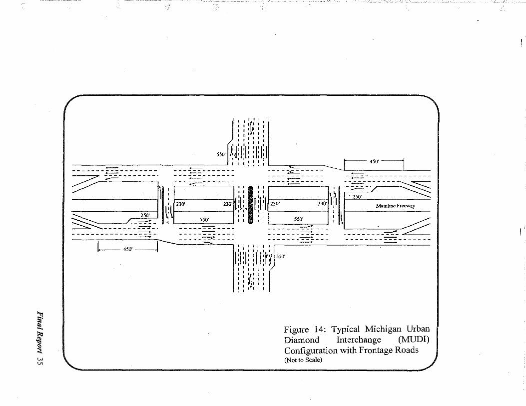
Figure 14: Typical Michigan Urban Diamond Interchange (MUDI) Configuration with Frontage Roads ................................................... 35
Figure 15: Link/Node Diagram for MUDI Configuration ......................................... 36
Figure 16: Typical Single Point Urban Interchange (SPUI) Configuration with Frontage Roads .......................................................................... 37
Figure 17: Link/Node Diagram for SPUI Configuration ........................................... 38
Figure 18: Phasing Diagram for MUDI Configuration .............................................. 42
Vll Final Report

viii
Figure 19: Phasing Diagram for MUDI Cross-overs ................................................. 43
Figure 20: Phasing Diagram for SPUI Configuration without Frontage Roads ........ 44
Figure 21: Phasing Diagram for SPUI Configuration with Frontage Roads ............. 45
Figure 22: Phasing Diagram for Diamond Configuration ......................................... 47
Figure 23: Interchange Area Total Time for 70% Left Turns, without Frontage Roads, 1.6 kilometer (1 mile), S-lane Arterial ................................... 51
Figure 24: Interchange Area Total Time for 50% Left Turns, without Frontage Roads, 1.6 kilometer (1 mile), S-lane Arterial... ................................ 53
Figure 25: Interchange Area Total Time for 30% Left Turns, without Frontage Roads, 1.6 kilometer (1 mile), S-lane Arterial ................................... 54
Figure 26: Interchange Area Total Time for 70% Left Turns, without Frontage Roads, 1.6 kilometer (1 mile), 7-lane Arterial... ................................ 56
Figure 27: Interchange Area Total Time for 50% Left Turns, without Frontage Roads, 1.6 kilometer (1 mile), 7-lane Arterial ................................... 57
Figure 28: Interchange Area Total Time for 30% Left Turns, without Frontage Roads, 1.6 kilometer (1 mile), 7-lane Arterial ................................... 58
Figure 29: Downstream Area Total Time for 50% Left Turns, without Frontage Roads, 1.6 kilometer (1 mile), S-lane Arterial... ................................ 59
Figure 30: Downstream Area Total Time for 50% Left Turns, without Frontage Roads, 1.6 kilometer (1 mile), 7-lane Arterial... ................................ 61
Figure 31: Interchange Area Total Time for 70% Left Turns, with Frontage Roads, 1.6 kilometer (1 mile), S-lane Arterial... ................................ 62
Figure 32: Interchange Area Total Time for 50% Left Turns, with Frontage Roads, 1.6 kilometer (1 mile), S-lane Arterial... ................ , ............... 64
Figure 33: Interchange Area Total Time for 30% Left Turns, with Frontage Roads, 1.6 kilometer (1 mile), S-lane Arterial.. ................................. 65
Figure 34: Interchange Area Total Time for 70% Left Turns, with Frontage Roads, 1.6 kilometer (1 mile), 7-lane Arterial.. ................................. 67
Figure 35: Interchange Area Total Time for 50% Left Turns, with Frontage Roads, 1.6 kilometer (1 mile), 7-lane Arterial.. ................................. 68
Final Report

IX
Figure 36: Interchange Area Total Time for 30% Left Turns, with Frontage Roads, 1.6 kilometer (1 mile), 7-lane Arterial ................................... 69
Figure 37: Downstream Area Total Time for 50% Left Turns, with Frontage Roads, 1.6 kilometer (1 mile), S-lane Arterial... ................................ 71
Figure 38: Downstream Area Total Time for 50% Left Turns, with Frontage Roads, 1.6 kilometer (1 mile), 7-lane Arterial ................................... 72
Figure 39: Interchange Area Total Time for 70% Left Turns, without Frontage Roads, S-lane Arterial, Varying Spacing Scenarios ........................... 74
Figure 40: Interchange Area Total Time for 50% Left Turns, without Frontage Roads, S-lane Arterial, Varying Spacing Scenarios ........................... 75
Figure 41: Interchange Area Total Time for 30% Left Turns, without Frontage Roads, S-lane Arterial, Varying Spacing Scenarios ........................... 76
Figure 42: Downstream Area Total Time for 50% Left Turns, without Frontage Roads, S-lane Arterial, Varying Spacing Scenarios ........................... 79
Figure 43: Downstream Area Total Time for 50% Left Turns, without Frontage Roads, 7-lane Arterial, Varying Spacing Scenarios ........................... 80
Figure B.1: Interchange Area Total Time for 70% Left Turns, without Frontage Roads, 1.6 kilometer (I mile), S-lane Arterial.. ................................ .! 03
Figure B.2: Interchange Area Total Time for 50% Left Turns, without Frontage Roads, 1.6 kilometer (1 mile), S-lane Arterial... ............................... .l04
Figure B.3: Interchange Area Total Time for 30% Left Turns, without Frontage Roads, 1.6 kilometer (1 mile), S-lane Arterial.. ................................ .! OS
Figure B.4: Interchange Area Total Time for 70% Left Turns, without Frontage Roads, 1.6 kilometer (1 mile), 7-lane Arterial... ................................ 106
Figure B.S: Interchange Area Total Time for 50% Left Turns, without Frontage Roads, 1.6 kilometer (1 mile), 7-lane Arterial ................................... 107
Figure B.6: Interchange Area Total Time for 30% Left Turns, without Frontage Roads, 1.6 kilometer (1 mile), 7-lane Arterial.. ................................. 108
Figure B.7: Downstream Area Total Time for 70% Left Turns, without Frontage Roads, 1.6 kilometer (1 mile), S-lane Arterial ................................... 109
Final Report

X
Figure B.8: Downstream Area Total Time for 50% Left Turns, without Frontage Roads, 1.6 kilometer (I mile), 5-lane Arterial ................................... !! 0
Figure B.9: Downstream Area Total Time for 30% Left Turns, without Frontage Roads, 1.6 kilometer (I mile), 5-lane Arterial ................................... lll
Figure B.! 0: Downstream Area Total Time for 70% Left Turns, without Frontage Roads, 1.6 kilometer (I mile), 7-lane Arterial... ............................... .112
Figure B. II: Downstream Area Total Time for 50% Left Turns, without Frontage Roads, 1.6 kilometer (I mile), 7-lane Arterial... ............................... .ll3
Figure B.12: Downstream Area Total Time for 30% Left Turns, without Frontage Roads, I mile, 1.6 kilometer (I mile), 7-lane Arterial... .................... ll4
Figure B.13: Interchange Area Total Time for 70% Left Turns, with Frontage Roads, 1.6 kilometer (I mile), 5-lane Arterial... ................................ ll5
Figure B.l4: Interchange Area Total Time for 50% Left Turns, with Frontage Roads, 1.6 kilometer (I mile), 5-lane Arterial... ............................... .116
Figure B.15: Interchange Area Total Time for 30% Left Turns, with Frontage Roads, 1.6 kilometer (I mile), 5-lane Arterial .................................. .117
Figure B.16: Interchange Area Total Time for 70% Left Turns, with Frontage Roads, 1.6 kilometer (I mile), 7-lane Arterial ................................... l18
Figure B.17: Interchange Area Total Time for 50% Left Turns, with Frontage Roads, 1.6 kilometer (I mile), 7-lane Arterial ................................... 119
Figure B.18: Interchange Area Total Time for 30% Left Turns, with Frontage Roads, 1.6 kilometer (I mile), 7-lane Arterial... ................................ l20
Figure B.19: Downstream Area Total Time for 70% Left Turns, with Frontage Roads, 1.6 kilometer (I mile), 5-lane Arterial .................................. cl21
Figure B.20: Downstream Area Total Time for 50% Left Turns, with Frontage Roads, 1.6 kilometer (I mile), 5-lane Arterial ................................... l22
Figure B.21: Downstream Area Total Time for 30% Left Turns, with Frontage Roads, 1.6 kilometer (I mile), 5-lane Arterial... ................................ l23
Figure B.22: Downstream Area Total Time for 70% Left Turns, with Frontage Roads, 1.6 kilometer (I mile), 7-lane Arterial ................................... l24
Final Report

XI
Figure B.23: Downstream Area Total Time for 50% Left Turns, with Frontage Roads, 1.6 kilometer (I mile), 7-lane Arterial ................................... l25
Figure B.24: Downstream Area Total Time for 30% Left Turns, with Frontage Roads, 1.6 kilometer (I mile), 7-lane Arterial... ............................... .126
Figure B.25: Interchange Area Total Time for 70% Left Turns, without Frontage Roads, S-lane Arterial, Varying Spacing Scenarios .......................... .127
Figure B.26: Interchange Area Total Time for 50% Left Turns, without Frontage Roads, S-lane Arterial, Varying Spacing Scenarios .......................... .128
Figure B.27: Interchange Area Total Time for 30% Left Turns, without Frontage Roads, S-lane Arterial, Varying Spacing Scenarios ........................... l29
Figure B.28: Interchange Area Total Time for 70% Left Turns, without Frontage Roads, 7-lane Arterial, Varying Spacing Scenarios ........................... l30
Figure B.29: Interchange Area Total Time for 50% Left Turns, without Frontage Roads, 7-lane Arterial, Varying Spacing Scenarios .......................... .131
Figure B.30: Interchange Area Total Time for 30% Left Turns, without Frontage Roads, 7-lane Arterial, Varying Spacing Scenarios ........................... 132
Figure B.31: Downstream Area Total Time for 70% Left Turns, without Frontage Roads, S-lane Arterial, Varying Spacing Scenarios ........................... 133
Figure B.32: Downstream Area Total Time for 50% Left Turns, without Frontage Roads, S-lane Arterial, Varying Spacing Scenarios .......................... .134
Figure B.33: Downstream Area Total Time for 30% Left Turns, without Frontage Roads, S-lane Arterial, Varying Spacing Scenarios .......................... .135
Figure B.34: Downstream Area Total Time for 70% Left Turns, without Frontage Roads, 7-lane Arterial, Varying Spacing Scenarios ........................... 136
Figure B.35: Downstream Area Total Time for 50% Left Turns, without Frontage Roads, 7-lane Arterial, Varying Spacing Scenarios ........................... l37
Figure B.36: Downstream Area Total Time for 30% Left Turns, without Frontage Roads, 7-lane Arterial, Varying Spacing Scenarios ........................... l38
Final Report

1.0 INTRODUCTION
As Michigan marks its 1 OOth year of auto manufacturing, it should also be noted
that the freeways in the Detroit area have been in service since 1942. The first II kilometers
(7 miles) were constructed in 1942 to get workers from Detroit to the World War II bomber
plant at Willow Run. On Dec 19, 1960, Michigan claimed to have the longest freeway (322
kilometers or 200 miles) in the nation. Many of these early interchanges preceded the
Interstate system and, thus, Interstate design standards. The Michigan Department of
Transportation (MDOT) is considering the much needed rehabilitation and upgrading of
many of these and other interchanges located in the urban environments. MDOT and
Michigan State University (MSU) have undertaken a joint effort to evaluate the
appropriateness of an urban interchange geometric configuration, the Single Point Urban
Interchange (SPUI) (Figures I and 2), as an alternative design to those presently used by
MDOT. In particular, the Michigan Urban Diamond Interchange (MUDI) (Figure 3) and the
traditional diamond (Figure 4) were investigated.
Most of the pre-interstate freeway interchanges in the city of Detroit and its environs
are directional, partial cloverleaf and diamond interchanges. Directional interchanges are
normally used to allow a freeway to interchange with another freeway. Conversely, partial
cloverleaf interchanges are often used when a freeway interchanges traffic with a major
arterial, such as a state trunkline. The loop ramps of the partial cloverleaf accommodate the
left-turning movements, thus reducing conflict on the major arterial. Finally, the simplest and
perhaps most common interchange used is the urban diamond. Diamond interchanges
Final Report 1

Figure 1: Typical Single Point Urban Interchange (SPUI) Configuration without Frontage Roads (Not to Scale)

'"'" . --~-'.::··-· -~-- ---~- .•.. -- .. ....: o.:."... •• :.;:... ~.
' ---~~~~~~~~~---~-~ --·-------
~
Mainline Freeway
Figure 2: Typical Single Point Urban Interchange (SPUI) Configuration with Frontage Roads (Not to Scale)

-------------------~~-=.:::----_-_--_----~-.
-'--------1) -------------..--
t 1 --------------------
-----~---·
I
----~-----
:,:,1,:,:,~------~i~ I I I I ~--------------~ I I I I
I I I I '-----------~--__J ------ _-:=-::--:_-----------------
Mainline Freeway
l ---------~ ~
I I I I I I r-------====--------------------~==~---------
l!lil! !J!Ilt!r I I I I I I
I I If I 1 I I 1)1 I
I I I I I I
Figure 3: Typical Michigan Urban Diamond Interchange (MUDI) Configuration with Frontage Roads (Notto Scale)

----~ _:::.------
_____ -::-.::;..--
--.o::..=._-----
- - - ---::::::-- :-::--_--=----
Figure 4. Interchange . C~ypical Diamond Frontage Roads nfiguration (Not to Scale)
with

:~
are used to accommodate traffic from major city streets and for freeways with parallel frontage
roads.
Tbe configuration shown in Figure 4 is an example of an urban diamond interchange
with a city street, freeway and parallel frontage roads. The frontage roads usually are one-way
streets and run in the same direction as the juxtaposed freeway lanes. The at-grade
intersections of the frontage roads with the crossroad usually have stop-and-go traffic signals.
If the freeway is below grade and the crossroad is at grade, then traffic exiting the freeway is
going uphill and traffic entering the freeway is going downhill which is beneficial for both
movements. Also, the design of the diamond interchange allows traffic entering and exiting
the freeway to do so at relatively high speeds. Moreover, if the freeway is depressed, the at
grade intersections have no sight restrictions typically created by freeway strnctures or
differences in grades. Unfortunately, this configuration has relatively low capacity because all
of the turning movements occur at the intersections and left-turning vehicles have to yield to
on coming traffic. Thus, there are several areas where traffic spill back may exceed the storage
space.
The Michigan Department of Transportation (MDOD, borrowing from its indirect
left-turn strategy implemented for most at-grade urban boulevards, modified the traditional
urban diamond in an effort to increase the design's capacity. This modified diamond
interchange configuration will be referred to as the Michigan Urban Diamond Interchange
(MUDI) (Figure 3). This configuration evolved during the design and constrnction of
freeways in the early and mid 1960s.
Final Report 6

There are no SPUis in Michigan and most of the known SPUis are located in
southern states. As a result, the first step was to determine the state of the practice for
SPUis. Next, a field review was conducted in 6 states. In Michigan, three areas of concern
were raised before the field reviews commenced. These areas are: a need to rely heavily on
traffic lane markings, the ability to progress traffic on the cross-road, and, the impact of
continuous frontage roads on the overall operation. The field review also concentrated on
collecting information about the geometric design, signal operation, pedestrian control,
pavement markings, and land use/landscaping of SPUis. Finally, all three interchange
configurations were computer modeled to examine their respective operational
characteristics.
2.0 OPERATION AND DESIGN OF THE MICHIGAN URBAN
DIAMOND INTERCHANGE (MUD I)
An example of a MUDI is shown in Figure 3. This configuration is an urban diamond
with left-turning vehicles being routed through separate left-tum structures known as
directional cross-overs. Thus, left-turning movements are prohibited at the intersection. As an
example, a driver traveling from bottom to top along the arterial wanting to access the left
entrance ramp to the freeway, which in the case of a standard diamond interchange, would
make a direct left-turning maneuver. For the MUDI, the driver would turn right at the first
frontage road, travel to the directional cross over, make aU-turn through the cross over, travel
from right to left to the arterial, cross the arterial and access the entrance ramp, thus
completing the desired left turn. Similarly, a driver desiring to access a business adjacent to
Final Report 7

the service road in the opposite direction would use the cross-overs to change direction and
gain access. Evident in these maneuvers is the associated increased travel distance to complete
them.
The distance that the directional cross over structure is placed from the crossroad is a
function of the cycle length of the traffic signals and the speed of the movement. Properly
designed, if the left-turning maneuver described above began from the start of green, it should
receive a green indication at both the cross over and the arterial. Thus, it does not have to stop
and the total travel time for this indirect left tum would equal approximately one-half of the
cycle length.
In urban areas, access to property abutting the freeway is often of such importance
as to require parallel frontage roads. In addition, Intelligent Transportation System (ITS)
strategies, such as ramp metering, function better with continuous frontage roads. However,
the· intersections of the frontage roads with the cross-road usually require the use of traffic
signals. These closely spaced traffic signals may have a significant negative impact upon
the operation and capacity of the cross-road. This impact may also be influenced by the
cross-section (divided multilane vs. non-divided multilane) of the cross-road.
The addition ofU-tum lanes to the cross over structures, as shown in Figure 3, is cost
effective when there is a major development or other large attractor of traffic located in the top
left or bottom right quadrants of the interchange. For example, freeway traffic traveling from
left to right destined for a development in the top left quadrant would exit normally at the
ramp to the arterial but immediately use the U-tum structure to access the top frontage road
Final Report 8

i-i
and, thus, the abutting property. This traffic never enters the intersection with the arterial and,
consequently, this strategy can significantly increase the capacity of the intersection.
3.0 OPERATION AND DESIGN OF THE SINGLE POINT URBAN
INTERCHANGE (SPUI)
An example of a SPUI without frontage roads is shown in Figure 1. Although this
interchange design has been around for over 25 years, it has only recently become more
prominent due to claims of its efficient operation. However, the benefits of the SPUI have
been the subject of some debate. The first SPUI was completed in Clearwater, Florida on
February 25, 1974 and was designed by Greiner Engineering. Since that time several other
states have adopted the design and have SPUI interchanges in place.
The primary feature of the SPUI is that all through and left-tum maneuvers
converge at one signalized intersection area as opposed to two separate, closely spaced
signals as with the traditional diamond. In addition, opposing left-tum movements operate
to the left of each other, contrary to the right-hand rnle. This allows for a relatively simple
phasing sequence to be used to control conflicting movements. This phasing sequence
typically consists of three phases accommodating: both crossroad through movements, both
off-ramp left-tum movements, and both crossroad left-tum movements. The right-tum
movements are usually allowed to free-flow. However, if frontage roads are present (Figure
2), there is a need to add a fourth phase, resulting in a reduction in capacity of the other
phases. In addition, because of the physical size of many of the SPUis, a relatively long
clearance interval is required between the phases.
Final Report 9

A limitation in the SPUI design is that the close physical relationship of the bridge
abutments, roadway cross-sections, and offset left-tum paths constrain the ability to easily
upgrade the design in the future. In addition, these limitations make it difficult to utilize this
design in an area where the crossroad and freeway intersect at a skew. Furthermore, the
horizontal alignment of the left-tum paths can affect the amount of right-of-way needed.
4.0 STATE OF THE PRACTICE
To determine the state of the practice with respect to Single Point Urban
Interchanges, a literature review, AASHTO e-mail survey and telephone survey were
conducted.
4.1 Literature Review
Much of the published literature on the design and operation of single point
interchanges was generated from research efforts by Bonneson, et. a!., at the Texas
Transportation Institute (TTI)(l ). The objective of that study was to evaluate the design of a
Single Point Urban Interchange (SPUI) with that of other interchange geometric
configurations. The preliminary results indicated a concern for pedestrians and the lack of a
protected pedestrian phase. Also, a concern that with the addition of continuous frontage
roads the capacity of the interchange would be reduced was expressed. Moreover, it was
found that SPUis appear to have a relatively large number of rear-end accidents.
The final report from the TTl project endorsed the SPUI as a safe and efficient
design alternative to a Tight Urban Diamond Interchange (TUDI) in restricted urban
conditions. However, there was still a concern for pedestrian safety and it was determined
Final Report 10
(_']

that SPUis cost more than TUDis. It was concluded that "motorist's driving skills at SPUis
are expected to improve with time" (2). It was also stated that "the tight urban interchange
is a viable alternative to all other interchange forms .... " (2). While, the capacity analyses
determined that a simple SPUI is slightly more efficient than a TUDI, but the advantage
diminishes as the size of the SPUI becomes larger. It was concluded that the SPUis with a
four-phase signal operation "clearly does not have as efficient lane capacities" (2).
Other authors have also stated a concern for pedestrian safety with SPUis. In
addition, a concern for vehicle traffic violations was expressed. Due to the SPUI's relatively
unusual design, several authors have expressed a need for excellent sight lines and a heavy
reliance on guide signs, pavement markings and lane use signing. A concern for the
impacts resulting from a skewed intersection was also found in the literature. Fowler (3)
concluded that as the directional split of the cross street through volumes increases, the
performance of a TUDI improves with respect to that of a SPUI.
Leisch, et.al. ( 4), stated in two publications that a SPUI is an effective design.
However, it was also stated that it has little potential for expansion and any possible
advantage diminishes as the clearance intervals increase. No conclusive observation of
safety differences between the two configurations was found and it was stated that the
potential exists for higher accident rates with a SPUI. In addition, an accident analyses of
the accident rate of three SPUis was compared to the rate of three Compressed Diamond
Interchanges (CDI) by the Utah DOT (5). UDOT found that the SPUI had an accident rate
that was 113 to 1/2 that of a CDI. However, the sample size available is to small which
could bias these results.
Final Report 11

4.2 AASHTO E-Mail Survey
A survey was submitted by e-mail to each of the other 49 state departments of
transportation. The survey requested fundamental information on the design and operation
of Single Point Urban Interchanges (SPUI). Although the survey was as succinct as
possible (i.e. only 11 questions), only 14 state DOTs responded. The responding states
were: Arkansas, California, Indiana, Iowa, Missouri, New Mexico, New York, North
Dakota, Oklahoma, Pennsylvania, Texas, Vermont, West Virginia and Wyoming. Of these,
only California, Indiana, Missouri, and New Mexico have operating SPUis. In addition,
New York is presently designing their first SPUI. None of the responding states with
existing SPUis reported having frontage roads as part of the design. As expected, the state
DOTs did not necessarily respond to each question.
Generally, the respondents reported that the maJor advantages of a SPUI
configuration with respect to other geometric configurations are: that it requires the same or
less Right-of-Way, has less delay and user costs, is adaptable to frontage roads, requires
fewer signals, is easier to coordinate the traffic signals with the surrounding system, costs
less, has fewer conflict points, allows for U-turn movements, and, has superior aesthetics.
The responding states also stated that the major disadvantages of a SPUI configuration with
respect to other interchange designs are: it is not an optimal solution if adequate Right-of
Way is available, it costs more, it has long or special bridge structures, signals are difficult
to mount, it has long clearance intervals, it has unbalanced traffic flows from the off ramps,
it is tough on pedestrians, it should not be considered where the Right-of-Way allows for
the construction of a Partial-Cloverleaf interchange, it has less capacity than a Partial-
Final Report 12

Cloverleaf, the downstream intersections may control the flow, left-tum storage capacity on
the cross-road is critical, and, sight distance shall always be a concern.
The responses received from different states varied widely. With respect to delay,
one state reported that delay decreased and another reported no noticeable increase in delay.
Accident rates were reported to be similar to diamond interchanges or having no noticeable
increase in accidents. One state reported that signing was more difficult and two other
states reported that they used conventional signing. One state reported that they used
conventional pavement markings, another state reported that pavement markings may be a
problem, and a third state reported that there is a need for extensive pavement markings. A
SPUI was reported to cost $2 to 4 million more than a conventional diamond, $8 to 12
million for converting an existing diamond, and, the same as a conventional diamond.
Finally, the Right-of-Way requirements were reported to be similar to a tight diamond, to
depend upon the use of retaining walls, and, to be less than a conventional diamond.
The limited number of responses to the survey restricted its usefulness for
comparison to the conditions found in Michigan. While maintenance of a SPUI was not a
problem for one state and was "little" problem for another state, snow plowing was not
considered, as none of the responding states with SPUis are considered to be in a climate
where snow plowing would be anticipated to be a problem. In addition, Michigan tries to
progress traffic on most of its cross-roads. However, only one state responded that they had
a cross-road with good progression. The other states did not address this issue.
4.3 Telephone Survey
The review of the literature and the response to the e-mail survey, while helpful, had
significant inconsistencies and lacked of information in key areas. A telephone survey was
Final Report 13

subsequently conducted with some of the e-mail states and with several additional states'
Departments of Transportation. The states called in the telephone survey were: Indiana,
Illinois, Minnesota, Florida, Arizona, Missouri, and, Texas. The objective of the phone
survey, in addition to collecting more information, was to locate the most appropriate sites
for a field review. Specifically, it was desired to observe the operation of SPUis with
frontage roads, the progression of the cross-road, and, the operation of SPUis under winter
time conditions.
The individuals having the greatest knowledge of the operations of the SPUis were
sought out. Thus, most of the phone conversations were with the district traffic engineers.
Of the seven state DOTs telephoned, four gave strong favorable recommendations on the
positive aspects of a SPUI. One state DOT could not recall its operation and had ambivalent
feelings. The remaining two state DOTs had very unfavorable opinions.
Of the favorable comments, one engineer responded that their operation was
"wonderful" and another responded that the SPUI was his preferred design. However, one
of the state engineers responded that the SPUI did not have a single advantage with respect
to the design and operation of a conventional tight diamond. Also on a negative note,
another state traffic engineer responded that when their first SPUI was open to traffic it was
like a "zoo" with the first six months of operation being "total chaos".
When attempting to narrow the search for appropriate field review sites, it was
discovered that only two of the states had any experience operating a SPUI with frontage
roads. Surprisingly, only two of the state traffic engineers reported that they progressed the
traffic on the cross-road arterial. Most of the states reported that they rely solely on traffic
actuated signalization. One state engineer reported that it is difficult to progress the cross-
Final Report 14

road traffic because the SPUI requues too long of a cycle length. Another engineer
responded that the older and smaller designs were much easier to operate.
The colf!fllents of the Minnesota DOT were of special interest since they have a
similar climate. The district traffic engineer in Duluth believed that a SPUI was easier to
operate than a conventional diamond interchange. In addition, he reported that pedestrians
did not have a problem and he knew of no winter time difficulties.
5.0 FIELD REVIEW OF THE SPUI
Based on information gathered through the e-mail and telephone surveys, sites were
selected in several states for inclusion, in the field review. These sites were located in
Indiana, Illinois, Minnesota, Florida, Missouri and Arizona. Without exception, the various
state DOTs and county Road Colflfllissions were very cooperative and their representatives
a pleasure to meet with.
During a typical field review, the engineers and technicians responsible for the
operation of the SPUI interchange being studied were interviewed. These interviews
included a visit to the site where the actual operation of the SPUI was discussed. If possible,
plan view drawings, signing plans, aerial photographs, signal timings, traffic volumes, in
house studies, and, economic data pertaining to the SPUI in question were collected. In the
field, extensive photographs and video of the interchange were taken.
Based on the field review conducted between January 1996 through May 1996,
subjective observations can be made about the design and operation of a SPUI. These
observations can best be presented by grouping them into several topic areas including:
Final Report 15

geometric design, signal operation, pedestrian control, pavement markings, and, land
use/landscaping.
5.1 Geometric Design
The geometric features of the SPUis varied greatly from state to state. The
difference in designs was much greater than anticipated and this difference may explain
some of the inconsistencies in the responses to the e-mail and phone surveys.
The most significant observed difference in design is between a SPUI with the
cross-road going over the freeway and a SPUI with the freeway going over the cross-road.
The SPUis with the cross-road going over the freeway were found to be a preferred design
(Figure 5). The resulting single-point intersection looks and operates more like a
conventional signalized intersection. Because of this, driver confusion is greatly reduced.
Conversely, significant driver confusion was observed at interchanges utilizing the cross
road under the freeway design. At times, vehicles became trapped in the intersection due to
driver confusion, creating a dangerous situation (Figure 6). An engineer in one state that had
recently opened a new SPUI of this design referred to "mass confusion when opened." In
addition, routing the freeway over the cross-road exposes the freeway and major traffic
volume to differential icing in cold weather climates.
Another significant difference in design is related to tl1e physical size of the
interchange. Some of the newer SPUI designs include the provision of a dedicated U-turn
lane to permit a U-turn maneuver from the exit ramp back onto the entrance ramp (Figure
7). These dedicated structures were located under the tailspans requiring the tailspans to be
much longer than normal. While the smaller designs can provide for most U-turns, this
dedicated lane is necessary to accommodate large trucks and to increase the speed of the
Final Report 16

·-·~-::..:.L.<
I I I '
I
Figure 5: SPUI with cross-road going over the freeway with all signal heads located on a single overhead tubular beam.

Figure 6: Confused driver (car with lights on) stopped in middle of a SPUI while traffic proceeds on either side
Figure 7: U-turn lane accommodates large trucks
Final Report 18

maneuver. Even at interchanges where this maneuver was prohibited, it was still observed
to occur regularly. However, the smaller designs were observed to function better than the
larger designs. In addition, the Right-of-Way requirements are obviously much less with the
smaller design.
The design of the structures varied from state to state. They are generally much
longer than those of conventional diamond interchanges. For example, some of the spans
measured were found to be greater than 146 meters ( 480 feet) in length. Often there are
three spans of nearly equal lengths. Some ofthe structures were very noisy and the resulting
booms could be heard for several kilometers. This noise was the source of almost constant
residential complaints. Because of the. large widths and lengths, the road under the
structures were dark. Lighting was often provided under the structures during the day and
visibility at locations that utilized light color bridge paints (e.g. sand or concrete) were
noticeably better than those with dark color bridge paints. These undesirable characteristics
were not evident when the cross-road went over the freeway.
The impact of continuous frontage roads on the overall operation of a SPUI was a
key area of interest. It was explicitly desired to observe the operation of a SPUI with
parallel frontage roads whose intersections with the cross-road are signalized and
accommodate significant through traffic. Two of the states visited were anticipated to have
these type of frontage roads based on responses from the e-mail and telephone surveys.
However, these frontage roads did not satisfY Michigan's requirements. One of the state's
frontage roads are what would be considered to be ramps with private driveways. The other
state had a frontage road that was a two-way road which did not appear to generate the
desired through traffic. Several of the district traffic engineers expressed strong opinions
Final Report 19

1
that providing for continuous frontage roads with a SPUI is a poor design and counteracts
the advantages of a SPUI.
The geometry of the exit ramps often flared from one lane to three at the ramp
terminus. Of these three lanes, two were for left-turning traffic and one for right-turning
traffic. The right- and left-turning lanes are separated by a large channelized island. The
dual left-turning traffic on the off-ramp often backs up during peak periods. This blocks
right-turning traffic from exiting and locks up the ramp (Figure 8). In the case where the
freeway goes over the cross-road, sight distance is a concern.
The geometry of the on-ramps normally consisted of two left-tum lanes, under
signal control, and a free-flow right-tum lane. These lanes merge down to one lane before
entering the freeway. This geometry causes a "race track" effect on the on-ramp as vehicles
vie for position to merge. This effect, along with the short distance allowed for the merge to
occur, results in a sideswipe crash problem. However, in at least one state, the crash
reporting system is structured in such a way that these sideswipe crashes are not referenced
to the interchange. Thus, it is difficult to get a clear picture of the crash experience of the
interchange.
Most of the SPUI designs, regardless of state, added several additional lanes to the
cross-road basic laneage at the interchange. A typical design would have a 6 lane cross-road
being widened to nine lanes at the interchange. The additional lanes are typically a right
turn bay and provision for dual left-tum lanes for the on-ramp. In addition to the auxiliary
lanes, most of the cross-roads had raised, concrete medians ranging in width from 1.2
meters (4 feet) to 3.6 meters (12 feet).
Final Report 20

Figure 8: Dual left-turning traffic is backing up, blocking right-turning traffic
5.2 Signal Operation
The operation and placement of traffic signals were of special interest. Each state's
practice differed significantly. The cycle lengths varied from 80 seconds to 180 . seconds.
The SPUis reviewed that had longer cycle lengths usually had fully actuated signal phases
for all movements which was not what was expected.
Of special interest was the ability to progress traffic on the cross-road. Two of the
SPUis reviewed have a cross-road arterial which was part of a pre-timed progressed
strategy. While the interchange was operating well below capacity, it was obvious that
providing progression would not be a problem. These interchanges were the smaller designs
which result in shorter clearance times and allows for a shorter cycle. However, the impact
of the SPUI on intersections downstream must be considered. Comments were made to the
Final Report 21

effect that the SPUI dwnps traffic on the downstream nodes causing a migration of delay.
This was hard to judge in the field as none of the SPUis reviewed were operating near their
capacity.
Most of the SPUis reviewed had a 3 phase signal operation. The 3 phases were
usually: left-tum entrance ramp movements, left-tum exit ramp movements, and, cross-road
through movements. One state provided for a right-tum exit ramp green arrow during the
left-tum entrance ramp phase. Usually the exiting right turn was accommodated via a free
flow, channelized merge with the cross-road traffic. However, a skewed intersection affects
the operation of the signal phasing. At these locations, there are 4 signal phases: first exit
ramp movement, opposing exit ramp movement, left-tum entrance ramp movements, and,
cross-road through movements. In addition, the skew causes the clearance times to increase.
The placement of the traffic signal heads also varied greatly from state to state and
by geometric design. In the case of a SPUI where the cross-road goes over the freeway, all
of the signal heads are located on a single overhead tubular beam (Figure 5). Thus, the 3
phase operation was analogous to a traditional at-grade intersection with a 3-phase signal.
This design typically took less Right-Of-Way. This SPUI design was observed to function
very well, although the traffic volwnes were not heavy. In the case of a SPUI where the
freeway goes over the cross-road, the signal heads are mounted on the structure. However,
some states have post-mounted signals located on traffic islands. In one interchange alone
there were 24 signal heads. With this proliferation of signal heads, it was possible to see
green, amber and red indicators at the same time depending on where one looked. In
addition, the signal heads when post-mounted were vulnerable to damage from motorists
running into them.
Final Report 22

The physical size of the interchange also affected the signal operation. If the
intersection area is very large, longer clearance times are required for traffic to clear the
intersection prior to allowing the next phase. Additionally, the green signal arrow for left
turning traffic was often canted to give the motorist a sense of direction in these large
intersection areas. Still, there was driver confusion resulting from the large distances needed
to clear the intersection (Figure 6). There were three common mistakes observed. The first
results when the lead car does not start on green because the driver is (presumably)
confused on which signal indication is theirs. The second results when a motorist entering
the intersection from the exit ramp on a green light has to drive through a red indication
meant for the cross-road. Vehicles were observed stopping in the middle of the interchange
and waiting for a green indication. The third results when a motorist starts into the
intersection and simply gets lost due to the large size of the interchange.
5.3 Pedestrian Control
The ability to accommodate pedestrian movements varied greatly from site to site.
Many of the locations simply had no pedestrian movements· to accommodate. Where
pedestrians were present, it was not difficult for them to move parallel to the cross-road and
cross the ramp movements. However, with all movements going through the center of the
interchange and a signal operation utilizing fully traffic actuated phases, there is always
traffic moving through the intersection. This makes it hard for pedestrians to cross the
cross-road. In addition, the width of the cross-road, often 6 to 8 lanes, makes it difficult for
pedestrians to cross the cross-road. Often, pedestrians would become trapped on the
concrete charmelization of the cross-road when attempting to cross. Some sites actually
prohibited pedestrians from crossing. However, this prohibition was often violated, as
Final Report 23

typically the only other opportunity to cross was at the next intersection which was usually
400 meters ( quruter of a mile) away.
5.4 Pavement Markings
With the potential for snow covering as in Michigan, the need to rely heavily on
traffic lane markings was a concern that was focused on. For the most prut the larger SPUis
have supplemental lane markings to assist the motorist with the left-turn movement. The
need for these pavement markings is pru·amount. However, even in the best case scenario,
these pavement mru·kings overlap creating driver confusion (Figure 9). In a skewed
configuration, this overlap is taken to the exh·eme and it can be confusing even to a driver
familiru· with the interchru1ge. However, the need for supplemental lane lines for the tmning
movement was not evident for the locations where the cross-road when over the freeway or
the interchange was small in size.
Figure 9: Pavement mru·king overlap creates driver confusion
Final Report 24

One location had lights placed in the pavement to help illuminate the turning path.
When left turning traffic was given a green light, these "runway" lights would light up
green along the path to be taken by the motorist (Figure 1 0). However, the design of these
lights is such that they are a maintenance problem as they fill with dirt which obscures the
. L·
lens. The engineer responsible for maintaining the operation of this location expressed a
concem that the lights may also raise several tort liability issues. For example, if the runway
lights are not working at the time of an accident, can it be said that one of the traffic control
devices (TCDs) was not working? Additionally, experience has shown that there is a
::.1 problem with motorcycles executing turning maneuvers and hitting the slick surface of the
lights when they are wet, causing an accident.
Figure 10: "Runway" lighting to help illuminate the turning path. Note the buildup of debris.
Final Report 25
,j

Many of the SPUis reviewed have channelized islands to help guide drivers as they
negotiate though the single-point intersection. On the center island, typically there was also
directional signing present. The location of this signing makes it extremely vulnerable to
damage from motorists who stray onto the island. During the field review, it became
obvious that motorists frequently strike these islands while negotiating the intersection.
Channelized islands are not as popular in Michigan because of their interference with snow
plowing.
5.5 Land Use/Landscaping
The land use surrounding the SPUis reviewed and type of landscaping varied
widely between states. In one case, the SPUI had no development in either direction along
the cross-road and was located in an almost rural setting. For the remaining cases, the main
difference in the type of land use surrounding the interchange was based on access control
to the cross-road.
Some states did not control access to the cross-road or, in some cases, the
interchange itself. This perpetuates a large number of driveway cuts in the median close to
the interchange and the resulting increase in conflicts in the interchange area. In one state,
driveway access was granted on the ramps themselves, greatly increasing the complexity of
their operation. Other states had complete access control to the abutting properties. A
narrow median was often used on the cross-road to limit access to properties except at
specific locations. When allowed, access was typically accommodated at signalized
intersections. This strategy reduced conflict areas and should also reduce the severity of
accidents that do occur.
Final Report 26

Landscaping was only present in two of the states reviewed and both of these states
had southem climates. In one state, much of the original landscaping had been removed.
The high cost of maintenance and problems with transients were cited as the reasons for the
removal. In Arizona, however, great effmts had been taken to landscape the interchanges.
·j The effect of this landscaping was spectacular, especially when the cross-road went over the
I
-1
freeway (Figure 11). The large island structures that result from the separation of the left-
and right-turn ramp movements in the SPUI design provide an excellent space for
landscaping. This landscaping varied from small flowers, slu·ubs and cactus to large palm
trees and flowering bushes.
-I
I
Figure 11: Typical Landscaping of a SPUI in Phoenix, AZ.
Final Report 27

5.6 Conclusions from the Field Review
Based on this field review, subjective observations can be made about the design
and operation of the SPUI. These observations were grouped into the areas of geometric
design, signal operation, pedestrian control, pavement markings and land use/landscaping
ofSPUis.
The most significant geometric design difference of the SPUis reviewed is between a
SPUI with the cross-road going over the freeway and a SPUI with the freeway going over
the cross-road. The SPUI with the cross-road going over the freeway was found to be a
preferred design. Another design difference was related to the physical size of the
interchange. SPU!s without dedicated U-turn lanes appeared to accommodate U-turns as ·
well as those with dedicated U-turn lanes. Thus, the smaller designs were observed to
function better than the larger designs. In addition, the Right-of-Way requirements are less
with the smaller designs. Moreover, the design of structures was observed to be very
important. In some cases, the structures were very noisy causing residential complaints.
Because of the large size of these structures, the roadway under the structure is dark. These
undesirable structure characteristics are not evident when the cross-road goes over the
freeway. In addition, several engineers expressed strong opinions that the use of continuous
frontage roads with a SPUI counteracts the advantages of the design. Furthermore, in the
case where the freeway goes over the cross-road, sight distance is a concern. Finally, the
geometry of the typical on-ramps results in a sideswipe crash problem.
The signal operation strategy employed by each state differed significantly. Cycle
lengths varied from 80 seconds to 180 seconds, with longer cycle lengths usually having
fully actuated signal phases for all movements. The interchanges reviewed were operating
Final Report 28

below capacity and, at this level, progression of the cross-road was not a problem. However,
the impact of the SPUI on intersections downstream must be considered. If the interchange
area was very large, the clearance times became quite long and there was significant driver
confusion. Finally, the best placement of traffic signal heads occurred in designs where the
cross-road went over the freeway, allowing the signal heads to be located on a single
overhead tubular beam .
. The ability to accommodate pedestrians varied greatly between designs. Typically,
it was not difficult for pedestrians to move parallel to the cross-road and cross the ramp
movements. However, due to the characteristics of the SPUI, there is always traffic moving
through the intersection. This makes it extremely difficult for pedestrians to cross the cross
road.
The need for pavement marking in large SPUis is paramount. However, these
pavement markings can overlap and cause driver confusion. This resultant driver confusion
is most pronounced when the cross-road is skewed. The use of "runway" lighting was not
observed to be an effective solution to this problem. Additionally, the use of chaunelized
islands to help guide drivers through the interchange was reviewed. This is also not an
effective solution in Michigan, due to the snow removal requirements.
The major differences in land use between the different states can mostly be
attributed to access control. Those states that did not control access near the interchange had
a large number of conflict areas in the interchange area. Those states that did control access .
had a limited number of conflict areas. Where landscaping was provided, the aesthetics of
the interchange were dramatically increased.
Final Report 29

Based on the field review, the Single Point Urban Interchange (SPUI), properly
situated, is a good design. However, some of the newer and enhanced designs with the
resulting increase in size may be counterproductive.
6.0 METHODOLOGY
Sufficient traffic volumes could not be found at any of the locations visited during the
field review to allow for a field determination of operation at capacity. Thus, it was
determined that the best possible approach to determine the operational characteristics of the
interchange configurations in question was to use computer modeling.
6.1 Selection ofthe Computer Model
The concept of traffic control is gtvmg way to the broader philosophy of
Transportatidn Systems Management (TSM), in which the purpose ts not to move
vehicles, but to optimize utilization of transportation resources in order to improve the
movement of people and goods without impairing other community values (6). To better
achieve this optimization, computer simulation techniques have been developed. These
models predict a system's or network's operational performance based only on data
inputs. This eliminates the need for an existing facility to be expanded or a proposed
facility to be constructed to conduct the analysis.
The computer simulation approach is considered more practical for evaluation of
network changer or operation than field experiments for the following reasons:
• It is less costly
• Results are obtained quickly
Final Report 30

• The data generated by simulation includes many measures of effectiveness
that cannot easily be obtained from field studies
• Disruption of traffic operations, which often accompany a field experiment, is
completely avoided
• Many schemes require significant physical changes to the facility which are
not acceptable for experimental purposes
• Evaluation of the operational impact of future traffic demand must be
conducted using simulation or equivalent analytical tools (6).
TRAF-NETSIM is a stochastic, microscopic model which describes the
operational performance of vehicles based on several measures of effectiveness (MOEs).
The internal logic of this model describes the movements of individual vehicles
responding to external stimuli including traffic control devices, the performance of other
vehicles, pedestrian activity, and driver performance characteristics. NETSIM applies
interval-based simulation to describe traffic operations. This means that every vehicle is a
distinct object which is moved every second, and that every variable control device
(traffic signals) and event are updated every second. Each time a vehicle is moved, its
position (both lateral and longitudinal) on the links and its relationship to other vehicles
nearby are recalculated. Its speed, acceleration and status are also recalculated. Vehicles
are moved according to car following logic, response to traffic control devices and
response to other demands (6). For these reasons, the TRAF-NETSIM model was
selected for use in this study.
Final Report 31

However, at the time this project was started, the TRAF-NETSIM model did not have
the ability to simulate dual left-turning traffic. After a waiting period, a "patch" was developed
for the program which allowed dual left-turns to be modeled. However, this "patch" limited
the vehicle array size. It was discovered that even with the modest network size that was
utilized in this project, this vehicle array was exceeded at low levels of network saturation.
When the vehicle array is exceeded, the model stops simulation. This resulted in further delay
until the beta version of CORSIM (the new package that TRAF-NETSIM is now a part) was
available from the Federal Department of Transportation. CORSIM was able to handle both
dual left-turning traffic and a large vehicle array.
6.2 Network Configuration
To compare the operation of a diamond interchange (Figures 12 and 13), a MUD!
(Figures 14 and 15), and a SPUI (Figures 16 and 17), several assumptions had to be made
about the network geometry to generate the necessary link/node diagrams. First, it was
decided to model the arterial crossroad as both a five-lane and seven-lane pavement. The
cross-section of the five-lane facility consists offour through lanes (two in each direction) and
a continuous center left-tum lane (CCLTL), while the seven-lane facility consists of six
through lanes (three in each direction) and a CCLTL.
Next, the size of the network had to be determined. A major concern with regard to
interchange operation is the interchange's effect on the downstream nodes of the arterial.
Thus, it was decided to model both the interchange area and one arterial downstream node on
either side of the interchange. These downs!J"eam nodes were modeled as the intersection of
the arterial with a five-lane CCL TL. Since an arterial is said to have "perfect geometry" if the
Final Report 32

----=-==---___;-----~--450'
I I I I I I
1.·,.·1 ~ : : : : : ~ ~:t:J:J I I I I I I
. 1 I I I I I
I.
450'
-----..::...::....-------- _c=-----
I'
550'
Figure 12· Int h · Typical ere ange C Diamond Frontage Roads onfiguration
with
(Not to Scale)

Figure 13: Link/Node Diagram for Diamond I Dt" amond.l Configuration (Not to Scale)
Final Report 34
_, _, __ ; - - - ----·
,---------
-_-_- -----------~-~ I
Figure 14- T · · yp1cal M. · Diamond I t Ichigan Urban
--------------------------------------------~~~~~::::n:e:r~ch:~an::~~~::::~ onfiguration w·th e MUDI) (Not to Scale)
1 Frontage Roads )

Figure 15: Link/Node Diagram for MUDI I MUD I I Configuration (Not to Scale)
Final Report 36

1 I I 1 1 I I 1
I 1 I I I I I I
)I:J!I ' I
225' 1 : 1: 1
I 1 I 1 I 1
225' 225'
~~ :::~ ::r:----~ r"'-1 -~"===---2"25"'-----' t I 1 I I I ~ ____ .._
~-====~=========.---~~1:1:1~ 1( 1~~---_=========~===~ -....,. 1111 II ... -& ~
-. ... ..., I I I I I I .........
22:5' ... - 225'
61S' I ~-;_----- :: ... - 2 115'
__/ -- 225' II
------= = =~= = = = = = = = =--- -=------ "J:t: ~-=~~!!
225' I ' I I
I I
I: I: I I I 1 I 1 I o I
I I I I ... -. 225'
1111~ 61S' 1111 -~
Nt:,:,~--~=======~=====-~ 111 - -
115' :::li7 ' I
I: I: I I I I I I I I I I I I o
225'
225'
Figure 16: Typical Single Point Urban Interchange (SPUI) Configuration with Frontage Roads (Not to Scale)

@D-{ii'//
~~ 21
Figure 17: Link/Node Configuration (Not to Scale)
lli•gmm foe SPliT [ s p UI I Final Report 38

intersections are 0.8 kilometers (one-half mile) or 1.6 kilometers (one mile) apart, these
downstream intersections were initially placed at 1.6 kilometers from the interchange. The
perfect geometric spacing of these intersections allows for optimal signal progression, thus
minimizing delay. The impact of minor crossroads and driveways was not modeled.
Once the spacing of these downstream intersections had been determined, their
geometry had to be determined. For each approach to the downstream intersections, a 168
meter (550 foot) left and right turning bay was provided. In the interchange area, a 168 meter
(550 foot) right tum bay was provided on the arterial approach for both the MUDI and
diamond interchange. Additionally, a 168 meter (550 foot) right tum bay was provided on the
frontage road for traffic wishing to make a right tum from the frontage road to the arterial for
both configurations. In the SPUI interchange area, the length of the right tum bays was
shortened to 84 meters (225 feet), as the right tum was operating in a free-flow condition.
63 Signal Operation
For the purposes of the computer model, a free flow speed of 72 kph ( 4 5 mph), or 20
meters per second ( 66 feet per second), was assumed for the arterial, minor crossroads and
frontage roads. Based on this free flow speed and an intersection separation of 1.6 kilometers
(one mile), the cycle length was determined to be a multiple of 40 seconds. Longer cycle
lengths (over 60 seconds) will accommodate more vehicles per hour due to the lower
frequency of starting delays and clearance intervals. Thus, a 80 second cycle was selected for
the downstream nodes for all cases. An 80 second cycle was also selected for the operation of
the MUDI, while a 160 second cycle (double cycle) was selected for both the SPUI and the
diamond interchange due to the need for long phase changes and clearance intervals. Further,
Final Report 39

given the freeflow speed of 72 kph ( 45 mph), the minimum phase change interval (yellow and
overlapping red) for each phase was determined to be 5 seconds. This phase change interval
ensures that approaching vehicles can either stop or clear the intersection without conflicts.
The modeled arterial was to be operated in a progressed-coordinated system, so a
defmite time relationship exists between the arterial start of green intervals and adjacent
intersection signals. Thus, offsets had to be determined. Since both downstream intersections
were placed with perfect geometric spacing from the interchange, the free flow speed was
assumed to be 72 kph (45 mph), and a cycle length of either 80 or 160 seconds was used, an
offset of 0 seconds was selected to best provide for progression of traffic along the arterial.
When the spacing of the closest downstream intersection was changed to 0.8 kilometers (one
half mile), this offSet was changed to one half a cycle or 40 seconds. Furthermore, when the
spacing of the closest downstream intersection was changed to 1.2 kilometers (three-fourths
mile), this offset was changed to 20 seconds for the closest node and 60 seconds for the node
placed at 2.0 kilometers (one and one-quarter mile).
The number of phases used depends upon the geometry of the intersection (number of
approaches, lanes) and the volumes and directional movements of traffic. The purpose of
phasing is to minimize the potential conflicts at an intersection by separating conflicting traffic
movements. However, as the number of phases increases, the total delay to vehicles is
increased and the total carrying capacity of the intersection may be reduced. Thus, it is
desirable to use the minimum number of phases that will accommodate the traffic demands.
The signal phasing diagram for the intersection of the minor five-lane CCL TL and the
arterial was the same for both downstream nodes to be modeled. It was assumed that the
Final Report 40

volume ratio between the arterial and the minor crossroads would be 70/30. Thus, the green
split between the arterial and crossroad would also be 70/30.
The signal phasing diagram for the MUDI was determined (Figures 18 and 19)
using a green split of 60/40. In addition, an offset had to be determined for the crossover
signals of the MUDI design. At the free flow speed of 72 kph (45 mph), or 20 mps (66
fps), a vehicle requires 8.3 seconds to traverse the 168 meters (550 feet) from the
intersection to the crossover. The desired offset for the crossover signal is one which
reduces the delay to arterial traffic wishing to make an indirect left tum while not
adversely affecting the progression of the arterial. If a vehicle left the stop bar of the
crossroad intersection at the free-flow speed and there were no cars at the crossover
signal, this offset would be 8.3 seconds. However, there is typically a queue of vehicles,
mostly comprised of exiting freeway traffic wishing to make an indirect left tum onto the
arterial, waiting at the crossover signal. For the best progression of the arterial traffic, this
queue must begin to dissipate before indirect left turning traffic from the arterial reaches
the crossover signal. This will result in an offset that is less than the 8.3 seconds of travel
time. Thus, to determine the best crossover signal offset, the sensitivity of the offset
setting was tested and a value of four seconds was chosen as optimal.
A signal phasing diagram was developed for the SPUI for the case where no frontage
roads were present (Figure 20) and for the case where frontage roads were present (Figure 21 ).
A concern with signalizing the SPUI is the need for a long phase change interval to allow
traffic to clear the intersection. Thus, the minimum phase change interval of 5 seconds was
increased to 9 seconds for all movements which are affected by the SPUI geometry.
Final Report 41

cP1=40s
)J~~
tttg:: ~~~
~ tlY( cP4=1s
ill1 mg::
~ill rrr
cP4=1s
ill1 §:= m
~ill rrr
cP2=4s
dll §:= ttt
~~~ ~ ..... nr{
¢s=26s
ill1 '---m-__ w ----"" rrr
cP3=4s
ill1 . ·~ rn
~11! rrr
<De=4s
ill1 :.·~ ...
m ill
~ ... ...
·· ... rrr
Figure 18: Phasing Diagram for MUDI Configuration
Final Report 42

<P1=60s <P2=4s <P3=1s
'll - - -
r I TT
¢4=20s <Ps=4s <Pe=1s
······ . " ... ......
/ .. 1- -,•
lT lT TT
Figure 19: Phasing Diagram for MUDI Cross-overs
Final Report 43

ct:>1=62s cD2=4s ct:>3=5s
/H\ ·~ ) ll \ ·~ f-- f--
_/ ~ _/ ~ All Red --1 --1
~ .. )tt( ~ . . ) TT(
¢4=32s ct:>s=4s ct:>s=5s
)11\ ) ll \ ·· .. ~ f-- f--
_/ ¥ __./' .~ All Red --1 --1
)TT( ~. ) TT(
ct:>10=39s ¢11=4s ct:>12=5s
,) ll ~ ·~ ,) 11 \ .. ·~ . f-- ·. f--
_/ ~ All Red --1 .· --1 ·.
~ .. ~ TT( ~ . ) TT(
Figure 20: Phasing Diagram for SPUI Configuration without Frontage Roads
Final Report 44

cD2=4s cD3=5s
)H~···~ ) 11 ~ ···~ I-- I--
__/' ~ All Red ---f .
~ .... )tt( ---f .. ~. · .. ) tr(
cD5=4s ¢a=5s
) 11 ~ ·· .. ~ I-- I--
_/' .~ All Red ---f
~. · .. ) TT(
¢a=4s cpg=1s
) 11 ~·· .. ~ ... 1---
__/' ~ All Red - ---f ...
~ .. ) TT( ~. ·.) TT(
cD10=33s cD11=4s ¢12=6s
)11\'~ ) 11 ~. ·~ I-- ·. I--
__/' ~ All Red ---f ---f ·.
~ .... "1 TT( ~ .. ·) TT(
Figure 21: Phasing Diagram for SPUI Configuration with Frontage Roads Final Report 45

Finally, the signal phasing diagram for the diamond (Figure 22) was detennined. A
concern with signalizing the diamond interchange is the need for a clearance interval to allow
time for traffic which has turned left from the ramp and is stored on the structure to begin
clearing before releasing arterial traffic. Thus, a 12 second clearance interval was provided.
6.4 Variables And Measures Of Effectiveness
There were four major variables of interest that needed to be addressed in this
study: traffic volumes, turning percentages, frontage roads and distan.ce to the closest
downstream node.
The networks were loaded by considering the percent saturation of the entry links
of the arterial. For the entry links of the arterial, it was assumed that each entry lane had a
hourly capacity of 1800 vehicles. With this in mind, a simple incremental volume
structure was identified for study based on arterial entry link saturation values of 0.3, 0.5,
0.7, 0.9, and 1.0. The minor downstream crossroad entry links were assumed to have a
per lane hourly volume ratio of 30/70 when compared to the arterial entry links.
Furthermore, the network was modeled with an inbalance in traffic flow for both the
frontage roads and exit ramps. It was assumed that there was a 70/30 imbalance in flow
between traffic approaching from the left and traffic approaching from the right (Figures
12, 14, and 16). The maximum frontage road volume was assumed to be 600 vehicles per
hour.
The second variable addressed was turning percentages. First, turns from the minor
crossroad to the arterial were fixed at 20 percent toward the interchange and 10 percent away
from the interchange. Turns from the arterial to the minor crossroad were fixed at 10 percent
Final Report 46

¢1=61s <l>2=4s 111 )H f--
f--.. f--f-- f--
~tt f-- H~~tt H~ ---1
---f ---1 ---f ---1 ---f
TP tt( <J)J=61s
11 ¢•=38s 11
f-- f--. f-- f--. f-- f--
ll1rTT ll~~TT .. . .
---f ---1 ---f ---1 ---f ---1
TT TT ¢ls=4s
11 ¢ls=1s ¢l r-31s
11 'iL f-- }-f--
111rTT f-- TTr All Red u
_;( ---f -! ---f ---f -,..
n TT ¢le=4s 11 ···~
¢ls=1s ¢l10=12s 11 ... ;;: I--
f--
.11 H I--
n· All Red tt ~·· ---1
---1 ~ ... n ---1 n
'
Figure 22: Phasing Diagram for Diamond Configuration Final Report 47

left and 10 percent right. Second, for arterial traffic approaching the interchange, it was
assumed that 25 percent wanted to tum left to access the on-ramp, 25 percent wanted to tum
right to access the other on-ramp, and 50 percent wanted to continue on the arterial. 1bird,
turning traffic exiting the freeway was varied to test the sensitivity of the designs to the
volume of left turning traffic. Thus, values of 30, 50, and 70 percent left turns from the exit
ramps were modeled. Finally, it was assumed that the volume of traffic entering on a
particular frontage road would also exit on that frontage road.
The third variable addressed was the existence of frontage roads. In Michigan,
depressed freeway segments typically are built with frontage roads to access the adjacent
properties. Thus, the operation of a particular interchange configuration with and without
frontage roads was determined to be of interest.
The final variable addressed was the distance to the closest downstream node. Early in
the project, a concern was raised about the affect that an interchange would have on a closely
spaced intersection. In addition, it was desired to determine how an interchange configuration
would function in an arterial that did not have perfect geometry. Thus, the distance to the
closest downstream node was varied. To keep the size of the network constant, as a
downstream node was moved closer to the interchange area, its counterpart on the other side
of the interchange was moved and equal distance away from the interchange. The first value
modeled was a spacing of 1.6 kilometers (one mile) to either side of the interchange area
allowing for perfect progression on the arterial while keeping separation. The second value
modeled was a spacing of0.8 kilometers (one-half mile) on one side and 2.4 kilometers (one
and one-half mile) on the other side. This spacing still allows for perfect progression of the
Final Report 48

arterial. However, the proximity of one of the downstream nodes to the interchange may be a
factor. Finally, a spacing of 1.2 kilometers (three-fourths mile) to one side and 2.0 kilometers
(one and one-quarter mile) to the other side of the interchange was modeled. This
configuration does not allow for perfect progression along the arterial, but does keep
separation between the closest intersection and the interchange.
A TRAF-NETSIM simulation run produces an output that summarizes the traffic
movements and various measures of effectiveness (MOEs) for both the network as a whole
and for individual links. The MOEs that were selected for this study were: interchange area
total time and downstream area total time.
An effort was made to delineate an interchange area and a downstream area in the
computer model. The physical size of these areas was the same for all models. However,
inside the area, the size of the interchange may vary. The nodes numbered 7 and 8 were coded
as dummy nodes (i.e. no change in the traffic stream occurs at them) to allow MOEs to be
gathered for both the interchange area (the area bounded by on the top by node 7 and on the
bottom by node 8) and the downstream area (the area above node 7 plus the area below node
8).
A criticism of the indirect left-tum strategy used by the MIJDI configuration is that
while conflict from left turning vehicles has been removed from the intersection, these drivers
are penalized by being forced to travel a greater distance to use the cross over. Thus, delay
cannot be used as a MOE, as it would be unclear if the delay savings at an intersection were
being offset by the extra travel time imposed on left-turning traffic. Therefore, total time,
Final Report 49

which represents the amount of time all vehicles spent in the network as a combination of
travel time and delay time, was selected as a MOE.
7.0 SIMULATION RESULTS
Based on the variables selected for study, an hour of operation for 300 individual
models was simulated. However, there were too many exhibits for the limits of this
publication. Thus, representative examples of the fmdings are presented here, while all
findings are presented in both tabular and graphical format in the appendix.
7.1 Interchange Performance without Frontage Roads
Figure 23 illustrates the performance of the interchange configurations without the
presence of frontage roads and with a five-lane arterial cross-section. Additionally, the
situation modeled in this scenario is for the extreme case of 70 percent of the vehicles exiting
the freeway and desiring to turn left onto the arterial. At 30 percent saturation, all three
interchange configurations performed approximately the same. However, at 50 percent
saturation, the total time for the MUDI and SPUI configurations was reduced by 60 percent
with respect to the total time of the traditional diamond. Additionally, at 70 percent saturation,
the total time for the MUDI configuration was reduced by 25 percent with respect to the SPUI
and 36 percent with respect to the traditional diamond Finally, at 90 percent saturation, the
total time for the MUDI configuration was reduced by 16 percent with respect to the SPUI
and 20 percent with respect to the traditional diamond.
Final Report 50

e ::1 0 J:
" '(; :E " z. " E i= iii 0 t-.. f! < " "' c .. J: u ~
$ .5
~ :::. -~ ~ "' ~ Vl -
800
700
600
500
400
300
_: _________ ,__;__:._,_.:_:;~_:__:_ _ _, -----·-· --- --- ---~-- .
Figure 23: Interchange Area Total Time For 70% Left Turns, w/out Frontage Roads, 1.6 kilometers (1 mile), 5-lane Arterial
--MUDI, 5-lane --·-·· --··
--111--SPUI, 5-lane
-A- Diamond, 5-lane ··---- ·- ---------·----------·
----·
~ /
lr- /' ------·~
/ ·~ ----··--
~ --
-="
200
100
0
30% 50%
-
I 70%
Percent Saturation of Major Entry Links
--·-----
'
I I _____. -
_.....-
'
90%

Figure 24 also illustrates interchange configurations without the presence of frontage
roads and a five-lane arterial cross-section. However, the percent left turns is reduced to 50
percent. Although the operational advantage of the MODI is less, it is still meaningful and
follows the same pattern as the 70 percent left case outlined above. At 30 percent saturation,
all three interchange configurations still performed approximately the same. At 50 percent
saturation, the total time for the MODI and SPUI configurations was reduced by 50 percent
with respect to the traditional diamond. Moreover, at 70 percent saturation, the total time for
the MODI configuration was reduced by 18 percent with respect to the SPUI and 38 percent
with respect to the traditional diamond. Finally, at 90 percent saturation, the total time for the
MUDI configuration was reduced by approximately 23 percent with respect to the SPUI and
32 percent with respect to the traditional diamond.
As the percentage of left turns is decreased to 30 percent (Figure 25), the operational
characteristics of both the MODI and the SPUI configuration change at higher levels of
saturation, as anticipated. At 30 percent saturation, all three interchange configurations are
again approximately equal. In addition, at 50 percent saturation, the total time for the MODI
and SPUI configuration was again reduced by 50 percent with respect to the traditional
diamond. However, at 70 percent saturation, the total time for the MUDI is reduced by 28
percent with respect to both the SPUI and traditional diamond, which perform approximately
the same. Finally, at 90 percent saturation, the total time for the MODI is reduced by 23
percent with respect to the SPUI and 10 percent with respect to the traditional diamond. Thus,
at 90 percent saturation, the traditional diamond is operationally superior to the SPUI.
Final Report 52

i " 0 .c
" u :E " ~ " E i=
~ .... " f! < " tn
" "' .c !:! " ~ .E
~ ;:, -~ ~
<:> ~
"' "'
Figure 24: Interchange Area Total Time For 50% left Turns, w/out Frontage Roads, 1.6 kilometers (1 mile), 5-lane Arterial
800 -----=-U I -+-MUDI, 5-lane
--sPUI, 5-lane ____ - r---.--Diamond, 5-lane I I
700
' ·--------- -····- l ----- - -------------------- -·- -- ------------
--------- - --- -------- --------
600
500
~
~/1 / /~
-~ ~ --~
400
300
200
100
0
30%
-, 50% 70%
Percent Saturation of Major Entry links
-·------+---------!
-·-·-··----- - -~-------·-------I
-- -----------
________.
-
90%

~ ;:, -=-= {l
"' :::;_
U> ~
Figure 25: Interchange Area Total Time For 30% Left Turns, w/out Frontage Roads, 1.6 kilometers (1 mile), 5-lane Arterial
BOOr-------------------------~------------------------~------------------------~-----------,
700 +--------1::~~~: ~:;:: / r--- _______________ ----r--- _____ _
~ /__ ------ ________. < 300 --c-------- ----j
t 200 l-------yC:/'------------+1
- /------~~-~----+-1 --~--1 ~ ~ / I 100~~~;;::~~~==~~::::::~1 ~-------------~--------------~------~
I
0 I 30% 50% 70% 90%
Percent Saturation of Major Entry Links

Much the same pattern is shown when the arterial cross-section is changed from a
five-lane cross-section to a seven-lane cross-section (Figures 26-28). The major differences
are that at 30 percent saturation, the total time for both the MUDI and SPUI was reduced by
35 to 40 percent with respect to the traditional diamond for all turning percentages. In
addition, the MUDI with a seven-lane arterial begins to operationally outperform the SPUl at
50 percent saturation as opposed to at 70 percent saturation with a five-lane arterial.
In all cases, the MUDI configuration either equals the operational performance of the
SPUI and traditional diamond configuration or exceeds it. These operational advantages are
most pronounced when the percentage ofleft-turning traffic is high and the level of saturation
is high. In addition, the operational advantages of the SPUI are greatly reduced as the
percentage of left-turning traffic is reduced, with the traditional diamond outperforming the
SPUl at high levels of saturation and low levels of left-turning traffic.
7.2 Migration of Delay without Frontage Roads
In this research effort, there is concern that greatly enhanced urban interchange
configurations may demonstrate an improved operation at the freeway, but may merely move
the delay to the first signalized intersection up or downstream. Thus, their advantages (if any)
may be exaggerated. Therefore, this analysis also evaluated the operation of the downstream
nodes.
As illustrated in Figure 29, which is a specific case with 50 percent left turns, five-lane
arterial cross-section and no frontage roads, there was no evidence that either the MUDI or
SPUI configuration resulted in "dumping" traffic and moving delay to the downstream nodes.
Final Report 55

!;1 1:> -;.;, ~ <:> ::t V> a,
Figure 26: Interchange Area Total Time For 70% left Turns, w/out Frontage Roads, 1.6 kilometers (1 mile), 7-lane Arterial
800r-------------------------r-------------------------r-------------------------r-----------·
700- --MUDI, 7-lane
--sPUI, 7-lane
500+--------------·-~------
100 ---+----------+----
0 30% 50% 70% 90%
Percent Saturation of Major Entry links

~ ;:, -::tl ~ ~ ~ Ul __,
Figure 27: Interchange Area Total Time For 50% Left Turns, w/out Frontage Roads, 1.6 kilometers (1 mile), 7-lane Arterial
800,-------------------------,--------------------------~,-------------------------~----------,
I --t- ------------- ,-- -f-----1--MUDI, 7-lane
--sPUI, 7-lane 700
' -A-Diamond, 7-la~ ~ 5 600 • ___ 1 ___ --------- -----~------------
.<:
"' £ .<: "' 500 z. "' E j:: Oi 400 0 1-.. "' ~ c( 300
"' C1 c .. .<:
" ~ 200 $ .E
100
0 30% 50% 70% 90%
Percent Saturation of Major Entry Links

~ ::· ;:, -::.:, ~ "' :t Ch 00
Figure 28: Interchange Area Total Time For 30% Left Turns, w/out Frontage Roads, 1.6 kilometers (1 mile), 7-lane Arterial
800r-------------------------,-------------------------r-------------------------,-----------,
100
0 30% 50% 70% 90%
Percent Saturation of Major Entry Links

Iii' ~
::l 0 J:
" 'll :c " z. " E i= Cii ~
0 t-
"' e <C E "' " ~ ~ .. c
~ c
~ ;::' ;:, -~ ~
<::> ::t V> '-0
Figure 29: Downstream Area Total Time For 50% Left Turns, w/out Frontage Roads, 1.6 kilometers (1 mile), 5-lane Arterial
1800"r--------------------------,---------------------------r--------------------------,-------------,
-+-MUDI, 5-lane 1 i 1600 --sPUI 5-lane -- "
~Diam~nd, 5-lane j !
1400 I 1200
1000
800
600
200
0 30% 50% 70% 90%
Percent Saturation of Major Entry Links

However, the total time for the downstream area when fed by traffic form the traditional
diamond interchange is greater for all but the 30 percent saturation level, suggesting a
dumping effect. In addition, when the specific case with 50 percent left turns, seven-lane
arterial cross-section and no frontage roads (Figure 30) is examined, this dumping trend
continues for the traditional diamond. Moreover, at 70 percent saturation, the modeling of the
SPUI also shows a dumping effect.
7.3 Interchange Performance with Frontage Roads
Many, if not most of, the MUD Is in Michigan are located where frontage roads are
provided. Usually these frontage roads parallel the urban freeway for a considerable distance
and provide access to abutting property. The need for local access in a major urban area was a
primary consideration in the evolution of the MUDI design since frontage roads would need to
be provided.
Figure 31 illustrates the performance of the interchange configurations with the
presence of frontage roads, a left-turning percentage of 70 percent and a five-lane cross
section. At 30 percent saturation, all three interchange configurations performed
approximately the same, which is consistent with the results from simulations without the
presence of frontage roads. However, at 50 percent saturation, the total time for the MUDI
configuration was reduced by 21 percent with respect to the SPUI and 59 percent with respect
to the traditional diamond. This represents a divergence from the results of simulations
without the presence of frontage roads, in which the MUDI and SPUI performed the same at
50 percent saturation. At 70 percent saturation, the total time for the MUDI configuration was
reduced by 18 percent with respect to the SPUI and 29 percent with respect to the traditional
Final Report 60

~
Figure 30: Downstream Area Total Time For 50% left Turns, w/out Frontage Roads, 1.6 kilometers (1 mile), 7-lane Arterial
1800r-------------------------,-------~----------------,-------------------------r-----------,
1600
i5 1400 . ---
l .c
"' <i :c 1200 ··f----------------+------
" ~ " ~ 1000 r--------------+----
~ .. £ E
~ j
SOOt--------------t--
~------------1----r---,
I ------~ -----1
0+---------------------~----------------------~---------------------~--------~ 30% 50% 70% 90%
Percent Saturation of Major Entry links

!;l ;:, -::.;, ~ "' ::.. a, N
Figure 31: Interchange Area Total Time For 70% Left Turns, with Frontage Roads, 1.6 kilometers (1 mile), 5-lane Arterial
800,-------------------------,-------------------------,------------------------,------------,
~------~~ -~---~1-- ~~---=----=--=r 700 -!:! " 0
J:: 600 .. ~ J:: .. > ;sao E i= -; 0400 1-.. e <C ~300 c .. J:: ~ .. :E 200 -
100
0
--+-MUDI, 5-lane I----1--SPUI, 5-lane
-.k-Diamond, 5-lane
30% 50% 70% 90%
Percent Saturation of Major Entry Links

diamond. Finally, at 90 percent saturation, the total time for the MUDI configuration was
reduced by 13 percent with respect to the SPUI and 33 percent with respect to the traditional
diamond.
Figure 32 further illustrates the performance of the interchange configurations with
both frontage roads and five-lane arterial cross-sections. However, the percentage of left
turning traffic has been reduced to 50 percent in this case. At 30 percent saturation, all three
interchange configurations continue to perform approximately the same. At 50 percent
saturation, the total time for the MUDI configuration was reduced by 12 percent with respect
to the SPUI and 59 percent with respect to the traditional diamond These results are
consistent with the scenario involving 70 percent left-turns outlined above. However, the
results diverge from the results of the scenario involving no frontage roads, in which the
MUDI and SPUI performed similarly at this level of saturation. At 70 percent saturation, the
total time for the MUDI configuration was reduced by 21 percent with respect to the SPUI and
38 percent with respect to the traditional diamond. Finally, at 90 percent saturation, the total
time for the MUDI configuration was reduced by 23 percent with respect to. the SPUI and 25
percent with respect to the traditional diamond.
Figure 33 illustrates the performance of the interchange configurations with the
presence of frontage roads, 30 percent left-turning traffic and a five-lane arterial cross-section.
At the lowest level of saturation, all three interchanges continue to perform approximately the
same. However, at 50 percent saturation, the total time for the MUDI configuration was
reduced by 25 percent with respect to the SPUI and 46 percent with respect to the traditional
diamond. This continues the trend of the SPUI operating at a lesser level than the MUDI (at
Final Report 63
Related Documents