Collaborative Computing Cloud: Architecture and ...

Collaborative Computing Cloud:

Architecture and Management Platform

Ahmed Abdelmonem Abuelfotooh Ali Khalifa

Dissertation submitted to the Faculty of the Virginia Polytechnic

Institute and State University in partial fulfillment of the requirements for the degree of

Doctor of Philosophy

In

Computer Engineering

Mohamed Y. Eltoweissy (Chair)

Y. Thomas Hou

Luiz A. DaSilva

Sedki M. Riad

Ing R. Chen

Mustafa Y. El-Nainay

February 9, 2015

Blacksburg, Virginia

Keywords: Cloud Computing; Mobile Computing; Collaborative Computing; On-Demand

Computing; Distributed Resource Management; Virtualization

Copyright © 2015 by Ahmed Khalifa

Collaborative Computing Cloud:

Architecture and Management Platform

Ahmed Abdelmonem Abuelfotooh Ali Khalifa

Abstract

We are witnessing exponential growth in the number of powerful, multiply-connected, energy-

rich stationary and mobile nodes, which will make available a massive pool of computing and

communication resources. We claim that cloud computing can provide resilient on-demand

computing, and more effective and efficient utilization of potentially infinite array of resources.

Current cloud computing systems are primarily built using stationary resources. Recently,

principles of cloud computing have been extended to the mobile computing domain aiming to

form local clouds using mobile devices sharing their computing resources to run cloud-based

services.

However, current cloud computing systems by and large fail to provide true on-demand

computing due to their lack of the following capabilities: 1) providing resilience and autonomous

adaptation to the real-time variation of the underlying dynamic and scattered resources as they

join or leave the formed cloud; 2) decoupling cloud management from resource management, and

hiding the heterogeneous resource capabilities of participant nodes; and 3) ensuring reputable

resource providers and preserving the privacy and security constraints of these providers while

allowing multiple users to share their resources. Consequently, systems and consumers are

hindered from effectively and efficiently utilizing the virtually infinite pool of computing

resources.

We propose a platform for mobile cloud computing that integrates: 1) a dynamic real-time

resource scheduling, tracking, and forecasting mechanism; 2) an autonomous resource

management system; and 3) a cloud management capability for cloud services that hides the

heterogeneity, dynamicity, and geographical diversity concerns from the cloud operation.

iii

We hypothesize that this would enable “Collaborative Computing Cloud (C3)” for on-demand

computing, which is a dynamically formed cloud of stationary and/or mobile resources to provide

ubiquitous computing on-demand. The C3 would support a new resource-infinite computing

paradigm to expand problem solving beyond the confines of walled-in resources and services by

utilizing the massive pool of computing resources, in both stationary and mobile nodes.

In this dissertation, we present a C3 management platform, named PlanetCloud, for enabling

both a new resource-infinite computing paradigm using cloud computing over stationary and

mobile nodes, and a true ubiquitous on-demand cloud computing. This has the potential to

liberate cloud users from being concerned about resource constraints and provides access to

cloud anytime and anywhere.

PlanetCloud synergistically manages 1) resources to include resource harvesting, forecasting

and selection, and 2) cloud services concerned with resilient cloud services to include resource

provider collaboration, application execution isolation from resource layer concerns, seamless

load migration, fault-tolerance, the task deployment, migration, revocation, etc. Specifically, our

main contributions in the context of PlanetCloud are as follows.

1. PlanetCloud Resource Management

• Global Resource Positioning System (GRPS):

Global mobile and stationary resource discovery and monitoring. A novel distributed

spatiotemporal resource calendaring mechanism with real-time synchronization is

proposed to mitigate the effect of failures occurring due to unstable connectivity and

availability in the dynamic mobile environment, as well as the poor utilization of

resources. This mechanism provides a dynamic real-time scheduling and tracking of idle

mobile and stationary resources. This would enhance resource discovery and status

tracking to provide access to the right-sized cloud resources anytime and anywhere.

• Collaborative Autonomic Resource Management System (CARMS):

Efficient use of idle mobile resources. Our platform allows sharing of resources, among

stationary and mobile devices, which enables cloud computing systems to offer much

higher utilization, resulting in higher efficiency. CARMS provides system-managed cloud

services such as configuration, adaptation and resilience through collaborative autonomic

iv

management of dynamic cloud resources and membership. This helps in eliminating the

limited self and situation awareness and collaboration of the idle mobile resources.

2. PlanetCloud Cloud Management

Architecture for resilient cloud operation on dynamic mobile resources to provide stable

cloud in a continuously changing operational environment. This is achieved by using

trustworthy fine-grained virtualization and task management layer, which isolates the

running application from the underlying physical resource enabling seamless execution

over heterogeneous stationary and mobile resources. This prevents the service disruption

due to variable resource availability. The virtualization and task management layer

comprises a set of distributed powerful nodes that collaborate autonomously with resource

providers to manage the virtualized application partitions.

v

Dedication

To my wonderful parents and my amazing wife for their endless encouragement, support and

love

To my lovely children, Mennat-Allah, Basmala, and Retaj, for lighting up my life with their

adorable smiles

vi

Acknowledgments

Above all, all praises and thanks are due to Allah, the Almighty, for His graces and help

throughout my life, though I cannot thank Him enough for His blessings. I thank Allah for

blessing me with many great people who have been my greatest support in both my personal and

professional life. This dissertation was only possible through the contribution, encouragement,

advice, support, and good will of a large number of people. I cannot hope to repay them in kind,

and I humbly thank them all for their efforts.

First and foremost, I am grateful to my advisor Prof. Mohamed Eltoweissy. Working with him

has been a real pleasure and a fantastic learning experience. His permanent support, warm

encouragement, and thoughtful guidance have been constant in this journey, and were essential to

bringing this work to the light of the day. He has been the source of countless good research ideas,

and at the same time his feedback has improved my research, papers, and talks. Without his

mentoring, I wouldn’t be where I am today.

I wish to thank the members of my committee, Prof. Thomas Hou, Prof. Luiz DaSilva, Prof.

Sedki Riad, Prof. Ing-Ray Chen, and Dr. Mustafa El-Nainay for their generosity in taking the time

to review and offer insightful suggestions to greatly improve this dissertation.

I especially wish to acknowledge Prof. Sedki Riad's for establishing the VT-MENA program.

He did great efforts to support members of the program and enrich the program environment.

Prof. Riad encouraged and helped me sincerely many times throughout my research work. I have

also gained much from his advice. He has always seemed to know the right thing to do in any

situation, academic or otherwise.

I would like to thank my collaborators for their contributions in the multiple papers that are

part of this dissertation: Mohamed Azab and Riham Hassan Abdel-Moneim. I am very privileged

and proud to have worked with each of them.

In addition, I wish to thank Prof. Ioannis Besieris, an emeritus professor in Virginia Tech, for

his support, help and hospitality.

To the faculty and administrative staff, in Virginia Tech and VT-MENA program, I would like

to express my heartfelt gratitude for their tireless assistance.

I’m undoubtedly forgetting to include many other people who have helped out, so apologies to

those left off and thank you from the bottom of my heart.

vii

Most importantly, I would like to thank my family members. I want to thank my parents, my

brother, and my sister, for the unfailing confidence and encouragement they have given me in my

life. I would not be me, without them. I would like to thank my daughters, Menatalla, Basmala,

and Retaj. Despite all of the times that I have been stressed or unavailable while finishing this

dissertation, their adorable smiles gave me the strength to overcome the challenges that looked

insurmountable. Finally, I must thank my wife. She gives meaning to my life and work. Her love,

dedication, and willingness to sacrifice have been unbounded over the past six years. I can never

repay her for the freedom and unwavering support and commitment she has afforded me in

allowing me to pursue a dream.

viii

Table of Contents

Abstract ...................................................................................................................................... ii

Dedication .................................................................................................................................. v

Acknowledgments ..................................................................................................................... vi

List of Figures ........................................................................................................................... xi

List of Tables ............................................................................................................................. xv

1 INTRODUCTION .............................................................................................................. 1

1.1 Motivation and Problem Statement .............................................................................. 1

1.2 Scenarios ..................................................................................................................... 6

1.2.1 Scenario 1: Resource Provisioning for Field Missions....................................................... 6

1.2.2 Scenario 2: Resource Provisioning for Health and wellness applications ........................... 8

1.3 Research Approach .................................................................................................... 10

1.4 Scenarios with PlanetCloud ....................................................................................... 15

1.4.1 MSF Scenario with PlanetCloud ..................................................................................... 15

1.4.2 Hospital Scenario with PlanetCloud ................................................................................ 17

1.5 Evaluation ................................................................................................................. 17

1.6 Contributions ............................................................................................................. 18

1.7 Document Organization ............................................................................................. 20

2 BACKGROUND AND RELATED WORK ...................................................................... 22

2.1 Overview of Cloud Computing Systems .................................................................... 22

2.2 Taxonomy of Cloud Computing Systems ................................................................... 24

2.2.1 Overview of Configuration Elements in CC .................................................................... 24

2.2.2 Cloud Computing Systems ............................................................................................. 33

2.3 Comparison ............................................................................................................... 48

2.4 Statistics on the Cloud Market ................................................................................... 52

2.5 State of Art of Mobile Cloud Computing Systems ..................................................... 54

2.5.1 Research Relevant to Collaborative Ad Hoc Cloud Formation ........................................ 55

2.5.2 Research Relevant to Scheduling and Allocating Reliable Resources .............................. 57

2.5.3 Research Relevant to Discovery and Exploiting Idle Resources ...................................... 59

2.5.4 Research Relevant to supporting the rapid elasticity characteristic .................................. 62

2.6 A Vision for C3 ......................................................................................................... 64

ix

2.7 Challenges in C3 ....................................................................................................... 66

2.8 Conclusion ................................................................................................................ 68

3 PLANETCLOUD DESIGN .............................................................................................. 70

3.1 Introduction ............................................................................................................... 70

3.2 PlanetCloud Architecture ........................................................................................... 73

3.3 Cloud Reference Model ............................................................................................. 76

3.4 Resource Management Platform ................................................................................ 79

3.4.1 Resource Management at Compute Node ....................................................................... 79

3.4.2 Resource Management at Control Node .......................................................................... 81

3.5 Cloud Management Platform ..................................................................................... 82

3.6 Applicability of PlanetCloud ..................................................................................... 87

3.7 Conclusion ................................................................................................................ 88

4 PLANETCLOUD RESOURCE MANAGEMENT ............................................................ 90

4.1 Global Resource Positioning System (GRPS) ............................................................ 90

4.1.1 GRPS Architecture ......................................................................................................... 90

4.2 Collaborative Autonomic Resource Management System (CARMS)........................ 106

4.2.1 CARMS Architecture ................................................................................................... 107

4.2.2 Proactive Adaptive Task Scheduling and Resource Allocation Algorithm ..................... 110

4.3 Evaluation ............................................................................................................... 119

4.3.1 Performance Metrics .................................................................................................... 120

4.3.2 Analytical Study of Applying GRPS in a Vehicular Cloud ............................................ 120

4.3.3 Simulation Platform ..................................................................................................... 131

4.3.4 Evaluation of Applying CARMS in a MAC .................................................................. 132

4.4 Conclusion .............................................................................................................. 144

5 PLANETCLOUD CLOUD MANAGEMENT ................................................................. 145

5.1 Trustworthy Dynamic Virtualization and Task Management Layer .......................... 145

5.1.1 Cell Oriented Architecture (COA) ................................................................................ 146

5.1.2 Inter-Cell Communications........................................................................................... 150

5.1.3 Multi-mode Failure Recovery ....................................................................................... 155

5.1.4 Virtualization Layer Managed Application ................................................................... 157

5.1.5 Cell Migration .............................................................................................................. 160

5.2 Evaluation ............................................................................................................... 162

x

5.2.1 Performance Metrics .................................................................................................... 162

5.2.2 Evaluation of Applying the Virtualization and Task Management Layer in a MAC ....... 162

5.2.3 Evaluation of Applying the Virtualization and Task Management Layer in a Hybrid MAC (HMAC) 169

5.2.4 PlanetCloud Efficiency ................................................................................................. 178

5.3 Conclusion .............................................................................................................. 198

6 CONCLUSION AND FUTURE WORK ......................................................................... 199

6.1 Conclusion .............................................................................................................. 199

6.2 Future Work ............................................................................................................ 202

Publications ............................................................................................................................ 202

References .............................................................................................................................. 204

xi

List of Figures

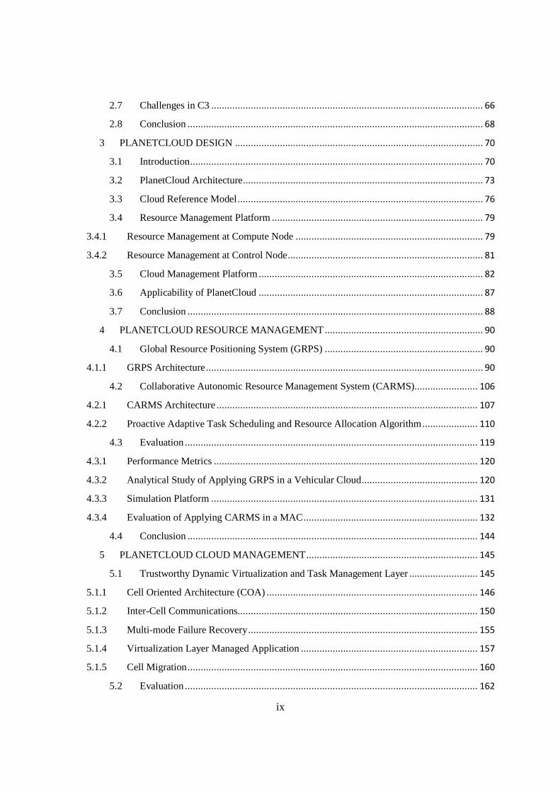
Figure 1.1Before crisis or disaster. .......................................................................................................... 6

Figure 1.2 After crisis or disaster: Loss of resources and Internet connectivity. ........................................ 7

Figure 1.3 Abstract View of PlanetCloud. .............................................................................................. 11

Figure 1.4 After crisis or disaster. .......................................................................................................... 16

Figure 1.5 After crisis or disaster: Formation of both on demand and hybrid clouds- Fast survey and data collection and analysis - Extend support of media coverage. .................................................................. 16

Figure 2.1 Taxonomy of Cloud Computing. ........................................................................................... 33

Figure 2.2 Architecture framework of a computing cloud by the Cloud Security Alliance. ..................... 38

Figure 3.1 PlanetCloud Concept. ........................................................................................................... 73

Figure 3.2 PlanetCloud Abstract Overview. ........................................................................................... 74

Figure 3.3 Agents Distribution Overview. .............................................................................................. 75

Figure 3.4 PlanetCloud Management of Mobile Cloud Computing. ........................................................ 76

Figure 3.5 Providing service models by using PlanetCloud. ................................................................... 78

Figure 3.6 Compute Node Building Blocks. ........................................................................................... 80

Figure 3.7 Control Node Building Blocks. ............................................................................................. 82

Figure 4.1 GRPS Architecture. .............................................................................................................. 92

Figure 4.2 Prediction Service. ................................................................................................................ 97

Figure 4.3 Trust Management Service. ................................................................................................... 99

Figure 4.4 Spatiotemporal Resource Calendar Example. ...................................................................... 100

Figure 4.5 Distributed GRCS s and zones. ........................................................................................... 101

Figure 4.6 PRCS to GRCS Synchronization. ...................................................................................... 102

Figure 4.7 Inter GRCS Synchronization “Between lower and higher level zones. ................................. 104

Figure 4.8 CARMS Architecture. ........................................................................................................ 110

Figure 4.9 Parallel task execution in MAC. .......................................................................................... 112

Figure 4.10 Work procedures of cloud formation. ................................................................................ 114

Figure 4.11 Initial task scheduling and assignment based on priorities. ................................................ 117

Figure 4.12 Adaptive task scheduling and assignment based on priorities. ............................................ 119

Figure 4.13 Linear Zones. .................................................................................................................... 121

Figure 4.14 Variation of a zone density with time. ............................................................................... 121

Figure 4.15 Network Model. ................................................................................................................ 125

Figure 4.16 Average resource request-response time vs. node density (vehicles/km) at different contention window size, zone length =20 km. ....................................................................................................... 127

Figure 4.17 Average Resource request-response time vs. node density (vehicles/km) at different zone lengths................................................................................................................................................. 127

Figure 4.18 Average resource request-response time vs. node density (vehicles/km) at different loads of a class per node, zone length =20 km. ..................................................................................................... 128

Figure 4.19 Analysis versus simulation at CW = 64. ............................................................................ 130

xii

Figure 4.20 Analysis versus simulation at CW = 16. ............................................................................ 130

Figure 4.21 Average Execution Time of Application Vs Number of nodes at different number of submitted tasks/application and number of cores/host. ......................................................................... 134

Figure 4.22 Average Execution Time of Applications Vs number of submitted tasks at different number of hosts. ............................................................................................................................................... 135

Figure 4.23 Average Execution Time of Applications Vs number of submitted tasks at different number of hosts and Comm. Ranges. ................................................................................................................ 136

Figure 4.24 Average Execution Time of Applications Vs number of hosts per application at different number of applications. ....................................................................................................................... 137

Figure 4.25Average Execution Time of Application Vs Number of Hosts per cloud at different scheduling mechanisms and rescheduling threshold. .............................................................................................. 138

Figure 4.26 Average Execution Time of Applications Vs number of hosts per cloud using dynamic scheduling mechanism at different communication range of a mobile node. ......................................... 139

Figure 4.27 Average Execution Time of Applications Vs number of hosts per cloud at different scheduling mechanisms and at different communication range of a mobile node. ................................. 140

Figure 4.28 Average Execution Time of Applications when applying different reliability based algorithms. .......................................................................................................................................... 141

Figure 4.29 Average MTTR Vs inactive node rates when applying different reliability based algorithms............................................................................................................................................................. 142

Figure 4.30 Average MTTR at different densities of nodes when applying P-ALSALAM algorithm. .. 143

Figure 5.1 Components of COA [105]. ................................................................................................ 147

Figure 5.2 COA Cell at runtime [105]. ................................................................................................. 148

Figure 5.3 Components of COA Cell [104]. ......................................................................................... 148

Figure 5.4 Security framework of the virtualization and task management layer [104]. ......................... 152

Figure 5.5 The Inter-Cell message format [104]. .................................................................................. 152

Figure 5.6 Secure Messaging System [104]. ......................................................................................... 153

Figure 5.7 Incoming router message [104]. .......................................................................................... 154

Figure 5.8 Router outgoing message [104]. .......................................................................................... 154

Figure 5.9 COA Cell migration process [105]. ..................................................................................... 161

Figure 5.10 The expected number of participants’ mobile nodes versus time. ....................................... 164

Figure 5.11 Average execution time of applications when applying different reliability based algorithms at static scenario. ................................................................................................................................. 167

Figure 5.12 Average number of VM migrations when applying different reliability based algorithms at static scenario. ..................................................................................................................................... 167

Figure 5.13 Average execution time of applications when applying different reliability based algorithms at dynamic scenario. ............................................................................................................................ 168

Figure 5.14 Average number of VM migrations when applying different reliability based algorithms at dynamic scenario. ................................................................................................................................ 169

Figure 5.15 Comparison between dynamic scenario and static scenario when applying different reliability based algorithms. ................................................................................................................................. 169

Figure 5.16 The expected number of mobile nodes versus time. ........................................................... 172

Figure 5.17 The expected number of cars versus time. ......................................................................... 172

xiii

Figure 5.18 The expected number of participants versus time............................................................... 173

Figure 5.19 Average execution time of an application when applying different reliability based algorithms at a small-sized hospital (25 beds). ...................................................................................................... 175

Figure 5.20 Average number of VM migrations when applying different reliability based algorithms at a small-sized hospital (25 beds). ............................................................................................................. 175

Figure 5.21 Performance comparison among different HMAC scenarios when applying P-ALSALAM algorithms at a small-sized hospital. .................................................................................................... 176

Figure 5.22 Average execution time of an application vs. communication range (km) when applying P-ALSALAM algorithms at a small-sized hospital. ................................................................................. 177

Figure 5.23 The expected number of mobile nodes versus time. ........................................................... 179

Figure 5.24 The expected number of cars versus time. ......................................................................... 180

Figure 5.25 The expected number of participants versus time............................................................... 181

Figure 5.26 Average execution time of an application when applying different reliability based algorithms at a small-sized hospital (25 beds). ...................................................................................................... 183

Figure 5.27 Average number of VM migrations when applying different reliability based algorithms at a small-sized hospital (25 beds). ............................................................................................................. 183

Figure 5.28 Average execution time of an application vs. communication range (km) when applying P-ALSALAM algorithms at a small-sized hospital at different number of submitted tasks. ...................... 184

Figure 5.29 Average number of VM migrations vs. communication range (km) when applying P-ALSALAM algorithms at a small-sized hospital at different number of submitted tasks. ...................... 184

Figure 5.30 Average execution time of an application vs. node density (nodes/km²) when applying P-ALSALAM algorithms at different-sized hospital models at different stationary nodes’ communication ranges. ................................................................................................................................................. 185

Figure 5.31 Average number of VM migrations vs. node density (nodes/km²) when applying P-ALSALAM algorithms at different-sized hospital models at different stationary nodes’ communication ranges. ................................................................................................................................................. 186

Figure 5.32 Average execution time of an application vs. node density (nodes/km²) when applying P-ALSALAM algorithms at different-sized hospital models at different number of submitted tasks. ........ 187

Figure 5.33 Average execution time of an application vs. node density (nodes/km²) when applying P-ALSALAM algorithms at different-sized hospital models at different arrival rates of inactive nodes. ... 188

Figure 5.34 Average execution time of an application at different number of submitted tasks. .............. 189

Figure 5.35 Average number of VM migrations at different number of submitted tasks. ....................... 190

Figure 5.36 Average execution time of an application at different arrival rates of inactive nodes at a small-sized hospital (25 beds). ...................................................................................................................... 191

Figure 5.37 Average number of VM migrations at different arrival rates of inactive nodes at a small-sized hospital (25 beds). ............................................................................................................................... 191

Figure 5.38 Comparison of application average execution time as more resources are added to a HMAC at different reliability based algorithms. ................................................................................................... 193

Figure 5.39 Comparison of Average number of VM migrations as more resources are added to a HMAC at different reliability based algorithms. ............................................................................................... 194

Figure 5.40 Comparison of application average execution time of a HMAC with low resource configurations as the number of submitted tasks increases when applying different reliability based algorithms. .......................................................................................................................................... 195

xiv

Figure 5.41 Comparison of Average number of VM migrations of a HMAC with low resource configurations as the number of submitted tasks increases when applying different reliability based algorithms. .......................................................................................................................................... 195

Figure 5.42 Application average execution time comparison for HMACs with different resource configurations when applying P-ALSALAM Algorithm. ..................................................................... 196

Figure 5.43 Average number of VM migrations comparison for HMACs with different resource configurations when applying P-ALSALAM Algorithm. ..................................................................... 197

xv

List of Tables

Table 1.1 The main limitations of the current MACs against the essential characteristics defined by the NIST ....................................................................................................................................................... 5

Table 2.1 Comparison among existing cloud computing technologies with respect to configuration elements. ............................................................................................................................................... 28

Table 2.2 Comparison of fixed cloud computing systems ....................................................................... 40

Table 2.3 Comparison of cloud computing systems. ............................................................................... 51

Table 2.4 Comparison of Mobile Cloud Computing Systems ................................................................. 54

Table 2.5 Approaches Related to Scheduling and Allocating Resources. ................................................ 61

Table 4.1 Advertized and Solicited Data ................................................................................................ 99

Table 4.2 Parameters and Values. ........................................................................................................ 126

Table 4.3 Parameters used in Validation. ............................................................................................. 129

Table 4.4 Parameters for evaluation of P-ALSALAM. ......................................................................... 133

Table 5.1 Parameters for Evaluation of the Virtualization and Task Management Layer. ...................... 165

Table 5.2 HMAC s with Different Host Configurations. ....................................................................... 192

1

Chapter 1

1 INTRODUCTION

1.1 Motivation and Problem Statement

Commonplace computing devices both stationary and mobile are becoming more powerful

proliferating in all aspects of our modern life. The computation resources of such devices are

increasing in terms of processing, storage and memory capabilities. In addition, emerging

devices are being richly connected through a wide spectrum of wireless communications

technologies to include to include Global System for Mobile Communications (GSM), Universal

Mobile Telecommunications System (UMTS), Long-Term Evolution (LTE), Wireless Fidelity

(Wi-Fi), Worldwide Interoperability for Microwave Access (WiMax), Zigbee, Bluetooth etc

[1][2]. Today, a device may have different simultaneously active interfaces and is likely

equipped with Global Positioning System (GPS) for location-based services. There are different

methods for localization [3], which can use technologies such as GSM/UMTS, GPS and WLAN.

While the battery lifetime is still a primary concern in mobile computing, fortunately some

types of mobile nodes such as vehicular nodes typically do not suffer from energy constraints

[4]. The anticipated exponential growth in the number of powerful, multiply-connected, energy-

rich mobile nodes will make available a massive pool of computing resources. However, if not

creatively and effectively utilized, then like their predecessors (such as the PCs), these resources

will remain largely idle or underutilized most of the time. Therefore, there is a need to exploit

their idle resources as suggested in [5]. We envision adopting cloud computing to effectively and

efficiently organize and make use of such an infinite pool of resources.

Cloud computing is a rapidly growing new paradigm promising more effective and efficient

utilization of computing resources by invariably all cyber-enabled domains ranging from

defense, to government, to commercial enterprises. In its most basic realization, cloud

computing involves dynamic, on-demand allocation of both physical and virtual computing

resources and software, usually as commodities from service providers over the public Internet

or private Intranets[6]. Cloud computing enables delivery of computing resources as a utility,

2

which drastically brings down the cost.

The area of cloud computing is also becoming increasingly important in a world with ever-

rising demand for more computational power. Service providers of cloud computing allow users

to allocate and release compute resources on-demand. However, the available computing

resources are limited. Therefore, there is a need to liberate cloud computing from being

concerned about resource constraints. This would provide opportunities to overcome technical

obstacles, e.g. scaling quickly without violating service level agreements, to both the adoption of

cloud computing and the growth of cloud computing once it has been adopted.

Current cloud computing suffers from the tight coupling with the Internet infrastructure to

access resources and services from cloud service providers like Google, Amazon and Microsoft

[7]. However, Internet connectivity may not always be available, especially in rural,

underdeveloped and disaster areas as well as some remote theatres of operation. Consequently,

this leads to a service disruption, decreasing resource availability, and computing efficiency. In

addition, there is no exploitation of the computing power of unreachable mobile and stationary

resources even when no Internet is available.

Recently, principles of cloud computing have been extended to the mobile computing domain,

leading to the emergence of Mobile Cloud Computing (MCC). There are two types of

architectures that have been proposed for MCC: 1) accessing and delivering cloud services to

users through their mobile devices where all computations, data handling, and resource

management are performed in the static cloud for the sake of offloading the computational

workload from the mobile nodes to the cloud [8][9][10]; and 2) utilizing the idle resources of

mobile devices and enabling them to work collaboratively as cloud resource providers to provide

a Mobile Ad-hoc Cloud (MAC)[11][12]. In this work, we adopt and extend the latter definition

of MCC as cloud computing, through the collaboration and virtualization, of heterogeneous,

mobile or stationary, scattered, and fractionalized computing resources forming a C3platform

that provisions ubiquitous computational services to its users.

Essential characteristics of the cloud computing model should be extended to the C3 domain,

which includes five essential characteristics defined by the National Institute of Standards and

Technology (NIST) described as follows.

1) On-demand self-service, which enables the provisioning of the needed computing

capabilities automatically without human intervention;

3

2) Broad network access, where computing capabilities can be reached over the network;

3) Resource pooling, where different physical and virtual computing resources of a provider

are pooled to serve multiple consumers and dynamically assigned and reassigned following their

variable demands;

4) Rapid elasticity, which rapidly scale up or down the computing capabilities according to

consumer demand, while appearing to be unlimited at any time; and

5) Measured service, by monitoring, controlling, and reporting the resource usage while

achieving transparency for both the provider and consumer of the service [13].

Unfortunately, the mobile resources are highly isolated and non-collaborative. Even for those

resources working in a networked fashion, they suffer from limited self and situation awareness

and collaboration. Additionally, given the high mobile nature of these devices, there is a large

possibility of failure such that permanent connectivity may not be always available. This

problem is common in wireless networks due to traffic congestion and network failures [14]. In

addition, mobile nodes cannot collaboratively contribute to form a C3 anymore if they are

susceptible to failure for many reasons, e.g., being out of battery or hijacked. Explicit failure

resolution and fault tolerance techniques were not efficient enough to guarantee safe and stable

operation for many of the targeted applications limiting the usability of such mobile resources.

The current propositions for MCC solutions [11][12][15][16][17]are entirely computing-

cluster like rather than cloud-like systems. These approaches facilitated the execution of a certain

distributed application(s) hosted on a stationary/semi-stationary stable mobile environment.

However, no prior research work realizes the five essential characteristics of the cloud model as

defined by the NIST and offers the various set of service deliver models provisioned by regular

clouds.

Most of the existing resource management systems [11][12][15]for MCC were designed to

select the available mobile resources in the same area or those following the same movement

pattern to overcome the instability of the mobile cloud environment. However, they did not

consider more general scenarios of users’ mobility where mobile resources should be

automatically and dynamically discovered, scheduled, allocated in a distributed manner largely

transparent to the users.

Additionally, current resource management and virtualization technologies fall short for

building a virtualization layer that can autonomously adapt to the real-time dynamic variation,

4

mobility, and fractionalization of such infrastructure [11][12]. Consequently, these limitations

make it almost impossible to isolate the resource layer concerns from the executing code logic.

Such isolation is an enabler for the cloud to operate and provision its basic services such as,

seamless task deployment, execution, migration, dynamic/adaptive resource allocation, and

automated failure recovery.

C3 has a dynamic nature as nodes, usually having heterogeneous capabilities, may join or

leave the formed cloud varying its computing capabilities. Also, the number of reachable nodes

may vary according to the mobility pattern of these nodes. Therefore, for the cloud to operate

reliably and safely, we need to accurately specify the expected amount of resources that will

participate in the C3 as a function of time to probabilistically ensure that we will always have the

needed resources at the right time to host the requested tasks. Selecting the right resource in a C3

environment for any submitted applications has a major role to ensure QoS in term of execution

times and performance.

Moreover, most current task scheduling and resource allocation algorithms

[18][19][20][21][22] did not consider the prediction of resource availability or the connectivity

among mobile nodes in the future, or the channel contention, which affects the performance of

submitted applications. Consequently, there is a need for a solution that effectively and

autonomically manages the high resource variations in a dynamic cloud environment. It should

include autonomic components for resource discovery, scheduling, allocation and monitoring to

provide ubiquitously available resources to cloud users.

The main limitations of the current attempts towards realizing MACs against the essential

characteristics defined by the NIST are summarized as shown in Table 1.1.

5

Table 1.1 The main limitations of the current MACs against the essential characteristics

defined by the NIST

NIST Essential

Characteristics

Limitations of the current attempts towards realizing

MACs

On-demand self-service • Limited provisioning of computing capabilities

where no global resource discovery or monitoring is

available.

Broad network access • Limited capabilities are only available over a local

network. However, computing capabilities are not

globally available and cannot used by heterogeneous

platforms (e.g., mobile phones, tablets, laptops, and

workstations).

Resource pooling • Execution is limited to distributed applications built

to execute on the targeted static platform.

• Resource sharing profile is limited, where resources

were shared among tasks built to execute on it.

• No virtualization layer and no isolation between the

physical resource, the data, and the task logic.

• Coarse grain sharing and task execution.

• Static task assignment, where no tailoring to the task

size to match the resources.

Rapid elasticity • Provisioning of limited resource pool while giving

the illusion of infinite resource availability.

• Limited failure resilience leads to unreliable

execution.

Measured service • Limited task mobility leads to limited load balancing.

• Poor resource utilization.

6

In general, the highly dynamic, mobile, heterogeneous, fractionalized, and scattered nature of

computing resources coupled with the isolated non-collaborative nature of current resource

management systems make it impossible for current virtualization and resource management

techniques to guarantee resilient or scalable cloud service delivery.

Consequently, there is a need for a solution that effectively and autonomically manages the

high resource variations in a dynamic cloud environment. It should include autonomic

components for resource discovery, scheduling, allocation, forecasting and monitoring to provide

ubiquitously available resources to cloud users.

1.2 Scenarios

1.2.1 Scenario 1: Resource Provisioning for Field Missions

As a working scenario, consider a resource-provisioning scenario for field missions of the

Medicins Sans Frontieres (MSF) organization [23], which is a secular humanitarian aid non-

governmental organization. MSF provides primary health care and assistance to people suffering

from distress or even disasters, natural or social, around the world. Figure 1.1 shows an area

before crisis occurs.

Figure 1.1Before crisis or disaster.

7

Before a field mission is established in a country, a MSF team visits the area to determine the

nature of the humanitarian emergency, the level of safety in the area and what type of aid is

needed. The field mission might arrive many days after the disaster occurs as shown in Figure

1.2.

To report accurately the conditions of a humanitarian emergency to the rest of the world and to

governing bodies, data on several factors are collected during each field mission. This survey

takes some times to gather the required information and report it to take the right decisions. In

addition, there is a need to analyze and collect a vast quantity of data for damages and losses in

infrastructure and humanities. However, performing such computations on a cloud by offloading

the computational workload, from the devices of MSF volunteers to the cloud is tight coupled

with the unstable Internet connectivity, e.g. in case of disasters. Consequently, MSF volunteers

may suffer from limited services and availability of needed powerful (in aggregate) computing

resources. In addition, the mission volunteers depend only on their limited resources which lead

to delayed reports. Although MSF has consistently attempted to increase media coverage of the

situation in these areas to increase international support, there is a lack of support to media

coverage due to extreme conditions e.g. lack of connectivity.

Figure 1.2 After crisis or disaster: Loss of resources and Internet connectivity.

Applications in this scenario generate a huge amount of data that need local computation rather

than accessing resources and services using Internet connectivity that may not always be

8

available in disaster areas. This would help in taking fast local decisions and reducing

communication costs between MSF volunteers and cloud data services. However, exploiting the

idle local computing capabilities to form a local cloud, in the disaster area, faces many

challenges. For example, it is difficult to monitor and track the other available resources to

collaborate in performing tasks of MSF volunteers. In addition, mission volunteers might travel

with their resources among different locations to assist in surgeries, and in collecting statistics on

civilians being harmed by disasters. In such highly dynamic environment, permanent

connectivity may not be always available for the mobile devices to access a formed local cloud.

Therefore, mobile resources of volunteers are highly isolated and non- collaborative. Moreover,

current solutions do not provide efficient failure resolution and fault tolerance techniques to

guarantee safe and stable operation for many of the targeted applications.

To further exacerbate the challenges, as is typically the case in disaster zones, some volunteers

and their heterogeneous mobile resources may withdraw or be lost due to deteriorating security

and safety conditions or to disaster damage impact. However, the MSF missions do not apply a

tool that could predict of resource availability or the connectivity among mobile resources, which

affects their performance.

It follows that, massive amounts of heterogeneous computing resources harbored in mobile

nodes of the volunteers and in their vicinity will go idle with no dynamic real-time scheduling,

tracking or forecasting system for these resources to help form cloud on-demand. Moreover, the

current resource and task management platforms lack to hide the heterogeneity of the underlying

geodistributed dynamic mobile resources from the executed application. This lacks make it

impossible to exploit these existing heterogeneous resources to support the mission on hand.

As an international relief organization, MSF is committed to building systems that can be

leveraged across missions. Therefore, a durable solution for computing on the move is

desperately needed [24].

1.2.2 Scenario 2: Resource Provisioning for Health and wellness applications

MCC is an attractive platform for delivering in healthcare domain. Health and wellness

applications can exploit the features and capabilities offered by mobile computing devices in a

MCC to a great extend. Such that medical applications could take advantage of mobile computing

to access to test results, emergency response and personalized monitoring. For example, a medical

application can produce distinct alert tones for signaling different severity levels of a patient’s

9

medical condition. In addition, most mobile devices have a graphics co-processor for supporting

photos and videos that can be taken advantage of, in image-dependent patient care applications. A

patient can have a running application on his nearby Smartphone, as real time data acquisition

system, that continuously interacts with sensors attached to the patient's body through a wireless

connection using the Near Field Communications (NFC). Many of these applications generate a

large amount of data that need to exploit the local computation in a MAC to do local decisions

based on these data [25].

We consider a hospital environment as working scenario, where both patients and employees,

persons who staff the hospital, have heterogeneous computing nodes. These nodes include

different types of mobile devices such as Smartphones and Laptop Computers and semi-stationary

devices such as on-board computing resources of vehicles in a long-term parking lot at a hospital.

Such rather huge pool of idle computing resources can serve as the basis of a local hybrid cloud as

a networked computing center. However, there is no current resource and task management

platform that could guarantee reliable resource provisioning, transparently maintaining

applications’ QoS and preventing service disruption in such highly dynamic environments.

Although, computing devices depend on the access network to connect to the formed cloud

and collaboratively share their resources with other nodes, permanent connectivity may not be

always available. This problem is common in wireless networks due to traffic congestion and

network failures. In addition, mobile nodes cannot collaboratively contribute to form a cloud

anymore if they are susceptible to failure for many reasons, e.g., being out of battery. Therefore,

in such highly dynamic networks, a local cloud in a hospital may suffer from service disruption

and lack of resilience. On the other hand, current resource management and virtualization

technologies fall short for building a virtualization layer that can autonomously adapt to the real-

time dynamic variation, mobility, and fractionalization of such infrastructure [11][12].

Objectives

To overcome limitations mentioned previously, we aim to achieve the following objectives:

� Ubiquitous cloud computing system to provide the right resources on-demand

anytime and anywhere;

10

� Distributed resource management system for dynamic real-time resource

harvesting, scheduling, tracking and forecasting at local, regional and global

levels; and

� Autonomic task management platform for hiding the underlying hardware

resources heterogeneity, the geographical diversity concern, and node failures and

mobility from the application to provide cloud services in a dynamic environment.

1.3 Research Approach

A possible solution would be to provide a dynamic real-time resource scheduling, tracking,

and forecasting of resources. Also, the solution should hide the underlying hardware resources

heterogeneity, the geographical diversity concern, and node failures and mobility from the

application. Further, the solution should enhance the computing efficiency, provide ”on-demand”

scalable computing capabilities, increase availability, and enable new economic models for

computing service. In this subsection, we provide our solution approach after showing our design

hypothesis and features. Then, we discuss the same mentioned scenario after applying our

solution.

Collaborative Computing Cloud (C3) Concept Goal and Overview

Un-tethering computing resources from Internet availability would enable us to tap into the

otherwise unreachable resources. We define a new concept of “Collaborative Computing Cloud

(C3)” as a dynamically formed cloud of stationary and/or mobile resources to provide ubiquitous

computing on-demand.

Hence we coin the concept of C3, where cloud resources and services may be located on any

opt-in reachable node, rather than exclusively on the providers’ side. The C3 effects a computing

on the move with resource-infinite computing paradigm. It exploits the computing power of

mobile and stationary devices directly even when no Internet is available. In doing so, the servers

themselves would have a mobility feature. The C3 would enable the formation and maintenance

of local and ad hoc clouds, providing ubiquitous cloud computing whenever and wherever

needed.

11

PlanetCloud Goal and Overview

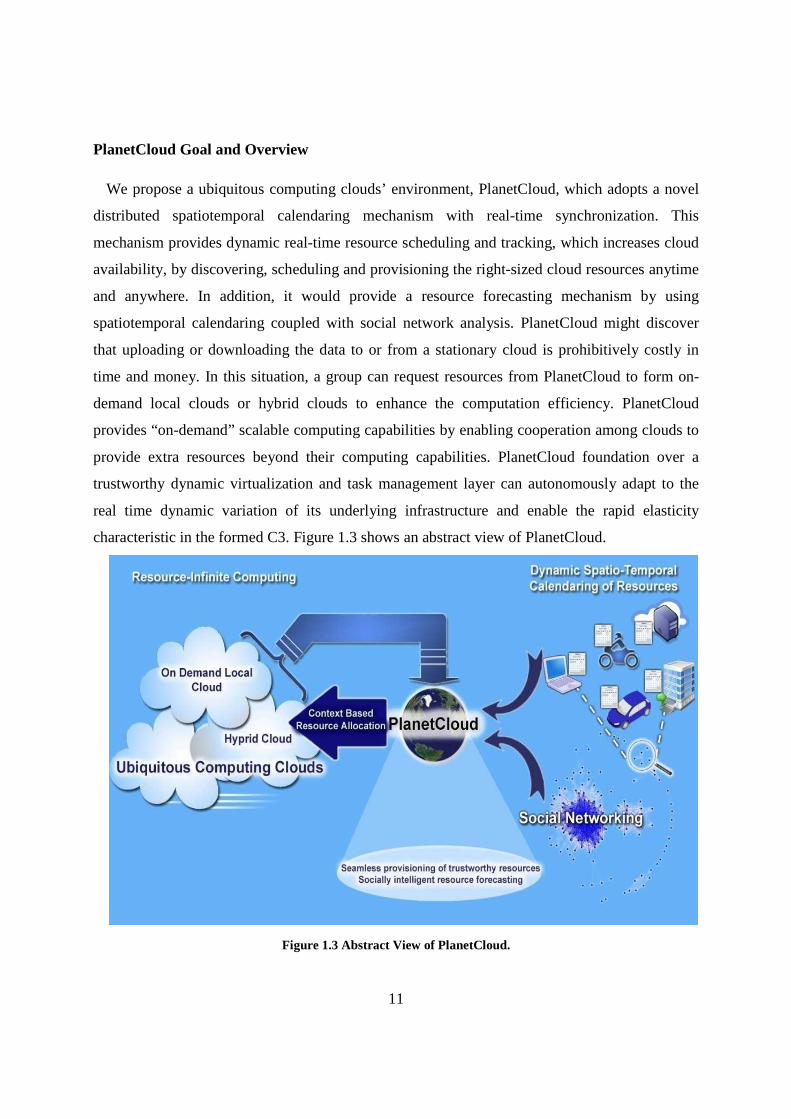
We propose a ubiquitous computing clouds’ environment, PlanetCloud, which adopts a novel

distributed spatiotemporal calendaring mechanism with real-time synchronization. This

mechanism provides dynamic real-time resource scheduling and tracking, which increases cloud

availability, by discovering, scheduling and provisioning the right-sized cloud resources anytime

and anywhere. In addition, it would provide a resource forecasting mechanism by using

spatiotemporal calendaring coupled with social network analysis. PlanetCloud might discover

that uploading or downloading the data to or from a stationary cloud is prohibitively costly in

time and money. In this situation, a group can request resources from PlanetCloud to form on-

demand local clouds or hybrid clouds to enhance the computation efficiency. PlanetCloud

provides “on-demand” scalable computing capabilities by enabling cooperation among clouds to

provide extra resources beyond their computing capabilities. PlanetCloud foundation over a

trustworthy dynamic virtualization and task management layer can autonomously adapt to the

real time dynamic variation of its underlying infrastructure and enable the rapid elasticity

characteristic in the formed C3. Figure 1.3 shows an abstract view of PlanetCloud.

Figure 1.3 Abstract View of PlanetCloud.

12

To build our solution we face the following research challenges:

� How to enable idle stationary/mobile resource exploitation in a heterogeneous computing

environment at both local and global levels?

� How to construct and use data of spatiotemporal calendars and other sources to better

harvest, schedule, track, and forecast the availability of resources in a dynamic resource

environment?

� How to transparently maintain applications’ QoS by providing an efficient mechanism

for hiding the underlying hardware resources heterogeneity, the geographical diversity

concern, node failure and mobility from the application in a highly dynamic

environment?

� How to provide resource-infinite computing to enable on-demand scalable computing

capability?

� How to mitigate the virtualization management overhead and elevate the performance of

the hosted application by providing an efficient autonomic cloud management platform

and deploying an efficient task scheduling and reliable resource allocation algorithm?

To overcome the aforementioned challenges, we propose PlanetCloud as a C3 platform using a

set of interrelated collaborative solutions (Pillars) taking the first step towards an actual hybrid

MACs (HMACs) formed from mobile and stationary computing resources.C3 provides the right

resources on-demand, anytime and anywhere, achieves the five essential characteristics listed by

NIST, and provides the main delivery service models (PaaS, IaaS& SaaS).

Hypothesis

A cloud computing system with: dynamic real-time scheduling, tracking, and forecasting of

resources of mobile and stationary nodes; a dynamic virtualization and task management layer,

and a collaborative autonomic resource management capability for cloud services would enable

C3. This system would enhance:

� Scalable computing on-demand

� Cloud computing efficiency

� Resiliency of service delivery in dynamic environment

13

Design Principles

Our main design principles are as follows.

� Physical resource management decoupled from cloud management.

� Cloud formation decoupled from Internet availability

� Resource management is a cooperative process

� Platform-managed resilience for cloud services over dynamic and mobile resources

System Components

The following are the core components of PlanetCloud:

1. Global Resource Positioning System (GRPS) to track current and future availability of

resources.

� Dynamic spatiotemporal resource calendaring mechanism with real-time

synchronization to provide a dynamic real-time scheduling and tracking of idle,

mobile and stationary, resources.

� Prediction service to forecast and improve the resource availability, anytime and

anywhere, by using a socially-intelligent resource discovery and forecasting.

� Trust management service to enable a symmetric trust relationship between

participants of GRCS.

� Ubiquitous cloud access application to access and manage data related to a C3.

� Hierarchical zone architecture with a synchronization protocol between different

levels of zones to enable resource-infinite computing.

2. Collaborative Autonomic Resource Management System (CARMS) to provide system-

managed cloud services such as configuration, adaptation and resilience through

collaborative autonomic management of dynamic cloud resources, services and

membership.

� Proactive Adaptive List-based Scheduling and Allocation AlgorithM (P-

ALSALAM) to dynamically maps applications' requirements to the currently or

potentially reliable mobile resources. P-ALSALAM selects appropriate mobile

nodes to participate informing clouds, and adjusts both task scheduling and

resource allocation according to the changing conditions due to the dynamicity of

14

resources and tasks in an existing cloud. The proper resource providers are selected

based on their future availability, resource utilization, spatiotemporal information,

computing capabilities, and their mobility pattern. This leads to mitigate both the

communication delay and the virtualization management overhead by keeping the

migration time minimum, and minimizing the number of migrations.

� Cloud manager to provide a self-controlled operation to automatically manage

interactions to form, maintain and disassemble a cloud.

� Performance monitoring and analyzing components to automatically track and

update the current status of resources.

3. Trustworthy dynamic virtualization and task management layer to isolate the

hardware concern from the task management. Such isolation empowered PlanetCloud to

support autonomous task deployment/execution, dynamic adaptive resource allocation,

seamless task migration and automated failure recovery for services running in a

continuously changing unstable operational environment.

� Biologically inspired Cell Oriented Architecture (COA) based platform with micro

virtual machines, termed Cells that support development, deployment, execution,

maintenance, and evolution of software. Cells separate logic, state and physical

resource management.

� Multi-mode recovery techniques to enhance service resilience against failures using

context and situation-aware adjustment of shuffling and recovery policies.

� Fixed control nodes to monitor outgoing or incoming Cell administrative messages

for the lifetime of the Cell, and store checkpoints changes for all running Cells for

failure recovery process. Also, they perform Cell deployment, facilitate and provide

a platform for administrative control. Further, they are responsible for holding and

maintaining all the data being processed, and any other sensitive data that the

management units want to store.

4. Portable Planet Cloud access application (we term iCloud) to provide seamless access

to and provisioning of resources.

15

1.4 Scenarios with PlanetCloud

1.4.1 MSF Scenario with PlanetCloud

PlanetCloud would provide the resources needed by the MSF field missions while they travel

among different locations. In situations similar to MSF’s, forecasting of resource availability is

invaluable before or even during disaster occurrence to save the time required for both surveys

and decision-making as shown in Figure 1.4. In case of the MSF scenario, the on-demand local

clouds or hybrid clouds can be used, if the disaster for example warrants evacuation, to assign

evacuation routes for the movement of tens of thousands of evacuees. Figure 1.5 depicts that

PlanetCloud may provide cooperation among the mission field’s cloud and the UN vehicle

computing cloud to increase the support of media coverage. Such that, UN vehicles may have

reliable on-board computing resources that typically do not suffer from energy constraints.

Therefore, the impact of PlanetCloud on the MSF missions would include:

1. Increase availability of needed resources by MSF field missions while traveling among

different locations;

2. Enable MSF to forecast or provide resources before or even during disaster occurrence, and

save time required for both surveys and decision making;

3. Hide and construct a virtualization layer to isolate the running application from the

underlying physical resource enabling seamless execution over heterogeneous resources,

stationary or mobile, and low cost of failure; and

4. Reduce cost and time of resource and service deployment.

16

Figure 1.4 After crisis or disaster.

Figure 1.5 After crisis or disaster: Formation of both on demand and hybrid clouds- Fast survey and data

collection and analysis - Extend support of media coverage.

17

1.4.2 Hospital Scenario with PlanetCloud

PlanetCloud utilizes its GRPS system to continuously monitor and track the resource arrivals

and departures of both patients and employees. This would help in managing the dynamic cloud

resources, services and membership. In addition, PlanetCloud exploits its prediction services to

predict the expected amount of computing resources of both patients and hospital staff that might

cooperate to participate to form a local hybrid cloud. This would guarantee reliable resource

provisioning, transparently maintaining applications’ QoS and preventing service disruption in

such highly dynamic environments. Moreover, the virtualization and task management layer

implemented in PlanetCloud enables medical applications to dynamically adapt to runtime

changes in their execution environment.

1.5 Evaluation

We started our evaluation by providing an analytical model to evaluate the efficiency of

PlanetCloud to provide the required resources using its underlying distributed spatiotemporal

resource calendaring mechanism in the mobile cloud environment. This evaluation helps in

determining the parameters that could be used to adapt the performance of our system response

and its capability to locate the required resources.

The effectiveness of PlanetCloud was evaluated through simulation using the CloudSim toolkit

[26][27], as it is a modern simulation framework aimed at Cloud computing environments. We

designed Java classes for employment of the spatiotemporal resource calendaring mechanism,

which feeds the simulation with the spatiotemporal data related to resources and their future

availability. In addition, we edit the CloudSim to implement our proposed P-ALSALAM

algorithm. Moreover, we have extended the CloudSim simulator to support the mobility of nodes

participating in a MAC by incorporating the Random Waypoint (RWP) model. We started our

simulation evaluations by implementing different task scheduling and resource allocation

algorithms. These evaluations show how the PlanetCloud could support formed cloud stability in

a dynamic resource environment and determine the parameters that could be tuned to adapt the

performance of formed hybrid cloud. We then feed the simulation with an expected number of

resource nodes that could participate in a HMAC, produced from an analysis we had performed,

in a different-sized hospital scenarios. Comprehensive simulation evaluations were conducted to

study the effects of different parameters related to connectivity, density of nodes, load of

18

submitted tasks, reliability, scalability, and management overhead. Results showed that

PlanetCloud can guarantee reliable resource provisioning transparently maintaining applications’

QoS and preventing service disruption in highly dynamic environments.

1.6 Contributions

Our main contribution in this dissertation is providing a C3platform, PlanetCloud, for enabling


mobile nodes, and a true ubiquitous on-demand cloud computing. This has the potential to

liberate cloud users from being concerned about resource constraints and provides access to

cloud anytime and anywhere. Such liberation provides new opportunities to expand problem

solving beyond the confines of walled-in resources and services.

PlanetCloud provides a hierarchical zone architecture to enable the cooperation among clouds

to provide extra resources beyond their computing capabilities. This architecture utilizes a

synchronization protocol between different levels of zones to enable resource-infinite computing.

PlanetCloud is a smart distributed reliable management platform that enables the provisioning

of the right, otherwise idle, stationary and mobile resources to provide ubiquitous cloud

computing on-demand. The PlanetCloud management platform utilizes its intrinsic autonomic

components to enable a large set of heterogeneous and scattered resources to work collaboratively

as cloud resource providers forming a resilient cloud on-demand. PlanetCloud synergistically

manages 1) resources to include resource harvesting, forecasting and selection, and 2) cloud

services concerned with resilient cloud services to include resource provider collaboration,

application execution isolation from resource layer concerns, seamless load migration, fault-

tolerance, the task deployment, migration, revocation, etc. Such PlanetCloud platform can fully

offer different service models and achieve the essential characteristics of cloud computing model.

The results obtained by an analytical study showed the efficiency of PlanetCloud and its GRPS

component to adapt the performance of a response according to both node density and number of

collided transmissions. On the other hand, simulation results showed the effectiveness of

PlanetCloud and its CARMS component to enable efficient cloud formation and maintenance

over mobile devices. In addition, the results showed the capability of our proposed P-ALSALAM

algorithm to map applications' requirements to the proper mobile resources which enhances both

application performance and management overhead by reducing the number of inter host VM

19

migrations as well as the communication delay. Also, results showed that we can adapt the

performance according to number of hosts per cloud, communication range and inactive node

rate. Moreover, the results showed that PlanetCloud, with its dynamic virtualization and task

management layer, can provision high level of resource availability and transparently maintaining

the applications’ QoS, while preventing service disruption even in highly dynamic environments.

Intellectual Merit:

Our main contributions are as follows:



Global mobile and stationary resource discovery and monitoring. A novel spatiotemporal

resource calendaring mechanism with real-time synchronization is proposed to mitigate

the effect of failures occurring due to unstable connectivity and availability in the dynamic

mobile environment, as well as the poor utilization of resources. This mechanism provides

a dynamic real-time scheduling and tracking of idle mobile and stationary resources. This

would enhance resource discovery and status tracking to provide access to the right-sized

cloud resources anytime and anywhere.














20




Broader Impact:

• PlanetCloud, as a ubiquitous computing cloud environment, would enhance on-demand

resource availability for under-connected areas, extreme environments and distress

situations. It enables ubiquitous resource-infinite computing paradigm by enabling

cooperation among clouds to provide extra resources beyond their computing

capabilities.

• Un-tethering computing resources from Internet availability using our proposed

PlanetCloud platform would enable us to tap into the otherwise unreachable resources,

where cloud resources and services may be located on any reachable mobile or

stationary nodes, rather than exclusively on the providers’ side.

• PlanetCloud enables a new economic model for computing service as computing

devices of users can act as resource providers. In this case, a user dedicates a certain

amount of his resources to earn some money and increase his income. This would

motivate people to participate in a C3.

• Planet Cloud could be used as a platform to provide network as a service in areas that

have poor infrastructure. This could be achieved by implementing distributed

cooperative networking tasks running on top of our micro virtual machine. These

networking tasks act as switching nodes that capable of forwarding data among

different interfaces. Where, the virtualization task management layer of the formed

cloud hides its underlying intermittent physical network while forming a stable virtual

overlay network.

1.7 Document Organization

The remainder of this dissertation is organized as follows. Chapter 2 contains background and

related work. A description of the PlanetCloud architecture and an overview of its subsystems,

i.e. GRPS architecture, CARMS architecture and the trustworthy virtualization and task

management layer are presented in Chapter 3. The PlanetCloud resource management is

21

presented in Chapter 4, including a detailed description of its subsystems, i.e. GRPS and

CARMS architectures. Also, an analytical model for evaluating the GRPS efficiency and a

simulation model for evaluating the CARMS performance and its intrinsic P-ALSALAM

algorithm are given in the same chapter. The PlanetCloud cloud management, using our

proposed trustworthy dynamic virtualization and task management layer, is presented and

evaluated using analysis and simulation in Chapter 5.Finally, Chapter 6 contains our conclusions

and outlines and directions for future work.

22

Chapter 2

2 BACKGROUND AND RELATED WORK

This chapter covers concepts and techniques underlying our work. We first present an

overview of cloud computing. Then to provide a context for research presented in this

dissertation, a taxonomy of cloud computing systems is constructed to classify and

compare the state of the art. Our taxonomy is developed in terms of service offerings, the

deployment model, the pooling of resources and the structure of a formed cloud. In

addition, a comparison is presented to show the difference between fixed cloud

computing, MCC, and hybrid clouds. Also, we present some important statistics on the

cloud computing market.

We present a comprehensive survey work of the mobile cloud computing area which is

our focus and we discuss our vision in constructing an infrastructure-less, ad hoc MCC.

Finally, we analyze the challenges facing infrastructure-less related clouds that require

further research efforts.

2.1 Overview of Cloud Computing Systems

Recently, a client of a computing cloud can enjoy massive computation resources

without the high one-time equipment cost, by outsourcing computing jobs and data to a

third party.

In literature works, there is no standard or uniform definition of cloud computing until

now [28][29][30]. The National Standards Institute of Technology defines cloud

computing as a model for enabling ubiquitous, convenient, on-demand network access to a

shared pool of configurable computing resources (e.g., networks, servers, storage,

applications, and services) that can be rapidly provisioned and released with minimal

management effort or service provider interaction. This cloud model is composed of five

essential characteristics, three service models, and four deployment models [13]. Authors

in [31] defined cloud computing as following: “Clouds are a large pool of easily usable

and accessible virtualized resources. These resources can be dynamically reconfigured to

23

adjust to a variable load, allowing also for optimum resource utilization. This pool of

resources is typically exploited by a pay-per-use model in which guarantees are offered by

the Infrastructure Provider by means of customized Service Level Agreement (SLA)”. In

[32], cloud computing is defined as, "A large-scale distributed computing paradigm that is

driven by economies of scale, in which a pool of abstracted, virtualized, dynamically-

scalable, managed computing power, storage, platforms, and services are delivered on

demand to external customers over the Internet."

Facility of fixed cloud computing is stationary since a data center takes up large

amount of space, must be in an area where energy is cheap to save cost, and the facility

usually cannot be easily moved. Since the hardware is stored in a stationary facility, its

physical connectivity is fixed over time even though the logical connectivity between

hardware may change. Moreover, today’s cloud providers are usually commercially driven

and do not usually cooperate with each other. Finally, a client can purchase the computing

service from one provider, but cannot easily purchase small pieces of resources that are

seamlessly integrated from multiple service providers.

Although, today’s fixed cloud computing service is provisioned in real time over the

Internet, i.e. Infrastructure based architecture [28], few works have recently appeared

which avoid the Internet infrastructure.

Most of previous surveys have been conducted on cloud providers of fixed cloud

computing and focused on the architecture of their systems, the services they provide,

open-source cloud computing solutions they implemented, and the virtualization

technologies they used to build the cloud. Goals of these surveys focused on knowing the

concept of cloud computing, helping clients to choose the cloud offer which fit their

needs, using the most suitable open source solution to build cloud infrastructure, and

identifying the challenges in current systems and areas requiring further research.

However, few works surveyed the research activities on MCC, which aim to present its

concept. MCC has been defined from different views in the literature [33][34][35].

1) One of these perspectives defines MCC as a way of outsourcing the computing power

and storage from mobile devices into an infrastructure cloud of fixed supercomputers.

This approach is considered as an agent-client scheme. Where, a mobile device

communicates with an agent assigned and generated for it on a cloud side. In this

24

architecture, a mobile device is simply a terminal which accesses services offered in

the cloud. This could help in avoiding limitations of a mobile device in terms of

resources, i.e. computing power and data storage, and energy usage

[8][33][34][36][37].

2) Another view defines mobile cloud computing as an infrastructure-less, e.g. ad hoc,

cloud, that represent a collaborated scheme for MCC architecture. In such architecture,

MAC is formed locally by a group of mobile devices those share their computing

power to run applications on them [33][34]. This definition might take advantage of

sensing, storage, and computational capabilities of multiple connected mobile devices

and support new applications.

2.2 Taxonomy of Cloud Computing Systems

In this section, we start with an overview of configuration elements that could be used

in CC. Then, we provide a taxonomy and a qualitative comparison of recent cloud

computing systems. We aim to exploit this taxonomy to identify the gaps of the current

cloud systems.

2.2.1 Overview of Configuration Elements in CC

We present an overview of configuration elements as follows. Table 2.1 shows a

comparison of existing technologies with respect to many of these configuration elements.

a) Service Type

Most of the taxonomies in the state of art address cloud computing from the perspective

of enterprise IT, or consumers [28]. From the perspective of a consumer, different

categories of X services offered from a cloud architecture, X-as-a-Service (XaaS), where

X is a software (SaaS), platform (PaaS), infrastructure (IaaS), etc. These services can be

accessed anywhere in the world [28][30]. Services are provided to the end users as

utilities, so they are billed by how much they used [30][38].

There are three general types of cloud computing services focus on the delivery manner

of a service. These services are: IaaS, PaaS, and SaaS [39][29][30][38][40].

Zhou et al. [41] divide services into six categories, including the three main categories

mentioned previously, and present those three extra services as Data as a Service (DaaS),

25

Identity and Policy Management as a Service (IPMaaS), and Network as a Service (NaaS).

IPMaaS is used to manage users’ identity and service policy [41]. DaaS enables users to

access and define data lists in a cloud service via an interface and then query against this

data, which is suitable for basic data management querying and manipulation. For

example, Data Direct and Strikeiron [41] provide DaaS. They differentiate these services

into three service levels: hardware level, system level and application level. IaaS and NaaS

belong to the hardware level. PaaS belongs to the system level. While, IPMaaS, DaaS and

SaaS belong to the application level [41].

b) Deployment Model

From the perspective of an enterprise IT, clouds can be operated in three deployment

models: private cloud, public cloud and hybrid cloud [28][13][30][42][43][44][45]. In

general, this classification of clouds is done according to nature of the owner of the cloud

data centers.

Private Cloud: It is fully owned and controlled by a single company, where internal

data centers are located. A private cloud depends on virtualization of the infrastructure.

Public Cloud: This cloud is available to public as a pay-as-you-go manner via the

Internet, where data centers run by third parties, e.g. Google and Amazon, those provide

services.

Hybrid cloud: It is a combination of private and public clouds, where some applications

are running on internal data centers and others on external data centers of public clouds.

Among the other classification elements, we quote:

c) Virtualization type

This defines the virtualization technology that is used for emulation of underlying

resources. The software that allows a single physical machine to support multiple virtual

machines is called a virtual machine monitor. Virtualization technologies might be one of

three types which are full virtualization, para-virtualization and OS-level virtualization

(Isolation) [42].

d) Architecture

This describes the architecture of a platform tells and how it works and how it was

built, e.g. centralized, hierarchical, and number of servers [42].

26

e) Virtual Machine Placement

It defines the location of the VM, which is important for resource optimization [42].

f) Storage

This aspect concerns the fact how data is stored on virtualized resources [42].

g) Access interface

This describes the way clients can access their leased resources [42].

h) Fault-tolerance

The ability of a system to continue operating properly even in case of some of its

components fail [28][42].

i) Load balancing

This defines the how to achieve optimal resource utilization using a networking

methodology to distribute the workload across multiple computers [42]. It could be used

to redistribute the work load after a failure occurs and minimize the resource consumption

[28].

j) Hardware

This refers to a set of hardware configurations offered by a cloud computing provider

which best suit the needs of its customers for three types of resources: compute units (e.g.

processor architecture and clock speed), memory, and hard disk [40].

k) Security

It refers to the elements used in a cloud environment to be secure. Different

authentication mechanisms could be used e.g. simple login and password, certificates,

Message-Digest, MD5, signature, and Virtual LAN (VLAN). Another element is using

static IP address which is assigned to a customer account. Moreover, a firewall is a

security element that could be used to prevent unauthorized access to cloud resources [40].

l) Business model

It includes three business elements: payment model (e.g. advance payment and

consumption payment), price element which contains many aspects (e.g. subscription fee,

use time, cost of managing data) and SLA [40].

m) Interoperability

This refers to the fact of allowing applications to be ported among clouds, or to use

multiple cloud infrastructures [28].

27

n) Bandwidth provisioning

It focuses on providing bandwidth-on-demand services in the cloud computing where

the capacity in bandwidth can be increased or decreased on-demand [41].

o) Scale of implementation

This refers to the size of a cloud project, e.g. a pilot implementation scope and

enterprise wide cloud deployment [45].

p) Architecture scheme of MCC

IT refers to the organization of MCC systems and what a mobile device plays in a

cloud, e.g. agent-client scheme and collaborated scheme [39].

q) Application partition

This refers to the process of decomposing complex application to atomic components,

thus can be processed concurrently [39].

r) Offloading

This defines how we can offload task from client to cloud to free burden of mobile

devices and save their energy consumption [39].

s) Context management method

It refers to a method that enables us to ascertain additional information from the

computing device without the need for explicit user input [39].

t) Access schemes

It refers to existing access schemes which define how to access services provided by

MCC [35].

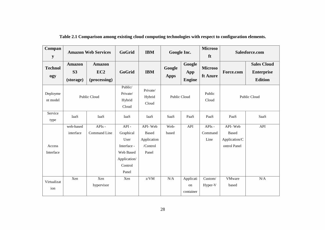
28

Table 2.1 Comparison among existing cloud computing technologies with respect to configuration elements.

Compan

y Amazon Web Services GoGrid IBM Google Inc.

Microso

ft Salesforce.com

Technol

ogy

Amazon

S3

(storage)

Amazon

EC2

(processing)

GoGrid IBM Google

Apps

Google

App

Engine

Microso

ft Azure Force.com

Sales Cloud

Enterprise

Edition

Deployme

nt model Public Cloud

Public/

Private/

Hybrid

Cloud

Private/

Hybrid

Cloud

Public Cloud Public

Cloud Public Cloud

Service

type IaaS IaaS IaaS IaaS SaaS PaaS PaaS PaaS SaaS

Access

Interface

web-based

interface

APIs -

Command Line

API -

Graphical

User

Interface -

Web Based

Application/

Control

Panel

API- Web

Based

Application

/Control

Panel

Web-

based

API APIs -

Command

Line

API- Web

Based

Application/C

ontrol Panel

API

Virtualizat

ion

Xen

Xen

hypervisor

Xen

z/VM N/A Applicati

on

container

Custom/

Hyper-V

VMware

based

N/A

29

Compatibl

e

Operating

Systems

N/A Linux /

Windows

Windows

Linux Cent

OS

Linux Linux /

Windows/

Mac

Linux /

Windows

Windows Linux /

Windows

N/A

SLA 99.99%

availability

99.95% uptime 100%

Uptime

N/A N/A 99.9%

Uptime

99.9% 99.9%

Uptime

N/A

Subscripti

on Type

Use Based

and

Subscription

Plans

Use Based and

Subscription

Plans

Use Based

and

Subscription

Plans

Use Based

and

Subscriptio

n Plans

N/A Use

Based

Use Based

and

Subscripti

on Plans

Subscription

Plans

N/A

Inbound

Bandwidth

Price

N/A 0¢ per GB 0¢ per GB 15¢ per GB N/A 10¢ per

GB

10¢ per

GB

0¢ per GB N/A

Outbound

Bandwidth

Price

N/A 12¢ per GB 29¢ per GB 15¢ per GB N/A 12¢ per

GB

15¢ per

GB

0¢ per GB N/A

Base Plan

Cost

N/A $0.08¢ per hour $8¢ per hour $15¢ per

hour

N/A $0¢ per

hour

$12¢ per

hour

$0¢ per hour N/A

Base Plan

Details

New AWS

customers

receive 5

GB of

Amazon S3

storage,

1.7GB RAM,

160GB local

storage, 1 EC2

Compute Unit

0.5 GB

RAM, 10

GB local

storage,

Free

inbound

One Virtual

32 bit

CPUs with

1.25GHz; 2

Gb Virtual

memory;

$5/user The first

500 MB

of

persistent

storage

are free

1.6 GHz

CPU, 1.75

GB RAM,

225 GB

Instance

Storage,

One month

free edition,

with 1 GB of

storage, 10

GB

Bandwidth.

$125 per User per

Month

612 MB per user

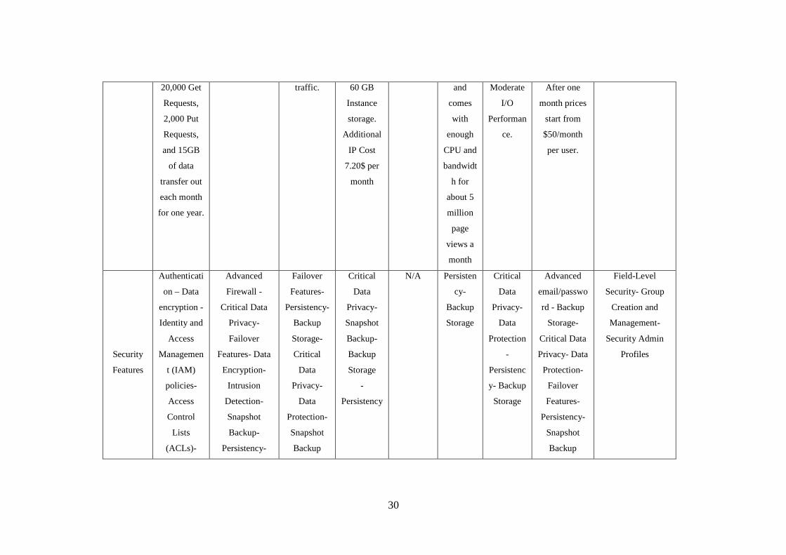
30

20,000 Get

Requests,

2,000 Put

Requests,

and 15GB

of data

transfer out

each month

for one year.

traffic. 60 GB

Instance

storage.

Additional

IP Cost

7.20$ per

month

and

comes

with

enough

CPU and

bandwidt

h for

about 5

million

page

views a

month

Moderate

I/O

Performan

ce.

After one

month prices

start from

$50/month

per user.

Security

Features

Authenticati

on – Data

encryption -

Identity and

Access

Managemen

t (IAM)

policies-

Access

Control

Lists

(ACLs)-

Advanced

Firewall -

Critical Data

Privacy-

Failover

Features- Data

Encryption-

Intrusion

Detection-

Snapshot

Backup-

Persistency-

Failover

Features-

Persistency-

Backup

Storage-

Critical

Data

Privacy-

Data

Protection-

Snapshot

Backup

Critical

Data

Privacy-

Snapshot

Backup-

Backup

Storage

-

Persistency

N/A Persisten

cy-

Backup

Storage

Critical

Data

Privacy-

Data

Protection

-

Persistenc

y- Backup

Storage

Advanced

email/passwo

rd - Backup

Storage-

Critical Data

Privacy- Data

Protection-

Failover

Features-

Persistency-

Snapshot

Backup

Field-Level

Security- Group

Creation and

Management-

Security Admin

Profiles

31

bucket

policies-

and query

string

authenticati

on

Custom/Secure

-Permissions

Scalability

Support

Storage,

request rate,

and users to

support an

unlimited

number of

web-scale

applications.

Yes Yes N/A N/A Yes N/A Yes N/A

Load

Balancing

Yes Yes N/A N/A Yes N/A Yes N/A

Supported

Services/

Common

Usage/Fea

tures

Content

Storage-

Storage for

Data

Analysis-

Backup,

Archiving

and Disaster

File Hosting

Service

File Hosting

Service

File

Hosting

Service

Diagramm

ing

Software-

Email

Client-

Formula

Editor-

HTML

File

Hosting

Service

File

Hosting

Service

No File

Hosting

Service

Analytics

- Channel

Management-

Customer Service-

Integration-

Collaboration-

Marketing

Automation- Sales

32

Recovery Editor-

Image

Viewer-

Presentati

on

Program-

Raster

Graphics

Editor-

Spreadshe

et

Program-

Vector

Graphics

Editor-

Word

Processor

Automation

Programm

ing

Languages

Supported

N/A Java-PHP-

Python-Ruby-

WinDev

all the

programmin

g languages

all the

programmi

ng

languages

N/A Java

Python

N/A Java-PHP-

Ruby

N/A

33

2.2.2 Cloud Computing Systems

Classifications of cloud computing systems are presented in terms of service offerings,

the deployment model, the pooling of resources and the structure of a formed cloud.

2.2.2.1 Service Based

The taxonomy of cloud computing systems includes the different types of X service

offerings, where service types could be divided into two categories according to who the

manager of the cloud services is. Thus, it can be distinguished between services managed

by service providers and services managed by service consumers, as shown in Figure 2.1.

Figure 2.1 Taxonomy of Cloud Computing.

Those services of the provider managed category can be divided into three main types,

say SaaS, PaaS and IaaS. These services are detailed as follows.

SaaS: This is a multi-tenant platform which uses common resources to support many

customers simultaneously. In SaaS, an application is transparently managed by the service

provider, and a customer uses an existing application, rather than install and run it on

customer’s own computer [41].

PaaS: This service, also known as cloudware [40], provides the consumer with a

platform which includes all required tools to develop, deploy and host web applications.

IaaS: It delivers the infrastructure requested by a consumer, who can use applications

and resources with more flexibility [28].

34

Examples of IaaS are Network-Infrastructure-as-a-Service (NIaaS) and Hardware-as-a-

Service (HaaS). NIaaS solution [42] is offered by PacketExchange, which provides

a scalable bandwidth on-demand. PacketExchange's NIaaS provides enterprise

organizations the ability to build their network infrastructure on the PacketExchange

private optical backbone instead of having to maintain expensive hardware assets,

engineering resources, and fixed capacity WAN circuits. It provides companies with a

scalable capacity and an infrastructure that optimizes the delivery of cloud-based

solutions. In [28], HaaS was presented. This service provides hardware to the enterprise

users, which saves the cost and efforts of building and managing data centers. Also,

Storage-as-a- Service is an example of IaaS which enables users to store data in a rented

storage space in the cloud. It provides a convenient way to manage backups. Examples of

Storage-as-a- Service providers are Amazon Simple Storage Service (S3) [30] and AT&T

Synaptic Storage as a Service. Other service providers such as Amazon Web Services with

its Elastic Compute Cloud (EC2) offers processing as a hardware configuration that best

suit the needs of its customers [30][40].

We define a consumer managed category named Hosting -as-a Service (HaaS): It

provides a package of services required to host Web, Web -as-a Service (WaaS), and

applications, hosted application solution, on a cloud with guaranteed QoS delivery.

Where, any of these services could be built directly on top of its lower layer, e.g. HaaS on

PaaS, or on any other lower layer, e.g. HaaS and IaaS, in order to deliver a service.

Virtualization is a key enabling technology for hosting a guest operating system on top

of the virtualization software, as in IaaS. It enables using resources in an efficient and

flexible manner [42]. Unlike SaaS, a hosted application is an individual copy of the

software runs on an off-premises server but may not be managed by the provider. Some

leading companies host applications and deliver such service over the internet such as

Microsoft Azure Services and Salesforce [41].

In WaaS, Web sites are hosted as a service on top of IaaS layer [40]. Companies those

are providing WaaS, such as Media Temple, Gridlayer [41], Google App Engine,

Agathon, and Elastra [40].

35

2.2.2.2 Deployment based

Clouds could be classified, from the point of deployment, to three kinds, which are

public cloud, private cloud and hybrid cloud. The infrastructure of a public cloud is

owned by an organization, which sell cloud computing services to the public through the

Internet. Private cloud means that the cloud infrastructure is owned and managed by only

one organization. The infrastructure of a hybrid cloud combines both private and public

clouds [43].

a) Public Clouds

The term “public” gives an indication that services are available to clients via the

Internet and their usages are fairly inexpensive [44]. Public clouds are dominated by SaaS

followed by IaaS [45].

Some open source solutions such as OpenNebula and Abicloud support public cloud

platform [43].OpenNebula provides interfaces and functions to virtual machines, storage

and network management and so on. Many cloud computing IaaS providers consider the

public cloud platform, e.g. Amazon Web Service, Flexiscale, and Mosso [28].

b) Private Clouds

The organization that owns a private cloud manages data and processes without the

restrictions of network bandwidth, security exposures and legal requirements, as in case of

public clouds [44]. Services are provided over an intranet within the enterprise and behind

the firewall of the organization [45]. Because of the access of users is restricted and

networks are designated, many advantages are obtained which include a greater control of

the cloud infrastructure, improving security and resiliency for providers and users [44].

Private clouds are dominated by IaaS followed by PaaS [45].

There are different open source IaaS cloud computing solutions used to build private

clouds. OpenNebula is one of these solutions, which might be integrated with networking

and storage solutions and fitted into existing data centers [42][46][43]. It works with

different virtualization solutions, e.g. Xen, KVM and VMware. Another private cloud

solution is called AbiCloud, which supports many virtualization techniques such as

VirtualBox, VMWare, XEN, and KVM. This platform is developed by Abiquo company

[42]. Eucalyptus and Enomaly are open source cloud computing solutions those support

private cloud deployment [28].

36

c) Hybrid Clouds

Interoperability is the main concern to combine a public and private cloud [44]. Each

kind of cloud might be independent; however, they are combined with some standards or

special techniques [43]. In this cloud, clients might outsource non-critical data and process

it in the public cloud, while keeping critical one in their control [44].

On the other hand, this mixed cloud environment may not be suited for applications

requiring complex databases or synchronization. This is because, some complexity may be

added regarding the distribution of applications, monitoring of the infrastructures, security

and privacy of the internal and external parts of the mixed environment [30].

Hybrid Clouds can be supported by OpenNebula [42] as an open source IaaS solution.

Sun Cloud [28] is an example of cloud computing PaaS provider that supports hybrid

cloud platform. It provides hardware architecture to customize workload, multi-tenancy

and resource sharing among a large pool of users.

2.2.2.3 Resource Pool Based

We classify the clouds in terms of their knowledge about the resources that could

participate in the cloud formation to two categories: a resource harvesting cloud and a

prior known-resource cloud.

a) Resource Harvesting Cloud

In this type of clouds, there is no prior knowledge about the resources that could to

contribute to form a cloud. An example of a resource harvesting cloud presented in [47],

where an execution of application can be partially delegated to an intermediate layer

formed from harvested resources of intelligent embedded devices, e.g. Smartphone.

b) Prior Known-resource Cloud

This type of cloud exploits unified predetermined elastic resources to serve a multitude

of users anywhere, anytime through the Internet regardless of heterogeneous environments

and platforms based on the pay-as-you-use principle. Most of conventional cloud

computing systems [48][49] are considered a prior known-resource clouds.

c) Hybrid Resource Pool Cloud

In this type of clouds, some resources are advertized and others are harvested as

presented in the local or hybrid cloud formed in [50][51].

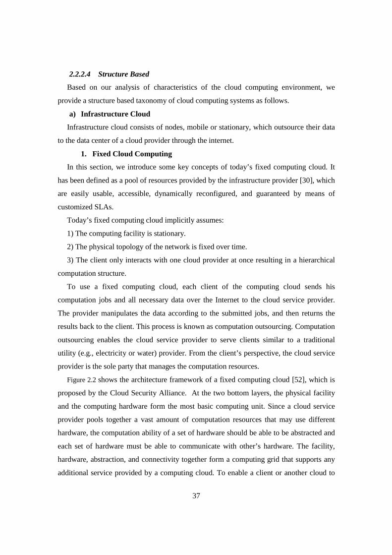
37

2.2.2.4 Structure Based

Based on our analysis of characteristics of the cloud computing environment, we

provide a structure based taxonomy of cloud computing systems as follows.

a) Infrastructure Cloud

Infrastructure cloud consists of nodes, mobile or stationary, which outsource their data

to the data center of a cloud provider through the internet.

1. Fixed Cloud Computing

In this section, we introduce some key concepts of today’s fixed computing cloud. It

has been defined as a pool of resources provided by the infrastructure provider [30], which

are easily usable, accessible, dynamically reconfigured, and guaranteed by means of

customized SLAs.

Today’s fixed computing cloud implicitly assumes:

1) The computing facility is stationary.

2) The physical topology of the network is fixed over time.

3) The client only interacts with one cloud provider at once resulting in a hierarchical

computation structure.

To use a fixed computing cloud, each client of the computing cloud sends his

computation jobs and all necessary data over the Internet to the cloud service provider.

The provider manipulates the data according to the submitted jobs, and then returns the

results back to the client. This process is known as computation outsourcing. Computation

outsourcing enables the cloud service provider to serve clients similar to a traditional

utility (e.g., electricity or water) provider. From the client’s perspective, the cloud service

provider is the sole party that manages the computation resources.

Figure 2.2 shows the architecture framework of a fixed computing cloud [52], which is

proposed by the Cloud Security Alliance. At the two bottom layers, the physical facility

and the computing hardware form the most basic computing unit. Since a cloud service

provider pools together a vast amount of computation resources that may use different

hardware, the computation ability of a set of hardware should be able to be abstracted and

each set of hardware must be able to communicate with other’s hardware. The facility,

hardware, abstraction, and connectivity together form a computing grid that supports any

additional service provided by a computing cloud. To enable a client or another cloud to

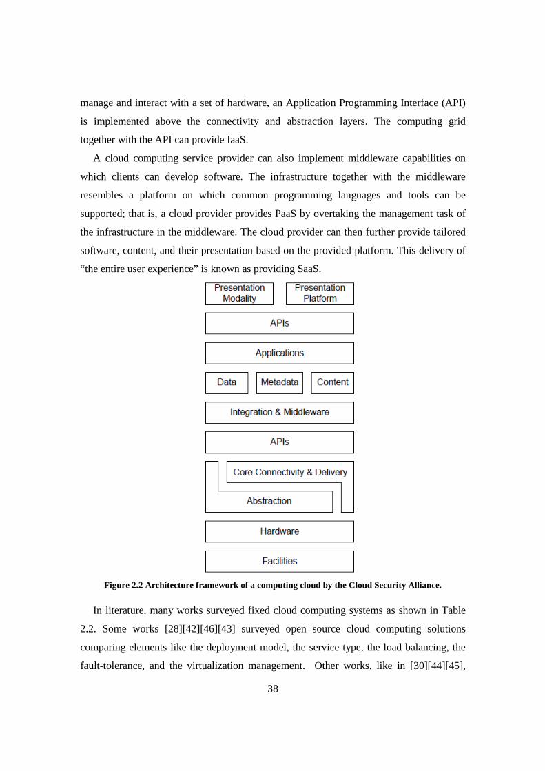
38

manage and interact with a set of hardware, an Application Programming Interface (API)

is implemented above the connectivity and abstraction layers. The computing grid

together with the API can provide IaaS.

A cloud computing service provider can also implement middleware capabilities on

which clients can develop software. The infrastructure together with the middleware

resembles a platform on which common programming languages and tools can be

supported; that is, a cloud provider provides PaaS by overtaking the management task of

the infrastructure in the middleware. The cloud provider can then further provide tailored

software, content, and their presentation based on the provided platform. This delivery of

“the entire user experience” is known as providing SaaS.

Figure 2.2 Architecture framework of a computing cloud by the Cloud Security Alliance.

In literature, many works surveyed fixed cloud computing systems as shown in Table

2.2. Some works [28][42][46][43] surveyed open source cloud computing solutions

comparing elements like the deployment model, the service type, the load balancing, the

fault-tolerance, and the virtualization management. Other works, like in [30][44][45],

39

have examined the cloud computing concepts in terms of the service type and the

deployment model. Different cloud service providers and their systems have been

addressed in literature works [28][41][40]. These works conducted taxonomy of some

important cloud computing elements like service type, deployment model, security,

business model, middleware, and virtualization management. A survey work in [42]gave

taxonomy of the virtualization technologies used to build the cloud and compared those

using criteria like virtualization type, platform and compatible operating system.

40

Table 2.2 Comparison of fixed cloud computing systems

Survey on Analyzed elements Description of Comparison Classification elements

Virtualization

technologies and

open source

solutions [42]

Open source virtual

machine solutions

Popular virtual machine monitors:

VMware, HypeV, VirtualBox,

OpenVZ, Xen, KVM

Virtualization type - Compatible OS –

Platform - Live migration - Free /

Shareware

Open source IaaS

Cloud Computing

solutions

Open source solutions: Eucalyptus,

OpenNebula, Xen Cloud Platform

(XCP), Nimbus, AbiCloud, OpenStack

Deployment model – Architecture -

Virtual Machine Placement – Storage –

Network - Access interface – Security -

Fault-tolerance - Load balancing

A selection of

Cloud providers

[40]

IaaS Cloud

providers

Amazon EC2, AppNexus, ENKI,

FlexiScale, GoGrid, Joyent

Accelerator, and NewServers

Service type - Virtualization type –

Hardware - Load balancing – Security -

Business model – Middleware -

Performance Web hosting

companies

Agathon, Elastra, ENKI,

GridLayer, Media Temple , Rackspace

Architecture and

owners of clouds

[30]

Cloud providers Amazon EC2, Amazon S3, Google

Apps, Salesforce.com, Force.com, Sun

Cloud

Service type

Cloud

environments

Single-Cloud environments and

multiple-Cloud environments

Deployment model

Different cloud Service providers IaaS providers: Amazon Web Service, Architecture - Deployment model -

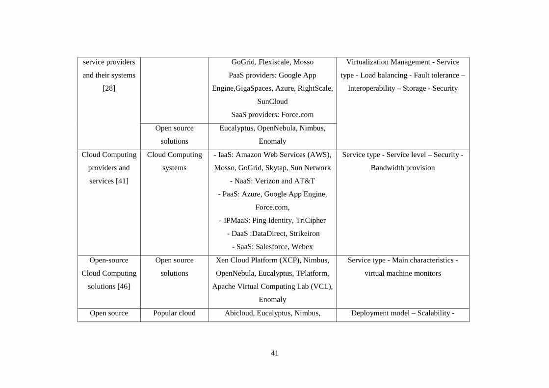
41

service providers

and their systems

[28]

GoGrid, Flexiscale, Mosso

PaaS providers: Google App

Engine,GigaSpaces, Azure, RightScale,

SunCloud

SaaS providers: Force.com

Virtualization Management - Service

type - Load balancing - Fault tolerance –

Interoperability – Storage - Security

Open source

solutions

Eucalyptus, OpenNebula, Nimbus,

Enomaly

Cloud Computing

providers and

services [41]

Cloud Computing

systems

- IaaS: Amazon Web Services (AWS),

Mosso, GoGrid, Skytap, Sun Network

- NaaS: Verizon and AT&T

- PaaS: Azure, Google App Engine,

Force.com,

- IPMaaS: Ping Identity, TriCipher

- DaaS :DataDirect, Strikeiron

- SaaS: Salesforce, Webex

Service type - Service level – Security -

Bandwidth provision

Open-source

Cloud Computing

solutions [46]

Open source

solutions

Xen Cloud Platform (XCP), Nimbus,

OpenNebula, Eucalyptus, TPlatform,

Apache Virtual Computing Lab (VCL),

Enomaly

Service type - Main characteristics -

virtual machine monitors

Open source Popular cloud Abicloud, Eucalyptus, Nimbus, Deployment model – Scalability -

42

cloud solutions

[43]

computing

platforms

OpenNebula

Service type – Compatibility -

Deployment aspects - VM support - web

interface - OS support

Cloud computing

concepts [44]

Service Provider Service type - Deployment Model

Cloud computing

implementations

[45]

Clients of cloud

computing

Service type - Deployment model -

Security - Scale of Implementation

43

2. Infrastructure Mobile cloud Computing

The Mobile Cloud Computing Forum defines MCC as a cloud where the computing

power and data storage are moved away from mobile phones and into the datacenter of a

cloud provider, bringing applications and mobile computing to be not just Smartphone

users but a much broader range of mobile subscribers [37].

The term MCC appears in [8][53], represents a concept that makes use of cloud

computing available for mobile users. This would help to offload required capabilities of

intensive computations from mobile devices and extend their battery life. It provides a

framework that uses the context information for the heterogeneous access management

service which is provided by the mobile cloud for the mobile terminals.

The MCC framework presented in [54]proposes an energy-efficient location-based

service (LBS) and mobile cloud convergence. Such that it is needed to offload the

computation-intensive part by partitioning of application functions across a cloud.

Similarly, authors in [55] proposed an energy cost model for executing a task in different

computing facilities by deploying an online algorithm for fairly offloading location-aware

tasks among mobile users.

Authors in [56][57] provide models of MCC. An economic service provisioning for

mobile cloud services is addressed in [56] using Semi-Markov Decision Process for

mobile cloud resource allocation. The economic model is used to manage the computing

tasks according to the configuration of the cloud system. MobiCloud [57] focuses on using

the capability of cloud computing for securing Mobile Ad hoc Networks (MANETs).

Each mobile node as a virtualized component is mirrored to one or more images in the

cloud in order to address the communication and computation deficiencies of this mobile

device.

A context model based on ontology has been proposed in [58]. It uses context

information in the mobile cloud environment to provide users with suitable services and

manage resources effectively. It provides service optimization modeling context-aware

information in mobile platform and reason.

The proposed approach in [33] provides a mobile cloud application, a photo-sharing

application. This application aims to share photo using storage capability of Amazon

cloud, rather on the device itself.

44

Authors in [59] propose a new green solution, using MCC, which saves Smartphones

energy. In this contribution, MCC temporary holds the required contents for the

Smartphones in a local cloud data center network, which are migrated from the main cloud

data center. The MCC is provided by a Internet Service Provider (ISP).

CroudSTag [60] is an application built for the Android devices, which helps members

of social networks of common interests to form social groups easily from the mobile

devices with reasonable latencies. It depends on a storage cloud, the face-recognition

cloud services, and Facebook to obtain a set of pictures, recognize people, and form social

groups, respectively.

Architecture of MCC [61] is proposed to use cloud computing techniques for storage

and processing of data on mobile devices. A three-tier framework is proposed consists of

presentation, application, and database tiers.

The research presented in [62] focuses on the resource allocation for security services,

e.g. authentication, digital signature, audition, of mobile cloud to mobile devices. It

presents an admission control mechanism based on the total cloud system reward with the

considerations of the cloud resource consumption and incomes generated from cloud

users.

b) Infrastructure-less Cloud

Infrastructure-less cloud consists of a group of nodes, participants, which communicate

directly with each other, in an Ad Hoc mode, to work collaboratively as cloud resource

providers to share their resources and make them available to whomever is in a given area.

1. Infrastructure-less Collaborative MCC (MAC)

Few works define mobile cloud computing as an infrastructure-less extension of the

traditional cloud which performs computing activities on mobile nodes.

In [15], a MCC framework is presented, where a mobile cloud is defined as a cloud

which is formed of local computing resources to achieve a common goal in a distributed

manner. Experiments for job sharing are conducted using Bluetooth to form a piconet,

which provides an ad-hoc network linking a user group of mobile devices. The prototype

compares the capabilities of the involved devices to determine a priori the usefulness of

sharing workload at runtime.

45

The work presented in [34] addresses how the mobility could enhance the

performances of distributed computation and the resilience of services in computing

clouds formed from mobile ad-hoc networks. Authors show that improvement can be

achieved in the performance of distributed computation with even a small percentage of

highly mobile nodes in a high localized network, as well as the resilience of mobile cloud

computing.

Authors in [11] present preliminary design for a framework to create a virtual mobile

cloud computing. The proposed approach allows mobile devices, as providers, to use Ad

Hoc WiFi for communication and execute jobs among them. This approach only considers

nearby nodes, which will remain on the same area or follow the same movement pattern

for stability.

A technique is proposed in [63] for reliable resource allocation to utilize mobile

devices as resources in mobile cloud environments. Resource allocation is initially based

on the reliability of mobile resources, which depends on the mobility pattern of mobile

devices, and the availability of these mobile resources.

Hyrax [12] introduced the concept of using mobile devices as resource providers.

Hyrax is a platform that develops a mobile cloud infrastructure and allows client

applications to conveniently use data and execute computing jobs on Smartphone

networks and heterogeneous networks of mobile devices and servers. This platform is

based on Hadoop can support cloud computing on Android Smartphones. It uses a central

server that coordinates data and jobs on connected mobile devices. However, the mobile

devices had to communicate through a WIFI central router because Android doesn’t

support ad-hoc network yet.

2. Why Infrastructure-less Collaborative MCC?

Infrastructure-less MCC delivers computing resources to the entities that want it while

an infrastructure cloud requires outsourcing computation by hauling data over the Internet.

This fundamental difference in providing computation as a utility yields many benefits

unique only to mobile clouds as follows.

• Liberate Cloud Computing Concerns from Resource Constraints

Cloud computing is designed to deliver as much computing power as any user wants,

while in practice the underlying infrastructure resources are limited [32]. Service providers

46

of cloud computing provides limited resource pool while giving the illusion of infinite

resource availability. They allow users to allocate and release compute resources on-

demand. Therefore, it is reasonable to assume that the number of resources is infinite.

Exploit the massive pool of idle computing resources in mobile devices can liberate cloud

computing from being concerned about resource constraints. This would provide

opportunities to enable a practical scalable cloud formation to overcome technical

obstacles, e.g. scaling quickly without violating service level agreements, to both the

adoption of Cloud Computing and the growth of Cloud Computing once it has been

adopted.

• Decouple Computation from Connectivity

The computation advantage of an infrastructure cloud can only be accessed via the

Internet. One must establish a connection to the cloud provider in order to submit jobs and

data for processing. That is, the computation ability is dependent on the Internet

connectivity. However, this dependency can be broken with the infrastructure-less MCC

since the mobile cloud physically delivers the computation ability. This decoupling is

important in delivering cloud service to areas where Internet speed is slow and massive

computation ability is only occasionally required.

• Mobile Facility Provides Self-Powered Service

A mobile cloud element can be externally powered (e.g., a requester can provide the

power necessary to operate the cloud), or it could be self-powered. That is, the energy

used to move the cloud element around can be used to power the computing module of

that cloud element. For example, modern vehicles can commonly each provide 240Wof

DC power from its DC connector when the vehicle engine is on. The self-sufficient power

allows the mobile cloud to be set up where stationary cloud cannot. The self-provided

power could also be used to supplement the external power as a secondary power source.

• Mobile Facility Provides Enforceability

Prior studies have stated that an infrastructure cloud service provider may provide

service from and over many different jurisdictions, thus enforcing policies in an SLA is

difficult [64]. However, an infrastructure-less MCC must gather around a particular

location, and is unlikely to be scattered in multiple jurisdictions that may not cooperate.

47

The client, especially a requester, can thus request a small set of jurisdiction districts to

cooperatively enforce the SLA. The enforceability can be used to elevate the importance

of the SLA from a mere agreement to a contract, and the clients may be more willing to

adopt mobile clouds given that the SLA carries enforceable legal liability.

• Altering Physical Topology Enables Physical Access Control

An infrastructure cloud is often deemed untrustworthy because the users only know a

virtual address at which their data is located and to which their jobs are sent. A user does

not know for certain that a second user cannot modify his data or if a foreign government

is monitoring his actions. Mobility allows the participants of an infrastructure-less MCC

and, more importantly, the requester of a mobile cloud to exercise a certain amount of

physical enforcement. In infrastructure-less MCC, the data is locally disseminated, where

the interface between the user and the cloud is under physical monitoring and can be

assumed to be secure. In addition, enhancement of the delivered security level might be

achieved by splitting the data needed to be processed into segments, encrypting the

segments, compressing the segments, distributing the segments via mobile nodes

participating in an infrastructure-less MCC while keeping one of the segments of data on

the device itself. This will prevent extracting the data such that the data, picture, could

never be decrypted/read/modified outside the mobile device [65].

• Altering Physical Topology Avoids Multi-Tenancy

In an infrastructure computing cloud, the cloud might store data and run jobs belonging

to multiple users on a single machine, known as multi-tenancy. Providers of infrastructure

cloud services thus spend great effort in securing process access by using VMs and

hypervisors, and also in securing data access by implementing sophisticated access control

protocols. In an infrastructure-less MCC, data need not be sent over the Internet and is

stored locally. Additionally, an infrastructure-less MCC has a single specific group of

clients. In other words, an infrastructure-less MCC does not provide multi-tenant service,

but only a time-shared single-tenant service to multiple clients. Thus, an infrastructure-less

MCC only needs to enforce a sanitizing policy rather than mitigating all possible adverse

privacy leaks in a multitenant system.

48

Providing a single-tenant environment also allows a mobile cloud to mitigate the

phishing attack. An infrastructure cloud needs to be resilient to social engineering attacks

in order to prevent attackers from accessing private data with stolen authorization at the

service provider side. However, an infrastructure-less MCC provides a local single-tenant

system, and phishing provides the attackers no benefits since all private data are sanitized

before the mobile cloud move away from the client.

c) Hybrid infrastructure cloud

A third view supports hybrid cloud formation by exploiting the computing power of

both mobile and stationary devices [50][66][67][68]. It coins the concept of ubiquitous

computing cloud, where cloud resources and services may be located on any opt-in

reachable node, rather than exclusively on the providers’ side. The C3 effects a computing

on the move with resource-infinite computing paradigm. PlanetCloud as a ubiquitous

computing cloud platform un-tethers computing resources from Internet availability. It

exploits the computing power of mobile and stationary devices directly even when no

Internet is available to form a HMAC. In doing so, the servers themselves would have a

mobility feature. The C3 would enable the formation and maintenance of local and ad hoc

clouds, providing ubiquitous cloud computing whenever and wherever needed.

2.3 Comparison

This section mainly compares the difference between fixed cloud computing, MCC,

and hybrid clouds, and analyzes the challenges face infrastructure-less related clouds. A

comparison of cloud computing systems is shown in Table 2.3.

The role of a client in offloading could be divided to client- server approach and

collaborative approach.

a) Client- server approach: In this approach, tasks are offloaded from client side to

stationary servers located in the cloud side to exploit their resources. This might

overcome limitations of mobile devices.

a) Collaborative approach: A client is a part of a cloud, which utilize its resources

and share them with other clients in the formed cloud in a distributive way.

From our taxonomy, the infrastructure cloud follows the client- server approach.

However, infrastructure-less MCC is a collaborative approach.

49

The computing facility is stationary in the infrastructure cloud. On the other hand, the

computing facility has a mobility feature in infrastructure-less MCC.

Fixed cloud computing has a physical topology of the network which is mostly fixed

over time, but dynamic topology for both types of MCC as well as hybrid clouds.

Different types of the infrastructure cloud computing share a particular weakness: the

prerequisite infrastructure makes the utility difficult to reach remote areas that have little

population. This is because the service providers usually give higher service priority to

denser cluster of clients. This weakness is known in the telecommunication community as

the “last mile problem”. In particular, Internet connectivity in remote areas is often either

slow or non-existing, thus a prospective client of cloud computing might elect not to use

the service since outsourcing computation (i.e., sending data and receiving results) may

require a prohibitive amount of time and money.

On the other hand, infrastructure-less clouds do not depend on the Internet

infrastructure to reach the resource providers. Moreover, a cloud is formed in an ad hoc

manner among mobile devices.

However, most of the existing resource management systems [11][12][15] for

infrastructure-less MCC were designed to select the available mobile resources in the

same area or those follow the same movement pattern to overcome the instability of the

mobile cloud environment. Also, they did not consider more general scenarios of users’

mobility where mobile resources should be automatically and dynamically discovered,

scheduled, allocated in a distributed manner largely transparent to the users. Additionally,

most current task scheduling and resource allocation algorithms [18][19][21] did not

consider the prediction of resource availability or the connectivity among mobile nodes in

the future, or the channel contention, which affects the performance of submitted

applications.

Our proposed PlanetCloud [50][66][67][68] enables the formation of hybrid clouds in

a dynamic resource environment by exploiting idle resources that could be either

stationary or mobile. PlanetCloud extends the concept of social network analysis to predict

and provide the right resources at anytime and anywhere. Moreover, it supports resource

infinite computing. An expected limitation of PlanetCloud is providing hard QoS

50

guarantees. PlanetCloud is anticipated to provide soft QoS guarantees based on resource

prediction, collection, and stability of environment.

The infrastructure clouds do not exploit the massive pool of computing resources of

mobile devises. Consequently, these resources might remain largely idle or underutilized

most of the time.

Two intuitive major advantages of both infrastructure-less and hybrid clouds over a

today’s technology are:

1) If a client cannot efficiently reach the computing resources, then the mobile

computing resources can be delivered to or pooled around that client. The resulting

infrastructure-less mobile computing cloud can provide localized computing resources.

2) If the computation capacity, of a set of mobile computation devices, is not fully

utilized, the mobile devices can assimilate their resources to solve a computation problem

or provide service to interested clients.

Both infrastructure-less MCC and hybrid can be viewed as autonomous computing

clouds with mobility. On the contrary, the infrastructure based cloud also often does not

support mobility. For example, wirelessly providing electricity using inductive coupling is

not yet commercially viable, and Internet hotspots often do not handle handoffs. A mobile

client thus might not be able to take advantage of the cloud computing service since the

infrastructure is not as supportive toward mobile clients as it is toward stationary clients.

The membership of a mobile computing cloud may be highly dynamic while the

membership of a fixed computing cloud is controlled by one or few central providers. An

infrastructure-less MCC thus is not very suitable to serve as a data storage cloud since the

locations of the storage devices may change with the cloud membership. However,

PlanetCloud as a hybrid cloud computing system enables this by providing a global

resource positioning system. Therefore, intuitively, a client of an infrastructure-less MCC

should store both the data waiting processing and the returned results on the client’s own

local storage. Availability of the data is then provided by using local backups or possibly

using a hybrid cloud.

51

Table 2.3 Comparison of cloud computing systems.

Hybrid

Clouds

MCC Fixed

Clouds Infrastructure MCC Infrastructure-less MCC

Feature PlanetCloud

[67][68]

[54][56][57

][58]

[33][59][

61][69] [62] [15] [34] [11] [63] [41][40]

Enable ubiquitous computing clouds Yes No No No No No No No No

Provide resource forecasting Yes No No No No No No Yes No Prediction of resource

availability Yes No No No No No No No No

Service delivery through Internet

Yes Yes Yes Yes No No No No Yes

Support of resource infinite computing

Yes No No No No No No No No

Provide geographic information of resources

Yes Yes No No No No No No No

Support dynamic nature of Mobile resources

Yes Yes No Yes Yes Yes No Yes No

Stationary / Mobile/ Hybrid computing facility

Hybrid Stationary Stationary Stationary Mobile Mobile Mobile Mobile Stationary

client- server approach or collaborative approach

Hybrid client- server

client- server

client- server

collaborative

collaborative

collaborative

collaborative

client- server

Topology Dynamic Dynamic Dynamic Dynamic Dynamic Dynamic Dynamic

Dynamic

Fixed

52

2.4 Statistics on the Cloud Market

Cloud services and virtualization were selected by CIOs as the most often and the top-two

technologies for 2011. It is a result of a worldwide CIO survey which was conducted by Gartner

EXP from September to December 2010 and represents CIO budget plans reported at that time.

Responses are included from 2,014 CIOs representing over $160 billion in corporate and public-

sector IT spending across 50 countries and 38 industries [70].

According to David Mitchell Smith, vice president and Gartner Fellow,” "The trend and

related technologies continue to evolve and change rapidly, and there is continuing confusion and

misunderstanding as vendors increasingly hype 'cloud' as a marketing term. This level of impact,

confusion, uncertainty and change make cloud computing one of Gartner's top 10 strategic

technology trends to address" [71].

Five cloud computing trends have been identified by Gartner that will affect the cloud strategy

through 2015, i.e. accelerate, shift or reach a tipping point over the next three years. Users must

factor these trends into their planning processes: Formal decision frameworks facilitate cloud

investment optimization, hybrid cloud computing is an Imperative, cloud brokerage will facilitate

cloud consumption, cloud-centric design becomes a necessity, and cloud computing influences

future data center and operational models.

We list some points, which are related to cloud computing area, from Gartner's top predictions

for 2012 as follows [72]:

a) Low-cost cloud services will cannibalize up to 15 percent of top outsourcing players'

revenue by 2015: Industrialized low-cost IT services (ILCS) will disrupt the projected $1

trillion IT services market, similar to the one the low-cost airlines have brought in the

transportation industry.

b) 40 percent of enterprises will make proof of independent security testing a precondition

for using any type of cloud service by 2016: To evaluate cloud services for their ability to

resist security threats and attacks, the enterprise will be satisfied by a cloud provider's

certificate stating that a reputable third-party security vendor has already tested its

applications. This means that inspectors' certifications will eventually become a viable

alternative or complement to third-party testing.

53

c) More than 50 percent of Global 1000 companies will have stored customer-sensitive data

in the public cloud by year-end 2016: In order to reduce operational costs and maintain

the efficiency, more than 20 percent of organizations have already begun to selectively

store their customer-sensitive data in a hybrid cloud.

d) The prices for 80 percent of cloud services will include a global energy surcharge by

2015: An energy surcharge is included by some cloud data center operators in their

pricing package, and Gartner analysts believe this trend will rapidly escalate to include

the majority of operators. Business and IT leaders and procurement specialists must be

ready to see energy costs included in future cloud service contracts.

Other statistics on cloud computing include:

The size of the Cloud Computing Market will be $150 Billion by 2013. An expert like Merrill

Lynch’s research [73] predicts that the cloud computing market will grow at such a high rate.

7 out of 10 companies are using cloud services that will move new applications to the cloud.

Mimecast, a company that offers SaaS, conducted a study which showed that companies have

started their transition into the cloud with a small trial. They test the infrastructure with some of

their data and applications. It is expected that within the next few years a large growth of

transitions will be from the companies which have a good experience of their trial period.

54% of respondents have citied security as their top concern for transitioning to the cloud.

LinkedIn has been conducted a recent survey with 7052 respondents. It showed that security has

been the higher preference for many business companies that are looking forward to use cloud

computing, especially for those make use and store sensitive data such as the financial and

healthcare industries.

60% of server workloads will be virtualized by 2014. Recently, Gartner has conducted a study

which revealed that many companies are directed by their customers' inclination to cloud

computing, which will improve the business performance and offers a variety of solutions to

computing limitations they face.

A new server is added to the cloud for every 600 Smartphones or 120 tablets. Intel admits that

a new server needs to be deployed for this number of mobile devices that hit the market and

connect to the cloud [74]. In 2012, 120 million tablet sales are predicted by Gartner and Credit

Suisse claiming Smartphone sales will hit one billion devices in 2014. This gives us an indication

of the huge spike in new servers being added to the cloud.

54

2.5 State of Art of Mobile Cloud Computing Systems

Few survey works have been conducted for mobile cloud computing as shown in Table 2.4,

like in [39][75][35]. Le Guan et al. [39] presented two architecture schemes for MCC represented

infrastructure and infrastructure-less (ad-hoc) architectures. While, [75] addressed the

infrastructure architecture of MCC and [35] focused on the infrastructure-less (ad-hoc

infrastructure) architecture. Application offloading and partitioning in MCC have been addressed

in [39][75] and many MCC applications have been introduced in [75]. Moreover, works like

[39][75]studied the context-aware service in terms of the management method and the context

type.

The state of the art in research shows that many of the existing MCC solutions focus on how

the mobile devices’ capabilities could be enhanced by migrating resource-intensive computations

tasks to the cloud through computation offloading techniques [11][15]. Some research work

discussed the idea of forming mobile cloud computing platform relaying on the hardware

resources provisioned by stationery or semi-stationery devices using the term MAC. However,

these solutions presented computational-clusters hosting certain distributed application(s) rather

than generic computing-clouds.

Table 2.4 Comparison of Mobile Cloud Computing Systems

Survey on Analyzed elements Classification elements

Research activities on

Mobile

Cloud Computing [39]

Architecture of

Mobile Cloud

Computing

Architecture scheme

Implementation of

elastic applications

Application Partition - Offloading

Context-aware

service

Context management- Context type

Mobile cloud computing

(Infrastructure) [75]

Architecture Service type

Applications Storage – Processing – Security -

Energy consumption - Offloading

Mobile cloud computing

(Ad hoc) [35]

Classes of architecture framework

Cloud platform - Access schemes

55

2.5.1 Research Relevant to Collaborative Ad Hoc Cloud Formation

In the next subsections we will briefly discuss the latest research targeting MACs classified by

the associated research objective:

2.5.1.1 Mobile-resource Sharing

In [11], authors proposed a preliminary design for a management framework that exploits the

resources of a collection of nearby mobile devices to construct a virtual ad hoc mobile computing

cluster. The framework creates a virtual service provider on-the-fly that utilizes the resource of a

set of stable mobile devices that will remain on the same area or follow a fixed limited movement

pattern. Building a mobile computing cluster on such assumption is invalid as there is no

consideration for system resilience, service stability, and failure recovery. Therefore, it is a

limited scenario that did not consider high node mobility cases where connectivity is not stable,

leading to disconnections and faults. Similarly, experiments for job sharing were conducted in

[15] over a stable ad-hoc network linking a user group of mobile device. Unfortunately, they

shared the same limitation as the aforementioned work; they presented a computing cluster

management platform with no consideration for resource mobility, heterogeneity, dynamic

connectivity of resources. Further, they system management did not consider operation resilience

and did not present any solution to handle potential failure events that might occur especially in

such unstable mobile environment.

Hyrax platform [12] was one of those who introduced the concept of using mobile devices as

computation resources. The platform used a central server to utilize data and execute computing

jobs on networks of homogeneously configured android smart phones. Hyrax did not consider the

general scenario where hardware resources are heterogeneously configured and highly mobile.

The system offered limited management automation, Hyrax did not consider a real users’ mobility

where mobile resources should be automatically and dynamically discovered, scheduled, allocated

in a distributed manner largely transparent to the users. Hyrax only provides an infrastructure for

MCC, providing an interface for executing tasks on a mobile device cloud.

In [16] researchers demonstrated the feasibility of exploiting the resources in mobile devices to

execute work units as part of a grid and upload results to a server. However, the model of this

approach was specifically developed to a single mobile hardware device or operating system. A

more generic solution presented in [17], they proposed a collaborative framework that enables

mobile devices to participate in executing computation-intensive tasks in a computing cluster to

56

expand the shared resources. They focused only on task partitioning and offloading where a ratio

of participation is determined depending on many factors, e.g., the system capability, the mobile

device’s performance, and the network state. However, the proposed framework did not consider

a real mobile network environment that is relatively unstable. The work presented in [34]

addresses how the mobility could enhance the performances of distributed computation and the

resilience of services in computing clusters formed from mobile ad-hoc networks. Authors show

that improvement can be achieved in the performance of distributed computation with even a

small percentage of highly mobile nodes in highly localized networks.

Most of the previously mentioned research works [11][15][34][17] did not take the rapid

elasticity the heterogeneity of pooled resources or the broad network access characteristics into

considerations.

2.5.1.2 Vehicular Cloud

Exploiting the virtually unlimited power supply in vehicles , researchers in [76][5][77]

discussed the possibility of having a MCC using a powerful on-board computers augmented with

huge storage devices hosted on stationary vehicles acting as networked computing centers on

wheels. Given the limited mobility of such solutions, we do not consider them as a realistic

implementation of a generic computing cloud. Moving away from the main objective of MCC, to

enhance the utilization of the ideal mobile resources in hosting computational tasks, and, it is

more like a relocation of the regular data center into a set of mobile small-scale centers where

hardware resources are explicitly added.

Additionally, the proposed approaches only focused on one delivery service model, the IaaS

and provided a virtual environment to satisfy specific client application. In [78], authors presented

an overview about a datacenter architecture for the management of physical resources of vehicular

nodes. The authors considered that vehicles are plugged into a standard power outlet and are

provided Ethernet connections. However, this scenario is considered as a stable environment,

such that the long-term parking lot of an international airport guarantees that there are at least a

specific number of vehicles parked in the airport at any time and ready for utilization. Therefore,

this solution does not provide the rapid elasticity characteristic. In addition, no solutions were

provided for dynamic environments with neither heterogeneous resources nor task scheduling and

resource allocation.

57

2.5.2 Research Relevant to Scheduling and Allocating Reliable Resources

We discuss related work in some areas relevant to scheduling and allocating reliable resources

for supporting stable MCC formation as follows:

2.5.2.1 Resource Management in MCC

Research in resource management systems and algorithms for mobile cloud computing is still

in its infancy. In [11], authors proposed a preliminary design for a framework to exploit resources

of a collection of nearby mobile devices as a virtual ad hoc cloud computing provider. In [15], a

mobile cloud computing framework was presented. Experiments for job sharing were conducted

over an ad-hoc network linking a user group of mobile devices. The Hyrax platform [12]

introduced the concept of using mobile devices as resource providers. The platform used a central

server to coordinate data and jobs on connected mobile devices. Task scheduling and resource

allocation algorithms were reported in [18][19][20][21][22]. These algorithms used cost, time,

reliability and energy as criteria for selection.

Most of the existing resource management systems [11][12][15] for MCC were designed to

select the available mobile resources in the same area or those follow the same movement pattern

to overcome the instability of the mobile cloud environment. However, they did not consider

more general scenarios of users’ mobility where mobile resources should be automatically and

dynamically discovered, scheduled, allocated in a distributed manner largely transparent to the

users. Additionally, most current task scheduling and resource allocation algorithms

[18][19][20][21][22] did not consider the prediction of resource availability or the connectivity

among mobile nodes in the future, or the channel contention, which affects the performance of

submitted applications. Consequently, there is a need for a solution that effectively and

autonomically manages the high resource variations in a dynamic cloud environment. It should

include autonomic components for resource discovery, scheduling, allocation and monitoring to

provide ubiquitously available resources to cloud users.

2.5.2.2 Availability of Clouds

Mobile clouds should be of highly dynamic nature with heterogeneous configuration and

capabilities, and ad-hoc join or leave attitude. Participants of a MCC should depend on the access

network to be able to connect to the cloud, while permanent connectivity may be not always

available. This problem is common in wireless networks due to traffic congestion and network

58

failures [79]. In addition, mobile nodes are susceptible to failure for many reasons, e.g., being out

of battery or hijacked. Therefore, the number of reachable nodes may vary according to the

mobility pattern of these nodes. Resource management systems for MCC should support this

dynamicity, hide the heterogeneity of resources, provide users with unified access, evaluate and

predict the availability and performance of resources, and guarantee the quality of service to meet

users’ requests.

In a cloud environment, it may be possible that some nodes will become inactive because of

failure. Therefore, the entire work of unsuccessful jobs has to be restarted, and the cloud should

migrate these jobs to the other node. The redundancy concept is a solution to achieve failover for

handling failures [79][80][81]. There are basically two options of redundancy: replication and

retry.

Replication is redundancy in space where a number of secondary nodes, in stand-by mode, are

used as exact replicas of a primary active node. They continuously monitor the work of the

primary node to take over if it fails. However, this approach is only feasible for stationary servers

or if the nodes are few [79]. As this work focuses on providing the high availability for mobile

nodes, having replica of all mobile nodes will not be feasible as it will increase complexity, cost

etc.

Retry is redundancy in time where a try again process starts after a failure is detected [81]. In

this work, we consider a retry options to achieve failover coupled with forecasted information

about the future resource availability, as an input to our proposed proactive management

algorithm, to minimize the Mean Time to Repair (MTTR). MTTR is the time required to detect

the failure and try again.

2.5.2.3 Reliability and reputability of resource providers

Task scheduling and resource allocation algorithms were reported in [18][19][20][21][22].

These algorithms used cost, time, reliability and energy as criteria for selection.

The majority of previous frameworks for service discovery and negotiation models between

cloud users and providers such as [82] did not consider the reliability of offered resources.

However, in all mentioned works [11][12][15][18][19][20][21][22][82], a method that can

determine the reputability of offered resources is missing.

59

2.5.3 Research Relevant to Discovery and Exploiting Idle Resources

We discuss related work in four areas relevant to discovering and exploiting idle resources

which inspire us to build our system for supporting stable MCC formation as follows:

2.5.3.1 Resource mapping and discovery techniques

The resource-mapping problem has been broadly considered in the literature. NETEMBED

considered allocating resources when deploying a distributed application [83]. In [84], an

approach is presented to generate automatically world-wide maps by using traceroute

measurement from multiple locations. A detailed survey of various decentralized resource

discovery techniques is presented in [85]. These techniques are driven by the P2P network model.

A layered architecture was presented to build an Internet-based distributed resource indexing

system.

2.5.3.2 Approaches for exploiting idle resources

Exploiting idle resources has been proposed in some work. For example, Search for Extra-

Terrestrial Intelligence (SETI) @ home focuses on analyzing radio signals, and searching for

signs of extra terrestrial intelligence. The software of SETI@home runs either as a screen saver on

home computer and only processing data when the screen saver is active, making use of processor

idle time [86]. In [87], the authors present the design of an environment - a virtual cluster project,

to exploit idle times in network resources. This environment could deal with usage of idle cycles,

handling of dynamic behavior of the nodes, and safe remote execution.

2.5.3.3 Approaches for analysis of complex graphs and networks

Authors in [88] used an extensible data structure for massive graphs: STINGER (Spatio-

Temporal Interaction Networks and Graphs (STING) Extensible Representation). It includes a

computational approach for the analysis based on the streaming input of spatiotemporal data.

GraphCT, a Graph Characterization Toolkit, for massive graphs representing social network data

has been presented in [89]. It has been used to analyze public data from Twitter, a micro-blogging

network. This work treated social network interactions as a graph and used graph metrics to

ascribe importance within the network.

60

2.5.3.4 Tracking applications

In [90], an application for the Apple iPhone™ was presented and used to report in real-time

flow of traffic in order to build the most accurate map of traffic patterns to be used by commuters

or departments of transportation for making decisions. The outcome of the case study is used to

determine that the iPhone™ is relatively as accurate as a vehicle tracking device.

Both resource mapping [83][84] and idle resource exploitation approaches [86] only consider

stationary resources. Such resources are globally distributed and directly connected to the Internet

as Internet-based systems. On the other hand, our PlanetCloud enables ubiquitous computing

clouds in a dynamic resource environment by exploiting idle resources that could be either

stationary or mobile. In addition, it supports cloud mobility and hybrid cloud formation.

PlanetCloud extends the concept of social network analysis presented in [89] to predict and

provide the right resources at anytime and anywhere. Moreover, PlanetCloud supports resource

infinite computing by enabling cooperation among clouds to provide extra resources beyond their

computing capabilities. An expected limitation of PlanetCloud is providing hard QoS guarantees.

PlanetCloud is anticipated to provide soft QoS guarantees based on resource prediction,

collection, and stability of environment.

A comparison between PlanetCloud and the recent research efforts is shown in Table 2.5.

61

Table 2.5 Approaches Related to Scheduling and Allocating Resources.

Feature PlanetCloud NETEMBE

D [83]

Decentralized

resource

discovery

techniques

[85]

Point of

Presence Geo-

Location [84]

Internet

topology

modeling

approach [91]

SETI@

Home

[86]

AVS [5]

Enable ubiquitous computing

clouds

Yes No No No No No No

Provide resource forecasting Yes No No No No No No

Idle Resource Usage Yes No No No No Yes Yes

Global view Yes No Yes Yes Yes No No

Enable resource prediction using

social networking data


Internet Resources Yes Yes Yes Yes Yes Yes No

Support of resource infinite

computing


Provide geographic information of

resources

Yes No Yes Yes Yes No No

Support dynamic nature of Mobile

resources

Yes No No No No No Yes

*AVS: Autonomous Vehicular Clouds.

62

2.5.4 Research Relevant to supporting the rapid elasticity characteristic

The state of the art in research shows two main areas relevant to support the rapid elasticity

characteristic of a MAC as follows.

2.5.4.1 Scalability

Scalability can be classified in two main types: Vertical Scalability and Horizontal Scalability.

Vertical Scalability denotes adding extra resources, e.g. more Random Access Memory (RAM),

storage and Central Processing Unit (CPU), to the same computing pool to handle the increased

demand. Horizontal Scalability denotes adding more number of computing nodes to the

computing pool to handle the increased demand [92][93]. Choosing of a scalability type is a

challenging issue. The cost of vertical scaling is directly proportional to the size of application.

However, it is wise to choose Vertical Scalability in urgent scaling case or when an application is

designed for a pre-determined number of users. On the other hand, Horizontal Scalability has a

comparatively lower cost than Vertical Scalability. But, Horizontal Scalability faces a major

hardware failure problem and high cost of data movement for transactions whose execution

cannot be contained to a single node [92].

A VM migration is an efficient approach that supports scalability. For example, a VM

migration with higher resource utilization may be triggered as a physical node becomes

overloaded. A new VM placement is selected where a VM could migrate to another node with

lower resource utilization. This helps the migrated VM to get better resource availability and to

scale up its computation [94].

Additionally, CPU scheduling configuration has a significant impact on the virtualization

platform’s performance. Scheduling configuration is influenced by the number of virtual CPUs

allocated to a VM, the assignment of virtual CPUs of VMs to dedicated physical cores, and the

assignment of different CPU priorities to the VMs [95]. To achieve high resource utilization and

scalability of the physical infrastructure, VM consolidation has been increasingly implemented in

cloud datacenter environments, where multiple VMs are hosted on the same physical host which

allows dynamic multiplexing of computation and communication resources [96].

63

2.5.4.2 Management Overhead

The deployment and management of VMs in a MAC provide an additional overhead that

impacts the performance of a MAC. This is because the deployment of VM requires computing

resources for VM creation, VM configuration, VM Operating System (OS) setup, VM startup,

and application deployment in VM. Moreover, the management of VM includes computing

resources utilization in the monitoring of VM in entire lifecycle, CPU scheduling, VM migration,

application processing management, VM state transitions and physical resources management for

VM. The deployment and management overhead, which requires additional computing resources,

increases the execution cost of the application [96].

There are some important parameters to quantify the performance overhead of the

virtualization platform of a MAC, which are described as follows.

1. VM creation Time: Which is the time taken to create a new VM, which depends on the

VM creation policy.

2. VM Scheduling Latency: All consolidated VMs share the same physical resources of a

hosting node. Consequently, the accessing of the same physical CPU of the hosting node

is scheduled for VMs. This leads to increase the execution time of application in VM.

Similarly, the performance is degraded when the CPU of VM is scheduled for multiple

applications.

3. Application Allocation to VM Time: Which is the time taken to allocate an application to

a VM for execution.

4. VM Migration time: Which is the time taken to move a VM from one physical host to

another in a MAC. Such that the inter host VM migration consumes computing resources,

e.g. network bandwidth and energy power.

5. VM termination time: It is the time taken to remove a VM completely and return

computing resources to a host.

To the best of our knowledge, the current propositions for MCC solutions [11][12]facilitated

the execution of a certain distributed application(s) hosted on a stationary/semi-stationary stable

mobile environment. However, no prior research works have been conducted that evaluate

scalability or the virtualization management overhead in a dynamic HMAC environment.

64

2.6 A Vision for C3

In this section, we discuss our vision forC3

a) Supporting Minimal Communication Connectivity

A requester of a C3 may have very minimal communication connectivity with the outside

world. Thus to avoid all-to-all broadcast of requests, a bulletin board can serve as a sink of all

requests from requesters. The bulletin board can then broadcast each request to prospective

computing cloud elements. Finally, the elements respond to the bulletin board, and the bulletin

board forwards the responses back to the requesters.

b) Providing Identity Management

A Public Key Infrastructure (PKI) provides means to verify an entity’s identity. In particular,

public key infrastructure enables an entity to digitally sign a document that can be considered as a

legal document. We thus suggest a public key infrastructure be used to provide identity

management in a C3.

c) Providing Elastic Resource Management

Since the membership of a C3 may change over the lifetime of the cloud, the roles of each

cloud element may also need to adopt according to the changing environment. For example, if a

node that serves as a coordinator to provide SaaS leaves the cloud, another cloud element should

step up, continue serving as the coordinator, and help the mobile cloud recover from the absence

of the original coordinator.

The ability of a cloud member to change his role in the mobile cloud is known as elasticity,

and is introduced by Eltarras et al. [97]. The authors note that elasticity enables a network to be

dynamic, flexible, and scalable. These properties are desirable in forming a mobile cloud as they

enable a mobile computing cluster to provide different levels of services reliably.

d) Providing Result Verifiability

Intuitively the client would not recompute and compare the results every time he requests

cloud computing service since re-computation defeats the purpose of outsourcing computation.

Thus, to prevent errors from being fed back and spread, the client can give multiple instances of

each job to the cloud in order to reach consensus. This redundancy is already incorporated by

some of today’s computing clusters, such as Stanford’s Folding@Home project.

65

e) Sanitizing Confidential Data

Each element of a C3 should sanitize its storage device to meet the privacy requirement stated

in the SLA. A requester can follow the guideline specified by the U.S. Department of Defense in

reusing hard disk drives³.

f) Providing Auditability

Auditing a C3is more difficult than an infrastructure cloud since C3 elements do not

necessarily belong to a single organization or have a single implementation. However, a local

cloud formed by C3 system has a definite location; thus, an auditor can audit an assembled mobile

cloud before the cloud leaves from the vicinity of the requester.

Privacy policy is a particular policy that requires careful treatment. Once a piece of data is

handed to a cloud element, that cloud element can ignore the privacy policy by secretly storing

and disseminating that piece of data.

A particular auditing mechanism is to watermark the data with the identity of the cloud

element. Thus when a piece of data is leaked, violating the privacy policy, the original requester

or collaborator can request law enforcement to penalize the source of data leak along with

negative impacts to the source’s reputation.

g) Enforcing the SLA

Since the C3 is able to manage identity, we can simply seek the help of law enforcement or

legal departments to enforce the SLA. This is similar to enforcing any of today’s contracts.

h) Managing Trust Using Reputation

Reputation system is often used to determine the trustworthiness of an entity based on the

historic performance of that entity. The identity management can be linked with a reputation

system so that when a C3 element responds to a cloud formation request, the requester (or the

collaboration initiator) can verify its reputation. Since all parties (requesters and cloud elements)

trust the PKI and the Certificate Authority, the Certificate Authority can also serve as the

reputation manager.

66

2.7 Challenges in C3

In this section, we identify some issues that require further research. We also discuss potential

directions.

• Design of the Reputation System

Clients often trust and choose a particular computing cloud provider based on the provider’s

reputation. As there are relatively few cloud providers today, their reputation can be easily

established in a few reviews. However, in C3 there are many computing devices belonging to a

multitude of organizations and/or individuals, whereof some organizations/individuals may not

have an extensive user history. A reputation system that can securely capture the trustworthiness

of a particular entity would thus be of great value in the adaptation of C3.

Hoffman et al. surveyed and documented several attacks and designs of reputation systems

[98]. The authors showed that no existing reputation system can defend against all known attacks.

While the mobility in C3 provides a certain level of physical protection against attacks, such as

the Sybil attack, targeting a reputation system, extensive research is required in order to make

reputation systems more trustworthy.

• Availability of the Reputation System

A reputation system ideally remains constantly online and provides real-time responses to

reputation queries. A reputation system that goes online and offline regularly must limit the

duration of its offline time. Otherwise, an attacker can build up his reputation, and misbehave

when the reputation system is offline. While a requester is likely to possess a minimal amount of

connectivity, and is able to reach the CA and the bulletin board. For example, it is now a common

assumption in the Vehicular Ad hoc Network (VANET) research community that special road-

side units (RSUs) will not be densely deployed in the near future. Thus, when a C3 queries the

CA for reputation information, the CA must be either unreachable from time to time, or a third-

party infrastructure (such as civilian Wi-Fi, or cellular networks) must be used as a supplement to

reach the CA.

• Preserve Privacy of Both Requester and Cloud Elements from Each Other

One privacy concern is that an adversary might be able to monitor a benign client’s cloud

request as a side channel to obtain information. This privacy concern may be exacerbated in

requesting C3 services since the requests may further reveal the physical location of the requester.

67

The location privacy of a C3 element is also a concern. A requester can track the C3 element by

setting up a data storage cloud, and request for that particular cloud element.

• Retain Data Confidentiality

Data confidentiality is a major concern of cloud computing: how can a client be sure that a

cloud service provider would not reveal sensitive data to untrusted third parties or the

government?

Homomorphic encryption scheme allows an authorized third party to manipulate encrypted

data without decryption. Van Dijk et al. propose a fully homomorphic encryption scheme over the

integer field [99]. A homomorphic encryption scheme holds great promise in being applied to

cloud computing where an authorized cloud provider performs specified jobs on a piece of data

that is encrypted by the client. The client can then enjoy the mass computation power offered by

the computing cloud while retaining confidentiality.

If elements in C3 belong to non-colluding entities, then secure multi-party computation can

also be used. The elements of the cloud serve as different parties in the multi-party computation.

The client can give small pieces of data to each element, the cloud elements then compute the

results without any decrypted information from other non-colluding cloud elements. Secure multi-

party computation may require a prohibitive amount of computation resources even for simple

computation jobs, but is nonetheless shown possible in a recent real-life auction [100].

• Resilient to Cloud Partitioning

In C3 results and data are shared among all participants. Thus any network partitioning will

reduce the computing ability of the formed cloud. The cloud might need to wait excessively for

pieces of results, or might not obtain all data needed for a correct solution. A C3 thus must be

resilient to the wormhole [101] and Sybil [102] attacks.

Churning can be seen as a particular type of partitioning since members leaving the cloud can

be viewed as being partitioned. Thus a C3 should mitigate partitioning by both preventing

partitioning and being able to recover from undesired partitioning events.

• Resilient to Virtual Machine Vulnerabilities

When a computing cloud provides platform-as-a-service, a malicious client can exploit

vulnerabilities in the operating system on the computing cloud. Thus, the cloud members should

provide services to each client using a disjoint set of VMs.

68

We also envision that, compared to a infrastructure cloud, a client of C3 would have less trust

in the results returned from a cloud. Faulty results known as injections can cause significant

adverse impact and must be sanitized before used [103]. Thus, a client of a C3 should confine the

result in a sandbox to prevent any faulty injections.

The security of the virtual machines and the sandboxes is crucial in providing a trustworthy

environment for C3.

• Resilient to malicious attacks

The security dimension is out of scope of this dissertation. Nonetheless, we build our

PlanetCloud based on adapted version of previously proposed architecture by our research group,

namely CyberX [104][105]. CyberX is designed to enhance the application resilience against

attacks by enabling the application to exchange real-time status and recommendation messages

with the host virtualized environment for administrative purposes to enhance the virtualized

environment local application awareness and to enable application driven adaptation. These

messages are used by CyberX to guide the Cell runtime quality-attribute manipulation towards

accurate and prompt adaptation. Further, CyberX collects, analyzes and securely shares these

messages and status reports constructing a real-time sharable global view of the virtualized

network. Malicious attacks, e.g. collusion attack, of a bad participant node in a formed cloud

should be investigated by deploying different methods that could discover and prevent these types

of attacks to prevent security threats from insiders.

2.8 Conclusion

In this chapter, we presented a comprehensive survey on a number of current research works

relevant to cloud computing. Our goal was to provide a taxonomy of recent cloud computing

systems as well as a comparison among these systems. We exploit this taxonomy to identify and

address the gaps of current cloud systems. We presented our vision to forma C3 as well as pointed

out the research challenges facing ubiquitous computing clouds.

The following are open research questions that we attempt to address in our work.

• How to enable idle resource exploitation in a heterogeneous computing environment at

local or even global levels?

69

• How to transparently maintain applications’ QoS by providing an efficient mechanism to

manage cloud data and state in a highly dynamic environment?

• How to provide on-demand scalable computing capability through inter-cloud cooperation

to enable resource-infinite computing?

• How to better schedule and forecast the availability of resources in a dynamic resource

environment?

How to develop a security mechanism to preserve the privacy and security constraints of

MCC resource provider, while allowing multiple users to share autonomous resources?

70

Chapter 3

3 PLANET CLOUD DESIGN

In this chapter, we present the architecture of our ubiquitous cloud computing platform

showing its hierarchical structure as a distributed agent running on a participating node. We also

present the capability of our architecture to support different service delivery models.

3.1 Introduction

Collaborated architecture of MAC utilizes the idle resources of mobile devices enabling them

to work collaboratively as cloud resource providers to provide a mobile cloud [11][12]. In this

work, we adopt and extend this definition of MAC, through the collaboration and virtualization,

of heterogeneous, mobile or stationary, scattered, and fractionalized computing resources

forming a C3 platform that provisions computational services to its remote users.

However, the current propositions for MAC solutions [11][12][15][16][17]are entirely

computing-cluster like rather than cloud-like systems. These approaches facilitated the execution

of a certain distributed application(s) hosted on a stationery/semi-stationery stable mobile

environment. However, no research work prior to ours presented a compressive Cloud-Like

MAC solution that realizes the five essential characteristics of the cloud model as defined by the

NIST and offers the various set of service deliver models provisioned by regular clouds.

In order to present a C3, there are multiple challenges that have to be addressed. The current

resource management and virtualization technologies fall short to build a virtualization layer that

can autonomously adapt to the real-time dynamic variation, mobility, and fractionalization of

such resources [11][12].

In order to make the C3 a more compelling paradigm, it is important to make the performance

of the applications hosted in a C3 scale up with the increase in demands while satisfying the

required QoS. However, current MACs faces many challenges, related to both the networking

and computing issues, hinder a MAC to scale up and efficiently utilize the infinite pool of idle

computing resources. Such that current MAC approaches lack capabilities to achieve the

following:

71

1) Support the dynamic, fractionalized, and scattered resource nature of participant nodes as

they join or leave the formed cloud to form a resilient MAC. Given the dynamic nature of the

mobile hardware resources, resource allocation is another vital issue that needs to be addressed

to construct a resilient MAC;

2) Manage and hide the heterogeneous geodistributed [11] resource capabilities of participant

nodes to isolate the resource layer concerns from the executing code logic;

3) Autonomously adapt to the real time dynamic variation of its underlying infrastructure

according to the mobility pattern of participant nodes to overcome the instability of the mobile

cloud environment;

4) Provide reputable resource providers and preserve the privacy and security constraints of

these providers, while allowing multiple users to share their resources; and

5) Predict the availability mobile resources. Generally, for the cloud to operate reliably and

safely, we need to accurately specify the expected amount of resources that will participate in the

MAC as a function of time to probabilistically ensure that we will always have the needed

resources at the right time to host the requested tasks. However, most of the existing task

scheduling and resource allocation algorithms [106][107][108]did not consider the prediction of

resource availability or the connectivity among mobile nodes in the future which affects the

performance of submitted applications.

Consequently, there is a need for a solution that effectively and autonomically manages the

high resource variations in a dynamic cloud environment while including the different main

types of X service offerings and satisfying the five essential characteristics of a cloud model

defined by the NIST. This solution should include autonomic components for service and

resource discovery, scheduling, allocation and monitoring to provide elastic and resilient cloud.

In this chapter, we address the aforementioned challenges by a set of interrelated collaborative

solutions (Pillars) taking the first step towards an actual C3, PlanetCloud as shown in Figure 3.1.

PlanetCloud achieves the five essential characteristics listed by NIST and provides the main

delivery service models (PaaS, IaaS, and SaaS). The following are the main PlanetCloud

supporting Pillars:

1. Global Resource Positioning System: GRPS provides both the broad network access

and the measured service characteristics of a cloud model. To achieve these

characteristics, GRPS adopts a novel spatiotemporal calendaring mechanism with real-

72

time synchronization to provide a dynamic real-time scheduling and tracking of idle,

mobile and stationary, resources. GRPS forecasts the resource availability resources,

anytime and anywhere, by using a prediction service. This service makes use of the

analysis of calendaring data coupled with data from social networking and other

sources to improve the prediction accuracy of resource availability. In addition, the

GRPS provides a hierarchical zone architecture with a synchronization protocol

between different levels of zones to provide the broad network access characteristic and

to enable resource-infinite computing;

2. Collaborative Autonomic Resource Management System: CARMS provides both the

on-demand self-service and the resource pooling characteristics, by interacting with the

GRPS, using an Adaptive task scheduling and resource allocation algorithm which

maps applications' requirements to the currently or potentially available mobile

resources. This would support formed cloud stability in a dynamic resource

environment. CARMS provides system-managed cloud services such as configuration,

adaptation and resilience through collaborative autonomic management of dynamic

cloud resources, services and membership;

3. Trustworthy dynamic virtualization and task management layer: This layer provides

the rapid elasticity characteristic, by interacting with the GRPS and CARMS, and

isolates the hardware concern from the task management. Such isolation empowered

PlanetCloud to support autonomous task deployment/execution, dynamic adaptive

resource allocation, seamless task migration and automated failure recovery for

services running in a continuously changing unstable operational environment.

PlanetCloud platform enhances service resilience against failures via multi-mode

recovery and real-time, context and situation-aware adjustment of shuffling and

recovery policies. Our virtualization and task management layer is an adapted version

of CyberX proposed in [104][105], which is a biologically inspired COA based

platform with active components, termed Cells. Cells support development,

deployment, execution, maintenance, and evolution of software. Also, Cells separate

logic, state and physical resource management. Cells are realized in the form of

intelligent capsules or micro virtual machines that encapsulates executable application-

partitions defined as code variants. Applications can be defined in one or more Cell-

73

encapsulated variants. Generic Cells are generated by the host middleware termed

COA-Cell-DNA. The virtualization and task management layer dynamically composes

such Cells into larger forms representing the full application. Such construction

facilitates hiding the heterogeneity of the underlying hardware resources from the

application concern enabling seamless deployment, distribution, and migration of

application on the cloud mobile nodes; and

4. iCloud App interface: It is a portable access application which achieves the broad

network access characteristic to provide seamless access to and provisioning of

resources.

Figure 3.1 PlanetCloud Concept.

3.2 PlanetCloud Architecture

PlanetCloud comprises two primary types of nodes, as shown in Figure 3.2: a fixed control

node, and a mobile compute node. Each type of node has an agent running on it, where we

propose a hierarchical model based on the concept of an agent as the fundamental building block

74

of our management platform. There are two types of agents, as shown in Figure 3.3: a Cloud

Agent (CA), which runs on a fixed control node, and a Tenant Agent (TA), which runs on a

mobile compute node. The TA manages the participant’s local spatiotemporal resource calendar.

It connects with all other agents involved in the cloud formations, and synchronizes the calendar’s

content with the global spatiotemporal resource calendar on a CA. A CA, as a requester to form a

cloud, manages the formed cloud by keeping track of all the resources joining its cloud. The CA is

deployed on a high capability node to manage and store the data related to spatiotemporal

calendars for all participants within a cloud. Both CA and TA will be detailed in a later section.

Figure 3.2 PlanetCloud Abstract Overview.

75

Figure 3.3 Agents Distribution Overview.

Our PlanetCloud management platform handles all the tasks related to both the resource

domain concerned with the spatiotemporal resource allocation, and the task domain concerned

with the task deployment, migration, revocation, etc. as shown in Figure 3.4. The next chapters

provide more details about the two domains.

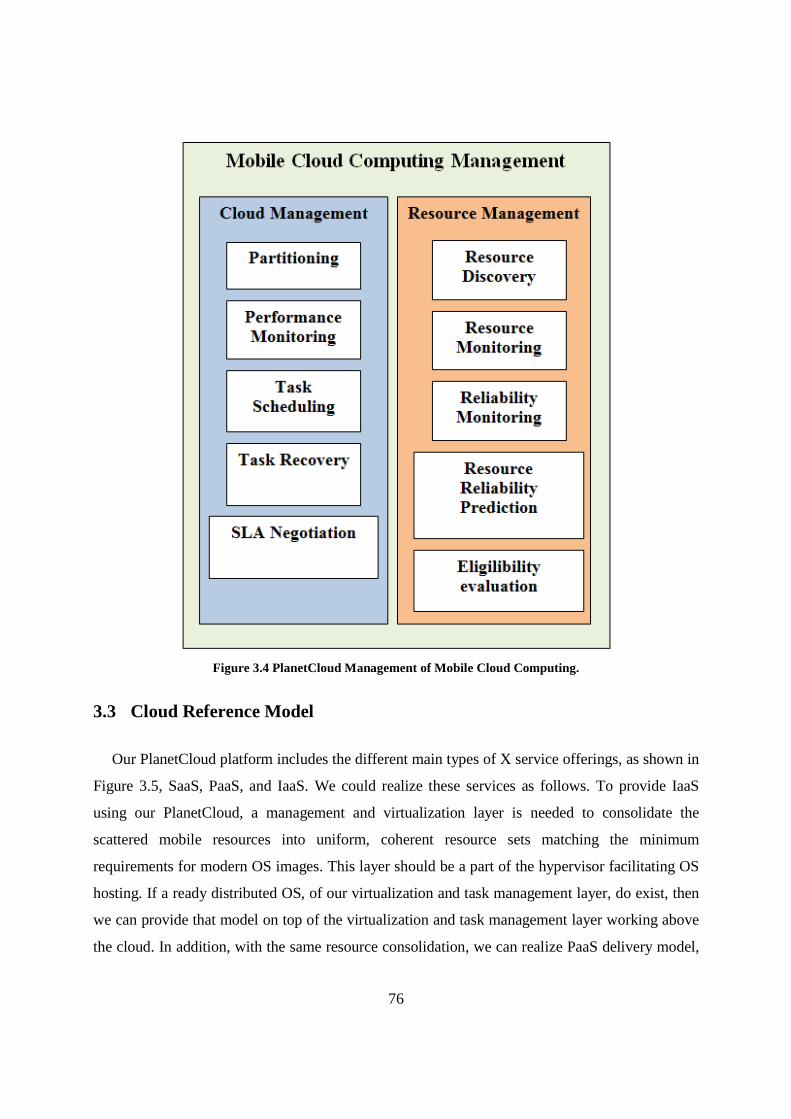
76

Figure 3.4 PlanetCloud Management of Mobile Cloud Computing.

3.3 Cloud Reference Model

Our PlanetCloud platform includes the different main types of X service offerings, as shown in

Figure 3.5, SaaS, PaaS, and IaaS. We could realize these services as follows. To provide IaaS

using our PlanetCloud, a management and virtualization layer is needed to consolidate the

scattered mobile resources into uniform, coherent resource sets matching the minimum

requirements for modern OS images. This layer should be a part of the hypervisor facilitating OS

hosting. If a ready distributed OS, of our virtualization and task management layer, do exist, then

we can provide that model on top of the virtualization and task management layer working above

the cloud. In addition, with the same resource consolidation, we can realize PaaS delivery model,

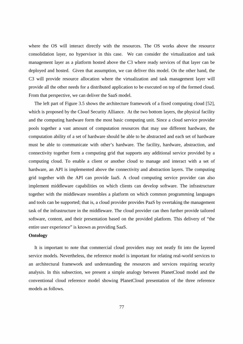
77

where the OS will interact directly with the resources. The OS works above the resource

consolidation layer, no hypervisor in this case. We can consider the virtualization and task

management layer as a platform hosted above the C3 where ready services of that layer can be

deployed and hosted. Given that assumption, we can deliver this model. On the other hand, the

C3 will provide resource allocation where the virtualization and task management layer will

provide all the other needs for a distributed application to be executed on top of the formed cloud.

From that perspective, we can deliver the SaaS model.

The left part of Figure 3.5 shows the architecture framework of a fixed computing cloud [52],

which is proposed by the Cloud Security Alliance. At the two bottom layers, the physical facility

and the computing hardware form the most basic computing unit. Since a cloud service provider

pools together a vast amount of computation resources that may use different hardware, the

computation ability of a set of hardware should be able to be abstracted and each set of hardware

must be able to communicate with other’s hardware. The facility, hardware, abstraction, and

connectivity together form a computing grid that supports any additional service provided by a

computing cloud. To enable a client or another cloud to manage and interact with a set of

hardware, an API is implemented above the connectivity and abstraction layers. The computing

grid together with the API can provide IaaS. A cloud computing service provider can also

implement middleware capabilities on which clients can develop software. The infrastructure

together with the middleware resembles a platform on which common programming languages

and tools can be supported; that is, a cloud provider provides PaaS by overtaking the management

task of the infrastructure in the middleware. The cloud provider can then further provide tailored

software, content, and their presentation based on the provided platform. This delivery of “the

entire user experience” is known as providing SaaS.

Ontology

It is important to note that commercial cloud providers may not neatly fit into the layered

service models. Nevertheless, the reference model is important for relating real-world services to

an architectural framework and understanding the resources and services requiring security

analysis. In this subsection, we present a simple analogy between PlanetCloud model and the

conventional cloud reference model showing PlanetCloud presentation of the three reference

models as follows.

78

Figure 3.5 Providing service models by using PlanetCloud.

• Realizing IaaS, which includes the entire infrastructure resource stack, on PlanetCloud is a

complicated task as the entire management platform and hypervisor layer should be working

through the virtualization and task management layer. The only piece of software that will be

statically available on the host is the CCDNA, which acts as a hypervisor, where its entire set of

services fractionalized and encapsulated in Cells. This model suits the mobile and resource

constrained and fractionalized nature of PlanetCloud resources. We can represent it from a

different perspective if we used a complicated version of the Cell built to provision all the features

of the regular hypervisor. However, such Cell will not have many of the useful features that the

fine-grained Cell had such as, low cost of failure, fast recovery, and resource efficient execution.

Additionally, this representation will limit the number of hosts that can cooperate with

PlanetCloud to those hosts with massive computational power. Ultimately, IaaS should provide a

set of APIs, which allow management and other forms of interaction with the infrastructure by

consumers with our model these API will be encapsulated as Cells too.

79

• PlanetCloud provides the PaaS model by virtualizing application development

frameworks, middleware capabilities, and functions such as database, messaging, and queuing,

and encapsulating it in Cells of the virtualization and task management layer. The CCDNA will

be hosting such services or part of these services, while the virtualization and task management

layer will seamlessly consolidate these parts emulating the natural behavior of these services

similar to the conventional model.

• We presented the SaaS model in details, as this is the simplest model to build in our case

given that the services will be built to suit service-execution model of our virtualization and task

management layer. The CCDNA represents a static middleware installed on all the hosts

facilitating Cell execution, and the software services are encapsulated as a number of Cells

operating above it. All the operation management, Cell deployment, revocation, failure recovery,

and other management tasks will be autonomously handled by the PlanetCloud cloud

management platform, the virtualization and task management layer, with no involvement from

the user or the cloud operator.

In this work, we only focus on the SaaS model as tasks are uniform where it is much easier to

represent. We build tasks as partitions that are deployed on ready cells, where users interact with

the application not the infrastructure.

The next sections detail the architecture of the proposed approach to provide resource and

cloud management in a dynamic environment, respectively.

3.4 Resource Management Platform

3.4.1 Resource Management at Compute Node

Figure 3.6 depicts the building blocks of a Compute Node. Resource management components

of the compute node are detailed as follows.

1) The iCloud interface: It is an interface between the agent and a user/ administrator, or

other systems, e.g., social networks and other database systems. A user/ administrator

uses the iCloud interface to manage all data in the spatiotemporal resource calendar. In

addition, the interface enables defining the settings required for a formed cloud.

80

Figure 3.6 Compute Node Building Blocks.

2) The knowledge unit: It consists of two subunits, a local spatiotemporal resource

calendar, which includes spatial and temporal information about the available

resources, and information bases, that contains predefined or on the fly policies created

by a cloud admin. The next chapter addresses the spatiotemporal resource calendar in

more details. Also, information bases contain information about the formed cloud, e.g.,

SLA, types of resources needed, amount of each resource type needed, and billing plan

for the service, etc.

3) Participant Resource Calendaring Service: PRCS includes a PCM which acts as a

service controller for managing the records of the local spatiotemporal resource

calendar. PCM interacts with the synchronizer to synchronize the spatiotemporal

resource calendar with other GRCSs. Also, PCM automatically monitors the internal

81

state of the participant’s resources. On the other hand, PRCS provides the trust

management services with the required data to perform trust and security operations.

4) The Input/Output (I/O) unit: It provides the required communications for different

activities such as cloud formation requests and responses.

The lowest layer, of the TA's building blocks, consists of the application, networking, and

computing resources, which are involved in the delivery of the service.

3.4.2 Resource Management at Control Node

The main building blocks of a Control Node are shown in Figure 3.7. The functionalities of

their resource management are described below.

1) The knowledge unit: A CA has a global spatiotemporal resource calendar which

includes spatial and temporal information, resource profiles, and event calendars of the

all available resources of a cloud’s participants. Therefore, the CA maintains the

overall picture of the resource capability within the cloud. The CA uses a global task

repository to store the all tasks within a cloud.

2) Group Resource Calendaring Service: Distributed GRCSs operate on the updated

data from participants’ calendars. These updated data are stored in a group

spatiotemporal resource calendar. GRCS and PRCS are the two primary types of

services forming a GRPS [66], for dynamic real-time resource harvesting, scheduling,

tracking and forecasting. GRCS comprises four types of modules: The Group Calendar

Manager module, the Synchronizer, the PS, and the Trust Management Services. GCM

acts as a service controller for managing records of group spatiotemporal resource

calendars. In addition, a calendar manager feeds the PS with the required data to

perform resource forecasting.

3) Collaborative Autonomic Resource Management System: We design our CARMS

architecture using the key features, concepts and principles of autonomic computing

systems to automatically manage resource allocation and task scheduling to affect

cloud computing in a dynamic mobile environment. More details about CARMS are

discussed in the next chapter.

82

Figure 3.7 Control Node Building Blocks.

3.5 Cloud Management Platform

PlanetCloud uses the trustworthy dynamic virtualization and task management layer to manage

the cloud tasks and the running applications on the cloud. The virtualization and task management

83

layer virtualizes the cloud resources creating a suitable execution environment for the

applications. The virtualization and task management layer uses the COA features to enable

applications to dynamically adapt to runtime changes in their execution environment. The details

of the COA will be illustrated in a later chapter. Such feature enables the virtualization and task

management layer to tolerate high frequency task preemption and migration that might be induced

by failures as a consequence of unexpected resource mobility or power failure. Due to the nature

of our resources the high level of heterogeneity is a major concern for task deployment and

migration. Using such vitalization architecture adequately resolves this issue.

The virtualization and task management layer enables the application to exchange real-time

status and recommendation messages with the host Cell for administrative purposes to enhance

the Cell local application awareness and to enable application driven adaptation. The

virtualization and task management layer uses these messages to guide the Cell runtime quality-

attribute manipulation towards accurate and prompt adaptation. Further, the virtualization and task

management layer collects, analyzes and trustworthy-share these messages and status reports,

constructing a real-time sharable global view of the Cell network.

The virtualization and task management layer enhances the system resilience by multiple

recovery modes to cover different application-requirements and host-configurations. The

virtualization and task management layer offers a prompt and accurate fine-grained recovery, hot-

recovery, for resourceful hosts executing critical applications, and a more resource efficient

course-grained recovery, cold-recovery, for less critical applications. In hot-recovery, the Cell can

have one or more fully-alive replicas on different mobile nodes which can do achieve virtually no

task failure downtime but on the account of increasing resource usage. The cold-recovery might

save some of the resources used by replicas, by deploying a replacement of the failed Cell, while

compromising some of the execution states, and increasing the failure downtime. The

virtualization and task management layer uses the COA loosely coupled features to allow

applications to seamlessly change their current active recovery modes based on context,

environment, or application-objective change.

The virtualization and task management layer is composed of a set of central powerful nodes

we will address them as servers. These servers collaborate autonomously to manage the whole

network of Cells. This platform is responsible for the organism creation “composition and

deployment of Cells”, management, the host side API(s) “CCDNA”, real-time monitoring and

84

evaluation of the executing Cells, and recovery management. Further, it provides the necessary

management tools for system administrators to manage, analyze, and evaluate the working

Cells/organisms. The virtualization and task management layer will act as an autonomously

managed resource and application virtualization platform of PlanetCloud.

3.5.1.1 Cloud Management at Control Node

All related task management procedures are performed on fixed control nodes as follows.

a) Auditing and Reputation Management Server (ARMS): Its main task is to monitor

outgoing or incoming Cell administrative messages for the lifetime of the Cell. This

information is used to assist evaluating the trustworthiness of the Cell. This server

cooperates with the recovery tracking servers and routing nodes to frequently evaluate

the Cell behavior for any malicious activities. This server will hold comprehensive

reports about each Cell for the lifetime of the Cell. A trust feedback will be generated

from ARMS and send to the Trust Management Services which helps in the evaluation

of the trustworthiness of a participant.

b) Recovery and Checkpoint Tracking Server (RCTS): This monitors and stores

checkpoints changes for all running Cells. Checkpoint updates are always enclosed as a

part of the Cell frequent beacon message updates. RCTS is also responsible for

reporting failure events by comparing the duration between consecutive beacon

messages to a certain threshold matching the reporting frequency settings of each Cell.

Failure events are validated by comparing the recently noticed reporting-delay for a

particular Cell to the average reporting-delay within its neighbors and other Cells

hosted on the same host. A Cell failure notice is reported to the global management

servers with the last known failure recovery settings, checkpoint, and variant settings to

start deploying replacement Cells.

c) Global Management Server (GMS): The main task of this server is to manage the

underlying COA infrastructure. GMS is responsible for Cell deployment, coordinating

between servers, facilitating and providing a platform for administrative control. GMS

is the only server authorized of issuing Cell termination signals. It can also force Cell

migration or change the current active recovery policy when needed. GMS is

responsible for assigning the infrastructure global policy, routing protocol, auditing

85

granularity, registering/revoking new hosts, and keeping/adjusting the host-platform

configuration file.

d) The Data-Warehouse Server (DWS): It is the main components of the infrastructure

that participates in the separation between the Data, Logic, and Physical-resources.

DWSs are distributed through the Cell network, they are responsible for holding and

maintaining all the data being processed, and any other sensitive data that the

management units want to store. All running Cells are not permitted to store sensitive

data on their local memory. All sensitive data has to be remotely stored in a specific

DWS through the dedicated data channel. DWSs synchronize their data independently.

e) Distributed Naming Server (DNS): It is responsible for resolving the real host IP/Port

mapping to the virtual Cell Id and organism names. The working Cells use this

mapping at runtime to direct incoming and outgoing communications. DNS is a major

player in the COA’s separation of concerns that enables virtually seamless, Cell

relocation, and workload transition in case of failure recovery. In case of Cell

movement, the DNS will be instructed by the GMS to maintain communication

redirection.

3.5.1.2 Cloud Management at Compute Node

GMS uses the resource-forecasting database to allocate resources for the Cells, of the

virtualization and task management layer, to be deployed on the Compute Node. The SM updates

the task repository by the tasks that should be executed, and the code variants associated with it.

The GMS encapsulates these variants into one of its Cells forming a suitable container that

matches one of the available resources. The selected resource will be the target of the Cell

deployment where the CCDNA is installed. That resource shall accept the deployment package

from the GMS, instantiate and execute the Cell.

In case of failure, or unavailability, the GMS will relocate the Cells into new active resource

seamlessly. All the concerns that might be involved with the task relocation will be autonomously

and seamlessly handled by the virtualization and task management layer.

86

A Scenario of Operation

This scenario presents an example that describes how our PlanetCloud provides a Software-as-

a-Service (SaaS), which is described by the following steps:

1) The user sends a request via the iCloud App interface to the CM, where the SM stores

the service request, its identifier and the application profile parameters, which describe

the resource needs. The user defines certain resource requirements such as hardware

specifications and the preferences on the QoS criteria.

2) The CM selects one of the predefined compute nodes and sends to it the service request

and the application profile parameters which describe the resource needs.

3) The Cloud Manager decomposes the requested service, upon receiving a cloud

formation request, to a set of tasks via its SM which define the parameters of a task and

its resource requirements. Then, tasks are encapsulated in cells by the GMS which

inform DWS to hold and maintain all the data being processed, and any other sensitive

data that the management units want to store. Each cell stores the identifier of other

cells it wants to communicate with. The communications among cells depends on the

dependency relationship among tasks executed on these compute nodes.

4) Each time a GMS finds the best participant of PlanetCloud that matches a task profile

of the request, by interacting with other CARMS and GRPS components, a request is

sent to that compute node to participate in a MAC.

5) In case of acceptance, the Resource Manager of the CARMS interacts with the GMS to

create a new CCDNA on that participant. Then, the GMS clones and sends the cell of

this task (which holds the task code, the request identifier, and the task profile) to the

TA running on the compute node.

6) The GMS creates new CCDNAs with cells for all tasks, or determines which TA each

cell should be sent to according to required resources. Once the cell is received, it starts

the execution of the included task.

7) As a compute node moves and changes its location, the Synchronizer on a TA

continuously updates the local/global spatiotemporal resource calendar on a TA and on

a CA, it communicates with, with the updated location information of the current TAs

running on it as well as the DNS.

87

8) Both ARMS and RCTS continuously monitor the execution of the task and the status of

resources in the cell. A malfunction could occur in a cell or a degradation of

performance may be obtained. Consequently, a GMS may decide that a cell should

leave the TA and migrate to another TA or clone a new cell and send it to another TA

to accomplish the task.

9) The result of a task is sent directly to the other tasks running on other TAs it

communicates with, which take this result as an input to accomplish their tasks.

10) A CM may interact with and send the Cell to be executed on other formed MACs via

distributed components of the PlanetCloud system. This may occur if the local

resources do not fit the requests in terms of the price, QoS requirements and reputation

of the resources, etc. Therefore, a CM can send the cell to other formed MAC that

matches with the local manage regulations. This would enable scalable resource-

infinite computing paradigm.

11) Once all tasks are accomplished, and the SM collects all results of tasks, the result of

the service request is now ready to send back to the user.

12) The SM maps the responses received from the TAs with the service requests from

users, and the result is sent back directly to the user.

3.6 Applicability of PlanetCloud

Cells run and are created in the tenant agents that act as execution environments, which should

be physically located on the same compute node where the CCDNA software is installed. The

tenant must be active on a node before the execution of Cells to provide the basic services that are

needed by Cells. For example, an agent provides Cells with a transportation service which enables

Cells to move to other execution environments by specifying the name of the target tenant agent.

In addition, a tenant agent manages the backup and monitor operations for the Cells reside on it.

Communications can be performed, among Cells or among Cells and other system

components, regardless of the location of Cells. Cells could be deployed on heterogeneous

computing nodes by exploiting the portability nature provided by agent platforms implemented

using Java programming language [109].

88

A simple prototype has been developed to implement simple and fast version of the Cell in

[105].The COA-Cell can be built with different techniques based on the targeted resource

virtualization depth.

3.7 Conclusion

Our definition of C3 as a consolidation of a vast number of the idle stationary and mobile

resources, for enabling both a new resource-infinite computing paradigm using cloud computing

over stationary and mobile nodes, and a true ubiquitous on-demand cloud computing. We

proposed PlanetCloud, a C3 management platform with an intrinsic support for highly-mobile

heterogeneously-composed and configured HMACs. PlanetCloud is powered by the following:

1) GRPS, a global resource positioning system which provides both the broad network

access and the measured service characteristics of a cloud model. To achieve these

characteristics, GRPS adopts a novel spatiotemporal calendaring mechanism with real-

time synchronization to provide a dynamic real-time scheduling and tracking of idle,

mobile and stationary, resources. A spatiotemporal resource calendar includes spatial

and temporal information about the available resources. GRPS forecasts the resource

availability, anytime and anywhere, by using a prediction service. This service makes

use of the analysis of calendaring data coupled with data from social networking and

other sources to improve the prediction accuracy of resource availability. The results of

resource forecasting enhance the HMAC resilience to failure by early discovery of all

different failures that might be encountered at different communications, resource

availability, or reputability levels. In addition, the GRPS provides a hierarchical zone

architecture with a synchronization protocol between different levels of zones to

provide the broad network access characteristic and to enable resource-infinite

computing;

2) CARMS, a collaborative autonomic resource management system which provides both

the on-demand self-service and the resource pooling characteristics, by interacting with

the GRPS, and by using its integral Proactive Adaptive List-based Scheduling and

Allocation AlgorithM (P-ALSALAM). P-ALSALAM algorithm efficiently selects

appropriate resource providers that could participate in a C3 based on many factors.

These factors include the future resource availability, spatial and temporal resource

89

information, resource utilization, available computing capabilities, and mobility pattern

of providers. Hence, this leads to low virtualization management overhead and

therefore enhance the hosted application performance. CARMS continuously monitors

the performance and workload of incoming applications. This helps in early error

detection, which lowering the risk of downtime. Therefore, CARMS provides system-

managed cloud services such as configuration, adaptation and resilience services

through transparent cooperative autonomic management of dynamic cloud resources,

services and cloud membership;

3) Trustworthy dynamic virtualization and task management layer, which provides the

rapid elasticity characteristic, by interacting with the GRPS and CARMS, and isolates

the hardware concern from the task management. Such isolation empowered

PlanetCloud to support autonomous task deployment/execution, dynamic adaptive

resource allocation, seamless task migration and automated failure recovery for

services running in a continuously changing unstable operational environment. The

virtualization and task management layer is composed of a set of central powerful fixed

nodes. These nodes collaborate autonomously to manage the whole network of micro

VMs. This platform is responsible for the composition and deployment of micro VMs,

management, the host side API(s), real-time monitoring and evaluation of the executing

micro VMs, and recovery management. Further, it provides the necessary management

tools for system administrators to manage, analyze, and evaluate the working micro

VMs. The virtualization and task management layer will act as an autonomously

managed resource and application virtualization platform of PlanetCloud. Micro VMs

are deployed to encapsulate executable application-partitions defined as code variants.

This separates logic, state and physical resource management. Applications can be

defined in one or more encapsulated variants. Such construction facilitates hiding the

heterogeneity of the underlying hardware resources from the application concern

enabling seamless deployment, distribution, and migration of application on the cloud

mobile nodes; and

4) iCloud App interface: It is a portable access application. It is an interface between the

agent and a user/ administrator, or other systems, which is used to manage all data in

the spatiotemporal resource calendar.

90

Chapter 4

4 PLANETCLOUD RESOURCE MANAGEMENT

In this chapter, we present the PlanetCloud resource management subsystems, GRPS and

CARMS that handle all the tasks related to the resource domain concerned with the

spatiotemporal resource allocation. We present the concept of both GRPS and CARMS and their

architectures.

4.1 Global Resource Positioning System (GRPS)

GRPS is a spatiotemporal calendaring system accessed via a portable “iCloud” application.

GRPS would enable the provisioning of, otherwise idle, stationary and mobile resources to effect

ubiquitous computing clouds. GRPS provides both the broad network access and the measured

service characteristics of a cloud model. To achieve these characteristics, GRPS provides a global

spatiotemporal resource calendar for dynamic real-time resource harvesting, scheduling, tracking

and forecasting.

In GRPS, each opt-in participant dynamically updates their resources in a spatiotemporal

calendar maintained by Participant Resource Calendaring Service (PRCS) and shared, in whole or

in part, through a distributed Group Resource Calendaring Service (GRCS).

GRPS aims to aid the formation of mobile computing clouds by providing a dynamic real-time

resource scheduling and tracking system that can be accessed through the iCloud. GPRS is

designed to access and maintain dynamic data from spatiotemporal calendars, social networking

and other sources to enhance resource discovery, forecasting and status tracking to provide access

to the right-sized cloud resources anytime and anywhere.

4.1.1 GRPS Architecture

The GRPS services and their interconnections are shown in Figure 4.1. GRPS comprises two

primary types of services: PRCS and GRCS. Modules of these services are detailed below.

91

4.1.1.1 Calendar Manager

It acts as a service controller for managing records of either local or group spatiotemporal

resource calendars. In addition, a calendar manager feeds the Prediction Service (PS) with the

required data to perform resource forecasting. Also, it provides the trust management services

with the required data to perform trust and security operations. The calendar manager interacts

with the synchronizer to synchronize the spatiotemporal resource calendar with other PRCSs and

GRCSs. The Participant Calendar Manager (PCM) module can automatically monitor the internal

state of the participant’s resources.

4.1.1.2 Synchronizer

There are participants who make changes to PRCSs, so periodic synchronization is needed to

push changes among PRCSs and GRCSs as well as among different levels of GRCSs. The

synchronizer is the unit, which periodically performs this synchronization and allows for bi-

directional and selective replication of records.GRPS synchronization has two aspects: Manual

synchronization of records, those are entered by a participant from the iCloud interface, between a

PRCS and a GRCS. Automatic synchronization of records, of resources those are dynamically

sensed and forecasted, among PRCSs and GRCSs.

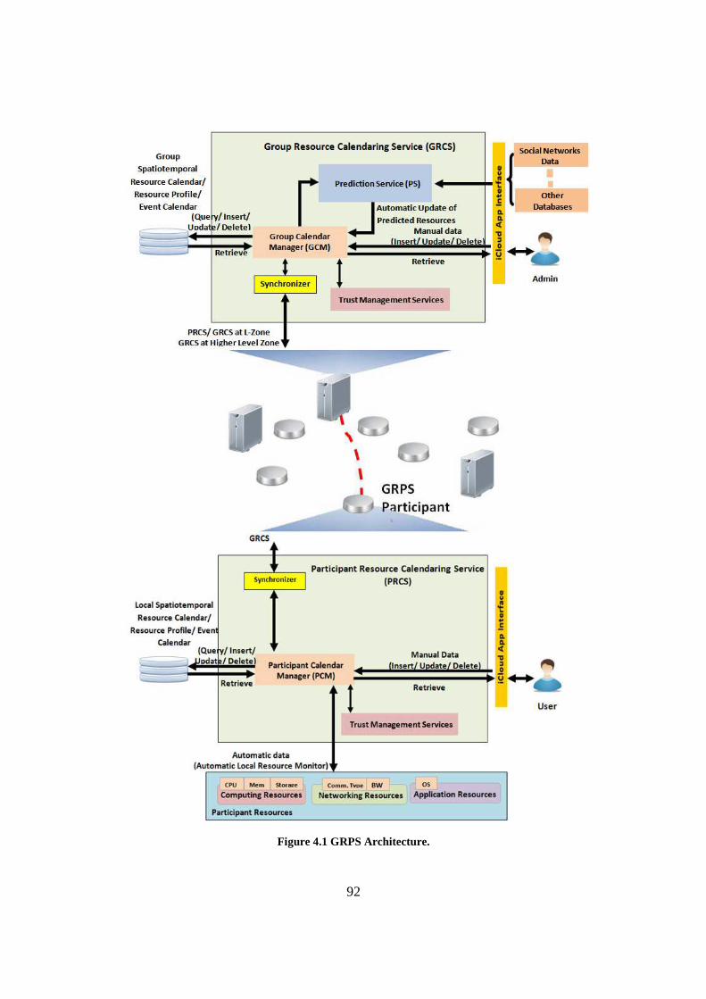
92

Figure 4.1 GRPS Architecture.

93

4.1.1.3 Prediction Service (PS)

The field of knowledge discovery in databases (KDD) is concerned with the development of

methods and techniques for extracting useful information, knowledge, from the rapidly growing

volumes of databases i.e. making sense of data. The application of specific data-mining methods

(algorithms) is the core of the KDD process for pattern discovery and extraction [110].

Association Rule Mining (ARM) is one of the most prominent data mining methods which

have a wider applicability. The main task of ARM is to discover associations or correlations

among the attributes in large databases [111].

Mainly, there are two types of goals of data mining (1) prediction, which some variables or

fields in the database to predict unknown or future values of other variables of interest; and (2)

description, which focuses on finding human-interpretable patterns describing the data [110].

Techniques of KDD have been successfully used in applications dealing with transactional and

relational data. However, extracting interesting patterns from spatial and temporal sets is more

difficult, due to the complexity of spatial and temporal data types and spatial relationships

changing over the time [112]. Additionally, all of the data mining query languages for KDD

treated separately the space and the time as they dealt with traditional, temporal, or spatial data

[112].

The state of the art in research shows four categories of solutions for ARM. They are

conventional association rule mining, time related association rule mining, spatial related

association rule mining, and spatial-temporal related association rule mining. Each category may

include one or more of the existing techniques which are applied on ARM. These techniques

include data mining methods, soft computing techniques, and evolutionary computation

techniques.

A. Conventional Association Rule Mining

• Data mining methods

Association rule mining algorithms which are applied on conventional association rule mining

include Apriori [113] that generate rules without time constraint. Also, Hash based algorithms

such as DHP [114] which focuses on mining sequential association rules in order to improve

efficiency of algorithm in terms of reducing execution time. Both APACS2 [115] and

QUANTMINER [116] are quantitative association rule based algorithms. They permit the user to

extract both positive and negative association rules. However, the previously mentioned data

94

mining methods did not focus on generating time based rules with spatial and temporal data set.

• Soft Computing Techniques

A fuzzy clustering algorithm, e.g. CBFAR [117], used cluster technique for fuzzy association

rules generation. It is defined for mining telecommunications customer and prospect databases.

Also, a fuzzy linguistic summary system [118] has been developed for mining time series data,

which is used to predict the on line utilization ranks of different resources.

B. Time Related Association Rule Mining


There is Apriori based method, T-Apriori [119], which is developed for temporal spatial

mining. However, this algorithm is restricted to generate time related rules in a range not in an

exact time so it may not be suitable for mobile cloud computing related applications.

Time based Association Rule Mining (TARM) is proposed in [111] to extract time based

association rules. Authors considered TARM more suitable for intelligent transportation

applications such as traffic prediction, travel time estimation, congestion prediction, etc. Such

that, these real world applications need time related prediction for near future traffic forecasting.

• Soft Computing Techniques

Neuro-fuzzy systems [120], [121] used in traffic related applications which are developed

using fuzzy auto regressive models, Hidden Markov models. These applications are used for

urban traffic flow prediction, traffic modeling, congestion control, traffic accident prediction, etc.

However, these systems do not consider the spatial dimension of data and they are employed

specifically for short-term traffic flow prediction. Also, they fail to extract large number of rules.

• Evolutionary computation Techniques

Genetic algorithms fail to extract sufficient amount of association rules as proposed in [122].

Also, genetic programming approach proposed in [123] can generate time related rules but

suffers with loose structures and bloating problem when it deals with dense databases.

C. Spatial Related Association Rule Mining


Spatial Pattern Discovery Algorithm (SPADA) proposed in [124] is used to discover spatial

association rules by using reasoning techniques. This algorithm is developed in the field of

Inductive Logic Programming. However, SPADA can’t process numerical data properly, where

data discretization of numerical features is performed with relatively large domain.

95

D. Spatial-Temporal Related Association Rule Mining


In [125], authors use data mining and propose Spatio-Temporal Ensemble Prediction (STEP)

technique that accurately predicts low traffic periods. STEP combines a spatio-temporal data

splitting and an ensemble prediction technique to achieve efficient network optimization for

saving energy. This could be accomplished by investigating the on the possibility to turn off

network nodes (cells), by network providers, fully or partly, in low traffic loads by predicting

very accurately low traffic periods.

Authors in [112] proposed a method based on the computation of neighborhood relationships

between geographical objects during a time interval. They mine spatio-temporal association

rules (STAR) that could be useful in improving the decision making process related to risk

prediction [112]. Authors only considered the case of discrete change. However, they don’t study

the continuous change, which results into motion, e.g. the position of a moving person.

In [126], authors proposed a Gradual-Spatio-Temporal rule Discovering (GSTD) algorithm in

which gradual pattern and spatio-temporal pattern are combined together to extract gradual-

spatio-temporal rules. However, this algorithm only considers the discovery of new interesting

moving object rules.

In [127] , authors presented a multi-space, real-time and robust human tracking system, that

exploits a multi-camera network monitoring the multi-space dynamic environment under

interest, detecting and tracking the humans in it. The deployed visual interactive tools provide

real-time spatio-temporal human presence analysis offering to the user the opportunity to capture

and isolate the areas/spaces with high human presence, the days and times of high human

presence, to correlate this information with the potential energy consumption and indicators such

as comfort.

All the previously mentioned ARM solutions did not consider a real world applications that a

collaborative computing cloud could take benefit from. The design of our system should consider

the spatial and temporal dimensions of our spatio-temporal calendaring database to discover

interesting patterns. Such that, a spatio-temporal related prediction is needed for short-term

and/or long-term resource forecasting. Additionally, there is a need to design a method that could

be able to extract large number of rules.

96

Spatio-Temporal Association Rule mining in Calendaring Mechanism

Let us define a set of records in spatio-temporal calendar, as transactions in

traditional database, contains a subset of the items, and each record has a unique ID.

Each record can be represented as a multi dimensional vector comprising elements that

describe attributes of computing capabilities, attributes of communication capabilities,

geometrical positions and temporal dimensions, respectively. Each element may have various

dimensions, e.g. geometrical position can have from one to three dimensions.

We depict that our method could include three phases:

The first phase calculates the spatial and resource sharing relationships among geographical

heterogeneous resource providers over time, by combining both gradual pattern and spatio-

temporal pattern. The results of this phase produces relationships with a reference cloud that

resource providers are participated. In the second phase, frequent item sets are generated that

match to a minimum threshold. Finally, we can use a spatio-temporal feature extractor module in

the third phase, for extracting of interesting spatiotemporal association rules.

Future direction for our prediction algorithm should study and compare the deployment of

algorithms.

A key module of the GRPS is a PS as shown in Figure 4.2. It uses different sources of data to

increase the forecasting precision of resource availability. We use different types of databases that

are related to the participant, (i.e. the group spatiotemporal resource calendar, event calendar, the

resource profile, data from social networks and other databases). PS contains three main processes

as follows:

a. Data preparation: Data may be collected and selected from different database inputs.

Cleaning and preprocessing are performed on the selected data set for removing

discrepancies, inconsistencies, and improving the quality of data set.

b. Knowledge extraction: It is used to find out the possible patterns and rules from existing

databases. Association Rules Mining Service is a major service of the PS, which is used

for turning the data of a participant into useful information and knowledge.

c. Prediction model: This uses the extracted knowledge, from both history and future data,

as an input of the prediction algorithm. This model gives a probabilistic value to the

expected availability of resources in the future.

97

PS delivers the data of resource availability in future to the calendar manager, which updates

them in a spatiotemporal resource calendar. These data can help in cloud maintenance.

Figure 4.2 Prediction Service.

4.1.1.4 Trust Management Services

Reputation is one measure by which trust among different participants of a C3 can be

quantified and reasoned about. Reputation systems can be used to manage reputation of mobile

nodes as resource providers, according to the QoS provided, as well as reputation of mobile nodes

as users, according to their usage of resources.

In our trust management service, as shown in Figure 4.3, automatic feedback, about

participants’ behavior are aggregated and distributed. In a C3, the resources allocated to a user’s

application are known to the user, as a CA, making it easy to obtain user’s feedback. This

feedback is an indication of the satisfaction a user achieves after obtaining a service. Thus, the

information of this feedback is used to create reputation about particular resource providers and

users. Reputation of resource providers could be used by our CARMS to improve allocation of

user tasks by selecting reputable mobile resource providers. While, reputation of users could be

used to achieve security level required by resource providers.

We integrate the trust management service as part of the GRPS to interact with CARMS and

help in selecting the resource providers based on their score of credibility to deliver the requested

computing capability. Integral to the trust management service is a reputation evaluator.

Trust Management Service provides a trust model which enables a symmetric trust relationship

between a participant and a GRCS. We quantify the trustworthiness of a participant in various

98

degrees of trust, which is expressed as a numerical range. The trust management services consist

of the following components.

1. Security Evaluator: evaluates the types of authentication and authorization mechanisms

considered in the security service. A numerical trust value, score of credibility, is

assigned for these mechanisms.

2. Reputation Evaluator: verifies the participant's response by comparing it with the data

of a participant which are saved in its group spatiotemporal resource calendar. The

result of this verification is evaluated by assigning a numerical trust value to a

participant. After, a participant finish execution of the assigned task, a CA sends a

feedback as an indication of the satisfaction a user achieves after obtaining a service.

The reputation evaluator assigns and adds the results of its evaluation to this feedback

to the total numerical trust value.

The more successful participation of a mobile node in a C3, the more credit a participant can

get in PlanetCloud related to its past behavior. The score of each mobile participant is an estimate

to its future credibility that the participant is reliable. These values might be used to improve both

reliability and fault tolerance of the cloud. A result a node will be accepted as a participant of a C3

if a participant owns at least the minimum threshold score.

Trust values of participants are stored and synchronized as records in both local and group

spatiotemporal resource calendars at PRCS and GRCS, respectively.

At time t, the score of credibility is computed by weighing the numerical trust value record in a

spatiotemporal calendar with a time decay weight. This would motivate the providers of mobile

resources to participate in a mobile cloud formation and not remain inactive for long period of

time.

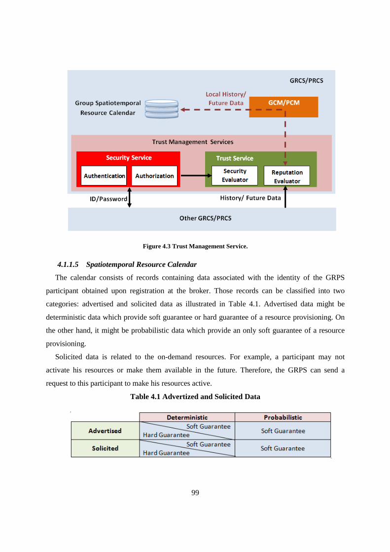
99

Figure 4.3 Trust Management Service.

4.1.1.5 Spatiotemporal Resource Calendar

The calendar consists of records containing data associated with the identity of the GRPS

participant obtained upon registration at the broker. Those records can be classified into two

categories: advertised and solicited data as illustrated in Table 4.1. Advertised data might be

deterministic data which provide soft guarantee or hard guarantee of a resource provisioning. On

the other hand, it might be probabilistic data which provide an only soft guarantee of a resource

provisioning.

Solicited data is related to the on-demand resources. For example, a participant may not

activate his resources or make them available in the future. Therefore, the GRPS can send a

request to this participant to make his resources active.

Table 4.1 Advertized and Solicited Data

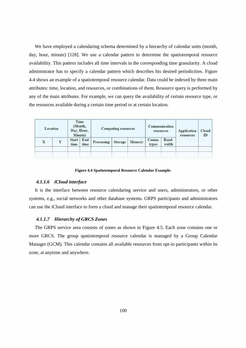
100

We have employed a calendaring schema determined by a hierarchy of calendar units (month,

day, hour, minute) [128]. We use a calendar pattern to determine the spatiotemporal resource

availability. This pattern includes all time intervals in the corresponding time granularity. A cloud

administrator has to specify a calendar pattern which describes his desired periodicities. Figure

4.4 shows an example of a spatiotemporal resource calendar. Data could be indexed by three main

attributes: time, location, and resources, or combinations of them. Resource query is performed by

any of the main attributes. For example, we can query the availability of certain resource type, or

the resources available during a certain time period or at certain location.

Figure 4.4 Spatiotemporal Resource Calendar Example.

4.1.1.6 iCloud interface

It is the interface between resource calendaring service and users, administrators, or other

systems, e.g., social networks and other database systems. GRPS participants and administrators

can use the iCloud interface to form a cloud and manage their spatiotemporal resource calendar.

4.1.1.7 Hierarchy of GRCS Zones

The GRPS service area consists of zones as shown in Figure 4.5. Each zone contains one or

more GRCS. The group spatiotemporal resource calendar is managed by a Group Calendar

Manager (GCM). This calendar contains all available resources from opt-in participants within its

zone, at anytime and anywhere.

101

Figure 4.5 Distributed GRCS s and zones.

4.1.1.8 GRPS-Sync Protocol

GRPS has its own synchronization protocol, GRPS-Sync, as shown in Figure 4.6 to

synchronize records of spatiotemporal resource calendars among PRCSs and GRCSs as well as

among different levels of GRCSs. After a participant discovers an appropriate GRCS server

within its local zone, it needs to log into the system using the participant’s access privileges.

Subsequent to authentication, the participant becomes connected to the GRPS system, and

authorization mechanism is done immediately upon connection. The participant synchronizes his

own local spatiotemporal calendar with the group spatiotemporal resource calendar of the

discovered GRCS. A sequence of transactions is generated by GRPS-Sync containing

delete/insert/update statements to fix discrepancies at the destination GRCS server to bring the

source and destination spatiotemporal resource calendars into convergence. The above procedure

is also implemented to synchronize group spatiotemporal resource calendars between GRCSs.

102

Figure 4.6 PRCS to GRCS Synchronization.

There are participants who make changes to PRCSs, so periodic synchronization is needed to

push changes among PRCSs and GRCSs as well as among different levels of GRCSs. The

synchronizer is the unit, which periodically performs this synchronization and allows for bi-

directional and selective replication of records.

GRPS synchronization has two aspects:

• Manual synchronization of scheduled records from the local spatiotemporal resource

calendar in PRCS to the group spatiotemporal resource calendar in the GRCS. Only

records, those are originated by a participant from iCloud interface, will be updated.

• Automatic synchronization of group spatiotemporal resource calendars among

different GRCSs as well as automatic synchronization of automatic updated records,

of dynamically sensed and forecasted resources, among PRCSs and GRCSs.

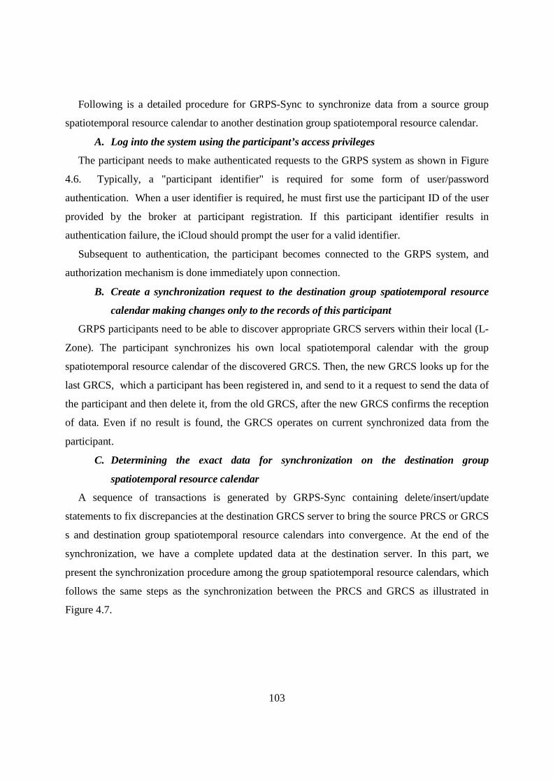
103

Following is a detailed procedure for GRPS-Sync to synchronize data from a source group

spatiotemporal resource calendar to another destination group spatiotemporal resource calendar.

A. Log into the system using the participant’s access privileges

The participant needs to make authenticated requests to the GRPS system as shown in Figure

4.6. Typically, a "participant identifier" is required for some form of user/password

authentication. When a user identifier is required, he must first use the participant ID of the user

provided by the broker at participant registration. If this participant identifier results in

authentication failure, the iCloud should prompt the user for a valid identifier.

Subsequent to authentication, the participant becomes connected to the GRPS system, and

authorization mechanism is done immediately upon connection.

B. Create a synchronization request to the destination group spatiotemporal resource

calendar making changes only to the records of this participant

GRPS participants need to be able to discover appropriate GRCS servers within their local (L-

Zone). The participant synchronizes his own local spatiotemporal calendar with the group

spatiotemporal resource calendar of the discovered GRCS. Then, the new GRCS looks up for the

last GRCS, which a participant has been registered in, and send to it a request to send the data of

the participant and then delete it, from the old GRCS, after the new GRCS confirms the reception

of data. Even if no result is found, the GRCS operates on current synchronized data from the

participant.

C. Determining the exact data for synchronization on the destination group

spatiotemporal resource calendar

A sequence of transactions is generated by GRPS-Sync containing delete/insert/update

statements to fix discrepancies at the destination GRCS server to bring the source PRCS or GRCS

s and destination group spatiotemporal resource calendars into convergence. At the end of the

synchronization, we have a complete updated data at the destination server. In this part, we

present the synchronization procedure among the group spatiotemporal resource calendars, which

follows the same steps as the synchronization between the PRCS and GRCS as illustrated in

Figure 4.7.

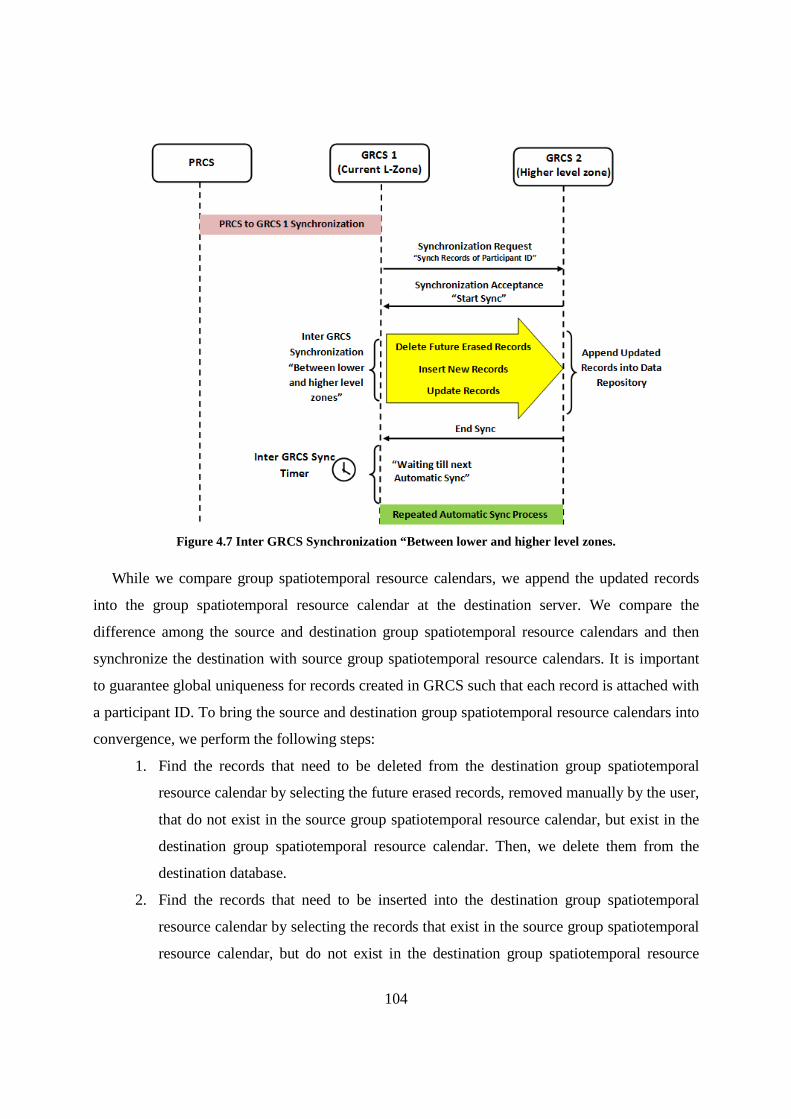
104

Figure 4.7 Inter GRCS Synchronization “Between lower and higher level zones.

While we compare group spatiotemporal resource calendars, we append the updated records

into the group spatiotemporal resource calendar at the destination server. We compare the

difference among the source and destination group spatiotemporal resource calendars and then

synchronize the destination with source group spatiotemporal resource calendars. It is important

to guarantee global uniqueness for records created in GRCS such that each record is attached with

a participant ID. To bring the source and destination group spatiotemporal resource calendars into

convergence, we perform the following steps:

1. Find the records that need to be deleted from the destination group spatiotemporal

resource calendar by selecting the future erased records, removed manually by the user,

that do not exist in the source group spatiotemporal resource calendar, but exist in the

destination group spatiotemporal resource calendar. Then, we delete them from the

destination database.

2. Find the records that need to be inserted into the destination group spatiotemporal

resource calendar by selecting the records that exist in the source group spatiotemporal

resource calendar, but do not exist in the destination group spatiotemporal resource

105

calendar. Then, we insert them into the destination group spatiotemporal resource

calendar.

3. Find the records that need to be updated in the destination group spatiotemporal

resource calendar by selecting the records that are differed from the source &

destination group spatiotemporal resource calendars. Then, we update them in the

destination group spatiotemporal resource calendar with the source database data.

Synchronize the source and destination group spatiotemporal resource calendars.

Both comparison and synchronization operations are done at a single query. In addition,

records are processed (deleted, inserted & updated) in a bulk manner.

The above procedure is implemented to synchronize a group spatiotemporal resource calendar,

which means that the group spatiotemporal resource calendar is locked while the synchronization

is in process. This could be a drawback because of the time-consuming process in case we have

large data to be synchronized at a destination group spatiotemporal resource calendar.

Communication overhead due to synchronization is measured during our evaluation for the

GRPS-Sync. Improve the performance of GRPS-Sync by reducing the synchronization execution

time and communication overhead are main challenges.

As a distributed system, more than one GRCS can execute a sequence of transactions at the

same time.

To prevent conflict at the data level, we do not allow modifying records at two locations, the

data of any participant only found in one location at any level (i.e., PRCS, or GRCS levels). If a

participant moves to another location, the new GRCS in its zone sends a request to the old GRCS

to delete the participant data after synchronization is done.

The size of a local spatiotemporal resource calendar could be limited by either the age of

timestamp of the entry or by the size of the saved data. On the other hand, the storage capacity of

GRCS is bigger than PRCS. Therefore, the history of the participant has more records in GRCS

than PRCS.

Full and Selective synchronization: GRCS can be configured to synchronize selective data

records. It can be configured with specific classes of current and future data only among different

levels of GRCSs, but full synchronization is performed, including the history data as in case of a

participant changes its zone, among the same level of GRCS. We use the timestamp of records

and compare it with the last synchronization time to identify the newly created or updated records

106

after the last synchronization. A group spatiotemporal resource calendar stores the Last

Synchronization Time (LST) on its database.

4.2 Collaborative Autonomic Resource Management System (CARMS)

Every mobile node with a connection to the C3 can be a user or a provider of the C3’s

resources. The mobile nodes freely using or providing the resources available are considered to be

self-directing, self-organizing and self-serving. But the providers of mobile resources can find it

difficult to remain motivated to participate in a C3. On the other hand, selecting the right resource

in a C3 environment for any submitted applications has a major role to ensure QoS in term of

execution times and performance. On the other hand, reputation mechanism acts as a

complementary approach which relies on analyzing the history of the quality of service provided

to do resource selection for submitted applications. However, most of the proposed approaches

[129][130]consider each participant locally stores its own rating values of reputation that would

be a threat when that self storage reputation information is not reachable. Consequently, there is a

need for a solution that globally monitors the runtime performances of services and provides

reputable mobile resource providers. In general, there is a need to know how a provider of mobile

resources is suitable to participate and form a C3.

In this section, we present our proposed CARMS architecture, which automatically manages

task scheduling and reliable resource allocation to realize efficient cloud formation and computing

in a dynamic mobile environment. CARMS utilizes our proposed GRPS to track current and

future availability of mobile resources. CARMS utilizes our new opt-in, prediction and trust

management services to realize reliable C3 formation and maintenance in a dynamic mobile

environment.

In addition, we present CARMS’s associated Proactive Adaptive List-based Scheduling and

Allocation AlgorithM (P-ALSALAM) for adaptive task scheduling and resource allocation for

C3. P-ALSALAM uses the continually updated data from the loosely federated GRPS to

automatically select appropriate mobile nodes to participate informing clouds, and to adjust both

task scheduling and resource allocation according to the changing conditions due to the

dynamicity of resources and tasks in an existing cloud. Consequently, this algorithm dynamically

maps applications' requirements to the currently or potentially reliable mobile resources. This

would support formed C3 stability in a dynamic resource environment.

107

4.2.1 CARMS Architecture

In this section, we describe our CARMS integral to PlanetCloud. In PlanetCloud, a cloud

application comprises a number of tasks. At the basic level, each task consists of a sequence of

instructions that must be executed on the same node. Tasks of a submitted application are

represented by nodes on a Directed Acyclic Graph (DAG) which is addressed in the next

subsection. The set of communication edges among these nodes show the dependencies among

the tasks. The edge ��,�joins nodes �� and �� , where �� is called the immediate predecessor of ��, and �� is called the immediate successor of �� . A task without any immediate predecessor is

called an entry task, and a task without any immediate successors is called an exit task. Only after

all immediate predecessors of a task finish, that task can start its execution.

CARMS manages clouds of mobile or hybrid resources (resources of mobile and fixed nodes).

A CARMS-managed cloud consists of resources of micro virtual machines running on

heterogeneous nodes. Such resources meet the cloud applications’ requirements. CARMS

attempts to provide a C3 with a sufficient number of real mobile nodes, such that in case of

failure, a redundant node can be ready to substitute the failed node.

A CA, as a requester to form a cloud, manages the formed cloud by keeping track of all the

resources joining its cloud using the updates received from the GRPS.

We design our CARMS architecture using the key features, concepts and principles of

autonomic computing systems as shown in Figure 4.8. Components of the CARMS and GRPS

architectures interact with each other to automatically manage resource allocation and task

scheduling to affect cloud computing in a dynamic mobile environment.

CARMS interacts with the information-base which maintains the necessary information about

a requested cloud. The information-base includes user information, e.g., personal information and

subscribed services, etc. Also, it contains information about the formed cloud, e.g., SLAs, types of

resources needed, the amount of each resource type needed, and billing plan for the service.

CARMS performs all required management functions on a CA using the components detailed

below.

1) Cloud Manager (CM): It provides a self-controlled operation to automatically take

appropriate actions according to the results of the evaluation received from the

Performance Analyzer, described below, due to variations in the performance and

workload in a cloud environment. The Cloud Manager manages interactions to form,

108

maintain and disassemble a cloud. A Cloud Manager comprises the following four

components:

a) Service Manager (SM): A SM stores the request and its identifier. The SM

maps the responses received from the participants with the service requests

from users, and the result is sent back directly to the user. The user defines

certain resource requirements such as hardware specifications and the

preferences on the QoS criteria. The Cloud Manager decomposes the

requested service, upon receiving a cloud formation request, to a set of tasks.

Tasks of a requested service need to be allocated to real mobile resources. The

Resource Manager handles the resource allocation on real mobile nodes using

its Resource Allocator component. Also, the Resource Allocator obtains the

required information about the available real resources from participants by

interacting with a GRCS. The Resource Allocator interacts with the registry of

CA to store and retrieve the periodically updated data related to all

participants within a cloud. The Cloud Manager interacts with servers of the

virtualization and task management layer to assign a set of virtual resources in

a cell to these tasks according to the received SLA information from the

Cloud Manager.

b) Policy Manager (PoM): The PoM prevents conflicts and inconsistency when

policies are updated due to changes in the demands of a cloud. In addition, it

distributes policies to other CARMS components.

c) Participant Manager (PrM): The PrM manages the interaction between a cloud

requester and resource providers, the cloud participants, to perform a SLA

negotiation. Once the negotiation is successful, the participant control

function updates the billing information and SLA of a participant in the

Information Bases.

d) Resource Manager (RM): Real mobile resources need to be allocated to the

requested application. On the other hand, tasks of a requested application need

to be scheduled. The Resource Manager component handles the resource

allocation and task scheduling processes on real mobile nodes. The Resource

Manager consists of two main units:

109

1. Resource Allocator: allocates local real resources for a task. Also, the

resource allocator obtains the required information about the available

real resources from (potential) participants by interacting with a GRCS

of GRPS system. The Resource Allocator interacts with the registry of

CA to store and retrieve the periodically updated data related to all

participants within a cloud.

2. Task Scheduler: distributes tasks to the appropriate real mobile nodes.

2) Monitoring Manager:

It consists of the following two units:

A. Performance Monitor: It monitors the performance measured by monitoring agents at

resource providers. Then, it provides the results of these measurements to the

Performance Analyzer component.

B. Workload Monitor: The workload information of the incoming request is periodically

collected by the Workload Monitor component.

3) Performance Analyzer: It continually analyzes the measurements received from the

Monitoring Manager to detect the status of tasks and operations, and evaluate both the

performance and SLA. The results are then sent to both the Cloud Manager and the

Account Manager.

4) Account Manager: In case of violation of SLA, adjustments are needed to the bill of a

particular participant. These adjustments are performed by the Account Manager

component depending on the billing policies negotiated by the requester of cloud

formation.

110

Figure 4.8 CARMS Architecture.

4.2.2 Proactive Adaptive Task Scheduling and Resource Allocation Algorithm

4.2.2.1 Application Model

For simplicity, we start with a basic application model. The load of submitted application is

defined by the following parameters: the number of submitted applications, the number of tasks

per application, and the settings of each task. For example, the input and the output file size of a

task before and after execution in bytes, the memory and the number of cores required to execute

this task, and the execution time of a task.

Based on the criteria for selection, we mainly define two matrices: Criteria costs matrix, C, of

size v ×p, i.e., c�,�gives the estimated time, cost, or energy consumption to execute task v�on

111

participant node p�; and a R matrix, of size p × p, which includes criteria costs per transferred

byte between any two participant nodes. For Example, time or cost to transfer n bytes of data from

task v�, scheduled on p�, to task v�, scheduled on p�. As an example of time-based selection criteria, a set of unlisted parent-trees is defined from the

graph where a Critical-Node (CN) represents the root of each parent-tree. A CN refers to the node

that has zero difference between its Earliest Start Time (EST) and Latest Start Time (LST).The

EST of a taskv� is shown in (1). It refers to the earliest time that all predecessor tasks can be

completed. ET is the average execution time of a task.

EST(v�) = max��∈��(��){ EST(v ) + ET(v )}(1) Where ET(v ) is the average execution time of a task v , and pred(v�) is the set of immediate

predecessors of v�. The LST of a task v�is shown in (2).

LST(v�) = max��∈%&''(��){ LST(v )} − ET(v�)(2) Where succ(v�) is the set of immediate successors of v�. 4.2.2.2 Resource Model

Our cloud system represents a heterogeneous environment since the mobile nodes have

different characteristics and capabilities, The total computing capability of the real mobile nodes,

hosts, within a cloud is a function of the number of hosts within a cloud and the configuration of

their resources, i.e., memory, storage, bandwidth, number of CPUs/Cores, and the number of

instructions a core can process per second.

4.2.2.3 MAC Formation using PlanetCloud

The MAC formation process can then be started by a CA by submitting an application which

details the preferred number participants, duration, etc. To form a MAC, we need to find suitable

participants during a node filtering phase as a shown in Figure 4.9. In node filtering phase, data is

needed from prospective participants in three categories: i) future availability, ii) reputation, and

iii) preferences. Data gathered in a node filtering phase enables the Resource Manager to form a

cloud which aims at increased reliability as an outcome.

112

Figure 4.9 Parallel task execution in MAC.

Participants willing to participate in the MAC can submit the required data to the CARMS

Resource Manager of a CA. All data are assessed, which results in a measure of fit between

participants and submitted applications.

The data required are already gathered such that the PS delivers the data of resource

availability in future to the calendar manager of a PRCS. Also, reputation data of resource

providers are obtained as the score of credibility provided by the trust management service of

their PRCSs. The preferences of resource providers are obtained from the knowledge unit of the

participants. The assessment of Preferences of participants determines the overlap between the

cloud characteristics and a participant related preferences. If they do not overlap, a participant will

not be included in a MAC formation, e.g., when a participant only want to participate in a traffic

management cloud, while the requested MAC will provide a multimedia services, thus this two

participant will never be included in a MAC. As a first step in the MAC formation process, the

preferences assessment can limit the number of resource providers to be considered. However,

113

resource providers could negotiate preferences and change them. After this first step is completed,

the cloud formation process continues with the reputation and future availability data. An example

of these interactions is illustrated in Figure 4.10, which depicts the procedures of cloud formation.

However, the main focus of this work is on how MAC can be formed when the data required is

already gathered. In this part, we only briefly introduce how the assessments are designed to

work.

We define general MAC formation rules are for targeting specific outcomes. Mainly, three

general MAC formation rules are defined, which enable the Resource Manager to form clouds

that are aimed at increased reliability as an outcome. Then, we translated the rules into MAC

formation expressions.

Assuming the data from the resource availability and reputation assessments and the

characteristics of requested MAC “preferred cloud size and duration” are available, the Resource

Manager combines the two separate sets of data by following particular MAC formation rules.

We consider prior research findings on MAC formation in the design of these rules. We present

the general rules we deduced for forming clouds suited to achieve a reliable cloud. Based on the

general rules, we present two MAC formation expressions.

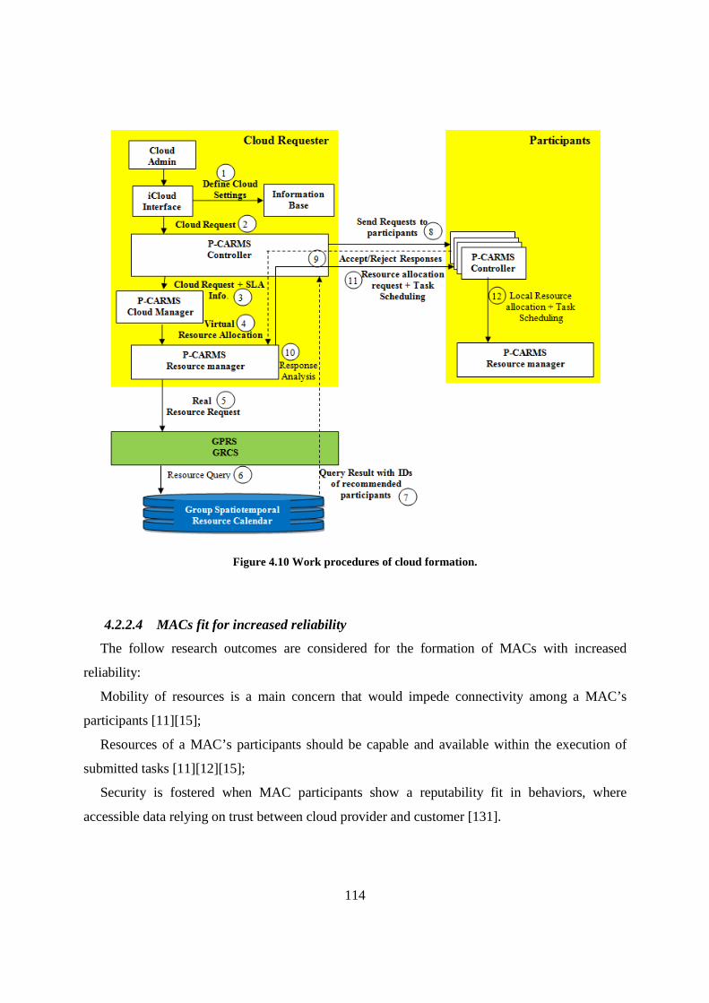
114

Figure 4.10 Work procedures of cloud formation.

4.2.2.4 MACs fit for increased reliability

The follow research outcomes are considered for the formation of MACs with increased

reliability:

Mobility of resources is a main concern that would impede connectivity among a MAC’s

participants [11][15];

Resources of a MAC’s participants should be capable and available within the execution of

submitted tasks [11][12][15];

Security is fostered when MAC participants show a reputability fit in behaviors, where

accessible data relying on trust between cloud provider and customer [131].

115

The general MAC formation rule we deduce from these findings is: Reliability is fostered

when participants show high levels of preferences, resource availability and trust between

resource providers and a CA for the requested MAC.

Based on this rule, we mainly define three matrices: Criteria preferences matrix, Pr, of size v

×p, i.e., Pr�,� gives the preferences to execute task v�on participant nodep�; a T matrix, of size p

×p, which includes trust score between any two participant nodes; and a Av matrix, of size v ×p,

which includes criteria availability of a participant node p� from the time a task v� has been

delivered to it till results are submitted to another participants. For example, Av�,� equals 0 when

the resources of a participant node p� is not available at least for a period of time required to

receive data of task v�, execute this task and submit its results.

We translate this rule into a MAC formation expression for reliable cloud participants as

shown in (3). When applied, it determines which participants have the highest average reliability

scores.

kj,ji,ji, T*APr_

PrTAPi WvW

MaxWFitR +∗+∗=

(3)

Where FitRi is the fitness of a participant i for reliability outcomes, Max_Pr is the maximum

possible preferences score of a submitted task, Tj,k is the trust score between node j and node k,

and WP, WA, WT are weights.

After the node filtering phase, task scheduling and resource allocation algorithm will come into

action to schedule and allocate the tasks of given applications to reliable nodes.

4.2.2.5 Proposed Algorithm

We propose a generic GRPS-driven algorithm for the task scheduling and resource allocation:

Proactive Adaptive List-based Scheduling and Allocation AlgorithM (P-ALSALAM) for mobile

cloud computing. P-ALSALAM supports the stability of a formed cloud in a dynamic resource

environment. Where, a certain resource provider is selected to run a task based on resource

discovery and forecasting information provided by the GRPS. The algorithm consists of two

phases: initial static scheduling and assignment phase, and an adaptive scheduling and

reallocation phase which are detailed as follows.

116

A. Initial static scheduling and assignment phase

After, the information of virtual resources is sent to the Resource Manager for the appropriate

real mobile nodes’ resource allocation, the Resource Manager uses its Resource Allocator unit,

which interacts with the GRPS to find the available resources of every possible node a CA could

reach. GRPS provides the requester of a cloud with the information that matches the application

requirements. The information includes location, time and the computing capabilities, future

availability of these resources, and reputation and preferences of the providers of these resources.

This information affects matrices of criteria for node selection. Based on the next waypoint, a

destination obtained from GRPS, of each mobile node and the updated location of the CA, we can

estimate which mobile nodes will pass through the transmission range of the CA.

After filtering node phase of nodes, a priority is assigned to a node depending on the criteria of

selection. For example, in a time-based approach, we may select a host such that the highest

priority is given to the nodes which are located inside the transmission range of a CA, followed by

the nodes which are located outside this transmission range and will cross it, and finally to the rest

of the nodes. Within each group, nodes are listed in descending order according to the available

computing capabilities, e.g. their number of cores or CPUs. Nodes, with the same computing

capabilities, are listed in descending order according to the time they will spend in the

transmission range of a CA. This could minimize the overall execution and communication time.

As a result, a host list, H, is formed based on the priorities as shown in Algorithm 1, in Figure

4.11.

The CA sends the cloud formation requests, through its Communicator unit, to all resource

providers to in the list of hosts H. According to the (earliest) responses received about resource

available time from all responders and the criteria of selection, the responders’ IDs are pushed by

the Resource Manager in increasing order of parameters which reduce their costs. For example,

the responding node,R �., with the minimum sum of Expected Computation Time (ECT) of a

task and Expected Ready Time (ERT) of a node is on the top of Responders Stack (RS), top(RS).

The expected ready time for a particular node is the time when that node becomes available after

being connected with their peers and having executed the tasks previously assigned to it. This

could reduce the queuing delay and therefore enhance the overall execution time.

The Task Scheduler unit of the resource manager assigns and distributes the task at the top of

the list of tasks L, top (L) to the host at the top of responders stack RS, top(RS).

117

Figure 4.11 Initial task scheduling and assignment based on priorities.

B. Adaptive scheduling and reallocation phase

The actual measures, e.g., time, cost or energy, required to finish a task may differ from the

estimated due to the mobility of hosts, the resource contention and the failure of mobile nodes.

For example, the mobility of hosts affects the actual finish time of a task due to the delay a host

takes to submit task results to other hosts in a MAC.

The Estimated Finish Time of a task v� on a node p�, EFT(v�, p�), is shown in (4), where ERAT

is the earliest resource available time.

EFT(v�, p�) = min{ERT(v�, p�) + ECT(v�, p�)}(4)

118

We propose an adaptive task scheduling and resource allocation phase to adjust the resource

allocation and reschedule the tasks dynamically based on both the updated measurements,

provided by the Monitoring Manager, as well as the evaluation results performed by the

Performance Analyzer.

The Monitoring Manager aggregates the information about the current executed tasks

periodically, as a pull mode. Due to the dynamic mobile environment, hosts of a cloud update the

Monitoring Manager with any changes in the status of their tasks, as a push mode. Also, hosts

periodically update the cloud registry of a CA with any changes in the status of resources.

Consequently, the Performance Analyzer could re-calculate the estimated measures of the

submitted tasks. As a result, tasks and resources could be rescheduled and reallocated according

to the latest evaluation results and measurements.

The Monitoring Manager of CARMS aggregates the information about the current executed

tasks periodically, as a pull mode. Due to the dynamic mobile environment, hosts of a cloud

update the Monitoring Manager with any changes in the status of their tasks, as a push mode.

Also, hosts periodically update the cloud registry of a CA with any changes in the status of

resources, e.g. in case of failure. Consequently, the Performance Analyzer could re-calculate the

estimated measures of the submitted tasks. As a result, tasks and resources could be rescheduled

and reallocated according to the latest evaluation results and measurements.

In algorithm 2, in Figure 4.12, a rescheduling threshold is predefined by the Performance

Analyzer such that tasks and resources could be rescheduled and reallocated periodically. If a

successor does not receive results of a task from its immediate predecessor within a period of time

equals a predefined rescheduling threshold,R45��%56��, then the Monitoring Manager of the CA

forms a task list, E, which contains the tasks needed to be scheduled. The Monitoring Manager of

the CA informs the Performance Analyzer to re-calculate the EFT of a task, top(E). The EFT is

computed according to the latest information obtained from the GRPS and the Monitoring

Managers of participants.

As a result, The Resource Manager interacts with the GRPS to find the available resources of

every possible node a CA could reach, which match the task requirements.

A priority is assigned to a node depending on the criteria of selection defined in the initial

static phase. Also, the responders’ IDs are pushed by the Resource Manager in increasing order of

parameters which reduce their costs, e.g. EFT(v�, p�). The Task Scheduler unit of the resource

119

manager, in the CA, assigns and distributes the task at the top of the list of tasks E, top(E) to the

host at the top of responders stack RS, top(RS).

Figure 4.12 Adaptive task scheduling and assignment based on priorities.

4.3 Evaluation

In this chapter, we start our evaluation by providing an analytical model to evaluate the

performance of GRPS in a Vehicular Cloud (VC) environment. This evaluation helps in

determining the parameters that could be used to adapt the performance of a response of the

GRPS and its capability to locate the required resources. Then, we perform a simulation

evaluation for CARMS and its integral P-ALSALAM algorithm. This evaluation is mainly

performed to show how the CARMS could support formed cloud stability in a dynamic resource

environment.

120

4.3.1 Performance Metrics

We use several metrics to evaluate the performance of our PlanetCloud and its subsystems.

Some of these metrics are used to compare the efficiency of applying different resource allocation

algorithms. Metrics are summarized as follows.

1) The resource request-response time, which is the amount of time a user takes to receive

a response which contains the status of each available resource provider in terms of

accepting, refusing, answering or not answering the request of utilizing its resources.

2) The average application execution time, which is the time elapsed from the application

submission to the application completion.

3) The MTTR, which is the time to detect the failure plus the time to make the backup

live.

4.3.2 Analytical Study of Applying GRPS in a Vehicular Cloud

Intervehicle communication (IVC) enables vehicles to exchange messages within a limited

transmission range and thus self-organize into dynamical vehicular ad hoc networks. However,

stable connectivity among vehicles is rarely possible. Therefore, an alternative mode has emerged

in which messages are stored by relay vehicles and forwarded to other vehicles when possible at a

later time. Many analytical models [132][133][134][135]have been proposed to study the quality

of IVC strategy for message forwarding in terms of message transmission times and related

propagation speeds.

The following subsections present our proposed model for determining the parameters that

could be used to adapt the performance of a response of the GRPS. We adopt these previously

validated models as a base for our model. The presented model is built to match our scenario

presented below. Latter, we used this model to evaluate the performance of GRPS in term of the

resource request-response time.

In this part of evaluation, a VC scenario is considered as a MCC that utilizes a powerful on-

board computers augmented with huge storage devices hosted on vehicles acting as networked

computing centers on wheels.

We consider a participant as a vehicle that moves on a two-lane bi-directional road as a one–

dimensional movement. The road is partitioned into adjacent linear zones that might be different

in length d8(km) as shown in Figure 4.13.

121

Figure 4.13 Linear Zones.

A participant is located in a certain zone, z. We consider a calendar with a time period,q, as the

finest granularity. We assume homogeneous traffic flows in each zone within each time periodq, those are characterized by the zone average velocities μ8 and the vehicle density β8(vehicles/km).

By virtue of the assumed average velocities, a vehicle does not leave the zone during this time

periodq , and the maximum velocity is limited by the maximum speed allowed in a road.

Otherwise, the vehicle densityβ8 in a zone varies with time as depicted in Figure 4.14.

<=(>) = ?@(A)B@ (1)

N8(t) is the total number of node located in a zone z at a given time period q, which can be

obtained directly from the spatiotemporal calendar.

Figure 4.14 Variation of a zone density with time.

122

4.3.2.1 Assumptions

• Assuming that the packets arrive at the node according to independent Poisson process

with rate λ� as presented in a previously proposed analytical traffic model [133] for a multi-

hop mobile ad hoc network (MANET). Also, the service time is an exponential distribution

with mean FG�.

• Communication between vehicles is possible within a limited maximum transmission

range, x (km), only located in the same zone. Within this range, the communication is

assumed to be error free and instantaneous.

• We assume that the distribution of speeds is normal, as it has been widely accepted in

vehicle traffic theory [134][136].

4.3.2.2 Expected waiting time in a queue H(IJ) for a packet of class p in a

nonpreemtive priority queue

We believe that the cloud formation request should be treated with a higher priority than other

data traffics in order to get an efficient performance. Therefore, we apply a non-preemptive

priority queue in our ad-hoc model.

To calculate the expected waiting time in a queueE(W�) , we use the analytical model

presented in [137] to describe the nonpreemptive priority queue model.

A vehicle can store the request message and forward it to a relay node, when this relay enters

the transmission range of the forwarding node. Therefore, the total waiting time for a packet of

class p is given by

W� =TL + ∑ T��NF + ∑ T�O + TP�QF�NF (2)

Where, TLis the residual waiting time in second; W�is the total waiting time of a packet of

class pin a nonpreemptive queue; ∑ T��NF is the delay due to the same and higher priority packets;

∑ T�O��NF is the delay due to the arrival of higher priority packets; And TP is the delay due to

isolation of a node, which means that no next hop in the transmission range of the forwarding

node. We can rewrite equation (2) to calculate the expected waiting time in a queueE(W�) as

following:

E(W�) = R(ST)UFQ∑ VWXWYZ [\FQ∑ VWX]ZWYZ ^ + E(TP) (3)

123

E(TL) = ∑ λ� �NF . `GWa (4)

Where m is the total number of class of services, m = 2. The load of a class or an utilization,

ρ�, which equals to cWGW.

4.3.2.3 Distribution of forwarding distance

We use the mathematical analysis of forwarding scheme in Vehicular Ad Hoc Networks

(VANETs) that is proposed in [135] to drive the mean forwarding distance.

We assume that the distribution of the inter-vehicle distance is an exponential distribution as

proposed in some previous works [138][139][134]. The distribution function of the forwarding

distance can be obtained as following:

f(L) = β8efg(hQi) (5)

Where L is the relative distance between two vehicles. L-x has a negative value, when L is

smaller than the maximum transmission range, x. The mean forwarding distance, Ljk, is given by

Ljk = EUf(L)[ = x − [1 − e(Qfgi)]/β8 (6)

4.3.2.4 Expected Isolation time period H(op) TP is a continuous random variable that measures the isolation period.

TP = XP(t). hQi∆s (7)

Where an indicator function, XP(t) = t1, L > v0,o. w z. ∆Vis the relative velocity, which is equal to V1 + V2, if the next hop node is moving closer to

the forwarding node, or |V1 − V2| , if they are in opposite directions.

4.3.2.5 Average amount of time to observe a successful transmission of a packet due to

collisions (o}~��~�) We use the analytical model of the IEEE 802.11 Distributed Coordination Function (DCF) that

had been proposed in [140] to compute the average amount of time to observe a successful

transmission of a packet due to collisions (T'6��%�6.) This T'6��%�6. is given by

T'6��%�6. = σ FQ�� + T'( F�� − 1) (8)

124

The size of a slot time,σ, is set equal to 50μsec for Frequency Hopping Spread Spectrum

(FHSS). T' is the average time the channel is sensed busy by each node during a collision. p% is a

probability of a successful transmission occurring on the channel, and it is given by

p% = ��6��4�6�6.�.6��4��.% �4%�� = .��(FQ�)��]ZFQ(FQ�)�� (9)

p4� = 1 − (1 − τ).� (10)

p4� is he probability that there is at least one node transmits.

n' is the number of stations contend on the channel. We consider the worst case, a saturation

condition, where each node has a packet to transmit in the transmission range.τis the probability

of a station transmitting in a randomly chosen slot within the Contention Window (CW). For

simplicity, we suppose that CW is a constant backoff window.

τ = `��F (11)

4.3.2.6 Average one way End-to-End delay (oH�H) between two nodes

We assume that processing delay and propagation delay are very small as compared to other

delays, therefore, we ignore them. The delay at intermediate nodes between source and

destination nodes includes the queuing delay, T�&�&� = EUW�[, transmission delay, T4��.%, and

the delay due to collisions, T'6��%�6.. Then, the total nodal delay is given by

T.6�� = T�&�&� + T4��.% + T'6��%�6. (12)

We assume that the location of a vehicle is uniform distributed in a zone. We suppose that

there are Q − 1 nodes in the distance D�� between a source node and a destination node. The

average end-to-end delay TR4R (sec) is given by

TR4R = ∑ T.6��F (13)

Where Q = ��h�� , andD�� ≤ ZoneLength. Q = ¤β. D��, L > v��

h�� ,L ≤ vz (14)

4.3.2.7 Average Resource Request-Response Time (o¥¥) RTT¦�4�§ = 2 × T¦�4�§ + T�¦ ,RTT¦�4�§ ≤ T6&4(15)

125

Where T¦�4�§ is the average one way delay between the GRCS and a resource provider.T�¦ is

the response time, which a provider takes to respond to a request.T6&4 is the maximum amount of

time a provider is allowed to respond to a GRCS.

In our model, as shown in Figure 4.15 , a GRCS sends requests to all resource providers those

have resources. The total average round trip delay, RTT¦�4�©�ª«X¬, between a GRCS and a group

of providers, g, which has a certain type of required resources is RTT¦�4�©�ª«X¬. We assume that

both probabilities of answering and accepting a request for all resource providers are 1. We can

get the average resource request-response time,T¦¦, as follows:

T¦¦ = RTT¦4¦� + T�6�� +max[RTT¦�4�©�ª«XZ , RTT¦�4�©�ª«Xa , … . , RTT¦�4�©�ª«X¬] (16)

Where RTT¦4¦� is the average Round Trip delay, in second, between a requester and the

GRCS. T�6�� is the time required by a GRCS to poll the participants those have the resources

which match cloud formation requirements.

Figure 4.15 Network Model.

4.3.2.8 Parameters

We investigate our metric, the resource request-response time, as a function of the following

parameters: the vehicle density within a zone, the length of a zone, contention window size, and

the load of traffic class per node. The settings of these parameters are shown in Table 4.2.

126

Table 4.2 Parameters and Values.

Parameter Values Parameter Values

Density of nodes 5 to 50

(vehicles/km)

Arrival rates of

Class 1 and 2 100 and 50 kbps

Mean provider

response time 60 seconds Load of class 0.1 to 0.5

Transmission

range of a vehicle 300 m Length of a zone 10, 20 km

4.3.2.9 Results of Analytical Study

The average resource request-response time is investigated at different vehicle densities. We

consider that all resource providers have an enabled automatic response feature, T�¦ = 0sec. Figure 4.16 shows that using a high value of CW, e.g. 64 and 128, at low node density leads to a

high resource request-response time. This is because of the average number of idle slot times per

packet transmission is high when compared with a lower CW value at low density value.

Conversely, the average amount of time spent on the channel in order to observe the successful

transmission decreases when the CW has a high value. This is because the average number of

collided transmissions per each successful transmission in decreases when the CW is increased,

for CW= 64 and 128. On the other hand, the mean forwarding distance increases when the node

density increases. Therefore, a small number of hops is needed at a high node density which

decreases the resource request-response time. In the contrary, at low density, a high number of

hops is needed at a small mean forwarding distance which leads to high resource request-response

time. For CW= 16 and 32, the resource request-response time increases when a density of nodes

increases, since the high value of node density causes a great collision probability between

transmitting nodes.

Figure 4.17 shows that the average resource request-response time when we consider different

lengths of a zone. A smaller zone length, with 10 km, means a smaller number of hops, to reach

the destinations, than in case of a higher zone length with 20 km. This leads to lower values of a

resource request-response time in case of a shorter zone length.

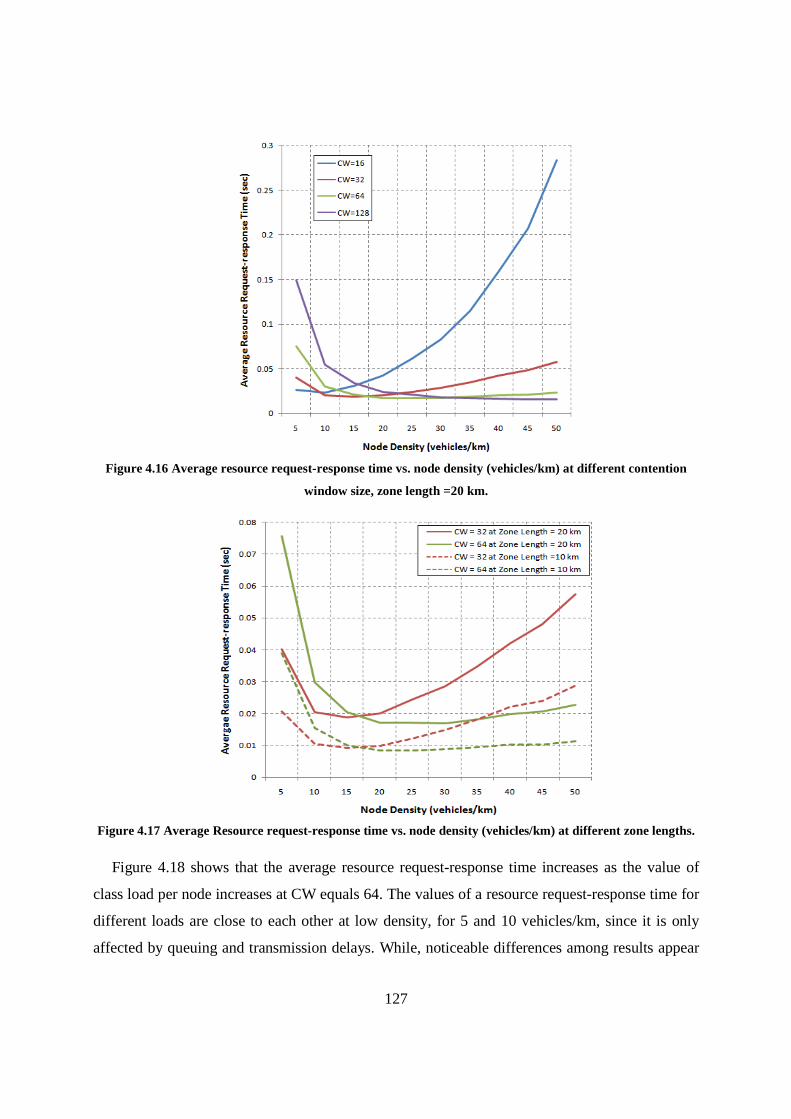
127

Figure 4.16 Average resource request-response time vs. node density (vehicles/km) at different contention

window size, zone length =20 km.

Figure 4.17 Average Resource request-response time vs. node density (vehicles/km) at different zone lengths.

Figure 4.18 shows that the average resource request-response time increases as the value of

class load per node increases at CW equals 64. The values of a resource request-response time for

different loads are close to each other at low density, for 5 and 10 vehicles/km, since it is only

affected by queuing and transmission delays. While, noticeable differences among results appear

128

at higher node densities due to a great effect of the delay due to collisions in addition to queuing

and transmission delays.

Figure 4.18 Average resource request-response time vs. node density (vehicles/km) at different loads of a class

per node, zone length =20 km.

4.3.2.10 Validation

We validate our proposed model by comparing the analytical results with that obtained by

means of simulation. Our simulator is written in Java programming language, which attempts to

emulate as closely as possible the real operation of each node, including transmission range,

collision delay, propagation times, mobility pattern, etc. We simulate vehicles that move on a

bidirectional road as a one–dimensional movement as followed in the analytical model.

We closely follow the 802.11 protocol details for each transmitting node for calculating the

collision delays. We set the size of a slot time,σ, is set equal to 50μsec for Frequency Hopping

Spread Spectrum (FHSS) [140]. It is the time needed at any station to detect the transmission of a

packet from any other station. Also, we set T' to be equal to the time period of a request to send

frame (RTS) plus the duration of distributed inter-frame space (DIFS). We set DIFS equals 128

µsec and RTS equals 288 bits, therefore, Tc equals 416 µsec [140]. The channel transmission rate

has been assumed equal to 1 Mbit/s. For simplicity, we suppose that the contention window is a

constant backoff window and no exponential backoff is considered. CWis set according to the

values defined in the table below.

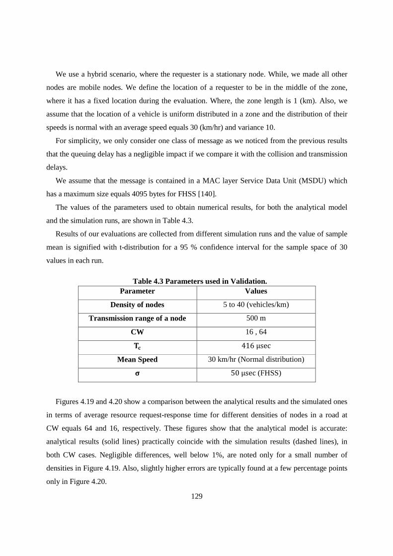
129

We use a hybrid scenario, where the requester is a stationary node. While, we made all other

nodes are mobile nodes. We define the location of a requester to be in the middle of the zone,

where it has a fixed location during the evaluation. Where, the zone length is 1 (km). Also, we

assume that the location of a vehicle is uniform distributed in a zone and the distribution of their

speeds is normal with an average speed equals 30 (km/hr) and variance 10.

For simplicity, we only consider one class of message as we noticed from the previous results

that the queuing delay has a negligible impact if we compare it with the collision and transmission

delays.

We assume that the message is contained in a MAC layer Service Data Unit (MSDU) which

has a maximum size equals 4095 bytes for FHSS [140].

The values of the parameters used to obtain numerical results, for both the analytical model

and the simulation runs, are shown in Table 4.3.

Results of our evaluations are collected from different simulation runs and the value of sample

mean is signified with t-distribution for a 95 % confidence interval for the sample space of 30

values in each run.

Table 4.3 Parameters used in Validation.

Parameter Values

Density of nodes 5 to 40 (vehicles/km)

Transmission range of a node 500 m

CW 16 , 64

®̄ 416μsec Mean Speed 30 km/hr (Normal distribution)

± 50μsec (FHSS)

Figures 4.19 and 4.20 show a comparison between the analytical results and the simulated ones

in terms of average resource request-response time for different densities of nodes in a road at

CW equals 64 and 16, respectively. These figures show that the analytical model is accurate:

analytical results (solid lines) practically coincide with the simulation results (dashed lines), in

both CW cases. Negligible differences, well below 1%, are noted only for a small number of

densities in Figure 4.19. Also, slightly higher errors are typically found at a few percentage points

only in Figure 4.20.

130

Figure 4.19 Analysis versus simulation at CW = 64.

Figure 4.20 Analysis versus simulation at CW = 16.

4.3.2.11 Findings

There is a tradeoff between a node density and the probability that a transmission occurring on

the channel is successful, which is based on the value of CW. When a CW has a high value, the

resource request-response time gets a lower value at high density values. While, it has higher

value at low node density due to high value of the average number of idle slot times per packet

131

transmission. In addition, there is a tradeoff between the mean forwarding distance and a density

of nodes. Ata high node density, the mean forwarding distance increases. This leads to decrease

the resource request-response time because of using a smaller number of forwarding nodes

between source and destination nodes.

Therefore, our results show that we can adapt the performance of a response according to node

density and contention window size.

4.3.3 Simulation Platform

As our proposed PlanetCloud platform is supposed to realize a resource-infinite computing

paradigm that provides unlimited computing resources to users, it is crucial to evaluate the

implementation of our proposed system and its integral task scheduling and resource allocation

algorithm on a large-scale virtualized data center infrastructure. However, performing repeatable

large-scale experiments on a real infrastructure is extremely laborious, which is required to

evaluate and compare the applied algorithms. Therefore, simulations have been chosen as a way

to evaluate the performance of the proposed architecture and its subsystems.

We choose the CloudSim toolkit [26][27]to be our simulation platform, as it is a modern

simulation framework aimed at Cloud computing environments. The CloudSim allows the

modeling of virtualized environments, simulating service applications with dynamic workloads,

supporting on demand resource provisioning, and their management.

To simulate the MAC environment, we have extended the CloudSim simulator to support the

mobility of nodes by incorporating the Random Waypoint (RWP) model. In the RWP model, a

mobile node moves along a line from one waypoint W� to the nextW��F. These waypoints are

uniformly distributed over a unit square area. At the start of each leg, a random velocity is drawn

from a uniform velocity distribution.

We designed Java classes for implementing the spatiotemporal data related to resources and

their future availability which is obtained from the calendaring mechanism. In addition, we edit

the CloudSim to implement our proposed P-ALSALAM algorithm.

In our evaluation model, an application is a set of tasks with one primary task executed on a

primary node. Each task, or cloudlet, runs in a single VM which is deployed on a participant node.

VMs on mobile nodes could only communicate with the VM of the primary task node and only

when a direct ad-hoc connection is established between them.

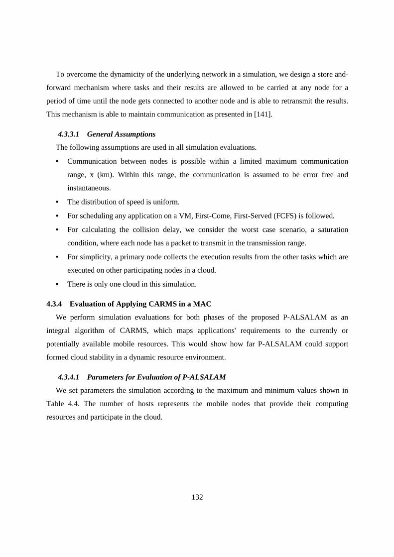
132

To overcome the dynamicity of the underlying network in a simulation, we design a store and-

forward mechanism where tasks and their results are allowed to be carried at any node for a

period of time until the node gets connected to another node and is able to retransmit the results.

This mechanism is able to maintain communication as presented in [141].

4.3.3.1 General Assumptions

The following assumptions are used in all simulation evaluations.

• Communication between nodes is possible within a limited maximum communication

range, x (km). Within this range, the communication is assumed to be error free and

instantaneous.

• The distribution of speed is uniform.

• For scheduling any application on a VM, First-Come, First-Served (FCFS) is followed.

• For calculating the collision delay, we consider the worst case scenario, a saturation

condition, where each node has a packet to transmit in the transmission range.

• For simplicity, a primary node collects the execution results from the other tasks which are

executed on other participating nodes in a cloud.

• There is only one cloud in this simulation.

4.3.4 Evaluation of Applying CARMS in a MAC

We perform simulation evaluations for both phases of the proposed P-ALSALAM as an

integral algorithm of CARMS, which maps applications' requirements to the currently or

potentially available mobile resources. This would show how far P-ALSALAM could support

formed cloud stability in a dynamic resource environment.

4.3.4.1 Parameters for Evaluation of P-ALSALAM

We set parameters the simulation according to the maximum and minimum values shown in

Table 4.4. The number of hosts represents the mobile nodes that provide their computing

resources and participate in the cloud.

133

Table 4.4 Parameters for evaluation of P-ALSALAM.

Parameters Values Parameters Values

Density of nodes 4 - 100

(Nodes/Km²) Communication

range 0.1-1 (km)

Number of Hosts/Cloud

2-24

Application Arrival Rate

(Poisson distribution)

7 (Applications/sec)

Number of tasks/Application

4-140 Expected

execution time for a task

800 (Sec)

Number of applications/Cloud

1 – 14

Number of CPUs/Cores

per host (Uniform

distribution)

1-8

Inactive Node rate (Node/Sec)

(Poisson Process)

1/300 -1/60

Average Node Speed

(Uniform distribution)

1.389,10,20 (m/sec)

4.3.4.1 Evaluation of Initial Static Scheduling and Assignment Phase of P-ALSALAM

Algorithm

Through this part of the evaluation, we only considered the initial static scheduling and

assignment phases. In this evaluation, a mobile node can always function well all the time with

high reliability and does not fail.

a) Experiments

We started this part of evaluation by studying the effect of collision delay due to channel

contention on the performance of the submitted application. In this evaluation, all nodes have the

same computing capabilities, i.e. homogeneous. Figure 4.21 shows the average execution time of

an application at a different number of nodes, ranging from 4 to 24 nodes, in a unit square area.

The average speed of a mobile node equals 10 (m/sec). We set the transmission range to be 0.8

(km), which has been obtained from an evaluation not presented here due to space limitation. At

this value, we can neglect the effect of the connectivity, i.e. a node is almost always connected

with others.

134

Figure 4.21 Average Execution Time of Application Vs Number of nodes at different number of submitted

tasks/application and number of cores/host.

Figure 4.21 shows that the worst performance is obtained when a host has a minimum number

of cores, i.e. 1 core, and at a maximum number of tasks per application, i.e. 30. This is because at

a small number of nodes, e.g. 4, most of the submitted tasks will be queued in a waiting list since

just one core is available per task. The more the available nodes participate in the formed cloud,

the more available cores to execute these tasks. Consequently, the average execution time of an

application decreases with the increase of the number of mobile nodes. The collision delay should

increase with node density, while results show that the collision delay is negligible if we compare

it with the queuing delay. The results at 1 and 8 cores per host are very close to each other at a

small number of tasks per application, at 4 tasks/application, since there is no effect of the

queuing delay. Noticeable differences between these results and the others appear at a higher

number of submitted tasks/application equals 15, at a number of cores/host equals 8, due to the

significant effect of the mobility of hosts. The reason is that these tasks are assigned to more

nodes in the formed cloud, and this leads to increase in the communication time until the primary

node collects results from the other nodes. These results show that the collision delay is also

negligible if we compare it with the communication delay. Conversely, the average execution

time of an application decreases when the number of nodes increases from 4 to 8 at a number of

135

tasks per application equals 30, and at a number of cores/host equals 8. This is because the more

the number of hosts, the more cores to execute these tasks. This reduces the queuing delay.

In the next experiments, we compare results of two cases: Using P-ALSALAM algorithm,

which is based on the information obtained from GRPS, e.g. location and available processors, in

resource scheduling and assignment and the random-based algorithm, which does not use this

information, where a random mobile nodes are selected to execute the submitted application.

Let all 40 mobile nodes have a random number of cores, heterogeneous resources, ranging

from 1 to 8 cores. Figure 4.22 shows that the average execution time of an application when we

consider one application is submitted to be executed. Each node has a transmission range equals

0.4 km, and its average speed equals 1.389 (m/sec). As expected, this evaluation provides

significant differences between results of the two cases, with/without using the P-ALSALAM.

The results of this figure show that executing the application on a smaller number of nodes, e.g. 8

hosts, has better performance in terms of average execution time of an application than in case of

results at a larger number of hosts, i.e. 24 hosts. The higher number of submitted tasks per

application leads to make some tasks waiting the previous ones in a waiting list to be executed.

The total delay becomes higher if these tasks are distributed on a higher number of nodes, e.g. 24

hosts. This is because the communication delay is dominant.

Figure 4.22 Average Execution Time of Applications Vs number of submitted tasks at different number of

hosts.

136

We repeat our evaluation at a different number of hosts equals 4, 8 and 24 hosts, and at a

different value of transmission ranges equals 0.4, and 1 (km). Figure 4.23 shows that the average

execution time of an application at a transmission range equals 1 (km) almost has a better

performance than the case of a transmission range equals 0.4 (km) at the same number of hosts.

Also, we can see that at a small transmission range, e.g. 0.4 (km), and a large number of hosts,

e.g., 24 hosts, a worst performance is obtained. While, it has a better performance, at a number of

hosts equals 8, than in case of a number of hosts equals 4. This observation is quite obvious

because at this large number of tasks, greater than the total computing capabilities of the selected

4 hosts, the queuing delay is dominant. On the other hand, the larger the value of a number of

hosts, at a high transmission range equals 1 (km), the better average execution time of an

application is, e.g. at 24 hosts.

Figure 4.23 Average Execution Time of Applications Vs number of submitted tasks at different number of

hosts and Comm. Ranges.

The results of Figure 4.24 show that the smaller the number of submitted applications, e.g. 7

applications, the better performance is obtained. Applications arrive into the system following a

Poisson process with arrival rate 7. Also, the results show that the execution of submitted

applications on a smaller number of hosts, e.g. 2 hosts/application, has a worst performance than

of executing them on larger number of hosts, e.g. 8 hosts/application. This is because at a small

number of hosts, e.g. 2, the queuing delay is dominant. The more the available number of hosts

participated in the formed cloud the more available cores to execute these tasks. Consequently,

137

the average execution time of an application decreases with the increase of a number of mobile

nodes, e.g. 8 hosts/application. On the other hand, the larger the value of a number of

hosts/application, the worst average execution time of an application is, e.g. at 20

hosts/application. This is because the communication delay is dominant.

Figure 4.24 Average Execution Time of Applications Vs number of hosts per application at different number

of applications.

4.3.4.2 Evaluation of Adaptive Scheduling and Reallocation Phase P-ALSALAM

Algorithm

Through this part of the evaluation, we considered two reliability scenarios: high reliability

scenario, where every mobile node can always function well all the time with high reliability and

does not fail; and a variable reliability scenario, where mobile nodes are different in their

reliability, in terms of future availability and reputation, for the requested MCC.

b) Experiments

1. High reliability Scenario

In this experiment, we consider that every mobile node can always function well all the time

with high reliability and does not fail. For example, all nodes are always available, reputable and

they have the highest preference value to accept the submitted applications.

We started our evaluation by studying the effect of applying adaptive scheduling and

reallocation phase on the performance of the submitted application. Let all 40 mobile nodes have

a random number of cores, heterogeneous resources, ranging from 1 to 8 cores. Figure 4.25 shows

138

the average execution time of an application at a different number of hosts, ranging from 2 to 22

hosts. We consider five applications are submitted to be executed. Each node has a transmission

range equals 0.4 km, and its average speed equals 1.389 (m/sec). This evaluation provides that

there are no significant differences between results of the two cases, static/ adaptive scheduling

using the P-ALSALAM at a larger number of hosts per cloud, e.g., 14 hosts/cloud. This is

because at transmission range equals 0.4 km, we can neglect the effect of the connectivity, i.e. a

node is almost always connected with others. However, at smaller number of hosts per cloud,

where the queuing delay is dominant, e.g., at2 hosts/cloud, dynamic scheduling has worst

performance than static one due to the overheads of rescheduling. The larger value of

rescheduling threshold, e.g. at threshold equals 1600 sec, leads to reduce the overheads of

rescheduling and slightly enhance the performance at a smaller number of hosts per cloud equals

2. The more the frequency of rescheduling in the formed cloud, e.g. at threshold equals 1100 sec,

the more overheads to execute these tasks.

Figure 4.25Average Execution Time of Application Vs Number of Hosts per cloud at different scheduling

mechanisms and rescheduling threshold.

In the next evaluation, we compare results at difference transmission ranges equal 0.2 km and

0.4 km, using dynamic scheduling of P-ALSALAM algorithm. In this evaluation, we set the value

of rescheduling threshold equals 1100 sec. Figure 4.26 shows that the average execution time of

an application at a transmission range equals 0.4 (km) almost has a better performance than the

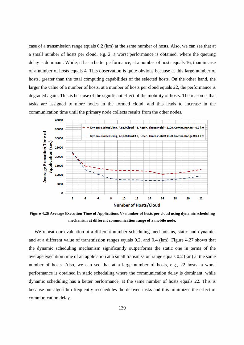
139

case of a transmission range equals 0.2 (km) at the same number of hosts. Also, we can see that at

a small number of hosts per cloud, e.g. 2, a worst performance is obtained, where the queuing

delay is dominant. While, it has a better performance, at a number of hosts equals 16, than in case

of a number of hosts equals 4. This observation is quite obvious because at this large number of

hosts, greater than the total computing capabilities of the selected hosts. On the other hand, the

larger the value of a number of hosts, at a number of hosts per cloud equals 22, the performance is

degraded again. This is because of the significant effect of the mobility of hosts. The reason is that

tasks are assigned to more nodes in the formed cloud, and this leads to increase in the

communication time until the primary node collects results from the other nodes.

Figure 4.26 Average Execution Time of Applications Vs number of hosts per cloud using dynamic scheduling

mechanism at different communication range of a mobile node.

We repeat our evaluation at a different number scheduling mechanisms, static and dynamic,

and at a different value of transmission ranges equals 0.2, and 0.4 (km). Figure 4.27 shows that

the dynamic scheduling mechanism significantly outperforms the static one in terms of the

average execution time of an application at a small transmission range equals 0.2 (km) at the same

number of hosts. Also, we can see that at a large number of hosts, e.g., 22 hosts, a worst

performance is obtained in static scheduling where the communication delay is dominant, while

dynamic scheduling has a better performance, at the same number of hosts equals 22. This is

because our algorithm frequently reschedules the delayed tasks and this minimizes the effect of

communication delay.

140

Figure 4.27 Average Execution Time of Applications Vs number of hosts per cloud at different scheduling

mechanisms and at different communication range of a mobile node.

2. Variable reliability Scenario

In this evaluation, we consider that mobile nodes are different in their reliability, in terms of

future availability and reputation, for the requested MCC.

We perform an evaluation to obtain the expected execution time of an application at number of

hosts per application equals 6. In this evaluation, we consider one application is submitted to be

executed, with a number of tasks equals 30. We consider the density of nodes equals 100

(nodes/km²). Each node has a transmission range equals 0.4 km, and its average speed equals

1.389 (m/sec). The results of this evaluation showed that the expected execution time of an

application equals 4000 seconds. We use it to calculate the number of inactive nodes at different

arrival rates of inactive nodes for the next evaluations. We set the rescheduling threshold equals

the expected execution time of an application, e.g. 4000 seconds. Also, we assume that the

primary node is always reliable.

In the next evaluation, we compare results of two cases: Using P-ALSALAM algorithm, which

determines the best participants that have the highest average reliability scores to the requested

cloud and the random-based algorithm, which does not use this information, where random

mobile nodes with random reliability scores are selected to execute the submitted application. We

perform the evaluation with various values of the arrival rate of inactive nodes, ranging from

1/300 to 1/60 (nodes/sec). As expected, this evaluation provides significant differences between

141

results of the two cases, with/without using the P-ALSALAM. The results of Figure 4.28 show

that a better performance, in terms of the average execution time of an application, is obtained at a

smaller arrival rate of inactive nodes, e.g. 1/300 (nodes/sec) than in case of results at a larger

arrival rate of inactive nodes, e.g. 1/60 (nodes/sec). This is because at larger arrival rate of

inactive nodes, the probability a node could fail increases.

Figure 4.28 Average Execution Time of Applications when applying different reliability based algorithms.

Figure 4.29 compares the results of applying P-ALSALAM algorithm and random-based

algorithm in terms of the average MTTR when we consider different arrival rate of inactive

nodes. The average MTTR has lower value at a smaller arrival rate of inactive nodes, e.g. 1/300

(nodes/sec) due to low probability a host might fail. While, noticeable differences among results

appear at a larger arrival rate of inactive nodes, e.g. 1/60 (nodes/sec) due to the high probability a

host could fail.

142

Figure 4.29 Average MTTR Vs inactive node rates when applying different reliability based algorithms.

Figure 4.30 depicts the results of applying P-ALSALAM algorithm in terms of the average

MTTR when we consider different densities of nodes at different values of reputation threshold.

We perform this evaluation with an arrival rate of inactive nodes equals 1/60 (nodes/sec). Each

node has a transmission range equals 1 km, to neglect the effect of communication disruptions.

Also, we consider two applications are submitted to be executed. Each application has an

expected execution time equals 1500 seconds. The results show that the average MTTR has a

higher value at a small node density, e.g. 35 (nodes/km²) due to low probability to find the

required number of reliable host to maintain the cloud in case of failure. While, the average

MTTR has a lower value at higher node densities, e.g. 55 nodes/km². Also, the figure shows that

the average MTTR at a smaller reputation threshold, e.g. zero threshold in case of all nodes are

reputable, than in case of results at a larger reputation threshold, e.g. 0.6, at the same density of

nodes. This is because the larger the reputation threshold the lower the probability to provide

nodes that could achieve the application requirements at the same time these nodes should be

available in future to participate in a MCC.

143

Figure 4.30 Average MTTR at different densities of nodes when applying P-ALSALAM algorithm.

4.3.4.3 Findings

Our findings can be summarized as follows.

1) There is a tradeoff between the communication delay and the queuing delay as the

number of hosts per submitted application is varied. The higher number of hosts per an

application, the higher total computing capability within the cloud is. Therefore, the

queuing delay of a task is decreased. While, increasing the number of nodes per

application leads to increasing the time until the primary node collects results from

other resource provider nodes, and therefore this increases the communication delay.

2) A better performance may be obtained, at a shorter transmission range, if we apply the

adaptive scheduling and reallocation phase especially at a larger number of hosts

assigned to a MCC. This is because our algorithm frequently reschedules the delayed

tasks and this minimizes the effect of communication delay. While at a longer

transmission range, where the communication delay could be neglected, we have to

select the static scheduling and assignment phase to eliminate the overhead of

rescheduling and slightly enhance the performance especially at a smaller number of

hosts per cloud.

144

3) The MTTR may be enhanced, at less density of nodes, if we use a low value of

reputation threshold per submitted application which maximizes the number of reliable

nodes that could meet the application requirements and therefore participate in a MAC.

4) The average execution time of an application is impacted by the connectivity among

hosts of a cloud, the load of submitted applications, and the total resources, computing

capabilities, confined in these hosts. The major factors affecting connectivity are hosts’

transmission range, node mobility, and node density. The mobility is impacted by the

hosts’ speed and movement direction (relative to primary nodes).

4.4 Conclusion

PlanetCloud resource management provides new opportunities to expand problem solving

beyond the confines of walled-in resources and services. In this chapter, we proposed GRPS, a

scalable spatiotemporal resource calendaring system accessed through a universal portable

application to enable ubiquitous computing clouds utilizing both stationary and mobile resources.

GRPS is powered by (1) a dynamic spatiotemporal calendaring mechanism, (2) socially-

intelligent resource discovery and forecasting, (3) an autonomic calendar management system,

and (4) a ubiquitous cloud access application. The results of our analysis for GRPS show that we

can adapt the performance according to both node density and number of collided transmissions.

Also, we presented CARMS as a distributed autonomic resource management system to enable

resilient dynamic resource allocation and task scheduling for mobile cloud computing. In

addition, we proposed the P-ALSALAM, a distributed Proactive Adaptive List-based Scheduling

and Allocation AlgorithM, to dynamically map applications' requirements to the currently or

potentially reliable mobile resources. This would support the stability of a formed cloud in a

dynamic resource environment. Results have shown that P-ALSALAM significantly outperforms

the random-based reliability algorithm in terms of the average execution time of an application

and the MTTR. Also, we can adapt the performance according to number of hosts per cloud,

communication range, density of mobile nodes and inactive node rate.

145

Chapter 5

5 PLANET CLOUD CLOUD MANAGEMENT

In this chapter, we present the trustworthy dynamic virtualization and task management layer

which performs all tasks related to the cloud management in PlanetCloud. Also, we present the

concept of the virtualization and task management layer and its architectures.

5.1 Trustworthy Dynamic Virtualization and Task Management Layer

Mobile computation devices are becoming ubiquitous to support various applications.

Unfortunately, these resources are highly isolated and non-collaborative. Even for those resources

working in a networked fashion, they suffer from limited self and situation awareness and

collaboration. Additionally, given the high mobile nature of these devices, there is a large

possibility of failure. Explicit failure resolution and fault tolerance techniques were not efficient

enough to guarantee safe and stable operation for many of the targeted applications limiting the

usability of such mobile resources.

The current resource management and virtualization technologies fall short for building a

virtualization layer that can autonomously adapt to the real-time dynamic variation, mobility, and

fractionalization of such infrastructure [11][12]. In general, hiding the underlying hardware

resources heterogeneity, the geographical diversity concern, and node failures and mobility from

the application, in a MAC, provides a strong motivation for dynamic virtualization and task

management capabilities for MACs to construct a resilient MAC.

In this chapter, we present the trustworthy dynamic virtualization and task management layer,

as an adaptation of CyberX [104][105] to construct a thin virtualization layer. PlanetCloud utilizes

such layer to perform all tasks related to the cloud management. The virtualization and task

management layer uses micro virtual machines, Cells, to encapsulate executable application-

partitions. At runtime, the virtualization and task management layer rebuilds the application from

such Cells enabling application to execute in total isolation from the host resources. Such

isolation enables seamless load migration, and cost-effective replication and fault-tolerance

enhancing the C3 resilience against potential failures.

146

In addition, the loosely coupled, collaborative nature of PlanetCloud foundation and the

resource prediction mechanism facilitate Cell runtime relocation from high risk resources to more

stable ones with minimal-to-no interruption to the running application.

The virtualization and task management layer provides the rapid elasticity characteristic, by

interacting with the GRPS and CARMS, and isolates the hardware concern from the task

management. Such isolation empowered PlanetCloud to support autonomous task

deployment/execution, dynamic adaptive resource allocation, seamless task migration and

automated failure recovery for services running in a continuously changing unstable operational

environment. As previously described, the virtualization and task management layer is composed

of a set of central powerful fixed nodes. These nodes collaborate autonomously to manage the

whole network of micro VMs. This platform is responsible for the composition and deployment

of micro VMs, management, the host side API(s), real-time monitoring and evaluation of the

executing micro VMs, and recovery management. Further, it provides the necessary management

tools for system administrators to manage, analyze, and evaluate the working micro VMs. The

virtualization and task management layer will act as an autonomously managed resource and

application virtualization platform of PlanetCloud. Micro VMs are deployed to encapsulate

executable application- partitions defined as code variants. This separates logic, state and physical

resource management. Applications can be defined in one or more encapsulated variants. Such

construction facilitates hiding the heterogeneity of the underlying hardware resources from the

application concern enabling seamless deployment, distribution, and migration of application on

the cloud mobile nodes

5.1.1 Cell Oriented Architecture (COA)

Both a mission-oriented application design and an inline code distribution are exploited by the

COA to enable adaptability, dynamic re-tasking, and re-programmability.

The main building block in the COA is a Cell, which is considered as an abstraction of a

mission-oriented autonomous active resource.

The CCDNA generates generic Cells that participate in varying tasks through a process called

specialization.

A Cell is an intelligent single-application capsule, which independently and autonomously

acquires, on the fly, an application specific functionality represented by an executable code

variant through the specialization process.

147

A cell is simplest single application virtualization environment, sandbox, which isolates the

executable Logic from the underlying physical resources.

A complex multi-tasking application represents a larger structure, organism, which

dynamically consists of single or multiple Cells, working together to accomplice a certain

mission.

Different components of the COA are illustrated in Figure 5.1.

A Cell comprises various tools to support its intrinsic features. These features includes

resilience to failure, dynamic performance optimization, Cell self and situation awareness, and

online programmability and adaptability.

We envision applications built over our COA as a group of cooperating roles representing a set

of objectives. An organism serves as a role player, which performs specific mission tasks. An

organism has a specific functional role at runtime.

Figure 5.1 Components of COA [105].

5.1.1.1 Cell of the virtualization and task management layer

The virtualization and task management layer uses Cells to encapsulate user tasks defined as a

set of binary code variants. These variants represent the user application that should run on top of

the participant resources. Figure 5.2 depicts an abstract view of Cell at runtime. A Cell is

represented as a micro virtual machine that isolates the application code logic from the underlying

148

hardware resources. Such isolation resolves the resource heterogeneity concern facilitating the

realization of the proposed solution.

Figure 5.2 COA Cell at runtime [105].

A flexible way to share the physical resources among multiple applications could be achieved

by hosting one or more cells by a single workstation.

Figure 5.3 shows the main components of the COA Cell. A brief overview of these

components is discussed as follows.

Figure 5.3 Components of COA Cell [104].

149

Instantiation of Cell begins when the bootstrap manager initializes the Cell components and

ports with the convenient parameters based on the bootstrap context.

The I/O manager, as a communications unit, performs local and remote I/O communication

setup, I/O logging, and IP/Port Virtual naming resolution.

When the execution unit receives an executable COA-ready code variant, the specialization

process begins. The executable COA-ready code variant represents the application specific

functionality that the Cell should acquire.

A COA-ready variant is a program that enables check-pointing and frequent reporting through

a predetermined channel using predetermined syntax.

The Data is isolated from the Logic by committing all sensitive data to a remote data storage

using a dedicated data channel provided by the infrastructure before each checkpoint.

An infrastructure provides a starting point to the program, which asked for, to start the

execution. This point is considered as a zero reference for fresh Cells. Finally, the programmer

has to implement at least two similar-function different-objective variants to enable the

virtualization and task management layer quality attribute manipulation.

The execution unit launches the selected variant with the appropriate parameters to start the

execution. Also, the execution unit might cause the termination and replacement of the executing

variants based on incoming shuffling commands.

The diversity-management unit handles all the issues regarding diversity employment-

methodology, shuffling policy, shuffling frequency, commanding, and variant selection.

The State Transaction Manager (STM) monitors the variant execution progress. In addition, it

is the only unit that has a direct access, through a dedicated communication channel, to the

executing application. Checkpoint change, incoming application requests and status reports are

sent from STM to the appropriate units “ex, holding shuffling frequency change, objective change

requests, etc”.

The recovery manager is the unit which is used to adjust the recovery settings, recovery mode

change. Also, this unit is used to restore and synchronize checkpoints at the time of failure-

recovery with the cooperation of the execution unit. The recovery manager sends Cell beacon

messages to the tracking servers. Such messages include the last checkpoint reported by STM,

reports regarding Cell state reported by the situational awareness unit and administrative

messages needs to be delivered to the Global Management Servers (GMS). The details about

150

multimodal failure recovery processes of our virtualization and task management layer are

illustrated in a later section.

All the needed situational and context awareness information is provided by the situational

awareness unit to the other Cell units to support their decisions.

The situational awareness unit is responsible for monitoring the internal and the external Cell

surroundings and generating guideline reports for all Cell units.

Another main function of situational awareness unit is to inform the GMS with awareness

reports through attached messages to the Cell frequent beacon messages. These stored beacons are

used by GMS to generate more meaningful status reports, which include information, directions,

and commands that the virtualization and task management layer wants to deliver to a certain area

in the network. For example, when a Cell reported a malicious event that could harm the other

neighbor Cells, GMS might inform other Cells to change the current variant to more secure

variant.

The tasks of decision-making are totally distributed in the Cell such that each unit takes its

own decisions regarding its specific task autonomously. The real time cooperation among all

these units handles the global operation of the Cell.

The virtualization and task management layer comprises a set of distributed powerful nodes,

i.e. servers, which cooperate autonomously to manage the whole network of Cells. The

responsibilities of this platform includes the organism creation “composition and deployment of

Cells”, management, the host side API(s) “CCDNA”, real-time monitoring and evaluation of the

executing Cells, and recovery management. Further, this platform provides the necessary

management tools for system administrators to manage, analyze, and evaluate the working Cells

/organisms.

5.1.2 Inter-Cell Communications

This section describes the inter-Cell communications and how the virtualization and task

management layer manage its secrecy, authenticity, and anonymity. A suitable key management

scheme is presented for various connection types in the system. Further, the detection mechanism

of malicious behavior and problematic Cells are discussed. Additionally, a secure authentication

mechanism is presented for securing the inter-Cell communications against identity theft attacks.

The virtualization and task management layer deploys an asymmetric key encryption scheme

to encrypt the sensitive information stored locally or externally, or being exchanged over

151

communication lines. Therefore, the virtualization and task management layer could maintain the

secrecy of the sensitive information. At the deployment time, a pair of keys, i.e. a public key and a

private key, is assigned to each cell by the GMS. The public key is used to encrypt the incoming

messages to the Cell. Where, the private key is used to decrypt these incoming messages. The

Cell may encrypt the sensitive data within the Cell itself using the private key, if the situation

necessitates that. For example, sensitive data, stored in the local hard drive, might be encrypted if

the drive is being shared by different Cells hosted in the same host. Figure 5.4, depicts the

architecture of local security mechanism in the virtualization and task management layer.

Data authenticity is maintained in the virtualization and task management layer using a set of

encryption/decryption keys.

At the deployment time, GMS attaches various parameters to the Cell deployment package.

These parameters include the Cell inputs, configuration parameters, the Cell public and private

keys, and a pool of public keys for other entities that the Cell might communicate with. There is a

pool of public keys which includes keys for the virtualization and task management layer servers

and routers that the Cell might need to be indirect contact with. Also, public keys for replicas of a

Cell, if founded at the deployment time, are included.

According to the change in the current recovery mechanism at runtime, Cells can acquire new

replicas. This process is initiated by a request from this Cell or the Recovery and Checkpoint

Tracking Server (RCTS) to GMS to deploy new replicas. The reply from the GMS includes the

public key and the unique Cell name of the new replica to the requester in a form of an encrypted

message using the requester public key.

The authenticity of all incoming messages is guaranteed by enclosing and encrypting the

source id with the message. The Auditing and Reputation Management Server (ARMS)

continuously monitors the inter-Cell behavior with the cooperation of RCTS that keeps track of

all Cells activities. Both malicious and problematic Cells will be terminated and their IDs will be

blacklisted and announced to all routing Cells.

152

Figure 5.4 Security framework of the virtualization and task management layer [104].

The inter-Cell communications can be classified into two main types within applications.

These types are administrative related communications, and application related communications.

Application related communications include messages being exchanged to serve the application

needs and identified by the application designer. The administrative related communications

include recovery beacon messages between Cells and replicas or RCTS, alerts and events between

Cells and ARMS, and messages between Cells and routing nodes.

An abstract view for the Inter-Cell message format is shown in Figure 5.5. The message

comprises two main parts, the destination id, encrypted data block.

Figure 5.5 The Inter-Cell message format [104].

153

The encrypted data block is divided into five parts, each is encrypted with a different key, sub

destination id, the source id, timestamp, message to be sent, and message integrity assurance data,

e.g. hash code.

To achieve inter-Cell communications anonymity, Cells are not allowed to directly exchange

messages. Cells communicate with intermediate routing nodes to conceal the physical location of

the communicating nodes, e.g. replicas, and Cells hosting partitions of the same application, and

to control administrative related communications. Intelligent routing cells are used by the

virtualization and task management layer to anonymize the source and destination of any

outgoing message. Consequently, attackers with access to the network might be blocked from

monitoring outgoing messages searching for a certain transmission pattern, e.g. Beacon messages

between Cells and replicas. These patterns, if identified, can expose the physical location, and the

functionality of the destination Cells.

A communication scenario among different nodes in the system, cells, replicas, and servers is

illustrated in Figure 5.6. Each node encrypts and signs all outgoing messages using the destination

public key.

Figure 5.6 Secure Messaging System [104].

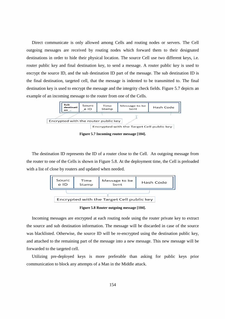
154

Direct communicate is only allowed among Cells and routing nodes or servers. The Cell

outgoing messages are received by routing nodes which forward them to their designated

destinations in order to hide their physical location. The source Cell use two different keys, i.e.

router public key and final destination key, to send a message. A router public key is used to

encrypt the source ID, and the sub destination ID part of the message. The sub destination ID is

the final destination, targeted cell, that the message is indented to be transmitted to. The final

destination key is used to encrypt the message and the integrity check fields. Figure 5.7 depicts an

example of an incoming message to the router from one of the Cells.

Figure 5.7 Incoming router message [104].

The destination ID represents the ID of a router close to the Cell. An outgoing message from

the router to one of the Cells is shown in Figure 5.8. At the deployment time, the Cell is preloaded

with a list of close by routers and updated when needed.

Figure 5.8 Router outgoing message [104].

Incoming messages are encrypted at each routing node using the router private key to extract

the source and sub destination information. The message will be discarded in case of the source

was blacklisted. Otherwise, the source ID will be re-encrypted using the destination public key,

and attached to the remaining part of the message into a new message. This new message will be

forwarded to the targeted cell.

Utilizing pre-deployed keys is more preferable than asking for public keys prior

communication to block any attempts of a Man in the Middle attack.

155

Using of asymmetric key encryption is better than symmetric key encryption, regardless of the

added computational cost. This is because it is hard to use one key for all communicating parties,

due to the high cost of key management, and replacement given the large scale of the network of

Cells. Further, asymmetric key encryption is used to authenticate the Cell identity and to protect

the network against identity theft attacks. The source id field is encrypted by the Cell using its

private key, later it can easily be authenticated by recipients using its unique public key.

Moreover, using asymmetric key encryption makes the cost of compromising a Cell is much less

as the other Cells will not be affected by revealing the compromised Cell keys. Such keys will be

revoked upon detection of exposure. However, all the Cells using the compromised keys , in case

of using symmetric key encryption, will be vulnerable to wide set of communication related

attacks until the keys gets replaced after detection of exposure.

The presented security mechanism doesn’t guarantee the protection of Cells from being

compromised. However, full time monitoring of Cells behavior is implemented by the

virtualization and task management layer to detect such events. Once a malicious behavior of a

Cell is detected, the virtualization and task management layer autonomously blocks and replaces

such Cell with a new one.

5.1.3 Multi-mode Failure Recovery

In order to enable autonomous adaptation and performance optimization, the virtualization and

task management layer deploys diversity techniques, which might involve multiple execution

interruptions. Doing so might lead to multiple coincident failures. The virtualization and task

management layer provides an autonomous, dynamic, and situational-aware multi-mode failure

recovery mechanism to resolve possible failures for COA based applications. This recovery

mechanism enables failure resilience enhancement not only against coincidental failures, but also

against malicious induced failures by adversaries.

Both dynamic and autonomous changes of Cell recovery-policy is provided by the

virtualization and task management layer to switch between different fault-tolerance granularity

levels. Such levels might target reliability, survivability, and resource usage optimization. The

virtualization and task management layer provides a fine-grained recovery, namely Hot-recovery,

using replication. Where, a Cell can have one or more replicas on the same physical host. Only

logical failure can be addressed by this type of local replication. On the other hand, to achieve a

finer-grained recovery against both logical and physical node failure, the Cell might have one or

156

more replicas on different physical hosts. The fine grained recovery has two types of mode, the

resource saver, and the fast-recovery modes.

The resource-saver mode includes only replicas of the STM, I/O unit and local data store units

of the Cell. While, the remaining Cell’s components stay in hibernation waiting for resurrection

when the replica takes over. Replicas have one working variant and no shuffling or recovery

policy change until resurrection. This mode minimizes the resource usage consumed by these

replicas and saves the resources but on the account of increasing failure downtime by the time

needed to resurrect the Cell.

In the fast-recovery mode, the task-transition downtime may be totally eliminated by using a

fully-alive replica Cells, which mimic all the actions of the source Cell except outgoing

communications and data change. In this case, the execution-transition is a simple network re-

routing which is done by a Distributed Naming Server (DNS) record update. The disadvantage of

this mode is the increasing of the resource usage where resource duplication is needed to keep

both Cells and their replicas alive.

On the other hand, the virtualization and task management layer can follow a more coarse-

grained recovery, namely cold-recovery, in a resource-constrained environment. This cold-

recovery might save some of the resources used by replicas while compromising some of the

execution states, and increasing the failure downtime.

COA Cells periodically send beacon messages to the RCTS. Such messages include the last

executed checkpoint, some sensitive data, and the currently executing variant. The RCTS detects

the delay in beacon message arrival, in case of failure, and investigates the possibility of failure. If

case of failure detection, the last recovery procedure will be executed as follows:

In case of applying a fine-grained recovery mode, the RCTS informs GMS to send a

resurrection signal to the replica and notify the routers. Moreover, GMS deploys new replicas to

replicate the resurrected one. After successful restoration, DNS entry will be adjusted.

In case of applying a coarse-grained recovery mode, a replacement of the failed Cell is

deployed by the GMS while attaching the last checkpoint received by the RCTS to the

deployment package. After successful restoration, an adjustment to DNS entry will be performed,

and the Cell starts execution in recovered-Cell mode. Also, a negotiation is performed with all

Cells in communication to resynchronize any lost execution steps.

157

The default setting of recovery mechanism is the coarse-grained recovery mode. Beacon

messages from all working Cells regularly updates the remote safe store. The setting of message

update frequency is defined independently and dynamically by each Cell. Where, the current

recovery policy affects on such update frequency. The update frequency might decrease in fine-

grained recovery mode; while it could increase with lower granularity recovery.

The Cell recovery policy is dynamically changed by the virtualization and task management

layer at runtime. The change depends on the application requirements and host conditions. A

coarse-grained recovery policy can be used in stable situations with non-mission critical

applications, while a fine-grained recovery is preferred in more hazardous situations. The

information about both application profile and current working environment helps in taking the

decision of applying an appropriate recovery policy. Consequently, the cell changes the current

recovery policy, as the surroundings change, to suit these changes.

5.1.4 Virtualization Layer Managed Application

Different techniques, based on the desired resource virtualization depth, might be used to build

the COA Cell. A thin hardware virtualization layer is used to address the host resources by a slow

and complex version of the Cell. This indirect addressing increases the execution complexity and

the computational cost of the Cell. The main advantage of this technique is enabling uniform

variant, application, design, where all variants are built to target a uniform virtualized platform

regardless of the heterogeneity of the host configuration. Consequently, this reduces the cost of

software production, management, and maintainability; and the effort involved in system

upgrades and/or changes. However, the main disadvantages of such technique are the added

workload, and higher risk of failure when compared to the simple version approach.

Variants which are built to match specific deployment platform provides a simple and fast

version technique. Such technique gives the executing variants a controlled direct access to the

actual host hardware with no need to hardware virtualization. The advantage of the direct access

is the enhancement of the system response time, and reduction of the Cell resource consumption

when compared to the complex version technique. Cells instantiate, monitor, and control all the

runtime aspects of the variant. Dedicated units/channels are only used to allow all

communications and data access within the Cell. Cell-relocation is enabled by providing the

variant pool with variants matching the destination platform configuration.

158

Data integrity requirements should be considered in the checkpoint reporting especially in case

of failure, such that all data has to be committed before checkpoints.

A new DNS record will be created, at the deployment time, by the GMS for each Cell. This

record includes the application virtual name to be used for inter-variant communications, if

needed by the application designer, the Cell unique id for inter-Cell communication, and the IP of

the physical-host hosting the Cell.

Once the CCDNA receives the deployment package from the GMS, the deployment starts. The

deployment package includes the Cell globally unique ID(s), the initial checkpoint value, and

variant pool setup (variant binaries, names; numbers; sets; variant-classification). Also, the

deployment package includes the configuration script describing the specs of each variant, the

global objective of the application, and any specific specs added by the developer to be

considered at time of execution, e.g. number of application partitions; partition-names, etc. In

addition, the deployment package involves the initial shuffling and recovery policy, the needed

security level, the list of security parameters and encryption keys.

The Cell is instantiate by the CCDNA by constructing the components described before

passing the provided unique id as a bootstrap parameter. Then a separate configuration file for

each Cell unit is generated by the CCDNA which interprets the deployment configuration file. At

the time of execution, these configuration files are used to describe the modifications to the

default task assignment, or special considerations to be taken care off.

Once the execution unit asks the STM for the starting checkpoint, the execution starts. The

STM gets this information as a part of the deployment configuration file. At each shuffling event,

the STM repeatedly provides this information to the execution unit. The execution unit launches

the first variant while passing the appropriate bootstrapping parameters.

The STM locally holds the last executed checkpoint value. While, the RCTS remotely holds

the last executed checkpoint value that is received via the Cell beacon messages.

Variants update the STM frequently, at runtime, with the checkpoint advance and any other

special needs via a dedicated communication channel.

To present the quality attribute manipulation, the following example is used to illustrate a

situation that necessitates manipulating the current targeted quality attribute. The example

involves an attacker that induces a change in the system surroundings, like a DOS attack that aims

to overload the network. In such situation, the virtualization and task management layer responds

159

to such change in the normal workload by shuffling the currently executing variant to a more

resource efficient variant. Then, the virtualization and task management layer will ask Cells close

to the induced event to change their variant to target a different quality attribute, e.g. performance

that suits the induced change in the environment.

The Cell diversity manager sends the shuffling signal to both the STM and the execution unit,

at the time of shuffling. Then, these units start the process after the next reported checkpoint and

based on the provided shuffling policy.

There are two main realization modes for the shuffling operation: the greedy and the light

modes. The system designer can select a shuffling operation mode based on the available

deployment-platform host resources, and the criticality of the application. The greedy-mode with

seamless handover offers virtually no-downtime but duplicates the resource usage at the time of

shuffling. On the other hand, the lightweight-mode offers no-resource increase at the time of

shuffling on the account of increasing the transition time by the time needed for variant loading

and synchronization. The modes for the shuffling operation are detailed as follows.

1) The greedy-mode (local replication): Once the execution unit receives the shuffling

signal, it starts to load the new variant in freeze, ideal, mode. This new variant will

connect to the STM that will locally synchronize the execution checkpoint with it.

Then, the communications unit will duplicate all the inputs to the old and the new

variant. The execution unit sends pause signal to the old variant, once the ACK Signal

from the STM is received and the communications unit confirms that the

synchronization is completed. The execution unit sends a resume signal to the new one

followed by a termination signal to the old variant.

2) The lightweight-mode: Once the execution unit receives the shuffling signal, it starts to

synchronize with the STM for the checkpoint update. Then, the execution unit pauses

the old variant, and informs the STM and communication unit about the execution

hold. All incoming messages are buffered by the communication unit for the duration

of the handover. The execution unit terminates the variant, and starts loading the new

variant with the last known checkpoint, and informs the communication unit and the

STM about the successful loading to resume execution. Finally, the buffered messages

will be sent by the communications unit to the new variant.

160

5.1.5 Cell Migration

The COA inherent separation of design concerns is exploited by the virtualization and task

management layer to migrate active Cells among hosts in order to balance the workload of the

whole network. In this section, the technical process of migrating a life Cell among different hosts

is briefly described. There are two modes of migration processes which depending on the level of

resources available at the destination Cell, and the time frame available before terminating the

source Cell. These modes include cold and hot migration modes. The hot migration mode, as a

default mode in the virtualization and task management layer, provides minimal transition time,

and zero execution steps losses.

The arrival of a migration request is the initiator of the migration process. Different entities can

issue this request. Such entities include the Cell, the ARMS, and the CCDNA on the host. Cell

migration can be requested by the CCDNA if the Cell was requesting too much resources than the

available resources while exceeding a certain threshold. This gives an indication that the Cell is a

threat to the other Cells, and either this Cell or the other Cells hosted on the same host might face

serious failures if the Cell is not migrated from this host. Cell migration is issued by the ARMS if

the Cell was marked dangerous due to the analysis of the feedback collected from the sensors

hosted on the CCDNA hosting the Cell. Migration from the current host to another one can be

issued by the Cell itself if the host was not capable of provisioning the needed resources to

support the hosted application within the Cell.

All migration requests are sent to the GMS to process and execute, regardless of the source or

the reason behind the migration request. GMS selects an appropriate host for the Cell to migrate

to based on the reason of migration. The reason behind migration is defined in a report within an

authentic migration request that comes to the GMS.

5.1.5.1 Cold Migration Mode

Once the migration command is issued, the Cell can be terminated. Then, the GMS replaces

the terminated Cell with a new fresh Cell in another host. The initialization of the new Cell

includes a Cold migration mode status and the last known Check point for the source Cell will be

provided upon initialization. The GMS can obtain this information from the RCTS. The new Cell

starts with the same variant that was executed on the source Cell. The variant ID is provided to the

new Cell at bootstrapping. Upon startup, if the running variant was in communication with any

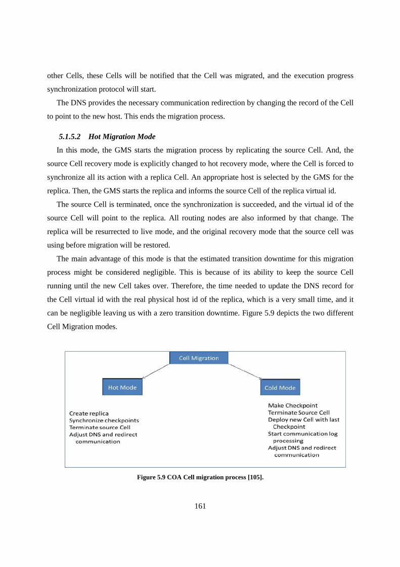
161

other Cells, these Cells will be notified that the Cell was migrated, and the execution progress

synchronization protocol will start.

The DNS provides the necessary communication redirection by changing the record of the Cell

to point to the new host. This ends the migration process.

5.1.5.2 Hot Migration Mode

In this mode, the GMS starts the migration process by replicating the source Cell. And, the

source Cell recovery mode is explicitly changed to hot recovery mode, where the Cell is forced to

synchronize all its action with a replica Cell. An appropriate host is selected by the GMS for the

replica. Then, the GMS starts the replica and informs the source Cell of the replica virtual id.

The source Cell is terminated, once the synchronization is succeeded, and the virtual id of the

source Cell will point to the replica. All routing nodes are also informed by that change. The

replica will be resurrected to live mode, and the original recovery mode that the source cell was

using before migration will be restored.

The main advantage of this mode is that the estimated transition downtime for this migration

process might be considered negligible. This is because of its ability to keep the source Cell

running until the new Cell takes over. Therefore, the time needed to update the DNS record for

the Cell virtual id with the real physical host id of the replica, which is a very small time, and it

can be negligible leaving us with a zero transition downtime. Figure 5.9 depicts the two different

Cell Migration modes.

Figure 5.9 COA Cell migration process [105].

162

5.2 Evaluation

Using analysis and simulation evaluations of our virtualization and task management layer, we

study the effect associated with execution of applications in different mobile computing

environments. Such environments considered a pure mobile model, MAC, consisting of mobile

nodes and a hybrid model, HMAC, consisting of portable mobile devices and semi-stationary on-

board computing resources of vehicles in different sizes hospital scenarios. Then, a

comprehensive evaluation is performed for PlanetCloud efficiency using different scenarios to

study its performance, while changing different parameters related to connectivity, density of

nodes, load of submitted tasks, reliability, scalability, and management overhead.

5.2.1 Performance Metrics

In this chapter, several metrics are used to evaluate the performance of our PlanetCloud and its

subsystems, while comparing the efficiency of applying different resource allocation algorithms.

These metrics are summarized as follows.

1) The average application execution time, which is the time elapsed from the application

submission to the application completion.

2) The mean number of VM migrations, which is the number of VM migrations during

the simulation time.

5.2.2 Evaluation of Applying the Virtualization and Task Management Layer in a MAC

In this evaluation, the virtualization and task management layer is considered, which manages

all issues related to the deployment and management of VMs including VM migrations. Where, a

VM can be migrated out from the mobile node as the node becomes unreliable to execute a task.

Migrations happen when communications are established among participating nodes.

For evaluation purposes, we present a scenario of dynamic resources in a medium hospital

model (50 beds). The model involves different types of mobile devices such as Smartphones and

Laptop Computers. Such rather huge pool of idle computing resources can serve as the basis of a

MAC as a networked computing center. We start our evaluation by predicting the average number

of participants in this scenario which reflects the amount of computing resources that might

participate in a MAC. Then, we perform evaluations, using the obtained average number of

participants, to study the effect associated with the performance of the formed MAC.

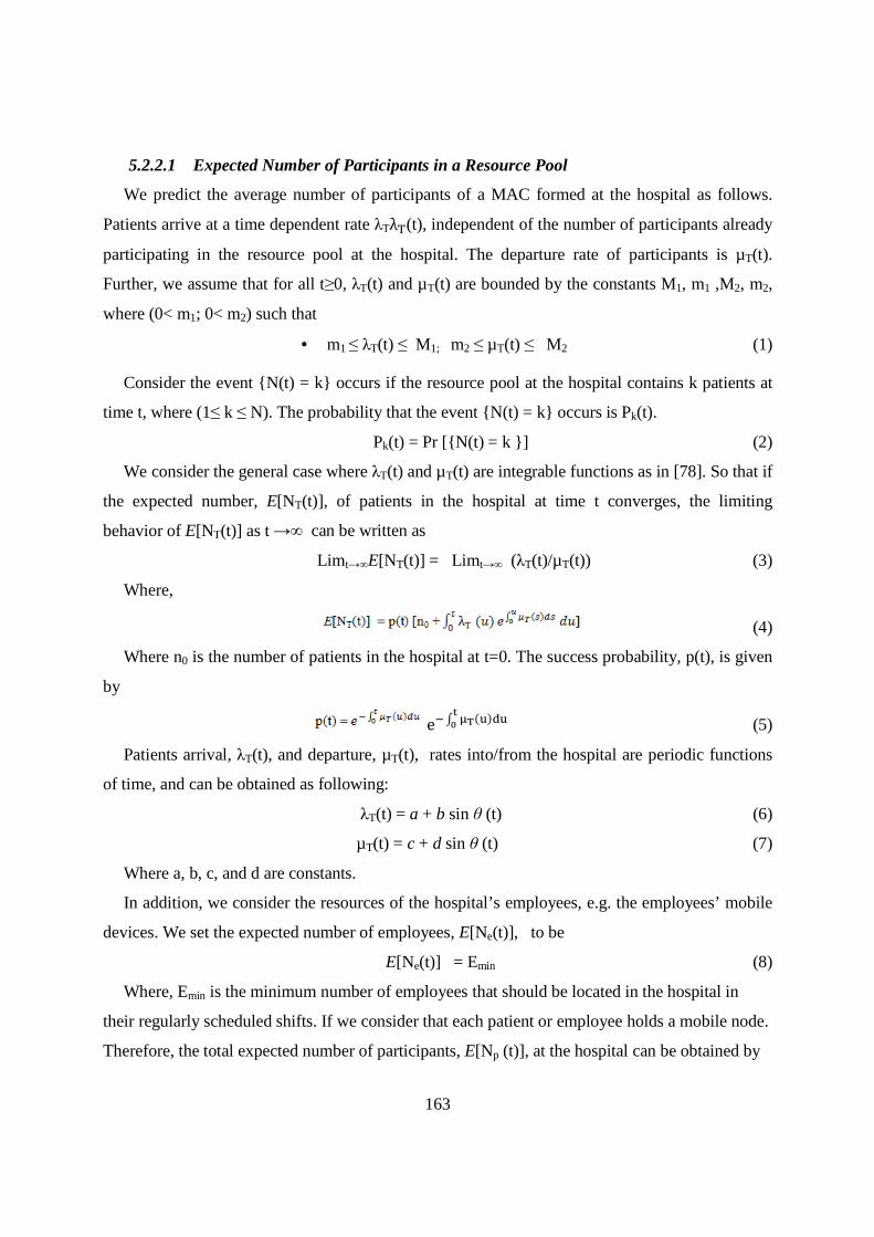
163

5.2.2.1 Expected Number of Participants in a Resource Pool

We predict the average number of participants of a MAC formed at the hospital as follows.

Patients arrive at a time dependent rate λTλS(t), independent of the number of participants already

participating in the resource pool at the hospital. The departure rate of participants is µT(t).

Further, we assume that for all t≥0, λT(t) and µT(t) are bounded by the constants M1, m1 ,M2, m2,

where (0< m1; 0< m2) such that

• m1 ≤ λT(t) ≤ M1; m2 ≤ µT(t) ≤ M2 (1)

Consider the event {N(t) = k} occurs if the resource pool at the hospital contains k patients at

time t, where (1≤ k ≤ N). The probability that the event {N(t) = k} occurs is Pk(t).

Pk(t) = Pr [{N(t) = k }] (2)

We consider the general case where λT(t) and µT(t) are integrable functions as in [78]. So that if

the expected number, E[NT(t)], of patients in the hospital at time t converges, the limiting

behavior of E[NT(t)] as t →∞ can be written as

Lim t→∞E[NT(t)] = Limt→∞ (λT(t)/µT(t)) (3)

Where,

(4)

Where n0 is the number of patients in the hospital at t=0. The success probability, p(t), is given

by

eQ² G³(&)�&�T (5)

Patients arrival, λT(t), and departure, µT(t), rates into/from the hospital are periodic functions

of time, and can be obtained as following:

λT(t) = a + b sin θ (t) (6)

µT(t) = c + d sin θ (t) (7)

Where a, b, c, and d are constants.

In addition, we consider the resources of the hospital’s employees, e.g. the employees’ mobile

devices. We set the expected number of employees, E[Ne(t)], to be

E[Ne(t)] = Emin (8)

Where, Emin is the minimum number of employees that should be located in the hospital in

their regularly scheduled shifts. If we consider that each patient or employee holds a mobile node.

Therefore, the total expected number of participants, E[Np (t)], at the hospital can be obtained by

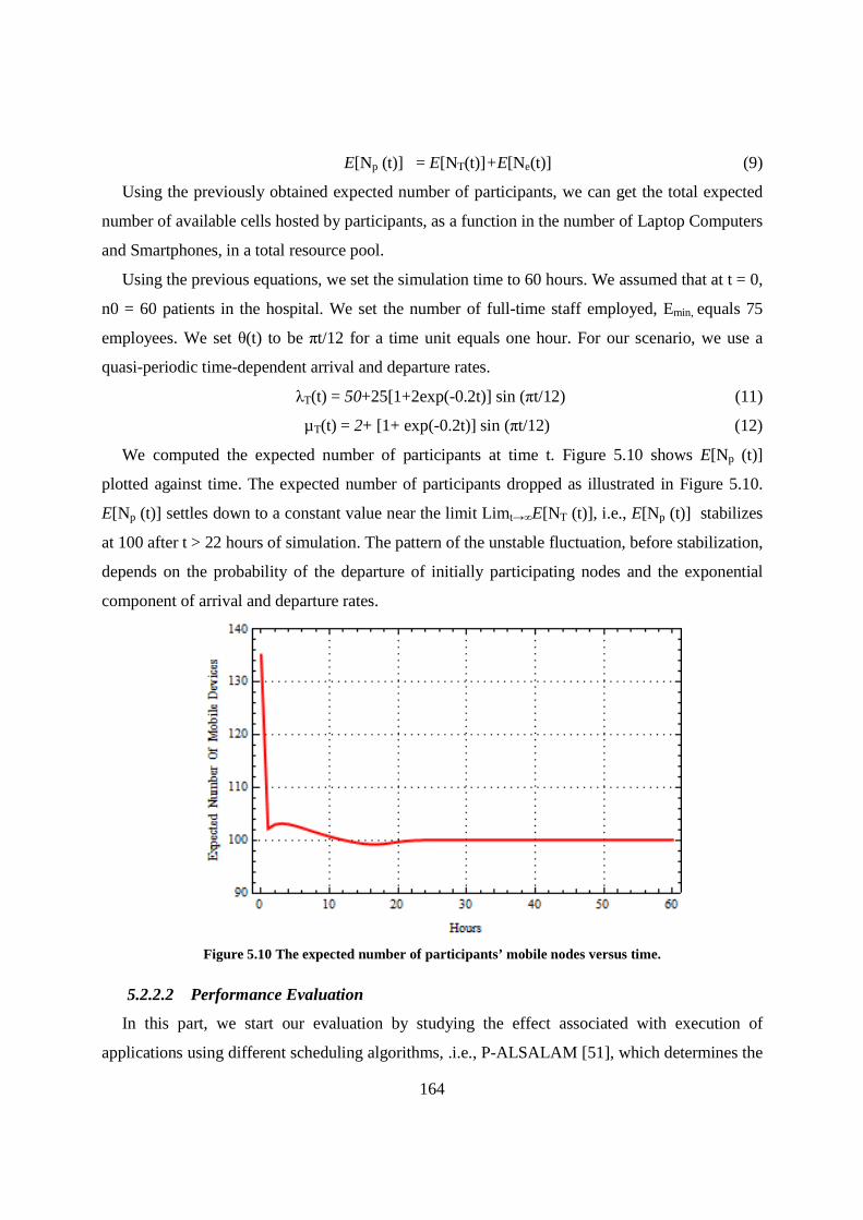
164

E[Np (t)] = E[NT(t)]+E[Ne(t)] (9)

Using the previously obtained expected number of participants, we can get the total expected

number of available cells hosted by participants, as a function in the number of Laptop Computers

and Smartphones, in a total resource pool.

Using the previous equations, we set the simulation time to 60 hours. We assumed that at t = 0,

n0 = 60 patients in the hospital. We set the number of full-time staff employed, Emin, equals 75

employees. We set θ(t) to be πt/12 for a time unit equals one hour. For our scenario, we use a

quasi-periodic time-dependent arrival and departure rates.

λT(t) = 50+25[1+2exp(-0.2t)] sin (πt/12) (11)

µT(t) = 2+ [1+ exp(-0.2t)] sin (πt/12) (12)

We computed the expected number of participants at time t. Figure 5.10 shows E[Np (t)]

plotted against time. The expected number of participants dropped as illustrated in Figure 5.10.

E[Np (t)] settles down to a constant value near the limit Lim t→∞E[NT (t)], i.e., E[Np (t)] stabilizes

at 100 after t > 22 hours of simulation. The pattern of the unstable fluctuation, before stabilization,

depends on the probability of the departure of initially participating nodes and the exponential

component of arrival and departure rates.

Figure 5.10 The expected number of participants’ mobile nodes versus time.

5.2.2.2 Performance Evaluation

In this part, we start our evaluation by studying the effect associated with execution of

applications using different scheduling algorithms, .i.e., P-ALSALAM [51], which determines the

165

best participants based on the availability of its resources to participate in a cloud and the random-

based algorithm, which does not use this information, where random mobile nodes with random

availability are selected to execute the submitted application.

We have extended the CloudSim simulator [26][27] to simulate the MAC environment in

hospital. Where, a MAC consists of N heterogeneous mobile nodes characterized by the number

of processing cores. CPU performance is defined in Millions Instructions Per Second (MIPS),

amount of RAM, storage and network bandwidth.

In the evaluations of our virtualization and task management layer, each task has a pre-

assigned instruction length and runs in a Cell. A Cell is simulated as a single VM deployed on a

mobile node. Also, a Cell must match the smallest computational power available in any

participants, which is simulated as a single VM deployed on a participant. A VM can be migrated

out from the mobile node as the node becomes unreliable to execute a task. Such that, we consider

that mobile nodes cannot always function well all the time and may fail. We set the number of

inactive nodes to be sampled following a Poisson Process during a time t. We suppose that the

distribution of detection time of failure is uniform from 0 to 1 second. Detection time represents

the length of a period from the time when a participant starts crashing to the time to be suspected.

In addition, we only consider the cold-recovery mode in case of node failure.

a) Parameters

For all evaluations of our virtualization and task management layer, we set parameters in the

simulation according to the maximum and minimum values shown in Table 5.1.

Table 5.1 Parameters for Evaluation of the Virtualization and Task Management Layer.

Parameters Values Parameters Values

Density of nodes 70-100

(Nodes/Km²)

Communication

range 0.2 (km)

Task length 500000 (MI)

Number of

CPUs/Cores per

host

1, 2

Number of

tasks/Application 20

Inactive Node rate

(Poisson Process)

1/45 -1/10

(Node/Sec)

166

b) Simulation Setup

The MAC in a hospital is composed of previously obtained 100 mobile nodes with

heterogeneous characteristics: 512 or 1024 MB RAM, 4 GB Storage, and 54 MB bandwidth. Each

mobile node may have one or two cores with processing capabilities of 2000 or 7500 (MIPS),

respectively. In our evaluations, we create VMs each has one processing core with processing

capability 1256 MIPS and 512 MB RAM. Also, we consider one application is submitted to be

executed.

c) Static Nodes Scenario

In this experiment, we consider that every mobile node has a fixed location. Also, the

communication among mobile nodes is always possible within the hospital.

We perform the evaluation at density of nodes equals 100 nodes/km². We perform the

evaluation with various values of the arrival rate of inactive nodes, ranging from 1/40 to 1/10

(nodes/sec). As expected, this evaluation provides significant differences between the results of

the two cases, with/without using the P-ALSALAM. The results of Figure 4.11 show that a better

performance, in terms of the average execution time of an application, is obtained at a smaller

arrival rate of inactive nodes, e.g. 1/40 (nodes/sec) than in the case of results at a larger arrival

rate of inactive nodes, e.g. 1/10 (nodes/sec). This is because at larger arrival rate of inactive

nodes, the probability a node could fail increases. Similarly, Figure 5.12 shows the average

number of migrations of a VM increases when the arrival rate of inactive nodes is increased. This

is because at larger arrival rate of inactive nodes the probability a node could fail increases. This

forces a VM to migrate to another reliable node.

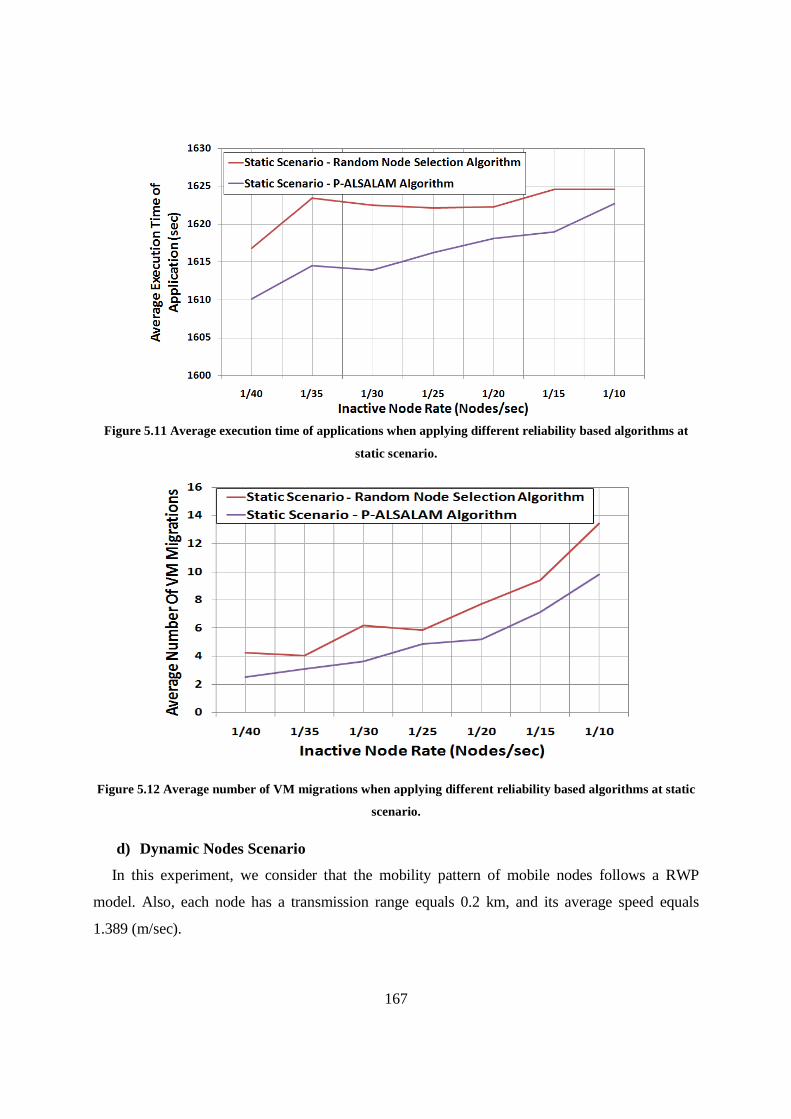
167

Figure 5.11 Average execution time of applications when applying different reliability based algorithms at

static scenario.

Figure 5.12 Average number of VM migrations when applying different reliability based algorithms at static

scenario.

d) Dynamic Nodes Scenario

In this experiment, we consider that the mobility pattern of mobile nodes follows a RWP

model. Also, each node has a transmission range equals 0.2 km, and its average speed equals

1.389 (m/sec).

168

As expected, this evaluation provides significant differences between the results of the two

cases, reliable/random node selection as depicted in Figure 5.13. The results of Figure 5.14 show

that a better performance, in terms of the average number of VM migrations, is obtained at a

smaller arrival rate of inactive nodes than in the case of results at a larger arrival rate of inactive

nodes where the probability a node could fail increases. This triggers a VM to migrate to another

reliable node.

e) Dynamicity Overhead

Figure 5.15 shows that the mobility of a node and its connectivity affects the performance of

the application such that a delay overhead is added to the average execution time of application

which makes it worse than the performance of the static scenario. The reason is that the short

transmission range of a mobile node in a dynamic scenario, i.e., 0.2 km leads to increase in the

communication time until the primary node collects results from the other nodes. The figure

shows that the overhead that is added to the average execution time of application increases with

the increase in the arrival rate of inactive nodes as the migrations increase.

Figure 5.13 Average execution time of applications when applying different reliability based algorithms at

dynamic scenario.

169

Figure 5.14 Average number of VM migrations when applying different reliability based algorithms at

dynamic scenario.

Figure 5.15 Comparison between dynamic scenario and static scenario when applying different reliability

based algorithms.

5.2.3 Evaluation of Applying the Virtualization and Task Management Layer in a Hybrid

MAC (HMAC)

In this evaluation, we present a scenario of dynamic resources in a small size hospital model

(25beds). The model involves different types of mobile devices such as Smartphones and Laptop

170

Computers and semi-stationary devices such as on-board computing resources of vehicles in a

long-term parking lot at a hospital. Such rather huge pool of idle computing resources can serve as

the basis of a HMAC as a networked computing center. Where, the previous evaluations did not

consider such a real hybrid model and only considered a MAC of mobile nodes. We start this

evaluation by predicting the average number of participants in this scenario, which reflects the

amount of computing resources that might cooperate to participate in a HMAC. Then, we perform

evaluations, using the obtained average number of participants, to study the effect associated with

the performance of the formed HMAC.


In this part, we predict the average number of participants of a HMAC formed at the hospital.

We can use the previous equations, from the previous section, to get the expected number of

cars, E[Nc(t)], in the parking lot at time t, where a relationship do exist between traffic and the

number of arriving/departing patients. Therefore, we can model the expected number of cars as a

percentage factor, v, using the following cars arrival, λC (t), and departure, µC (t), rates

λ�(t) = v*λS(t) (8)

µC(t) = x+ y sin θ (t) (9)

Similarly, we can calculate E[Nc(t)] and we set the number of patients’ cars in the hospital at

t=0 to be equal v*n0. The limiting behavior of E[Nc (t)] as t →∞ can be written as

Lim t→∞E[Nc (t)] = Limt→∞ (λC(t)/µC(t)) (10)

Let E[Nm(t)] be the expected number of patients’ mobile nodes, in the hospital at time t, where

each patient holds a mobile node. This allows us to write

E[Nm(t)] =E[NT(t)] (11)

In addition, we consider the resources of the hospital’s employees as valuable participants in

the formed cloud. Such resources may include the computational power of the employees’ mobile

devices as well as on-board computing resources of employees’ cars in the employee parking lots

at the hospital. We set the expected number of employees, E[Ne(t)], to be

E[Ne(t)] = Emin (12)

Similarly, we set the expected number of employee cars, E[Nec(t)], as a percentage factor, f,

of the number of employees. We can write

E[Nec(t)] = f*E[Ne(t)] (13)

The total expected number of participants, E[Np (t)], in the airport can be obtained by

171

E[Np (t)] = E[Nc(t)] + E[Nm(t)] + E[Nec(t)] +E[Ne(t)] (14)

Using the previously obtained expected number of participants, we can get the total number of

available cells hosted by participants in a total resource pool. For example, the on-board

computing resources of a vehicle can host an expected number of cells equals V cells, while a

Smartphone or Laptop Computer can host expected number of cells equals M cells. Therefore, the

total expected number of cells could be calculated as a function in the number of Laptop

Computers or Smartphones and vehicles.

We set the simulation time to 60 hours. We assumed that at t = 0, n0 equals 35 patients.

Similarly, we set the number of full-time staff employed, Emin, equals 35 employees [142]. We set

θ(t) to be πt/12 for a time unit equals one hour. We use a quasi-periodic time-dependent arrival

and departure rates as follows.

λT(t) = 32+16[1+2exp(-0.2t)] sin (πt/12) (15)

λC(t) = 0.3* (32+16[1+2exp(-0.2t)] sin (πt/12)) (16)

Where,

µT(t) = µC(t) = 2+ [1+ exp(-0.2t)] sin (πt/12) (23)

We computed the expected number of mobile nodes at time t as shown in Figure 5.16 shows

E[Np (t)]. The expected number of mobile nodes dropped as illustrated in Figure 5.16 and settles

down to a constant value at 51after t > 20 hours of simulation. The pattern of the unstable

fluctuation, before stabilization, depends on the probability of the departure of initially

participating nodes and the exponential component of arrival and departure rates. Similarly,

Figure 5.17 shows the expected number of cars in the parking lot of the hospital stabilizes to a

constant number at 19 after 20 hours.

Next, we turned our attention to compute the expected number of participants in the hospital

versus time. Figure 5.18 shows E[Np (t)] plotted against time. The expected number of

participants dropped as illustrated in Figure 5.18. E[Np (t)] stabilizes at 70 participants after t > 20

hours of simulation.

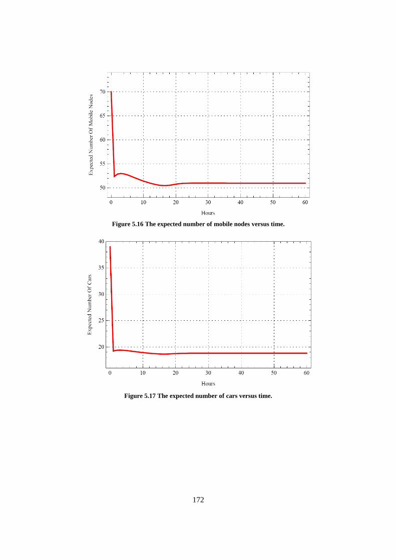
172

Figure 5.16 The expected number of mobile nodes versus time.

Figure 5.17 The expected number of cars versus time.

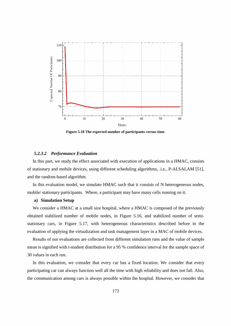
173

Figure 5.18 The expected number of participants versus time.


In this part, we study the effect associated with execution of applications in a HMAC, consists

of stationary and mobile devices, using different scheduling algorithms, .i.e., P-ALSALAM [51],

and the random-based algorithm.

In this evaluation model, we simulate HMAC such that it consists of N heterogeneous nodes,

mobile/ stationary participants. Where, a participant may have many cells running on it.

a) Simulation Setup

We consider a HMAC at a small size hospital, where a HMAC is composed of the previously

obtained stabilized number of mobile nodes, in Figure 5.16, and stabilized number of semi-

stationary cars, in Figure 5.17, with heterogeneous characteristics described before in the

evaluation of applying the virtualization and task management layer in a MAC of mobile devices.


mean is signified with t-student distribution for a 95 % confidence interval for the sample space of

30 values in each run.

In this evaluation, we consider that every car has a fixed location. We consider that every

participating car can always function well all the time with high reliability and does not fail. Also,

the communication among cars is always possible within the hospital. However, we consider that

174

the mobility pattern of mobile nodes follows a RWP model. Also, each node has an average speed

equals 1.389 (m/sec). We consider that mobile nodes are different in their reliability, in terms of

future availability, which follow the values of the arrival rate of inactive nodes.

b) Results

The average execution time of an application is investigated at different values of the arrival

rate of inactive nodes, ranging from 1/45 to 1/15 (nodes/sec). We consider a small-sized hospital

(25 beds) with total number of participants equals 70 (19 cars and 51 mobile nodes). Also, we

consider that each node has a transmission range equals 0.2 km. We consider one application is

submitted to be executed, with a number of tasks equals to 20, and we set the task length to be

equal to 500000 MI.

Figure 5.19 shows that at a larger value of arrival rate of inactive nodes, e.g. 1/15 (nodes/sec),

the worst performance is obtained than in the case of results at a smaller arrival rate of inactive

nodes, e.g. 1/45 (nodes/sec). This is because of the probability a node could fail is high when

compared with a lower arrival rate of inactive nodes value. Consequently, the average number of

migrations of a VM increases when the arrival rate of inactive nodes is increased as shown in

Figure 5.20.

The node failure forces a VM to migrate to another reliable node. This leads to an extra time

overhead of VM migration which is added to the execution time of an application. These results

showed that our PlanetCloud performs well in terms of the average execution time of application

with a smaller number of VM migrations even in case when a large number of mobile nodes have

left the HMAC. Also, results showed that PlanetCloud has a better capability to minimize the

delay overhead added to the average execution time of an application due to mobility of

participants than the case of random selection of participant nodes.

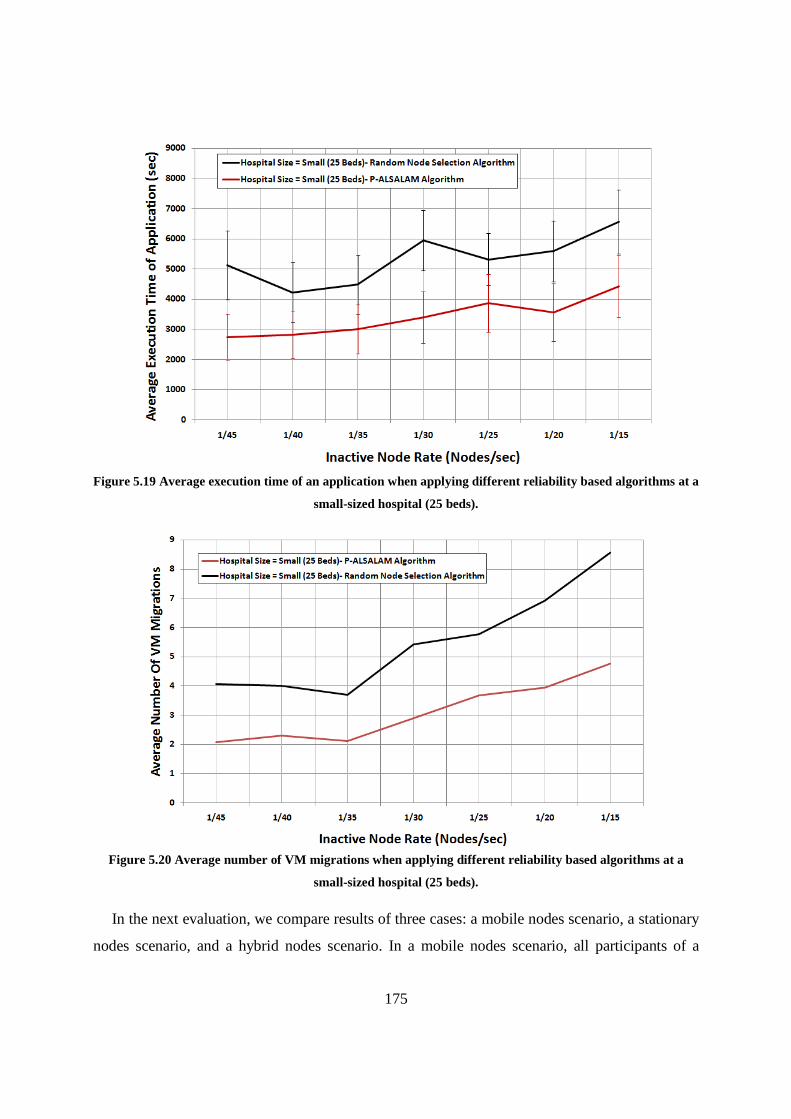
175

Figure 5.19 Average execution time of an application when applying different reliability based algorithms at a

small-sized hospital (25 beds).

Figure 5.20 Average number of VM migrations when applying different reliability based algorithms at a


In the next evaluation, we compare results of three cases: a mobile nodes scenario, a stationary

nodes scenario, and a hybrid nodes scenario. In a mobile nodes scenario, all participants of a

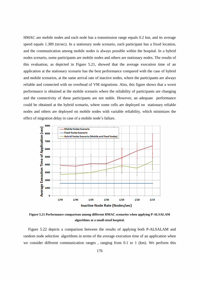
176

HMAC are mobile nodes and each node has a transmission range equals 0.2 km, and its average

speed equals 1.389 (m/sec). In a stationary node scenario, each participant has a fixed location,

and the communication among mobile nodes is always possible within the hospital. In a hybrid

nodes scenario, some participants are mobile nodes and others are stationary nodes. The results of

this evaluation, as depicted in Figure 5.21, showed that the average execution time of an

application at the stationary scenario has the best performance compared with the case of hybrid

and mobile scenarios, at the same arrival rate of inactive nodes, where the participants are always

reliable and connected with no overhead of VM migrations. Also, this figure shows that a worst

performance is obtained at the mobile scenario where the reliability of participants are changing

and the connectivity of these participants are not stable. However, an adequate performance

could be obtained at the hybrid scenario, where some cells are deployed on stationary reliable

nodes and others are deployed on mobile nodes with variable reliability, which minimizes the

effect of migration delay in case of a mobile node’s failure.

Figure 5.21 Performance comparison among different HMAC scenarios when applying P-ALSALAM

algorithms at a small-sized hospital.

Figure 5.22 depicts a comparison between the results of applying both P-ALSALAM and

random node selection algorithms in terms of the average execution time of an application when

we consider different communication ranges , ranging from 0.1 to 1 (km). We perform this

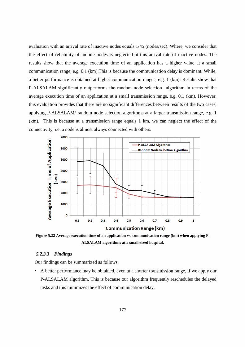
177

evaluation with an arrival rate of inactive nodes equals 1/45 (nodes/sec). Where, we consider that

the effect of reliability of mobile nodes is neglected at this arrival rate of inactive nodes. The

results show that the average execution time of an application has a higher value at a small

communication range, e.g. 0.1 (km).This is because the communication delay is dominant. While,

a better performance is obtained at higher communication ranges, e.g. 1 (km). Results show that

P-ALSALAM significantly outperforms the random node selection algorithm in terms of the

average execution time of an application at a small transmission range, e.g. 0.1 (km). However,

this evaluation provides that there are no significant differences between results of the two cases,

applying P-ALSALAM/ random node selection algorithms at a larger transmission range, e.g. 1

(km). This is because at a transmission range equals 1 km, we can neglect the effect of the

connectivity, i.e. a node is almost always connected with others.

Figure 5.22 Average execution time of an application vs. communication range (km) when applying P-

ALSALAM algorithms at a small-sized hospital.

5.2.3.3 Findings


• A better performance may be obtained, even at a shorter transmission range, if we apply our

P-ALSALAM algorithm. This is because our algorithm frequently reschedules the delayed

tasks and this minimizes the effect of communication delay.

178

• The performance is affected by the percentage of the number of fixed nodes within the total

density of available nodes. It means the more fixed reliable nodes participate in a HMAC,

the less dependency on mobile variable reliability nodes. This could enhance the

performance of the submitted application.

5.2.4 PlanetCloud Efficiency

In this part, we evaluate our proposed PlanetCloud platform using different scenarios to study

its performance while changing different parameters related to connectivity, density of nodes,

load of submitted tasks, reliability, scalability, and management overhead.

For evaluation purposes, we present a scenario of dynamic resources in different-sized hospital

models, small, medium, large and huge with 25, 50, 75, and 100 beds, respectively. Similar to the

previous evaluation, the model involves different types of mobile devices, e.g. Smartphones,

Laptop Computers, and on-board computing resources of vehicles in a long-term parking lot at a

hospital. Such rather huge pool of idle computing resources can serve as the basis of a HMAC.

We start this evaluation by predicting the average number of participants in this scenario at

hospitals of different sizes, which reflects the amount of computing resources that might

participate in a HMAC. Then, we perform evaluations, using the obtained average number of

participants, to study the effect associated with the performance of the formed HMAC.


Using the previous equations, we set the simulation time to 60 hours. We assumed that at t = 0,

n0 equals 35, 60, 85, 100 patients, respectively, according to the size of the hospital. Similarly, we

set the number of full-time staff employed, Emin, equals 35, 61, 94, 116 employees, respectively,

according to the size of the hospital [142]. We set θ(t) to be πt/12 for a time unit equals one hour.

For each size of a hospital, we use a quasi-periodic time-dependent arrival and departure rates as

follows.

At hospital size equals 25 beds,

λT(t) = 32+16[1+2exp(-0.2t)] sin (πt/12) (15)

λC(t) = 0.3* (32+16[1+2exp(-0.2t)] sin (πt/12)) (16)


λT(t) = 72+36[1+2exp(-0.2t)] sin (πt/12) (17)

λC(t) = 0.3* (72+36[1+2exp(-0.2t)] sin (πt/12)) (18)

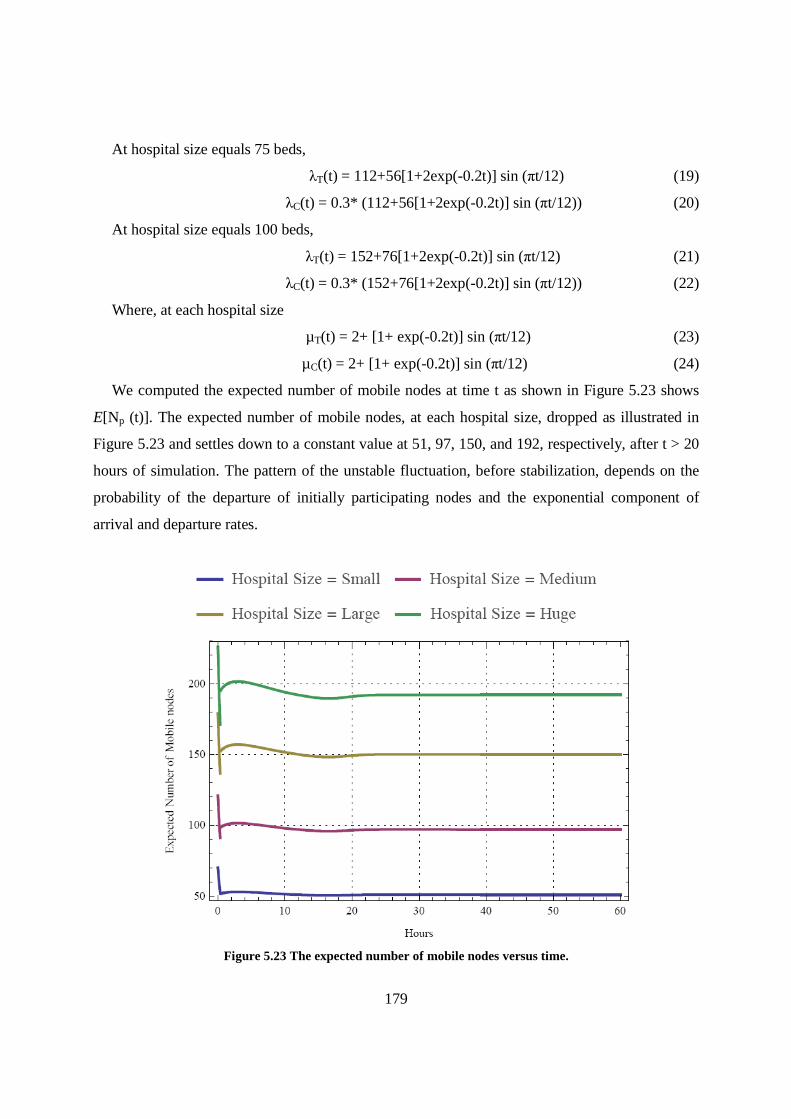
179


λT(t) = 112+56[1+2exp(-0.2t)] sin (πt/12) (19)

λC(t) = 0.3* (112+56[1+2exp(-0.2t)] sin (πt/12)) (20)


λT(t) = 152+76[1+2exp(-0.2t)] sin (πt/12) (21)

λC(t) = 0.3* (152+76[1+2exp(-0.2t)] sin (πt/12)) (22)

Where, at each hospital size

µT(t) = 2+ [1+ exp(-0.2t)] sin (πt/12) (23)

µC(t) = 2+ [1+ exp(-0.2t)] sin (πt/12) (24)

We computed the expected number of mobile nodes at time t as shown in Figure 5.23 shows

E[Np (t)]. The expected number of mobile nodes, at each hospital size, dropped as illustrated in

Figure 5.23 and settles down to a constant value at 51, 97, 150, and 192, respectively, after t > 20

hours of simulation. The pattern of the unstable fluctuation, before stabilization, depends on the

probability of the departure of initially participating nodes and the exponential component of

arrival and departure rates.

Figure 5.23 The expected number of mobile nodes versus time.

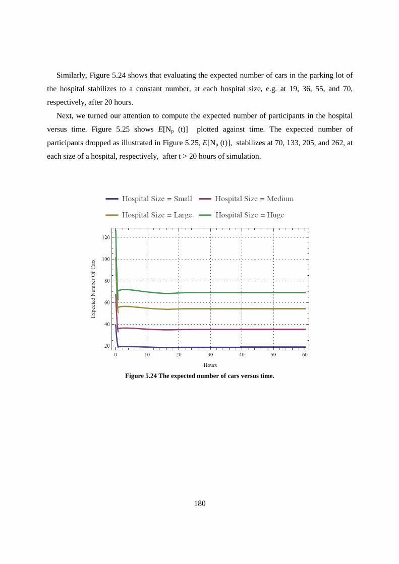
180

Similarly, Figure 5.24 shows that evaluating the expected number of cars in the parking lot of

the hospital stabilizes to a constant number, at each hospital size, e.g. at 19, 36, 55, and 70,

respectively, after 20 hours.

Next, we turned our attention to compute the expected number of participants in the hospital

versus time. Figure 5.25 shows E[Np (t)] plotted against time. The expected number of

participants dropped as illustrated in Figure 5.25, E[Np (t)], stabilizes at 70, 133, 205, and 262, at

each size of a hospital, respectively, after t > 20 hours of simulation.

Figure 5.24 The expected number of cars versus time.

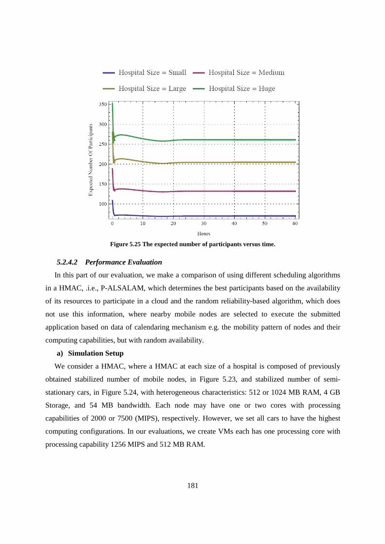
181

Figure 5.25 The expected number of participants versus time.


In this part of our evaluation, we make a comparison of using different scheduling algorithms

in a HMAC, .i.e., P-ALSALAM, which determines the best participants based on the availability

of its resources to participate in a cloud and the random reliability-based algorithm, which does

not use this information, where nearby mobile nodes are selected to execute the submitted

application based on data of calendaring mechanism e.g. the mobility pattern of nodes and their

computing capabilities, but with random availability.

a) Simulation Setup

We consider a HMAC, where a HMAC at each size of a hospital is composed of previously

obtained stabilized number of mobile nodes, in Figure 5.23, and stabilized number of semi-

stationary cars, in Figure 5.24, with heterogeneous characteristics: 512 or 1024 MB RAM, 4 GB

Storage, and 54 MB bandwidth. Each node may have one or two cores with processing

capabilities of 2000 or 7500 (MIPS), respectively. However, we set all cars to have the highest

computing configurations. In our evaluations, we create VMs each has one processing core with

processing capability 1256 MIPS and 512 MB RAM.

182


mean is signified with t-student distribution for a 95 % confidence interval for the sample space of

30 values in each run.

In our evaluation, we consider that every car has a fixed location. We consider that every

participating car can always function well all the time with high reliability and does not fail.

However, we consider that the mobility pattern of mobile nodes follows a RWP model. Also, each

node has an average speed equals 1.389 (m/sec). We consider that mobile nodes are different in

their reliability, in terms of future availability and reputation, which follow the values of the

arrival rate of inactive nodes.

b) Results

1. Connectivity Effect at Different Number of Tasks

The average execution time of an application is investigated at different communication ranges

of stationary nodes, cars, ranging from 0.1 to 1 (km) when we consider one application is

submitted to be executed, with different number of tasks, ranging from 20 to 70 tasks. We

consider a small-sized hospital (25 beds) with total number of participant equals 70 (19 cars and

51 mobile nodes). Also, we consider that all nodes are reputable and each mobile node has a

transmission range equals 0.4 km, and its average speed equals 1.389 (m/sec). We set the task

length to be equal to 500000 MI. We perform this evaluation with an arrival rate of inactive nodes

equals 1/45 (nodes/sec). Where, we consider that the effect of reliability of mobile nodes is

neglected at this arrival rate of inactive nodes.


random reliability-based node selection algorithms in terms of the average execution time of an

application at a small-sized hospital. Results show that P-ALSALAM significantly outperforms

the random reliability-based node selection algorithm in terms of the average execution time of an

application at all transmission ranges. Similarly, the average number of VM migrations when

applying P-ALSALAM significantly is smaller than the case when applying the random

reliability-based node selection algorithm as shown in Figure 5.27.

183

Figure 5.26 Average execution time of an application when applying different reliability based algorithms at a


Figure 5.27 Average number of VM migrations when applying different reliability based algorithms at a


The results of Figure 5.28 show that the average execution time of an application has a higher

value at a small communication range, e.g. 0.1 (km). This is because the smaller the

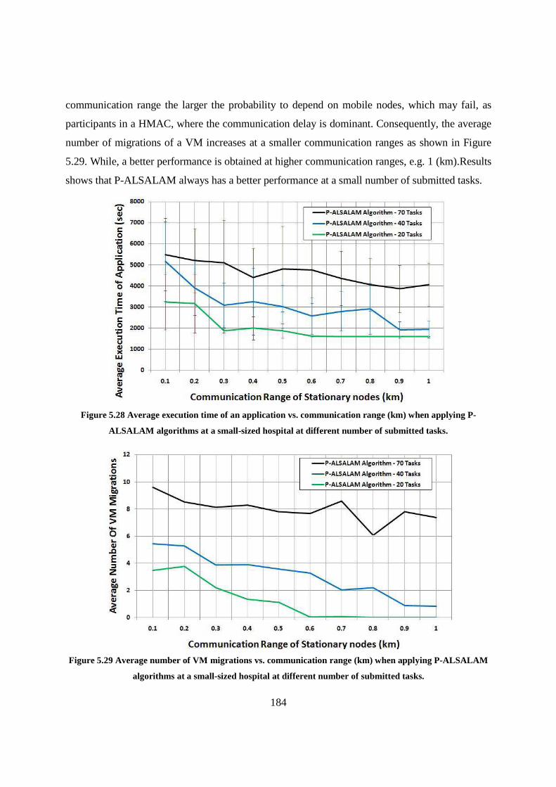
184

communication range the larger the probability to depend on mobile nodes, which may fail, as

participants in a HMAC, where the communication delay is dominant. Consequently, the average

number of migrations of a VM increases at a smaller communication ranges as shown in Figure

5.29. While, a better performance is obtained at higher communication ranges, e.g. 1 (km).Results

shows that P-ALSALAM always has a better performance at a small number of submitted tasks.

Figure 5.28 Average execution time of an application vs. communication range (km) when applying P-

ALSALAM algorithms at a small-sized hospital at different number of submitted tasks.

Figure 5.29 Average number of VM migrations vs. communication range (km) when applying P-ALSALAM

algorithms at a small-sized hospital at different number of submitted tasks.

185

2. Density Effect at Different Communication Ranges of Stationary Nodes

We repeat the evaluation of P-ALSALAM algorithm at a different size of a hospital, i.e., small,

medium, large or huge hospital which represents different node densities when we consider

different communication ranges of stationary nodes, e.g. 0.2 and 1 (km), respectively. We set the

arrival rate of inactive nodes to be 1/45 (Node/Sec). We consider one application is submitted to

be executed, with a number of tasks equals to 70. Figure 5.30 shows that a small-sized hospital

with low node density, e.g. 70 (Nodes/Km²), has a high average execution time of an application.

This is because of the average number of fixed reliable cars, e.g. 19, is small when compared with

a larger number of fixed at high density value. Conversely, a better performance is obtained at a

huge-sized hospital with high node density, e.g. 262 (Nodes/Km²), when the average number of

fixed reliable cars is large, e.g. 70. This is because the performance is enhanced when our P-

ALSALAM algorithm can assign the requested tasks to a larger number of reliable resources and

less depends on variable reliability mobile nodes. Similarly, Figure 5.31 shows that the higher the

node density the higher dependency on reliable and connected fixed nodes to execute the

submitted tasks, and therefore the lower probability of VM migrations is obtained.

Figure 5.30 Average execution time of an application vs. node density (nodes/km²) when applying P-

ALSALAM algorithms at different-sized hospital models at different stationary nodes’ communication

ranges.

186

Figure 5.31 Average number of VM migrations vs. node density (nodes/km²) when applying P-ALSALAM

algorithms at different-sized hospital models at different stationary nodes’ communication ranges.

3. Density Effect at Different Number of Tasks

We repeat the evaluation of P-ALSALAM algorithm at a different number of submitted tasks

equals to 20 and 70, respectively. We consider the communication range of a stationary node

equals 1 (km). We set the arrival rate of inactive nodes to be 1/45 (Node/Sec). The results of this

evaluation , as depicted in Figure 5.32, showed that the average execution time of an application

at a small number of tasks, e.g., 20 tasks has a best performance than the case of a large number

of tasks, at the same small density of nodes, e.g. 70 (Nodes/Km²). However, this evaluation

provides that there are no significant differences between results of the two cases at a larger

density of nodes, e.g. 133, 205, or 262 (Nodes/Km²). This is because at transmission range equals

1 km, we can neglect the effect of the connectivity, i.e. a stationary node is almost always

connected with others. Therefore, the only factor which affects on the performance is the load of

submitted tasks with respect to the number of available and reliable nodes. Since, the number of

participant in a small-sized hospital (25 beds) equals 70 (19 cars and 51 mobile nodes), at this

number there is almost the guaranteed number of participants with their reliable resources that

satisfy the application, with 20 tasks, requirements. However, a worst performance is obtained at

a small size hospital where the number of stationary cars, e.g. 19, does not satisfy the

requirements of an application with 70 tasks. In this case, there will be more dependency of

187

mobile nodes with their limited communication ranges, e.g. 0.4 (km), which could fail. At a larger

density of nodes, 133 and more, our system can always guarantee the required number of

participants that could satisfy the application requirements.

Also, this figure shows that a worst performance is obtained at the mobile scenario where the

reliability of participants are changing and the connectivity of these participants are not stable.

However, an adequate performance could be obtained at the hybrid scenario, where some cells

are deployed on fixed reliable nodes and others are deployed on mobile nodes with variable

reliability which minimizes the effect of migration delay in case of a mobile node’s failure. We

need to do this at same arrival rate of inactive nodes = 1/45.


ALSALAM algorithms at different-sized hospital models at different number of submitted tasks.

4. Density Effect at Different Arrival Rates of Inactive Nodes

Similarly, we repeat the evaluation of P-ALSALAM algorithm at a different arrival rate of

inactive nodes equals 1/45 and 1/15 (Node/Sec), respectively. Figure 5.33, showed that the

average execution time of an application at a large density of nodes, e.g. 262 (Nodes/Km²) has a

better performance than the case of a small density of node, e.g. 70 (Nodes/Km²), at the same

number of tasks, e.g., 20 tasks and the same arrival rate of inactive nodes, e.g. 1/45 (Node/Sec).

This is because the larger the density of nodes the more dependency on reliable stationary nodes.

188

However, the smaller the density of nodes the more dependency on variable reliability mobile

nodes that could fail, and therefore the performance may degraded due to the migration delay.

Results depict that the effect of node failure may be neglected at arrival rate of inactive nodes

equals 1/45 (Node/Sec) at different density of nodes.


ALSALAM algorithms at different-sized hospital models at different arrival rates of inactive nodes.

5. Task Load Effect

Figure 5.34 depicts results of applying both P-ALSALAM and random reliability-based node

selection algorithms in terms of the average execution time of an application when we consider

different task load in terms of the number of submitted tasks, ranging from 10 to 70 tasks at a

small-sized hospital. To neglect the effect of connectivity and reliability of nodes we consider the

communication range of a stationary node equals 1 (km) and we set the arrival rate of inactive

nodes to be 1/45 (Node/Sec).

The results of this evaluation showed that the average execution time of an application at a

smaller task load, e.g. 10 submitted tasks, has a better performance than the case of a larger load

of tasks, e.g. 70 tasks. This is because the more number of submitted tasks the more number of

participants is needed for their executions. Although, the small-sized hospital has a limited

number of high reliable stationary cars, e.g. 19 cars. Consequently, the larger the number of

189

submitted tasks, e.g. at 70 tasks, the more dependency on the variable reliability mobile nodes that

could fail, this leads to extra delay overhead of VM migrations. However, a better performance

could be obtained at a smaller number of tasks, e.g. 10 tasks, where task encapsulated in cells are

deployed on fixed reliable nodes which eliminates the effect of migration delay in case of a

mobile node’s failure as depicted in Figure 5.35.

Also, results shows that P-ALSALAM outperforms the random reliability-based node selection

algorithm at a larger number of tasks, e.g. more than 40. This is because of the dependency on the

mobile nodes as resource providers increases at these values, where our P-ALSALAM algorithms

could efficiently provides reliable resource providers.

Figure 5.34 Average execution time of an application at different number of submitted tasks.

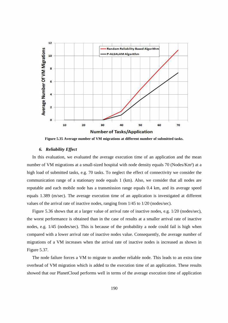
190

Figure 5.35 Average number of VM migrations at different number of submitted tasks.

6. Reliability Effect

In this evaluation, we evaluated the average execution time of an application and the mean

number of VM migrations at a small-sized hospital with node density equals 70 (Nodes/Km²) at a

high load of submitted tasks, e.g. 70 tasks. To neglect the effect of connectivity we consider the

communication range of a stationary node equals 1 (km). Also, we consider that all nodes are

reputable and each mobile node has a transmission range equals 0.4 km, and its average speed

equals 1.389 (m/sec). The average execution time of an application is investigated at different

values of the arrival rate of inactive nodes, ranging from 1/45 to 1/20 (nodes/sec).

Figure 5.36 shows that at a larger value of arrival rate of inactive nodes, e.g. 1/20 (nodes/sec),

the worst performance is obtained than in the case of results at a smaller arrival rate of inactive

nodes, e.g. 1/45 (nodes/sec). This is because of the probability a node could fail is high when

compared with a lower arrival rate of inactive nodes value. Consequently, the average number of

migrations of a VM increases when the arrival rate of inactive nodes is increased as shown in

Figure 5.37.

The node failure forces a VM to migrate to another reliable node. This leads to an extra time

overhead of VM migration which is added to the execution time of an application. These results

showed that our PlanetCloud performs well in terms of the average execution time of application

191

with a smaller number of VM migrations even in case when a large number of mobile nodes have

left the HMAC.

Figure 5.36 Average execution time of an application at different arrival rates of inactive nodes at a small-

sized hospital (25 beds).

Figure 5.37 Average number of VM migrations at different arrival rates of inactive nodes at a small-sized

hospital (25 beds).

192

7. Scalability and Management Overhead effect

In our evaluation a distinct VM instance is created for each task; therefore there is no overhead

of VM scheduling for task processing.

In this experiment, we consider a HMAC at three different configurations, as depicted in Table

5.2. We set the number of fixed nodes equals 10 nodes, and all of them have the highest

computing configurations. On the other hand, we consider that each mobile node has a

transmission range equals 0.2 km, and its average speed equals 1.389 (m/sec). The performance is

investigated at arrival rate of inactive nodes equals 1/50 (nodes/sec).

Table 5.2 HMAC s with Different Host Configurations.

Parameters Values

HMAC with

low resource

configurations

HMAC with

Medium

resource

configurations

HMAC with

High resource

configurations

Number of

CPUs/node 1, 2 2, 2 2, 4

Processing

Capabilities

2000 ,7500

(MIPS)

7500, 14564

(MIPS)

7500, 49160

(MIPS)

RAM 512, 1024

(MB)

1024 , 2048

(MB)

1024 , 4096

(MB)

Storage 4 (GB) 16 (GB) 16 (GB)

Bandwidth 54 (MB) 54 (MB) 54 (MB)

We start this evaluation by investigating the performance of a HMAC as more nodes,

resources, are added to the system, ranging from 40 to 100 nodes, when we consider one

application is submitted to be executed, with a fixed number of tasks equals 35.


random reliability-based node selection algorithms in terms of the average execution time of an

193

application at a HMAC with low resource configurations. Results show that P-ALSALAM

significantly outperforms the random reliability-based node selection algorithm at all node

densities.

Analysis of the results indicates that average execution time of an application decreases with

the increasing in number of nodes that could participate in a HMAC, i.e. more resources are added

to a HMAC computing pool. This is because the more resources added to the computing pool of a

HMAC, the larger the probability to select a new VM placement, another node, where a VM

could migrate to. This helps the migrated VM to get better resource availability and to scale up its

computation. While, noticeable performance degradation in P-ALSALAM results appear at higher

node densities, e.g. 100 (Nodes/Km²), due to a great effect of the delay due to collisions in

addition to the transmission delay.

Figure 5.38 Comparison of application average execution time as more resources are added to a HMAC at

different reliability based algorithms.

Similarly, the average number of VM migrations when applying P-ALSALAM is smaller than

the case when applying the random reliability-based node selection algorithm as shown in Figure

5.39.

Results show that the higher the node density the lower probability of VM migrations is

obtained. This is because of the probability a node could fail is high at high node density, e.g. 40

(Nodes/Km²), at the same arrival rate of inactive nodes, when compared with a lower node

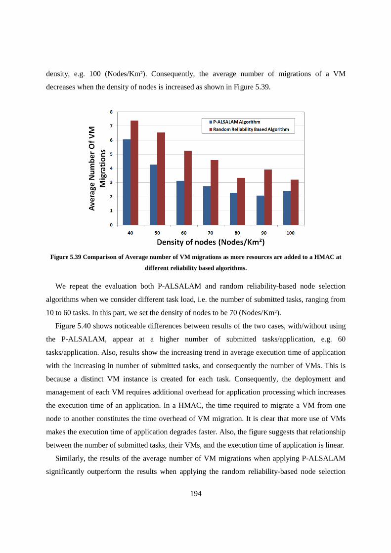
194

density, e.g. 100 (Nodes/Km²). Consequently, the average number of migrations of a VM

decreases when the density of nodes is increased as shown in Figure 5.39.

Figure 5.39 Comparison of Average number of VM migrations as more resources are added to a HMAC at

different reliability based algorithms.

We repeat the evaluation both P-ALSALAM and random reliability-based node selection

algorithms when we consider different task load, i.e. the number of submitted tasks, ranging from

10 to 60 tasks. In this part, we set the density of nodes to be 70 (Nodes/Km²).

Figure 5.40 shows noticeable differences between results of the two cases, with/without using

the P-ALSALAM, appear at a higher number of submitted tasks/application, e.g. 60

tasks/application. Also, results show the increasing trend in average execution time of application

with the increasing in number of submitted tasks, and consequently the number of VMs. This is

because a distinct VM instance is created for each task. Consequently, the deployment and

management of each VM requires additional overhead for application processing which increases

the execution time of an application. In a HMAC, the time required to migrate a VM from one

node to another constitutes the time overhead of VM migration. It is clear that more use of VMs

makes the execution time of application degrades faster. Also, the figure suggests that relationship

between the number of submitted tasks, their VMs, and the execution time of application is linear.

Similarly, the results of the average number of VM migrations when applying P-ALSALAM

significantly outperform the results when applying the random reliability-based node selection

195

algorithm as shown in Figure 5.41. Results show that more use of VMs the more probability of

VMs migrations could occur.

Figure 5.40 Comparison of application average execution time of a HMAC with low resource configurations

as the number of submitted tasks increases when applying different reliability based algorithms.

Figure 5.41 Comparison of Average number of VM migrations of a HMAC with low resource configurations

as the number of submitted tasks increases when applying different reliability based algorithms.

In the next evaluation, we evaluated P-ALSALAM algorithm at different resource

configurations of a HMAC as shown in Table 5.2.

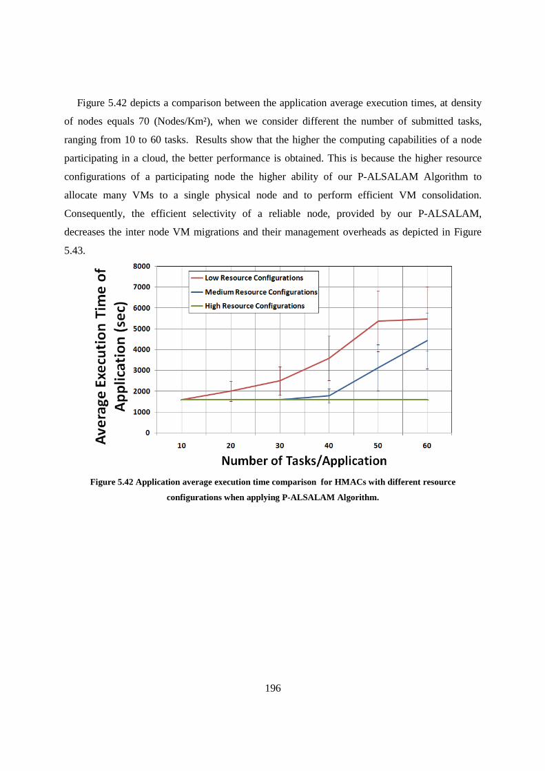
196

Figure 5.42 depicts a comparison between the application average execution times, at density

of nodes equals 70 (Nodes/Km²), when we consider different the number of submitted tasks,

ranging from 10 to 60 tasks. Results show that the higher the computing capabilities of a node

participating in a cloud, the better performance is obtained. This is because the higher resource

configurations of a participating node the higher ability of our P-ALSALAM Algorithm to

allocate many VMs to a single physical node and to perform efficient VM consolidation.

Consequently, the efficient selectivity of a reliable node, provided by our P-ALSALAM,

decreases the inter node VM migrations and their management overheads as depicted in Figure

5.43.

Figure 5.42 Application average execution time comparison for HMACs with different resource

configurations when applying P-ALSALAM Algorithm.

197

Figure 5.43 Average number of VM migrations comparison for HMACs with different resource

configurations when applying P-ALSALAM Algorithm.

5.2.4.3 Findings


• The performance is affected by the percentage of the number of fixed nodes within the

total density of available nodes. It means the more fixed reliable nodes, participate in a

HMAC, the less dependency on mobile variable reliability nodes. This could enhance

the performance of the submitted application.

• A better performance may be obtained, even at a shorter transmission range, if we

apply our P-ALSALAM algorithm. This is because our algorithm frequently

reschedules the delayed tasks and this minimizes the effect of communication delay.

• Performance enhancement of a HMAC is provided by applying the efficient dynamic

VM consolidation. This could be achieved by selecting reliable and powerful

computing nodes to participate in a HMAC. This enhances both scalability and

management overhead by reducing the number of inter host VM migrations.

• The performance is affected by the percentage of the reliable resources that could be

added to the computing pool of a HMAC. It means the more reliable nodes, participate

198

in a HMAC, the larger the probability to select a new VM placement, where a VM

could migrate to. This leads to get better resource availability and scalability.

5.3 Conclusion

In this chapter, we presented a trustworthy dynamic virtualization and task management layer

for resilient cloud management with an intrinsic support for highly-mobile heterogeneously-

composed and dynamically-configured MACs. PlanetCloud is powered by an autonomously

managed virtualization layer for encapsulating cloud applications and facilitating safe and reliable

execution over scattered heterogeneous resources. PlanetCloud provides multiple recovery modes

which enhance the system resilience and cover different application requirements and host-

configurations. Through analysis and simulation, we evaluated a pure mobile model, MAC,

consisting of mobile nodes and a hybrid model, HMAC, consisting of portable mobile devices and

semi-stationary on-board computing resources of vehicles in different sizes hospital scenarios.

Results showed that our PlanetCloud always performs well in terms of the average execution time

of application with a small number of VM migrations even in case of unstable environment. Also,

results showed that PlanetCloud enabling resource collaboration enhanced the cloud capability to

reduce the delay overhead added to the average execution time of applications due to the lack of

connectivity of participants.

199

Chapter 6

6 CONCLUSION AND FUTURE WORK

6.1 Conclusion

In this dissertation, we presented a C3 platform, termed PlanetCloud, which enables the

provisioning of the right, otherwise idle, stationary and mobile resources to provide ubiquitous

cloud computing on-demand. PlanetCloud utilizes its intrinsic autonomic components to enable


mobile nodes, and a true ubiquitous on-demand cloud computing.

We design PlanetCloud as a first realization of ubiquitous cloud computing formed from

stationary and mobile resources that fully fits the essential characteristics of cloud computing

model and offers different service models. Our design liberates cloud computing from being

concerned about resource constraints.

PlanetCloud synergistically manages 1) resources to include resource harvesting, forecasting

and selection, and 2) cloud services concerned with resilient cloud services to include resource

provider collaboration, application execution isolation from resource layer concerns, seamless

load migration, fault-tolerance, the task deployment, migration, revocation, etc.

Our PlanetCloud platform provides new opportunities to overcome technical, policy and

business obstacles to both the adoption of cloud computing and the growth of cloud computing

once it has been adopted.

The main contributions of our work are outlined as follows.

Intellectual Merit:



Global mobile and stationary resource discovery and monitoring. A novel spatiotemporal

resource calendaring mechanism with real-time synchronization is proposed to mitigate

the effect of failures occurring due to unstable connectivity and availability in the dynamic

mobile environment, as well as the poor utilization of resources. This mechanism provides

200

a dynamic real-time scheduling and tracking of idle mobile and stationary resources. This

would enhance resource discovery and status tracking to provide access to the right-sized

cloud resources anytime and anywhere.

















Our analytical study evaluating GRPS as a key component of PlanetCloud showed its

efficiency to adapt the performance of the system response. The effectiveness of CARMS

component of PlanetCloud has been evaluated through simulations employing different

scheduling and resource allocation algorithms. Simulations showed that PlanetCloud offers

effective and efficient MAC formation and maintenance over mobile devices. The ability

of PlanetCloud and its underlying virtualization management layer to form a HMAC have

been evaluated through analysis and simulations. These evaluations illustrated that

PlanetCloud can safely and reliably provide and maintain the needed computational power

to form a reliable HMAC operating in a dynamic, unstable, and heterogeneous resource

environment. Also, these evaluations showed the benefits of enabling resource

collaboration, provided by PlanetCloud, to achieve better capability to minimize

201

management overhead. Additionally, evaluations showed that PlanetCloud can guarantee

reliable resource provisioning, transparently maintaining applications’ QoS and preventing

service disruption in highly dynamic environments.

Broader Impact:

• PlanetCloud, as a ubiquitous computing cloud environment, would enhance on-demand

resource availability for under-connected areas, extreme environments and distress

situations. It enables ubiquitous resource-infinite computing paradigm by enabling

cooperation among clouds to provide extra resources beyond their computing

capabilities.

• Un-tethering computing resources from Internet availability using our proposed

PlanetCloud platform would enable us to tap into the otherwise unreachable resources,

where cloud resources and services may be located on any reachable mobile or

stationary nodes, rather than exclusively on the providers’ side.

• PlanetCloud enables a new economic model for computing service as computing

devices of users can act as resource providers. In this case, a user dedicates a certain

amount of his resources to earn some money and increase his income. This would

motivate people to participate in a MAC.

• Planet Cloud could be used as a platform to provide network as a service in areas that

have poor infrastructure. This could be achieved by implementing distributed

cooperative networking tasks running on top of our micro virtual machine. These

networking tasks act as switching nodes that capable of forwarding data among

different interfaces. Where, the virtualization task management layer of the formed

cloud hides its underlying intermittent physical network while forming a stable virtual

overlay network.

PlanetCloud Limitations

• Permanent connectivity may not be always available, which cannot be ignored in real

settings, due to wireless access limitations of a mobile node. This would result in some

management overhead, i.e. time delay due to the deployment and management of VMs in a MAC,

which provides an additional overhead that impacts the performance.

202

• The employed prediction algorithm and its inputs, i.e. the type and source of data, might

affect the forecasting precision of resource availability, which in turn impacts on the stability and

reliability of the formed MAC.

6.2 Future Work

Our future work includes the following:

1) Develop a security mechanism to preserve the privacy and security constraints of a

MAC/HMAC resource provider, while allowing multiple users to share its resources

and data for calendaring. There is a need to support distributed data access and

computations without compromising the raw data of cloud nodes;

2) Develop a security mechanism to enhance the system resilience against malicious

attacks, e.g. collusion attacks by bad nodes.

3) Extend our proposed architecture to enhance the prediction accuracy of resource

availability by utilizing complementary data sources, such as from social networking.

4) Develop methodology to enhance the analysis of vast quantity of dynamic data from

both social networking and spatiotemporal calendars to provide efficient resource

discovery, assignment and forecasting. Enhancement is achieved by providing efficient

data structure to calculate all association rules among different resource types to find

the interesting resource pattern;

5) Study the effect of replicas on the survivability of the running service in a dynamic

MAC environment; and

6) Study and compare the migration overhead using different recovery modes.

Publications

Published Papers

1) A. Khalifa, R. Hassan, and M. Eltoweissy, “Towards ubiquitous computing clouds,” in The

Third International Conference on Future Computational Technologies and Applications,

Rome, Italy, September, 2011, pp. 52–56.

203

2) A. Khalifa and M. Eltoweissy, “A global resource positioning system for ubiquitous clouds,”

in the Eighth International Conference on Innovations in Information Technology (IIT),

UAE, 2012, pp. 145–150.

3) A. Khalifa and M. Eltoweissy, “Collaborative Autonomic Resource Management System for

Mobile Cloud Computing,” in the Fourth International Conference on Cloud Computing,

GRIDs, and Virtualization, Spain, 2013, pp. 115–12.

4) A. Khalifa and M. Eltoweissy, “MobiCloud: A Reliable Collaborative MobileCloud

Management System,” In the 9th IEEE International Conference on Collaborative

Computing: Networking, Applications and Worksharing, United States, 2013, pp. 158 – 167.

5) A. Khalifa, M. Azab, and M. Eltoweissy, "Resilient Hybrid Mobile Ad-hoc Cloud Over

Collaborating Heterogeneous Nodes", in the 10th IEEE International Conference on

Collaborative Computing: Networking, Applications and Worksharing (CollaborateCom

2014), Miami, Florida, United States, October, 2014.

6) A. Khalifa, M. Azab, and M. Eltoweissy, "Towards a Mobile Ad-hoc Cloud Management

Platform", in the 7th IEEE/ACM International Conference on Utility and Cloud Computing

(UCC 2014), London, United Kingdom, December, 2014.

Submitted Papers

1) A. Khalifa, M. Azab, and M. Eltoweissy, A Vision of Service Delivery Using a Reliable

Mobile Ad-hoc Cloud Platform Networks, submitted to the ElSEVIER Journal of Network

and Computer Applications (JNCA).

204

References

[1] G. Li, H. Sun, H. Gao, H. Yu, and Y. Cai, "A survey on wireless grids and clouds," in Eighth

International Conference on Grid and Cooperative Computing, GCC ’09, Gansu, China, 2009, pp.

261–267.

[2] S. P.Warhekar and V.T.Gaikwad, "Mobile Cloud Computing: Approaches and Issues," International

journal of emerging trends and technology in computer science (IJETTCS), vol. 2, no. 2, pp. 366-

370, March – April 2013.

[3] G. Eichler, K.-H. Luke, and B. Reufenheuser, "Context information as enhancement for mobile

solutions and services," in 13th International Conference on Intelligence in Next Generation

Networks (ICIN 2009), Bordeaux, France, Oct. 2009, pp. 1-5.

[4] C. Tee and A.Lee, "Survey of position based routing for inter vehicle communication system," in

First International Conference on Distributed Framework and Applications, DFmA, Oct. 2008, pp.

174-182.

[5] M. Eltoweissy, S. Olariu, and M. Younis, "Towards autonomous vehicular clouds," in Ad Hoc

Networks, ser. Lecture Notes of the Institute for Computer Sciences, Social Informatics and

Telecommunications Engineering.Springer Berlin Heidelberg, vol. 49, pp. 1-16, 2010.

[6] C. Wang, K. Ren, W. Lou, and J. Li, "Toward publicly auditable secure cloud data storage services,"

IEEE Network, vol. 24, no. 4, pp. 19-24, July-August 2010.

[7] R. Buyya, C. S. Yeo, S. Venugopal, J. Broberg, and I. Brandic, "Cloud Computing and Emerging IT

Platforms: Vision, Hype, and Reality for Delivering Computing as the 5th Utility," Future

Generation Computer Systems, Elsevier Science, vol. 25, no. 6, pp. 599-616, June 2009.

[8] A. Klein, C. Mannweiler, J. Schneider, and H. D. Schotten, "Access schemes for mobile cloud

computing," in Eleventh International Conference on Mobile Data Management (MDM), 2010, pp.

387-392.

[9] T. Xing, D. Huang, S. Ata, and D. Medhi, "Mobicloud: A geodistributed mobile cloud computing

platform," in 8th International Conference on Network and ServiceManagement (CNSM), 2012, pp.

164–168.

[10] T. Xing, H. Liang, D. Huang, and L. X. Cai, "Geographic-based service request scheduling model for

mobile cloud computing," in IEEE 11th International Conference on Trust,Security and Privacy in

Computing and Communications (TrustCom 2012), 2012, pp. 1446–1453.

205

[11] G. Huerta-Canepa and D. Lee, "A virtual cloud computing provider for mobile devices," in 1st ACM

Workshop on Mobile Cloud Computing & Services: Social Networks and Beyond, California, USA,

2010, pp. 1-5.

[12] E. Marinelli, "Hyrax: cloud computing on mobile devices using MapReduce," Carnegie Mellon

University, Master thesis 2009.

[13] P. Mell and T. Grance, "The NIST Definition of Cloud Computing (ver. 16th and final definition),"

National Institute of Standards and Technology, Information Technology Laboratory, Sept. 2011.

[14] M. Bourguiba, K.A. Agha, and K. Haddadou, "Improving networking performance in virtual mobile

clouds," in Third International Conference on the Network of the Future (NOF), 21-23 Nov. 2012,

pp. 1-6.

[15] N. Fernando, S.W. Loke, and W. Rahayu, "Dynamic mobile cloud computing: Ad hoc and

opportunistic job sharing," in Fourth IEEE International Conference on Utility and Cloud Computing

(UCC), Australia, 5-8 Dec. 2011, pp. 281-286.

[16] M. Black and W. Edgar, "Exploring mobile devices as Grid resources: Using an x86 virtual machine

to run BOINC on an iPhone," in 10th IEEE/ACM International Conference on GridComputing, 2009,

pp. 9-16.

[17] W. Lee, S. K. Lee, S. Yoo, and H. Kim, "A collaborative framework of enabling device participation in

mobile cloud computing," Mobile and Ubiquitous Systems: Computing, Networking, and Services,

Springer Berlin Heidelberg, vol. 120, pp. 37-49, 2013.

[18] L. F. Bittencourt and E. R. M. Madeira, "HCOC: a cost optimization algorithm for workflow

scheduling in hybrid clouds," Journal of Internet Services and Applications, vol. 2, pp. 207-227,

December 2011.

[19] C. Lin and S. Lu, "Scheduling scientific workflows elastically for cloud computing," in IEEE 4th

International Conference on Cloud Computing, USA, 2011, pp. 746 - 747.

[20] K. Bessai, S. Youcef, A. Oulamara, C. Godart, and S. Nurcan, "Bi-criteria workflow tasks allocation

and scheduling in cloud computing environments," in 5th International Conference on Cloud

Computing, USA, 2012, pp. 638-645.

[21] B. Yang, X. Xu, F. Tan, and D. H. Park, "An utility-based job scheduling algorithm for cloud

computing considering reliability factor," in International Conference on Cloud and Service

Computing (CSC), Hong Kong, 2011, pp. 95-102.

[22] L. Wang, G. von Laszewski, J. Dayal, and F. Wang, "Towards energy aware scheduling for

precedence constrained parallel tasks in a cluster with DVFS," in 10th IEEE/ACM International

206

Symposium on Cluster, Cloud and Grid Computing (CCGRID’10), Australia, 2010, pp. 368–377.

[23] B. Kouchner, "Globalization and new world order: are we ready for ”scientists without borders”?,"

IEEE Transactions on Applied Superconductivity, vol. 15, no. 2, pp. 1071–1077, 2005.

[24] J. Dwek, "The doctors without borders experience: mission to afghanistan," Pediatric Radiology,

vol. 32, pp. 541–544, 2002.

[25] M. George and O. Zoran, "Improving Computational Efficiency for Personalized Medical

Applications in Mobile Cloud Computing Environment," in IEEE International Conference on

Healthcare Informatics (ICHI), Sept. 2013, pp. 535-540.

[26] S. K. Garg and R. Buyya, "NetworkCloudSim: modelling parallel applications in cloud simulations,"

in 4th IEEE International Conference on Utility and Cloud Computing (UCC 2011), Melbourne,

Australia, Dec. 2011, pp. 105–113.

[27] R. N. Calheiros, R. Ranjan, A. Beloglazov, C.A.F.D. Rose, and R. Buyya, "CloudSim: a toolkit for

modeling and simulation of cloud computing environments and evaluation of resource

provisioning algorithms," Software: Practice and Experience, vol. 41, no. 1, pp. 23-50, January

2011.

[28] B.P. Rimal, C. Eunmi, and I. Lumb, "A Taxonomy and Survey of Cloud Computing Systems," in Fifth

International Joint Conference on INC, IMS and IDC (NCM '09), 2009, pp. 44-51.

[29] B. Yu, J. Tian, S. Ma, S. Yi, and D. Yu, "Gird or cloud? Survey on scientific computing infrastructure,"

in IEEE International Conference on Cloud Computing and Intelligence Systems (CCIS), 15-17 Sept.

2011, pp. 244-249.

[30] S. Patidar, D. Rane, and P. Jain, "A Survey Paper on Cloud Computing," in Second International

Conference on Advanced Computing & Communication Technologies (ACCT), 7-8 Jan. 2012, pp.

394-398.

[31] L. M. Vaquero, L.Rodero-Merino, J. Caceres, and M. Lindner, "A break in the clouds: towards a

cloud definition," ACM SIGCOMM Computer Communication Review, vol. 39, no. 1, pp. 50-55 ,

January 2009.

[32] A.J.Younge, G.von Laszewski, L. Wang, S. Lopez-Alarcon, and W. Carithers, "Efficient resource

management for Cloud computing environments," in International Conference on Green

Computing, 15-18 Aug. 2010, pp. 357-364.

[33] I. Chandrasekaran, "Mobile Computing with Cloud," Advances in Parallel Distributed Computing,

Communications in Computer and Information Science, vol. 203, no. 1, pp. 513–522, 2011.

207

[34] Anh-Dung Nguyen, P. Senac, and V. Ramiro, "How Mobility Increases Mobile Cloud Computing

Processing Capacity," in First International Symposium on Network Cloud Computing and

Applications (NCCA), 21-23 Nov. 2011, pp. 50-55.

[35] X. Fan, J. Cao, and H. Mao, "A Survey of Mobile Cloud Computing," ZTE Corporation, 2011.

[36] D. Kovachev, D. Renzel, R. Klamma, and Y. Cao, "Mobile community cloud computing: emerges

and evolves," in 1st Intl. Workshop on Mobile Cloud Computing (in conjunction with) 11th Intl.

Conf. on Mobile Data Management (MDM’10), Kansas, MO, 2010, pp. 393-395.

[37] [Online]. http://www.mobilecloudcomputingforum.com/

[38] Wei-Tek Tsai, X. Sun, and J. Balasooriya, "Service-Oriented Cloud Computing Architecture," in

Seventh International Conference on Information Technology: New Generations (ITNG), 12-14 April

2010, pp. 684-689.

[39] L. Guan, X. Ke, M. Song, and J. Song, "A Survey of Research on Mobile Cloud Computing," in 10th

International Conference on Computer and Information Science (ICIS), 16-18 May 2011, pp. 387-

392.

[40] R. Prodan and S. Ostermann, "A survey and taxonomy of infrastructure as a service and web

hosting cloud providers," in 10th IEEE/ACM International Conference on Grid Computing, 13-15

Oct. 2009, pp. 17-25.

[41] M. Zhou, R. Zhang, D. Zeng, and W. Qian, "Services in the Cloud Computing era: A survey," in 4th

International Universal Communication Symposium (IUCS), 18-19 Oct. 2010, pp. 40-46.

[42] M. Mahjoub, A. Mdhaffar, R.B. Halima, and M. Jmaiel, "A Comparative Study of the Current Cloud

Computing Technologies and Offers," in First International Symposium on Network Cloud

Computing and Applications (NCCA), 21-23 Nov. 2011, pp. 131-134.

[43] J. Peng et al., "Comparison of several cloud computing platforms," in the Second International

Symposium on Information Science and Engineering (ISISE '09), Washington DC, USA, 2009, pp. 23-

27.

[44] OpenCloud. (2010) Cloud Computing Use Cases Whitepaper – Version 4.0. [Online].

http://opencloudmanifesto.org/Cloud_Computing_Use_Cases_Whitepaper-4_0.pdf

[45] IBM Academy of Technology. (2010, October) Cloud computing insights from110 implementation

projects. [Online]. http://www-304.ibm.com/easyaccess3/fileserve?contentid=215289

[46] J. Kelner. T. Endo, G. E. Gon calves, and D. Sadok, "A survey on open-source cloud computing

solutions," in Brazilian Symposium on Computer Networks and Distributed Systems, May 2010.

208

[47] Y.H. Jung, M. Szczodrak, R. Neill, and L.P. Carloni, "Altocumulus: Harvesting Computational

Resources from Devices at the Edge of the Cloud," in 1st International Workshop on the Swarm at

the Edge of the Cloud, 2013.

[48] Z.Sanaei, S. Abolfazli, A. Gani, and R. Buyya, "Heterogeneity in Mobile Cloud Computing:

Taxonomy and Open Challenges," IEEE Communications Surveys & Tutorials , vol. 16, no. 1, pp.

369-392, First Quarter 2014.

[49] S. Abolfazli, Z. Sanaei, E. Ahmed, A. Gani, and R. Buyya, "Cloud-Based Augmentation for Mobile

Devices: Motivation, Taxonomies, and Open Challenges," IEEE Communications Surveys &

Tutorials, vol. 16, no. 1, pp. 337-368, First Quarter 2014.

[50] A. Khalifa, R. Hassan, and M. Eltoweissy, "Towards Ubiquitous Computing Clouds," in The Third

International Conference on Future Computational Technologies and Applications (FUTURE

COMPUTING), Rome, Italy, September, 2011, pp. 52-56.

[51] A. Khalifa and M. Eltoweissy, "MobiCloud: A Reliable Collaborative MobileCloud Management

System," in the 9th IEEE International Conference on Collaborative Computing:Networking,

Applications and Worksharing, United States, 2013, pp. 158 – 167.

[52] Cloud Security Alliance, "Security Guidance for Critical Areas of Focus in Cloud Computing V2.1,"

2009.

[53] W. Ren, L. Yu, R. Gao, and F. Xiong, "Lightweight and compromise resilient storage outsourcing

with distributed secure accessibility in mobile cloud computing," Tsinghua Science and

Technology, vol. 16, no. 5, pp. 520-528, October 2011.

[54] M. Choi, J. Park, and Young-Sik Jeong, "Mobile cloud computing framework for a pervasive and

ubiquitous environment," The Journal of Supercomputing, vol. 64, no. 2, pp. 331-356, September

2011.

[55] Q. Xia, W.Liang, Z. Xu, and B. Zhou, "Online Algorithms for Location-Aware Task Offloading in Two-

Tiered Mobile Cloud Environments," in IEEE/ACM 7th International Conference on Utility and Cloud

Computing, London, UK, 2014, pp. 109-116.

[56] H. Liang, D. Huang, and D. Peng, "On Economic Mobile Cloud Computing Model," in the

International Workshop on Mobile Computing and Clouds (MobiCloud in conjunction with

MobiCASE), 2010.

[57] D. Huang, m. Kang X. Zhang, and J. Luo, "Mobicloud: A secure mobile cloud framework for

pervasive mobile computing and communication," in 5th IEEE International Symposium on Service-

Oriented System Engineering, 2010.

209

[58] C. Jang and E. Choi, "Context Model Based on Ontology in Mobile Cloud Computing," Advanced

Communication and Networking, Communications in Computer and Information Science, vol. 199,

pp. 146-151, 2011.

[59] M. Altamimi and K. Naik, "The Concept of a Mobile Cloud Computing to Reduce Energy Cost of

Smartphones and ICT Systems," Information and Communication on Technology for the Fight

against Global Warming, Lecture Notes in Computer Science, vol. 6868, pp. 79-86, 2011.

[60] S. N. Srirama, C. Paniagua, and H. Flores, "CroudSTag: Social Group Formation with Facial

Recognition and Mobile Cloud Services," Procedia Computer Science, Elsevier,The 2nd

International Conference on Ambient Systems, Networks and Technologies (ANT-2011) / The 8th

International Conference on Mobile Web Information Systems (MobiWIS 2011), vol. 5, pp. 633-640,

2011.

[61] J. Mishra, S. K. Dash, and S. Dash, "Mobile-Cloud: A Framework of Cloud Computing for Mobile

Application," Advances in Computer Science and Information Technology. Computer Science and

Information Technology, Lecture Notes of the Institute for Computer Sciences, Social Informatics

and Telecommunications Engineering, vol. 86, no. 2, pp. 347-356, 2012.

[62] H. Liang, D. Huang, L.X. Cai, X. Shen, and D. Peng, "Resource allocation for security services in

mobile cloud computing," in IEEE Conference on Computer Communications Workshops (INFOCOM

WKSHPS), April 2011, pp. 191-195.

[63] J.S. Park, H.C. Yu, and E.Y.Lee, "Resource Allocation Techniques Based on Availability and

Movement Reliability for Mobile Cloud Computing," Distributed Computing and Internet

Technology, Lecture Notes in Computer Science, vol. 7154, pp. 263-264, 2012.

[64] R. Chow et al., "Controlling data in the cloud: outsourcing computation without outsourcing

control," in the 2009 ACM workshop on Cloud computing security (CCSW ’09), Illinois, USA, 2009,

pp. 85–90.

[65] H. S. Alqahtani and G. K. Mostefaoui, "Multi-Clouds Mobile Computing for the Secure Storage of

Data," in IEEE/ACM 7th International Conference on Utility and Cloud Computing, London, UK,

2014, pp. 495 -496.

[66] A. Khalifa and M. Eltoweissy, "A Global Resource Positioning System for Ubiquitous Clouds," in the

Eighth International Conference on Innovations in Information Technology (Innovations'12), Abu-

Dhabi, United Arab Emirates, March, 2012, pp. 145-150.

[67] A. Khalifa, M. Azab, and M. Eltoweissy, "Resilient Hybrid Mobile Ad-hoc Cloud Over Collaborating

Heterogeneous Nodes," in the 10th IEEE International Conference on Collaborative Computing:

Networking, Applications and Worksharing (CollaborateCom 2014), Miami, Florida, United States,

210

October, 2014.

[68] A. Khalifa, M. Azab, and M. Eltoweissy, "Towards a Mobile Ad-hoc Cloud Management Platform,"

in the 7th IEEE/ACM International Conference on Utility and Cloud Computing (UCC 2014), London,

United Kingdom, December, 2014.

[69] J. Maan, "Extending the Principles of Cloud Computing in Mobile Domain," Trends in Network and

Communications, Communications in Computer and Information Science, vol. 197, no. 1, pp. 197-

203, 2011.

[70] Conn. STAMFORD. (2011, January) Gartner Executive Programs Worldwide Survey of More Than

2,000 CIOs Identifies Cloud Computing as Top Technology Priority for CIOs in 2011. [Online].

http://www.gartner.com/it/page.jsp?id=1526414

[71] Conn. STAMFORD. (2012, April) Gartner Outlines Five Cloud Computing Trends That Will Affect

Cloud Strategy Through 2015. [Online]. http://www.gartner.com/it/page.jsp?id=1971515

[72] Gartner Reveals Top Predictions for IT Organizations and Users for 2012 and Beyond. [Online].

http://www.gartner.com/it/page.jsp?id=1862714

[73] K. Rangan, A. Cooke, J. Post, and N. Schindler, "The Cloud Wars : 100 + billion at stake," The

Analyst, pp. 1-90, May 2008.

[74] Intel Corporation. (2011) Cloud Computing Fun Facts. [Online].

http://download.intel.com/newsroom/kits/istcs/pdfs/CloudFunFacts.pdf

[75] H. T. Dinh, C. Lee, D. Niyato, and P. Wang, "A Survey of Mobile Cloud Computing: Architecture,

Applications and Approaches," Wireless Communications and Mobile Computing, Wiley Journals,

vol. 13, no. 18, October 2011.

[76] M. Abuelela and S. Olariu, "Taking VANET to the Clouds," in the 8th International Conference on

Advances in Mobile Computing and Multimedia (MoMM), New York, USA, 2010, pp. 6-13.

[77] T. Hristov, and G. Yan S. Olariu, "The Next Paradigm Shift: FromVehicular Networks to Vehicular

Clouds," in Mobile Ad Hoc Networking:The Cutting Edge Directions.: Wiley-IEEE Press, 2013, pp.

645 - 700.

[78] S. Arif et al., "Datacenter at the Airport: Reasoning about Time-Dependent Parking Lot

Occupancy," IEEE Transactions on Parallel and Distributed Systems, vol. 23, no. 11, pp. 2067-2080,

November 2012.

[79] D. Singh, J. Singh, and A. Chhabra, "High Availability of Clouds: Failover Strategies for Cloud

Computing Using Integrated Checkpointing Algorithms," in International Conference on

211

Communication Systems and Network Technologies (CSNT), May 2012, pp. 698-703.

[80] S. Pandey and S. Nepal, "Modeling Availability in Clouds for Mobile Computing," in IEEE First

International Conference on Mobile Services (MS), June 2012, pp. 80-87.

[81] [Online]. http://web.mit.edu/6.826/www/notes/HO28.pdf

[82] F. H. Zulkernime and P. Martin, "An adaptive and intelligent SLA negotiation system for Web

servcies," IEEE Transactions On Services Computing, vol. 4, no. 1, pp. 31-43, Jan.-March 2011.

[83] J. Londono and A. Bestavros, "Netembed: A network resource mapping service for distributed

applications," in IEEE International Symposium on In Parallel and Distributed Processing (IPDPS),

2008, pp. 1-8.

[84] Y. Shavitt and N. Zilberman, "A structural approach for pop geo-location," in INFOCOM IEEE

Conference on Computer Communications Workshops, 2010, pp. 1-6.

[85] R. Ranjan, A. Harwood, and R. Buyya, "Peer-to-peer-based resource discovery in global grids: a

tutorial," IEEE Communications Surveys Tutorials, vol. 10, no. 2, pp. 6-33, Second Quarter 2008.

[86] D. Werthimer, J. Cobb, M. Lebofsky, D. Anderson, and E. Korpela, "Seti@homemassively

distributed computing for seti," Computing in Science and Engineering, vol. 3, no. 1, pp. 78–83,

January 2001.

[87] C. De Rose et al., "The virtual cluster: a dynamic network environment for exploitation of idle

resources," in 14th Symposium on Computer Architectureand High Performance Computing, 2002,

pp. 141- 148.

[88] D. Ediger, K. Jiang, J. Riedy, and D. Bader, "Massive streaming data analytics: A case study with

clustering coefficients," in IEEE International Symposium on In Parallel Distributed Processing,

Workshops and Phd Forum (IPDPSW), 2010 , pp. 1-8.

[89] D. Ediger et al., "Massive social network analysis: Mining twitter for social good," in 39th

International Conference on In Parallel Processing (ICPP), 2010, pp. 583 –593.

[90] T. Menard and J. Miller, "FreeSim_Mobile: A novel approach to real-time traffic gathering using

the apple iPhone," in IEEE in Vehicular Networking Conference (VNC), 2010, pp. 57-63.

[91] D. Alderson, L. Li, W. Willinger, and J. Doyle, "Understanding internet topology: principles, models,

and validation," IEEE/ACM Transactions on Networking, vol. 13, no. 6, pp. 1205 – 1218, 2005.

[92] R. Anandhi and K. Chitra, "A Challenge in Improving the Consistency of Transactions in Cloud

Databases – Scalability," International Journal of Computer Applications , vol. 52, no. 2, pp. 0975 –

212

8887, August 2012.

[93] A Joyent White Paper. Performance and Scale in Cloud Computing. [Online].

https://www.joyent.com/developers/resources/performance-and-scale-in-cloudcomputing

[94] S. Imai, T. Chestna, and C.A. Varela, "Elastic Scalable Cloud Computing Using Application-Level

Migration," in the 2012 IEEE/ACM Fifth International Conference on Utility and Cloud Computing,

Illinois, USA, 2012, pp. 91-98.

[95] N.Huber, M.v.Quast, M.Hauck, and S. Kounev, "Evaluating and Modeling Virtualization

Performance Overhead for Cloud Environments," in the 1st International Conference on Cloud

Computing and Services Science (CLOSER 2011), Noordwijkerhout, The Netherlands, May 7-9,

2011, pp. 563 - 573.

[96] M. Shiraz, S. Abolfazli, Z. Sanaei, and A.Gani, "A study on virtual machine deployment for

application outsourcing in mobile cloud computing," The Journal of Supercomputing, vol. 63, no. 3,

pp. 946-964, March 2013.

[97] R. Eltarras, M. Eltoweissy, and M. Youssef, "Towards evolving sensor actor networks," in IEEE

INFOCOM Workshops, Phoenix, AZ, USA, Apr. 2008, pp. 1-6.

[98] K. Hoffman, D. Zage, and C. Nita-Rotaru, "A survey of attack and defense techniques for reputation

systems," ACM Computing Surveys, vol. 42, no. 1, pp. 1-31, 2009.

[99] M. van Dijk, C. Gentry, S. Halevi, and V. Vaikuntanathan, "Fully homomorphic encryption over the

integers," Advances in Cryptology EUROCRYPT 2010, Lecture Notes in Computer Science. Springer,

vol. 6110, pp. 24-43, 2010.

[100] P. Bogetoft et al., "Multiparty computation goes live," Cryptology ePrint Archive, Report 2008/068

2008.

[101] Y.-C. Hu, A. Perrig, and D. Johnson, "Wormhole attacks in wireless networks," IEEE Journal on

Selected Areas in Communications, vol. 24, no. 2, pp. 370 – 380, February 2006.

[102] J. Douceur, "The Sybil attack," Peer-to-Peer Systems, ser. Lecture Notes in Computer Science.

Springer, Berlin / Heidelberg, vol. 2429, pp. 251–260, 2002.

[103] T. Pietraszek and C. Berghe, "Defending against injection attacks through context-sensitive string

evaluation," Recent Advances in Intrusion Detection, ser. Lecture Notes in Computer Science.

Springer, Berlin / Heidelberg, vol. 3858, pp. 124–145, 2006.

[104] M. Azab and M. Eltoweissy, "CyberX: A Biologically-inspired Platform for Cyber Trust

Management," in 8th International Conference on Collaborative Computing, 2012, pp. 655- 663.

213

[105] M. M. M. Azab, "Cooperative Autonomous Resilient Defense Platform for Cyber-Physical Systems,"

Virginia Polytechnic Institute and State University, Doctor of Philosophy 2013.

[106] A. Bhattacharya, "Mobile agent based elastic executor service," in International Joint Conference

on Computer Science and Software Engineering (JCSSE), 2012, pp. 351-356.

[107] A. Singh and M. Malhotra, "Analysis for Exploring Scope of Mobile Agents in Cloud Computing,"

International Journal of Advancements in Technology, vol. 3, no. 3, July 2012.

[108] Z. Zhang and X. Zhang, "Realization of open cloud computing federation based on mobile agent,"

in IEEE International Conference on Intelligent Computing and Intelligent Systems, 2009, pp. 642 -

646.

[109] O. Urra, S. Ilarri, and E. Mena, "Testing Mobile Agent Platforms Over the Air," in 1st Workshop on

Data and Services Management in Mobile Environments (DS2ME´08), In conjunction with the 24th

International Conference on Data Engineering (ICDE'08), April 2008, pp. 152-159.

[110] U. Fayyad, G. Piatesky-Shapiro, and P. Smyth, "From data mining to knowledge discovery: an

overview," in Advances in knowledge discovery and data mining. Menlo Park, CA, USA: American

Association for Artificial Intelligence, 1996, pp. 1-34.

[111] S. Lanka and S.K. Jena, "A study on time based association rule mining on spatial-temporal data for

intelligent transportation applications," in First International Conference on Networks & Soft

Computing (ICNSC), Aug. 2014, pp. 395-399.

[112] H. Alouaoui, S.Y. Turki, and S. Faiz, "Mining spatiotemporal associations using queries," in

International Conference on Information Technology and e-Services (ICITeS), 2012, pp. 1-5.

[113] JiaweiHang and K. Micheline, Data mining: Concepts and Techniques, Second Edition, Ed.: Morgan

Kaufmann Publishers, 2006.

[114] S. Shilpa and M. Amrita, "DHPID-HYBBRID Algorithm: A hybrid algorithm for association rule

mining," advanced data mining applications, Springer, vol. 6440, 2010.

[115] C. Keith, C. Chan, and Au. Wai-Ho, "An elective algorithm for mining interesting quantitative

association rules," in ACM symposium on Applied computing, ACM Press, 1997.

[116] S. Ansaf, V. Christel, and N. Cyril, "Quant miner: A genetic algorithm for mining quantitative

association rules," IJCAI, vol. 7, no. 1, 2007.

[117] W. Jing, L. Huang, and Y. Luo, "An Algorithm for Privacy-Preserving Quantitative Association Rules

Mining," in 2nd IEEE International Symposium, Indianapolis, 2006.

214

[118] B. Bernadette and M. Gilles, "Fuzzy Linguistic Summaries: Where Are We, Where Can We Go?," in

Computational Intelligence for Financial Engineering & Economics Conference, NewYork, 2012.

[119] X. Tung, L. Li L. Zhai, "Temporal Association Rule Mining based On T-Apriori Algorithm And Its

Typical Application," Journal of Intelligent Information Systems, vol. 22, no. 1, 2005.

[120] Q. Chai, P. Michel, and B. Bernard, "POP-TRAFFIC: A Novel Fuzzy Neural Approach to Road Traffic

Analysis and PredictionNeural Approach to Road Traffic Analysis and Prediction," IEEE Transactions

on intelligent transportation systems, vol. 7, no. 2, 2006.

[121] R. Yasdi, "Prediction of Road Traffic using a Neural Network Approach," Neural Computing &

Applications, vol. 8, no. 2, 1999.

[122] D. Sufal and S. Banasi, "Data quality mining using genetic algorithm," International journal of

computer science and security, vol. 3, no. 2, 2009.

[123] L. Magnus and S. pal, "Temporal rule discovery using genetic programming and specialized

hardware," Applications and science in soft computing, vol. 24, 2007.

[124] A. Annalisa, C. Michelangelo, and L. Antonietta, "Discovery of spatial association rules in geo-

referenced census data: A relational mining approach," Intelligent Data Analysis, vol. 7, no. 6, pp.

541-566, December 2003.

[125] S. Samulevicius, Y. Pitarch, T.B. Pedersen, and T.B. Sorensen, "Spatio-Temporal Ensemble

Prediction on Mobile Broadband Network Data," in IEEE 77th Vehicular Technology Conference

(VTC Spring), June 2013, pp. 1-5.

[126] Phan Nhat Hai, P. Poncelet, and M. Teisseire, "Moving objects: Combining gradual rules and

spatio-temporal patterns," in IEEE International Conference on Spatial Data Mining and

Geographical Knowledge Services (ICSDM), 2011, pp. 131-136.

[127] D. Ioannidis, S.Krinidis, D.Tzovaras, and S. Likothanassis, "Human tracking & visual spatio-temporal

statistical analysis," in IEEE International Conference on Image Processing (ICIP), Oct. 2014, pp.

3417-3419.

[128] J.-Y. Jiang, W.-J. Lee, and S.-J. Lee, "Mining calendar-based asynchronous periodical association

rules with fuzzy calendar constraints," in 14th IEEE International Conference on Fuzzy Systems,

2005, pp. 773–778.

[129] J. Hongmei and W. Lianhua, "Interval-valued Fuzzy Subsemigroups and Subgroups Associated by

Interval-valued Fuzzy Graphs," in theWRI Global Congress on intelligent Systems, Washington DC,

USA, May 2009, pp. 484-487.

215

[130] L. Hao, S. Lu, J. Tang, and S. Yang, "An Efficient and Robust Self-Storage P2P Reputation System,"

International Journal of Distributed Sensor Networks, vol. 5, no. 1, pp. 40-40, 2009.

[131] Behl, "Emerging Security Challenges in Cloud Computing:An insight to Cloud security challenges

and their mitigation," in World Congress on Information and Communication Technologies (WICT),

Mumbai, 2011, pp. 217 -222.

[132] A. Kesting, M. Treiber, and D. Helbing, "Connectivity Statistics of Store-and-Forward Intervehicle

Communication," IEEE Transactions on Intelligent Transportation Systems, vol. 11, no. 1, pp. 172-

181, March 2010.

[133] S. Tang and W. Li, "QoS provisioning and queue management in mobile ad hoc networks," in IEEE

Wireless Communications and Networking Conference (WCNC 2006), April 2006, pp. 400-405.

[134] S. Yousefi, E. Altman, and R. El-Azouzi, "Study of connectivity in vehicular ad hoc networks," in 5th

International Symposium on Modeling and Optimization in Mobile, Ad Hoc and Wireless Networks

and Workshops, April 2007, pp. 1-6.

[135] W. Zhang, "Analysis of Packet Forwarding in VANETs Using Probabilistic Channel Model," in IEEE

69th Vehicular Technology Conference, April 2009, pp. 1-5.

[136] M. Rudack, M. Meincke, and M. Lott, "On the dynamics of ad hoc networks for inter vehicles

communications (IVC)," in International Conference on Wireless Networks, Las Vegas, USA, 2002.

[137] Jr. Shaler Stidham, Optimal Design of Queueing Systems, Taylor & Francis Group, Ed. USA:

Chapman and Hall/CRC , 2009.

[138] H. Wu, R. Fujimoto, and G. Riley, "Analytical Models for Information Propagation in Vehicle-to-

Vehicle Networks," in IEEE VTC, 2004.

[139] S. Tsugawa and S. Kato, "Evaluation of incident information transmission on highways over inter-

vehicle communications," in IEEE Intelligent Vehicles Symposium, 2003.

[140] G. Bianchi, "Performance analysis of the ieee 802.11 distributed coordination function," IEEE

Journal on Selected Areas in Communications, vol. 18, no. 1, pp. 535–547, 2000.

[141] A. Alghamdi, R. Alghamdi, J. DeDourek, and P. Pochec, "Store-and-Forward Protocol Advantage in

a M2ANET Network," in The Fourth International Conference on Advances in Future Internet (AFIN

2012), 2012, pp. 42-47.

[142] Margaret K. Schafer, "Staffing the General Hospital: 25 to 100 Beds," U.S. Federal Security Agency,

Public Health Service, Division of Hospital Facilities, Hospital Services Branch, 1955.

Collaborative Computing Cloud: Architecture and ...

Documents