Cointegration of International Stock Markets: An Investigation of Diversification Opportunities Taimur Ali Khan February 2011 Comprehensive Exercise in Economics Carleton College Advisor: Pavel Kapinos Abstract: This paper examines the long-run convergence of the United States and 22 other developed and developing countries. I use daily data and run the Johansen (1988) and the Gregory and Hansen (1996) test to show that stock markets of most countries have become cointegrated by 2010. I also look at short- run diversification opportunities across the countries by comparing their daily returns to the daily returns of the global index (S&P 1200). China, Malaysia and Austria stand out as countries with highly favorable diversification opportunities as they are not cointegrated about with the US and are insensitive to the global index. Finally, I use the relative risk of each country (obtained from the CAPM model) to measure performance of each country over the great recession of the 2000s. I find that the relative risk of a country is a good predictor of country performance in a recession. JEL Categories: C-22, F-36, G-15 Keywords: Stock market integration, Long‐run convergence, Cointegration, Portfolio diversification, Capital Asset Pricing Model

Welcome message from author
This document is posted to help you gain knowledge. Please leave a comment to let me know what you think about it! Share it to your friends and learn new things together.
Transcript
Cointegration of International Stock Markets: An Investigation of Diversification Opportunities
Taimur Ali Khan
February 2011 Comprehensive Exercise in Economics
Carleton College Advisor: Pavel Kapinos
Abstract: This paper examines the long-run convergence of the United States and 22 other developed and developing countries. I use daily data and run the Johansen (1988) and the Gregory and Hansen (1996) test to show that stock markets of most countries have become cointegrated by 2010. I also look at short-run diversification opportunities across the countries by comparing their daily returns to the daily returns of the global index (S&P 1200). China, Malaysia and Austria stand out as countries with highly favorable diversification opportunities as they are not cointegrated about with the US and are insensitive to the global index. Finally, I use the relative risk of each country (obtained from the CAPM model) to measure performance of each country over the great recession of the 2000s. I find that the relative risk of a country is a good predictor of country performance in a recession.
JEL Categories: C-22, F-36, G-15
Keywords: Stock market integration, Long‐run convergence, Cointegration, Portfolio diversification,
Capital Asset Pricing Model
1
1. Introduction
One of the fundamental tenants of investing is holding a diversified portfolio of securities
and reducing one’s exposure to risk. Consequently, fund managers are always on the look-out for
securities that do not correlate together and hence provide for better opportunities to hedge risk.
In recent years that has meant moving beyond the confines of one’s borders and investing in
other countries as well. Geographic diversification generates superior risk-adjusted returns for
institutional investors while capturing the higher rates of returns offered by the emerging
markets. There are two main reasons for why investing across countries has been increasing. The
first has to do with the global trend of liberalization of capital flows. Most developed countries
eased capital controls around 1980s and 1990s (Yang, Khan and Pointer, 2003) with the
developing countries following suit. While the Asian Financial Crisis of 1997 certainly
challenged the notion of the supremacy of free capital flows, liberalization still very much
remained the global trend until 20091. Secondly, globalization has resulted in a better network of
communication through which it has become very easy for institutional as well as individual
investors to invest in international stock markets. Indeed, this desire to invest abroad and to
diversify one’s portfolio has resulted in a flow of capital across borders, especially from the
developed to developing economies.
The increasing mobility of capital implies that we are moving towards a more financially
and economically integrated world. While this results in a more efficient global financial sphere,
it also means stock markets will stop exhibiting independent price behavior and so it will not be
possible to reap the benefits of diversification across borders. Consequently, we need to examine
the cointegration of stock markets using the latest data to investigate which countries are the
1 Post the Great Recession, there has been a resurgence of Keynesian thought and implementing stricter restrictions of capital flows.
2
least integrated and hence provide with the most diversification opportunity. In this paper, I
examine the co-integration of international stock markets of various countries over the past 11
years.
The study of cointegration of stock markets is essential because it is a direct consequence
of globalization and it has important implications for investors. One other motivation I have for
using the latest data is that I want to examine country and stock performance over the global
financial crisis that spanned from 2007 to 2010. An examination of the crisis reveals that
economies are already fairly integrated which has resulted in the crisis spreading from the United
States to the rest of the world. I want to see if countries that were more closely integrated were
hit more adversely by the recession than countries that were segmented.
I use the Johansen and Gregory and Hansen tests to investigate cointegration in the stock
markets of the US, Australia, Austria, Brazil, Canada, China, France, Germany, Hong Kong,
India, Japan, Korea, Malaysia, Mexico, Netherlands, New Zealand, Norway, Singapore, Spain,
Sweden, Switzerland, Taiwan and United Kingdom. These countries are all important players in
the global economy and they form a geographically diverse mix of developing and developed
countries. Moreover, they have large capitalization, huge volume of shares traded, and most of
them are affiliated with one of the three major economic blocks namely the Association of
Southeast Asian Nations (ASEAN block), the European Union (EU) or the North Atlantic Free
Trade Agreement (NAFTA). Together, these three primary blocks account for 80 percent of the
world trade and so I am confident that the inclusion of these countries paints a complete picture
of the global economic climate.
While previous studies have focused on only developed or developing countries or have
focused on regional analyses, my study is unique because it takes into account some of the
3
leading developed countries and developing countries. Furthermore, I use daily stock market
indices values for each of these countries whereas most studies use monthly values. I use daily
data because I believe that information flows instantly and markets react to the information
revealed in prices on other markets very quickly. Cerny and Koblas (2008) find that information
flows (from Europe) and is reflected in the stock markets of other countries (including the United
States) within an hour. Consequently, using monthly values is rather arbitrary and one should use
daily values to see if stock markets move together in the long-run. Finally, I believe that using a
data set that includes the 2007 global recession will provide interesting results.
While studying stock market indices, I look to answer three questions. Firstly, does a
stable, long-run bivariate relationship between the US and each of the other country’s stock
markets exist? This tests the efficient market hypothesis. If I find that the chosen markets
cointegrate, then there will be no arbitrage opportunity and hence it will not be possible to make
abnormal profits in the long-run. The efficient market hypothesis will be proven. On the other
hand, while it might not be possible to make abnormal profits through international portfolio
diversification in the long-run, it is still possible to make abnormal profits in the short-run. Part
two of my study looks to answer the question: What are the sensitivities of stock markets to
global events and where exactly do we expect to find the greatest opportunities for
diversification? I answer this question by using the Capital Asset Pricing Model (CAPM) and
comparing individual stock market returns to a global index (obtained from Standard and Poor’s
Global 1200 Index). Finally, I compare the sensitivities (or relative risk) of individual countries
to the country’s performance over the current financial crisis. Essentially, the question I am
looking to answer in the third part of my study is: Did the markets with a low sensitivity (β) fare
well in the global recession?
4
My results indicate that the stock markets of almost all countries (16 out of the sample of
22) are cointegrated with the United States. That would mean that there is no diversification
opportunity for investors looking to invest pairwise into the stock market indices of these
countries. However, the CAPM analysis shows that countries do have diversification
opportunities in the short-run. Finally, an analysis of country performance from the 1st quarter of
2007 to the 3rd quarter of 2010 produces intuitive results. My results indicate that the countries
that were more closely integrated with the world economy fared worse over the recession in
terms of maximum percentage fall in real gross domestic product as compared to countries that
were less sensitive to the world economy.
The rest of the paper is organized as follows. Section 2 provides an overview of existing
literature on the topic. Section 3 discusses the data and the specific methodology I used to
conduct my tests. Section 4 reports and provides an interpretation of the results. Section 5
suggests other avenues for future research on the topic and concludes.
2. Review of Existing Literature
The existing literature can be broken down along the lines of cointegration of stock
markets, which is provided in Section 2.1, and correlation of stock markets, which is discussed in
Section 2.2.
2.1: Cointegration Analysis:
The topic of cointegration amongst stock markets has been thoroughly explored in
existing literature. The first body of research focused on using the Johansen (1988) test towards
finding cointegration across the various international stock markets. In this basic model, one
regresses the stock market index price of one country against that of the other. If the residuals
obtained from the regression are stationary, then a long-run relationship exists between the two
countries, or in other words, the stock markets of the countries are cointegrated. The results from
5
such analyses were generally mixed. Jochum (1999) examined the price patterns of the Eastern
European stock markets from 1995 to 1998 and found that long-run linkages existed in the stock
markets leading into the 1997/98 market crisis. However, he found that during and post-crisis the
common stochastic trend seemed to vanish. Herein lies the limitation of such an approach. As
Gregory, Nason and Watt (1994) showed, the power of the Johansen test falls sharply in the
presence of a structural break. The Johansen test does not account for structural breaks in the
stock market data, which can be caused by major political or economic events or policy changes.
Hence, they might falsely signal the absence of cointegration in a system while actually it might
be present. However, advances in the field of econometrics have refined the techniques to also
account for structural breaks in the data. The Gregory and Hansen (1996) residual-based
cointegration analysis tests for cointegration in the presence of structural shifts.
Consequently, the focus of the literature shifted to studying cointegration using the
Gregory and Hansen test. Cointegration in the presence of structural breaks can be thought of as
holding over some long period of time and then shifting to a new ‘long-run’ relationship
(Gregory and Hansen, 1996). According to Gregory and Hansen, we postulate that a single break
of unknown timing occurs in the time series data. The break can be a level shift, which is a
change in the intercept, a level shift with trend, which introduces a time trend into the level shift
model or it can be a regime shift which changes the y-intercept and the slope of the model with a
time trend. The standard testing procedure is to evaluate modified ADF, Za and Zt statistics in
the presence of a one-time regime shift of unknown timing to see if one can reject the null of no
cointegration.
Most papers used identical models to evaluate cointegration of stock markets; however,
they differed from each other because they used different countries and different time periods in
their analyses. The authors usually selected countries and dates based on the premise of

6
investigating the effects of various financial events and trends. For example, Narayan and Smyth
(2005) used both the Johansen and the Gregory and Hansen test to examine the cointegration
between the New Zealand and the G-7 economies. They chose to focus on New Zealand because
it witnessed a period of major financial deregulation in the mid-1980s. Theory tells us that
financial deregulation would be accompanied by investment flows and an increase of trade. This
would result in closer integration with other countries. They did not find any evidence of
cointegration using the Johansen methodology, however, when they accounted for structural
breaks using the Gregory and Hansen methodology, they found that the stock markets of New
Zealand and the United states were cointegrated.
Similarly, Fernandez-Serrano and Sosvilla-Rivero (2001) used both methods to
investigate linkages between the Far East Asian economies. According to the Johansen test, there
was no cointegration between the stock markets of Asia from 1977 to 1999. However, when they
ran the Gregory and Hansen test, they found that there was a major break around October 1987,
which was the stock market crash on Black Monday. When structural breaks are taken into
account, they find that there is strong cointegration between Taiwan and Japan post-1987 and
marginal cointegration (cointegration in event windows) between Japan and Singapore and Japan
and Korea. Chiang and Wang (2008) further examined the relationship between the stock
markets of Taiwan, Japan, Hong Kong and Singapore. Specifically, they used daily spot and
nearby futures prices for MSCI Taiwan, the Nikkei 225, the Hong Kong Hang-Seng and the
Singapore Straits Times index from 1995 to 2003. They employed the Gregory and Hansen test
and found that they could reject the null of no cointegration at a 95% level of confidence. Their
significant results are one of the reasons I want to run my model using current data. Even though
some studies haven’t found cointegration in the international stock markets, I believe that we are
going towards a more globalized world with free flow of capital across borders. If this is the
7
case, then I need to look at the latest data from various developed and developing countries for
my cointegration analysis.
Yang, Khan and Pointer (2003) also investigate the 1987 stock market crash and its
impact on the long-run integration between the United States and 14 developed countries. As
expected, the Johansen test does not find any cointegration between the countries from 1970 to
2001. However, the authors also employ a recursive cointegration analysis to examine the time-
varying nature of long-run relationships. Specifically, they test to see if the number of
cointegration vectors between each county remains constant after the abolition of capital control
and the 1987 crash. They find no marked change in constancy of the number of cointegration
vectors after the stock market crash and the abolition of capital control. While they do not find
any proof of long-run cointegration between the US and the larger markets (Japan, United
Kingdom and Germany), they do find increasing integration between the US and many smaller
markets such as Belgium, Norway, Denmark and Sweden in the late 1990s.
Fraser and Oyefeso (2005) examine a similar time frame (monthly data from January
1974 to January 2001) but get slightly different results. They run a Johansen multivariate
cointegration test between the US, the UK, Germany, France, Italy, Germany, Belgium, Spain,
Denmark and Sweden and find that there is a single common stochastic trend to which all
markets have a long- run relationship. Although the aforementioned studies use different models
to test for cointegration, one other reason for the discrepancy might be that Fraser and Oyefeso
(2005) use real stock prices in their model. These are calculated by using Consumer Price Index
(CPI) as a deflator for stock price indices. The premise is that using real prices abstracts from
inflationary and exchange rate dynamics. Their approach is a significant departure from the other
literature. It seems sensible to control for inflationary and exchange rate movements across
countries when looking to identify common trends. However, I do not use such an approach in
8
my study because I am using daily data whereas data on CPI is available on a monthly basis. So,
it is not possible to calculate real prices on a daily basis. Additionally, there is less theoretical
justification for using real prices in my study because the time frame is much smaller (11 years
versus 27 years) and this time period did not experience as much exchange rate and inflationary
movement.
As the overview of current literature shows, there is a lack of consensus about the
presence of cointegration in international stock markets. However, the literature does seem to
support the view that cointegration may exist for certain regions or certain time periods and that
generally, there is a trend of moving towards increasing integration. As I use the latest data, my
study builds on the existing literature by investigating whether the observed trend of increasing
integration actually transforms to cointegration amongst the countries by 2010. As mentioned
earlier, the other way in which my study builds on the current literature is that I use daily data,
which not only provides a better means to investigate cointegration, but which also controls for
inflation and exchange rate swings.
2.2: Analysis of Diversification Opportunities:
Cointegration of stock markets has a direct impact on diversification opportunities. If
cointegration is present, then that means that there is a long-run relationship between the two
series. In other words, it indicates the presence of common factors which limit the amount of
independent variation among the series. But what does one mean by common factors? What is
the mechanism through which it is ensured that stock markets are forced to move together? Lack
of barriers and free capital flows ensure that investors can exploit arbitrage opportunities in
different countries. Consequently, we would expect similar yields for financial assets of similar
risk and liquidity irrespective of nationality or location (von Furstenberg and Jeon, 1989) and
thus a high degree of shared price movement. So, while cointegration implies the absence of
invisible
Highlight
9
long-run diversification opportunities, it is still possible to derive gains from portfolio
diversification in the short run. The second part of my study looks to investigate which countries
provide the most opportunities for diversification in the short-run.
Lagoarde-Segot and Lucey (2007) consider the same question but they focus their study
on the Middle Eastern and North African (MENA) countries. Using daily data, they use various
cointegration analyses to find that the markets of MENA are not cointegrated with the European
Union, a regional index or the United States. On the other hand, they use a recursive
cointegration analysis to prove that the MENA markets have started to move toward more
international financial integration. Next they investigate the diversification opportunities across
the different markets. They decompose each country’s stock market variance into regional
variance and global variance. When these scores are normalized for market capitalization, they
provide measures of integration with the European Union, the Middle Eastern and North African
countries and the world. The countries which are the least integrated, Tunisia and Lebanon,
provide the most diversification opportunity.
The international risk decomposition model, as used by Lagoarde et. al. was a modified
version of the original model used by Akdogan (1996). Akdogan measured the time-varying
integration of 26 national equity markets against a global benchmark. He used a version of the
Capital Asset Pricing Model where the returns of each country were regressed against the global
benchmark from 1972 to 1980 and from 1980 to 1990. The resulting coefficient, β, represented
the sensitivity of the country’s stock market to the global benchmark. This coefficient, when
normalized for market capitalization, represented the fraction of systematic risk in total country
risk relative to the global benchmark. A growing systematic risk fraction suggested that the
market had become more integrated with the world. There are many other studies (For example
Errunza and Losq,1985; Solnik, 1974) that used variations of the CAPM to measure degree of
10
integration with the world. However, Barari (2004) modified the model used by Akdogan (1996)
to also incorporate regional integration by regressing a country’s returns against global returns
and regional returns. She examined countries in Latin America and found that post mid-1990
global integration was taking place at a faster rate than regional integration.
This result is significant for my study as it provides a motive to examine the latest data to
see how far the countries are in the integration process. My process of obtaining global
integration scores (βs) is similar to that of Lagoarde et. al. I run the CAPM model to examine
how the daily returns of the stock market in a country correlate with the daily returns of the
‘global market.’ However, in a departure from Lagoarde et. al, I do not normalize the global
integration score by the market capitalization because that would assign weights to countries in a
global portfolio, which is irrelevant to the scope of my study. Finally, my study goes a step
further to see if integrated stock markets are a good explanation for country performance in the
great recession of the 2000s.
3. Data and Methodology
Section 3.1 gives an overview of the data sources and the data transformations used for
my study. In Section 3.2, I explain in detail the empirical models used to conduct this study.
3.1: Data:
The data for the cointegration analysis comprised of daily opening price for the major
stock market index for each country. I chose stock market indices based on what had been used
in existing literature and what was considered as the most comprehensive index for the country.
The time frame for my analysis was from 1st January 1999 to 1st November 2010. I chose the
start year to be 1999 because 11 years is a sufficient period to be considered long-run and
because I wanted to avoid the influence of the Asian Financial Crisis of 1997/98 and I wanted to
include data after the formation of the European Union. I was able to obtain data from 1999 for
11
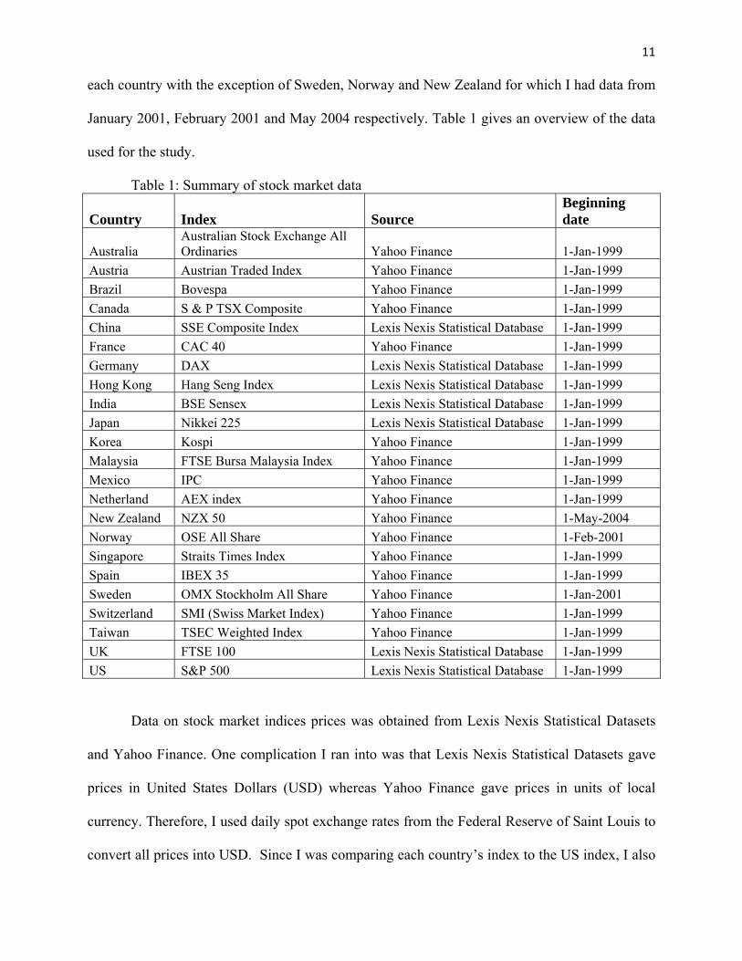
each country with the exception of Sweden, Norway and New Zealand for which I had data from
January 2001, February 2001 and May 2004 respectively. Table 1 gives an overview of the data
used for the study.
Table 1: Summary of stock market data
Country Index Source Beginning date
Australia Australian Stock Exchange All Ordinaries Yahoo Finance 1-Jan-1999
Austria Austrian Traded Index Yahoo Finance 1-Jan-1999
Brazil Bovespa Yahoo Finance 1-Jan-1999
Canada S & P TSX Composite Yahoo Finance 1-Jan-1999
China SSE Composite Index Lexis Nexis Statistical Database 1-Jan-1999
France CAC 40 Yahoo Finance 1-Jan-1999
Germany DAX Lexis Nexis Statistical Database 1-Jan-1999
Hong Kong Hang Seng Index Lexis Nexis Statistical Database 1-Jan-1999
India BSE Sensex Lexis Nexis Statistical Database 1-Jan-1999
Japan Nikkei 225 Lexis Nexis Statistical Database 1-Jan-1999
Korea Kospi Yahoo Finance 1-Jan-1999
Malaysia FTSE Bursa Malaysia Index Yahoo Finance 1-Jan-1999
Mexico IPC Yahoo Finance 1-Jan-1999
Netherland AEX index Yahoo Finance 1-Jan-1999
New Zealand NZX 50 Yahoo Finance 1-May-2004
Norway OSE All Share Yahoo Finance 1-Feb-2001
Singapore Straits Times Index Yahoo Finance 1-Jan-1999
Spain IBEX 35 Yahoo Finance 1-Jan-1999
Sweden OMX Stockholm All Share Yahoo Finance 1-Jan-2001
Switzerland SMI (Swiss Market Index) Yahoo Finance 1-Jan-1999
Taiwan TSEC Weighted Index Yahoo Finance 1-Jan-1999
UK FTSE 100 Lexis Nexis Statistical Database 1-Jan-1999
US S&P 500 Lexis Nexis Statistical Database 1-Jan-1999
Data on stock market indices prices was obtained from Lexis Nexis Statistical Datasets
and Yahoo Finance. One complication I ran into was that Lexis Nexis Statistical Datasets gave
prices in United States Dollars (USD) whereas Yahoo Finance gave prices in units of local
currency. Therefore, I used daily spot exchange rates from the Federal Reserve of Saint Louis to
convert all prices into USD. Since I was comparing each country’s index to the US index, I also
12
had to make sure that all the dates lined up for comparison. There were some dates where I had
the price for the index of one country but not the other. This was due to the fact that each country
had different holidays on which the stock markets are closed. Rather than taking a weekly or 3
day average, I chose to ignore such data points. Since the stock prices evolved in a clearly
monotonous nonlinear fashion, I took the natural logarithm of all the series.
For the CAPM analysis, I use Standard and Poor’s Global 1200 Index as the global index.
The S&P Global 1200 Index, which is available for free at the Standard and Poor’ website, is a
free-float weighted stock market index of global equities that covers 31 countries and
approximately 70 percent of global stock market capitalization. The index is a good proxy for the
global stock market. Barari (2004) used the Morgan Stanley Capital International All Country
World Free Index (ACWFI) which is another good proxy for the world stock market; however, I
decided not to use it because it has daily data for only a few years.
I used daily values of the S&P 1200 and the country’s index to get daily returns (again
making sure that all the dates lined up). Since the scope of this part of my study is the short-run, I
used data from 2005 to 2007 to estimate the βs and then compared each β to real GDP
performance of the country from 2007 to 2010.
I obtained quarterly nominal GDP and the GDP deflator (with 2005 as the base year)
from International Financial Statistics. I found the real GDP for each country (from Q1 2007 to
Q3 2010) by dividing the nominal GDP by the GDP deflator. However, this figure was in units
of local currency so I used quarterly exchange rates to convert it to United States Dollars.
3.2: Methodology:
The methodology section is divided into three sections, the Johansen test, the Gregory
and Hansen test and the Capital asset pricing model.

13
3.2(a) Johansen Test (1988):
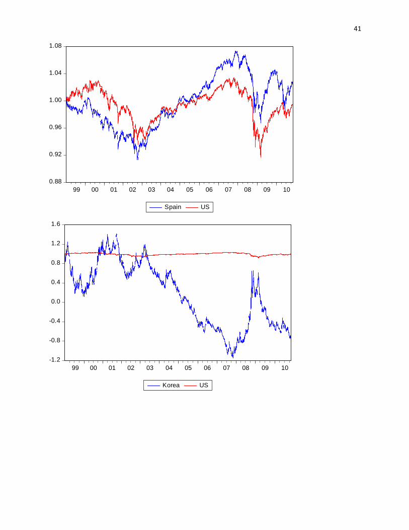
I started by plotting the logarithmic values of each country’s time series with that of the
United States. As the graphs in the appendix show, most of the country indices follow a trend of
decline from 2000 to 2002, followed by about 5 years of steady growth and then a sharp plunge
in 2007. Since these graphs are normalized by the value of the index at the starting date, it is easy
to make comparisons across the two countries. The time series do seem to vary together which
does imply the existence of a long-run relationship, however, I needed a more thorough analysis
before I could conclude that cointegration exists in the stock markets.
Cointegration is defined as a situation where linear combinations of non-stationary time
series are stationary. This implies the existence of a long-run equilibrium between the variables.
Therefore, before I could proceed with the tests of cointegration, I had to make sure that the
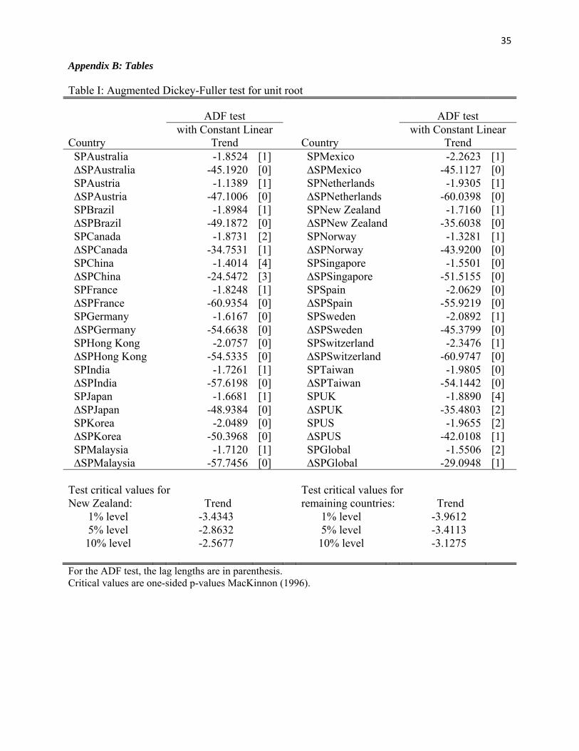
series were non-stationary and hence integrated of order 1. I ran the Augmented Dickey Fuller
tests on the series and the differenced series to confirm that the series were indeed I (1). I used
the Schwartz Information Criterion (SIC) for lag selection as it seems to be the criterion of
choice in most studies. The ADF test is as follows:
∆ μ ∑ ∆ (1)
where is a constant, µ the coefficient on a time trend and k the lag order of the autoregressive
process. The unit root test is then carried out under the null hypothesis = 0 against the
alternative hypothesis of < 0. If we can reject the null, we know the series is stationary and if
the null cannot be rejected, we proceed with the assumption that the time series is non-stationary.
The table I in the appendix shows the results for the ADF test for each country. The ADF test on
the stock market time series tells us that we cannot reject the null. On the other hand, I can reject
14
the null for the differenced series. This means that all the time series are integrated to the order
of 1.
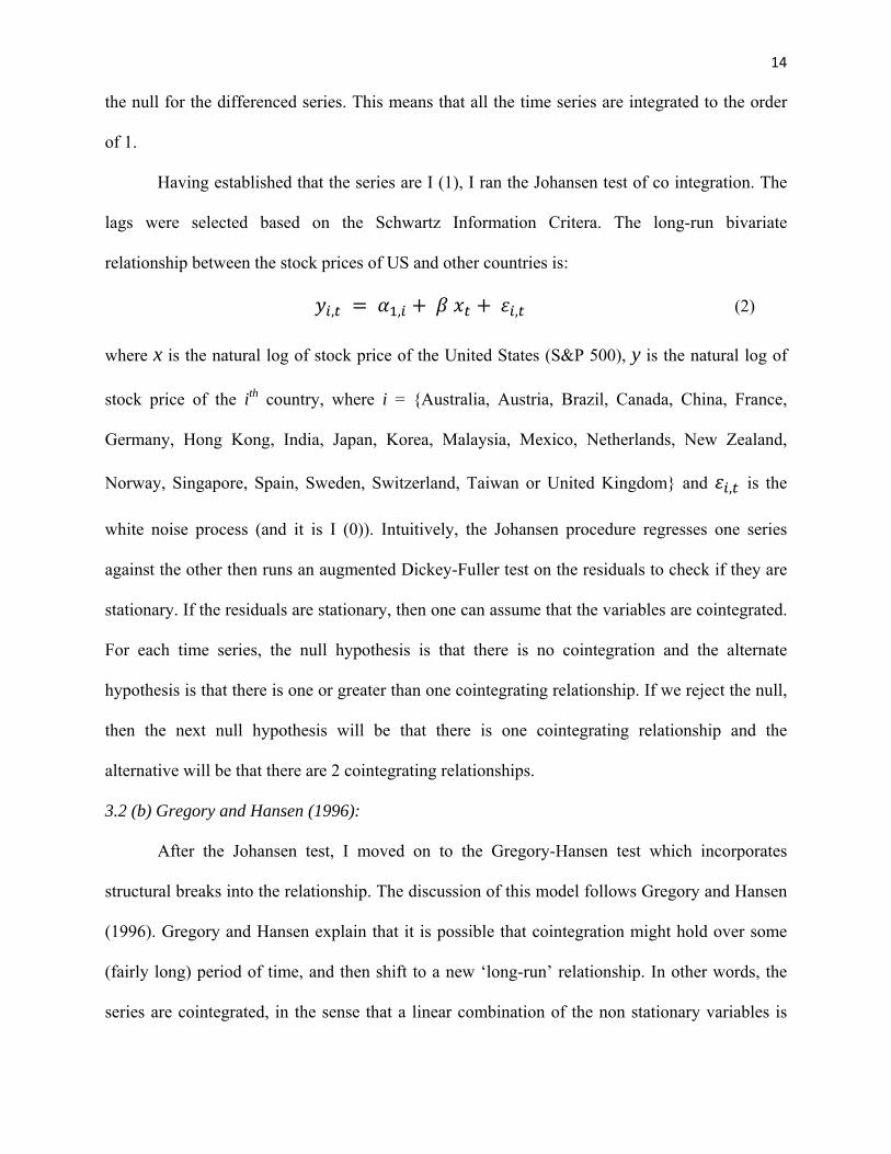
Having established that the series are I (1), I ran the Johansen test of co integration. The
lags were selected based on the Schwartz Information Critera. The long-run bivariate
relationship between the stock prices of US and other countries is:
, , , (2)
where x is the natural log of stock price of the United States (S&P 500), y is the natural log of
stock price of the ith country, where i = {Australia, Austria, Brazil, Canada, China, France,
Germany, Hong Kong, India, Japan, Korea, Malaysia, Mexico, Netherlands, New Zealand,
Norway, Singapore, Spain, Sweden, Switzerland, Taiwan or United Kingdom} and , is the
white noise process (and it is I (0)). Intuitively, the Johansen procedure regresses one series
against the other then runs an augmented Dickey-Fuller test on the residuals to check if they are
stationary. If the residuals are stationary, then one can assume that the variables are cointegrated.
For each time series, the null hypothesis is that there is no cointegration and the alternate
hypothesis is that there is one or greater than one cointegrating relationship. If we reject the null,
then the next null hypothesis will be that there is one cointegrating relationship and the
alternative will be that there are 2 cointegrating relationships.
3.2 (b) Gregory and Hansen (1996):
After the Johansen test, I moved on to the Gregory-Hansen test which incorporates
structural breaks into the relationship. The discussion of this model follows Gregory and Hansen
(1996). Gregory and Hansen explain that it is possible that cointegration might hold over some
(fairly long) period of time, and then shift to a new ‘long-run’ relationship. In other words, the
series are cointegrated, in the sense that a linear combination of the non stationary variables is
15
stationary, but that this linear combination (the cointegrating vector) has shifted at one unknown
point in the sample. In such a scenario, the standard test for cointegration (Johansen test) is not
appropriate since it presumes that the cointegrating vector is time-invariant under the alternative
hypothesis. Gregory, Nason, and Watt (1994) proved that the power of the conventional ADF
test falls sharply in the presence of a structural break. Consequently, Gregory and Hansen (1996)
propose models where the cointegrating vector is allowed to change at a single unknown time
during the sample period. They use dummy variables to model the structural change through a
change in slope and/or y-intercept.
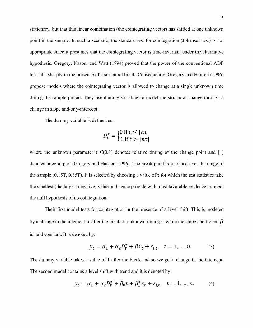
The dummy variable is defined as:
0if τ 1if τ
where the unknown parameter τ Є(0,1) denotes relative timing of the change point and [ ]
denotes integral part (Gregory and Hansen, 1996). The break point is searched over the range of
the sample (0.15T, 0.85T). It is selected by choosing a value of τ for which the test statistics take
the smallest (the largest negative) value and hence provide with most favorable evidence to reject
the null hypothesis of no cointegration.
Their first model tests for cointegration in the presence of a level shift. This is modeled
by a change in the intercept after the break of unknown timing τ. while the slope coefficient
is held constant. It is denoted by:
, 1, … , . (3)
The dummy variable takes a value of 1 after the break and so we get a change in the intercept.
The second model contains a level shift with trend and it is denoted by:
, 1, … , . (4)
16
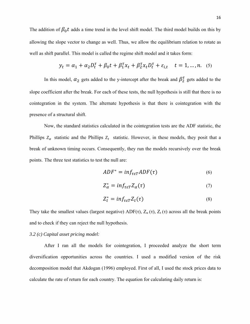
The addition of adds a time trend in the level shift model. The third model builds on this by
allowing the slope vector to change as well. Thus, we allow the equilibrium relation to rotate as
well as shift parallel. This model is called the regime shift model and it takes form:
, 1, … , . (5)
In this model, gets added to the y-intercept after the break and gets added to the
slope coefficient after the break. For each of these tests, the null hypothesis is still that there is no
cointegration in the system. The alternate hypothesis is that there is cointegration with the
presence of a structural shift.
Now, the standard statistics calculated in the cointegration tests are the ADF statistic, the
Phillips statistic and the Phillips statistic. However, in these models, they posit that a
break of unknown timing occurs. Consequently, they run the models recursively over the break
points. The three test statistics to test the null are:
∗ (6)
∗ (7)
∗ (8)
They take the smallest values (largest negative) ADF(τ), Zα (τ), Zt (τ) across all the break points
and to check if they can reject the null hypothesis.
3.2 (c) Capital asset pricing model:
After I ran all the models for cointegration, I proceeded analyze the short term
diversification opportunities across the countries. I used a modified version of the risk
decomposition model that Akdogan (1996) employed. First of all, I used the stock prices data to
calculate the rate of return for each country. The equation for calculating daily return is:
17
, , ∗ 100 (9)
where y is the stock price for the global index or the stock price for the index of country i (i
being all the countries in the sample). After calculating the daily returns for each country, I
compared them to the daily global rate of return (obtained from the S&P Global 1200 index).
The model for obtaining each country’s β is:
(10)
Where Ri is the rate of return on the ith country, Rg is the global rate of return and β is the
sensitivity of the ith country to the global index. β is essentially the country’s exposure to
worldwide systematic risk and hence it can be used to measure market integration.
After ranking all countries based on diversification opportunities, I moved on to the final
part of my study, where I compared each country’s sensitivity to the global index to how its
economy fared from Q1 2007 to Q3 2010. For each country, I picked a value where the real GDP
peaked (before the recession) and then I picked a value where real GDP was the smallest. Using
these two values, I calculated the negative growth rate or fall in real GDP. The formula I used is:
ln , , ∗ 100 (11)
After calculating the βs and the maximum fall in real GDP for each country, I plotted a
scatter plot to see whether there was a significant relationship between the two. Theory tells us
that the greater the β or sensitivity or relative risk of a country, the bigger should be the fall in
real GDP in a recession. Consequently, I also ran a regression with β as the explanatory variable
to the fall in real GDP. This regression took the form:
μ (12)
where α is the y-intercept and µ is the slope of the relationship. µ tells us how a unit increase in
relative risk of a country corresponds to a percentage fall in real GDP.
18
4. Discussion of Results
4.1: Cointegration Analysis:
This paper has used daily opening prices of stock market indices from the USA and 22
developing and developed countries. The ADF test characterized all series as I (1) allowing me
to proceed with the cointegration analysis. As mentioned earlier, the Johansen procedure tests for
cointegration in the absence of any structural break in the data. Therefore, it is used as a
benchmark test for cointegration before the more appropriate tests for cointegration in the
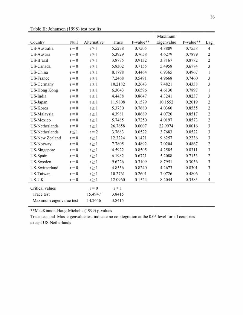
presence of structural breaks are run. I did not find any evidence of cointegration between the
United States and the 21 other countries in the sample; however, I found strong evidence of
cointegration between the United States and the Netherlands. The trace test rejects the null
hypothesis of no cointegration with a low p-value of 0.0007 and the maximum eigenvalue test
rejects the null of no cointegration with a p-value of 0.0016. Since the null of at least one
cointegrating relationship cannot be rejected, I have shown that the stock markets of the United
States and the Netherlands do have a long-run relationship.
My results for the Johansen test are in line with most of the existing studies which do not
find cointegration amongst stock markets when using this rather rudimentary test. On the other
hand, I found cointegration between US-Netherlands whereas Yang, Khan and Pointer (2003)
failed to do so even though they used the more sophisticated recursive cointegration analysis.
This could be due to the fact that they used the time frame 1970-2001 whereas I look at 1999-
2010. My data is more recent, and if the hypothesis that we are moving towards a more
financially integrated world is correct, then, we would expect to see cointegration in the more
recent data. One other reason could be the fact that I use daily data in my model whereas Yang
et. al. (2003) used monthly data. I believe that using monthly data unnecessarily reduces one’s
19
data points and makes it harder to get a read on a long term relationship between two series as it
tosses out 29 of the 30 readings.
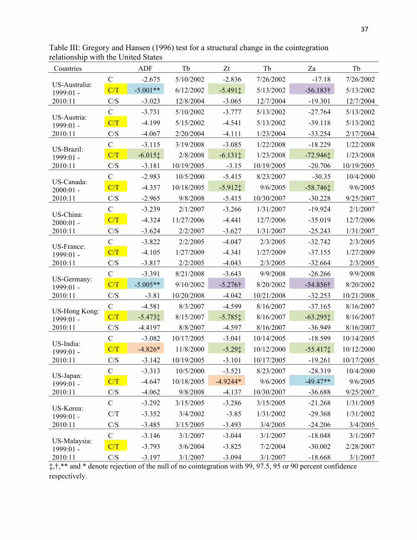
As the plots of the time series in the Appendix C show, there does seem to be a
common trend which binds the series together in the long-run. While the Johansen test did not
find such a relationship, the Gregory and Hansen test did a much better job at finding the long-
run relationship between the series. I found even more proof that either countries are becoming
more integrated or that using daily data is a better measure of finding cointegration. As the
results in Table III show, I was able to reject the null hypothesis of no cointegration for 16 of the
22 countries. These results build on the results of Yang et. al. (2003) for they found evidence of
cointegration between the US and Australia, Hong Kong, Norway, Sweden and Canada in event
windows that started in the late 1990s. They interpreted this as evidence that stock market
cointegration was increasing. My study proves that from 1999 onwards, these markets are
cointegrated. I also found the US to be cointegrated with New-Zealand (in line with the findings
of Narayan and Smyth, 2005), the UK and Japan (corresponding with the findings of Awokuse,
Chopra and Bessler, 2009).
I found cointegration between the S&P 500 and the Mexican IPC and the Brazilian
Bovespa, which is consistent with the findings of Fernandez-Serrano and Sosvilla-Rivero (2003).
Yang et. al. (2003) did not found any evidence of cointegration with Netherlands, Switzerland,
UK and Germany using the recursive cointegration analysis, however, Fernandez-Serrano and
Sosvilla-Rivero (2001) used the Stochastic Permanent Breaks (STOPBREAK) model to find that
Germany, Netherlands and Switzerland are temporally cointegrated with the US stock market.
When compared with the existing literature, my results for the afore mentioned countries show
that the countries evolved from being temporarily cointegrated (in event windows) to being
strongly cointegrated. Studies conducted in the early 2000s that had employed the recursive
20
cointegration analysis had found a trend of increasing integration. My results show that the
countries did follow that trend and they were cointegrated by 2010.
There can be two reasons for this. The first could be due to the fact that I am using the
latest data and so my results reflect the global trend towards more financial integration.
Secondly, it could be due to the fact that I am using daily data which could be a better instrument
for finding cointegration.
The case of India also proves to be very interesting. The government of India took
significant measures in 1990s to open up its capital markets. Furthermore, since 1999, there have
been structural reforms in the Indian financial markets which have enhanced the investibility of
Indian securities globally (Mukherjee and Bose, 2008). In fact, by 2003 India ranked third in
Asia in terms of citizen’s access to foreign capital markets, foreign access to domestic capital
markets, and foreign ownership restrictions2. Theory implies that free capital flows should result
in cointegration between the financial markets. My results prove this as the S&P 500 and the
Sensex are found to be significantly cointegrated.
My results for the countries that are cointegrated are interesting because they use the
Gregory and Hansen methodology to prove cointegration whereas the older studies which used
this methodology were not as successful at finding cointegration. However, they are consistent
with other studies which use the more advanced methods (such as recursive cointegration or
rolling cointegration) to find cointegration. The implications for institutional investors are that
the potential long-term gains from international portfolio diversification into these countries may
not be substantial. On the other hand, there seem to be significant gains from diversification in
Austria, China, France, Korea, Malaysia and Spain as I found no evidence of cointegration
2 As measured by the Economic Freedom index of the World subindex
21
between the United States and these countries. These findings merit a closer look as some of
them, for example the lack of cointegration between the US and France, are surprising.
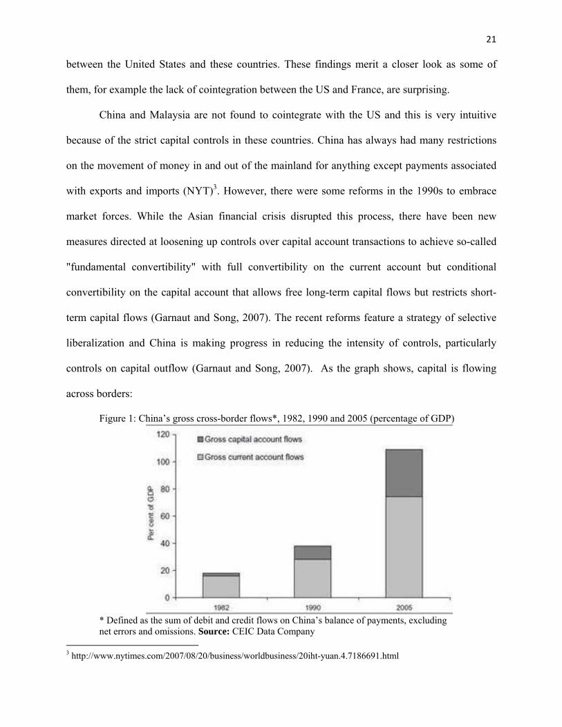
China and Malaysia are not found to cointegrate with the US and this is very intuitive
because of the strict capital controls in these countries. China has always had many restrictions
on the movement of money in and out of the mainland for anything except payments associated
with exports and imports (NYT)3. However, there were some reforms in the 1990s to embrace
market forces. While the Asian financial crisis disrupted this process, there have been new
measures directed at loosening up controls over capital account transactions to achieve so-called
"fundamental convertibility" with full convertibility on the current account but conditional
convertibility on the capital account that allows free long-term capital flows but restricts short-
term capital flows (Garnaut and Song, 2007). The recent reforms feature a strategy of selective
liberalization and China is making progress in reducing the intensity of controls, particularly
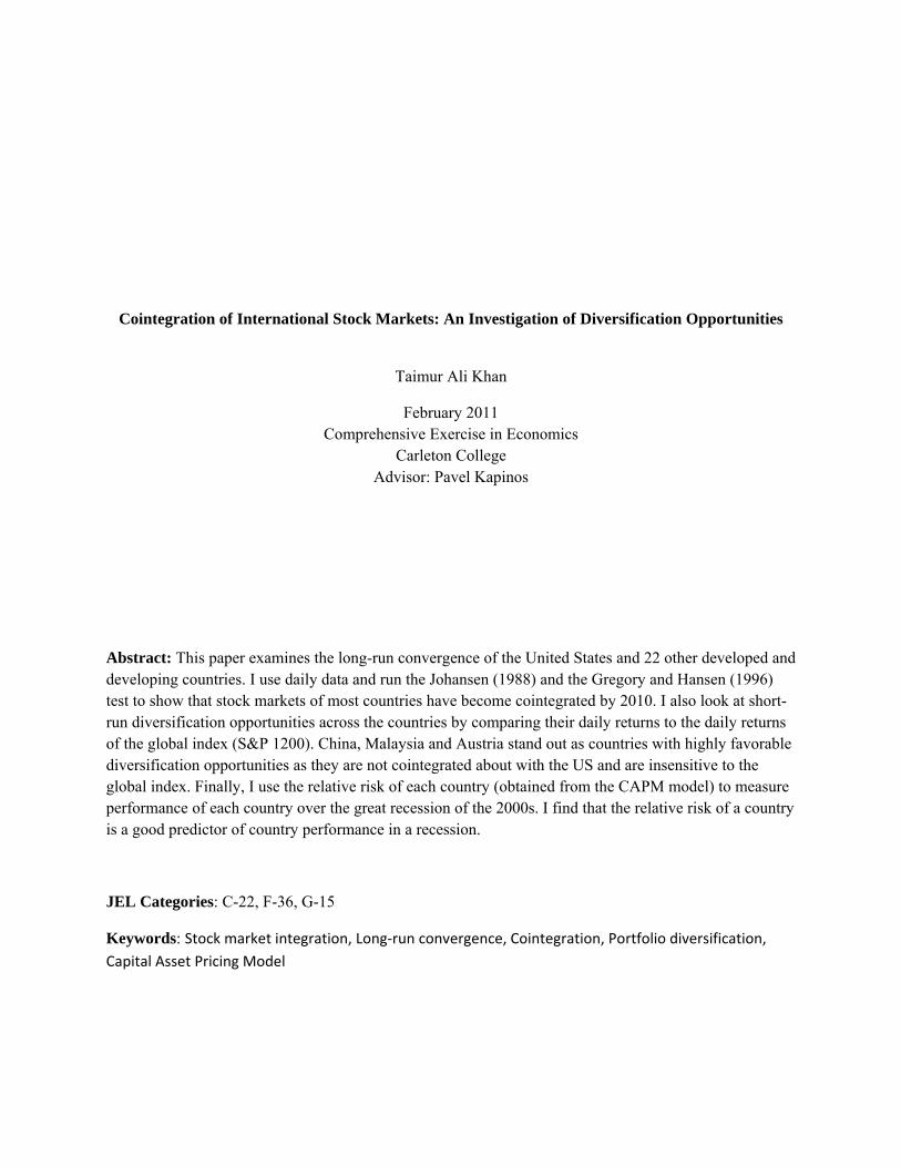
controls on capital outflow (Garnaut and Song, 2007). As the graph shows, capital is flowing
across borders:
Figure 1: China’s gross cross-border flows*, 1982, 1990 and 2005 (percentage of GDP)
* Defined as the sum of debit and credit flows on China’s balance of payments, excluding
net errors and omissions. Source: CEIC Data Company 3 http://www.nytimes.com/2007/08/20/business/worldbusiness/20iht-yuan.4.7186691.html
22
So, according to the theory, we would expect to find increasing integration between the
US and China. I failed to find cointegration between the S&P 500 and the SSE. This could be
due to two reasons. First, that some capital controls are still in place, so there is not enough
capital flow between the two countries. Second, it could be because it takes some time after
(relatively) free capital flow results in the markets entering a long run relationship. Whatever the
reason might be, my results identify China as a country where there are significant
diversification opportunities for US investors
I also did not find any cointegration between the stock markets of the US and Malaysia.
This is to be expected because the Malaysian government imposed restrictions on the
international purchases and sales of financial assets on September 1, 1998 (post the Asian
Financial Crisis of 1997/98). These measures restricted the amount of currency and investments
that Malaysians could take abroad and foreign investors were required to have a one-year “stay
period” before they could withdraw capital. This policy was aimed at reducing exposure to
financial speculators and the global financial turmoil4 by restricting free flow of capital.
Consequently, there should be no cointegration between the stock markets of Malaysia and the
United States.
While the results for China and Malaysia are very intuitive, the results for France, Spain
and Austria are not. My results contradict the findings of Ruxanda and Stoenescu (2009) who use
daily data in the Engle Granger procedure to show that France and Romania are cointegrated and
use the Johansen procedure to show that the US, France and Romania form a cointegrated
system. The time frame they looked at was January 2006 to December 2007. Yang, Khan and
Pointer (2006) also found cointegration between US-France in the window of late 1998 to early
2000. On the other hand, Fadhlaouia, Bellalahb, Dherryc and Zouaouiid (2009) did not find
4 http://www.henciclopedia.org.uy/autores/Khor/Malaysia.htm
23
cointegration between the United States and France from 2000 to 2006. However, they used the
Johansen test for finding cointegration, which we have established is a poor method for finding
cointegration. It is interesting to note that Spain, Austria and France are all members of the
Eurozone. Perhaps the fact that they use a common currency means that they are closely
integrated to each other but not to the United States. On the other hand, the Netherlands and
Germany are also members of the Eurozone and are found to be cointegrated with the US.
Consequently, the lack of cointegration between the US, France Spain and Austria remains a
puzzle.
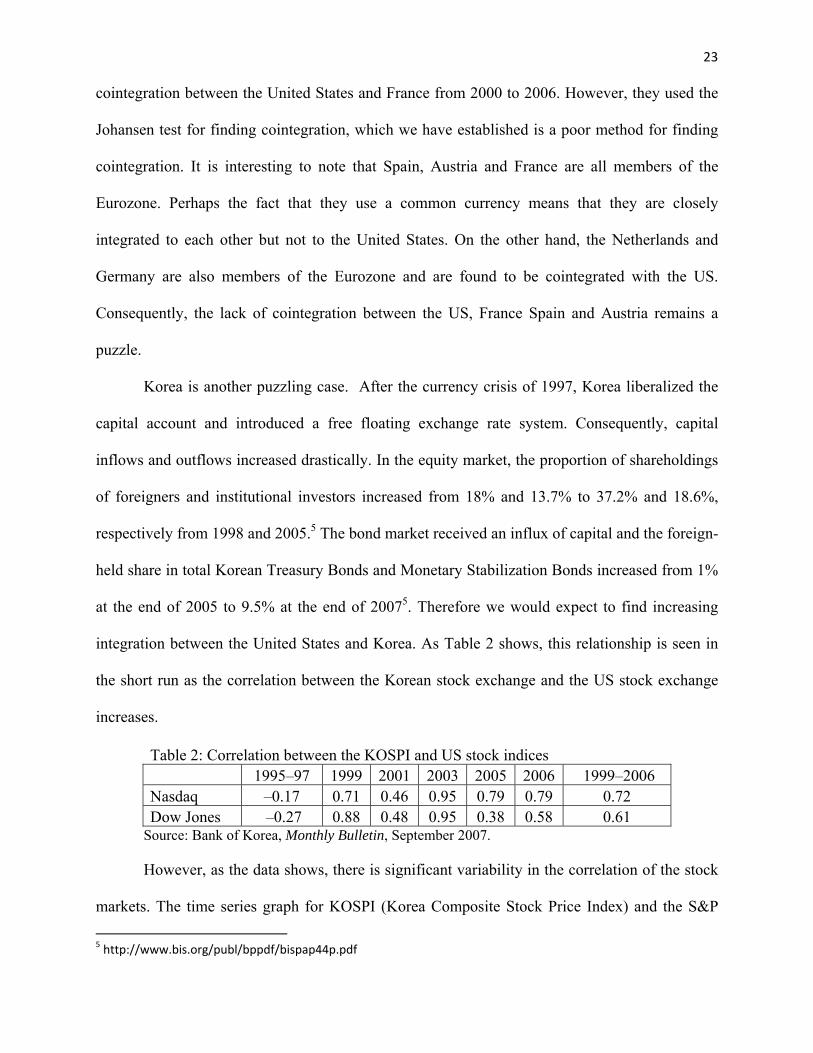
Korea is another puzzling case. After the currency crisis of 1997, Korea liberalized the
capital account and introduced a free floating exchange rate system. Consequently, capital
inflows and outflows increased drastically. In the equity market, the proportion of shareholdings
of foreigners and institutional investors increased from 18% and 13.7% to 37.2% and 18.6%,
respectively from 1998 and 2005.5 The bond market received an influx of capital and the foreign-
held share in total Korean Treasury Bonds and Monetary Stabilization Bonds increased from 1%
at the end of 2005 to 9.5% at the end of 20075. Therefore we would expect to find increasing
integration between the United States and Korea. As Table 2 shows, this relationship is seen in
the short run as the correlation between the Korean stock exchange and the US stock exchange
increases.
Table 2: Correlation between the KOSPI and US stock indices 1995–97 1999 2001 2003 2005 2006 1999–2006 Nasdaq –0.17 0.71 0.46 0.95 0.79 0.79 0.72 Dow Jones –0.27 0.88 0.48 0.95 0.38 0.58 0.61
Source: Bank of Korea, Monthly Bulletin, September 2007.
However, as the data shows, there is significant variability in the correlation of the stock
markets. The time series graph for KOSPI (Korea Composite Stock Price Index) and the S&P
5 http://www.bis.org/publ/bppdf/bispap44p.pdf
24
500 (provided in Appendix C) also shows this trend as the graph fluctuates wildly over the 11
year period. One possible reason for this is that the South Korean Won fluctuated tremendously
in the 2000s. It depreciated suddenly in 2000, followed by a slow appreciation till 2008 followed
by another significant and sudden depreciation. Since I use stock index price in dollars, the
exchange rate movements translate to movements of the index which could be the reason that I
could not find cointegration with the United States.
To reiterate, my results show that the stock markets of the United States, China,
Malaysia, France, Spain, Austria and Korea are not cointegrated. This implies that US investors
can reap significant diversification benefits by investing in these countries.
4.2: Analysis of Diversification Opportunities:
The second part of my model pertained to finding short-run diversification opportunities
across the countries. However, unlike the cointegration analysis, where I was comparing each
country to the United States, I compared each country to the global index. Using equation (9) I
got daily returns and equation (10) gave me the βs or relative risk of each country. Table 3
summarizes the relative risk of each country. The t-statistic provides an analysis of significance
and it is calculated by dividing the coefficient of the regression (β) by the standard error. If the
absolute value of the t-statistic is greater than 2, we know with 90% confidence that the variable
is significantly different from 0. I found that the βs of China and the UK were not statistically
significant. Consequently I excluded them from the third part of my study.
The βs for the other countries, however, are significant, and very intriguing. I found that
some of the countries which were not cointegrated with the US, namely China, Austria and
Malaysia were very insensitive to the global index (βs of 0.0087, 0.15868 and 0.177512
respectively). Whereas, some of the countries that had very strong evidence of cointegration
were very sensitive to the global index. For example, Brazil, Canada, Netherlands and
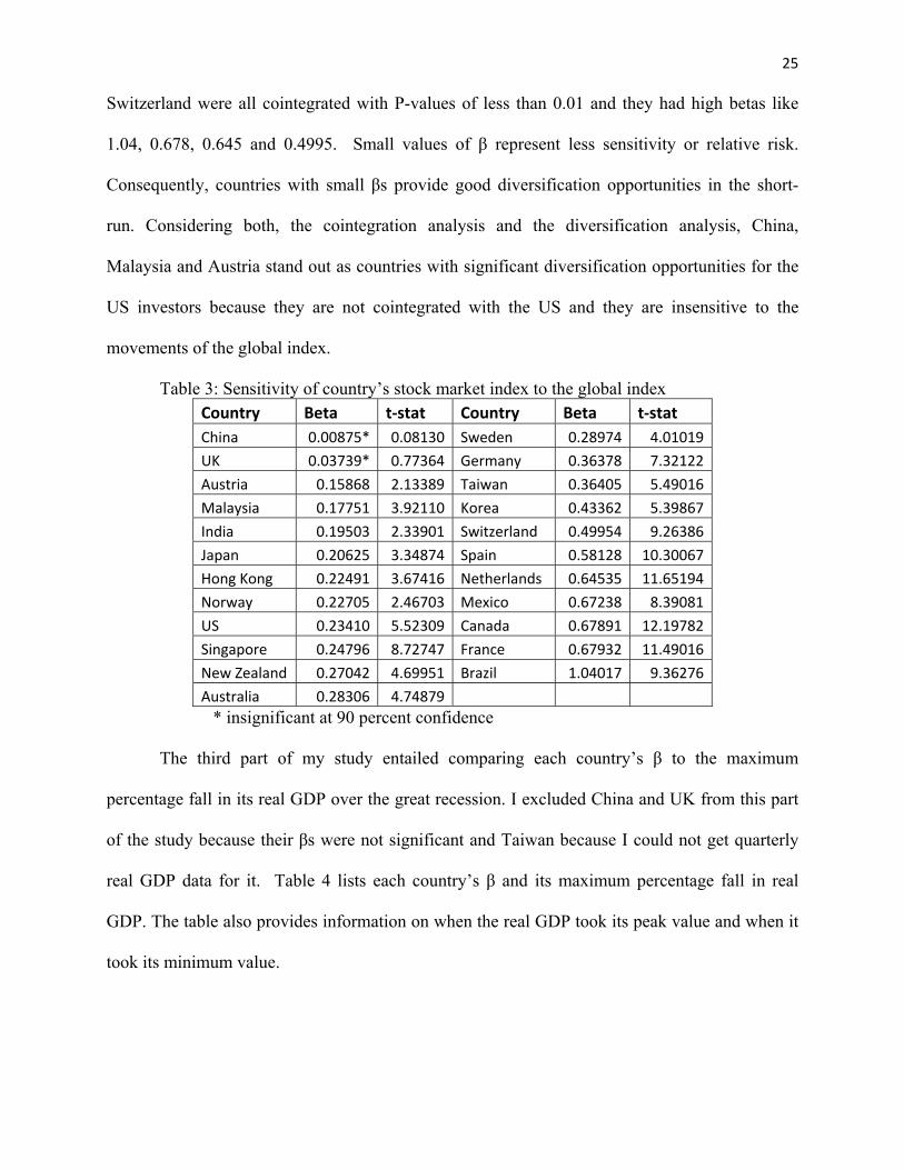
25
Switzerland were all cointegrated with P-values of less than 0.01 and they had high betas like
1.04, 0.678, 0.645 and 0.4995. Small values of β represent less sensitivity or relative risk.
Consequently, countries with small βs provide good diversification opportunities in the short-
run. Considering both, the cointegration analysis and the diversification analysis, China,
Malaysia and Austria stand out as countries with significant diversification opportunities for the
US investors because they are not cointegrated with the US and they are insensitive to the
movements of the global index.
Table 3: Sensitivity of country’s stock market index to the global index Country Beta t‐stat Country Beta t‐stat
China 0.00875* 0.08130 Sweden 0.28974 4.01019
UK 0.03739* 0.77364 Germany 0.36378 7.32122
Austria 0.15868 2.13389 Taiwan 0.36405 5.49016
Malaysia 0.17751 3.92110 Korea 0.43362 5.39867
India 0.19503 2.33901 Switzerland 0.49954 9.26386
Japan 0.20625 3.34874 Spain 0.58128 10.30067
Hong Kong 0.22491 3.67416 Netherlands 0.64535 11.65194
Norway 0.22705 2.46703 Mexico 0.67238 8.39081
US 0.23410 5.52309 Canada 0.67891 12.19782
Singapore 0.24796 8.72747 France 0.67932 11.49016
New Zealand 0.27042 4.69951 Brazil 1.04017 9.36276
Australia 0.28306 4.74879
* insignificant at 90 percent confidence
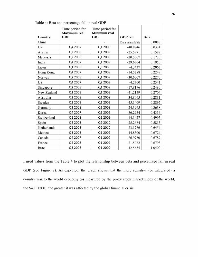
The third part of my study entailed comparing each country’s β to the maximum
percentage fall in its real GDP over the great recession. I excluded China and UK from this part
of the study because their βs were not significant and Taiwan because I could not get quarterly
real GDP data for it. Table 4 lists each country’s β and its maximum percentage fall in real
GDP. The table also provides information on when the real GDP took its peak value and when it
took its minimum value.
26
Table 4: Beta and percentage fall in real GDP
Country
Time period for Maximum real GDP
Time period for Minimum real GDP GDP fall Beta
China ‐ ‐ Data unavailable 0.0088
UK Q4 2007 Q1 2009 -40.8746 0.0374
Austria Q2 2008 Q1 2009 -25.5971 0.1587
Malaysia Q2 2008 Q1 2009 -20.5567 0.1775
India Q4 2007 Q1 2009 -29.6304 0.1950
Japan Q1 2008 Q3 2008 -4.3437 0.2063
Hong Kong Q4 2007 Q1 2009 -14.5288 0.2249
Norway Q2 2008 Q1 2009 -30.6007 0.2270
US Q4 2007 Q2 2009 -4.2300 0.2341
Singapore Q2 2008 Q1 2009 -17.8196 0.2480
New Zealand Q1 2008 Q1 2009 -41.2159 0.2704
Australia Q2 2008 Q1 2009 -34.8065 0.2831
Sweden Q2 2008 Q1 2009 -45.1409 0.2897
Germany Q2 2008 Q1 2009 -24.3965 0.3638
Korea Q4 2007 Q1 2009 -56.2954 0.4336
Switzerland Q2 2008 Q1 2009 -14.1427 0.4995
Spain Q2 2008 Q2 2010 -25.2684 0.5813
Netherlands Q2 2008 Q2 2010 -23.1766 0.6454
Mexico Q3 2008 Q1 2009 -44.8300 0.6724
Canada Q4 2007 Q1 2009 -26.9760 0.6789
France Q2 2008 Q1 2009 -21.5062 0.6793
Brazil Q3 2008 Q1 2009 -42.5635 1.0402
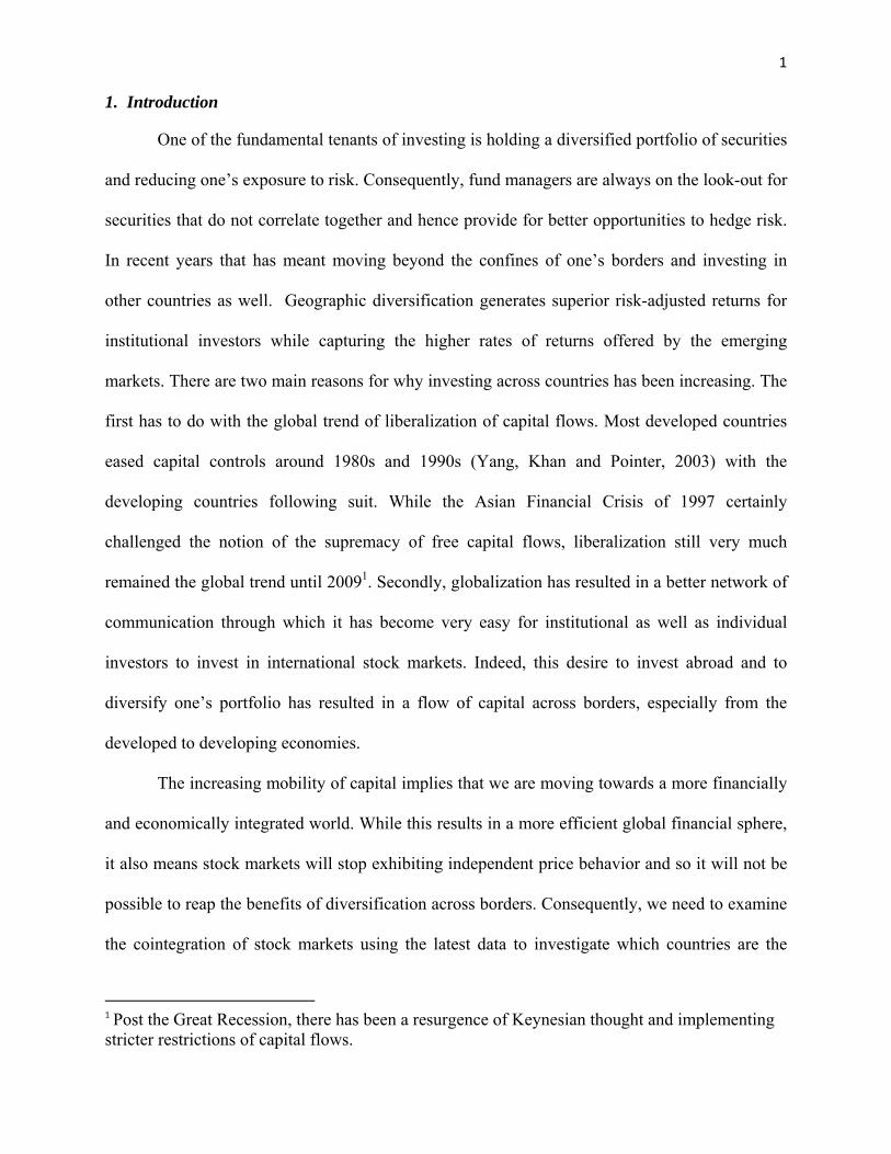
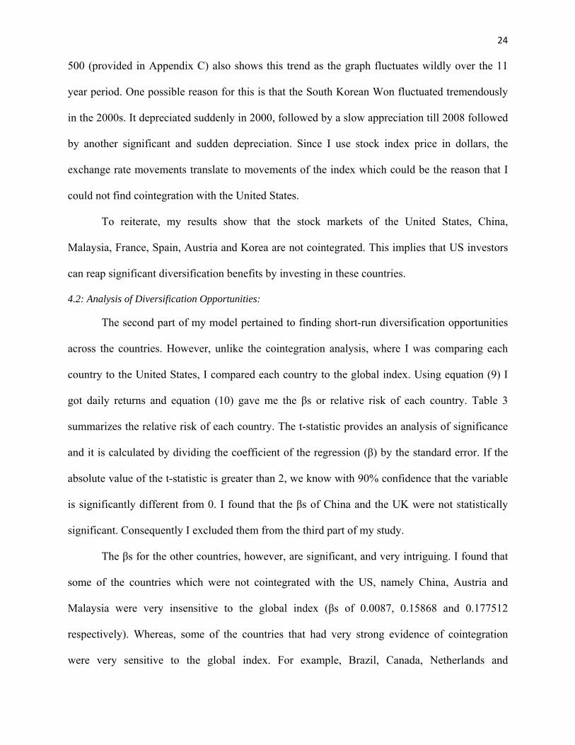
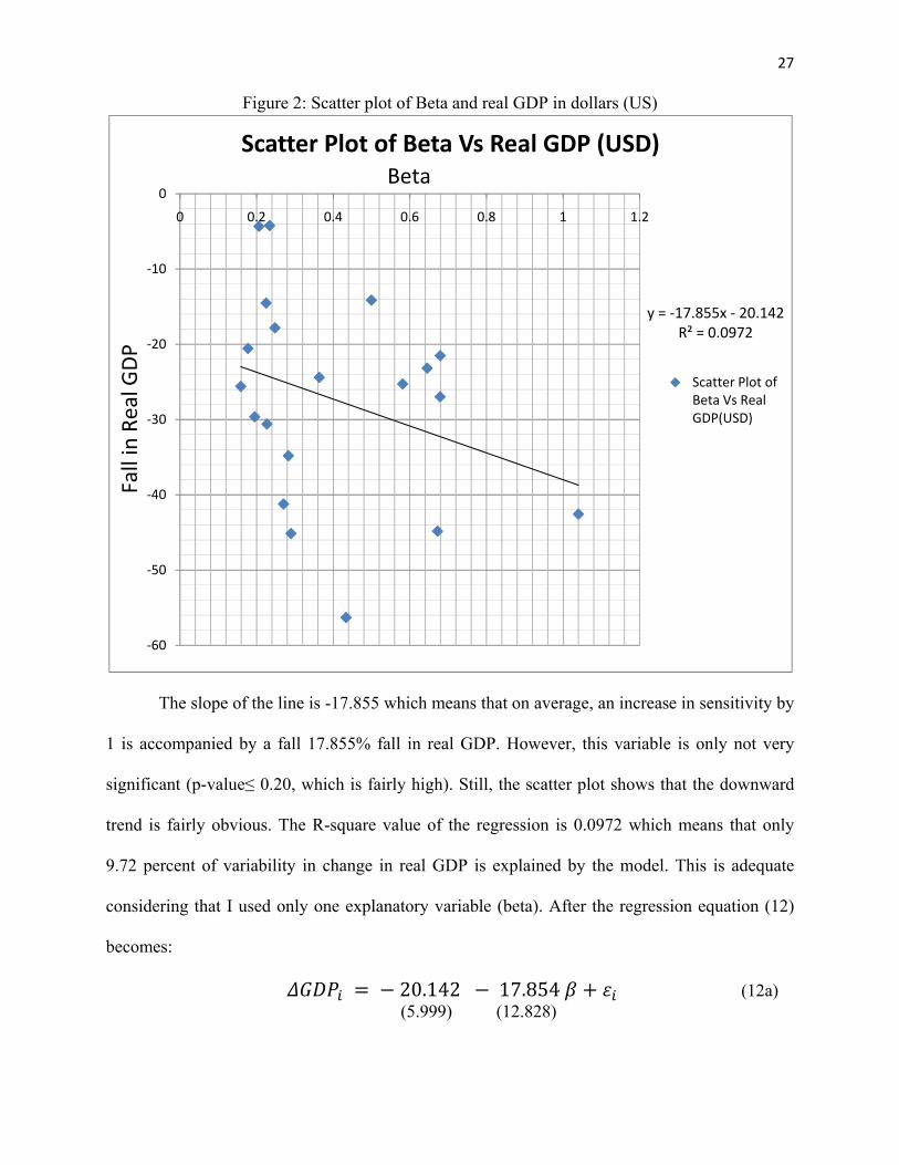
I used values from the Table 4 to plot the relationship between beta and percentage fall in real
GDP (see Figure 2). As expected, the graph shows that the more sensitive (or integrated) a
country was to the world economy (as measured by the proxy stock market index of the world,
the S&P 1200), the greater it was affected by the global financial crisis.
27
Figure 2: Scatter plot of Beta and real GDP in dollars (US)
The slope of the line is -17.855 which means that on average, an increase in sensitivity by
1 is accompanied by a fall 17.855% fall in real GDP. However, this variable is only not very
significant (p-value≤ 0.20, which is fairly high). Still, the scatter plot shows that the downward
trend is fairly obvious. The R-square value of the regression is 0.0972 which means that only
9.72 percent of variability in change in real GDP is explained by the model. This is adequate
considering that I used only one explanatory variable (beta). After the regression equation (12)
becomes:
20.142 17.854 (12a) (5.999) (12.828)
y = ‐17.855x ‐ 20.142R² = 0.0972
‐60
‐50
‐40
‐30
‐20
‐10
0
0 0.2 0.4 0.6 0.8 1 1.2
Scatter Plot of Beta Vs Real GDP (USD)
Scatter Plot of Beta Vs Real GDP(USD)
Beta
Fall in Real G
DP
28
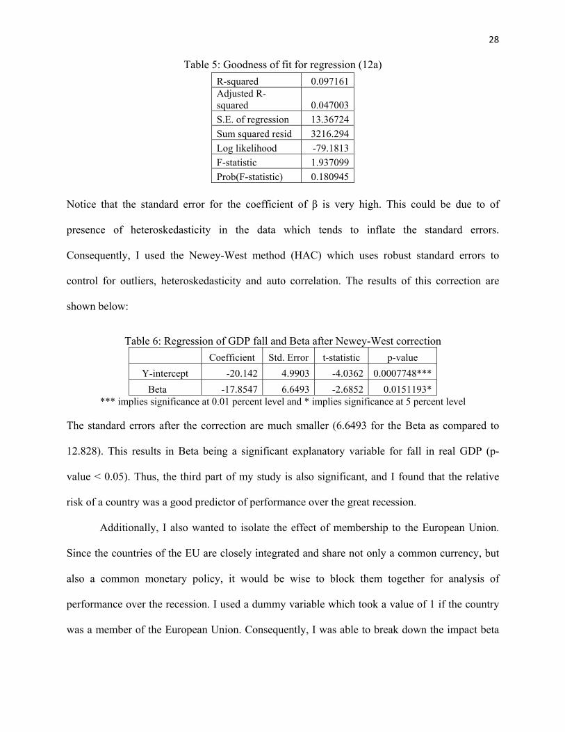
Table 5: Goodness of fit for regression (12a)
R-squared 0.097161Adjusted R-squared 0.047003
S.E. of regression 13.36724
Sum squared resid 3216.294
Log likelihood -79.1813
F-statistic 1.937099
Prob(F-statistic) 0.180945 Notice that the standard error for the coefficient of β is very high. This could be due to of
presence of heteroskedasticity in the data which tends to inflate the standard errors.
Consequently, I used the Newey-West method (HAC) which uses robust standard errors to
control for outliers, heteroskedasticity and auto correlation. The results of this correction are
shown below:
Table 6: Regression of GDP fall and Beta after Newey-West correction
Coefficient Std. Error t-statistic p-value
Y-intercept -20.142 4.9903 -4.0362 0.0007748***
Beta -17.8547 6.6493 -2.6852 0.0151193* *** implies significance at 0.01 percent level and * implies significance at 5 percent level
The standard errors after the correction are much smaller (6.6493 for the Beta as compared to
12.828). This results in Beta being a significant explanatory variable for fall in real GDP (p-
value < 0.05). Thus, the third part of my study is also significant, and I found that the relative
risk of a country was a good predictor of performance over the great recession.
Additionally, I also wanted to isolate the effect of membership to the European Union.
Since the countries of the EU are closely integrated and share not only a common currency, but
also a common monetary policy, it would be wise to block them together for analysis of
performance over the recession. I used a dummy variable which took a value of 1 if the country
was a member of the European Union. Consequently, I was able to break down the impact beta
29
had on percentage fall in real GDP and the impact membership to the European Union had on
real GDP. The equation took the form:
μ μ (13)
Note that this equation is identical to equation (12) except that there is a dummy variable, D,
which denotes membership to the EU. The regression output is given below:
20.729 23.116 15.793 (13a) (5.703) (8.897) (6.737)
The y-intercept and the Beta are significant with p-value < 0.05 and the dummy variable is
significant with p-value < 0.10. The regression tells us that on average, a unit increase in Beta is
accompanied with a 23.116% fall in real GDP for non European Union countries but only a
7.3234% fall for EU countries. This implies that on average, members of the EU performed
better over the recession. However, it does not tell us anything about why this might be the case.
My results from this section also have real world implications for investors. The ordered
list of countries (obtained from the CAPM analysis) can be used as a rough guide to exploit
arbitrage opportunities in the short-run. Countries with low values of beta serve as good avenues
to hedge risk. The analysis of country performance over the 2007 recession can also be used by
investors. First of all, it can be used as a rough guide on how different countries act in a
recession as my results indicate that one should invest in countries with low betas during a
recession as they tend to do better. Secondly, it can also be used to make some predictions during
booms. Most analysts predict a strong rebound from the recession in coming years and thus
investors should invest in countries with high betas as these economies are predicted to grow
more.
30
5. Concluding Remarks and Suggestions for Future Research
I had posed three questions in the beginning of this study. Are the stock markets of US
and 22 other major economies cointegrated? What are the short-run diversification opportunities
across the countries? Does sensitivity to the world economy explain country performance over
the great recession?
To test for cointegration, I ran the Johansen (1998) test and the Gregory and Hansen
(1996) test. One way my study differed from the existing literature was that I not only used daily
values but I was also used the latest data. While the Johansen test failed to find cointegration in
most cases (only US and Netherlands were found to be cointegrated), the Gregory and Hansen
test found cointegration in almost all the cases. This result has implications for institutional
investors because it suggests that there are limited diversification opportunities in these countries
in the long-run. On the other hand, China, Malaysia, Korea, France, Spain and Austria are not
found to be cointegrated with the United States and hence are identified as countries where
investors can attain significant gains from diversification. While the results from this section
were very satisfactory, one way this study can be improved is by including more developing
countries into the mix. Developed countries are more likely to have free capital flows and hence
are more likely to be cointegrated. However, in recent years, an increasing number of investors
are looking to invest in developing countries. Therefore, it would be interesting to see how
integrated these economies are with the United States. While I included some developing
countries in my data, I was limited by the unavailability of free data on the stock market indices
of these countries.
In order to check for diversification opportunities, I ran a capital asset pricing model
using daily returns from 2005 to 2007. I was able to generate a list based on which countries
31
were the least sensitive to changes in the global index and hence provided the most scope for
diversification opportunity. Austria, Malaysia, India, Japan, Hong Kong, Norway and the United
States were found to be the least sensitive (or risky) to movements of the global index.
Compounded with the cointegration analysis, my study identifies Austria, Malaysia and China as
countries most favorable for diversification.
Finally, I was able to show that sensitivity to the global index can be used to explain the
maximum fall in real GDP that a country experienced. One way in which I can build on this
study is by including more countries in my sample. I found that my regression had a high
standard error and a low adjusted R2 value. Adding more countries to the mix will give stronger
results and will be more useful for forecasting country performance in not only recessions but
also booms.
32 References:
Akdogan H. (1996). “A suggested approach to country selection in international portfolio diversification.” Journal of Portfolio, 33-40.
Awokuse, Titus, Aviral Chopra and David A. Bessler (2009). “Structural Change and International Stock Market Interdependence: Evidence from Asian Emerging Markets.” Economic Modelling, vol.26, 549-559 Barari, Mahua (2004). “Equity market integration in Latin America: A time-varying integration score analysis.” International Review of Financial Analysis, 13, no. 5, 649-668 Cerny, Alexandr and Michal Koblas (2008). “Stock Market Integration and the Speed of Information Transmission.” Czech Journal of Economics and Finance, vol. 58, no. 1-2, pp. 2-20 Chiang, Min-Hsien and Jo-Yu Wang (2008). “Regime switching cointegration tests for the Asian Stock index futures: evidence for MSCI Taiwan, Nikkei 225, Hong Kong Hang-Seng, and SGX Straits Times indices.” Applied Economics vol. 40, 285-293 Errunza, Vihang and Etienne Losq (2004). “International Asset Pricing under Mild Segmentation: Theory and Test.” The Journal of Finance, Vol. 40, no. 1, 105-124 Fadhlaouia, Kais, Makram Bellalahb, Armand Dherryc and Mhamed Zouaouiid (2009). “An Empirical Examination of International Diversification Benefits in Central European Emerging Equity Markets.” International Journal of Business, 14(2), 163-173 Fernandez-Serrano, Jose and Simon Sosvilla-Rivero (2003). “Modelling the linkages between US and Latin American Stock Markets.”Applied Economics, 35, 12, 1423-1434
Fernandez-Serrano, Jose and Simon Sosvilla-Rivero (2001). “ Modeling evolving long-run relationships: the linkages between stock markets in Asia.”Japan and the World Economy, 13, 145-160
Fraser, Patricia and Oluwatobi Oyefeso (2005). “US, UK and European Stock Market Integration.” Journal of Business Finance and Accounting, Vol. 32, no. 1-2, 161-181 Garnaut, Ross and Ligang Song (2007). “China: Linking Markets for Growth.” Anu E Press and Asia Pacific Press, 267-270. http://epress.anu.edu.au/chinalink/pdf/ch14.pdf Gregory, Allan W. and Bruce E. Hansen (1996) “Residual-based Tests for Cointegration in Models with Regime Shifts.” Journal of Econometrics, vol. 70, 99–126. Gregory, Allan W., James M. Nason, and David G. Watt (1996). "Testing for Structural Breaks in Cointegrated Relationships," Journal of Econometrics, vol. 71, no. 1-2, 321-341 Jochum, C (1999).“A long-run relationship between Eastern European stock markets? Cointegration and the 1997/98 crisis in emerging markets.” Review of World Economics, vol. 135, 454-479
33
Johansen, Søren (1988). “Statistical Analysis of Cointegrating Vectors.” Journal of Economic Dynamics and Control, vol. 12, 231–54. Lagoarde-Segot, Thomas and Brian M Lucey (2007). “The Capital Markets of the Middle East and North Africa.” Emerging Markets Finance and Trade, vol. 43, 34–57 MacKinnon, J.G.(1996). "Numerical Distribution Functions for Unit Root and Cointegration Tests."Journal of Applied Econometrics, vol. 11, 601-618. Mukherjee, Paramita and Suchismita Bose (2008). “ Does the Stock Market in India Move with Asia? A Multivariate Cointegration-Vector Autoregression Approach.” Emerging Markets Finance and Trade, vol. 44, 5, 5-22 Narayan, Kumar and Russell Smyth (2005). “Cointegration of Stock Markets between New Zealand, Australia and the G7 Economics: Searching for Co-movement under Structural Change.” Australian Economic Papers, 44, 231-247.
Ruxanda, Gheorgh.and Smaranda Stoenescu, (2009). “Bivariate and Multivariate Cointegration and their Application in Stock Markets.” Economic Computation and Economic Cybernetics Studies and Research 43(4): 17–31. Solnik, B. (1974). “The International Pricing of Risk: An Empirical Investigation of the World Capital Market Structure.” The Journal of Finance, Vol. 29, 365– 378 Von Furstenberg, George and Bang Nam Jeon (1989). “International Stock Price Movements: Links and Messages.” Brookings Papers on Economic Activity, no. 1, 125-67 Yang, Jian, Moosa Khan and Lucille Pointer (2003). “ Increasing Integration Between the United States and Other International Stock Markets?”Emerging Markets Finance and Trade, vol.39, no.6, 39 -53
Zivot, Eric and Donald W. K. Andrews (1992), “Further Evidence of the Great Crash, the Oil price Shock and the Unit-root Hypothesis.” Journal of Business and Economic Statistics, vol. 10, 251–70
34 Appendix A: Data Description
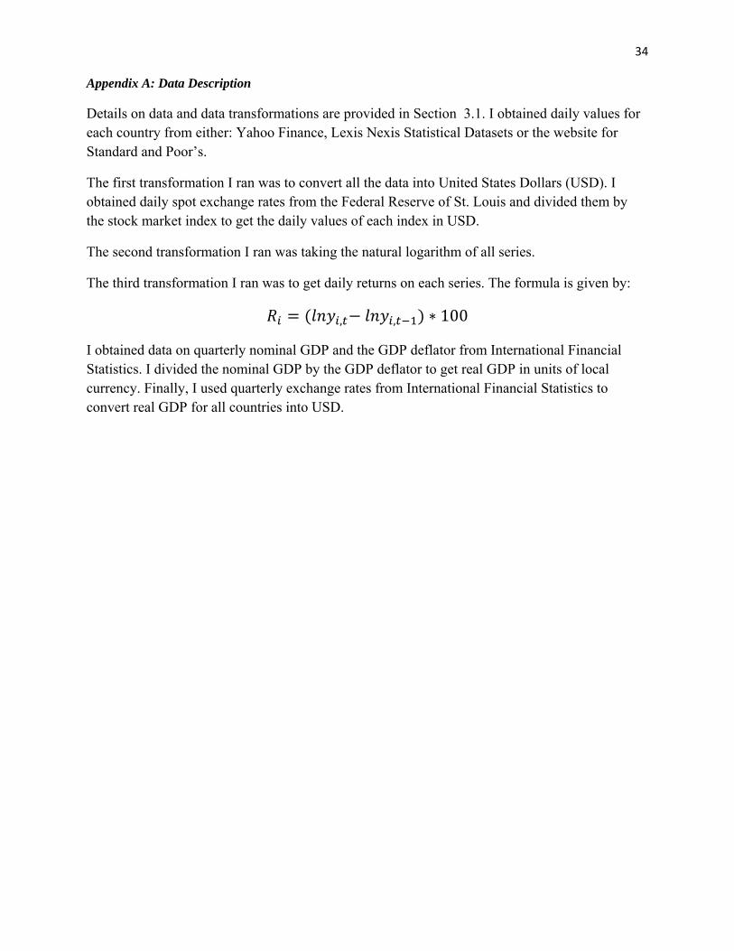
Details on data and data transformations are provided in Section 3.1. I obtained daily values for each country from either: Yahoo Finance, Lexis Nexis Statistical Datasets or the website for Standard and Poor’s.
The first transformation I ran was to convert all the data into United States Dollars (USD). I obtained daily spot exchange rates from the Federal Reserve of St. Louis and divided them by the stock market index to get the daily values of each index in USD.
The second transformation I ran was taking the natural logarithm of all series.
The third transformation I ran was to get daily returns on each series. The formula is given by:
, , ∗ 100
I obtained data on quarterly nominal GDP and the GDP deflator from International Financial Statistics. I divided the nominal GDP by the GDP deflator to get real GDP in units of local currency. Finally, I used quarterly exchange rates from International Financial Statistics to convert real GDP for all countries into USD.
35 Appendix B: Tables
Table I: Augmented Dickey-Fuller test for unit root
ADF test ADF test
Country with Constant Linear
Trend Country with Constant Linear
Trend SPAustralia -1.8524 [1] SPMexico -2.2623 [1] ∆SPAustralia -45.1920 [0] ∆SPMexico -45.1127 [0] SPAustria -1.1389 [1] SPNetherlands -1.9305 [1] ∆SPAustria -47.1006 [0] ∆SPNetherlands -60.0398 [0] SPBrazil -1.8984 [1] SPNew Zealand -1.7160 [1] ∆SPBrazil -49.1872 [0] ∆SPNew Zealand -35.6038 [0] SPCanada -1.8731 [2] SPNorway -1.3281 [1] ∆SPCanada -34.7531 [1] ∆SPNorway -43.9200 [0] SPChina -1.4014 [4] SPSingapore -1.5501 [0] ∆SPChina -24.5472 [3] ∆SPSingapore -51.5155 [0] SPFrance -1.8248 [1] SPSpain -2.0629 [0] ∆SPFrance -60.9354 [0] ∆SPSpain -55.9219 [0] SPGermany -1.6167 [0] SPSweden -2.0892 [1] ∆SPGermany -54.6638 [0] ∆SPSweden -45.3799 [0] SPHong Kong -2.0757 [0] SPSwitzerland -2.3476 [1] ∆SPHong Kong -54.5335 [0] ∆SPSwitzerland -60.9747 [0] SPIndia -1.7261 [1] SPTaiwan -1.9805 [0] ∆SPIndia -57.6198 [0] ∆SPTaiwan -54.1442 [0] SPJapan -1.6681 [1] SPUK -1.8890 [4] ∆SPJapan -48.9384 [0] ∆SPUK -35.4803 [2] SPKorea -2.0489 [0] SPUS -1.9655 [2] ∆SPKorea -50.3968 [0] ∆SPUS -42.0108 [1] SPMalaysia -1.7120 [1] SPGlobal -1.5506 [2] ∆SPMalaysia -57.7456 [0] ∆SPGlobal -29.0948 [1]
Test critical values for Test critical values for New Zealand: Trend remaining countries: Trend
1% level -3.4343 1% level -3.9612 5% level -2.8632 5% level -3.4113 10% level -2.5677 10% level -3.1275
For the ADF test, the lag lengths are in parenthesis. Critical values are one-sided p-values MacKinnon (1996).
36
Table II: Johansen (1998) test results
Maximum Country Null Alternative Trace P-value** Eigenvalue P-value** Lag
US-Australia r = 0 r ≥ 1 5.5278 0.7505 4.8889 0.7558 4 US-Austria r = 0 r ≥ 1 5.3929 0.7658 4.6279 0.7879 2 US-Brazil r = 0 r ≥ 1 3.8775 0.9132 3.8167 0.8782 2 US-Canada r = 0 r ≥ 1 5.8302 0.7155 5.4958 0.6784 3 US-China r = 0 r ≥ 1 8.1798 0.4464 6.9365 0.4967 1 US-France r = 0 r ≥ 1 7.2468 0.5491 4.9668 0.7460 3 US-Germany r = 0 r ≥ 1 10.2182 0.2643 7.4821 0.4338 3 US-Hong Kong r = 0 r ≥ 1 6.3043 0.6596 4.6130 0.7897 1 US-India r = 0 r ≥ 1 4.4438 0.8647 4.3241 0.8237 3 US-Japan r = 0 r ≥ 1 11.9808 0.1579 10.1552 0.2019 2 US-Korea r = 0 r ≥ 1 5.3730 0.7680 4.0360 0.8555 2 US-Malaysia r = 0 r ≥ 1 4.3981 0.8689 4.0720 0.8517 2 US-Mexico r = 0 r ≥ 1 5.7485 0.7250 4.0197 0.8573 2 US-Netherlands r = 0 r ≥ 1 26.7658 0.0007 22.9974 0.0016 3 US-Netherlands r ≤ 1 r = 2 3.7683 0.0522 3.7683 0.0522 3 US-New Zealand r = 0 r ≥ 1 12.3224 0.1421 9.8257 0.2236 3 US-Norway r = 0 r ≥ 1 7.7805 0.4892 7.0204 0.4867 2 US-Singapore r = 0 r ≥ 1 4.5922 0.8505 4.2585 0.8311 3 US-Spain r = 0 r ≥ 1 6.1982 0.6721 5.2088 0.7153 2 US-Sweden r = 0 r ≥ 1 9.6226 0.3109 8.7951 0.3036 3 US-Switzerland r = 0 r ≥ 1 4.8556 0.8240 4.2673 0.8301 3 US-Taiwan r = 0 r ≥ 1 10.2761 0.2601 7.0726 0.4806 1 US-UK r = 0 r ≥ 1 12.0960 0.1524 8.2044 0.3583 4
Critical values r = 0 r ≤ 1 Trace test 15.4947 3.8415
Maximum eigenvalue test 14.2646 3.8415
**MacKinnon-Haug-Michelis (1999) p-values Trace test and Max-eigenvalue test indicate no cointegration at the 0.05 level for all countries except US-Netherlands
37
Table III: Gregory and Hansen (1996) test for a structural change in the cointegration relationship with the United States Countries ADF Tb Zt Tb Za Tb
US-Australia: 1999:01 - 2010:11
C -2.675 5/10/2002 -2.836 7/26/2002 -17.18 7/26/2002
C/T -5.001** 6/12/2002 -5.491‡ 5/13/2002 -56.183† 5/13/2002
C/S -3.023 12/8/2004 -3.065 12/7/2004 -19.301 12/7/2004
US-Austria: 1999:01 - 2010:11
C -3.731 5/10/2002 -3.777 5/13/2002 -27.764 5/13/2002
C/T -4.199 5/15/2002 -4.541 5/13/2002 -39.118 5/13/2002
C/S -4.067 2/20/2004 -4.111 1/23/2004 -33.254 2/17/2004
US-Brazil: 1999:01 - 2010:11
C -3.115 3/19/2008 -3.085 1/22/2008 -18.229 1/22/2008
C/T -6.015‡ 2/8/2008 -6.131‡ 1/23/2008 -72.946‡ 1/23/2008
C/S -3.181 10/19/2005 -3.15 10/19/2005 -20.706 10/19/2005
US-Canada: 2000:01 - 2010:11
C -2.983 10/5/2000 -5.415 8/23/2007 -30.35 10/4/2000
C/T -4.357 10/18/2005 -5.912‡ 9/6/2005 -58.746‡ 9/6/2005
C/S -2.965 9/8/2008 -5.415 10/30/2007 -30.228 9/25/2007
US-China: 2000:01 - 2010:11
C -3.239 2/1/2007 -3.266 1/31/2007 -19.924 2/1/2007
C/T -4.324 11/27/2006 -4.441 12/7/2006 -35.019 12/7/2006
C/S -3.624 2/2/2007 -3.627 1/31/2007 -25.243 1/31/2007
US-France: 1999:01 - 2010:11
C -3.822 2/2/2005 -4.047 2/3/2005 -32.742 2/3/2005
C/T -4.105 1/27/2009 -4.341 1/27/2009 -37.155 1/27/2009
C/S -3.817 2/2/2005 -4.043 2/3/2005 -32.664 2/3/2005
US-Germany: 1999:01 - 2010:11
C -3.391 8/21/2008 -3.643 9/9/2008 -26.266 9/9/2008
C/T -5.005** 9/10/2002 -5.276† 8/20/2002 -54.856† 8/20/2002
C/S -3.81 10/20/2008 -4.042 10/21/2008 -32.253 10/21/2008
US-Hong Kong: 1999:01 - 2010:11
C -4.581 8/3/2007 -4.599 8/16/2007 -37.165 8/16/2007
C/T -5.473‡ 8/15/2007 -5.785‡ 8/16/2007 -63.295‡ 8/16/2007
C/S -4.4197 8/8/2007 -4.597 8/16/2007 -36.949 8/16/2007
US-India: 1999:01 - 2010:11
C -3.082 10/17/2005 -3.041 10/14/2005 -18.599 10/14/2005
C/T -4.826* 11/8/2000 -5.29‡ 10/12/2000 -55.417‡ 10/12/2000
C/S -3.142 10/19/2005 -3.101 10/17/2005 -19.261 10/17/2005
US-Japan: 1999:01 - 2010:11
C -3.313 10/5/2000 -3.521 8/23/2007 -28.319 10/4/2000
C/T -4.647 10/18/2005 -4.9244* 9/6/2005 -49.47** 9/6/2005
C/S -4.062 9/8/2008 -4.137 10/30/2007 -36.688 9/25/2007
US-Korea: 1999:01 - 2010:11
C -3.292 3/15/2005 -3.286 3/15/2005 -21.268 1/31/2005
C/T -3.352 3/4/2002 -3.85 1/31/2002 -29.368 1/31/2002
C/S -3.485 3/15/2005 -3.493 3/4/2005 -24.206 3/4/2005
US-Malaysia: 1999:01 - 2010:11
C -3.146 3/1/2007 -3.044 3/1/2007 -18.048 3/1/2007
C/T -3.793 5/6/2004 -3.825 7/2/2004 -30.002 2/28/2007
C/S -3.197 3/1/2007 -3.094 3/1/2007 -18.668 3/1/2007 ‡,†,** and * denote rejection of the null of no cointegration with 99, 97.5, 95 or 90 percent confidence respectively.
38
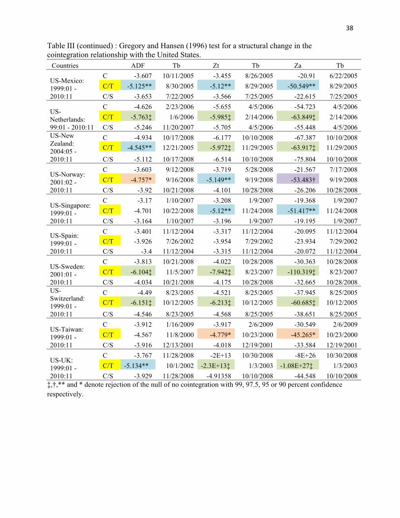
Table III (continued) : Gregory and Hansen (1996) test for a structural change in the cointegration relationship with the United States. Countries ADF Tb Zt Tb Za Tb
US-Mexico: 1999:01 - 2010:11
C -3.607 10/11/2005 -3.455 8/26/2005 -20.91 6/22/2005
C/T -5.125** 8/30/2005 -5.12** 8/29/2005 -50.549** 8/29/2005
C/S -3.653 7/22/2005 -3.566 7/25/2005 -22.615 7/25/2005
US-Netherlands: 99:01 - 2010:11
C -4.626 2/23/2006 -5.655 4/5/2006 -54.723 4/5/2006
C/T -5.763‡ 1/6/2006 -5.985‡ 2/14/2006 -63.849‡ 2/14/2006
C/S -5.246 11/20/2007 -5.705 4/5/2006 -55.448 4/5/2006 US-New Zealand: 2004:05 - 2010:11
C -4.934 10/17/2008 -6.177 10/10/2008 -67.387 10/10/2008
C/T -4.545** 12/21/2005 -5.972‡ 11/29/2005 -63.917‡ 11/29/2005
C/S -5.112 10/17/2008 -6.514 10/10/2008 -75.804 10/10/2008
US-Norway: 2001:02 - 2010:11
C -3.603 9/12/2008 -3.719 5/28/2008 -21.567 7/17/2008
C/T -4.757* 9/16/2008 -5.149** 9/19/2008 -53.483† 9/19/2008
C/S -3.92 10/21/2008 -4.101 10/28/2008 -26.206 10/28/2008
US-Singapore: 1999:01 - 2010:11
C -3.17 1/10/2007 -3.208 1/9/2007 -19.368 1/9/2007
C/T -4.701 10/22/2008 -5.12** 11/24/2008 -51.417** 11/24/2008
C/S -3.164 1/10/2007 -3.196 1/9/2007 -19.195 1/9/2007
US-Spain: 1999:01 - 2010:11
C -3.401 11/12/2004 -3.317 11/12/2004 -20.095 11/12/2004
C/T -3.926 7/26/2002 -3.954 7/29/2002 -23.934 7/29/2002
C/S -3.4 11/12/2004 -3.315 11/12/2004 -20.072 11/12/2004
US-Sweden: 2001:01 - 2010:11
C -3.813 10/21/2008 -4.022 10/28/2008 -30.363 10/28/2008
C/T -6.104‡ 11/5/2007 -7.942‡ 8/23/2007 -110.319‡ 8/23/2007
C/S -4.034 10/21/2008 -4.175 10/28/2008 -32.665 10/28/2008 US-Switzerland: 1999:01 - 2010:11
C -4.49 8/23/2005 -4.521 8/25/2005 -37.945 8/25/2005
C/T -6.151‡ 10/12/2005 -6.213‡ 10/12/2005 -60.685‡ 10/12/2005
C/S -4.546 8/23/2005 -4.568 8/25/2005 -38.651 8/25/2005
US-Taiwan: 1999:01 - 2010:11
C -3.912 1/16/2009 -3.917 2/6/2009 -30.549 2/6/2009
C/T -4.567 11/8/2000 -4.779* 10/23/2000 -45.265* 10/23/2000
C/S -3.916 12/13/2001 -4.018 12/19/2001 -33.584 12/19/2001
US-UK: 1999:01 - 2010:11
C -3.767 11/28/2008 -2E+13 10/30/2008 -8E+26 10/30/2008
C/T -5.134** 10/1/2002 -2.3E+13‡ 1/3/2003 -1.08E+27‡ 1/3/2003
C/S -3.929 11/28/2008 -4.91358 10/10/2008 -44.548 10/10/2008 ‡,†,** and * denote rejection of the null of no cointegration with 99, 97.5, 95 or 90 percent confidence respectively.
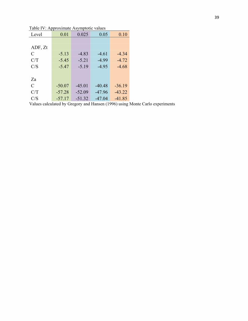
39 Table IV: Approximate Asymptotic values
Level 0.01 0.025 0.05 0.10
ADF, Zt C -5.13 -4.83 -4.61 -4.34C/T -5.45 -5.21 -4.99 -4.72C/S -5.47 -5.19 -4.95 -4.68
Za C -50.07 -45.01 -40.48 -36.19C/T -57.28 -52.09 -47.96 -43.22C/S -57.17 -51.32 -47.04 -41.85
Values calculated by Gregory and Hansen (1996) using Monte Carlo experiments
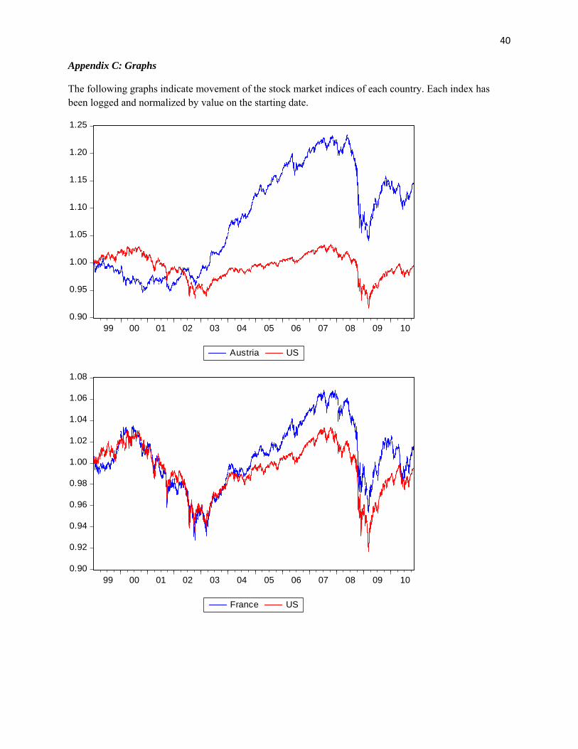
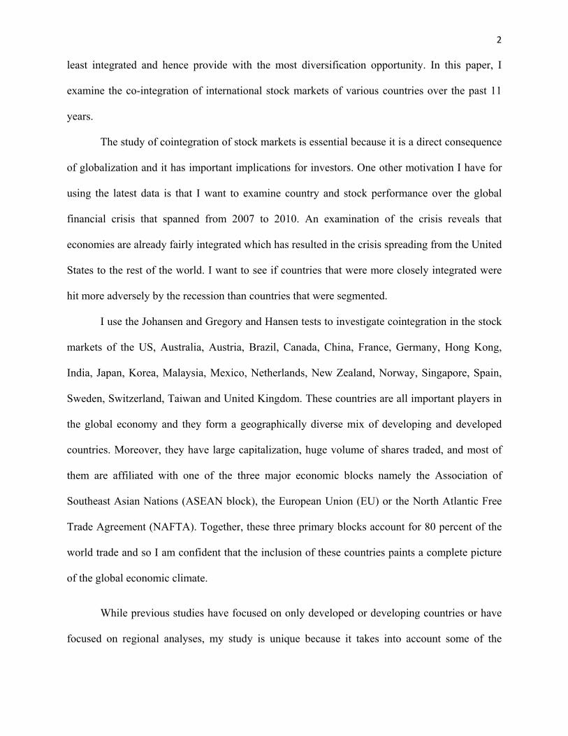
40 Appendix C: Graphs
The following graphs indicate movement of the stock market indices of each country. Each index has been logged and normalized by value on the starting date.
0.90
0.95
1.00
1.05
1.10
1.15
1.20
1.25
99 00 01 02 03 04 05 06 07 08 09 10
Austria US
0.90
0.92
0.94
0.96
0.98
1.00
1.02
1.04
1.06
1.08
99 00 01 02 03 04 05 06 07 08 09 10
France US
41
0.88
0.92
0.96
1.00
1.04
1.08
99 00 01 02 03 04 05 06 07 08 09 10
Spain US
-1.2
-0.8
-0.4
0.0
0.4
0.8
1.2
1.6
99 00 01 02 03 04 05 06 07 08 09 10
Korea US
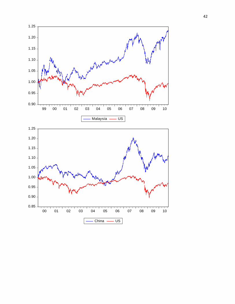
42
0.90
0.95
1.00
1.05
1.10
1.15
1.20
1.25
99 00 01 02 03 04 05 06 07 08 09 10
Malaysia US
0.85
0.90
0.95
1.00
1.05
1.10
1.15
1.20
1.25
00 01 02 03 04 05 06 07 08 09 10
China US
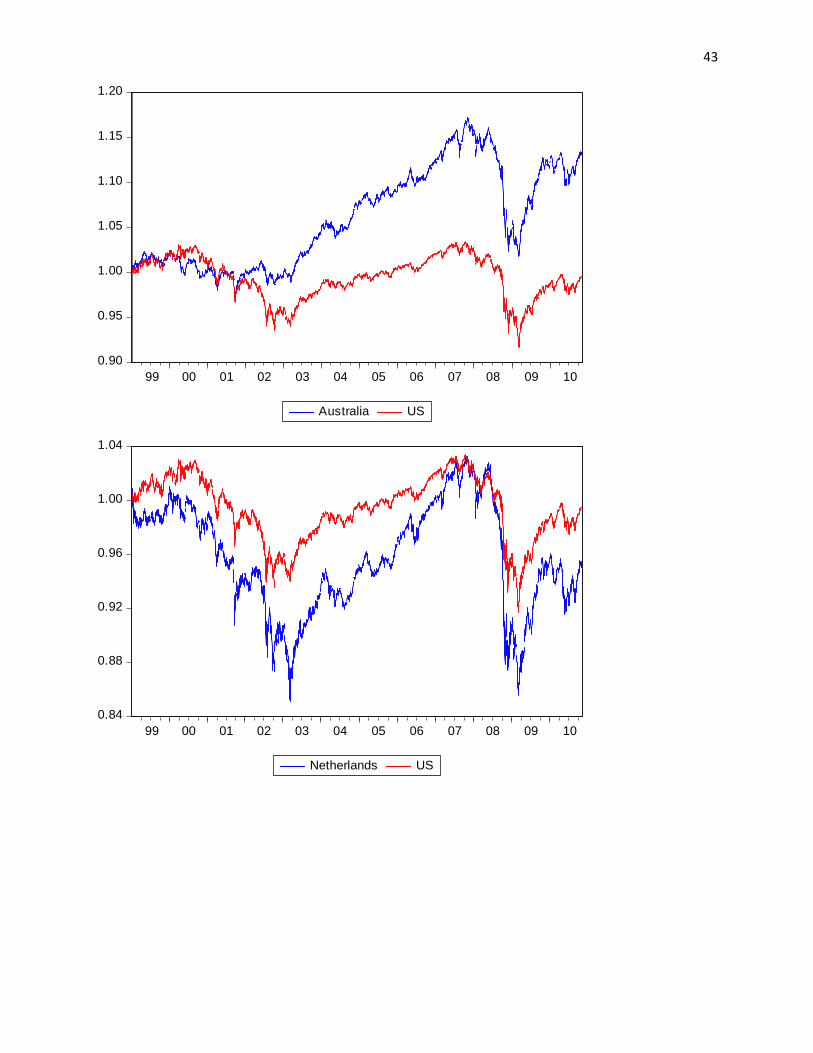
43
0.90
0.95
1.00
1.05
1.10
1.15
1.20
99 00 01 02 03 04 05 06 07 08 09 10
Australia US
0.84
0.88
0.92
0.96
1.00
1.04
99 00 01 02 03 04 05 06 07 08 09 10
Netherlands US
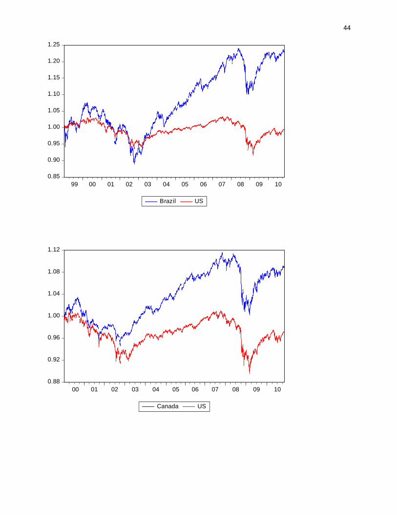
44
0.85
0.90
0.95
1.00
1.05
1.10
1.15
1.20
1.25
99 00 01 02 03 04 05 06 07 08 09 10
Brazil US
0.88
0.92
0.96
1.00
1.04
1.08
1.12
00 01 02 03 04 05 06 07 08 09 10
Canada US
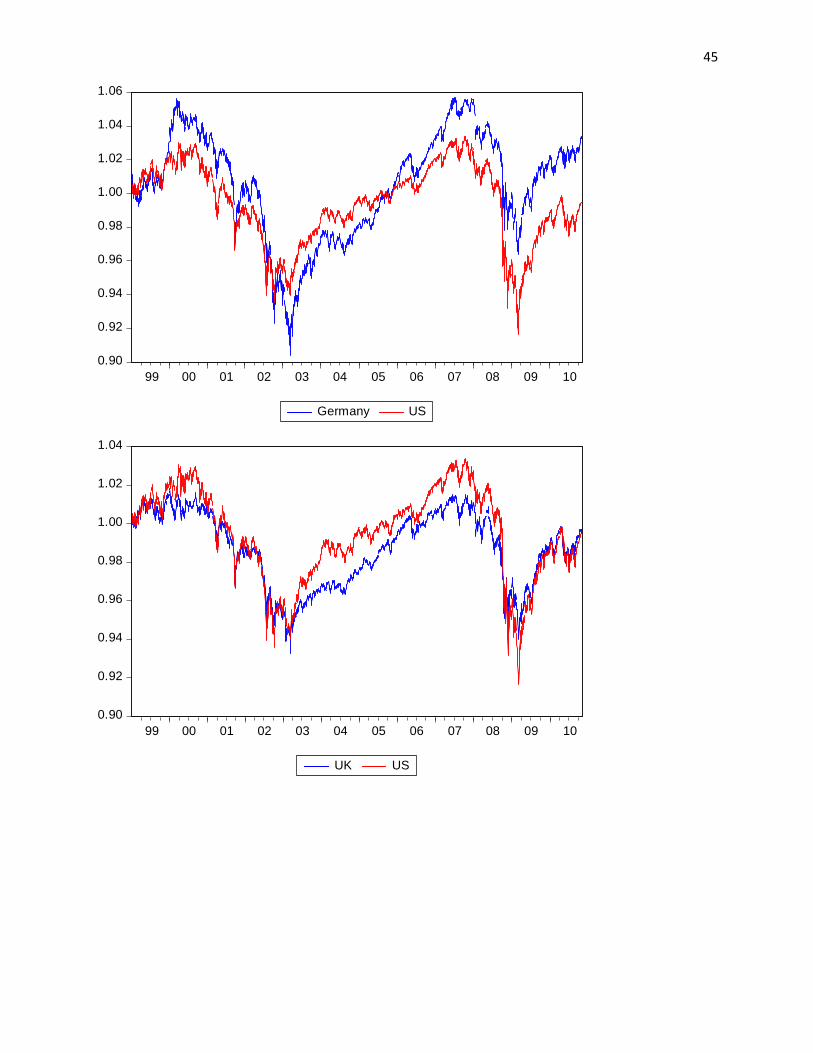
45
0.90
0.92
0.94
0.96
0.98
1.00
1.02
1.04
1.06
99 00 01 02 03 04 05 06 07 08 09 10
Germany US
0.90
0.92
0.94
0.96
0.98
1.00
1.02
1.04
99 00 01 02 03 04 05 06 07 08 09 10
UK US
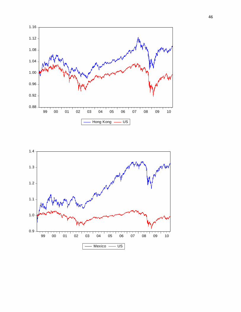
46
0.88
0.92
0.96
1.00
1.04
1.08
1.12
1.16
99 00 01 02 03 04 05 06 07 08 09 10
Hong Kong US
0.9
1.0
1.1
1.2
1.3
1.4
99 00 01 02 03 04 05 06 07 08 09 10
Mexico US
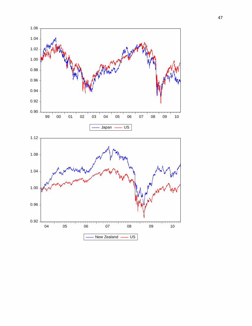
47
0.90
0.92
0.94
0.96
0.98
1.00
1.02
1.04
1.06
99 00 01 02 03 04 05 06 07 08 09 10
Japan US
0.92
0.96
1.00
1.04
1.08
1.12
04 05 06 07 08 09 10
New Zealand US
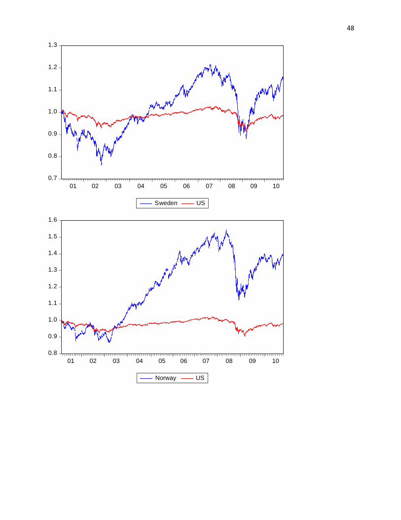
48
0.7
0.8
0.9
1.0
1.1
1.2
1.3
01 02 03 04 05 06 07 08 09 10
Sweden US
0.8
0.9
1.0
1.1
1.2
1.3
1.4
1.5
1.6
01 02 03 04 05 06 07 08 09 10
Norway US
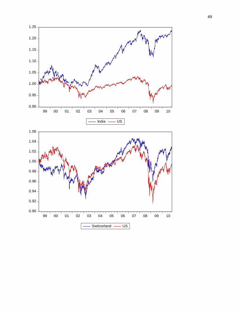
49
0.90
0.95
1.00
1.05
1.10
1.15
1.20
1.25
99 00 01 02 03 04 05 06 07 08 09 10
India US
0.90
0.92
0.94
0.96
0.98
1.00
1.02
1.04
1.06
99 00 01 02 03 04 05 06 07 08 09 10
Switzerland US
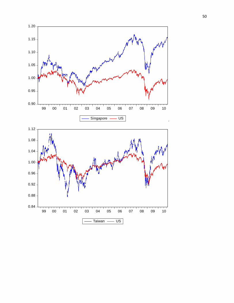
50
.
0.90
0.95
1.00
1.05
1.10
1.15
1.20
99 00 01 02 03 04 05 06 07 08 09 10
Singapore US
0.84
0.88
0.92
0.96
1.00
1.04
1.08
1.12
99 00 01 02 03 04 05 06 07 08 09 10
Taiwan US
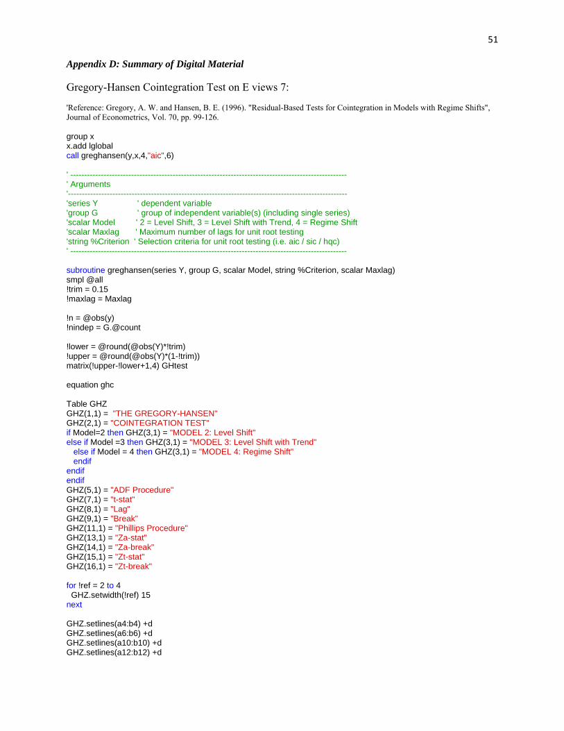
51 Appendix D: Summary of Digital Material
Gregory-Hansen Cointegration Test on E views 7: 'Reference: Gregory, A. W. and Hansen, B. E. (1996). "Residual-Based Tests for Cointegration in Models with Regime Shifts", Journal of Econometrics, Vol. 70, pp. 99-126. group x x.add lglobal call greghansen(y,x,4,"aic",6) ' ---------------------------------------------------------------------------------------------------- ' Arguments '----------------------------------------------------------------------------------------------------- 'series Y ' dependent variable 'group G ' group of independent variable(s) (including single series) 'scalar Model ' 2 = Level Shift, 3 = Level Shift with Trend, 4 = Regime Shift 'scalar Maxlag ' Maximum number of lags for unit root testing 'string %Criterion ' Selection criteria for unit root testing (i.e. aic / sic / hqc) ' ---------------------------------------------------------------------------------------------------- subroutine greghansen(series Y, group G, scalar Model, string %Criterion, scalar Maxlag) smpl @all !trim = 0.15 !maxlag = Maxlag !n = @obs(y) !nindep = G.@count !lower = @round(@obs(Y)*!trim) !upper = @round(@obs(Y)*(1-!trim)) matrix(!upper-!lower+1,4) GHtest equation ghc Table GHZ GHZ(1,1) = "THE GREGORY-HANSEN" GHZ(2,1) = "COINTEGRATION TEST" if Model=2 then GHZ(3,1) = "MODEL 2: Level Shift" else if Model =3 then GHZ(3,1) = "MODEL 3: Level Shift with Trend" else if Model = 4 then GHZ(3,1) = "MODEL 4: Regime Shift" endif endif endif GHZ(5,1) = "ADF Procedure" GHZ(7,1) = "t-stat" GHZ(8,1) = "Lag" GHZ(9,1) = "Break" GHZ(11,1) = "Phillips Procedure" GHZ(13,1) = "Za-stat" GHZ(14,1) = "Za-break" GHZ(15,1) = "Zt-stat" GHZ(16,1) = "Zt-break" for !ref = 2 to 4 GHZ.setwidth(!ref) 15 next GHZ.setlines(a4:b4) +d GHZ.setlines(a6:b6) +d GHZ.setlines(a10:b10) +d GHZ.setlines(a12:b12) +d
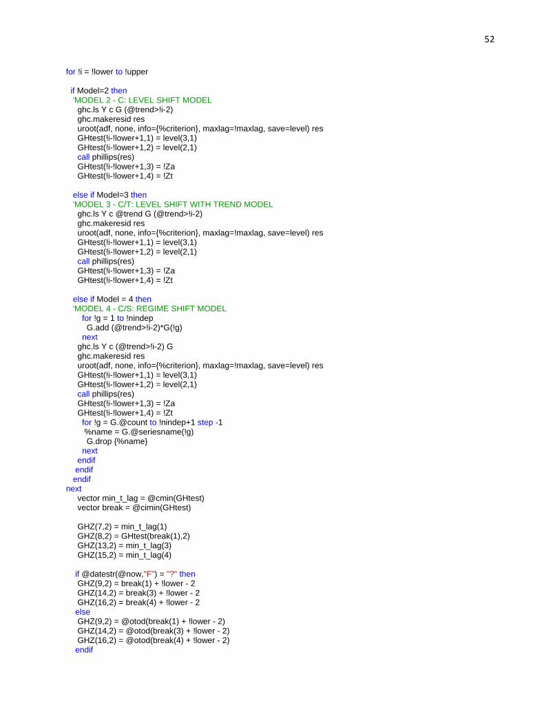
52 for !i = !lower to !upper if Model=2 then 'MODEL 2 - C: LEVEL SHIFT MODEL ghc.ls Y c G (@trend>!i-2) ghc.makeresid res uroot(adf, none, info={%criterion}, maxlag=!maxlag, save=level) res GHtest(!i-!lower+1,1) = level(3,1) GHtest(!i-!lower+1,2) = level(2,1) call phillips(res) GHtest(!i-!lower+1,3) = !Za GHtest(!i-!lower+1,4) = !Zt else if Model=3 then 'MODEL 3 - C/T: LEVEL SHIFT WITH TREND MODEL ghc.ls Y c @trend G (@trend>!i-2) ghc.makeresid res uroot(adf, none, info={%criterion}, maxlag=!maxlag, save=level) res GHtest(!i-!lower+1,1) = level(3,1) GHtest(!i-!lower+1,2) = level(2,1) call phillips(res) GHtest(!i-!lower+1,3) = !Za GHtest(!i-!lower+1,4) = !Zt else if Model = 4 then 'MODEL 4 - C/S: REGIME SHIFT MODEL for !g = 1 to !nindep G.add (@trend>!i-2)*G(!g) next ghc.ls Y c (@trend>!i-2) G ghc.makeresid res uroot(adf, none, info={%criterion}, maxlag=!maxlag, save=level) res GHtest(!i-!lower+1,1) = level(3,1) GHtest(!i-!lower+1,2) = level(2,1) call phillips(res) GHtest(!i-!lower+1,3) = !Za GHtest(!i-!lower+1,4) = !Zt for !g = G.@count to !nindep+1 step -1 %name = G.@seriesname(!g) G.drop {%name} next endif endif endif next vector min_t_lag = @cmin(GHtest) vector break = @cimin(GHtest) GHZ(7,2) = min_t_lag(1) GHZ(8,2) = GHtest(break(1),2) GHZ(13,2) = min_t_lag(3) GHZ(15,2) = min_t_lag(4) if @datestr(@now,"F") = "?" then GHZ(9,2) = break(1) + !lower - 2 GHZ(14,2) = break(3) + !lower - 2 GHZ(16,2) = break(4) + !lower - 2 else GHZ(9,2) = @otod(break(1) + !lower - 2) GHZ(14,2) = @otod(break(3) + !lower - 2) GHZ(16,2) = @otod(break(4) + !lower - 2) endif
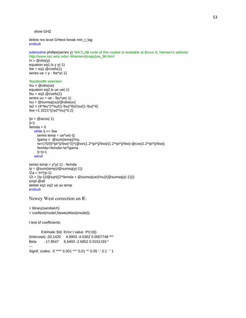
53 show GHZ delete res level GHtest break min_t_lag endsub subroutine phillips(series y) 'MATLAB code of this routine is available at Bruce E. Hansen's website: http://www.ssc.wisc.edu/~bhansen/progs/joe_96.html !n = @obs(y) equation eq1.ls y y(-1) !be = eq1.@coefs(1) series ue = y - !be*y(-1) 'Bandwidth selection !nu = @obs(ue) equation eq2.ls ue ue(-1) !bu = eq2.@coefs(1) series uu = ue - !bu*ue(-1) !su = @sumsq(uu)/@obs(uu) !a2 = (4*!bu^2*!su/(1-!bu)^8)/(!su/(1-!bu)^4) !bw =1.3221*((!a2*!nu)^0.2) !pi = @acos(-1) !j=1 !lemda = 0 while !j <= !bw series temp = ue*ue(-!j) !gama = @sum(temp)/!nu !w=(75/(6*!pi*!j/!bw)^2)*(@sin(1.2*!pi*!j/!bw)/(1.2*!pi*!j/!bw)-@cos(1.2*!pi*!j/!bw)) !lemda=!lemda+!w*!gama !j=!j+1 wend series temp = y*y(-1) - !lemda !p = @sum(temp)/@sumsq(y(-1)) !Za = !n*(!p-1) !Zt = (!p-1)/@sqrt((2*!lemda + @sumsq(ue)/!nu)/(@sumsq(y(-1)))) smpl @all delete eq1 eq2 ue uu temp endsub
Newey West correction on R:
> library(sandwich) > coeftest(model,NeweyWest(model)) t test of coefficients: Estimate Std. Error t value Pr(>|t|) (Intercept) -20.1420 4.9903 -4.0362 0.0007748 *** Beta -17.8547 6.6493 -2.6852 0.0151193 * --- Signif. codes: 0 ‘***’ 0.001 ‘**’ 0.01 ‘*’ 0.05 ‘.’ 0.1 ‘ ’ 1
Related Documents


![Pairs Trading, Convergence Trading, Cointegration - Freedocs.finance.free.fr/DOCS/Yats/cointegration-en[1].pdf · Pairs Trading, Convergence Trading, Cointegration ... ”Trying to](https://static.cupdf.com/doc/110x72/5aad9ad77f8b9a9c2e8e8580/pairs-trading-convergence-trading-cointegration-1pdfpairs-trading-convergence.jpg)