Coin Changing Chapter 4 - Computer Science … · Coin Changing: Cashier's Algorithm ... Cashier's algorithm is optimal for U.S. coinage. ... Discover a simple "structural" bound

1

Chapter 4

GreedyAlgorithms

Slides by Kevin Wayne.Copyright © 2005 Pearson-Addison Wesley.All rights reserved.

Coin Changing

3

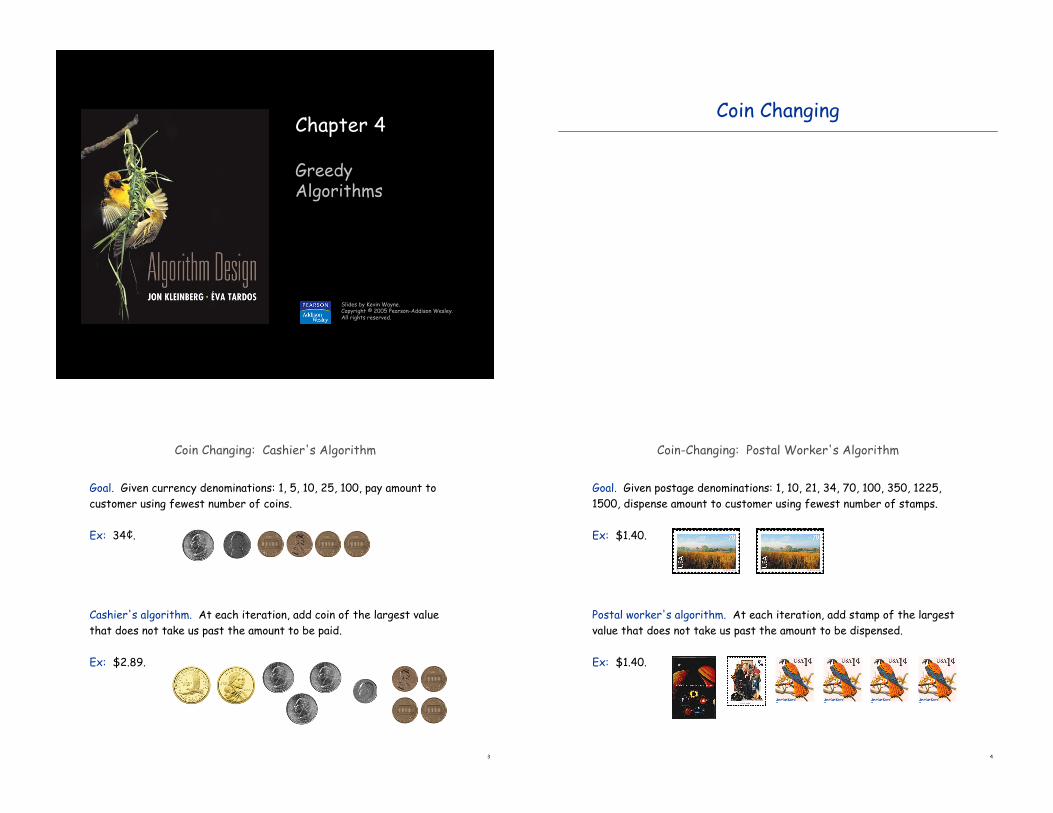
Coin Changing: Cashier's Algorithm

Goal. Given currency denominations: 1, 5, 10, 25, 100, pay amount to

customer using fewest number of coins.

Ex: 34¢.

Cashier's algorithm. At each iteration, add coin of the largest value

that does not take us past the amount to be paid.

Ex: $2.89.

4

Coin-Changing: Postal Worker's Algorithm

Goal. Given postage denominations: 1, 10, 21, 34, 70, 100, 350, 1225,

1500, dispense amount to customer using fewest number of stamps.

Ex: $1.40.

Postal worker's algorithm. At each iteration, add stamp of the largest

value that does not take us past the amount to be dispensed.

Ex: $1.40.

5

Coin-Changing

Observation. Postal worker's algorithm is not optimal for U.S. postage.

Theorem. Cashier's algorithm is optimal for U.S. coinage.

Pf sketch.

(via ad hoc exchange arguments)

P ! 4 P ! 4

N + D ! 2 P + 5N + 10D ! 24

Q ! 3 if amount to change is " $k,optimal solution uses k dollar coin

#P + 5N + 10D + 25Q ! 99

N ! 1 P + 5N ! 9

optimal solution must satisfy

4.1 Interval Scheduling (CLRS 16.1)

7

Interval Scheduling

Interval scheduling.

! Job j starts at sj and finishes at fj.

! Two jobs compatible if they don't overlap.

! Goal: find maximum subset of mutually compatible jobs.

Time0 1 2 3 4 5 6 7 8 9 10 11

f

g

h

e

a

b

c

d

8

Interval Scheduling: Greedy Algorithms

Greedy template. Consider jobs in some natural order.

Take each job provided it's compatible with the ones already taken.

! [Earliest start time] Consider jobs in ascending order of sj.

! [Earliest finish time] Consider jobs in ascending order of fj.

! [Shortest interval] Consider jobs in ascending order of fj - sj.

! [Fewest conflicts] For each job j, count the number of

conflicting jobs cj. Schedule in ascending order of cj.

9

Interval Scheduling: Greedy Algorithms

Greedy template. Consider jobs in some natural order.


counterexample for earliest start time

counterexample for shortest interval

counterexample for fewest conflicts

10

Greedy algorithm. Consider jobs in increasing order of finish time.


Implementation. O(n log n).

! Remember job j* that was added last to A.

! Job j is compatible with A if sj " fj*.

Sort jobs by finish times so that f1 ! f2 ! ... ! fn.

A $ %

for j = 1 to n {

if (job j compatible with A)

A $ A & {j}

}

return A

set of jobs selected

Interval Scheduling: Greedy Algorithm

11

Interval Scheduling: Analysis

Theorem. Greedy algorithm is optimal.

Pf. (by contradiction)

! Assume greedy is not optimal, and let's see what happens.

! Let i1, i2, ... ik denote set of jobs selected by greedy.

! Let j1, j2, ... jm denote set of jobs in the optimal solution with

i1 = j1, i2 = j2, ..., ir = jr for the largest possible value of r.

j1 j2 jr

i1 i2 ir ir+1

. . .

Greedy:

OPT: jr+1

why not replace job jr+1with job ir+1?

job ir+1 finishes before jr+1

12

j1 j2 jr

i1 i2 ir ir+1

Interval Scheduling: Analysis


Pf. (by contradiction)

! Assume greedy is not optimal, and let's see what happens.

! Let i1, i2, ... ik denote set of jobs selected by greedy.

! Let j1, j2, ... jm denote set of jobs in the optimal solution with

i1 = j1, i2 = j2, ..., ir = jr for the largest possible value of r.

. . .

Greedy:

OPT:

solution still feasible and optimal,but contradicts maximality of r.

ir+1

job ir+1 finishes before jr+1

4.1 Interval Partitioning

14

Interval Partitioning

Interval partitioning.

! Lecture j starts at sj and finishes at fj.

! Goal: find min number of classrooms to schedule all lectures

so that no two occur at the same time in the same room.

Ex: This schedule uses 4 classrooms to schedule 10 lectures.

Time9 9:30 10 10:30 11 11:30 12 12:30 1 1:30 2 2:30

h

c

b

a

e

d g

f i

j

3 3:30 4 4:30

1

2

3

4

15

Interval Partitioning

Interval partitioning.

! Lecture j starts at sj and finishes at fj.

! Goal: find min number of classrooms to schedule all lectures

so that no two occur at the same time in the same room.

Ex: This schedule uses only 3.

Time

h

c

a e

f

g i

jd

b

1

2

3

9 9:30 10 10:30 11 11:30 12 12:30 1 1:30 2 2:30 3 3:30 4 4:30

16

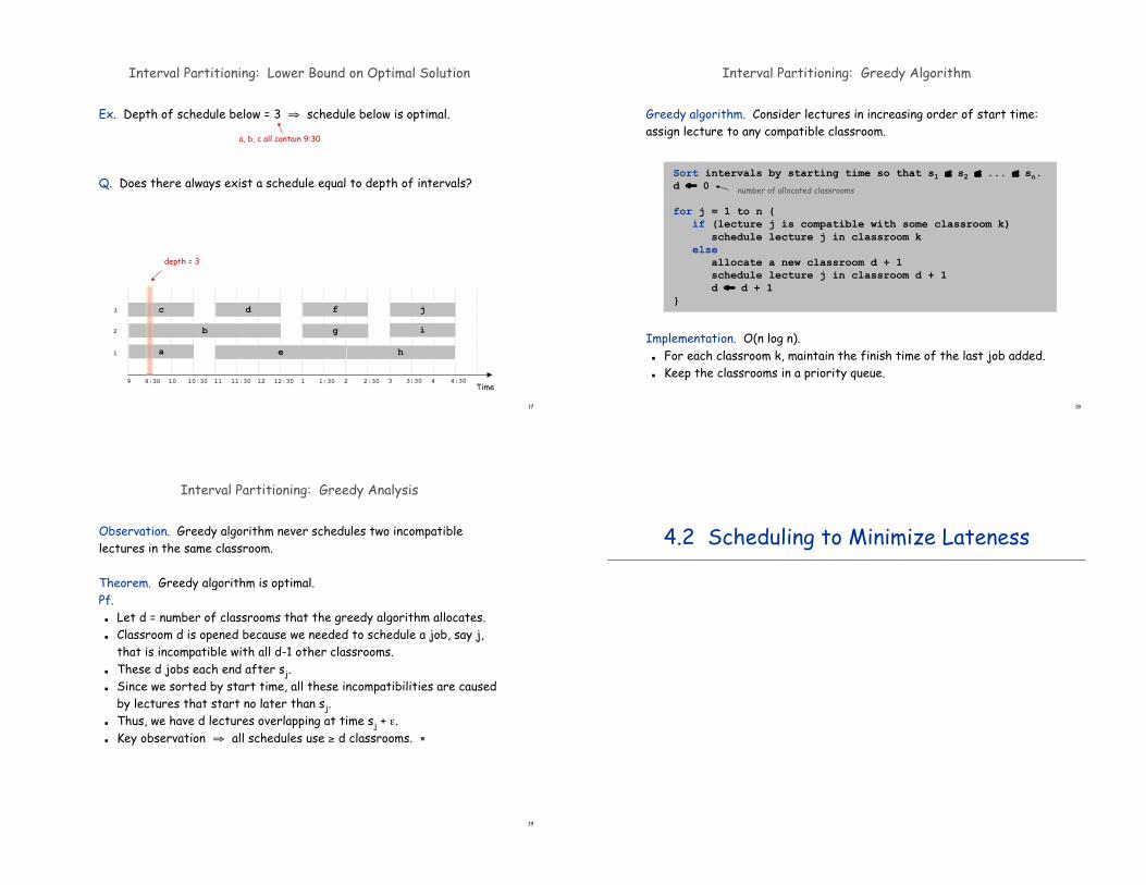
Interval Partitioning: Lower Bound on Optimal Solution

Def. The depth of a set of open intervals is the max number

that contain any given time.

Key observation. Number of classrooms needed " depth.

Time

h

c

a e

f

g i

jd

b

1

2

3

9 9:30 10 10:30 11 11:30 12 12:30 1 1:30 2 2:30 3 3:30 4 4:30

depth = 3

17

Interval Partitioning: Lower Bound on Optimal Solution

Ex. Depth of schedule below = 3 # schedule below is optimal.

Q. Does there always exist a schedule equal to depth of intervals?

Time

h

c

a e

f

g i

jd

b

a, b, c all contain 9:30

1

2

3

9 9:30 10 10:30 11 11:30 12 12:30 1 1:30 2 2:30 3 3:30 4 4:30

depth = 3

18

Interval Partitioning: Greedy Algorithm

Greedy algorithm. Consider lectures in increasing order of start time:

assign lecture to any compatible classroom.

Implementation. O(n log n).

! For each classroom k, maintain the finish time of the last job added.

! Keep the classrooms in a priority queue.

Sort intervals by starting time so that s1 ! s2 ! ... ! sn.

d $ 0

for j = 1 to n {

if (lecture j is compatible with some classroom k)

schedule lecture j in classroom k

else

allocate a new classroom d + 1

schedule lecture j in classroom d + 1

d $ d + 1

}

number of allocated classrooms

19

Interval Partitioning: Greedy Analysis

Observation. Greedy algorithm never schedules two incompatible

lectures in the same classroom.


Pf.

! Let d = number of classrooms that the greedy algorithm allocates.

! Classroom d is opened because we needed to schedule a job, say j,

that is incompatible with all d-1 other classrooms.

! These d jobs each end after sj.

! Since we sorted by start time, all these incompatibilities are caused

by lectures that start no later than sj.

! Thus, we have d lectures overlapping at time sj + '.

! Key observation # all schedules use " d classrooms. !

4.2 Scheduling to Minimize Lateness

21

Scheduling to Minimizing Lateness

Minimizing lateness problem.

! Single resource processes one job at a time.

! Job j requires tj units of processing time and is due at time dj.

! If j starts at time sj, it finishes at time fj = sj + tj.! Lateness: lj = max { 0, fj - dj }.

! Goal: schedule all jobs to minimize maximum lateness L = max lj.

Ex:

0 1 2 3 4 5 6 7 8 9 10 11 12 13 14 15

d5 = 14d2 = 8 d6 = 15 d1 = 6 d4 = 9d3 = 9

l 5 = 2l 1 = 2

dj 6

tj 3

1

8

2

2

9

1

3

9

4

4

14

3

5

15

2

6

max lateness L = l 4 = 6

22

Minimizing Lateness: Greedy Algorithms

Greedy template. Consider jobs in some order.

! [Shortest processing time first] Consider jobs in ascending order

of processing time tj.

! [Earliest deadline first] Consider jobs in ascending order of

deadline dj.

! [Smallest slack] Consider jobs in ascending order of slack dj - tj.

23

Greedy template. Consider jobs in some order.

! [Shortest processing time first] Consider jobs in ascending order

of processing time tj.

! [Smallest slack] Consider jobs in ascending order of slack dj - tj.

counterexample

counterexample

dj

tj

100

1

1

10

10

2

dj

tj

2

1

1

10

10

2

Minimizing Lateness: Greedy Algorithms

24

0 1 2 3 4 5 6 7 8 9 10 11 12 13 14 15

d5 = 14d2 = 8 d6 = 15d1 = 6 d4 = 9d3 = 9

max lateness = 1

Sort n jobs by deadline so that d1 ! d2 ! … ! dn

t $ 0

for j = 1 to n

Assign job j to interval [t, t + tj]

sj $ t, fj $ t + tj t $ t + tjoutput intervals [sj, fj]

Minimizing Lateness: Greedy Algorithm

Greedy algorithm. Earliest deadline first.

25

Minimizing Lateness: No Idle Time

Observation. There exists an optimal schedule with no idle time.

Observation. The greedy schedule has no idle time.

0 1 2 3 4 5 6

d = 4 d = 6

7 8 9 10 11

d = 12

0 1 2 3 4 5 6

d = 4 d = 6

7 8 9 10 11

d = 12

26

Minimizing Lateness: Inversions

Def. Given a schedule S, an inversion is a pair of jobs i and j such that:

i < j but j scheduled before i.

Observation. Greedy schedule has no inversions.

Observation. If a schedule (with no idle time) has an inversion, it has

one with a pair of inverted jobs scheduled consecutively.

ijbefore swap

fi

inversion

27

Minimizing Lateness: Inversions

Def. Given a schedule S, an inversion is a pair of jobs i and j such that:

i < j but j scheduled before i.

Claim. Swapping two consecutive, inverted jobs reduces the number of

inversions by one and does not increase the max lateness.

Pf. Let l be the lateness before the swap, and let l ' be it afterwards.

! l 'k = lk for all k ( i, j

! l 'i ! li! If job j is late:

ij

i j

before swap

after swap

!

" l j = " f j # d j (definition)

= fi # d j ( j finishes at time fi )

$ fi # di (i < j)

$ l i (definition)

f'j

fi

inversion

28

Minimizing Lateness: Analysis of Greedy Algorithm

Theorem. Greedy schedule S is optimal.

Pf. Define S* to be an optimal schedule that has the fewest number of

inversions, and let's see what happens.

! Can assume S* has no idle time.

! If S* has no inversions, then S = S*.

! If S* has an inversion, let i-j be an adjacent inversion.

– swapping i and j does not increase the maximum lateness and

strictly decreases the number of inversions

– this contradicts definition of S* !

29

Greedy Analysis Strategies

Greedy algorithm stays ahead. Show that after each step of the greedy

algorithm, its solution is at least as good as any other algorithm's.

Structural. Discover a simple "structural" bound asserting that every

possible solution must have a certain value. Then show that your

algorithm always achieves this bound.

Exchange argument. Gradually transform any solution to the one found

by the greedy algorithm without hurting its quality.

Other greedy algorithms. Kruskal, Prim, Dijkstra, Huffman, …

30

Chapter 6

Dynamic Programming

Slides by Kevin Wayne.Copyright © 2005 Pearson-Addison Wesley.All rights reserved.

31

Algorithmic Paradigms

Greed. Build up a solution incrementally, myopically optimizing some

local criterion.

Divide-and-conquer. Break up a problem into sub-problems, solve each

sub-problem independently, and combine solution to sub-problems to

form solution to original problem.

Dynamic programming. Break up a problem into a series of overlapping

sub-problems, and build up solutions to larger and larger sub-problems.

32

Dynamic Programming History

Bellman. [1950s] Pioneered the systematic study of dynamic programming.

Etymology.

! Dynamic programming = planning over time.

! Secretary of Defense was hostile to mathematical research.

! Bellman sought an impressive name to avoid confrontation.

Reference: Bellman, R. E. Eye of the Hurricane, An Autobiography.

"it's impossible to use dynamic in a pejorative sense"

"something not even a Congressman could object to"

33

Dynamic Programming Applications

Areas.

! Bioinformatics.

! Control theory.

! Information theory.

! Operations research.

! Computer science: theory, graphics, AI, compilers, systems, ….

Some famous dynamic programming algorithms.

! Unix diff for comparing two files.

! Viterbi for hidden Markov models.

! Smith-Waterman for genetic sequence alignment.

! Bellman-Ford for shortest path routing in networks.

! Cocke-Kasami-Younger for parsing context free grammars.

6.1 Weighted Interval Scheduling

35

Weighted Interval Scheduling

Weighted interval scheduling problem.

! Job j starts at sj, finishes at fj, and has weight or value vj .

! Two jobs compatible if they don't overlap.

! Goal: find maximum weight subset of mutually compatible jobs.

Time

f

g

h

e

a

b

c

d

0 1 2 3 4 5 6 7 8 9 10

36

Unweighted Interval Scheduling Review

Recall. Greedy algorithm works if all weights are 1.

! Consider jobs in ascending order of finish time.

! Add job to subset if it is compatible with previously chosen jobs.

Observation. Greedy algorithm can fail spectacularly if arbitrary

weights are allowed.

Time0 1 2 3 4 5 6 7 8 9 10 11

b

a

weight = 999

weight = 1

37

Weighted Interval Scheduling

Notation. Label jobs by finishing time: f1 ! f2 ! . . . ! fn .

Def. p(j) = largest index i < j such that job i is compatible with j.

Ex: p(8) = 5, p(7) = 3, p(2) = 0.

Time0 1 2 3 4 5 6 7 8 9 10 11

6

7

8

4

3

1

2

5

38

Dynamic Programming: Binary Choice

Notation. OPT(j) = value of optimal solution to the problem consisting

of job requests 1, 2, ..., j.

! Case 1: OPT selects job j.

– collect profit vj

– can't use incompatible jobs { p(j) + 1, p(j) + 2, ..., j - 1 }

– must include optimal solution to problem consisting of remaining

compatible jobs 1, 2, ..., p(j)

! Case 2: OPT does not select job j.

– must include optimal solution to problem consisting of remaining

compatible jobs 1, 2, ..., j-1

!

OPT( j) =0 if j = 0

max v j + OPT( p( j)), OPT( j "1){ } otherwise

# $ %

optimal substructure

39

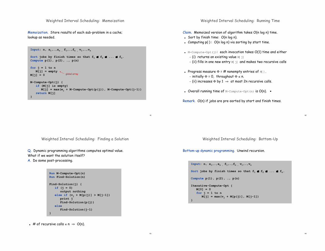
Input: n, s1,…,sn , f1,…,fn , v1,…,vn


Compute p(1), p(2), …, p(n)

Compute-Opt(j) {

if (j = 0)

return 0

else

return max(vj + Compute-Opt(p(j)), Compute-Opt(j-1))

}

Weighted Interval Scheduling: Brute Force

Brute force algorithm.

40

Weighted Interval Scheduling: Brute Force

Observation. Recursive algorithm fails spectacularly because of

redundant sub-problems # exponential algorithms.

Ex. Number of recursive calls for family of "layered" instances grows

like Fibonacci sequence.

3

4

5

1

2

p(1) = 0, p(j) = j-2

5

4 3

3 2 2 1

2 1

1 0

1 0 1 0

41




for j = 1 to n

M[j] = empty

M[j] = 0

M-Compute-Opt(j) {

if (M[j] is empty)

M[j] = max(wj + M-Compute-Opt(p(j)), M-Compute-Opt(j-1))

return M[j]

}

global array

Weighted Interval Scheduling: Memoization

Memoization. Store results of each sub-problem in a cache;

lookup as needed.

42

Weighted Interval Scheduling: Running Time

Claim. Memoized version of algorithm takes O(n log n) time.

! Sort by finish time: O(n log n).

! Computing p()) : O(n log n) via sorting by start time.

! M-Compute-Opt(j): each invocation takes O(1) time and either

– (i) returns an existing value M[j]

– (ii) fills in one new entry M[j] and makes two recursive calls

! Progress measure * = # nonempty entries of M[].

– initially * = 0, throughout * ! n.

– (ii) increases * by 1 # at most 2n recursive calls.

! Overall running time of M-Compute-Opt(n) is O(n). !

Remark. O(n) if jobs are pre-sorted by start and finish times.

43

Weighted Interval Scheduling: Finding a Solution

Q. Dynamic programming algorithms computes optimal value.

What if we want the solution itself?

A. Do some post-processing.

! # of recursive calls ! n # O(n).

Run M-Compute-Opt(n)

Run Find-Solution(n)

Find-Solution(j) {

if (j = 0)

output nothing

else if (vj + M[p(j)] > M[j-1])

print j

Find-Solution(p(j))

else

Find-Solution(j-1)

}

44

Weighted Interval Scheduling: Bottom-Up

Bottom-up dynamic programming. Unwind recursion.




Iterative-Compute-Opt {

M[0] = 0

for j = 1 to n

M[j] = max(vj + M[p(j)], M[j-1])

}

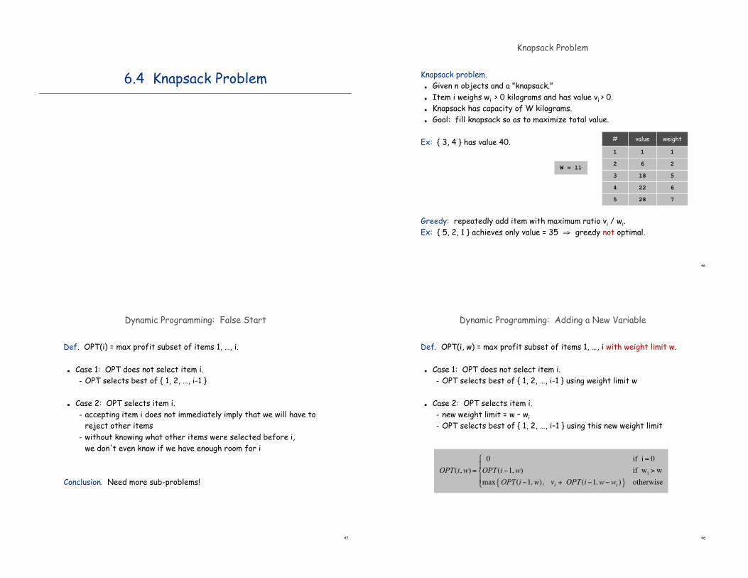
6.4 Knapsack Problem

46

Knapsack Problem

Knapsack problem.

! Given n objects and a "knapsack."

! Item i weighs wi > 0 kilograms and has value vi > 0.

! Knapsack has capacity of W kilograms.

! Goal: fill knapsack so as to maximize total value.

Ex: { 3, 4 } has value 40.

Greedy: repeatedly add item with maximum ratio vi / wi.

Ex: { 5, 2, 1 } achieves only value = 35 # greedy not optimal.

1

value

18

22

28

1

weight

5

6

6 2

7

#

1

3

4

5

2W = 11

47

Dynamic Programming: False Start

Def. OPT(i) = max profit subset of items 1, …, i.

! Case 1: OPT does not select item i.

– OPT selects best of { 1, 2, …, i-1 }

! Case 2: OPT selects item i.

– accepting item i does not immediately imply that we will have to

reject other items

– without knowing what other items were selected before i,

we don't even know if we have enough room for i

Conclusion. Need more sub-problems!

48

Dynamic Programming: Adding a New Variable

Def. OPT(i, w) = max profit subset of items 1, …, i with weight limit w.

! Case 1: OPT does not select item i.

– OPT selects best of { 1, 2, …, i-1 } using weight limit w

! Case 2: OPT selects item i.

– new weight limit = w – wi

– OPT selects best of { 1, 2, …, i–1 } using this new weight limit

!

OPT(i, w) =

0 if i = 0

OPT(i "1, w) if wi > w

max OPT(i "1, w), vi+ OPT(i "1, w"w

i){ } otherwise

#

$ %

& %

49

Input: n, w1,…,wN, v1,…,vN

for w = 0 to W

M[0, w] = 0

for i = 1 to n

for w = 1 to W

if (wi > w)

M[i, w] = M[i-1, w]

else

M[i, w] = max {M[i-1, w], vi + M[i-1, w-wi ]}

return M[n, W]

Knapsack Problem: Bottom-Up

Knapsack. Fill up an n-by-W array.

50

Knapsack Algorithm

n + 1

1

value

18

22

28

1

weight

5

6

6 2

7

#

1

3

4

5

2

+

{ 1, 2 }

{ 1, 2, 3 }

{ 1, 2, 3, 4 }

{ 1 }

{ 1, 2, 3, 4, 5 }

0

0

0

0

0

0

0

1

0

1

1

1

1

1

2

0

6

6

6

1

6

3

0

7

7

7

1

7

4

0

7

7

7

1

7

5

0

7

18

18

1

18

6

0

7

19

22

1

22

7

0

7

24

24

1

28

8

0

7

25

28

1

29

9

0

7

25

29

1

34

10

0

7

25

29

1

34

11

0

7

25

40

1

40

W + 1

W = 11

OPT: { 4, 3 }value = 22 + 18 = 40

51

Knapsack Problem: Running Time

Running time. ,(n W).

! Not poly-time in input size!

! "Pseudo-polynomial."

! Decision version of knapsack problem is NP-complete.

Knapsack approximation algorithm. There exists a poly-time algorithm

that produces a feasible solution that has value within 0.01% of optimum.

6.6 Sequence Alignment

53

String Similarity

How similar are two strings?! ocurrance

! occurrence

o c u r r a n c e

c c u r r e n c eo

-

o c u r r n c e

c c u r r n c eo

- - a

e -

o c u r r a n c e

c c u r r e n c eo

-

6 mismatches, 1 gap

1 mismatch, 1 gap

0 mismatches, 3 gaps

54

Applications.

! Basis for Unix diff.

! Speech recognition.

! Computational biology.

Edit distance. [Levenshtein 1966, Needleman-Wunsch 1970]

! Gap penalty -; mismatch penalty .pq.

! Cost = sum of gap and mismatch penalties.

2- + .CA

C G A C C T A C C T

C T G A C T A C A T

T G A C C T A C C T

C T G A C T A C A T

-T

C

C

C

.TC + .GT + .AG+ 2.CA

-

Edit Distance

55

Goal: Given two strings X = x1 x2 . . . xm and Y = y1 y2 . . . yn find

alignment of minimum cost.

Def. An alignment M is a set of ordered pairs xi-yj such that each item

occurs in at most one pair and no crossings.

Def. The pair xi-yj and xi'-yj' cross if i < i', but j > j'.

Ex: CTACCG vs. TACATG.

Sol: M = x2-y1, x3-y2, x4-y3, x5-y4, x6-y6.

Sequence Alignment

!

cost(M ) = " xi y j(xi , y j ) # M

$

mismatch

1 2 4 4 3 4 4

+ %i : xi unmatched

$ + %j : y j unmatched

$

gap

1 2 4 4 4 4 4 3 4 4 4 4 4

C T A C C -

T A C A T-

G

G

y1 y2 y3 y4 y5 y6

x2 x3 x4 x5x1 x6

56

Sequence Alignment: Problem Structure

Def. OPT(i, j) = min cost of aligning strings x1 x2 . . . xi and y1 y2 . . . yj.

! Case 1: OPT matches xi-yj.

– pay mismatch for xi-yj + min cost of aligning two strings

x1 x2 . . . xi-1 and y1 y2 . . . yj-1

! Case 2a: OPT leaves xi unmatched.

– pay gap for xi and min cost of aligning x1 x2 . . . xi-1 and y1 y2 . . . yj

! Case 2b: OPT leaves yj unmatched.

– pay gap for yj and min cost of aligning x1 x2 . . . xi and y1 y2 . . . yj-1

!

OPT (i, j) =

"

#

$ $ $

%

$ $ $

j& if i = 0

min

' xi y j+OPT (i(1, j (1)

& +OPT (i(1, j)

& +OPT (i, j (1)

"

# $

% $

otherwise

i& if j = 0

57

Sequence Alignment: Algorithm

Analysis. ,(mn) time and space.

English words or sentences: m, n ! 10.

Computational biology: m = n = 100,000. 10 billions ops OK, but 10GB array?

Sequence-Alignment(m, n, x1x2...xm, y1y2...yn, -, .) {

for i = 0 to m

M[0, i] = i-

for j = 0 to n

M[j, 0] = j-

for i = 1 to m

for j = 1 to n

M[i, j] = min(.[xi, yj] + M[i-1, j-1],

- + M[i-1, j],

- + M[i, j-1])

return M[m, n]

}

Coin Changing Chapter 4 - Computer Science … · Coin Changing: Cashier's Algorithm ... Cashier's algorithm is optimal for U.S. coinage. ... Discover a simple "structural" bound

Documents