COIL CONDENSATION DETECTION FOR HUMIDITY ...

COIL CONDENSATION DETECTION FOR HUMIDITY CONTROL

A Thesis

by

CHARLES PECKITT KANEB

Submitted to the Office of Graduate and Professional Studies of Texas A&M University

in partial fulfillment of the requirements for the degree of

MASTER OF SCIENCE

Chair of Committee, Charles Culp Members of Committee, David Claridge

Bryan Rasmussen Head of Department, Andreas Polycarpou

May 2014

Major Subject: Mechanical Engineering

Copyright 2014

ii

ABSTRACT

Conditioning the air inside a building requires controlling both primary

components of its enthalpy: temperature and humidity. Temperature sensors used in

buildings are sufficiently reliable, durable, accurate, and precise that they can be relied

on for sophisticated building control systems. Commercial resistive and capacitive

humidity sensors become inaccurate near saturation and often fail permanently when

exposed to liquid water. Excessive humidity can cause both occupant discomfort and

permanent damage to buildings. In American climates dehumidification accounts for the

vast majority of the energy used to control humidity. Therefore, a sensor which can

survive and accurately measure humidity in hot, wet conditions will allow considerable

savings.

Simulations of the energy consumption and savings available from enthalpy

economizer control and supply air temperature resets were performed for buildings in

Houston, Dallas, and Philadelphia. Temperature economizers were shown to attain

between 90% and 95% of the savings of an enthalpy economizer. A spreadsheet

simulation of enthalpy economizer use showed that the savings available are heavily

dependent on the ability to avoid its use on very hot, humid days.

A newly-designed condensation sensor was developed for this project. It relies

on the order-of-magnitude difference in AC reactance between humid air and liquid

water. When installed on an AHU, it detects water condensing off the cooling coil as the

temperature of the air drops below the dew point. Electronics were designed to provide

the 0.25 V, 131 kHz current required and to obtain a 0 V output when dry and a 5 V

output when wet.

iii

A field reliability test was successfully performed with the sensor passively

monitoring the transitions from wet to dry at Langford Building A and the Jack E. Brown

Building at Texas A&M University, College Station, TX. The sensor was shown to be

able to provide the reliable state change detection needed to control an economizer.

The main limitation of this sensor is slow response on dry-to-wet and wet-to-dry

transitions. Most measured dry-to-wet response times were between 5 and 10 minutes,

which were driven by the time required to saturate the cooling coil.

iv

DEDICATION

To my uncle, Guy Peckitt, for encouraging my interest in scientific and technical

matters, and helping me explore them for the past twenty years.

v

ACKNOWLEDGEMENTS

This project was made possible by the support of the Energy Systems

Laboratory at Texas A&M University. Thanks go to Dr. Charles Culp for advising me

and supporting me as I navigated past its problems and pitfalls. Kevin Christman, Jim

Watt, Joseph Martinez, and Dr. Lei Wang contributed to my knowledge of building

science and asked questions that helped drive development.

Steve Payne and Erwin Thomas of the Texas A&M Physics Electronics Shop

helped me work out electronics and instrumentation problems; without the Physics

Electronics Shop it would be virtually impossible to develop electronics in College

Station. Layne Wylie generously gave me access to the Mechanical Engineering

Student Machine Shop’s equipment. Mathew Wiederstein and Michael Martine provided

invaluable help with measurements and building access.

vi

TABLE OF CONTENTS

Page

1. INTRODUCTION ....................................................................................................... 1

2. LITERATURE REVIEW ............................................................................................. 4

2.1 Psychrometrics, Humidity, Humidity Control (Sections 1, 3, and 4) ...................... 5 2.2 Economizers and Outside Air Control (Section 3) ................................................ 7 2.3 Present Commercial Humidity Sensors (Section 4) .............................................. 9 2.4 Properties of Water, Electrochemistry of Materials (Sections 5 and 6) ............... 14 2.5 Analog Electronics and Test Equipment (Sections 7 and 8) ............................... 16 2.6 Literature Summary ........................................................................................... 17

3. ECONOMIZERS ...................................................................................................... 19

3.1 Spreadsheet Simulations ................................................................................... 21 3.2 Economizer Index .............................................................................................. 32 3.3 WinAM Simulations ............................................................................................ 35

4. COMMERCIAL HUMIDITY SENSOR TESTS .......................................................... 42

5. INITIAL TESTING AND DEVELOPMENT ................................................................ 49

5.1 Response To State Changes ............................................................................. 51 5.2 Clip-On Sensor and Testing ............................................................................... 54

6. SENSOR DESIGN ................................................................................................... 60

6.1 Electrical and Chemical Design .......................................................................... 63 6.1.1 Corrosion Avoidance ................................................................................... 63 6.1.2 Condensate Quantity Calculation ................................................................ 66

6.2 Resistance Calculations ..................................................................................... 69 6.3 Mechanical and Assembly Design ...................................................................... 75 6.4 Sensor Manufacturing ........................................................................................ 80 6.5 Bench Testing .................................................................................................... 82

7. ELECTRONICS ....................................................................................................... 84

7.1 1 kHz Circuits ..................................................................................................... 88 7.2 131 kHz Circuits ................................................................................................. 92

8. RESULTS .............................................................................................................. 105

vii

8.1 Operational Testing .......................................................................................... 105 8.2 Timed Testing .................................................................................................. 110 8.3 Run-to-Run Differences In Dew Point and Coil Water Capacity Calculations ... 117

8.3.1 Difference Between Measured Dew Point and True Dew Point ................. 117 8.3.2 Run-to-Run Differences In Coil Water Capacity ......................................... 120

8.4 GE Telaire Vaporstat 9002 Testing .................................................................. 123 8.5 Durability Testing ............................................................................................. 126 8.6 Applications ..................................................................................................... 128

8.6.1 Confirmation of Weather Station Dew Point .............................................. 128 8.6.2 Economizer Control – High Limit At SAT ................................................... 130

9. CONCLUSIONS .................................................................................................... 131

REFERENCES .......................................................................................................... 134

viii

LIST OF FIGURES

Page

Figure (1.1) Psychrometric Chart Shows Benefits of Enthalpy Sensors ......................... 2

Figure (2.1) Water Runoff On Tilted Plate (Redrawn from Rame-Hart [44]) ................. 15

Figure (3.1) AHU with Economizer Active (Redrawn from Lee et al. [50]) .................... 19

Figure (3.2) AHU Drawing With Economizer Inactive (Redrawn from Lee et al. [50]) ... 20

Figure (3.3) Enthalpy Versus Temperature and Dew Point .......................................... 22

Figure (3.4) Economizer Savings and Losses versus Temperature and Dew Point ..... 24

Figure (3.5) Economizer Savings or Losses versus Temperature and Dew Point: Concentrated Region ............................................................................... 24

Figure (3.6) Houston Annual Occurrence For Dry Bulb and Dew Point Bins Using TMY Hourly Data ..................................................................................... 26

Figure (3.7) Houston Bin Results ................................................................................. 28

Figure (3.8) Dallas Bin Results .................................................................................... 30

Figure (3.9) Philadelphia Bin Results ........................................................................... 31

Figure (3.10) Economizer With High-Limit Cutoffs At 78°F Dry Bulb and 58°F Dew Point, Philadelphia ................................................................................... 33

Figure (3.11) Overall Savings From Enthalpy Economizers ......................................... 37

Figure (3.12) Houston Enthalpy Economizer Savings Beyond Temperature Economizer (Bin Method) ........................................................................ 38

Figure (3.13) Dallas Enthalpy Economizer Savings Beyond Temperature Economizer 39

Figure (3.14) Philadelphia Enthalpy Economizer Savings Beyond Temperature Economizer ............................................................................................. 40

ix

Figure (4.1) HIH-5030 and HS1101LF Test Results ..................................................... 45

Figure (4.2) TDK CHS-MSS Resistive Humidity Sensor With Built-In Electronics To Deliver Voltage Output (Digikey Image)....................................................46

Figure (4.3) TDK CHS-CSC-20 Capacitive Humidity Sensor With Built-In Electronics To Deliver Voltage Output (Digikey Image) .............................................. 46

Figure (4.4) Parallax HS1101 Capacitive Humidity Sensor .......................................... 47

Figure (4.5) Measurement Specialties HS1101LF Capacitive Humidity Sensor ........... 47

Figure (4.6) Honeywell HIH-5030 Capacitive Humidity Sensor With Built-In Electronics to Deliver Voltage Output (Allied Electronics Image) ............. 48

Figure (5.1) Test Tube Test “Sensor” ........................................................................... 50

Figure (5.2) Control Sequence For Dew Point Measurement ....................................... 52

Figure (5.3) Drawing of Clip-On Sensor ....................................................................... 54

Figure (5.4) Clip-On Sensor ......................................................................................... 55

Figure (6.1) Angle Necessary For Runoff (Redrawn from Rame-Hart [45]) .................. 66

Figure (6.2) Sensor Clamped to Drip Rail .................................................................... 68

Figure (6.3) Drawing of Plates and Gaps ..................................................................... 70

Figure (6.4) Uniform Resistivity and Cross Section. ..................................................... 72

Figure (6.5) Horizontal Slice......................................................................................... 72

Figure (6.6) Stainless Steel Sheet Electrodes .............................................................. 74

Figure (6.7) Free Body Diagram of Sensor Electrode .................................................. 76

Figure (6.8) Free Body Diagram of Sensor Cap ........................................................... 77

Figure (6.9) FBD of Screw Engagement in Sensor Body ............................................. 78

Figure (6.10) Sensor Assembly Cross-Section Showing Plate Attachment .................. 79

Figure (6.11) Sensor Installed on Coil .......................................................................... 81

x

Figure (7.1) Components of Impedance ....................................................................... 85

Figure (7.2) Drawing of Square Wave Circuit ............................................................... 87

Figure (7.3) Square Wave Outputs .............................................................................. 88

Figure (7.4) Dual Schmitt Trigger Oscillator ................................................................. 89

Figure (7.5) PhiTech Multiple Sensor Prototype ........................................................... 90

Figure (7.6) Version 12 Circuit ..................................................................................... 91

Figure (7.7) Sensor Circuit (Version 18) Schematic ..................................................... 93

Figure (7.8) Resistor Network Between Oscillator and Ground .................................... 96

Figure (7.9) Output from First Order Low Pass Filter ................................................... 97

Figure (7.10) Noninverting Amplifier ............................................................................. 98

Figure (7.11) Schematic of V18 Circuit ...................................................................... 100

Figure (7.12) PCB Layout of 131kHz Circuit .............................................................. 101

Figure (7.13) Output Provided to Sensor (V2 in Figure 7.11) and Oscillator Output (V1 in Figure 7.11) ................................................................................. 102

Figure (7.14) Dry Output from Sensor Circuit ............................................................. 103

Figure (7.15) Wet Output from Sensor Circuit ............................................................ 104

Figure (8.1) Photo of Sensor and Stand ..................................................................... 106

Figure (8.2) Inverted Functional Test – 0 V Output When Wet ................................... 107

Figure (8.3) Normal Functional Test – 0 V Output When Dry ..................................... 108

Figure (8.4) Sensor After Test .................................................................................... 109

Figure (8.5) Langford A Test Shows Slow Response ................................................. 111

Figure (8.6) Humidity Ratio and Latent Enthalpy vs Dew Point .................................. 118

xi

Figure (8.7) Time versus Temperature Difference ...................................................... 120

Figure (8.8) Dew Point Difference Versus Coil Transition Time .................................. 123

Figure (8.9) Jack E. Brown Test – Poor Location for Mixed Air Testing ...................... 124

Figure (8.10) GE Telaire Vaporstat 9002 Test ........................................................... 125

Figure (8.11) Voltage Output From Sensor During Two Months In AHU .................... 126

Figure (8.12) Sensor With Magnet and Stand After Test ............................................ 127

Figure (8.13) Flowchart of OA Weather Station Dew Point Confirmation ................... 129

Figure (8.14) Economizer Savings Using Coil Enthalpy Sensor as Dew Point High Limit.........................................................................................................130

xii

LIST OF TABLES

Page Table (3.1) Table of Results From Economizer Simulation .......................................... 34

Table (3.2) Test Building Parameters for WinAM Model ............................................... 36

Table (4.1) Results of Commercial Humidity Sensor Test ............................................ 44

Table (5.1) LCR Meter Results .................................................................................... 57

Table (6.1) Properties of Air and Water ........................................................................ 61

Table (6.2) Resistivity of Materials ............................................................................... 69

Table (6.3) Variables in Resistance Calculations ......................................................... 71

Table (6.4) Results From Tenma LCR Meter, Unvarnished Sensor ............................. 82

Table (6.5) Results from Tenma LCR Meter, Varnished Sensor, Tap Water ................ 82

Table (6.6) Results from Tenma LCR Meter, Varnished Sensor, RO Water ................. 83

Table (7.1) Sensor Characteristics ............................................................................... 84

Table (7.2) Impedance of Coil Enthalpy Sensor (Sensor Only) .................................... 95

Table (8.1) Summary of Timed Dry-to-Wet Tests ....................................................... 116

Table (8.2) Individual Dry-to-Wet Run Results ........................................................... 121

xiii

NOMENCLATURE

Variable Definition

TOA Dry bulb temperature of the outside air, °F

TRA Dry bulb temperature of the return air, °F

TMA Dry bulb temperature of the mixed air, °F

TSA Dry bulb temperature of the supply air, °F

hOA Total enthalpy of the outside air, 𝐵𝑡𝑢𝑙𝑏

hRA Total enthalpy of the return air, 𝐵𝑡𝑢𝑙𝑏

hMA Total enthalpy of the mixed air, 𝐵𝑡𝑢𝑙𝑏

has Total enthalpy of the supply air, 𝐵𝑡𝑢𝑙𝑏

DPOA Dew point temperature of the outside air, °F

DPRA Dew point temperature of the return air, °F

DPMA Dew point temperature of the mixed air, °F

DPSA Dew point temperature of the supply air, °F

Sensible Sensible heat flow provided by the AHU’s cooling or heating

coil to the mixed air, 𝐵𝑡𝑢𝑚𝑖𝑛

Latent Latent heat flow provided by the AHU’s cooling or heating

coil to the mixed air, 𝐵𝑡𝑢𝑚𝑖𝑛

Supply air volumetric flow rate, 𝑓𝑡3

𝑚𝑖𝑛

ρair Density of supply air, 𝑙𝑏𝑓𝑡3

xiv

(Maximum of [ΔT, 0]) Temperature difference across the cooling coil used to

calculate energy consumption for sensible cooling

(Maximum of [Δw, 0]) Humidity ratio difference across the cooling coil used to

calculate energy consumption for latent cooling

xOA Mass fraction of outside air in the mixed air

wOA Outside air humidity ratio, 𝑙𝑏𝑠 𝑤𝑎𝑡𝑒𝑟𝑙𝑏𝑠 𝑑𝑟𝑦 𝑎𝑖𝑟

wRA Return air humidity ratio, 𝑙𝑏𝑠 𝑤𝑎𝑡𝑒𝑟𝑙𝑏𝑠 𝑑𝑟𝑦 𝑎𝑖𝑟

wSA Supply air humidity ratio, 𝑙𝑏𝑠 𝑤𝑎𝑡𝑒𝑟𝑙𝑏𝑠 𝑑𝑟𝑦 𝑎𝑖𝑟

𝐴𝐼𝑅 Mass flow rate of supply air to a space, 𝑙𝑏𝑠𝑚𝑖𝑛∗𝑓𝑡2

Δh Difference in enthalpy between using 100% outside air and

mixed air using the minimum outside air fraction, 𝐵𝑡𝑢𝑙𝑏

Δcost Difference in cost between using 100% outside air and

mixed air using the minimum outside air fraction, $1000 𝑓𝑡2∗𝑦𝑒𝑎𝑟

ηecon 𝐴𝑛𝑛𝑢𝑎𝑙 𝑒𝑛𝑒𝑟𝑔𝑦 𝑠𝑎𝑣𝑖𝑛𝑔𝑠 𝑜𝑓 𝑎𝑛 𝑒𝑐𝑜𝑛𝑜𝑚𝑖𝑧𝑒𝑟

𝑤𝑖𝑡ℎ 𝑠𝑝𝑒𝑐𝑖𝑓𝑖𝑒𝑑 ℎ𝑖𝑔ℎ 𝑙𝑖𝑚𝑖𝑡𝑠, 𝐵𝑡𝑢𝐴𝑛𝑛𝑢𝑎𝑙 𝑒𝑛𝑒𝑟𝑔𝑦 𝑠𝑎𝑣𝑖𝑛𝑔𝑠 𝑜𝑓 𝑎

𝑝𝑠𝑦𝑐ℎ𝑟𝑜𝑚𝑒𝑡𝑟𝑖𝑐𝑎𝑙𝑙𝑦 𝑖𝑑𝑒𝑎𝑙 𝑒𝑐𝑜𝑛𝑜𝑚𝑖𝑧𝑒𝑟, 𝐵𝑡𝑢

tcheck Time required to determine whether the cooling coil is wet or

dry at a given supply air temperature, minutes

τcoil Time constant of the coil with regards to changes in

temperature when the CHWV setting is changed, minutes

Tsensor Time required for the sensor to change state once the

cooling coil leaving temperature has decreased below the

dew point, minutes

xv

Tmeasurement Time required to measure a mixed-air dew point temperature

by stepped reductions in cooling coil leaving temperature,

minutes

Roperating Ratio of the time spent with the AHU operating normally to

the time spent at alternate supply temperatures while

measuring dew points

ZR Resistive component of the total sensor impedance, Ω

ZC Capacitive component of the total sensor impedance, Ω

ZL Inductive component of the total sensor impedance, Ω

Zsensor Total impedance of the sensor, Ω

F Oscillation frequency of the relaxation oscillator in Section

7.1, hz

Vout Output voltage from a stage of a circuit, V

Vin Input voltage to a stage of a circuit, V

P Power dissipated by the voltage divider, W

DPOA, DPRA,

DPMA, DPSA Dew point temperatures of outside air, return air, mixed air,

and supply air, °F

MA Volumetric flow rate of mixed air, 𝑓𝑡3 𝑚𝑖𝑛⁄

MA Mass flow rate of mixed air, 𝑙𝑏𝑠 𝑚𝑖𝑛⁄

𝑉 Component of air velocity perpendicular to coil, 𝑓𝑡 𝑚𝑖𝑛⁄

w,MA Mass flow rate of water contained in the mixed air, 𝑙𝑏 𝑚𝑖𝑛⁄

w,SA Mass flow rate of water contained in the supply air, 𝑙𝑏 𝑚𝑖𝑛⁄

removed Mass flow rate of water removed from the mixed air by the

cooling coil, 𝑙𝑏 𝑚𝑖𝑛⁄

xvi

w,actual Measured mass flow rate of water removed from the mixed

air by the cooling coil, 𝑙𝑏 𝑚𝑖𝑛⁄

mtrapped Mass of water trapped in the boundary layer near the fins of

the cooling coil, lbs

ρtrapped Ratio of mtrapped to the total internal volume of the coil, 𝑙𝑏𝑠𝑓𝑡3

PSAT Saturation vapor pressure of water in air at a given

temperature, kPa

TCCL Cooling coil leaving temperature at any given time, °F

Tinitial Original cooling coil leaving temperature before a change in

CHWV position, °F

Tfinal Final cooling coil leaving temperature, °F

Mean of the measured coil water capacities, lbs

Sx Sample deviation of the measured coil water capacities, lbs

ta/2, ν T-statistic for a given confidence level a and number of

degrees of freedom ν that the sample mean of the coil water

capacities is within the interval given for its value

1

1. INTRODUCTION

Cooling and space heating of American commercial buildings consumed 650

TBtu of electrical energy in 2003, according to the U.S. Energy Information

Administration [1]. This accounted for 19% of the 3.5 quadrillion Btu total electricity

consumption of commercial buildings, at a cost of approximately $10 billion. Controlling

indoor humidity and temperature requires this energy expenditure for occupant comfort

and building protection.

Humidity and temperature are usually controlled in commercial buildings by the

heating and cooling coils in air-handling units (AHUs). Dehumidification is traditionally

provided by cooling the mixed air to 55°F, which is the dew point traditionally needed to

make the indoor air comfortable. Overcooling can result if the space loads are less than

the cooling capacity of the air discharged into the space. When this occurs, reheating

the air is often done to offset overcooling. Energy will then be consumed to reheat the

air to maintain a comfortable space temperature.

In hot and humid climates, humidity control makes up a significant portion of

building energy consumption. According to TIAX [2], sensible heat ratios vary from 0.5

to 0.8 depending on weather conditions, meaning 20% to 50% of the total cooling

energy is used for dehumidification. An Energy Management and Control System

(EMCS) is normally used to control the HVAC systems. For the EMCS to be able to

control the humidity in the spaces supplied by the AHU, it must have reliable data about

the mixed air humidity, or adopt a control strategy that ensures that the design latent

2

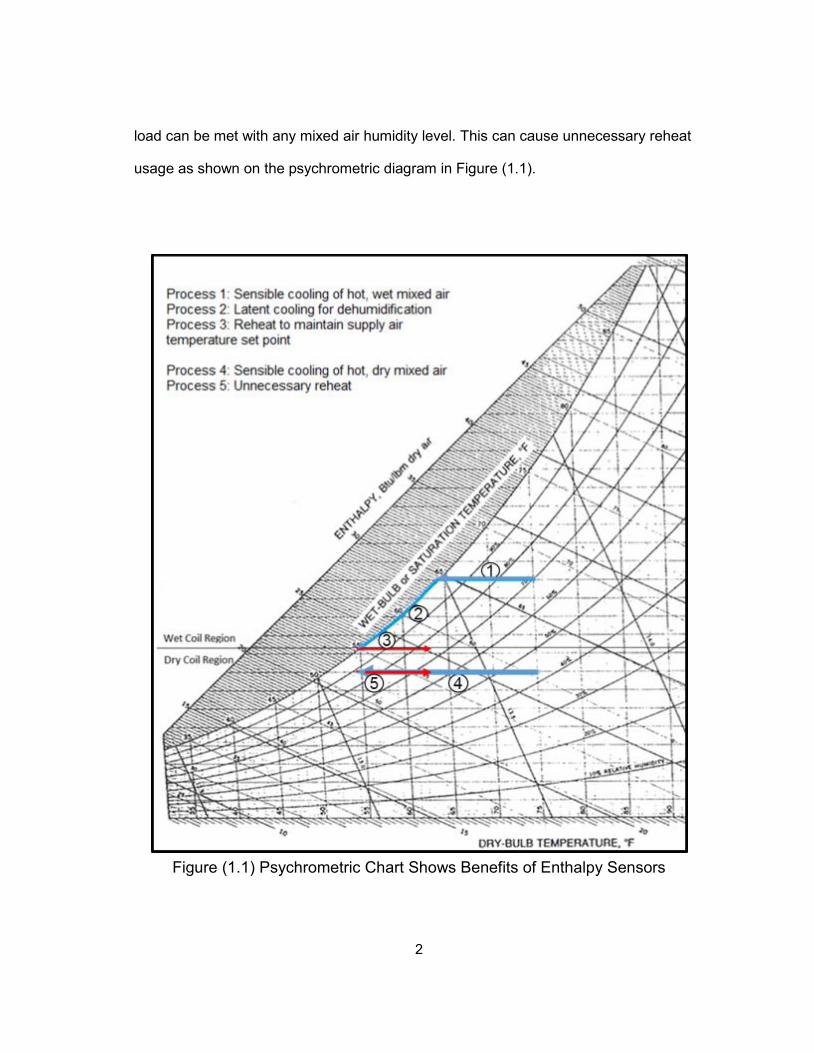
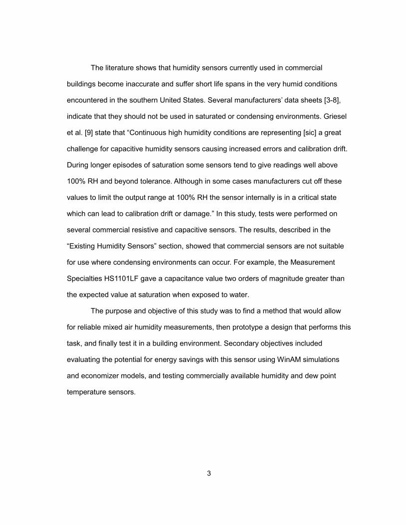
load can be met with any mixed air humidity level. This can cause unnecessary reheat

usage as shown on the psychrometric diagram in Figure (1.1).

Figure (1.1) Psychrometric Chart Shows Benefits of Enthalpy Sensors

3

The literature shows that humidity sensors currently used in commercial

buildings become inaccurate and suffer short life spans in the very humid conditions

encountered in the southern United States. Several manufacturers’ data sheets [3-8],

indicate that they should not be used in saturated or condensing environments. Griesel

et al. [9] state that “Continuous high humidity conditions are representing [sic] a great

challenge for capacitive humidity sensors causing increased errors and calibration drift.

During longer episodes of saturation some sensors tend to give readings well above

100% RH and beyond tolerance. Although in some cases manufacturers cut off these

values to limit the output range at 100% RH the sensor internally is in a critical state

which can lead to calibration drift or damage.” In this study, tests were performed on

several commercial resistive and capacitive sensors. The results, described in the

“Existing Humidity Sensors” section, showed that commercial sensors are not suitable

for use where condensing environments can occur. For example, the Measurement

Specialties HS1101LF gave a capacitance value two orders of magnitude greater than

the expected value at saturation when exposed to water.

The purpose and objective of this study was to find a method that would allow

for reliable mixed air humidity measurements, then prototype a design that performs this

task, and finally test it in a building environment. Secondary objectives included

evaluating the potential for energy savings with this sensor using WinAM simulations

and economizer models, and testing commercially available humidity and dew point

temperature sensors.

4

2. LITERATURE REVIEW

The literature review for this thesis was comprised of sections on psychrometrics

and humidity control, economizers and outside air control, present commercial humidity

sensors, electrochemical and physical properties of water, and analog electronics. The

first three sections established the state of equipment used in buildings for humidity and

air control, while the last two aided the design of the new sensor.

Many different types of air humidity sensors exist, with different conditions where

they will provide accurate results [10]. These sensors use the changes in the electrical,

mechanical, and physical properties of materials to detect changes in humidity. Most

building humidity sensors use the change of capacitance or resistance in a porous

medium due to water absorption, or the change of reflectivity when water begins to

condense on a chilled mirror [10]. Infrared sensors that detect water vapor directly

recently became available [11]. Metal oxide, absorbent salt, soil conductivity, human

hair and direct capacitance sensors are the current technologies used to detect or

measure the presence of water vapor [10]. Wilson and Fontes, in the “Sensor

Technology Handbook” [10] stated that sensors drift under conditions of high humidity

and are damaged by liquid water.

Outside air is used to displace and dilute contaminants inside a building, and to

maintain positive pressure to prevent infiltration of unconditioned, unfiltered air.

Occupants, furnishings, cooking, and industrial processes produce building air

contamination, so the minimum quantity of outside air needed to maintain acceptable

indoor air quality will depend on the sizes of these sources. ASHRAE Standard 62.1-

2010 [12] provides procedures to “specify minimum ventilation rates and other

5

measures intended to provide indoor air quality that is acceptable to human occupants

and that minimizes adverse health effects.”

Since conditioning incoming outside air usually involves heating, cooling, or

dehumidifying the air, the outside airflow rate is often kept near this minimum to save

energy [13]. Both Harriman et al. [13] and Henderson [14] point out that an additional

energy cost will be incurred when controlling humidity. Under wet coil conditions both

sensible and latent heat is removed from the supply air.

However, when the enthalpy or temperature of the outside air is less than that of

the return air, and the internal gains of the building would otherwise require cooling,

replacing more return air with outside air can reduce the energy consumption. This is

known as an “economizer” cycle and if correctly controlled can reduce or eliminate

cooling energy consumption when the outside air enthalpy is below that of the return air.

2.1 Psychrometrics, Humidity, Humidity Control (Sections 1, 3, and 4)

Harriman et al. [13] define humidity moderation as “…the HVAC system helps

the building avoid extremes of humidity, but that humidity can still swing, uncontrolled,

throughout a broad range over 24 hours” [13, p4] and humidity control as “…the indoor

humidity is held within a defined range at all times. That range may be wide or narrow,

and it may only have a high or low limit rather than both. But when a building is said to

require humidity control, we assume the system must not allow the indoor humidity to

rise or fall beyond the limits specified by the owner” [13, p4]. Sections 5 - 9 from this

reference describe the problems which can occur with poor humidity control. Insufficient

humidity causes static charge buildup and promotes viral growth; excessive humidity

allows mold and bacteria to grow.

6

Rose [15] points out that any surface that offers resistance to water vapor

passing through will have condensation on it whenever its temperature drops below the

dew point of the air next to it. Such surfaces include walls, windows, doors, or vapor

barriers. This causes problems when insulation or paneling is installed on the “wet side”

of any water retarder, which argues against the recommendations of Harriman et al. [13]

that demand a very watertight and airtight building envelope for several types of

commercial buildings. Rose gives recommendations that are determined by the climate,

recommending: “For hot humid climates such as Houston, Miami, or Charleston, no

interior vapor retarder and no low-permeance finishes such as vinyl wall covering on

interior surfaces” [15, p182]. The wet side of a vapor retarder changes with the weather

– an exterior window may have condensation on the inside surface on a cold day and

on the outside surface on a hot, humid day.

Preventing condensation on surfaces and maintaining comfort over a fairly

broad range of room temperatures lead to the recommendations in a paper by Schell

[16] of measuring and controlling the dew point. The dew point is a function of the water

concentration – for any given air temperature, there is a maximum amount of water

vapor that can be dissolved in it. Thermal comfort depends on the occupants’ ability to

shed heat to the surrounding air, which is heavily affected by the water concentration.

Schell [16] points out that a 10°F span of dew point temperatures (55°F to 65°F)

corresponds to a fairly narrow span of relative humidity at 75°F (50% to 70% RH).

Therefore, if the dew point can be measured accurately, very tight control of humidity in

a given airstream can be maintained. Shah et al., in a 1993 U.S. patent [17] described

a control system dependent on dew point control which used a chilled mirror dew point

sensor to measure it.

7

2.2 Economizers and Outside Air Control (Section 3)

Outside air temperature or outside air enthalpy is measured in order to control

an economizer. In Taylor and Cheng’s paper, “Economizer High Limit Controls and Why

Enthalpy Economizers Don’t Work” [18], the energy required to condition the mixed air

depends on the difference between the mixed and supply temperature if the cooling coil

is dry, and on enthalpy if the cooling coil is wet. Taylor and Cheng then describe the

need for accurate humidity measurement when running an “enthalpy economizer” and

recommends against their use given the inaccuracy of commercial humidity sensors.

Their results, from San Francisco, Atlanta, and Albuquerque, show that differential

enthalpy control cannot be accurately maintained when using a capacitive humidity

sensor.

Wang and Song [19], show that over 70% of the energy used by a normal air-

side system can be saved by running a strictly temperature controlled economizer when

only sensible loads need to be met. With high-temperature cutoffs at close to 75°F and

large supply volumes, it was possible to avoid cooling whenever the outside air

temperature was below the room set point. Their simulation charted the possible

savings or costs over a range of possible weather conditions. However, this paper

makes no mention of humidity control, their temperature economizer use allowed

outside air at up to 75 °F to be used as supply air regardless of outside air humidity. The

Oklahoma climate that they simulated contains a large number of hours with high

outside air humidity. Harriman et al. describe [13] many situations where economizer

operation would be harmful, including when the outside air dew point is above the

desired value for the space.

8

Feng et. al. [20], describe a test and an hour-by-hour simulation of a building in

Lincoln, Nebraska, first with no economizer, then with a temperature economizer, then

with an enthalpy economizer. Their results showed a 15% energy consumption

reduction for a properly working enthalpy economizer when compared to a temperature

economizer. Compensating for a ± 10% error in the mixed air relative humidity

measurement gave a 0.8% to 1.2% increase in energy consumption. Therefore, tight

accuracy in measurement wasn’t necessary for good results. However, Feng et al.

suffered repeated failures of humidity sensors when trying to test long-term accuracy

over a few months. All-Weather Inc. [21] and Supco [22] recommend against the use of

capacitive humidity sensors in saturated conditions, and Feng et al. explicitly note

failures of these sensors.

Papers by Mumma [23] and Shank and Mumma [24] describe the design of

control systems for dedicated outside air systems. They demonstrate that knowledge of

outside air humidity is necessary for control of dampers and energy recovery devices.

An energy recovery ventilator can only outperform a sensible heat recovery ventilator if

it is operated when the outside air is humid. These conditions cause transfer of water

from the incoming outside air to the exhaust air, reducing latent loads.

In a 1993 U.S. patent, Shah, Krueger, and Strand [17] designed a control

system that took signals from both a dew point sensor and a relative humidity sensor

and combined them into one controlling variable. They had previously encountered

difficulty when trying to operate near the boundary between wet and dry coils. When the

space was cooled by a dry coil, the temperature would decrease, causing the relative

humidity to rise, which would force the control to reduce the discharge air temperature

to condense water out of the mixed air. Incorporating a dew point check allowed

compensation for this by keeping the system in the dehumidification mode only if the

9

dew point was too high for comfort.

2.3 Present Commercial Humidity Sensors (Section 4)

Many different types of air humidity sensors exist, with different conditions where

they will provide accurate results. Electrical, mechanical, and physical properties of

materials change when exposed to wetter or drier air. Many types of sensors have been

used industrially to measure humidity or detect water, and these are described below.

Wilson and Fontes [10] give a general overview of the porous medium and

chilled mirror sensors. Porous medium sensors work by having water absorbed into one

side of an electrical component, changing its electrical properties. Since water has a

high dielectric constant compared to air, the capacitance of an element with a porous

electrode will increase when exposed to a more humid atmosphere. Since water has a

lower resistance than air, allowing an element to be saturated will allow more current

flow. Wilson states that this allows for both capacitive and resistive humidity sensors to

be built.

Capacitive porous medium sensors are in broad use in buildings due to their 2%

- 5% accuracy over the 10% - 90% range of relative humidity and their low cost [10, 25].

However, their response was slower than resistive porous medium sensors; Wilson and

Fontes state “Response time is from 30 to 60 seconds for a 63% RH step change” [10,

p 271] for the capacitive sensors, while Wilson and Fontes [10] cite 10 to 30 seconds for

a resistive sensor. The chilled mirror type is suitable for measuring the dew point over a

broad range of water concentrations, limited mainly by the built-in junction

chiller/heater’s ability to reach that temperature. In service, its main limitation is

cleanliness. The mirror must be kept clean to reflect light adequately. Roveti [25]

10

concentrates on the electrical outputs of these sensors. The capacitive and thermal

conductivity sensors were found to have a nearly linear output over their working range,

while the resistive sensor had a 10:1 difference between 90% and 100% relative

humidity. This indicates its suitability as a “wet-dry” sensor if its durability is adequate.

Problems encountered with capacitive sensors included failure in condensing

and saturated environments. A “saturated” environment is one where the relative

humidity reaches the maximum value that can be maintained. A “condensing”

environment occurs when air is cooled below its dew point and liquid water is separated

from the air. Consense Corp. points out [26] that “The onset of condensation is a binary

event” – liquid water is either present or absent. Griesel et al. state in their paper [9] that

“Continuous high humidity conditions are representing [sic] a great challenge for

capacitive humidity sensors causing increased errors and calibration drift. During longer

episodes of saturation some sensors tend to give readings well above 100% RH and

beyond tolerance. Although in some cases manufacturers cut off these values to limit

the output range at 100% RH the sensor internally is in a critical state which can lead to

calibration drift or damage.”

Feng et al. [20] has several examples of sensor failure preventing enthalpy

economizer use, and shows poor results from previously saturated sensors. Kang and

Wise [27] describe the construction of a porous medium polyimide sensor, the working

principle, and the difficulty in returning the porous layer to a dry state before the

dielectric material is damaged by the water when saturated. Their test sensors included

a heater to reduce the RH whenever it rose above 80% - as warmer air can contain

more water, a heated sensor can avoid condensation and extend the measurement

range. Vaisala Inc. claims in an advertisement [28] that their “Humicap” sensors are

capable of full recovery from saturation, but do not indicate what sort of technology is

11

used to allow this.

Several other papers and sales documents recommend against using the

porous medium resistive and capacitive sensors in wet environments. Chen and Lu [29]

provide several microscope photographs and drawings showing absorption in the

porous layer of humidity sensors and damage caused to metal oxide and polyimide

humidity sensors due to condensation. Most of their tests, both static and transient,

were performed at low (< 10% RH) humidity to avoid damage. All-Weather Inc. [21],

and Supco [24], both issue recommendations to avoid saturated and condensing

environments with their porous medium sensors. Stokes [30] describes an air handling

unit with a capacitive humidity sensor following the cooling coil, where the sensor

indicated an apparent 100.6% RH continuously.

Chilled mirror sensors work on a different principle. Air passes through a tube

containing a light, a mirror, and a photocell. Behind the mirror is a Peltier junction

device, capable of rapidly cooling the mirror, and a temperature sensor. The light

reflects off of the mirror and is detected by the photocell when dry. When the mirror is

chilled to below the dew point water condenses on it and prevents reflection to the

photocell. Charles Francisco’s 1963 U.S. patent for this cycling chilled mirror system is

given as reference [31].

Able Instruments and Controls [32] compared several types of sensors to

determine which work best over several ranges of humidity. They found that “Accuracies

of ± 0.2°C are possible with chilled mirror hygrometry. Multi-stages of Peltier cooling

supplemented in some cases with either additional air or water cooling can provide an

overall measurement range of - 85°C to almost 100°C dew point. Response times are

fast and operation is relatively drift free. Inert construction and minimal maintenance

requirements (the two features are intrinsically linked) also considered [sic], the chilled

12

mirror hygrometer is an excellent choice of sensor for demanding applications where

the cost can be justified.”

Heinonen’s paper [33] describes operating a chilled mirror sensor as a dew point

sensor between 0°C and - 40°C in a measurements and standards facility. Cooper’s

patent [34] is for a sapphire mirror coating that improves reflectivity of IR at the

frequencies that water absorbs, allowing for increased precision and detection of a

contaminated sensor.

Disadvantages of chilled mirror sensors include their cost, with current prices

ranging from $2570 [35] to $5190 [36]. Another problem is keeping them clean. General

Eastern describes a sophisticated “PACER” system to reduce contamination on the

mirror in reference [37]. Able Instruments’ guide [11] gives the reduced time that

condensate is in contact with the mirror as an advantage of a cycling chilled mirror

sensor over a sensor that continuously tries to maintain itself near the dew point.

Difficulties with the porous medium and chilled mirror building humidity sensors

have led to investigation of several other types. Ueno and Straube were able to get

accurate long-term results at high humidity levels using a block of wood as a capacitive

sensor in their paper [38], but the response times were slow (36 - 48 hours for a step

change). Consense Corp. in Maine sells what they claim to be a highly sensitive

condensation sensor, but their website [26] does not give any information about how the

sensor works. Human hair based humidity sensors were used for many years before

the development of electronic sensors, but availability of suitable hair is limited. Nguyen

Thi Thu Ha et al. [39] developed a hair sensor that rotated a mirror to direct light to

different locations in order to improve sensitivity. Their results were consistent for

individual sensors, but large sample-to-sample variations impeded calibration. General

Electric [11] has developed and is selling a sensor based on IR absorption of specific

13

wavelengths by water vapor in the supply air. The data sheet for the GE Telaire

Vaporstat 9002 provides expected values up to 95% RH.

Other types of water sensors are used in agriculture to detect the water content

of the soil and in the oil and gas fields to detect liquid water in a pipe. A similar, thin gap

sensor appears to be a viable water detector for this project. Soil water content is

measured by several methods, and “holdup meters” are used to determine when a

water injection into a well should end. Operation and characteristics of a capacitive, fluid

contact holdup meter are described in Liu et al.’s paper [40]. Both holdup and soil

sensors are capable of measuring the concentration of liquid water in a mixture and

therefore must survive in a wet environment.

In a 1970 paper [41] Davis and Hughes describe a water contact resistance

sensor using a pair of conductive grids with a small (50 µm) gap between them to allow

measurements of small quantities of water. The response from the sensor was not

measured as it was significantly shorter than the time it took for the soil water

concentration to change. They reported that the sensors lasted for the length of their

study. Blad et al. measured the capacitance of a similar sensor in their paper [42]. They

found that they could measure the water content in unsaturated soil as well due to the

difference in the dielectric properties between water and air.

Seyfried and Murdock [43] describe an alternating current “reflectometry” soil

sensor. AC is provided to a soil sample via a pair of steel rods. As the water content of

the soil increases, so does its capacitance. The bistable multivibrator circuit they use is

set up to change frequency with a change in capacitance. The frequency is recorded

and the instrument is calibrated against ethanol, water, and dry soil to allow it to

measure the water content of various soil samples. It was able to measure the quantity

of water within 2% for a given soil type, but output varied between different soils. Hanek

14

et al. [44] give the results of a multiyear test of similar sensors, all of which survived.

Other types of sensors have been tested for soil moisture measurement. A

porous, needle type capacitive sensor similar to those used in air handlers was tested

by Iwashita and Katayangi [45]. They were able to calibrate it and get accurate results

for the soil water content, but no long-term testing was done. Malazian et al. [46] tested

a vapor pressure measurement sensor using a porous block that absorbed water and

was constrained against a load cell. It gave accurate measurements over an 18-month

test but large device-to-device variations.

A broad variety of methods to measure humidity have been tested and

commercially sold. These devices all have their own advantages and limitations. No

device that detects water condensing off the coil in order to measure humidity has been

found in the literature. A sensor which uses coil condensate in direct contact with

electrodes in order to change the properties of an electrical circuit component will be

original work.

2.4 Properties of Water, Electrochemistry of Materials (Sections 5 and 6)

In this project, water condensing off the cooling coil is to be used to complete a

circuit in the sensor. Therefore, the electrical properties of the water determine the

design of the sensor. The sensor’s output must change significantly between wet and

dry. Air’s electrical resistance is in excess of 1*1011Ω/cm, while the resistivity of pure

water is 18 MΩ/cm, as given by [47, 48, and 49].

Mealy and Bowman describe in their paper [47] how any salt or metallic impurity

in water rapidly reduces resistance – 100 ppb of sodium chloride reduces resistance to

approximately 2 MΩ/cm. The New Mexico Department of the Environment paper [49]

15

details how various purification processes remove ions and how high the resistance

rises. Above 10MΩ/cm, an ion exchange resin is needed to remove impurities.

Information was not found in the literature about the electrical conductivity of coil

condensate; testing several samples from different buildings will be part of this project.

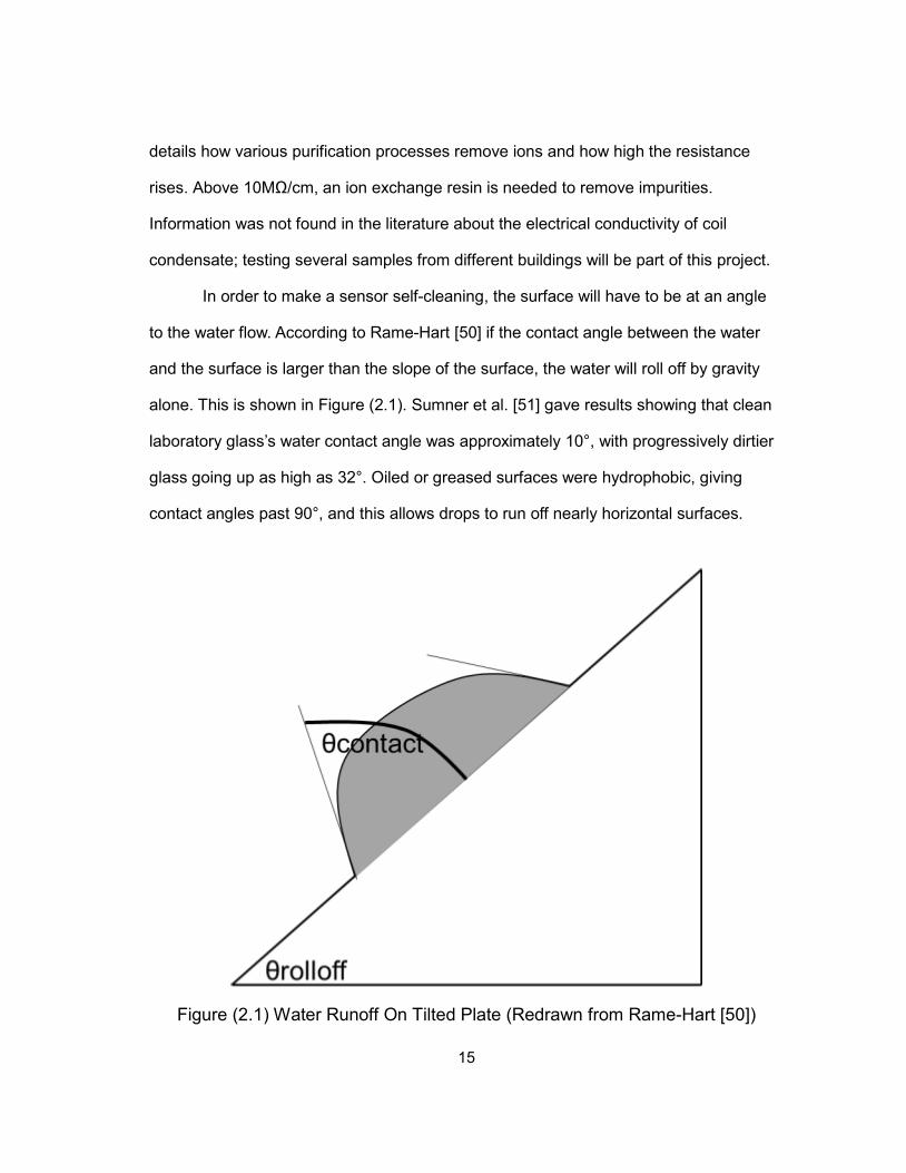
In order to make a sensor self-cleaning, the surface will have to be at an angle

to the water flow. According to Rame-Hart [50] if the contact angle between the water

and the surface is larger than the slope of the surface, the water will roll off by gravity

alone. This is shown in Figure (2.1). Sumner et al. [51] gave results showing that clean

laboratory glass’s water contact angle was approximately 10°, with progressively dirtier

glass going up as high as 32°. Oiled or greased surfaces were hydrophobic, giving

contact angles past 90°, and this allows drops to run off nearly horizontal surfaces.

Figure (2.1) Water Runoff On Tilted Plate (Redrawn from Rame-Hart [50])

16

These electrical and mechanical properties of water will be used to design the

coil enthalpy sensor. Differences in resistance will cause differences in electrical output

if resistance is the measured property. Water must be able to run off sensing surfaces in

order to make the sensor “self-cleaning.”

2.5 Analog Electronics and Test Equipment (Sections 7 and 8)

Analog electronics are used in this project to provide the desired distinct wet and

dry states from the sensor. The AC frequencies used are typical of audio electronics,

allowing use of common circuit elements. The output from the sensor electronics was

monitored by an Onset Electronics Hobo U12-012 Logger, with inputs to the logger

specified in its data sheet [52].

Storr, on the “electronicstutorials.ws” website [53] describes several circuits that

can produce AC signals. Storr states that “Schmitt Waveform Generators can also be

made using standard CMOS Logic NAND gates connected to produce an inverter circuit.

Here, two NAND gates are connected together to produce another type of RC

relaxation oscillator circuit that will generate a square wave shaped output waveform.”

The circuit described by [53] was used for the 10 V, 1 kHz oscillator. Fairchild

Semiconductor’s datasheet [54] for the Schmitt triggers used described their operating

conditions. Later circuits used a Maxim 1099DS integrated circuit as a square wave

oscillator. In its datasheet [55], Maxim Semiconductor describes the circuit, which

“consists of a fixed-frequency 1.048 MHz master oscillator followed by two independent

factory-programmable dividers.”

17

Filtering and amplification were required to get the desired output from the

sensor. Shrader, in “Electronic Communication” [56], describes a filter as a

“combination of capacitors, coils, and resistance that will allow certain frequencies to

pass through or be impeded.” The average DC level of the sensor’s output had to be

separated from the AC signal, and Shrader states that a filter is appropriate here: “Low-

pass filters are used in electronic power supplies to pass DC but not variations of

current or voltage…They can be employed between a transmitter and an antenna to

prevent frequencies higher than the desired frequencies (such as harmonics) from

appearing in the antenna.”

Sinclair and Dunton, in their “Practical Electronics Handbook” [57] describe the

use of operational amplifiers to amplify signals in inverting and noninverting

configurations and gives the equations necessary for design. Sinclair and Dunton claim

that “The frequency range of an op-amp depends on two factors, the gain-bandwidth

product for small signals, and the slew rate for large signals.” The required gain-

bandwidth product for this application was calculated to be 5 MHz, which was satisfied

by the Texas Instruments LME49710 amplifier, whose data sheet [58] claims a 45 MHz

minimum gain-bandwidth product.

2.6 Literature Summary

The literature shows that the savings available from enthalpy economizers are

heavily dependent on climate and on the accuracy of the humidity measurement

provided to the Energy Management and Control System (EMCS). Existing humidity

sensors have limitations that prevent their being used to determine a coil wet/dry state.

The only sources found in the literature for a sensor that detects water in contact with

18

electrodes used it for soil moisture measurement. A sensor operating on a similar

principle for building control has not been investigated. A reliable “coil enthalpy” sensor

will significantly increase the operating range of an economizer in climates where

outside air humidity varies widely.

19

3. ECONOMIZERS

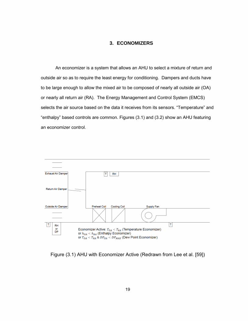
An economizer is a system that allows an AHU to select a mixture of return and

outside air so as to require the least energy for conditioning. Dampers and ducts have

to be large enough to allow the mixed air to be composed of nearly all outside air (OA)

or nearly all return air (RA). The Energy Management and Control System (EMCS)

selects the air source based on the data it receives from its sensors. “Temperature” and

“enthalpy” based controls are common. Figures (3.1) and (3.2) show an AHU featuring

an economizer control.

Figure (3.1) AHU with Economizer Active (Redrawn from Lee et al. [59])

20

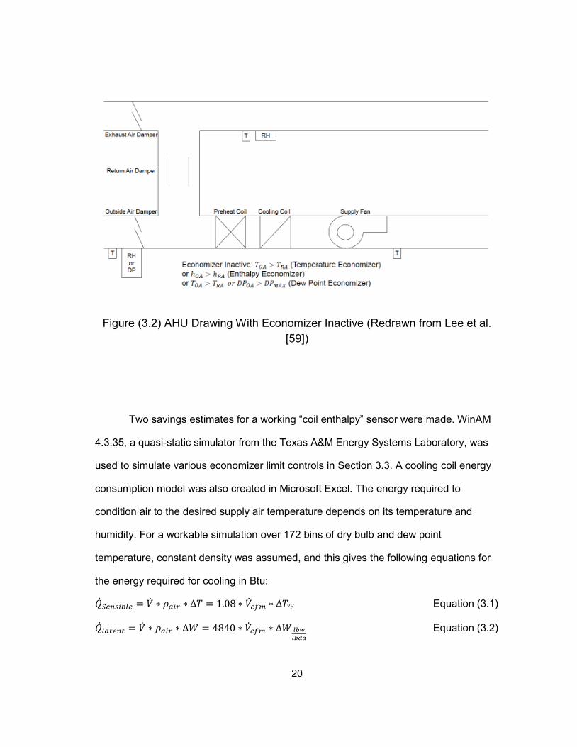
Figure (3.2) AHU Drawing With Economizer Inactive (Redrawn from Lee et al.

[59])

Two savings estimates for a working “coil enthalpy” sensor were made. WinAM

4.3.35, a quasi-static simulator from the Texas A&M Energy Systems Laboratory, was

used to simulate various economizer limit controls in Section 3.3. A cooling coil energy

consumption model was also created in Microsoft Excel. The energy required to

condition air to the desired supply air temperature depends on its temperature and

humidity. For a workable simulation over 172 bins of dry bulb and dew point

temperature, constant density was assumed, and this gives the following equations for

the energy required for cooling in Btu:

𝑆𝑒𝑛𝑠𝑖𝑏𝑙𝑒 = ∗ 𝜌𝑎𝑖𝑟 ∗ ∆𝑇 = 1.08 ∗ 𝑐𝑓𝑚 ∗ ∆𝑇 Equation (3.1)

𝑙𝑎𝑡𝑒𝑛𝑡 = ∗ 𝜌𝑎𝑖𝑟 ∗ ∆𝑊 = 4840 ∗ 𝑐𝑓𝑚 ∗ ∆𝑊𝑙𝑏𝑤𝑙𝑏𝑑𝑎

Equation (3.2)

21

A “dry” cooling coil needs to remove only sensible heat from the mixed air, as

the water concentration of the air is less than or equal to the saturation limit at the

supply temperature. If the mixed air temperature is already below the desired supply

temperature, the chilled water valve is closed and no energy is consumed by the coil. A

“wet” cooling coil removes sensible heat from the air until the saturation limit is reached,

and then removes both sensible and latent heat until the saturated design condition is

reached. The energy consumption of the coil is then given by Equation (3.3).

𝑇𝑜𝑡𝑎𝑙 = ∗ 𝜌𝑎𝑖𝑟 ∗ (𝑀𝑎𝑥𝑖𝑚𝑢𝑚 𝑜𝑓 [∆𝑇, 0] +𝑀𝑎𝑥𝑖𝑚𝑢𝑚 𝑜𝑓 [∆𝑊, 0]) Equation (3.3)

3.1 Spreadsheet Simulations

The energy savings for the economizer are then given by the difference between

the energy requirement for conditioning the return air/outside air mix and the energy

requirement for conditioning only the outside air. Tables of the energy savings, or

energy losses, from running an economizer during various weather conditions were

then generated.

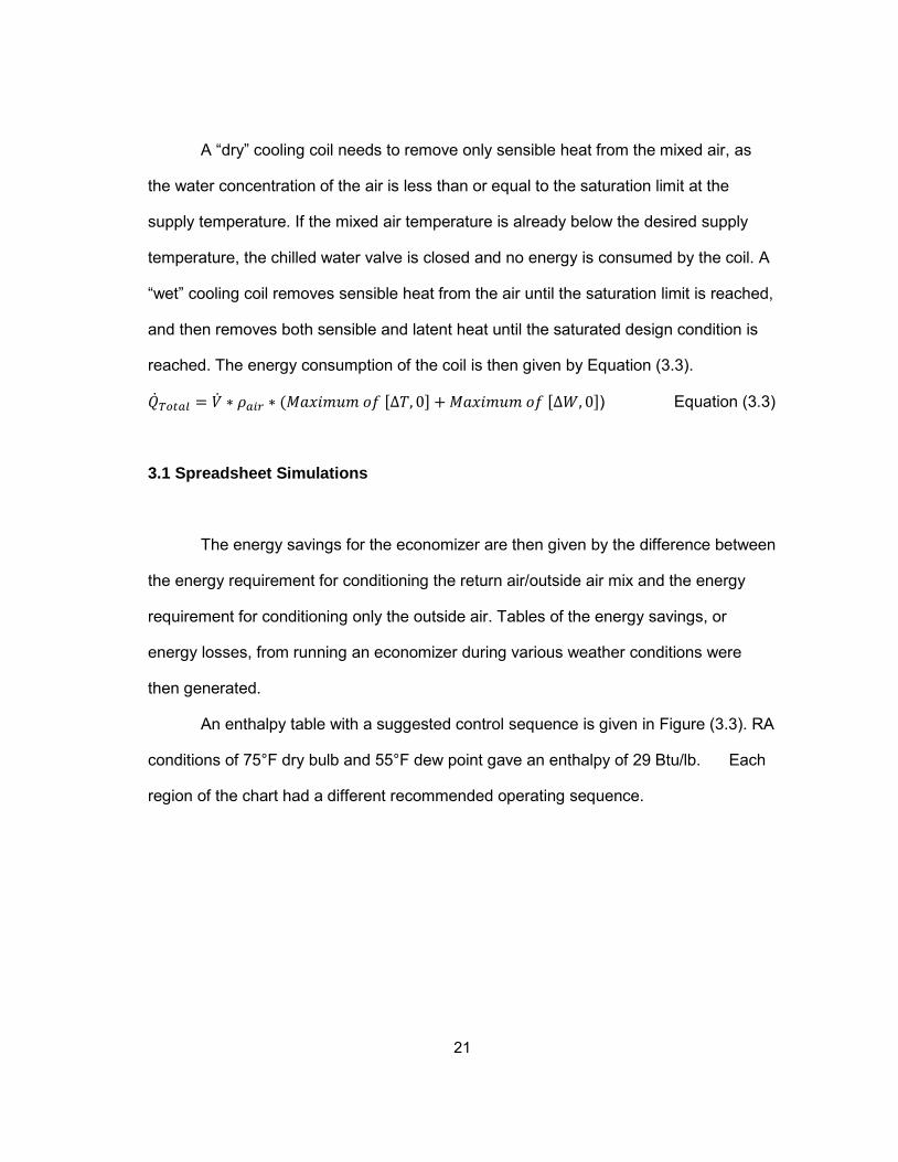
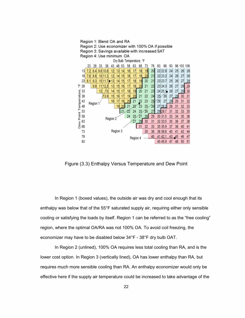
An enthalpy table with a suggested control sequence is given in Figure (3.3). RA

conditions of 75°F dry bulb and 55°F dew point gave an enthalpy of 29 Btu/lb. Each

region of the chart had a different recommended operating sequence.

22

Figure (3.3) Enthalpy Versus Temperature and Dew Point

In Region 1 (boxed values), the outside air was dry and cool enough that its

enthalpy was below that of the 55°F saturated supply air, requiring either only sensible

cooling or satisfying the loads by itself. Region 1 can be referred to as the “free cooling”

region, where the optimal OA/RA was not 100% OA. To avoid coil freezing, the

economizer may have to be disabled below 34°F - 38°F dry bulb OAT.

In Region 2 (unlined), 100% OA requires less total cooling than RA, and is the

lower cost option. In Region 3 (vertically lined), OA has lower enthalpy than RA, but

requires much more sensible cooling than RA. An enthalpy economizer would only be

effective here if the supply air temperature could be increased to take advantage of the

23

free latent cooling. In Region 4 (horizontally lined) of Figure (3.3), OA use should be

minimized, as its enthalpy is greater than that of the RA.

An alternate method of using this information to determine an efficient control

sequence is to calculate the cost of conditioning this air in Btu/lb using Equation (3.4).

The results are shown in Figure (3.4). This chart suggests two possibly advantageous

control strategies: one featuring a dry bulb temperature cutoff at 75°F and a dew point

cutoff at 60°F, and one with a dry bulb temperature cutoff at 70°F. Figures (3.4) and

(3.5) use Equation (3.4), derived from Equation (3.3). In Equation (3.4), the outside air

mass fraction when the economizer is disabled is 𝑥𝑂𝐴, with the return air fraction

represented by 1 − 𝑥𝑂𝐴. An 𝑥𝑂𝐴 of 0.2 is used for the remainder of the spreadsheet

analysis.

𝑄𝑠𝑎𝑣𝑒𝑑𝑠𝑢𝑝𝑝𝑙𝑖𝑒𝑑

= (𝑥𝑂𝐴 ∗ 0.24𝐵𝑡𝑢𝑙𝑏 ∗

∗ (𝑇𝑂𝐴 − 𝑇𝑆𝐴) + (1 − 𝑥𝑂𝐴) ∗ 0.24 ∗ (𝑇𝑅𝐴 − 𝑇𝑆𝐴) −

0.24 𝐵𝑡𝑢𝑙𝑏∗

∗ (𝑇𝑂𝐴 − 𝑇𝑆𝐴) + 970 𝐵𝑡𝑢𝑙𝑏𝑚

∗ 𝑀𝐴𝑋0, 𝑥𝑂𝐴 ∗ (𝑤𝑂𝐴 − 𝑤𝑠𝑎) + (1 − 𝑥𝑂𝐴) ∗

(𝑤𝑅𝐴 − 𝑤𝑆𝐴) − (970 𝐵𝑡𝑢𝑙𝑏𝑚

∗ (𝑀𝐴𝑋(0,𝑤𝑂𝐴 − 𝑤𝑆𝐴) Equation (3.4)

Equation (3.4) can be considered descriptive for any economizer when using U.S.

Customary System units. Figures (3.4) and (3.5) apply at elevations below 500’.

24

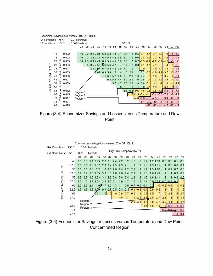
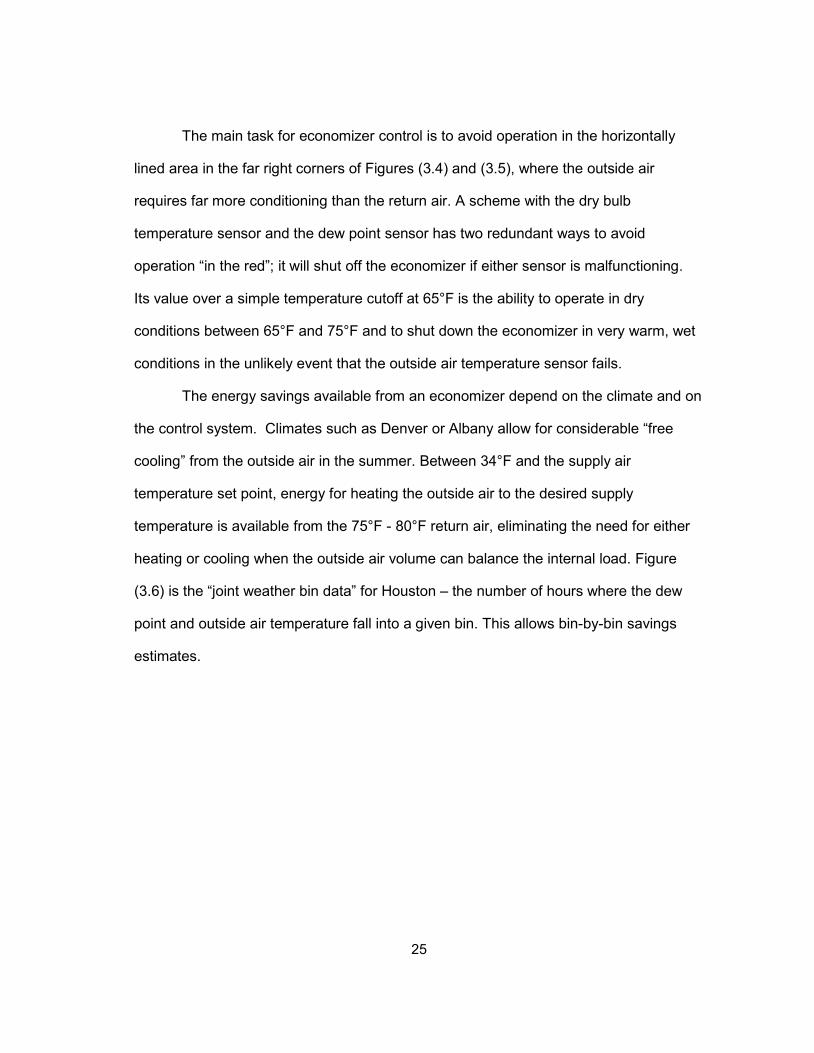
Figure (3.4) Economizer Savings and Losses versus Temperature and Dew Point

Figure (3.5) Economizer Savings or Losses versus Temperature and Dew Point:

Concentrated Region

25

The main task for economizer control is to avoid operation in the horizontally

lined area in the far right corners of Figures (3.4) and (3.5), where the outside air

requires far more conditioning than the return air. A scheme with the dry bulb

temperature sensor and the dew point sensor has two redundant ways to avoid

operation “in the red”; it will shut off the economizer if either sensor is malfunctioning.

Its value over a simple temperature cutoff at 65°F is the ability to operate in dry

conditions between 65°F and 75°F and to shut down the economizer in very warm, wet

conditions in the unlikely event that the outside air temperature sensor fails.

The energy savings available from an economizer depend on the climate and on

the control system. Climates such as Denver or Albany allow for considerable “free

cooling” from the outside air in the summer. Between 34°F and the supply air

temperature set point, energy for heating the outside air to the desired supply

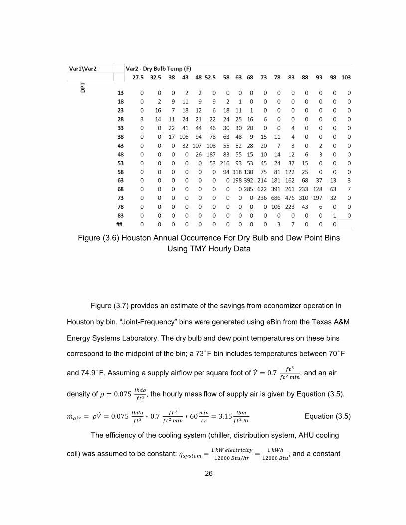
temperature is available from the 75°F - 80°F return air, eliminating the need for either

heating or cooling when the outside air volume can balance the internal load. Figure

(3.6) is the “joint weather bin data” for Houston – the number of hours where the dew

point and outside air temperature fall into a given bin. This allows bin-by-bin savings

estimates.

26

Figure (3.6) Houston Annual Occurrence For Dry Bulb and Dew Point Bins

Using TMY Hourly Data

Figure (3.7) provides an estimate of the savings from economizer operation in

Houston by bin. “Joint-Frequency” bins were generated using eBin from the Texas A&M

Energy Systems Laboratory. The dry bulb and dew point temperatures on these bins

correspond to the midpoint of the bin; a 73°F bin includes temperatures between 70°F

and 74.9°F. Assuming a supply airflow per square foot of = 0.7 𝑓𝑡3

𝑓𝑡2 𝑚𝑖𝑛, and an air

density of 𝜌 = 0.075 𝑙𝑏𝑑𝑎𝑓𝑡3

, the hourly mass flow of supply air is given by Equation (3.5).

𝑎𝑖𝑟 = 𝜌 = 0.075 𝑙𝑏𝑑𝑎𝑓𝑡3

∗ 0.7 𝑓𝑡3

𝑓𝑡2 𝑚𝑖𝑛∗ 60𝑚𝑖𝑛

ℎ𝑟= 3.15 𝑙𝑏𝑚

𝑓𝑡2 ℎ𝑟 Equation (3.5)

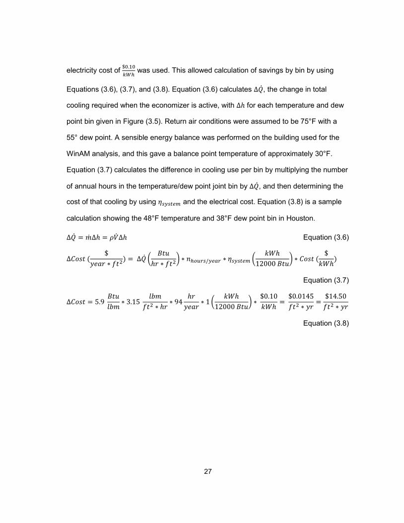
The efficiency of the cooling system (chiller, distribution system, AHU cooling

coil) was assumed to be constant: 𝜂𝑠𝑦𝑠𝑡𝑒𝑚 = 1 𝑘𝑊 𝑒𝑙𝑒𝑐𝑡𝑟𝑖𝑐𝑖𝑡𝑦12000 𝐵𝑡𝑢/ℎ𝑟

= 1 𝑘𝑊ℎ12000 𝐵𝑡𝑢

, and a constant

27

electricity cost of $0.10𝑘𝑊ℎ

was used. This allowed calculation of savings by bin by using

Equations (3.6), (3.7), and (3.8). Equation (3.6) calculates ∆, the change in total

cooling required when the economizer is active, with ∆ℎ for each temperature and dew

point bin given in Figure (3.5). Return air conditions were assumed to be 75°F with a

55° dew point. A sensible energy balance was performed on the building used for the

WinAM analysis, and this gave a balance point temperature of approximately 30°F.

Equation (3.7) calculates the difference in cooling use per bin by multiplying the number

of annual hours in the temperature/dew point joint bin by ∆, and then determining the

cost of that cooling by using 𝜂𝑠𝑦𝑠𝑡𝑒𝑚 and the electrical cost. Equation (3.8) is a sample

calculation showing the 48°F temperature and 38°F dew point bin in Houston.

∆ = ∆ℎ = 𝜌∆ℎ Equation (3.6)

∆𝐶𝑜𝑠𝑡 ($

𝑦𝑒𝑎𝑟 ∗ 𝑓𝑡2) = ∆

𝐵𝑡𝑢ℎ𝑟 ∗ 𝑓𝑡2

∗ 𝑛ℎ𝑜𝑢𝑟𝑠/𝑦𝑒𝑎𝑟 ∗ 𝜂𝑠𝑦𝑠𝑡𝑒𝑚 𝑘𝑊ℎ

12000 𝐵𝑡𝑢 ∗ 𝐶𝑜𝑠𝑡 (

$𝑘𝑊ℎ

)

Equation (3.7)

∆𝐶𝑜𝑠𝑡 = 5.9 𝐵𝑡𝑢𝑙𝑏𝑚

∗ 3.15 𝑙𝑏𝑚

𝑓𝑡2 ∗ ℎ𝑟∗ 94

ℎ𝑟𝑦𝑒𝑎𝑟

∗ 1 𝑘𝑊ℎ

12000 𝐵𝑡𝑢 ∗

$0.10𝑘𝑊ℎ

= $0.0145𝑓𝑡2 ∗ 𝑦𝑟

=$14.50𝑓𝑡2 ∗ 𝑦𝑟

Equation (3.8)

28

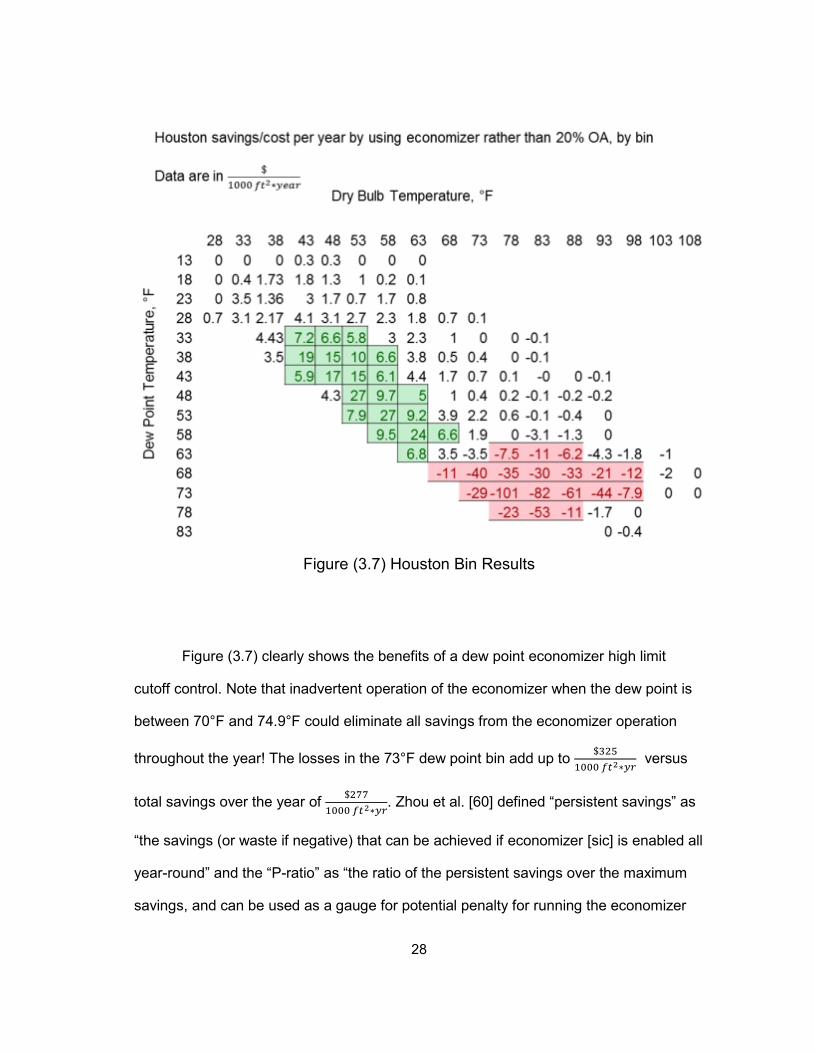
Figure (3.7) Houston Bin Results

Figure (3.7) clearly shows the benefits of a dew point economizer high limit

cutoff control. Note that inadvertent operation of the economizer when the dew point is

between 70°F and 74.9°F could eliminate all savings from the economizer operation

throughout the year! The losses in the 73°F dew point bin add up to $3251000 𝑓𝑡2∗𝑦𝑟

versus

total savings over the year of $2771000 𝑓𝑡2∗𝑦𝑟

. Zhou et al. [60] defined “persistent savings” as

“the savings (or waste if negative) that can be achieved if economizer [sic] is enabled all

year-round” and the “P-ratio” as “the ratio of the persistent savings over the maximum

savings, and can be used as a gauge for potential penalty for running the economizer

29

all year-round. The penalties range from “minor” for Denver to “devastating” for Houston

and Miami.” Zhou et al. give P-ratio values of 88% for Denver, - 427% for Houston, and

- 2936% for Miami. The results from Figure (3.7) confirm that losses for year-round

operation in Houston would be 4 times the available savings from correct operation.

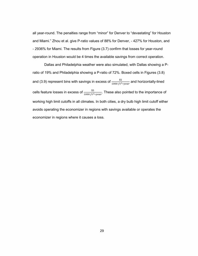
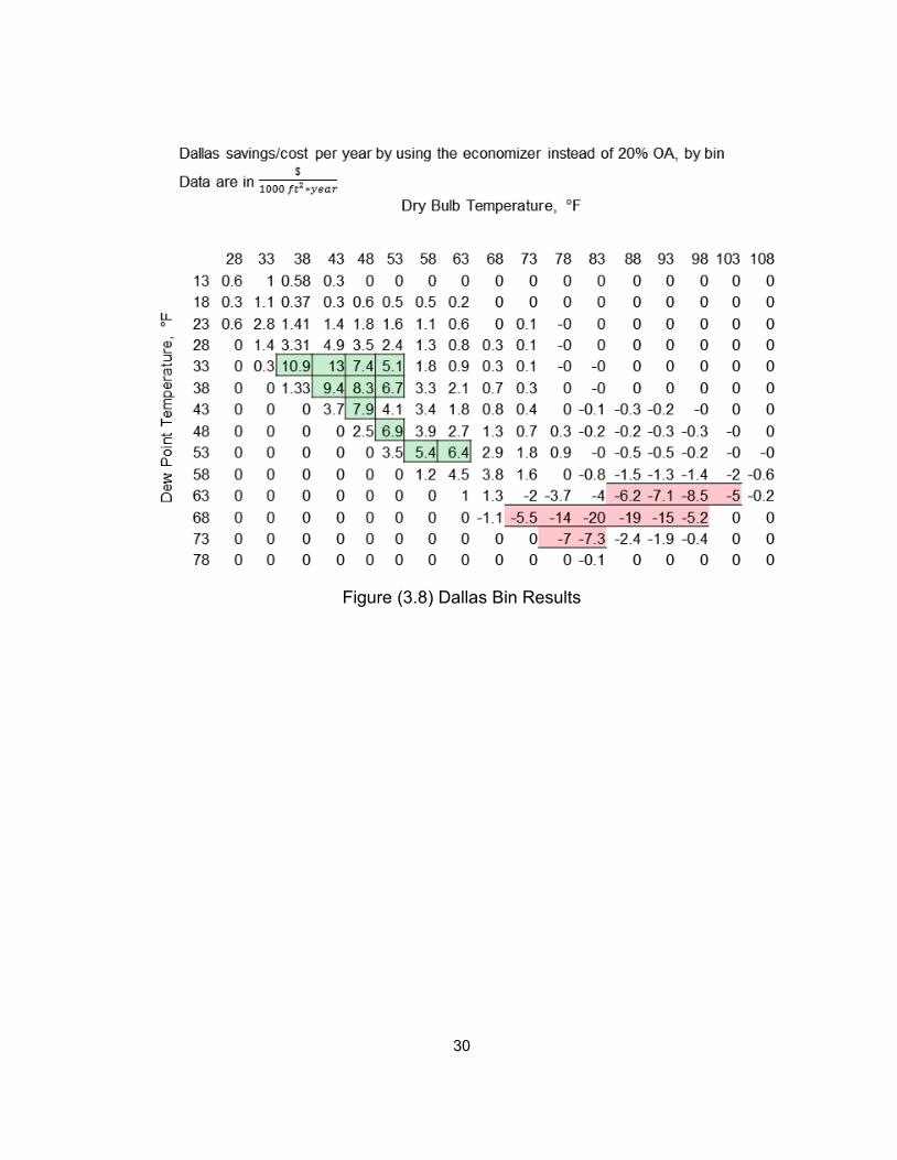
Dallas and Philadelphia weather were also simulated, with Dallas showing a P-

ratio of 19% and Philadelphia showing a P-ratio of 72%. Boxed cells in Figures (3.8)

and (3.9) represent bins with savings in excess of $51000 𝑓𝑡2∗𝑦𝑒𝑎𝑟

and horizontally-lined

cells feature losses in excess of $51000 𝑓𝑡2∗𝑦𝑒𝑎𝑟

. These also pointed to the importance of

working high limit cutoffs in all climates. In both cities, a dry bulb high limit cutoff either

avoids operating the economizer in regions with savings available or operates the

economizer in regions where it causes a loss.

30

Figure (3.8) Dallas Bin Results

31

Figure (3.9) Philadelphia Bin Results

Taylor [18] and Zhou et al. [60] compared economizers using hourly building

simulations. Taylor’s method modeled sensor error in DOE 2.2 for several different

types of high limit cutoff and manufacturer specified errors: fixed dry bulb temperature,

differential dry bulb temperature, fixed enthalpy, differential enthalpy, differential

enthalpy with fixed dry bulb, fixed enthalpy with fixed dry bulb, and fixed dry bulb and

fixed dew point. Zhou et al. compared economizer high limit cutoff temperatures per

pound of air provided.

32

3.2 Economizer Index

A single “Economizer Index” can be used to compare economizer control

strategies. A theoretical “ideal” economizer control would operate the economizer

whenever the energy required to condition the outside air was less than the energy

needed to condition the return air, and would reduce to a minimum outside air condition

at all other times. This ideal economizer would require perfect (zero-error) temperature

and humidity sensors on both outside and return air streams. Any other control scheme

will achieve a lower level of savings than this, allowing the “Economizer Index” to be

defined as:

𝜂𝐸𝐶𝑂𝑁 = ∑𝑆𝑎𝑣𝑖𝑛𝑔𝑠∑𝑆𝑎𝑣𝑖𝑛𝑔𝑠,𝐼𝑑𝑒𝑎𝑙

Equation (3.9)

This index varies heavily with climate, as with any calculation involving

economizers. The bin method used for the analysis of 100% outside air economizers

allows rapid comparison of different economizer limit cutoffs and provides estimates for

the losses that can occur when sensors fail. Several different economizer schemes

were compared for each climate:

1) 100% OA at all times, which should provide identical results to the “Persistence Index” in Zhou et al. [60]

2) Temperature high-limit cutoff at 58°F 3) Temperature high-limit cutoff at 63°F 4) Temperature high-limit cutoff at 68°F 5) Temperature high-limit cutoff at 73°F 6) Temperature high-limit cutoff at 78°F 7) Temperature high-limit cutoff at 78°F with enthalpy cutoff at 27 Btu/lb 8) Temperature high-limit cutoff at 78°F with enthalpy cutoff at 29 Btu/lb 9) Temperature high-limit cutoff at 78°F with dew point cutoff at 53°F 10) Temperature high-limit cutoff at 78°F with dew point cutoff at 58°F

33

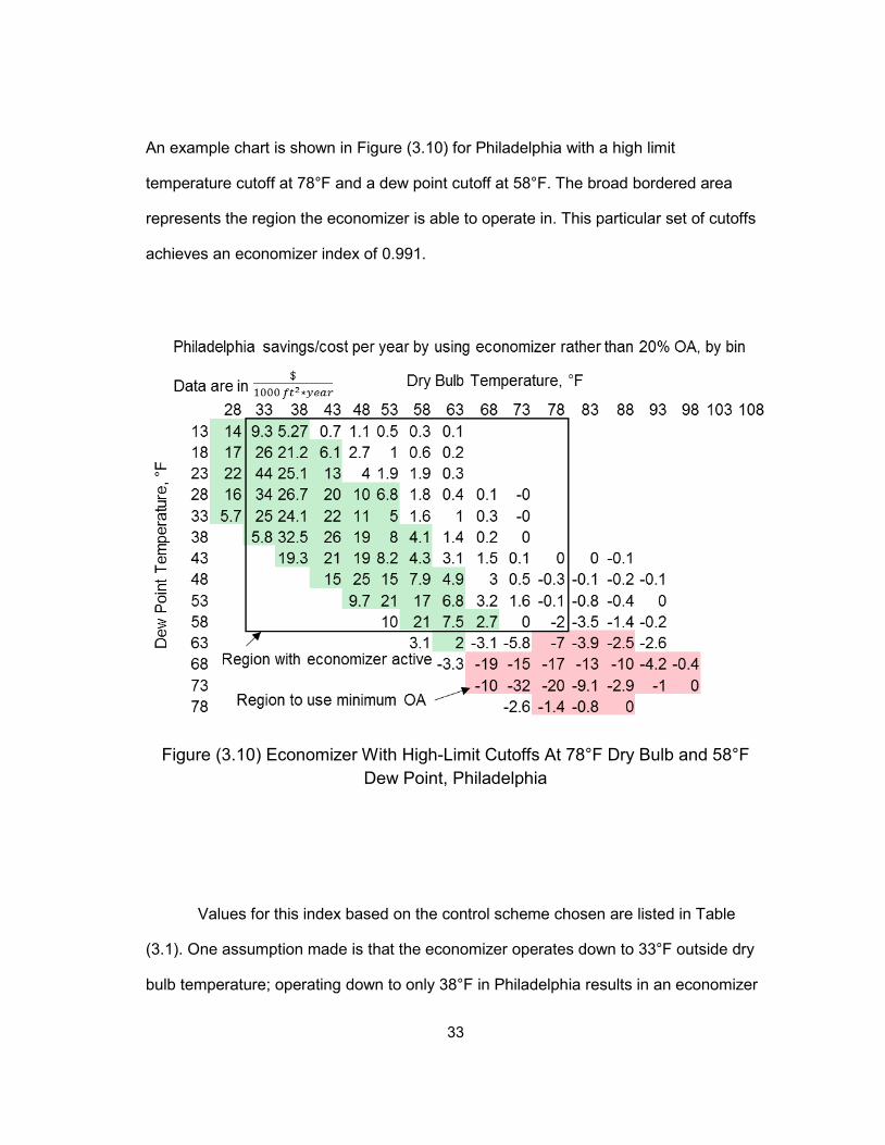
An example chart is shown in Figure (3.10) for Philadelphia with a high limit

temperature cutoff at 78°F and a dew point cutoff at 58°F. The broad bordered area

represents the region the economizer is able to operate in. This particular set of cutoffs

achieves an economizer index of 0.991.

Figure (3.10) Economizer With High-Limit Cutoffs At 78°F Dry Bulb and 58°F

Dew Point, Philadelphia

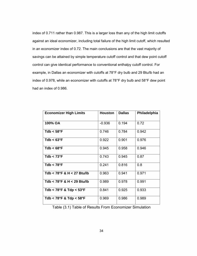
Values for this index based on the control scheme chosen are listed in Table

(3.1). One assumption made is that the economizer operates down to 33°F outside dry

bulb temperature; operating down to only 38°F in Philadelphia results in an economizer

34

index of 0.711 rather than 0.987. This is a larger loss than any of the high limit cutoffs

against an ideal economizer, including total failure of the high limit cutoff, which resulted

in an economizer index of 0.72. The main conclusions are that the vast majority of

savings can be attained by simple temperature cutoff control and that dew point cutoff

control can give identical performance to conventional enthalpy cutoff control. For

example, in Dallas an economizer with cutoffs at 78°F dry bulb and 29 Btu/lb had an

index of 0.978, while an economizer with cutoffs at 78°F dry bulb and 58°F dew point

had an index of 0.986.

Economizer High Limits Houston Dallas Philadelphia

100% OA -0.936 0.194 0.72

Tdb < 58°F 0.746 0.784 0.942

Tdb < 63°F 0.922 0.901 0.976

Tdb < 68°F 0.945 0.958 0.946

Tdb < 73°F 0.743 0.945 0.87

Tdb < 78°F 0.241 0.816 0.8

Tdb < 78°F & H < 27 Btu/lb 0.963 0.941 0.971

Tdb < 78°F & H < 29 Btu/lb 0.989 0.978 0.991

Tdb < 78°F & Tdp < 53°F 0.841 0.925 0.933

Tdb < 78°F & Tdp < 58°F 0.969 0.986 0.989

Table (3.1) Table of Results From Economizer Simulation

35

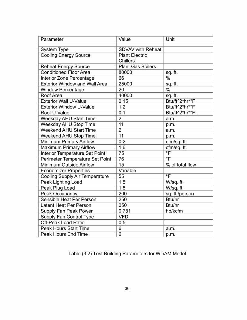
3.3 WinAM Simulations

WinAM 4.3.35, a simulator from the Texas A&M Energy Systems Laboratory,

was then used to generate year-round savings. WinAM calculated the energy

consumption of the AHU each hour for one year (8760 hours) to evaluate the effects of

temperature and enthalpy economizers. The WinAM simulation used a hypothetical

80,000 ft2 commercial building with a single SDVAV AHU. The building’s parameters

are given in Table (3.2) and are meant to be typical for an office building.

Temperature, enthalpy, and inactive economizers were simulated using 2012

weather data from Houston, Dallas, and Philadelphia. Temperature economizer high-

limit control parameters for minimum energy consumption were optimized by trial and

error. Enthalpy economizer control parameters were set to exclude air above 78°F and

29 Btu/lb; above those values return air requires less cooling. WinAM does not feature

dew point high-limit cutoffs; 78°F and 29 Btu/lb give a 55°F dew point.

36

Parameter Value Unit System Type SDVAV with Reheat Cooling Energy Source Plant Electric

Chillers

Reheat Energy Source Plant Gas Boilers Conditioned Floor Area 80000 sq. ft. Interior Zone Percentage 66 % Exterior Window and Wall Area 25000 sq. ft. Window Percentage 20 % Roof Area 40000 sq. ft. Exterior Wall U-Value 0.15 Btu/ft^2*hr*°F Exterior Window U-Value 1.2 Btu/ft^2*hr*°F Roof U-Value 0.1 Btu/ft^2*hr*°F . Weekday AHU Start Time 2 a.m. Weekday AHU Stop Time 11 p.m. Weekend AHU Start Time 2 a.m. Weekend AHU Stop Time 11 p.m. Minimum Primary Airflow 0.2 cfm/sq. ft. Maximum Primary Airflow 1.6 cfm/sq. ft. Interior Temperature Set Point 75 °F Perimeter Temperature Set Point 76 °F Minimum Outside Airflow 15 % of total flow Economizer Properties Variable Cooling Supply Air Temperature 55 °F Peak Lighting Load 1.5 W/sq. ft. Peak Plug Load 1.5 W/sq. ft. Peak Occupancy 200 sq. ft./person Sensible Heat Per Person 250 Btu/hr Latent Heat Per Person 250 Btu/hr Supply Fan Peak Power 0.781 hp/kcfm Supply Fan Control Type VFD Off-Peak Load Ratio 0.5 Peak Hours Start Time 6 a.m. Peak Hours End Time 6 p.m.

Table (3.2) Test Building Parameters for WinAM Model

37

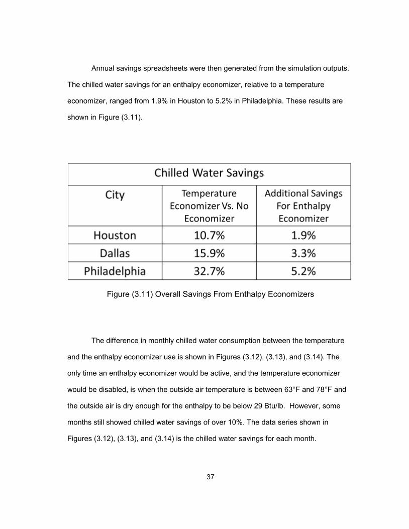
Annual savings spreadsheets were then generated from the simulation outputs.

The chilled water savings for an enthalpy economizer, relative to a temperature

economizer, ranged from 1.9% in Houston to 5.2% in Philadelphia. These results are

shown in Figure (3.11).

Figure (3.11) Overall Savings From Enthalpy Economizers

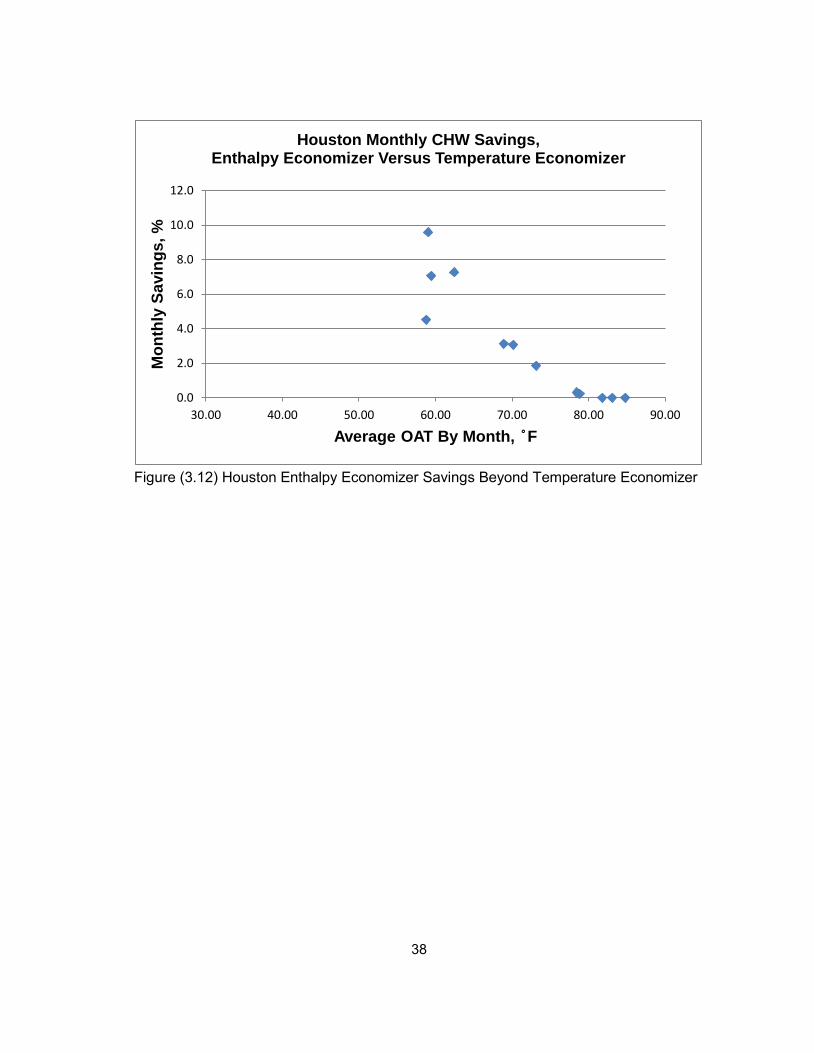
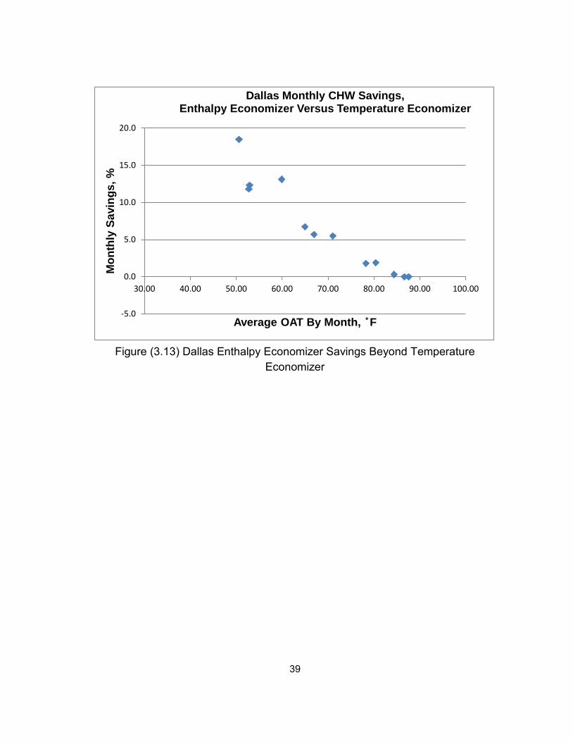
The difference in monthly chilled water consumption between the temperature

and the enthalpy economizer use is shown in Figures (3.12), (3.13), and (3.14). The

only time an enthalpy economizer would be active, and the temperature economizer

would be disabled, is when the outside air temperature is between 63°F and 78°F and

the outside air is dry enough for the enthalpy to be below 29 Btu/lb. However, some

months still showed chilled water savings of over 10%. The data series shown in

Figures (3.12), (3.13), and (3.14) is the chilled water savings for each month.

38

Figure (3.12) Houston Enthalpy Economizer Savings Beyond Temperature Economizer

0.0

2.0

4.0

6.0

8.0

10.0

12.0

30.00 40.00 50.00 60.00 70.00 80.00 90.00

Mon

thly

Sav

ings

, %

Average OAT By Month, °F

Houston Monthly CHW Savings, Enthalpy Economizer Versus Temperature Economizer

39

Figure (3.13) Dallas Enthalpy Economizer Savings Beyond Temperature

Economizer

-5.0

0.0

5.0

10.0

15.0

20.0

30.00 40.00 50.00 60.00 70.00 80.00 90.00 100.00

Mon

thly

Sav

ings

, %

Average OAT By Month, °F

Dallas Monthly CHW Savings, Enthalpy Economizer Versus Temperature Economizer

40

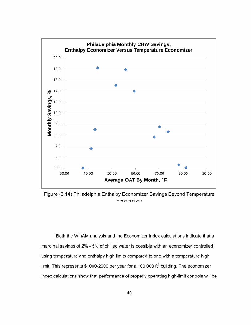
Figure (3.14) Philadelphia Enthalpy Economizer Savings Beyond Temperature

Economizer

Both the WinAM analysis and the Economizer Index calculations indicate that a

marginal savings of 2% - 5% of chilled water is possible with an economizer controlled

using temperature and enthalpy high limits compared to one with a temperature high

limit. This represents $1000-2000 per year for a 100,000 ft2 building. The economizer

index calculations show that performance of properly operating high-limit controls will be

0.0

2.0

4.0

6.0

8.0

10.0

12.0

14.0

16.0

18.0

20.0

30.00 40.00 50.00 60.00 70.00 80.00 90.00

Mon

thly

Sav

ings

, %

Average OAT By Month, °F

Philadelphia Monthly CHW Savings, Enthalpy Economizer Versus Temperature Economizer

41

similar between enthalpy and dew point cutoffs, and that the “freeze stat” low limit set

point is also important. One additional benefit of a dew point or humidity sensor in an

economizer application is that it provides an independent high-limit cutoff that will avoid

operating the economizer in conditions that destroy savings. Either a 58°F maximum

dew point or a 73°F maximum dry bulb temperature will avoid these conditions in any

climate analyzed.

42

4. COMMERCIAL HUMIDITY SENSOR TESTS

A sensor was required to detect if water is condensing on the coil. The minimum

requirements for this sensor were to provide a clear difference between the “wet” and

“dry” states and to survive for several years in an AHU. If a commercially available

sensor were able to achieve these, it would save a considerable amount of time in

design, fabrication, testing, and electronics for a new sensor design.

Humidity sensors of the resistive, capacitive, and chilled mirror types are widely

available commercially. In the literature review, several sources [9, 20, 27] pointed to

possible problems when using capacitive or resistive sensors to detect the difference

between condensing and noncondensing states. Six different resistive or capacitive

sensors were purchased from Digikey (http://www.digikey.com/). Their data sheets are

in references [3-8]. Their cost ranged from $5 to $10.

The sensors were installed in a solderless breadboard and connected to power,

ground, and the signal as specified in the pin-out diagrams in their datasheets. The

TDK CHS-MSS and TDK CHS-CSC-20 were connected to a National Instruments

analog input board with an analog-to-digital converter. A National Instruments LabView

Virtual Instrument was then used to record the voltage while the sensor was under test.

The Parallax HS1101, Measurement Specialties HS1101LF, and Honeywell HIH-1000

were simple two-terminal components whose capacitance varied with humidity. They

were connected to a multimeter capable of measuring capacitance. The multimeter

used a 10 kHz, 0.5 V triangle waveform to perform capacitance measurements. The

Honeywell HIH-5030 was connected to 5 V power and ground, with the voltage output

displayed on an oscilloscope.

43

Once connected, several tests were performed to determine the suitability of

these sensors for the task of determining the state of the coil. Their response to

changes in relative humidity was tested by using a portable electric heater to raise the

temperature without adding water to the air, thus decreasing the relative humidity. The

Honeywell HIH-1000 failed to show any difference in capacitance and was removed

from further tests. This may have been caused by shipping or handling damage, or a

sample defect.

The other five sensors were then subjected to the “dunk” test to determine how

quickly and completely they could recover from total inundation. These sensors have a

top surface area of less than 5 cm2, so a single, large, 1 cm3 drop of water falling from

the cooling coil directly onto the sensor can cover it completely to a depth of 2 mm. With

power, signal, and ground connected and data being recorded, the sensor was briefly

placed in a jar of tap water and then removed.

The results are shown in Table (4.1) and Figure (4.1). The TDK CHS-MSS,

shown in Figure (4.2) failed completely, registering a constant high output after the

dunk. The TDK CHS-CSC-20, shown in Figure (4.3) failed completely, giving an

apparently completely random output regardless of conditions, varying between 0 V and

0.75 V. The Parallax HS1101, shown in Figure (4.4) also failed, with its capacitance

dropping by three orders of magnitude.

44

Table (4.1) Results of Commercial Humidity Sensor Test

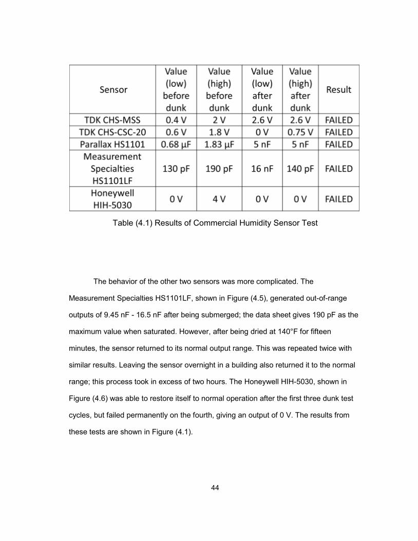
The behavior of the other two sensors was more complicated. The

Measurement Specialties HS1101LF, shown in Figure (4.5), generated out-of-range

outputs of 9.45 nF - 16.5 nF after being submerged; the data sheet gives 190 pF as the

maximum value when saturated. However, after being dried at 140°F for fifteen

minutes, the sensor returned to its normal output range. This was repeated twice with

similar results. Leaving the sensor overnight in a building also returned it to the normal

range; this process took in excess of two hours. The Honeywell HIH-5030, shown in

Figure (4.6) was able to restore itself to normal operation after the first three dunk test

cycles, but failed permanently on the fourth, giving an output of 0 V. The results from

these tests are shown in Figure (4.1).

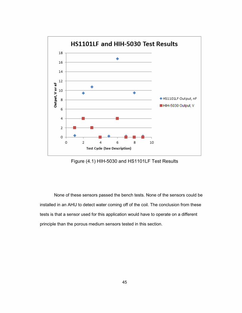
45

Figure (4.1) HIH-5030 and HS1101LF Test Results

None of these sensors passed the bench tests. None of the sensors could be

installed in an AHU to detect water coming off of the coil. The conclusion from these

tests is that a sensor used for this application would have to operate on a different

principle than the porous medium sensors tested in this section.

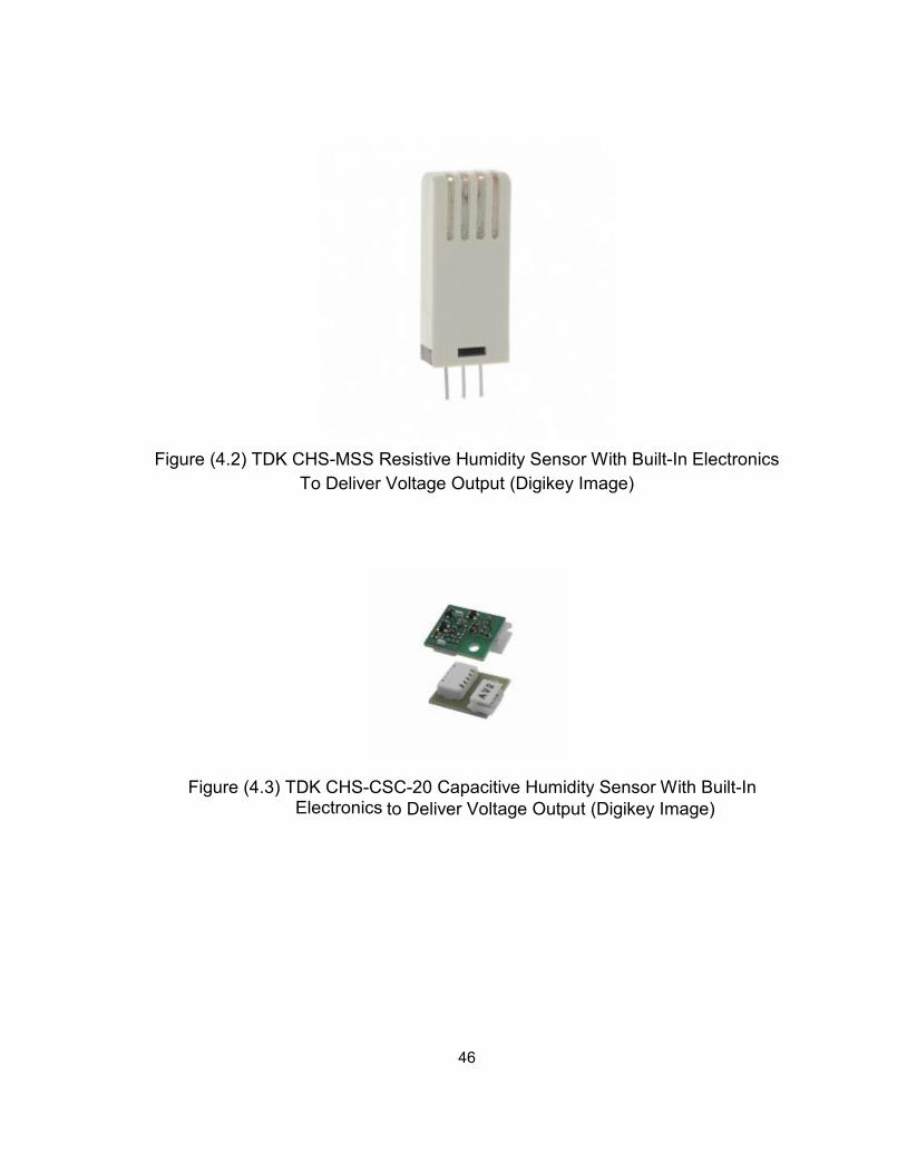
46

Figure (4.2) TDK CHS-MSS Resistive Humidity Sensor With Built-In Electronics

To Deliver Voltage Output (Digikey Image)

Figure (4.3) TDK CHS-CSC-20 Capacitive Humidity Sensor With Built-In Electronics to Deliver Voltage Output (Digikey Image)

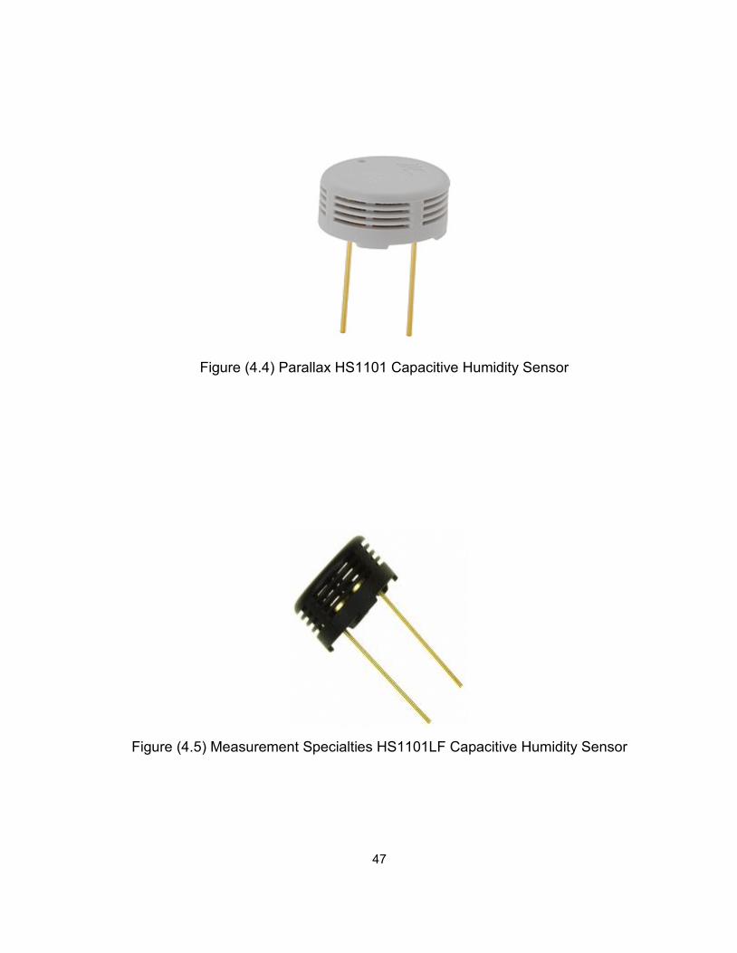
47

Figure (4.4) Parallax HS1101 Capacitive Humidity Sensor

Figure (4.5) Measurement Specialties HS1101LF Capacitive Humidity Sensor

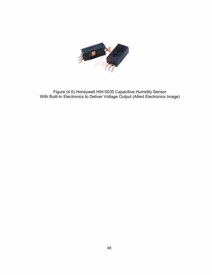
48

Figure (4.6) Honeywell HIH-5030 Capacitive Humidity Sensor With Built-In Electronics to Deliver Voltage Output (Allied Electronics Image)

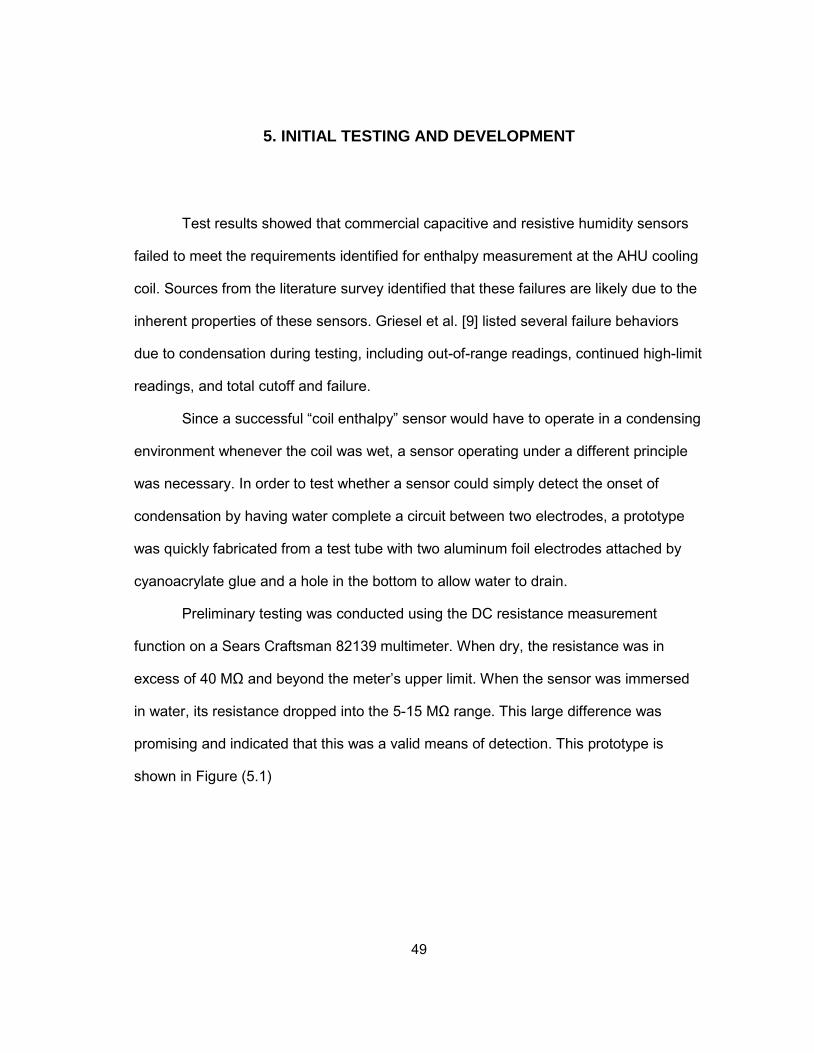
49

5. INITIAL TESTING AND DEVELOPMENT

Test results showed that commercial capacitive and resistive humidity sensors

failed to meet the requirements identified for enthalpy measurement at the AHU cooling

coil. Sources from the literature survey identified that these failures are likely due to the

inherent properties of these sensors. Griesel et al. [9] listed several failure behaviors

due to condensation during testing, including out-of-range readings, continued high-limit

readings, and total cutoff and failure.

Since a successful “coil enthalpy” sensor would have to operate in a condensing

environment whenever the coil was wet, a sensor operating under a different principle

was necessary. In order to test whether a sensor could simply detect the onset of

condensation by having water complete a circuit between two electrodes, a prototype

was quickly fabricated from a test tube with two aluminum foil electrodes attached by

cyanoacrylate glue and a hole in the bottom to allow water to drain.

Preliminary testing was conducted using the DC resistance measurement

function on a Sears Craftsman 82139 multimeter. When dry, the resistance was in

excess of 40 MΩ and beyond the meter’s upper limit. When the sensor was immersed

in water, its resistance dropped into the 5-15 MΩ range. This large difference was

promising and indicated that this was a valid means of detection. This prototype is

shown in Figure (5.1)

50

Figure (5.1) Test Tube Test “Sensor”

Several limitations of this sensor were immediately apparent and further testing

used different designs. The hole in the bottom had a diameter of approximately 1 cm,

preventing the contacts from being bridged by small quantities of water. The electrodes

were vulnerable to mechanical damage and tearing. Permanent attachment of the

electrodes would require a different adhesive. A new sensor would have to be able to

operate on as little as one drop of water, with a volume of roughly 1 cm3, and would

have to respond within five to ten minutes. This time requirement is analyzed in Section

5.1.

51

5.1 Response To State Changes

A fast response from the sensor was desired for control purposes and

measurement accuracy. If frequent measurements of the dew point are to be taken as

part of a building control sequence, the time required to take the measurements can be

a significant portion of the time the AHU is operating. Several sensor “wet or dry”

checks must be performed for each dew point temperature measurement. To perform

one of these checks, the coil must first reach the steady state target temperature after

approximately 5 coil time constants, and then the sensor must be monitored for its

characteristic response time. The total time for a dew point measurement is given by

Equations (5.1) and (5.2).

𝑡𝑐ℎ𝑒𝑐𝑘 = 5 ∗ 𝜏𝑐𝑜𝑖𝑙 + 𝑡𝑠𝑒𝑛𝑠𝑜𝑟 Equation (5.1)

𝑡𝑚𝑒𝑎𝑠𝑢𝑟𝑒𝑚𝑒𝑛𝑡 = 𝑡𝑐ℎ𝑒𝑐𝑘 ∗ 𝐴𝐵𝑆(𝑇𝑖𝑛𝑖𝑡𝑖𝑎𝑙−𝑇𝑑𝑒𝑤 𝑝𝑜𝑖𝑛𝑡)

𝑇𝑠𝑡𝑒𝑝+ 1 Equation (5.2)

where tmeasurement is the total time needed to take a dew point

measurement, 𝐴𝐵𝑆(𝑇𝑖𝑛𝑖𝑡𝑖𝑎𝑙 − 𝑇𝑑𝑒𝑤 𝑝𝑜𝑖𝑛𝑡) is the difference between the supply air

temperature at the start of the measurement and the dew point, and 𝑇𝑠𝑡𝑒𝑝 is the amount

the temperature is changed between each attempt to detect water. A sample control

sequence to measure the dew point when the supply air temperature can be controlled

is shown in Figure (5.2).

52

Start

End

Figure (5.2) Control Sequence For Dew Point Measurement

An upper limit on the time allowed is provided by occupant comfort concerns. If

the supply temperature used in the measurement is above the temperature needed to

satisfy the sensible load, the room temperature will rise unless the mass of supply

airflow is increased. Another limitation is the ratio of time spent testing to the time in

normal operation. If three dew point measurements are taken per day, then this ratio is

given by Equation (5.3).

53

𝑅𝑜𝑝𝑒𝑟𝑎𝑡𝑖𝑛𝑔 = 𝑡𝐴𝐻𝑈𝑜𝑛𝑡𝑚𝑒𝑎𝑠∗𝑛𝑚𝑒𝑎𝑠

= 𝑡𝐴𝐻𝑈𝑜𝑛3∗𝑡𝑚𝑒𝑎𝑠

Equation (5.3)

For testing purposes, it was estimated that the maximum acceptable 𝑡𝑚𝑒𝑎𝑠 would be 15

minutes, and in order to measure mixed air dew points between 50 °F and 60 °F, up to

5 measurements would be required, meaning that the maximum acceptable 𝑡𝑐ℎ𝑒𝑐𝑘

would be 3 minutes.

Factors influencing the delay between the supply air temperature falling below

the dew point and water being detected at a given sensor location include the mass

airflow, the humidity ratio difference between the actual dew point and the new supply

temperature, the height and width of the cooling coil, the spacing between fins on the

cooling coil, the design of the internal drains of the cooling coil, and the distance

between the drip rail and the coil drain. The complexity of these calculations and the

possibility of any one factor introducing a significant error meant that experimentally

determining these delays appeared to be a more reliable method.

Timed testing of the delays involved was performed in Section 8.2, using

SDVAV AHUs with coils featuring 12 fins/inch with external dimensions of 8’ x 4’ x 12”.

Dry-to-wet time delays ranged from 45 seconds to 21 minutes. Wet-to-dry time delays

were between 30 minutes and 45 minutes. Two applications were developed where this

dry-to-wet response time was acceptable. In Section 8.6.1 a procedure was found to

confirm a dew point provided by a weather station by testing the coil state with the coil

leaving temperature above and below the dew point. In Section 8.6.2, economizer

control using this sensor was determined to be practical.

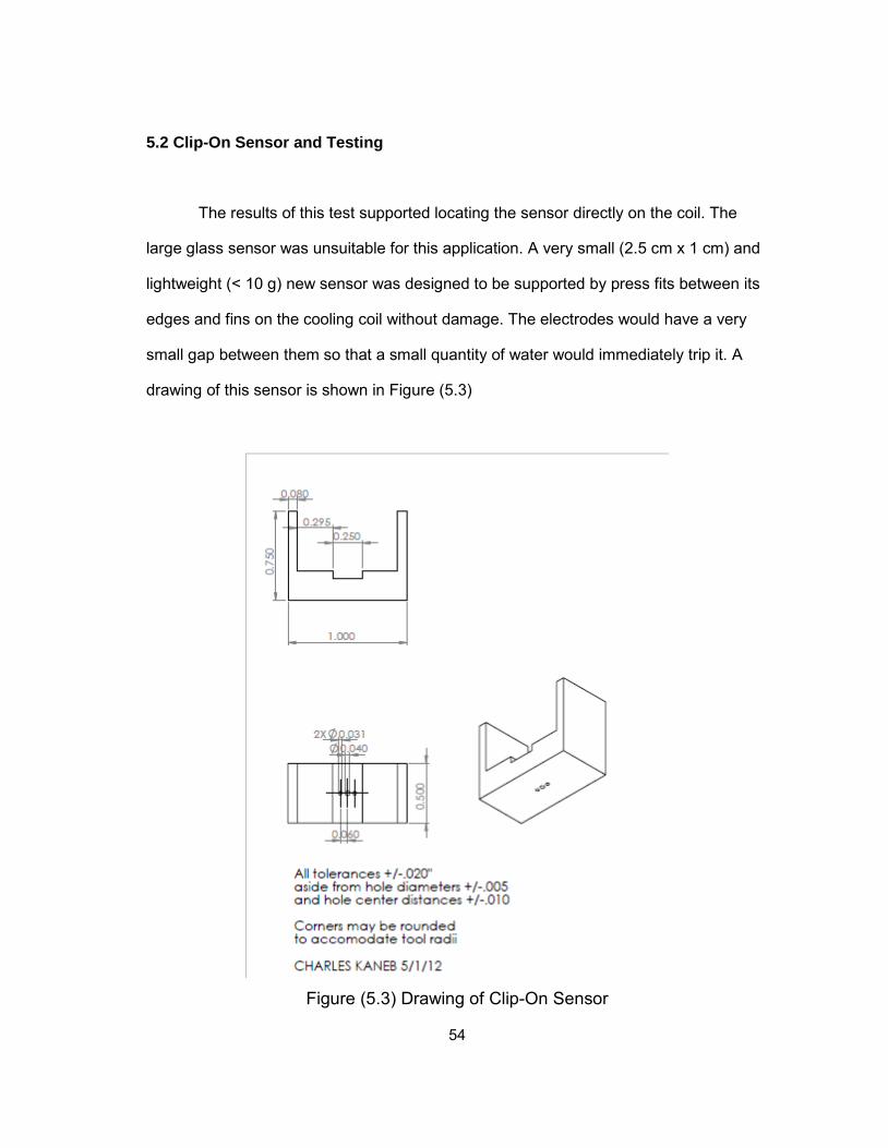
54

5.2 Clip-On Sensor and Testing

The results of this test supported locating the sensor directly on the coil. The

large glass sensor was unsuitable for this application. A very small (2.5 cm x 1 cm) and

lightweight (< 10 g) new sensor was designed to be supported by press fits between its

edges and fins on the cooling coil without damage. The electrodes would have a very

small gap between them so that a small quantity of water would immediately trip it. A

drawing of this sensor is shown in Figure (5.3)

Figure (5.3) Drawing of Clip-On Sensor

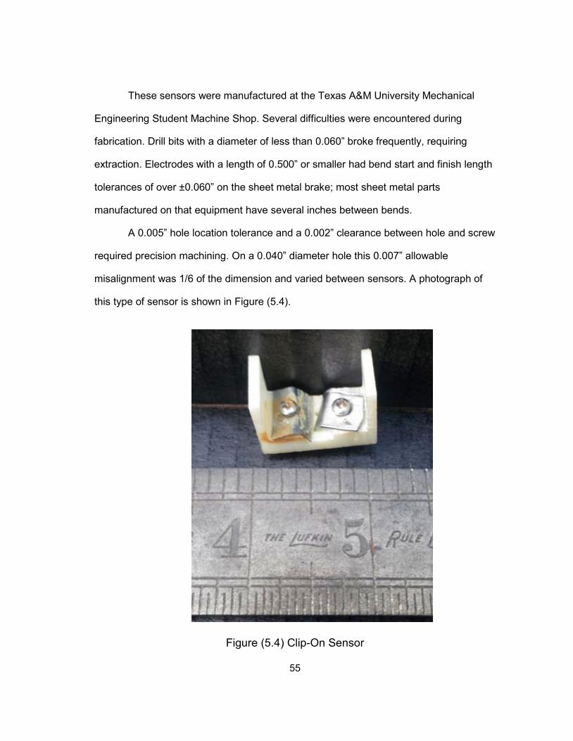
55

These sensors were manufactured at the Texas A&M University Mechanical

Engineering Student Machine Shop. Several difficulties were encountered during

fabrication. Drill bits with a diameter of less than 0.060” broke frequently, requiring

extraction. Electrodes with a length of 0.500” or smaller had bend start and finish length

tolerances of over ±0.060” on the sheet metal brake; most sheet metal parts

manufactured on that equipment have several inches between bends.

A 0.005” hole location tolerance and a 0.002” clearance between hole and screw

required precision machining. On a 0.040” diameter hole this 0.007” allowable

misalignment was 1/6 of the dimension and varied between sensors. A photograph of

this type of sensor is shown in Figure (5.4).

Figure (5.4) Clip-On Sensor

56

Preliminary measurements of the electrical properties were then measured

using a multimeter to guide the initial design of the sensor electronics. The glass

sensors had wet resistances of 1 MΩ - 10 MΩ, resulting in currents of a few hundred nA

when connected to a 5 V circuit. Circuit design to differentiate between a resistance this

large and an open circuit proved difficult. The small currents involved also made them

vulnerable to electromagnetic interference. Similar results were observed for the DC

resistance of the clip-on sensors. These problems meant that more precise

measurements were necessary.

A Fluke PM6303A LCR (Inductance (L), Capacitance (C), and Resistance (R))

meter was then used to evaluate the AC properties of these sensors. It was set to

operate at 1 kHz, passing current through the sensor and measuring its impedance and

phase angle. From these the meter was able to calculate the resistance and inductance

or capacitance of the device connected to its terminals. The tests were performed on

July 12, 2012 using 316 stainless steel electrodes on the sensor. The results are shown

in Table (5.1)

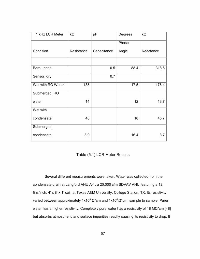
57

Table (5.1) LCR Meter Results

Several different measurements were taken. Water was collected from the

condensate drain at Langford AHU A-1, a 20,000 cfm SDVAV AHU featuring a 12

fins/inch, 4’ x 8’ x 1’ coil, at Texas A&M University, College Station, TX. Its resistivity

varied between approximately 1x103 Ω*cm and 1x106 Ω*cm sample to sample. Purer

water has a higher resistivity. Completely pure water has a resistivity of 18 MΩ*cm [48]

but absorbs atmospheric and surface impurities readily causing its resistivity to drop. It

1 kHz LCR Meter kΩ pF Degrees kΩ

Condition Resistance Capacitance

Phase

Angle Reactance

Bare Leads

0.5 88.4 318.6

Sensor, dry

0.7

Wet with RO Water 185

17.5 176.4

Submerged, RO

water 14

12 13.7

Wet with

condensate 48

18 45.7

Submerged,

condensate 3.9

16.4 3.7

58

was thought that water with a higher resistivity would be more difficult to detect, so

reverse osmosis water was obtained for testing. This water had resistivity in excess of 1

MΩ*cm. Results from these tests are shown in Table (5.1).

These properties showed clear differences in reactance between the dry and

wet states. Schmitt trigger oscillators giving a 1 kHz square wave output were then built,

and a PCB was iteratively developed with an oscillator, terminals for the sensor, an

averaging capacitor, and DC output terminals. The oscillator gave a square wave with a

peak of +10 V. Since the voltage needed to electrolyze water is 1.23 V, and electrolytic

cells for water operate on 1.8 - 2.2 V, electrolytic breakdown occurred between the

terminals, shown by bubbles of hydrogen and oxygen at the terminals when

submerged. This was sufficient to detect small quantities (< 1 cm3) of water and give a

DC output when the electrodes were bridged.

Many different combinations of electrodes were tested. Since these sensors

were expected to last several years in an air handling unit without service, the

electrodes needed to be capable of withstanding continuously wet conditions while

connected to power. Electrodes and electronics were tested by submerging the sensor

in a container of water while connected to power. Any continued visible corrosion, or

loss of electrical continuity, was considered a failure. Sheet metal electrodes were

secured to the sensor body and wiring with self-tapping screws. Stainless steel (316

austenitic alloy) and aluminum electrodes were fabricated from 22-gauge sheets and

tested. The 10 V difference across the sensor was enough to cause electrolytic

corrosion of at least one metallic component of the system. Since the standard

electrode potential of every metal is well below 5 V, conductors will be oxidized if they

operate in this application.

59

Difficulties were encountered with both the sensor electrodes and the wiring to

the anode. Stainless steel and aluminum form protective oxides, so these materials

were used for both electrodes and wiring, but continuous exposure to large electric

currents and water allowed continued corrosion. This allowed thick oxide layers to

continue to form, corroding the electrodes and forming a very effective electrical

insulation. Copper wires failed rapidly when submerged and exposed to current. All

combinations failed to give an acceptable life span in submerged tests. Corrosion was

visible within 72 hours on electrodes, fasteners, or wires.

The final attempt to operate this sensor featured an all-aluminum anode and an all-

316 stainless steel cathode, with the electrode, screw, and wire all made from the same

material. All submerged tests showed corrosion within one week, showing that a

completely new sensor design was necessary. This initial testing and development

identified the requirements and highlighted practical issues to be solved with a new

sensor design. The new sensor design is described in Section 6.

60

6. SENSOR DESIGN

A new “Coil Enthalpy Limit” sensor was designed and built based on the results

of testing prototypes and observations of operating conditions. The requirements are

summarized in the following “need statement”: A reliable, inexpensive, durable, and low

maintenance device is needed to detect the transition between the dry and wet cooling

coil states. To satisfy that description, the sensor had to satisfy the following list of

requirements:

1. It must have a life span of several years in a condensing environment.

2. It must be self-cleaning and operate autonomously without maintenance.

3. It must provide a 0 – 5 V DC output with a clear difference between wet and

dry states.

4. It must collect water from enough area on the coil to register a wet condition

when the dew point is reached. It must activate with less than 2 cm3 of water.

5. For active measurement of the mixed air dew point by incremental

adjustment of cooling coil leaving temperature, the coil state must change

and the sensor must respond within 3 minutes of the air crossing the dew

point. For operation as a high-limit economizer control, shutting off the

economizer when the coil becomes wet, the sensor and coil system must

respond within 10 minutes.

6. It must operate at a low voltage, below the voltage needed to harm

occupants or technicians.

7. It must operate at a low enough voltage to avoid corrosion.

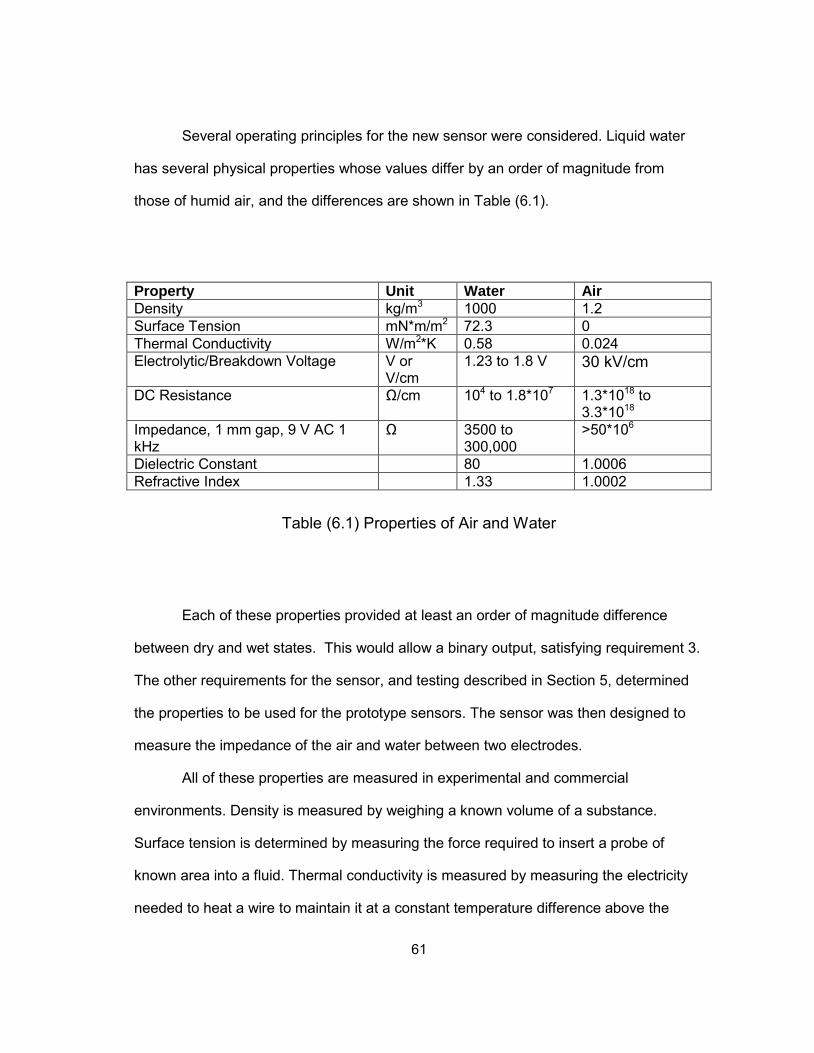
61

Several operating principles for the new sensor were considered. Liquid water

has several physical properties whose values differ by an order of magnitude from

those of humid air, and the differences are shown in Table (6.1).

Property Unit Water Air Density kg/m3 1000 1.2 Surface Tension mN*m/m2 72.3 0 Thermal Conductivity W/m2*K 0.58 0.024 Electrolytic/Breakdown Voltage V or

V/cm 1.23 to 1.8 V 30 kV/cm

DC Resistance Ω/cm 104 to 1.8*107 1.3*1018 to 3.3*1018

Impedance, 1 mm gap, 9 V AC 1 kHz

Ω 3500 to 300,000

>50*106

Dielectric Constant 80 1.0006 Refractive Index 1.33 1.0002

Table (6.1) Properties of Air and Water

Each of these properties provided at least an order of magnitude difference

between dry and wet states. This would allow a binary output, satisfying requirement 3.

The other requirements for the sensor, and testing described in Section 5, determined

the properties to be used for the prototype sensors. The sensor was then designed to

measure the impedance of the air and water between two electrodes.

All of these properties are measured in experimental and commercial

environments. Density is measured by weighing a known volume of a substance.

Surface tension is determined by measuring the force required to insert a probe of

known area into a fluid. Thermal conductivity is measured by measuring the electricity

needed to heat a wire to maintain it at a constant temperature difference above the

62

temperature of the flow. The impedance or dielectric constant can be measured by

determining the current produced by a known input voltage. Agilent Technologies [61]

states that “The unknown impedance (Zx) can be calculated from measured voltage

and current values. Current is calculated by using the voltage measurement across an

accurately known low value resistor (R).”

The difficulty of measuring density, surface tension, thermal conductivity, or

electrolytic breakdown voltage using a device capable of lasting several years in a

condensing environment removed these properties from consideration. Measurement of

thermal conductivity is used in hot wire anemometry, and Lomas [62] stated that “It has

been said that one remains a novice in hot wire anemometry until the first probe has

been broken, and whether or not this is true, probe breakage is so common that a quick

and easy method of repair is desirable.” Measuring the breakdown voltage required a

potential difference between submerged electrodes greater than the 1.23 V needed to

break down water, causing corrosion of the electrodes as discussed in Section 5. The

change in the refractive index was used by the existing chilled mirror sensors, with

prices of $2570 [35] or more.

Resistivity and the dielectric constant could be measured by the use of

stationary electrodes with potential differences of 0.25 V. One sensor was then

designed that could measure either the dielectric constant or the resistivity of the water

or air in the gap between electrodes, depending on whether the plates were insulated.

The resistivity of impure water, including the coil condensate detected by this sensor, is

several orders of magnitude smaller than that of pure water, as dissolved metallic salts

conduct electricity by motion of ions. The dielectric constant of water is 80, while that of

air is 1.005.

63

The design of this “Coil Enthalpy Limit” sensor was dependent on the

electrochemical properties of available conductors and the flow rate of condensate

available to be collected on the electrodes. The quantity of condensate that could be

collected from the cooling coil was then calculated and used to determine the size and

position of electrodes that would meet the response and reliability requirements. With

the size, properties, and spacing of the electrodes known, the electrical properties of the

sensor were then calculated. The body of the sensor was then designed to hold the

electrodes at the separation and angle required by the desired electrical properties and

to meet the need for the sensor to be self-cleaning.

6.1 Electrical and Chemical Design

6.1.1 Corrosion Avoidance

The electrodes used for the impedance sensor were expected to pass between

1 µA and 100 µA of current through water in the gap. In order to meet the durability

requirements, the corrosion at the anode that was experienced (see Section 5.2 for

details) had to be avoided. Connections from the electronics to the sensor would have

to be completely sealed to avoid galvanic corrosion at junctions between the copper

wires and the electrodes. Crimp-on terminals were welded to the sensing plates and the

junction with the wire was then sealed.

Sensor failure from corrosion can occur by creation of an oxide layer with

insufficient conductivity, creation of an oxide layer which flakes off, or electrochemical

corrosion. Stainless steel sheet electrodes, 316 alloy, with a 0.25 V potential difference

64

across the gap avoid all three types of failure and allow the sensor to meet requirement

1, lasting a three-month test in a building as a prototype.

Stainless steel electrodes provide adequate conductivity when corroded to allow

a sensor to continue to operate. The resistivity of iron oxides at 300° K ranges from 6.07

* 10-3 Ω*cm for Fe3O4 to 2.5 * 10-1 Ω*cm for Fe2O3 [63], while the resistivity of aluminum

oxide is 1 * 1014 Ω*cm [64]. An additional resistance of 100 kΩ on a sensing area of 1

cm2 of aluminum only requires a 100 nm thick layer of aluminum oxide, while an iron

oxide layer with the same thickness would have a resistance of 0.25 µΩ. Therefore, if

oxidation could be stopped after a protective layer, steel or 316 stainless steel would be

suitable for the electrodes.

The metal used for the sensor plate needed to form a passive oxide layer to

avoid further corrosion. The main criterion for this is the Pilling-Bedworth ratio R, the

ratio of the volume of a metal oxide to the volume of the metal that was used to create

the oxide layer. According to McCafferty [65] “Metals which are normally passive have

values of R between 1 and 2.” Aluminum has a Pilling-Bedworth ratio of 1.28, allowing it

to form a protective oxide layer, while carbon steel has a ratio of 2.1 - 2.14, causing rust

to flake off. The chromium in 316 stainless steel gives it a Pilling-Bedworth ratio of 2.00

and a protective oxide layer that prevents further corrosion. Austenitic 316 stainless

steel was chosen to meet the longevity requirement.

Electrochemical corrosion occurs when the potential difference across a pair of

electrodes submerged in water is larger than the standard electrode potential of the

reaction between the anode material and its oxide. “Corrosion involves the destructive

attack of metal by chemical or electrochemical reaction with its environment. Usually

corrosion consists of a set of redox reactions that are electrochemical in nature. The

metal is oxidized to corrosion products [66] at anodic sites: M ⇔ M+2 + 2 e-.” The

65

standard electrode potential between iron and the iron (II) ion is 0.44 V, and a sensing

voltage lower than this will avoid ionization and electrochemical corrosion. Once the

voltage needed to cause corrosion is exceeded, the rate of corrosion is dependent on

the current passing through the electrode into the electrolyte. A potential difference of

0.25 V between the 316 stainless steel electrodes was selected to avoid

electrochemical corrosion.

In order to register a “wet” state only when water was condensing on the coil,

water on the sensor plates had to be cleared off by gravity. Rame-Hart Instrument Corp.

[50] describes the angle necessary to have drops roll off a plate: “The tilting plate

method captures the contact angles measurements on both the left and right sides of a

sessile drop while the solid surface is being inclined typically from 0° to 90°. As the

surface is inclined, gravity causes the contact angle on the downhill side to increase

while the contact angle on the uphill side decreases. Respectively, these contact angles

are referred to as advancing and receding angles. The difference between them is the

contact angle hysteresis. In some cases, the drop will roll off the solid as wetting occurs

at the roll-off angle. The last valid readings are captured and normally represent the

advancing and receding contact angles. In some cases, the solid can tilt all the way

to 90° without the drop releasing. The final left and right contact angles are used.”

A drawing of the angle necessary to allow runoff, given by Rame-Hart, is shown

in Figure (6.1). The contact angles for water on stainless steels were between 37° and

43° [67], and a 60° plate angle from horizontal was chosen in order to ensure runoff

from the surfaces. Drops between 0.1 ml and 2 ml ran off when water was dripped on a

sheet of 316 stainless steel held at this angle. In order to meet requirements 1, 2, and 3,

the sensor body had to hold stainless steel plates at a 60° angle, and the electronics

had to supply 0.25 V.

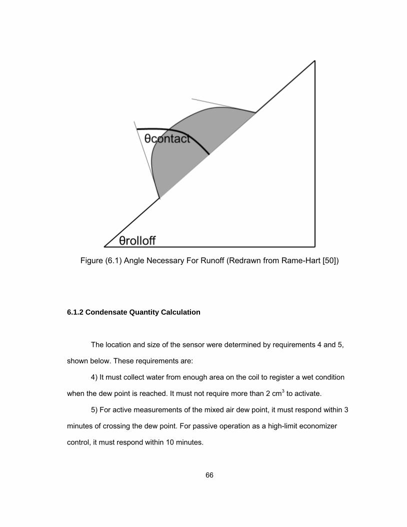
66

Figure (6.1) Angle Necessary For Runoff (Redrawn from Rame-Hart [50])

6.1.2 Condensate Quantity Calculation

The location and size of the sensor were determined by requirements 4 and 5,

shown below. These requirements are:

4) It must collect water from enough area on the coil to register a wet condition

when the dew point is reached. It must not require more than 2 cm3 to activate.

5) For active measurements of the mixed air dew point, it must respond within 3

minutes of crossing the dew point. For passive operation as a high-limit economizer

control, it must respond within 10 minutes.

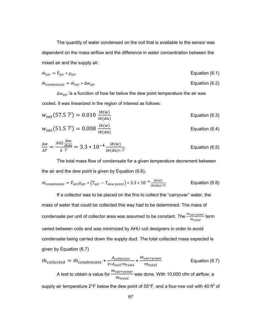
67

The quantity of water condensed on the coil that is available to the sensor was

dependent on the mass airflow and the difference in water concentration between the

mixed air and the supply air.

𝑎𝑖𝑟 = 𝑎𝑖𝑟 ∗ 𝜌𝑎𝑖𝑟 Equation (6.1)

𝑐𝑜𝑛𝑑𝑒𝑛𝑠𝑎𝑡𝑒 = 𝑎𝑖𝑟 ∗ ∆𝑤𝑎𝑖𝑟 Equation (6.2)

∆𝑤𝑎𝑖𝑟 is a function of how far below the dew point temperature the air was

cooled. It was linearized in the region of interest as follows:

𝑤𝑠𝑎𝑡(57.5) = 0.010 𝑙𝑏(𝑤)𝑙𝑏(𝑑𝑎)

Equation (6.3)

𝑤𝑠𝑎𝑡(51.5) = 0.008 𝑙𝑏(𝑤)𝑙𝑏(𝑑𝑎)

Equation (6.4)

∆𝑤∆𝑇

=.002 𝑙𝑏𝑤𝑙𝑏𝑑𝑎6

= 3.3 ∗ 10−4 𝑙𝑏(𝑤)𝑙𝑏(𝑑𝑎)∗

Equation (6.5)

The total mass flow of condensate for a given temperature decrement between

the air and the dew point is given by Equation (6.6).

𝑐𝑜𝑛𝑑𝑒𝑛𝑠𝑎𝑡𝑒 = 𝑎𝑖𝑟𝜌𝑎𝑖𝑟 ∗ 𝑇𝑎𝑖𝑟 − 𝑇𝑑𝑒𝑤 𝑝𝑜𝑖𝑛𝑡 ∗ 3.3 ∗ 10−4 𝑙𝑏(𝑤)𝑙𝑏(𝑑𝑎)∗

Equation (6.6)

If a collector was to be placed on the fins to collect the “carryover” water, the

mass of water that could be collected this way had to be determined. The mass of

condensate per unit of collector area was assumed to be constant. The 𝑚𝑐𝑎𝑟𝑟𝑦𝑜𝑣𝑒𝑟

𝑚𝑡𝑜𝑡𝑎𝑙 term

varied between coils and was minimized by AHU coil designers in order to avoid

condensate being carried down the supply duct. The total collected mass expected is

given by Equation (6.7)

𝑐𝑜𝑙𝑙𝑒𝑐𝑡𝑒𝑑 = 𝑐𝑜𝑛𝑑𝑒𝑛𝑠𝑎𝑡𝑒 ∗𝐴𝑐𝑜𝑙𝑙𝑒𝑐𝑡𝑜𝑟

2∗𝐴𝑐𝑜𝑖𝑙∗𝑛𝑟𝑜𝑤𝑠∗ 𝑚𝑐𝑎𝑟𝑟𝑦𝑜𝑣𝑒𝑟

𝑚𝑡𝑜𝑡𝑎𝑙 Equation (6.7)

A test to obtain a value for 𝑚𝑐𝑎𝑟𝑟𝑦𝑜𝑣𝑒𝑟

𝑚𝑡𝑜𝑡𝑎𝑙 was done. With 10,000 cfm of airflow, a

supply air temperature 2°F below the dew point of 55°F, and a four-row coil with 40 ft2 of

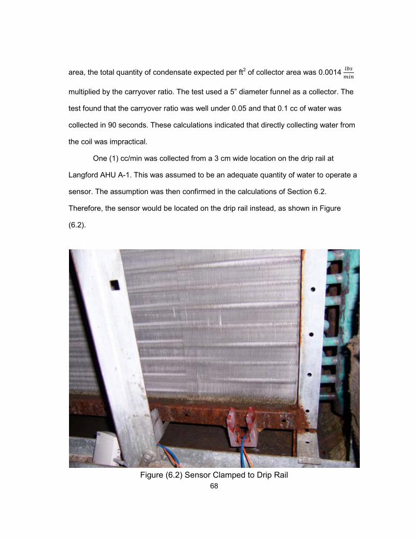
68

area, the total quantity of condensate expected per ft2 of collector area was 0.0014 𝑙𝑏𝑠𝑚𝑖𝑛

multiplied by the carryover ratio. The test used a 5” diameter funnel as a collector. The

test found that the carryover ratio was well under 0.05 and that 0.1 cc of water was

collected in 90 seconds. These calculations indicated that directly collecting water from

the coil was impractical.

One (1) cc/min was collected from a 3 cm wide location on the drip rail at

Langford AHU A-1. This was assumed to be an adequate quantity of water to operate a

sensor. The assumption was then confirmed in the calculations of Section 6.2.

Therefore, the sensor would be located on the drip rail instead, as shown in Figure

(6.2).

Figure (6.2) Sensor Clamped to Drip Rail

69

6.2 Resistance Calculations

The electrical properties for this sensor were calculated for measurement of both

impedance and dielectric constant. Measuring impedance required the 316 stainless

steel sensing plates to be exposed to the air and water, while dielectric constant

measurements were made by encapsulating the plates with a varnish that had a

dielectric strength of 1700 V/mil. Bench tests showed that the varnished sensor failed to

return to its dry capacitance in ambient (75°F, 50% RH) conditions, and only the

resistive impedance sensor was used for further testing. To pass currents of more than

1 µA and avoid noise with a 0.25 V input, the plates and the area in contact with water

had to be large enough to give an impedance of less than 250 kΩ when wet.

Electrical properties of an impedance sensor depended on the size and shape of

the gap between conductors and the resistivity of the substance filling the gap. The

resistivity of the relevant materials is given in Table (6.2).

Material Resistivity (Ω*cm)

Copper 0.00000168 316 Stainless Steel 0.000069 Water (Condensate)

1000-100,000 Water (Pure) 18,000,000 Air 3*10

18 Table (6.2) Resistivity of Materials

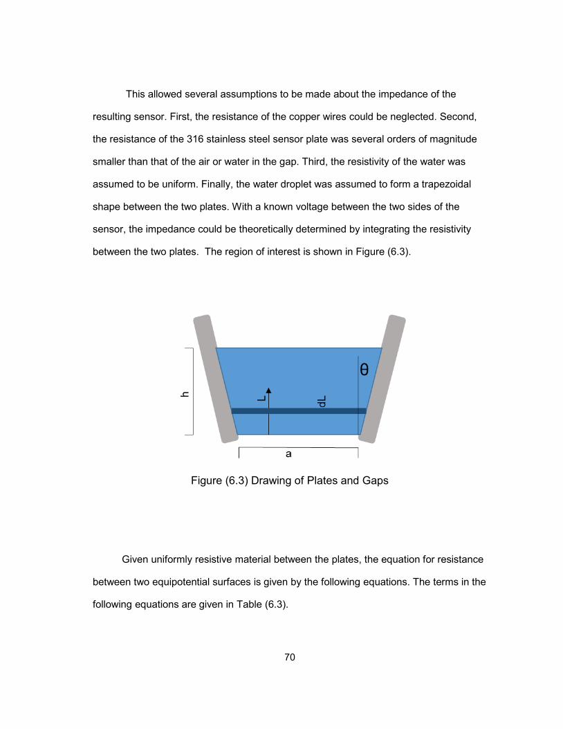
70

This allowed several assumptions to be made about the impedance of the

resulting sensor. First, the resistance of the copper wires could be neglected. Second,

the resistance of the 316 stainless steel sensor plate was several orders of magnitude

smaller than that of the air or water in the gap. Third, the resistivity of the water was

assumed to be uniform. Finally, the water droplet was assumed to form a trapezoidal

shape between the two plates. With a known voltage between the two sides of the

sensor, the impedance could be theoretically determined by integrating the resistivity

between the two plates. The region of interest is shown in Figure (6.3).

Figure (6.3) Drawing of Plates and Gaps

Given uniformly resistive material between the plates, the equation for resistance

between two equipotential surfaces is given by the following equations. The terms in the

following equations are given in Table (6.3).

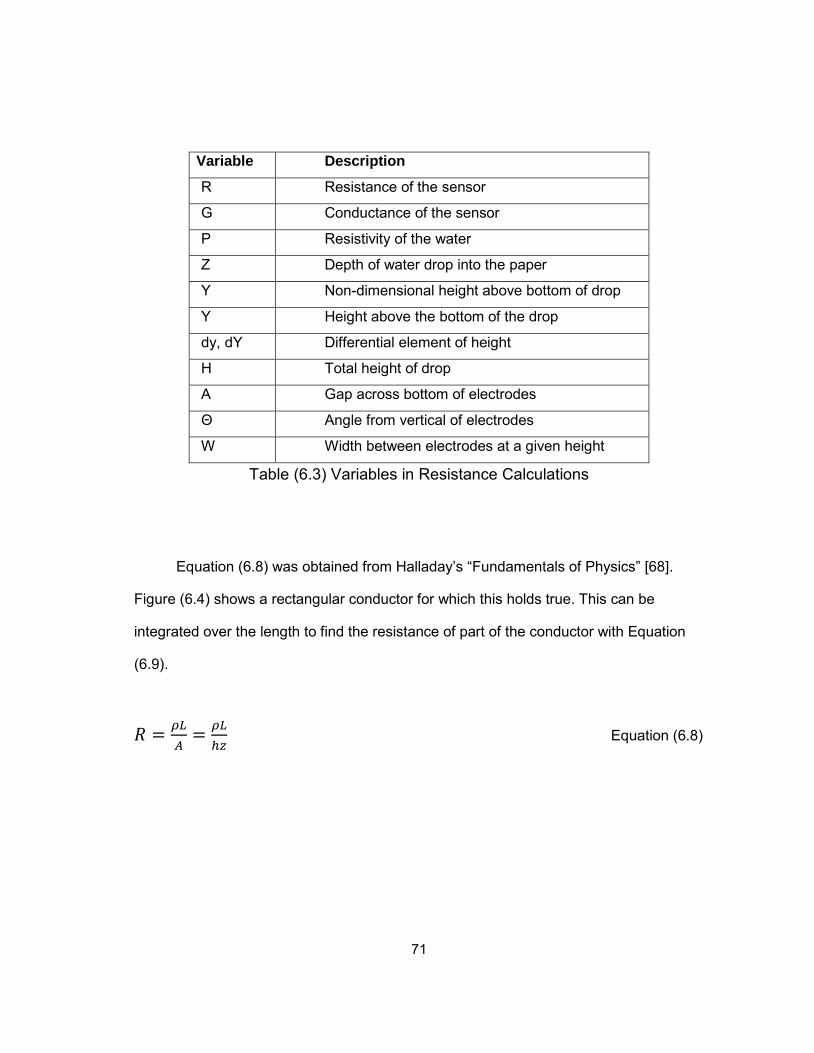
71

Variable Description

R Resistance of the sensor

G Conductance of the sensor

Ρ Resistivity of the water

Z Depth of water drop into the paper

Y Non-dimensional height above bottom of drop

Y Height above the bottom of the drop

dy, dY Differential element of height

H Total height of drop

A Gap across bottom of electrodes

Θ Angle from vertical of electrodes

W Width between electrodes at a given height

Table (6.3) Variables in Resistance Calculations

Equation (6.8) was obtained from Halladay’s “Fundamentals of Physics” [68].

Figure (6.4) shows a rectangular conductor for which this holds true. This can be

integrated over the length to find the resistance of part of the conductor with Equation

(6.9).

𝑅 = 𝜌𝐿𝐴

= 𝜌𝐿ℎ𝑧

Equation (6.8)

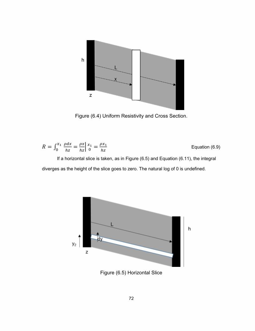
72

Figure (6.4) Uniform Resistivity and Cross Section.

𝑅 = ∫ 𝜌𝑑𝑥ℎ𝑧

𝑥10 = 𝜌𝑥

ℎ𝑧 𝑥10 = 𝜌𝑥1

ℎ𝑧 Equation (6.9)

If a horizontal slice is taken, as in Figure (6.5) and Equation (6.11), the integral

diverges as the height of the slice goes to zero. The natural log of 0 is undefined.

Figure (6.5) Horizontal Slice

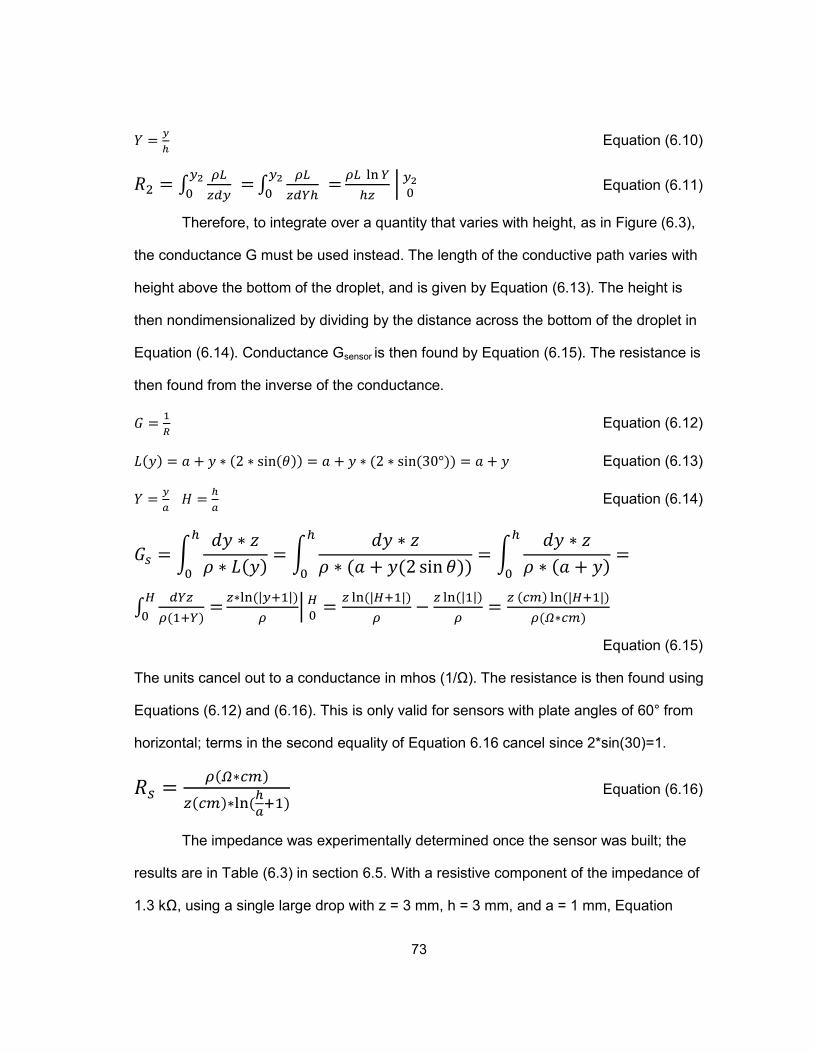
73

𝑌 = 𝑦ℎ Equation (6.10)

𝑅2 = ∫ 𝜌𝐿𝑧𝑑𝑦

=𝑦20 ∫ 𝜌𝐿

𝑧𝑑𝑌ℎ =𝑦2

0𝜌𝐿 ln 𝑌ℎ𝑧

𝑦20 Equation (6.11)

Therefore, to integrate over a quantity that varies with height, as in Figure (6.3),

the conductance G must be used instead. The length of the conductive path varies with

height above the bottom of the droplet, and is given by Equation (6.13). The height is

then nondimensionalized by dividing by the distance across the bottom of the droplet in

Equation (6.14). Conductance Gsensor is then found by Equation (6.15). The resistance is

then found from the inverse of the conductance.

𝐺 = 1𝑅 Equation (6.12)

𝐿(𝑦) = 𝑎 + 𝑦 ∗ (2 ∗ sin(𝜃)) = 𝑎 + 𝑦 ∗ (2 ∗ sin(30°)) = 𝑎 + 𝑦 Equation (6.13)

𝑌 = 𝑦𝑎 𝐻 = ℎ

𝑎 Equation (6.14)

𝐺𝑠 = 𝑑𝑦 ∗ 𝑧𝜌 ∗ 𝐿(𝑦) =

𝑑𝑦 ∗ 𝑧𝜌 ∗ (𝑎 + 𝑦(2 sin𝜃)) =

𝑑𝑦 ∗ 𝑧𝜌 ∗ (𝑎 + 𝑦) =

ℎ

0

ℎ

0

ℎ

0

∫ 𝑑𝑌𝑧𝜌(1+𝑌)

=𝐻0

𝑧∗ln (|𝑦+1|)𝜌

𝐻0 = 𝑧 ln(|𝐻+1|)𝜌

− 𝑧 ln(|1|)𝜌

= 𝑧 (𝑐𝑚) ln(|𝐻+1|)𝜌(𝛺∗𝑐𝑚)

Equation (6.15)

The units cancel out to a conductance in mhos (1/Ω). The resistance is then found using

Equations (6.12) and (6.16). This is only valid for sensors with plate angles of 60° from

horizontal; terms in the second equality of Equation 6.16 cancel since 2*sin(30)=1.

𝑅𝑠 = 𝜌(𝛺∗𝑐𝑚)

𝑧(𝑐𝑚)∗ln(ℎ𝑎+1) Equation (6.16)

The impedance was experimentally determined once the sensor was built; the

results are in Table (6.3) in section 6.5. With a resistive component of the impedance of

1.3 kΩ, using a single large drop with z = 3 mm, h = 3 mm, and a = 1 mm, Equation

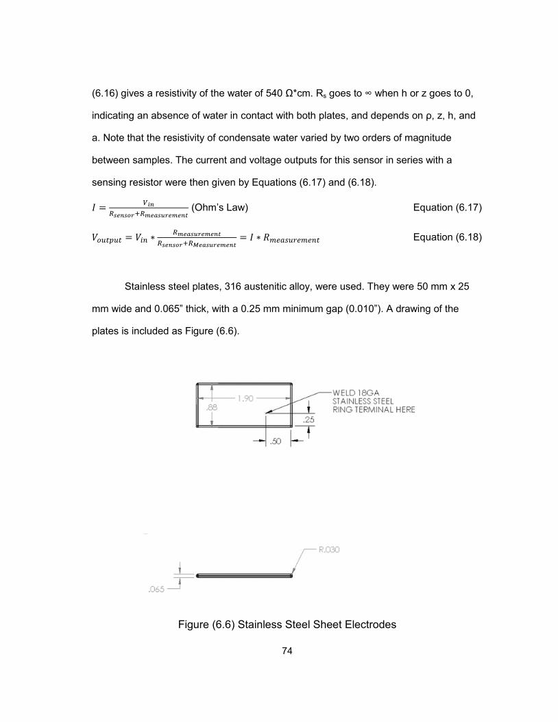
74

(6.16) gives a resistivity of the water of 540 Ω*cm. Rs goes to ∞ when h or z goes to 0,

indicating an absence of water in contact with both plates, and depends on ρ, z, h, and

a. Note that the resistivity of condensate water varied by two orders of magnitude

between samples. The current and voltage outputs for this sensor in series with a

sensing resistor were then given by Equations (6.17) and (6.18).

𝐼 = 𝑉𝑖𝑛𝑅𝑠𝑒𝑛𝑠𝑜𝑟+𝑅𝑚𝑒𝑎𝑠𝑢𝑟𝑒𝑚𝑒𝑛𝑡

(Ohm’s Law) Equation (6.17)

𝑉𝑜𝑢𝑡𝑝𝑢𝑡 = 𝑉𝑖𝑛 ∗𝑅𝑚𝑒𝑎𝑠𝑢𝑟𝑒𝑚𝑒𝑛𝑡

𝑅𝑠𝑒𝑛𝑠𝑜𝑟+𝑅𝑀𝑒𝑎𝑠𝑢𝑟𝑒𝑚𝑒𝑛𝑡= 𝐼 ∗ 𝑅𝑚𝑒𝑎𝑠𝑢𝑟𝑒𝑚𝑒𝑛𝑡 Equation (6.18)

Stainless steel plates, 316 austenitic alloy, were used. They were 50 mm x 25

mm wide and 0.065” thick, with a 0.25 mm minimum gap (0.010”). A drawing of the

plates is included as Figure (6.6).

Figure (6.6) Stainless Steel Sheet Electrodes

75

6.3 Mechanical and Assembly Design

A clamping system was required to secure the plates in a location where water

could be gathered from the coil. The plates needed to be secured to the sensor body

while maintaining a constant gap at the bottom. The sensor needed to be drained by

either gravity or by the airflow coming through the sensor body. Finally, the sensor

needed to be clamped to the cooling coil drip rail.

After an unsuccessful attempt to build sensors with a “straight-grooved” clamp at

the top of the body, the clamps were redesigned to provide flat, angled clamping faces.

High-density polypropylene was chosen for the sensor body due to its resistance to

polar solvents such as condensate water, compressive strength of 6000 psi, and tensile

strength of 4800 psi.

In order to prevent movement of the plates, at least 10 lbs of friction force was

required between the plates and the body of the sensor. This is shown in the free body

diagram of the plate, Figure (6.7).

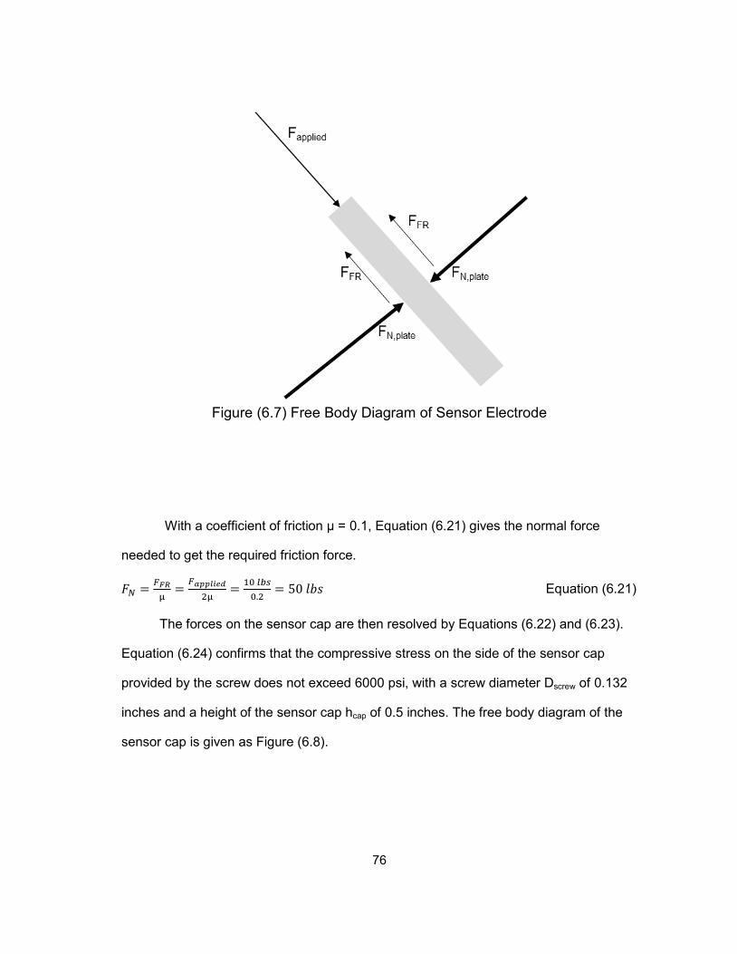
76

Figure (6.7) Free Body Diagram of Sensor Electrode

With a coefficient of friction µ = 0.1, Equation (6.21) gives the normal force

needed to get the required friction force.

𝐹𝑁 = 𝐹𝐹𝑅µ

= 𝐹𝑎𝑝𝑝𝑙𝑖𝑒𝑑2µ

= 10 𝑙𝑏𝑠0.2

= 50 𝑙𝑏𝑠 Equation (6.21)

The forces on the sensor cap are then resolved by Equations (6.22) and (6.23).

Equation (6.24) confirms that the compressive stress on the side of the sensor cap

provided by the screw does not exceed 6000 psi, with a screw diameter Dscrew of 0.132

inches and a height of the sensor cap hcap of 0.5 inches. The free body diagram of the

sensor cap is given as Figure (6.8).

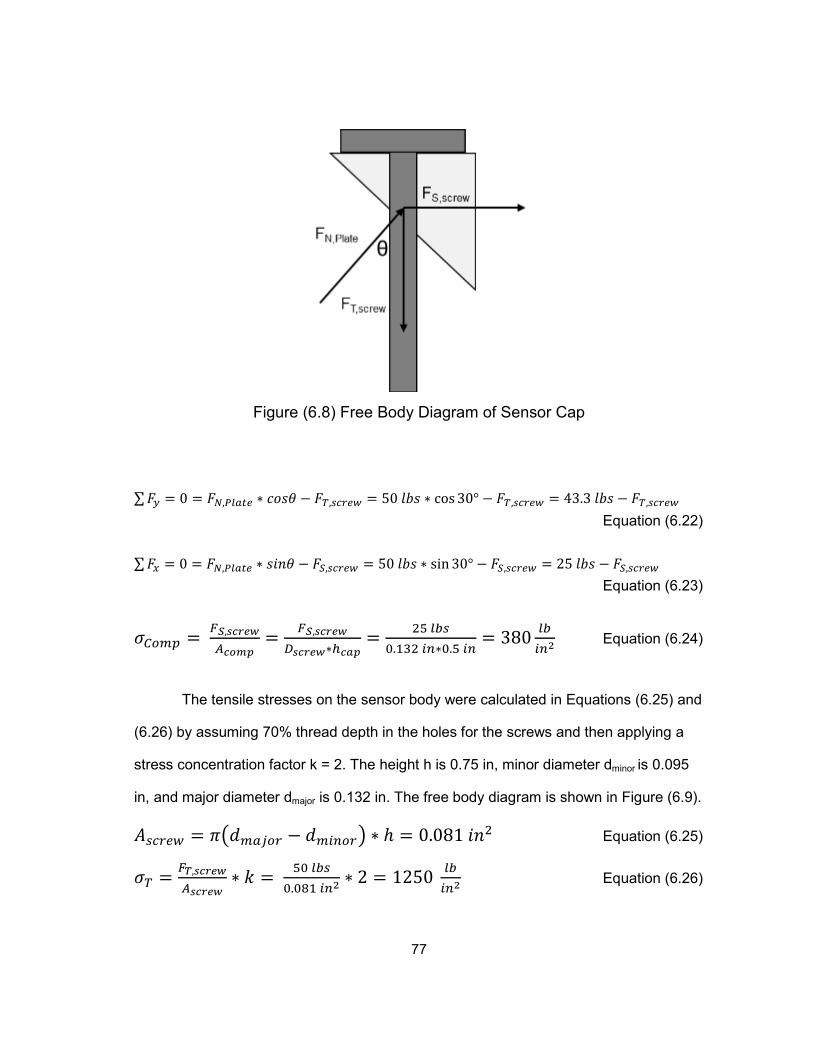
77

Figure (6.8) Free Body Diagram of Sensor Cap ∑𝐹𝑦 = 0 = 𝐹𝑁,𝑃𝑙𝑎𝑡𝑒 ∗ 𝑐𝑜𝑠𝜃 − 𝐹𝑇,𝑠𝑐𝑟𝑒𝑤 = 50 𝑙𝑏𝑠 ∗ cos 30° − 𝐹𝑇,𝑠𝑐𝑟𝑒𝑤 = 43.3 𝑙𝑏𝑠 − 𝐹𝑇,𝑠𝑐𝑟𝑒𝑤 Equation (6.22) ∑𝐹𝑥 = 0 = 𝐹𝑁,𝑃𝑙𝑎𝑡𝑒 ∗ 𝑠𝑖𝑛𝜃 − 𝐹𝑆,𝑠𝑐𝑟𝑒𝑤 = 50 𝑙𝑏𝑠 ∗ sin 30° − 𝐹𝑆,𝑠𝑐𝑟𝑒𝑤 = 25 𝑙𝑏𝑠 − 𝐹𝑆,𝑠𝑐𝑟𝑒𝑤 Equation (6.23)

𝜎𝐶𝑜𝑚𝑝 = 𝐹𝑆,𝑠𝑐𝑟𝑒𝑤

𝐴𝑐𝑜𝑚𝑝= 𝐹𝑆,𝑠𝑐𝑟𝑒𝑤

𝐷𝑠𝑐𝑟𝑒𝑤∗ℎ𝑐𝑎𝑝= 25 𝑙𝑏𝑠

0.132 𝑖𝑛∗0.5 𝑖𝑛= 380 𝑙𝑏

𝑖𝑛2 Equation (6.24)

The tensile stresses on the sensor body were calculated in Equations (6.25) and

(6.26) by assuming 70% thread depth in the holes for the screws and then applying a

stress concentration factor k = 2. The height h is 0.75 in, minor diameter dminor is 0.095

in, and major diameter dmajor is 0.132 in. The free body diagram is shown in Figure (6.9).

𝐴𝑠𝑐𝑟𝑒𝑤 = 𝜋𝑑𝑚𝑎𝑗𝑜𝑟 − 𝑑𝑚𝑖𝑛𝑜𝑟 ∗ ℎ = 0.081 𝑖𝑛2 Equation (6.25)

𝜎𝑇 = 𝐹𝑇,𝑠𝑐𝑟𝑒𝑤

𝐴𝑠𝑐𝑟𝑒𝑤∗ 𝑘 = 50 𝑙𝑏𝑠

0.081 𝑖𝑛2∗ 2 = 1250 𝑙𝑏

𝑖𝑛2 Equation (6.26)

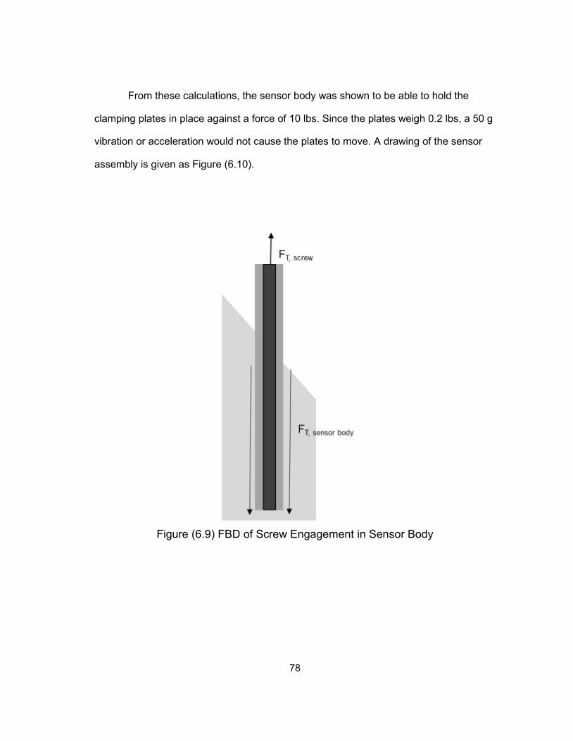
78

From these calculations, the sensor body was shown to be able to hold the

clamping plates in place against a force of 10 lbs. Since the plates weigh 0.2 lbs, a 50 g

vibration or acceleration would not cause the plates to move. A drawing of the sensor

assembly is given as Figure (6.10).

Figure (6.9) FBD of Screw Engagement in Sensor Body

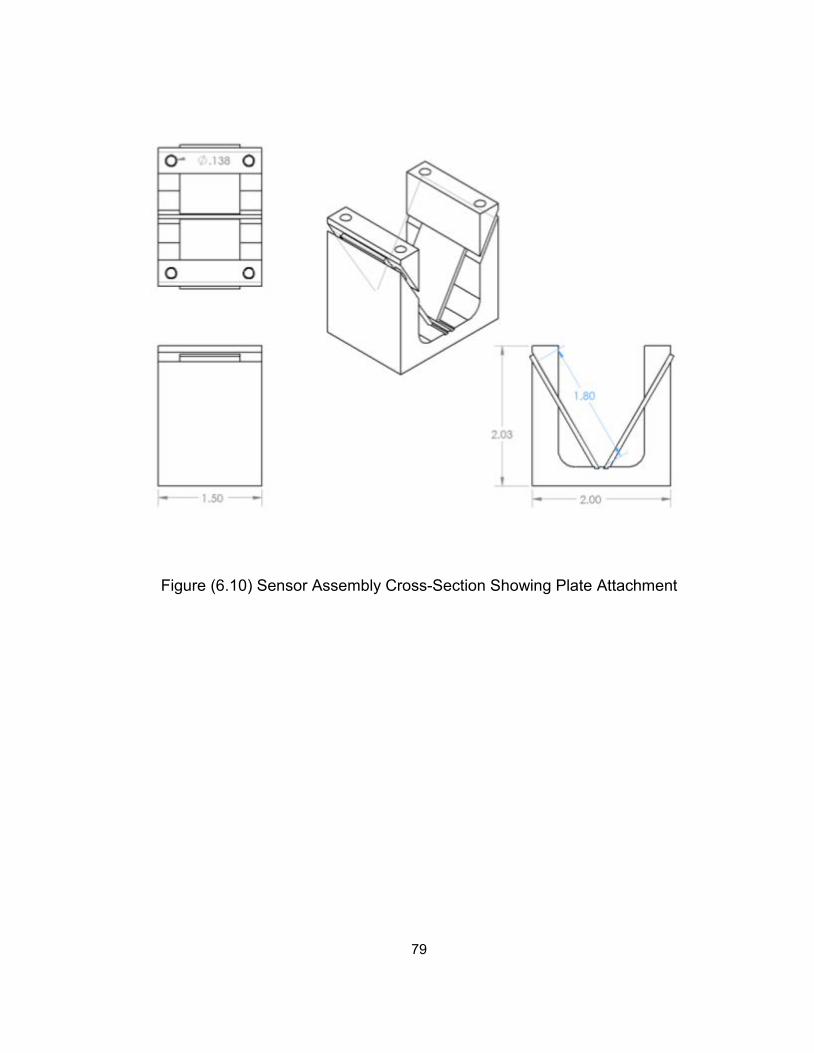
79

Figure (6.10) Sensor Assembly Cross-Section Showing Plate Attachment

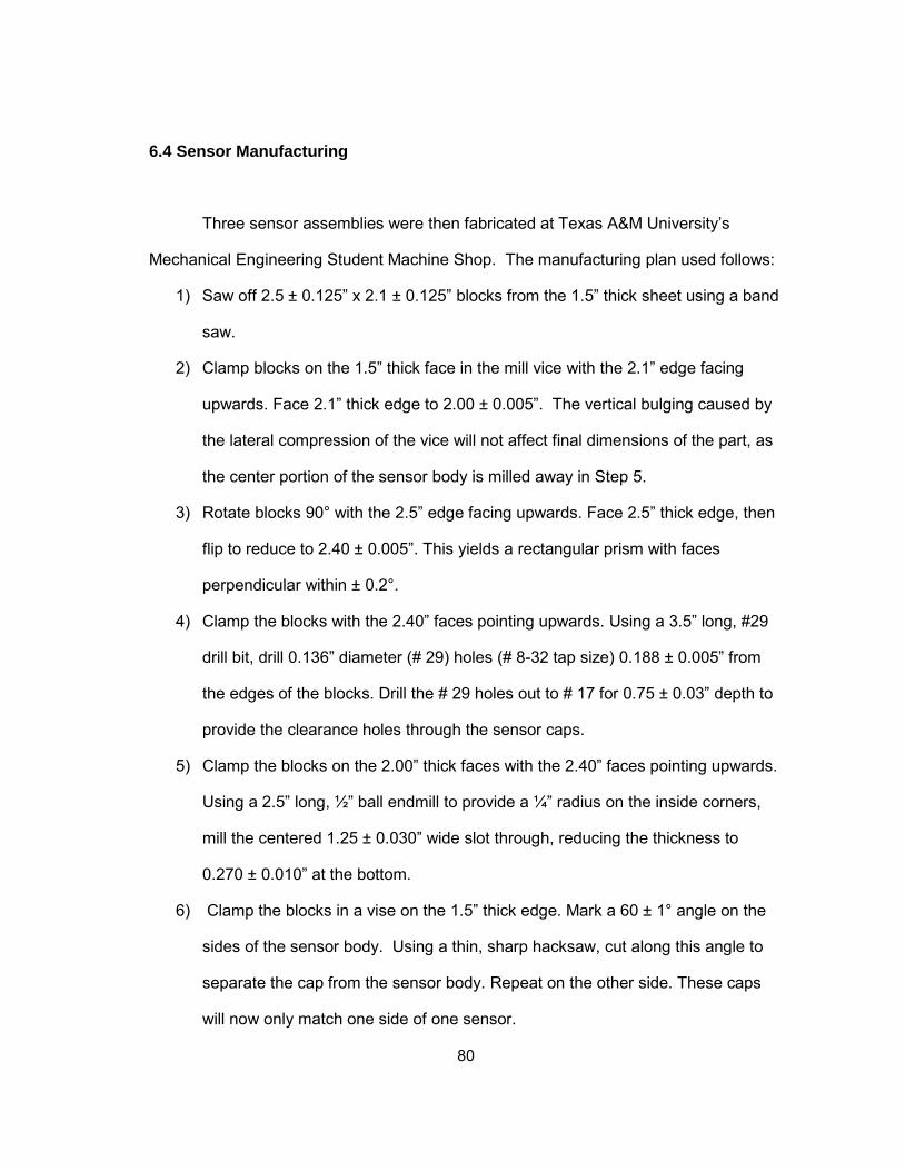
80

6.4 Sensor Manufacturing

Three sensor assemblies were then fabricated at Texas A&M University’s

Mechanical Engineering Student Machine Shop. The manufacturing plan used follows:

1) Saw off 2.5 ± 0.125” x 2.1 ± 0.125” blocks from the 1.5” thick sheet using a band

saw.

2) Clamp blocks on the 1.5” thick face in the mill vice with the 2.1” edge facing

upwards. Face 2.1” thick edge to 2.00 ± 0.005”. The vertical bulging caused by

the lateral compression of the vice will not affect final dimensions of the part, as

the center portion of the sensor body is milled away in Step 5.

3) Rotate blocks 90° with the 2.5” edge facing upwards. Face 2.5” thick edge, then

flip to reduce to 2.40 ± 0.005”. This yields a rectangular prism with faces

perpendicular within ± 0.2°.

4) Clamp the blocks with the 2.40” faces pointing upwards. Using a 3.5” long, #29

drill bit, drill 0.136” diameter (# 29) holes (# 8-32 tap size) 0.188 ± 0.005” from

the edges of the blocks. Drill the # 29 holes out to # 17 for 0.75 ± 0.03” depth to

provide the clearance holes through the sensor caps.

5) Clamp the blocks on the 2.00” thick faces with the 2.40” faces pointing upwards.

Using a 2.5” long, ½” ball endmill to provide a ¼” radius on the inside corners,

mill the centered 1.25 ± 0.030” wide slot through, reducing the thickness to

0.270 ± 0.010” at the bottom.

6) Clamp the blocks in a vise on the 1.5” thick edge. Mark a 60 ± 1° angle on the

sides of the sensor body. Using a thin, sharp hacksaw, cut along this angle to

separate the cap from the sensor body. Repeat on the other side. These caps

will now only match one side of one sensor.

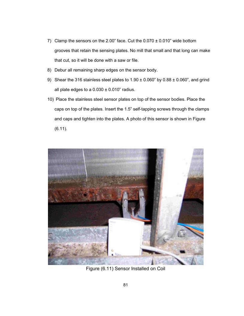
81

7) Clamp the sensors on the 2.00” face. Cut the 0.070 ± 0.010” wide bottom

grooves that retain the sensing plates. No mill that small and that long can make

that cut, so it will be done with a saw or file.

8) Debur all remaining sharp edges on the sensor body.

9) Shear the 316 stainless steel plates to 1.90 ± 0.060” by 0.88 ± 0.060”, and grind

all plate edges to a 0.030 ± 0.010” radius.

10) Place the stainless steel sensor plates on top of the sensor bodies. Place the

caps on top of the plates. Insert the 1.5” self-tapping screws through the clamps

and caps and tighten into the plates. A photo of this sensor is shown in Figure

(6.11).

Figure (6.11) Sensor Installed on Coil

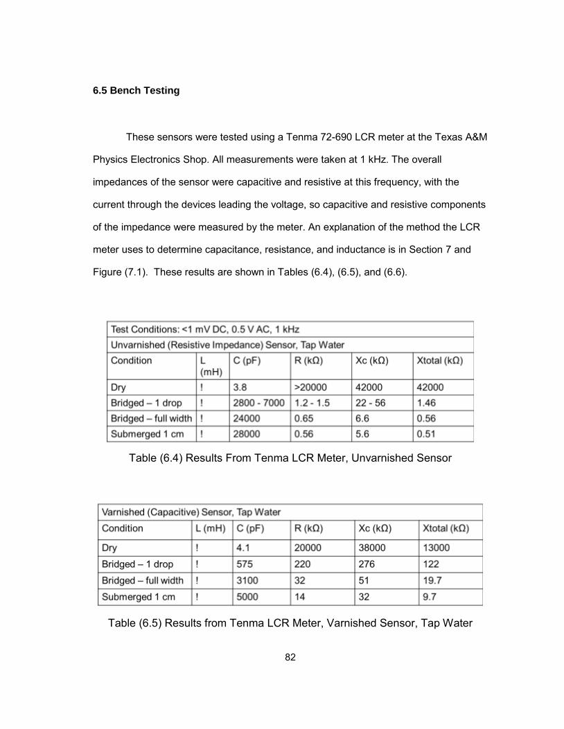
82

6.5 Bench Testing

These sensors were tested using a Tenma 72-690 LCR meter at the Texas A&M

Physics Electronics Shop. All measurements were taken at 1 kHz. The overall

impedances of the sensor were capacitive and resistive at this frequency, with the

current through the devices leading the voltage, so capacitive and resistive components

of the impedance were measured by the meter. An explanation of the method the LCR

meter uses to determine capacitance, resistance, and inductance is in Section 7 and

Figure (7.1). These results are shown in Tables (6.4), (6.5), and (6.6).

Table (6.4) Results From Tenma LCR Meter, Unvarnished Sensor

Table (6.5) Results from Tenma LCR Meter, Varnished Sensor, Tap Water

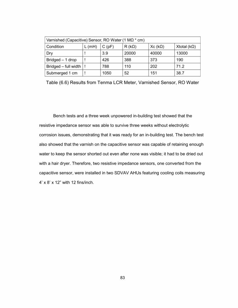
83

Table (6.6) Results from Tenma LCR Meter, Varnished Sensor, RO Water

Bench tests and a three week unpowered in-building test showed that the

resistive impedance sensor was able to survive three weeks without electrolytic

corrosion issues, demonstrating that it was ready for an in-building test. The bench test

also showed that the varnish on the capacitive sensor was capable of retaining enough

water to keep the sensor shorted out even after none was visible; it had to be dried out

with a hair dryer. Therefore, two resistive impedance sensors, one converted from the

capacitive sensor, were installed in two SDVAV AHUs featuring cooling coils measuring

4’ x 8’ x 12” with 12 fins/inch.

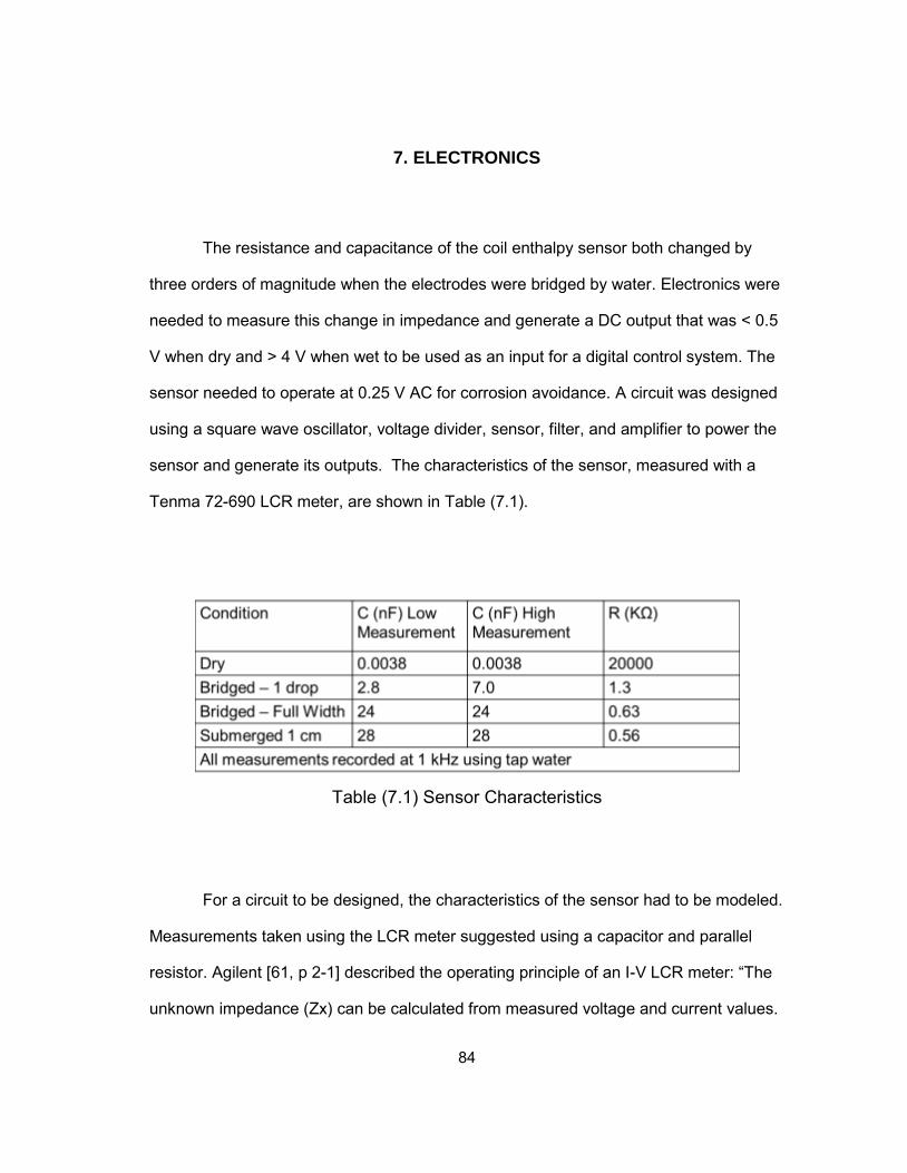
84

7. ELECTRONICS

The resistance and capacitance of the coil enthalpy sensor both changed by

three orders of magnitude when the electrodes were bridged by water. Electronics were

needed to measure this change in impedance and generate a DC output that was < 0.5

V when dry and > 4 V when wet to be used as an input for a digital control system. The

sensor needed to operate at 0.25 V AC for corrosion avoidance. A circuit was designed

using a square wave oscillator, voltage divider, sensor, filter, and amplifier to power the

sensor and generate its outputs. The characteristics of the sensor, measured with a

Tenma 72-690 LCR meter, are shown in Table (7.1).

Table (7.1) Sensor Characteristics

For a circuit to be designed, the characteristics of the sensor had to be modeled.

Measurements taken using the LCR meter suggested using a capacitor and parallel

resistor. Agilent [61, p 2-1] described the operating principle of an I-V LCR meter: “The

unknown impedance (Zx) can be calculated from measured voltage and current values.

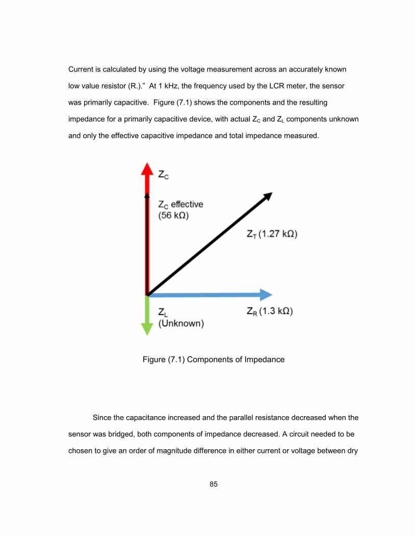
85

Current is calculated by using the voltage measurement across an accurately known

low value resistor (R.).” At 1 kHz, the frequency used by the LCR meter, the sensor

was primarily capacitive. Figure (7.1) shows the components and the resulting

impedance for a primarily capacitive device, with actual ZC and ZL components unknown

and only the effective capacitive impedance and total impedance measured.

Figure (7.1) Components of Impedance

Since the capacitance increased and the parallel resistance decreased when the

sensor was bridged, both components of impedance decreased. A circuit needed to be

chosen to give an order of magnitude difference in either current or voltage between dry

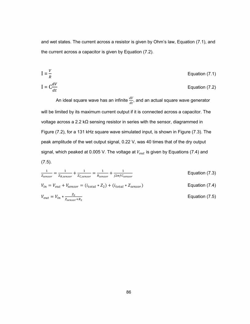
86

and wet states. The current across a resistor is given by Ohm’s law, Equation (7.1), and

the current across a capacitor is given by Equation (7.2).

I = 𝑉𝑅

Equation (7.1)

I = C𝑑𝑉𝑑𝑡

Equation (7.2)

An ideal square wave has an infinite 𝑑𝑉𝑑𝑡 , and an actual square wave generator

will be limited by its maximum current output if it is connected across a capacitor. The

voltage across a 2.2 kΩ sensing resistor in series with the sensor, diagrammed in

Figure (7.2), for a 131 kHz square wave simulated input, is shown in Figure (7.3). The

peak amplitude of the wet output signal, 0.22 V, was 40 times that of the dry output

signal, which peaked at 0.005 V. The voltage at 𝑉𝑜𝑢𝑡 is given by Equations (7.4) and

(7.5).

1𝑍𝑠𝑒𝑛𝑠𝑜𝑟

= 1𝑍𝑅,𝑠𝑒𝑛𝑠𝑜𝑟

+ 1𝑍𝐶,𝑠𝑒𝑛𝑠𝑜𝑟

= 1𝑅𝑠𝑒𝑛𝑠𝑜𝑟

+ 1𝑗2𝜋𝑓𝐶𝑠𝑒𝑛𝑠𝑜𝑟

Equation (7.3)

𝑉𝑖𝑛 = 𝑉𝑜𝑢𝑡 + 𝑉𝑠𝑒𝑛𝑠𝑜𝑟 = (𝑖𝑡𝑜𝑡𝑎𝑙 ∗ 𝑍2) + (𝑖𝑡𝑜𝑡𝑎𝑙 ∗ 𝑍𝑠𝑒𝑛𝑠𝑜𝑟) Equation (7.4)

𝑉𝑜𝑢𝑡 = 𝑉𝑖𝑛 ∗𝑍2

𝑍𝑠𝑒𝑛𝑠𝑜𝑟+𝑅2 Equation (7.5)

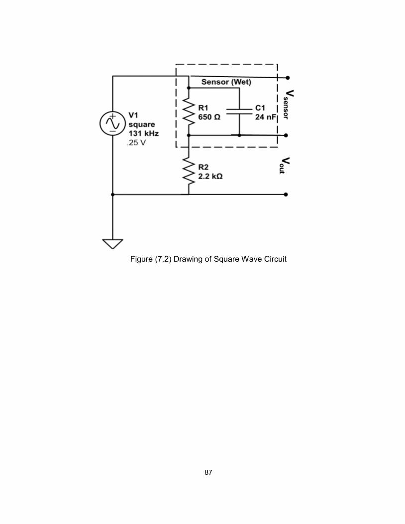
87

Figure (7.2) Drawing of Square Wave Circuit

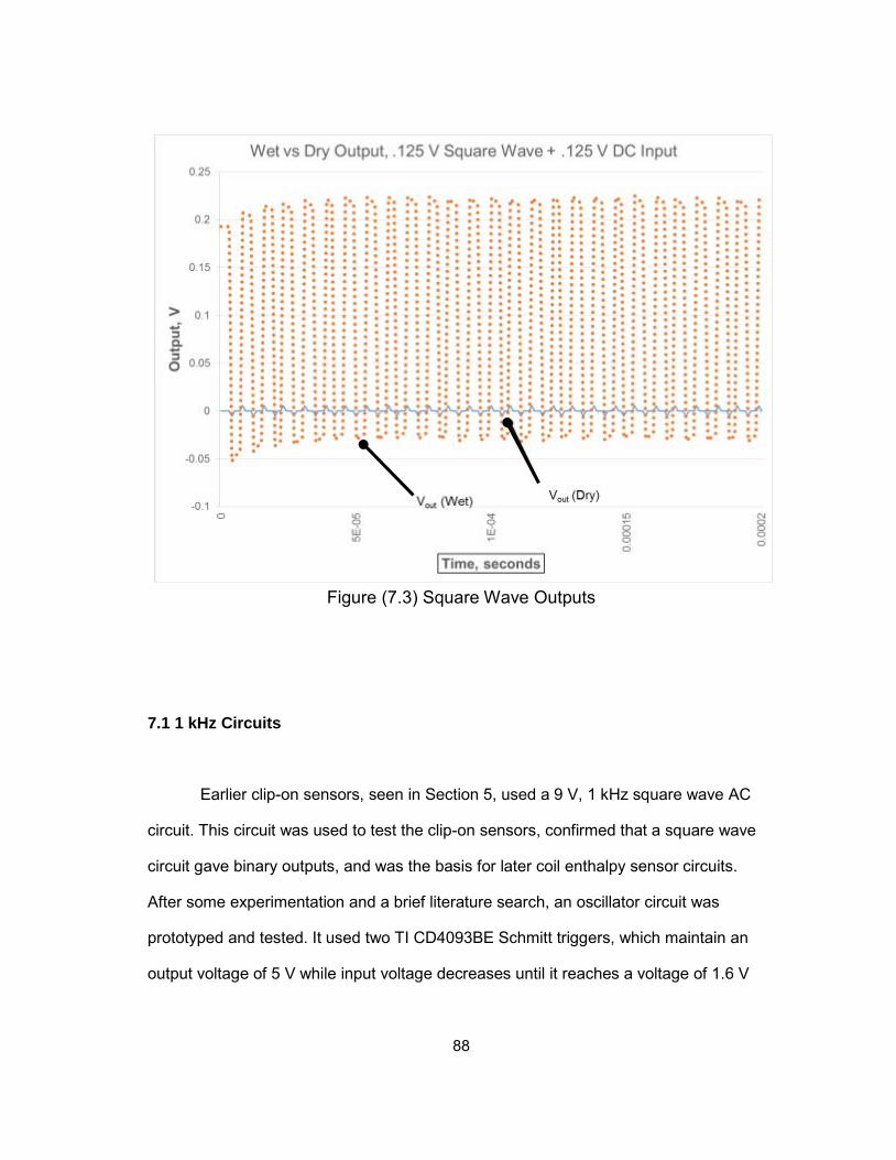
88

Figure (7.3) Square Wave Outputs

7.1 1 kHz Circuits

Earlier clip-on sensors, seen in Section 5, used a 9 V, 1 kHz square wave AC

circuit. This circuit was used to test the clip-on sensors, confirmed that a square wave

circuit gave binary outputs, and was the basis for later coil enthalpy sensor circuits.

After some experimentation and a brief literature search, an oscillator circuit was

prototyped and tested. It used two TI CD4093BE Schmitt triggers, which maintain an

output voltage of 5 V while input voltage decreases until it reaches a voltage of 1.6 V

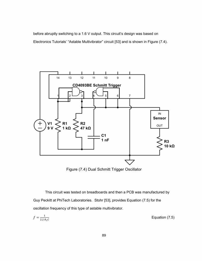
89

before abruptly switching to a 1.6 V output. This circuit’s design was based on

Electronics Tutorials’ “Astable Multivibrator” circuit [53] and is shown in Figure (7.4).

Figure (7.4) Dual Schmitt Trigger Oscillator

This circuit was tested on breadboards and then a PCB was manufactured by

Guy Peckitt at PhiTech Laboratories. Stohr [53], provides Equation (7.5) for the

oscillation frequency of this type of astable multivibrator.

𝑓 = 12.2 𝑅1𝐶

Equation (7.5)

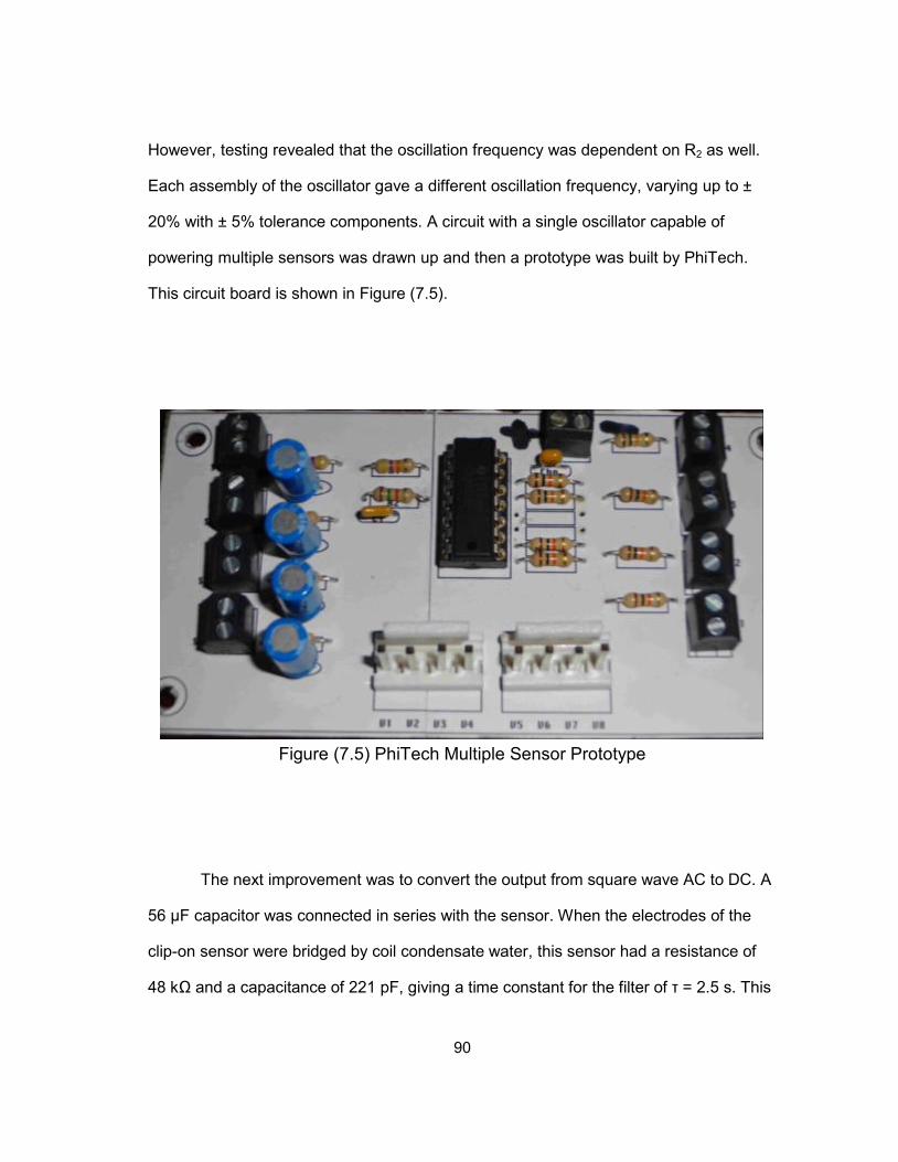
90

However, testing revealed that the oscillation frequency was dependent on R2 as well.

Each assembly of the oscillator gave a different oscillation frequency, varying up to ±

20% with ± 5% tolerance components. A circuit with a single oscillator capable of

powering multiple sensors was drawn up and then a prototype was built by PhiTech.

This circuit board is shown in Figure (7.5).

Figure (7.5) PhiTech Multiple Sensor Prototype

The next improvement was to convert the output from square wave AC to DC. A

56 µF capacitor was connected in series with the sensor. When the electrodes of the

clip-on sensor were bridged by coil condensate water, this sensor had a resistance of

48 kΩ and a capacitance of 221 pF, giving a time constant for the filter of τ = 2.5 s. This

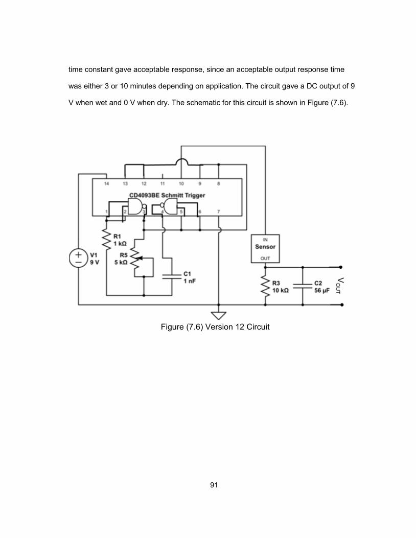
91

time constant gave acceptable response, since an acceptable output response time

was either 3 or 10 minutes depending on application. The circuit gave a DC output of 9

V when wet and 0 V when dry. The schematic for this circuit is shown in Figure (7.6).

Figure (7.6) Version 12 Circuit

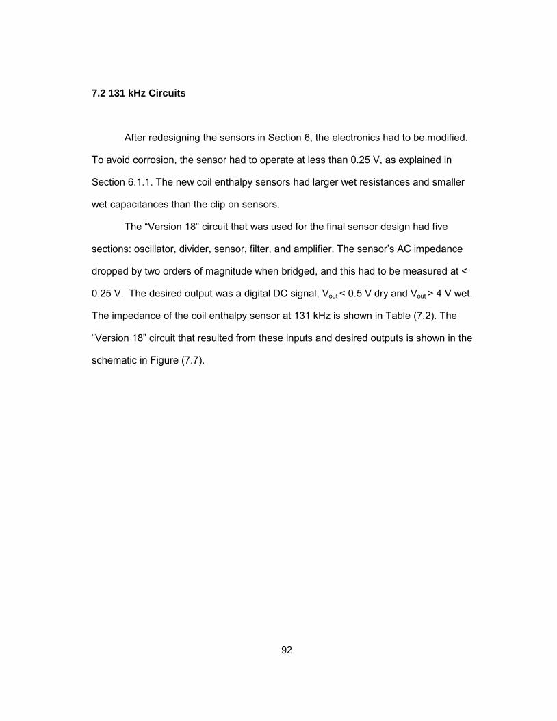
92

7.2 131 kHz Circuits

After redesigning the sensors in Section 6, the electronics had to be modified.

To avoid corrosion, the sensor had to operate at less than 0.25 V, as explained in

Section 6.1.1. The new coil enthalpy sensors had larger wet resistances and smaller

wet capacitances than the clip on sensors.

The “Version 18” circuit that was used for the final sensor design had five

sections: oscillator, divider, sensor, filter, and amplifier. The sensor’s AC impedance

dropped by two orders of magnitude when bridged, and this had to be measured at <

0.25 V. The desired output was a digital DC signal, Vout < 0.5 V dry and Vout > 4 V wet.

The impedance of the coil enthalpy sensor at 131 kHz is shown in Table (7.2). The

“Version 18” circuit that resulted from these inputs and desired outputs is shown in the

schematic in Figure (7.7).

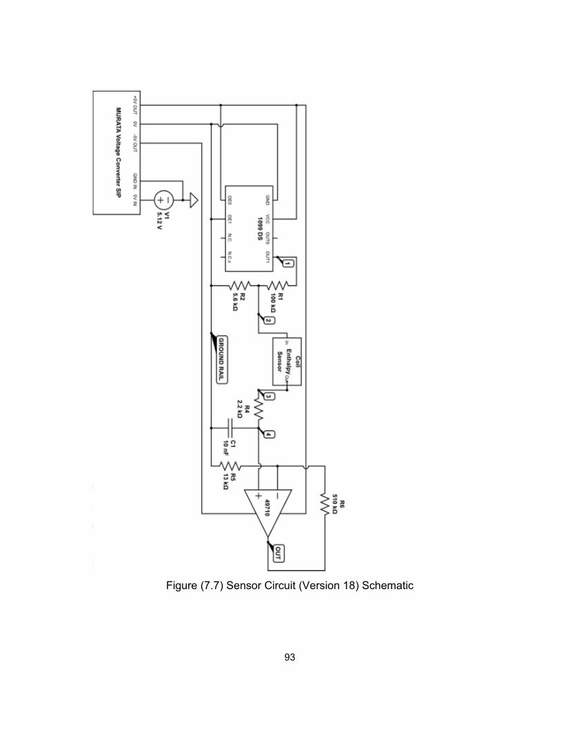
93

Figure (7.7) Sensor Circuit (Version 18) Schematic

94

The voltages at each stage of the circuit were calculated to satisfy the sensor

input and circuit output requirements. The oscillator stage consisted of a commercial

131 kHz oscillator with an output of a square wave with an amplitude of 2.5 V and a DC

level of +2.5 V. The voltage divider reduced this peak-to-trough voltage from 5 V to 0.25

V. The sensor gave an AC output dependent on its state. The filter removed the AC

component from the signal, giving only the DC level. Finally, the amplifier boosted this

DC level to the high-rail voltage when wet and the low-rail voltage when dry. The input

and output for each stage is calculated below. The final schematic and PCB layout are

shown in Figures (7.9) and (7.10).

Oscillator: The steady state AC current through a circuit element is given by the

equation 𝑖 = 𝑉𝑍 where Z is the impedance of the circuit element. Since the sensor was

supplied with 0.25 VAC it would pass 12 µA when the plates were bridged by one drop

of water, when connected to an equal series resistor for measurement. This would

require careful encapsulation to avoid noise. Therefore, the new oscillator section would

have to operate at a higher frequency than 1 kHz, reducing the reactance.

A commercial 131 kHz oscillator was selected due to its low cost and consistent

frequency output. Its output was a square wave with a peak amplitude of 5 V and a

trough of 0 V. At 131 kHz, the dry impedance is 310 kΩ, the bridged impedance is 240

Ω, and the submerged impedance is 40Ω.

Sensor: The electrical characteristics of the sensor at 131 kHz are given in

Table (7.2), calculated from the resistance and capacitance measurements taken at 1

kHz. Since the sensor is primarily capacitive at this frequency, inductance could not be

measured, as shown in Figure (7.1). The wet and dry voltage outputs versus time are

shown in Figure (7.3).

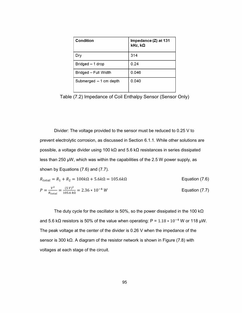
95

Table (7.2) Impedance of Coil Enthalpy Sensor (Sensor Only)

Divider: The voltage provided to the sensor must be reduced to 0.25 V to

prevent electrolytic corrosion, as discussed in Section 6.1.1. While other solutions are

possible, a voltage divider using 100 kΩ and 5.6 kΩ resistances in series dissipated

less than 250 µW, which was within the capabilities of the 2.5 W power supply, as

shown by Equations (7.6) and (7.7).

𝑅𝑡𝑜𝑡𝑎𝑙 = 𝑅1 + 𝑅2 = 100𝑘Ω + 5.6𝑘Ω = 105.6𝑘Ω Equation (7.6)

𝑃 = 𝑉2

𝑅𝑡𝑜𝑡𝑎𝑙= (5 𝑉)2

105.6 𝑘Ω= 2.36 ∗ 10−4 𝑊 Equation (7.7)

The duty cycle for the oscillator is 50%, so the power dissipated in the 100 kΩ

and 5.6 kΩ resistors is 50% of the value when operating: P = 1.18 ∗ 10−4 W or 118 µW.

The peak voltage at the center of the divider is 0.26 V when the impedance of the

sensor is 300 kΩ. A diagram of the resistor network is shown in Figure (7.8) with

voltages at each stage of the circuit.

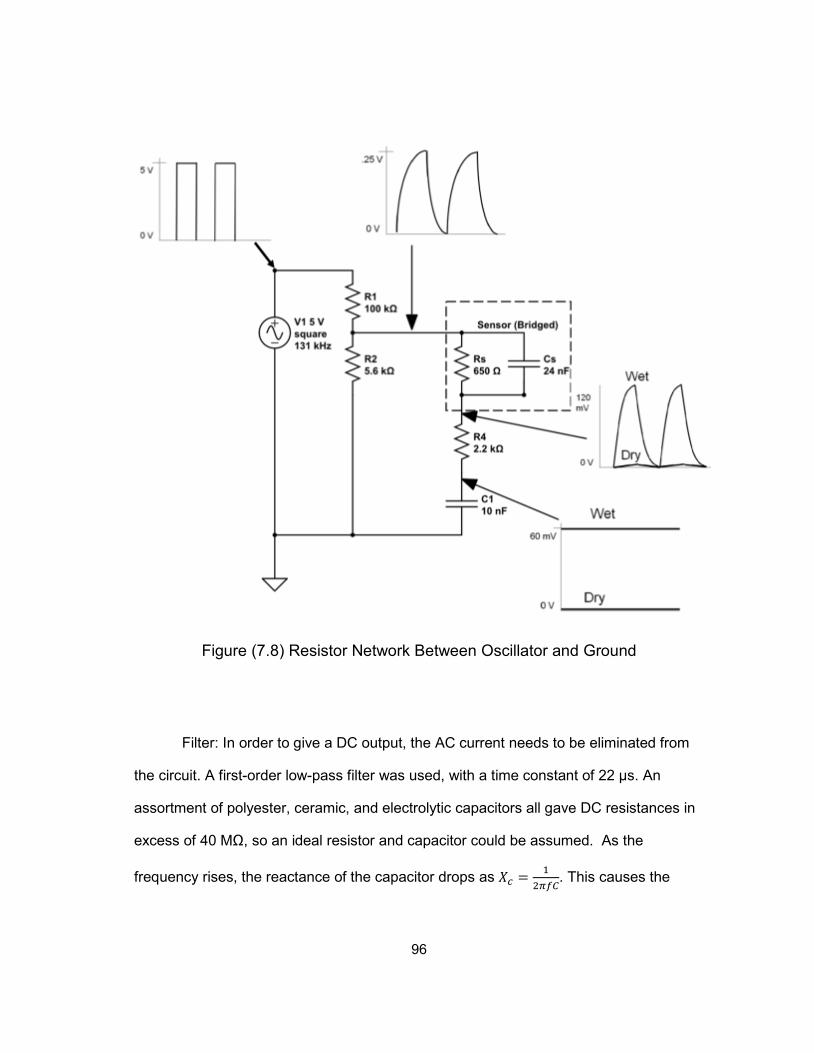
96

Figure (7.8) Resistor Network Between Oscillator and Ground

Filter: In order to give a DC output, the AC current needs to be eliminated from

the circuit. A first-order low-pass filter was used, with a time constant of 22 µs. An

assortment of polyester, ceramic, and electrolytic capacitors all gave DC resistances in

excess of 40 MΩ, so an ideal resistor and capacitor could be assumed. As the

frequency rises, the reactance of the capacitor drops as 𝑋𝑐 = 12𝜋𝑓𝐶

. This causes the

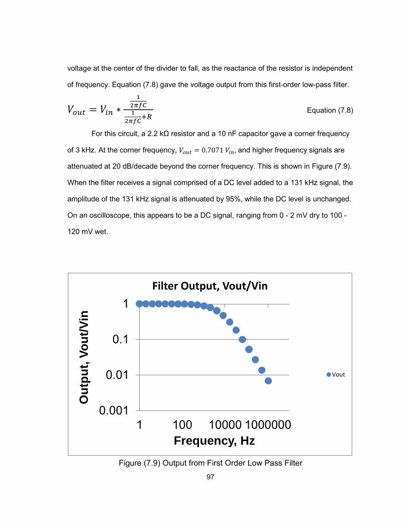
97

voltage at the center of the divider to fall, as the reactance of the resistor is independent

of frequency. Equation (7.8) gave the voltage output from this first-order low-pass filter.

𝑉𝑜𝑢𝑡 = 𝑉𝑖𝑛 ∗1

2𝜋𝑓𝐶1

2𝜋𝑓𝐶+𝑅 Equation (7.8)

For this circuit, a 2.2 kΩ resistor and a 10 nF capacitor gave a corner frequency

of 3 kHz. At the corner frequency, 𝑉𝑜𝑢𝑡 = 0.7071 𝑉𝑖𝑛, and higher frequency signals are

attenuated at 20 dB/decade beyond the corner frequency. This is shown in Figure (7.9).

When the filter receives a signal comprised of a DC level added to a 131 kHz signal, the

amplitude of the 131 kHz signal is attenuated by 95%, while the DC level is unchanged.

On an oscilloscope, this appears to be a DC signal, ranging from 0 - 2 mV dry to 100 -

120 mV wet.

Figure (7.9) Output from First Order Low Pass Filter

0.001

0.01

0.1

1

1 100 10000 1000000

Out

put,

Vout

/Vin

Frequency, Hz

Filter Output, Vout/Vin

Vout

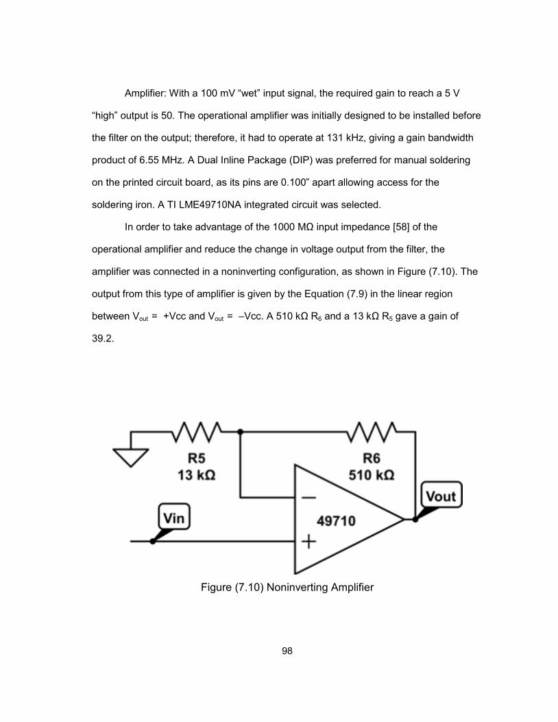
98

Amplifier: With a 100 mV “wet” input signal, the required gain to reach a 5 V

“high” output is 50. The operational amplifier was initially designed to be installed before

the filter on the output; therefore, it had to operate at 131 kHz, giving a gain bandwidth

product of 6.55 MHz. A Dual Inline Package (DIP) was preferred for manual soldering

on the printed circuit board, as its pins are 0.100” apart allowing access for the

soldering iron. A TI LME49710NA integrated circuit was selected.

In order to take advantage of the 1000 MΩ input impedance [58] of the

operational amplifier and reduce the change in voltage output from the filter, the

amplifier was connected in a noninverting configuration, as shown in Figure (7.10). The

output from this type of amplifier is given by the Equation (7.9) in the linear region

between Vout = +Vcc and Vout = –Vcc. A 510 kΩ R6 and a 13 kΩ R5 gave a gain of

39.2.

Figure (7.10) Noninverting Amplifier

99

𝑉𝑜𝑢𝑡 = 𝑉𝑖𝑛 1 + 𝑅6𝑅5 Equation (7.9)

This circuit was prototyped on a breadboard, and then three PCBs were

manufactured. The schematic and PCB layout are shown in Figures (7.11) and (7.12).

The outputs when connected to a sensor are shown in the photographs, Figures (7.13),

(7.14), and (7.15). Dry output was – 4 V, and wet output was 4.4 V.

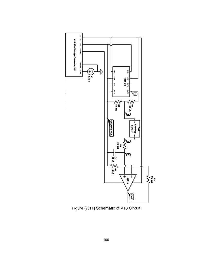
100

Figure (7.11) Schematic of V18 Circuit

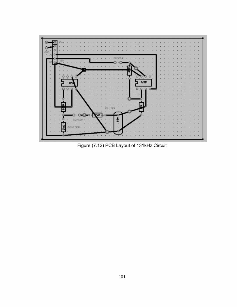
101

Figure (7.12) PCB Layout of 131kHz Circuit

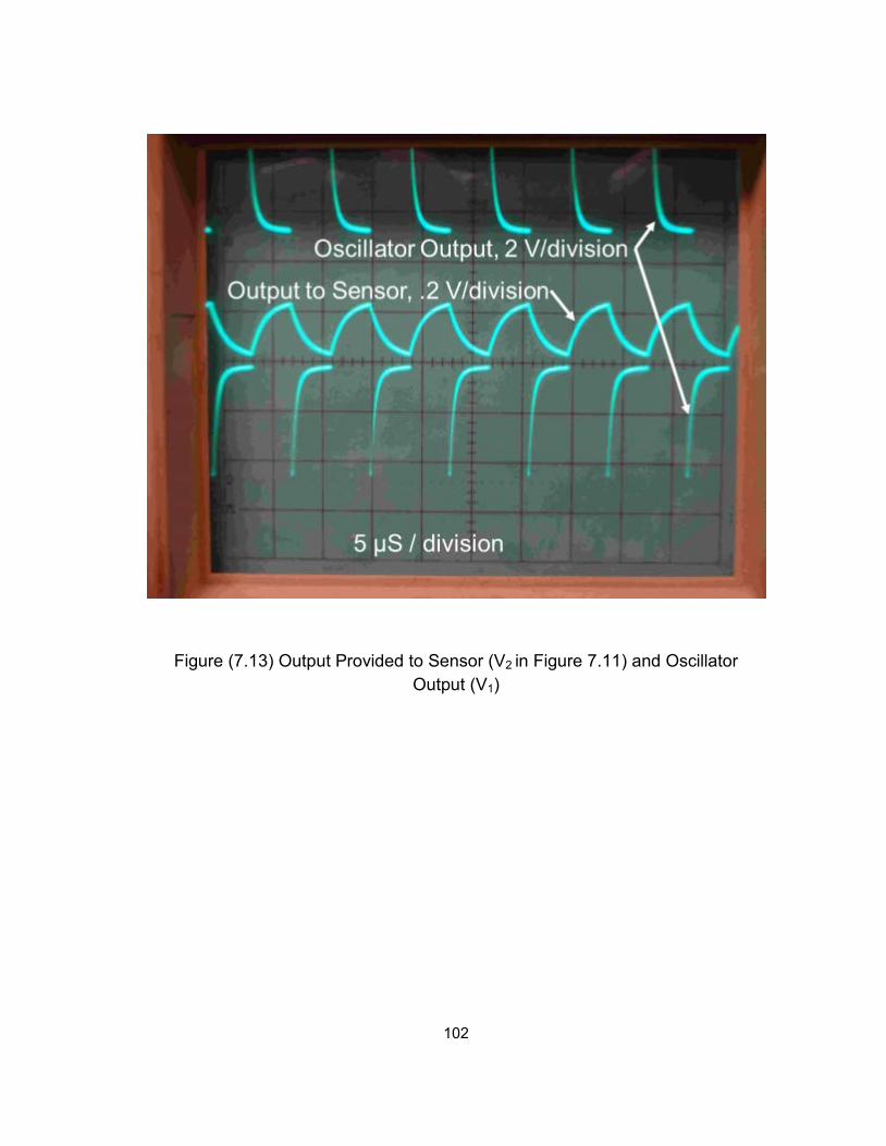
102

Figure (7.13) Output Provided to Sensor (V2 in Figure 7.11) and Oscillator Output (V1)

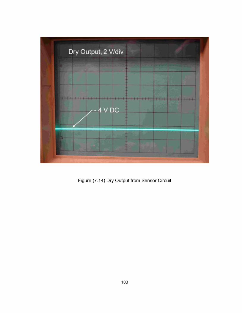
103

Figure (7.14) Dry Output from Sensor Circuit

+ 4 V DC

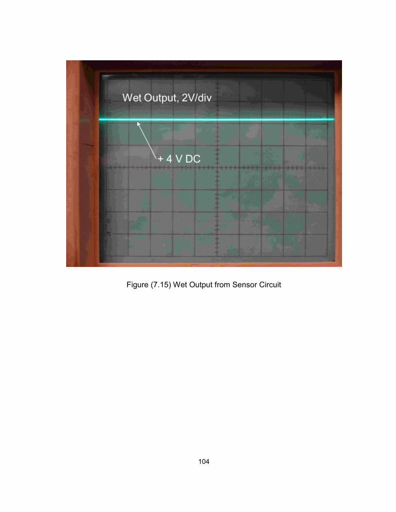
104

Figure (7.15) Wet Output from Sensor Circuit

105

8. RESULTS

In-building tests were performed on Coil Enthalpy Limit sensors to test reliability,

time response, and durability. Operational testing confirmed that the sensors were able

to detect water dripping from the coil into the drain pan when the coil was wet. Timed

testing determined that the sensor registered a change from dry to wet between 6 and

45 minutes after the supply air temperature dropped below the mixed air dew point.

Durability tests showed that the electrical properties of the sensor were retained after

three months in an AHU.

8.1 Operational Testing

Two impedance sensors were installed in Langford AHU A-1, which serves the

first floor perimeter zones of an office/classroom building at Texas A&M University.

These sensors were initially hung below the drip rail using magnetic clamps, but after

observations showed that the sides of the sensor blocked flow from the plates, sheet

metal stands were fabricated to hold the sensors underneath the rail in the drip pan. A

sensor on its stand is shown in Figure (8.1). Onset Computer HOBO U12-012 data

loggers were used to record the supply air temperature, supply air relative humidity, and

voltage output from these sensors. The operating sequence for the AHU was left

unchanged for this test.

106

Figure (8.1) Photo of Sensor and Stand

Two sensors were installed in Langford AHU A-1 on May 22, 2013 and their

voltage output was monitored by individual HOBO U12-012 loggers. The first sensor

was connected in an “inverted” configuration, giving a 1 - 4 V output when dry. The

second sensor was connected in the “normal” configuration, giving a 1 - 4 V output

when wet. This allowed for testing of reliability and sensor hysteresis. If the sensors

gave a positive voltage output simultaneously, then there was a time delay between the

coil becoming dry and the sensors registering this change of state.

At the end of this test, both sensors were free from contamination, indicating that

the sensors were being kept clean by air and water flow. These results show successful

operation of these sensors, with voltage outputs corresponding to dry coil conditions

(positive voltages on the “inverted” sensor) after the AHU was shut off at night, and

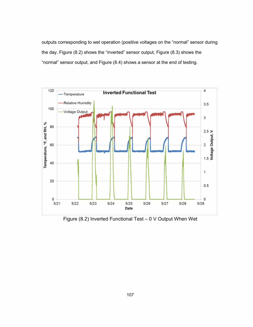
107

outputs corresponding to wet operation (positive voltages on the “normal” sensor during

the day. Figure (8.2) shows the “inverted” sensor output, Figure (8.3) shows the

“normal” sensor output, and Figure (8.4) shows a sensor at the end of testing.

Figure (8.2) Inverted Functional Test – 0 V Output When Wet

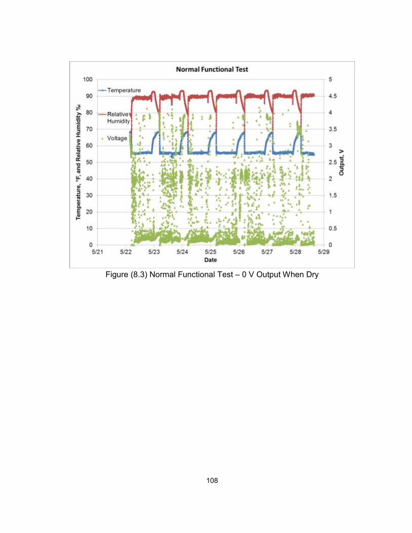
108

Figure (8.3) Normal Functional Test – 0 V Output When Dry

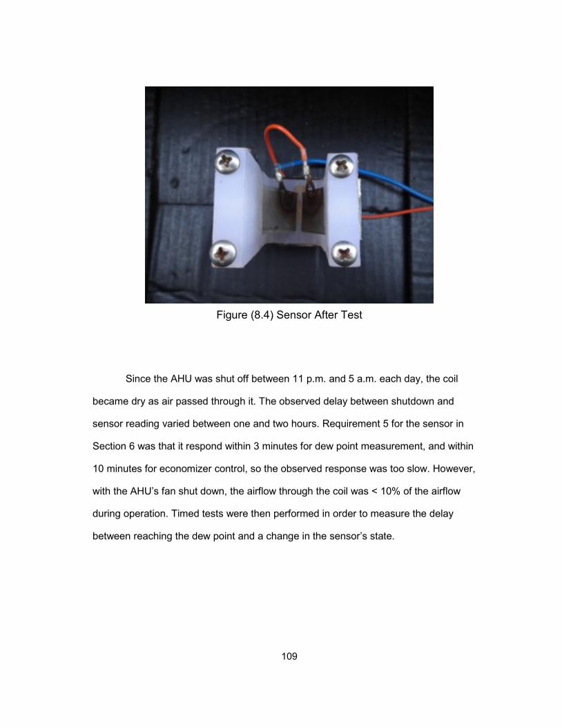
109

Figure (8.4) Sensor After Test

Since the AHU was shut off between 11 p.m. and 5 a.m. each day, the coil

became dry as air passed through it. The observed delay between shutdown and

sensor reading varied between one and two hours. Requirement 5 for the sensor in

Section 6 was that it respond within 3 minutes for dew point measurement, and within

10 minutes for economizer control, so the observed response was too slow. However,

with the AHU’s fan shut down, the airflow through the coil was < 10% of the airflow

during operation. Timed tests were then performed in order to measure the delay

between reaching the dew point and a change in the sensor’s state.

110

8.2 Timed Testing

Two sensors were mounted below the drip rail of the cooling coil in the same

locations as used in the reliability tests. The chilled water valve was then manually

closed in order to test wet-to-dry sensor response. After the sensors had reached a 0 V

output, the chilled water valve was opened in order to measure the delay between the

coil reaching the dew point and the sensor returning to >5 V output.

The first test of sensor and coil response was performed at Langford AHU A-1.

The chilled water valve was allowed to reopen at 3:50 p.m. By 4:05 p.m., the supply air

temperature had reached its set point of 53°F. It took until 4:30 p.m. for water droplets

to begin dripping off the rail, and at 4:35 p.m. the sensor returned to a wet state. The

45-minute response time is shown in Figure (8.5). This required an investigation to see

if there was a problem with dehumidification in this AHU. The quantity of water

condensed in this coil was calculated and then compared against a measurement.

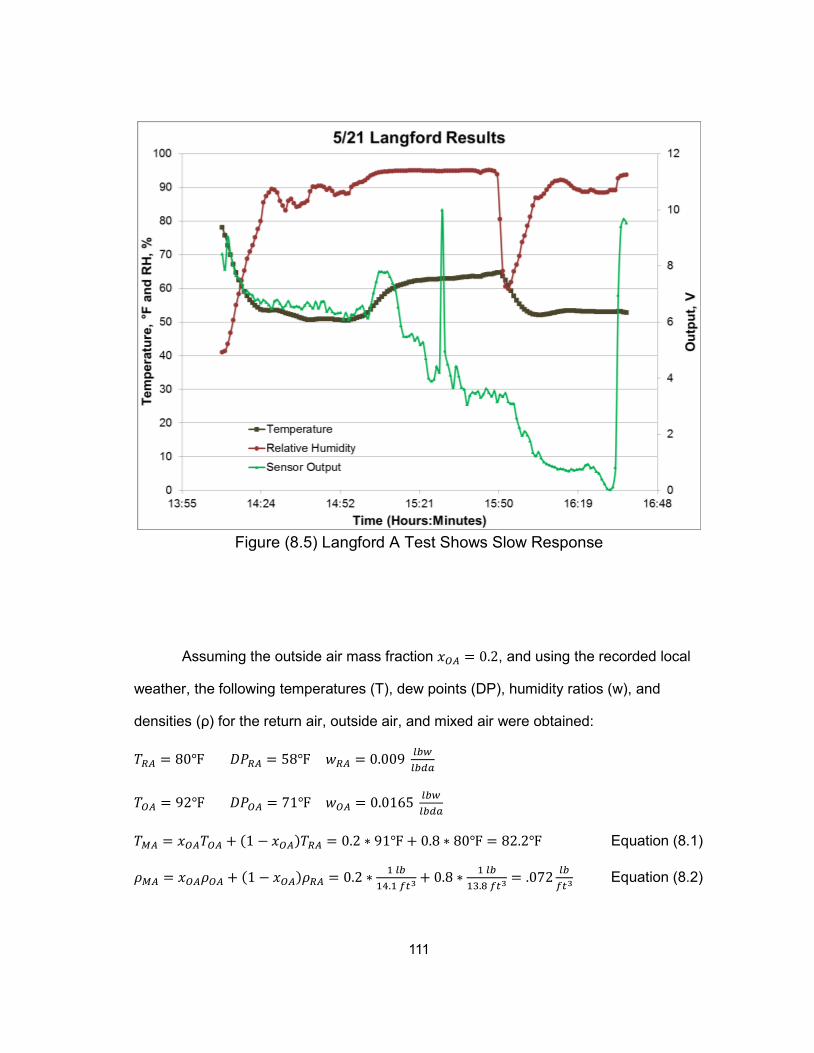
111

Figure (8.5) Langford A Test Shows Slow Response

Assuming the outside air mass fraction 𝑥𝑂𝐴 = 0.2, and using the recorded local

weather, the following temperatures (T), dew points (DP), humidity ratios (w), and

densities (ρ) for the return air, outside air, and mixed air were obtained:

𝑇𝑅𝐴 = 80 𝐷𝑃𝑅𝐴 = 58 𝑤𝑅𝐴 = 0.009 𝑙𝑏𝑤𝑙𝑏𝑑𝑎

𝑇𝑂𝐴 = 92 𝐷𝑃𝑂𝐴 = 71 𝑤𝑂𝐴 = 0.0165 𝑙𝑏𝑤𝑙𝑏𝑑𝑎

𝑇𝑀𝐴 = 𝑥𝑂𝐴𝑇𝑂𝐴 + (1 − 𝑥𝑂𝐴)𝑇𝑅𝐴 = 0.2 ∗ 91 + 0.8 ∗ 80 = 82.2 Equation (8.1)

𝜌𝑀𝐴 = 𝑥𝑂𝐴𝜌𝑂𝐴 + (1 − 𝑥𝑂𝐴)𝜌𝑅𝐴 = 0.2 ∗ 1 𝑙𝑏14.1 𝑓𝑡3

+ 0.8 ∗ 1 𝑙𝑏13.8 𝑓𝑡3

= .072 𝑙𝑏𝑓𝑡3

Equation (8.2)

112

This allowed the assumption of constant density throughout the remainder of these

calculations, as return air and outside air densities were within ± 2%.

𝑤𝑀𝐴 = 𝑥𝑂𝐴𝑤𝑂𝐴 + (1 − 𝑥𝑂𝐴)𝑤𝑅𝐴 = 0.0105 𝑙𝑏𝑤𝑙𝑏𝑑𝑎

Equation (8.3)

The supply air properties were then calculated. Assuming that the coil is wet, the air

leaving the coil will be saturated and at the coil leaving temperature.

𝑇𝑆𝐴 = 53 𝐷𝑃𝑆𝐴 = 53 𝑤𝑆𝐴 = 0.0085 𝑙𝑏𝑤𝑙𝑏𝑑𝑎

𝜌𝑆𝐴 = 1 𝑙𝑏13.3 𝑓𝑡3

Equation (8.4)

The volumetric and mass airflow were then calculated, based on the assumption that

the component of the mean air velocity perpendicular to the coil is constant.

𝑉 = 600 𝑓𝑡𝑚𝑖𝑛

𝐴𝑐𝑜𝑖𝑙 = 30 𝑓𝑡2

𝑚𝑎 = 𝑉 𝑋 𝐴𝑐𝑜𝑖𝑙 = 18000 𝑓𝑡3

𝑚𝑖𝑛 Equation (8.5)

𝑀𝐴 = 𝑚𝑎𝜌𝑀𝐴 = 18000 𝑓𝑡3

𝑚𝑖𝑛∗ 1 𝑙𝑏𝑑𝑎13.8 𝑓𝑡3

= 1300 𝑙𝑏𝑑𝑎𝑚𝑖𝑛

Equation (8.6)

This then allowed the calculation of the amount of water removed from the mixed air.

𝑊,𝑀𝐴 = 𝑀𝐴𝑤𝑀𝐴 = 1300 𝑙𝑏𝑑𝑎𝑚𝑖𝑛

∗ 0105 𝑙𝑏𝑤𝑙𝑏𝑑𝑎

= 13.7 𝑙𝑏𝑤𝑚𝑖𝑛

Equation (8.7)

𝑊,𝑆𝐴 = 𝑆𝐴𝑤𝑆𝐴 = 1300 𝑙𝑏𝑑𝑎𝑚𝑖𝑛

∗ 0085 𝑙𝑏𝑤𝑙𝑏𝑑𝑎

= 10.95 𝑙𝑏𝑤𝑚𝑖𝑛

Equation (8.8)

𝑟𝑒𝑚𝑜𝑣𝑒𝑑=𝑊,𝑀𝐴 − 𝑊,𝑆𝐴 = 2.75 𝑙𝑏𝑤𝑚𝑖𝑛

Equation (8.9)

If this water was trapped for 30 minutes within the boundary layer near the

cooling coil fins, 82 lbs of water, or 10.2 gallons, was contained there at the end. 30% of

the total internal volume of the coil would have been taken up by water in this state.

The quantity of water condensed at steady state was then measured. It took 4 minutes

5 seconds to fill a 16 fluid ounce cup. Equation (8.10) shows that the condensate flow

rate was less than 10% of the calculated value.

113

𝑤,𝐴𝑐𝑡𝑢𝑎𝑙 = 𝑚𝑤𝑎𝑡𝑒𝑟𝑡

= 1 𝑙𝑏4 𝑚𝑖𝑛

= 0.25 𝑙𝑏𝑚𝑖𝑛

Equation (8.10)

This discrepancy needed further investigation. Langford AHU-A1 is on Texas

A&M’s Siemens APOGEE EMCS, and the flow rates and temperatures used for control

are available. Since 𝑇𝑀𝐴 = 𝑇𝑅𝐴, and the outside air temperature is 10°F hotter, too little

outside air is being provided to this AHU to be able to calculate the outside air fraction.

As the building was unoccupied during this test, the latent load on the coil was much

smaller than assumed. The measured and recorded temperatures and humidities are

given below.

𝑇𝑅𝐴 = 73 𝑅𝐻𝑅𝐴 = 55% 𝑤𝑅𝐴 = 0.009 𝑙𝑏𝑤𝑙𝑏𝑑𝑎

𝑇𝑂𝐴 = 80 𝐷𝑃𝑂𝐴 = 70 𝑤𝑂𝐴 = 0.016 𝑙𝑏𝑤𝑙𝑏𝑑𝑎

𝑇𝑀𝐴 = 73 𝑅𝐴 = 7400 𝑓𝑡3

𝑚𝑖𝑛 𝑆𝐴,𝐴𝑃𝑂𝐺𝐸𝐸 = 8300 𝑓𝑡3

𝑚𝑖𝑛

𝑇𝑆𝐴 = 53 𝐷𝑃𝑆𝐴 = 53 𝑤𝑆𝐴 = 0.0085 𝑙𝑏𝑤𝑙𝑏𝑑𝑎

OA Damper Position = 10% RA Damper Position = 10%

CHWV Position = 44% HWV Position = 0%

This allowed calculation of the quantity of water condensed and trapped within

the coil.

𝑆𝐴,𝑎𝑐𝑡𝑢𝑎𝑙 = 6200𝑓𝑡3

𝑚𝑖𝑛

𝑆𝐴 = 𝜌𝑆𝐴𝑆𝐴,𝑎𝑐𝑡𝑢𝑎𝑙 = 1 𝑙𝑏𝑑𝑎13.2 𝑓𝑡3

∗ 6200 𝑓𝑡3

𝑚𝑖𝑛= 469 𝑙𝑏𝑑𝑎

𝑚𝑖𝑛 Equation (8.11)

𝑊,𝑀𝐴 = 𝑀𝐴𝑤𝑀𝐴 = 469 𝑙𝑏𝑑𝑎𝑚𝑖𝑛

∗ 0.009 𝑙𝑏𝑤𝑙𝑏𝑑𝑎

= 4.22 𝑙𝑏𝑤𝑚𝑖𝑛

Equation (8.12)

𝑊,𝑆𝐴 = 𝑆𝐴𝑤𝑆𝐴 = 469 𝑙𝑏𝑑𝑎𝑚𝑖𝑛

∗ 0.0085 𝑙𝑏𝑤𝑙𝑏𝑑𝑎

= 3.99 𝑙𝑏𝑤𝑚𝑖𝑛

Equation (8.13)

114

𝑟𝑒𝑚𝑜𝑣𝑒𝑑=𝑊,𝑀𝐴 − 𝑊,𝑆𝐴 = 0.234 𝑙𝑏𝑤𝑚𝑖𝑛

Equation (8.14)

This result is within ± 7% of the measured value. Over 30 minutes, 7.5 lbs,

approximately 1 gallon, of water was trapped in a coil measuring 4’ x 8’ x 1’. This gave a

“trapped water density” of

𝜌𝑡𝑟𝑎𝑝𝑝𝑒𝑑 = 𝑚𝑡𝑟𝑎𝑝𝑝𝑒𝑑

𝑉𝑐𝑜𝑖𝑙= 7.5 𝑙𝑏𝑠

32 𝑓𝑡3= 0.23 𝑙𝑏

𝑓𝑡3 Equation (8.15)

Since water has a density of 8 𝑙𝑏𝑠 𝑓𝑡3 , 3% of the total internal volume of the coil was

occupied by water when the coil reached its carrying capacity.

Another SDVAV air handler, AHU 1-2 at the Jack E. Brown Building, was

selected for further timed testing. Timed tests were performed there showing wet-to-dry

delays between 6 and 30 minutes, depending primarily on the difference between the

outside air temperature and dew point, and dry-to-wet delays between 45 seconds and

6 minutes. Figure (8.9) shows voltage spikes when the timed tests were performed. The

results from the first test, along with calculations of the theoretical carrying capacity of

AHU 1-2 at the Jack E. Brown building are as follows.

𝑇𝑂𝐴 = 87 𝑇𝑅𝐴 = 74 𝑇𝑀𝐴 = 78 𝑂𝐴 = 1800 𝑓𝑡3

𝑚𝑖𝑛

𝐷𝑃𝑂𝐴 = 73 𝐷𝑃𝑅𝐴 = 54 𝑤𝑂𝐴 = 0.0175 𝑙𝑏𝑤𝑙𝑏𝑑𝑎

𝑤𝑅𝐴 = 0.009 𝑙𝑏𝑤𝑙𝑏𝑑𝑎

𝑇𝑀𝐴 = 𝑥𝑂𝐴𝑇𝑂𝐴 + (1 − 𝑥𝑂𝐴)𝑇𝑅𝐴 Equation (8.16)

𝑇𝑀𝐴 = 𝑥𝑂𝐴𝑇𝑂𝐴 + 𝑇𝑅𝐴 − 𝑥𝑂𝐴𝑇𝑅𝐴 Equation (8.17)

𝑇𝑀𝐴 − 𝑇𝑅𝐴 = 𝑥𝑂𝐴(𝑇𝑂𝐴 − 𝑇𝑅𝐴) Equation (8.18)

𝑥𝑂𝐴 = 𝑇𝑀𝐴−𝑇𝑅𝐴𝑇𝑂𝐴−𝑇𝑅𝐴

= 78−7487−74

= 0.31 Equation (8.19)

𝑀𝐴 = 𝑂𝐴𝑥𝑂𝐴

= 5850 𝑓𝑡3

𝑚𝑖𝑛 Equation (8.20)

𝑤𝑀𝐴 = 𝑥𝑂𝐴𝑤𝑂𝐴 + (1 − 𝑥𝑂𝐴)𝑤𝑅𝐴 = 0.0115 𝑙𝑏𝑤𝑙𝑏𝑑𝑎

Equation (8.21)

115

Given these coil entering conditions, the expected condensate flow was then

calculated using the measured coil leaving conditions using Equations (8.22), (8.23),

and (8.24):

𝑇𝑆𝐴 = 53.5 𝐷𝑃𝑆𝐴 = 53.5 𝑤𝑆𝐴 = 0.0085 𝑙𝑏𝑤𝑙𝑏𝑑𝑎

𝑤,𝑀𝐴 = 𝑀𝐴 ∗ 𝑤𝑀𝐴 = 𝑀𝐴 ∗ 𝜌𝑀𝐴 ∗ 𝑤𝑀𝐴 = 5850 𝑓𝑡3

𝑚𝑖𝑛∗

1 𝑙𝑏𝑑𝑎13.6 𝑓𝑡3

∗ 0.0115𝑙𝑏𝑤𝑙𝑏𝑑𝑎

= 4.94 𝑙𝑏𝑤𝑚𝑖𝑛

Equation (8.22)

𝑤,𝑆𝐴 = 𝑆𝐴 ∗ 𝑤𝑆𝐴 = 430 𝑙𝑏𝑑𝑎𝑚𝑖𝑛

∗ 0.0085 𝑙𝑏𝑤𝑙𝑏𝑑𝑎

= 3.65 𝑙𝑏𝑤𝑙𝑏𝑑𝑎

Equation (8.23)

𝑟𝑒𝑚𝑜𝑣𝑒𝑑=𝑊,𝑀𝐴 − 𝑊,𝑆𝐴 = 1.29 𝑙𝑏𝑤𝑚𝑖𝑛

Equation (8.24)

This was approximately 5 times the quantity of water removed by the coil in

Langford AHU A-1. A “cup and stopwatch” method was used and 9 oz. of water was

collected in 27 seconds. Using equation (8.10) this gives a flow rate of 1.25 𝑙𝑏𝑤𝑚𝑖𝑛

. Both

the Langford A-1 and Jack E. Brown 1-2 calculations were within ±7% of the measured

results; therefore, these measurements can be useful for investigation of comfort or

control issues.

The volume and fin density of the cooling coil in the Jack E Brown AHU 1-2, 4’ x

8.5’ x 1’ and 12 fins/inch, are within ± 5% of the coil in Langford A-1. The water carrying

capacity of the coil should be similar in these two AHUs. Therefore, the response time

from the sensor at Jack E. Brown should have been approximately 1/5 of that at

Langford. Timed tests agreed with this hypothesis during dry-to-wet transitions when

the chilled water valve was suddenly opened as shown in Figure (8.7). Measurement 4

took place when the mixed air dew point was between 55°F and 56°F and the discharge

temperature set point was 55° F. This indicated that measurement of the dew point

within ±1°F was possible using this method, if 34 minutes is an acceptable time for

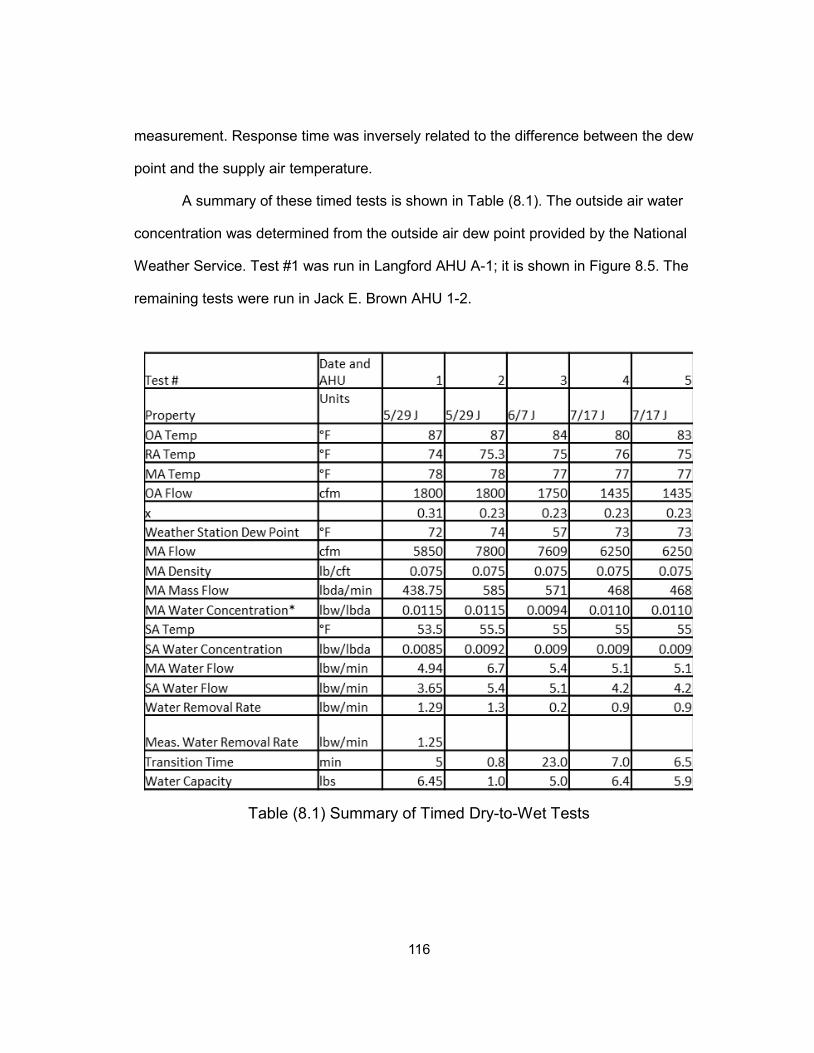
116

measurement. Response time was inversely related to the difference between the dew

point and the supply air temperature.

A summary of these timed tests is shown in Table (8.1). The outside air water

concentration was determined from the outside air dew point provided by the National

Weather Service. Test #1 was run in Langford AHU A-1; it is shown in Figure 8.5. The

remaining tests were run in Jack E. Brown AHU 1-2.

Table (8.1) Summary of Timed Dry-to-Wet Tests

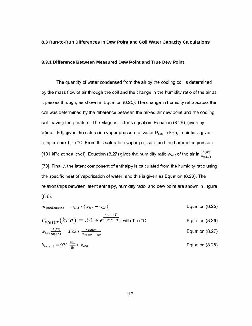
117

8.3 Run-to-Run Differences In Dew Point and Coil Water Capacity Calculations

8.3.1 Difference Between Measured Dew Point and True Dew Point

The quantity of water condensed from the air by the cooling coil is determined

by the mass flow of air through the coil and the change in the humidity ratio of the air as

it passes through, as shown in Equation (8.25). The change in humidity ratio across the

coil was determined by the difference between the mixed air dew point and the cooling

coil leaving temperature. The Magnus-Tetens equation, Equation (8.26), given by

Vömel [69], gives the saturation vapor pressure of water Psat, in kPa, in air for a given

temperature T, in °C. From this saturation vapor pressure and the barometric pressure

(101 kPa at sea level), Equation (8.27) gives the humidity ratio wAIR of the air in 𝑙𝑏(𝑤)𝑙𝑏(𝑑𝑎)

[70]. Finally, the latent component of enthalpy is calculated from the humidity ratio using

the specific heat of vaporization of water, and this is given as Equation (8.28). The

relationships between latent enthalpy, humidity ratio, and dew point are shown in Figure

(8.6).

𝑚𝑐𝑜𝑛𝑑𝑒𝑛𝑠𝑎𝑡𝑒 = 𝑚

𝑀𝐴 ∗ (𝑤𝑀𝐴 − 𝑤𝑆𝐴) Equation (8.25)

𝑃𝑤𝑎𝑡𝑒𝑟(𝑘𝑃𝑎) = .61 ∗ 𝑒17.3∗𝑇237.7+𝑇, with T in °C Equation (8.26)

𝑤𝑠𝑎𝑡𝑙𝑏(𝑤)𝑙𝑏(𝑑𝑎)

= .622 ∗ 𝑃𝑤𝑎𝑡𝑒𝑟𝑃𝑤𝑎𝑡𝑒𝑟+𝑃𝑎𝑖𝑟

Equation (8.27)

ℎ𝑙𝑎𝑡𝑒𝑛𝑡 = 970 𝐵𝑡𝑢𝑙𝑏∗ 𝑤𝐴𝐼𝑅 Equation (8.28)

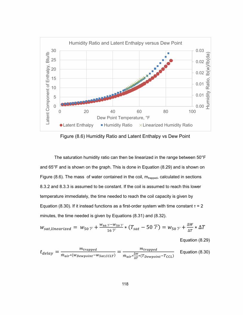
118

Figure (8.6) Humidity Ratio and Latent Enthalpy vs Dew Point

The saturation humidity ratio can then be linearized in the range between 50°F

and 65°F and is shown on the graph. This is done in Equation (8.29) and is shown on

Figure (8.6). The mass of water contained in the coil, mtrapped, calculated in sections

8.3.2 and 8.3.3 is assumed to be constant. If the coil is assumed to reach this lower

temperature immediately, the time needed to reach the coil capacity is given by

Equation (8.30). If it instead functions as a first-order system with time constant τ = 2

minutes, the time needed is given by Equations (8.31) and (8.32).

𝑤𝑠𝑎𝑡,𝑙𝑖𝑛𝑒𝑎𝑟𝑖𝑧𝑒𝑑 = 𝑤50 + 𝑤66−𝑤5016

∗ (𝑇𝑠𝑎𝑡 − 50) = 𝑤50 + ∆𝑊∆𝑇∗ ∆𝑇

Equation (8.29)

𝑡𝑑𝑒𝑙𝑎𝑦 = 𝑚𝑡𝑟𝑎𝑝𝑝𝑒𝑑

𝑎𝑖𝑟∗(𝑤𝐷𝑒𝑤𝑝𝑜𝑖𝑛𝑡−𝑤𝑆𝑎𝑡,𝐶𝐶𝐿𝑇)= 𝑚𝑡𝑟𝑎𝑝𝑝𝑒𝑑

𝑎𝑖𝑟∗∆𝑤∆𝑇∗(𝑇𝐷𝑒𝑤𝑝𝑜𝑖𝑛𝑡−𝑇𝐶𝐶𝐿)

Equation (8.30)

0.00

0.01

0.01

0.02

0.02

0.03

0

5

10

15

20

25

30

0 20 40 60 80 100

Hum

idity

Rat

io, l

b(w

)/lb(

da)

Late

nt C

ompo

nent

of E

ntha

lpy,

Btu

/lb

Dew Point Temperature, °F

Humidity Ratio and Latent Enthalpy versus Dew Point

Latent Enthalpy Humidity Ratio Linearized Humidity Ratio

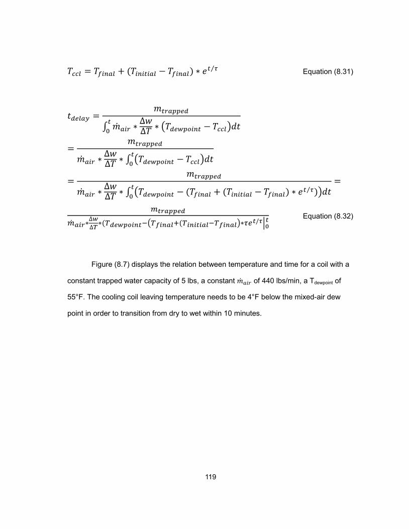
119

𝑇𝑐𝑐𝑙 = 𝑇𝑓𝑖𝑛𝑎𝑙 + (𝑇𝑖𝑛𝑖𝑡𝑖𝑎𝑙 − 𝑇𝑓𝑖𝑛𝑎𝑙) ∗ 𝑒𝑡 𝜏⁄ Equation (8.31)

𝑡𝑑𝑒𝑙𝑎𝑦 =𝑚𝑡𝑟𝑎𝑝𝑝𝑒𝑑

∫ 𝑎𝑖𝑟 ∗∆𝑤∆𝑇 ∗ 𝑇𝑑𝑒𝑤𝑝𝑜𝑖𝑛𝑡 − 𝑇𝑐𝑐𝑙𝑑𝑡

𝑡0

=𝑚𝑡𝑟𝑎𝑝𝑝𝑒𝑑

𝑎𝑖𝑟 ∗∆𝑤∆𝑇 ∗ ∫ 𝑇𝑑𝑒𝑤𝑝𝑜𝑖𝑛𝑡 − 𝑇𝑐𝑐𝑙𝑑𝑡

𝑡0

=𝑚𝑡𝑟𝑎𝑝𝑝𝑒𝑑

𝑎𝑖𝑟 ∗∆𝑤∆𝑇 ∗ ∫ 𝑇𝑑𝑒𝑤𝑝𝑜𝑖𝑛𝑡 − (𝑇𝑓𝑖𝑛𝑎𝑙 + (𝑇𝑖𝑛𝑖𝑡𝑖𝑎𝑙 − 𝑇𝑓𝑖𝑛𝑎𝑙) ∗ 𝑒𝑡 𝜏⁄ )𝑑𝑡𝑡

0

=

𝑚𝑡𝑟𝑎𝑝𝑝𝑒𝑑

𝑎𝑖𝑟∗∆𝑤∆𝑇∗(𝑇𝑑𝑒𝑤𝑝𝑜𝑖𝑛𝑡−𝑇𝑓𝑖𝑛𝑎𝑙+(𝑇𝑖𝑛𝑖𝑡𝑖𝑎𝑙−𝑇𝑓𝑖𝑛𝑎𝑙∗𝜏𝑒𝑡/𝜏𝑡0

Equation (8.32)

Figure (8.7) displays the relation between temperature and time for a coil with a

constant trapped water capacity of 5 lbs, a constant 𝑎𝑖𝑟 of 440 lbs/min, a Tdewpoint of

55°F. The cooling coil leaving temperature needs to be 4°F below the mixed-air dew

point in order to transition from dry to wet within 10 minutes.

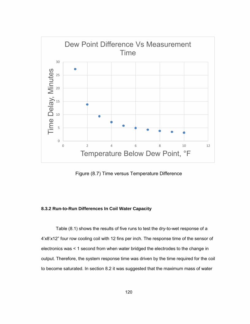
120

Figure (8.7) Time versus Temperature Difference

8.3.2 Run-to-Run Differences In Coil Water Capacity

Table (8.1) shows the results of five runs to test the dry-to-wet response of a

4’x8’x12” four row cooling coil with 12 fins per inch. The response time of the sensor of

electronics was < 1 second from when water bridged the electrodes to the change in

output. Therefore, the system response time was driven by the time required for the coil

to become saturated. In section 8.2 it was suggested that the maximum mass of water

0

5

10

15

20

25

30

0 2 4 6 8 10 12

Tim

e D

elay

, Min

utes

Temperature Below Dew Point, °F

Dew Point Difference Vs Measurement Time

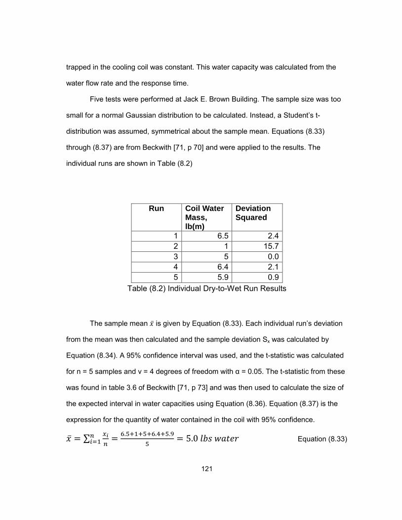
121

trapped in the cooling coil was constant. This water capacity was calculated from the

water flow rate and the response time.

Five tests were performed at Jack E. Brown Building. The sample size was too

small for a normal Gaussian distribution to be calculated. Instead, a Student’s t-

distribution was assumed, symmetrical about the sample mean. Equations (8.33)

through (8.37) are from Beckwith [71, p 70] and were applied to the results. The

individual runs are shown in Table (8.2)

Run Coil Water Mass, lb(m)

Deviation Squared

1 6.5 2.4 2 1 15.7 3 5 0.0 4 6.4 2.1 5 5.9 0.9

Table (8.2) Individual Dry-to-Wet Run Results

The sample mean is given by Equation (8.33). Each individual run’s deviation

from the mean was then calculated and the sample deviation Sx was calculated by

Equation (8.34). A 95% confidence interval was used, and the t-statistic was calculated

for n = 5 samples and ν = 4 degrees of freedom with α = 0.05. The t-statistic from these

was found in table 3.6 of Beckwith [71, p 73] and was then used to calculate the size of

the expected interval in water capacities using Equation (8.36). Equation (8.37) is the

expression for the quantity of water contained in the coil with 95% confidence.

= ∑ 𝑥𝑖𝑛

𝑛𝑖=1 = 6.5+1+5+6.4+5.9

5= 5.0 𝑙𝑏𝑠 𝑤𝑎𝑡𝑒𝑟 Equation (8.33)

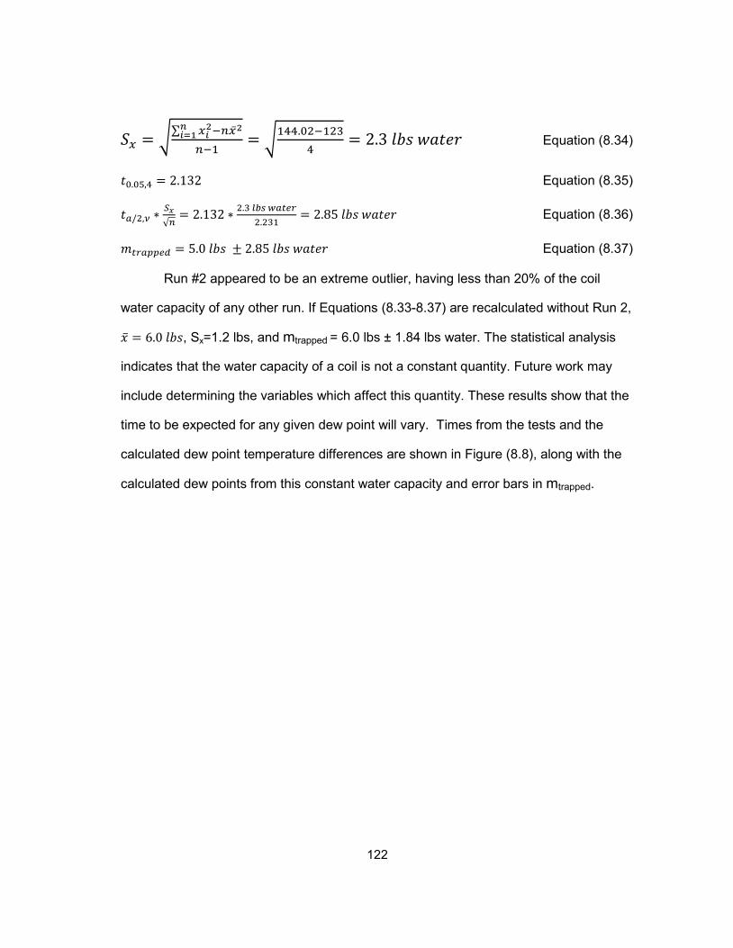
122

𝑆𝑥 = ∑ 𝑥𝑖2−𝑛2𝑛

𝑖=1𝑛−1

= 144.02−1234

= 2.3 𝑙𝑏𝑠 𝑤𝑎𝑡𝑒𝑟 Equation (8.34)

𝑡0.05,4 = 2.132 Equation (8.35)

𝑡𝑎/2,𝜈 ∗𝑆𝑥√𝑛

= 2.132 ∗ 2.3 𝑙𝑏𝑠 𝑤𝑎𝑡𝑒𝑟2.231

= 2.85 𝑙𝑏𝑠 𝑤𝑎𝑡𝑒𝑟 Equation (8.36)

𝑚𝑡𝑟𝑎𝑝𝑝𝑒𝑑 = 5.0 𝑙𝑏𝑠 ± 2.85 𝑙𝑏𝑠 𝑤𝑎𝑡𝑒𝑟 Equation (8.37)

Run #2 appeared to be an extreme outlier, having less than 20% of the coil

water capacity of any other run. If Equations (8.33-8.37) are recalculated without Run 2,

= 6.0 𝑙𝑏𝑠, Sx=1.2 lbs, and mtrapped = 6.0 lbs ± 1.84 lbs water. The statistical analysis

indicates that the water capacity of a coil is not a constant quantity. Future work may

include determining the variables which affect this quantity. These results show that the

time to be expected for any given dew point will vary. Times from the tests and the

calculated dew point temperature differences are shown in Figure (8.8), along with the

calculated dew points from this constant water capacity and error bars in mtrapped.

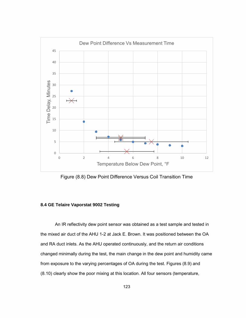
123

Figure (8.8) Dew Point Difference Versus Coil Transition Time

8.4 GE Telaire Vaporstat 9002 Testing

An IR reflectivity dew point sensor was obtained as a test sample and tested in

the mixed air duct of the AHU 1-2 at Jack E. Brown. It was positioned between the OA

and RA duct inlets. As the AHU operated continuously, and the return air conditions

changed minimally during the test, the main change in the dew point and humidity came

from exposure to the varying percentages of OA during the test. Figures (8.9) and

(8.10) clearly show the poor mixing at this location. All four sensors (temperature,

0

5

10

15

20

25

30

35

40

45

0 2 4 6 8 10 12

Tim

e D

elay

, Min

utes

Temperature Below Dew Point, °F

Dew Point Difference Vs Measurement Time

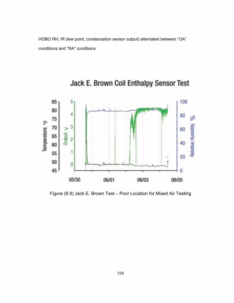
124

HOBO RH, IR dew point, condensation sensor output) alternated between “OA”

conditions and “RA” conditions.

Figure (8.9) Jack E. Brown Test – Poor Location for Mixed Air Testing

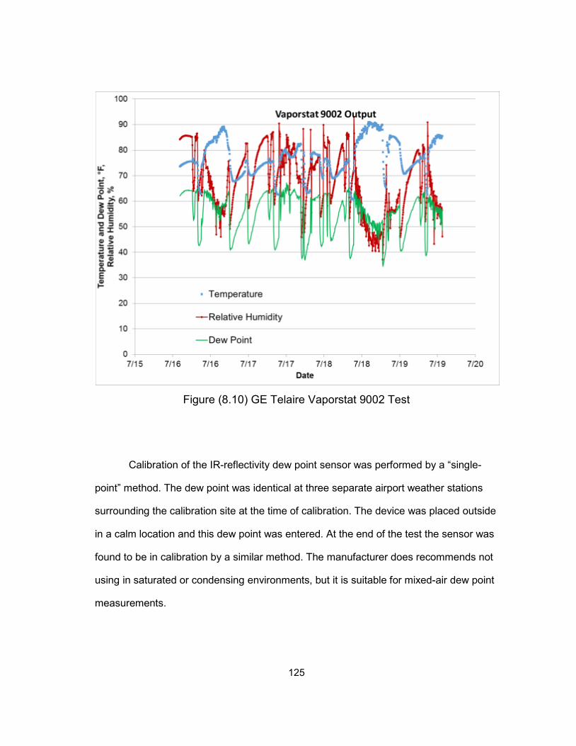
125

Figure (8.10) GE Telaire Vaporstat 9002 Test

Calibration of the IR-reflectivity dew point sensor was performed by a “single-

point” method. The dew point was identical at three separate airport weather stations

surrounding the calibration site at the time of calibration. The device was placed outside

in a calm location and this dew point was entered. At the end of the test the sensor was

found to be in calibration by a similar method. The manufacturer does recommends not

using in saturated or condensing environments, but it is suitable for mixed-air dew point

measurements.

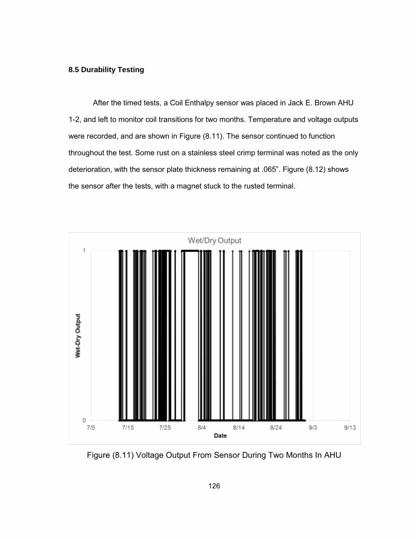
126

8.5 Durability Testing

After the timed tests, a Coil Enthalpy sensor was placed in Jack E. Brown AHU

1-2, and left to monitor coil transitions for two months. Temperature and voltage outputs

were recorded, and are shown in Figure (8.11). The sensor continued to function

throughout the test. Some rust on a stainless steel crimp terminal was noted as the only

deterioration, with the sensor plate thickness remaining at .065”. Figure (8.12) shows

the sensor after the tests, with a magnet stuck to the rusted terminal.

Figure (8.11) Voltage Output From Sensor During Two Months In AHU

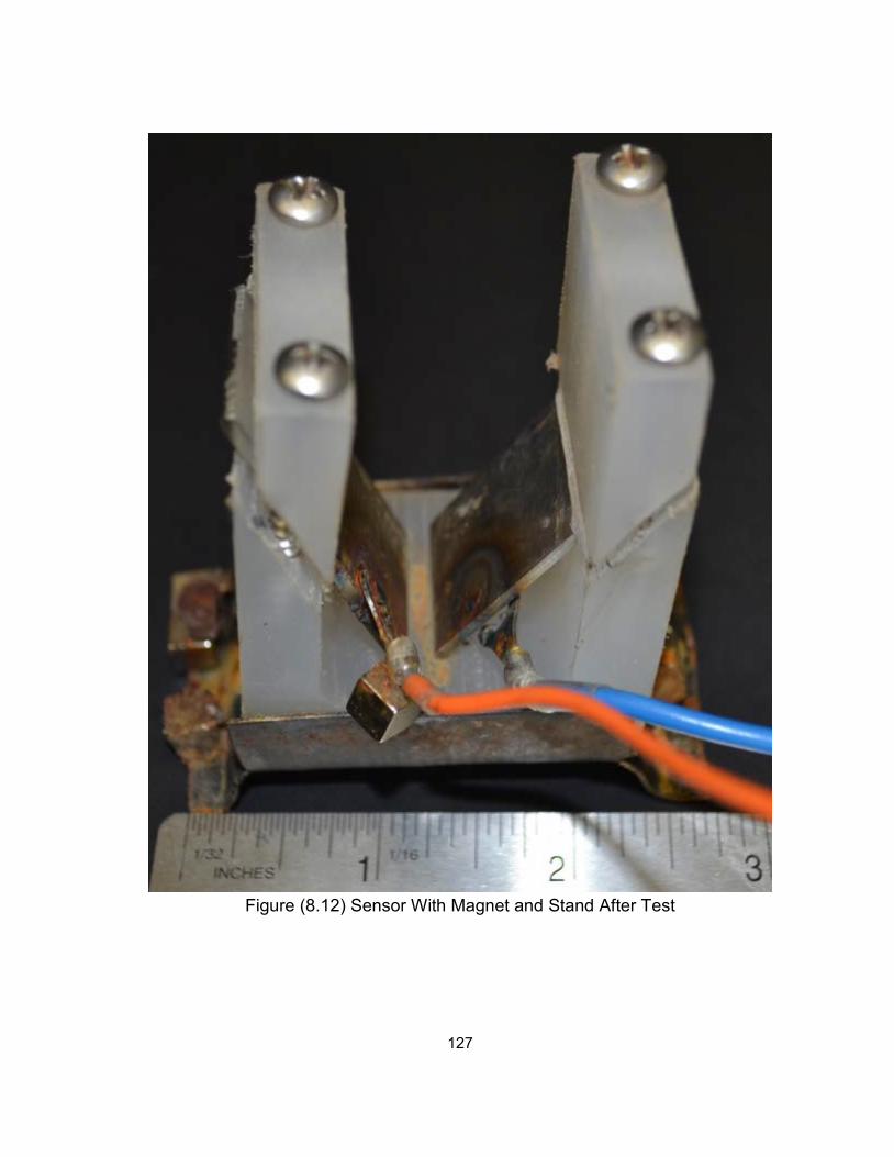
127

Figure (8.12) Sensor With Magnet and Stand After Test

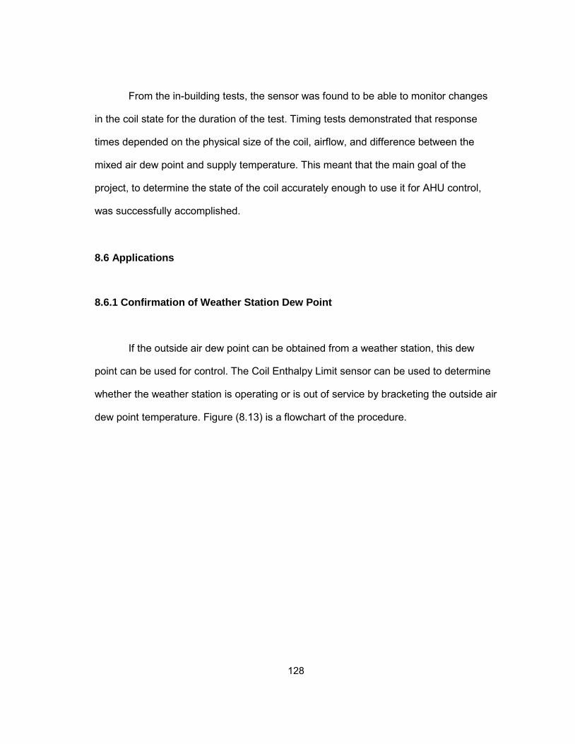
128

From the in-building tests, the sensor was found to be able to monitor changes

in the coil state for the duration of the test. Timing tests demonstrated that response

times depended on the physical size of the coil, airflow, and difference between the

mixed air dew point and supply temperature. This meant that the main goal of the

project, to determine the state of the coil accurately enough to use it for AHU control,

was successfully accomplished.

8.6 Applications

8.6.1 Confirmation of Weather Station Dew Point

If the outside air dew point can be obtained from a weather station, this dew

point can be used for control. The Coil Enthalpy Limit sensor can be used to determine

whether the weather station is operating or is out of service by bracketing the outside air

dew point temperature. Figure (8.13) is a flowchart of the procedure.

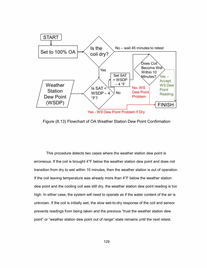
129

Figure (8.13) Flowchart of OA Weather Station Dew Point Confirmation

This procedure detects two cases where the weather station dew point is

erroneous. If the coil is brought 4°F below the weather station dew point and does not

transition from dry to wet within 10 minutes, then the weather station is out of operation.

If the coil leaving temperature was already more than 4°F below the weather station

dew point and the cooling coil was still dry, the weather station dew point reading is too

high. In either case, the system will need to operate as if the water content of the air is

unknown. If the coil is initially wet, the slow wet-to-dry response of the coil and sensor

prevents readings from being taken and the previous “trust the weather station dew

point” or “weather station dew point out of range” state remains until the next retest.

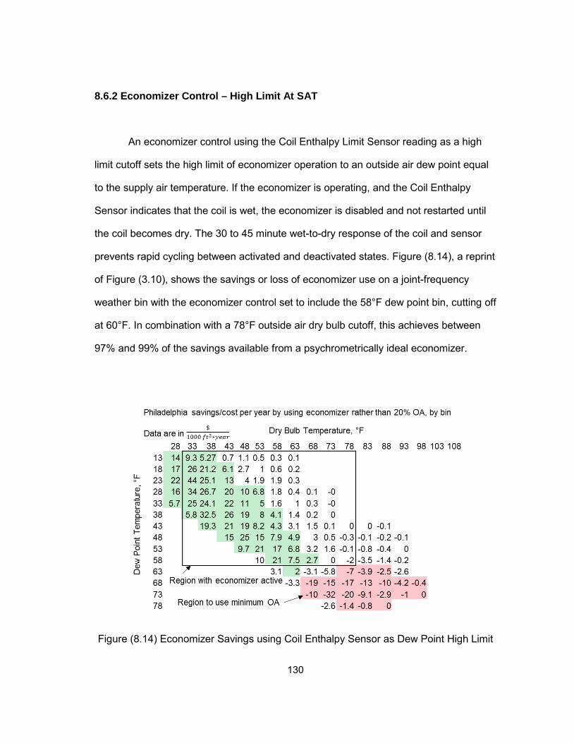
130

8.6.2 Economizer Control – High Limit At SAT

An economizer control using the Coil Enthalpy Limit Sensor reading as a high

limit cutoff sets the high limit of economizer operation to an outside air dew point equal

to the supply air temperature. If the economizer is operating, and the Coil Enthalpy

Sensor indicates that the coil is wet, the economizer is disabled and not restarted until

the coil becomes dry. The 30 to 45 minute wet-to-dry response of the coil and sensor

prevents rapid cycling between activated and deactivated states. Figure (8.14), a reprint

of Figure (3.10), shows the savings or loss of economizer use on a joint-frequency

weather bin with the economizer control set to include the 58°F dew point bin, cutting off

at 60°F. In combination with a 78°F outside air dry bulb cutoff, this achieves between

97% and 99% of the savings available from a psychrometrically ideal economizer.

Figure (8.14) Economizer Savings using Coil Enthalpy Sensor as Dew Point High Limit

131

9. CONCLUSIONS

Development of a reliable enthalpy sensor using the state of the chilled water

coil was the primary goal of this project. The design of a sensor with a gap between

two electrodes to be bridged by coil condensate was described in Section 6, and the

successful results of testing that sensor were described in Section 8.

One of the conclusions from the literature survey was that common porous

medium capacitive and resistive sensors fail to operate properly when exposed to

condensing conditions. The tests performed on commercially available sensors support

this conclusion. Cycling chilled mirror sensors last several years between repairs but

cost in excess of $1500. Sensors that directly detect and measure water vapor

concentration by measuring how much infrared radiation is absorbed by the air passing

through the sensor may be able to provide dew point measurements indefinitely. Future

work in building humidity measurement includes multiyear testing of commercial IR dew

point sensors to determine whether calibration can be maintained over a long

unattended interval.

WinAM models and the spreadsheet economizer simulations agreed with the

literature that enthalpy economizers are ineffective in climates similar to Houston’s, but

showed areas where enthalpy control can allow for savings. Approximately 90% of the

savings available from the use of an economizer in buildings in Dallas or Philadelphia

can be attained with an appropriate dry bulb temperature cutoff. Conservative low-limit

controls on the economizer can easily reduce the savings by more than 10%. A reliable

dew point or humidity sensor serving as a high-limit cutoff allows the remainder of the

savings to be captured.

132

Future work in economizer control includes using transient building models to

consider the effects of night purge modes and supply air temperature resets based on

time varying latent loads. Dessicant dehumidification may also require different air

control strategies if waste heat can be used for reheat without additional energy inputs.

Reliable wet-or-dry measurements for economizer control can be made without

sensor corrosion if the electrodes are made from 316 austenitic stainless steel sheet,

the wires are fully encapsulated in crimped and welded terminals, and the potential

difference between the electrodes is 0.25 V AC. These sensors can be made on a 3-

axis mill out of high-density polypropylene.

One significant limitation of this type of measurement is the slow response time.

A typical cooling coil in a 10,000 cfm air handler unit traps almost a gallon of water in

the boundary layer near the fins. Condensation of enough water to fill the coil and begin

dripping on the sensor took 5 to 10 minutes in a properly operating air handler. Active

measurement of the dew point for supply air temperature resets and outside air dew

point measurement is impractical.

Measurement of the rate of condensate flow from an AHU can help the

diagnosis of comfort complaints. Insufficient outside airflow, insufficient total primary

flow, and a partially blocked coil can cause unexpectedly low condensate production,

while excessive outside airflow away from economizer-friendly conditions, high return

air humidity due to infiltration, a chilled water valve stuck all the way open, or an

inoperative economizer can cause excessive condensate flow.

The electronics described in this thesis gave a clear output difference between

wet and dry states use commonly available analog components. The circuit consisted of

an oscillator to generate the AC signal, a voltage divider to bring the voltage below the

half-cell potential needed to oxidize the electrodes, the sensor and its leads, a filter to

133

convert the AC signal to its DC level, and an amplifier to give a ±5 V output. The cost of

the components on the printed circuit board is approximately $10.

Electronically detecting water condensing on the coil by measuring the AC

reactance across a gap between conductors can determine whether the dew point is

above or below the cooling coil leaving temperature. This was demonstrated early in the

development of the sensor and iteratively refined into the final device.

134

REFERENCES

1. U.S. Energy Information Administration, 2013, “2012 Annual Review of Energy,” p

82, accessed on April 18, 2014 from

http://www.eia.gov/totalenergy/data/annual/index.cfm

2. TIAX LLC, 2003. “Matching the Sensible Heat Ratio of Air Conditioning Equipment

with the SHR,” accessed on April 18, 2014 from

http://www.airxchange.com/Collateral/Documents/English-US/SHR_Report.pdf

3. Honeywell Sensing and Control, 2007, Honeywell HIH-1000 Data Sheet, accessed

on April 18, 2014 from http://sensing.honeywell.com/index.php?ci_id=54699

4. Honeywell Sensing and Control, 2010, Honeywell HIH-5030 Data Sheet, accessed

on April 18, 2014 from http://sensing.honeywell.com/honeywell-sensing-hih5030-

5031%20series-product-sheet-009050-2-en.pdf?name=HIH-5030-001

5. Measurement Specialties Inc., 2012, Measurement Specialties HS1101LF Data

Sheet, accessed on April 18, 2014 from http://www.meas-

spec.com/downloads/hs1101lf.pdf

6. Parallax Inc., 2009, Parallax HS1101 Data Sheet, accessed on April 18, 2014 from

http://parallax.com/sites/default/files/downloads/27920-Humidity-Sensor-

Documention-S1101-v1.0.pdf

7. TDK Inc, 2007, TDK CHS-MSS Data Sheet, accessed on April 18, 2014 from

http://www.farnell.com/datasheets/84894.pdf

8. TDK Inc, 2005, TDK CHS-CSC-20 Data Sheet, accessed on April 18, 2014 from

http://media.digikey.com/pdf/Data%20Sheets/TDK%20PDFs/CHS-CSC-

20%20Specification.pdf

135

9. Griesel, S., M. Theel, H. Niemand, E. Lanzinger, 2012. “Acceptance Test

Procedure for Capacitive Humidity Sensors In Saturated Conditions,” WMO CIMO

TECO-2012, Brussels, Belgium, 2012, accessed on April 18, 2014 from

http://www.wmo.int/pages/prog/www/IMOP/publications/IOM-109_TECO-

2012/Session1/P1_09_Griesel_Acceptance_test_procedure_humidity_sensors.pdf

10. Wilson, J., Fontes, J. 2005. “Sensor Technology Handbook”, Elsevier, Burlington,

MA, ISBN 0-7506-7729-5

11. General Electric Measurement and Control, 2006, “GE Sensing Telaire Vaporstat

9002,” accessed on April 18, 2014 from http://www.ge-mcs.com/download/co2-

flow/920_332a.pdf

12. ASHRAE Standard 62.1-2010 Committee. 2010. “ASHRAE Standard 62.1

Ventilation for Acceptable Indoor Air Quality” ASHRAE, Atlanta, GA

13. Harriman, L., G. Brundrett, R. Kittler. 2001. “ASHRAE Humidity Control Design

Guide For Commercial and Institutional Buildings,” ASHRAE Publications, Atlanta,

GA, ISBN 1-883413-98-2

14. Henderson, H.L.1990. “An Experimental Investigation of the Effects of Wet and Dry

Coil Conditions on Cyclic Performance in the SEER Procedure,” Florida Solar

Energy Center, accessed on April 18, 2014 from

http://docs.lib.purdue.edu/cgi/viewcontent.cgi?article=1082&context=iracc

15. Rose, W.B. 2005. “Water in Buildings: An Architect’s Guide To Moisture and Mold,”

Wiley, Hoboken, NJ, ISBN 0471468509

16. Schell, M. 2004. “Measuring the Right Thing For Humidity Control – It’s the Dew

Point, Stupid,” AirTest Technology, accessed on April 18, 2014 from

https://www.airtest.com/support/reference/dpstupid.pdf

136

17. Shah, D., J. Krueger, R. Strand, 1993. U.S. Patent 5346129, “Indoor Climate

Controller System Adjusting Both Dry Bulb Temperature and Wet-Bulb Or Dew

Point Temperature In The Enclosure”, accessed on April 18, 2014 from

http://www.google.com.ar/patents/US5346129

18. Taylor, S., C. H. Cheng. 2010. “Economizer High Limit Controls and Why Enthalpy

Economizers Don’t Work,” accessed on April 18, 2014 from http://www.taylor-

engineering.com/downloads/articles/ASHRAE%20Journal%20-

%20Economizer%20High%20Limit%20Devices%20and%20Why%20Enthalpy%20

Economizers%20Don't%20Work%20-%20Taylor%20&%20Cheng.pdf

19. Wang, G., L. Song. 2012. “Air handling unit supply air temperature optimal control

during economizer cycles,” University of Miami/University of Oklahoma, Elsevier

“Energy and Buildings” June 2012, accessed on April 18, 2014 from

http://www.sciencedirect.com/science/article/pii/S0378778812001016

20. Feng, Jingjuang., M. Liu., X. Pang. 2005. “Economizer Control Using Mixed Air

Enthalpy,” accessed on April 18, 2014 from

http://digitalcommons.unl.edu/cgi/viewcontent.cgi?article=1024&context=archengfa

cpub&sei-

redir=1&referer=http%3A%2F%2Fscholar.google.com%2Fscholar%3Fhl%3Den%2

6q%3Deconomizer%2Bcondensation%2BHVAC%26btnG%3DSearch%26as_sdt%

3D0%252C44%26as_ylo%3D%26as_vis%3D0#search=%22economizer%20conde

nsation%20HVAC%22

21. All-Weather Inc., “Model 5190-E Temperature-Humidity Probe,” 2010, accessed on

April 18, 2014 from http://www.allweatherinc.com/reference/sensors/5190-e-

001.pdf

137

22. Sealed Unit Parts Company, no copyright date given, “DTVH Temperature

Humidity Logger With Display,”, accessed on April 18, 2014 from

http://www.supco.com/images/pdfs/Manuals-Instructions/DVTH%20Manualpdf.pdf

23. Mumma, S., 2001. “Designing Dedicated Outdoor Air Systems,” ASHRAE Journal

2001, accessed on April 18, 2014 from http://doas-radiant.psu.edu/Journal1.pdf

24. Shank, K. M., S. Mumma, 2001. “Selecting the Supply Air Conditions for a

Dedicated Outdoor Air System Working in Parallel with Distributed Sensible

Cooling Terminal Equipment,” ASHRAE Transactions 2001, V107, p 562.

25. Roveti, D., 2001. “Choosing A Humidity Sensor, A Review Of Three Technologies,”

Sensors Magazine, accessed on April 18, 2014 from

http://www.sensorsmag.com/sensors/humidity-moisture/choosing-a-humidity-

sensor-a-review-three-technologies-840

26. Consense Corp, “Consensor”, no copyright date given, accessed on April 18 2014

from www.consense.com.

27. Kang, Uksong., K.D.Wise. April 2000. “A High-Speed Capacitive Humidity Sensor

With On-Chip Thermal Reset,” IEEE Transactions, accessed on April 18, 2014 from

http://www.umel.feec.vutbr.cz/~hubalek/skola/vyuka/zima%202005%5Csenzor%20

vlhkosti%5Ccapacit_humidit_sens.pdf

28. Vaisala, Inc., 2010, “Choice of outdoor humidity sensors critical to economical free

cooling system,” accessed on April 18, 2014 from

http://www.vaisala.com/Vaisala%20Documents/Application%20notes/Outdoor-

Humidity-App%20Note-B210967EN-A-lores.pdf

29. Chen, Z., C. Lu, 2005. “Humidity Sensors, A Review of Materials and

Mechanisms,” University of Kentucky, American Scientific Publishers Sensor

Letters Vol 3, 274-295

138

30. Stokes, W., 2006. “Discharge Humidity Sensor Saturated.” Accessed on April 18,

2014 from http://www.eng-tips.com/viewthread.cfm?qid=166897

31. Francisco, C. C., 1963, U.S. Patent 3195344. Accessed on April 18, 2014 from

http://www.google.com/patents/US3195344

32. Able Instruments and Controls, 2006. “Humidity Sensors for Industrial

Applications,” accessed on April 18, 2014 from

http://www.iceweb.com.au/Analyzer/humidity_sensors.html,

33. Heinonen, M. 1999. “Investigation of the Dew-Point Temperature Scale Maintained

at the MIKES,” Measurement Science Technology Vol 10 36, accessed on April 18,

2014 from http://iopscience.iop.org/0957-0233/10/1/010/pdf/0957-

0233_10_1_010.pdf

34. Cooper, F.G., 1996, U.S. Patent 5507175. “Cycling Chilled Mirror Hygrometer

Including a Sapphire Optical Mirror” Accessed on April 18, 2014 from

http://www.google.com/patents/US5507175

35. EdgeTech Moisture and Humidity, no copyright date given. “DewTrak II Model DT-

PL-W-AT/W-RD,” Accessed on April 18, 2014 from

http://www.edgetechinstruments.com/moisture-humidity/gallery/item/dewtrak-ii-

chilled-mirror-transmitter

36. GE General Eastern, 2011. “Optisonde Chilled Mirror Hygrometer,” accessed on

April 18, 2014 from http://store.ge-mcs.com/products/23780/ge-general-eastern-

optisonde-chilled-mirror-hygrometer

37. GE General Eastern, 2011. “Optisonde Chilled Mirror Hygrometer,” accessed on

April 18, 2014 from http://www.ge-mcs.com/download/moisture-humidity/920-423B-

LR.pdf

139

38. Ueno, K., J. Straube, 2008. ”Laboratory Calibration and Field Results of Wood

Resistance Humidity Sensors,” accessed on April 18, 2014 from

http://c.ymcdn.com/sites/www.nibs.org/resource/resmgr/BEST/BEST1_004.pdf

39. Nguyen Thi Thu Ha, et al., 2000. “Study and performance of humidity sensor based

on the mechanical-optoelectronic principle for the measurement and control of

humidity in storehouses,” Elsevier Sensors and Actuators B, Chemical, Volume 66

Issues 1-3, accessed on April 18, 2014 from

http://www.sciencedirect.com/science/article/pii/S0925400500003609

40. Liu, Xingbin., et al. 1998. “A theoretical model for a capacitance tool and its

application to production logging,” Daqing Production Well Logging Institute,

Daqing City, PRC, Elsevier Flow Measurement and Instrumentation Volume 9

Issue 4, accessed on April 18, 2014 from

http://www.sciencedirect.com/science/article/pii/S0955598698000211

41. Davis, D.R., J. E. Hughes. 1970. “A New Approach To Recording The Wetting

Parameter By The Use Of Electrical Resistance Sensors,” The Plant Disease

Reporter, Volume 54 Issue 6, p474-9.

42. Blad, B.l., J. R. Steadman, A.Weiss. 1978. “Canopy Structure and Irrigation

Influence White Mold Disease and Microclimate of Dry Edible Beans,” accessed on

April 18, 2014 from

http://www.apsnet.org/publications/phytopathology/backissues/Documents/1978Arti

cles/Phyto68n10_1431.pdf

43. Seyfried, M.S., M.D. Murdock. 2001. “Response of a New Soil Water Sensor to

Variable Soil, Water Content, and Temperature,” Soil Science Society of America

Journal, accessed on April 18, 2014 from

https://www.soils.org/publications/sssaj/abstracts/65/1/28

140

44. Hanek, G., M.Truebe, M. Kestler, 2001. “Using Time-Domain Reflectrometry (TDR)

and Radio Frequency (RF) Devices to Monitor Seasonal Variation in Forest Road

Subgrade and Base Materials,” US Forest Service 2001, accessed on April 18,

2014 from http://www.fs.fed.us/t-d/pubs/html/00771805/00771805.html

45. Iwashita,T., H. Katayanagi. 2011. “Needle-type in situ water content sensor with

polyethersulfone polymer membrane,” Keio University, Kanagawa, Japan, Elsevier

“Sensors and Actuators B: Chemical,” Volume 154 Issue 1, accessed on April 18,

2014 from http://www.sciencedirect.com/science/article/pii/S0925400509008843

46. Malazian, A. et al. 2011. “Evaluation of MPS-1 soil water potential sensor,”

University of California Davis/Decagon Devices, Elsevier Journal of Hydrology,

Volume 402 Issues 1-2, accessed on April 18, 2014 from

http://www.sciencedirect.com/science/article/pii/S0022169411001661

47. Mealy, R., G. Bowman. No copyright date given. “Lab Regent Water Concerns”

Wisconsin Department of Natural Resources, accessed on April 18, 2014 from

http://dnr.wi.gov/regulations/labcert/documents/training/ReagentH2O.pdf

48. Lenntech B.V. No copyright date given. “Water Conductivity,” accessed on April 18,

2014 from http://www.lenntech.com/applications/ultrapure/conductivity/water-

conductivity.htm

49. Roby, D. New Mexico Department of the Environment, 2007. “Reagent Water,”

accessed on April 18, 2014 from

http://www.nmrwa.org/sites/nmrwa.org/files/WWLabStudyGuide.pdf

50. Rame-Hart Instrument Co, 2013. “Contact Angle,” accessed on April 18, 2014 from

http://www.ramehart.com/contactangle.htm

141

51. Sumner, A. L., et al. 2004. “The nature of water on surfaces of laboratory systems

and implications for heterogenous chemistry in the trophosphere,” Phys. Chem,

Chem. Phys, accessed on April 18, 2014 from

http://132.68.226.240/english/pdf/Professors/Yael_Dubowski/1.pdf

52. Onset Computer Corp., 2008. “HOBO U12-012 Data Logger,” accessed on April

18, 2014 from

http://wpc.306e.edgecastcdn.net/80306E/onsetcomp_com/files/manual_pdfs/7661_

C_MAN_U12_012.pdf

53. Storr, W., 1999. “Electronics Tutorials, Waveform Generators,” accessed on April

18, 2014 from http://www.electronics-tutorials.ws/waveforms/generators.html

54. Fairchild Semiconductor, 1983. “MM74HC14 Schmitt Trigger,” accessed on April

18, 2014 from http://www.fairchildsemi.com/ds/MM/MM74HC14.pdf

55. Maxim Semiconductor, 2007. “Low Frequency Dual EconOscillator,” accessed on

April 18, 2014 from http://datasheets.maximintegrated.com/en/ds/DS1099.pdf

56. Shrader, R. 1975. “Electronic Communication,” 3rd Edition, McGraw-Hill, New York,

ISBN 9780070571389

57. Sinclair, I., J. Dunton. 2007. “Practical Electronics Handbook,” 6th edition, Newnes,

Oxford, UK, ISBN 978-0750680714

58. Texas Instruments, 2013 “LME49710 High-Performance, High-Fidelity Operational

Amplifier,” accessed April 18, 2014 from

http://www.ti.com/lit/ds/snas376c/snas376c.pdf

59. Lee, W.Y., J.M. House, N-H. Kyong. 2004. “Subsystem level fault diagnosis of a

building’s air handling unit using general regression neural networks,” Elseveir

Applied Energy, Volume 77, Issue 2, accessed on April 18, 2014 from

http://www.sciencedirect.com/science/article/pii/S0306261903001077

142

60. Zhou, J., G. Wei, W.D. Turner, D.E. Claridge, 2008. “Airside Economizer -

Comparing Different Control Strategies and Common Misconceptions,” ESL-IC-08-

10-54, accessed on April 18, 2014 from

http://repository.tamu.edu/bitstream/handle/1969.1/90822/ESL-IC-08-10-

54.pdf?sequence=1

61. Agilent Technologies, 2013. “Agilent Impedance Measurement Handbook, 4th

Edition,” accessed on April 18, 2014 from

http://literature.agilent.com/litweb/pdf/5950-3000.pdf

62. Lomas, C. G, 2011. “Fundamentals of Hot Wire Anemometry,” Cambridge

University Press, Cambridge, UK, ISBN 0521283183

63. Mei, Y., Z.J. Zhou, H.L. Luo, “Electrical resistivity of rf-sputtered iron oxide thin

films,” Journal of Applied Physics, 1987, Volume 61, p 4388-4389, accessed on

April 18, 2014 from

http://scitation.aip.org/getpdf/servlet/GetPDFServlet?filetype=pdf&id=JAPIAU00006

1000008004388000001&idtype=cvips&doi=10.1063/1.338431&prog=normal

64. Accuratus Corporation, 2013. “Aluminum Oxide, Al2O3 Ceramic Properties,”

accessed on April 18, 2014 from http://accuratus.com/alumox.html

65. McCafferty, E. 2010. “Introduction to Corrosion Science,” Springer Science and

Business Media, New York, NY, ISBN 978-1-4419-0455-3

66. Popov, Branko, 2007. “Basics of Corrosion Measurements,” accessed on April 18,

2014 from

http://www.che.sc.edu/faculty/popov/drbnp/ECHE789b/Corrosion%20Measurement

s.pdf

143

67. Boulangé-Petermann, L., J. C. Joud, B. Baroux. 2008. “Wettability Parameters

Controlling the Surface Cleanability of Stainless Steel,” Contact Angle, Wettability,

and Adhesion, Volume 5, p139-151

68. Halladay, D., 1974. “Fundamentals of Physics,” Wiley Publishing, New York, ISBN

0471344311

69. The Engineering Toolbox, 2014. “Humidity Ratio of Air,” accessed on April 18, 2014

from http://www.engineeringtoolbox.com/humidity-ratio-air-d_686.html

70. Vömel, Holger, 2011. “Saturation Vapor Pressure Formulations,” accessed on April

18, 2014 from http://cires.colorado.edu/~voemel/vp.html

71. Beckwith, T., R.D. Marangoni, J.H. Lienhard. 1993. “Mechanical Measurements,

Fifth Edition,” Addison-Wesley, Reading, MA, ISBN 0-201-56947-7