Cohesive motion in one-dimensional flockingphysics.unm.edu/kenkre/pdflink/Dossetti12-JPA.pdf · J. Phys. A: Math. Theor. 45 (2012) 035003 V Dossetti Finally, it is worth pointing

IOP PUBLISHING JOURNAL OF PHYSICS A: MATHEMATICAL AND THEORETICAL

J. Phys. A: Math. Theor. 45 (2012) 035003 (20pp) doi:10.1088/1751-8113/45/3/035003

Cohesive motion in one-dimensional flocking

V Dossetti

Instituto de Fısica, Benemerita Universidad Autonoma de Puebla, Apartado Postal J-48,Puebla 72570, MexicoandConsortium of the Americas for Interdisciplinary Science and Department of Physics andAstronomy, University of New Mexico, Albuquerque, NM 87131, USA

E-mail: [email protected]

Received 9 March 2011, in final form 16 November 2011Published 15 December 2011Online at stacks.iop.org/JPhysA/45/035003

AbstractA one-dimensional rule-based model for flocking, which combines velocityalignment and long-range centering interactions, is presented and studied. Theinduced cohesion in the collective motion of the self-propelled agents leads tounique group behavior that contrasts with previous studies. Our results showthat the largest cluster of particles, in the condensed states, develops a meanvelocity slower than the preferred one in the absence of noise. For strongnoise, the system also develops a non-vanishing mean velocity, alternating itsdirection of motion stochastically. This allows us to address the directionalswitching phenomenon. The effects of different sources of stochasticity on thesystem are also discussed.

PACS numbers: 05.40.−a, 05.45.Xt, 64.60.−i, 87.10.−e

1. Introduction

The phenomenon of flocking (also known as swarming) refers to the emergent collectivemotion regularly seen in groups of animals such as bird flocks, fish schools, bison or sheepherds, insect or bacteria swarms, etc [1–7]. In simple terms, the formation of these sort ofgroups in nature implies some kind of condensation in position and/or velocity spaces. Themechanisms or behavior followed by the individuals that compose the group, which leadto this type of condensation, have been classified by Reynolds [8] as the desire to matchthe velocity of flockmates (alignment), the desire to stay close to flockmates (centering)and the desire to avoid collisions (separation). These definitions have been widely adopted byresearchers from a variety of disciplines.

In the realm of the physical sciences, the study of flocking has greatly benefited fromthe insight of statistical mechanics to describe dynamical phase transitions and cooperativephenomena [9]. The interest in the study of these kinds of system comes from the fact thatthey represent prototypical out-of-equilibrium systems. The formulations to study the flocking

1751-8113/12/035003+20$33.00 © 2012 IOP Publishing Ltd Printed in the UK & the USA 1

J. Phys. A: Math. Theor. 45 (2012) 035003 V Dossetti

phenomenon can be succinctly classified into rule-based [10–18], Lagrangian (trajectory-based) [19–26] and Eulerian (continuum) models [27–29]. Regarding the dimensionality ofthe models developed, most of them have been defined in dimensions higher than one [10–15,20–25, 27–30], since the velocity of the self-propelled particles (SPP) in these models can havecontinuous values. In contrast, only a few one-dimensional (1D) models have been studied[5, 16–19, 26, 31]. For these, the direction of the particles velocity can only take discretevalues, in fact, only two. Nonetheless, recent experimental and theoretical studies by Buhlet al [5] and Yates et al [6] have proven the usefulness of 1D models in elucidating thedirectional switching phenomenon. This phenomenon regards a very interesting aspect of themovement of many animal groups, when they suddenly switch their direction of motion in acoherent form. This seems to be an intrinsic property of the collective motion of animals as ithas been observed, e.g., in groups of locusts and starlings (see [6] for more details).

Among the 1D models, one can find of the Lagrangian kind like the one by Mikhailovand Zanette [19] that describes a population of SPP with attractive long-range interactions, i.e.includes centering as the only ingredient from the Reynolds considerations. Here, the particlestry to attain one of the two preferred velocities (v0 or −v0) through a nonlinear friction termcubic in nature. The system presents multistable dynamics and can be found either in coherenttraveling motion (ordered state) where all the particles move together in a condensed group,developing a non-zero mean velocity with the same direction, or in an incoherent oscillatorystate (disordered state) where the particles perform random-phase oscillations around a fixedposition with zero mean velocity. By increasing the additive noise intensity, the system canbe driven from the coherent traveling state to the oscillatory state through a discontinuousphase transition. However, for noise intensities below the critical point, the two states areaccessible depending on the initial conditions since the system shows a strong hysteresis.

On the other hand, one can find rule-based models like the 1D version of the famousVicsek et al model [10], by Czirok et al [31], that describes a population of SPP thatinteract only through condensation in velocity space (alignment according to Reynolds).Via short-range interactions and a majority rule, the particles try to match the velocity of theirnearest flockmates. The system exhibits spontaneous symmetry breaking and self-organizationdepending on the intensity of the additive noise, leading to a continuous kinetic phase transitionfrom a homogeneous to a condensed phase. In contrast to the two-dimensional Vicsek model[10] where the speed of the particles is fixed, i.e. |v0| = constant, in the 1D version [31],at each time step, particles try to acquire a velocity close to the two prescribed ones (v0 or−v0) through an antisymmetric function G(u) that depends linearly on the local mean velocity〈u(t)〉i of the neighbors of a given particle i. This function can also be written in a continuousform with no change in the scaling properties of the system as claimed in [31].

Let us also consider the lattice model by O’Loan and Evans [16] where the velocity ofthe particles can take three discrete values (−1, 0, 1). Here, through an alignment interactionin the form of a majority rule, which is applied asynchronously with probabilistic updates(particles are selected and updated randomly in a Monte Carlo fashion), the system showsa continuous phase transition from a homogeneous to a condensed phase similar to that ofthe previous model. However, and in contrast with the previous model, the condensed phaseis not symmetry-broken but alternating. We must point out the two sources of noise in thismodel—coming from the way particles are updated and how the alignment rule is applied—since no additive noise is present. The later generalization of this model by Raymond andEvans [17] includes all three types of Reynolds’ flocking behavior that translates into richerdynamics: the system also shows an homogeneous flock with homogeneous density and afixed global non-zero velocity, and dipole states. However, the different interactions presentin these models are local, i.e. short in range regarding the spatial coordinate.

2

J. Phys. A: Math. Theor. 45 (2012) 035003 V Dossetti

Finally, it is worth pointing out the variations of the two previous rule-based modelsintroduced by Buhl et al [5], Yates et al [6] and Bode et al [18] that also show an alternatingcondensed phase that resembles the directional switching phenomenon mentioned before. Inthe first, Buhl et al consider a generalization of the Czirok et al model that weights the localmean direction of motion of the neighbors of a given particle with that of the particle itself ina deterministic way. In the second, Yates et al adapted the Buhl et al model with an additivenoise whose intensity is weighted with a non-trivial function of the local mean velocity:the individuals increase the randomness of their motion when the local alignment is low. Inthe third, Bode et al mix features from the Czirok et al, O’Loan and Evans, and Raymondand Evans models, concentrating on how noise enters the system. There, they have identifiedthree different approaches (that can be generalized to higher dimensions) to include stochasticerrors in 1D SPP models and classified them as follows:

(i) Adding a random variable to the preferred direction of individuals (i.e. the inclusion ofadditive noise as in [19, 31]).

(ii) Asynchronous and probabilistic updates (as in [16, 17]).(iii) Varying the probability and accuracy with which individuals execute their behavioral rules

(as in [16, 17] also).

In this way, Bode et al have included local alignment and centering interactions in theirmodel that are applied taking inspiration from the approaches (ii) and (iii). Nonetheless, theinteractions considered in all of these models are short ranged from the point of view of theposition of the particles as well.

Our aim in this work is to extend the 1D model of Czirok et al [31] by providing itwith a long-range centering interaction (much in the spirit of Mikhailov and Zanette) alongwith the already included local alignment interaction and additive noise. We demonstrate avariety of new flocking regimes: some of them resemble those found in the models describedin the previous paragraph. We also show that the noise-induced phase transition, from thehomogeneous to the symmetry-broken condensed phases, changes into what seems a phasetransition between two kinds of condensed states: one with broken symmetry and one withan alternating flock that moves with non-zero mean velocity, changing its direction of motionstochastically. The latter seems stable even for strong noise and different system sizes.Additionally, we explore two ways to implement the centering and alignment interactions—one probabilistic and one deterministic—that allows us to address the relation of the directionalswitching phenomenon with different sources of stochasticity in 1D SPP models.

2. Model

The 1D model by Czirok et al [31] consists of N off-lattice SPP along a line of length L. Theparticles are characterized by their coordinate xi and dimensionless velocity ui updated as

xi(t + 1) = xi(t) + v0ui(t),

ui(t + 1) = G(〈u(t)〉i) + ξi. (1)

The local average velocity 〈u(t)〉i for the ith particle is calculated within an interval[xi − �, xi + �], where � = 1 is fixed, and updated for all particles at every time step.Propulsion and friction forces are incorporated through the antisymmetric function G whichsets the average velocity to a prescribed value v0, in such a way that G(u) > u for 0 < u < 1and G(u) < u for u > 1. In this case, one cannot apply the constant velocity constraint of[10] since it strongly discretizes the system, leading to a discrete state cellular automaton.It is also important to remark that, similar to the Raymond and Evans model [17], function

3

J. Phys. A: Math. Theor. 45 (2012) 035003 V Dossetti

(a) (b) (c) (d )

Figure 1. The lower plots represent the dynamics of the 1D Czirok et al model for L = 1000,N = 1000 and ρa = 1 for increasing values of η (from left to right η = 0, 3, 5, 7, respectively).The darker gray level represents higher particle density and the systems were allowed to evolve15 000 time steps. The upper plots represent the corresponding normalized distribution P(u) of thevelocities ui of the individual particles in the steady state. Note how the steady state of the systemchanges from one with broken symmetry to a homogeneous one as the noise amplitude increases.

G(u) also works as the interaction term. The noise, ξi, is distributed uniformly in the interval[−η/2, η/2] and directly affects the velocity of the particles, while an update time �t = 1 hasalready been applied.

In this work v0 is kept constant (v0 = 0.1), and the adjustable control parameters forthe model described above are the average density of the particles, ρa = N/L, and the noiseamplitude η. Function G was implemented in [31] in a very simple way as

G(u) = 12 [u + sign(u)]. (2)

The results do not depend on the properties of G(u) for u ≈ 0 as stated in [31]. In ourcase, simulations with continuous choices of G(u) were carried out leading to similar results.Random initial conditions are applied along with periodic boundary conditions.

In the lower plots of figure 1, we show the time evolution of the density of particles, ρ(x, t),and the normalized distribution P(u) of the velocities ui of the particles, in the upper plots, forthe model given in (1) and (2) with L = 1000, N = 1000 and increasing values of the noiseamplitude η(∈ [0, 7]). The corresponding average density of particles is ρa = 1. Depending onthe chosen noise amplitude, η, the system can be driven through an order–disorder continuousphase transition. For example, for η < ηc ≈ 5, the system reaches an ordered state in ashort time (see figures 1(a) and (b)), characterized by a spontaneous symmetry breaking andclustering of the particles. In contrast, for larger values of η (> ηc), a disordered phase can befound characterized by a random velocity field, see e.g. figure 1(d). As one increases η, onecan appreciate how the distribution P(u) in the steady state, which starts single-peaked andnarrow for η = 0 (see upper plots in figure 1), flattens and broadens out when going from theordered to the disordered state (from left to right).

4

J. Phys. A: Math. Theor. 45 (2012) 035003 V Dossetti

In order to quantify the time evolution of the system, we define the instantaneous orderparameter as

φ(t) = 1

N

∣∣∣∣∣N∑

i=1

ui(t)

∣∣∣∣∣ . (3)

We also measured the instantaneous position and velocity of the center of mass, given by

xCM(t) = 1

N

N∑i=1

xi(t) (4)

and

uCM(t) = 1

N

N∑i=1

ui(t), (5)

respectively.Before we proceed, there is one thing that needs to be clarified. Due to periodic

boundary conditions, a 1D system has the topology of a ring. This implies that there aretwo distances (running in opposite directions) from any particle to any specified point in thering. Additionally, let us not forget that random initial conditions are taken both in the positionand in the initial direction of the particles velocity, and that alignment interactions favor theformation of clusters as shown in figure 1. For simplicity, the position of the center of mass,as given in (4), is determined with the particles position, xi(t), measured with respect to theorigin from which the length L of the system is measured as well. However, this does not affectthe overall results obtained as we will see below.

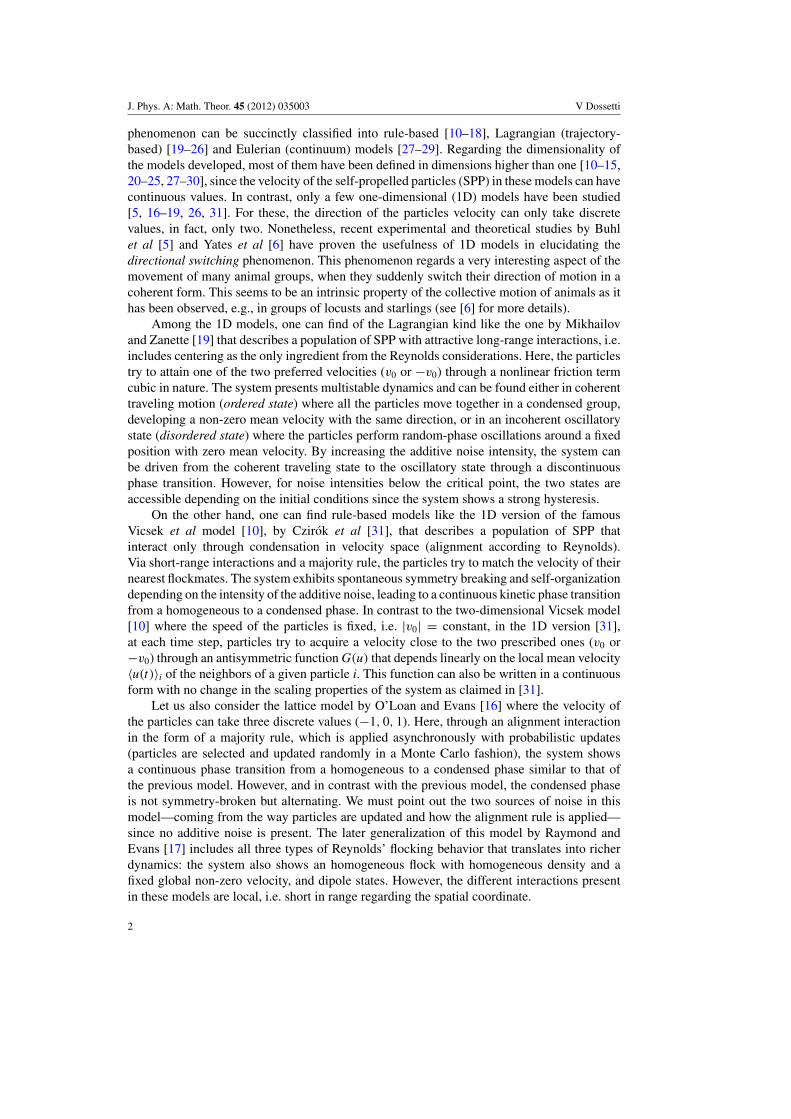
To account quantitatively for the transition from the ordered to the disordered state, infigure 2(a) we plot the steady-state accumulated order parameter, defined as

φss = limT→∞

1

T

∫ T

0φ(t) dt, (6)

as a function of the noise amplitude η for ρa = 0.5, 1, 2. This figure makes evident thedependence of the critical point ηc on the average density of the system ρa (see more detailsin [31]).

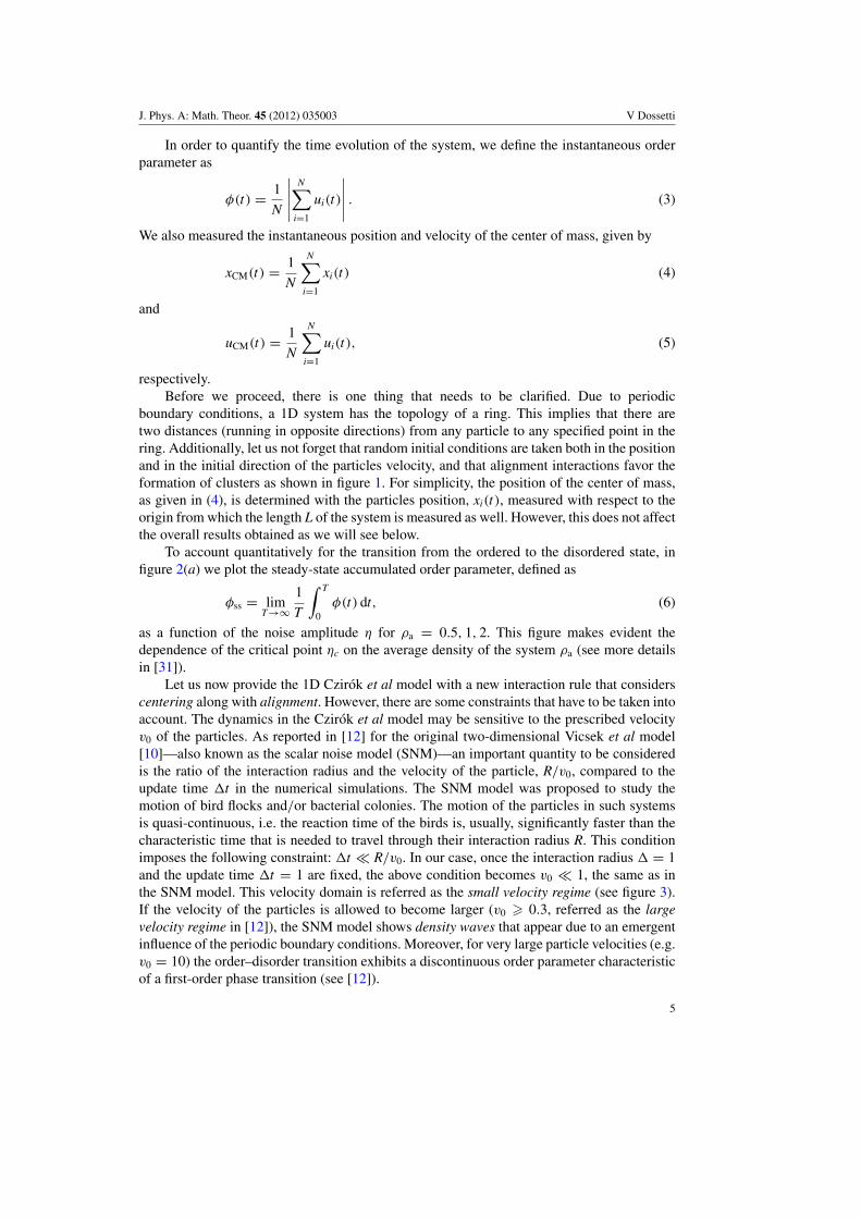
Let us now provide the 1D Czirok et al model with a new interaction rule that considerscentering along with alignment. However, there are some constraints that have to be taken intoaccount. The dynamics in the Czirok et al model may be sensitive to the prescribed velocityv0 of the particles. As reported in [12] for the original two-dimensional Vicsek et al model[10]—also known as the scalar noise model (SNM)—an important quantity to be consideredis the ratio of the interaction radius and the velocity of the particle, R/v0, compared to theupdate time �t in the numerical simulations. The SNM model was proposed to study themotion of bird flocks and/or bacterial colonies. The motion of the particles in such systemsis quasi-continuous, i.e. the reaction time of the birds is, usually, significantly faster than thecharacteristic time that is needed to travel through their interaction radius R. This conditionimposes the following constraint: �t � R/v0. In our case, once the interaction radius � = 1and the update time �t = 1 are fixed, the above condition becomes v0 � 1, the same as inthe SNM model. This velocity domain is referred as the small velocity regime (see figure 3).If the velocity of the particles is allowed to become larger (v0 � 0.3, referred as the largevelocity regime in [12]), the SNM model shows density waves that appear due to an emergentinfluence of the periodic boundary conditions. Moreover, for very large particle velocities (e.g.v0 = 10) the order–disorder transition exhibits a discontinuous order parameter characteristicof a first-order phase transition (see [12]).

5

J. Phys. A: Math. Theor. 45 (2012) 035003 V Dossetti

(a)

(d )

(e) (f )

(b) (c)

Figure 2. In (a), (b), (c), (e) and ( f ) the steady-state accumulated order parameter φss, givenin (6), is plotted as a function of the noise amplitude η. In each case, the system evolved over50 000 time steps until it reached the steady state, and the order parameter was accumulated over250 000 time steps after the transient. In (a) the 1D Czirok et al model, given in (1) in its originalform, is considered for different values of ρa and N = 1000. In (b) and (c), and the details (e)and ( f ) corresponding to the grayed out portions of (b) and (c), respectively, Version 1 (V1) andVersion 2 (V2) of our model, given in (7) and (8), are considered for ρa = 1, μ = 0.05, 0.1 anddifferent system sizes (N = 500, 1000, 4000). In (d) the instantaneous velocity of the center ofmass uCM(t), given in (5), is plotted for ρa = 1, μ = 0.1, η = 7 and different system sizes in thesteady state: the black solid lines correspond to Version 1 of our model while the gray solid linesto Version 2 (see the text for more details).

Figure 3. Schematic diagram of the small velocity regime compared to the large velocity regime.

As far as we know, the properties of the Czirok et al model, as given in (1) and (2), havenot yet been studied in detail outside the small velocity regime. Nonetheless, it is known thatfor certain combination of the parameters, this model can develop directional switching (seee.g. [18]).

Taking into account the previous statements, we will keep the system in the small velocityregime (v0 � 1), as we add centering to the type of interactions experienced by the particles.In this way, on top of the majority rule that allows particles to match the velocity of theirneighbors (interacting in the velocity space), we will introduce a simple attractive long-range

6

J. Phys. A: Math. Theor. 45 (2012) 035003 V Dossetti

rule (an interaction in the position space) that resembles the one used in the Mikhailov–Zanettemodel [19]. However, in contrast with the pairwise linear forces that attach the particles in theMikhailov–Zanette model, in order to determine the new direction for a given particle, ourcentering rule for the Czirok et al model will only take into account the shortest distance fromthe position of that particle relative to the position of the center of mass of the group xCM; thisis done because of the ring topology of the system. Additionally, to make the implementationof this centering rule simple, the mean velocity of the particle’s neighbors (obtained throughfunction G(〈u(t)〉i)) will then be directed toward the center of mass whenever this rule isapplied: we will call this function H(〈u(t)〉i; xCM). In this way, we will be able to keep thevelocity of the particles within the small velocity regime, so they will not be allowed to abandontheir interaction regions in less than the characteristic time defined by the quantities �, v0 and�t. This will also allow us to define two versions of the Czirok et al model, which includecentering, in which these two rules are applied taking inspiration from two of the approachesto include stochastic errors as classified by Bode et al [18], listed in the introduction of thiswork.

In Version 1 (V1) of our model we consider a probabilistic approach to apply the alignmentand centering rules—similar to approach (ii) according to Bode et al (see above)—but withsynchronous updates. To weight one rule above the other we introduce the centering parameterμ in the following way:

• With probability (1 − μ), a given bird in the flock will follow the original majority ruleG(〈u(t)〉i), trying to match its velocity with the mean velocity of its neighbors (itselfincluded).

• With probability μ, it will acquire the magnitude of the mean velocity of its neighbors, butwill move toward the center of mass of the flock instead, following rule H(〈u(t)〉i; xCM) asdescribed above.

We also keep the additive noise ξi as in the original Czirok et al model. Thus, in this versionof our model, the coordinate xi and dimensionless velocity ui of the particles are updated as

xi(t + 1) = xi(t) + v0ui(t),

ui(t + 1) = I(μ) + ξi, (7)

where I is replaced by rule G(〈u(t)〉i) or H(〈u(t)〉i; xCM) according to the value of μ in aprobabilistic way.

In Version 2 (V2) of our model only the additive noise ξi is kept as a source of stochasticity,applying the rules in a deterministic fashion like in the model of Buhl et al [5]. In consequence,in this version of our model, the coordinate xi and dimensionless velocity ui of the particlesare updated as

xi(t + 1) = xi(t) + v0ui(t),

ui(t + 1) = (1 − μ)G(〈u(t)〉i) + μH(〈u(t)〉i; xCM) + ξi. (8)

In this way, in both versions of our model one can go from the original Czirok et al model(for μ = 0) to the one that resembles the interaction type present in the Mikhailov–Zanette(for μ > 0). This allows us to continuously go from a purely alignment type of model to apurely centering one (for μ = 1). However, let us not forget that the scaling in the Cziroket al model depends on the average density of the particles ρa and the size of the system L, acharacteristic not shared by the Mikhailov–Zanette model where none of its properties dependon the density of particles.

7

J. Phys. A: Math. Theor. 45 (2012) 035003 V Dossetti

(a) (b) (c ) (d )

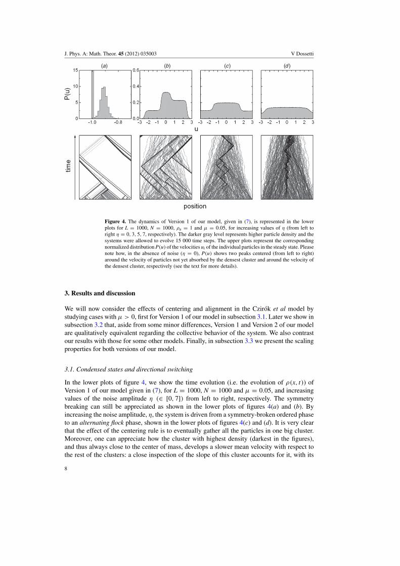
Figure 4. The dynamics of Version 1 of our model, given in (7), is represented in the lowerplots for L = 1000, N = 1000, ρa = 1 and μ = 0.05, for increasing values of η (from left toright η = 0, 3, 5, 7, respectively). The darker gray level represents higher particle density and thesystems were allowed to evolve 15 000 time steps. The upper plots represent the correspondingnormalized distribution P(u) of the velocities ui of the individual particles in the steady state. Pleasenote how, in the absence of noise (η = 0), P(u) shows two peaks centered (from left to right)around the velocity of particles not yet absorbed by the densest cluster and around the velocity ofthe densest cluster, respectively (see the text for more details).

3. Results and discussion

We will now consider the effects of centering and alignment in the Czirok et al model bystudying cases with μ > 0, first for Version 1 of our model in subsection 3.1. Later we show insubsection 3.2 that, aside from some minor differences, Version 1 and Version 2 of our modelare qualitatively equivalent regarding the collective behavior of the system. We also contrastour results with those for some other models. Finally, in subsection 3.3 we present the scalingproperties for both versions of our model.

3.1. Condensed states and directional switching

In the lower plots of figure 4, we show the time evolution (i.e. the evolution of ρ(x, t)) ofVersion 1 of our model given in (7), for L = 1000, N = 1000 and μ = 0.05, and increasingvalues of the noise amplitude η (∈ [0, 7]) from left to right, respectively. The symmetrybreaking can still be appreciated as shown in the lower plots of figures 4(a) and (b). Byincreasing the noise amplitude, η, the system is driven from a symmetry-broken ordered phaseto an alternating flock phase, shown in the lower plots of figures 4(c) and (d). It is very clearthat the effect of the centering rule is to eventually gather all the particles in one big cluster.Moreover, one can appreciate how the cluster with highest density (darkest in the figures),and thus always close to the center of mass, develops a slower mean velocity with respect tothe rest of the clusters: a close inspection of the slope of this cluster accounts for it, with its

8

J. Phys. A: Math. Theor. 45 (2012) 035003 V Dossetti

(a) (b) (c ) (d )

Figure 5. The dynamics of Version 1 of our model, given in (7), is represented in the lowerplots for L = 1000, N = 1000, ρa = 1 and μ = 0.1, for increasing values of η (from left toright η = 0, 3, 5, 7, respectively). The darker gray level represents higher particle density and thesystems were allowed to evolve 15 000 time steps. The upper plots represent the correspondingnormalized distribution P(u) of the velocities ui of the individual particles in the steady state. Asη increases, the frequency of changes in the direction of motion of the densest cluster increases aswell.

slope being higher compared to the slope of other clusters. This can be better appreciated bylooking at the distribution P(u) of the velocities of the individual particles, shown in the upperplots of figure 4. In particular, note the bimodal distribution of figure 4(a), where the narrowpeak centered at −1 corresponds to those particles not yet absorbed by the densest cluster,while the wider one, centered a little to the left of −0.9, corresponds to the latter. As a result,the order parameter in the steady state, φss, never reaches a value equal to 1, even in the absenceof noise (η = 0). On the other hand, as the noise intensity increases, φss never vanishes asthe system develops a mean velocity with a positive magnitude in the alternating flock phase,contrary to what happens in the absence of centering. See e.g. figure 2(b) for ρa = 1 andμ = 0.05 where different system sizes are considered (lines with solid symbols).

These effects are only enhanced as μ increases. For μ = 0.1 and η = 0, the orderparameter, φss, reaches a smaller value in comparison with the case μ = 0.05. In contrast,for strong values of the noise intensity η, the alternating flock phase develops an orderparameter with higher values than for μ = 0.05. See the lines with solid symbols infigure 2(c) (ρa was kept constant in both cases).

To better illustrate this, the lower plots in figure 5 show the dynamics of Version 1 of ourmodel with μ = 0.1. As expected, as μ increases, both condensed phases are reached faster.Yet again, the densest cluster develops a slower mean velocity than the ‘free’ particles thathave not yet been absorbed by it, shown by the double-peaked distribution in the upper plotof figure 5(a), with a wide peak centered a little less than 0.9 and a narrow one centered at1, respectively. As noise increases, for strong values of the noise intensity η, the alternatingflock phase becomes more evident as shown in the lower plots of figures 5(c) and (d). As

9

J. Phys. A: Math. Theor. 45 (2012) 035003 V Dossetti

(a) (b) (c)

(d )

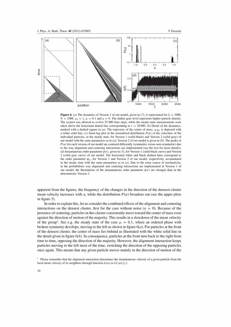
Figure 6. (a) The dynamics of Version 1 of our model, given in (7), is represented for L = 1000,N = 1000, ρa = 1, μ = 0.1 and η = 0. The darker gray level represents higher particle density.The system was allowed to evolve 25 000 time steps, while the steady-state measurements weretaken above the horizontal dotted line corresponding to t = 20 000. (b) Detail of the dynamics,marked with a dashed square in (a). The trajectory of the center of mass, xCM, is depicted witha white solid line. (c) Semi-log plot of the normalized distribution P(u) of the velocities of theindividual particles, in the steady state, for Version 1 (solid black) and Version 2 (solid gray) ofour model with the same parameters as in (a); Version 2 of our model is given in (8). The peaks ofP(u) for each version of our model are centered differently (symmetric versus non-symmetric) dueto the way alignment and centering interactions are implemented (see the text for more details).(d) Instantaneous order parameter φ(t), given in (3), for Version 1 (solid black curve) and Version2 (solid gray curve) of our model. The horizontal white and black dashed lines correspond tothe order parameter φss, for Version 1 and Version 2 of our model, respectively, accumulatedin the steady state with the same parameters as in (a). Due to the extra source of stochasticity,in the probabilistic way alignment and centering interactions are implemented in Version 1 ofour model, the fluctuations of the instantaneous order parameter φ(t) are stronger than in thedeterministic Version 2.

apparent from the figures, the frequency of the changes in the direction of the densest-clustermean velocity increases with η, while the distribution P(u) broadens out (see the upper plotsin figure 5).

In order to explain this, let us consider the combined effects of the alignment and centeringinteractions on the densest cluster, first for the case without noise (η = 0). Because of thepresence of centering, particles in this cluster consistently move toward the center of mass evenagainst the direction of motion of the majority. This results in a slowdown of the mean velocityof the group1. See e.g. the steady state of the case μ = 0.1, where an ordered phase withbroken symmetry develops, moving to the left as shown in figure 6(a). For particles at the frontof the densest cluster, the center of mass lies behind as illustrated with the white solid line inthe detail given in figure 6(b). In consequence, particles at the front turn back to the right fromtime to time, opposing the direction of the majority. However, the alignment interaction keepsparticles moving to the left most of the time, switching the direction of the opposing particlesonce again. This means that any given particle moves mainly in the direction of motion of the

1 Please remember that the alignment interaction determines the instantaneous velocity of a given particle from thelocal mean velocity of its neighbors through function G(u) as G(〈u(t)〉i).

10

J. Phys. A: Math. Theor. 45 (2012) 035003 V Dossetti

(a) (b) (c)

(d )

(e)

Figure 7. (a) The dynamics of Version 1 of our model, given in (7), is represented for L = 1000,N = 1000, ρa = 1, μ = 0.1 and η = 7. The darker gray level represents higher particle density.The system was allowed to evolve 25 000 time steps, while the steady-state measurements weretaken above the horizontal dotted line corresponding to t = 15 000. (b) Detail of the dynamics,marked with a dashed square in (a). The trajectory of the center of mass, xCM, is depicted with awhite solid line. Note how, on one side, the densest cluster effectively oscillates around the centerof mass, while a tail of defecting particles counterbalances its mass on the other. (c) Semi-log plotof the normalized distribution P(u) of the velocities of the individual particles in the steady state.(d) Instantaneous order parameter φ(t), given in (3), for the whole time evolution of the system.(e) Instantaneous velocity of the center of mass uCM(t), given in (5), for the steady state of thesystem. In (d) and (e), the horizontal gray lines correspond to the accumulated mean values φssand ±φss, respectively.

group, but it also moves in the opposite one as corroborated by looking at P(u) in figure 6(c),depicted with the solid black curve for this case. There, the higher peak is centered around theemergent mean velocity of the group, while the shorter one (in a symmetric position) appearsdue to the opposing particles.

In this way, once a cluster is formed around the center of mass, this will grow denserover the rest of the systems’ time evolution, gathering more particles together and, at the sametime, hindering their ability to fully develop the preferred velocity as dictated by functionG(u), given in (2). In some sense, inside the densest cluster, the combination of centering andalignment works as a source of ‘noise’ itself (also established in [18]), inducing fluctuationsin the steady-state mean velocity of the group even for η = 0. See e.g. figure 6(d) where theinstantaneous order parameter φ(t) is plotted as a function of time (solid black curve). Thehorizontal white dashed line corresponds to the value of φss measured in the steady state, abovethe horizontal dashed line shown in figure 6(a). Regarding the ‘free’ particles not yet absorbedby the densest cluster, in the early stages of evolution, the effect of centering on their speedis negligible compared to the alignment interaction, due to the much lower density in theseregions. In the end, when the noise is weak or absent, the magnitude of the emergent velocityof the densest cluster will depend on the balance of the centering and alignment interactions.

Let us now consider the case when the noise is strong. Here again, the combined effectsof alignment and centering are stronger on the densest cluster. In figure 7(a), the evolutionof ρ(x, t) is shown for a system with μ = 0.1. One can appreciate that, as soon as a large

11

J. Phys. A: Math. Theor. 45 (2012) 035003 V Dossetti

(a) (b) (c )

Figure 8. Semi-log plots of the density of particles ρ, as a function of the position x, taken over62 consecutive time steps. In (a), (b) and (c), three cases are plotted before, at and after the turnmarked with a small arrow in figure 7(b), around t = 18 475, 18 847 and 19 095, respectively. Thelevels of gray correspond to the local mean velocity, uloc, as shown in the scale at the bottomright, while the horizontal black and white arrows point in its direction. Note the development ofdomains with a different local mean velocity.

and dense cluster is formed, it starts to change its direction of motion with some periodicity.In consequence, the system develops an alternating flock phase that resembles the one in themodels of Evans et al [16, 17]. To quantify this, it is better to look at the instantaneous velocityof the center of mass, uCM, given in (5). As shown in figure 7(e), in the steady state, the velocityof the center of mass develops a constant mean magnitude (see the horizontal gray lines) butwith an alternating direction. In contrast with the zero-noise case, due to the presence of noise(η > 0), particles are able to drift away from the center of mass in a ‘diffusive’ fashion. Thiscan be observed when looking at the steady state of the system, above the horizontal dottedline in figure 7(a). As more particles leave the densest cluster, this becomes dilute and wideras the center of mass is ‘pulled’ to its back as shown by the solid white line in the detail plottedin figure 7(b). The turn marked with the small arrow in this figure is analyzed in more detail infigure 8. There, the density of particles (accumulated over 62 consecutive time steps) is plottedas a function of the position around three different configurations: before, at and after theturn. The different levels of gray clearly point out the development of domains with differentlocal mean velocity, uloc. As shown in figures 8(a) and (c), before and after the turn, whenthe center of mass is closer to the densest cluster (see figure 7(b)), the latter is surroundedby domains with small uloc. However, at the turn, the densest cluster is at its farthest positionrelative to the position of the center of mass (see figure 7(b)). A fluctuation develops at thefront of the flock, followed by a small-uloc domain as shown in figure 8(b). This fluctuationmoves against the direction of the flock, gaining density and momentum, and finally invertingthe direction of the flock as it passes through. This mechanism effectively renders the particlesin the system oscillating around the center of mass, with the densest cluster on one side,and the defecting particles counterbalancing its mass on the other as can be appreciated infigure 7(b). In this way, the alternating flock phase in our model resembles the oscillatoryphase in the Mikhailov and Zanette model [19] that also considers long-range centering butnot alignment.

Two conclusions can be drawn from this analysis. The first relates the frequency of theturns to the intensity of the noise. As explained before, the presence of noise allows particlesto drift away from the densest cluster that always remains close to the center of mass. Themore intense the noise is, the faster the particles are able to move away. Consequently, thefrequency of the turns should increase with the noise amplitude as figures 5(c) and (d) can

12

J. Phys. A: Math. Theor. 45 (2012) 035003 V Dossetti

confirm, a trend that is consistent with previous results; see e.g. [6, 16, 18]. The second regardsthe development of a mean velocity different from zero by the densest cluster when strongnoise is present. In contrast with the case without centering (μ = 0), where strong noisemakes the mean velocity of the flock vanish in a continuous phase transition, when centeringis introduced (μ > 0) the accumulated order parameter φss is far from zero—it even increaseswith μ.

For strong noise, centering in combination with the alignment interaction provokes anordering effect on the densest cluster. This can be understood considering that, due to centering,particles try to move toward the center of mass of the group eventually gathering together. Withthe aid of the alignment interaction, correlations in the velocities ui of the particles developthat cannot be destroyed by simple additive noise. This is due to the long-range character of thecentering interaction and the high density of this cluster. In contrast, the alignment interactionbeing short range in nature is more sensitive to the noise when taken alone. This may alsoexplain the increase of φss with μ, with centering being the dominant interaction for strongnoise.

3.2. Different sources of stochasticity and free flocks

Regarding the collective behavior of the system, Version 2 of our model shows the same overallfeatures as Version 1. For that matter, the dynamics of four systems with different combinationsof the parameters N, ρa and μ is presented in figure 9 for both versions, side-by-side, in twolimit cases: η = 0 and η = 7. These examples illustrate the qualitative equivalence (and, ingreat measure, quantitative too) between the two versions of our model—as apparent from thefigures—including the alternating flock phase. The case N = 1000, ρa = 1 and μ = 0.4 inthe third row is of particular interest since this phase is absent even for strong noise (η = 7).We will discuss this case later.

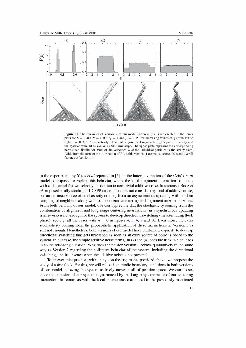
More details of the dynamics of Version 2 are presented in figure 10 for μ = 0.15, withthe same values of ρa, N, L and η as in the two cases presented for Version 1 in figures 4 and5. Again, the system shows collective behavior equivalent to that of Version 1. Moreover, themechanism that produces the alternating flock phase in Version 2 is exactly the same as the onedescribed in subsection 3.1. Nonetheless, there are some differences that need to be pointedout. The first regards the distribution P(u) of the velocities of the individual particles for thecase η = 0, shown in the upper plot of figure 10(a), as this exhibits two peaks centered around−0.9 and −0.6.2 As in Version 1, in Version 2 of our model particles moving in the directionof the densest cluster move with speeds close to |1|, in contrast, particles moving in theopposite direction move with speeds around |1| − 2μ. These values correspond to the centersof the two peaks of P(u) as shown in figure 10(a). This comes as a result of the deterministicway the alignment and centering rules are applied in Version 2; see (8). Also, please note thatthese peaks are narrower and comparable in height, in contrast to the corresponding ones forVersion 1—wider, symmetric in position, but highly asymmetric in height—as illustrated infigure 6(c) for both versions with the solid gray and black filled curves, respectively (μ = 0.1in this case).

This comes about the fact that, in both versions of our model, the combination of alignmentand centering is a source of noise in itself—all the more so, considering the additive noiseis absent for η = 0. However, Version 1 of our model has an extra source of stochasticity inthe probabilistic way these interactions are applied; see (7). As a result, the fluctuations of theinstantaneous order parameter φ(t) are stronger in Version 1 than in Version 2, as shown in

2 A third peak should appear around −1, corresponding to particles not yet absorbed by the densest cluster. Thispeak is not present here since there were no such particles when P(u) was measured.

13

J. Phys. A: Math. Theor. 45 (2012) 035003 V Dossetti

Figure 9. Dynamics of Version 1 and Version 2 of our model for different combinations of theparameters N, ρa and μ in two limit cases: η = 0 and η = 7. The darker gray level representshigher particle density. The case on the third row is of particular interest since the alternating flockphase is fully suppressed even for strong noise (see the text for more details).

figure 6(d) for μ = 0.1 with the solid black and gray curves, respectively. Before we go on withthe discussion, let us provide a context regarding the development of directional switching andits relation with different sources of stochasticity in 1D SPP models.

In [18], Bode et al state that the addition of simple noise terms in the particles direction ofmotion is not necessarily sufficient to describe and explain collective motion in animal groups.This remark is made in regard of the directional switching shown by the marching locusts

14

J. Phys. A: Math. Theor. 45 (2012) 035003 V Dossetti

(a) (b) (c ) (d )

Figure 10. The dynamics of Version 2 of our model, given in (8), is represented in the lowerplots for L = 1000, N = 1000, ρa = 1 and μ = 0.15, for increasing values of η (from left toright η = 0, 3, 5, 7, respectively). The darker gray level represents higher particle density andthe systems were let to evolve 15 000 time steps. The upper plots represent the correspondingnormalized distribution P(u) of the velocities ui of the individual particles in the steady state.Aside from the form of the distribution of P(u), this version of our model shows the same overallfeatures as Version 1.

in the experiments by Yates et al reported in [6]. In the latter, a variation of the Czirok et almodel is proposed to explain this behavior, where the local alignment interaction competeswith each particle’s own velocity in addition to non-trivial additive noise. In response, Bode etal proposed a fully stochastic 1D SPP model that does not consider any kind of additive noise,but an intrinsic source of stochasticity coming from an asynchronous updating with randomsampling of neighbors, along with local concentric centering and alignment interaction zones.From both versions of our model, one can appreciate that the stochasticity coming from thecombination of alignment and long-range centering interactions (in a synchronous updatingframework) is not enough for the system to develop directional switching (the alternating flockphase); see e.g. all the cases with η = 0 in figures 4, 5, 6, 9 and 10. Even more, the extrastochasticity coming from the probabilistic application of these interactions in Version 1 isstill not enough. Nonetheless, both versions of our model have built-in the capacity to developdirectional switching that gets unleashed as soon as an extra source of noise is added to thesystem. In our case, the simple additive noise term ξi in (7) and (8) does the trick, which leadsus to the following question: Why does the noisier Version 1 behave qualitatively in the sameway as Version 2 regarding the collective behavior of the system, including the directionalswitching, and its absence when the additive noise is not present?

To answer this question, with an eye on the arguments provided above, we propose thestudy of a free flock. For this, we will relax the periodic boundary conditions in both versionsof our model, allowing the system to freely move in all of position space. We can do so,since the cohesion of our system is guaranteed by the long-range character of our centeringinteraction that contrasts with the local interactions considered in the previously mentioned

15

J. Phys. A: Math. Theor. 45 (2012) 035003 V Dossetti

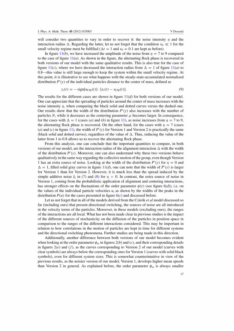
(a) (b) (c ) (d )

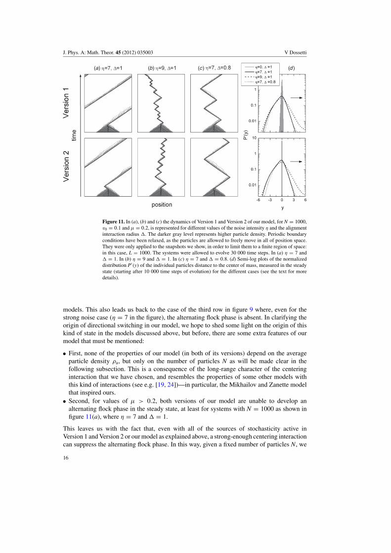
Figure 11. In (a), (b) and (c) the dynamics of Version 1 and Version 2 of our model, for N = 1000,v0 = 0.1 and μ = 0.2, is represented for different values of the noise intensity η and the alignmentinteraction radius �. The darker gray level represents higher particle density. Periodic boundaryconditions have been relaxed, as the particles are allowed to freely move in all of position space.They were only applied to the snapshots we show, in order to limit them to a finite region of space:in this case, L = 1000. The systems were allowed to evolve 30 000 time steps. In (a) η = 7 and� = 1. In (b) η = 9 and � = 1. In (c) η = 7 and � = 0.8. (d) Semi-log plots of the normalizeddistribution P′(y) of the individual particles distance to the center of mass, measured in the steadystate (starting after 10 000 time steps of evolution) for the different cases (see the text for moredetails).

models. This also leads us back to the case of the third row in figure 9 where, even for thestrong noise case (η = 7 in the figure), the alternating flock phase is absent. In clarifying theorigin of directional switching in our model, we hope to shed some light on the origin of thiskind of state in the models discussed above, but before, there are some extra features of ourmodel that must be mentioned:

• First, none of the properties of our model (in both of its versions) depend on the averageparticle density ρa, but only on the number of particles N as will be made clear in thefollowing subsection. This is a consequence of the long-range character of the centeringinteraction that we have chosen, and resembles the properties of some other models withthis kind of interactions (see e.g. [19, 24])—in particular, the Mikhailov and Zanette modelthat inspired ours.

• Second, for values of μ > 0.2, both versions of our model are unable to develop analternating flock phase in the steady state, at least for systems with N = 1000 as shown infigure 11(a), where η = 7 and � = 1.

This leaves us with the fact that, even with all of the sources of stochasticity active inVersion 1 and Version 2 or our model as explained above, a strong-enough centering interactioncan suppress the alternating flock phase. In this way, given a fixed number of particles N, we

16

J. Phys. A: Math. Theor. 45 (2012) 035003 V Dossetti

will consider two quantities to vary in order to recover it: the noise intensity η and theinteraction radius �. Regarding the latter, let us not forget that the condition v0 � 1 for thesmall velocity regime must be fulfilled (�t = 1 and v0 = 0.1 are kept as before).

In figure 11(b), we have increased the amplitude of the noise from η = 7 to 9 comparedto the case of figure 11(a). As shown in the figure, the alternating flock phase is recovered inboth versions of our model with the same qualitative results. This is also true for the case offigure 11(c), where we have decreased the interaction radius from � = 1 of figure 11(a) to0.8—this value is still large enough to keep the system within the small velocity regime. Atthis point, it is illustrative to see what happens with the steady-state-accumulated normalizeddistribution P′(y) of the individual particles distance to the center of mass, defined as

yi(t) = − sign[uCM(t)] · [xi(t) − xCM(t)]. (9)

The results for the different cases are shown in figure 11(d) for both versions of our model.One can appreciate that the spreading of particles around the center of mass increases with thenoise intensity η, when comparing the black solid and dotted curves versus the dashed one.Our results show that the width of the distribution P′(y) also increases with the number ofparticles N, while it decreases as the centering parameter μ becomes larger. In consequence,for the cases with � = 1 (cases (a) and (b) in figure 11), as noise increases from η = 7 to 9,the alternating flock phase is recovered. On the other hand, for the cases with η = 7 (cases(a) and (c) in figure 11), the width of P′(y) for Version 1 and Version 2 is practically the same(black solid and dotted curves), regardless of the value of �. Thus, reducing the value of thelatter from 1 to 0.8 allows us to recover the alternating flock phase.

From this analysis, one can conclude that the important quantities to compare, in bothversions of our model, are the interaction radius of the alignment interaction � with the widthof the distribution P′(y). Moreover, one can also understand why these two versions behavequalitatively in the same way regarding the collective motion of the group, even though Version1 has an extra source of noise. Looking at the width of the distribution P′(y) for η = 0 and� = 1, filled solid gray curves in figure 11(d), one can note that the width of P′(y) is largerfor Version 1 than for Version 2. However, it is much less than the spread induced by thesimple additive noise ξi in (7) and (8) for η > 0. In contrast, the extra source of noise inVersion 1, coming from the probabilistic application of alignment and centering interactions,has stronger effects on the fluctuations of the order parameter φ(t) (see figure 6(d)), i.e. onthe values of the individual particle velocities ui as shown by the widths of the peaks in thedistribution P(u) for the cases presented in figure 6(c) and discussed before.

Let us not forget that in all of the models derived from the Czirok et al model discussed sofar (including ours) that present directional switching, the sources of noise are all introducedin the velocity terms of the particles. Moreover, in these models (excluding ours), the rangesof the interactions are all local. What has not been made clear in previous studies is the impactof the different sources of stochasticity on the diffusion of the particles in position space incomparison to the ranges of the different interactions considered. This may be important inrelation to how correlations in the motion of particles are kept in time for different systemsand the directional switching phenomena. Further studies are being made in this direction.

Additionally, another difference between both versions of our model becomes evidentwhen looking at the order parameter φss in figures 2(b) and (c), and their corresponding detailsin figures 2(e) and ( f ), as the curves corresponding to Version 2 of our model (curves withclear symbols) are always below the corresponding ones for Version 1 (curves with solid blacksymbols), even for different system sizes. This is somewhat counterintuitive in view of theprevious results, as the noisier version of our model, Version 1, develops higher mean speedsthan Version 2 in general. As explained before, the order parameter φss is always smaller

17

J. Phys. A: Math. Theor. 45 (2012) 035003 V Dossetti

than 1 for both versions of our model, even in the absence of the additive noise (η = 0).A plausible explanation leads us back to the two peaks shown by P(u) in the steady state forthis case (see figure 6(c)). While those for Version 1 of our model are symmetric, they arealso wider and clearly asymmetric in height, i.e. there is a peak that dominates the distributioncentered around a larger value than the narrower and more-balanced-in-height peaks of P(u)

for Version 2. Considering that these peaks correspond to the distribution of the velocities ofthe individual particles, this fact could account for the difference in the order parameter φss

for the different cases of the two versions of our model—in principle, one could obtain theaccumulated steady-state order parameter as φss = | ∫ ∞

−∞ u P(u) du|.At this point, it is worth drawing attention to the cases with η = 7 in the upper plots

of figures 4(d), 5(d) and 10(d), where P(u) becomes almost flat and symmetric, very similarto the case without centering (μ = 0) shown in the upper plot of figure 1(d). In the latter,this distribution corresponds to the strong-noise-induced disordered phase, characterized by arandom velocity field, where the velocity of every individual particle should average to zerothroughout the whole evolution of the system. This is also true in the presence of centering(μ > 0) if we were to look just at the distribution P(u). However, there is a big differencewhen we focus on the collective behavior of the system. Whereas the mean velocity of thegroup tends to zero for μ = 0, as μ increases, the mean velocity of the group also increaseswith the noise amplitude as explained before. One could wonder about the diffusion of thecenter of mass for μ > 0 and the net displacement it may develop in the long run, or at least,the mean square displacement.

3.3. Scaling

Let us now briefly analyze how the properties of both versions of our model scale with thesize of the system N. First, we focus on the accumulated order parameter φss. As shownin figures 2(b) and (c), and their corresponding details in figures 2(e) and ( f ), for weaknoise (including η = 0) the curves are rather flat regarding their dependence on η andshow almost no difference as N changes. This is followed by a crossover region and, as η

increases, the order parameter increases with N. In second place, we have already mentioned, insubsection 3.2, that the spread of the position of particles around the center of mass (thewidth of the distribution P′(y)) increases with N as well. This leads to the conclusionthat larger systems will tolerate larger values of μ before the alternating flock phase iskilled, given the interaction radius � of the alignment interaction is kept constant. In thirdplace comes the frequency of the changes in direction in the same phase. As shown infigure 2(d) for both versions of our model (solid black lines for Version 1 and solid gray linesfor Version 2), as N increases, the frequency of the changes in direction becomes smaller. Inother words, the intervals between changes in direction increase with the size of the system.This is consistent with the trends reported for some other models that also show directionalswitching [6, 16].

Overall, both versions of our model scale in the same way. Moreover, aside from theeffects of the extra source of noise in Version 1, and fluctuations intrinsic to any numericalanalysis, the functional dependence of the quantities mentioned in the previous paragraph onsome of the parameters (e.g. the dependence of φss on η) seem to be quantitatively equivalentacross different system sizes. On the other hand, since we only analyzed three system sizes,N = 500, 1000, 4000, it is not possible for us to provide how these quantities depend explicitlyon N. We will leave this analysis for a future work, given that all our results point to the factthat it is equivalent to study Version 1 or Version 2 of our model regarding the collectivebehavior of the system and its scaling.

18

J. Phys. A: Math. Theor. 45 (2012) 035003 V Dossetti

4. Conclusions

We have successfully introduced a long-range centering interaction in the model of Czirok et al[19] via two approaches for applying centering and alignment, that derives two characteristiccondensed states. The first, for weak noise, consists in a coherent state with broken symmetry.Here, the fluctuations induced by the combination of centering and alignment in the meanvelocity of the densest cluster seem to be stronger than the noise-induced ones. Thus, thesystem reaches a steady-state speed smaller than the prescribed one even in the absence ofnoise. The second, for strong noise, consists in an alternating flock phase with a non-vanishingmean velocity. In this case, the centering interaction combined with the alignment one providesan ordering mechanism for the densest cluster that effectively performs oscillations aroundthe center of mass as it changes its direction of motion alternatively. This phase resemblesalternating states shown by some other models [5, 6, 16–18], but also the oscillatory noisystate of the Mikhailov and Zanette model [19].

The two versions of our model, one where alignment and centering interactions areapplied in a probabilistic way and one deterministic, have allowed us to address the directionalswitching phenomenon that seems to be an intrinsic property of the motion of animal groupsas recent experimental results show [5, 6]. Even though the origin of the stochasticity in realsystems is far from clear, we were able to introduce and understand a new mechanism fordirectional switching in 1D SPP systems with long-range centering. From our results, newinsight has been gained into the effects of different sources of stochasticity on the diffusionof particles in position and velocity spaces, and its relation with the ranges of the differentinteractions considered for the development of alternating flock phases. In these terms, wehave shown how the alternating flock phase of our model can be suppressed and how torecover it.

On the other hand, due to the long-range character of the centering interaction introduced,the properties of our model do not depend on the mean density of particles, but only on thenumber of particles. In consequence, periodic boundary conditions, typically used in 1D SPPmodels [5, 6, 16, 17, 31], can be dropped as the system is able to maintain its cohesion.Nonetheless, the scaling properties of our model show the same trends as those reported forsome other models [6, 16, 18]. A more detailed scaling analysis is in the works in order todetermine their functional dependence.

Finally, as our model does not show a truly disordered phase (with a random velocityfield), it would be worth to study the diffusion of the center of mass, e.g. its net and meansquare displacements throughout the time evolution of the system. We believe our results maybe relevant for the understanding of the directional switching phenomenon and, in general, forthe theory of flocking.

Acknowledgments

This work was partially supported by CONACyT (Mexico), by SEP (Mexico) under grantPROMEP/103.5/10/7296 and by the NSF under grant INT-0336343. The author is also gratefulfor the comments and suggestions from the three anonymous referees and from M M Delmas.

References

[1] Lorch P D and Gwynne D T 2000 Naturwissenschaften 87 370[2] Bonabeau E, Dagorn L and Freon P 1998 J. Phys. A: Math. Gen. 31 L731[3] Parrish J K and Edelstein-Keshet L 1999 Science 284 99

Parrish J K, Viscido S V and Grunbaum D 2002 Biol. Bull. 202 296

19

J. Phys. A: Math. Theor. 45 (2012) 035003 V Dossetti

[4] Couzin I D, Krause J, Franks N R and Levin S A 2005 Nature 433 513[5] Buhl J, Sumpter D J T, Couzin I D, Hale J J, Despland E, Miller E R and Simpson S J 2006 Science 312 1402[6] Yates C A, Erban R, Escudero C, Couzin I D, Buhl J, Kevrekidis I G, Maini P K and Sumpter D J T 2009 Proc.

Natl Acad. Sci. 106 5464[7] Wu X-L and Libchaber A 2000 Phys. Rev. Lett. 84 3017[8] Reynolds C W 1987 Comput. Graph. 21 4[9] Toner J, Tu Y and Ramaswamy S 2005 Ann. Phys. 318 170

Vicsek T, Czirok A, Farkas I J and Helbing D 1999 Physica A 274 182[10] Vicsek T, Czirok A, Ben-Jacob E, Cohen I and Shochet O 1995 Phys. Rev. Lett. 75 1226[11] Gregoire G, Chate H and Tu Y 2003 Physica D 181 157

Gregoire G and Chate H 2004 Phys. Rev. Lett. 92 025702[12] Nagy M, Daruka I and Vicsek T 2007 Physica A 373 445[13] Peruani F and Sibona G J 2008 Phys. Rev. Lett. 100 168103[14] Bussemaker H J, Deutsch A and Geigant E 1997 Phys. Rev. Lett. 78 5018[15] Aldana M and Huepe C 2003 J. Stat. Phys. 112 135

Aldana M, Dossetti V, Huepe C, Kenkre V M and Larralde H 2007 Phys. Rev. Lett. 98 095702[16] O’Loan O J and Evans M R 1999 J. Phys. A: Math. Gen. 32 L99[17] Raymond J R and Evans M R 2006 Phys. Rev. E 76 036112[18] Bode N W F, Franks D W and Wood A J 2010 J. Theor. Biol. 267 292[19] Mikhailov A S and Zanette D H 1999 Phys. Rev. E 60 4571[20] Erdmann U, Ebeling W and Mikhailov 2005 Phys. Rev. E 71 051904[21] Shimoyama N, Sugawara K, Mizuguchi T, Hayakawa Y and Sano M 1996 Phys. Rev. Lett. 76 3870[22] Levine H, Rappel W-J and Cohen I 2000 Phys. Rev. E 63 017101[23] D’Orsogna M R, Chuang Y L, Bertozzi A L and Chayes L S 2006 Phys. Rev. Lett. 96 104302[24] Dossetti V, Sevilla F J and Kenkre V M 2009 Phys. Rev. E 79 051115[25] Strefler J, Erdmann U and Schimansky-Geier L 2008 Phys. Rev. E 78 031927[26] Iwasa M, Iida K and Tanaka D 2010 Phys. Rev. E 81 046220[27] Topaz C M and Bertozzi A L 2004 SIAM J. Appl. Math. 65 152[28] Bertin E, Droz M and Gregoire G 2006 Phys. Rev. E 74 022101

Bertin E, Droz M and Gregoire G 2009 J. Phys. A: Math. Theor. 42 445001[29] Mogilner A and Edelstein-Keshet L 1996 Physica D 89 346[30] Gonci B, Nagy M and Vicsek T 2008 Eur. Phys. J. Spec. Top. 157 53[31] Czirok A, Barabasi A-L and Vicsek T 1999 Phys. Rev. Lett. 82 209

20