Coexistence of Limit Cycles and Homoclinic Loops in a SIRS Model with a Nonlinear Incidence Rate

Copyright © by SIAM. Unauthorized reproduction of this article is prohibited.

SIAM J. APPL. MATH. c© 2008 Society for Industrial and Applied MathematicsVol. 69, No. 2, pp. 621–639

COEXISTENCE OF LIMIT CYCLES AND HOMOCLINIC LOOPS INA SIRS MODEL WITH A NONLINEAR INCIDENCE RATE∗

YILEI TANG† , DEQING HUANG‡ , SHIGUI RUAN§, AND WEINIAN ZHANG‡

Abstract. Recently, Ruan and Wang [J. Differential Equations, 188 (2003), pp. 135–163]studied the global dynamics of a SIRS epidemic model with vital dynamics and a nonlinear saturatedincidence rate. Under certain conditions they showed that the model undergoes a Bogdanov–Takensbifurcation; i.e., it exhibits saddle-node, Hopf, and homoclinic bifurcations. They also consideredthe existence of none, one, or two limit cycles. In this paper, we investigate the coexistence of a limitcycle and a homoclinic loop in this model. One of the difficulties is to determine the multiplicityof the weak focus. We first prove that the maximal multiplicity of the weak focus is 2. Thenfeasible conditions are given for the uniqueness of limit cycles. The coexistence of a limit cycle and ahomoclinic loop is obtained by reducing the model to a universal unfolding for a cusp of codimension3 and studying degenerate Hopf bifurcations and degenerate Bogdanov–Takens bifurcations of limitcycles and homoclinic loops of order 2.

Key words. degenerate Bogdanov–Takens bifurcation, degenerate Hopf bifurcation, limit cycle,homoclinic loop, revised sign list

AMS subject classifications. 34C23, 92D30

DOI. 10.1137/070700966

1. Introduction. Periodic oscillations are common phenomena observed in theincidence of many infectious diseases such as chickenpox, influenza, measles, mumps,rubella, etc. (see Hethcote [10, 11], Hethcote and Levin [12], Hethcote, Stech, and vanden Driessche [13]). It is very important to understand such epidemic patterns in orderto introduce public health interventions and control the spread of diseases. Recentstudies have demonstrated that the incidence rate plays a crucial role in producingperiodic oscillations in epidemic models (Alexander and Moghadas [1, 2], Derrick andvan den Driessche [6], Hethcote and van den Driessche [14], Liu et al. [17, 18], Lizanaand Rivero [19], Moghadas [21], Moghadas and Alexander [22], Ruan and Wang [25],Wang [26]).

In most epidemic models (see Anderson and May [3]), the incidence rate (thenumber of new cases per unit time) takes the mass-action form with bilinear inter-actions, namely, κS(t)I(t), where S(t) and I(t) are the numbers of susceptible andinfectious individuals at time t, respectively, and the constant κ is the probability oftransmission per contact. Epidemic models with such bilinear incidence rates usuallyhave at most one endemic equilibrium and do not exhibit periodicity; the diseasewill be eradicated if the basic reproduction number is less than one and will per-sist otherwise (Anderson and May [3], Hethcote [11]). There are many reasons forusing nonlinear incidence rates, and various forms of nonlinear incidence rates have

∗Received by the editors August 23, 2007; accepted for publication (in revised form) August 5,2008; published electronically December 3, 2008.

http://www.siam.org/journals/siap/69-2/70096.html†Department of Mathematics, Shanghai Jiao Tong University, Shanghai 200240, China and De-

partment of Mathematics, Sichuan University, Chengdu, Sichuan 610064, China ([email protected]).‡Department of Mathematics, Sichuan University, Chengdu, Sichuan 610064, China (toglyhdq@

sina.com, [email protected]). The work of the fourth author was supported by NSFC (China) grants10571127 and 10825104 and SRFDP 20050610003.

§Department of Mathematics, University of Miami, Coral Gables, FL 33124-4250 ([email protected]). This author’s research was supported by NSF grant DMS-0715772.

621

Copyright © by SIAM. Unauthorized reproduction of this article is prohibited.

622 Y. TANG, D. HUANG, S. RUAN, AND W. ZHANG

been proposed recently. For example, in order to incorporate the effect of behavioralchanges, Liu, Levin, and Iwasa [18] used a nonlinear incidence rate of the form

(1.1) g(I)S =κI�S

1 + αIh,

where κI� measures the infection force of the disease, 1/(1+αIh) describes the inhibi-tion effect from the behavioral change of the susceptible individuals when the numberof infectious individuals increases, �, h, and κ are all positive constants, and α is anonnegative constant. See also Alexander and Moghadas [1, 2], Derrick and van denDriessche [6], Hethcote and van den Driessche [14], Moghadas [21], etc. Notice thatthe bilinear interaction is a special case of (1.1) with α = 0 and � = 1.

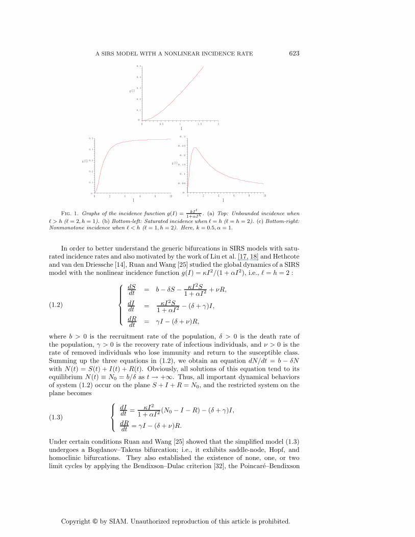
The nonlinear function g(I) given by (1.1) includes three types. (a) Unboundedincidence function: � > h. The case when � = h + 1 was considered by Hethcoteand van den Driessche [14]. The function is unbounded as the bilinear incidencerate (see Figure 1(a)). (b) Saturated incidence function: � = h. The case when� = h = 1, i.e., g(I) = κI/(1+αI), was proposed by Capasso and Serio [5] to describea “crowding effect” or “protection measures” in modeling the cholera epidemics inBari in 1973. A similar type of sigmoidal function was also used to represent dose-response relationships observed in parasite infection experiments (Regoes, Ebert, andBonhoeffer [23]). The function tends to a saturation level as the number of infectiousindividuals I becomes large (see Figure 1(b)). (c) Nonmonotone incidence function:� < h. Such functions can be used to interpret the “psychological effects” (Capassoand Serio [5]): for a very large number of infectious individuals the infection force maydecrease as the number of infectious individuals increases (see Figure 1(c)), becausein the presence of a large number of infectious individuals the population may tendto reduce the number of contacts per unit time, as seen with the spread of SARS (seeWang [26], Xiao and Ruan [28]).

From the graphs in Figure 1, one would expect that the dynamics of epidemicmodels with unbounded incidence rates are similar to those with bilinear incidencerates. In fact, Hethcote and van den Driessche [14] found that in a SEIRS modelwith � = h + 1, the classical threshold results hold; namely, the disease dies outbelow the threshold, and the disease level approaches the endemic equilibrium abovethe threshold. For a SIRS model with the nonmonotone incidence function g(I) =kI/(1 + αI2), Xiao and Ruan [28] demonstrated that either the number of infectiousindividuals tends to zero as time evolves or the disease persists. We conjecture thatthe dynamics of SIRS models with nonmonotone incidence rates are similar to thoseobserved by Xiao and Ruan [28].

On the other hand, the dynamics of epidemic models with saturated incidencerates (when � = h) have been shown to be very rich and complex. For a SEIRSmodel with � = h, Hethcote and van den Driessche [14] observed that the thresholdconcept becomes more complicated since the asymptotic behavior can depend on boththe threshold and the initial values. The model can have none, one, or two endemicequilibria, and the disease can die out above the threshold for some initial values.Periodic solutions appear through Hopf bifurcation. The results are analogous tothose obtained by Liu, Hethcote, and Levin [17] for SIRS models with � = h. Thecase � = h = 1 has been discussed briefly by Capasso and Serio [5] and recently insome detail by Gomes et al. [8], who obtained the existence of backward bifurcations,oscillations, and Bogdanov–Takens points in SIR and SIS models. These indicate thatthe case when � = h ≥ 2 can be very complicated and deserves further investigation.

Copyright © by SIAM. Unauthorized reproduction of this article is prohibited.

A SIRS MODEL WITH A NONLINEAR INCIDENCE RATE 623

Fig. 1. Graphs of the incidence function g(I) = kI�

1+αIh . (a) Top: Unbounded incidence when

� > h (� = 2, h = 1). (b) Bottom-left: Saturated incidence when � = h (� = h = 2). (c) Bottom-right:Nonmonotone incidence when � < h (� = 1, h = 2). Here, k = 0.5, α = 1.

In order to better understand the generic bifurcations in SIRS models with satu-rated incidence rates and also motivated by the work of Liu et al. [17, 18] and Hethcoteand van den Driessche [14], Ruan and Wang [25] studied the global dynamics of a SIRSmodel with the nonlinear incidence function g(I) = κI2/(1 + αI2), i.e., � = h = 2 :

(1.2)

⎧⎪⎪⎪⎪⎨⎪⎪⎪⎪⎩dSdt

= b − δS − κI2S1 + αI2 + νR,

dIdt = κI2S

1 + αI2 − (δ + γ)I,

dRdt

= γI − (δ + ν)R,

where b > 0 is the recruitment rate of the population, δ > 0 is the death rate ofthe population, γ > 0 is the recovery rate of infectious individuals, and ν > 0 is therate of removed individuals who lose immunity and return to the susceptible class.Summing up the three equations in (1.2), we obtain an equation dN/dt = b − δNwith N(t) = S(t) + I(t) + R(t). Obviously, all solutions of this equation tend to itsequilibrium N(t) ≡ N0 = b/δ as t → +∞. Thus, all important dynamical behaviorsof system (1.2) occur on the plane S + I + R = N0, and the restricted system on theplane becomes ⎧⎪⎨⎪⎩

dIdt = κI2

1 + αI2 (N0 − I − R) − (δ + γ)I,

dRdt

= γI − (δ + ν)R.

(1.3)

Under certain conditions Ruan and Wang [25] showed that the simplified model (1.3)undergoes a Bogdanov–Takens bifurcation; i.e., it exhibits saddle-node, Hopf, andhomoclinic bifurcations. They also established the existence of none, one, or twolimit cycles by applying the Bendixson–Dulac criterion [32], the Poincare–Bendixson

Copyright © by SIAM. Unauthorized reproduction of this article is prohibited.

624 Y. TANG, D. HUANG, S. RUAN, AND W. ZHANG

theorem [9], and a classic method for uniqueness of limit cycles in the Lienard equation[32], respectively. The coexistence (Theorem 2.9 in [25]) of two limit cycles is obtainedby assuming that the successor function [32] (denoted by d in [25]) can switch its signs.

In Ruan and Wang [25] the uniqueness of limit cycles was obtained under theassumption that a polynomial h(x) of degree 6 is nonpositive for all x in a definiteinterval, which is actually not easy to check. Moreover, only the first order Liapunovvalue of the weak focus (I2, R2) in Theorem 2.6 of [25] was calculated. To havea better understanding of the dynamics of the system, we need to calculate higherorder Liapunov values of the weak focus, which is difficult in general. In fact, theweak focus (I2, R2) in Theorem 2.6 of [25] (E+ in this paper) may have multiplicity2, two limit cycles may arise from a degenerate Hopf bifurcation, and a limit cycleand a homoclinic loop may coexist via the degenerate Bogdanov–Takens bifurcation.

The study of model (1.3) is interesting and significant since it exhibits differentand complicated dynamics such as periodic solutions, homoclinic orbits, multiple en-demic equilibria, etc. The global dynamics is still not well understood. In this paperwe further study the dynamical behavior of system (1.3). By rescaling the variables

x =(√

κ

δ + ν

)I, y =

(√κ

δ + ν

)R, dτ = (δ + ν)dt/(1 + pI2)

and parameters

p =α(δ + ν)

κ, A = N0

√κ

δ + ν, m =

δ + γ

δ + ν, q =

γ

δ + ν,

system (1.3) is transformed into an equivalent system

(1.4)

⎧⎨⎩dIdt

= −I[(mp + 1)I2 + (R − A)I + m] =: I(I, R),

dRdt = (1 + pI2)(qI − R) =: R(I, R),

where we still use I, R, t to present x, y, τ for simplicity and I, R ≥ 0, A, m, p, q > 0.We first calculate the second order Liapunov value at the weak focus and prove thatthe maximal multiplicity of the weak focus is 2 by technically dealing with somecomplicated multivariable polynomials, which implies that at most two limit cyclescan arise near the weak focus. Then, by reducing the determination of the sign forpolynomials of higher degrees to revised sign lists [31], we give some clean conditionson the parameters for the uniqueness of limit cycles. Finally, we reduce system (1.4) toa form of universal unfolding for a cusp of codimension 3 so as to give the bifurcationsurfaces and display all limit cycles and homoclinic loops of order up to 2, from whichthe coexistence of limit cycles and homoclinic loops is established.

The paper is organized as follows. Some preliminary results on the existence andproperties of equilibria are reviewed in section 2. Section 3 is devoted to the study ofdegenerate Hopf bifurcation. The uniqueness of limit cycles is considered in section 4.In section 5, we study the degenerate Bogdanov–Takens bifurcation of the model. Abrief discussion on the models, motivations, methods, and results is given in section6.

2. Preliminaries. We first recall some known results on the existence of equi-libria. As shown in Ruan and Wang [25], system (1.4) has at most three equilibriaO = (0, 0), E− = (I−, R−), and E+ = (I+, R+) in the first quadrant, where

I± =A ± (A2 − 4m(mp + q + 1))1/2

2(mp + q + 1), R± = qI±.

Copyright © by SIAM. Unauthorized reproduction of this article is prohibited.

A SIRS MODEL WITH A NONLINEAR INCIDENCE RATE 625

It is easy to see that O is the disease-free equilibrium of system (1.4) and is a stablenode. Moreover, there are no positive equilibria if A2 < 4m(mp + q + 1) and twopositive ones E− and E+ if A2 > 4m(mp + q + 1). They coincide at E0 = (I0, R0) =(A/2(mp + q + 1), qA/2(mp + q + 1)) if A2 = 4m(mp + q + 1). It is indicated in [25]that E− is a saddle and E+ is a node, a focus, or a center. Moreover, the followingresults are given in Theorem 2.1 in [25].

Lemma 2.1. The equilibrium E+ is stable if one of the following inequalitiesholds:

A2 > A2c , m ≤ 1, q <

2mp + 1m − 1

,

where

A2c =:

(mq + 2m − 1 − q + 2m2p)2

(m − 1)(mp + p + 1).

E+ is unstable if

A2 < A2c , m > 1, and q >

2mp + 1m − 1

.

When the parameters lie in the region

(2.1) Ω = {(A, m, p, q)|m > 1, q > (2mp + 1)/(m − 1), A2 = A2c},

the linearization of system (1.4) at E+ has a pair of purely imaginary eigenvalues.Let

(2.2) μ = (1+2m− q(m−1))+(4+2m+4q−6mq +6m2+2m2q)p+4m(m2 +2)p2.

The following results on Hopf bifurcation are given in Theorem 2.6 in [25].Lemma 2.2. Suppose that conditions in Ω hold. If μ < 0, then there is a stable

periodic orbit in (1.4) as A2 decreases from A2c . If μ > 0, there is an unstable periodic

orbit in (1.4) as A2 increases from A2c . If μ = 0, a Hopf bifurcation with codimension

2 may occur.Obviously, in [25] a question remains open: Is E+ possibly a center when μ = 0?

A negative answer will be given in section 3. Regarding μ as a quadratic polynomialof p, we can easily see that the case μ = 0 happens if and only if the discriminant of(2.2) is ≥ 0.

As shown previously, when A = A0 =: 2√

m(mp + q + 1), the equilibrium E0

appears in the interior of the first quadrant and is degenerate because the Jacobianmatrix of the linearized system of (1.4) at E0 has determinant 0.

Lemma 2.3. When A = A0, E0 is either a saddle-node if p �= ((m−1)q−1)/(2m)or a cusp otherwise.

Proof. For p = ((m − 1)q − 1)/(2m) it was proved in [25] that system (1.4) hasa cusp at E0. Consider the case that p �= ((m − 1)q − 1)/(2m). With the change ofvariables (I, R) �→ (x, y) defined by

x = − (1 + q + 2mp)(I − I0)1 + q + mp

+m(R − R0)1 + q + mp

, y = −mq(I − I0)1 + q + mp

+m(R − R0)1 + q + mp

,

Copyright © by SIAM. Unauthorized reproduction of this article is prohibited.

626 Y. TANG, D. HUANG, S. RUAN, AND W. ZHANG

system (1.4) is rewritten as

(2.3)⎧⎪⎪⎪⎪⎪⎨⎪⎪⎪⎪⎪⎩

x = −d0√

1+mp+q√

m(b0q−d0)2

x2 + 2(pqb20+b0d0+b0d0mp−b0pd0+d20)√

m

b0√

1+mp+q(b0q−d0)2xy

− (2pqb20−b0d0q+b0d0−2b0pd0+b0d0mp+2d20)√

m

b0√

1+mp+q(b0q−d0)2y2 + O(|(x, y)|3) =: X1(x, y),

y = (d0 − b0q)y − b0q√

1+mp+q√

m(b0q−d0)2

x2 + 2(b0q+qmpb0+qpb0+qd0−pd0)√

m√1+mp+q(b0q−d0)2

xy

− (−b0q2+b0q+qmpb0+2qpb0+2qd0−2pd0)√

m√1+mp+q(b0q−d0)2

y2 + O(|(x, y)|3) =: Y1(x, y),

where b0 = −m/(1+ q +mp), d0 = −(1+ q +2mp)/(1+ q+mp), and E0 is translatedto the origin. By the implicit function theorem, there is a unique function y = ς(x)such that ς(0) = 0 and Y1(x, ς(x)) = 0. Actually, we can solve from Y1(x, y) = 0 that

ς(x) = −qb0√

1 + q + mp√

m

(b0q − d0)3x2 + O(|x|3).

Substituting y = ς(x) into the first equation of (2.3), we get

(2.4) x = X1(x, ς(x)) = −d0

√1 + q + mp

√m

(b0q − d0)2x2 + O(|x|3).

Theorem 7.1 in Chapter 2 of [32] implies that the origin is a saddle-node of system(2.3). Thus, E0 is a saddle-node of system (1.4).

3. Degenerate Hopf bifurcation. This section is a complement to the Hopfbifurcation analysis in Ruan and Wang [25]. In Lemma 2.2 the sign of μ is the sameas the sign of the first Liapunov value of (1.4) if E+ is a weak focus, but [25] does notdetermine the sign of the higher order Liapunov values and whether E+ is a center. Inthis section, we overcome some technical difficulties in the computation of the higherorder Liapunov values and prove that E+ is a weak focus of multiplicity at most 2.

As in section 2, we consider those parameters in the region Ω, defined in (2.1),where the Jacobian matrix at E+ has a pair of purely imaginary eigenvalues and theparameters A, m, p, and q satisfy A2 = A2

c > 4m(mp + q + 1). In this case, thefirst coordinate of E+ takes the form I+ = (2m2p − q + mq − 1 + 2m)/(A(mp + p +1)). A simple transformation (I, R) �→ (x, y), which translates E+ to the origin anddiagonalizes the linear part, reduces system (1.4) to⎧⎪⎨⎪⎩

dxdt

= −wy + ma1x2 + 2a1wxy − ma2

1x3 − a2

1wx2y,

dydt = wx − a1b2x

2 − 2a1xy + a21b1x

3 + a21x

2y,

(3.1)

where

w =√

k1, k1 = − (2mp+1)(2mp−mq+1+q)(mp+p+1)2 , a1 = mp+p+1√

(m−1)(mp+p+1),

b1 = 2m3p2+pqm2+3m2p+2mp2−2pqm+m+p+qp(mp+p+1)2w ,

b2 = 2m3p2−2m2p2+3m2p+2qm2p+4mp2−4pqm−mp+m+2qp+2p(mp+p+1)2w .

Obviously, k1 > 0 because m > 1 and q > (2mp + 1)/(m − 1). Using the polar

Copyright © by SIAM. Unauthorized reproduction of this article is prohibited.

A SIRS MODEL WITH A NONLINEAR INCIDENCE RATE 627

coordinates x1 = r cos θ, y1 = r sin θ, we obtain from (3.1) that

(3.2)drdθ

= G2(θ)w r2 + (G3(θ)

w − G2(θ)H1(θ)w2 )r3 + (−G3(θ)H1(θ)

w2 − G2(θ)H2(θ)w2 + G2(θ)H2

1 (θ)w3 )r4

+(−G3(θ)H2(θ)w2 + 2G2(θ)H1(θ)H2(θ)

w3 + G3(θ)H21(θ)

w3 − G2(θ)H31 (θ)

w4 )r5 + h.o.t.,

where

G2(θ) = a1(m + 2) sin3 θ + a1(2w − b2) sin2 θ cos θ − 2a1 sin θ,G3(θ) = −a2

1(m + 1) sin4 θ + a21(b1 − w) sin3 θ cos θ + a2

1 sin2 θ,H1(θ) = a1(2w − b2) sin3 θ − a1(m + 2) sin2 θ cos θ − 2a1w sin θ,H2(θ) = a2

1(b1 − w) sin4 θ + a21(m + 1) sin3 θ cos θ + a2

1w sin2 θ,

and

G4(θ) = G5(θ) = H3(θ) = H4(θ) = H5(θ) = 0.

Consider solutions of (3) in the formal series r(θ, r0) =∑+∞

j=1 rj(θ)rj0 together with

the initial condition r(0, r0) = r0, where |r0| is sufficiently small. Obviously, r1(0) =1, r2(0) = r3(0) = · · · = 0. Substituting the series into (3) and comparing thecoefficients, we obtain a system of differential equations for rj(θ), j = 1, 2, . . ., i.e.,(3.3)dr1

dθ= 0,

dr2

dθ= r2

1

G2(θ)w

,dr3

dθ= r3

1

(G3(θ)

w− G2(θ)H1(θ)

w2

)+ 2r1r2

G2(θ)w

, . . . .

Solving them together with the initial conditions, we get

r1(θ) ≡ 1, r2(θ) =∫ θ

0

G2(ξ)w

dξ,

r3(θ) =∫ θ

0

{G3(ξ)

w− G2(ξ)H1(ξ)

w2+

2G2(ξ)r2(ξ)w

}dξ, . . . .

Using Maple V.7 software, we compute the Liapunov value as follows:

(3.4) L3(m, w, a1, b1, b2) =12π

r3(2π) =a21(m − 1)(2b2 − w)

8w2.

For parameters in Ω, the sign of L3 is determined by 2b2 − w and therefore is thesame as the sign of μ, which demonstrates the corresponding results in Lemma 2.2.

If w = 2b2 (i.e., μ = 0), then L3(m, w, a1, b1, b2) = 0. In this case the Liapunovvalue of order 5 can be calculated as follows:

(3.5) L5(m, w, a1, b1, b2) =12π

r5(2π) =a41(m − 1)κ(m, w, a1, b1, b2)

768w4> 0,

where, using (3.1) and the fact that μ = 0, we have

κ(m, w, a1, b1, b2) = 121w3 − 332w2b2 + 143w2b1 − 75wm2 − 218wm− 190wb2b1

−8w + 155wb22 + 150b2m

2 + 436mb2 + 16b2 + 50b32

=(2p + 1)(mp + p + 1)3(−4mp + 8p + 2)1/2

64(m − 1)(2mp + 1)2(m2p + mp + m)1/2> 0.

Copyright © by SIAM. Unauthorized reproduction of this article is prohibited.

628 Y. TANG, D. HUANG, S. RUAN, AND W. ZHANG

By the theory of Hopf bifurcation [20, 32], we obtain the following results.Theorem 3.1. Suppose that A2 > 4m(mp + q + 1) and conditions in Ω hold.(i) If μ �= 0, then the equilibrium E+ of system (1.4) is a weak focus of multiplicity

1 and at most one limit cycle arises from the Hopf bifurcation. Moreover, E+ is stableand the limit cycle is also stable when μ < 0, or E+ is unstable and the limit cycle isalso unstable when μ > 0.

(ii) If μ = 0, then the equilibrium E+ is a weak focus of multiplicity 2 and at mosttwo limit cycles arise from the Hopf bifurcation. Moreover, E+ is unstable and theouter cycle is also unstable, but the inner cycle (if it appears) is stable.

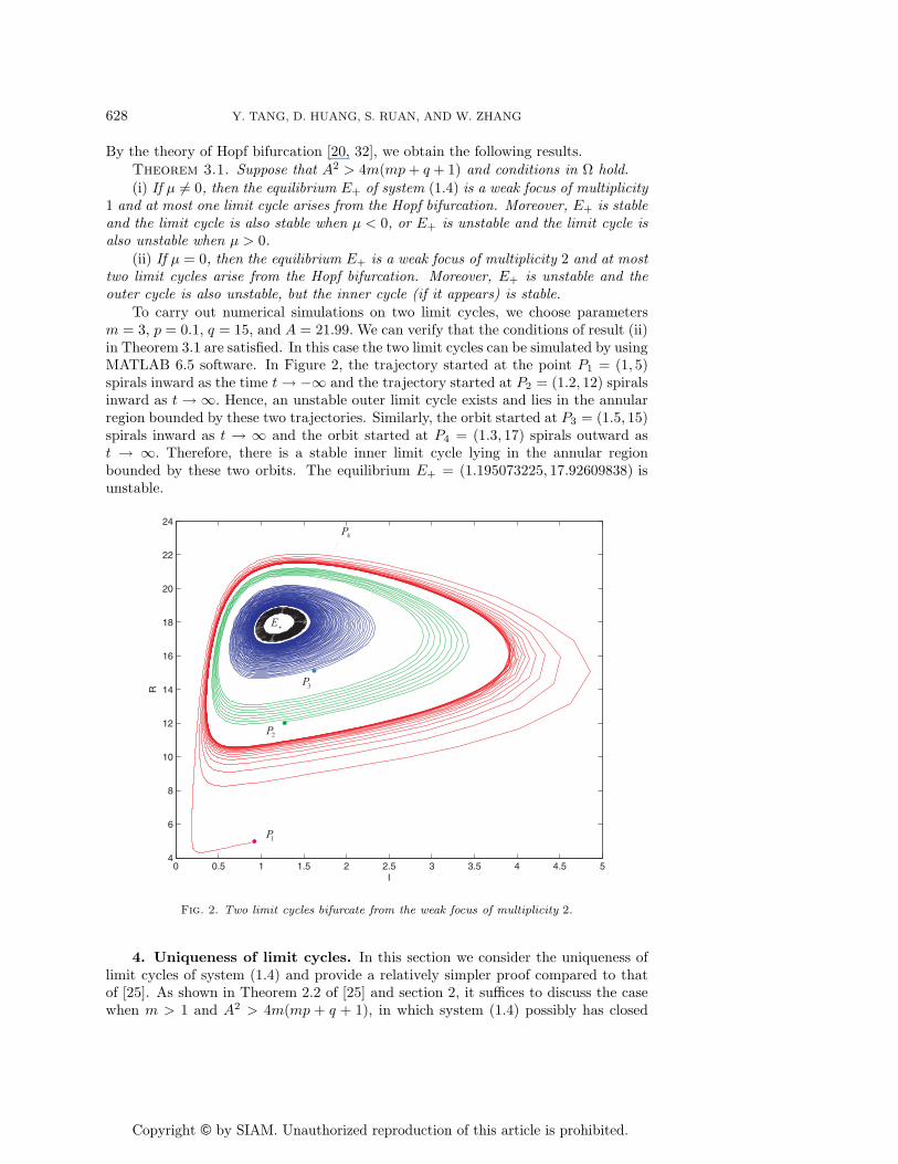
To carry out numerical simulations on two limit cycles, we choose parametersm = 3, p = 0.1, q = 15, and A = 21.99. We can verify that the conditions of result (ii)in Theorem 3.1 are satisfied. In this case the two limit cycles can be simulated by usingMATLAB 6.5 software. In Figure 2, the trajectory started at the point P1 = (1, 5)spirals inward as the time t → −∞ and the trajectory started at P2 = (1.2, 12) spiralsinward as t → ∞. Hence, an unstable outer limit cycle exists and lies in the annularregion bounded by these two trajectories. Similarly, the orbit started at P3 = (1.5, 15)spirals inward as t → ∞ and the orbit started at P4 = (1.3, 17) spirals outward ast → ∞. Therefore, there is a stable inner limit cycle lying in the annular regionbounded by these two orbits. The equilibrium E+ = (1.195073225, 17.92609838) isunstable.

1P

2P

3P

4P

�E

Fig. 2. Two limit cycles bifurcate from the weak focus of multiplicity 2.

4. Uniqueness of limit cycles. In this section we consider the uniqueness oflimit cycles of system (1.4) and provide a relatively simpler proof compared to thatof [25]. As shown in Theorem 2.2 of [25] and section 2, it suffices to discuss the casewhen m > 1 and A2 > 4m(mp + q + 1), in which system (1.4) possibly has closed

Copyright © by SIAM. Unauthorized reproduction of this article is prohibited.

A SIRS MODEL WITH A NONLINEAR INCIDENCE RATE 629

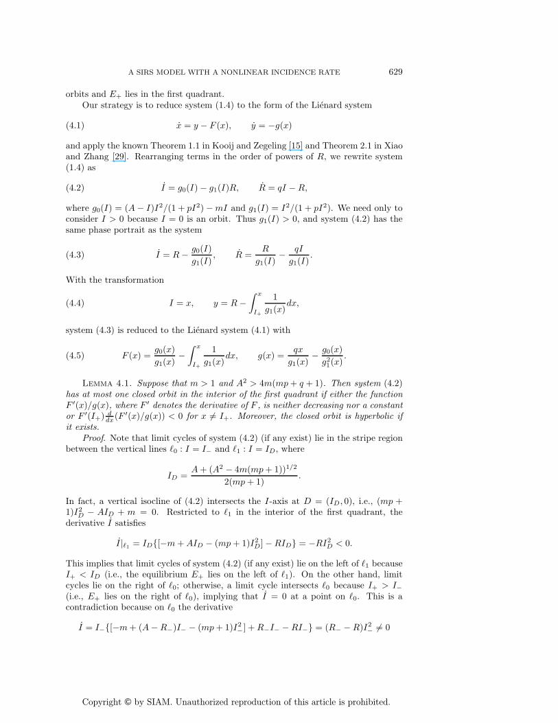
orbits and E+ lies in the first quadrant.Our strategy is to reduce system (1.4) to the form of the Lienard system

x = y − F (x), y = −g(x)(4.1)

and apply the known Theorem 1.1 in Kooij and Zegeling [15] and Theorem 2.1 in Xiaoand Zhang [29]. Rearranging terms in the order of powers of R, we rewrite system(1.4) as

I = g0(I) − g1(I)R, R = qI − R,(4.2)

where g0(I) = (A − I)I2/(1 + pI2) − mI and g1(I) = I2/(1 + pI2). We need only toconsider I > 0 because I = 0 is an orbit. Thus g1(I) > 0, and system (4.2) has thesame phase portrait as the system

I = R − g0(I)g1(I)

, R =R

g1(I)− qI

g1(I).(4.3)

With the transformation

I = x, y = R −∫ x

I+

1g1(x)

dx,(4.4)

system (4.3) is reduced to the Lienard system (4.1) with

F (x) =g0(x)g1(x)

−∫ x

I+

1g1(x)

dx, g(x) =qx

g1(x)− g0(x)

g21(x)

.(4.5)

Lemma 4.1. Suppose that m > 1 and A2 > 4m(mp + q + 1). Then system (4.2)has at most one closed orbit in the interior of the first quadrant if either the functionF ′(x)/g(x), where F ′ denotes the derivative of F , is neither decreasing nor a constantor F ′(I+) d

dx(F ′(x)/g(x)) < 0 for x �= I+. Moreover, the closed orbit is hyperbolic ifit exists.

Proof. Note that limit cycles of system (4.2) (if any exist) lie in the stripe regionbetween the vertical lines �0 : I = I− and �1 : I = ID, where

ID =A + (A2 − 4m(mp + 1))1/2

2(mp + 1).

In fact, a vertical isocline of (4.2) intersects the I-axis at D = (ID, 0), i.e., (mp +1)I2

D − AID + m = 0. Restricted to �1 in the interior of the first quadrant, thederivative I satisfies

I|�1 = ID{[−m + AID − (mp + 1)I2D] − RID} = −RI2

D < 0.

This implies that limit cycles of system (4.2) (if any exist) lie on the left of �1 becauseI+ < ID (i.e., the equilibrium E+ lies on the left of �1). On the other hand, limitcycles lie on the right of �0; otherwise, a limit cycle intersects �0 because I+ > I−(i.e., E+ lies on the right of �0), implying that I = 0 at a point on �0. This is acontradiction because on �0 the derivative

I = I−{[−m + (A − R−)I− − (mp + 1)I2−] + R−I− − RI−} = (R− − R)I2

− �= 0

Copyright © by SIAM. Unauthorized reproduction of this article is prohibited.

630 Y. TANG, D. HUANG, S. RUAN, AND W. ZHANG

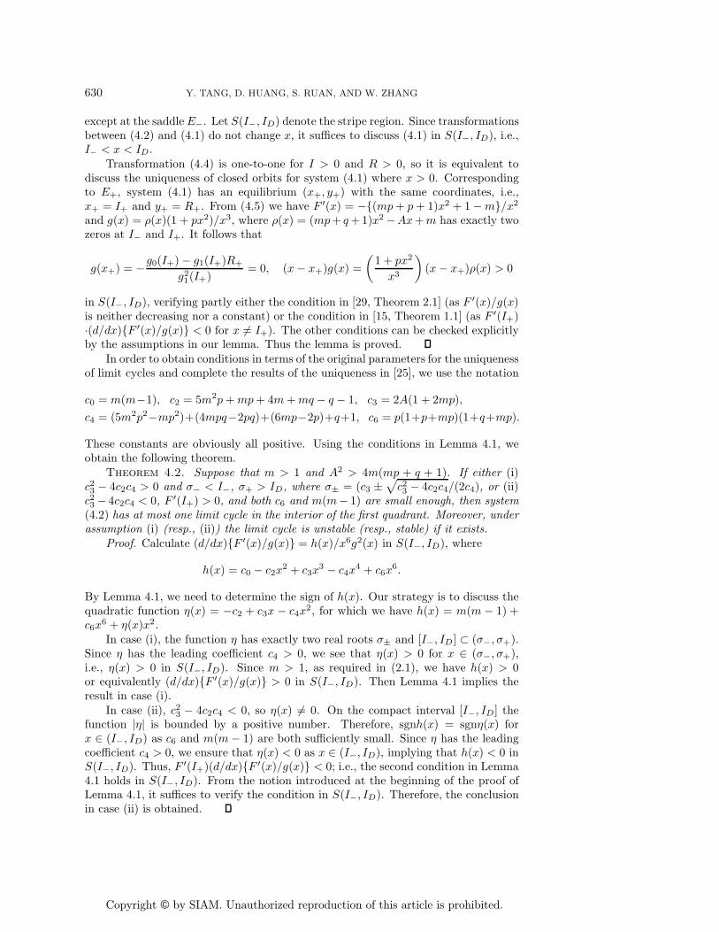
except at the saddle E−. Let S(I−, ID) denote the stripe region. Since transformationsbetween (4.2) and (4.1) do not change x, it suffices to discuss (4.1) in S(I−, ID), i.e.,I− < x < ID.

Transformation (4.4) is one-to-one for I > 0 and R > 0, so it is equivalent todiscuss the uniqueness of closed orbits for system (4.1) where x > 0. Correspondingto E+, system (4.1) has an equilibrium (x+, y+) with the same coordinates, i.e.,x+ = I+ and y+ = R+. From (4.5) we have F ′(x) = −{(mp + p + 1)x2 + 1 − m}/x2

and g(x) = ρ(x)(1 + px2)/x3, where ρ(x) = (mp + q +1)x2 −Ax + m has exactly twozeros at I− and I+. It follows that

g(x+) = −g0(I+) − g1(I+)R+

g21(I+)

= 0, (x − x+)g(x) =(

1 + px2

x3

)(x − x+)ρ(x) > 0

in S(I−, ID), verifying partly either the condition in [29, Theorem 2.1] (as F ′(x)/g(x)is neither decreasing nor a constant) or the condition in [15, Theorem 1.1] (as F ′(I+)·(d/dx){F ′(x)/g(x)} < 0 for x �= I+). The other conditions can be checked explicitlyby the assumptions in our lemma. Thus the lemma is proved.

In order to obtain conditions in terms of the original parameters for the uniquenessof limit cycles and complete the results of the uniqueness in [25], we use the notation

c0 = m(m−1), c2 = 5m2p + mp + 4m + mq − q − 1, c3 = 2A(1 + 2mp),c4 = (5m2p2−mp2)+(4mpq−2pq)+(6mp−2p)+q+1, c6 = p(1+p+mp)(1+q+mp).

These constants are obviously all positive. Using the conditions in Lemma 4.1, weobtain the following theorem.

Theorem 4.2. Suppose that m > 1 and A2 > 4m(mp + q + 1). If either (i)c23 − 4c2c4 > 0 and σ− < I−, σ+ > ID, where σ± = (c3 ±

√c23 − 4c2c4/(2c4), or (ii)

c23 − 4c2c4 < 0, F ′(I+) > 0, and both c6 and m(m− 1) are small enough, then system

(4.2) has at most one limit cycle in the interior of the first quadrant. Moreover, underassumption (i) (resp., (ii)) the limit cycle is unstable (resp., stable) if it exists.

Proof. Calculate (d/dx){F ′(x)/g(x)} = h(x)/x6g2(x) in S(I−, ID), where

h(x) = c0 − c2x2 + c3x

3 − c4x4 + c6x

6.

By Lemma 4.1, we need to determine the sign of h(x). Our strategy is to discuss thequadratic function η(x) = −c2 + c3x − c4x

2, for which we have h(x) = m(m − 1) +c6x

6 + η(x)x2.In case (i), the function η has exactly two real roots σ± and [I−, ID] ⊂ (σ−, σ+).

Since η has the leading coefficient c4 > 0, we see that η(x) > 0 for x ∈ (σ−, σ+),i.e., η(x) > 0 in S(I−, ID). Since m > 1, as required in (2.1), we have h(x) > 0or equivalently (d/dx){F ′(x)/g(x)} > 0 in S(I−, ID). Then Lemma 4.1 implies theresult in case (i).

In case (ii), c23 − 4c2c4 < 0, so η(x) �= 0. On the compact interval [I−, ID] the

function |η| is bounded by a positive number. Therefore, sgnh(x) = sgnη(x) forx ∈ (I−, ID) as c6 and m(m − 1) are both sufficiently small. Since η has the leadingcoefficient c4 > 0, we ensure that η(x) < 0 as x ∈ (I−, ID), implying that h(x) < 0 inS(I−, ID). Thus, F ′(I+)(d/dx){F ′(x)/g(x)} < 0; i.e., the second condition in Lemma4.1 holds in S(I−, ID). From the notion introduced at the beginning of the proof ofLemma 4.1, it suffices to verify the condition in S(I−, ID). Therefore, the conclusionin case (ii) is obtained.

Copyright © by SIAM. Unauthorized reproduction of this article is prohibited.

A SIRS MODEL WITH A NONLINEAR INCIDENCE RATE 631

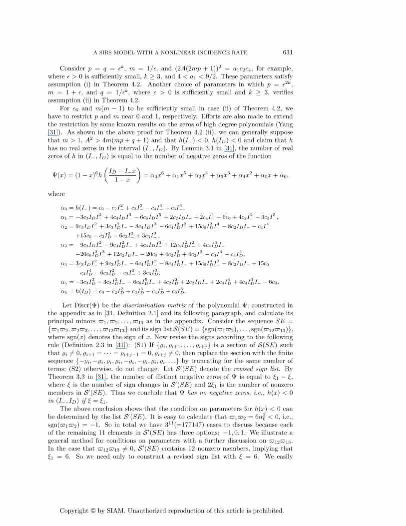
Consider p = q = εk, m = 1/ε, and (2A(2mp + 1))2 = a1c2c4, for example,where ε > 0 is sufficiently small, k ≥ 3, and 4 < a1 < 9/2. These parameters satisfyassumption (i) in Theorem 4.2. Another choice of parameters in which p = ε2k,m = 1 + ε, and q = 1/εk, where ε > 0 is sufficiently small and k ≥ 3, verifiesassumption (ii) in Theorem 4.2.

For c6 and m(m − 1) to be sufficiently small in case (ii) of Theorem 4.2, wehave to restrict p and m near 0 and 1, respectively. Efforts are also made to extendthe restriction by some known results on the zeros of high degree polynomials (Yang[31]). As shown in the above proof for Theorem 4.2 (ii), we can generally supposethat m > 1, A2 > 4m(mp + q + 1) and that h(I−) < 0, h(ID) < 0 and claim that hhas no real zeros in the interval (I−, ID). By Lemma 3.1 in [31], the number of realzeros of h in (I−, ID) is equal to the number of negative zeros of the function

Ψ(x) = (1 − x)6h(

ID − I−x

1 − x

)= α0x

6 + α1x5 + α2x

4 + α3x3 + α4x

2 + α5x + α6,

where

α0 = h(I−) = c0 − c2I2− + c3I

3− − c4I

4− + c6I

6−,

α1 = −3c3IDI2− + 4c4IDI3

− − 6c6IDI5− + 2c2IDI− + 2c4I

4− − 6c0 + 4c2I

2− − 3c3I

3−,

α2 = 9c3IDI2− + 3c3I

2DI− − 8c4IDI3

− − 6c4I2DI2

− + 15c6I2DI4

− − 8c2IDI− − c4I4−

+15c0 − c2I2D − 6c2I

2− + 3c3I

3−,

α3 = −9c3IDI2− − 9c3I

2DI− + 4c4IDI3

− + 12c4I2DI2

− + 4c4I3DI−

−20c6I3DI3

− + 12c2IDI− − 20c0 + 4c2I2D + 4c2I

2− − c3I

3− − c3I

3D,

α4 = 3c3IDI2− + 9c3I

2DI− − 6c4I

2DI2

− − 8c4I3DI− + 15c6I

4DI2

− − 8c2IDI− + 15c0

−c4I4D − 6c2I

2D − c2I

2− + 3c3I

3D,

α5 = −3c3I3D − 3c3I

2DI− − 6c6I

5DI− + 4c2I

2D + 2c2IDI− + 2c4I

4D + 4c4I

3DI− − 6c0,

α6 = h(ID) = c0 − c2I2D + c3I

3D − c4I

4D + c6I

6D.

Let Discr(Ψ) be the discrimination matrix of the polynomial Ψ, constructed inthe appendix as in [31, Definition 2.1] and its following paragraph, and calculate itsprincipal minors �1, �2, . . . , �13 as in the appendix. Consider the sequence SE ={�1�2, �2�3, . . . , �12�13} and its sign list S(SE) = {sgn(�1�2), . . . , sgn(�12�13)},where sgn(x) denotes the sign of x. Now revise the signs according to the followingrule (Definition 2.3 in [31]): (S1) If {�i, �i+1, . . . , �i+j} is a section of S(SE) suchthat �i �= 0, �i+1 = · · · = �i+j−1 = 0, �i+j �= 0, then replace the section with the finitesequence {−�i,−�i, �i, �i,−�i,−�i, �i, �i, . . .} by truncating for the same number ofterms; (S2) otherwise, do not change. Let S′(SE) denote the revised sign list. ByTheorem 3.3 in [31], the number of distinct negative zeros of Ψ is equal to ξ1 − ξ,where ξ is the number of sign changes in S′(SE) and 2ξ1 is the number of nonzeromembers in S′(SE). Thus we conclude that Ψ has no negative zeros, i.e., h(x) < 0in (I−, ID) if ξ = ξ1.

The above conclusion shows that the condition on parameters for h(x) < 0 canbe determined by the list S′(SE). It is easy to calculate that �1�2 = 6α3

0 < 0, i.e.,sgn(�1�2) = −1. So in total we have 311(=177147) cases to discuss because eachof the remaining 11 elements in S′(SE) has three options: −1, 0, 1. We illustrate ageneral method for conditions on parameters with a further discussion on �12�13.In the case that �12�13 �= 0, S′(SE) contains 12 nonzero members, implying thatξ1 = 6. So we need only to construct a revised sign list with ξ = 6. We easily

Copyright © by SIAM. Unauthorized reproduction of this article is prohibited.

632 Y. TANG, D. HUANG, S. RUAN, AND W. ZHANG

find such a list {−1, 1,−1, 1,−1, 1,−1,−1,−1,−1,−1,−1}, which gives a conditionon parameters:

(C1) :�2�3 ≥ 0, �3�4 < 0, �4�5 > 0, �5�6 < 0, �6�7 > 0, �7�8 < 0,

�8�9 < 0, �9�10 < 0, �10�11 < 0, �11�12 < 0, �12�13 < 0.

In the case that �12�13 = 0, the number of nonzero members in S′(SE) is < 12, i.e.,ξ1 ≤ 5. Note that the list {−1, 1,−1, 1,−1, 1, 1, 1, 1, 1, 0, 0} has ξ = 5. Being a revisedsign list, it gives a condition of parameters:

(C2) :�2�3 ≥ 0, �3�4 < 0, �4�5 > 0, �5�6 < 0, �6�7 > 0, �7�8 > 0,

�8�9 > 0, �9�10 > 0, �10�11 > 0, �11�12 = �12�13 = 0.

Finally, Lemma 4.1 and the conclusion given in the last paragraph enable us to sum-marize that if m > 1, A2 > 4m(mp+ q +1), h(I−) < 0, h(ID) < 0, F ′(I+) > 0, and ifeither (C1) or (C2) holds, then system (4.2) has at most one limit cycle in the interiorof the first quadrant. Moreover, the limit cycle is stable if it exists. More conditionsother than (C1) and (C2) can similarly be obtained for the uniqueness of limit cycles.

5. Degenerate Bogdanov–Takens bifurcation. By Lemma 2.3, when A =A0 =: 2

√m(mp + q + 1) and p = p0 =: ((m − 1)q − 1)/(2m), the equilibrium E0 =:

(A0/(2(mp0 + q + 1)), qA0/(2(mp0 + q + 1))) is a cusp, where the Bogdanov–Takensbifurcation may occur by a perturbation. By the standard theory of the Bogdanov–Takens bifurcation (of codimension 2), Ruan and Wang [25] assert only that thesystem has at most one limit cycle and the obtained homoclinic loop is of order 1 (seethe definition in [16]).

In the following, we display the possible bifurcations of multiple limit cycles andhomoclinic loops of order higher than 1. Note that as A = A0 and p = p0, we have(m − 1)q = 2mp0 + 1 > 0, implying m > 1. So we fix m0 > 1 near 1 arbitrarily andconsider three bifurcation parameters A, p, m near A0, p0, m0, respectively. Let

A = A0 + ε1, p = p0 + ε2, m = m0 + ε3,(5.1)

where ε3 > 0. Then, we discuss bifurcations of the equivalent system (1.4) for theparameters ε = (ε1, ε2, ε3) near (0, 0, 0).

Lemma 5.1. For A, p, m close to A0, p0, m0, respectively, (1.4) is equivalent tothe system

dx

dt= y,

dy

dt= μ1 + x2 + (μ2 + μ3x + x3 + O(|x|4))y + G(x, μ)y2,(5.2)

where μi’s are functions of ε1, ε2, ε3 such that ∂(μ1,μ2,μ3)∂(ε1,ε2,ε3)

|ε=0 �= 0 and G(x, μ) is a C∞

function.Proof. With the substitution (5.1), equation (1.4) can be written as{

I = I(I + A02((m0+ε3)(p0+ε2)+q+1) , R + qA0

2((m0+ε3)(p0+ε2)+q+1) ),

R = R(I + A02((m0+ε3)(p0+ε2)+q+1) , R + qA0

2((m0+ε3)(p0+ε2)+q+1) ),(5.3)

where I and R are defined in (1.4). When ε = 0, system (5.3) has a cusp at the originO2 = (0, 0), as shown in [25]; i.e., the equilibrium E0 is translated to O2. Expanding(5.3) at O2, rescaling time by t = τ(q + 1 + qm0)/(2qm0), and then applying a linear

Copyright © by SIAM. Unauthorized reproduction of this article is prohibited.

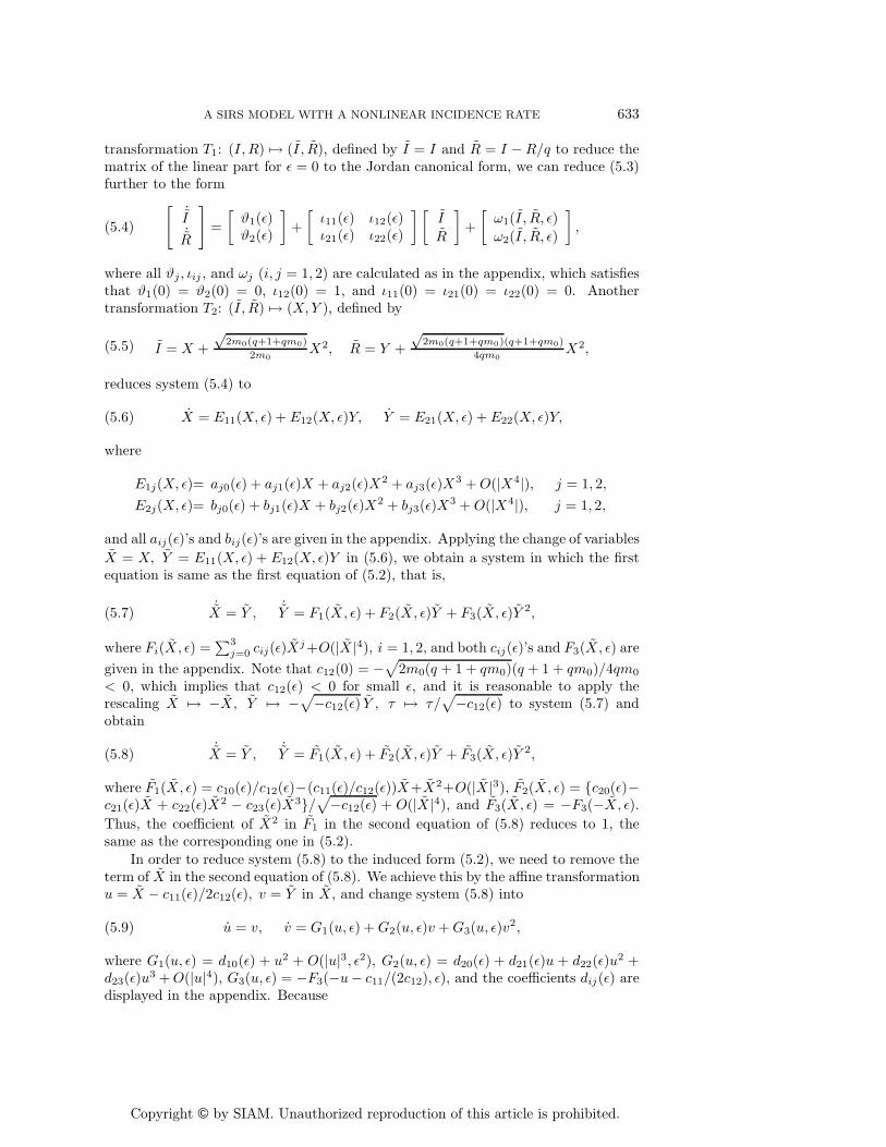
A SIRS MODEL WITH A NONLINEAR INCIDENCE RATE 633

transformation T1: (I, R) �→ (I , R), defined by I = I and R = I − R/q to reduce thematrix of the linear part for ε = 0 to the Jordan canonical form, we can reduce (5.3)further to the form[ ˙I

˙R

]=

[ϑ1(ε)ϑ2(ε)

]+

[ι11(ε) ι12(ε)ι21(ε) ι22(ε)

] [I

R

]+

[ω1(I , R, ε)ω2(I , R, ε)

],(5.4)

where all ϑj , ιij , and ωj (i, j = 1, 2) are calculated as in the appendix, which satisfiesthat ϑ1(0) = ϑ2(0) = 0, ι12(0) = 1, and ι11(0) = ι21(0) = ι22(0) = 0. Anothertransformation T2: (I , R) �→ (X, Y ), defined by

I = X +√

2m0(q+1+qm0)

2m0X2, R = Y +

√2m0(q+1+qm0)(q+1+qm0)

4qm0X2,(5.5)

reduces system (5.4) to

X = E11(X, ε) + E12(X, ε)Y, Y = E21(X, ε) + E22(X, ε)Y,(5.6)

where

E1j(X, ε)= aj0(ε) + aj1(ε)X + aj2(ε)X2 + aj3(ε)X3 + O(|X4|), j = 1, 2,

E2j(X, ε)= bj0(ε) + bj1(ε)X + bj2(ε)X2 + bj3(ε)X3 + O(|X4|), j = 1, 2,

and all aij(ε)’s and bij(ε)’s are given in the appendix. Applying the change of variablesX = X, Y = E11(X, ε) + E12(X, ε)Y in (5.6), we obtain a system in which the firstequation is same as the first equation of (5.2), that is,

˙X = Y , ˙Y = F1(X, ε) + F2(X, ε)Y + F3(X, ε)Y 2,(5.7)

where Fi(X, ε) =∑3

j=0 cij(ε)Xj+O(|X |4), i = 1, 2, and both cij(ε)’s and F3(X, ε) aregiven in the appendix. Note that c12(0) = −√

2m0(q + 1 + qm0)(q + 1 + qm0)/4qm0

< 0, which implies that c12(ε) < 0 for small ε, and it is reasonable to apply therescaling X �→ −X, Y �→ −√−c12(ε) Y , τ �→ τ/

√−c12(ε) to system (5.7) andobtain

˙X = Y , ˙Y = F1(X, ε) + F2(X, ε)Y + F3(X, ε)Y 2,(5.8)

where F1(X, ε) = c10(ε)/c12(ε)−(c11(ε)/c12(ε))X+X2+O(|X|3), F2(X, ε) = {c20(ε)−c21(ε)X + c22(ε)X2 − c23(ε)X3}/√−c12(ε) + O(|X |4), and F3(X, ε) = −F3(−X, ε).Thus, the coefficient of X2 in F1 in the second equation of (5.8) reduces to 1, thesame as the corresponding one in (5.2).

In order to reduce system (5.8) to the induced form (5.2), we need to remove theterm of X in the second equation of (5.8). We achieve this by the affine transformationu = X − c11(ε)/2c12(ε), v = Y in X, and change system (5.8) into

u = v, v = G1(u, ε) + G2(u, ε)v + G3(u, ε)v2,(5.9)

where G1(u, ε) = d10(ε) + u2 + O(|u|3, ε2), G2(u, ε) = d20(ε) + d21(ε)u + d22(ε)u2 +d23(ε)u3 + O(|u|4), G3(u, ε) = −F3(−u− c11/(2c12), ε), and the coefficients dij(ε) aredisplayed in the appendix. Because

Copyright © by SIAM. Unauthorized reproduction of this article is prohibited.

634 Y. TANG, D. HUANG, S. RUAN, AND W. ZHANG

d23(0) =2−

34 {m0(q + 1 + qm0)}1/4(q + 1 + qm0)1/2(3m0 − 1)(q + 1 + qm0)

m20(qm0)1/2

> 0,

for small ε �= 0 system (5.9) can be rescaled by u = d2/523 (ε)u, v = d

3/523 (ε)v, τ =

d−1/523 (ε)τ into the form

˙u = v, ˙v = G1(u, ε) + G2(u, ε)v + G3(u, ε)v2,(5.10)

where G1(u, ε) = d4/523 d10(ε) + u2 + O(|u|3), G2(u, ε) = d

1/523 d20(ε) + d

−1/523 d21(ε)u +

d−3/523 d22(ε)u2 + u3 + O(|u|4), and G3(u, ε) = −d

−2/523 F3(−d

−2/523 u − c11/(2c12), ε), so

that the coefficient of the term u3v in the second equation of (5.10) becomes 1, thesame as in the corresponding term in system (5.2). The invertibility of all undergonetransformations for small ε �= 0 implies that system (5.10) is topologically conjugateto system (5.2) locally. Hence (5.3) is an induced family of vector fields from system(5.2), the universal unfolding of the degenerate cusp as shown in the Main Theoremin [7]. Comparing the 4-jet of (5.10) with (5.2), we obtain the relation between theinduced system and the universal unfolding, i.e.,

μ1(ε) = d4/523 d10(ε), μ2(ε) = d

1/523 d20(ε), μ3(ε) = d

−1/523 d21(ε).(5.11)

In particular, μ1(0) = μ2(0) = μ3(0) = 0. Computing the Jacobian determinant ofrelation (5.11) at (0, 0, 0) with Maple V.7 software, we get

∂(μ1, μ2, μ3)∂(ε1, ε2, ε3)

∣∣∣∣ε=0

=1 + q + 4m0 + 3qm0 + 5qm2

0 − m20 − m3

0q)(q + 1 + qm0)2

2,

which is > 0 for m0 near 1. This implies that the induced family (5.3) parameterizedby ε, and therefore (1.4), is locally equivalent to the unfolding (5.2). The proof iscompleted.

Concerning the universal unfolding (5.2), Theorem 4 in [7] gives bifurcation sur-faces

SN = {(μ1, μ2, μ3) ∈ V |μ1 = 0},H = {(μ1, μ2, μ3) ∈ V |μ2 = μ3(−μ1)

12 + (−μ1)

32 + O((−μ1)

74 ), μ1 < 0},

HL =: {(μ1, μ2, μ3) ∈ V |μ2 = 57μ3(−μ1)

12 + 103

77 (−μ1)32 + O((−μ1)

74 ), μ1 < 0},

L =: {(μ1, μ2, μ3) ∈ V |Ξ(μ1, μ2, μ3) = 0, μ1 < 0},

where V is a neighborhood of (0, 0, 0) and the surface Ξ(μ1, μ2, μ3) = 0 is defined by

μ2 = (−μ1)32

(− 6P (b)

11P ′(b)+

6b

11) + o((−μ1)

32

), μ3 = −μ1

(− 6

11P ′(b)− 15

11

)+ o(−μ1)

for μ1 < 0 with the parameter b. Here P (b) is a solution of the Riccati equation(9b2 − 4)P ′ = 7P 2 + 3bP − 5, as shown in [7]. Applying the inverse of (5.11) togetherwith (5.1), from SN ,H,HL, and L we can give for system (1.4) the correspondingbifurcation surfaces SN ′,H′,HL′, and L′, respectively. Thus, Theorem 4 in [7] impliesthe following.

Theorem 5.2. In the (A, p, m)-space there are four surfaces SN ′,H′,HL′, L′

near (A0, p0, m0), defined as above, such that system (1.4) produces a saddle-node bi-furcation near E0 as (A, p, m) crosses SN ′, a Hopf bifurcation near E0 as (A, p, m)

Copyright © by SIAM. Unauthorized reproduction of this article is prohibited.

A SIRS MODEL WITH A NONLINEAR INCIDENCE RATE 635

Υ

Fig. 3. Projections of SN ,H, HL, and L on the (μ2, μ3)-plane.

crosses H′, a homoclinic bifurcation near E0 as (A, p, m) crosses HL′, and a coales-cence of two limit cycles near E0 as (A, p, m) crosses L′.

The expressions of these bifurcation surfaces given in Theorem 5.2 can be com-puted by using (5.11) and (5.1). For example, consider A0 = 63.73, p0 = 4.45, m0 =1.01, and q = 1000. The surface HL′ is presented as

57(0.003018260808ε2 + 1.509170071ε3)Θ(ε1, ε2, ε3)

+10377

(Θ(ε1, ε2, ε3))3 + o(|(ε1, ε2, ε3)|3/2) = 0,

where Θ(ε1, ε2, ε3) =√

0.09569545272ε1 − 0.003062992329ε2− 3.033146367ε3. Pa-rameter values are given by the expression where the homoclinic bifurcation occurs.Expressions of other bifurcation surfaces SN ′,H′, and L′ can be given similarly. Fora better understanding of the bifurcation diagram, let us observe bifurcation surfacesSN ,H,HL, and L in Figure 3. Since each of them is a cone with vertex at the origin(up to a homeomorphism in the parameter space), as in [7], it suffices to observe thebifurcation diagram in a small half ball Sμ0 = {(μ1, μ2, μ3)|μ2

1+μ22+μ2

3 < μ0, μ1 < 0}for sufficiently small μ0 > 0 and project the diagram to the plane SN (i.e., μ1 = 0). Asindicated in [7], projected on the disk Υ = Sμ0 ∩SN , the curve H intersects the curveHL at a point s0 and L is tangent to curves H and HL at two points s1 and s2, respec-tively. Thus the half ball Sμ0 is divided into five open regions Dj (j = I, II, . . . , V ),as shown in Figure 3. Let D′

j (j = I, II, . . . , V ) be the corresponding regions in the(A, p, m)-space and s′0, s′1, s′2 be the corresponding intersection points, which can becalculated with (5.11). When (A, p, m) lies in these regions, by Theorem 3.1, system(1.4) has two equilibria E+ and E− in the interior of the first quadrant and E− is

Copyright © by SIAM. Unauthorized reproduction of this article is prohibited.

636 Y. TANG, D. HUANG, S. RUAN, AND W. ZHANG

Table 1

Qualitative properties for various parameters.

(A, p, m) E+ Limit cycles Homoclinic orbitsD′

I unstable focus or node no no

H′\{s′0s′1} weak focus(order 1) no nos′1 weak focus(order 2) no no

s′0s′1 stable weak focus(order 1) 1(order 1) 0D′

II stable focus or node 1(order 1) no

HL′\{s′0s′2} focus or node no 1(order 1)s′0 stable weak focus(order 1) no 1(order 1)

D′III stable focus or node no no

D′IV unstable focus or node 1(order 1) nos′2 unstable focus or node no 1(order 2)

s′0s′2 unstable focus or node 1(order 1) 1(order 1)D′

V unstable focus or node 2(order 1) noL′ unstable focus or node 1(order 2) 0

always a saddle but E+ is either a focus or a node. Furthermore, by Lemma 4.1 andTheorem 5.2 together with the theorems in [7] and [25], we can list more detaileddynamical behaviors in Table 1, where s′0s

′1 and s′0s

′2 denote the parts of bifurcation

surfaces determined by the arcs on H and HL, respectively, as shown in Figure 3.More concretely, neither a limit cycle nor a homoclinic loop appears in D′

I ; a limitcycle arises as parameters go through H′ from D′

I to D′II ; the limit cycle expands,

deforms into a homoclinic loop and finally breaks as parameters go through HL′ fromD′

II to D′III ; a limit cycle arises again as parameters go through H′ from D′

III toD′

IV . By continuity, if parameters go through the part of HL′ below s′2 and returnto D′

I from D′IV , the limit cycle disappears; if parameters go from D′

IV and hit thearc s′0s

′2, the limit cycle coexists with a homoclinic loop. Furthermore, if parameters

enter the region D′V , the limit cycle persists and another limit cycle arises as the

homoclinic loop breaks, i.e., two cycles coexist.

6. Discussion. The existence of limit cycles in epidemic models can be used toexplain oscillatory phenomena observed in the dynamics of some infectious diseases.One of the mechanisms by which epidemic models exhibit periodic oscillations isbifurcation, which occurs when the parameters vary. Early work on studying thedynamics of epidemic models focused on Hopf bifurcation, homoclinic bifurcation, orsaddle-node bifurcation separately by using only one bifurcation parameter (Derrickand van den Driessche [6], Hethcote and van den Driessche [14], Liu et al. [17,18]). Recent studies indicate that some epidemic models undergo codimension 2bifurcations near degenerate equilibria; i.e., a Bogdanov–Takens bifurcation, whichincludes a Hopf bifurcation, a homocline bifurcation and a saddle-node bifurcation,can occur when two parameters vary near their critical values (Lizana and Rivero [19],Ruan and Wang [25], Alexander and Moghadas [1, 2], Moghadas [21], Wang [26]).It is interesting to notice that not only epidemic models with nonlinear incidencerates but also simple epidemic models with bilinear mass-action incidence rates canhave complex dynamics such as the occurrence of Bogdanov–Takens bifurcations.For instance, Wang and Ruan [27] considered an epidemic model with a bilinearmass-action incidence rate and a constant removal rate of infectious individuals andshowed that the model undergoes a sequence of bifurcations, including saddle-nodebifurcation, subcritical Hopf bifurcation, and homoclinic bifurcation.

Copyright © by SIAM. Unauthorized reproduction of this article is prohibited.

A SIRS MODEL WITH A NONLINEAR INCIDENCE RATE 637

In those epidemic models exhibiting Bogdanov–Takens bifurcations, periodic so-lutions can arise through a Hopf bifurcation for some parameter values and disappearthrough a homoclinic bifurcation for some other parameter values, but neither theexistence of multiple limit cycles nor the coexistence of a limit cycle and a homoclinicloop is revealed. However, recent work (Alexander and Moghadas [1, 2], Liu, Heth-cote, and Levin [17], Moghadas and Alexander [22], Ruan and Wang [25], Wang [26])indicates that some epidemic models can have two limit cycles. One may expect thatthe appearance of two limit cycles is due to the fact that degenerate Hopf and degen-erate Bogdanov–Takens bifurcations [4] may occur in such epidemic models as well.However, to the best of our knowledge, so far there is no such study on the degenerateHopf bifurcation and degenerate Bogdanov–Takens bifurcation on epidemic models.One of the difficulties is the lack of general criteria in calculating the multiplicity of aweak focus (see Xiao and Zhu [30] for such a criterion for a predator-prey model; seealso Ruan and Xiao [24]).

In this paper, we continued studying the dynamics of a simplified epidemic model(1.3) with a nonlinear incidence rate that was originally considered by Ruan andWang [25] (see also Liu et al. [17, 18] and Hethcote and van den Driessche [14]).Under certain conditions Ruan and Wang [25] showed that the simplified model (1.3)undergoes a Bogdanov–Takens bifurcation; i.e., it exhibits saddle-node, Hopf, andhomoclinic bifurcations. They also established the existence of none, one, or twolimit cycles. In this paper, we first calculated the second order Liapunov value ofthe weak focus and proved that the maximal multiplicity of the weak focus is 2 bytechnically dealing with some complicated multivariable polynomials, which impliesthat at most two limit cycles can arise near the weak focus. Then, by reducing thedetermination of the sign for polynomials of higher degrees to revised sign lists, were-established the uniqueness of the limit cycle. Finally, we reduced system (1.4) toa form of universal unfolding for a cusp of codimension 3 and showed the coexistenceof limit cycles and homoclinic loops via a degenerate Bogdanov–Takens bifurcation.

The coexistence of limit cycles and homoclinic loops demonstrates that epidemicmodels with saturated incidence rates exhibit very different and complex dynamics.Furthermore, the results indicate that the dynamical behavior of the model is verysensitive to the initial densities of the susceptible and infectious individuals. When theinitial values lie inside the homoclinic loop, the numbers of susceptible and infectiousindividuals fluctuate periodically about the endemic levels. Such periodic patterns willbe helpful in designing control and intervention policies for the disease. When theinitial values lie outside the homoclinic loop, the disease will die out even if there aretwo endemic equilibria (see Figure 3). This means that the disease can be controlledand eradicated even above the threshold.

To the best of our knowledge, this is the first time that a limit cycle and ahomoclinic loop have been shown to coexist in a realistic epidemic model. Thoughwe focused on a simple case of SIRS models with a specific saturated incidence rate,we believe that such rich and complex dynamics can occur in other epidemic modelswith general saturated incidence rates as well as other types of nonlinear incidencerates (Hethcote and van den Driessche [14], Liu et al. [17, 18]).

Appendix.

(A1) As claimed in section 4, for each j = 1, . . . , 13, the polynomial �j in variables

Copyright © by SIAM. Unauthorized reproduction of this article is prohibited.

638 Y. TANG, D. HUANG, S. RUAN, AND W. ZHANG

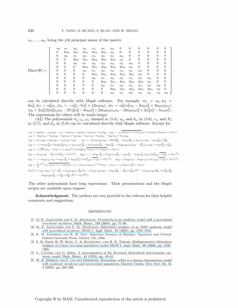
α1, . . . , α6, being the jth principal minor of the matrix

Discr(Ψ) =

⎡⎢⎢⎢⎢⎢⎢⎢⎢⎢⎢⎢⎢⎢⎢⎣

α0 α1 α2 α3 α4 α5 α6 0 0 0 0 0 00 6α0 5α1 4α2 3α3 2α4 α5 0 0 0 0 0 00 α0 α1 α2 α3 α4 α5 α6 0 0 0 0 00 0 6α0 5α1 4α2 3α3 2α4 α5 0 0 0 0 00 0 α0 α1 α2 α3 α4 α5 α6 0 0 0 00 0 0 6α0 5α1 4α2 3α3 2α4 α5 0 0 0 00 0 0 α0 α1 α2 α3 α4 α5 α6 0 0 00 0 0 0 6α0 5α1 4α2 3α3 2α4 α5 0 0 00 0 0 0 α0 α1 α2 α3 α4 α5 α6 0 00 0 0 0 0 6α0 5α1 4α2 3α3 2α4 α5 0 00 0 0 0 0 α0 α1 α2 α3 α4 α5 α6 00 0 0 0 0 0 6α0 5α1 4α2 3α3 2α4 α5 00 0 0 0 0 0 α0 α1 α2 α3 α4 α5 α6

⎤⎥⎥⎥⎥⎥⎥⎥⎥⎥⎥⎥⎥⎥⎥⎦,

can be calculated directly with Maple software. For example, �1 = α0, �2 =6α2

0, �3 = α20α1, �4 = −α2

0(−5α21 + 12α2α0), �5 = α2

0(α21α2 − 4α0α

22 + 3α0α3α1),

�6 = 2α20(24α2

0α4α2 − 27α20α

23 − 8α0α

32 + 24α0α3α1α2 − 10α0α4α

21 + 2α2

2α21 − 5α3α

31).

The expressions for others will be much longer.(A2) The polynomials ϑj , ιij , ωj claimed in (5.4), aij and bij in (5.6), cij and F3

in (5.7), and dij in (5.9) can be calculated directly with Maple software. Except for

c10 = a20b10 − a10b20, c11 = a20b11−a10b21+a21b10−a11b20, c12 = −√

2m0(q+1+qm0)(q+1+qm0)/(4qm0) + O(|ε|),c13 = −b22a11 + b13a20 − b23a10 + b10a23 − b21a12 + b12a21 − b20a13 + b11a22,

c20 = (a11a20 + b20a20 − a10a21)/a20, c21 = −(2a10a22a20 − bb21a220 − 2a12a

220 + a21a11a20 − a10a

221)/a

220,

c22 = −(−3a13a320 + 2a22a

220a11 + a21a12a

220 + 3a10a23a

220 − b22a

320 − 3a22a20a10a21 − a

221a11a20 + a10a

321)/a

320,

c23 = −{√2(3m0 − 1)(q + 1 + qm0)3}/{4m20q

√m0(q + 1 + qm0)} + O(|ε|),

d10 = (4c10c12 − c211)/(4c212) + O(|ε|2), d20 = −(−8c20c312 + 4c21c11c212 + c23c311 − 2c22c211c12)/(8c312√

−c12) + O(|ε|2),

d21 = −(−4c22c11c12 + 4c21c212 + 3c23c

211)/(4c

212

√−c12) + O(|ε|2), d22 = (2c22c12 − 3c23c11)/(2c12

√−c12) + O(|ε|2),

d23 = (1

2)3/4(

√m0(q + 1 + qm0)(q + 1 + qm0)/(qm0))1/2(3m0 − 1)(q + 1 + qm0)/m

20 + O(|ε|),

F3(X) = a21/a20 + {(−a221 + 2a22a20)/a

220}X − {(3a21a22a20 − 3a23a

220 − a

321)/a

320}X

2 − {(4a21a23a220 + 2a

222a

220

− 4a22a20a221 + a

421)/a

420}X

3 + O(|X4 |).

The other polynomials have long expressions. Their presentations and the Maplescripts are available upon request.

Acknowledgment. The authors are very grateful to the referees for their helpfulcomments and suggestions.

REFERENCES

[1] M. E. Alexander and S. M. Moghadas, Periodicity in an epidemic model with a generalizednon-linear incidence, Math. Biosci., 189 (2004), pp. 75–96.

[2] M. E. Alexander and S. M. Moghadas, Bifurcation analysis of an SIRS epidemic modelwith generalized incidence, SIAM J. Appl. Math., 65 (2005), pp. 1794–1816.

[3] R. M. Anderson and R. M. May, Infectious Diseases of Humans: Dynamics and Control,Oxford University Press, Oxford, UK, 1992.

[4] S. M. Baer, B. W. Kooi, Y. A. Kuznetsov, and H. R. Thieme, Multiparametric bifurcationanalysis of a basic two-stage population model, SIAM J. Appl. Math., 66 (2006), pp. 1339–1365.

[5] V. Capasso and G. Serio, A generalization of the Kermack–Mckendrick deterministic epi-demic model, Math. Biosci., 42 (1978), pp. 43–61.

[6] W. R. Derrick and P. van den Driessche, Homoclinic orbits in a disease transmission modelwith nonlinear incidence and nonconstant population, Discrete Contin. Dyn. Syst. Ser. B,3 (2003), pp. 299–309.

Copyright © by SIAM. Unauthorized reproduction of this article is prohibited.

A SIRS MODEL WITH A NONLINEAR INCIDENCE RATE 639

[7] F. Dumortier, R. Roussarie, and J. Sotomayor, Generic 3-parameter families of vectorfields on the plane, unfolding a singularity with nilpotent linear part. The cusp case ofcodimension 3, Ergodic Theory Dynam. Systems, 7 (1987), pp. 375–413.

[8] M. G. M. Gomes, A. Margheri, G. F. Medley, and C. Rebelo, Dynamical behaviour ofepidemiological models with sub-optimal immunity and nonlinear incidence, J. Math. Biol.,51 (2005), pp. 414–430.

[9] J. K. Hale, Ordinary Differential Equations, 2nd ed., Wiley-Interscience, New York, 1980.[10] H. W. Hethcote, A thousand and one epidemic models, in Frontiers in Theoretical Biology, S.

A. Levin, ed., Lecture Notes in Biomath. 100, Springer-Verlag, Berlin, 1994, pp. 504–515.[11] H. W. Hethcote, The mathematics of infectious diseases, SIAM Rev., 42 (2000), pp. 599–653.[12] H. W. Hethcote and S. A. Levin, Periodicity in epidemiological models, in Applied Math-

ematical Biology, Biomath. Texts 18, S. A. Levin, T. G. Hallam and L. J. Gross, eds.,Springer-Verlag, New York, 1989, pp. 193–211.

[13] H. W. Hethcote, H. W. Stech, and P. van den Driessche, Periodicity and stability in epi-demic models: A survey, in Differential Equations and Applications in Ecology, Epidemicsand Population Problems, S. N. Busenberg and K. L. Cook, eds., Academic Press, NewYork, 1981, pp. 65–82.

[14] H. W. Hethcote and P. van den Driessche, Some epidemiological models with nonlinearincidence, J. Math. Biol., 29 (1991), pp. 271–287.

[15] R. E. Kooij and A. Zegeling, A predator-prey model with Ivlev’s functional response, J.Math. Anal. Appl., 198 (1996), pp. 473–489.

[16] C.-Z. Li and C. Rousseau, A system with three cycles appearing in a Hopf bifurcation anddying in a homoclinic bifurcation: The cusp of order 4, J. Differential Equations, 23 (1986),pp. 187–204.

[17] W. Liu, H. W. Hethcote, and S. A. Levin, Dynamical behavior of epidemiological modelswith non-linear incidence rate, J. Math. Biol., 25 (1987), pp. 359–380.

[18] W. Liu, S. A. Levin, and Y. Iwasa, Influence of nonlinear incidence rate upon the behaviorof SIRS epidemiological models, J. Math. Biol., 23 (1986), pp. 187–204.

[19] M. Lizana and J. Rivero, Multiparametric bifurcations for a model in epidemiology, J. Math.Biol., 35 (1996), pp. 21–36.

[20] N. G. Lloyd, Limit cycles of polynomial systems—some recent developments, in New Direc-tions in Dynamical Systems, T. Bedford and J. Swift, eds., LMS Lect. Notes 127, CambridgeUniversity Press, Cambridge, UK, 1988, pp. 192–238.

[21] S. M. Moghadas, Analysis of an epidemic model with bistable equilibria using the Poincareindex, Appl. Math. Comput., 149 (2004), pp. 689–702.

[22] S. M. Moghadas and M. E. Alexander, Bifurcations of an epidemic model with non-linearincidence and infection-dependent removal rate, Math. Med. Biol., 23 (2006), pp. 231–254.

[23] R. R. Regoes, D. Ebert, and S. Bonhoeffer, Dose-dependent infection rates of parasitesproduce the Allee effect in epidemiology, Proc. Roy. Soc. London Ser. B, 269 (2002), pp.271–279.

[24] S. Ruan and D. Xiao, Global analysis in a predator-prey system with nonmonotonic functionalresponse, SIAM J. Appl. Math., 61 (2001), pp. 1445–1472.

[25] S. Ruan and W. Wang, Dynamical behaviour of an epidemic model with a nonlinear incidencerate, J. Differential Equations, 188 (2003), pp. 135–163.

[26] W. Wang, Epidemic models with nonlinear infection forces, Math. Biosci. Engrg., 3 (2006),pp. 267–279.

[27] W. Wang and S. Ruan, Bifurcations in an epidemic model with constant removal rate of theinfectives, J. Math. Anal. Appl., 291 (2004), pp. 775–793.

[28] D. Xiao and S. Ruan, Global analysis of an epidemic model with nonmonotone incidence rate,Math. Biosci., 208 (2007), pp. 419–429.

[29] D. Xiao and Z.-F. Zhang, On the uniqueness and nonexistence of limit cycles for predator-prey systems, Nonlinearity, 16 (2003), pp. 1185–1201.

[30] D. Xiao and H. Zhu, Multiple focus and Hopf bifurcations in a predator-prey system withnonmonotonic functional response, SIAM J. Appl. Math., 66 (2006), pp. 802–819.

[31] L. Yang, Recent advances on determining the number of real roots of parametric polynomials,J. Symbolic Comput. 28 (1999), pp. 225–242.

[32] Z.-F. Zhang, T.-R. Ding, W.-Z. Huang, and Z.-X. Dong, Qualitative Theory of DifferentialEquations, AMS, Providence, RI, 1992.