Coevolution for classification

TECHNICAL UNIVERSITY OF DORTMUND

REIHE COMPUTATIONAL INTELLIGENCE

COLLABORATIVE RESEARCH CENTER 531

Design and Management of Complex Technical Processesand Systems by means of Computational Intelligence Methods

Coevolution for Classification

Catalin Stoean, Ruxandra Stoean, Mike Preussand D. Dumitrescu

No. CI-239/08

Technical Report ISSN 1433-3325 January 2008

Secretary of the SFB 531 · Technical University of Dortmund · Dept. of ComputerScience/LS 2 · 44221 Dortmund · Germany

This work is a product of the Collaborative Research Center 531, “ComputationalIntelligence,” at the Technical University of Dortmund and was printed with financialsupport of the Deutsche Forschungsgemeinschaft.

Coevolution for Classification

Catalin Stoean1, Ruxandra Stoean1, Mike Preuss2, and D. Dumitrescu3

1 University of Craiova, A. I. Cuza, 13, 200585, Craiova, Romania{catalin.stoean, ruxandra.stoean}@inf.ucv.ro

2 University of Dortmund, Otto-Hahn 14, 44221, Dortmund, [email protected]

3 Babes-Bolyai University, M. Kogalniceanu, 1B, 400084, Cluj, [email protected]

1 Introduction

A data mining field with daily, and sometimes even vital, practical applica-tions, classification has been addressed by many powerful paradigms, amongwhich evolutionary algorithms (EAs) play a successful role. Nevertheless, asevolutionary computation (EC) progresses, there appear new possibilities ofdeveloping simpler and yet robust classification techniques.

The aim of this paper is hence to put forward a novel evolutionary classifi-cation framework which embodies two contradictory prototypes coming fromthe state-of-the-art field of coevolution and which has proven to be a viablealternative.

Coevolution between individuals assumes two opposite interactions: coop-erative and competitive. Analogously, coevolution for classification assumestwo possible and opposed manners of solving the task. Within both ap-proaches, the solution of a classification problem is regarded as a set of IF-THEN conjunctive rules in first order logic. As a consequence, learning willbe driven either by the cooperation between rules towards a complete andaccurate rule set or by the competition between rules and training samples inthe direction of extensive and hard testing on each side.

The paper is organized as follows. The next section introduces a generalpoint of view upon classification. Section three brings an overview on coevolu-tion: The cooperative and competitive archetypes are outlined and explained.Section four describes the proposed manner of approaching classification fromthe cooperative side, while section five presents the application of the com-petitive counterpart. Experiments on three data sets, two benchmark and onereal-world, are depicted in section six and the paper closes with the concludingremarks.

2 Catalin Stoean, Ruxandra Stoean, Mike Preuss, and D. Dumitrescu

2 Classification. A Perspective

Classification can assume different characterizations, however this paper re-gards it from a general point of view. Given {(xi, yi)}i=1,2,...,m, a training setwhere every xi ∈ Rn represents a data sample (values that correspond to asequence of attributes or indicators) and each yi ∈ 1, 2, ..., p represents a class(outcome, decision attribute), a classification task consists in learning the op-timal mapping that minimizes the discrepancy between the given classes ofdata sample and the actual classes produced by the learning machine. Subse-quently, the learnt patterns are confronted with each of the test data samples,without an a priori knowledge of their real classes. The predicted outcome isthen compared with the given class: If the two are identical for a certain sam-ple, then the sample is considered to be correctly classified. The percentageof correctly labelled test data is reported as the classification accuracy of theconstructed learning machine.

The data are split into the training set consisting of a higher number ofsamples and a test set that contains the rest of the data. The training andtest sets are disjoint. In present discussion, the samples that form the trainingset are chosen in a random manner from the entire specific data set.

The aim of a classification technique is, consequently, to stepwise learn aset of rules that model the training set as good as possible. When the learningstage is finished, the obtained rules are applied on previously unseen sampleswithin the test set.

3 Evolutionary Approaches to Classification

Apart from the hybridization with non-evolutionary specialized classificationtechniques, such as fuzzy sets, neural networks or decision trees, the evolu-tionary computation community has targeted classification through the de-velopment of special standalone EAs for the particular task.

On a broader sense, an evolutionary classification technique is concernedwith the discovery of IF-THEN rules that reproduce the correspondence be-tween the given samples and corresponding classes. Given an initial set oftraining samples, the system learns the patterns, i.e. evolves the classificationrules, which are then expected to predict the class of new examples.

Remark: An IF-THEN rule is imagined as a first-order logic implicationwhere the condition part is made of attributes and the conclusion part isrepresented by the class.

There are two state-of-the-art approaches to evolutionary classificationtechniques. The first direction ([11]) is represented by De Jong’s classifierthat is an evolutionary system which considers an individual to represent anentire set of rules. Rule sets are evolved using a canonical EA and the bestindividual from all generations represents the solution of the classificationproblem. The opposite related approach is Holland’s classifier system ([10],

Coevolution for Classification 3

[11]). Here, each individual encodes only one conjunctive rule and the entirepopulation represents the rule set. Thus, detection and maintenance of mul-tiple solutions (rules) in a multiple sub-populations environment is required.As a canonical EA cannot evolve non-homogeneous individuals, Holland’s ap-proach suggested doubling the EA by a credit assignment system that wouldassign positive credit to rules that cooperate and negative credit to the oppo-site.

Another standard method is characterized by a genetic programming ap-proach to rule discovery ([4], [5]). The internal nodes of the individual encodemathematical functions (e.g. AND, OR, +, -, *, <, =) while the leaf nodesrefer the attributes. Given a certain individual, the output of the tree is com-puted and, if it is greater than a given threshold, a certain outcome of theclassification task is predicted.

If discussion evolves around those classification evolutionary models thatare specifically for coadapted components, then we must refer the above-mentioned Holland’s classifier system [10] and the REGAL system [6], wherestimulus-response rules in conjunctive form were evolved by EAs. In Hol-land’s system, cooperation is achieved through a bucket brigade algorithmthat awards rules for collaboration and penalizes them otherwise. In the RE-GAL classifier, a problem decomposition is performed by a selection operator,complete solutions are found by choosing best rules from each component,a seeding operator maintains diversity and fitness of individuals within onecomponent depends on their consistency with the negative samples and ontheir simplicity [19].

However, the existing evolutionary classification techniques have quite in-tricate engines and thus their application is not always straightforward: theyuse complex credit assignment systems that penalize or reward good rules, aswell as very complicated schemas of the entire system.

To the best of our knowledge, there has been no attempt in applying eithercooperative or competitive coevolution to classification based on individualsthat encode simple conjunctive IF-THEN rules in first order logic.

4 Coevolution. Prerequisites

According to the Darwinian principles, an individual evolves through the inter-action with the environment. However, a significant segment of its surround-ings is, in fact, represented by other individuals. As a consequence, evolutionactually implies coevolution. This interactive process may assume collabora-tion towards the achievement of a specific mutual purpose, or, on the contrary,competition for the common resources in the spirit of the survival of the fittest.Accordingly, two kinds of artificial coevolutionary systems exist: cooperativeand competitive, respectively.

In cooperative coevolution, collaborations between two or more individualsare necessary in order to evaluate one complete potential solution, while in

4 Catalin Stoean, Ruxandra Stoean, Mike Preuss, and D. Dumitrescu

competitive coevolution, the evaluation of an individual is determined by aset of competitions between the current individual and several others.

Coevolutionary algorithms bring an interesting angle of perception uponevolution, as they promote a different manner of fitness evaluation of a candi-date solution, which takes into account its relation to the other surroundingindividuals. In addition, the coevolutionary evaluation is continuously alteredthroughout the existence of an individual as a result of various tests.

4.1 Cooperative Coevolution

Cooperative coevolution implies a decomposition of a candidate solution ofthe problem to be solved into a number of components [18], [25]. Each ofthese parts is subsequently attributed to a population (species) of an EA.The species evolve independently (although concurrently), while interactionsbetween populations appear only at the moment when fitness is computed.Each individual of a species stands for a part of the solution, therefore, acandidate for each component in turn cannot be evaluated separately fromthe complementary ones. Hence, when the fitness of an individual is assessed,collaborators from each of the remaining populations are selected in orderto form a complete solution. The performance of the established solution ismeasured and returned as the fitness evaluation of the considered individual.

Evolution is thus directed by the collaboration between species towardsthe joint goal of assembling a near optimal solution to the problem.

Algorithm 1 simulates the mechanisms of a canonical cooperative coevo-lutionary method.

Algorithm 1 A canonical cooperative coevolutionary algorithmt ← 0;for each species s do

randomly initialize population Pops(t);end forfor each species s do

evaluate Pops(t);end forwhile termination condition = false do

t ← t + 1;for each species s do

select population Pops(t) from Pops(t - 1);apply variation operators to Pops(t);evaluate Pops(t);

end forend while

The evolutionary process starts with the initialization of each population.In order to evaluate the initial fitness of each individual, a random selection

Coevolution for Classification 5

of collaborators from each of the other populations is performed and obtainedsolutions are measured and attributed accordingly. After this starting phase,each population is evolved through a canonical EA. Subsequently, the evalua-tion of a member of one species is performed through its fusion to individualsof the complementary population, which are this point selected through acertain strategy.

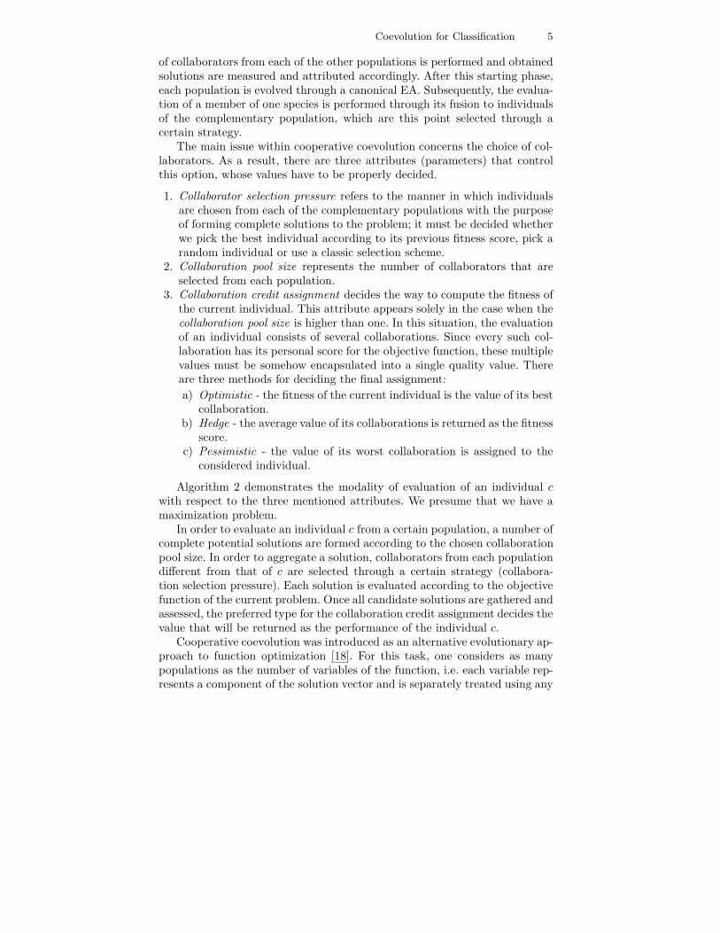
The main issue within cooperative coevolution concerns the choice of col-laborators. As a result, there are three attributes (parameters) that controlthis option, whose values have to be properly decided.

1. Collaborator selection pressure refers to the manner in which individualsare chosen from each of the complementary populations with the purposeof forming complete solutions to the problem; it must be decided whetherwe pick the best individual according to its previous fitness score, pick arandom individual or use a classic selection scheme.

2. Collaboration pool size represents the number of collaborators that areselected from each population.

3. Collaboration credit assignment decides the way to compute the fitness ofthe current individual. This attribute appears solely in the case when thecollaboration pool size is higher than one. In this situation, the evaluationof an individual consists of several collaborations. Since every such col-laboration has its personal score for the objective function, these multiplevalues must be somehow encapsulated into a single quality value. Thereare three methods for deciding the final assignment:a) Optimistic - the fitness of the current individual is the value of its best

collaboration.b) Hedge - the average value of its collaborations is returned as the fitness

score.c) Pessimistic - the value of its worst collaboration is assigned to the

considered individual.

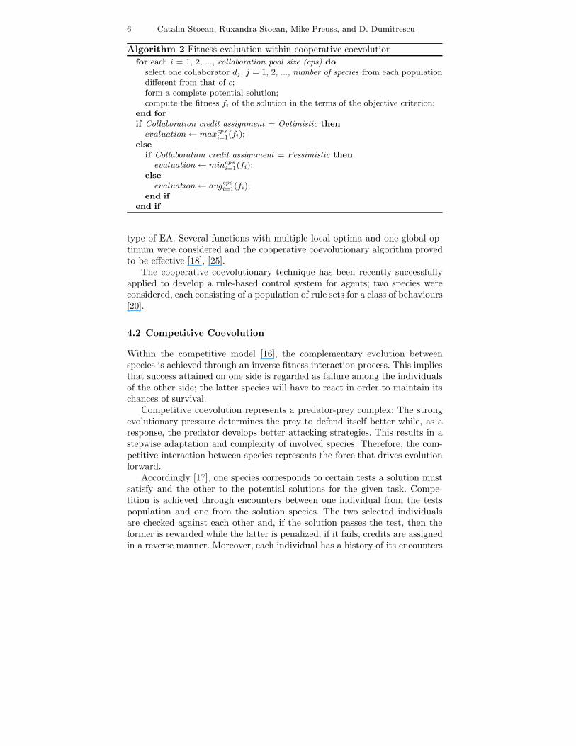
Algorithm 2 demonstrates the modality of evaluation of an individual cwith respect to the three mentioned attributes. We presume that we have amaximization problem.

In order to evaluate an individual c from a certain population, a number ofcomplete potential solutions are formed according to the chosen collaborationpool size. In order to aggregate a solution, collaborators from each populationdifferent from that of c are selected through a certain strategy (collabora-tion selection pressure). Each solution is evaluated according to the objectivefunction of the current problem. Once all candidate solutions are gathered andassessed, the preferred type for the collaboration credit assignment decides thevalue that will be returned as the performance of the individual c.

Cooperative coevolution was introduced as an alternative evolutionary ap-proach to function optimization [18]. For this task, one considers as manypopulations as the number of variables of the function, i.e. each variable rep-resents a component of the solution vector and is separately treated using any

6 Catalin Stoean, Ruxandra Stoean, Mike Preuss, and D. Dumitrescu

Algorithm 2 Fitness evaluation within cooperative coevolutionfor each i = 1, 2, ..., collaboration pool size (cps) do

select one collaborator dj , j = 1, 2, ..., number of species from each populationdifferent from that of c;form a complete potential solution;compute the fitness fi of the solution in the terms of the objective criterion;

end forif Collaboration credit assignment = Optimistic then

evaluation← maxcpsi=1(fi);

elseif Collaboration credit assignment = Pessimistic then

evaluation← mincpsi=1(fi);

elseevaluation← avgcps

i=1(fi);end if

end if

type of EA. Several functions with multiple local optima and one global op-timum were considered and the cooperative coevolutionary algorithm provedto be effective [18], [25].

The cooperative coevolutionary technique has been recently successfullyapplied to develop a rule-based control system for agents; two species wereconsidered, each consisting of a population of rule sets for a class of behaviours[20].

4.2 Competitive Coevolution

Within the competitive model [16], the complementary evolution betweenspecies is achieved through an inverse fitness interaction process. This impliesthat success attained on one side is regarded as failure among the individualsof the other side; the latter species will have to react in order to maintain itschances of survival.

Competitive coevolution represents a predator-prey complex: The strongevolutionary pressure determines the prey to defend itself better while, as aresponse, the predator develops better attacking strategies. This results in astepwise adaptation and complexity of involved species. Therefore, the com-petitive interaction between species represents the force that drives evolutionforward.

Accordingly [17], one species corresponds to certain tests a solution mustsatisfy and the other to the potential solutions for the given task. Compe-tition is achieved through encounters between one individual from the testspopulation and one from the solution species. The two selected individualsare checked against each other and, if the solution passes the test, then theformer is rewarded while the latter is penalized; if it fails, credits are assignedin a reverse manner. Moreover, each individual has a history of its encounters

Coevolution for Classification 7

which embodies the penalizations/rewards it has received. The fitness of theindividual is computed on this basis, as the sum of its most recent behaviours(successes/failures).

An important remark is that, since tests are a priori defined, it is only thepopulation of potential solutions that evolves; the opposite species containsthe same individuals (tests) until the end of the evolutionary process. Theonly fluctuation that appears within the latter population solely regards theranking of the individuals according to fitness (their satisfiability hardness). Itmust be however noted that, in certain cases when tests cannot be exhaustivelygiven, the tests population may also evolve.

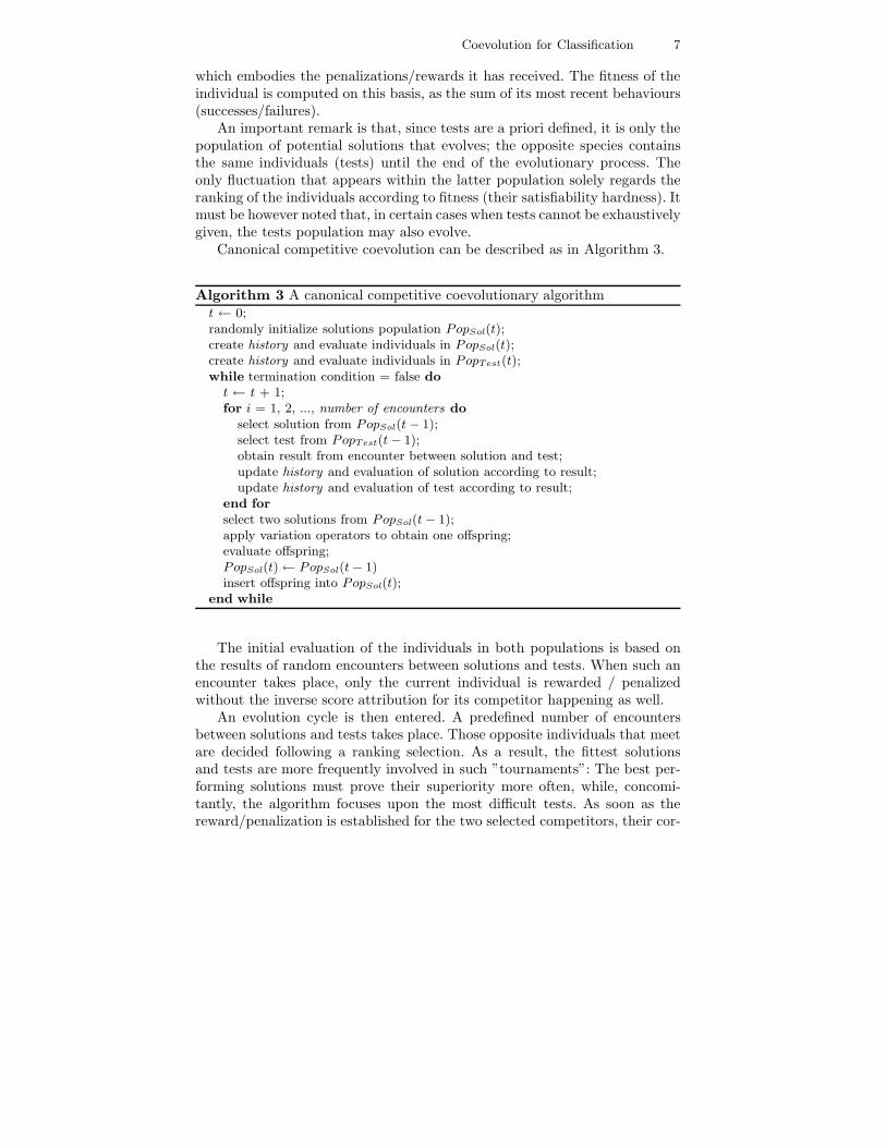
Canonical competitive coevolution can be described as in Algorithm 3.

Algorithm 3 A canonical competitive coevolutionary algorithmt ← 0;randomly initialize solutions population PopSol(t);create history and evaluate individuals in PopSol(t);create history and evaluate individuals in PopTest(t);while termination condition = false do

t ← t + 1;for i = 1, 2, ..., number of encounters do

select solution from PopSol(t− 1);select test from PopTest(t− 1);obtain result from encounter between solution and test;update history and evaluation of solution according to result;update history and evaluation of test according to result;

end forselect two solutions from PopSol(t− 1);apply variation operators to obtain one offspring;evaluate offspring;PopSol(t)← PopSol(t− 1)insert offspring into PopSol(t);

end while

The initial evaluation of the individuals in both populations is based onthe results of random encounters between solutions and tests. When such anencounter takes place, only the current individual is rewarded / penalizedwithout the inverse score attribution for its competitor happening as well.

An evolution cycle is then entered. A predefined number of encountersbetween solutions and tests takes place. Those opposite individuals that meetare decided following a ranking selection. As a result, the fittest solutionsand tests are more frequently involved in such ”tournaments”: The best per-forming solutions must prove their superiority more often, while, concomi-tantly, the algorithm focuses upon the most difficult tests. As soon as thereward/penalization is established for the two selected competitors, their cor-

8 Catalin Stoean, Ruxandra Stoean, Mike Preuss, and D. Dumitrescu

responding history is updated: The score of the most recent encounter replacesthat of the oldest one and evaluation is revised.

After the considered encounters are finished, a single offspring is created.Two parents are selected according to the same selection scheme and recom-bination and mutation on the resulting solution are subsequently applied. Apersonal history of the offspring is created through a number of encountersequal to the defined history length. The tests are again selected accordingto a ranking scheme. Following such an encounter, only the history of theoffspring is modified; unlike a standard encounter between a solution and atest, no simultaneous penalization/reward of the involved test is conducted.This stems from the simple reason that a mediocre offspring might lead to anunreliable change in the behaviour of the considered test. After the offspringis evaluated, it will replace the weakest individual in the solutions population.

During the entire evolutionary process, the tests population suffers novariation.

The two species thus evolve together, through the inverse fitness interac-tion mechanism: As soon as the potential solutions satisfy certain tests, thelatter receive a weaker evaluation score which leads to omission from furtherselection. As a result, other more difficult tests are subsequently more oftenselected for tournaments, while the solutions must evolve to adapt to the newrequirements that must be fulfilled.

The parameters that are associated with competitive coevolution are thehistory length of an individual (the number of meetings that provide a measureof its performance) and the number of encounters between solutions and testswithin an evolutionary cycle.

The importance of the personal history is manifold [16]. For one, it offersa continuous evaluation of an individual. Then, its partial nature leads to amajor decrease in the computational expense of testing a potential solutionagainst all the given tests, while it offers dynamics and keep of pace betweenthe two species.

The competitive paradigm has been applied to a wide range of problems,i.e. path planning [14], constraint satisfaction [13] and classification. As clas-sification is concerned, known techniques involve the evolution of neural net-works [12], decision trees [21], cellular automata rules [8], [15] and the use ofgenetic programming for the problem of intertwined spirals [9]. Again, it hasto be stated that to the best of our knowledge, the competitive coevolutionbetween simple IF-THEN rules and the training set has not been achievedyet.

5 Cooperative Coevolution Approach to Classification

The solution to the classification problem is imagined as to be represented bya set of rules that contains at least one rule for each class. Therefore, the de-composition of each potential problem solution into components is performed

Coevolution for Classification 9

by assigning to each species (population) the task of building the rule(s) forone certain class [22], [23], [24]. Thus, the number of species equals the num-ber of outcomes of the classification problem. A rule is considered to be a firstlogic entity in conjunctive form, i.e.:

if (a1 = v1) ∧ (a2 = v2) ∧ ... ∧ (an = vn) then class k

where a1, a2, , ..., an are the attributes, v1, v2, , ..., vn are the values in theirdomain of definition and k = 1, 2, ..., p.

5.1 Training Stage. The Evolutionary Algorithm Behind

Recall the training data set {(xi, yi)}i=1,2,...,m, where xi ∈ Rn and yi ∈ {1,2, ..., p}. As the task of the cooperative coevolution technique is to build prules, one for each class, p populations are considered, each with the purposeof evolving one of the p individuals.

Representation

Each individual (or rule) c in every population follows the same encoding asa sample from the data set, i.e. it contains values for the corresponding at-tributes, c = (c1, c2, ..., cn). As already stated, individuals represent simpleIF-THEN rules having the condition part in the attributes space and the con-clusion in the classes space. Within the cooperative approach to classification,an individual will not however encode the class, as all individuals within apopulation have the same outcome.

Initialization

The values for the genes of all individuals are randomly initialized following auniform distribution in the definition intervals of the corresponding attributesin the data set.

In case the considered data set is normalized, the values for the genes ofthe individuals are initialized in the interval [0, 1], again following a uniformdistribution.

Fitness Evaluation

In order to measure the quality of a rule, this has to be integrated into acomplete set of rules which is to be subsequently applied to the training set.The obtained accuracy reflects the quality of the initial rule. Of course, thevalue of the accuracy very much depends on the other rules that are selectedin order to form a complete set of rules: For a more objective assessment ofits quality by means of the accuracy value, the rule is tested within severaldifferent sets of rules, i.e. different values for the collaboration pool size areconsidered.

10 Catalin Stoean, Ruxandra Stoean, Mike Preuss, and D. Dumitrescu

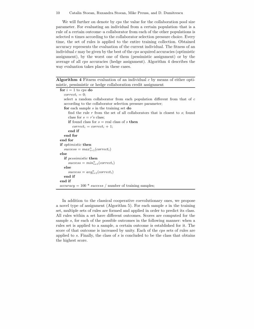
We will further on denote by cps the value for the collaboration pool sizeparameter. For evaluating an individual from a certain population–that is arule of a certain outcome–a collaborator from each of the other populations isselected n times according to the collaborator selection pressure choice. Everytime, the set of rules is applied to the entire training collection. Obtainedaccuracy represents the evaluation of the current individual. The fitness of anindividual c may be given by the best of the cps acquired accuracies (optimisticassignment), by the worst one of them (pessimistic assignment) or by theaverage of all cps accuracies (hedge assignment). Algorithm 4 describes theway evaluation takes place in these cases.

Algorithm 4 Fitness evaluation of an individual c by means of either opti-mistic, pessimistic or hedge collaboration credit assignment

for i = 1 to cps docorrecti = 0;select a random collaborator from each population different from that of caccording to the collaborator selection pressure parameter;for each sample s in the training set do

find the rule r from the set of all collaborators that is closest to s; foundclass for s = r’s class;if found class for s = real class of s then

correcti = correcti + 1;end if

end forend forif optimistic then

success = maxni=1(correcti)

elseif pessimistic then

success = minni=1(correcti)

elsesuccess = avgn

i=1(correcti)end if

end ifaccuracy = 100 * success / number of training samples;

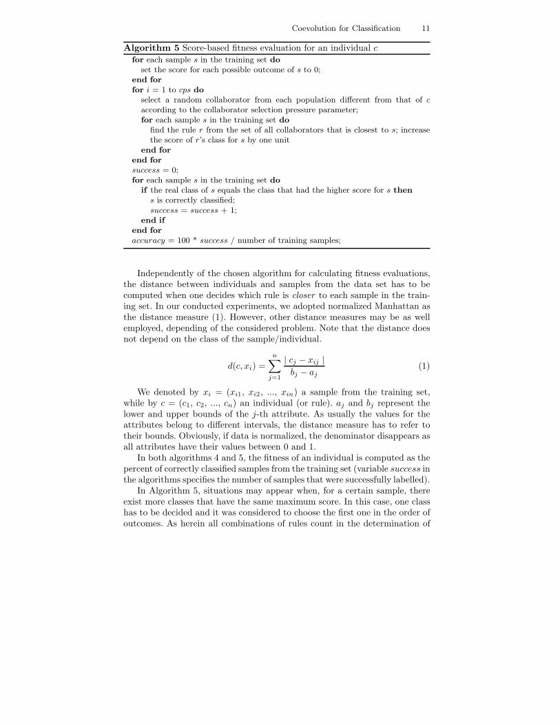
In addition to the classical cooperative coevolutionary ones, we proposea novel type of assignment (Algorithm 5). For each sample s in the trainingset, multiple sets of rules are formed and applied in order to predict its class.All rules within a set have different outcomes. Scores are computed for thesample s, for each of the possible outcomes in the following manner: when arules set is applied to a sample, a certain outcome is established for it. Thescore of that outcome is increased by unity. Each of the cps sets of rules areapplied to s. Finally, the class of s is concluded to be the class that obtainsthe highest score.

Coevolution for Classification 11

Algorithm 5 Score-based fitness evaluation for an individual c

for each sample s in the training set doset the score for each possible outcome of s to 0;

end forfor i = 1 to cps do

select a random collaborator from each population different from that of caccording to the collaborator selection pressure parameter;for each sample s in the training set do

find the rule r from the set of all collaborators that is closest to s; increasethe score of r’s class for s by one unit

end forend forsuccess = 0;for each sample s in the training set do

if the real class of s equals the class that had the higher score for s thens is correctly classified;success = success + 1;

end ifend foraccuracy = 100 * success / number of training samples;

Independently of the chosen algorithm for calculating fitness evaluations,the distance between individuals and samples from the data set has to becomputed when one decides which rule is closer to each sample in the train-ing set. In our conducted experiments, we adopted normalized Manhattan asthe distance measure (1). However, other distance measures may be as wellemployed, depending of the considered problem. Note that the distance doesnot depend on the class of the sample/individual.

d(c, xi) =n∑

j=1

| cj − xij |bj − aj

(1)

We denoted by xi = (xi1, xi2, ..., xin) a sample from the training set,while by c = (c1, c2, ..., cn) an individual (or rule). aj and bj represent thelower and upper bounds of the j-th attribute. As usually the values for theattributes belong to different intervals, the distance measure has to refer totheir bounds. Obviously, if data is normalized, the denominator disappears asall attributes have their values between 0 and 1.

In both algorithms 4 and 5, the fitness of an individual is computed as thepercent of correctly classified samples from the training set (variable success inthe algorithms specifies the number of samples that were successfully labelled).

In Algorithm 5, situations may appear when, for a certain sample, thereexist more classes that have the same maximum score. In this case, one classhas to be decided and it was considered to choose the first one in the order ofoutcomes. As herein all combinations of rules count in the determination of

12 Catalin Stoean, Ruxandra Stoean, Mike Preuss, and D. Dumitrescu

accuracies, we might state that the new choice of assignment is closer to theclassical hedge type.

Selection and Variation Operators

The selection operator presently discussed refers to the selection for reproduc-tion within each population, not to the collaborators selection. We employedfitness proportional selection, but any other selection scheme [3] may be suc-cessfully applied.

Intermediate recombination was used – having two randomly selected par-ents P and Q, the value of a gene i of the offspring O is obtained accordingto (2).

Oi = Pi + R · (Qi − Pi), (2)

where R is a uniformly distributed random number over [0, 1]. The obtainedoffspring individual replaces the worst of its two parents.

Mutation with normal perturbation was used for the experiments per-formed in current paper – a value of the gene i of an individual P is changedaccording to (3).

Pi = Pi + R · (bi − ai)/ms, (3)

where R is a random number with normal distribution, bi and ai are the upperand lower bounds of the i-th attribute in the data set and ms is the mutationstrength parameter. As the domains for the values of the attributes in thedata set have different sizes, we again have to refer to the size of the intervalfor each attribute when we perturb the values of the genes through mutation.In case the data set is normalized, the way the value of the gene i is modifiedchanges to (4).

Pi = Pi + R · ms (4)

We cannot imagine any obstacle for using any other recombination ormutation operators [3].

Stop Condition

In our experiments, we set a fixed number of generations for the evolutionaryprocess.

5.2 Cooperative Coevolution Parameters

In order to achieve the optimal configurations for the parameters of the co-operative approach, experiments were carried out as follows.

Concerning the collaborator selection pressure attribute, we used randomselection, on the one hand, and, on the other hand, we employed a fitnessproportional scheme.

Coevolution for Classification 13

All the three types of fitness assignment presented in Algorithm 4 togetherwith the one based on scores are tested.

As for the collaboration pool size, we varied the number of collaboratorsin order to find the optimum balance between accuracy and runtime.

5.3 Test Stage. Rules Application

After the stop condition is reached, we dispose of p populations of rules thatwere evolved against the training set. In order to form a complete set of rules,we have to choose an item from each population. There rules may be selectedrandomly, the best ones can be considered or a selection scheme can be used.In the last two cases, we take into account the final fitness evaluations of theindividuals. It is not always the case that, by selecting the fittest rule fromeach population, we obtain the best accuracy on the test set. Even if thesebest rules would give very good results on the training set, they may be infact not general enough to be applied to previously unseen data.

In the experiments we conducted, for a number of cps times, we randomlyselected one rule from each population in order to form cps complete sets ofrules. Each time, the rule set is applied to the test data in a similar mannerto the fitness calculation in Algorithm 5 and the classification accuracy isacquired.

6 Competitive Coevolution Approach to Classification

Similarly to the cooperative approach for classification, the aim of the com-petitive classifier is to construct, based on a training set, a set of rules thatmodel the data and which will be subsequently applied to the test set. Withinproposed competitive approach, the population of tests is represented by thesamples in the training data, while the other population, that of solutions,will contain only the rules that are to be evolved.

6.1 Training Stage. The Evolutionary Algorithm Behind

Keeping the same notations as in the cooperative approach, the task in thiscase will be once more to build p rules, one for each class. Consequently, inorder to form a solution to the classification problem, a complete set of ruleshas to be selected from the solutions population, which must therefore containrules for every outcome.

Representation

The same representation for the individuals (rules) as in the cooperative ap-proach is adopted. The only difference is that herein a better tracking of the

14 Catalin Stoean, Ruxandra Stoean, Mike Preuss, and D. Dumitrescu

class for each rule has to be kept. Since, in the cooperative case, the outcomeof each rule was identified with the population class, in present methodologyall rules, indifferent of the class they have, lie in the same population. As aresult, this time the rules will also encode the class, i.e. c = (c1, c2, ..., cn | k),k = 1, 2, ..., p.

Initialization

As previously stated, at least p rules have to be obtained. Recombination willtake place only between individuals with the same outcome, therefore, thesize of the solutions population has to be of at least 2p individuals, i.e. differ-entiating two individuals per class. However, we only state here the minimumsize of the rules population; a higher number of individuals would obviouslybring a better covering of the search space.

Fitness Evaluation

For each individual and for each sample from the tests population, we have toconstruct a history of the scores they obtained during encounters. The actualfitness evaluation of each individual/sample will be equal to the sum of allscores in their history.

The main question is: How are the scores given? When an encounter be-tween a rule and a sample takes place, the distance (we used the same nor-malized Manhattan distance as before) between them is computed. The taskfor the rules is to be as similar as possible to the samples in the training set,therefore the aim is to minimize the distance between them and the samplesfrom the training set with the same outcome. The score that is attached to arule is given by the negative value of the distance; the maximum score a ruleaims to attain is thus 0, meaning that the rule is identical to the sample itencountered.

Conversely, for a sample in the tests population, we attach the actual valueof the distance between it and the rule that it met. As rules get closer to acertain pattern of samples, they will subsequently encounter other samplesthat have larger fitness values (and as a consequence higher chances of beingselected for encounters) because they are very different from those rules. Thus,new fitter samples are continuously selected in order to adapt the rules sothat they will resemble them too, i.e. evolve the solutions according to a highvariety of tests.

Immediately after the initialization of the rules population, the fitnessevaluations for both the rules and the samples have to be computed. In thisrespect, for each rule, a sample with the same outcome as its label is randomlyselected and the encounter takes place: This has to be performed for a numberof times equal to the history length. Each individual will thus posses a historyand, as a result, an evaluation. In a similar manner, for a number of times equalto the history length, each sample from the training set will be considered and

Coevolution for Classification 15

random individuals with the same outcome are selected in order to form theencounters that will complete their histories.

After the initial fitness calculation, each time an encounter takes place,solutions and samples are chosen from each population by means of rankingselection. As encounters take place only between solutions and samples withthe same outcome, they will occur separately and in turn for each class (Algo-rithm 6). After the encounter, the new score is added to the history queue andthe oldest score is removed, such that the same history length is maintained.

An individual that is obtained after the variation operators is evaluated asfollows: for a number of times equal to the history length, a sample with thesame outcome as its own is selected using ranking selection and encounterstake place. Its fitness may now be computed by summing all the scores in thehistory. It is then included in the population by replacing the individual withthe worst fitness evaluation.

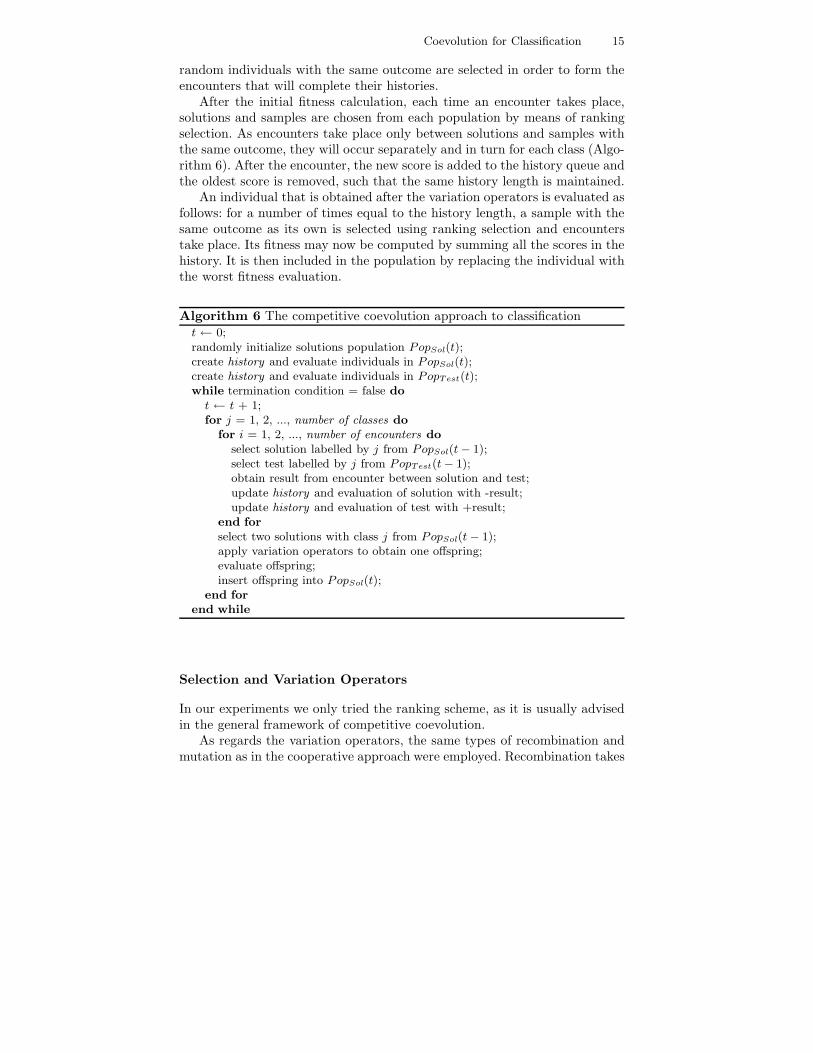
Algorithm 6 The competitive coevolution approach to classificationt ← 0;randomly initialize solutions population PopSol(t);create history and evaluate individuals in PopSol(t);create history and evaluate individuals in PopTest(t);while termination condition = false do

t ← t + 1;for j = 1, 2, ..., number of classes do

for i = 1, 2, ..., number of encounters doselect solution labelled by j from PopSol(t− 1);select test labelled by j from PopTest(t− 1);obtain result from encounter between solution and test;update history and evaluation of solution with -result;update history and evaluation of test with +result;

end forselect two solutions with class j from PopSol(t− 1);apply variation operators to obtain one offspring;evaluate offspring;insert offspring into PopSol(t);

end forend while

Selection and Variation Operators

In our experiments we only tried the ranking scheme, as it is usually advisedin the general framework of competitive coevolution.

As regards the variation operators, the same types of recombination andmutation as in the cooperative approach were employed. Recombination takes

16 Catalin Stoean, Ruxandra Stoean, Mike Preuss, and D. Dumitrescu

place only between individuals within the same class and, therefore, the off-spring inherits the outcome of the parents. The mutation operator does notapply to the class gene.

Again, any other variation operators may be successfully tried.Remark: Variation and replacement take place for every class in turn

(Algorithm 6).

Stop Condition

Competitive techniques usually require more iterations than a canonical EA,as in each generation there is only one new descendant that enters the pop-ulation. However, in our approach for classification, we apply the variationoperators for individuals of every class in the same generation, a change thatmakes several individuals (descendants), i.e. p instances (one for each class),enter the population within that iteration.

The stop condition we used refers to a fixed number of generations, justlike in the cooperative approach.

6.2 Competitive Coevolution Parameters

There are two important parameters related to the competitive coevolutiontechnique: The history length and the number of encounters that take placewithin one generation. The larger the values for both of them, the more accu-rate the fitness evaluation is for an individual/sample. Unfortunately, togetherwith the raise in the values for either of the two, the runtime of the algorithmalso increases.

The value for the number of encounters parameter directly depends on thepopulation size of the two species: If there are many individuals in any of thepopulations, then a high value for the number of encounters have to be set inorder to update the fitness evaluations of a great amount of the individuals.

A value that is too small for the history length parameter could make thefitness evaluation of an individual/sample change too drastically after eachencounter and thus the fitness evaluation would not objectively reflect thequality of the individual/sample in contrast to the other population.

6.3 Test Stage. Rules Application

After the evolutionary process stops, one rule for every class is selected andthese are applied to the test set. For each sample in the test set, the dissim-ilarity to each of the rules is computed. The found outcome of the sample istaken from the rule it resembles the most.

Coevolution for Classification 17

7 Experiments

For each of the two coevolutionary approaches for classification, we considerthe same data sets for experiments: Two data sets concerning benchmark clas-sification problems coming from the University of California at Irvine (UCI)Repository of Machine Learning Databases4, i.e. Wisconsin breast cancer di-agnosis and iris recognition, are selected for reasons of validation and com-parison. Besides, the former is a two-class instance, while the latter representsa multi-class task, which should reveal whether the classification algorithmsremain flexible and feasible with some increase in the number of outcomes.

Finally, a real-world data set, courtesy of the University Hospital inCraiova, Romania, is also considered with the purpose of testing and ap-plication on an unpredictable environment that is usually associated with rawdata. For all grounds mentioned above, the selection of test problems certainlycontains a variety of situations that is necessary for the objective validationof the new framework of coevolution in application to classification.

In all conducted experiments, for each parameter setting, the training setis formed of randomly picked samples and the test set contains the rest ofthe samples. In order to prove the stability of the approaches, each reportedaverage result is obtained after 30 runs of the algorithm.

The experiments section is organized as follows: A small description of eachdata set is first outlined; it is then continued with the results obtained for boththe cooperative coevolution technique and the competitive counterpart. Thesection closes by undertaking a comparison to accuracies obtained by standarddata mining techniques.

7.1 Data sets description

The significant information on the each of the considered classification tasksis given in the following lines.

Breast Cancer Diagnosis

The data set contains 699 observations on nine discrete cytological factorsand reflects a chronological grouping of the data. The objective is to identifywhether a sample corresponds either to a benign or a malignant tumour.Class distribution is 65.5% for benign and 34.5% for malignant. There are 16missing values for attribute 6; we replaced them by the average value for thatattribute.

Iris Plants Classification

There are 150 samples with three possible classes pertaining to this data set.Each sample consists of four attributes which denote the length and width for4 Available at http://www.ics.uci.edu/∼mlearn/MLRepository.html

18 Catalin Stoean, Ruxandra Stoean, Mike Preuss, and D. Dumitrescu

petals and sepals of the iris flowers. Samples are equally distributed amongclasses.

Hepatic Cancer Early Diagnosis

Hepatocellular carcinoma (HCC/hepatoma) is the primary malignancy (can-cer) of the liver that ranks fifth in frequency among all malignancies in theworld. In patients with a higher suspicion of HCC, the best method of diag-nosis involves a scan of the abdomen, but only at a high cost. A cheap andeffective alternative consists in detecting small or subtle increases for serumenzymes levels. Consequently, based on a set of fourteen significant serumenzymes, a group of 299 individuals and two possible outcomes (HCC andnon-HCC), we aim to provide an efficient computational means of checkingthe consistency of decision making in the early detection of HCC at signifi-cantly low expense.

7.2 Experiment 1: Cooperative Classification Validation

Pre-experimental planning: In preliminary experiments, we tested differ-ent settings for the coevolutionary parameters in order to verify their suit-ability for the classification problems. However, in these initial experiments,we tested the technique only on the breast cancer and iris data sets.

We observed that there are not major differences between results obtainedwhen different types of collaboration credit assignments are used: Slightlybetter results appeared to be achieved for the score-based fitness.

As it was expected, when the collaboration pool size value is increased, theruntime of the algorithm also raises. As concerning the results, they also seemto be improved to some extent by the increase of the value for this parameter.The technique had been tested from one up to seven collaborators.

As regards the collaborator selection pressure parameter, we initially em-ployed random selection which drove the coevolutionary process to very com-petitive results. We then chose the best individual from each population forcollaborations, but, surprisingly, the obtained results were worse than in thecase of a random selection pressure. The next step we took was that of usinga selection scheme for choosing the collaborators. Proportional selection wasemployed and it proved to be efficient as results were slightly better thanthose obtained through random selection.Task: We want to evaluate whether the cooperative approach produces vi-able results if compared to those obtained by other approaches (informationon these is given in subsection 7.4) and how appropriate parameters will bechosen.Setup: The values for all the parameters were manually tuned. Table 1 con-tains the values for both the parameters of the EA and the coevolutionaryones. The population size refers to the number of individuals from each of

Coevolution for Classification 19

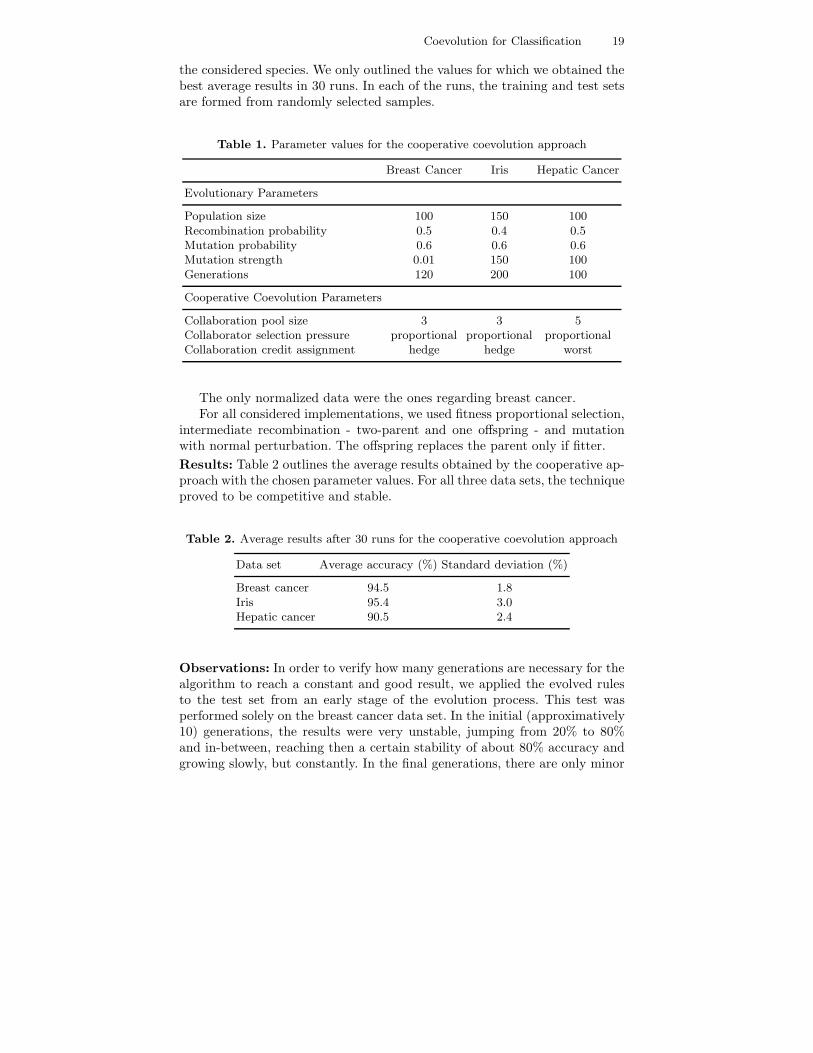
the considered species. We only outlined the values for which we obtained thebest average results in 30 runs. In each of the runs, the training and test setsare formed from randomly selected samples.

Table 1. Parameter values for the cooperative coevolution approach

Breast Cancer Iris Hepatic Cancer

Evolutionary Parameters

Population size 100 150 100Recombination probability 0.5 0.4 0.5Mutation probability 0.6 0.6 0.6Mutation strength 0.01 150 100Generations 120 200 100

Cooperative Coevolution Parameters

Collaboration pool size 3 3 5Collaborator selection pressure proportional proportional proportionalCollaboration credit assignment hedge hedge worst

The only normalized data were the ones regarding breast cancer.For all considered implementations, we used fitness proportional selection,

intermediate recombination - two-parent and one offspring - and mutationwith normal perturbation. The offspring replaces the parent only if fitter.Results: Table 2 outlines the average results obtained by the cooperative ap-proach with the chosen parameter values. For all three data sets, the techniqueproved to be competitive and stable.

Table 2. Average results after 30 runs for the cooperative coevolution approach

Data set Average accuracy (%) Standard deviation (%)

Breast cancer 94.5 1.8Iris 95.4 3.0Hepatic cancer 90.5 2.4

Observations: In order to verify how many generations are necessary for thealgorithm to reach a constant and good result, we applied the evolved rulesto the test set from an early stage of the evolution process. This test wasperformed solely on the breast cancer data set. In the initial (approximatively10) generations, the results were very unstable, jumping from 20% to 80%and in-between, reaching then a certain stability of about 80% accuracy andgrowing slowly, but constantly. In the final generations, there are only minor

20 Catalin Stoean, Ruxandra Stoean, Mike Preuss, and D. Dumitrescu

modifications of the test accuracy of up to one percent. However, the resultsgreatly depend of the way the training/test sets were generated as there existcases when the accuracy starts with 80% even from the early stages of theevolutionary process.

It has to be noted that there is not a very strong dependence betweenthe EA parameters and obtained results as very competitive accuracies areobtained for a large scale of their values.

Concerning the coevolution parameters, changes within the collaborationcredit assignments do not bring vital modifications to the final average results:The differences between various settings as regards the final accuracies do notovercome one percent.

As previously stated, the collaboration pool size parameter directly influ-ences the runtime of the program that implements the approach; the finaltest accuracy is also affected by the increase in this value, but a balance hasto be established between runtime and accuracy. For the two test problemswe considered in the pre-experimental stage, better results were obtained foran odd number of collaborators. Another important observation is that whena certain threshold for the collaboration pool size parameter is surpassed nofurther gain in accuracy is reached. We generally achieved the best resultswhen three collaborators were considered.

The cooperative parameter that brought the most important change inthe final result of the algorithm was the collaborator selection pressure. Aselection scheme is preferred to a random selection; selecting only the bestcollaborator seems to be the worst of the three choices.Discussion: The proposed classification approach based on cooperative co-evolution provides very accurate results in a relatively small amount of time.For instance, on the breast cancer data set, the runtime lasts from 7 secondsper run when the collaboration pool size is one, up to 24 for three collabora-tors and to around 37 seconds when five collaborators are used. Note that forexperiments, we used a computer with the following characteristics: PentiumIV CPU 3.0 GHz and 1 GB of RAM.

7.3 Experiment 2: Competitive Classification Validation

Pre-experimental planning: The same two benchmark data sets from theUCI repository were used for preliminary experiments. The first observationin these tests refers to the high amount of time necessary for the algorithmto run: The explanation lies in the fact that the tests population is very largeand, at the beginning of the evolutionary process, all samples are evaluated.This means that for each sample, for a number of times equal to the historylength, an individual is selected and an encounter takes place between thetwo, assigning a score to the sample.

We also noticed at this stage the importance of the two competitive co-evolution parameters: history length and the number of encounters. They also

Coevolution for Classification 21

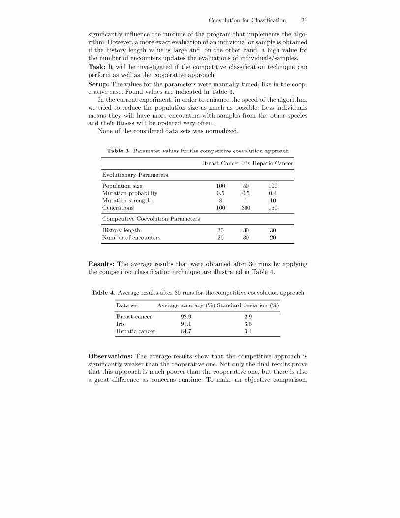
significantly influence the runtime of the program that implements the algo-rithm. However, a more exact evaluation of an individual or sample is obtainedif the history length value is large and, on the other hand, a high value forthe number of encounters updates the evaluations of individuals/samples.Task: It will be investigated if the competitive classification technique canperform as well as the cooperative approach.Setup: The values for the parameters were manually tuned, like in the coop-erative case. Found values are indicated in Table 3.

In the current experiment, in order to enhance the speed of the algorithm,we tried to reduce the population size as much as possible: Less individualsmeans they will have more encounters with samples from the other speciesand their fitness will be updated very often.

None of the considered data sets was normalized.

Table 3. Parameter values for the competitive coevolution approach

Breast Cancer Iris Hepatic Cancer

Evolutionary Parameters

Population size 100 50 100Mutation probability 0.5 0.5 0.4Mutation strength 8 1 10Generations 100 300 150

Competitive Coevolution Parameters

History length 30 30 30Number of encounters 20 30 20

Results: The average results that were obtained after 30 runs by applyingthe competitive classification technique are illustrated in Table 4.

Table 4. Average results after 30 runs for the competitive coevolution approach

Data set Average accuracy (%) Standard deviation (%)

Breast cancer 92.9 2.9Iris 91.1 3.5Hepatic cancer 84.7 3.4

Observations: The average results show that the competitive approach issignificantly weaker than the cooperative one. Not only the final results provethat this approach is much poorer than the cooperative one, but there is alsoa great difference as concerns runtime: To make an objective comparison,

22 Catalin Stoean, Ruxandra Stoean, Mike Preuss, and D. Dumitrescu

we measured the average runtime for the same breast cancer data set, byusing the competitive approach with the parameters indicated in Table 3; theobtained value was of around 480 seconds, that is almost 13 times slower thanthe cooperative approach with 5 collaborators.

The standard deviation of the results is also significantly higher, whichindicates the fact that this technique is not as stable as the cooperative ap-proach. Nevertheless, it has to be stated that in an objective judgement, thereare not too many perturbations that appear in 100, or even 300 generations,since only two individuals per class recombine during one generation and mu-tation is applied solely to the obtained offspring. To conclude, at least 1000generations would probably be necessary for the variation operators to con-siderably change the population. That would, on the other hand, slow downthe program even more.Discussion: The obtained results and the large runtime of the competitivetechnique indicate the cooperative approach as much more viable as com-pared to the state-of-the-art techniques for classification. Note however thatthis is only the first time the competitive approach for classification is pro-posed and we believe that it represents a good starting point, as there isdefinitely potential within this technique as well. To outline some ideas for fu-ture research concerning the competitive technique for classification, perhapsa preprocessing technique step could be first applied to the training data inorder to substantially reduce them. In conjunction with that (or by itself),we presume that employing a chunking technique in order to pick only smallparts from the training set and use them as the static species could signifi-cantly improve runtime (maybe even the accuracy). Then, after the rules arespecialized on the selected samples, the tests species could bring new ones,while the dynamic population of rules could resume the evolution.

An important enhancement could be brought if the very good rules thatare evolved at a certain point could be blocked for further modifications:Make one such individual a tabu rule and maybe move it in a rules archivethat will be applied when the termination condition is reached. In the waythe technique is now built, these good rules have the highest chances to beselected over and over again, therefore modified many times, maybe for theworse.

In the end of the evolutionary run, the best rule of each class in the finalpopulation was taken and the entire formed set was applied to the test data.Obviously, a different way of choosing the rules could be imagined, e.g. takeseveral rules for one class or apply an archive variant as suggested above.

7.4 Comparison to Standard Data Mining Approaches

Comparison of obtained results can be made only for the breast cancer andiris data sets, since they are public benchmark problems. The resulting rulesof the hepatic data set were however confronted with the specialized opinionof the physician and were found to be consistent with the medical diagnosis.

Coevolution for Classification 23

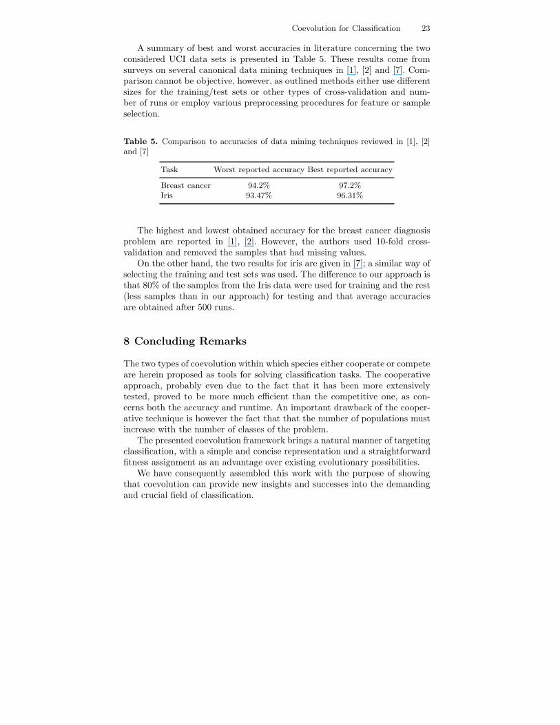
A summary of best and worst accuracies in literature concerning the twoconsidered UCI data sets is presented in Table 5. These results come fromsurveys on several canonical data mining techniques in [1], [2] and [7]. Com-parison cannot be objective, however, as outlined methods either use differentsizes for the training/test sets or other types of cross-validation and num-ber of runs or employ various preprocessing procedures for feature or sampleselection.

Table 5. Comparison to accuracies of data mining techniques reviewed in [1], [2]and [7]

Task Worst reported accuracy Best reported accuracy

Breast cancer 94.2% 97.2%Iris 93.47% 96.31%

The highest and lowest obtained accuracy for the breast cancer diagnosisproblem are reported in [1], [2]. However, the authors used 10-fold cross-validation and removed the samples that had missing values.

On the other hand, the two results for iris are given in [7]; a similar way ofselecting the training and test sets was used. The difference to our approach isthat 80% of the samples from the Iris data were used for training and the rest(less samples than in our approach) for testing and that average accuraciesare obtained after 500 runs.

8 Concluding Remarks

The two types of coevolution within which species either cooperate or competeare herein proposed as tools for solving classification tasks. The cooperativeapproach, probably even due to the fact that it has been more extensivelytested, proved to be more much efficient than the competitive one, as con-cerns both the accuracy and runtime. An important drawback of the cooper-ative technique is however the fact that that the number of populations mustincrease with the number of classes of the problem.

The presented coevolution framework brings a natural manner of targetingclassification, with a simple and concise representation and a straightforwardfitness assignment as an advantage over existing evolutionary possibilities.

We have consequently assembled this work with the purpose of showingthat coevolution can provide new insights and successes into the demandingand crucial field of classification.

24 Catalin Stoean, Ruxandra Stoean, Mike Preuss, and D. Dumitrescu

References

1. Bennett K. P., Blue J. (1997) A Support Vector Machine Approach to DecisionTrees, R.P.I Math Report No. 97–100 Rensselaer Polytechnic Institute Troy,New York

2. Duch W., Adamczak R., Grabczewski K., Zal G. (1999) Hybrid neural-globalminimization method of logical rule extraction, Journal of Advanced Compu-tational Intelligence, Volume 3, Number 5: 348–356

3. Eiben A. E., Smith J. E. (2003) Introduction to Evolutionary Computing.Springer–Verlag, Berlin Heidelberg New York

4. Freitas A. A. (2002) A Survey of Evolutionary Algorithms for Data Mining andKnowledge Discovery, Advances in Evolutionary Computation, 819–845

5. Freitas A. A. (2002) Data Mining and Knowledge Discovery with EvolutionaryAlgorithms. Springer–Verlag, Berlin Heidelberg

6. Giordana A., Saitta L., Zini F. (2000) Learning Disjunctive Concepts by Meansof Genetic Algorithms, Proceedings of the 11th International Conference onMachine Learning: 96–104

7. Iacus S., Porro G. (2006) Missing Data Imputation, Classification, Predictionand Average Treatment Effect Estimation via Random Recursive Partitioning,UNIMI - Research Papers in Economics, Business, and Statistics

8. Juille H., Pollack J. B. (1996) Dynamics of Co-evolutionary Learning, Proceed-ings of the 4th International Conference on Simulation of Adaptive Behavior:526–534

9. Juille H., Pollack J. B. (1998) Coevolutionary Learning: a Case Study, Proceed-ings of the 15th International Conference on Machine Learning: 251–259

10. Holland J.H., (1986) Escaping Brittleness: The possibilities of General Pur-pose Learning Algorithms Applied to Parallel Rule-Based Systems, MachineLearning 2:593–623

11. Michalewicz Z. (1996) Genetic Algorithms + Data Structures = Evolution Pro-grams. Springer–Verlag, New York

12. Paredis J. (1994) Steps towards Co-evolutionary Classification Neural Net-works, Artificial Life IV: 102-108

13. Paredis J. (1994) Coevolutionary Constraint Satisfaction, Proceedings of the3rd Conference on Parallel Problem Solving from Nature, LNCS, 866: 46-55

14. Paredis J., Westra R. (1997) Coevolutionary Computation for Path Planning,Proceedings EUFIT 1997, 1: 394–398

15. Paredis J. (1997) Coevolving Cellular Automata: Be Aware of the Red Queen!Proceedings of the 7th International Conference on Genetic Algorithms: 393–399

16. Paredis J. (1999) Constraint Satisfaction with Coevolution, In: New Ideas inOptimization, Corne D., Dorigo M., Glover F. (Eds.), McGraw-Hill, London:359–366

17. Paredis J. (2002) Coevolutionary Algorithms,www.evalife.dk/ToEC2002/publications/paredis coevo survey HEC.ps

18. Potter M. A., De Jong K. A. (1994) A Cooperative Coevolutionary Approach toFunction Optimization, Proceedings of the 3rd Conference on Parallel ProblemSolving from Nature: 249–257

19. Potter M. A., De Jong K. A., (2000) Cooperative Coevolution: An Architecturefor Evolving Coadapted Subcomponents, Evolutionary Computation, 8(1): 1-29

Coevolution for Classification 25

20. Potter M. A., Meeden L. A., Schultz A. C. (2001) Heterogeneity in the Coe-volved Behaviors of Mobile Robots: The Emergence of Specialists, Proceedingsof the 17th International Conference on Artificial Intelligence: 1337-1343

21. Siegel E. V. (1994) Competitively Evolving Decision Trees Against Fixed Train-ing Cases for Natural Language Processing, Advances in Genetic Programming,409–423

22. Stoean C., Dumitrescu D., Preuss M., Stoean R. (2006) Cooperative Coevolu-tion for Classification, Bio-Inspired Computing: Theory and Applications 2006:289–298

23. Stoean C., Preuss M., Dumitrescu D., Stoean R. (2006) Cooperative Evolu-tion of Rules for Classification, IEEE Post-proceedings Symbolic and NumericAlgorithms for Scientific Computing 2006: 317-322

24. Stoean C., Stoean R., El-Darzi E. (2007) Breast Cancer Diagnosis by Meansof Cooperative Coevolution, 3rd ACM International Conference on IntelligentComputing and Information Systems: 493–497

25. Wiegand R. P. (2003) Analysis of Cooperative Coevolutionary Algorithms, PhDThesis, George Mason University, Virginia