Coefficient Path Algorithms Karl Sjöstrand Informatics and Mathematical Modelling, DTU

Coefficient Path Algorithms Karl Sjöstrand Informatics and Mathematical Modelling, DTU.
Dec 19, 2015
Welcome message from author
This document is posted to help you gain knowledge. Please leave a comment to let me know what you think about it! Share it to your friends and learn new things together.
Transcript
Coefficient Path Algorithms
Karl SjöstrandInformatics and Mathematical Modelling, DTU
What’s This Lecture About?
• The focus is on computation rather than methods.– Efficiency– Algorithms provide insight

Loss Functions
• We wish to model a random variable Y by a function of a set of other random variables f(X)
• To determine how far from Y our model is we define a loss function L(Y, f(X)).

Loss Function Example
• Let Y be a vector y of n outcome observations• Let X be an (n×p) matrix X where the p
columns are predictor variables• Use squared error loss L(y,f(X))=||y -f(X)||2
• Let f(X) be a linear model with coefficients β, f(X) = Xβ.
• The loss function is then • The minimizer is the familiar OLS solution
yXXX TTXfYL 1)())(,(minargˆ
)()(2
2βββ T XyXyXy
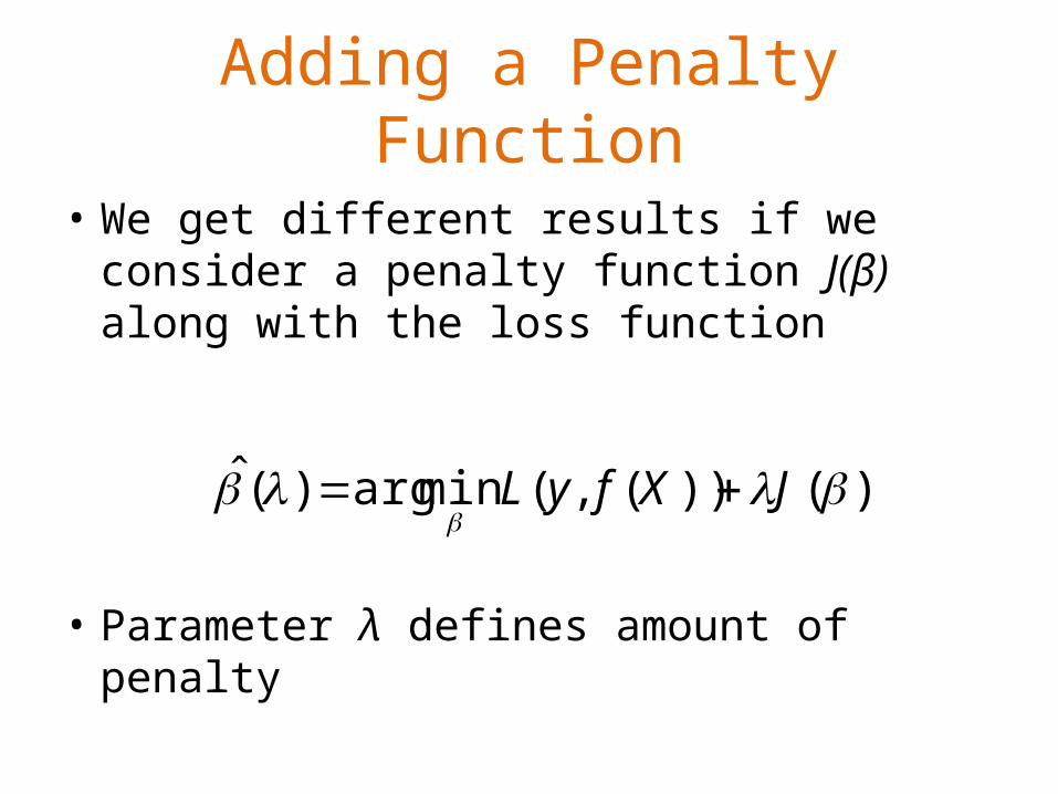
Adding a Penalty Function
• We get different results if we consider a penalty function J(β) along with the loss function
• Parameter λ defines amount of penalty
)())(,(minarg)(ˆ
JXfyL

Virtues of the Penalty Function
• Imposes structure on the model– Computational difficulties• Unstable estimates• Non-invertible matrices
– To reflect prior knowledge– To perform variable selection• S p a r s e solutions are easier to interpret
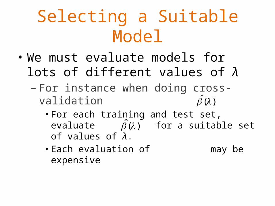
Selecting a Suitable Model
• We must evaluate models for lots of different values of λ– For instance when doing cross-validation• For each training and test set, evaluate for a
suitable set of values of λ.• Each evaluation of may be expensive
)(ˆ
)(ˆ
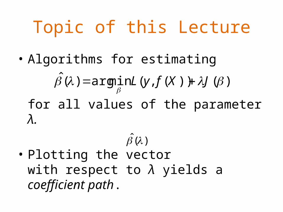
Topic of this Lecture
• Algorithms for estimating
for all values of the parameter λ.
• Plotting the vector with respect to λ yields a coefficient path.
)())(,(minarg)(ˆ
JXfyL
)(ˆ
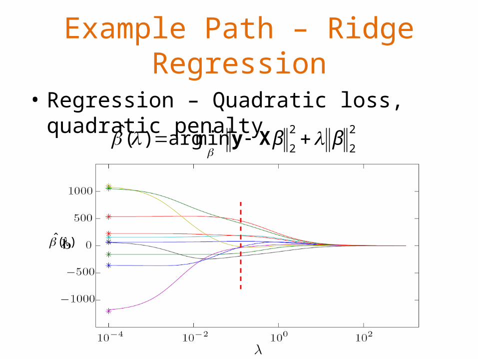
Example Path – Ridge Regression
• Regression – Quadratic loss, quadratic penalty2
2
2
2minarg)(ˆ ββ
Xy
)(ˆ

Example Path - LASSO
• Regression – Quadratic loss, piecewise linear penalty
1
2
2minarg)(ˆ ββ
Xy
)(ˆ

Example Path – Support Vector Machine
• Classification – details on loss and penalty later
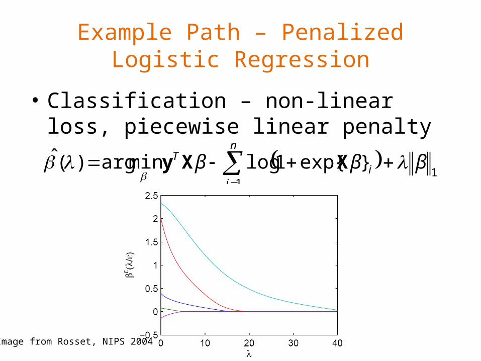
Example Path – Penalized Logistic Regression
• Classification – non-linear loss, piecewise linear penalty
1
1
}exp{1logminarg)(ˆ βββn
ii
T
XXy
Image from Rosset, NIPS 2004
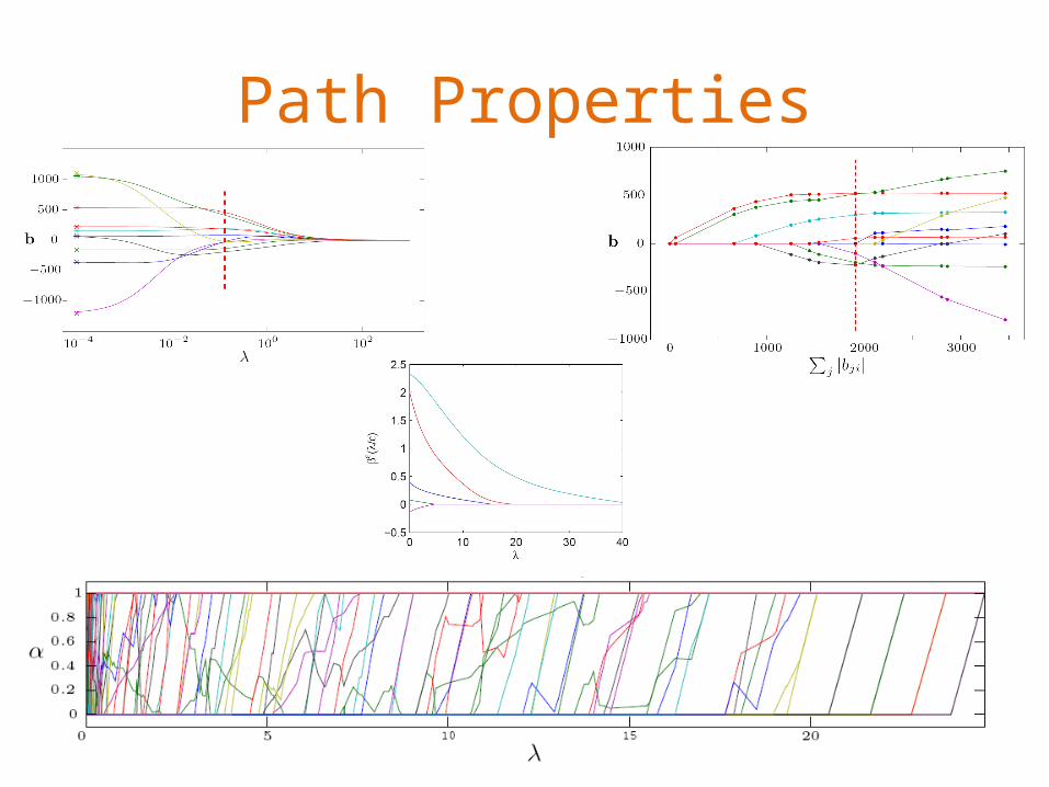
Path Properties

Piecewise Linear Paths
• What is required from the loss and penalty functions for piecewise linearity?
• One condition is that is a piecewise constant vector in λ.
)(ˆ

Condition for Piecewise Linearity
0 200 400 600 800 1000 1200 1400 1600 1800-300
-200
-100
0
100
200
300
400
500
600
||()||1
( )
0 200 400 600 800 1000 1200 1400 1600 1800
-0.4
-0.3
-0.2
-0.1
0
0.1
0.2
0.3
0.4
||()||1
d()/d

Tracing the Entire Path
• From a starting point along the path (e.g. λ=∞), we can easily create the entire path if:– is known– the knots where change can be worked out
)(ˆ
)(ˆ
)(ˆ

The Piecewise Linear Condition
)(ˆ)(ˆ)(ˆ)(ˆ 122
JJL

Sufficient and Necessary Condition
• A sufficient and necessary condition for linearity of at λ0:– expression above is a constant vector with respect
to λ in a neighborhood of λ0.
)(ˆ)(ˆ)(ˆ)(ˆ 122
JJL
)(ˆ
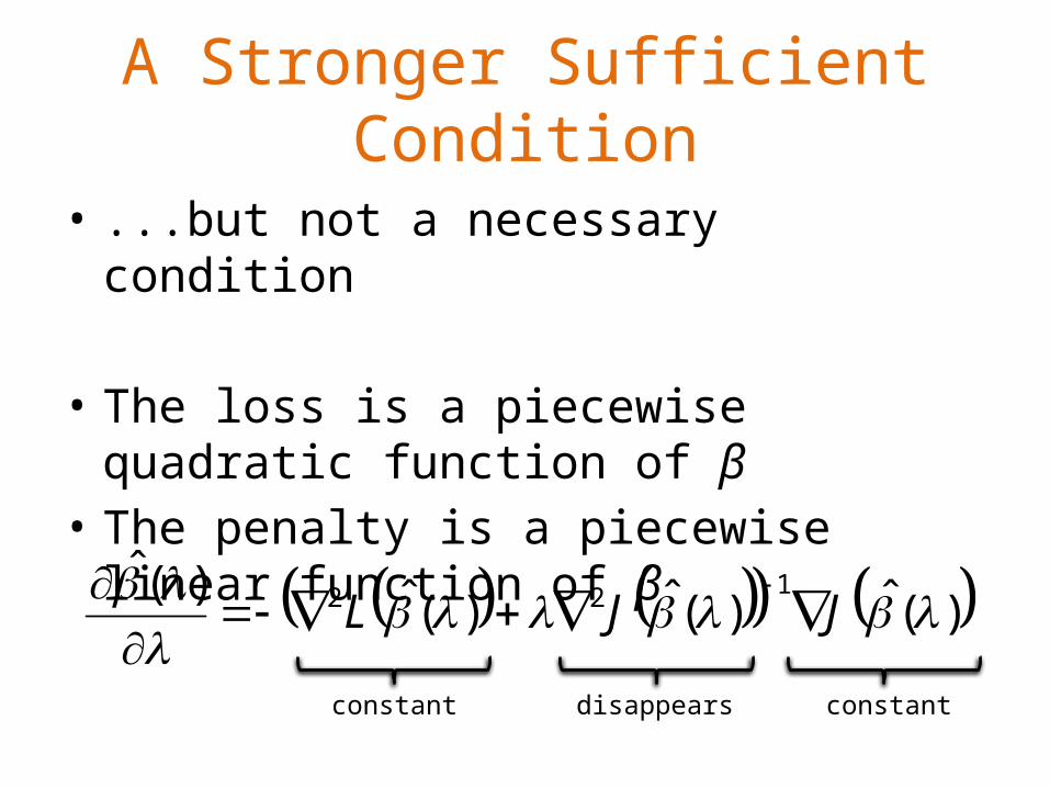
A Stronger Sufficient Condition
• ...but not a necessary condition
• The loss is a piecewise quadratic function of β• The penalty is a piecewise linear function of β
)(ˆ)(ˆ)(ˆ)(ˆ 122
JJL
constant disappears constant

Implications of this Condition
• Loss functions may be– Quadratic (standard squared error loss)– Piecewise quadratic– Piecewise linear (a variant of piecewise quadratic)
• Penalty functions may be– Linear (SVM ”penalty”)– Piecewise linear (L1 and Linf)

Condition Applied - Examples
• Ridge regression– Quadratic loss – ok– Quadratic penalty – not ok
• LASSO– Quadratic loss – ok– Piecewise linear penalty - ok

When do Directions Change?
• Directions are only valid where L and J are differentiable.– LASSO: L is differentiable everywhere, J is not at
β=0.
• Directions change when β touches 0. – Variables either become 0, or leave 0– Denote the set of non-zero variables A – Denote the set of zero variables I

An algorithm for the LASSO
• Quadratic loss, piecewise linear penalty
• We now know it has a piecewise linear path!
• Let’s see if we can work out the directions and knots
1
2
2minarg)(ˆ ββ
Xy
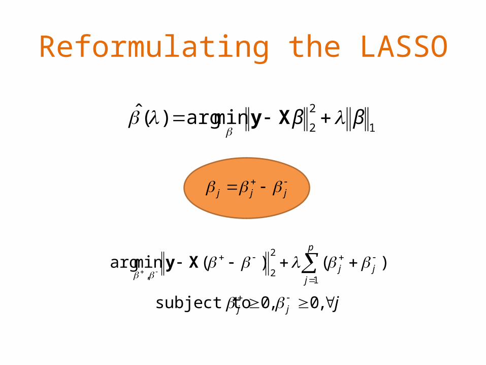
Reformulating the LASSO
jjj
p
jjj
,0,0 subject to
)()(minarg1
2
2,
Xy
jjj
1
2
2minarg)(ˆ ββ
Xy
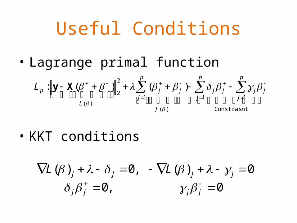
Useful Conditions
sConstraint
11
)(
1)(
2
2)()(:
p
jjj
p
jjj
J
p
jjj
L
pL
Xy
• Lagrange primal function
• KKT conditions
0,0
0)(,0)(
jjjj
jjjj LL
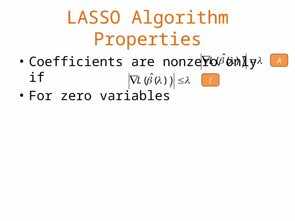
LASSO Algorithm Properties
• Coefficients are nonzero only if• For zero variables
jL ))(ˆ(
jL ))(ˆ( I
A
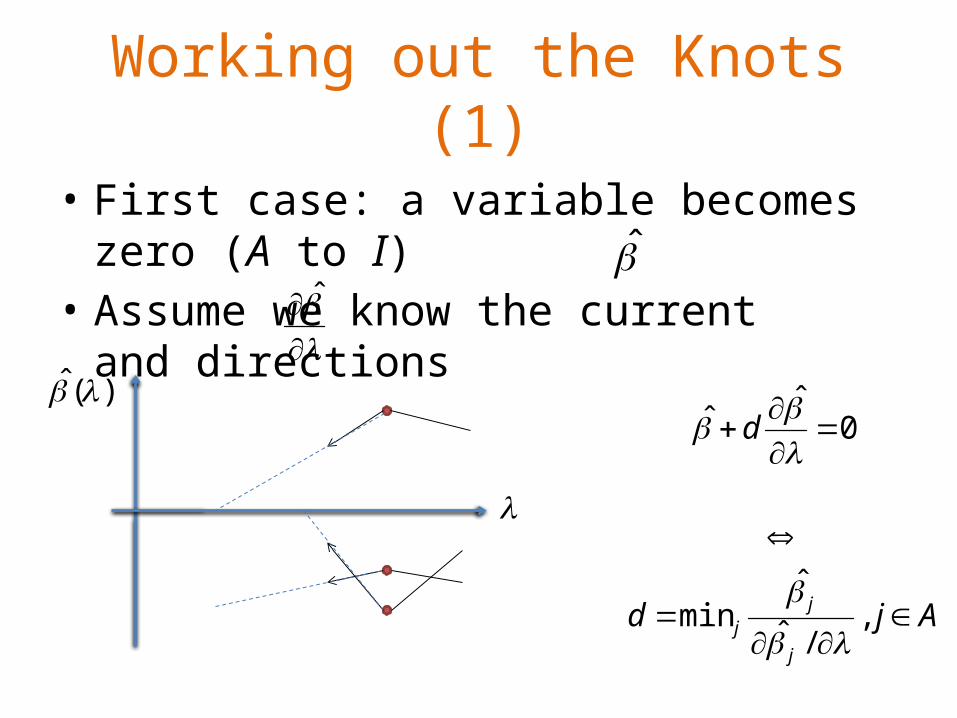
Working out the Knots (1)
• First case: a variable becomes zero (A to I)• Assume we know the current and
directions
ˆ
)(ˆ 0
ˆˆ
d
Ajdj
jj
,/ˆ
ˆmin
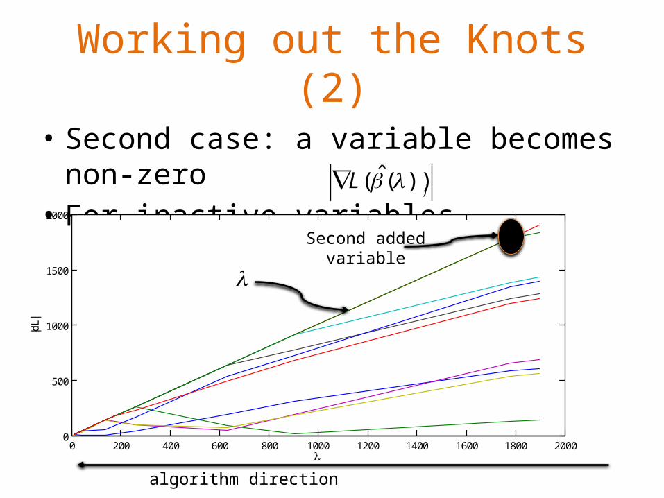
Working out the Knots (2)
• Second case: a variable becomes non-zero• For inactive variables change with λ.jL ))(ˆ(
0 200 400 600 800 1000 1200 1400 1600 1800 20000
500
1000
1500
2000
|dL|
algorithm direction
Second addedvariable

Working out the Knots (3)
• For some scalar d, will reach λ.– This is where variable j becomes active!– Solve for d :
jdL )ˆ(
Ijdd
d
dLdL
j
Tji
Tji
Tji
Tji
j
AiIj
,min
)(
)()(,
)(
)()(min
)ˆ()ˆ(
Xxx
Xyxx
Xxx
Xyxx

Path Directions
• Directions for non-zero variables
))(ˆsgn()2()(ˆ)(ˆ)(ˆ112
AAT
AAA JL
XX
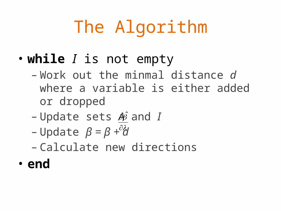
The Algorithm
• while I is not empty– Work out the minmal distance d where a variable
is either added or dropped– Update sets A and I– Update β = β + d– Calculate new directions
• end
ˆ
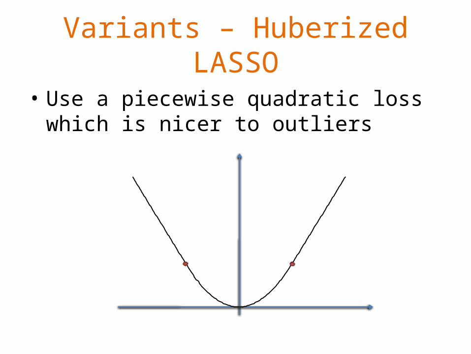
Variants – Huberized LASSO
• Use a piecewise quadratic loss which is nicer to outliers

Huberized LASSO
• Same path algorithm applies– With a minor change due to the piecewise loss
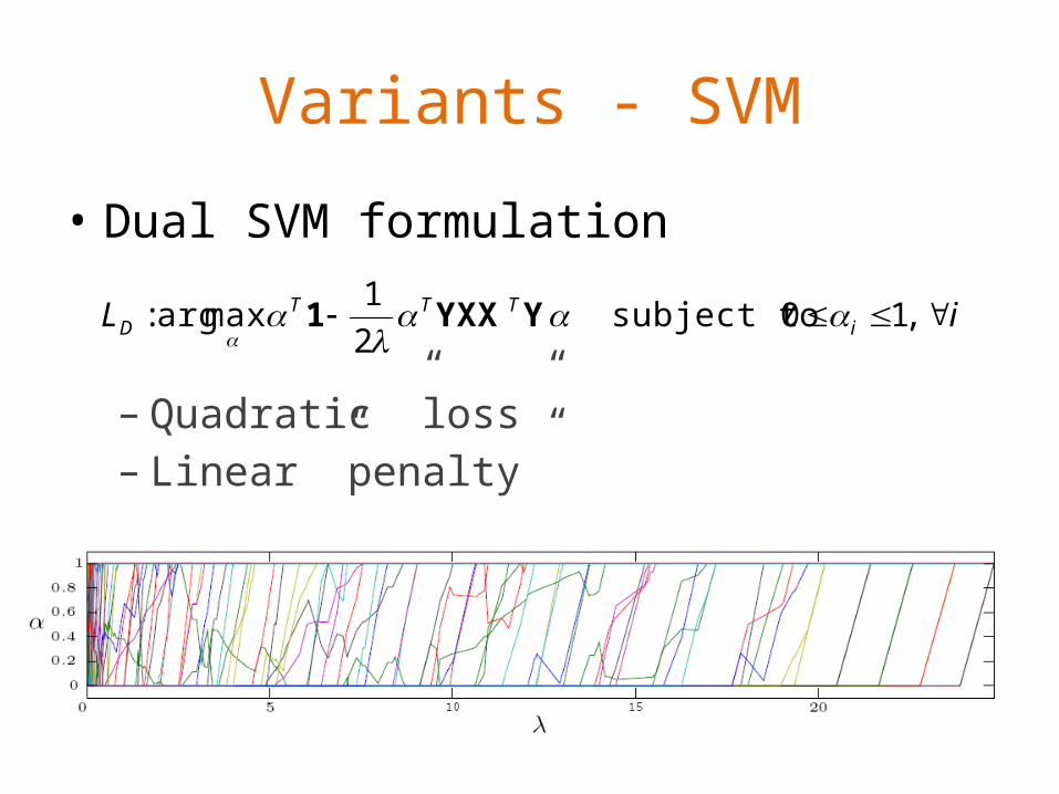
Variants - SVM
• Dual SVM formulation
– Quadratic ”loss”– Linear ”penalty”
iL iTTT
D ,10 subject to 2
1maxarg:
YYXX1

A few Methods with Piecewise Linear Paths
• Least Angle Regression• LASSO (+variants)• Forward Stagewise Regression• Elastic Net• The Non-Negative Garotte• Support Vector Machines (L1 and L2)• Support Vector Domain Description• Locally Adaptive Regression Splines
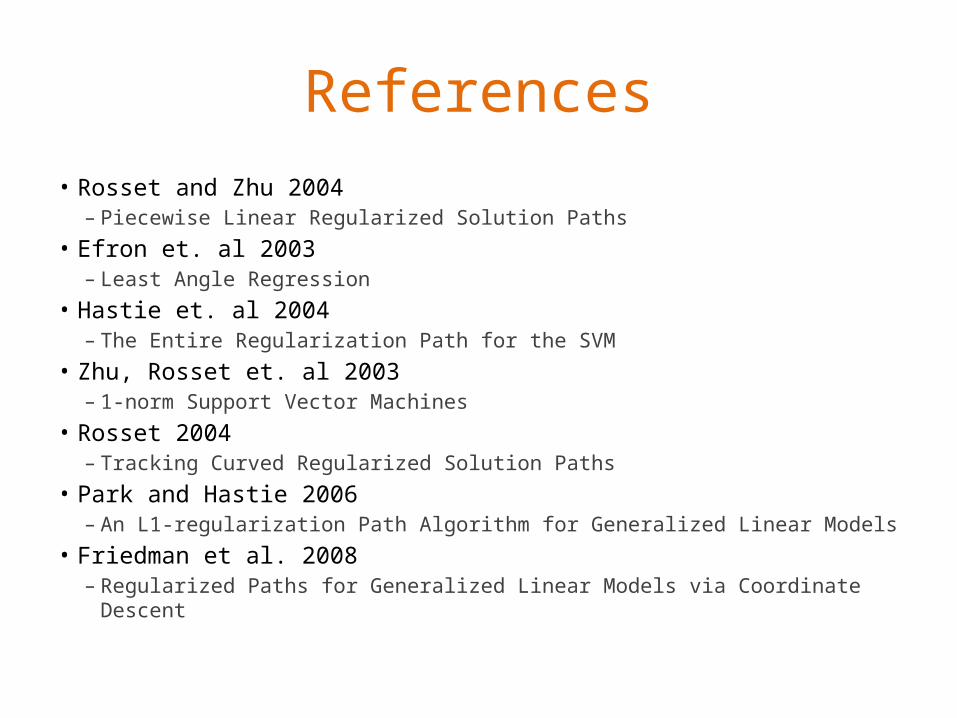
References• Rosset and Zhu 2004
– Piecewise Linear Regularized Solution Paths• Efron et. al 2003
– Least Angle Regression• Hastie et. al 2004
– The Entire Regularization Path for the SVM• Zhu, Rosset et. al 2003
– 1-norm Support Vector Machines• Rosset 2004
– Tracking Curved Regularized Solution Paths• Park and Hastie 2006
– An L1-regularization Path Algorithm for Generalized Linear Models• Friedman et al. 2008
– Regularized Paths for Generalized Linear Models via Coordinate Descent
Conclusion
• We have defined conditions which help identifying problems with piecewise linear paths– ...and shown that efficient algorithms exist
• Having access to solutions for all values of the regularization parameter is important when selecting a suitable model
Related Documents