Coding and Multiple-Access over Fading Channels by Raymond Knopp B. Eng. Honours Electrical Engineering McGill University, Montreal, Canada 1992 M. Eng. Electrical Engineering McGill University, Montreal, Canada 1994 Citizen of Canada Submitted to the Section Syst` emes de Communication/Institut Eur´ ecom Ecole Polytechnique F´ ed´ erale de Lausanne in partial fulfillment of the requirements for the degree of docteur ` es sciences Jury members President: Prof. M. Vetterli (EPFL) Thesis supervisor: Prof. P.A. Humblet (Eur´ ecom) Reviewers: Dr. J.C. Belfiore (ENST) Dr. G. Caire (Politecnico di Torino) Dr. B.H. Fleury (ETHZ) Prof. J. Mosig (EPFL) Prof. Ch. Wellekens (Eur´ ecom) Lausanne/Sophia Antipolis EPFL/Institut Eur´ ecom 1997

Welcome message from author
This document is posted to help you gain knowledge. Please leave a comment to let me know what you think about it! Share it to your friends and learn new things together.
Transcript
Coding and Multiple-Access over Fading Channels
by
Raymond Knopp
B. Eng. Honours Electrical Engineering
McGill University, Montreal, Canada 1992
M. Eng. Electrical Engineering
McGill University, Montreal, Canada 1994
Citizen of Canada
Submitted to theSection Syst`emes de Communication/Institut Eur´ecom
Ecole Polytechnique Federale de Lausanne
in partial fulfillment of the requirements for the degree of
docteur es sciences
Jury members
President: Prof. M. Vetterli (EPFL)
Thesis supervisor: Prof. P.A. Humblet (Eur´ecom)
Reviewers: Dr. J.C. Belfiore (ENST)
Dr. G. Caire (Politecnico di Torino)
Dr. B.H. Fleury (ETHZ)
Prof. J. Mosig (EPFL)
Prof. Ch. Wellekens (Eur´ecom)
Lausanne/Sophia Antipolis
EPFL/Institut Eurecom
1997

Summary
The field of wireless radio communications is undoubtedly one of the most active and econom-
ically rewarding sectors in technology today. Existing terrestrial cellular networks already offer both
voice and data services at reasonably affordable prices and there will soon be satellite networks which
will offer communication services to and from any point on the globe.
This thesis takes a fundamental look at the communication problem over so-called fading chan-
nels which are the types of channels encountered in many radio communication systems. The main
obstacle that the radio system designer has to cope with is the channel’s underlying time-varying and
time-dispersive nature. We strive towards a better understanding of the fundamental limits for the com-
munication process over such channels and at the same time, wherever possible, indicate ways for ap-
proaching these limits with practical devices. Moreover, in many cases we use channel models which
accurately describe the physical media, at the expense of giving up the possibilityof presenting analytical
solutions.
We show that the channel is prone to outages, in the sense that there is irreducible probability
that reliable communication is impossible. These outages can only be avoided if there is some form of
channel state feedback from the receiver to the transmitter. We discuss issues such as coding and power
control and how they can be used jointly to improve performance both for long-term and short-term
measures. Spread-spectrum systems are treated in a general sense and different coding alternatives are
compared for such applications.
We examine coding schemes for a particular class of fading channels, known as block-fading
channels and show that very practical codes can come close to fundamental limits on performance.
Moreover, we have shown that there is a bound on the fundamental performance of such codes which
depends on several design factors. We have found a series of block and trellis codes for moderate spectral
efficiencies and present computer simulation of their performance.
The last part of this work is concerned with the multiple-access problem over such channels, which
is the problem of sharing a common radio medium between a collection of user terminals wishing to
communicate with a single base-station. We show that by performing a certain type of dynamic channel
allocation using channel state information at the user terminals, we can achieve performances which
surpass those of a non-fading environment. The development is simple and relies on the time-varying
nature of the fading channel.
Resume
Les telecommunications par transport hertzien constitue certainement un des domaines des plus
actifs et lucratifs de la technologie moderne. Les r´eseaux cellulaires terrestres offrent d´eja des services
de transfert de parole et de donn´eesa des prix abordables et il y aura bientˆot des reseaux de satellites qui
offriront des services vari´es.
L’obstacle principal que doit surmonter l’ing´enieur radio est que l’att´enuationelectromagn´etique
du signalemis est souvent une fonction des positions du transmetteur et du r´ecepteur ´etant variables.
D’autant plus, la g´eometrie de l’environnement introduit un effet dispersif du signal dans le temps. On
essaiera de mieux comprendre les limites fondamentales du processus de communication sur cescanaux
a evanouissementet, autant que faire se peut, d’indiquer des m´ethodes pratiques afin de s’y approcher.
On demontre que la probabilit´e de perte pour ces canaux est born´ee par une valeur non-nulle, qui
ne depend pas de la complexit´e du codeur de canal, ce qui rend impossible une communication fiable.
Ces pertes peuvent ˆetreeliminees seulement s’il existe un moyen de mettre le transmetteur au courant
de l’etat du canal `a tout moment. On indique comment des syst`emes de codage du canal et contrˆole
de puissance peuvent ˆetre combin´es pour am´eliorer la performance selon des mesures `a court eta long
terme.
Le probleme de codage du canal pour la famille des canaux `a evanouissement en bloc est ex-
pose. On demontre qu’il existe une borne fondamentale sur la performance qui d´epend des choix
d’implantation du syst`eme (modulation, taux de codage, d´elai de decodage, largeur de bande). Dans
certains cas, on peut s’approcher de cette borne avec des codes tr`es simples pour des efficacit´es spec-
trales mod´erees. On donne des exemples de codes en blocs et en trellis et on pr´esente des simulations
par ordinateur pour ´etudier leurs performances.
Dans la derni`ere partie de ce travail on traite l’acc`es-multiple sur les canaux `a evanouissement,
c’est-a-dire les m´ethodes pour partager le canal radio parmi un ensemble d’utilisateurs qui veulent com-
muniquer simultan´ement avec une station de base centralis´ee. On d´emontre qu’en utilisant un m´ethode
d’allocation dynamique du spectre qui exploite des mesures de l’att´enuation de tous les canaux en paral-
lele, on peut atteindre des niveaux de performance qui d´epassent mˆeme ceux du canal sans ´evanouisse-
ment.

Acknowledgements
First and foremost I wish to thank my supervisor, Professor Pierre Humblet, who gave me the op-
portunity to work on interesting problems at my own pace. His deep insight and experience in so many
different areas was definitely a great help in understanding some of the finer points of digital communi-
cations. I am truly fortunate to have worked with him. The comments made by my jury members were
very helpful and I am very grateful for their diligence in reviewing my thesis. Special thanks must go
to Dr. Giuseppe Caire from the Politecnico di Torino, with whom I had many stimulating discussions
during his stay at Eur´ecom. This collaboration was a great pleasure which I hope will continue in the
future.
The financial aid provided by Eur´ecom and the Fonds FCAR (Fonds pour la formationde chercheurs
et l’aide a la recherche -Qu´ebec) was greatly appreciated.
My friends in the Eur´ecom community have made my stay on the Cˆote d’Azur the most memorable
experience of my life. Although I am leaving out many people, who I hope will not hold it against me, I
wish to thank in particular for their friendship and kindness: Karim Maouche, Didier Samfat, Christian
Blum, Alaa Dakroub, Christoph Bernhardt, Markos Troulis, Constantinos Papadias, Christian Bonnet,
Dirk Slock, Ubli Mitra, Jorg Nonnenmacher, St´ephane Decrauzat and Philippe G´elin. Eurecom is a truly
wonderful place which I hope will continue to grow and prosper.
My father’s moral support was instrumental in my obtaining my doctorate. Everything I have
accomplished is due to him. My late mother will always be in my heart and has always been able to
guide me in her own special way. I wish to thank my grandmother who has always been a source of
wisdom and encouragement.
Finally, I must thank Cathy. Her unfailing love and strength was an enormous help during the final
stage of my studies. Putting up with me while I was hospitalized and the following month at home was
not an easy task. I can only hope to play the same role in her life as she does in mine.

Contents
1 Introduction 1
1.1 Thesis Outline. . . . . . . . . . . . . . . . . . . . . . . . . . . . . . . . . . . . . . . . 2
2 Mobile Radio Channels 5
2.1 A Basic Overview of Radio Communications and Propagation Effects . . . . . . . . . . 5
2.2 Models for Path Loss and Shadowing . . . . . . . . . . . . . . . . . . . . . . . . . . . 9
2.2.1 Path Loss in Free–Space . . . . . . . . . . . . . . . . . . . . . . . . . . . . . . 9
2.2.2 Measurement-based Models . . . . . . . . . . . . . . . . . . . . . . . . . . . . 10
2.2.3 Lognormal Shadowing . .. . . . . . . . . . . . . . . . . . . . . . . . . . . . . 12
2.3 Short–term Fading . . . . . . . . . . . . . . . . . . . . . . . . . . . . . . . . . . . . . 13
2.3.1 An Illustrative Example . . . . . . . . . . . . . . . . . . . . . . . . . . . . . . 13
2.3.2 The Gaussian Fading Model . . . . . . . . . . . . . . . . . . . . . . . . . . . . 15
2.4 Wideband channel models . . . . . . . . . . . . . . . . . . . . . . . . . . . . . . . . . 21
2.4.1 Poisson arrival models . . . . . . . . . . . . . . . . . . . . . . . . . . . . . . . 22
2.4.2 COST 207 models . . . . . . . . . . . . . . . . . . . . . . . . . . . . . . . . . 23
2.4.3 Indoor Models . . . . . . . . . . . . . . . . . . . . . . . . . . . . . . . . . . . 23
3 Signaling over Fading Channels 25
3.1 Performance Measures . . . . . . . . . . . . . . . . . . . . . . . . . . . . . . . . . . . 27
3.2 Diversity Reception. . . . . . . . . . . . . . . . . . . . . . . . . . . . . . . . . . . . . 28
3.3 Narrow-band Information Signals over Doppler–Spread Channels. . . . . . . . . . . . 30
3.3.1 Optimal Receivers. . . . . . . . . . . . . . . . . . . . . . . . . . . . . . . . . 32
3.3.2 Pairwise Error Probability - Binary Signals . .. . . . . . . . . . . . . . . . . . 35
3.3.3 Coded Quadrature Amplitude Modulated Signals. . . . . . . . . . . . . . . . . 40

ii CONTENTS
3.3.4 Interleaved Signals . . . . . . . . . . . . . . . . . . . . . . . . . . . . . . . . . 47
3.4 Wide-band Direct–Sequence Spread-Spectrum . . . . . . . . . . . . . . . . . . . . . . . 50
3.4.1 Receiver Structures. . . . . . . . . . . . . . . . . . . . . . . . . . . . . . . . . 51
3.4.2 RAKE Receiver Performance. . . . . . . . . . . . . . . . . . . . . . . . . . . 54
3.5 Multitone Signaling. . . . . . . . . . . . . . . . . . . . . . . . . . . . . . . . . . . . . 55
3.5.1 Multitone Receiver and Performance Criteria .. . . . . . . . . . . . . . . . . . 56
3.5.2 Multitone spread–spectrum. . . . . . . . . . . . . . . . . . . . . . . . . . . . . 57
3.6 Block Fading Channels . . . . . . . . . . . . . . . . . . . . . . . . . . . . . . . . . . . 58
3.6.1 System Model and Examples . . . . . . . . . . . . . . . . . . . . . . . . . . . . 58
4 Mutual Information and Information Outage Rates 69
4.1 A generic time–varying channel model and basic definitions . . . . . . . . . . . . . . . 70
4.1.1 Block–Fading Channels . . . . . . . . . . . . . . . . . . . . . . . . . . . . . . 74
4.2 Additive White Gaussian Noise (AWGN) Channels with Fading . . . . . . . . . . . . . 76
4.2.1 Calculating the Average Mutual Information . . . . . . . . . . . . . . . . . . . 76
4.2.2 Static Multipath Channels. . . . . . . . . . . . . . . . . . . . . . . . . . . . . 78
4.2.3 Multi-tone Signals. . . . . . . . . . . . . . . . . . . . . . . . . . . . . . . . . 80
4.2.4 Block–Fading AWGN Channels . . . . . . . . . . . . . . . . . . . . . . . . . . 88
4.3 Chapter Summary . . . . . . . . . . . . . . . . . . . . . . . . . . . . . . . . . . . . . . 89
5 Code Design for Block–Fading Channels 93
5.1 System Model and Outage Probability Analysis. . . . . . . . . . . . . . . . . . . . . . 95
5.2 Maximum Code Diversity . . . . . . . . . . . . . . . . . . . . . . . . . . . . . . . . . 98
5.2.1 An introductory example .. . . . . . . . . . . . . . . . . . . . . . . . . . . . . 105
5.2.2 Maximum Diversity Bound . . . . . . . . . . . . . . . . . . . . . . . . . . . . 108
5.2.3 Block Codes . . . . . . . . . . . . . . . . . . . . . . . . . . . . . . . . . . . . 110
5.2.4 Trellis Codes. . . . . . . . . . . . . . . . . . . . . . . . . . . . . . . . . . . . 114
5.3 Computer simulation of various codes . . . . . . . . . . . . . . . . . . . . . . . . . . . 122
5.4 Chapter Summary . . . . . . . . . . . . . . . . . . . . . . . . . . . . . . . . . . . . . . 123
6 Systems Exploiting Channel State Feedback 137
6.1 Variable Power Constant Rate Systems . . . . . . . . . . . . . . . . . . . . . . . . . . . 138
6.1.1 Multiple Receivers in Single–Path Rayleigh Fading. . . . . . . . . . . . . . . . 138

CONTENTS iii
6.1.2 Spread–Spectrum . . . . . . . . . . . . . . . . . . . . . . . . . . . . . . . . . . 140
6.2 Variable Rate Schemes . . . . . . . . . . . . . . . . . . . . . . . . . . . . . . . . . . . 142
6.2.1 Average Information Rates . . . . . . . . . . . . . . . . . . . . . . . . . . . . . 142
6.2.2 Water–Filling. . . . . . . . . . . . . . . . . . . . . . . . . . . . . . . . . . . . 143
6.3 Simple two–rate schemes with and without power control. . . . . . . . . . . . . . . . . 146
6.3.1 BER Comparison for Uncoded Transmission . . . . . . . . . . . . . . . . . . . 148
6.4 Average information rate with retransmissions . . . . . . . . . . . . . . . . . . . . . . . 154
6.5 Chapter Summary . . . . . . . . . . . . . . . . . . . . . . . . . . . . . . . . . . . . . . 159
7 Multiuser Channels and Multiuser Diversity 163
7.1 Multiple–Access Channels without fading. . . . . . . . . . . . . . . . . . . . . . . . . 164
7.1.1 Orthogonal Multiplexing .. . . . . . . . . . . . . . . . . . . . . . . . . . . . . 165
7.1.2 Non–Orthogonal Multiplexing. . . . . . . . . . . . . . . . . . . . . . . . . . . 167
7.1.3 Joint Detection on the MAC . . . . . . . . . . . . . . . . . . . . . . . . . . . . 170
7.2 Outage Probability Analysis of Single–User Decoding in the Multiple–Access Channel
with Multipath Fading . . . . . . . . . . . . . . . . . . . . . . . . . . . . . . . . . . . 175
7.3 Average Information Rates - Multiuser Diversity . . .. . . . . . . . . . . . . . . . . . 179
7.3.1 Generalizing the Single–User Average Mutual Information for the Fading MAC . 179
7.3.2 Systems Without Fast Power Control. . . . . . . . . . . . . . . . . . . . . . . 181
7.3.3 Channel State Feedback and Multiuser Diversity. . . . . . . . . . . . . . . . . 184
7.3.4 The Fading Channel Capacity Region . . . . . . . . . . . . . . . . . . . . . . . 186
7.3.5 Multiuser Diversity with Perfect Power Control. . . . . . . . . . . . . . . . . . 194
7.4 Chapter Summary . . . . . . . . . . . . . . . . . . . . . . . . . . . . . . . . . . . . . . 197
8 Conclusions and Areas for Further Research 203
8.1 Conclusions . . . . . . . . . . . . . . . . . . . . . . . . . . . . . . . . . . . . . . . . . 203
8.2 Areas for further research . . . . . . . . . . . . . . . . . . . . . . . . . . . . . . . . . . 205

Chapter 1
Introduction
The field of wireless radio communications is undoubtedly one of the most active and economically
rewarding sectors in technology today. Over the last decade we have all grown accustomed to seeing
people walking in city streets with hand–held portable phones. Whether we are ready to accept it or not
at this point, it is inevitable that we will all soon make use of some form of wireless communication. The
existing terrestrial cellular networks already offer both voice and data services at reasonably affordable
prices and there will soon be satellite networks which will offer communication services to and from any
point on the globe.
The technology breakthroughs inVery Large Scale Integration (VLSI)have made this explosion
we are witnessing today possible since they have paved the way for the implementation of all–digital
signal processing in the radio transmitters and receivers. This, in turn, allows for very sophisticated
communication techniques, such as digital modulation, equalization, error control coding and others
which were very difficult and expensive to implement until now. With this powerful tool at our disposal,
we can really take advantage of the enourmous wealth of knowledge that communication theorists have
amassed since the pioneering work of Claude Shannon [Sha48a][Sha48b] first appeared. The result of his
ideas has pushed digital communications over the telephone channel to the limit and there is no reason
why the same cannot be accomplished on the mobile radio channel. The latter seems to be formidable
task however, because of the underlying physical nature of the medium.
The goal of this thesis is to take a small step towards a better understanding of the fundamental
limits for the communication process over a mobile radio channel and at the same time, wherever pos-
sible, indicate methods for approaching these limits with practical devices. We will see that the mobile
radio channel is quite difficult to characterize, in comparison to wired channels, and as a result we often

2 Introduction
have to resort to heuristic models to analyse certain situations.
1.1 Thesis Outline
The main obstacle that the radio system designer has to cope with is the channel’s underlying time–
varying and time–dispersive nature. This type of channel is commonly refered to as afadingchannel.
We have chosen to focus our study on the communication problem over such a channel. We have tried
to keep our treatment as close to practical systems as possible without dwelling too much on theoretical
details. We use propagation models from systems in use today to apply the theories we develop, with our
primary objective being to gain insight into practical system design issues.
In order to better understand the physical nature of the medium we begin with a short chapter
dealing with basic issues in radio propagation. It goes without saying that a sufficient understanding of
the underlying physics is a prerequisite for achieving performance approaching fundamental limits. This
is at the same time necessary todefinethe fundamental limits. We stress, however, that our treatment of
radio propagation is by no means complete and is only meant to introduce the reader to the subject. At
the same time, we define the propagation models used in the remainder of the work. We describe the
three–scale model for the fluctuations of the radio signal strength as the receiver moves in space, which is
composed of very short and very long–scale time–varying phenomena. We show that the time–dispersive
nature of the channel also causes strong variations in the frequency spectrum of the radio signal, which
is an important issue for wideband systems. We describe basic statistical models which characterize the
time–varying and time–dispersive nature of the channels.
Chapter 3 deals with issues in signal design for fading channels for the different types of system
alternatives. No new results are presented, but we treat many topics which are not included in standard
texts on the subject but which have appeared in the litterature. This chapter is crucial for understanding
the models and approaches for analysing fundamental limits in subsequent chapters. We define the notion
of signaldiversityand how it is related to the number of degrees of freedom needed to characterize the
underlying channel process. We consider three basic ways of achieving diversity
1. Multireceiver Diversity
2. Time Diversity
3. Frequency Diversity
1.1 Thesis Outline 3
We show that each is due to a different phenomenon but all three are analysed in the same way and are
essentially equivalent.
The fourth chapter defines the basic information theoretic quantities needed to determine the fun-
damental limits for communication over point–to–point fading channels. On wired channels, such as
the telephone channel, which are practically time–invariant, the basic quantity defining the fundamental
limit on the amount of information that can be transmitted is thechannel capacitydefined by Shan-
non [Sha48a][Sha48b]. The channel capacity is the maximum information rate in bits/second at which
reliable communication is possible. In his theory, reliable communication was taken to mean that by
appropriately coding the information at the transmitter, arbitrarily low probability of decoding error can
be achieved. There is no guarantee, however, that the complexity of the decoding process is low, and
generally it is not. We show that on a fading channel, no such maximum limit need exist and it is often
the case that reliable communication, in Shannon’s sense, is impossible. This fact is solely due to the
time–varying nature of the channel.
If the transmitter has noa priori knowledge of the state of the channel at any given time and he is
subject to some processing delay constraint, the communication is always corrupted by outages. These
are due to the times when the signal strength drops to an unacceptable level during the transmission of
the “short” message. By short we mean relative to the speed at which the channel fluctuates. Another
explanation for the presence of outages in the communication process is that when insufficient processing
time is available, we are not able to average (or spread information) over the different realizations of the
channel.
In the fourth chapter we look at practical coding schemes for approaching the fundamental limits
for a certain class of channels. These are called block–fading channels and from a practical point of
view can represent a variety of systems. We are interested in finding error–control codes and bounds
on the ultimate performance of practical codes with reasonable complexity which perform close to the
fundamental limits defined in Chapter 4. We show that in some cases, this can be done without too much
effort.
We then examine the case when channel state information is available at the transmission end in
Chapter 5. We demonstrate that outages can be avoided in some cases using power control, or utilized
effectively to conserve power and increase long–term information rates. We give simple examples of
variable–rate schemes which can potentially come very close to optimal performance.
Chapter 6 deals with multiple–accessing. Simply put, this is a problem of allocating the energy
of several independent users on the same physical channel. This can be done in various ways, and we

4 Introduction
examine the achievable performance for the different alternatives on the fading channel. We focus our
treatment on themany–to–onecommunication problem, which in cellular communications is called the
uplink. Here many users share a common medium and transmit their information to the same receiver.
We show that the achievable performance over a fading channel can actually surpass that of a non–
fading channel because of the time/frequency–varying nature of the channel coupled with the fact that the
medium has to be shared. The key lies in using an allocation strategy which forces the users to transmit
only when their respective channel conditions are favourable, or equivalently, at points in time/frequency
where reliable communication is more likely to take place.

Chapter 2
Mobile Radio Channels
This chapter gives a small introduction to the propagation characteristics of typical mobile radio chan-
nels, such as those encountered in today’s personal communications systems (e.g. theGlobal System for
Mobile Communications (GSM)[GSM90]). It is not a complete treatment of the subject and it is only
meant to define the necessary propagation effects and models which will be used in the remainder of this
thesis. More complete treatment of the subject can be found in classic books such as Lee [Lee82] and
Jakes [Jak74]. Many of the recent advances in the characterization of the mobile radio channel has come
out of European research, and the success of the GSM system came to a great extent as a result of it.
A recent article which gives a very complete description of the the past and current European research
results is Fleury [FL96].
In our treatment, we begin with a general description of the electromagnetic spectrum and the
different bands in which today’s and future systems lie. We then go on to explain the three scale models
for the attenuation effects on typical land–mobile radio channels. Each effect is then treated in turn with
an emphasis on the short–term attenuation characteristics, since the main goal of this thesis is to find
communication methods which are robust in the presence of these characteristics. The basic statistical
models for predicting signal fluctuations are described using a framework suitable for the analyses of
later chapters. We describe a few generic propagation models for urban, rural and hilly terrain which we
use for numerical computations throughout this thesis.
2.1 A Basic Overview of Radio Communications and Propagation Effects
Radio communications occupy a large part of the electromagnetic spectrum. As a result of international
agreement the radio frequency spectrum is divided into the bands shown in Table 2.1 The VLF band

6 Mobile Radio Channels
Frequency band Frequency range
Extremely low frequency (ELF) < 3kHz
Very low frequency (VLF) 3-30kHz
Low frequency (LF) 30-300kHz
Medium frequency (MF) 300kHz-3MHz
High frequency (HF) 3-30MHz
Very high frequency (VHF) 30-300MHz
Ultra high frequency (UHF) 300MHz-3GHz
Super high frequency (SHF) 3-30GHz
Extra high frequency (EHF) 30-300GHz
Table 2.1: Radio Frequency Bands
is used only for very special applications such as communication with submarines and some navigation
systems. In general, the bands below MF have limited application due to the large size of the transmitting
antennas. The MF band is used for commercial AM broadcasting. The HF band is not used for land–
mobile communications even though long–distance communication is possible due to reflections off the
different layers of the ionosphere [Par92]. The unpopularity of this band is mainly due to the fact that the
height of the different layers varies greatly as a function of the time of day, the season and the geograph-
ical location. The most common bands for mobile radio as well as FM radio and television broadcasting
are the VHF and UHF bands. Communication is achieved mainly by a direct path and a ground reflected
component. What makes these bands most challenging from the point of view of the system designer
is that he must cope with the possibility of signal reflection, refraction and diffraction from natural and
man–made obstructions. The SHF band is used mainly for satellite communications, point–to–point ter-
restrial links, radar and short–range communications. The EHF or millimeter–wave band is receiving
considerably more attention recently in theliterature because of the enormous amount of spectrum avail-
able for use. The main problems with this band, again from the point of view of the system designer, are
scattering due to rain and snow and the strong absorption lines at 22GHz (water–vapour) and 60 GHz
(oxygen). There are bands between these lines (absorption bands) which are currently being considered
for mobile communications [BR97].
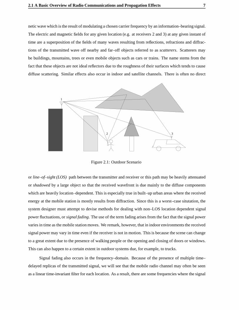
Let us take a closer look at the propagation effects on mobile radio channels by considering the
outdoor communication scenario depicted in Figure 2.1. The antenna at point 1 radiatess an electromag-
2.1 A Basic Overview of Radio Communications and Propagation Effects 7
netic wave which is the result of modulating a chosen carrier frequency by an information–bearing signal.
The electric and magnetic fields for any given location (e.g. at receivers 2 and 3) at any given instant of
time are a superposition of the fields of many waves resulting from reflections, refractions and diffrac-
tions of the transmitted wave off nearby and far–off objects referred to asscatterers. Scatterers may
be buildings, mountains, trees or even mobile objects such as cars or trains. The name stems from the
fact that these objects are not ideal reflectors due to the roughness of their surfaces which tends to cause
diffuse scattering. Similar effects also occur in indoor and satellite channels. There is often no direct
1
2 3
Figure 2.1: Outdoor Scenario
or line–of–sight (LOS)path between the transmitter and receiver or this path may be heavily attenuated
or shadowedby a large object so that the received wavefront is due mainly to the diffuse components
which are heavily location–dependent. This is especially true in built–up urban areas where the received
energy at the mobile station is mostly results from diffraction. Since this is a worst–case situtation, the
system designer must attempt to devise methods for dealing with non–LOS location dependent signal
power fluctuations, orsignal fading. The use of the term fading arises from the fact that the signal power
varies in time as the mobile station moves. We remark, however, that in indoor environments the received
signal power may vary in time even if the receiver is not in motion. This is because the scene can change
to a great extent due to the presence of walking people or the opening and closing of doors or windows.
This can also happen to a certain extent in outdoor systems due, for example, to trucks.
Signal fading also occurs in the frequency–domain. Because of the presence of multiple time–
delayed replicas of the transmitted signal, we will see that the mobile radio channel may often be seen
as a linear time-invariant filter for each location. As a result, there are some frequencies where the signal
8 Mobile Radio Channels
power at the receiver is higher than others, so that the signal powerfadesin frequency.
One often models the location dependent propagation effects statistically. This allows the system
designer to predict system performance, usually by averaging over the statistics of the received signal
power or, equivalently, over all possible relative positions of the receiver/transmitter pair. The use of
statistical models is not solely for mathematical convenience, since they were, for the most part, based
on the results of empirical data. Later, different physical explanations for these measurements were used
to develop the statistical descriptions. In a very simple sense, the source of randomness can be explained
firstly by the fact that attenuation due to scattering off rough surfaces are random due to the position
and electromagnetic properties of the objects. Secondly, the location of the mobile station has a certain
degree of uncertainty.
One can distinguish three levels of signal attenuation which are due topropagation path loss,
shadowingand multipath propagation. The first can sometimes be explained physically and can be
accurately measured. The other two are usually modeled statistically.
Propagation path loss is dependent on the distance between the receiver and transmitter and is
random only due to the position of the mobile station. For practical systems where the processing time
of information bursts is not very long, the path loss, even for quickly moving objects, changes very little.
Moreover, many systems are designed to offer the same quality of service independently of the distance
between the mobile user and the basestation so that some form of power control is needed to counter the
path loss and usually shadowing too.
Fading due to shadowing is slow, in the sense that it changes little over fairly large regions. The
degree of variation is an issue which is constantly being debated. Some believe that it can be noticeable
when the mobile moves only a few meters, as some paths are blocked by large objects such as trees or
buildings. Shadowing and path loss can be seen as slow fluctuations of the mean signal power as the
mobile moves and are virtually frequency–invariant. If we consider Figure 2.2 we see that for a far–off
receiver/transmitter the long–term fading components are more or less constant within the differently
shaded regions.
As we already mentioned, multipath propagation causes rapid power fluctuations as the mobile
station moves, even over very short distances. For this reason, it is calledshort–termor fast fading. Since
these fluctuations are heavily frequency–dependent the bandwidth of the transmitted signal is critical in
describing the effects of multipath.

2.2 Models for Path Loss and Shadowing 9
Figure 2.2: Long–term fading component
2.2 Models for Path Loss and Shadowing
The most widely employed mathematical models for path loss and shadowing came about from the
results of numerous experimental studies in a wide variety of environments. Some more recent studies
for dense urban areas, for example [WB88], are based on approximations using the theory of diffraction
and some empirical corrections.
These models are extremely important for the planning phase during the deployment of a cellular
network. The more accurate the model, the less the need for on–site measurements when placing base
stations. In addition to these models, computer simulations based on optical approximations for electro-
magnetic propagation (ray–tracing [RH92][Kim97]) accurately describing the spatial distributions of the
path loss/shadowing. These software tools are especially powerful for indoor systems, where the basic
geometry of the environment is easily described.
2.2.1 Path Loss in Free–Space
Path loss in free–space can be analytically described by thefree–space transmission formula
PRPT
=
��
4�d
�2GTGR (2.1)
wherePR andPT are the received and transmitted powers at the respective antennas,� is the wavelength,
d is the distance between the receiver and the transmitter in meters, whileGT andGR are the antenna
gains. This is useful in obtaining a rough idea of the true path loss in an outdoor environment. For

10 Mobile Radio Channels
isotropic antennasGT = GR = 1 so that the path loss can be expressed in decibels as
LFS = 32:4 + 20 log10 d+ 20 log10 f dB (2.2)
whered is now in kilometers andf is the frequency in MHz. We see that the power decays with
20 dB/decade in both frequency and distance. This means, first of all, that path loss is a virtually
time–invariant phenomenon for practical mobile speeds. Secondly, it is also practically frequency–
invariant. As an example, imagine a high data–rate system with carrier frequency 1.25 GHz and sig-
nalling bandwidth 10MHz. The path loss difference at the two extreme points of the signal bandwidth is
20 log10 1:26=1:24 = :139 dB. In reality, the presence of a strong reflection off the ground causes the
power to decay with 40 dB/decade (or inverse4th power) when the distance separating the transmitter
and receiver is much larger than the heights of the two antennas. [Lee82].
2.2.2 Measurement-based Models
We now briefly describe a few classic models for the path loss which were based on measurements.
Okumura’s Tokyo Model
The first empirical model for path loss in an urban area was proposed by Okumura [OOKF68]. It is based
on extensive measurements made in Tokyo. It adjusts the free–space path loss equation with empirical
constants depending on the heights of the fixed and mobile terminals and the type of terrain and area
geometry (hilly, sloping, land–sea, presence of foliage and street orientation with respect to the fixed
terminal). The path loss formula is given by
LOkumura = LFS +Am(f; d)�HB(hB ; d)�HM(hM ; f)�KU(f)�K dB (2.3)
whereLFS is the free–space path loss given in (2.2),AM (f; d) is a frequency and distance dependent
factor indicating the median attenuation with respect to free–space loss in an urban area over quasi–
smooth terrain. His measurements assumed a fixed terminal antenna height ofhB = 200m and mobile
terminal antenna heigh ofhM = 3m. HB(hB; d) andHM(hM ; f) are the distance/frequency–dependent
height gain factors,KU(f) is the so–called urbanization factor (depending on whether the environment
is urban, suburban or an open area) andK is an additional term for taking account certain characteristics
of the terrain (hilly, sloping, land-sea, foliage, etc.) These adjustment factors are all tabulated in curves
for different environmental parameters [OOKF68].

2.2 Models for Path Loss and Shadowing 11
Hata’s and COST 231 Refinements
The main problem with Okumura’s model is computing the different adjustment factors from tabulated
data. Hata [Hat80] came up with the following formula which yields path–loss predictions which are
almost indistinguishable from Okumura’s without the need for these curves
LHata = 69:55 + 26:16 log10 f � 13:82 log10 hB �Am(hM ; f) + (2.4)
(44:9� 6:55 log10 hM) log10 d+KU(f) dB (2.5)
where
Am(hM ; f) = (1:1 log10 f � :7)hM � (1:56 log10 f � :8) dB (2.6)
is the correction factor for the mobile terminal’s antenna height in a small or medium–sized city and
Am(hM ; f) =
8><>:8:29(log1:54hM)2 � 1:1 f � 200MHz
3:2(log 11:75hM)2 � 4:97 f � 400MHz
(2.7)
is the same factor for a large–sized city. The urbanization correction factor,KU(f), is zero in an urban
area. In a suburban area it is given by
KU(f) = �2(log10(f=28))2� 5:4 dB (2.8)
and in an open–area by
KU(f) = �4:78(log10 f)2 + 18:33 log10 f � 40:94 dB: (2.9)
This model is valid in the 150-1000 MHz frequency range and for distances of 1-20km. Also, the fixed
terminal antenna height is 30-200m and for the mobile station 1-10m.
A similar model was proposed within the COST 231 project for the 1500-2000MHz frequency
range for use in analyzing the DCS 1800 and PCS 1900 microcellular systems. We see that these empir-
ical models aim at capturing the effects not predicted by the free–space transmission formula since the
attenuation drops off with around 40 dB/decade and not 20 dB/decade.
Diffraction Models and Ray–Tracing
For microcellular and picocellular systems, the simple models for predicting path loss start to break
down. This is due to several reasons, most notably the reduced height of the base stations. As shown in

12 Mobile Radio Channels
Figure 2.1 , because of the presence of buildings and the fact that base stations are normally placed on
the rooftops, the propagation path to the mobile station often is the result of a diffraction off the edge of
a building. As a result, the empirical formulations based on Okumura’s model had to be modified to take
this new effect into account. We do not go into any details of these models except to make reference to the
work of Walfisch and Bertoni [WB88] and Ikegamiet al [IYTU84]. These methods were also used in the
COST 207 and 231 projects [FL96]. For the case of rural mountainous areas, similar diffraction–based
models are reviewed in K¨urneret al [KCW93].
For indoor channels much less empirical modeling of path loss has been performed. One of the
main problems is that the path loss properties vary greatly from one room to another or one corridor to
another. For this reason, many computer simulation based studies using ray–tracing algorithms have been
proposed [RH92][Kim97]. These algorithms use ray–optical approximations for reflections, refractions
and diffractions to model the electromagnetic propagation within buildings. These are particularly ap-
pealing since the number of base stations required to service the location can be roughly determined and
placed without having to resort to electromagnetic measurement. Their placement can then be adjusted
once the system is in operation based on observed performance. In fact, some wireless companies sell
systems which have signal–to–noise ratio measurement as a built–in feature in the handset to help in the
placement of the base stations. Another possible advantage of Ray–Tracing algorithms is that the next
generation ofintelligentbuildingscan potentially be designed by architects with wireless communication
in mind.
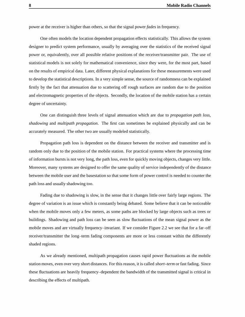
2.2.3 Lognormal Shadowing
The other long–term fading effect, calledshadowingis a result of the fact that waves incident at the
receiver are attenuated or vanish due to the presense of large objects. The characterization of this phe-
nomenon is usually done statistically as for the short–term fading component described in the following
sections. If we examine a typical average received power measurement as the mobile moves as in Figure
2.3, where the average is taken across distances of several hundreds of wavelengths. This averages–out
the short–term fading component and leaves only the components due to path loss and shadowing which
vary insignificantly over these intervals. It was found [ACM88] that the variation around the mean of
this curve on a dB scale, which is the path–loss component, is approximately Gaussian with standard
deviation,�sh, from 6–8 dB. The amplitude factor due to shadowing is therefore a lognormal random
2.3 Short–term Fading 13
variable given by
Ash = 10:1�sh� (2.10)
where� is a zero–mean Gaussian random variable with variance 1.
100
101
−240
−220
−200
−180
−160
−140
−120
mean-signal
d (km)
power (Path loss)
Variation of received
signal power with short
term fading component
averaged-out.
dB
Figure 2.3: Variation of the mean signal strength
The spatial correlation of the shadowing component receives relativelylittle attention in the lit-
erature. Some authors make conjectures about these statistics [Ker96],[Gud91], however it is not clear
whether there are any physical grounds to support them. Most seem to be chosen to simplify mathe-
matical performance analysis, the goal only being to have a rough idea as to the effect of shadowing
correlation.
2.3 Short–term Fading
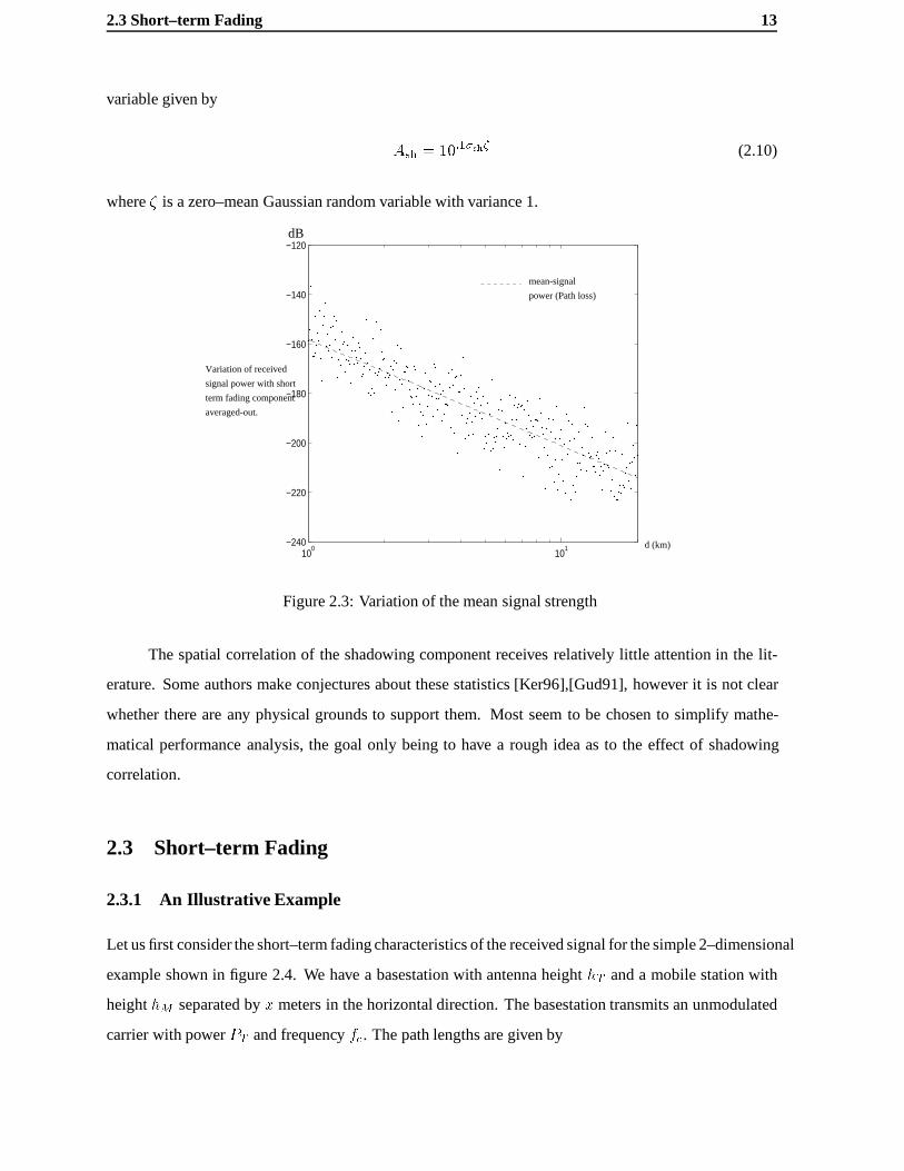
2.3.1 An Illustrative Example
Let us first consider the short–term fading characteristics of the received signal for the simple 2–dimensional
example shown in figure 2.4. We have a basestation with antenna heighthT and a mobile station with
heighthM separated byx meters in the horizontal direction. The basestation transmits an unmodulated
carrier with powerPT and frequencyfc. The path lengths are given by
14 Mobile Radio Channels
hT
xD
hM
dLOSd2
d1d3
Figure 2.4: An illustrative example of short–term fading
dLOS =px2 + (hT � hM )2 (2.11)
d1 =px2 + (hT + hM )2
d2 =px2 + 4D2 � 4Dx+ (hT � hM )2
d3 =px2 + 4D2 � 4Dx+ (hT + hM )2
and their corresponding phases are
�i =2�fcdi
c
wherec = 3 � 108 m/s is the speed of light. We have assumed that the leftmost building is a perfect
absorber so that no received energy is due to a reflection off of it. The ratio of received to transmitted
power is therefore
PRPT
=
�c
4�fc
�2 ���� 1
dLOSej�LOS +
a1d1ej�1 +
a2d2ej�2 +
a1a2d3
ej�3����2 (2.12)
wherea1 anda2 are the reflection coefficients of the ground and the rightmost building respectively . In
Figure 2.5 we show the variation of the power ratio with distance assuminghT = 30m, hM = 2m,D =
1km, anda1 = a2 = �1(total reflection) andfc =100MHz, 1GHz and 10GHz. We see that the received
power fluctuates greatly as a function of the mobile position, especially as we approach the rightmost
building where it exhibits an almost random behaviour. This behaviour is especially pronounced at higher
carrier frequencies. This is due to the increasing complexity of the interference pattern as the powers of
all paths start to become similar. For real mobile radio channels in urban environments where there are
many paths this randomness is even more evident. In Figure 2.6 we show the frequency response in a
1MHz bandwidth starting at1GHz. Here the fading effect in the frequency domain is evident and leads

2.3 Short–term Fading 15
0 100 200 300 400 500 600 700 800 900 1000−130
−120
−110
−100
−90
−80
−70
−60
−50
−40
−30
x (m)
fc = 100 MHz
fc = 1 GHz
fc = 10 GHz
PRPT
(dB)
Figure 2.5: Received to transmitted power ratio as a function of mobile position
us to the notion of acoherence bandwidth, which indicates the signal bandwidth where the channel is
practically flat or non time–dispersive. This allows the system designer to quantify the border between
narrow and wideband signals. If we defineflat as a 3dB bandwidth, then coherence bandwidth is on the
order of 200 kHz for this example.
2.3.2 The Gaussian Fading Model
The statistical description of multipath propagation was given by Clarke [Cla68] and further refinements
were done by Jakes [Jak74]. We summarize these results for bothstaticanddynamicmultipath channels.
A static channel is one where the mobile station is stationary or virtually stationary and we are interested
in a statistical description of the received power which does not change in time. A dynamic channel is
one where the mobile station is moving with a specified velocity.
In the following chapters we will mainly be concerned withblockstatic multipath channels. This
is an approximation of a dynamic channel which changes very slowly so that it may be considered as
static over blocks or intervals of time.

16 Mobile Radio Channels
1 1.0001 1.0002 1.0003 1.0004 1.0005 1.0006 1.0007 1.0008 1.0009 1.001
x 109
−96
−94
−92
−90
−88
−86
−84
−82
−80
PR=PT
f
Figure 2.6: Frequency response atx = 870m
Static multipath channels
Assume we transmit a quadrature signal with complex envelope~s(t) = sc(t)+ jss(t) by modulating the
in–phase and quadrature carriers at frequencyfc. The signal fed to the transmitting antenna is given by
u(t) = sc(t) cos 2�fct� ss(t) sin 2�fct: (2.13)
Considering only the electric field components of the electromagnetic wave at the receiving antenna, we
write the received signal vector for a stationary receiver as
r(t) =
0@rv(t)rh(t)
1A = kRe
(NXi=0
G(�i)Aiej2�fct~s(t � di)
)(2.14)
wherek is a proportionality factor depending on the antenna characteristic. The angle�i represents the
two angles of arrival (i.e. azimuthal and elevation) of theith wave component at the receiver,Ai is a
column vector holding its horizontal and vertical complex amplitudes anddi its propagation delay. The
2� 2 diagonal matrixG(�i) holds the horizontal and vertical field gains for the given angles of arrival.
If the antenna is polarized in either of the vertical or horizontal direction, one of the diagonal elements is
zero. The path index 0 corresponds to the LOS path, so that in the case where it is not presentA0 = 0.
The complex envelope ofr(t) is given by
~r(t) = k
NXi=1
G(�i)Ai~s(t � di) (2.15)

2.3 Short–term Fading 17
and its corresponding Fourier transform
~R(f) = k ~S(f)NXi=1
G(�i)Aiej2�fdi (2.16)
From this point onward we assume the antenna is omnidirectional and polarized in the vertical direction
so thatG(�) =
0@1 0
0 0
1A. For convenience we assume that thedi are in increasing order. Dropping
vector notation we may write~R(f) = k ~S(f)H(f) whereH(f) is a random frequency response (or
filter) given by
H(f) =NXi=0
Aiej2�fdi (2.17)
with covariance between frequency samplesf1 andf2
�(f1; f2) = �(f1 � f2) = EH(f1)H�(f2) =
NXi=1
EjAij2ej2�(f1�f2)di (2.18)
In writing this covariance functions, we have assumed that the path gains are independent zero–mean
random variables which is usually known as theuncorrelated scattering assumption. This is justifiable
since they are results of reflections off of rough surfaces [Lee82] whose electromagnetic properties have
a certain degree of uncertainty. Provided that the number of paths is large, which is almost always the
case and that a significant number of these contribute to the total received power, it is permissible to
invoke the central limit theorem [Pap82] and approximateH(f) as a Gaussian random variable for each
f . We must stress, however, that the processH(f) is not a Gaussian process. This follows from the
fact that the Fourier transform is a linear operator and the process defined by the path strengths is not
necessarily Gaussian. This approximation is very strongly corroborated by measurement [Jak74], and as
a result is usually termedRayleigh fadingwhen no LOS path exists since the envelope of a zero–mean
complex Gaussian random variable is Rayleigh distributed as
fRayleighjHj (a) =2a
�2Hexp
�� a2
�2H
�; a � 0 (2.19)
where�2H =PN
i=1EjAij2 is the total power of the random component of the received wavefront. In
the case of a strong LOS path it is calledRicean fadingsince the mean of eachH(f) is A0 so that the
envelope has a Ricean distribution given by
fRicejH j (a) =2a
�2Hexp
��a
2 + jA0j2�2H
�I0
�2ajA0j�2H
�; a � 0 (2.20)

18 Mobile Radio Channels
whereI0(�) is the zero–order modified Bessel function of the first kind. The ratioK = jA0j2=�2H is
commonly referred to as the Ricean factor. The density and distribution functions of the energy at a
given frequencyjH(f)j2 are usually more useful for calculation purposes and are given by
fRayleighjHj2 (a) =
1
�2Hexp
�� a
�2H
�; a � 0 (2.21)
FRayleighjHj2 (a) = 1� exp
�� a
�2H
�; a � 0 (2.22)
fRicejHj2 (a) =K
jA0j2e�K(a+jA0 j2)=jA0j2I0
�paK
jA0j�; a � 0 (2.23)
FRicejH j2 (a) = 1�Q1
p2K;
s2aK
jA0j2!; a � 0 (2.24)
whereQ1(�; �) is the first order Marcum Q–function. Efficient numerical methods for calculating it are
given in [Shn89]. In figure 2.7 we show the density functions of the received energy at a particular
frequency as a function ofK assuming the average received power is unity (i.e.�2H + jA0j2 = 1). We
0 0.5 1 1.5 2 2.5 3 3.5 40
0.5
1
1.5
2
2.5
3
fRicejHj2 (a)
K = 20 dB
K = 10 dB
a
K = 0 dB
K = �1 dB
Figure 2.7: Ricean probability density for increasingK and normalized received energy
see that asK increases the channel becomes more and more deterministic.K is typically zero in urban
environments but may rise to 6 dB in an indoor setting [Bul87]. If the transmitted signals(t) lies in a
band[fc �W=2; fc + W=2] andW is such that�(u) is almost constant for�W=2 � u � W=2 (i.e.

2.3 Short–term Fading 19
W (dN � d0)� 1) then
~r(t) � H(fc)~s(t � d0) (2.25)
This is a narrowband or single–path channel model.
There are other statistical models for fading which combine the shadowing and multipath phenom-
ena. A popular one is theNakagami distribution[Nak60]. The latter model is simply the square–root of
Gamma distributed random variable.
Dynamic multipath channels
Let us now assume that the mobile station is moving with velocityv in the horizontal plane as shown in
figure 2.8. This introduces a Doppler shift at each frequencyf given by
�fDi (f; t) =vf
ccos(�i(t)) (2.26)
where�i(t) is the time–varying angle between theith incoming path (assumed to be traveling horizon-
tally) and direction of motion of the mobile station. This 2–dimensional model is due to Clarke[Cla68]
v
�N (t)
�2(t)�1(t)
PathN
Path1
Path2
Figure 2.8: Two–dimensional Doppler model
and Jakes [Jak74]. An extension in 3–dimensions for which the significant conclusions regarding sys-
tem design remain unchanged is considered by Aulin [Aul79]. If we consider modulating signals with
bandwidths significantly less than the carrier frequency, which is always the case in mobile radio com-
munications, then all frequencies are affected by virtually the same Doppler shift at any instant in time.
20 Mobile Radio Channels
This allows us to write the complex envelope of the received signal as
~r(t) = k
NXi=0
A(�i(t))ej2��fDi (fc;t)t~s(t � di(t)) (2.27)
In most cases where processing of~r(t) is done in a short timespandi(t) � di so that the time–varying
nature of the delays may be ignored. This is further justified by the fact that the amplitudes change much
more quickly than do the delays. This assumes, of course, that the mobile speed is not very large, and
therefore may not apply to some aeronautical or satellite channels. For simplicity let us focus on the
narrowband signal case so that
~r(t) � k
(NXi=0
A(�i(t))ej2�fDi (fc;t)t
)s(t� d0) (2.28)
As before, providedN is large enough and significant number ofA(�i(t)) contribute to the sum, the
samples of the process�(t) =PN
i=0A(�i(t))ejfDi (fc;t)t are approximately Gaussian. If the paths are
results of far–off reflections, the Doppler shift for each path changes very slowly (i.e.�i(t) changes
slowly) so that, at least on intervals of a certain length, we may justifiably approximate the process�(t)
as a stationary Gaussian process with correlation function
R�(t; �) = E�(t)��(t+ �) =NXi=0
EjA(�i)j2Eej2�fD cos �i � ; (2.29)
where�fD = vfc=c is the maximum Doppler shift. In the classic model by Clarke and Jakes it is
assumed that the angles of arrival are uniformly distributed on[0; 2�) so that
Eej2�fd cos �i � =1
2�
Z 2�
0ej2�fd cos �i �d�i = J0 (2�fD�) ; (2.30)
whereJ0(_) is the zero–order Bessel function. In the frequency domain the power spectrum of the fading
process is
S�(f) =
8><>:
�2H
2�
q1
f2�f2D
jf j < fD ;
0 elsewhere:
(2.31)
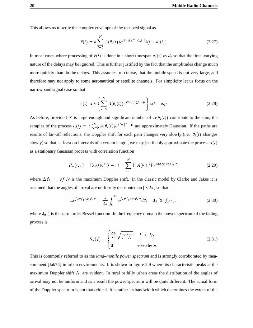
This is commonly referred to as theland–mobile power spectrumand is strongly corroborated by mea-
surement [Jak74] in urban environments. It is shown in figure 2.9 where its characteristic peaks at the
maximum Doppler shiftfD are evident. In rural or hilly urban areas the distribution of the angles of
arrival may not be uniform and as a result the power spectrum will be quite different. The actual form
of the Doppler spectrum is not that critical. It is rather its bandwidth which determines the extent of the
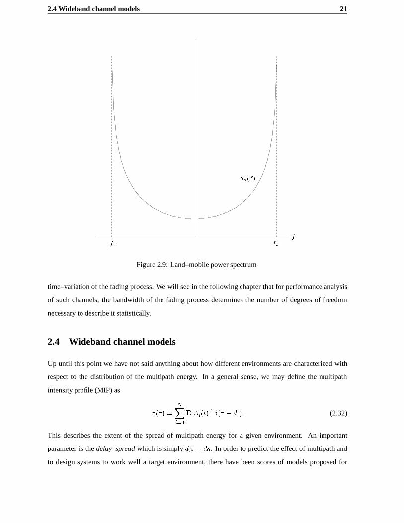
2.4 Wideband channel models 21
�fD fDf
S�(f)
Figure 2.9: Land–mobile power spectrum
time–variation of the fading process. We will see in the following chapter that for performance analysis
of such channels, the bandwidth of the fading process determines the number of degrees of freedom
necessary to describe it statistically.
2.4 Wideband channel models
Up until this point we have not said anything about how different environments are characterized with
respect to the distribution of the multipath energy. In a general sense, we may define the multipath
intensity profile (MIP) as
�(�) =NXi=0
EjAi(t)j2�(� � di): (2.32)
This describes the extent of the spread of multipath energy for a given environment. An important
parameter is thedelay–spreadwhich is simplydN � d0. In order to predict the effect of multipath and
to design systems to work well a target environment, there have been scores of models proposed for

22 Mobile Radio Channels
CLUSTERS
t
EjAij2
Figure 2.10: Clustering Effect of Multipath Channels
the MIP. These models attempt not to perfectly described a given multipath environment, since this is an
impossible task, but rather to capture the key features from a series of measurements in the desired system
setting (i.e. frequency band and physical environment). At the same time as being representative of a
typical channel, they should be mathematically suitable for performing an analytical/simulation system
performance analysis. Without going into too much detail of the different models, we briefly describe a
few here.
2.4.1 Poisson arrival models
Turin [TCJ+72] considered the static multipath channel for an urban environment and modeled the se-
quence of delaysfdig as a Poisson point process. The simplest approach is to consider a homogeneous
process so that delay differences�di = di�di�1 are i.i.d. exponential random variables. This, however,
does not capture the clustering effect which is typical of real channels. We show this in figure 2.10. Each
cluster corresponds to a series of scatterers closely located to each other. A simple non–homogeneous
process was proposed to model this effect. This technique was later extended by Suzuki[Suz77] and
Hashemi [Has79].

2.4 Wideband channel models 23
2.4.2 COST 207 models
In order to analyze the GSM cellular telephone system, a series of propagation studies were performed
as part of the COST 207 project. These studies yielded a series of models for outdoor channels, denoted
by TU(typical urban), RU(rural area) and HT(hilly terrain), which we show in Table 2.2. These are tap
delay line models with regularly spaced taps which have the drawback that they are applicable only for a
limited signaling bandwidth. We will see in the remainder of this thesis that the performance of a system
depends on the degree of randomness of the channel which is closely related to the signaling bandwidth.
For wideband analysis, such as for spread spectrum or slow frequency hopping systems these models are
not necessarily applicable.
Each path has an associated Doppler which is not indicated in this table. For our purposes we will
only use the static fading characteristics of these channels. Paths from local scatterers have been found
to be accurately modeled by the classic land–mobile model given in 2.30. For those caused by distant
scatterers in the BU and HT channels the Doppler spectrum have a particular two–lobe Gaussian Doppler
spread under the assumption of two significant scatterers. We only include the MIP statistics since we
will only use them for frequency–domain computations.
2.4.3 Indoor Models
Saleh and Valenzuela [SV87] consider a ncatenation of two Poisson point processes for describing the
indoor propagation channel. One process defines the positions of clusters of paths and the second the
positions of the paths within clusters. The modified Poisson process models described in section 2.4.1
were extended for typical indoor channels by Ganesh and Pahlavan in [GP89].

24 Mobile Radio Channels
Rural Area (RU6) Hilly Terrain (HT6) Typical Urban (TU6)
di(�s) jAij2 (dB) di(�s) jAij2 (dB) di(�s) jAij2 (dB)
0 0 0 0 0 -3
.1 -4 .1 -1.5 .2 0
.2 -8 .3 -4.5 .5 -2
.3 -12 .5 -7.5 1.6 -6
.4 -16 15 -8 2.3 -8
.5 -20 17.2 -17.7 5.0 -10
Typical Urban (TU12) Hilly Terrain (HT12)
di(�s) jAij2 (dB) di(�s) jAij2 (dB)
0 -4 0 -10.01
.1 -3.01 .1 -8.01
.3 0 .3 -6
.5 -2.6 .5 -4.01
.8 -3 .7 .01
1.1 -5 1 0
1.3 -7 1.3 -4
1.7 -5 15 -8
2.3 -6.5 15.2 -9
3.1 -8.6 15.7 -10
3.2 -11 17.2 -12
5.0 -10 20 -14
Table 2.2: ETSI-COST 207 Channel Models
Chapter 3
Signaling over Fading Channels
Signal fading is arguably the most difficult phenomenon that radio communication system designers have
to cope with. As we saw in Chapter 2, the average received signal strength can drop tens of decibels due
to the destructive interference of delayed reflections of the transmitted signal [Jak74]. This is especially
the case in non line–of–sight communications. Moreover, for slowly moving mobile transceivers, such
“deep fades” result in unacceptably long periods of time where reliable communication is impossible.
In wide-band systems the receivers are sensitive enough to distinguish (or resolve) different faded
replica of the transmitted signal, orpaths, which can be used jointly to improve performance. In spread–
spectrum based systems, such as IS–95 [IS992], where the signal bandwidth is much larger than the
symbol rate, some paths can be combined by what is commonly referred to as a RAKE receiver [Pro95]
to improve performance. Medium–band systems are subject tointersymbol interference(ISI) due to
time dispersion so that the use of an equalizer also benefits from frequency–diversity. This is actually a
situation where ISI is desirable.
In order to operate efficiently in such a hazardous environment, the system designer often opts to
use so-calleddiversitymethods. Simply put, the diversity is the number of independent replica of the
transmitted signal that are made available to the receiver. In the absence of multiple antennas, this calls
for the exploitation of either the frequency or the time-variation properties of the fading signal or both.
The former can be calledfrequency diversity, and makes use of the amplitude of the transfer function
of the channel in different parts of the spectrum. Frequency–diversity schemes are quite popular in
multiuser systems due to the large amount of bandwidth that is available, and can be achieved in different
ways.
Another way of exploiting frequency–diversity is to use coded narrow or medium–band signals
26 Signaling over Fading Channels
with slow frequency–hopping. This technique is used in the GSM system and its derivatives DCS 1800
and PCS 1900 [GSM90]. Here, the information is coded and interleaved overF = 4 (half–rate) or
F = 8 (full–rate) blocks of lengthN = 208 orN = 378 symbols, and each block modulates a different
carrier (ideally) according to some predefined hopping pattern. This is achieved by altering the FDMA
allocation of users every block. It has the effect of ensuring that after deinterleaving anyF adjacent
received symbols modulated a different carrier. If the carriers are sufficiently separated, the resulting
received symbols have uncorrelated strengths. It is well known that error–control coding can yield a
significant diversity effect in such cases [Pro95].
Time diversity can also be exploited to some extent using interleaving even without frequency–
hopping. Assuming that the receiver/transmitter is in motion, interleaving spreads the information across
different channel strengths whose correlation depends on the mobile speed and interleaving delay. For
example, the IS54 system [IS592] encodes the information and interleaves it overF = 2 blocks of length
N = 178 separated by 20ms. For low mobile speeds this can result in highly correlated symbols after
deinterleaving. For this reason, systems exploiting frequency diversity are more desirable when reliable
performance is desired at low mobile speeds.
In this chapter we will consider the different ways signaling is performed over the various types
of fading channels. There is nothing really new, but much of the material is presented in a way that is
not found in most classic textbooks on digital communications. More precisely we look at the different
diversity methods and show that performance criteria are computed in essentially the same way in each
case. Once the signal has been characterized statistically, the computation of performance criteria is
a question of performing aneigenvalue analysisof a kernel or quadratic form representing the energy
of the received signal in some observation interval/bandwidth. The number of significant eigenvalues
or degrees of freedomof the channel process in a given frequency band or time interval will play an
important role.
We end with a generic model which is useful for describing many systems which operate with a
small number of degrees of freedom or eigenvalues, which we call theblock–fading model. In practice,
this model is applicable to systems where processing is performed over a few different channel realiza-
tions which can result for instance from afrequency–hoppingmechanism. Chapters 4 and 5 will treat the
fundamental aspects of this model in more detail.

3.1 Performance Measures 27
3.1 Performance Measures
Imagine a communication system where signal blocks or messages of durationT seconds are used to
convey information from the sender to the receiver. We assume that a finite number,M , of message
waveforms exist, which we denote by the setfxm(t); m = 0; � � � ;M � 1g. The amount of information
per message islog2M bits so that the bit rate is
R =1
Tlog2M bits=s (3.1)
For simplicity, we will assume that the receiver requires the entire message in order to make a decision
about which message was sent, so that the processing or decoding delay isT seconds. In many systems,
there is a limit to the tolerable decoding delay. A long decoding delay for voice telephony results in
an unacceptable audible delay. Some data transmission protocols also have stringent decoding delay
constraints due to some quality of service requirement or limited buffer size.
The message orcodeword error–rateis a critical measure of the robustness of a coding scheme
in noise. Under the assumption that messages are transmitted with equal probability it can be bounded
from above using the union bound [Pro95]
Pe =1
M
M�1Xm=0
M�1Xn=0
Prob(m! n) (3.2)
whereProb(m! n) is the called thepairwise error probability (PEP)between messagesm andn and
indicates the probability of decodingn given thatm is transmitted if they were the only two possible
messages.
The analysis of the PEP for systems working in a fading environment is usually based on charac-
terizing the statistics of the total received energy in the interval[�T=2; T=2]. It is therefore not surprising
that most formulations yield very similar forms for the PEP. The goal of this chapter is to describe differ-
ent narrow and wide-band systems which we will refer to in the remainder of this thesis by defining the
basic receiver structures and their performance measures. We begin by defining the notion ofdiversity
using a simple two–channel receiver which can be seen as a dual–antenna receiver.
Throughout this chapter we express all transmitted and received messages as complex baseband
signals representing the complex envelope of real signals centered at a certain carrier frequency.

28 Signaling over Fading Channels
3.2 Diversity Reception
Let us consider transmission of a binary message overtwostatic independent single–path Rayleigh fad-
ing channels. Physically, this could represent a dual–antenna receiver where one antenna is vertically
polarized the other is horizontally polarized and the receiver can process both polarizations. Here the
receiver has access to two faded versions of the same signal which is known asdiversity reception. The
received signals can be written as
y(t) =
0@y0(t)y1(t)
1A =
0@�0�1
1Ax(t) +
0@z0(t)z1(t)
1A ; �T=2 � t � T=2 (3.3)
where�i are the two independent zero–mean complex circular symmetric Gaussian random variables,
x(t) is a binary message taking on valuesx0(t) andx1(t) with equal probability andzi(t) is additive
white complex circular symmetric Gaussian noise with two–sided power spectral densityN0. Let us
assume that the receiver is capable of perfectly estimating the�i. Furthermore we takeEj�ij2 = 1 so
that any average attenuation factor is included in the transmitted signal energyE which now becomes the
average received signal energy. In this case, the optimal receiver, in the sense of minimum probability of
error, is themaximum–likelihoodreceiver [VT68]
m = argminm=0;1
Z T=2
�T=2jy(t)� �xm(t)j2dt
= argmaxm=0;1
Z T=2
�T=2RefyMR(t)x
�m(t)g �
1
2
pj�0j2 + j�1j2jxm(t)j2 (3.4)
where
yMR(t) =1p
j�0j2 + j�1j2(��0y0(t) + ��1y1(t)) (3.5)
is thecombinedreceived signal. The receiver in (3.4) is depicted in figure 3.1 and is known as amaximal
ratio combiner. It has been given this name since the front end of the receiver combines the two diversity
branches in such a way as to assure that the resulting signal takes most of its energy from the stronger
branch. The rest of the circuit works as a regular maximum–likelihood receiver with fading strength
equal to�c =pj�0j2 + j�1j2.
Another sub–optimal receiver structure known asselection combininguses a front end with com-
bined signal
ySD(t) = yi(t); i = argmaxj=0;1
j�j j (3.6)

3.2 Diversity Reception 29
so that the combined signal strength is�c = maxfj�0j; j�1jg. The rest of the receiver is maximum–
likelihood as with maximal–ratio combining. We will meet this structure again in Chapter 7 when we
consider multiuser communications.
-
-
Re
Re
CHOOSE
MAX:5pj�0j2 + �1j2jx0(t)j2
:5pj�0j2 + �1j2jx1(t)j2
��0pj�0j
2+j�1j2
��1pj�0j
2+j�1j2
R T=2�T=2
R T=2�T=2
x�0(t)
x�1(t)
Figure 3.1: Maximal–ratio combining
Let us assume an antipodal system sox0(t) = �x1(t) withR T=2�T=2 jxi(t)j2dt = E . The PEP
conditioned on the fading level for maximum–likelihood reception is given by [VT68]
Pej�c(0! 1) = Q
r2j�cj2 E
N0
!(3.7)
whereQ(�) is the area under the tail of a normalized Gaussian distribution given by
Q(x) =
r1
2�
Z 1
xe�u
2=2du (3.8)
In order to calculate the average PEP we must average (3.7) over the density ofj�cj2. Let us first consider
the selection combining case. The distribution function of the maximum of two unit-mean exponential
random variables is given by
FSDj�cj2
(u) = (1� e�u)2; u � 0 (3.9)
so that its density is
fSDj�cj2(u) = 2e�u � 2e�2u; u � 0 (3.10)
The effect of diversity is clear since the density of the average received power is small around the origin,
so that a lowsignal–to–noise ratio (SNR), �cE=N0 is unlikely. Using the fact that
Z 1
0aQ(
pu)e�audu = :5
1�
r1
1 + 2a
!(3.11)

30 Signaling over Fading Channels
we have that the average PEP for selection combining is given by
PSDe (0! 1) = E
"Q
r2j�cj2 E
N0
!#= :5
1� 2
sE=N0
1 + E=N0+
sE=N0
2 + E=N0
!(3.12)
Turning to the case of maximal–ratio combining we see thatj�cj is the sum of two unit–mean exponential
random variables so it has a central Chi-square distribution with 4 degrees of freedom. Thus,j�cj2 has
density
fMRj�cj2
(u) = ue�u; u � 0: (3.13)
It is shown in [Pro95, Chap 14] that
PMRe (0! 1) = :25
1�
sE=N0
1 + E=N0
!2 1 + :5
1 +
sE=N0
1 + E=N0
!!(3.14)
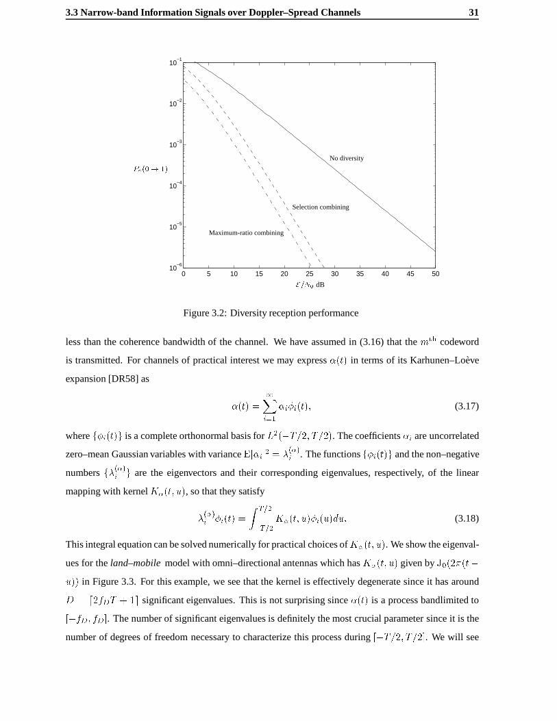
We plot the PEP for both cases as a function of the signal–to–noise ratioE=N0 in Figure 3.2. We also
show the PEP if we use only one of the branches. In this case we have thatfj�cj2(u) = e�u; u � 0 and
Pe(0! 1) = :5
1�
sE=N0
1 + E=N0
!(3.15)
We see that by having two replicas of the transmitted signal, which are subject to independent channel
realizations, we can significantly reduce the error–rate performance. In what follows we will see similar
effects which are due to coding the information signal in such a way to take advantage of the time and/or
frequency–selective nature of fading channels, without the need for multiple antennas. The number of
diversity branches will become the number of degrees of freedom (either in time or in frequency or both)
needed to characterize the fading process.
3.3 Narrow-band Information Signals over Doppler–Spread Channels
A narrow-band system, as shown in chapter 1, can often be described by the single–path time–varying
fading channel as
y(t) = �(t)x(m)(t) + z(t); jtj < T=2 (3.16)
where�(t) is a circular symmetric zero–mean complex Gaussian process over the vector space of square–
integrable functions over[�T=2; T=2), L2(�T=2; T=2), with autocorrelation functionK�(t; u). This
corresponds to Rayleigh fading which has no LOS path and holds if the bandwidth ofx(t) is much
3.3 Narrow-band Information Signals over Doppler–Spread Channels 31
0 5 10 15 20 25 30 35 40 45 5010
−6
10−5
10−4
10−3
10−2
10−1
No diversity
Maximum-ratio combining
Selection combining
Pe(0! 1)
E=N0 dB
Figure 3.2: Diversity reception performance
less than the coherence bandwidth of the channel. We have assumed in (3.16) that themth codeword
is transmitted. For channels of practical interest we may express�(t) in terms of its Karhunen–Lo`eve
expansion [DR58] as
�(t) =1Xi=1
�i�i(t); (3.17)
wheref�i(t)g is a complete orthonormal basis forL2(�T=2; T=2). The coefficients�i are uncorrelated
zero–mean Gaussian variables with varianceEj�ij2 = �(�)i . The functionsf�i(t)g and the non–negative
numbersf�(�)i g are the eigenvectors and their corresponding eigenvalues, respectively, of the linear
mapping with kernelK�(t; u), so that they satisfy
�(�)i �i(t) =
Z T=2
�T=2K�(t; u)�i(u)du: (3.18)
This integral equation can be solved numerically for practical choices ofK�(t; u). We show the eigenval-
ues for theland–mobilemodel with omni–directional antennas which hasK�(t; u) given byJ0(2�(t�u)) in Figure 3.3. For this example, we see that the kernel is effectively degenerate since it has around
D = d2fDT + 1e significant eigenvalues. This is not surprising since�(t) is a process bandlimited to
[�fD; fD]. The number of significant eigenvalues is definitely the most crucial parameter since it is the
number of degrees of freedom necessary to characterize this process during[�T=2; T=2]. We will see

32 Signaling over Fading Channels
0 2 4 6 8 10 120
0.05
0.1
0.15
0.2
0.25
0 2 4 6 8 10 120
0.05
0.1
0.15
0.2
0.25
0.3
0.35
1 2 3 4 5 6 7 80
0.1
0.2
0.3
0.4
0.5
0.6
0.7
fDT = 3
fDT = 1:5
fDT = :5
Figure 3.3: Eigenvalue spread for differentfDT
that this turns out to be equivalent, from the point of view of performance, to the number of diversity
branches in a multiple antenna system. We consider the types of optimal receivers in Section 3.3.1 and
their performance in Sections 3.3.2 and 3.3.3. Starting with the uncoded binary message case, we move
on to coded systems with a discretized approximation for the fading process.
3.3.1 Optimal Receivers
We consider two possible receiver scenarios, one where the fading process is known perfectly to the
receiver, and one where only its statistics are known. We will refer to the first case as acoherentreceiver
and to the second as anon–coherentreceiver. We use the term non–coherent in a very general sense.
Traditionally, it is reserved for detection without an absolute phase reference, whereas here we include
the unknown signal amplitude as well. If the signal changes very quickly, it is often impossible to perform
coherent detection. Nevertheless, it is still reasonable to consider a performance analysis in this case for
comparison purposes.

3.3 Narrow-band Information Signals over Doppler–Spread Channels 33
Coherent Receivers
The optimal receiver assuming equally likely messages is the maximum–likelihood receiver we saw in
(3.4) generalized forM–ary signals
m = argminm=0;��� ;M�1
Z T=2
�T=2jy(t)� �(t)x(m)(t)j2dt
m = argmaxm=0;��� ;M�1
Z T=2
�T=2Reny(t)��(t)x�(m)(t)
odt� 1
2
Z T=2
�T=2j�(t)x(m)(t)j2dt
(3.19)
In the first case, the receiver simply chooses the weighted signal,�(t)x(m)(t)which is closest in terms of
Euclidean distance, whereas in the second case it chooses the message most correlated with the received
signal biased by the energy of the message. Its performance analysis is left to Section 3.3.2.
Non–Coherent Receivers
The non–coherent detection problem is much more delicate, since it is a Gaussian signal detection prob-
lem. The difference between the two problems, in a few words, is that the information in the non–
coherent case is hidden in the correlation function of the received signal and not the mean. We define
the attenuated information signals(m)(t) = �(t)x(m)(t), which is conditionally Gaussian given the hy-
pothesis that themth waveform is transmitted. The conditional mean is zero (Rayleigh Fading) and the
conditional correlation function is
K(m)(t; u) = K�(t; u)x(m)(t)x(m)(u) (3.20)
We now perform a Karhunen–Lo`eve expansion oneachs(m)(t) as
s(m)(t) =1Xi=1
s(m)i �
(m)i (t) (3.21)
wherefs(m)i ; i = 1; � � � ;1g are independent zero–mean circularly symmetric Gaussian random vari-
ables with variancesf�(m)i ; i = 1; � � � ;1g which satisfy
�(m)i �
(m)i (t) =
Z T=2
�T=2K(m)(t; u)�
(m)i (u)du (3.22)
If we project the received signal on the firstK of these basis functions we have
y(m)K (t) =
KXi=1
y(m)i �
(m)i (t) (3.23)

34 Signaling over Fading Channels
and
y(t) = l: i:m:K!1
y(m)K (t) (3.24)
The coordinates of themth representation are related by
y(m)i = s
(m)i + z
(m)i (3.25)
wherez(m)i are i.i.d. complex Gaussian circularly symmetric random variables with varianceN0 and
Ey(m)i y
(m)�j = (�
(m)i +N0)�ij so that theK–dimensional density function fory conditioned on themth
input signal is
fY(m)(y(m)) =
KYi=1
1
�(�(m)i +N0)1=2
!exp
�1
2
KXi=1
jy(m)i j2
�(m)i +N0
!(3.26)
The optimal detection rule under the assumptionof equally–likely transmitted signals and theK–dimensional
approximation is
mK = argmaxm=0;��� ;M�1
fY(m)(y(m)) (3.27)
= argmaxm=0;��� ;M�1
log fY(m)(y(m))
= argmaxm=0;��� ;M�1
KXi=1
jy(m)i j2
�(m)i +N0
+KXi=1
log
1 +
�(m)i
N0
!
LettingK !1 yields
m = argmaxm=0;��� ;M�1
1Xi=1
jy(m)i j2
�(m)i +N0
+1Xi=1
log
1 +
�(m)i
N0
!(3.28)
We would now like to express this in terms of the received signal and some filtering operation. The
inverse kernel of the received signal correlation function under themth hypothesis is
Q(m)y (t; u) =
1Xi=1
1
�(m)i +N0
�(m)i (t)�
�(m)i (u) (3.29)
and is also the solution to the integral equation [VT68]Z T=2
�T=2Q(m)y (t; z)K(m)
y (z; u)dz = �(t� u) (3.30)
After expressing the coordinatesfy(m)i g as integrals, we obtain the decision rule
m = argminm=0;��� ;M�1
Z T=2
�T=2
Z T=2
�T=2y(t)Q(m)
y (t; u)y�(u)dtdu+1Xi=1
log
1 +
�(m)i
N0
!(3.31)

3.3 Narrow-band Information Signals over Doppler–Spread Channels 35
The rightmost term in (3.31) is the bias term for each decision statistic and is directly related to the
energy of each input signal. Using the fact thatlog(1 + x) � x it is upper bounded byEm=N0 where
Em =P1
i=1 �(m)i is the energy of themth weighted waveform.
The decision rule in (3.31) has a very interesting interpretation in terms of the theory of optimum
linear filtering. After some manipulation [VT72], the decision rule may be cast into a form known as an
estimator–correlatorreceiver. The decision rule now takes on the following form
m = argmaxm=0;��� ;M�1
Z T=2
�T=22Re
ny(t)s(m)(t)
o� js(m)(t)j2dt�
1Xi=1
log
1 +
�(m)i
N0
!(3.32)
= argminm=0;��� ;M�1
Z T=2
�T=2jy(t)� s(m)(t)j2dt+
1Xi=1
log
1 +
�(m)i
N0
!
wheres(m)(t) is optimal realizable point estimator for the attenuated message signals(m)(t) given by
s(m)(t) =
Z t
�T=2h(m)(t; u)y(u)du (3.33)
The estimate for the instantt is based on the received signal in the interval[�T=2; t] and the symmetric
time–varying estimation filterh(m)(t; u) is the solution to the integral equation
N0h(m)(t; u) +
Z t
�T=2h(m)(t; z)K(m)
s (z; u)dz = K(m)s (t; u); �T=2 � u � t (3.34)
Another by–product of this realization is that the bias term is the estimation error of the filter
1Xi=1
log
1 +
�(m)i
N0
!=
1
N0
Z T=2
�T=2h(m)(t; t)dt (3.35)
which we will meet again when we consider average mutual information in the next chapter. This is also
known as aFredholm determinant.
The practical interpretation of this analysis is that we perform the same operation as in the coherent
case, namely minimum distance or maximum correlation reception using the optimal linear estimate of
the information processs(m)(t). The bias is different, however, and takes into account both the energy
and associated mean–squared estimation error of each signal.
3.3.2 Pairwise Error Probability - Binary Signals
Here we perform performance analyses for the special case of binary message signals. We start with
coherent case and then continue with one example of a non–coherent system. Suppose that there are two
possible information signals,x(0)(t) andx(1)(t). We denote the conditional PEP by
Pej�(t)(0! 1) = Prob(decide on x(1)(t)jx(0)(t) transmitted; �(t)): (3.36)

36 Signaling over Fading Channels
Using the decision rule in (3.19) the conditional PEP is given by [VT68]
Pej�(t)(0! 1) = Q
0B@vuutR T=2�T=2
j�(t)(x(0)(t)� x(1)(t))j22N0
dt
1CA (3.37)
whereR T=2�T=2
j�(t)(x(0)(t)�x(1)(t))j2dt is the Euclidean distance between the two weighted information
signals.
Let us now consider a few examples. We start with antipodal signals, namelyx(0)(t) = �x(1)(t) =p(t) wherep(t) is chosen such that
R T=2�T=2 jp(t)j2 = E and for simplicity we choose a square pulse shape
p(t) =pE=T; t 2 [�T=2; T=2]. We have, therefore, that the conditional PEP is given by
Pej�(t)(0! 1) = Q
s2EN0
1
T
Z T=2
�T=2j�(t)j2dt
!(3.38)
Another example, which we will use later for comparison with the non–coherent case ison–off
keying (OOK)wherex(0)(t) = p(t) andx(1)(t) = 0. Again we choose a square pulse, but this time with
twice as much energyp(t) =q
2ET ; t 2 [�T=2; T=2] so that the average energy is stillE . Here we have
Pej�(t)(0! 1) = Q
sEN0
1
T
Z T=2
�T=2j�(t)j2dt
!(3.39)
A final example is another orthogonal scheme using binaryWalsh–Hadamard pulseswherex(0)(t) =
p(t) andx(1)(t) = sgn(t)p(t) andp(t) is as with antipodal. In this case, the conditional PEP is given by
Pej�(t)(0! 1) = Q
0@s
2EN0
1
T
Z T=2
0j�(t)j2dt
1A (3.40)
In the three cases, we see that the conditional PEP is a function of the received power of the fading
process over some time interval. This quantity is a random variable which we denote by
PR(T ) =1
T
Z T=2
�T=2j�(t)j2dt (3.41)
In the third example, we must remember to cut the time interval in half. In order to compute the average
PEP we need the distributionofPR(T )which is found easily using the KL expansion for�(t). Replacing
thef�ig by their corresponding integrals we have that
PR(T ) =1
T
1Xi=1
j�ij2 (3.42)

3.3 Narrow-band Information Signals over Doppler–Spread Channels 37
which is a sum of independent exponentially distributed random variables with means�i = �i=T . It
follows that the moment–generating function forPR(T ) is given by
GP (s) =1Yi=1
1
1� s�i(3.43)
In most cases the�i are distinct so that we may perform a simple partial fraction expansion onGP (s) as
GP (s) =1Xi=1
Ai
1� s�i(3.44)
whereAi = (1� s�i)GP (s)js=1=�i =Q
j 6=i�i
�i��j. By straightforward Laplace inversion we obtain the
density function forPR(t)
fPR(p) =1Xi=1
Ai
�iexp
�� p
�i
�U(p) (3.45)
whereU(p) is the unit–step function. It follows that the average PEP for antipodal signals is given by
Pe(0! 1) =1Xi=1
Ai
Z 1
0Q
r2EN0
PR(T )
!exp
�� p
�i
�dp (3.46)
=1Xi=1
Ai
2
1�
s2E�i=N0
1 + 2E�i=N0
!
The others are calculated in an identical fashion.
We now consider a bound on the average PEP. Using the Chernov bound on theQ(�) function
Q(x) � 1
2e�x
2=2 (3.47)
we may upper–bound the PEP usingGP (s) as
Pe(0! 1) = E Q
r2EN0
PR(T )
!
� 1
2E exp
�� EN0
PR(T )
�
=1
2GP
�� EN0
�
=1
2
1Yi=1
1
1 + EN0�i
(3.48)
� 1
2
�N0
E��D
(3.49)
whereD =����i : �i � N0
E
�� and
� =
DYi=1
�i
! 1D
(3.50)

38 Signaling over Fading Channels
The final approximation is valid only if a the total energy of the process is concentrated in a small number
of eigenvalues. The parameterD is the number of significant eigenvalues with respect to the SNR and
� is their geometric mean. The upper bound has the characteristics of aBode plotwhereD is the slope
of the PEP vs. SNR curve on a log–log scale and is traditionally referred to as thediversity orderof the
system.
In Figure 3.4 we show the true PEP for antipodal signals forfDT = 0; :1 and 1 along with
the upper–bound in (3.48). We also show the straight-line approximations from (3.49) which show the
similarity to a Bode plot. In Figure 3.5 we compare the PEP for the three examples. The performance
0 5 10 15 20 25 30 35 40 45 5010
−6
10−5
10−4
10−3
10−2
10−1
fDT = 0
Pe(0! 1)
fDT = :1
fDT = 1
exact
bound
E=N0 dB
Figure 3.4: PEP and its upper–bound for antipodal signals
penalty in using a pulse shape where the energy of the difference signal is not equally distributed in
[�T=2; T=2] is evident, since the Walsh–Hadamard pulse performs much worse than the other two.
This is due to the energy has a smaller number of significant eigenvalues which is seen in the curve for
fDT = 3 which has a smaller slope (i.e. less diversity). This is the first example of the importance of
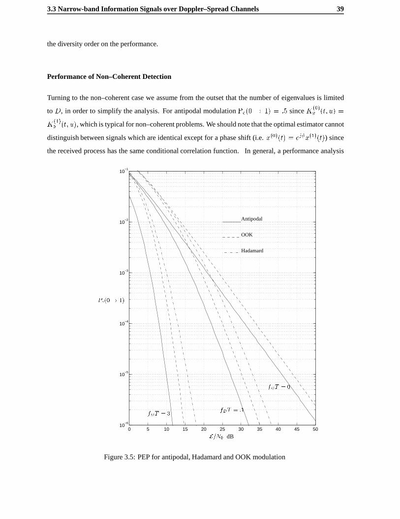
3.3 Narrow-band Information Signals over Doppler–Spread Channels 39
the diversity order on the performance.
Performance of Non–Coherent Detection
Turning to the non–coherent case we assume from the outset that the number of eigenvalues is limited
to D, in order to simplify the analysis. For antipodal modulationPe(0 ! 1) = :5 sinceK(0)y (t; u) =
K(1)y (t; u), which is typical for non–coherent problems. We should note that the optimal estimator cannot
distinguish between signals which are identical except for a phase shift (i.e.x(0)(t) = ej�x(1)(t)) since
the received process has the same conditional correlation function. In general, a performance analysis
0 5 10 15 20 25 30 35 40 45 5010
−6
10−5
10−4
10−3
10−2
10−1
Antipodal
OOK
Hadamard
Pe(0! 1)
E=N0 dB
fDT = 0
fDT = :1fDT = 3
Figure 3.5: PEP for antipodal, Hadamard and OOK modulation

40 Signaling over Fading Channels
of Gaussian signal detection problems is difficult. The OOK example, however, is tractable with the
degenerate kernel approximation. Here,K(0)y (t; u) = 2E
T K�(t; u) + N0�(t � u) andK(1)y (t; u) =
N0�(t� u) so that
Pe(0! 1) = Prob
DXi=1
jy(0)i j2�(0)i +N0
+DXi=1
log
1 +
�(0)i
N0
!�
DXi=1
jy(1)i j2N0
(3.51)
jx(0)(t) transmitted�
In this case we may take�(0)i (t) = �(1)i (t) so thaty(0)i = y
(1)i which allows us to simply the decision
rule as
Pe(0! 1) = Prob
DXi=1
�(0)i
N0j�ij2 �
DXi=1
log
1 +
�(0)i
N0
!!(3.52)
where�i are i.i.d. random variables with mean zero and variance 1. Normalizing the fading process so
thatEj�(t)j2 = 1, we have thatPD
i=1 �(1)i � 2E . This approximation can be made arbitrarily precise by
increasingD. We now define the normalized eigenvalues�i = �(0)i =2E yielding
Pe(0! 1) = Prob
DXi=1
�ij�ij2 � N0
2EDXi=1
log
�1 +
2EN0
�i
�!(3.53)
=DXi=1
Ai
�1� e�B=�i
�
whereB = N02E
PDi=1 log
�1 + 2E
N0�i
�. This is plotted in Figure 3.6 as a function of the SNR and
compared with the corresponding coherent case, where we see that for low fade rates the loss due to
non–coherent detection is large.
3.3.3 Coded Quadrature Amplitude Modulated Signals
We now consider the possibility of performing non–coherent detection of non–binary messages, where
the detection is performed across several symbols. We quickly realize that implementing the optimal re-
ceiver structures is a more or less an impossible task whenM is large and the channel varies greatly dur-
ing the duration of a message. Unfortunately, this is precisely the case of coded systems withquadrature
amplitude modulation (QAM)on fast–fading channels. As a result, one must resort to some discretized
approximation. We consider a piecewise constant approximation for the fading process as follows
�(t) =
dNs2 �1eXi=d�Ns
2 e�iq(t� iT=Ns) (3.54)

3.3 Narrow-band Information Signals over Doppler–Spread Channels 41
0 5 10 15 20 25 30 35 40 45 5010
−6
10−5
10−4
10−3
10−2
10−1
coh. nc coh nc
cohnc
Pe(0 ! 1)
fDT = 3 fDT = :1
fDT = 0
E=N0 dB
Figure 3.6: Performance of non-coherent OOK

42 Signaling over Fading Channels
whereq(t) is a rectangular pulse shape orchip
q(t) =
8><>:q
NsT t 2 [0; T=Ns)
0 elsewhere
(3.55)
andNs can be arbitrarily large. Provided thatfDT � Ns this will be a close approximation to the actual
fading process.
Now consider the QAM signal
x(m)(t) =
dNx=2�1eXi=�dNx=2e
x(m)i p(t� iT=Nx) (3.56)
with Nx being the number of coded symbols orcomplex dimensionsused during the time–interval
[�T=2; T=2]. Thex(m)i belong to an arbitrary complex alphabet and we assume that the pulse shape
may be expressed as
p(t) =
Ns=Nx�1Xi=0
piq(t � iT=Ns) (3.57)
withPNs=Nx�1
i=0 jpij2 = 1. The ratiok = Ns=Nx is assumed to be an integer. We show a particular
example whereNs = 8 andNx = 4 in figure 3.7. This formulation allows us to express the detection
T=2x2
x3
x1
x0T=2
x(t)
�T=2
T=2
T=2�(t)x(t)
�T=2
�(t)
Figure 3.7: A QAM example withNs = 8 andNx = 4
problem vectorially as we now show. The received signal is given by
y(t) = �(t)x(m)(t) + z(t) (3.58)
=
�dNs=2�1eXi=�dNs=2e
�ipi modkxi�kq(t � iT=Ns) + z(t)

3.3 Narrow-band Information Signals over Doppler–Spread Channels 43
wherei � k is taken to mean integer division. In complex circular symmetric white noise with power
spectral densityN0, the set of statistics
yi =
Z T=2
�T=2y(t)q(t� iT=Ns)dt (3.59)
is sufficient for the detection ofx(m)(t) sincefq(t � iT=Ns); i = 0; � � � ; Nsg forms a suitable basis for
the signal. We may therefore write
y =
0BBBBBB@
y0
y1
...
yNs�1
1CCCCCCA= X(m)
0BBBBBB@
�0
�1
...
�Ns�1
1CCCCCCA+
0BBBBBB@
z0
z1
...
zNs�1
1CCCCCCA
(3.60)
= X(m)�+ z
wherezi are zero–mean i.i.d. circular symmetric random variables with varianceN0 and
X(m) = diag(p0x(m)0 ; p1x
(m)0 ; � � � ; pk�1x(m)
0 ; p0x(m)1 ; � � �pk�1x(m)
Nx�1) (3.61)
Optimal Receiver Structure
Not surprisingly, this discrete–time system is completely analogous to the exact continuous–time model
outlined earlier. Under hypothesism the correlation matrix ofs(m) = X(m)� is
K(m)s = X(m)K�X
(m)� (3.62)
whereK(ij)� = K�(iT=Ns; jT=Ns). The eigenvalues ofK� are a close approximation to those of the
kernelK�(t; s) if Nx is sufficiently large. As before, we perform a KL expansion ony using the basis
of eigenvectors ofK(m)s = U(m)�(m)U(m)� yielding
y(m) =U(m)�y = U(m)�X(m)�+ z(m) (3.63)
= x0(m)
+ z(m)
withK(m)x0 = �(m). The decision rule is identical to (3.28) withK replaced byNs � 1. In terms of the
original observation vector we have
m = argminm=0;��� ;M�1
y��N0I+K
(m)s
��1y+ log det(N0I+K
(m)s ) (3.64)
We note the similarity of this decision rule with (3.31).

44 Signaling over Fading Channels
Similarly to the continuous case we may express the decision rule in (3.64) in an estimator–
correlator form using innovations. This type of approach is taken in [VT95]. The correlation matrix
of received samples may be factored asN0I +R(m)s = L(m)L(m)�, whereL(m) is an upper–triangular
matrix, which is known as aCholesky factorization. We now define the innovations vectori(m) = �(m)y
where�(m) = L(m)�1 =pD(m)P(m) andP(m) is theN th
s –order forward linear predictor fory under
hypothesism andD(m) is a diagonal matrix containing the prediction errors for eachyi. The innovations
vector has i.i.d. zero–mean Gaussian components with variance 1. It follows, therefore, that the decision
rule may be written as
m = argminm=0;��� ;M�1
i(m)�i(m) +Xk
log d(m)k (3.65)
For practical reasons, this form of the decision rule is convenient since it can be implemented
recursively. We may define the metric�(Ns) =PNs�1
k=0 ji(m)k j2 + log d
(m)k so that�(k) = �(k � 1) +
ji(m)k j2+log d
(m)k . If the fading process has very short memory (i.e. very fast fading) sayL samples, then
the computation ofi(m)k andd(m)
k depend only thefyk�L; � � � ; ykg and therefore the Viterbi algorithm
[For73] with2L states may be used effectively to decode the data sequence. This technique only becomes
useful for fading speeds which do not occur in terrestrial mobile communication systems because of the
slow mobile speed. In the future low–earth orbit mobile satellite systems however, these types of receiver
structures may be interesting. The same holds true for aeronautical channels where fast Ricean fading is
experienced due to scattering off the ocean surface. A difficult practical problem is that the complexity
of the receiver structure is very dependent on the memory of the channel which is directly related to the
mobile speed which changes in time.
We now examine the PEP which in this case is given by
Pe(0! 1) = Prob
ji(1)j2 � ji(2)j2 <
Xk
logd(1)k
d(2)k
�����X(1) transmitted
!(3.66)
The random variablez = ji(1)j2 � ji(2)j2 = ��Q� is a quadratic form of the Gaussian random vector
� =
0@i(1)i(2)
1A with correlation matrix
K� =
0@ I L(1)�(2)
�(2)�L(1)� I
1A (3.67)
andQ =
0@I 0
0 �I
1A. The moment–generating function for a quadratic form of correlated Gaussian
3.3 Narrow-band Information Signals over Doppler–Spread Channels 45
random variables is derived in [SBS66, App. B] which forz yields
�z(s) =Ns�1Yk=0
1
1� s�i(3.68)
where thef�ig are the eigenvalues of the matrixR�Q. Denotingz12 = logd(1)k
d(2)k
it follows that the PEP
is given by
Pe(0! 1) =1
2�j
Z z12
�1
Z �+j1
��j1�z(s)e
�szdsdz (3.69)
=1
2�j
Z �+j1
��j1
�z(s)
se�sz12ds
which can be computed numerically using Gauss Chebychev quadrature [BCTV96] or, in some cases,
by the residue method.
Phase–Modulated Signals
For an important class of signals, namely those with phase modulated symbols (i.e.jxij2 = E=T ), the
bias terms may be neglected since they are all identical. When the fading is very slow (i.e.fD = 0) it is
easily shown using the matrix inversion lemma in this case that the decision rule reduces to the classic
non–coherent detection rule
m = argmaxm=0;��� ;M�1
jy�x(m)j (3.70)
Let us consider phase–modulated signals with rectangular pulse shapesp(t). For anM–ary system,
the coded symbols take on one ofM valuesfej 2�aM ; a = 0; � � � ;M � 1g. We assume detection can
be performed on groups ofNx � 2 symbols. For a non–fading channel this type of multi–symbol
non–coherent detection of uncodedM–DPSK modulation was considered in [DS90] and [LP91]. These
results were extended for block–coded systems in [KL94] and for trellis–coded systems in [Rap96a].
Recently, Kofmanet al. [KZS97a][KZS97b] have considered the design of binary convolutional for this
application. We now briefly consider the general fading case where we have multiple fading levels per
symbol, in order to show the difficulty in designing codes for this situation.
It is straightforward to show that the matrixK� depends onX(m) andX(n) only throughX(m)X(n)�
and consequentlyProb(m ! n) = Prob(q ! 0) whereq is the codeword index corresponding to
X(m)X(n)� and 0 is the all–zero codeword. This holds true for any coding scheme where the set of
codewords forms a group under complex component-wise multiplication.

46 Signaling over Fading Channels
We show the PEP with respect to the all–zero codeword(1; 1; � � � ; 1) for QPSK modulation
with three codewords of lengthNx = 4 in Figure 3.8. The symbols, therefore, take on the values
f1; j;�1;�jg. We chose fade rates offDTs = 1 and 0 whereTs = T=4 and we used 5 discretization
steps per symbol for the fading process. The three codewords are identical except for the positions of the
non–zero symbols. On the static channel, therefore, the three have identical expressions for the PEP. We
see that the positions of the non–zero symbols within the codeword are critical for the higher fade rate
case. The code design problem is therefore much more difficult than for a static channel.
10 15 20 25 30 35 4010
−6
10−5
10−4
10−3
fDT = 0
fDT = 1
E=N0 dB
Pe(0! 1)
�1;1; j; 1
�1;1; 1; j
�1; j; 1;1
Figure 3.8: PEP for a non–coherent QPSK example
A practical solution to this problem would be to consider a concatenated coding scheme using
a binary code and an interleaver (see the following section) whose output drives a simpleM–ary code
which is decoded non–coherently (ideally with a MAP decision rule on the individual bits) and deinter-
leaved. The bits passed to the binary decoder will have been subject to uncorrelated channel strengths
so that traditional codes can be applied. This will become more clear after having read the following
section.
3.3 Narrow-band Information Signals over Doppler–Spread Channels 47
3.3.4 Interleaved Signals
Let us now assume that the Doppler spread is significantlysmaller than the signal bandwidth (i.e.fDTs �0) and there is a modest or no time–delay constraint. A common method for achieving diversity is
interleaving. We assume that coherent detection is possible because the channel varies very slowly. The
simplest interleaving scheme is calleddiagonalor periodic interleaving. It is shown in Figure 3.9, where
we also assume a discretized fading process. The coded symbols are placed into anL �N dimensional
array columnwise and are read out rowwise before transmission. The interleaved signal is transmitted
across a single–path channel and processed by a filter matched to the pulse shapep(t). The samples at
the output of the matched filter are fed into a similar array rowwise and read–out columnwise. The width
of the arrayL determines the correlation of the variables�0i at the output of the de-interleaver as well
as the total decoding delay,LN . The depth of the interleaver,N , should be chosen to be larger than
the memory of the code (for a block code, it would be the block length and for a convolutional code
at least as long as the constraint length). This is because we want to avoid strong cyclic correlations,
since two symbols separated byLTs will be highly correlated. In many cases, a strict decoding delay
constraint does not permit this type of arrangement and strong cyclic correlations are inevitable. We treat
this situation in detail in Section 3.6 and Chapter 5.
In addition to coherent detection being possible in this case, it is often simple to achieve perfect
knowledge of the�0i at the receiving end. Under these assumptions, let us examine the PEP between two
arbitrary codewords of lengthNx � N which is given by (using 3.36)
Pej�0i(0! 1) = Q
0@sPNx
i=0 j�0ij2jx(0)i � x(1)i j2
2N0
1A : (3.71)
Definingd2i (0; 1) = jx(0)i �x(1)i j2 andz =PNx
i=0 j�0ij2d2i (0; 1)=2N0 = ��0D�0 where�0 =��00 � � ��0Nx
�andD = diag
�d2i (0; 1)
we have that the moment–generating function forz is
�z(s) =Nx�1Yi=0
1
1� s �i2N0
(3.72)
wheref�ig is the set of eigenvalues ofK�0D. Consider the simplest case whereL!1 andK�0 = I.
This is known asidealor perfect interleavingwhich assures that the�0i are uncorrelated. In practice, this
is achieved by choosingL to be larger than the coherence time of the fading process�(t). In this case
we have that
�z(s) =
dH(0;1)�1Yi=0
1
1� sd2i (0;1)2N0
(3.73)

48 Signaling over Fading Channels
xN�1 x2N�1 xLN�1
x1 xN+1 xN(L�1)+1
xN(L�1)xNx0
rL�1 r0
r2L�1 rL
rNL�1 r(N�1)L
rk = �kx0k + zk
Pk �kx
0kp(t� kTs) + z(t)
p�(�t)
z(t)
�(t)
p(t)x0i
r0k = �0kxk + z0kDECODER
xiENCODER
Pk x
0kp(t� kTs)
t = kTs
Figure 3.9: Periodic interleaving

3.3 Narrow-band Information Signals over Doppler–Spread Channels 49
wheredH(0; 1) is theHamming distancebetween the two codewords on the symbol level. The average
PEP can be computed numerically, and as before, we may consider the upper–bound in (3.48) which now
becomes
Pe(0! 1) � 1
2
dH(0;1)Yi=0
1
1 +d2i (0;1)4N0
<1
2
�4N0
�
�dH(0;1)(3.74)
where� =�QdH(0;1)
i=0 d2i (0; 1)�1=dH(0;1)
. An important observation is that the main performance indica-
tor,dH(0; 1), is a purely algebraic measure of the code symbols so that in order to maximize diversity we
must simply maximize the Hamming distance. This is quite different from the non–fading case where
Euclidean distance is the quantity to be maximized. The secondary parameter which acts as a gain in
SNR is the geometric mean of the non–zerod2i (0; 1)which must lie between the minimum and maximum
squared Euclidean distances of the underlying constellation.
When we do not have a perfect interleaving situation, which is almost always the case, we will say
that the channel ispartially interleaved. Let us now examine a numerical example to see the effect of
symbol correlation on a partially interleaved channel. We chooseN = Nx = 8 and assumeL is chosen
so thatfDLTs = :1; 1 and1. The symbols are modulated using 8–PSK modulation. Figure 3.10 shows
the PEP for two code sequences with respect to the all–zero codeword which differ only in the positions
of the non–zero symbols. We see, as in the non–coherent case, that the PEP is heavily dependent on
0 5 10 15 20 25 3010
−6
10−5
10−4
10−3
10−2
(1 2 4 0 0 0 0 0)(1 0 0 2 0 0 0 4)
fDTL = 1
fDTL = :1
fDTL =1
Pe(0! 1)
E=N0 dB
Figure 3.10: Effect of symbol positioning on the PEP
the positions of the non–zero symbols except in the perfectly interleaved case. The codeword with the

50 Signaling over Fading Channels
symbols evenly spaced performs better since the positions become less correlated as their separation
increases. As a result, the code design problem is more complex than simply maximizing the Hamming
distance. Fortunately we will see that by appropriately choosing the interleaver dimensions, we can
turn this correlated channel problem into ablock fading channelfor which code design is simpler. We
consider this in Section 3.6 and Chapter 5.
3.4 Wide-band Direct–Sequence Spread-Spectrum
Now we will consider schemes which exploit diversity in the frequency domain by using wide–band sig-
nals. Let us examine wide-band signals strictly band-limited toW Hz transmitted over a static multipath
channel
h(t) =PXi=1
�i�(t� di): (3.75)
We now look at a particular class of wide-band signals known asdirect sequence spread–spectrum
(DSSS)signals. Here, we use more physical bandwidth than necessary to convey the information signal.
A DSSS pulse–shape ideally band-limited toW Hz may be expressed as
s(t) =Nc�1Xi=0
cisin �W (t� i=W )
�W (t� i=W )(3.76)
which is a bandlimitedversion of a classical DSSS system. Most transmission schemes have bandlimiting
filters before transmission, so even if the original DSSS signal was rectangular, the actual transmitted
signals look more like (3.76). The transmitted signal is given by
x(m)(t) =Xk
x(m)k s(t � kTs) (3.77)
whereNc = WTs is the spreading factor assumed to be an integer andTs is the symbol time. We see that
Nc is simply the number of degrees of freedom for a signal band-limited toW Hz and approximately
time–limited toTs seconds. Theci are calledchipsand are usually chosen to be apseudo–noise (PN)�1sequence. The vector formed by the chip sequence is therefore the basis vector for a one–dimensional
subspace of the space of signals band-limited toW and approximately time–limited toTs in which
the transmitted signal lies. In essence, we have just described a repetition coding scheme with code-
rate1=Nc. Although not DSSS, we could equally well choose to code several adjacent information
symbols jointly while keeping the same overall code-rate (or bandwidth expansion factor). A much more
elaborate extension of this idea is used on the up-link of the IS-95 CDMA mobile cellular telephone
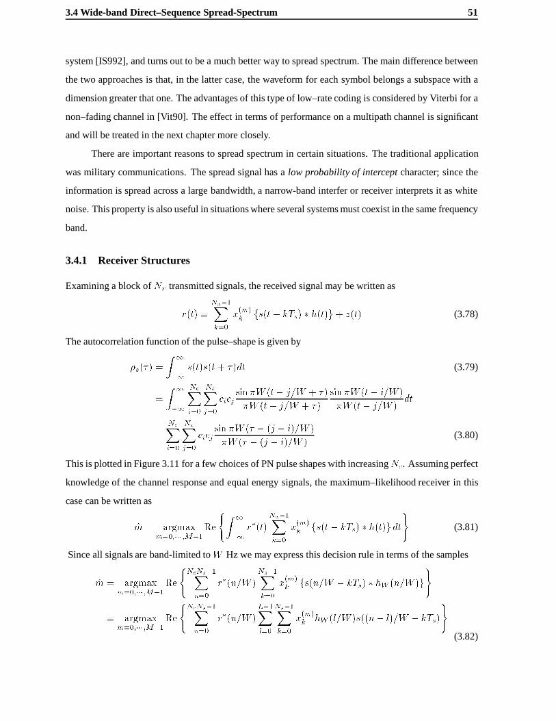
3.4 Wide-band Direct–Sequence Spread-Spectrum 51
system [IS992], and turns out to be a much better way to spread spectrum. The main difference between
the two approaches is that, in the latter case, the waveform for each symbol belongs a subspace with a
dimension greater that one. The advantages of this type of low–rate coding is considered by Viterbi for a
non–fading channel in [Vit90]. The effect in terms of performance on a multipath channel is significant
and will be treated in the next chapter more closely.
There are important reasons to spread spectrum in certain situations. The traditional application
was military communications. The spread signal has alow probability of interceptcharacter; since the
information is spread across a large bandwidth, a narrow-band interfer or receiver interprets it as white
noise. This property is also useful in situations where several systems must coexist in the same frequency
band.
3.4.1 Receiver Structures
Examining a block ofNx transmitted signals, the received signal may be written as
r(t) =Nx�1Xk=0
x(m)k fs(t � kTs) � h(t)g+ z(t) (3.78)
The autocorrelation function of the pulse–shape is given by
�s(�) =
Z 1
�1s(t)s(t+ �)dt (3.79)
=
Z 1
�1
NcXi=0
NcXj=0
cicjsin �W (t� j=W + �)
�W (t� j=W + �)
sin �W (t� i=W )
�W (t� j=W )dt
=NcXi=0
NcXj=0
cicjsin �W (� � (j � i)=W )
�W (� � (j � i)=W )(3.80)
This is plotted in Figure 3.11 for a few choices of PN pulse shapes with increasingNc. Assuming perfect
knowledge of the channel response and equal energy signals, the maximum–likelihood receiver in this
case can be written as
m = argmaxm=0;��� ;M�1
Re
(Z 1
�1r�(t)
Nx�1Xk=0
x(m)k fs(t � kTs) � h(t)gdt
)(3.81)
Since all signals are band-limited toW Hz we may express this decision rule in terms of the samples
m = argmaxm=0;��� ;M�1
Re
(NcNs�1Xn=0
r�(n=W )Ns�1Xk=0
x(m)k fs(n=W � kTs) � hW (n=W )g
)
= argmaxm=0;��� ;M�1
Re
(NcNs�1Xn=0
r�(n=W )L�1Xl=0
Ns�1Xk=0
x(m)k hW (l=W )s((n� l)=W � kTs)
)(3.82)
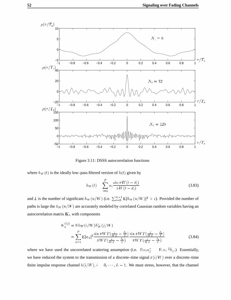
52 Signaling over Fading Channels
−1 −0.8 −0.6 −0.4 −0.2 0 0.2 0.4 0.6 0.8 1−5
0
5
10
−1 −0.8 −0.6 −0.4 −0.2 0 0.2 0.4 0.6 0.8 1−20
0
20
40
−1 −0.8 −0.6 −0.4 −0.2 0 0.2 0.4 0.6 0.8 1−50
0
50
100
150
Nc = 8
Nc = 32
Nc = 128
�(�=Ts)
�(�=Ts)
�(�=Ts)
�=Ts
�=Ts
�=Ts
Figure 3.11: DSSS autocorrelation functions
wherehW (t) is the ideally low–pass filtered version ofh(t) given by
hW (t) =PXi=1
�isin �W (t� di)
�W (t� di)(3.83)
andL is the number of significanthW (n=W ) (i.e.PL�1
l=0 EjhW (n=W )j2 > �). Provided the number of
paths is large thehW (n=W ) are accurately modeled by correlated Gaussian random variables having an
autocorrelation matrixKh with components
K(ij)h = EhW (i=W )h�W (j=W )
=PXk=1
Ej�kj2sin �WT ( i
WT � dkT )
�WT ( iWT � dk
T )
sin �WT ( jWT � dk
T )
�WT ( jWT � dk
T )(3.84)
where we have used the uncorrelated scattering assumption (i.e.E�i��j = Ej�ij2�ij .) Essentially,
we have reduced the system to the transmission of a discrete–time signalx(i=W ) over a discrete–time
finite impulse response channelh(i=W ); i = 0; � � � ; L � 1. We must stress, however, that the channel

3.4 Wide-band Direct–Sequence Spread-Spectrum 53
coefficients are highly correlated. It is common in the literature when using discrete–time multipath
models to assume uncorrelated taps which can yield highly optimistic performance results. To see the
extent of this correlation consider the ETSI TU channel described in Chapter 2 withTs = 104:67�s. The
significant number of taps in the filter response and the correlation matrices for differentNc = WTs for
the first 5 taps are shown in Table 3.1.
WTs Number of significant taps Correlation of taps 1-5
8 2
0BBBBBBBBB@
0:9671 0:0726 �0:0331 0:0214 �0:01590:0726 0:0153 �0:0065 0:0041 �0:0030�0:0331 �0:0065 0:0028 �0:0018 0:0013
0:0214 0:0041 �0:0018 0:0011 �0:0008�0:0159 �0:0030 0:0013 �0:0008 0:0006
1CCCCCCCCCA
32 3
0BBBBBBBBB@
0:7554 0:1662 �0:0689 0:0423 �0:03070:1662 0:1701 �0:0284 0:0197 �0:0145�0:0689 �0:0284 0:0231 �0:0109 0:0075
0:0423 0:0197 �0:0109 0:0057 �0:0040�0:0307 �0:0145 0:0075 �0:0040 0:0028
1CCCCCCCCCA
128 8
0BBBBBBBBB@
0:3822 0:1321 �0:0627 0:0400 �0:02860:1321 0:3040 �0:0066 0:0060 �0:0058�0:0627 �0:0066 0:1278 �0:0053 0:0055
0:0400 0:0060 �0:0053 0:0586 �0:0056�0:0286 �0:0058 0:0055 �0:0056 0:0519
1CCCCCCCCCA
Table 3.1: Significant taps and tap correlation
We now make a critical assumption which holds true in many spread–spectrum applications by
takingL � Nc which means that the channel is practically free of multipath inducedintersymbol inter-
ference (ISI). In the example we just mentioned this is definitely the case since the delay spread is on
the order of 5�s. Under this assumption, the proportion of received energy in[kTs; (k + 1)Ts] due to
symbolsx(m)i ; i 6= k is neglible so that the decision rule may be approximated by
m = argmaxm=0;��� ;M�1
Re
(Ns�1Xk=0
Nc�1Xn=0
L�1Xl=0
x(m)k r�(kTs + n=W )hW (l=W )s((n� l)=W )
)(3.85)
54 Signaling over Fading Channels
We may define the set of sufficient statistics
rk =Nc�1Xn=0
L�1Xl=0
r�(kTs + n=W )hW (l=W )s((n� l)=W ) (3.86)
so that the decision rule becomes
m = argmaxm=0;��� ;M�1
Re
(Ns�1Xk=0
r�kx(m)k
)(3.87)
The operation in (3.86) is known as acoherent RAKEreceiver since it acts like a garden rake on the
multipath components by combining their energies in the same fashion as the maximal–ratio combiner
we considered in Section 2.1.
3.4.2 RAKE Receiver Performance
Let us assume that messagefx(0)k g is sent so that
rk =Nc�1Xn=0
x(0)k
L�1Xl=0
h�W (l=W )s((n� l)=W ) + z(n=W )
!L�1Xl0=0
hW (l0=W )s((n� l0)=W )
= x(0)k
L�1Xl=0
L�1Xl0=0
hW (l0=W )h�W (l=W )�s((l� l0)=W ) +Nc�1Xn=0
L�1Xl=0
hW (l=W )s((n� l)=W )z(n=W )
= x(1)k h�Ph+ zk (3.88)
whereEjzkj2 = N0PL�1
l=0 jhW (l=W )j2 � N0, h =�hW (0) � � � hW ((L� 1)=W )
�TandP i;j =
�s((i�j)=W ). As before, the PEP between arbitrary code sequences conditioned on a particular channel
realization is given by
Pejh(0! 1) = Q
0@sjjx(0)� x(1)jj2
2NcN0h�Ph
1A (3.89)
where we have included the normalization factorNc which takes into account the bandwidth expansion
factor. The quadratic form� = h�Ph has moment–generating function
��(s) =L�1Yl=0
1
1� s�l(3.90)
and�l are now the eigenvalues ofKhP. Evaluation of the average PEP is identical to the coherent case
outlined described earlier. In Figure 3.12 we plot the average PEP vs. the signal–to–noise ratio per
information bit for uncoded antipodal signals for different values of the spreading gainWTs. The effect
of spreading on the performance is evident. The number of significant eigenvalues at the SNR shown for
the three spreading bandwidths are 2,3 and 6 which roughly correspond to the slopes of the three curves.

3.5 Multitone Signaling 55
0 5 10 15 20 25 3010
−6
10−5
10−4
10−3
10−2
WTs = 8
WTs = 32
WTs = 128
Pe(0! 1)
E=NcN0 dB
Figure 3.12: DSSS performance for different spreading gains
3.5 Multitone Signaling
We now consider another wideband approach where the signals are described directly in the frequency
domain. As before, we assume complex baseband band-limited signals with a two–sided bandwidth of
W hertz. Let us expand the transmitted signal in time and frequency as
x(t) =S�1Xs=0
N�1Xn=0
xs;n�s;n(t) (3.91)
where the time/frequency ormultitonebasis functions are
�s;n(t) =pWBe
j�fst sin �W (t� n=WB)
�WB(t� n=WB); (3.92)
fs = �W=2 + (s� 1=2)WB andWB = W=S. These basis functions are simply sampling functions for
signals band-limited toWB hertz aroundfs. Although we have chosen the sampling functions as a basis
set, any set of (sufficiently) band-limited time/frequency orthogonal functions will suffice (for instance
raised–cosine pulses). We stress that this is a subset of the set of signals band-limited to[�W=2;W=2],
since we assume that they are flat in any sub-band of bandwidthWB. This is not a significant restriction,
since the sub-bands can be made arbitrarily small. This type of modulation scheme is often also referred
to asorthogonal frequency–division multiplexing (OFDM).

56 Signaling over Fading Channels
One of the main practical problems with this type of signaling is the high peak–to–average power
ratio when a large number of sub-bands are used. This is especially problematic in wireless applications
since there is a need for highly linear power amplifiers over the large dynamic range of the signal. A
clever way to reduce the dynamic range of the signal when the number of sub-bands is not too large is to
use specially designed coding schemes which reduce the peak–to–average power ratio [WJ95],[VN96].
3.5.1 Multitone Receiver and Performance Criteria
The received signal may now be written as
y(t) =S�1Xs=0
N�1Xn=0
xs;nhs(t � n=WB) + z(t); (3.93)
wherehs(t) is the portion of the channel response in sub-bands given by
hs(t) =
Z fs+WB=2
fs�WB=2ej2�ftH(f)df; (3.94)
andH(f) is the Fourier Transform ofh(t). Projecting the output onf�f;n(t)g yields
ys;n =N�1Xn0=0
xs;n0hs;n;n0 + zs;n (3.95)
where
hs;n;n0 =
Z fs+WB=2
fs�WB=2H(f)e
j2�(n�n0)
WBfdf (3.96)
We assume thatWB is small enough (or equivalentlyF is large enough) to assure thatdLWB � 1,
wheredL is the delay spread, yielding
hs;n;n0 � H(fs)�n;n0 (3.97)
For this assumption to be valid in practice, we require thatWB be much less than the coherence band-
width of the channel as described in Chapter 2.
The frequency autocorrelation function of the channel responseH(f) was given in Chapter 2 and
denoted�(f1 � f2). We now denote the autocorrelation matrix for the sub-band strengths by
KH =
0BBBBBBBBBB@
�(0) �(W=S) �(2W=S) � � � �((S � 1)W=S)
�(W=S). .. . .. . .. �((S � 2)W=S)
�(2W=S). .. . .. . ..
......
. .. . .. . .....
�((S � 1)W=S) �((S � 2)W=S) � � � � � � �(0)
1CCCCCCCCCCA (3.98)
3.5 Multitone Signaling 57
This significant eigenvalues of this matrix are good approximations to those of the corresponding kernel
�(f1� f2) [VT68]. The conditional PEP in this case between arbitrary sequencesx(0)s;n andx(1)s;n is given
by
Pejh(0! 1) = Q
0@sd2(0; 1)
2N0
1A (3.99)
where
d2(0; 1) =N�1Xn=0
S�1Xs=0
jx(0)s;n � x(1)s;nj2jH(fs)j2
=S�1Xs=0
jH(fs)j2d2s(0; 1) (3.100)
whered2s(0; 1) is the Euclidean distance between the signal components in sub-bands. The performance
computation is identical to earlier coherent cases and the moment–generating function of the pairwise
distance is given by
�d(s) =S�1Yi=0
1
1� s�i(3.101)
where�i are now the eigenvalues ofKHD withD = diag(d2s(0; 1)). Not surprisingly, this is an analo-
gous result to the partially–interleaved narrow-band channel and similarly with appropriate interleaving
can be cast into the framework the block–fading channel discussed in section 3.6.
3.5.2 Multitone spread–spectrum
As in the case of DSSS, let us now assume that each codewordx(t) lies in aWLT–dimensional subspace
of theWT–dimensional signal space, so that the number of Shannon dimensions is less than the number
of degrees of freedom that the channel has to offer. For simplicity, we takeWL = KWB with K being
some integer so that the spreading factor isS=K. Here we opt to perform spreading in the frequency
domain. This has been considered by several authors such as [Van95]. We denote theK–dimensional
information vector for a given time coordinaten by un and write the correspondingF–dimensional
frequency vector as
xn = Gun (3.102)
whereG =�g1 � � � gK
�is thespreading matrix. In order to preserve the input energy, we take the
gi to have unit–norm.
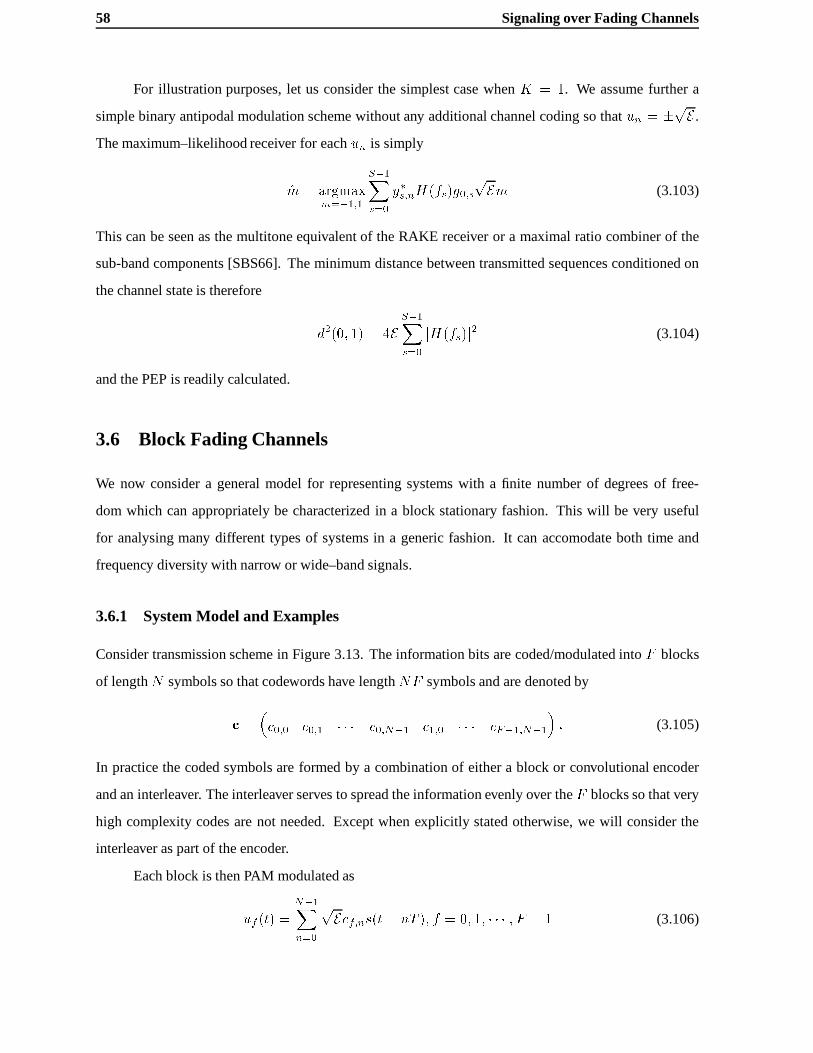
58 Signaling over Fading Channels
For illustration purposes, let us consider the simplest case whenK = 1. We assume further a
simple binary antipodal modulation scheme without any additional channel coding so thatun = �pE .
The maximum–likelihood receiver for eachun is simply
m = argmaxm=�1;1
S�1Xs=0
y�s;nH(fs)g0;spEm (3.103)
This can be seen as the multitone equivalent of the RAKE receiver or a maximal ratio combiner of the
sub-band components [SBS66]. The minimum distance between transmitted sequences conditioned on
the channel state is therefore
d2(0; 1) = 4ES�1Xs=0
jH(fs)j2 (3.104)
and the PEP is readily calculated.
3.6 Block Fading Channels
We now consider a general model for representing systems with a finite number of degrees of free-
dom which can appropriately be characterized in a block stationary fashion. This will be very useful
for analysing many different types of systems in a generic fashion. It can accomodate both time and
frequency diversity with narrow or wide–band signals.
3.6.1 System Model and Examples
Consider transmission scheme in Figure 3.13. The information bits are coded/modulated intoF blocks
of lengthN symbols so that codewords have lengthNF symbols and are denoted by
c =�c0;0 c0;1 � � � c0;N�1 c1;0 � � � cF�1;N�1
�: (3.105)
In practice the coded symbols are formed by a combination of either a block or convolutional encoder
and an interleaver. The interleaver serves to spread the information evenly over theF blocks so that very
high complexity codes are not needed. Except when explicitly stated otherwise, we will consider the
interleaver as part of the encoder.
Each block is then PAM modulated as
uf (t) =N�1Xn=0
pEcf;ns(t� nT ); f = 0; 1; � � � ; F � 1 (3.106)

3.6 Block Fading Channels 59
ML
RECEI
VER
NFR
Pi c0;is(t� iT )
Pi c1;is(t� iT )
Pi cF�1;is(t� iT )
z1(t)
z0(t)
zF�1(t)
Information Bits
ENCODER
S c
NF
cF�1
c1
c0
Interleaver
hF�1(t; �)
h1(t; �)
h0(t; �)
CodedModulation
Figure 3.13: Block–Fading System Model
wheres(t) is some unit–energy pulse shape, andE is the energy per coded symbol. The blocks are
transmitted over different time–varying channels, so that the complex baseband received signals before
processing are given by
rf(t) = uf (t) � hf (t; �) + zf (t); t 2 [0; NT ] ; f = 0; 1; � � � ; F � 1 (3.107)
wherehf (t; �) is the channel response at timet to an impulse at time� on thef th channel, andz(t) is
complex white Gaussian noise with power spectral densityN0.
In what follows we will assume that theF channel realizations are correlated, although it may
well be the case in some systems that they can be taken to be uncorrelated. A system where this model
is appropriate is theGlobal System for Mobile Communication (GSM). Here, blocks modulateF = 4
(half–rate) orF = 8 (full–rate) carriers whose spacing is larger than the coherence bandwidth, resulting
in virtually uncorrelated blocks. This is achieved by changing the frequency allocation scheme inF
adjacent TDMA frames and is known asslow frequency–hopping. The number of blocks is determined
by the tolerable decoding delay�T . Such a system withF = 4 is depicted in Figure 3.14(a). For
reasonable mobile speeds, the channel is stationary during the block. The practical advantages of such
a system are firstly that reliable coherent communication is possible. Secondly and more importantly,
the amount of diversity is independent of the rate of channel variation, since it is a result of exploiting
frequency–selectivity. For mobile telephony, this is crucial since the majority of calls are made at low
speed. Another example is the IS54 standard where coding is performed acrossF = 2 TDMA blocks
separated in time by 20ms so they become less correlated for high mobile speeds. In complete anal-
ogy with the frequency–based scheme, we may call thistime–hoppingand an example withF = 2 is
illustrated in Figure 3.14(b).
We now assume that the time–variation of the channel is slow (i.e. that the coherence time is
greater than the duration of a block) so that that the channel path strengths can be taken to be constant

60 Signaling over Fading Channels
������������������������������
������������������������������
������������������������������
������������������������������������������������������������������������������������������������
������������������������������������������������������������������
������������������������������
������������������������������
��
������������������������������
��������������������������������������������������������������������������������
��������������������������������������������������
�������������������������
�������������������������������������������������������
��������������������������������������������������������������������������������
��������������������������������������������������
�������������������������
�������������������������
������������������������������
������������������������������
������������������������������������������������������������
������������������������������������������������������������
������������������������������������
������������������������������������
������������������������������������������������������������
������������������������������������������������������������
������������������������������
������������������������������
������������������������������������������������������������
������������������������������������������������������������
������������������������������
��������������������������������������������������������������������������������
��������������������������������������������������
������������������������������������
������������������������������������������
������������������������
������������������������������
����������
����������
���������������
���������������
��������������������
��������������������
��������������������
���������������
���������������
���������������
���������������
f
t
t
fc1
fc2
fc3
fc4
BLOCK
1
BLOCK
2
BLOCK
3
BLOCK
4
BLOCK
1
BLOCK
2
�T
(a)
BLOCK 1 BLOCK 2
(b)
�T
Figure 3.14: Frequency and time–hopping
over blocks. We therefore express the complex baseband channel response for each block as
hf (t) =L�1Xl=0
�f;l�(t� df;l); (3.108)
where�f;l anddf;l are the complex attenuation and delay of thelth path in thef th block. As before we
will use the COST 207 models for numerical calculations. The channel realizations are assumed to be
random from block to block but known without error to the receiver. We assume the statistics of the�f;l
to be independent off and further that
E (�f;l � �f;l)��f 0;l0 � �f 0;l0
��= %f;f 0�
2l �l;l0 ; (3.109)
where%f;f 0 is the correlation coefficient between blocksf andf 0. We have, therefore, that different paths
are uncorrelated but that the strengths for a given path are correlated, in general, from block to block.
Furthermore, we assume that the path strengths are normalized asPL�1
l=0 �2l = 1, so that the average
attenuation is included in the transmitted signal strength.

3.6 Block Fading Channels 61
The received signal is processed by a maximum–likelihood decoding rule as
argminm=0;��� ;2FNR�1
F�1Xf=0
Z NT
0
������rf (t)�F�1Xf=0
u(m)f (t�NT ) � hf (t; �)
������2
dt: (3.110)
Decoding in this fashion is too complex to be carried out in practice, and it is usually done in two
steps, depending on the relationship between the coherence bandwidth of the channel and the bandwidth
of s(t). In medium-band systems like GSM where the multipath induces intersymbol interference, a
sub–optimal approach is taken by first equalizing theF channels with a soft–output algorithm (e.g.
soft–output Viterbi equalization [HH89]). These outputs are then deinterleaved and passed to a Viterbi
decoder to retrieve the information bits. In narrow-band systems such as IS-54, the channel has ISI not
extending over more than one symbol time, so that either a very simple equalizer or none at all is needed
prior to deinterleaving/decoding. In wide-band systems with little ISI, equalization is also not required
and some of the multipath can be exploited with a RAKE receiver prior to decoding as we outlined
earlier.
Many systems which use coding schemes over a fading channel with a finite number of degrees
of freedom can be cast into the framework. We mentioned earlier that this was both the case for the
partially–interleaved narrow-band channel and the static multitone channel. Let us consider this more
closely now that we have defined them precisely. In the partially–interleaved narrow-band case, the
number of degrees of freedom was aroundF = d2fDT + 1e whereT = NLTs was the total decoding
delay. Similarly the number of degrees of freedom for the multitone case was aroundF = dWdL + 1e.Suppose now we use an interleaver with depthN = F and widthL = T=(FTs). This arrangement is
close to the block–fading channel withF blocks each containingL symbols. Every set ofF adjacent
symbols are virtually uncorrelated at the receiver and symbols separated by multiples ofF symbols (i.e.
belonging to the same block) are strongly correlated. Without this choice for the interleaver, the coding
problem was difficult because the location of non–zero symbols in the error–event was critical in the
expression for the PEP. We will show in the remainder of this section that for the block–fading channel
this is not a problem and in Chapter 5, how high performance codes can be designed.
Denoting the codewords asc =�c0 c1 � � � cF�1
�, the PEP conditioned on a particular set
of channel realizations is given by
Pejhi(t)(0! 1) = Q
rd2(0; 1)
E2N0
!; (3.111)

62 Signaling over Fading Channels
whered2(0; 1) is the squared Euclidean distance between the code sequences given by
d2(0; 1) =F�1Xf=0
Z NT
0
�����N�1Xn=0
L�1Xl=0
�c(0)f;n � c
(1)f;n
��f;ls(t� nT � df;l)
�����2
dt
=F�1Xf=0
N�1Xn;n0=0
L�1Xl;l0=0
�c(0)f;n � c
(1)f;n
��f;l�
�f;l0
�c(0)�f;n0 � c
(1)�f;n0
��s�(n� n0)T + (df;l � df;l0)
�
=F�1Xf=0
(c(0)f � c(1)f )
8<:
L�1Xl;l0=0
�f;l��f;l0Pf;l;l0
9=; (c
(0)f � c(1)f )� (3.112)
whereP (ij)f;l;l0 = �s
�(i� j)T + (df;l � df;l0)
�and�s(t) is given by (3.79). This can be simplified to the
quadratic form
d2(0; 1) =F�1Xf=0
��f�f(0; 1)�f
=h��0 ��1 � � � ��F�1
i26666666664
�0(a; b) 0 0 � � � 0
0 �1(a; b) 0 � � � 0
0 0... 0 0
: : : : : : : : : : : : : : : : : : : : : : : : : : : : : : : : : :
0 � � � 0 0 �F�1
37777777775
26666664
�0
�1
� � ��F�1
37777775 (3.113)
= ����; (3.114)
where�(ll0)
f (0; 1) = (c(0)f � c(0)f )Pf;l;l0(c
(0)f � c(1)f )�, and�f =
��f;0 � � ��f;L�1
�T. Again we have
a quadratic form of a correlated Gaussian random vector so that the moment–generating function of
z = d2(0; 1) Es2N0
is
�z(s) =
dFHL�1Yi=0
1
1� s�iEs=2N0; (3.115)
wheref�ig are thenon–zeroeigenvalues of the matrix
R�� =
26666664
��0(0; 1) %1;0��1(0; 1) : : : %F�1;0��F�1(0; 1)
%0;1��0(0; 1) ��1(0; 1) : : : %F�1;1��F�1(0; 1)
: : : : : : : : : : : : : : : : : : : : : : : : : : : : : : : : : : : : : : : : : : : : : : : : : : : : : : : : : : :
%0;F�1��0(0; 1) %1;F�1��1(0; 1) : : : ��F�1(0; 1)
37777775;
(3.116)
anddFH is the number of non–zero�f (0; 1) (or equivalently theHamming distancebetweenc(a) andc(b)
with the symbols taken as the sub–vectorscf ) and� = diag(�20; �21; � � � ; �2L�1).

3.6 Block Fading Channels 63
For the even simpler case where the blocks are uncorrelated (i.e.%f;f 0 = �f;f 0) (3.115) can be
written as
�z(s) =
dFHYi=0
L�1Yl=0
1
1� s�i;lEs=2N0; (3.117)
where�i;l is thelth eigenvalue of the non–zero matrix�i = ��i(0; 1). For very wide-band systems
without ISI (i.e. the bandwidth ofs(t) is much larger than the coherence bandwidth and the symbol
rate),Pf;l;l0 � �ll0I so that�f;l = j�f;lj2d2�c(0)f ; c
(1)f
�. For narrow-band systems without ISI (i.e.
jdf;l � df;l0j � T ) Pf;l;l0 � I so that�f;l = d2�c(0)f ; c
(1)f
��l. These are the two limiting cases for
the diversity offered by multipath. The first corresponds to when it can be completely resolved, and the
second when it cannot be resolved at all. The theoretical performance of a system will fall somewhere
between the performance of these two limits which are straightforward to compute. The diversity factor
due to coding isdFH and is completely independent of the extent of multipath, as long as the channels are
independent. This means that from the point of view of code design, it is sufficient to consider only a
narrow-band channel which greatly simplifies the problem. We note, however, in contrast to the perfectly
interleaved case the diversity factor due to coding is limited toF and does not grow with the length of
the codewords. These issues will be the focus of Chapter 5.
The computation of the average PEP is identical to the earlier cases once the eigenvalues have
been determined. We have computed it exactly for narrow, medium and wide-band pulse shapes and
chose examples inspired the IS–54, GSM and IS–95 cellular radio systems which respectively fall into
these three categories. The narrow–band pulse shape is a root raised cosine with roll–off .35 andT =
41:15�swhile the medium–band is GMSK withBT = :3 andT = 3:69�s (see Feher [Feh95] regarding
GMSK.) For the wide-band pulse shape we used an FIR filtered 128 chip/symbol PN sequence with
T = 164:16�s, with the filter coefficients taken from the IS–95 specifications [IS992]. We also compute
the PEP for an un-filtered PN pulse to identify the loss due to filtering. The goal is not to compare the
systems, since this is by no means a fair comparison, but to determine to what degree the multipath can
be exploited on typical channels. In Figures 3.15–3.17 we show the PEP vs.Es=N0 for the TU, RA and
HT responses given in Chapter 2 along with the significant eigenvalue spread. We have assumedF = 2
blocks of lengthN = 100 antipodal symbols withd2(c(0)0 ; c(1)0 ) = 4 andd2(c(0)1 ; c
(1)1 ) = 8, so that there
two sets of eigenvalues corresponding to the two blocks. In all cases the narrow-band system is almost
completely unresolved and has two significant eigenvalues equal to the two Euclidean distances between
the codewords. The medium-band system benefits greatly from multipath, especially on the urban and
hilly channels which have delay spreads extending over several symbols. This shows the effect that

64 Signaling over Fading Channels
equalization can have in a multipath environment. The wide-band pulse exploits the multipath to a great
extent, but it is still far from being completely resolved. Moreover, there is a noticeable loss due to
filtering. In Fig. 3.18 we examine the effect of correlation betweenF = 2 blocks with the narrow–band
pulse shape. Surprisingly, even with a correlation coefficient as high as .5, there is very little degradation.
0 10 20 30 40 50 60 7010
−2
10−1
100
101
0 2 4 6 8 10 12 14 16 18 2010
−5
10−4
10−3
10−2
0 0.5 1 1.5 2 2.5 3 3.5 4 4.5 50
0.05
0.1
0.15
0.2
0.25
0.3
0.35
0.4
Significant Eigenvalues
(filtered)
Es=N0
Delay Spread
t(�s)
Pr(c(a) ! c(b))
Res. PN PN
Medium
Narrow
ResolvedPN
Medium Narrow
PN (filtered)
Figure 3.15: PEP and eigenvalues for the TU channel
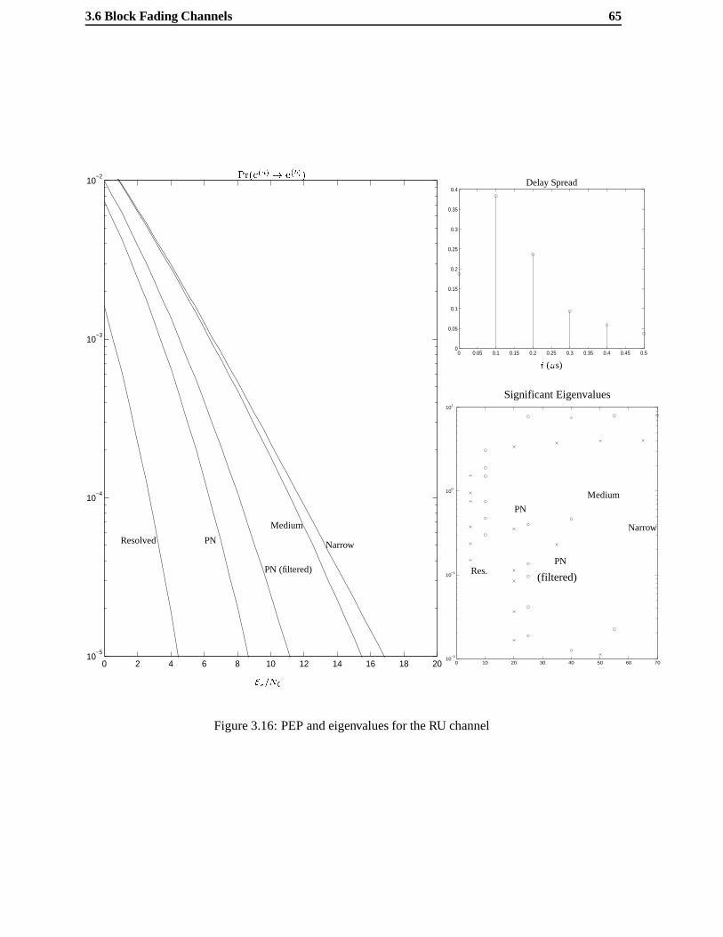
3.6 Block Fading Channels 65
Significant Eigenvalues
0 2 4 6 8 10 12 14 16 18 2010
−5
10−4
10−3
10−2
0 0.05 0.1 0.15 0.2 0.25 0.3 0.35 0.4 0.45 0.50
0.05
0.1
0.15
0.2
0.25
0.3
0.35
0.4
0 10 20 30 40 50 60 7010
−2
10−1
100
101
(filtered)
Es=N0
Delay Spread
t (�s)
Pr(c(a) ! c(b))
Res.
PN
PN
Medium
NarrowResolved PN
PN (filtered)
Medium
Narrow
Figure 3.16: PEP and eigenvalues for the RU channel

66 Signaling over Fading Channels
Significant Eigenvalues
0 2 4 6 8 10 12 14 16 18 200
0.05
0.1
0.15
0.2
0.25
0.3
0.35
0.4
0.45
0 10 20 30 40 50 60 7010
−2
10−1
100
101
0 2 4 6 8 10 12 14 16 18 2010
−5
10−4
10−3
10−2
Filtered
(filtered)
Es=N0
Delay Spread
t (�s)
Pr(c(a) ! c(b))
ResolvedPN
Medium
PN
Narrow
Res. PN
PN
Medium Narrow
Figure 3.17: PEP and eigenvalues for the HT channel

3.6 Block Fading Channels 67
0 2 4 6 8 10 12 14 16 18 2010
−8
10−7
10−6
10−5
10−4
10−3
10−2
10−1
.1
.01
.001
1
10
% = 1 % = :9 % = :5 % = 0
Significant Eigenvalues
% = 0
Es=N0 (dB)
% = :9
% = :5
% = 1
Pr(c(a) ! c(b))
Figure 3.18: PEP and eigenvalues for a 2 block example

68 Signaling over Fading Channels

Chapter 4
Mutual Information and Information
Outage Rates
In this chapter we take a fundamental look at the achievable performance for the coded systems described
in Chapter 2 and we restrict our treatment to single–user channels. The multiuser case will be considered
in Chapter 7. To this end we use information–theoretic techniques to analyze the average probability
of codeword error and the achievable information rates under different system model assumptions. We
rely heavily on some previous work and extend their results. First is the classic text by Gallager [Gal68]
which is referenced often in this chapter. Second is the recent work by Ozarowet al.defining the concept
of information outage probability[OSSW94]. We will see that for systems with a time–delay constraint
that this quantity is crucial in defining system performance limits. This is often the case in mobile radio
systems.
We first describe a generic discrete–time model for time–varying channels in order to describe the
role of average mutual informationand how it naturally leads to the information outage probability and
to a lower–bound on the achievable error–rate performance. We then turn our attention to the additive
white Gaussian noise channel with fading described in Chapter 2. We consider the case of systems
operating without channel state feedback and give numerical examples of the information outage rates.

70 Mutual Information and Information Outage Rates
4.1 A generic time–varying channel model and basic definitions
Consider the discrete–time communication system in Figure 4.1 which operates overNx dimensions and
has code-rate
R =log2M
Nxbits=dim; (4.1)
whereM is the number of codewords used by the transmitter. The input symbolsfxk; k = 0; � � � ; Nx�1g are drawn from a continuous real alphabetSX j R. TheNx input symbols are transmitted across a
channelC : X ! Y with transition probabilityfYjX;H(yjx; h) which depends on an auxiliary random
variableH . This plays the role of the state of the channel during transmission of theNx symbols or
codeword. We denote the distribution function of the channel state byFH(h). The channel output
symbols belong to another continuous alphabetSY j Rwhich need not be the same asSX . We will
assume throughout that the receiver has complete knowledge of the channel stateH , and that, in this
chapter, the transmitter has noaccess to this information.
H;FH(h)
yi 2 SYxi 2 SXx = fx0; x1; � � � ; xNx�1g y = fy0; y1; � � � ; yNy�1g
X
fYjX;H(yjx; h)
C : X ! Y
Y
Figure 4.1: Generic fading channel model
Since there is no channel state feedback, the transmitter and receiver agree beforehand on accept-
able choices forR andfX and do not modify them during the course of communication. We first recall
an upper–bound on the ensemble average probability of codeword error (i.e. taken over all possible
codes chosen at random) conditioned on the channel stateH . We denote this probability byPensjH .
From [Gal68] we have the following theorem and note that the only deviation from its original form is
the additional conditioning on the channel stateH .
Theorem 1 (Gallager)
An input source withNx–dimensional joint probability densityfX(x) transmitting over a channel with
transition probabilityfYjX;H(yjx; h) depending on an auxiliary random variableH has an ensemble
average probability of codeword error taken conditioned onH which is upper–bounded by
PensjH=h � 2�Nx(E0(�;fX;H=h)��R) (4.2)

4.1 A generic time–varying channel model and basic definitions 71
R0
R0 I(Y;X)Rc
Er(R)
R
Figure 4.2: A typical random coding exponent curve
where
E0(�; fX; H = h) = � 1
Nxlog2
Z� � �Z
y
0@Z � � �
Zx
fX(x)fYjX;H(yjx; h)1
1+�dx
1A1+�
dy;
(4.3)
R is given by (4.1) and� is arbitrary in [0; 1].
The quantity in (4.3) is commonly referred to as theGallager function. The exponent in (4.2) is always
maximized over� to yield the tightest upper bound. The maximum for eachH is denoted
Er(R; fX; H = h) = max0���1
E0(�; fX; H = h)� �R; (4.4)
When it is maximized over the input distribution,fX, it is known as the random coding exponent. Its
typical shape is shown in figure 4.2 and it can normally only be expressed in parametric form.
There is a straight–line portion between[0; Rc(H)]whereRc(H) is known as thecritical rate and
is given byRc(H) = @E0(�;fX;H=h)@�
����=1
. The random coding exponent in this region isEr(R; fX; H =
h) = R0(H) � R whereR0(H) = E0(1; fX; H = h) is known as thecutoff–rate. The maximum
value ofR for which the random coding exponent remains non–negative isR = @E0(�;fX;H=h)@�
����=0
=
I(Y;XjH = h) = IH is theaverage mutual informationbetween the input and output vectors condi-

72 Mutual Information and Information Outage Rates
tioned on aparticular realizationH = h of the channel state. It is given by
IH =1
Nx
Z� � �Z
x
Z� � �Z
y
fX(x)fYjX;H(yjx; h) (4.5)
log2fYjX;H(yjx; h)R � �� R
x
fX(x)fYjX;H(yjx; h)dxdydx bits=dim:
We must stress that this is not a conditional mutual information functional and to avoid confusion we
have used a slightly different notation. The conditional average mutual information betweenY andX is
I(Y;XjH) = EH IH . We will see the importance of this functional later.
The first important observation is thatIH is a random variable. This means that, depending on the
nature of the underlying channel process, it is possible thatIH < R for some realizations ofH . For this
reason, it is more appropriate to express the bound in (4.2) as
PensjH=h �
8><>:1 IH < R
2�NxEr(R;fX;H=h) IH � R
(4.6)
We may now bound the code–ensemble average probability of error as
Pens = EHPejH � Pout(R; fX) +
Zh:IH�R
2�NxEr(R;fX;H=h)dFH(h) (4.7)
where
Pout(R; fX) = Prob(IH < R): (4.8)
Since the code ensemble average error–probability is upper–bounded by the right–hand side of (4.7)
there is at least one code for which (4.7) holds. Unlike the time–invariant channel case, however, the ir-
reducible term in (4.7) (Pout(R; fX)) is independent of the number of code dimensionsNx and therefore
casts some doubt as to whether arbitrarily small error probabilities can be achieved.
To get an idea of the achievable performance we now express the average codeword error proba-
bility for a particular code (i.e. not an ensemble average) as
Pe = PejIH�R (1� Pout(R; fX)) + PejIH<RPout(R; fX) (4.9)
� PejIH<RPout(R; fX)
Practically speaking, this lower–bound onPe is meaningful if we consider what is known as the strong
converse to the coding theorem:

4.1 A generic time–varying channel model and basic definitions 73
Theorem 2 ([Wol78])
The probability of codeword error conditioned on the channel state,H whenR > IH is lower–bounded
by
PejH > 1� 4A(h)
Nx(R� I(X;YjH = h))2� 2�
Nx(R�I(X;YjH=h))2 (4.10)
whereA(h) is a finite positive constant independent ofNx and the number of codewordsM .
As a result of this theorem, forR > IH we have thatPejH=h must tend to 1 with increasingNx for all
codes. This result can be extended to show [Gal68] thatPejH must tend to 1 exponentially inN . In our
context, this ensures thatPejIH<R � 1 if Nx is large so thatPe ' Pout(R; fX). In the limitNx !1 we
have thatPe = Pout(R; fX) since the inequalities in (4.7) and (4.10) converge. Ozarowet al[OSSW94]
recognized the importance ofPout(R; fX) for systems operating over fading channels but its relationship
with the achievable codeword error probability was not explicitly shown.
The reader may wonder whether why this is an important result since the use of the strong con-
verse says nothing about the error probability of the individual source symbols or thesymbol error rate.
We note, however, that for many practical systems which are burst or block oriented, it is precisely the
codeword error rate that is important. This is true for the transmission of some forms of digitized speech
and in packet data communications. Typically, data is arranged into bursts and then coded for transmis-
sion using both error correction and error detection techniques. At the receiver the information burst is
decoded and then checked for data integrity using the error detection scheme. If the burst is deemed
intact, the data is passed to the next level of the system. On the other hand, if the data is corrupted then
the burst is often discarded or a retransmission is requested. Provided the number of symbols in the burst
(Nx) is large and a sophisticated coding scheme is used,Pout(R; fX) will be a good indicator of the
achievable codeword error rate performance.
The weak converse (Fano’s inequality) yields a less useful lower bound on the codeword error
probability since it only shows thatPejIH>R is bounded away from zero when in an outage state. From
[CT91] we have explicitly that
Pe � 1� 1
NxR� IH
R; IH < R; (4.11)
so that the average probability of codeword error is lower bounded by
Pe ��1� 1
NxR
�Pout(R; fX)� 1
R
Zh:IH�R
IHdFH(h): (4.12)

74 Mutual Information and Information Outage Rates
It is, however, more useful for obtaining a lower–bound to the bit error probability,Pb. It is shown in
[Bla87] that the bit error probability conditioned onIH > R satisfies
H(PbjIH>R) � 1� IHR
(4.13)
whereH(�) is the binary entropy function
H(x) = �x log2(x)� (1� x) log2(1� x): (4.14)
The expression in (4.13) is only valid when the information source has maximum entropy. This yields
the lower bound on the bit error probability
Pb �Zh:IH�R
H�1
�1� IH
R
�dFH(h); (4.15)
whereH�1(�) is taken to mean the smaller of the two roots of (4.13).
4.1.1 Block–Fading Channels
In some cases the information outage probability may be zero. We will see that this can occur when
the transmitter hasa priori knowledge of the channel state and can adjust eitherR or fx accordingly.
Another instance where this is the case is when coding can be performed across many channel states,
sayF , as shown in figure 4.3. Here each block usesN dimensions so thatNx = NF . Under the
assumption that theF channel outputsyi; i = 0; � � � ; F � 1 are independent then the total average
mutual information conditioned on theF channel states is
IfH0;H1;��� ;HF�1g =1
NF
F�1Xi=0
I(Yi;XijHi = hi) ,1
F
F�1Xi=0
IHi: (4.16)
This is simply the block–fading channel we consider in section 3.6 on a more abstract level. This is also
referred to as a block–interference channel by McEliece and Stark in [MS84], who considered different
interference models, including the Rayleigh fading channel. If the set of channel realizations is an ergodic
sequence then in the limitF !1 we fall back on the traditional conditional average mutual information
since
I1 = limF!1
1
F
F�1Xi=0
IHi= EHIH = I(Y;XjH); (4.17)
and consequently
Pout(R; fX) = I(I(Y;XjH) < R); (4.18)
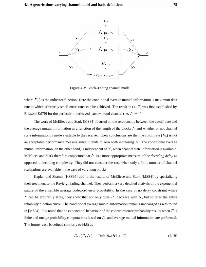
4.1 A generic time–varying channel model and basic definitions 75
H0
H1
HF�1
fY0jX0;H0
fY1jX1;H1
fYF�1jXF�1;HF�1
x yx1 y1
yF�1
y0
xF�1
x0
Figure 4.3: Block–Fading channel model
whereI(�) is the indicator function. Here the conditional average mutual information is maximum data
rate at which arbitrarily small error–rates can be achieved. The result in (4.17) was first established by
Ericson [Eri70] for the perfectly–interleaved narrow–band channel (i.e.N = 1).
The work of McEliece and Stark [MS84] focused on the relationship between the cutoff–rate and
the average mutual information as a function of the length of the blocksN and whether or not channel
state information is made available to the receiver. Their conclusions are that the cutoff rate (R0) is not
an acceptable performance measure since it tends to zero with increasingN . The conditional average
mutual information, on the other hand, is independent ofN , when channel state information is available.
McEliece and Stark therefore conjecture thatR0 is a more appropriate measure of thedecoding delayas
opposed to decoding complexity. They did not consider the case when only a finite number of channel
realizations are available in the case of very long blocks.
Kaplan and Shamai [KSS95] add to the results of McEliece and Stark [MS84] by specializing
their treatment to the Rayleigh fading channel. They perform a very detailed analysis of the exponential
nature of the ensemble average codeword error probability. In the case of no delay constraint where
F can be arbitrarily large, they show that not only doesR0 decrease withN , but so does the entire
reliability function curve. The conditional average mutual information remains unchanged as was found
in [MS84]. It is noted that no exponential behaviour of the codeword error probability results whenF is
finite and outage probability computations based onR0 and average mutual information are performed.
The former case is defined similarly to (4.8) as
Pout(R; fX) = Prob(R0(H) < R): (4.19)

76 Mutual Information and Information Outage Rates
The behaviour of this measure is similar to (4.8) except that the outages are noticeably higher. It has
less theoretical justification than (4.8) and may yield pessimistic results. Traditionally [Mas74],[Vit79]
R0 was taken to be the highest rate at which practical coding schemes can be implemented on ergodic
channels. Humblet [Hum85] showed that on a direct detection optical channel there exist reasonably
simple codes whose rates exceed those predicted byR0 with acceptably low error probability. In recent
years, the invention ofturbo codes[BGT93] has given rise to practical evidence thatR0 may not be a
practical limit even on a Gaussian channel. We will see in the next chapter that some practical codes,
which are not even as complex as turbo codes, can come very close to (4.8) when the number of blocks
is small which shows that mutual information outage is sometimes more appropriate in our case as well.
The main reason for this is that when the number of blocks (or degrees of freedom) is small,Pout(R) is
quite high and even fairly simple codes have average error probabilities on the order ofPout(R) when
IH > R (i.e. when the system is not operating in an outage situation.)
4.2 Additive White Gaussian Noise (AWGN) Channels with Fading
We would now like to apply the ideas of the previous section for a communication system modeled by
y(t) =
Z T=2
�T=2x(�)h(t; �)d� + z(t) = s(t) + z(t) (4.20)
The continuous–time random message sent across the channel by the transmitter,x(t), is time–limited
to [�T=2; T=2] and has correlation functionKx(t; u) . The channel is modeled by a time–variant filter,
h(t; �), which is response at timet to an impulse at time� , and has duration (delay spread)Th. The noise
signal,z(t), is a complex, zero–mean, circular symmetric Gaussian process with correlation function
Kz(t; �) = N0�(t � �) andy(t) is the signal at the receiver. We assume that the channel response is
known perfectly to the receiver.
4.2.1 Calculating the Average Mutual Information
The received signal in the absence of noise,s(t), can be expressed in terms of its Karhunen-Lo`eve
expansion
s(t) =1Xi=1
si�i(t) (4.21)

4.2 Additive White Gaussian Noise (AWGN) Channels with Fading 77
wheresi are independent random variables with variance�i(T;H) which, along with the basisf�i(t :T;H); �To=2 � t � To=2g, are the solution to
�i(T;H)�i(t : T;H) =
Z To=2
�To=2Ks(t; u)�i(u : T;H)du (4.22)
withKs(t; u) =R T=2�T=2
R T=2�T=2
Kx(�; �0)h(t; �)h�(u; � 0)d�d� 0 and whereTo = T+Th. Note that we have
explicitly indicated the dependence of the eigenvalues and eigenfunctions on the codeword duration and
the channel state. This expansion allows us to write (4.20) equivalently as
yi = si + zi (4.23)
whereyi andzi are projections of the received signal and noise on the signal basisf�i(t : H)g given by
[yi; zi] =
Z T=2
�T=2[y(t); z(t)]�i(t : T;H)dt; (4.24)
where since the noise is white, thezi are independent and have varianceN0. We have assumed that
the channel response is known perfectly to the receiver and thus can, at least in principle, determine the
message which was transmitted froms(t). As a result, we are interested in the quantity
IT;H =1
TI(S(t); Y (t)jH(t; �) = h(t; �))
=1
T
1Xi=1
I(Si; YijH(t; �) = h(t; �)) bits=s (4.25)
We have been rather cavalier in writing (4.25) and this deserves some explanation. In reality it only
holds in a mean–square sense since the KL expansion is a mean–square representation of the process.
It was shown by Kadotaet al [KZZ71] that IT;H is simply the mean–squared error of the optimal point
estimator of the processs(t)
IT;H =1
T
Z To=2
�To=2Ejs(t)� s(t)j2dt; (4.26)
where
s(t) =
Z t
�To=2g(t; u)y(u)du (4.27)
whereg(t; u) is the solution to the integral equation
g(t; u) +
Z t
�To=2g(t; z)Ks(z; u)dz = Ks(t; u): (4.28)

78 Mutual Information and Information Outage Rates
If x(t) is a Gaussian process we saw in Chapter 3 when we were dealing with the Gaussian signal
detection problem that
IT;H = � 1
T
Z To=2
�To=2g(t; t)dt =
1
T
1Xi=0
log2
�1 +
�i(T;H)
N0
�bits=s: (4.29)
We quickly run into difficulties using this general approach to solve the problem at hand since in order to
compute the outage probability we need the statistical description ofIT;H . While the numerical compu-
tation ofIT;H for a particular channel realization is straightforward, the computation of its distribution is
a hopeless task. We will now consider different approaches to determine the mutual information between
the input and output signals in (4.20) for specific channel models.
4.2.2 Static Multipath Channels
We begin with an analysis of static multipath channels. We use the term static in the sense that they are
stationary for the duration of a codeword so
h(t; �) =
8><>:h(t � �) �T=2 � � � T=2; �To � t � To=2
0 elsewhere
In the limit of large codeword duration (i.e.T !1), the stationarity of the channel response assures that
Ks(t; �) = Ks(t � �). If we assume further that the channel response is band-limited then by invoking
theSzeg¨o eigenvalue distribution theorem[GS83] yields
IH = limT!1
IT;H =
Z W=2
�W=2log2
�1 +
1
N0Ss(f)
�df bits=s (4.30)
whereSs(f) is the power spectrum of the information process at the output of the channel given by
Ss(f) = Sx(f)jH(f)j2; �W=2 � f � W=2: (4.31)
In a simple sense, this theorem just says that the countable set of eigenvalues�i(T;H) approaches the
power spectrum of the random process, if it is stationary. Assuming an input process bandlimited to
[�W=2;W=2], we introduce the average power constraint on the input process asZ W=2
�W=2Sx(f)df � P: (4.32)
Since average mutual information is a non–increasing function ofT , for a finiteT it follows that
IT;H � IH and consequently thatPout(R; T ) � Pout(R). For largeWT both will practically hold with
equality, since as the number of significant eigenvalues increases they become a very close approximation
to the squared–magnitude of the channel response [VT68].

4.2 Additive White Gaussian Noise (AWGN) Channels with Fading 79
Narrow–band channels
We now use (4.30) to determine the information outage probability for a narrow–band channel example.
If the bandwidthW is considerably less that the coherence bandwidth of the multipath channel, then we
showed in Chapter 2 thatjH(f)j2 = �; �W=2 � f � W=2. Let us assume that the transmitted signal
is chosen to be flat in[�W=2;W=2] asSx(f) = P=W . The information outage probability is therefore
given by
Pout(R) = Prob(W�1IH < R)
= Prob
�� � (2R � 1)
WN0
P
�
= 1� F�
�(2R � 1)
WN0
P
�(4.33)
which in unit–mean square Rayleigh fading gives
Pout(R) = 1� exp
��(2R � 1)
WN0
P
�(4.34)
This was found by Ozarowet al in [OSSW94]. For the more general case of Ricean fading with unit
average attenuation we have from Chapter 2
Pout(R) = 1� Q1
p2K;
r2(2R � 1)
WN0
P(1 +K)
!(4.35)
We plot (4.35) in figure 4.4 as the Ricean factor increases for an SNR of10 log10
�P
WN0
�= 10dB. The
non–fading channel is indicated by a dashed line which is the standard Gaussian channel capacity
CG = W log2
�1 +
P
WN0
�bits=s (4.36)
We see that low codeword error–rates are practically impossible even with a significant LOS component.
As we mentioned in Chapter 2, Ricean factors on the order of 6 dB are common in indoor applications
so that severe degradation can still be expected. We only begin to approach a non–fading channel with
a very strong LOS component. For a non–flat channel closed–form solutions such as (4.35) are unlikely
to exist except in very special cases. Ozarowet al [OSSW94] have considered a two–path channel of the
form
h(t) = �0�(t) + �1�(t� d): (4.37)
They showed that ifd is a multiple of1=W , thenPout(R) can be expressed in terms of the Lobaschevski
functions. For other values ofd it must be computed numerically. Nevertheless, important conclusions

80 Mutual Information and Information Outage Rates
0 0.5 1 1.5 2 2.5 3 3.5 4 4.5 510
−6
10−5
10−4
10−3
10−2
10−1
100
K = 1dB
K = 20dB
K = 10dB
K = 0dB
K = �1dB
W�1R bits/s/Hz
Pout(R)
Figure 4.4: Information Outage Probability for Ricean Fading and Narrow–band Signals forP=WN0 =
10 dB
concerning the effect of multiple–paths were drawn. In general, the added diversity significantly reduces
Pout(R). In order to gain more insight we now consider non–flat channels using the multi-tone signal
model from Chapter 3 which allows for simpler numerical computation.
4.2.3 Multi-tone Signals
In order to use the multi-tone system model which was described in Chapter 3, we must drop the as-
sumption of time–limited signals. We now have a situation characterized byWT dimensions. As long
asWT is large, the proportion of signal energy outside of[�T=2; T=2] is negligible so that we may con-
sider codewords as being practically time–limited. The multi-tone model is mathematically convenient
for analysing wide-band systems, even if the actual system does not use multi-tone modulation. This
is especially true if the bandwidth of the sub–bands is small, since the set of multi-tone basis functions
is almost sufficient for characterizing arbitrary band-limited signals. Another possible system which is
appropriately characterized in this fashion is a multiuser orthogonal frequency–hopping system with cod-
ing which allocates sub-bands equally to all users. A wide-bandtime–division multiple access (TDMA)
system with equalization (either in the time domain or via multi-tone) would also be subject to the same
performance limits.
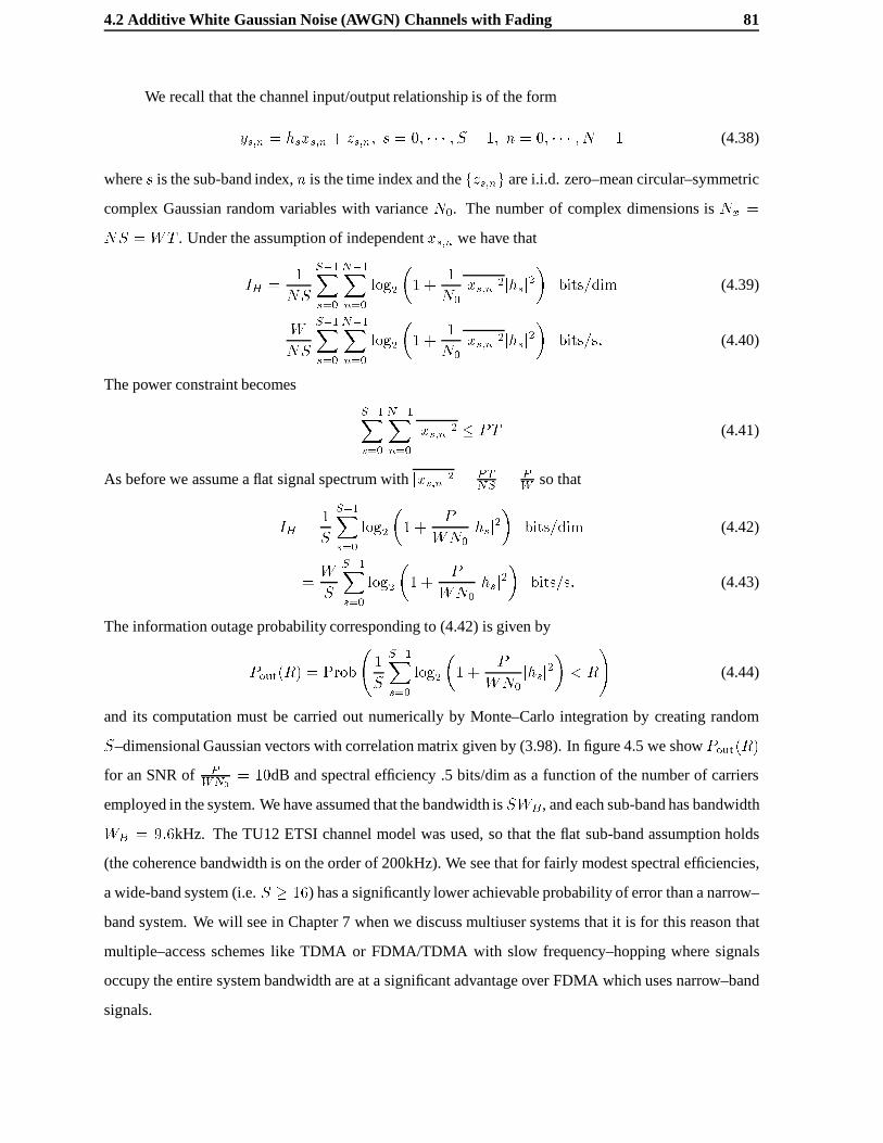
4.2 Additive White Gaussian Noise (AWGN) Channels with Fading 81
We recall that the channel input/output relationship is of the form
ys;n = hsxs;n + zs;n; s = 0; � � � ; S � 1; n = 0; � � � ; N � 1 (4.38)
wheres is the sub-band index,n is the time index and thefzs;ng are i.i.d. zero–mean circular–symmetric
complex Gaussian random variables with varianceN0. The number of complex dimensions isNx =
NS = WT . Under the assumption of independentxs;n we have that
IH =1
NS
S�1Xs=0
N�1Xn=0
log2
�1 +
1
N0jxs;nj2jhsj2
�bits=dim (4.39)
=W
NS
S�1Xs=0
N�1Xn=0
log2
�1 +
1
N0jxs;nj2jhsj2
�bits=s: (4.40)
The power constraint becomes
S�1Xs=0
N�1Xn=0
jxs;nj2 � PT (4.41)
As before we assume a flat signal spectrum withjxs;nj2 = PTNS = P
W so that
IH =1
S
S�1Xs=0
log2
�1 +
P
WN0jhsj2
�bits=dim (4.42)
=W
S
S�1Xs=0
log2
�1 +
P
WN0jhsj2
�bits=s: (4.43)
The information outage probability corresponding to (4.42) is given by
Pout(R) = Prob
1
S
S�1Xs=0
log2
�1 +
P
WN0jhsj2
�< R
!(4.44)
and its computation must be carried out numerically by Monte–Carlo integration by creating random
S–dimensional Gaussian vectors with correlation matrix given by (3.98). In figure 4.5 we showPout(R)
for an SNR of PWN0
= 10dB and spectral efficiency .5 bits/dim as a function of the number of carriers
employed in the system. We have assumed that the bandwidth isSWB, and each sub-band has bandwidth
WB = 9:6kHz. The TU12 ETSI channel model was used, so that the flat sub-band assumption holds
(the coherence bandwidth is on the order of 200kHz). We see that for fairly modest spectral efficiencies,
a wide-band system (i.e.S � 16) has a significantly lower achievable probability of error than a narrow–
band system. We will see in Chapter 7 when we discuss multiuser systems that it is for this reason that
multiple–access schemes like TDMA or FDMA/TDMA with slow frequency–hopping where signals
occupy the entire system bandwidth are at a significant advantage over FDMA which uses narrow–band
signals.

82 Mutual Information and Information Outage Rates
0 0.5 1 1.5 2 2.5 310
−4
10−3
10−2
10−1
100
R bits/s/Hz
S = 1 (9.6kHz)
Pout(R)
PWN0
= 10dB
S = 4 (38.4kHz)
S = 16(153.6kHz)
S = 64(614.4kHz)
S = 128(1.23MHz)
Figure 4.5:Pout(R) as a function of bandwidth forP=(WN0) = 10dB
S = 1 S = 4 S = 16 S = 64 S = 128
(9.6kHz) (38.4kHz) (153.6kHz) (614.4kHz) (1.2288MHz)
1 0.9953 0.9357 0.6926 0.5242
0.1961 0.2222
0.1103
0.0614 0.0772 0.0619
0.0493
0.0230 0.0222
0.0047 0.0028 0.0107 0.0094
Table 4.1: Significant eigenvalues for different bandwidths using the TU12 ETSI model

4.2 Additive White Gaussian Noise (AWGN) Channels with Fading 83
0 2 4 6 8 10 12 14 16 18 2010
−4
10−3
10−2
10−1
100
PWN0
dB
Pout(:5)
S = 1
S = 4
S = 16
S = 64S = 128
Figure 4.6:Pout(:5) as a function of SNR and bandwidth

84 Mutual Information and Information Outage Rates
0 2 4 6 8 10 12 14 16 18 2010
−4
10−3
10−2
10−1
100
S = 64(614kHz)S = 128(1.2MHz)
Pout(1)
PWN0
dB
S = 1 (9.6kHz)
S = 4 (38.4kHz)
S = 16 (153.6kHz)
Figure 4.7:Pout(1) as a function of SNR and bandwidth

4.2 Additive White Gaussian Noise (AWGN) Channels with Fading 85
In spite of the large difference between narrow and wide–band signals, the spectral efficiency for
reasonable outage rates is still only on the order of 1 bit/dim even for a fairly high diversity system. The
system withS = 128 which uses the entire 1.2288MHz still only achieves an outage rate of10�3 at
R = 1 bit/dim. To see the effect of diversity more concretely consider figures 4.6 and 4.7, where we plot
Pout(R) as a function of the SNR. We find that the slopes of the curves in the high SNR region are on
the order of the number of significant eigenvalues for the channel bandwidth which are shown in Table
4.1. We note that the simulation points have been interpolated with a curve of best fit.
Spread–Spectrum Signals
Let us now examine spread–spectrum signals using the multitone model with spreading factorS. The
received signal to be considered here is
yn =
0BBBBBB@
h0g0
h1g1...
hS�1gS�1
1CCCCCCAun + zn (4.45)
wherefgsg is the spreading–sequence satisfyingPS�1
s=0 jgsj2 = 1. We assume uniform spreading so that
jgsj2 = 1=S and, in turn, the power constraint becomes
N�1Xn=0
junj2 � PT: (4.46)
We may transform the problem using thesingular value decompositionof�h0g0 � � � hS�1gS�1
�T=
U�V�. The matrixV is simply 1,� is anN–dimensional vector with one non–zero entry equal toq1S
PS�1s=0 jhsj2 andU is some unitary matrix. The received signal and noise vectors can be transformed
asy0 = U�y andz0 = U�z so that theF frequency dimensions collapse into one and the channel may
be written equivalently as
y0n =
vuut 1
S
S�1Xs=0
jhsj2un + z0n (4.47)
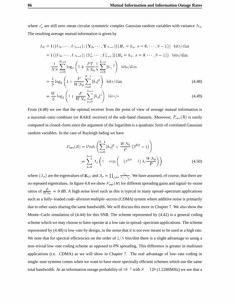
86 Mutual Information and Information Outage Rates
wherez0n are still zero–mean circular symmetric complex Gaussian random variables with varianceN0.
The resulting average mutual information is given by
IH = I (fU0; � � � ; UN�1g; fY0; � � � ;YN�1gjfHs = hs; s = 0; � � � ; S � 1g) bits=dim
= I�fU0; � � � ; UN�1g; fY 0
0; � � � ; Y 0N�1gjfHs = hs; s = 0; � � � ; S � 1g� bits=dim
=1
NS
N�1Xn=0
log2
1 +
PT
NN0
1
S
S�1Xs=0
jhsj2!
bits=dim
=1
Slog2
1 +
P
WN0
S�1Xs=0
jhsj2!
bits=dim (4.48)
=W
Slog2
1 +
P
WN0
S�1Xs=0
jhsj2!
bits=s (4.49)
From (4.48) we see that the optimal receiver from the point of view of average mutual information is
a maximal–ratio combiner (or RAKE receiver) of the sub–band channels. Moreover,Pout(R) is easily
computed in closed–form since the argument of the logarithm is a quadratic form of correlated Gaussian
random variables. In the case of Rayleigh fading we have
Pout(R) = Prob
S�1Xs=0
jhsj2 < WN0
P
�2RS � 1
�!
=S�1Xs=0
As
�1� exp
�� �2RS � 1
��iWN0
P
��(4.50)
wheref�sg are the eigenvalues ofKH andAs =Q
j 6=s�s
�s��j. We have assumed, of course, that there are
no repeated eigenvalues. In figure 4.8 we showPout(R) for different spreading gains and signal–to–noise
ratios of PWN0
= 0 dB. A high noise level such as this is typical in many spread–spectrum applications
such as a fully–loadedcode–division multiple–access (CDMA)system where additive noise is primarily
due to other users sharing the same bandwidth. We will discuss this more in Chapter 7. We also show the
Monte–Carlo simulation of (4.44) for this SNR. The scheme represented by (4.42) is a general coding
scheme which we may choose to have operate at a low rate in spread–spectrum applications. The scheme
represented by (4.48) is low–rate by design, in the sense that it is not ever meant to be used at a high rate.
We note that for spectral efficiencies on the order of1=S bits/dim there is a slight advantage to using a
non–trivial low–rate coding scheme as opposed to PN spreading. This difference is greater in multiuser
applications (i.e. CDMA) as we will show in Chapter 7. The real advantage of low–rate coding in
single–user systems comes when we want to have more spectrally efficient schemes which use the same
total bandwidth. At an information outage probability of10�3 with S = 128 (1.2288MHz) we see that a

4.2 Additive White Gaussian Noise (AWGN) Channels with Fading 87
10−2
10−1
100
10−4
10−3
10−2
10−1
100
S = 1
S = 4(PN)
S = 16(PN)
S = 64(PN)
S = 128(PN)
S = 4(optimal)S = 16(optimal)S = 64(optimal)S = 128(optimal)
R bits/dim
Pout(R)
Figure 4.8: Comparison of low–rate coding and PN spreadingP=WN0 = 0 dB

88 Mutual Information and Information Outage Rates
fivefold increase in spectral efficiency is possible using a sophisticated coding/spreading scheme. These
types of low–rate coding systems are discussed for non–fading channels in [Vit90][Hui84].
4.2.4 Block–Fading AWGN Channels
Let us now examine the block–fading AWGN channel where each block is transmitted across a single–
path or frequency–flat channel with signals band-limited toW Hz. This would be the case, for instance,
in a slow–frequency hopping system with narrow-band signals. We devote more attention to this channel
when we consider code design in the next chapter. Generalizing (4.30) to the case ofF blocks each
having indepedent and identically distributed channel responsesHi(f) = �i, we have using (4.16),
IH0;��� ;HF�1 =W
F
F�1Xf=0
log2
�1 +
P
WN0�i
�: (4.51)
As in the multi-tone case,Pout(R) must be calculated numerically. The independence of the channel
gains in each block allow us to perform this calculation via anF–fold convolution of the density function
of log2�1 + P
WN0��
(the derivative of (4.33)). A Chernov upper–bound is also found in [KSS95]. In
figure 4.9 we plotPout(R) for PWN0
= 10dB for unit–mean Rayleigh fading in each block. We see as
before that coding across several degrees of freedom (in this case the independent block fading levels)
has a significant diversity effect in the outage probability. We showPout(1) as a function of the SNR in
figure 4.10, where we note that the curves have an inverseF th power behaviour in the SNR.
For the case of perfect interleaving or an unlimited number of independent frequency bands and
no delay constraint, the conditional average mutual information (4.17) on an AWGN channel with unit–
mean Rayleigh fading is given by
I1 = W
Z 1
0log2
�1 + �
P
WN0
�e��d�
=We
WN0P
ln 2E1
�WN0
P
�; bits=s (4.52)
whereE1(x) is the first order exponential integral [AS65] given by
E1(x) =
Z 1
x
1
ue�udu: (4.53)
Although Lee [Lee90] showedI1 to be given by (4.52), it was also computed numerically much earlier
by Ericson [Eri70], without explicit mention of the exponential integral function. We also showI1 in
Figure 4.9 along with the non–fading channel capacity in (4.36). Even for a fairly high diversity system,
the practical information rates are very far from those of an ergodic or perfectly–interleaved system.
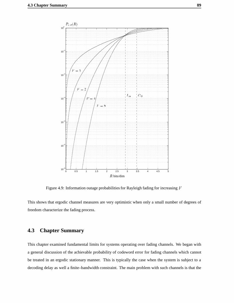
4.3 Chapter Summary 89
0 0.5 1 1.5 2 2.5 3 3.5 4 4.5 510
−6
10−5
10−4
10−3
10−2
10−1
100
CGI1
F = 8
F = 4
F = 2
F = 1
R bits/dim
Pout(R)
Figure 4.9: Information outage probabilities for Rayleigh fading for increasingF
This shows that ergodic channel measures are very optimistic when only a small number of degrees of
freedom characterize the fading process.
4.3 Chapter Summary
This chapter examined fundamental limits for systems operating over fading channels. We began with
a general discussion of the achievable probability of codeword error for fading channels which cannot
be treated in an ergodic stationary manner. This is typically the case when the system is subject to a
decoding delay as well a finite–bandwidth constraint. The main problem with such channels is that the

90 Mutual Information and Information Outage Rates
4 5 6 7 8 9 10 11 12 13 1410
−6
10−5
10−4
10−3
10−2
10−1
100
F = 1
Pout(1)
PWN0
dB
F = 2
F = 4
F = 8
Figure 4.10: Information outage probabilities vs. SNR for Rayleigh fading
fading process cannot be sufficiently averaged during the decoding process, and as a result a channel
capacity does not exist. It was shown that the probability of codeword error is bounded away from zero
by a quantity called theinformation outage probability. This is the probability that the instantaneous
average mutual information between the transmitted and received codeword is less than the information
rate agreed upon by the communicating parties. When channel ergodicity cannot be exploited, it becomes
a lower–bound to the achieveable codeword error–rate.
Using models for static multipath fading channels, we showed that theinformation outage proba-
bility exhibits a diversity effect similar to the pairwise–error–probability analyses we performed in Chap-
ter 2. The codeword error–rate performance cannot be made arbitrarily small and decreases as theDth

4.3 Chapter Summary 91
power of the signal–to–noise ratio, whereD is the number of degrees of freedom or eigenvalues needed
to characterize the fading process during the transmission of the codeword. We used the TU12 ESTI
channel response model with the multitone representation of a wide–band transmission system to evalu-
ate achievable spectral efficiency. We showed that with signals with a bandwidth of 1.2288MHz we could
expect spectral efficiencies on the order of 2 bit/s/Hz with codeword error–rates of10�3. Transmission
schemes such as frequency–hopping with coding or wide–band bursty transmission (such as TDMA) can
exploit this bandwidth efficiently. Narrowband signals suffer hopelessly from lack of diversity. Using
the same model, we considered spread–spectrum signals operating at a low signal–to–noise ratio. We
found that when designed to operate at a spectral efficiency which is the inverse of the spreading gain,
there is a slight advantage to using a non–trivial low–rate coding scheme as opposed to PN spreading,
which can be seen as repetition coding. The main advantage for using low–rate coding comes when more
bandwidth efficient schemes are required (i.e. for high data rate spread spectrum applications), where
very large reductions in codeword error–rate can be achieved.
We have not considered the issue of imperfect estimation of the channel at the receiver. This
clearly will have the effect of reducing achievable data rates across the channel. These issues are treated
for time–varying channels in [Med95].

92 Mutual Information and Information Outage Rates

Chapter 5
Code Design for Block–Fading Channels
In the last chapter we were interested in defining the information–theoretic framework for communica-
tion over general fading channels. We did not, however, give any examples of practical coding schemes
for approaching the performances given in our analyses. We now consider such issues for the particular
class of systems appropriately modeled by the so–calledblock–fading channel. As we already mentioned
in the two previous chapters this is an accurate model for systems where the channel state for blocks of
lengthN symbols, and decoding only be performed on a finite and small number,F , of such blocks. In
applications like GSM or IS54N is quite large (hundreds of symbols) and there is a constraint on the
interleaving depth due to a stringent processing delay requirement. Even in the absence of such delay
constraints, there may be a maximum number of uncorrelated channel realizations (for instance FDMA
slots in GSM). Both amount to the same thing, namely that the number of uncorrelated channel realiza-
tions over which coding is performed,F , is small, so that as we saw in the previous chapter, the channel
may not be treated in an ergodic and stationary manner.
Most work dealing with code design for fading channels assumes an ideal interleaving situation
[Pro95, BDMS91] which, in the context of block–fading channels, is equivalent to lettingF tend to
infinity. On ergodic channels parallel concatenated codes have proven to be effective [BGT93] and offer
astoundingly good performance. For near–optimal performance, however, they can be quite complex for
some applications. In addition, codes designed for ergodic channels need not be effective when applied
to a system whereF is small, which is often the case in PCS applications. Our goal here is to find
coded–modulation schemes using relatively simple constellations and encoders/decoders of reasonable
complexity which are especially well–suited for non–ergodic channels. We will show that there are
reasonably simple codes for low spectral efficiencies (<2 bits/dim) which can achieve close to optimal
94 Code Design for Block–Fading Channels
performance. This is appropriate in light of the results of the previous chapter where we showed that
for typical wide–band urban channels (i.e. around 1MHz bandwidth), we cannot expect to be able to
transmit at much more than 1 bit/dim at an SNR of 10dB.
Besides slow frequency–hopping systems, another application of a block–fading model is in fast
frequency–hopping systems whereN is small (on the order of a few symbols). The work of Kaplanet
al. in [KSSK95] considers coding for these systemswithouta constraint on the number of frequencies
over which the signal can hop. This amounts again to an ideal interleaving situation, where the fast
frequency–hopping pattern takes the place of the interleaver. The work of Lapidoth in [Lap94] addresses
the construction and performance of binary codesmatchedto the depth of the interleaver (or number of
blocks) which, as in our case, is assumed to be small. This introduces strong cyclic correlations in the
sequence to be decoded. Lapidoth’s analysis was performed using anerasure–channelmodel of a fading
channel and for various interleaving techniques.
In [LWK93] the coding problem was treated for the block fading channel. They showed that
in order for the diversity order to be maximum (i.e.F ) the code rate (in input/output symbols) must
not exceed1=F . We will extend these results by considering arbitrary diversity orders. For the case
of trellis codes with rate1=F they consider an analytical approach for determining the pairwise error
probability based on a generalized transfer function from the state diagram of the code. Trellis codes
based on linear convolutional codes withM–PSK modulation andF = 2 blocks are considered and a
few low–complexity examples are given. This approach was also recently considered for rate1=F binary
convolutional codes with antipodal signals over Ricean channels by Malkamaki and Leib in [ML97].
The work of Giraud and Belfiore [GB96] and Boutroset al. [BVRB96] examines the coding
problem for fading channels from a different point of view. They both focus of the design of multidi-
mensional lattice constellations which, using sufficient interleaving, are assumed to have an independent
fading strengths in each dimension. The specially designed constellations have the property that the di-
versity order is equal to the number of dimensions. We will discuss these schemes in the context of our
work shortly, since they can be applied directly to the block–fading channel.
We begin with a simplified discrete–time system model for the code design problem and perform
an information outage probability analysis for the case of non–Gaussian discrete signal alphabets. Recall
that in the last chapter we always assumed the transmitter used a continuous Gaussian symbol alphabet.
The goal of this analysis is to gain insight regarding the choice of signal constellation size on the achiev-
able codeword error–rate performance. We then examine the coding problem from the point of view of
the diversity order. We show that the block–fading channel can be considered as a non–binary coding

5.1 System Model and Outage Probability Analysis 95
scheme with block lengthF with N dimensional symbols. It follows that the diversity order,dFH, can be
upper–bounded using standard techniques, and it turns out that theSingleton boundis the most appropri-
ate of such techniques. We show how it can be used to determine the maximum diversity as a function
of the information rate in bits/dim, the number of fading blocksF and the size of the signalling con-
stellation. A code which meets the Singleton bound is known as aMaximal Distance Seperable (MDS)
code, and therefore any MDS code achieves maximum diversity. Using the Singleton bound as target
diversity order for any coded system, we provide examples for codes which achieve it. We first consider
block codes and multidimensional constellations followed by trellis codes. Results of computer searches
for maximal–diversity trellis codes of varying complexity for binary and non–binary constellations are
given. We end with some computer simulations of some of the reported codes and compare them to
codes already in use at the present time.
5.1 System Model and Outage Probability Analysis
We saw in Chapter 3 that the performance of the block–fading channel, in the case of uncorrelated
blocks, is due to two factors which act independently. This is first the relation between the underlying
signaling pulse shape and the multipath delay spread. The second is the effect of coding, more precisely
the minimum Hamming distance between pairs of signals on a block–basis. Because of this separation
between the two factors, it is sufficient to consider the simplest channel model which allows us to analyse
the effects of coding without having to worry about the pulse–shape/multipath relationship. We therefore
assume a narrow–band pulse shape so that there is no ISI due to multipath and amplitude statistics are
Rayleigh. In addition, we assume the coded symbols belong to a real–valued symbol alphabetS � R(i.e.
each symbol uses 1 signaling dimension.) Extending this analysis to complex symbols is straightforward
and brings no significant additional insight into the problem. Moreover, this allows us to determine
how close we can expect to get to the performance of the continuous Gaussian symbol case with simple
constellations.
We show the discrete–time channel model in figure 5.1. Assuming a system havingF channels
with blocks of lengthN symbols we have codewords occupyingNF dimensions written as
cm =�c0;0; c0;1; � � � ; c0;N�1; c1;0; � � � ; cF�1;N�1
�; m = 0; 1; � � � ;M � 1; (5.1)
whereM is the size of the codebook. Each block is assumed to have a channel gain�f ; f = 0; � � � ; F�1which is the same for each symbol in the block and independent from block to block. Under the Rayleigh

96 Code Design for Block–Fading Channels
assumption each channel gain is exponentially distributed with unit mean as
f�f (u) = e�u; u � 0: (5.2)
The receiver uses a filter matched to the chosen pulse–shape which is sampled at the symbol rate so that
we may may write the continuous–time problem equivalently as
rf;n =p�fcf;n + zf;n ; f = 0; � � � ; F � 1; n = 0; � � � ; N � 1; (5.3)
where thezf;k are i.i.d. zero–mean real Gaussian random variables with varianceN0=2. Let theNF–
dimensional vectorsr andz denote the received signal and noise samples andrf , cm;f andzf the samples
in each blockf = 0; � � � ; F � 1. We take for granted that the transmitter and receiver have agreed
beforehand to use a codebook havingM codewords so that the information rate isR = (log2M)=NF
bits/dimension. We denote theF–dimensional vector of signal amplitudes by�, and assume that there
is no feedback path for channel state information so that the transmitter has noa priori knowledge of�.
ErrorControlCode
M
L
R
E
C
E
I
V
E
R
cF�1
c1
c0
z0
z1
zF�1 �F�1
�1
�0
Information Bits
Interleaver
ENCODER
S c
NFNFR
Figure 5.1: Discrete–time system model
We begin with an outage probability analysis for general non–Gaussian symbol alphabets in order
to see the effects of using pragmatic constellations. From the results of Chapter 2, in order to compute

5.1 System Model and Outage Probability Analysis 97
the average probability of codeword error, we must consider the average mutual information functional
IH =1
NFI(C;RjA = �) =
1
NF
Zc2SNF
Z 1
�1fR;CjA(r; cj�) � (5.4)
log2fRjC;A(rjc;�)fRjA(rj�)
drdc bits=dimension:
using which we can compute the information outage probability
Pout(R) = Prob(IH < R): (5.5)
This quantity defines the practical lower–limit to the codeword error–rate in the limit of largeNF . We
recall that under an average power constraint
N�1Xn=0
F�1Xf=0
c2n;f < NFEs; (5.6)
the quantityIH is maximum for independent Gaussian symbols and is given by
IH =1
F
F�1Xf=0
1
2log2
�1 +
2�fEsN0
�bits=dim: (5.7)
We have already computed the corresponding information outage probability in this case numerically. In
a practical sense, this quantity is useful for assessing the potential performance gains afforded by the use
of large constellations. For small constellations with equiprobable and independent symbols,Pout(R)
can similarly be computed numerically using [Bla87]
IH = log2 jSj �1
F jSjF�1Xf=0
Xsi2S
Z 1
�1
1p�N0
exp
�� 1
N0r2�� (5.8)
log2Xsj2S
exp
�� 1
N0
�(r� �f(sj � si))
2 � r2��
dr bits=dimension (5.9)
The simplest modulation scheme to consider is uniformly–spacedAmplitude Modulation(AM), which is
shown in figure 5.2.
In Figs. 5.3–5.7 we show the information outage probability now as a function of the the signal–to–
noise ratio per information bitEb=N0 (whereREb = Es) for both small AM constellations and Gaussian
signals. We see that by doubling the constellation size with respect to the minimum constellation which
achieves the desired information rate, we quickly approach the performance achievable with a continuous
Gaussian input signal. This is similar to the effect of coding with expanded signal sets on the non–fading
AWGN channel [Ung82]. We notice also that the diversity (i.e. the slope of the error–rate curve) is
reduced for small constellations. In other words, constellation expansion can increase diversity. In some

98 Code Design for Block–Fading Channels
2-AM
4-AM
8-AM
16-AM
Figure 5.2: AM Modulation
cases, the increase can be very significant (e.g. 1.5 bits/dim with 4 or 8 AM.) In the following section we
derive a bound on the diversity which allows us to quantify this observation more precisely.
In Figure 5.8 we show the lower bound on the bit–error probability given in (4.15). Again we see
the same effect from constellation expansion but that the error rates are two orders of magnitude lower.
We will see that this bound is much less indicative of practical bit error rates thanPout is for block error
rates.
5.2 Maximum Code Diversity
This section addresses the issue of designing coded–modulation schemes which attain maximum code
diversity (dFH) for a given number of uncorrelated blocks and information rate. Using the techniques from
Chapter 2, we recall that the conditional pairwise–error probability between two arbitrary codewords is
given by
Pej�(c(a) ! c(b)) = Q
0@sd2(a; b)
2N0
1A : (5.10)
For the system at hand the Euclidean distance between the two codewords conditioned on the channel
state is
d2(a; b) =F�1Xf=0
�fd2f(a; b) (5.11)
and
d2f (a; b) =NXn=0
(c(a)f;n � c
(b)f;n)
2: (5.12)

5.2 Maximum Code Diversity 99
3 4 5 6 7 8 9 10 11 12 1310
−7
10−6
10−5
10−4
10−3
10−2
10−1
2AM
Gaussian
2AM
4AMGaussian
Eb=N0
Pout(:25)
F = 4
F = 8
Figure 5.3: Information Outage Probabilities (R = :25 bits/dim)
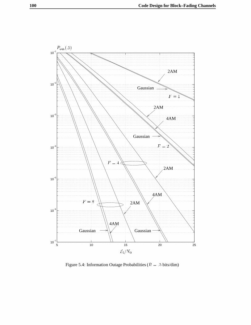
100 Code Design for Block–Fading Channels
5 10 15 20 2510
−7
10−6
10−5
10−4
10−3
10−2
10−1
2AM
Gaussian
2AM
Gaussian
4AM
2AM
4AM
Gaussian
2AM
4AM
Gaussian
F = 8
F = 4
F = 1
F = 2
Eb=N0
Pout(:5)
Figure 5.4: Information Outage Probabilities (R = :5 bits/dim)
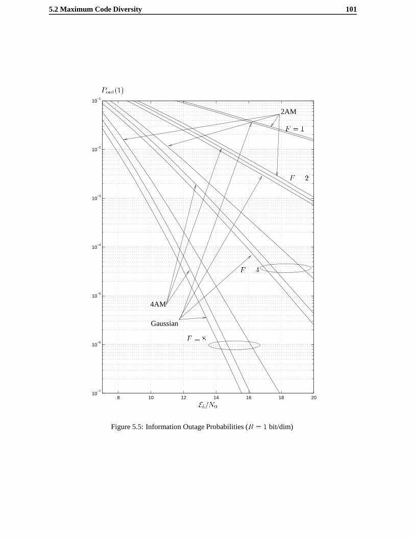
5.2 Maximum Code Diversity 101
8 10 12 14 16 18 2010
−7
10−6
10−5
10−4
10−3
10−2
10−1
4AM
2AM
Gaussian
F = 8
F = 4
F = 2
F = 1
Pout(1)
Eb=N0
Figure 5.5: Information Outage Probabilities (R = 1 bit/dim)

102 Code Design for Block–Fading Channels
10 12 14 16 18 20 22 2410
−7
10−6
10−5
10−4
10−3
10−2
10−1
F = 8,Gaussian
F = 4,Gaussian
F = 2,Gaussian
F = 8, 8AM
F = 2, 4AM
F = 4, 4AM
F = 8, 4AM
F = 4, 8AM
F = 2,8AM
Pout(1:5)
Eb=N0
Figure 5.6: Information Outage Probabilities (R = 1:5 bits/dim)

5.2 Maximum Code Diversity 103
10 12 14 16 18 20 22 2410
−7
10−6
10−5
10−4
10−3
10−2
10−1
8AM16AM
GaussianF = 8
F = 2
F = 4
Pout(2)
Eb=N0
Figure 5.7: Information Outage Probabilities (R = 2 bits/dim)
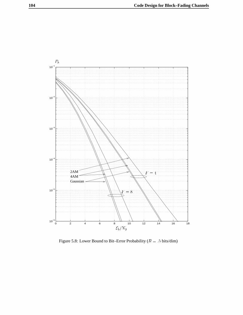
104 Code Design for Block–Fading Channels
0 2 4 6 8 10 12 14 16 1810
−6
10−5
10−4
10−3
10−2
10−1
2AM4AMGaussian
F = 4
F = 8
Pb
Eb=N0
Figure 5.8: Lower Bound to Bit–Error Probability (R = :5 bits/dim)

5.2 Maximum Code Diversity 105
Defining the variablez = d2(a; b)=(2N0) we have that its moment–generating function is given by
Gz(s) =F�1Yf=0
1
1� sd2f(a;b)
2N0
=
dFH(a;b)�1Yi=0
1
1� s �i2N0
wheref�ig are the non–zero block Euclidean distancesfd2f(a; b)g anddFH(a; b) is the Hamming distance
between the codewords on a block basis. The average PEP is therefore
Pe(c(a) ! c(b)) = E�Pej�(c
(a) ! c(b)) � :5Gz
��1
2
�=
dFH(a;b)�1Yi=0
1
1 + :5�i(5.13)
We saw in Chapter 2 that in these cases, the error probability curve decreases as the inversedFHth
power
of the signal–to–noise ratio, so clearlydFH(a; b) is the most critical performance indicator. Nevertheless,
the secondary parameter
�(a; b) =
0@dFH(a;b)�1Y
i=0
�i
1A1=dFH(a;b)
(5.14)
acts as a SNR gain factor which also must be considered. It is simply thegeometric meanof the Euclidean
distancesd2f(a; b).
From the average PEP we may invoke the union bound on the probability of error for an arbitrary
code as
Pe =1
M
M�1Xa=0
M�1Xb=0
Pe(c(a) ! c(b)); (5.15)
and if the code isgeometrically uniform[For91],
Pe =M�1Xb=0
Pe(c(0) ! c(b)): (5.16)
This just means that the probability of error is indenpendent of the codeword that is being transmitted and
there is no loss of generality in assuming that any one particular codeword is continuously transmitted.
5.2.1 An introductory example
We now consider a simple illustrative example which shows that the code design problem is different
from the classic approach of maximizing the Hamming or Euclidean distances. In practice, the encoder

106 Code Design for Block–Fading Channels
includes an interleaver, although in theory it is not required. The reason for its use is simply to reduce
the computational complexity of the encoding and decoding processes. We require that theF degrees of
freedom appear in the span of a codeword (or memory of a trellis code) which is assured by interleaving
without needed very long codes (many states.) We will assume that the interleaver is of the diagonal
type as described in Chapter 3 with depthF . If we denote the sequence at the output of the encoder
by q = fq0; q1; � � �g; qk 2 S, at the output of the interleaver the coded symbols in each block will be
c0 = fq0; qF ; � � � ; qkF ; � � �g; � � � ; cf = fqf ; qF+f ; � � �qkF+f ; � � �g.Let us examine the rate 1/2 binary convolutional code with binary modulation (.5 bits/dim) em-
ployed in the full–rate GSM standard shown in Fig.5.9. The output bits are interleaved overF = 8
blocks transmitted on widely spaced carriers, so that the channel strength in each block will be fairly
uncorrelated from those in the other blocks. The minimum free Hamming distance path
q = f0; 0; � � � ; 0; 0; 1; 1; 0; 1; 0; 0; 1; 1; 1; 1; 0; 0; � � � ; 0g (5.17)
hasdfree = 7 (after deinterleaving) and is shown along with the blocks over which each bit were trans-
mitted. As for the symbols ineach block, we have
c0 = f0; � � � ; 0; 1; 1; 0; � � � ; 0gc1 = f0; � � � ; 0; 1; 1; 0; � � � ; 0gc2 = f0; � � � ; 0gc3 = f0; � � � ; 0; 1; 0; � � � ; 0gc4 = f0; � � � ; 0g
c5 = f0; � � � ; 0gc6 = f0; � � � ; 0; 1; 0; � � � ; 0gc7 = f0; � � � ; 0; 1; 0; � � � ; 0g
so that this path achievesd8H = 5. It turns out that this is also the minimum diversity path for this code
and, as we shall soon see, that there is no other code which achieves a higher diversity order with binary
modulation andR = 1=2 bits/dim.
Kaplanet al. [KSSK95] consider a similar trellis coding problem for an uninterleaved binary fast–
frequency hopping system, without a constraint on the number of hopping frequencies. Their system
model assumes that the hopping period extends overJ (J < 3) trellis branches of a rate1=n trellis code
so that by grouping together the output bits over theJ branches, we may see this as aJ=Jn code. This

5.2 Maximum Code Diversity 107
0,1 2,3 4,5 6,7 0,1
0000 0000 0000 0000 0000 0000
1000
0100
0010
0001
1/11
0/01
0/00
0/11
0/00 0/00 0/00 0/00 0/00
0/11
Block:
d8H = 5
dfree = 7
Figure 5.9: Minimum diversity/weight error event for full–rate GSM,
code design problem is quite different from the one we treat in this chapter for two reasons. Firstly,
as the code complexity increases, the diversity also increases, since it is not fundamentally limited by
a finite number of degrees of freedom. In fact, Kaplanet al. [KSSK95] give a bound on the diversity
as a function of the number of states of the encoder. Secondly, the code search procedure is simpler
since, although there is no interleaving, the frequency–hopping takes the place of an ideal interleaver
usingJ adjacent bits at a time. In the case we treat here, the cyclic nature of the correlations can
yield very long code sequences with low diversity. We are therefore often required to scan the trellis
to a great depth to assure that these codewords are not in the code. This is easily explained with an
example: consider the 16–state rate 1/2 code with generatorsg1 = (10101) andg2 = (11111)which has
dfree = 6. Let us use it on a channel withF = 8. An input(10 � � �0) yields(11011101110 � � �0) which
hasd8H = 6. Similarly (1010 � � �0) yields (110100000001110 � � �0) with d8H = 5 and(101010 � � �0)yields(1101000011000001110 � � �0) with d8H = 4. This example shows that it is possible that long low
diversity codewords with highdfree can exist and have to be accounted for. We have found that in some
cases they can be much longer than in this example. Even for this example an input of(1010001010 � � �0)yields a codeword withd8H = 4.

108 Code Design for Block–Fading Channels
5.2.2 Maximum Diversity Bound
We begin by deriving a upper–bound ondFH taken over all codeword pairs as a function ofR and the
constellation size. AlthoughdFH is the principle asymptotic indicator of the PEP for any coding scheme,
we must keep in mind that it does not necessarily accurately indicate the total probability of error for low
signal–to–noise ratios.
In order to determine the minimum pairwisedFH, it is convenient to group together theN symbols
which are transmitted in the same block, and view them as a super-symbol overSN . The codeword is
then a vector of lengthF super-symbols. Using this interpretation,dFH is simply the Hamming distance
in SN . This reduces the analysis to one of non–binary block codes with a fixed block lengthF , and
therefore all traditional bounding techniques apply.
An important first observation is that the highest rate code which achievesdFH = F hasR =
1F log2 jSj bits/dim. This follows directly from the fact that no two codewords can have identical symbols
in the same position ifdFH = F . We can achieve this, for example, using a repetition code overSN , or
the multidimensional constellations of Giraud and Belfiore [GB96] and Boutroset al. [BVRB96], which
we will consider shortly. This was also remarked in [LWK93].
The question remains, therefore, how close we can get todFH = F with high–rate codes and simple
constellations. The answer lies in the Singleton bound [Sin64] which is proven in this context, for the
sake of completeness, in the following theorem:
Theorem 3 (Singleton Bound)
Any codeC of rateR bits/dim withM codewords consisting ofF blocks of lengthN symbols from a
one–dimensional alphabetS hasdFH satisfying
dFH � 1 +
�F
�1� R
log2 jSj��
: (5.18)
Proof: Let k (0 < k � F � 1) denote the integer value satisfyingjSjN(k�1) < M � jSjNk,
whereM = 2NFR. Consider any set ofk � 1 coordinates, for instancei = 0; 1; � � � ; k� 2. SinceM >
jSjN(k�1) there are necessarily at least two codewords,x;y 2 C such thatxi = yi; 8i 2 f0; 1; � � � ; k�2g. It follows thatdFH � F � k + 1 and therefore that
M � jSjN(F�dFH+1): (5.19)
Using the fact thatdFH must be an integer yields (5.18).�
We show the bound ondFH as a function ofR= log2 jSj andF in Fig. 5.10, where the value ofF
for each curve is simply the horizontal intercept.

5.2 Maximum Code Diversity 109
0 0.1 0.2 0.3 0.4 0.5 0.6 0.7 0.8 0.9 10
2
4
6
8
10
12
14
16
dFH
F is the horizontal intercept
R= log2 jSj
Figure 5.10: Singleton bound ondFH as a function ofR= log2 jSj
The first interesting result of this analysis is that the shape of the constellation is not important
with regard to the code diversity since it is a completely algebraic measure of the performance. The class
of maximum distance separable codes(MDS) therefore play a large role in this context. An MDS code
is one which meets the Singleton bound, such as theReed–Solomon (RS) codes. There is a downside,
however, which is that the block length of the code is constrained to beF which means that many
existing codes cannot necessarily be used effectively. Shortly, however, we give some examples of
codes which can be used with practical choices forF and guarantee maximum diversity. Secondly, and
more importantly, we see what was remarked earlier in the information–theoretic analysis concerning
constellation expansion. Take for example transmission atR = :5 bits/dimension overF = 8 blocks
as in full–rate GSM . With binary modulation (jSj = 2), the maximum pairwise diversity is 5, which
incidently is what is achieved by the coding scheme used in GSM. With quaternary modulation we see
that it can be increased to 7. Examining the slopes of the information outage curves in Fig. 5.4 we see
that both results agree. On the downside, for high code rates (> 2 bits/dimension) very large symbol
alphabets are required to achieve high asymptotic diversity. For example, withF = 8 andR = 3
bits/dimension, a 16-point constellation can only achieve a diversity ofd8H = 3. To achieved8H = 7 a
constellation with 4096 points per dimension is needed. Since these are only asymptotic results, they
may be somewhat pessimistic at low signal–to–noise ratios. We see from the information outage curves

110 Code Design for Block–Fading Channels
that this is indeed the case, since the slopes of the curves start to decrease towards their asymptotic value
as the SNR increases.
5.2.3 Block Codes
Let us first consider some examples of linear block codes of codeword lengthF with k information
symbols, so that the rates of the codes areR = kF log2 jSj bits/dim. For this case the Singleton bound
assures thatdFH � F � k + 1.
Repetition codes
As we already pointed out, the simplest possible coding scheme for achieving diversityF is repetition
coding. A generalized repetition code for the caseN = 1 has generator matrixG =�1 1 � � � 1
�so that codewords are formed as
c = uG (5.20)
whereu 2 S. The number of codewords isM = jSj and the spectral efficiency islog2 jSj=F bits/dim.
Multidimensional Constellations
The multidimensional lattice codes considered by Giraud and Belfiore [GB96] and Boutroset al. [BVRB96]
are perfectly suited for the block–fadingchannel, since they consider constellationsover a finite and small
number of dimensions. Each dimension has an independent signal attenuation, and therefore in the con-
text of the block–fading model, this is equivalent to lettingF be the number of dimensions andN = 1. In
[GB96] the constructed codes have dimensionality2 � F � 8 andM = 22F points (codewords) which
have diversityF . We show a particular constellation carved out of a hexagonal lattice for the caseF = 2
in figure 5.11(a). If we project the points of the lattice for this example oneach dimension, we obtain a
one–dimensional constellation withjSj = 16 points. The lattice may therefore be considered as a block
code withF = 2 over this one–dimensional alphabet. This code therefore satisfies the Singleton bound
with equality and uses the smallest constellation size to achieved2H = 2. The repetition code forF = 2
using a 16-AM constellation looks different (see figure 5.11(b)), but has the same number of codewords
and spectral efficiency. It makes much less efficient use of the signal space, however, which has a sig-
nificant effect on the Euclidean distance between signal points, and thus on the secondary performance
measure,�. In general, when the multidimensional constellations are projected onto the coordinate axes,

5.2 Maximum Code Diversity 111
(a) (b)
Figure 5.11: Giraud and Belfiore’s 2-dimensional Lattice constellationvs. repetition coding
they produce non–uniformly spaced AM constellations. Another simple two–dimensional example to il-
lustrate this point is the rotated QPSK constellation shown in figure 5.12 with spectral efficiency 1 bit/dim
which was considered by Boull´e and Belfiore in [BB92]. They showed that by rotating the constellation
by �=8, the inherent diversity of the constellation is 2 and� is maximum, under the assumption, of
course, that both dimensions undergo independent channel realizations. We show the projection of the
constellation on each axis where we note that it is a non–uniform 4AM constellation. In what follows
we will consider the combination of a trellis code with uniform AM constellations, however, in light of
this observation, it may also be appropriate to consider non–uniformly spaced constellations in order to
improve performance. Boutroset al. [BVRB96] applied this rotation idea to known lattices which work
well on the Gaussian channel to yield constellations with high diversity on the fading channel.
The parameter� for these constellations is limited because of the fact thatN = 1. In order to
achieve higher coding gain, therefore, they must be concatenated with an error–control code, which will
reduce the spectral efficiency of the system. Moreover, this places a significant burden on the receiver
if high diversity is sought since the constellation itself is difficult to decode. In section 5.2.4, we take
a different approach by considering simple constellations with binary trellis codes for achieving high
diversity. This has the advantage of yielding larger values for� since coding is performed across a larger
number of symbols per block (i.e.N > 1.)

112 Code Design for Block–Fading Channels
Figure 5.12: Rotated QPSK constellation
Short non–binary codes
We now consider MDS code families for systems havingF = 4; 6; 8 formed by either shortening or
lengthening RS codes such that they have block lengthF . Shortening RS codes by removing infor-
mation symbols results in a code with the samedFH as the base code[Wil96]. Similarly, it is shown in
[Wol69] that up to 2 information symbols can be added to an RS code without changingdFH. For the
caseF = 6 we also consider a particular less complex extended Hamming code which is also MDS. The
combination of the constraints imposed by the structure of the codes and the number of blocks in the
system does not assure minimal complexity, nor the flexibility of choosing arbitrary symbol alphabets.
Another negative aspect is that the purely algebraic structure of the codes pays no attention to the other
less critical performance indicator,�.
Example A : F = 4
Consider a family of codes with rateR = k=4 bits/dimension for use with binary modulation.
Assuming we form symbols over GF(4) by forming pairs of bits from the same block, we start with the
(3; k�1)RS code over GF(4) withd4H = 5�k and lengthen it to(4; k). Following [Wol69] the resulting
parity check matrix for this code family is
H =
0BBBBBB@
1 1 � �2
0 1 �2 (�2)2
......
......
0 1 �k (�k)2
1CCCCCCA: (5.21)
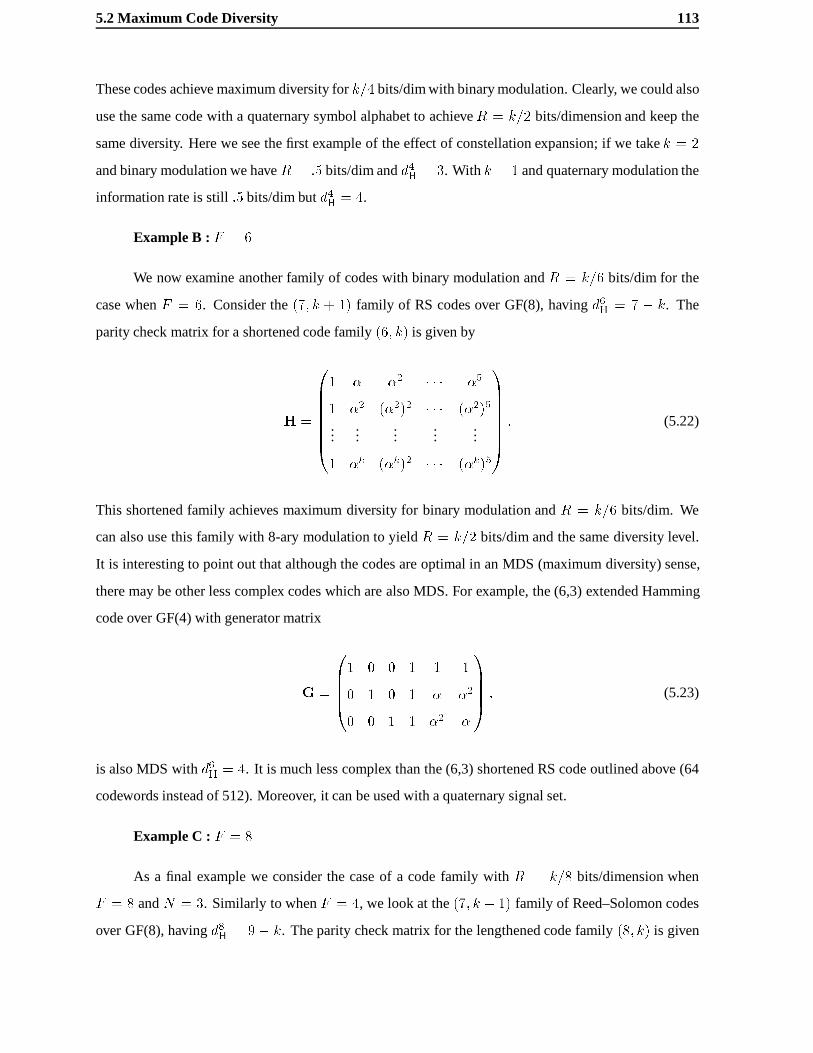
5.2 Maximum Code Diversity 113
These codes achieve maximum diversity fork=4 bits/dim with binary modulation. Clearly, we could also
use the same code with a quaternary symbol alphabet to achieveR = k=2 bits/dimension and keep the
same diversity. Here we see the first example of the effect of constellation expansion; if we takek = 2
and binary modulation we haveR = :5 bits/dim andd4H = 3. With k = 1 and quaternary modulation the
information rate is still:5 bits/dim butd4H = 4.
Example B :F = 6
We now examine another family of codes with binary modulation andR = k=6 bits/dim for the
case whenF = 6. Consider the(7; k + 1) family of RS codes over GF(8), havingd6H = 7 � k. The
parity check matrix for a shortened code family(6; k) is given by
H =
0BBBBBB@
1 � �2 � � � �5
1 �2 (�2)2 � � � (�2)5
......
......
...
1 �k (�k)2 � � � (�k)5
1CCCCCCA: (5.22)
This shortened family achieves maximum diversity for binary modulation andR = k=6 bits/dim. We
can also use this family with 8-ary modulation to yieldR = k=2 bits/dim and the same diversity level.
It is interesting to point out that although the codes are optimal in an MDS (maximum diversity) sense,
there may be other less complex codes which are also MDS. For example, the (6,3) extended Hamming
code over GF(4) with generator matrix
G =
0BBB@1 0 0 1 1 1
0 1 0 1 � �2
0 0 1 1 �2 �
1CCCA ; (5.23)
is also MDS withd6H = 4. It is much less complex than the (6,3) shortened RS code outlined above (64
codewords instead of 512). Moreover, it can be used with a quaternary signal set.
Example C : F = 8
As a final example we consider the case of a code family withR = k=8 bits/dimension when
F = 8 andN = 3. Similarly to whenF = 4, we look at the(7; k � 1) family of Reed–Solomon codes
over GF(8), havingd8H = 9 � k. The parity check matrix for the lengthened code family(8; k) is given

114 Code Design for Block–Fading Channels
by
H =
0BBBBBB@
1 1 � �2 � � � �6
0 1 �2 (�2)2 � � � (�2)6
......
......
......
0 1 �k (�k)2 � � � (�k)6
1CCCCCCA: (5.24)
This family achieves maximum diversity for binary modulation andR = k=8 bits/dim. As before, we
can also use this family with 8–ary modulation yieldR = 3k=8 bits/dim and the same diversity level.
5.2.4 Trellis Codes
In the GSM system today, as previously mentioned, rate 1/2 binary trellis (convolutional) codes are
used. This is mainly due to the computational simplicity of implementing the Viterbi algorithm with
soft decisions. The Singleton bound is also applicable to convolutional codes, since they can always be
interpreted as very long block codes. In fact, in systems like GSM the convolutional codes are used in a
block fashion by appending trailing zeros to the information sequence, and a one–shot decoding of the
entire block is performed.
Let us consider two examples of trellis codes withM–ary constellations. We have been unable to
find simple design rules for such codes which guarantee maximum diversity, as well as high values for�.
Similar problems occur when trying to apply Ungerb¨ock’s techniques [Ung82] to perfectly interleaved
Rayleigh channels. The main problem with Ungerb¨ock’s construction is the parallel transitions in the
trellis representation of the codes imply that the diversity order is 1. Divsalar and Simon [DS88] came
up with a way around this problem by describing some multi–dimensional trellis codes for 8–PSK mod-
ulation. They were designed for perfectly interleaved channels, but suffer from very low diversity orders,
and therefore offer very poor performance. Schlegel and Costello [SC89] proposed new 8–PSK trellis
codes for perfectly interleaved channels using such techniques, but these only offer high diversity for a
large number of states (>64). In the multidimensional approach, the trellis still has parallel transitions,
but several output dimensions are associated with each branch. Provided the parallel transitions have
large mutual Hamming distances, diversity is increased.
We can apply the same multi–dimensionalapproach to a block–fading channel if we let the number
of output dimensions in each branch beF . We illustrate this with the two 2–state trellises in figure 5.13
for F = 4, both having .5 bits/dim. The trellis in figure 5.13(a) uses binary modulation and the one in
figure 5.13(b) quaternary AM modulation. We have assumed unit energy constellations and we denote
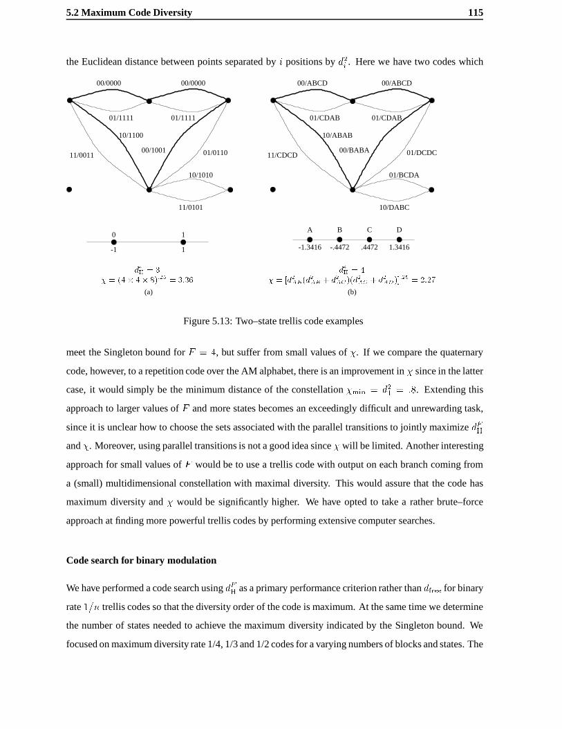
5.2 Maximum Code Diversity 115
the Euclidean distance between points separated byi positions byd2i . Here we have two codes which
-1.3416 -.4472 .4472 1.3416
A B C D
00/ABCD 00/ABCD
01/CDAB 01/CDAB
11/CDCD00/BABA 01/DCDC
01/BCDA
10/DABC
00/0000 00/0000
01/1111 01/1111
11/001100/1001 01/0110
10/1010
11/0101
10/1100 10/ABAB
(a) (b)
0 1
-1 1
� = (4� 4� 8):25 = 3:36 � = [d2AB(d2AB + d2AC)(d
2AC + d2AD)]:25 = 2:27
d4H = 4d4H = 3
Figure 5.13: Two–state trellis code examples
meet the Singleton bound forF = 4, but suffer from small values of�. If we compare the quaternary
code, however, to a repetition code over the AM alphabet, there is an improvement in� since in the latter
case, it would simply be the minimum distance of the constellation�min = d21 = :8. Extending this
approach to larger values ofF and more states becomes an exceedingly difficult and unrewarding task,
since it is unclear how to choose the sets associated with the parallel transitions to jointly maximizedFH
and�. Moreover, using parallel transitions is not a good idea since� will be limited. Another interesting
approach for small values ofF would be to use a trellis code with output oneach branch coming from
a (small) multidimensional constellation with maximal diversity. This would assure that the code has
maximum diversity and� would be significantly higher. We have opted to take a rather brute–force
approach at finding more powerful trellis codes by performing extensive computer searches.
Code search for binary modulation
We have performed a code search usingdFH as a primary performance criterion rather thandfree for binary
rate1=n trellis codes so that the diversity order of the code is maximum. At the same time we determine
the number of states needed to achieve the maximum diversity indicated by the Singleton bound. We
focused on maximum diversity rate 1/4, 1/3 and 1/2 codes for a varying numbers of blocks and states. The
116 Code Design for Block–Fading Channels
results are summarized in Tables 5.1–5.3, where we have followed the convention of [LC83] regarding
the octal representation of the generator polynomials. The table lists the codes which maximizedFH first
and then� as a secondary requirement and those marked in bold type meet the Singleton bound. We
should note that searching for these codes is more computationally intensive than for those maximizing
dfree since a simple dynamic–programming approach cannot be used to determine the minimumdFH path
in the trellis because of the finite–depth interleaving. As a result of this and the fact that the trellis must
be scanned to a very low depth to assure that there are no low diversity codewords, it is difficult to
search for low–rate codes with many states. The search procedure was reduced somewhat by ruling out
catastrophic codes.
As a first example, consider the case ofR = :5 bits/dim withF = 8. We can achieve maximum
diversity with an eight–state code, and moreover, it turns out that it does not exhibit maximum free
Hamming distance (dfree = 5, not 6). It is the only such code, so that it is a perfect example of the
danger of using codes designed for ergodic channels. It is interesting to note that the GSM standard
uses a 16–state maximum free Hamming distance code, which offers a slightly larger� than its 8–state
couterpart. The 16–state code listed in the table has a slightly larger� than the GSM code, but we have
found that the performance improvement is negligible. For the case ofF = 4, maximum diversity can
be obtained with a 4–state code, whereas in the GSM standard a 64–state code is used.
There are other important issues requiring the use of more complex codes. For instance, the 16-
state code used in full–rate GSM achieves maximum diversity withF = 2; 4; 6and 8, whereas the 8–state
code achieves maximum diversity only withF = 2; 4; 8. This is important since in a frequency–hopping
system, the number of hopping frequency is left up to the operator. Although we have not considered
this issue, it would be interesting to determine “universally” good codes which achieve acceptable perfor-
mance for many different values ofF . The more important reason for increasing complexity, as we will
see in section 5.3, is that larger values of�min can yield significant coding gain in the frame error–rate
performance.
Binary trellis codes with non–binary modulation
Since the first and most important goal is to maximizedFH we will consider linear binary trellis codes as
before with an appropriate mapping of adjacent output bits to the non–binary constellation,jSj. We have,
therefore, that groups oflog2 jSj adjacent bits are mapped into one symbol fromS. The interleaving is
done on a symbol basis so thatF adjacent symbols at the output of the encoder are transmitted in different
blocks. We show two examples with 4–AM modulation in figure 5.14 which have .5 and 1 bits/dim. The
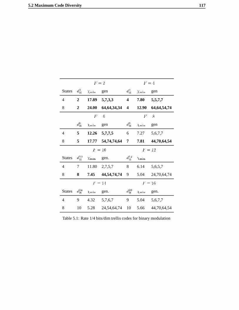
5.2 Maximum Code Diversity 117
F = 2 F = 4
States d2H �min gen d4H �min gen
4 2 17.89 5,7,3,3 4 7.80 5,5,7,7
8 2 24.00 64,64,34,34 4 12.90 64,64,54,74
F = 6 F = 8
d6H �min gen d8H �min gen
4 5 12.26 5,7,7,5 6 7.27 5,6,7,7
8 5 17.77 54,74,74,64 7 7.81 44,70,64,54
F = 10 F = 12
States d10H �min gen. d12H �min
4 7 11.80 2,7,5,7 8 6.14 5,6,5,7
8 8 7.45 44,54,74,74 9 5.04 24,70,64,74
F = 14 F = 16
States d14H �min gen. d16H �min gen.
4 9 4.32 5,7,6,7 9 5.04 5,6,7,7
8 10 5.28 24,54,64,74 10 5.66 44,70,64,54
Table 5.1: Rate 1/4 bits/dim trellis codes for binary modulation
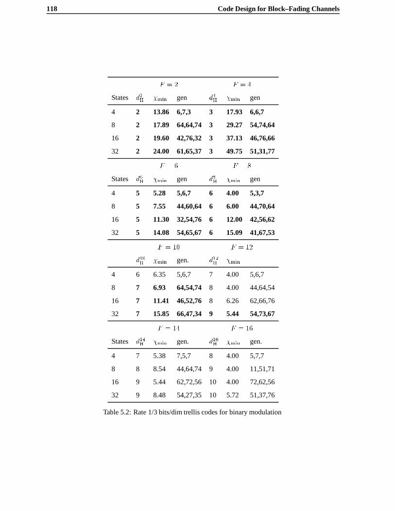
118 Code Design for Block–Fading Channels
F = 2 F = 4
States d2H �min gen d4H �min gen
4 2 13.86 6,7,3 3 17.93 6,6,7
8 2 17.89 64,64,74 3 29.27 54,74,64
16 2 19.60 42,76,32 3 37.13 46,76,66
32 2 24.00 61,65,37 3 49.75 51,31,77
F = 6 F = 8
States d6H �min gen d8H �min gen
4 5 5.28 5,6,7 6 4.00 5,3,7
8 5 7.55 44,60,64 6 6.00 44,70,64
16 5 11.30 32,54,76 6 12.00 42,56,62
32 5 14.08 54,65,67 6 15.09 41,67,53
F = 10 F = 12
d10H �min gen. d12H �min
4 6 6.35 5,6,7 7 4.00 5,6,7
8 7 6.93 64,54,74 8 4.00 44,64,54
16 7 11.41 46,52,76 8 6.26 62,66,76
32 7 15.85 66,47,34 9 5.44 54,73,67
F = 14 F = 16
States d14H �min gen. d16H �min gen.
4 7 5.38 7,5,7 8 4.00 5,7,7
8 8 8.54 44,64,74 9 4.00 11,51,71
16 9 5.44 62,72,56 10 4.00 72,62,56
32 9 8.48 54,27,35 10 5.72 51,37,76
Table 5.2: Rate 1/3 bits/dim trellis codes for binary modulation

5.2 Maximum Code Diversity 119
F = 2 F = 4
States d2H �min gen d4H �min gen
4 2 9.80 5,7 3 6.35 5,7
8 2 12.00 64,54 3 10.08 64,54
16 2 12.65 62,72 3 13.21 62,46
32 2 16.00 62,72 3 14.54 75,57
64 2 17.89 704,564 3 17.93 724,564
F = 6 F = 8
States d6H �min gen. d8H �min gen.
4 4 5.66 5,7 4 5.66 5,7
8 4 6.26 64,74 5 4.00 44,64
16 4 8.24 62,56 5 5.28 46,66
32 4 11.31 21,75 5 8.19 51,66
64 4 14.65 664,854 5 10.90 444,774
F = 10 F = 12
States d10H �min gen. d12H �min gen.
4 5 4.00 5,7 5 4.00 5,7
8 5 5.28 64,74 6 4.00 64,54
16 5 7.55 62,46 6 4.00 42,76
32 6 5.04 61,75 7 4.42 51,67
64 6 7.27 644,564 7 6.30 724,534
F = 14 F = 16
States d14H �min gen. d16H �min gen.
4 5 4.00 5,7 5 4.00 5,7
8 6 4.00 64,54 6 4.00 64,54
16 6 5.04 62,66 7 4.00 62,66
32 7 5.38 51,67 8 4.00 75,57
64 7 6.30 604,634 8 4.76 704,564
Table 5.3: Rate 1/2 bits/dim trellis codes for binary modulation

120 Code Design for Block–Fading Channels
use of binary linear codes simplifies the code search sincedFH preserves the linearity of the code. To see
this letc(a) andc(b) be any two output paths in the trellis. Sincec(a) � c(b) = c(q), wherec(q) is some
other path and� is binary addition, we have clearly that
dFH(ca; cb) = dFH(0; c(q)): (5.25)
This means that as far as the diversity order is concerned, it suffices to compute the Hamming weight of
INTERLEAVER
INTERLEAVER
01
pE
00
�pE
10
�p3E
11
p3E
01
pE
00
�pE
10
�p3E
11
p3E
01
pE
00
�pE
10
�p3E
11
p3E
g1
g0
g0
g1
g2
g3
Figure 5.14: 4-AM Coding Example
each path as we did for the binary case, the only difference being that it must be performed on the symbol
level. It is not necessary to consider all pairs of paths, which would greatly complicate the code search.
The secondary performance measure in the PEP,�min depends on theF Euclidean distances between
the sub–codewords transmitted ineach block. If we useGray codingas in figure 5.14, then with 4–AM
we cannot exploit the linearity of the code with respect to�, but we can use it to lower bound� as
�(c(a); c(b)) � �lb(c(a); c(b)) = �(0; c(a) � c(b)) (5.26)
This lower bound is possible since under the Gray mappingd2(a; b) � d2(0; a� b); 8a; b and in order
to maximize it, we do not have to consider all pairs of paths in the trellis. This bound using the Gray
mapping does not hold for larger AM constellations.
At the bottom of Table 5.4 we list some codes havingR = 1=2; 1 bits/dimension forF = 4; 8.
We must note that some of these codes were found with an incomplete search, due to the complexity of
the search process (indicated in italics).

5.2 Maximum Code Diversity 121
F = 4 F = 8
States d4H �lbmin gen. d8H �lbmin gen.
4 3 1.6 5,7 3 2.02 5,7
8 3 2.02 44,64 4 1.60 64,54
16 3 2.78 26,76 5 1.27 26,74
32 3 3.33 51,76 5 1.84 75,23
64 3 4.25 364,574 5 2.21 744,634
Table 5.4: Rate 1 bit/dim trellis–coded 4-AM modulations
F = 4 F = 8
States d4H �lbmin gen. d8H �lbmin gen.
4 4 2.58 5,7,6,7 6 2.02 5,7,6,7
8 4 3.76 44,64,54,34 7 1.77 44,30,50,34
16 4 4.60 62,72,46,56 7 2.55 62,56,50,66
32 4 5.55 65,75,43,57 7 3.27 44,57,67,51
64 4 6.04 644,474,554,534 7 3.79 544,464,704,750
Table 5.5: Rate 1/2 bits/dim trellis–coded 4-AM modulation

122 Code Design for Block–Fading Channels
5.3 Computer simulation of various codes
We have found that a union–bound approach for assessing the performance analytically yields quite
unfruitful results for trellis codes. The reason is that as we approach the maximum diversityF , the
number of paths which share a given diversity level increases quickly as we progress through the code’s
trellis and enumerating them becomes difficult since they cannot be discarded. Another by–product of
this effect which we remarked when the simulations were performed, is that error–patterns can be quite
long (several times the constraint length) due to the limited diversity.
In our simulations, we assumed a block lengthN = 100n= log2 jSj coded symbols, wheren is the
number of output bits of a rate1=n binary trellis code. We used a one–shot Viterbi decoder with trellis
termination. The channel is assumed to be a single–path Rayleigh fading channel and soft–decision
decoding is performed with perfect channel state information. The results are shown in figure 5.15–5.26
and cover a wide range of systems. We considered systems withF = 4 andF = 8 blocks, information
rates from .25 bits/dim to 1 bit/dim and simulated both frame and bit–error rates. We remark in general
that for the frame error–rates, performance increases as we increase the complexity since the value of
�min increases. Since the block–length is fairly long, we may justifiably compare these results to the
information outage probabilities we computed earlier. It is rather remarkable that we can come so close
to the theoretical limit with reasonably simple codes. The binary code used in the half–rate GSM standard
is less than one half of a decibel off from the information outage curve. We remark that this code is not
the one listed in the tables since it has a�min slightly less than the optimal code. Their performances are
indistiguishable however. ForF = 8, there is more of a gap between the codes and the theoretical limit.
This can be explained by the fact that the channel is becoming more ergodic than withF = 4 and the
code has to work much harder to get closer to the information outage probability. Examining the 4AM
codes, the increase in diversity is evident. For low SNR, however, the frame–error rate performance is
not significantly better than the binary codes. The performances of the 64–state codes for bothF = 4
andF = 8 fall within two decibels of the information outage curves.
In terms of the bit–error rate performances, increasing complexity has less of an effect, especially
for the caseF = 4. We have observed that although less frame errors occur, the erroneous sequences
tend to be much longer for the more complex codes and as a result contain many bit errors. We see
that constellation expansion yields much more significant gains here than in the frame–error rate perfor-
mance.

5.4 Chapter Summary 123
5.4 Chapter Summary
This chapter considered coding for block–fading channels with a small number of blocks. This channel
model has significant practical importance for delay–constrained block–oriented communications, a cat-
egory in which many mobile radio systems fall. The slow frequency–hopping scheme used in the current
GSM mobile radio systems is a prime example. It is reasonable to assume that next generation systems
will also use similar, and perhaps more complex techniques.
We focused our attention on the attainable diversity due to coding. We showed that there is a
upper–limit to the diversity which depends on the number of blocks, the code rate and the size of the
signaling constellation. This was shown in two ways; the first was based on the computation of the
information outage probability for various constellations. We then computed a bound, which turns out
to be a disguised version of the Singleton bound, which indicates the maximum achievable asymptotic
diversity for a code of a given rate and constellation size. Both methods indicate that diversity is limited
and that it can be increased by constellation expansion. A rather unfortunate result is that for high
spectral–efficiency systems, in order to achieve a high asymptotic diversity level, very large constellations
are required.
We gave examples of block and trellis codes, with more of an emphasis on the latter, which achieve
maximum diversity. An important result is that maximum diversity can be achieved with rather simple
codes and that, in terms of bit error–rate performance, increased complexity may not yield significant
gains. This is not true, however, for the frame–error rate performance, which is often important in both
speech and data applications.
We gave a few examples of trellis–coded AM modulation schemes which yield a higher level of
diversity than binary modulation schemes of equal information rate. This is an area for further research,
since similar higher spectral–efficiency schemes should be found with more appropriate modulation
methods.
The channel model and codes covered in this chapter can be applied to several types of situations.
For instance, a coded wideband multitone system or a partially interleaved narrowband channel. The
performance analysis would be different since the blocks may be correlated, but the central conclusions
of this chapter would remain valid.

124 Code Design for Block–Fading Channels
4 5 6 7 8 9 10 11 12 13 1410
−4
10−3
10−2
10−1
100
Pout(:25)
FER
64-states
16-states
4-states
Eb=N0 (dB)
Figure 5.15: Frame Error Probabilities forF = 4 andR = :25 bits/dim (antipodal modulation)

5.4 Chapter Summary 125
4 6 8 10 12 14 1610
−6
10−5
10−4
10−3
10−2
10−1
4-states
16-states
64-states
BER
Eb=N0
Figure 5.16: Bit Error Probabilities forF = 4 andR = :25 bits/dim (antipodal modulation)
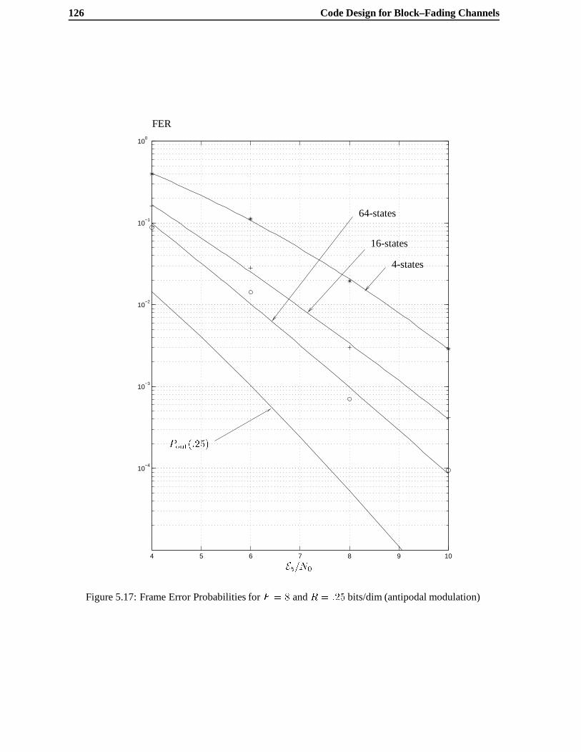
126 Code Design for Block–Fading Channels
4 5 6 7 8 9 10
10−4
10−3
10−2
10−1
100
64-states
16-states
4-states
Pout(:25)
FER
Eb=N0
Figure 5.17: Frame Error Probabilities forF = 8 andR = :25 bits/dim (antipodal modulation)

5.4 Chapter Summary 127
4 5 6 7 8 9 1010
−6
10−5
10−4
10−3
10−2
10−1
4-state
16-state
64-state
BER
Eb=N0
Figure 5.18: Bit Error Probabilities forF = 8 andR = :25 bits/dim (antipodal modulation)
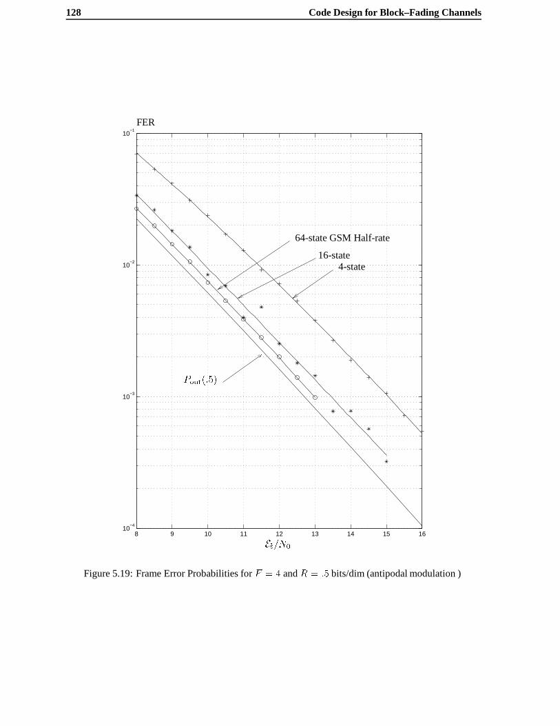
128 Code Design for Block–Fading Channels
8 9 10 11 12 13 14 15 1610
−4
10−3
10−2
10−1
64-state GSM Half-rate
16-state4-state
FER
Pout(:5)
Eb=N0
Figure 5.19: Frame Error Probabilities forF = 4 andR = :5 bits/dim (antipodal modulation )

5.4 Chapter Summary 129
8 9 10 11 12 13 14 15 16
10−4
10−3
10−2
4-state
16-state
64-state GSM Half Rate
BER
Eb=N0
Figure 5.20: Bit Error Probabilities forF = 4 andR = :5 bits/dim (antipodal modulation )

130 Code Design for Block–Fading Channels
6 7 8 9 10 11 12 13 1410
−4
10−3
10−2
10−1
64-state
16-state GSM Full Rate
8-state
Pout(:5)
FER
Eb=N0
Figure 5.21: Frame Error Probabilities forF = 8 andR = :5 bits/dim (antipodal modulation)
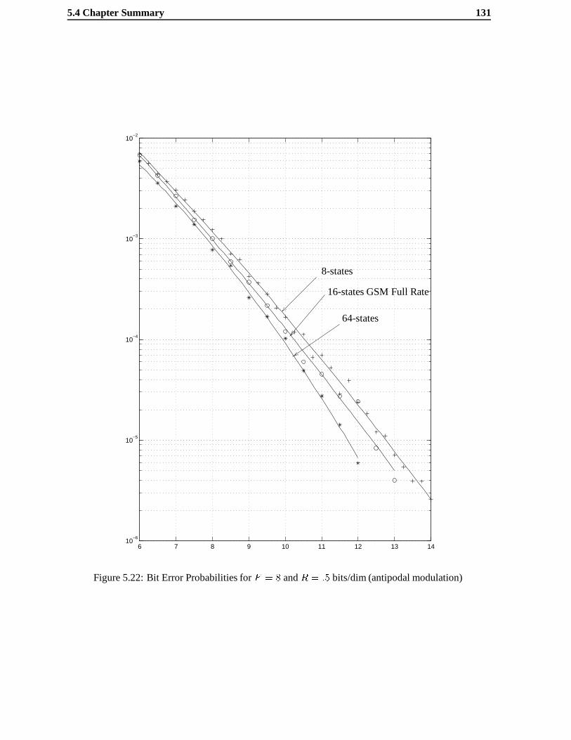
5.4 Chapter Summary 131
6 7 8 9 10 11 12 13 1410
−6
10−5
10−4
10−3
10−2
16-states GSM Full Rate
8-states
64-states
Figure 5.22: Bit Error Probabilities forF = 8 andR = :5 bits/dim (antipodal modulation)
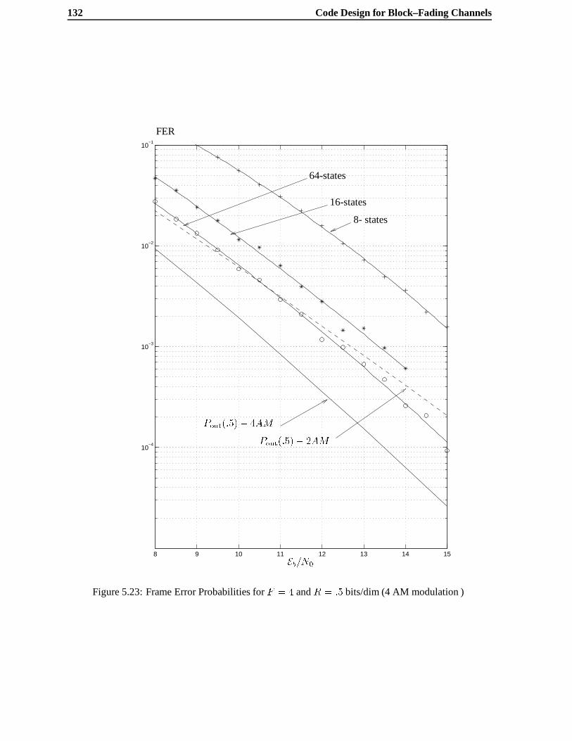
132 Code Design for Block–Fading Channels
8 9 10 11 12 13 14 15
10−4
10−3
10−2
10−1
Pout(:5)� 4AM
Pout(:5)� 2AM
64-states
16-states
8- states
FER
Eb=N0
Figure 5.23: Frame Error Probabilities forF = 4 andR = :5 bits/dim (4 AM modulation )

5.4 Chapter Summary 133
8 9 10 11 12 13 14 15
10−4
10−3
10−2
4-states
16-states
64-states(2AM GSM)
64-states
BER
Eb=N0
Figure 5.24: Bit Error Probabilities forF = 4 andR = :5 bits/dim (4 AM modulation )
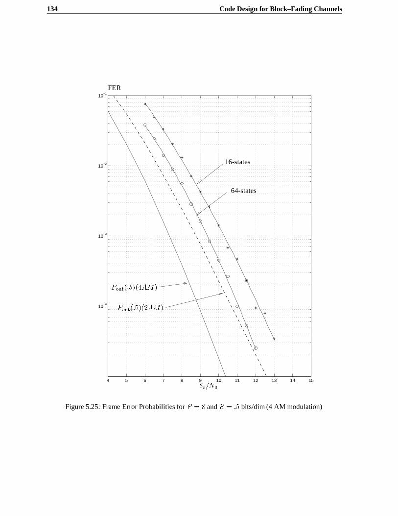
134 Code Design for Block–Fading Channels
4 5 6 7 8 9 10 11 12 13 14 15
10−4
10−3
10−2
10−1
16-states
64-states
Pout(:5)(4AM)
Pout(:5)(2AM)
FER
Eb=N0
Figure 5.25: Frame Error Probabilities forF = 8 andR = :5 bits/dim (4 AM modulation)

5.4 Chapter Summary 135
6 7 8 9 10 11 1210
−6
10−5
10−4
10−3
10−2
64-states (2AM)
16-states
64-states
BER
Eb=N0
Figure 5.26: Bit Error Probabilities forF = 8 andR = :5 bits/dim (4 AM modulation)

136 Code Design for Block–Fading Channels
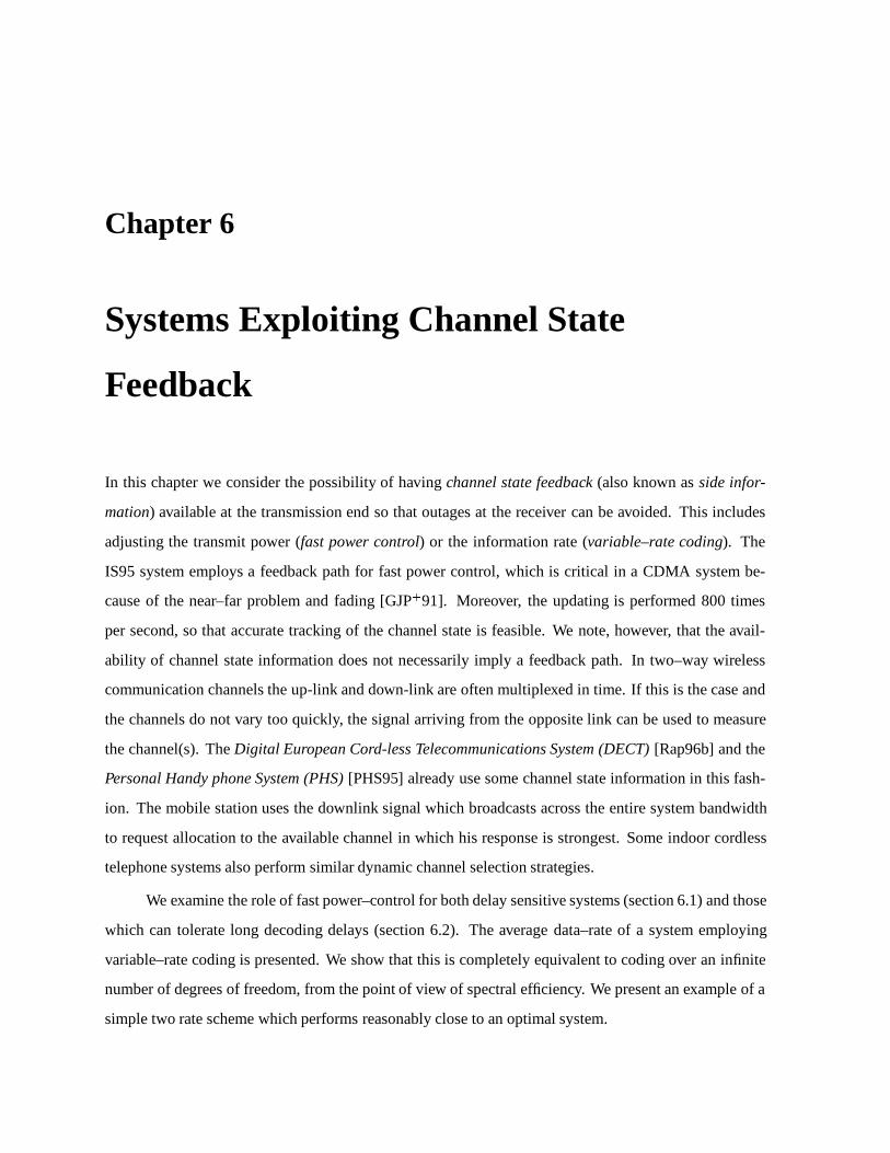
Chapter 6
Systems Exploiting Channel State
Feedback
In this chapter we consider the possibility of havingchannel state feedback(also known asside infor-
mation) available at the transmission end so that outages at the receiver can be avoided. This includes
adjusting the transmit power (fast power control) or the information rate (variable–rate coding). The
IS95 system employs a feedback path for fast power control, which is critical in a CDMA system be-
cause of the near–far problem and fading [GJP+91]. Moreover, the updating is performed 800 times
per second, so that accurate tracking of the channel state is feasible. We note, however, that the avail-
ability of channel state information does not necessarily imply a feedback path. In two–way wireless
communication channels the up-link and down-link are often multiplexed in time. If this is the case and
the channels do not vary too quickly, the signal arriving from the opposite link can be used to measure
the channel(s). TheDigital European Cord-less Telecommunications System (DECT)[Rap96b] and the
Personal Handy phone System (PHS)[PHS95] already use some channel state information in this fash-
ion. The mobile station uses the downlink signal which broadcasts across the entire system bandwidth
to request allocation to the available channel in which his response is strongest. Some indoor cordless
telephone systems also perform similar dynamic channel selection strategies.
We examine the role of fast power–control for both delay sensitive systems (section 6.1) and those
which can tolerate long decoding delays (section 6.2). The average data–rate of a system employing
variable–rate coding is presented. We show that this is completely equivalent to coding over an infinite
number of degrees of freedom, from the point of view of spectral efficiency. We present an example of a
simple two rate scheme which performs reasonably close to an optimal system.

138 Systems Exploiting Channel State Feedback
The last part of this section deals with packet transmission over fading channels with a retransmis-
sion protocol, so that outages are corrected by anAutomatic Repeat reQuest (ARQ)scheme [BG92]. We
examine the maximum average information rate that can be expected on a collision–free channel, where
outages are purely due to deep fades. This type of system is already in use in the data transmission mode
of the GSM standard.
6.1 Variable Power Constant Rate Systems
When the transmitted signal can be tailored to the channel response, its statistics should be chosen to
maximize average mutual information. Normally this maximum is given the namechannel capacity,
since this is the absolute maximum information rate at which communication can take place. Throughout
this section we will assume that codewords are transmitted continuously across static multipath channels
(for the duration of a codeword). The codewords are subject to the following average energy constraint
E Sx;n(f) � P
W(6.1)
whereSx;n(f) is the power spectral density during the transmission of codewordn. We now adjust the
power spectrum of thenth codeword according the state of the channel,Hn(f), asSx;n(f) = P(Hn(f))
such that the average mutual information at the receiver is constant and maximum for each codeword.
This is known as thedelay–limitedcapacity, defined by Hanly and Tse [HT96], which can be written
explicitly as
Cd = maxP
Z W=2
�W=2log2
�1 +
jHn(f)j2P(Hn(f))
N0
�df bits=s (6.2)
subject toEHP(Hn(f)) � PW . It was given this name since the tolerable decoding delay is assumed to
be small so that ergodic channel arguments cannot be used.
6.1.1 Multiple Receivers in Single–Path Rayleigh Fading
Let us consider the simplest case, namely frequency–flat channels. We may write the maximization
problem as
Cd = maxP
W log2
�1 +
P
WN0�nP(�n)
�bits=s (6.3)

6.1 Variable Power Constant Rate Systems 139
subject toR10 P(u)f�(u)du = 1. Clearly the only power control function which yields a constant
average mutual information isP(u) = K=u so that
Cd = W log2
1 +
P
WN0
1R10 f�(u)
duu
!bits=s: (6.4)
This expression was also found by Goldsmith in her doctoral thesis [Gol94]. We see, therefore, that
in this simple case, the optimal delay–limited power control function is nothing but a perfect power
controller, which attempts to keep the received SNR constant. If we use the Rayleigh fading model in
(6.4) we see immediately thatCd = 0 sinceK =R10 e�u duu = E1(0) = 1 and therefore outages are
inevitable. For systems employing some diversity this will not be the case, and outages can be avoided
at the expense of transmitting at a high power when the channel state is weak. Let us examine simple
multiple–antenna diversity schemes with maximal–ratio combining in Rayleigh fading. Assuming a
system withL receivers the density function of the received energy is given by
f�(u) =uL�1
(L� 1)!e�u; u � 0 (6.5)
so that
K =
�Z 1
0f�(u)
du
u
��1= L� 1 (6.6)
and
Cd = W log2
�1 + (L� 1)
P
WN0
�; (6.7)
If there were no fading, the capacity of the multichannel system would be
C(L) = W log2
�1 + L
P
WN0
�; (6.8)
so that for largeL, the fading channel with power control loses very little in terms of spectral efficiency.
In order to better appreciate the effect of power control, let us compute the information outage
probability for this example using (4.33) forL = 2 which yields
Pout(R) = 1��1 + (2R � 1)
WN0
P
�exp
��WN0
P
�2R � 1
��: (6.9)
The power controlled information rateCd for PWN0
= 10 dB is plotted alongside (6.9) in Figure 6.1.
We see that power control has a very significant effect since the outage probability is very high (.3) at
R = Cd, which means that rates much less thanCd can be expected for practical outage rates. This outage
rate is even close to a system without diversity which is shown in the second curve. The explanation for
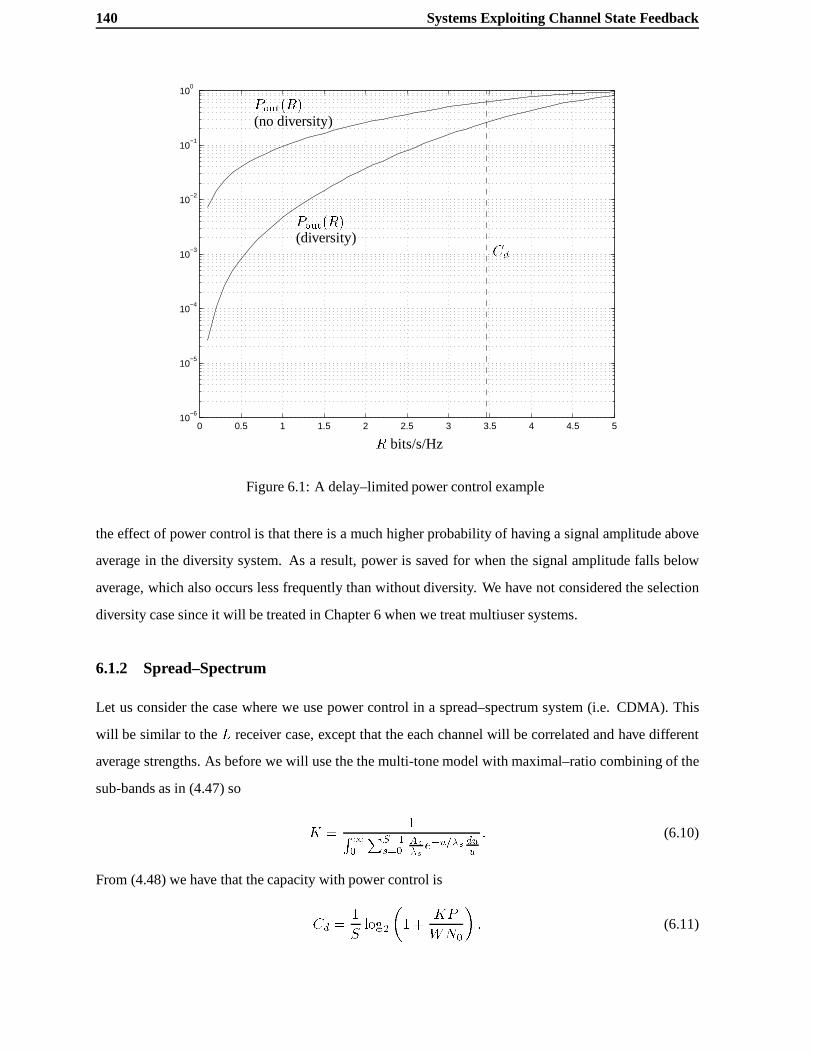
140 Systems Exploiting Channel State Feedback
0 0.5 1 1.5 2 2.5 3 3.5 4 4.5 510
−6
10−5
10−4
10−3
10−2
10−1
100
Cd
Pout(R)(diversity)
Pout(R)(no diversity)
R bits/s/Hz
Figure 6.1: A delay–limited power control example
the effect of power control is that there is a much higher probability of having a signal amplitude above
average in the diversity system. As a result, power is saved for when the signal amplitude falls below
average, which also occurs less frequently than without diversity. We have not considered the selection
diversity case since it will be treated in Chapter 6 when we treat multiuser systems.
6.1.2 Spread–Spectrum
Let us consider the case where we use power control in a spread–spectrum system (i.e. CDMA). This
will be similar to theL receiver case, except that the each channel will be correlated and have different
average strengths. As before we will use the the multi-tone model with maximal–ratio combining of the
sub-bands as in (4.47) so
K =1R1
0
PS�1s=0
As�se�u=�s duu
: (6.10)
From (4.48) we have that the capacity with power control is
Cd =1
Slog2
�1 +
KP
WN0
�: (6.11)

6.1 Variable Power Constant Rate Systems 141
The values forK in dB as a function ofS for the TU12 channel are -1.2860, 7.3224, 15.8094, and
19.6477 forS = 4; 16; 64; 128. If there were no fading,K would be equal to the number of sub–bandsS
so that the losses due to fading in dB are 7.3066, 4.7188, 2.25 and 1.42. As in the multichannel case, the
diversity brings the performance of the system much closer that of the non–fading channel as the number
of degrees of freedom increases.
We compare the information outage rates from (4.50) withCd in figure 6.3 for the ETSI TU12
channel. As before we assume the bandwidth isSWB with WB = 9:6kHz and an SNR of PWN0= 0 dB.
We see that as the bandwidth increases, the diversity has the effect of bringing the outage curve closer to
Cd, so that power control has less of an effect. The reason for this is that the output of the maximal–ratio
combiner tends quickly to 1 with increasing diversity, so that outages do not occur as frequently. For low
diversity, as in the previous example we see that power control has a dramatic effect, even if the loss with
respect to a non–fading channel is substantial. Even when the channel is more or less flat, for instance for
S = 4, the second eigenvalue, which is almost insignificant (see Table 4.1), forces the density function of
the channel gain to zero at the origin. This is shown in figure 6.2. As a result, outages can be effectively
avoided by power control.
10−6
10−5
10−4
10−3
10−2
10−1
100
101
0
2
4
6
8
10
12
14
u
f�(u)(S = 4)
Figure 6.2: Probability density of channel gain forS = 4
The constraint (6.1) allows the transmit power of each codeword to vary according to the channel
state, so that at certain times it can be quite high, in order to compensate for a poor channel state. If the
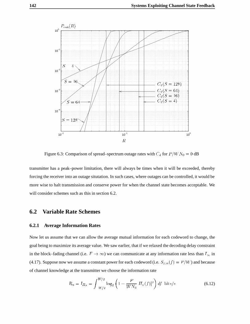
142 Systems Exploiting Channel State Feedback
10−2
10−1
100
10−4
10−3
10−2
10−1
100Pout(R)
R
Cd(S = 128)
Cd(S = 64)Cd(S = 16)Cd(S = 4)S = 64
S = 128
S = 4
S = 16
Figure 6.3: Comparison of spread–spectrum outage rates withCd for P=WN0 = 0 dB
transmitter has a peak–power limitation, there will always be times when it will be exceeded, thereby
forcing the receiver into an outage situtation. In such cases, where outages can be controlled, it would be
more wise to halt transmission and conserve power for when the channel state becomes acceptable. We
will consider schemes such as this in section 6.2.
6.2 Variable Rate Schemes
6.2.1 Average Information Rates
Now let us assume that we can allow the average mutual information for each codeword to change, the
goal being to maximize its average value. We saw earlier, that if we relaxed the decoding delay constraint
in the block–fading channel (i.e.F ! 1) we can communicate at any information rate less thanI1 in
(4.17). Suppose now we assume a constant power for each codeword (i.e.Sx;n(f) = P=W ) and because
of channel knowledge at the transmitter we choose the information rate
Rn = IHn =
Z W=2
�W=2log2
�1 +
P
WN0jHn(f)j2
�df bits=s (6.12)
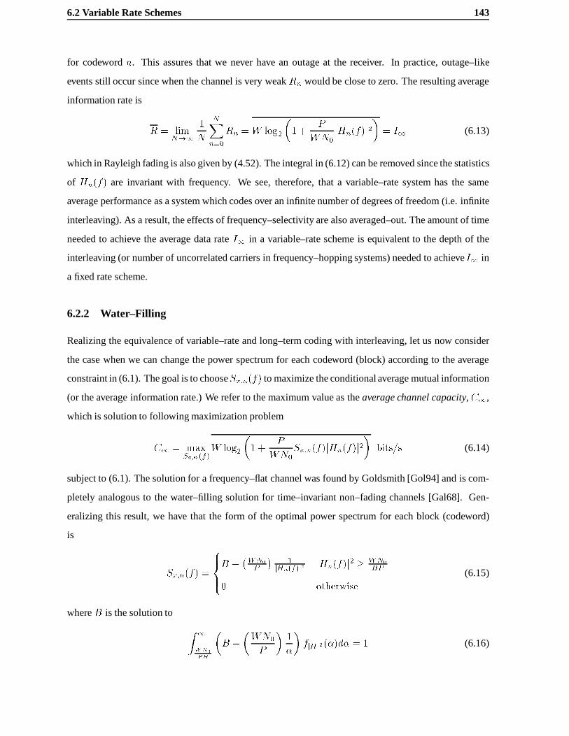
6.2 Variable Rate Schemes 143
for codewordn. This assures that we never have an outage at the receiver. In practice, outage–like
events still occur since when the channel is very weakRn would be close to zero. The resulting average
information rate is
R = limN!1
1
N
NXn=0
Rn = W log2
�1 +
P
WN0jHn(f)j2
�= I1 (6.13)
which in Rayleigh fading is also given by (4.52). The integral in (6.12) can be removed since the statistics
of Hn(f) are invariant with frequency. We see, therefore, that a variable–rate system has the same
average performance as a system which codes over an infinite number of degrees of freedom (i.e. infinite
interleaving). As a result, the effects of frequency–selectivity are also averaged–out. The amount of time
needed to achieve the average data rateI1 in a variable–rate scheme is equivalent to the depth of the
interleaving (or number of uncorrelated carriers in frequency–hopping systems) needed to achieveI1 in
a fixed rate scheme.
6.2.2 Water–Filling
Realizing the equivalence of variable–rate and long–term coding with interleaving, let us now consider
the case when we can change the power spectrum for each codeword (block) according to the average
constraint in (6.1). The goal is to chooseSx;n(f) to maximize the conditionalaverage mutual information
(or the average information rate.) We refer to the maximum value as theaverage channel capacity,C1,
which is solution to following maximization problem
C1 = maxSx;n(f)
W log2
�1 +
P
WN0Sx;n(f)jHn(f)j2
�bits=s (6.14)
subject to (6.1). The solution for a frequency–flat channel was found by Goldsmith [Gol94] and is com-
pletely analogous to the water–filling solution for time–invariant non–fading channels [Gal68]. Gen-
eralizing this result, we have that the form of the optimal power spectrum for each block (codeword)
is
Sx;n(f) =
8><>:B � �WN0
P
�1
jHn(f)j2jHn(f)j2 � WN0
BP
0 otherwise
(6.15)
whereB is the solution to
Z 1
WN0PB
�B �
�WN0
P
�1
�
�fjHj2(�)d� = 1 (6.16)
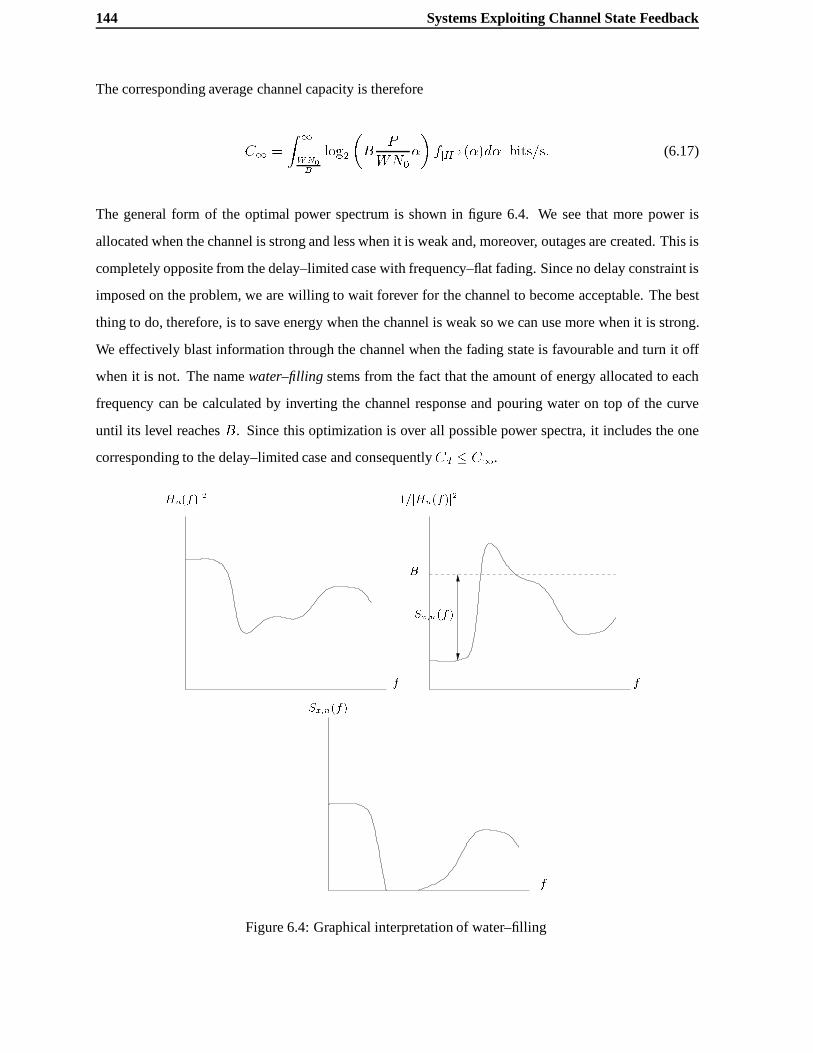
144 Systems Exploiting Channel State Feedback
The corresponding average channel capacity is therefore
C1 =
Z 1
WN0B
log2
�B
P
WN0�
�fjHj2(�)d� bits=s: (6.17)
The general form of the optimal power spectrum is shown in figure 6.4. We see that more power is
allocated when the channel is strong and less when it is weak and, moreover, outages are created. This is
completely opposite from the delay–limited case with frequency–flat fading. Since no delay constraint is
imposed on the problem, we are willing to wait forever for the channel to becomeacceptable. The best
thing to do, therefore, is to save energy when the channel is weak so we can use more when it is strong.
We effectively blast information through the channel when the fading state is favourable and turn it off
when it is not. The namewater–fillingstems from the fact that the amount of energy allocated to each
frequency can be calculated by inverting the channel response and pouring water on top of the curve
until its level reachesB. Since this optimization is over all possible power spectra, it includes the one
corresponding to the delay–limited case and consequentlyCd � C1.
jHn(f)j2 1=jHn(f)j
2
B
Sx;n(f)
f f
Sx;n(f)
f
Figure 6.4: Graphical interpretation of water–filling
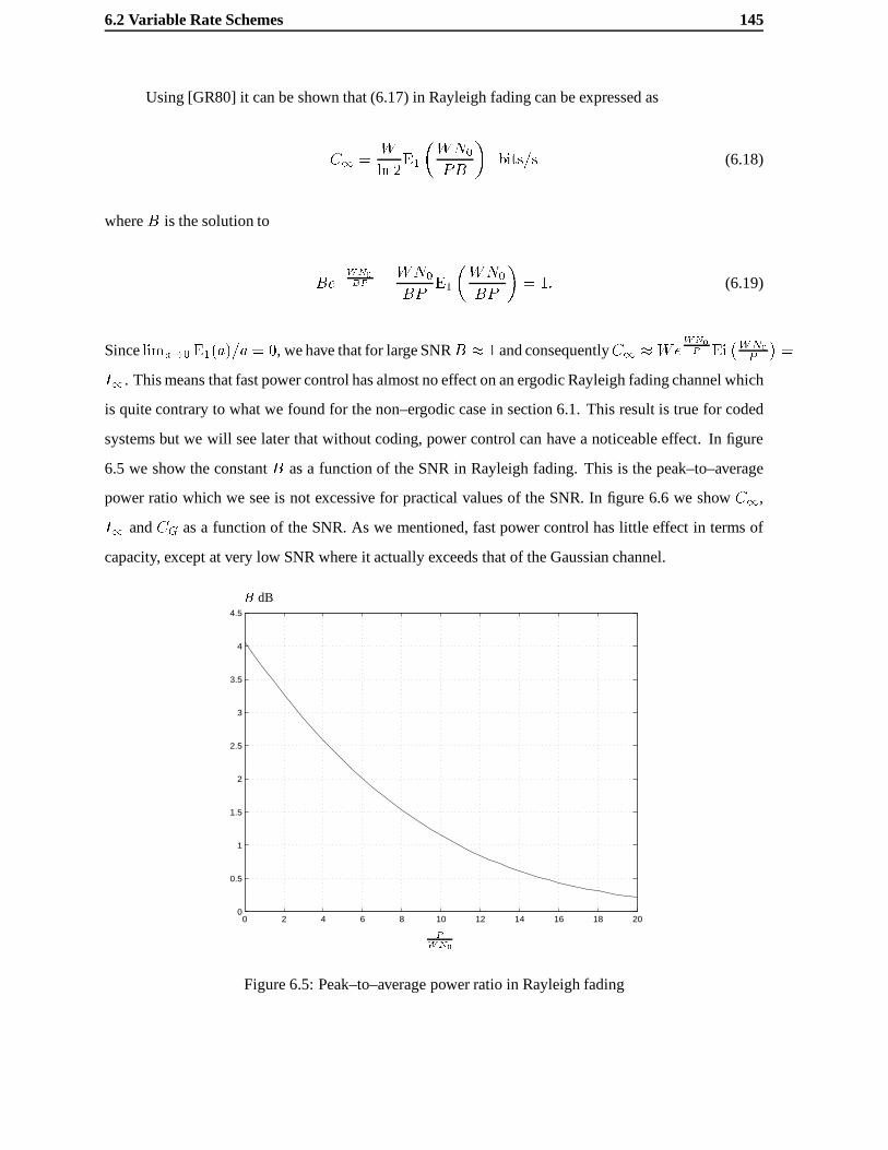
6.2 Variable Rate Schemes 145
Using [GR80] it can be shown that (6.17) in Rayleigh fading can be expressed as
C1 =W
ln 2E1
�WN0
PB
�bits=s (6.18)
whereB is the solution to
Be�WN0BP � WN0
BPE1
�WN0
BP
�= 1: (6.19)
Sincelima!0E1(a)=a = 0, we have that for large SNRB � 1 and consequentlyC1 � WeWN0P Ei
�WN0P
�=
I1. This means that fast power control has almost no effect on an ergodic Rayleigh fading channel which
is quite contrary to what we found for the non–ergodic case in section 6.1. This result is true for coded
systems but we will see later that without coding, power control can have a noticeable effect. In figure
6.5 we show the constantB as a function of the SNR in Rayleigh fading. This is the peak–to–average
power ratio which we see is not excessive for practical values of the SNR. In figure 6.6 we showC1,
I1 andCG as a function of the SNR. As we mentioned, fast power control has little effect in terms of
capacity, except at very low SNR where it actually exceeds that of the Gaussian channel.
0 2 4 6 8 10 12 14 16 18 200
0.5
1
1.5
2
2.5
3
3.5
4
4.5
B dB
PWN0
Figure 6.5: Peak–to–average power ratio in Rayleigh fading
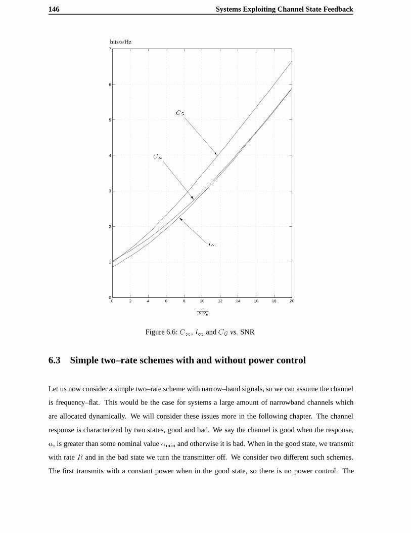
146 Systems Exploiting Channel State Feedback
0 2 4 6 8 10 12 14 16 18 200
1
2
3
4
5
6
7
CG
C1
I1
PWN0
bits/s/Hz
Figure 6.6:C1, I1 andCG vs.SNR
6.3 Simple two–rate schemes with and without power control
Let us now consider a simple two–rate scheme with narrow–band signals, so we can assume the channel
is frequency–flat. This would be the case for systems a large amount of narrowband channels which
are allocated dynamically. We will consider these issues more in the following chapter. The channel
response is characterized by two states, good and bad. We say the channel is good when the response,
�, is greater than some nominal value�min and otherwise it is bad. When in the good state, we transmit
with rateR and in the bad state we turn the transmitter off. We consider two different such schemes.
The first transmits with a constant power when in the good state, so there is no power control. The

6.3 Simple two–rate schemes with and without power control 147
second, described by Goldsmith [Gol94], uses power control to keep a constant received power when
transmission takes place.
Chua and Goldsmith[CG96][CG97] have considered variable rate schemes with more than two
rates and find that average spectral efficiencies very close toI1 can be expected with and without addi-
tional coding. These results are also obtained with reasonable outage rates (on the order of10�2). The
need for additional coding depends on the target bit–error rate of the system. Here we will show that the
same is possible with uncoded two–rate transmission, if the system can spend large amounts of time in
the outage state.
Scheme 1: Constant Transmit Power
In this scheme, the transmitter chooses to use the channel it knows that there will not be an outage at the
receiver. The power control is of the form
P(�) =
8><>:
11�F�(�min)
� > �min
0 � � �min
(6.20)
so that its average value is unity. The transmitter uses an information rate
R = W log2
�1 +
P
WN0
�min1� F�(�min)
�bits=s (6.21)
when in the good channel state, so that as long as� � �min we are guaranteed not to have an outage at
the receiver. The average information rate is therefore
R = R(1� F�(�min)) (6.22)
and the peak–to–average power ratio is1� F�(�min). We now maximize (6.22) with respect to�min by
setting@R=@�min = 0 yielding the non–linear equation
PWN0
e�min(1 + �min)
1 + PWN0
�mine�min= ln
�1 +
P
WN0�mine
�min
�(6.23)
for Rayleigh fading.
Scheme 2: Constant Received Power
Now we assume a power controller of the form
P(�) =
8><>:
K(�min)� � � �min
0 � < �min
(6.24)

148 Systems Exploiting Channel State Feedback
so that the received power is constant when the channel is in the good state. This was considered by
Goldsmith in her thesis [Gol94]. The information rate in the good state is given by
R = W log2
�1 +
P
WN0K(�min)
�(6.25)
and the average information is again given by (6.22). As in earlier sections, we chooseK(�min) to yield
a unit average power control level as
K(�min) =
�Z 1
�min
f�(u)du
u
��1: (6.26)
The peak–to–average power ratio isK(�min)=�min. Again we maximize (6.22) with respect to�min
which in Rayleigh fading yields the non–linear equation governing the optimal�min
P
WN0
e��min
�min (E1(�min))2 =
�1 +
P
WN0
1
E1(�min)
�ln
�1 +
P
WN0
1
E1(�min)
�(6.27)
We note that in Rayleigh fading
K(�min) =1
E1(�min): (6.28)
We compare the two schemes in figures 6.7–6.9 for Rayleigh fading. We see that with power con-
trol and moderate SNR, the two–rate scheme comes very close to optimal performance, which in terms of
implementation complexity is an important result. Without power control there is a more significant loss.
The peak–to–average power of scheme 2 is higher, but at the same time is rather invariant with respect to
the average SNR. If we consider the peak–to–average power ratio for scheme 2,1=(�minE1(�min)), as
shown in figure 6.10 we see that the optimized scheme operates in the vicinity of the minimum, 5.5 dB.
If we consider the optimal threshold level for both cases in figure 6.10, we remark the two schemes work
quite differently. With scheme 1, the variation of the threshold with the average SNR is significant, and
more importantly the transmitter is turned off more often than with scheme 2. Scheme 2, on the other
hand, has a more or less constant threshold and transmits around 75% of the time.
6.3.1 BER Comparison for Uncoded Transmission
The previous results on average information rates assumes the use of some form of error–control coding.
Let us now consider the same two–rate channel control schemes without any coding at all. We will use
different size QAM constellations to achieve average information rates of 1 and 2 bits/s/Hz and compare
their performance to uncoded BPSK and QPSK.
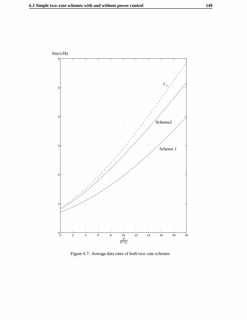
6.3 Simple two–rate schemes with and without power control 149
0 2 4 6 8 10 12 14 16 18 200
1
2
3
4
5
6
I1
Scheme2
Scheme 1
PWN0
bits/s/Hz
Figure 6.7: Average data rates of both two–rate schemes

150 Systems Exploiting Channel State Feedback
0 2 4 6 8 10 12 14 16 18 201
1.5
2
2.5
3
3.5
4
4.5
5
5.5
6
Scheme 1
Scheme 2
PWN0
Peak-to-average Power Ratio (dB)
Figure 6.8: Peak–to–average Power Ratios
0 2 4 6 8 10 12 14 16 18 200.2
0.3
0.4
0.5
0.6
0.7
0.8
0.9
1
1.1
1.2
�min
Scheme 1
Scheme 2
PWN0
Figure 6.9: Threshold Comparison

6.3 Simple two–rate schemes with and without power control 151
0 0.2 0.4 0.6 0.8 1 1.2 1.4 1.6 1.8 25
6
7
8
9
10
11
12
13
14
�
1=�E1(�) (dB)
5.5dB
Figure 6.10: Minimum–Peak to Average Power Ratio for Scheme 2

152 Systems Exploiting Channel State Feedback
We choose 4 different modulation schemes for numerical computations: BPSK (R = 1 bit/s/Hz),
QPSK (R = 2 bits/s/Hz), 8-PSK (R = 3 bits/s/Hz) and 16-QAM (R = 4 bits/s/Hz). The BER condi-
tioned on the channel strength� for the these QAM modulations are (from Proakis [Pro95])
PBPSKbj� = PQPSK
bj�= Q
r2P(�)� Eb
N0
!
P 8�PSKbj�
� 1
3Q
r:8787P(�)� Eb
N0
!
P 16�QAMbj�
=3
8Q
r:8P(�)� Eb
N0
!"1� 3
8Q
r:8P(�)� Eb
N0
!#(6.29)
We take three values for�min such that1� F�(�min) = 1=2; 1=3; 1=4, which in Rayleigh fading
are�min(1=2) = ln 2 = :6931; �min(1=3) = ln 3 = 1:0986; �min(1=4) = ln 4 = 1:3863. These are
simply the proportion of time communication is allowed. In order to calculate the average BER we use
the density
f 0�(�0) =
8><>:
11�F�(�min)
f�(�0); �0 � �min
0 otherwise
which is the density of� conditioned on� � �min, or equivalently the time when transmission takes
place.
Under scheme 1, the peak–to–average power ratios (1 � F�(�min) for the three choices of�min
are 3 dB, 4.77 dB and 6 dB. Using QPSK with�min(1=2) and 8–PSK with�min(1=3) for an average
spectral spectral efficiency of 1 bit/s/Hz we have the BERs
PQPSKb = e�min
Z 1
�min(1=2)Q
r2e�min(1=2)
EbN0
�0
!e��
0d�0
= Q
r2:7724
EbN0
!� 2
sEb=N0
:5 + Eb=N0Q
s1:3862
�1 + 2
EbN0
�!(6.30)
P 8�PSKb � 1
3e�min(1=3)
Z 1
�min(1=3)Q
r:8787e�min(1=3)
EbN0
�0
!e��
0d�0
=1
3
"Q
r2:8960
EbN0
!� 3
sEb=N0
:7587 + Eb=N0Q
s2:1972
�1 + 1:3180
EbN0
�!#(6.31)
We have used the fact thatZ 1
�Q�p
�x�e�xdx = e��Q
�p�x��s
�
� + 2Q�p
(� + 2)x�: (6.32)

6.3 Simple two–rate schemes with and without power control 153
We note that the uncoded BER for BPSK/QPSK can be found from (6.32) by setting� = 0 and� =
2Eb=N0 yielding
PB=QPSKb = :5
1�
sEb=N0
1 + Eb=N0
!: (6.33)
For 16–QAM with�min(1=4) and�min(1=2) for average spectral efficiencies of 1 bit/s/Hz and 2
bit/s/Hz respectively, the BERs must be computed numerically.
Examining now scheme 2 in Rayleigh fading, we have that the power control constantK for
the three values chosen for�min isK(1=2) = 2:6406; K(1=3) = 5:3644; K(1=4) = 8:4274. These
correspond to peak–to–average power ratios (K=�min) of 5.80 dB, 6.89 dB and 7.83 dB. For transmission
at an average spectral efficiency of 1 bit/s/Hz we have the three average error probabilities of
PQPSKb = Q
r2K(1=2)
EbN0
!= Q
r5:2812
EbN0
!(6.34)
P 8�PSKb = Q
r:8787K(1=3)
EbN0
!= Q
r4:6161
EbN0
!(6.35)
P 16�QAMb = Q
r:8K(1=4)
EbN0
!= Q
r6:7419
EbN0
!(6.36)
and similarly at 2 bits/s/Hz we have
P 16�QAMb = Q
r:8K(1=2)
EbN0
!= Q
r2:1125
EbN0
!(6.37)
We plot the BER for the two schemes at 1 and 2 bits/s/Hz in figures 6.11 and 6.12 where we
notice that both have comparable performance, with a slight advantage for scheme 2 at 1 bit/s/Hz. The
most important practical conclusion to be drawn from this analysis is that exploitation of channel state
information is a very efficient means for achieving acceptable performance on a fading channel, when
we do not have decoding delay constraints. We see that we can even achieve an SNR gain with respect
to a non–fading channelwithout coding. This is possible by taking advantage of the time–varying nature
of the fading channel by transmitting with a higher rate constellation when the attenuation is greater than
unity. We will meet this effect again in Chapter 6 when we treat the multiuser channel. In that case, we
do not even require constellation expansion to achieve an SNR gain without coding. Provided channel
state information exploitation is feasible for given system parameters, it is a much simpler solution than
using error–control codes with interleaving.
Here we have achieved an SNR gain at the expense of transmitting very infrequently on a single
channel. In future (and already in some current) wireless systems, the transmitter may haveaccess
154 Systems Exploiting Channel State Feedback
to many channels, sayL, over which to transmit information. These on/off schemes would be very
attractive in this type of scenario. Suppose we choose some proportion of time,p, where the transmitter
remains silent on any given channel and that when transmitting on a given channel we use rateR. The
total average rate would beLR(1 � p) and the instantaneous number of channels in use, assuming all
channels had uncorrelated strengths (i.e. carrier spacings much greater than the coherence bandwidth),
is a binomial random variable with density
Prob(Cn = c) =
�L
c
�(1� p)cpL�c: (6.38)
By choosingL to be large enough andp small enough, we have a variable–rate scheme withL rates and
outage probabilitypL, which is small. We will come across these types of allocation strategies in the
following chapter.
6.4 Average information rate with retransmissions
We now consider a single–user system with anAutomatic Repeat reQuest (ARQ)mechanism as shown
in figure 6.13. The transmitter generates packets continuously which are stored in a buffer of unlimited
size. We interpret each packet as a separate codeword which, after having been transmitted, remains in
the buffer until an acknowledgment of successful decoding is returned by the receiver. Furthermore, we
assume that the feedback path is error–free which is somewhat unrealistic on wireless channels. Using
the information outage probability we have, for reasonable packet sizes, that the probability of correctly
decoding the packet is1�Pout(R). In a mobile environment where the channel state changes from packet
to packet it is reasonable to assume that it is independent for each transmission of the same packet. Under
this assumption, the average number of transmissions necessary to transmit the packet is
(1� Pout(R))1Xi=1
i[Pout(R)]i�1 =
1
1� Pout(R)(6.39)
yielding an average data rate of
R = R(1� Pout(R)) bits=s: (6.40)
This type of system is very similar to scheme 1 in the previous section. The main difference is that
instantaneouschannel knowledge at the transmitter allows for power conservation by detecting the outage
before it happens. Here the transmitter only learns of the outage by virtue of the repeat request. In a
multiuser system this difference would be more important, since thea priori channel knowledge would

6.4 Average information rate with retransmissions 155
0 1 2 3 4 5 6 7 8 9 1010
−6
10−5
10−4
10−3
10−2
10−1
100
EbN0
BER
BPSK-Rayleigh Fading
BPSK- No fading
QPSK8-PSK
16-QAM
Scheme 1
Scheme 2
QPSK8-PSK
16-QAM
Figure 6.11: BER for 1 bit/s/Hz variable rate schemes

156 Systems Exploiting Channel State Feedback
0 1 2 3 4 5 6 7 8 9 1010
−6
10−5
10−4
10−3
10−2
10−1
100
BER
QPSK- Rayleigh Fading
QPSK-No FadingScheme 1
Scheme 2
EbN0
Figure 6.12: BER for 2 bit/s/Hz variable rate schemes

6.4 Average information rate with retransmissions 157
Packets
Channel Decoder
ARQ
Reliable packetsEncoder
Packet 1Packet 2
Packet N
Figure 6.13: System model with repeat requests
also reduce the number of collisions as well as allow for a higher transmit power. We do not consider
this effect here.
We plotR vs.R for single–path Rayleigh fading withPWN0= 10 dB in figure 6.14 where we see
that there is an operating information rate at whichR is maximum. By straightforward maximization we
find using (4.34) thatRopt is the solution to
Ropt2R =
P
WN0ln 2: (6.41)
0 1 2 3 4 5 6 70
0.2
0.4
0.6
0.8
1
1.2
1.4
1.6
PWN0
= 10 dB
R bits/s/Hz
Tmax
R bits/s/Hz
Figure 6.14: Reliable throughput as a function ofR in Rayleigh fading
We now consider a system which employs some diversity. This can be achieved via slow–
frequency hopping for instance, where a packet is split and transmitted in different parts of the spec-

158 Systems Exploiting Channel State Feedback
trum. The multiple–access protocol considered by Humbletet al in [HHR96], which we depict in figure
6.15, uses a similar approach. Here the packet is transmitted with a sweeping carrier frequency in or-
der to exploit diversity. This has the effect of turning a frequency–selective channel into a narrowband
time–selective channel. It also has the advantage that several users can transmit concurrently without
collisions, provided their sweeps do not overlap at the outset. This situtation is reduced by introducing
a header at a given frequency which indicates when a user is about to begin transmission of the packet.
As long as users do not initiate transmissions within a time–period equal to the header length they will
t
f
T
W
Figure 6.15: Frequency–sweeping transmission scheme
not collide. The bandwidth of the wideband system, either with a frequency–sweep or with frequency–
hopping will be characterized by a certain number of degrees of freedom, but we simplify the problem
by considering it as a block fading channel withF independent blocks, whereF will be proportional
to the available bandwidth. The optimal information ratesRopt can be calculated numerically using the
results of section 3.6. In figure 6.16 we showRmax as a function of the SNR andF and in figure 6.16
we show the information outage rate which yieldsRmax.
We see that the average data rate increases as a function of the diversity order, except it does so
rather slowly. If we consider the optimal information outage rates, we see that they are all quite high, and
they decrease with increasing diversity. This means that we are effectively using the channel at a very
high information rate when it is favourable. This result was shown by Knopp and Humblet in [KH96].
This is not surprising, since it is exactly the same effect as with variable–rate coding. The merits of
variable–rate coding and long decoding delays (i.e. interleaving) are clear, sinceI1 is noticeably higher
than any of the diversity–based systems with ARQ. Nevertheless, an ARQ–based system in Rayleigh
fading can still offer spectral efficiencies exceeding 2 bits/s/Hz for reasonable signal–to–noise ratios.
6.5 Chapter Summary 159
6.5 Chapter Summary
In this chapter, we considered the exploitation of channel knowledge at the transmission end, either in the
form of fast power control or variable–rate coding, in order to eliminate or exploit information outages.
This can be achieved in practice in two–way systems either by a feedback mechanism or by measuring
the channel response of the opposite link when time–division duplex is used. We first considered the
delay–constrained case for narrow–band signals with optimal perfect power control, under an average
power constraint. Using the definition ofdelay–limited capacitywe showed that when some form of
diversity can be exploited, not only can outages be eliminated, but significantly higher information rates
can be expected. The price to be paid for using such a scheme is an unlimited peak–to–average power
ratio. We then considered the case where the information rate of each codeword could be adjusted to
avoid outages. We showed that this is completely equivalent to coding over a very large number of
independent channel states, which in practice can be achieved by interleaving. When the power of each
codeword can also be tailored to the channel response, the optimal power allocation scheme iswater–
filling in time and frequency, which effectively uses a high power when the channel is in a favourable
state (so that a large amount of information can be transmitted) and halts transmission when the channel
is weak. The optimal strategy suffers from outages, in the sense that no information is conveyed, but
uses them to conserve energy for future transmissions, which occur at a much higher rate. It does not
suffer, however, from an excessive peak–to–average power ratio. In Rayleigh fading an optimal power
allocation scheme has little advantage over one which keeps the transmit power constant, and therefore
over an optimal ideally interleaved coded system, since they offer practically identical average spectral
efficiencies.
We considered simple two–rate sub–optimal power control schemes for narrow–band channels
which work along the lines of the optimal scheme. They use a fixed information rate when the channel
response is above a certain threshold and halt transmission when it falls below this threshold. We have,
therefore, a system which controls outages.
The first scheme keeps the transmitter power constant when not in a outage state, has an average
data rate which depends on the information rate agreed upon by the communicating parties. This rate
is chosen to maximize the average spectral efficiency, which is on the order of 2 bits/s/Hz at an average
SNR of 10dB. The second scheme keeps the received power constant when transmitting using a perfect
power controller, and the outage threshold is chosen to maximize the average information rate. Such a
scheme becomes possible in Rayleigh fading for peak–to–average power ratios which exceed 5.5 dB,

160 Systems Exploiting Channel State Feedback
and the optimal operating point is always around this value. For average signal–to–noise ratios on the
order of 10 dB it is possible to achieve average spectral efficiencies on the order of 2.5 bits/s/Hz which
are only slightly less than optimal. For higher average signal–to–noise ratios the loss is more significant.
We considered the bit error–rate of the two simple schemes with uncoded QAM modulation. The
main conclusion is that significant performance gains can be had in comparison to an uncoded system
without channel state feedback without the need for channel coding/interleaving. Practically speaking,
this says that by exploiting channel state feedback we can avoid complex coding/interleaving schemes
altogether.
Finally we considered an ARQ–based single–user scheme, as is already used in the data transmis-
sion mode of the GSM standard. We showed that this scheme is identical to the second of the two–rate
coding schemes considered previously, except for the fact that the power cannot be conserved during an
outage event since the transmitter does not have this information at its disposal. The only means to avoid
outages is by requesting retransmissions. The maximum average data rate is also found by choosing
an optimum information rate which is effectively used only when the channel state is favourable. We
computed these rates for block–fading channels, usingF = 1; 2; 4; 8 blocks, and results indicate that
average spectral efficiencies on the order of 2 bits/s/Hz in Rayleigh fading could be expected even with
ARQ, and that diversity (i.e. number of independent blocks) increases the average spectral efficiency
slowly. The outage rates are quite high ranging from 40% (F = 1) down to 10% (F = 8) at an SNR of
10 dB.
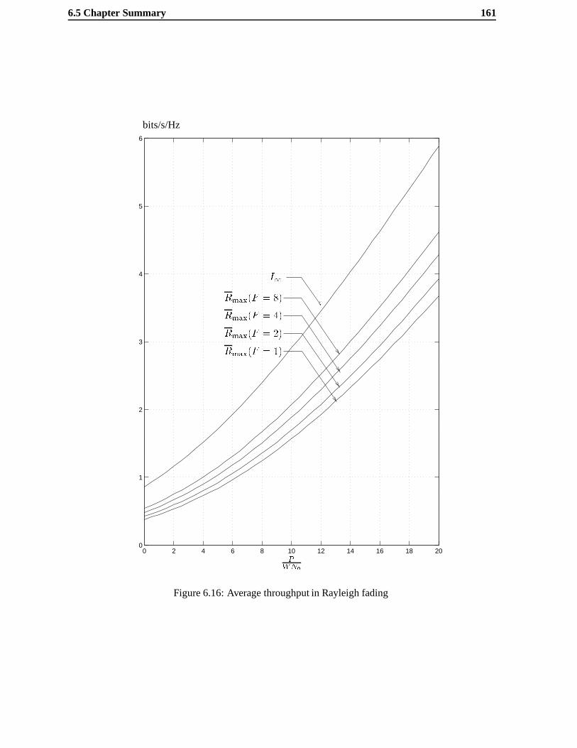
6.5 Chapter Summary 161
0 2 4 6 8 10 12 14 16 18 200
1
2
3
4
5
6
Rmax(F = 4)
Rmax(F = 8)
Rmax(F = 2)
Rmax(F = 1)
I1
bits/s/Hz
PWN0
Figure 6.16: Average throughput in Rayleigh fading

162 Systems Exploiting Channel State Feedback
0 2 4 6 8 10 12 14 16 18 200.05
0.1
0.15
0.2
0.25
0.3
0.35
0.4
0.45
0.5
0.55
F = 1
F = 2
F = 4
F = 8
PWN0
Pout(Ropt)
Figure 6.17: Optimal information outage rates as a function ofR andF
Chapter 7
Multiuser Channels and Multiuser
Diversity
In the multiuser cellular systems in use today, there are two primary communication links between the
users located in the cell and the cell’s central base station as shown in Figure 7.1. Theup-linkrefers to the
information flow from the users to the base station and is an example of a classicmultiple–access channel
(MAC), or a many–to–one communication problem. The down-link refers to the opposite situation,
namely the flow of information from the base station to the users. This is an example of abroadcast
channelor a one–to–many communication problem. There has been much recent interest in determining
which types of multiple–access methods are best, and this chapter we examine such issues, albeit in a
rather general sense. Here we will concern ourselves only with case of the MAC. Another important
aspect of multiuser cellular systems which we do not consider here is adjacent cell interference. Our
results, therefore, apply mainly to single–cell systems (i.e. when there is only one base station) or also
for systems where inter-cell–interference can be ignored. An information–theoretic treatment of Cellular
systems without fading are given in [Wyn94]
We begin this chapter with a discussion of the Gaussian MAC without fading to familiarize our-
selves with the different types of multiple–access schemes. One of the main goals of this is toillustrate
that a multiple-access scheme is simply a way of sharing dimensions and distributing energy in such
a way that the receiver can distinguish between different users. We introduce the basic information–
theoretic tools needed to handle these systems and and we use them to analyze a specific example with
multipath fading.
We then turn our attention to the average information rates that can be expected with different

164 Multiuser Channels and Multiuser Diversity
UPLINK DOWNLINK
Basestation Basestation
Figure 7.1: Communication Links in Cellular Systems
multiple–access schemes over fading channels. In the case where the system has access to channel
state information either via feedback path or in time–division duplex, the users can allocate the power
according to their channel and the channels of the other users. We show that when this is feasible, we
have an inherent diversity effect that is due the nature of the time/frequency–varying MAC which was
not present in the single–user channel we treated in Chapter 3. This effect can yield significant increases
in the achievable data rates.
7.1 Multiple–Access Channels without fading
In order to familiarize the reader with the basic ideas in multiple–access communications we begin
with a short treatment for a non–fading Gaussian channel. Consider the simple discrete–time channel
x0
x1
xL�1
z
y
Figure 7.2: Gaussian Multiple–Access Channel (MAC)
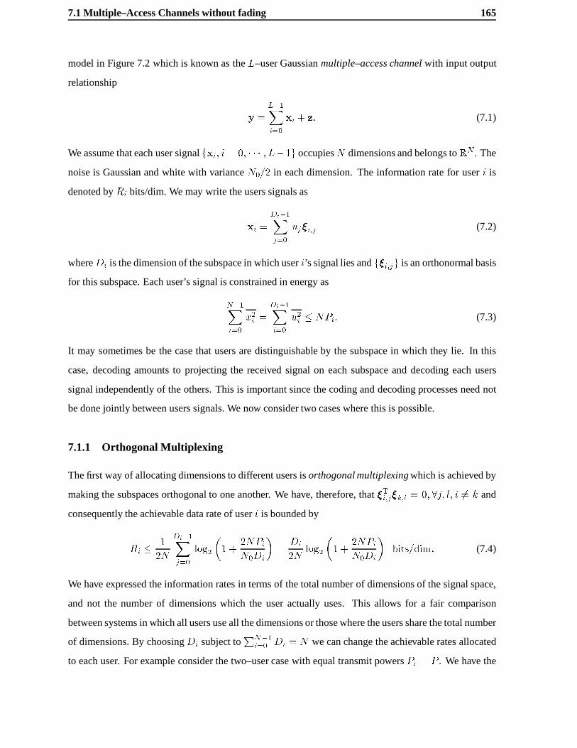
7.1 Multiple–Access Channels without fading 165
model in Figure 7.2 which is known as theL–user Gaussianmultiple–access channelwith input output
relationship
y =L�1Xi=0
xi + z: (7.1)
We assume that each user signalfxi; i = 0; � � � ; L�1g occupiesN dimensions and belongs toRN. The
noise is Gaussian and white with varianceN0=2 in each dimension. The information rate for useri is
denoted byRi bits/dim. We may write the users signals as
xi =
Di�1Xj=0
uj�i;j (7.2)
whereDi is the dimension of the subspace in which useri’s signal lies andf�i;jg is an orthonormal basis
for this subspace. Each user’s signal is constrained in energy as
N�1Xi=0
x2i =
Di�1Xi=0
u2i � NPi: (7.3)
It may sometimes be the case that users are distinguishable by the subspace in which they lie. In this
case, decoding amounts to projecting the received signal on each subspace and decoding each users
signal independently of the others. This is important since the coding and decoding processes need not
be done jointly between users signals. We now consider two cases where this is possible.
7.1.1 Orthogonal Multiplexing
The first way of allocating dimensions to different users isorthogonal multiplexingwhich is achieved by
making the subspaces orthogonal to one another. We have, therefore, that�Ti;j�k;l = 0; 8j; l; i 6= k and
consequently the achievable data rate of useri is bounded by
Ri � 1
2N
Di�1Xj=0
log2
�1 +
2NPiN0Di
�=
Di
2Nlog2
�1 +
2NPiN0Di
�bits=dim: (7.4)
We have expressed the information rates in terms of the total number of dimensions of the signal space,
and not the number of dimensions which the user actually uses. This allows for a fair comparison
between systems in which all users use all the dimensions or those where the users share the total number
of dimensions. By choosingDi subject toPN�1
i=0 Di = N we can change the achievable rates allocated
to each user. For example consider the two–user case with equal transmit powersPi = P . We have the
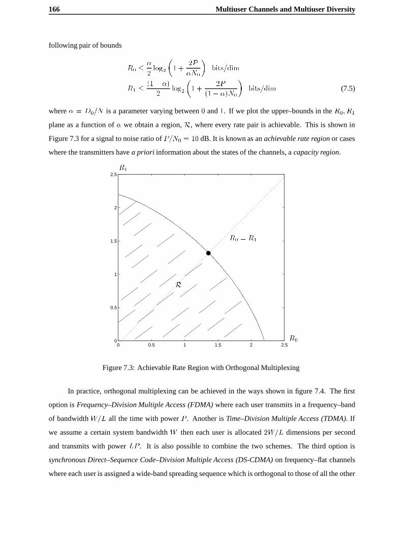
166 Multiuser Channels and Multiuser Diversity
following pair of bounds
R0 � �
2log2
�1 +
2P
�N0
�bits=dim
R1 � (1� �)
2log2
�1 +
2P
(1� �)N0
�bits=dim (7.5)
where� = D0=N is a parameter varying between0 and1. If we plot the upper–bounds in theR0; R1
plane as a function of� we obtain a region,R, where every rate pair is achievable. This is shown in
Figure 7.3 for a signal to noise ratio ofP=N0 = 10 dB. It is known as anachievable rate regionor cases
where the transmitters havea priori information about the states of the channels, acapacity region.
0 0.5 1 1.5 2 2.50
0.5
1
1.5
2
2.5
R
R0
R1
R0 = R1
Figure 7.3: Achievable Rate Region with Orthogonal Multiplexing
In practice, orthogonal multiplexing can be achieved in the ways shown in figure 7.4. The first
option isFrequency–Division Multiple Access (FDMA)where each user transmits in a frequency–band
of bandwidthW=L all the time with powerP . Another isTime–Division Multiple Access (TDMA). If
we assume a certain system bandwidthW then each user is allocated2W=L dimensions per second
and transmits with powerLP . It is also possible to combine the two schemes. The third option is
synchronous Direct–Sequence Code–Division Multiple Access (DS-CDMA)on frequency–flat channels
where each user is assigned a wide-band spreading sequence which is orthogonal to those of all the other

7.1 Multiple–Access Channels without fading 167
users. This is more difficult to illustrate since users occupy all frequencies and all times and is therefore
not included in the figure. It can be achieved using orthogonal spread–spectrum pulse shapes and can be
defined either in the frequency–domain using a multi-tone approach [Van95] or in the time–domain with
a classical direct–sequence approach.
USER 0
USER2
USERL� 1
t
f
USER 0 USER1 USERL� 1
USER 0
USER 0 USERL=N � 1
USERN�1N
L USERL� 1
USER 0
USER 0
USER 0USERL� 1
USERL� 1
f
tf f
t t
FDMA TDMA
FDMA/TDMA Slow Frequency-Hopping
Figure 7.4: Orthogonal Multiplexing Schemes
7.1.2 Non–Orthogonal Multiplexing
When orthogonality cannot be achieved, or is avoided on purpose then the inter-user interference must be
handled in some fashion. The simplest way is to have a bank ofL decoders where each user is decoded
separately treating the others as part of the background noise. We will refer to this type of decoding as
single–user decoding. The received signal treated by decoderi is
y = xi + zi (7.6)
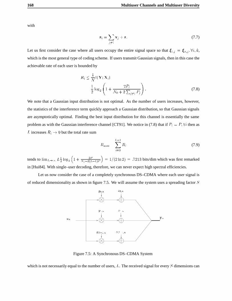
168 Multiuser Channels and Multiuser Diversity
with
zi =Xj 6=i
xj + z: (7.7)
Let us first consider the case where all users occupy the entire signal space so that�i;j = �k;j ; 8i; k,
which is the most general type of coding scheme. If users transmit Gaussian signals, then in this case the
achievable rate of each user is bounded by
Ri � 1
NI(Y;Xi)
=1
2log2
1 +
2PiN0 + 2
Pj 6=i Pj
!: (7.8)
We note that a Gaussian input distribution is not optimal. As the number of users increases, however,
the statistics of the interference term quickly approach a Gaussian distribution, so that Gaussian signals
are asymptotically optimal. Finding the best input distribution for this channel is essentially the same
problem as with the Gaussian interference channel [CT91]. We notice in (7.8) that ifPi = P; 8i then as
L increasesRi ! 0 but the total rate sum
Rsum =L�1Xi=0
Ri (7.9)
tends tolimL!1 L12 log2
�1 + 2P
N0+2(L�1)P
�= 1=(2 ln 2) = :7213 bits/dim which was first remarked
in [Hui84]. With single–user decoding, therefore, we can never expect high spectral efficiencies.
Let us now consider the case of a completely synchronous DS–CDMA where each user signal is
of reduced dimensionality as shown in figure 7.5. We will assume the system uses a spreading factorS
g0;n
gS�1;n
g1;n
z0;n
z1;n
ynun
zS�1;n
Figure 7.5: A Synchronous DS–CDMA System
which is not necessarily equal to the number of users,L. The received signal for everyS dimensions can
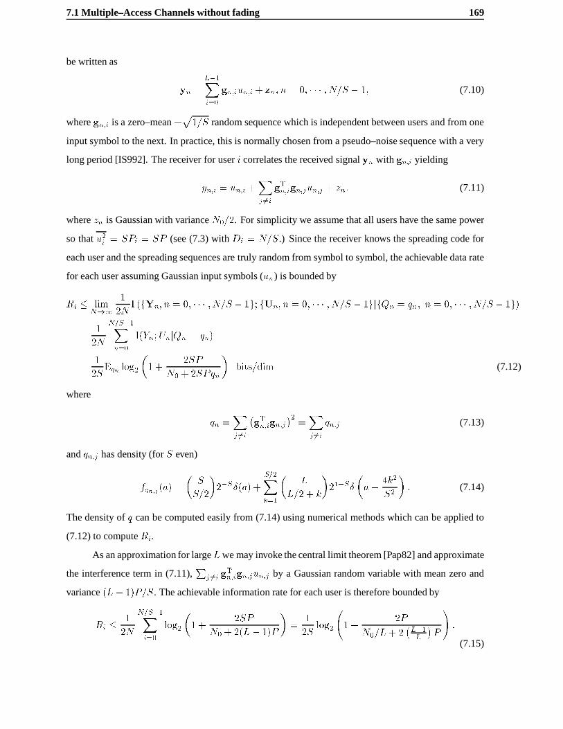
7.1 Multiple–Access Channels without fading 169
be written as
yn =L�1Xi=0
gn;iun;i + zn; n = 0; � � � ; N=S � 1; (7.10)
wheregn;i is a zero–mean�p1=S random sequence which is independent between users and from one
input symbol to the next. In practice, this is normally chosen from a pseudo–noise sequence with a very
long period [IS992]. The receiver for useri correlates the received signalyn with gn;i yielding
yn;i = un;i +Xj 6=i
gTn;ign;jun;j + zn: (7.11)
wherezn is Gaussian with varianceN0=2. For simplicity we assume that all users have the same power
so thatu2i = SPi = SP (see (7.3) withDi = N=S.) Since the receiver knows the spreading code for
each user and the spreading sequences are truly random from symbol to symbol, the achievable data rate
for each user assuming Gaussian input symbols (un) is bounded by
Ri � limN!1
1
2NI (fYn; n = 0; � � � ; N=S � 1g; fUn; n = 0; � � � ; N=S � 1gjfQn = qn; n = 0; � � � ; N=S � 1g)
=1
2N
N=S�1Xn=0
I(Yn;UnjQn = qn)
=1
2SEqn log2
�1 +
2SP
N0 + 2SPqn
�bits=dim (7.12)
where
qn =Xj 6=i
�gTn;ign;j
�2=Xj 6=i
qn;j (7.13)
andqn;j has density (forS even)
fqn;j (a) =
�S
S=2
�2�S�(a) +
S=2Xk=1
�L
L=2 + k
�21�S�
�a� 4k2
S2
�: (7.14)
The density ofq can be computed easily from (7.14) using numerical methods which can be applied to
(7.12) to computeRi.
As an approximation for largeLwe may invoke the central limit theorem [Pap82] and approximate
the interference term in (7.11),P
j 6=i gTn;ign;jun;j by a Gaussian random variable with mean zero and
variance(L� 1)P=S. The achievable information rate for each user is therefore bounded by
Ri � 1
2N
N=S�1Xi=0
log2
�1 +
2SP
N0 + 2(L� 1)P
�=
1
2Slog2
1 +
2P
N0=L+ 2�L�1L
�P
!:
(7.15)

170 Multiuser Channels and Multiuser Diversity
We see right away that ifS is finite, in the limit of largeL, the total rate sumLRi also tends to .7213
bits/dim. If, on the other hand,L=S = K thenLRi tends to:5 log2 (1 + 1=K)K � :7213 bits/dim.
In the special case whereK = 1 (i.e. the spreading gain is equal to the number of users), we see that
the total rate sum tends to .5 bits/dim. In figure 7.6 we plotRsum for both types of systems with and
without the approximation forP=N0 = 10dB for the special caseK = 1 in the DS–CDMA system. We
see that both decrease to their asymptotic values quite quickly. The central limit theorem approximation
is only slightly pessimistic for reasonableL. We may conclude, therefore, that on a Gaussian channel
there is an advantage to using a low–rate coding scheme as opposed to simple DS–CDMA. We note also
the non–optimality of Gaussian signals when the number of users is small, since the DS–CDMA system
has a larger total sum rate. The transmitted signal foreach user for each symbol isun;ign;i which is not
Gaussian.
The issue of spreadingvs. low–rate coding was first considered by Hui [Hui84] and later by
Viterbi [Vit90]. Hui suggested that users should each use different low–rate convolutional codes with
no (or very little) PN spreading. Viterbi’s approach uses the same low–rate code foreach user whose
output modulates a very–long period and user–dependent PN sequence which may or may not provide
additional bandwidth expansion. The PN sequences distiguish the users and allows each to use the same
code. The coding scheme is based on mapping the output of a convolutional code to large set of Walsh–
Hadamard sequences. We will soon see that the advantage of using such low–rate coding schemes is
even greater on a multipath channel.
7.1.3 Joint Detection on the MAC
When the receiver can decode the signals jointly, Liao [Lia72] and Ahlswede [Ahl71] showed that the
achievable rate region for two users is defined by
R0 � I(Y;X0jX1) � maxk
I(Y;X0jX1 = x1;k)
R1 � I(Y;X1jX0) � maxk
I(Y;X1jX0 = x0;k)
R0 +R1 � I(Y;X0;X1) (7.16)
which generalizes forL users as
R =\U�U
(Xi2U
Ri � I(Y; fXi; i 2 UgjfXj; j 2 Ug)); U = f0; 1; � � � ; L� 1g
(7.17)

7.1 Multiple–Access Channels without fading 171
5 10 15 20 25 300.4
0.6
0.8
1
1.2
1.4
1.6
1.8
2
2.2
2.4
.7213
.5
bits/dim
L
Low-rate coding
PN Spreading
Gaussian approximation
Figure 7.6: Total Sum of Rates Comparison for Low–Rate Coded CDMA and PN Spreading
This region is shown forL = 2 in Figure 7.7 and is known as theCover–Wyner pentagon. We remark
that its shape is quite different from the region for orthogonal multiplexing. For a Gaussian MAC the
achievable rate region can be shown to be [CT91]
\U�U
Xi2U
Ri � 1
2log2
1 +
2
N0
Xi2U
Pi
!(7.18)
This results from the fact that the conditional mutual information functionals in (7.17) are maximum
when the power of all the conditioned users is zero. The region in (7.17) corresponds to the case where
all users occupy the entire signal space so that the region of a DS–CDMA system, which is a special case,
will necessarily lie within. The practical interpretation of the corner points of the region is important,
since it can be shown that they can be achieved by single–user decoding. The basic idea is that the
codeword for a given user is decoded considering the other users as part of the noise, as we did earlier.
His codeword is recreated and subtracted from the received signal and the next user is decoded in a similar
fashion. The different rates achieved by these corner points depends on the order in which the successive
decoding algorithm is performed. By changing the decoding order periodically, any point on the rate
region boundary can be achieved. This assumes, of course that the users change their transmission rates

172 Multiuser Channels and Multiuser Diversity
I(Y;X0jX1)
R0
R1
I(Y;X0)
I(Y;X1jX0)
I(Y;X1)
Figure 7.7: The Cover–Wyner Pentagon
according to the decoding order used at that time instant.
Another recent and promising technique for achieving any point on the rate region was developed
by Rimoldi and Urbanke [RU96]. Here each user but one splits his source into two separate sources
whose outputs are added before transmitting across the channel. By controlling the relative rates of the
split sources, any point on the achievable rate region lying between the corner points can be used with
single–user successive decoding. Practically speaking, this is very important since neither the decoding
order nor the code rates need to be changed during transmission. The disadvantage of this technique,
however, is that the decoding complexity is twice as high.
We show the Cover–Wyner pentagon compared to orthogonal multiplexing for equal signal–to–
noise ratiosPi=N0 = 10 dB in Figure 7.8. We see that orthogonal multiplexing is optimal at the equal–
rate point when we have equal transmitter powers. The total rate sum also increases without bound with
the number of users which was not the case when single–user decoding was performed.

7.1 Multiple–Access Channels without fading 173
0 0.5 1 1.5 2 2.50
0.5
1
1.5
2
2.5
R0
R1
Optimal Region Boundary
OrthogonalRegion Boundary
Figure 7.8: Comparison of the Optimal Rate Region with Orthogonal Multiplexing
DS–CDMA with Joint Detection
If we consider the perfectly symmetric power case, we can compute the total rate sum for joint detection
of a synchronous DS–CDMA system. We may write (7.10) equivalently as
yn =�g0;n g1;n � � � gL�1;n
�0BBBBBB@
u0;n
u1;n...
uS�1;n
1CCCCCCA
+ zn; n = 0; 1; � � � ; N=S � 1
=Wn
p�nV
Tn
0BBBBBB@
u0;n
u1;n...
uL�1;n
1CCCCCCA
+ zn; (7.19)
whereWn andVn are unitary matrices andp�n is a diagonal matrix containing the singular values of
theL � S matrix,Gn = Wn
p�nV
Tn , whose columns are the spreading sequences for symboln. We
may therefore consider the equivalent decomposed channel
y0n;i =p�n;iu
0n;i + z0n;i; n = 0; � � � ; N=L� 1; i = 0; � � � ; L� 1 (7.20)

174 Multiuser Channels and Multiuser Diversity
whereu0n;i2 = LP . The total rate sum (for largeN=S) is
Rsum =1
N
N=S�1Xn=0
I(Yn;UnjGn = Gn)
=1
2LE�n;i
S�1Xi=0
log2
�1 +
2�n;iP
N0
�: (7.21)
This can be computed numerically by Monte–Carlo averaging. We show the comparison between the
total rate sumRsum for the two non–orthogonal approaches with joint detection in Figure 7.9 for an SNR
of P=N0 = 10 dB and assumingS = L. As was the case for single–user decoding, we can achieve
higher data rates with low–rate coding than with DS–CDMA.
5 10 15 20 25 302
2.5
3
3.5
4
4.5
5
L
bits/dim
DS-CDMA
Low-Rate Coding
Figure 7.9: Comparison of Joint Detection of DS–CDMA and Low–Rate Coding Systems
There has been a great deal of research in the last ten years on joint detection schemes for the mul-
tiuser channel, the majority of which deal with the DS–CDMA case. A recent review of these techniques
is given in [BJK96]. These were sparked by the work of Verd´u in [Ver86] who considered the optimal
joint detection of asynchronous DS–CDMA on a Gaussian channel.
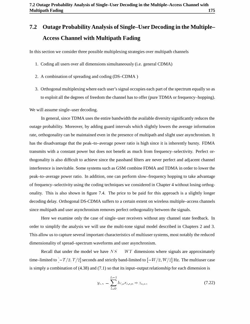
7.2 Outage Probability Analysis of Single–User Decoding in the Multiple–Access Channel withMultipath Fading 175
7.2 Outage Probability Analysis of Single–User Decoding in the Multiple–
Access Channel with Multipath Fading
In this section we consider three possible multiplexing strategies over multipath channels
1. Coding all users over all dimensions simultaneously (i.e. general CDMA)
2. A combination of spreading and coding (DS–CDMA )
3. Orthogonal multiplexing whereeach user’s signal occupies each part of the spectrum equally so as
to exploit all the degrees of freedom the channel has to offer (pure TDMA or frequency–hopping).
We will assume single–user decoding.
In general, since TDMA uses the entire bandwidth the available diversity significantly reduces the
outage probability. Moreover, by adding guard intervals which slightly lowers the average information
rate, orthogonality can be maintained even in the presence of multipath and slight user asynchronism. It
has the disadvantage that the peak–to–average power ratio is high since it is inherently bursty. FDMA
transmits with a constant power but does not benefit as much from frequency–selectivity. Perfect or-
thogonality is also difficult to achieve since the passband filters are never perfect and adjacent channel
interference is inevitable. Some systems such as GSM combine FDMA and TDMA in order to lower the
peak–to–average power ratio. In addition, one can perform slow–frequency hopping to take advantage
of frequency–selectivity using the coding techniques we considered in Chapter 4 without losing orthog-
onality. This is also shown in figure 7.4. The price to be paid for this approach is a slightly longer
decoding delay. Orthogonal DS-CDMA suffers to a certain extent on wireless multiple–access channels
since multipath and user asynchronism removes perfect orthogonality between the signals.
Here we examine only the case of single–user receivers without any channel state feedback. In
order to simplify the analysis we will use the multi-tone signal model described in Chapters 2 and 3.
This allow us to capture several important characteristics of multiuser systems, most notably the reduced
dimensionality of spread–spectrum waveforms and user asynchronism.
Recall that under the model we haveNS = WT dimensions where signals are approximately
time–limited to[�T=2; T=2] seconds and strictly band-limited to[�W=2;W=2]Hz. The multiuser case
is simply a combination of (4.38) and (7.1) so that its input–output relationship for each dimension is
ys;n =L�1Xl=0
hl;sxl;s;n + zs;n; (7.22)
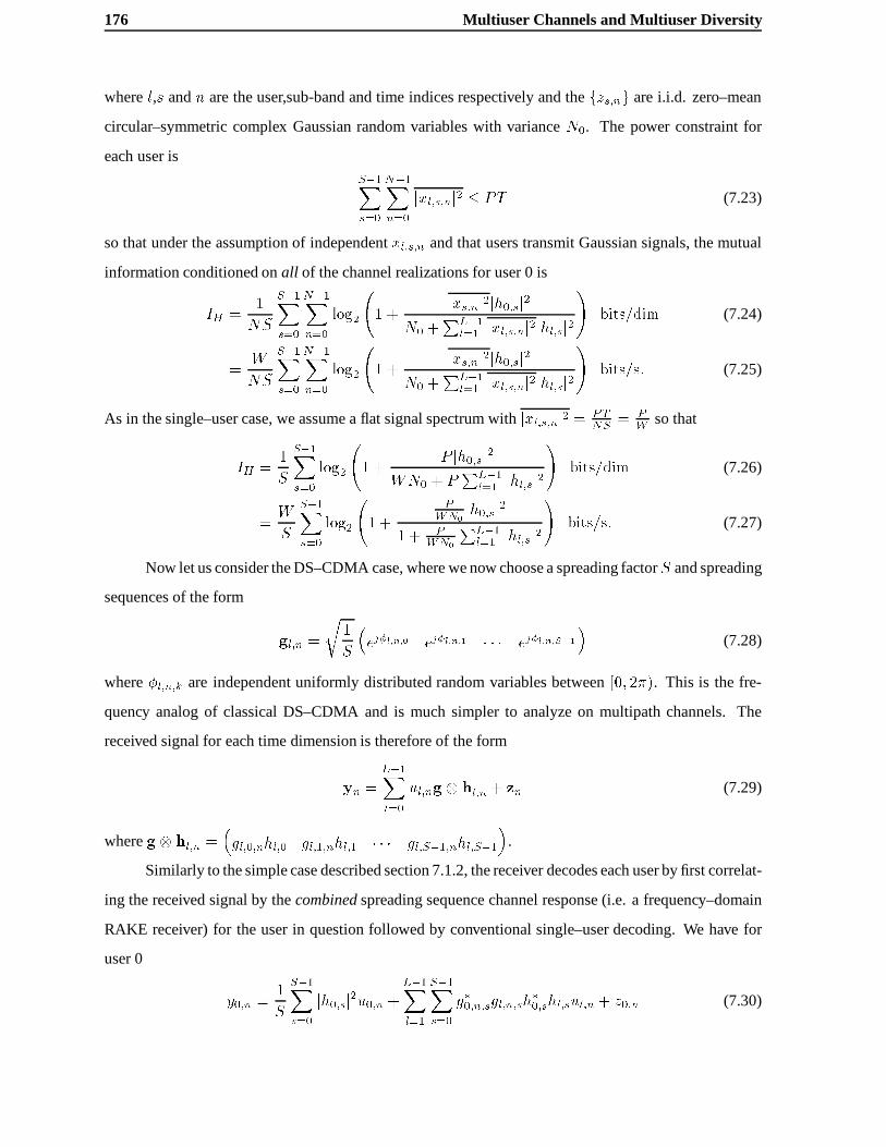
176 Multiuser Channels and Multiuser Diversity
wherel,s andn are the user,sub-band and time indices respectively and thefzs;ng are i.i.d. zero–mean
circular–symmetric complex Gaussian random variables with varianceN0. The power constraint for
each user isS�1Xs=0
N�1Xn=0
jxl;s;nj2 � PT (7.23)
so that under the assumption of independentxl;s;n and that users transmit Gaussian signals, the mutual
information conditioned onall of the channel realizations for user 0 is
IH =1
NS
S�1Xs=0
N�1Xn=0
log2
1 +
jxs;nj2jh0;sj2N0 +
PL�1l=1 jxl;s;nj2jhl;sj2
!bits=dim (7.24)
=W
NS
S�1Xs=0
N�1Xn=0
log2
1 +
jxs;nj2jh0;sj2N0 +
PL�1l=1 jxl;s;nj2jhl;sj2
!bits=s: (7.25)
As in the single–user case, we assume a flat signal spectrum withjxl;s;nj2 = PTNS = P
W so that
IH =1
S
S�1Xs=0
log2
1 +
P jh0;sj2WN0 + P
PL�1l=1 jhl;sj2
!bits=dim (7.26)
=W
S
S�1Xs=0
log2
1 +
PWN0
jh0;sj21 + P
WN0
PL�1l=1 jhl;sj2
!bits=s: (7.27)
Now let us consider the DS–CDMA case, where we now choose a spreading factorS and spreading
sequences of the form
gl;n =
r1
S
�ej�l;n;0 ej�l;n;1 � � � ej�l;n;S�1
�(7.28)
where�l;n;k are independent uniformly distributed random variables between[0; 2�). This is the fre-
quency analog of classical DS–CDMA and is much simpler to analyze on multipath channels. The
received signal for each time dimension is therefore of the form
yn =L�1Xl=0
ul;ng hl;n + zn (7.29)
whereg hl;n =�gl;0;nhl;0 gl;1;nhl;1 � � � gl;S�1;nhl;S�1
�.
Similarly to the simple case described section 7.1.2, the receiver decodes each user by first correlat-
ing the received signal by thecombinedspreading sequence channel response (i.e. a frequency–domain
RAKE receiver) for the user in question followed by conventional single–user decoding. We have for
user 0
y0;n =1
S
S�1Xs=0
jh0;sj2u0;n +L�1Xl=1
S�1Xs=0
g�0;n;sgl;n;sh�0;shl;sul;n + z0;n (7.30)

7.2 Outage Probability Analysis of Single–User Decoding in the Multiple–Access Channel withMultipath Fading 177
wherez0;n is a complex circular symmetric Gaussian random variable with mean zero and variance
1S
PS�1s=0 jh0;sj2. We have, therefore, that the average mutual information conditioned on the channel
realizations and the spreading sequences is
IH =1
Slog2
1 +
PWN0
Sk0
1 + PWN0
j0
!bits=dim (7.31)
wherek0 = 1S
PS�1s=0 jh0;sj2 andj0 =
PL�1l=1
PS�1s=0
PS�1s0=0 e
j(�l;s;n��0;s0 ;n)h�0;sh�l;s=k0. The basic dif-
ference between (7.31) and (7.27) is the type of averaging which is performed. In the DS–CDMA case,
both the averaging over fading (k0) and over interference (j0) are achieved by lowering the information
rate in a rather brute–force fashion. Note the presence of1=S outside the logarithm. The averaging effect
is reduced since it is inside the logarithm. In the general low–rate coding case, the achievable code rate is
raised/lowered by the extent of the fading and interference and not by an imposed by a particular coding
scheme.
The information outage probabilities in both cases must be calculated by Monte Carlo integration.
This has been done using for the same system parameters as in Chapter 3 (i.e.S = 128, W = 1:2288
MHz, ETSI TU12 channel) for different numbers of users and an SNR ofP=WN0 = 10 dB. The results
are shown in Figure 7.10 where we plot the information outage probabilityvs. the total rate sumLR. We
see that fairly low spectral efficiencies can be expected but that those where low–rate codes are used as
opposed to PN spreading are significantly higher. We note that as the number of users increases, the total
sum rate increases in the DS system. This is because the signal space is being used more efficiently as
the number of users increases (i.e. the factor1=F in front of the mutual information functional gradually
disappears.)
Let us now use the IS-95 CDMA system as a means for comparison. The data rate is 9.6kb/s
and the maximum number of users per 1.2288MHz is 64. With a voice activity factor of .5 (i.e. at any
given time about half the users are actually transmitting and the signals for the others are squelched)
this corresponds to a total rate sum spectral efficiency of 9.6*32/1229 = .25 bits/s/Hz. The information
outage rate curve for 32 users crosses .25 bits/s/Hz at aroundPout(:25) = 10�2 which is an acceptable
frame error rate for modern vocoders1. This shows that our analysis is not that far off from reality.
We also plot the single–user information outage we computed in Chapter 3 which corresponds to
the total rate sum for an orthogonal multiplexing system which uses the entire bandwidth. We see that it
is noticeably lower (i.e. that higher spectral efficiencies can be expected.)
1the GSM vocoder is designed to operate at this speech frame error rate

178 Multiuser Channels and Multiuser Diversity
10−2
10−1
100
101
10−4
10−3
10−2
10−1
100
Pout(R)
LR bits/s/Hz
Orthogonal
L = 2 (LRC)L = 4 (LRC)L = 32 (DS)
L = 4 (DS)
L = 2 (DS)L = 32 (LRC)
DS = Direct SequenceLRC =Low-Rate Coding
Figure 7.10: Comparison of Low–Rate Coding and Direct–Sequence CDMA schemes

7.3 Average Information Rates - Multiuser Diversity 179
For a single–cell system such as this we really must question the use of a non–orthogonalapproach
such as CDMA. Even if we could perform joint detection which would be a difficult task in a multipath
fading environment, the amount that has to be gained to catch up to an othogonal scheme (with diversity)
is huge. The real advantage of CDMA comes in cellular systems where co–channel interference is a
significant problem [GJP+91]. Here the orthogonal scheme is at a real disadvantage since frequency–
reuse must be used which significantly reduces system capacity. The effect of co–channel interference in
CDMA is simply a slight reduction of the signal–to–noise ratio so that it does not suffer to a great extent.
It has recently been shown [PC95][CKH97] that orthogonal schemes need not be limited by co–channel
interference and that frequency–reuse may not be necessary. Moreover, they can offer system capacities
comparable with CDMA, at the expense of increased decoding delay.
7.3 Average Information Rates - Multiuser Diversity
In Chapter 3 we considered average information rates and showed that they can be achieved in two ways.
The first was by coding over a long time-scale (i.e. over an infinite number of degrees of freedom of
the channel process) without the need for channel state information at the transmission end. The second
was by variable–rate coding when channel state information is available. These results relied on the fact
that the channel was block stationary, and that coding or channel control was performed over many such
blocks. As a result, ergodic arguments could be used to determine the average or long–term information
rates at which reliable communication is possible. We now generalize these ideas to the Gaussian MAC.
7.3.1 Generalizing the Single–User Average Mutual Information for the Fading MAC
We generalize the single user waveform channel from Chapter 3 to theL–user channel as
yn(t) =L�1Xl=0
Z T=2
�T=2xn;l(�)hn;l(t; �)d� + zn(t); t 2 [�To=2; To=2] (7.32)
wherehn;l(t; �) is now the response of userl’s channel at timet to an impulse at time� . The subscript
n in all the signals denotes thenth realization or block of the corresponding process. We assume that the
difference between the durations of the output signal and input signalsTo�T is larger than all the delays
due to multipath propagation and user asynchronism. The noise process is again a zero–mean, circular
symmetric, white complex Gaussian process with power spectral densityN0 and the channel responses
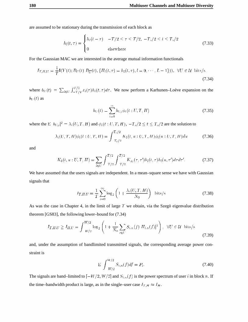
180 Multiuser Channels and Multiuser Diversity
are assumed to be stationary during the transmission of each block as
hl(t; �) =
8><>:hl(t� �) �T=2 � � � T=2; �To=2 � t � To=2
0 elsewhere
(7.33)
For the Gaussian MAC we are interested in the average mutual information functionals
IT;H;U =1
TI(Y (t);BU(t)jBU(t); fHl(t; �) = hl(t; �); l = 0; � � � ; L� 1g)); 8U 2 U bits=s
(7.34)
wherebU(t) =P
l2U
R T=2�T=2
xl(�)hl(t; �)d� . We now perform a Karhunen–Lo`eve expansion on the
bU(t) as
bU(t) =1Xi=0
bU;i�i(t : U; T;H) (7.35)
where theE jbU;ij2 = �i(U; T;H) and�i(t : U; T;H); �To=2 � t � To=2 are the solution to
�i(U; T;H)�i(t : U; T;H) =
Z To=2
�To=2Kb(t; u : U; T;H)�i(u : U; T;H)du (7.36)
and
Kb(t; u : U; T;H) =Xl2U
Z T=2
�T=2
Z T=2
�T=2Kxl(�; �
0)hl(t; �)hl(u; �0)d�d� 0: (7.37)
We have assumed that the users signals are independent. In a mean–square sense we have with Gaussian
signals that
IT;H;U =1
T
1Xi=0
log2
�1 +
�i(U; T;H)
N0
�bits=s (7.38)
As was the case in Chapter 4, in the limit of largeT we obtain, via the Szeg¨o eigenvalue distribution
theorem [GS83], the following lower–bound for (7.34)
IT;H;U � IH;U =
Z W=2
�W=2log2
1 +
1
N0
Xi2U
Si;n(f)jHi;n(f)j2!; 8U 2 U bits=s
(7.39)
and, under the assumption of bandlimited transmitted signals, the corresponding average power con-
straint is
E
Z W=2
�W=2Si;n(f)df = Pi: (7.40)
The signals are band–limited to[�W=2;W=2] andSi;n(f) is the power spectrum of useri in blockn. If
the time–bandwidth product is large, as in the single–user caseIT;H � IH .

7.3 Average Information Rates - Multiuser Diversity 181
7.3.2 Systems Without Fast Power Control
Let us now compare two alternative systems. The first is orthogonal multiplexing whereeach user uses
shares bandwidth/time equally. For FDMAeach user would use a bandwidthW=L and transmit all the
time. TheF block average mutual information conditioned on the channel realizations for useri with
FDMA is
Iorthi;H =1
F
F�1Xn=0
Z W=L
�W=Llog2
�1 +
1
N0Si;n(f)jHi;n(f)j2
�bits=s: (7.41)
Let us assume that the users have flat input spectra soSi;n(f) = LPi=W and thatF is large so that the
rate sum for anyU � U tends to
IorthU;H =Xi2U
W
LEhi log2
�1 +
LPiWN0
hi
�bits=s (7.42)
wherehi is the random variable describing the channel strengthjHi;n(f)j2 which is assumed to be
identically distributed at each frequency and in each block and independent from user to user. This
allows us to remove the integral in (7.41). Note that (7.41) holds for slow–frequency hopping as well as
long as the statistics of the different frequency bands where the signal hops are identical. The TDMA
case is also given by (7.42) since each user would use bandwidthW with powerLPi a fraction1=L of
the time.
Now consider the general non–orthogonal approach which has the rate sum taken over a large
number of blocks and using uniform power spectra
IoptU;H = WEfhi; i2Ug log2 1 +
1
WN0
Xi2U
Pihi
!bits=s: (7.43)
By virtue of the concavity of the logarithm and Jensen’s inequality [CT91] we have that
IorthU;H � W jU jL
Efhi; i2Ug log2
1 +
L
jU jWN0
Xi2U
Pihi
!bits=s (7.44)
which, using the fact thatx log2(1 + b=x) is increasing for anyb > 0, can be bounded further as
IorthU;H � WEfhi; i2Ug log2 1 +
1
WN0
Xi2U
Pihi
!= IoptU;H bits=s (7.45)
with strict inequality unlessjU j = L.
These important results are due to Gallager [Gal94] and show that the achievable rate region for
orthogonal multiplexing (when users share the dimensions on an equal basis) always lies within that of an

182 Multiuser Channels and Multiuser Diversity
optimal scheme which codes users over all the dimensions. Moreover, they are valid for TDMA,FDMA
or slow–frequency hopping systems. Let us examine the implication of these results with a numerical
example, by assuming that the fading process is Rayleigh distributed andPi = P; 8i. This symmetric
situation arises in practice if we have a perfectslow power controller which assures that the average
received SNR remains constant and equal for every user. This is important since it assures an equal
quality of service (on a long–term basis) for all users. In this case, all the channel strengthshl are
exponentially distributed as
fh(�) = e��; � � 0 (7.46)
so that the rate sums are
IoptU;H = W
Z 1
0log2
�1 +
P
WN0a
�f�jU j(a)da bits=s (7.47)
where�jU j =P
i2U hi is the sum of the channel strengths inU , which is anErlang random variable
with density
f�jU j(a) =ajU j�1
(jU j � 1)!e�a; a � 0: (7.48)
The rate sums in (7.47) can be expressed in terms of theMeijer G-function[GR80] but are simpler to
calculate via numerical integration. The orthogonal rates are just the single–user rates as in Chapter 3
IorthU;H =W jU jL ln 2
eWN0=(LP )E1
�WN0
LP
�: (7.49)
In figure 7.11 we show the achievable rate regions for three two–user systems, the two we just described
and an orthogonal scheme where we can adjust the proportion of the total dimensions allocated to each
user. This was described in section 7.1.1 and for the fading case, we simply have
R1 � (1� �)W
ln 2exp
�(1� �)
WN0
P
�E1
�(1� �)
WN0
P
�
R2 � �W
ln 2exp
��WN0
P
�E1
��WN0
P
�(7.50)
We chose a signal to noise ratioP=(WN0) = 10 dB. We see that there is a significant increase in
spectral efficiency for the non–orthogonal scheme even at the equal rate point, which shows that the
fading channel behaves quite differently than the non-fading channel. As pointed out by Gallager
a rather peculiar result is thatL users transmitting overL different channels can transmit more total
average information than a single user transmitting over one channel usingL times as much power. This
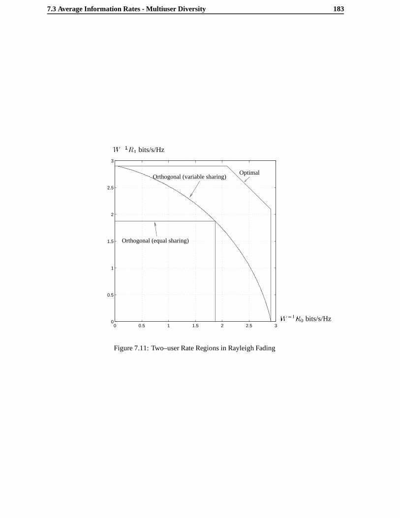
7.3 Average Information Rates - Multiuser Diversity 183
0 0.5 1 1.5 2 2.5 30
0.5
1
1.5
2
2.5
3
OptimalOrthogonal (variable sharing)
Orthogonal (equal sharing)
W�1R0 bits/s/Hz
W�1R1 bits/s/Hz
Figure 7.11: Two–user Rate Regions in Rayleigh Fading

184 Multiuser Channels and Multiuser Diversity
is due to an averaging effect inside the logarithm in the multiuser case since the sum signal has a total
received energy which hasL degrees of freedom and not a single one as would be the case with one user.
This can be made more clear if we consider the special case where the bandwidth is proportional to the
number of users, sayW = LWB , whereWB can be thought of as the bandwidth per user. If we focus on
the total rate sum (i.e. whenU = U ), the orthogonal schemes with equal transmitted powers will have
IorthU;H = LWBEh log2
�1 +
P
WBN0h
�(7.51)
and the optimal scheme will have
IoptU;H = LWBE�L log2
�1 +
P
WBN0
�LL
�: (7.52)
We note that forL!1, the random variable�L=L is 1 with probability 1 since thehi are independent
and consequently the total rate sum tends toL times the Gaussian channel capacity given by
CG = LWB log2
�1 +
P
WBN0
�bits=s: (7.53)
If we now compute the difference in spectral efficiency on a per user level between the Gaussian channel
capacity and orthogonal multiplexing on a Rayleigh fading channel, we have that [AS65]
(LWB)�1(CG � IorthU;H ) = log2
�1 +
P
WBN0
�� exp
�WBN0
P
�E1
�WBN0
P
�= ln 2
= log2
�1 +
P
WBN0
��
exp
�WBN0
P
�0@� � ln
�WBN0
P
��
1Xn=1
(�1)n�WBN0P
�nnn!
1A = ln 2� bits=s=Hz
(7.54)
which for large PWBN0
tends to� = ln 2 = :8327 bits/s/Hz, where = :57721 is Euler’s constant. This
shows that the most that can be gained by using a non–orthogonal scheme such as CDMA on a multipath
channel as opposed to any type of orthogonal multiplexing is .8327 bits/s/Hz. It assumes, of course, that
we have a coding scheme with no delay constraint and that some optimal successive decoding scheme,
such asonion peeling[RU96] can be used.
7.3.3 Channel State Feedback and Multiuser Diversity
We now move on to the case when channel knowledge is available at the transmission end and some
form of channel control can be performed. When we considered this possibility for the single–user case
we were only able to control the transmitter power and the code rate. On the multiuser channel we have
one more possibility, the allocation strategy. We begin with a simple example.

7.3 Average Information Rates - Multiuser Diversity 185
A Two–User Frequency Flat Channel
Let us assume we have a two–user system and that we wish to allocate users equally in time using TDMA.
We know that each user will transmit half the time with a peak–to–average power ratio of 2. Normally,
we would alternate between the users everyT seconds as shown in figure 7.12(a). Now let us assume
that the transmitters have knowledge ofbothchannel responses at any instant in time and the user with
the stronger received signal strength is allocated to the channel. This is shown in 7.12(b). We no longer
have a regular allocation strategy, but if both users have equal average received strengths then they will
share the channel equally just like with regular TDMA, and will transmit with the same peak–to–average
power ratio. Again we will assume that the channel stays constant for reasonably long periods of time
USER 1 USER 2 USER 1 USER 1 USER 1USER 2 USER 2 USER 2
Regular TDMA
(a)
(b)
TDMA with Multiuser Diversity
User 1’s signal strengthUser 2’s signal strength
User 1’s signal strengthUser 2’s signal strength
USER 1 USER 2 USER 1
Figure 7.12: Illustrating Multiuser diversity
so that we can use the block–fading assumption. The average mutual information for regular TDMA is

186 Multiuser Channels and Multiuser Diversity
given by
ITDMAH =
W
2Eh log2
�1 +
2P
WN0h
�bits=s=Hz: (7.55)
In the second case, when a given user is transmitting, we are sure to have a channel attenuationh =
maxfh0; h1g so that its statistics are quite different. Its average mutual information is still given by
(7.55) but with a different distribution function forh. We see that this channel allocation strategy has
given us a form of diversity which does not exist in the single–user case. We have given it the name
multiuser diversityalthough it is simply selection diversityperformed at the transmission end. This has
the effect of a power boost at the receiver since the mean ofh will be greater than the means ofh0 and
h1 (for this example the mean channel strength is 1.5 and not 1). Let us see what effect this has on the
average mutual information. We saw in Chapter 2, that the density function of a 2–channel selection
diversity system was given by
fH(u) = 2e�u � 2e�2u (7.56)
so that the average mutual information in Rayleigh fading is given by
ITDMA�divH
W
ln 2
�exp
�WN0
2P
�E1
�WN0
2P
�� exp
�WN0
P
�E1
�WN0
P
��bits=s:
(7.57)
We plot (7.57) and (7.55) along with the Gaussian channel capacity for a two–user TDMA system
CTDMAG =
W
2log2
�1 +
2P
WN0
�(7.58)
in figure 7.13 as a function of the signal–to–noise ratioP=WN0. We see that not only is an improvement
over the regular TDMA case, but the performance even surpasses that of a non–fading Gaussian channel.
The reason for this is the power boost from the selection diversity, which forces the transmitter to operate
only when the channel strength is above average. Unlike the single–user case, there is no penalty in using
the channel only part of the time since it must be shared between the two users.
7.3.4 The Fading Channel Capacity Region
In order to explain the effect of multiuser diversity more carefully, we must compute the capacity region
of the multiple–access channel with fading, since this will tell us the optimal channel–control policy, in
the sense of maximum average information rates. In Chapter 5 we saw that there were two basic types
of channel capacity and they were achieved by adjusting the power spectra of the user according to the
channel state.

7.3 Average Information Rates - Multiuser Diversity 187
0 5 10 15 20 25 300
1
2
3
4
5
6
Regular TDMA, Rayleigh Fading
TDMA- Multiuser Diversity
TDMA- Gaussian Channel
bits/s/Hz
PWN0
dB
Figure 7.13: Mutual Information for Different 2-User Multiuser Channel Allocation Strategies
The first was thedelay–limited capacitywhere the power was adjusted such that the average mu-
tual information was constant and maximum at the receiver. This idea was also very recently generalized
to the multiuser channel by Hanly and Tse in [HT96], where they define adelay–limited capacity region
in the same way, which insures that the receiver is operating at a fixed set of data rates at any given time
instant. They show that any point on the delay–limited capacity region can be achieved by a successive
decoding strategy whose decoding order depends on the channel states of the different users, but their
rates remain fixed in time. This is a particularly appealing result since as in Rimoldi’s rate–splitting
approach to the Gaussian MAC [RU96], no variable rate coding schemes are necessary.
The other type of capacity was theaverage capacity, where either the code rate was variable or
the code extended across the different channel realizations. We will focus on this case and show that
under some circumstances the optimal channel control scheme is orthogonal multiplexing with dynamic
allocation as in the simple example we just outlined. In general, we are interested in letting the users
adjust their power spectra assuming they havea priori knowledge ofall the channel responses.
The complete capacity region for this problem has recently been found by Tse and Hanly [TH96].
They generalized the techniques of Cheng and Verdu in [CV93] who solved the problem for the non–

188 Multiuser Channels and Multiuser Diversity
fading two–user Gaussian MAC with intersymbol interference. Tse and Hanly’s result exploits the poly-
matroidal structure of the capacity region and describes the power control policies for an arbitrary number
of users. An important result is that it is a convex region traced out from all possible combinations of
power control strategies satisfying the energy constraints in (7.40). For each set of power control policies,
the achievable rate region will be a Cover–Wyner pentagon, so that the capacity region will be the supre-
mum of all the corner points from these pentagons. We illustrate this for two users in figure 7.14. They
R0
R1
R0 = R1
Figure 7.14: Fading Channel Capacity Region
also show that any point on the boundary of the region can be achieved by successive decoding without
having to change the decoding order, the averaging effect achieved by timesharing on the Gaussian MAC
is taken care of by the variations of the channel in the fading MAC.
In most cases, we are interested only in the situation where all users have the same average power
at the receiver, which would be accomplished in practice using some form of slow power control. As
we already mentioned, this would be to assure the same long–term quality of service foreach user. If
this is the case, all the power constraints in (7.40) will be the same and under the reasonable assumption
of identical channel statistics, all power controllers will also be the same. In terms of the capacity
region, we see that it is symmetric [TH96] around the equal rate line. If we focus on this case, the only
quantity to maximize is the total rate sum which corresponds to the equal rate point on the capacity region
boundary (i.e.R0 = R1 = � � � = RL�1). This maximization was first done by Knopp and Humblet

7.3 Average Information Rates - Multiuser Diversity 189
[KH95a][KH95b]. Here we must maximize
Rsum =L�1Xl=0
Ri =
Z W=2
�W=2EfH0;��� ;HL�1g log2
1 +
1
N0
L�1Xi=0
Si;n(f)jHi;n(f)j2!df
(7.59)
subject to (7.40), withPi = P; 8i. Introducing a single Lagrange multiplier (since the problem is
symmetric)1=B and by applying the Kuhn–Tucker conditions for the maximization of a concave cost
function [Gal68], we have the following set of inequalities governing the optimalSi;n(f)
@
@Si;n(f)log2
1 +
1
N0
L�1Xi=0
Si;n(f)jHi;n(f)j2!� 1
B
@
@Si;n(f)
�Si;n(f)� P
W
�� 0
(7.60)
with equality if and only ifSi;n(f) > 0. Rearranging terms we have that the solution must be of the form
Si;n(f) =
8><>:B � N0
jHi;n(f)j2jHi;n(f)j2 � N0
B ; jHi;n(f)j2 � jHj;n(f)j2; j 6= i
0 otherwise
(7.61)
whereB satisfies the power constraints and is the solution toZ 1
N0=B
�B � N0
�
�f�(�)d� =
LP
W(7.62)
andh = maxfjH0(f)j2; � � � ; jHL�1(f)j2g. The total rate sum is therefore
Rsum = W
Z 1
N0=B
log2
�B
�
N0
�fh(h)dh: (7.63)
This power control scheme is nothing but a generalization of the water–filling scheme described in
Chapter 5 but has a very important practical implication. It says that at any given frequency in any given
block, the only user who should be transmitting is the one with the strongest response at that frequency,
provided his channel strength is greater than a thresholdN0=B. We illustrate this for a two–usersystem in
figure 7.15. This scheme is another form of orthogonal multiplexing combined with dynamic frequency
allocation. As in the Gaussian MAC, the equal rate point is achieved by orthogonal multiplexing,when
channel knowledge is available at the transmitters. This is critical since no joint decoding is required to
operate at this point. It can be seen as a TDMA system for each frequency where the allocation method
is virtually the same as the simple example we used to introduce this section, except for the water–filling
power allocation similar to the single–user case. This type of time–varying TDMA would be difficult to
achieve if the channel changes too rapidly for accurate estimation to be performed.2 The latter would
2In the IS-95 standard [IS992], channel state estimation is performed 800 times/sec in order to update the power control.

190 Multiuser Channels and Multiuser Diversity
jH0;n(f)j2
jH1;n(f)j2
S0;n(f) = 0
S1;n(f) = 0
N0
B
N0
BS1;n(f) > 0
S0;n(f) > 0S1;n(f) = 0
S0;n(f) = 0
jH 0;nj2 =jH 1
;nj2
Figure 7.15: Illustrating the Optimal Power Controllers for a Two–User System
cause problems since as the number of users increases, the amount of time any one user remains in a
given frequency would decrease. In addition, it should be evident the fading must not be too slow, so as
to insure that the average time any user accesses a given frequency band is not too long so that others
waiting for service do not get back-logged. This scheme may not be suitable for voice transmission
because of the uncertainty in the channel access time. For bursty data, however, this may pose less of a
problem.
Optimal bandwidth partitioning based on channel state information being available at the trans-
mission end would be hard to achieve in practice. A more realistic alternative would be to divide the
entire bandwidth intoN equal size sub-bands and allocate a single user to each of these sub-bands based
on the instantaneous frequency responses of all the users. The DECT system employs a technique along
these lines. In this system, the available bandwidth is divided into several sub-bands, which we assume
to be frequency flat. The users measure the strength of each sub-band, and choose the best available
sub-band on which to transmit. In our case, the user with the best channel response in a particular sub-
band uses that sub-band alone. This need not require too much effort to put into practice. As we already
mentioned in Chapter 3, two–way systems which operate in a time–division duplex fashion can estimate
the strengths of their channels via the opposite link, provided the channel responses do not change too
quickly. This could be used in the following fashion: the users waiting for service would measure their

7.3 Average Information Rates - Multiuser Diversity 191
own channels from the down-link signal and compare the strengths to those of the currently active users
which could be broadcast by the base-station on some control channel. Once they have detected a sub-
band where their channel strength is maximum they request allocation to that band, and the base-station
decides.
If the subbands are not flat, as is the case in a system like GSM, a time/frequency allocation
strategy such as this would still benefit from multiuser diversity but to a lesser extent. The diversity
factor gained from using a medium or wide–band signal would tend to reduce the variance of the set of
channel strengths over which the selection is performed. At the same time, the average power of each
users signal when transmitting would be reduced since the channel strength with diversity would have
a much lower probability of being above average. This has a very important practical implication: if
the system designer’s goal is to maximize the average data rates, we must use narrowband signals with
dynamic time/frequency allocation in order to benefit from multiuser diversity.
The type of system is very similar to the on/off multiple channel scheme briefly described in the
last chapter. Suppose a user hasS uncorrelated frequency bands at his disposal and multiuser diversity
amongL users is performed on each. The probability of a given user occupying a particular band is1=L.
The number of bands,Nb, occupied by this user at any given time is binomial with density
Prob(Nb = nb) =
�S
nb
��1
L
�nb(1� 1=L)S�nb : (7.64)
The outage probability is(1 � 1=L)S which is approximatelye�S=L if L is large. Thus, whenS � L
we have effectively no outages.
Numerical Results in Rayleigh Fading
Let us now compute the total rate sum for Rayleigh fading statistics. We have, therefore, that each of the
channel responses are exponentially distributed. It follows that the random variable
h = maxfjH0(f)j2; � � � ; jHL�1(f)j2g (7.65)
has a probability distribution function given by
Fh(u) = Prob (h < u) = (1� e�u)L (7.66)
so that its density is
fh(u) = Le�u(1� e�u)L�1 =LXk=1
(�1)k�1�L� 1
k � 1
�e�ku; (7.67)

192 Multiuser Channels and Multiuser Diversity
which is nothing but traditional selection diversity [WJ65]. The total sum of rates is therefore
Rsum = LW
LXk=1
(�1)k�1�L� 1
k � 1
�Z 1
N0=Be�ku log2(
B
N0u)du
= LW
LXk=1
(�1)k�1�L� 1
k � 1
�B
N0
Z 1
1e�kN0Bu log2(u)du
=W
ln 2
LXk=1
(�1)k�1�L
k
�E1
�kN0
B
�bits=s (7.68)
and the constantB is the solution to
LP
W=
LXk=1
(�1)k�1�L� 1
k � 1
�Z 1
N0=B
e�ku�B � N0
u
�du
=LXk=1
(�1)k�1�L
k
�Z 1
N0=Bke�u
�B � kN0
u
�du
=LXk=1
(�1)k�1�L
k
��Be�
N0Bk � kN0E1
�N0k
B
��: (7.69)
If we make the substitutionA = BW=P then we have
Rsum =W
ln 2
LXk=1
(�1)k�1�L
k
�E1
�kWN0
PA
�bits=s (7.70)
andA is the solution to
LXk=1
(�1)k�1�L
k
��Ae�
WN0PA
k � k
�WN0
P
�E1
�kN0W
PA
��= L: (7.71)
We see that as the signal to noise ratioP=WN0 increasesA tends toL. If we again consider the case
when the bandwidth is proportional to the number of users,W = LWB, we may compare the spectral
efficiencies on an equal footing. This is shown in figure 7.16.
We see two things as the number of users increases. First, for the case of no channel state feedback,
the sum capacities for the optimal non–orthogonal scheme in (7.52) quickly rise to the Gaussian channel
capacity. The difference between their performance and that of orthogonal multiplexing is also around
.8327 bits/s/Hz as predicted. The second observation is that multiuser diversity has an enormous effect at
increasing achievable data rates. WithL = 16 users we are around 1.5 bits/s/Hz higher than the Gaussian
channel which is quite remarkable. For low SNR the sum capacity is double that of the Gaussian channel.
Moreover, the curves will continue to rise, although slowly, with the number of users since the mean of
the channel strength with multiuser diversity is unbounded.
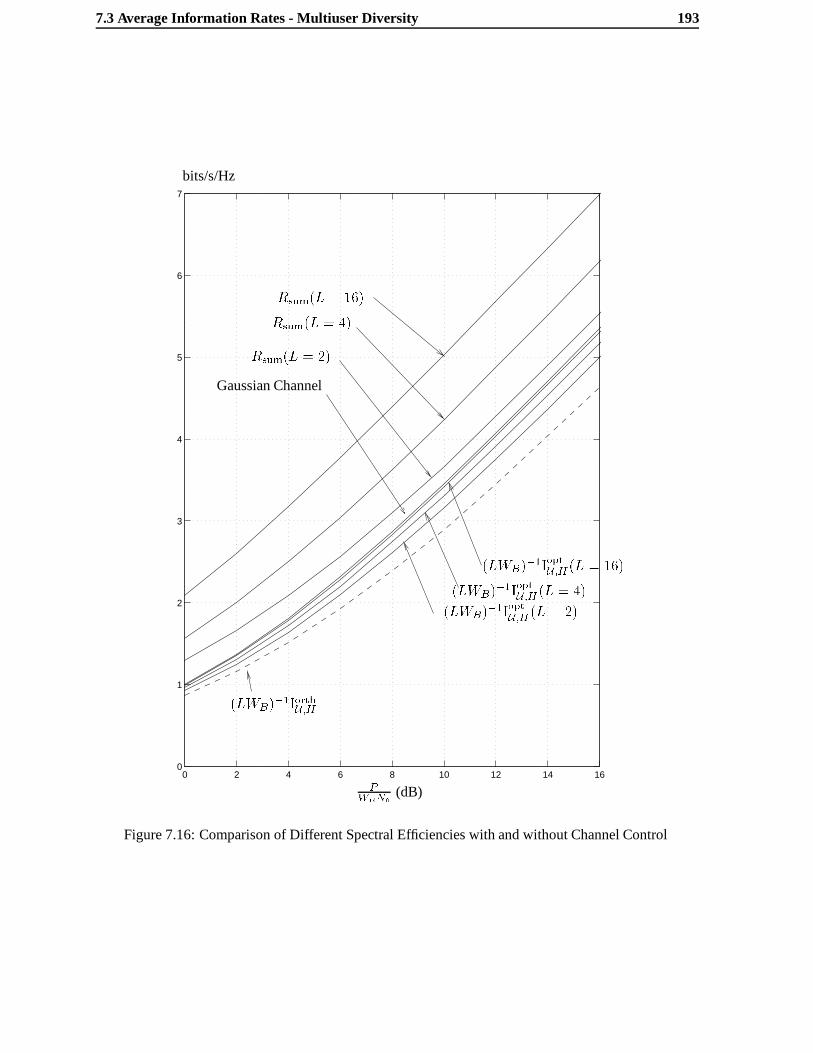
7.3 Average Information Rates - Multiuser Diversity 193
0 2 4 6 8 10 12 14 160
1
2
3
4
5
6
7
(LWB)�1IorthU;H
Gaussian Channel
Rsum(L = 2)
Rsum(L = 4)
Rsum(L = 16)
(LWB)�1IoptU ;H(L = 2)
PWBN0
(dB)
bits/s/Hz
(LWB)�1IoptU;H(L = 16)
(LWB)�1IoptU;H(L = 4)
Figure 7.16: Comparison of Different Spectral Efficiencies with and without Channel Control
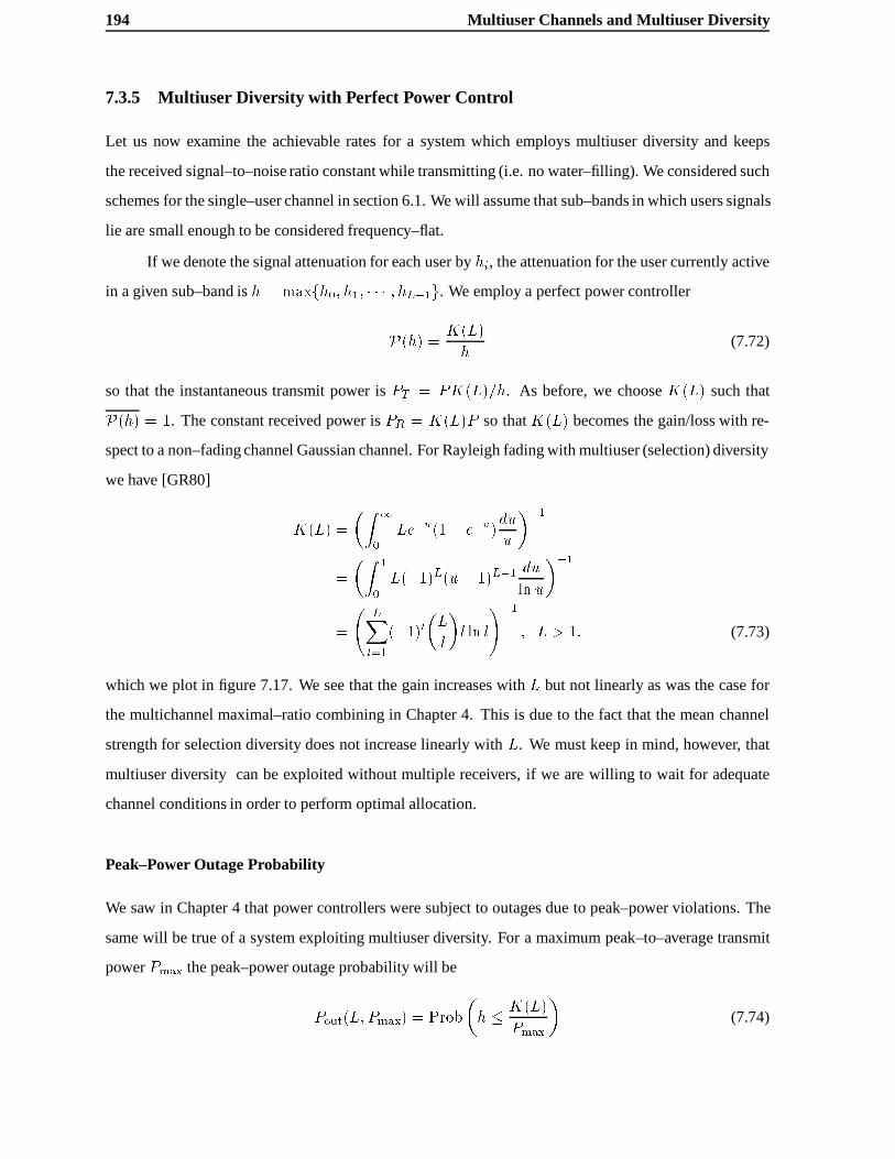
194 Multiuser Channels and Multiuser Diversity
7.3.5 Multiuser Diversity with Perfect Power Control
Let us now examine the achievable rates for a system which employs multiuser diversity and keeps
the received signal–to–noise ratio constant while transmitting (i.e. no water–filling). We considered such
schemes for the single–user channel in section 6.1. We will assume that sub–bands in which users signals
lie are small enough to be considered frequency–flat.
If we denote the signal attenuation for each user byhi, the attenuation for the user currently active
in a given sub–band ish = maxfh0; h1; � � � ; hL�1g. We employ a perfect power controller
P(h) = K(L)
h(7.72)
so that the instantaneous transmit power isPT = PK(L)=h. As before, we chooseK(L) such that
P(h) = 1. The constant received power isPR = K(L)P so thatK(L) becomes the gain/loss with re-
spect to a non–fading channel Gaussian channel. For Rayleigh fading with multiuser (selection) diversity
we have [GR80]
K(L) =
�Z 1
0Le�u(1� e�u)
du
u
��1
=
�Z 1
0L(�1)L(u� 1)L�1
du
ln u
��1
=
LXl=1
(�1)l�L
l
�l ln l
!�1
; L > 1: (7.73)
which we plot in figure 7.17. We see that the gain increases withL but not linearly as was the case for
the multichannel maximal–ratio combining in Chapter 4. This is due to the fact that the mean channel
strength for selection diversity does not increase linearly withL. We must keep in mind, however, that
multiuser diversity can be exploited without multiple receivers, if we are willing to wait for adequate
channel conditions in order to perform optimal allocation.
Peak–Power Outage Probability
We saw in Chapter 4 that power controllers were subject to outages due to peak–power violations. The
same will be true of a system exploiting multiuser diversity. For a maximum peak–to–average transmit
powerPmax the peak–power outage probability will be
Pout(L; Pmax) = Prob
�h � K(L)
Pmax
�(7.74)

7.3 Average Information Rates - Multiuser Diversity 195
0 5 10 15 20 25 30 35−2
0
2
4
6
8
10
12
14
16
K = L� 1 (maximal ratio)
Multiuser diversity
L
K (dB)
Figure 7.17: Multiuser Diversity Gain over Non–Fading Channel
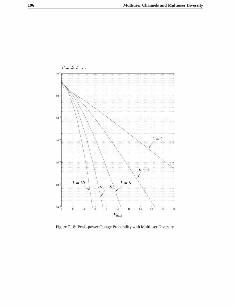
196 Multiuser Channels and Multiuser Diversity
0 2 4 6 8 10 12 14 16 18 2010
−6
10−5
10−4
10−3
10−2
10−1
100
L = 32L = 16
L = 8
L = 4
L = 2
Pout(L; Pmax)
Pmax
Figure 7.18: Peak–power Outage Probability with Multiuser Diversity

7.4 Chapter Summary 197
which for unit–mean square Rayleigh fading is
Pout(L; Pmax) =
�1� e�
K(L)Pmax
�L: (7.75)
We plotPout(L) as a function ofPmax in figure 7.18.
Bit Error–Probability for Uncoded BPSK with Multiuser Diversity
As an example of using multiuser diversity with common signaling schemes, let us consider uncoded
BPSK with and without power control. When no power control is employed, we have that the error
probability conditioned on the maximum channel stateh is
Pbjh = Q
r2hEbN0
!(7.76)
whereEb is the energy per information bit. Averaging overh in (7.67) yields
Pb = EhPbjh = :5LXl=1
(�1)l�1�L
i
�0@1� 1q1 + iN0
Eb
1A (7.77)
For the case with power control we have the following average error probability
Pb = (1� Pout(L; Pmax))Q
r2K(L)
EbN0
!+
Z K(L)=Pmax
0Q
r2uEbN0
!fh(u)du
(7.78)
The bit–error–rates are shown in figures 7.19 and 7.20 for a varying number of users and peak–to–average
power ratiosPmax. We see that in the case of no power control, we have performance superior to that of
a non–fading channel forL � 8 at practical signal–to–noise ratios. In the case with power control, even
better performance is possible. Moreover, forL � 4 we notice that peak–power constraints do not pose
a significant problem.
The important conclusion to be drawn from this analysis is that channel state feedback, as in the
single–user case, has a dramatic effect and that it may be a simpler option than sophisticated coding
schemes for achieving acceptable performance on fading multiuser channels. Moreover, with multiuser
diversity we do not need large QAM alphabets to improve performance as for single–user channels.
7.4 Chapter Summary
This chapter was concerned with multiuser communications and we focused on the up-link direction,
which is appropriately modeled by a Gaussian multipleaccess channel. We began with a general discus-
sion about the Gaussian MAC without fading and described the different dimension allocation strategies

198 Multiuser Channels and Multiuser Diversity
that are available. These were orthogonal multiplexing, which includes TDMA, FDMA and combina-
tions of the two. We also considered a simplified CDMA systems and the two main types of coding
strategies, namely PN spreading or low–rate coding. An approach based on decoding a particular user’s
signal while considering other users as background noise was examined for the two cases and we showed
that the low–rate coding alternative has some advantage.
We described the achievable rate region for the Gaussian MAC. In order to operate at an arbitrary
set of rates on the boundary of this region one is forced to decode the users signals jointly, which is an
arduous task. In the special case of equal transmitter powers, orthogonal multiplexing achieves the equal
rate point on the region, and for this point is optimal.
We then moved on to the fading channel by first considering a comparison of single–user decoding
for CDMA. We used the multi-tone model with the TU12 channel to compare a DS–CDMA approach to
a general low–rate coding scheme. We found that much higher spectral efficiencies are attainable with
low–rate coding. The results we obtained are comparable to the performance of the IS95 system in use
today, indicating that our analysis approach is not that far off from reality.
The last section dealt with average information rates, which as in the case of the single–user
channel can be achieved by either tolerating a long decoding delay or by performing variable–rate coding.
In both cases, the quantities of interest are long–term average rates. We showed that the achievable
rate region for an optimal joint coding scheme without channel control lies strictly outside the region
of orthogonal multiplexing schemes, unlike the Gaussian MAC. Furthermore, for Rayleigh fading we
showed that the total sum rate for a large number of users and a high signal–to–noise ratio exceeds that
of orthogonal multiplexing by .8327 bits/s/Hz.
We then turned our attention to systems employing channel control. We showed that there is
another inherent feature in multiuser systems which allows for very efficient exploitation of channel
state information at the transmission end. This aspect is called multiuser diversity and arises from the fact
that the medium must be shared by the users. With channel state information for all channels available
at the user terminals, they can choose to transmit when their channels are stronger than all the rest.
This is an inherent form of selection diversity and yields significant increases in the achievable data
rates. In Rayleigh fading, the data rates even exceed a non–fading Gaussian channel. While schemes
employing this form of diversity may not be suitable for delay constrained traffic, such as voice, some
data communication systems may be able to benefit greatly from such schemes. An important result is
that even without any error–control coding, the bit–error–rate of systems employing multiuser diversity
is comparable to a non–fading channel. If, in addition, we employ power control, significantly lower

7.4 Chapter Summary 199
BER can be expected with respect to an uncoded non–fading channel. The performance is also rather
insensitive to peak–power constraints.
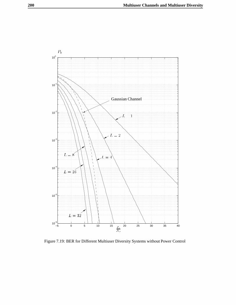
200 Multiuser Channels and Multiuser Diversity
−5 0 5 10 15 20 25 30 35 4010
−6
10−5
10−4
10−3
10−2
10−1
100
Gaussian Channel
L = 1
L = 2
L = 4
L = 32
L = 16
L = 8
EbN0
Pb
Figure 7.19: BER for Different Multiuser Diversity Systems without Power Control

7.4 Chapter Summary 201
−5 0 5 10 15 20 2510
−9
10−8
10−7
10−6
10−5
10−4
10−3
10−2
10−1
100
Gaussian Channel
L = 2L = 4L = 8
L = 16L = 32
Eb=N0 dB
Pb
L = 4; Pmax = 3 dB
L = 4; Pmax = 6 dB
L = 8; Pmax = 3 dB
L = 2; Pmax = 3 dB
L = 2; Pmax = 6 dB
L = 2; Pmax = 10 dB
Figure 7.20: BER for a Multiuser Diversity Systems with Power Control

202 Multiuser Channels and Multiuser Diversity
Chapter 8
Conclusions and Areas for Further
Research
8.1 Conclusions
We now summarize the main results of this thesis. In Chapter 3 we showed that the communication
problem over fading channels with a small number of degrees of freedom, or stated otherwise, indepen-
dent realizations of a random process, is fundamentally limited by a quantityPout(R), or the information
outage rate. This quantity defines the minimum achievable probability of codeword error. We have ap-
plied these ideas to practical situations and have drawn a number of conclusions regarding what can be
expected in terms of attainable performance. Even for high diversity systems, we should not expect to
be able transmit at more than 1 bit/s/Hz for modest signal–to–noise ratios ( on the order of 10 dB). We
demonstrated that for spread–spectrum signals there is a large performance difference between using a
direct–sequence and a very low rate coding technique. The latter approach benefits greatly in terms of
spectral efficiency.
In chapter 4 we tackled the coding problem for channels with a small number of degrees of free-
dom by modeling them as block–fading channels. We have shown that diversity is limited not only by
the number of degrees of freedom, but also by the size of the signaling constellation and the desired
code rate. The Singleton bound turns out to be the tool which gives us this information. We found that
both the Singleton bound and the information outage probability are linked in the sense that they predict
the achievable diversity for any coding system over a finite number of degrees of freedom. Examples
of block and trellis codes were given which attain maximum diversity. We have found, by computer

204 Conclusions and Areas for Further Research
search, a wide variety of practical coding schemes for spectral efficiencies less than or equal to 1 bit/dim
which, in some cases, achieve close to optimal performance. Their performance has been verified by
computer simulation, both in terms of bit and frame error rates. It seems that the bit error rate is much
less sensitive to the complexity of the coding scheme than the frame error rate. An important conclusion
is that information outage probability is a good indicator of practical frame error rates.
Chapter 5 treated systems which employ channel state information at the transmission end in order
to control or eliminate outages. This can be achieved either by fast power control or variable rate coding.
We showed that systems with some diversity, such as multiple receivers or spread–spectrum signaling,
can benefit tremendously with fast power control. Not only are outages eliminated but performance
quickly approaches that of the non–fading channel with increasing diversity. For systems employing
variable–rate coding, we found that simple two–rate schemes with power control can provide close to
optimal performance. In the case of uncoded transmission, these simple schemes achieve performance
comparable (or even better) than the uncoded AWGN channel without fading. This is important since
it shows that channel state feedback can play the role of sophisticated coding/interleaving schemes over
ergodic fading channels. We ended the chapter with a demonstration that the use of ARQ protocols
on fading channels can achieve high average data rates, although slightly lower rates than for systems
exploiting a priori channel knowledge. The key is to operate at a high spectral efficiency and high
information outage rate (on the order of 50The downside is that the ARQ protocol has to work very hard
to achieve these average rates.
Finally, in Chapter 6, we considered single–cell multiuser channels. After an introduction where
we treated non–fading AWGN channels we examined different multiple–access approaches for single–
user decoding of a wide–band (1.2288MHz) multiuser channel. We found, using the information outage
probability, that a low–rate coding based CDMA system is far superior in terms of spectral efficiency to
a direct–sequence based system. Moreover, we showed that our analysis is very accurate at predicting
the spectral efficiency of practical CDMA systems such as IS95. In a single–cell system, the spectral–
efficiency of an orthogonal scheme such as TDMA or FDMA/TDMA with frequency–hopping is much
higher than CDMA. We then turned to average information rates, where it was found that the spectral
efficiency of an optimal jointly–decoded CDMA system exceeds than of any orthogonal multiplexing
system by .8723 bits/s/Hz for a large number of users and signal–to–noise ratio. For systems exploiting
channel state feedback, we demonstrated that there is an inherent feature in multiuser systems which
allows for significantly higher average data rates than even a non–fading channel. We have called this
effect multiuser diversity, although it is simply selection diversity at the transmission end. Schemes

8.2 Areas for further research 205
employing are potentially optimal for symmetric multiuser channels (i.e. where the average received
power of all users is equal.) It allows for a completely orthogonal dynamically allocated FDMA/TDMA
multiplexing so joint detection is not required. While systems employing this type of diversity may not
by suitable for delay–constrained traffic, such as voice, some data communication systems may be able
to benefit greatly from it. An important result is that even without any error–control coding, the bit error–
rate of systems employing multiuser diversity is comparable (or even lower) than a non–fading channel.
This is true both with and without power control.
8.2 Areas for further research
We have been unable to find construction methods for coding schemes with higher spectral efficiencies
for the block–fading channel model and a small number of degrees of freedom. This is an important area
for further research, since data systems working at higher signal–to–noise ratios (e.g. wireless local–area
networks) will definitely require such coded–modulation schemes. The codes found in Chapter 4 should
be analyzed for both partially–interleaved and multi-tone systems. In addition, for fast–fading chan-
nels, concatenation of these codes with multiple–symbol non–coherent detection would be an interesting
problem to pursue.
We have completely ignored multiuser cellular systems where interference from other cells is an
important issue. In some cases these can also be characterized using information outage techniques. An
initial step in this direction has been taken in [CKH97]. As far as coding is concerned, the techniques
from Chapter 4 should be applied to systems such as those described in [CKH97] and [PC95].
For the results on channel state feedback exploitation, we have not considered the channel estima-
tion problem which, of course, is critical. At the same time practical protocols for exploiting multiuser
diversity should be found and analyzed. These ideas must also be applied to interference–limited sys-
tems.

206 Conclusions and Areas for Further Research

Bibliography
[ACM88] H.W. Arnold, D.C. Cox, and R.R Murray. “Macroscopic diversity performance meansured
in the 800–MHz portable radio communications environment”.IEEE Trans. Antennas Prop-
agat., 36:277–280, February 1988.
[Ahl71] R. Ahlswede. “Multi-way Communication Channels”. InProc. 2nd. Int. Symp. Information
Theory(Tsahkadsor, Armenian S.S.R), pages 23–52, Prague, 1971. Publishing House of the
Hungarian Academy of Sciences.
[AS65] M. Abramovitz and I.A. Stegun.Handbook of Mathematical Functions. Dover, 1965.
[Aul79] T. Aulin. “A Modified Model for the Fading Signal at a Mobile Radio Channel”.VT,
28(3):182–203, 1979.
[BB92] K. Boulle and J.C. Belfiore. “Modulation Scheme Designed for the Rayleigh Fading Chan-
nel”. In Proc. CISS ’92, Princeton, N.J., March 1992.
[BCTV96] E. Biglieri, G. Caire, G. Taricco, and J. Ventura. “Simple Method for Evaluating Error
Probabilities”.Electronic Letters, 32(3):191–192, feb 1996.
[BDMS91] E. Biglieri, D. Divsalar, P.J. McLane, and M.K. Simon.Introduction to Trellis–Coded Mod-
ulation with Applications. MacMillan, New York, 1991.
[BG92] D.P. Bertsekas and R.G. Gallager.Data Networks. Prentice Hall, 1992.
[BGT93] C. Berrou, A. Glavieux, and P. Thitimajshima. “Near Shannon Limit Error–Correcting Cod-
ing and Decoding: Turbo–Codes”. InProc. IEEE ICC ’93, May 1993.
[BJK96] P.W. Baier, P. Jung, and A. Klein. “Taking the challenge of multipleaccess for third-
generation cellular mobile radio systems-a European view”.IEEE Communications Maga-
zine, 34(2):82–89, February 1996.

208 BIBLIOGRAPHY
[Bla87] R.E. Blahut. Principles and Practice of Information Theory. Addison-Wesley, Reading,
Massachusetts, 1987.
[BR97] T.E. Bell and M.J. Riezenman. “Communications”.IEEE Spectrum, 34(1):27–37, January
1997.
[Bul87] R.J.C. Bultitude. “Measurement, Characterization and Modeling of Indoor 800/900 MHz
Radio Channels for Digital Communications”.IEEE Commun. Mag., 25(6):5–12, 1987.
[BVRB96] J. Boutros, E. Viterbo, C. Rastello, and J.C. Belfiore. “Good Lattice Constellations for
Both Rayleigh Fading and Gaussian Channels”.IEEE Transactions on Information Theory,
42(2):502–518, March 1996.
[CG96] S.G. Chua and A. Goldsmith. “Variable–Rate Variable–Power MQAM for Fading Chan-
nels”. InProc. VTC, pages 815–819, April 1996.
[CG97] S.G. Chua and A. Goldsmith. “Adaptive Coded Modulation for Fading Channels”. InProc.
ICC, pages 1488–1492, 1997.
[CKH97] G. Caire, R. Knopp, and P.A. Humblet. “System Capacity of F-TDMA Cellular Systems”.
submitted to IEEE Trans. on Comm., March 1997.
[Cla68] R.H. Clarke. “A Statistical Theory of Mobile Radio Reception”.Bell Systems Technical
Journal, 47:957–1000, 1968.
[CT91] T. Cover and J. Thomas.Elements of Information Theory. John Wiley and Sons, New York,
1991.
[CV93] R.S. Cheng and S. Verd´u. “Gaussian Multiaccess Channels with Capacity Region and Mul-
tiuser Water–Filling”.IEEE Transactions on Information Theory, 39(3), may 1993.
[DR58] W.B. Davenport Jr. and W.L. Root.An Introduction the the Theory of Random Signals and
Noise. McGraw Hill, New York, 1958.
[DS88] D. Divsalar and M.K. Simon. “The Design of Trellis Coded MPSK for Fading Channels:
Performance Criteria”.IEEE Transactions on Communications, 36:1004–1012, 1988.
[DS90] D. Divsalar and M.K. Simon. “Multiple–Symbol Differential Detection of MPSK”.IEEE
Transactions on Communications, 38:300–308, 1990.
BIBLIOGRAPHY 209
[Eri70] T. Ericson. “A Gaussian Channel with Slow Fading”.IEEE Transactions on Information
Theory, 1970.
[Feh95] K. Feher.Wireless Digital Communications. Prentice Hall, 1995.
[FL96] B.H. Fleury and P.E. Leuthold. “Radiowave Propagation in Mobile Communications: An
Overview of European Research”.IEEE Comm. Mag., pages 70–81, February 1996.
[For73] G.D. Forney Jr. “The Viterbi Algorithm”.Proceedings of the IEEE, 61(3):268–278, March
1973.
[For91] G.D. Forney Jr. “Geometrically Uniform Codes”.IEEE Transactionson InformationTheory,
37:223–236, September 1991.
[Gal68] R.G. Gallager.Information Theory and Reliable Communication. John Wiley and Sons,
1968.
[Gal94] R.G. Gallager. “An Inequality on the Capacity Region of Multiaccess Multipath Channels”.
In U. Maurer, T. Mittelholzer, G.D. Forney, and R.E. Blahut, editors,Communications and
Cryptography – Two Sides of One Tapestry–, pages 129–139. Kluwer Academic Publishers,
1994.
[GB96] X. Giraud and J.C. Belfiore. “Constellations Matched to the Rayleigh Fading Channel”.
IEEE Transactions on Information Theory, 42(1):106–115, January 1996.
[GJP+91] K. Gilhousen, I. Jacobs, A. Padovani, A.J. Viterbi, L. Weaver, and C. Wheatly. “On the
Capacity of a Cellular CDMA System”. IEEE Transactions on Vehicular Technology,
40(2):303–312, 1991.
[Gol94] A. Goldsmith.Design and Performance of High-Speed Communication Systems over Time–
Varying Radio Channels. PhD thesis, University of California at Berkeley, 1994.
[GP89] R. Ganesh and K. Pahlavan. “On the Arrival of the Paths in Multipath Fading Indoor Radio
Channels”.IEE Electr. Lett., 25:763–765, 1989.
[GR80] I. Gradsteyn and I. Ryzhik.Tables of Integrals, series and products. Academic Press, New
York, 1980.
[GS83] U. Grenander and G. Szeg¨o. Toeplitz Forms and their Applications. Chelsea, 1983.

210 BIBLIOGRAPHY
[GSM90] European Telecommunications Standards Institute.European Digital Cellular Telecommu-
nications System : Physical Layer on the Radio Path (GSM 05.02), 1990.
[Gud91] M. Gudmundson. “Correlation Model For Shadow Fading in Mobile Radio Systems”.Elec.
Lett., 27:2145–2146, Nov. 7 1991.
[Has79] H. Hashemi. “Simulation of the Urban Radio Propagation Channel”.VT, 28(3):213–225,
79.
[Hat80] M. Hata. “Empirical Formula for Propagation Loss in Land Mobile Radio Services”.VT,
29(3):317–325, 1980.
[HH89] J. Hagenauer and P. Heoher. “A Viterbi Algorithm with Soft–Decision Outputs and its Ap-
plications”. InProceedings of IEEE Globecom, pages 47.1.1–47.1.7, Dallas, Tx, feb 1989.
IEEE.
[HHR96] P.A. Humblet, S. Hethuin, and L. Ramel. “A multiaccess protocol for high-speed WLAN”.
In Proceedings of IEEE VTC ’96, May 1996.
[HT96] S.V. Hanly and D.N. Tse. “Multi–Access Fading Channels: Part II: Delay–Limited Capac-
ities”. Technical Report UCB/ERL M96/69, Electronics Research Laboratory, College of
Engineering, University of California, Berkeley, 1996.
[Hui84] J.Y.N. Hui. “Throughput Analysis for Code Division Multiple Accessing of the Spread
Spectrum Channel”.IEEE Journal on Selected Areas in Communications, 2:482–486, July
1984.
[Hum85] P.A. Humblet. “Error Exponents for a Direct Detection Optical Channel”. InProc. 23rd
Allerton Conference on Communication, Control, and Computing, October 1985.
[IS592] Telecommunications Industry Association.EIA/TIA Interim Standard, Cellular System Dual
mode Mobile-Station Base-Station Compatibility Standard IS-54B, 1992.
[IS992] Proposed EIA/TIA Interim Standard.Wideband Spread Spectrum Digital Cellular System
Dual–Mode Mobile Station–Base Station Compatibility Standard, 1992.
[IYTU84] F. Ikegami, S. Yoshida, T. Takeuchi, and M. Umehira. “Propagation Factors Controlling
Mean Field Strength on Urban Streets”.IEEE Trans. on Antennas and Propagation, 1984.

BIBLIOGRAPHY 211
[Jak74] W.C. Jakes, editor.Microwave Mobile Communications. John Wiley and Sons, New York,
1974.
[KCW93] T. Kurner, D. Cichon, and W. Wiesbeck. “Concepts and Results for 3D Digital Terrain–
base Wave Propagation Models: An Overview”.IEEE Transactions on Communications,
COM-11:1002–1012, September 1993.
[Ker96] K.J. Kerpez. “Radio Access System with Distributed Antennas”.IEEE Transactions on
Vehicular Technology, 45(2):265–275, May 1996.
[KH95a] R. Knopp and P.A. Humblet. “Information Capacity and Power Control in Single–Cell Mul-
tiuser Communications”. InProc. IEEE ICC’95, Seattle, Wa., June 1995.
[KH95b] R. Knopp and P.A. Humblet. “Multiple–Accessing over Frequency–Selective Fading Chan-
nels”. InProc. IEEE PIMRC’95, Toronto, Ont., Sept. 1995.
[KH96] R. Knopp and P.A. Humblet.Multiacces, Mobility and Teletraffic for Mobile and Personal
Communications, chapter Channel Control and Multiple Access. Kluwer, 1996.
[Kim97] M. Kimpe. “A Fast Algorithm for Computerized Indoor Radio Channel Estimation”. In
Proc. IEEE ICC’97, Montreal, Canada, pages 66–70, June 1997.
[KL94] R. Knopp and H. Leib. “M–ary Phase Coding for the Non–Coherent AWGN Channel”.
IEEE Transactions on Information Theory, 40(6):1968–1984, November 1994.
[KSS95] G. Kaplan and S. Shamai (Shitz). “Error Probabilities for the Block–Fading Gaussian Chan-
nel”. Archiv fur Elektronik undUbertragungstechnik, 49(4):192–205, 1995.
[KSSK95] G. Kaplan, S. Shamai (Shitz), and Y. Kofman. “On the Design and Selection of Convolu-
tional Codes for and Uninterleaved, Bursty Rician Channel”.IEEE Transactions on Com-
munications, 23(12), 1995.
[KZS97a] Y. Kofman, E. Zehavi, and S. Shamai(Shitz). “nd–Convolutional Codes- Part I: Performance
Analysis”. IEEE Transactions on Information Theory, 43(2):558–575, March 1997.
[KZS97b] Y. Kofman, E. Zehavi, and S. Shamai(Shitz). “nd–Convolutional Codes- Part I: Structural
Analysis”. IEEE Transactions on Information Theory, 43(2):576–589, March 1997.
212 BIBLIOGRAPHY
[KZZ71] T.T Kadota, M. Zakai, and J. Ziv. “Capacity of a continuous memoryless channel with
feedback”.IEEE Transactions on Information Theory, 17:372–378, 1971.
[Lap94] A. Lapidoth. “The Performance of Convolutional codes over the Block Erasure Channel
Using Various Finite Interleaving Techniques”.IEEE Transactions on Information Theory,
40(5), 1994.
[LC83] S. Lin and D.J. Costello Jr.Error Control Coding: Fundamentals and Applications. Prentice
Hall, Englewood Cliffs, New Jersey, 1983.
[Lee82] W.C.Y. Lee.Mobile Communications Engineering. McGraw Hill, New York, 1982.
[Lee90] W.C.Y. Lee. “Estimate of Channel Capacity in Rayleigh Fading Environment”.IEEE Trans-
actions on Vehicular Technology, 39(3):187–189, August 1990.
[Lia72] H. Liao. Multiple Access Channels. PhD thesis, University of Hawaii, Dept. of Electrical
Engineering, Honolulu, 1972.
[LP91] H. Leib and S. Pasupathy. “Optimal Noncoherent Block Demodulation of Differential Phase
Shift Keying”. Archiv fur Elektronik undUbertragungstechnik, 45:299–305, 1991.
[LWK93] Y.S. Leung, S.G. Wilson, and J.W. Ketchum. “Multi-frequency Trellis Coding with Low-
Delay for Fading Channels”.COM, 41(10):1450–1459, October 1993.
[Mas74] J.L. Massey. “Coding and Modulation in Digital Communications”. InProc. Int. Zurich
Sem. Digital Commun., Zurich, Switzerland, March 1974.
[Med95] M. Medard.The Capacity of Time–Varying Multiple–User Channels in Wireless Communi-
cations. PhD thesis, Massachusetts Institute of Technology, 1995.
[ML97] E. Malkamaki and H. Leib. “Rate1=n Convolutional Codes with Interleaving Depth ofn
over a Block-Fading Ricean Channel”. InProc. IEEE Vehicular Technology Conference,
pages 2002–2006, May 1997.
[MS84] R. McEliece and W.E. Stark. “Channels with Block Interference”.IEEE Transactions on
Information Theory, 30(1):44–53, January 1984.
[Nak60] M. Nakagami. “TheM–distribution. A General Formula of Intensity Distribution of Rapid
Fading”. In W.C. Hoffman, editor,Statistical Methods in Radio Wave Propagation. Perga-
mon Press, 1960.
BIBLIOGRAPHY 213
[OOKF68] Y. Okumura, E. Ohmori, T. Kawano, and K. Fukuda. “Field Strength and its Variability in the
VHF and UHF Land Mobile Radio Service”.Review Elec. Commun. Lab., 16(9–10):825–
873, 1968.
[OSSW94] L. Ozarow, S. Shamai (Shitz), and A.D. Wyner. “Information Theoretic Considerations for
Cellular Mobile Radio”.IEEE Transactions on Vehicular Technology, 43(2):359–378, May
1994.
[Pap82] A. Papoulis.Probability, Random Variables and Stochastic Processes. McGraw Hill, New
York, 1982.
[Par92] D. Parsons.The Mobile Radio Propagation Channel. Pentech Press, London, England,
1992.
[PC95] G. Pottie and R. Calderbank. “Channel Coding Strategies for Cellular Mobile Radio”.IEEE
Transactions on Vehicular Technology, 44(4):763–769, November 1995.
[PHS95] ARIB. Personal Handy Phone System ARIB Standard, version 2, 1995.
[Pro95] J.G. Proakis.Digital Communications. McGraw Hill, New York, third edition, 1995.
[Rap96a] D. Raphaeli. “Non–Coherent Coded Modulation”.IEEE Transactions on Communications,
44(2):172–183, 1996.
[Rap96b] T. Rappaport.Wireless Communications. Prentice Hall, Englewood Cliffs, New Jersey,
1996.
[RH92] T.S. Rappaport and D.A. Hawbaker. “A Ray Tracing Technique to Predict Path Loss and
Delay Spread Inside Buildings”. InProc. IEEE GLOBECOM ’92, pages 649–653, December
1992.
[RU96] B. Rimoldi and R. Urbanke. “A Rate–Splitting Approach to the Gaussian Multiple–Access
Channel”.IEEE Transactions on Information Theory, 42(2):364–375, March 1996.
[SBS66] M. Schwartz, W.R. Bennett, and Stein S.Communication Systems and Techniques. McGraw
Hill, New York, 1966.
[SC89] C. Schlegel and D.J. Costello Jr. “Bandwidth Efficient Coding for Fading Channels: Code
Construction and Performance Analysis”.IEEE Journal on Selected Areas in Communica-
tions, 7(9), December 1989.

214 BIBLIOGRAPHY
[Sha48a] C.E. Shannon. “A Mathematical Theory of Communication: Part I”.Bell Systems Technical
Journal, 27:379–423, jul 1948.
[Sha48b] C.E. Shannon. “A Mathematical Theory of Communication: Part II”.Bell Systems Technical
Journal, 27:353–355, oct 1948.
[Shn89] D.A. Shnidman. “The Calculation of the Probability of Detection and the Generalized Mar-
cumQ–Function”.IEEE Transactions on Information Theory, 35(2):?, March 1989.
[Sin64] R.C. Singleton. “Maximum Distanceq–Nary Codes”. IEEE Transactions on Information
Theory, 10:116–118, 1964.
[Suz77] H. Suzuki. “A Statistical Model for Urban Multipath Propagation”.COM, 25(7):673–680,
77.
[SV87] A.A.M. Saleh and R.A. Valenzuela. “A Statistical Model for Indoor Multipath Propagation”.
IEEE Journal on Selected Areas in Communications, 5:127–137, February 1987.
[TCJ+72] G.L. Turin, F.D. Clapp, T.L. Johnston, S.B. Fine, and D. Lavry. “A Statistical Model of
Urban Multipath Propagation”.VT, 21(1):1–9, 72.
[TH96] D.N. Tse and S.V. Hanly. “Multi–Access Fading Channels: Part I: Polymatroidal Structure,
Optimal Resource Allocation and Throughput Capacities”. Technical Report UCB/ERL
M96/69, Electronics Research Laboratory, College of Engineering, University of California,
Berkeley, 1996.
[Ung82] G. Ungerb¨ock. “Channel Coding with Multilevel/Phase Signals”.IEEE Transactions on
Information Theory, 28:55–67, January 1982.
[Van95] L. Vandendorpe. “Multitone Spread Spectrum Communications Systems in a Multipath
Rician Fading channel”.IEEE Transactions on Vehicular Technology, pages 327–337, May
1995.
[Ver86] S. Verdu. “Minimum Probability of Error for Asynchronous Gaussian Multiple–Access
Channels”.IEEE Transactions on Information Theory, 32(1), January 1986.
[Vit79] A.J. Viterbi. “Spread–Spectrum Communications- Myths and Realities”.IEEE Comm. Mag.,
4:11–18, May 1979.

BIBLIOGRAPHY 215
[Vit90] A.J. Viterbi. “Very Low–Rate Convolutional Codes for Maximum Theoretical Perofmance
of Spread–Spectrum Multiple–Access Channels”.IEEE Journal on Selected Areas in Com-
munications, 8(4), May 1990.
[VN96] R. Van Nee. “OFDM Codes for Peak–to–Average Power Reduction and Error Correction”.
Proceedings of IEEE Globecom, November 1996.
[VT68] H.L. Van Trees. Detection, Estimation and Modulation Theory: Part I. John Wiley and
Sons, New York, 1968.
[VT72] H.L. Van Trees.Detection, Estimation and Modulation Theory: Part III. John Wiley and
Sons, New York, 1972.
[VT95] G. Vitetta and D.P. Taylor. “Maximum Likelihood Decoding of Uncoded and Coded PSK
Signal Sequences Transmitted over Rayleigh Flat–Fading Channels”.IEEE Transactions on
Communications, 43(11):2750–2758, November 1995.
[WB88] J. Walfisch and H.L. Bertoni. “A Theoretical Model of UHF Propagation in Urban Environ-
ments”. IEEE Trans. Antennas and Propagation, AP-38:1788–1796, December 1988.
[Wil96] S.G. Wilson.Digital Modulation and Coding. Prentice Hall, Englewood Cliffs, New Jersey,
1996.
[WJ65] J. Wozencraft and I. Jacobs.Principles of Communication Engineering. John Wiley and
Sons, New York, 1965.
[WJ95] T. Wilkinson and A. Jones. “Minimization of the Peak–to-Mean Envelope Power Ratio of
Multicarrier Transmission Schemes by Block Coding”.Proceedings of the IEEE Interna-
tional Conference on Vehicular Technology, July 1995.
[Wol69] J.K. Wolf. “Adding Two Information Symbols to Certain Non–Binary BCH Codes and Some
Applications”.Bell Systems Technical Journal, 48:2405–2424, 1969.
[Wol78] J. Wolfowitz. Coding Theorems of Information Theory. Springer–Verlag, 1978.
[Wyn94] A.D. Wyner. “Shannon–Theoretic Approach to a Gaussian Cellular Multiple–Access Chan-
nel”. IEEE Transactions on Information Theory, 40(6), November 1994.
Related Documents


![[PPT]Wireless Channels: Small Scale Fading (Multipath …web2.uwindsor.ca/.../uwireless/channels_smallscalefading.ppt · Web viewWireless Channels: Small Scale Fading (Multipath and](https://static.cupdf.com/doc/110x72/5b3cfdd57f8b9a0e628df536/pptwireless-channels-small-scale-fading-multipath-web2-web-viewwireless.jpg)

