Technical Report Number 607 Computer Laboratory UCAM-CL-TR-607 ISSN 1476-2986 Code size optimization for embedded processors Neil E. Johnson November 2004 15 JJ Thomson Avenue Cambridge CB3 0FD United Kingdom phone +44 1223 763500 http://www.cl.cam.ac.uk/

Welcome message from author
This document is posted to help you gain knowledge. Please leave a comment to let me know what you think about it! Share it to your friends and learn new things together.
Transcript
Technical ReportNumber 607
Computer Laboratory
UCAM-CL-TR-607ISSN 1476-2986
Code size optimization forembedded processors
Neil E. Johnson
November 2004
15 JJ Thomson Avenue
Cambridge CB3 0FD
United Kingdom
phone +44 1223 763500
http://www.cl.cam.ac.uk/

c© 2004 Neil E. Johnson
This technical report is based on a dissertation submitted May2004 by the author for the degree of Doctor of Philosophy to theUniversity of Cambridge, Robinson College.
Technical reports published by the University of CambridgeComputer Laboratory are freely available via the Internet:
http://www.cl.cam.ac.uk/TechReports/
ISSN 1476-2986
Abstract
This thesis studies the problem of reducing code size produced by an optimizing compiler. Wedevelop the Value State Dependence Graph (VSDG) as a powerful intermediate form. Nodesrepresent computation, and edges represent value (data) and state (control) dependencies be-tween nodes. The edges specify a partial ordering of the nodes—sufficient ordering to maintainthe I/O semantics of the source program, while allowing optimizers greater freedom to movenodes within the program to achieve better (smaller) code. Optimizations, both classical andnew, transform the graph through graph rewriting rules prior to code generation. Additional(semantically inessential) state edges are added to transform the VSDG into a Control FlowGraph, from which target code is generated.
We show how procedural abstraction can be advantageously applied to the VSDG. Graphpatterns are extracted from a program’s VSDG. We then select repeated patterns giving thegreatest size reduction, generate new functions from these patterns, and replace all occurrencesof the patterns in the original VSDG with calls to these abstracted functions. Several embeddedprocessors have load- and store-multiple instructions, representing several loads (or stores) asone instruction. We present a method, benefiting from the VSDG form, for using these instruc-tions to reduce code size by provisionally combining loads and stores before code generation.The final contribution of this thesis is a combined register allocation and code motion (RACM)algorithm. We show that our RACM algorithm formulates these two previously antagonis-tic phases as one combined pass over the VSDG, transforming the graph (moving or cloningnodes, or spilling edges) to fit within the physical resources of the target processor.
We have implemented our ideas within a prototype C compiler and suite of VSDG opti-mizers, generating code for the Thumb 32-bit processor. Our results show improvements foreach optimization and that we can achieve code sizes comparable to, and in some cases bet-ter than, that produced by commercial compilers with significant investments in optimizationtechnology.
4
Contents
1 Introduction 151.1 Compilation and Optimization . . . . . . . . . . . . . . . . . . . . . . . . . . 16
1.1.1 What is a Compiler? . . . . . . . . . . . . . . . . . . . . . . . . . . . 161.1.2 Intermediate Code Optimization . . . . . . . . . . . . . . . . . . . . . 171.1.3 The Phase Order Problem . . . . . . . . . . . . . . . . . . . . . . . . 18
1.2 Size Reducing Optimizations . . . . . . . . . . . . . . . . . . . . . . . . . . . 181.2.1 Compaction and Compression . . . . . . . . . . . . . . . . . . . . . . 191.2.2 Procedural Abstraction . . . . . . . . . . . . . . . . . . . . . . . . . . 191.2.3 Multiple Memory Access Optimization . . . . . . . . . . . . . . . . . 191.2.4 Combined Code Motion and Register Allocation . . . . . . . . . . . . 21
1.3 Experimental Framework . . . . . . . . . . . . . . . . . . . . . . . . . . . . . 211.4 Thesis Outline . . . . . . . . . . . . . . . . . . . . . . . . . . . . . . . . . . . 21
2 Prior Art 252.1 A Cornucopia of Program Graphs . . . . . . . . . . . . . . . . . . . . . . . . 26
2.1.1 Control Flow Graph . . . . . . . . . . . . . . . . . . . . . . . . . . . 262.1.2 Data Flow Graph . . . . . . . . . . . . . . . . . . . . . . . . . . . . . 262.1.3 Program Dependence Graph . . . . . . . . . . . . . . . . . . . . . . . 272.1.4 Program Dependence Web . . . . . . . . . . . . . . . . . . . . . . . . 272.1.5 Click’s IR . . . . . . . . . . . . . . . . . . . . . . . . . . . . . . . . . 272.1.6 Value Dependence Graph . . . . . . . . . . . . . . . . . . . . . . . . . 282.1.7 Static Single Assignment . . . . . . . . . . . . . . . . . . . . . . . . . 292.1.8 Gated Single Assignment . . . . . . . . . . . . . . . . . . . . . . . . . 30
2.2 Choosing a Program Graph . . . . . . . . . . . . . . . . . . . . . . . . . . . . 312.2.1 Best Graph for Control Flow Optimization . . . . . . . . . . . . . . . 322.2.2 Best Graph for Loop Optimization . . . . . . . . . . . . . . . . . . . . 322.2.3 Best Graph for Expression Optimization . . . . . . . . . . . . . . . . . 322.2.4 Best Graph for Whole Program Optimization . . . . . . . . . . . . . . 33
2.3 Introducing the Value State Dependence Graph . . . . . . . . . . . . . . . . . 332.3.1 Control Flow Optimization . . . . . . . . . . . . . . . . . . . . . . . . 332.3.2 Loop Optimization . . . . . . . . . . . . . . . . . . . . . . . . . . . . 33
CONTENTS 6
2.3.3 Expression Optimization . . . . . . . . . . . . . . . . . . . . . . . . . 332.3.4 Whole Program Optimization . . . . . . . . . . . . . . . . . . . . . . 34
2.4 Our Approaches to Code Compaction . . . . . . . . . . . . . . . . . . . . . . 342.4.1 Procedural Abstraction . . . . . . . . . . . . . . . . . . . . . . . . . . 342.4.2 Multiple Memory Access Optimization . . . . . . . . . . . . . . . . . 362.4.3 Combining Register Allocation and Code Motion . . . . . . . . . . . . 37
2.5 10002 Code Compacting Optimizations . . . . . . . . . . . . . . . . . . . . . 392.5.1 Procedural Abstraction . . . . . . . . . . . . . . . . . . . . . . . . . . 392.5.2 Cross Linking . . . . . . . . . . . . . . . . . . . . . . . . . . . . . . . 402.5.3 Algebraic Reassociation . . . . . . . . . . . . . . . . . . . . . . . . . 412.5.4 Address Code Optimization . . . . . . . . . . . . . . . . . . . . . . . 412.5.5 Leaf Function Optimization . . . . . . . . . . . . . . . . . . . . . . . 422.5.6 Type Conversion Optimization . . . . . . . . . . . . . . . . . . . . . . 422.5.7 Dead Code Elimination . . . . . . . . . . . . . . . . . . . . . . . . . . 432.5.8 Unreachable Code Elimination . . . . . . . . . . . . . . . . . . . . . . 44
2.6 Summary . . . . . . . . . . . . . . . . . . . . . . . . . . . . . . . . . . . . . 45
3 The Value State Dependence Graph 473.1 A Critique of the Program Dependence Graph . . . . . . . . . . . . . . . . . . 48
3.1.1 Definition of the Program Dependence Graph . . . . . . . . . . . . . . 483.1.2 Weaknesses of the Program Dependence Graph . . . . . . . . . . . . . 49
3.2 Graph Theoretic Foundations . . . . . . . . . . . . . . . . . . . . . . . . . . . 503.2.1 Dominance and Post-Dominance . . . . . . . . . . . . . . . . . . . . . 503.2.2 The Dominance Relation . . . . . . . . . . . . . . . . . . . . . . . . . 503.2.3 Successors and Predecessors . . . . . . . . . . . . . . . . . . . . . . . 513.2.4 Depth From Root . . . . . . . . . . . . . . . . . . . . . . . . . . . . . 52
3.3 Definition of the Value State Dependence Graph . . . . . . . . . . . . . . . . . 533.3.1 Node Labelling with Instructions . . . . . . . . . . . . . . . . . . . . . 54
3.4 Semantics of the VSDG . . . . . . . . . . . . . . . . . . . . . . . . . . . . . . 573.4.1 The VSDG’s Pull Semantics . . . . . . . . . . . . . . . . . . . . . . . 573.4.2 A Brief Summary of Push Semantics . . . . . . . . . . . . . . . . . . 603.4.3 Equivalence Between Push and Pull Semantics . . . . . . . . . . . . . 613.4.4 The Benefits of Pull Semantics . . . . . . . . . . . . . . . . . . . . . . 63
3.5 Properties of the VSDG . . . . . . . . . . . . . . . . . . . . . . . . . . . . . . 633.5.1 VSDG Well-Formedness . . . . . . . . . . . . . . . . . . . . . . . . . 633.5.2 VSDG Normalization . . . . . . . . . . . . . . . . . . . . . . . . . . . 643.5.3 Correspondence Between θ-nodes and GSA Form . . . . . . . . . . . . 64
3.6 Compiling to VSDGs . . . . . . . . . . . . . . . . . . . . . . . . . . . . . . . 663.6.1 The LCC Compiler . . . . . . . . . . . . . . . . . . . . . . . . . . . . 663.6.2 VSDG File Description . . . . . . . . . . . . . . . . . . . . . . . . . . 673.6.3 Compiling Functions . . . . . . . . . . . . . . . . . . . . . . . . . . . 673.6.4 Compiling Expressions . . . . . . . . . . . . . . . . . . . . . . . . . . 693.6.5 Compiling if Statements . . . . . . . . . . . . . . . . . . . . . . . . 703.6.6 Compiling Loops . . . . . . . . . . . . . . . . . . . . . . . . . . . . . 71
3.7 Handling Irreducibility . . . . . . . . . . . . . . . . . . . . . . . . . . . . . . 733.7.1 The Reducibility Property . . . . . . . . . . . . . . . . . . . . . . . . 73
CONTENTS 7
3.7.2 Irreducible Programs in the Real World . . . . . . . . . . . . . . . . . 763.7.3 Eliminating Irreducibility . . . . . . . . . . . . . . . . . . . . . . . . 76
3.8 Classical Optimizations and the VSDG . . . . . . . . . . . . . . . . . . . . . . 773.8.1 Dead Node Elimination . . . . . . . . . . . . . . . . . . . . . . . . . . 783.8.2 Common Subexpression Elimination . . . . . . . . . . . . . . . . . . 793.8.3 Loop-Invariant Code Motion . . . . . . . . . . . . . . . . . . . . . . . 813.8.4 Partial Redundancy Elimination . . . . . . . . . . . . . . . . . . . . . 813.8.5 Reassociation . . . . . . . . . . . . . . . . . . . . . . . . . . . . . . . 823.8.6 Constant Folding . . . . . . . . . . . . . . . . . . . . . . . . . . . . . 833.8.7 γ Folding . . . . . . . . . . . . . . . . . . . . . . . . . . . . . . . . . 83
3.9 Summary . . . . . . . . . . . . . . . . . . . . . . . . . . . . . . . . . . . . . 84
4 Procedural Abstraction via Patterns 854.1 Pattern Abstraction Algorithm . . . . . . . . . . . . . . . . . . . . . . . . . . 864.2 Pattern Generation . . . . . . . . . . . . . . . . . . . . . . . . . . . . . . . . 87
4.2.1 Pattern Generation Algorithm . . . . . . . . . . . . . . . . . . . . . . 884.2.2 Analysis of Pattern Generation Algorithm . . . . . . . . . . . . . . . . 88
4.3 Pattern Selection . . . . . . . . . . . . . . . . . . . . . . . . . . . . . . . . . 904.3.1 Pattern Cost Model . . . . . . . . . . . . . . . . . . . . . . . . . . . . 914.3.2 Observations on the Cost Model . . . . . . . . . . . . . . . . . . . . . 914.3.3 Overlapping Patterns . . . . . . . . . . . . . . . . . . . . . . . . . . . 92
4.4 Abstracting the Chosen Pattern . . . . . . . . . . . . . . . . . . . . . . . . . . 924.4.1 Generating the Abstract Function . . . . . . . . . . . . . . . . . . . . 924.4.2 Generating Abstract Function Calls . . . . . . . . . . . . . . . . . . . 92
4.5 Summary . . . . . . . . . . . . . . . . . . . . . . . . . . . . . . . . . . . . . 93
5 Multiple Memory Access Optimization 955.1 Examples of MMA Instructions . . . . . . . . . . . . . . . . . . . . . . . . . 965.2 Simple Offset Assignment . . . . . . . . . . . . . . . . . . . . . . . . . . . . 965.3 Multiple Memory Access on the Control Flow Graph . . . . . . . . . . . . . . 97
5.3.1 Generic MMA Instructions . . . . . . . . . . . . . . . . . . . . . . . . 985.3.2 Access Graph and Access Paths . . . . . . . . . . . . . . . . . . . . . 985.3.3 Construction of the Access Graph . . . . . . . . . . . . . . . . . . . . 995.3.4 SOLVEMMA and Maximum Weight Path Covering . . . . . . . . . . . 1005.3.5 The Phase Order Problem . . . . . . . . . . . . . . . . . . . . . . . . 1015.3.6 Scheduling SOLVEMMA Within A Compiler . . . . . . . . . . . . . . 1015.3.7 Complexity of Heuristic Algorithm . . . . . . . . . . . . . . . . . . . 102
5.4 Multiple Memory Access on the VSDG . . . . . . . . . . . . . . . . . . . . . 1035.4.1 Modifying SOLVEMMA for the VSDG . . . . . . . . . . . . . . . . . 103
5.5 Target-Specific MMA Instructions . . . . . . . . . . . . . . . . . . . . . . . . 1045.6 Motivating Example . . . . . . . . . . . . . . . . . . . . . . . . . . . . . . . 1045.7 Summary . . . . . . . . . . . . . . . . . . . . . . . . . . . . . . . . . . . . . 105
6 Resource Allocation 1076.1 Serializing VSDGs . . . . . . . . . . . . . . . . . . . . . . . . . . . . . . . . 1086.2 Computing Liveness in the VSDG . . . . . . . . . . . . . . . . . . . . . . . . 1086.3 Combining Register Allocation and Code Motion . . . . . . . . . . . . . . . . 109
CONTENTS 8
6.3.1 A Non-Deterministic Approach . . . . . . . . . . . . . . . . . . . . . 1096.3.2 The Classical Algorithms . . . . . . . . . . . . . . . . . . . . . . . . . 110
6.4 A New Register Allocation Algorithm . . . . . . . . . . . . . . . . . . . . . . 1116.5 Partitioning the VSDG . . . . . . . . . . . . . . . . . . . . . . . . . . . . . . 112
6.5.1 Identifying if/then/else . . . . . . . . . . . . . . . . . . . . . . 1126.5.2 Identifying Loops . . . . . . . . . . . . . . . . . . . . . . . . . . . . . 112
6.6 Calculating Liveness Width . . . . . . . . . . . . . . . . . . . . . . . . . . . . 1146.6.1 Pass Through Edges . . . . . . . . . . . . . . . . . . . . . . . . . . . 115
6.7 Register Allocation . . . . . . . . . . . . . . . . . . . . . . . . . . . . . . . . 1156.7.1 Code Motion . . . . . . . . . . . . . . . . . . . . . . . . . . . . . . . 1156.7.2 Node Cloning . . . . . . . . . . . . . . . . . . . . . . . . . . . . . . . 1166.7.3 Spilling Edges . . . . . . . . . . . . . . . . . . . . . . . . . . . . . . 116
6.8 Summary . . . . . . . . . . . . . . . . . . . . . . . . . . . . . . . . . . . . . 117
7 Evaluation 1197.1 VSDG Framework . . . . . . . . . . . . . . . . . . . . . . . . . . . . . . . . 1197.2 Code Generation . . . . . . . . . . . . . . . . . . . . . . . . . . . . . . . . . 120
7.2.1 CFG Generation . . . . . . . . . . . . . . . . . . . . . . . . . . . . . 1207.2.2 Register Colouring . . . . . . . . . . . . . . . . . . . . . . . . . . . . 1207.2.3 Stack Frame Layout . . . . . . . . . . . . . . . . . . . . . . . . . . . 1207.2.4 Instruction Selection . . . . . . . . . . . . . . . . . . . . . . . . . . . 1207.2.5 Literal Pool Management . . . . . . . . . . . . . . . . . . . . . . . . . 121
7.3 Benchmark Code . . . . . . . . . . . . . . . . . . . . . . . . . . . . . . . . . 1217.4 Effectiveness of the RACM Algorithm . . . . . . . . . . . . . . . . . . . . . . 1217.5 Procedural Abstraction . . . . . . . . . . . . . . . . . . . . . . . . . . . . . . 1227.6 MMA Optimization . . . . . . . . . . . . . . . . . . . . . . . . . . . . . . . . 1247.7 Summary . . . . . . . . . . . . . . . . . . . . . . . . . . . . . . . . . . . . . 125
8 Future Directions 1278.1 Hardware Compilation . . . . . . . . . . . . . . . . . . . . . . . . . . . . . . 1278.2 VLIW and SuperScalar Optimizations . . . . . . . . . . . . . . . . . . . . . . 128
8.2.1 Very Long Instruction Word Architectures . . . . . . . . . . . . . . . . 1298.2.2 SIMD Within A Register . . . . . . . . . . . . . . . . . . . . . . . . . 129
8.3 Instruction Set Design . . . . . . . . . . . . . . . . . . . . . . . . . . . . . . . 129
9 Conclusion 131
A Concrete Syntax for the VSDG 133A.1 File Structure . . . . . . . . . . . . . . . . . . . . . . . . . . . . . . . . . . . 133A.2 Visibility of Names . . . . . . . . . . . . . . . . . . . . . . . . . . . . . . . . 134A.3 Grammar . . . . . . . . . . . . . . . . . . . . . . . . . . . . . . . . . . . . . 135
A.3.1 Non-Terminal Rules . . . . . . . . . . . . . . . . . . . . . . . . . . . 136A.3.2 Terminal Rules . . . . . . . . . . . . . . . . . . . . . . . . . . . . . . 137
A.4 Parameters . . . . . . . . . . . . . . . . . . . . . . . . . . . . . . . . . . . . . 138A.4.1 Node Parameters . . . . . . . . . . . . . . . . . . . . . . . . . . . . . 138A.4.2 Edge Parameters . . . . . . . . . . . . . . . . . . . . . . . . . . . . . 139A.4.3 Memory Parameters . . . . . . . . . . . . . . . . . . . . . . . . . . . 139
CONTENTS 9
B Survey of MMA Instructions 141B.1 MIL-STD-1750A . . . . . . . . . . . . . . . . . . . . . . . . . . . . . . . . . 141B.2 ARM . . . . . . . . . . . . . . . . . . . . . . . . . . . . . . . . . . . . . . . 141B.3 Thumb . . . . . . . . . . . . . . . . . . . . . . . . . . . . . . . . . . . . . . . 142B.4 MIPS16 . . . . . . . . . . . . . . . . . . . . . . . . . . . . . . . . . . . . . . 143B.5 PowerPC . . . . . . . . . . . . . . . . . . . . . . . . . . . . . . . . . . . . . 143B.6 SPARC V9 . . . . . . . . . . . . . . . . . . . . . . . . . . . . . . . . . . . . 144B.7 Vector Co-Processors . . . . . . . . . . . . . . . . . . . . . . . . . . . . . . . 144
C VSDG Tool Chain Reference 145C.1 C Compiler . . . . . . . . . . . . . . . . . . . . . . . . . . . . . . . . . . . . 145C.2 Classical Optimizer . . . . . . . . . . . . . . . . . . . . . . . . . . . . . . . . 147C.3 Procedural Abstraction Optimizer . . . . . . . . . . . . . . . . . . . . . . . . 147C.4 MMA Optimizer . . . . . . . . . . . . . . . . . . . . . . . . . . . . . . . . . 148C.5 Register Allocator and Code Scheduler . . . . . . . . . . . . . . . . . . . . . . 148C.6 Thumb Code Generator . . . . . . . . . . . . . . . . . . . . . . . . . . . . . . 148C.7 Graphical Output Generator . . . . . . . . . . . . . . . . . . . . . . . . . . . 149C.8 Statistical Analyser . . . . . . . . . . . . . . . . . . . . . . . . . . . . . . . . 149
Bibliography 151
CONTENTS 10
List of Figures
1.1 A simplistic view of procedural abstraction . . . . . . . . . . . . . . . . . . . 201.2 Block diagram of VECC . . . . . . . . . . . . . . . . . . . . . . . . . . . . . 22
2.1 A Value Dependence Graph . . . . . . . . . . . . . . . . . . . . . . . . . . . . 282.2 Example showing SSA-form for a single loop . . . . . . . . . . . . . . . . . . 292.3 A Program Dependence Web . . . . . . . . . . . . . . . . . . . . . . . . . . . 312.4 Example showing cross-linking on a switch statement . . . . . . . . . . . . 402.5 Reassociation of expression-rich code . . . . . . . . . . . . . . . . . . . . . . 41
3.1 A VSDG and its dominance and post-dominance trees . . . . . . . . . . . . . . 523.2 A recursive factorial function illustrating the key VSDG components . . . . . . 543.3 Two different code schemes (a) & (b) map to the same γ-node structure . . . . 563.4 A θ-node example showing a for loop . . . . . . . . . . . . . . . . . . . . . 563.5 Pull-semantics for the VSDG . . . . . . . . . . . . . . . . . . . . . . . . . . . 583.6 Equivalence of push and pull semantics . . . . . . . . . . . . . . . . . . . . . 623.7 Acyclic theta node version of Figure 3.4 . . . . . . . . . . . . . . . . . . . . . 643.8 Why some nodes cannot be combined without introducing loops into the VSDG 653.9 An example of C function to VSDG function translation. . . . . . . . . . . . . 683.10 VSDG of example code loop. . . . . . . . . . . . . . . . . . . . . . . . . . . . 743.11 Reducible and Irreducible Graphs . . . . . . . . . . . . . . . . . . . . . . . . 753.12 Duff’s Device . . . . . . . . . . . . . . . . . . . . . . . . . . . . . . . . . . . 763.13 Node duplication breaks irreducibility . . . . . . . . . . . . . . . . . . . . . . 773.14 Dead node elimination of VSDGs . . . . . . . . . . . . . . . . . . . . . . . . 79
4.1 Two programs which produce similar VSDGs suitable for Procedural Abstraction 864.2 VSDGs after Procedural Abstraction has been applied to Figure 4.1 . . . . . . 874.3 The pattern generation algorithm GenerateAllPatterns and support func-
tion GeneratePatterns . . . . . . . . . . . . . . . . . . . . . . . . . . . 89
5.1 An example of the SOLVESOA algorithm . . . . . . . . . . . . . . . . . . . . 975.2 Scheduling MMA optimization with other compiler phases. . . . . . . . . . . . 1025.3 The VSDG of Figure 5.1 . . . . . . . . . . . . . . . . . . . . . . . . . . . . . 104
LIST OF FIGURES 12
5.4 A motivating example of MMA optimization . . . . . . . . . . . . . . . . . . 105
6.1 Two different code schemes (a) & (b) map to the same γ-node structure . . . . 1106.2 The locations of the five spill nodes associated with a θ-node. . . . . . . . . . . 1116.3 Illustrating the θ-region of a θ-node . . . . . . . . . . . . . . . . . . . . . . . 1146.4 Node cloning can reduce register pressure by recomputing values . . . . . . . . 116
A.1 Illustrating the VSDG description file hierarchy . . . . . . . . . . . . . . . . . 134
C.1 Block diagram of the VECC framework . . . . . . . . . . . . . . . . . . . . . 146
List of Tables
3.1 Comparison of PDG data-dependence edges and VSDG edges . . . . . . . . . 50
7.1 Performance of VECC with just the RACM optimizer . . . . . . . . . . . . . . 1227.2 Effect of Procedural Abstraction on program size . . . . . . . . . . . . . . . . 1237.3 Patterns and pattern instances generated by Procedural Abstraction . . . . . . . 1247.4 Measured behaviour of MMA optimization on benchmark functions. . . . . . . 124

LIST OF TABLES 14
CHAPTER 1
Introduction
We are at the very beginning of time for the human race.It is not unreasonable that we grapple with problems.But there are tens of thousands of years in the future.
Our responsibility is to do what we can, learn what we can,improve the solutions, and pass them on.
RICHARD FEYNMAN (1918–1988)
Computers are everywhere. Beyond the desktop PC, embedded computers dominate ourlives: from the moment our electronic alarm clock wakes us up; as we drive to work sur-
rounded by micro-controllers in the engine, the lights, the radio, the heating, ensuring our safetythrough automatic braking systems and monitoring road conditions; to the workplace, whereevery modern appliance comes with at least one micro-controller; and when we relax in theevening, watching a film on our digital television, perhaps from a set-top box, or recorded ear-lier on a digital video recorder. And all the while, we have been carrying micro-controllers inour credit cards, watches, mobile phones, and electronic organisers.
Vital to this growth of ubiquitous computing is the embedded processor—a computer systemhidden away inside a device that we would not otherwise call a computer, but perhaps mobilephone, washing machine, or camera. Characteristics of their design include compactness, abilityto run on a battery for weeks, months or even years, and robustness 1.
Central to all embedded systems is the software that instructs the processor how to behave.Whereas the modern PC is equipped with many megabytes (or even gigabytes) of memory,embedded systems must fit inside ever-shrinking envelopes, limiting the amount of memory
1While it is rare to see a kernel panic in a washing machine, it is a telling fact that software failures in embeddedsystems are now becoming more and more commonplace. This is a worrying trend as embedded processors takecontrol of increasingly important systems, such as automotive engine control and braking systems.
Chapter 1. Introduction 16
available to the system designer. Together with the increasing push for more features, the needfor storage space for programs is at an increasing premium.
In this thesis, we tackle the code size issue from within the compiler. We examine thecurrent state of the art in code size optimization, and present a new dependence-based programgraph, together with three optimizations for reducing code size.
We begin this introductory chapter with a look at the role of the compiler, and introduce ourthree optimization strategies—pattern-based procedural abstraction, multiple-memory accessoptimization, and combined register allocation and code motion.
1.1 Compilation and OptimizationEarlier we made mention of what is called a compiler, and in particular an optimizing compiler.In this section we develop these terms into a description of what a compiler is and does, andwhat we mean by optimizing.
1.1.1 What is a Compiler?In the sense of a compiler being a person who compiles, then the term compiler has been knownsince the 1300’s. Our more usual notion of a compiler—a software tool that translates a programfrom one form to another form—has existed for little over half a century. For a definition ofwhat a compiler is, we refer to Aho et al [6]:
A compiler is a program that reads a program written in one language—the sourcelanguage—and translates it into an equivalent program in another language—thetarget language.
Early compilers were simple machines, that did little more than macro expansion or direct trans-lation; these exist today as assemblers, translating assembly language (e.g., “add r3,r1,r2”)into machine code (“0xE0813002” in ARM code).
Over time, the capabilities of compilers have grown to match the size of programs beingwritten. However, Proebsting [90] suggests that while processors may be getting faster at therate originally proposed by Moore [79], compilers are not keeping pace with them, and in-deed seem to be an order of magnitude behind. When we say “not keeping pace” we meanthat, where processors have been doubling in capability every eighteen months or so, the samedoubling of capability in compilers seems to take around eighteen years!
Which then leads to the question of what we mean by the capability of a compiler. Specifi-cally, it is a measure of the power of the compiler to analyse the source program, and translate itinto a target program that has the same meaning (does the same thing) but does it in fewer pro-cessor clock cycles (is faster) or in fewer target instructions (is smaller) than a naıve compiler.
Improving the power of an optimizing compiler has many attractions:
Increase performance without changing the system Ideally, we would like to see an improve-ment in the performance of a system just by changing the compiler for a better one, with-out upgrading the processor or adding more memory, both of which incur some cost eitherin the hardware itself, or indirectly through, for example, higher power consumption.
More features at zero cost We would like to add more features (i.e., software) to an embeddedprogram. But this extra software will require more memory to store it. If we can reduce
Chapter 1. Introduction 17
the target code size by upgrading our compiler, we can squeeze more functionality intothe same space as was used before.
Good programmers know their worth The continual drive for more software, sooner, drivesthe need for more programmers to design and implement the software. But the numberof good programmers who are able to produce fast or compact code is limited, leadingtechnology companies to employ average-grade programmers and rely on compilers tobridge (or at the very least, reduce) this ability gap.
Same code, smaller/faster code One mainstay of software engineering is code reuse, for twogood reasons. Firstly, it takes time to develop and test code, so re-using existing compo-nents that have proven reliable reduces the time necessary for modular testing. Secondly,the time-to-market pressures mean there just is not the time to start from scratch on everyproject, so reusing software components can help to reduce the development time, andalso reduce the development risk. The problem with this approach is that the reused codemay not achieve the desired time or space requirements of the project. So it becomes thecompiler’s task to transform the code into a form that meets the requirements.
CASE in point Much of today’s embedded software is automatically generated by computer-aided software engineering (CASE) tools, widely used in the automotive and aerospaceindustries, and becoming more popular in commercial software companies. They are ableto abstract low-level details away from the programmers, allowing them to concentrateon the product functionality rather than the minutiæ of coding loops, state machines,message passing, and so on. In order to make these tools as generic as possible, theytypically emit C or C++ code as their output. Since these tools are primarily concernedwith simplifying the development process rather than producing fast or small code, theiroutput can be large, slow, and look nothing like any software that a programmer mightproduce.
In some senses the name optimizing compiler is misleading, in that the optimal solution israrely achieved on a global scale simply due to the complexity of analysis. A simplified modelof optimization is:
Optimization = Analysis + Transformation.
Analysis identifies opportunities for changes to be made (to instructions, to variables, to thestructure of the program, etc); transformation then changes the program as directed by theresults of the analysis.
Some analyses are undecidable in some respect; e.g., optimal register allocation via graphcolouring [25] is NP-Complete for three or more physical registers (it is reducible to the 3-SATproblem [46]). In practice heuristics (often tuned to a particular target processor) are employedto produce near-optimal solutions. Other analyses exhibit too high a complexity and thus eitherless-powerful analyses must be used, or those that only exhibit locally-high globally-low cost.
1.1.2 Intermediate Code OptimizationOptimizations applied at the intermediate code level are appealing for three reasons:
1. Intermediate code statements are semantically simpler than source program statements,thus simplifying analysis.
Chapter 1. Introduction 18
2. Intermediate code has a normalizing effect on programs: different source code producesthe same, or similar, intermediate code.
3. Intermediate code tends to be uniform across a number of target architectures, so the sameoptimization algorithm can be applied to a number of targets.
This thesis introduces the Value State Dependence Graph (VSDG). It is a graph-based inter-mediate language building on the ideas presented in the Value Dependence Graph [112]. Ourimplementation is based on a human-readable text-based graph description language, on whicha variety of optimizers can be applied.
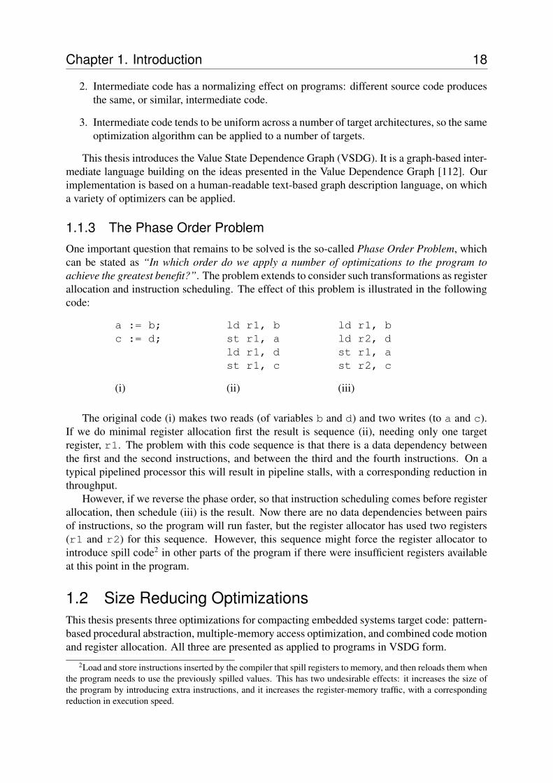
1.1.3 The Phase Order ProblemOne important question that remains to be solved is the so-called Phase Order Problem, whichcan be stated as “In which order do we apply a number of optimizations to the program toachieve the greatest benefit?”. The problem extends to consider such transformations as registerallocation and instruction scheduling. The effect of this problem is illustrated in the followingcode:
a := b;c := d;
ld r1, bst r1, ald r1, dst r1, c
ld r1, bld r2, dst r1, ast r2, c
(i) (ii) (iii)
The original code (i) makes two reads (of variables b and d) and two writes (to a and c).If we do minimal register allocation first the result is sequence (ii), needing only one targetregister, r1. The problem with this code sequence is that there is a data dependency betweenthe first and the second instructions, and between the third and the fourth instructions. On atypical pipelined processor this will result in pipeline stalls, with a corresponding reduction inthroughput.
However, if we reverse the phase order, so that instruction scheduling comes before registerallocation, then schedule (iii) is the result. Now there are no data dependencies between pairsof instructions, so the program will run faster, but the register allocator has used two registers(r1 and r2) for this sequence. However, this sequence might force the register allocator tointroduce spill code2 in other parts of the program if there were insufficient registers availableat this point in the program.
1.2 Size Reducing OptimizationsThis thesis presents three optimizations for compacting embedded systems target code: pattern-based procedural abstraction, multiple-memory access optimization, and combined code motionand register allocation. All three are presented as applied to programs in VSDG form.
2Load and store instructions inserted by the compiler that spill registers to memory, and then reloads them whenthe program needs to use the previously spilled values. This has two undesirable effects: it increases the size ofthe program by introducing extra instructions, and it increases the register-memory traffic, with a correspondingreduction in execution speed.
Chapter 1. Introduction 19
1.2.1 Compaction and CompressionIt is worth highlighting the differences between compaction and compression of program code.Compaction transforms a program, P , into another program, P ′, where |P ′| < |P |. Note thatP ′ is still directly executable by the target processor—no preprocessing is required to executeP ′. We say that the ratio of |P | and |P ′| is the Compaction Ratio:
Compaction Ratio =|P ′||P | × 100%.
Compression, on the other hand, transforms P into one or more blocks of non-executabledata, Q. This then requires runtime decompression to turn Q back into P (or a part of P ) beforethe target processor can execute it. This additional step requires both time (to run the decom-presser) and space (to store the decompressed code). Hardware decompression schemes, suchas used by ARM’s Thumb processor, reduce the process of decompression to a simple transla-tion function (e.g., table look-up). This has predictable performance, but fixes the granularity of(de)compression to individual instructions or functions (e.g., the ARM Thumb executes either16-bit Thumb instructions or 32-bit ARM instructions, specified on a per-function basis).
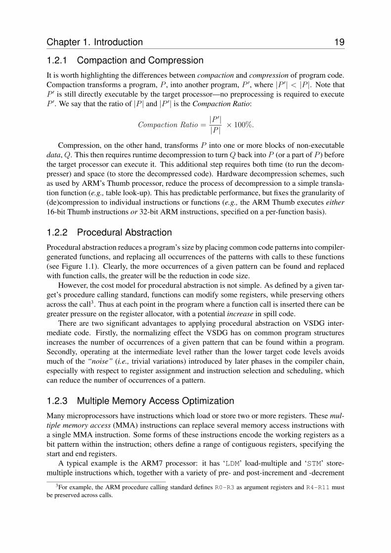
1.2.2 Procedural AbstractionProcedural abstraction reduces a program’s size by placing common code patterns into compiler-generated functions, and replacing all occurrences of the patterns with calls to these functions(see Figure 1.1). Clearly, the more occurrences of a given pattern can be found and replacedwith function calls, the greater will be the reduction in code size.
However, the cost model for procedural abstraction is not simple. As defined by a given tar-get’s procedure calling standard, functions can modify some registers, while preserving othersacross the call3. Thus at each point in the program where a function call is inserted there can begreater pressure on the register allocator, with a potential increase in spill code.
There are two significant advantages to applying procedural abstraction on VSDG inter-mediate code. Firstly, the normalizing effect the VSDG has on common program structuresincreases the number of occurrences of a given pattern that can be found within a program.Secondly, operating at the intermediate level rather than the lower target code levels avoidsmuch of the “noise” (i.e., trivial variations) introduced by later phases in the compiler chain,especially with respect to register assignment and instruction selection and scheduling, whichcan reduce the number of occurrences of a pattern.
1.2.3 Multiple Memory Access OptimizationMany microprocessors have instructions which load or store two or more registers. These mul-tiple memory access (MMA) instructions can replace several memory access instructions witha single MMA instruction. Some forms of these instructions encode the working registers as abit pattern within the instruction; others define a range of contiguous registers, specifying thestart and end registers.
A typical example is the ARM7 processor: it has ‘LDM’ load-multiple and ‘STM’ store-multiple instructions which, together with a variety of pre- and post-increment and -decrement
3For example, the ARM procedure calling standard defines R0-R3 as argument registers and R4-R11 mustbe preserved across calls.
Chapter 1. Introduction 20
call
call
call
Figure 1.1: Original program (left) has common code sequences (shown in dashed boxes).After abstraction, the resulting program (right) has fewer instructions.
addressing modes, can load or store one or more of its sixteen registers. The working registersare encoded as a bitmap within the instruction, scanning the bitmap from the lowest bit (repre-senting R0) to the highest bit (R15). Effective use of this instruction can save up to 480 bits ofcode space4.
This thesis describes the SOLVEMMA algorithm as a way of using MMA instructions toreduce code size. MMA optimization can be applied to both source-defined loads and stores(e.g., array or struct accesses), or spill code inserted by the compiler during register allocation.
In the first case, the algorithm is constrained by the programmer’s expectation of treatingglobal memory as a large struct, with each global variable at a known offset from its schematicneighbour5. The algorithm can only combine loads from, or stores to, contiguous blocks wherethe variables appear in order. In addition, the register allocator can bias allocations whichpromote combined loads and stores.
The second case—local variables and compiler-generated temporaries—provides a greaterdegree of flexibility. The algorithm defines the order of temporary variables on the stack tomaximise the use of MMA instructions. This is beneficial for two reasons: many load andstore instructions are generated from register spills, so giving the algorithm a greater degree offreedom will have a greater benefit; and as spills are invisible to the programmer the compilercan infer a greater degree of information about the use of spill code (e.g., its address is never
4Sixteen separate loads (or stores) would require 512 bits, but only 32 bits for a single LDM or STM.5One could argue that since such behaviour is not specified in the language then the compiler should be free to
do what it likes with the layout of global variables. Sadly, such expectation does exist, and programmers complainif the compiler does not honour this expectation.
Chapter 1. Introduction 21
taken outside the enclosing function).
1.2.4 Combined Code Motion and Register Allocation
The third technique presented in this thesis for compacting code is a method of combining twotraditionally antagonistic compiler phases: code motion and register allocation. We distinguishbetween register allocation—transforming the program such that at every point of executionthere are guaranteed to be sufficient registers to ensure assignment—and register assignment—the process of assigning physical registers to the virtual registers in the intermediate graph.
We present our Register Allocation and Code Motion (RACM) algorithm, which aims toreduce register pressure (i.e., the number of live values at any given point) firstly by movingcode (code motion), secondly by live-range splitting (code cloning), and thirdly by spilling.
This optimization is applied to the VSDG intermediate code, which greatly simplifies thetask of code motion. Data (value) dependencies are explicit within the graph, and so movingan operation node within the graph ensures that all relationships with dependent nodes aremaintained. Also, it is trivial to compute the live range of variables (edges) within the graph;computing register requirements at any given point (called a cut) within the graph is a matter ofenumerating all of the edges (live variables) that are intersected by that cut.
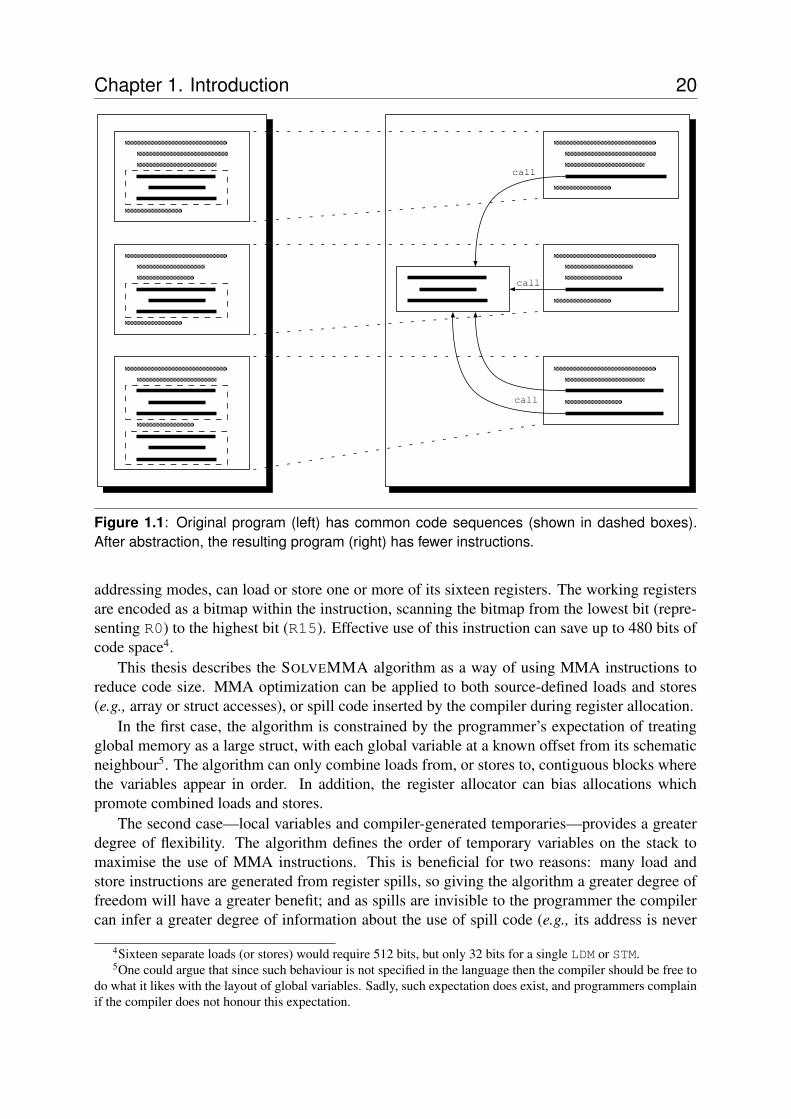
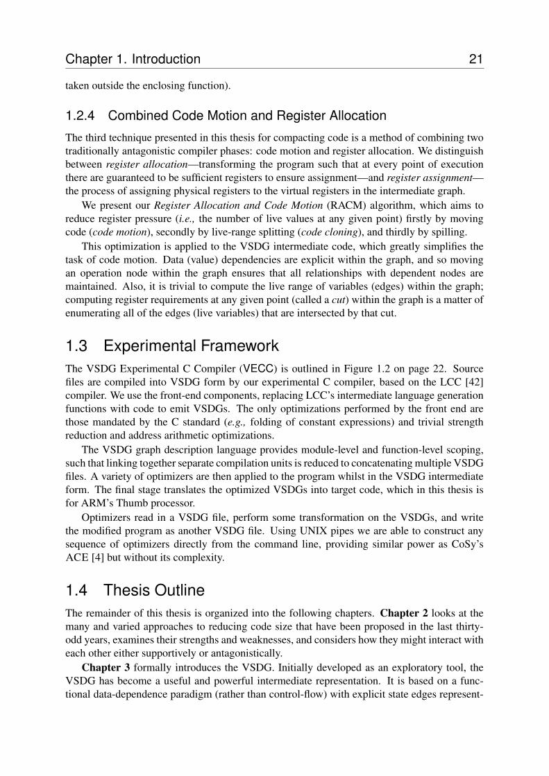
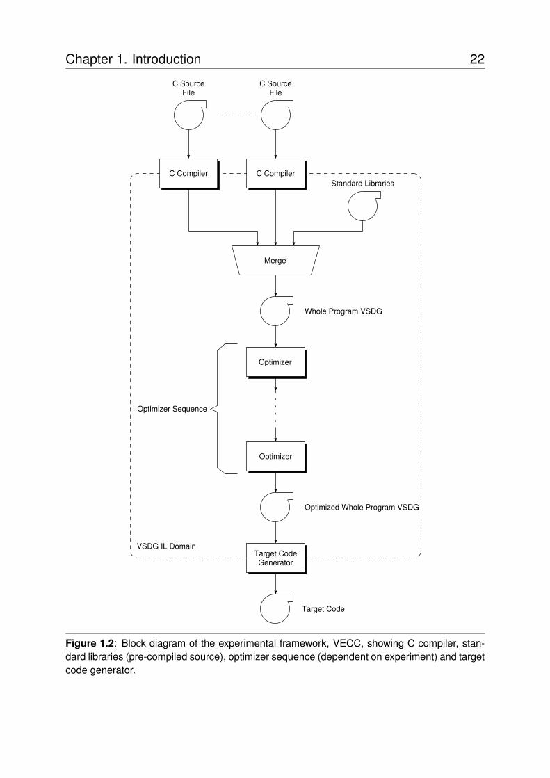
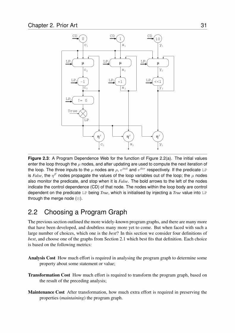
1.3 Experimental FrameworkThe VSDG Experimental C Compiler (VECC) is outlined in Figure 1.2 on page 22. Sourcefiles are compiled into VSDG form by our experimental C compiler, based on the LCC [42]compiler. We use the front-end components, replacing LCC’s intermediate language generationfunctions with code to emit VSDGs. The only optimizations performed by the front end arethose mandated by the C standard (e.g., folding of constant expressions) and trivial strengthreduction and address arithmetic optimizations.
The VSDG graph description language provides module-level and function-level scoping,such that linking together separate compilation units is reduced to concatenating multiple VSDGfiles. A variety of optimizers are then applied to the program whilst in the VSDG intermediateform. The final stage translates the optimized VSDGs into target code, which in this thesis isfor ARM’s Thumb processor.
Optimizers read in a VSDG file, perform some transformation on the VSDGs, and writethe modified program as another VSDG file. Using UNIX pipes we are able to construct anysequence of optimizers directly from the command line, providing similar power as CoSy’sACE [4] but without its complexity.
1.4 Thesis OutlineThe remainder of this thesis is organized into the following chapters. Chapter 2 looks at themany and varied approaches to reducing code size that have been proposed in the last thirty-odd years, examines their strengths and weaknesses, and considers how they might interact witheach other either supportively or antagonistically.
Chapter 3 formally introduces the VSDG. Initially developed as an exploratory tool, theVSDG has become a useful and powerful intermediate representation. It is based on a func-tional data-dependence paradigm (rather than control-flow) with explicit state edges represent-
Chapter 1. Introduction 22
C SourceFile
Merge
C Compiler C CompilerStandard Libraries
C SourceFile
Whole Program VSDG
Optimizer
Optimizer
Optimized Whole Program VSDG
Target CodeGenerator
Target Code
VSDG IL Domain
Optimizer Sequence
Figure 1.2: Block diagram of the experimental framework, VECC, showing C compiler, stan-dard libraries (pre-compiled source), optimizer sequence (dependent on experiment) and targetcode generator.
Chapter 1. Introduction 23
ing the monadic-like system state. It has several important properties, most notably a powerfulnormalizing effect, and is somewhat simpler than prior representations in that it under-specifiesthe program structure, while retaining sufficient structure to maintain the I/O semantics. Wealso present CCS-style pull semantics and show, through an informal bisimulation, equivalenceto traditional push semantics6.
Chapter 4 examines the application of pattern matching techniques to the VSDG for pro-cedural abstraction. We make a clear distinction between procedural abstraction, as applied tothe VSDG, and other code factoring techniques (tail merging, cross-linking, etc).
Chapter 5 describes the use of multiple-load and -store instructions for reducing code size.We show that systematic use of MMA instructions can reduce target code by combining loads orstores into single MMA instructions, and show that our SOLVEMMA algorithm never increasescode size.
In Chapter 6 we show how combining register allocation and instruction scheduling as asingle pass over the VSDG both reduces the effects of the phase-ordering problem, and re-sults in a simpler algorithm for resource allocation (where we define resources as both time—instruction scheduling—and space—register allocation).
Chapter 7 presents experimental evidence of the effectiveness of the work presented inthis thesis, by applying the VSDG-based optimizers to benchmark code. The results of theseexperiments show that the VSDG is a powerful and effective data structure, and provides aframework in which to explore code space optimizations.
Chapter 8 discusses future directions and applications of the VSDG to both software andhardware compilation. Finally, Chapter 9 concludes.
6Think of values as represented by tokens: push semantics describes producers pushing the tokens around thegraph, while pull semantics describes tokens being pulled (demanded) by consumers.

Chapter 1. Introduction 24
CHAPTER 2
Prior Art
To acquire knowledge, one must study;but to acquire wisdom, one must observe.
MARILYN VOS SAVANT (1946–)
Interest in compact representations of programs has been the subject of much research, be ittarget code for direct execution on a processor or high-level intermediate code for execution
on a virtual machine. Most of this research can be split into two areas: the development ofintermediate program graphs, and analyses and transformations on these graphs1.
This chapter examines both areas of research. We begin with a review of the more popu-lar program representation graphs, and for four areas of optimization we choose among thosepresented. For the same four optimizations we briefly describe how they are supported inour new Value State Dependence Graph. We then compare the three techniques developedin this thesis—procedural abstraction, multiple memory access optimization, and combinedregister allocation and code motion—with comparable approaches proposed by other compilerresearchers. Finally, we present a selection of favourable optimization algorithms that eitherdirectly or indirectly produce compact code.
1It should be noted that considerably more effort has been put into making programs faster rather than smaller.Fortunately, many of these optimizations also benefit code size, such as fitting inner loops into instruction caches.
Chapter 2. Prior Art 26
2.1 A Cornucopia of Program GraphsThere have been many program graphs presented in the literature. Here we review the moreprominent ones, and consider their individual strengths and weaknesses.
2.1.1 Control Flow Graph
The Control Flow Graph (CFG) [6] is perhaps the oldest program graph. The basis of thetraditional flowchart, each node in the CFG corresponds to a linear block of instructions suchthat if one instruction executes then all execute, with a unique initial instruction, and with thelast instruction in the block being a (possibly predicated) jump to one or more successor blocks.Edges represent the flow of control between blocks. A CFG represents a single function with aunique entry node, and zero or more exit nodes.
The CFG has no means of representing inter-procedural control flow. Such informationis separately described by a Call Graph. This is a directed graph with nodes representingfunctions, and an edge (p, q) if function p can call function q, and cycles are permitted. Notethat there is no notion of sequence in the call graph, only that on any given trace of executionfunction p may call function q zero or more times.
The CFG is a very simple graph, presenting an almost mechanical view of the program.It is trivial to compute the set of next instructions which may be executed after any giveninstruction—in a single block the next instruction is that which follows the current instruc-tion; after a predicate the set of next instructions is given by the first instruction of the blocks atthe tails of the predicated edges.
Being so simple, the CFG is an excellent graph for both control-flow-based optimizations(e.g., unreachable code elimination [6] or cross-linking [114]) and for generating target code,whose structure is almost an exact duplicate of the CFG. However, other than the progress ofthe the program counter, the CFG says nothing about what the program is computing.
2.1.2 Data Flow Graph
The Data Flow Graph (DFG) is the companion to the CFG: nodes still represent instructions,but with edges now indicating the flow of data from the output of one data operation to theinput of another. A partial order on the instructions is such that an instruction can only executeonce all its input data values have been consumed. The instruction computes a new value whichpropagates along the outward edges to other nodes in the DFG.
The DFG is state-less: it says nothing about what the next instruction to be executed is(there is no concept of the program counter as there is in the CFG). In practice, both the CFGand the DFG can be computed together to support a wider range of optimizations: the DFG isused for dead code elimination (DCE) [94], constant folding, common subexpression elimina-tion (CSE) [7], etc. Together with the CFG, live range analysis [6] determines when a variablebecomes live and where it is last used, with this information being used during register alloca-tion [25].
Separating out the control- and data-flow information is not a good thing. Firstly, there arenow two separate data structures to manage within the compiler—changes to the program re-quire both graphs to be updated, with seemingly trivial changes requiring considerable effort inregenerating one or both of the graphs (e.g., loop unrolling). Secondly, analysis of the programmust process two data structures, with very little commonality between the two. And thirdly,
Chapter 2. Prior Art 27
any relationship between control-flow and data-flow is not expressed, but is split across the twodata structures.
2.1.3 Program Dependence Graph
The Program Dependence Graph (PDG) [39] is an attempt to combine the CFG and the DFG.Again, nodes represent instructions, but now there are edges to represent the essential flow ofcontrol and data within the program. Control dependencies are derived from the usual CFG,while data dependencies represent the relevant data flow relationships between instructions.
There are several advantages to this combined approach: many optimizations can now beperformed in a single walk of the PDG; there is now only one data structure to maintain withinthe compiler; and optimizations that would previously have required complex analysis of theCFG and DFG are more easily achieved (e.g., vectorization [16]).
But this tighter integration of the two types of flow information comes at a cost. The PDG(and one has also to say whose version of the PDG one is using: e.g., the original Ferrante et alPDG [39], Horwitz et al’s PDG [55], or the System Dependence Graph [56] which extends thePDG to incorporate collections of procedures) is a multigraph, with typically six different typesof edges (control, output, anti, loop-carried, loop-independent, and flow). Merge nodes withinthe PDG make some operations dependent on their location within the PDG.
The Hierarchical Task Graph (HTG) [48] is a similar structure to the PDG. It differs fromthe PDG in constructing a graph based on a hierarchy of loop structures rather than the gen-eral control-dependence structure of the PDG. Its main focus is a more general approach tosynchronization between data dependencies, resulting in a potential increase in parallelism.
2.1.4 Program Dependence Web
The Program Dependence Web (PDW) [14] is an augmented PDG. Construction of the PDWfollows on from the construction of the PDG, replacing data dependencies by Gated SingleAssignment form (Section 2.1.8).
PDWs are costly to generate—the original presentation requires fives passes over the PDGto generate the corresponding PDW, with time complexity of O(N 3) in the size of the program.The PDW restricts the control-flow structure to reducible flow graphs [58], spending consider-able effort in determining the control-flow predicates for gated assignments.
2.1.5 Click’s IR
Click and Paleczny’s Intermediate Representation (IR) [27] is an interesting variation of thePDG. They define a model of execution based on Petri nets, where control tokens move fromnode to node as execution proceeds. Their IR can be viewed as two subgraphs—the controlsubgraph and the data subgraph—which meet at their PHI-nodes and IF-nodes (comparable toφ-functions of SSA-form, described below).
The design and implementation of this IR is focused on simplicity and speed of compilation.Having explicit control edges solves the VDG’s (described below) problem of not preservingthe terminating properties of programs.
Chapter 2. Prior Art 28
c = 10;x = 0;y = 1;do {
c = c - 1;x = x + 1;y = y << 1;
} while (c != 0);print(c,x,y);
+- <<
γ γ γ
!=
0
c x y
c x y
TF FTTF
call
1 1 1
0
call
call
10 1
(a) (b)
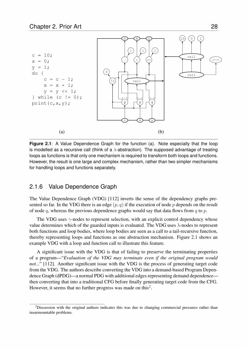
Figure 2.1: A Value Dependence Graph for the function (a). Note especially that the loopis modelled as a recursive call (think of a λ-abstraction). The supposed advantage of treatingloops as functions is that only one mechanism is required to transform both loops and functions.However, the result is one large and complex mechanism, rather than two simpler mechanismsfor handling loops and functions separately.
2.1.6 Value Dependence Graph
The Value Dependence Graph (VDG) [112] inverts the sense of the dependency graphs pre-sented so far. In the VDG there is an edge (p, q) if the execution of node p depends on the resultof node q, whereas the previous dependence graphs would say that data flows from q to p.
The VDG uses γ-nodes to represent selection, with an explicit control dependency whosevalue determines which of the guarded inputs is evaluated. The VDG uses λ-nodes to representboth functions and loop bodies, where loop bodies are seen as a call to a tail-recursive function,thereby representing loops and functions as one abstraction mechanism. Figure 2.1 shows anexample VDG with a loop and function call to illustrate this feature.
A significant issue with the VDG is that of failing to preserve the terminating propertiesof a program—“Evaluation of the VDG may terminate even if the original program wouldnot...” [112]. Another significant issue with the VDG is the process of generating target codefrom the VDG. The authors describe converting the VDG into a demand-based Program Depen-dence Graph (dPDG)—a normal PDG with additional edges representing demand dependence—then converting that into a traditional CFG before finally generating target code from the CFG.However, it seems that no further progress was made on this2.
2Discussion with the original authors indicates this was due to changing commercial pressures rather thaninsurmountable problems.
Chapter 2. Prior Art 29
(1) c = 10; c1 = 10;(2) x = 0; x1 = 0;(3) y = 1; y1 = 1;(4) do { do {(5) c2 = φ(c1, c3);(6) x2 = φ(x1, x3);(7) y2 = φ(y1, y3);(8) c = c− 1; c3 = c2 − 1;(9) x = x + 1; x3 = x2 + 1;(10) y = y << 1; y3 = y2 << 1;(11) } while(c ! = 0); } while(c3 ! = 0);(12) print(c, x, y); print(c3, x3, y3);
(a) (b)
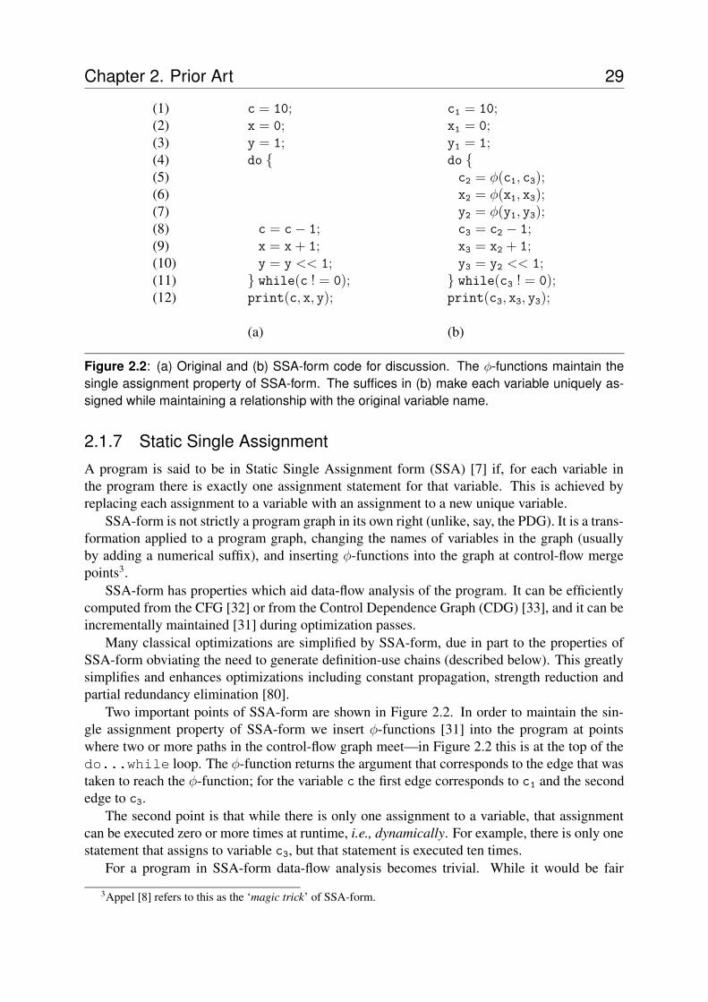
Figure 2.2: (a) Original and (b) SSA-form code for discussion. The φ-functions maintain thesingle assignment property of SSA-form. The suffices in (b) make each variable uniquely as-signed while maintaining a relationship with the original variable name.
2.1.7 Static Single AssignmentA program is said to be in Static Single Assignment form (SSA) [7] if, for each variable inthe program there is exactly one assignment statement for that variable. This is achieved byreplacing each assignment to a variable with an assignment to a new unique variable.
SSA-form is not strictly a program graph in its own right (unlike, say, the PDG). It is a trans-formation applied to a program graph, changing the names of variables in the graph (usuallyby adding a numerical suffix), and inserting φ-functions into the graph at control-flow mergepoints3.
SSA-form has properties which aid data-flow analysis of the program. It can be efficientlycomputed from the CFG [32] or from the Control Dependence Graph (CDG) [33], and it can beincrementally maintained [31] during optimization passes.
Many classical optimizations are simplified by SSA-form, due in part to the properties ofSSA-form obviating the need to generate definition-use chains (described below). This greatlysimplifies and enhances optimizations including constant propagation, strength reduction andpartial redundancy elimination [80].
Two important points of SSA-form are shown in Figure 2.2. In order to maintain the sin-gle assignment property of SSA-form we insert φ-functions [31] into the program at pointswhere two or more paths in the control-flow graph meet—in Figure 2.2 this is at the top of thedo...while loop. The φ-function returns the argument that corresponds to the edge that wastaken to reach the φ-function; for the variable c the first edge corresponds to c1 and the secondedge to c3.
The second point is that while there is only one assignment to a variable, that assignmentcan be executed zero or more times at runtime, i.e., dynamically. For example, there is only onestatement that assigns to variable c3, but that statement is executed ten times.
For a program in SSA-form data-flow analysis becomes trivial. While it would be fair
3Appel [8] refers to this as the ‘magic trick’ of SSA-form.
Chapter 2. Prior Art 30
to say that SSA-form by itself does not provide any new optimizations, it does make manyoptimizations—DCE, CSE, loop-invariant code motion, and so on—far easier. For example,Alpern et al [7] invented SSA-form to improve on value numbering, a technique used exten-sively for CSE.
Another data structure previously non-trivial to compute is the definition-use (def-use) chain [6].A def-use chain is a set of uses S of a variable, x say, such that there is no redefinition of x onany path between the definition of x and any element of S. In SSA-form this is trivial: with ex-actly one definition of x there can be no redefinition of x (if there were, the program would notbe in SSA-form), and so all uses of x are in the def-use chain for x. For example, in Figure 2.2variable c3 is defined in line 8 and used in lines 5, 11 and 12.
2.1.8 Gated Single Assignment
Originally formulated as an intermediate step in forming the PDW [14], Gated SSA-form (GSA)is generated from a CFG in SSA-form, replacing φ-functions with gating (γ-) functions. Theγ-functions turn the non-interpretable SSA-form into the directly interpretable GSA-form. Thegating functions combine SSA-form φ-functions with explicit control flow edges. For example,in Figure 2.2 the φ-function in line 5, φ(c1, c3), is replaced with γ(c3 ! = 0, c1, c3), the firstargument being the control condition for choosing between c1 and c3.
A refinement of GSA-form was proposed by Havlak: Thinned GSA-form (TGSA) [53].The thinned form uses fewer γ-functions than the original GSA-form, reducing the amount ofwork in maintaining the program graph. The formulation of TGSA-form relies on the inputCFG being reducible [58]. Irreducible CFGs can be converted to reducible ones through codeduplication or additional Boolean variables.
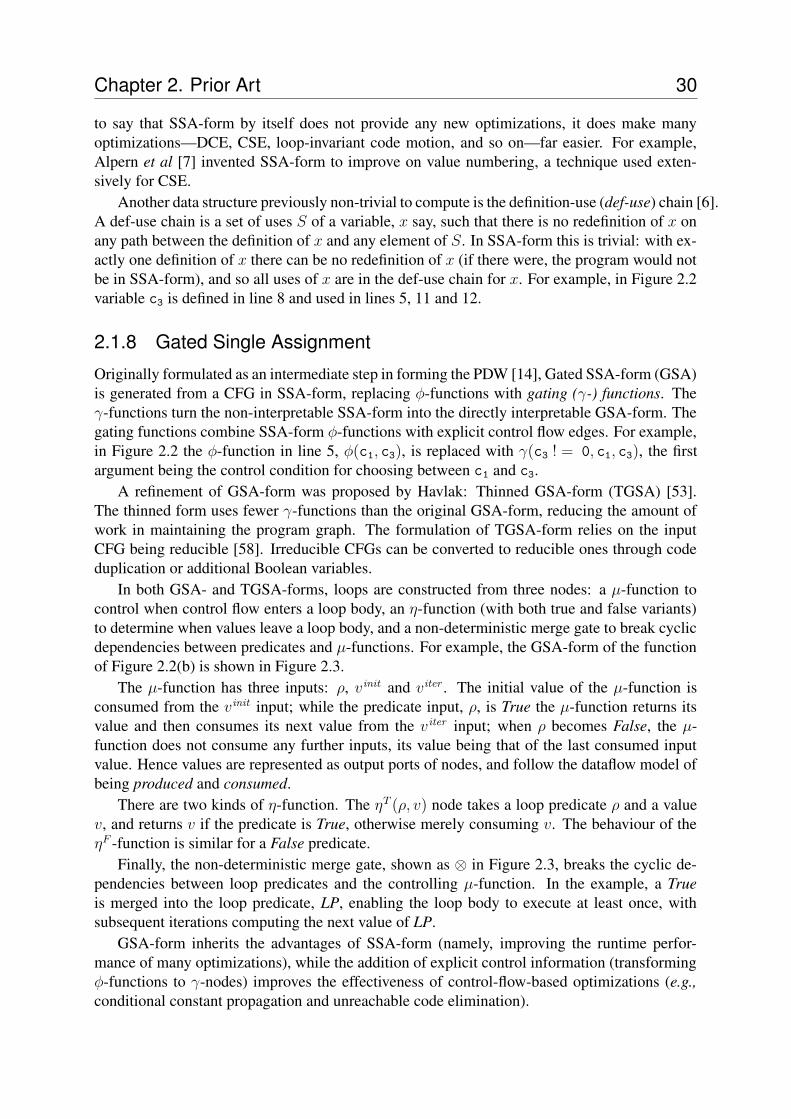
In both GSA- and TGSA-forms, loops are constructed from three nodes: a µ-function tocontrol when control flow enters a loop body, an η-function (with both true and false variants)to determine when values leave a loop body, and a non-deterministic merge gate to break cyclicdependencies between predicates and µ-functions. For example, the GSA-form of the functionof Figure 2.2(b) is shown in Figure 2.3.
The µ-function has three inputs: ρ, vinit and viter . The initial value of the µ-function isconsumed from the vinit input; while the predicate input, ρ, is True the µ-function returns itsvalue and then consumes its next value from the viter input; when ρ becomes False, the µ-function does not consume any further inputs, its value being that of the last consumed inputvalue. Hence values are represented as output ports of nodes, and follow the dataflow model ofbeing produced and consumed.
There are two kinds of η-function. The ηT (ρ, v) node takes a loop predicate ρ and a valuev, and returns v if the predicate is True, otherwise merely consuming v. The behaviour of theηF -function is similar for a False predicate.
Finally, the non-deterministic merge gate, shown as ⊗ in Figure 2.3, breaks the cyclic de-pendencies between loop predicates and the controlling µ-function. In the example, a Trueis merged into the loop predicate, LP, enabling the loop body to execute at least once, withsubsequent iterations computing the next value of LP.
GSA-form inherits the advantages of SSA-form (namely, improving the runtime perfor-mance of many optimizations), while the addition of explicit control information (transformingφ-functions to γ-nodes) improves the effectiveness of control-flow-based optimizations (e.g.,conditional constant propagation and unreachable code elimination).
Chapter 2. Prior Art 31
µ
!= 0
-1
c
c
LP
2
3
c3
µ
+1
x2
x3
0
c1 x1
µy2
y3
<<1
y1
x3 y3
LPTLPTLPT
True
LPT
LPT LPT LPT
1 10CDCDCD
ηF ηFηF
Figure 2.3: A Program Dependence Web for the function of Figure 2.2(a). The initial valuesenter the loop through the µ nodes, and after updating are used to compute the next iteration ofthe loop. The three inputs to the µ nodes are ρ, vinit and viter respectively. If the predicate LPis False, the ηF nodes propagate the values of the loop variables out of the loop; the µ nodesalso monitor the predicate, and stop when it is False. The bold arrows to the left of the nodesindicate the control dependence (CD) of that node. The nodes within the loop body are controldependent on the predicate LP being True, which is initialised by injecting a True value into LPthrough the merge node (⊗).
2.2 Choosing a Program GraphThe previous section outlined the more widely-known program graphs, and there are many morethat have been developed, and doubtless many more yet to come. But when faced with such alarge number of choices, which one is the best? In this section we consider four definitions ofbest, and choose one of the graphs from Section 2.1 which best fits that definition. Each choiceis based on the following metrics:
Analysis Cost How much effort is required in analysing the program graph to determine someproperty about some statement or value;
Transformation Cost How much effort is required to transform the program graph, based onthe result of the preceding analysis;
Maintenance Cost After transformation, how much extra effort is required in preserving theproperties (maintaining) the program graph.
Chapter 2. Prior Art 32
The first two metrics are derived from the informal notion that
Optimization = Analysis + Transformation.
The third metric encapsulates the wider context of a program graph within a compiler: notonly must we analyse the program graph to identify the opportunity for, and then perform, atransformation, we must also maintain the properties (whatever they may be) of the chosenprogram graph for subsequent optimization passes.
2.2.1 Best Graph for Control Flow Optimization
The category of control flow optimization includes unreachable code elimination, block re-ordering, tail merging, cross-linking/jumping, and partial redundancy elimination. All of theseare chiefly concerned with the progress of the Program Counter, i.e., which statement is next tobe executed.
The obvious candidate is, naturally, the CFG. It captures the essential flow of control withina program, with edges representing potentially non-incremental changes to the Program Counter,such as might be taken after a conditional test or the backwards branch at the end of a loop.
By not considering data flows or dependencies, the CFG is both fast to analyse and trans-form, and has low maintenance costs associated with it.
2.2.2 Best Graph for Loop Optimization
There are many optimizations aimed at loops—fusion, peeling, reversal, induction variableelimination, and unrolling to name a few (see Bacon et al [11] for more details on a range ofloop optimizations)—that choosing one program graph that best supports loop optimization isdifficult. However, the majority of these optimizations require a combination of control- anddata-flow information, which simplifies the choice.
The PDG would be a reasonable choice, combining both control- and data-flow, and havingexplicit loop-aware edges. The PDW is also a good choice, with its explicit loop operators (µ, η
and⊗). The VDG treats loops as functions which, on the one hand means that optimizations forloops are automatically applicable to functions as well, but on the other hand complicates thedesign of optimizers, which must now handle loops and functions, with no distinction betweenthe two.
2.2.3 Best Graph for Expression Optimization
Expression optimizations include algebraic reassociation, common subexpression elimination,strength reduction, and constant folding. Clearly, a graph that focuses on data (or values) willprovide the best support for these optimizations.
The CFG is certainly not the best graph for expression optimization. The combined graphs(PDG, PDW and Click’s IR) could be used, but the presence of the control-flow information(which must also be maintained during optimization) can complicate expression optimizationon these graphs.
The two graphs that would be good for expression optimization are the DFG and the VDG.Both graphs are primarily concerned with data (values). Excluding γ-nodes, both graphs arealmost identical, save the direction of the edges.
Chapter 2. Prior Art 33
2.2.4 Best Graph for Whole Program Optimization
There are few graphs which truly reflect the whole program in a single graph. With the exceptionof the SDG, all the graphs presented here are intraprocedural, i.e., they describe the behaviourof single functions, without consideration of other functions within the program.
The best candidate currently is the SDG (the extended form of the PDG with edges to con-nect caller arguments with callee parameters, and vice versa for return values). By representingthe global flow of control and data within a multi-function program, the SDG supports suchglobal optimizations as global constant propagation, function inlining, global register alloca-tion, and global code motion.
2.3 Introducing the Value State Dependence GraphThe previous section chose from the graphs presented in section 2.1 those that would be suitablefor four goals of program optimization. However, the basis of this thesis is the Value StateDependence Graph (described fully in the next chapter). For the same four optimization goals,we describe briefly how this new graph is a suitable candidate.
2.3.1 Control Flow Optimization
The VSDG does not explicitly identify the flow of control within a function. Instead, it describesessential sequential dependencies between I/O nodes, loops, and the enclosing function, and allother information is solely concerned with the flow of data. In essence, there are no explicitbasic blocks within the VSDG.
Of the optimizations listed in section 2.2.1, block re-ordering, tail merging and cross-linkinghave no direct equivalents in the VSDG. Unreachable code is readily computed by walking thevalue and state edges in the VSDG from the function exit node, marking all reachable nodes,and then deleting all the unmarked nodes. Partial redundancy elimination requires additionalanalysis to identify partially redundant expressions, and this can be incorporated into CSE op-timization on the VSDG.
2.3.2 Loop Optimization
The VSDG distinguishes between functions and loops, unlike the VDG. Also, like the PDW,loops are explicitly identified with loop entry and exit nodes. The VSDG is different to manyprogram graphs in that, initially, it does not specify whether loop-invariant nodes are placedinside or outside loops; this decision is left to later phases to decide, based on specific optimiza-tion goals (e.g., putting loop-invariant code inside a loop can reduce register pressure over theloop body, potentially reducing spill code, but may increase its execution time).
2.3.3 Expression Optimization
As its name suggests, the VSDG is derived from the VDG. The addition of the state edges to de-scribe the essential control flow information frees the graph from overly constraining the orderof subexpressions within the graph. This leads to greater freedom and simplicity in optimizingthe expressions described in VSDG form, for optimizations such as CSE, strength reduction,reassociation, etc. The graph properties of the VSDG even simplify the task of transforming
Chapter 2. Prior Art 34
and maintaining the data structure.
2.3.4 Whole Program OptimizationThe VSDG is not a whole-program graph like the SDG. However, the structure of the VSDGcan be readily extended in the same way as the SDG is an extension of the PDG. Then allthe usual whole-program optimizations—function inlining, cloning and specialization, globalconstant propagation, etc—can be supported, with all the inherent benefits of the VSDG.
2.4 Our Approaches to Code CompactionThe previous sections described the major program graph representations that have been pre-sented in the literature. In this section we discuss the three main approaches that are developedin this thesis.
2.4.1 Procedural AbstractionProcedural abstraction takes a whole-program view of code compaction. Common sequencesof instructions from any of the procedures (including library code) within the program can beextracted, and replaced by one abstract procedure and a corresponding number of calls to thatabstract procedure. The potential costs of procedural abstraction are register marshalling beforeand after the procedure call, and the extra processing overhead associated with the procedurecall and return.
2.4.1.1 Transforming Intermediate Code
Runeson applied procedural abstraction to intermediate code prior to register allocation [95].Their implementation, based on a commercial C compiler, achieved up to 30% reduction incode size4.
Fraser and Proebsting [44] analysed common intermediate instruction patterns derived froma C program to generate a customized interpretive code and compact interpreter. They achievedup to 50% reduction in code size, but at considerable runtime penalty due to the interpretivemodel of execution (reportedly 20 times slower than native code).
2.4.1.2 Transforming Target Code
A significant advantage of transforming target code is that the optimizer can be developed eitherindependently from the compiler, or as a later addition to the compiler chain, even from adifferent vendor (e.g., aiPop [3], which can reduce Siemens C16x5 native code by 4–20%).
De Sutter et al’s Squeeze++ [34] achieved an impressive 33% reduction on C++ bench-mark code through aggressive post-link optimization, including procedural abstraction. In onecase (the gtl test program from the Graph Template Library) procedural abstraction reducedthe size of the original code by more than half. Its predecessor, Alto [84], achieved a reductionof 4.2% due to factoring (procedural abstraction) alone. In both cases the target architecture wasthe Alpha RISC processor.
4In private communication with the authors this figure was later revised to 12% due to errors in their imple-mentation.
5A 16-bit embedded microcontroller, used in mobile phones and automotive engine control units.
Chapter 2. Prior Art 35
Cooper and McIntosh [29] developed techniques to compress target code for embeddedRISC processors through cross-linking and procedural abstraction. But, as for Squeeze++and Alto, transforming target code requires care in ensuring variations in register colouringbetween similar code blocks do not reduce the effectiveness of their algorithms. As they noted:“[register] Renaming can sometimes fail to make two fragments equivalent, since the compilermust work within the constraints imposed by the existing register allocation.”
In Liao’s thesis [74], two methods were developed—one purely in software, the other requir-ing some (albeit minimal) hardware support. In the software-only approach, where the searchfor repeating patterns was restricted to basic blocks, Liao achieved a reduction of approximately15% for TMS320C256 target code.
Fraser, Myers and Wendt [43] used suffix trees and normalization on VAX assembler codeto reduce code size by 7% on average, and also noted that while the CPU time of compressedprograms was slightly higher (1-5%) they found that programs actually ran faster overall, whichthey attributed to shorter load times. A similar scheme [69], using illegal processor instructionsto indicate tokens, achieved compression ratios of between 52-70% of the original size over arange of large applications. For the same set of programs, the Unix utility compress—usingLZW coding—achieved a compression ratio of only about 5% better. However, it could beargued that compress’s encoding scheme may not be optimal because of the differing statisticaldistributions of opcodes and operands [9, 93].
An early form of procedural abstraction, due to Marks [76], is related to table-based com-pression, where common instruction sequences were placed in a table, and pseudo-instructionsinserted into the instruction stream in place of the original instruction sequences (tailored inter-pretation). On the IBM System/370, this method achieved a typical saving of 15% at a runtimecost of 15% in execution speed. Storer and Szymanski [102] formulated this as the externalpointer macro, where the pointers into the dictionary were implemented as calls to abstractedprocedures.
2.4.1.3 Parameterized Procedural Abstraction
The power of procedural abstraction is enhanced yet further by parameterizing the abstract pro-cedures [115]. This allows a degree of approximate-matching [12, 13] between the code blocks;the differences are parameterized, and each call site specifies, through additional parameters,the required behaviour of the abstract procedure.
The area of parameterized procedural abstraction has concentrated mainly on the use ofsuffix trees [77, 47] to highlight sections of similar code. Finding a degree of equivalence be-tween two code blocks allows parameterization of the mismatch between blocks. For instance,block B1 may differ from block B2 in one instruction; this difference can be parameterizedwith an if...then...else placed around both instructions, and a selection parameter passed tothe abstract procedure to control which of the two instructions is to be executed. Other near-equivalences can be merged into abstract procedures in a similar way, the limit being whenthere is no further code size reduction benefit in mapping any additional code sequences ontoan abstract procedure.
6A popular 16-bit fixed-point digital signal processor developed and sold by Texas Instruments.
Chapter 2. Prior Art 36
2.4.1.4 Pattern Fingerprinting
Identifying isomorphic regions of a program efficiently is very important, both for speed ofcompilation in finding matching blocks of code, and in compact representations of code blocksfor later matching. The general approach is that of fingerprinting—computing some fingerprintfor a given block of code which can be compared with other fingerprints very quickly.
Several fingerprinting algorithms have been proposed. Debray et al [36] computed a finger-print by concatenating the 4-bit encoded opcodes of the first sixteen instructions in a code block.The question of which opcodes are encoded in these four bits was determined at compile-timeby choosing the fifteen most common instructions in a static instruction count, with the spe-cial code 0000 representing all other instructions. Uniqueness was not guaranteed, for whichthey implemented a hashing scheme on top of their fingerprinting to minimize the number ofpairwise comparisons.
The approach taken by Fraser, Myers and Wendt [43] was to construct a suffix tree [111],comparing instructions based on their hash address (derived from the hashing of the assemblycode). Thus comparable code sequences are rooted at the same node of the suffix tree. Branchinstructions require special handling, as do variations in register colourings.
2.4.2 Multiple Memory Access Optimization
Multiple Memory Access (MMA) optimization is a new idea, with very little directly relatedwork for comparison. However, one related area is that of optimizing address computation codefor Digital Signal Processors (DSPs).
For architectures with no register-plus-offset addressing modes, such as many DSPs, overhalf of the instructions in a typical program are spent computing addresses and accessing mem-ory [107]. The problem of generating optimal address-computing code has been formulated asthe Simple Offset Assignment (SOA) problem, first studied by Bartley [15] and Liao et al [72],the latter formulating the SOA problem for a single address register, and then extending it tothe General Offset Assignment (GOA) problem for k address registers. Liao et al showed thatSOA (and GOA) are NP-hard, reducing the problem to the Hamiltonian path problem. Theirapproximating heuristic is similar to Kruskal’s maximum spanning tree algorithm.
Rao and Pande [91] generalized the SOA problem for optimizing expression trees [99] tominimize address computation code. Their formulation of the problem—Least Cost AccessSequence—is also NP-Complete, but achieved a gain of 2% over Liao et al’s earlier work [72].This approach reordered a sequence of loads without consideration of the store of the result.However, breaking big expression trees into smaller sub-trees can reduce optimization possibil-ities if the stores are seen as fixed.
Leupers and Marwedel [70] adopted a tie-breaking heuristic for SOA and a variable parti-tioning strategy for GOA. Later, Liao, together with Sudarsanam and Devadas [103] extendedk-register GOA by considering auto-increment/decrement over the range −l . . . + l. Both SOAand GOA optimize target code in the absence of register-plus-offset addressing modes, whichwould otherwise render trivial the SOA problem.
Lim, Kim and Choi [75] took a more general approach to reordering code to improve theeffectiveness of SOA optimization. Their algorithm was implemented at the medium-level in-termediate representation within the SPAM compiler, and achieved an improvement of 3.6%over fixed-schedule SOA, when generating code for the TMS320C25 DSP. This was a moregeneral approach to that taken by Rao and Pande, with their most favourable algorithm being a
Chapter 2. Prior Art 37
hybrid of a greedy list scheduling algorithm and an exhaustive search algorithm.DSP-enhanced architectures (e.g., Intel MMX [57], PowerPC AltiVec [81] and Sun VIS [104])
include MMA-like block loads and stores. However, these instructions are limited to fixed blockloads and stores to special data or vector registers, not general purpose registers. This restric-tion limits the use of these MMA instructions to specific data processing code, not to generalpurpose code (e.g., spilling code).
A related area to MMA optimization is that of SIMD Within A Register (SWAR) [40]. Theresearch presented in this thesis considers only word-sized variables; applying the same algo-rithm to sub-word-sized variables could achieve additional reductions in code size (e.g., com-bining four byte-sized loads into a single word load).
SOA was recently applied by Sharma and Gupta [100] to GCC’s intermediate language.They achieved an average code size reduction of 3.5% over a range of benchmarks for theTMS320C25. Interestingly, while for most benchmarks there was a reduction in code size, fora few benchmarks there was a measurable increase. The authors attributed this to deficienciesin later phases in the GCC compiler chain.
All of the above approaches have been applied to the Control Flow Graph [6], which pre-cisely specifies the sequence of memory access instructions. Koseki et al considered the prob-lem of colouring a CFG (where the order of instructions is fixed) in the presence of instructionswhich have particular preferences for register assignment [66]. They suggested using thesepreferences to guide register assignment to enable the use of MMA instructions. The work pre-sented in Chapter 5 differs from their work in two ways: (1) because the VSDG underspecifiesthe ordering of instructions in a graph7 we can consider combining loads and stores that arenot adjacent to each other in the CFG into provisional MMA nodes; and (2) we use the AccessGraph to bias the layout of the stack frame for spilled and local variables during target codegeneration.
2.4.3 Combining Register Allocation and Code Motion
Formulating register allocation as a graph colouring problem was originally proposed by Chaitin [25].The intermediate code is analysed to determine live variable ranges [6], producing a clashgraph, G(N,E), where each node n ∈ N represents a single live range, and there is an edgee(p, q) ∈ E if the two live ranges p and q clash (are live at the same time) within the program.
Colouring proceeds by assigning (colouring) physical registers to nodes whose degree is lessthan the number of physical registers, and removing them from the clash graph. This processrepeats until either there are no more nodes in the clash graph to colour (in which case theprocess is complete), or there are nodes that cannot be coloured. Uncoloured nodes are split intwo, with a partitioning of the incident clash edges, together with the insertion of spill code intothe intermediate code. Colouring then continues as before, splitting nodes where necessary.
This is a formulation of the k-register graph colouring problem, which is NP-Completein the number of registers (colours) available to colour the graph: for k >= 3 the colouringproblem is reducible to the 3-SAT problem [45]. However, carefully-designed heuristics canproduce near-optimal results in the majority of cases, and with acceptable performance even inpathological cases.
Chow and Hennessey [26] proposed a modification of Chaitin’s original graph colouring
7We show in Chapter 6 that the special case of a VSDG with enough serializing edges to enforce a linear ordercorresponds to a CFG.
Chapter 2. Prior Art 38
algorithm. They split the uncolourable nodes into two separate live ranges [26], and tailorheuristics to favour more frequently-accessed nodes (e.g., inner loop variables).
Goodwin and Wilken [50] formulated global register allocation (including all possible spillplacements) as a 0-1 integer programming problem. While they did achieve quite impressiveresults, the cost was very high: the complexity of their algorithm is O(n3), and for a given timeperiod their allocator did not guarantee to allocate all functions.
All of the register allocation approaches described so far are applied to fixed-order blocks ofinstructions. The only transformation possible is to insert spill code to reduce register pressure;the goal being to minimize the amount of spill code inserted into the program. Another wayto reduce register pressure, and hence reduce spill code, is to move code in a way that reducesregister pressure.
Code motion as an optimization is not new (e.g., Partial Redundancy Elimination [80]).Perhaps the work closest in spirit to that presented in Chapter 6 is that of Ruthing et al [96]who presented algorithms for optimal placement of expressions and sub-expressions, combiningboth raising and lowering of code within basic blocks.
The CRAIG framework [20], implemented within the ROCKET compiler [105], took abrute force approach:
1. Attempt register allocation after instruction scheduling.
2. If the schedule cost is not acceptable (by some defined metric) attempt register allocationbefore scheduling.
3. While the cost is acceptable (i.e., there is some better schedule) add back in informationfrom the first pass until the schedule just becomes too costly.
Brasier et al’s experience with an instance of CRAIG (CRAIG0) defined the metric as the exis-tence of spill code (a schedule is considered unacceptable in the presence of spill code). Theirexperimental results showed improvements in execution time, but did not document the changein code size. Rao [92] improved on CRAIG0 with additional heuristics to allow some spilling,where it could be shown that spilling had a beneficial effect.
Touati’s thesis [106] argued that register allocation is the primary determinant of perfor-mance, not scheduling. The goal of his thesis was again to minimize the insertion of spill code,both through careful analysis of register pressure, and by adding serializing edges to each basicblock’s data dependency DAG. By using integer linear programming (cf. Goodwin and Wilken)Touati achieved optimal solutions for cyclic register allocation (where the output register map-ping of one loop iteration is the input register mapping for the next loop iteration, thus avoidingregister copies at loop iteration boundaries), allowing for a trade-off between ILP efficiency andregister usage.
An early attempt at combining register allocation with instruction scheduling was proposedby Pinter [88]. That work was based on an instruction level register-based intermediate code,and was preceded by a phase to determine data dependencies. This dependence informationthen drove the allocator, generating a Parallelizable Interference Graph to suggest possibleregister allocations. Further, the Global Scheduling Graph (i.e., global in the sense of crossingbasic block boundaries) was then used to schedule instructions within a region.
Another approach was the region-based algorithm of Janssen and Corporaal [59], whichdefined regions as corresponding to the bodies of natural loops. They then used this hierarchy
Chapter 2. Prior Art 39
of nested regions to focus register allocation, with the inner-most regions being favoured bybetter register allocation.
The “Resource Spackling Framework” of Berson et al [18] applied a Measure and Reduceparadigm to combine both phases—their approach first measured the resource requirements ofa program using a unified representation, and then moved instructions out of excessive sets intoresource holes. This approach was basic-block-based: a local scheduler attempted to satisfy thetarget constraints without increasing the execution time of a block, while the more complicatedglobal scheduler moved instructions between blocks. This approach most closely matches theapproach described in Chapter 6, which by design is a global version of their local schedulersince the VSDG does not have explicit basic blocks.
2.5 10002 Code Compacting OptimizationsThere have been many optimization algorithms discussed in the literature over the last thirty orforty years. Some are designed to improve the execution speed of a program; some aim to re-duce the size of a program, either through compaction or compression; and other optimizationsreduce the runtime data storage requirements of programs.
In this section we choose eight8 optimizations which have the effect of reducing a program’ssize. For each optimization, we discuss their merits, their algorithmic complexity, and theireffectiveness at reducing code size. While we do not claim this list to be exhaustive, we believethe ones presented here to be the most beneficial.
2.5.1 Procedural Abstraction
Procedural abstraction makes significant changes to a whole program. It is a form of code com-pression, replacing multiple instances of a repeating code block with a single instance (function)and multiple references (calls) to that instance. As a concrete example of procedural abstrac-tion, De Sutter et al’s Squeeze++ [34] demonstrates how effective procedural abstraction canbe on modern code.
But why is procedural abstraction so effective, and does it have a future? The answer tothis question lies in modern approaches to software engineering. Large applications are writtenby teams of programmers9, and in many cases the problems that the individual teams are tosolve look similar (e.g., walking a list, sorting, iterating over arrays, etc). Additionally, someof the code will be produced by programmers copying other sections of code (“cut-n-pasteprogramming”).
As projects are maintained over a period of time, programmers prefer to copy a known,working, function and make minor changes than risk changing a tested function. Or simply thata maintenance programmer writes a function to implement some new behaviour, unaware thata function already exists in another module (perhaps among millions of lines of code).
Use of object-oriented programming languages like C++, Java and C#, further increases theopportunities for code compaction from procedural abstraction. Software engineering methodsemphasise the use of subclassing, part of which includes overriding methods with specialisedmethods particular to the derived class. In many cases, these new methods are very similar to
8Eight being the closest binary number to ten.9One could even argue that a lone programmer is actually part of a large team if you factor in the operating
system and third-party library developers.
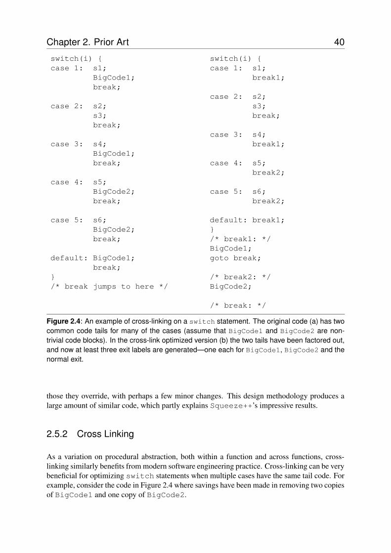
Chapter 2. Prior Art 40
switch(i) {case 1: s1;
BigCode1;break;
case 2: s2;s3;break;
case 3: s4;BigCode1;break;
case 4: s5;BigCode2;break;
case 5: s6;BigCode2;break;
default: BigCode1;break;
}/* break jumps to here */
switch(i) {case 1: s1;
break1;
case 2: s2;s3;break;
case 3: s4;break1;
case 4: s5;break2;
case 5: s6;break2;
default: break1;}/* break1: */BigCode1;goto break;
/* break2: */BigCode2;
/* break: */
Figure 2.4: An example of cross-linking on a switch statement. The original code (a) has twocommon code tails for many of the cases (assume that BigCode1 and BigCode2 are non-trivial code blocks). In the cross-link optimized version (b) the two tails have been factored out,and now at least three exit labels are generated—one each for BigCode1, BigCode2 and thenormal exit.
those they override, with perhaps a few minor changes. This design methodology produces alarge amount of similar code, which partly explains Squeeze++’s impressive results.
2.5.2 Cross Linking
As a variation on procedural abstraction, both within a function and across functions, cross-linking similarly benefits from modern software engineering practice. Cross-linking can be verybeneficial for optimizing switch statements when multiple cases have the same tail code. Forexample, consider the code in Figure 2.4 where savings have been made in removing two copiesof BigCode1 and one copy of BigCode2.
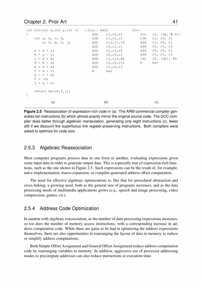
Chapter 2. Prior Art 41
int foo(int x,int y,int z){
int a, b, c, d,e, f, g, h, j;
a = x + y;b = y - z;c = a + b;d = b + x;e = x + a;f = a + c;g = c + d;h = -d;j = g + h;
return bar(e,f,j);}
||foo|| PROCADD r3,r0,r1SUB r1,r1,r2ADD r12,r1,r0ADD r2,r3,r1ADD r1,r3,r2ADD r0,r0,r3RSB r3,r12,#0ADD r2,r2,r12ADD r2,r2,r3B bar
foo:str lr, [sp, #-4]!rsb r2, r2, r1add r1, r0, r1add r2, r1, r2add r0, r0, r1add r1, r1, r2ldr lr, [sp], #4b bar
(a) (b) (c)
Figure 2.5: Reassociation of expression-rich code in (a). The ARM commercial compiler gen-erates ten instructions (b) which almost exactly mirror the original source code. The GCC com-piler does better through algebraic manipulation, generating only eight instructions (c), fewerstill if we discount the superfluous link register-preserving instructions. Both compilers wereasked to optimize for code size.
2.5.3 Algebraic Reassociation
Most computer programs process data in one form or another, evaluating expressions givensome input data in order to generate output data. This is especially true of expression-rich func-tions, such as the one shown in Figure 2.5. Such expressions can be the result of, for example,naıve implementation, macro expansion, or compiler-generated address offset computation.
The need for effective algebraic optimizations is, like that for procedural abstraction andcross-linking, a growing need, both as the general size of programs increases, and as the dataprocessing needs of multimedia applications grows (e.g., speech and image processing, videocompression, games, etc).
2.5.4 Address Code Optimization
In tandem with algebraic reassociation, as the number of data processing expressions increases,so too does the number of memory access instructions, with a corresponding increase in ad-dress computation code. While there are gains to be had in optimizing the address expressionsthemselves, there are also opportunities in rearranging the layout of data in memory to reduceor simplify address computations.
Both Simple Offset Assignment and General Offset Assignment reduce address computationcode by rearranging variables in memory. In addition, aggressive use of processor addressingmodes to precompute addresses can also reduce instructions or execution time.
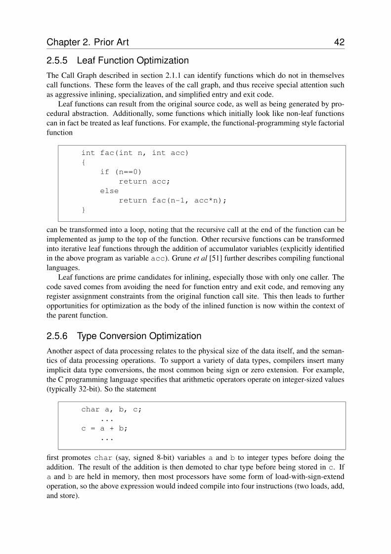
Chapter 2. Prior Art 42
2.5.5 Leaf Function OptimizationThe Call Graph described in section 2.1.1 can identify functions which do not in themselvescall functions. These form the leaves of the call graph, and thus receive special attention suchas aggressive inlining, specialization, and simplified entry and exit code.
Leaf functions can result from the original source code, as well as being generated by pro-cedural abstraction. Additionally, some functions which initially look like non-leaf functionscan in fact be treated as leaf functions. For example, the functional-programming style factorialfunction
int fac(int n, int acc){
if (n==0)return acc;
elsereturn fac(n-1, acc*n);
}
can be transformed into a loop, noting that the recursive call at the end of the function can beimplemented as jump to the top of the function. Other recursive functions can be transformedinto iterative leaf functions through the addition of accumulator variables (explicitly identifiedin the above program as variable acc). Grune et al [51] further describes compiling functionallanguages.
Leaf functions are prime candidates for inlining, especially those with only one caller. Thecode saved comes from avoiding the need for function entry and exit code, and removing anyregister assignment constraints from the original function call site. This then leads to furtheropportunities for optimization as the body of the inlined function is now within the context ofthe parent function.
2.5.6 Type Conversion OptimizationAnother aspect of data processing relates to the physical size of the data itself, and the seman-tics of data processing operations. To support a variety of data types, compilers insert manyimplicit data type conversions, the most common being sign or zero extension. For example,the C programming language specifies that arithmetic operators operate on integer-sized values(typically 32-bit). So the statement
char a, b, c;...
c = a + b;...
first promotes char (say, signed 8-bit) variables a and b to integer types before doing theaddition. The result of the addition is then demoted to char type before being stored in c. Ifa and b are held in memory, then most processors have some form of load-with-sign-extendoperation, so the above expression would indeed compile into four instructions (two loads, add,and store).
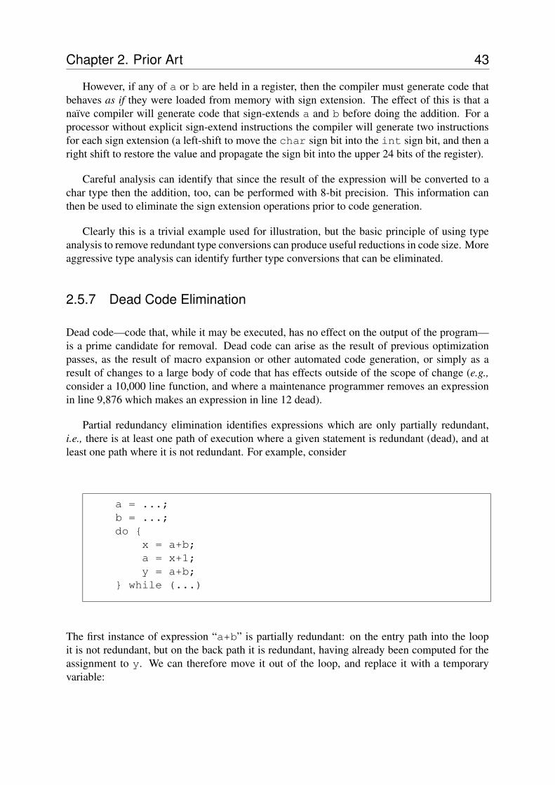
Chapter 2. Prior Art 43
However, if any of a or b are held in a register, then the compiler must generate code thatbehaves as if they were loaded from memory with sign extension. The effect of this is that anaıve compiler will generate code that sign-extends a and b before doing the addition. For aprocessor without explicit sign-extend instructions the compiler will generate two instructionsfor each sign extension (a left-shift to move the char sign bit into the int sign bit, and then aright shift to restore the value and propagate the sign bit into the upper 24 bits of the register).
Careful analysis can identify that since the result of the expression will be converted to achar type then the addition, too, can be performed with 8-bit precision. This information canthen be used to eliminate the sign extension operations prior to code generation.
Clearly this is a trivial example used for illustration, but the basic principle of using typeanalysis to remove redundant type conversions can produce useful reductions in code size. Moreaggressive type analysis can identify further type conversions that can be eliminated.
2.5.7 Dead Code Elimination
Dead code—code that, while it may be executed, has no effect on the output of the program—is a prime candidate for removal. Dead code can arise as the result of previous optimizationpasses, as the result of macro expansion or other automated code generation, or simply as aresult of changes to a large body of code that has effects outside of the scope of change (e.g.,consider a 10,000 line function, and where a maintenance programmer removes an expressionin line 9,876 which makes an expression in line 12 dead).
Partial redundancy elimination identifies expressions which are only partially redundant,i.e., there is at least one path of execution where a given statement is redundant (dead), and atleast one path where it is not redundant. For example, consider
a = ...;b = ...;do {
x = a+b;a = x+1;y = a+b;
} while (...)
The first instance of expression “a+b” is partially redundant: on the entry path into the loopit is not redundant, but on the back path it is redundant, having already been computed for theassignment to y. We can therefore move it out of the loop, and replace it with a temporaryvariable:
Chapter 2. Prior Art 44
a = ...;b = ...;T = a+b;do {
x = T;a = x+1;y = a+b;T = y;
} while (...)
with the added advantage of exposing the first instance of a+b to optimizations with the pre-ceding code.
Dead code elimination may be one of the oldest optimizations known, but it still has itsplace in modern optimizing compilers. This is especially so with automated code generationand object-oriented languages emphasising code reuse—it is better to leave redundant code inthe unchanged source code, and let the optimizer remove it during compilation.
2.5.8 Unreachable Code EliminationWhile dead code is code that may execute but have no effect on the output of the program,unreachable code is that code which will never be executed. For example, in
#define DEBUG ( 0 )
...
if (DEBUG)print(...);
the print statement is unreachable, and both it and the enclosing if can be deleted. However,in considering
int bigfunc(int n){
if (n>10){
... HUGE CODE ...}
}
it would be very beneficial if we could determine if the predicate n>10was always false, as thenthe “HUGE CODE” could be removed, with potentially huge savings. The only way to achievethis is by interprocedural analysis, firstly to determine all of the call sites for this function, andsecondly to determine the range of values that can be passed into the function. The predicatecan then be identified as being always-false, always-true, or otherwise. If the result of analysisis always-false, the body of the if statement can be deleted.
Chapter 2. Prior Art 45
Such global analysis is non-trivial, and the safe option is simply not to delete any code ifthere is even the slightest doubt that it might not be dead. Leaving the code in place will onlyresult in a program larger than necessary; deleting it will produce a broken program.
The same is true of predicate analysis: in simple cases, like the example above, the predicateis trivial to analyse. However, in general, predicate analysis is undecidable, and so we mighttake the conservative approach of restricting analysis to schematic equivalence. For example, isthe following predicate always-true, always-false, or otherwise for all values of x?
if ( ((x+1)*(x+1)) == (x*x + 2*x + 1) ){
...}
The problem is especially difficult for floating point types, where it is entirely possible for theleft and right hand sides of this predicate to compute different results for the same value of x.
2.6 SummaryThis chapter has taken a broad look at the more significant program graphs that have beenproposed and used within compilers. From the original Control Flow Graph and the Data FlowGraph, Ferrante et al’s Program Dependence Graph, to Ballance et al’s Program DependenceWeb and Click’s Intermediate Representation, to the Value Dependence Graph of Weise et al.
As well as the graphs themselves, we have also reviewed two forms of expressing valueswithin these graphs: Static Single Assignment form and Gated Single Assignment form. Theysimplify dataflow analyses by placing a program in a form where there exists exactly one as-signment statement for every variable in the program.
We the considered four important optimization goals—control flow optimization, loop opti-mization, expression optimization, and whole program optimization—and chose from the pro-gram graphs previously described the one that best supported each given optimization goal.
We then briefly described how our new Value State Dependence Graph (presented in thenext chapter) can be applied to all of these optimization goals, before going on to describe thethree main approaches to code size optimization presented in this thesis: procedural abstrac-tion, multiple memory access optimization, and combined register allocation and code motion,described in chapters 4, 5, and 6 respectively.
Finally we chose eight code size optimizations that are important for code size: proceduralabstraction, cross-linking, algebraic reassociation and address code optimization, leaf functionoptimization, type conversion optimization, dead code elimination, and unreachable code elim-ination.
In the next chapter we introduce the foundation of this thesis: the Value State DependenceGraph, and describe how some of the optimizations presented in this chapter can be applied toprograms described in VSDG form.

Chapter 2. Prior Art 46
CHAPTER 3
The Value State Dependence Graph
The secret to creativity is knowinghow to hide your sources.
ALBERT EINSTEIN (1879–1955)
An important decision when building a compiler is the choice of the internal data structurefor representing the program. Amongst its many properties it should simplify analysis of
the program and minimize the effort in transforming and maintaining the structure.The previous chapter reviewed a range of program graphs. It showed that they have various
desirable features, but that there are issues relating to the implementation of analyses and trans-formations. This chapter begins with a critique of the Program Dependence Graph, showingthat its complex structure over-specifies (and thus overly constrains) the program graph.
The Value State Dependence Graph (VSDG) is then described, showing how it solves theinherent problems of its predecessor, the Value Dependence Graph, through the addition of stateedges and by careful treatment of loops. The pull-model semantics of the VSDG are given, andshown to be equivalent to the push-model semantics of the PDG.
Generating VSDGs from syntax-directed translation of structured C programs is describedin detail, together with the implementation of a C-subset1 compiler. Finally, the benefits of theVSDG are demonstrated with a number of well-known control- and data-flow optimizations.
1Excluding goto and labels. This is fixable, through code duplication or boolean variables, but not the focusof this thesis.
Chapter 3. The Value State Dependence Graph 48
3.1 A Critique of the Program Dependence GraphThe Program Dependence Graph (PDG) [39] is a multigraph, combining the Control FlowGraph (CFG) and the Data Dependence Graph (DDG) into a single, unified graph structure. Inthis section we describe in sufficient detail the PDG, and then discuss its weaknesses, showingthat the VSDG (Section 3.3) offers a better framework for optimization.
3.1.1 Definition of the Program Dependence GraphVertices in the PDG represent single statements and predicate expressions (or operators andoperands), and edges represent both data-dependencies and control-dependencies.
Definition 3.1 (Program Dependence Graph) The Program Dependence Graph of a pro-gram P is a directed graph G = (V,E), where V is the set of vertices (statements, operators,predicate expressions, etc), E ⊆ V × V is the set of dependence edges (of which the fourcategories of edge are further defined below), where each edge (p, q) ∈ E connects fromvertex p ∈ V to vertex q ∈ V .
There are two main categories of edge in the PDG: control dependence edges and datadependence edges.
Definition 3.2 (Control Dependence Edge) There exists a control dependence edge (p, q)iff either:
1. p is the entry vertex and q is a vertex in P that is not within any loop or conditional;or
2. p is a control vertex, and q is a vertex in P immediately dominated by p.
In the PDG there are several types of data dependence edges. In the original Ferrante,Ottenstein and Warren formulation of the PDG [39] there are three types of data dependenceedge.
Definition 3.3 (Flow Dependence Edge) There exists a flow dependence edge (p, q) iff
1. p is a vertex that defines variable x,
2. q is a vertex that uses x, and
3. control can reach q after p via an execution path within the CFG of P along whichthere is no intervening definition of x.
Flow dependences are further classified as loop-carried dependencies, for definitions thatare referenced on subsequent iterations of a loop, and loop-independent dependencies, for defi-nitions that are independent of loop iteration.
The definitions for output dependence edges and anti-dependence edges follow from theusual definitions:
Definition 3.4 (Output Dependence Edge) There exists an output dependence edge (p, q)iff both p and q define the same variable x, and control can reach q after p via an executionpath within the CFG of P .
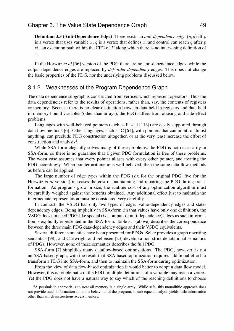
Chapter 3. The Value State Dependence Graph 49
Definition 3.5 (Anti-Dependence Edge) There exists an anti-dependence edge (p, q) iff p
is a vertex that uses variable x, q is a vertex that defines x, and control can reach q after p
via an execution path within the CFG of P along which there is no intervening definition ofx.
In the Horwitz et al [56] version of the PDG there are no anti-dependence edges, while theoutput dependence edges are replaced by def-order dependency edges. This does not changethe basic properties of the PDG, nor the underlying problems discussed below.
3.1.2 Weaknesses of the Program Dependence GraphThe data dependence subgraph is constructed from vertices which represent operators. Thus thedata dependencies refer to the results of operations, rather than, say, the contents of registersor memory. Because there is no clear distinction between data held in registers and data heldin memory-bound variables (other than arrays), the PDG suffers from aliasing and side-effectproblems.
Languages with well-behaved pointers (such as Pascal [113]) are easily supported throughdata flow methods [6]. Other languages, such as C [61], with pointers that can point to almostanything, can preclude PDG construction altogether, or at the very least increase the effort ofconstruction and analysis2.
While SSA-form elegantly solves many of these problems, the PDG is not necessarily inSSA-form, so there is no guarantee that a given PDG formulation is free of these problems.The worst case assumes that every pointer aliases with every other pointer, and treating thePDG accordingly. When pointer arithmetic is well-behaved, then the same data flow methodsas before can be applied.
The large number of edge types within the PDG (six for the original PDG, five for theHorwitz et al version) increases the cost of maintaining and repairing the PDG during trans-formation. As programs grow in size, the runtime cost of any optimization algorithm mustbe carefully weighed against the benefits obtained. Any additional effort just to maintain theintermediate representation must be considered very carefully.
In contrast, the VSDG has only two types of edge: value-dependency edges and state-dependency edges. Being implicitly in SSA-form (in that values have only one definition), theVSDG does not need PDG-like special (i.e., output- or anti-dependence) edges as such informa-tion is explicitly represented in the SSA-form. Table 3.1 (above) describes the correspondencebetween the three main PDG data-dependency edges and their VSDG equivalents.
Several different semantics have been presented for PDGs. Selke provides a graph rewritingsemantics [98], and Cartwright and Felleisen [23] develop a non-strict denotational semanticsof PDGs. However, none of these semantics describes the full PDG.
SSA-form [7] simplifies many dataflow-based optimizations. The PDG, however, is notan SSA-based graph, with the result that SSA-based optimization requires additional effort totransform a PDG into SSA-form, and then to maintain the SSA-form during optimization.
From the view of data flow-based optimization it would better to adopt a data flow model.However, this is problematic in the PDG: multiple definitions of a variable may reach a vertex.Yet the PDG does not have a natural way to say which of the reaching definitions to choose
2A pessimistic approach is to treat all memory is a single array. While safe, this monolithic approach doesnot provide much information about the behaviour of the program, so subsequent analysis yields little informationother than which instructions access memory.
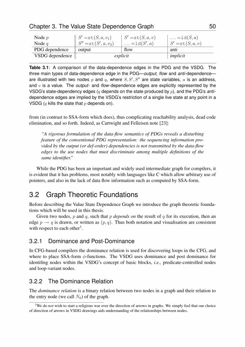
Chapter 3. The Value State Dependence Graph 50
Node p S ′ =st(S, a, v1) S ′ =st(S, a, v) . . . =ld(S, a)Node q S ′′ =st(S ′, a, v2) . . . =ld(S ′, a) S ′ =st(S, a, v)PDG dependence output flow antiVSDG dependence explicit implicit
Table 3.1: A comparison of the data-dependence edges in the PDG and the VSDG. Thethree main types of data-dependence edge in the PDG—output, flow and anti-dependence—are illustrated with two nodes p and q, where S, S ′, S′′ are state variables, a is an address,and v is a value. The output- and flow-dependence edges are explicitly represented by theVSDG’s state-dependency edges (q depends on the state produced by p), and the PDG’s anti-dependence edges are implied by the VSDG’s restriction of a single live state at any point in aVSDG (q kills the state that p depends on).
from (in contrast to SSA-form which does), thus complicating reachability analysis, dead codeelimination, and so forth. Indeed, as Cartwight and Felleisen note [23]:
“A rigorous formulation of the data-flow semantics of PDGs reveals a disturbingfeature of the conventional PDG representation: the sequencing information pro-vided by the output (or def-order) dependencies is not transmitted by the data-flowedges to the use nodes that must discriminate among multiple definitions of thesame identifier.”
While the PDG has been an important and widely used intermediate graph for compilers, itis evident that it has problems, most notably with languages like C which allow arbitrary use ofpointers, and also in the lack of data flow information such as computed by SSA-form.
3.2 Graph Theoretic FoundationsBefore describing the Value State Dependence Graph we introduce the graph theoretic founda-tions which will be used in this thesis.
Given two nodes, p and q, such that p depends on the result of q for its execution, then anedge p → q is drawn, or written as (p, q). Thus both notation and visualisation are consistentwith respect to each other3.
3.2.1 Dominance and Post-DominanceIn CFG-based compilers the dominance relation is used for discovering loops in the CFG, andwhere to place SSA-form φ-functions. The VSDG uses dominance and post dominance foridentifing nodes within the VSDG’s concept of basic blocks, i.e., predicate-controlled nodesand loop-variant nodes.
3.2.2 The Dominance RelationThe dominance relation is a binary relation between two nodes in a graph and their relation tothe entry node (we call N0) of the graph.
3We do not wish to start a religious war over the direction of arrows in graphs. We simply feel that our choiceof direction of arrows in VSDG drawings aids understanding of the relationships between nodes.
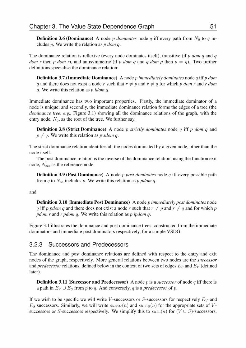
Chapter 3. The Value State Dependence Graph 51
Definition 3.6 (Dominance) A node p dominates node q iff every path from N0 to q in-cludes p. We write the relation as p dom q.
The dominance relation is reflexive (every node dominates itself), transitive (if p dom q and qdom r then p dom r), and antisymmetric (if p dom q and q dom p then p = q). Two furtherdefinitions specialise the dominance relation:
Definition 3.7 (Immediate Dominance) A node p immediately dominates node q iff p domq and there does not exist a node r such that r 6= p and r 6= q for which p dom r and r domq. We write this relation as p idom q.
Immediate dominance has two important properties. Firstly, the immediate dominator of anode is unique; and secondly, the immediate dominance relation forms the edges of a tree (thedominance tree, e.g., Figure 3.1) showing all the dominance relations of the graph, with theentry node, N0, as the root of the tree. We further say,
Definition 3.8 (Strict Dominance) A node p strictly dominates node q iff p dom q andp 6= q. We write this relation as p sdom q.
The strict dominance relation identifies all the nodes dominated by a given node, other than thenode itself.
The post dominance relation is the inverse of the dominance relation, using the function exitnode, N∞, as the reference node.
Definition 3.9 (Post Dominance) A node p post dominates node q iff every possible pathfrom q to N∞ includes p. We write this relation as p pdom q.
and
Definition 3.10 (Immediate Post Dominance) A node p immediately post dominates nodeq iff p pdom q and there does not exist a node r such that r 6= p and r 6= q and for which ppdom r and r pdom q. We write this relation as p ipdom q.
Figure 3.1 illustrates the dominance and post dominance trees, constructed from the immediatedominators and immediate post dominators respectively, for a simple VSDG.
3.2.3 Successors and PredecessorsThe dominance and post dominance relations are defined with respect to the entry and exitnodes of the graph, respectively. More general relations between two nodes are the successorand predecessor relations, defined below in the context of two sets of edges ES and EV (definedlater).
Definition 3.11 (Successor and Predecessor) A node p is a successor of node q iff there isa path in EV ∪ ES from p to q. And conversely, q is a predecessor of p.
If we wish to be specific we will write V -successors or S-successors for respectively EV andES successors. Similarly, we will write succV (n) and succS(n) for the appropriate sets of V -successors or S-successors respectively. We simplify this to succ(n) for (V ∪ S)-successors,
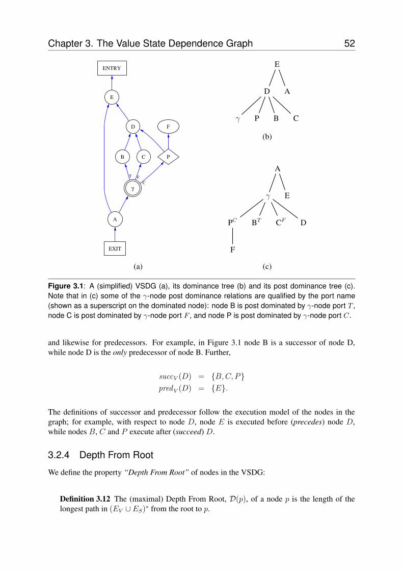
Chapter 3. The Value State Dependence Graph 52
A
EXIT
E
D
γ
C
F
B
T
P
C
F
ENTRY
(a)
E
D
γ P B C
A
(b)
A
γ
PC
F
BT CF D
E
(c)
Figure 3.1: A (simplified) VSDG (a), its dominance tree (b) and its post dominance tree (c).Note that in (c) some of the γ-node post dominance relations are qualified by the port name(shown as a superscript on the dominated node): node B is post dominated by γ-node port T ,node C is post dominated by γ-node port F , and node P is post dominated by γ-node port C.
and likewise for predecessors. For example, in Figure 3.1 node B is a successor of node D,while node D is the only predecessor of node B. Further,
succV (D) = {B,C, P}predV (D) = {E}.
The definitions of successor and predecessor follow the execution model of the nodes in thegraph; for example, with respect to node D, node E is executed before (precedes) node D,while nodes B, C and P execute after (succeed) D.
3.2.4 Depth From Root
We define the property “Depth From Root” of nodes in the VSDG:
Definition 3.12 The (maximal) Depth From Root, D(p), of a node p is the length of thelongest path in (EV ∪ ES)∗ from the root to p.
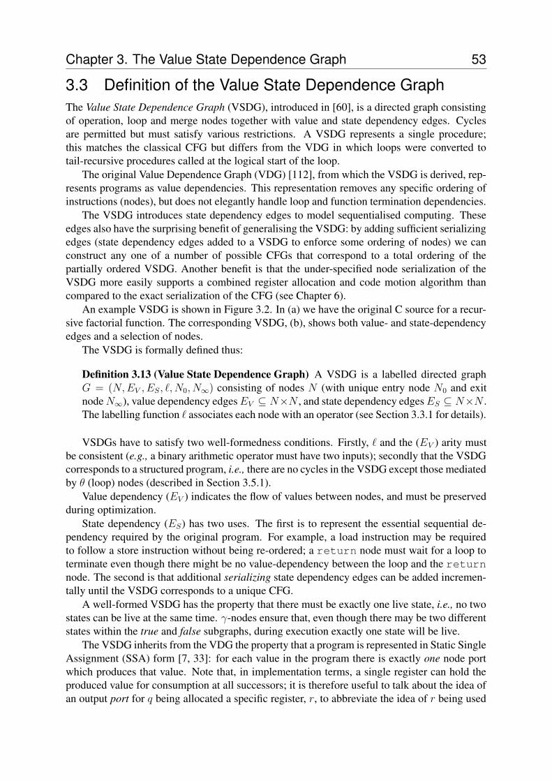
Chapter 3. The Value State Dependence Graph 53
3.3 Definition of the Value State Dependence GraphThe Value State Dependence Graph (VSDG), introduced in [60], is a directed graph consistingof operation, loop and merge nodes together with value and state dependency edges. Cyclesare permitted but must satisfy various restrictions. A VSDG represents a single procedure;this matches the classical CFG but differs from the VDG in which loops were converted totail-recursive procedures called at the logical start of the loop.
The original Value Dependence Graph (VDG) [112], from which the VSDG is derived, rep-resents programs as value dependencies. This representation removes any specific ordering ofinstructions (nodes), but does not elegantly handle loop and function termination dependencies.
The VSDG introduces state dependency edges to model sequentialised computing. Theseedges also have the surprising benefit of generalising the VSDG: by adding sufficient serializingedges (state dependency edges added to a VSDG to enforce some ordering of nodes) we canconstruct any one of a number of possible CFGs that correspond to a total ordering of thepartially ordered VSDG. Another benefit is that the under-specified node serialization of theVSDG more easily supports a combined register allocation and code motion algorithm thancompared to the exact serialization of the CFG (see Chapter 6).
An example VSDG is shown in Figure 3.2. In (a) we have the original C source for a recur-sive factorial function. The corresponding VSDG, (b), shows both value- and state-dependencyedges and a selection of nodes.
The VSDG is formally defined thus:
Definition 3.13 (Value State Dependence Graph) A VSDG is a labelled directed graphG = (N,EV , ES, `, N0, N∞) consisting of nodes N (with unique entry node N0 and exitnode N∞), value dependency edges EV ⊆ N×N , and state dependency edges ES ⊆ N×N .The labelling function ` associates each node with an operator (see Section 3.3.1 for details).
VSDGs have to satisfy two well-formedness conditions. Firstly, ` and the (EV ) arity mustbe consistent (e.g., a binary arithmetic operator must have two inputs); secondly that the VSDGcorresponds to a structured program, i.e., there are no cycles in the VSDG except those mediatedby θ (loop) nodes (described in Section 3.5.1).
Value dependency (EV ) indicates the flow of values between nodes, and must be preservedduring optimization.
State dependency (ES) has two uses. The first is to represent the essential sequential de-pendency required by the original program. For example, a load instruction may be requiredto follow a store instruction without being re-ordered; a return node must wait for a loop toterminate even though there might be no value-dependency between the loop and the returnnode. The second is that additional serializing state dependency edges can be added incremen-tally until the VSDG corresponds to a unique CFG.
A well-formed VSDG has the property that there must be exactly one live state, i.e., no twostates can be live at the same time. γ-nodes ensure that, even though there may be two differentstates within the true and false subgraphs, during execution exactly one state will be live.
The VSDG inherits from the VDG the property that a program is represented in Static SingleAssignment (SSA) form [7, 33]: for each value in the program there is exactly one node portwhich produces that value. Note that, in implementation terms, a single register can hold theproduced value for consumption at all successors; it is therefore useful to talk about the idea ofan output port for q being allocated a specific register, r, to abbreviate the idea of r being used
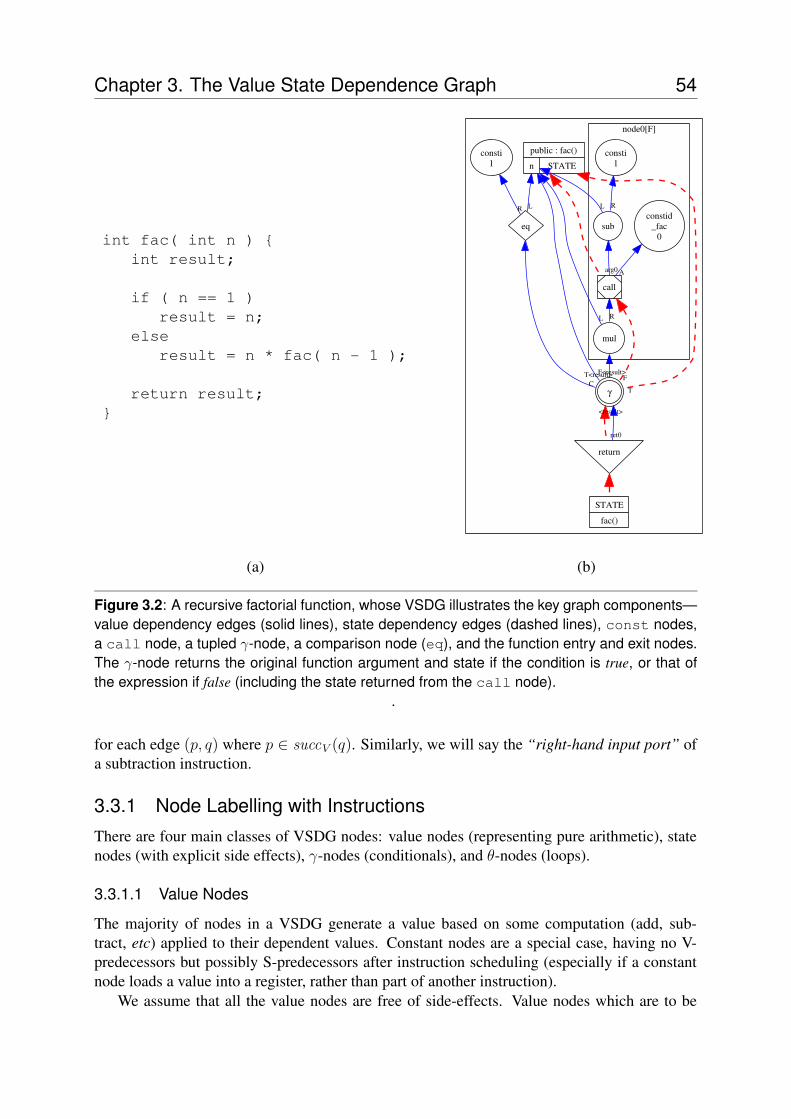
Chapter 3. The Value State Dependence Graph 54
int fac( int n ) {int result;
if ( n == 1 )result = n;
elseresult = n * fac( n - 1 );
return result;}
node0[F]
return
STATE
fac()
γ
ret0
<result>
call
F
mul
R
public : fac()
n STATE
T
T<result>
L
sub
L
eq
L
F<result>
constid_fac
0
Aarg0
consti1
R
C
consti1
R
(a) (b)
Figure 3.2: A recursive factorial function, whose VSDG illustrates the key graph components—value dependency edges (solid lines), state dependency edges (dashed lines), const nodes,a call node, a tupled γ-node, a comparison node (eq), and the function entry and exit nodes.The γ-node returns the original function argument and state if the condition is true, or that ofthe expression if false (including the state returned from the call node).
.
for each edge (p, q) where p ∈ succV (q). Similarly, we will say the “right-hand input port” ofa subtraction instruction.
3.3.1 Node Labelling with InstructionsThere are four main classes of VSDG nodes: value nodes (representing pure arithmetic), statenodes (with explicit side effects), γ-nodes (conditionals), and θ-nodes (loops).
3.3.1.1 Value Nodes
The majority of nodes in a VSDG generate a value based on some computation (add, sub-tract, etc) applied to their dependent values. Constant nodes are a special case, having no V-predecessors but possibly S-predecessors after instruction scheduling (especially if a constantnode loads a value into a register, rather than part of another instruction).
We assume that all the value nodes are free of side-effects. Value nodes which are to be
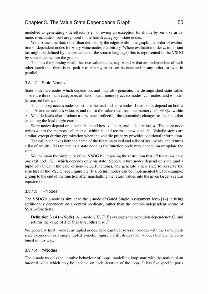
Chapter 3. The Value State Dependence Graph 55
modelled as generating side-effects (e.g., throwing an exception for divide-by-zero, or arith-metic over/under-flow) are placed in the fourth category—state nodes.
We also assume that, other than defined by the edges within the graph, the order of evalua-tion of dependent nodes for n-ary value nodes is arbitrary. Where evaluation order is important(as might be defined by the semantics of the source language) this is represented in the VSDGby state edges within the graph.
This has the pleasing result that two value nodes, say, p and q, that are independent of eachother (such that there is no path p to q nor q to p) can be executed in any order, or even inparallel.
3.3.1.2 State Nodes
State nodes are nodes which depend on, and may also generate, the distinguished state value.There are three main categories of state nodes: memory access nodes, call nodes, and θ-nodes(discussed below).
The memory access nodes constitute the load and store nodes. Load nodes depend on both astate, S, and an address value, a, and return the value read from the memory cell MEM[a] withinS. Volatile loads also produce a new state, reflecting the (potential) changes to the state thatexecuting the load might cause.
Store nodes depend on a state, S, an address value, a, and a data value, d. The store nodewrites d into the memory cell MEM[a] within S, and returns a new state, S ′. Volatile stores aresimilar, except during optimization when the volatile property provides additional information.
The call node takes both the name of the function to call and a list of arguments, and returnsa list of results. It is treated as a state node as the function body may depend on or update thestate.
We maintain the simplicity of the VSDG by imposing the restriction that all functions haveone exit node N∞, which depends only on state. Special return nodes depend on state (and atuple of values in the case of non-void functions), and generate a new state to preserve thestructure of the VSDG (see Figure 3.2 (b)). Return nodes can be implemented by, for example,a jump to the end of the function after marshalling the return values into the given target’s returnregister(s).
3.3.1.3 γ-Nodes
The VSDG’s γ-node is similar to the γ-node of Gated Single Assignment form [14] in beingadditionally dependent on a control predicate, rather than the control-independent nature ofSSA φ-functions.
Definition 3.14 (γ-Node) A γ-node γ(C, T, F ) evaluates the condition dependency C, andreturns the value of T if C is true, otherwise F .
We generally treat γ-nodes as tupled nodes. One can treat several γ-nodes with the same pred-icate expression as a single tupled γ-node. Figure 3.3 illustrates two γ-nodes that can be com-bined in this way.
3.3.1.4 θ-Nodes
The θ-node models the iterative behaviour of loops, modelling loop state with the notion of aninternal value which may be updated on each iteration of the loop. It has five specific ports
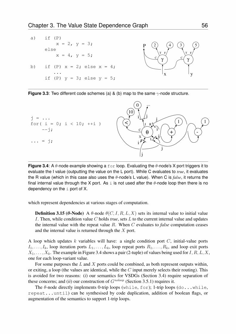
Chapter 3. The Value State Dependence Graph 56
a) if (P)x = 2, y = 3;
elsex = 4, y = 5;
b) if (P) x = 2; else x = 4;...
if (P) y = 3; else y = 5;
2 4
γ
P
C
T F
x y
3 5
γC
T F
Figure 3.3: Two different code schemes (a) & (b) map to the same γ-node structure.
j = ...for( i = 0; i < 10; ++i )
--j;
... = j;
10
<
θ +I R
L
1
C -
1
X
...
j
}
0
i j
ii}
}
j
j
}i
Figure 3.4: A θ-node example showing a for loop. Evaluating the θ-node’s X port triggers it toevaluate the I value (outputting the value on the L port). While C evaluates to true, it evaluatesthe R value (which in this case also uses the θ-node’s L value). When C is false, it returns thefinal internal value through the X port. As i is not used after the θ-node loop then there is nodependency on the i port of X.
which represent dependencies at various stages of computation.
Definition 3.15 (θ-Node) A θ-node θ(C, I,R, L,X) sets its internal value to initial valueI . Then, while condition value C holds true, sets L to the current internal value and updatesthe internal value with the repeat value R. When C evaluates to false computation ceasesand the internal value is returned through the X port.
A loop which updates k variables will have: a single condition port C, initial-value portsI1, . . . , Ik, loop iteration ports L1, . . . , Lk, loop repeat ports R1, . . . , Rk, and loop exit portsX1, . . . , Xk. The example in Figure 3.4 shows a pair (2-tuple) of values being used for I, R, L,X ,one for each loop-variant value.
For some purposes the L and X ports could be combined, as both represent outputs within,or exiting, a loop (the values are identical, while the C input merely selects their routing). Thisis avoided for two reasons: (i) our semantics for VSDGs (Section 3.4) require separation ofthese concerns; and (ii) our construction of Gnoloop (Section 3.5.1) requires it.
The θ-node directly implements 0-trip loops (while, for); 1-trip loops (do...while,repeat...until) can be synthesised by code duplication, addition of boolean flags, oraugmentation of the semantics to support 1-trip loops.
Chapter 3. The Value State Dependence Graph 57
Code duplication has two important benefits: it exposes the first loop iteration to optimiza-tion (cf. loop-peeling [86]), and it normalizes all loops to one loop structure, which both reducesthe cost of optimization, and increases the likelihood of two schematically-dissimilar loops be-ing isomorphic in the VSDG. A boolean flag avoids duplicating code, but increases the com-plexity of the loop predicate, and does not benefit from normalization. Finally, augmenting thesemantics with an additional loop node type does not increase code size per se, but does reducethe benefits of loop normalization.
Note also that the VSDG neither forces loop invariant code (Section 3.8.3) into nor out-of loop bodies, but rather allows later phases to determine, by adding serializing edges, suchplacement of loop invariant nodes.
3.4 Semantics of the VSDGGiven the definition of the VSDG from the previous section we define pull (or lazy) semanticsin terms of CCS operators [78]. We also compare the pull semantics with traditional pushsemantics (i.e., data flow machine).
We use the following notations:
• inputs are Ii,
• outputs are Q,
• Z is a reinitialisation port needed for loops,
• θ- and γ-nodes are augmented with a C (condition) input,
• we write ‘+’ for choice,
• ‘|’ for concurrency,
• ‘.’ for serial composition,
• ‘I?x’ for a read from port I , placing the value read into x, and
• ‘Q!e’ for a write to port Q of the value of expression e.
In the demand-driven pull semantics, each input port I (including C) has an associatedrequest Ireq (a null, i.e., pure, synchronisation) port written to before the value on I is read.Similarly output ports Q await input on Qreq before proceeding.
The pull semantics for the main types of VSDG node are shown in Figure 3.5 (page 58).From these it is trivial to generate the pull-semantics for the remaining VSDG nodes.
3.4.1 The VSDG’s Pull SemanticsThe semantics of the constant nodes—integer, float, and identifier—are all identical:
constpull(v)def= Qreq?().Q!v.constpull(v)
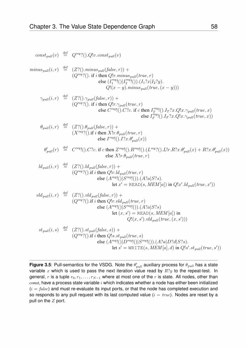
Chapter 3. The Value State Dependence Graph 58
constpull(v)def= Qreq?().Q!v.constpull(v)
minuspull(i, r)def= (Z?().minuspull(false, r)) +
(Qreq?(). if i then Q!r.minuspull(true, r)else (Ireq
1 !()|Ireq2 !()).(I1?x|I2?y).
Q!(x− y).minuspull(true, (x− y)))
γpull(i, r)def= (Z?().γpull(false, r)) +
(Qreq?(). if i then Q!r.γpull(true, r)else Creq !().C?c. if c then I
reqT !().IT ?x.Q!x.γpull(true, x)
else IreqF !().IF ?x.Q!x.γpull(true, x))
θpull(i, r)def= (Z?().θpull(false, r)) +
(Xreq?().if i then X!r.θpull(true, r)else Ireq !().I?x.θ′pull(x))
θ′pull(r)def= Creq !().C?c. if c then Zreq !().Rreq !().(Lreq?().L!r.R?x.θ′pull(x) + R?x.θ′pull(x))
else X!r.θpull(true, r)
ldpull(i, r)def= (Z?().ld pull(false, r)) +
(Qreq?().if i then Q!r.ld pull(true, r)else (Areq !()|Sreq !()).(A?a|S?s).
let x′ = READ(s,MEM [a]) in Q!x′.ldpull(true, x′))
vldpull(i, r)def= (Z?().vld pull(false, r)) +
(Qreq?().if i then Q!r.vld pull(true, r)else (Areq !()|Sreq !()).(A?a|S?s)
let (x, s′) = READ(s,MEM [a]) inQ!(x, s′).vldpull(true, (x, s′)))
stpull(i, s)def= (Z?().stpull(false, s)) +
(Qreq?().if i then Q!s.stpull(true, s)else (Areq !()|Dreq !()|Sreq !()).(A?a|D?d|S?s).
let s′ = WRITE(s,MEM [a], d) in Q!s′.stpull(true, s′))
Figure 3.5: Pull-semantics for the VSDG. Note the θ′pull auxiliary process for θpull has a statevariable x which is used to pass the next iteration value read by R?y to the repeat-test. Ingeneral, r is a tuple r0, r1, . . . , rN−1 where at most one of the r is state. All nodes, other thanconst, have a process state variable i which indicates whether a node has either been initialized(i = false) and must re-evaluate its input ports, or that the node has completed execution andso responds to any pull request with its last computed value (i = true). Nodes are reset by apull on the Z port.
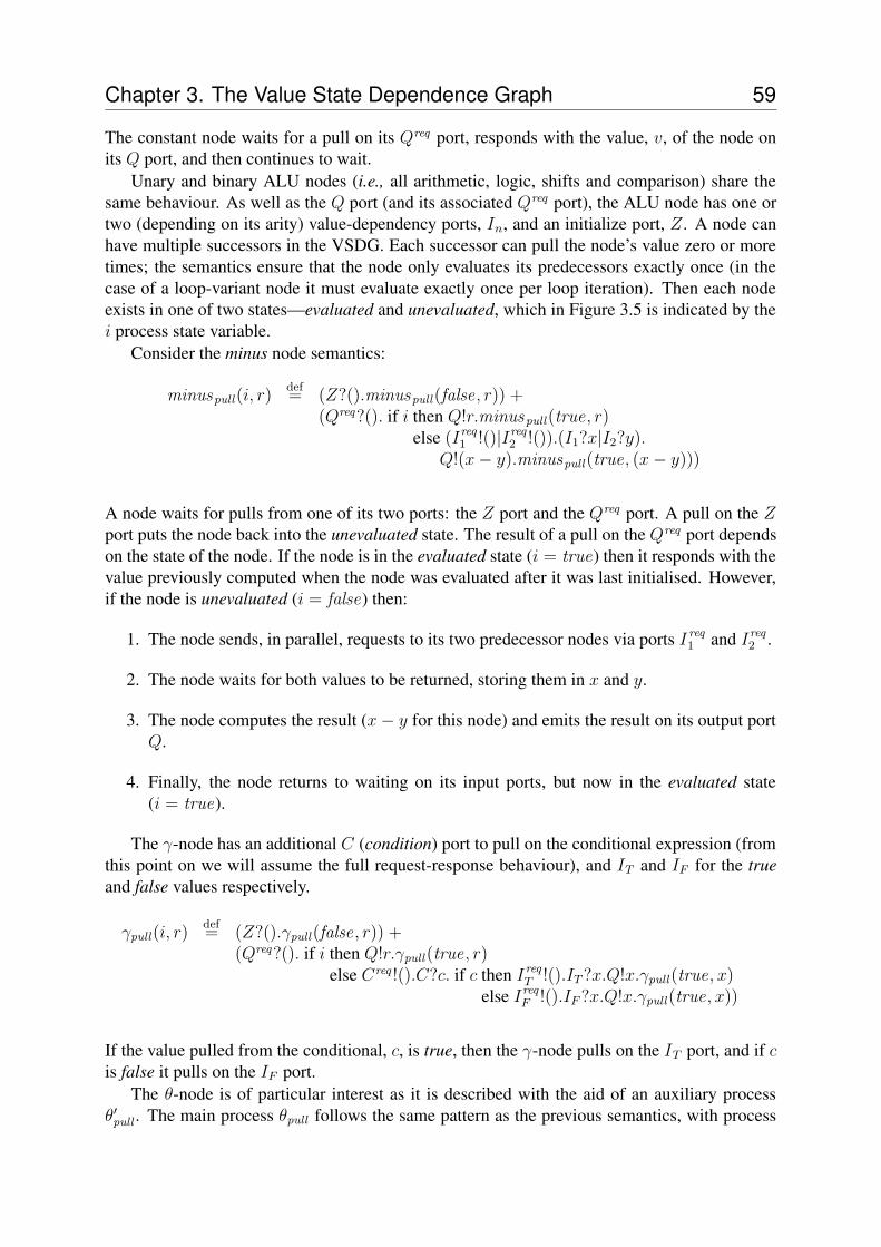
Chapter 3. The Value State Dependence Graph 59
The constant node waits for a pull on its Qreq port, responds with the value, v, of the node onits Q port, and then continues to wait.
Unary and binary ALU nodes (i.e., all arithmetic, logic, shifts and comparison) share thesame behaviour. As well as the Q port (and its associated Qreq port), the ALU node has one ortwo (depending on its arity) value-dependency ports, In, and an initialize port, Z. A node canhave multiple successors in the VSDG. Each successor can pull the node’s value zero or moretimes; the semantics ensure that the node only evaluates its predecessors exactly once (in thecase of a loop-variant node it must evaluate exactly once per loop iteration). Then each nodeexists in one of two states—evaluated and unevaluated, which in Figure 3.5 is indicated by thei process state variable.
Consider the minus node semantics:
minuspull(i, r)def= (Z?().minuspull(false, r)) +
(Qreq?(). if i then Q!r.minuspull(true, r)else (Ireq
1 !()|Ireq2 !()).(I1?x|I2?y).
Q!(x− y).minuspull(true, (x− y)))
A node waits for pulls from one of its two ports: the Z port and the Qreq port. A pull on the Z
port puts the node back into the unevaluated state. The result of a pull on the Qreq port dependson the state of the node. If the node is in the evaluated state (i = true) then it responds with thevalue previously computed when the node was evaluated after it was last initialised. However,if the node is unevaluated (i = false) then:
1. The node sends, in parallel, requests to its two predecessor nodes via ports Ireq1 and I
req2 .
2. The node waits for both values to be returned, storing them in x and y.
3. The node computes the result (x− y for this node) and emits the result on its output portQ.
4. Finally, the node returns to waiting on its input ports, but now in the evaluated state(i = true).
The γ-node has an additional C (condition) port to pull on the conditional expression (fromthis point on we will assume the full request-response behaviour), and IT and IF for the trueand false values respectively.
γpull(i, r)def= (Z?().γpull(false, r)) +
(Qreq?(). if i then Q!r.γpull(true, r)else Creq !().C?c. if c then I
reqT !().IT ?x.Q!x.γpull(true, x)
else IreqF !().IF ?x.Q!x.γpull(true, x))
If the value pulled from the conditional, c, is true, then the γ-node pulls on the IT port, and if c
is false it pulls on the IF port.The θ-node is of particular interest as it is described with the aid of an auxiliary process
θ′pull . The main process θpull follows the same pattern as the previous semantics, with process
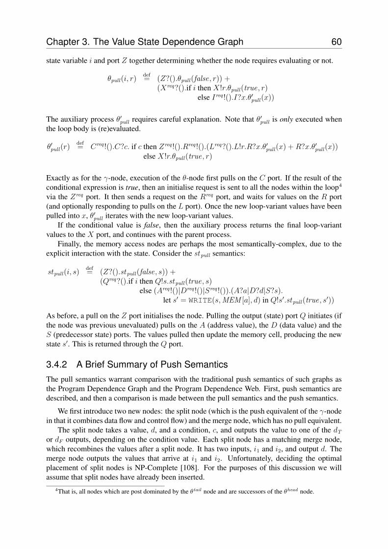
Chapter 3. The Value State Dependence Graph 60
state variable i and port Z together determining whether the node requires evaluating or not.
θpull(i, r)def= (Z?().θpull(false, r)) +
(Xreq?().if i then X!r.θpull(true, r)else Ireq !().I?x.θ′pull(x))
The auxiliary process θ′pull requires careful explanation. Note that θ′pull is only executed when
the loop body is (re)evaluated.
θ′pull(r)def= Creq !().C?c. if c then Zreq !().Rreq !().(Lreq?().L!r.R?x.θ′pull(x) + R?x.θ′pull(x))
else X!r.θpull(true, r)
Exactly as for the γ-node, execution of the θ-node first pulls on the C port. If the result of theconditional expression is true, then an initialise request is sent to all the nodes within the loop4
via the Zreq port. It then sends a request on the Rreq port, and waits for values on the R port(and optionally responding to pulls on the L port). Once the new loop-variant values have beenpulled into x, θ′pull iterates with the new loop-variant values.
If the conditional value is false, then the auxiliary process returns the final loop-variantvalues to the X port, and continues with the parent process.
Finally, the memory access nodes are perhaps the most semantically-complex, due to theexplicit interaction with the state. Consider the st pull semantics:
stpull(i, s)def= (Z?().stpull(false, s)) +
(Qreq?().if i then Q!s.stpull(true, s)else (Areq !()|Dreq !()|Sreq !()).(A?a|D?d|S?s).
let s′ = WRITE(s,MEM [a], d) in Q!s′.stpull(true, s′))
As before, a pull on the Z port initialises the node. Pulling the output (state) port Q initiates (ifthe node was previous unevaluated) pulls on the A (address value), the D (data value) and theS (predecessor state) ports. The values pulled then update the memory cell, producing the newstate s′. This is returned through the Q port.
3.4.2 A Brief Summary of Push SemanticsThe pull semantics warrant comparison with the traditional push semantics of such graphs asthe Program Dependence Graph and the Program Dependence Web. First, push semantics aredescribed, and then a comparison is made between the pull semantics and the push semantics.
We first introduce two new nodes: the split node (which is the push equivalent of the γ-nodein that it combines data flow and control flow) and the merge node, which has no pull equivalent.
The split node takes a value, d, and a condition, c, and outputs the value to one of the dT
or dF outputs, depending on the condition value. Each split node has a matching merge node,which recombines the values after a split node. It has two inputs, i1 and i2, and output d. Themerge node outputs the values that arrive at i1 and i2. Unfortunately, deciding the optimalplacement of split nodes is NP-Complete [108]. For the purposes of this discussion we willassume that split nodes have already been inserted.
4That is, all nodes which are post dominated by the θtail node and are successors of the θhead node.
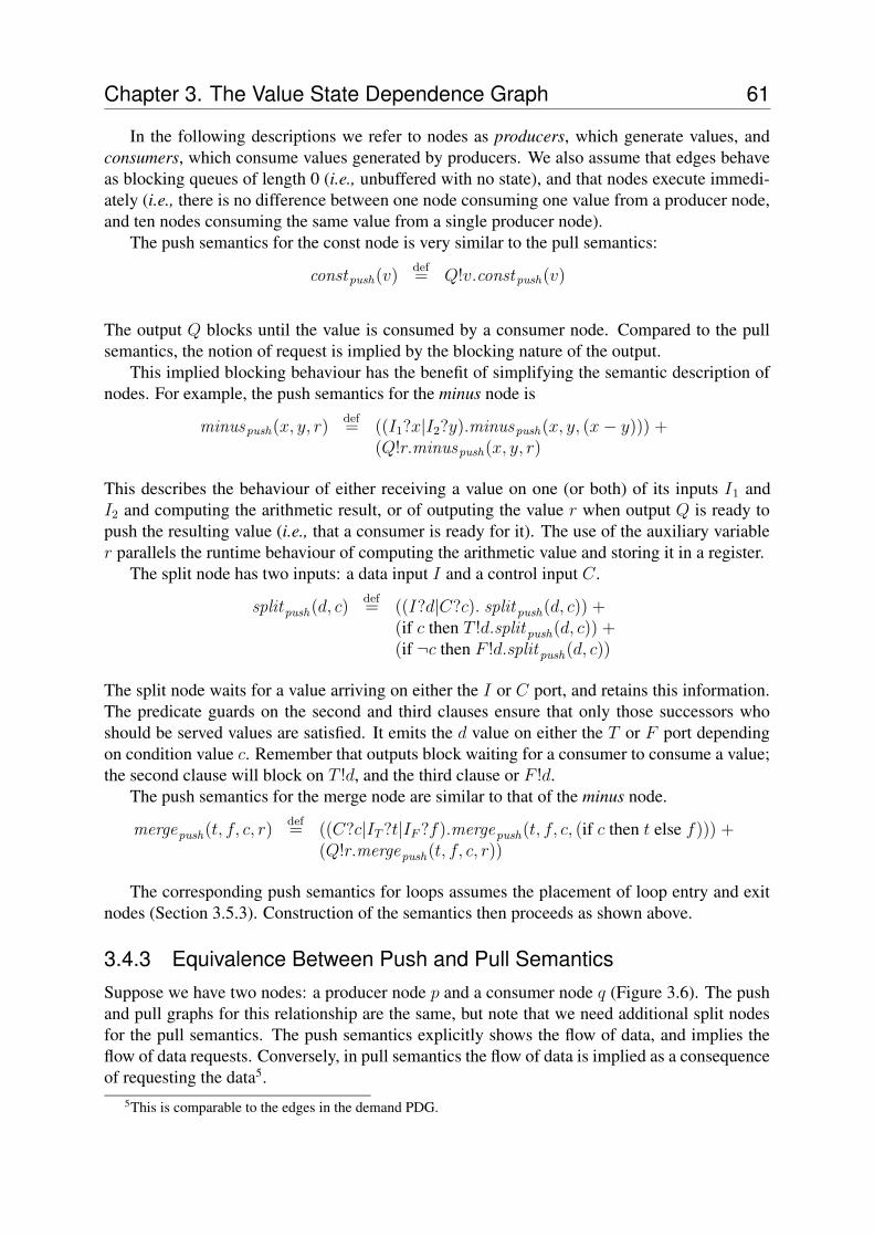
Chapter 3. The Value State Dependence Graph 61
In the following descriptions we refer to nodes as producers, which generate values, andconsumers, which consume values generated by producers. We also assume that edges behaveas blocking queues of length 0 (i.e., unbuffered with no state), and that nodes execute immedi-ately (i.e., there is no difference between one node consuming one value from a producer node,and ten nodes consuming the same value from a single producer node).
The push semantics for the const node is very similar to the pull semantics:
constpush(v)def= Q!v.constpush(v)
The output Q blocks until the value is consumed by a consumer node. Compared to the pullsemantics, the notion of request is implied by the blocking nature of the output.
This implied blocking behaviour has the benefit of simplifying the semantic description ofnodes. For example, the push semantics for the minus node is
minuspush(x, y, r)def= ((I1?x|I2?y).minuspush(x, y, (x− y))) +
(Q!r.minuspush(x, y, r)
This describes the behaviour of either receiving a value on one (or both) of its inputs I1 andI2 and computing the arithmetic result, or of outputing the value r when output Q is ready topush the resulting value (i.e., that a consumer is ready for it). The use of the auxiliary variabler parallels the runtime behaviour of computing the arithmetic value and storing it in a register.
The split node has two inputs: a data input I and a control input C.
splitpush(d, c)def= ((I?d|C?c). splitpush(d, c)) +
(if c then T !d.splitpush(d, c)) +(if ¬c then F !d.splitpush(d, c))
The split node waits for a value arriving on either the I or C port, and retains this information.The predicate guards on the second and third clauses ensure that only those successors whoshould be served values are satisfied. It emits the d value on either the T or F port dependingon condition value c. Remember that outputs block waiting for a consumer to consume a value;the second clause will block on T !d, and the third clause or F !d.
The push semantics for the merge node are similar to that of the minus node.
mergepush(t, f, c, r)def= ((C?c|IT ?t|IF ?f).mergepush(t, f, c, (if c then t else f))) +
(Q!r.mergepush(t, f, c, r))
The corresponding push semantics for loops assumes the placement of loop entry and exitnodes (Section 3.5.3). Construction of the semantics then proceeds as shown above.
3.4.3 Equivalence Between Push and Pull SemanticsSuppose we have two nodes: a producer node p and a consumer node q (Figure 3.6). The pushand pull graphs for this relationship are the same, but note that we need additional split nodesfor the pull semantics. The push semantics explicitly shows the flow of data, and implies theflow of data requests. Conversely, in pull semantics the flow of data is implied as a consequenceof requesting the data5.
5This is comparable to the edges in the demand PDG.
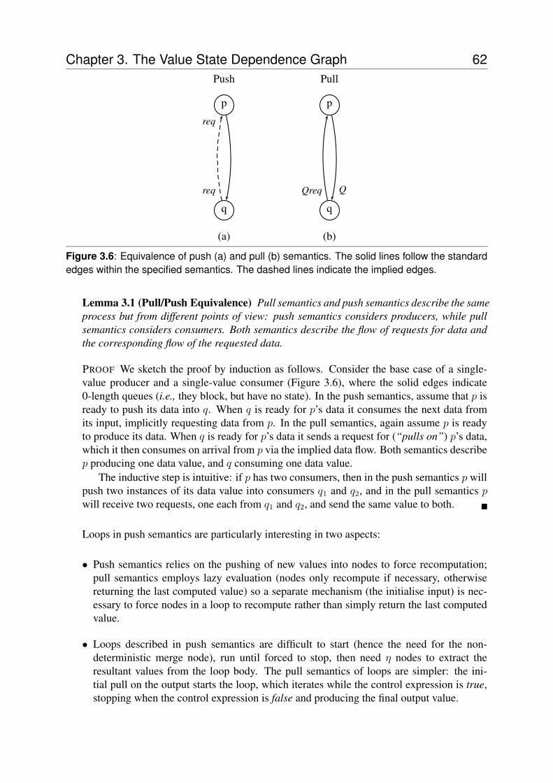
Chapter 3. The Value State Dependence Graph 62
p
q
(a)
Push
req
req
p
q
(b)
Pull
QQreq
Figure 3.6: Equivalence of push (a) and pull (b) semantics. The solid lines follow the standardedges within the specified semantics. The dashed lines indicate the implied edges.
Lemma 3.1 (Pull/Push Equivalence) Pull semantics and push semantics describe the sameprocess but from different points of view: push semantics considers producers, while pullsemantics considers consumers. Both semantics describe the flow of requests for data andthe corresponding flow of the requested data.
PROOF We sketch the proof by induction as follows. Consider the base case of a single-value producer and a single-value consumer (Figure 3.6), where the solid edges indicate0-length queues (i.e., they block, but have no state). In the push semantics, assume that p isready to push its data into q. When q is ready for p’s data it consumes the next data fromits input, implicitly requesting data from p. In the pull semantics, again assume p is readyto produce its data. When q is ready for p’s data it sends a request for (“pulls on”) p’s data,which it then consumes on arrival from p via the implied data flow. Both semantics describep producing one data value, and q consuming one data value.
The inductive step is intuitive: if p has two consumers, then in the push semantics p willpush two instances of its data value into consumers q1 and q2, and in the pull semantics p
will receive two requests, one each from q1 and q2, and send the same value to both. �
Loops in push semantics are particularly interesting in two aspects:
• Push semantics relies on the pushing of new values into nodes to force recomputation;pull semantics employs lazy evaluation (nodes only recompute if necessary, otherwisereturning the last computed value) so a separate mechanism (the initialise input) is nec-essary to force nodes in a loop to recompute rather than simply return the last computedvalue.
• Loops described in push semantics are difficult to start (hence the need for the non-deterministic merge node), run until forced to stop, then need η nodes to extract theresultant values from the loop body. The pull semantics of loops are simpler: the ini-tial pull on the output starts the loop, which iterates while the control expression is true,stopping when the control expression is false and producing the final output value.
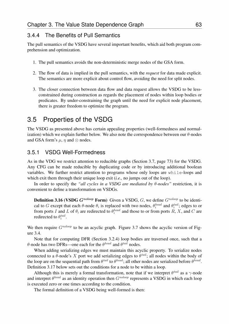
Chapter 3. The Value State Dependence Graph 63
3.4.4 The Benefits of Pull Semantics
The pull semantics of the VSDG have several important benefits, which aid both program com-prehension and optimization.
1. The pull semantics avoids the non-deterministic merge nodes of the GSA form.
2. The flow of data is implied in the pull semantics, with the request for data made explicit.The semantics are more explicit about control flow, avoiding the need for split nodes.
3. The closer connection between data flow and data request allows the VSDG to be less-constrained during construction as regards the placement of nodes within loop bodies orpredicates. By under-constraining the graph until the need for explicit node placement,there is greater freedom to optimize the program.
3.5 Properties of the VSDGThe VSDG as presented above has certain appealing properties (well-formedness and normal-ization) which we explain further below. We also note the correspondence between our θ-nodesand GSA form’s µ, η and ⊗ nodes.
3.5.1 VSDG Well-Formedness
As in the VDG we restrict attention to reducible graphs (Section 3.7, page 73) for the VSDG.Any CFG can be made reducible by duplicating code or by introducing additional booleanvariables. We further restrict attention to programs whose only loops are while-loops andwhich exit them through their unique loop exit (i.e., no jumps out of the loop).
In order to specify the “all cycles in a VSDG are mediated by θ-nodes” restriction, it isconvenient to define a transformation on VSDGs.
Definition 3.16 (VSDG Gnoloop Form) Given a VSDG, G, we define Gnoloop to be identi-cal to G except that each θ-node θi is replaced with two nodes, θhead
i and θtaili ; edges to or
from ports I and L of θi are redirected to θheadi and those to or from ports R, X , and C are
redirected to θtaili .
We then require Gnoloop to be an acyclic graph. Figure 3.7 shows the acyclic version of Fig-ure 3.4.
Note that for computing DFR (Section 3.2.4) loop bodies are traversed once, such that aθ-node has two DFRs—one each for the θhead and θtail nodes.
When adding serializing edges we must maintain this acyclic property. To serialize nodesconnected to a θ-node’s X port we add serializing edges to θtail ; all nodes within the body ofthe loop are on the sequential path from θtail to θhead ; all other nodes are serialized before θhead .Definition 3.17 below sets out the conditions for a node to be within a loop.
Although this is merely a formal transformation, note that if we interpret θtail as a γ-nodeand interpret θhead as an identity operation then Gnoloop represents a VSDG in which each loopis executed zero or one times according to the condition.
The formal definition of a VSDG being well-formed is then:
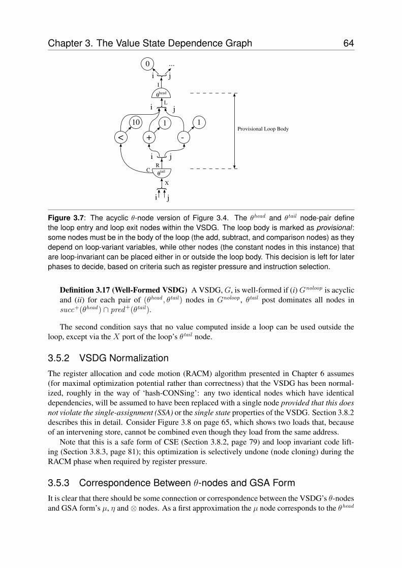
Chapter 3. The Value State Dependence Graph 64
+
I
R
L
1
-
1
X
...
j
0i j
i
i }
}
j
j}
i
θtail
θhead
}
10
<
C
Provisional Loop Body
Figure 3.7: The acyclic θ-node version of Figure 3.4. The θhead and θtail node-pair definethe loop entry and loop exit nodes within the VSDG. The loop body is marked as provisional :some nodes must be in the body of the loop (the add, subtract, and comparison nodes) as theydepend on loop-variant variables, while other nodes (the constant nodes in this instance) thatare loop-invariant can be placed either in or outside the loop body. This decision is left for laterphases to decide, based on criteria such as register pressure and instruction selection.
Definition 3.17 (Well-Formed VSDG) A VSDG, G, is well-formed if (i) Gnoloop is acyclicand (ii) for each pair of (θhead , θtail) nodes in Gnoloop , θtail post dominates all nodes insucc+(θhead) ∩ pred+(θtail).
The second condition says that no value computed inside a loop can be used outside theloop, except via the X port of the loop’s θtail node.
3.5.2 VSDG NormalizationThe register allocation and code motion (RACM) algorithm presented in Chapter 6 assumes(for maximal optimization potential rather than correctness) that the VSDG has been normal-ized, roughly in the way of ‘hash-CONSing’: any two identical nodes which have identicaldependencies, will be assumed to have been replaced with a single node provided that this doesnot violate the single-assignment (SSA) or the single state properties of the VSDG. Section 3.8.2describes this in detail. Consider Figure 3.8 on page 65, which shows two loads that, becauseof an intervening store, cannot be combined even though they load from the same address.
Note that this is a safe form of CSE (Section 3.8.2, page 79) and loop invariant code lift-ing (Section 3.8.3, page 81); this optimization is selectively undone (node cloning) during theRACM phase when required by register pressure.
3.5.3 Correspondence Between θ-nodes and GSA FormIt is clear that there should be some connection or correspondence between the VSDG’s θ-nodesand GSA form’s µ, η and⊗ nodes. As a first approximation the µ node corresponds to the θhead
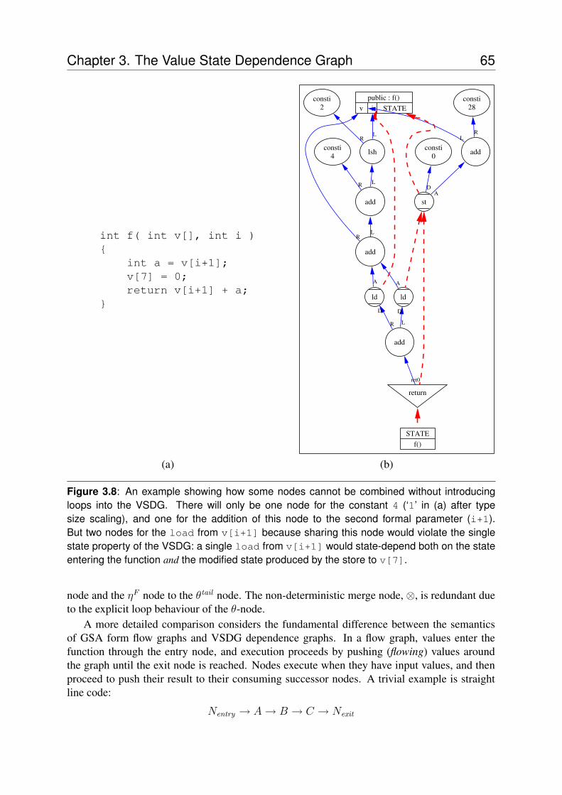
Chapter 3. The Value State Dependence Graph 65
int f( int v[], int i ){
int a = v[i+1];v[7] = 0;return v[i+1] + a;
}
add
ld
A
ld
A
add
R
D
public : f()v i STATE
R
add
L
st
lsh
L
A
consti28
R
return
consti0
D
add
L
consti2
R
L
consti4
R
L
D
ret0
STATEf()
(a) (b)
Figure 3.8: An example showing how some nodes cannot be combined without introducingloops into the VSDG. There will only be one node for the constant 4 (‘1’ in (a) after typesize scaling), and one for the addition of this node to the second formal parameter (i+1).But two nodes for the load from v[i+1] because sharing this node would violate the singlestate property of the VSDG: a single load from v[i+1] would state-depend both on the stateentering the function and the modified state produced by the store to v[7].
node and the ηF node to the θtail node. The non-deterministic merge node, ⊗, is redundant dueto the explicit loop behaviour of the θ-node.
A more detailed comparison considers the fundamental difference between the semanticsof GSA form flow graphs and VSDG dependence graphs. In a flow graph, values enter thefunction through the entry node, and execution proceeds by pushing (flowing) values aroundthe graph until the exit node is reached. Nodes execute when they have input values, and thenproceed to push their result to their consuming successor nodes. A trivial example is straightline code:
Nentry → A→ B → C → Nexit
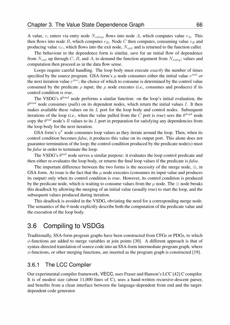
Chapter 3. The Value State Dependence Graph 66
A value, v, enters via entry node Nentry , flows into node A, which computes value vA. Thisthen flows into node B, which computes vB . Node C then computes, consuming value vB andproducing value vC , which flows into the exit node, Nexit and is returned to the function caller.
The behaviour in the dependence form is similar, save for an initial flow of dependencefrom Nexit up through C, B, and A, to demand the function argument from Nentry ; values andcomputation then proceed as in the data flow sense.
Loops require careful handling. The loop body must execute exactly the number of timesspecified by the source program. GSA form’s µ node consumes either the initial value v init orthe next iteration value viter ; the choice of which to consume is determined by the control valueconsumed by the predicate ρ input; the µ node executes (i.e., consumes and produces) if itscontrol condition is true.
The VSDG’s θhead node performs a similar function: on the loop’s initial evaluation, theθhead node consumes (pulls) on its dependent nodes, which return the initial values I . It thenmakes available these values on its L port for the loop body and control nodes. Subsequentiterations of the loop (i.e., when the value pulled from the C port is true) sees the θhead nodecopy the θtail node’s R values to its L port in preparation for satisfying any dependencies fromthe loop body for the next iteration.
GSA form’s ηF node consumes loop values as they iterate around the loop. Then, when itscontrol condition becomes false, it produces this value on its output port. This alone does notguarantee termination of the loop; the control condition produced by the predicate node(s) mustbe false in order to terminate the loop.
The VSDG’s θtail node serves a similar purpose: it evaluates the loop control predicate andthen either re-evaluates the loop body, or returns the final loop values if the predicate is false.
The important difference between the two forms is the necessity of the merge node, ⊗, inGSA form. At issue is the fact that the µ node executes (consumes its input value and producesits output) only when its control condition is true. However, its control condition is producedby the predicate node, which is waiting to consume values from the µ node. The ⊗ node breaksthis deadlock by allowing the merging of an initial value (usually true) to start the loop, and thesubsequent values produced during iteration.
This deadlock is avoided in the VSDG, obviating the need for a corresponding merge node.The semantics of the θ-node explicitly describe both the computation of the predicate value andthe execution of the loop body.
3.6 Compiling to VSDGsTraditionally, SSA-form program graphs have been constructed from CFGs or PDGs, to whichφ-functions are added to merge variables at join points [30]. A different approach is that ofsyntax-directed translation of source code into an SSA-form intermediate program graph, whereφ-functions, or other merging functions, are inserted as the program graph is constructed [19].
3.6.1 The LCC Compiler
Our experimental compiler framework, VECC, uses Fraser and Hanson’s LCC [42] C compiler.It is of modest size (about 11,000 lines of C), uses a hand-written recursive-descent parser,and benefits from a clean interface between the language-dependent front end and the target-dependent code generator.
Chapter 3. The Value State Dependence Graph 67
We replace the intermediate and backend functions of the compiler with functions whichdirectly emit VSDG nodes and edges (Appendix A). At the point in the compiler where thesefunctions are called, all types have been decomposed into suitably aligned byte-addressed vari-ables, and all pointer arithmetic, index scaling, and struct and union address offsets have beengenerated. Target-specific details, such as the sizes of the C data types, are described to thecompiler with a machine description file.
During compilation LCC performs some simple transformations (strength reduction, con-stant folding, etc), some of which are mandated by the language standard (e.g., constant fold-ing). For each statement, LCC generates an abstract syntax tree (AST), recursively descendinginto source-level statement blocks. VSDG nodes and edges are generated directly from the ASTwith the aid of the symbol tables.
Symbols in the compiler are augmented with the current VSDG node name and a stack forstoring VSDG node names, employing a similar approach to that of Brandis and Mossenbock [19].In straight-line code each new assignment of a variable, v, updates the VSDG node name fieldin v’s symbol table entry. Selection constructs use the name stack to save, and later restore, thenames of the VDSG nodes when control paths split and later merge.
Expressions naturally translate into VSDG graphs, and control structures (if, while, etc)generate γ- and θ-nodes. Functions generate special entry and exit nodes, as well as a compiler-defined intrinsic variable STATE , added to the symbol table at the function scope. VSDGnodes which touch the state graph access and/or modify this STATE variable.
3.6.2 VSDG File DescriptionThe compiler reads in a C source file and emits a VSDG file. The VSDG file is a human-readabledescription of the resulting VSDG. The syntax of the VSDG file is given in Appendix A. Thekey points are:
• A VSDG file contains one or more module definitions, each of which contains one ormore data or function definitions. Each source file read by the compiler creates a newVSDG module, whose name is that of the source file. All data and functions within thesource file are emitted into the module, providing module-level name scoping.
• Functions contain data definitions, nodes and edges.
• The name scoping rules follow those of C: names declared at the module scope are visibleonly within that module, unless given the public attribute; names declared within afunction are only visible within that function.
The compiler automatically renames function scope static variables so that they are onlyaccessible from within the enclosing function. For example, a static variable foo in functionbar might be renamed LS 2, and would be defined at the module scope level, correspondingto the C source file scope.
3.6.3 Compiling FunctionsEach C function generates a VSDG function definition. A C function can return at most onevalue, either a scalar (integer, float or pointer) value, or a struct value6; void functions do not
6Most compilers implement functions returning structs using anonymous pointers and/or block copying; a fewarchitectures support returning structs by combining multiple physical registers.
Chapter 3. The Value State Dependence Graph 68
int glbVar;
int foo(int a, int b){
int lclVar;lclVar = glbVar + a + b;return lclVar;
}
module funcvsdg.c {public function foo (a,b), 1 {
node node0 [op=ld,size=-4];node node1 [op=constid,value=_glbVar];edge node0:A -> node1 [type=value];edge node0:__STATE__ -> foo:__STATE__ [type=state];node node2 [op=add];edge node2:L -> node0:D [type=value];edge node2:R -> foo:a [type=value];node node3 [op=add];edge node3:L -> node2 [type=value];edge node3:R -> foo:b [type=value];node node4 [op=return];edge node4:ret1 -> node3 [type=value];edge node4:__STATE__ -> foo:__STATE__ [type=state];edge foo:__STATE__ -> node4 [type=state];
}data _glbVar [size=4];
}
12345678910111213141516171819
Figure 3.9: An example of C function to VSDG function translation. The C function on theleft produces the VSDG description on the right (line numbers added for illustration purposes).A single module is generated from the source file funcvsdg.c. The function foo takes twonamed parameters, a and b, and returns one value. Node node0 (line 3) is a signed wordload. The size parameter indicates both the type size (in this case four bytes) and whether itis a signed (negative value, as in this case) or unsigned (positive value) type. node0 is value-dependent on node1 for its address (lines 4, 5), and state-dependent on the function entrynode (line 6). The first add node, node2 (line 7), is value-dependent on node0’s D-port (line 8)and function parameter a (line 9). The second add node, node3, is similarly value-dependenton nodes node2 and function parameter b (lines 11, 12). Return node node4 (line 13) dependson both the value produced by node3 (line 14), and the initial state of the function (line 15).Finally, the function exits with the final state (line 16). The global variable glbVar is declared inline 18 with a size of four bytes, as specified for our chosen target machine (the ARM Thumb).
return a value, only state. The VSDG function definition includes the names of the arguments,and the number of return values. The argument names are derived from the source names.
During function generation the intrinsic variable, STATE 7, is added to the function’ssymbol table. Additionally, the function exit node state-depends on the final definition of theSTATE variable. An example is shown in Figure 3.9.
The compiler supports the use of registers for the first few function arguments as specified bythe target’s Application Binary Interface (ABI). On entry, the first NUM ARG REGS argumentsare placed in registers; subsequent arguments are placed in special memory cells which are latertranslated into stack offsets by the target code generator.
A special VSDG node, the return node, provides an exit from a function while maintain-ing the consistency of the state graph. It value-depends on the return value of the function, ifany, and also depends on state. It produces a new state, which may be depended on by subse-quent nodes (e.g., the function exit node). Lines 13–16 of Figure 3.9 illustrate this.
Variadic functions require special handling. A variadic function is one which takes one ormore fixed arguments, and zero or more optional arguments. An example of a variadic functionis the standard library function printf, declared as:
7The C standard [22] specifies all names beginning with two underscores are reserved for the implementation.
Chapter 3. The Value State Dependence Graph 69
int printf( char *fmt, ... );
The fixed argument is “fmt”, and the “...” identifies where the optional arguments appear inthe function invocation. The traditional stack model of the C machine pushes arguments right-to-left, thus guaranteeing that the fixed arguments (left-most) are always at a known location onthe stack, and that subsequent arguments can be found by walking the stack.
This leads to two separate issues when compiling C into VSDGs: compiling variadic func-tion invocations, and compiling variadic function definitions. The solution we adopt solves bothproblems. In essence, we compile a variadic function, f V , such that the rightmost fixed and allof its optional arguments are placed in stack memory cells8. This is achieved by setting thenumber of function argument registers for f V to one less than NUM ARG REGS and the numberof fixed arguments.
For example, the printf function has one fixed argument—the format specifier stringfmt. When compiling the function definition, we set the number of register arguments to zero,and generate a suitable function definition. When compiling a call to printf all arguments,including fmt, are placed in stack memory cells. Within the body of the function, references tothe address of fmt will refer to the stack as expected.
3.6.4 Compiling Expressions
Expressions in C produce two results: the algebraic result as expected by the programmer (e.g.,in “x=a+b” the programmer expects x to be assigned the sum of a and b), and side-effects suchas accessing memory or calling functions. It is not safe to consider that operators such as ‘+’or ‘-’ have no side-effects since it is entirely possible that, for a given target, these operationscould be performed by a library function which may raise exceptions. For example, manyembedded processors implement floating point operations as calls to a support library suppliedas part of the compiler.
The VSDG explicitly supports both results of expressions. The algebraic result is expressedas a value dependency, and the side-effect is represented as a state dependency.
Memory accesses, both explicit such as array accesses, and implicit such as accesses toglobal or address-taken variables, depend on state, and in the case of stores and volatile loads,produce a new state. Again, in many cases it is not immediately clear from the source codewhether or not an expression depends on, or modifies, state.
Conditional expressions produce exactly the same VSDG as if-statements (Section 3.6.5).This normalizing effect benefits program analysis by minimizing different program forms. Italso removes artifacts due to differing programming styles, e.g., if a is a local variable then thetwo statements below produce the exact same VSDG:
if ( P )a = 5;
elsea = 6;
a = ( P ) ? 5 : 6;
8The rightmost fixed argument needs to be on the stack so that its address can be computed by the variable-argument access macros va start, va arg and va end [89].
Chapter 3. The Value State Dependence Graph 70
Compiling expressions walks the AST provided by the front end, emitting VSDG nodes andedges during traversal. Nodes which assign to variables (and this includes nodes which modifythe STATE variable) also update the symbol table information for each modified variable,setting the current VSDG node name (Section 3.6.1) to the names of the defining VSDG nodes.
3.6.5 Compiling if StatementsBoth if-statements and conditional expressions are described in the VSDG by γ-nodes (Sec-tion 3.3.1.3). A γ-node has a control (C) value-dependency, and true (T ) and false (F ) depen-dencies, one of which is depended on as determined by the control value.
Side-effect-free if-statements have only value-dependencies; if any predicated expressionor statement block has state-changing nodes (i.e., function calls, stores, or volatile loads) thenthe γ-node will also have state-dependencies on its T and F ports.
Compiling if-statements requires compiling the predicated statements and expressions,with the addition of γ-nodes to merge multiple value- and state-dependencies. Prior approachesto compiling code into SSA-form add the φ-functions after the program graph has been gener-ated, requiring effort in computing the minimal number of φ-functions to add [33].
Single-pass construction of SSA-form is not new. Brandis and Mossenbock [19] insert splitnodes where control flow diverges as repositories for φ-function variable information. Thisinformation is later used to generate φ-functions on exit of loops and conditional statements.
Our approach is different in that the information necessary to generate γ-nodes is maintainedas part of the symbol data within the symbol tables. Each symbol in the compiler’s symbol tablehas a private name stack, onto which VSDG node names are temporarily stored, reflecting the“stack” of lexical scoping expressed in the source code. A simple example helps illustrate theconcepts:
a = ... ; /* node1 */b = ... ; /* node2 */if ( P )
a = 12; /* node3 */else
b = a;print( a, b );
The steps to compile this are as follows:
• On entry to the if for each register variable push the current node name onto its nodename stack (the current node name remains unchanged).
For variable a then a.VSDGnode=node1 and its name stack becomes:
a.stack={node1, ...}.
• On exit of the then block and entry to the else block for each register variable swapthe top of the node name stack with the current node name. This restores the originalvariable node name prior to entry of the else block.
Variable a was changed after the assignment to constant node node3, so after the swapa.VSDGnode=node1 and its name stack becomes:
Chapter 3. The Value State Dependence Graph 71
a.stack={node3, ...}.
• On exit of the else block for each register variable the current VSDG node name iscompared with that on the top of the node name stack. If the names are different, thenadd edges from the gamma node T and F ports to the respective nodes.
In the example, variable a requires a γ-node as a.VSDGnode 6= a.stack[TOP]. Vari-able b was changed in the else block to node1, so that too will require a γ-node. A2-tuple γ-node is emitted, with two true edges γT (a) → node3 and γT (b) → node2for variables a and b respectively, and two false edges γF (a) → node1 and γF (b) →node1.
• Finally, for each register variable pop the old name off the top of the node name stack(undoing the initial push) and set the current VDSG node name to that of the γ-node ifthe two names were different.
To complete the example, after the if-statement a.VSDGnode= γ(a) and b.VSDGnode=γ(b).
This algorithm leads to an efficient implementation. Each register variable requires oneadditional field for the current VSDG node name, and a name stack of depth proportional to theworst-case nesting depth of the program. Empirical evidence [65] suggests that many programshave at most three loop nesting levels9. Applying the same argument to γ-nodes, we can saywith some degree of certainty that for all practical programs, there is a constant increase in theruntime storage and processing requirement per variable.
3.6.6 Compiling LoopsLoops are perhaps the most interesting part of the C language to compile into VSDGs. Theymay never execute, they may execute exactly once, they may execute a number of times, or theymay execute forever. Some variables in loops change (are variant) while others remain constant(invariant). The controlling predicate may be executed before the loop body (for and whileloops) or after (do...while loops).
In addition, loops can restart with continue, or finish early with break. Note that bothmaintain the semantics of loops as they can be synthesized from boolean variables and γ-nodes.For compiling loops to VSDGs two restrictions are enforced. Firstly, that there is exactly oneentry node into the loop; and secondly, that there is exactly one exit node out of the loop. Thesetwo nodes correspond to the two components of the θ-node: θhead and θtail respectively.
During compilation we treat all register variables (i.e., non-address-taken local variables)as live over the entire loop body. Delaying the optimization of loop-invariant edges greatlysimplifies the compiler.
In order to preserve the terminating property of a program, all loops that cannot be deter-mined if they terminate or not10 modify state. Remember that state also describes progress(imagine a clock ticking) so each iteration of the loop by itself modifies state, and thus the stateedge from θtail to θhead must be preserved.
9This famous empirical study analysed approximately 40,000 cards of human-generated FORTRAN programs.As to whether the same results would be found with today’s increasing use of machine-generated source coderemains to be seen.
10Deciding this for the general case is equivalent to solving the halting problem.
Chapter 3. The Value State Dependence Graph 72
For example, consider the following function:
int foo( void ){
int i = 0;while( 1 ) { i++; }return 0;
}
It is trivial in this example to determine that the loop control expression is always true; inthe general case it might not be so easy to determine this. Also note that even if the loop didterminate, the final value of variable i has no effect on the result of the function. By keeping thestate edge in the loop, a dead node elimination pass (Section 3.8.1) will remove the redundantvariable and produce the following, smaller, function:
int foo( void ){
while( 1 ) { /* empty */ }return 0;
}
Note that the return statement also depends on state, as every function returns a (possiblymodified) state.
Two special nodes modify the runtime execution of loops: break and continue. Bothnodes have the exact same value and state dependencies as the θtail node, and produce a newstate11. These nodes indicate early termination (break) or restart (continue) of loops. Dur-ing target code generation they generate jumps to the loop exit and loop entry labels respectively.
The steps to compile a loop are described with the aid of the following example code:
a = 1 ; /* local variable (nodeP) */b = 2 ; /* global variable (nodeQ stores to loc. B) */for ( i = 0; i < 10; ++i ){
a = a + 10; /* nodeR */b = b * 2; /* nodeS */
}print( a, b );
• Before to entry to the loop for each register variable we add an edge from the θhead nodeI-port to the source node.
For the example, the value edge θheadI (a)→ nodeP and the state edge θhead
I ( STATE )→nodeQ are emitted (note that nodeQ is a store node, generating a new state).
11While these nodes do more than simply consume values, treating them as generating a new state maintains theconsistency of the state graph within the loop.
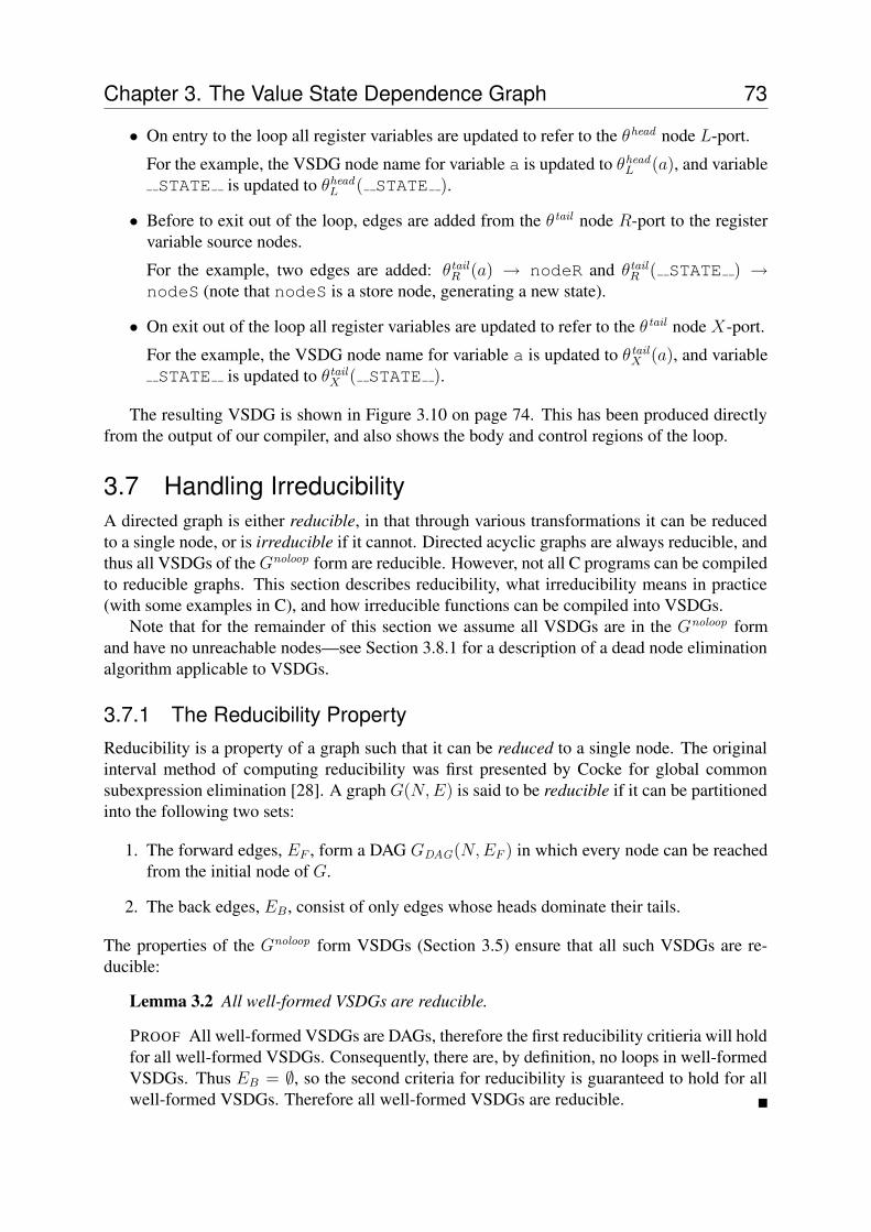
Chapter 3. The Value State Dependence Graph 73
• On entry to the loop all register variables are updated to refer to the θhead node L-port.
For the example, the VSDG node name for variable a is updated to θheadL (a), and variable
STATE is updated to θheadL ( STATE ).
• Before to exit out of the loop, edges are added from the θtail node R-port to the registervariable source nodes.
For the example, two edges are added: θtailR (a) → nodeR and θtail
R ( STATE ) →nodeS (note that nodeS is a store node, generating a new state).
• On exit out of the loop all register variables are updated to refer to the θtail node X-port.
For the example, the VSDG node name for variable a is updated to θtailX (a), and variable
STATE is updated to θtailX ( STATE ).
The resulting VSDG is shown in Figure 3.10 on page 74. This has been produced directlyfrom the output of our compiler, and also shows the body and control regions of the loop.
3.7 Handling IrreducibilityA directed graph is either reducible, in that through various transformations it can be reducedto a single node, or is irreducible if it cannot. Directed acyclic graphs are always reducible, andthus all VSDGs of the Gnoloop form are reducible. However, not all C programs can be compiledto reducible graphs. This section describes reducibility, what irreducibility means in practice(with some examples in C), and how irreducible functions can be compiled into VSDGs.
Note that for the remainder of this section we assume all VSDGs are in the Gnoloop formand have no unreachable nodes—see Section 3.8.1 for a description of a dead node eliminationalgorithm applicable to VSDGs.
3.7.1 The Reducibility PropertyReducibility is a property of a graph such that it can be reduced to a single node. The originalinterval method of computing reducibility was first presented by Cocke for global commonsubexpression elimination [28]. A graph G(N,E) is said to be reducible if it can be partitionedinto the following two sets:
1. The forward edges, EF , form a DAG GDAG(N,EF ) in which every node can be reachedfrom the initial node of G.
2. The back edges, EB , consist of only edges whose heads dominate their tails.
The properties of the Gnoloop form VSDGs (Section 3.5) ensure that all such VSDGs are re-ducible:
Lemma 3.2 All well-formed VSDGs are reducible.
PROOF All well-formed VSDGs are DAGs, therefore the first reducibility critieria will holdfor all well-formed VSDGs. Consequently, there are, by definition, no loops in well-formedVSDGs. Thus EB = ∅, so the second criteria for reducibility is guaranteed to hold for allwell-formed VSDGs. Therefore all well-formed VSDGs are reducible. �
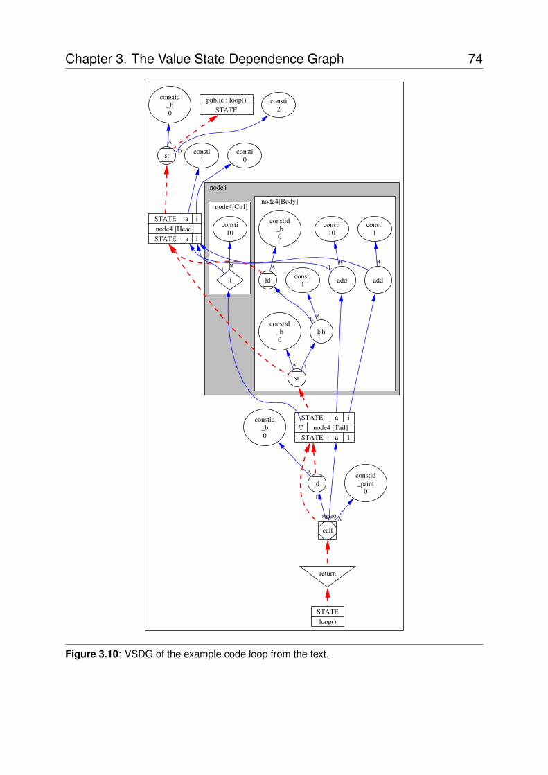
Chapter 3. The Value State Dependence Graph 74
node4
node4[Body]node4[Ctrl]
return
STATEloop()
call
constid_print
0
A
STATE a iC node4 [Tail]STATE a i
arg0
ld
arg1
D
constid_b0
A
st
addadd
consti1
R
STATE a inode4 [Head]STATE a i
LL
ldlt
L
lsh
D
consti1
RL
D
constid_b0
A
constid_b0
A
consti10
R
consti10
R
st consti0
consti1
consti2
D
public : loop()STATE
constid_b0
A
Figure 3.10: VSDG of the example code loop from the text.
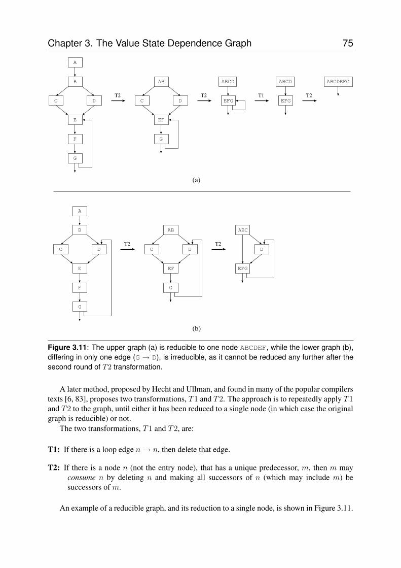
Chapter 3. The Value State Dependence Graph 75
C D
EF
G
AB
T2 T2EFG
ABCD
T1EFG
ABCD
T2
ABCDEFG
(a)
A
C D
E
F
G
B
A
C D
E
F
G
B
T2C D
EF
G
AB
T2D
EFG
ABC
(b)
Figure 3.11: The upper graph (a) is reducible to one node ABCDEF, while the lower graph (b),differing in only one edge (G → D), is irreducible, as it cannot be reduced any further after thesecond round of T2 transformation.
A later method, proposed by Hecht and Ullman, and found in many of the popular compilerstexts [6, 83], proposes two transformations, T1 and T2. The approach is to repeatedly apply T1and T2 to the graph, until either it has been reduced to a single node (in which case the originalgraph is reducible) or not.
The two transformations, T1 and T2, are:
T1: If there is a loop edge n→ n, then delete that edge.
T2: If there is a node n (not the entry node), that has a unique predecessor, m, then m mayconsume n by deleting n and making all successors of n (which may include m) besuccessors of m.
An example of a reducible graph, and its reduction to a single node, is shown in Figure 3.11.
Chapter 3. The Value State Dependence Graph 76
send(to, from, count)register short *to, *from;register count;{
register n=(count+7)/8;switch(count%8){case 0: do{ *to = *from++;case 7: *to = *from++;case 6: *to = *from++;case 5: *to = *from++;case 4: *to = *from++;case 3: *to = *from++;case 2: *to = *from++;case 1: *to = *from++;
}while(--n>0);}
}
Figure 3.12: The original presentation of “Duff’s Device”. The switch is used as a computedgoto, jumping to one of the case labels inside the while loop. This is presented as a portableloop-unrolled block copy, as an alternative to the standard C library memcpy or memmove func-tions. It is clearly irreducible—there are multiple entries into the loop (eight in this case).
3.7.2 Irreducible Programs in the Real WorldInformal experiments of over 22,000 functions indicate that functions with irreducible flowgraphs account for about 0.07% of those functions, most of which appear to be machine-generated code.
One interesting source of irreducibility arises from unstructured, or multiple, jumps (edges)into loops. Such edges add additional predecessor nodes to the arrival node (the loop node atthe tail of the flow edge), thus blocking transformation T2 from consuming the arrival node.
Another source of irreducibility is unreachable nodes. These fail the first property of re-ducibility, in that such nodes are unreachable from the entry node. An unreachable node elimi-nation pass can remove such nodes (Section 3.8.1).
One interesting program structure that is irreducible is Duff’s Device [37], named after TomDuff. His original C source is shown in Figure 3.12. Fortunately such programs are rare. Infact, Duff presents his device with the following observation:
“Many people have said that the worst feature of C is that switches don’t breakautomatically before each case label. This code forms some sort of argument inthat debate, but I’m not sure whether it’s for or against.”
3.7.3 Eliminating IrreducibilitySo, irreducible programs do exist, but are generally quite rare. This leads to two approaches todealing with irreducible graphs.
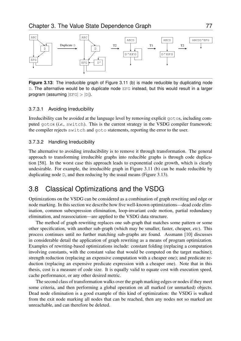
Chapter 3. The Value State Dependence Graph 77
T2D
EFG
ABC ABC
D
D’EFG
T2
D’EFG
ABCD
T1
D’EFG
ABCD
Duplicate D
ABCDD’EFG
Figure 3.13: The irreducible graph of Figure 3.11 (b) is made reducible by duplicating nodeD. The alternative would be to duplicate node EFG instead, but this would result in a largerprogram (assuming |EFG| > |D|).
3.7.3.1 Avoiding Irreducibility
Irreducibility can be avoided at the language level by removing explicit gotos, including com-puted gotos (i.e., switch). This is the current strategy in the VSDG compiler framework:the compiler rejects switch and goto statements, reporting the error to the user.
3.7.3.2 Handling Irreducibility
The alternative to avoiding irreducibility is to remove it through transformation. The generalapproach to transforming irreducible graphs into reducible graphs is through code duplica-tion [58]. In the worst case this approach leads to exponential code growth, which is clearlyundesirable. For example, the irreducible graph in Figure 3.11 (b) can be made reducible byduplicating node D, and then reducing by the usual means (Figure 3.13).
3.8 Classical Optimizations and the VSDGOptimizations on the VSDG can be considered as a combination of graph rewriting and edge ornode marking. In this section we describe how five well-known optimizations—dead code elim-ination, common subexpression elimination, loop-invariant code motion, partial redundancyelimination, and reassociation—are applied to the VSDG data structure.
The method of graph rewriting replaces one sub-graph that matches some pattern or someother specification, with another sub-graph (which may be smaller, faster, cheaper, etc). Thisprocess continues until no further matching sub-graphs are found. Assmann [10] discussesin considerable detail the application of graph rewriting as a means of program optimization.Examples of rewriting-based optimizations include: constant folding (replacing a computationinvolving constants, with the constant value that would be computed on the target machine);strength reduction (replacing an expensive computation with a cheaper one); and predicate re-duction (replacing an expensive predicate expression with a cheaper one). Note that in thisthesis, cost is a measure of code size. It is equally valid to equate cost with execution speed,cache performance, or any other desired metric.
The second class of transformation walks over the graph marking edges or nodes if they meetsome criteria, and then performing a global operation on all marked (or unmarked) objects.Dead node elimination is a good example of this kind of optimization: the VSDG is walkedfrom the exit node marking all nodes that can be reached, then any nodes not so marked areunreachable, and can therefore be deleted.
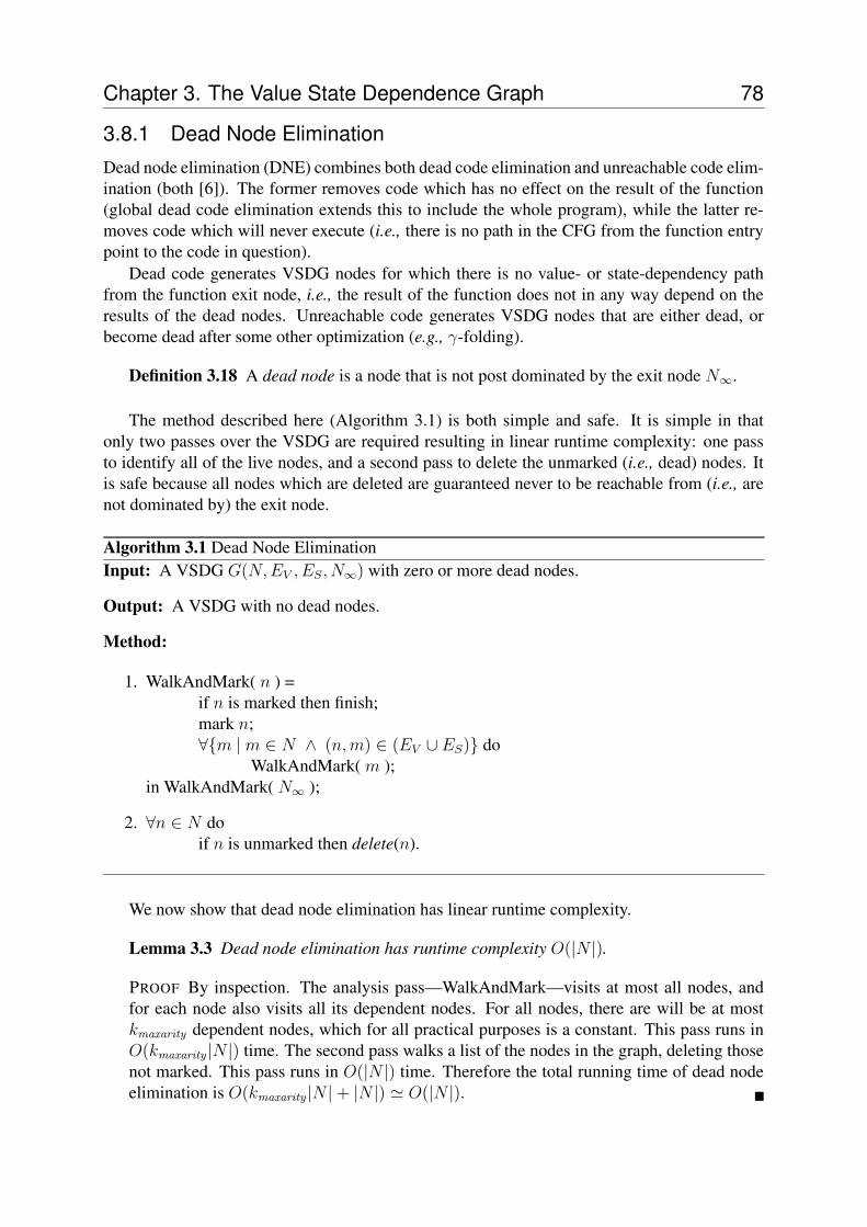
Chapter 3. The Value State Dependence Graph 78
3.8.1 Dead Node EliminationDead node elimination (DNE) combines both dead code elimination and unreachable code elim-ination (both [6]). The former removes code which has no effect on the result of the function(global dead code elimination extends this to include the whole program), while the latter re-moves code which will never execute (i.e., there is no path in the CFG from the function entrypoint to the code in question).
Dead code generates VSDG nodes for which there is no value- or state-dependency pathfrom the function exit node, i.e., the result of the function does not in any way depend on theresults of the dead nodes. Unreachable code generates VSDG nodes that are either dead, orbecome dead after some other optimization (e.g., γ-folding).
Definition 3.18 A dead node is a node that is not post dominated by the exit node N∞.
The method described here (Algorithm 3.1) is both simple and safe. It is simple in thatonly two passes over the VSDG are required resulting in linear runtime complexity: one passto identify all of the live nodes, and a second pass to delete the unmarked (i.e., dead) nodes. Itis safe because all nodes which are deleted are guaranteed never to be reachable from (i.e., arenot dominated by) the exit node.
Algorithm 3.1 Dead Node EliminationInput: A VSDG G(N,EV , ES, N∞) with zero or more dead nodes.
Output: A VSDG with no dead nodes.
Method:
1. WalkAndMark( n ) =if n is marked then finish;mark n;∀{m |m ∈ N ∧ (n,m) ∈ (EV ∪ ES)} do
WalkAndMark( m );in WalkAndMark( N∞ );
2. ∀n ∈ N doif n is unmarked then delete(n).
We now show that dead node elimination has linear runtime complexity.
Lemma 3.3 Dead node elimination has runtime complexity O(|N |).
PROOF By inspection. The analysis pass—WalkAndMark—visits at most all nodes, andfor each node also visits all its dependent nodes. For all nodes, there are will be at mostkmaxarity dependent nodes, which for all practical purposes is a constant. This pass runs inO(kmaxarity |N |) time. The second pass walks a list of the nodes in the graph, deleting thosenot marked. This pass runs in O(|N |) time. Therefore the total running time of dead nodeelimination is O(kmaxarity |N |+ |N |) ' O(|N |). �
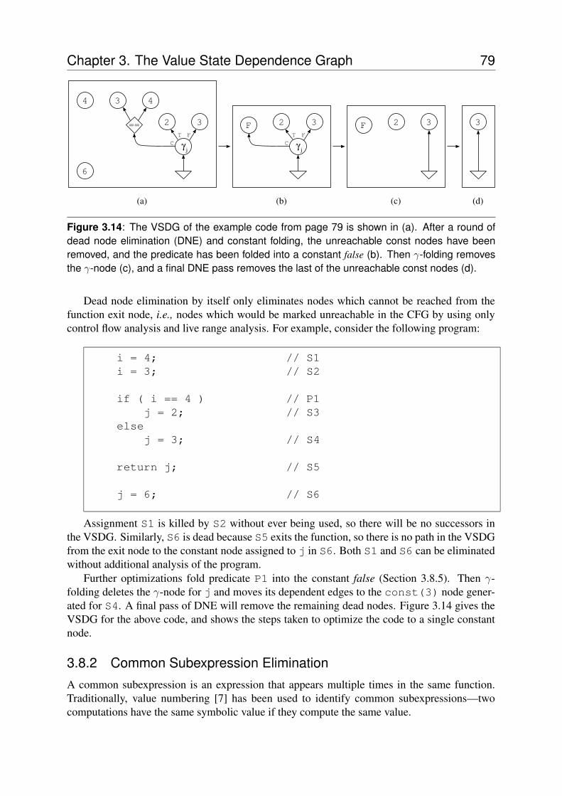
Chapter 3. The Value State Dependence Graph 79
4 3 4
== 2 3
γCT F
F 2 3
γCT F
F 2 3 3
(a) (b) (c) (d)
6
j j
Figure 3.14: The VSDG of the example code from page 79 is shown in (a). After a round ofdead node elimination (DNE) and constant folding, the unreachable const nodes have beenremoved, and the predicate has been folded into a constant false (b). Then γ-folding removesthe γ-node (c), and a final DNE pass removes the last of the unreachable const nodes (d).
Dead node elimination by itself only eliminates nodes which cannot be reached from thefunction exit node, i.e., nodes which would be marked unreachable in the CFG by using onlycontrol flow analysis and live range analysis. For example, consider the following program:
i = 4; // S1i = 3; // S2
if ( i == 4 ) // P1j = 2; // S3
elsej = 3; // S4
return j; // S5
j = 6; // S6
Assignment S1 is killed by S2 without ever being used, so there will be no successors inthe VSDG. Similarly, S6 is dead because S5 exits the function, so there is no path in the VSDGfrom the exit node to the constant node assigned to j in S6. Both S1 and S6 can be eliminatedwithout additional analysis of the program.
Further optimizations fold predicate P1 into the constant false (Section 3.8.5). Then γ-folding deletes the γ-node for j and moves its dependent edges to the const(3) node gener-ated for S4. A final pass of DNE will remove the remaining dead nodes. Figure 3.14 gives theVSDG for the above code, and shows the steps taken to optimize the code to a single constantnode.
3.8.2 Common Subexpression EliminationA common subexpression is an expression that appears multiple times in the same function.Traditionally, value numbering [7] has been used to identify common subexpressions—twocomputations have the same symbolic value if they compute the same value.
Chapter 3. The Value State Dependence Graph 80
Unfortunately value numbering is an expensive process—a symbolic value must be com-puted for each computation, in a manner that guarantees only equivalent computations are as-signed the same value. Only after the value numbering phase can any subsequent optimizationprocess begin. There is also the issue of efficiently maintaining the value numbering duringtransformation.
Algorithm 3.2 aggressively combines all common expressions (nodes) in a VSDG such thattwo nodes p and q are guaranteed to be common (equivalent) if nodes p and q perform the samecomputation, and the (V ∪ S)-predecessors of both nodes are the same. If both conditions aremet then q can be merged into p.
The first criterion is easy to test, based solely on the node operator. The second criterionuses the address of the node data as a unique symbolic value for that node. Additionally, usingthe address of the node as its symbolic value automates the maintenance of the symbolic valuesduring transformation.
While the algorithm is guaranteed to terminate, due to the VSDG being a reducible DAG(Section 3.7), this optimization can be potentially costly to reach a fixed point: combining onecommon subexpression may then make two previously non-matching expressions common,which may make further expressions common, and so on.
Algorithm 3.2 Common Subexpression EliminationInput: A VSDG G(N,EV , ES).
Output: A VSDG with all common subexpressions combined.
Method:
1. Nsort = SORTBYDESCENDINGDFR(N );
2. ∀n ∈ Nsort doNsort = Nsort − n;if n is not marked do
Msort = Nsort ;∀m ∈Msort do
Msort = Msort −m;if n.marked and m.marked and op(n) == op(m) and
pred(n) == pred(m) thenmove all dependency edges from m to n;mark m;
3. ∀n ∈ N doif n is marked then delete(n).
By marking nodes the algorithm does not processes those nodes that will be deleted by thefinal DNE pass. The sorting guarantees that the algorithm moves edges from a later (lowerDFR) node to an earlier (higher DFR) node.
Lemma 3.4 The common subexpression elimination algorithm has runtime complexity ofO(|N |2).
Chapter 3. The Value State Dependence Graph 81
PROOF The complexity of the first stage is O(|N | log |N |). Two loops range over the set ofnodes, giving rise to O(|N |2). We move all edges at most once. In general E ⊆ N × N .But under the condition that all nodes have at most kmaxarity dependence edges, then thisreduces to O(kmaxarity |N |). The final stage is a simplified dead node elimination pass, withrunning time O(|N |). Thus the overall complexity is O(N 2). �
The high runtime cost of this algorithm can, in practice, be reduced by pre-sorting nodes bytheir operation type into sets (e.g., Nadd , Nsub), at a cost of O(|N |). This removes the need totest for operation equality in the above algorithm, and in general reduces the size of the set ofnodes to be optimized. So while it is still an O(|N |2) algorithm, we have significantly reduced|N |.
It would be possible to perform this operation during construction of the VSDG by the com-piler. However, other optimizations (e.g., constant folding or strength reduction) can generatecommon subexpressions, leading to a need for this algorithm.
The algorithm presented above is an aggressive algorithm, combining all common subex-pressions within the function, even when doing so might have a detrimental effect on registerpressure or instruction scheduling. This can be undone (either through node duplication or byspilling) as needed by later phases.
3.8.3 Loop-Invariant Code MotionExpressions that compute the same value on each iteration of a loop are loop invariant and canbe placed outside the loop, computing their value into a register which remains constant overthe loop. Examples of loop-invariant code include address computation and macro-expandedexpressions, and may also be the result of other optimizations on the program.
The VSDG does not explicitly specify the position of loop-invariant expressions, other thanthey are post dominated by the θtail node and not a successor of the θhead node. Later phasescan then choose to place the code in the loop, or move the code outside the loop and place theinvariant value in a (possibly spilled) register.
Definition 3.19 A node n is loop-invariant in a loop θl iff (a) n is post dominated by θtaill ,
and (b) n 6∈ succ(θheadl ).
A loop invariant node, v, is moved out of the loop by adding a value dependency edge fromthe θhead node’s I port to v, and moving all value dependencies previously to v to the θhead
node’s L port. A loop invariant node is placed within the loop by the addition of serializingedges from the invariant node to the θhead node.
3.8.4 Partial Redundancy EliminationA statement is partially redundant if it is redundant on some, but not all, paths of execution fromthat statement to the exit of the function. The original formulation of partial redundancy (busycode motion) is due to Morel and Renvoise [80]. Later work by Knoop et al has refined themethod as lazy code motion [63]. Horspool and Ho formulate partial redundancy eliminationusing a cost-benefit analysis [54], producing significant improvements to loop-intensive flow-graphs, and avoiding unnecessary code motion compared to the original Morel and Renvoiseapproach.
Chapter 3. The Value State Dependence Graph 82
Busy code motion moves computations as far up the program graph as is possible, con-strained only by the position of the definitions of its arguments. This extends the live range(register lifetime) of such computations as far as possible, allowing for reuse later in the pro-gram. Lazy code motion, on the other hand, moves computations to where they achieve thesame result as for busy code motion, but also where the register lifetime is shortest. The advan-tage of this over the former is in the reduced lifetimes of registers, such that registers are keptalive over the optimal range of code.
The VSDG naturally represents lazy code motion: a node is placed only as high as to beabove its highest (greatest DFR) successor node, and no higher. The dependency nature ofthe VSDG ensures that as the graph is transformed during optimization and allocation, suchcomputations are kept precisely where they need to be in relation to their successors, whilemaintaining minimal register lifetimes.
3.8.5 ReassociationReassociation [83, pages 333–343] uses specific algebraic properties—associativity, commu-tativity and distributivity—to simplify expressions. Opportunities for reassociation stem fromthe original source code (e.g., macro expansion), address arithmetic (e.g., array indexing andpointer arithmetic), to side-effects from other optimizations (e.g., constant folding).
Care must be taken in applying reassociation, especially with regards to integer and float-ing point arithmetic. For integer arithmetic, care must be taken with over- or under-flow ofintermediate expressions. Address arithmetic is generally less-sensitive to these problems sinceoverflow makes no difference in address calculations12.
Floating point arithmetic [49] requires care with precision and special values (e.g., NaN ).Farnum [38] suggests that the only safe floating point optimizations are removing unnecessarytype coercions and replacing division by a constant with multiplication by a constant if thereciprocal of the constant can be exactly represented, and the multiplication operator has thesame effects as the division operator it replaces.
3.8.5.1 Algebraic Reassociation
Applying reassociation to the VSDG is most naturally implemented as a graph rewriting system,replacing one expression graph with another, cheaper, graph. Some integer reassociations areapplicable irrespective of target machine arithmetic specifics. Others require special care toensure that the optimized computation produces exactly the same result for all arguments (e.g.,overflow of intermediate results). For example, Muchnick [83] catalogues twenty graph rewriterules for address arithmetic alone.
Other transformations replace expensive operations with cheaper ones (strength reduction).For example, multiplication is slow on many embedded processors. Quite often, multiplicationby a constant can be replaced by a number of shifts and additions from expansion of the binaryseries of the n-bit multiplicand:
x× y = 2n−1xyn−1 + 2n−2xyn−2 + . . . + 21xy1 + 20xy0
where ym ∈ {0, 1}. For example, the right-hand expression in
b = a * 512Although some processors are sensitive to bad address formation.
Chapter 3. The Value State Dependence Graph 83
noting that 510 = 01012, can be transformed into
b = a << 2 + a
Booth’s algorithm (most commonly used to simplify hardware multipliers) can also be ap-plied, noting that
2m + 2m−1 + . . . + 2n+1 + 2n = 2m+1 − 2n.
For example, the expression “a * 14” (1410 = 011102, giving m = 3 and n = 1) can bereplaced with a faster expression involving two shifts and a subtraction:
b = (a << 4) - (a << 1)
As a concrete example for the Thumb processor, consider the expression “a * 1025”. TheThumb has a single register-to-register multiplication operation, and additionally can only move8-bit constants into registers (larger constants are either generated in one or two instructions, orloaded from a literal pool). A direct compilation of this expression would yield a load from theliteral pool and a multiply, with a total size of 64 bits.
However, this expression can be rewritten as “(a<<10)+a”, which can be compiled intojust two instructions—a left shift, and an add—occupying only 32 bits of code space.
3.8.6 Constant FoldingConstant folding computes constant expressions at compile time rather than at runtime. Theoptimizer must ensure that the computed constant is that which would be computed by thetarget processor, and not that computed by the compiler’s host processor (e.g., “100 + 200”on an 8-bit microcontroller would compute 44, while the compiler running on a 32-bit desktopprocessor would compute 300). This is especially important for intermediate values within morecomplex expressions.
A variant of constant folding is predicate folding. This is applied to predicate expressions,where the result is either true or false. Some predicate folds derive from the identity functions,while others must be computed within the optimizer. For example
a ∨ true = a ∨ ¬a = true
a ∧ false = a ∧ ¬a = false
Note that in the case that a modifies state (e.g., a volatile load), then while we can eliminatethe value dependencies on a we must maintain the state dependencies.
3.8.7 γ FoldingFor γ-nodes whose predicates have been simplified to a constant true or false, the γ-node can beeliminated, and its successor edges moved to either the T -predecessors or the F -predecessorsas appropriate. A subsequent DNE pass over the VSDG will then remove any dead nodes in theunused γ-region.
This is equivalent to branch folding on the CFG, since it replaces the conditional branchesof an if/then/else with a jump to the appropriate label.t

Chapter 3. The Value State Dependence Graph 84
3.9 SummaryThis chapter has introduced the Value State Dependence Graph (VSDG). It has shown thatthe VSDG exhibits many useful properties, particularly for program optimization. The VSDGrepresents the same information as the PDG but with fewer edges types (five or six for thePDG versus two for the VSDG), and the VSDG is more normalising, in that more programsmap to the same VSDG than to the same PDG—in the PDG the assignment “x:=a+b+c”would be represented as a single node, and thus if we wish to exploit the subexpression “a+b”we must transform the PDG, inserting a temporary variable, etc Whereas the VSDG employsa three-address-like form that has the benefit of breaking up large expressions into a tree ofsubexpressions, making them available for later CSE passes.
It has also been shown how to construct the VSDG from a fast and efficient syntax-directedtranslation of a subset of C, together with guidance on the parts of the language that are not sotrivial to compile into VSDGs (most notably irreducible programs).
A number of well-known classical optimizations have been shown to be applicable to theVSDG, demonstrating the elegance of the VSDG in both describing and implementing powerfuloptimizations.
The VSDG is particularly effective in expressing loops, with θ-nodes encapsulating thecyclic nature of loops. Loop invariants are naturally represented: in the VSDG they are neither“in” nor “out of” the loop in the traditional sense of the PDG: they are undefined until allocation,which decides on a node-by-node basis if it should be in or out of the loop.
While the data dependencies of the DDG can be modelled in the VSDG, the VSDG’s θ-nodeencapsulates cyclic behaviour, rather than explicit general cycles of the CFG.
CHAPTER 4
Procedural Abstraction via Patterns
When truth is nothing but the truth, it’s unnatural,it’s an abstraction that resembles nothing in the real world.
In nature there are always so many other irrelevant thingsmixed up with the essential truth.
ALDOUS HUXLEY (1894–1963)
Compiling source code into VSDG intermediate code has an effect of normalizing differentsource structures into similar VSDGs. One result of this normalizing effect is to pro-
duce multiple occurrences of a relatively small number of common code patterns. Proceduralabstraction replaces these multiple occurrences of common code patterns with calls to new,compiler-generated, functions containing just single copies of the code patterns. Clearly, themore occurrences of a pattern are found, the greater the benefit achieved from abstraction.
Procedural abstraction can be applied at the source level, at the target code level, and atthe intermediate levels within the compiler. In this chapter we apply procedural abstraction atthe VSDG intermediate level. This has the advantage of avoiding many of the variations andirrelevant information present in source code—differing variable names, schematically differentcode structures—and in target code—differing register assignments and instruction schedules.
Illustrative Example
To illustrate how the VSDG aids procedural abstraction, consider Figure 4.1. The two functionsfoo and bar perform similar computations: multiplying or left-shifting the second argumentby five depending on the value of the first parameter. In foo the scaled value is then added tothe first parameter, and the result passed back to the caller. The behaviour of bar is similar,except it subtracts the scaled value rather than adding it.
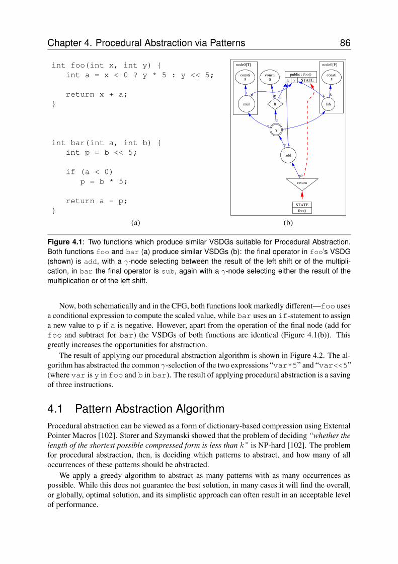
Chapter 4. Procedural Abstraction via Patterns 86
int foo(int x, int y) {int a = x < 0 ? y * 5 : y << 5;
return x + a;}
int bar(int a, int b) {int p = b << 5;
if (a < 0)p = b * 5;
return a - p;}
node0[T] node0[F]
public : foo()x y STATE
lt
L
mul
R
lsh
L
add
L
return
γ
C
consti0
R
R
consti5
L
TF
consti5
R
ret0
STATEfoo()
(a) (b)
Figure 4.1: Two functions which produce similar VSDGs suitable for Procedural Abstraction.Both functions foo and bar (a) produce similar VSDGs (b): the final operator in foo’s VSDG(shown) is add, with a γ-node selecting between the result of the left shift or of the multipli-cation, in bar the final operator is sub, again with a γ-node selecting either the result of themultiplication or of the left shift.
Now, both schematically and in the CFG, both functions look markedly different—foo usesa conditional expression to compute the scaled value, while bar uses an if-statement to assigna new value to p if a is negative. However, apart from the operation of the final node (add forfoo and subtract for bar) the VSDGs of both functions are identical (Figure 4.1(b)). Thisgreatly increases the opportunities for abstraction.
The result of applying our procedural abstraction algorithm is shown in Figure 4.2. The al-gorithm has abstracted the common γ-selection of the two expressions “var*5” and “var<<5”(where var is y in foo and b in bar). The result of applying procedural abstraction is a savingof three instructions.
4.1 Pattern Abstraction AlgorithmProcedural abstraction can be viewed as a form of dictionary-based compression using ExternalPointer Macros [102]. Storer and Szymanski showed that the problem of deciding “whether thelength of the shortest possible compressed form is less than k” is NP-hard [102]. The problemfor procedural abstraction, then, is deciding which patterns to abstract, and how many of alloccurrences of these patterns should be abstracted.
We apply a greedy algorithm to abstract as many patterns with as many occurrences aspossible. While this does not guarantee the best solution, in many cases it will find the overall,or globally, optimal solution, and its simplistic approach can often result in an acceptable levelof performance.
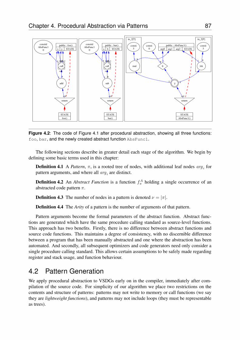
Chapter 4. Procedural Abstraction via Patterns 87
tn_2[T] tn_2[F]
return
STATEfoo()
public : foo()x y STATE
add
L
call
arg0arg1arg2
ret0
R
ret0
constidAbsFunc1
0
A
return
STATEbar()
public : bar()a b STATE
sub
L
call
arg0arg1arg2
ret0
R
ret0
constidAbsFunc1
0
A
γ
return
ret0
STATEAbsFunc1()
lt
C
public : AbsFunc1()arg0 arg1 arg2 STATE
L
mul
R
lsh
L
consti0
R
T
consti5
L
F
consti5
R
Figure 4.2: The code of Figure 4.1 after procedural abstraction, showing all three functions:foo, bar, and the newly created abstract function AbsFunc1.
The following sections describe in greater detail each stage of the algorithm. We begin bydefining some basic terms used in this chapter:
Definition 4.1 A Pattern, π, is a rooted tree of nodes, with additional leaf nodes arg i forpattern arguments, and where all arg i are distinct.
Definition 4.2 An Abstract Function is a function fAπ holding a single occurrence of an
abstracted code pattern π.
Definition 4.3 The number of nodes in a pattern is denoted ν = |π|.
Definition 4.4 The Arity of a pattern is the number of arguments of that pattern.
Pattern arguments become the formal parameters of the abstract function. Abstract func-tions are generated which have the same procedure calling standard as source-level functions.This approach has two benefits. Firstly, there is no difference between abstract functions andsource code functions. This maintains a degree of consistency, with no discernible differencebetween a program that has been manually abstracted and one where the abstraction has beenautomated. And secondly, all subsequent optimizers and code generators need only consider asingle procedure calling standard. This allows certain assumptions to be safely made regardingregister and stack usage, and function behaviour.
4.2 Pattern GenerationWe apply procedural abstraction to VSDGs early on in the compiler, immediately after com-pilation of the source code. For simplicity of our algorithm we place two restrictions on thecontents and structure of patterns: patterns may not write to memory or call functions (we saythey are lightweight functions), and patterns may not include loops (they must be representableas trees).
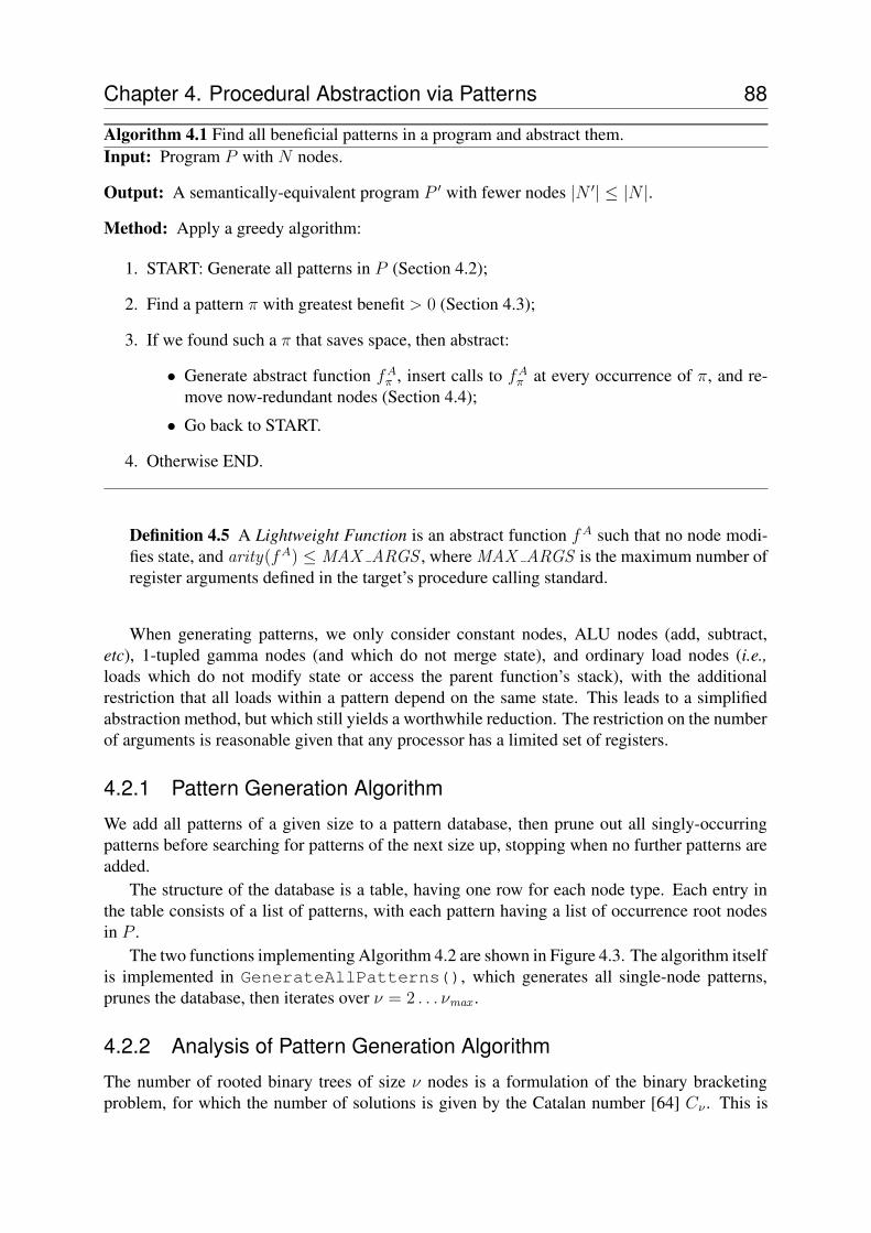
Chapter 4. Procedural Abstraction via Patterns 88
Algorithm 4.1 Find all beneficial patterns in a program and abstract them.Input: Program P with N nodes.
Output: A semantically-equivalent program P ′ with fewer nodes |N ′| ≤ |N |.
Method: Apply a greedy algorithm:
1. START: Generate all patterns in P (Section 4.2);
2. Find a pattern π with greatest benefit > 0 (Section 4.3);
3. If we found such a π that saves space, then abstract:
• Generate abstract function fAπ , insert calls to fA
π at every occurrence of π, and re-move now-redundant nodes (Section 4.4);
• Go back to START.
4. Otherwise END.
Definition 4.5 A Lightweight Function is an abstract function f A such that no node modi-fies state, and arity(fA) ≤ MAX ARGS , where MAX ARGS is the maximum number ofregister arguments defined in the target’s procedure calling standard.
When generating patterns, we only consider constant nodes, ALU nodes (add, subtract,etc), 1-tupled gamma nodes (and which do not merge state), and ordinary load nodes (i.e.,loads which do not modify state or access the parent function’s stack), with the additionalrestriction that all loads within a pattern depend on the same state. This leads to a simplifiedabstraction method, but which still yields a worthwhile reduction. The restriction on the numberof arguments is reasonable given that any processor has a limited set of registers.
4.2.1 Pattern Generation Algorithm
We add all patterns of a given size to a pattern database, then prune out all singly-occurringpatterns before searching for patterns of the next size up, stopping when no further patterns areadded.
The structure of the database is a table, having one row for each node type. Each entry inthe table consists of a list of patterns, with each pattern having a list of occurrence root nodesin P .
The two functions implementing Algorithm 4.2 are shown in Figure 4.3. The algorithm itselfis implemented in GenerateAllPatterns(), which generates all single-node patterns,prunes the database, then iterates over ν = 2 . . . νmax .
4.2.2 Analysis of Pattern Generation Algorithm
The number of rooted binary trees of size ν nodes is a formulation of the binary bracketingproblem, for which the number of solutions is given by the Catalan number [64] Cν . This is
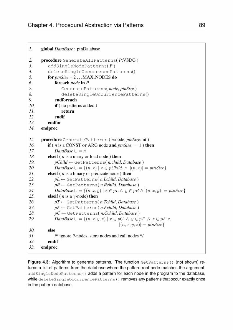
Chapter 4. Procedural Abstraction via Patterns 89
1. global DataBase : ptnDatabase
2. procedure GenerateAllPatterns( P:VSDG )3. addSingleNodePatterns( P )4. deleteSingleOccurrencePatterns()5. for ptnSize = 2 . . . MAX NODES do6. foreach node in P7. GeneratePatterns( node, ptnSize )8. deleteSingleOccurrencePatterns()9. endforeach10. if ( no patterns added )11. return12. endif13. endfor14. endproc
15. procedure GeneratePatterns ( n:node, ptnSize:int )16. if ( n is a CONST or ARG node and ptnSize == 1 ) then17. DataBase ∪ = n18. elseif ( n is a unary or load node ) then19. pChild← GetPatterns( n.child, Database )20. DataBase ∪ = {(n, x) | x ∈ pChild ∧ |(n, x)| = ptnSize}21. elseif ( n is a binary or predicate node ) then22. pL← GetPatterns( n.Lchild, Database )23. pR← GetPatterns( n.Rchild, Database )24. DataBase ∪ = {(n, x, y) | x ∈ pL ∧ y ∈ pR ∧ |(n, x, y)| = ptnSize}25. elseif ( n is a γ-node) then26. pT← GetPatterns( n.Tchild, Database )27. pF← GetPatterns( n.Fchild, Database )28. pC← GetPatterns( n.Cchild, Database )29. DataBase ∪ = {(n, x, y, z) | x ∈ pC ∧ y ∈ pT ∧ z ∈ pF ∧
|(n, x, y, z)| = ptnSize}30. else31. /* ignore θ-nodes, store nodes and call nodes */32. endif33. endproc
Figure 4.3: Algorithm to generate patterns. The function GetPatterns() (not shown) re-turns a list of patterns from the database where the pattern root node matches the argument.addSingleNodePatterns() adds a pattern for each node in the program to the database,while deleteSingleOccurrencePatterns() removes any patterns that occur exactly oncein the pattern database.
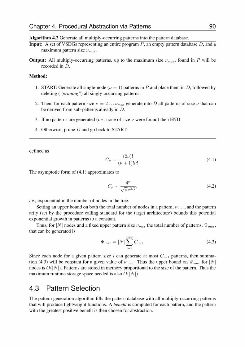
Chapter 4. Procedural Abstraction via Patterns 90
Algorithm 4.2 Generate all multiply-occurring patterns into the pattern database.Input: A set of VSDGs representing an entire program P , an empty pattern database D, and a
maximum pattern size νmax .
Output: All multiply-occurring patterns, up to the maximum size νmax , found in P will berecorded in D.
Method:
1. START: Generate all single-node (ν = 1) patterns in P and place them in D, followed bydeleting (“pruning”) all singly-occurring patterns.
2. Then, for each pattern size ν = 2 . . . νmax generate into D all patterns of size ν that canbe derived from sub-patterns already in D.
3. If no patterns are generated (i.e., none of size ν were found) then END.
4. Otherwise, prune D and go back to START.
defined as
Cν ≡(2ν)!
(ν + 1)!ν!. (4.1)
The asymptotic form of (4.1) approximates to
Cν ∼4ν
√πν3/2
, (4.2)
i.e., exponential in the number of nodes in the tree.Setting an upper bound on both the total number of nodes in a pattern, νmax , and the pattern
arity (set by the procedure calling standard for the target architecture) bounds this potentialexponential growth in patterns to a constant.
Thus, for |N | nodes and a fixed upper pattern size νmax the total number of patterns, Ψmax ,that can be generated is
Ψmax = |N |νmax∑
i=2
Ci−1. (4.3)
Since each node for a given pattern size i can generate at most Ci−1 patterns, then summa-tion (4.3) will be constant for a given value of νmax . Thus the upper bound on Ψmax for |N |nodes is O(|N |). Patterns are stored in memory proportional to the size of the pattern. Thus themaximum runtime storage space needed is also O(|N |).
4.3 Pattern SelectionThe pattern generation algorithm fills the pattern database with all multiply-occurring patternsthat will produce lightweight functions. A benefit is computed for each pattern, and the patternwith the greatest positive benefit is then chosen for abstraction.
Chapter 4. Procedural Abstraction via Patterns 91
4.3.1 Pattern Cost ModelOur model considers the following parameters:
Number of Occurrences For a given pattern, determines both the cost (each occurrence willinsert a call node into the parent function) and benefit (abstraction removes all occurrencesof the pattern from the program, and inserts a new occurrence of the pattern into theabstract function).
Pattern Size This directly affects the number of nodes saved (together with the number ofoccurrences) but must also offset the costs of call nodes and the abstract function returnnode.
During pattern selection, we apply the following cost function to compute the benefit, βπ,for pattern π:
βπ = Gain − Loss (4.4)where Gain = (nπ − 1)νπ
Loss = nπ + 1
and where nπ is the number of occurrences of pattern π, and νπ is the number of nodes in π.The Gain term describes the number of nodes that are removed from the program: for nπ
occurrences, we delete nπνπ nodes, but add νπ nodes into the newly-created abstract function.The Loss term accounts for nπ call nodes inserted into the program, and for the additional returnnode appended to the abstract function.
Rearranging (4.4) as an inequality to say if it is worth abstracting a pattern (i.e., βπ > 0)gives
(nπ − 1)(νπ − 1) > 2. (4.5)
The least benefit is from either a four-node pattern appearing twice, or a two-node patternappearing four times in the program. The example in Figure 4.2 (page 87) has nπ = 2 andνπ = 7, giving a benefit of 4, i.e., it is worth doing the abstraction.
4.3.2 Observations on the Cost ModelThere are several issues that we have avoided in our simplistic cost model.
Foremost is the potential cost of additional spill code that may be generated in the parentfunctions. This is a difficult figure to quantify: on the one hand the additional abstract functioncalls will increase pressure on the variable (non-scratch) registers, with a potential increase inspilling; on the other hand, the resulting simplification of the parent functions can reduce theregister pressure1.
Another issue is the runtime penalty. In straight-line code this is minimal, as the abstractcall will be made at most once. However, where the abstracted code is inside a loop then theadditional processing time of the call is likely to be significant. However, because we onlygenerate lightweight abstract functions, this cost is minimised, and in the best case the penaltyis the cost of the call and the return.
1A first approximation might be to consider that half the abstract function arguments will need register spillingor copying.
Chapter 4. Procedural Abstraction via Patterns 92
Finally, our cost model is based on intermediate code size, not target code size. While thishas the benefits of platform-independence and of working on the intermediate levels within thecompiler, the cost model does suffer from loss of precision due to the abstract nature of theintermediate code.
Our main interest is embedded systems, where code size is the dominant factor. We con-sider these (potential) runtime penalties to be worth the significant savings achieved throughprocedural abstraction.
4.3.3 Overlapping PatternsMaximum benefit from procedural abstraction is obtained when for any two pattern occurrencesπm and πn there are no common nodes (i.e., πm ∩ πn = ∅).
The problem of deciding which of a number of overlapping pattern occurrences to abstract isNP-Complete in the number of clashing pattern occurrences. It can be formulated as finding theminimum weighted path of a graph where nodes correspond to pattern occurrences, and there isan edge (πm, πn) in the graph if patterns πm and πn overlap, and where the weight of the edge= |πm ∩ πn|. Pattern occurrences that do not overlap with any other pattern occurrences can beabstracted without further consideration.
In practice we have found that, even though we do suffer some clashes, the overall effect istolerable—in the worst-case we replace the root node with a call to the abstract function, at acost of one call node in place of the original root node.
4.4 Abstracting the Chosen PatternHaving chosen the pattern that is to be abstracted, the final stage is to perform the actual ab-straction process.
4.4.1 Generating the Abstract FunctionWe have as input a tree pattern from which we generate a new function. The function is placedinto a new module (“ AbstractLib ”) created specifically to hold the abstract functions.
Because only lightweight functions (Section 4.2) are abstracted the upper limit on the num-ber of function arguments is set by the chosen target’s procedure calling standard. The functionbody is then generated from the tree pattern, with VSDG nodes and edges emitted as necessary.
4.4.2 Generating Abstract Function CallsFor each occurrence of the abstraction pattern we add a new call node. Value dependencyedges are inserted from the call node to the corresponding V-predecessors of the pattern occur-rence. If the abstract function contains one or more load nodes then a state-dependency edge isadded from the call node to the S-predecessor of the load node(s) being abstracted. All value-dependency edges from the occurrence’s root node V-successors are then moved to the call node,resulting in at least the occurrence root node becoming dead, and all nodes post-dominated bythe root node.
Finally, a dead node elimination pass will remove at least the pattern occurrence root node,and any other nodes that become unreachable. For example, consider Figure 4.1(b): after in-serting the call to the abstract function and moving the edge from the output of the γ-node to
Chapter 4. Procedural Abstraction via Patterns 93
the output of the call node, both the γ-node and every node post-dominated by the γ-node arenow dead and can be removed from the graph.
4.5 SummaryProcedural abstraction has been the subject of research for many years. However, it is only in re-cent times that it is being implemented in production compilers, either as part of the compilationprocess itself, or as a post-compilation pass.
The approach we have taken to procedural abstraction achieves a reduction of around 18%(Chapter 7). This compares favourably with prior research, e.g., aiPop [3], Squeeze++ [35]and Liao’s work [74].
Though we take a simplified view of program analysis (we do not abstract loops, functioncalls or memory store operations) we attribute this result to applying procedural abstractionat a higher level within the compiler chain, and in particular the VSDG. This has the benefitof removing many of the variations between regions of code, allowing potentially many moreopportunities for abstraction.
Adding support for the remaining operations could increase the effectiveness of the algo-rithm. All three remaining VSDG nodes place artificial boundaries on the size of patterns thatcan be abstracted. Supporting function calls in abstract patterns would increase the potentialcost of abstraction, due to additional instructions to save and restore the callee-preserved regis-ters, and a greater potential for introducing spill code within abstract functions due to increasedregister pressure in the presence of call nodes.
Supporting θ-nodes in patterns would also remove an artificial boundary to abstract patterns.However, abstracting loops is an all-or-nothing transformation: we either abstract the entireloop body and enclosing θ-node, or just (a part of) the loop body: we could not abstract a θhead
node without its matching θtail node, nor a loop without its control predicate.As well as reducing code size, lightweight procedural abstraction is also a suitable tool for
instruction set exploration, where we consider abstract functions as potential candidates for newinstructions. In this context, we gain execution speed since we no longer suffer the penalty of afunction call and execution of multiple instructions.
The potential number of patterns that can be generated from intermediate code is huge,with a corresponding runtime cost during pattern generation. Our pattern generation algorithm,coupled with aggressive database pruning during the pattern generation phase, and hard limitson the dimensions of patterns, keeps this potentially prohibitive cost in check.
Chapter 4. Procedural Abstraction via Patterns 94
CHAPTER 5
Multiple Memory Access Optimization
As memory may be a paradisefrom which we cannot be driven,
it may also be a hellfrom which we cannot escape.
JOHN LANCASTER SPALDING (1840–1916)
Memory is a blessing and a curse. It allows a processor with limited internal memory (i.e.,registers) to handle large data sets, but the additional instructions that access the memory
increase the code size by a considerable amount. One potentially profitable route to reducingcode size, for processors that support them, is through the effective use of Multiple MemoryAccess (MMA) instructions. These combine several loads or stores into a single instruction,where a set of registers (typically defined by some range or bitmap representation) are loadedfrom, or stored to, successive words in memory. Their compactness comes from expressing aset of registers with only a few instruction-word bits; for example, the ARM LDM instructionuses only sixteen bits to encode up to sixteen register loads in a single 32 bit instruction (cf. 512bits without the use of the LDM instruction).
This chapter begins with a review of an algorithm with properties appealing to MMA op-timization: Liao et al’s SOLVESOA algorithm. We then describe the SOLVEMMA algorithm,which identifies profitable memory access sequences for combining into MMA instructions,and selects stack frame layouts that facilitate multiple reads and writes of local variables. Inter-estingly, it turns out that array accesses and local variable accesses are best treated separately.
We describe SOLVEMMA as applied to the Control Flow Graph, and then show how theless-constrained VSDG provides greater opportunities for merging multiple load and store in-structions. Finally, we specialize the algorithm to the Thumb processor.
Chapter 5. Multiple Memory Access Optimization 96
5.1 Examples of MMA InstructionsThe Thumb processor [97] executes a compact version of the ARM instruction set. A hardwaretranslator expands, at runtime, the 16-bit Thumb instructions into 32-bit ARM instructions (asimilar approach is taken in the MIPS16 embedded processor [62]). A disadvantage of this ap-proach is that fewer instruction bits are available to specify registers. This restriction artificiallystarves the register allocator, resulting in more register spill code (providing more potentialsources of MMA optimization, which is poorly done in existing compilers).
The load-store nature of a RISC architecture also gives rise to many explicit memory accessinstructions. In contrast, a CISC machine with memory-access-with-operation instructions canachieve better code size by combining a load or store operation (especially where the addressoffset is small) with an arithmetic operation (e.g., “add EAX,ESI[EBX*4]+Offset” onthe Intel x86 [1]). Restricting the number of accessible registers, as described above, increasesthe number of memory access instructions: by way of example, the adpcm benchmark from Me-diaBench [68] generates approximately 35% more memory access instructions for the Thumbthan for the ARM.
However, the state of the art in commercial compilers appears1 to be based on opportunis-tic peephole-style optimization. The GCC compiler also takes an ad-hoc approach to MMAoptimization2.
5.2 Simple Offset AssignmentLiao et al’s Simple Offset Assignment (SOA) algorithm [72] rearranges local variables withina function’s stack frame in order to minimize address computations. It was originally for-mulated for a single address register Digital Signal Processor (DSP) with word-oriented auto-increment/decrement addressing modes. While not directly solving the MMA optimizationproblem, it forms the starting point of our approach, and so deserves explanation as a founda-tion for this chapter.
The input to the algorithm is an instruction-scheduled and register-allocated program, i.e.,a Control Flow Graph, with a fixed memory access sequence. The SOLVESOA algorithm con-structs an Access Graph (V,E), an undirected graph with vertices V and edges E, where ver-tices correspond to variables, and there is an edge e = (p, q) between vertices p and q withweight w(e) if there are w(e) adjacent accesses to variables p and q. The algorithm then coversthe Access Graph with one or more maximally-weighted disjoint paths.
A covering of a graph is a subset of its edges, and where a path is an alternating sequenceof vertices and edges, with each edge connecting its adjacent vertices, and there are no cyclesin the path. Each path specifies an ordering on the stack of the variables in the path, therebyminimizing the number of address computations through the use of auto-increment/decrementaddressing to walk along the access path, where each increment or decrement is a step forwardsor backwards. The number of address computations is then given by the sum of the weights ofthe uncovered edges in the Access Graph.
Finding an optimal path covering is a formulation of the Maximum Weight Path Covering(MWPC) problem, which has been shown [72] to be NP-Complete in the number of nodes in
1Through literature and private communication with industrial compiler developers.2For example, the GCC compiler uses hard registers to enforce a particular register assignment within the RTL
intermediate form.
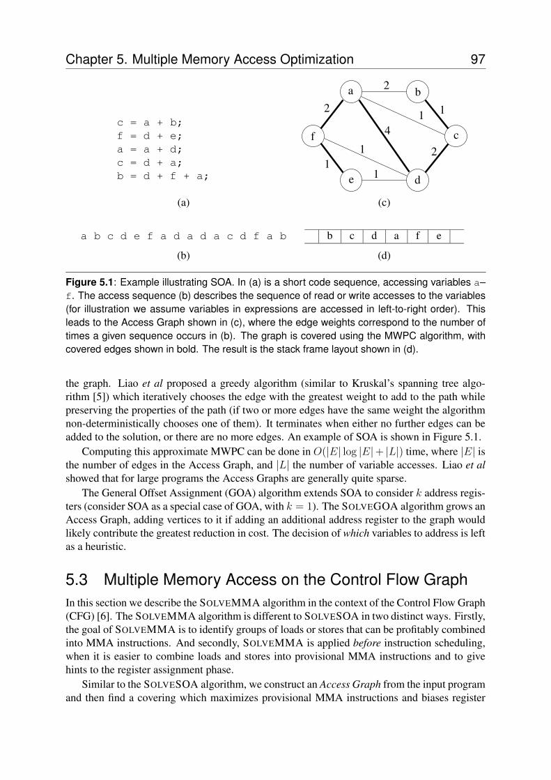
Chapter 5. Multiple Memory Access Optimization 97
c = a + b;f = d + e;a = a + d;c = d + a;b = d + f + a;
a b
c
de
f
2
11
2
2
4
11
1
(a) (c)
a b c d e f a d a d a c d f a b b c d a f e
(b) (d)
Figure 5.1: Example illustrating SOA. In (a) is a short code sequence, accessing variables a–f. The access sequence (b) describes the sequence of read or write accesses to the variables(for illustration we assume variables in expressions are accessed in left-to-right order). Thisleads to the Access Graph shown in (c), where the edge weights correspond to the number oftimes a given sequence occurs in (b). The graph is covered using the MWPC algorithm, withcovered edges shown in bold. The result is the stack frame layout shown in (d).
the graph. Liao et al proposed a greedy algorithm (similar to Kruskal’s spanning tree algo-rithm [5]) which iteratively chooses the edge with the greatest weight to add to the path whilepreserving the properties of the path (if two or more edges have the same weight the algorithmnon-deterministically chooses one of them). It terminates when either no further edges can beadded to the solution, or there are no more edges. An example of SOA is shown in Figure 5.1.
Computing this approximate MWPC can be done in O(|E| log |E|+ |L|) time, where |E| isthe number of edges in the Access Graph, and |L| the number of variable accesses. Liao et alshowed that for large programs the Access Graphs are generally quite sparse.
The General Offset Assignment (GOA) algorithm extends SOA to consider k address regis-ters (consider SOA as a special case of GOA, with k = 1). The SOLVEGOA algorithm grows anAccess Graph, adding vertices to it if adding an additional address register to the graph wouldlikely contribute the greatest reduction in cost. The decision of which variables to address is leftas a heuristic.
5.3 Multiple Memory Access on the Control Flow GraphIn this section we describe the SOLVEMMA algorithm in the context of the Control Flow Graph(CFG) [6]. The SOLVEMMA algorithm is different to SOLVESOA in two distinct ways. Firstly,the goal of SOLVEMMA is to identify groups of loads or stores that can be profitably combinedinto MMA instructions. And secondly, SOLVEMMA is applied before instruction scheduling,when it is easier to combine loads and stores into provisional MMA instructions and to givehints to the register assignment phase.
Similar to the SOLVESOA algorithm, we construct an Access Graph from the input programand then find a covering which maximizes provisional MMA instructions and biases register
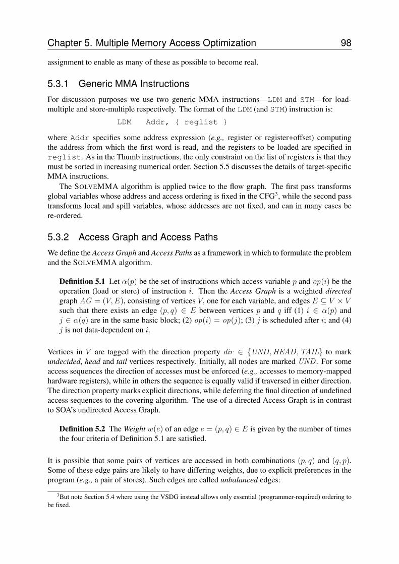
Chapter 5. Multiple Memory Access Optimization 98
assignment to enable as many of these as possible to become real.
5.3.1 Generic MMA Instructions
For discussion purposes we use two generic MMA instructions—LDM and STM—for load-multiple and store-multiple respectively. The format of the LDM (and STM) instruction is:
LDM Addr, { reglist }
where Addr specifies some address expression (e.g., register or register+offset) computingthe address from which the first word is read, and the registers to be loaded are specified inreglist. As in the Thumb instructions, the only constraint on the list of registers is that theymust be sorted in increasing numerical order. Section 5.5 discusses the details of target-specificMMA instructions.
The SOLVEMMA algorithm is applied twice to the flow graph. The first pass transformsglobal variables whose address and access ordering is fixed in the CFG3, while the second passtransforms local and spill variables, whose addresses are not fixed, and can in many cases bere-ordered.
5.3.2 Access Graph and Access Paths
We define the Access Graph and Access Paths as a framework in which to formulate the problemand the SOLVEMMA algorithm.
Definition 5.1 Let α(p) be the set of instructions which access variable p and op(i) be theoperation (load or store) of instruction i. Then the Access Graph is a weighted directedgraph AG = (V,E), consisting of vertices V, one for each variable, and edges E ⊆ V × V
such that there exists an edge (p, q) ∈ E between vertices p and q iff (1) i ∈ α(p) andj ∈ α(q) are in the same basic block; (2) op(i) = op(j); (3) j is scheduled after i; and (4)j is not data-dependent on i.
Vertices in V are tagged with the direction property dir ∈ {UND ,HEAD ,TAIL} to markundecided, head and tail vertices respectively. Initially, all nodes are marked UND . For someaccess sequences the direction of accesses must be enforced (e.g., accesses to memory-mappedhardware registers), while in others the sequence is equally valid if traversed in either direction.The direction property marks explicit directions, while deferring the final direction of undefinedaccess sequences to the covering algorithm. The use of a directed Access Graph is in contrastto SOA’s undirected Access Graph.
Definition 5.2 The Weight w(e) of an edge e = (p, q) ∈ E is given by the number of timesthe four criteria of Definition 5.1 are satisfied.
It is possible that some pairs of vertices are accessed in both combinations (p, q) and (q, p).Some of these edge pairs are likely to have differing weights, due to explicit preferences in theprogram (e.g., a pair of stores). Such edges are called unbalanced edges:
3But note Section 5.4 where using the VSDG instead allows only essential (programmer-required) ordering tobe fixed.
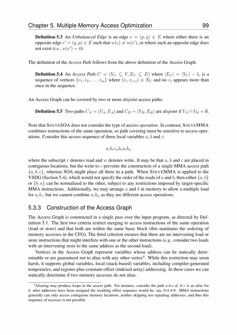
Chapter 5. Multiple Memory Access Optimization 99
Definition 5.3 An Unbalanced Edge is an edge e = (p, q) ∈ E where either there is anopposite edge e′ = (q, p) ∈ E such that w(e) 6= w(e′), or where such an opposite edge doesnot exist (i.e., w(e′) = 0).
The definition of the Access Path follows from the above definition of the Access Graph.
Definition 5.4 An Access Path C = (VC ⊆ V,EC ⊆ E) where |EC | = |VC | − 1, is asequence of vertices {v1, v2, . . . , vm} where (vi, vi+1) ∈ EC and no vi appears more thanonce in the sequence.
An Access Graph can be covered by two or more disjoint access paths:
Definition 5.5 Two paths CA = (VA, EA) and CB = (VB, EB) are disjoint if VA ∩ VB = ∅.
Note that SOLVESOA does not consider the type of access operation. In contrast, SOLVEMMAcombines instructions of the same operation, so path covering must be sensitive to access oper-ations. Consider this access sequence of three local variables a, b and c:
arbrcwbrarbw
where the subscript r denotes read and w denotes write. It may be that a, b and c are placed incontiguous locations, but the write to c prevents the construction of a single MMA access path{a, b, c}, whereas SOA might place all three in a path. When SOLVEMMA is applied to theVSDG (Section 5.4), which would not specify the order of the reads of a and b, then either {a, b}or {b, a} can be normalized to the other, subject to any restrictions imposed by target-specificMMA instructions. Additionally, we may arrange a and b in memory to allow a multiple loadfor arbr, but we cannot combine arbw as they are different access operations.
5.3.3 Construction of the Access Graph
The Access Graph is constructed in a single pass over the input program, as directed by Def-inition 5.1. The first two criteria restrict merging to access instructions of the same operation(load or store) and that both are within the same basic block (this maintains the ordering ofmemory accesses in the CFG). The third criterion ensures that there are no intervening load orstore instructions that might interfere with one or the other instructions (e.g., consider two loadswith an intervening store to the same address as the second load).
Vertices in the Access Graph represent variables whose address can be statically deter-minable or are guaranteed not to alias with any other vertex4. While this restriction may seemharsh, it supports global variables, local (stack-based) variables, including compiler-generatedtemporaries, and register-plus-constant-offset (indexed array) addressing. In these cases we canstatically determine if two memory accesses do not alias.
4Aliasing may produce loops in the access path. For instance, consider the path a-b-c-d; if c is an alias forb, after addresses have been assigned the resulting offset sequence would be, say, 0-4-4-8. MMA instructionsgenerally can only access contiguous memory locations, neither skipping nor repeating addresses, and thus thissequence of accesses is not possible.
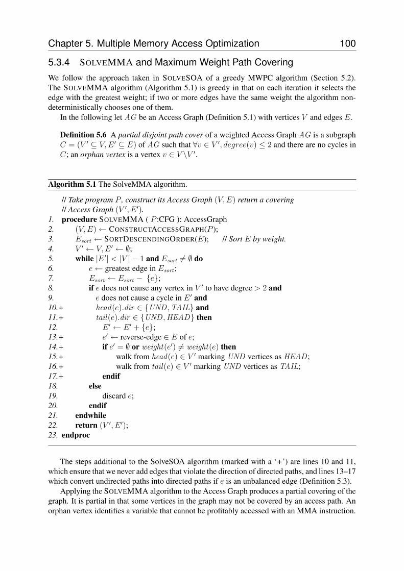
Chapter 5. Multiple Memory Access Optimization 100
5.3.4 SOLVEMMA and Maximum Weight Path CoveringWe follow the approach taken in SOLVESOA of a greedy MWPC algorithm (Section 5.2).The SOLVEMMA algorithm (Algorithm 5.1) is greedy in that on each iteration it selects theedge with the greatest weight; if two or more edges have the same weight the algorithm non-deterministically chooses one of them.
In the following let AG be an Access Graph (Definition 5.1) with vertices V and edges E.
Definition 5.6 A partial disjoint path cover of a weighted Access Graph AG is a subgraphC = (V ′ ⊆ V,E ′ ⊆ E) of AG such that ∀v ∈ V ′, degree(v) ≤ 2 and there are no cycles inC; an orphan vertex is a vertex v ∈ V \V ′.
Algorithm 5.1 The SolveMMA algorithm.
// Take program P , construct its Access Graph (V,E) return a covering// Access Graph (V ′, E ′).
1. procedure SOLVEMMA ( P :CFG ): AccessGraph2. (V,E)← CONSTRUCTACCESSGRAPH(P );3. Esort ← SORTDESCENDINGORDER(E); // Sort E by weight.4. V ′ ← V,E ′ ← ∅;5. while |E ′| < |V | − 1 and Esort 6= ∅ do6. e← greatest edge in Esort ;7. Esort ← Esort − {e};8. if e does not cause any vertex in V ′ to have degree > 2 and9. e does not cause a cycle in E ′ and10.+ head(e).dir ∈ {UND ,TAIL} and11.+ tail(e).dir ∈ {UND ,HEAD} then12. E ′ ← E ′ + {e};13.+ e′ ← reverse-edge ∈ E of e;14.+ if e′ = ∅ or weight(e′) 6= weight(e) then15.+ walk from head(e) ∈ V ′ marking UND vertices as HEAD ;16.+ walk from tail(e) ∈ V ′ marking UND vertices as TAIL;17.+ endif18. else19. discard e;20. endif21. endwhile22. return (V ′, E ′);23. endproc
The steps additional to the SolveSOA algorithm (marked with a ‘+’) are lines 10 and 11,which ensure that we never add edges that violate the direction of directed paths, and lines 13–17which convert undirected paths into directed paths if e is an unbalanced edge (Definition 5.3).
Applying the SOLVEMMA algorithm to the Access Graph produces a partial covering of thegraph. It is partial in that some vertices in the graph may not be covered by an access path. Anorphan vertex identifies a variable that cannot be profitably accessed with an MMA instruction.
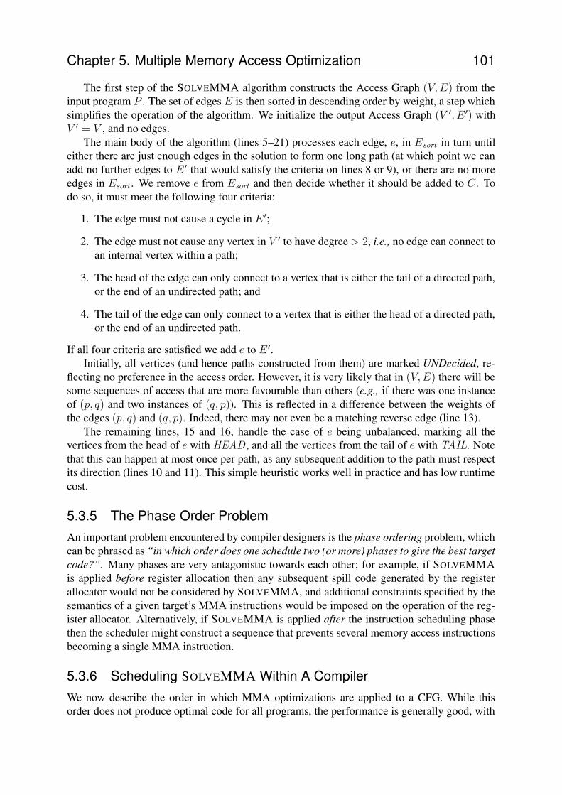
Chapter 5. Multiple Memory Access Optimization 101
The first step of the SOLVEMMA algorithm constructs the Access Graph (V,E) from theinput program P . The set of edges E is then sorted in descending order by weight, a step whichsimplifies the operation of the algorithm. We initialize the output Access Graph (V ′, E ′) withV ′ = V , and no edges.
The main body of the algorithm (lines 5–21) processes each edge, e, in Esort in turn untileither there are just enough edges in the solution to form one long path (at which point we canadd no further edges to E ′ that would satisfy the criteria on lines 8 or 9), or there are no moreedges in Esort . We remove e from Esort and then decide whether it should be added to C. Todo so, it must meet the following four criteria:
1. The edge must not cause a cycle in E ′;
2. The edge must not cause any vertex in V ′ to have degree > 2, i.e., no edge can connect toan internal vertex within a path;
3. The head of the edge can only connect to a vertex that is either the tail of a directed path,or the end of an undirected path; and
4. The tail of the edge can only connect to a vertex that is either the head of a directed path,or the end of an undirected path.
If all four criteria are satisfied we add e to E ′.Initially, all vertices (and hence paths constructed from them) are marked UNDecided, re-
flecting no preference in the access order. However, it is very likely that in (V,E) there will besome sequences of access that are more favourable than others (e.g., if there was one instanceof (p, q) and two instances of (q, p)). This is reflected in a difference between the weights ofthe edges (p, q) and (q, p). Indeed, there may not even be a matching reverse edge (line 13).
The remaining lines, 15 and 16, handle the case of e being unbalanced, marking all thevertices from the head of e with HEAD , and all the vertices from the tail of e with TAIL. Notethat this can happen at most once per path, as any subsequent addition to the path must respectits direction (lines 10 and 11). This simple heuristic works well in practice and has low runtimecost.
5.3.5 The Phase Order ProblemAn important problem encountered by compiler designers is the phase ordering problem, whichcan be phrased as “in which order does one schedule two (or more) phases to give the best targetcode?”. Many phases are very antagonistic towards each other; for example, if SOLVEMMAis applied before register allocation then any subsequent spill code generated by the registerallocator would not be considered by SOLVEMMA, and additional constraints specified by thesemantics of a given target’s MMA instructions would be imposed on the operation of the reg-ister allocator. Alternatively, if SOLVEMMA is applied after the instruction scheduling phasethen the scheduler might construct a sequence that prevents several memory access instructionsbecoming a single MMA instruction.
5.3.6 Scheduling SOLVEMMA Within A CompilerWe now describe the order in which MMA optimizations are applied to a CFG. While thisorder does not produce optimal code for all programs, the performance is generally good, with
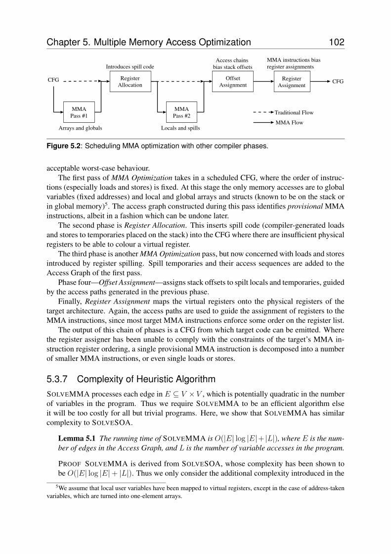
Chapter 5. Multiple Memory Access Optimization 102
CFG
Arrays and globals
Introduces spill code
Locals and spills
Access chains bias stack offsets
CFG
MMA instructions biasregister assignments
MMAPass #1
RegisterAllocation
MMAPass #2
OffsetAssignment
RegisterAssignment
Traditional Flow
MMA Flow
Figure 5.2: Scheduling MMA optimization with other compiler phases.
acceptable worst-case behaviour.The first pass of MMA Optimization takes in a scheduled CFG, where the order of instruc-
tions (especially loads and stores) is fixed. At this stage the only memory accesses are to globalvariables (fixed addresses) and local and global arrays and structs (known to be on the stack orin global memory)5. The access graph constructed during this pass identifies provisional MMAinstructions, albeit in a fashion which can be undone later.
The second phase is Register Allocation. This inserts spill code (compiler-generated loadsand stores to temporaries placed on the stack) into the CFG where there are insufficient physicalregisters to be able to colour a virtual register.
The third phase is another MMA Optimization pass, but now concerned with loads and storesintroduced by register spilling. Spill temporaries and their access sequences are added to theAccess Graph of the first pass.
Phase four—Offset Assignment—assigns stack offsets to spilt locals and temporaries, guidedby the access paths generated in the previous phase.
Finally, Register Assignment maps the virtual registers onto the physical registers of thetarget architecture. Again, the access paths are used to guide the assignment of registers to theMMA instructions, since most target MMA instructions enforce some order on the register list.
The output of this chain of phases is a CFG from which target code can be emitted. Wherethe register assigner has been unable to comply with the constraints of the target’s MMA in-struction register ordering, a single provisional MMA instruction is decomposed into a numberof smaller MMA instructions, or even single loads or stores.
5.3.7 Complexity of Heuristic AlgorithmSOLVEMMA processes each edge in E ⊆ V × V , which is potentially quadratic in the numberof variables in the program. Thus we require SOLVEMMA to be an efficient algorithm elseit will be too costly for all but trivial programs. Here, we show that SOLVEMMA has similarcomplexity to SOLVESOA.
Lemma 5.1 The running time of SOLVEMMA is O(|E| log |E|+ |L|), where E is the num-ber of edges in the Access Graph, and L is the number of variable accesses in the program.
PROOF SOLVEMMA is derived from SOLVESOA, whose complexity has been shown tobe O(|E| log |E|+ |L|). Thus we only consider the additional complexity introduced in the
5We assume that local user variables have been mapped to virtual registers, except in the case of address-takenvariables, which are turned into one-element arrays.
Chapter 5. Multiple Memory Access Optimization 103
construction of the MMA Access Graph and in lines 10–11 and 13–16 of Algorithm 5.1.For every variable access l ∈ L there can be at most 1 adjacent variable access. Lines 10, 11and 14 incur a constant cost per edge, as does line 13 in a well-implemented program. Lines15–16 together walk paths to convert them into directed paths. A path can be converted fromundirected to directed at most once. The total complexity is then O(|E| log |E|+ |E|+ |E|+|E|+ |L|), i.e., O(|E| log |E|+ |L|). �
Using path elements [72] the test for whether an edge e forms a cycle in C is reduced totesting whether the head and tail vertices of e are common to a single path element. This testcan be performed in constant time.
5.4 Multiple Memory Access on the VSDGThe previous section applied MMA optimization to a program in CFG form. The transforma-tions that are possible are constrained by the precise ordering specified by the CFG. In thissection MMA optimization is applied to the Value State Dependence Graph (Chapter 3), whichhas fewer constraints on the ordering of instructions.
Figure 5.3 shows the VSDG of the example program from Figure 5.1, showing memoryload, memory store and add nodes, with value- and state-dependency edges, together with theresulting Access Graph and memory layout.
5.4.1 Modifying SOLVEMMA for the VSDG
The VSDG under-specifies the ordering of instructions. Thus we can reformulate the fourcriteria of Definition 5.1 to “(1) i ∈ α(p) and j ∈ α(q) are in the same γ- and θ-dominatedregions6; (2) op(i) = op(j); (3) for loads, j has the same state-dependent node as i; for stores,j state-depends on i; and (4) j is not value-dependent on i.”
For example, in “x=v[a+b]” there are three loads—one each for a, b and the indexedaccess into array v[]. But the order of the first two loads is unspecified. This is represented inthe Access Graph by two edges, (a, b) and (b, a), of equal weight.
We gain two benefits from using the VSDG. The first is due to the state dependency edgesdefining the necessary ordering of loads and stores. For example, if a group of loads all dependon the same state, then those loads can be scheduled in any order; the VSDG underspecifies theorder of the loads, allowing MMA optimization to find an order that benefits code size.
The second benefit is due to the separation of value dependency and state dependency. Sucha separation facilitates a simple method of code motion by inserting additional serializing edgesinto the VSDG. For example, we can hoist an expression from between two stores, allowingthem to be combined into a single MMA store.
The VSDG does not change the SOLVEMMA algorithm itself, but it is a better data struc-ture, allowing greater flexibility in the mixing of phases within the compiler. For example, theregister allocation phase (Chapter 6) can favour an instruction ordering which allows provisionalMMA instructions to become actual MMA instructions.
6These are equivalent to basic blocks in the VSDG—see Chapter 6, page 112

Chapter 5. Multiple Memory Access Optimization 104
ld.a ld.b
Entry
+
st.c
......
Exit
st.c
ld.ald.fld.d
+
st.b
c = a + b;
b = d + f + a;
c = ... ;
ba
ed
f 3
1
1
1 1
1
1
3
1
1
c
(b)
b a d f e c
(c)(a)
Figure 5.3: The VSDG of Figure 5.1. The solid lines in (a) are value dependencies, and thedashed lines state dependencies (the middle portion of the graph is not shown, but can bereadily constructed). The labels of the memory load ‘ld’ and memory store ‘st’ nodes includethe variable name after the period. The Access Graph of (a) is shown in (b), with the coverededges in bold, resulting in memory layout (c).
5.5 Target-Specific MMA InstructionsThe generic MMA instructions (Section 5.3.1) do not specify any addressing mode, since theunderlying algorithm is neutral in this respect. Its purpose is to combine multiple instructionsinto a single instruction to reduce code size.
Tailoring the algorithm for a given architecture requires adding constraints to the code gen-erator and register assigner. For example, the PowerPC’s lmw and stmw instructions require acontiguous block of registers ending in R31. Appendix B describes the MMA instructions of anumber of popular MMA-capable embedded and desktop processors.
The Thumb LDM and STM instructions use a post-incremented register. Thus we only con-sider access paths where the address is increasing. Raddr is updated with the address of theword after the last word accessed by the MMA instruction. This gives another form of registerre-use similar to GOA which we resolve opportunistically: after an MMA instruction the baseregister may be available for re-use later, saving an address computation.
5.6 Motivating ExampleThe SOLVEMMA algorithm has been implemented as a transformation tool within our exper-imental compiler, VECC (Chapter 7). The Thumb’s MMA instructions (LDMIA and STMIA)
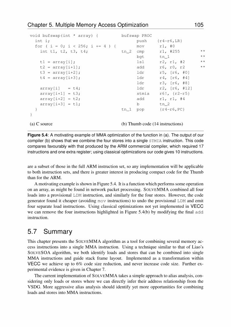
Chapter 5. Multiple Memory Access Optimization 105
void bufswap(int * array) {int i;for ( i = 0; i < 256; i += 4 ) {int t1, t2, t3, t4;
t1 = array[i];t2 = array[i+1];t3 = array[i+2];t4 = array[i+3];
array[i] = t4;array[i+1] = t3;array[i+2] = t2;array[i+3] = t1;
}}
bufswap PROCpush {r4-r6,LR}mov r1, #0
tn_2 cmp r1, #255 **bgt tn_1 **lsl r2, r1, #2 **add r6, r0, r2 **ldr r5, [r6, #0]ldr r4, [r6, #4]ldr r3, [r6, #8]ldr r2, [r6, #12]stmia r6!, {r2-r5}add r1, r1, #4b tn_2
tn_1 pop {r4-r6,PC}
(a) C source (b) Thumb code (14 instructions)
Figure 5.4: A motivating example of MMA optimization of the function in (a). The output of ourcompiler (b) shows that we combine the four stores into a single STMIA instruction. This codecompares favourably with that produced by the ARM commercial compiler, which required 17instructions and one extra register; using classical optimizations our code gives 10 instructions.
are a subset of those in the full ARM instruction set, so any implementation will be applicableto both instruction sets, and there is greater interest in producing compact code for the Thumbthan for the ARM.
A motivating example is shown in Figure 5.4. It is a function which performs some operationon an array, as might be found in network packet processing. SOLVEMMA combined all fourloads into a provisional LDM instruction, and similarly for the four stores. However, the codegenerator found it cheaper (avoiding mov instructions) to undo the provisional LDM and emitfour separate load instructions. Using classical optimizations not yet implemented in VECCwe can remove the four instructions highlighted in Figure 5.4(b) by modifying the final addinstruction.
5.7 SummaryThis chapter presents the SOLVEMMA algorithm as a tool for combining several memory ac-cess instructions into a single MMA instruction. Using a technique similar to that of Liao’sSOLVESOA algorithm, we both identify loads and stores that can be combined into singleMMA instructions and guide stack frame layout. Implemented as a transformation withinVECC we achieve up to 6% code size reduction, and never increase code size. Further ex-perimental evidence is given in Chapter 7.
The current implementation of SOLVEMMA takes a simple approach to alias analysis, con-sidering only loads or stores where we can directly infer their address relationship from theVSDG. More aggressive alias analysis should identify yet more opportunities for combiningloads and stores into MMA instructions.
Chapter 5. Multiple Memory Access Optimization 106
One wider question that remains unanswered is which of the possible MMA instructionsproduces the best results for code compaction. In our choice of the Thumb we have a singleaddress register and a bitmap to specify the desired data registers. In contrast the MMA instruc-tions of the PowerPC support register+offset addressing and specify the start index of a blockof contiguous registers ending in R31.
CHAPTER 6
Resource Allocation
We are generally the better persuadedby the reasons we discover ourselves
than by those given to us by others.BLAISE PASCAL (1623–1662)
Consider two important resources that target code consumes: time and space. Statically,we can view time as a schedule of instructions; we can view space as the registers and
temporary variables that the compiler fills with intermediate values (subexpression values, loopcounters, etc). The challenge, then, is to allocate these two resources in such a way as tominimize code size.
This leads to the phase order problem—which can be phrased as “in which order does oneschedule two (or more) compiler phases to give the best target code?”, where best in this thesisis smallest. Many phases are very antagonistic towards each other; two examples being codemotion (which may increase register pressure) and register allocation (which places additionaldependencies between instructions, artificially constraining instruction scheduling).
In this chapter we show that a unified approach, in which both register allocation (space) andcode motion (time) are considered together, resolves the problem of which phase to do first. Ourapproach uses the flexibility and simplicity of the Value State Dependence Graph (Chapter 3)to present an elegant solution to this problem.
Chapter 6. Resource Allocation 108
6.1 Serializing VSDGsWeise et al [112] observe that their mapping from CFGs to VDGs is many-to-one; they alsosuggest that “Code motion optimizations are decided when the demand dependence graph1 isconstructed from the VDG”—i.e., that a VDG should be turned back into a CFG for furtherprocessing—but do not give an algorithm for this or consider which of the many CFGs corre-sponding to a VDG should be selected.
We identify VSDGs with enough serializing edges with CFGs. Such VSDGs can be simplytransformed into CFGs if desired, the task of resource allocation then being to make the VSDGsufficiently sequential.
Definition 6.1 A sequential VSDG is one which has enough serializing edges and matchingsplit nodes for every γ-node to make it correspond to a single CFG.
Here ‘enough’ means in essence that each node in the VSDG has a unique (EV ∪ ES)immediate dominator which can be seen as its predecessor in the CFG. Exceptions arise forthe start node (which has no predecessors in the VSDG or corresponding CFG), γ-nodes andθ-nodes.
Given a γ-node g we interpret those nodes which the T port post-dominates as the true sub-VSDG (the T γ-region) and those which the F port post-dominates as the false sub-VSDG;a control-split node (corresponding to a CFG test-and-branch node) is added to the VSDG asthe immediate ES-dominator of both sub-VSDGs. For a θ-node, we recursively require thissequential property for its body and interpret the unique immediate post-dominator property asa constraint on its I port.
Upton [108] has shown that optimal placement of these split nodes is NP-Complete. Whilethis is unfortunate, it should be noted that once the split nodes have been placed, then generatinggood code from the split-augmented VSDG is no longer NP-Complete.
6.2 Computing Liveness in the VSDGFor the purposes of register allocation we need to know which (output ports of) VSDG nodesmay hold values simultaneously so we can forbid them being allocated the same register. Wedefine a cut as a partition of a VSDG in Gnoloop form (Chapter 3, page 63), and the notion ofinterfering nodes in a given cut.
Definition 6.2 A cut is a partition N1 ∪ N2 of nodes in the VSDG with the property thatthere is no EV ∪ ES edge from N2 to N1.
Definition 6.3 Nodes n and n′ are said to interfere if there is a cut N1 ∪N2 with n, n′ ∈ N1
and with both succV ∪S(n) and succV ∪S(n′) having non-empty intersections with N2.
This generalises the normal concept of register interference in a CFG; there a cut is just aprogram point and interference means “simultaneously live at any program point”. Similarly“virtual register” corresponds to our “output port of a node” and note that we use the conceptof “cut based on Depth From Root” in Section 6.4 for our new greedy algorithm.
1The demand dependence graph (DDG) has a similar structure to the control dependence graph (CDG) [39].The DDG is constructed using the predicates that lead to a computation contributing to the output of the program,while the CDG uses the predicates that lead to a computation being performed, even if that computation does notcontribute to the program’s output.
Chapter 6. Resource Allocation 109
6.3 Combining Register Allocation and Code MotionThe goal of register allocation in the VSDG is to allocate one physical register (from a limitedset) to each node’s output port. Tupled nodes are a special case, as they require multiple registerson their tupled ports. To whit: these are non-trivial γ- and θ-nodes, and multiple loads and stores(Chapter 5).
Register requirements can be reduced by serializing computations (two live ranges can betargeted to the same physical register if they are disjoint), or by reducing the range over whicha value is live by duplicating a computation, or by spilling a value to memory.
6.3.1 A Non-Deterministic ApproachGiven a VSDG we repeatedly apply the following non-deterministic algorithm until all thenodes are coloured and the VSDG is sequential. In the following discussion we assume the useof an interference graph (e.g., see [25]), where nodes correspond to live ranges of variables (i.e.,virtual registers), and there is an edge between two nodes if the two live ranges overlap.
1. Colour a port with a physical register—provided no port it interferes with is alreadycoloured with the same register;
2. Add a serializing edge to force one node before another—this removes edges from theclassical register interference graph by forbidding interleaving of computations;
3. Clone a node, i.e., recalculate it to reduce register pressure (a form of rematerializa-tion [21]).
4. Tunnel values through memory by introducing store/load spill nodes.
5. Merge two γ-nodes γa and γb into a tuple, provided their C ports depend on the samepredicate node and there is no path from γa to γb or from γb to γa.
6. Insert a split node for a γ-node to identify the boundaries of the γ-node regions (Sec-tion 6.5.1).
The first action assigns a physical register to a port of a given node. The second moves a node;the choice of which node to move is determined by specific algorithms (Sections 6.3.2 and 6.4).
Node cloning replaces a single instance of a node that has multiple uses, with multiple copies(clones) of the node, each with a subset of the original dependency edges. For example, a noden with two successor nodes p and q, can be cloned into nodes n′ and n′′, with p dependent onn′ and q dependent on n′′.
Spilling follows the traditional Chaitin-style register spilling [25] where we add store andload nodes, together with some temporary storage in memory.
The cost of spilling loop-variant variables is higher than the store-and-reload for a normalspill. For θ-nodes where the tuple is wider than the available physical registers, we must spillone or more of the θ-node variables over the loop test code, not merely within the loop itself.At most this requires two stores and three loads for each variable spilled. Figure 6.2 shows thelocation of the five spill nodes and when they are needed.
Finally, we can arrange to move nodes out of a γ-node region by inserting a split node. Thiswill reduce the number of live edges in the γ-node region, at the cost of increasing the overallnumber of live edges over the γ-node. For example, consider the following
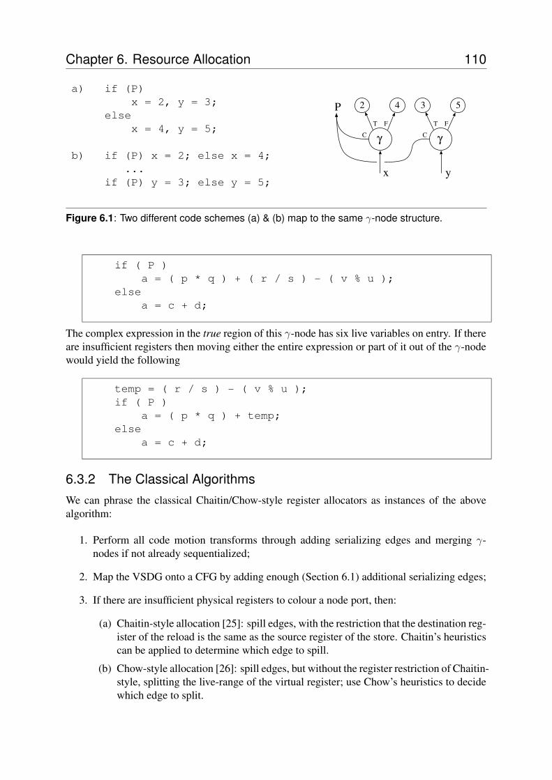
Chapter 6. Resource Allocation 110
a) if (P)x = 2, y = 3;
elsex = 4, y = 5;
b) if (P) x = 2; else x = 4;...
if (P) y = 3; else y = 5;
2 4
γ
P
C
T F
x y
3 5
γC
T F
Figure 6.1: Two different code schemes (a) & (b) map to the same γ-node structure.
if ( P )a = ( p * q ) + ( r / s ) - ( v % u );
elsea = c + d;
The complex expression in the true region of this γ-node has six live variables on entry. If thereare insufficient registers then moving either the entire expression or part of it out of the γ-nodewould yield the following
temp = ( r / s ) - ( v % u );if ( P )
a = ( p * q ) + temp;else
a = c + d;
6.3.2 The Classical AlgorithmsWe can phrase the classical Chaitin/Chow-style register allocators as instances of the abovealgorithm:
1. Perform all code motion transforms through adding serializing edges and merging γ-nodes if not already sequentialized;
2. Map the VSDG onto a CFG by adding enough (Section 6.1) additional serializing edges;
3. If there are insufficient physical registers to colour a node port, then:
(a) Chaitin-style allocation [25]: spill edges, with the restriction that the destination reg-ister of the reload is the same as the source register of the store. Chaitin’s heuristicscan be applied to determine which edge to spill.
(b) Chow-style allocation [26]: spill edges, but without the register restriction of Chaitin-style, splitting the live-range of the virtual register; use Chow’s heuristics to decidewhich edge to split.
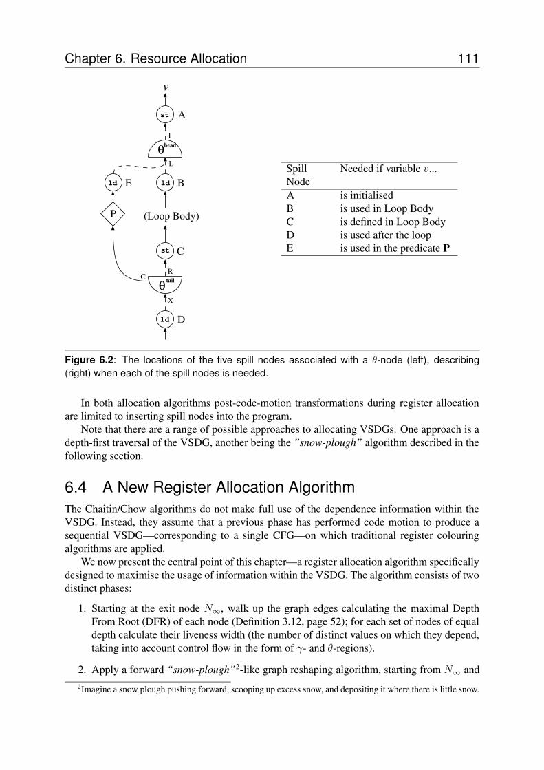
Chapter 6. Resource Allocation 111
st A
C
I
R
X
L
θhead
θ tail
ld
st
(Loop Body)
C
B
ld D
ld
P
E
v
SpillNode
Needed if variable v...
A is initialisedB is used in Loop BodyC is defined in Loop BodyD is used after the loopE is used in the predicate P
Figure 6.2: The locations of the five spill nodes associated with a θ-node (left), describing(right) when each of the spill nodes is needed.
In both allocation algorithms post-code-motion transformations during register allocationare limited to inserting spill nodes into the program.
Note that there are a range of possible approaches to allocating VSDGs. One approach is adepth-first traversal of the VSDG, another being the ”snow-plough” algorithm described in thefollowing section.
6.4 A New Register Allocation AlgorithmThe Chaitin/Chow algorithms do not make full use of the dependence information within theVSDG. Instead, they assume that a previous phase has performed code motion to produce asequential VSDG—corresponding to a single CFG—on which traditional register colouringalgorithms are applied.
We now present the central point of this chapter—a register allocation algorithm specificallydesigned to maximise the usage of information within the VSDG. The algorithm consists of twodistinct phases:
1. Starting at the exit node N∞, walk up the graph edges calculating the maximal DepthFrom Root (DFR) of each node (Definition 3.12, page 52); for each set of nodes of equaldepth calculate their liveness width (the number of distinct values on which they depend,taking into account control flow in the form of γ- and θ-regions).
2. Apply a forward “snow-plough”2-like graph reshaping algorithm, starting from N∞ and2Imagine a snow plough pushing forward, scooping up excess snow, and depositing it where there is little snow.
Chapter 6. Resource Allocation 112
pushing up towards N0, to ensure that the liveness width (Section 6.6) is never more thanthe number of physical registers. This is achieved by moving or cloning nodes, or spillingedges, in a greedy way so that the previously smoothed-out parts of the graph (nearer theexit) are not re-visited.
The result is a colourable VSDG; colouring it constitutes register assignment. The followingsections describe the steps necessary to allocate physical registers to a VSDG.
6.5 Partitioning the VSDGThe first pass annotates a VSDG with the DFR. The second pass then processes each cut of theVSDG in turn.
Definition 6.4 A depth-first cut Sd is the set of nodes with the same DFR d:
Sd = {n ∈ N | D(n) = d}
It is also convenient to write
S≤d = {n ∈ N | D(n) ≤ d}S>d = {n ∈ N | D(n) > d}
Note that the partition (S≤d,S>d) is a cut according to Definition 6.2 (page 108).
6.5.1 Identifying if/then/else
A necessary task during VSDG register allocation and code motion is to identify γ-regions, i.e.,the nodes which will be in the true or false regions of the γ-nodes in a VSDG.
Definition 6.5 A γ-region for a γ-node g is the set of nodes, Rγ(gp), strictly post-dominatedby port p of g, such that
Rγ(gp) = {n | n ∈ N ∧ gp spdom n}.
During sequentialization of a VSDG we identify the node which the γ-node’s C port de-pends on as the split node, and insert serializing edges from all nodes in the two γ-regions tothis split node.
6.5.2 Identifying LoopsThe second region of interest in the VSDG is the θ-region: the set of loop-variant nodes thatmust be in a loop body.
Definition 6.6 A θ-region for a θ-node l is the set of nodes, Rθ(l), such that
Rθ(l) = {n | n ∈ N ∧ ltail spdom n ∧ ∃ nEV ∪ES−→ lhead},
where EV ∪ES−→ denotes a path in (EV ∪ ES).
The goal is to even out the peaks and troughs.
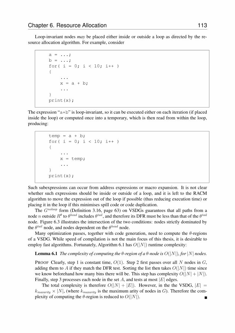
Chapter 6. Resource Allocation 113
Loop-invariant nodes may be placed either inside or outside a loop as directed by the re-source allocation algorithm. For example, consider
a = ...;b = ...;for( i = 0; i < 10; i++ ){
...x = a + b;...
}print(x);
The expression “a+b” is loop-invariant, so it can be executed either on each iteration (if placedinside the loop) or computed once into a temporary, which is then read from within the loop,producing:
temp = a + b;for( i = 0; i < 10; i++ ){
...x = temp;...
}print(x);
Such subexpressions can occur from address expressions or macro expansion. It is not clearwhether such expressions should be inside or outside of a loop, and it is left to the RACMalgorithm to move the expression out of the loop if possible (thus reducing execution time) orplacing it in the loop if this minimises spill code or code duplication.
The Gnoloop form (Definition 3.16, page 63) on VSDGs guarantees that all paths from anode n outside Rθ to θhead includes θtail , and therefore its DFR must be less than that of the θtail
node. Figure 6.3 illustrates the intersection of the two conditions: nodes strictly dominated bythe θtail node, and nodes dependent on the θhead node.
Many optimization passes, together with code generation, need to compute the θ-regionsof a VSDG. While speed of compilation is not the main focus of this thesis, it is desirable toemploy fast algorithms. Fortunately, Algorithm 6.1 has O(|N |) runtime complexity:
Lemma 6.1 The complexity of computing the θ-region of a θ-node is O(|N |), for |N | nodes.
PROOF Clearly, step 1 is constant time, O(1). Step 2 first passes over all N nodes in G,adding them to A if they match the DFR test. Sorting the list then takes O(|N |) time sincewe know beforehand how many bins there will be. This step has complexity O(|N |+ |N |).Finally, step 3 processes each node in the set A, and tests at most |E| edges.
The total complexity is therefore O(|N | + |E|). However, in the the VSDG, |E| =kmaxarity × |N |, (where kmaxarity is the maximum arity of nodes in G). Therefore the com-plexity of computing the θ-region is reduced to O(|N |). �
Chapter 6. Resource Allocation 114
θ-Region
θhead
Nodes post dominated by
θ tail
Nodes depending on θhead
θ tail
Figure 6.3: Illustrating the θ-region (hatched) of a θ-node as the intersection of nodes postdominated by the θtail node (dashed line), and nodes dependent on the θhead node (dash-dotline). The Gnoloop form ensures the former, while Algorithm 6.1 computes the latter.
Algorithm 6.1 Compute Theta RegionInput: A VSDG G = (N,EV , ES, `, N0, N∞) and a θ-node l ∈ N .
Output: All loop-variant nodes in N are in Rθ(l).
Method:
1. Initialise Rθ(l) = {l}.
2. Let A = SORTBYDESCENDINGDFR({n | n ∈ N ∧ D(ltail) < D(n) < D(lhead)}).
3. For each a ∈ A, from first to last, if a is (EV ∪ ES)-dependent on a node in Rθ(l), thenmove a from A to Rθ(l).
6.6 Calculating Liveness WidthWe wish to transform each cut so that the number of nodes having edges passing through it isno greater thanR, the number of registers available for colouring.
For a cut of depth d the set of such live nodes is given by
Win(d) = S>d ∩ predV (S≤d)
i.e., those nodes which are further than d from the exit node but whose values may be used onthe path to the exit node. Note that only EV and not ES edges count towards liveness, and thatnodes which will not require registers (e.g., small constants, labels for call nodes, etc) do notcontribute towardsWin .
One might expect that |Win(d)| is the number of registers required to compute the nodes inS≤d but this overstates the number of registers required for γ-nodes. The edges of each γ-regionare disjoint—on any given execution trace, exactly one path to a γ-node, g, will be executed ata time, and so we can reuse the same registers for colouring Rγ(gT ) and Rγ(gF ).
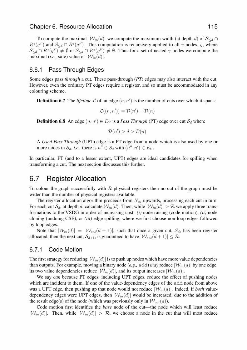
Chapter 6. Resource Allocation 115
To compute the maximal |Win(d)| we compute the maximum width (at depth d) of S≤d ∩Rγ(gT ) and S≤d ∩ Rγ(gF ). This computation is recursively applied to all γ-nodes, g, whereS≤d ∩ Rγ(gT ) 6= ∅ or S≤d ∩ Rγ(gF ) 6= ∅. Thus for a set of nested γ-nodes we compute themaximal (i.e., safe) value of |Win(d)|.
6.6.1 Pass Through EdgesSome edges pass through a cut. These pass-through (PT) edges may also interact with the cut.However, even the ordinary PT edges require a register, and so must be accommodated in anycolouring scheme.
Definition 6.7 The lifetime L of an edge (n, n′) is the number of cuts over which it spans:
L((n, n′)) = D(n′)−D(n)
Definition 6.8 An edge (n, n′) ∈ EV is a Pass Through (PT) edge over cut Sd when:
D(n′) > d > D(n)
A Used Pass Through (UPT) edge is a PT edge from a node which is also used by one ormore nodes in Sd, i.e., there is n′′ ∈ Sd with (n′′, n′) ∈ EV .
In particular, PT (and to a lesser extent, UPT) edges are ideal candidates for spilling whentransforming a cut. The next section discusses this further.
6.7 Register AllocationTo colour the graph successfully with R physical registers then no cut of the graph must bewider than the number of physical registers available.
The register allocation algorithm proceeds from N∞ upwards, processing each cut in turn.For each cut Sd, at depth d, calculateWin(d). Then, while |Win(d)| > R we apply three trans-formations to the VSDG in order of increasing cost: (i) node raising (code motion), (ii) nodecloning (undoing CSE), or (iii) edge spilling, where we first choose non-loop edges followedby loop edges.
Note that |Win(d)| = |Wout(d + 1)|, such that once a given cut, Sd, has been registerallocated, then the next cut, Sd+1, is guaranteed to have |Wout(d + 1)| ≤ R.
6.7.1 Code MotionThe first strategy for reducing |Win(d)| is to push up nodes which have more value dependenciesthan outputs. For example, moving a binary node (e.g., add) may reduce |Win(d)| by one edge:its two value dependencies reduce |Win(d)|, and its output increases |Win(d)|.
We say can because PT edges, including UPT edges, reduce the effect of pushing nodeswhich are incident to them. If one of the value-dependency edges of the add node from abovewas a UPT edge, then pushing up that node would not reduce |Win(d)|. Indeed, if both value-dependency edges were UPT edges, then |Win(d)| would be increased, due to the addition ofthe result edge(s) of the node (which was previously only inWout(d)).
Code motion first identifies the base node of the cut—the node which will least reduce|Win(d)|. Then, while |Win(d)| > R, we choose a node in the cut that will most reduce
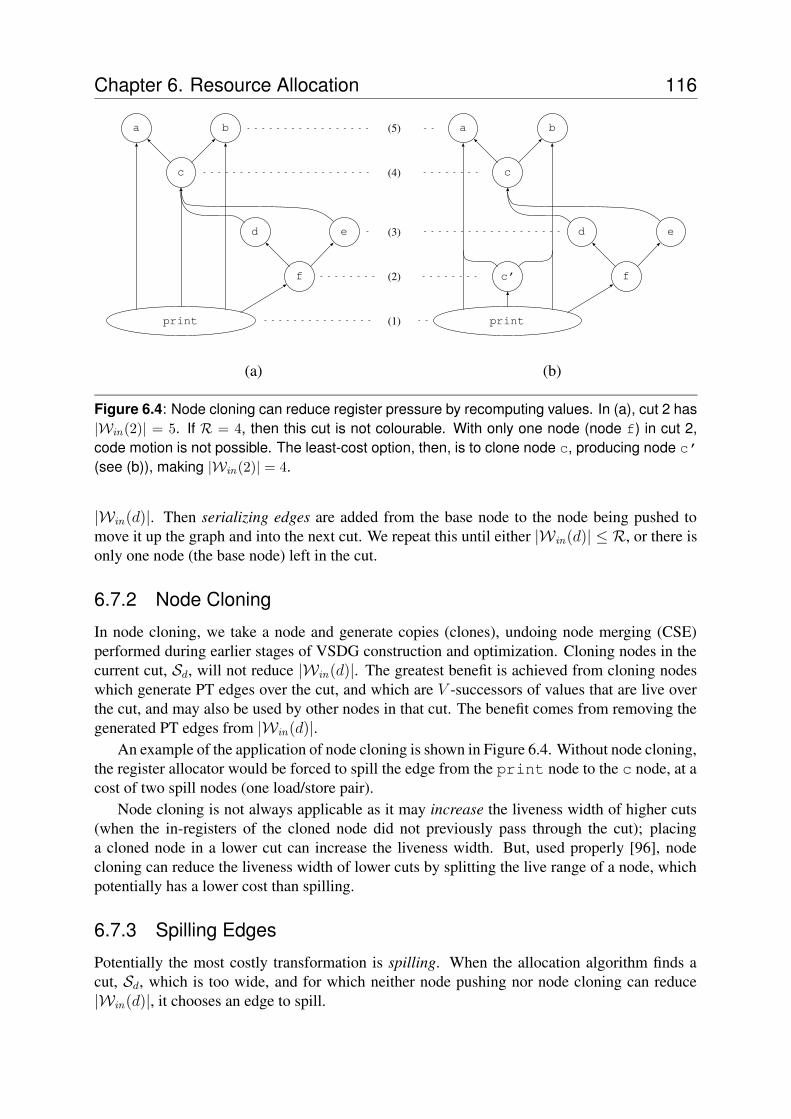
Chapter 6. Resource Allocation 116
a b
c
d e
f
(1)
(2)
(3)
(4)
(5)
a b
c
d e
fc’
(a) (b)
Figure 6.4: Node cloning can reduce register pressure by recomputing values. In (a), cut 2 has|Win(2)| = 5. If R = 4, then this cut is not colourable. With only one node (node f) in cut 2,code motion is not possible. The least-cost option, then, is to clone node c, producing node c’(see (b)), making |Win(2)| = 4.
|Win(d)|. Then serializing edges are added from the base node to the node being pushed tomove it up the graph and into the next cut. We repeat this until either |Win(d)| ≤ R, or there isonly one node (the base node) left in the cut.
6.7.2 Node Cloning
In node cloning, we take a node and generate copies (clones), undoing node merging (CSE)performed during earlier stages of VSDG construction and optimization. Cloning nodes in thecurrent cut, Sd, will not reduce |Win(d)|. The greatest benefit is achieved from cloning nodeswhich generate PT edges over the cut, and which are V -successors of values that are live overthe cut, and may also be used by other nodes in that cut. The benefit comes from removing thegenerated PT edges from |Win(d)|.
An example of the application of node cloning is shown in Figure 6.4. Without node cloning,the register allocator would be forced to spill the edge from the print node to the c node, at acost of two spill nodes (one load/store pair).
Node cloning is not always applicable as it may increase the liveness width of higher cuts(when the in-registers of the cloned node did not previously pass through the cut); placinga cloned node in a lower cut can increase the liveness width. But, used properly [96], nodecloning can reduce the liveness width of lower cuts by splitting the live range of a node, whichpotentially has a lower cost than spilling.
6.7.3 Spilling Edges
Potentially the most costly transformation is spilling. When the allocation algorithm finds acut, Sd, which is too wide, and for which neither node pushing nor node cloning can reduce|Win(d)|, it chooses an edge to spill.
Chapter 6. Resource Allocation 117
The aim of spilling is to reduce |Win(d)| of cut Sd. By the time the algorithm considersspilling both node pushing and cloning have already been exhaustively applied to the cut inquestion. Therefore the algorithm only considers PT edges for spilling, since spilling a UPTedge will not change |Win(d)|.
Given a set of PT edges over a cut Sd, the choice then is which edge to spill. This is decidedby a heuristic cost (Equation 6.1) computed for each edge, with the edge with the lowest costbeing chosen. As discussed previously (page 109), spilling variant θ-node edges (Figure 6.2)suffers the highest cost of spilling, with up to two stores and three loads.
Our initial heuristic cost function for edge spilling is
C(e) =
{
5L(e)−1 if e is loop-variant,2L(e)−1 otherwise. (6.1)
It favours loop-invariant edges over loop-variant edges since we save on not storing the updatedvalue, with savings both in static and dynamic instruction counts. The constant factors reflect thenumber of nodes added to the program when spilling both types of edge. It also favours edgeswith greater lifetimes, i.e., greater separation between the spill node and the correspondingreload node(s), which affords good performance on modern pipelined RISC processors.
6.8 SummaryCombining code motion and register allocation avoids the well-known conflict between thesetwo antagonistic phases. The method presented in this chapter uses the inherent flexibilityof the VSDG as a step towards this goal, due to its underspecification of the ordering of theinstructions (nodes) within a program.
A levelling, single-pass, algorithm walks up the VSDG, from the exit node, moving orcloning nodes, or spilling edges, to reshape the graph so that it can later be coloured withphysical registers.
Experimental evidence presented in the next chapter shows that this relatively simple, andplatform-neutral, algorithm can achieve results as good as, or better than, those of carefully-tuned commercial compilers.

Chapter 6. Resource Allocation 118
CHAPTER 7
Evaluation
Advice is judged by results, not by intentions.CICERO (106–43 BC)
The goal of this thesis is reducing code size for embedded systems through the optimizationof intermediate code. The chapter begins with a description of the process of generating
Thumb target code from a VSDG, including register assignment and instruction scheduling. Wethen present the results of experiments on procedural abstraction, MMA optimization, and theRACM algorithm.
Our experimental compiler generates VSDG intermediate code from a large subset of C (ex-cluding labels for convenience), a number of optimizations are applied to the intermediate code,which is then turned into target code for the Thumb 32-bit processor. The framework includesthe optimizations described in Chapter 4 (Pattern-based Procedural Abstraction), Chapter 5(Multiple Memory Access Optimization), and Chapter 6 (Combined Register Allocation andCode Motion).
7.1 VSDG FrameworkThe VECC (VSDG Experimental C Compiler) framework, shown in Figure 1.2 on page 22,provides a complete tool set, including a C compiler, a variety of optimizers and analysis tools,and a Thumb target code generator. Between the various components of VECC the program isrepresented as text files, as described in Appendix A. This allows experimentation with differentoptimization strategies through the use of shell scripts, and intermediate results can be easily
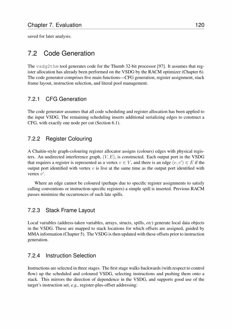
Chapter 7. Evaluation 120
saved for later analysis.
7.2 Code Generation
The vsdg2thm tool generates code for the Thumb 32-bit processor [97]. It assumes that reg-ister allocation has already been performed on the VSDG by the RACM optimizer (Chapter 6).The code generator comprises five main functions—CFG generation, register assignment, stackframe layout, instruction selection, and literal pool management.
7.2.1 CFG Generation
The code generator assumes that all code scheduling and register allocation has been applied tothe input VSDG. The remaining scheduling inserts additional serializing edges to construct aCFG, with exactly one node per cut (Section 6.1).
7.2.2 Register Colouring
A Chaitin-style graph-colouring register allocator assigns (colours) edges with physical regis-ters. An undirected interference graph, (V,E), is constructed. Each output port in the VSDGthat requires a register is represented as a vertex v ∈ V , and there is an edge (v, v ′) ∈ E if theoutput port identified with vertex v is live at the same time as the output port identified withvertex v′.
Where an edge cannot be coloured (perhaps due to specific register assignments to satisfycalling conventions or instruction-specific registers) a simple spill is inserted. Previous RACMpasses minimize the occurrences of such late spills.
7.2.3 Stack Frame Layout
Local variables (address-taken variables, arrays, structs, spills, etc) generate local data objectsin the VSDG. These are mapped to stack locations for which offsets are assigned, guided byMMA information (Chapter 5). The VSDG is then updated with these offsets prior to instructiongeneration.
7.2.4 Instruction Selection
Instructions are selected in three stages. The first stage walks backwards (with respect to controlflow) up the scheduled and coloured VSDG, selecting instructions and pushing them onto astack. This mirrors the direction of dependence in the VSDG, and supports good use of thetarget’s instruction set, e.g., register-plus-offset addressing:
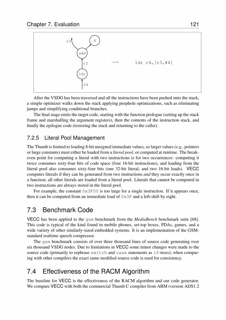
Chapter 7. Evaluation 121
add
r3
r3
r4
ldr
4
−→ ldr r4,[r3,#4]
After the VSDG has been traversed and all the instructions have been pushed onto the stack,a simple optimizer walks down the stack applying peephole optimizations, such as eliminatingjumps and simplifying conditional branches.
The final stage emits the target code, starting with the function prologue (setting up the stackframe and marshalling the argument registers), then the contents of the instruction stack, andfinally the epilogue code (restoring the stack and returning to the caller).
7.2.5 Literal Pool Management
The Thumb is limited to loading 8-bit unsigned immediate values, so larger values (e.g., pointersor large constants) must either be loaded from a literal pool, or computed at runtime. The break-even point for computing a literal with two instructions is for two occurrences: computing ittwice consumes sixty-four bits of code space (four 16-bit instructions), and loading from theliteral pool also consumes sixty-four bits (one 32-bit literal, and two 16-bit loads). VECCcomputes literals if they can be generated from two instructions and they occur exactly once ina function; all other literals are loaded from a literal pool. Literals that cannot be computed intwo instructions are always stored in the literal pool.
For example, the constant 0x3F00 is too large for a single instruction. If it appears once,then it can be computed from an immediate load of 0x3F and a left-shift by eight.
7.3 Benchmark CodeVECC has been applied to the gsm benchmark from the MediaBench benchmark suite [68].This code is typical of the kind found in mobile phones, set-top boxes, PDAs, games, and awide variety of other similarly-sized embedded systems. It is an implementation of the GSM-standard realtime speech compressor.
The gsm benchmark consists of over three thousand lines of source code generating oversix thousand VSDG nodes. Due to limitations in VECC some minor changes were made to thesource code (primarily to rephrase switch and case statements as if-trees); when compar-ing with other compilers the exact same modified source code is used for consistency.
7.4 Effectiveness of the RACM AlgorithmThe baseline for VECC is the effectiveness of the RACM algorithm and our code generator.We compare VECC with both the commercial Thumb C compiler from ARM (version ADS1.2
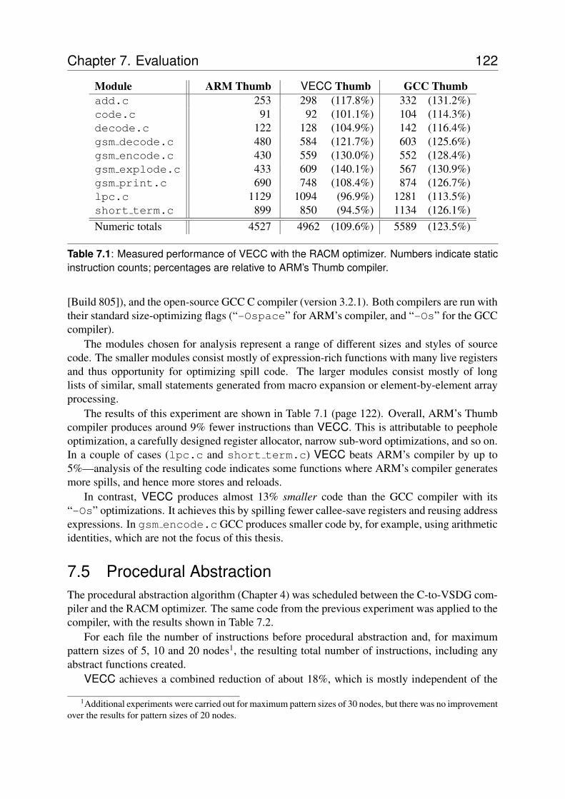
Chapter 7. Evaluation 122
Module ARM Thumb VECC Thumb GCC Thumbadd.c 253 298 (117.8%) 332 (131.2%)code.c 91 92 (101.1%) 104 (114.3%)decode.c 122 128 (104.9%) 142 (116.4%)gsm decode.c 480 584 (121.7%) 603 (125.6%)gsm encode.c 430 559 (130.0%) 552 (128.4%)gsm explode.c 433 609 (140.1%) 567 (130.9%)gsm print.c 690 748 (108.4%) 874 (126.7%)lpc.c 1129 1094 (96.9%) 1281 (113.5%)short term.c 899 850 (94.5%) 1134 (126.1%)Numeric totals 4527 4962 (109.6%) 5589 (123.5%)
Table 7.1: Measured performance of VECC with the RACM optimizer. Numbers indicate staticinstruction counts; percentages are relative to ARM’s Thumb compiler.
[Build 805]), and the open-source GCC C compiler (version 3.2.1). Both compilers are run withtheir standard size-optimizing flags (“-Ospace” for ARM’s compiler, and “-Os” for the GCCcompiler).
The modules chosen for analysis represent a range of different sizes and styles of sourcecode. The smaller modules consist mostly of expression-rich functions with many live registersand thus opportunity for optimizing spill code. The larger modules consist mostly of longlists of similar, small statements generated from macro expansion or element-by-element arrayprocessing.
The results of this experiment are shown in Table 7.1 (page 122). Overall, ARM’s Thumbcompiler produces around 9% fewer instructions than VECC. This is attributable to peepholeoptimization, a carefully designed register allocator, narrow sub-word optimizations, and so on.In a couple of cases (lpc.c and short term.c) VECC beats ARM’s compiler by up to5%—analysis of the resulting code indicates some functions where ARM’s compiler generatesmore spills, and hence more stores and reloads.
In contrast, VECC produces almost 13% smaller code than the GCC compiler with its“-Os” optimizations. It achieves this by spilling fewer callee-save registers and reusing addressexpressions. In gsm encode.c GCC produces smaller code by, for example, using arithmeticidentities, which are not the focus of this thesis.
7.5 Procedural AbstractionThe procedural abstraction algorithm (Chapter 4) was scheduled between the C-to-VSDG com-piler and the RACM optimizer. The same code from the previous experiment was applied to thecompiler, with the results shown in Table 7.2.
For each file the number of instructions before procedural abstraction and, for maximumpattern sizes of 5, 10 and 20 nodes1, the resulting total number of instructions, including anyabstract functions created.
VECC achieves a combined reduction of about 18%, which is mostly independent of the
1Additional experiments were carried out for maximum pattern sizes of 30 nodes, but there was no improvementover the results for pattern sizes of 20 nodes.
Chapter 7. Evaluation 123
File # Insn 5 Node Patterns 10 Node Patterns 20 Node Patternsadd.c 253 228 (90%) 228 (90%) 228 (90%)code.c 91 91 (100%) 91 (100%) 91 (100%)decode.c 122 122 (100%) 122 (100%) 122 (100%)gsm decode.c 480 399 (83%) 399 (83%) 399 (83%)gsm encode.c 430 289 (67%) 289 (67%) 289 (67%)gsm explode.c 433 367 (85%) 367 (85%) 367 (85%)gsm implode.c 490 377 (77%) 377 (77%) 377 (77%)gsm print.c 690 601 (87%) 601 (87%) 601 (87%)long term.c 793 635 (80%) 635 (80%) 635 (80%)lpc.c 1129 1011 (89%) 1011 (89%) 1011 (89%)preprocess.c 115 100 (87%) 100 (87%) 100 (87%)rpe.c 701 552 (79%) 565 (81%) 531 (76%)short term.c 899 783 (87%) 801 (89%) 792 (88%)COMBINED 6626 5446 (82%) 5450 (82%) 5466 (82%)
Table 7.2: Applying pattern abstraction algorithm to the gsm benchmark for three pattern max-ima. The first node column is for the unmodified program. The following columns indicate thetotal number of instructions after procedural abstraction, and the resulting compaction ratio.The final row is for procedural abstraction applied to all files combined into one program; notethat this is not the same as the arithmetic sum due to common patterns shared between files.
maximum pattern size. Interestingly, the size reduction decreases slightly as the maximumpattern size increases. This is due to the increased likelihood of two patterns overlapping asthe abstract pattern size increases, reducing the effectiveness of the algorithm and distorting thebenefit cost model.
Table 7.3 (page 124) shows the number of abstract functions created (and thus the numberof beneficial patterns found in the source program) and the total numbers of calls made to theabstract functions (i.e., the total number of pattern occurrences).
Most of the reduction in size is due to smaller patterns occurring very frequently, rather thanlarger patterns occurring once or twice. For example, short term.c and rpe.c generatetwo more pattern instances when increasing the maximum pattern size from five to ten nodes.Note that while adding support for loops would allow even larger patterns to be abstracted, asthe majority of abstracted patterns are small (patterns of five nodes or less account for almostall of the abstractions) the benefit would be small.
The COMBINED figures show the results after applying the procedural abstractor to all ofthe modules combined into a single VSDG. This provides more program for the abstractionalgorithm to analyse and to find more occurrences of common patterns. For example, for 5-node patterns, considered separately there were 67 patterns abstracted, but together only 32patterns abstracted.
Also note that while fewer patterns were abstracted, over 10% more pattern occurrenceswere abstracted. This is due to the greater number of pattern occurrences found in the largerbody of code, thus making it beneficial to abstract pattern occurrences that may occur only onceor twice in a module, but overall many times in the program. This clearly shows the benefitsof whole-program optimization: the more code that is visible to the optimizer, the more patternoccurrences it finds, and so the greater the degree of compaction of the code.
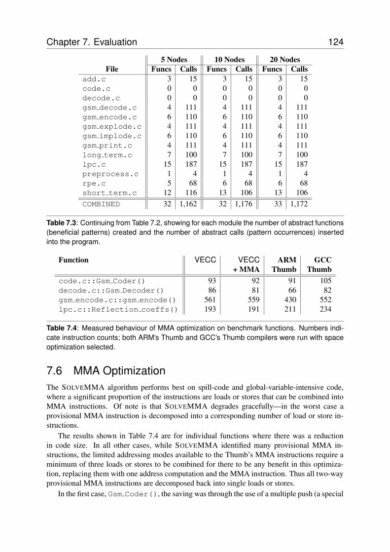
Chapter 7. Evaluation 124
5 Nodes 10 Nodes 20 NodesFile Funcs Calls Funcs Calls Funcs Calls
add.c 3 15 3 15 3 15code.c 0 0 0 0 0 0decode.c 0 0 0 0 0 0gsm decode.c 4 111 4 111 4 111gsm encode.c 6 110 6 110 6 110gsm explode.c 4 111 4 111 4 111gsm implode.c 6 110 6 110 6 110gsm print.c 4 111 4 111 4 111long term.c 7 100 7 100 7 100lpc.c 15 187 15 187 15 187preprocess.c 1 4 1 4 1 4rpe.c 5 68 6 68 6 68short term.c 12 116 13 106 13 106COMBINED 32 1,162 32 1,176 33 1,172
Table 7.3: Continuing from Table 7.2, showing for each module the number of abstract functions(beneficial patterns) created and the number of abstract calls (pattern occurrences) insertedinto the program.
Function VECC VECC ARM GCC+ MMA Thumb Thumb
code.c::Gsm Coder() 93 92 91 105decode.c::Gsm Decoder() 86 81 66 82gsm encode.c::gsm encode() 561 559 430 552lpc.c::Reflection coeffs() 193 191 211 234
Table 7.4: Measured behaviour of MMA optimization on benchmark functions. Numbers indi-cate instruction counts; both ARM’s Thumb and GCC’s Thumb compilers were run with spaceoptimization selected.
7.6 MMA OptimizationThe SOLVEMMA algorithm performs best on spill-code and global-variable-intensive code,where a significant proportion of the instructions are loads or stores that can be combined intoMMA instructions. Of note is that SOLVEMMA degrades gracefully—in the worst case aprovisional MMA instruction is decomposed into a corresponding number of load or store in-structions.
The results shown in Table 7.4 are for individual functions where there was a reductionin code size. In all other cases, while SOLVEMMA identified many provisional MMA in-structions, the limited addressing modes available to the Thumb’s MMA instructions require aminimum of three loads or stores to be combined for there to be any benefit in this optimiza-tion, replacing them with one address computation and the MMA instruction. Thus all two-wayprovisional MMA instructions are decomposed back into single loads or stores.
In the first case, Gsm Coder(), the saving was through the use of a multiple push (a special
Chapter 7. Evaluation 125
form of STM using the stack pointer as the address register with pre-decrement) to place twofunction arguments onto the stack prior to a function call.
The remaining cases utilise LDM or STM instructions to reduce code size. Further examina-tion of the generated Thumb code indicates places where provisional MMA instructions havebeen decomposed into single instructions during register allocation. These suggest improve-ments to the processor instruction set2 where there may be potential savings in code size.
7.7 SummaryThis chapter has shown the effectiveness of the algorithms presented in this thesis on benchmarkcode typical of smaller, code size critical, embedded systems. The results indicate three mainpoints: that the VSDG is a viable intermediate language for code size optimization researchand development; that the simplified procedural abstraction algorithm of Chapter 4 achieves arespectable 18% reduction in code size; and that MMA optimization, while being less effectivethan the RACM or procedural abstraction algorithms, still offers a worthwhile reduction in codesize.
2Assuming, of course, that we have the luxury of defining or modifying the processor’s instruction set.

Chapter 7. Evaluation 126
CHAPTER 8
Future Directions
Prediction is very difficult,especially about the future.
NIELS BOHR (1885–1962)
This thesis considers the code size optimization of program code for embedded systems. Itsfoundation is the Value State Dependence Graph (VSDG), and in this section we consider
three future directions of research that the VSDG is eminently suitable for, in addition to thetechniques already described.
8.1 Hardware CompilationThe growing complexity of logic circuits (microprocessors, image processors, network routers,etc) is driving the need for increasingly-higher level languages to describe these circuits, usingthe power of abstraction and ever-more powerful compilers and optimizers to produce circuitsbetter and faster than can be achieved with current tools.
The spectrum of hardware design languages extends from high-level languages, such asSharp’s SAFL [85] and SAFL+ [101] based on a functional programming style, Frankau’sSASL [41] extending the functional style to include lazy streams, and the family of synchronousdeclarative languages, such as the control-flow oriented Esterel [17], and the data-flow orientedLustre [24].
Other languages present a more familiar C-like programming paradigm; for example, C++-based SystemC [73], the SPARK [52] project, and OCCAM-like Handel-C [87], as well as theindustry-standard VHDL and Verilog, both of which have been standardised by the IEEE (IEEE
Chapter 8. Future Directions 128
Std 1076 and IEEE Std 1364 respectively).During the VSDG’s development it has often been observed that it has some very interesting
properties relating to generation of hardware. Almost all of the VSDG’s nodes have a closemapping to a hardware equivalent form:
• γ-nodes naturally map to multiplexers;
• θ-nodes map to Moore state machines, where the body of the loop generates the logicwhich computes the next-state information, the θhead node generates an input multiplexer,the θtail node generates a set of registers for all loop-variant variables, and the control-region nodes generate a loop controller that determines when to stop the loop iteratingand when to generate a “data ready” signal for the following circuits;
• load and store nodes map to memory access cycles over a shared memory system;
• arithmetic and predicate nodes generate combinatorial logic.
Sharing of resources and scheduling function calls could be managed through the use of,say, SAFL as the target language.
Interestingly, most of the components required to translate C source code to Verilog hard-ware description language: a C-to-VSDG compiler, a set of VSDG optimizers, and a functionalhardware compiler (SAFL). The remaining component, the VSDG-to-SAFL code generator,is all that is needed to explore the use of the VSDG as a potential intermediate language forhardware compilation.
8.2 VLIW and SuperScalar OptimizationsMany high-performance embedded processors and DSPs are based on multi-issue very longinstruction word (VLIW) architectures. VLIW processors have multiple processor cores run-ning in parallel. Examples include the Phillips Trimedia PNX1500 (5-way issue), and TexasInstruments’ C64x DSP family (8-way issue).
A difficulty with such processors is identifying parallelism from legacy source code (some-thing that Fortran compiler writers have been solving for many years). Previous program graphshave over-specified the ordering of instructions within a program, so any effort to identify setsof parallelizable instructions first have to remove the inessential relations between instructions,and then discover groups of instructions that can be executed in parallel. The goal being tofill all the instruction slots within the target code with useful instructions, rather than simplypadding with no-ops.
The VSDG seems to offer an elegant solution to this problem. By under-specifying therelationships between instructions (maintaining only the essential I/O semantics) schedulinginstructions for parallel execution is a modification of the RACM algorithm, with a modifiedconstraint on the number of (and perhaps the type of) instructions in each cut. Then each cutbecomes a single VLIW instruction, with empty slots filled with no-ops.
The recent introduction of the restrict keyword to the C language [22] can enable twosequential stores (e.g., “st a,[r]; st b,[s]”) to be considered randomly reorderable ifr and s are marked as restricted pointers, i.e., that the programmer guarantees that they willnever alias. For a VLIW target we can place both stores in the same instruction, gaining bothexecution speed and reduced code size; even more so if r and s are adjacent words in memory(Section 5).
Chapter 8. Future Directions 129
8.2.1 Very Long Instruction Word ArchitecturesA variation on VLIW is Single Instruction Multiple Data (SIMD) architectures, such as the Mo-torola AltiVec vector co-processor (Appendix B). This can perform an arithmetic operation onsixteen 8-bit variables, eight 16-bit variables, or four 32-bit (float or long) variables in parallel.Aimed at multimedia data processing applications (audio and video processing, 3D image ren-dering, desktop publishing, etc), access to these instructions is usually through vendor-suppliedhand-written libraries, rather than from the compiler itself, and requiring special data types toguarantee correct alignment of variables in memory.
Again, the VSDG provides an intermediate language where any parallelism in a programcan be readily identified. In the case of SIMD the goal is to find or generate cuts where all ofthe ALU operations are the same (e.g., add) and the data types are the same (e.g.,int).
8.2.2 SIMD Within A RegisterA generally applicable variation of SIMD is SWAR—SIMD Within A Register [40]. The goalis to combine several similar operations into one single common operation, fitting the operandsinto a single physical register, and executing a single instruction.
Polymorphic SWAR instructions, such as bitwise AND, OR and NOT, are easily imple-mented. Other SWAR instructions (ADD, SUBTRACT, etc) require some additional effort tohandle over- or under-flow between fields in the physical register. One software solution is toseparate the data fields with guard bits, ensuring that any carry-over from one addition will notaffect another addition; for example three 8-bit additions within a single 32-bit register.
Some hardware solutions already support this feature, with special instructions like ”add.8”,that do not propagate the carry bit between specific bits in the ALU (e.g., from bit 7 to bit 8 inthe case of an 8-bit addition).
Further benefit can be achieved if the data is stored in memory in prepacked form, reduc-ing the need to pack and unpack them at runtime. It should be possible to extend the MMAalgorithm (Chapter 5) to consider variables of sizes other than int and thus to prepack thesenarrower variables in an order favourable to SIMD or SWAR instruction generation.
8.3 Instruction Set DesignAnother area that the VSDG could be applied is that of processor instruction set design. Whendesigning a new processor, there are many choices about which instructions are worth includingin the instruction set, and those which either never occur at all (perhaps due to limitations ofa compiler), or occur so infrequently in benchmark code that the cost of including them in theinstruction set is greater than emulating the functionality in a software library.
On the VSDG, the procedural abstraction optimizer (Chapter 4) could be used. The ap-proach might take the following steps:
• Start with a simple RISC machine;
• Compile up lots of benchmark code into VSDGs;
• Analyse the programs with the Procedural Abstraction optimizer;
• Identify the most used abstract functions;
Chapter 8. Future Directions 130
• Create new custom VSDG nodes which implement the functionality of these abstractfunctions;
• Repeat the above, refining the instruction set until some pre-defined goal is reached (e.g.,code size).
The custom VSDG nodes then describe the additional instructions that could be added tothe processor’s instruction set.
CHAPTER 9
Conclusion
Every day you may make progress. Every step may be fruitful. Yet there will stretchout before you an ever-lengthening, ever-ascending, ever-improving path.
You know you will never get to the end of the journey.But this, so far from discouraging, only adds
to the joy and glory of the climb.SIR WINSTON CHURCHILL (1874–1965)
Computers—in the form of embedded systems—are everywhere. And just as they grow innumbers, they shrink in size. This thesis has studied the problem of reducing code size
from within the compiler, benefiting both legacy applications ported to new systems, and newapplications made possible through reduced code size.
Previous work in optimizing code for size has been influenced by the choice of the inter-mediate representation—the more powerful the representation, the more powerful the optimiza-tions that can be applied to it.
Many such intermediate representations have been developed: from the original ControlFlow Graph and the Data Flow Graph, Ferrante et al’s Program Dependence Graph, Ballanceet al’s Program Dependence Web and Click’s Intermediate Representation, to the Value Depen-dence Graph of Weise et al. Developments in the Static Single Assignment and Gated SingleAssignment forms have augmented these intermediate representations, simplifying many opti-mizations (of which there are many), and making others viable within a practical compiler.
The first contribution of this thesis is the Value State Dependence Graph (VSDG) as anintermediate form for compilers. Primarily developed for compiling for small code size, itcan equally be applied to producing fast code, or parallel code. The VSDG has the propertyof partially specifying (through essential value and state dependencies) the order of instruc-tions within the program. Subsequent optimization phases are at liberty to transform the graphthrough graph rewriting rules. Code generation from the VSDG applies sufficient serializing
Chapter 9. Conclusion 132
edges to the VSDG to construct a single CFG, from which code is generated.The next contribution showed how procedural abstraction can be applied to the VSDG. Code
patterns are generated from the VSDGs of a program, and stored in a database. Transformationthen selects patterns with the greatest benefit—from these patterns new compiler-generatedabstract functions are created, and all occurrences of the patterns in the original VSDG arereplaced by calls to the abstract functions.
Several popular embedded processors have load-multiple and store-multiple instructions.On first inspection, these would seem to be ideal instructions to use in generating compactcode—representing multiple (perhaps as many as thirty two) loads or stores in a single instruc-tion. However, it seems that most commercial compilers seem only to combine multiple loadsor stores opportunistically during peephole optimization. This makes such optimization sub-ject to unfortunate instruction schedules and register assignments. As a first attempt at tacklingthis problem, we presented a new method specifically targeted at using these multiple-memory-access instructions, combining loads and stores within the VSDG before target code generation,in a way that can be undone during later stages to avoid spilling or code duplication.
The final contribution of this thesis is a combined approach to register allocation and codemotion (RACM). These two separate phases have been shown to be antagonistic towards eachother: register allocation can artificially constrain instruction scheduling, while the instructionscheduler can produce a schedule that forces a poor register allocation, perhaps even generatingspill code. We have shown that our RACM algorithm formulates these two previously antago-nistic phases as one combined pass over the VSDG, transforming nodes (moving, cloning, orspilling) as directed by the register pressure measured from the graph. Additionally, preferencesfor instruction schedules (e.g., separating loads and stores to minimize load/store dependenciesin pipelined architectures) can be factored into the algorithm.
The ideas presented in this thesis have been implemented within a prototype compiler. OurC front end is based on Fraser and Hanson’s LCC compiler, modified to generate VSDGs fromC source. All other transformation and analysis tools have been implemented as stand-alonecommand line utilities reading, transforming, and writing VSDGs as text files. Our resultsshow that, even though we implement a subset of all the possible optimizations described in theliterature, we can achieve code sizes comparable to, and in some cases better than, that producedby commercial compilers.
Finally, the ideas in this thesis can be both extended in the original problem domain—compacting code for embedded systems—and also in other areas, from hardware descriptionlanguages, parallelizing code for VLIW or SIMD processors (and software emulation of SIMD),to instruction set design.
APPENDIX A
Concrete Syntax for the VSDG
The Value State Dependence Graph data structure, described in Chapter 3, formally repre-sents the VSDG within the context of a software tool. Here we describe, in a format suitable
for a grammar generator tool such as YACC [71], the structure of the VSDG syntax. This syntaxserves two purposes: it provides a clean, human-readable, portable file format to support thedevelopment of analysis and transformation tools, and it clearly defines the structure of VS-DGs, from the whole-program level down to the individual components of a VSDG (modules,functions, etc).
A.1 File StructureA VSDG description file is a two-level description of a VSDG. The upper level defines modules,and the lower level defines the functions within each module.
Description files by themselves do not define any scope—they provide storage for mod-ule definitions. There is no difference between a single file containing multiple modules, andmultiple files containing single modules. This approach has the benefit of allowing textual con-catenation of VSDG files to combine multiple modules. VSDG transformation tools can thusread in one or more VSDG files (e.g., programmer-generated VSDG files and library VSDGfiles) and treat them as a single, large, application file.
Modules contain data definitions, constant definitions, and function definitions. Names ofobjects defined within a module are only visible within the enclosing module. This can beoverridden with the public attribute.
Data definitions define both initialised and uninitialised statically-allocated variables. Theparameter list for a data definition (Section A.4.3) specifies the size, in bytes, of the data object,and optionally a contiguous ordered list of byte-sized and byte-aligned initial values. Constantdefinitions are of the same format as initialised data definitions.
Function definitions take a function name, an argument name list (which is empty for voidfunctions), the number of return values, and a body.
A function’s body consists of an unordered list of node definitions, edge definitions, and dataand constant definitions. The data and constant definitions are exactly the same as described
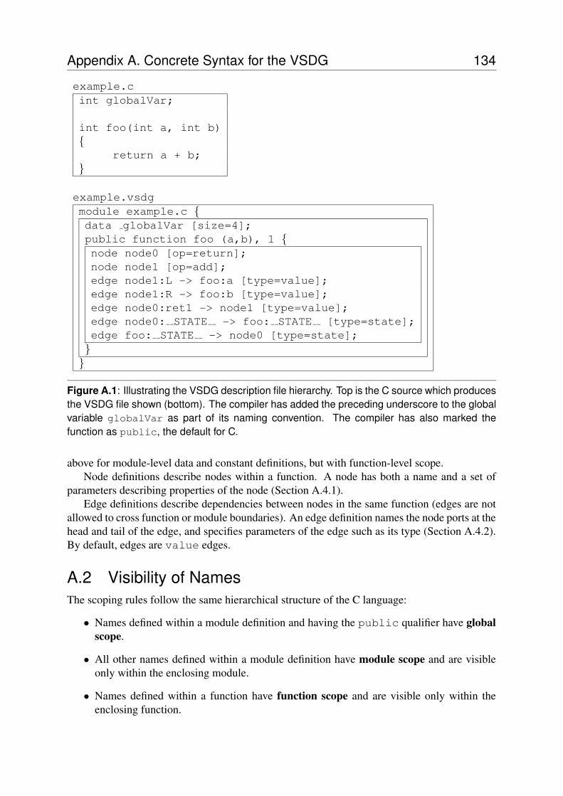
Appendix A. Concrete Syntax for the VSDG 134
example.cint globalVar;
int foo(int a, int b){
return a + b;}
example.vsdgmodule example.c {data globalVar [size=4];public function foo (a,b), 1 {node node0 [op=return];node node1 [op=add];edge node1:L -> foo:a [type=value];edge node1:R -> foo:b [type=value];edge node0:ret1 -> node1 [type=value];edge node0: STATE -> foo: STATE [type=state];edge foo: STATE -> node0 [type=state];}}
Figure A.1: Illustrating the VSDG description file hierarchy. Top is the C source which producesthe VSDG file shown (bottom). The compiler has added the preceding underscore to the globalvariable globalVar as part of its naming convention. The compiler has also marked thefunction as public, the default for C.
above for module-level data and constant definitions, but with function-level scope.Node definitions describe nodes within a function. A node has both a name and a set of
parameters describing properties of the node (Section A.4.1).Edge definitions describe dependencies between nodes in the same function (edges are not
allowed to cross function or module boundaries). An edge definition names the node ports at thehead and tail of the edge, and specifies parameters of the edge such as its type (Section A.4.2).By default, edges are value edges.
A.2 Visibility of NamesThe scoping rules follow the same hierarchical structure of the C language:
• Names defined within a module definition and having the public qualifier have globalscope.
• All other names defined within a module definition have module scope and are visibleonly within the enclosing module.
• Names defined within a function have function scope and are visible only within theenclosing function.
Appendix A. Concrete Syntax for the VSDG 135
A.3 GrammarThe grammar is described in the following pages in a form suitable for processing with YACC [71].This is followed by definitions of the terminal symbols, which can be similarly turned into pat-tern definitions suitable for a lexical analysis tool such as LEX [71]. The following table liststhe font styles and their meanings used in the syntax:
Style Meaningtypewriter literal terminal symbols (keywords, punctuation, etc)bold italicized other terminal symbols (literals, constants, etc)italicized non-terminals
Note: the suffix “opt” indicates optional symbols.
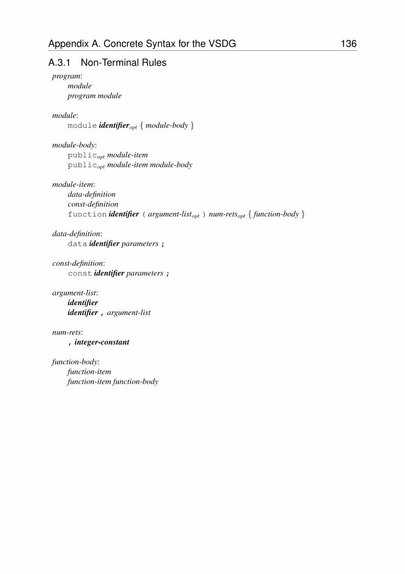
Appendix A. Concrete Syntax for the VSDG 136
A.3.1 Non-Terminal Rulesprogram:
moduleprogram module
module:module identifieropt { module-body }
module-body:publicopt module-itempublicopt module-item module-body
module-item:data-definitionconst-definitionfunction identifier ( argument-listopt ) num-retsopt { function-body }
data-definition:data identifier parameters ;
const-definition:const identifier parameters ;
argument-list:identifieridentifier , argument-list
num-rets:, integer-constant
function-body:function-itemfunction-item function-body
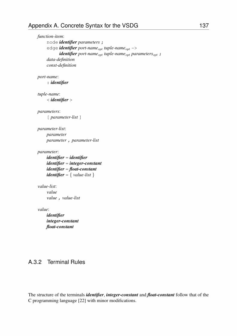
Appendix A. Concrete Syntax for the VSDG 137
function-item:node identifier parameters ;edge identifier port-nameopt tuple-nameopt ->
identifier port-nameopt tuple-nameopt parametersopt ;data-definitionconst-definition
port-name:: identifier
tuple-name:< identifier >
parameters:[ parameter-list ]
parameter-list:parameterparameter , parameter-list
parameter:identifier = identifieridentifier = integer-constantidentifier = float-constantidentifier = { value-list }
value-list:valuevalue , value-list
value:identifierinteger-constantfloat-constant
A.3.2 Terminal Rules
The structure of the terminals identifier, integer-constant and float-constant follow that of theC programming language [22] with minor modifications.
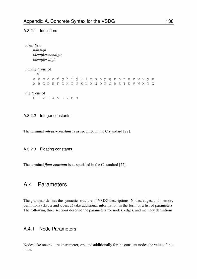
Appendix A. Concrete Syntax for the VSDG 138
A.3.2.1 Identifiers
identifier:nondigitidentifier nondigitidentifier digit
nondigit: one of$
a b c d e f g h i j k l m n o p q r s t u v w x y zA B C D E F G H I J K L M N O P Q R S T U V W X Y Z
digit: one of0 1 2 3 4 5 6 7 8 9
A.3.2.2 Integer constants
The terminal integer-constant is as specified in the C standard [22].
A.3.2.3 Floating constants
The terminal float-constant is as specified in the C standard [22].
A.4 Parameters
The grammar defines the syntactic structure of VSDG descriptions. Nodes, edges, and memorydefinitions (data and const) take additional information in the form of a list of parameters.The following three sections describe the parameters for nodes, edges, and memory definitions.
A.4.1 Node Parameters
Nodes take one required parameter, op, and additionally for the constant nodes the value of thatnode.
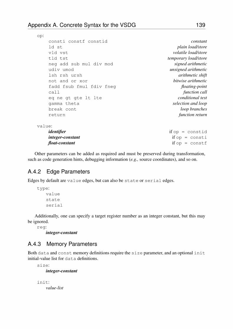
Appendix A. Concrete Syntax for the VSDG 139
op:consti constf constid constantld st plain load/storevld vst volatile load/storetld tst temporary load/storeneg add sub mul div mod signed arithmeticudiv umod unsigned arithmeticlsh rsh ursh arithmetic shiftnot and or xor bitwise arithmeticfadd fsub fmul fdiv fneg floating-pointcall function calleq ne gt gte lt lte conditional testgamma theta selection and loopbreak cont loop branchesreturn function return
value:identifier if op = constidinteger-constant if op = constifloat-constant if op = constf
Other parameters can be added as required and must be preserved during transformation,such as code generation hints, debugging information (e.g., source coordinates), and so on.
A.4.2 Edge ParametersEdges by default are value edges, but can also be state or serial edges.
type:valuestateserial
Additionally, one can specify a target register number as an integer constant, but this maybe ignored.
reg:integer-constant
A.4.3 Memory ParametersBoth data and const memory definitions require the size parameter, and an optional initinitial-value list for data definitions.
size:integer-constant
init:value-list
Appendix A. Concrete Syntax for the VSDG 140
APPENDIX B
Survey of MMA Instructions
Many processors have instructions which implement some form of multiple memory access.In this appendix summarises the MMA instructions of a variety of popular processors:
MIL-STD-1750A, ARM and Thumb, PowerPC, MIPS16, SPARC V9, and the vector-based co-processors now popular in desktop systems—Intel’s MMX, Motorola’s AltiVec, and Sun’s VIS.In all cases the instruction mnemonics are those used in the relevant source material.
B.1 MIL-STD-1750AThe MIL-STD-1750A 16-bit processor [109] is used primarily in the military and aerospaceindustries, not least because of its availability in radiation-hardened form. It has sixteen 16-bitregisters, with a 64k word address space for both program code, data and stack.
The 1750A has four MMA instructions. The first two are load multiple LM and store multipleSTM. The two addressing modes for these instructions are immediate (constant address) andregister-plus-offset; the address counter is incremented after each access (there is no registerwrite-back like the ARM). All register transfers start at register R0 and stop at the end registerspecified in the instruction.
The other two MMA instructions are PUSH and POP, for transferring data between regis-ters and the stack. Both instructions implicitly use R15 as the Stack Pointer. The instructionspecifies the lowest and highest registers to be transferred. Interestingly, if the the end regis-ter number is lower than the start register number (e.g.,PUSH R14,R2), then the processorproceeds up to R15, wraps round to R0, and continues up to the end register.
B.2 ARMThe ARM [97] load-multiple and store-multiple instructions are very capable instructions, ableto load or store a non-contiguous subset of all sixteen registers (including the Stack Pointer andthe Program Counter) with four addressing modes. While the ARM MMA instructions lackthe register+displacement addressing modes compared to other architectures described in thisappendix, this is partly compensated by a choice of four address register modes, and an optional
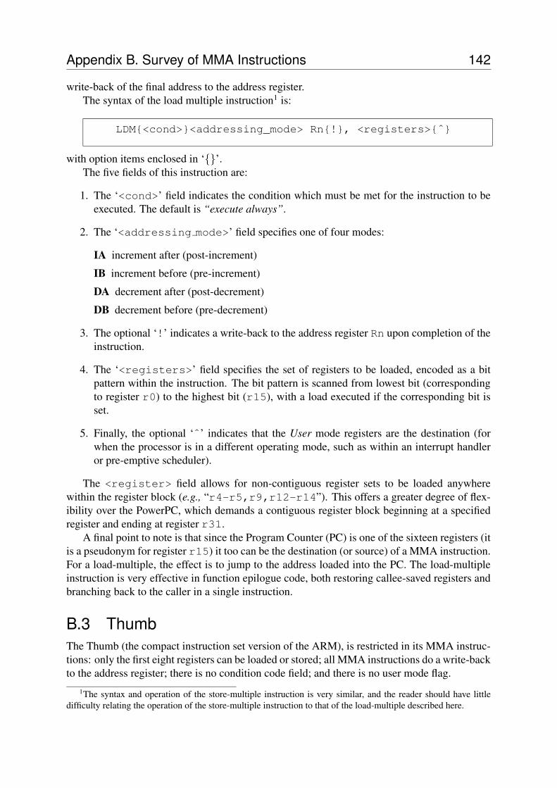
Appendix B. Survey of MMA Instructions 142
write-back of the final address to the address register.The syntax of the load multiple instruction1 is:
LDM{<cond>}<addressing_mode> Rn{!}, <registers>{ˆ}
with option items enclosed in ‘{}’.The five fields of this instruction are:
1. The ‘<cond>’ field indicates the condition which must be met for the instruction to beexecuted. The default is “execute always”.
2. The ‘<addressing mode>’ field specifies one of four modes:
IA increment after (post-increment)
IB increment before (pre-increment)
DA decrement after (post-decrement)
DB decrement before (pre-decrement)
3. The optional ‘!’ indicates a write-back to the address register Rn upon completion of theinstruction.
4. The ‘<registers>’ field specifies the set of registers to be loaded, encoded as a bitpattern within the instruction. The bit pattern is scanned from lowest bit (correspondingto register r0) to the highest bit (r15), with a load executed if the corresponding bit isset.
5. Finally, the optional ‘ˆ’ indicates that the User mode registers are the destination (forwhen the processor is in a different operating mode, such as within an interrupt handleror pre-emptive scheduler).
The <register> field allows for non-contiguous register sets to be loaded anywherewithin the register block (e.g., “r4-r5,r9,r12-r14”). This offers a greater degree of flex-ibility over the PowerPC, which demands a contiguous register block beginning at a specifiedregister and ending at register r31.
A final point to note is that since the Program Counter (PC) is one of the sixteen registers (itis a pseudonym for register r15) it too can be the destination (or source) of a MMA instruction.For a load-multiple, the effect is to jump to the address loaded into the PC. The load-multipleinstruction is very effective in function epilogue code, both restoring callee-saved registers andbranching back to the caller in a single instruction.
B.3 ThumbThe Thumb (the compact instruction set version of the ARM), is restricted in its MMA instruc-tions: only the first eight registers can be loaded or stored; all MMA instructions do a write-backto the address register; there is no condition code field; and there is no user mode flag.
1The syntax and operation of the store-multiple instruction is very similar, and the reader should have littledifficulty relating the operation of the store-multiple instruction to that of the load-multiple described here.
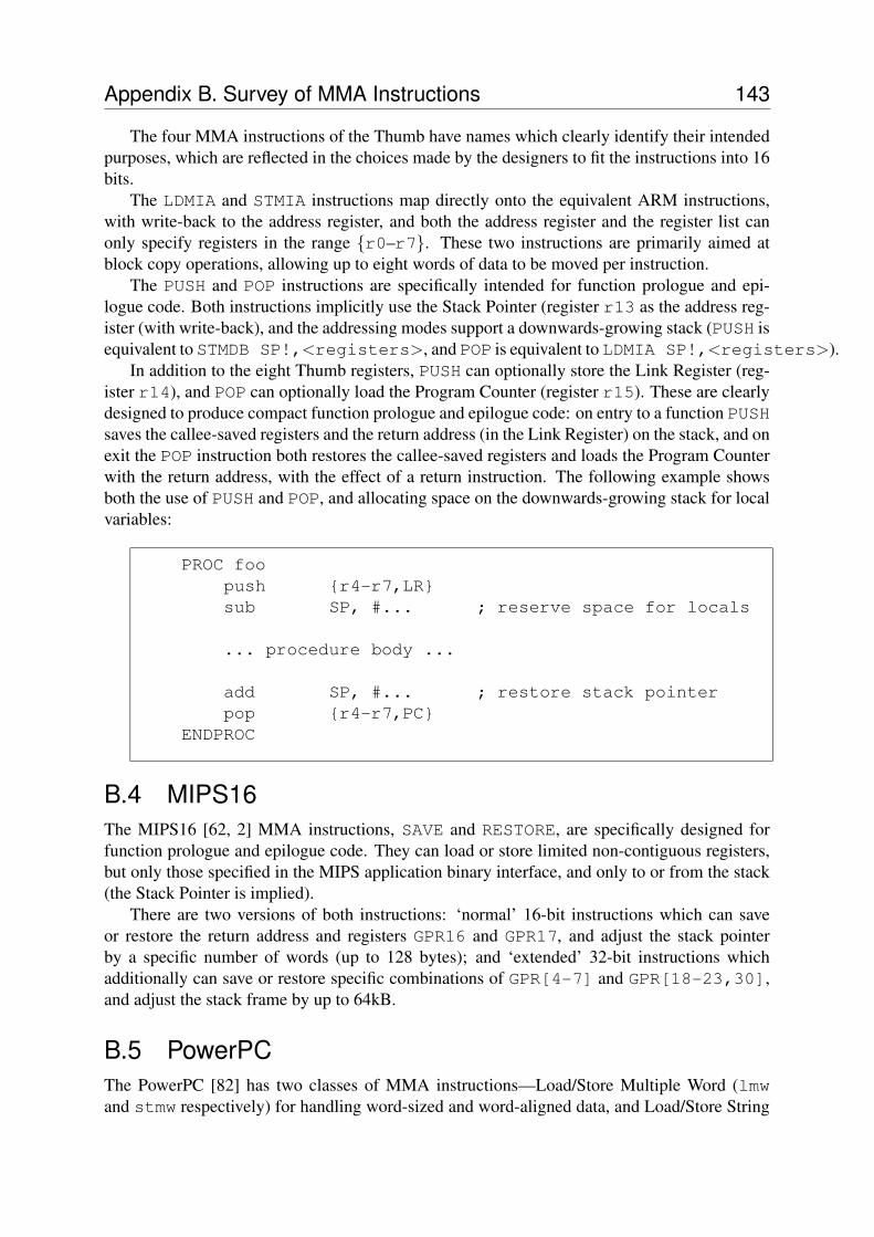
Appendix B. Survey of MMA Instructions 143
The four MMA instructions of the Thumb have names which clearly identify their intendedpurposes, which are reflected in the choices made by the designers to fit the instructions into 16bits.
The LDMIA and STMIA instructions map directly onto the equivalent ARM instructions,with write-back to the address register, and both the address register and the register list canonly specify registers in the range {r0–r7}. These two instructions are primarily aimed atblock copy operations, allowing up to eight words of data to be moved per instruction.
The PUSH and POP instructions are specifically intended for function prologue and epi-logue code. Both instructions implicitly use the Stack Pointer (register r13 as the address reg-ister (with write-back), and the addressing modes support a downwards-growing stack (PUSH isequivalent to STMDB SP!,<registers>, and POP is equivalent to LDMIA SP!,<registers>).
In addition to the eight Thumb registers, PUSH can optionally store the Link Register (reg-ister r14), and POP can optionally load the Program Counter (register r15). These are clearlydesigned to produce compact function prologue and epilogue code: on entry to a function PUSHsaves the callee-saved registers and the return address (in the Link Register) on the stack, and onexit the POP instruction both restores the callee-saved registers and loads the Program Counterwith the return address, with the effect of a return instruction. The following example showsboth the use of PUSH and POP, and allocating space on the downwards-growing stack for localvariables:
PROC foopush {r4-r7,LR}sub SP, #... ; reserve space for locals
... procedure body ...
add SP, #... ; restore stack pointerpop {r4-r7,PC}
ENDPROC
B.4 MIPS16The MIPS16 [62, 2] MMA instructions, SAVE and RESTORE, are specifically designed forfunction prologue and epilogue code. They can load or store limited non-contiguous registers,but only those specified in the MIPS application binary interface, and only to or from the stack(the Stack Pointer is implied).
There are two versions of both instructions: ‘normal’ 16-bit instructions which can saveor restore the return address and registers GPR16 and GPR17, and adjust the stack pointerby a specific number of words (up to 128 bytes); and ‘extended’ 32-bit instructions whichadditionally can save or restore specific combinations of GPR[4-7] and GPR[18-23,30],and adjust the stack frame by up to 64kB.
B.5 PowerPCThe PowerPC [82] has two classes of MMA instructions—Load/Store Multiple Word (lmwand stmw respectively) for handling word-sized and word-aligned data, and Load/Store String
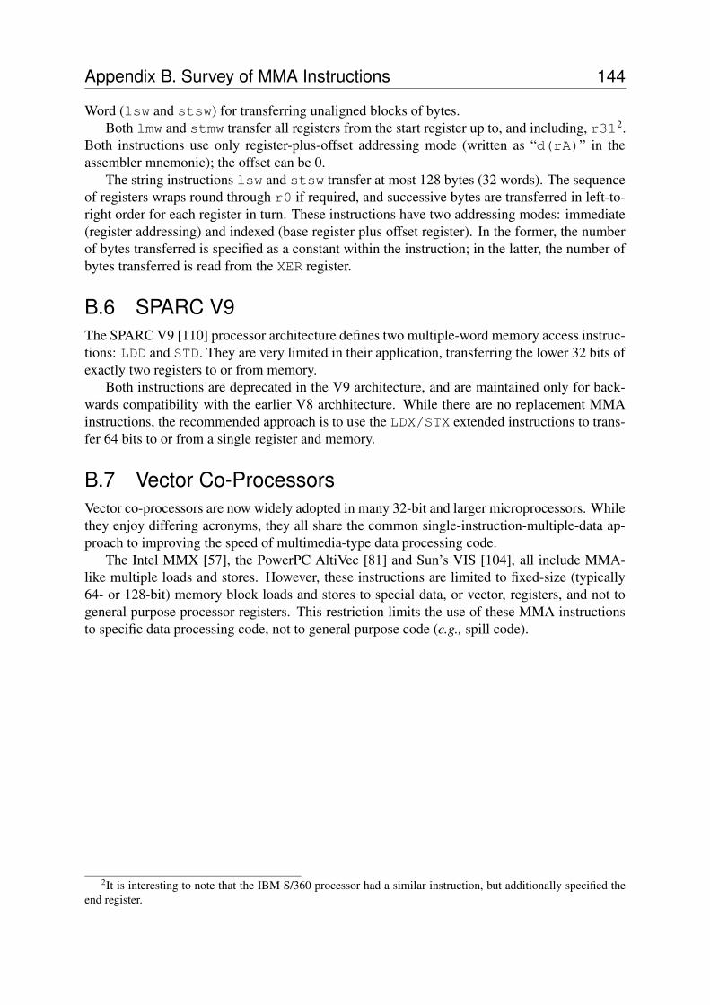
Appendix B. Survey of MMA Instructions 144
Word (lsw and stsw) for transferring unaligned blocks of bytes.Both lmw and stmw transfer all registers from the start register up to, and including, r312.
Both instructions use only register-plus-offset addressing mode (written as “d(rA)” in theassembler mnemonic); the offset can be 0.
The string instructions lsw and stsw transfer at most 128 bytes (32 words). The sequenceof registers wraps round through r0 if required, and successive bytes are transferred in left-to-right order for each register in turn. These instructions have two addressing modes: immediate(register addressing) and indexed (base register plus offset register). In the former, the numberof bytes transferred is specified as a constant within the instruction; in the latter, the number ofbytes transferred is read from the XER register.
B.6 SPARC V9The SPARC V9 [110] processor architecture defines two multiple-word memory access instruc-tions: LDD and STD. They are very limited in their application, transferring the lower 32 bits ofexactly two registers to or from memory.
Both instructions are deprecated in the V9 architecture, and are maintained only for back-wards compatibility with the earlier V8 archhitecture. While there are no replacement MMAinstructions, the recommended approach is to use the LDX/STX extended instructions to trans-fer 64 bits to or from a single register and memory.
B.7 Vector Co-ProcessorsVector co-processors are now widely adopted in many 32-bit and larger microprocessors. Whilethey enjoy differing acronyms, they all share the common single-instruction-multiple-data ap-proach to improving the speed of multimedia-type data processing code.
The Intel MMX [57], the PowerPC AltiVec [81] and Sun’s VIS [104], all include MMA-like multiple loads and stores. However, these instructions are limited to fixed-size (typically64- or 128-bit) memory block loads and stores to special data, or vector, registers, and not togeneral purpose processor registers. This restriction limits the use of these MMA instructionsto specific data processing code, not to general purpose code (e.g., spill code).
2It is interesting to note that the IBM S/360 processor had a similar instruction, but additionally specified theend register.
APPENDIX C
VSDG Tool Chain Reference
The VECC framework (Figure C.1) provides a complete toolset, including a C compiler, avariety of optimizers and analysis tools, and a Thumb target code generator.During processing, all intermediate files are stored as text files, either as files written to and
read from disk, or as Unix pipes. This allows experimentation with different optimizers and op-timization strategies through the use of shell scripts, simple textual analysis of the intermediatefiles, such as comments against specific instructions, and inspection and modification of inter-mediate files during testing and development. The format of the intermediate files is specifiedin Appendix A.
In addition to the command line flags described below, all of the VSDG tools may be in-voked with a -v (“verbose”) flag . This generates additional debugging and progress informa-tion to the standard error file1.
C.1 C CompilerThe experimental C compiler is based on Fraser and Hanson’s LCC compiler [42]. Our modifi-cations to the compiler are described in detail in Chapter 3. The compiler is invoked as
mlcc -S infile -o outfile
1Note that for non-trivial programs the amount of debugging information can be very large.
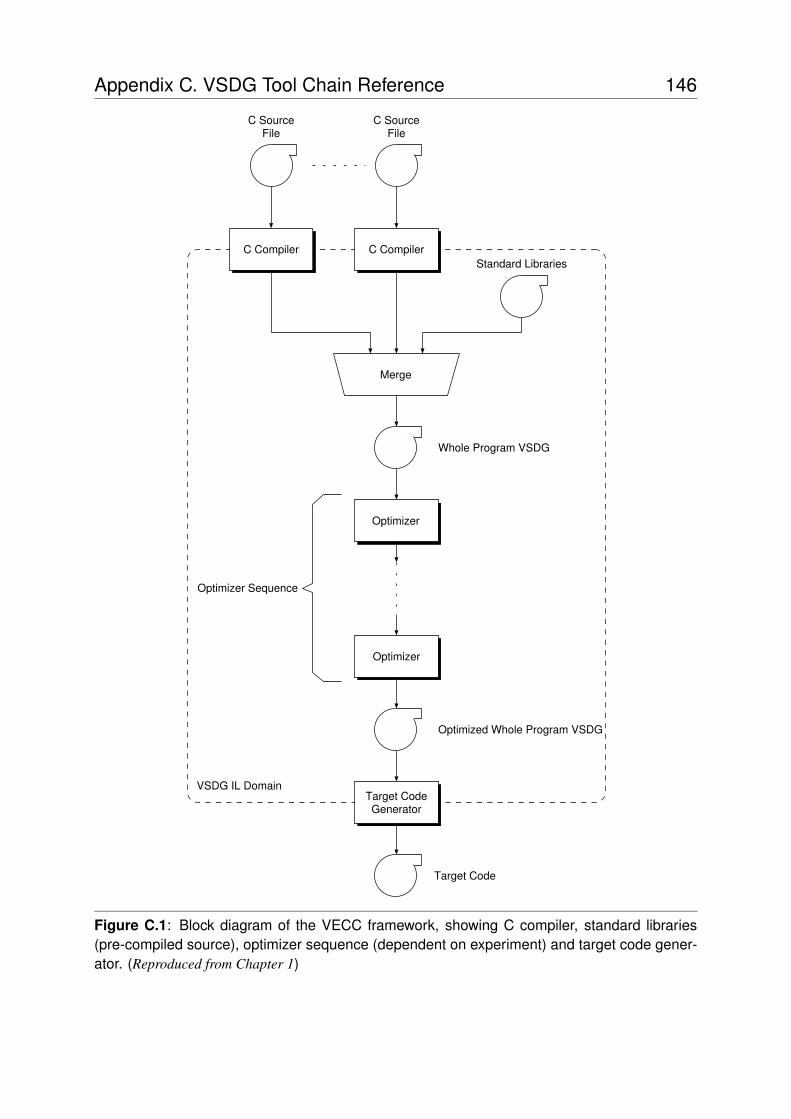
Appendix C. VSDG Tool Chain Reference 146
C SourceFile
Merge
C Compiler C CompilerStandard Libraries
C SourceFile
Whole Program VSDG
Optimizer
Optimizer
Optimized Whole Program VSDG
Target CodeGenerator
Target Code
VSDG IL Domain
Optimizer Sequence
Figure C.1: Block diagram of the VECC framework, showing C compiler, standard libraries(pre-compiled source), optimizer sequence (dependent on experiment) and target code gener-ator. (Reproduced from Chapter 1)
Appendix C. VSDG Tool Chain Reference 147
The “-S” flag specifies only the preprocessor and compiler proper (the other parts of the LCCcompiler are not used in this project). If outfile is “-” then the output of the compiler is redi-rected to the standard output. This is useful for piping the output of the compiler through, say,the classical optimizer:
mlcc -S foo.c -o - | vsdgopt -O D+ -o foo.vsdg
C.2 Classical OptimizerThe classical optimizer provides a framework for up to 26 individual optimizers (Chapter 3),each identified with a letter ‘A-Z’. An optimization command string is supplied as a commandline argument specifying which optimizations to apply, in what order, and whether a fixed-pointshould be reached before completion of any given pass (including nested passes). The optimizertool has the following command line invocation:
vsdgopt flags [infiles...] [-o outfile]
If no infiles are specified the tool reads from the standard input. Similarly, if no outfile isspecified the tool sends its output to the standard output.
Command Line Flags
-O sequence The string sequence specifies the sequence of optimization passesto be applied to the input.
The optimization sequence string consists of the letters ‘A-Z’, to invoke each of the 26possible optimizations, the ‘+’ operator to mark a pass that should be repeated until no furtherchanges (fixed point) have been made to the program, and ‘[...]’ to indicate substrings(which may also be specified with the fixed point operator). For example, the command string
AB+[C[D+E]+]+
applies optimization A, then B repeatedly until fixed point, then the substring “C[D+E]+” untilfixed point. The substring applies C, then substring “D+E” repeatedly until fixed point. Thissubstring, in turn, applies D repeatedly, until fixed point, and then a single application of E.
C.3 Procedural Abstraction OptimizerThe procedural abstraction optimizer tool applies procedural abstraction optimization (Chap-ter 4) to a VSDG. The procedural abstraction tool has the following command line invocation:
vsdgabs flags [infiles...] [-o outfile]
If no infiles are specified the tool reads from the standard input. Similarly, if no outfile isspecified the tool sends all output to the standard output.
Command Line Flags
Appendix C. VSDG Tool Chain Reference 148
--maxsize n n specifies the maximum number of nodes in a pattern (the defaultvalue is 6).
--showtable Dump the pattern table after it has finished processing the input.The table is sent on the standard error output, which can be redi-rected to a file for later analysis.
C.4 MMA OptimizerMMA optimization (Chapter 5) is performed by the MMA optimizer tool. It has the followingcommand line invocation:
vsdgmma flags [infiles...] [-o outfile]
If no infiles are specified the tool reads from the standard input. Similarly, if no outfile isspecified the tool sends all output to the standard output.
In addition to the output file, the MMA optimizer generates a file, ag.dot, which can bepost-processed by dot [67] to view the access graph constructed during analysis.
Command Line Flags
--maxtuples n n specifies the maximum number of loads or stores that may becombined into a single MMA instruction (the default value is 6).
--showalledges Show all edges in the access graph, not just the covered ones.--portrait Specify portrait page orientation of the access graph. This is the
default.--landscape Specify landscape page orientation of the access graph.
C.5 Register Allocator and Code SchedulerThe register allocation and code scheduling tool applies the RACM algorithm (Chapter 6) to aVSDG. The RACM tool has the following command line invocation:
vsdgracm flags [infiles...] [-o outfile]
If no infiles are specified the tool reads from the standard input. Similarly, if no outfile isspecified the tool sends all output to the standard output.
Command Line Flags
-r n n specifies the maximum number of registers available to the algo-rithm (the default value is 8).
C.6 Thumb Code GeneratorThe Thumb target code generator produces a Thumb assembler file from the supplied VSDGsource files. The code generator tool has the following command line invocation:
vsdg2thm flags [infiles...] [-o outfile]
Appendix C. VSDG Tool Chain Reference 149
If no infiles are specified the tool reads from the standard input. Similarly, if no outfile isspecified the tool sends all output to the standard output.
Command Line Flags
--dumpvsdg Dumps the scheduled and register-coloured VSDG to the standardoutput, which can be captured and processed with the vsdg2dottool.
C.7 Graphical Output GeneratorAs an aid to debugging and presenting VSDGs, the graphical output generator reads in VSDGsand emits a layout file suitable for the dot graph drawing tool [67]. The graphical generator toolhas the following command line invocation:
vsdg2dot flags [infiles...] [-o outfile]
If no infiles are specified the tool reads from the standard input. Similarly, if no outfile isspecified the tool sends all output to the standard output.
Command Line Flags
--noserial Turns off the plotting of serialising state-dependency edges.--showcut Forces the layout of nodes to reflect the depth from root as com-
puted from the graph, overriding the node placement algorithm ofdot.
The two-level module/function hierarchy is displayed, together with data and const memoryobjects. There are many examples of the output of this tool in this thesis (e.g., Figure 4.1,page 86).
C.8 Statistical AnalyserThe statistical analyser prints the total number of nodes, edges, arguments and return valuesfor each function, together with module-by-module node and edge totals, and overall node andedge totals. The statistical analyser has the following command line invocation:
vsdgstat flags [infiles...]
If no infiles are specified the tool reads from the standard input.
Command Line Flags
--summary Prints only the overall totals for nodes and edges.
Appendix C. VSDG Tool Chain Reference 150
Bibliography
[1] i486 Processor Programmer’s Reference Manual. Intel Corp./Osborne McGraw-Hill,San Francisco, CA, 1990.
[2] MIPS32 Architecture for Programmers Volume IV-a: The MIPS16e Application-SpecificExtension to the MIPS32 Architecture. MIPS Technologies, Inc, Mountain View, CA,2003.
[3] ABSINT ANGEWANDTE INFORMATIK GMBH. aiPop: Code Compaction forC16x/ST10. http://www.AbsInt.com.
[4] ACE ASSOCIATED COMPUTER EXPERTS BV. Product details available fromhttp://www.ace.nl/products/cosy.htm.
[5] AHO, A. V., HOPCROFT, J. E., AND ULLMAN, J. D. The Design and Analysis ofComputer Algorithms. Addison Wesley, 1974.
[6] AHO, A. V., SETHI, R., AND ULLMAN, J. D. Compilers: Principles, Techniques andTools. Addison Wesley, 1986.
[7] ALPERN, B., WEGMAN, M. N., AND ZADECK, F. K. Detecting Equality of Variables inPrograms. In Proc. Conf. Principles of Programming Languages (January 1988), vol. 10,ACM Press, pp. 1–11.
[8] APPEL, A. W. Compiling with Continuations. Cambridge University Press, Cambridge,UK, 1992.
[9] ARAUJO, G., CENTODUCATTE, P., CORTES, M., AND PANNAIN, R. Code Compres-sion Based on Operand Factorization. In Proc. of 31st Annual Intl. Symp. on Microarchi-tecture (MICRO’31) (December 1998), pp. 194–201.
[10] ASSMANN, U. Graph Rewrite Systems for Program Optimization. ACM Trans. Pro-gramming Languages and Systems 22, 4 (July 2000), 583–637.
[11] BACON, D. F., GRAHAM, S. L., AND SHARP, O. J. Compiler Transformations forHigh-Performance Computing. Tech. rep., University of California, Berkeley, CA, 1993.
BIBLIOGRAPHY 152
[12] BAKER, B. S. A Theory of Parameterized Pattern Matching: Algorithms and Applica-tions (Extended Abstract). In Proc. of the 25th Annual Symp. on Theory of Computing(San Diego, California, 1993), ACM Press, pp. 71–80.
[13] BAKER, B. S. Parameterized Pattern Matching by Boyer-Moore-type Algorithms. InProc. of the 6th ACM-SIAM Annual Symp. on Discrete Algorithms (San Francisco, Cali-fornia, 1995), ACM Press, pp. 541–550.
[14] BALLANCE, R. A., MACCABE, A. B., AND OTTENSTEIN, K. J. The Program Depen-dence Web: A Representation Supporting Control-, Data-, and Demand-Driven Interpre-tation of Imperative Languages. In Proc. ACM SIGPLAN Conf. on Prog. Lang. Designand Implementation (PLDI’90) (June 1990), ACM Press, pp. 257–271.
[15] BARTLEY, D. H. Optimizing Stack Frame Accesses for Processors with Restricted Ad-dressing Modes. Software—Practice and Experience 22, 2 (February 1992), 101–110.
[16] BAXTER, W., AND HENRY R. BAUER, III. The Program Dependence Graph and Vec-torization. In Proc. 16th ACM Symp. on the Principles of Programming Languages(POPL’89) (Austin, TX, January 1989), pp. 1–11.
[17] BERRY, G., AND GONTHIER, G. The Esterel Synchronous Programming Language:Design, Semantics, Implementation. Science of Computer Programming 19, 2 (1992),87–152.
[18] BERSON, D. A., GUPTA, R., AND SOFFA, M. L. Resource Spackling: A Frameworkfor Integrating Register Allocation in Local and Global Schedulers. Tech. rep., Dept.Computer Science, University of Pittsburgh, February 1994.
[19] BRANDIS, M. M., AND MOSSENBOCK, H.-P. Single-Pass Generation of Single StaticAssignment Form for Structured Languages. ACM Trans. Programming Languages andSystems 16, 6 (November 1994), 1684–1698.
[20] BRASIER, T. S., SWEANY, P. H., BEATY, S. J., AND CARR, S. CRAIG: A Prac-tical Framework for Combining Instruction Scheduling and Register Assignment. InProc. Intl. Conf. Parallel Architectures and Compilation Techniques (PACT’95) (Limas-sol, Cyprus, June 1995), V. Malyshkin, Ed., vol. 964 of Lecture Notes in Computer Sci-ence, Springer-Verlag.
[21] BRIGGS, P., COOPER, K. D., AND TORCZON, L. Rematerialization. In Proc. ACMSIGPLAN Conf. on Prog. Lang. Design and Implementation (PLDI’92) (New York, NY,1992), vol. 27, ACM Press, pp. 311–321.
[22] BRITISH STANDARDS INSTITUTE. The C Standard. John Wiley & Sons Ltd, 2003.
[23] CARTWRIGHT, R., AND FELLEISEN, M. The Semantics of Program Dependence. InProceedings of the ACM SIGPLAN’89 Conference on Programming Language Designand Implementation (Portland, OR, June 1989), vol. 24, pp. 13–27.
[24] CASPI, P., PILAUD, D., HALBWACHS, N., AND PLAICE, J. Lustre: A Declarative Lan-guage for Programming Synchronous Systems. In Proc. 14th ACM Conf. on Principlesof Programming Languages (POPL’87) (Munich, Germany, January 1987), ACM Press.
BIBLIOGRAPHY 153
[25] CHAITIN, G. Register Allocation and Spilling via Graph Coloring. ACM SIGPLANNotices 17, 6 (June 1982), 98–105.
[26] CHOW, F. C., AND HENNESSY, J. L. The Priority-Based Coloring Approach to RegisterAllocation. ACM Trans. Prog. Lang. and Syst. 12, 4 (October 1990), 501–536.
[27] CLICK, C., AND PALECZNY, M. A Simple Graph-Based Intermediate Language. InProc. ACM SIGPLAN Workshop on Intermediate Representations (IR’95) (San Fran-cisco, CA, January 1995), ACM Press.
[28] COCKE, J. Global Common Subexpression Elimination. In Proc. ACM Symp. on Com-piler Optimization (July 1970), vol. 7 of SIGPLAN Notices, pp. 20–24.
[29] COOPER, K. D., AND MCINTOSH, N. Enhanced Code Compression for EmbeddedRISC Processors. In Proc. ACM SIGPLAN Conf. on Prog. Lang. Design and Implemen-tation (PLDI’99) (May 1999), vol. 34, ACM Press, pp. 139–149.
[30] CYTRON, R., FERRANTE, J., AND SARKAR, V. Compact representations for controldependence. In Proc. of the ACM SIGPLAN Conf. on Prog. Lang. Design and Implemen-tation (1990), ACM Press, pp. 337–351.
[31] CYTRON, R. K., AND FERRANTE, J. Efficiently computing nodes φ-nodes on-the-fly.ACM Trans. Programming Languages and Systems 17, 3 (May 1995), 487–506.
[32] CYTRON, R. K., FERRANTE, J., ROSEN, B. K., WEGMAN, M. N., AND ZADECK,F. K. An efficient method of computing the static single assignment form. In Proc. ACMSymp. Principles of Programming Languages (POPL’89) (January 1989), ACM Press,pp. 25–35.
[33] CYTRON, R. K., FERRANTE, J., ROSEN, B. K., WEGMAN, M. N., AND ZADECK,F. K. Efficiently Computing the Static Single Assignment Form and the Control Depen-dence Graph. ACM Trans. Programming Languages and Systems 12, 4 (October 1991),451–490.
[34] DE BUS, B., KASTNER, D., CHANET, D., VAN PUT, L., AND DE SUTTER, B. Post-Pass Compaction Techniques. Comm. ACM 46, 8 (August 2003), 41–46.
[35] DE SUTTER, B., DE BUS, B., AND DE BOSSCHERE, K. Sifting out the Mud: LowLevel C++ Code Reuse. In Proc. ACM Conf Object Oriented Programming, Sys-tems, Languages and Applications (OOPSLA’02) (Seattle, Washington, USA, November2002), pp. 275–291.
[36] DEBRAY, S. K., EVANS, W., MUTH, R., AND DE SUTTER, B. Compiler Techniquesfor Code Compaction. ACM Trans. Programming Languages and Systems 22, 2 (March2000), 378–415.
[37] DUFF, T. Duff’s Device. Webpage summarising Duff’s Device can be found athttp://www.lysator.liu.se/c/duffs-device.html.
[38] FARNUM, C. Compiler Support for Floating-point Computation. Software—Practiceand Experience 18, 7 (July 1988), 701–709.
BIBLIOGRAPHY 154
[39] FERRANTE, J., OTTENSTEIN, K. J., AND WARREN, J. D. The program dependencegraph and its use in optimization. ACM Trans. Prog. Lang. and Syst. 9, 3 (July 1987),319–349.
[40] FISHER, R. J., AND DIETZ, H. G. Compiling For SIMD Within A Register. In Proc.11th Annual Workshop on Languages and Compilers for Parallel Computing (LCPC’98)(August 1998), vol. 1656 of LNCS (Springer-Verlag), pp. 290–304.
[41] FRANKAU, S., AND MYCROFT, A. Stream Processing Hardware from Functional Lan-guage Specifications. In Proc. 36th Hawaii Intl. Conf. on Systems Sciences (HICSS-36)(Big Island, Hawaii, January 2003), IEEE.
[42] FRASER, C. W., AND HANSON, D. R. A Retargetable C Compiler: Design and Imple-mentation. Benjamin/Cummings, 1995.
[43] FRASER, C. W., MYERS, E. W., AND WENDT, A. L. Analyzing and CompressingAssembly Code. In Proc. ACM SIGPLAN Symp. Compiler Construction (June 1984),vol. 19, ACM Press, pp. 117–121.
[44] FRASER, C. W., AND PROEBSTING, T. A. Custom Instruction Sets for Code Compres-sion. http://research.microsoft.com/˜toddpro, October 1995.
[45] GAREY, M., AND JOHNSON, D. The Complexity of Near-Optimal Graph Coloring.J. ACM 23, 1 (January 1976), 43–49.
[46] GAREY, M. R., AND JOHNSON, D. S. Computers and Intractability—A Guide to theTheory of NP-Completeness. W. H. Freeman, New York, 1979.
[47] GIEGERICH, R., AND KURTZ, S. From Ukkonen to McCreight and Weiner: A unifyingview of linear-time suffix tree construction. Algorithmica 19 (1997), 331–353.
[48] GIRKAR, M., AND POLYCHRONOPOULOS, C. D. Automatic Extraction of FunctionalParallelism from Ordinary Programs. IEEE Trans. Parallel and Distributed Systems 3, 2(March 1992), 166–178.
[49] GOLDBERG, D. What every computer scientist should know about floating-point arith-metic. In ACM Computing Surveys (1991), ACM Press.
[50] GOODWIN, D. W., AND WILKEN, K. D. Optimal and Near-optimal Global RegisterAllocation Using 0-1 Integer Programming. Software—Practice and Experience 26, 8(August 1996), 929–965.
[51] GRUNE, D., BAL, H. E., JACOBS, C. J. H., AND LANGENDOEN, K. G. ModernCompiler Design. John Wiley & Sons Ltd, Chichester, England, 2000.
[52] GUPTA, S., DUTT, N., GUPTA, R., AND NICOLAU, A. SPARK : A High-Level Synthe-sis Framework For Applying Parallelizing Compiler Transformations. In Proc. Intl Conf.on VLSI Design (January 2003).
BIBLIOGRAPHY 155
[53] HAVLAK, P. Construction of thinned gated single-assignment form. In Proc. SixthWorkshop on Languages and Compilers for Parallel Computing (Portland, Ore., August1993), U. Banerjee, D. Gelernter, A. Nicolau, and D. Padua, Eds., no. 768 in LectureNotes in Computer Science, Springer Verlag, pp. 477–499.
[54] HORSPOOL, R. N., AND HO, H. C. Partial Redundancy Elimination Driven by a Cost-Benefit Analysis. In Proc. 8th Israli Conf. on Computer Systems Engineering (ICSSE’97)(Herzliya, Israel, June 1997), IEEE Computer Society, pp. 111–118.
[55] HORWITZ, S., PRINS, J., AND REPS, T. On the Adequacy of Program DependenceGraphs for Representing Programs. In Proc. Fifteenth Annual ACM Symp. on Principlesof Programming Languages (San Diego, California, 1988), pp. 146–157.
[56] HORWITZ, S., REPS, T., AND BINKLEY, D. Interprocedural Slicing Using DependenceGraphs. ACM Trans. Prog. Langs and Systems 12, 1 (January 1990), 26–60.
[57] INTEL. Intel Architecture Software Developer’s Manual vol. 2. Intel, 1999.
[58] JANSSEN, J., AND CORPORAAL, H. Making Graphs Reducible with Controlled NodeSplitting. ACM Trans. Prog. Lang. and Systems 19, 6 (November 1997), 1031–1052.
[59] JANSSEN, J., AND CORPORAAL, H. Registers on Demand: An Integrated RegionScheduler and Register Allocator. In Proc. Conf. on Compiler Construction (April 1998).
[60] JOHNSON, N., AND MYCROFT, A. Combined Code Motion and Register Allocationusing the Value State Dependence Graph. In Proc. 12th Intl. Conf. on Compiler Con-struction (CC’03) (April 2003), vol. 2622 of LNCS, pp. 1–16.
[61] KERNIGHAN, B. W., AND RITCHIE, D. M. The C Programming Language, 2nd ed.Prentice Hall, 1988.
[62] KISSELL, K. MIPS16: High-density MIPS for the Embedded Market. In Proc. Conf.Real Time Systems (RTS’97) (1997).
[63] KNOOP, J., RUTHING, O., AND STEFFEN, B. Lazy Code Motion. In Proc. ACMSIGPLAN Conf. on Prog. Lang. Design and Implementation (PLDI’92) (1992), pp. 224–234.
[64] KNUTH, D. The Art of Computer Programming, Volume 3: Sorting and Searching.Addison-Wesley, 1998.
[65] KNUTH, D. E. An Empirical Study of FORTRAN Programs. Software—Practice andExperience 1, 2 (April–June 1971), 105–133.
[66] KOSEKI, A., KOMATSU, H., AND NAKATANI, T. Preference-Directed Graph Coloring.In Proc. ACM SIGPLAN 2002 Conference on Prog. Lang. Design and Implementation(June 2002), ACM Press, pp. 33–44.
[67] KOUTSOFIOS, E., AND NORTH, S. C. Drawings graphs with dot. Tech. rep., AT & TBell Laboratories, Murray Hill, NJ, October 1993.
BIBLIOGRAPHY 156
[68] LEE, C., POTKONJAK, M., AND MANGIONE-SMITH, W. H. Mediabench: A Tool forEvaluating and Synthesizing Multimedia and Communications Systems. In Proc. 30thIntl. Symp. Microarchitectures (MICRO’30) (December 1997), ACM/IEEE, pp. 330–335.
[69] LEFURGY, C., BIRD, P., CHEN, I.-C., AND MUDGE, T. Improving Code Density usingCompression Techniques. Tech. Rep. CSE-TR-342-97, EECS Department, University ofMichigan, Ann Arbor, MI, 1997.
[70] LEUPERS, R., AND MARWEDEL, P. Algorithms for Address Assignment in DSPCode Generation. In Proceedings of the 1996 IEEE/ACM International Conference onComputer-Aided Design (1996), IEEE Computer Society Press, pp. 109–112.
[71] LEVINE, J. R., MASON, T., AND BROWN, D. Lex and Yacc. O’Reilly & Associates,Inc., 1992.
[72] LIAO, S., DEVADAS, S., KEUTZER, K., TJIANG, S., AND WANG, A. Storage Assign-ment to Decrease Code Size. In Proceedings of the ACM SIGPLAN 1995 conference onProgramming Language Design and Implementation (June 1995), ACM Press, pp. 186–195.
[73] LIAO, S., TIJANG, S., AND GUPTA, R. An Efficient Implementation of Reactivity forModeling Hardware in the Scenic Design Environment. In Proc. Design AutomationConference (DAC’97) (Anaheim, California, USA, June 1997), pp. 70–75.
[74] LIAO, S. Y.-H. Code Generation for Embedded Digital Signal Processors. PhD thesis,Massachusetts Institute of Technology, June 1996.
[75] LIM, S., KIM, J., AND CHOI, K. Scheduling-based Code Size Reduction in Proces-sors with Indirect Addressing Mode. In Proc. Ninth Intl. Symp. on Hardware/SoftwareCodesign (CODES 2001) (April 2001), pp. 165–169.
[76] MARKS, B. Compilation to Compact Code. IBM J. Research and Development 22, 6(November 1980), 684–691.
[77] MCCREIGHT, E. A space-economical suffix tree construction algorithm. J. ACM 23, 2(April 1976), 262–272.
[78] MILNER, R. Communication and Concurrency. Computer Science. Prentice Hall Intl.,1989.
[79] MOORE, G. E. Cramming more components onto integrated circuits. Electronics 38, 8(April 1965).
[80] MOREL, E., AND RENVOISE, C. Global optimization by suppression of partial redun-dancies. Comm. ACM 22, 2 (February 1979), 96–103.
[81] MOTOROLA INC. AltiVec Technology Programming Interface Manual. No. AL-TIVECPIM/D. Motorola Inc, 1999.
[82] MOTOROLA, INC. Programming Environments Manual For 32-Bit Implementations ofthe PowerPC Architecture. Motorola, Inc., 2001.
BIBLIOGRAPHY 157
[83] MUCHNICK, S. S. Advanced Compiler Design and Implementation. Morgan KaufmannPublishers, San Francisco, CA, 1997.
[84] MUTH, R. ALTO: A Platform for Object Code Modification. PhD thesis, Dept. ComputerScience, University of Arizona, 1999.
[85] MYCROFT, A., AND SHARP, R. A Statically Allocated Parallel Functional Language. InProc. Intl Conf. on Automata, Languages and Programming (2000), no. 1853 in LNCS,Springer-Verlag.
[86] PADUA, D. A., AND WOLFE, M. J. Advanced Compiler Optimizations for Supercom-puters. Comm. ACM 29, 12 (December 1986), 1184–1201.
[87] PAGE, I. Constructing Hardware-Software Systems from a Single Description. J. VLSISignal Processing 12, 1 (1996), 87–107.
[88] PINTER, S. S. Register Allocation with Instruction Scheduling: A New Approach. InProc. ACM SIGPLAN Conference on Prog. Lang. Design and Implementation (Albu-querque, NM, June 1993), pp. 248–257.
[89] PLAUGER, P. The Standard C Library. Prentice Hall, 1992.
[90] PROEBSTING, T. Proebsting’s law. May be accessed from the websitehttp://research.microsoft.com/∼toddpro/papers/law.htm, May1999.
[91] RAO, A., AND PANDE, S. Storage Assignment Optimizations to Generate Compactand Efficient Code on Embedded DSPs. In Proc. ACM SIGPLAN Conf. on Prog. Lang.Design and Implementation (1999), ACM Press, pp. 128–138.
[92] RAO, M. P. Combining register assignment and instruction scheduling. Master’s thesis,Michigan Technological University, 1998.
[93] RICHARDS, M. Compact Target Code Design for Interpretation and Just-in-Time Com-pilation. (unpublished).
[94] ROSEN, B. K., WEGMAN, M. N., AND ZADECK, F. K. Global Value Numbers andRedundant Computations. In Proc. ACM SIGPLAN Conf. Principles of Prog. Langs(POPL’88) (January 1988), vol. 10, ACM Press, pp. 12–27.
[95] RUNESON, J. Code Compression Through Procedural Abstraction Before Register Al-location. Master’s thesis, Computer Science Department, Uppsala University, 2000.
[96] RUTHING, O., KNOOP, J., AND STEFFEN, B. Sparse code motion. In Proc. 27th ACMSIGPLAN-SIGACT Symp. Principles of Prog. Langs (POPL) (Boston, MA, 2000), ACMPress, pp. 170–183.
[97] SEAL, D. ARM Architecture Reference Manual. Addison-Wesley, UK, 2000.
[98] SELKE, R. P. A Rewriting Semantics for Program Dependence Graphs. In Proc. ACMSymp. Principles of Programming Languages (January 1989), ACM Press, pp. 12–24.
BIBLIOGRAPHY 158
[99] SETHI, R., AND ULLMAN, J. D. The Generation of Optimal Code for Arithmetic Ex-pressions. J. ACM 17, 4 (October 1970), 715–728.
[100] SHARMA, N., AND GUPTA, S. K. Optimal Stack Slot Assignment in GCC. In Proc.GCC Developers Summit (May 2003), pp. 223–228.
[101] SHARP, R., AND MYCROFT, A. A Higher-Level Language for Hardware Synthesis. InProc. 11th Advanced Research Working Conf. on Correct Hardware Design and Verifi-cation Methods (2001), no. 2144 in LNCS, Springer-Verlag.
[102] STORER, J., AND SZYMANSKI, T. Data Compression via Textual Substitution. J. ACM49, 4 (October 1982), 928–951.
[103] SUDARSANAM, A., LIAO, S., AND DEVADAS, S. Analysis and Evaluation of AddressArithmetic Capabilities in Custom DSP Architectures. In Proceedings of the 34th AnnualDesign Automation Conference (1997), ACM Press, pp. 287–292.
[104] SUN MICROSYSTEMS. VIS Instruction Set User’s Manual. No. 805-1394-03. Sun Mi-crosystems, May 2001.
[105] SWEANY, P., AND BEATY, S. Post-Compaction Register Assignment in a RetargetableCompiler. In Proc. 23rd Annual Workshop on Microprogramming and Microarchitecture(November 1990), pp. 107–116.
[106] TOUATI, S.-A.-A. Register Pressure in Instruction Level Parallelism. PhD thesis, Uni-versite de Versailles Saint-Quentin, June 2002.
[107] UDAYANARAYANAN, S., AND CHAKRABARTI, C. Address Code Generation for DigitalSignal Processors. In Proceedings of the 38th Conference on Design Automation (2001),ACM Press, pp. 353–358.
[108] UPTON, E. Optimal Sequentialization of Gated Data Dependence Graphs is NP-Complete. In Proc. 2003 Intl. Conf. on Parallel and Distributed Processing Techniquesand Applications (PDPTA’03) (June 2003), CSREA Press.
[109] USAF. MIL-STD-1750A: SIXTEEN-BIT COMPUTER INSTRUCTION SET ARCHI-TECTURE, 1980.
[110] WEAVER, D. L., AND GERMOND, T. The SPARC Architecture Manual (version 9).SPARC International, Inc, Santa Clara, CA, 2000.
[111] WEINER, P. Linear pattern matching algorithms. In Proc. 14th IEEE Annual Symp. onSwitching and Automata Theory (1973), IEEE, pp. 1–11.
[112] WEISE, D., CREW, R. F., ERNST, M., AND STEENSGAARD, B. Value DependenceGraphs: Representation Without Taxation. In ACM SIGPLAN-SIGACT Symp. on Princi-ples of Prog. Langs (POPL) (January 1994), ACM Press.
[113] WIRTH, N. The Programming Language PASCAL. Acta Informatica 1 (1971), 35–63.
[114] WULF, W., JOHNSSON, R. K., WEINSTOCK, C. B., HOBBS, S. O., AND GESCHKE,C. M. The Design of an Optimizing Compiler. Elsevier Computer Science Library, 1975.

BIBLIOGRAPHY 159
[115] ZASTRE, M. J. Compacting Object Code via Parameterized Procedural Abstraction.Master’s thesis, Department of Computer Science, University of Victoria, Canada, 1995.
Related Documents