PILOT ANALYSIS OF GLOBAL ECOSYSTEMS Coastal Ecosystems LAURETT A BURKE YUMIKO KURA KEN K ASSEM CARMEN REVENGA MARK SPALDING DON M CALLISTER

Welcome message from author
This document is posted to help you gain knowledge. Please leave a comment to let me know what you think about it! Share it to your friends and learn new things together.
Transcript
P I L O T A N A L Y S I S O F G L O B A L E C O S Y S T E M S
CoastalEcosystems
LAURETT A BURKE
YUMIKO KURA
KEN K ASSEM
CARMEN REVENGA
MARK SPALDING
DON M CALLISTER
CAROL ROSEN
PUBLICATIONS DIRECTOR
HYACINTH BILLINGS
PRODUCTION MANAGER
MAGGIE POWELL
COVER DESIGN AND LAYOUT
CAROLL YNE HUTTER
EDITING
Copyright © 2001 World Resources Institute. All rights reserved.ISBN: 1-56973-458-5
Library of Congress Catalog Card No. 2001088657
Printed in the United States of America on chlorine-free paper withrecycled content of 50%, 20% of which is post-consumer.
Photo Credits: Cover: Digital Vision, Ltd., Smaller ecosystem photos: Forests: Digital Vision, Ltd.,Agriculture: Viet Nam, IFPRI Photo/P. Berry, Grasslands: PhotoDisc, Freshwater: Dennis A. Wentz,Coastal: Digital Vision, Ltd., Extent and Change: Patuxent River, Maryland/NOAA, ShorelineStabilization: Georgetown, Guyana/L. Burke, Water Quality: Noctiluca bloom, California/P.J.S.Franks, Scripps Institution of Oceanography, Biodiversity: Caribbean Sea/NOAA, Marine Fisheries:NOAA, Tourism: Bunaken, North Sulawesi, Indonesia/L. Burke.
Each World Resources Institute Report represents a timely, scholarly treat-ment of a subject of public concern. WRI takes responsibility for choosingthe study topics and guaranteeing its authors and researchers freedom of
inquiry. It also solicits and responds to the guidance of advisory panels and expertreviewers. Unless otherwise stated, however, all the interpretation and findings setforth in WRI publications are those of the authors.
P i l o t A n a l y s i s o f G l o b a l E c o s y s t e m s
CoastalEcosystems
LAURETT A BURKE –WRI
YUMIKO KURA–WRI
KEN K ASSEM –WRI
CARMEN REVENGA –WRI
MARK SPALDING –UNEP-WCMC
DON M CALLISTER –OCEAN V OICE I NTERNA TIONAL
With analytical contributions from:John Caddy, Luca Garibaldi, and Richard Grainger, FAO FisheriesDepartment: trophic analysis of marine fisheries;
Jaime Baquero, Gary Spiller, and Robert Cambell, Ocean Voice Interna-tional: distribution of known trawling grounds;
Lorin Pruett, Hal Palmer, and Joe Cimino, Veridian-MRJ TechnologySolutions: area of maritime zones and coastline length.
Published by World Resources InstituteWashington, DC
This report is also available at http://www.wri.org/wr2000
iv P I L O T A N A L Y S I S O F G L O B A L E C O S Y S T E M S
Pilot Analysis ofGlobal Ecosystems (PAGE)
A series of five technical reports, available in print and on-line athttp://www.wri.org/wr2000.
AGROECOSYSTEMSStanley Wood, Kate Sebastian, and Sara J. Scherr, Pilot Analysis of Global Ecosystems:
Agroecosystems, A joint study by International Food Policy Research Institute and World
Resources Institute, International Food Policy Research Institute and World Resources Institute,
Washington D.C.
December 2000 / paperback / ISBN 1-56973-457-7 / US$20.00
COASTAL ECOSYSTEMSLauretta Burke, Yumiko Kura, Ken Kassem, Carmen Revenga, Mark Spalding, and
Don McAllister, Pilot Analysis of Global Ecosystems: Coastal Ecosystems, World Resources
Institute, Washington D.C.
April 2001 / paperback / ISBN 1-56973-458-5 / US$20.00
FOREST ECOSYSTEMSEmily Matthews, Richard Payne, Mark Rohweder, and Siobhan Murray, Pilot Analysis
of Global Ecosystems: Forest Ecosystems, World Resources Institute, Washington D.C.
December 2000 / paperback / ISBN 1-56973-459-3 / US$20.00
FRESHWATER SYSTEMSCarmen Revenga, Jake Brunner, Norbert Henninger, Ken Kassem, and Richard Payne
Pilot Analysis of Global Ecosystems: Freshwater Systems, World Resources Institute,
Washington D.C.
October 2000 / paperback / ISBN 1-56973-460-7 / US$20.00
GRASSLAND ECOSYSTEMSRobin White, Siobhan Murray, and Mark Rohweder, Pilot Analysis of Global Ecosystems:
Grassland Ecosystems, World Resources Institute, Washington D.C.
December 2000 / paperback / ISBN 1-56973-461-5 / US$20.00
The full text of each report will be available on-line at the time of publication. Printedcopies may be ordered by mail from WRI Publications, P.O. Box 4852, HampdenStation, Baltimore, MD 21211, USA. To order by phone, call 1-800-822-0504 (withinthe United States) or 410-516-6963 or by fax 410-516-6998. Orders may also beplaced on-line at http://www.wristore.com.
The agroecosystem report is also available at http://www.ifpri.org. Printed copies maybe ordered by mail from the International Food Policy Research Institute, Communica-tions Service, 2033 K Street, NW, Washington, D.C. 20006-5670, USA.
Project ManagementNorbert Henninger, WRI
Walt Reid, WRI
Dan Tunstall, WRI
Valerie Thompson, WRI
Arwen Gloege, WRI
Elsie Velez-Whited, WRI
AgroecosystemsStanley Wood, International Food
Policy Research Institute
Kate Sebastian, International FoodPolicy Research Institute
Sara J. Scherr, University ofMaryland
Coastal EcosystemsLauretta Burke, WRI
Yumiko Kura, WRI
Ken Kassem, WRI
Carmen Revenga, WRI
Mark Spalding, UNEP-WCMC
Don McAllister, Ocean VoiceInternational
Forest EcosystemsEmily Matthews, WRI
Richard Payne, WRI
Mark Rohweder, WRI
Siobhan Murray, WRI
Freshwater SystemsCarmen Revenga, WRI
Jake Brunner, WRI
Norbert Henninger, WRI
Ken Kassem, WRI
Richard Payne, WRI
Grassland EcosystemsRobin White, WRI
Siobhan Murray, WRI
Mark Rohweder, WRI
C o a s t a l E c o s y s t e m s v
Contents
FOREWORD ................................................................................................................................................................................................... ix
ACKNOWLEDGEMENTS ............................................................................................................................................................................. xi
INTRODUCTION TO THE PILOT ANALYSIS OF GLOBAL ECOSYSTEMS ................................................................ Introduction/1
COASTAL ECOSYSTEMS: EXECUTIVE SUMMARY .............................................................................................................................. 1
Scope of the AnalysisKey Findings and Information Issues
Conclusions
COASTAL ZONE: EXTENT AND CHANGE ............................................................................................................................................. 11
Working Definition of Coastal ZoneEstimating Area and Length of Coastal ZoneCharacterizing the Natural Coastal FeaturesExtent and Change in Area of Selected Coastal Ecosystem TypesHuman Modification of Coastal Ecosystems
Information Status and Needs
SHORELINE STABILIZATION ................................................................................................................................................................... 25
Importance of Shoreline StabilizationEffects of Artificial Structures on the ShorelineCondition of Shoreline Stabilization ServicesCapacity of Coastal Ecosystems to Continue to Provide Shoreline Stabilization
Information Status and Needs
WATER QUALITY ......................................................................................................................................................................................... 31
Coastal Water QualityCondition of Coastal WatersCapacity of Coastal Ecosystems to Continue to Provide Clean Water
Information Status and Needs
BIODIVERSITY ............................................................................................................................................................................................. 39
Importance of BiodiversityDiversity of Coastal EcosystemsCondition of Coastal and Marine BiodiversityCapacity of Coastal Ecosystems to Sustain Biodiversity
Information Status and Needs
vi P I L O T A N A L Y S I S O F G L O B A L E C O S Y S T E M S
FOOD PRODUCTION—MARINE FISHERIES ....................................................................................................................................... 51
Importance of Marine Fisheries ProductionStatus and Trends in Marine Fisheries ProductionPressures on Marine Fishery ResourcesCondition of Marine Fisheries ResourcesCapacity of Coastal and Marine Ecosystems to Continue to Provide FishInformation Status and Needs
TOURISM AND RECREATION .................................................................................................................................................................. 63
Growth of Global TourismStatus and Trends of Tourism in the CaribbeanImpacts of Tourism on the Environment and the EconomyTourism Carrying CapacitySustainable TourismThe Role of Protected AreasInformation Status and Needs
TABLES
Table 1. Coastal Environments ............................................................................................................................................................ 11Table 2. Coastal Zone Statistics by Country .................................................................................................................................. 14–15Table 3. Coastal Characterization Summary ........................................................................................................................................ 16Table 4. Mangrove Area by Country .................................................................................................................................................... 18Table 5. Mangrove Loss for Selected Countries ................................................................................................................................... 19Table 6. Coastal Wetland Extent and Loss for Selected Countries ....................................................................................................... 20Table 7. Comparison of Two Coral Reef Area Estimates ...................................................................................................................... 21Table 8. Coastal Population Estimates for 1990 and 1995 .................................................................................................................. 23Table 9. Average Beach Profile Change in Selected Eastern Caribbean Islands ................................................................................. 27Table 10. Number of Known Littoral Species for Selected Species Groups ........................................................................................... 41Table 11. Number of Known Marine Species for Selected Species Groups ........................................................................................... 42Table 12. Threatened Littoral Species ................................................................................................................................................... 44Table 13. Threatened Marine Species ............................................................................................................................................. 46–47Table 14. Level of Threats to Coral Reefs Summarized by Region and Country .................................................................................... 48Table 15. Number of Invasive Species in the Mediterranean, Baltic Sea, and Australian Waters .......................................................... 50Table 16. Comparison of Maximum Landings to 1997 Landings by Fishing Area ................................................................................. 53Table 17. State of Exploitation and Discards by Major Fishing Area .................................................................................................... 54Table 18. Trophic Categories ................................................................................................................................................................. 56Table 19. Tourist Arrivals in the Caribbean by Main Markets ............................................................................................................... 64Table 20. Leakages of Gross Tourism Expenditures .............................................................................................................................. 67
FIGURES
Figure 1. UNEP Regional Seas ............................................................................................................................................................. 13Figure 2. Natural versus Altered Land Cover Summary ........................................................................................................................ 22Figure 3. Number of Oil Spills .............................................................................................................................................................. 34Figure 4. Total Quantity of Oil Spilled .................................................................................................................................................. 35Figure 5. Number of Harmful Algal Bloom Events: 1970s–1990s ........................................................................................................ 36Figure 6. Growth in Number of Marine Protected Areas over the Last 100 Years ................................................................................. 43Figure 7. Pelagic and Demersal Fish Catch for the North Atlantic: 1950–1997 ................................................................................... 52Figure 8. Commercial Harvest of Important Fish Stocks in the Northwest Atlantic .............................................................................. 55Figure 9. Catches by Trophic Level for the Two Northern Atlantic Fishing Areas in 1950–54 and 1993–97 ....................................... 57Figure 10. Piscivore/Zooplanktivore (PS/ZP) Ratio for the Northwest Atlantic ....................................................................................... 58Figure 11. PS/ZP Ratio for the Mediterranean and the Black Sea .......................................................................................................... 59Figure 12. PS/ZP Ratio for the Northwest Pacific ................................................................................................................................... 60Figure 13. Catches by Trophic Level for the Northeast Pacific Fishing Areas in 1950–54 and 1993–97 ............................................... 60Figure 14. Travel and Tourism GDP in the Caribbean ............................................................................................................................ 64Figure 15. Travel and Tourism Employment in the Caribbean ................................................................................................................ 65Figure 16. Per Capita GDP and Tourism as Percentage of GDP for Selected Countries in the Caribbean .............................................. 66
C o a s t a l E c o s y s t e m s vii
BOXES
Box 1. Maritime Areas Definitions ................................................................................................................................................... 12Box 2. Global Distribution of Known Trawling Grounds ................................................................................................................... 23Box 3. Coral Bleaching ..................................................................................................................................................................... 47Box 4. Classification of Catch Data into Trophic Categories ............................................................................................................. 56Box 5. Voluntary Guidelines for Sustainable Coastal Tourism Development in Quintana Roo, Mexico ............................................ 69
MAPS
Map 1. Characterization of Natural Coastal FeaturesMap 2. Natural versus Altered Land Cover within 100 km of CoastlineMap 3. Population Distribution within 100 km of CoastlineMap 4. Distribution of Known Trawling GroundsMap 5. Low-lying Areas within 100 km of CoastlineMap 6. Eutrophication-related ParametersMap 7. PCB Concentration in Mussels in the U.S. Coastal Waters: 1986–1996Map 8. Global Occurrence of Hypoxic ZonesMap 9. Shellfish Bed Closures in the Northeast U.S.: 1995Map 10. Beach Tar Ball Observations in Japan: 1975–1995Map 11. Global Distribution and Species Richness of Pinnipeds and Marine TurtlesMap 12. Global Distribution of Mangrove DiversityMap 13. Global Distribution of Coral DiversityMap 14. Distribution of Coral Bleaching Events and Sea Surface Temperature Anomaly Hot Spots, 1997–1998Map 15. Threatened Marine Important Bird Areas in Middle EastMap 16. Major Observed Threats to Coral ReefsMap 17. Period of Peak Fish Catch and Percent Decline Since the Peak YearMap 18. Piscivore and Zooplanktivore Catch Trend: 1950–97
REFERENCES ............................................................................................................................................................................................... 71
C o a s t a l E c o s y s t e m s ix
food and timber, the study also analyzes the condition of abroad array of ecosystem goods and services that people need,or enjoy, but do not buy in the marketplace.
The five PAGE reports show that human action has pro-foundly changed the extent, condition, and capacity of allmajor ecosystem types. Agriculture has expanded at the ex-pense of grasslands and forests, engineering projects havealtered the hydrological regime of most of the world’s majorrivers, settlement and other forms of development have con-verted habitats around the world’s coastlines. Human activi-ties have adversely altered the earth’s most important bio-geochemical cycles — the water, carbon, and nitrogen cycles— on which all life forms depend. Intensive managementregimes and infrastructure development have contributedpositively to providing some goods and services, such as foodand fiber from forest plantations. They have also led to habi-tat fragmentation, pollution, and increased ecosystem vul-nerability to pest attack, fires, and invasion by nonnative spe-cies. Information is often incomplete and the picture con-fused, but there are many signs that the overall capacity ofecosystems to continue to produce many of the goods andservices on which we depend is declining.
The results of the PAGE are summarized in World Resources2000–2001, a biennial report on the global environment pub-lished by the World Resources Institute in partnership withthe United Nations Development Programme, the United Na-tions Environment Programme, and the World Bank. Theseinstitutions have affirmed their commitment to making theviability of the world’s ecosystems a critical development pri-ority for the 21st century. WRI and its partners began workwith a conviction that the challenge of managing earth’s eco-systems — and the consequences of failure — will increasesignificantly in coming decades. We end with a keen aware-ness that the scientific knowledge and political will requiredto meet this challenge are often lacking today. To make soundecosystem management decisions in the future, significantchanges are needed in the way we use the knowledge andexperience at hand, as well as the range of information broughtto bear on resource management decisions.
Earth’s ecosystems and its peoples are bound together in agrand and complex symbiosis. We depend on ecosystems tosustain us, but the continued health of ecosystems depends,in turn, on our use and care. Ecosystems are the productiveengines of the planet, providing us with everything from thewater we drink to the food we eat and the fiber we use forclothing, paper, or lumber. Yet, nearly every measure we useto assess the health of ecosystems tells us we are drawing onthem more than ever and degrading them, in some cases atan accelerating pace.
Our knowledge of ecosystems has increased dramaticallyin recent decades, but it has not kept pace with our ability toalter them. Economic development and human well-being willdepend in large part on our ability to manage ecosystemsmore sustainably. We must learn to evaluate our decisions onland and resource use in terms of how they affect the capac-ity of ecosystems to sustain life — not only human life, butalso the health and productive potential of plants, animals,and natural systems.
A critical step in improving the way we manage the earth’secosystems is to take stock of their extent, their condition,and their capacity to provide the goods and services we willneed in years to come. To date, no such comprehensive as-sessment of the state of the world’s ecosystems has been un-dertaken.
The Pilot Analysis of Global Ecosystems (PAGE) beginsto address this gap. This study is the result of a remarkablecollaborative effort between the World Resources Institute(WRI), the International Food Policy Research Institute(IFPRI), intergovernmental organizations, agencies, researchinstitutes, and individual experts in more than 25 countriesworldwide. The PAGE compares information already avail-able on a global scale about the condition of five major classesof ecosystems: agroecosystems, coastal areas, forests, fresh-water systems, and grasslands. IFPRI led the agroecosystemanalysis, while the others were led by WRI. The pilot analy-sis examines not only the quantity and quality of outputs butalso the biological basis for production, including soil andwater condition, biodiversity, and changes in land use overtime. Rather than looking just at marketed products, such as
Foreword
x P I L O T A N A L Y S I S O F G L O B A L E C O S Y S T E M S
A truly comprehensive and integrated assessment of glo-bal ecosystems that goes well beyond our pilot analysis isnecessary to meet information needs and to catalyze regionaland local assessments. Planning for such a Millennium Eco-system Assessment is already under way. In 1998, represen-tatives from international scientific and political bodies be-gan to explore the merits of, and recommend the structurefor, such an assessment. After consulting for a year and con-sidering the preliminary findings of the PAGE report, theyconcluded that an international scientific assessment of thepresent and likely future condition of the world’s ecosystemswas both feasible and urgently needed. They urged local,national, and international institutions to support the effortas stakeholders, users, and sources of expertise. If concludedsuccessfully, the Millennium Ecosystem Assessment will gen-erate new information, integrate current knowledge, developmethodological tools, and increase public understanding.
Human dominance of the earth’s productive systems givesus enormous responsibilities, but great opportunities as well.The challenge for the 21st century is to understand the vul-nerabilities and resilience of ecosystems, so that we can find
ways to reconcile the demands of human development withthe tolerances of nature.
We deeply appreciate support for this project from theAustralian Centre for International Agricultural Research,The David and Lucile Packard Foundation, The NetherlandsMinistry of Foreign Affairs, the Swedish International Devel-opment Cooperation Agency, the United Nations Develop-ment Programme, the United Nations EnvironmentProgramme, the Global Bureau of the United States Agencyfor International Development, and The World Bank.
A special thank you goes to the AVINA Foundation, theGlobal Environment Facility, and the United Nations Fundfor International Partnerships for their early support of PAGEand the Millennium Ecosystem Assessment, which was in-strumental in launching our efforts.
JONATHAN LASH
PresidentWorld Resources Institute
C o a s t a l E c o s y s t e m s xi
Acknowledgments
The World Resources Institute and the International FoodPolicy Research Institute would like to acknowledge the mem-bers of the Millennium Assessment Steering Committee, whogenerously gave their time, insights, and expert review com-ments in support of the Pilot Analysis of Global Ecosystems.
Edward Ayensu, Ghana; Mark Collins, United NationsEnvironment Programme - World Conservation MonitoringCentre (UNEP-WCMC), United Kingdom; Angela Cropper,Trinidad and Tobago; Andrew Dearing, World Business Coun-cil for Sustainable Development (WBCSD); Janos Pasztor,UNFCCC; Louise Fresco, FAO; Madhav Gadgil, Indian In-stitute of Science, Bangalore, India; Habiba Gitay, Austra-lian National University, Australia; Gisbert Glaser, UNESCO;Zuzana Guziova, Ministry of the Environment, Slovak Re-public; He Changchui , FAO; Calestous Juma, Harvard Uni-versity; John Krebs, National Environment Research Coun-cil, United Kingdom; Jonathan Lash, World Resources Insti-tute; Roberto Lenton, UNDP; Jane Lubchenco, Oregon StateUniversity; Jeffrey McNeely, World Conservation Union(IUCN), Switzerland; Harold Mooney, International Councilof Scientific Unions; Ndegwa Ndiangui, Convention to Com-bat Desertification; Prabhu L. Pingali, CIMMYT; Per Pinstrup-Andersen, Consultative Group on International AgriculturalResearch; Mario Ramos, Global Environment Facility; PeterRaven, Missouri Botanical Garden; Walter Reid, Secretariat;Cristian Samper, Instituto Alexander Von Humboldt, Colom-bia; José Sarukhán, CONABIO, Mexico; Peter Schei, Direc-torate for Nature Management, Norway; Klaus Töpfer, UNEP;José Galízia Tundisi, International Institute of Ecology, Bra-zil; Robert Watson, World Bank; Xu Guanhua, Ministry ofScience and Technology, People’s Republic of China; A.H.Zakri, Universiti Kebangsaan Malaysia, Malaysia.
The Pilot Analysis of Global Ecosystems would not havebeen possible without the data provided by numerous insti-tutions and agencies.
The authors of the coastal ecosystem analysis wish to ex-press their gratitude for the generous cooperation and invalu-able information we received from the following organizations:
Caribbean Association for Sustainable Tourism; CaribbeanTourism Organization; Center for International Earth Science
Information Network (CIESIN); Coastal Resources Center,University of Rhode Island; Fisheries Department, Food andAgriculture Organization of the United Nations (FAO); Inter-national Tanker Owners Pollution Federation; Island Re-sources Foundation, Virgin Islands; Japan OceanographicData Center; National Ocean Service, National Oceanic andAtmospheric Administration (NOAA); Ocean Voice Interna-tional, Ottawa, Canada; UNEP/Global Resource InformationDatabase, Nairobi, Kenya; Veridian-MRJ Technology Solu-tions, Virginia, U.S.A.; UNEP-World Conservation Monitor-ing Centre (UNEP-WCMC); World Travel and Tourism Coun-cil.
The authors would also like to express their gratitude tothe many individuals who contributed data and advice, at-tended expert workshops, and reviewed successive drafts ofthis report.
Tundi Agardy, Conservation International; Salvatore Arico,Division of Ecological Sciences, UNESCO; Jaime Baquero,Gary Spiller, and Robert Cambell, Ocean Voice International;Barbara Best, USAID; Simon Blyth, Lucy Conway, Neil Cox,Ed Green, Brian Groombridge, Chantal Hagen, JoannaHugues, and Corinna Ravillious, UNEP-WCMC; CharlesEhler, Suzanne Bricker, Paul Orlando, Tom O’Connor, DanBasta, Al Strong, Jim Hendee, and Ingrid Guch, NOAA; JohnCaddy, Luca Garibaldi, Richard Grainger, Serge Garcia, andDavid James, Fisheries Department, FAO; Gillian Cambers,Coast and Beach Stability in the Lesser Antilles Project; SteveColwell and Shawn Reifsteck, Coral Reef Alliance; Ned Cyr,Global Ocean Observing System, UNESCO; Charlotte DeFontaubert, IUCN; Uwe Deichmann, World Bank; RobertDiaz, Virginia Institute of Marine Science; Paul Epstein,Harvard Medical School; Jonathan Garber, US Environmen-tal Protection Agency; Lynne Hale, James Tobey, PamRubinoff, and Maria Haws, Coastal Resources Center, Uni-versity of Rhode Island; Giovanni Battista La Monica, De-partment of Land Science, University of Rome; JohnMcManus, International Center for Living Aquatic ResourcesManagement; Bruce Potter, Island Resources Foundation;Lorin Pruett, Hal Palmer, and Joe Cimino, Veridian-MRJ Tech-
xii P I L O T A N A L Y S I S O F G L O B A L E C O S Y S T E M S
nology Solutions; Kelly Robinson, Caribbean Association forSustainable Tourism; Charles Sheppard, University ofWarwick; Ben Sherman, University of New Hampshire;Mercedes Silva, Caribbean Tourism Organization; Matt Stutz,Division of Earth and Ocean Sciences, Duke University; SylviaTognetti, University of Maryland.
We also wish to thank the many individuals at WRI whowere generous with their time and comments as this report
progressed: Dan Tunstall, Norbert Henninger, EmilyMatthews, Siobhan Murray, Gregory Mock, Jake Brunner, andTony Janetos. Johnathan Kool and Armin Jess were extremelyhelpful in producing final maps and figures. A special thankyou goes to Hyacinth Billings, Kathy Doucette, Maggie Powell,and Carollyne Hutter for their editorial and design guidancethrough the production of the report.
C o a s t a l E c o s y s t e m s Introduction / 1
I n t r o d u c t i o n t o t h e P A G E
Introduction to the Pilot Analysis of
Global Ecosystems
may not know of each other’s relevantfindings.
OBJECTIVESThe Pilot Analysis of Global Ecosystems(PAGE) is the first attempt to synthesizeinformation from national, regional, andglobal assessments. Information sourcesinclude state of the environment re-ports; sectoral assessments of agricul-ture, forestry, biodiversity, water, andfisheries, as well as national and glo-bal assessments of ecosystem extentand change; scientific research articles;and various national and internationaldata sets. The study reports on five ma-jor categories of ecosystems:♦ Agroecosystems;♦ Coastal ecosystems;♦ Forest ecosystems;♦ Freshwater systems;♦ Grassland ecosystems.
These ecosystems account for about90 percent of the earth’s land surface,excluding Greenland and Antarctica.PAGE results are being published as aseries of five technical reports, each cov-ering one ecosystem. Electronic versionsof the reports are posted on the Websiteof the World Resources Institute [http://www.wri.org/wr2000] and theagroecosystems report also is availableon the Website of the International FoodPolicy Research Institute [http://www/ifpri.org].
The primary objective of the pilotanalysis is to provide an overview of eco-system condition at the global and con-tinental levels. The analysis documents
the extent and distribution of the fivemajor ecosystem types and identifiesecosystem change over time. It analyzesthe quantity and quality of ecosystemgoods and services and, where dataexist, reviews trends relevant to the pro-duction of these goods and services overthe past 30 to 40 years. Finally, PAGEattempts to assess the capacity of eco-systems to continue to provide goodsand services, using measures of biologi-cal productivity, including soil andwater conditions, biodiversity, and landuse. Wherever possible, information ispresented in the form of indicators andmaps.
A second objective of PAGE is toidentify the most serious informationgaps that limit our current understand-ing of ecosystem condition. The infor-mation base necessary to assess ecosys-tem condition and productive capacityhas not improved in recent years, andmay even be shrinking as funding forenvironmental monitoring and record-keeping diminishes in some regions.
Most importantly, PAGE supports thelaunch of a Millennium Ecosystem As-sessment, a more ambitious, detailed,and integrated assessment of global eco-systems that will provide a firmer basisfor policy- and decision-making at thenational and subnational scale.
AN INTEGRATED APPROACH TOASSESSING ECOSYSTEM GOODSAND SER VICESEcosystems provide humans with awealth of goods and services, including
PEOPLE AND ECOSYSTEMSThe world’s economies are based on thegoods and services derived from ecosys-tems. Human life itself depends on thecontinuing capacity of biological pro-cesses to provide their multitude of ben-efits. Yet, for too long in both rich andpoor countries, development prioritieshave focused on how much humanitycan take from ecosystems, and too littleattention has been paid to the impact ofour actions. We are now experiencingthe effects of ecosystem decline in nu-merous ways: water shortages in thePunjab, India; soil erosion in Tuva, Rus-sia; fish kills off the coast of North Caro-lina in the United States; landslides onthe deforested slopes of Honduras; firesin the forests of Borneo and Sumatra inIndonesia. The poor, who often dependdirectly on ecosystems for their liveli-hoods, suffer most when ecosystems aredegraded.
A critical step in managing our eco-systems is to take stock of their extent,their condition, and their capacity tocontinue to provide what we need. Al-though the information available todayis more comprehensive than at any timepreviously, it does not provide a com-plete picture of the state of the world’secosystems and falls far short of man-agement and policy needs. Informationis being collected in abundance butefforts are often poorly coordinated.Scales are noncomparable, baselinedata are lacking, time series are incom-plete, differing measures defy integra-tion, and different information sources
Introduction / 2 P I L O T A N A L Y S I S O F G L O B A L E C O S Y S T E M S
I n t r o d u c t i o n t o t h e P A G E
food, building and clothing materials,medicines, climate regulation, water pu-rification, nutrient cycling, recreationopportunities, and amenity value. Atpresent, we tend to manage ecosystemsfor one dominant good or service, suchas grain, fish, timber, or hydropower,without fully realizing the trade-offs weare making. In so doing, we may be sac-rificing goods or services more valuablethan those we receive — often thosegoods and services that are not yet val-ued in the market, such as biodiversityand flood control. An integrated ecosys-tem approach considers the entire rangeof possible goods and services a givenecosystem provides and attempts to op-timize the benefits that society can de-rive from that ecosystem and across eco-systems. Its purpose is to help maketrade-offs efficient, transparent, and sus-tainable.
Such an approach, however, presentssignificant methodological challenges.Unlike a living organism, which mightbe either healthy or unhealthy but can-not be both simultaneously, ecosystemscan be in good condition for producingcertain goods and services but in poorcondition for others. PAGE attempts toevaluate the condition of ecosystems byassessing separately their capacity toprovide a variety of goods and servicesand examining the trade-offs humanshave made among those goods and ser-vices. As one example, analysis of aparticular region might reveal that foodproduction is high but, because of irri-gation and heavy fertilizer application,the ability of the system to provide cleanwater has been diminished.
Given data inadequacies, this sys-tematic approach was not always fea-sible. For each of the five ecosystems,PAGE researchers, therefore, focus ondocumenting the extent and distributionof ecosystems and changes over time.We develop indicators of ecosystem con-dition — indicators that inform us about
the current provision of goods and ser-vices and the likely capacity of the eco-system to continue providing thosegoods and services. Goods and servicesare selected on the basis of their per-ceived importance to human develop-ment. Most of the ecosystem studies ex-amine food production, water qualityand quantity, biodiversity, and carbonsequestration. The analysis of forestsalso studies timber and woodfuel pro-duction; coastal and grassland studiesexamine recreational and tourism ser-vices; and the agroecosystem study re-views the soil resource as an indicatorof both agricultural potential and its cur-rent condition.
PARTNERS AND THE RESEARCHPROCESSThe Pilot Analysis of Global Ecosys-tems was a truly international collabo-rative effort. The World Resources In-stitute and the International FoodPolicy Research Institute carried outtheir research in partnership with nu-merous institutions worldwide (see Ac-knowledgments). In addition to thesepartnerships, PAGE researchers reliedon a network of international expertsfor ideas, comments, and formal re-views. The research process includedmeetings in Washington, D.C., attendedby more than 50 experts from devel-oped and developing countries. Themeetings proved invaluable in devel-oping the conceptual approach andguiding the research program towardthe most promising indicators giventime, budget, and data constraints.Drafts of PAGE reports were sent to over70 experts worldwide, presented andcritiqued at a technical meeting of theConvention on Biological Diversity inMontreal (June, 1999) and discussedat a Millennium Assessment planningmeeting in Kuala Lumpur, Malaysia(September, 1999). Draft PAGE mate-rials and indicators were also presented
and discussed at a Millennium Assess-ment planning meeting in Winnipeg,Canada, (September, 1999) and at themeeting of the Parties to the Conven-tion to Combat Desertification, held inRecife, Brazil (November, 1999).
KEY FINDINGSKey findings of PAGE relate both to eco-system condition and the informationbase that supported our conclusions.
T h e C u r r e n t S t a t e o f
E c o s y s t e m sThe PAGE reports show that human ac-tion has profoundly changed the extent,distribution, and condition of all majorecosystem types. Agriculture has ex-panded at the expense of grasslands andforests, engineering projects have al-tered the hydrological regime of most ofthe world’s major rivers, settlement andother forms of development have con-verted habitats around the world’s coast-lines.
The picture we get from PAGE re-sults is complex. Ecosystems are in goodcondition for producing some goods andservices but in poor condition for pro-ducing others. Overall, however, thereare many signs that the capacity of eco-systems to continue to produce many ofthe goods and services on which we de-pend is declining. Human activitieshave significantly disturbed the globalwater, carbon, and nitrogen cycles onwhich all life depends. Agriculture, in-dustry, and the spread of human settle-ments have permanently converted ex-tensive areas of natural habitat and con-tributed to ecosystem degradationthrough fragmentation, pollution, andincreased incidence of pest attacks,fires, and invasion by nonnative species.
The following paragraphs look acrossecosystems to summarize trends in pro-duction of the most important goods and
C o a s t a l E c o s y s t e m s Introduction / 3
I n t r o d u c t i o n t o t h e P A G E
services and the outlook for ecosystemproductivity in the future.
Food ProductionFood production has more than keptpace with global population growth. Onaverage, food supplies are 24 percenthigher per person than in 1961 and realprices are 40 percent lower. Productionis likely to continue to rise as demandincreases in the short to medium term.Long-term productivity, however, isthreatened by increasing water scarcityand soil degradation, which is now se-vere enough to reduce yields on about16 percent of agricultural land, espe-cially cropland in Africa and CentralAmerica and pastures in Africa. Irri-gated agriculture, an important compo-nent in the productivity gains of theGreen Revolution, has contributed towaterlogging and salinization, as well asto the depletion and chemical contami-nation of surface and groundwater sup-plies. Widespread use of pesticides oncrops has lead to the emergence of manypesticide-resistant pests and pathogens,and intensive livestock production hascreated problems of manure disposaland water pollution. Food productionfrom marine fisheries has risen sixfoldsince 1950 but the rate of increase hasslowed dramatically as fisheries havebeen overexploited. More than 70 per-cent of the world’s fishery resources forwhich there is information are now fullyfished or overfished (yields are static ordeclining). Coastal fisheries are underthreat from pollution, development, anddegradation of coral reef and mangrovehabitats. Future increases in productionare expected to come largely fromaquaculture.
Water QuantityDams, diversions, and other engineer-ing works have transformed the quan-tity and location of freshwater availablefor human use and sustaining aquatic
ecosystems. Water engineering has pro-foundly improved living standards, byproviding fresh drinking water, water forirrigation, energy, transport, and floodcontrol. In the twentieth century, waterwithdrawals have risen at more thandouble the rate of population increaseand surface and groundwater sources inmany parts of Asia, North Africa, andNorth America are being depleted.About 70 percent of water is used in ir-rigation systems where efficiency is of-ten so low that, on average, less than halfthe water withdrawn reaches crops. Onalmost every continent, river modifica-tion has affected the flow of rivers to thepoint where some no longer reach theocean during the dry season. Freshwa-ter wetlands, which store water, reduceflooding, and provide specializedbiodiversity habitat, have been reducedby as much as 50 percent worldwide.Currently, almost 40 percent of theworld’s population experience seriouswater shortages. Water scarcity is ex-pected to grow dramatically in some re-gions as competition for water grows be-tween agricultural, urban, and commer-cial sectors.
Water QualitySurface water quality has improved withrespect to some pollutants in developedcountries but water quality in develop-ing countries, especially near urban andindustrial areas, has worsened. Water isdegraded directly by chemical or nutri-ent pollution, and indirectly when landuse change increases soil erosion or re-duces the capacity of ecosystems to fil-ter water. Nutrient runoff from agricul-ture is a serious problem around theworld, resulting in eutrophication andhuman health hazards in coastal regions,especially in the Mediterranean, BlackSea, and northwestern Gulf of Mexico.Water-borne diseases caused by fecalcontamination of water by untreatedsewage are a major source of morbidity
and mortality in the developing world.Pollution and the introduction of non-native species to freshwater ecosystemshave contributed to serious declines infreshwater biodiversity.
Carbon StorageThe world’s plants and soil organismsabsorb carbon dioxide (CO2) during pho-tosynthesis and store it in their tissues,which helps to slow the accumulationof CO2 in the atmosphere and mitigateclimate change. Land use change thathas increased production of food andother commodities has reduced the netcapacity of ecosystems to sequester andstore carbon. Carbon-rich grasslandsand forests in the temperate zone havebeen extensively converted to croplandand pasture, which store less carbon perunit area of land. Deforestation is itselfa significant source of carbon emissions,because carbon stored in plant tissue isreleased by burning and accelerated de-composition. Forests currently storeabout 40 percent of all the carbon heldin terrestrial ecosystems. Forests in thenorthern hemisphere are slowly increas-ing their storage capacity as they regrowafter historic clearance. This gain, how-ever, is more than offset by deforesta-tion in the tropics. Land use change ac-counts for about 20 percent of anthro-pogenic carbon emissions to the atmo-sphere. Globally, forests today are a netsource of carbon.
BiodiversityBiodiversity provides many direct ben-efits to humans: genetic material for cropand livestock breeding, chemicals formedicines, and raw materials for indus-try. Diversity of living organisms and theabundance of populations of many spe-cies are also critical to maintaining bio-logical services, such as pollination andnutrient cycling. Less tangibly, but noless importantly, diversity in nature isregarded by most people as valuable in
Introduction / 4 P I L O T A N A L Y S I S O F G L O B A L E C O S Y S T E M S
I n t r o d u c t i o n t o t h e P A G E
its own right, a source of aesthetic plea-sure, spiritual solace, beauty, and won-der. Alarming losses in globalbiodiversity have occurred over the pastcentury. Most are the result of habitatdestruction. Forests, grasslands, wet-lands, and mangroves have been exten-sively converted to other uses; only tun-dra, the Poles, and deep-sea ecosystemshave experienced relatively littlechange. Biodiversity has suffered asagricultural land, which supports far lessbiodiversity than natural forest, has ex-panded primarily at the expense of for-est areas. Biodiversity is also diminishedby intensification, which reduces thearea allotted to hedgerows, copses, orwildlife corridors and displaces tradi-tional varieties of seeds with modernhigh-yielding, but genetically uniform,crops. Pollution, overexploitation, andcompetition from invasive species rep-resent further threats to biodiversity.Freshwater ecosystems appear to be themost severely degraded overall, with anestimated 20 percent of freshwater fishspecies becoming extinct, threatened, orendangered in recent decades.
I n f o r m a t i o n S t a t u s
a n d N e e d s
Ecosystem Extent and Land UseCharacterizationAvailable data proved adequate to mapapproximate ecosystem extent for mostregions and to estimate historic changein grassland and forest area by compar-ing current with potential vegetationcover. PAGE was able to report only onrecent changes in ecosystem extent atthe global level for forests and agricul-tural land.
PAGE provides an overview of hu-man modifications to ecosystemsthrough conversion, cultivation,firesetting, fragmentation by roads anddams, and trawling of continentalshelves. The study develops a number
of indicators that quantify the degree ofhuman modification but more informa-tion is needed to document adequatelythe nature and rate of human modifica-tions to ecosystems. Relevant data at theglobal level are incomplete and someexisting data sets are out of date.
Perhaps the most urgent need is forbetter information on the spatial distri-bution of ecosystems and land uses. Re-mote sensing has greatly enhanced ourknowledge of the global extent of veg-etation types. Satellite data can provideinvaluable information on the spatialpattern and extent of ecosystems, ontheir physical structure and attributes,and on rates of change in the landscape.However, while gross spatial changes invegetation extent can be monitored us-ing coarse-resolution satellite data,quantifying land cover change at thenational or subnational level requireshigh-resolution data with a resolution oftens of meters rather than kilometers.
Much of the information that wouldallow these needs to be met, at both thenational and global levels, already ex-ists, but is not yet in the public domain.New remote sensing techniques and im-proved capabilities to manage complexglobal data sets mean that a completesatellite-based global picture of theearth could now be made available, al-though at significant cost. This informa-tion would need to be supplemented byextensive ground-truthing, involving ad-ditional costs. If sufficient resourceswere committed, fundamentally impor-tant information on ecosystem extent,land cover, and land use patterns aroundthe world could be provided at the levelof detail needed for national planning.Such information would also prove in-valuable to international environmentalconventions, such as those dealing withwetlands, biological diversity, desertifi-cation, and climate change, as well asthe international agriculture, forest, andfishery research community.
Ecosystem Condition and Capacityto Provide Goods and Services
In contrast to information on spatial ex-tent, data that can be used to analyzeecosystem condition are often unavail-able or incomplete. Indicator develop-ment is also beset by methodological dif-ficulties. Traditional indicators, for ex-ample, those relating to pressures on en-vironments, environmental status, or so-cietal responses (pressure-state-re-sponse model indicators) provide onlya partial view and reveal little about theunderlying capacity of the ecosystem todeliver desired goods and services.Equally, indicators of human modifica-tion tell us about changes in land use orbiological parameters, but do not nec-essarily inform us about potentially posi-tive or negative outcomes.
Ecosystem conditions tend to behighly site-specific. Information on ratesof soil erosion or species diversity in onearea may have little relevance to an ap-parently similar system a few miles away.It is expensive and challenging to moni-tor and synthesize site-specific data andpresent it in a form suitable for nationalpolicy and resource management deci-sions. Finally, even where data are avail-able, scientific understanding of howchanges in biological systems will affectgoods and services is limited. For ex-ample, experimental evidence showsthat loss of biological diversity tends toreduce the resilience of a system to per-turbations, such as storms, pest out-breaks, or climate change. But scien-tists are not yet able to quantify howmuch resilience is lost as a result of theloss of biodiversity in a particular siteor how that loss of resilience might af-fect the long-term provision of goods andservices.
Overall, the availability and qualityof information tend to match the recog-nition accorded to various goods and ser-vices by markets. Generally good dataare available for traded goods, such as
C o a s t a l E c o s y s t e m s Introduction / 5
I n t r o d u c t i o n t o t h e P A G E
grains, fish, meat, and timber productsand some of the more basic relevant pro-ductivity factors, such as fertilizer ap-plication rates, water inputs, and yields.Data on products that are exchanged ininformal markets, or consumed directly,are patchy and often modeled. Examplesinclude fish landings from artisanal fish-eries, woodfuels, subsistence food cropsand livestock, and nonwood forest prod-ucts. Information on the biological fac-tors that support production of thesegoods — including size of fish spawn-ing stocks, biomass densities, subsis-tence food yields, and forest food har-vests — are generally absent.
The future capacity (long-term pro-ductivity) of ecosystems is influenced bybiological processes, such as soil forma-tion, nutrient cycling, pollination, andwater purification and cycling. Few ofthese environmental services have, asyet, been accorded economic value thatis recognized in any functioning market.There is a corresponding lack of sup-port for data collection and monitoring.This is changing in the case of carbonstorage and cycling. Interest in the pos-sibilities of carbon trading mechanismshas stimulated research and generatedmuch improved data on carbon storesin terrestrial ecosystems and the dimen-sions of the global carbon cycle. Fewcomparable data sets exist for elementssuch as nitrogen or sulfur, despite their
fundamental importance in maintainingliving systems.
Although the economic value of ge-netic diversity is growing, informationon biodiversity is uniformly poor.Baseline and trend data are largely lack-ing; only an estimated 15 to 20 percentof the world’s species have been identi-fied. The OECD Megascience Forumhas launched a new international pro-gram to accelerate the identification andcataloging of species around the world.This information will need to be supple-mented with improved data on speciespopulation trends and the numbers andabundance of invasive species. Devel-oping databases on population trends (andthreat status) is likely to be a major chal-lenge, because most countries still needto establish basic monitoring programs.
The PAGE divides the world’s eco-systems to examine them at a globalscale and think in broad terms about thechallenges of managing themsustainably. In reality, ecosystems arelinked by countless flows of material andhuman actions. The PAGE analysis doesnot make a distinction between naturaland managed ecosystems; human inter-vention affects all ecosystems to somedegree. Our aim is to take a first steptoward understanding the collective im-pacts of those interventions on the fullrange of goods and services that ecosys-tems provide. We conclude that we lack
much of the baseline information nec-essary to determine ecosystem condi-tions at a global, regional or, in manyinstances, even a local scale. We alsolack systematic approaches necessary tointegrate analyses undertaken at differ-ent locations and spatial scales.
Finally, it should be noted that PAGElooks at past trends and current status,but does not try to project future situa-tions where, for example, technologicaldevelopment might increase dramati-cally the capacity of ecosystems to de-liver the goods and services we need.Such considerations were beyond thescope of the study. However, technolo-gies tend to be developed and appliedin response to market-related opportu-nities. A significant challenge is to findthose technologies, such as integratedpest management and zero tillage culti-vation practices in the case of agricul-ture, that can simultaneously offer mar-ket-related as well as environmentalbenefits. It has to be recognized, none-theless, that this type of “win-win” so-lution may not always be possible. Insuch cases, we need to understand thenature of the trade-offs we must makewhen choosing among different combi-nations of goods and services. At presentour knowledge is often insufficient to tellus where and when those trade-offs areoccurring and how we might minimizetheir effects.
C o a s t a l E c o s y s t e m s 1
E x e c u t i v e S u m m a r y
Coastal ecosystems, found along continental margins, are re-gions of remarkable biological productivity and high accessi-bility. This has made them centers of human activity for millen-nia. Coastal ecosystems provide a wide array of goods and ser-vices: they host the world’s primary ports of commerce; they arethe primary producers of fish, shellfish, and seaweed for bothhuman and animal consumption; and they are also a consider-able source of fertilizer, pharmaceuticals, cosmetics, householdproducts, and construction materials.
Encompassing a broad range of habitat types and harboringa wealth of species and genetic diversity, coastal ecosystemsstore and cycle nutrients, filter pollutants from inland freshwa-ter systems, and help to protect shorelines from erosion andstorms. On the other side of shorelines, oceans play a vital rolein regulating global hydrology and climate and they are a majorcarbon sink and oxygen source because of the high productiv-ity of phytoplankton. The beauty of coastal ecosystems makesthem a magnet for the world’s population. People gravitate tocoastal regions to live as well as for leisure, recreational activi-ties, and tourism.
For purposes of this analysis, the coastal zone has been de-fined to include the intertidal and subtidal areas on and abovethe continental shelf (to a depth of 200 meters) and immedi-ately adjacent lands. This definition therefore includes areasthat are routinely inundated by saltwater. Because the defini-tion of coastal ecosystems is based on their physical character-istics (their proximity to the coast) rather than a distinct set ofbiological features, they encompass a much more diverse arrayof habitats than do the other ecosystems in the Pilot Analysis ofGlobal Ecosystems (PAGE), such as grasslands or forests. Coralreefs, mangroves, tidal wetlands, seagrass beds, barrier islands,estuaries, peat swamps, and a variety of other habitats eachprovides its own distinct bundle of goods and services and facessomewhat different pressures.
S c o p e o f t h e A n a l y s i s
This study analyzes quantitative and qualitative information anddevelops selected indicators on the condition of the world’scoastal zone, where condition is defined as the current and fu-ture capacity of coastal ecosystems to provide the full range ofgoods and services needed or valued by humans.
In addition to assessing the condition of the different coastalhabitats, with the exception of continental slope and deep-seahabitats, the PAGE analysis also includes marine fisheries. Thebulk of the world’s marine fish harvest—as much as 95 per-cent, by some estimates—is caught or reared in coastal waters(Sherman 1993:3). Only a small percentage comes from the openocean.
This study relied on global and regional data sets providedby many organizations, including the United Nations Environ-ment Programme-World Conservation Monitoring Centre(UNEP-WCMC), the Food and Agriculture Organization of theUnited Nations (FAO), the World Wildlife Fund-US (WWF),IUCN- The World Conservation Union, and others. These glo-bal and regional data sets generally focus on a single issue ordistinct habitat type, and rarely cover the entire coastal ecosys-tem. The PAGE analysis also benefited from a variety of na-tional assessments and reviews that provide a wealth of infor-mation for certain countries, particularly the United States,Australia, and parts of Europe. These reviews attempt to inte-grate and summarize the best available information to developa comprehensive picture of the status of coastal ecosystems.Most of these efforts, however, remain hampered by the limitedavailability and inconsistencies of the data, and therefore relyheavily upon expert opinion. In addition to these global, re-gional and national data sets, the PAGE analysis also used casestudies from around the world to illustrate important issues,concepts, and trends in the coastal zone.
C O A S T A L E C O S Y S T E M S :E X E C U T I V E S U M M A R Y
2 P I L O T A N A L Y S I S O F G L O B A L E C O S Y S T E M S
E x e c u t i v e S u m m a r y
Because of the lack of global data on coastal habitats, a largepart of the efforts in this analysis went into identifying data andinformation gaps, as well as developing useful, but often proxy,indicators to assess the condition of goods and services derivedfrom coastal ecosystems. Throughout the study the emphasiswas placed on quantitative and geographically referenced in-formation.
As mentioned earlier, the coastal zone provides goods andservices of immeasurable value to human society. The goodsfrom marine and coastal habitats include food for humans andanimals (including fish, shellfish, krill, and seaweed); salt; min-erals and oil resources; construction materials (sand, rock, coral,lime, and wood); and biodiversity, including the genetic stockthat has potential for various biotechnology and medicinal ap-plications. The services provided by coastal ecosystems are lessreadily quantified in absolute terms, but are also invaluable tohuman society and to life on earth. These include shorelineprotection (buffering the coastline, protecting it from storms anderosion from wind and waves), storing and cycling nutrients,sustaining biodiversity, maintaining water quality (through fil-tering and degrading pollutants), and serving as areas for recre-ation and tourism.
This analysis only considers a subset of goods and servicesderived from coastal ecosystems. The five categories consid-ered are:♦ Shoreline stabilization;♦ Water quality;♦ Biodiversity;♦ Food production – marine fisheries; and♦ Tourism and recreation.
Other more limited services such as marine transport, in-cluding port facilities and channel dredging, are not consid-ered even though marine transport has shaped the developmentof human history and remains of critical importance today. Like-wise, extractive activities, such as the mining of minerals orextraction of oil and construction materials, are not covered.
This study also excludes discussion of the global climateand hydrologic functions of the oceans. Examining these ser-vices would be more appropriate in an assessment of the entiremarine environment. Activities in the coastal zone only play asmall role in the overall volume, carbon storage, and heat stor-age capacity of oceans. As such, the topic of oceans as climateregulators is beyond the scope of this report.
K e y F i n d i n g s a n d I n f o r m a t i o n I s s u e sThe following tables summarize the study’s key findings regard-ing the condition of coastal ecosystems and marine fisheries, aswell as the quality and availability of the data.
C o a s t a l E c o s y s t e m s 3
E x e c u t i v e S u m m a r y
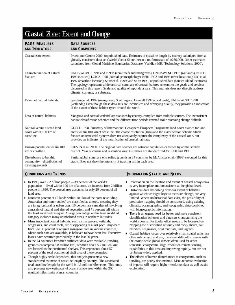
Coastal Zone: Extent and ChangePAGE MEASURESAND INDICATORS
DATA SOURCESAND COMMENTS
Coastal zone extent Pruett and Cimino 2000, unpublished data. Estimates of coastline length by country calculated from aglobally consistent data set (World Vector Shoreline) at a uniform scale of 1:250,000. Other estimatescalculated from Global Maritime Boundaries Database (Veridian-MRJ Technology Solutions, 2000).
Characterization of naturalfeatures
UNEP-WCMC 1999a and 1999b (coral reefs and mangroves); UNEP-WCMC 1998 (wetlands); NSIDC1999 (sea ice); LOICZ 1998 (coastal geomorphology); ESRI 1992 and 1993 (river locations); IOC et al.1997 (coastline location); Stutz et al. 1999; and Stutz 1999, unpublished data (barrier island locations).The typology represents a hierarchical summary of coastal features relevant to the goods and servicesdiscussed in this report. Scale and quality of input data vary. This analysis does not directly addressclimate, currents, or substrate.
Extent of natural habitats Spalding et al. 1997 (mangroves); Spalding and Grenfell 1997 (coral reefs); UNEP-WCMC 1998(wetlands); Even though these data sets are incomplete and of varying quality, they provide an indicationof the extent of these habitat types around the world.
Loss of natural habitats Mangrove and coastal wetland loss statistics by country, compiled from multiple sources. The inconsistenthabitat classification schemes and the different time periods covered make assessing change difficult.
Natural versus altered landcover within 100 km ofcoastline
GLCCD 1998. Summary of International Geosphere-Biosphere Programme land cover classes for landareas within 100 km of coastline. The coarse resolution (1km) and the classification scheme whichfocuses on terrestrial systems does not adequately capture the complexity of the coastal zone, butprovides an indicator of the modification of coastal habitats.
Human population within 100km of coastline
CIESEN et al. 2000. The original data sources are national population censuses by administrativedistrict. Year of census and resolution vary. Estimates are standardized for 1990 and 1995.
Disturbance to benthiccommunity—distribution oftrawling grounds
Partial global summary of trawling grounds in 24 countries by McAllister et al. (1999) executed for thisstudy. Does not show the intensity of trawling within each area.
CONDITIONS AND TRENDS INFORMATION STATUS AND NEEDS
♦ In 1995, over 2.2 billion people —39 percent of the world'spopulation— lived within 100 km of a coast, an increase from 2 billionpeople in 1990. The coastal area accounts for only 20 percent of allland area.
♦ Nineteen percent of all lands within 100 km of the coast (excludingAntarctica and water bodies) are classified as altered, meaning theyare in agricultural or urban uses; 10 percent are semialtered, involvinga mosaic of natural and altered vegetation; and 71 percent fall withinthe least modified category. A large percentage of this least modifiedcategory includes many uninhabited areas in northern latitudes.
♦ Many important coastal habitats, such as mangroves, wetlands,seagrasses, and coral reefs, are disappearing at a fast pace. Anywherefrom 5 to 80 percent of original mangrove area in various countries,where such data are available, is believed to have been lost. Extensivelosses have occurred particularly in the last 50 years.
♦ In the 24 countries for which sufficient data were available, trawlinggrounds encompass 8.8 million km², of which about 5.2 million km²are located on the continental shelves. This represents about 57percent of the total continental shelf area of these countries.
♦ Though highly scale dependent, this analysis presents a newstandardized estimate of coastline length by country. The associatedtotal coastline length for the world is 1.6 million kilometers. This studyalso presents new estimates of ocean surface area within the 200nautical miles limits of most countries.
♦ Information on the location and extent of coastal ecosystemsis very incomplete and inconsistent at the global level.
♦ Historical data describing previous extent of habitats,against which we might hope to measure change, are verylimited. Where no historical data exist, the possibility ofpredictive mapping should be considered, using existingclimatic, oceanographic, and topographic data combinedwith biogeographic information.
♦ There is an urgent need for better and more consistentclassification schemes and data sets characterizing theworld's coasts. Particular effort needs to be focussed onmapping the distribution of sandy and rocky shores, saltmarshes, seagrasses, tidal mudflats, and lagoons.
♦ Coastal habitats occur over relatively small spatial units, areoften submerged, and are, therefore, difficult to assess withthe coarse-scale global sensors often used for otherterrestrial ecosystems. High-resolution remote sensingcapabilities in this area are improving rapidly, but are notyet being widely applied.
♦ The effects of human disturbances to ecosystems, such astrawling, are poorly documented. More accurate evaluationof impacts will require higher resolution data as well as siteexploration.
4 P I L O T A N A L Y S I S O F G L O B A L E C O S Y S T E M S
E x e c u t i v e S u m m a r y
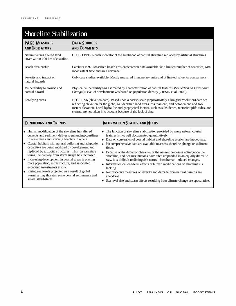
Shoreline StabilizationPAGE MEASURESAND INDICATORS
DATA SOURCESAND COMMENTS
Natural versus altered landcover within 100 km of coastline
GLCCD 1998. Rough indicator of the likelihood of natural shoreline replaced by artificial structures.
Beach area/profile Cambers 1997. Measured beach erosion/accretion data available for a limited number of countries, withinconsistent time and area coverage.
Severity and impact ofnatural hazards
Only case studies available. Mostly measured in monetary units and of limited value for comparisons.
Vulnerability to erosion andcoastal hazard
Physical vulnerability was estimated by characterization of natural features. (See section on Extent andChange.) Level of development was based on population density (CIESIN et al. 2000).
Low-lying areas USGS 1996 (elevation data). Based upon a coarse-scale (approximately 1 km grid resolution) data setreflecting elevation for the globe, we identified land areas less than one, and between one and twometers elevation. Local hydraulic and geophysical factors, such as subsidence, tectonic uplift, tides, andstorms, are not taken into account because of the lack of data.
CONDITIONS AND TRENDS INFORMATION STATUS AND NEEDS
♦ Human modification of the shoreline has alteredcurrents and sediment delivery, enhancing coastlinesin some areas and starving beaches in others.
♦ Coastal habitats with natural buffering and adaptationcapacities are being modified by development andreplaced by artificial structures. Thus, in monetaryterms, the damage from storm surges has increased.
♦ Increasing development in coastal areas is placingmore population, infrastructure, and associatedeconomic investments at risk.
♦ Rising sea levels projected as a result of globalwarming may threaten some coastal settlements andsmall island-states.
♦ The function of shoreline stabilization provided by many natural coastalfeatures is not well documented quantitatively.
♦ Data on conversion of coastal habitat and shoreline erosion are inadequate.♦ No comprehensive data are available to assess shoreline change or sediment
flows.♦ Because of the dynamic character of the natural processes acting upon the
shoreline, and because humans have often responded in an equally dramaticway, it is difficult to distinguish natural from human-induced changes.
♦ Information on long-term effects of human modifications on shorelines islacking.
♦ Nonmonetary measures of severity and damage from natural hazards areanecdotal.
♦ Sea level rise and storm effects resulting from climate change are speculative.
C o a s t a l E c o s y s t e m s 5
E x e c u t i v e S u m m a r y
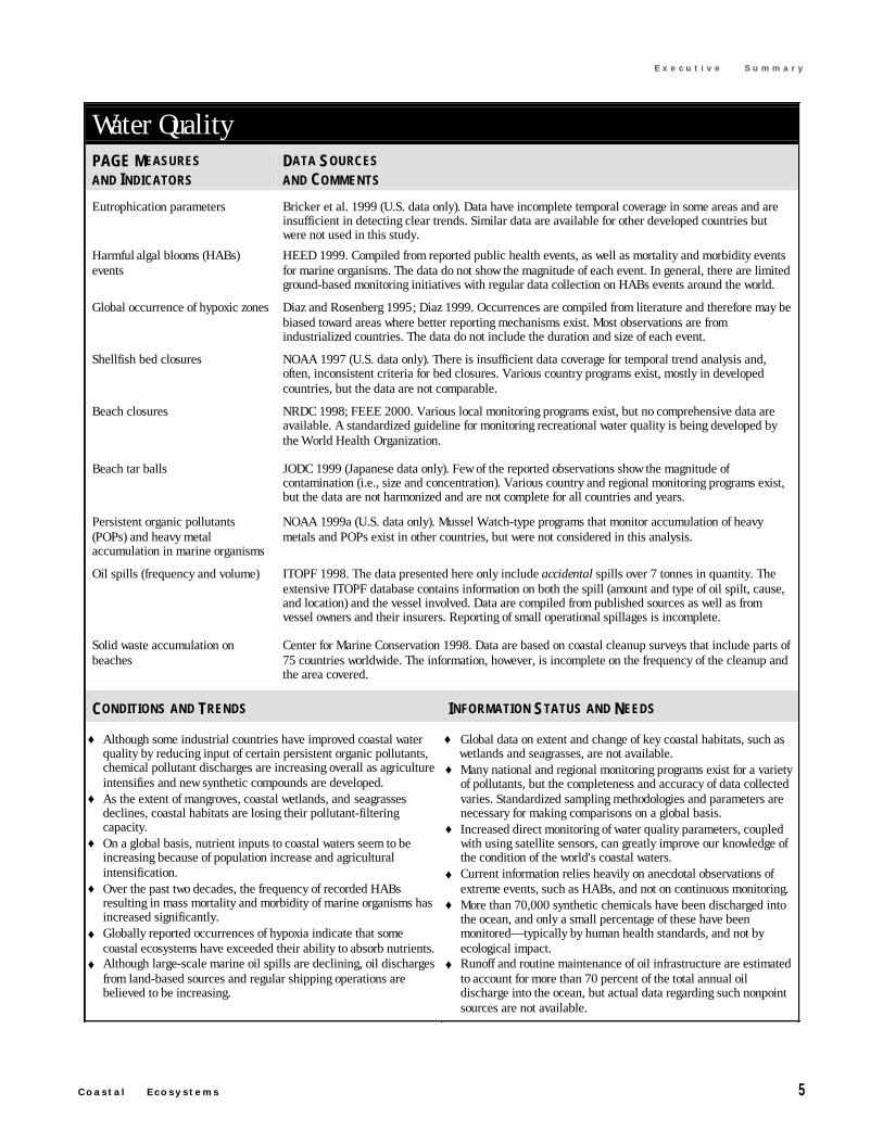
Water QualityPAGE MEASURESAND INDICATORS
DATA SOURCESAND COMMENTS
Eutrophication parameters Bricker et al. 1999 (U.S. data only). Data have incomplete temporal coverage in some areas and areinsufficient in detecting clear trends. Similar data are available for other developed countries butwere not used in this study.
Harmful algal blooms (HABs)events
HEED 1999. Compiled from reported public health events, as well as mortality and morbidity eventsfor marine organisms. The data do not show the magnitude of each event. In general, there are limitedground-based monitoring initiatives with regular data collection on HABs events around the world.
Global occurrence of hypoxic zones Diaz and Rosenberg 1995; Diaz 1999. Occurrences are compiled from literature and therefore may bebiased toward areas where better reporting mechanisms exist. Most observations are fromindustrialized countries. The data do not include the duration and size of each event.
Shellfish bed closures NOAA 1997 (U.S. data only). There is insufficient data coverage for temporal trend analysis and,often, inconsistent criteria for bed closures. Various country programs exist, mostly in developedcountries, but the data are not comparable.
Beach closures NRDC 1998; FEEE 2000. Various local monitoring programs exist, but no comprehensive data areavailable. A standardized guideline for monitoring recreational water quality is being developed bythe World Health Organization.
Beach tar balls JODC 1999 (Japanese data only). Few of the reported observations show the magnitude ofcontamination (i.e., size and concentration). Various country and regional monitoring programs exist,but the data are not harmonized and are not complete for all countries and years.
Persistent organic pollutants(POPs) and heavy metalaccumulation in marine organisms
NOAA 1999a (U.S. data only). Mussel Watch-type programs that monitor accumulation of heavymetals and POPs exist in other countries, but were not considered in this analysis.
Oil spills (frequency and volume) ITOPF 1998. The data presented here only include accidental spills over 7 tonnes in quantity. Theextensive ITOPF database contains information on both the spill (amount and type of oil spilt, cause,and location) and the vessel involved. Data are compiled from published sources as well as fromvessel owners and their insurers. Reporting of small operational spillages is incomplete.
Solid waste accumulation onbeaches
Center for Marine Conservation 1998. Data are based on coastal cleanup surveys that include parts of75 countries worldwide. The information, however, is incomplete on the frequency of the cleanup andthe area covered.
CONDITIONS AND TRENDS INFORMATION STATUS AND NEEDS
♦ Although some industrial countries have improved coastal waterquality by reducing input of certain persistent organic pollutants,chemical pollutant discharges are increasing overall as agricultureintensifies and new synthetic compounds are developed.
♦ As the extent of mangroves, coastal wetlands, and seagrassesdeclines, coastal habitats are losing their pollutant-filteringcapacity.
♦ On a global basis, nutrient inputs to coastal waters seem to beincreasing because of population increase and agriculturalintensification.
♦ Over the past two decades, the frequency of recorded HABsresulting in mass mortality and morbidity of marine organisms hasincreased significantly.
♦ Globally reported occurrences of hypoxia indicate that somecoastal ecosystems have exceeded their ability to absorb nutrients.
♦ Although large-scale marine oil spills are declining, oil dischargesfrom land-based sources and regular shipping operations arebelieved to be increasing.
♦ Global data on extent and change of key coastal habitats, such aswetlands and seagrasses, are not available.
♦ Many national and regional monitoring programs exist for a varietyof pollutants, but the completeness and accuracy of data collectedvaries. Standardized sampling methodologies and parameters arenecessary for making comparisons on a global basis.
♦ Increased direct monitoring of water quality parameters, coupledwith using satellite sensors, can greatly improve our knowledge ofthe condition of the world's coastal waters.
♦ Current information relies heavily on anecdotal observations ofextreme events, such as HABs, and not on continuous monitoring.
♦ More than 70,000 synthetic chemicals have been discharged intothe ocean, and only a small percentage of these have beenmonitored—typically by human health standards, and not byecological impact.
♦ Runoff and routine maintenance of oil infrastructure are estimatedto account for more than 70 percent of the total annual oildischarge into the ocean, but actual data regarding such nonpointsources are not available.
6 P I L O T A N A L Y S I S O F G L O B A L E C O S Y S T E M S
E x e c u t i v e S u m m a r y
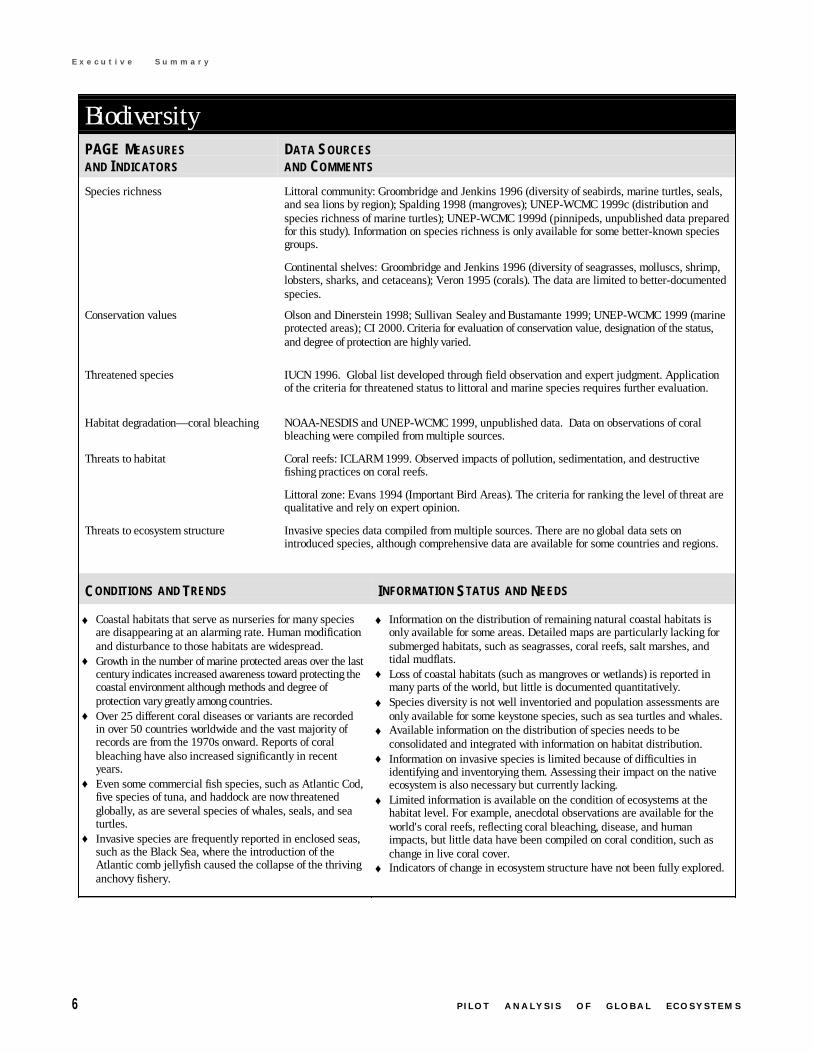
BiodiversityPAGE MEASURESAND I NDICATORS
DATA SOURCESAND COMMENTS
Littoral community: Groombridge and Jenkins 1996 (diversity of seabirds, marine turtles, seals,and sea lions by region); Spalding 1998 (mangroves); UNEP-WCMC 1999c (distribution andspecies richness of marine turtles); UNEP-WCMC 1999d (pinnipeds, unpublished data preparedfor this study). Information on species richness is only available for some better-known speciesgroups.
Species richness
Continental shelves: Groombridge and Jenkins 1996 (diversity of seagrasses, molluscs, shrimp,lobsters, sharks, and cetaceans); Veron 1995 (corals). The data are limited to better-documentedspecies.
Conservation values Olson and Dinerstein 1998; Sullivan Sealey and Bustamante 1999; UNEP-WCMC 1999 (marineprotected areas); CI 2000. Criteria for evaluation of conservation value, designation of the status,and degree of protection are highly varied.
Threatened species IUCN 1996. Global list developed through field observation and expert judgment. Applicationof the criteria for threatened status to littoral and marine species requires further evaluation.
Habitat degradation—coral bleaching NOAA-NESDIS and UNEP-WCMC 1999, unpublished data. Data on observations of coralbleaching were compiled from multiple sources.
Coral reefs: ICLARM 1999. Observed impacts of pollution, sedimentation, and destructivefishing practices on coral reefs.
Threats to habitat
Littoral zone: Evans 1994 (Important Bird Areas). The criteria for ranking the level of threat arequalitative and rely on expert opinion.
Threats to ecosystem structure Invasive species data compiled from multiple sources. There are no global data sets onintroduced species, although comprehensive data are available for some countries and regions.
CONDITIONS AND TRENDS INFORMATION STATUS AND NEEDS
♦ Coastal habitats that serve as nurseries for many speciesare disappearing at an alarming rate. Human modificationand disturbance to those habitats are widespread.
♦ Growth in the number of marine protected areas over the lastcentury indicates increased awareness toward protecting thecoastal environment although methods and degree ofprotection vary greatly among countries.
♦ Over 25 different coral diseases or variants are recordedin over 50 countries worldwide and the vast majority ofrecords are from the 1970s onward. Reports of coralbleaching have also increased significantly in recentyears.
♦ Even some commercial fish species, such as Atlantic Cod,five species of tuna, and haddock are now threatenedglobally, as are several species of whales, seals, and seaturtles.
♦ Invasive species are frequently reported in enclosed seas,such as the Black Sea, where the introduction of theAtlantic comb jellyfish caused the collapse of the thrivinganchovy fishery.
♦ Information on the distribution of remaining natural coastal habitats isonly available for some areas. Detailed maps are particularly lacking forsubmerged habitats, such as seagrasses, coral reefs, salt marshes, andtidal mudflats.
♦ Loss of coastal habitats (such as mangroves or wetlands) is reported inmany parts of the world, but little is documented quantitatively.
♦ Species diversity is not well inventoried and population assessments areonly available for some keystone species, such as sea turtles and whales.
♦ Available information on the distribution of species needs to beconsolidated and integrated with information on habitat distribution.
♦ Information on invasive species is limited because of difficulties inidentifying and inventorying them. Assessing their impact on the nativeecosystem is also necessary but currently lacking.
♦ Limited information is available on the condition of ecosystems at thehabitat level. For example, anecdotal observations are available for theworld's coral reefs, reflecting coral bleaching, disease, and humanimpacts, but little data have been compiled on coral condition, such aschange in live coral cover.
♦ Indicators of change in ecosystem structure have not been fully explored.
C o a s t a l E c o s y s t e m s 7
E x e c u t i v e S u m m a r y
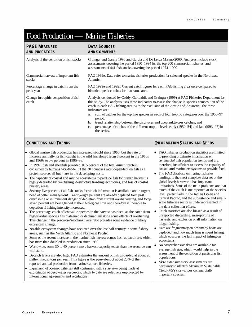
Food Production — Marine FisheriesPAGE MEASURESAND INDICATORS
DATA SOURCESAND COMMENTS
Analysis of the condition of fish stocks Grainger and Garcia 1996 and Garcia and De Leiva Moreno 2000. Analyses include stockassessments covering the period 1950–1994 for the top 200 commercial fisheries, andassessments of 441 fish stocks covering the period 1974–1999.
Commercial harvest of important fishstocks
FAO 1999e. Data refer to marine fisheries production for selected species in the NorthwestAtlantic.
Percentage change in catch from thepeak year
FAO 1999e and 1999f. Current catch figures for each FAO fishing area were compared tohistorical peak catches for that same area.
Change in trophic composition of fishcatch
Analysis conducted by Caddy, Garibaldi, and Grainger (1999) at FAO Fisheries Department forthis study. The analysis uses three indicators to assess the change in species composition of thecatch in each FAO fishing area, with the exclusion of the Arctic and Antarctic. The threeindicators are:a. sum of catches for the top five species in each of four trophic categories over the 1950–97
period;b. trend relationship between the piscivores and zooplanktivores catches; andc. percentage of catches of the different trophic levels early (1950–54) and late (l993–97) in
the series.
CONDITIONS AND TRENDS INFORMATION STATUS AND NEEDS
♦ Global marine fish production has increased sixfold since 1950, but the rate ofincrease annually for fish caught in the wild has slowed from 6 percent in the 1950sand 1960s to 0.6 percent in 1995–96.
♦ In 1997, fish and shellfish provided 16.5 percent of the total animal proteinconsumed by humans worldwide. Of the 30 countries most dependent on fish as aprotein source, all but 4 are in the developing world.
♦ The capacity of coastal and marine ecosystems to produce fish for human harvest ishighly degraded by overfishing, destructive trawling techniques, and loss of coastalnursery areas.
♦ Seventy-five percent of all fish stocks for which information is available are in urgentneed of better management. Twenty-eight percent are already depleted from pastoverfishing or in imminent danger of depletion from current overharvesting, and forty-seven percent are being fished at their biological limit and therefore vulnerable todepletion if fishing intensity increases.
♦ The percentage catch of low-value species in the harvest has risen, as the catch fromhigher-value species has plateaued or declined, masking some effects of overfishing.This change in the piscivore/zooplanktivore ratio provides some evidence of likelyecosystem change.
♦ Notable ecosystem changes have occurred over the last half century in some fisheryareas, such as the North Atlantic and Northeast Pacific.
♦ Some of the recent increase in the marine fish harvest comes from aquaculture, whichhas more than doubled in production since 1990.
♦ Worldwide, some 30 to 40 percent more harvest capacity exists than the resource canwithstand.
♦ Bycatch levels are also high. FAO estimates the amount of fish discarded at about 20million metric tons per year. This figure is the equivalent of about 25% of thereported annual production from marine capture fisheries.
♦ Expansion of oceanic fisheries still continues, with a start now being made atexploitation of deep-water resources, which to date are relatively unprotected byinternational agreements and regulations.
♦ FAO fisheries production statistics are limitedto providing proximate information oncommercial fish population trends and are,therefore, insufficient to assess the capacity ofcoastal and marine ecosystems to provide food.
♦ The FAO database on marine fisherieslandings is the most complete data set at theglobal level; however it has importantlimitations. Some of the main problems are thatmuch of the catch is not reported at the specieslevel, particularly in the Indian Ocean andCentral Pacific, and the subsistence and small-scale fisheries sector is underrepresented inthe data collection efforts.
♦ Catch statistics are also biased as a result ofunreported discarding, misreporting ofharvests, and exclusion of all information onillegal fishing.
♦ Data are fragmentary on how many boats aredeployed, and how much time is spent fishing,which obscures the full impact of fishing onecosystems.
♦ No comprehensive data are available foraverage fish size, which would help in theassessment of the condition of particular fishpopulations.
♦ More extensive stock assessments arenecessary to identify Maximum SustainableYield (MSY) for various commerciallyimportant species.
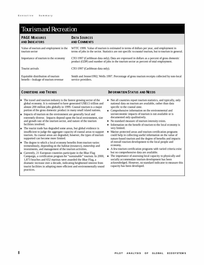
8 P I L O T A N A L Y S I S O F G L O B A L E C O S Y S T E M S
E x e c u t i v e S u m m a r y
Tourism and RecreationPAGE MEASURESAND INDICATORS
DATA SOURCESAND COMMENTS
Value of tourism and employment in thetourism sector
WTTC 1999. Value of tourism is estimated in terms of dollars per year, and employment interms of jobs in the sector. Statistics are not specific to coastal tourism, but to tourism in general.
Importance of tourism to the economy CTO 1997 (Caribbean data only). Data are expressed in dollars as a percent of gross domesticproduct (GDP) and number of jobs in the tourism sector as percent of total employment.
Tourist arrivals CTO 1997 (Caribbean data only).
Equitable distribution of tourismbenefit—leakage of tourism revenue
Smith and Jenner1992; Wells 1997. Percentage of gross tourism receipts collected by non-localservice providers.
CONDITIONS AND TRENDS INFORMATION STATUS AND NEEDS
♦ The travel and tourism industry is the fastest growing sector of theglobal economy. It is estimated to have generated US$3.5 trillion andalmost 200 million jobs globally in 1999. Coastal tourism is a majorportion of the gross domestic product in many small island nations.
♦ Impacts of tourism on the environment are generally local andextremely diverse. Impacts depend upon the local environment, sizeand growth rate of the tourism sector, and nature of the tourismfacilities involved.
♦ The tourist trade has degraded some areas, but global evidence isinsufficient to judge the aggregate capacity of coastal areas to supporttourism. As coastal areas are degraded, however, the types of tourismsupported can become more limited.
♦ The degree to which a local economy benefits from tourism variestremendously, depending on the habitat (resource), ownership andinvestments, and management of the tourism activities.
♦ Currently, 21 European countries participate in the Blue FlagCampaign, a certification program for “sustainable” tourism. In 2000,1,873 beaches and 652 marinas were awarded the Blue Flag, adramatic increase over a decade, indicating heightened interest fromtourist facilities in adopting more efficient and environmentally soundpractices.
♦ Not all countries report tourism statistics, and typically, onlynational data on tourism are available, rather than dataspecific to the coastal zone.
♦ Comprehensive information on the environmental andsocioeconomic impacts of tourism is not available or isdocumented only qualitatively.
♦ No standard measure of tourism intensity exists.♦ Information on the benefit of tourism to the local economy is
very limited.♦ Marine protected areas and tourism certification programs
could help in collecting useful information on the value ofnature-based tourism and the degree of benefits and impactsof overall tourism development to the local people andeconomy.
♦ A few tourism certification programs with varied criteria existbut no comprehensive data are available.
♦ The importance of assessing local capacity to physically andsocially accommodate tourism development has beenacknowledged. However, no standard indicator to measure thiscapacity has been developed.
C o a s t a l E c o s y s t e m s 9
E x e c u t i v e S u m m a r y
C o n c l u s i o n sAlong with direct loss of area, a variety of other factors are sig-nificantly altering coastal ecosystems around the world. Someof the major pressures are population growth, pollution, over-harvesting and destructive fishing practices, and the loomingthreat of climate change.
Globally, the number of people living within 100 km of thecoast increased from roughly 2 billion in 1990 to 2.2 billion in1995—39 percent of the world’s population. However, the num-ber of people whose activities affect coastal ecosystems is muchlarger than the actual coastal population because rivers deliverpollutants from inland watersheds and populations to estuariesand surrounding coastal waters. As coastal and inland popula-tions continue to grow, their impacts—in terms of pollutant loadsand the development and conversion of coastal habitats—canbe expected to grow as well.
An increasing number of pollutants affect the world’s coastsand oceans. Most pollution of coastal waters comes from theland, but atmospheric sources and marine-based sources suchas oil leaks and spills from vessels also play a role. Nutrientpollution, especially nitrates and phosphates, has increaseddramatically this century. Greater use of fertilizers, growth inquantities of domestic and industrial sewage, and increasedaquaculture, which releases considerable amounts of waste di-rectly into the water, are all contributing factors (GESAMP1990:96).
In terms of food production, forty-five years of increasingfishing pressure have left many major fish stocks depleted or indecline. The scale of the global fishing enterprise has grownrapidly and exploitation of fish stocks has followed a predict-able pattern, progressing from region to region across the world’soceans. As each area in turn reaches its maximum productionlevel, it then begins to decline (Grainger and Garcia 1996:8,42–44). Overexploitation of fish, shellfish, seaweeds, and othermarine organisms not only diminishes production of the har-vested species but can profoundly alter species compositionand the biological structure of coastal ecosystems.
Global climate change may compound other pressures oncoastal ecosystems through the additional effects of warmerocean temperatures, altered ocean circulation patterns, chang-ing storm frequency, and rising sea levels. Changing concen-trations of CO2 in ocean waters may also affect marine produc-tivity or even change the rate of coral calcification (Kleypas etal. 1999). Rising sea level, associated with climate change, islikely to affect virtually all of the world’s coasts. During the pastcentury, sea level has risen at a rate of 1.0–2.5 mm per year(IPCC 1996:296). Rising sea levels will also increase the im-pact of storm surges. This, in turn, could accelerate erosion andassociated habitat loss, increase salinity in estuaries and fresh-
water aquifers, alter tidal ranges, change sediment and nutrienttransport, and increase coastal flooding.
Because of the current pressures on coastal ecosystems, andthe immense value of the goods and services derived from them,there is an increasing need to evaluate tradeoffs between differ-ent activities that may be proposed for a particular coastal area.However, to integrate this evaluation into the decisionmakingprocess, better information on the location, extent, and changein coastal habitats is urgently needed. Information regardingthe interaction between ocean, land, and atmosphere is also akey to understanding the functions of the coastal zone but so farmost of the information is anecdotal or fragmentary. One factorcontributing to this lack of information is the partitioning ofdisciplines into separate entities. Terrestrial ecology, wetlandecology, and marine ecology are, for example, distinct fieldsamong the biological sciences. The separation between theseand the physical, chemical, and social sciences is even greater,making it difficult to conduct a more integrated analysis.
The problems affecting the coastal zone are cross-sectoraland complex. Collaboration among climatologists, ecologists,ocean chemists, toxicologists, soil scientists, statisticians, coastalengineers, economists, and practitioners of monitoring and in-formation technology will be needed to develop the informationbase and linkages necessary to fully assess the condition of theworld’s coastal environments.Recommendations for the Millennium Ecosystem Assessmentinclude the following:♦ There is an urgent need to fully utilize existing information
on location and extent of coastal habitats. Standardizedclassification schemes characterizing the world’s coastsneed to be developed. Amalgamating and harmonizingexisting maps and chart series into global data sets basedon such classification schemes, combined with the use ofhigh-resolution remote sensing imagery, could moredirectly assess gaps in knowledge on the location andextent of coastal habitats. Particular efforts need to bedirected toward submerged habitats.
♦ Further descriptive information about the distribution andstatus of marine and coastal biodiversity is a priority. Basicinventory of coastal and marine species by habitat type isfundamental to subsequent research, management, andconservation. Work needs to include basic taxonomy andspecies inventory, but also analysis of community struc-ture, ecosystem function, and habitat distribution.
♦ Identifying and describing areas of high conservationimportance at species and ecosystem levels would helpimprove the effectiveness of conservation activities.Further research into the patterns of interlinkage andenergy flow between marine ecosystems is also critical ifsuch high priority areas are to maintain their ecologicalintegrity.

10 P I L O T A N A L Y S I S O F G L O B A L E C O S Y S T E M S
E x e c u t i v e S u m m a r y
♦ Compilation of historic or baseline data against which wemay measure the condition of ecosystems is a prerequisitefor any assessment of current status. Localized baselinedata and the identification of thresholds are particularlyimportant for water quality. In order for the conditionindicators to be useful as early warning systems, it isimportant to distinguish between human caused anomaliesand natural fluctuations in the system.
♦ Causal relationships in biological, chemical, and physicalsystems are also poorly understood, and in the coastalrealm are particularly complex and varied. Our predictivecapabilities are limited when we attempt to examine howcertain threats affect an environment, such as the intro-duction of nonnative species. Understanding linksbetween pressure and condition would improve ourassessment of future trends and human activities that mayhave profound implications for coastal habitats andbiodiversity.
♦ In many cases, combining the use of low, medium, andhigh-resolution satellite imagery will be vital to calibratingdata and refining observations for conditions in nearshoreand surface waters. Satellite data will be useful for habitatmapping, estimating turbidity and organic pollutantdischarge, identifying sediment plumes, monitoring theoccurrence and extent of algal blooms, mapping theoccurrence and extent of oil spills, and monitoring thermal
pollution and sea surface temperature anomalies. At thesame time, other more direct methods need to be devel-oped to map and monitor the status of the continentalshelf, which lies below the shallow layers visible fromsatellites.
♦ More integration and collaboration among the variousagencies working in the coastal zone, particularly with thedifferent monitoring initiatives, such as the Global OceanObserving System (GOOS) should be encouraged (GOOSProject Office 1998 and 1999; Summerhayes, personalcommunication, 1999). Such organizations include theUnited Nations Environment Programme (UNEP), theIntergovernmental Oceanographic Commission (IOC), theUnited Nations Educational, Scientific, and CulturalOrganization (UNESCO), the United Nations DevelopmentProgramme (UNDP), the Food and Agriculture Organiza-tion of the United Nations (FAO), the InternationalGeosphere-Biosphere Programme (IGBP), nongovernmen-tal organizations, and academic centers.
♦ There is a need to better understand, evaluate and monitorthe goods and services provided by coastal and marineecosystems.
♦ Governments and nongovernmental organizations areencouraged to develop techniques for engagingpolicymakers and civil society so they can evaluatetradeoffs and make decisions with greater understandingand awareness of the consequences.
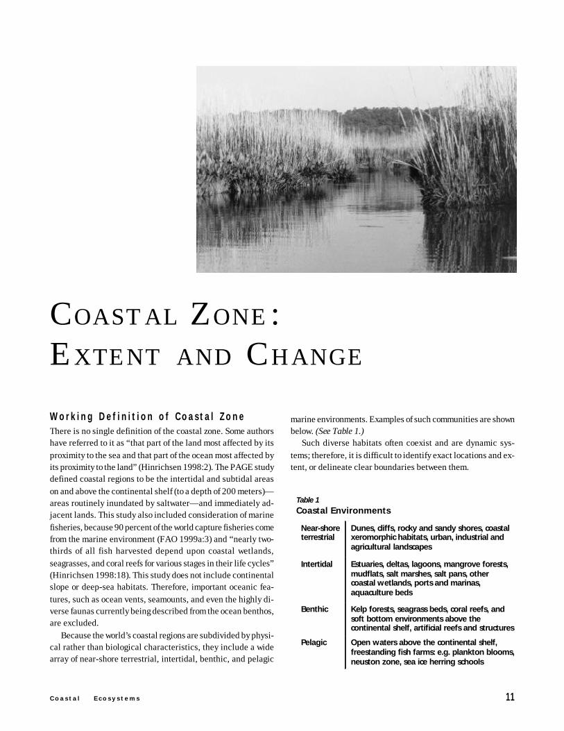
C o a s t a l E c o s y s t e m s 11
C o a s t a l Z o n e : E x t e n t a n d C h a n g e
C O A S T A L Z O N E :E X T E N T A N D C H A N G E
marine environments. Examples of such communities are shownbelow. (See Table 1.)
Such diverse habitats often coexist and are dynamic sys-tems; therefore, it is difficult to identify exact locations and ex-tent, or delineate clear boundaries between them.
Work ing Def in i t ion of Coasta l ZoneThere is no single definition of the coastal zone. Some authorshave referred to it as “that part of the land most affected by itsproximity to the sea and that part of the ocean most affected byits proximity to the land” (Hinrichsen 1998:2). The PAGE studydefined coastal regions to be the intertidal and subtidal areason and above the continental shelf (to a depth of 200 meters)—areas routinely inundated by saltwater—and immediately ad-jacent lands. This study also included consideration of marinefisheries, because 90 percent of the world capture fisheries comefrom the marine environment (FAO 1999a:3) and “nearly two-thirds of all fish harvested depend upon coastal wetlands,seagrasses, and coral reefs for various stages in their life cycles”(Hinrichsen 1998:18). This study does not include continentalslope or deep-sea habitats. Therefore, important oceanic fea-tures, such as ocean vents, seamounts, and even the highly di-verse faunas currently being described from the ocean benthos,are excluded.
Because the world’s coastal regions are subdivided by physi-cal rather than biological characteristics, they include a widearray of near-shore terrestrial, intertidal, benthic, and pelagic
Table 1
Coastal Environments
Near-shoreterrestrial
Dunes, cliffs, rocky and sandy shores, coastalxeromorphic habitats, urban, industrial andagricultural landscapes
Intertidal Estuaries, deltas, lagoons, mangrove forests,mudflats, salt marshes, salt pans, othercoastal wetlands, ports and marinas,aquaculture beds
Benthic Kelp forests, seagrass beds, coral reefs, andsoft bottom environments above thecontinental shelf, artificial reefs and structures
Pelagic Open waters above the continental shelf,freestanding fish farms: e.g. plankton blooms,neuston zone, sea ice herring schools
12 P I L O T A N A L Y S I S O F G L O B A L E C O S Y S T E M S
C o a s t a l Z o n e : E x t e n t a n d C h a n g e
Est imat ing Area and Length of
Coasta l ZoneTo get a rough indicator and a better understanding of the rela-tive size and distribution of coastal areas, this study calculatedthe spatial extent of coastal zone and maritime areas withinnational jurisdiction (up to 200 nautical miles from the coast-line), such as territorial seas and exclusive economic zones.Although these are not ecologically oriented statistics, juris-diction over resources has significant implications for gover-nance and effective management of coastal and marine resources(see Box 1). Furthermore, this analysis presents statistics com-piled for the first time from a new, globally consistent source.
Table 2 presents coastal zone statistics for selected coun-tries.
Character i z ing the Natura l Coasta l
FeaturesThe habitats and features along the world’s coastline are highlyvaried—from the flat, coastal plains of Argentina, to the man-grove and coral reef-lined shores of Sulawesi, to the rugged,rocky coastline of Norway. The descriptive attributes of coastsprovide baseline information and reference points for assessingthe condition of the ecosystem’s goods and services. They alsoare a major factor in the vulnerability and resilience of an areato a particular pressure. The extent and loss of these naturalhabitat types serve as a proxy condition indicator for many ofthe ecosystem services and values that are otherwise difficult toquantify.
This study’s examination of the world’s shoreline begins withan exploration of some of the natural characteristics of tidaland near-shore areas. The characterization of the world’s shore-line is based upon the occurrence of certain habitats, such ascoral reefs, mangroves, other tidal wetlands, barrier islands,
Box 1
Maritime Areas Definitions
The United Nations Convention on the Law of the Sea(UNCLOS) is an international agreement that sets conditionsand limits on the use and exploitation of the world’s oceans.This convention also rules on how the maritime jurisdictionalboundaries of member states are set. UNCLOS defines terri-torial sea as the 12-nautical-mile zone from the baseline orlow-water line along the coast, on which the coastal statehas sovereignty. Even though the established maximum limitfor a territorial sea is 12 nautical miles, some countries claimlarger areas. A country’s Exclusive Economic Zone (EEZ), asestablished by UNCLOS, extends from the baseline out be-yond the territorial sea, up to a width of 200 nautical miles.In cases where countries’ baselines are within 400 nauticalmiles of each other, the EEZ boundaries are generally estab-lished by treaty, although there are many cases where theseare in dispute. Moreover, many states have yet to sign or ratifyUNCLOS, while still others have yet to claim their EEZ. Whereclaimed and undisputed, a coastal country has certain sover-eign rights over the EEZ, namely, rights to exploration, exploi-tation, conservation, and management of all natural resourcesof the seabed, its subsoil, and the overlying waters (Baretta-Bekker et al. 1998:118). Some countries have claimed an ex-clusive fishing zone instead of the more encompassing EEZ.The exclusive fishing zone, in these cases, refers to an areabeyond the outer limit of the territorial sea in which the coastalstate has the right to fish, subject to any concessions thatmay be granted to foreign fishermen. The territorial sea andthe EEZ or the fishing zone, depending on which has been
claimed, comprise what is defined as the total potential mari-time area of a country—that is, the total marine surface area(claimed or unclaimed) within 200 nautical miles from thecoast. The maritime area definition only applies to marineareas that are not currently under dispute. Given the uncer-tainties surrounding much of the delimitation of the EEZ, anymaps and statistics portraying these boundaries are subjectto certain limitations and should be treated with caution.
In contrast to the territorial sea and EEZ, which are essen-tially political boundaries, the coastline and continental shelfarea are delineations based on a natural feature. Coastallength is a frequently cited statistic to indicate the importanceof coastal zone to a country. However, its measurement isfraught with difficulty. The main problem is that the mea-surement of an irregular and curving feature is scale-depen-dent. Maps of individual islands, for example, frequently showgreat detail, whereas regional maps summarize complex coast-lines into a few simple lines. Coastline lengths are also af-fected by inclusion or exclusion of coastal features such asbays, lagoons, and river mouths. More detailed maps will,thus, result in longer estimates. For the PAGE analysis, coast-line lengths were summarized from a globally consistent dataset—the 1:250,000 scale World Vector Shoreline. (See Table2.) Although the estimates presented here can differ signifi-cantly from previously published sources, it should be notedthat this is the first time such statistics have been developedfrom a globally consistent source.
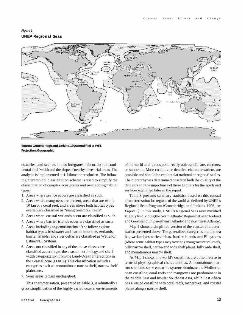
C o a s t a l E c o s y s t e m s 13
C o a s t a l Z o n e : E x t e n t a n d C h a n g e
estuaries, and sea ice. It also integrates information on conti-nental shelf width and the slope of nearby terrestrial areas. Theanalysis is implemented at 1-kilometer resolution. The follow-ing hierarchical classification scheme is used to simplify theclassification of complex ecosystems and overlapping habitattypes.1. Areas where sea ice occurs are classified as such.2. Areas where mangroves are present, areas that are within
10 km of a coral reef, and areas where both habitat typesoverlap are classified as “mangroves/coral reefs”.
3. Areas where coastal wetlands occur are classified as such.
4. Areas where barrier islands occur are classified as such.5. Areas including any combination of the following four
habitat types: freshwater and marine interface, wetlands,barrier islands, and river deltas are classified as Wetland/Estuary/BI Systems.
6. Areas not classified in any of the above classes areclassified according to the coastal morphology and shelfwidth categorization from the Land-Ocean Interactions inthe Coastal Zone (LOICZ). This classification includescategories such as: mountainous narrow shelf, narrow shelfplains, etc.
7. Some areas remain unclassified.
This characterization, presented in Table 3, is admittedly agross simplification of the highly varied coastal environments
of the world and it does not directly address climate, currents,or substrate. More complex or detailed characterizations arepossible and should be explored at national or regional scales.The hierarchy was determined based on both the quality of thedata sets and the importance of these habitats for the goods andservices examined later in the report.
Table 3 presents summary statistics based on this coastalcharacterization for regions of the world as defined by UNEP’sRegional Seas Program (Groombridge and Jenkins 1996, seeFigure 1). In this study, UNEP’s Regional Seas were modifiedslightly by dividing the North Atlantic Region between Icelandand Greenland, into northeast Atlantic and northwest Atlantic.
Map 1 shows a simplified version of the coastal character-ization presented above. The generalized categories include seaice, wetlands/estuaries/deltas, barrier islands and BI systems(where some habitat types may overlap), mangroves/coral reefs,hilly narrow shelf, narrow and wide shelf plains, hilly wide shelf,and mountainous narrow shelf.
As Map 1 shows, the world’s coastlines are quite diverse interms of physiographical characteristics. A mountainous, nar-row shelf and some estuarine systems dominate the Mediterra-nean coastline, coral reefs and mangroves are predominant inthe Middle East and Insular Southeast Asia, while East Africahas a varied coastline with coral reefs, mangroves, and coastalplains along a narrow shelf.
Figure 1
UNEP Regional Seas
Source: Groombridge and Jenkins, 1996; modified at WRI.
Projection: Geographic
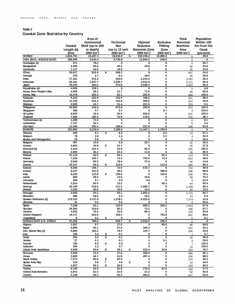
14 P I L O T A N A L Y S I S O F G L O B A L E C O S Y S T E M S
C o a s t a l Z o n e : E x t e n t a n d C h a n g e
Table 2
Coastal Zone Statistics by Country
CoastalLength {a}
(km)
Area ofContinental
Shelf (up to 200m depth)(000 km2)
TerritorialSea
(up to 12 nm)(000 km2)
ClaimedExclusive
Economic Zone(000 km2)
ExclusiveFishingZone
(000 km2)
TotalPotentialMaritime
Area(000 km2)
PopulationWithin 100
km from theCoast
(percent)WORLD 1,634,701 24,287.1 18,816.9 b 102,108.4 12,885.2 X 39.0ASIA (EXCL. MIDDLE EAST) 288,459 5,515.4 5,730.9 11,844.2 249.5 X XAzerbaijan {c} 871 78.0 X X X X 55.7Bangladesh 3,306 59.6 40.3 39.9 X 80 54.8Cambodia 1,127 34.6 19.9 X X 35 23.8China 30,017 810.4 d 348.1 X X 847 24.0Georgia 376 2.7 6.1 18.9 X 25 38.8India 17,181 372.4 193.8 2,103.4 X 2,297 26.3Indonesia 95,181 1,847.7 3,205.7 2,915.0 X 6,121 95.9Japan 29,020 304.2 373.8 3,648.4 X 4,022 96.3Kazakhstan {c} 4,528 139.1 X X X X 3.6Korea, Dem People's Rep 4,009 26.3 12.7 72.8 X 86 92.9Korea, Rep 12,478 226.3 81.1 202.6 X 284 100.0Malaysia 9,323 335.9 152.4 198.2 X 351 98.0Myanmar 14,708 216.4 154.8 358.5 X 514 49.0Pakistan 2,599 43.7 31.4 201.5 X 233 9.1Philippines 33,900 244.5 679.8 293.8 X 974 100.0Singapore 268 0.7 0.7 X 0.7 2 100.0Sri Lanka 2,825 19.2 30.5 500.8 X 531 100.0Thailand 7,066 185.4 75.9 176.5 X 252 38.7Turkmenistan {c} 1,289 72.4 X X X X 8.1Uzbekistan 1,707 26.1 X X X X 2.6Viet Nam 11,409 352.4 158.6 237.8 X 396 82.8EUROPE 325,892 6,316.0 2,589.4 11,447.1 1,783.0 X XAlbania 649 6.1 d 6.2 X 6.2 13 97.1Belgium 76 3.6 1.5 X 2.1 4 83.0Bosnia and Herzegovina 23 0.0 X X X X 46.6Bulgaria 457 10.9 6.5 25.7 X 32 29.2Croatia 5,663 44.9 d 31.7 X X 55 37.9Denmark {e} 5,316 102.4 24.8 80.4 X 10⁵ 100.0Estonia 2,956 36.2 24.3 11.6 X 36 85.9Finland 31,119 82.5 d 55.1 X 55.1 110 72.8France 7,330 160.7 73.4 706.4 73.4 853 39.6Germany 3,624 55.5 18.4 37.4 X 56 14.6Greece 15,147 94.3 d 114.9 X 114.9 494 99.2Iceland 8,506 108.7 73.0 678.7 X 752 99.9Ireland 6,437 151.9 39.4 X 358.9 398 99.9Italy 9,226 110.8 d 155.6 X 155.6 536 79.1Latvia 565 28.0 12.6 15.6 X 28 75.2Lithuania 258 5.7 2.0 3.6 X 6 22.9Netherlands 1,914 64.0 13.2 X 50.3 64 93.4Norway 53,199 218.5 111.2 1,095.1 X 1,206 95.4Poland 1,032 30.0 10.6 19.4 X 30 13.5Portugal 2,830 20.1 64.1 1,656.4 X 1,721 92.7Romania 696 18.6 5.3 18.0 X 23 6.3Russian Federation {c} 110,310 4,137.0 1,318.1 6,255.8 X 7,574 14.9Slovenia 41 0.2 0.2 X X 0 60.6Spain 7,268 62.1 115.8 683.2 205.2 1,004 67.9Sweden 26,384 153.8 85.3 73.2 X 158 87.7Ukraine 4,953 78.0 53.9 86.4 X 140 20.9United Kingdom 19,717 522.6 168.1 X 753.8 922 98.6Yugoslavia X 3.1 d X X X X 8.1MIDDLE EAST & N. AFRICA 47,282 786.5 649.7 b 2,016.0 196.0 X XAlgeria 1,557 9.7 27.9 X 60.5 88 68.8Egypt 5,898 50.1 57.0 185.3 X 242 53.1Iran, Islamic Rep {c} 5,890 160.2 76.4 129.7 X 206 23.9Iraq 105 1.0 d 0.7 X X 1 5.7Israel 205 3.2 d 4.1 X X 26 96.6Jordan 27 0.1 0.1 X 0.1 0 29.0Kuwait 756 6.5 d 5.4 X X 7 100.0Lebanon 294 1.2 4.7 X X 19 100.0Libyan Arab Jamahiriya 2,025 63.6 d 38.1 b 222.4 20.9 419 78.7Morocco 2,008 70.4 37.5 328.4 X 366 65.1Oman 2,809 46.7 51.8 487.4 X 539 88.5Saudi Arabia 7,572 95.6 d 82.0 X X 214 30.2Syrian Arab Rep 212 0.9 f 3.9 b X X 10 34.5Tunisia 1,927 65.3 d 36.8 X X 103 84.0Turkey 8,140 53.3 81.0 176.6 81.0 339 57.5United Arab Emirates 2,871 51.4 31.0 21.2 X 52 84.9Yemen 3,149 65.3 82.4 465.0 X 547 63.5
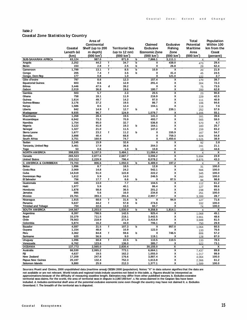
C o a s t a l E c o s y s t e m s 15
C o a s t a l Z o n e : E x t e n t a n d C h a n g e
Table 2
Coastal Zone Statistics by Country
CoastalLength {a}
(km)
Area ofContinental
Shelf (up to 200m depth)(000 km2)
Territorial Sea(up to 12 nm)
(000 km2)
ClaimedExclusive
Economic Zone(000 km2)
ExclusiveFishingZone
(000 km2)
TotalPotentialMaritime
Area(000 km2)
PopulationWithin 100
km from theCoast
(percent)SUB-SAHARAN AFRICA 63,124 987.0 871.9 b 7,866.1 3,111.1 X XAngola 2,252 44.2 f 34.7 b X 438.0 473 29.4Benin 153 2.8 f 2.5 b X 26.8 29 62.4Cameroon 1,799 13.1 f 8.5 b 10.9 X 20 21.9Congo 205 7.4 f 3.5 b X 41.4 45 24.5Congo, Dem Rep 177 0.8 1.0 X 121.0 122 2.7Côte d'Ivoire 797 8.6 12.3 157.4 X 170 39.7Equatorial Guinea 603 8.6 12.9 291.4 X 304 72.3Eritrea 3,446 47.5 d 39.2 X X 75 73.5Gabon 2,019 36.8 19.6 180.7 X 200 62.8Gambia 503 5.7 2.3 20.5 X 23 90.8Ghana 758 18.1 11.9 216.9 X 229 42.5Guinea 1,614 49.7 14.2 97.0 X 111 40.9Guinea-Bissau 3,176 37.2 19.5 86.7 X 10⁶ 94.6Kenya 1,586 8.5 12.4 104.1 X 116 7.6Liberia 842 14.9 f 12.7 b X 239.1 252 57.9Madagascar 9,935 96.7 124.9 1,079.7 X 1,205 55.1Mauritania 1,268 28.4 19.5 141.3 X 161 39.6Mozambique 6,942 73.3 70.9 493.7 X 565 59.0Namibia 1,754 95.0 32.7 536.8 X 570 4.7Nigeria 3,122 41.8 19.3 b 164.1 X 183 25.7Senegal 1,327 21.0 11.5 147.2 X 159 83.2Sierra Leone 1,677 23.2 f 11.2 b X 155.9 167 54.7Somalia 3,898 40.4 68.8 X 759.3 828 54.8South Africa 3,751 160.9 74.7 X 1,450.6 1,525 38.9Sudan 2,245 15.9 32.6 X X 92 2.8Tanzania, United Rep 3,461 17.9 36.6 204.3 X 241 21.1Togo 53 0.6 1.0 b 10.8 X 13 44.6NORTH AMERICA 398,835 5,107.5 3,484.1 11,084.4 X X XCanada 265,523 2,877.6 2,687.7 3,006.2 X 5,694 23.9United States 133,312 2,229.9 796.4 8,078.2 X 8,875 43.3C. AMERICA & CARIBBEAN 73,703 806.6 1,050.0 b 6,489.0 197.2 X XBelize 1,996 8.7 18.5 12.8 X 31 100.0Costa Rica 2,069 14.8 24.2 542.1 X 566 100.0Cuba 14,519 51.0 122.8 222.2 X 345 100.0Dominican Rep 1,612 5.9 14.0 246.5 X 260 100.0El Salvador 756 17.7 f 6.6 b X 87.5 94 98.8Guatemala 445 13.0 7.7 104.5 X 112 61.2Haiti 1,977 5.9 40.1 86.4 X 127 99.6Honduras 1,878 58.8 36.5 201.2 X 238 65.5Jamaica 895 5.6 16.0 234.8 X 251 100.0Mexico 23,761 393.3 291.6 2,997.7 X 3,289 28.7Nicaragua 1,915 68.6 f 31.6 b X 94.9 127 71.6Panama 5,637 44.2 f 57.8 b 274.6 X 332 100.0Trinidad and Tobago 704 22.6 13.0 60.7 X 74 100.0SOUTH AMERICA 144,567 2,203.0 1,030.0 b 9,358.8 1,814.1 X XArgentina 8,397 798.5 142.5 925.4 X 1,068 45.1Brazil 33,379 711.5 218.1 3,442.5 X 3,661 48.6Chile 78,563 218.9 271.9 3,415.9 X 3,688 81.5Colombia 5,874 16.2 44.0 706.1 X 750 29.9Ecuador 4,597 31.5 f 107.3 b X 957.0 1,064 60.5Guyana 1,154 48.8 10.9 122.0 X 133 76.6Peru 3,362 84.8 f 59.6 b X 746.5 806 57.2Suriname 620 56.9 9.0 119.1 X 128 87.0Uruguay 1,096 68.8 f 22.5 b 110.5 110.5 133 78.5Venezuela 6,762 123.6 136.0 385.7 X 522 73.1OCEANIA 137,772 2,565.0 2,830.4 30,155.0 X X XAustralia 66,530 2,065.2 773.1 6,664.1 X 7,437 89.8Fiji 4,637 19.5 162.2 1,055.0 X 1,217 99.9New Zealand 17,209 247.8 176.6 3,887.4 X 4,064 100.0Papua New Guinea 20,197 132.4 752.3 1,613.8 X 2,366 61.2Solomon Islands 9,880 25.9 212.3 1,377.1 X 1,589 100.0
Sources: Pruett and Cimino, 2000 unpublished data (maritime areas); CIESIN 2000 (population). Notes: "X" in data column signifies that the data arenot available or are not relevant. World totals and regional totals include countries not listed in this table. a. Figures should be interpreted asapproximations because of the difficulty of measuring coastline length. Estimates may differ from other published sources. b. Excludes excessiveterritorial seas claims. For the world, the area of territorial seas in dispute is 2,867,050 km². c. No areas claimed in the Caspian Sea have beenincluded. d. Includes continental shelf area of the potential exclusive economic zone even though the country may have not claimed it. e. ExcludesGreenland. f. The breadth of the territorial sea is disputed.
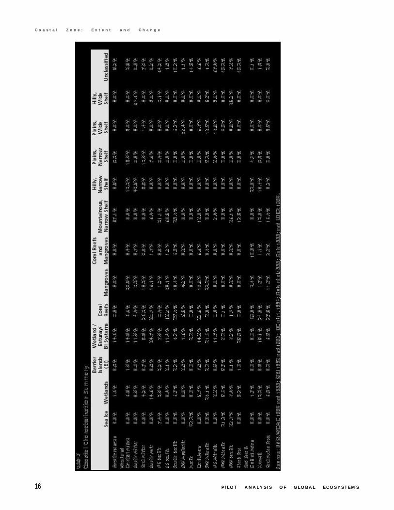
16 P I L O T A N A L Y S I S O F G L O B A L E C O S Y S T E M S
C o a s t a l Z o n e : E x t e n t a n d C h a n g e
C o a s t a l E c o s y s t e m s 17
C o a s t a l Z o n e : E x t e n t a n d C h a n g e
Characterizing underwater and benthic ecosystems is evenmore difficult than describing terrestrial ecosystems. Until themiddle of this century, most of our knowledge of continentalshelf communities was based on samples dredged or capturedby trawls, grab-samples, or even the wax or tallow affixed to thebase of plumblines used in hydrographic surveys. The adventof scuba diving, combined with increasing use of manned andremote submersibles, has greatly improved our knowledge base.Unfortunately, this knowledge has expanded in parallel withvastly increased fishing efforts on almost all of the world’s con-tinental shelves, including the highly destructive use of benthictrawls. (See Box 2.) Thus, we have little knowledge of what pris-tine environments in the waters just off our shores may havebeen like even 50 years ago, unless we examine such historicrecords as the trawl samples taken by early oceanographiccruises and compare them with modern samples.
One of the most fundamental descriptive approaches in ter-restrial biogeography at global and regional levels is the identi-fication and description of potential vegetation and the subse-quent subdivision of the world into biogeographic ecoregions.Ecoregional mapping combines habitat or ecosystem identifi-cation with knowledge of physio-chemical parameters and alsohistorical factors of species evolution and distribution. Suchwork has also been attempted in the marine environment by anumber of authors. Biogeographic patterns in the water columnare determined most notably by water circulation patterns drivenby wind, Coriolis force, and temperature, as well as salinity andnutrient availability. For example, various researchers have stud-ied patterns of pelagic ecosystems and prepared schemes basedon ocean currents, temperatures, productivity, or salinity(Hayden et al. 1984; Bailey 1998; Longhurst 1998). Others havelooked at patterns in benthic communities (Ekman 1953;Hedgpeth 1957; Briggs 1974), although the availability of datafrom nonshelf benthos is so poor that they have only describedthese in general terms.
The classification used by Bailey and Longhurst includesecological domains, such as the polar/boreal region, westerlydrifts, and trade winds. Longhurst further delineated 56 sec-ondary biogeochemical provinces within such domains, includ-ing coastal waters, and used them to report the pelagic primaryproduction (Longhurst 1995). Sherman (1993) developed LargeMarine Ecosystems (LMEs) as ecological subdivisions of coastalwaters, which are targeted for ecosystem-based monitoring andmanagement, although the LMEs are incomplete in their globalcoverage. Such biogeographic regionalization is more ecologi-cally grounded than are political units and provide a better spa-tial analytical framework in organizing the data collection, as-sessment, and reporting of ecosystem conditions.
The existing regionalization schemes are useful in charac-terizing various coastal areas; however, no single scheme is ei-ther possible or suitable for summarizing all of the data as-
sembled for this study. Some of the data sets presented in thefollowing sections are gathered under particular schemes, oftenpolitical regions, and reaggregation of such data is not possible.
Extent and Change in Area of Se lected
Coasta l Ecosystem TypesThe extent and change of coastal ecosystems is poorly knownrelative to most other terrestrial habitat types. Because indi-vidual coastal ecosystems, such as wetlands or coral reefs, tendto cover relatively small areas, detailed mapping is needed tomeasure extent or change. Until the advent of remote sensing,such mapping was beyond the reach of most nations. Even to-day, high resolution mapping of these systems is imperfect, ex-pensive, and has not been attempted globally.
Wetlands are among the most highly altered ecosystemsworldwide. Coastal wetlands (both tidal and nontidal) have beendestroyed by direct actions (draining, dredging, landfill, spoildisposal, and conversion for aquaculture), and indirect pres-sures (sediment diversion and hydraulic alteration). The runoffof polluted waters (nonpoint-source pollution) has stressedcoastal wetlands, which are already at risk from urban expan-sion and development in general. Natural processes, such aserosion and subsidence, also contribute to wetland loss, althoughhuman actions often aggravate these.
To provide a global overview of the extent and change in thediverse coastal habitat types, this study looked at mangroves,other coastal wetlands, seagrasses, and coral reefs.
MANGROVESUnlike for most other coastal ecosystems, considerable data areavailable on the global distribution of mangrove forests. Basedon the coastal characterization presented above, mangroves lineapproximately 8 percent of the world’s coastline. A previousestimate by Spalding et al. (1997:20–23) concludes that man-groves are distributed along approximately one-quarter of theworld’s tropical coastlines, covering a surface area of 181,000km2. About 112 countries and territories have mangroves withintheir borders. Estimates of current mangrove extent vary sig-nificantly from one source to another, possibly because of thedifference in definition, methodology, and land cover informa-tion used (see Spalding et al. 1997, for more discussion on thisissue). Table 4 presents mangrove area estimates by countryderived from maps and other published sources.
No global or even regional map shows the “original” distri-bution of mangroves with sufficient resolution to measure thedifferences between such a distribution and current mangrovearea. Scientists are unable to estimate exactly how extensivemangroves were before people began to alter coastlines. How-ever, based on historical records, it can be said that mangrove
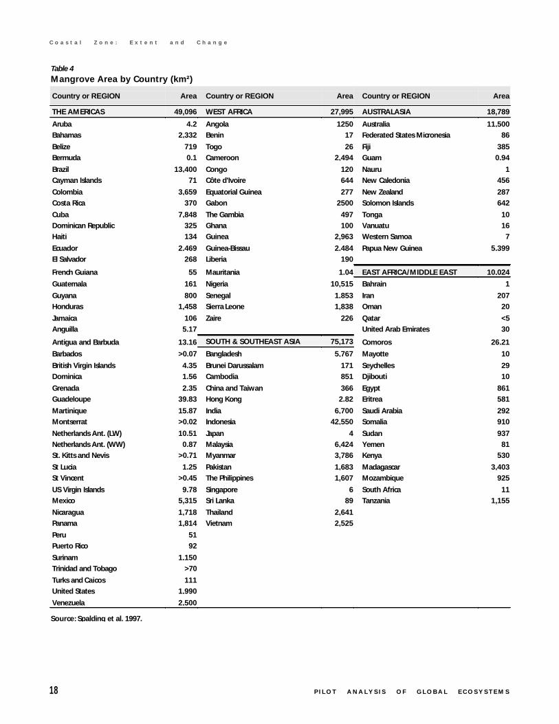
18 P I L O T A N A L Y S I S O F G L O B A L E C O S Y S T E M S
C o a s t a l Z o n e : E x t e n t a n d C h a n g e
Table 4
Mangrove Area by Country (km²)
Country or REGION Area Country or REGION Area Country or REGION Area
THE AMERICAS 49,096 WEST AFRICA 27,995 AUSTRALASIA 18,789
Aruba 4.2 Angola 1250 Australia 11,500
Bahamas 2,332 Benin 17 Federated States Micronesia 86
Belize 719 Togo 26 Fiji 385
Bermuda 0.1 Cameroon 2,494 Guam 0.94
Brazil 13,400 Congo 120 Nauru 1 Cayman Islands 71 Côte d'Ivoire 644 New Caledonia 456
Colombia 3,659 Equatorial Guinea 277 New Zealand 287
Costa Rica 370 Gabon 2500 Solomon Islands 642
Cuba 7,848 The Gambia 497 Tonga 10
Dominican Republic 325 Ghana 100 Vanuatu 16
Haiti 134 Guinea 2,963 Western Samoa 7 Ecuador 2,469 Guinea-Bissau 2,484 Papua New Guinea 5,399
El Salvador 268 Liberia 190 French Guiana 55 Mauritania 1.04 EAST AFRICA/MIDDLE EAST 10,024
Guatemala 161 Nigeria 10,515 Bahrain 1 Guyana 800 Senegal 1,853 Iran 207
Honduras 1,458 Sierra Leone 1,838 Oman 20
Jamaica 106 Zaire 226 Qatar <5
Anguilla 5.17 United Arab Emirates 30
Antigua and Barbuda 13.16 SOUTH & SOUTHEAST ASIA 75,173 Comoros 26.21
Barbados >0.07 Bangladesh 5,767 Mayotte 10
British Virgin Islands 4.35 Brunei Darussalam 171 Seychelles 29
Dominica 1.56 Cambodia 851 Djibouti 10
Grenada 2.35 China and Taiwan 366 Egypt 861
Guadeloupe 39.83 Hong Kong 2.82 Eritrea 581
Martinique 15.87 India 6,700 Saudi Arabia 292
Montserrat >0.02 Indonesia 42,550 Somalia 910
Netherlands Ant. (LW) 10.51 Japan 4 Sudan 937
Netherlands Ant. (WW) 0.87 Malaysia 6,424 Yemen 81
St. Kitts and Nevis >0.71 Myanmar 3,786 Kenya 530
St Lucia 1.25 Pakistan 1,683 Madagascar 3,403
St Vincent >0.45 The Philippines 1,607 Mozambique 925
US Virgin Islands 9.78 Singapore 6 South Africa 11
Mexico 5,315 Sri Lanka 89 Tanzania 1,155
Nicaragua 1,718 Thailand 2,641 Panama 1,814 Vietnam 2,525 Peru 51 Puerto Rico 92 Surinam 1,150 Trinidad and Tobago >70 Turks and Caicos 111 United States 1,990 Venezuela 2,500
Source: Spalding et al. 1997.
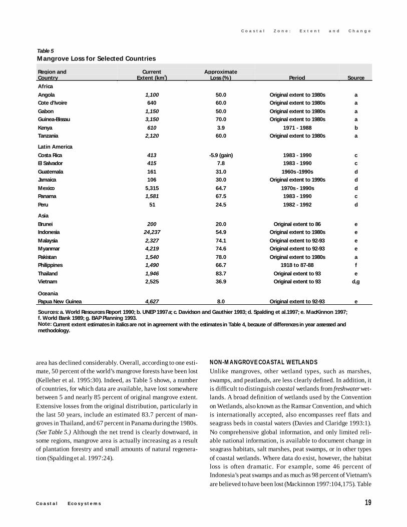
C o a s t a l E c o s y s t e m s 19
C o a s t a l Z o n e : E x t e n t a n d C h a n g e
area has declined considerably. Overall, according to one esti-mate, 50 percent of the world’s mangrove forests have been lost(Kelleher et al. 1995:30). Indeed, as Table 5 shows, a numberof countries, for which data are available, have lost somewherebetween 5 and nearly 85 percent of original mangrove extent.Extensive losses from the original distribution, particularly inthe last 50 years, include an estimated 83.7 percent of man-groves in Thailand, and 67 percent in Panama during the 1980s.(See Table 5.) Although the net trend is clearly downward, insome regions, mangrove area is actually increasing as a resultof plantation forestry and small amounts of natural regenera-tion (Spalding et al. 1997:24).
NON-MANGROVE COASTAL WETLANDSUnlike mangroves, other wetland types, such as marshes,swamps, and peatlands, are less clearly defined. In addition, itis difficult to distinguish coastal wetlands from freshwater wet-lands. A broad definition of wetlands used by the Conventionon Wetlands, also known as the Ramsar Convention, and whichis internationally accepted, also encompasses reef flats andseagrass beds in coastal waters (Davies and Claridge 1993:1).No comprehensive global information, and only limited reli-able national information, is available to document change inseagrass habitats, salt marshes, peat swamps, or in other typesof coastal wetlands. Where data do exist, however, the habitatloss is often dramatic. For example, some 46 percent ofIndonesia’s peat swamps and as much as 98 percent of Vietnam’sare believed to have been lost (Mackinnon 1997:104,175). Table
Table 5
Mangrove Loss for Selected Countries
Region andCountry
CurrentExtent (km2)
ApproximateLoss (%) Period Source
Africa
Angola 1,100 50.0 Original extent to 1980s a
Cote d'Ivoire 640 60.0 Original extent to 1980s a
Gabon 1,150 50.0 Original extent to 1980s a
Guinea-Bissau 3,150 70.0 Original extent to 1980s a
Kenya 610 3.9 1971 - 1988 b
Tanzania 2,120 60.0 Original extent to 1980s a
Latin America
Costa Rica 413 -5.9 (gain) 1983 - 1990 c
El Salvador 415 7.8 1983 - 1990 c
Guatemala 161 31.0 1960s -1990s d
Jamaica 106 30.0 Original extent to 1990s d
Mexico 5,315 64.7 1970s - 1990s d
Panama 1,581 67.5 1983 - 1990 c
Peru 51 24.5 1982 - 1992 d
Asia
Brunei 200 20.0 Original extent to 86 e
Indonesia 24,237 54.9 Original extent to 1980s e
Malaysia 2,327 74.1 Original extent to 92-93 e
Myanmar 4,219 74.6 Original extent to 92-93 e
Pakistan 1,540 78.0 Original extent to 1980s a
Philippines 1,490 66.7 1918 to 87-88 f
Thailand 1,946 83.7 Original extent to 93 e
Vietnam 2,525 36.9 Original extent to 93 d,g
Oceania
Papua New Guinea 4,627 8.0 Original extent to 92-93 e
Sources: a. World Resources Report 1990; b. UNEP 1997a; c. Davidson and Gauthier 1993; d. Spalding et al.1997; e. MacKinnon 1997;f. World Bank 1989; g. BAP Planning 1993.Note: Current extent estimates in italics are not in agreement with the estimates in Table 4, because of differences in year assessed andmethodology.
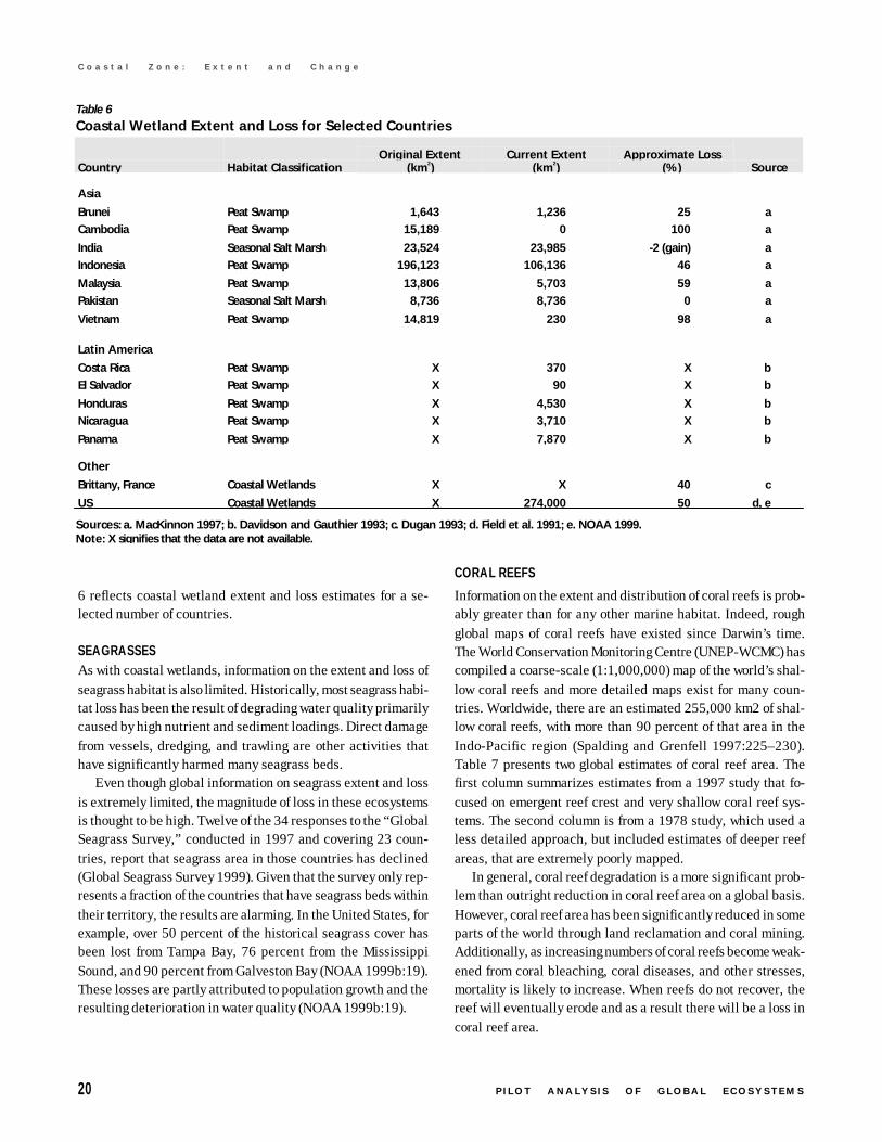
20 P I L O T A N A L Y S I S O F G L O B A L E C O S Y S T E M S
C o a s t a l Z o n e : E x t e n t a n d C h a n g e
6 reflects coastal wetland extent and loss estimates for a se-lected number of countries.
SEAGRASSESAs with coastal wetlands, information on the extent and loss ofseagrass habitat is also limited. Historically, most seagrass habi-tat loss has been the result of degrading water quality primarilycaused by high nutrient and sediment loadings. Direct damagefrom vessels, dredging, and trawling are other activities thathave significantly harmed many seagrass beds.
Even though global information on seagrass extent and lossis extremely limited, the magnitude of loss in these ecosystemsis thought to be high. Twelve of the 34 responses to the “GlobalSeagrass Survey,” conducted in 1997 and covering 23 coun-tries, report that seagrass area in those countries has declined(Global Seagrass Survey 1999). Given that the survey only rep-resents a fraction of the countries that have seagrass beds withintheir territory, the results are alarming. In the United States, forexample, over 50 percent of the historical seagrass cover hasbeen lost from Tampa Bay, 76 percent from the MississippiSound, and 90 percent from Galveston Bay (NOAA 1999b:19).These losses are partly attributed to population growth and theresulting deterioration in water quality (NOAA 1999b:19).
CORAL REEFS
Information on the extent and distribution of coral reefs is prob-ably greater than for any other marine habitat. Indeed, roughglobal maps of coral reefs have existed since Darwin’s time.The World Conservation Monitoring Centre (UNEP-WCMC) hascompiled a coarse-scale (1:1,000,000) map of the world’s shal-low coral reefs and more detailed maps exist for many coun-tries. Worldwide, there are an estimated 255,000 km2 of shal-low coral reefs, with more than 90 percent of that area in theIndo-Pacific region (Spalding and Grenfell 1997:225–230).Table 7 presents two global estimates of coral reef area. Thefirst column summarizes estimates from a 1997 study that fo-cused on emergent reef crest and very shallow coral reef sys-tems. The second column is from a 1978 study, which used aless detailed approach, but included estimates of deeper reefareas, that are extremely poorly mapped.
In general, coral reef degradation is a more significant prob-lem than outright reduction in coral reef area on a global basis.However, coral reef area has been significantly reduced in someparts of the world through land reclamation and coral mining.Additionally, as increasing numbers of coral reefs become weak-ened from coral bleaching, coral diseases, and other stresses,mortality is likely to increase. When reefs do not recover, thereef will eventually erode and as a result there will be a loss incoral reef area.
Table 6
Coastal Wetland Extent and Loss for Selected Countries
Country Habitat ClassificationOriginal Extent
(km2)Current Extent
(km2)Approximate Loss
(%) Source
Asia
Brunei Peat Swamp 1,643 1,236 25 a
Cambodia Peat Swamp 15,189 0 100 a
India Seasonal Salt Marsh 23,524 23,985 -2 (gain) a
Indonesia Peat Swamp 196,123 106,136 46 a
Malaysia Peat Swamp 13,806 5,703 59 a
Pakistan Seasonal Salt Marsh 8,736 8,736 0 a
Vietnam Peat Swamp 14,819 230 98 a
Latin America
Costa Rica Peat Swamp X 370 X b
El Salvador Peat Swamp X 90 X b
Honduras Peat Swamp X 4,530 X b
Nicaragua Peat Swamp X 3,710 X b
Panama Peat Swamp X 7,870 X b
Other
Brittany, France Coastal Wetlands X X 40 c
US Coastal Wetlands X 274,000 50 d, e
Sources: a. MacKinnon 1997; b. Davidson and Gauthier 1993; c. Dugan 1993; d. Field et al. 1991; e. NOAA 1999.Note: X signifies that the data are not available.
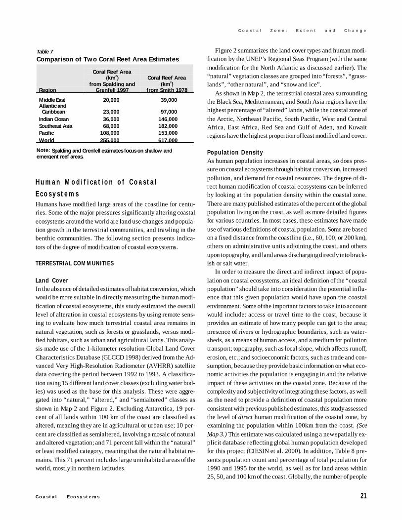
C o a s t a l E c o s y s t e m s 21
C o a s t a l Z o n e : E x t e n t a n d C h a n g e
Human Modi f i cat ion of Coasta l
E c o s y s t e m sHumans have modified large areas of the coastline for centu-ries. Some of the major pressures significantly altering coastalecosystems around the world are land use changes and popula-tion growth in the terrestrial communities, and trawling in thebenthic communities. The following section presents indica-tors of the degree of modification of coastal ecosystems.
TERRESTRIAL COMMUNITIES
Land CoverIn the absence of detailed estimates of habitat conversion, whichwould be more suitable in directly measuring the human modi-fication of coastal ecosystems, this study estimated the overalllevel of alteration in coastal ecosystems by using remote sens-ing to evaluate how much terrestrial coastal area remains innatural vegetation, such as forests or grasslands, versus modi-fied habitats, such as urban and agricultural lands. This analy-sis made use of the 1-kilometer resolution Global Land CoverCharacteristics Database (GLCCD 1998) derived from the Ad-vanced Very High-Resolution Radiometer (AVHRR) satellitedata covering the period between 1992 to 1993. A classifica-tion using 15 different land cover classes (excluding water bod-ies) was used as the base for this analysis. These were aggre-gated into “natural,” “altered,” and “semialtered” classes asshown in Map 2 and Figure 2. Excluding Antarctica, 19 per-cent of all lands within 100 km of the coast are classified asaltered, meaning they are in agricultural or urban use; 10 per-cent are classified as semialtered, involving a mosaic of naturaland altered vegetation; and 71 percent fall within the “natural”or least modified category, meaning that the natural habitat re-mains. This 71 percent includes large uninhabited areas of theworld, mostly in northern latitudes.
Figure 2 summarizes the land cover types and human modi-fication by the UNEP’s Regional Seas Program (with the samemodification for the North Atlantic as discussed earlier). The“natural” vegetation classes are grouped into “forests”, “grass-lands”, “other natural”, and “snow and ice”.
As shown in Map 2, the terrestrial coastal area surroundingthe Black Sea, Mediterranean, and South Asia regions have thehighest percentage of “altered” lands, while the coastal zone ofthe Arctic, Northeast Pacific, South Pacific, West and CentralAfrica, East Africa, Red Sea and Gulf of Aden, and Kuwaitregions have the highest proportion of least modified land cover.
Population DensityAs human population increases in coastal areas, so does pres-sure on coastal ecosystems through habitat conversion, increasedpollution, and demand for coastal resources. The degree of di-rect human modification of coastal ecosystems can be inferredby looking at the population density within the coastal zone.There are many published estimates of the percent of the globalpopulation living on the coast, as well as more detailed figuresfor various countries. In most cases, these estimates have madeuse of various definitions of coastal population. Some are basedon a fixed distance from the coastline (i.e., 60, 100, or 200 km),others on administrative units adjoining the coast, and othersupon topography, and land areas discharging directly into brack-ish or salt water.
In order to measure the direct and indirect impact of popu-lation on coastal ecosystems, an ideal definition of the “coastalpopulation” should take into consideration the potential influ-ence that this given population would have upon the coastalenvironment. Some of the important factors to take into accountwould include: access or travel time to the coast, because itprovides an estimate of how many people can get to the area;presence of rivers or hydrographic boundaries, such as water-sheds, as a means of human access, and a medium for pollutiontransport; topography, such as local slope, which affects runoff,erosion, etc.; and socioeconomic factors, such as trade and con-sumption, because they provide basic information on what eco-nomic activities the population is engaging in and the relativeimpact of these activities on the coastal zone. Because of thecomplexity and subjectivity of integrating these factors, as wellas the need to provide a definition of coastal population moreconsistent with previous published estimates, this study assessedthe level of direct human modification of the coastal zone, byexamining the population within 100km from the coast. (SeeMap 3.) This estimate was calculated using a new spatially ex-plicit database reflecting global human population developedfor this project (CIESIN et al. 2000). In addition, Table 8 pre-sents population count and percentage of total population for1990 and 1995 for the world, as well as for land areas within25, 50, and 100 km of the coast. Globally, the number of people
Table 7
Comparison of Two Coral Reef Area Estimates
Region
Coral Reef Area(km2)
from Spalding andGrenfell 1997
Coral Reef Area(km2)
from Smith 1978
Middle East 20,000 39,000Atlantic and Caribbean 23,000 97,000Indian Ocean 36,000 146,000Southeast Asia 68,000 182,000Pacific 108,000 153,000World 255,000 617,000
Note: Spalding and Grenfell estimates focus on shallow andemergent reef areas.
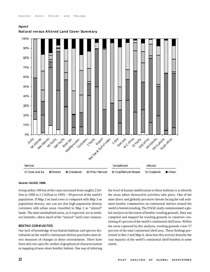
22 P I L O T A N A L Y S I S O F G L O B A L E C O S Y S T E M S
C o a s t a l Z o n e : E x t e n t a n d C h a n g e
living within 100 km of the coast increased from roughly 2 bil-lion in 1990 to 2.2 billion in 1995—39 percent of the world’spopulation. If Map 2 on land cover is compared with Map 3 onpopulation density, one can see that high population densitycorrelates with urban areas classified in Map 2 as “altered”lands. The most uninhabited areas, as is expected, are in north-ern latitudes, where much of the “natural” land cover remains.
BENTHIC COMMUNITIESOur lack of knowledge of sea bottom habitats and species dis-tribution on the world’s continental shelves precludes most di-rect measures of changes in these environments. There havebeen only site-specific studies of geophysical characterizationor mapping of near-shore benthic habitat. One way of inferring
the level of human modification to these habitats is to identifythe areas where destructive activities take place. One of themost direct and globally pervasive threats facing the soft sedi-ment benthic communities on continental shelves around theworld is bottom trawling. The PAGE study commissioned a glo-bal analysis on the extent of benthic trawling grounds. Data wascompiled and mapped for trawling grounds in countries con-taining 41 percent of the world’s continental shelf area. Withinthe areas captured by this analysis, trawling grounds cover 57percent of the total continental shelf area. These findings pre-sented in Box 2 and Map 4, show that this activity disturbs thevast majority of the world’s continental shelf benthos to someextent.
Figure 2
Natural versus Altered Land Cover Summary
Source: GLCCD, 1998.
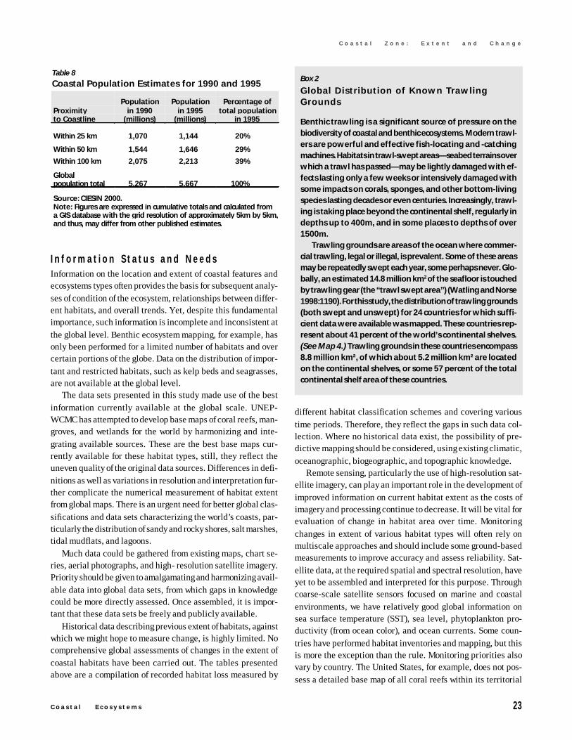
C o a s t a l E c o s y s t e m s 23
C o a s t a l Z o n e : E x t e n t a n d C h a n g e
In format ion Status and NeedsInformation on the location and extent of coastal features andecosystems types often provides the basis for subsequent analy-ses of condition of the ecosystem, relationships between differ-ent habitats, and overall trends. Yet, despite this fundamentalimportance, such information is incomplete and inconsistent atthe global level. Benthic ecosystem mapping, for example, hasonly been performed for a limited number of habitats and overcertain portions of the globe. Data on the distribution of impor-tant and restricted habitats, such as kelp beds and seagrasses,are not available at the global level.
The data sets presented in this study made use of the bestinformation currently available at the global scale. UNEP-WCMC has attempted to develop base maps of coral reefs, man-groves, and wetlands for the world by harmonizing and inte-grating available sources. These are the best base maps cur-rently available for these habitat types, still, they reflect theuneven quality of the original data sources. Differences in defi-nitions as well as variations in resolution and interpretation fur-ther complicate the numerical measurement of habitat extentfrom global maps. There is an urgent need for better global clas-sifications and data sets characterizing the world’s coasts, par-ticularly the distribution of sandy and rocky shores, salt marshes,tidal mudflats, and lagoons.
Much data could be gathered from existing maps, chart se-ries, aerial photographs, and high- resolution satellite imagery.Priority should be given to amalgamating and harmonizing avail-able data into global data sets, from which gaps in knowledgecould be more directly assessed. Once assembled, it is impor-tant that these data sets be freely and publicly available.
Historical data describing previous extent of habitats, againstwhich we might hope to measure change, is highly limited. Nocomprehensive global assessments of changes in the extent ofcoastal habitats have been carried out. The tables presentedabove are a compilation of recorded habitat loss measured by
different habitat classification schemes and covering varioustime periods. Therefore, they reflect the gaps in such data col-lection. Where no historical data exist, the possibility of pre-dictive mapping should be considered, using existing climatic,oceanographic, biogeographic, and topographic knowledge.
Remote sensing, particularly the use of high-resolution sat-ellite imagery, can play an important role in the development ofimproved information on current habitat extent as the costs ofimagery and processing continue to decrease. It will be vital forevaluation of change in habitat area over time. Monitoringchanges in extent of various habitat types will often rely onmultiscale approaches and should include some ground-basedmeasurements to improve accuracy and assess reliability. Sat-ellite data, at the required spatial and spectral resolution, haveyet to be assembled and interpreted for this purpose. Throughcoarse-scale satellite sensors focused on marine and coastalenvironments, we have relatively good global information onsea surface temperature (SST), sea level, phytoplankton pro-ductivity (from ocean color), and ocean currents. Some coun-tries have performed habitat inventories and mapping, but thisis more the exception than the rule. Monitoring priorities alsovary by country. The United States, for example, does not pos-sess a detailed base map of all coral reefs within its territorial
Box 2
Global Distribution of Known TrawlingGrounds
Benthic trawling is a significant source of pressure on thebiodiversity of coastal and benthic ecosystems. Modern trawl-ers are powerful and effective fish-locating and -catchingmachines. Habitats in trawl-swept areas—seabed terrains overwhich a trawl has passed—may be lightly damaged with ef-fects lasting only a few weeks or intensively damaged withsome impacts on corals, sponges, and other bottom-livingspecies lasting decades or even centuries. Increasingly, trawl-ing is taking place beyond the continental shelf, regularly indepths up to 400m, and in some places to depths of over1500m.
Trawling grounds are areas of the ocean where commer-cial trawling, legal or illegal, is prevalent. Some of these areasmay be repeatedly swept each year, some perhaps never. Glo-bally, an estimated 14.8 million km2 of the seafloor is touchedby trawling gear (the “trawl swept area”) (Watling and Norse1998:1190). For this study, the distribution of trawling grounds(both swept and unswept) for 24 countries for which suffi-cient data were available was mapped. These countries rep-resent about 41 percent of the world’s continental shelves.(See Map 4.) Trawling grounds in these countries encompass8.8 million km², of which about 5.2 million km² are locatedon the continental shelves, or some 57 percent of the totalcontinental shelf area of these countries.
Table 8
Coastal Population Estimates for 1990 and 1995
Proximityto Coastline
Populationin 1990
(millions)
Populationin 1995
(millions)
Percentage oftotal population
in 1995
Within 25 km 1,070 1,144 20%
Within 50 km 1,544 1,646 29%
Within 100 km 2,075 2,213 39%
Globalpopulation total 5,267 5,667 100%
Source: CIESIN 2000.Note: Figures are expressed in cumulative totals and calculated froma GIS database with the grid resolution of approximately 5km by 5km,and thus, may differ from other published estimates.
24 P I L O T A N A L Y S I S O F G L O B A L E C O S Y S T E M S
C o a s t a l Z o n e : E x t e n t a n d C h a n g e
waters, but has performed detailed mapping of all major estuar-ies by salinity zone.
Although the extent and change data presented above arean important basis for assessing the condition of other ecosys-tem goods and services—and are referred to as such through-out this report—these are mere proxies for measuring the con-dition of the ecosystems. Data with higher resolution and accu-racy are needed to sufficiently capture the level of human modi-fication in the complex and narrow coastal zone. We do not havea good understanding of the overall impacts on coastal ecosys-
tems caused by human modification of landscape and otheranthropogenic disturbances, such as dredging and trawling.These changes and disturbances influence the quality and struc-ture of these ecosystems, which may not be as easily observedas habitat loss. We need better quantitative analysis of how thechange in the extent of various habitats is affecting the array ofgoods and services that are derived from them. Nevertheless,the degree of degradation suggested by the available informa-tion reinforces the need for precautionary action.
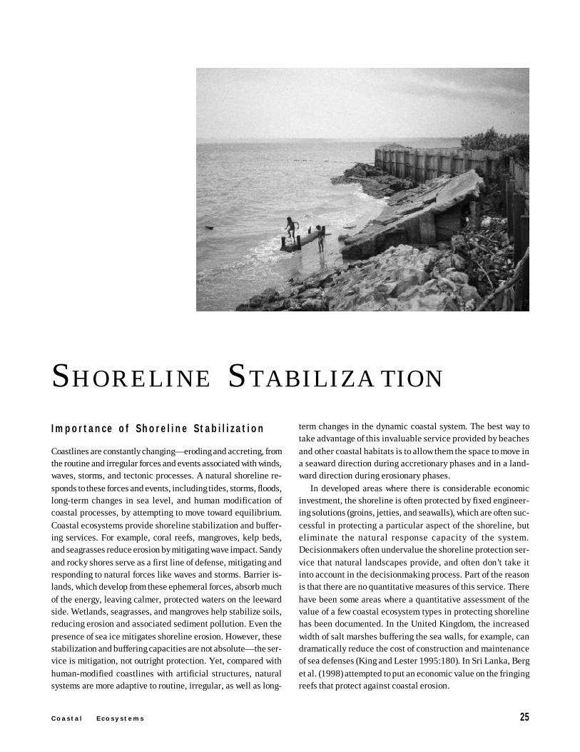
C o a s t a l E c o s y s t e m s 25
C o a s t a l Z o n e : E x t e n t a n d C h a n g e
Importance of Shore l ine S tab i l i za t ion
Coastlines are constantly changing—eroding and accreting, fromthe routine and irregular forces and events associated with winds,waves, storms, and tectonic processes. A natural shoreline re-sponds to these forces and events, including tides, storms, floods,long-term changes in sea level, and human modification ofcoastal processes, by attempting to move toward equilibrium.Coastal ecosystems provide shoreline stabilization and buffer-ing services. For example, coral reefs, mangroves, kelp beds,and seagrasses reduce erosion by mitigating wave impact. Sandyand rocky shores serve as a first line of defense, mitigating andresponding to natural forces like waves and storms. Barrier is-lands, which develop from these ephemeral forces, absorb muchof the energy, leaving calmer, protected waters on the leewardside. Wetlands, seagrasses, and mangroves help stabilize soils,reducing erosion and associated sediment pollution. Even thepresence of sea ice mitigates shoreline erosion. However, thesestabilization and buffering capacities are not absolute—the ser-vice is mitigation, not outright protection. Yet, compared withhuman-modified coastlines with artificial structures, naturalsystems are more adaptive to routine, irregular, as well as long-
term changes in the dynamic coastal system. The best way totake advantage of this invaluable service provided by beachesand other coastal habitats is to allow them the space to move ina seaward direction during accretionary phases and in a land-ward direction during erosionary phases.
In developed areas where there is considerable economicinvestment, the shoreline is often protected by fixed engineer-ing solutions (groins, jetties, and seawalls), which are often suc-cessful in protecting a particular aspect of the shoreline, buteliminate the natural response capacity of the system.Decisionmakers often undervalue the shoreline protection ser-vice that natural landscapes provide, and often don’t take itinto account in the decisionmaking process. Part of the reasonis that there are no quantitative measures of this service. Therehave been some areas where a quantitative assessment of thevalue of a few coastal ecosystem types in protecting shorelinehas been documented. In the United Kingdom, the increasedwidth of salt marshes buffering the sea walls, for example, candramatically reduce the cost of construction and maintenanceof sea defenses (King and Lester 1995:180). In Sri Lanka, Berget al. (1998) attempted to put an economic value on the fringingreefs that protect against coastal erosion.
SH O R E L I N E S TABILIZA TION
26 P I L O T A N A L Y S I S O F G L O B A L E C O S Y S T E M S
S h o r e l i n e S t a b i l i z a t i o n
Shoreline protection is a very important issue, particularlyin countries with small land area or limited arable land, be-cause any erosion or change in the shoreline can affect theamount of land available for different activities. One way of es-timating the value of this service is to estimate the cost of re-placing it, which in many cases can be extremely expensive. Ameasurement of the relative importance of shoreline stability toa country or area can be estimated by how much monetary in-vestment is made on shoreline protection, and by the percent-age of the shoreline on which some stabilization measures aretaken. The most well-known example is the Netherlands, wherethe extensive system of dikes and dams protects nearly half ofthe total land area from being flooded (Central IntelligenceAgency 1998). Japan has identified approximately 46 percentof its shoreline as requiring stabilization measures, and during1970–98 the total investment on shoreline protection works was4.5 trillion Yen (more than US$40 billion) (Japan Ministry ofConstruction 1998). Sri Lanka provides an example that di-rectly relates the loss of coastal habitat to the cost of replacingthe service lost. It spent US$30 million on revetments, groins,and breakwaters in response to severe coastal erosion that oc-curred in areas where coral reefs were heavily mined (Berg etal. 1998:630).
Effects of Art i f i c ia l S t ructures on the
Shore l ineFor centuries, human activities have modified shorelines andinterfered with coastal processes. The exploitation of shorelineand near-shore environments for transportation, industry, resi-dential development, and recreation has had profound impactson the ecosystem as well as on other chemical, material, andenergy cycles in the near-shore aquatic environment. Coastalcivil engineering works disrupt natural sediment movement ina variety of ways, in many cases causing accelerated erosion orunforeseen problems in adjacent shorelines. Efforts to stabilizeshorelines have been substantial in many parts of the worldbecause property values are high and development has oftenoccurred too close to the shoreline.
Major human modifications to the shoreline include: con-struction of harbors with breakwaters; construction or modifi-cation of inlets for navigational purposes; intentional modifica-tion of longshore sediment transport; construction of dams; sandmining from riverbeds near coastal areas; and extraction ofground fluids resulting in coastal subsidence (National ResearchCouncil 1990). Modification of the river flow through dams hasled to changes in sediment budgets, with deposition in reser-voirs and frequent erosion of deltas. The impacts have beenobserved in several parts of the world. In the north of Italy, forexample, reduced sediment loads in the Arno River have re-
sulted in a shoreline retreat of 1.3 km—as much as 20m peryear in recent years (Aminti et al. 1999:7).
Another example of a jetty’s impact on coastal morphology isthe accelerated migration of Assateague Island along the At-lantic coast of the United States. A hurricane striking in 1933opened an inlet between what are now called Fenwick andAssateague Islands. Jetties were built on either side to main-tain the inlet. These jetties trapped sand to form a wide beachat Ocean City, on the northern side, resulting in a sediment-starved Assateague Island. The situation accelerated the re-treat of the shoreline from 5 ft per year to 30 ft per year. Theretreating island now has a 500 meter offset from a once straightbarrier island (Williams et al. 1995).
Partly because of the negative aspects of hard stabilizationtechniques, sand replenishment in beaches has become increas-ingly popular as a shoreline stabilization measure. Sand or beachreplenishment is an expensive technique that must be imple-mented properly and repeatedly to be effective. The grain sizeof replacement sand must be the same size or slightly largerthan that of the natural beach. The source of the sand must bechosen carefully to make sure that removal does not result inunwanted side effects. This technique is more in line with natu-ral processes than hard stabilization approaches, but is expen-sive. Since 1965, the United States has spent US$3.5 billion on1,305 beach replenishment projects. For example, the beachreplenishment of Miami Beach in the late 1970s alone costUS$64 million (Williams et al. 1995). The beach nourishmentof the East Coast barrier island shoreline of the United States isby far the most extensive in terms of both sand volume and cost.It is estimated that the state of New Jersey would require US$1.6billion over 10 years to replenish and maintain its 90 miles ofdeveloped open ocean shoreline (Trembanis et al. 1998:246–251).
For many countries, protection of coastal ecosystems is likelyto be one of the most cost-effective means of defending coastaldevelopment from the impact of storms and floods. As in the SriLankan example mentioned earlier, it is clear that, with the sig-nificant loss in extent of various coastal ecosystems, the capa-bility of most nations’ coasts to provide this service has beensignificantly diminished, resulting in additional investment forartificial protection.
Condi t ion of Shore l ine S tab i l i za t ion
Serv i cesUseful indicators to assess the condition of the world’s shore-line stabilization services can be grouped into three broad cat-egories. (1) Measures that show the extent and change in areaand quality of coastal habitats from which a loss or gain in sta-bilization services can be inferred. (2) Indicators that measure
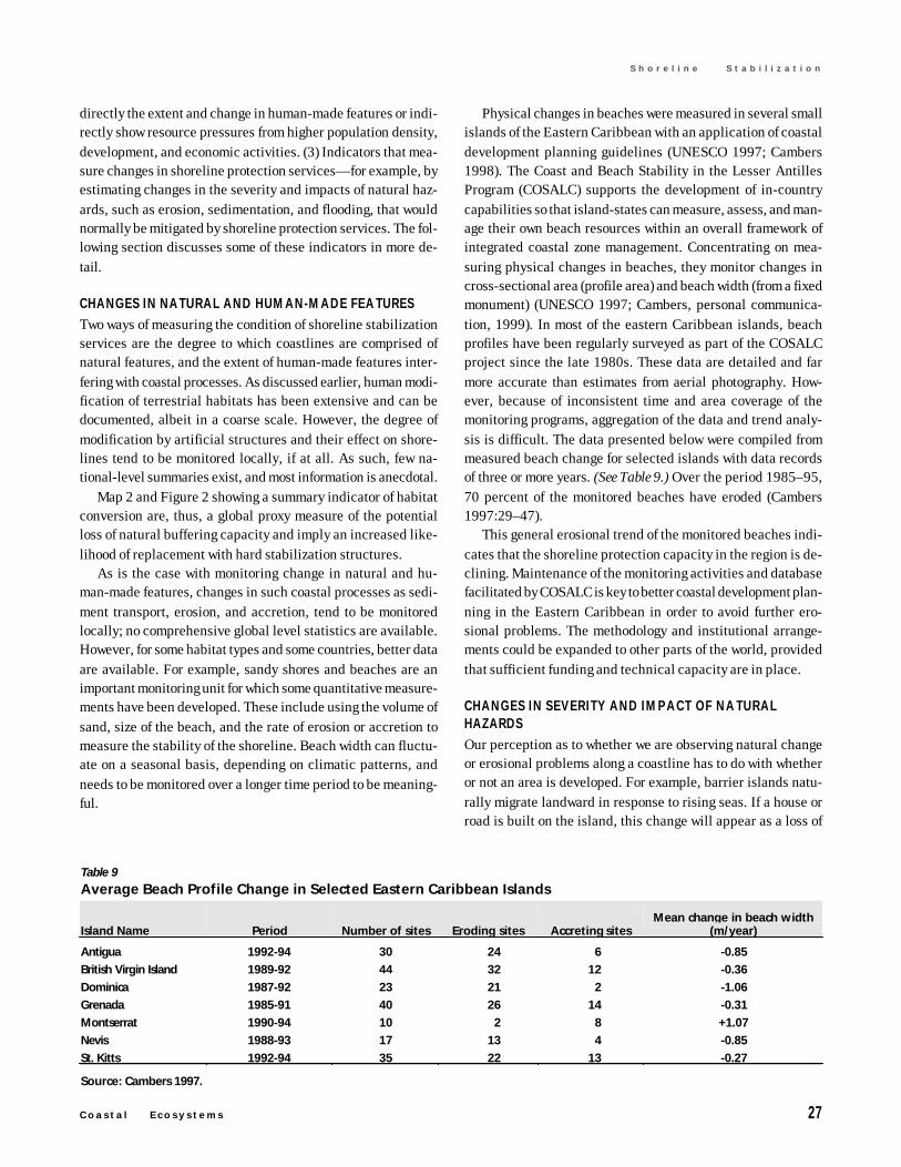
C o a s t a l E c o s y s t e m s 27
S h o r e l i n e S t a b i l i z a t i o n
directly the extent and change in human-made features or indi-rectly show resource pressures from higher population density,development, and economic activities. (3) Indicators that mea-sure changes in shoreline protection services—for example, byestimating changes in the severity and impacts of natural haz-ards, such as erosion, sedimentation, and flooding, that wouldnormally be mitigated by shoreline protection services. The fol-lowing section discusses some of these indicators in more de-tail.
CHANGES IN NATURAL AND HUMAN-MADE FEATURESTwo ways of measuring the condition of shoreline stabilizationservices are the degree to which coastlines are comprised ofnatural features, and the extent of human-made features inter-fering with coastal processes. As discussed earlier, human modi-fication of terrestrial habitats has been extensive and can bedocumented, albeit in a coarse scale. However, the degree ofmodification by artificial structures and their effect on shore-lines tend to be monitored locally, if at all. As such, few na-tional-level summaries exist, and most information is anecdotal.
Map 2 and Figure 2 showing a summary indicator of habitatconversion are, thus, a global proxy measure of the potentialloss of natural buffering capacity and imply an increased like-lihood of replacement with hard stabilization structures.
As is the case with monitoring change in natural and hu-man-made features, changes in such coastal processes as sedi-ment transport, erosion, and accretion, tend to be monitoredlocally; no comprehensive global level statistics are available.However, for some habitat types and some countries, better dataare available. For example, sandy shores and beaches are animportant monitoring unit for which some quantitative measure-ments have been developed. These include using the volume ofsand, size of the beach, and the rate of erosion or accretion tomeasure the stability of the shoreline. Beach width can fluctu-ate on a seasonal basis, depending on climatic patterns, andneeds to be monitored over a longer time period to be meaning-ful.
Physical changes in beaches were measured in several smallislands of the Eastern Caribbean with an application of coastaldevelopment planning guidelines (UNESCO 1997; Cambers1998). The Coast and Beach Stability in the Lesser AntillesProgram (COSALC) supports the development of in-countrycapabilities so that island-states can measure, assess, and man-age their own beach resources within an overall framework ofintegrated coastal zone management. Concentrating on mea-suring physical changes in beaches, they monitor changes incross-sectional area (profile area) and beach width (from a fixedmonument) (UNESCO 1997; Cambers, personal communica-tion, 1999). In most of the eastern Caribbean islands, beachprofiles have been regularly surveyed as part of the COSALCproject since the late 1980s. These data are detailed and farmore accurate than estimates from aerial photography. How-ever, because of inconsistent time and area coverage of themonitoring programs, aggregation of the data and trend analy-sis is difficult. The data presented below were compiled frommeasured beach change for selected islands with data recordsof three or more years. (See Table 9.) Over the period 1985–95,70 percent of the monitored beaches have eroded (Cambers1997:29–47).
This general erosional trend of the monitored beaches indi-cates that the shoreline protection capacity in the region is de-clining. Maintenance of the monitoring activities and databasefacilitated by COSALC is key to better coastal development plan-ning in the Eastern Caribbean in order to avoid further ero-sional problems. The methodology and institutional arrange-ments could be expanded to other parts of the world, providedthat sufficient funding and technical capacity are in place.
CHANGES IN SEVERITY AND IMP ACT OF NATURALHAZARDSOur perception as to whether we are observing natural changeor erosional problems along a coastline has to do with whetheror not an area is developed. For example, barrier islands natu-rally migrate landward in response to rising seas. If a house orroad is built on the island, this change will appear as a loss of
Table 9
Average Beach Profile Change in Selected Eastern Caribbean Islands
Island Name Period Number of sites Eroding sites Accreting sitesMean change in beach width
(m/year)
Antigua 1992-94 30 24 6 -0.85
British Virgin Island 1989-92 44 32 12 -0.36
Dominica 1987-92 23 21 2 -1.06
Grenada 1985-91 40 26 14 -0.31
Montserrat 1990-94 10 2 8 +1.07
Nevis 1988-93 17 13 4 -0.85
St. Kitts 1992-94 35 22 13 -0.27
Source: Cambers 1997.
28 P I L O T A N A L Y S I S O F G L O B A L E C O S Y S T E M S
S h o r e l i n e S t a b i l i z a t i o n
beachfront. Similarly, wetland accretion in response to risingseas, if limited by development will result in a decrease in wet-land area. Whether such problems are intensifying, and howthey relate to the loss of the shoreline stabilization function pro-vided by the ecosystems, is hard to discern. However, it is im-portant to describe the magnitude of the problems to fully real-ize the importance of this ecosystem service to humans.
Quantitative measurements of the change in the magnitudeof, and the damage caused by, coastal hazards, such as storms,floods, and erosion, are useful statistics for describing the ex-tent of the problems. However, such statistics are often onlyavailable as a country aggregate and in monetary terms. In ad-dition, the level of damage caused by a coastal hazard is a func-tion of the magnitude of the event and the local vulnerability—including the level of investment already made in the area.
The economic and human costs of coastal storm damage aregrowing as expanding coastal settlements place more peopleand property at risk. Economic losses in Europe from floodsand landslides between 1990–96 were 4 times the losses suf-fered in the 1980s, and 12.5 times those of the 1960s (Euro-pean Environment Agency 1998:274). From 1988–99, theUnited States sustained 38 weather-related disasters thatreached or exceeded US$1 billion each, adding up to a totalcost in excess of US$170 billion (NCDC 2000). In both Europeand the United States, many of these weather-related naturaldisasters involved flooding in coastal areas or, in the case of theUnited States, hurricane impacts in coastal regions. Worldwide,an estimated 46 million people per year are currently at risk offlooding from storm surges (IPCC 1996).
The level of severity and impact of a natural hazard cannotsimply be compared in monetary terms from one country to an-other. Susceptibility to natural hazards may differ between de-veloped and developing countries. Developed countries canmitigate fatalities through evacuation directed by early warn-ing systems and through better emergency support after the di-saster occurs. In the United States, all Atlantic and Gulf coastalareas are subject to hurricanes and tropical storms. Parts of theSouthwest United States and Pacific Coast also suffer heavyrains and floods each year from the remnants of hurricanesspawned off Mexico. However, such tropical cyclone fatalitiesare relatively small: 17 persons in 1995, 37 in 1996 (an activeyear for tropical storms and hurricanes because of La Niña),and only 1 in 1997 (National Weather Service 1995, 1996, and1997). The economic recovery after the event is also faster.However, insured damage can be enormous because of highproperty values. In developing countries, where emergency plan-ning and disaster mitigation measures are weak and the peopleoften reside in more vulnerable areas or conditions (Anderson1990), slow recovery from the hazardous event causes disrup-tion in other socioeconomic functions of society, which can bemore devastating. One of the worst examples is hurricane Mitch
in 1998, causing more than 11,000 deaths and severely affect-ing 3 million people in Central America, particularly in Hon-duras and Nicaragua (NCDC 1999).
Bangladesh is a good example of systematically monitoringthe magnitude of floods and assessing the damage in nonmon-etary terms. The severity of a flood event is measured by itsduration above the so-called Danger Level, a fixed water levelthreshold. Although there is no clear indication of the peak floodlevel increasing, longer duration of floods above Danger Levelwere observed in 1998, compared to 1987 and 1988 (Matin1998). Damage was substantial to Bangladesh’s food produc-tion—a 10 percent shortfall from the expected production levelof 21 million tons for that year (Shahabuddin 1999). This cropdamage was estimated to be around 7 percent of Bangladesh’sGDP. As a result, average daily per capita food grain availablefor consumption was estimated to be 443g as opposed to therequirement of 465g (Shahabuddin 1999). An analysis of thevulnerability of Bangladesh to climate change and sea level rise,conducted under the Intergovernmental Panel on ClimateChange (IPCC) Working Group III, indicated that under thebusiness-as-usual scenario (IPCC 1990 estimate), the increasein inundation resulting from severe climate change would af-fect 17.5 percent of the total land area, and 71 million people—or 60 percent of the total population (IPCC 1994).
Capac i ty of Coasta l Ecosystems to
Cont inue to Prov ide Shore l ine
Stab i l i za t ion
Assessing whether there has been or will be a change in theunderlying capacity of coastal ecosystems to provide shorelinestabilization services is a challenge, especially considering thedifficulties that exist in obtaining a global picture of the extentand magnitude of these services. We will discuss two indicatorsin more detail: one looking at areas at risk of losing the buffer-ing capacity provided by living coastal habitats; the other look-ing at areas at risk of sea level rise. These indicators will pro-vide a crude impression of where this shoreline stabilizationcapacity could be undermined in the future.
AREAS AT RISK OF LOSING SHORELINE PROTECTIONSERVICESThe vulnerability of coastal areas to erosion and storm effectsvaries according to a range of factors including topography, sub-strate, habitat types, coastal morphology, and climate. Physicalcharacteristics are important factors in the relative vulnerabil-ity of a particular area to future erosion and natural hazards.Our characterization of natural shoreline features presented inMap 1 reflects some of the natural habitat features protectingthe shoreline. This indicates areas where conversion of natural
C o a s t a l E c o s y s t e m s 29
S h o r e l i n e S t a b i l i z a t i o n
habitat would reduce the natural buffering capacity of the eco-system.
INCREASED POPULATION AND DEVELOPMENTIncreased development in coastal areas amplifies the risk fromcoastal hazards in two ways. First, development often results inthe conversion of natural habitat, with associated loss of thebuffering capacity described earlier. Secondly, developmentclose to the coast or in low-lying areas results in increased popu-lation, infrastructure, and the associated economic investmentsat risk. As presented earlier, as of 1995, 39 percent of the world’spopulation lived within 100 km of coastline with an increasingdensity. Increasing population means that more investments inshoreline protection are necessary to accommodate the popula-tion where the shoreline is physically susceptible to erosion.Good coastal development planning, evaluation, and use of pre-cautionary measures, such as construction setbacks, can greatlyreduce the risks and costs associated with coastal developmentin vulnerable areas.
The Italian shoreline was assessed for susceptibility to ero-sion by combining the two types of information described above:physical characterization of shoreline, and level of developmentand economic activities along the coasts. Although qualitative,this analysis provides a helpful framework for combining thetwo major components of the erosion risk (D’Alessandro and LaMonica 1998).
CLIMATE CHANGE AND SEA LEVEL RISEThe frequency, magnitude, and consequences of coastal haz-ards may increase in the future with changes in global climate.Current research focuses on reducing uncertainties in this area.Sea level rise (SLR) associated with global warming can in-crease the vulnerability of some coastal populations to floodingand erosional land loss by displacing the habitats that protectshoreline and increasing the severity of storm surges. In manyareas, intensive human alteration and use of coastal environ-ments have reduced the capacity of natural systems to responddynamically to such threats.
During the past century, global sea level has risen between10 and 25cm (Warrick et al. 1996). The IPCC Working Group Iprojected global SLR of 15 to 95cm by the year 2100, primarilybecause of the thermal expansion of the ocean and the meltingof small mountain glaciers (IPCC 1996). Rising sea level pre-sents the risk of increased impact associated with storm surges,which in turn could accelerate erosion and associated habitatloss, increase salinity in estuaries and freshwater aquifers, al-ter tidal ranges, change sediment and nutrient transport, andincrease coastal flooding. Reduction in the extent and durationof seasonal sea ice will increase erosion in those areas (Martinson
and Steele 1999). Habitats particularly at risk from sea levelrise are saltwater marshes, coastal wetlands, coral reefs, andriver deltas (NOAA 1999b). Coastal states with a high percent-age of tidal area, and small island nations, especially those thatare low-lying, are particularly at risk from sea level rise.
Global projections only provide a generalized view of whatthe magnitude of SLR might be. The impact would more likelybe felt locally. Various regional hydraulic and geophysical fac-tors, such as subsidence, tectonic uplift, tides, and storms, needto be taken into account but global data on these variables arelacking (Hoozemans et al. 1993). However, an analysis of coastalareas below a certain elevation still points to the distribution ofareas that are potentially vulnerable to SLR. The low-lyingcoastal areas that are most at risk, are those where developmentlimits options for landward retreat of the shore, and where im-portant urban and agricultural areas are concentrated. Addi-tionally, small island states, which typically have very long shore-lines relative to their land area, can be seriously affected byeven a slight retreat of the shoreline. The increasing popularityof coastal areas for housing and tourism has led to more devel-opment investment in these areas and higher potential for dam-age caused by SLR, floods, hurricanes, and storms.
Based upon a coarse scale (approximately 1-km grid resolu-tion) data set reflecting worldwide elevation, we identified landareas that are at less than one, and between one and two meterselevation. Map 5 presents the results for the Caribbean, andSoutheast Asia.
Based on the IPCC WGI scenario, the Coastal Zone Man-agement Subgroup of Working Group III developed a frame-work for assessing the vulnerability of coastal areas to a 1 meterSLR. The assessment based on this framework is completed orplanned to be implemented in 30 countries. An exploratory glo-bal assessment used countries as a unit of analysis and includedsocioeconomic impact as well as ecological impact. The majorparameters assessed were limited to population, irrigated ar-eas, wetlands in low-lying areas, and protection cost by coun-try, largely because of the lack of reliable global data sets forother parameters. In addition, the hydraulic and geophysicalconditions, such as subsidence and mean high water were takeninto account to rank vulnerability. The impact of the SLR on theecosystem itself is only estimated by the loss of wetland habitatextent, in combination with “coastal configuration types,” whichare similar to the shoreline characterization parameters pre-sented earlier (Hoozemans et al. 1993; IPCC 1994). The resultsindicate that coastal wetlands in the United States, the Medi-terranean Sea, the African Atlantic coast, the Asian IndianOcean coast, Australia, and Papua New Guinea are more sus-ceptible to accelerated sea level rise at a global scale compari-son (Hoozemans et al. 1993; IPCC 1994:viii).
30 P I L O T A N A L Y S I S O F G L O B A L E C O S Y S T E M S
S h o r e l i n e S t a b i l i z a t i o n
In format ion Status and Needs
We do not fully understand how and to what extent each ecosys-tem type stabilizes the shoreline, or how human modification ofthe coastal ecosystems and processes affects this capacity. Asdiscussed previously, information on the current, as well as his-toric, distribution of natural coastal features and human modi-fication of the coastal zone is essential for identifying areas wherethe natural capacity of shoreline protection has been reduced,and therefore, are vulnerable to SLR. Such data are limited atthe global scale. (See Extent and Change section.) Therefore,our analysis of shoreline stabilization services, which uses ex-isting country and regional statistics, was confined to present-ing the type of information that is helpful for inferring the ca-pacity of ecosystems to stabilize the shoreline.
With regard to monitoring coastal change, there are threebroad categories of parameters that require improved data col-lection: (1) changes in coastal habitat extent (wetlands, man-groves, seagrasses, coral reefs, and others); (2) shoreline changes,coastal transport processes, and sediment budgets; and (3) cli-mate change-related aspects (ocean currents, storm frequency,and SLR).
In general, quantitative, rather than qualitative, documen-tation of the shoreline stabilization function provided by differ-ent ecosystem types, and the damages caused by the loss of thisservice, are needed to better evaluate the importance of thenatural coastal features and processes. Likewise, a quantitativeunderstanding of short- and long-term shoreline changes is es-sential for establishing rational policies to regulate develop-ment in the coastal zone (National Research Council 1990).Shoreline position, and the rate of erosion or accretion are thetwo major indicators for assessing the change, but they are not
extensively monitored on a global scale. In many areas, exist-ing knowledge and data on the process and the mechanism ofshoreline change are inadequate for managing beaches andbarrier islands. Hydraulic and geophysical parameters that areimportant in assessing the local and regional variability of rela-tive SLR are often not available at appropriate levels.
Difficulty in quantifying the change in this shoreline stabili-zation capacity stems from three factors: (1) the world’s coastalzone consists of a number of relatively small and distinct forms;(2) coastal change is affected by a wide range of natural pro-cesses and human activities; and (3) although records of coast-line change are kept by most coastal nations, these records arehighly varied in type, length, and accuracy (Turner 1990). Be-cause of the dynamic character of the natural processes actingupon the coast, and because humans have often responded inan equally dramatic way, it is difficult to distinguish naturalfrom human-induced changes.
Proper management of shoreline protection requires infor-mation on both local and large-scale phenomena. Although field-based measurements will be necessary for refined estimates ofsediment budgets and transport, remote sensing (including theuse of aerial photography and new high-resolution sensors) willbe valuable for monitoring changes in shoreline extent and sedi-ment movement. Remotely-sensed data can provide valuablepreliminary estimates of change.
In many instances, we do not have sufficient baseline infor-mation to assess the implications of coastal modifications andhabitat alterations, or to track down the causes of adverse im-pacts that occur. The damage and the cost of intervention areusually very high. To avoid inappropriate and costly develop-ment actions in vulnerable coastal areas, more research andmonitoring are needed.
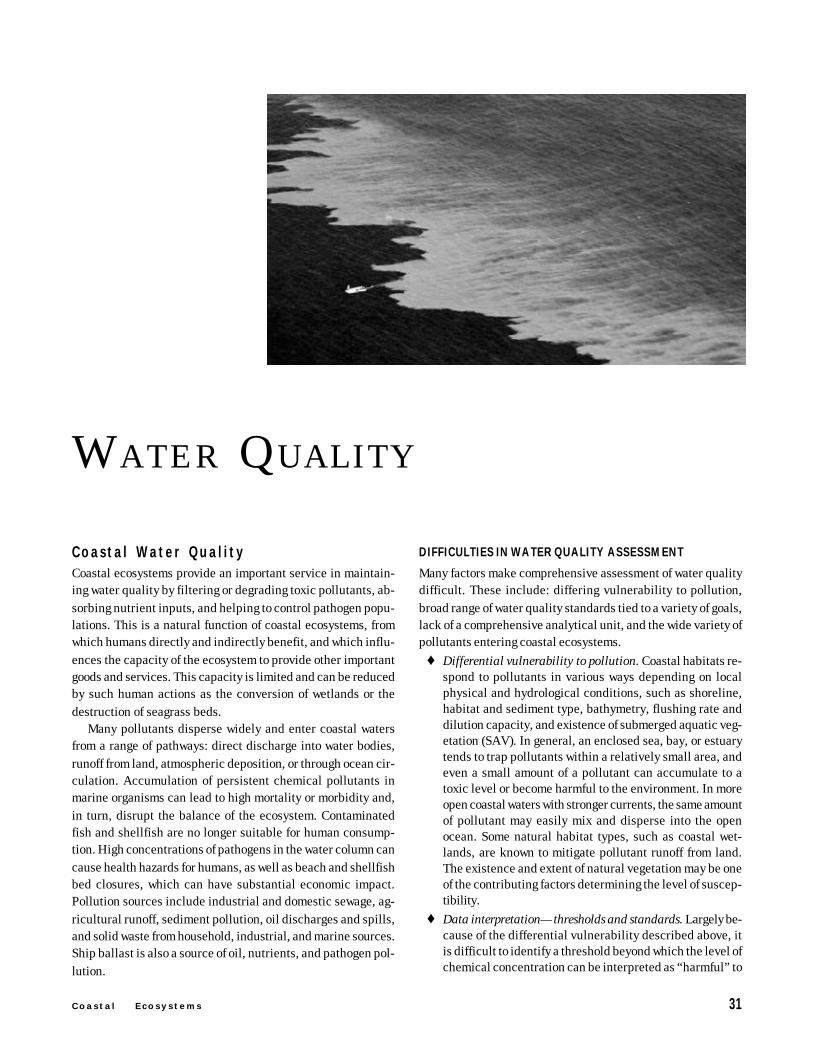
C o a s t a l E c o s y s t e m s 31
S h o r e l i n e S t a b i l i z a t i o n
W A T E R Q UALITY
DIFFICULTIES IN WATER QUALITY ASSESSMENT
Many factors make comprehensive assessment of water qualitydifficult. These include: differing vulnerability to pollution,broad range of water quality standards tied to a variety of goals,lack of a comprehensive analytical unit, and the wide variety ofpollutants entering coastal ecosystems.
♦ Differential vulnerability to pollution. Coastal habitats re-spond to pollutants in various ways depending on localphysical and hydrological conditions, such as shoreline,habitat and sediment type, bathymetry, flushing rate anddilution capacity, and existence of submerged aquatic veg-etation (SAV). In general, an enclosed sea, bay, or estuarytends to trap pollutants within a relatively small area, andeven a small amount of a pollutant can accumulate to atoxic level or become harmful to the environment. In moreopen coastal waters with stronger currents, the same amountof pollutant may easily mix and disperse into the openocean. Some natural habitat types, such as coastal wet-lands, are known to mitigate pollutant runoff from land.The existence and extent of natural vegetation may be oneof the contributing factors determining the level of suscep-tibility.
♦ Data interpretation—thresholds and standards. Largely be-cause of the differential vulnerability described above, itis difficult to identify a threshold beyond which the level ofchemical concentration can be interpreted as “harmful” to
Coasta l Water Qua l i tyCoastal ecosystems provide an important service in maintain-ing water quality by filtering or degrading toxic pollutants, ab-sorbing nutrient inputs, and helping to control pathogen popu-lations. This is a natural function of coastal ecosystems, fromwhich humans directly and indirectly benefit, and which influ-ences the capacity of the ecosystem to provide other importantgoods and services. This capacity is limited and can be reducedby such human actions as the conversion of wetlands or thedestruction of seagrass beds.
Many pollutants disperse widely and enter coastal watersfrom a range of pathways: direct discharge into water bodies,runoff from land, atmospheric deposition, or through ocean cir-culation. Accumulation of persistent chemical pollutants inmarine organisms can lead to high mortality or morbidity and,in turn, disrupt the balance of the ecosystem. Contaminatedfish and shellfish are no longer suitable for human consump-tion. High concentrations of pathogens in the water column cancause health hazards for humans, as well as beach and shellfishbed closures, which can have substantial economic impact.Pollution sources include industrial and domestic sewage, ag-ricultural runoff, sediment pollution, oil discharges and spills,and solid waste from household, industrial, and marine sources.Ship ballast is also a source of oil, nutrients, and pathogen pol-lution.
32 P I L O T A N A L Y S I S O F G L O B A L E C O S Y S T E M S
W a t e r Q u a l i t y
the ecosystem. Unlike conventional water quality standardsthat are identified based on potential human health im-pacts, ecosystem health-based standards would have to takeinto account a range of concerns. In addition, indirect orlong-term effects of exposure to contaminants, such as en-docrine disruption, are difficult to distinguish from naturalchanges and fluctuations (GESAMP 1990).
♦ Lack of comprehensive analytical unit. In order for the wa-ter quality monitoring data to be meaningful, a spatial frame-work for organizing the information is required. Monitor-ing sites need to be selected such that they are representa-tive of an area within which physical conditions are fairlyhomogenous. Identifying key analytical units with bound-aries that can be delineated is useful to this end. Estuariesare a commonly used unit, although these are sometimestoo large and need subdivisions. Defining analytical unitsfor specific habitat types, such as for coral reef or seagrassareas, is more difficult as these tend to be patchy, discon-tinuous habitats. Sandy beaches are another common unitfor analysis because of the direct link between water qual-ity and economic value.
♦ Variety of pollutants. Many pollutants entering coastal wa-ters have different chemical properties and require differ-ent data collection and monitoring methodologies, depend-ing on their intrinsic characteristics, such as toxicity andpersistence in the environment. The adverse effects causedby water contamination can have acute, seasonal, or chronicimpacts on the ecosystem.
Condit ion of Coasta l WatersA vast range of pollutants affects the world’s coasts and oceans.This study selected key pollutants and categorized them, basedon their implications for ecosystem integrity, and on existingindicators and relevant monitoring programs. The groups ofpollutants selected are nutrients, pathogens, persistent organicpollutants and heavy metals, oil, and solid waste.
NUTRIENTSImportant parameters for monitoring nutrient pollution in coastalwaters include the following: nitrogen and phosphorus concen-trations; maximum bottom dissolved oxygen levels; extent andduration of anoxic and hypoxic conditions; extent of SAV; chlo-rophyll-a concentrations; turbidity; and duration and extent ofalgal blooms (by type). Some parameters are important in as-sessing the vulnerability of an area to the pollutants, such asnitrogen and phosphorus, or in determining baseline conditionsof the area.
Estuaries—semienclosed waterbodies where fresh- and salt-water mix—are among the most productive ecosystems on earth.Their semienclosed physiography makes them more susceptibleto pollution, and the variable temperature and salinity condi-tions within an estuary make it more difficult to monitor its eco-
logical health. Estuarine eutrophication can have significantadverse effects on overall biological productivity, in light of thecrucial role of estuaries on at least one trophic stage of manymarine organisms.
Analysis of nutrients and potential eutrophication within anestuary needs to be watershed-based. All land within the water-shed can contribute nutrients to the estuary. It is necessary tocharacterize land cover within the watershed, including agri-cultural use and agricultural inputs of nutrients, and examinechanges in land cover. Point sources of nutrients, such as sew-age outflows, must also be considered as part of the nutrientbudget. These nutrient sources can then be linked with observednutrient levels and other condition indicators described above.
Within the United States, NOAA developed a “Coastal As-sessment Framework” for the watershed-based collection, or-ganization, and presentation of data related to coastal waterquality. Spatial analytical units called “Estuarine DrainageAreas” were identified based on local typography, includingboth land and water components (NOAA 1998). This unit hasbeen linked with a national eutrophication survey that assessesexisting conditions and trends for 16 water quality parameters,providing insight into the magnitude, timing, frequency, andspatial extent of eutrophication-related conditions in 137 estu-aries in U.S. waters. Monitoring is performed for three salinityzones: tidal freshwater, saltwater, and mixed (Bricker et al. 1999).
Map 6 identifies areas of high and increasing nutrient con-centration; however, the data are insufficient to detect the over-all trend. Of the 137 estuaries assessed, high nitrogen concen-trations (greater than 1 mg per liter) occur in 55 estuaries, cov-ering a spatial extent of 13 percent of the nation’s estuarinearea, mostly in the tidal freshwater and mixing zones. It is ex-tremely difficult to identify the threshold beyond which nutri-ent loading is excessive and contributes to eutrophication. Thecapacity of particular coastal areas to assimilate nutrients andmaintain trophic balance varies, depending on the physical andchemical conditions. Hence, the vulnerability, or susceptibil-ity, of the coastal area is an important consideration, beyondsimply looking at nutrient loadings in a waterbody.
PATHOGENSA variety of pathogenic organisms, including viruses, bacteria,protozoa, and parasitic worms, exist in seawater and can causediseases in plants, animals, and people. Impacts include hu-man illness, seafood contamination, and recreational beach clo-sures. Pathogens are discharged to coastal waters through bothpoint and nonpoint sources, especially insufficiently treatedsewage that is released from septic systems on land and on ships,and from agriculture and stormwater runoff. Higher concentra-tions tend to occur after storms and related overflow of sewersystems, making it difficult to interpret trend and temporal fluc-tuations (Natural Resources Defense Council 1998). Because
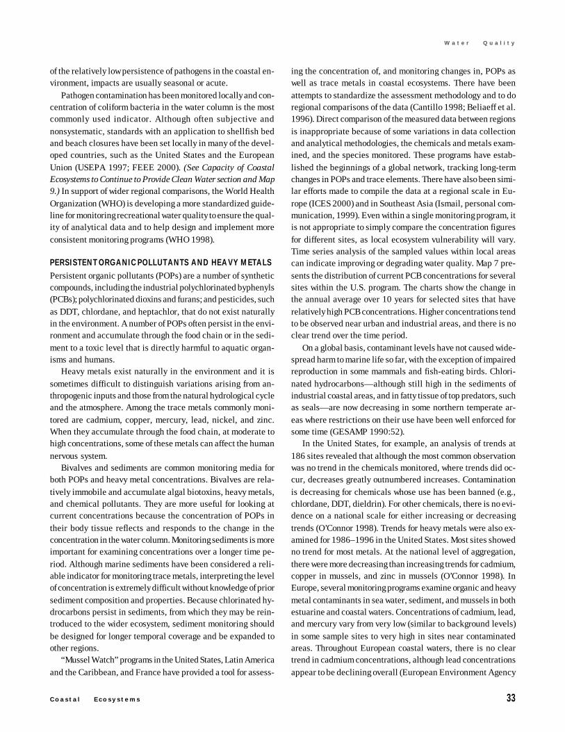
C o a s t a l E c o s y s t e m s 33
W a t e r Q u a l i t y
of the relatively low persistence of pathogens in the coastal en-vironment, impacts are usually seasonal or acute.
Pathogen contamination has been monitored locally and con-centration of coliform bacteria in the water column is the mostcommonly used indicator. Although often subjective andnonsystematic, standards with an application to shellfish bedand beach closures have been set locally in many of the devel-oped countries, such as the United States and the EuropeanUnion (USEPA 1997; FEEE 2000). (See Capacity of CoastalEcosystems to Continue to Provide Clean Water section and Map9.) In support of wider regional comparisons, the World HealthOrganization (WHO) is developing a more standardized guide-line for monitoring recreational water quality to ensure the qual-ity of analytical data and to help design and implement moreconsistent monitoring programs (WHO 1998).
PERSISTENT ORGANIC POLLUTANTS AND HEAVY METALSPersistent organic pollutants (POPs) are a number of syntheticcompounds, including the industrial polychlorinated byphenyls(PCBs); polychlorinated dioxins and furans; and pesticides, suchas DDT, chlordane, and heptachlor, that do not exist naturallyin the environment. A number of POPs often persist in the envi-ronment and accumulate through the food chain or in the sedi-ment to a toxic level that is directly harmful to aquatic organ-isms and humans.
Heavy metals exist naturally in the environment and it issometimes difficult to distinguish variations arising from an-thropogenic inputs and those from the natural hydrological cycleand the atmosphere. Among the trace metals commonly moni-tored are cadmium, copper, mercury, lead, nickel, and zinc.When they accumulate through the food chain, at moderate tohigh concentrations, some of these metals can affect the humannervous system.
Bivalves and sediments are common monitoring media forboth POPs and heavy metal concentrations. Bivalves are rela-tively immobile and accumulate algal biotoxins, heavy metals,and chemical pollutants. They are more useful for looking atcurrent concentrations because the concentration of POPs intheir body tissue reflects and responds to the change in theconcentration in the water column. Monitoring sediments is moreimportant for examining concentrations over a longer time pe-riod. Although marine sediments have been considered a reli-able indicator for monitoring trace metals, interpreting the levelof concentration is extremely difficult without knowledge of priorsediment composition and properties. Because chlorinated hy-drocarbons persist in sediments, from which they may be rein-troduced to the wider ecosystem, sediment monitoring shouldbe designed for longer temporal coverage and be expanded toother regions.
“Mussel Watch” programs in the United States, Latin Americaand the Caribbean, and France have provided a tool for assess-
ing the concentration of, and monitoring changes in, POPs aswell as trace metals in coastal ecosystems. There have beenattempts to standardize the assessment methodology and to doregional comparisons of the data (Cantillo 1998; Beliaeff et al.1996). Direct comparison of the measured data between regionsis inappropriate because of some variations in data collectionand analytical methodologies, the chemicals and metals exam-ined, and the species monitored. These programs have estab-lished the beginnings of a global network, tracking long-termchanges in POPs and trace elements. There have also been simi-lar efforts made to compile the data at a regional scale in Eu-rope (ICES 2000) and in Southeast Asia (Ismail, personal com-munication, 1999). Even within a single monitoring program, itis not appropriate to simply compare the concentration figuresfor different sites, as local ecosystem vulnerability will vary.Time series analysis of the sampled values within local areascan indicate improving or degrading water quality. Map 7 pre-sents the distribution of current PCB concentrations for severalsites within the U.S. program. The charts show the change inthe annual average over 10 years for selected sites that haverelatively high PCB concentrations. Higher concentrations tendto be observed near urban and industrial areas, and there is noclear trend over the time period.
On a global basis, contaminant levels have not caused wide-spread harm to marine life so far, with the exception of impairedreproduction in some mammals and fish-eating birds. Chlori-nated hydrocarbons—although still high in the sediments ofindustrial coastal areas, and in fatty tissue of top predators, suchas seals—are now decreasing in some northern temperate ar-eas where restrictions on their use have been well enforced forsome time (GESAMP 1990:52).
In the United States, for example, an analysis of trends at186 sites revealed that although the most common observationwas no trend in the chemicals monitored, where trends did oc-cur, decreases greatly outnumbered increases. Contaminationis decreasing for chemicals whose use has been banned (e.g.,chlordane, DDT, dieldrin). For other chemicals, there is no evi-dence on a national scale for either increasing or decreasingtrends (O’Connor 1998). Trends for heavy metals were also ex-amined for 1986–1996 in the United States. Most sites showedno trend for most metals. At the national level of aggregation,there were more decreasing than increasing trends for cadmium,copper in mussels, and zinc in mussels (O’Connor 1998). InEurope, several monitoring programs examine organic and heavymetal contaminants in sea water, sediment, and mussels in bothestuarine and coastal waters. Concentrations of cadmium, lead,and mercury vary from very low (similar to background levels)in some sample sites to very high in sites near contaminatedareas. Throughout European coastal waters, there is no cleartrend in cadmium concentrations, although lead concentrationsappear to be declining overall (European Environment Agency
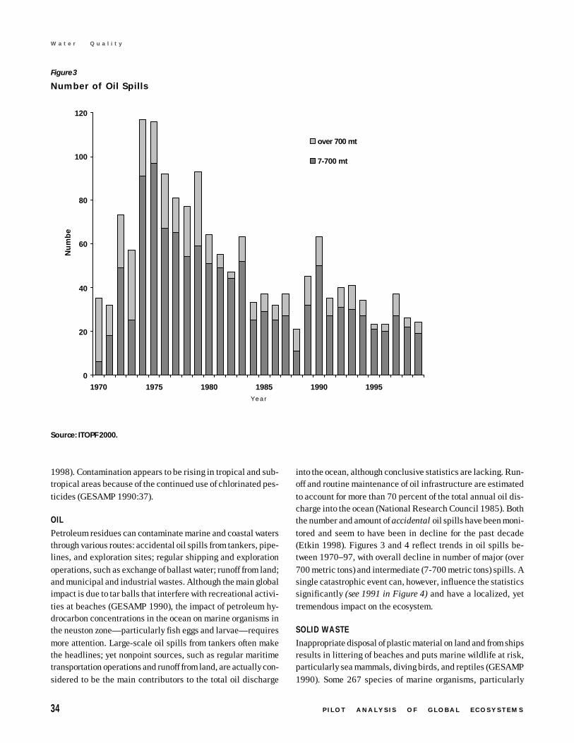
34 P I L O T A N A L Y S I S O F G L O B A L E C O S Y S T E M S
W a t e r Q u a l i t y
1998). Contamination appears to be rising in tropical and sub-tropical areas because of the continued use of chlorinated pes-ticides (GESAMP 1990:37).
OILPetroleum residues can contaminate marine and coastal watersthrough various routes: accidental oil spills from tankers, pipe-lines, and exploration sites; regular shipping and explorationoperations, such as exchange of ballast water; runoff from land;and municipal and industrial wastes. Although the main globalimpact is due to tar balls that interfere with recreational activi-ties at beaches (GESAMP 1990), the impact of petroleum hy-drocarbon concentrations in the ocean on marine organisms inthe neuston zone—particularly fish eggs and larvae—requiresmore attention. Large-scale oil spills from tankers often makethe headlines; yet nonpoint sources, such as regular maritimetransportation operations and runoff from land, are actually con-sidered to be the main contributors to the total oil discharge
into the ocean, although conclusive statistics are lacking. Run-off and routine maintenance of oil infrastructure are estimatedto account for more than 70 percent of the total annual oil dis-charge into the ocean (National Research Council 1985). Boththe number and amount of accidental oil spills have been moni-tored and seem to have been in decline for the past decade(Etkin 1998). Figures 3 and 4 reflect trends in oil spills be-tween 1970–97, with overall decline in number of major (over700 metric tons) and intermediate (7-700 metric tons) spills. Asingle catastrophic event can, however, influence the statisticssignificantly (see 1991 in Figure 4) and have a localized, yettremendous impact on the ecosystem.
SOLID WASTEInappropriate disposal of plastic material on land and from shipsresults in littering of beaches and puts marine wildlife at risk,particularly sea mammals, diving birds, and reptiles (GESAMP1990). Some 267 species of marine organisms, particularly
Figure 3
Number of Oil Spills
Source: ITOPF 2000.
0
20
40
60
80
100
120
1970 1975 1980 1985 1990 1995
Y e a r
Nu
mb
e
over 700 mt
7-700 mt
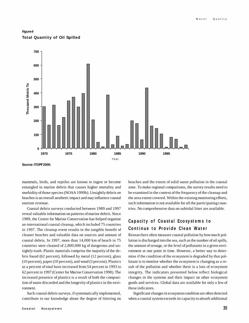
C o a s t a l E c o s y s t e m s 35
W a t e r Q u a l i t y
mammals, birds, and reptiles are known to ingest or becomeentangled in marine debris that causes higher mortality andmorbidity of those species (NOAA 1999b). Unsightly debris onbeaches is an overall aesthetic impact and may influence coastaltourism revenue.
Coastal debris surveys conducted between 1989 and 1997reveal valuable information on patterns of marine debris. Since1989, the Center for Marine Conservation has helped organizean international coastal cleanup, which included 75 countriesin 1997. The cleanup event results in the tangible benefit ofcleaner beaches and valuable data on sources and amount ofcoastal debris. In 1997, more than 14,000 km of beach in 75countries were cleaned of 2,800,000 kg of dangerous and un-sightly trash. Plastic materials comprise the majority of the de-bris found (62 percent), followed by metal (12 percent), glass(10 percent), paper (10 percent), and wood (3 percent). Plasticsas a percent of total have increased from 54 percent in 1993 to62 percent in 1997 (Center for Marine Conservation 1998). Theincreased presence of plastics is a result of both the composi-tion of waste discarded and the longevity of plastics in the envi-ronment.
Such coastal debris surveys, if systematically implemented,contribute to our knowledge about the degree of littering on
beaches and the extent of solid waste pollution in the coastalzone. To make regional comparisons, the survey results need tobe examined in the context of the frequency of the cleanup andthe area extent covered. Within the existing monitoring efforts,such information is not available for all the participating coun-tries. No comprehensive data on subtidal litter are available.
Capac i ty of Coasta l Ecosystems to
Cont inue to Provide C lean WaterResearchers often measure coastal pollution by how much pol-lution is discharged into the sea, such as the number of oil spills,the amount of sewage, or the level of pollutants in a given envi-ronment at one point in time. However, a better way to deter-mine if the condition of the ecosystem is degraded by that pol-lutant is to monitor whether the ecosystem is changing as a re-sult of the pollution and whether there is a loss of ecosystemintegrity. The indicators presented below reflect biologicalchanges in the systems and their impact on other ecosystemgoods and services. Global data are available for only a few ofthese indicators.
Significant changes in ecosystem condition are often detectedwhen a coastal system exceeds its capacity to absorb additional
Figure 4
Total Quantity of Oil Spilled
Source: ITOPF 2000.
0
100
200
300
400
500
600
700
1970 1975 1980 1985 1990 1995
Y e a r
Tho
usa
nd
Met
ric
Ton
36 P I L O T A N A L Y S I S O F G L O B A L E C O S Y S T E M S
W a t e r Q u a l i t y
nutrients. Dissolved oxygen levels below 2 mg/liter is a condi-tion called hypoxia where a majority of the marine organismscannot survive. Although historical information on hypoxia islimited, experts believe that the prevalence and extent of hy-poxic zones have increased in recent decades. Map 8 presentsobservations of hypoxic zones around the world. This map shouldnot be considered a complete representation of hypoxia occur-rence, but rather a subset of the areas where it occurs. Suchmapping is inevitably biased toward areas with better reportingmechanisms. Consequently, most observations take place in in-dustrialized countries.
Somewhat better historical information exists for algal blooms.In particular, scientists have assembled information on Harm-ful Algal Blooms (HAB), which are comprised of species pro-ducing compounds that can cause health hazards. Over 60 harm-ful algal toxins are known today, which are responsible for atleast 6 types of food poisoning, including several that can belethal (National Research Council 1999:52). The cause of theHABs is not entirely clear and is often attributed to the intro-duction and colonization of some exotic algal species which sub-sequently develop toxicity. Algal blooms are also associated with
an increase in nutrient pollution, which may enhance the rapidincrease of such species. Global and regional initiatives, suchas the International Oceanographic Commission (IOC) andWoods Hole Oceanographic Institution (WHOI), have compiledinformation on the frequency and impact of such HAB eventsdocumented at national or local scales (UNESCO 2000; WHOI2000). Over the past two decades, the frequency of recordedHABs has increased significantly. The total number of incidentsthat are known to have affected public health, fish, shellfish,and birds has increased from around 200 in the 1970s to morethan 700 in the 1990s. (See Figure 5.) This trend is, in part,due to an increase in the likelihood that an event will be re-ported, but a similar trend was observed even in coastal regionswhere monitoring systems have been in place for decades(Anderson 1998).
HAB events can be linked to economic impacts (associatedwith mass fish mortality) and health concerns. Since 1991, HABsin the United States have caused nearly US$300 million in eco-nomic losses in the form of fish kills, public health problems,and lost revenue from tourism and the sale of seafood (McGinn1999:25).
Figure 5
Number of Harmful Algal Bloom Events: 1970s–1990s
Source: HEED-MMED 1999.
91
197157
71
236 299
219
46
10
5
209
60
0
200
400
600
800
1970s 1980s 1990s
Shellfish Events
Bird Events
Fish Events
Human Health Events
C o a s t a l E c o s y s t e m s 37
W a t e r Q u a l i t y
The data sets presented above are based on a compilation ofanecdotal events, most of which are extracted from literature ormedia coverage. Only limited ground-based monitoring initia-tives with regular data collection exist. These monitoring pro-grams may help prevent public health events by allowing forinterventions before the events occur.
Better monitoring mechanisms exist for pathogen contami-nation. Shellfish bed and beach closures are symptoms of theecosystem’s declining capacity to provide clean water identi-fied by locally set thresholds. The declining capacity also rep-resents an economic loss, linking this ecosystem’s service toprovide clean water to other ecosystem goods, particularly foodand tourism. By combining this information with a spatial frame-work, such as the Estuarine Drainage Areas described earlier,it is possible to summarize and interpret the results reported foreach shellfish growing area, or each beach, in a more logicalwatershed-oriented manner. Despite its importance in linkingcause and effect of water quality degradation, current monitor-ing of pathogen contamination is inadequate in terms of regionalcomparisons and trend analysis because this is an indirect andsubjective indicator that relies upon the selection of a thresh-old at each reporting location.
Shellfish-growing waters are more consistently monitored insome countries. For example, in the United States in 1995, outof over 10 million hectares of shellfish-growing waters that weremonitored, some 69 percent were approved for harvest—up from58 percent in 1985 (Alexander 1998:6). In 1995, the commer-cial harvest of these waters totaled 77 million pounds of oys-ters, clams, and mussels, worth approximately US$200 millionat dockside (Alexander 1998). (See Map 9 for closures in North-east United States.)
Another indicator directly linked to loss of other ecosystemgoods is beach tar balls. Oil residue stranded on the beach orfloating in the open ocean is a direct hindrance to tourism andbiodiversity. IOC’s Marine Pollution Monitoring Programme(MARPOLMON) was implemented in the 1980s and has com-piled data collected by ships and coastal monitoring stations onoil residue in the ocean. The major limitations of this data setare the following: only a few of the reported observations showthe magnitude of contamination (size and concentration); thetrend in frequency may be the result of increased shipping traf-fic and reporting; and data are not complete for all countriesand years. Map 10 reflects recent observations and trends forseveral sites in Japan, which is a subset of the data collectedunder MARPOLMON. Some of the sites are located in majorcoastal tourism destinations. The general trend seems to be adecline, although the incidence of accidental spills skewed thestatistics in some sites.
In format ion Status and Needs
IDENTIFICATION OF THRESHOLDSThere are a number of monitoring programs at national and re-gional scales around the world. The completeness and accu-racy of the data they provide vary, often relying upon differentsampling methodologies and parameters. The data, therefore,are not comparable on a global basis, but are still useful forexamining trends and making local comparisons (EuropeanEnvironment Agency 1998). Increased direct monitoring of waterquality parameters, coupled with using satellite sensors, cangreatly improve our knowledge of the condition of the world’scoastal waters. Wider and more consistent data coverage, iden-tification of ecosystem-based thresholds, and baseline data tohelp identify those thresholds are all required for the directly-measured pollution parameters to be useful. The U.S. Environ-mental Protection Agency’s (USEPA) Total Maximum Daily Load(TMDL) Program encourages subnational governments to moni-tor and regulate pollutant inputs to freshwater bodies. TMDL isa calculation of the maximum amount of a pollutant that awaterbody can receive and still meet water quality standards,which local governments set based on their own criteria, fordrinking water, recreation, or ecological uses (USEPA 2000).Identification of the ecosystem-based threshold is a major chal-lenge, considering the varied ecological characteristics andvulnerability of different coastal areas. However, for more pro-active policy interventions to take place, setting conservativestandards and systematic monitoring are essential.
REMOTE SENSINGBeyond traditional direct monitoring of water quality, satelliteimagery can be used to monitor a number of key parametersover a wide spatial scale. In many cases, the use of high-resolu-tion satellite imagery and in-situ monitoring data will be vital tocalibrate lower-resolution remote sensing data and refine ob-servations. For example, SeaWifs is a relatively new, coarse reso-lution sensor designed to monitor sea surface characteristics,particularly ocean color and marine phytoplankton concentra-tions. Phytoplankton concentrations, as indicated by chloro-phyll-A, is relatively easy to detect, but determining concen-trations is complicated by suspended sediments and dissolvedorganic matter in the water (Edwards and Clark 2000). For theSeaWifs sensors to be useful for differentiating types of algalblooms, improved calibration of the sensor and integration withdata from ground and higher-resolution satellites is necessary.This calibration is the focus of a large research effort at present:SIMBIOS—Sensor Intercomparison and Merger for BiologicalAnd Interdisciplinary Oceanic Studies (Mueller et al. 1998).
There is a mismatch between the temporal and spatial scaleof most of the pollution events, and the information provided by
38 P I L O T A N A L Y S I S O F G L O B A L E C O S Y S T E M S
W a t e r Q u a l i t y
satellite sensors, which make the sensors of limited use formonitoring. It is possible to obtain data with an appropriatetemporal and spatial scale, but it may not be cost-effective, andcareful assessment of how to balance this with the cost of in-situ monitoring is necessary.
Satellite data can be useful for the following:1. Habitat mapping, such as wetland extent and submerged
aquatic vegetation extent. (Described previously in theCoastal Zone: Extent and Change section.)
2. Turbidity and sediment plumes. The extent of sedimentplumes and sediment transport along the coast in surfacewaters is easily detected in visible wavelengths. Addition-ally, water color, clarity, and turbidity can be evaluated.
3. Sea surface temperature (SST). Thermal pollution and SSTanomalies can be measured using either coarse-resolutionor high-resolution imagery, depending upon the scale ofthe phenomena to be quantified.
4. Algal blooms. Coarse-resolution satellite imagery can beused to monitor the occurrence and extent of algal bloomsas an early warning system.
5. Oil slicks. The occurrence of oil slicks can be detectedusing a wide range of satellite sensors, including visible,infrared, and microwave wavelengths, in addition toSynthetic Aperture Radar (SAR) (Edwards and Clark2000).
IN-SITU WATER QUALITY MONITORINGTo quantitatively describe pollution and related problems, wa-ter quality parameters require ground-based monitoring andcollection of baseline information. The U.S. National Eutrophi-cation Survey is a prime example. It is not possible or feasible
to try to monitor every single pollutant. Careful selection andprioritization of the monitoring parameters would be necessarybased on the relevance and vulnerability of the locality.
Enhanced in-situ monitoring is needed for the following:1. Eutrophication-related parameters (see Nutrients section).
2. Coliform concentrations and harmful bacteria. Fecalcoliform, such as Escherichia coli, is a commonly moni-tored water quality parameter, but monitoring needs to beexpanded in many areas. Additionally, other harmfulbacteria need to be monitored in areas of elevated risk.
3. Persistent Organic Pollutants (POPs) and heavy metals.Long-term monitoring of sediment and bivalves wouldimprove our understanding of changes in the accumulationof these toxic substances. Mussel Watch-type programsneed to be more widely adopted.
4. Salinity. Salinity is a factor affecting vulnerability topollution and is important in understanding the stratifica-tion of estuaries.
5. Indicator species. Identification of key species that aremore susceptible to changes in water quality, and monitor-ing of that population can be useful in assessing the healthof the system. No such species have been identified at aglobal scale.
6. Endocrine disrupters. Although causes are complex anduncertain, monitoring changes in species populations willbe an important aspect of monitoring overall water quality.
7. Marine organisms mortality and morbidity events. Anotherway of tracking the condition of coastal waters relates toquantifying the impacts of changes. Although many effectscannot be directly tied to a single cause, they remain goodindicators of when the capacity of the system has beenexceeded.
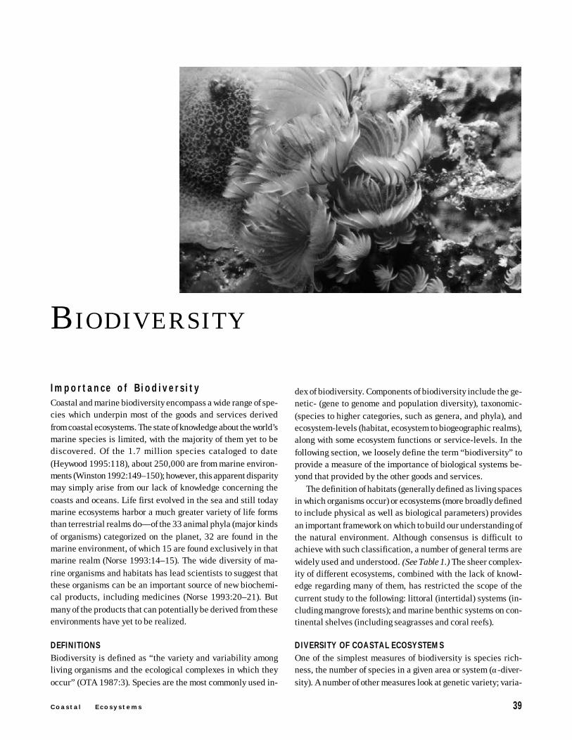
C o a s t a l E c o s y s t e m s 39
W a t e r Q u a l i t y
B IODIVERSITY
dex of biodiversity. Components of biodiversity include the ge-netic- (gene to genome and population diversity), taxonomic-(species to higher categories, such as genera, and phyla), andecosystem-levels (habitat, ecosystem to biogeographic realms),along with some ecosystem functions or service-levels. In thefollowing section, we loosely define the term “biodiversity” toprovide a measure of the importance of biological systems be-yond that provided by the other goods and services.
The definition of habitats (generally defined as living spacesin which organisms occur) or ecosystems (more broadly definedto include physical as well as biological parameters) providesan important framework on which to build our understanding ofthe natural environment. Although consensus is difficult toachieve with such classification, a number of general terms arewidely used and understood. (See Table 1.) The sheer complex-ity of different ecosystems, combined with the lack of knowl-edge regarding many of them, has restricted the scope of thecurrent study to the following: littoral (intertidal) systems (in-cluding mangrove forests); and marine benthic systems on con-tinental shelves (including seagrasses and coral reefs).
DIVERSITY OF COASTAL ECOSYSTEMSOne of the simplest measures of biodiversity is species rich-ness, the number of species in a given area or system (α-diver-sity). A number of other measures look at genetic variety; varia-
Importance of B iod ivers i tyCoastal and marine biodiversity encompass a wide range of spe-cies which underpin most of the goods and services derivedfrom coastal ecosystems. The state of knowledge about the world’smarine species is limited, with the majority of them yet to bediscovered. Of the 1.7 million species cataloged to date(Heywood 1995:118), about 250,000 are from marine environ-ments (Winston 1992:149–150); however, this apparent disparitymay simply arise from our lack of knowledge concerning thecoasts and oceans. Life first evolved in the sea and still todaymarine ecosystems harbor a much greater variety of life formsthan terrestrial realms do—of the 33 animal phyla (major kindsof organisms) categorized on the planet, 32 are found in themarine environment, of which 15 are found exclusively in thatmarine realm (Norse 1993:14–15). The wide diversity of ma-rine organisms and habitats has lead scientists to suggest thatthese organisms can be an important source of new biochemi-cal products, including medicines (Norse 1993:20–21). Butmany of the products that can potentially be derived from theseenvironments have yet to be realized.
DEFINITIONSBiodiversity is defined as “the variety and variability amongliving organisms and the ecological complexes in which theyoccur” (OTA 1987:3). Species are the most commonly used in-
40 P I L O T A N A L Y S I S O F G L O B A L E C O S Y S T E M S
B i o d i v e r s i t y
tion at higher taxonomic levels, such as genus, family, or phy-lum; and variation in the habitat composition of a region or sys-tem (β-diversity). The presence of species with highly restricteddistribution has been used with considerable success in high-lighting areas of conservation importance in the terrestrial en-vironment. Levels of endemism have also been used in identi-fying biogeographic realms and provinces. The high degree ofconnectivity in marine and coastal communities is responsiblefor generally lower levels of endemism; however, knowledgerelating to marine species distribution is still insufficient fordetailed analysis of patterns for most groups. Endemism is im-portant in particularly isolated marine ecosystems, such as theHawaiian Archipelago or hydro-thermal vent communities.
DISTRIBUTION OF REMAINING NATURAL ECOSYSTEMSCurrent extent is the descriptive measurement of these biologi-cal systems using a range of measures, including the distribu-tion of habitats (see Coastal Zone: Extent and Change section)and the numbers of species or endemic species, associated withthe habitat. With these biological systems as a baseline we areable to assess the status or condition of these systems, usingdirect measures of habitat loss, degradation, or threatened spe-cies, or using proxy measures that may indicate the same thing.
At the national and subnational level, increasingly detailedand accurate maps are becoming available that show the distri-bution of coastal and marine ecosystems. Global maps are stillpoor and largely restricted to a few physical and oceanographiclayers and a few ecosystems, although broader biogeographicrealms, such as the large marine ecosystems (LMEs) have beenmapped at the global level (see Coastal Zone: Extent and Changesection for habitat extent discussion). These biogeographic char-acterization schemes capture “natural” or “potential” distribu-tion of habitat types and can only infer where those habitatsmay occur without human modification of the coastal areas.
SPECIES RICHNESSTwo sources of data are available for the compilation ofmultispecies distribution data sets: checklists for particular sitesor countries; and global distribution maps for particular spe-cies or restricted groups. Typically, the former provide highlyaccurate location information, but are unavailable for manygeographic areas, while the latter are often less accurate andtend to fill in gaps in apparent distribution, including smallcountries. Increasingly, global data are becoming available thathave been compiled using either or both methods. Some of theseare presented in this section.
a. Littoral EcosystemsThe communities that have adapted to live in the littoral zoneare unique and of critical importance. Here, one finds a vastdiversity of evolutionary adaptations, with widely differing com-
munities often within a few centimeters of one another. Such ahigh β-diversity is probably unparalleled elsewhere on theplanet, while α-diversity is also often very high. Littoral eco-systems contain some of the most highly productive benthic com-munities, with a high turnover rate, high nutrient levels, andhigh-energy inputs. Moreover, the littoral zone is a place of greatvalue in many cultural and religious settings, as well as of greataesthetic significance.
The availability of data describing patterns of species rich-ness is poor for most littoral habitats, although some data areavailable for the better known groups, including pinnipeds (sealsand sea lions), marine turtles, and seabirds. Table 10 presentsnumbers of species of seabirds, marine turtles, and pinnipedsknown to occur in different regional sea areas, together withpercentage of global totals, and numbers of endemic species.Data were only compiled for species whose distribution is welldocumented and, hence, totals are comparable, but may notreflect true totals for all species in a group. Although often foundin the open sea, each of these groups makes at least some use ofthe littoral zone.
In addition to this general information, detailed global mapsare now available showing the distribution of turtle nestingbeaches, and pinniped haul-out and pupping localities. Theformer data set has been developed over the last five years andprovides comprehensive global coverage. The pinniped datawere prepared for the present work and have been completedfor 23 species, including all species in the subfamiliesArtocephalinae (fur seals, family Otariidae) and Phocine (north-ern seals, family Phocidae). The data have been summarizedinto species totals in different coastal nations, with subdivisionof larger nations into smaller political units (i.e., states, prov-inces, territories, island groups). Map 11 provides a visual pre-sentation of the turtle and seal diversity along different coastalregions.
MangrovesThe term mangrove is alternately used to describe a group ofplants and the communities in which these plants occur. Man-grove plants are shrubs or trees that live in or adjacent to theintertidal zone and have adapted to a regime of widely varyingsalinities, and to periodic and sometimes prolonged inunda-tion. There are some differences in definition of which plantsare truly mangrove species, however, the World Mangrove Atlas(Spalding et al. 1997) uses a broad definition, including some70 species worldwide, which is widely applicable to most map-ping studies and, hence, is also used here. Typically, mangrovecommunities are restricted to the tropics and are located alongmore sheltered shores and in estuarine environments. Mangrovesare of considerable importance to humanity. Their role in fish-eries has been widely recognized: many fish species use man-groves as breeding and nursery grounds. They are also a source
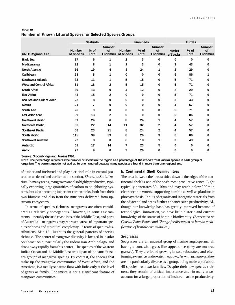
C o a s t a l E c o s y s t e m s 41
B i o d i v e r s i t y
of timber and fuelwood and play a critical role in coastal pro-tection as described earlier in the section, Shoreline Stabiliza-tion. In many areas, mangroves are also highly productive, typi-cally exporting large quantities of carbon to neighboring sys-tems, but also becoming important carbon sinks, both from theirown biomass and also from the nutrients delivered from up-stream ecosystems.
In terms of species richness, mangroves are often consid-ered as relatively homogenous. However, in some environ-ments—notably the arid coastlines of the Middle East, and partsof Australia—mangroves may represent areas of important spe-cies richness and structural complexity. In terms of species dis-tributions, Map 12 illustrates the general patterns of speciesrichness. The center of mangrove diversity is located in insularSoutheast Asia, particularly the Indonesian Archipelago, anddrops away rapidly from this center. The species of the westernIndian Ocean and the Middle East are all part of the same “east-ern group” of mangrove species. By contrast, the species thatmake up the mangrove communities of West Africa, and theAmericas, is a totally separate flora with links only at the levelof genus or family. Endemism is not a significant feature ofmangrove communities.
b. Continental Shelf CommunitiesThe area between the lowest tides down to the edges of the con-tinental shelf is one of the sea’s most productive zones. Lighttypically penetrates 50-100m and may reach below 200m inclear oceanic waters, supporting benthic as well as planktonicphotosynthesis. Inputs of organic and inorganic materials fromthe adjacent land areas further enhance such productivity. Al-though our knowledge base has greatly improved because oftechnological innovation, we have little historic and currentknowledge of the status of benthic biodiversity. (See section onCoastal Zone: Extent and Change for discussion on human modi-fication of benthic communities.)
SeagrassesSeagrasses are an unusual group of marine angiosperms, allhaving a somewhat grass-like appearance (they are not truegrasses). They are found growing in soft substrates, and oftenforming extensive underwater meadows. As with mangroves, theyare not particularly diverse as a group, being made up of about48 species from two families. Despite their low species rich-ness, they remain of critical importance and, in many areas,account for a large proportion of inshore marine productivity.
Table 10
Number of Known Littoral Species for Selected Species Groups
Seabirds Pinnipeds Turtles
UNEP Regional SeaNumber
of Species% ofTotal
Numberof
EndemicsNumber
of Species% ofTotal
Numberof
EndemicsNumber
of Species% ofTotal
Numberof
Endemics
Black Sea 17 6 1 2 3 0 0 0 0
Mediterranean 22 8 1 1 3 0 3 43 0
North Atlantic 56 19 4 8 24 1 2 29 0
Caribbean 23 8 1 0 0 0 6 86 1
Southwest Atlantic 33 11 1 5 15 0 5 71 0
West and Central Africa 51 18 2 5 15 0 5 71 0
South Africa 39 13 0 4 12 0 2 29 0
East Africa 44 15 2 0 0 0 5 71 0
Red Sea and Gulf of Aden 22 8 0 0 0 0 3 43 0
Kuwait 21 7 0 0 0 0 4 57 0
South Asia 26 9 0 0 0 0 5 71 0
East Asian Seas 39 13 2 0 0 0 6 86 0
Northwest Pacific 69 24 6 8 24 1 4 57 0
Northeast Pacific 66 22 14 11 32 2 4 57 0
Southeast Pacific 68 23 21 8 24 2 4 57 0
South Pacific 115 39 39 8 26 3 6 86 0
Southwest Australia 22 8 0 6 18 1 3 43 0
Antarctic 51 17 14 7 23 5 0 0 0
Arctic 27 9 0 9 26 0 0 0 0
Source: Groombridge and Jenkins 1996.Note: The percentage represents the number of species in the region as a percentage of the world's total known species in each group oforganism. The percentages do not add up to one hundred because many species are found in more than one regional sea.
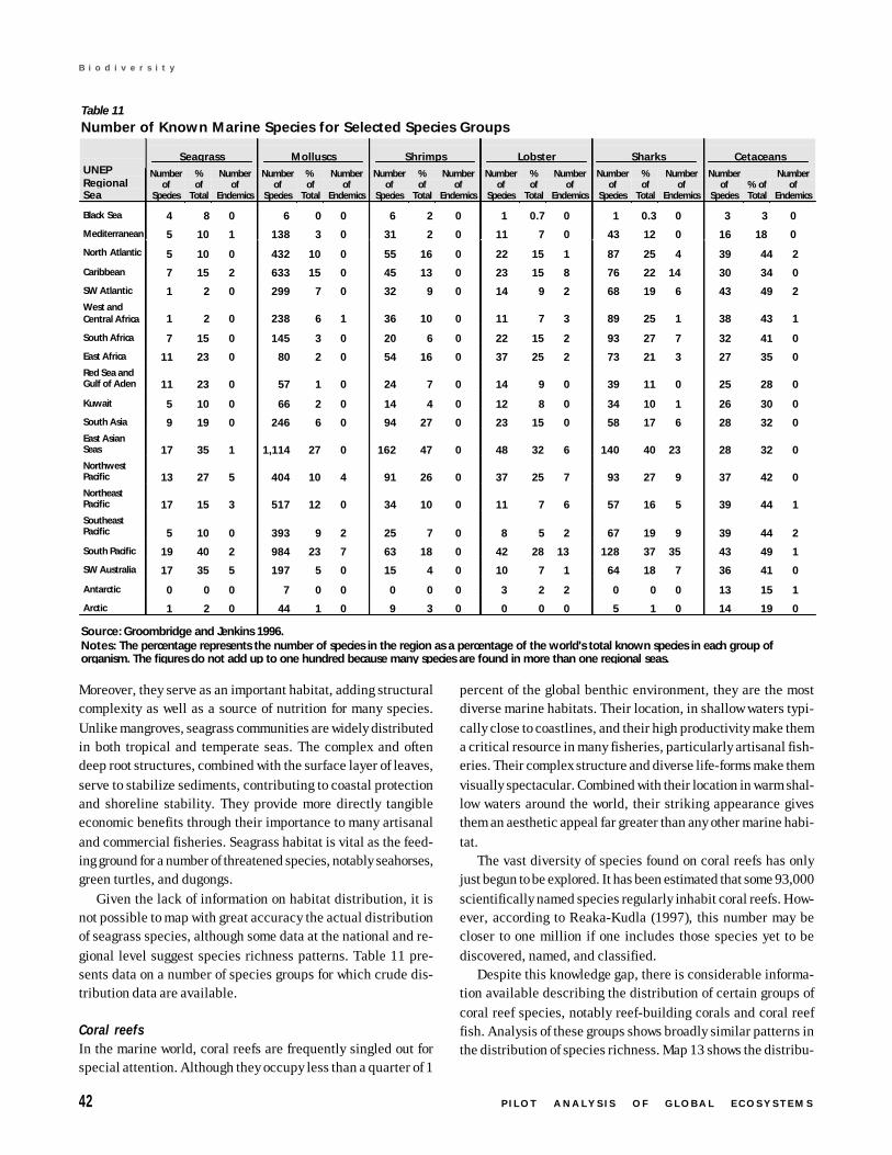
42 P I L O T A N A L Y S I S O F G L O B A L E C O S Y S T E M S
B i o d i v e r s i t y
Moreover, they serve as an important habitat, adding structuralcomplexity as well as a source of nutrition for many species.Unlike mangroves, seagrass communities are widely distributedin both tropical and temperate seas. The complex and oftendeep root structures, combined with the surface layer of leaves,serve to stabilize sediments, contributing to coastal protectionand shoreline stability. They provide more directly tangibleeconomic benefits through their importance to many artisanaland commercial fisheries. Seagrass habitat is vital as the feed-ing ground for a number of threatened species, notably seahorses,green turtles, and dugongs.
Given the lack of information on habitat distribution, it isnot possible to map with great accuracy the actual distributionof seagrass species, although some data at the national and re-gional level suggest species richness patterns. Table 11 pre-sents data on a number of species groups for which crude dis-tribution data are available.
Coral reefsIn the marine world, coral reefs are frequently singled out forspecial attention. Although they occupy less than a quarter of 1
percent of the global benthic environment, they are the mostdiverse marine habitats. Their location, in shallow waters typi-cally close to coastlines, and their high productivity make thema critical resource in many fisheries, particularly artisanal fish-eries. Their complex structure and diverse life-forms make themvisually spectacular. Combined with their location in warm shal-low waters around the world, their striking appearance givesthem an aesthetic appeal far greater than any other marine habi-tat.
The vast diversity of species found on coral reefs has onlyjust begun to be explored. It has been estimated that some 93,000scientifically named species regularly inhabit coral reefs. How-ever, according to Reaka-Kudla (1997), this number may becloser to one million if one includes those species yet to bediscovered, named, and classified.
Despite this knowledge gap, there is considerable informa-tion available describing the distribution of certain groups ofcoral reef species, notably reef-building corals and coral reeffish. Analysis of these groups shows broadly similar patterns inthe distribution of species richness. Map 13 shows the distribu-
Table 11
Number of Known Marine Species for Selected Species Groups
Seagrass Molluscs Shrimps Lobster Sharks CetaceansUNEPRegionalSea
Numberof
Species
%of
Total
Numberof
Endemics
Numberof
Species
%of
Total
Numberof
Endemics
Numberof
Species
%of
Total
Numberof
Endemics
Numberof
Species
%of
Total
Numberof
Endemics
Numberof
Species
%of
Total
Numberof
Endemics
Numberof
Species% ofTotal
Numberof
Endemics
Black Sea 4 8 0 6 0 0 6 2 0 1 0.7 0 1 0.3 0 3 3 0
Mediterranean 5 10 1 138 3 0 31 2 0 11 7 0 43 12 0 16 18 0
North Atlantic 5 10 0 432 10 0 55 16 0 22 15 1 87 25 4 39 44 2
Caribbean 7 15 2 633 15 0 45 13 0 23 15 8 76 22 14 30 34 0
SW Atlantic 1 2 0 299 7 0 32 9 0 14 9 2 68 19 6 43 49 2West andCentral Africa 1 2 0 238 6 1 36 10 0 11 7 3 89 25 1 38 43 1
South Africa 7 15 0 145 3 0 20 6 0 22 15 2 93 27 7 32 41 0
East Africa 11 23 0 80 2 0 54 16 0 37 25 2 73 21 3 27 35 0Red Sea andGulf of Aden 11 23 0 57 1 0 24 7 0 14 9 0 39 11 0 25 28 0
Kuwait 5 10 0 66 2 0 14 4 0 12 8 0 34 10 1 26 30 0
South Asia 9 19 0 246 6 0 94 27 0 23 15 0 58 17 6 28 32 0East AsianSeas 17 35 1 1,114 27 0 162 47 0 48 32 6 140 40 23 28 32 0NorthwestPacific 13 27 5 404 10 4 91 26 0 37 25 7 93 27 9 37 42 0NortheastPacific 17 15 3 517 12 0 34 10 0 11 7 6 57 16 5 39 44 1SoutheastPacific 5 10 0 393 9 2 25 7 0 8 5 2 67 19 9 39 44 2
South Pacific 19 40 2 984 23 7 63 18 0 42 28 13 128 37 35 43 49 1
SW Australia 17 35 5 197 5 0 15 4 0 10 7 1 64 18 7 36 41 0
Antarctic 0 0 0 7 0 0 0 0 0 3 2 2 0 0 0 13 15 1
Arctic 1 2 0 44 1 0 9 3 0 0 0 0 5 1 0 14 19 0
Source: Groombridge and Jenkins 1996.Notes: The percentage represents the number of species in the region as a percentage of the world's total known species in each group oforganism. The figures do not add up to one hundred because many species are found in more than one regional seas.
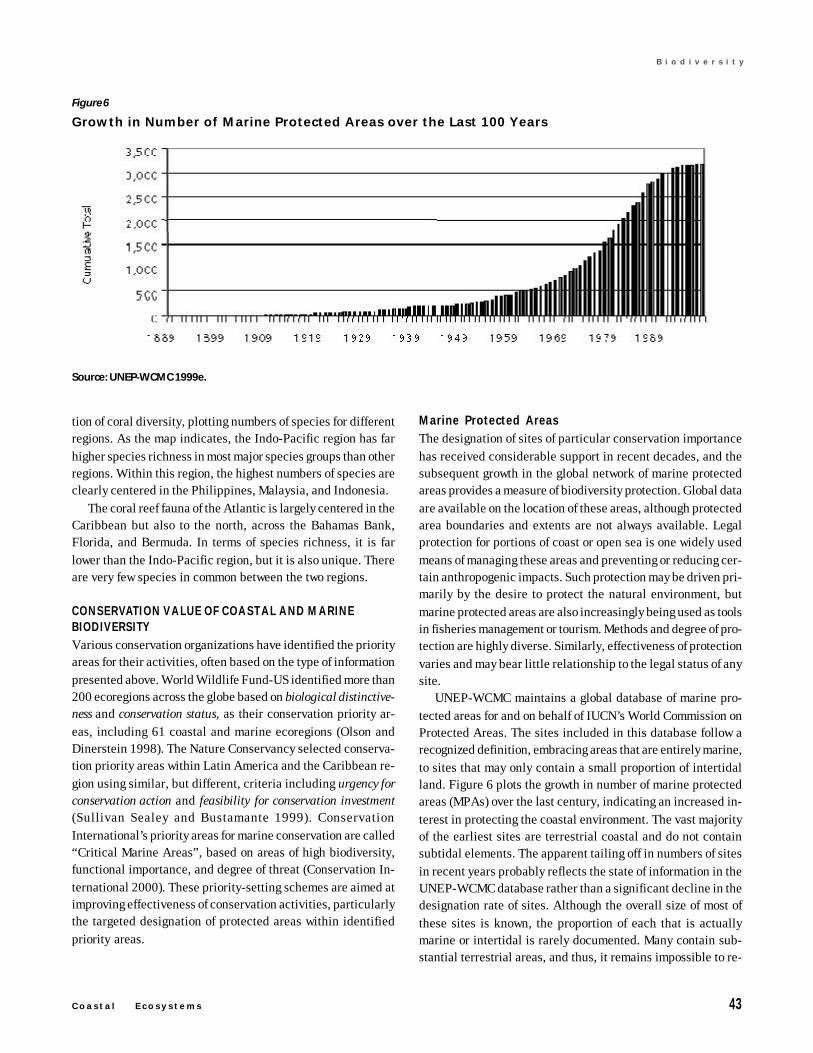
C o a s t a l E c o s y s t e m s 43
B i o d i v e r s i t y
tion of coral diversity, plotting numbers of species for differentregions. As the map indicates, the Indo-Pacific region has farhigher species richness in most major species groups than otherregions. Within this region, the highest numbers of species areclearly centered in the Philippines, Malaysia, and Indonesia.
The coral reef fauna of the Atlantic is largely centered in theCaribbean but also to the north, across the Bahamas Bank,Florida, and Bermuda. In terms of species richness, it is farlower than the Indo-Pacific region, but it is also unique. Thereare very few species in common between the two regions.
CONSERVATION VALUE OF COAST AL AND MARINEBIODIVERSITYVarious conservation organizations have identified the priorityareas for their activities, often based on the type of informationpresented above. World Wildlife Fund-US identified more than200 ecoregions across the globe based on biological distinctive-ness and conservation status, as their conservation priority ar-eas, including 61 coastal and marine ecoregions (Olson andDinerstein 1998). The Nature Conservancy selected conserva-tion priority areas within Latin America and the Caribbean re-gion using similar, but different, criteria including urgency forconservation action and feasibility for conservation investment(Sullivan Sealey and Bustamante 1999). ConservationInternational’s priority areas for marine conservation are called“Critical Marine Areas”, based on areas of high biodiversity,functional importance, and degree of threat (Conservation In-ternational 2000). These priority-setting schemes are aimed atimproving effectiveness of conservation activities, particularlythe targeted designation of protected areas within identifiedpriority areas.
Marine Protected AreasThe designation of sites of particular conservation importancehas received considerable support in recent decades, and thesubsequent growth in the global network of marine protectedareas provides a measure of biodiversity protection. Global dataare available on the location of these areas, although protectedarea boundaries and extents are not always available. Legalprotection for portions of coast or open sea is one widely usedmeans of managing these areas and preventing or reducing cer-tain anthropogenic impacts. Such protection may be driven pri-marily by the desire to protect the natural environment, butmarine protected areas are also increasingly being used as toolsin fisheries management or tourism. Methods and degree of pro-tection are highly diverse. Similarly, effectiveness of protectionvaries and may bear little relationship to the legal status of anysite.
UNEP-WCMC maintains a global database of marine pro-tected areas for and on behalf of IUCN’s World Commission onProtected Areas. The sites included in this database follow arecognized definition, embracing areas that are entirely marine,to sites that may only contain a small proportion of intertidalland. Figure 6 plots the growth in number of marine protectedareas (MPAs) over the last century, indicating an increased in-terest in protecting the coastal environment. The vast majorityof the earliest sites are terrestrial coastal and do not containsubtidal elements. The apparent tailing off in numbers of sitesin recent years probably reflects the state of information in theUNEP-WCMC database rather than a significant decline in thedesignation rate of sites. Although the overall size of most ofthese sites is known, the proportion of each that is actuallymarine or intertidal is rarely documented. Many contain sub-stantial terrestrial areas, and thus, it remains impossible to re-
Figure 6
Growth in Number of Marine Protected Areas over the Last 100 Years
Source: UNEP-WCMC 1999e.
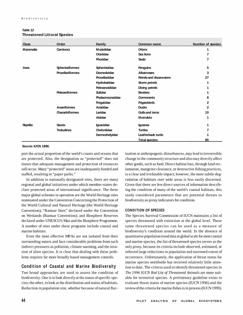
44 P I L O T A N A L Y S I S O F G L O B A L E C O S Y S T E M S
B i o d i v e r s i t y
port the actual proportion of the world’s coasts and oceans thatare protected. Also, the designation as “protected” does notinsure that adequate management and protection of resourceswill occur. Many “protected” areas are inadequately funded andstaffed, resulting in “paper parks.”
In addition to nationally designated sites, there are manyregional and global initiatives under which member-states de-clare protected areas of international significance. The threemajor global schemes in operation are the World Heritage sitesnominated under the Convention Concerning the Protection ofthe World Cultural and Natural Heritage (the World HeritageConvention); “Ramsar Sites” declared under the Conventionon Wetlands (Ramsar Convention); and Biosphere Reservesdeclared under UNESCO’s Man and the Biosphere Programme.A number of sites under these programs include coastal andmarine habitats.
Even the most effective MPAs are not isolated from theirsurrounding waters and face considerable problems from suchindirect pressures as pollution, climate warming, and the inva-sion of alien species. It is clear that dealing with these prob-lems requires far more broadly based management controls.
Condition of Coastal and Marine BiodiversityTwo broad approaches are used to assess the condition ofbiodiversity. One is to look directly at the status of specific spe-cies; the other, to look at the distribution and status of habitats.Reduction in population size, whether because of natural fluc-
tuation or anthropogenic disturbances, may lead to irreversiblechange in the community structure and also may directly affectother goods, such as food. Direct habitat loss, through land rec-lamation, mangrove clearance, or destructive fishing practices,is a clear and irrefutable impact; however, the more subtle deg-radation of habitats over wide areas is less easily discerned.Given that there are few direct sources of information describ-ing the condition of many of the world’s coastal habitats, thisstudy considered parameters that are potential threats tobiodiversity as proxy indicators for condition.
CONDITION OF SPECIESThe Species Survival Commission of IUCN maintains a list ofspecies threatened with extinction at the global level. Thesesame threatened species can be used as a measure ofbiodiversity’s condition around the world. In the absence ofquantitative population trend data at global scale for most coastaland marine species, the list of threatened species serves as theonly proxy, because its criteria include observed, estimated, orinferred large reductions in population and narrowed extent ofoccurrence. Unfortunately, the application of threat status formarine species worldwide has received relatively little atten-tion to date. The criteria used to identify threatened species inThe 1996 IUCN Red List of Threatened Animals are more suit-able for terrestrial species. A preliminary guideline exists toevaluate threat status of marine species (IUCN 1996) and thereview of the criteria for marine fishes is in process (IUCN 1999).
Table 12
Threatened Littoral Species
Class Order Family Common name Number of species
Mammalia Carnivora Mustelidae Otters 1 Otariidae Sea lions 7 Phocidae Seals 7
Aves Sphenisciformes Spheniscidae Penguins 5 Procellariiformes Diomedeidae Albatrosses 3 Procellariidae Petrels and shearwaters 27
Hydrobatidae Storm petrels 1 Pelecanoididae Diving petrels 1 Pelecaniformes Sulidae Boobies 1 Phalacrocoracidae Cormorants 8 Fregatidae Frigatebirds 2 Anseriformes Anatidae Ducks 2 Charadriiformes Laridae Gulls and terns 10
Alcidae Murrulets 1
Reptilia Sauria Iguanidae Iguanas 1 Testudines Cheloniidae Turtles 7 Dermochelyidae Leatherback turtle 1 Total species 85
Source: IUCN 1996.
C o a s t a l E c o s y s t e m s 45
B i o d i v e r s i t y
Therefore, the following lists for littoral and marine species arepreliminary and should be interpreted with caution.
Littoral speciesDirect measurement of species’ condition in littoral environ-ments is limited to a small number of case examples. Table 12provides a list of all the threatened species from the IUCN RedList that can be regarded as littoral. The total of some 85 spe-cies is probably an accurate reflection of the groups that havebeen studied, as the status of most mammals, birds, and rep-tiles in the marine environment is relatively well known. Notethat the table only includes species that spend part of their liveson intertidal or terrestrial environments. All other marine spe-cies are listed in Table 13.
Marine SpeciesThe state of marine fisheries with respect to future supplies offood from the continental shelves and oceans of the world isconsidered in a separate section of this report (see Food Pro-duction–Marine Fisheries section). Various human activities havehad adverse impacts on biodiversity in marine environments.The collapse of the great whale stocks in the first half of thiscentury, for example, is a classic case; however, this is not anisolated case. As described in the Marine Fisheries section, themajority of fisheries, at least in terms of catch statistics, focuson a limited number of highly abundant species. Even here over-fishing is taking a toll. Some stocks have now almost disap-peared from commercial catches. A small number of these com-mercially important species are now on the IUCN list of threat-ened species, including the Atlantic cod (Gadus morhua) andfive pelagic species of tuna, as well as some benthic species,such as the haddock (Melanogrammus aeglefinus), Atlantichalibut (Hippoglossus hippoglossus), and yellowtail flounder(Pleuronectes ferrugineus). Aside from these species, numerousothers that form the basis of more specialized fisheries are threat-ened—many shark stocks around the world have significantlydecreased as have some swordfish species. Numerous speciesof seahorse (Family Syngnathidae) and sea-moth (Pegasidae)have been added to the list of threatened species as a result ofextensive collection for traditional medicines. Other species havebeen impacted in collection for high-value specialty food mar-kets and the aquarium trade.
The application of threat status to wholly marine species is achallenge. Efforts are underway to improve knowledge of threatstatus for marine species, however, and significant numbers havebeen added to The 1996 IUCN Red List of Threatened Animals.(See Table 13.) Although this list is far from comprehensive formost groups (with possible exceptions being marine mammalsand seahorses), it warns that the extinction crisis may not onlybe a problem for terrestrial species. Note that other marine spe-
cies that spend part of their lives on intertidal or terrestrial en-vironments are listed in Table 12.
CONDITION OF HABITATSMeasures of habitat loss and degradation are useful indicatorsof habitat condition. If there are sufficiently accurate data onhistorical extent and status of habitats, it could be comparedwith the current situation. Unfortunately, for the majority ofcases, even current extent data in the form of maps are highlylimited at the global level and such work is usually restricted tocase studies. An alternative to such data is anecdotal informa-tion reporting known localities of degradation. In such cases,there is difficulty in differentiating increased cases of true deg-radation from increased reporting-frequency, but such modelsmay provide a critical tool in the absence of better information.
One example of such anecdotal information is the reportedincidence of coral reef degradation. Coral reef degradation maybe manifest in a number of ways, including loss of coral coveror species, and macroalgal or plankton blooms. There is con-cern about apparent increases in the incidence of coral dis-eases and coral bleaching, although the ultimate causes of theformer are sometimes unclear. Coral diseases are a broad rangeof apparently pathogenic attacks that are being reported fromreef sites across the world. In a new survey of these diseases,Green and Bruckner (2000) have developed a database withrecords of over 2,000 individual disease incidents. Althoughearliest records date back to 1902, the vast majority is from the1970s onward. Over 25 different diseases or variants are re-corded from over 50 countries. Although the mechanisms oftransmission and the causes of these diseases remain unclear,they have been linked to the increasing vulnerability of coralsas a result of other stresses, notably pollution and siltation, andpathogenic infection.
One further direct measure of coral stress is the phenom-enon of coral bleaching and mortality associated with widespreadelevated sea surface temperatures (SSTs) during the last de-cade (Hoegh-Guldberg 1999). This is widely predicted to in-crease in the future. (See Box 3.)
THREATS TO HABITATSDirect measures of state and change in biodiversity are cur-rently lacking for most coastal ecosystems. Therefore, it is nec-essary to infer the condition of biodiversity, at habitat level,based on some of the other measures already described in theprevious sections. Knowledge of the causal relationships driv-ing change allows the development of proxy indicators whereno direct measures exist. The proxy indicators might includelevel of pollution, human population density, urban growth pa-rameters, or even terrestrial land-use patterns or fisheries in-formation. A number of these pressure indicators have already
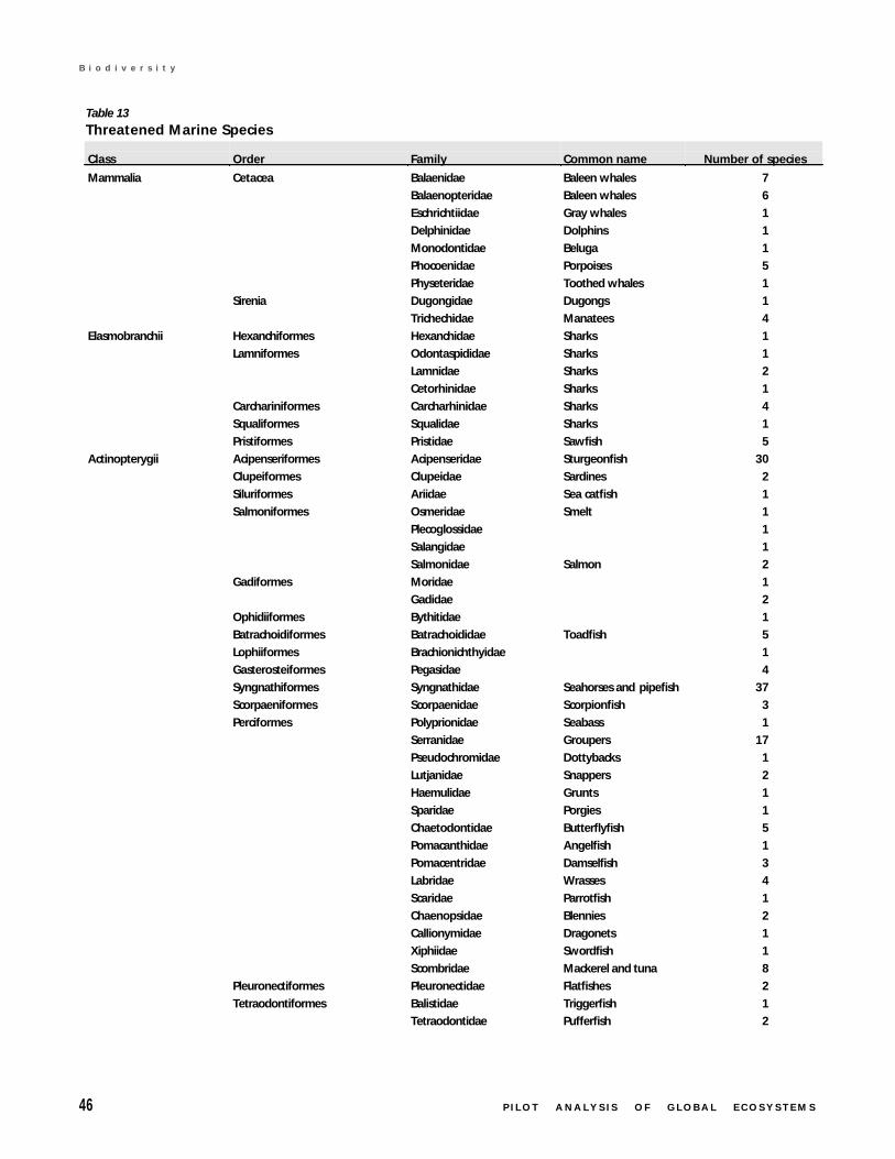
46 P I L O T A N A L Y S I S O F G L O B A L E C O S Y S T E M S
B i o d i v e r s i t y
Table 13
Threatened Marine Species
Class Order Family Common name Number of species
Mammalia Cetacea Balaenidae Baleen whales 7
Balaenopteridae Baleen whales 6
Eschrichtiidae Gray whales 1
Delphinidae Dolphins 1
Monodontidae Beluga 1
Phocoenidae Porpoises 5
Physeteridae Toothed whales 1
Sirenia Dugongidae Dugongs 1
Trichechidae Manatees 4
Elasmobranchii Hexanchiformes Hexanchidae Sharks 1
Lamniformes Odontaspididae Sharks 1
Lamnidae Sharks 2
Cetorhinidae Sharks 1
Carchariniformes Carcharhinidae Sharks 4
Squaliformes Squalidae Sharks 1
Pristiformes Pristidae Sawfish 5
Actinopterygii Acipenseriformes Acipenseridae Sturgeonfish 30
Clupeiformes Clupeidae Sardines 2
Siluriformes Ariidae Sea catfish 1
Salmoniformes Osmeridae Smelt 1
Plecoglossidae 1
Salangidae 1
Salmonidae Salmon 2
Gadiformes Moridae 1
Gadidae 2
Ophidiiformes Bythitidae 1
Batrachoidiformes Batrachoididae Toadfish 5
Lophiiformes Brachionichthyidae 1
Gasterosteiformes Pegasidae 4
Syngnathiformes Syngnathidae Seahorses and pipefish 37
Scorpaeniformes Scorpaenidae Scorpionfish 3
Perciformes Polyprionidae Seabass 1
Serranidae Groupers 17
Pseudochromidae Dottybacks 1
Lutjanidae Snappers 2
Haemulidae Grunts 1
Sparidae Porgies 1
Chaetodontidae Butterflyfish 5
Pomacanthidae Angelfish 1
Pomacentridae Damselfish 3
Labridae Wrasses 4
Scaridae Parrotfish 1
Chaenopsidae Blennies 2
Callionymidae Dragonets 1
Xiphiidae Swordfish 1
Scombridae Mackerel and tuna 8
Pleuronectiformes Pleuronectidae Flatfishes 2
Tetraodontiformes Balistidae Triggerfish 1
Tetraodontidae Pufferfish 2
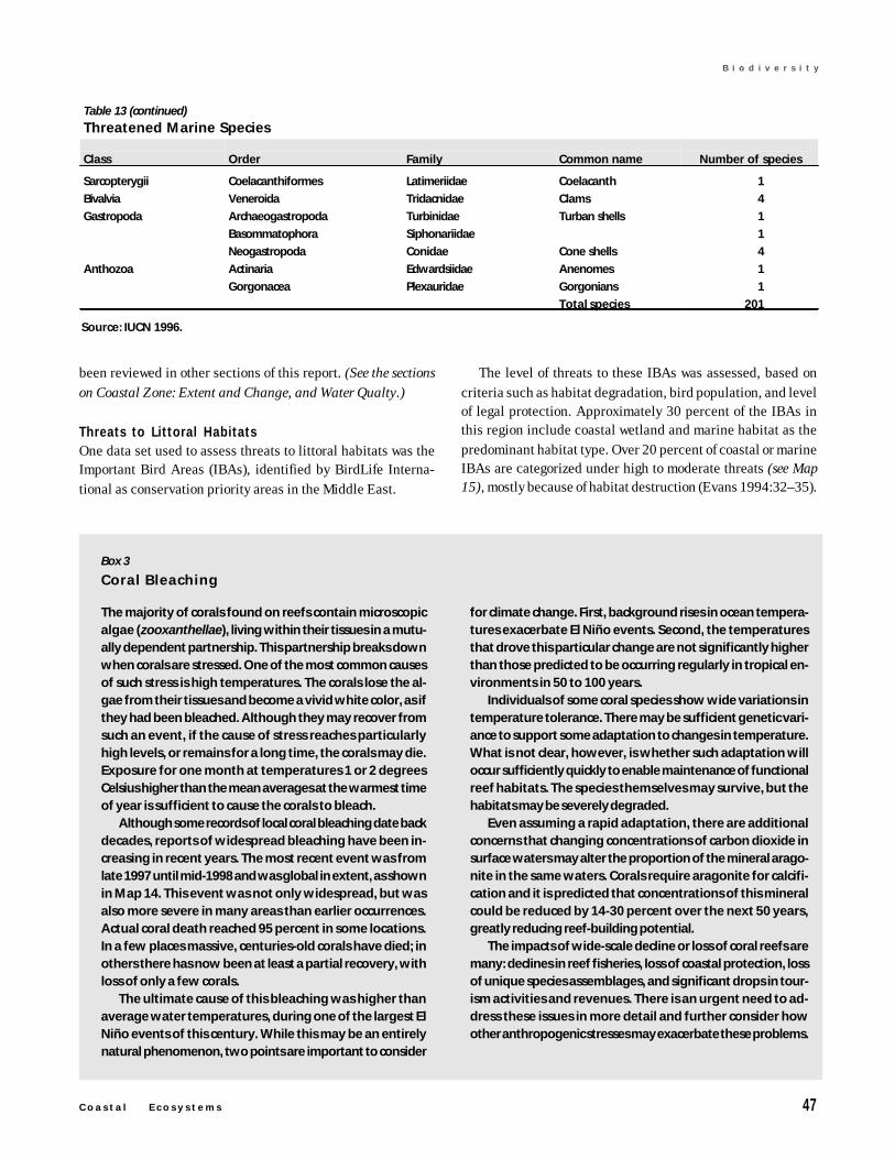
C o a s t a l E c o s y s t e m s 47
B i o d i v e r s i t y
been reviewed in other sections of this report. (See the sectionson Coastal Zone: Extent and Change, and Water Qualty.)
Threats to Littoral HabitatsOne data set used to assess threats to littoral habitats was theImportant Bird Areas (IBAs), identified by BirdLife Interna-tional as conservation priority areas in the Middle East.
The level of threats to these IBAs was assessed, based oncriteria such as habitat degradation, bird population, and levelof legal protection. Approximately 30 percent of the IBAs inthis region include coastal wetland and marine habitat as thepredominant habitat type. Over 20 percent of coastal or marineIBAs are categorized under high to moderate threats (see Map15), mostly because of habitat destruction (Evans 1994:32–35).
Box 3
Coral Bleaching
The majority of corals found on reefs contain microscopicalgae (zooxanthellae), living within their tissues in a mutu-ally dependent partnership. This partnership breaks downwhen corals are stressed. One of the most common causesof such stress is high temperatures. The corals lose the al-gae from their tissues and become a vivid white color, as ifthey had been bleached. Although they may recover fromsuch an event, if the cause of stress reaches particularlyhigh levels, or remains for a long time, the corals may die.Exposure for one month at temperatures 1 or 2 degreesCelsius higher than the mean averages at the warmest timeof year is sufficient to cause the corals to bleach.
Although some records of local coral bleaching date backdecades, reports of widespread bleaching have been in-creasing in recent years. The most recent event was fromlate 1997 until mid-1998 and was global in extent, as shownin Map 14. This event was not only widespread, but wasalso more severe in many areas than earlier occurrences.Actual coral death reached 95 percent in some locations.In a few places massive, centuries-old corals have died; inothers there has now been at least a partial recovery, withloss of only a few corals.
The ultimate cause of this bleaching was higher thanaverage water temperatures, during one of the largest ElNiño events of this century. While this may be an entirelynatural phenomenon, two points are important to consider
for climate change. First, background rises in ocean tempera-tures exacerbate El Niño events. Second, the temperaturesthat drove this particular change are not significantly higherthan those predicted to be occurring regularly in tropical en-vironments in 50 to 100 years.
Individuals of some coral species show wide variations intemperature tolerance. There may be sufficient genetic vari-ance to support some adaptation to changes in temperature.What is not clear, however, is whether such adaptation willoccur sufficiently quickly to enable maintenance of functionalreef habitats. The species themselves may survive, but thehabitats may be severely degraded.
Even assuming a rapid adaptation, there are additionalconcerns that changing concentrations of carbon dioxide insurface waters may alter the proportion of the mineral arago-nite in the same waters. Corals require aragonite for calcifi-cation and it is predicted that concentrations of this mineralcould be reduced by 14-30 percent over the next 50 years,greatly reducing reef-building potential.
The impacts of wide-scale decline or loss of coral reefs aremany: declines in reef fisheries, loss of coastal protection, lossof unique species assemblages, and significant drops in tour-ism activities and revenues. There is an urgent need to ad-dress these issues in more detail and further consider howother anthropogenic stresses may exacerbate these problems.
Table 13 (continued)
Threatened Marine Species
Class Order Family Common name Number of species
Sarcopterygii Coelacanthiformes Latimeriidae Coelacanth 1
Bivalvia Veneroida Tridacnidae Clams 4
Gastropoda Archaeogastropoda Turbinidae Turban shells 1
Basommatophora Siphonariidae 1
Neogastropoda Conidae Cone shells 4
Anthozoa Actinaria Edwardsiidae Anenomes 1
Gorgonacea Plexauridae Gorgonians 1
Total species 201
Source: IUCN 1996.
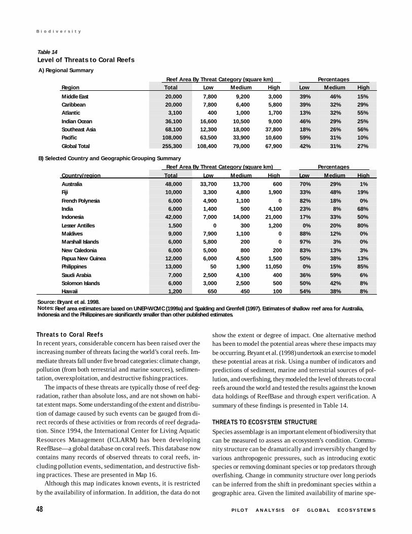
48 P I L O T A N A L Y S I S O F G L O B A L E C O S Y S T E M S
B i o d i v e r s i t y
Threats to Coral ReefsIn recent years, considerable concern has been raised over theincreasing number of threats facing the world’s coral reefs. Im-mediate threats fall under five broad categories: climate change,pollution (from both terrestrial and marine sources), sedimen-tation, overexploitation, and destructive fishing practices.
The impacts of these threats are typically those of reef deg-radation, rather than absolute loss, and are not shown on habi-tat extent maps. Some understanding of the extent and distribu-tion of damage caused by such events can be gauged from di-rect records of these activities or from records of reef degrada-tion. Since 1994, the International Center for Living AquaticResources Management (ICLARM) has been developingReefBase—a global database on coral reefs. This database nowcontains many records of observed threats to coral reefs, in-cluding pollution events, sedimentation, and destructive fish-ing practices. These are presented in Map 16.
Although this map indicates known events, it is restrictedby the availability of information. In addition, the data do not
show the extent or degree of impact. One alternative methodhas been to model the potential areas where these impacts maybe occurring. Bryant et al. (1998) undertook an exercise to modelthese potential areas at risk. Using a number of indicators andpredictions of sediment, marine and terrestrial sources of pol-lution, and overfishing, they modeled the level of threats to coralreefs around the world and tested the results against the knowndata holdings of ReefBase and through expert verification. Asummary of these findings is presented in Table 14.
THREATS TO ECOSYSTEM STRUCTURESpecies assemblage is an important element of biodiversity thatcan be measured to assess an ecosystem’s condition. Commu-nity structure can be dramatically and irreversibly changed byvarious anthropogenic pressures, such as introducing exoticspecies or removing dominant species or top predators throughoverfishing. Change in community structure over long periodscan be inferred from the shift in predominant species within ageographic area. Given the limited availability of marine spe-
Table 14
Level of Threats to Coral Reefs
A) Regional Summary
Reef Area By Threat Category (square km) Percentages
Region Total Low Medium High Low Medium High
Middle East 20,000 7,800 9,200 3,000 39% 46% 15%
Caribbean 20,000 7,800 6,400 5,800 39% 32% 29%
Atlantic 3,100 400 1,000 1,700 13% 32% 55%
Indian Ocean 36,100 16,600 10,500 9,000 46% 29% 25%
Southeast Asia 68,100 12,300 18,000 37,800 18% 26% 56%
Pacific 108,000 63,500 33,900 10,600 59% 31% 10%
Global Total 255,300 108,400 79,000 67,900 42% 31% 27%
B) Selected Country and Geographic Grouping Summary
Reef Area By Threat Category (square km) Percentages
Country/region Total Low Medium High Low Medium High
Australia 48,000 33,700 13,700 600 70% 29% 1%
Fiji 10,000 3,300 4,800 1,900 33% 48% 19%
French Polynesia 6,000 4,900 1,100 0 82% 18% 0%
India 6,000 1,400 500 4,100 23% 8% 68%
Indonesia 42,000 7,000 14,000 21,000 17% 33% 50%
Lesser Antilles 1,500 0 300 1,200 0% 20% 80%
Maldives 9,000 7,900 1,100 0 88% 12% 0%
Marshall Islands 6,000 5,800 200 0 97% 3% 0%
New Caledonia 6,000 5,000 800 200 83% 13% 3%
Papua New Guinea 12,000 6,000 4,500 1,500 50% 38% 13%
Philippines 13,000 50 1,900 11,050 0% 15% 85%
Saudi Arabia 7,000 2,500 4,100 400 36% 59% 6%
Solomon Islands 6,000 3,000 2,500 500 50% 42% 8%
Hawaii 1,200 650 450 100 54% 38% 8%
Source: Bryant et al. 1998.Notes: Reef area estimates are based on UNEP-WCMC (1999a) and Spalding and Grenfell (1997). Estimates of shallow reef area for Australia,Indonesia and the Philippines are significantly smaller than other published estimates.
C o a s t a l E c o s y s t e m s 49
B i o d i v e r s i t y
cies population data, we can only discuss this as a potentialarea of new indicator development.
Fishing PracticesOne way to assess the structure of marine ecosystems is to lookat changes in species assemblages in terms of trophic levels.The change in the relative abundance of top predators affectsthe lower trophic level species, leading to a shift in communitystructure. This approach to analyzing the FAO fisheries datasetwas introduced by Pauly et al. (1998a), and further evaluatedin the Marine Fisheries section of this report. The FAO data setprimarily consists of commercially exploited species groups;therefore, it is inadequate in detecting a change in the overallstructure of the marine ecosystem. In areas such as the NorthAtlantic and Northeast Pacific, however, significant transitionsin the trophic level composition of catches seem to have oc-curred between the 1950s and 1990s, indicating dramaticchanges in community structure and subsequent change in theexploitation pattern for those particular areas (see Marine Fish-eries section). Pauly et al. (1998b) also estimated trophic cat-egories for 97 marine mammals based on literature about thediet composition, which, if combined with population studies,can be useful for assessing ecosystem change at the structurallevel.
Aside from the direct effects of fishing on the target speciesthemselves, there are considerable indirect effects caused bydestructive fishing practices, which are less well documented.Bycatch is a widespread problem (see a more detailed discus-sion in the Marine Fisheries section). Early attention was drawnto this problem, focussing on high profile species, such as dol-phins being captured in tuna fisheries. More recently, the mas-sive and indiscriminate catches of large driftnets have receivedsimilar attention and resulted in a U.N. ban on high-seas driftnetfisheries. Apart from the impact on the bycatch species them-selves, discards affect the wider marine commuunity, present-ing a considerable input of fish protein to scavenging species.Removing large numbers of target species and unwanted bycatchcan also have a significant bearing on biodiversity and on com-munity structures, by altering patterns of competition or preda-tor-prey relations. A number of fish and invertebrate specieshave high mortality rates following discard. Bottom trawling isanother fishing method that has gained increasing attention be-cause of its adverse impact on benthic communities. (See Box 2in Coastal Zone: Extent and Change section.)
Invasive Species
One of the most underreported and globally pervasive threatsto natural ecosystems worldwide is the arrival of invasive spe-cies. Although some movement of species from region to regionaround the globe can be regarded as a natural process, humanvectors have greatly exacerbated the rates of these movements
and the distances covered. Proliferation of introduced algaespecies is sometimes attributed as a cause of Harmful AlgalBlooms (HABs), posing direct threats to biodiversity as well aspublic health. (See section on Water Quality for a discussion onHABs.)
In the marine environment, one of the most significant andproblematic sources of biological invasion is from the ballastwater of ships. On any given day, it is estimated that perhaps3,000 different species are carried alive in the ballast water ofthe world’s ocean fleets (Bright 1999:156). One of the worstexamples is the introduction of the so-called Leidy’s comb jelly(Mnemiopsis leidyi) from the American Atlantic into the watersof the Black Sea in 1982. Unchallenged by natural predators,this species proliferated to peak numbers in 1989, 1994, and1995 comprising about 95 percent of the entire wet weight bio-mass in the Black Sea (Shiganova 1997, 1998, and 2000). Theseanimals devastated the natural zooplankton stocks, drivingmassive algal blooms and disrupting the natural food chains.This, subsequently, contributed to the collapse of the importantanchovy fishing industry in the Black Sea (Bright 1999:157).This invasive also migrated from the Black Sea to adjacent ba-sins, such as the Sea of Marmara and the eastern Mediterra-nean, in the early 1990s (Shiganova 1998:306). In addition,increased abundance of invasive Mnemiopsis has recently beenobserved in the Caspian Sea. The origin and cause of this intro-duction are still unknown, although it is most likely to be throughballast water (Shiganova 2000).
Other causes of biological invasion include the intentionalintroduction of nonnative species for fisheries stocking or orna-mental purposes, and the accidental introduction associated withaquaculture. One final mechanism is that of Lessepsian migra-tion, where species move through artificial canals, most nota-bly through the Suez Canal from the Red Sea into the Mediter-ranean and vice versa.
There are no global data sets on introduced species, althoughcomprehensive data are available for some countries and re-gions. A number of these have been gathered together for thisreport and Table 15 presents summary data for the waters wheresuch data are available. The marine ecosystems in the Mediter-ranean now contain 480 invasive species, the Baltic Sea con-tains 89, while Australian waters contain 124 species.
Capac i ty of Coasta l Ecosystems to
Susta in B iod ivers i tyThe condition indicators presented above do not provide a com-plete picture of how well biological systems are functioning glo-bally in terms of maintaining biodiversity. From the evidence ofhabitat loss and the increasing level of threats, however, thecapacity to maintain biodiversity seems to be declining in manyparts of the world. Because of the lack of directly measured
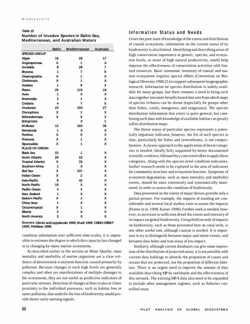
50 P I L O T A N A L Y S I S O F G L O B A L E C O S Y S T E M S
B i o d i v e r s i t y
condition information over sufficient time-scales, it is impos-sible to estimate the degree to which this capacity has changedor is changing for many marine ecosystems.
As described earlier in the section on Water Quality, massmortality and morbidity of marine organisms are a clear evi-dence of deteriorated ecosystem function caused primarily bypollution. Because changes at such high levels are generallycomplex and often are manifestations of multiple damages tothe ecosystems, they are not useful as predictive indicators ofparticular stresses. Detection of changes at finer scales or closerproximity to the individual pressures, such as habitat loss orwater pollution, that underlie the loss of biodiversity would pro-vide better early warning signals.
In format ion Status and NeedsGiven the poor state of knowledge of the extent and distributionof coastal ecosystems, information on the current status of itsbiodiversity is also limited. Identifying and describing areas ofhigh conservation importance at genetic, species, and ecosys-tem levels, or areas of high natural productivity, would helpimprove the effectiveness of conservation activities with lim-ited resources. Basic taxonomic inventory of coastal and ma-rine ecosystems requires special efforts (Convention on Bio-logical Diversity 1998:21) to support subsequent biogeographicresearch. Information on species distribution is widely avail-able for many groups, but there remains a need to bring suchdata together into more broadly based data sets from which mapsof species richness can be drawn (especially for groups otherthan fishes, corals, mangroves, and seagrasses). The speciesdistribution information that exists is quite general, but com-bining such data with knowledge of available habitat can greatlyrefine distribution maps.
The threat status of particular species represents a poten-tially important indicator; however, the list of such species todate, particularly for fishes and invertebrates, is not compre-hensive. A clearer approach to the application of threat catego-ries is needed, ideally fully supported by better documentedscientific evidence, followed by a concerted effort to apply thesecategories. Along with the species-level condition indicators,further research needs to be explored in the area of indicatorsfor community structure and ecosystem function. Symptoms ofecosystem degradation, such as mass mortality and morbidityevents, should be more extensively and systematically moni-tored, in order to assess the condition of biodiversity.
Data presented on the extent of major threats provide only apartial picture. For example, the impacts of trawling are con-siderable and several local studies exist to assess the impacts(Poiner et al. 1998; Kaiser 1998). Further work is needed, how-ever, to ascertain in sufficient detail the extent and intensity ofits impact on global biodiversity. Using field records of impactson biodiversity, such as those presented here on coral reefs, isone other useful tool, although caution is needed. It is impor-tant to try to distinguish between major and minor events, andbetween data holes and true areas of low impact.
Similarly, although current databases can give some impres-sion of the distribution of protected areas, it is not possible withcurrent data holdings to identify the proportion of coasts andoceans that are protected, nor the proportion of different habi-tats. There is an urgent need to improve the amount of dataavailable describing MPAs worldwide and the effectiveness ofthis network. The existing MPA data also need to be expandedto include other management regimes, such as fisheries con-trolled areas.
Table 15
Number of Invasive Species in Baltic Sea,Mediterranean, and Australian Waters
Baltic Mediterranean Australia SPECIES GROUPAlgae 16 25 17Angiospermae X 1 XAnnelida 8 28 7Bryozoa 1 7 9Chaetognatha X 1 XChelicerata X 1 XAscidea 1 9 3Pisces 20 115 16Aves 1 X XMammalia 2 1 XCnidaria 4 7 5Crustacea 23 104 27Ctenophora X 1 XEchinodermata X 5 3Entoprocta X 1Mollusca 12 164 36Nematoda 1 X XPorifera X 9 XProtozoa X 1 XSipunculida X 1 X PLACE OF ORIGINBlack Sea 22 1 XNorth Atlantic 29 22 XTropical Atlantic X 33 XSouthern Africa 1 X XRed Sea X 337 XIndian Ocean X 2 X
Indo-Pacific 8 42 XNorth Pacific 15 3 XPacific Ocean 4 3 XNew Zealand 1 X XEastern Pacific X 1 XChina Seas 1 X XCircumtropical X 1 XSiberia 2 X XNorth America 2 X X
Sources: Olenin and Leppäkoski 1999; Madl 1999; CSIRO-CRIMP1999; FishBase 1998.
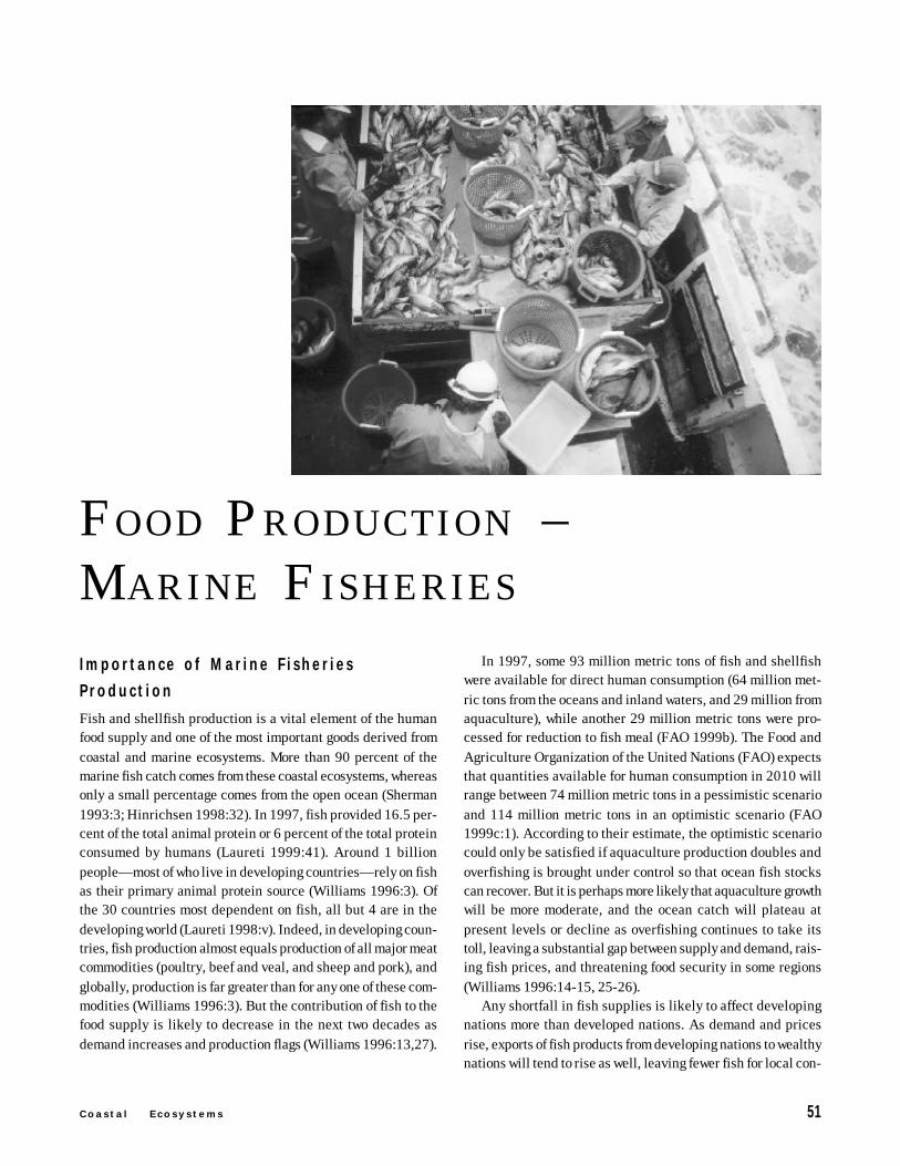
C o a s t a l E c o s y s t e m s 51
B i o d i v e r s i t y
F O O D P R O D U C T I O N –M A R I N E F ISHERIES
In 1997, some 93 million metric tons of fish and shellfishwere available for direct human consumption (64 million met-ric tons from the oceans and inland waters, and 29 million fromaquaculture), while another 29 million metric tons were pro-cessed for reduction to fish meal (FAO 1999b). The Food andAgriculture Organization of the United Nations (FAO) expectsthat quantities available for human consumption in 2010 willrange between 74 million metric tons in a pessimistic scenarioand 114 million metric tons in an optimistic scenario (FAO1999c:1). According to their estimate, the optimistic scenariocould only be satisfied if aquaculture production doubles andoverfishing is brought under control so that ocean fish stockscan recover. But it is perhaps more likely that aquaculture growthwill be more moderate, and the ocean catch will plateau atpresent levels or decline as overfishing continues to take itstoll, leaving a substantial gap between supply and demand, rais-ing fish prices, and threatening food security in some regions(Williams 1996:14-15, 25-26).
Any shortfall in fish supplies is likely to affect developingnations more than developed nations. As demand and pricesrise, exports of fish products from developing nations to wealthynations will tend to rise as well, leaving fewer fish for local con-
Importance of Mar ine F i sher ies
P roduct ion
Fish and shellfish production is a vital element of the humanfood supply and one of the most important goods derived fromcoastal and marine ecosystems. More than 90 percent of themarine fish catch comes from these coastal ecosystems, whereasonly a small percentage comes from the open ocean (Sherman1993:3; Hinrichsen 1998:32). In 1997, fish provided 16.5 per-cent of the total animal protein or 6 percent of the total proteinconsumed by humans (Laureti 1999:41). Around 1 billionpeople—most of who live in developing countries—rely on fishas their primary animal protein source (Williams 1996:3). Ofthe 30 countries most dependent on fish, all but 4 are in thedeveloping world (Laureti 1998:v). Indeed, in developing coun-tries, fish production almost equals production of all major meatcommodities (poultry, beef and veal, and sheep and pork), andglobally, production is far greater than for any one of these com-modities (Williams 1996:3). But the contribution of fish to thefood supply is likely to decrease in the next two decades asdemand increases and production flags (Williams 1996:13,27).
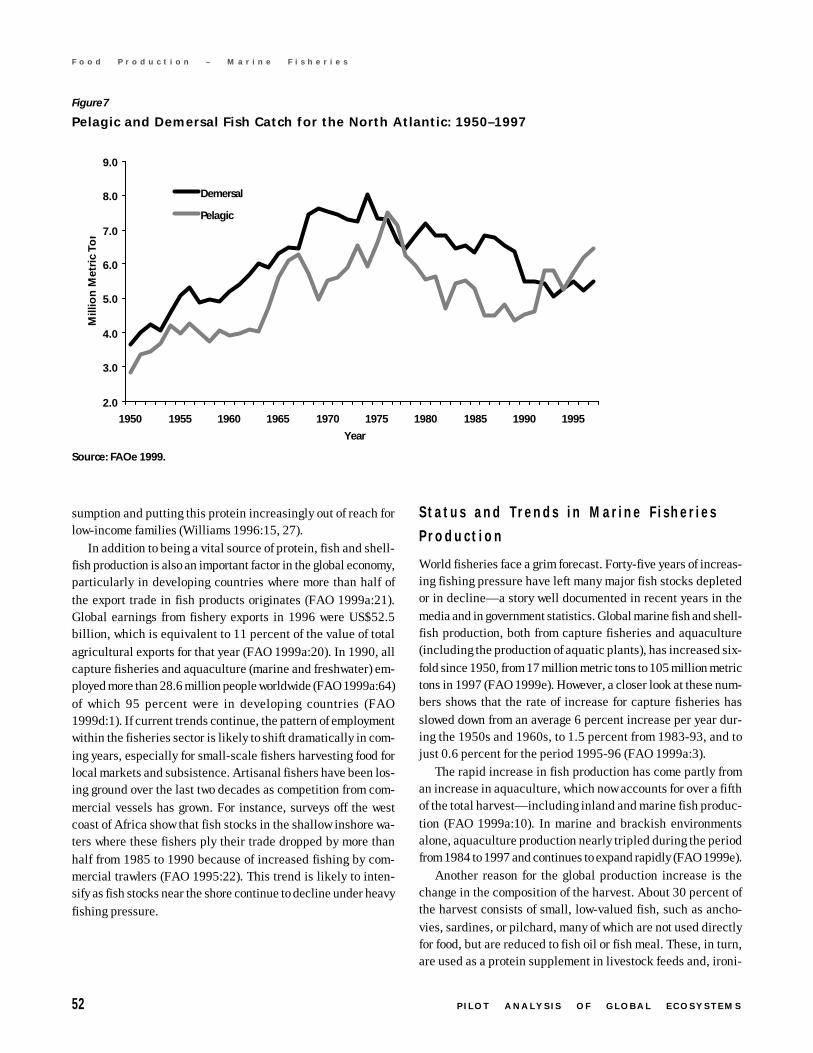
52 P I L O T A N A L Y S I S O F G L O B A L E C O S Y S T E M S
F o o d P r o d u c t i o n – M a r i n e F i s h e r i e s
sumption and putting this protein increasingly out of reach forlow-income families (Williams 1996:15, 27).
In addition to being a vital source of protein, fish and shell-fish production is also an important factor in the global economy,particularly in developing countries where more than half ofthe export trade in fish products originates (FAO 1999a:21).Global earnings from fishery exports in 1996 were US$52.5billion, which is equivalent to 11 percent of the value of totalagricultural exports for that year (FAO 1999a:20). In 1990, allcapture fisheries and aquaculture (marine and freshwater) em-ployed more than 28.6 million people worldwide (FAO 1999a:64)of which 95 percent were in developing countries (FAO1999d:1). If current trends continue, the pattern of employmentwithin the fisheries sector is likely to shift dramatically in com-ing years, especially for small-scale fishers harvesting food forlocal markets and subsistence. Artisanal fishers have been los-ing ground over the last two decades as competition from com-mercial vessels has grown. For instance, surveys off the westcoast of Africa show that fish stocks in the shallow inshore wa-ters where these fishers ply their trade dropped by more thanhalf from 1985 to 1990 because of increased fishing by com-mercial trawlers (FAO 1995:22). This trend is likely to inten-sify as fish stocks near the shore continue to decline under heavyfishing pressure.
Status and Trends in Mar ine F isher ies
P roduct ion
World fisheries face a grim forecast. Forty-five years of increas-ing fishing pressure have left many major fish stocks depletedor in decline—a story well documented in recent years in themedia and in government statistics. Global marine fish and shell-fish production, both from capture fisheries and aquaculture(including the production of aquatic plants), has increased six-fold since 1950, from 17 million metric tons to 105 million metrictons in 1997 (FAO 1999e). However, a closer look at these num-bers shows that the rate of increase for capture fisheries hasslowed down from an average 6 percent increase per year dur-ing the 1950s and 1960s, to 1.5 percent from 1983-93, and tojust 0.6 percent for the period 1995-96 (FAO 1999a:3).
The rapid increase in fish production has come partly froman increase in aquaculture, which now accounts for over a fifthof the total harvest—including inland and marine fish produc-tion (FAO 1999a:10). In marine and brackish environmentsalone, aquaculture production nearly tripled during the periodfrom 1984 to 1997 and continues to expand rapidly (FAO 1999e).
Another reason for the global production increase is thechange in the composition of the harvest. About 30 percent ofthe harvest consists of small, low-valued fish, such as ancho-vies, sardines, or pilchard, many of which are not used directlyfor food, but are reduced to fish oil or fish meal. These, in turn,are used as a protein supplement in livestock feeds and, ironi-
Figure 7
Pelagic and Demersal Fish Catch for the North Atlantic: 1950–1997
Source: FAOe 1999.
2.0
3.0
4.0
5.0
6.0
7.0
8.0
9.0
1950 1955 1960 1965 1970 1975 1980 1985 1990 1995
Year
Mill
ion
Met
ric
Ton
Demersal
Pelagic
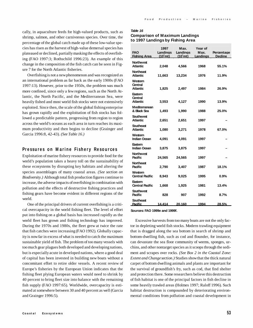
C o a s t a l E c o s y s t e m s 53
F o o d P r o d u c t i o n – M a r i n e F i s h e r i e s
cally, in aquaculture feeds for high-valued products, such asshrimp, salmon, and other carnivorous species. Over time, thepercentage of the global catch made up of these low-value spe-cies has risen as the harvest of high-value demersal species hasplateaued or declined, partially masking the effects of overfish-ing (FAO 1997:3; Rothschild 1996:23). An example of thischange in the composition of the fish catch can be seen in Fig-ure 7 for the North Atlantic fisheries.
Overfishing is not a new phenomenon and was recognized asan international problem as far back as the early 1900s (FAO1997:13). However, prior to the 1950s, the problem was muchmore confined, since only a few regions, such as the North At-lantic, the North Pacific, and the Mediterranean Sea, wereheavily fished and most world fish stocks were not extensivelyexploited. Since then, the scale of the global fishing enterprisehas grown rapidly and the exploitation of fish stocks has fol-lowed a predictable pattern, progressing from region to regionacross the world’s oceans as each area in turn reaches its maxi-mum productivity and then begins to decline (Grainger andGarcia 1996:8, 42-43). (See Table 16.)
Pressures on Mar ine F i shery ResourcesExploitation of marine fishery resources to provide food for theworld’s population takes a heavy toll on the sustainability ofthese ecosystems by disrupting key habitats and altering thespecies assemblages of many coastal areas. (See section onBiodiversity.) Although total fish production figures continue toincrease, the adverse impacts of overfishing in combination withpollution and the effects of destructive fishing practices andfishing gears have become evident in different regions of theworld.
One of the principal drivers of current overfishing is a criti-cal overcapacity in the world fishing fleet. The level of effortput into fishing on a global basis has increased rapidly as theworld fleet has grown and fishing technology has improved.During the 1970s and 1980s, the fleet grew at twice the ratethat fish catches were increasing (FAO 1992). Globally capac-ity is now far in excess of what is needed to catch the maximumsustainable yield of fish. The problem of too many vessels withtoo much gear plagues both developed and developing nations,but is especially acute in developed nations, where a good dealof capital has been invested in building new boats without aconcomitant effort to retire older vessels. A recent review ofEurope’s fisheries by the European Union indicates that thefishing fleet plying European waters would need to shrink by40 percent to bring fleet size into balance with the remainingfish supply (FAO 1997:65). Worldwide, overcapacity is esti-mated at somewhere between 30 and 40 percent as well (Garciaand Grainger 1996:5).
Excessive harvests from too many boats are not the only fac-tor in depleting world fish stocks. Modern trawling equipmentthat is dragged along the sea bottom in search of shrimp andbottom-dwelling fish, such as cod and flounder, for instance,can devastate the sea floor community of worms, sponges, ur-chins, and other nontarget species as it scoops through the sedi-ment and scrapes over rocks. (See Box 2 in the Coastal Zone:Extent and Change section.) Studies show that the thick naturalcarpet of bottom dwelling animals and plants are important forthe survival of groundfish’s fry, such as cod, that find shelterand protection there. Some researchers believe this destructionof fish habitat is one of the principal factors in fish decline insome heavily trawled areas (Holmes 1997; Raloff 1996). Suchhabitat destruction is compounded by deteriorating environ-mental conditions from pollution and coastal development in
Table 16
Comparison of Maximum Landingsto 1997 Landings by Fishing Area
FAOFishing Area
1997Landings(103mt)
Max.Landings(103mt)
Year ofMax.
LandingsPercentage
Decline
NorthwestAtlantic 2,048 4,566 1968 55.1%
NortheastAtlantic 11,663 13,234 1976 11.9%
WesternCentralAtlantic 1,825 2,497 1984 26.9%
EasternCentralAtlantic 3,553 4,127 1990 13.9%
Mediterranean& Black Sea 1,493 1,990 1988 25.0%
SouthwestAtlantic 2,651 2,651 1997 –
SoutheastAtlantic 1,080 3,271 1978 67.0%
WesternIndian Ocean 4,091 4,091 1997 –
EasternIndian Ocean 3,875 3,875 1997 –
NorthwestPacific 24,565 24,565 1997 –
NortheastPacific 2,790 3,407 1987 18.1%
WesternCentral Pacific 8,943 9,025 1995 0.9%
EasternCentral Pacific 1,668 1,925 1981 13.4%
SouthwestPacific 828 907 1992 8.7%
SoutheastPacific 14,414 20,160 1994 28.5%
Sources: FAO 1999e and 1999f.
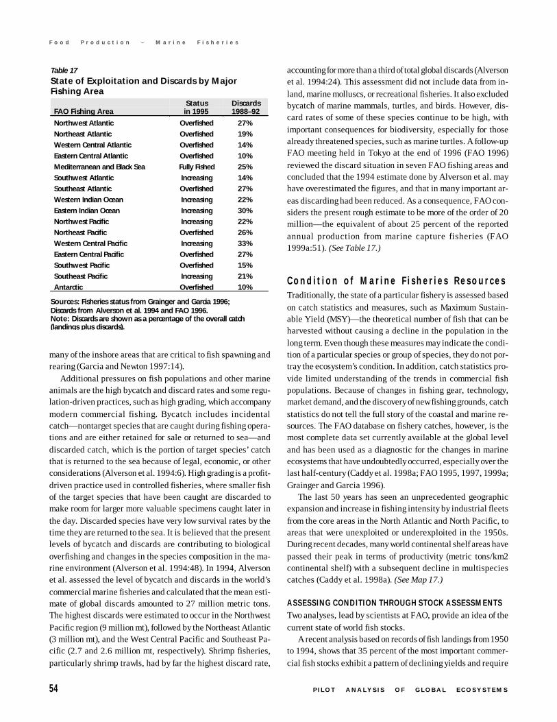
54 P I L O T A N A L Y S I S O F G L O B A L E C O S Y S T E M S
F o o d P r o d u c t i o n – M a r i n e F i s h e r i e s
many of the inshore areas that are critical to fish spawning andrearing (Garcia and Newton 1997:14).
Additional pressures on fish populations and other marineanimals are the high bycatch and discard rates and some regu-lation-driven practices, such as high grading, which accompanymodern commercial fishing. Bycatch includes incidentalcatch—nontarget species that are caught during fishing opera-tions and are either retained for sale or returned to sea—anddiscarded catch, which is the portion of target species’ catchthat is returned to the sea because of legal, economic, or otherconsiderations (Alverson et al. 1994:6). High grading is a profit-driven practice used in controlled fisheries, where smaller fishof the target species that have been caught are discarded tomake room for larger more valuable specimens caught later inthe day. Discarded species have very low survival rates by thetime they are returned to the sea. It is believed that the presentlevels of bycatch and discards are contributing to biologicaloverfishing and changes in the species composition in the ma-rine environment (Alverson et al. 1994:48). In 1994, Alversonet al. assessed the level of bycatch and discards in the world’scommercial marine fisheries and calculated that the mean esti-mate of global discards amounted to 27 million metric tons.The highest discards were estimated to occur in the NorthwestPacific region (9 million mt), followed by the Northeast Atlantic(3 million mt), and the West Central Pacific and Southeast Pa-cific (2.7 and 2.6 million mt, respectively). Shrimp fisheries,particularly shrimp trawls, had by far the highest discard rate,
accounting for more than a third of total global discards (Alversonet al. 1994:24). This assessment did not include data from in-land, marine molluscs, or recreational fisheries. It also excludedbycatch of marine mammals, turtles, and birds. However, dis-card rates of some of these species continue to be high, withimportant consequences for biodiversity, especially for thosealready threatened species, such as marine turtles. A follow-upFAO meeting held in Tokyo at the end of 1996 (FAO 1996)reviewed the discard situation in seven FAO fishing areas andconcluded that the 1994 estimate done by Alverson et al. mayhave overestimated the figures, and that in many important ar-eas discarding had been reduced. As a consequence, FAO con-siders the present rough estimate to be more of the order of 20million—the equivalent of about 25 percent of the reportedannual production from marine capture fisheries (FAO1999a:51). (See Table 17.)
Condi t ion of Mar ine F i sher ies ResourcesTraditionally, the state of a particular fishery is assessed basedon catch statistics and measures, such as Maximum Sustain-able Yield (MSY)—the theoretical number of fish that can beharvested without causing a decline in the population in thelong term. Even though these measures may indicate the condi-tion of a particular species or group of species, they do not por-tray the ecosystem’s condition. In addition, catch statistics pro-vide limited understanding of the trends in commercial fishpopulations. Because of changes in fishing gear, technology,market demand, and the discovery of new fishing grounds, catchstatistics do not tell the full story of the coastal and marine re-sources. The FAO database on fishery catches, however, is themost complete data set currently available at the global leveland has been used as a diagnostic for the changes in marineecosystems that have undoubtedly occurred, especially over thelast half-century (Caddy et al. 1998a; FAO 1995, 1997, 1999a;Grainger and Garcia 1996).
The last 50 years has seen an unprecedented geographicexpansion and increase in fishing intensity by industrial fleetsfrom the core areas in the North Atlantic and North Pacific, toareas that were unexploited or underexploited in the 1950s.During recent decades, many world continental shelf areas havepassed their peak in terms of productivity (metric tons/km2continental shelf) with a subsequent decline in multispeciescatches (Caddy et al. 1998a). (See Map 17.)
ASSESSING CONDITION THROUGH STOCK ASSESSMENTSTwo analyses, lead by scientists at FAO, provide an idea of thecurrent state of world fish stocks.
A recent analysis based on records of fish landings from 1950to 1994, shows that 35 percent of the most important commer-cial fish stocks exhibit a pattern of declining yields and require
Table 17
State of Exploitation and Discards by MajorFishing Area
FAO Fishing AreaStatusin 1995
Discards1988–92
Northwest Atlantic Overfished 27%
Northeast Atlantic Overfished 19%
Western Central Atlantic Overfished 14%
Eastern Central Atlantic Overfished 10%
Mediterranean and Black Sea Fully Fished 25%
Southwest Atlantic Increasing 14%
Southeast Atlantic Overfished 27%
Western Indian Ocean Increasing 22%
Eastern Indian Ocean Increasing 30%
Northwest Pacific Increasing 22%
Northeast Pacific Overfished 26%
Western Central Pacific Increasing 33%
Eastern Central Pacific Overfished 27%
Southwest Pacific Overfished 15%
Southeast Pacific Increasing 21%
Antarctic Overfished 10%
Sources: Fisheries status from Grainger and Garcia 1996;Discards from Alverson et al. 1994 and FAO 1996.Note: Discards are shown as a percentage of the overall catch(landings plus discards).
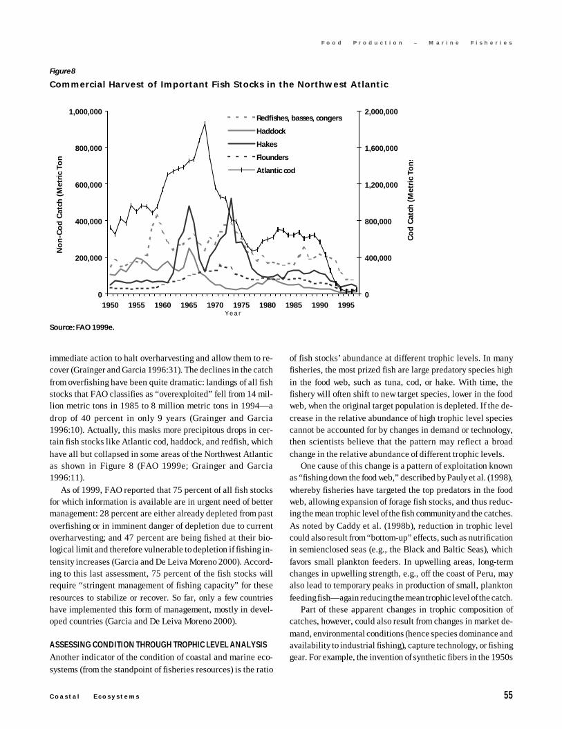
C o a s t a l E c o s y s t e m s 55
F o o d P r o d u c t i o n – M a r i n e F i s h e r i e s
immediate action to halt overharvesting and allow them to re-cover (Grainger and Garcia 1996:31). The declines in the catchfrom overfishing have been quite dramatic: landings of all fishstocks that FAO classifies as “overexploited” fell from 14 mil-lion metric tons in 1985 to 8 million metric tons in 1994—adrop of 40 percent in only 9 years (Grainger and Garcia1996:10). Actually, this masks more precipitous drops in cer-tain fish stocks like Atlantic cod, haddock, and redfish, whichhave all but collapsed in some areas of the Northwest Atlanticas shown in Figure 8 (FAO 1999e; Grainger and Garcia1996:11).
As of 1999, FAO reported that 75 percent of all fish stocksfor which information is available are in urgent need of bettermanagement: 28 percent are either already depleted from pastoverfishing or in imminent danger of depletion due to currentoverharvesting; and 47 percent are being fished at their bio-logical limit and therefore vulnerable to depletion if fishing in-tensity increases (Garcia and De Leiva Moreno 2000). Accord-ing to this last assessment, 75 percent of the fish stocks willrequire “stringent management of fishing capacity” for theseresources to stabilize or recover. So far, only a few countrieshave implemented this form of management, mostly in devel-oped countries (Garcia and De Leiva Moreno 2000).
ASSESSING CONDITION THROUGH TROPHIC LEVEL ANALYSISAnother indicator of the condition of coastal and marine eco-systems (from the standpoint of fisheries resources) is the ratio
of fish stocks’ abundance at different trophic levels. In manyfisheries, the most prized fish are large predatory species highin the food web, such as tuna, cod, or hake. With time, thefishery will often shift to new target species, lower in the foodweb, when the original target population is depleted. If the de-crease in the relative abundance of high trophic level speciescannot be accounted for by changes in demand or technology,then scientists believe that the pattern may reflect a broadchange in the relative abundance of different trophic levels.
One cause of this change is a pattern of exploitation knownas “fishing down the food web,” described by Pauly et al. (1998),whereby fisheries have targeted the top predators in the foodweb, allowing expansion of forage fish stocks, and thus reduc-ing the mean trophic level of the fish community and the catches.As noted by Caddy et al. (1998b), reduction in trophic levelcould also result from “bottom-up” effects, such as nutrificationin semienclosed seas (e.g., the Black and Baltic Seas), whichfavors small plankton feeders. In upwelling areas, long-termchanges in upwelling strength, e.g., off the coast of Peru, mayalso lead to temporary peaks in production of small, planktonfeeding fish—again reducing the mean trophic level of the catch.
Part of these apparent changes in trophic composition ofcatches, however, could also result from changes in market de-mand, environmental conditions (hence species dominance andavailability to industrial fishing), capture technology, or fishinggear. For example, the invention of synthetic fibers in the 1950s
Figure 8
Commercial Harvest of Important Fish Stocks in the Northwest Atlantic
Source: FAO 1999e.
0
200,000
400,000
600,000
800,000
1,000,000
1950 1955 1960 1965 1970 1975 1980 1985 1990 1995Y e a r
No
n-C
od
Cat
ch (
Met
ric
Ton
0
400,000
800,000
1,200,000
1,600,000
2,000,000
Co
d C
atch
(M
etri
c To
ns
Redfishes, basses, congers
Haddock
Hakes
Flounders
Atlantic cod
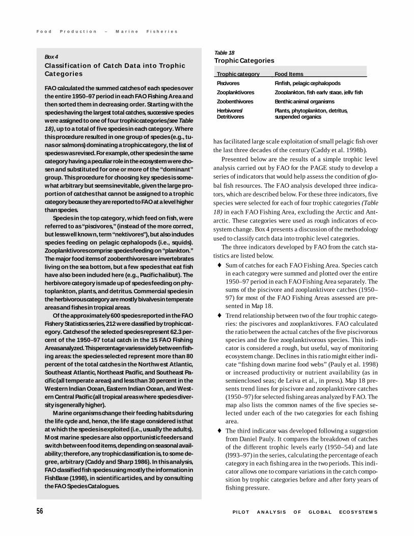
56 P I L O T A N A L Y S I S O F G L O B A L E C O S Y S T E M S
F o o d P r o d u c t i o n – M a r i n e F i s h e r i e s
has facilitated large scale exploitation of small pelagic fish overthe last three decades of the century (Caddy et al. 1998b).
Presented below are the results of a simple trophic levelanalysis carried out by FAO for the PAGE study to develop aseries of indicators that would help assess the condition of glo-bal fish resources. The FAO analysis developed three indica-tors, which are described below. For these three indicators, fivespecies were selected for each of four trophic categories (Table18) in each FAO Fishing Area, excluding the Arctic and Ant-arctic. These categories were used as rough indicators of eco-system change. Box 4 presents a discussion of the methodologyused to classify catch data into trophic level categories.
The three indicators developed by FAO from the catch sta-tistics are listed below.
♦ Sum of catches for each FAO Fishing Area. Species catchin each category were summed and plotted over the entire1950–97 period in each FAO Fishing Area separately. Thesums of the piscivore and zooplanktivore catches (1950–97) for most of the FAO Fishing Areas assessed are pre-sented in Map 18.
♦ Trend relationship between two of the four trophic catego-ries: the piscivores and zooplanktivores. FAO calculatedthe ratio between the actual catches of the five piscivorousspecies and the five zooplanktivorous species. This indi-cator is considered a rough, but useful, way of monitoringecosystem change. Declines in this ratio might either indi-cate “fishing down marine food webs” (Pauly et al. 1998)or increased productivity or nutrient availability (as insemienclosed seas; de Leiva et al., in press). Map 18 pre-sents trend lines for piscivore and zooplanktivore catches(1950–97) for selected fishing areas analyzed by FAO. Themap also lists the common names of the five species se-lected under each of the two categories for each fishingarea.
♦ The third indicator was developed following a suggestionfrom Daniel Pauly. It compares the breakdown of catchesof the different trophic levels early (1950–54) and late(l993–97) in the series, calculating the percentage of eachcategory in each fishing area in the two periods. This indi-cator allows one to compare variations in the catch compo-sition by trophic categories before and after forty years offishing pressure.
Box 4
Classification of Catch Data into TrophicCategories
FAO calculated the summed catches of each species overthe entire 1950–97 period in each FAO Fishing Area andthen sorted them in decreasing order. Starting with thespecies having the largest total catches, successive specieswere assigned to one of four trophic categories (see Table18), up to a total of five species in each category. Wherethis procedure resulted in one group of species (e.g., tu-nas or salmons) dominating a trophic category, the list ofspecies was revised. For example, other species in the samecategory having a peculiar role in the ecosystem were cho-sen and substituted for one or more of the “dominant”group. This procedure for choosing key species is some-what arbitrary but seems inevitable, given the large pro-portion of catches that cannot be assigned to a trophiccategory because they are reported to FAO at a level higherthan species.
Species in the top category, which feed on fish, werereferred to as “piscivores,” (instead of the more correct,but less well known, term “nektivores”), but also includesspecies feeding on pelagic cephalopods (i.e., squids).Zooplanktivores comprise species feeding on “plankton.”The major food items of zoobenthivores are invertebratesliving on the sea bottom, but a few species that eat fishhave also been included here (e.g., Pacific halibut). Theherbivore category is made up of species feeding on phy-toplankton, plants, and detritus. Commercial species inthe herbivorous category are mostly bivalves in temperateareas and fishes in tropical areas.
Of the approximately 600 species reported in the FAOFishery Statistics series, 212 were classified by trophic cat-egory. Catches of the selected species represent 62.3 per-cent of the 1950–97 total catch in the 15 FAO FishingAreas analyzed. This percentage varies widely between fish-ing areas: the species selected represent more than 80percent of the total catches in the Northwest Atlantic,Southeast Atlantic, Northeast Pacific, and Southeast Pa-cific (all temperate areas) and less than 30 percent in theWestern Indian Ocean, Eastern Indian Ocean, and West-ern Central Pacific (all tropical areas where species diver-sity is generally higher).
Marine organisms change their feeding habits duringthe life cycle and, hence, the life stage considered is thatat which the species is exploited (i.e., usually the adults).Most marine species are also opportunistic feeders andswitch between food items, depending on seasonal avail-ability; therefore, any trophic classification is, to some de-gree, arbitrary (Caddy and Sharp 1986). In this analysis,FAO classified fish species using mostly the information inFishBase (1998), in scientific articles, and by consultingthe FAO Species Catalogues.
Table 18
Trophic Categories
Trophic category Food Items
Piscivores Finfish, pelagic cephalopods
Zooplanktivores Zooplankton, fish early stage, jelly fish
Zoobenthivores Benthic animal organisms
Herbivores/Detritivores
Plants, phytoplankton, detritus,suspended organics
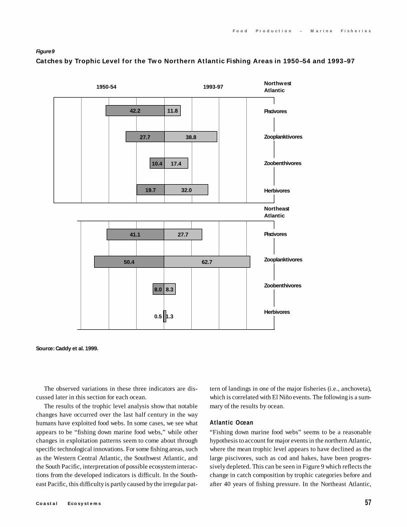
C o a s t a l E c o s y s t e m s 57
F o o d P r o d u c t i o n – M a r i n e F i s h e r i e s
The observed variations in these three indicators are dis-cussed later in this section for each ocean.
The results of the trophic level analysis show that notablechanges have occurred over the last half century in the wayhumans have exploited food webs. In some cases, we see whatappears to be “fishing down marine food webs,” while otherchanges in exploitation patterns seem to come about throughspecific technological innovations. For some fishing areas, suchas the Western Central Atlantic, the Southwest Atlantic, andthe South Pacific, interpretation of possible ecosystem interac-tions from the developed indicators is difficult. In the South-east Pacific, this difficulty is partly caused by the irregular pat-
tern of landings in one of the major fisheries (i.e., anchoveta),which is correlated with El Niño events. The following is a sum-mary of the results by ocean.
Atlantic Ocean
“Fishing down marine food webs” seems to be a reasonablehypothesis to account for major events in the northern Atlantic,where the mean trophic level appears to have declined as thelarge piscivores, such as cod and hakes, have been progres-sively depleted. This can be seen in Figure 9 which reflects thechange in catch composition by trophic categories before andafter 40 years of fishing pressure. In the Northeast Atlantic,
Figure 9
Catches by Trophic Level for the Two Northern Atlantic Fishing Areas in 1950–54 and 1993–97
Source: Caddy et al. 1999.
32.0
17.4
38.8
11.8
19.7
10.4
27.7
42.2
1950-54 1993-97
Piscivores
Zooplanktivores
Zoobenthivores
Herbivores
1.3
8.3
62.7
27.741.1
50.4
8.0
0.5
Piscivores
Zooplanktivores
Zoobenthivores
Herbivores
Northwest Atlantic
Northeast Atlantic
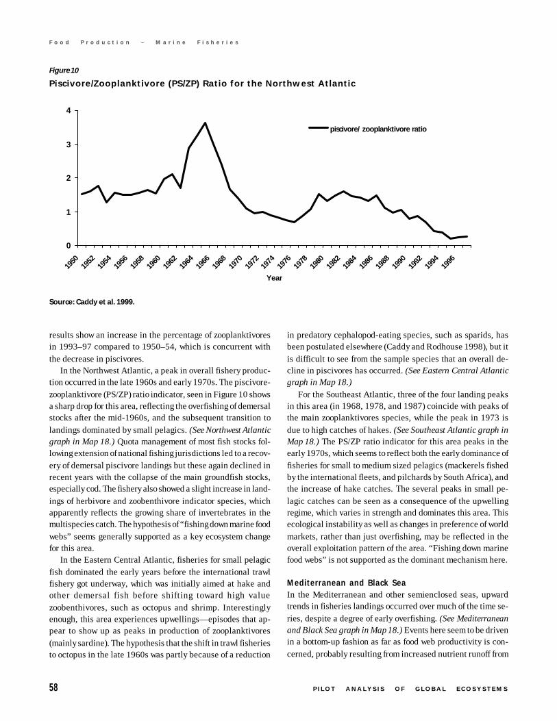
58 P I L O T A N A L Y S I S O F G L O B A L E C O S Y S T E M S
F o o d P r o d u c t i o n – M a r i n e F i s h e r i e s
results show an increase in the percentage of zooplanktivoresin 1993–97 compared to 1950–54, which is concurrent withthe decrease in piscivores.
In the Northwest Atlantic, a peak in overall fishery produc-tion occurred in the late 1960s and early 1970s. The piscivore-zooplanktivore (PS/ZP) ratio indicator, seen in Figure 10 showsa sharp drop for this area, reflecting the overfishing of demersalstocks after the mid-1960s, and the subsequent transition tolandings dominated by small pelagics. (See Northwest Atlanticgraph in Map 18.) Quota management of most fish stocks fol-lowing extension of national fishing jurisdictions led to a recov-ery of demersal piscivore landings but these again declined inrecent years with the collapse of the main groundfish stocks,especially cod. The fishery also showed a slight increase in land-ings of herbivore and zoobenthivore indicator species, whichapparently reflects the growing share of invertebrates in themultispecies catch. The hypothesis of “fishing down marine foodwebs” seems generally supported as a key ecosystem changefor this area.
In the Eastern Central Atlantic, fisheries for small pelagicfish dominated the early years before the international trawlfishery got underway, which was initially aimed at hake andother demersal fish before shifting toward high valuezoobenthivores, such as octopus and shrimp. Interestinglyenough, this area experiences upwellings—episodes that ap-pear to show up as peaks in production of zooplanktivores(mainly sardine). The hypothesis that the shift in trawl fisheriesto octopus in the late 1960s was partly because of a reduction
Figure 10
Piscivore/Zooplanktivore (PS/ZP) Ratio for the Northwest Atlantic
Source: Caddy et al. 1999.
in predatory cephalopod-eating species, such as sparids, hasbeen postulated elsewhere (Caddy and Rodhouse 1998), but itis difficult to see from the sample species that an overall de-cline in piscivores has occurred. (See Eastern Central Atlanticgraph in Map 18.)
For the Southeast Atlantic, three of the four landing peaksin this area (in 1968, 1978, and 1987) coincide with peaks ofthe main zooplanktivores species, while the peak in 1973 isdue to high catches of hakes. (See Southeast Atlantic graph inMap 18.) The PS/ZP ratio indicator for this area peaks in theearly 1970s, which seems to reflect both the early dominance offisheries for small to medium sized pelagics (mackerels fishedby the international fleets, and pilchards by South Africa), andthe increase of hake catches. The several peaks in small pe-lagic catches can be seen as a consequence of the upwellingregime, which varies in strength and dominates this area. Thisecological instability as well as changes in preference of worldmarkets, rather than just overfishing, may be reflected in theoverall exploitation pattern of the area. “Fishing down marinefood webs” is not supported as the dominant mechanism here.
Mediterranean and Black SeaIn the Mediterranean and other semienclosed seas, upwardtrends in fisheries landings occurred over much of the time se-ries, despite a degree of early overfishing. (See Mediterraneanand Black Sea graph in Map 18.) Events here seem to be drivenin a bottom-up fashion as far as food web productivity is con-cerned, probably resulting from increased nutrient runoff from
0
1
2
3
4
1950
1952
1954
1956
1958
1960
1962
1964
1966
1968
1970
1972
1974
1976
1978
1980
1982
1984
1986
1988
1990
1992
1994
1996
Year
piscivore/ zooplanktivore ratio
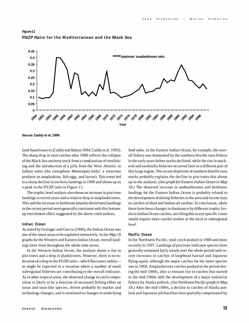
C o a s t a l E c o s y s t e m s 59
F o o d P r o d u c t i o n – M a r i n e F i s h e r i e s
land-based sources (Caddy and Bakun 1994; Caddy et al. 1995).The sharp drop in total catches after 1988 reflects the collapseof the Black Sea anchovy stock from a combination of overfish-ing and the introduction of a jelly from the West Atlantic inballast water (the ctenophore Mnemiopsis leidyi, a voraciouspredator on zooplankton, fish eggs, and larvae). This event ledto a sharp decline in anchovy landings in 1989 and shows up asa peak in the PS/ZP ratio in Figure 11.
The trophic level analysis also shows an increase in piscivorelandings in recent years and a relative drop in zooplanktivores.This and the increase in herbivore (mainly detritivore) landingsin the recent period seem generally consistent with this bottom-up enrichment effect suggested by the above cited authors.
Indian OceanAs noted by Grainger and Garcia (1996), the Indian Ocean wasone of the latest areas to be exploited intensively. In the Map 18graphs for the Western and Eastern Indian Ocean, overall land-ings have risen throughout the whole time series.
In the Western Indian Ocean, the analysis shows a rise inpiscivores and a drop in planktivores. However, there is no in-dication of a drop in the PS/ZP ratio—which fluctuates widely—as might be expected in a situation where a number of smallsubregional fisheries are contributing to the overall indicator.As in other tropical areas, the observed change in catch compo-sition is likely to be a function of increased fishing effort ontunas and tuna-like species, driven probably by market andtechnology changes, and is unrelated to changes in underlying
food webs. In the Eastern Indian Ocean, for example, the over-all fishery was dominated by the southern bluefin tuna fisheryin the early years before stocks declined, while the rise in mack-erel and sardinella fisheries occurred later in a different part ofthis large region. The recent depletion of southern bluefin tunastocks probably explains the decline in piscivores that showsup in the analysis. (See graph for Eastern Indian Ocean in Map18.) The observed increase in zoobenthivores and herbivorelandings for the Eastern Indian Ocean is probably related tothe development of shrimp fisheries in the area and recent risesin catches of shad and Indian oil sardine. In conclusion, whilethere have been changes in dominance by different trophic lev-els in Indian Ocean catches, ascribing this to any specific causewould require more careful studies at the local or subregionallevel.
Pacific OceanIn the Northwest Pacific, total catch peaked in 1988 and morerecently in 1997. Landings of piscivore indicator species havegenerally remained fairly steady over the whole period with re-cent increases in catches of largehead hairtail and Japaneseflying squid, although the major catches for the latter specieswas in 1968. Zooplanktivore catches peaked in the period dur-ing the mid-1980s, after a constant rise in catches that startedin the mid-1960s with the development of a major industrialfishery for Alaska pollock. (See Northwest Pacific graph in Map18.) After the mid-1980s, a decline in catches of Alaska pol-lock and Japanese pilchard has been partially compensated by
Figure 11
PS/ZP Ratio for the Mediterranean and the Black Sea
Source: Caddy et al. 1999.
0
0.05
0.1
0.15
0.2
0.25
0.3
0.35
0.4
0.45
1950
1952
1954
1956
1958
1960
1962
1964
1966
1968
1970
1972
1974
1976
1978
1980
1982
1984
1986
1988
1990
1992
1994
1996
Year
piscivore/ zooplanktivore ratio
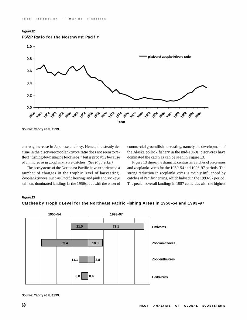
60 P I L O T A N A L Y S I S O F G L O B A L E C O S Y S T E M S
F o o d P r o d u c t i o n – M a r i n e F i s h e r i e s
a strong increase in Japanese anchovy. Hence, the steady de-cline in the piscivore/zooplanktivore ratio does not seem to re-flect “fishing down marine food webs,” but is probably becauseof an increase in zooplanktivore catches. (See Figure 12.)
The ecosystems of the Northeast Pacific have experienced anumber of changes in the trophic level of harvesting.Zooplanktivores, such as Pacific herring, and pink and sockeyesalmon, dominated landings in the 1950s, but with the onset of
commercial groundfish harvesting, namely the development ofthe Alaska pollock fishery in the mid-1960s, piscivores havedominated the catch as can be seen in Figure 13.
Figure 13 shows the dramatic contrast in catches of piscivoresand zooplanktivores for the 1950-54 and 1993-97 periods. Thestrong reduction in zooplanktivores is mainly influenced bycatches of Pacific herring, which halved in the 1993-97 period.The peak in overall landings in 1987 coincides with the highest
Figure 12
PS/ZP Ratio for the Northwest Pacific
Source: Caddy et al. 1999.
Figure 13
Catches by Trophic Level for the Northeast Pacific Fishing Areas in 1950–54 and 1993–97
Source: Caddy et al. 1999.
0.4
18.8
72.1
8.0
11.1
59.4
21.5
8.8
Piscivores
Zooplanktivores
Zoobenthivores
Herbivores
1950–54 1993–97
0.0
0.2
0.4
0.6
0.8
1.0
1950
1952
1954
1956
1958
1960
1962
1964
1966
1968
1970
1972
1974
1976
1978
1980
1982
1984
1986
1988
1990
1992
1994
1996
Year
piscivore/ zooplanktivore ratio
C o a s t a l E c o s y s t e m s 61
F o o d P r o d u c t i o n – M a r i n e F i s h e r i e s
catches of Alaska pollock, which have been declining in recentyears (1994-97).
In the Central Pacific, as in other tropical areas, overall land-ings show a steady upward trend. (See the Central Pacific graphsfrom Map 18.) In the western region, major increases in land-ings of the selected species started in the 1970s, with piscivoresprogressively becoming dominant. Among these, the tuna-likespecies are the most important with a peak in 1991, primarilybecause of skipjack tuna catches. Fisheries of zooplanktivorespecies remained undeveloped in the 1950s. In the EasternCentral Pacific, the overall landings peaked in 1981 and havesubsequently declined somewhat. The zooplanktivores’ peaksin 1981-82 and in 1989 are due to high catches of Californiapilchard in both periods and of California anchovy in the firstperiod, with concomitant peaks of the piscivores—skipjack tunain 1981, and yellowfin tuna in 1989. In 1995-97, a substantialincrease in the landings of the jumbo flying squid, a piscivore,was registered and can be seen in the Eastern Central Pacificpiscivore graph in Map 18.
Capac i ty of Coasta l and Mar ine
Ecosystems to Cont inue to Provide F ishIt is reasonable to conclude, at the beginning of the new millen-nium, that most shelf resources and most open ocean resourcesare fully exploited or overexploited. Although fishery regula-tions are now in place in many areas, management of shared,highly migratory, and straddling stocks still presents many loop-holes, permitting overexploitation. This continues to occur, de-spite unprecedented agreements over the last few years, suchas the Code of Conduct for Responsible Fisheries, and the U.N.Fish Stocks Agreement, which support proper management prac-tices for aquatic resources. Expansion of oceanic fisheries stillcontinues, with a movement toward exploiting deep-water re-sources, which are relatively unprotected by international agree-ments and regulations.
Although the use of FAO landing statistics for ecosystemchanges has limitations for the reasons mentioned earlier, itprovides some insights that supplement the conclusions drawnfrom existing analyses of simple catch trends such as in FAO(1995, 1997, and 1999a), Grainger and Garcia (1996), andCaddy et al. (1998a). The analysis of the catch species compo-sition presented shows that notable changes have occurred overthe last half century in some fishery areas, such as the northernAtlantic and Northeast Pacific. The piscivore/zooplanktivoreratio also provides some evidence for likely ecosystem change.These indicators do not point, however, to a single unambigu-ous cause for ecosystem change, although there seems no doubtthat this is occurring in many marine ecosystems because of
fisheries and other anthropogenic and natural environmentalchanges.
The broad-brush trophic analysis presented in the preced-ing pages is not intended to be a substitute for more detailedlocal ecosystem analyses. These analyses are needed to illumi-nate the mechanisms influencing the major changes in fishingstrategy. What is clear is that a number of key factors have beenoperating, often simultaneously. These include the developmentof new markets for fish; changes in the species compositionbecause of fishing pressures; expansion in fish trade; environ-mentally driven fluctuations such as El Niño-type phenomena;and new technologies for capture, processing (often at sea), andstorage.
Fisheries production relies on the condition of coastal habi-tats and other services provided by coastal ecosystems, namelybiodiversity and water quality. As previously discussed, humanmodification and pollution are threatening important coastalhabitats for many major fisheries. (See sections on Coastal Zone:Extent and Change for habitat loss and modification, and WaterQuality.) Although available data are insufficient to detect cleartrends for those parameters, there is evidence of increasing over-all pressure on the ecosystems that sustain fishery resources.
In format ion Status and NeedsAs stated earlier, FAO fisheries production statistics are lim-ited to providing proximate information on commercial fish popu-lation trends and, therefore, are insufficient to assess the ca-pacity of coastal and marine ecosystems to provide food. One ofthe limitations of production statistics is that the composition ofthe catch is not well known. Although 80-90 percent of the spe-cies caught from the North Atlantic are reported to FAO at thespecies level, the catch proportion misreported by individualstocks is higher. Between 50 and 70 percent reporting by spe-cies is typical of most other world areas, while for the IndianOcean and West Central Pacific, only 20-30 percent of land-ings and harvests are reported by species; the rest being in-cluded in higher taxonomic categories or as mixed fish. An-other limitation of production statistics is that they include bi-ases from unreported discarding or misreporting of harvests byarea and species, and exclude all information from illegal fish-ing, which is high for some species.
For some countries, including some developed countries,scientists believe that catch reporting systems are of dubiousaccuracy, especially with respect to landings and harvests ofsmall vessels. The infrastructure for collecting and assemblingdata is often absent, and data on discards are fragmentary andmissing in most fisheries. With respect to species identifica-tion, especially in tropical areas, high diversity poses a prob-lem. The lack of emphasis placed on practical taxonomy overthe last few decades has led to a dire shortage of top experts for
62 P I L O T A N A L Y S I S O F G L O B A L E C O S Y S T E M S
F o o d P r o d u c t i o n – M a r i n e F i s h e r i e s
identifying many taxonomic groups, so that accurate speciesidentifications are not easily achieved.
In addition, there is a wide information gap in our under-standing of marine fisheries ecosystems. For example, moreextensive stock assessments are necessary to identify maximumsustainable yields (MSYs) for various commercially importantspecies. In order to detect the decline in fish stock or imbal-ance in the ecosystems, collection of a few indicators, such asaverage fish size or species composition (trophic level ratio),need to be considered; however, monitoring of commercial land-ings for species, size, and age composition, is costly and labor-intensive.
The application of military technologies has improved di-rect and indirect fish population estimates and this could befurther improved by the use of laser technologies or bottom-mounted sonar arrays. The requirement for fishing vessels tocarry a black box that monitors vessel position, speed, and op-eration of fishing gear has helped collect more precise commer-cial data on when and where fish are caught and could make
the measurement of fishing effort much more precise. For ex-ample, trawling areas could be tracked, and geographical andseasonal concessions of fishing grounds could be specified toreduce capture of protected species or juveniles. With com-plete remote coverage of fishing operations, closed areas mightbe more effectively monitored. In addition, areas with high dis-cards, fragile bottom fauna, or vulnerable spawning concentra-tions might be largely avoided. The current situation is, how-ever, that reporting of data to FAO on fishing effort or even ofup-to-date fleet size is fragmentary. Databases on operations ofsmaller vessels are almost nonexistent, even at the national level,in many countries.
Regarding the fisheries manager’s use of data, a key concernis how scientific data is used, if at all, in management. Betterdata collection is a praiseworthy and feasible goal, but it im-proves only one part of the management cycle. Given currentinformation limitation and the inevitably high variance of fishpopulation estimates, managers must use precautionary ap-proaches in making decisions.
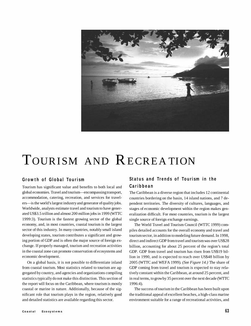
C o a s t a l E c o s y s t e m s 63
F o o d P r o d u c t i o n – M a r i n e F i s h e r i e s
T O U R I S M A N D R E C R E A TION
Status and Trends of Tourism in theC a r i b b e a nThe Caribbean is a diverse region that includes 12 continentalcountries bordering on the basin, 14 island nations, and 7 de-pendent territories. The diversity of cultures, languages, andstages of economic development within the region makes gen-eralization difficult. For most countries, tourism is the largestsingle source of foreign exchange earnings.
The World Travel and Tourism Council (WTTC 1999) com-piles detailed accounts for the overall economy and travel andtourism sector, in addition to modeling future demand. In 1998,direct and indirect GDP from travel and tourism was over US$28billion, accounting for about 25 percent of the region’s totalGDP. GDP from travel and tourism has risen from US$19 bil-lion in 1990, and is expected to reach over US$48 billion by2005 (WTTC and WEFA 1999). (See Figure 14.) The share ofGDP coming from travel and tourism is expected to stay rela-tively constant within the Caribbean, at around 25 percent, andin real terms, to grow by 35 percent over the next decade (WTTC1996:4).
The success of tourism in the Caribbean has been built uponthe traditional appeal of excellent beaches, a high-class marineenvironment suitable for a range of recreational activities, and
Growth of Global Tour ismTourism has significant value and benefits to both local andglobal economies. Travel and tourism—encompassing transport,accommodation, catering, recreation, and services for travel-ers—is the world’s largest industry and generator of quality jobs.Worldwide, analysts estimate travel and tourism to have gener-ated US$3.5 trillion and almost 200 million jobs in 1999 (WTTC1999:3). Tourism is the fastest growing sector of the globaleconomy, and, in most countries, coastal tourism is the largestsector of this industry. In many countries, notably small islanddeveloping states, tourism contributes a significant and grow-ing portion of GDP and is often the major source of foreign ex-change. If properly managed, tourism and recreation activitiesin the coastal zone can promote conservation of ecosystems andeconomic development.
On a global basis, it is not possible to differentiate inlandfrom coastal tourism. Most statistics related to tourism are ag-gregated by country, and agencies and organizations compilingstatistics typically do not make this distinction. This section ofthe report will focus on the Caribbean, where tourism is mostlycoastal or marine in nature. Additionally, because of the sig-nificant role that tourism plays in the region, relatively goodand detailed statistics are available regarding this sector.
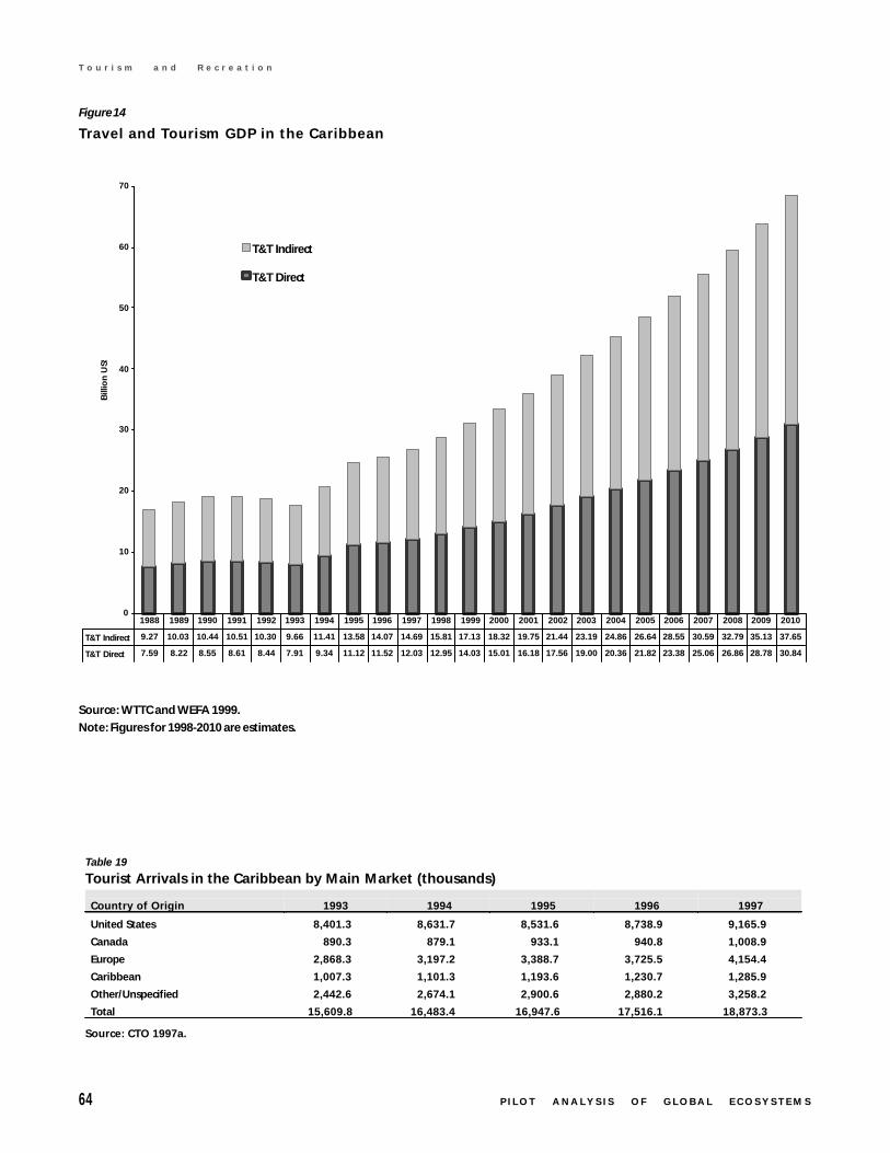
64 P I L O T A N A L Y S I S O F G L O B A L E C O S Y S T E M S
T o u r i s m a n d R e c r e a t i o n
Figure 14
Travel and Tourism GDP in the Caribbean
Source: WTTC and WEFA 1999.
Note: Figures for 1998-2010 are estimates.
0
10
20
30
40
50
60
70
Bill
ion
US$
T&T Indirect
T&T Direct
T&T Indirect 9.27 10.03 10.44 10.51 10.30 9.66 11.41 13.58 14.07 14.69 15.81 17.13 18.32 19.75 21.44 23.19 24.86 26.64 28.55 30.59 32.79 35.13 37.65
T&T Direct 7.59 8.22 8.55 8.61 8.44 7.91 9.34 11.12 11.52 12.03 12.95 14.03 15.01 16.18 17.56 19.00 20.36 21.82 23.38 25.06 26.86 28.78 30.84
1988 1989 1990 1991 1992 1993 1994 1995 1996 1997 1998 1999 2000 2001 2002 2003 2004 2005 2006 2007 2008 2009 2010
Table 19
Tourist Arrivals in the Caribbean by Main Market (thousands)
Country of Origin 1993 1994 1995 1996 1997
United States 8,401.3 8,631.7 8,531.6 8,738.9 9,165.9
Canada 890.3 879.1 933.1 940.8 1,008.9
Europe 2,868.3 3,197.2 3,388.7 3,725.5 4,154.4
Caribbean 1,007.3 1,101.3 1,193.6 1,230.7 1,285.9
Other/Unspecified 2,442.6 2,674.1 2,900.6 2,880.2 3,258.2
Total 15,609.8 16,483.4 16,947.6 17,516.1 18,873.3
Source: CTO 1997a.
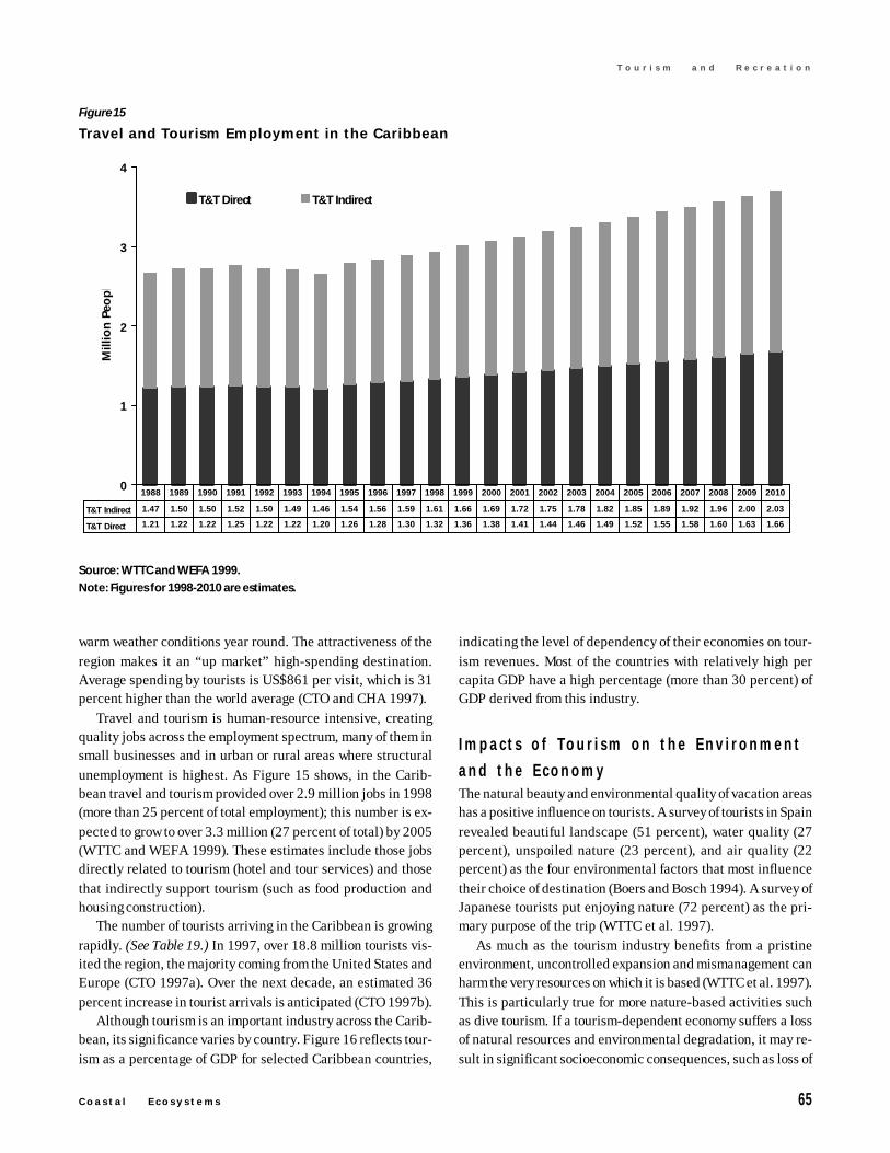
C o a s t a l E c o s y s t e m s 65
T o u r i s m a n d R e c r e a t i o n
warm weather conditions year round. The attractiveness of theregion makes it an “up market” high-spending destination.Average spending by tourists is US$861 per visit, which is 31percent higher than the world average (CTO and CHA 1997).
Travel and tourism is human-resource intensive, creatingquality jobs across the employment spectrum, many of them insmall businesses and in urban or rural areas where structuralunemployment is highest. As Figure 15 shows, in the Carib-bean travel and tourism provided over 2.9 million jobs in 1998(more than 25 percent of total employment); this number is ex-pected to grow to over 3.3 million (27 percent of total) by 2005(WTTC and WEFA 1999). These estimates include those jobsdirectly related to tourism (hotel and tour services) and thosethat indirectly support tourism (such as food production andhousing construction).
The number of tourists arriving in the Caribbean is growingrapidly. (See Table 19.) In 1997, over 18.8 million tourists vis-ited the region, the majority coming from the United States andEurope (CTO 1997a). Over the next decade, an estimated 36percent increase in tourist arrivals is anticipated (CTO 1997b).
Although tourism is an important industry across the Carib-bean, its significance varies by country. Figure 16 reflects tour-ism as a percentage of GDP for selected Caribbean countries,
indicating the level of dependency of their economies on tour-ism revenues. Most of the countries with relatively high percapita GDP have a high percentage (more than 30 percent) ofGDP derived from this industry.
Impacts of Tour ism on the Environment
and the EconomyThe natural beauty and environmental quality of vacation areashas a positive influence on tourists. A survey of tourists in Spainrevealed beautiful landscape (51 percent), water quality (27percent), unspoiled nature (23 percent), and air quality (22percent) as the four environmental factors that most influencetheir choice of destination (Boers and Bosch 1994). A survey ofJapanese tourists put enjoying nature (72 percent) as the pri-mary purpose of the trip (WTTC et al. 1997).
As much as the tourism industry benefits from a pristineenvironment, uncontrolled expansion and mismanagement canharm the very resources on which it is based (WTTC et al. 1997).This is particularly true for more nature-based activities suchas dive tourism. If a tourism-dependent economy suffers a lossof natural resources and environmental degradation, it may re-sult in significant socioeconomic consequences, such as loss of
Figure 15
Travel and Tourism Employment in the Caribbean
Source: WTTC and WEFA 1999.
Note: Figures for 1998-2010 are estimates.
0
1
2
3
4
Mill
ion
Peo
pl
T&T Direct T&T Indirect
T&T Indirect 1.47 1.50 1.50 1.52 1.50 1.49 1.46 1.54 1.56 1.59 1.61 1.66 1.69 1.72 1.75 1.78 1.82 1.85 1.89 1.92 1.96 2.00 2.03
T&T Direct 1.21 1.22 1.22 1.25 1.22 1.22 1.20 1.26 1.28 1.30 1.32 1.36 1.38 1.41 1.44 1.46 1.49 1.52 1.55 1.58 1.60 1.63 1.66
1988 1989 1990 1991 1992 1993 1994 1995 1996 1997 1998 1999 2000 2001 2002 2003 2004 2005 2006 2007 2008 2009 2010
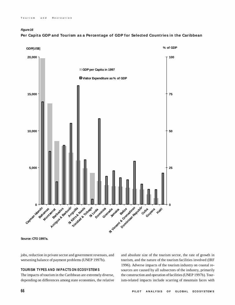
66 P I L O T A N A L Y S I S O F G L O B A L E C O S Y S T E M S
T o u r i s m a n d R e c r e a t i o n
jobs, reduction in private sector and government revenues, andworsening balance of payment problems (UNEP 1997b).
TOURISM TYPES AND IMPACTS ON ECOSYSTEMSThe impacts of tourism in the Caribbean are extremely diverse,depending on differences among state economies, the relative
and absolute size of the tourism sector, the rate of growth intourism, and the nature of the tourism facilities involved (IRF1996). Adverse impacts of the tourism industry on coastal re-sources are caused by all subsectors of the industry, primarilythe construction and operation of facilities (UNEP 1997b). Tour-ism-related impacts include scarring of mountain faces with
Figure 16
Per Capita GDP and Tourism as a Percentage of GDP for Selected Countries in the Caribbean
Source: CTO 1997a.
0
5,000
10,000
15,000
20,000
Caym
an Is
lands
Baham
as
Montse
rrat
Barbad
os
Antigua &
Bar
buda
Anguilla
St K
itts &
Nev
is
Trin
idad
& To
bago
St Lu
cia
Domin
ica
Grenad
a
Jam
aica
Belize
St V
ince
nt & G
renad
ines
Domin
ican R
epublic
Cuba
Guyana
Haiti
GDP(US$)
0
25
50
75
100
% of GDP
GDP per Capita in 1997
Visitor Expenditure as % of GDP
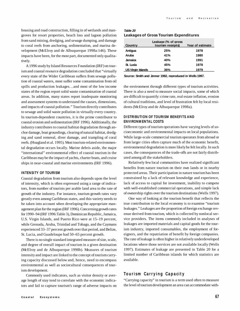
C o a s t a l E c o s y s t e m s 67
T o u r i s m a n d R e c r e a t i o n
housing and road construction, filling in of wetlands and man-groves for resort properties, beach loss and lagoon pollutionfrom sand mining, dredging, and sewage dumping, and damageto coral reefs from anchoring, sedimentation, and marina de-velopment (McElroy and de Albuquerque 1998a:146). Theseimpacts have been, for the most part, documented only qualita-tively.
A 1996 study by Island Resources Foundation (IRF) on tour-ism and coastal resource degradation concluded that “virtuallyevery state of the Wider Caribbean suffers from sewage pollu-tion of coastal waters, most suffer some contamination from oilspills and production leakages…and most of the low incomestates of the region report solid waste contamination of coastalareas. In addition, many states report inadequate monitoringand assessment systems to understand the causes, dimensions,and impacts of coastal pollution.” Tourism directly contributesto sewage and solid waste pollution in virtually every country.In tourism-dependent countries, it is the prime contributor tocoastal erosion and sedimentation (IRF 1996). Additionally, theindustry contributes to coastal habitat degradation through an-chor damage, boat groundings, clearing of natural habitat, dredg-ing and sand removal, diver damage, and trampling of coralreefs. (Hoagland et al. 1995). Most tourism-related environmen-tal degradation occurs locally. Marine debris aside, the major“international” environmental effect of coastal tourism in theCaribbean may be the impact of yachts, charter boats, and cruiseships in near-coastal and marine environments (IRF 1996).
INTENSITY OF TOURISMCoastal degradation from tourism also depends upon the levelof intensity, which is often expressed using a range of indica-tors, from number of tourists per arable land area to the rate ofgrowth of the industry. For instance, tourism growth rates varygreatly even among Caribbean states, and this variety needs tobe taken into account when developing the appropriate man-agement plan for the region (IRF 1996). Concerning growth ratesfor 1990–94 (IRF 1996:Table 3), Dominican Republic, Jamaica,U.S. Virgin Islands, and Puerto Rico were at 15–19 percent,while Grenada, Aruba, Trinidad and Tobago, and the Caymansexperienced 33–37 percent growth over that period, and Belize,St. Lucia, and Guadeloupe had 50–65 percent growth.
There is no single standard integrated measure of size, scale,and degree of overall impact of tourism in a given destination(McElroy and de Albuquerque 1998b). Measures of tourismintensity and impact are linked to the concept of tourism carry-ing capacity discussed below and, hence, need to encompassenvironmental as well as sociocultural consequences of tour-ism development.
Commonly used indicators, such as visitor density or aver-age length of stay tend to correlate with the economic indica-tors and fail to capture tourism’s range of adverse impacts on
the environment through different types of tourism activities.There is also a need to measure social impacts, some of whichare difficult to quantify: crime rate, real estate inflation, erosionof cultural traditions, and level of frustration felt by local resi-dents (McElroy and de Albuquerque 1998a).
DISTRIBUTION OF TOURISM BENEFITS ANDENVIRONMENTAL COSTSDifferent types of tourism operations have varying levels of so-cioeconomic and environmental impacts on local populations.While large-scale commercial tourism operators from abroad orfrom larger cities often capture much of the economic benefit,environmental degradation is more likely be felt locally. In suchcases, the consequences of the trade-offs are not fairly distrib-uted among all the stakeholders.
Relatively few local communities have realized significantbenefits from nature tourism on their own lands or in nearbyprotected areas. Their participation in nature tourism has beenconstrained by a lack of relevant knowledge and experience,lack of access to capital for investment, inability to competewith well-established commercial operations, and simple lackof ownership rights over the tourism destinations (Wells 1997).
One way of looking at the tourism benefit that reflects thetrue contribution to the local economy is to examine “tourismleakages.” Leakages are the proportion of foreign exchange rev-enue derived from tourism, which is collected by nonlocal ser-vice providers. The items commonly included in analyses ofleakages are imported materials and capital goods for the tour-ism industry, imported consumables, the employment of for-eigners, and the repatriation of benefit by foreign companies.The rate of leakage is often higher in relatively underdevelopedlocations where those services are not available locally (Wells1997). Estimates of leakage are presented in Table 20 for alimited number of Caribbean islands for which statistics areavailable.
Tour i sm Carry ing Capac i ty“Carrying capacity” in tourism is a term used often to measurethe level of tourism development an area can accommodate with-
Table 20
Leakages of Gross Tourism Expenditures
CountryLeakage (% of gross
tourism receipts) Year of estimate
Antigua 25% 1978
Aruba 41% 1980
Jamaica 40% 1991
St. Lucia 45% 1978
US Virgin Islands 36% 1979
Source: Smith and Jenner 1992, reproduced in Wells 1997.
68 P I L O T A N A L Y S I S O F G L O B A L E C O S Y S T E M S
T o u r i s m a n d R e c r e a t i o n
out adverse effects on the resident community, the natural en-vironment, or the quality of visitor experience (UNEP and WTO1992). This concept can be broken down into types of limits,such as ecological or environmental, physical (threshold limitfor space or accommodation), and social (level of tolerance ofthe host population to the presence of tourists) (Lim 1998:3).
Tourism is growing rapidly, but the local capacity to dealwith it does not grow as fast. When local capacity to deal withthe level of tourism intensity is saturated, negative consequencesoccur. The threshold of the capacity can depend on the level ofphysical infrastructure, such as waste treatment, as well as so-cial infrastructure, such as regulations or codes of conduct, thatmake tourism activities less harmful to the natural environmentand local culture.
The measure of carrying capacity has been examined withlimited success. Important factors include land area, soil andhabitat types, and availability of freshwater, in addition to arange of cultural and socioeconomic factors. Perhaps there isno simple indicator of tourism carrying capacity in terms ofnumber of tourists, but rather it is the type of tourism and na-ture of tourist consumption and activities that really matter.
There have been some attempts to develop carrying capac-ity indicators by combining the type of tourism impact indica-tors discussed above. It is difficult to establish the threshold atwhich carrying capacity is exceeded because different naturaland sociocultural settings can sustain vastly different levels ofvisitation (McElroy and de Albuquerque 1998a).
Susta inable Tour i smCurrent efforts to develop indicators in this area are important,as are certification programs that encourage tourist facilities toadopt more efficient and environmentally sound practices.
“Sustainable tourism” has the potential for longer-term eco-nomic benefits for a community and serves to limit environ-mental degradation. According to the definition by WTTC, WorldTourism Organization (WTO), and Earth Council, “sustainabletourism development is envisaged as leading to management ofall resources in such a way that economic, social and aestheticneeds can be fulfilled while maintaining cultural integrity, es-sential ecological processes, biological diversity, and life sup-port systems.” (WTTC et al. 1997:30).
The tourism industry recognizes the importance of maintain-ing the quality of the natural environment and the cultural in-tegrity of a local community as a resource base of tourism at-tractions. Some certification of “best practices” or “ecolabeling”schemes has been developed as self-regulatory and voluntarymeasures to promote sustainable tourism. The certification cri-teria vary depending on the focus area of each scheme: fromenergy efficiency and waste treatment, to staff training and edu-
cation (UNEP 1998). The following are examples of the criteriaused by the schemes particularly relevant to coastal tourism.
In 1994, the WTTC launched Green Globe, a worldwideenvironmental management and awareness program for thetravel and tourism industry. The program includes a series ofpackages designed to help staff at all levels bring about envi-ronmental improvements. A number of national tourist associa-tions and businesses are participating in this program, whichprovides standards and mechanisms for “green” certification ofhotels and resorts (UNEP 1998; Green Globe Website: http://www.greenglobe.org/).
Foundation for Environmental Education in Europe (FEEE)manages the Blue Flag Campaign, currently in 21 Europeancountries, focusing on environmental management performanceof beaches and marinas (FEEE Website: http://www.blueflag.org).In 2000, 1,873 beaches and 652 marinas were awarded theBlue Flag, a dramatic increase from 244 beaches and 208 ma-rinas in 1987 (FEEE 2000), indicating increased interest bybeaches and marinas in participating in the campaign. (See Box5 for an example of voluntary guidelines for sustainable tour-ism.)
The Role of Protected AreasEcotourism, or nature-based tourism, although accounting for asmall fraction of the fast-growing tourism industry, has a highpotential to generate revenue and employment for local popula-tions, and provide incentives for protecting natural ecosystems.Protected areas are often a desirable aspect of a tourist destina-tion and, therefore, a valuable component of nature-based tour-ism.
Although often thought of as areas protected from tourismand other intrusions, parks and protected areas throughout theWider Caribbean are major factors in attracting and managingtourists and tourism. Throughout the eastern Caribbean, cruiseship visitor surveys indicate that 30 percent of passengers whogo ashore want to visit natural areas and parks (OAS and CTRDC1988, cited in IRF 1996). The negative environmental effectsof tourism in parks and protected areas tend to be small, but theability to tolerate such impacts is also small (IRF 1996).
However, some marine protected areas (MPAs) have failedto capture their share of the growing tourism revenue. Someoften lack sufficient funding to enforce protection of the areasand monitor environmental quality. A World Bank report exam-ining nature tourism and economic development concluded thatmany protected areas that often supply the most valuable partof the nature tourism experience, charge relatively low entryfees and therefore capture little of the economic value of tour-ism. Although many governments have successfully increasedtourist numbers by marketing their country’s nature tourismdestinations, most have not invested sufficiently in managing
C o a s t a l E c o s y s t e m s 69
T o u r i s m a n d R e c r e a t i o n
the natural assets that attract tourists or in the infrastructureneeded to support nature tourism. This has exposed ecologi-cally or culturally sensitive sites to the risk of degradation byunregulated development, too many visitors, and the impact ofrapid immigration linked to new jobs and business opportuni-ties (Wells 1997).
On the other hand, there are parks where tourism has provena valuable means of preserving biological diversity. Protectedareas, such as the Great Barrier Reef Marine Park, in Austra-lia, and Antarctica, have long been used to bring in incomefrom tourism, while protecting the environment (WTTC et al.1997).
Box 5
Voluntary Guidelines for Sustainable Coastal Tourism Development in Quintana Roo, Mexico
tourism development complements these regulatory ap-proaches—which often lack adequate resources for effec-tive implementation and enforcement—with a voluntary ap-proach. A proven-effective tool of the voluntary initiative isa practitioner’s manual of guidelines for low-impact tour-ism development practices.
The guidelines address issues concerning managementof beaches, dunes, wetlands, vegetation, wastewater, solidwaste, and use of energy and water resources. They arebased on a comprehensive assessment of the coastal re-source base and ecosystem dynamics, incorporating designand management techniques that have proven effective inother regions around the world. One of the key messages isthe benefit to both industry and society of mitigating dam-age from natural hazards through low-cost and straightfor-ward preconstruction practices, such as use of constructionsetbacks, incorporating vegetated dunes with native veg-etation, and taking into account previous hurricane and ero-sion history in development planning.
The guidelines have reached a constituency of privatesector developers and government officials in Costa Mayaand have initiated a constructive dialogue on local coastalstewardship and resource conservation. Government, non-governmental organizations, and the private sector are us-ing these guidelines in workshops and field demonstrationsto define and incorporate specific techniques into develop-ment practices, environmental impact assessments, landzoning ordinances, and urban plans at both the site andregional levels. In the future, they may be used as part ofindustry-based incentive programs, as well as criteria to guidepublic land development.
Prepared by Pam Rubinoff and James Tobey, The CoastalResources Center, University of Rhode Island.
In format ion Status and NeedsConventional economic statistics do not properly capture thecontribution of a pristine environment to the growth of coastaltourism. The relative importance of nature-based tourism to thewhole tourism sector needs to be measured not only in terms oftotal foreign exchange revenue but also in nonmonetary indica-tors, such as local employment. Currently, basic statistics, suchas GDP and employment, are not collected specifically forcoastal tourism. Because diverse types of businesses constitutethe industry, it is not easy to differentiate tourism as an eco-nomic sector. Moreover, the value of ecosystems to sustain thetourism industry has been underappreciated because of infor-mation limitations.
Tourism represents one of the most important sources ofrevenue and foreign exchange for Mexico: it is the drivingforce for economic development in the state of QuintanaRoo. For example, 25 years ago the small fishing village ofCancun in Quintana Roo was transformed into a popularinternational tourist destination, which today hosts over 2million visitors annually and over 300,000 residents. Al-though Cancun’s development has resulted in environmen-tal problems for the area, the economic importance of tour-ism makes further development desirable, but necessitatesdevelopment in a more environmentally sustainable man-ner—where environmental impact is limited and economicbenefits are derived locally.
Invariably, there are trade-offs between the economicbenefits of tourism development and the negative impactsto cultural amenities and environmental services. The newfrontier for tourism development in Quintana Roo is nowCosta Maya along the southern coast, a region of highbiodiversity and rich coastal ecosystems. The region is bor-dered by the Sian Ka’an Biosphere Reserve, Belize’s Hol ChanMarine Reserve, and the Mesoamerican reef system. Withtourism development investment rapidly increasing, the stateis working to improve the balance of costs and benefits bypromoting “low-impact” tourism development that bothprotects the long-term sustainability of tourism investmentand preserves the coastal environment.
Quintana Roo has an extensive regulatory system of le-gal instruments for resource management and developmentwhich is aimed at limiting inappropriate development, butneeds to be more consistently implemented to be truly ef-fective. The state is on the “vanguard” with its system ofprotected areas and the first ecological land zoning plansadopted in Mexico. The strategy for promoting low-impact
70 P I L O T A N A L Y S I S O F G L O B A L E C O S Y S T E M S
T o u r i s m a n d R e c r e a t i o n
Although tourism plays a vital role in the economies of manycountries, the existing information does not provide a compre-hensive view of the full costs and benefits of the industry. Thisis due to a lack of information on both sides of this equation:benefits from income and employment generation; and environ-mental and sociocultural costs from adverse impacts of rapid,uncontrolled tourism development. Reliable data or an adequateframework to measure the actual benefits of tourism to the localeconomy and people are currently lacking. Many of the ben-efits often go to foreign investors and outside service providers.Identifying who benefits from tourism development and whobears the environmental cost would lead to more rational and
conscious decisions on the trade-offs involved in tourism de-velopment, which are key to more equitable and sustainablemanagement of the ecosystems.
One can only assess the effectiveness of existing sustainabletourism initiatives and certification programs if one developsthe criteria and the indicators of “sustainability.” Since eachprogram has its own concerns about what to “sustain,” suchcriteria and measures can also vary. Although some useful con-cepts such as carrying capacity have been developed, there arecritical gaps in the type of information that is necessary to quan-tify them.
C o a s t a l E c o s y s t e m s 71
T o u r i s m a n d R e c r e a t i o n
REFERENCES
Briggs, J.C. 1974. Marine Zoogeography. New York: McGraw-Hill Book
Company.
Bright, C. 1999. Life Out of Bounds: Bioinvasion in a Borderless World. New
York: W.W. Norton & Company.
Bryant, D., L. Burke, J. McManus, and M. Spalding. 1998. Reefs at Risk: A
Map-Based Indicator of Threats to the World’s Coral Reefs. Washington,
DC: World Resources Institute. Available on-line at: http://www.wri.org/
indictrs/reefrisk.htm.
Caddy, J.F. and A. Bakun. 1994. “A Tentative Classification of Coastal
Marine Ecosystems of Enclosed and Semi-enclosed Seas.” Ocean &
Coastal Management (23): 201–211.
Caddy, J.F. and G.D. Sharp. 1986. An Ecological Framework for Marine
Fishery Investigations. FAO Fisheries Technical Paper No. 283. Rome,
Italy: FAO.
Caddy, J.F. and P.G. Rodhouse, 1998. “Cephalopod and Groundfish
Landings: Evidence for Ecological Change in Global Fisheries?” Rev.
Fish Biol. Fisheries 8 (4): 431–444.
Caddy, J.F., F. Carocci, and S. Coppola. 1998a. “Have Peak Fishery
Production Levels been Passed in Continental Shelf Areas? Some
Perspectives Arising from Historical Trends in Production per Shelf
Area.” Journal of Northwestern Atlantic Fisheries Science (23): 191–
219.
Caddy, J.F., J. Csirke, S.M. Garcia, and R.J.R. Grainger. 1998b. “How
Pervasive is ‘Fishing down marine food webs’?” Science (282): 1383.
Caddy, J.F., L. Garibaldi, and R.J.R. Grainger. 1999. “Changes in World
Marine Fishery Ecosystems as Judged from the FAO Fishery Catch
Database.” Unpublished paper prepared for PAGE.
Caddy, J.F., R. Refk, and T. Do Chi. 1995. “Productivity Estimates for the
Mediterranean: Evidence of Accelerating Ecological Change.” Ocean &
Coastal Management 26(1): 1–18.
Cambers, G. 1997. “Beach Changes in the Eastern Caribbean islands:
Hurricane Impacts and Implications for Climate Change.” Pages 29–47
in Letherman, Stephen P., ed. 1997. Island States at Risk: Global
Climate Change, Development and Population. Journal of Coastal
Research Special Issue No.24. Charlottesville, VA: Coastal Education &
Research Foundation.
Cambers, G. 1998. Coping with Beach Erosion: with Case Studies from the
Caribbean. Coastal Management Source Books 1. Paris, France:
UNESCO.
Cambers, G. Project Coordinator, Coast and Beach Stability in the Lesser
Antilles Program, University of Puerto Rico, Mayagüez, Puerto Rico.
1999. Personal Communication. February 18.
Alexander, C. E. 1998. “Classified Shellfish Growing Waters.” NOAA’s
State of the Coast Report. Silver Spring, MD: NOAA. On-line at: http://
state_of_coast.noaa.gov/bulletins/html/sgw_04/sgw.html.
Alverson, D.L., M.H. Freeberg, J.G. Pope and S.A. Murawski, 1994. A
Global Assessment of Fisheries Bycatch and Discards. FAO Fisheries
Technical Paper No. 339. Rome, Italy: FAO.
Aminti, P., L.E. Cipriani, and E. Pranzini. 1999. “An Innovative, Non-
structural, Solution to Beach Erosion: Costs Less and Delivers More
Benefit.” InterCoast Winter 1999: 34–35.
Anderson, D. 1998. “Expansion of HAB problems in the US.” Woods Hole,
MA: National Office for Marine Biotoxins and Harmful Algal Blooms,
Woods Hole Oceanographic Institution. On-line at: http://
www.redtide.whoi.edu/hab/HABdistribution/habexpand.html Viewed 8/
2/00.
Anderson, M. B. 1990. Analyzing the Costs and Benefits of Natural Disaster
Responses in the Context of Development. Environment Working Paper
No. 29. Washington, DC: World Bank.
Arreguín-Sánchez, F., J.L. Munro, M.C. Balgos, and D. Pauly, eds. 1996.
Biology, Fisheries and Culture of Tropical Groupers and Snappers.
ICLARM Conference Proceedings No. 48. Manila, Philippines:
International Center for Living Aquatic Resources Management.
Bailey, R.G. 1998. Ecoregions: the Ecosystem Geography of the Oceans and
Continents. New York: Springer-Verlag.
BAP Planning Team. 1993. Biodiversity Action Plan for Vietnam. Hanoi,
Vietnam: BAP Planning Team.
Baretta-Bekker, J.G., E.K. Duursma, and B.R. Kuipers. 1998. Encyclopedia
of Marine Sciences, Second, Corrected and Enlarged Edition. Berlin,
Germany: Springer-Verlag.
Beliaeff, B., T.P. O’Connor, and D. Claisse, 1996. “Comparison of Chemical
Concentrations in Mussels and Oysters from the United States and
France.” Environmental Monitoring and Assessment 49: 87-95.
Berg, H., M. C. Öhman, S. Troëng, and O. Lindén. 1998. “Environmental
Economics of Coral Reef Destruction in Sri Lanka.” Ambio 27(8): 627–
634.
Boers, H. and M. Bosch. 1994. The Earth as a Holiday Resort. Utrecht, The
Netherlands: Institute for Environmental Communications and
Netherlands Institute for Transport and Tourism Studies.
Bricker, S.B., C.G. Clement, D.E. Pirhalla, S.P. Orlando, and D.R.G. Farrow.
1999. National Estuarine Eutrophication Assessment: Effects of Nutrient
Enrichment in the Nation’s Estuaries. Silver Spring, MD: National
Oceanic and Atmospheric Administration. Available on-line at: http://
sposerver.nos.noaa.gov:80/
72 P I L O T A N A L Y S I S O F G L O B A L E C O S Y S T E M S
R e f e r e n c e s
Cantillo, A.Y. 1998. “Comparison of Results of Mussel Watch Programs of
the United States and France with Worldwide Mussel Watch Studies.”
Marine Pollution Bulletin. 36 (9): 712–717.
Center for Marine Conservation. 1998. 1997 International Coastal Cleanup:
Results. Washington, DC: Center for Marine Conservation.
Central Intelligence Agency. 1998. “The World Fact Book 1998.” On-line
at: http://www.odci.gov/cia/publications/factbook/index.html. Viewed 7/
30/99.
CIESIN (Center for International Earth Science Information Network),
International Food Policy Research Institute, and World Resources
Institute. 2000. Gridded Population of the World, Version 2. Palisades,
NY: CIESIN, Columbia University. On-line at http://sedac.ciesin.org/
plue/gpw.
CIESM (International Commission for the Scientific Exploration of the
Mediterranean Sea). 1999. “CIESM Atlas of Exotic Species in the
Mediterranean Sea.” On-line at: http://www.ciesm.org/atlas/index.html
Viewed 9/20/00.
Conservation International. 2000. “Critical Marine Areas.” On-line at:
http://www.conservation.org/marine/map.htm Viewed 8/4/00.
Convention on Biological Diversity (CBD). 1998. The Jakarta Mandate on
the Conservation and Sustainable Use of Marine and Coastal Biological
Diversity. First Version October, 1998. Montreal, Canada: CBD.
CSIRO-CRIMP (Centre for Research on Introduced Marine Pests). 1999.
“Introduced Australian Species.” Hobart, Tasmania, Australia: CSIRO-
CRIMP. On-line at: http://www.marine.csiro.au/CRIMP/index.html
Viewed 9/20/00.
CTO (Caribbean Tourism Organization) and CHA (Caribbean Hotel
Association) 1997. Caribbean Tourism Investment Guide. St. Michael,
Barbados: CTO and San Juan, PR: CHA.
CTO (Caribbean Tourism Organization). 1997a. Caribbean Tourism
Statistical Report, 1997. St. Michael, Barbados: CTO.
CTO (Caribbean Tourism Organization). 1997b. Caribbean Basin Profile.
Caribbean Latin American Action, Caribbean Publishing Co., and
Caribbean Hotel Association.
D’Alessandro, L. and G.B. La Monica. 1998. Rischio per Erosione dei
Litorali Italiani (Risk of Erosion of the Italian Coastal Zones). Map,
1:750,000. Rome, Italy: University of Rome.
Davidson, I. and M. Gauthier. 1993. Wetland Conservation in Central
America. Ottawa, Canada: North American Wetlands Conservation
Council.
Davies, J. and G. Claridge, eds. 1993. Wetland Benefits. The Potential for
Wetlands to Support and Maintain Development. Kuala Lumpur,
Malaysia: Asian Wetland Bureau, Gloucester, UK: International
Waterfowl and Wetland Research Bureau, and Manomet MA: Wetlands
for the Americas.
De Leiva, J.I., V. Agostini, J.F. Caddy, and F. Carocci. In press. “Is the
Pelagic-Demersal Ratio from Fishery Landings a Useful Indicator of
Nutrient Availability? A Preliminary Data Exploration for the Semi-
Enclosed Seas of Europe.” ICES Journal of Marine Science.
Diaz, R.J. and R. Rosenberg. 1995. “Marine Benthic Hypoxia: A Review of
its Ecological Effects and the Behavioural Responses of Benthic
Macrofauna.” Oceanography and Marine Biology : an Annual Review
1995 33: 245–303.
Diaz, R.J., Virginia Institute of Marine Science, School of Marine Science,
College of William and Mary, Gloucester Point, VA. 1999. Personal
Communication. November 28.
Dugan, P. 1993. Wetlands in Danger: A World Conservation Atlas. New York:
Oxford University.
Edwards, A.J. and C.D. Clark. 2000. “Monitoring Coastal Water Quality.”
Pages 201–218 in E.P. Green, P.J. Mumby, A.J. Edwards, and C.D.
Clark. (A.J. Edwards, ed). Remote Sensing Handbook for Tropical
Coastal Management. Coastal Management Sourcebooks 3. Paris:
UNESCO.
Ekman, S. 1953. Marine Zoogeography. London, UK: Sidgwick and Jackson
Limited.
ESRI (Environmental Systems Research Institute, Inc). 1992. ArcWorld
1:3M. Continental Coverage. CD-ROM. Redlands, CA: ESRI.
ESRI (Environmental Systems Research Institute, Inc). 1993. Digital Chart
of the World. CD-ROM. Redlands, CA: ESRI.
Etkin, D. S. 1998. International Oil Spill Statistics: 1997. Arlington, MA:
Cutter Information Corp.
European Environment Agency. 1998. Europe’s Environment: The Second
Assessment. Copenhagen, Denmark: Office for Official Publication of
the European Communities and Elsevier Science Ltd.
Evans, M.I. 1994. Important Bird Areas in the Middle East. Cambridge, UK:
BirdLife International.
FAO (Food and Agriculture Organization of the United Nations). 1992.
“World Fisheries Situation.” Paper prepared for the International
Conference on Responsible Fishing, May 6–8, Cancun, Mexico. Rome,
Italy: FAO.
FAO (Food and Agriculture Organization of the United Nations). 1995.
Review of the State of World Fishery Resources: Marine Fisheries. FAO
Fisheries Circular No. 884. Rome, Italy: FAO.
FAO (Food and Agriculture Organization of the United Nations). 1996.
Report of the Technical Consultation on Reduction of Wastage in
Fisheries, Tokyo, Japan, October 28–November 1 1996. FAO Fisheries
Report No. 547 and Supplement. Rome, Italy: FAO.
FAO (Food and Agriculture Organization of the United Nations). 1997. The
State of World Fisheries and Aquaculture 1996. Rome, Italy: FAO.
FAO (Food and Agriculture Organization of the United Nations). 1999a. The
State of World Fisheries and Aquaculture 1998. Rome, Italy: FAO.
C o a s t a l E c o s y s t e m s 73
R e f e r e n c e s
FAO (Food and Agriculture Organization of the United Nations). 1999b.
Yearbook of Fishery Statistics – Commodities 1997. Vol. 85. FAO
Fisheries Series No. 53. Rome, Italy: FAO.
FAO (Food and Agriculture Organization of the United Nations). 1999c.
“Projection of World Fishery Production in 2010.” On-line at: http://
www.fao.org/fi/highligh/2010.asp. Viewed 7/10/2000.
FAO (Food and Agriculture Organization of the United Nations). 1999d.
“Number of Fishers Doubled Since 1970.” On-line at: http://
www.fao.org/fi/highligh/fisher/c929.asp. Viewed 7/10/2000.
FAO (Food and Agriculture Organization of the United Nations). 1999e.
FAO Fishery Statistics Database – FISHSTAT Plus Software. Available
On-line at: http://www.fao.org/WAICENT/FAOINFO/FISHERY/statist/
statist.htm.
FAO (Food and Agriculture Organization of the United Nations). 1999f.
Yearbook of Fishery Statistics – Capture Production 1997. Vol. 84. FAO
Fisheries Series No. 52. Rome, Italy: FAO.
FEEE (Foundation for Environmental Education in Europe). 2000. “Blue
Flag Campaign.” On-line at: http://www.blueflag.org/frameset/
general_history.htm Viewed 9/20/00.
Field, D.W., A.J. Reyer, P.V. Genovese, and B.D. Shearer. 1991. Coastal
Wetlands of the United States: An Accounting of a Valuable National
Resource. Silver Spring, MD: National Oceanic and Atmospheric
Administration.
FishBase. 1998. FishBase 98. CD-ROM. Makati City, Philippines:
International Center for Living Aquatic Resources Management.
Garcia, S.M. and C. Newton. 1997. “Current Situation, Trends and
Prospects in World Capture Fisheries.” In E.L. Pikitch, D.D. Huppert,
and M.P. Sissenwine, eds. Global Trends: Fisheries Management.
American Fisheries Society Symposium 20. Betheda, MD, USA:
American Fisheries Society and Rome, Italy: FAO.
Garcia, S.M. and I. De Leiva Moreno. 2000. “Trends in World Fisheries and
their Resources.” In FAO. The State of World Fisheries and Aquacul-
ture. Rome, Italy: FAO.
Garcia, S.M. and R.J.R. Grainger. 1996. “Fisheries Management and
Sustainability: A New Perspective of an Old Problem.” Paper prepared
for the Second World Fisheries Congress, Brisbane, Australia, July
1996. Rome, Italy: FAO.
GESAMP (Joint Group of Experts on the Scientific Aspects of Marine
Pollution). 1990. The State of Marine Environment. UNEP Regional
Seas Reports and Studies No.115. United Nations Environment
Programme.
GLCCD (Global Land Cover Characteristics Database), Version 1.2. 1998.
Loveland, T.R., B.C. Reed, J.F. Brown, D.O. Ohlen, Z. Zhu, L. Yang,
and J. Merchant. 2000. “Development of a Global Land Cover
Characteristics Database and IGBP DISCover from 1-km AVHRR
data.” International Journal of Remote Sensing 21(6-7): 1303–1330.
Data available on-line at: http://edcdaac.usgs.gov/glcc/glcc.html.
Global Seagrass Survey. 1999. “Global Seagrass Survey Results 1997–
1998.” On-line at http://www.seagrass.unh.edu. Last Updated on 10/
23/99. Viewed 4/5/00.
GOOS (Global Ocean Observing System) Project Office. 1998. Second
Session of the GOOS Coastal Panel (Curitiba, Brazil, 29 October–1
November 1998), Summary Report. Available on-line at: http://
ioc.unesco.org/goos/Cst2_toc.htm. Paris, France: IOC/UNESCO.
GOOS (Global Ocean Observing System) Project Office. 1999. “Report on
Progress with Coastal GOOS (Extract from Draft Report of 2nd GOOS
Steering Committee, Beijing, April 26–29, 1999).” Unpublished report.
Paris, France: IOC/UNESCO.
Goreau, T.J. and Hayes, R.L. 1994. “Coral Bleaching and Ocean Hotspots.”
Ambio 23(3): 176–180.
Grainger, R.J.R. and S.M. Garcia. 1996. Chronicles of Marine Fishery
Landings (1950-94): Trend Analysis and Fisheries Potential. FAO
Fisheries Technical Paper No. 359. Rome, Italy: FAO.
Green E.P. and A.W. Bruckner. 2000. “The Significance of Coral Disease
Epizootiology for Coral Reef Conservation.” Biological Conservation
96(3): 347–361.
Groombridge, B. and M.D. Jenkins, eds. 1996. The Diversity of the Seas: A
Regional Approach. Cambridge, UK: World Conservation Press, World
Conservation Monitoring Centre.
Groombridge, B. and M.D. Jenkins. 2000. Global Biodiversity: Earth’s Living
Resources in the 21st Century. Cambridge, UK: World Conservation
Press, World Conservation Monitoring Centre.
Hayden, B.P., G.C. Ray, and R. Dolan. 1984. “Classification of Coastal and
Marine Environments.” Environmental Conservation 11:199–207.
Hedgepeth, J.W. 1957. “Marine Biogeography.” Treatise on Marine Ecology
and Paloecology, Volume1, Geological Society of America, Memoir 67:
359–382.
HEED (Health Ecological and Economic Dimensions of Global Change
Program). 1998. Marine Ecosystems: Emerging Diseases as Indicators of
Change. Boston, MA: Harvard Medical School.
HEED-MMED (Health Ecological and Economic Dimensions of Major
Marine Ecological Disturbances Program), Harvard University and
University of New Hampshire, and B.H. Sherman. 1999. HEED
Database. On-line at: http://heed.unh.edu/
HEED-MMED (Health Ecological and Economic Dimensions of Major
Marine Ecological Disturbances Program). 2000. “HEED Home Page.”
On-line at: http://heed.unh.edu/ (May 05, 2000 1:31:32 PM GMT).
Heywood, V.H. 1995. Global Biodiversity Assessment. Cambridge, UK:
United Nations Environment Programme and Cambridge University
Press.
Hinrichsen, D. 1998. Coastal Waters of the World : Trends, Threats, and
Strategies. Washington, DC: Island Press.
74 P I L O T A N A L Y S I S O F G L O B A L E C O S Y S T E M S
R e f e r e n c e s
Hoagland, P., M.E. Schumacher, and A.G. Gaines. 1995. Toward An
Effective Land-based Marine Pollution Protocol in the Wider Caribbean
Region. WHOI-95-10. Woods Hole, MA: Woods Hole Oceanographic
Institution.
Hoegh-Guldberg, O. 1999. “Climate Change, Coral Bleaching and the
Future of the World’s Coral Reefs.” Marine and Freshwater Research
50: 839-866
Holmes, B. 1997. “Destruction Follows in Trawlers’ Wake.” New Scientist
June 14, 1997.
Hoozemans, F. M. J., M. Marchand, and H. A. Pennekamp. 1993. Sea Level
Rise: A Global Vulnerability Assessment: Vulnerability Assessments for
Population, Coastal Wetlands and Rice Production on a Global Scale.
2nd Revised Edition. Delft, The Netherlands: Delft Hydraulics.
ICES (International Council for the Exploration of the Sea). 2000. “ICES
Environmental Data Centre.” On-line at: http://www.ices.dk/env/
Viewed 9/20/00.
ICLARM (International Center for Living Aquatic Resources Management).
1999. ReefBase 3.0. CD-ROM. Makati City, Philippines: ICLARM.
ICLARM (International Center for Living Aquatic Resources Management).
2000. ReefBase 4.0. CD-ROM. Makati City, Philippines: ICLARM.
IOC (Intergovernmental Oceanographic Commission), IHO (International
Hydrographic Organization), and BODC (British Oceanographic Data
Centre). 1997. General Bathymetric Chart of the Oceans (GEBCO) 97:
The 1997 Edition of the GEBCO Digital Atlas. Birkenhead, UK: British
Oceanographic Data Centre.
IPCC (Intergovernmental Panel on Climate Change) (R.T. Watson, M.C.
Zinyowera, and R.H. Moss, eds). 1996. Climate Change 1995: Impact,
Adaptations, and Mitigation of Climate Change: Scientific-Technical
Analyses (IPCC 1995 WGII). New York: Cambridge University Press.
IPCC (Intergovernmental Panel on Climate Change). 1994. “Preparing to
Meet the Coastal Challenges of the 21st Century.” Conference Report,
World Coast Conference 1993. The Hague, The Netherlands: National
Institute for Coastal and Marine Management (RIKZ).
IRF (Island Resources Foundation). 1996. Tourism and Coastal Resources
Degradation in the Wider Caribbean. St. Thomas, Virgin Islands: IRF.
Available on-line at: http://www.irf.org/irtourdg.html
Ismail, Ahmad, Associate Professor, Department of Biology, Universiti Putra
Malaysia, Selangor, Malaysia. 1999. Personal Communication.
December 17th.
ITOPF (International Tanker Owners Pollution Federation Limited). 2000.
“Historical Data.” On-line at: http://www.itopf.com/stats.html Viewed
10/27/00.
IUCN (World Conservation Union). 1996. “Threatened Fish? Initial
Guideline for Applying the IUCN Red List Criteria to Marine Fishes.”
On-line at: http://www.iucn.org/themes/ssc/redlists/fish.htm. Viewed 8/
2/00.
IUCN (World Conservation Union). 1996. IUCN Red List of Threatened
Animals. Cambridge, UK: IUCN.
IUCN (World Conservation Union). 1999. “The IUCN Criteria Review:
Report of the Marine Workshop, Tokyo, Japan, January 16–17th 1999.”
On-line at: http://www.iucn.org/themes/ssc/redlists/marine/marine.htm
Viewed 8/2/00.
Japan Oceanographic Data Center (JODC). 1999. Intergovernmental
Oceanographic Commission (IOC) Marine Pollution Monitoring
Programme (MARPOLMON) Data. Tokyo, Japan: JODC.
Japanese Ministry of Construction. 1998. “General Information on Present
Situation and Issues of Infrastructure. Fiscal Year 1998 Version.” On-
line at: http://www.moc.go.jp/cgi-bin/ids_binran.pl. Viewed 4/14/99.
Kaiser, M.J. 1998. “Significance of Bottom–Fishing Disturbance.”
Conservation Biology 12(6): 1230–1235.
Kelleher, G., C. Bleakley, and S. Wells, eds. 1995. A Global Representative
System of Marine Protected Areas, Volume 1. Washington, DC: World
Bank.
King, S.E. and J.N. Lester. 1995. “The Value of Salt Marsh as a Sea
Defence.” Marine Pollution Bulletin 30(3): 180–189.
Klein, R.J.T. and R. J. Nicholls. 1999. “Assessment of Coastal Vulnerability
to Climate Change.” Ambio 28(2): 182–187.
Kleypas, J.A., R.W. Buddemeier, D. Archer, J.-P. Gattuso, C. Langdon, and
B.N. Opdyke. 1999. “Geochemical Consequences of Increased
Atmospheric Carbon Dioxide on Coral Reefs. ” Science 284:118–120.
Laureti, E. 1999. 1961–1997 Fish and Fishery Products: World Apparent
Consumption Statistics Based on Food Balance Sheets. FAO Fisheries
Circular No. 821 Revision 5. Rome, Italy: FAO.
Lim, L.C. 1998. Carrying Capacity Assessment of Pulau Payar Marine Park,
Malaysia. Madras, India: Bay of Bengal Programme.
LOICZ (Land-Ocean Interactions in the Coastal Zone). 1998. Coastal
Typology Dataset. Texel, The Netherlands: LOICZ International Project
Office, International Geosphere-Biosphere Programme. Available on-
line at: http://kellia.nioz.nl/loicz/data.htm
Longhurst, A. 1995. “Seasonal Cycles of Pelagic Production and Consump-
tion.” Progress in Oceanography. 36(2): 77–167.
Longhurst, A. 1998. Ecological Geography of the Sea. San Diego, CA:
Academic Press.
Mackinnon, J., ed. 1997. Protected Areas Systems Review of the Indo-
Malayan Realm. Canterbury, UK: Asian Bureau for Conservation.
Madl, P. 1999. “Essay about the Phenomenon of Lessepsian Migration.”
Colloquial Meeting of Marine Biology I, Salzburg, April 1999.
Available on-line at: http://www.sbg.ac.at/ipk/avstudio/pierofun/lm/
Lesseps.htm Viewed 9/15/00.
Martinson, D. G. and M. Steele. 1999. “Future of the Arctic Sea Ice Cover:
Implications of an Antarctic Analog.” Unpublished article submitted to
Science.
C o a s t a l E c o s y s t e m s 75
R e f e r e n c e s
Matin, M.A. 1998. “Table of Estimation of Flood Distress Level and
Comparison with 1987 and 1988 Flood.” Dhaka, Bangladesh:
Programme for Research on Poverty Alleviation, Grameen Trust. On-
line at: http://bangladeshflood98.org/research/article3.html Viewed 5/
12/99.
McAllister, D.E. 1995. Status of the World Ocean and its Biodiversity. Sea
Wind 9(4). Ottawa, Canada: Ocean Voice International.
McAllister, D.E. J. Baquero, G.Spiller, and R.Campbell. 1999. “A Global
Trawling Ground Survey.” Unpublished paper prepared for PAGE.
McElroy, J.L. and K. de Albuquerque. 1998a. “Tourism Penetration Index
in Small Caribbean Islands.” Annals of Tourism Research 25(1):145–
168.
McElroy, J.L. and K. de Albuquerque. 1998b. “Measuring Tourism
Penetration in Small Islands.” Paper Presented to the 23rd Annual
Caribbean Studies Association Meeting, St. John’s, Antigua, West
Indies, May 26–30, 1998.
McGinn, A. P. 1999. Safeguarding the Health of Oceans. Washington, DC:
Worldwatch Institute.
Mueller, J., C. McClain, B. Caffrey, and G. Feldman. 1998. “The NASA
SIMBIOS Program.” On-line at: http://simbios.gsfc.nasa.gov/
Greenbelt, MD: NASA, GSFC.
National Research Council. 1985. Oil in the Sea. Washington, DC: National
Academy Press.
National Research Council. 1990. Managing Coastal Erosion. Washington,
DC: National Academy Press.
National Research Council. 1999. From Monsoons to Microbes: Understand-
ing the Ocean’s Role in Human Health. Washington, DC: National
Academy Press.
National Weather Service. 1995. “Tropical Cyclone Fatalities.” On-line at:
http://www.nws.noaa.gov/om/95tcycl.htm Viewed 4/12/99.
National Weather Service. 1996. “Tropical Cyclone Fatalities.” On-line at:
http://www.nws.noaa.gov/om/severe_weather/hurric96.htm Viewed 10/
2/00.
National Weather Service. 1997. “Tropical Cyclone Fatalities.” On-line at:
http://www.nws.noaa.gov/om/severe_weather/hurric97.htm Viewed 10/
2/00.
Natural Resources Defense Council. 1998. Testing the Waters VIII: Has Your
Vacation Beach Cleaned Up Its Act? New York, NY: Natural Resources
Defense Council.
NCDC (National Climatic Data Center) 1999. “Mitch: The Deadliest
Atlantic Hurricane Since 1780.” Ashville, NC: NCDC. On–line at
http://www.ncdc.noaa.gov/ol/reports/mitch/mitch.html#LIST Viewed
10/2/00.
NCDC (National Climatic Data Center) 2000. “Billion Dollar U.S. Weather
Disasters. National Climatic Data Center – April 10, 2000.” Ashville,
NC: NCDC. On–line at http://www.ncdc.noaa.gov/ol/reports/
billionz.html (May 05, 2000 7:43:01 PM GMT).
NOAA (National Oceanic and Atmospheric Administration). 1997. The
1995 National Shellfish Register. CD-ROM. Silver Spring, MD: NOAA.
NOAA (National Oceanic and Atmospheric Administration). 1999a.
National Status and Trends (NS&T) SQL Data. Silver Spring, MD:
NOAA. Available on-line at: http://ccma.nos.noaa.gov:80/nsandtdata/
NSandTdata.html
NOAA (National Oceanic and Atmospheric Administration). 1999b. Trends
in U. S. Coastal Regions, 1970–1998. Silver Spring, MD: NOAA.
NOAA (National Oceanic and Atmospheric Administration). 2000. “ORCA’s
Coastal Assessment Framework (CAF).” ORCA/NOS/NOAA. On-line
at: http://www-orca.nos.noaa.gov/project/caf/caf.html, viewed 5/10/00.
NOAA-NESDIS (National Oceanic and Atmospheric Administration,
National Environmental Satellite Data and Information Service) and
UNEP-WCMC (United Nations Environment Programme - World
Conservation Monitoring Centre). 1999. Observed Coral Bleaching
Events: 1997–1998. Unpublished data integrated at WCMC from: J.
Hendee, 1999. “Coral-list listserver coral bleaching archives.” On-line
at: ftp://coral.aoml.noaa.gov/pub/champ/bleach, C. Wilkinson, 1998.
Status of the Coral Reefs of the World, and T. McClannahan, CORDIO
data set for the Indian Ocean, online at: http://www.cordio.org/
NOAA-NESDIS (National Oceanic and Atmospheric Administration,
National Environmental Satellite Data and Information Service). 2000.
Seasurface Temperature Anomalies. Unpublished data provided by
Marguerite Toscano.
Norse, E.A. 1993. Global Marine Biological Diversity: A Strategy for
Building Conservation into Decision Making. Covelo, CA: Island Press.
NSIDC (National Snow and Ice Data Center). 1999. DMSP SSM/I Brightness
Temperatures and Sea Ice Concentration Grids for the Polar Regions,
1987–1998. Boulder, CO: NSIDC Distributed Active Archive Center,
University of Colorado at Boulder.
O’Connor, T. 1998. “Chemical Contaminants in Oysters and Mussels.” In
NOAA’s State of the Coast Report. Silver Spring, MD: NOAA. On-line
at: http://state-of-coast.noaa.gov/.
OAS (Organization of American States) and CTRDC (Caribbean Tourism
Research and Development Centre). 1988. Caribbean Cruise Ship
Study. Volumes I–IV. Washington DC: Department of Regional
Development.
Olenin, S. and E. Leppäkoski, eds. 1999. “Inventory of the Baltic Sea Alien
Species.” Baltic Marine Biologists Working Group on Non-Indigenous
Estuarine and Marine species. Klaipeda, Lithuania: Klaipeda
University. Available On-line at: http://www.ku.lt/nemo/species.htm
Viewed 9/15/00.
Olson, D.M. and E. Dinerstein. 1998. “The Global 200: A Representation
Approach to Conserving the Earth’s Most Biologically Valuable
Ecoregions.” Conservation Biology 12(3): 502–515.
OTA (Office of Technology Assessment, U.S. Congress). 1987. Technologies
to Maintain Biological Diversity. OTA-F-330. Washington, DC: U.S.
Government Printing Office.
76 P I L O T A N A L Y S I S O F G L O B A L E C O S Y S T E M S
R e f e r e n c e s
Pauly, D., A.W. Trites, E. Capuli, and V. Christensen. 1998. “Diet
Composition and Trophic Levels of Marine Mammals.” ICES Journal of
Marine Science 55:467–481.
Pauly, D., V. Christensen, J. Dalsgaard, R. Froese and F. Torres Jr, 1998.
“Fishing Down Marine Food Webs.” Science (279): 860–863.
Poiner, I., J. Glaister, R. Pitcher, C. Burridge, T. Wassenberg, N. Gribble, B.
Hill, S. Blaber, D. Milton, D. Brewer, N. Ellis. 1998. The Environmen-
tal Effects of Prawn Trawling in the Far Northern Section of the Great
Barrier Reef Marine Park: 1991–1996. CD–ROM. Collingwood,
Australia: CSIRO Publishing.
Pruett, L. and J. Cimino. 2000. Coastal Length, Area of Continental Shelf,
Territorial Ssea, Claimed Exclusive Economic Zone, and Exclusive
Fishing Zone. Unpublished data derived from Global Maritime
Boundaries Database. Fairfax VA: Veridian-MRJ Technology Solutions.
Raloff, J. 1996. “Fishing for Answers: Deep Trawls Leave Destruction in
Their Wake—But for How Long?” Science News Vol. 150, 1996.
Reaka-Kudla, M.L. 1997. “The Global Biodiversity of Coral Reefs: A
Comparison with Rain Forests.” In M.L. Reaka-Kudla, D.E. Wilson,
and E.O. Wilson, eds. Biodiversity II: Uunderstanding and Protecting
Our Biological Resources. Washington, DC: Joseph Henry Press.
Rothschild, B. 1996. “How Bountiful are Ocean Fisheries?” Consequences
2(1).
Shahabuddin, Quazi. 1999. “Assessment of Crop Damage, Prospect of
Foodgrain Production and Food Gap in 1998-1999: Some Suggested
Intervention.” Dhaka, Bangladesh: Programme for Research on Poverty
Alleviation, Grameen Trust. Available On-line at: http://
bangladeshflood98.org/research/article5.html. Viewed 4/12/99.
Sherman, K. 1993. “Large Marine Ecosystems as Global Units for Marine
Resource Management - An Ecological Perspective.” In K. Sherman, L.
Alexander, and B. Gold, eds. Large Marine Ecosystems: Stress,
Mitigation and Sustainability. Washington, DC: AAAS.
Shiganova, T.A. 1997. “Mnemiopsis leidyi Abundance in the Black Sea and
Its Impact on the Pelagic Community.” Pages 117–130 in E. Ozsoy and
A. Mikaelyan eds. Sensivity of the North, Baltic Sea and Black Sea to
Anthropogenic and Climatic Changes, Special Volume. Dordrecht, The
Netherlands: Kluwer Academic.
Shiganova, T.A. 1998. “Invasion of the Black Sea by the Ctenophore
Mnemiopsis leidyi and Recent Changes in Pelagic Community
Structure.” S. Coombs, ed. Fisheries Oceanography GLOBEC Special
Issue: 305-310.
Shiganova, T.A., Shirshov Institute of Oceanology, Russian Academy of
Science. 2000. Personal Communication. October 23.
Smith, C. and P. Jenner. 1992. “The Leakage of Foreign Exchange Earnings
from Tourism.” Travel and Tourism Analyst 3: 52–66. London, UK:
Economist Intelligence Unit.
Smith, S.V., 1978. “Coral–Reef Area and the Contributions of Reef to
Processes and Resources of the World’s Oceans.” Nature 273:225–226.
Spalding, M.D. 1998. “Biodiversity Patterns in Coral Reefs and Mangrove
Forests: Global and Local Scales.” Ph.D. thesis, Cambridge, UK:
University of Cambridge.
Spalding M.D., F. Blasco, C.D. Field. eds. 1997. World Mangrove Atlas.
Okinawa, Japan: The International Society for Mangrove Ecosystems.
Spalding, M.D. and A.M. Grenfell. 1997. “New Estimates of Global and
Regional Coral Reef Areas.“ Coral Reefs 16: 225–230.
Stutz, M.L. 1999. Distribution of Barrier Islands. Unpublished data.
Stutz, M.L., A.C. Trembanis, and O.H. Pilkey. 1999. “Barrier Island
Morphology on the U.S., Canadian, and Russian Arctic Coasts.” EOS
Transactions, AGU 80(46): F519.
Sullivan Sealey, K. and G. Bustamante. 1999. Setting Geographic Priorities
for Marine Conservation in Latin America and the Caribbean. Arlington,
VA: The Nature Conservancy.
Summerhayes, C., Director, GOOS Project Office, Paris, France. 1999.
Personal Communication. June 1.
Travis, J. 1993. “Invader Threatens Black, Azov Seas.” Science 262: 1366–
1367.
Trembanis, A. C., H. R. Valverde, and O. H. Pilkey. 1998. “Comparison of
Beach Nourishment Along the US Atlantic, Great Lakes, Gulf of
Mexico and New England Shorelines.” Journal of Coastal Research
Special Issue (26): 246–251.
Turner, B. L. II, ed. 1990. The Earth as Transformed by Human Action:
Global and Regional Changes in the Biosphere over the Past 300 Years.
New York: Cambridge University Press and Clark University.
UNEP (United Nations Environment Programme) and WTO (World Tourism
Organisation). 1992. Guidelines: Development of National Parks and
Protected Areas for Tourism. Paris, France: UNEP/IE and WTO
publication.
UNEP (United Nations Environment Programme). 1997a. Eastern African
Coastal and Marine Environment Resouce Database. GIS data. Nairobi,
Kenya: UNEP Global Resource Information Database.
UNEP (United Nations Environment Programme). 1997b. Coastal Tourism
in the Wider Caribbean Region: Impacts and Best Management
Practices. CEP Technical Report No.38. Kingston, Jamaica: UNEP-
Caribbean Environment Programme.
UNEP (United Nations Environment Programme). 1998. Ecolabels in the
Tourism Industry. Paris, France: UNEP/IE.
UNEP-WCMC (United Nations Environment Programme - World Conserva-
tion Monitoring Centre). 1998. Global Wetland Distribution. GIS data
from the UNEP-WCMC Biodiversity Map Library. Cambridge, UK:
UNEP-WCMC.
UNEP-WCMC (United Nations Environment Programme - World Conserva-
tion Monitoring Centre). 1999a. Global Coral Reef Distribution. GIS
data from the UNEP-WCMC Biodiversity Map Library. Cambridge, UK:
UNEP-WCMC.
C o a s t a l E c o s y s t e m s 77
R e f e r e n c e s
UNEP-WCMC (United Nations Environment Programme - World Conserva-
tion Monitoring Centre). 1999b. Global Mangrove Distribution. GIS
data from the UNEP-WCMC Biodiversity Map Library. Cambridge, UK:
UNEP-WCMC.
UNEP-WCMC (United Nations Environment Programme - World Conserva-
tion Monitoring Centre). 1999c. Marine Turtle Nesting Beaches. GIS
data from the UNEP-WCMC Biodiversity Map Library. Cambridge, UK:
UNEP-WCMC.
UNEP-WCMC (United Nations Environment Programme - World Conserva-
tion Monitoring Centre). 1999d. Global Distribution of Pinnipeds.
Unpublished data. Cambridge, UK: UNEP-WCMC.
UNEP-WCMC (United Nations Environment Programme - World Conserva-
tion Monitoring Centre). 1999e. Protected Areas Database. Cambridge,
UK: UNEP-WCMC.
UNESCO (United Nations Educational, Scientific, and Cultural Organiza-
tion). 1997. “Coast and Beach Stability in the Lesser Antilles
(COSALC): An Overview.” On-line at: http://www.unesco.org/csi/act/
cosalc/projec11.htm Viewed 11/ 22/1999.
UNESCO (United Nations Educational, Scientific, and Cultural Organiza-
tion). 2000. “The IOC Harmful Algal Bloom Programme.” On-line at:
http://ioc.unesco.org/hab/ Viewed 9/20/00.
USEPA (U.S. Environmental Protection Agency). 1997. “The BEACH
Program.” Washington, DC: USEPA-Office of Water. On-line at: http://
www.epa.gov/ost/beaches/2000/
USEPA (U.S. Environmental Protection Agency). 2000. “Total Maximum
Daily Load (TMDL) Program.” Washington, DC: USEPA-Office of
Water. On-line at: http://www.epa.gov/owow/tmdl/
USGS (U.S. Geological Survey). 1996. Global 30-Arc-Second Elevation Data
Set. Sioux Falls, SD: USGS-EROS Data Center.
Veron, J.E.N. 1995. Corals in Space and Time: the Biogeography and
Evolution of the Scleractinia. Sydney, Australia: University of New
South Wales Press.
Warrick, R.A. et al. 1996. “Changes in Sea Level.“ Pages 359–405 in J.T.
Houghton et al., eds. Climate Change 1995: The Science of Climate
Change. Contribution of Working Group I to the Second Assessment
Report of the IPCC. Cambridge, UK: Cambridge University Press.
Watling, L. and E.A. Norse. 1998. “Disturbance of the Seabed by Mobile
Fishing Gear: A Comparison to Forest Clearcutting.“ Conservation
Biology 12(6): 1180–1197.
Wells, M.P. 1997. Economic Perspectives on Nature Tourism, Conservation
and Development. Environmental Economics Series No. 55. Washing-
ton, DC: World Bank.
WHO (World Health Organization). 1998. “Guideline for Safe Recreational-
water Environments: Coastal and Fresh-waters.“ EOS/Draft/98.14.
Geneva, Switzerland: WHO. Available On-line at http://www.who.int/
water_sanitation_health/Recreational_water/eosdraft9814.htm
WHOI (Woods Hole Oceanographic Institution). 2000. “The Harmful Algae
Page.“ On-line at: http://www.redtide.whoi.edu/hab/ Viewed 9/20/00.
Williams, M. 1996. The Transition in the Contribution of Living Aquatic
Resources to Food Security, Food, Agriculture, and the Environment.
Discussion Paper 13. Washington, DC: International Food Policy
Research Institute.
Williams, S. J., K. Dodd, and K.K. Gohn. 1995. Coast in Crisis. U.S.
Geological Survey Circular 1075. Denver, CO: USGS.
Winston, J. 1992. “Systematics and Marine Conservation.“ In N. Eldredge,
ed. Systematics, Ecology, and the Biodiversity Crisis. New York, NY:
Columbia University Press.
World Bank. 1989. Philippines: Environment and Natural Resource
Management Study. Washington DC: World Bank.
World Resources Institute in collaboration with the United Nations
Environment Programme and the United Nations Development
Programme. 1990. World Resources 1990–1991. New York, NY: Oxford
University Press.
WTTC (World Travel & Tourism Council) and WEFA. 1999. WTTC/WEFA
Satellite Accounting Research - Caribbean Economic Impact 1998.
London, UK: WTTC.
WTTC (World Travel & Tourism Council), WTO (World Tourism Organiza-
tion), and Earth Council. 1997. Agenda 21 for the Travel and Tourism
Industry: Towards Environmentally Sustainable Development. London,
UK: WTTC, Madrid, Spain: WTO, San José, Costa Rica: Earth Council.
WTTC (World Travel & Tourism Council). 1996. Caribbean Travel and
Tourism: Millennium Version. London, UK: WTTC. Available On-line
at: http://www.wttc.org/reports/1996caribbean.htm Viewed 8/9/00.
WTTC (World Travel & Tourism Council). 1999. Travel and Tourism’s
Economic Impact. London, UK: WTTC.
WTTC (World Travel & Tourism Council). 2000. World Travel & Tourism
Council Year 2000 TSA Research Tables: The Caribbean. London, UK:
WTTC.
Related Documents