IMPERIAL COLLEGE LONDON Faculty of Engineering Department of Civil and Environmental Engineering Coastal ecosystem dynamics affected by climate change feedbacks Alfie Hewetson 2019-2020 Submitted in fulfilment of the requirements for the MSc and the Diploma of Imperial College London

Welcome message from author
This document is posted to help you gain knowledge. Please leave a comment to let me know what you think about it! Share it to your friends and learn new things together.
Transcript
IMPERIAL COLLEGE LONDON
Faculty of Engineering
Department of Civil and Environmental Engineering
Coastal ecosystem dynamics affected by climate change feedbacks
Alfie Hewetson
2019-2020
Submitted in fulfilment of the requirements for the MSc and the Diploma of Imperial College London

DECLARATION OF OWN WORK
Declaration:
This submission is my own work. Any quotation from, or description of, the work of others is acknowledged herein by reference to the sources, whether published or
unpublished.
Signature : __Alfie Hewetson_________________________________
Coastal ecosystem dynamics affected by climate change feedbacks
Alfie Hewetson 1
Abstract
The purpose of this study is to investigate the effect that mangroves can have on
mitigating coastal flooding. This is attempted by employing theoretical and analytical
models that characterise the flow conditions, the vegetation properties and the
geographic conditions, in order to find the dissipation rate.
To successfully build the model a test area, of 3 tiles 5 degree by 5 degree each is
chosen along the coast of Vietnam.
Within this study, satellite survey databases will be used to build a model where by a
1 in 100-year storm event, caused by storm surge, tide and waves can be measured in
terms of it’s total flood. This will then be compared in situation in which mangrove do
and do not interact with the flow.
This wave attenuation is modelled by investigating individual wave rays which make
up a wave front. The flooding is comprised of the flooding potential of the wave height
of the wave ray. This wave ray, when passing through mangroves will be attenuated
and thus lose some of its flooding potential.
This method of analysis performed well during the validation stage, with the wave
dissipation being in similar regions as found in other papers and field studies within
the area. When applying the full flooding model an error appeared where by the waves
of the wrong angle were selected, causing a reduction in the wave height, due to the
use of fetch limited waves. As such the final results at this stage are inconclusive, with
a single grid now taking 6 hours to complete, this has yet to be run.
.
Coastal ecosystem dynamics affected by climate change feedbacks
Alfie Hewetson 2
Acknowledgements
Have to thank my dad for helping with the proof reading and the rest of my family for
putting up with me during the stressful time.
Also thank you to Ali for not only the support through the project but of proposing a
project I have thoroughly enjoyed.
Coastal ecosystem dynamics affected by climate change feedbacks
Alfie Hewetson 3
Contents
Abstract ......................................................................................................................... 1
Acknowledgements ........................................................................................................ 2
Contents ........................................................................................................................ 3
1 Introduction ........................................................................................................... 4
2 Background ............................................................................................................ 5
2.1 Literature review of wave attenuation through vegetation .................................... 5 2.2 Paramertization of the drag coefficient ................................................................... 7 2.3 Exploration of the terms within the wave attenuation equation .......................... 10
3 Datasets ............................................................................................................... 13
3.1 Mangrove location ................................................................................................. 13 3.2 Extreme sea-level tide and storm .......................................................................... 15 3.3 MERIT topography ................................................................................................. 16 3.4 Wave data .............................................................................................................. 17
4 Methodology ........................................................................................................ 22
4 Results and Discussion .......................................................................................... 29
4.1 Validation ............................................................................................................... 29 4.2 Limitations ............................................................................................................. 33 4.3 Flooding extent ...................................................................................................... 36
5 Conclusions .......................................................................................................... 40
References ................................................................................................................... 41
Database References .................................................................................................... 48
A Significant wave height with respect to direction ................................................... 49
B Peak frequency with respect to direction .............................................................. 55
Coastal ecosystem dynamics affected by climate change feedbacks
Alfie Hewetson 4
1 Introduction
Coastal flooding is predicted to become more severe in the coming decades due to the
onset of climate change [IPCC chapter 4]. This is compounded by the fact that
population densities are 5 times higher than the global mean in low elevation coastal
zones [Neumann et al 2015]. [Mendelsohn et al. 2012] has predicted that the economic
damage from extreme sea levels, ESL, will double as a result of this increased
development, with the onset of climate change causing a further doubling. As such
adequate coastal defences are required to offset the threat from extreme sea levels to
coastal land and communities. However, current hard structures commonly used in
coastal protection do not have the ability to respond to the changing conditions brought
on by a changing climate [Conger and Chang 2019, McGranahan et al., 2007, Borsje
et al., 2011]. This has led to a change in thinking towards natural infrastructure in flood
defences.
These natural ecosystems have proven coastal protection benefits and studies by
[Zhang et al., 2012, Barbier 2016, Narayan et al., 2016, Menendez et al., 2018] show
mangrove ecosystems can cause wave attenuation and shoreline stabilisation. Yet
natural infrastructure also has the ability to self-maintain and repair itself after major
storms [Gedan et al., 2011, Ferrario et al., 2014]. This results in a cost-saving, due to
increased maintenance of hard solutions, but as [Narayan et al., 2016] shows, natural
infrastructure can be several times cheaper than the equivalent breakwater in initial
cost. Natural infrastructure can also keep up with the effects of climate change; either
through horizontal migration, moving over time to higher ground on the landward side,
or through vertical build up from sediment, increasing the height of the mangrove’s
bathymetry/topography [Sasmito et al., 2015, Gholami et al., 2020].
[Giesen et al., 2007] describes mangroves as woody vegetation types occurring in
marine and brackish environments, this study goes onto say they are generally
restricted in habitat from between the lowest low water to the highest high water in the
tidal cycle. As such mangroves are not necessarily a type of plant but a habitat in which
various species of plants can live. Due to their coastal location they interact with
incoming waves and cause a reduction in the wave height, due to the work performed
on the root and trunks [Dalrymple et al., 1984, Mork, 1996].
A number of field observations have already been undertaken to find the wave
attenuation performed by mangroves [Mazda et al., 1997, Mazda et al, 2006, Vo-
Coastal ecosystem dynamics affected by climate change feedbacks
Alfie Hewetson 5
Luong and Massel, 2006, Quartel et al., 2007, Bao, 2011]. The number of these studies
are limited by the difficulty and inaccessibility of mangroves [Horstman et al., 2014].
These studies tend to be categorised by finding the wave height reduction at a certain
distance and quantifying it as a ratio of wave height reduction per unit meter,
r=ΔH/(H*Δx). The findings for the value of r vary significantly on the conditions, such
as wave height, period, location and species of mangrove.
This ratio of wave height reduction assumes a linear change with distance. When
experimental and analytical studies [Dalrymple et al., 1984, Kobayashi et al., 1993]
suggests that the wave attenuation is either a parabolic or an exponential decay.
The object of this report is to try and use the results from experimental and analytical
studies, regarding wave attenuation by vegetation, and apply them to real world data
to the find the resultant effect mangroves can have on flooding under a 1 in 100-year
storm event. This will require a coupled model taking into account the
topography/bathymetry, mangrove locations, wave data and tide/storm surge data.
This coupled model will be developed on three, 5degreex5degree, tiles situated along
the coast of Vietnam. Vietnam was chosen as the test case for several reasons. Current
literature has already had a large focus on this country, including both field and
numerical studies [Mazda et al., 1997, Mazda et al., 2006, Vo-Luong and Massel,
2006, Quartel et al., 2007, Bao, 2011, Phan et al., 2019]. Vietnam also has both types
of mangrove location, coastal fringe and riverine mangrove, figure 6 shows that each
tile varies in regard to this location description. As a region, it is also particularly at
risk to coastal flooding as shown by [Neumann et al., 2015], which ranks Vietnam as
one of the top ten most at risk to flooding events. Plus, as it is part of mainland Asia,
the tiles do not require inland shielding, whereby the wave rays are limited from
extending over the island to shorelines that the wave ray would not overwise interact
with, this thus simplifies the model.
2 Background 2.1 Literature review of wave attenuation through
vegetation
In order to find the decrease in coastal flooding due to the effect of mangrove
Coastal ecosystem dynamics affected by climate change feedbacks
Alfie Hewetson 6
ecosystems, a suitable parametrisation for the wave attenuation must be found. The
relationship between the dissipation of wave height and the distance travelled through
mangroves can be described in several ways. One being an increase in bottom friction
factors, to account for the friction caused by vegetation as suggested by [Camfield
1977, Mӧller et al. 1999, Anderson et al. 2011]. However, most studies use either an
exponential decay or a parabolic decay model, which apply a drag coefficient from the
vegetation to find the wave-induced drag forces and the degree to which this drag force
attenuates the wave, these types of models will be further investigated here.
Equation (1) shows this relationship between the wave transmission coefficient, kt, and
the damping factor due to wave-trunk interactions, α. With the wave transmission
coefficient being the wave height/amplitude at a certain distance into the mangroves
over the wave height/amplitude at point of entry to the mangroves.
𝑘𝑡 =𝑎𝑥𝑎0
=1
1 + 𝛼𝑥 (1)
Using this parabolic model (1), [Dalrymple et al., 1984] suggested a method to find
the damping coefficient. This was derived using the conservation of energy equation
and linear wave theory and assumes that the vegetation is composed of an array of
vertical rigid cylinders, with a constant drag coefficient with respect to depth, as well
as a flat bottom surface. The damping coefficient shown in (2) was found by
integrating the force on the rigid cylinders and as such takes into account both the
wave conditions and the plants properties. The plant properties are found with D, b
and s being the diameter of the cylinder, spacing between cylinders and the height of
the cylinder relative to the bottom, respectively.
𝛼 =2𝐶𝐷3𝜋
(𝐷
𝑏) (
𝑎0𝑏) (𝑠𝑖𝑛ℎ3(𝑘𝑠)
+ 3sinh(𝑘𝑠)) [4𝑘
3sinh(kh)(sinh(2𝑘ℎ) + 2𝑘ℎ)]
(2)
The exponential decay model suggested by [Kobayashi et al., 1993] is shown in (3). It
was derived using the continuity and linearized momentum equation and assumes
linear wave theory is valid and the vegetation is rigid. Where gamma is the exponential
decay coefficient. This value of gamma is found by comparing a calculated normalised
decay coefficient with a measured value. This decay coefficient is found by the
normalised wave number multiplied by the dissipation, γ=εkr, for subaerial vegetation.
The dissipation is shown in equation (4). With b now equal to the area per unit height
of each vegetation strand normal to the horizontal velocity and N is equal to the
Coastal ecosystem dynamics affected by climate change feedbacks
Alfie Hewetson 7
number of vegetation strands per unit horizontal area. Although the solution was first
approached as a solution for submerged vegetation, it is shown to be applicable for
subaerial vegetation such as mangroves.
𝑘𝑡 =𝑎𝑥𝑎0
= exp(−𝛾𝑥) (3)
𝜀 =1
9𝜋𝐶𝐷𝑏𝑁𝐻0
sinh(3𝑘𝑟𝑑) + 9sinh(𝑘𝑟𝑑)
[2𝑘𝑟𝑑 + sinh(2𝑘𝑟𝑑)]sinh[𝑘𝑟(ℎ + 𝑑)] (4)
Within this paper the decay coefficient used will be the one used within [Kobayashi et
al., 1993] for subaerial vegetation shown in equation (5) but altered for bv in a way
used by [He et al., 2019]. Where bv is the vegetation area per unit height of each plant
normal to the wave direction and N being t number of plants per unit horizontal area.
𝛾 =1
9𝜋𝐶𝐷𝑏𝑣𝑁𝐻0𝑘
sinh(3𝑘𝑑) + 9sinh(𝑘𝑑)
[2𝑘𝑑 + sinh(2𝑘𝑑)]sinh(𝑘𝑑) (5)
In [Darylympe et al., 1984] the damping coefficient, α is related to the exponential
decay coefficient γ, by investigating the expansion of both (1+ αx)-1 and exp(-γx).
From this for small values of γx and αx the functions act alike. This comparison of
expansions is done in order to relate the damping factor, α with an unspecified
damping factor w, shown in equation (6); this equation comes from the Berkhoff’s
equation being reduced down to the Helmholtz equation for pure damping and the
linear shallow water theory in small depths. Where the solution to w in relation to the
exponential decay coefficient is given in (7).
𝛻ℎ ∙ (𝑛𝑐2𝛻ℎ��) + (𝑛𝜎2 + 𝑖𝜎𝑤)�� = 0
(6)
𝑤 = 2𝑛𝜎 (𝛾
𝑘) [1 + (
𝛾
𝑘)2
]1/2
(7)
For the purposes of this study the exponential decay model will be chosen, as the
parabolic decay equation relies on the assumption that αx is small and can thusly be
related to γx. However, within this study the distances x can grow to be quite large;
with αx and γx possibly exceeding 0.1 breaking the required argument for this
assumption.
2.2 Parameterization of the drag coefficient
The drag coefficient in equation (2) and (5), is due to the assumption that dissipation
is only caused by the drag force [Dalrymple et al., 1984]. As such the dissipation is
Coastal ecosystem dynamics affected by climate change feedbacks
Alfie Hewetson 8
equal to the drag force multiplied by the horizontal velocity. With the drag force
equalling the drag term of the Morison equation integrated across the depth of the
vegetation. A recent study by [Suzuki et al., 2019] suggested that the inertial term of
the equation also had an affect on the forcing experienced by the vegetation.
With the choice of the exponential decay model, several variables within equation (5)
must be found, including the drag coefficient, CD. To do this an empirical
parameterization of the flow characteristics are taken to find the bulk drag coefficient.
This parameterization can be conducted in 3 ways, using the Reynolds number (Re),
the Keulegan-Carpenter (KC) number and the Ursell (Ur) number. Equations (8), (9)
and (10) show the Re, KC and Ur number respectively. All 3 terms have a
characteristic length, L, which varies depending on the dimensionless number.
𝑅𝑒 =𝑢𝐿
𝜈 (8)
𝐾𝐶 =𝑢𝑇
𝐿 (9)
𝑈𝑟 =𝐿2𝐻0
ℎ3 (10)
For Ur this length is the wavelength of the wave and a relation between this and the
drag coefficient has been found [He et al., 2019]. However, this approach doesn’t take
into account the mangrove properties, so from an intuitive stand point, it is difficult to
relate the change in mangrove density on the change in the drag coefficient. Therefore,
this approach is only applicable for areas where the mangrove properties match those
used in that experiment. This is further shown in [Nepf, 1999], where a dependence of
the drag coefficient is the stem population density.
For KC this length scale is usually the diameter of the mangrove’s roots or stem. As
such, [Mendez and Losada, 2004] found an empirical relationship between the KC
number and CD using experimental results shown in (11) and (12). Where (12) is a
modified KC number and alpha is a relative stem length. [He et al.,2019] when
parametrising CD found a closer correlation with the KC number than with the Re
number.
𝐶𝐷 =exp(−0.0138𝑄)
𝑄0.3 (11)
𝑄 =𝐾𝐶
𝛼0.76
(12)
The most common parametrisation is using the Reynold’s number [Kobayashi et al.,
Coastal ecosystem dynamics affected by climate change feedbacks
Alfie Hewetson 9
1993, Mendez et al., 1999, Maza et al., 2013, Massel et al., 1999, Mazda et al., 1997].
Usually, the characteristic length L, is the diameter of the mangrove root/stem,
however [Mazda et al., 1997] suggested a length scale based upon the total volume of
section minus the volume of vegetation divided by the projected area of the obstacles,
L=(V-VM)/A. This idea can be continued upon as shown by [Maza et al., 2017] to find
a frontal area per unit height, which [He et al., 2019] uses as the length to parametrise
the Re and KC. Due to the variability in root/stem diameter of mangroves, not just
between species but within specific plants, this length scale was chosen.
Several empirical parametrizations have been suggested for the drag coefficient with
respect to the Reynolds number and are found by fitting the values around
experimental results. With [Kobayashi et al., 1993] this was conducted using the value
from ta kelp experiment. This was followed up by [Mendez et al. 1999] who
incorporated the effect of motion, from swaying, shown in (13) (14) for without and
with swaying respectively. This led to a 20% improvement for the correlation
coefficient. This was further calibrated with the inclusion of further experimental
results in the paper by [Maza et al 2013], this is shown in (15) and also includes
movement.
𝐶𝐷 = 0.08 + (2200
𝑅𝑒)2.2
(13)
𝐶𝐷 = 0.40 + (4600
𝑅𝑒)2.9
(14)
𝐶𝐷 = 1.61 + (4600
𝑅𝑒)1.9
(15)
Within this paper (15) will be used to find the drag coefficient. This is due to the work
done by [Augustin et al., 2009, Bradley and Houser, 2009] when comparing the
correlation between the drag coefficient and the parametrization by Re and KC.
[Bradley and Houser, 2009] found there to be no difference between the correlation
coefficient between Re and KC in regard to CD. [Augustin et al., 2009] came to the
conclusion that for emergent vegetation the Re number has a better correlation than
the KC number. As this investigation is conducted on mangroves, which are an
emergent vegetation equation parametrization with the Reynolds number seems the
most appropriate.
Coastal ecosystem dynamics affected by climate change feedbacks
Alfie Hewetson 10
2.3 Exploration of terms within the wave attenuation equation
To satisfy the exponential decay equation (3), several more terms are still needed to
be found, these can be split into two categories, those associated with the wave
properties, which will be found in section 3.5, and those associated with the mangrove
properties. In (5) the mangrove properties are denoted by bv, the frontal area of
mangroves per unit height, and N, which is the number of plants per unit area.
Therefore, bv and N must be found for an average mangrove situation. This leads to
several problems due to variability not just of mangrove species but in individual
mangrove shape. [Giesen et al., 2007] Recorded 268 different forms of mangrove
vegetation and narrowed this down to 42 true mangrove species, just for South-East
Asia. [Saenger et al., 1983] had previously recorded a worldwide study which included
60 plant species. It is noted in [Ohira et al., 2013] that 90% of the world’s mangroves
distribution are of the species Rhizophora, this further reduces [Giesen et al., 2007]
from 42 true mangrove species down to the 12 species within the Rhizophoraceae.
Plants of this species are characterised by stilt root [Gil and Tomlison, 1977] as shown
in figure 1.
Figure 1-Mangrove root type, [Tomlinson 1986]
[Ohira et al., 2013] provides a relationship between the diameter at breast height
(DBH) of the stem and the resultant root profile. This was achieved by assuming the
roots have a quadratic relationship with the stem and the ground. With other properties
such as the highest root height and number of the roots being taken as a function of
the DBH. These relationships between the DBH and other properties were found by
fitting observational data from mangrove forests, to form equations to equate the
properties. This approach assumes only primary roots are considered, meaning only
roots that directly connect to the stem. However, [Ohira et al., 2013] further states the
root order as predominantly primary, so this approach is applicable.
This approach allows the problem of finding the mangrove physical properties to just
requiring a value for DBH. This same method was followed by [Maza et al., 2017]
which used a DBH=0.2m, a value that comes from [Alongi, 2008] concerning mature
Coastal ecosystem dynamics affected by climate change feedbacks
Alfie Hewetson 11
mangrove trees. Following the method [Ohira et al., 2013], [Maza et al., 2017] found
the values are within the range reported by [Mendez-Alonzo et al., 2015].
Using DBH=0.2m, the mangrove properties results are; highest root height=2.012m,
number of roots=24, with the diameters being from between 0.033 to 0.042. This now
needs to be converted to a frontal area per unit height per tree. Each root is attached to
the stem at evenly spaced distances along the length of the tree from the highest root
height to 0.25m above the ground, each root also has its own diameter which is
consistent along the length of the root. However, this would currently only equate to a
2-dimensional mangrove, in terms of the frontal area, with each root overarching the
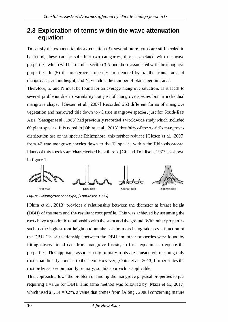
preceding root along the same plane. As such each root requires to be given a random
angle at which it emerges from the main stem, assuming this angle isn’t either 0 or 180
degrees, the frontal area associated with this root changes. 4 examples of this are seen
in figure 2, with the total height of the tree being 12m in height, so as to make sure the
tree is always above sea level no matter where the plant sits in the tidal range.
Figure 2- shows 4 randomly generated mangrove trees with varying roots
The frontal area however, is only the area of the mangrove that is submerged in the
water. So, the frontal area becomes dependant on the depth. [Ohira et al., 2013] uses
an integration method to find the value of the frontal area and [Maza et al., 2017] uses
an image processing toolbox to find the frontal area. Using the 1st mangrove in figure
1, the image was dissected using MATLAB, so as to only include any area below a
certain height, which would be defined by the depth. This was repeated for depths from
0 to 12 meters in height. 3 examples are shown in figure 3. As previously stated,
variability between mangrove plants is an issue to be overcome. This is achieved by
repeating the process again with 100 individually random generated mangroves before
the area at the specific depth is averaged, shown in figure 4.
Coastal ecosystem dynamics affected by climate change feedbacks
Alfie Hewetson 12
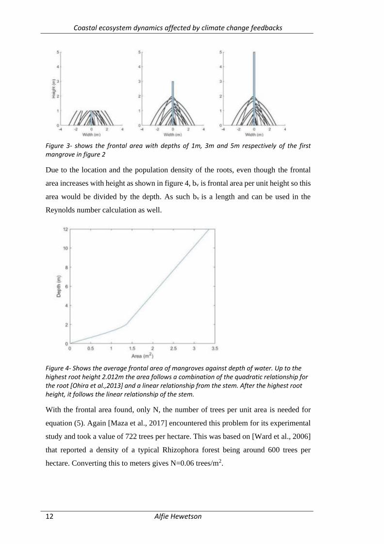
Figure 3- shows the frontal area with depths of 1m, 3m and 5m respectively of the first mangrove in figure 2
Due to the location and the population density of the roots, even though the frontal
area increases with height as shown in figure 4, bv is frontal area per unit height so this
area would be divided by the depth. As such bv is a length and can be used in the
Reynolds number calculation as well.
Figure 4- Shows the average frontal area of mangroves against depth of water. Up to the highest root height 2.012m the area follows a combination of the quadratic relationship for the root [Ohira et al.,2013] and a linear relationship from the stem. After the highest root height, it follows the linear relationship of the stem.
With the frontal area found, only N, the number of trees per unit area is needed for
equation (5). Again [Maza et al., 2017] encountered this problem for its experimental
study and took a value of 722 trees per hectare. This was based on [Ward et al., 2006]
that reported a density of a typical Rhizophora forest being around 600 trees per
hectare. Converting this to meters gives N=0.06 trees/m2.
Coastal ecosystem dynamics affected by climate change feedbacks
Alfie Hewetson 13
3 Datasets 3.1 Mangrove location
To find the affect that mangroves can have on coastal flooding, the location of
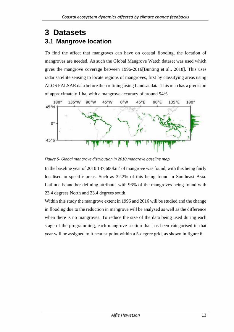
mangroves are needed. As such the Global Mangrove Watch dataset was used which
gives the mangrove coverage between 1996-2016[Bunting et al., 2018]. This uses
radar satellite sensing to locate regions of mangroves, first by classifying areas using
ALOS PALSAR data before then refining using Landsat data. This map has a precision
of approximately 1 ha, with a mangrove accuracy of around 94%.
Figure 5- Global mangrove distribution in 2010 mangrove baseline map.
In the baseline year of 2010 137,600km2 of mangrove was found, with this being fairly
localised in specific areas. Such as 32.2% of this being found in Southeast Asia.
Latitude is another defining attribute, with 96% of the mangroves being found with
23.4 degrees North and 23.4 degrees south.
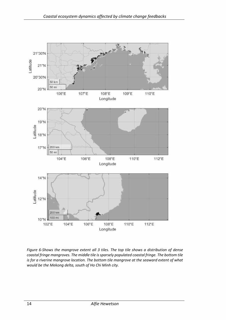
Within this study the mangrove extent in 1996 and 2016 will be studied and the change
in flooding due to the reduction in mangrove will be analysed as well as the difference
when there is no mangroves. To reduce the size of the data being used during each
stage of the programming, each mangrove section that has been categorised in that
year will be assigned to it nearest point within a 5-degree grid, as shown in figure 6.
Coastal ecosystem dynamics affected by climate change feedbacks
Alfie Hewetson 14
Figure 6-Shows the mangrove extent all 3 tiles. The top tile shows a distribution of dense coastal fringe mangroves. The middle tile is sparsely populated coastal fringe. The bottom tile is for a riverine mangrove location. The bottom tile mangrove at the seaward extent of what would be the Mekong delta, south of Ho Chi Minh city.
Coastal ecosystem dynamics affected by climate change feedbacks
Alfie Hewetson 15
3.2 Extreme sea level-tide and storm
Extreme sea levels are a function of 3 factors; meteorological effects, such as storm
surges and waves, astronomical, such as the tides and sea-level rise [Vousdoukas et
al., 2018]. This study does not currently look at future scenarios under climate change,
therefore extreme sea-level is governed by just the meteorological and astronomical
forcing.
While there is evidence that mangroves attenuate storm surges [Zhang et al., 2012,
Montgomery et al., 2019], there is less understanding in this area when compared to
mangroves ability to attenuate waves. So, in investigating coastal flooding only the
effects that mangroves can have on wave reduction will be included. This means the
extreme sea-level can be split into 2 components, 1st being waves, where mangrove
interaction is studied, and 2nd being tide and storm surges, which do not interact with
mangroves. The wave data is presented in section 3.5.
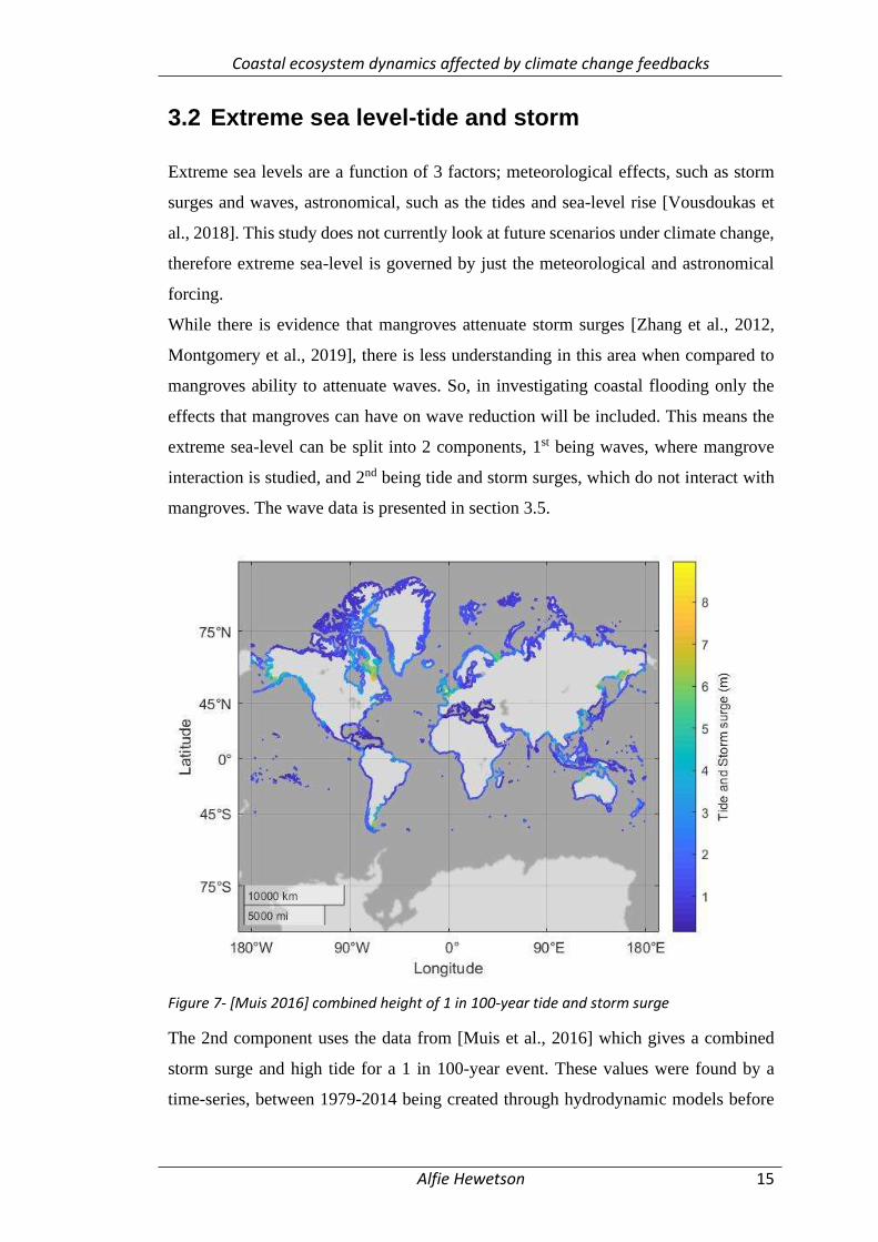
Figure 7- [Muis 2016] combined height of 1 in 100-year tide and storm surge
The 2nd component uses the data from [Muis et al., 2016] which gives a combined
storm surge and high tide for a 1 in 100-year event. These values were found by a
time-series, between 1979-2014 being created through hydrodynamic models before
Coastal ecosystem dynamics affected by climate change feedbacks
Alfie Hewetson 16
using the annual maxima method fitted to a Gumbel distribution, to find the 1 in 100-
year event. This data can be seen as an underestimate of extremes due to the resolution
of the data [Muis et al., 2016]. The results for this are imposed along the world’s
coastlines, the results of this is shown in figure 7.
3.3 MERIT topography
The degree to which land is flooded is dependent on the underlying topography and
what the height of this is relative to the extreme sea-level. As such a suitable
topographic map must be found. 2 areas are of particular importance; coastal low-lying
areas, the areas that are of particular risk of flooding, and locations that have
mangroves. The land that is of particular risk of flooding is inherently required to
produce a flood risk map. The land height in which mangroves is situated is needed
for another aspect of the calculations, as equation (5) requires the depth of the body of
mangroves. Considering that mangroves live in the intertidal region; accurate
topographic measurements are required for when this area is inundated during the
extreme flooding event, so as to apply this inundation depth to (5). As figure 6 shows
mangroves are also particularly prone to growing in rivers and the deltas of rivers,
therefore the topographic map will have particular focus on these areas.
The map chosen was the MERIT DEM hydrologically adjusted elevation, which uses
the MERIT DEM as the baseline before adjusting river networks to satisfy the
condition that ‘downstream is not higher than its upstream [Yamazaki et al 2019]. This
map will improve the accuracy in estuaries and deltas when calculating the depth
acting on the mangroves. The elevation data is given in 5-degree x 5-degree grids made
up of 6000x6000 cells, with an elevation resolution of 10cm. This means it is accurate
to 3 arc seconds, roughly 90m at the equator.
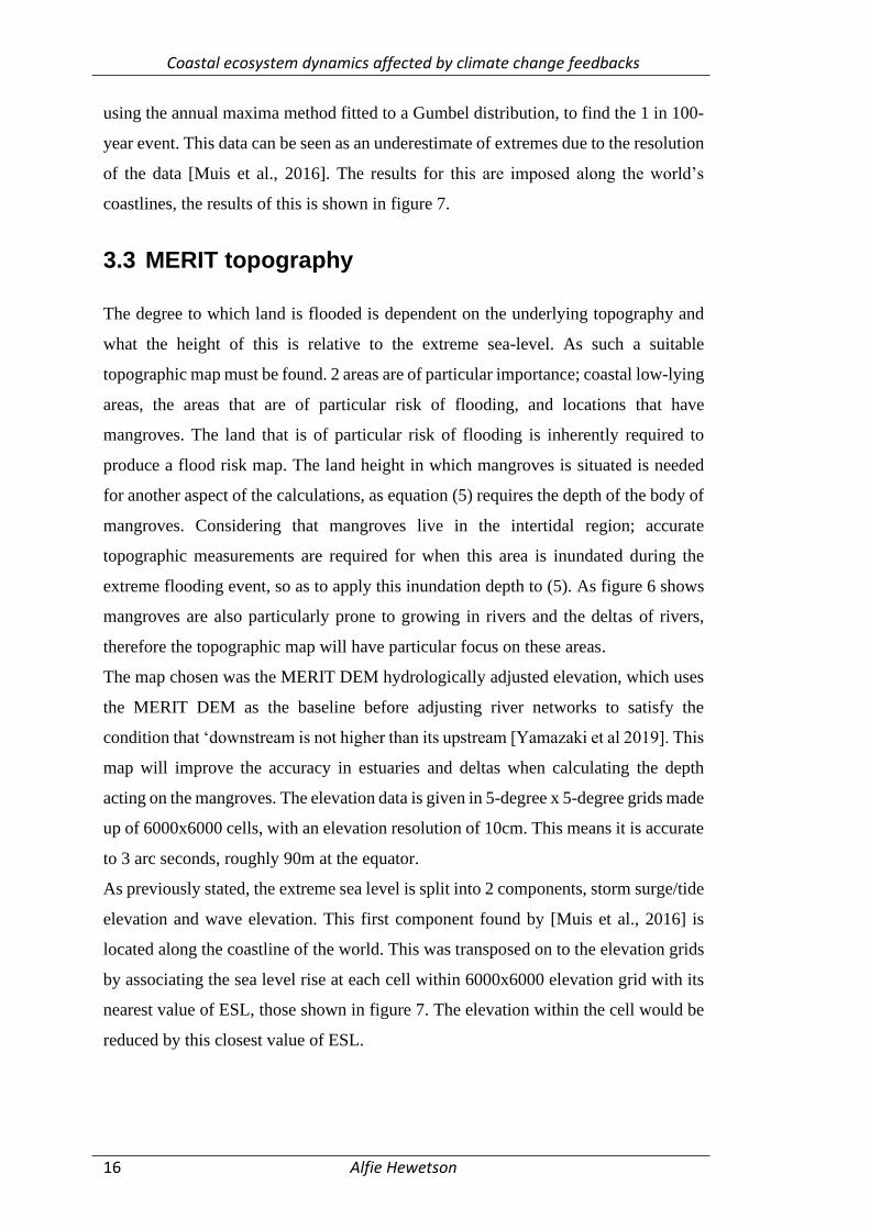
As previously stated, the extreme sea level is split into 2 components, storm surge/tide
elevation and wave elevation. This first component found by [Muis et al., 2016] is
located along the coastline of the world. This was transposed on to the elevation grids
by associating the sea level rise at each cell within 6000x6000 elevation grid with its
nearest value of ESL, those shown in figure 7. The elevation within the cell would be
reduced by this closest value of ESL.
Coastal ecosystem dynamics affected by climate change feedbacks
Alfie Hewetson 17
Figure 8-Shows the topography for Northern Vietnam region, where the height is between 10m and -10m. This topography has already been dropped down relative to the SLR at the location.
This method to superimpose the ESL from tide and storm surge onto land can lead to
jumps in the value of reduction, as the nearest data point for the ESL moves from one
spot to another despite only 1 step between cells. Meaning 2 cells which are next to
each other with equal elevation could be reduced by different ESL values and thus
appear not level. However as seen in figure 7, ESL from tide and storms doesn’t have
large changes in values between data points, as the data points are scattered regularly
along the coastlines. Also, elevations in the centre of landmasses could be reduced
incorrectly in regards to flooding. This would be caused by a cell being reduced in
height by its closest point of ESL; but due to surrounding topography shielding this
area from flooding, the flood may be driven at this location by a different point of ESL.
However, this would happen in the centre of landmasses, which characteristically have
a greater elevation at least to escape the effects of coastal flooding, as such this
shouldn’t affect the results.
3.4 Wave data The second component of the extreme sea-level is the increase in surface elevation
Coastal ecosystem dynamics affected by climate change feedbacks
Alfie Hewetson 18
caused by the waves. The objective of analysing the wave data is to find a 1 in 100-
year wave event that will be a driver for coastal flooding. This component is the
variable in which mangroves can affect and cause reduction to total flooding. To find
the 1 in 100-year event a time-series of wave heights is analysed and a probability
density function is created, whereby the 1 in a 100-year wave can be taken.
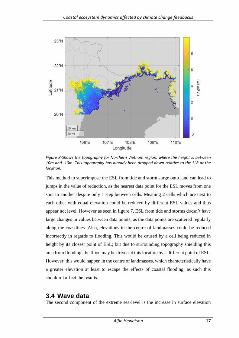
The wave data is based on the analysis by [Hemer and Trenham, 2016], whereby 8
separate CMIP5 global wind-wave climate models were evaluated for accuracy based
on the ensemble average of the dataset. The 8 different models are shown in table 1.
As noted in [Hemer and Trenham, 2016], the underperformance of CNRM-CM5,
means this model will not be included within the analysis.
ID Full model name Model
1 Australian Community Climate and Earth System
Simulator 1.0
ACCESS1.0
2 Beijing Climate Centre, Climate System Model 1-
1
BCC-CSM1.1
3 Centre National de Recherches Meteorologiques
Coupled Global Climate Model, version 5
CNRM-CM5
4 Geophysical Fluid Dynamics Laboratory Earth
System Model 2M
GFDL-ESM2M
5 Hadley Centre Global Environment Model 2, earth
System
HadGEM2-ES
6 Institute of Numerical Mathematics Coupled
Model, version 4.0
INMCM4
7 Model for Interdisciplinary Research on Climate,
version 5
MIROC5
8 Meteorological Research Institute Coupled
Atmosphere-Ocean General circulation model,
version 3
MRI-CGCM3
Table 1- showing the 8 models that were applied to WaveWatch III by [Hemer and Trenham, 2016] to find the wave time-series at each point. Including CNRM-CM5, which was removed
due to underperformance when compared to the ensembled average.
The original dataset for hindcast data runs from the beginning of 1979 to the end of
2005. To reduce the computational requirement only 10 years are taken from 1995 to
2005. Although the CMIP5 models have various spatial resolutions, these have already
Coastal ecosystem dynamics affected by climate change feedbacks
Alfie Hewetson 19
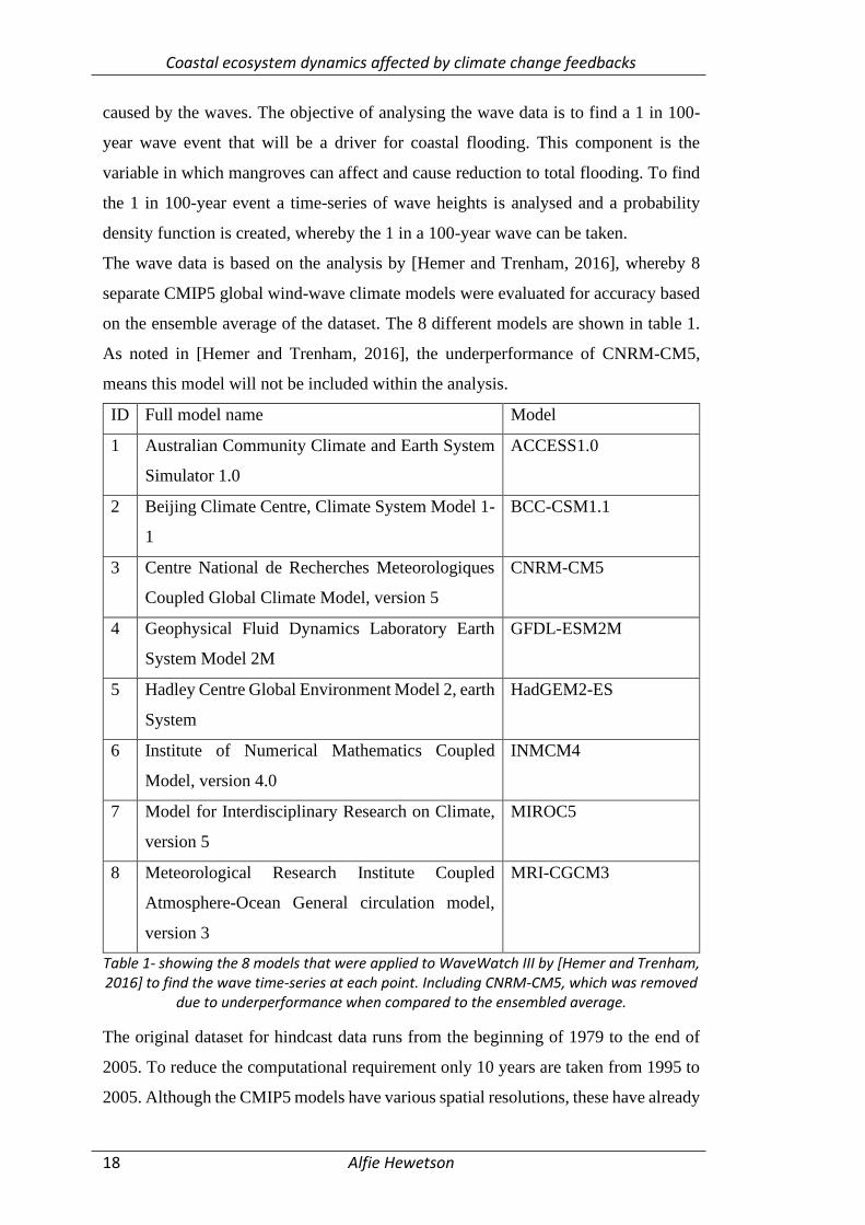
been interpolated onto a 1-degree x 1-degree map. The dataset is made up of a time-
series of 6-hour intervals, within each interval the values for significant wave height,
peak frequency and the wave direction were taken to be further used. This time-series
was made up of 14720 individual timesteps for each point.
Figure 9- Value of significant wave height for the first timestep in December 2005, ACCESS1.0. This has no respect to direction and waves could be propagating in any direction
The wave direction is given as a degree relative to North as a whole number. Meaning
the direction can be anywhere from 0degrees to 359degrees. The time-series was taken
at each location on the grid and discretised into 12 bins relative to the wave direction.
The bins each account for 30 degrees of possible wave direction, centred on points 0
to 330. For example, the bin centred on 0 takes values from 346 degrees to 15 degrees.
Each bin accounts for the significant wave height and peak frequency at that point on
the map.
This discretising process splits the total time-series into 12 parts at each location. For
each of these 12 sections a 1 in 100-year wave needed to be found. This required the
distribution of significant wave heights to be fitted to a statistical model, relating the
height of the waves to the probability of occurrence of the wave.
Coastal ecosystem dynamics affected by climate change feedbacks
Alfie Hewetson 20
𝑦 = 𝑓(𝑥|𝑎, 𝑏) = (1
𝑏𝑎𝛤(𝑎)) 𝑥𝑎−1𝑒−𝑥/𝑏
(15)
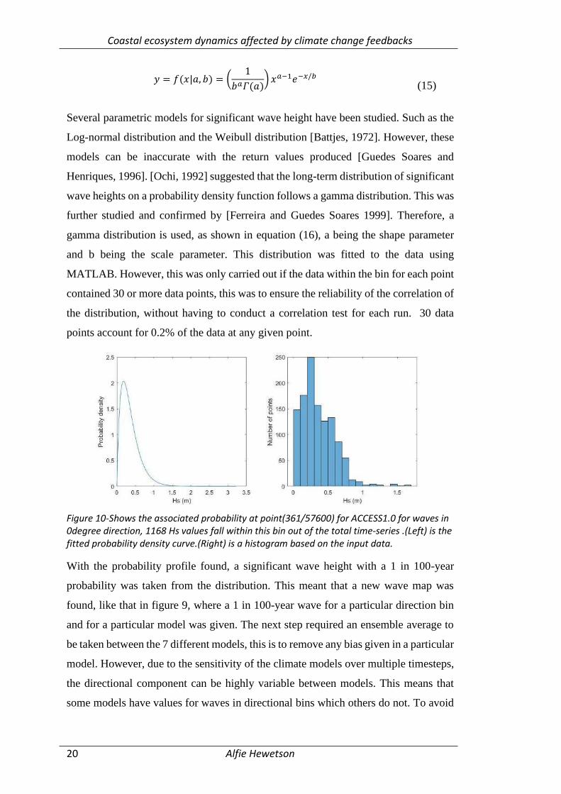
Several parametric models for significant wave height have been studied. Such as the
Log-normal distribution and the Weibull distribution [Battjes, 1972]. However, these
models can be inaccurate with the return values produced [Guedes Soares and
Henriques, 1996]. [Ochi, 1992] suggested that the long-term distribution of significant
wave heights on a probability density function follows a gamma distribution. This was
further studied and confirmed by [Ferreira and Guedes Soares 1999]. Therefore, a
gamma distribution is used, as shown in equation (16), a being the shape parameter
and b being the scale parameter. This distribution was fitted to the data using
MATLAB. However, this was only carried out if the data within the bin for each point
contained 30 or more data points, this was to ensure the reliability of the correlation of
the distribution, without having to conduct a correlation test for each run. 30 data
points account for 0.2% of the data at any given point.
Figure 10-Shows the associated probability at point(361/57600) for ACCESS1.0 for waves in 0degree direction, 1168 Hs values fall within this bin out of the total time-series .(Left) is the fitted probability density curve.(Right) is a histogram based on the input data.
With the probability profile found, a significant wave height with a 1 in 100-year
probability was taken from the distribution. This meant that a new wave map was
found, like that in figure 9, where a 1 in 100-year wave for a particular direction bin
and for a particular model was given. The next step required an ensemble average to
be taken between the 7 different models, this is to remove any bias given in a particular
model. However, due to the sensitivity of the climate models over multiple timesteps,
the directional component can be highly variable between models. This means that
some models have values for waves in directional bins which others do not. To avoid
Coastal ecosystem dynamics affected by climate change feedbacks
Alfie Hewetson 21
averaging against empty values, which in turn would reduce the results. Each location,
would only be averaged by models in which a significant 1 in 100-year wave was
found. For example, if at a point only ACCESS1.0 and MIROC5 had a value for
significant wave height for that particular direction, then the resultant wave height
would be the sum of these 2 models divided by 2. Likewise, if all 7 models have a
value at a particular point in a particular direction, then the resultant wave height would
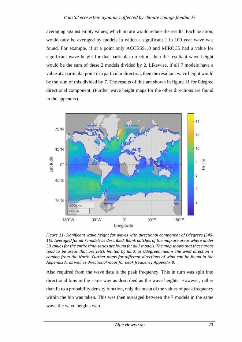
be the sum of this divided by 7. The results of this are shown in figure 11 for 0degree
directional component. (Further wave height maps for the other directions are found
in the appendix).
Figure 11- Significant wave height for waves with directional component of 0degrees (345-15). Averaged for all 7 models as described. Blank patches of the map are areas where under 30 values for the entire time-series are found for all 7 models. The map shows that these areas tend to be areas that are fetch limited by land, as 0degrees means the wind direction is coming from the North. Further maps for different directions of wind can be found in the Appendix A, as well as directional maps for peak frequency Appendix B.
Also required from the wave data is the peak frequency. This in turn was split into
directional bins in the same way as described as the wave heights. However, rather
than fit to a probability density function, only the mean of the values of peak frequency
within the bin was taken. This was then averaged between the 7 models in the same
wave the wave heights were.
Coastal ecosystem dynamics affected by climate change feedbacks
Alfie Hewetson 22
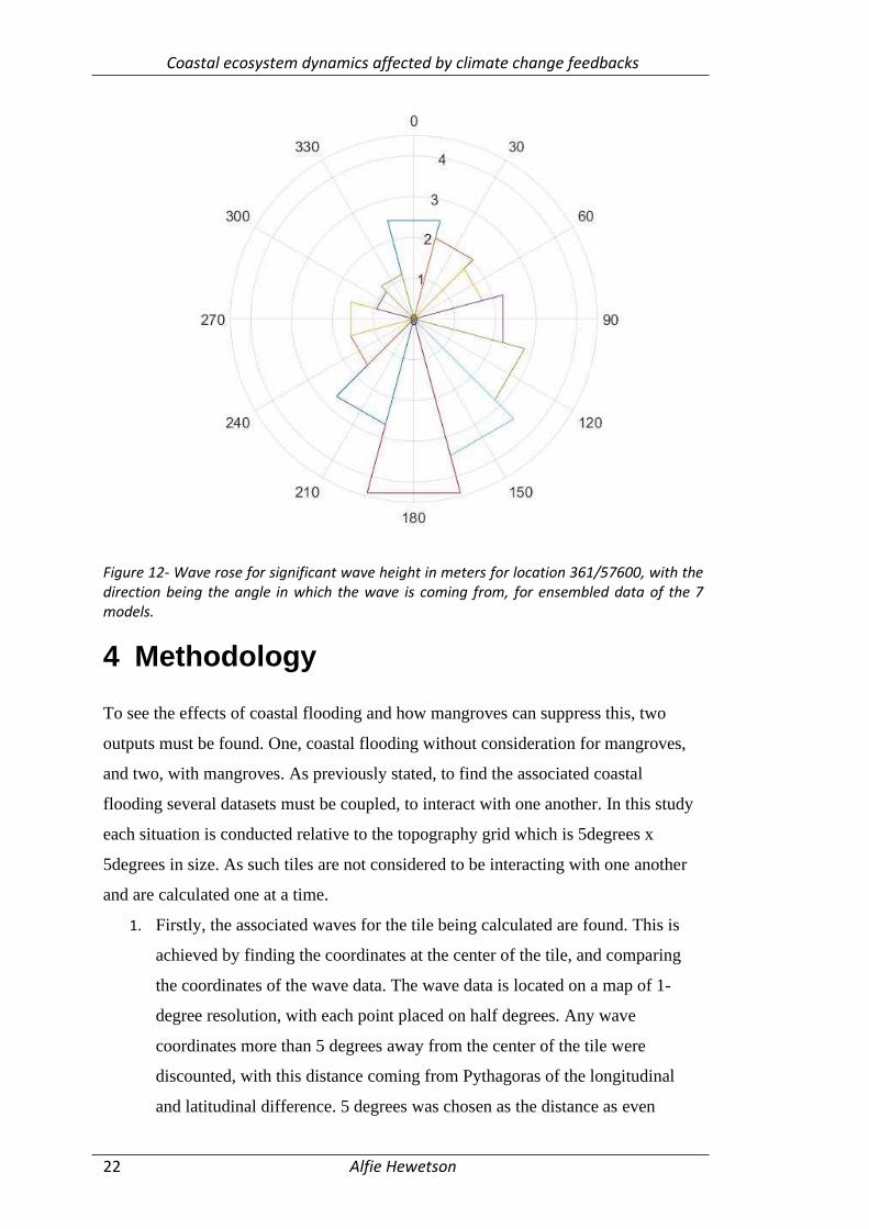
Figure 12- Wave rose for significant wave height in meters for location 361/57600, with the direction being the angle in which the wave is coming from, for ensembled data of the 7 models.
4 Methodology
To see the effects of coastal flooding and how mangroves can suppress this, two
outputs must be found. One, coastal flooding without consideration for mangroves,
and two, with mangroves. As previously stated, to find the associated coastal
flooding several datasets must be coupled, to interact with one another. In this study
each situation is conducted relative to the topography grid which is 5degrees x
5degrees in size. As such tiles are not considered to be interacting with one another
and are calculated one at a time.
1. Firstly, the associated waves for the tile being calculated are found. This is
achieved by finding the coordinates at the center of the tile, and comparing
the coordinates of the wave data. The wave data is located on a map of 1-
degree resolution, with each point placed on half degrees. Any wave
coordinates more than 5 degrees away from the center of the tile were
discounted, with this distance coming from Pythagoras of the longitudinal
and latitudinal difference. 5 degrees was chosen as the distance as even
Coastal ecosystem dynamics affected by climate change feedbacks
Alfie Hewetson 23
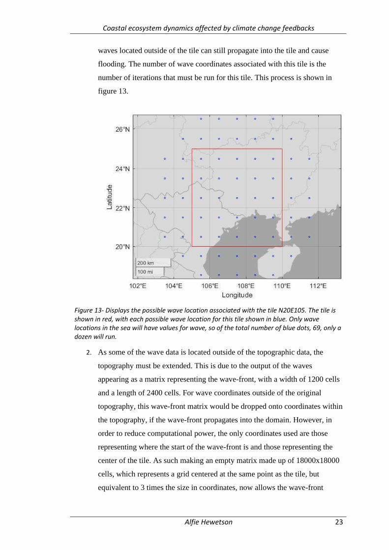
waves located outside of the tile can still propagate into the tile and cause
flooding. The number of wave coordinates associated with this tile is the
number of iterations that must be run for this tile. This process is shown in
figure 13.
Figure 13- Displays the possible wave location associated with the tile N20E105. The tile is shown in red, with each possible wave location for this tile shown in blue. Only wave locations in the sea will have values for wave, so of the total number of blue dots, 69, only a dozen will run.
2. As some of the wave data is located outside of the topographic data, the
topography must be extended. This is due to the output of the waves
appearing as a matrix representing the wave-front, with a width of 1200 cells
and a length of 2400 cells. For wave coordinates outside of the original
topography, this wave-front matrix would be dropped onto coordinates within
the topography, if the wave-front propagates into the domain. However, in
order to reduce computational power, the only coordinates used are those
representing where the start of the wave-front is and those representing the
center of the tile. As such making an empty matrix made up of 18000x18000
cells, which represents a grid centered at the same point as the tile, but
equivalent to 3 times the size in coordinates, now allows the wave-front
Coastal ecosystem dynamics affected by climate change feedbacks
Alfie Hewetson 24
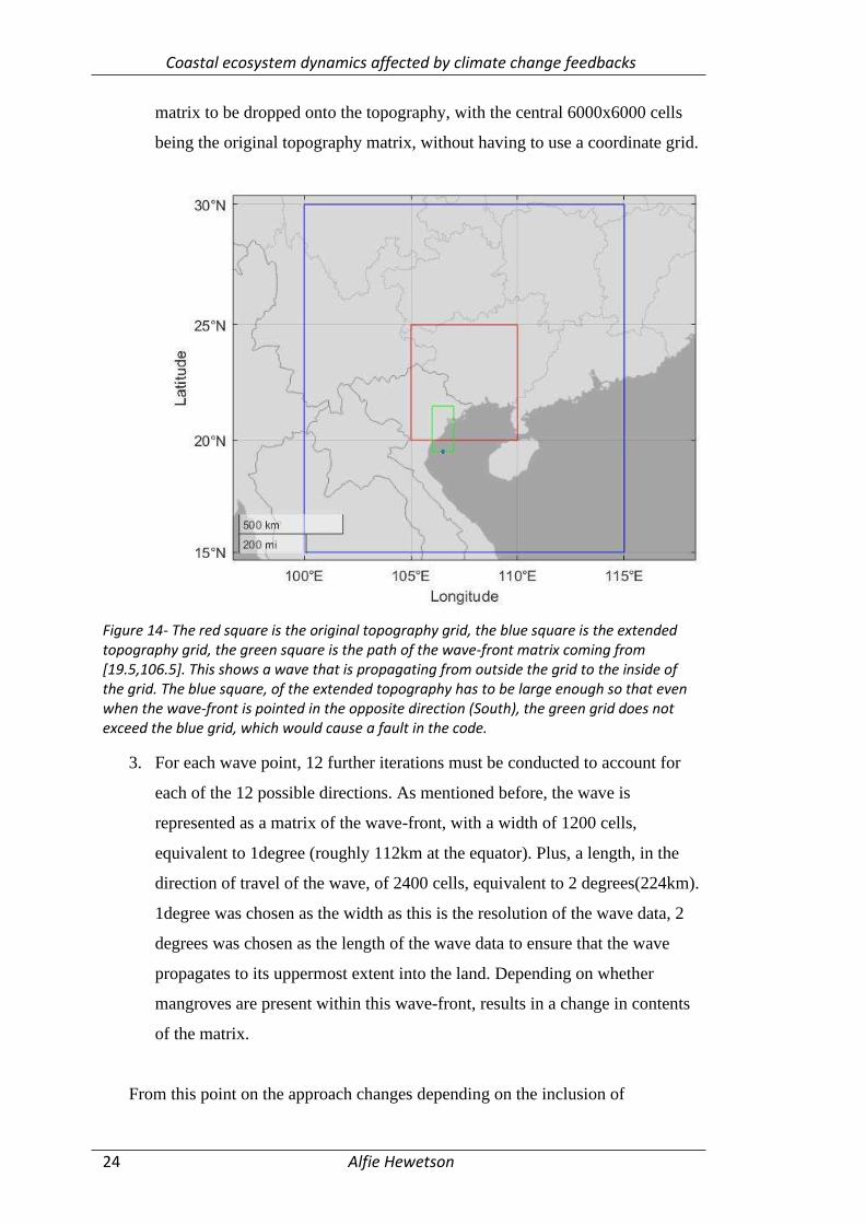
matrix to be dropped onto the topography, with the central 6000x6000 cells
being the original topography matrix, without having to use a coordinate grid.
Figure 14- The red square is the original topography grid, the blue square is the extended topography grid, the green square is the path of the wave-front matrix coming from [19.5,106.5]. This shows a wave that is propagating from outside the grid to the inside of the grid. The blue square, of the extended topography has to be large enough so that even when the wave-front is pointed in the opposite direction (South), the green grid does not exceed the blue grid, which would cause a fault in the code.
3. For each wave point, 12 further iterations must be conducted to account for
each of the 12 possible directions. As mentioned before, the wave is
represented as a matrix of the wave-front, with a width of 1200 cells,
equivalent to 1degree (roughly 112km at the equator). Plus, a length, in the
direction of travel of the wave, of 2400 cells, equivalent to 2 degrees(224km).
1degree was chosen as the width as this is the resolution of the wave data, 2
degrees was chosen as the length of the wave data to ensure that the wave
propagates to its uppermost extent into the land. Depending on whether
mangroves are present within this wave-front, results in a change in contents
of the matrix.
From this point on the approach changes depending on the inclusion of

Coastal ecosystem dynamics affected by climate change feedbacks
Alfie Hewetson 25
mangroves into the study. The following is for when mangroves are present and
included.
4. For when mangroves are present the associated wave attenuation is a function
of the properties of the wave. Therefore, the Deepwater wave number, k, and
the wave frequency, ω, are found at this point based on the peak frequency at
this location, for the direction.
5. The wave matrix is split into 1200 straight lines with a length of 2 degrees.
The lines are placed evenly alongside the coordinate point half a degree either
side and propagate out 2 degrees from the original point. Each line is then
calculated individually, so as to work out the value of the wave height along
the corresponding column of the wave matrix.
Figure 15- Shows the wave-front at point [20.5,107.5], for visualization only 10 of the lines have been shown, propagating from the original point 2 degrees forward.
6. Taking an individual line, representing a column of the wave matrix, is first
rotated around the wave coordinate to represent the direction of the wave
propagation. This line is then passed through the mangrove data, to see
if/where the line intersects the mangrove forest. Each point of intersection is
recorded.
Coastal ecosystem dynamics affected by climate change feedbacks
Alfie Hewetson 26
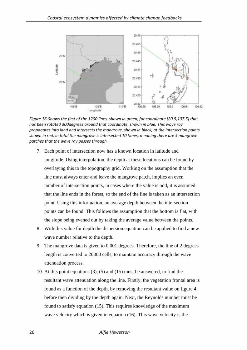
Figure 16-Shows the first of the 1200 lines, shown in green, for coordinate [20.5,107.5] that has been rotated 300degrees around that coordinate, shown in blue. This wave ray propagates into land and intersects the mangrove, shown in black, at the intersection points shown in red. In total the mangrove is intersected 10 times, meaning there are 5 mangrove patches that the wave ray passes through.
7. Each point of intersection now has a known location in latitude and
longitude. Using interpolation, the depth at these locations can be found by
overlaying this to the topography grid. Working on the assumption that the
line must always enter and leave the mangrove patch, implies an even
number of intersection points, in cases where the value is odd, it is assumed
that the line ends in the forest, so the end of the line is taken as an intersection
point. Using this information, an average depth between the intersection
points can be found. This follows the assumption that the bottom is flat, with
the slope being evened out by taking the average value between the points.
8. With this value for depth the dispersion equation can be applied to find a new
wave number relative to the depth.
9. The mangrove data is given to 0.001 degrees. Therefore, the line of 2 degrees
length is converted to 20000 cells, to maintain accuracy through the wave
attenuation process.
10. At this point equations (3), (5) and (15) must be answered, to find the
resultant wave attenuation along the line. Firstly, the vegetation frontal area is
found as a function of the depth, by removing the resultant value on figure 4,
before then dividing by the depth again. Next, the Reynolds number must be
found to satisfy equation (15). This requires knowledge of the maximum
wave velocity which is given in equation (16). This wave velocity is the
Coastal ecosystem dynamics affected by climate change feedbacks
Alfie Hewetson 27
characteristic wave velocity given in [Kobayashi et al., 1993]. This
characteristic velocity is the maximum velocity of the flow field, when the
interaction of the vegetation with the flow field is included, due to the
vegetation being subaerial the cosh terms cancel. With these known, the γ
value can be found, equation (5) for the patch of mangrove between the
points of intersection. Alongside this, the distance between the intersection
points are required, as well as how far along the new 20000 cell line that
these intersection points sit. With this distance known equation (3) can be
applied to find a resultant wave height on leaving the patch of mangrove. If
this mangrove patch is the first patch along the line, the value for H0 is taken
as the Hs dictated by the wave data. However, if this is a subsequent
mangrove patch H0 is given as the wave height on leaving the previous
mangrove patch.
𝑢𝑚𝑎𝑥 =𝑘𝑔𝐻𝑠
2𝜔
cosh(𝑘𝑑)
cosh(𝑘(ℎ + 𝑑))=𝑘𝑔𝐻𝑠
2𝜔
(16)
11. Next, the rest of the points along this line must be filled in following an
exponential relationship between intersection points of mangroves, and
continuous values of Hs the preceding Hs elsewhere. This 20000-cell line now
must be interpolated onto a 2400 cell line, before being introduced as a single
column of the wave matrix.
12. This column of the wave matrix is then converted to a flooding matrix by
using equation (17) from [U.S. Army Corps of engineers, 2002] to find the
change in sea level due to wave set-up.
𝜂 = 0.2 ∗ 𝐻𝑠
(17)
13. This process from 6 to 11 must then be repeated for all 1200 lines.
Coastal ecosystem dynamics affected by climate change feedbacks
Alfie Hewetson 28
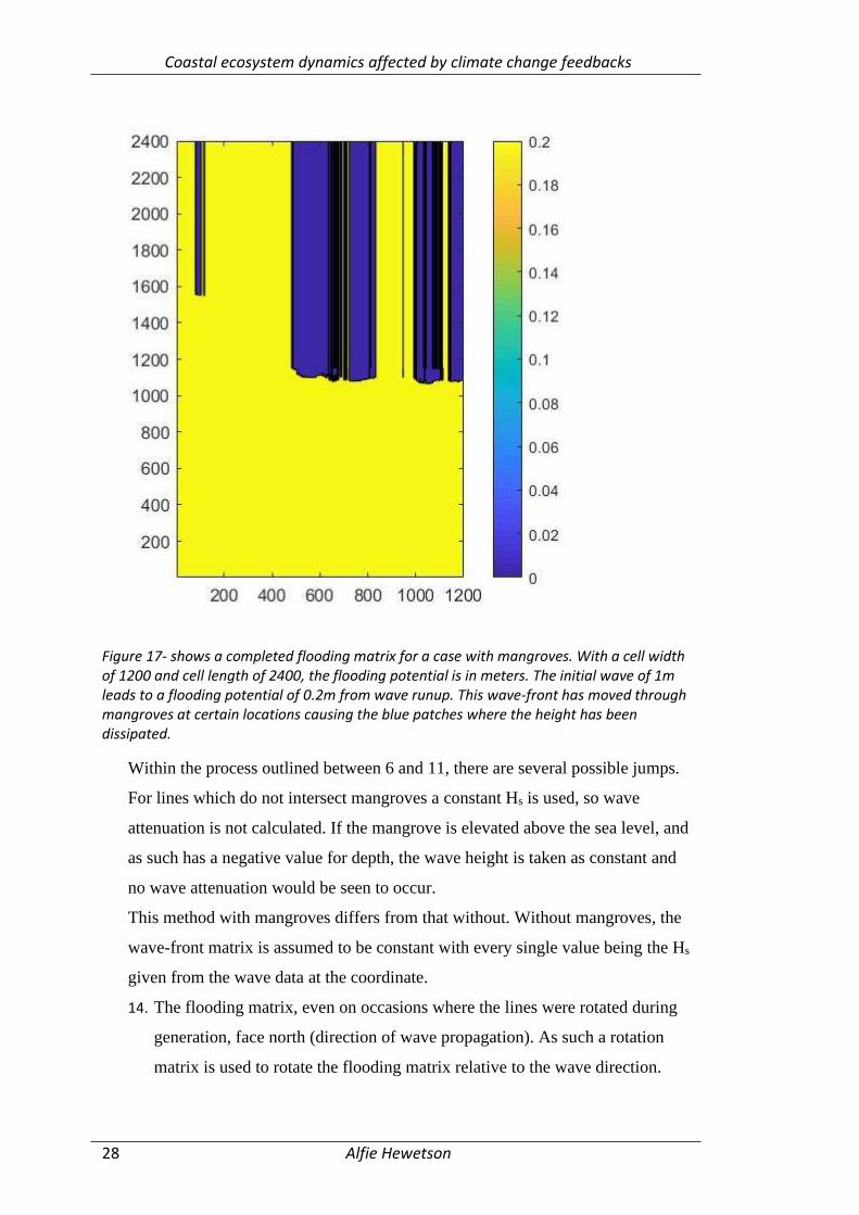
Figure 17- shows a completed flooding matrix for a case with mangroves. With a cell width of 1200 and cell length of 2400, the flooding potential is in meters. The initial wave of 1m leads to a flooding potential of 0.2m from wave runup. This wave-front has moved through mangroves at certain locations causing the blue patches where the height has been dissipated.
Within the process outlined between 6 and 11, there are several possible jumps.
For lines which do not intersect mangroves a constant Hs is used, so wave
attenuation is not calculated. If the mangrove is elevated above the sea level, and
as such has a negative value for depth, the wave height is taken as constant and
no wave attenuation would be seen to occur.
This method with mangroves differs from that without. Without mangroves, the
wave-front matrix is assumed to be constant with every single value being the Hs
given from the wave data at the coordinate.
14. The flooding matrix, even on occasions where the lines were rotated during
generation, face north (direction of wave propagation). As such a rotation
matrix is used to rotate the flooding matrix relative to the wave direction.
Coastal ecosystem dynamics affected by climate change feedbacks
Alfie Hewetson 29
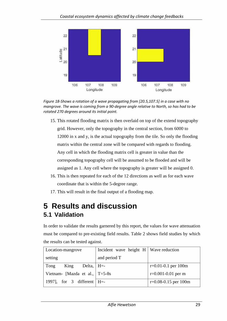
Figure 18-Shows a rotation of a wave propagating from [20.5,107.5] in a case with no mangrove. The wave is coming from a 90-degree angle relative to North, so has had to be rotated 270 degrees around its initial point.
15. This rotated flooding matrix is then overlaid on top of the extend topography
grid. However, only the topography in the central section, from 6000 to
12000 in x and y, is the actual topography from the tile. So only the flooding
matrix within the central zone will be compared with regards to flooding.
Any cell in which the flooding matrix cell is greater in value than the
corresponding topography cell will be assumed to be flooded and will be
assigned as 1. Any cell where the topography is greater will be assigned 0.
16. This is then repeated for each of the 12 directions as well as for each wave
coordinate that is within the 5-degree range.
17. This will result in the final output of a flooding map.
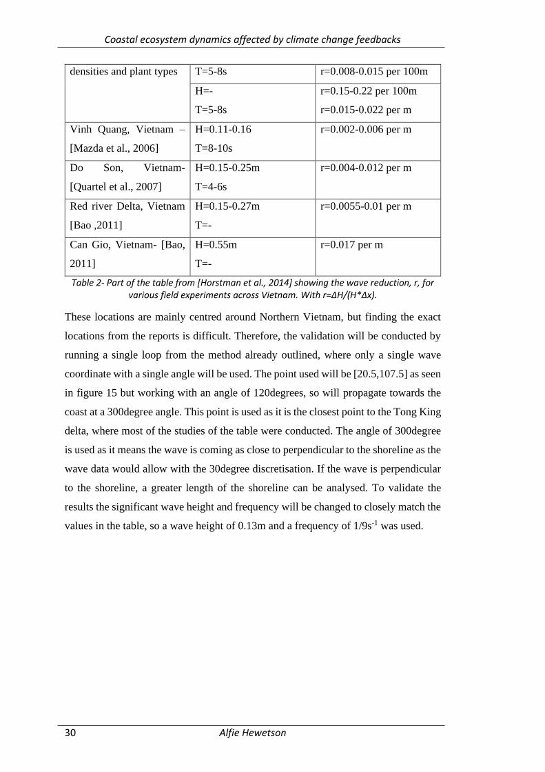
5 Results and discussion 5.1 Validation
In order to validate the results garnered by this report, the values for wave attenuation
must be compared to pre-existing field results. Table 2 shows field studies by which
the results can be tested against.
Location-mangrove
setting
Incident wave height H
and period T
Wave reduction
Tong King Delta,
Vietnam- [Mazda et al.,
1997], for 3 different
H=-
T=5-8s
r=0.01-0.1 per 100m
r=0.001-0.01 per m
H=- r=0.08-0.15 per 100m
Coastal ecosystem dynamics affected by climate change feedbacks
Alfie Hewetson 30
densities and plant types T=5-8s r=0.008-0.015 per 100m
H=-
T=5-8s
r=0.15-0.22 per 100m
r=0.015-0.022 per m
Vinh Quang, Vietnam –
[Mazda et al., 2006]
H=0.11-0.16
T=8-10s
r=0.002-0.006 per m
Do Son, Vietnam-
[Quartel et al., 2007]
H=0.15-0.25m
T=4-6s
r=0.004-0.012 per m
Red river Delta, Vietnam
[Bao ,2011]
H=0.15-0.27m
T=-
r=0.0055-0.01 per m
Can Gio, Vietnam- [Bao,
2011]
H=0.55m
T=-
r=0.017 per m
Table 2- Part of the table from [Horstman et al., 2014] showing the wave reduction, r, for various field experiments across Vietnam. With r=ΔH/(H*Δx).
These locations are mainly centred around Northern Vietnam, but finding the exact
locations from the reports is difficult. Therefore, the validation will be conducted by
running a single loop from the method already outlined, where only a single wave
coordinate with a single angle will be used. The point used will be [20.5,107.5] as seen
in figure 15 but working with an angle of 120degrees, so will propagate towards the
coast at a 300degree angle. This point is used as it is the closest point to the Tong King
delta, where most of the studies of the table were conducted. The angle of 300degree
is used as it means the wave is coming as close to perpendicular to the shoreline as the
wave data would allow with the 30degree discretisation. If the wave is perpendicular
to the shoreline, a greater length of the shoreline can be analysed. To validate the
results the significant wave height and frequency will be changed to closely match the
values in the table, so a wave height of 0.13m and a frequency of 1/9s-1 was used.
Coastal ecosystem dynamics affected by climate change feedbacks
Alfie Hewetson 31
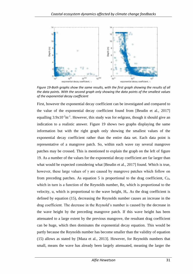
Figure 19-Both graphs show the same results, with the first graph showing the results of all the data points. With the second graph only showing the data points of the smallest values of the exponential decay coefficient
First, however the exponential decay coefficient can be investigated and compared to
the value of the exponential decay coefficient found from [Beudin et al., 2017]
equalling 3.9x10⁻³m-1. However, this study was for eelgrass, though it should give an
indication to a realistic answer. Figure 19 shows two graphs displaying the same
information but with the right graph only showing the smallest values of the
exponential decay coefficient rather than the entire data set. Each data point is
representative of a mangrove patch. So, within each wave ray several mangrove
patches may be crossed. This is mentioned to explain the graph on the left of figure
19. As a number of the values for the exponential decay coefficient are far larger than
what would be expected considering what [Beudin et al., 2017] found. Which is true,
however, these large values of γ are caused by mangrove patches which follow on
from preceding patches. As equation 5 is proportional to the drag coefficient, CD,
which in turn is a function of the Reynolds number, Re, which is proportional to the
velocity, u, which is proportional to the wave height, Hs. As the drag coefficient is
defined by equation (15), decreasing the Reynolds number causes an increase in the
drag coefficient. The decrease in the Reynold’s number is caused by the decrease in
the wave height by the preceding mangrove patch. If this wave height has been
attenuated to a large extent by the previous mangrove, the resultant drag coefficient
can be huge, which then dominates the exponential decay equation. This would be
partly because the Reynolds number has become smaller than the validity of equation
(15) allows as stated by [Maza et al., 2013]. However, for Reynolds numbers that
small, means the wave has already been largely attenuated, meaning the larger the
Coastal ecosystem dynamics affected by climate change feedbacks
Alfie Hewetson 32
value of the incorrect exponential decay coefficient, the closer it is to zero. This
knowledge can then be coupled with the general shape of the right graph of figure 19.
The general trend of the data shows an exponential decrease when seen from a log axis
with the horizontal spread being successive mangrove patches changing the wave
height at input. These values are larger than the value suggested by [Beudin et al.,
2017] which would make sense due to the physical parameters dictated by the eelgrass
and mangrove plants. More importantly these values are larger than the value for the
exponential decay coefficient for bed friction, suggested by [MacVean and Lacy,
2014] of 3.2x10⁻⁴m-1. This means the assumption that wave-trunk interaction
dominates over the dissipation by bed friction.
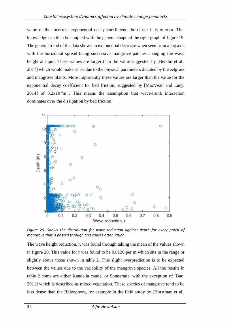
Figure 20- Shows the distribution for wave reduction against depth for every patch of mangrove that is passed through and causes attenuation.
The wave height reduction, r, was found through taking the mean of the values shown
in figure 20. This value for r was found to be 0.0126 per m which sits in the range or
slightly above those shown in table 2. This slight overprediction is to be expected
between the values due to the variability of the mangrove species. All the results in
table 2 come are either Kandelia candel or Sonneratia, with the exception of [Bao,
2011] which is described as mixed vegetation. These species of mangrove tend to be
less dense than the Rhizophora, for example in the field study by [Horstman et al.,
Coastal ecosystem dynamics affected by climate change feedbacks
Alfie Hewetson 33
2014], Sonneratia have a volumetric density of roughly 4.5% while Rhizophora has a
density of 5.8% to 20% and reaching 32% in water less than 1m. This increased density
would lead to an increase in the wave reduction factor. This slight over prediction is
likely to be larger than the r value which has been currently found. As figure 19 shows,
increasing the depth decreases the exponential decay coefficient, in turn reducing the
wave reduction coefficient. Currently the model is using the depth in mangroves from
the extreme sea-level from high tide and storm surge. The field data is unlikely to have
been recorded in these conditions and as such was likely recorded in shallower waters,
with a higher decay coefficient caused by the decrease in depth.
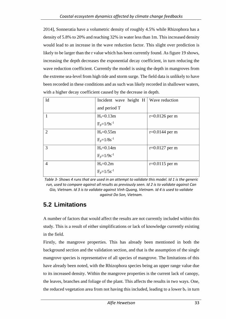
Id Incident wave height H
and period T
Wave reduction
1 Hs=0.13m
Fp=1/9s-1
r=0.0126 per m
2 Hs=0.55m
Fp=1/8s-1
r=0.0144 per m
3 Hs=0.14m
Fp=1/9s-1
r=0.0127 per m
4 Hs=0.2m
Fp=1/5s-1
r=0.0115 per m
Table 3- Shows 4 runs that are used in an attempt to validate this model. Id 1 is the generic run, used to compare against all results as previously seen. Id 2 is to validate against Can
Gio, Vietnam. Id 3 is to validate against Vinh Quang, Vietnam. Id 4 is used to validate against Do Son, Vietnam.
5.2 Limitations
A number of factors that would affect the results are not currently included within this
study. This is a result of either simplifications or lack of knowledge currently existing
in the field.
Firstly, the mangrove properties. This has already been mentioned in both the
background section and the validation section, and that is the assumption of the single
mangrove species is representative of all species of mangrove. The limitations of this
have already been noted, with the Rhizophora species being an upper range value due
to its increased density. Within the mangrove properties is the current lack of canopy,
the leaves, branches and foliage of the plant. This affects the results in two ways. One,
the reduced vegetation area from not having this included, leading to a lower bv in turn
Coastal ecosystem dynamics affected by climate change feedbacks
Alfie Hewetson 34
reducing the exponential decay coefficient than if a canopy was included. Two, [He,
et al., 2019] found that models with a canopy produce a larger drag force than models
with just the stem and the roots. Meaning canopies can have a major effect on the
results. This is compounded within this study due to the use of extreme sea-levels
elevating the sea-level, leading to conditions which would place the flow in the region
that contains canopy. These factors could be improved by an inclusion of the species
type within the mangrove data for all locations, plus by finding an empirical
relationship for canopy density, like what [Ohira et al., 2013] did for the roots. These
improvements could also be enhanced by associating the mangrove with above ground
biomass density as used [Mafi-Gholami et al., 2020] but using volume density rather
than mass density. This could then be used in a similar manner to the length scale of
L=(V-VM)/A proposed by [Mazda et al, 1997].
The next limitation comes from the natural geography and the possible changes on the
account of rivers and estuaries. Currently, the code is set to give an exponential decay
coefficient of 0 if the mangroves are above the extreme sea-level. This is wrong in two
ways. One, if there is still flooding of the wave up to this point as found using 0.2*Hs
[U.S. Army Corps of engineers, 2002], the mangrove would still obstruct the wave.
However, equation (5) requires a known depth of water, and would not function for
mangrove dissipation in the swash zone. Two, rivers and estuaries would allow waves
to propagate up their length, while the relative water height above sea level would
increase, due to the increased water level that causes rivers to flow. This issue was
partially resolved by using the MERIT topographic map [Yamazaki et al 2019], which
thus corrects the bottom surface of the river bed. However, it does not go as far as
giving the depth of the river at each section along its length, which in turn can also be
highly variable due to seasonal changes. More work is required on how mangroves
can attenuate flooding in the swash zone before it can be empirically implemented. To
find the depth of river at each section and thus an increased depth of the wave, an
adjusted water body map could be made, but the height of the river would likely be
found from the height of the banks of the river and would likely overcomplicate the
simplified flooding model.
Human geography also causes a limitation due to the built landscape. As built flood
defences are not currently considered, which would block the flood potential on low
lying land. This could be rectified in the model by knowing the locations of the defence
and knowing the height required to overtop the defence. However [Hillen et al., 2010]
Coastal ecosystem dynamics affected by climate change feedbacks
Alfie Hewetson 35
found that characteristically, at time of writing, hard coastal defences in Vietnam could
only withstand a 1 in 50-year flooding event.
Another limitation is that of mangrove interaction between patches. As the results of
equation (3) results in a change of wave height, but assumes the wave characteristics
do not change beyond that. [Beudin et al., 2017] reported a 15% change in the mean
wavelength and a 10% change in the mean wave period. This isn’t too much of an
issue as no change in the peak wave frequency was observed, which is used in the
calculations. On leaving the mangrove patch, the waves become scattered due to the
irregularity of damping of the patch causing diffraction [Dalrymple et al., 1984].
Scattered waves can cause early breaking due to constructive interference, but also
change the flow conditions on entering the next patch.
[Beudin et al., 2017] further studied the effects of tide/currents on the dissipation of
waves through vegetation. This found that the difference in wave height dissipation
can double in ebb conditions or reduce by 40% in flood conditions. Currently in this
study however no currents are included either from rivers or tides.
The biggest limitation currently observed is that of wave breaking. According to [Vo-
luong and Massel, 2008], the two principal drivers of wave energy dissipation are
wave-trunk interaction and wave breaking, assuming a mild slope thus reducing the
bed friction. This implies that wave breaking and wave-trunk interaction are of similar
magnitudes. This non-inclusion of the wave breaking causes several problems. Firstly,
in terms of the attenuation from mangroves, as if the wave has already broken, then
the interacting wave may already be reduced in height by the breaking process.
Secondly, mangroves have been shown to suppress wave set-up [Suzuki et al., 2019].
Which according to [Bowen et al., 1968], wave set up results from wave shoaling and
breaking. A solution for wave energy dissipation in vegetation under breaking waves
has been proposed by [Mendez and Losada, 2004], which combines a vegetation
energy dissipation rate with the wave breaking energy dissipation rate.
Beyond wave breaking, several other coastal processes have been ignored within this
study. First, wave refraction; currently the wave rays travel only in straight lines from
the wave-front origin and are not affected by the bathymetry. Secondly, wave shoaling
is only accounted for as a function of the wave setup as outlined by [Bowen et al.,
1968]. When wave shoaling would lead to an increase in wave height as the wave
moves into shallower water. To incorporate these coastal processes into this current
model would be computationally expensive. However, if the model was changed with
Coastal ecosystem dynamics affected by climate change feedbacks
Alfie Hewetson 36
respect to the wave data, so the wave data points are placed along the shoreline, with
only the waves travelling perpendicular to the shore being analysed. This would result
in a model which would account for wave refraction, by removing the cause of
refraction.
Of these limitations some solutions have been provided, however this model currently
acts to simplify the conditions in a way that can then be validated to field data and
applied anywhere. A limitation, currently, to using this code anywhere in the world is
how the code is applied to small land masses, such as islands. Currently, the wave rays
are fixed at 2 degrees length, and if the wave is unattenuated, the wave height and
consequent flooding is fixed along this length. This causes a problem in the cases of
small islands with a diameter of less than two degrees. As waves from one side of the
island could cause flooding on the far side of the island despite an increased inland
topography shielding the area from flooding. This could be achieved by limiting the
wave ray length to stop on reaching a height greater than the possible flooding.
However, this would require another coupling between the wave ray and the
topography, which would further strain the computational requirements. In this paper,
the answer was to use Vietnam as a case study due, to it not being an island.
5.3 Flooding extent
The same forcing conditions were applied to 3 scenarios; a case with no mangroves, a
case with the mangrove distribution in 1996 and a case with mangrove distribution in
2016. The results of this are given in table 4. What can be clearly seen across all 3 tiles
is for coastal Vietnam the main flood forcing comes from storm surge and tidal
component. The top tile has 81.1% of its flooding caused by tide and storm surge, for
the middle and bottom tile it is 79.77% and 59.24% respectively. This shows that the
wave component is of increasing importance especially considered that the storm and
tide forcing is relatively consistent along the Vietnam coast as shown in figure 7. This
is likely due to the sheltering Vietnam receives from neighbouring islands, with
Northern Vietnam being sheltered by the island Hainan. This in turn reduces the fetch
and the subsequent wave heights.
Top tile Middle tile Lower tile
Coastal ecosystem dynamics affected by climate change feedbacks
Alfie Hewetson 37
[22.5,107.5] [17.5,107.5] [12.5,107.5]
Flood due to mean sea level 6276238 19048899 8623465
Flood due to storm surge plus tide 6921875 19342865 8793928
Flood due to storm surge plus tide
plus wave (no mangrove)
7072074 19417408 8911216
Flood due to storm surge plus tide
plus wave (1996 mangrove)
7071965 19417408 8911216
Flood due to storm surge plus tide
plus wave (2016 mangrove)
7071965 19417408 8911216
Table 4- shows the total number of cells which have been flooded within each tile. The flood due to mean sea level, is just the cells accounting for region of the tile already in the sea and
has no result from flood forcing, but is there to note the difference.
The degree of flooding can also be seen between the samples, table 5 shows the area
of flooding in hectares of each tile. Clearly from this it can be seen that the top tile has
the greatest degree of flooding by more than twice the amount of flooding than the
middle and lower tile. This is largely to due with the increased amount of low-lying
land that can become easily flooded.
Table 5-shows the area in hectares(10000m2) of the associated flooding, 1996 and 2016 mangroves have been compiled to a single variable due to no change being seen in table 4. Each cell is 3 seconds by 3 seconds in size, which equates to roughly 90m by 90m, giving an
area per cell of 8100m2
The objective of this paper was to produce a model whereby the effects of wave
attenuation by vegetation are included on a flood risk map. Only in the top tile did
vegetation make an impact on the resultant flooding. This largely comes down to the
dominance of the forcing of storm surge and tide on the flooding map. As figure 17
shows mangroves do have an ability to reduce the wave height and to reduce the flood
potential coming from the waves. For the middle tile, where the mangrove was a sparse
coastal fringe, mangroves had no affect on the attenuation. The same is true for the
Top tile
[22.5,107.5]
Middle tile
[17.5,107.5]
Lower tile
[12.5,107.5]
Flood due to storm surge plus tide 522966 238112 138075
Flood due to storm surge plus tide
plus wave (no mangrove)
644627 298492 233078
Flood due to storm surge plus tide
plus wave (mangrove)
644539 298492 233078
Coastal ecosystem dynamics affected by climate change feedbacks
Alfie Hewetson 38
bottom tile where the mangrove was predominately riverine.
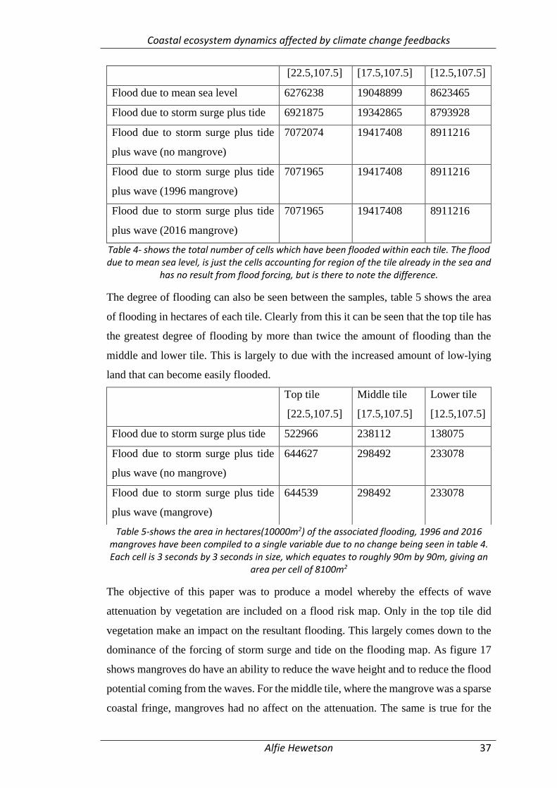
Figure 21- Shows the total flooding in the top tile. Where red is the flooding from storm and tide and blue is the increase through wave set up.
On seeing the visualisation of the flooding, a reanalysis of the original input data was
conducted. In doing this the wave forcing was found to be incorrect, by virtue of the
wave angle being 180 degrees off. As the direction that the wave was coming from
was used as the direction the wave was propagating. This results in a major reduction
in wave height, as any wave that is currently implemented in the results, can have no
more than 2 degrees of fetch. It cannot have more than two degrees as that is the length
of the wave ray, So, to have more than 2 degrees of fetch means the wave location is
more than 2 degrees from land and as such wouldn’t have an affect on the study.
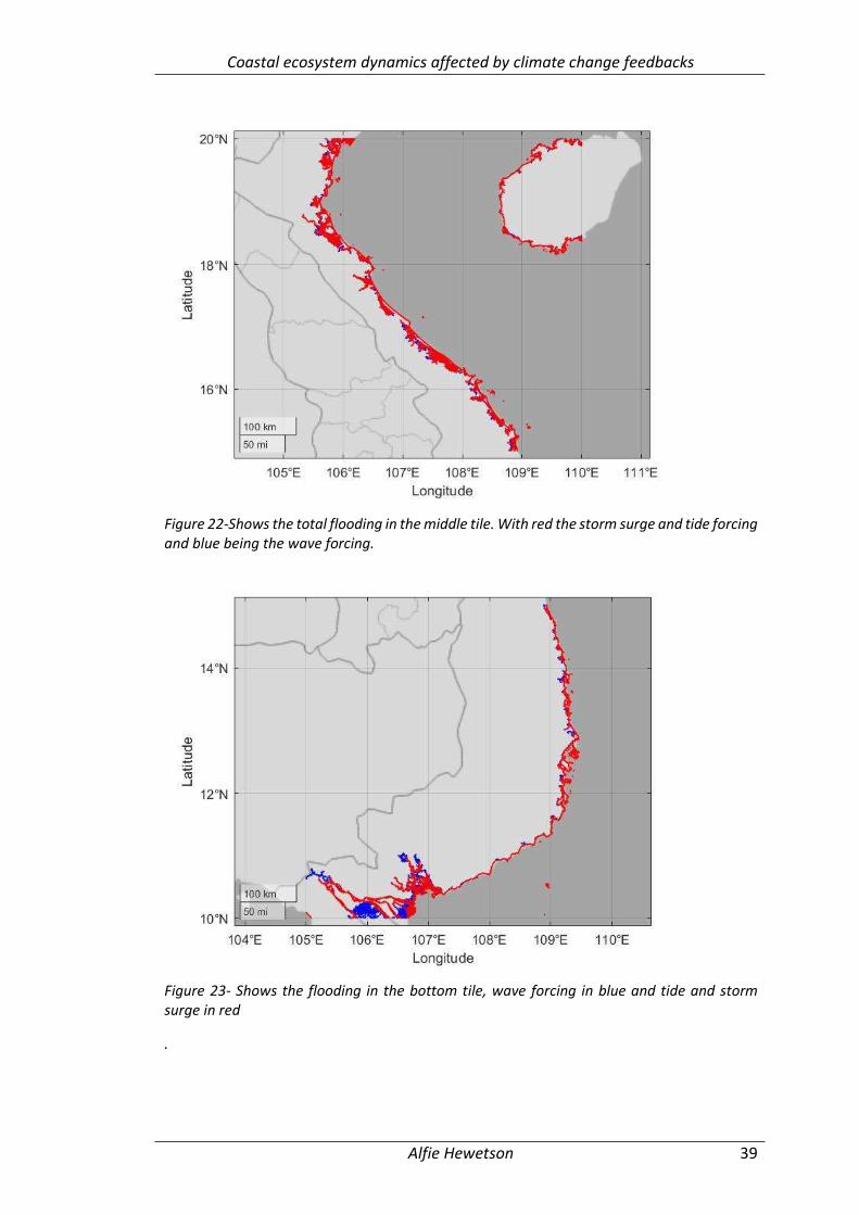
This also explains why the bottom tile has a greater percentage of its flooding from
waves than the other tiles. Due to the circular curve of the shoreline, waves propagating
at angles to the shoreline can have an increased fetch by being blown at a tangent to
the coastline. This would develop larger waves which would increase the flooding
from the wave component.
Coastal ecosystem dynamics affected by climate change feedbacks
Alfie Hewetson 39
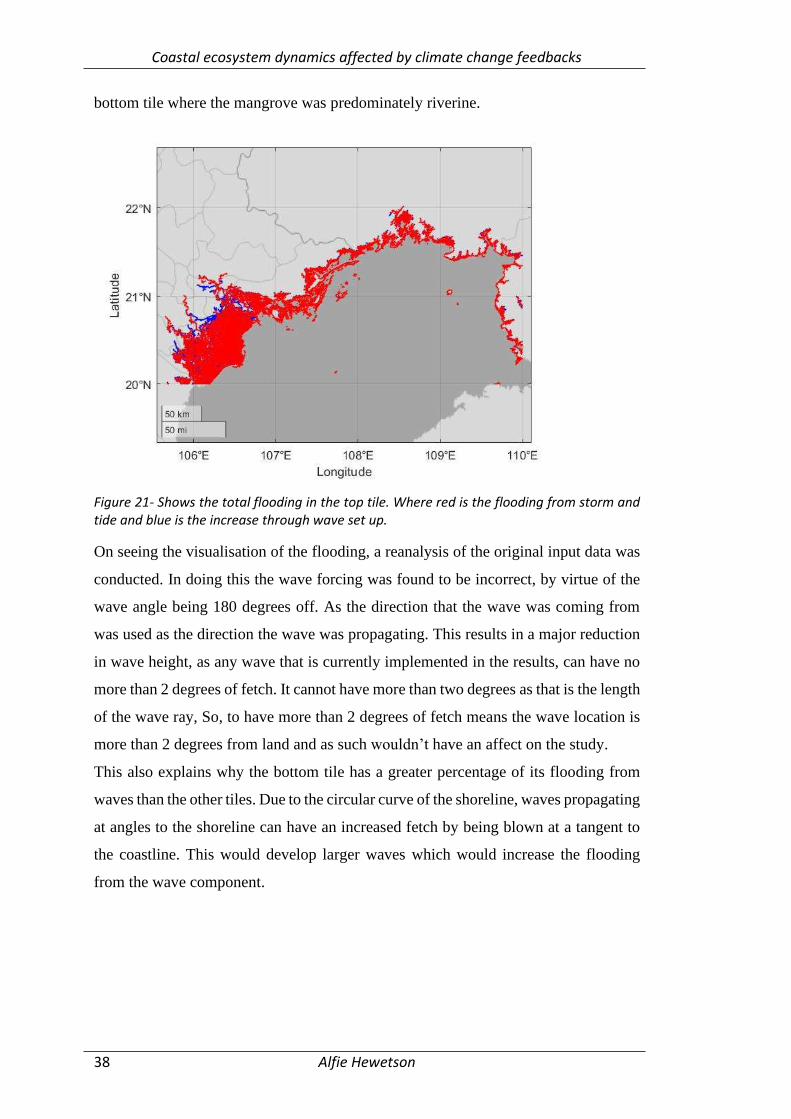
Figure 22-Shows the total flooding in the middle tile. With red the storm surge and tide forcing and blue being the wave forcing.
Figure 23- Shows the flooding in the bottom tile, wave forcing in blue and tide and storm surge in red
.
Coastal ecosystem dynamics affected by climate change feedbacks
Alfie Hewetson 40
6 Conclusions
To fully extend this model to find the resultant flooding extent a reassessment of the
wave data is required. This would be accomplished by finding the waves which are
travelling perpendicular to the coastline at nearshore locations.
The validation section showed that when waves were travelling perpendicular to the
shoreline, due to the chosen wave direction, a realistic attenuation was found which
fit field values, if over predicting the dissipation, due to the increased vegetation
density. As such the use of wave rays and mangrove data collected from satellites
can be used to estimate the resultant wave attenuation.
To fully complete the aims of this project the code must be run again but with a
change to the wave conditions. On attempting this before, it was found that the new
wave conditions take on average twice as long as before. This at least implies that a
change is occurring to the results. This is likely because more wave states exist, in
areas that would be otherwise heavily fetch limited. However, due to the time
limitations of this project this has not yet happened.
To take the project further though would be possible, with the validation showing the
possibilities of combining satellite measurements of coastal ecosystems and wave
data, to create flooding maps. Numerous other forms of ecosystem have the ability to
attenuate wave [Narayan et al., 2016], such as salt marshes, coral reefs and sea
grasses. [Kobayashi et al., 1993] was originally implemented for wave dissipation
through submerged kelp beds, as such the method outlined in this paper can be
applied and used in the same manner and would only require, inputs of the physical
characteristics of the kelp beds. Similar implementation could be carried out on other
ecosystems.
Coastal ecosystem dynamics affected by climate change feedbacks
Alfie Hewetson 41
References
Alongi DM (2008) Mangrove forests: resilience, protection from tsunamis, and
responses to global climate change. Estuarine, coastal and shelf science, volume 76,
issue 1, page 1-13. Available from: https://doi.org/10.1016/j.ecss.2007.08.024
Anderson, M.E., Smith, J.M., & McKay, S. (2011). Wave dissipation by vegetation,
U.S. Army Engineer Research and Development Center Coastal and Hydraulics
Laboratory, Vicksburg, United States. Available from:
https://doi.org/10.21236/ad1003881
Augustin LN, Irish JL & Lynett P (2009) Laboratory and numerical studies of wave
damping by emergent and near emergent wetland vegetation. Coastal engineering,
volume 56, issue 3, page 332-340. Available from:
https://doi.org/10.1016/j.coastaleng.2008.09.004
Bao TQ (2011) Effect of mangrove forest structure on wave attenuation in coastal
Vietnam. Oceanologia, volume 53, issue 3, page 807-818. Available from:
https://doi.org/10.5697/oc.53-3.807
Barbier EB (2016) The protective service of mangrove ecosystems: A review of
valuation methods. Marine pollution bulletin, volume 109, issue 2, pages 676-681.
Available from: https://doi.org/10.1016/j.marpolbul.2016.01.033
Battjes JA (1972) Long-term wave height distributions at seven stations around the
British Isles. Deutsche Hydrographische Zeitschrift, volume 25, page179–189.
Available from: https://doi.org/10.1007/BF02312702
Beudin A, Kalra TS, Ganju NK & Warner JC (2017) Development of a coupled wave-
flow-vegetation interaction model. Computers & Geosciences, volume 100, pages 76-
86. Available from: https://doi.org/10.1016/j.cageo.2016.12.010
Borsje BW, van Wesenbeeck BK, Dekker F, Paalvast P, Bouma TJ, van Katwijk MM
Coastal ecosystem dynamics affected by climate change feedbacks
Alfie Hewetson 42
& de Vries MB (2011) How ecological engineering can serve in coastal protection.
Ecological engineering, volume 37, issue 2, pages 113-122. Available from:
https://doi.org/10.1016/j.ecoleng.2010.11.027
Bowen AJ, Inman DL & Simmons VP (1968), Wave ‘set‐down’ and set‐up. J.
Geophys. Res., volume 73, page 2569–2577. Available from:
doi:10.1029/JB073i008p02569.
Bradley K & Houser C (2009) Relative velocity of seagrass blades: implications for
wave attenuation in low energy environments. Journal of geophysical research: Earth
surface, volume 114, issue F1. Available from: https://doi.org/10.1029/2007JF000951
Camfield FE (1977) A method for estimating wind-wave growth and decay in shallow
water with high values of bottom friction. CETA 77-6. Fort Belvoir, VA: Coastal
Engineering Research Center.
Conger T & Chang S (2019) Developing indicators to identify coastal green
infrastructure potential: the case of the Salish Sea region. Ocean & Coastal
Management, volume 175, pages 53-69. Available from:
https://doi.org/10.1016/j.ocecoaman.2019.03.011
Dalrymple RA, Kirby JT & Hwang P (1984) Wave diffraction due to areas of energy
dissipation. Journal of waterway port coastal and ocean engineering, volume 110,
issue 1. Available from: https://doi.org/10.1061/(ASCE)0733-950X(1984)110:1(67)
Ferreira JA & Guedes Soares C (1999) Modelling the long-term distribution of
significant wave height with the Beta and Gamma models. Ocean engineering, volume
26, issue 8, page 713-725. Available from: https://doi.org/10.1016/S0029-
8018(98)00022-5
Ferrario F, Beck MW, Storlazzi CD, Micheli FM, Shepard CC& Airoldi L (2014). The
effectiveness of coral reefs for coastal hazard risk reduction and adaptation. Nature
Communications, volume 5, article number 2794. Available from:
https://doi.org/10.1038/ncomms4794
Coastal ecosystem dynamics affected by climate change feedbacks
Alfie Hewetson 43
Gedan KB, Kirwan ML, Wolanski E, Barbier EB & Silliman BR (2011) The present
and future role of coastal wetland vegetation in protecting shorelines: answering recent
challenges to the paradigm. Climate change, volume 106, pages 7-29. Available from:
https://doi.org/10.1007/s10584-010-0003-7
Giesen W, Wulffraat S, Zieren M & Scholten L (2006) The mangrove habitat in
southeast Asia. Mangrove Guidebook for Southeast Asia. Dharmasarn Co., Ltd.,
Bangkok. Available at: http://www.fao.org/3/a-ag132e.pdf
Gill AM, Tomlinson PB (1977) Studies on the growth of red mangrove (Rhizophora
mangle L.) 4. Adult root system. Biotropica, volume 9, issue 3, pages145–155.
Available from: https://www.jstor.org/stable/2387877
Guedes Soares C & Henriques AC (1996) Statistical uncertainty in long-term
distributions of significant wave height. J. Offshore Mech. Arct. Eng, volume 118,
issue 4, page 284-291. Available from: https://doi.org/10.1115/1.2833917
He F, Chen J & Jiang C (2019) Surface wave attenuation by vegetation with the stem,
root and canopy. Coastal engineering, volume 152. Available from:
https://doi.org/10.1016/j.coastaleng.2019.103509
Hillen M, Jonkman S, Kanning W, Kok M, Geldenhuys M & Stive M (2010) Coastal
defence cost estimates: Case study of the Netherlands, New Orleans and Vietnam. TU
Delft, Department Hydraulic Engineering. 0169–6548 0169–6548.
Horstman EM, Dohmen-Janssen CM, Narra PMF, van den Berg NJF, Siemerink M &
Hulscher SJMH (2014) Wave attenuation in mangroves: A quantitative approach to
field observations. Coastal engineering, volume 94, pages 47-62. Available from:
https://doi.org/10.1016/j.coastaleng.2014.08.005
Kobayashi N, Raichle AW & Asano T (1993) Wave attenuation by vegetation. Journal
of waterway, port, coastal and ocean engineering, volume 119, issue 1. Available
from: https://doi.org/10.1061/(ASCE)0733-950X(1993)119:1(30)
Coastal ecosystem dynamics affected by climate change feedbacks
Alfie Hewetson 44
MacVean LJ & Lacy JR (2014) Interactions between waves, sediments, and turbulence
on a shallow estuarine mudflat. Journal of geophysical research: Oceans, volume 119,
issue 3. Available from: https://doi.org/10.1002/2013JC009477
Mafi-Gholami D, Zenner EK, Jaafari A & Dui DT (2020) Spatially explicit predictions
of changes in the extent of mangroves of Iran at the end of the 21st century. Estuarine,
coastal and shelf science, volume 237, 106644. Available from:
https://doi.org/10.1016/j.ecss.2020.106644
Massel SR, Furukawa K & Brinkman RM (1999) Surface wave propagation in
mangrove forests. Fluid dynamics research, volume 24, issue 4, page 219-249.
Available from: https://doi.org/10.1016/S0169-5983(98)00024-0
Maza M, Adler K, Ramos D, Garcia AM & Nepf H (2017) Velocity and drag evolution
from the leading edge of a model mangrove forest. Journal of geophysical research:
Oceans, volume 122, issue 11. Available from: https://doi.org/10.1002/2017JC012945
Maza M, Lara JL & Losada IJ (2013) A coupled model of submerged vegetation under
oscillatory flow using Navier-Stokes equations. Coastal engineering, volume 80,
pages 16-34. Available from: https://doi.org/10.1016/j.coastaleng.2013.04.009
Mazda Y, Wolanski E, King B, Sase A, Ohtsuke D & Magi M (1997) Drag force due
to vegetation in mangrove swamps. Mangroves and salt marshes, volume 1, page 193-
199. Available from: https://doi.org/10.1023/A:1009949411068
Mazda Y, Magi M, Ikeda Y, Kurokawa T & Asano T (2006) Wave reduction in a
mangrove forest dominated by sonneratia sp. Wetlands ecology and management,
volume 14, page 365-378. Available from: https://doi.org/10.1007/s11273-005-5388-
0
McGranahan G, Balk D & Anderson B (2007) The rising tide: assessing the risks of
climate change and human settlements in low elevation coastal zones. Environment &
Urbanization, vol 19, issue 1, pages 17-37. Available from:
https://doi.org/10.1177%2F0956247807076960
Coastal ecosystem dynamics affected by climate change feedbacks
Alfie Hewetson 45
Menéndez P, Losada IJ, Beck MW, Torres-Ortega S, Espejo A, Narayan S, Díaz-Simal
P & Lange GM (2018) Valuing the protection services of mangroves at national scale:
The Philippines. Ecosystem services, volume 34, part A, pages 24-36. Available from:
https://doi.org/10.1016/j.ecoser.2018.09.005
Mendelsohn R, Emanuel K, Chonabayashi S & Bakkensen L (2012) The impact of
climate change on global tropical cyclone damage. Nature Clim Change 2, pages 205-
209. Available from: https://doi.org/10.1038/nclimate1357
Mendez FJ, Losada IJ & Losada MA (1999) Hydrodynamics induced by wind waves
in a vegetation field. Journal of geophysical research: Oceans, volume 104 issue C8.
Available from: https://doi.org/10.1029/1999JC900119
Mendez FJ & Losada IJ (2004) An empirical model to estimate the propagation of
random breaking and nonbreaking waves over vegetation fields. Coastal engineering,
Volume 51, issue 2, page 103-118. Available form:
https://doi.org/10.1016/j.coastaleng.2003.11.003
Mendez-Alonzo R, Moctezuma C, Ordonez VR, Angeles G, Martinez AJ & Lopez-
Portillo J (2015) Root biomechanics in Rhizophora mangle: anatomy morphology and
ecology of mangrove’s flying buttresses. Annals of Botany, volume 115, issue 5, page
833-840. Available from: https://doi.org/10.1093/aob/mcv002
Möller, I, & Spencer T (2002) Wave dissipation over macro-tidal saltmarshes: Effects
of marsh edge typology and vegetation change. Journal of Coastal Research. SI36,
page 506-521. Available from: https://www.jstor.org/stable/26477839
Montgomery JM, Bryan KR, Mullarney JC & Horstman EM (2019) Attenuation of
storm surges by coastal mangroves. Geophysical research letters, volume 46, issue 5.
Available from: https://doi.org/10.1029/2018GL081636
Mork M. (1996) Wave Attenuation due to Bottom Vegetation. In: Grue J., Gjevik B.,
Weber J.E. (eds) Waves and Nonlinear Processes in Hydrodynamics. Fluid Mechanics
Coastal ecosystem dynamics affected by climate change feedbacks
Alfie Hewetson 46
and Its Applications, vol 34. Springer, Dordrecht. https://doi.org/10.1007/978-94-009-
0253-4_30
Narayan S, Beck MW, Reguero BG, Losada IJ, van Wesenbeeck B, Pontee N,
Sanchirico JN, Ingram JC, Lange GM & Burks-Copes KA (2016) The effectiveness,
costs and coastl protection benefits of natural and nature-based defences. Available
from: PLoS ONE 11(5): e0154735. https://doi.org/10.1371/journal.pone.0154735
Nepf, HM (1999), Drag, turbulence, and diffusion in flow through emergent
vegetation. Water Resources Research, volume 35, issue 2, page 479– 489. Available
from: doi:10.1029/1998WR900069.
Neumann B, Vafeidis AT, Zimmermann J & Nicholls RJ (2015) Future Coastal
Population Growth and Exposure to Sea-Level Rise and Coastal Flooding - A Global
Assessment. Available from: PLoS ONE 10(3): e0118571.
https://doi.org/10.1371/journal.pone.0118571
Ochi MK (1992) New approach for estimating the severest sea state from statistical
data. Coastal engineering 1992: Proceedings of the 23rd international conference,
Venice, Italy; 1992. p. 512–25. Available from:
https://doi.org/10.1061/9780872629332.038
Ohira W, Honda K, Nagai M & Ratanasuwan A (2013) mangrove stilt root
morphology modeling for estimating hydraulic drag in tsunami inundation simulation.
Trees, volume 27, pages 141-148. Available from: https://doi.org/10.1007/s00468-
012-0782-8
Oppenheimer, M., B.C. Glavovic , J. Hinkel, R. van de Wal, A.K. Magnan, A. Abd-
Elgawad, R. Cai, M. Cifuentes-Jara, R.M. DeConto, T. Ghosh, J. Hay, F. Isla, B.
Marzeion, B. Meyssignac, & Z. Sebesvari, (2019) Sea Level Rise and Implications for
Low-Lying Islands, Coasts and Communities. IPCC Special Report on the Ocean and
Cryosphere in a Changing Climate [H.-O. Portner, D.C. Roberts, V. Masson-
Delmotte, P. Zhai, M. Tignor, E. Poloczanska, K. Mintenbeck, A. Alegria, M. Nicolai,
A. Okem, J. Petzold, B. Rama, N.M. Weyer (eds.)]
Coastal ecosystem dynamics affected by climate change feedbacks
Alfie Hewetson 47
Phan KL, Stive MJF, Zijlema M, Truong HS & Aarninkhof SGJ (2019) The effects of
wave non-linearity on wave attenuation by vegetation. Coastal engineering, volume
147, pages 63-74. Available from: https://doi.org/10.1016/j.coastaleng.2019.01.004
Quartel S, Kroon A, Augustinus P.G.E.F, Van Santen P & Tri NH (2007) Wave
attenuation in coastal mangroves in the red river delta, Vietnam. Journal of Asian Earth
sciences, volume 29, issue 4, page 576-584. Available from:
https://doi.org/10.1016/j.jseaes.2006.05.008
Sasmito SD, Murdiyarso D, Friess DA & Kurnianto S (2016) Can mangroves keep
pace with contemporary sea level rise? A global data review. Wetlands ecology and
management, volume 24 pages 263-278. Available from:
https://doi.org/10.1007/s11273-015-9466-7
Saenger, P, Hegerl, EJ, Davie, J.D.S. & International Union for Conservation of
Nature and Natural Resources. Working Group on Mangrove Ecosystems and United
Nations Environment Programme and World Wildlife Fund,(1983) The resource.
Global status of mangrove ecosystems. International Union for Conservation of Nature
and Natural Resources.
Suzuki T, Hu Z, Kumada K, Phan LK & Zijlema M (2019) Non-hydrostatic modelling
of drag, inertia and porous effects in wave propagation over dense vegetation fields.
Coastal engineering, volume 149, pages 49-64. Available from:
https://doi.org/10.1016/j.coastaleng.2019.03.011
U.S. Army Corps of Engineers (2002), Coastal Engineering Manual, U.S. Army Corps
of Engineers, Washington, DC.
Vo-Luong HP & Massel SR (2006) Experiments on wave motion and suspended
sediment concentration at Nang Hai, Can Gio mangrove forest, Southern Vietnam.
Oceanologia, volume 48, issue 1, page 23-40. Available from:
http://www.iopan.gda.pl/oceanologia/48_1.html#A3
Coastal ecosystem dynamics affected by climate change feedbacks
Alfie Hewetson 48
Vousdoukas MI, Mentaschi L, Voukouvalas E, Verlaan M, Jevrejeva S, Jackson LP &
Feyen L (2018) Global probabilistic projections of extreme sea levels show
intensification of coastal flood hazard. Nature communications, volume 9, 2360.
Available from: https://doi.org/10.1038/s41467-018-04692-w
Ward GA, Smith III TJ, Whelan KRT & Doyle TW (2006) regional processes in
mangrove ecosystems: spatial scaling relationships, biomass, and turnover rates
following catatrophic disturbances. Hydrobiologia, volume 569, page 517-527.
Available from: https://doi.org/10.1007/s10750-006-0153-9
Zhang k, Liu H, Li Y, Xu H, Shen J, Rhome J & Smith TJ (2012) Estuarine coastal
and shelf science, volumes 102-103, pages 11-23. Available from:
https://doi.org/10.1016/j.ecss.2012.02.021
Database References
Citations taken exactly from the source, and are listed in order they appear in the
text.
Mangrove citation
Bunting P., Rosenqvist A., Lucas R., Rebelo L-M., Hilarides L., Thomas N., Hardy
A., Itoh T., Shimada M. and Finlayson C.M. (2018). The Global Mangrove Watch –
a New 2010 Global Baseline of Mangrove Extent. Remote Sensing 10(10): 1669.
doi: 10.3390/rs1010669.
Storm and tidal surge citation
Muis, S (2016): Global Tide and Surge Reanalysis (GTSR). 4TU.ResearchData.
Dataset. https://doi.org/10.4121/uuid:aa4a6ad5-e92c-468e-841b-de07f7133786
MERIT citation
Yamazaki D., D. Ikeshima, J. Sosa, P.D. Bates, G.H. Allen, T.M. Pavelsky
MERIT Hydro: A high-resolution global hydrography map based on latest
topography datasets
Water Resources Research, vol.55, pp.5053-5073, 2019, doi:
10.1029/2019WR024873
Wave data citation
Hemer, Mark; Trenham, Claire; Durrant, Tom; Greenslade, Diana (2015): CAWCR
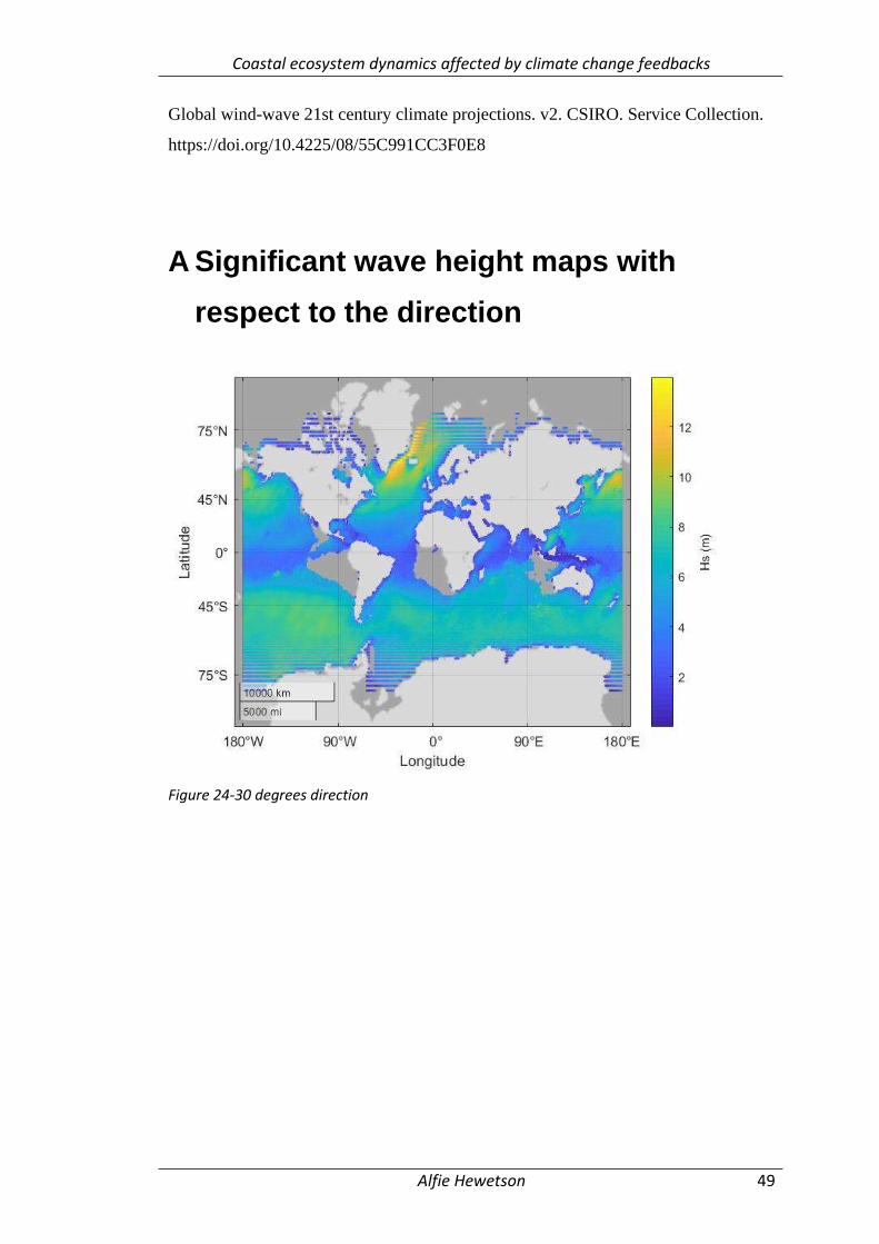
Coastal ecosystem dynamics affected by climate change feedbacks
Alfie Hewetson 49
Global wind-wave 21st century climate projections. v2. CSIRO. Service Collection.
https://doi.org/10.4225/08/55C991CC3F0E8
A Significant wave height maps with
respect to the direction
Figure 24-30 degrees direction
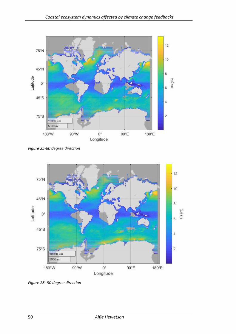
Coastal ecosystem dynamics affected by climate change feedbacks
Alfie Hewetson 50
Figure 25-60 degree direction
Figure 26- 90 degree direction
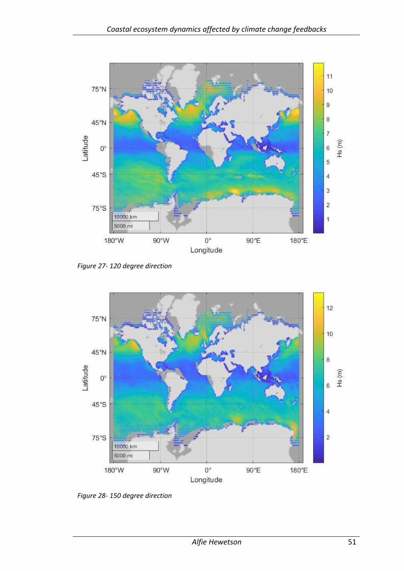
Coastal ecosystem dynamics affected by climate change feedbacks
Alfie Hewetson 51
Figure 27- 120 degree direction
Figure 28- 150 degree direction
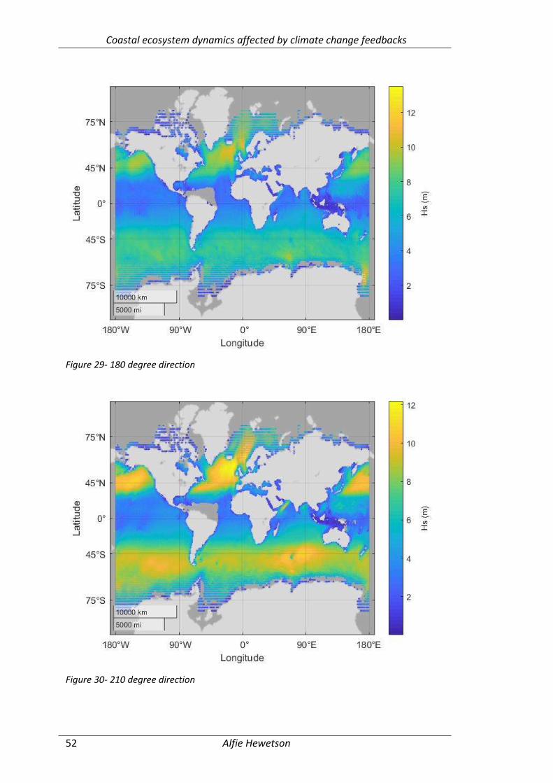
Coastal ecosystem dynamics affected by climate change feedbacks
Alfie Hewetson 52
Figure 29- 180 degree direction
Figure 30- 210 degree direction
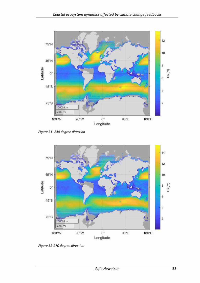
Coastal ecosystem dynamics affected by climate change feedbacks
Alfie Hewetson 53
Figure 31- 240 degree direction
Figure 32-270 degree direction
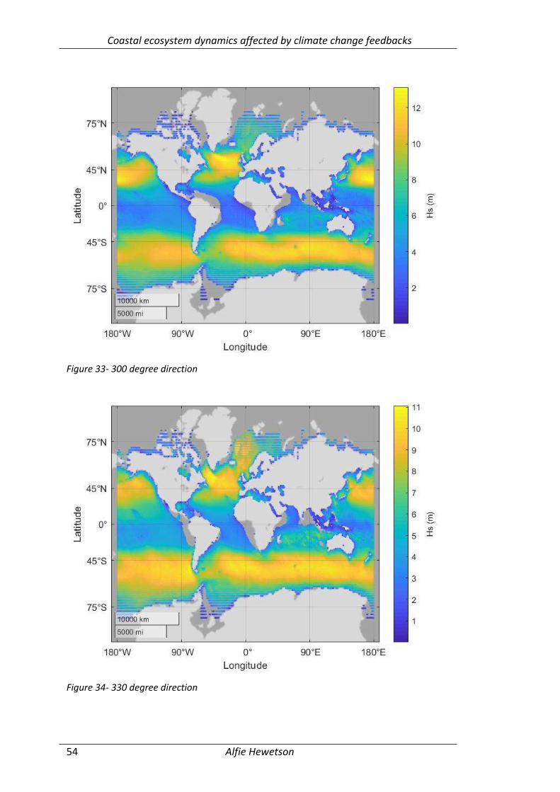
Coastal ecosystem dynamics affected by climate change feedbacks
Alfie Hewetson 54
Figure 33- 300 degree direction
Figure 34- 330 degree direction
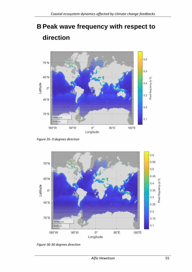
Coastal ecosystem dynamics affected by climate change feedbacks
Alfie Hewetson 55
B Peak wave frequency with respect to
direction
Figure 35- 0 degrees direction
Figure 36-30 degrees direction
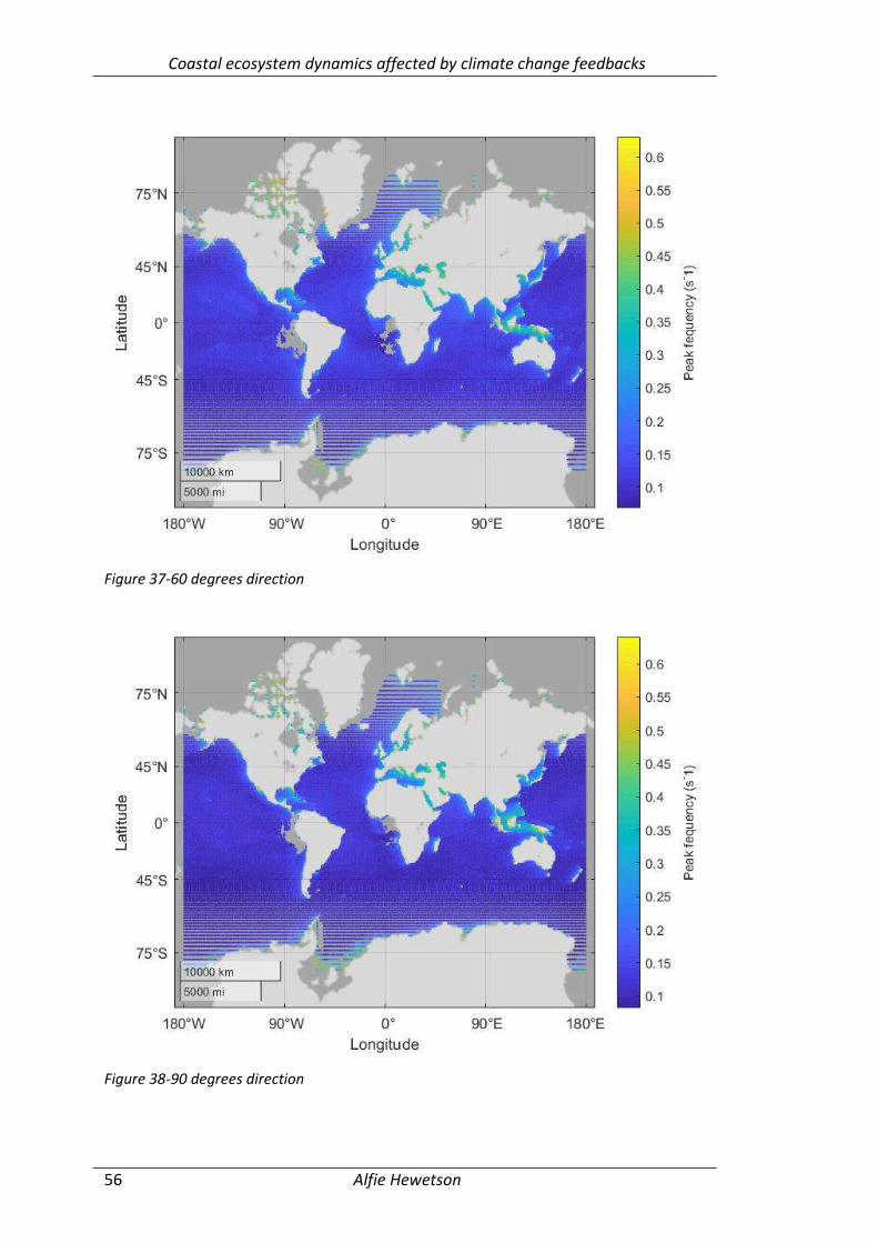
Coastal ecosystem dynamics affected by climate change feedbacks
Alfie Hewetson 56
Figure 37-60 degrees direction
Figure 38-90 degrees direction
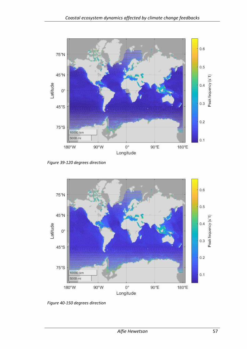
Coastal ecosystem dynamics affected by climate change feedbacks
Alfie Hewetson 57
Figure 39-120 degrees direction
Figure 40-150 degrees direction
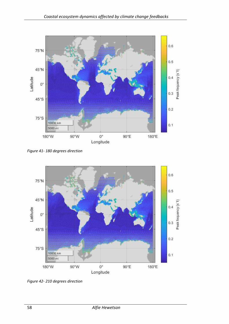
Coastal ecosystem dynamics affected by climate change feedbacks
Alfie Hewetson 58
Figure 41- 180 degrees direction
Figure 42- 210 degrees direction
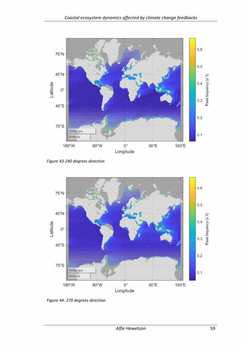
Coastal ecosystem dynamics affected by climate change feedbacks
Alfie Hewetson 59
Figure 43-240 degrees direction
Figure 44- 270 degrees direction
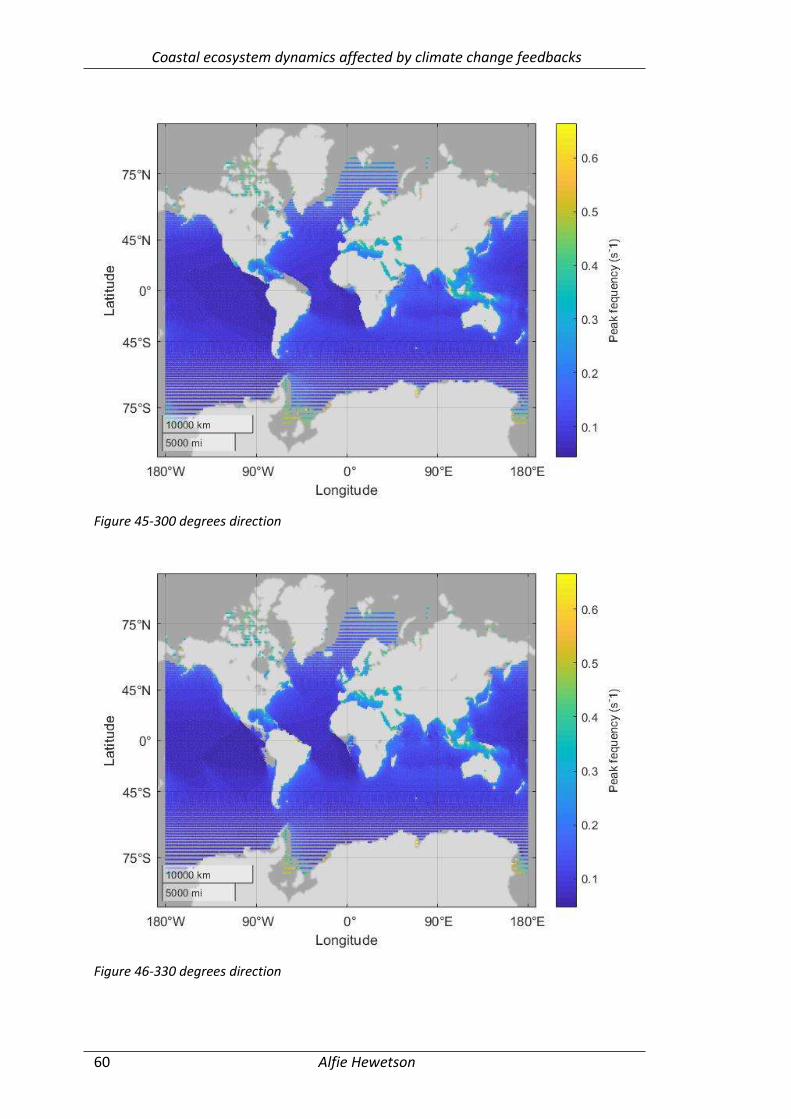
Coastal ecosystem dynamics affected by climate change feedbacks
Alfie Hewetson 60
Figure 45-300 degrees direction
Figure 46-330 degrees direction
Coastal ecosystem dynamics affected by climate change feedbacks
Alfie Hewetson 61
C MATLAB code used
Code is available by request to: [email protected]
• Wave_replace.m- converts the monthly time-series nc files into MATLAB
files.
• Wave_struct.m- converts the monthly time-series into a yearly time-series
• Wave_direction.m- uses the yearly timeseries and carries out the procedure
outlined in section 3.4 to find the 1 in 100 year significant wave height.
• Wave_freq.m- Then find the associated mean peak frequency for the 1 in 100
year significant wave heights, as outlined in section 3.4.
• Wave_grid.m- makes a grid for the wave data relative to an nd grid
• rerun.m- opens up the tif file of the topography data and converts it to a mat
file. It then changes the topography based on the closest point of storm/tide
surge to the new topography height.
• Frontal_area.m- applies [Ohira, 2013] to find the mangrove frontal area, as
described in section 2.3
• Mangrove_shorten.m-This reduces the entire shapefile from section 3.1 to
mangrove relative to 5degree by 5degree grids
• Var_change.m-Is used to select the tiles that are going to be used in the analysis
in this case Vietnam tiles it picks out the 3 tiles within that region
• Land_grid.m-Reads the tiles and finds each tiles centre point
• Land_coord.m- This takes the 6000 by 6000 topography grid and applies a
coordinate system to each cell within the topography grid.
• Flood_Mangrove_finalN_shorten.m- This is the overarching flooding code.
That takes the outputs from the previous codes in order to run. Require the
significant wave height grid, peak frequency grid, wave grid, topography grid,
mangrove location, mangrove frontal area and knowing the selected tiles. It
then runs the code onto the associated flood grid. Using the method in section
4.
Related Documents