Coastal and mesoscale dynamics characterization using altimetry and gliders: A case study in the Balearic Sea

Coastal and mesoscale dynamics characterization using altimetryand gliders: A case study in the Balearic Sea

Jérôme Bouffard,1 Ananda Pascual,1 Simón Ruiz,1 Yannice Faugère,2

and Joaquín Tintoré1,3

Received 29 December 2009; revised 9 June 2010; accepted 21 June 2010; published 13 October 2010.

[1] Dynamics along the continental slopes are difficult to observe given the widespectrum of temporal and spatial variability of physical processes which occur (coastalcurrents, meanders, eddies, etc.). Studying such complex dynamics requires thedevelopment of synergic approaches that use integrated observing systems. In this context,we present the results of an observational program conducted in the Balearic Seacombining coastal gliders and altimetry. The objectives of this experiment are to studyregional dynamics using new technologies, such as gliders, in synergy with satellitealtimetry and to investigate the limitations and potential improvement to altimetric datasets in the coastal zone. In this regard, new methodologies have been developed tocompute consistent altimetric and glider velocities, and a novel technique to estimateabsolute glider velocities, combining surface glider geostrophic velocities with integratedcurrents estimated from the glider GPS positioning, has been applied. In addition, thealtimetric velocity computation has been improved, especially in the coastal zone, usinghigh‐frequency along‐track sampling associated with new filtering and editing techniques.This approach proves efficient for homogenizing the physical contents of altimetry andglider surface currents (percentage of standard deviation explained is >40) andcharacterizing regional dynamics in the Balearic Sea through a combined analysis of ahigh‐resolution observing system, such as the appearance of anomalous intense mesoscalefeatures missing in the classical circulation scheme of the Balearic Sea.

Citation: Bouffard, J., A. Pascual, S. Ruiz, Y. Faugère, and J. Tintoré (2010), Coastal and mesoscale dynamics characterizationusing altimetry and gliders: A case study in the Balearic Sea, J. Geophys. Res., 115, C10029, doi:10.1029/2009JC006087.

1. Introduction

[2] New monitoring technologies are being progressivelyimplemented in coastal ocean observatories, increasing ourunderstanding of coastal and nearshore processes and con-tributing to a more science based and sustainable manage-ment of the coastal area.[3] By autonomously collecting high‐quality observations

in three dimensions, gliders allow high‐resolution oceano-graphic monitoring and provide useful contributions to theunderstanding of mesoscale dynamics [e.g., Hodges andFratantoni, 2009; Ruiz et al., 2009a] and multidisciplinaryinteractions that significantly affect upper ocean biogeo-chemical exchanges, an issue of worldwide relevance in thecontext of climate change. However, isolated measurementsfrom fleets of gliders are not sufficient as, for many pro-cesses, glider measurements remain scarce, both in space

and time. Instead, a multisensor approach that combines insitu and remote‐sensing measurements should provide abetter understanding of observed features, especially throughan increase of space‐time coverage. This is one of the keyconclusions and recommendations reached during the recentOceanObs09 Conference.[4] To properly address the new scientific challenges asso-

ciated with the coastal marine variability (including physical,biogeochemical, and ecosystem variations), an intensiveobservational program has been conducted in the BalearicSea (western Mediterranean), in particular aiming at com-bining coastal glider and satellite altimetry data. The phys-ical content of the two data sets and their potential synergyand limitations in the coastal domain have been explored.Four glider missions have been used, carried out from July2007 to June 2008. These missions were approximatelysimultaneous and well colocalized with Envisat satellite pas-sages whose measurements are almost perpendicular to themain Balearic oceanographic features (see Figure 1). TheBalearic subbasin is a region of worldwide interest charac-terized by both permanent and variable signals, covering awide range of dynamical scales from intense mesoscale (interms of filaments, eddies, or shelf‐slope flow modifications)to seasonal and interannual variability. The main Balearic

1Marine Technologies, Operational Oceanography, and SustainabilityDepartment, Mediterranean Institute for Advanced Studies, Mallorca,Spain.

2CLS Space Oceanography Division, Ramonville, France.3Also at Balearic Islands Coastal Observatory System, Mallorca, Spain.

Copyright 2010 by the American Geophysical Union.0148‐0227/10/2009JC006087

JOURNAL OF GEOPHYSICAL RESEARCH, VOL. 115, C10029, doi:10.1029/2009JC006087, 2010

C10029 1 of 17

oceanographic features share the results of process interac-tions at basin, subbasin, and local scales. Thermohalineadjustments take place over the western Mediterranean Seaand govern the eastward and northeastward spreading ofAtlantic Water (AW) inflowing through Gibraltar Strait.This flow can reach the Balearic Islands, therefore influ-encing north and south heat transport and exchanges thatappear to have key relevance to upper level ecosystem vari-ability and fisheries.[5] The general surface circulation of the Balearic Sea is

controlled by the presence of two fronts and their associatedcurrents [Font et al., 1988; Font, 1990; Pinot et al., 1994;Onken et al., 2008]. The Catalan front is a shelf‐slope frontthat separates old AW, in the centre of the Balearic subba-sin, from the less dense water transported by the NorthernCurrent (NC), which is also old AW but is fed into the Gulfof Lions and the Catalan shelves by fresh continental water.The NC flows southwestward along the continental slopeuntil it either exits the basin through the Ibiza Channel, orretroflects cyclonically over the insular slope forming theBalearic Current (BC; see Figure 1). The BC is also fed byrecent warm and fresh AW waters coming from the AlgerianBasin through the Mallorca and Ibiza channels. Both theNorthern and Balearic currents have widths of the order of50 km and are in good geostrophic balance, as winds onlyseem to produce transient perturbations in near‐inertialoscillations [Font, 1990]. In addition to the general basinscale circulation, the Balearic subbasin is also characterizedby frontal dynamics near the slope areas: Mesoscale eddies[Tintoré et al., 1990; Pinot et al., 2002; Rubio et al., 2009]as well as filaments and shelf‐slope flow modifications [La

Violette et al., 1990] have been found to modify, not onlythe local dynamics (significant vertical motion associated[Pascual et al., 2004]), but also the large scale patterns, asshown by Pascual et al. [2002] in a detailed study of theblocking effect of a large anti‐cyclonic eddy, as well asshowing a clear influence of basin circulation on phyto-plankton biomass [Jordi et al., 2009]. Seasonal frequencyobservations of the NC [Béthoux, 1980; Font et al., 1988]reveal higher transports in winter than in summer (1.5–2 Svand 1 Sv, respectively), while the opposite is found in theBC (0.3 Sv in winter compared with 0.6 Sv in summer).Regarding interannual variability, a recent study with along‐track satellite altimetry [Birol et al., 2010], has shown largeyear‐to‐year differences, suggesting complex non‐linearinteractions between basin scale and mesoscale circulations.[6] Several previous studies at the Balearic subbasin scale

have been done, however most were from observationalcruises carried out on the mainland side and focused on theNC or on the exchanges of water through the Balearicchannels; few experiments have been devoted to study the BCand its associated front. In a recent work, Ruiz et al. [2009b]provided the first positive insights concerning the use ofgliders in synergywith altimetry in order tomonitor dynamicsin semi‐enclosed basins such as the Balearic area. That papershowed reasonable qualitative agreements between absolutedynamic topography (ADT) from altimetry and dynamicheight (DH) derived from glider measurements. However,although the first results were encouraging, the study waslimited to only two glider missions over a relatively shortdistance (<90 km) that did not allow robust altimetry‐glidervelocity comparisons (especially in terms of velocity gra-

Figure 1. Location of Envisat track 773, bathymetry and main surface circulation characteristics of theBalearic subbasin (western Mediterranean) [modified from Pascual et al., 2004].

BOUFFARD ET AL.: SYNERGY BETWEEN ALTIMETRY AND GLIDER C10029C10029

2 of 17

dients in the coastal zone). Moreover, the use of a referencelevel at 180 m to compute glider DHz180 does not appear tototally satisfy the dynamical processes marked by a deepthermocline, such as eddies or coastal currents which mightbe expected in this area. In addition, some altimetric datanear the coast was missing, especially due to land contam-ination in the altimeter footprint and associated data elim-inations. This last issue suggested the need for specificalgorithms dedicated to coastal zone applications (e.g., alti-metric waveform retracking, dedicated quality control pro-cedure, etc.).[7] On the basis of these issues, new strategies have been

developed within the framework of this study in order tomore precisely characterize coastal and mesoscale dynamicsin terms of current velocity. The altimetric velocity com-putation has been improved, especially in the coastal zone,by associating high‐frequency along‐track sampling to newfiltering and editing techniques, and a new methodology hasbeen applied to estimate absolute glider velocities by usingvelocities derived from glider GPS positions, a comple-mentary and relevant variable not fully exploited in previousstudies. Thus, beside the main scientific objective of ourstudy, which consists at characterizing dynamical processesat regional and coastal scales, the two complementaryobjectives are to investigate limitations and potential im-provements to altimetric velocity computation in the coastalarea; and to develop and assess methods for future com-bining of glider and altimetry data sets by homogenizingtheir physical content.[8] To give an answer to the questions addressed, this

study is organized as follows: After a detailed presentationof the data sets used, we explain the strategies developed tocompute homogeneous altimetric and glider surface absolutegeostrophic currents (SAGC) with a special emphasis onerror budget evaluation. We then provide qualitative andquantitative cross validations between altimetric and glidercurrent velocity through four examples corresponding tocharacteristic dynamical events associated with the Baleariccurrent dynamical system. Finally, our conclusions aresummarized.

2. Data Sets and Variables Used

2.1. Sea Surface Height From Altimetry

[9] Altimetry allows a direct computation of geostrophicvelocity anomalies [e.g., Pascual et al., 2009, and referencestherein]; by adding the geostrophic mean currents derivedfrom a mean dynamic topography (MDT) [Rio et al., 2007],it is then possible to build SAGC. However, conventionalaltimetry measurements remain largely unusable in thecoastal zone [Anzenhofer et al., 1999; Volkov et al., 2007;

Bouffard et al., 2010] due to several factors such as inac-curate geophysical corrections (e.g., atmospheric and tidalsignals) as well as environmental issues (e.g., land con-tamination in altimetric and radiometric footprints). Atpresent, new coastal altimeter products are under develop-ment (COASTALT, PISTACH, X‐TRACK). Several stud-ies show that we can now be confident of such experimentaldata for scales greater than 20 km and up to 15 km far fromthe coast [Vignudelli et al., 2005; Bouffard et al., 2008,2010; Durand et al., 2008, 2010; Cipollini et al., 2010]. Themain developments involve the application of coastal‐oriented corrections and the review of the data recoverystrategies near the coast.[10] In this paper, we will specifically focus on the impact

of filtering and new editing strategies, combined with high‐frequency along‐track sampling. In this regard, we will usethree different altimetric data sets (see Table 1 for altimetricproduct characteristics): Two along‐track data (1 and 20 Hz)and a multisatellite gridded field, the map of sea levelanomalies (M)SLA.2.1.1. Along‐Track Data Sets[11] We used Envisat data sets provided by CLS

(Y. Faugère et al., personal communication, 2009) for track773, cycles 59, 63, 67, and 69 being associated with the datesof passage of the satellite of 8 July 2007, 25 November 2007,13 April 2008, and 22 June 2008 respectively. These arealmost simultaneous with the glider missions; in each casethere is a temporal lag of less than 1 week.[12] The processing of altimeter data used here is similar

to the one described in the “Ssalto/Duacs User Handbook”[Ssalto/Duacs, 2006]. The only differences were the sam-pling, editing, and filtering of the along‐track data. The seasurface height (SSH) built from ocean retracking (seeEnvisat RA2‐MWR Handbook, 2007, http://envisat.esa.int/handbooks/ra2‐mwr/) is corrected for path delay effects(wet and dry troposphere, ionosphere, etc.) (see Le Traonand Ogor [1998] and Le Traon and Ogor [2003] fordetails) and for geophysical effects. The tide model used isGOT00.2 (based on spectral analysis of tide gauge and alti-metric signals) [Ray, 1998]. The barotropic response of theocean to atmospheric pressure forcing and wind effects ismodeled by a correction based on a combination of theclassical inverse barometer (IB) correction for low frequen-cies (lower than 1/20 day−1) and the Modèle aux Ondes deGravité 2‐dimensions (MOG2D) [Carrère and Lyard, 2003]for higher frequencies.[13] The data are sampled every 350 m (for 20 Hz data) or

resampled every 7 km (for 1 Hz data) along the tracks usingcubic splines. A mean profile, <SSH>, is removed from theindividual SSH measurements, yielding sea level anomaly(SLA) values. The mean profile contains the geoid signal

Table 1. Altimetric Product Characteristics

Products Resolution Spatial Filtering Editing Time Sampling

Along‐track 1 Hz SLAc Envisat track 773 ∼7 km 20 kma Newb 35 days InstantaneousAlong‐track 20 Hz SLA Envisat track 773 ∼0.350 km 20 km Newb 35 days InstantaneousGridded field ((M)SLA)d Multimissions 1/8° >42 km Standard 7 days Time‐averaged

aForty‐two kilometers in Ruiz et al. [2009a].bSee section 3.1.1.cSea level anomaly, SLA.dMap of sea level anomaly, (M)SLA.

BOUFFARD ET AL.: SYNERGY BETWEEN ALTIMETRY AND GLIDER C10029C10029

3 of 17

and the mean dynamic topography over a 7 year averagingperiod (1993–1999).[14] A key aspect of our data processing is the editing,

that is to say, the method of selecting good altimetric dataover corrupted data (see section 3.1.1). In official standardproducts, for example that of Ruiz et al. [2009b], theremaining measurement noise is reduced by applyingLanczos cutoff and median filters for a 42 km window to the1 Hz SLA. That 42 km filter could, however, generate toomuch smoothing of the SLA, given the spatial scales asso-ciated with coastal dynamics (first Rossby radius of ∼14 kmin the Mediterranean Sea) [Robinson et al., 2001]. More-over, the small length of glider cruises associated with thiswindow size could entail predominant edge effects along thewhole track (see section 3.1.3).2.1.2. Gridded Field Product[15] Multisatellite AVISO (M)SLA are also used. The

corrected along‐track SSH obtained for each mission(Jason‐1 and Envisat for the period analyzed in this study)have been inter‐calibrated with a global crossover adjust-ment of the Envisat data using Jason‐1 data as a reference[Le Traon and Ogor, 1998]. The mapping method to produce(M)SLA from along‐track data is detailed in Le Traon et al.[2003] and consists of a suboptimal space‐time objectiveanalysis that takes into account along‐track correlated errors.The products used in this study are specific for the Medi-terranean Sea. For information on resolution, correlationscales, andmeasurement noise seePujol and Larnicol [2005].[16] For each set of SLA (1 Hz, 20 Hz, and (M)SLA), a

mean dynamic topography (MDT) has been added in orderto obtain the ADT. Here, we use a regional MDT of theMediterranean Sea, as described byRio et al. [2007], resultingfrom a combination of model outputs, drifting buoys, andaltimeter data. This MDT was built to be compatible withaltimetry, i.e., it represents a MDT averaged over the sameperiod (1993–1999) as the temporal mean that is removed tocompute SLA.

2.2. Data From Gliders

[17] We used data from repeated glider surveys in theBalearic Sea conducted between July 2007 and June 2008(see Table 2 for details). Gliders are autonomous underwatervehicles providing high‐resolution hydrographic and bio-geochemical measurements. These vehicles control theirbuoyancy to allow vertical motion in the water column andmake use of their hydrodynamic shape and small fins toinduce horizontal motions. The platform used in this study isa Teledyne Webb Research Slocum Electric glider forshallow water (200 m maximum depth) with a net horizontalspeed of ∼25 km/d, which takes into account data trans-mission when the glider is at the surface, once every 6 hoursin this type of survey.

[18] In all of the missions, the glider operated betweensurface and 180 m. During the first surveys in 2007, onlydowncasts were collected whereas for the missions in 2008both downcasts and upcasts were registered, obtaining spatialresolutions of ∼600 and ∼300 m, respectively. However, asshown in Table 2, spatial resolution is not a constant valueas it depends on how the glider is ballasted as well as on thepresence of intense currents. Glider conductivity‐temperature‐depth (CTD) profiles were processed and calibrated againstindependent CTD casts from the SeaBird‐19 probe installedon the Mediterranean Institute for Advanced Studies(IMEDEA) ship. Profiles extracted from glider data werecorrected for thermal lag using the recursive filter introducedby Lueck and Picklo [1990] and Morison et al. [1994]. Thefinal profiles were vertically averaged into 1 m bins.[19] Surface geostrophic currents can be estimated from

the glider surface DH (obtained from temperature andsalinity fields) with respect to an arbitrary reference levelwhich is in general considered to be at the maximum depthof the glider measurements (here 180 m). This implies thatgeostrophic velocities at this reference level are negligible,which is not always a correct assumption as many dynam-ical features usually have a deeper extension. However,depth averaged absolute currents can also be retrieved fromGPS glider positioning, which gives one reference velocityvector for every ∼7 km at every glider surfacing. The atti-tude sensor of the platform and the angle of attack canintroduce an associated error in the cross‐ and along‐trackestimates of depth averaged currents of about 2–3 cm/s[Merckelbach et al., 2008].

3. Absolute Sea Surface Geostrophic CurrentComputation

3.1. Absolute Surface Geostrophic Current FromAltimetry

3.1.1. Editing Procedure and Impact on the CoastalData Retrieval[20] The use of high‐frequency along‐track sampling

(20 Hz, ∼350 m) allows small scale dynamics, as present inthe northwestern Mediterranean, to be captured. However,this high‐resolution altimetric data is extremely noisy andmust be edited [see Bouffard et al., 2008]. In this study, thedetermination of altimetric outliers is based on the assump-tion that deviations of measurements from the mean valueshould vary spatially smoothly and follow a uniform distri-bution. Outliers can be detected when the deviations exceed apre‐determined range in the ranked deviation series. Wepropose here to use three times the standard deviation (3s) ofalong‐track SLA as the upper and lower limits to removemain residual outliers related to land contaminations. This 3sselection procedure is repeated 10 times (iterative process).

Table 2. Glider Cruise Characteristics: Dates, Total Length (Lineal and Real Distances) and Number of Profiles

Go Date Return DateTotal Cruise Lineal Distance

(Go + Return, km)Total Cruise Real Distance

(Go + Return, km)Mean Distance Between

Profiles (km) Total Profilesa

Jul 2007 06072007 13072007 176 188 0.71 269Nov 2007 23112007 30112007 88 107 0.54 201Apr 2008 07042008 23042008 318 388 0.30 1321Jun 2008 20062008 24062008 84 97 0.29 335

aDuring the 2007 missions, only downcasts were collected, whereas for the missions in 2008, both downcasts and upcasts were collected.

BOUFFARD ET AL.: SYNERGY BETWEEN ALTIMETRY AND GLIDER C10029C10029

4 of 17

The edited along‐track SLA are then spatially low‐pass (LP)filtered using a 20 km Loess filter [Cleveland and Devlin,1988]. This quality control procedure is applied to the20 Hz (or 1 Hz) fully corrected along‐track data (see Figure 2).[21] Our editing strategy has no impact on the 1 Hz data

(data are pre‐edited, for more details refer to section 4 ofthe Envisat RA2/MWR ocean data validation and cross‐calibration activities, yearly report 2008, http://www.aviso.oceanobs.com/fileadmin/documents/calval/validation_report/EN/annual_report_en_2008.pdf). The data selection,however, impacts on the 20 Hz along‐track altimetric SLAeliminating efficiently land‐contaminated data from 2%–15% of the 20 Hz original data set, especially in the 20 kmcoastal band (see triangles in Figure 3, right).[22] In general, in the 50 km coastal band, data close to

the coast are more likely to be eliminated by the editingprocedure because altimeter and on‐board radiometer foot-prints may encounter land. Apart from November 2007,where only few data points are eliminated along the wholetrack (<2%), more than 25% (65% in July 2007) of theoriginal data are excluded at 21–28 km distances from thecoast (see Figure 3, left). Despite data eliminations by ourediting procedure, Table 3 shows that the 20 Hz samplingallows us to recover more data than the 1 Hz data in closeproximity to the coast; between 6 and 13 km closer to thecoast by recovering 10 points measurements between thelast 1 Hz available data and the coastline and by applyingthe 3 s statistical criterion to more data (20 times more thanat 1 Hz).3.1.2. From Sea Level Anomaly to Surface AbsoluteGeostrophic Current[23] The across‐track SAGC is calculated by adding the

interpolated MDT to the edited and filtered SLA (seesection 3.1.1 and Figure 2). By construction, this current isperpendicular to the satellite track, so in our case it is almostparallel to the Balearic and Iberic shelf break (see Figure 1)which should allow us to intercept the main components ofdynamics related to BC and NC.

[24] The across‐track altimetric SAGC is given by

Vgabs ¼ g

f

@ SLA0 þMDT

� �

@x; ð1Þ

where g is the gravitational acceleration, f is the Coriolisparameter, x is the axis set along the track direction, SLA′ isthe residual filtered sea level anomaly (from both edited1 and 20 Hz data) and MDT is the mean dynamic topog-raphy [from Rio et al., 2007].[25] The along‐track altimetric gradient is estimated by

using the optimal filter developed by Powell and Leben[2004] with a spatial frame of 20 km. In the next sections,even if not precise, the computed altimetric SAGC corre-sponds to components that are perpendicular to Envisattrack 773.3.1.3. Sensitivity to Altimetric Noise[26] Very few studies have analyzed the noise content of

20 Hz altimetric SLA. Recent comparisons between 20 Hzaltimetric SLA and tide gauges in the western MediterraneanSea indicate that 20 Hz altimeter measurement errors rangefrom 2 to 5 cm, mainly depending on the data editing andsmoothing process [Bouffard et al., 2008, 2010].[27] Here, a Monte Carlo procedure is employed in order

to test the sensitivity of the SAGC computations to anyremaining noise in the 20 Hz edited SLA. To perform theMonte Carlo simulation, an artificial data set was created byadding Gaussian random noise with zero mean to the orig-inal SLA. Here, for 20 Hz altimetric signals (before thespatial filtering), the spatial standard deviation (STD) noiselevel is set at 5 cm (which approximately corresponds to thespatial STD of the edited 20 Hz SLA for the missions used).The resulting corrupted SLA was used to generate new esti-mates of the SAGC following the methodology described inFigure 2. A total of 10,000 Monte Carlo simulations werecarried out for each of the four missions.[28] For the missions of July 2007, November 2007, April

2008, and June 2008 the spatial mean of the STD difference

Figure 2. Altimetric surface absolute geostrophic current (SAGC) processing scheme.

BOUFFARD ET AL.: SYNERGY BETWEEN ALTIMETRY AND GLIDER C10029C10029

5 of 17

Figure 3. (left) Percentage of raw 20 Hz altimetric data eliminated (black histograms) and number oforiginal data (shaded curve) as functions of distance to the coast (by 7 km class). (right) Sea level anomaly(SLA; 20 Hz, cm) as a function of latitude (°N) and corresponding impact of editing. Triangle, eliminatedSLA; shaded curve, edited SLA; black curve, edited and 20 km low‐pass (LP)‐filtered SLA.

BOUFFARD ET AL.: SYNERGY BETWEEN ALTIMETRY AND GLIDER C10029C10029

6 of 17

between signals a and b (STD(a‐b)) between uncorruptedand corrupted SAGC are 6.3, 9.5, 4.7, and 8.5 cm/s,respectively, while the mean differences are close to 0 cm/salong the whole transect (see Figure 4, shaded curve). Thismeans that the SLA noise impacts the SAGC gradient butnot its spatial average. The differences of mean STD errorsas a function of missions are mainly due to the length oftrack used (see Table 2) and the relative weight of edgeeffects used to determine the averaged errors along the wholetrack. Thus, the longer the mission, the lower the averagedSTD error. Figure 4 shows an example of the Monte Carlosimulation for the mission of April 2008.[29] As shown in Figure 4 (black curve), outside of the

20 km edge of the track (i.e., the window used both for theLP Loess filtering and slope calculations), the Monte CarloSTD are less than 5 cm/s whereas in the first and last 20 kmof the track, the associated errors increase and becomehigher than 10 cm/s because of edge effects. This suggeststhat only missions of sufficient length (i.e., >40 km as in theJuly 2007 and April 2008 missions) can be used to effi-ciently assess the gradient of across‐track SAGC withrespect to the geostrophic velocities computed from glider.

The other missions, November 2007 and June 2008, havetoo short a length for gradient SAGC comparisons; how-ever, they can be used to assess the mean SAGC.[30] In summary, when we look at the whole mission, the

averaged error due to the altimetric noise is about 0 cm/salong the whole track, whereas the associated STD errorsare between 4 cm/s (>20 km from the coast) and 10 cm/s(within 20 km of coast). These error values are of the sameorder of magnitude as the STD differences that Vignudelliet al. [2005] (respectively, Bouffard et al. [2008]) found byperforming a direct comparison in the Corsica Channelbetween improved along‐track TOPEX/Poseidon‐derived(respectively, improved multisatellite‐derived) velocities andmooring velocity anomalies.3.1.4. Impact of Sampling and Editing on the VelocityComputation[31] As shown previously, the geostrophic slope calcula-

tion is sensitive to the SLA noise, especially in the coastalzone. This indicates the crucial importance of SLA editingbefore SAGC computation. Figure 5 clearly shows the impactof this editing on altimetric velocities for the missions ofJuly 2007 and April 2008.[32] From Figure 5 it appears that the SLA editing has a

strong influence on the SAGC computation, especially withina 50 km coastal zone (Figure 5, dashed boxes). Indeed whenthe editing procedure is not applied, the resulting coastalSAGC values are unrealistically large in July 2007 (>80 cm/s).In April 2008, the editing also entails deep modifications inthe coastal area where the SAGC values derived from editedSLA are about 15 cm/s. Beyond a 50 km coastal band, theediting has less influence as less data are eliminated (seesection 3.1.1).

Table 3. Distance From the Coast to the Closest Valid AltimetricMeasurements for Each Missiona

Jul 2007 Nov 2007 Apr 2008 Jun 2008

1 Hz 34.2 27.2 20.3 26.820 Hz 20.6 20.0 12.8 14.720 Hz + editing 21.4 20.0 14.1 16.4

aDistances in km.

Figure 4. Errors (cm/s) obtained from Monte Carlo simulation as a function of latitude (°N), for the mis-sion of April 2008. Shaded curve, average error; black curve, standard deviation (STD) error. The dashedorange rectangles indicate areas where the STD error is greater.

BOUFFARD ET AL.: SYNERGY BETWEEN ALTIMETRY AND GLIDER C10029C10029

7 of 17

[33] When comparing with velocities computed from 1 HzSLA, significant differences are also observed. In July 2007,the 1 Hz SAGC are very low in the 50 km coastal zonewhereas a relative strong current (between 10 and 20 cm/s)is observed by using the 20 Hz edited data. In April 2008,differences are also observed in the neighborhood of the BCwhere the 1 Hz SAGC exhibits a current 5 cm/s less thanthat from edited 20 Hz data. This is also the case between40.1°N and 40.4°N.[34] In section 3.2, a direct comparison with glider calcu-

lated velocities provides robust insights about the respectiveperformance of these different along‐track altimetric datasets.

3.2. Absolute Surface Geostrophic Velocity FromGlider Data

3.2.1. General Methodology and Reference Level Issue[35] Ruiz et al. [2009b] used a reference depth level of

180 m to estimate DHz180 from glider data and obtainedcoherent glider geostrophic velocities flowing northeastwardalong the north Mallorca coast. For specific events, velocityestimates from 42 km smoothed DHz180 appeared to be notvery sensitive to the test reference level, seeming to indicatethat the layer between 200 and the bottom does not play akey role in the dynamics of the upper layer. However, oncloser consideration, small differences in DHz180 gradientsentail significant modifications in the geostrophic velocitypattern and magnitude. For this reason, a more robuststrategy has been developed in this study. This strategy aimsat solving the reference level issue by combining gliderCTD current (Vgz180: cross‐track geostrophic component ofthe baroclinic current relative to 180 m), glider GPS current(Vabs: 180 m depth average absolute current), and modeloutputs. Figure 6 shows the scheme used to process gliderSAGC.[36] At each vertical level z, Vgz180 is derived from the

DHz180 using an optimal filter as described by Powell andLeben [2004] (as used in the altimetry data). Then, the

difference between the 180 m depth average Vgz180 and Vabs

should correspond to the absolute velocity at 180 m. Byadding a reference level correction (RLC, Vabs − Vgz180 ) toVgz = 0180 at the surface, we should therefore be able tocompute the glider SAGC.[37] However, these two averaged velocities do not have

exactly the same physical content. Whereas Vabs is influ-enced by the whole depth averaged dynamical components,including ageostrophy, high‐frequency barotropic signals,cyclostrophy, and inertial current, Vgz180 is only the result ofthe baroclinic geostrophy contribution. Therefore, Vabs

needs to be partially corrected by using modeled high fre-quency geophysical corrections (HFGC, MOG2D + Ekmancurrents).3.2.2. High‐Frequency Geophysical Corrections(HFGC)3.2.2.1. Ageostrophic Ekman Effects[38] The Ekman current is the motion induced by the wind

according to the theory of Ekman [1905] and should rep-resent one of the main ageostrophic contributions includedin Vabs but which is missing in Vgz180. In this study, an Ekmancomponent has been estimated following the method ofPoulain et al. [2009]. The wind data used are from Sea-Winds on QuikSCAT Level 2B Ocean Wind Vectors in25 km Swath Grid (http://cersat.ifremer.fr/fr/data/discovery/by_parameter/ocean_wind/quikscat_l2b). To remove the veryhigh frequency signals, which have no impact on the Ekmanoceanic motion, the data have been filtered with a low‐passfilter at a 36 hours cutoff frequency. Given that the angle �between the wind and surface motion (in theory p/4) andEkman depth D strongly depend on location and time [Rioand Hernandez, 2003], we therefore evaluate those para-meters by using three drifters launched over the Balearic Sea.We found values of � = 24° and averaged depth D = 36 m,which are in agreement with past studies of theMediterraneanSea [see Ursella et al., 2006; Poulain et al., 2009]. TheEkman current was then validated with independent driftervelocities [Escudier, 2009], 180 m depth averaged (assuming

Figure 5. Altimetric across‐track surface absolute geostrophic current (SAGC; cm/s) as a function oflatitude (°N) derived from 1 Hz (pink thin curve), raw 20 Hz (shaded thick curve), and edited 20 HzSLA (red thick curve) in (left) July 2007 and (right) April 2008. Areas with major differences are locatedinside the orange dashed boxes.

BOUFFARD ET AL.: SYNERGY BETWEEN ALTIMETRY AND GLIDER C10029C10029

8 of 17

the theoretical spiral in the Ekman layer and approximating to0 cm/s below), space‐time interpolated at glider positions,and removed from Vabs.3.2.2.2. Barotropic High‐Frequency Current[39] Barotropic currents induced by high‐frequency

atmospheric forcing are not included in Vgz180 and, in theory,have also to be removed from Vabs (see Figure 6). For this,we use a correction of the ocean response to atmosphericwind and pressure forcing from the MOG2D finite elementbarotropic model [Carrère and Lyard, 2003] for high fre-quencies (i.e., <20 days), and an IB correction for lowerfrequencies. The model is forced by surface atmosphericpressure and wind from European Centre for Medium‐Range Weather Forecasts analysis. Barotropic currents areprovided on a regular grid of 0.25° × 0.25° every 6 hoursand space‐time interpolated at glider positions.

4. Dynamical Structures Observed

4.1. Surface Patterns and Associated VerticalStructures

[40] In this section, surface patterns (from remote sensing)are qualitatively compared to the vertical structures (fromglider). We use both Vabs, sea surface temperature (SST),SAGC derived from (M)SLA, and glider baroclinic geo-strophic velocities derived from single CTD measurements(Vgz180) projected onto the Envisat‐altimetric track 773position. Figure 7 shows an example of the combined use ofremote sensing and a glider when observing dynamics in ourstudy area during the “go” glider transect (northward). Forthe missions of July 2007, November 2007, and June 2008(respectively, April 2008), the glider cruise began approxi-mately 3 days (respectively, 7 days) before the Envisatpassage and crossed several dynamical patterns where sig-nificant across‐track surface currents were observed (seeFigure 7).[41] In July 2007, the glider intercepts the BC in the

coastal Balearic zone (Figure 7a). Farther north, the remote

sensed SST data shows a marked thermal front correspondingto the Catalan front and an associated south border of the NCis seen. In addition, between these two major dynamicalpatterns an eddy is also observed in the velocities. Thesouthwestern branch of this eddy is almost parallel to theglider position which means that the associated across‐trackvelocity would not be clearly seen by the glider. This isconfirmed when we look at the glider transect where, out ofthe BC, the across‐track velocity is low. It also appears thatthe BC, which borders the coast of Mallorca, is enlarged byabout 40 km large and marked by a significant velocity in thefirst 50 m depth (double that at 100 m).[42] Figure 7b shows that the general situation in

November 2007 is close to the one observed in July 2007.The SST also shows a marked Catalan front in the northassociated with the NC cooling. In the south, the BC isfurther away from the coast (about 10 km). A current loop,which extends at 60 km from the Mallorca coast, is clearlyobserved in both SST and SAGC velocity. This loop joinsthe western branch of an eddy based north of the BC.Unfortunately, the length of the glider cruise does not allowus to capture the vertical structure of this eddy. When welook at the glider transect it can be seen that the BC surfaceintensity is approximately double that of July 2007, more-over the current has a deeper expression extending to ∼100m.The computed velocities from remote sensing, indicate thatthe BC flows at distance higher than 10 km to the Mallorcacoast whereas it was close along the coast in July 2007, whichis also confirmed by Vabs.[43] In April 2008, the general circulation characteristics

are quite different (compare Figure 7c). The SST imageshows a marked Balearic front whereas the Catalan front ismuch weaker. Moreover, the glider cruise intercepts threemajor dynamical structures: the BC in the south, the NC inthe north, and an eddy in between. The across‐trackvelocities associated with these features appear clearly bothat surface and along the whole 180 m water column in theglider CTD and GPS measurements. The velocities associ-

Figure 6. Glider surface absolute geostrophic current (SAGC) processing scheme.

BOUFFARD ET AL.: SYNERGY BETWEEN ALTIMETRY AND GLIDER C10029C10029

9 of 17

Figure 7

BOUFFARD ET AL.: SYNERGY BETWEEN ALTIMETRY AND GLIDER C10029C10029

10 of 17

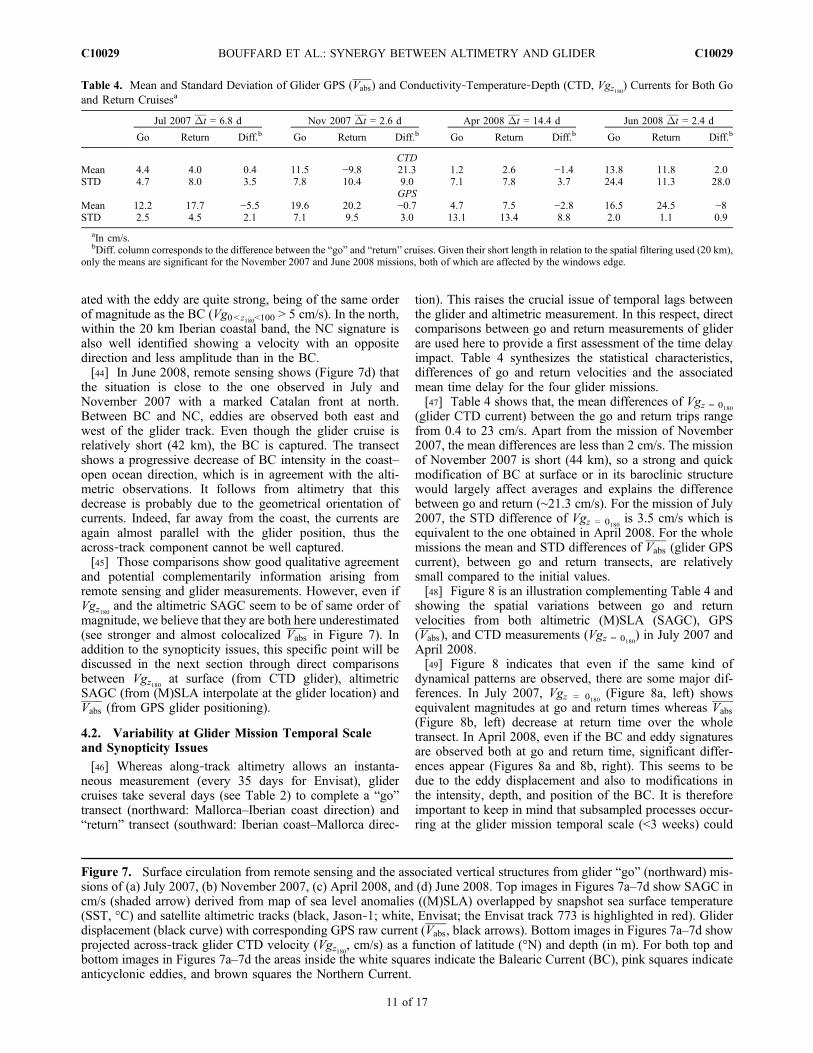
ated with the eddy are quite strong, being of the same orderof magnitude as the BC (Vg0< z180<100 > 5 cm/s). In the north,within the 20 km Iberian coastal band, the NC signature isalso well identified showing a velocity with an oppositedirection and less amplitude than in the BC.[44] In June 2008, remote sensing shows (Figure 7d) that

the situation is close to the one observed in July andNovember 2007 with a marked Catalan front at north.Between BC and NC, eddies are observed both east andwest of the glider track. Even though the glider cruise isrelatively short (42 km), the BC is captured. The transectshows a progressive decrease of BC intensity in the coast–open ocean direction, which is in agreement with the alti-metric observations. It follows from altimetry that thisdecrease is probably due to the geometrical orientation ofcurrents. Indeed, far away from the coast, the currents areagain almost parallel with the glider position, thus theacross‐track component cannot be well captured.[45] Those comparisons show good qualitative agreement

and potential complementarily information arising fromremote sensing and glider measurements. However, even ifVgz180 and the altimetric SAGC seem to be of same order ofmagnitude, we believe that they are both here underestimated(see stronger and almost colocalized Vabs in Figure 7). Inaddition to the synopticity issues, this specific point will bediscussed in the next section through direct comparisonsbetween Vgz180 at surface (from CTD glider), altimetricSAGC (from (M)SLA interpolate at the glider location) andVabs (from GPS glider positioning).

4.2. Variability at Glider Mission Temporal Scaleand Synopticity Issues

[46] Whereas along‐track altimetry allows an instanta-neous measurement (every 35 days for Envisat), glidercruises take several days (see Table 2) to complete a “go”transect (northward: Mallorca–Iberian coast direction) and“return” transect (southward: Iberian coast–Mallorca direc-

tion). This raises the crucial issue of temporal lags betweenthe glider and altimetric measurement. In this respect, directcomparisons between go and return measurements of gliderare used here to provide a first assessment of the time delayimpact. Table 4 synthesizes the statistical characteristics,differences of go and return velocities and the associatedmean time delay for the four glider missions.[47] Table 4 shows that, the mean differences of Vgz = 0180

(glider CTD current) between the go and return trips rangefrom 0.4 to 23 cm/s. Apart from the mission of November2007, the mean differences are less than 2 cm/s. The missionof November 2007 is short (44 km), so a strong and quickmodification of BC at surface or in its baroclinic structurewould largely affect averages and explains the differencebetween go and return (∼21.3 cm/s). For the mission of July2007, the STD difference of Vgz = 0180 is 3.5 cm/s which isequivalent to the one obtained in April 2008. For the wholemissions the mean and STD differences of Vabs (glider GPScurrent), between go and return transects, are relativelysmall compared to the initial values.[48] Figure 8 is an illustration complementing Table 4 and

showing the spatial variations between go and returnvelocities from both altimetric (M)SLA (SAGC), GPS(Vabs), and CTD measurements (Vgz = 0180) in July 2007 andApril 2008.[49] Figure 8 indicates that even if the same kind of

dynamical patterns are observed, there are some major dif-ferences. In July 2007, Vgz = 0180 (Figure 8a, left) showsequivalent magnitudes at go and return times whereas Vabs

(Figure 8b, left) decrease at return time over the wholetransect. In April 2008, even if the BC and eddy signaturesare observed both at go and return time, significant differ-ences appear (Figures 8a and 8b, right). This seems to bedue to the eddy displacement and also to modifications inthe intensity, depth, and position of the BC. It is thereforeimportant to keep in mind that subsampled processes occur-ring at the glider mission temporal scale (<3 weeks) could

Table 4. Mean and Standard Deviation of Glider GPS (Vabs) and Conductivity‐Temperature‐Depth (CTD, Vgz180) Currents for Both Goand Return Cruisesa

Jul 2007 Dt = 6.8 d Nov 2007 Dt = 2.6 d Apr 2008 Dt = 14.4 d Jun 2008 Dt = 2.4 d

Go Return Diff.b Go Return Diff.b Go Return Diff.b Go Return Diff.b

CTDMean 4.4 4.0 0.4 11.5 −9.8 21.3 1.2 2.6 −1.4 13.8 11.8 2.0STD 4.7 8.0 3.5 7.8 10.4 9.0 7.1 7.8 3.7 24.4 11.3 28.0

GPSMean 12.2 17.7 −5.5 19.6 20.2 −0.7 4.7 7.5 −2.8 16.5 24.5 −8STD 2.5 4.5 2.1 7.1 9.5 3.0 13.1 13.4 8.8 2.0 1.1 0.9

aIn cm/s.bDiff. column corresponds to the difference between the “go” and “return” cruises. Given their short length in relation to the spatial filtering used (20 km),

only the means are significant for the November 2007 and June 2008 missions, both of which are affected by the windows edge.

Figure 7. Surface circulation from remote sensing and the associated vertical structures from glider “go” (northward) mis-sions of (a) July 2007, (b) November 2007, (c) April 2008, and (d) June 2008. Top images in Figures 7a–7d show SAGC incm/s (shaded arrow) derived from map of sea level anomalies ((M)SLA) overlapped by snapshot sea surface temperature(SST, °C) and satellite altimetric tracks (black, Jason‐1; white, Envisat; the Envisat track 773 is highlighted in red). Gliderdisplacement (black curve) with corresponding GPS raw current (Vabs, black arrows). Bottom images in Figures 7a–7d showprojected across‐track glider CTD velocity (Vgz180, cm/s) as a function of latitude (°N) and depth (in m). For both top andbottom images in Figures 7a–7d the areas inside the white squares indicate the Balearic Current (BC), pink squares indicateanticyclonic eddies, and brown squares the Northern Current.

BOUFFARD ET AL.: SYNERGY BETWEEN ALTIMETRY AND GLIDER C10029C10029

11 of 17

Figure 8. LP‐filtered 20 km across‐track currents (cm/s) interpolated at the Envisat track location in(left) July 2007 and (right) April 2008 as a function of latitude (°N) for both for “go” (thin curves)and “return” (southward; thick curves) missions: (a) surface glider CTD current (Vgz = 0180, blue curves),(b) glider GPS current (Vabs, black curves), (c) altimetric across‐track SAGC derived from (M)SLA(brown curve), with time interpolated at glider passage.

BOUFFARD ET AL.: SYNERGY BETWEEN ALTIMETRY AND GLIDER C10029C10029

12 of 17

potentially affect the comparison between glider and along‐track altimetry in section 5. They can also be the consequenceof inexact colocalization between the two passages. In addi-tion to high‐frequency 3D processes, the differences couldalso have several causes that are difficult to distinguish suchas error in glider measurements, especially concerning posi-tioning at surface during data transmission or from attitudesensors providing glider heading, pitch and roll (seeMerckelbach et al. [2008] for technical details). For the alti-metric SAGC derived from (M)SLA (Figure 8c) no signifi-cant differences are observed between go and returnmissions,certainly because of the temporal smoothing effect due to theoptimal interpolation (OI; 7 day windows) procedure.[50] The altimetric SAGC from (M)SLA show a satis-

factory agreement with Vgz = 0180 and Vabs for the July 2007and April 2008 missions except in the 40 km coastal bandwhere the altimetric SAGC shows weaker gradients andamplitudes. Moreover, the magnitude of Vabs appear to besignificantly stronger (>30%) compared to both Vgz = 0180and altimetric SAGC. There are several hypotheses that canexplain these discrepancies; they will be discussed in thenext section through the assessment of our new glider andaltimetry SAGC processing. In addition to physical contentnonhomogeneity and errors related to Vabs, differencesobserved between Vgz = 0180 and Vabs could result froma reference level issue (issue specifically addressed insection 5.1.1). Concerning, the observed underestimation ofaltimetry SAGC toward Vabs, it could be partially due tospatial smoothing. Indeed, (M)SLA has been smoothedthrough an OI procedure which uses a correlation lengthscale of 100 km. Moreover, before OI, the altimetric along‐track data (refer to the track positions in Figure 7) has beenlow‐pass filtered with a cutoff of 42 km. This is why, in thenext sections, we will compute altimetric SAGC directlyfrom along‐track data following the methodologies describedin section 3.1. Impact of the MDT, spatial filtering, sam-pling, and editing will be evaluated by direct comparisonswith glider SAGC.

5. Cross‐Validation of Along‐Track Altimetryand Glider Velocities

5.1. Assessment of the Glider Velocity Processing

5.1.1. Impact of the Reference Level Correction[51] Figure 9 shows comparisons between altimetric (built

from 20 and 1 Hz edited along‐track data) and temporalinterpolated glider SAGC (using go and return transects) forthe missions of July 2007 and April 2008 with and withoutthe application of RLC (impact of HFGC is very small hereand thus will be discussed independently in section 5.1.2).[52] From Figures 9a and 9b it follows that there is a very

good coherency between glider and altimetric velocities,coherency that is better than the observed with (M)SLA inthe previous section. The signals are very well phased bothwith and without the application of RLC.[53] In July 2007, a progressive decrease of velocity is

seen in the Mallorca coast–open ocean direction. Between40.0° and 40.2°N (i.e., inside the BC current), the glider andaltimetry curves show a very similar slope. After 40.2°N,the velocity increases slightly in altimetry data whereas thisis not the case with glider data. In April 2008, the BC is wellidentified. This current is associated with a relatively strong

velocity (>15 cm/s) which progressively decreases movingoffshore from the Mallorca coast. The anticyclonic eddy isobserved in the two data sets; this dynamical structure,which crosses the Envisat track, is centered at about 40.5°Nin latitude and its associated velocity is between −20 and20 cm/s (see Figures 9a and 9b).[54] Even if glider and altimetric velocity show a good

agreement, significant differences are observed if RLC isnot applied. In July 2007, the altimetric SAGC is strongerthan Vgz = 0180 (by 7.5 cm/s on average, see Figure 9a);however, the application of the RLC increases the meanglider velocity and therefore improves the agreement withaltimetry (mean difference of 3.5 cm/s, see Figure 9b).Moreover, the percentage of STD explained by glider inaltimetry becomes 75% with RLC application against 68%without RLC. In April 2008, the use of the RLC also im-proves significantly the agreement between glider andaltimetry by increasing the glider velocity magnitudes (STDof 6.9 cm/s without RLC against 14.9 cm/s with). Thepercentage of STD explained by glider SAGC in altimetricSAGC is thus again improved (47% with RLC against 6%without).[55] For missions of November 2007 and June 2008 the

length of missions are too short for statistical comparisonsof STD (see section 3.1.3). However, we can look at themean SAGC inside the BC. For June 2008, the RLC alsoallows significant increases in the agreement between gliderand altimetric SAGC with a mean difference of 17.4 cm/swithout RLC against 0.7 cm/s with RLC (for a mean currentof ∼30 cm/s). In November 2007, Vgz = 0180 shows a meanvelocity of 5 cm/s. If the RLC is added, the glider SAGCbecomes 25.5 cm/s, which is 13.9 cm/s more than foraltimetry. This difference could be due to high‐frequencydynamics not captured at the time of altimetric satellitepassage. Indeed the mean difference between the go andreturn glider cruise is large for this mission (see Table 4)which support this suggestion.[56] To sum up, the application of RLC enables the gen-

eral improvement of the agreement between the glider andaltimetry currents. However, it is important to note that forthe whole mission the glider SAGC magnitudes are strongerthan the altimetric ones. In addition to the combined effectsof different errors (such as residual coastal altimetry con-tamination, inaccuracy of the MDT, and compass error forgliders), the underestimation observed in altimetry could bepartially due to its inexact colocalization with the glider thatcan be influenced and partially advected by the strong cur-rents (see differences between lineal and total glider cruisedistances in Table 2). In April 2008, such differences areparticularly observed at the eddy location. There, the alti-metric SAGC underestimation could also come from thecyclostrophic acceleration, neglected in the geostrophicframework computation. This component, in the case of ananticyclonic eddy with the characteristics of the one studiedhere could be around 10%–20% of the geostrophic part ofthe velocity [Gomis et al., 2001].5.1.2. Impact of the High‐Frequency GeophysicalCorrection[57] The HFGC consists of the Ekman and MOG2D

velocities which have been interpolated spatially and tem-porally along the glider position measurements. Table 5summarizes their statistical characteristics for the missions

BOUFFARD ET AL.: SYNERGY BETWEEN ALTIMETRY AND GLIDER C10029C10029

13 of 17

Figure 9

BOUFFARD ET AL.: SYNERGY BETWEEN ALTIMETRY AND GLIDER C10029C10029

14 of 17

of July 2007 and April 2008 and highlights that both Ekmanand barotropic high‐frequency velocities are very small(subcentimetric) for the considered period.[58] The impact of HFGC is therefore marginal, especially

compared to the RLC (small for Ekman and negligible forMOG2D). Moreover, the Ekman and MOG2D velocities areless than the amplitude of errors associated with both gliderand altimetric velocity computations (problem of spatialsynopticity, noise, etc.). In this respect, even if the use ofHFGC is theoretically justified, the present comparisonbetween glider and altimetry does not allow us to evaluatequantitatively its impact. However, the small reduction of theglider and altimetric SAGCmean differences for all missions(between 0.3 and 0.6 cm/s) gives few positive insights.

5.2. Assessment of the Coastal Altimetric VelocityProcessing

[59] In the coastal zone, altimetric velocities are particu-larly affected by noise measurements (see section 3.1.3)while this is less the case for glider velocities. In this regard,the glider velocities are now used in order to evaluate theimpact of high‐frequency sampling combined with our edit-ing strategy in order to capture small scale coastal signatures.We will also briefly discuss the influence of MDT on glider‐altimetry comparisons.5.2.1. Impact of the MDT[60] Table 6 summarizes statistical comparisons of the

impact of the MDT in the glider and altimetric SAGCcomparisons and shows that when the velocity derived fromtheMDT is added to the altimetric surface geostrophic velocityanomaly, agreementwith the glider SAGC is improved. Indeedthe mean difference between the two velocities is stronglyreduced for all missions. This reduction is of ∼10 cm/s formissions of July 2007, November 2007, and June 2008 whileit is ∼2 cm/s for the mission of April 2008. Concerning theSTD, the use of MDT also enables a decrease in the STDdifference for the missions of July 2007 and April 2008.[61] The improvements in terms of mean difference show

that MDT performance is satisfactory for wavelengths

>40 km (approximately the length of the November 2007and June 2008 missions). The smaller spatial scale varia-tions cannot be correctly reproduced and thus well evaluatedin term of STD given the spatial smoothing and OI proce-dures used to build the MDT [cf. Rio et al., 2007].5.2.2. Impact of Sampling and Editing Strategy[62] In section 3.1.4, we highlighted that both editing

strategy and sampling play key roles in the altimetric velocitycalculation, especially in the coastal zone. From Figures 9band 9c, it follows that altimetric SAGC computed from edi-ted 20 Hz altimetric data shows better agreement with theglider SAGC thanwhen using 1Hz data. This is especially thecase in the 50 km coastal zone where a relative strong BC,observed by glider in July 2007, is also captured with 20 Hzdata but not seen with 1 Hz data, while out of this area it isinteresting to note that the 1 and 20 Hz velocities are con-sistent. In April 2008, 20 Hz along‐track data show SAGCclose to that observed by the gliders, the 1 Hz velocity alsoreproduces the BC in the coastal zone; however, the currentexhibits less amplitude than with the glider and 20 Hz data(10–20 cm/s less). The 1 Hz velocities seem also to under-estimate the eddy intensity between 40.1°N and 40.4°N,whereas the 20 Hz data shows a better agreement with theglider SAGC. When (M)SLA or standard 42 km smoothed1 Hz along‐track data are used for comparison with the gli-ders (not shown) the results are worse due to too much spatialsmoothing.[63] From these previous examples, it appears that the

20 Hz altimetric data associated with an adapted editingstrategy can recover more data close to the coast and alsoproduce better constraints on coastal altimetric SAGCcomputations.

6. Conclusions and Perspectives

[64] In the present study, we analyzed the compatibilitybetween glider and altimetry measurements in view ofdeveloping an integrated coastal observing system. Alti-metric data have been specifically processed to assess a newmethodology dedicated to glider SAGC computation. Thisapproach also provided interesting insights into the presentlimitations and potential improvements of coastal altimetry.The analysis was two‐way, using altimetry in support to theglider velocity processing and glider measurements in sup-port of coastal altimetric techniques. We believe that such anapproach is necessary before undertaking multisensor datafusions or applications aiming at a quantitative understandingof coastal physical processes.[65] As a first conclusion, we have shown that simple new

processing strategies allow us to generate glider and alti-metric SAGC with very good agreement (percentage of STDexplained >40% over spatial scales of 20 km). For the gliderdata set, the importance of the reference level and synopti-

Table 5. Ekman and Barotrophic Current Statistical CharacteristicsInterpolated (in Space and Time) at Go and Return Glider Positionsa

Jul 2007 Apr 2008

Go Return Go Return

EkmanMean 0.3 0.1 0.5 0.2STD 0.1 0.0 0.2 0.2

MOG2DMean 0.1 0.1 0.1 0.2STD 0.1 0.1 0.2 0.0

aIn cm/s.

Figure 9. Glider versus altimetric across‐track 20 km LP‐filtered currents (cm/s) for (left) July 2008 and (right) April 2008missions. From top to bottom: (a) altimetric SAGC derived from edited 20 Hz data (red curve) vs. surface glider CTD current(Vgz = 0180, thin blue curve), (b) SAGC derived from edited 20 Hz data (red curve) vs. glider SAGCwith application of referencelevel correction (RLC) and high‐frequency geophysical correction (HFGC; blue curve), (c) SAGC derived from 1 Hz data(thin pink curve) vs. glider SAGC with application of RLC and HFGC (blue curve).

BOUFFARD ET AL.: SYNERGY BETWEEN ALTIMETRY AND GLIDER C10029C10029

15 of 17

city issues, due to baroclinic short timescale signals, havebeen confirmed, whereas Ekman and the high‐frequencybarotropic component show marginal impacts in our casestudies. For altimetry, the use of MDT improve the spatialconsistency between the altimetric and glider SAGC despitea lack of spatial resolution that could entail an underesti-mation of the mean circulation. The use of edited 20 Hzrather than standard 1 Hz and (M)SLA altimetry allows us togo closer to the coast, to increase altimetry‐glider agreementand to keep physical signals otherwise eliminated. The mainbenefit of using 20 Hz data lies more in the greater qualitycontrol procedure possibilities with more data, than in spa-tial scale resolving, given that a 20 km LP filtering isapplied.[66] The combined use of altimetry and glider is promis-

ing, allowing observation of coherent general characteristicsof the circulation in the Balearic Sea both at the surface andfor the whole 180 m water column. High‐resolutionhydrographic fields from glider and altimetry have revealedthe presence of permanent BC and NC signals and non-permanent signals, such as the relatively strong anticycloniceddy intercepted in April 2008. The synoptic view fromremote sensing during the glider missions also suggested amore detailed picture of the mesoscale structures that mayplay a key role in the exchanges and transport of heat andother biogeochemical properties across the basin. The anti-cyclonic eddies observed during these missions confirm paststudies such as the work of Pascual et al. [2002]. This raisesthe need to quantify the recurrence of such structures that donot appear in the standard circulation scheme but that haveimpacts on the general circulation in the Mediterranean.Thus, the use of altimetry in combination with gliders couldplay a major role in revising the general pattern and bettercharacterizing the associated forcing of the Balearic Seacirculation.[67] As a general conclusion, this study highlights the

need for high‐resolution coastal measurements made pos-sible thought the development of synergic approaches andthe combined use of observing systems at several spatial/temporal scales. Future works could evaluate and comparevelocities derived from new coastal altimetric products(PISTACH, COASTALT, etc.) with glider velocities fol-lowing the approach described in this paper. On a longer term,the Surface Water and Ocean Topography (SWOT) missioncan provide very valuable information, complementary toin‐situ measurement, for monitoring mesoscale and sub-mesoscale coastal processes. In a more general framework,we believe that multisensor approaches, combining com-plementary in‐situ and remote sensing, will contribute to abetter understanding of physical and multidisciplinaryprocesses within the coastal domain. In combination withmodeling, multisensor data can significantly help to quantify

changes in coastal systems, to comprehend the mechanismsthat regulate them, and to forecast their evolution.

Notation

DHz180 dynamic height derived from the glider conductivity‐temperature‐depth (CTD) profile at depth = z meters(with a reference level at 180 m); also refer to Figure 6.

Vgabs surface absolute geostrophic current (SAGC).Vgz180 glider CTD current: cross‐track baroclinic compo-

nent of geostrophic velocity derived from the gliderCTD profile at depth = z meters (with a referencelevel at 180 m); also refer to Figure 6.

Vabs glider GPS current:180 m depth average absolutevelocity derived from glider GPS positions; also referto Figure 6.

[68] Acknowledgments. We deeply acknowledge the valuable con-tribution of M. Martínez‐Ledesma and B. Casas during the data acquisitionphase of the glider missions. Special thanks are also due to B. Garau forprocessing glider data, to E. Heslop for valuable editing comments, andto R. Escudier and L. Carrère for providing the Ekman and barotropic currents,respectively. The altimeter data were produced by Ssalto/Duacs and distributedby Aviso with support from CNES. Sea surface temperature images wereacquired and processed by EUMETSAT. This work has been partially fundedby the CICYT‐funded projects COOL (CTM2006‐12072/MAR) andECOOP (CTM 2007‐31006‐E) and by EU‐funded projects FP6 ECOOPand FP7 MyOcean.

ReferencesAnzenhofer, M., C. K. Shum, and M. Rentsh (1999), Coastal altimetry andapplications, Tech. Rep., 464, Geod. Sci. and Survey., Ohio State Univer-sity, Columbus.

Bethoux, J. P. (1980), Mean water fluxes across sections in the Mediterra-nean Sea, evaluated on the basis of water and salt budgets and ofobserved salinities, Oceanol. Acta, 3, 79–88.

Birol, F., M. Cancet, and C. Estournel (2010), Aspects of the seasonal var-iability of the Northern Current (NW Mediterranean Sea) observed byaltimetry, J. Mar. Syst., 81, 297–311, doi:10.1016/j.jmarsys.2010.01.005.

Bouffard, J., S. Vignudelli, P. Cipollini, and Y. Menard (2008), Exploitingthe potential of an improved multimission altimetric data set over thecoastal ocean, Geophys. Res. Lett., 35 , L10601, doi:10.1029/2008GL033488.

Bouffard, J., L. Roblou, F. Birol, A. Pascual, L. Fenoglio‐Marc, M. Cancet,R. Morrow, and Y. Ménard (2010), Introduction and assessment ofimproved coastal altimetry strategies: Case study over the northwesternMediterranean Sea, in Coastal Altimetry, edited by S. Vignudelli et al.,chap. 12, Springer, New York, in press.

Carrère, L., and F. Lyard (2003), Modeling the barotropic response of theglobal ocean to atmospheric wind and pressure forcing: Comparisonswith observations, Geophys. Res. Lett., 30(6), 1275, doi:10.1029/2002GL016473.

Cipollini, P., et al. (2010), The role of altimetry in coastal observing sys-tems, in Proceedings of OceanObs’09: Sustained Ocean Observationsand Information for Society, vol. 2, edited by J. Hall, D. E. Harrison,and D. Stammer, Eur. Space Agency Publ., WPP‐306, in press.

Cleveland, W. S., and S. Devlin (1988), Locally weighted regression: Anapproach to regression analysis by local fitting, J. Am. Stat. Assoc., 83,596–610.

Durand, F., D. Shankar, F. Birol, and S. S. C. Shenoi (2008), Estimatingboundary currents from satellite altimetry: A case study for the east coastof India, J. Oceanogr., 64, 831–845, doi:10.1007/s10872-008-0069-2.

Table 6. Statistical Comparisons Between Glider (With Application of RLC and HFGC) and Altimetric (20 Hz) SAGC by Using or NotUsing the Mean Velocity Derived From the MDT

Jul 2007

Nov 2007 Mean Diff.

Apr 2008

Jun 2008 Mean Diff.Mean Diff. STD Diff. Mean Diff. STD Diff.

No MDT 13.6 2.9 23.2 4.8 8.6 9.5MDT 3.5 1.4 13.9 2.8 7.8 0.7

BOUFFARD ET AL.: SYNERGY BETWEEN ALTIMETRY AND GLIDER C10029C10029

16 of 17

Durand, F., D. Shankar, F. Birol, and S. S. C. Shenoi (2010), Spatio‐temporalstructure of the East India Coastal Current from satellite altimetry, J. Geo-phys. Res., 114, C02013, doi:10.1029/2008JC004807.

Ekman, V. W. (1905), On the influence of the Earth’s rotation on ocean‐currents, Ark. Mat. Astron. Fys., 2(11), 1–52.

Escudier, R. (2009), Estimating surface ocean currents using a multisensorapproach, in Internship Report of ENSTA Engineering School, edited byA. Pascual and J. Bouffard, Institut Mediterrani d’Estudis Avançats,Mallorca, Spain.

Font, J. (1990), A comparison of seasonal winds with currents on the con-tinental slope of the Catalan Sea (northwestern Mediterranean), J. Geo-phys. Res., 95(C2), 1537–1546.

Font, J., J. Salat, and J. Tintoré (1988), Permanent features of the circula-tion in the Catalan Sea, Oceanol. Acta, 9, 51–57.

Gomis, D., S. Ruiz, and M. A. Pedder (2001), Diagnostic analysis of the 3Dageostrophic circulation from a multivariate spatial interpolation of CTDand ADCP data, Deep Sea Res., Part I, 48, 269–295, doi:10.1016/S0967-0637(00)00060-1.

Hodges, B. A., and D. M. Fratantoni (2009), A thin layer of phytoplank-ton observed in the Philippine Sea with a synthetic moored array ofautonomous gliders, J. Geophys. Res., 114, C10020, doi:10.1029/2009JC005317.

Jordi, A., G. Basterretxea, and S. Anglès (2009), Influence of ocean circu-lation on phytoplankton biomass distribution in the Balearic Sea: Studybased on sea‐viewing wide field‐of‐view sensor and altimetry satellitedata, J. Geophys. Res., 114, C11005, doi:10.1029/2009JC005301.

La Violette, P. E., J. Tintoré, and J. Font (1990), The surface circulation ofthe Balearic Sea, J. Geophys. Res., 95, 1559–1568.

Le Traon, P.‐Y., Y. Faugère, F. Hernandez, J. Dorandeu, F. Mertz, andM.Ablain (2003), CanwemergeGeosat follow‐onwith TOPEX/Poseidonand ERS‐2 for an improved description of the ocean circulation?, J. Atmos.Oceanic Technol., 20, 889–895.

Le Traon, P.‐Y., and F. Ogor (1998), ERS‐1/2 orbit improvement usingTOPEX/POSEIDON: The 2 cm challenge, J. Geophys. Res., 103(C4),8045–8057, doi:10.1029/97JC01917.

Lueck, R. G., and J. J. Picklo (1990), Thermal inertia of conductivitycells: Observations with a Sea‐Bird cell, J. Atmos. Oceanic Technol.,7, 756–768.

Merckelbach, L. M., R. D. Briggs, D. A. Smeed, and G. Griffiths (2008),Current measurements from autonomous underwater gliders, paper pre-sented at Current Measurement Technology, 2008, 9th Working Confer-ence on Current Measurement Technology, Inst. of Electr. and Electr.Eng., New York.

Morison, J., R. Andersen, N. Larson, E. D’Asaro, and T. Boyd (1994), Thecorrection for thermal‐lag effects in Sea‐Bird CTD data, J. Atmos. OceanicTechnol., 11, 1151–1164.

Onken, R., A. Alvarez, V. Fernandez, G. Vizoso, J. Tintore, P. Haley, andE. Nacini (2008), A forecast experiment in the Balearic Sea, J. Mar.Syst., 71, 79–98, doi:10.1016/j.jmarsys.2007.05.008.

Pascual, A., B. Buongiorno Nardelli, G. Larnicol, M. Emelianov, andD. Gomis (2002), A case of an intense anticyclonic eddy in the BalearicSea (western Mediterranean), J. Geophys. Res., 107(C11), 3183,doi:10.1029/2001JC000913.

Pascual, A., D. Gomis, R. L. Haney, and S. Ruiz (2004), A quasigeos-trophic analysis of a meander in the Palamós canyon: Vertical velocity,geopotential tendency, and a relocation technique, J. Physical Oceanogr.,34, 2274–2287.

Pascual, A., C. Boone, G. Larnicol, and P. Y. Le Traon (2009), On the qualityof real‐time altimeter gridded fields: Comparison with in situ data, J. Atmos.Oceanic Technol., 26, 556–569, doi:10.1175/2008JTECHO556.1.

Pinot, J. M., J. Tintore, and D. Gomis (1994), Quasi‐synoptic mesoscalevariability in the Balearic sea, Deep Sea Res., Part, 1, 41, 897–914,doi:10.1016/0967-0637(94)90082-5.

Pinot, J. M., J. L. López‐Jurado, and M. Riera (2002), The CANALESexperiment (1996‐1998). Interannual, seasonal, and mesoscale variabilityof the circulation in the Balearic Channels, Prog. Oceanogr., 55, 335–370,doi:10.1016/S0079-6611(02)00139-8.

Poulain, P. M., R. Gerin, E. Mauri, and R. Pennel (2009), Wind effects ondrogued and undrogued drifters in the eastern Mediterranean, J. Atmos.Oceanic Technol., 26, 1144–1156.

Powell, B. S., and R. R. Leben (2004), An optimal filter for geostrophicmesoscale currents from along‐track satellite altimetry, J. Atmos. OceanicTechnol., 21, 1633–1642.

Pujol, M. I., and G. Larnicol (2005), Mediterranean Sea eddy kineticenergy variability from 11 years of altimetric data, J. Mar. Syst., 58,121–142, doi:10.1016/j.jmarsys.2005.07.005.

Ray, R. D. (1998), Spectral analysis of highly aliased sea‐level signals,J. Geophys. Res., 103(C11), 24,991–25,003, doi:10.1029/98JC02545.

Rio, M.‐H., and F. Hernandez (2003), High‐frequency response of wind‐driven currents measured by drifting buoys and altimetry over the worldocean, J. Geophys. Res., 108(C8), 3283, doi:10.1029/2002JC001655.

Rio,M. H., P.M. Poulain, A. Pascual, E.Mauri, G. Larnicol, and R. Santoleri(2007), A mean dynamic topography of the Mediterranean Sea computedfrom altimetric data, in situ measurements and a general circulation model,J. Mar. Syst., 65, 484–508, doi:10.1016/j.jmarsys.2005.02.006.

Robinson, A., W. Leslie, A. Theocharis, and A. Lascaratos (2001),Encyclopedia of Ocean Sciences, in Mediterranean Sea Circulation,pp. 1689–1706, Academic, London.

Rubio, A., B. Barnier, G. Jordà, M. Espino, and P. Marsaleix (2009), Originand dynamics ofmesoscale eddies in the Catalan Sea (NWMediterranean):Insight from a numerical model study, J. Geophys. Res., 114, C06009,doi:10.1029/2007JC004245.

Ruiz, S., A. Pascual, B. Garau, I. Pujol, and J. Tintore (2009a), Verticalmotion in the upper ocean from glider and altimetry data, Geophys.Res. Lett., 36, L14607, doi:10.1029/2009GL038569.

Ruiz, S., A. Pascual, B. Garau, Y. Faugere, A. Alvarez, and J. Tintoré(2009b), Mesoscale dynamics of the Balearic Front, integrating glider,ship and satellite data, J. Mar. Syst., 78, S3‐S16, doi:10.1016/j.jmarsys.2009.01.007.

Ssalto/Duacs (2006), Ssalto/Duacs user handbook: (M)SLA and (M)ADTnear‐real‐time and delayed‐time products, Rep. SALP‐MU‐P‐EA‐21065‐CLS, Aviso, Ramonville‐Saint‐Agne, France.

Tintoré, J., D. P. Wang, and P. E. La Violette (1990), Eddies and thermo-haline intrusions of the shelf‐slope front off Northeast Spain, J. Geophys.Res., 95(C2), 1627–1633.

Ursella, L., P.‐M. Poulain, and R. Signell (2006), Circulation in the northernand middle Adriatic Sea using surface drifters: Mesoscale to seasonal vari-abilities, J. Geophys. Res., 111, C03S04, doi:10.1029/2005JC003177.

Vignudelli, S., P. Cipollini, L. Roblou, F. Lyard, G. P. Gasparini, G. Manzella,and M. Astraldi (2005), Improved satellite altimetry in coastal systems:Case study of the Corsica Channel (Mediterranean Sea), Geophys. Res.Lett., 32, L07608, doi:10.1029/2005GL022602.

Volkov, D., G. Larnicol, and J. Dorandeu (2007), Improving the quality ofsatellite altimetry data over continental shelves, J. Geophys. Res., 112,C06020, doi:10.1029/2006JC003765.

J. Bouffard, A. Pascual, S. Ruiz, and J. Tintoré, Marine Technologies,Operational Oceanography, and Sustainability Department, MediterraneanInstitute for Advanced Studies, 21 Miquel Marquès, E‐07190 Mallorca,Spain. ([email protected])Y. Faugère, CLS Space Oceanography Division, 8‐10 Hermès, F‐31526,

Ramonville CEDEX, France.

BOUFFARD ET AL.: SYNERGY BETWEEN ALTIMETRY AND GLIDER C10029C10029

17 of 17