Copyright © 2005 by the Genetics Society of America DOI: 10.1534/genetics.104.031799 Coalescent-Based Association Mapping and Fine Mapping of Complex Trait Loci Sebastian Zo ¨llner 1 and Jonathan K. Pritchard Department of Human Genetics, University of Chicago, Chicago, Illinois 60637 Manuscript received May 28, 2004 Accepted for publication October 21, 2004 ABSTRACT We outline a general coalescent framework for using genotype data in linkage disequilibrium-based mapping studies. Our approach unifies two main goals of gene mapping that have generally been treated separately in the past: detecting association (i.e., significance testing) and estimating the location of the causative variation. To tackle the problem, we separate the inference into two stages. First, we use Markov chain Monte Carlo to sample from the posterior distribution of coalescent genealogies of all the sampled chromosomes without regard to phenotype. Then, averaging across genealogies, we estimate the likelihood of the phenotype data under various models for mutation and penetrance at an unobserved disease locus. The essential signal that these models look for is that in the presence of disease susceptibility variants in a region, there is nonrandom clustering of the chromosomes on the tree according to phenotype. The extent of nonrandom clustering is captured by the likelihood and can be used to construct significance tests or Bayesian posterior distributions for location. A novelty of our framework is that it can naturally accommodate quantitative data. We describe applications of the method to simulated data and to data from a Mendelian locus (CFTR, responsible for cystic fibrosis) and from a proposed complex trait locus (calpain-10, implicated in type 2 diabetes). O NE of the primary goals of modern genetics is to (1996) argued that, under certain assumptions, associa- understand the genetic basis of complex traits. tion mapping is far more powerful than family-based What are the genes and alleles that contribute to suscep- methods. They proposed that to unravel the basis of tibility to a particular disease, and how do they interact complex traits, the field needed to develop the technical with each other and with environmental and stochastic tools for genome-wide association studies (including a factors to produce phenotypes? genome-wide set of SNPs and affordable genotyping The traditional gene-mapping approach of positional technology). Those tools are now becoming available, cloning starts by using linkage analysis in families to and it will soon be possible to test the efficacy of genome- identify chromosomal regions that contain genes of in- wide association studies. Moreover, association mapping terest. These chromosomal regions are typically several is already extremely widely used in candidate gene stud- centimorgans in size and may contain hundreds of genes. ies (e.g., Lohmueller et al. 2003). Next, linkage analysis is normally followed by linkage For all these studies, whether or not they start with disequilibrium and association analysis to help narrow linkage mapping, association analysis is used to try to de- the search down to the functional gene and active vari- tect or localize the active variants at a fine scale. At that ants (e.g., Kerem et al. 1989; Hastbacka et al. 1992). point, the data in the linkage disequilibrium (LD)-map- The positional cloning approach has been very success- ping phase typically consist of genotypes from a subset ful at identifying Mendelian genes, but mapping genes for of the common SNPs in a region. The investigator aims complex traits has turned out to be extremely challenging to use these data to detect unobserved variants that im- (Risch 2000). Despite these difficulties, there have been pact the trait of interest. For complex traits, it will nor- a mounting number of recent successes in which posi- mally be the case that the active variants have a relatively tional cloning has led to the identification of at-risk modest impact on total disease risk. This small signal haplotypes or occasionally causal mutations, in humans will be further attenuated if the nearest markers are in and model organisms (e.g., Horikawa et al. 2000; Gre- only partial LD with the active site (Pritchard and tarsdottir et al. 2003; Korstan je and Paigen 2002; Przeworski 2001). Moreover, if there are multiple risk Laere et al. 2003). alleles in the same gene, these will often arise on differ- In view of the challenges of detecting genes of small ent haplotype backgrounds and may tend to cancel out effect using linkage methods, Risch and Merikangas each other’s signals. [There is a range of views on how serious this problem of allelic heterogeneity is likely to be for complex traits (Terwilliger and Weiss 1998; 1 Corresponding author: Department of Human Genetics, University Hugot et al. 2001; Pritchard 2001; Reich and Lander of Chicago, 920 E. 58th St., CLSC 507, Chicago, IL 60637. E-mail: [email protected] 2001; Lohmueller et al. 2003).] Genetics 169: 1071–1092 (February 2005)

Welcome message from author
This document is posted to help you gain knowledge. Please leave a comment to let me know what you think about it! Share it to your friends and learn new things together.
Transcript
Copyright © 2005 by the Genetics Society of AmericaDOI: 10.1534/genetics.104.031799
Coalescent-Based Association Mapping and Fine Mapping of Complex Trait Loci
Sebastian Zollner1 and Jonathan K. Pritchard
Department of Human Genetics, University of Chicago, Chicago, Illinois 60637
Manuscript received May 28, 2004Accepted for publication October 21, 2004
ABSTRACTWe outline a general coalescent framework for using genotype data in linkage disequilibrium-based
mapping studies. Our approach unifies two main goals of gene mapping that have generally been treatedseparately in the past: detecting association (i.e., significance testing) and estimating the location of thecausative variation. To tackle the problem, we separate the inference into two stages. First, we use Markovchain Monte Carlo to sample from the posterior distribution of coalescent genealogies of all the sampledchromosomes without regard to phenotype. Then, averaging across genealogies, we estimate the likelihoodof the phenotype data under various models for mutation and penetrance at an unobserved disease locus.The essential signal that these models look for is that in the presence of disease susceptibility variants ina region, there is nonrandom clustering of the chromosomes on the tree according to phenotype. Theextent of nonrandom clustering is captured by the likelihood and can be used to construct significancetests or Bayesian posterior distributions for location. A novelty of our framework is that it can naturallyaccommodate quantitative data. We describe applications of the method to simulated data and to datafrom a Mendelian locus (CFTR, responsible for cystic fibrosis) and from a proposed complex trait locus(calpain-10, implicated in type 2 diabetes).
ONE of the primary goals of modern genetics is to (1996) argued that, under certain assumptions, associa-understand the genetic basis of complex traits. tion mapping is far more powerful than family-based
What are the genes and alleles that contribute to suscep- methods. They proposed that to unravel the basis oftibility to a particular disease, and how do they interact complex traits, the field needed to develop the technicalwith each other and with environmental and stochastic tools for genome-wide association studies (including afactors to produce phenotypes? genome-wide set of SNPs and affordable genotyping
The traditional gene-mapping approach of positional technology). Those tools are now becoming available,cloning starts by using linkage analysis in families to and it will soon be possible to test the efficacy of genome-identify chromosomal regions that contain genes of in- wide association studies. Moreover, association mappingterest. These chromosomal regions are typically several is already extremely widely used in candidate gene stud-centimorgans in size and may contain hundreds of genes. ies (e.g., Lohmueller et al. 2003).Next, linkage analysis is normally followed by linkage For all these studies, whether or not they start withdisequilibrium and association analysis to help narrow linkage mapping, association analysis is used to try to de-the search down to the functional gene and active vari- tect or localize the active variants at a fine scale. At thatants (e.g., Kerem et al. 1989; Hastbacka et al. 1992). point, the data in the linkage disequilibrium (LD)-map-
The positional cloning approach has been very success- ping phase typically consist of genotypes from a subsetful at identifying Mendelian genes, but mapping genes for of the common SNPs in a region. The investigator aimscomplex traits has turned out to be extremely challenging to use these data to detect unobserved variants that im-(Risch 2000). Despite these difficulties, there have been pact the trait of interest. For complex traits, it will nor-a mounting number of recent successes in which posi- mally be the case that the active variants have a relativelytional cloning has led to the identification of at-risk modest impact on total disease risk. This small signalhaplotypes or occasionally causal mutations, in humans will be further attenuated if the nearest markers are inand model organisms (e.g., Horikawa et al. 2000; Gre- only partial LD with the active site (Pritchard andtarsdottir et al. 2003; Korstanje and Paigen 2002; Przeworski 2001). Moreover, if there are multiple riskLaere et al. 2003). alleles in the same gene, these will often arise on differ-
In view of the challenges of detecting genes of small ent haplotype backgrounds and may tend to cancel outeffect using linkage methods, Risch and Merikangas each other’s signals. [There is a range of views on how
serious this problem of allelic heterogeneity is likely tobe for complex traits (Terwilliger and Weiss 1998;
1Corresponding author: Department of Human Genetics, University Hugot et al. 2001; Pritchard 2001; Reich and Landerof Chicago, 920 E. 58th St., CLSC 507, Chicago, IL 60637.E-mail: [email protected] 2001; Lohmueller et al. 2003).]
Genetics 169: 1071–1092 (February 2005)
1072 S. Zollner and J. K. Pritchard
Figure 1.—Schematic example of the datastructure. The lines indicate the chromosomesof three affected individuals (solid) and ofthree healthy control individuals (dashed).The solid circles indicate unobserved variantsthat increase disease risk. Each column of rect-angles indicates the position of a SNP in thedata set. The goal is to use the SNP data todetect the presence of the disease variants andto estimate their location. Note that for a com-plex disease we expect to see the “at-risk” al-leles at appreciable frequency in controls, andwe also expect to find cases without these al-leles. As a further complication, there may bemultiple disease mutations, each on a differenthaplotype background.
For all these reasons, it is important to develop statisti- The current statistical methods in this field tend tobe designed for one goal or the other, but in this articlecal methods that can extract as much information from
the data as possible. Certainly, some complex trait loci we describe a full multipoint approach for treating bothproblems in a unified coalescent framework. Our aimcan be detected using very simple analyses. However,
by developing more advanced statistical approaches it is to provide rigorous inference that is more accurateand more robust than existing approaches.should be possible to retain power under a wider range
of scenarios: e.g., where the signal is rather weak, where In the first part of this article, we give a brief overviewof existing methods for significance testing and finethe relevant variation is not in strong LD with any single
genotyped site (Carlson et al. 2003), or where there is mapping. Then we describe the general framework of ourmoderate allelic heterogeneity. approach. The middle part outlines our current imple-
Furthermore, for fine mapping, it is vital to use a sensi- mentation, developed for case-control data. Finally, we de-ble model to generate the estimated location of disease scribe results of applications to real and simulated data.variants as naive approaches tend to underestimate theuncertainty in the estimates (Morris et al. 2002).
EXISTING METHODSIn this article, we focus on the following problem.Consider a sample of unrelated individuals, each geno- Significance testing: The simplest approach to sig-typed at a set of markers across a chromosomal region nificance testing is simply to test each marker separatelyof interest. We assume that the marker spacing is within for association with the phenotype (using a chi-squarethe typical range of LD, but that it does not exhaustively test of independence, for example). This approach issample variation. In humans this might correspond to
most effective when there is a single common disease�5-kb spacing on average (Kruglyak 1999; Zollnervariant and less so when there are multiple variants
and von Haeseler 2000; Gabriel et al. 2002). Each(Slager et al. 2000). When there is a single variant,
individual has been measured for a phenotype of inter-power is a simple function of r 2, the coefficient of LDest, and our ultimate goal is to identify genetic variationbetween the disease variant and the SNP (Pritchardthat contributes to this phenotype (Figure 1).and Przeworski 2001) and the penetrance of the dis-With such data, there are two distinct kinds of statisti-ease variant. In some recent mapping studies, this sim-cal goals:ple test has been quite successful (e.g., Van Eerdeweghet al. 2002; Tokuhiro et al. 2003).1. Testing for association : Do the data provide evidence
The simplest multipoint approach to significance test-that there is genetic variation in this region that con-ing is to use two or more adjacent SNPs to define haplo-tributes to the phenotype? (Typically, we would wanttypes and then test the haplotypes for association (Dalyto see a systematic difference between the genotypeset al. 2001; Johnson et al. 2001; Rioux et al. 2001; Gre-of individuals with high and low phenotype values,tarsdottir et al. 2003). It is argued that haplotype-respectively, or between cases and controls.) Thebased testing may be more efficient than SNP-basedstrength of evidence is typically summarized using atesting at screening for unobserved variants (JohnsonP -value.
2. Fine mapping : Assuming that there is variation in this et al. 2001; Gabriel et al. 2002). However, there is stilluncertainty about how best to implement this type ofregion that impacts the phenotype, then what is the
most likely location of the variant(s) and what is the strategy in a systematic way and how the resulting powercompares to other approaches after multiple-testing cor-smallest subregion that we are confident contains the
variant(s)? This type of information is conveniently rections.Various other more complex methods have been pro-summarized as a Bayesian posterior distribution.

1073Mapping of Complex Trait Loci
posed for detecting disease association. These include Markov model for the LD between adjacent sites. TheMcPeek and Strahs model assumed a star-shaped geneal-a data-mining algorithm (Toivonen et al. 2000), multi-
point schemes for identifying identical-by-descent re- ogy for the case chromosomes and applied a correctionfactor to account for the pairwise correlation of chromo-gions in inbred populations (Service et al. 1999; Abney
et al. 2002), and schemes for detecting multipoint associ- somes due to shared ancestry.Subsequent variations on this theme have includedation in outbred populations (Liang et al. 2001; Tzeng
et al. 2003). other methods based on star-shaped genealogies (Mor-ris et al. 2000; Liu et al. 2001) and methods involvingPerhaps closest in spirit to the approach taken here
is the cladistic approach developed by Alan Templeton bifurcating genealogies of case chromosomes includingthose of Rannala and Reeve (2001), Morris et al. (2002),and colleagues (Templeton et al. 1987; see also Selt-
man et al. 2001). Their approach is first to construct a and Lam et al. (2000). Two other methods have also usedgenealogical approaches, but seem to be practical onlyset of cladograms on the basis of the marker data by
using methods for phylogenetic reconstruction and for very small data sets or numbers of markers (Grahamand Thompson 1998; Larribe et al. 2002). Morris et al.then to test whether the cases and controls are nonran-
domly distributed among the clades. In contrast, the (2002) provide a helpful review of many of these methods.More recently, Molitor et al. (2003) presented a lessinference scheme presented here is based on a formal
population genetic model with recombination. This model-based multipoint approach to fine mapping. Theyused ideas from spatial statistics, grouping haplotypesshould enable a more accurate estimation of topology
and branch lengths. Our approach also differs from from cases and controls into distinct clusters and as-sessing evidence for the location of the disease mutationthose methods in that we perform a more model-based
analysis of the resulting genealogy. from the distribution of cases across the clusters. Theirapproach may be more computationally feasible forFine mapping: In contrast to the available methods
for significance testing, the literature on fine mapping large data sets than are fully model-based genealogicalmethods, but it is unclear if some precision is lost byhas a heavier emphasis on model-based methods that
consider the genealogical relationships among chromo- not using a coalescent model.The procedure described in this article differs fromsomes. This probably reflects the view that a formal
model is necessary to estimate uncertainty accurately existing methods in several important aspects. Our ap-proach estimates the joint genealogy of all individuals,(Morris et al. 2002), and that estimates of location
based on simple summary measures of LD do not pro- not just of cases. This should allow us to model the an-cestry of the sample more accurately and to include al-vide accurate assessments of uncertainty. The challenge
is to develop algorithms that are computationally practi- lelic heterogeneity in a more realistic way. We also ana-lyze the evidence for the presence of a disease mutationcal, yet extract as much of the signal from the data as
possible. The methods should work well for the interme- after inferring the ancestry of a locus. This enables usto apply realistic models of penetrance and to analyzediate penetrance values expected for complex traits and
should be able to deal with allelic heterogeneity. quantitative traits. Furthermore, in our Markov chainalgorithm we do not record the full ancestral sequencesThough one might ideally wish to perform inference
using the ancestral recombination graph (Nordborg at every node, which should enable better mixing andallow analysis of larger data sets.2001), this turns out to be extremely challenging computa-
tionally (e.g., Fearnhead and Donnelly 2001; Larribeet al. 2002). Instead, most of the existing methods make
MODELS AND METHODSprogress by simplifying the full model in various waysto make the problem more computationally tractable We consider the situation where the data consist of a
sample of individuals who have been genotyped at a set(as we do here).The first full multipoint, model-based method was of markers spaced across a region of interest (Figure 1).
Each individual has been assessed for some phenotype,developed by McPeek and Strahs (1999). Some ele-ments of their model have been retained in most subse- which can be either binary (e.g., affected with a disease
or unaffected) or quantitative. Our framework can also ac-quent models, including ours. Most importantly, theysimplified the underlying model by focusing attention commodate transmission disequilibrium test data (Spiel-
man et al. 1993), where the untransmitted genotypes areonly on the ancestry of the chromosomes at each of aseries of trial positions for the disease mutation. They treated as controls.
We are most interested in the setting where the geno-then calculated the likelihood of the data at each ofthose positions and used the likelihoods to obtain a typed markers represent only a small fraction of the
variation in the region, and our goal is to use LD andpoint estimate and confidence interval for the locationof the disease variant. Under that model, nonancestral association to detect unobserved susceptibility variants.
We allow for the possibility of allelic heterogeneity (theresequence could recombine into the data set. The likeli-hood of nonancestral sequence was computed using the might be multiple independent mutation events that
produce susceptibility alleles), but we assume that allcontrol allele frequencies and assuming a first-degree

1074 S. Zollner and J. K. Pritchard
these mutations occur close enough together (e.g.,within a few kilobases) that we can treat them as havinga single location within the region.
The genealogical approach: The underlying modelfor our approach is derived from the coalescent (re-viewed by Hudson 1990; Nordborg 2001). The coales-cent refers to the conceptual idea of tracing the ancestryof a sample of chromosomes back in time. Even chromo-somes from “unrelated” individuals in a populationshare a common ancestor at some time in the past.Moving backward in time, eventually all the lineagesthat are ancestral to a modern day sample “coalesce”to a single common ancestor. The timescales for thisprocess are typically rather long—for example, the mostrecent common ancestor of human �-globin sequencesis estimated to have been �800,000 years ago (Hardinget al. 1997).
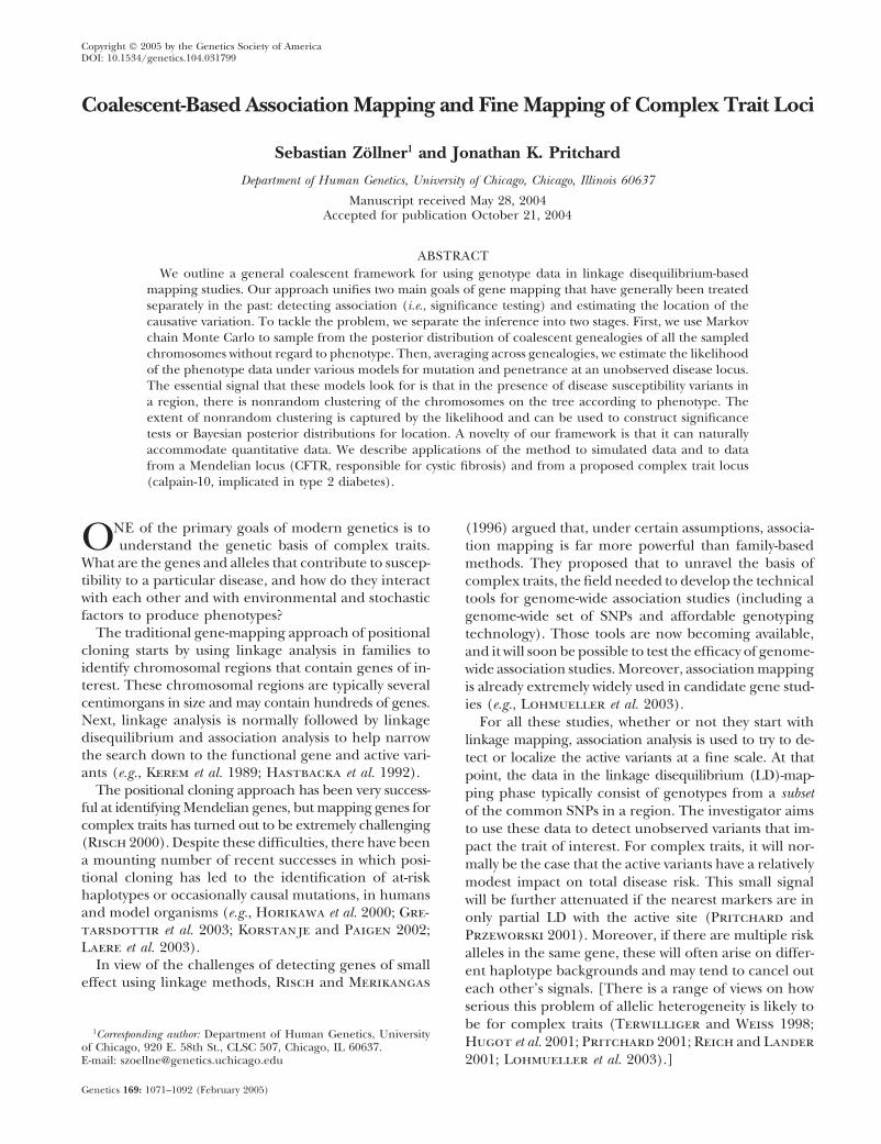
When there is recombination, the ancestral relation-ships among chromosomes are more complicated. Atany single position along the sequence, there is still asingle tree, but the trees at nearby positions may differ.It is possible to represent the full ancestral relationshipsamong chromosomes using a concept known as the “an- Figure 2.—Hypothetical example of a coalescent genealogycestral recombination graph” (ARG; Nordborg 2001; for a sample of 28 chromosomes, at the locus of a diseaseNordborg and Tavare 2002), although it is difficult susceptibility gene. Each tip at the bottom of the tree repre-
sents a sampled chromosome; the lines indicate the ancestralto visualize the ARG except in small samples or shortrelationships among the chromosomes. The two solid circleschromosomal regions (Figure 3).on the tree represent two independent mutation events pro-
Considering the coalescent process provides useful ducing susceptibility variants. These are inherited by the chro-insight into the nature of the information about associa- mosomes marked with hatched circles. Individuals carryingtion that is contained in the data. Figure 2 shows a hypo- those chromosomes will be at increased risk of disease. This
means that there will be a tendency for chromosomes fromthetical example of the coalescent ancestry of a sampleaffected individuals to cluster together on the tree, in twoof chromosomes at the position of a disease susceptibil-mutation-carrying clades. The degree of clustering depends
ity locus. In this example, two disease susceptibility mu- in part on the penetrance of the mutation.tations are present in the sample. By definition, thesewill be carried at a higher rate in affected individualsthan in controls. This implies that chromosomes from mation to learn as much as we can about the coalescent
genealogy of the sample at different points along theaffected individuals will tend to be nonrandomly clus-tered on the tree. Each independent disease mutation chromosome. Our statistical inference for association
mapping or fine mapping will be based on this. In whatgives rise to one cluster of “affected” chromosomes.Traditional methods of association mapping work by follows, we outline our approach of using marker data
to estimate the unknown coalescent ancestry of a sampletesting for association between the phenotype status andalleles at linked marker loci (or with haplotypes). In and describe how this information can be used to per-
form inference. Unlike in previous mapping methodseffect, association at a marker indicates that in the neigh-borhood of this marker, chromosomes from affected (e.g., Morris et al. 2002), we aim to reconstruct the
genealogy of the entire sample and not just the geneal-individuals are more closely related to one another thanby random. Fundamentally, the marker data are infor- ogy of cases. This extension allows us to extract substan-
tially more information from the data and enables sig-mative because they provide indirect information aboutthe ancestry of unobserved disease variants. Detecting nificance testing.
Performing inference: We start by developing someassociation at noncausative SNPs implies that case chro-mosomes are nonrandomly clustered on the tree. notation. Consider a sample of n haplotypes from n/2
unrelated individuals. The phenotype of individual i isIn fact, unless we have the actual disease variants inour marker set, the best information that we could possibly φi , and � represents the vector of phenotype data for
the full sample of n/2 individuals. The phenotypes mightget about association is to know the full coalescent genealogyof our sample at that position. If we knew this, the marker be qualitative (e.g., affected/unaffected) or quantitative
measurements.genotypes would provide no extra information; all theinformation about association is contained in the gene- Each individual is genotyped at a series of marker loci
from one or more genomic regions (or in the future pos-alogy. Hence, our approach is to use the marker infor-

1075Mapping of Complex Trait Loci
sibly from genome-wide scans). Let G denote the multi- tion about the location of the disease mutation. Thus,we ignore the possible impact of selection and over-dimensional vector of haplotype data—i.e., the geno-
types for n haplotypes at L loci (possibly with missing ascertainment of affected individuals in changing thedistribution of branch times at the disease locus. Ourdata). Let X be the set of possible locations of the QTL
or disease susceptibility gene and let x � X represent expectation is that the data will be strong enough toovercome minor misspecification of the model in thisits (unknown) position. Our approach is to scan sequen-
tially across the regions containing genotype data, con- respect (this was the experience of Morris et al. 2002,in a similar situation). The second approximation is asidering many possible positions for x. A natural mea-
sure of support for the presence of a disease mutation good assumption if the active disease mutation is notactually in our marker set and if mutations at differentat position x is given by the likelihood ratio (LR),positions occur independently. We can then write
LR �LA(�; x, Palt, G)
L0(�; P0, G), (1)
Pr(�, G |x) � �Pr(� |x , Tx)Pr(G |Tx)Pr(Tx)dTx
where LA and L0 represent likelihoods under the alterna-and since Pr(G |Tx)Pr(Tx) � Pr(Tx |G)Pr(G) we obtaintive model (disease mutation at x) and null hypothesis
(no disease mutation in the region), respectively. Palt Pr(�, G |x) � �Pr(� |x , Tx)Pr(Tx |G)Pr(G)dTxand P0 are the vectors of penetrance parameters underthe alternative and null hypotheses, respectively, that
� �Pr(� |x , Tx)Pr(Tx |G)dTx . (5)maximize the likelihoods. Large values of the likelihoodratio indicate that the null hypothesis should be re-
Expression (5) consists of two parts. Pr(� |x , Tx) is thejected. Specific models to calculate these likelihoodsprobability of the phenotype data given the tree at x .are described below (see Equations 7 and 8).To compute this, we specify a disease model and thenWe also want to estimate the location of disease muta-integrate over the possible branch locations of diseasetions. For this purpose it is convenient to adopt a Bayes-mutations in the tree (see below for details). Pr(Tx |G)ian framework, as this makes it more straightforwardrefers to the posterior density of trees given the markerto account for the various sources of uncertainty in adata and a population genetic model to be specified;coherent way (Morris et al. 2000, 2002; Liu et al. 2001).the next section outlines our approach to drawingThe posterior probability that a disease mutation is atMonte Carlo samples from this density.x is then
In summary, our approach is to scan sequentiallyacross the region(s) of interest, considering a dense setPr(x |�, G) �
Pr(�, G |x)Pr(x)�XPr(�, G |y)Pr(y)dy
(2)of possible positions of the disease location x . At eachposition x , we sample M trees [denoted T (m )
x ] from the� Pr(�, G |x)Pr(x), (3) posterior distribution of trees. For Bayesian inference of
location, we apply Equation 2 to estimate the posteriorwhere Pr(x) gives the prior probability that the diseasedensity Pr(x |�, G) at x by computinglocus is at x. Pr(x) will normally be set uniform across
the genotyped regions, but this prior can easily be modi-fied to take advantage of prior genomic information if Pr(x |�, G) �
(1/M)�Mm�1Pr(� |x, T (m )
x )Pr(x)
�Yi�1(1/M)�M
m�1Pr(� |yi , T (m )yi
)Pr(yi),
desired (see discussion in Rannala and Reeve 2001;Morris et al. 2002). (6)
To evaluate expressions (1) and (2), we need to com-where {y1, . . . , yY } denote a series of Y trial values of xpute Pr(�, G |x). To do so, we introduce the notationspaced across the region of interest. We will occasionallyTx , to represent the (unknown) coalescent genealogyrefer to the numerator of Equation 6, divided by Pr(x),of the sample at x. Tx records both the topology of theas the “average posterior likelihood” at x . For signifi-ancestral relationships among the sampled chromo-cance testing at x, we maximizesomes and the times at each internal node. Then
Pr(�, G |x) � �Pr(�, G |x, Tx)Pr(Tx |x)dTx LA(�; x, Palt , G) � 1M �
M
m�1
Pr(� |x, T (m )x , Palt ) (7)
� �Pr(�|x, Tx)Pr(G |�, x, Tx)Pr(Tx |x)dTx , and
(4) L0(�; P0 , G) � Pr(� |P0) (8)
with respect to Palt and P0 . See below for details aboutwhere the integral is evaluated over all possible trees. Wenow make the following approximations: (i) Pr(Tx |x) � how these probabilities are computed.
Sampling from the genealogy, Tx : To perform thesePr(Tx) and (ii) Pr(G |�, x , Tx) � Pr(G |Tx). The firstapproximation implies that in the absence of the pheno- calculations, it is necessary to sample from the posterior
density, Tx |G (loosely speaking, we wish to draw fromtype data, the tree topology itself contains no informa-
1076 S. Zollner and J. K. Pritchard
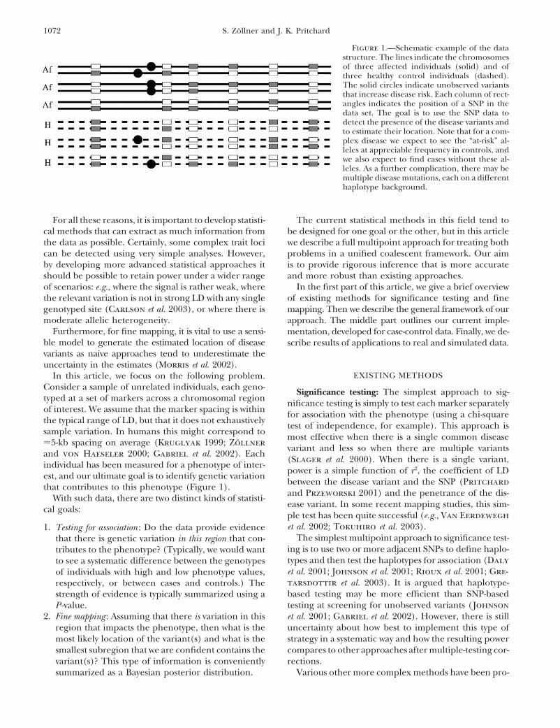
Figure 3.—Hypothetical example of theancestral recombination graph (ARG) for asample of six chromosomes, labeled A–F (leftplot), along with our representation (middleand right plots). (Left plot) The ARG con-tains the full information about the ancestralrelationships among a sample of chromo-somes. Moving up the tree from the bottom(backward in time), points where branchesjoin indicate coalescent events, while splittingbranches represent recombination events. Ateach split, a number indicates the positionof the recombination event (for concrete-ness, we assume nine intermarker intervals,labeled 1–9). By convention, the genetic ma-terial to the left of the breakpoint is assignedto the left branch at a split. See Nordborg(2001) for a more extensive description ofthe ARG. (Middle and right plots) At eachpoint along the sequence, it is possible to ex-tract a single genealogy from the ARG. Theplots show these genealogies at two “focalpoints,” located in intervals 4 and 7, respec-tively. The numbers in parentheses indicatethe total region of sequence that is inheritedwithout recombination, along with the focalpoint, by at least one descendant chromo-some. (1, 9) indicates inheritance of the en-tire region. For clarity, not all intervals withcomplete inheritance (1, 9) are shown.
the set of coalescent genealogies that are consistent with sample. It is likely that the region around the focal pointshared by the three chromosomes is smaller. In ourthe genotype data). We adopt a fairly standard population
genetic model, namely the neutral coalescent with recom- representation of the genealogy, we store the topologyat the focal point, along with the extent of sequence atbination (i.e., the ARG; Nordborg 2001). Our current
implementation assumes constant population size. each node that is ancestral to at least one of the sampledchromosomes without recombination (Figure 3).A number of recent studies have aimed to perform
full-likelihood or Bayesian inference under the ARG An example of this is provided in Figure 4. Each tipof the tree records the full sequence (across the entire(Griffiths and Marjoram 1996; Kuhner et al. 2000;
Nielsen 2000; Fearnhead and Donnelly 2001; Lar- region) of one observed haplotype. Then, moving upthe tree, as the result of a recombination event a partribe et al. 2002; reviewed by Stephens 2001). The expe-
rience of these earlier studies indicates that this is a of the sequence may split off and evolve on a differentbranch of the ARG. When this happens, the amounttechnically challenging problem, and that existing
methods tend to perform well only for quite small data of sequence that is coevolving with the focal point isreduced. The length of the sequence fragment thatsets (e.g., Wall 2000; Fearnhead and Donnelly 2001).
Therefore, we have decided to perform inference under coevolves with the focal point can increase during acoalescent event, as the sequence in the resulting nodea simpler, local approximation to the ARG, reasoning
that this might allow accurate inference for much larger is the union of the two coalescing sequences. In otherwords, the amount of sequence surrounding the focaldata sets. Our implementation applies Markov chain
Monte Carlo (MCMC) techniques (see appendix a). point shrinks when a recombination event occurs andmay increase at a coalescent event. A marker is retainedIn our approximation, we aim to reconstruct the coa-
lescent tree only at a single “focal point” x , although up to a particular node as long as there is at least onelineage leading to this node in which that SNP is notwe use the full genotype data from the entire region,
as all of this is potentially informative about the tree at separated from the focal point by recombination. Wedo not model coalescent events in the ARG where onlythat focal point. Consider two chromosomes that have
a very recent common ancestor (at the focal point). one of the two lines carries the focal point. Therefore,the sequence at internal nodes will always consist of oneThese chromosomes will normally both inherit a large
region of chromosome around the focal point, uninter- contiguous fragment of sequence.Our MCMC implementation stores the tree topology,rupted by recombination, from that one common ances-
tor. Then consider a more distant ancestor that the two node times, and the ancestral sequence at each node.We assume a finite sites mutation model for the markerschromosomes share with a third chromosome in the

1077Mapping of Complex Trait Loci
Indeed, if one wished to perform inference across aninfinitely long chromosomal region, the total amountof sequence stored at the ancestral nodes in our rep-resentation would be finite, while that in the earliermethods would not.
A more fundamental difference is that, unlike mostof the previous model-based approaches to this prob-lem, our genealogical reconstruction is independent ofthe phenotype data. There are trade-offs in choosing to
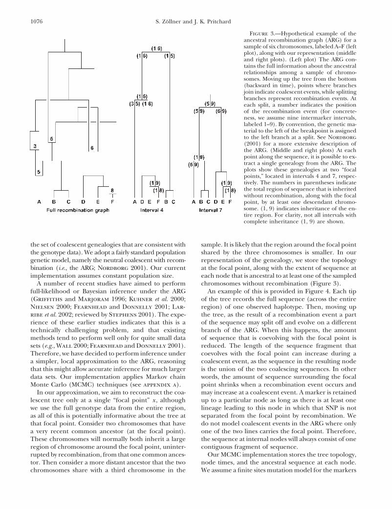
Figure 4.—Example of an ancestral genealogy as modeled frame the problem in this way, as follows. When theby our tree-building algorithm. The ancestry of a single focal alternative model is true, the phenotype data containpoint (designated F) as inferred from three biallelic markers
some information about the topology that could helpis shown (alleles are shown as 0 and 1). Branches with recombi-to guide the search through tree space. In contrast, ournation events on them are depicted as red lines, showing at
the tip of the arrow the part of the sequence that evolves on procedure weights the trees after sampling them froma different genealogy. As can be seen at the coalescent event Pr(Tx |G) according to how consistent they are with theat time t4, if no recombination occurs on either branch, the phenotype data (Equations 6 and 7), ignoring addi-entire sequence is transmitted along a branch and coalesces,
tional information from the phenotype data. However,generating a full-length sequence. If on the other hand a re-tackling the problem in this way makes it far easier tocombination event occurs, the amount of sequence that reaches
the coalescent event is reduced (indicated by the dashes). If assess significance, because we know that under the nullthis reduction occurs on only one of the two branches, the the phenotypes are randomly distributed among tips ofsequence can be restored from the information on the other the tree. It also means that we can calculate posteriorbranch (as at time t3). But if recombination events occur on
densities for multiple disease models using a singleboth branches, the length of the sequence is reduced (t2).MCMC run.
Modeling the phenotypes: To compute expressions (6)and (7), we use the following model to evaluate Pr(�|x,Tx).that are retained on each branch. (This rather simplistic
model is far more computationally convenient than At the unobserved disease locus, let A denote the geno-type at the root of the tree Tx . We assume that genotypemore realistic alternatives.) At some points, sequence is
introduced into the genealogy through recombination A mutates to genotype a at rate �/2 per unit time,independently on each branch. We further assume thatevents. We approximate the probability for the intro-
duced sequence by assuming a simple Markov model on alleles in state a do not undergo further mutation.Next, we need to define a model for the genotype-the basis of the allele frequencies in the sample (similar
approximations have been used previously by McPeek phenotype relationship for each of the three diploidgenotypes at the susceptibility locus: namely, Pr(φ |AA),and Strahs 1999; Morris et al. 2000; Liu et al. 2001;
Morris et al. 2002). The population recombination rate Pr(φ |Aa), and Pr(φ |aa), where φ refers to a particularphenotype value (e.g., affected/unaffected or a quan-� and the mutation rate � are generally unknown in
advance and are estimated from the data within the titative measure). For a binary trait, these three proba-bilities denote simply the genotypic penetrances: e.g.,MCMC scheme, assuming uniform rates along the se-
quence. A more precise specification of the model and Pr(Affected|AA). In practice, the situation is often com-plicated by the fact that the sampled individuals may notalgorithms is provided in appendix a.
Overall, our model is similar to those of earlier ap- be randomly ascertained. In that case, the estimated “pene-trances” really correspond to Pr(φ |AA, S), Pr(φ |Aa, S),proaches such as the haplotype-sharing model of McPeek
and Strahs (1999) and the coalescent model of Morris and Pr(φ |aa, S), where S refers to some sampling scheme(e.g., choosing equal numbers of cases and controls).et al. (2002). However, we focus on chromosomal shar-
ing backward in time, rather than on decay of sharing In the algorithm presented here, we assume that theaffection status of the two chromosomes in an individualfrom an ancestral haplotype. In part, this reflects our
shift away from modeling only affected chromosomes can be treated independently from each other and fromthe frequency of the disease mutation: i.e., PA(φ) is theto modeling the tree for all chromosomes. The repre-
sentation used by those earlier studies means that they probability that a chromosome with genotype A comes from anindividual with phenotype φ, and analogously for Pa(φ). Inpotentially have to sum over possible ancestral geno-
types at sites far away from the focal point x, which are the binary situation, this model has two independentparameters: PA(1) � 1 � PA(0) and Pa(1) � 1 � Pa(0).not ancestral to any of the sampled chromosomes and
about which there is therefore no information. Storing In this case the ratio PA(φ)/Pa(φ) corresponds directly tothe relative risk of allele A, conditional on the samplingall this extra information is likely to be detrimental in
an MCMC scheme, as it presumably impedes rearrange- scheme. As another example, for a normally distributedtrait, PA(φ) and Pa(φ) are the densities of two normalments of the topology. Thus, we believe that our repre-
sentation can potentially improve both MCMC mixing distributions at φ and would be characterized by meanand variance parameters. Note that most values of PA(φ)and the computational burden involved in each update.

1078 S. Zollner and J. K. Pritchard
and Pa(φ) do not correspond to a single genetic model Finally, it remains to determine the mutation rate, �,at the unobserved disease locus. It seems unlikely thatthat exists as the mapping from (PA(φ), Pa(φ)) to (Pr(φ|AA),
Pr(φ |Aa), Pr(φ |aa)) is dependent on the frequency of much information about � will be in the data; hencewe prefer to set it to a plausible value, a priori. For athe disease mutation. Nevertheless, this factorization of
the penetrance parameters is computationally conve- similar model, Pritchard (2001) argued that the mostbiologically plausible values for this parameter are in thenient and allows for an efficient analysis of Tx .
Of course, it is not known in advance which chromo- range of �0.1–1.0, corresponding to low and moderatelevels of allelic heterogeneity, respectively.somes are A and which are a , so we compute the likeli-
hood of the phenotype data by summing over the possi- Multiple testing: Typically, association-mapping stud-ies consist of large numbers of statistical tests. To ac-ble arrangements of mutations at the disease locus.
Under the alternative hypothesis, most arrangements count for this, it is common practice to report a P -valuethat measures the significance of the largest departureof mutations will be relatively unsupported by the data,
while branches leading to clusters of affected chromo- from the null hypothesis anywhere in the data set. Thesimplest approach is to apply a Bonferroni correctionsomes will have high support for containing mutations.
Let M record which branches of the tree contain disease (i.e., multiplying the P -value by the number of tests),but this tends to be unnecessarily conservative becausemutations and � {1, . . . , n } be the set of chromosomes
that carry a disease mutation according to M (i.e., the the association tests at neighboring positions are corre-lated.descendants of M) and let � be the set of chromosomes
that do not carry a mutation, i.e., � � {1, . . . , n } \. A more appealing solution is to use randomizationtechniques to obtain an empirical overall P -value (cf.Then we calculateMcIntyre et al. 2000). The basic idea is to hold all
Pr(� |x , Tx , �) � �M��
i�
PA(φi)�i��
Pa(φi)Pr(M |x , Tx , �)� . the genotype data constant and randomly permute thephenotype labels. For each permuted set, the tests of(9)association are repeated, and the smallest P -value forthat set is recorded. Then the experiment-wide signifi-For a case-control data set this can be written ascance of an observed P -value pi is estimated by the frac-
Pr(� |x, Tx , �) � �M
P nAd
A (1 � PA)n AhP na
da (1 � Pa)n ah Pr(M |x, Tx , �), tion of random data sets whose smallest value is pi .
The latter procedure is practical only if the test ofwhere ni
d and nih count the number of i-type chromo- association is computationally fast. For the method pro-
somes (where i � {A, a }) from affected and healthy posed in this article, the inference of ancestries is inde-individuals, respectively. Equation 9 can be evaluated pendent of phenotypes. Therefore, the trees need toefficiently using a peeling algorithm (Felsenstein 1981). be generated only once in this scheme and the sampledThe details of this algorithm are provided in appendix trees are stored in computer memory. Then, the likeli-b. Calculations for general diploid penetrance models hood calculations can be performed on these trees usingare much more computationally intensive, and we will both the real and randomized phenotype data to obtainpresent those elsewhere. the appropriate empirical distribution.
For our Bayesian analysis, we take the prior for the For a whole-genome scan, a permutation test with theparameters governing PA(φ) and Pa(φ) to be uniform proposed peeling strategy is rather daunting. Per-and independent on a bounded set � and average the forming the peeling analysis for 1000 permutations onlikelihoods over this prior. By allowing any possible or- one tree of 100 cases and 100 controls takes �6 minder for the penetrances under the alternative model, on a modern desktop machine. Thus, a whole-genomewe allow for the possibility that the ancestral allele may permutation test with one focal point every 50 kb, 100actually be the high-risk allele, as observed at some hu- trees per focal point, and a penetrance grid of 19 � 19man disease loci, including ApoE (Fullerton et al. 2000). values would take �750,000 processor hours.
For significance testing, we test the null hypothesis that A rather different solution for genome-wide scansPA(φ) � Pa(φ) compared to the alternative model where of association may be to apply the false discovery ratethe parameters governing PA(φ) and Pa(φ) can take on criterion, as this tends to be robust to local correlationany values independently. Standard theory suggests that when there are enough independent data (Benjaminitwice the log-likelihood ratio of the alternative model, and Hochberg 1995; Sabatti et al. 2003).compared to the null, should be asymptotically distrib- Unknown haplotype phase: Our current implementa-uted as 2 random values with d d.f., where d is the tion assumes that the individual genotype data can benumber of extra parameters in the alternative model resolved into haplotypes. However, in many currentcompared with the null. Thus, for case-control studies studies, haplotypes are not experimentally determinedour formulation suggests that twice the log-likelihood and must instead be estimated by statistical methods.ratio should have a 2
1 distribution. In fact, simulations In principle, it would be natural to update the unknownthat we have done (results not shown) indicate that this haplotype phase within our MCMC coalescent framework
described below (Lu et al. 2003; Morris et al. 2003). Byassumption is somewhat conservative.
1079Mapping of Complex Trait Loci
doing so, we would properly account for the impact of about the presence of disease variation will come fromthe degree to which case and control chromosomeshaplotype uncertainty on the analysis. In fact, Morris
et al. (2004) concluded that doing so increased the accu- cluster on the tree, so bias in the branch length estimatesmay not have a serious impact on inferences about theracy of their fine-mapping algorithm (compared to the
answers obtained after estimating haplotypes via a rather location of disease variation. The next section providesresults supporting this view.simple EM procedure). However, it is already a difficult
problem to sample adequately from the posterior distri- Another factor not considered in our current imple-mentation is the possibility of variable recombinationbution of trees given known haplotypes and it is unclear
to us that the added burden of estimating haplotypes rate (e.g., Jeffreys et al. 2001). Since recombinationrates appear to vary considerably over quite fine scales,within the MCMC scheme represents a sensible trade-
off. Therefore, we currently use point estimates of the this is probably an important biological feature to includein analysis. One route forward would be for us to estimatehaplotypes obtained from PHASE 2.0 (Stephens et al.
2001; Stephens and Donnelly 2003). We also currently separate recombination parameters in each intermarkerinterval, within the MCMC scheme (perhaps correlateduse PHASE to impute missing genotypes.
False positives due to population structure: It has across neighboring intervals). It is unclear how much thiswould add to the computational burden of convergencelong been known that case-control studies of association
are susceptible to high type 1 error rates when the sam- and mixing. In the short term, it would be possible to usea separate computational method to estimate these ratesples are drawn from structured or admixed populations
(Lander and Schork 1994). Therefore, we advise using prior to analysis with local approximation to the ances-tral recombination graph (LATAG; e.g., using Li andunlinked markers to detect problems of population
structure (Pritchard and Rosenberg 1999), prior to Stephens 2003) and to modify the input file to reflectthe estimated genetic distances.using the association-mapping methods presented here.
When population structure is problematic, there are Software: The algorithms presented here have beenimplemented in a program called LATAG. The programtwo types of methods that aim to correct for it: genomic
control (Devlin and Roeder 1999) and structured asso- is available on request from S. Zollner.ciation (Pritchard et al. 2000; Satten et al. 2001). Itseems likely that some form of genomic control correc-
TESTING AND APPLICATIONS: SIMULATED DATAtion might apply to our new tests, but it is not clear tous how to obtain this correction theoretically. It should To provide a systematic assessment of our algorithm
we simulated 50 data sets, each representing a fine-be possible to obtain robust P-values using the struc-tured association approach roughly as follows. First, one mapping study or a test for association within a candi-
date region. Each data set consists of 30 diploid caseswould apply a clustering method to the unlinked mark-ers to estimate the ancestry of the sampled individuals and 30 diploid controls that have been genotyped for
a set of markers across a region of 1 cM. Our model(Pritchard et al. 2000; Satten et al. 2001) and thephenotype frequencies across subpopulations. Then, the corresponds to a scenario of a complex disease locus
with relatively large penetrance differences (since thephenotype labels could be randomly permuted acrossindividuals while preserving the overall phenotype fre- sample sizes are small) and with moderate allelic hetero-
geneity at the disease locus.quencies within subpopulations. As before, the test sta-tistic of interest would be computed for each permuta- The data sets were generated as follows. We simulated
the ARG, assuming a constant population size of 10,000tion.SNP ascertainment and heterogeneous recombination diploid individuals and a uniform recombination rate.
On the branches of this ARG, mutations occurred as arates: In the MCMC algorithm described above, and morefully in appendix a, we assume—for convenience—that Poisson process according to the infinite sites model.
The mutation rate was set so that in typical realizationsmutation at the markers can be described using a stan-dard finite sites mutation model with mutation parame- there would be 45–65 markers with minor allele fre-
quency �0.1 across the 1-cM region. The position of theter �. However, in practice, we aim to apply our methodto SNPs: markers for which the mutation rate per site disease locus xs was drawn from a uniform distribution
across the region. Mutation events at the disease locusis likely to be very low, but that have been specificallyascertained as polymorphic. Hence, our estimate of � were simulated on the tree at that location at rate 1 per
unit branch length (in coalescent time), with no backshould not be viewed as an estimate of the neutral muta-tion rate; it is more likely to be roughly the inverse of mutations (cf. Pritchard 2001). This process deter-
mines whether each chromosome does, or does not,the expected tree length (if there has usually been onemutation per SNP in the history of the sample). More- carry a disease mutation. We required that the total
frequency of mutation-bearing chromosomes be in theover, the fact that SNPs are often ascertained to haveintermediate frequency and that we overestimate � may range 0.1–0.2, and if it was not, then we simulated a
new set of disease mutations at the same location. Thislead to some distortion in the estimated branch lengths.However, we anticipate that most of the information procedure generated a total of 10–25 disease mutations

1080 S. Zollner and J. K. Pritchard
across the entire population, although many of the mu- posterior probability. The running time for each data setwas �5 hr on a 2.4-GHz processor with 512 K memory.tations were redundant or at low frequency.
To assign phenotypes, we used the following pene- For comparison, we also analyzed each data set withDHSMAP-map 2.0 using the standard settings suggestedtrances: a homozygote wild type showed the disease
phenotype with probability Phw � 0.05, a heterozygous in the program package. This program generated pointestimates for the locus of disease mutation and twogenotype showed it with probability Phe � 0.1, and a
homozygous mutant showed it with probability Phm � 95% confidence intervals: the first assuming a star-likephylogeny among cases, and the second using a correc-0.8. According to these penetrances, we then created
30 case and 30 control individuals by sampling without tion to account for the additional correlation amongcases that results from relatedness.replacement from the simulated population of 20,000
chromosomes, as follows. Let n be the remaining num- Significance tests were performed by two methods.First we calculatedber of wild-type chromosomes in the population and m
be the remaining number of mutant chromosomes inLm � max{LA(�; xi , Palt , G) : i � {1, . . . , 50}, Palt � �}the population. Then the next case individual was ho-
(10)mozygous for the mutation with probability (Phm · m ·(m � 1)) · (Phm · m · (m � 1) � 2 · Phe · m · n � Phw ·
and calculated the likelihood ratio according to (1),n · (n � 1))�1, heterozygous with probability (2 · Phe ·m · n) · (Phm · m · (m � 1) � 2 · Phe · m · n � Phw · n ·
LR �Lm
L0
,(n � 1))�1, and otherwise homozygous for the mutantallele. The diplotypes for each case were then createdby sampling the corresponding number of mutant or with L0 � 0.5120. We assigned pointwise significance towild-type chromosomes. Control individuals were gener- this ratio by assuming that 2 ln(LR) is 2-distributedated analogously. Across the 50 replicates, we found with 1 d.f. (Other simulations that we have done indicatethat 10–33 of the 60 case chromosomes and 0–9 of the that this assumption is somewhat conservative; resultscontrol chromosomes carried a disease mutation. not shown.) To estimate global significance, we per-
As might be expected for the simulation of a complex muted case and control status among the 60 individualsdisease, not all of the simulated data sets carried much 1000 times, recalculated Lm for each permutation (usinginformation about the presence of genetic variation in- the original trees obtained from the data), and countedfluencing the phenotype. For instance, in 22 of the the number of permutations that showed a higher Lmgenerated data sets, the highest single-point association than the original data set anywhere in the region. Thesignal among the generated markers, calculated as Pear- permutation procedure corrects for multiple testingson’s 2, is �6.5. across the region and does not rely on the predicted
We analyzed each simulated data set by considering distribution of the likelihood ratio.50 focal points x 1, . . . , x 50, spaced equally across the For comparison we assessed the performance of sin-1-cM region. For each point xi we used LATAG to draw gle-point association analysis by calculating the associa-50 trees from the distribution Pr(Txi
|G , xi). To ensure tion of each observed marker in a 2 � 2-contingencyconvergence of the MCMC, we used a burn-in period table with a 2-statistic and recorded the 2 of the markerof 2.5 � 106 iterations for x 1. As the tree at location xi with the highest value. We assigned significance to thisis a good starting guess for trees of the adjacent tree at test statistic in two ways: first, on the basis of the 2-distri-xi�1 we used a burn-in of 0.5 � 106 iterations for x 2, . . . , bution with 1 d.f., and second, by performing 1000xk . We sampled each set of trees {T (1)
xi, . . . , T (50)
xi} using permutations of phenotypes among the 60 individuals
a thinning interval of 10,000 steps and estimated Pr(�, and counting the number of permutations in which theG |xi) according to (6) and (B2) without assuming any highest observed 2 was higher than that observed inprior information about the location of disease muta- the sample.tions. We found that the mean was somewhat unstable To assess convergence, we then repeated the analysisdue to occasional large outliers and therefore substi- of each data set an additional four times and comparedtuted the median for the average in (6). To evaluate (B2) the estimated posterior distributions to assess the con-we summed over a grid of penetrances � � {0.05, 0.1, vergence of the MCMC and the variability in estimation.. . . , 0.95} � {0.05, 0.1, . . . , 0.95}, setting the disease We calculated the overlap of two credible intervals C 1mutation rate � to 1.0. We calculated the posterior prob- and C 2 obtained from multiple MCMC analyses of theability at each locus xi by evaluating same data set as
Pr(xi |�, G) �Pr(�, G |xi)
�50j�1Pr(�, G |xj)
. � |C 1 � C 2 ||C 1 |
�|C 1 � C 2 |
|C 2 | ��2,
In addition, we recorded the point estimate for thelocation of the disease mutation as the xi with the highest where |I | is the length of interval I.
1081Mapping of Complex Trait Loci
tively flat across the entire region. Some of the data setscontain very little information about the presence orlocation of disease mutations, and so small random fluc-tuations in the estimation can shift the peak from onepart of the region to another. To further quantify thisobservation, we computed the correlation between theaverage pairwise difference of the point estimates withthe average posterior likelihood at the point estimatefor each data set. We observed that these were stronglynegatively correlated (correlation coefficient � �0.29).The higher the signal that is present in the data (ex-pressed in posterior probability), the smaller the differ-ence is between the point estimates.
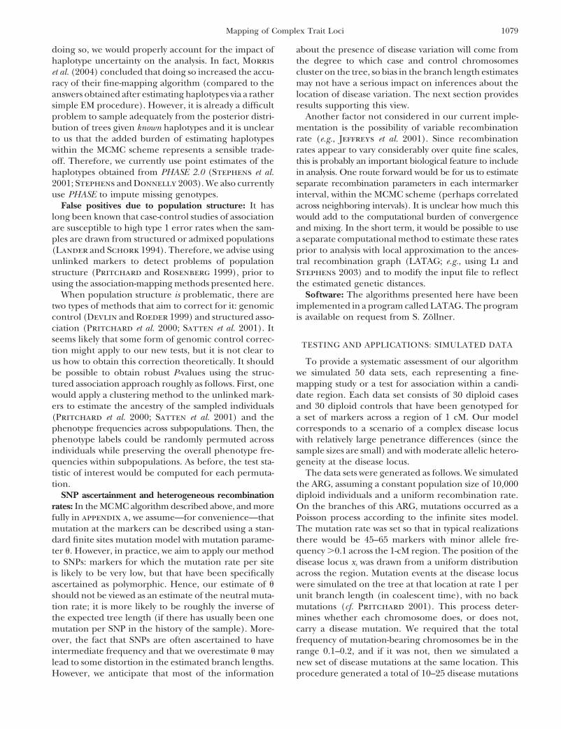
In summary, when the data sets contained a strongsignal, the concordance between individual runs wasFigure 5.—Point estimates of the locus of disease mutationquite high, indicating good convergence. On the otherfor five independent MCMC analyses of each of 50 simulated
data sets. The data sets are ordered from left to right by the hand, when the information about location was weak,median point estimate across the five replicates. The shading random variation across runs meant that the point esti-of the point indicates the strength of the signal at the point mates sometimes varied considerably. In such cases,estimate: darker points indicate stronger signals in the data.
longer runs would be needed to obtain really accurateOpen points correspond to estimates where the average poste-estimates. For analyzing real data, it is certainly impor-rior likelihood is �1.2-fold higher than the expected posterior
likelihood in the absence of disease mutations, shaded trian- tant to use multiple LATAG runs to ensure the ro-gles correspond to estimates that are 1.2–12-fold higher than bustness of the results.the background, and solid circles correspond to estimates that Point estimates of location: The mode of the posteriorare �12-fold higher than background.
distribution is a natural “best guess” for the location ofthe disease variation. To assess the accuracy of this esti-mate, we calculated the distance between this pointRESULTSestimate and the real locus of the disease mutation for
Assessing convergence: An important issue for each simulated data set. Overall, we observed an averageMCMC applications is to check the convergence of the error of 0.19 cM with a standard deviation of 0.23 cM.Markov chain, since poor convergence or poor mixing To evaluate this result, we compared it to the accuracycan lead to unreliable results. While numerous methods of two other point estimators. As a naive estimator, weexist to diagnose MCMC performance (Gammerman chose the position of the marker that has the highest1997), the most direct approach is to compare the re- level of association with the phenotype, measured usingsults from multiple MCMC runs. If the Markov chain the Pearson 2 statistic. This choice is based on the ob-performs well, and the samples drawn from the posterior servation that, on average, LD declines with distance.are sufficiently large, then different runs will produce As an example of an estimator provided by a multipointsimilar results. (Conversely, good performance by this method, we analyzed the prediction generated bycriterion does not absolutely guarantee that the Markov DHSMAP.chain is working well, but it is certainly encouraging.) We found that the average distance between the dis-
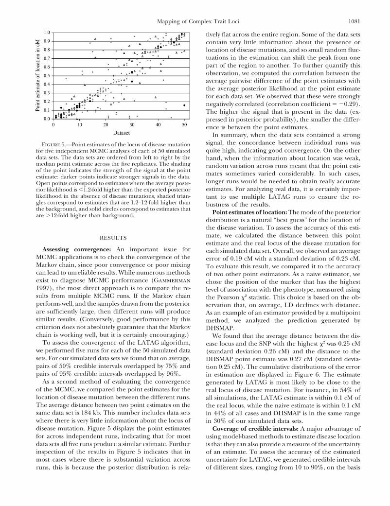
To assess the convergence of the LATAG algorithm, ease locus and the SNP with the highest 2 was 0.25 cMwe performed five runs for each of the 50 simulated data (standard deviation 0.26 cM) and the distance to thesets. For our simulated data sets we found that on average, DHSMAP point estimate was 0.27 cM (standard devia-pairs of 50% credible intervals overlapped by 75% and tion 0.25 cM). The cumulative distributions of the errorpairs of 95% credible intervals overlapped by 96%. in estimation are displayed in Figure 6. The estimate
As a second method of evaluating the convergence generated by LATAG is most likely to be close to theof the MCMC, we compared the point estimates for the real locus of disease mutation. For instance, in 54% oflocation of disease mutation between the different runs. all simulations, the LATAG estimate is within 0.1 cM ofThe average distance between two point estimates on the the real locus, while the naive estimate is within 0.1 cMsame data set is 184 kb. This number includes data sets in 44% of all cases and DHSMAP is in the same rangewhere there is very little information about the locus of in 30% of our simulated data sets.disease mutation. Figure 5 displays the point estimates Coverage of credible intervals: A major advantage offor across independent runs, indicating that for most using model-based methods to estimate disease locationdata sets all five runs produce a similar estimate. Further is that they can also provide a measure of the uncertaintyinspection of the results in Figure 5 indicates that in of an estimate. To assess the accuracy of the estimatedmost cases where there is substantial variation across uncertainty for LATAG, we generated credible intervals
of different sizes, ranging from 10 to 90%, on the basisruns, this is because the posterior distribution is rela-
1082 S. Zollner and J. K. Pritchard
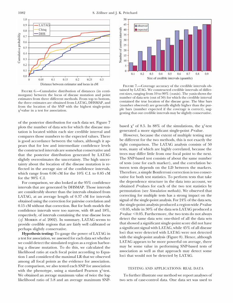
Figure 7.—Coverage accuracy of the credible intervals ob-tained by LATAG. We constructed credible intervals of differ-Figure 6.—Cumulative distribution of distances (in centi-ent sizes, ranging from 10 to 90% (x-axis). The y-axis shows themorgans) between the locus of disease mutation and pointnumber of data sets (out of 50) for which the credible intervalestimates from three different methods. From top to bottom,contained the true location of the disease gene. The blue barsthe three estimates are obtained from LATAG, DHSMAP, and(number observed) are generally slightly higher than the pur-from the location of the SNP with the highest single-pointple bars (number expected if the coverage is correct), sug- 2-value in a test for association.gesting that our credible intervals may be slightly conservative.
of the posterior distribution for each data set. Figure 7based 2 of 8.5. In 88% of the simulations, the 2-testplots the number of data sets for which the disease mu-generated a more significant single-point P -value.tation is located within each size credible interval and
However, because the extent of multiple testing maycompares those numbers to the expected values. Therebe different for the two methods, this is not exactly theis good accordance between the values, although it ap-right comparison. The LATAG analysis consists of 50pears that for low and intermediate confidence levelstests, many of which are highly correlated, because thethe constructed intervals are somewhat conservative andtrees may differ little from one focal point to the next.that the posterior distribution generated by LATAGThe SNP-based test consists of about the same numberslightly overestimates the uncertainty. The high uncer-of tests (one for each marker), and the correlation be-tainty about the location of the disease mutation is re-tween tests depends on the LD between the markers.flected in the average size of the confidence intervals,Therefore, a simple Bonferroni correction is too conser-which range from 0.06 cM for the 10% C.I. to 0.85 cMvative for both test statistics. To perform tests that takefor the 90% C.I.the dependence structure in the data into account, weFor comparison, we also looked at the 95% confidenceobtained P -values for each of the two test statistics byintervals that are generated by DHSMAP. Those intervalspermutation (see Simulation methods). We observed thatare considerably shorter than the intervals obtained fromcorrecting for multiple tests has a strong impact on theLATAG, at an average length of 0.37 cM for intervalssignal of the single-point analysis. For 24% of the data sets,obtained using the correction for pairwise correlation andthe single-point analysis produced a region-wide P -value0.15 cM without that correction. But for both models the�0.05, while in 30% of the data sets LATAG produced aconfidence intervals were too narrow, with 48 and 18%,P -value �0.05. Furthermore, the two tests do not alwaysrespectively, of intervals containing the true disease locusdetect the same data sets: one-third of all the data sets(cf. Morris et al. 2002). In summary, LATAG seems tothat showed a significant single-point score did not haveprovide credible regions that are fairly well calibrated ora significant signal with LATAG, while 45% of all diseaseperhaps slightly conservative.loci that were detected with LATAG were not detectedHypothesis testing: To gauge the power of LATAG inwith the single-point analysis (Figure 8). Hence, althougha test for association, we assessed for each data set whetherLATAG appears to be more powerful on average, therewe could detect the simulated region as a region harbor-may be some value in performing SNP-based tests ofing a disease mutation. To do this, we calculated theassociation as well as that approach may detect somelikelihood ratio at each focal point according to Equa-loci that would not be detected by LATAG.tion 1 and considered the maximal LR that we observed
among all focal points as the evidence for association.For comparison, we also tested each SNP for association
TESTING AND APPLICATIONS: REAL DATAwith the phenotype, using a standard Pearson 2-test.We obtained an average maximum value of twice the log- To further illustrate our method we report analyses of
two sets of case-control data. One data set was used tolikelihood ratio of 5.8 and an average maximum SNP-

1083Mapping of Complex Trait Loci
Figure 8.—Comparison of the ability of LATAG (x-axis)and a SNP-based 2-test (y-axis) to detect disease-causing loci Figure 9.—Repeatability across runs. Average posterior like-in a test for association. Each point corresponds to one of the lihoods for 10 independent LATAG analyses of the CF data50 simulated data sets and plots the most significant P-values set are shown. For the location of the disease locus and theobtained for that data set using each method, corrected for resulting posterior credible region refer to Figure 10.multiple testing within the region. The dotted lines depictthe P � 0.05 cutoffs and the diagonal line plots the regressionline through the log-log-transformed data.
calculated P(� |Ti , x) with the peeling algorithm. Asthe resulting posterior likelihoods seemed to be heavilydependent on a few outliers, we estimated the likelihoodmap the gene responsible for cystic fibrosis, a simple
recessive disorder (Kerem et al. 1989), while the other P(x |�, G) at each position x by taking the median ofthe likelihoods P(� |Ti , x) instead of the average sug-data set is from a positional cloning study of a complex
disease, type 2 diabetes (Horikawa et al. 2000). gested by theory. As before, we used the posterior modeas our point estimate for location. Missing data wereExample application 1: Cystic fibrosis: The cystic fibro-
sis (CF) data set used by Kerem et al. (1989) to map the imputed using PHASE 2.0 (Stephens et al. 2001).Results: To provide a simple check of convergence,CFTR locus has been used to evaluate several previous
fine-mapping procedures, thus allowing an easy compar- Figure 9 shows the results from the 10 independent analy-ses of the CF data set. As can be seen, all 10 runs haveison between LATAG and other multipoint methods.
The data set was generated to find the gene responsible modes in the same region and yield the same conclusionabout the location of the causative variation.for CF, a fully penetrant recessive disorder with an inci-
dence of 1/2500 in Caucasians. Many different disease- Figure 10 summarizes our results across the 10 runs.The posterior distribution is sharply peaked at 867 kb,causing mutations have been observed at the CFTR lo-
cus, but the most common mutation, �F508, is at quite near the true location of �F508 (which is at 885 kb).The 95% credible interval is rather narrow, extendinghigh frequency, accounting for 66% of all mutant chro-
mosomes. from 814 to 920 kb. Even though several markers withlittle association to the trait are in the vicinity of theThe data set consists of 23 RFLPs distributed over
1.8 Mb; these were genotyped in 47 affected individuals. deletion (Figure 10), the LATAG estimate is quite accu-rate. It is useful to compare our results to those obtainedIn addition, 92 control haplotypes were obtained by
sampling the nontransmitted parental chromosomes. by other multipoint methods (see Table 1, modifiedfrom Morris et al. 2002). For this data set, most of theHigh levels of association were observed for almost all
markers in the region; the marker with the highest highest single-point 2 values lie to the left of the truelocation of �F508, and so most of the methods err tosingle-point association ( 2 � 63) is located at 870 kb
from the left-hand end of the region. The �F508 muta- the left, with some of the earliest methods (Terwil-liger 1995) actually excluding the true location fromtion is at 885 kb and is present in 62 of the 94 case
chromosomes. the confidence interval. Note that the LATAG estimateis closer to the true location, and that the 95% credibilityWe ran 10 independent runs of the Markov chain,
estimating the average posterior likelihood at each of region is narrower than that obtained by any of theprevious methods.50 evenly distributed points across the region. Each run
had a burn-in of 2.5 � 106 steps for the first focal point To assess the ability of LATAG to detect the CF regionby association, we calculated a likelihood ratio accord-and 106 steps for each following focal point. In each
run, we sampled 50 trees at each focal point, with a ing to (1) and obtained 2 ln(LR) � 40. Assuming a 2-distribution with 1 d.f., this log-likelihood ratio has anthinning interval of 10,000 steps. The runs took 8 hr
each on a Pentium III processor. For each tree Ti , we associated P -value of 3.7 � 10�10. While this is extremely

1084 S. Zollner and J. K. Pritchard
of 85 SNPs distributed over an area of 876 kb. Themarkers were genotyped in 108 cases and 112 controls.No individual marker shows high association; themarker with the highest LD ( 2 � 9) is located at 121 kbfrom the left-hand end of the region. The original studyalso used some additional information from family-shar-ing patterns that we do not consider here. On the basisof detailed analysis of those data, Horikawa et al. (2000)proposed that a combination of two haplotypes, eachconsisting of 3 SNPs within the CAPN10 gene, increasesthe risk of diabetes by two- to fivefold. The three SNPsthat make up the haplotype are located at 121, 124, and134 kb.
We used the PHASE 2.0 algorithm, with recombina-Figure 10.—Average posterior likelihoods generated by tion in the model (Stephens et al. 2001), to impute the
LATAG for the CF data set (Kerem et al. 1989). The dots depict phase information and missing genotypes for both casesthe association signals of the individual markers as 2-statistics and controls. Then we used LATAG to infer the poste-(see scale on the right). We display the likelihoods here be-
rior distribution of the location of the disease mutationcause the posterior density is extremely peaked, with 95% ofand a P -value for association, as described above. Per-its mass inside the box marked by the dashed lines.forming eight independent runs of the MCMC, we gen-erated a total of 800 draws from the posterior distribu-
significant, it is less significant than that obtained from tion P(T |G , x) for each of 50 positions in the sequence.simple tests of association with individual SNPs (six of Each run had a burn-in of 5 � 106 steps for the firstwhich yield 2-values �50). This may indicate that our point and 106 steps for each following point, a thinninglikelihood-ratio test does not fit the 2-approximation interval of 10,000 steps between draws, and took 36 hrvery well, particularly far out in the tail of the distribu- on a Pentium III processor.tion, or that our test is slightly less powerful in this ex- Results: Figure 11 plots the estimated posterior distri-treme setting. Due to the extremely high level of signifi- bution for the location of diabetes-associated variationcance, it is infeasible to generate an accurate P -value in this region. From this distribution we estimate theby permutation. position of the disease mutation at 131 kb, at the same
Example application 2: Calpain-10: Our second appli- location as the SNPs that Horikawa et al. (2000) reportedcation comes from a positional cloning study that was as defining the key haplotypes. However, the posteriorsearching for disease variation underlying type 2 diabe- distribution is quite wide, with 50% of its mass betweentes. Type 2 diabetes is the most common form of diabe- 70 and 245 kb. The full 95% credibility region extendstes and in developed countries it affects 10–20% of in- between 0 and 660 kb, indicating that we can really ex-dividuals over the age of 45 (Horikawa et al. 2000). clude only the right-hand end of this region. We wouldThis appears to be a highly complex disease, with no need larger samples to obtain more precision.gene of major effect, and with environmental factors To assess whether we would have detected this regionplaying an important role. A linkage study in Mexican by association, on the basis of this data set, we evaluatedAmericans localized a susceptibility gene to a region (1) and obtained 2 ln(LR) � 6.0 at the posterior mode,on chromosome 2 containing three genes, RNEPEPL1, corresponding to a single-point P -value of 5.3 � 10�4.CAPN10, and GPR35. A data set that was generated by When we correct for multiple testing using the simula-
tion procedure, the overall significance level drops toHorikawa et al. (2000) for positional cloning consists
TABLE 1
Estimates of locations of the CF-causing allele, as taken from Morris et al. (2002)
Method Estimate Variability Comments
Terwilliger (1995) 770 690–870 (99.9% support interval)McPeek and Strahs (1999) 950 440–1460 (95% confidence interval) Pairwise correctionMorris et al. (2000) 800 610–1070 (95% credible interval) Pairwise correctionLiu et al. (2001) — 820–930 (95% credible interval)Morris et al. (2002) 850 650–1000 (95% credible interval)LATAG 867 814–920 (95% credible interval)
The �F508 mutation, which is responsible for 66% of all CF cases, is located at position 885. Only estimatesthat are based on the entire data set are presented.

1085Mapping of Complex Trait Loci
across multiple blocks are potentially quite informativeabout the order of recent coalescent events. In ourmethod, rather than forcing the user to predefine re-gions of limited recombination, the algorithm “adapts”to the data, in the sense that quite large regions ofshared haplotypes may help to resolve recent coalescentevents, while much smaller regions (e.g., correspondingto haplotype blocks) may be the relevant scale for recon-structing the topology of the more ancient coalescentevents. Hence, we gather information both from muta-tion and from recombination events to reconstruct theancestral trees. By doing so, we can detect associationeven when there is allelic heterogeneity, and we cangain information about low-frequency disease muta-
Figure 11.—Posterior distribution for the location of the tions, even using only intermediate-frequency SNPs.diabetes-affecting variant(s) in the calpain-10 region (solid line;Our simulations indicated that LATAG is substantiallysee scale on the left). The dots represent the association ofmore powerful than single-point SNP-based tests of asso-individual markers with the phenotype (see 2-scale on the right).
The red dots indicate the three markers that define the disease- ciation, at least for the scenario considered.associated haplotypes reported by Horikawa et al. (2000). It is also natural to compare LATAG to recent fine-
mapping algorithms. One major difference betweenLATAG and most of the previous coalescent-based algo-
a mildly significant P � 0.02. In contrast, if we assess rithms is that LATAG aims to reconstruct the ancestrythe significance of the highest observed single-point of all the sampled chromosomes, not just of case chro- 2 by permuting case and control labels, we obtain a mosomes. By considering the ancestry of all individualsnonsignificant P -value of 0.11. at once, we can deal with more general phenotype mod-
Overall, our results are consistent with the conclusion els and we can model allelic heterogeneity and incom-of Horikawa et al. (2000), that CAPN10 is the gene that plete penetrance in a natural way, although includingwas responsible for their diabetes linkage signal in this re- this additional information may increase computationgion. However, our analysis cannot exclude GPR35 as the time. This also represents the first multipoint fine-map-disease gene. As with the original analysis, our strongest ping method for quantitative traits. Our approach cansignal is in the CAPN10 region, but our overall signal also produce penetrance estimates under haploid andis only modestly significant. diploid models (the latter to be presented elsewhere),
although these estimates may not be straightforwardto interpret when the ascertainment of samples is notrandom. We have not focused on this here, but ourDISCUSSIONapproach also produces a posterior probability that each
We have described a new unified method, LATAG, for chromosome carries a disease mutation. This can beassociation mapping and fine mapping with multipoint used to guide full resequencing of implicated regions.data. Our approach, based on a local approximation to Including control chromosomes in the tree allows us tothe ARG, strikes a compromise between modeling the make better use of the control data than earlier methodspopulation genetic processes that produce the data and that used just controls to estimate the SNP allele fre-the need for a model that is computationally tractable quencies, as exemplified by the strong performance offor large data sets. our method on the CF data and on the simulated data.
Our association-mapping method is similar in spirit For any model-based approach such as LATAG, it isto earlier tree-based methods (e.g., Templeton et al. worth considering the various modeling assumptions1987). However, we take a more probabilistic approach and how these might affect the results. In general, itin the sense that we average over the uncertainty in trees seems that most of the inaccuracies of the model canand consider an explicit mutation model at the unob- be overcome by informative data; at worst they mightserved disease locus. A more fundamental difference is slightly reduce our power and precision (cf. Morristhat our tree inference scheme aims to model recombi- et al. 2002). For instance, the Markov model that wenation explicitly, while the earlier methods make the use for LD outside the inherited region is not strictlymost sense in small regions without evidence for recom- accurate and might be expected to produce a slightbination. Moreover, even for estimating the tree within a bias toward keeping too much sequence on the tree.haplotype block, markers outside the block may contain Inaccuracies there may explain the tendency towardadditional information about that tree. It is typical for conservativeness in the coverage of our credible inter-there to be at least some LD between haplotype blocks vals (Figure 7). Similarly, the finite sites model used for
SNP mutation, ignoring SNP ascertainment, is clearly(Daly et al. 2001), and patterns of haplotype sharing

1086 S. Zollner and J. K. Pritchard
inaccurate. However, this model is computationally con- puting facilities. Nevertheless, improving the algorithmto deal with larger data sets is a focus of our ongoingvenient, and it seems likely that the data should over-research.whelm deficiencies here; again, that view is supported
One question that arises in this context is whether toby the results. Besides, allowing recurrent SNP mutationtreat haplotype phase from diploid genotypes as knownprovides an ad hoc way of allowing for gene conversion,when inferring the trees (here we estimated phase usingwhich might otherwise confound our inference.Phase 2.0 ; Stephens et al. 2001). The alternative—whichAnother issue is that we ignore the ascertainment ofis more statistically sound—is to use the MCMC coales-cases and natural selection on the disease variants.cent algorithm to mix over unknown phase along withThese processes are expected to distort the shape oftree topology. Morris et al. (2004) implemented suchthe tree (cases will be more closely related than pre-a method and reported that it produced more accuratedicted under the coalescent model). But this distortionfine-mapping results than did a method that used haplo-effect will be most pronounced when the signal is verytypes estimated by a simple EM algorithm. However,strong (e.g., for a recent highly penetrant mutation, asgiven that it is already difficult to achieve good MCMCin the CF data). In that case, the data will usually beperformance in large data sets of known haplotypes, itstrong enough to overwhelm the rather weak coalescentis unclear to us that also mixing over haplotypes is neces-prior. In other words, when the coalescent model issarily a good strategy. We look forward to further re-furthest from the truth, the data are likely to be verysearch on this issue.informative and should override the misspecifications
In summary, our new methods provide a coherentof the prior.framework for achieving different goals of LD-basedAt present we also assume that even if there are multi-mapping. Furthermore, they perform well on real andple disease mutations in a region all of these occur atsimulated data, compared to standard existing methods.essentially the same position. This may well be a poorOne of the biggest challenges for the future will be toassumption. For example, mutations in different exonsdevelop our current framework so that it can be appliedof a single gene might be many kilobases apart. Neitherto the massive data sets that will soon be forthcomingour method nor any other existing method would han-in the human genetics community.dle this well; however, dealing with this issue is surely
We thank Nancy Cox, Dick Hudson, Dan Nicolae, Matthew Ste-an important problem for the future.phens, and two anonymous reviewers, plus the other members of ourFull-likelihood coalescent methods such as LATAGlab, for helpful discussions and/or comments on the manuscript and
pose considerable computational challenges. It is not Nancy Cox for giving us access to the calpain-10 data. This work waseasy to design MCMC algorithms that can traverse through supported by grant HG 2772 to J.K.P. from the National Institutes of
Health.tree space efficiently and produce robust, repeatableresults for large data sets (Wall 2000). As noted above,we use a local approximation to the ARG to substantiallysimplify the space that we are mixing through. We also LITERATURE CITEDclip off upper parts of the sequence that are not inher-
Abney, M., C. Ober and M. S. McPeek, 2002 Quantitative-trait ho-ited (Figures 3 and 4) to further improve mixing. In mozygosity and association mapping and empirical genomewide
significance in large, complex pedigrees: fasting serum-insulinour MCMC design, we chose to augment the data bylevel in the Hutterites. Am. J. Hum. Genet. 70: 920–934.storing, and mixing over, the sequence at internal nodes. Benjamini, Y., and Y. Hochberg, 1995 Controlling the false discov-
Doing so makes the Metropolis-Hastings calculations ery rate—a practical and powerful approach to multiple testing.J. R. Stat. Soc. B 57: 289–300.for each proposed update extremely fast and allows the
Carlson, C. S., M. A. Eberle, M. J. Rieder, J. D. Smith, L. Kruglyakalgorithm to use the sequence identity to propose more et al., 2003 Additional SNPs and linkage-disequilibrium analyseseffective tree rearrangements. On the down side, storing are necessary for whole-genome association studies in humans.
Nat. Genet. 33: 518–521.this extra information may plausibly impede mixing;Daly, M. J., J. D. Rioux, S. F. Schaffner, T. J. Hudson and E. S.
further experimentation will be required to help deter- Lander, 2001 High-resolution haplotype structure in the hu-man genome. Nat. Genet. 29: 229–232.mine the best design. The calpain-10 data set, consisting
Devlin, B., and K. Roeder, 1999 Genomic control for associationof 85 SNPs genotyped in 440 chromosomes, is at thestudies. Biometrics 55: 997–1004.
upper end of what our current algorithm can handle Fearnhead, P., and P. Donnelly, 2001 Estimating recombinationrates from population genetic data. Genetics 159: 1299–1318.reliably (and is also very large by the current standards
Felsenstein, J., 1981 Evolutionary trees from DNA sequences: aof other full-likelihood coalescent methods). One ad- maximum likelihood approach. J. Mol. Evol. 17 (6): 368–376.vantage of our approach over other genealogy-based Fullerton, S. M., A. G. Clark, K. M. Weiss, D. A. Nickerson, S. L.
Taylor et al., 2000 Apolipoprotein E variation at the sequencemethods is that LATAG can be easily parallelized, sincehaplotype level: implications for the origin and maintenance ofthe trees are reconstructed independently of each other a major human polymorphism. Am. J. Hum. Genet. 67: 881–900.
at different focal points and the analysis of trees can be Gabriel, S. B., S. F. Schaffner, H. Nguyen, J. M. Moore, J. Royet al., 2002 The structure of haplotype blocks in the humanperformed independently of their generation process.genome. Science 296: 2225–2229.
Each of these operations can run on a different proces- Gammerman, D., 1997 Markov Chain Monte Carlo: Stochastic Simulationfor Bayesian Inference. Chapman & Hall, London.sor and LATAG can make efficient use of modern com-

1087Mapping of Complex Trait Loci
Graham, J., and E. A. Thompson, 1998 Disequilibrium likelihoods Molitor, J., P. Majoram and D. Thomas, 2003 Fine-scale mappingof disease genes with multiple mutations via spatial clusteringfor fine-scale mapping of a rare allele. Am. J. Hum. Genet. 63:techniques. Am. J. Hum. Genet. 73: 1368–1384.1517–1530.
Morris, A. P., J. C. Whittaker and D. J. Balding, 2000 BayesianGretarsdottir, S., G. Thorleifsson, S. T. Reynisdottir, A. Mano-fine-scale mapping of disease loci, by hidden Markov models.lescu, S. Jonsdottir et al., 2003 The gene encoding phospho-Am. J. Hum. Genet. 67: 155–169.diesterase 4d confers risk of ischemic stroke. Nat. Genet. 35:
Morris, A. P., J. C. Whittaker and D. J. Balding, 2002 Fine-scale131–138.mapping of disease loci via shattered coalescent modeling ofGriffiths, R. C., and P. Marjoram, 1996 Ancestral inference fromgenealogies. Am. J. Hum. Genet. 70: 686–707.samples of DNA sequences with recombination. J. Comp. Biol.
Morris, A. P., J. C. Whittaker, C. F. Xu, L. K. Hosking and D. J.3: 479–502.Balding, 2003 Multipoint linkage-disequilibrium mapping nar-Harding, R. M., S. M. Fullerton, R. C. Griffiths, J. Bond, M. J. Coxrows location interval and identifies mutational heterogeneity.et al., 1997 Archaic African and Asian lineages in the geneticProc. Natl. Acad. Sci. USA 100: 13442–13446.ancestry of modern humans. Am. J. Hum. Genet. 60: 772–789.
Morris, A. P., J. C. Whittaker and D. J. Balding, 2004 Little lossHastbacka, J., A. de la Chapelle, I. Kaitila, P. Sistonen, A. Weaverof information due to unknown phase for fine-scale linkage-et al., 1992 Linkage disequilibrium mapping in isolated founderdisequilibrium mapping with single-nucleotide-polymorphismpopulations: diastrophic dysplasia in Finland. Nat. Genet. 2:genotype data. Am. J. Hum. Genet. 74: 945–953.204–211.
Nielsen, R., 2000 Estimation of population parameters and recom-Horikawa, Y., N. Oda, N. Cox, X. Li, M. Orho-Melander et al., 2000bination rates from single nucleotide polymorphisms. GeneticsGenetic variation in the gene encoding calpain-10 is associated154: 931–942.with type 2 diabetes mellitus. Nat. Genet. 26: 163–175.
Nordborg, M., 2001 Coalescent theory, pp. 179–212 in HandbookHudson, R. R., 1990 Gene genealogies and the coalescent process,of Statistical Genetics, edited by D. Balding, M. Bishop and C.pp. 1–44 in Oxford Surveys in Evolutionary Biology, Vol. 7, editedCannings. Wiley, New York.by D. Futuyma and J. Antonovics. Oxford University Press,
Nordborg, M., and S. Tavare, 2002 Linkage disequilibrium: whatOxford.history has to tell us. Trends Genet. 18: 83–90.Hugot, J. P., M. Chamaillard, H. Zouali, S. Lesage, J. P. Cezard
Pritchard, J. K., 2001 Are rare variants responsible for susceptibilityet al., 2001 Association of NOD2 leucine-rich repeat variantsto common diseases? Am. J. Hum. Genet. 69: 124–137.with susceptibility to Crohn’s disease. Nature 411: 599–603.
Pritchard, J. K., and M. Przeworski, 2001 Linkage disequilibriumJeffreys, A. J., L. Kauppi and R. Neumann, 2001 Intensely punctatein humans: models and data. Am. J. Hum. Genet. 69: 1–14.meiotic recombination in the class II region of the major histo-
Pritchard, J. K., and N. A. Rosenberg, 1999 Use of unlinked ge-compatability complex. Nat. Genet. 29: 233–235.netic markers to detect population stratification in associationJohnson, G. C., L. Esposito, B. J. Barratt, A. N. Smith, J. Hewardstudies. Am. J. Hum. Genet. 65: 220–228.et al., 2001 Haplotype tagging for the identification of common
Pritchard, J. K., M. Stephens, N. A. Rosenberg and P. Donnelly,disease genes. Nat. Genet. 29: 233–237.2000 Association mapping in structured populations. Am. J.Kerem, B.-S., J. Rommens, J. M. Buchanan, J. A. Markiewicz, T. K.Hum. Genet. 67: 170–181.Cox et al., 1989 Identification of the cystic fibrosis gene: genetic
Rannala, B., and J. P. Reeve, 2001 High-resolution multipoint link-analysis. Science 245: 1073–1080.age-disequilibrium mapping in the context of a human genomeKorstanje, R., and B. Paigen, 2002 From QTL to gene: the harvestsequence. Am. J. Hum. Genet. 69: 159–178.begins. Nat. Genet. 31: 235–236.
Reich, D. E., and E. S. Lander, 2001 On the allelic spectrum ofKruglyak, L., 1999 Prospects for whole-genome linkage disequilib-human disease. Trends Genet. 17: 502–510.rium mapping of common disease genes. Nat. Genet. 22: 139–144.
Rioux, J. D., M. J. Daly, M. S. Silverberg, K. Lindblad, H.Kuhner, M. K., J. Yamato and J. Felsenstein, 2000 Maximum likeli-Steinhart et al., 2001 Genetic variation in the 5q31 cytokinehood estimation of recombination rates from population data.gene cluster confers susceptibility to Crohn’s disease. Nat. Genet.Genetics 156: 1393–1401.29: 223–228.Laere, A.-S. V., M. Nguyen, M. Braunschweig, C. Nezer, C. Col-
Risch, N., 2000 Searching for genetic determinants in the new mil-lette et al., 2003 A regulatory mutation in IGF2 causes a major lennium. Nature 405: 847–856.QTL effect on muscle growth in the pig. Nature 425: 832–836. Risch, N., and K. Merikangas, 1996 The future of genetic studiesLam, J. C., K. Roeder and B. Devlin, 2000 Haplotype fine mapping of complex human diseases. Science 273: 1516–1517.by evolutionary trees. Am. J. Hum. Genet. 66: 659–673. Sabatti, C., S. Service and N. Freimer, 2003 False discovery rateLander, E. S., and N. Schork, 1994 Genetic dissection of complex in linkage and association genome screens for complex disorders.
traits. Science 265: 2037–2048. Genetics 164: 829–833.Larribe, F., S. Lessard and N. J. Schork, 2002 Gene mapping Satten, G. A., W. D. Flanders and Q. Yang, 2001 Accounting
via the ancestral recombination graph. Theor. Popul. Biol. 62: for unmeasured population structure in case-control studies of215–229. genetic association using a novel latent-class model. Am. J. Hum.
Li, N., and M. Stephens, 2003 Modeling linkage disequilibrium Genet. 68: 466–477.and identifying recombination hotspots using single-nucleotide Seltman, H., K. Roeder and B. Devlin, 2001 Transmission/disequi-polymorphism data. Genetics 165: 2213–2233. librium test meets measured haplotype analysis: family-based asso-
Liang, K.-Y., F.-C. Hsu, T. Beaty and K. Barnes, 2001 Multipoint ciation analysis guided by evolution of haplotypes. Am. J. Hum.linkage-disequilibrium-mapping approach based on the case-par- Genet. 68: 1250–1263.ent trio design. Am. J. Hum. Genet. 68: 937–950. Service, S. K., D. W. T. Lang, N. B. Freimer and L. A. Sandkuil,
Liu, J. S., C. Sabatti, J. Teng, B. J. Keats and N. Risch, 2001 Bayes- 1999 Linkage-disequilibrium mapping of disease genes by re-ian analysis of haplotypes for linkage disequilibrium mapping. construction of ancestral haplotypes in founder populations. Am.Genome Res. 11: 1716–1724. J. Hum. Genet. 64: 1728–1738.
Lohmueller, K. E., C. L. Pearce, M. Pike, E. S. Lander and J. N. Slager, S. L., J. Huang and V. J. Vieland, 2000 Effect of allelicHirschhorn, 2003 Meta-analysis of genetic association studies heterogeneity on the power of the transmission disequilibriumsupports a contribution of common variants to susceptibility to test. Genet. Epidemiol. 18: 143–156.common disease. Nat. Genet. 33: 177–182. Spielman, R. S., R. E. McGinnis and W. J. Ewens, 1993 Transmission
Lu, X., T. Niu and J. S. Liu, 2003 Haplotype information and linkage test for linkage disequilibrium: the insulin gene region and insu-disequilibrium mapping for single nucleotide polymorphisms. lin-dependent diabetes mellitus (IDDM). Am. J. Hum. Genet. 52:Genome Res. 13: 2112–2117. 506–513.
McIntyre, L. M., E. R. Martin, K. L. Simonsen and N. L. Kaplan, Stephens, M., 2001 Inference under the coalescent, pp. 213–2382000 Circumventing multiple testing: a multilocus Monte Carlo in Handbook of Statistical Genetics, edited by D. Balding, M. Bishopapproach to testing for association. Genet. Epidemiol. 19: 18–29. and C. Cannings. Wiley, New York.
McPeek, M. S., and A. Strahs, 1999 Assessment of linkage disequi- Stephens, M., and P. Donnelly, 2003 A comparison of Bayesianlibrium by the decay of haplotype sharing, with application to methods for haplotype reconstruction from population genotype
data. Am. J. Hum. Genet. 73: 1162–1169.fine-scale genetic mapping. Am. J. Hum. Genet. 65: 858–875.

1088 S. Zollner and J. K. Pritchard
Stephens, M., N. J. Smith and P. Donnelly, 2001 A new statistical Tokuhiro, S., R. Yamada, X. Chang, A. Suzuki, Y. Kochi et al., 2003An intronic SNP in a RUNX1 binding site of SLC22A4, encodingmethod for haplotype reconstruction from population data. Am.
J. Hum. Genet. 68: 978–989. an organic cation transporter, is associated with rheumatoid ar-thritis. Nat. Genet. 35: 341–348.Templeton, A. R., E. Boerwinkle and C. F. Sing, 1987 A cladistic
analysis of phenotypic associations with haplotypes inferred from Tzeng, J.-Y., B. Devlin, L. Wasserman and K. Roeder, 2003 Onthe identification of disease mutations by the analysis of haplotyperestriction endonuclease mapping. I. Basic theory and an analysis
of alcohol dehydrogenase activity in Drosophila. Genetics 117: similarity and goodness of fit. Am. J. Hum. Genet. 72: 891–902.343–351. Van Eerdewegh, P., R. D. Little, J. Dupuis, R. G. Del Mastro, K.
Terwilliger, J. D., 1995 A powerful likelihood method for the Falls et al., 2002 Association of the ADAM33 gene with asthmaanalysis of linkage disequilibrium between trait loci and one or and bronchial hyperresponsiveness. Nature 418: 426–430.more polymorphic marker loci. Am. J. Hum. Genet. 56: 777–787. Wall, J. D., 2000 A comparison of estimators of the population
Terwilliger, J. D., and K. M. Weiss, 1998 Linkage disequilibrium recombination rate. Mol. Biol. Evol. 17: 156–163.mapping of complex disease: Fantasy or reality? Curr. Opin. Bio- Zollner, S., and A. von Haeseler, 2000 A coalescent approach totech. 6: 578–594. study linkage disequilibrium between single-nucleotide polymor-
Toivonen, H. T., P. Onkamo, K. Vasko, V. Ollikainen, P. Sevon phisms. Am. J. Hum. Genet. 66: 615–628.et al., 2000 Data mining applied to linkage disequilibrium map-ping. Am. J. Hum. Genet. 67: 133–145. Communicating editor: J. Wakeley
APPENDIX A: THE MCMC ALGORITHM
The goal of the Markov chain Monte Carlo algorithm is to generate trees from the distribution Pr(Tx |X � x, G).As before, G denotes haplotype data across some region, and x is a focal point within that region. We treat theunknown genealogy, node times, and ancestral sequence at each node as missing data and use MCMC to integrateover these missing data. For a more detailed description, we need to introduce some more notation. As an aid tothe reader, the notation used in this appendix is summarized in Table A1.
We assume that recombination events and mutation events on one side of x occur independently of events onthe other side of x, so that conditional on the tree topology and branch lengths, the full likelihood can becomputed as the product of the left-hand and right-hand likelihoods. Thus, it is sufficient to describe mutationsand recombinations on the right side of x with the understanding that the same process occurs on the left side.Let us therefore assume, without loss of generality, that x is immediately to the left of marker 1.
The sample we are looking at consists of n chromosomes that are typed at L loci. The marker map can be describedby the following variables. Let di , i � {1, . . . , L } be the physical distance between the focal point x and marker iand let �i be the number of alleles at marker i . Let �/2 be the mutation rate of each marker per unit coalescenttime, and let �/2 be the recombination rate per unit coalescent time per unit distance. That is, recombinationevents occur between the focal point x and marker i at rate � · di/2 per unit coalescent time.
The coalescent tree Tx is described by the following two variables: Let � � (�n, . . . , �2) denote the times betweensuccessive coalescent events (e.g., �n is the time during which there are n lineages in the tree). Let � denote thelabeled topology of the tree. For notational purposes, it is convenient to introduce Kj , j � {1, . . . , 2n � 1} as theordered set of nodes on the tree, so that {K1, . . . , Kn } are the external nodes, Kn�1 is the node of the first coalescentevent, and K2n�1 is the most recent common ancestor (MRCA). Furthermore, let B � (b 1, . . . , b 2n�2) be the vectorof branch lengths, where bj is the branch length between node Kj and its parental node.
Let s ji � {1, . . . , �i } be the observed or inferred allele at node Kj at marker i , and let s j denote the full haplotype
{s j1, s j
2 , . . . s jL}. If marker i has no sequence in Kj , then s j
i is set to 0. Let S � (s1, . . . , s 2n�1) be the vector of allsequence information in internal and external nodes. In this notation G � {s1, . . . , sn }. Let rj � {1, . . . , L � 1} bethe marker closest to x that is not inherited to node Kj from its ancestor due to recombination, where rj � L � 1indicates that the entire set of markers is inherited. Let R be the vector of all rj . Using this notation, the goal ofour algorithm is to sample from Pr(�, � |s1 , . . . , s n), while treating (�, �, R, s n�1, . . . , s 2n�1) as augmented data. LetA � (�, �, �, �, R, s n�1, . . . , s 2n�1) be the joint vector of unknown parameters. At each step of the algorithm, wedraw a candidate value A from a proposal density O(· |A, G). Details about the proposals are given below. Thecandidate value A is accepted to replace A with probability �(A, A), where
�(A, A) � min 1,Pr(A |G) · O(A |A, G)Pr(A |G) · O(A |A, G) (A1)
is the usual Metropolis-Hastings ratio; otherwise the old value A is retained. The probabilities Pr(A |G) and Pr(A|G)are calculated according to the details given below. As is standard, the initial steps of the Markov chain are discarded,as they are heavily influenced by the starting condition. Inference is then performed on the subsequent set oftopologies, with an appropriate thinning interval.
To evaluate (A1), we need to calculate the probabilities Pr(A |G) and Pr(A |G). To this end, we first need toestablish some basic models for recombination and mutation.

1089Mapping of Complex Trait Loci
TABLE A1
Summary list of notation for the MCMC
Parameter Meaning
x Focal pointTx Bifurcating tree at locus xG Genotypes (marker data)
n No. of chromosomes in the sampleL No. of markersdi Distance between x and marker i � {1, . . . , L }�i No. of alleles at marker i
�/2 Mutation rate of each marker per coalescent time unit�/2 Recombination rate per kilobase per coalescent time unit
�i Times between coalescent events� Vector of coalescent times �i
� Labeled topology of the treeKj Ordered set of nodes on the treebj Branch length between node Kj and its parental nodeB Vector of branch lengths bj
s ji Sequence information in node Kj at marker i
rj Marker closest to x that is not inherited to node Kj due to recombinationR Vector of recombinations rj
A (�, �, �, �, R, s n�1, . . . , s 2n�1), the joint vector of unknown parameters
For a more detailed description refer to the text.
Mutation model: We assume a finite sites mutation model with parent-independent mutation at rate �/2 perbranch, per unit coalescent time. That is, at each marker, mutations occur as a Poisson process at rate �/2, andthe new allele following a mutation is drawn uniformly at random from the �i possible alleles. (Hence, at a site withtwo alleles, �/2 is twice the biological mutation rate, which counts only mutations that change the allele.) It shouldbe pointed out that � as it is used here represents the mutation rate of a preascertained SNP, not the usual mutationrate of a random base pair. Letting node Kl be ancestral to Kk , then conditional on the fact that no recombinationoccurs between x and marker i between Kl and Kk , the allelic state of marker i has the distribution
Pr(s ki � a1 |s l
i � a2 , bk , r rk � i) �
1�i
(1 � e��·bk /2) if a1 � a2
1�i
(1 � e��·bk /2) � e��·bk/2 if a1 � a2 , (A2)
where a1 , a2 � {1, . . . , �i }.Background haplotype probabilities: For the model of the recombination process it is necessary to provide the
probability that a haplotype could arise on the part of the ancestry that is not described by Tx. Let q , v � {1, . . . ,L � 1} be positions on the marker map and (si)qi�v be the sequence between those two positions. Then H((si)qi�v)designates the probability of drawing the haplotype (si)qi�v from the population. As in some previous work in thisarea (e.g., McPeek and Strahs 1999; Morris et al. 2002), we model the likelihood for sequence that recombinesinto the tree as a first-order Markov process, estimating the allele frequencies and two-site haplotype frequenciesas proportional to the sample frequencies plus 1.
Recombination model: Letting the nodes Kk , Kq be the descendants of node Kj , then zj � {1, . . . , L � 1} is definedas zj � max {rk , rq }. Thus zj is the marker closest to x in node Kj that will not be inherited to the present. For i � {1,. . . , n }, by definition zi � L � 1. Then the probabilities of recombination events on the branch from Kj , conditionalon the state at Kj , are

1090 S. Zollner and J. K. Pritchard
Pr(rj � c |bj , zj) �
⎧⎪⎪⎪⎭⎫⎪⎪⎪⎩
0 if c � zj
�dc
0
bj �/(2e�bj �t/2)dt if c � 1
�dc
dc�1
bj �/(2e�bj �t/2)dt if 1 � c � zj
�∞
dc�1
bj �/(2e�bj �t/2)dt if c � zj , (A3)
for c � {1, . . . , L � 1}. For some rearrangements in the tree in the MCMC, it is necessary to calculate the probabilityof a recombination on bj , conditional on the state of nodes that are ancestral to Kj . In our model, the amount ofinformation at a node is dependent on the recombination events that occur on branches descending from thatnode. Thus certain rearrangements may be incompatible with the rest of the tree, as they may provide an upperbound to sequence lengths in ancestral nodes. If the sequence in an ancestral node is longer than this upper bound,the resulting tree is impossible. This has to be taken into account when calculating the probability of a givenrecombination conditional on the sequence length at nodes. Let Ku be a node that is ancestral to Kj . Then, rj isconsistent with zu if it allows sequence information up to zu to reach node Ku . Then, the distribution for recombinationevents in Kj is
Pr(rj � c |bj , zj , zu) � 0 if c is not consistent with zu
Pr(rj � c |bj , zj) if c is consistent with zu .
Prior probabilities: In our current implementation, the priors for � and � are those given by the standard neutralmodel for a single locus. That is, �l , the time during which there are l lineages, is exponentially distributed withparameter � l
2 ��1
, independently for each l. The topology � is a bifurcating tree with n labeled tips; when there are l lin-eages, the probability that two particular lineages coalesce is � l
2 ��1
for all pairs. The priors for � and � are takenas uniform.
Probability of a tree: With these models in place, we can now write the probability of the tree and augmenteddata, conditional on the observed data, as
Pr(�, �, �, �, R, s n�1, . . . , s 2n�1 |s1, . . . , s n) �Pr(�, �) · Pr(�) · Pr(�)
Pr(s1, . . . , s n)· Pr(R, S |�, �, �, �), (A4)
assuming independence of the prior probabilities for (�, �), �, and �. The prior probabilities in (A4) [i.e., Pr(�,�), Pr(�), and Pr(�)] are computed as above. Pr(s1, . . . , s n) is constant and cancels out of the Metropolis-Hastingsratio. The last factor can be calculated as
Pr(R, S |�, �, �, �) � Pr(R |�, �, �) · Pr(S |R, �, �, �). (A5)
Now, as the nodes are ordered by their time since the present, we can calculate the first term of (A5) as
Pr(R |�, �, �) � Pr(r1 |�, �, �) · Pr(r2 |r1 , �, �, �) · . . . · Pr(r2n�2 |r1, . . . , r2n�3 , �, �, �). (A6)
The individual terms in (A6) can be calculated according to (A3), as for any node Kj the recombinations for allnodes “below” Kj are in the conditional; therefore zj is known. The second term of (A5) can be calculated as
Pr(S |R, �, �, �) � Pr(s 2 n�1 |R, �, �, �) · . . . · Pr(s1 |s 2, . . . , s 2n�1 , R, �, �, �). (A7)
The first term of (A7) represents the sequence at the MRCA of the coalescent tree and can be approximated bydrawing from H((s 2n�1
i )yri�z2n�1). Every other term in (A7) calculates the probability of sequence in node Kv conditional
on the sequence of its ancestral node Kj while nodes that are descendants of Kv are not in the conditional. Therefore,it can be written as
Pr(sv |s j , bv , zv , rv , �) � H((s 2n�1i )rvi�zv
) �rv�1
i�yr
Pr(s vi |s j
i , bv),
where the probabilities in the second term are calculated according to (A2).MCMC updates: The MCMC algorithm draws trees from T |G , while treating (�, �, R , s n�1, . . . , s 2n�1) as augmented
data. We start with an initial value for each of these variables, chosen either at random from the prior or usingsome heuristic guess. Then at each step of the algorithm, we propose a change of one or more parameters. Eachstep includes the “local update of internal nodes” for all nodes and one or more of the topology rearrangements.The updates for � and � are performed less often. Each proposal is accepted according to the Metropolis-Hastings

1091Mapping of Complex Trait Loci
Figure A1.—Proposal of major rearrangements of the topol-ogy of the tree. Nodes Ki are displayed as i. One node (I ) andall its descendants are moved from one clade of the tree to adifferent clade.
ratio (A1). In the following, we describe the different proposals employed. Dependent on the nature of the dataset, we perform the different proposals at different rates. For every parameter z let z denote the proposed newparameter. Furthermore, we define ti to be the time between node Ki and the present. The different changes wepropose are:
Propose new �: A new � is drawn from a uniform distribution on the interval (0.5 · �, 2 · �).
Propose new �: A new � is drawn from a uniform distribution on the interval (0.5 · �, 2 · �).
Local update of internal nodes: Starting at the terminal nodes, we propose for each node Ki an ri , a time ti , and asequence s i conditional on the sequence and recombination events at surrounding loci. All nodes are visited ineach step of the Markov chain.
Major rearrangements: We randomly select a node Ki that can be removed from its location, without causinginconsistencies among its parental nodes (Figure A1). Using the notation illustrated in Figure A1, Ki is a candidateto be moved if
max{rq , bj } � bo .
Then we consider all other nodes whose parental nodes are older than Ki and weight them according to theirsequence similarity with Ki. Given those weights, we draw one node Kc . Let Kk be the parental node of Kc. Wethen draw a time t uniformly from the interval (max{tc , ti }, tk) and propose a new tree where Ki coalesces with Kj
at node Kp at time t , while Kj and Kq coalesce at node Ko (see Figure A1). We draw new recombinations rj , rc , ri ,and rp and a new sequence s r conditional on the information at surrounding nodes.
Minor rearrangements: We draw an internal node Ki of the tree. Let Ki and Kj coalesce at Kp and Kp and Kq coalesceat Ko . Then we propose a tree, where Kj and Kq coalesce at Kp and Ki and Kp coalesce at Ko , while the coalescenttimes remain unchanged. We also propose a new sp and rp .
Reordering of coalescent events: We select a internal node Ki that has the direct descendants Kk and Kl and theparental node Km . Then we select a second internal node Kj that has the direct descendants Ko and Kp and theparental node Kq with tj � (max{tk , tl }, tm) and ti � (max{to , tp }, tq) and propose an exchange of times ti and tj .
APPENDIX B: CALCULATING THE PHENOTYPE LIKELIHOODS
Given a tree Tx , we need to compute Pr(� |X � x , Tx), the probability of observing the arrangement of phenotypeson the tree. To do this, we assume that all disease mutations occur as a Poisson process with rate �/2. Furthermore,we assume that multiple mutations on the same chromosomes have no further effect; thus every chromosome thatcarries at least one mutation has the same distribution of phenotypes. Under this model we have developed thefollowing approach to calculate Pr(� |X � x , Tx).
Peeling algorithm: Recall that P φm denotes the probability that a chromosome comes from an individual with
phenotype φ given that it has mutation (m � 0) or at least one mutation (m � 1). Then Pr(� |X � x, Tx) can becalculated exactly, using the peeling algorithm (Felsenstein 1981).
Let mi be an indicator for the mutation status at node Ki, where mi � 1, if node Ki carries at least one diseasemutation and mi � 0 otherwise. Furthermore, let �i be the phenotypes of all terminal nodes that descend fromnode Ki. Then it is straightforward to calculate Pr(�i |mi � 1), as further mutations on branches below Ki do notaffect the phenotype (by assumption). Therefore,
Pr(�i |mi � 1) � �Kj is terminal descendants of Ki
P φj1 , (B1)
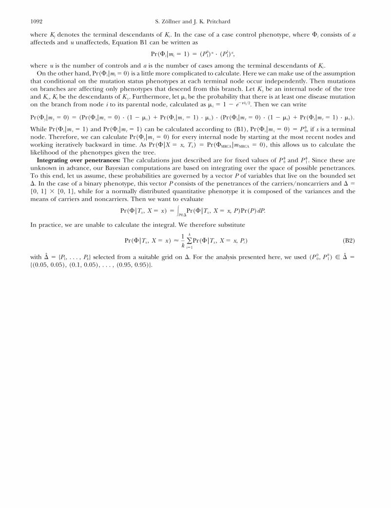
1092 S. Zollner and J. K. Pritchard
where Kj denotes the terminal descendants of Ki . In the case of a case control phenotype, where �i consists of aaffecteds and u unaffecteds, Equation B1 can be written as
Pr(�i |mi � 1) � (P 01)u · (P 1
1)a,
where u is the number of controls and a is the number of cases among the terminal descendants of Ki .On the other hand, Pr(�i |mi � 0) is a little more complicated to calculate. Here we can make use of the assumption
that conditional on the mutation status phenotypes at each terminal node occur independently. Then mutationson branches are affecting only phenotypes that descend from this branch. Let Ky be an internal node of the treeand Ks , Kt be the descendants of Ky . Furthermore, let �i be the probability that there is at least one disease mutationon the branch from node i to its parental node, calculated as �i � 1 � e��bi/2. Then we can write
Pr(�y |m y � 0) � (Pr(�s |m s � 0) · (1 � �s ) � Pr(�s |m s � 1) · �s ) · (Pr(�t |m t � 0) · (1 � �t) � Pr(�t |m t � 1) · �t ).
While Pr(�s |ms � 1) and Pr(�t |mt � 1) can be calculated according to (B1), Pr(�s |ms � 0) � P φ0, if s is a terminal
node. Therefore, we can calculate Pr(�y |my � 0) for every internal node by starting at the most recent nodes andworking iteratively backward in time. As Pr(� |X � x, Tx) � Pr(�MRCA |mMRCA � 0), this allows us to calculate thelikelihood of the phenotypes given the tree.
Integrating over penetrances: The calculations just described are for fixed values of P φ0 and P φ
1 . Since these areunknown in advance, our Bayesian computations are based on integrating over the space of possible penetrances.To this end, let us assume, these probabilities are governed by a vector P of variables that live on the bounded set�. In the case of a binary phenotype, this vector P consists of the penetrances of the carriers/noncarriers and � �[0, 1] � [0, 1], while for a normally distributed quantitative phenotype it is composed of the variances and themeans of carriers and noncarriers. Then we want to evaluate
Pr(� |Tx , X � x) � �P��
Pr(� |Tx , X � x, P)Pr(P)dP.
In practice, we are unable to calculate the integral. We therefore substitute
Pr(� |Tx , X � x) � 1k �
k
i�1
Pr(� |Tx , X � x, Pi) (B2)
with � � {P1, . . . , Pk } selected from a suitable grid on �. For the analysis presented here, we used (P 00 , P 0
1) � � �{(0.05, 0.05), (0.1, 0.05), . . . , (0.95, 0.95)}.
Related Documents