PRIMARY RESEARCH ARTICLE CO 2 exchange and evapotranspiration across dryland ecosystems of southwestern North America Joel A. Biederman 1 | Russell L. Scott 1 | Tom W. Bell 2 | David R. Bowling 3 | Sabina Dore 4 | Jaime Garatuza-Payan 5 | Thomas E. Kolb 4 | Praveena Krishnan 6 | Dan J. Krofcheck 7 | Marcy E. Litvak 7 | Gregory E. Maurer 7 | Tilden P. Meyers 6 | Walter C. Oechel 8,9 | Shirley A. Papuga 10 | Guillermo E. Ponce-Campos 1 | Julio C. Rodriguez 11 | William K. Smith 10 | Rodrigo Vargas 12 | Christopher J. Watts 13 | Enrico A. Yepez 5 | Michael L. Goulden 14 1 Southwest Watershed Research Center, Agricultural Research Service, Tucson, AZ, USA 2 Earth Research Institute, University of California Santa Barbara, Santa Barbara, CA, USA 3 Department of Biology, University of Utah, Salt Lake City, UT, USA 4 School of Forestry, Merriam-Powell Center for Environmental Research, Northern Arizona University, Flagstaff, AZ, USA 5 Departamento de Ciencias del Agua y Medio Ambiente, Instituto Tecnol ogico de Sonora, Ciudad Obreg on, Sonora, Mexico 6 Atmospheric Turbulence and Diffusion Division, Air Resources Laboratory, National Oceanographic and Atmospheric Administration, Oak Ridge, TN, USA 7 Department of Biology, University of New Mexico, Albuquerque, NM, USA 8 Global Change Research Group, Department of Biology, San Diego State University, San Diego, CA, USA 9 Department of Geography, College of Life and Environmental Sciences, Exeter, UK 10 School of Natural Resources and the Environment, University of Arizona, Tucson, AZ, USA 11 Departamento de Agricultura y Ganaderia, Universidad de Sonora, Hermosillo, Sonora, Mexico 12 Department of Plant and Soil Sciences, University of Delaware, Newark, DE, USA 13 Departamento de Fisica, Universidad de Sonora, Hermosillo, Sonora, Mexico 14 Department of Earth System Science, University of California Irvine, Irvine, CA, USA Correspondence Joel Biederman, USDA-ARS, Tucson, AZ, USA. Email: [email protected] Funding information U.S. Department of Energy’s Office of Science; National Science Foundation, Grant/Award Number: EAR-125501; NSF SGER; SDSU; SDSU Field Stations; NSF International Program; CONACyT; CIBNOR Abstract Global-scale studies suggest that dryland ecosystems dominate an increasing trend in the magnitude and interannual variability of the land CO 2 sink. However, such analy- ses are poorly constrained by measured CO 2 exchange in drylands. Here we address this observation gap with eddy covariance data from 25 sites in the water-limited Southwest region of North America with observed ranges in annual precipitation of 100–1000 mm, annual temperatures of 2–25°C, and records of 3–10 years (150 site- years in total). Annual fluxes were integrated using site-specific ecohydrologic years to group precipitation with resulting ecosystem exchanges. We found a wide range of carbon sink/source function, with mean annual net ecosystem production (NEP) vary- ing from -350 to +330 gCm 2 across sites with diverse vegetation types, contrasting with the more constant sink typically measured in mesic ecosystems. In this region, only forest-dominated sites were consistent carbon sinks. Interannual variability of NEP, gross ecosystem production (GEP), and ecosystem respiration (R eco ) was larger ---------------------------------------------------------------------------------------------------------------------------------------------------------------------- Published 2017. This article is a U.S. Government work and is in the public domain in the USA Received: 14 September 2016 | Revised: 9 February 2017 | Accepted: 7 March 2017 DOI: 10.1111/gcb.13686 4204 | wileyonlinelibrary.com/journal/gcb Glob Change Biol. 2017;23:4204–4221.

Welcome message from author
This document is posted to help you gain knowledge. Please leave a comment to let me know what you think about it! Share it to your friends and learn new things together.
Transcript

P R IMA R Y R E S E A R CH A R T I C L E
CO2 exchange and evapotranspiration across drylandecosystems of southwestern North America
Joel A. Biederman1 | Russell L. Scott1 | Tom W. Bell2 | David R. Bowling3 |
Sabina Dore4 | Jaime Garatuza-Payan5 | Thomas E. Kolb4 | Praveena Krishnan6 |
Dan J. Krofcheck7 | Marcy E. Litvak7 | Gregory E. Maurer7 | Tilden P. Meyers6 |
Walter C. Oechel8,9 | Shirley A. Papuga10 | Guillermo E. Ponce-Campos1 |
Julio C. Rodriguez11 | William K. Smith10 | Rodrigo Vargas12 | Christopher J. Watts13 |
Enrico A. Yepez5 | Michael L. Goulden14
1Southwest Watershed Research Center, Agricultural Research Service, Tucson, AZ, USA
2Earth Research Institute, University of California Santa Barbara, Santa Barbara, CA, USA
3Department of Biology, University of Utah, Salt Lake City, UT, USA
4School of Forestry, Merriam-Powell Center for Environmental Research, Northern Arizona University, Flagstaff, AZ, USA
5Departamento de Ciencias del Agua y Medio Ambiente, Instituto Tecnol�ogico de Sonora, Ciudad Obreg�on, Sonora, Mexico
6Atmospheric Turbulence and Diffusion Division, Air Resources Laboratory, National Oceanographic and Atmospheric Administration, Oak Ridge, TN, USA
7Department of Biology, University of New Mexico, Albuquerque, NM, USA
8Global Change Research Group, Department of Biology, San Diego State University, San Diego, CA, USA
9Department of Geography, College of Life and Environmental Sciences, Exeter, UK
10School of Natural Resources and the Environment, University of Arizona, Tucson, AZ, USA
11Departamento de Agricultura y Ganaderia, Universidad de Sonora, Hermosillo, Sonora, Mexico
12Department of Plant and Soil Sciences, University of Delaware, Newark, DE, USA
13Departamento de Fisica, Universidad de Sonora, Hermosillo, Sonora, Mexico
14Department of Earth System Science, University of California Irvine, Irvine, CA, USA
Correspondence
Joel Biederman, USDA-ARS, Tucson, AZ,
USA.
Email: [email protected]
Funding information
U.S. Department of Energy’s Office of
Science; National Science Foundation,
Grant/Award Number: EAR-125501; NSF
SGER; SDSU; SDSU Field Stations; NSF
International Program; CONACyT; CIBNOR
Abstract
Global-scale studies suggest that dryland ecosystems dominate an increasing trend in
the magnitude and interannual variability of the land CO2 sink. However, such analy-
ses are poorly constrained by measured CO2 exchange in drylands. Here we address
this observation gap with eddy covariance data from 25 sites in the water-limited
Southwest region of North America with observed ranges in annual precipitation of
100–1000 mm, annual temperatures of 2–25°C, and records of 3–10 years (150 site-
years in total). Annual fluxes were integrated using site-specific ecohydrologic years to
group precipitation with resulting ecosystem exchanges. We found a wide range of
carbon sink/source function, with mean annual net ecosystem production (NEP) vary-
ing from -350 to +330 gCm�2 across sites with diverse vegetation types, contrasting
with the more constant sink typically measured in mesic ecosystems. In this region,
only forest-dominated sites were consistent carbon sinks. Interannual variability of
NEP, gross ecosystem production (GEP), and ecosystem respiration (Reco) was larger
- - - - - - - - - - - - - - - - - - - - - - - - - - - - - - - - - - - - - - - - - - - - - - - - - - - - - - - - - - - - - - - - - - - - - - - - - - - - - - - - - - - - - - - - - - - - - - - - - - - - - - - - - - - - - - - - - - - - - - - - - - - - - - - - - - - - - - - - - - - - - - - - - - - - - - - - - - - - - - - - - - - - - -Published 2017. This article is a U.S. Government work and is in the public domain in the USA
Received: 14 September 2016 | Revised: 9 February 2017 | Accepted: 7 March 2017
DOI: 10.1111/gcb.13686
4204 | wileyonlinelibrary.com/journal/gcb Glob Change Biol. 2017;23:4204–4221.

than for mesic regions, and half the sites switched between functioning as C sinks/C
sources in wet/dry years. The sites demonstrated coherent responses of GEP and
NEP to anomalies in annual evapotranspiration (ET), used here as a proxy for annually
available water after hydrologic losses. Notably, GEP and Reco were negatively related
to temperature, both interannually within site and spatially across sites, in contrast to
positive temperature effects commonly reported for mesic ecosystems. Models based
on MODIS satellite observations matched the cross-site spatial pattern in mean annual
GEP but consistently underestimated mean annual ET by ~50%. Importantly, the
MODIS-based models captured only 20–30% of interannual variation magnitude.
These results suggest the contribution of this dryland region to variability of regional
to global CO2 exchange may be up to 3–5 times larger than current estimates.
K E YWORD S
climate, moderate resolution imaging spectroradiometer, net ecosystem exchange,
photosynthesis, remote sensing, respiration, semiarid, water
1 | INTRODUCTION
Dryland ecosystems (arid and semiarid) occupy approximately 40%
of the terrestrial surface (Reynolds et al., 2007), and global-scale
studies suggest they strongly influence the carbon cycle due to
the inherent variability of water, their main limiting resource
(Ahlstr€om et al., 2015; Jung et al., 2011; Middleton & Thomas,
1992; Poulter et al., 2014). Unfortunately, the availability of contin-
uous, long-term measurements of water and CO2 exchange has
lagged in drylands as compared to wetter regions (mesic and
humid). Therefore, understanding of dryland ecosystem-atmosphere
exchanges relies heavily upon remote sensing models (RSM),
coarse-scale atmospheric inversion models, empirical regression
models, or terrestrial biosphere models, all of which are poorly
constrained by dryland ecosystem data (Ahlstr€om et al., 2015; Jung
et al., 2011; Ma, Huete, Moran, Ponce-Campos, & Eamus, 2015;
Poulter et al., 2014; Verma et al., 2014; Xiao et al., 2014). While
much has been learned from field measurements such as plot-scale
aboveground net primary production (ANPP) (Huxman et al., 2004;
Lauenroth & Sala, 1992; Noy-Meir, 1973; Ponce-Campos et al.,
2013), the maturation of multi-annual, multisite eddy covariance
datasets presents an opportunity to advance understanding of (i)
diverse dryland ecosystems for which ANPP data lack; (ii) tower
footprint-scale net and gross CO2 fluxes from entire ecosystems
(i.e., above- and below-ground); and (iii) bidirectional, coupled, land-
atmosphere exchanges of CO2 and water, the critical limiting
resource in drylands.
Until recently, efforts to synthesize direct observations of CO2
and water exchange across multiple eddy covariance sites were
weighted toward productive, mesic ecosystems, especially forests
(Baldocchi, 2008; Chen et al., 2015; Keenan et al., 2012; Law et al.,
2002; Luyssaert et al., 2007; Valentini et al., 2000; Williams et al.,
2012). These studies suggest that annual NEP is usually positive
(sink of ~100–300 gCm�2) and that annual GEP is positively related
to both water availability and temperature (Yi et al., 2010), while
annual ET tends to closely track seasonal changes in available energy
(Williams et al., 2012). Meanwhile, annual Reco appears to be posi-
tively related to mean annual temperature in some cases (Reichstein
et al., 2007; Yu et al., 2013) or unrelated in others (Janssens et al.,
2001). In mesic to humid systems, where water is not limiting,
annual ET tends to be relatively depend on available energy (Wil-
liams et al., 2012). Drought tends to reduce GEP more strongly than
Reco, resulting in reduced, but usually positive, net CO2 uptake (Bal-
docchi, 2008; Reichstein et al., 2007; Schwalm et al., 2010). Flux
data syntheses weighted to mesic sites suggest relative interannual
variability of GEP and Reco ranges from ~5 to 20% (Keenan et al.,
2012; Yuan et al., 2009), whereas less is known about interannual
variability of ET, especially for drylands (Villarreal et al., 2016). While
model studies suggest larger interannual variability in dryland fluxes
(Ahlstr€om et al., 2015; Jung et al., 2011), measured interannual vari-
ability remains largely unknown (Tramontana et al., 2016).
While a growing number of studies present dryland fluxes, none
has included sufficient sites and years of data to characterize the
regional magnitude and interannual variability of CO2 exchange and
ET (Anderson-Teixeira, Delong, Fox, Brese, & Litvak, 2011; Baldoc-
chi, 2014; Dore et al., 2010; Luo et al., 2007; Ma, Baldocchi, Xu, &
Hehn, 2007; Pereira et al., 2007; Scott, Biederman, Hamerlynck, &
Barron-Gafford, 2015; Thomas et al., 2009). These studies suggest
unique dryland characteristics requiring more comprehensive evalua-
tion including: (i) a wider range of site mean NEP than mesic biomes,
including persistent carbon sources and sinks (Baldocchi, 2008; Bie-
derman et al., 2016; Ma, Baldocchi, Wolf, & Verfaillie, 2016; Yu
et al., 2013); (ii) large interannual variability of CO2 exchange and
ET, including sites that ‘pivot’ between carbon sink/source function
at site-specific ‘pivot points’ in water availability, demonstrating the
strong linkage between CO2 and water in drylands (Kurc & Small,
2007; Ma et al., 2016; Pereira et al., 2007; Scott et al., 2015); and
(iii) unique seasonal dynamics of temperature, precipitation, and
BIEDERMAN ET AL. | 4205

phenology, which can sometimes drive two distinct seasons (winter/
spring, summer) of elevated CO2 exchange and ET, depending on
the relative timing of water and radiation inputs (Anderson-Teixeira
et al., 2011; Dore et al., 2010; Scott, Serrano-Ortiz, Domingo,
Hamerlynck, & Kowalski, 2012). These unique traits call for caution
in extrapolating ecological understanding from measurements in
more well-studied mesic regions and highlight the need for directly
comparable measurements in drylands.
In the absence of widespread ground observations, RSM are
commonly used to estimate dryland CO2 exchange and ET (Ma
et al., 2015; Ponce-Campos et al., 2013; Poulter et al., 2014). Satel-
lite-derived greenness (EVI, NDVI) may be empirically related to
point measurements of CO2 exchange and ET (Goulden et al.,
2012; Ponce-Campos et al., 2013; Sims et al., 2006) or used with
climate data to derive process-based RSM for GEP and ET (Mu,
Zhao, & Running, 2011; Sims et al., 2006; Smith et al., 2016;
Turner et al., 2006). Evaluation of RSM across flux tower networks
suggests that RSM capture spatial patterns of GEP but contain rel-
atively little information about GEP interannual variability (Jin &
Goulden, 2014; Verma et al., 2014). RSM are expected to find par-
ticular challenges in drylands due mainly to (i) satellite-derived
greenness indices that do not capture the physiological properties
of the vegetation that control photosynthesis, and (ii) assumptions
of static, biome-level parameters (e.g., light-use efficiency), which
vary seasonally with root zone soil moisture and other factors
(Krofcheck et al., 2015; Kurc & Small, 2007; Liu, Rambal, & Mouil-
lot, 2015; Verma et al., 2014). Prior data-RSM comparisons have
included few dryland sites (Mu et al., 2011; Sims et al., 2006;
Turner et al., 2006), and there is a need to understand how well
commonly used RSM capture the magnitude and interannual vari-
ability of measured CO2 exchange and ET.
Here we address the gap in dryland flux observations and evalu-
ate whether common assumptions from mesic regions are valid in a
water-limited region. We present a synthesis of site-level climate
and ecosystem-atmosphere exchange of water and CO2 at monthly
and annual time scales for 25 sites with a combined 150 site-years
of measurements. The questions addressed here are: (i) Do the spa-
tially diverse seasonal patterns of precipitation, temperature, and
phenology combine to produce identifiable patterns of CO2
exchange and ET across the Southwest region of North America?
We expect more diverse seasonality than in mesic regions including
winter-dominated, summer-dominated, and bimodal ecosystems. (ii)
What are the magnitudes of spatial and interannual variability CO2
exchange and ET? We expect variability to be larger in water-limited
ecosystems than in mesic ecosystems limited by energy or nutrients
(Ma et al., 2015; Noy-Meir, 1973; Yuan et al., 2009). (iii) How well
do MODIS-based models capture spatial and interannual variability
of measured CO2 exchange and ET? Detailed diagnosis of RSM
errors is beyond the scope of this paper, as our purpose here is to
provide a first model-data comparison focused on the magnitude
and interannual variability of CO2 exchange and ET fluxes in this
water-limited region.
2 | MATERIALS AND METHODS
2.1 | Study region: southwestern North America
The study region (hereafter referred to as ‘the Southwest’) comprises
sites in the US states of Arizona, New Mexico, southern portions of
Utah and California, and the Mexican states of Sonora and Baja Califor-
nia Sur (Figure 1a). The Southwest is characterized by water limitation
at the annual scale (potential ET >> precipitation). The Southwest has
large spatial gradients in mean annual precipitation (MAP 40–
1200 mm, Figure 1) and temperature (MAT �4 to +26°C, Fig. S1) due
to interactions among topography, latitude, wind patterns, and distance
from oceans. The 25 study sites represent the majority of the South-
west in this two-dimensional climate space, especially the most fre-
quent portion of MAT ~10–20°C and MAP ~200–600 mm (Figure 1b).
Seasonal weather dynamics drive distinct spatial patterns of
ecosystem CO2 exchange and ET across the Southwest. The western
portion adjacent to the Pacific Ocean experiences a Mediterranean
climate with up to 90% of MAP occurring during winter months (de-
fined here as November–April, Fig. S2). In contrast, the central, east-
ern, and southeastern portions are heavily influenced by the North
American Monsoon (Douglas, Maddox, Howard, & Reyes, 1993),
which brings a majority of the annual precipitation during summer
(Junuary–October) from moisture sources in the Gulfs of Mexico and
California (Fig. S2). Across the Southwest, winter precipitation from
Pacific frontal systems tends to be greater during negative phases of
the El Ni~no Southern Oscillation (ENSO) and less during positive, La
Ni~na phases (Andrade & Sellers, 1988). Baja California receives pre-
cipitation mainly from Pacific tropical storms during early fall
(September–October) and is influenced by teleconnections with the
Southern California current (Reimer et al., 2015).
2.2 | Study sites
We used 25 eddy covariance flux sites with 3–10 years of measure-
ments (mean of 6 years, total n = 150 years) representing the cli-
mate and ecosystems of the Southwest (Figure 1, Table 1, Table S1,
Figs S1 and S2). Observations were made between 1999 and 2014,
with greatest data density during 2005–2014 (Table 1). The major
regional IGBP vegetation classes represented, identified by site
teams, include grassland, open and closed shrubland, savanna and
woody savanna, mixed forest, and evergreen needleleaf forest. Study
sites were initially classified into based on based on K€oppen climate
(http://koeppen-geiger.vu-wien.ac.at/present.htm). However, pat-
terns of distinct climate and flux dynamics (Figure 2) warranted
some separation/ combination of K€oppen classes, resulting in seven
subregional groups (Table 1, Figure 1). For site details, see refer-
ences in Table 1 and www.fluxdata.org.
2.3 | Flux data collection and processing
We assembled 30-min measurements of precipitation, ET, NEP, and
GEP and Reco derived from NEP using methods similar to those
4206 | BIEDERMAN ET AL.

described in Biederman et al. (2016). Measurements of terrestrial-
atmosphere gas exchange were made at the ecosystem level using
the eddy covariance technique (Goulden, Munger, Fan, Daube, &
Wofsy, 1996). Data collection and regular calibrations of eddy
covariance flux measurement systems followed accepted guidelines
(Lee, Massman, & Law, 2006). Periods of insufficient turbulent mix-
ing were screened using a friction velocity filter (Reichstein et al.,
2005). Gross fluxes were partitioned from the net CO2 exchange
measurements based on the observed relationship between night-
time respiration and temperature, which was then used to separately
derive daytime GEP and Reco.
Precipitation falling late in the calendar year is often stored as
snowpack or soil moisture and should be associated with plant
productivity in the following growing season (Ma et al., 2007; Per-
eira et al., 2007; Thomas et al., 2009). Therefore, annual flux sums
and metrological driving variables were calculated using an ecohy-
drologic year spanning November–October. Because multiyear
records at 12 of the sites commenced with the calendar year, the
first two months of these records (November and December of
the first hydrologic year in each record) were filled using mean
monthly fluxes of remaining years (Biederman et al., 2016), repre-
senting 2–5% of data presented. This gap filling had minimal
impact on annual sums because November and December are rel-
atively low-flux months, together comprising only 5–15% of mean
annual fluxes at a given site (Figure 2). No filling of missing
months was applied at MX-lpa, which has warmer winters with
higher fluxes.
Because US-cop is the only long-term eddy covariance dataset in
the dry northern portion of the Colorado Plateau, we took additional
steps to produce annual sums from the published weekly values
(Bowling, Bethers-Marchetti, Lunch, Grote, & Belnap, 2010), enabling
the site to be included here. Multiple linear regression was used to
gap-fill missing weekly values of NEP, GEP, and ET using 10-cm soil
moisture, solar radiation, and air temperature with separate regres-
sion models for each season. Reco was calculated as NEP minus GEP.
Approximately 20% of weekly values at US-cop were thus modeled,
with the majority of filled weeks (>70%) occurring during low-flux
winter periods.
2.4 | Use of ET as a proxy for ecosystem wateravailability
As the most widely measured hydrologic flux, precipitation (P) is the
common proxy for annual ecosystem water availability (Sala,
(a)
(b)
F IGURE 1 (a) Map of flux observationsites with regional mean annualprecipitation (1950–2000) and (b) meanannual precipitation (MAP) andtemperature (MAT) of flux sites mappedonto a scaled probability density functionof the 2D climate space of southwesternNorth America (most frequent = yellow,least = dark blue). Flux site marker colorsindicate subregional groups of flux sitessharing similar seasonal climatic andecological dynamics. For sites codes anddescriptions, see Table 1 [Colour figure canbe viewed at wileyonlinelibrary.com]
BIEDERMAN ET AL. | 4207

TABLE
1Site
descriptions,m
eanclim
atea,a
ndobservationye
ars
Subreg
ion
Site
IDDescription
Dominan
tspec
ies
IGBPclass
K€ opp
enclim
ate
Eleva
tion
(m)
MAP
(mm)
MAT
(°C)
Obs.ye
ars
Site
reference
Med
iterrane
an
mid-elevation
US-scf
Southe
rnCalifornia
oak-pineforest
Quercus
spp.Pinu
sedulis
Woody
savann
aCsa
1702
692
10.9
2007–2
012
Goulden
etal.(2012)
US-soo/
sobb
SkyOaksOld
Stan
d
chap
arral
Adeno
stom
afasciculatum
Closedshrublan
dCsa
1406
558
13.0
1999–0
2/
2004–0
8,11
Luoet
al.(2007)
US-son
SkyOaksNew
Stan
d
chap
arral
Adeno
stom
afasciculatum
Closedshrublan
dCsa
1444
573
12.9
2004–2
006
Luoet
al.(2007)
US-soy
SkyOaksYoun
g
Stan
dch
aparral
Adeno
stom
afasciculatum
Closedshrublan
dCsa
1412
591
12.7
2002,2004–2
006
Luoet
al.(2007)
Med
iterrane
an
low
elev
ation
US-scw
Southe
rnCalifornia
piny
on-junipe
r
Pinu
sedulis,Juniperus
mon
osperm
a
Woody
savann
aBwh
1274
403
14.1
2007–2
013
Goulden
etal.(2012)
US-scc
Southe
rnCalifornia
chap
arral
Adeno
stom
afasciculatum
Ope
nshrublan
dsBwh
1296
409
13.9
2007–2
013
Goulden
etal.(2012)
Colorado
Plateau
US-co
pCorral
grasslan
d
Hilariajamesii,
Stipa
hymenoides,Coleogyne
ramosissima
Grassland
Bsk
1522
247
11.6
2001–2
003,
2006–2
007
Bowlin
get
al.(2010)
Monsoonhigh
elev
ation
US-vcm
VallesCalde
ramixed
coniferforest
Piceaengelman
nii,Picea
pugens,Abies
lasiocarpa
var.
lasiocarpa
,Abies
concolor
Eve
rgreen
need
leleaf
forest
Dfb
3042
724
2.9
2007–2
012
Anderson-Teixe
ira
etal.(2011)
Monsoonmid
elev
ation
US-vcp
VallesCalde
ra
pond
erosa
forest
Pinu
spo
nderosa,
Quercus
gambeli
Eve
rgreen
need
leleaf
forest
Dfb
2501
547
5.7
2007–2
012
Anderson-Teixe
ira
etal.(2011)
US-mpj
HeritageLand
Conservanc
y
piny
on-junipe
r
Pinu
sedulis,Juniperus
mon
osperm
a
Savann
a2200
423
9.6
2008–2
013
Anderson-Teixe
ira
etal.(2011)
US-wjs
Tab
leland
sjunipe
r
savann
a
Juniperusmon
osperm
a,
Bou
teloua
gracilis
Savann
aBsk
1931
349
10.9
2008–2
013
Anderson-Teixe
ira
etal.(2011)
US-fuf
Flagstaff
unman
aged
pond
erosa
Pinu
spo
nderosa
Eve
rgreen
need
leleaf
forest
Csb/D
sb2215
607
7.1
2006–2
010
Dore
etal.(2012)
(Continues)
4208 | BIEDERMAN ET AL.

TABLE
1(Continue
d)
Subreg
ion
Site
IDDescription
Dominan
tspec
ies
IGBPclass
K€ opp
enclim
ate
Eleva
tion
(m)
MAP
(mm)
MAT
(°C)
Obs.ye
ars
Site
reference
Monsoonlow
elev
ation
US-seg
Sevilleta
grasslan
d:
burned
2009
Bou
teloua
eriopo
da,
Gutierrezia
sarothrae,
Ceratoideslana
ta
Grassland
Bsk
160
250
12.6
2010–2
014
Petrie,
Collins,Sw
ann,Ford,
andLitvak
(2015)
US-ses
Sevilleta
creo
sote
shrublan
d
Larrea
tridentata,
G.sarothrae
Ope
nshrublan
dBsk
1610
252
12.6
2007–2
014
Petrieet
al.(2015)
US-sen
Sevilleta
grasslan
d
new:un
burned
Bou
teloua
eriopo
da,
Gutierrezia
sarothrae,
Ceratoideslana
ta
Grassland
Bsk
1603
255
12.5
2009–2
014
Petrieet
al.(2015)
US-whs
Walnu
tGulch
Lucky
Hillsshrublan
d
Larrea
tridentata,Pa
rthenium
incanu
m,Acaciaconstricta,
Rhu
smicroph
ylla
Ope
nshrublan
dBsk
1376
352
16.8
2008–2
014
Scott
(2010)
US-src
SantaRitaCreosote
shrublan
d
Larrea
tridentata
Ope
nshrublan
dBsh
1000
378
18.4
2008–2
013
Kurc
andBen
ton(2010)
US-wkg
Walnu
tGulch
Ken
dallgrasslan
d
Eragrostislehm
annian
a,
Bou
teloua
spp.
Calliand
ra
erioph
ylla
Grassland
Bsk
1529
386
15.8
2005–2
014
Scott,Ham
erlynck,Jenerette,
Moran,an
dBarron-G
afford
(2010)
US-srm
SantaRitamesqu
ite
savann
a
Prosop
isvelutina
,Eragrostis
lehm
annian
a
Woody
savann
aBsk
1122
421
17.7
2005–2
014
Scott,Jenerette,Potts,an
d
Huxm
an(2009)
US-au
dAud
ubongrasslan
dBou
telouagracilis,
B.curtipendu
la,Eragrostisspp.
Grassland
Bsk
1472
463
15.3
2004–2
009
Krishnan
,Mey
ers,Sc
ott,
Ken
ned
y,an
dHeu
er(2012)
MX-ray
Rayonsubtropical
shrublan
d
Fouq
uieria
macdo
ugalii,
Acaciacochliacantha
,
Parkinsoniapraecox,
Mim
osa
distachya,
Prosop
isvelutina
Savann
aBsh
634
475
21.7
2009–2
012
M� en
dez-B
arroso
etal.(2014)
US-srg
SantaRitagrasslan
dEragrostislehm
annian
aSa
vann
aBsh
1292
494
16.7
2009–2
014
Scott
etal.(2015)
MX-tes
Tesopa
cosemiarid
tropicalsavann
a
Lysilomadivaricatum,Ipom
ea
arbo
recens,Acacia
cochliacantha
Woody
savann
aBsh
467
721
23
2005–2
008
Perez-Ruiz
etal.(2010)
BajaSu
rMX-lpa
LaPaz
arid-tropical
scrub
Prosop
isarticulata,Fo
uguieria
diguetti,Bursera
microph
ylla,Cyrtocarpa
edulis,Jatrop
hacinere,
J.cuneata
Ope
nshrublan
dBwh
18
167
23.6
2003–2
008
Hastings,Oechel,&
Muhlia-M
elo,
2005;Bell,Men
zer,
Troyo
-Di� equez,an
dOechel
(2012)
a Mea
nan
nual
tempe
rature
(MAT)an
dmea
nan
nual
precipitation(M
AP)1950–2
000from
theW
orldC
lim1-km
dataset(w
ww.w
orldc
lim.org).
bObservations
collected
atsooaftera2003stan
d-replacingwild
fire
arede
noted‘sob’
andan
alyzed
asaun
ique
site.
BIEDERMAN ET AL. | 4209

Gherardi, Reichmann, Jobb�agy, & Peters, 2012). However, some por-
tion of P is lost to runoff and drainage and is unavailable to the
ecosystem. Therefore, we also used ET as a metric of annual water
availability. At shorter time scales (diurnal to seasonal), rates of ET
are related to many factors including available energy, root density,
leaf area and soil water retention properties. However, water-limited
ecosystems frequently experience exhaustions of soil moisture, the
limiting resource, throughout the year (Thomas et al., 2009). Regard-
less of shorter-term temporal dynamics, annually integrated ET rep-
resents the efflux of soil moisture that has been available to drive
ecosystem exchanges after some precipitation is lost to runoff and
drainage (Q) (Biederman et al., 2016; Briggs & Shantz, 1913; Noy-
Meir, 1973). The local water balance reflects this hydrologic parti-
tioning of P to hydrologic losses (Q), storage changes (S, usually neg-
ligible at the annual scale), and soil moisture recharge, the main
source of ET (Equation 1).
P ¼ ETþQ� S: (1)
Hydrologic losses (Q) tend to be larger in wetter years and at
wetter sites, increasing the amount by which precipitation
overestimates water available to drive CO2 exchange (Biederman
et al., 2016; Ponce-Campos et al., 2013; Villarreal et al., 2016).
While ecosystem-level ET does not provide details on the partition-
ing of evaporation and transpiration, removal of hydrologic losses
makes ET a better metric of available water than precipitation.
2.5 | Remote sensing model estimates ofecosystem exchange
We used the enhanced vegetation index (EVI) from the Moderate
Resolution Imaging Spectroradiometer (MODIS) Collection 5. We ini-
tially used EVI to explore seasonal similarities between greenness
and fluxes of CO2 and water. As RSM of these fluxes rely on satel-
lite indices closely correlated to EVI, this comparison provides insight
into RSM performance across this region. This index is distributed as
MOD13Q1 data product with 16-day temporal resolution. We used
the single 250-m pixel containing each flux tower. Mean monthly
EVI values were computed using data classified as best quality to
reduced contamination associated with clouds, shadows, and snow/
ice. We obtained monthly aggregates of MODIS GEP (MOD17A2)
and ET (MOD16A2) for the 1-km pixel containing each flux tower
F IGURE 2 (a–c) Mean monthly (�SD)precipitation (P, mm), evapotranspiration(ET, mm), gross ecosystem productivity(GEP gC m-2), and enhanced vegetationindex (EVI). Each panel shows asubregional grouping (Figure 1, Table 1)sharing similar seasonal climatic andecological dynamics. Vertical scales varydue to differences among subregions. (d–g)continued for the remaining subregions[Color figure can be viewed atwileyonlinelibrary.com]
4210 | BIEDERMAN ET AL.

from the Numerical Terradynamic Simulation Group (http://files.ntsg.
umt.edu/data/NTSG_Products/). MODIS ET calculates daily esti-
mates based on the Penman-Monteith equation, driven by multiple
satellite-based data (FPAR, LAI, albedo) as well as daily meteorologi-
cal reanalysis (Mu et al., 2011). MODIS GEP calculates daily esti-
mates based on light-use efficiency logic, driven by multiple satellite
datasets (FPAR, LAI) as well as daily meteorological reanalysis. For
more details on the MODIS GEP and ET algorithms refer to Mu
et al. (2011) and Zhao & Running (2010), respectively.
2.6 | Calculation of annual anomalies
We assessed regional patterns in climate and flux anomalies with
time series of annual z-scores (standard deviations from the mean
annual value at a given site). Because the years of measurements at
each site varied, we defined a common baseline around which to
compute z-scores by excluding regionally wet years (2004, 2005,
2010) and dry years (2002, 2003, 2012) during which precipitation
was more than one standard deviation from the mean (1999–2014)
according to the NOAA climate data for the US Southwest region
http://www.ncdc.noaa.gov/cag. For each year, we calculated the
mean and spatial standard deviation of z-scores across available
sites.
2.7 | Separating spatial and temporal relationships
We separated spatial patterns across sites from site-level temporal
variability using linear fits between a driver and response variable
(e.g., precipitation and productivity). This spatial-temporal separation
approach differs from the common practice in synthesis studies of
eddy covariance data in which a single relationship between two
variables is determined across pooled site years (Baldocchi, 2008;
Law et al., 2002; Luyssaert et al., 2007; Yu et al., 2013), represent-
ing the approximate spatial relationship. One interpretation of the
separated temporal and spatial patterns is that site-level temporal
slopes represent ecophysiological responses to annually varying fac-
tors such as precipitation, while spatial relationships fit to mean
annual values across sites reflect slow-changing controls such as
plant community adaptation to long-term climate (Biederman et al.,
2016; Chen et al., 2015; Lauenroth & Sala, 1992).
F IGURE 2 Continued.
BIEDERMAN ET AL. | 4211

3 | RESULTS
3.1 | Mediterranean
The six sites in southern California (Figure 1, Table 1) have a
Mediterranean climate with hot, dry summers (June–October) and
cool, wet winters (November–May) during which >65% of annual
precipitation typically falls. The Mediterranean Mid-elevation subre-
gion includes four sites in K€oppen class Csa (temperate with dry, hot
summers) comprising one oak-pine forest and three chamise cha-
parral ecosystems with elevation ~1500–1700 m, MAP ~550–
700 mm, and MAT ~13°C. Winter precipitation (November–Febru-
ary) stored as soil moisture or occasionally as snowmelt drives ET
and GEP peaking in May (Figure 2a). Productivity is sometimes sus-
tained through summer months, depending upon stored soil moisture
from winter and variable summer rainfall.
Two lower-elevation (~1300 m) Mediterranean sites in class Bwh
(arid, desert, hot summers) including pinyon-juniper and chaparral
ecosystems are warmer (~14°C) and receive less precipitation
(~400 mm). Peak ET and GEP occur earlier in the spring (March–
April) than at the Mid-elevation sites and are followed by an early
summer dry-down. Summer precipitation drives a second ET peak
sometimes accompanied by a smaller GEP peak (Figure 2b), suggest-
ing that a greater fraction of ET is abiotic evaporation during the hot
summer months than during spring. In these Mediterranean subre-
gions (Figure 2a, b), Both GEP and EVI show single peaks at mid-ele-
vation and two peaks at low elevation, although the EVI signal
amplitude is small, as shown by Sims et al. (2006).
3.2 | Colorado Plateau
This site is dry (MAP~250 mm) with precipitation split evenly
between cold winters (~0–3°C) and hot summers (~25–30°C). Stored
winter moisture drives spring peaks in ET and GEP (May), which are
weakly captured in EVI (Figure 2c). Summer precipitation drives ET
without accompanying GEP, suggesting most ET in summer is evapo-
ration, not transpiration. This site was separated from other Bsk sites
(dry steppe, cold winters) in Monsoon Low (Figure 2f) due to higher
winter precipitation (~50% of annual as compared to ~20–30% in
Monsoon Low) and associated predominance of spring productivity.
3.3 | Monsoon
The Monsoon High-elevation subregion (Figure 2d) is represented by
a mixed conifer forest at 3000 m elevation with MAT ~3°C. Mean
annual precipitation is ~730 mm, split equally between winter and
summer, with 20–50% falling as snow. Spring snowmelt typically
provides sufficient soil moisture recharge to sustain ET and produc-
tivity through May and June until the monsoon onset in July. EVI
captures these single peaks in GEP and ET.
The Monsoon Mid-elevation subregion (Figure 2e) comprises
ponderosa pine, pinyon pine, and juniper woodlands at 1900–
2500 m. MAT ranges from 6 to 11°C and MAP varies from 350 to
600 mm, with 50–70% during summer and some winter snowfall.
Stored winter moisture drives spring ET and GEP (March–May). Pro-
ductivity declines with soil moisture during early summer and then
resumes with arrival of monsoon precipitation in July–August. It is
this double peak in mean seasonal fluxes which characterizes this
subregion, despite disparate K€oppen classes (Table 1). EVI peaks
once, in July, and fails to capture the spring GEP/ET peak.
The Monsoon Low subregion comprises desert grassland, shrub-
land, savanna, and deciduous forest at 500 to 1600 m. Mean climate
varies widely (MAT ~12–23°C, MAP ~250–720 mm). These sites are
unified by the dominant role of summer precipitation (65–85% of
MAP) driving single peaks of ET, GEP, and EVI (Figure 2f). Classes
include Bsk and Bsh (dry steppe and classified as k-cold or h-hot,
although MAT does not affect seasonal flux timing).
3.4 | Baja California Sur
This sea-level subtropical desert scrub site (MX-lpa) represents the
only long-term eddy flux measurements (Figure 2g) in this hot, dry
subregion (MAT = 24°C, MAP = 167 mm). Annual precipitation is
dominated by moisture from Pacific tropical storms around Septem-
ber, which can drive ecosystem exchanges through the warm winter
until as late as April. Therefore, we used a modified ecohydrologic
year running June–May for annual flux integration.
3.5 | Patterns and drivers of regional CO2 exchange
Across the dataset of 150 site-years, annual NEP varied between -
550 and + 420 gCm�2, and mean annual NEP varied between -350
and + 330 gCm�2 among sites (Figure 3, Table S1). While several
ecosystems were persistently sinks or sources of CO2, about half the
sites pivoted between sink and source functioning. Monsoon High
and Mid sites were persistent sinks, most Monsoon Low sites piv-
oted, and Mediterranean sites exhibited the full range of sink/
source/pivot function. All IGBP classes showed instances of both
sink and source behavior except for mixed forest and evergreen
needleleaf forests, which were sinks (Fig. S3). NEP interannual varia-
tion showed no identifiable spatial pattern, with standard deviations
ranging between 20 and 230 gCm�2 (Table S1). NEP interannual
variability was highest at the Mediterranean sites (Table S2), which
corresponded closely with mixed forest and closed shrubland classes
(Table S3).
We evaluated the relationship of CO2 exchange with climatic
variables using the gross fluxes GEP and Reco. Despite distinct sea-
sonal dynamics across subregions (Figure 2), previous work has
shown that annual climate values are strongly associated with annual
CO2 exchange across ecohydrologic years (Biederman et al., 2016;
Pereira et al., 2007; Scott et al., 2015; Thomas et al., 2009). Mean
annual GEP showed negative spatial relationships (ANOVA F-test ver-
sus a constant model) to MAT (Figure 4, R2 = 0.28, p < .05) and
mean annual vapor pressure deficit (VPD, R2 = 0.26, p < .05, not
shown) and a positive relationship to MAP (R2 = 0.41, p < .01). To
reduce possible effects of a negative relationship between MAP and
4212 | BIEDERMAN ET AL.

MAT (e.g., high-elevation sites are wetter and colder, Fig. S41), we
repeated the analysis with ten lower-elevation sites restricted to
270 mm < MAP < 450 mm and again found negative temperature
effects on GEP (Fig. S5). Mean annual ET described the most spatial
variability in GEP (R2 = 0.62, p < .01), as previously shown for sub-
sets of sites in this region (Biederman et al., 2016; Scott et al.,
2015). Mean annual ecosystem respiration (Reco) showed no spatial
relationship with MAT, VPD, or MAP, but there was a positive spa-
tial relationship between Reco and mean annual ET (R2 = 0.26,
p < .01), possibly due to increased substrate production associated
with GEP.
Interannual relationships of gross CO2 fluxes with T, P, and ET
were analyzed using the full dataset of annual deviations (denoted
by D) from site-specific multiannual means (Figure 5, all fits
p < 0.01). We found negative temporal responses of DGEP to DT
(-139gC m�2 °C�1, R2 = 0.23) and DVPD (-884 gC m�2 kPa�1,
R2 = 0.34, not shown) and a positive response to DP (0.51 gC
m�2 mm�1, R2 = 0.28). Annual DET explained more DGEP variabil-
ity (1.19 gC m�2 mm�1, R2 = 0.60) than was explained by DP.
Annual DReco showed positive temporal slopes to DP (0.27 gC
m�2 mm�1, R2 = 0.17) and DET (0.58 gC m�2 mm�1, R2 = 0.33).
Annual DReco showed a weak negative relationship with DT (Fig-
ure 5d), meaning that warmer years had less respiration (-55
gCm�2 °C�1, R2 = 0.09). To reduce possible effects of a negative
relationship between ΔT and ΔP (Fig. S4b, e.g., cooler years are
wetter), we repeated the analysis restricted to years with |ΔP| <
50 mm and again found negative temperature effects on both
DGEP and DReco (Fig. S6).
Relative interannual variation of water availability (P, ET) and CO2
fluxes (GEP, Reco) was largest at sites with lowest water availability
(mean ET) (Figure 6). Coefficient of variation of annual precipitation
(CVP) decreased from ~40% to 20% (not significant, p = .14, ANOVA F-
test). CVET was lower than CVP across the gradient with a declining
trend from ~30% to 10%, (p < .01). Of the measured fluxes, CVGEP
decreased most steeply across the gradient, from ~60% at the driest
sites to ~10% at the wettest sites (p < .01), while CVReco showed a
marginally declining trend from ~20% to ~10% (p = .06). Trends were
computed excluding the Sky Oaks sites (US-sox), where 2005 precipi-
tation was > two standard deviations above normal.
3.6 | Regional variations of CO2 exchange acrossthe Southwest: 2005–2014
The Southwest exhibited regionally coherent anomalies in annual
variability of CO2 exchange (Figure 7). During 2005–2014, the por-
tion of the study with greatest spatial representation of sites
(Table 1), temporal precipitation anomalies (zP) were related to those
of water availability (zET), productivity (zGEP), and net CO2 uptake
(zNEP) (Table 2, Figure 7). The annual fluctuation of zReco, (not
shown) was similar to zGEP.
The El Ni~no year 2005 (http://www.ncdc.noaa.gov/teleconnections/
enso/indicators/soi/) was extraordinarily wet at the Mediterranean sites,
F IGURE 3 Mean (�SD) annual net ecosystem production, with sites ordered by mean annual NEP. The Southwest ecosystems ranged frompersistent sinks to persistent sources, although 13 of 25 ecosystems pivoted between sink/source years. Colors correspond to those inFigure 1. For NEP classification by IGBP vegetation, see Fig. S3, Table S3 [Color figure can be viewed at wileyonlinelibrary.com]
BIEDERMAN ET AL. | 4213

F IGURE 4 Spatial relationship of long-term mean annual GEP (top row a–c) and Reco (bottom row d–f) with mean annual temperature (a, d),mean annual precipitation (b, e), and mean annual evapotranspiration (c, f). All slopes shown are significantly different from zero (panel a:p < .05; panels b, c, f: p < .01, n = 25 sites) [Color figure can be viewed at wileyonlinelibrary.com]
F IGURE 5 Temporal variations expressed as annual deviations from each site’s long-term mean values of the same variables shown inFigure 4. All linear fits shown are significant (p < .01) n = 150 site-years
4214 | BIEDERMAN ET AL.

F IGURE 6 Coefficients of interannualvariation (CV) of (a) P and ET, and (b) GEPand Reco across the gradient of site wateravailability (mean ET). Solid lines representsignificant trends (p < .01). Dotted linesare not significant (p = .18 forprecipitation, p = .13 for Reco). Opensymbols are for the Sky Oaks cluster (sob,son, soy), where 2005 precipitation was >
2 standard deviations above normal [Colorfigure can be viewed atwileyonlinelibrary.com]
F IGURE 7 Normalized annualanomalies (z-scores) of (a) precipitation (P),(b) evapotranspiration (ET), (c) grossecosystem production (GEP), and (d) netecosystem production (NEP). Shown arethe mean and spatial standard deviation ofz-scores across sites. The 10-year timeperiod shown represents years withsimultaneous measurements available forat least six sites representing at least foursubregions (Table 1) [Color figure can beviewed at wileyonlinelibrary.com]
BIEDERMAN ET AL. | 4215
with some precipitation totals > 300% of normal (Figure 7a). However,
the wet 2005 precipitation anomaly was weaker elsewhere in the South-
west, as reflected in the large spatial standard deviation of zP. The regio-
nal mean GEP and NEP in 2005 were close to average (mean zGEP = 0,
mean zNEP = -0.1, Figure 7b–d). The El Ni~no year of 2010 was associ-
ated with increased precipitation across the Southwest, with zP = +0.9
(spatial SD = 0.5) driving positive anomalies for ET, GEP, and NEP
(zNEP = 1.1 (0.4). In contrast to the regionally coherent precipitation
increase of 2010, the 2011 La Ni~na year had spatially variable precipita-
tion anomalies, reflected by a large standard deviation of precipitation zP
~ -0.4 (1.1) (Figure 7a). 2011 Mediterranean site precipitation was above
average (zP~ + 0.5), while Monsoon site precipitation was below average
(zP ~ -0.5), resulting in regional mean ET, GEP, and NEP that were all
close to normal (Figure 7b–d).
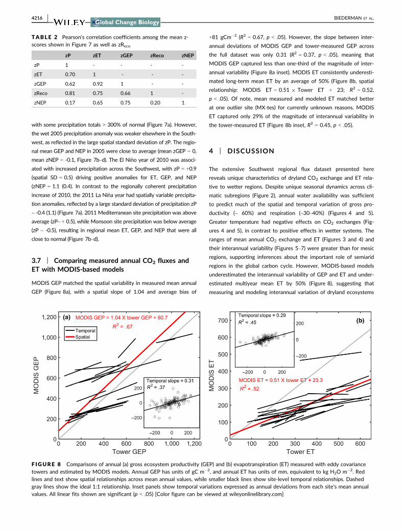
3.7 | Comparing measured annual CO2 fluxes andET with MODIS-based models
MODIS GEP matched the spatial variability in measured mean annual
GEP (Figure 8a), with a spatial slope of 1.04 and average bias of
+81 gCm�2 (R2 = 0.67, p < .05). However, the slope between inter-
annual deviations of MODIS GEP and tower-measured GEP across
the full dataset was only 0.31 (R2 = 0.37, p < .05), meaning that
MODIS GEP captured less than one-third of the magnitude of inter-
annual variability (Figure 8a inset). MODIS ET consistently underesti-
mated long-term mean ET by an average of 50% (Figure 8b, spatial
relationship: MODIS ET = 0.51 9 Tower ET + 23; R2 = 0.52,
p < .05). Of note, mean measured and modeled ET matched better
at one outlier site (MX-tes) for currently unknown reasons. MODIS
ET captured only 29% of the magnitude of interannual variability in
the tower-measured ET (Figure 8b inset, R2 = 0.45, p < .05).
4 | DISCUSSION
The extensive Southwest regional flux dataset presented here
reveals unique characteristics of dryland CO2 exchange and ET rela-
tive to wetter regions. Despite unique seasonal dynamics across cli-
matic subregions (Figure 2), annual water availability was sufficient
to predict much of the spatial and temporal variation of gross pro-
ductivity (~ 60%) and respiration (~30–40%) (Figures 4 and 5).
Greater temperature had negative effects on CO2 exchanges (Fig-
ures 4 and 5), in contrast to positive effects in wetter systems. The
ranges of mean annual CO2 exchange and ET (Figures 3 and 4) and
their interannual variability (Figures 5–7) were greater than for mesic
regions, supporting inferences about the important role of semiarid
regions in the global carbon cycle. However, MODIS-based models
underestimated the interannual variability of GEP and ET and under-
estimated multiyear mean ET by 50% (Figure 8), suggesting that
measuring and modeling interannual variation of dryland ecosystems
TABLE 2 Pearson’s correlation coefficients among the mean z-scores shown in Figure 7 as well as zReco
zP zET zGEP zReco zNEP
zP 1 - - - -
zET 0.70 1 - - -
zGEP 0.62 0.92 1 - -
zReco 0.81 0.75 0.66 1 -
zNEP 0.17 0.65 0.75 0.20 1
F IGURE 8 Comparisons of annual (a) gross ecosystem productivity (GEP) and (b) evapotranspiration (ET) measured with eddy covariancetowers and estimated by MODIS models. Annual GEP has units of gC m�2, and annual ET has units of mm, equivalent to kg H2O m�2. Redlines and text show spatial relationships across mean annual values, while smaller black lines show site-level temporal relationships. Dashedgray lines show the ideal 1:1 relationship. Inset panels show temporal variations expressed as annual deviations from each site’s mean annualvalues. All linear fits shown are significant (p < .05) [Color figure can be viewed at wileyonlinelibrary.com]
4216 | BIEDERMAN ET AL.

exchanges remains a primary research challenge (Tramontana et al.,
2016).
4.1 | Seasonal dynamics of subregions across theSouthwest
Differences in seasonal timing of water availability and plant phenol-
ogy (Figure 2) imply that dryland ecossytems in each subregion may
respond differently to specific characteristics of climate change, such
as seasonal precipitation shifts (Wolf et al., 2016). Apparent lags of
up to several months between precipitation and ecosystem ET and
CO2 exchanges (Figure 2) suggest seasonal water storage was most
important at Mediterranean sites and high-elevation sites, where
winter precipitation is asynchronous with the warm temperatures
and phenology conducive to ecosystem exchanges (Figure 2a, b, d,
e) (Scott et al., 2012; Villarreal et al., 2016). An important implication
is that seasonal- to annual-scale analyses should be integrated over
ecohydrologic years that pair incoming precipitation with resulting
ecosystem exchange rather than using calendar-year values. This has
been shown previously (Ma et al., 2007; Thomas et al., 2009) but
not adopted as common practice in annual flux integrations. EVI cou-
pling with ecosystem exchanges appeared to be weaker at sites
where winter moisture is an important driver, such as the spring
peaks in juniper, pinyon pine, and ponderosa pine ecosystems (Fig-
ure 2e), possibly because spring exchanges are dominated by ever-
green overstory vegetation not showing strong changes in greenness
(Barnes et al., 2016; Walther et al., 2016).
4.2 | Spatial variability: long-term mean ET andcarbon sink/source function
The wide range of CO2 source and sink functioning (mean annual
NEP of -350 to + 330 gCm�2 Figure 3, Table S1) contrasts with bet-
ter-studied mesic to humid ecosystems, which are usually sinks (Bal-
docchi, 2008; Chen et al., 2015; Law et al., 2002; Luyssaert et al.,
2007). The range of sink/source functioning observed across the
Southwest also contrasts with concerns that eddy covariance data
are suspect in drylands based on a limited number of sites that
showed only sink behavior (Schlesinger, 2017). Wide variability in
multiannual mean NEP could reflect legacies of ecosystem distur-
bance (e.g., drought, fire, insect infestation, harvest, grazing), which
alter slow-changing controls on CO2 exchange such as plant commu-
nity structure and soil biogeochemical pools (Amiro et al., 2010; Bal-
docchi, 2008; Biederman et al., 2016; Dore et al., 2012).
The spatial patterns found here between long-term mean fluxes
and water availability were broadly similar to those reported in prior
flux data syntheses at continental to global scales (Figure 4,
Table S4). As in prior studies, we did not force these relationships
through the origin. We suggest that a negative GEP intercept in the
GEP vs. ET spatial relationship represents a threshold of annual
water availability (ET ~ 80 mm, Figure 4c) below which no produc-
tivity occurs (Biederman et al., 2016; Noy-Meir, 1973). Although this
intercept represents an extrapolation from the data, the inclusion of
arid sites in this study allows such extrapolation to remain small. A
linear relationship between GEP and ET implies constant marginal
water use efficiency for annually available water increments above
this threshold. Further work is needed to characterize the physical
and biological controls on the value of this ET threshold for produc-
tivity.
Notably, GEP showed a negative spatial relationship with MAT,
in contrast to positive relationships from syntheses predominated by
wetter sites. We found no spatial relationship between Reco and
MAT, in contrast to positive relationships in two prior studies
(Table S4). Our results imply that future warming and drying could
work in parallel to reduce the land carbon sink in drylands (Ander-
son-Teixeira et al., 2011) or even change it to a source (Figure 3).
4.3 | Interannual variability of dryland ecosystemexchange
Measured CO2 exchanges suggest the Southwest is a hot spot for
interannual variability not identified in previous global modeling or
empirical data upscaling studies, which lacked sufficient dryland flux
data (Jung et al., 2011; Poulter et al., 2014). We found interannual
variability of GEP and Reco as high as 60% and 30%, respectively
(Figure 6), with the highest variability at Mediterranean sites
(Table S2) and in shrublands (Table S3), similar to the driest sites
reported for China (Yu et al., 2013; see Table S1). Meanwhile, mesic
forested sites in North America showed ~7% interannual variability
(Keenan et al., 2012), while 39 sites weighted toward mesic ecosys-
tems had interannual variability of 5 to 25% (Yuan et al., 2009),
comparable to the evergreen needleleaf and mixed forest sites in
this study (Table S3). These differences likely reflect that dryland
water availability is inhernently more variable over time than the lim-
iting resources in mesic ecosystems, such as temperature or nutri-
ents. More than half of Southwest sites in the present study pivoted
between functioning as CO2 sources in dry years to sinks in wet
years, as previously suggested for isolated sites or small site clusters
(Ma et al., 2007; Pereira et al., 2007; Scott et al., 2015). While prior
mesic flux studies have shown that drought reduces GEP more
strongly than Reco, reducing the carbon sink (Schwalm et al., 2010),
we show here a prevalence of dryland sites acting as carbon sources
(Figure 3) in warm, dry years (Figure 5, Table 2), supporting the idea
that drylands strongly influence temporal variations in global CO2
(Ahlstr€om et al., 2015).
Interannual variation in water availability drove spatially coherent
Southwest regional anomalies in GEP and NEP (Figure 7). The corre-
lation between annual anomalies in ET and productivity (gross and
net) was stronger than between P and productivity (Table 2), demon-
strating the value of ET as a metric of ecosystem-available water fol-
lowing variable hydrologic losses (Equation 1). The strong correlation
between zGEP and zNEP implies that interannual variability in net
CO2 exchange (not necessarily NEP magnitude) can be predicted
from gross uptake, due to the interannual coupling of GEP and Reco
found in both observations (Baldocchi, Sturtevant, & Contributors,
2015; Biederman et al., 2016; Waring, Landsberg, & Williams, 1998)
BIEDERMAN ET AL. | 4217

and models (Jung et al., 2011). In recent work, we showed that a
change of �100 mm in annual water availability results in an average
change of �64 gC m�2 of NEP across a subset of semiarid flux sites
(Biederman et al., 2016). NEP magnitude, however, also depends on
slow-changing controls (i.e., soil biogeochemistry, plant community)
(Biederman et al., 2016; Ma et al., 2016).
The negative interannual relationships of temperature with GEP
and Reco (Figure 5, Fig. S6) contrast with positive relationships
expected from prior analyses that aggregated site-years (Luyssaert
et al., 2007; Reichstein et al., 2007). To our knowledge, the interan-
nual sensitivity of Reco to temperature across a regional flux dataset
has not previously been reported, although Yu et al. (2013) reported
a positive spatial relationship (Table S4). In the water-limited South-
west, higher temperatures could increase abiotic evaporative losses
at the expense of water for photosynthesis (Mekonnen, Grant, &
Schwalm, 2016; Noy-Meir, 1973) and raise vapor pressure deficit
(VPD), reducing plant water use efficiency (Beer et al., 2009; Zhou,
Yu, Huang, & Wang, 2015). Meanwhile, direct temperature limitation
of Reco contrasts with conventional understanding of plant and
microbial kinetics (Reichstein et al., 2005; Ryan & Law, 2005). We
think it more likely that the negative temperature-Reco relationships
reflect a causal chain in which higher VPD reduces stomatal opening
and further production of the photosynthates which supply an array
of autotrophic and heterotrophic respiration processes (Chen et al.,
2015; Ma et al., 2007; Ryan & Law, 2005; Sampson, Janssens, Curiel
Yuste, & Ceulemans, 2007; Vargas et al., 2011; Waring et al., 1998).
4.4 | Comparison of remote sensing models withmeasured carbon and water exchanges
Our results suggest that RSM reasonably predict spatial patterns of
average annual GEP across the Southwest (Figure 8a), similar to
prior results in water-limited regions (Jin & Goulden, 2014; Verma
et al., 2014). However, RSM systematically underestimated ET by
50% (Figure 8b), in contrast with Mu et al. (2011), who found 86%
accuracy compared to a North American set of 46 eddy covariance
towers. This bias suggests that MODIS ET overestimates water use
efficiency (GEP/ET) by ~100%, supporting the idea that ET-GEP rela-
tionships in observational data should be used to constrain model
estimates of each flux (Mystakidis, Davin, Gruber, & Seneviratne,
2016). Notably, RSM captured only 20–30% of measured interannual
variability magnitude for both GEP and ET (Figure 8 insets, temporal
slopes ~0.2–0.3). Larger interannual variability in the measurements
implies semiarid regions such as the Southwest likely regulate global
CO2 variation even more strongly than suggested by model-based
studies (Ahlstr€om et al., 2015; Poulter et al., 2014). Furthermore,
semiarid regional CO2 exchange may be even more sensitive to pre-
cipitation anomalies (e.g., wet periods or droughts), than previously
thought (Haverd, Ahlstr€om, Smith, & Canadell, 2017; Poulter et al.,
2014).
Several factors could underlie these significant RSM-data mis-
matches in dryland ecosystems. Dryland ecosystems of the South-
west show low spectral sensitivity to water stress (Figure 2), limiting
the information content of EVI, FPAR, and/or LAI inputs to RSM (Ha
et al., 2015; Sims, Brzostek, Rahman, Dragoni, & Phillips, 2014). Fur-
thermore, sparse weather observational data may introduce errors in
gridded meteorological inputs to RSM, especially in the Southwest,
where weather may vary strongly over short temporal and spatial
scales (Goodrich et al., 2008; Noy-Meir, 1973; Zhao, Running, &
Nemani, 2006). However, a RSM-data comparison of daily ET (Mu
et al., 2011) for a subset of three Southwest sites that were also
included in this study suggests that inadequate model structure and/
or parameterization was more important than the choice of weather
forcing between tower and gridded datasets (Table S5; first 3 rows).
Meanwhile, for one forested SW site (US-fuf) and the full dataset of
46 North American towers in the study of Mu et al. (2011), with
heavy representation by forest sites, RSM-data agreement was
impacted to similar degrees by model changes and weather forcing.
RSM-data agreements for drylands are likely disproportionately influ-
enced by model representation and parameterization of water con-
straints. MODIS GEP and ET estimates are based on only
atmospheric VPD constraints and thus do not consider potential soil
moisture constraints (Krofcheck et al., 2015; Liu et al., 2015; Sims
et al., 2014; Verma et al., 2014). Recent work has demonstrated soil
moisture is more important than VPD for control of stomatal con-
ductance at dryland flux sites (Novick et al., 2016), suggesting added
soil moisture constraints could significantly improve RSM-data agree-
ment. Additionally, emerging satellite indices that better capture
changes in plant physiological function (e.g., water stress), such as
solar-induced fluorescence (SIF), could also improve RSM-data agree-
ment (Zhang et al., 2014).
4.5 | Directions for future work to improvesemiarid CO2 and water exchange estimates
The dryland flux dataset assembled here can help address a signifi-
cant paradox: Model analyses indicate the importance of drylands
globally, while the models remain under-constrained by data in
water-limited regions (Ahlstr€om et al., 2015; Jung et al., 2011; Poul-
ter et al., 2014). Model-derived maps of ecosystem exchanges are
needed to place regions within a global context to understand the
impacts of vegetation change and land management, and to predict
terrestrial feedbacks to climate change (Friedlingstein et al., 2013).
We suggest several activities for improved understanding of ET
and CO2 exchanges in drylands: (i) Continuous, long-term dryland
flux datasets present opportunities for testing and improving data
inputs and model structure for RSM. Specifically, work is needed to
evaluate how moisture stress is represented (i.e., VPD vs. soil mois-
ture control of stomatal conductance). (ii) Dryland flux datasets could
be scaled regionally using data-driven approaches (Jung et al., 2011)
to constrain models more broadly than at the 25 sites presented
here, and/or as an alternative method of quantifying regional CO2
exchanges through time by translating normalized anomalies (Fig-
ure 7) into mass fluxes (e.g., Haverd et al., 2013); and (iii) Regional
datasets (present study, Haverd et al., 2013; Ma et al., 2013; Yu
et al., 2013) should be used to enhance the representation of
4218 | BIEDERMAN ET AL.

semiarid regions within global datasets such as La Thuile 2007 and
FluxNet 2015 (http://fluxnet.fluxdata.org/data/) enabling model-data
fusion exercises across a broader range of gradients in environmental
drivers.
ACKNOWLEDGEMENTS
Funding for J.A.B. and the AmeriFlux core sites run by R.L.S. and
M.E.L. was provided by the U.S. Department of Energy’s Office of
Science. USDA is an equal opportunity employer. Research at site
US-cop was supported by the University of Utah and the USGS.
S.A.P. acknowledges National Science Foundation grant EAR-
125501. Research at San Diego State University Sky Oaks Biological
Field Station (US-soo/sob, son, soy) was supported by the NSF
SGER, SDSU and SDSU Field Stations. Research in La Paz, BCS, MX
(MX-lpa) was supported by NSF International Program, CONACyT,
SDSU, and CIBNOR. We thank B. Poulter and three anonymous
reviewers for feedback on earlier drafts of the manuscript and R.
Bryant for extensive data processing. The data and analysis codes
for the figures and tables in this study are available upon request
from the corresponding author.
CONFLICT OF INTEREST
The authors declare no conflict of interest.
AUTHOR CONTRIBUTION
J.A.B., R.L.S., and M.L.G. conceived the study. J.A.B., G.P.C., and D.K.
assembled the data; J.A.B. produced preliminary results and wrote
the manuscript. All authors analyzed data, contributed to the inter-
pretation of results, and helped revise the manuscript.
REFERENCES
Ahlstr€om, A., Raupach, M. R., Schurgers, G., Smith, B., Arneth, A., Jung, M.,
. . . Zeng, N. (2015). The dominant role of semi-arid ecosystems in the
trend and variability of the land CO2 sink. Science, 348, 895–899.
Amiro, B. D., Barr, A. G., Barr, J. G., Black, T. A., Bracho, R., Brown, M.,
. . . Xiao, J. (2010). Ecosystem carbon dioxide fluxes after disturbance
in forests of North America. Journal of Geophysical Research: Biogeo-
sciences, 115, G00K02.
Anderson-Teixeira, K. J., Delong, J. P., Fox, A. M., Brese, D. A., & Litvak,
M. E. (2011). Differential responses of production and respiration to
temperature and moisture drive the carbon balance across a climatic
gradient in New Mexico. Global Change Biology, 17, 410–424.
Andrade, E. R., & Sellers, W. D. (1988). El Ni~no and its effect on precipi-
tation in Arizona and Western New Mexico. Journal of Climatology, 8,
403–410.
Baldocchi, D. (2008). Turner Review No. 15’. Breathing’of the terrestrial
biosphere: lessons learned from a global network of carbon dioxide
flux measurement systems. Australian Journal of Botany, 56, 1–26.
Baldocchi, D. (2014). Measuring fluxes of trace gases and energy
between ecosystems and the atmosphere – the state and future of
the eddy covariance method. Global Change Biology, 20, 3600–3609.
Baldocchi, D., Sturtevant, C., & Contributors, F. (2015). Does day and
night sampling reduce spurious correlation between canopy
photosynthesis and ecosystem respiration? Agricultural and Forest
Meteorology, 207, 117–126.
Barnes, M. L., Moran, M. S., Scott, R. L., Kolb, T. E., Ponce-Campos, G. E.,
Moore, D. J., . . . Dore, S. (2016). Vegetation productivity responds to
sub-annual climate conditions across semiarid biomes. Ecosphere, 7(5).
Beer, C., Ciais, P., Reichstein, M., Baldocchi, D., Law, B. E., Papale, D., . . .
Wohlfahrt, G. (2009). Temporal and among-site variability of inherent
water use efficiency at the ecosystem level. Global Biogeochemical
Cycles, 23, GB2018.
Bell, T. W., Menzer, O., Troyo-Di�equez, E., & Oechel, W. C. (2012). Car-
bon dioxide exchange over multiple temporal scales in an arid shrub
ecosystem near La Paz, Baja California Sur, Mexico. Global Change
Biology, 18, 2570–2582.
Biederman, J. A., Scott, R. L., Goulden, M. L., Vargas, R., Litvak, M. E.,
Kolb, T. E., . . . Burns, S. P. (2016). Terrestrial carbon balance in a
drier world: the effects of water availability in southwestern North
America. Global Change Biology, 22, 1867–1879.
Bowling, D. R., Bethers-Marchetti, S., Lunch, C. K., Grote, E. E., & Belnap,
J. (2010). Carbon, water, and energy fluxes in a semiarid cold desert
grassland during and following multiyear drought. Journal of Geophysi-
cal Research, 115, G04026. doi:10.1029/2010JG001322
Briggs, L. J., & Shantz, H. L. (1913). The water requirement of plants.
Washington, DC: United States Department of Agriculture. 172 pp.
Chen, Z., Yu, G., Zhu, X., Wang, Q., Niu, S., & Hu, Z. (2015). Covariation
between gross primary production and ecosystem respiration across
space and the underlying mechanisms: A global synthesis. Agricultural
and Forest Meteorology, 203, 180–190.
Dore, S., Kolb, T., Montes-Helu, M., Eckert, S., Sullivan, B., Hungate, B.,
. . . Finkral, A. (2010). Carbon and water fluxes from ponderosa pine
forests disturbed by wildfire and thinning. Ecological Applications, 20,
663–683.
Dore, S., Montes-Helu, M., Hart, S. C., Hungate, B. A., Koch, G. W.,
Moon, J. B., . . . Kolb, T. E. (2012). Recovery of ponderosa pine
ecosystem carbon and water fluxes from thinning and stand-replacing
fire. Global Change Biology, 18, 3171–3185.
Douglas, M. W., Maddox, R. A., Howard, K., & Reyes, S. (1993). The
Mexican monsoon. Journal of Climate, 6, 1665–1677.
Friedlingstein, P., Meinshausen, M., Arora, V. K., Jones, C. D., Anav, A., Lid-
dicoat, S. K., & Knutti, R. (2013). Uncertainties in CMIP5 climate
projections due to carbon cycle feedbacks. Journal of Climate, 27,
511–526.
Goodrich, D. C., Unkrich, C. L., Keefer, T. O., Nichols, M. H., Stone, J. J.,
Levick, L. R., & Scott, R. L. (2008). Event to multidecadal persistence
in rainfall and runoff in southeast Arizona. Water Resources Research,
44, W05S14.
Goulden, M. L., Anderson, R. G., Bales, R. C., Kelly, A. E., Meadows, M.,
& Winston, G. C. (2012). Evapotranspiration along an elevation gradi-
ent in California’s Sierra Nevada. Journal of Geophysical Research: Bio-
geosciences, 117(G3).
Goulden, M. L., Munger, J. W., Fan, S., Daube, B. C., & Wofsy, S. C.
(1996). Measurements of carbon sequestration by long-term eddy
covariance: Methods and a critical evaluation of accuracy. Global
Change Biology, 2, 169–182.
Ha, W., Kolb, T. E., Springer, A. E., Dore, S., O’Donnell, F. C., Martinez
Morales, R., . . . Koch, G. W. (2015). Evapotranspiration comparisons
between eddy covariance measurements and meteorological and
remote-sensing-based models in disturbed ponderosa pine forests.
Ecohydrology, 8, 1335–1350.
Hastings, S. J., Oechel, W. C., & Muhlia-Melo, A. (2005). Diurnal, seasonal
and annual variation in the net ecosystem CO2 exchange of a desert
shrub community (Sarcocaulescent) in Baja California, Mexico. Global
Change Biology, 11, 927–939.
Haverd, V., Ahlstr€om, A., Smith, B., & Canadell, J. G. (2017). Carbon cycle
responses of semi-arid ecosystems to positive asymmetry in rainfall.
Global Change Biology, 23(2), 793–800.
BIEDERMAN ET AL. | 4219

Haverd, V., Raupach, M. R., Briggs, P. R., Canadell, J. G., Isaac, P., Pickett-
Heaps, C., . . . Wang, Z. (2013). Multiple observation types reduce
uncertainty in Australia’s terrestrial carbon and water cycles. Biogeo-
sciences, 10, 2011–2040.
Huxman, T. E., Smith, M. D., Fay, P. A., Knapp, A. K., Shaw, M. R., Loik,
M. E., . . . Williams, D. G. (2004). Convergence across biomes to a
common rain-use efficiency. Nature, 429, 651–654.
Janssens, I. A., Lankreijer, H., Matteucci, G., Kowalski, A. S., Buchmann,
N., Epron, D., . . . Valentini, R. (2001). Productivity overshadows tem-
perature in determining soil and ecosystem respiration across Euro-
pean forests. Global Change Biology, 7, 269–278.
Jin, Y., & Goulden, M. L. (2014). Ecological consequences of variation in
precipitation: separating short-versus long-term effects using satellite
data. Global Ecology and Biogeography, 23, 358–370.
Jung, M., Reichstein, M., Margolis, H. A., Cescatti, A., Richardson, A. D.,
Arain, M. A., . . . Williams, C. (2011). Global patterns of land-atmo-
sphere fluxes of carbon dioxide, latent heat, and sensible heat derived
from eddy covariance, satellite, and meteorological observations. Jour-
nal of Geophysical Research: Biogeosciences, 116(G3).
Keenan, T. F., Baker, I., Barr, A., Ciais, P., Davis, K., Dietze, M., . . .
Richardson, A. D. (2012). Terrestrial biosphere model performance
for inter-annual variability of land-atmosphere CO2 exchange. Global
Change Biology, 18, 1971–1987.
Krishnan, P., Meyers, T. P., Scott, R. L., Kennedy, L., & Heuer, M. (2012).
Energy exchange and evapotranspiration over two temperate semi-
arid grasslands in North America. Agricultural and Forest Meteorology,
153, 31–44.
Krofcheck, D. J., Eitel, J. U. H., Lippitt, C. D., Vierling, L. A., Schulthess,
U., & Litvak, M. E. (2015). Remote sensing based simple models of
GPP in both disturbed and undisturbed Pi~non-Juniper woodlands in
the Southwestern U.S. Remote Sensing, 8, 20.
Kurc, S. A., & Benton, L. M. (2010). Digital image-derived greenness links
deep soil moisture to carbon uptake in a creosotebush-dominated
shrubland. Journal of Arid Environments, 74, 585–594.
Kurc, S. A., & Small, E. E. (2007). Soil moisture variations and ecosystem-
scale fluxes of water and carbon in semiarid grassland and shrubland.
Water Resources Research, 43, W06416.
Lauenroth, W. K., & Sala, O. E. (1992). Long-term forage production of
North American shortgrass steppe. Ecological Applications, 2, 397–403.
Law, B. E., Falge, E., Gu, L. V., Baldocchi, D. D., Bakwin, P., Berbigier, P.,
. . . Wofsy, S. (2002). Environmental controls over carbon dioxide and
water vapor exchange of terrestrial vegetation. Agricultural and Forest
Meteorology, 113, 97–120.
Lee, X., Massman, W., & Law, B. (2006). Handbook of micrometeorology: a
guide for surface flux measurement and analysis. Dordrecht, The
Netherlands: Springer Science & Business Media, 261 pp.
Liu, J., Rambal, S., & Mouillot, F. (2015). Soil drought anomalies in
MODIS GPP of a Mediterranean Broadleaved evergreen forest.
Remote Sensing, 7, 1154–1180.
Luo, H., Oechel, W. C., Hastings, S. J., Zulueta, R., Qian, Y., & Kwon, H.
(2007). Mature semiarid chaparral ecosystems can be a significant sink
for atmospheric carbon dioxide. Global Change Biology, 13, 386–396.
Luyssaert, S., Inglima, I., Jung, M., Richardson, A. D., Reichstein, M.,
Papale, D., . . . Janssens, I. A. (2007). CO2 balance of boreal, temper-
ate, and tropical forests derived from a global database. Global
Change Biology, 13, 2509–2537.
Ma, S., Baldocchi, D., Wolf, S., & Verfaillie, J. (2016). Slow ecosystem
responses conditionally regulate annual carbon balance over 15 years
in Californian oak-grass savanna. Agricultural and Forest Meteorology,
228–229, 252–264.
Ma, S., Baldocchi, D. D., Xu, L., & Hehn, T. (2007). Inter-annual variability
in carbon dioxide exchange of an oak/grass savanna and open grass-
land in California. Agricultural and Forest Meteorology, 147, 157–171.
Ma, X., Huete, A., Moran, S., Ponce-Campos, G., & Eamus, D. (2015).
Abrupt shifts in phenology and vegetation productivity under climate
extremes. Journal of Geophysical Research: Biogeosciences, 120,
2015JG003144.
Ma, X., Huete, A., Yu, Q., Coupe, N. R., Davies, K., Broich, M., . . . Eamus,
D. (2013). Spatial patterns and temporal dynamics in savanna vegeta-
tion phenology across the North Australian Tropical Transect. Remote
sensing of Environment, 139, 97–115.
Mekonnen, Z. A., Grant, R. F., & Schwalm, C. (2016). Contrasting changes
in gross primary productivity of different regions of North America
as affected by warming in recent decades. Agricultural and Forest
Meteorology, 218–219, 50–64.
M�endez-Barroso, L. A., Vivoni, E. R., Robles-Morua, A., Mascaro, G.,
Y�epez, E. A., Rodr�ıguez, J. C., . . . Sa�ız-Hern�andez, J. A. (2014). A mod-
eling approach reveals differences in evapotranspiration and its parti-
tioning in two semiarid ecosystems in Northwest Mexico. Water
Resources Research, 50, 3229–3252.
Middleton, N., & Thomas, D. (1992). World atlas of desertification. Lon-
don, UK: United Nations Environment Programme/Edward Arnold.
Mu, Q. Z., Zhao, M. S., & Running, S. W. (2011). Improvements to a
MODIS global terrestrial evapotranspiration algorithm. Remote Sensing
of Environment, 115, 1781–1800.
Mystakidis, S., Davin, E. L., Gruber, N., & Seneviratne, S. I. (2016). Con-
straining future terrestrial carbon cycle projections using observation-
based water and carbon flux estimates. Global Change Biology, 22,
2198–2215.
Novick, K. A., Ficklin, D. L., Stoy, P. C., Williams, C. A., Bohrer, G., Oishi,
A. C., . . . Phillips, R. P. (2016). The increasing importance of atmo-
spheric demand for ecosystem water and carbon fluxes. Nature Cli-
mate Change, 6, 1023–1027.
Noy-Meir, I. (1973). Desert ecosystems: Environment and producers.
Annual Review of Ecology and Systematics, 4(1), 25–51.
Pereira, J. S., Mateus, J. A., Aires, L. M., Pita, G., Pio, C., David, J. S., . . .
Rodrigues, A. (2007). Net ecosystem carbon exchange in three con-
trasting Mediterranean ecosystems ? the effect of drought. Biogeo-
sciences, 4, 791–802.
Perez-Ruiz, E. R., Garatuza-Payan, J., Watts, C. J., Rodriguez, J. C., Yepez, E.
A., & Scott, R. L. (2010). Carbon dioxide and water vapour exchange in
a tropical dry forest as influenced by the North American Monsoon
System (NAMS). Journal of Arid Environments, 74, 556–563.
Petrie, M. D., Collins, S. L., Swann, A. M., Ford, P. L., & Litvak, M. E.
(2015). Grassland to shrubland state transitions enhance carbon
sequestration in the northern Chihuahuan Desert. Global Change Biol-
ogy, 21, 1226–1235.
Ponce-Campos, G. E., Moran, M. S., Huete, A., Zhang, Y., Bresloff, C.,
Huxman, T. E., . . . Starks, P. J. (2013). Ecosystem resilience despite
large-scale altered hydroclimatic conditions. Nature, 494, 349–352.
Poulter, B., Frank, D., Ciais, P., Myneni, R. B., Andela, N., Bi, J., . . . van
der Werf, G. R. (2014). Contribution of semi-arid ecosystems to inter-
annual variability of the global carbon cycle. Nature, 509, 600–603.
Reichstein, M., Falge, E., Baldocchi, D., Papale, D., Aubinet, M., Berbigier,
P., . . . Valentini, R. (2005). On the separation of net ecosystem
exchange into assimilation and ecosystem respiration: review and
improved algorithm. Global Change Biology, 11, 1424–1439.
Reichstein, M., Papale, D., Valentini, R., Aubinet, M., Bernhofer, C., Knohl,
A., . . . Seufert, G. (2007). Determinants of terrestrial ecosystem car-
bon balance inferred from European eddy covariance flux sites. Geo-
physical Research Letters, 34, L01402.
Reimer, J. J., Vargas, R., Rivas, D., Gaxiola-Castro, G., Hernandez-Ayon, J.
M., & Lara-Lara, R. (2015). Sea surface temperature influence on ter-
restrial gross primary production along the southern California cur-
rent. PLoS ONE, 10, e0125177.
Reynolds, J. F., Smith, D. M. S., Lambin, E. F., Turner, B. L., Mortimore,
M., Batterbury, S. P. J., . . . Walker, B. (2007). Global desertification:
Building a science for dryland development. Science, 316, 847–851.
Ryan, M. G., & Law, B. E. (2005). Interpreting, measuring, and modeling
soil respiration. Biogeochemistry, 73, 3–27.
4220 | BIEDERMAN ET AL.

Sala, O. E., Gherardi, L. A., Reichmann, L., Jobb�agy, E., & Peters, D.
(2012). Legacies of precipitation fluctuations on primary production:
theory and data synthesis. Philosophical Transactions of the Royal Soci-
ety B: Biological Sciences, 367, 3135–3144.
Sampson, D. A., Janssens, I. A., Curiel Yuste, J., & Ceulemans, R. (2007).
Basal rates of soil respiration are correlated with photosynthesis in a
mixed temperate forest. Global Change Biology, 13, 2008–2017.
Schlesinger, W. H. (2017). An evaluation of abiotic carbon sinks in
deserts. Global Change Biology, 23(1), 25–27.
Schwalm, C. R., Williams, C. A., Schaefer, K., Arneth, A., Bonal, D., Buch-
mann, N., . . . Richardson, A. D. (2010). Assimilation exceeds respira-
tion sensitivity to drought: A FLUXNET synthesis. Global Change
Biology, 16, 657–670.
Scott, R. L. (2010). Using watershed water balance to evaluate the accu-
racy of eddy covariance evaporation measurements for three semi-
arid ecosystems. Agricultural and Forest Meteorology, 150, 219–225.
Scott, R. L., Biederman, J. A., Hamerlynck, E. P., & Barron-Gafford, G. A.
(2015). The carbon balance pivot point of southwestern U.S. semiarid
ecosystems: Insights from the 21st century drought. Journal of Geo-
physical Research: Biogeosciences, 120, 2612–2624.
Scott, R. L., Hamerlynck, E. P., Jenerette, G. D., Moran, M. S., & Barron-
Gafford, G. A. (2010). Carbon dioxide exchange in a semidesert grass-
land through drought-induced vegetation change. Journal of Geophysi-
cal Research: Biogeosciences, 115, G03026.
Scott, R. L., Jenerette, G. D., Potts, D. L., & Huxman, T. E. (2009). Effects
of seasonal drought on net carbon dioxide exchange from a woody-
plant-encroached semiarid grassland. Journal of Geophysical Research:
Biogeosciences, 114, G04004.
Scott, R. L., Serrano-Ortiz, P., Domingo, F., Hamerlynck, E. P., & Kowalski,
A. S. (2012). Commonalities of carbon dioxide exchange in semiarid
regions with monsoon and Mediterranean climates. Journal of Arid
Environments, 84, 71–79.
Sims, D. A., Brzostek, E. R., Rahman, A. F., Dragoni, D., & Phillips, R. P.
(2014). An improved approach for remotely sensing water stress
impacts on forest C uptake. Global Change Biology, 20, 2856–2866.
Sims, D. A., Rahman, A. F., Cordova, V. D., El-Masri, B. Z., Baldocchi, D.
D., Flanagan, L. B., . . . Xu, L. (2006). On the use of MODIS EVI to
assess gross primary productivity of North American ecosystems.
Journal of Geophysical Research: Biogeosciences, 111, G04015.
Smith, W. K., Reed, S. C., Cleveland, C. C., Ballantyne, A. P., Anderegg,
W. R., Wieder, W. R., . . . Running, S. W. (2016). Large divergence of
satellite and Earth system model estimates of global terrestrial CO2
fertilization. Nature Climate Change, 6, 306–310.
Thomas, C. K., Law, B. E., Irvine, J., Martin, J. G., Pettijohn, J. C., & Davis,
K. J. (2009). Seasonal hydrology explains interannual and seasonal
variation in carbon and water exchange in a semiarid mature pon-
derosa pine forest in central Oregon. Journal of Geophysical Research:
Biogeosciences, 114, G04006.
Tramontana, G., Jung, M., Schwalm, C. R., Ichii, K., Camps-Valls, G.,
R�aduly, B., . . . Papale, D. (2016). Predicting carbon dioxide and
energy fluxes across global FLUXNET sites with regression algo-
rithms. Biogeosciences, 13, 4291–4313.
Turner, D. P., Ritts, W. D., Cohen, W. B., Gower, S. T., Running, S. W.,
Zhao, M., . . . Ahl, D. E. (2006). Evaluation of MODIS NPP and GPP
products across multiple biomes. Remote Sensing of Environment, 102,
282–292.
Valentini, R., Matteucci, G., Dolman, A. J., Schulze, E.-D., Rebmann, C.,
Moors, E. J., . . . Jarvis, P. G. (2000). Respiration as the main determi-
nant of carbon balance in European forests. Nature, 404, 861–865.
Vargas, R., Baldocchi, D. D., Bahn, M., Hanson, P. J., Hosman, K. P., Kul-
mala, L., . . . Yang, B. (2011). On the multi-temporal correlation
between photosynthesis and soil CO2 efflux: reconciling lags and
observations. New Phytologist, 191, 1006–1017.
Verma, M., Friedl, M. A., Richardson, A. D., Kiely, G., Cescatti, A., Law, B.
E., . . . Propastin, P. (2014). Remote sensing of annual terrestrial gross
primary productivity from MODIS: an assessment using the FLUX-
NET La Thuile data set. Biogeosciences, 11, 2185.
Villarreal, S., Vargas, R., Yepez, E. A., Acosta, J. S., Castro, A., Escoto-Rodri-
guez, M., . . . Vivoni, E. R. (2016). Contrasting precipitation seasonality
influences evapotranspiration dynamics in water-limited shrublands.
Journal of Geophysical Research: Biogeosciences.
Walther, S., Voigt, M., Thum, T., Gonsamo, A., Zhang, Y., K€ohler, P., . . .
Guanter, L. (2016). Satellite chlorophyll fluorescence measurements
reveal large-scale decoupling of photosynthesis and greenness
dynamics in boreal evergreen forests. Global Change Biology, 22,
2979–2996.
Waring, R. H., Landsberg, J. J., & Williams, M. (1998). Net primary pro-
duction of forests: a constant fraction of gross primary production?
Tree Physiology, 18, 129–134.
Williams, C. A., Reichstein, M., Buchmann, N., Baldocchi, D., Beer, C.,
Schwalm, C., . . . Schaefer, K. (2012). Climate and vegetation controls
on the surface water balance: Synthesis of evapotranspiration mea-
sured across a global network of flux towers. Water Resources
Research, 48, W06523.
Wolf, S., Keenan, T. F., Fisher, J. B., Baldocchi, D. D., Desai, A. R.,
Richardson, A. D., . . . van der Laan-Luijkx, I. T. (2016). Warm spring
reduced carbon cycle impact of the 2012 US summer drought. Pro-
ceedings of the National Academy of Sciences, 113, 5880–5885.
Xiao, J., Ollinger, S. V., Frolking, S., Hurtt, G. C., Hollinger, D. Y., Davis, K.
J., . . . Suyker, A. E. (2014). Data-driven diagnostics of terrestrial car-
bon dynamics over North America. Agricultural and Forest Meteorol-
ogy, 197, 142–157.
Yi, C., Ricciuto, D., Li, R., Wolbeck, J., Xu, X., Nilsson, M., . . . Zhao, X.
(2010). Climate control of terrestrial carbon exchange across biomes
and continents. Environmental Research Letters, 5, 34007.
Yu, G.-R., Zhu, X.-J., Fu, Y.-L., He, H.-L., Wang, Q.-F., Wen, X.-F., . . . Tong,
C.-L. (2013). Spatial patterns and climate drivers of carbon fluxes in ter-
restrial ecosystems of China. Global Change Biology, 19, 798–810.
Yuan, W., Luo, Y., Richardson, A. D., Oren, R., Luyssaert, S., Janssens, I. A.,
. . . Wofsy, S. C. (2009). Latitudinal patterns of magnitude and interan-
nual variability in net ecosystem exchange regulated by biological and
environmental variables. Global Change Biology, 15, 2905–2920.
Zhang, Y., Guanter, L., Berry, J. A., Joiner, J., van der Tol, C., Huete, A.,
. . . K€ohler, P. (2014). Estimation of vegetation photosynthetic capac-
ity from space-based measurements of chlorophyll fluorescence for
terrestrial biosphere models. Global Change Biology, 20, 3727–3742.
Zhao, M., Running, S. W., & Nemani, R. R. (2006). Sensitivity of Moderate
Resolution Imaging Spectroradiometer (MODIS) terrestrial primary
production to the accuracy of meteorological reanalyses. Journal of
Geophysical Research: Biogeosciences, 111, G01002.
Zhou, S., Yu, B., Huang, Y., & Wang, G. (2015). Daily underlying water
use efficiency for AmeriFlux sites. Journal of Geophysical Research:
Biogeosciences, 120, 2015JG002947.
SUPPORTING INFORMATION
Additional Supporting Information may be found online in the sup-
porting information tab for this article.
How to cite this article: Biederman JA, Scott RL, Bell TW,
et al. CO2 exchange and evapotranspiration across dryland
ecosystems of southwestern North America. Glob Change Biol.
2017;23:4204–4221. https://doi.org/10.1111/gcb.13686
BIEDERMAN ET AL. | 4221
Related Documents