1 CO 2 Capture by Aqueous Absorption Summary of Fourth Quarterly Progress Reports 2012 by Gary T. Rochelle Supported by the Luminant Carbon Management Program and the Industrial Associates Program for CO 2 Capture by Aqueous Absorption Department of Chemical Engineering The University of Texas at Austin January 31, 2013 Introduction This research program is focused on the technical obstacles to the deployment of CO 2 capture and sequestration from flue gas by alkanolamine absorption/stripping and on integrating the design of the capture process with the aquifer storage/enhanced oil recovery process. The objective is to develop and demonstrate evolutionary improvements to monoethanolamine (MEA) absorption/stripping for CO 2 capture from gas-fired and coal-fired flue gas. The Luminant Carbon Management Program and the Industrial Associates Program for CO 2 Capture by Aqueous Absorption support 16 graduate students. Most of these students have prepared detailed quarterly progress reports for the period October 1, 2012 to December 31, 2012. Conclusions Thermodynamics and Rates The high temperature P CO2 * result for 8 m MAPA matches low temperature data at low loading. The heat of CO 2 absorption in 8 m MAPA is 81 kJ/mol at lean loading. 6 m PZ/2 m EDA has a capacity of 0.63 mol CO 2 /kg solv, which is about 25% lower than that of 8 m PZ but 25% higher than 7 m MEA. The heat of absorption is 75 kJ/mol at lean loading, which is competitive with 7 m MEA. This blend has a high absorption rate across the operating range, with a k g ’ avg of 8.6 Х10 7 mol/Pa·s·m 2 , which is competitive with 8 m PZ, and approximately twice that of 7 m MEA. A rigorous thermodynamic model has been developed for PZ-AEP-H 2 O-CO 2 in Aspen Plus ® using the Electrolyte Nonrandom Two-Liquid (e-NRTL) activity coefficient model. Modeling Increasing the solvent flow rate from 1.1 times the minimum L/G to 1.2 times the minimum L/G decreases absorber height by 25 to 30% and decreases capacity by 8 to 11%. The interheated stripper reduces W EQ by reducing steam losses in the stripper. Increasing the regeneration temperature from 120 o C to 150 o C for 8 m PZ improves W EQ for all configurations, but the improvement is on the order of 0.1–0.3 kJ/mol CO 2 .

Welcome message from author
This document is posted to help you gain knowledge. Please leave a comment to let me know what you think about it! Share it to your friends and learn new things together.
Transcript

1
CO2 Capture by Aqueous Absorption Summary of Fourth Quarterly Progress Reports 2012
by Gary T. Rochelle
Supported by the Luminant Carbon Management Program
and the
Industrial Associates Program for CO2 Capture by Aqueous Absorption
Department of Chemical Engineering
The University of Texas at Austin
January 31, 2013
Introduction This research program is focused on the technical obstacles to the deployment of CO2 capture and sequestration from flue gas by alkanolamine absorption/stripping and on integrating the design of the capture process with the aquifer storage/enhanced oil recovery process. The objective is to develop and demonstrate evolutionary improvements to monoethanolamine (MEA) absorption/stripping for CO2 capture from gas-fired and coal-fired flue gas. The Luminant Carbon Management Program and the Industrial Associates Program for CO2 Capture by Aqueous Absorption support 16 graduate students. Most of these students have prepared detailed quarterly progress reports for the period October 1, 2012 to December 31, 2012.
Conclusions
Thermodynamics and Rates
The high temperature PCO2* result for 8 m MAPA matches low temperature data at low loading.
The heat of CO2 absorption in 8 m MAPA is 81 kJ/mol at lean loading.
6 m PZ/2 m EDA has a capacity of 0.63 mol CO2/kg solv, which is about 25% lower than that of 8 m PZ but 25% higher than 7 m MEA. The heat of absorption is 75 kJ/mol at lean loading, which is competitive with 7 m MEA. This blend has a high absorption rate across the operating range, with a kg’avg of 8.6 Х107 mol/Pa·s·m2, which is competitive with 8 m PZ, and approximately twice that of 7 m MEA.
A rigorous thermodynamic model has been developed for PZ-AEP-H2O-CO2 in Aspen Plus® using the Electrolyte Nonrandom Two-Liquid (e-NRTL) activity coefficient model.
Modeling
Increasing the solvent flow rate from 1.1 times the minimum L/G to 1.2 times the minimum L/G decreases absorber height by 25 to 30% and decreases capacity by 8 to 11%.
The interheated stripper reduces WEQ by reducing steam losses in the stripper.
Increasing the regeneration temperature from 120 oC to 150 oC for 8 m PZ improves WEQ for all configurations, but the improvement is on the order of 0.1–0.3 kJ/mol CO2.

2
Adding a low temperature adiabatic flash to the two-stage flash with cold rich bypass has a negligible effect on process performance.
Comparison of 3 intercooling configurations for NGCC applications (4.1% CO2) resulted in the following:
When compared at an operating point of 1.2*Lminimum, the simple recycle intercooling design provides benefits (reduced packing requirement, increased rich loading) over in and out intercooling at recycle rates above ~ 1 LRecycle/G.
When compared at constant rich loading (0.365 mols CO2/mols alkalinity), recycle with bypass resulted in the lowest packing requirements at low recycle rates (0.5 to 2 LRecycle/G). The bypass intercooling reduced packing requirements by 47% over simple recycle and by 8% over in and out intercooling when operated at 0.5 LRecycle/G.
At higher recycle rates (>2 LRecycle/G), the bypass and simple recycle design are indistinguishable. At a recycle rate of 8 LRecycle/G, a packing reduction of 46% compared to in and out intercooling is achieved with either recycle design.
The bypass configuration should be used at low recycle rates (0.5 to 2 LRecycle/G) while the simple recycle design should be used for high recycle rates (>2 LRecycle/G). Economic analysis is needed to determine the operating point which maximizes benefits over standard in and out intercooling design.
In the simple stripper with cold rich bypass, rich packing height affects energy equivalent work more significantly than lean packing.
By varying rich packing from no packing to 1.0 meter, 12.7% energy savings can be achieved, however, the effect of increasing lean packing height is less than 1% improvement.
In a simple stripper with rich exchanger bypass configuration, optimum bypass is 6.5% giving 29.6 (kJ/mol CO2) equivalent work.
For structured packing, mixing point density can be calculated by the equation:
tan**
6
BhBM
Random packing with a smaller nominal size has larger kL/G because it has more mixing points.
For random packing, mixing points density can be calculated by the equation:
0
000
**
a
MaMM P
kL and kG models considering mixing points density (M), liquid/gas superficial velocity (uL/G), and packing size (aP) were developed giving:
For structured packing: 46.138.071.0*024.0 PLL aMuk
19.244.053.0*2.13 PGG aMuk
For random packing: 55.4,* 125.071.0
1 ECMuCk LL
795.2,* 281.088.0
2 ECMuCk GG

3
The Advanced Flash Stripper with cold, warm, and hot bypass and excess packing provides an equivalent work value of 29.7 kJ/mol (7.5% improvement) with 8 m PZ.
A pilot plant configuration with rich exchange bypass and warm rich bypass should provide an equivalent work of 29.0 kJ/mol.
Solvent Management
PZ has a higher thermal degradation rate (50–150%) than the tertiary amines in PZ-activated solutions containing DEA, DMAE, MDEA, EDEA, and DEAE, suggesting that reactive intermediate degradation products are responsible for the loss of PZ.
In thermal degradation, PZ loss is nearly identical in magnitude to the tertiary amine loss in PZ-activated DMAP and DMAEE, suggesting that the intermediate breakdown product is relatively stable.
HMDA and BAE have thermal degradation rates of about a quarter and about a half, respectively, of PZ when used to activate MDEA. HMDA and BAE also have higher rates of thermal degradation than MDEA, suggesting that the reactive intermediates of thermal degradation degrade the activator.
PZ-activated DMAB has a thermal loss rate about an order of magnitude greater than other tertiary amines, suggesting that another reaction mechanism is responsible for degradation in addition to SN2 substitution.
The structure of the tertiary amine appears to have a strong effect on thermal degradation. SN2 attack of hydroxyethyl groups is the slowest, followed by ethyl groups and then by methyl groups in PZ-activated tertiary amine solvents.
All amines found to be stable to oxidation at low temperature oxidized at high temperatures. Amine stability was in the order of AMP > PZ = PZ+2MPZ > MDEA = MDEA+PZ >= MEA.
Dissolved oxygen uptake can be used as an indicator of oxidative stability at high temperature. Oxidation continued after all dissolved oxygen was consumed; no plateau was observed for high-temperature oxidation up to 160 °C.
AMP was the most resistant to oxidation at 120 °C but increased most rapidly at higher temperatures
Ammonia production can be used as an absolute indicator of oxidation for MEA, PZ, and 2MPZ, and as a relative indicator for AMP oxidation.
Oxidized MDEA did not produce any gas phase ammonia; acetaldehyde and formaldehyde were produced.
Oxidation of MDEA with high-temperature cycling was first-order in oxygen concentration in the oxidative reactor
Oxidation of 4 m PZ + 4 m 2MPZ increased with higher oxidative reactor temperatures
Formaldehyde was not a significant degradation product for any of the pilot plant campaigns studied.

4
Significant degradation has occurred in the pilot plant samples in the form of currently unquantified aldehydes or ketones, as measured by the reaction of DNPH with the degraded PZ pilot plant samples.
Hydrogen peroxide can be used to rapidly oxidize PZ. The degradation products observed from peroxide oxidation are similar to those observed in other experiments, including 10% of degradation in the form of total formate.
2.7 mmol/kg of MNPZ accumulated during OE25 at 70 °C, showing that MNPZ can form from the oxidation of PZ to nitrite even without the addition of nitrite or cycling to higher temperatures. This represents 0.1% of total PZ oxidation.
Laboratory Safety All experimental work is performed under the Laboratory Safety Guidelines (http://www.utexas.edu/safety/ehs/lab/manual/) of the University of Texas. The laboratory personnel have all completed four safety training courses certified by the University: general lab safety, hazardous materials, fire extinguisher, and site specific safety. Routine personal safety protection includes safety glasses, lab coats, gloves, long pants, and closed toe shoes. Goggles are used for specific hazardous operations. Food and drink are prohibited in the laboratories. Safety inspections of all labs are conducted by a different student every month. The University Safety Office conducts random safety evaluations of each lab, usually about twice a year.
Most of the experimental work with amines is conducted in exhaust hoods. We have recently added ventilated gas cabinets for cylinders of nitrogen mixed with ammonia, NO, NO2, and SO2. All work on undiluted nitrosamine samples is contained in one laboratory that has no desks assigned to students for continuous occupancy. We have developed a standard operating procedure to be used in an experiment with closed cylinders of amine solution heated to 175 oC in convection ovens. These experiments are also contained in the nitrosamines lab.
Dr. Rochelle is the Chairman of the Safety Committee of the Department of Chemical Engineering. The committee meets once a month to review safety issues and safety experiences, and to address initiatives for improving safety.
1. CO2 Solubility and Absorption Rate in Aqueous Amines p. 12 by Le Li
High temperature CO2 solubility in 8 m MAPA was measured using the total pressure apparatus during this quarter to confirm the temperature dependence observed in the low temperature results. The high temperature results match low temperature data at low loading, but show inconsistency around 0.5 loading. A consistent semi-empirical model using all experimental data cannot be generated with physical significance. This is likely the result of both slight inaccuracies in the experimental data, and also the simplicity in the mathematical form of the empirical model, which cannot describe complex change in the VLE of 8 m MAPA. Thus, two models were each regressed using part of the experimental data to best predict solvent performance. The new heat of absorption for the solvent is calculated to be 81 kJ/mol at lean loading and 77 kJ/mol at mid-loading, which is higher than 7 m MEA and only slightly lower than the previously calculated values.
A new PZ blend using ethylenediamine (EDA) was screened as a potential solvent for CO2 absorption at 6 m PZ/2 m EDA. The new solvent was tested in the WWC for PCO2
* and liquid

5
film mass transfer coefficient (kg’), and in the total pressure apparatus for high temperature VLE. The VLE results from the WWC and the total pressure apparatus agree well with each other. A semi-empirical model was regressed and used to calculate solvent capacity and heat of absorption. The new blend has a capacity of 0.63 mol/kg solv, which is lower than 8 m PZ and similar to other PZ blends using primary diamines. 6 m PZ/2 m EDA has a competitive heat of absorption at lean loading, 75 kJ/mol, and 68 kJ/mol at mid-loading, which is similar to 8 m PZ. The absorption rate of the new blend is high, at 8.6 Х107 mol/Pa∙s·m2, which is competitive with 8 m PZ and similar to other PZ blends.
2. Aqueous Piperazine/aminoethylpiperazine for CO2 Capture p. 24 by Yang Du
A model accurately predicting thermodynamic and kinetic properties for CO2 absorption in aqueous amine solutions is essential for simulation and design of such CO2 capture process. In this quarter, a rigorous thermodynamic model has been developed for the PZ-AEP-H2O-CO2 system in Aspen Plus® using the Electrolyte Nonrandom Two-Liquid (e-NRTL) activity coefficient model. Unavailable thermodynamic parameters of AEP related species, including AEP, AEPH+, AEP(H+)2, AEPCOO-, AEP(COO-)2, H+AEPCOO- and H+AEP(COO-)2, were estimated by built-in models in Aspen Plus®, or by referring to corresponding PZ-related species as the starting point, and then sequential regressions were applied using related experimental data. The vapor-liquid equilibrium (VLE) data for AEP-H2O-CO2 were used to determine the standard-state properties (free energy of formation and heat of formation) of the AEP-related species. After that, the VLE data for PZ-AEP-H2O-CO2 were used to identify the e-NRTL interaction parameters for the molecule-electrolyte binaries. The heat capacity and the species concentrations for PZ-AEP-H2O-CO2 were predicted using this model as validation
3. Rate-Based Absorber and Stripper Model p. 36 by Peter Frailie
The goal of this study is to evaluate the performance of an absorber/stripper operation that utilizes MDEA/PZ. Before analyzing unit operations and process configurations, thermodynamic, hydraulic, and kinetic properties for the blended amine must be satisfactorily regressed in Aspen Plus®. The approach used in this study is first to construct separate MDEA and PZ models that can later be reconciled via cross parameters to model accurately the MDEA/PZ blended amine. During the past quarter a rate-based absorber model was constructed for both intercooled and non-intercooled cases. Using the rich solutions generated by the absorber models, four stripper configurations were evaluated: (1) simple stripper, (2) interheated stripper, (3) two-stage flash with cold rich bypass, and (4) two-stage flash with cold rich bypass and a low temperature adiabatic flash. All results were generated using the Independence model. The goal for the next quarter is to finish testing process configurations and conditions so that Q2 2013 can be spent writing the dissertation.
Increasing the solvent flow rate from 1.1 times the minimum L/G to 1.2 times the minimum L/G decreases absorber height by 25 to 30% and decreases capacity by 8 to 11%. The interheated stripper reduces WEQ by reducing steam losses in the stripper. Increasing the regeneration temperature from 120 oC to 150 oC for 8 m PZ improves WEQ for all configurations, but the improvement is on the order of 0.1–0.3 kJ/mol CO2. Adding a low temperature adiabatic flash to the two-stage flash with cold rich bypass has a negligible effect on process performance.

6
4. Pilot Plant Testing of Advanced Process Concepts using Concentrated Piperazine by Dr. Eric Chen
In this reporting period, the proposal to DOE for aerosol work in the 2013 SRP pilot plant campaign was approved. New considerations regarding the aerosol analyzer have resulted in the decision to pursue the purchase of an in-situ Phase Doppler Interferometry analyzer (PDI) by Artium Technologies Inc. for $120,000 instead of the TSI Laser Aerosol Spectrometer, which uses extractive sampling.
New developments of advanced absorber and stripper configurations have resulted in plans for modifications to the two-stage flash and SRP pilot plant. The new advanced stripper configuration uses rich bypass exchange and warm rich bypass to improve energy performance. The new absorber configuration utilizes double intercooling spray configuration to enhance mass transfer performance in the SRP absorber column. Another possibility under consideration is to use the existing SRP stripper column as an extension of the absorber column and use the top stripper section as a water wash.
Finally, parametric runs at the CSIRO Tarong pilot plant in Australia using concentrated piperazine (PZ) and stripping temperatures of 120 and 150 °C have been completed. The Tarong pilot plant will be operated for another 3 months through March 2013 to complete two long duration runs, each at one specific operating condition.
5. Novel Absorber Intercooling Configurations p. 44 by Darshan Sachde
A modeling study was initiated to evaluate three intercooling design configurations (“in-and-out” intercooling, recycle intercooling, recycle intercooling with bypass) for 3 CO2 flue gas concentrations corresponding to potential capture applications (natural gas combined cycle (4% CO2), coal-fired power plant (12–14% CO2), and cement/steel/industrial (>20% CO2). During the past quarter, preliminary analysis of the natural gas combined cycle application was completed. Results for a constant rich loading analysis at low recycle rates (0.5 to 2 LRecycle/G) indicate that the recycle with bypass is significantly better than the simple recycle design (up to 47% packing reduction) and provides benefits over in-and-out intercooling (up to 13% packing reduction). At higher recycle rates (> 2 LRecycle/G), the simple recycle and bypass become indistinguishable, and no longer justify the use of a bypass. At the maximum recycle rate considered in this work (8 LRecycle/G), and at a constant rich loading, the simple recycle design results in a 46% packing reduction compared to the intercooling design. The simple recycle design shows improvements in both rich loading and packing requirements when compared to in-and-out intercooling as the recycle rate is increased, though diminishing returns occur with the incremental recycle rate increases. Therefore, recycle intercooling designs show improvement over in-and-out intercooling over the full range of recycle rates (bypass design at low rates, simple design at high rates). Economic analysis is required to determine plausible operating points and potential optimum operating conditions for the recycle intercooling configurations.
The natural gas application design cases for TOTAL have been completed, including equipment and stream tables. All results and data will be included in a report to be completed in early 2013.
6. Stripper Modeling and Optimization p. 57

7
by Yu-Jeng Lin
In this work, alternative stripper configurations have been modeled and optimized using Aspen Plus®. Equivalent work is used as an indicator of energy performance instead of only heat duty. Two configurations are investigated, a simple stripper with cold rich bypass and a simple stripper with rich bypass.
In the simple stripper with cold rich bypass configuration, stripping steam heat is recovered using cold rich bypass. Optimization of packing height has been done using 0.30 lean loading with 7.5% bypass. Rich packing height affects energy equivalent work more significantly than lean packing. By varying the rich packing from no packing to 1.0 meter, 12.7% energy savings can be realized. However, the energy improvement of increased packing height is less than 1%.
In the simple stripper with rich exchanger bypass, a cross exchanger is applied to recover heat from hot stripped vapor using cold rich solvent. Optimum bypass is obtained at 6.5% with 29.6 (kJ/mol CO2) equivalent work.
7. Measurement of Packing Effective Area and Mass Transfer Coefficients p. 65 by Chao Wang
In this quarter, liquid film and gas film mass transfer coefficients models including the influence of corrugation angle and packing nominal size were developed. A new concept, mixing points density (M), was introduced to represent the impact of corrugation angle and nominal size on mass transfer.
Mixing points are the turning points where liquid and gas flows change directions, mix with each other, and create turbulence. Intensive mass transfer between liquid and gas phase happens at the mixing points. Structured packing with a lower corrugation angle has larger kL/G because it has more mixing points than packing with a higher corrugation angle at the same packed height.
To quantify the mixing points density in packing, packing geometric structures were studied. Structured packings are composed of corrugated metal sheets crossing with each other. The crossing points are the mixing points, which divide structured packings into hundreds of small square pyramids. The number of mixing points per m3 equals to the number of square pyramids per m3 multiplied by the number of mixing points per pyramid. Thus, mixing points density (M)
for structured packing can be calculated by the equation:
tan**
6
BhBM
Random packings are composed of hundreds of small packing pieces. The mixing points are the turning points at each piece. The number of mixing points per m3 equals the number of packing pieces per m3 (0) multiplied by the number of mixing points per piece (M0). Thus, mixing points density (M) for random packing can be calculated by the equation:
0
000
**
a
MaMM P .
Preliminary mass transfer models are developed based on three factors influencing mass transfer: the liquid/gas superficial velocity (uL/G), the packing size (aP), and the mixing points density (M). Through data regression, the experimental constant and the exponents for each factor can be calculated. The mass transfer models are:

8
For structured packing: 46.138.071.0*024.0 PLL aMuk
19.244.053.0*2.13 PGG aMuk
For random packing: 55.4,* 125.071.0
1 ECMuCk LL
795.2,* 281.088.0
2 ECMuCk GG
8. Stripper Modeling and Pilot Plant Configurations p. 77 by Tarun Madan
Stripper complexity is an important tool in minimizing the energy penalty of amine scrubbing. Different stripper and flash configurations can be optimized for energy consumption by identifying and changing the various degrees of freedom. A new configuration of ‘Advanced Flash Stripper’ was studied in this quarter. This configuration recovers the waste heat of stripping steam more reversibly by using a combination of cold, warm, and rich bypass. Complex advanced flash configurations, corresponding to warm bypass, cold and hot bypass, and cold, warm, and rich bypass had equivalent work values of 31.4, 30.3, and 29.7 kJ/mol CO2 using the Independence solvent model for 8 m PZ in Aspen Plus®.
Alternate pilot plant configurations based on the advanced flash stripper were also modeled. Best performance of 29.0 kJ/mol CO2 was achieved using heat recovery by warm rich bypass and heat exchange between cold rich and hot CO2 streams.
9. Non-rigorous 4 m 2MPZ/4 m PZ and Rigorous 8 m 2MPZ Thermodynamic Models p. 86 by Brent Sherman
A non-rigorous 4 m 2MPZ/4 m PZ model was made by modifying in the rigorous 8 m PZ model. This model does not include 2MPZ or its derivative species, and so PZ and its derivatives serve as pseudocomponents. Still, this non-rigorous thermodynamic model gives acceptable performance. A kinetic model was attempted, but not completed owing to a shift in focus to the rigorous 8 m 2MPZ model. The current version (V0.0) improves on the prior version by stripping the model down to just a 2MPZ in addition to changing the chemistry set and viscosity subroutine to conform to current standards, specifically the elimination of proton and hydroxide ions and use of the modified Weiland equation. In examining this rigorous model for weaknesses, a ~5 kJ/mol discrepancy at high loadings between calculating the heat of absorption via calorimetry and via Lewis-and-Randall (formerly Gibbs-Helmholtz) was uncovered. All recent and under development models have been centralized, assigned a version number, and a metadata file to ensure consistency among modelers present and future.
10. Equation-Based Representations of Mass Transfer, Heat Transfer, and Reaction Kinetics in Gas/Liquid Contactors p. 98 by Matt Walters Co-supervised by Thomas EdgarDifferences exist in previously developed models of gas/liquid contactors used in amine scrubbing. It is recommended that the continuity equation approach be used to represent mass and heat transfer in a continuous packed bed, but discontinuous sections of the bed, including liquid feed points, intercooling sections, and interheating sections, be

9
treated as a well-mixed segment. Two-film theory assuming binary diffusion should be used to avoid the estimation of multiple binary diffusion coefficients needed in the Maxwell-Stefan formulation. In the liquid phase, it is valid to assume that the internal energy hold-up of a segment is equal to enthalpy hold-up, but this is not valid for the compressible vapor phase. It is most advantageous to represent reaction kinetics in the absorber using a liquid film mass transfer coefficient since this can be experimentally determined and enhancement factors have additional parameter uncertainty. These recommendations will be used when implementing a gas/liquid contactor model in gPROMS® for an amine scrubbing system.
11. Thermal Degradation of Activated Tertiary Amine Blends for Carbon Capture from Coal Combustion and Gas Treating p. 107
by Omkar Namjoshi
The thermal degradation of activated tertiary amine solvents has been studied this quarter. The thermal degradation of triethanolamine (TEA), dimethylaminoethanol (DMAE), methyldiethanolamine (MDEA), diethylaminoethanol (DEAE), dimethylaminopropanol (DMAP), dimethylaminobutanol (DMAB), ethyldiethanolamine (EDEA), and 2-[2-(Dimethylamino)ethoxy]ethanol (DMAEE) activated by piperazine (PZ) was studied. The thermal degradation of MDEA activated by hexamethylenediamine (HMDA) and 2-(2-aminoethoxy)ethylamine (BAE) was also studied. The solvent composition was as follows for each amine system: 5 m tertiary amine/5 m activator with an initial loading of 0.225 mol CO2/mol alkalinity. Degradation was studied at 135–175 oC. A first-order rate model with respect to parent amine concentration was used to estimate thermal degradation rates.
Tertiary amine pKa does not appear to influence thermal degradation rates of the tertiary amine; however, the structure of the tertiary amine does appear to have a strong effect on thermal degradation. SN2 attack of hydroxyethyl groups is the slowest, followed by ethyl groups and then by methyl groups in PZ-activated tertiary amine solvents. Intermediate secondary amine breakdown products of the tertiary amine can rapidly react with the amine activator and accelerate the loss of the activator if the breakdown product contains a hydroxyethyl functional group.
At 150 oC and with an initial concentration of 5 m tertiary amine/5 m PZ, thermal degradation was quantified for the following amines: TEA (5.81E-4 1/h), MDEA (1.17E-3 1/h), EDEA (7.15E-4 1/h), DMAE (1.50E-3 1/h), DMAP (8.63E-4 1/h), DMAB (8.08E-3 1/h), DMAEE (1.22E-3 1/h). PZ has a higher thermal degradation rate (50–150%) than the tertiary amines in PZ-activated solutions containing DEA, DMAE, MDEA, EDEA, and DEAE, suggesting that reactive intermediate degradation products are responsible for the loss of PZ. However, PZ loss is nearly identical in magnitude to the tertiary amine loss in PZ-activated DMAP and DMAEE, suggesting that the intermediate breakdown product is relatively stable.
HMDA and BAE have thermal degradation rates of about a quarter and a half, respectively, of PZ when used to activate MDEA. HMDA and BAE also have higher rates of thermal degradation than MDEA, suggesting that the reactive intermediates of thermal degradation degrade the activator. PZ-activated DMAB has a loss rate about an order of magnitude greater than other tertiary amines, suggesting that another reaction mechanism is responsible for degradation in addition to SN2 substitution.
12. Oxidation of Amines with High Temperature Cycling p. 120

10
by Alex Voice Screening of CO2 capture amine solvents for oxidative stability was carried out by cycling the amine to stripper temperatures in the presence of dissolved oxygen (DO). Performance of each amine solvent was assessed using four metrics: amine loss, DO uptake, ammonia production, and total formate production. To cycling systems, the integrated solvent degradation apparatus (ISDA) and high temperature cycling system (HTCS) were used in this evaluation.
Oxidative stability was found to be in the order: 2-amino-2-methyl-1-propanol (AMP) > (PZ) and PZ+2-methyl-piperazine (2MPZ) > methyl-diethanolamine (MDEA) and MDEA+PZ > monoethanolamine (MEA). MEA is the only amine susceptible to oxidation at low temperature; these results provide differentiation among the other oxidatively stable amines.
These four indicators of amine oxidation showed good agreement, with the exception of MDEA. MDEA, MDEA+PZ, and MEA showed similar levels of total formate production and amine loss in the ISDA, however DO uptake in the ISDA and amine loss in the HTCS were both higher for MEA. No ammonia production was observed from MDEA, however formaldehyde and acetaldehyde were observed in the gas phase
13. Aerosol and Volatile Emission Control in CO2 Capture p. 129 by Steven Fulk
In this quarter, a concentric-tube particle growth column was designed in more detail. Droplet growth will be measured under varying operating conditions representative of CO2 capture in an amine scrubbing system. The miniature absorber column will have an inner diameter of 1.5 inches with a packed height of up to 6 feet. The gas rate will vary from 25–125 LPM. The solvent rate will vary from 0.05–1.00 GPM corresponding to an L/G range of 6–30 mol/mol under all gas flow rates. A heating jacket along the length of the packed section using externally-circulated oil will maintain isothermal conditions (40 °C) during absorption and provide heat (80 °C) for stripping.
Seed particles will be generated by either salt nuclei from a Brechtel Manufacturing Inc. model 9200 Aerosol Generation System or by injecting vaporized H2SO4 using a syringe pump connected to a heated injection port. Particle count and size will be measured in-situ using a Phase Doppler Particle Analyzer (PDPA). Droplet content will also be measured using in-situ swirl-tubes and inertial impactors connected to an FTIR analyzer. The FTIR will quantify the content and composition of droplets not collected on the upstream gas-particle separators.
Goals for next quarter include continued design and construction of the aerosol growth chamber.
14. Amine Degradation in Pilot Plants p. 134 by Paul Nielsen
In this quarter, a method for detecting formaldehyde and other aldehydes and ketones in degraded solvent was developed. The method consists of reacting 2,4-dinitrophenylhydrazine (DNPH) with degraded solvent to produce an aldehyde-DNPH derivative that can be separated and detected by HPLC with UV. DNPH reacts selectively with aldehydes and ketones, and does not react with alcohols, carboxylic acids, amino acids, amides, or carbamates. Testing previously-collected pilot plant samples, insubstantial amounts of formaldehyde were detected. However, a significant amount of DNPH reacted with the degraded samples, equivalent to 75 mmol/kg of aldehyde in the degraded SRP PZ sample and 130 mmol/kg in the degraded PP2

11
MEA sample. This indicates the presence of an unidentified significant degradation product that is likely an aldehyde or ketone.
PZ was shown to react with hydrogen peroxide. Total formate accounted for 10% of the total degradation observed. This is an identical ratio to that observed in previous oxidation experiments, indicating that oxidation almost certainly occurs along a radical peroxide pathway. Adding hydrogen peroxide may be an easy way to rapidly simulate oxidation in future experiments.
2.7 mmol/kg of MNPZ was measured at the end of the OE25 batch PZ oxidation experiment. This accounts for 0.1% of the oxidation observed in the experiment.
15. Quantification of Nitrosamines in Amine Scrubbing p. 144 by Nathan Fine
This quarter, a group analysis method was developed for the quantification of nitrosamines in amine scrubbing conditions. The total nitrosamine (TONO) method uses hydrobromic acid to selectively produce nitric oxide (NO) gas from a nitrosamine. The NO is purged from the reactor and enters a chemiluminescent NOx analyzer, which produces a voltage proportional to the NO concentration. The area under the voltage-time curve is integrated and then calibrated with the total nitrosamine concentration. The calibration is linear across three orders of magnitude with a limit of quantification (LOQ) of 0.1 ppm nitrosamine in the amine sample. The LOQ can be easily decreased to 1 ppb by using a more sensitive NOx analyzer.
Appendix Goldman MJ, Fine NA, Rochelle GT. Kinetics of N-nitrosopiperazine formation from
nitrite and piperazine in CO2 capture. Submitted to IECR. p. 154
Ziaii S, Rochelle GT, Edgar TF. An effective multi-loop control system with storage tanks to improve control performance of CO2 capture. Submitted to AIChE J. p. 169

1
CO2 solubility and absorption rate measurements
Quarterly Report for October 1 – December 31, 2012
by Le Li
Supported by the Luminant Carbon Management Program
McKetta Department of Chemical Engineering
The University of Texas at Austin
January 31, 2013
Abstract
High temperature CO2 solubility in 8 m MAPA was measured using the total pressure apparatus during this quarter to confirm the temperature dependence observed in the low temperature results. The high temperature results match low temperature data at low loading, but show inconsistency around 0.5 loading. A consistent semi-empirical model using all experimental data cannot be generated with physical significance. This is likely the result of both slight inaccuracies in the experimental data, and also the simplicity in the mathematical form of the empirical model, which cannot describe complex change in the VLE of 8 m MAPA. Thus, two models were each regressed using part of the experimental data to best predict solvent performance. The new heat of absorption for the solvent is calculated to be 81 kJ/mol at lean loading and 77 kJ/mol at mid-loading, which are higher than 7 m MEA and only slightly lower than the previously calculated values.
A new PZ blend using ethylenediamine (EDA) was screened as a potential solvent for CO2 absorption at 6 m PZ/2 m EDA. The new solvent was tested in the WWC for PCO2
* and liquid film mass transfer coefficient (kg’), and in the total pressure apparatus for high temperature VLE. The VLE results from the WWC and the total pressure apparatus agree well with each other. A semi-empirical model was regressed and used to calculate solvent capacity and heat of absorption. The new blend has a capacity of 0.63 mol/kg solv, which is lower than 8 m PZ and similar to other PZ blends using primary diamines. 6 m PZ/2 m EDA has a competitive heat of absorption at lean loading, 75 kJ/mol; and 68 kJ/mol at mid-loading, which is similar to 8 m PZ. The absorption rate of the new blend is high, at 8.6 Х107 mol/Pa∙s·m2, which is competitive with 8 m PZ and similar to other PZ blends.
Introduction The solvent 8 m (methylamino)propylamine (MAPA) was tested previously in the wetted wall column. VLE and absorption rate were measured at 40–100 ˚C (Chen, 2011). The WWC result shows 8 m MAPA to have a high heat of absorption, which is competitive with 7 m MEA. However, it has lower absorption rate and cyclic capacity than 8 m PZ. During this quarter, the total pressure apparatus was used to measure CO2 VLE in 8 m MAPA at variable rich loading at 100–160 ˚C. High temperature VLE measurements would improve the accuracy in the
2
estimation of heat of absorption for 8 m MAPA by expanding the temperature range of the available data.
Amine blends using piperazine (PZ) and a small amount of a primary diamine were screened previously as potentially good solvents. Among the primary diamines tested are hexamethylenediamine (HMDA) and diaminobutane (DAB). Both molecules have a straight carbon chain with the amino groups on its ends, and DAB has two fewer carbons than HMDA. Structurally similar to these two amines is ethylenediamine (EDA), which has two fewer carbons than DAB). Previously, 12 m EDA has been tested in the WWC, and was shown to have a high heat of absorption, a moderate capacity, and low absorption rates. This quarter, 6 m PZ/2 m EDA was tested using the WWC and total pressure apparatus. The measured absorption rate and CO2 VLE of the new blend was then compared with 6 m PZ/2 m HMDA, 6 m PZ/2 m DAB, 12 m EDA, and 8 m PZ.
The molecular structures of MAPA, EDA, and PZ are shown in Table 1.
Table 1: Molecular structures of MAPA, EDA, and PZ
CH3 NH
NH2
(methylamino)propylamine
(MAPA)
NH2
NH2
Ethylenediamine
(EDA)
NH
NH
Piperazine
(PZ)
Experimental Methods The total pressure apparatus was used for high temperature VLE measurements. The equipment and experimental procedures are identical to those by Xu (2011), and the details of data analysis were described in previous reports (Rochelle, 2012).
The wetted wall column apparatus is the same as that used by Chen (2011).
Materials The amine solvents were prepared gravimetrically. To achieve each CO2 loading, gaseous CO2 (99.99%, Matheson Tri-Gas) was bubbled into the solvent. The chemicals used in solvent preparation are listed in Table 1.
Table 2: Materials Used for Solvent Preparation
Chemical Purity Source
(methylamino)propylamine 99% Sigma-Aldridge
Piperazine 98% Sigma-Aldridge
Ethylenediamine 99% Sigma-Aldridge
DDI Water 100.00% Millipore, Direct-Q

3
Analytical Methods Liquid samples for each experiment were analyzed for CO2 content and total alkalinity. The total inorganic carbon (TIC) method was used to measure the total moles of CO2 per unit mass of liquid sample. For each sample, TIC was performed in triplicate and the average value was reported. The cation chromatography method was used to determine total alkalinity, which is measured as the sum of the amines in each sample. The apparatus and method for both TIC and cation chromatography are identical to those used by Freeman (2011).
Safety considerations During the WWC experiment, solvent samples are taken periodically at each experimental condition. A small syringe is used to extract the liquid sample from a sampling septum on the liquid circulation line. The sample septum is made of rubber material which can hold internal system pressure. During the sampling process, the syringe needle is inserted into the rubber septum and stays in the septum as the liquid sample fills the syringe.
In the case of high experimental temperatures, the liquid sample is hot and can burn if contacted directly. Thus, it is important to hold the syringe at the designated edges where it is safe. Typically, at high temperature conditions the WWC apparatus needs to operate with up to 60–80 psi internal pressure. At these high pressure conditions, the samples need to be extracted with extra care. The experimentalist should press the back end of the piston on the syringe at all times, in order to exert external pressure to balance the internal pressure of the WWC. When the syringe is safely inserted in the septum, the back pressure needs to be slowly released in a controlled manner for the liquid sample to fill the syringe. As the syringe is filled, the pressure on the end of the piston must be maintained to prevent the liquid leaving the system. The back pressure on the syringe must be maintained as the syringe is removed from the system.
Minor splashing of hot liquid solvent can occur during the insertion and extraction steps, which can be minimized by careful and slow handling of the syringe. If pressure is not properly exerted on the syringe, it is possible for internal system pressure to push out parts of the syringe and cause hot liquid solvent to spray out of the septum. In this case, removing all remaining parts of the syringe from the septum should stop the leak of liquid solvent. Personal protective gear should be worn at all times.
Results and discussion
CO2 solubility
CO2 equilibrium partial pressure (PCO2*) in 8 m MAPA was measured at 100–160 ˚C and rich
CO2 loading (higher than 0.5 mol/mol alk). The high temperature results show good internal consistency and suggest a reasonable trend with CO2 loading and temperature dependence (Figure 1). Compared with WWC results, high temperature data match low temperature VLE well at two low loadings, and show slight inconsistency around 0.5 loading (Figure 2).

4
Figure 1: CO2 solubility in 8 m MAPA at high temperature. Solid circles: total pressure results. Solid lines: 1st empirical model (Table 3).
The measured CO2 partial pressure data are regressed to generate the parameters of the semi-empirical VLE model for 8 m MAPA. The form of the semi-empirical model equation is shown in Equation 1.
∗ ∙ ∙ ∙ ∙ (1)
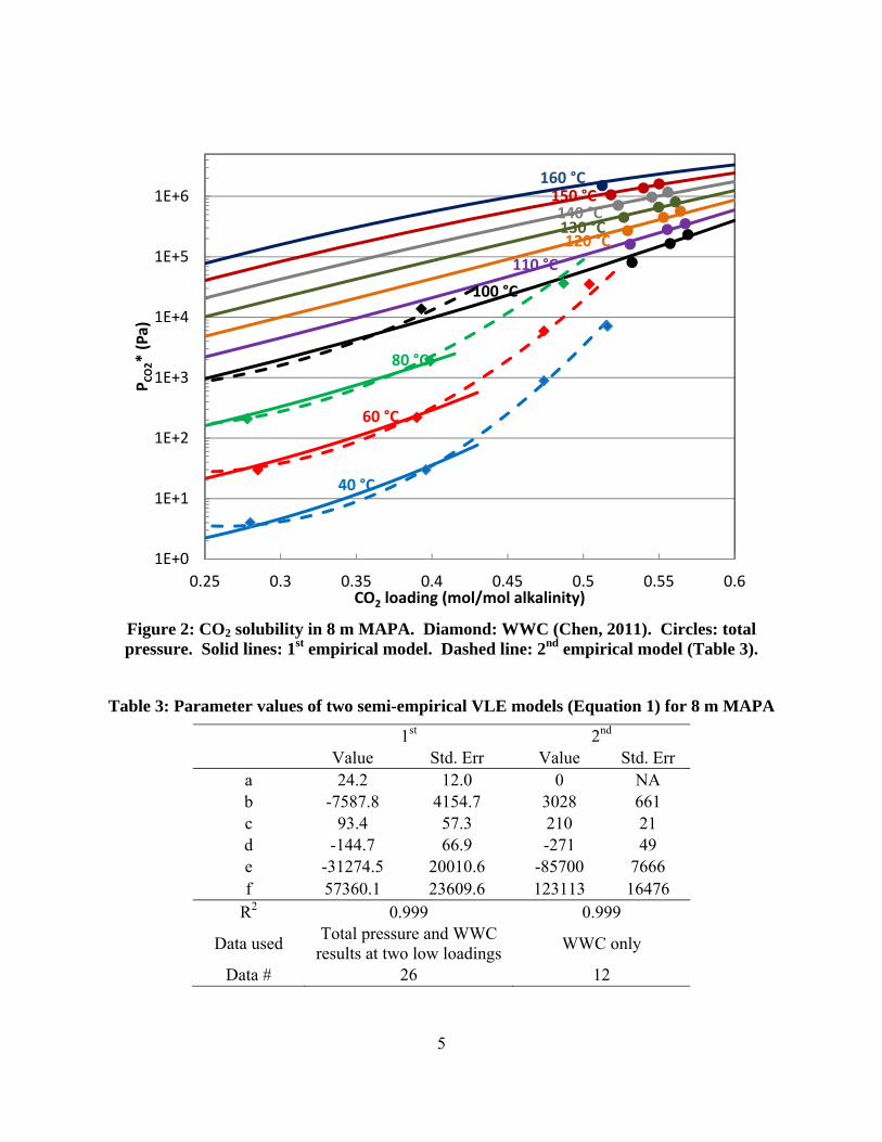
Two semi-empirical models were calculated for 8 m MAPA, the parameters of the models are summarized in Table 3. The model-predicted VLE curves are shown in Figure 2 with experimental results. The first VLE model is regressed using high temperature data and low temperature data at low loading. This model has a high R2 value at 0.999, indicating good agreement of the experimental data. Also, the model predicts the temperature dependence of the experimental result at both low and rich loading. However, this model does not match data at rich loading and 40–80 ˚C (not included in the regression). The second semi-empirical VLE model is regressed using data at 40–100 ˚C collected by the WWC. The model can better predict experimental results at 40–80 ˚C at rich loading, but does not match high temperature data. A semi-empirical model was not calculated using all VLE data because the model result is not physically realistic.
5E+4
5E+5
0.5 0.52 0.54 0.56 0.58
PCO2* (Pa)
CO2 loading (mol/mol alkalinity)
110 °C
100 °C
120 °C
140 °C
160 °C
150 °C
130 °C
5
Figure 2: CO2 solubility in 8 m MAPA. Diamond: WWC (Chen, 2011). Circles: total pressure. Solid lines: 1st empirical model. Dashed line: 2nd empirical model (Table 3).
Table 3: Parameter values of two semi-empirical VLE models (Equation 1) for 8 m MAPA
1st 2nd Value Std. Err Value Std. Err
a 24.2 12.0 0 NA b -7587.8 4154.7 3028 661 c 93.4 57.3 210 21 d -144.7 66.9 -271 49 e -31274.5 20010.6 -85700 7666 f 57360.1 23609.6 123113 16476
R2 0.999 0.999
Data used Total pressure and WWC
results at two low loadings WWC only
Data # 26 12
1E+0
1E+1
1E+2
1E+3
1E+4
1E+5
1E+6
0.25 0.3 0.35 0.4 0.45 0.5 0.55 0.6
PCO2* (Pa)
CO2 loading (mol/mol alkalinity)
40 °C
60 °C
80 °C
110 °C
100 °C
120 °C
140 °C
160 °C150 °C
130 °C

6
The inconsistencies between the two models are due to the inconsistency in the experimental data. At loadings close to 0.5 mol/mol alk, the WWC measurements are significantly higher than the values suggested by high temperature results. Experimentally, accurately measuring CO2 loading at rich loadings can be difficult and slightly affect the quality of data. Physically, at around 0.5 CO2 loading, carbamate forming species, free MAPA and MAPA carbamate, are mostly consumed. As a result, the CO2 solubility of the solvent reduces significantly faster than at lower loadings. Due to its simple mathematical form, the semi-empirical model cannot describe the physical change in VLE around 0.5 loading and low temperature while maintaining good fit with data at other conditions.
The semi-empirical models are used to predict the operating lean and rich loading of 8 m MAPA, which correspond to PCO2* of 0.5 and 5 kPa at 40 ˚C. The cyclic capacity (∆Csolv) of the solvent is calculated using Equation 2.
∆ ∙ (2)
The calculated lean/rich loadings and ∆Csolv of 8 m MAPA are summarized in Table 4. The results of the two models are very different from each other. The first model predicts lean/rich loadings that are much higher than the second model (approximately 0.06 mol/mol alk). Also, the first model predicts a ∆Csolv more than 50% higher than the second. This is because of the uncertainties in the shape of the VLE curve at 40 ˚C (Figure 2). The loadings and ∆Csolv
calculated by the second model should be used since this model better match the available experimental data at conditions critical to these properties.
Table 4: Capacity, -Habs, and operating loading range of 8 m MAPA predicted using two empirical models (Table 3).
1st 2nd αlean (mol/mol alk) 0.494 0.464 αrich (mol/mol alk) 0.562 0.507 ∆Csolv (mol/kg solv) 0.63 0.40 -Habs at αlean (kJ/mol) 75 85 81* -Habs at αmid(kJ/mol) 67 80 77*
*Calculated using the first model at loadings calculated by the second model The heat of absorption of CO2 in 8 m MAPA is calculated as the temperature dependence of the CO2 VLE using in Equation 3.
∆ ∙
⁄ ,∙ ∙ ∙ (3)
The ∆Habs of a solvent is a function of CO2 loading, and not dependent on temperature. Also, the calculation of ∆Habs depends on the semi-empirical model. The ∆Habs calculated using two models for 8 m MAPA are summarized in Table 4 and plotted in Figure 3. Since ∆Habs decreases with an increase in CO2 loading, the first model calculates a lower ∆Habs than the second model mostly due to the higher loadings suggested by the first model. The ∆Habs predicted by the two models are similar, as shown in Figure 3. The second model (WWC only) predicts slightly higher ∆Habs at low loadings and lower ∆Habs at rich loadings. However, the differences between the two models are within 5 kJ/mol at the operating condition. The ∆Habs of

7
8 m MAPA should be calculated using the first model, since it is regressed using more data and from a greater temperature and loading range. Typically, the ∆Habs of a solvent is reported at its lean loading and mid-loading (PCO2
* at 1.5 kPa). In the case of 8 m MAPA, these loadings are to be calculated using the second model. The ∆Habs calculated by a combination of the two models is slightly lower than the first model and much higher than the second.
The PCO2* experimental data at high temperature are summarized in Table 5.
Figure 3: CO2 heat of absorption in 8 m MAPA predicted by two empirical models (Table 3)
Table 5: PCO2
* for 8 m MAPA at high temperature
T CO2 ldg PCO2* Pmeas Ptotal
˚C mol/mol alk kPa 100 0.532 81 298 170 100 0.557 166 390 255 100 0.569 234 451 322 110 0.531 162 412 287 110 0.555 284 543 409 110 0.567 353 629 478 120 0.529 272 580 445 120 0.553 450 766 624 120 0.564 571 880 745 130 0.527 449 817 685 130 0.550 667 1044 903
40
50
60
70
80
90
100
0.35 0.4 0.45 0.5 0.55 0.6
‐Hab
s(kJ/mol)
CO2 loading (mol/mol alk)
Lean
Rich
LeanRich
1st model2nd model

8
130 0.561 809 1203 1044 140 0.523 712 1167 1028 140 0.545 976 1438 1291 140 0.556 1174 1642 1489 150 0.518 1064 1621 1479 150 0.540 1375 1941 1790 150 0.550 1614 2185 2029 160 0.512 1507 2191 2046
The PCO2* in 6 m PZ/2 m EDA was measured at 40–100 ˚C using the WWC, and at 100–160 ˚C using the total pressure apparatus at loading across the operating range. A total of 40 experimental points were collected and plotted in Figure 4. The experimental data are regressed using Equation 2 to generate a semi-empirical VLE model for the solvent. The parameters of the model are summarized in Table 6, and the model results are plotted also in Figure 4. The WWC and total pressure results for this blend agree well with each other. The semi-empirical model matches experimental data well, and has a high R2 value at 0.998.
Figure 4: CO2 solubility in 6 m PZ/2 m EDA. Diamond: WWC. Circles: total pressure. Solid lines: empirical model (Table 6). Dashed line: empirical model of 8 m PZ (Xu, 2011).
The operating lean/rich loadings, ∆Csolv, and ∆Habs for 6 m PZ/2 m EDA are calculated using the semi-empirical model and compared with 6 m PZ/2 m HMDA, 6 m PZ/2 m DAB, 12 m EDA, 8 m PZ, and 7 m MEA in Table 7. At 40 ˚C, 6 m PZ/2 m EDA has a similar VLE curve to 6 m PZ/2 m DAB. As a result, the two solvents have similar lean/rich loadings and ∆Csolv. 6 m PZ/2
1E+1
1E+2
1E+3
1E+4
1E+5
1E+6
0.28 0.33 0.38 0.43
PCO2* (Pa)
CO2 loading (mol/mol alkalinity)
40 °C
60 °C
80 °C
20 °C
100 °C
110 °C120 °C130 °C
160 °C150 °C140 °C
PZ @ 40 °C
9
m EDA has ∆Csolv of 0.63 mol CO2/kg solv, which is higher than 6 m PZ/2 m HMDA and 7 m MEA, but lower than 8 m PZ and 12 m EDA. The temperature dependence of CO2 VLE in 6 m PZ/2 m EDA is more significant than 8 m PZ, which results in higher ∆Habs for the blend at a higher loading than 8 m PZ. The ∆Habs for 6 m PZ/2 m EDA is competitive with 7 m MEA at low loadings, and similar to 8 m PZ and other PZ blends at mid-loading.
Table 6: Parameter values of the semi-empirical VLE model (Equation 1) of 6 m PZ/2 m EDA
Value Std. Erra 47.4 1.7 b -16889 642 c -36.2 4.3 d / / e 22575 1654 f / /
R2 0.998 Data # 40
Absorption rates
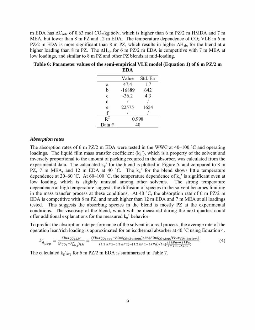
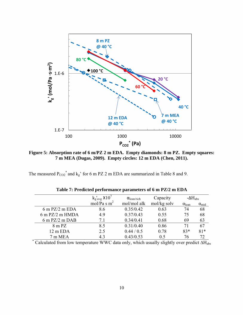
The absorption rates of 6 m PZ/2 m EDA were tested in the WWC at 40–100 ˚C and operating loadings. The liquid film mass transfer coefficient (kg’), which is a property of the solvent and inversely proportional to the amount of packing required in the absorber, was calculated from the experimental data. The calculated kg’ for the blend is plotted in Figure 5, and compared to 8 m PZ, 7 m MEA, and 12 m EDA at 40 ˚C. The kg’ for the blend shows little temperature dependence at 20–60 ˚C. At 60–100 ˚C, the temperature dependence of kg’ is significant even at low loading, which is slightly unusual among other solvents. The strong temperature dependence at high temperature suggests the diffusion of species in the solvent becomes limiting in the mass transfer process at these conditions. At 40 ˚C, the absorption rate of 6 m PZ/2 m EDA is competitive with 8 m PZ, and much higher than 12 m EDA and 7 m MEA at all loadings tested. This suggests the absorbing species in the blend is mostly PZ at the experimental conditions. The viscosity of the blend, which will be measured during the next quarter, could offer additional explanations for the measured kg’ behavior.
To predict the absorption rate performance of the solvent in a real process, the average rate of the operation lean/rich loading is approximated for an isothermal absorber at 40 ˚C using Equation 4.
,∗
, , , / ,⁄
. . . . . .
(4)
The calculated kg’avg for 6 m PZ/2 m EDA is summarized in Table 7.
10
Figure 5: Absorption rate of 6 m/PZ 2 m EDA. Empty diamonds: 8 m PZ. Empty squares: 7 m MEA (Dugas, 2009). Empty circles: 12 m EDA (Chen, 2011).
The measured PCO2* and kg’ for 6 m PZ 2 m EDA are summarized in Table 8 and 9.
Table 7: Predicted performance parameters of 6 m PZ/2 m EDA
kg'avg Х107 αlean/rich Capacity -∆Habs mol/Pa s m2 mol/mol alk mol/kg solv αlean αmid
6 m PZ/2 m EDA 8.6 0.35/0.42 0.63 74 68 6 m PZ/2 m HMDA 4.9 0.37/0.43 0.55 75 68 6 m PZ/2 m DAB 7.1 0.34/0.41 0.68 69 63
8 m PZ 8.5 0.31/0.40 0.86 71 67 12 m EDA 2.5 0.44 / 0.5 0.78 83* 81* 7 m MEA 4.3 0.43/0.53 0.5 76 72
* Calculated from low temperature WWC data only, which usually slightly over predict ∆Habs
1.E‐7
1.E‐6
100 1000 10000
k g' (mol/Pa ∙s∙m
2)
PCO2* (Pa)
40 °C
60 °C
80 °C
20 °C
100 °C
8 m PZ @ 40 °C
12 m EDA @ 40 °C
7 m MEA@ 40 °C
11
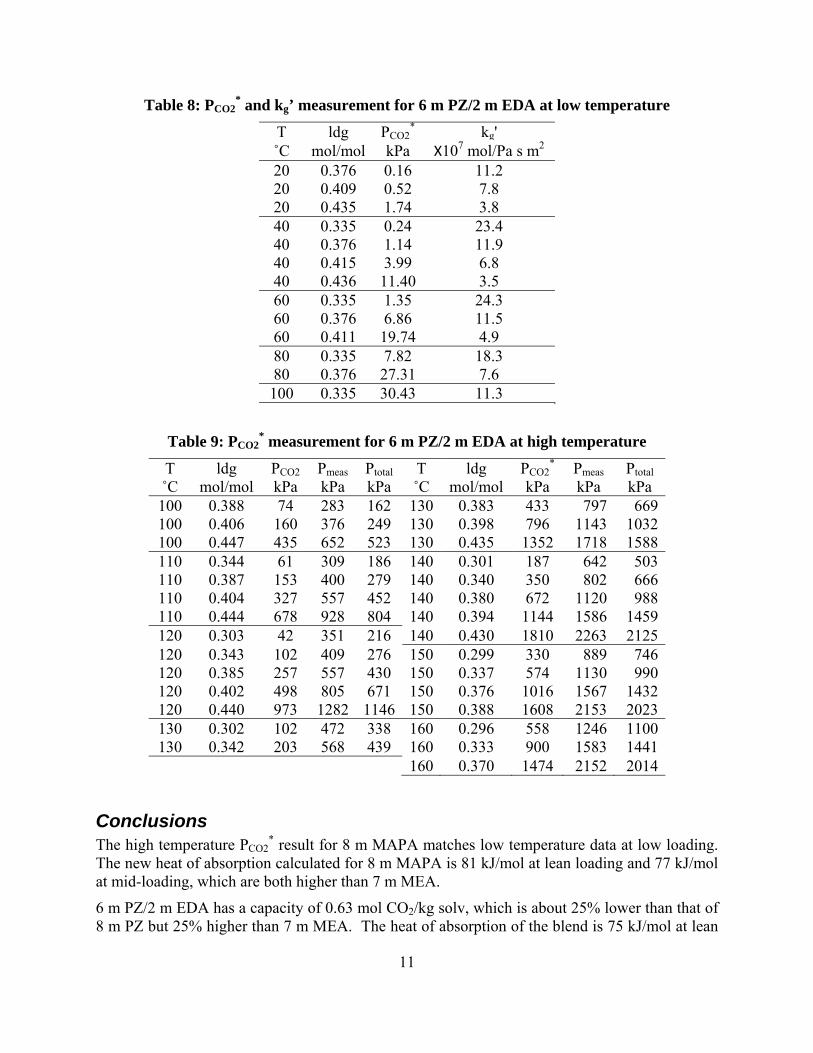
Table 8: PCO2* and kg’ measurement for 6 m PZ/2 m EDA at low temperature
T ldg PCO2* kg'
˚C mol/mol kPa Х107 mol/Pa s m2 20 0.376 0.16 11.2 20 0.409 0.52 7.8 20 0.435 1.74 3.8 40 0.335 0.24 23.4 40 0.376 1.14 11.9 40 0.415 3.99 6.8 40 0.436 11.40 3.5 60 0.335 1.35 24.3 60 0.376 6.86 11.5 60 0.411 19.74 4.9 80 0.335 7.82 18.3 80 0.376 27.31 7.6 100 0.335 30.43 11.3
Table 9: PCO2* measurement for 6 m PZ/2 m EDA at high temperature
T ldg PCO2 Pmeas Ptotal T ldg PCO2* Pmeas Ptotal
˚C mol/mol kPa kPa kPa ˚C mol/mol kPa kPa kPa 100 0.388 74 283 162 130 0.383 433 797 669100 0.406 160 376 249 130 0.398 796 1143 1032100 0.447 435 652 523 130 0.435 1352 1718 1588110 0.344 61 309 186 140 0.301 187 642 503110 0.387 153 400 279 140 0.340 350 802 666110 0.404 327 557 452 140 0.380 672 1120 988110 0.444 678 928 804 140 0.394 1144 1586 1459120 0.303 42 351 216 140 0.430 1810 2263 2125120 0.343 102 409 276 150 0.299 330 889 746120 0.385 257 557 430 150 0.337 574 1130 990120 0.402 498 805 671 150 0.376 1016 1567 1432120 0.440 973 1282 1146 150 0.388 1608 2153 2023130 0.302 102 472 338 160 0.296 558 1246 1100130 0.342 203 568 439 160 0.333 900 1583 1441
160 0.370 1474 2152 2014
Conclusions The high temperature PCO2
* result for 8 m MAPA matches low temperature data at low loading. The new heat of absorption calculated for 8 m MAPA is 81 kJ/mol at lean loading and 77 kJ/mol at mid-loading, which are both higher than 7 m MEA.
6 m PZ/2 m EDA has a capacity of 0.63 mol CO2/kg solv, which is about 25% lower than that of 8 m PZ but 25% higher than 7 m MEA. The heat of absorption of the blend is 75 kJ/mol at lean

12
loading, which is competitive with 7 m MEA, and it is 68 kJ/mol at the mid-loading condition, which is similar to 8 m PZ and 4 kJ less than 7 m MEA. The blend has a high absorption rate across the operating range, with a kg’avg of 8.6 Х107 mol/Pa∙s·m2, which is competitive with 8 m PZ, and approximately twice that of 7 m MEA.
Future Work Other PZ blends using N-(2-hydroxyethyl)piperazine (HEP) and 2 piperidine ethanol (2-PE), and other amine blends will be tested in the WWC and total pressure apparatus in the next quarter.
References Chen X, Closmann F, Rochelle GT. “Accurate screening of amines by the wetted wall column.”
Energy Proc. 2011;4:101–108.
Dugas RE. Carbon dioxide absorption, desorption, and diffusion in aqueous piperazine and monoethanolamine. The University of Texas at Austin. Ph.D. Dissertation. 2009.
Freeman SA. Thermal degradation and oxidation of aqueous piperazine for carbon dioxide capture. The University of Texas at Austin. Ph.D. Dissertation. 2011.
Rochelle GT et al. "CO2 Capture by Aqueous Absorption, First Quarterly Progress Report 2012." Luminant Carbon Management Program. The University of Texas at Austin. 2012.
Xu Q. Thermodynamics of CO2 loaded aqueous amines. The University of Texas at Austin. Ph.D. Dissertation. 2011.

1
Aqueous piperazine/aminoethylpiperazine for CO2 Capture
Quarterly Report for October 1 – December 31, 2012
by Yang Du
Supported by the Luminant Carbon Management Program
McKetta Department of Chemical Engineering
The University of Texas at Austin
January 31, 2013
Abstract A model accurately predicting thermodynamic and kinetic properties for CO2 absorption in aqueous amine solutions is essential for simulation and design of such CO2 capture process. In this quarter, a rigorous thermodynamic model has been developed for the PZ-AEP-H2O-CO2 system in Aspen Plus® using the Electrolyte Nonrandom Two-Liquid (e-NRTL) activity coefficient model. Unavailable thermodynamic parameters of AEP related species, including AEP, AEPH+, AEP(H+)2, AEPCOO-, AEP(COO-)2, H+AEPCOO- and H+AEP(COO-)2, were estimated by built-in models in Aspen Plus®, or by referring to corresponding PZ-related species as the starting point, and then sequential regressions were applied using related experimental data. The vapor-liquid equilibrium (VLE) data for AEP-H2O-CO2 were used to determine the standard-state properties (free energy of formation and heat of formation) of the AEP-related species. After that, the VLE data for PZ-AEP-H2O-CO2 were used to identify the e-NRTL interaction parameters for the molecule-electrolyte binaries. The heat capacity and the species concentrations for PZ-AEP-H2O-CO2 were predicted using this model as validation.
Introduction Amine scrubbing has shown the most promise for effective capture of CO2 from coal-fired flue gas. Piperazine/N-(2-aminoethyl) piperazine (PZ/AEP) was investigated in this study as a novel solvent for CO2 capture. In previous reports, we have confirmed that PZ/AEP has a larger solid solubility window than concentrated PZ, slightly lower CO2 absorption capacity, but comparable resistance to degradation, CO2 absorption rate and viscosity, which indicates PZ/AEP is a superior solvent for CO2 capture by absorption/stripping.
To properly simulate and design the CO2 capture process using PZ/AEP, it is a prerequisite to develop a rigorous thermodynamic model which can accurately predict the thermodynamic properties, specifically vapor-liquid equilibrium (VLE), calorimetric properties, and chemical reaction equilibrium.
In this quarter, a rigorous thermodynamic model has been developed for PZ-AEP-H2O-CO2 in Aspen Plus® using the Electrolyte Nonrandom Two-Liquid (e-NRTL) activity coefficient model, based on the Independence model for concentrated PZ established by Frailie (Rochelle, 2012).
2
PZ-AEP-H2O-CO2 Thermodynamic Model
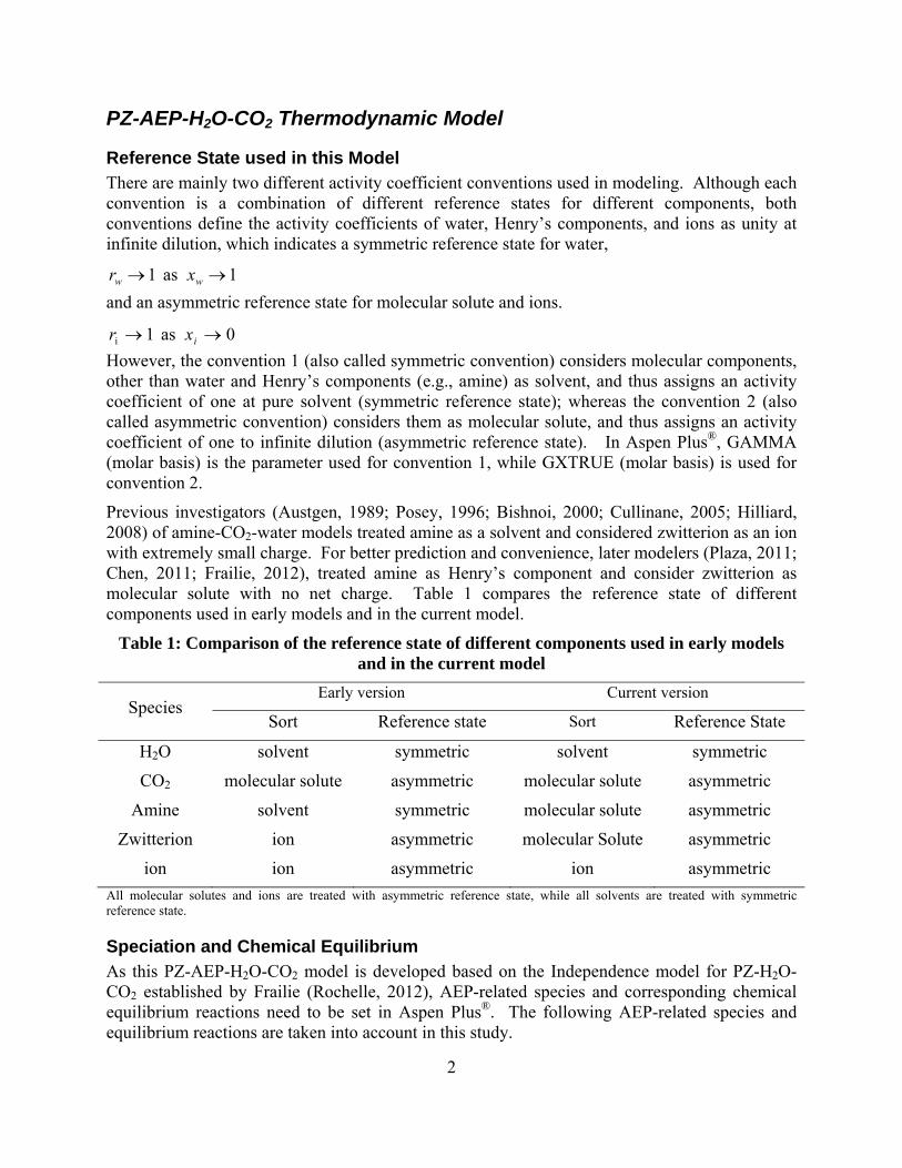
Reference State used in this Model There are mainly two different activity coefficient conventions used in modeling. Although each convention is a combination of different reference states for different components, both conventions define the activity coefficients of water, Henry’s components, and ions as unity at infinite dilution, which indicates a symmetric reference state for water,
and an asymmetric reference state for molecular solute and ions.
However, the convention 1 (also called symmetric convention) considers molecular components, other than water and Henry’s components (e.g., amine) as solvent, and thus assigns an activity coefficient of one at pure solvent (symmetric reference state); whereas the convention 2 (also called asymmetric convention) considers them as molecular solute, and thus assigns an activity coefficient of one to infinite dilution (asymmetric reference state). In Aspen Plus®, GAMMA (molar basis) is the parameter used for convention 1, while GXTRUE (molar basis) is used for convention 2.
Previous investigators (Austgen, 1989; Posey, 1996; Bishnoi, 2000; Cullinane, 2005; Hilliard, 2008) of amine-CO2-water models treated amine as a solvent and considered zwitterion as an ion with extremely small charge. For better prediction and convenience, later modelers (Plaza, 2011; Chen, 2011; Frailie, 2012), treated amine as Henry’s component and consider zwitterion as molecular solute with no net charge. Table 1 compares the reference state of different components used in early models and in the current model.
Table 1: Comparison of the reference state of different components used in early models and in the current model
Species Early version Current version
Sort Reference state Sort Reference State
H2O solvent symmetric solvent symmetric
CO2 molecular solute asymmetric molecular solute asymmetric
Amine solvent symmetric molecular solute asymmetric
Zwitterion ion asymmetric molecular Solute asymmetric
ion ion asymmetric ion asymmetric
All molecular solutes and ions are treated with asymmetric reference state, while all solvents are treated with symmetric reference state.
Speciation and Chemical Equilibrium As this PZ-AEP-H2O-CO2 model is developed based on the Independence model for PZ-H2O-CO2 established by Frailie (Rochelle, 2012), AEP-related species and corresponding chemical equilibrium reactions need to be set in Aspen Plus®. The following AEP-related species and equilibrium reactions are taken into account in this study.
1 as 1 ww xr
0 as 1i ixr

3
Table 2: AEP-related species considered in this model
Species Alias Charge state
AEP C6H15N3 0
H+AEPCOO- C7H15N3O2 0
AEPH+ C6H16N3 +1
AEP(H+)2 C6H17N3 +2
AEPCOO- C7H14N3O2 -1
AEP(COO-)2 C8H13N3O4 -2
H+AEP(COO-)2 C8H13N3O4 -1
Table 3: AEP-related equilibrium reactions considered in this model
Rxn No. Stoichiometry
1 AEPH+ <--> AEP + H+
2 AEP + HCO3- <--> AEPCOO- + H2O
3 AEPCOO- + HCO3- <--> AEP(COO-)2 + H2O
4 H+AEPCOO- <--> AEPCOO- + H+
5 AEP(H+)2 <--> AEPH++ H+
6 H+AEP(COO-)2 <--> AEP(COO-)2 + H+
7 H+AEP(COO-)2 + H2O <--> H+AEPCOO- + HCO3-
Estimation of Unavailable Parameters To accurately predict thermodynamic properties, a set of parameters need to be input into Aspen Plus®, including Δf Gi
ig, Δf Hiig and Cpi
ig for all molecular components, Δf Gi∞,aq, ΔfHi
∞,aq and Cpi
∞, aq for all ionic components, and Henry’s constant for Henry’s components, as well as binary parameters for molecule-electrolyte. Although not all the parameters are available in the Aspen Plus® database, various ways can be used to determine or estimate their values. In our model, Δf
Giig and Δf Hi
ig of AEP were estimated by Aspen Plus® using the Benson method by providing structure information of AEP. For the Henry’s constant for AEP, values were calculated from the volatility measurement of AEP by Nguyen (Rochelle, 2012) (Figure 1).

4
Figure 1: Henry’s constant for AEP as a function of T from 40 °C to 65 °C
As modeled as Henry’s components, Δf Gi∞, aq and Δf Hi
∞, aq of AEP can be calculated from the following equations.
)ln( + Δ =Δ ,,ref
OΗiigif
aqif P
HRTGG 2 (1)
)(
ln + Δ =Δ
,,
1/T
HRHH
OΗiigif
aqif
2
(2)
where Η2OiH , is the Henry’s constant of solute i in water and Pref is the reference pressure of 1 bar.
Δf Hi∞, aq of AEPH+ and AEP(H+)2 was calculated from the protonation reactions of AEPH+ and
AEP(H+)2 measured by Pagano (1961).
H+ AEP AEPH , log Km,1 = 9.538 and 1Δ Hr = - 48.56 kJ/mol at 25 °C
H+ AEPH )AEP(H 2 , log Km,2 = 8.453 and 2Δ Hr = - 42.70 kJ/mol at 25 °C
1r,, Δ+ Δ =Δ HHH aq
faq
f AEPAEPH
2,, Δ+ Δ =Δ
2)(HHH f
aqf
aqf AEPHHAEP
1aq
fraq
faq
f KRTGGGGAEPAEPAEPH ,x
,1
,, ln- Δ=Δ+ Δ =Δ
Ln HAEP,H20 = -5396.1/T + 20.077
2
2.5
3
3.5
4
4.5
0.00293 0.00298 0.00303 0.00308 0.00313 0.00318
ln H
AE
P,H
20
1/T(K)
5
2,x,
2,, ln- Δ=Δ+ Δ =Δ
2)(KRTGGGG aq
fraq
faq
f AEPAEPHHAEP
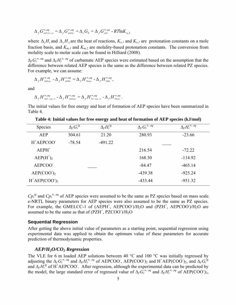
where 1rΔ H and 2rΔ H are the heat of reactions, Kx,1 and Kx,2 are protonation constants on a mole fraction basis, and Km,1 and Km,2 are molality-based protonation constants. The conversion from molality scale to molar scale can be found in Hilliard (2008).
Δf Gi∞, aq and Δf Hi
∞, aq of carbamate AEP species were estimated based on the assumption that the difference between related AEP species is the same as the difference between related PZ species. For example, we can assume:
aqf
aqf
aqf
aqf PPAEPAEP
HHHH ,,,,ZH-ZcooH-coo
Δ-Δ = Δ-Δ ,
and
aqf
aqf
aqf
aqf PPZAEPAEP
HHHH ,,,,-Zcoo2-coo-coo2-coo
Δ-Δ = Δ-Δ )()(
.
The initial values for free energy and heat of formation of AEP species have been summarized in Table 4.
Table 4: Initial values for free energy and heat of formation of AEP species (kJ/mol)
Species Δf Giig Δf Hi
ig Δf Gi∞, aq Δf Hi
∞, aq
AEP 304.61 21.20 280.93 -23.66
H+AEPCOO- -78.54 -491.22 ____
AEPH+
____
216.54 -72.22
AEP(H+)2 168.30 -114.92
AEPCOO- -84.47 -465.14
AEP(COO-)2 -439.38 -925.24
H+AEP(COO-)2 -433.44 -951.32
Cpiig and Cpi
∞, aq of AEP species were assumed to be the same as PZ species based on mass scale. e-NRTL binary parameters for AEP species were also assumed to be the same as PZ species. For example, the GMELCC-1 of (AEPH+, AEPCOO-)/H2O and (PZH+, AEPCOO-)/H2O are assumed to be the same as that of (PZH+, PZCOO-)/H2O
Sequential Regression After getting the above initial value of parameters as a starting point, sequential regression using experimental data was applied to obtain the optimum value of these parameters for accurate prediction of thermodynamic properties.
AEP/H2O/CO2 Regression The VLE for 6 m loaded AEP solutions between 40 °C and 100 °C was initially regressed by adjusting the Δf Gi
∞, aq and Δf Hi∞, aq of AEPCOO-, AEP(COO-)2 and H+AEP(COO-)2, and Δf Gi
ig and Δf Hi
ig of H+AEPCOO-. After regression, although the experimental data can be predicted by the model, the large standard error of regressed value of Δf Gi
∞, aq and Δf Hi∞, aq of AEP(COO-)2,
6
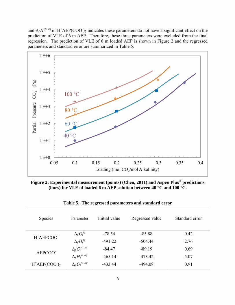
and Δf Hi∞, aq of H+AEP(COO-)2 indicates these parameters do not have a significant effect on the
prediction of VLE of 6 m AEP. Therefore, these three parameters were excluded from the final regression. The prediction of VLE of 6 m loaded AEP is shown in Figure 2 and the regressed parameters and standard error are summarized in Table 5.
Figure 2: Experimental measurement (points) (Chen, 2011) and Aspen Plus® predictions (lines) for VLE of loaded 6 m AEP solution between 40 °C and 100 °C.
Table 5. The regressed parameters and standard error
Species Parameter Initial value Regressed value Standard error
H+AEPCOO- Δf Gi
ig -78.54 -85.88 0.42
Δf Hiig -491.22 -504.44 2.76
AEPCOO- Δf Gi
∞, aq -84.47 -89.19 0.69
Δf Hi∞, aq -465.14 -473.42 5.07
H+AEP(COO-)2 Δf Gi∞, aq -433.44 -494.08 0.91
1.E+0
1.E+1
1.E+2
1.E+3
1.E+4
1.E+5
1.E+6
0.05 0.1 0.15 0.2 0.25 0.3 0.35 0.4
Par
tial
P
ress
ure
CO
2(P
a)
Loading (mol CO2/mol Alkalinity)
60 °C
100 °C
80 °C
40 °C

7
PZ/AEP/H2O/CO2 Regression With the parameters obtained in the AEP/H2O/CO2 regression, VLE of 5 m PZ/2 m AEP can be adequately predicted by this model without adjusting any other parameters (Figure 3).
Figure 3: Comparison of Aspen Plus® predictions (lines) and experimental data (points) for loaded 6 m AEP between 40 °C and 160 °C
A better prediction can be obtained by adjusting the e-NRTL binary parameters (Figure 4), and the regressed values are summarized in Table 6.
1.E+2
1.E+3
1.E+4
1.E+5
1.E+6
1.E+7
0.23 0.28 0.33 0.38
Par
tial
Pre
ssur
e C
O2
(Pa)
Loading (mol CO2/mol Alkalinity)
100 °C
80 °C
60 °C
40 °C
160 °C140 °C
120 °C

8
Figure 4: Comparison of Aspen Plus® predictions (lines) and experimental data (points) for loaded 6 m AEP between 40 °C and 160 °C, after regression.
Table 6: PZ/AEP/H2O/CO2 Regression Results
Parameter Component i Component j Value Standard deviation GMELCC/1 (AEPH+,PZCOO-) H2O 0 0 GMELCC/1 (AEPH+,PZCOO-2) H2O -6.46 4.88 GMELCC/1 (PZH+,AEPCOO-) H2O -2.86 0.29 GMELCC/1 (PZH+,HAEPCOO) H2O -1.02 8.34 GMELCC/1 (AEPH+2,PZCOO-) H2O -3.21 2.54 GMELCC/1 (AEPH+2,PZCOO-2) H2O -6.56 3.52 GMELCC/1 (AEPH+2,PZCOO-) HPZCOO -8.91 4.27 GMELCC/1 (AEPH+2,PZCOO-2) HPZCOO -10.54 8.03 GMELCC/1 (PZH+,PZCOO-2) HAEPCOO -8.28 0.72 GMELCC/1 (AEPH+2,AEPCOO-) HPZCOO -11.21 1.91 GMELCC/1 (PZH+,AEPCOO-) HPZCOO -8.56 0.40
Validation of the Thermodynamic Model As no experimental data are available at the moment for the speciation and heat capacity of AEP or PZ/AEP, we can only roughly validate this model by examining the behaviors of these predicted properties as a function of loading or temperature.
1.E+2
1.E+3
1.E+4
1.E+5
1.E+6
1.E+7
0.23 0.28 0.33 0.38
Par
tial
Pre
ssur
e C
O2
(Pa)
Loading (mol CO2/mol Alkalinity)
100 °C
80 °C
60 °C
40 °C
160 °C
140 °C120 °C

9
Speciation Validation The predicted speciation of 6 m AEP as a function of loading at 40 °C is given in Figure 5.
Figure 5: Prediction of speciation of 6 m AEP as a function of loading at 40 °C.
As can be seen in Figure 5, at very lean loading (0–0.05) AEP is the dominant species in the solution. With the increase in loading, AEP decreases sharply while AEPH+, AEPCOO- and H+AEPCOO- play a more significant role. At very high loading (0.35–0.5), AEP, AEPH+ and AEPCOO- all disappear, with HCO3
-, AEP(H+)2 and H+AEP(COO-)2 as dominant species. This relative abundance of these species and their trend with loading is similar to that for corresponding PZ species (Frailie, 2012).
0
0.02
0.04
0.06
0.08
0.1
0 0.1 0.2 0.3 0.4 0.5 0.6
Liq
uid
Mol
e F
ract
ion
Loading (mol CO2/mol alk)
AEP
HCO3
CO3
CO2
HAEPCOO2
HAEPCOO AEPH2
AEPH
AEPCOO2
AEPCOO

10
Heat Capacity Validation
Figure 6: Prediction of heat capacity of 6 m AEP as a function of T.
2.9
3.1
3.3
3.5
3.7
3.9
4.1
4.3
4.5
310 330 350 370 390 410 430
Cp
(kJ/
kg-K
)
T (K)
2 m AEP
6 m AEP
2 m PZ
6 m PZ
11
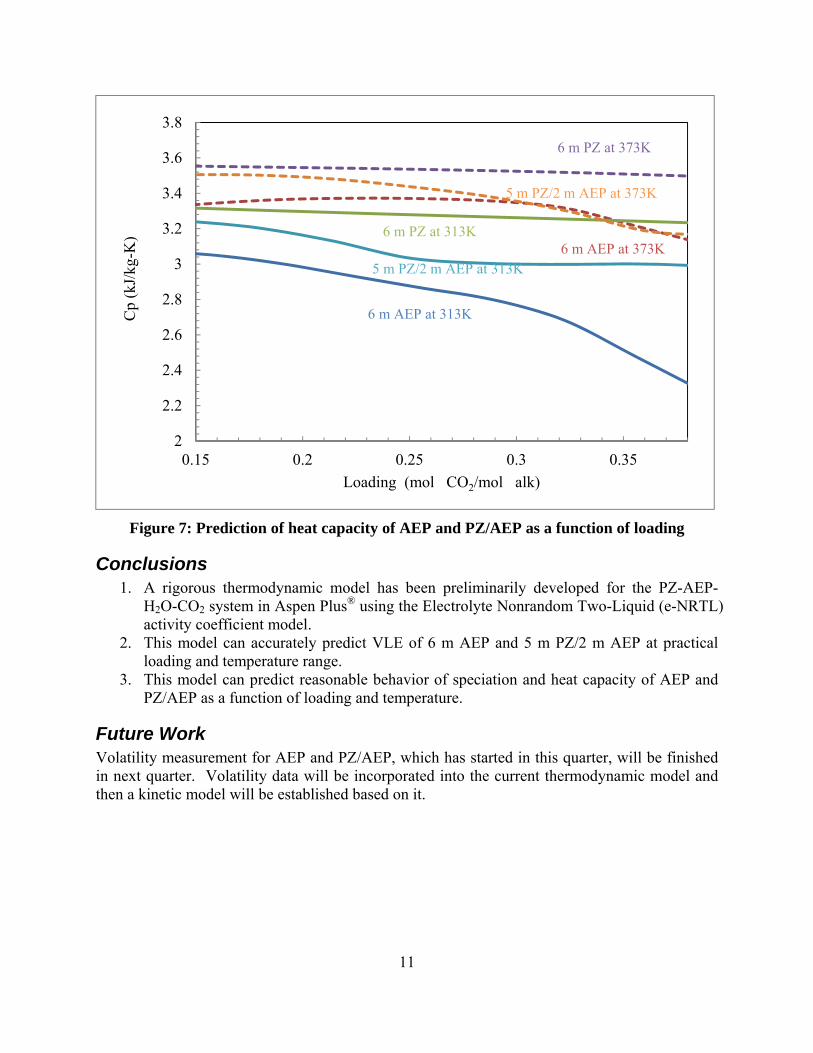
Figure 7: Prediction of heat capacity of AEP and PZ/AEP as a function of loading
Conclusions 1. A rigorous thermodynamic model has been preliminarily developed for the PZ-AEP-
H2O-CO2 system in Aspen Plus® using the Electrolyte Nonrandom Two-Liquid (e-NRTL) activity coefficient model.
2. This model can accurately predict VLE of 6 m AEP and 5 m PZ/2 m AEP at practical loading and temperature range.
3. This model can predict reasonable behavior of speciation and heat capacity of AEP and PZ/AEP as a function of loading and temperature.
Future Work Volatility measurement for AEP and PZ/AEP, which has started in this quarter, will be finished in next quarter. Volatility data will be incorporated into the current thermodynamic model and then a kinetic model will be established based on it.
2
2.2
2.4
2.6
2.8
3
3.2
3.4
3.6
3.8
0.15 0.2 0.25 0.3 0.35
Cp
(kJ/
kg-K
)
Loading (mol CO2/mol alk)
6 m AEP at 313K
6 m AEP at 373K6 m PZ at 313K
6 m PZ at 373K
5 m PZ/2 m AEP at 313K
5 m PZ/2 m AEP at 373K

12
References. Austgen, DM. A Model of Vapor-Liquid Equilibria for Acid Gas-Alkanolamine-Water Systems.
The University of Texas at Austin. Ph.D. Dissertation. 1989.
Bishnoi S. Carbon Dioxide Absorption and Solution Equilibrium in Piperazine Activated Methyldiethanolamine. The University of Texas at Austin. Ph.D. Dissertation. 2000.
Chen X. Carbon dioxide thermodynamics, kinetics, and mass transfer in aqueous piperazine derivatives and other amines. The University of Texas at Austin. Ph.D. Dissertation. 2011.
Cullinane JT. Thermodynamics and Kinetics of Aqueous Piperazine with Potassium Carbonate for Carbon Dioxide Absorption. The University of Texas at Austin. Ph.D. Dissertation. 2005.
Hilliard MD. A Predictive Thermodynamic Model for an Aqueous Blend of Potassium Carbonate, Piperazine, and Monoethanolamine for Carbon Dioxide Capture from Flue Gas. The University of Texas at Austin. Ph.D. Dissertation. 2008.
Pagano JM., Goldberg DE. Fernelius WC. A Thermodynamic study of homopiperazine, piperazine, and N-(2-aminoethyl)-piperazine and their complexes with copper(II) ion. J Phys Chem. 1961;65:1062–1064.
Plaza JM. Modeling of Carbon Dioxide Absorption using Aqueous Monoethanolamine, Piperazine and Promoted Potassium Carbonate. The University of Texas at Austin. Ph.D. Dissertation. 2011.
Posey, ML. Thermodynamic Model for Acid Gas Loaded Aqueous Alkanolamine Solutions. The University of Texas at Austin. Ph.D. Dissertation. 1996.
Rochelle GT, et al. "CO2 Capture by Aqueous Absorption, Third Quarterly Progress Report 2012." Luminant Carbon Management Program. The University of Texas at Austin. 2012.

1
Advanced Absorber and Stripper Configurations
Quarterly Report for October 1 – December 31, 2012
by Peter Frailie
Supported by the Luminant Carbon Management Program
McKetta Department of Chemical Engineering
The University of Texas at Austin
January 31, 2013
Abstract The goal of this study is to evaluate the performance of an absorber/stripper operation that utilizes MDEA/PZ. Before analyzing unit operations and process configurations, thermodynamic, hydraulic, and kinetic properties for the blended amine must be satisfactorily regressed in Aspen Plus®. The approach used in this study is first to construct separate MDEA and PZ models that can later be reconciled via cross parameters to model accurately the MDEA/PZ blended amine. During the past quarter a rate-based absorber model was constructed for both intercooled and non-intercooled cases. Adding intercooling improved solvent capacity by as much as 80% for 5 m MDEA/5 m PZ, but it requires the use of twice as much packing. Another absorber modification that was tested was the use of higher solvent flowrates, which have the potential to reduce packing volumes by 25 to 30% while only decreasing solvent capacity by 8 to 11%. Using the rich solutions generated by the absorber models, four stripper configurations were evaluated: (1) simple stripper, (2) interheated stripper, (3) two-stage flash with warm rich bypass, and (4) two-stage flash with warm rich bypass and a low temperature adiabatic flash. All results were generated using the Independence model. All three advanced configurations reduced the equivalent work relative to the simple stripper, but a techno-economic analysis is needed to determine the optimum configuration. This report is an expansion of the presentation given at GHGT-11, delivering new data concerning operating conditions, process efficiencies, and interactions between process modifications.
Introduction The removal of CO2 from process gases using alkanolamine absorption/stripping has been extensively studied for several solvents and solvent blends. An advantage of using blends is that the addition of certain solvents can enhance the overall performance of the CO2 removal system. A disadvantage of using blends is that they are very complex compared to a single solvent, thus making them much more difficult to model.
This study will focus on a blended amine solvent containing piperazine (PZ) and methyldiethanolamine (MDEA). Previous studies have shown that this particular blend has the potential to combine the high capacity of MDEA with the attractive kinetics of PZ (Bishnoi, 2000). These studies have supplied a rudimentary Aspen Plus®-based model for an absorber with MDEA/PZ. The previous work recommended that more kinetic and thermodynamic data should be acquired for the MDEA/PZ blend before the model can be significantly improved.
2
Three researchers in the Rochelle lab have been acquiring these data, which are being incorporated into the model. One of the major goals of this study will be to improve the supplied Aspen Plus® absorber model with up-to-date thermodynamic and kinetic data. Another major goal will be to make improvements to the MDEA and PZ thermodynamic models, which should simplify the construction of the blended amine model.
Methods and Discussion During the past quarter novel absorber and stripper configurations were designed and evaluated for 8 m PZ, 7 m MDEA/2 m PZ, and 5 m MDEA/5 m PZ. What follows is a description of those novel configurations as well as the results of the evaluations.
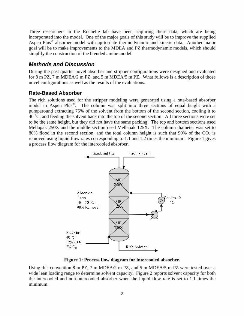
Rate-Based Absorber The rich solutions used for the stripper modeling were generated using a rate-based absorber model in Aspen Plus®. The column was split into three sections of equal height with a pumparound extracting 75% of the solvent from the bottom of the second section, cooling it to 40 oC, and feeding the solvent back into the top of the second section. All three sections were set to be the same height, but they did not have the same packing. The top and bottom sections used Mellapak 250X and the middle section used Mellapak 125X. The column diameter was set to 80% flood in the second section, and the total column height is such that 90% of the CO2 is removed using liquid flow rates corresponding to 1.1 and 1.2 times the minimum. Figure 1 gives a process flow diagram for the intercooled absorber.
Figure 1: Process flow diagram for intercooled absorber.
Using this convention 8 m PZ, 7 m MDEA/2 m PZ, and 5 m MDEA/5 m PZ were tested over a wide lean loading range to determine solvent capacity. Figure 2 reports solvent capacity for both the intercooled and non-intercooled absorber when the liquid flow rate is set to 1.1 times the minimum.
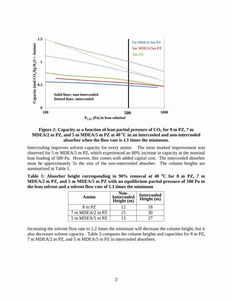
3
Figure 2: Capacity as a function of lean partial pressure of CO2 for 8 m PZ, 7 m MDEA/2 m PZ, and 5 m MDEA/5 m PZ at 40 oC in an intercooled and non-intercooled
absorber when the flow rate is 1.1 times the minimum.
Intercooling improves solvent capacity for every amine. The most marked improvement was observed for 5 m MDEA/5 m PZ, which experienced an 80% increase in capacity at the nominal lean loading of 500 Pa. However, this comes with added capital cost. The intercooled absorber must be approximately 3x the size of the non-intercooled absorber. The column heights are summarized in Table 1.
Table 1: Absorber height corresponding to 90% removal at 40 oC for 8 m PZ, 7 m MDEA/2 m PZ, and 5 m MDEA/5 m PZ with an equilibrium partial pressure of 500 Pa in the lean solvent and a solvent flow rate of 1.1 times the minimum
Amine Non-
Intercooled Height (m)
Intercooled Height (m)
8 m PZ 12 187 m MDEA/2 m PZ 15 305 m MDEA/5 m PZ 13 27
Increasing the solvent flow rate to 1.2 times the minimum will decrease the column height, but it also decreases solvent capacity. Table 2 compares the column heights and capacities for 8 m PZ, 7 m MDEA/2 m PZ, and 5 m MDEA/5 m PZ in intercooled absorbers.
0
0.5
1
1.5
100 1000
Cap
acit
y (m
ol C
O2/
kg
H2O
+ A
min
e)
PCO2 (Pa) in lean solution
8m PZ
7m MDEA/2m PZ
5m MDEA/5m PZ
Solid lines: non-intercooledDotted lines: intercooled
500 P
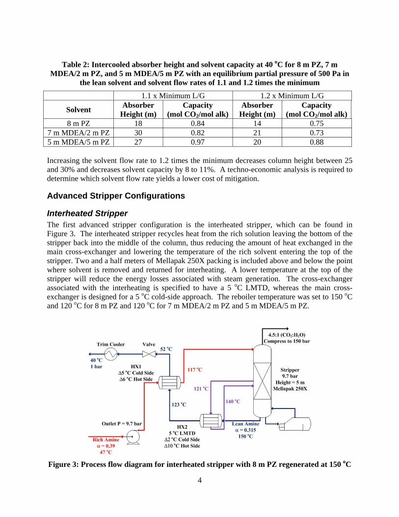
4
Table 2: Intercooled absorber height and solvent capacity at 40 oC for 8 m PZ, 7 m MDEA/2 m PZ, and 5 m MDEA/5 m PZ with an equilibrium partial pressure of 500 Pa in
the lean solvent and solvent flow rates of 1.1 and 1.2 times the minimum
1.1 x Minimum L/G 1.2 x Minimum L/G
Solvent Absorber
Height (m) Capacity
(mol CO2/mol alk) Absorber
Height (m) Capacity
(mol CO2/mol alk)8 m PZ 18 0.84 14 0.75
7 m MDEA/2 m PZ 30 0.82 21 0.73 5 m MDEA/5 m PZ 27 0.97 20 0.88 Increasing the solvent flow rate to 1.2 times the minimum decreases column height between 25 and 30% and decreases solvent capacity by 8 to 11%. A techno-economic analysis is required to determine which solvent flow rate yields a lower cost of mitigation.
Advanced Stripper Configurations
Interheated Stripper The first advanced stripper configuration is the interheated stripper, which can be found in Figure 3. The interheated stripper recycles heat from the rich solution leaving the bottom of the stripper back into the middle of the column, thus reducing the amount of heat exchanged in the main cross-exchanger and lowering the temperature of the rich solvent entering the top of the stripper. Two and a half meters of Mellapak 250X packing is included above and below the point where solvent is removed and returned for interheating. A lower temperature at the top of the stripper will reduce the energy losses associated with steam generation. The cross-exchanger associated with the interheating is specified to have a 5 oC LMTD, whereas the main cross-exchanger is designed for a 5 oC cold-side approach. The reboiler temperature was set to 150 oC and 120 oC for 8 m PZ and 120 oC for 7 m MDEA/2 m PZ and 5 m MDEA/5 m PZ.
Figure 3: Process flow diagram for interheated stripper with 8 m PZ regenerated at 150 oC

5
Two-Stage Flash (2SF) with Warm Rich Bypass (WRB) Just as with the interheated stripper, the 2SF with CRB cools the exiting vapor to minimize steam losses. Anywhere from 5–30% of the solvent is removed after passing through a cross-exchanger, where it was heated by the lean amine. The 70–95% that is not bypassed goes directly into another cross-exchanger, where it is again heated by the lean amine before being fed into a heated high pressure flash vessel. Half of the cooler amine removed before the second cross-exchanger is sprayed into the top of the vessel and passes through 1 foot (~0.3 m) of packing. The other half is sent to the low pressure flash vessel. The first cross-exchanger is designed with a 5 oC cold-side approach, and the second cross-exchanger is designed with a 5 oC LMTD. Both flash tanks are heated to the same temperature. For 8 m PZ they are heated to 150 oC, and for the MDEA PZ blends they are heated to 120 oC. This configuration can be found in Figure 4. The optimum case had a 7.5% bypass, with 5% going to the low pressure flash and 2.5% going to the high pressure flash. At the top of each flash tank is 1.5 ft (~0.46 m) of Mellapak 500Y packing. The pressure of the high pressure flash was fixed at 1.5 times that of the low pressure flash.
Figure 4: Process flow diagram for 2SF with CRB with 8 m PZ regenerated at 150 oC
2SF with WRB and a Low Temperature Flash (LTF) This configuration is very similar to the one in the previous section, except it has an additional low temperature adiabatic flash immediately after the first cross-exchanger (Figure 5). This flash serves two purposes: (1) it makes the process more reversible by removing the CO2 in more steps, and (2) it removes any entrained oxygen before introducing the solvent to the higher temperature flash vessels. The same temperature and pressure constraints applied to the 2SF with CRB were applied to this configuration. For 8 m PZ the flash tanks were held at 150 oC, and for 7 m MDEA/2 m PZ and 5 m MDEA/5 m PZ they were held at 120 oC. The pressure of the high pressure flash was fixed to be 1.5 times that of the low pressure flash. A total of 7.5% of the solvent was bypassed with 5% going to the low pressure flash and 2.5% going to the high pressure flash. At the top of each flash tank is 1.5 ft of Mellapak 500Y.

6
Figure 5: Process flow diagram for 2SF with CRB and LTF for oxygen removal with 8 m PZ regenerated at 150 oC
Comparing Configurations
Table 3 reports the equivalent work in kJ/mol CO2 for each amine using the three advanced stripper configurations as well as the simple stripper.
Table 3: WEQ (kJ/mol CO2) for 8 m PZ, 7 m MDEA/2 m PZ, and 5 m MDEA/5 m PZ with an intercooled absorber and a simple stripper (SS), interheated stripper (IH), two-stage flash with WRB (2SF/WRB), or two-stage flash with WRB and LT flash (2SF/WRB/LTF) assuming a 500 Pa lean loading equilibrium PCO2.
Amine SS IH 2SF/WRB 2SF/WRB/LTF
8 m PZ (150 oC) 33.3 31.0 31.3 31.1
8 m PZ (120 oC) 33.4 31.3 31.7 31.4
7 m MDEA/2 m PZ 34.6 32.1 32.2 32.0
5 m MDEA/5 m PZ 32.6 31.6 30.5 30.4
Equation 1 was used to calculate equivalent work, and Equations 2 and 3 were used to calculate compressor work.
compspumps
n
i i
kiieq WW
KT
TKTQW
reboilers
1
sin
5
575.0 (1)

7
atmP
atmPCOmolkJW in
incomps 5.4096.4
148log572.4/ 2
(2)
atmP
atmPCOmolkJW in
incomps 5.4181.2
148log023.4/ 2
(3)
In Equation 1, Qi is the reboiler duty, Tsink is 313 K, and Ti is the reboiler temperature. In Equations 2 and 3, Pin is the total pressure of the stream being fed into the compressor. Adding interheating to the stripper reduces the equivalent work by 1–2.5 kJ/mol CO2. This improvement may be attributed to the reduced steam losses. Table 4 reports the steam losses for the three solvents with a simple stripper and an interheated stripper.
Table 4: Relative molar quantities of CO2 and H2O in the product streams of a simple stripper (SS) and interheated stripper (IHS) for 8 m PZ, 7 m MDEA/2 m PZ, and 5 m MDEA/5 m PZ when using a lean loading corresponding to a 500 Pa equilibrium partial pressure of CO2.
Amine SS molar ratio of
CO2:H2O
IHS molar ratio of
CO2:H2O
8 m PZ (150 oC) 2.2 4.5
8 m PZ (120 oC) 1.6 2.8
7 m MDEA/2 m PZ 1.7 3.1
5 m MDEA/5 m PZ 2.1 3.1
The greater the change in CO2:H2O the greater the reduction in WEQ. Adding the adiabatic LTF does not significantly impact the equivalent work of the 2SF with CRB configurations. The LTF impacts process performance in two ways: (1) improving process reversibility by removing CO2 in more steps and (2) decreasing process efficiency by requiring more mechanical compression for the CO2 removed in the LTF. These results suggest that the effects offset each other, and, if there is significant concern surrounding oxidative degradation of the amine, the LTF is a feasible process modification.
Conclusions Increasing the solvent flow rate from 1.1 times the minimum L/G to 1.2 times the minimum
L/G decreases absorber height by 25 to 30% and decreases capacity by 8 to 11%. The interheated stripper reduces WEQ by reducing steam losses in the stripper. Increasing the regeneration temperature from 120 oC to 150 oC for 8 m PZ improves WEQ for
all configurations, but the improvement is on the order of 0.1–0.3 kJ/mol CO2. Adding a low temperature adiabatic flash to the two-stage flash with warm rich bypass has a
negligible effect on process performance.

8
Future Work The remainder of this study will focus on process design and optimization. The effect of absorber temperature on process performance will be determined for 8 m PZ, 7 m MDEA/2 m PZ, and 5 m MDEA/5 m PZ. Novel stripper configurations will be developed and evaluated using the recently updated thermodynamic, hydraulic, and kinetic model. All work will be performed with the intention of graduating in Spring 2013.
References
Bishnoi S. Carbon Dioxide Absorption and Solution Equilibrium in Piperazine Activated Methyldiethanolamine. The University of Texas at Austin. Ph.D. Dissertation. 2000.
Cullinane JT. Thermodynamics and Kinetics of Aqueous Piperazine with Potassium Carbonate for Carbon Dioxide Absorption. The University of Texas at Austin. Ph.D. Dissertation. 2005.
Ko JJ, Li MH. Kinetics of absorption of carbon dioxide into solutions of N-methyldiethanolamine + water. Chem Eng Sci. 2000;55:4139–4147.
Plaza JM. Modeling of Carbon Dioxide Absorption using Aqueous Monoethanolamine, Piperazine and Promoted Potassium Carbonate. The University of Texas at Austin. Ph.D. Dissertation. 2011.

1
Novel Absorber Intercooling Configurations
Quarterly Report for October 1 – December 31, 2012
by Darshan Sachde
Supported by the Luminant Carbon Management Program
McKetta Department of Chemical Engineering
The University of Texas at Austin
January 31, 2013
Abstract A modeling study was initiated to evaluate 3 intercooling design configurations (“in-and-out” intercooling, recycle intercooling, recycle intercooling with bypass) for 3 CO2 flue gas concentrations corresponding to potential capture applications (natural gas combined cycle (4% CO2), coal-fired power plant (12–14% CO2), and cement/steel/industrial (>20% CO2). During the past quarter, preliminary analysis of the natural gas combined cycle application was completed. Results for a constant rich loading analysis at low recycle rates (0.5 to 2 LRecycle/G) indicate that the recycle with bypass is significantly better than the simple recycle design (up to 47% packing reduction) and provides benefits over in-and-out intercooling (up to 13% packing reduction). At higher recycle rates (> 2 LRecycle/G), the simple recycle and bypass become indistinguishable, and no longer justifies the use of a bypass. At the maximum recycle rate considered in this work (8 LRecycle/G), and at a constant rich loading, the simple recycle design results in a 46% packing reduction compared to the intercooling design. The simple recycle design shows improvements in both rich loading and packing requirements when compared to in-and-out intercooling as the recycle rate is increased, though diminishing returns occur with the incremental recycle rate increases. Therefore, recycle intercooling designs show improvement over in-and-out intercooling over the full range of recycle rates (bypass design at low rates, simple design at high rates). Economic analysis is required to determine plausible operating points and potential optimum operating conditions for the recycle intercooling configurations.
The natural gas application design cases for TOTAL have been completed, including equipment and stream tables. All results and data will be included in a report to be completed in the early part of 2013.
Introduction During the past quarter, an intercooling comparison summary was initiated including 3 intercooling designs (in-and-out, simple recycle, recycle with bypass) at 3 CO2 concentrations (NGCC = 4.1%, coal = 13.5%, cement/steel = >20%). The work is an extension of the initial development of the recycle intercooling design as part of previous natural gas absorber modeling (Rochelle et al., 2012b) and seeks to confirm and quantify the benefits of the recycle intercooling design. Preliminary results have been generated for the NGCC scenario and are presented in this report.

2
Absorber Intercooling Design Comparison Study Previous work (Rochelle et al., 2012b) with natural gas combined cycle (NGCC) applications introduced the concept of recycle intercooling and included preliminary sensitivity results for recycle process parameters (e.g., solvent recycle rate and packing height). Recycle intercooling was implemented as a potential improvement over the “in-and-out” intercooling concepts studied and developed in detail by Plaza for coal applications (Plaza, 2011). The expected improvement with recycle intercooling was, in part, due to the additional benefit of cooling the gas as well as the solvent in a well-mixed section. However, the previous analyses did not directly compare recycle intercooling to the in-and-out design and did not consider different CO2 concentrations (capture applications). In the past quarter, a rigorous comparison study was initiated with intercooling comparison for NGCC applications. Table 1 includes NGCC flue gas conditions. Table 2 summarizes equipment design parameters used in the NGCC intercooling comparison.
Table 1: Natural Gas Capture Application, Flue Gas Conditions
Gas Conditions
Gas Feed Rate
114,000 kg‐mol/hr
3,230,000 kg/hr
Temperature 106 °C
Pressure 0.1 MPa
Composition (Mole %)
CO2 4.0%
H2O 8.7%
N2 74.3%
O2 12.1%
Data from NETL Case 13 (NETL, 2010)
Table 2: Intercooling Comparison Study: Equipment and Process Design Summary
Equipment and Process Design Parameters
CO2 Removal 90% Lean Loading (mols CO2/ mols
alkalinity) 0.25
Flue Gas CO2 Concentration (mol%) 4%, 14%, >20%
Recycle Rate (Lrecycle/G)
0.5–8
Maximum Approach to Flooding 70% Packing
(No Solvent Recycle in Section)** MP 250X
Packing (Solvent Recycle in Section)**
0.5 LRecycle/G: MP 250X
1 LRecycle/G: MP 250X

3
2 LRecycle/G: MP 2X
3 LRecycle/G: MP 170X
5 LRecycle/G: MP 125X
8 LRecycle/G: MP 64X **Coarse Packing required to meet flooding criteria in packing section
with solvent recycle. Packing type varied to approximate identical flooding profiles in each case.
Table 2 includes the range of recycle rates evaluated in this study (defined in the table as liquid rate in the recycle relative to the overall gas rate in the column). In addition, the table reflects an important design choice regarding packing. MP 250X is the standard packing used in all cases in packing sections without recycled solvent. However, in the cases with solvent recycle (around the middle of 3 sections of packing), the maximum approach to flooding is reached in the recycle section due to high liquid rates compared to the rest of the column. Instead of increasing the column diameter with increasing recycle liquid rate, coarse packing was used to minimize pressure drop and flooding with limited change to column diameter from case to case. By using a nearly constant column diameter, the sections outside of the recycle maintain a nearly constant liquid rate per wetted perimeter (or superficial velocity). This superficial velocity is correlated to mass transfer performance via the Reynolds number dependence of liquid side mass transfer coefficients. If the superficial velocity in the top and bottom sections of packing dropped significantly from case to case (as the diameter of the column increased), the mass transfer performance of the column would deteriorate and offset the benefit of recycle intercooling.
Figure 1 through Error! Reference source not found. are PFDs for the intercooling configurations considered in the study and reflect the packing configuration described in the preceding paragraph.

4
Figure 1: Absorber PFD for In-and-out Intercooling Design. Two equal sections of packing (MP 250X) are used with liquid draw-off, cooling, and return between the packed sections.
The solvent is cooled to 40 °C before returning to the column.

5
Figure 2: Absorber PFD for Simple Recycle Intercooling Design. Three packing sections are used, with the packing height of each section optimized for each design case to
minimize total packing area. MP-250X is used in the top and bottom section and various coarse structured packing is used in the middle (recycle section) to maintain 70% max approach to flood. Solvent is drawn off the bottom of the middle section, cooled, and
returned to the top of the middle section of packing at 40 °C.

6
Figure 3: Absorber PFD for Recycle Intercooling with Bypass Design. Three packing sections are used, with the packing height of each section optimized for each design case to minimize total packing area. MP-250X is used in the top and bottom section and various
coarse structured packing is used in the middle (recycle section) to maintain 70% max approach to flood. Solvent is drawn off the bottom of the middle section and cooled to
40 °C. A portion of the solvent is sent directly to the bottom section of the column (equal to the nominal liquid feed rate of the column) while the remaining liquid is recycled to the top
of the middle section.
As mentioned, the recycle design is expected to more effectively cool the gas (particularly important in the NGCC cases with high gas rates or relatively low L/G ratios). In addition, the recycle is expected to provide some additional benefit due to a high liquid rate per wetted perimeter. The draw-back of the recycle design is the mixing of the solvent on the recycle section. The driving forces of the column are reduced by mixing a richer solvent with lean solvent entering the middle section of the column. In addition, the temperature leaving the recycle section will be higher than 40 °C, diminishing the benefits of intercooling realized in the bottom section of the column. The bypass design was developed to address the latter shortcoming of the simple recycle design. By splitting a portion of the recycled solvent after cooling and sending it to the bottom section directly, the solvent entering the bottom of the column is 40 °C, and the full benefit of intercooling in the bottom section should be achieved.
Methodology Two approaches were used to compare the intercooling designs. First, the simple recycle design was compared to the in-and-out intercooling design and a case with no intercooling at an
7
operating point of 1.2*minimum liquid flow rate for each case (all achieving 90% CO2 removal). This approach allows comparison of the designs at a common operating point; the packing requirement and energy performance (as reflected in the rich loading) can be compared for all designs. However, this method requires interpretation or weighting of the capital cost benefits (packing) and the energy benefits (rich loading) on a common basis to provide an absolute comparison of designs.
The second approach involved comparison of intercooling designs at a common rich loading. By fixing the rich loading (and, in conjunction with the 90% removal requirement, fixing the absolute solvent rate), the packing requirements of each design could be compared directly without consideration of energy performance implications.
In both approaches, the recycle intercooling designs were designed to minimize the total packing requirement in the column for every case that was run. This was accomplished by optimizing the packing split between the three sections in the column. As in previous work, the packing split optimization was incorporated into the Aspen Plus® simulation as an objective function of the following form:
∗ , ∗ , ∗ , ∗ (1)
: %, %
Where: ap = Specific area of packing (m2/m3); hsection = Specific area of packing (m2/m3); ACross-Section= Cross-sectional area of column (m2).
Result Figure 4 and 5 provide a comparison of the simple recycle intercooling design to both in-and-out intercooling and a baseline of no intercooling.

8
Figure 4: Intercooling configuration comparison in terms of total packing requirement: simple recycle intercooling, in-and-out intercooling, and no intercooling. For cases without recycle, the maximum L/G corresponds to the nominal feed L/G. For the recycle cases, this
corresponds to the L/G in the recycle section (feed L + recycle L). Recycle intercooling simulated at a series of recycle solvent flow rates (and corresponding max L/G).
0
200
400
600
800
1000
1200
0 2 4 6 8 10
Total Interfacial A
rea (m
2)
Max L/G (mol/mol)
0.5 LRecycle/G
In‐and‐out IC
8 LRecycle/G
NO IC
1
23
5
ConditionsNGCC (4.1% CO2)
LLDG = 0.25 mols CO2/mols alk.CO2 Removal = 90%
1.2*Lmin

9
Figure 5: Intercooling configuration comparison in terms of rich loading achieved: simple recycle intercooling, in-and-out intercooling, and no intercooling. For cases without
recycle, the maximum L/G corresponds to the nominal feed L/G. For the recycle cases, this corresponds to the L/G in the recycle section (feed L + recycle L). Recycle intercooling
simulated at a series of recycle solvent flow rates (and corresponding max L/G). No intercooling point is out of the scope of the chart; raw data included for comparison.
The preceding figures should be used together when evaluating the designs. For example, Figure 4 indicates that a design without intercooling will provide the lowest packing requirement; however, the high liquid rate required leads to a rich loading (Figure 5: 0.302 mols CO2/mols alkalinity) that is impractical from an energy and stripping performance perspective.
More importantly, the chart highlights the minimum recycle rate required for the simple recycle design to become competitive with the in-and-out intercooling design. In terms of both packing requirement and rich loading, a recycle rate of 1 L/G is required (max L/G = 2.28) to make the recycle design comparable to in-and-out intercooling. Given the additional cost associated with the recycle design (pumping liquid around the middle section of packing, potentially larger intercooling equipment, etc.), a higher recycle rate would be needed to justify the recycle design. As both figures show, the higher recycle rates provide both reduced packing requirements and improved rich loading performance. However, the benefits show diminishing returns with incremental increases in recycle rate, and when considered with costs associated with higher
0.350
0.355
0.360
0.365
0.370
0.375
0 2 4 6 8 10
Rich Load
ing (m
ols CO
2/m
ols alk)
Max L/G (mol/mol)
0.5 LRecycle/G
In‐and‐out IC
8 LRecycle/G
NO ICL/G = 1.28
RLDG = 0.302
12
35
ConditionsNGCC (4.1% CO2)
LLDG = 0.25 mols CO2/mols alk.CO2 Removal = 90%
1.2*Lmin

10
recycle rates, indicate potential for an optimal recycle rate somewhere above 1 L/G but below the 8 L/G value simulated here.
To compare the configurations on a common basis, Figure 6 compares all 3 intercooling designs (now including the recycle with bypass design) at a constant rich loading of 0.365 mols CO2/mols alkalinity (constant L/G of 1.28 mol/mol). The fixed rich loading corresponds to that achieved by in-and-out intercooling at 1.2*minimum liquid rate.
Figure 6: Intercooling configuration comparison at constant rich loading (solvent rate) in terms of total interfacial area: simple recycle intercooling, recycle with bypass, and in-and-out intercooling. For cases without recycle, the maximum L/G corresponds to the nominal feed L/G. For the recycle cases, this corresponds to the L/G in the recycle section (feed L +
recycle L). Recycle intercooling simulated at a series of recycle solvent flow rates (and corresponding max L/G).
As in the previous figures, simple recycle intercooling must utilize a recycle rate greater than 1 LRecycle/G to be competitive with the in-and-out intercooling design. At a recycle rate of 8 LRecycle/G, the maximum packing reduction of 46% is achieved compared to in-and-out intercooling. However, the implementation of the recycle with bypass (sending 40 °C solvent to the bottom section of the column and maintaining intercooling benefit) shows drastic improvements at the low recycle rates. At a recycle rate of 0.5 LRecycle/G, the implementation of
0
200
400
600
800
1000
1200
1400
0 2 4 6 8 10
Total Interfacial A
rea (1000 m
2)
Max L/G (mol/mol)
RecycleRecycle‐Bypass
0.5 LRecycle/G
In‐and‐out IC
8 LRecycle/G
1
23
5
ConditionsNGCC (4.1% CO2)
LLDG = 0.25 mols CO2/mols alk.CO2 Removal = 90%
RLDG = 0.365
46% Packing Reduction

11
bypass reduces the packing requirement by 47% compared to the simple recycle case and by 8% compared to the in-and-out recycle intercooling case. The benefit of recycling solvent is effectively combined with the intercooling benefit realized with the standard in-and-out design. A similar improvement is seen at a recycle rate of 1 LRecycle/G; however, beyond this rate, the benefit of the bypass design is marginal and eventually the bypass and simple recycle designs become indistinguishable. At higher solvent recycle rates, the temperature of the solvent leaving the recycle section is lower and lower, approaching 40 °C; therefore, the bypass is providing less benefit compared to the simple recycle case of sending the solvent directly to the bottom section of the column. This is illustrated in Figure 7.
Figure 7: The benefit of recycle intercooling with bypass compared to simple recycle intercooling as a function of the solvent recycle rate and corresponding temperature
leaving the recycle section.
As expected, at higher recycle rates the temperature leaving the recycle drops; the temperature is as low as 42.4 °C at the highest recycle rate of 8 LRecycle/G. With the drop in temperature leaving the recycle, the benefit of the bypass design compared to the recycle design is diminished. By a recycle rate of 3 LRecycle/G (temperature leaving recycle = 44.3 °C), the benefit is less than 5% reduction in packing.
0%
5%
10%
15%
20%
25%
30%
35%
40%
45%
50%
42 43 44 45 46 47 48 49
Packing Reduction W
ith Bypass (%
)
Liquid Temperature Leaving Recycle (°C)
8 5 3
1
2
0.5 LRecycle/GConditions
NGCC (4.1% CO2)LLDG = 0.25 mols CO2/mols alk.
CO2 Removal = 90%RLDG = 0.365

12
The preliminary results of the NGCC application intercooling comparison revealed the operating range in which recycle intercooling may be beneficial. At low recycle rates (0.5–2 LRecycle/G), the bypass design must be implemented to realize benefits when compared to in-and-out intercooling. Beyond a recycle rate of 2 LRecycle/G, the simple recycle design should be used since the benefit of the bypass design is lost. However, at higher recycle rates, benefits (reduced packing and higher rich loadings) show diminishing returns, so an optimal rate likely exists for simple recycle. With a range of potentially feasible recycle intercooling designs identified, future work will include economic analyses to validate and confirm the benefits of the recycle intercooling designs.
Conclusions Comparison of 3 intercooling configurations for NGCC applications (4.1% CO2) resulted in the following:
When compared at an operating point of 1.2*Lminimum, the simple recycle intercooling design provides benefits (reduced packing requirement, increased rich loading) over in-and-out intercooling at recycle rates above ~ 1 LRecycle/G.
When compared at constant rich loading (0.365 mols CO2/mols alkalinity), recycle with bypass resulted in the lowest packing requirements at low recycle rates (0.5 to 2 LRecycle/G). The bypass intercooling reduced packing requirements by 47% over simple recycle and by 8% over in-and-out intercooling when operated at 0.5 LRecycle/G.
At higher recycle rates (>2 LRecycle/G), the bypass and simple recycle design are indistinguishable. At a recycle rate of 8 LRecycle/G, a packing reduction of 46% compared to in-and-out intercooling is achieved with either recycle design.
The bypass configuration should be used at low recycle rates (0.5 to 2 LRecycle/G) while the simple recycle design should be used for high recycle rates (>2 LRecycle/G). Economic analysis is needed to determine the operating point which maximizes benefits over standard in-and-out intercooling design.
Future Work The NGCC intercooling comparison will be expanded to include preliminary economic analysis to identify operating points where recycle intercooling provides benefits over in-and-out intercooling. In addition, the full comparative analysis will be extended to coal and cement/steel applications to represent higher CO2 concentration sources. Finally, new absorber designs will be developed based on the results of the intercooling comparison analysis.
References National Energy Technology Laboratory. Cost and Performance Baseline for Fossil Energy
Plants Volume 1: Bituminous Coal and Natural Gas to Electricity. Washington D.C.: U.S. Department of Energy, 2010.
13
Plaza JM. Modeling of Carbon Dioxide Absorption using Aqueous Monoethanolamine, Piperazine, and Promoted Potassium Carbonate. The University of Texas at Austin. Ph.D. Dissertation. 2011.
Rochelle GT et al. "CO2 Capture by Aqueous Absorption, First Quarterly Progress Report 2012." Luminant Carbon Management Program. The University of Texas at Austin. 2012a.
Rochelle GT et al. "CO2 Capture by Aqueous Absorption, Second Quarterly Progress Report 2012." Luminant Carbon Management Program. The University of Texas at Austin. 2012b.
Rochelle GT et al. "CO2 Capture by Aqueous Absorption, Third Quarterly Progress Report 2012." Luminant Carbon Management Program. The University of Texas at Austin. 2012c.
1
Stripper Modeling and Optimization
Quarterly Report for October 1 – December 31, 2012
by Yu-Jeng Lin
Supported by the Luminant Carbon Management Program
McKetta Department of Chemical Engineering
The University of Texas at Austin
January 31, 2013
Abstract In this work, alternative stripper configurations have been modeled and optimized using Aspen Plus®. Equivalent work is used as indicator of energy performance instead of only heat duty. Two configurations are investigated, a simple stripper with cold rich bypass and a simple stripper with rich exchanger bypass.
In the simple stripper with cold rich bypass, stripping steam heat is recovered using a bypass of rich solvent around the cross exchanger to the top of the stripper. Optimization of packing height has been done using 0.30 lean loading with 7.5% bypass. Rich packing height affects energy equivalent work more significantly than lean packing. By varying the rich packing from no packing to 1.0 meter, 12.7% energy savings can be realized. However, the energy improvement of increased packing height is less than 1%.
In the simple stripper with rich exchanger bypass, a cross exchanger is applied to recover heat from hot stripped vapor using cold rich solvent. Optimum bypass is obtained at 6.5% with 29.6 (kJ/mol CO2) equivalent work.
Introduction For post-combustion CO2 capture, steam usage for lean solvent regeneration in the stripper and CO2 compression work are the main contributions to the energy requirement of the process. Implementing CO2 capture incurs 20~30% penalty of electricity output for typical coal-fired power plant (Rochelle, 2009). Alternative stripper configurations could improve capture efficiency significantly compared to a simple stripper. Also, solvent selection only can be made after applying to optimum stripper operating conditions.
Several previous studies have been done to improve equivalent work by introducing alternative stripper configurations. Oyenekan (2007) proposed matrix, internal exchange, multi-pressure and flashing feed stripper configurations. The best performance case was obtained in matrix with MDEA/PZ giving 22% of energy savings over the simple stripper. Van Wagener (2011) emphasized the importance of increasing process reversibility by introducing more complex configurations including multi-stage flash, cold rich bypass and interheated column. Van Wagener showed that interheated column with 8 m PZ has the best energy improvement.

2
To provide potential process flowsheet improving capture efficiency, stripper modeling and optimization of novel configurations have been done using Aspen Plus® software.
Methods In this work, two configurations are studied:
1. Simple stripper with cold rich bypass.
2. Simple stripper with rich exchanger bypass.
Simple Stripper with Cold Rich Bypass Figure 1 is the flowsheet of a simple stripper with cold rich bypass. Cold rich solvent from the absorber is heated in the main heat exchanger by hot lean solvent. To mitigate water flashing at the top of stripper due to high temperature, part of the cold rich solvent is drawn and sent to top of stripper without being heated by the main exchanger. There are two sections of packing in stripper, lean packing at the top and rich packing at the bottom. Hot rich solvent is fed into the stripper between lean and rich packing.
Specifications The following are the process specifications used in simulations of this configuration:
Process modeling tool: Aspen Plus® v7.3 Thermodynamic model: Independence model developed in-house Solvent: 8 m PZ Packing type: Mellapak standard 500Y Rich loading: 0.4 (mol CO2/mol alkalinity) Rich solvent temperature: 40 oC Main exchanger: 5 oC LMTD approach Reboiler temperature: 150 oC Pump efficiency: 72%

3
Main Exchanger
Hot Lean
Cold Rich
CO2 to compression
Reboiler
Rich Packing
Lean Packing
Cold Rich Bypass
Figure 1: Simple stripper with cold rich bypass flowsheet
Simple Stripper with Rich Exchanger Bypass Figure 2 is the flowsheet of a simple stripper with rich exchanger bypass. In this configuration, a cross exchanger is applied to recover heat from stripped vapor. Part of the cold rich solvent is drawn to the rich exchanger instead of the main exchanger. Sensible heat and latent heat of water in stripped vapor can be partly recovered by implementing this heat integration.
Specifications
The following are the process specifications used in simulations of this configuration:
Process modeling tool: Aspen Plus® v7.3 Thermodynamic model: Independence model developed in house Solvent: 8 m PZ Packing type: Mellapak standard 500Y Rich loading: 0.4 (mol CO2/mol alkalinity) Rich solvent temperature: 40 oC Main exchanger: 5 oC LMTD approach Reboiler temperature: 150 oC Pump efficiency: 72%

4
Main Exchanger
Hot Lean
Cold Rich
CO2 Vapor
Reboiler
CO2 Vapor ExchangerCO2 to
Compression
Figure 2: Simple stripper with rich exchanger bypass.
Equivalent Work Calculation To evaluate energy requirement, instead of only using heat duty, equivalent work is more comprehensive for energy requirement estimation. As Equation 1 shows, equivalent work consists of pump work, compression work, and heat work. The pump is required to move the solvent from the absorber to the pressure and height of the stripper. Heat work is obtained from heat duty by Equation 2. The work-heat transfer efficiency is set to a typical value of 75%.
1
∆∆
2
Compression work is calculated by Equation 3 as a function of suction pressure to a discharge pressure of 150 bar.
4.572 ln150
4.096 4.56
4.023 ln150
2.181 4.56 3

5
Results and Discussion
Simple Stripper with Cold Rich Bypass In this configuration, part of the cold rich solvent is used to mitigate water vapor flashing at the top of the stripper. By bypassing 5~15% of the cold rich solvent, stripping steam can be condensed in the stripper. The stripper needs extra packing for cold liquid contacting with hot vapor. However, the sensitivity of rich packing height and lean packing height is unknown. Van Wagener (2011) found that the case with 0.30 lean loading and 7.5% bypass has the best energy performance in a simple stripper with cold rich bypass configuration. Therefore, this case is chosen as the base case for simulating different rich and lean packing heights.
Figure 3 gives energy performance at 1.0 m lean packing height as a function of rich packing height. The benefit of increasing rich packing diminishes and converges to near 31 kJ/mol CO2. From the stripper temperature profile shown in Figure 4, temperature at the top decreases with increasing rich packing height which gives effective heat transfer area. Also, lean packing height is varied with fixed rich packing height at 1.0 meter, as Figure 5 shows. However, the effect of lean packing height is much less than rich packing height. Only 0.1 meter rich packing is needed to give equivalent work of 31 kJ/mol CO2.
Figure 3: Relationship between equivalent work and rich packing height. Lean packing height is 1.0 meter. 0.30 lean loading with 7.5% bypass.
30
31
32
33
34
35
36
0 0.5 1 1.5 2 2.5
Weq
(k
J/m
ol C
O2)
Rich packing height (m)

6
Figure 4: Temperature profile of stripper when rich packing height is varied.
Figure 5: Relationship between equivalent work and lean packing height. Rich packing height is 1.0 meter. 0.30 lean loading with 7.5% bypass.
40
60
80
100
120
140
160
1 3 5 7 9 11
Tem
per
atu
re (
C)
Stage
Rich packing= 0 m
Rich packing=0.5m
Rich packing=1.5m
30
31
32
33
34
0 0.5 1 1.5 2
Weq
(k
J/m
ol C
O2)
Lean packing height (m)
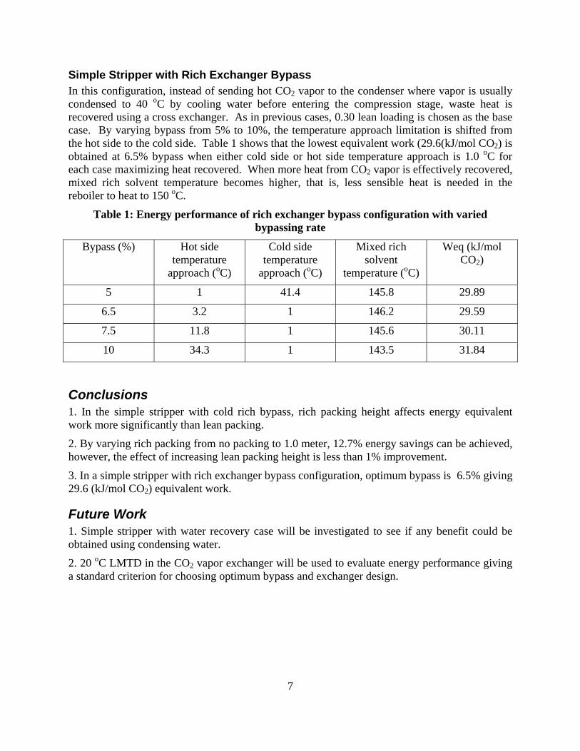
7
Simple Stripper with Rich Exchanger Bypass In this configuration, instead of sending hot CO2 vapor to the condenser where vapor is usually condensed to 40 oC by cooling water before entering the compression stage, waste heat is recovered using a cross exchanger. As in previous cases, 0.30 lean loading is chosen as the base case. By varying bypass from 5% to 10%, the temperature approach limitation is shifted from the hot side to the cold side. Table 1 shows that the lowest equivalent work (29.6(kJ/mol CO2) is obtained at 6.5% bypass when either cold side or hot side temperature approach is 1.0 oC for each case maximizing heat recovered. When more heat from CO2 vapor is effectively recovered, mixed rich solvent temperature becomes higher, that is, less sensible heat is needed in the reboiler to heat to 150 oC.
Table 1: Energy performance of rich exchanger bypass configuration with varied bypassing rate
Bypass (%) Hot side temperature
approach (oC)
Cold side temperature
approach (oC)
Mixed rich solvent
temperature (oC)
Weq (kJ/mol CO2)
5 1 41.4 145.8 29.89
6.5 3.2 1 146.2 29.59
7.5 11.8 1 145.6 30.11
10 34.3 1 143.5 31.84
Conclusions 1. In the simple stripper with cold rich bypass, rich packing height affects energy equivalent work more significantly than lean packing.
2. By varying rich packing from no packing to 1.0 meter, 12.7% energy savings can be achieved, however, the effect of increasing lean packing height is less than 1% improvement.
3. In a simple stripper with rich exchanger bypass configuration, optimum bypass is 6.5% giving 29.6 (kJ/mol CO2) equivalent work.
Future Work 1. Simple stripper with water recovery case will be investigated to see if any benefit could be obtained using condensing water.
2. 20 oC LMTD in the CO2 vapor exchanger will be used to evaluate energy performance giving a standard criterion for choosing optimum bypass and exchanger design.

8
References Oyenekan BA. Modeling of Strippers for CO2 Capture by Aqueous Amines. The University of
Texas at Austin. Ph.D. Dissertation. 2007.
Rochelle GT. "Amine scrubbing for CO2 capture". Science. 2009; 325,1652–4.
Van Wagener DH. Stripper Modeling for CO2 Removal Using Monoethanolamine and Piperazine Solvents. The University of Texas at Austin. Ph.D. Dissertation. 2011.
1
Measurement of Effective Packing Area and
Mass Transfer Coefficients
Quarterly Report for October 1 – December 31, 2012
by Chao Wang
Supported by the Luminant Carbon Management Program,
and Process Science and Technology Center
Department of Chemical Engineering
The University of Texas at Austin
January 31, 2013
Abstract In this quarter, liquid film and gas film mass transfer coefficients models including the influence of corrugation angle and packing nominal size were developed. A new concept, mixing points density (M), was introduced to represent the impact of corrugation angle and nominal size on mass transfer.
Mixing points are the turning points where liquid and gas flows change directions, mix with each other, and create turbulence. Intensive mass transfer between liquid and gas phase happens at the mixing points. Structured packing with a lower corrugation angle has larger kL/G because it has more mixing points than packing with a higher corrugation angle at the same packed height.
To quantify the mixing point density in packing, packing geometric structures were studied. Structured packings are composed of corrugated metal sheets crossing with each other. The crossing points are the mixing points, which divide structured packings into hundreds of small square pyramids. The number of mixing points per m3 equals to the number of square pyramids per m3 multiplied by the number of mixing points per pyramid. Thus, mixing points density (M)
for structured packing can be calculated by the equation:
tan**
6
BhBM
Random packings are composed of hundreds of small packing pieces. The mixing points are the turning points at each piece. The number of mixing points per m3 equals the number of packing pieces per m3 (0) multiplied by the number of mixing points per piece (M0). Thus, mixing points density (M) for random packing can be calculated by the equation:
0
000
**
a
MaMM P .
Preliminary mass transfer models are developed based on three factors influencing mass transfer: the liquid/gas superficial velocity (uL/G), the packing size (aP), and the mixing points density (M). Through data regression, the experimental constant and the exponents for each factor can be calculated. The mass transfer models are:
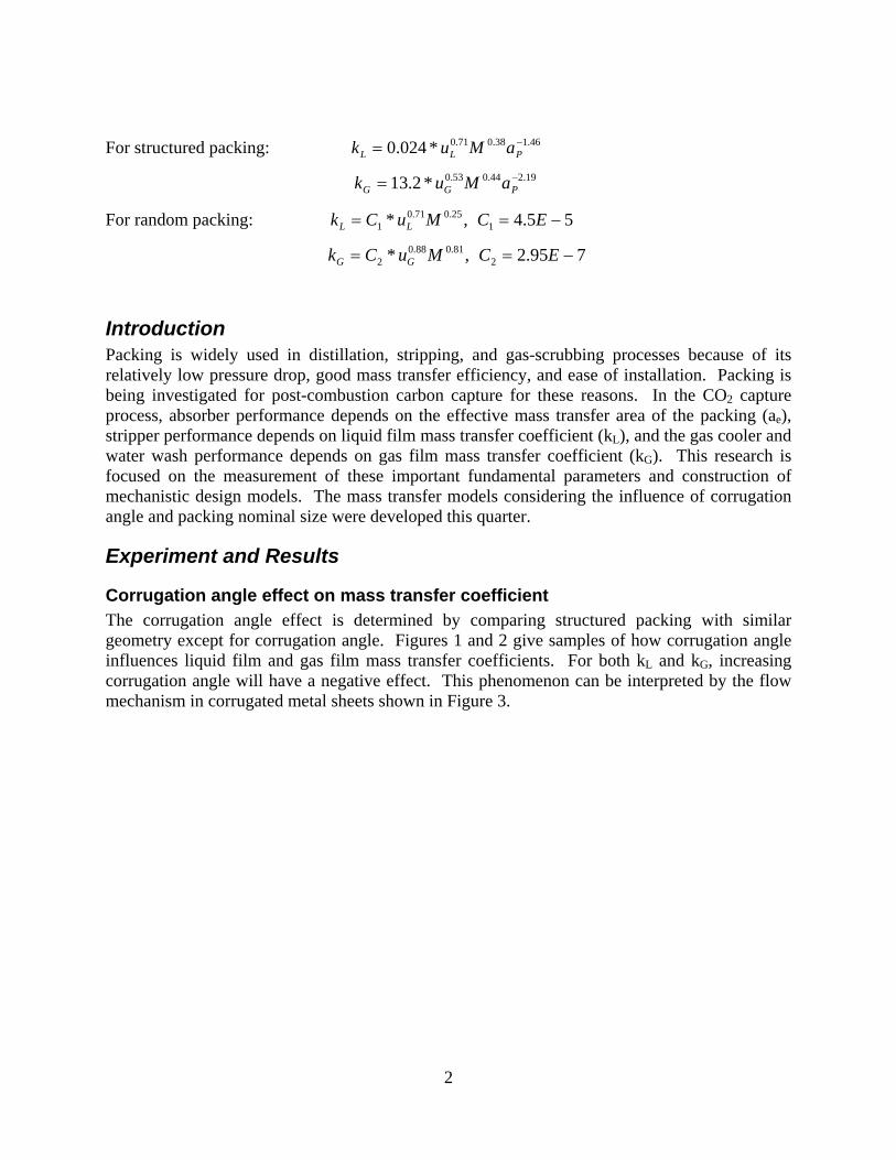
2
For structured packing: 46.138.071.0*024.0 PLL aMuk
19.244.053.0*2.13 PGG aMuk
For random packing: 55.4,* 125.071.0
1 ECMuCk LL
795.2,* 281.088.0
2 ECMuCk GG
Introduction Packing is widely used in distillation, stripping, and gas-scrubbing processes because of its relatively low pressure drop, good mass transfer efficiency, and ease of installation. Packing is being investigated for post-combustion carbon capture for these reasons. In the CO2 capture process, absorber performance depends on the effective mass transfer area of the packing (ae), stripper performance depends on liquid film mass transfer coefficient (kL), and the gas cooler and water wash performance depends on gas film mass transfer coefficient (kG). This research is focused on the measurement of these important fundamental parameters and construction of mechanistic design models. The mass transfer models considering the influence of corrugation angle and packing nominal size were developed this quarter.
Experiment and Results
Corrugation angle effect on mass transfer coefficient The corrugation angle effect is determined by comparing structured packing with similar geometry except for corrugation angle. Figures 1 and 2 give samples of how corrugation angle influences liquid film and gas film mass transfer coefficients. For both kL and kG, increasing corrugation angle will have a negative effect. This phenomenon can be interpreted by the flow mechanism in corrugated metal sheets shown in Figure 3.
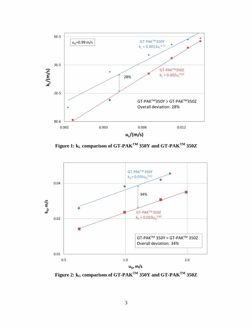
3
Figure 1: kL comparison of GT-PAKTM 350Y and GT-PAKTM 350Z
Figure 2: kG comparison of GT-PAKTM 350Y and GT-PAKTM 350Z
GT‐PAKTM350YkL = 0.0013uL
0.71
GT‐PAKTM350ZkL = 0.002uL
0.87
8E‐6
2E‐5
3E‐5
6E‐5
0.002 0.003 0.006 0.012
k L/(m/s)
uL/(m/s)
28%
GT‐PAKTM350Y > GT‐PAKTM350ZOverall deviation: 28%
uG=0.99 m/s
GT‐PAKTM350YkG= 0.035uG
0.62
GT‐PAKTM350ZkG = 0.023uG
0.60
0.01
0.02
0.04
0.5 1.0 2.0
k G, m
/s
uG, m/s
GT‐PAKTM 350Y > GT‐PAKTM 350ZOverall deviation: 34%
34%

4
Figure 3: Liquid flow along corrugated metal sheets
Structured packing is composed of corrugated metal sheets. Liquid flow inside the packing can be seen as flowing along these corrugated sheets. At the joint points of metal sheets (marked by circles in Figure 3), flows mix with each other, change directions, and create turbulence. Thus, these mixing points are believed to be the key points for mass transfer in structured packing. In packing with a lower corrugation angle, there will be more mixing points than packing with a higher corrugation angle at the same packed height, which means liquid and gas flows mix with each other more often, change direction more frequently, and create more turbulence. Therefore, the phenomenon that lower corrugation angle packing has a higher kG and kL can be explained.
Mixing points density in structured packing To quantify the number of mixing points inside structured packing, packing geometric structures are studied. Figure 4 shows the lateral view of a structured packing with a corrugation angle . From the lateral view, the corrugated metal sheets can be seen as bunches of parallel lines with a tilt angle to the horizontal line. In the structured packing, each corrugated metal sheet contacts with the one next to it. In the lateral view, it is expressed by the parallel lines crossing with another set of reversed parallel lines. The crossed corrugated metal sheets form hundreds of square pyramids, which are the triangles in the lateral view. The mixing points are the vertices of the triangles, which are marked in black circles in the lateral view. The bottom of the triangle
is the channel base B, and the height of the triangle is tan2
B.
Low corrugation angle
High corrugation angle

5
Figure 4: Lateral view of a structured packing with a corrugation angle
The square pyramids formed by the crossed metal sheets can be better seen from the top view of
the packing (Figure 5). The height of the square pyramid is tan2
B, the bottom area of the
pyramid is B*h. The volume of the square pyramid is tan**6
1BhB . Thus, the number of
square pyramids per m3 volume is tan**
6
BhB. Each pyramid has five mixing points;
however, each pyramid is also sharing mixing points with other four adjacent pyramids. Thus, the number of mixing points per pyramid is 5/5. The total number of mixing points per m3 (M) = the number of square pyramids per m3 * the number of mixing points per pyramid =
tan**
6
BhB.
Figure 5: Top view of a structured packing with a corrugation angle
2
B
tan2
B
h
tan2
B
2
B
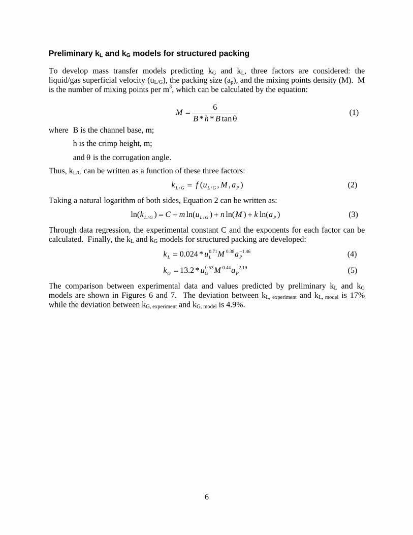
6
Preliminary kL and kG models for structured packing
To develop mass transfer models predicting kG and kL, three factors are considered: the liquid/gas superficial velocity (uL/G), the packing size (ap), and the mixing points density (M). M is the number of mixing points per m3, which can be calculated by the equation:
tan**
6
BhBM (1)
where B is the channel base, m;
h is the crimp height, m;
and is the corrugation angle.
Thus, kL/G can be written as a function of these three factors:
),,( // PGLGL aMufk (2)
Taking a natural logarithm of both sides, Equation 2 can be written as:
)ln()ln()ln()ln( // PGLGL akMnumCk (3)
Through data regression, the experimental constant C and the exponents for each factor can be calculated. Finally, the kL and kG models for structured packing are developed:
46.138.071.0*024.0 PLL aMuk (4)
19.244.053.0*2.13 PGG aMuk (5)
The comparison between experimental data and values predicted by preliminary kL and kG models are shown in Figures 6 and 7. The deviation between kL, experiment and kL, model is 17% while the deviation between kG, experiment and kG, model is 4.9%.

7
Figure 6: Comparison between experimental data and kL model for structured packing
Figure 7: Comparison between experimental data and kG model for structured packing
y = x+20%
‐20%
0E+0
2E‐5
4E‐5
6E‐5
8E‐5
0E+0 2E‐5 4E‐5 6E‐5 8E‐5
k L,m
odel, m/s
kL,exp, m/s
MP2X
GTC350Z
MP250Y
MP250X
GTC350Y
Average deviation: 17%
46.138.071.0*024.0 PLL aMuk
y = x+20%
‐20%
0
0.02
0.04
0.06
0 0.02 0.04 0.06
k G,m
odel, m
/s
kG,exp, m/s
GTC350Z
MP250Y
MP250X
GTC350Y
Average deviation: 4.9%
19.244.053.0*2.13 PGG aMuk
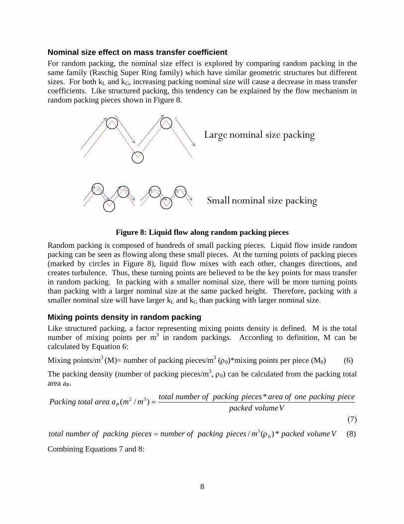
8
Nominal size effect on mass transfer coefficient For random packing, the nominal size effect is explored by comparing random packing in the same family (Raschig Super Ring family) which have similar geometric structures but different sizes. For both kL and kG, increasing packing nominal size will cause a decrease in mass transfer coefficients. Like structured packing, this tendency can be explained by the flow mechanism in random packing pieces shown in Figure 8.
Figure 8: Liquid flow along random packing pieces
Random packing is composed of hundreds of small packing pieces. Liquid flow inside random packing can be seen as flowing along these small pieces. At the turning points of packing pieces (marked by circles in Figure 8), liquid flow mixes with each other, changes directions, and creates turbulence. Thus, these turning points are believed to be the key points for mass transfer in random packing. In packing with a smaller nominal size, there will be more turning points than packing with a larger nominal size at the same packed height. Therefore, packing with a smaller nominal size will have larger kL and kG than packing with larger nominal size.
Mixing points density in random packing Like structured packing, a factor representing mixing points density is defined. M is the total number of mixing points per m3 in random packings. According to definition, M can be calculated by Equation 6:
Mixing points/m3 (M)= number of packing pieces/m3 (0)*mixing points per piece (M0) (6)
The packing density (number of packing pieces/m3, 0) can be calculated from the packing total area aP.
Vvolumepacked
piecepackingoneofareapiecespackingofnumbertotalmmaareatotalPacking P
*)/( 32
(7)
Vvolumepackedmpiecespackingofnumberpiecespackingofnumbertotal *)(/ 03 (8)
Combining Equations 7 and 8:
Large nominal size packing
Small nominal size packing

9
Vvolumepacked
apieceoneofareaVvolumempiecespackingofnumbermmaP
)(**)(/)/( 00
332 (9)
Thus, the packing density can be calculated:
00
3/apieceoneofarea
aareatotalpackingmpiecespackingofnumber P (10)
Finally, the mixing points density (M) can be calculated by combining Equations 6 and 10:
0
000
**
a
MaMM P (11)
Table 1 lists the number of mixing points density (M), packing density (0), area of one packing piece (a0), and total area (aP) for the random packings studied in this work.
Table 1: Random packing parameters
RSR#0.3 RSR#0.5 RSR#0.7
Nominal size (mm) 15 20 25
Number pieces/m3,0 180,000 145,000 45,500
Total area (m2/m3), aP 315 250 180
Mixing points per piece, M0 12 8 12
Area of one packing piece (cm2), a0 17.5 17.24 39.56
Mixing points/m3, M 2,160,000 1,160,000 546,000
Preliminary kL and kG models for random packing
To develop mass transfer models predicting kG and kL, the mixing points density (M) as well as liquid/gas superficial velocity (uL/G) are considered. Models for random packing do not consider packing total area (aP) separately because it is already included in the mixing points density factor (M). The mixing points density is the number of mixing points per m3, which can be calculated by Equation 11.
Thus, kL/G can be written as a function of M and uL/G:
),( // Mufk GLGL (12)
Taking a natural logarithm of both sides, Equation 12 can be written as:
)ln()ln()ln( // MnumCk GLGL (13)
Through data regression, the experimental constant C and the exponents for each factor can be calculated. Finally, the kL and kG models for random packings are developed:
55.4,* 125.071.0
1 ECMuCk LL (14)
795.2,* 281.088.0
2 ECMuCk GG (15)

10
For random packing, the comparison between experimental data and values predicted by preliminary kL and kG models is shown in Figures 9 and 10. The deviation between kL, experiment and kL, model is 15% while the deviation between kG, experiment and kG, model is 5%.
Figure 9: Comparison between experimental data and kL model for random packing
y = x+20%
‐20%
0E+0
2E‐5
4E‐5
6E‐5
8E‐5
0E+0 2E‐5 4E‐5 6E‐5 8E‐5
k L,m
odel, m
/s
kL,exp, m/s
RSR#0.3
RSR#0.5
RSR#0.7
Average deviation: 15%
25.071.01 * MuCk LL

11
Figure 10: Comparison between experimental data and kG model for random packing
Conclusions In this quarter, work has focused on developing mass transfer models including a new concept: mixing points density (M).
1. Mixing points are the turning points where flows change directions, mix with each other, and create turbulence. Mixing points contribute directly to mass transfer.
2. Structured packing with a lower corrugation angle has larger kL/G because it has more mixing points.
3. For structured packing, mixing points density can be calculated by the equation:
tan**
6
BhBM
4. Random packing with a smaller nominal size has larger kL/G because it has more mixing points.
5. For random packing, mixing points density can be calculated by the equation:
0
000
**
a
MaMM P
6. kL and kG models considering mixing points density (M), liquid/gas superficial velocity (uL/G), and packing size (aP) are developed:
kP
nmGLGL aMuCk /1/ * (16)
y = x+20%
‐20%
0E+0
2E‐2
4E‐2
6E‐2
0.00 0.02 0.04 0.06
k G,m
odel, m
/s
kG,exp, m/s
RSR#0.3
RSR#0.5
Average deviation: 5%
81.088.01 * MuCk GG
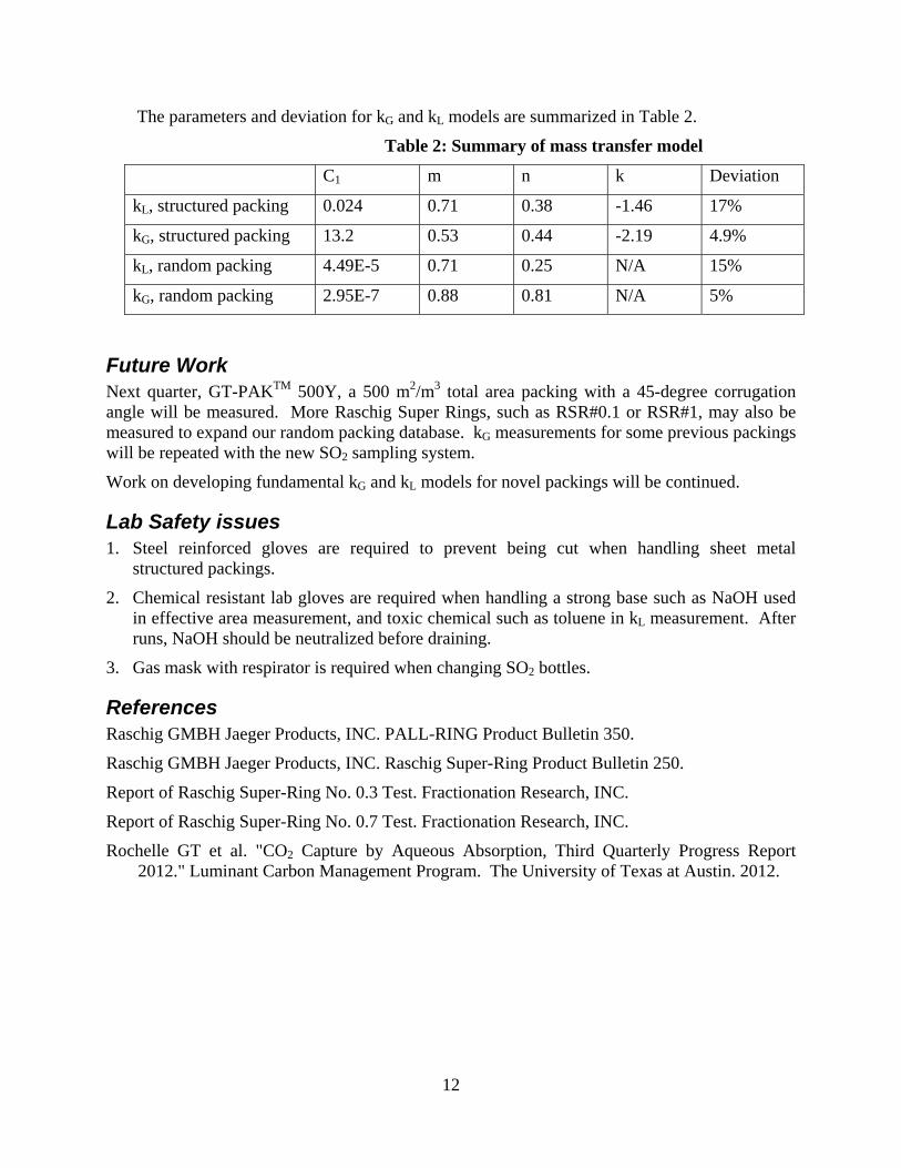
12
The parameters and deviation for kG and kL models are summarized in Table 2.
Table 2: Summary of mass transfer model
C1 m n k Deviation
kL, structured packing 0.024 0.71 0.38 -1.46 17%
kG, structured packing 13.2 0.53 0.44 -2.19 4.9%
kL, random packing 4.49E-5 0.71 0.25 N/A 15%
kG, random packing 2.95E-7 0.88 0.81 N/A 5%
Future Work Next quarter, GT-PAKTM 500Y, a 500 m2/m3 total area packing with a 45-degree corrugation angle will be measured. More Raschig Super Rings, such as RSR#0.1 or RSR#1, may also be measured to expand our random packing database. kG measurements for some previous packings will be repeated with the new SO2 sampling system.
Work on developing fundamental kG and kL models for novel packings will be continued.
Lab Safety issues 1. Steel reinforced gloves are required to prevent being cut when handling sheet metal
structured packings.
2. Chemical resistant lab gloves are required when handling a strong base such as NaOH used in effective area measurement, and toxic chemical such as toluene in kL measurement. After runs, NaOH should be neutralized before draining.
3. Gas mask with respirator is required when changing SO2 bottles.
References Raschig GMBH Jaeger Products, INC. PALL-RING Product Bulletin 350.
Raschig GMBH Jaeger Products, INC. Raschig Super-Ring Product Bulletin 250.
Report of Raschig Super-Ring No. 0.3 Test. Fractionation Research, INC.
Report of Raschig Super-Ring No. 0.7 Test. Fractionation Research, INC.
Rochelle GT et al. "CO2 Capture by Aqueous Absorption, Third Quarterly Progress Report 2012." Luminant Carbon Management Program. The University of Texas at Austin. 2012.

1
Stripper Modeling and Pilot Plant Configurations
Quarterly Report for October 1 – December 31, 2012
by Tarun Madan
Supported by the Luminant Carbon Management Program
McKetta Department of Chemical Engineering
The University of Texas at Austin
January 31, 2013
Abstract Stripper complexity is an important tool in minimizing the energy penalty of amine scrubbing. Different stripper and flash configurations can be optimized for energy consumption by identifying and changing the various degrees of freedom. A new configuration of ‘Advanced Flash Stripper’ was studied in this quarter. This configuration recovers the waste heat of stripping steam more reversibly by using a combination of cold, warm, and rich bypass. Complex advanced flash configurations, corresponding to warm bypass, cold and hot bypass, and cold, warm, and rich bypass had equivalent work values of 31.4, 30.3, and 29.7 kJ/mol CO2 using the Independence solvent model for 8 m PZ in Aspen Plus®.
Alternate pilot plant configurations based on the advanced flash stripper were also modeled. Best performance of 29.0 kJ/mol CO2 was achieved using heat recovery by warm rich bypass and heat exchange between cold rich and hot CO2 streams.
Introduction Stripper complexity and advanced stripper configurations have been studied in the past to minimize the energy requirement of amine scrubbing for post-combustion carbon capture. Increasing the reversibility of the process using advanced configurations improves the energy performance. This complexity can be increased by using recycles, better heat recovery, splits, multiple pressure stages, and other features (Leites et al., 2003). For post-combustion CO2 capture with 8 m PZ, Oyenekan (2007) and Van Wagener (2012) have evaluated advanced configurations including multi-stage flash, cold rich bypass, and interheated stripper. These configurations were investigated using Aspen Plus® with thermodynamic models developed using experimental data. For 8 m PZ, equivalent work of 30.5–35.3 kJ/mol CO2 has been reported for different configurations.
A new configuration of the ‘Advanced Flash Stripper,’ which recovers waste stripping steam heat more reversibly using combinations of warm, cold, and hot rich bypass, was studied in this quarter. Based on this advanced flash stripper, pilot plant cases were modeled to identify configurations.

2
Methods and Discussion
Advanced Flash Stripper This configuration has various complexities associated with combinations of warm, cold, and hot bypass. The following combinations were modeled.
1. Warm rich bypass (Advanced Flash 1, AF1) 2. Cold and hot rich bypass (Advanced Flash 2, AF2) 3. Cold, warm and hot rich bypass (Advanced Flash 3, AF3)
The following modeling and design specifications were held constant in all the configurations.
1. Process modeling software – Aspen Plus® 2. Solvent – 8 m piperazine (PZ) 3. Solvent model – Independence 4. Rich loading – 0.4 mol/mol(alk) 5. Cross exchanger – LMTD of 5 °C 6. Packing – Mellapak 250X (3 m for AF1, 5 m for AF2 and AF3)
Equivalent work for each case was calculated using the following equation.
0.75
∆∆
; ; .
Figures 1 to 3 show the process flow diagram of these three configurations in increasing complexity of the Advanced Flash.
Figure 1: Flash with warm rich bypass (Advanced Flash 1, 2 m Mellapak 250X packing, 8 m PZ, 5 °C LMTD Cross exchanger)

3
Advanced Flash 2 uses a combination of cold and hot rich bypass to recover the waste heat of stripping steam in the flash. Advanced Flash 3 has a combination of cold, warm, and hot rich bypass as shown in Figure 3.
0.4 rich ldg
Rich
CrossExchanger
Lean
Flash
CO2 to compressor
Heater
~150 C
Hot Rich Bypass
CrossExchanger
Cold Rich bypass
Flash
Figure 2: Flash with hot and cold rich bypass (Advanced Flash 2, Mellapak 250X packing, 8 m PZ, 5 °C LMTD Cross exchanger)
0.4 rich ldg
Rich
CrossExchanger
Lean
Flash
CO2 to compressor
Heater
~150 C
Hot Rich Bypass
CrossExchanger
Cold Rich bypass
Flash
Warm Rich bypass
Flash
Figure 3: Flash with hot, warm and cold rich bypass (Advanced Flash 3, Mellapak 250X packing, 8 m PZ, 5 °C LMTD Cross exchanger)

4
Pilot Plant Configurations Pilot plant configurations based on the advanced flash stripper concept were modeled with the following changes over the base design.
1. Flashing allowed in the cross exchanger design. 2. Heat Recovery from hot CO2 using a rich bypass exchange with a 15 °C LMTD heat
exchanger instead of cold rich bypass (to minimize packing requirement). 3. Fixed total amount of packing (5 m Mellapak 250X). 4. Other specifications: 8m PZ, 0.4 rich ldg, 0.29/0.27 lean ldg, 150 °C stripping T.
The resulting configurations are shown in Figures 4 to 8.
0.4 rich ldg
Rich
CrossExchanger
5 C LMTD
Lean
Flash
CO2 to compressor
Heater
~150 C
~120 C (Bubble Point)
CrossExchanger
Flashing
Figure 4: Warm Rich bypass at rich liquid bubble point
Figure 5: Single stage flash with rich bypass exchange and hot bypass

5
0.4 rich ldg
Rich
CrossExchanger
5 C LMTD
Lean
Flash
CO2 to compressor
Heater
~150 C
~120 C (Bubble Point)
CrossExchanger
Flashing
Rich exchange bypass (46 C)
Heat Recovery Exchanger15 C LMTD
~121 C
~116 C
0.4 rich ldg
Rich
CrossExchanger
5 C LMTD
Lean
Flash
CO2 to compressor
Heater
~150 C
~120 C (Bubble Point)
CrossExchanger
Flashing
Rich bypass exchange (46 C)
Heat Recovery Exchanger15 C LMTD
~122 C
~117 C
Flash
~139 C
Figure 6: Single flash with rich bypass exchange and warm bypass
Figure 7: Single flash with rich bypass exchange, warm bypass (at bubble point), and hot bypass

6
A combination of hot and warm bypass was also tested with vapor recycle in which vapor from partially heated solvent is sent to flash directly as shown in Figure 8.
Results
Advanced Flash Stripper Figure 9 compares the equivalent work values for various complex configurations of the Advanced Flash and Simple Stripper over a range of lean loadings.
Table 1 shows the improvement of the advanced flash compared with the base case of the simple stripper.
0.4 rich ldg
Rich
CrossExchanger
5 C LMTD
Lean
Flash
CO2 to compressor
~150 C
~120 C (Bubble Point)
CrossExchanger
Flashing
Rich bypass exchange (46 C)
Heat Recovery Exchanger15 C LMTD
~122 C
~117 C
Flash
146 C
Figure 8: Advanced Flash with vapor recycle

7
.
Figure 9: Equivalent work of various stripper configurations for a range of lean loading (Independence model, 8 m PZ, 5 °C LMTD cross exchanger, 150 °C stripping T,
compression to 150 bar, 3 m packing for AF1, 5 m packing AF2 and AF3)
Table 1: Improvement of equivalent work for different stripper configurations compared to base case of simple stripper (8 m PZ, 5 °C LMTD cross exchanger, 150 °C stripping T,
compression to 150 bar)
Configuration Equivalent Work (kJ/mol CO2)
Improvement over base case
Simple Stripper (Fawkes) 32.6 -
Interheated Stripper (Fawkes) 30.0 -
Simple Stripper (Independence, Base case)
32.1 -
Advanced Flash 1 31.4 2.2%
Advanced Flash 2 30.3 5.6%
Advanced Flash 3 29.7 7.5%
29
30
31
32
33
34
35
0.26 0.27 0.28 0.29 0.30 0.31 0.32 0.33 0.34
Eq
uiv
alen
t W
ork
(k
J/m
ol C
O2)
Lean ldg (mol/mol alk)
AFS-1
1-SF with hot rich bypass
1-SF with cold rich bypass
AFS-2
AFS-3
Simple Stripper
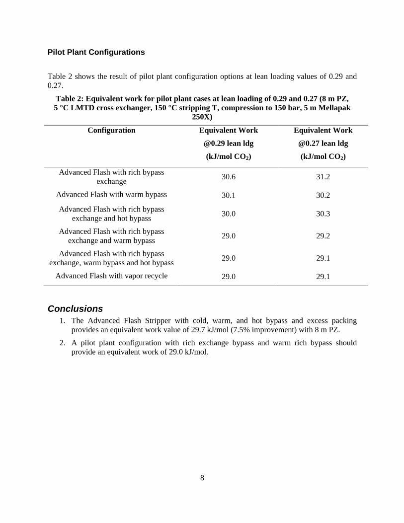
8
Pilot Plant Configurations
Table 2 shows the result of pilot plant configuration options at lean loading values of 0.29 and 0.27.
Table 2: Equivalent work for pilot plant cases at lean loading of 0.29 and 0.27 (8 m PZ, 5 °C LMTD cross exchanger, 150 °C stripping T, compression to 150 bar, 5 m Mellapak
250X)
Configuration Equivalent Work
@0.29 lean ldg
(kJ/mol CO2)
Equivalent Work
@0.27 lean ldg
(kJ/mol CO2)
Advanced Flash with rich bypass exchange
30.6 31.2
Advanced Flash with warm bypass 30.1 30.2
Advanced Flash with rich bypass exchange and hot bypass
30.0 30.3
Advanced Flash with rich bypass exchange and warm bypass
29.0 29.2
Advanced Flash with rich bypass exchange, warm bypass and hot bypass
29.0 29.1
Advanced Flash with vapor recycle 29.0 29.1
Conclusions 1. The Advanced Flash Stripper with cold, warm, and hot bypass and excess packing
provides an equivalent work value of 29.7 kJ/mol (7.5% improvement) with 8 m PZ.
2. A pilot plant configuration with rich exchange bypass and warm rich bypass should provide an equivalent work of 29.0 kJ/mol.

9
References Leites IL, Sama DA, Lior N. "The theory and practice of energy saving in the chemical industry:
some methods for reducing the thermodynamic irreversibility in chemical technology processes." Energy, Volume 28, Issue 1, January 2003; 55–97.
Oyenekan B. Modeling of Strippers for CO2 Capture by Aqueous Amines. The University of Texas at Austin. Ph.D. Dissertation. 2007.
Rochelle GT et al. "CO2 Capture by Aqueous Absorption, First Quarterly Progress Report 2012." Luminant Carbon Management Program. The University of Texas at Austin. 2012.
Van Wagener DH. Stripper Modeling for CO2 Removal Using Monoethanolamine and Piperazine Solvents. The University of Texas at Austin. Ph.D. Dissertation. 2011.

1
Thermodynamic Models for 4 m 2MPZ/4 m PZ and 8 m 2MPZ
Quarterly Report for October 1 – December 31, 2012
by Brent Sherman
Supported by the Luminant Carbon Management Program
McKetta Department of Chemical Engineering
The University of Texas at Austin
January 31, 2013
Abstract
A non-rigorous model for 4 m 2MPZ/4 m PZ was made by modifying in the rigorous 8 m PZ model. This model does not include 2MPZ or its derivative species, and so PZ and its derivatives serve as pseudocomponents. Still, this non-rigorous thermodynamic model gives acceptable performance. A kinetic model was begun, but not completed owing to a shift in focus to the rigorous 8 m 2MPZ model. The current version (V0.0) improves upon the prior version by stripping the model down to just 2MPZ in addition to changing the chemistry set and viscosity subroutine to conform to current standards, specifically the elimination of proton and hydroxide ions and use of the modified Weiland equation. In examining this rigorous model for weaknesses, a ~5 kJ/mol discrepancy at high loadings between calculating the heat of absorption via calorimetry and via Lewis-and-Randall (formerly Gibbs-Helmholtz) was uncovered. All recent and under development models have been centralized, assigned a version number, and a metadata file to ensure consistency among present and future modelers.
Introduction The overarching goal of this project is to develop a generic amine model and to use this model to systematically investigate the impact of amine properties on process performance. Subordinate goals include developing more models, developing new modeling methods, and ensuring consistency across models.
A generic amine model would allow for more rapid amine solvent screening. There are currently models for sundry piperazine (PZ) blends, including PZ with methyl diethanolamine (MDEA), 2-methylpiperazine (2MPZ), 2-amino-2-methyl-1-proponol (AMP), and aminoethylpiperazine (AEP). All of these blends broaden the solid solubility window of PZ while minimally compromising its beneficial properties. Each of these models represents a substantial investment of man hours, and so I seek to streamline this process. Furthermore, a different model maker has crafted each aforementioned model. Without a system for version control, tracking changes between versions will become increasingly problematic.
Immediate work focused on a non-rigorous 4 m 2MPZ/4 m PZ model, a rigorous 8 m 2MPZ model, and version control.
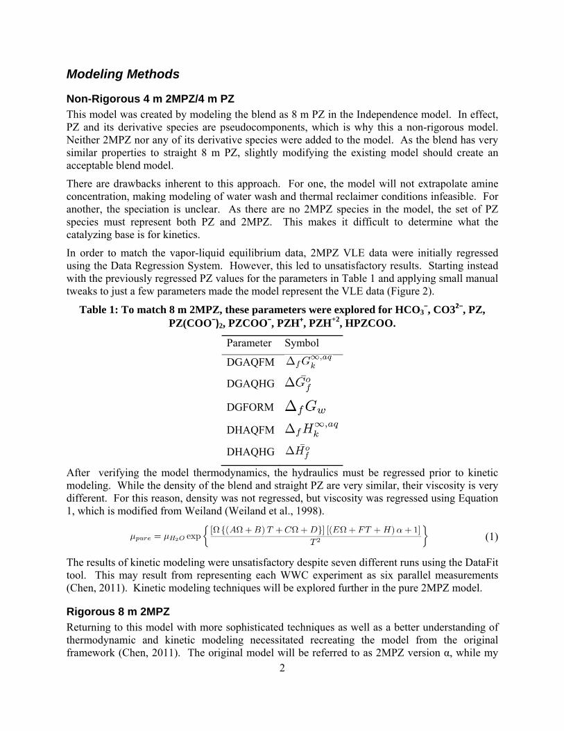
2
Modeling Methods
Non-Rigorous 4 m 2MPZ/4 m PZ This model was created by modeling the blend as 8 m PZ in the Independence model. In effect, PZ and its derivative species are pseudocomponents, which is why this a non-rigorous model. Neither 2MPZ nor any of its derivative species were added to the model. As the blend has very similar properties to straight 8 m PZ, slightly modifying the existing model should create an acceptable blend model.
There are drawbacks inherent to this approach. For one, the model will not extrapolate amine concentration, making modeling of water wash and thermal reclaimer conditions infeasible. For another, the speciation is unclear. As there are no 2MPZ species in the model, the set of PZ species must represent both PZ and 2MPZ. This makes it difficult to determine what the catalyzing base is for kinetics.
In order to match the vapor-liquid equilibrium data, 2MPZ VLE data were initially regressed using the Data Regression System. However, this led to unsatisfactory results. Starting instead with the previously regressed PZ values for the parameters in Table 1 and applying small manual tweaks to just a few parameters made the model represent the VLE data (Figure 2).
Table 1: To match 8 m 2MPZ, these parameters were explored for HCO3‒, CO32‒, PZ,
PZ(COO‒)2, PZCOO‒, PZH+, PZH+2, HPZCOO.
Parameter Symbol
DGAQFM
DGAQHG
DGFORM
DHAQFM
DHAQHG
After verifying the model thermodynamics, the hydraulics must be regressed prior to kinetic modeling. While the density of the blend and straight PZ are very similar, their viscosity is very different. For this reason, density was not regressed, but viscosity was regressed using Equation 1, which is modified from Weiland (Weiland et al., 1998).
(1)
The results of kinetic modeling were unsatisfactory despite seven different runs using the DataFit tool. This may result from representing each WWC experiment as six parallel measurements (Chen, 2011). Kinetic modeling techniques will be explored further in the pure 2MPZ model.
Rigorous 8 m 2MPZ Returning to this model with more sophisticated techniques as well as a better understanding of thermodynamic and kinetic modeling necessitated recreating the model from the original framework (Chen, 2011). The original model will be referred to as 2MPZ version α, while my

3
model is 2MPZ Version 0.0. α is based on a Fawkes model, and so it contains many parameters, reactions, and associated code blocks necessary for modeling PZ/MDEA. To isolate problems, these parts – the chemistry reactions, the subroutine code, the analysis blocks, etc. – were eliminated. Then, the default chemistry set was stripped down to agree with our current methods, namely not modeling the proton and hydroxide ions. These ions are not modeled owing to their insignificantly low concentration throughout operating conditions.
Table 2: The chemistry blocks of the two models differ in the presence of proton and hydroxide ions.
2MPZ Version α 2MPZ V0.0 2MPZ + HCO3- ↔ 2MPZCOO + H2O 2 2MPZ + CO2 ↔ 2MPZCOO + 2MPZH+
H2MPZCOO ↔ 2MPZCOO + H+ 2 2MPZCOO + CO2 ↔ 2MPZCOO2 + H2MPZCOO
2MPZCOO + HCO3- ↔ 2MPZCOO2 + H2O
2MPZCOO + CO2 + H2O ↔ HCO3- + H2MPZCOO
2MPZH+ ↔ 2MPZ + H+ 2MPZ + H2MPZCOO ↔ 2MPZH+ + 2MPZCOO
H2O ↔ H+ + OH- 2MPZCOO + HCO3- ↔ CO3-- + H2MPZCOO CO2 + H2O ↔ H+ + HCO3- HCO3- ↔ H+ + CO3--
To ensure that these changes did not harm the model, the validation was repeated. The model was verified as thermodynamically sound. This process showed a large discrepancy between the calorimetric and Lewis-and-Randall (formerly referred to as the Gibbs-Helmholtz) methods for calculating heat of absorption. The latter method uses Equation 2), while the former uses Equation 3. Prior work reduced the difference between the two by eliminating the inconsistency between thermodynamic properties and equilibrium constants, yet a discrepancy persists (Rochelle et al., 2011).
(2)
(3)
where Q is the net-duty of the flash block, and 2COn is the molar flow rate of gaseous CO2. The
heat of absorption is calculated by sending a loaded solvent stream and a gaseous CO2 stream to a flash block for a bubble point calculation.
Once the review was complete, hydraulic regression began. The viscosity subroutine used a different equation (Freeman, 2011: Equation 4.3). While this was functional, having all models use the same set of equations will allow easy comparison of the significance of parameters across amine systems, so the viscosity data were fit with Equation 1.

4
Version Control Last quarter, version control for the uncompiled source code for all Fortran subroutines was implemented. This took advantage of the dynamic linker option in Aspen Plus® to centralize all Fortran subroutines. This quarter, version control for the binary model files (*.bkp) was implemented by centralizing all recent models with a focus on those under active development.
2MPZ (Chen, 2011; Rochelle et al., 2013)
2MPZ/PZ (this report) AMP/PZ (Rochelle et al., 2012) KPZ (Hilliard, 2008)
MEA (Phoenix, Model A, Model B) (Plaza, 2011; Xu, 2011)
PZ & MDEA/PZ (Fawkes, Independence) (Frailie, Plaza, Van Wagener, & Rochelle, 2011)
AEP/PZ (Rochelle et al, 2013) Each model has an associated metadata file detailing its creation history and changes between versions.
Results and Discussion
Non-Rigorous 4 m 2MPZ/4 m PZ A thermodynamic model in good agreement with the experimental data was obtained by
adjusting from -4.99E+08 to -4.80E+08 ⁄ . The results are shown below in Figures 1–5.
Figure 1: Loaded amine volatility of 4 m 2MPZ/4 m PZ. Points are data (Nguyen, 2011); lines are model predictions.
α=0
α=0.328
α=0.40
0.0001
0.001
0.01
0.1
1
10
100
1000
0 20 40 60 80 100
PAm (Pa)
T (°C)

5
Figure 2: VLE for 4 m 2MPZ/4 m PZ. The experimental data are well fit by manually
changing . Lines are the model; filled points WWC data (Chen, 2011); empty points total pressure (Xu, 2011).
Figure 3: Heat of absorption of 4 m 2MPZ/4 m PZ calculated using Equation 2. The inflection is poorly defined and the higher loadings are muddy, but the curves are
reasonable.
40 C
60 C
80 C
100 C120 C
140 C
160 C
1.E+00
1.E+01
1.E+02
1.E+03
1.E+04
1.E+05
1.E+06
1.E+07
1.E+08
0 0.05 0.1 0.15 0.2 0.25 0.3 0.35 0.4 0.45 0.5
P*CO2(Pa)
Loading (mol CO2/mol alk)
10
20
30
40
50
60
70
80
90
0.05 0.1 0.15 0.2 0.25 0.3 0.35 0.4 0.45 0.5
‐ΔHabs
(kJ/mol)
Loading (mol CO2/mol alk.)
40 °C
80 °C60 °C
100 °C120 °C

6
Figure 4: Non-rigorous speciation 4 m 2MPZ/4 m PZ at 40 °C. As expected, more bicarbonate forms due to the hindered 2MPZ than in the pure PZ system, as seen in Figure
5.
PZ
PZCOO2
PZCOO‐
PZH+
HCO3‐
HPZCOO
0
0.02
0.04
0.06
0.08
0.1
0.12
0.14
0 0.1 0.2 0.3 0.4 0.5
Liquid MoleFraction
Loading (mol CO2/mol alk)

7
Figure 5: Speciation of 8 m PZ at 40 °C from Independence. The solid solubility limit is exceeded above 0.45 loading.
An intermediary step between the thermodynamic and kinetic models is regression of the hydraulics. Whereas density is not critically important to kinetics, and the two amines have similar densities, that hydraulic parameter was calculated as straight 8 m PZ. Contrariwise, the viscosity of the blend differs substantially from that of pure PZ, so the parameters of Equation 1 were changed to the values in Table 3.
Table 3: Viscosity parameters of Equation 1 for 4 m 2MPZ/4 m PZ and 8 m 2MPZ.
Parameter 4 m 2MPZ/4 m PZ 8 m 2MPZ
A 2.56E+03 4.85E+02B 7.64E+02 1.52E+03C 1.00E+00 2.07E+00D 4.01E+00 5.13E+00E -3.46E+01 -4.38E+00F 3.03E-03 -1.05E-02H 1.45E+01 7.16E+00
PZCOO2
PZCOO‐PZH+
HCO3‐
PZ
HPZCOO
0
0.02
0.04
0.06
0.08
0.1
0.12
0.14
0 0.1 0.2 0.3 0.4 0.5
Liquid MoleFraction
Loading (mol CO2/mol alk)

8
Figure 6: Viscosity of 4 m 2MPZ/4 m PZ. Lines are the model; points are data (Chen, 2011).
The kinetic model failed to match the experimental flux within ±20%. There was no clear trend in the disagreement with regards to loading, temperature, or magnitude of flux.
Rigorous 8 m 2MPZ Model Despite removal of protons and hydroxide ions and changing the chemistry reaction set, the thermodynamic model shows just as good agreement as shown elsewhere (Chen, 2011). This confirms the insignificance of those ions, and their elimination should aid convergence. While verifying the heat of absorption, the two different methods outlined previously were compared. The results are shown in Figures 7–9. It is suspected that the deviation above a loading of 0.25 mol CO2/mol alk. is due to the zwitterion becoming a significant species.
40C
60C
20C50C
150C
1.0
10.0
100.0
0 0.1 0.2 0.3 0.4 0.5
Viscosity(cP)
Loading (mol CO2/mol alk.)

9
Figure 7: Heat of absorption of 8 m 2MPZ calculated from Equation 2.
Figure 8: Heat of absorption of 8 m 2MPZ calculated from Equation 3. The disagreement between the two methods occurs above a loading of 0.25 (compare Figure 9).
‐95
‐85
‐75
‐65
‐55
‐45
‐35
‐25
0.00 0.05 0.10 0.15 0.20 0.25 0.30 0.35 0.40 0.45 0.50
ΔHabs
(kJ/mol)
Loading (mol CO2/mol alk.)
25 °C
40 °C
60 °C
80 °C
100 °C
120 °C
140 °C
‐95
‐85
‐75
‐65
‐55
‐45
‐35
‐25
0.00 0.05 0.10 0.15 0.20 0.25 0.30 0.35 0.40 0.45 0.50
ΔHabs
(kJ/mol)
Loading (mol CO2/mol alk.)
25 °C
40 °C
60 °C
80 °C
100 °C
120 °C
140 °C
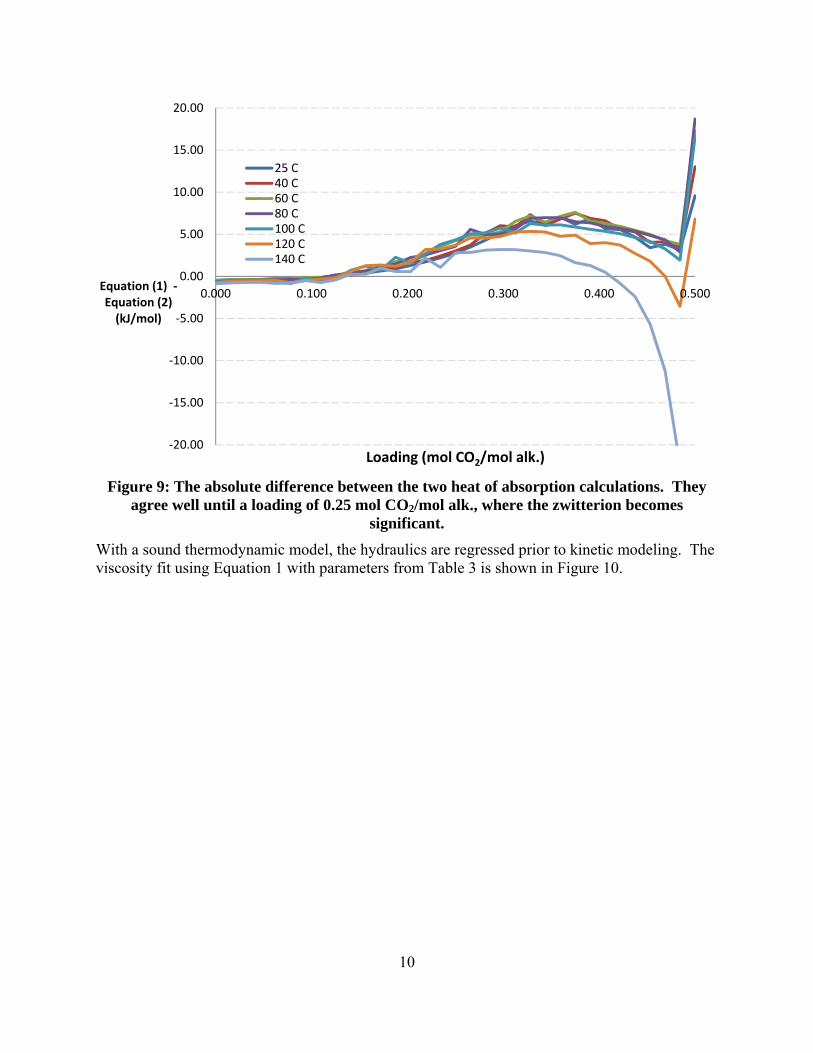
10
Figure 9: The absolute difference between the two heat of absorption calculations. They agree well until a loading of 0.25 mol CO2/mol alk., where the zwitterion becomes
significant.
With a sound thermodynamic model, the hydraulics are regressed prior to kinetic modeling. The viscosity fit using Equation 1 with parameters from Table 3 is shown in Figure 10.
‐20.00
‐15.00
‐10.00
‐5.00
0.00
5.00
10.00
15.00
20.00
0.000 0.100 0.200 0.300 0.400 0.500Equation (1) ‐Equation (2)(kJ/mol)
Loading (mol CO2/mol alk.)
25 C40 C60 C80 C100 C120 C140 C
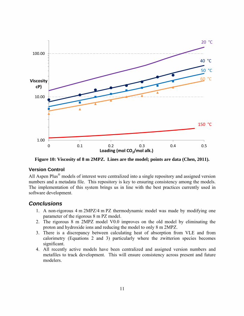
11
Figure 10: Viscosity of 8 m 2MPZ. Lines are the model; points are data (Chen, 2011).
Version Control All Aspen Plus® models of interest were centralized into a single repository and assigned version numbers and a metadata file. This repository is key to ensuring consistency among the models. The implementation of this system brings us in line with the best practices currently used in software development.
Conclusions 1. A non-rigorous 4 m 2MPZ/4 m PZ thermodynamic model was made by modifying one
parameter of the rigorous 8 m PZ model. 2. The rigorous 8 m 2MPZ model V0.0 improves on the old model by eliminating the
proton and hydroxide ions and reducing the model to only 8 m 2MPZ. 3. There is a discrepancy between calculating heat of absorption from VLE and from
calorimetry (Equations 2 and 3) particularly where the zwitterion species becomes significant.
4. All recently active models have been centralized and assigned version numbers and metafiles to track development. This will ensure consistency across present and future modelers.
1.00
10.00
100.00
0 0.1 0.2 0.3 0.4 0.5
Viscosity cP)
Loading (mol CO2/mol alk.)
20 °C
40 °C
50 °C
60 °C
150 °C

12
Future Work Next quarter work will focus on the creation of a kinetic 2MPZ model. This process will explore multiple kinetic modeling methods and compare their end results to determine the best practice. Once this is complete, focus will shift to the 4 m 2MPZ/4 m PZ model, which also needs a kinetic model. Other projects include improving version control, finding the root of the heat of absorption discrepancy, and solid solubility studies for various systems of 2MPZ/PZ.
References Chen X. Carbon Dioxide Thermodynamics, Kinetics, and Mass Transfer in Aqueous Piperazine
Derivatives and Other Amines. The University of Texas at Austin. Ph.D. Dissertation. 2011.
Frailie PT, Plaza JM, Van Wagener DH, Rochelle GT. “Modeling Piperazine Thermodynamics.” Energy Proc. 2011;4:35–42.
Freeman SA. Thermal Degradation and Oxidation of Aqueous Piperazine for Carbon Dioxide Capture. The University of Texas at Austin. Ph.D. Dissertation. 2011.
Hilliard MD. A Predictive Thermodynamic Model for an Aqueous Blend of Potassium Carbonate, Piperazine, and Monoethanolamine for Carbon Dioxide. The University of Texas at Austin. Ph.D. Dissertation. 2008.
Nguyen T. Personal communication. 2011.
Plaza JM. Modeling of Carbon Dioxide Absorption using Aqueous Monoethanolamine, Piperazine and Promoted Potassium Carbonate. The University of Texas at Austin. Ph.D. Dissertation. 2011.
Rochelle GT et al. "CO2 Capture by Aqueous Absorption, First Quarterly Progress Report 2011." Luminant Carbon Management Program. The University of Texas at Austin. 2011.
Rochelle GT et al. "CO2 Capture by Aqueous Absorption, Second Quarterly Progress Report 2012.” Luminant Carbon Management Program. The University of Texas at Austin. 2012.
Rochelle GT et al. "CO2 Capture by Aqueous Absorption, Fourth Quarterly Progress Report 2012." Luminant Carbon Management Program. The University of Texas at Austin. 2013.
Weiland RH, Dingman JC, Cronin DB, Browning GJ. “Density and Viscosity of Some Partially Carbonated Aqueous Alkanolamine Solutions and Their Blends.” J Chem Eng Data. 1998;43(3):378–382.
Xu Q. Thermodynamics of CO2 Loaded Aqueous Amines. University of Texas at Austin. Ph.D. Dissertation. 2011.

1
Equation-Based Representations of Mass Transfer, Heat Transfer, and Reaction Kinetics in Gas/Liquid Contactors
Quarterly Report for October 1 – December 31, 2012
by Matthew S. Walters
Supported by the Luminant Carbon Management Program
McKetta Department of Chemical Engineering
The University of Texas at Austin
January 31, 2013
Abstract Previously developed models of gas/liquid contactors used in amine scrubbing have been analyzed for accuracy and practicality based on their representations of mass transfer, heat transfer, and reaction kinetics. It is recommended that the continuity equation approach be used to represent mass and heat transfer in a continuous packed bed, but discontinuous sections of the bed, including liquid feed points, intercooling sections, and interheating sections, be treated as a well-mixed segment. Two-film theory assuming binary diffusion should be used to avoid the estimation of multiple binary diffusion coefficients needed in the Maxwell-Stefan formulation. In the liquid phase, it is valid to assume that the internal energy holdup of a segment is equal to enthalpy holdup, but this is not valid for the compressible vapor phase. The liquid film mass transfer coefficient can be experimentally determined in a wetted wall column, so this is the most advantageous representation of reaction kinetics in the absorber. Additional parameter uncertainty is introduced when an enhancement factor is used as an alternative representation of reaction kinetics. These recommendations will be used when implementing a gas/liquid contactor model in gPROMS® for an amine scrubbing system.
Introduction Equation-based models, in contrast to closed-source process simulators, provide a transparent set of physically significant relations with explicit expressions describing system parameters. An equation-based model may be advantageous for a process in the development stage like amine scrubbing where the solvent and operating conditions will likely change between initial pilot plant testing and commercial scale implementation. Several similar, yet unique approaches have been applied to the equation-based modeling of gas/liquid contactors used in amine scrubbing. The most notable research in this area has taken place at the Norwegian University of Science and Technology (Kvamsdal et al., 2009), Cranfield University (Lawal et al., 2009), and the University of Texas at Austin (Ziaii, 2012). The goal of this work is to understand the underlying theory and assumptions used in previously developed models, compile the most useful components of these models, and implement a new plantwide amine scrubbing simulator in gPROMS®, an advanced process modeling platform. This report provides a thorough examination of how mass transfer, heat transfer, and reaction kinetics have been previously represented, and attempts to examine the advantages and shortcomings of each method in order

2
to better understand the applicability of the model. A final model for an absorber and stripper will be proposed for implementation in gPROMS® using piperazine solvent.
Representing Mass and Heat Transfer Mass and heat transfer are the foundations of an equation-based model for a gas/liquid contactor. Based on the laws of conservation of mass and conservation of energy, dynamic equations can be written that describe the state of the system. This section examines various ways of representing the laws of conservation and associated driving forces when modeling an amine scrubbing system.
Discrete versus Continuous Representation First, consider the case where a continuous packed bed is treated as a series of well-mixed segments using ordinary differential equations (ODEs). This is the method used by Ziaii for amine scrubbing, and it is also commonly seen in reactive distillation literature (Taylor and Krishna, 2000; Peng et al., 2003). Each segment is treated as two phases, and conservation equations can be applied to each phase. Performing a mass balance on a discrete, well-mixed phase is relatively straightforward, as shown in Equation 1, which states that the change in mass of phase j in a given segment is equal to the flow of mass in and mass out of the segment plus the interphase flux.
∑ , ∙ ∙ (1)
An energy balance for a discrete control volume is a direct result of the First Law of Thermodynamics, which is shown for an open system in Equation 2 (Sandler, 2006).
∑ (2)
In a gas/liquid contactor, changes in kinetic and potential energy are negligible and can therefore be ignored. Although liquid can perform work on the gas through holdup volume changes, the associated work from this is expected to be small compared to other energy flows and is also neglected. Equation 2 can then be simplified to Equation 3, which states that the change in energy is equal to the flow of enthalpy in and enthalpy out of the segment (including interphase flux) plus heat added to the system. In the case of two phase flow in a separation column, heat is added in the form of convection between the gas and liquid and convection to the ambient surroundings. Heat of reaction is accounted for in the enthalpy definitions.
∑ (3)
Using the discrete approach shown in Equations 1 and 3 for a series of small segments, the continuous solution can be approximated. As the number of well-mixed segments goes to infinity, the solution approaches the continuous case. The appropriate number of segments needed to represent a column is usually selected by sequentially adding more segments until a system parameter, such as reboiler heat duty or product mole fraction, approaches a constant value for a given set of operating conditions within some error tolerance. Figure 1 shows a simple case where the number of segments needed to represent the column is grossly underestimated, leading to significant loss of information in the column temperature profile. Failure to include an adequate number of segments will lead to unrealistic simulation results.

3
Figure 1: Example showing that a column represented as three well-mixed segments (blue) has a significant loss of information relative to the true temperature profile (red).
Kvamsdal and Lawal used the continuous approach where partial differential equations (PDEs) can be used to represent heat and mass transfer. The continuity equation is shown in generic form for either heat or mass transfer in Equation 4, where f refers to either concentration (for mass transfer) or energy (for heat transfer), j is the total flux vector, and s is a source or sink term.
∙ s (4)
For a separation column, flux by diffusion or conduction along the axis of the column is negligible compared to bulk flow; therefore only the advective component of the total flux term is significant. The source/sink term for mass transfer is interphase flux and for heat transfer is heat of reaction or vaporization, convection between the gas and liquid, and convection to the ambient surroundings. Equation 4 can thus be written as Equation 5 for mass transfer and Equation 6 for heat transfer. The heat of reaction and vaporization terms in Equation 6 only apply to the liquid phase.
∙ a ∙ V ∙ (5)
∙ H (6)
Equations 5 and 6 represent continuous contact between a plug flow liquid and a plug flow gas. Plug flow is expected in commercial columns with structured packing greater than approximately three meters in height (Ellenberger and Krishna, 1999), so this is probably an accurate representation.
40 45 50 55 60 65 70 75 800
10
20
30
40
50
60
70
80
90
100
1
2
3
Hypothetical Temperature Profile
Temperature (C)
Dis
tan
ce fr
om
bo
ttom
of b
ed
(%
)

4
Two-Film Theory All equation-based models that have been developed use two-film theory to describe the driving force behind mass transfer, although the theory has been executed in different ways. Kvamsdal calculates flux using the driving force between the bulk gas and bulk liquid, shown in Equation 7. Ziaii calculates flux in the absorber equivalently to Equation 7, but in the stripper the driving force for CO2 flux is the difference between the equilibrium concentration at the bulk liquid and the interface, shown in Equation 8. Ktot is the mass transfer coefficient of the overall gas and liquid film resistance, discussed later.
,∗ ∗ (7)
(8)
There are n-1 independent expressions for flux, where n is the number of components. However, in the dilute limit the binary fluxes become independent since the convective term in Equation 9 is approximately equal to zero. Kvamsdal and Ziaii assumed the concentration of CO2 in the gas is small in the absorber due to a large amount of N2 compared to CO2 in the flue gas and use Equation 7 independently for both water and CO2.
, ≪ 1 (9)
In the stripper, Ziaii used Equation 10, which is a direct result of the full form of Equation 9, to relate the flux of water to the flux of CO2 since the dilute limit assumption is not valid under stripper conditions.
ln (10)
Lawal used the Maxwell-Stefan Equations for multicomponent mass transfer to calculate flux, including resistance in both the vapor and liquid phases. Equation 11 shows the Maxwell-Stefan formulation, which is applied to both the vapor and liquid films.
∑,
(11)
There are n-1 independent equations, along with the conditions that the sum of the component fluxes must equal the total flux and the sum of the mole fractions must equal unity.
Internal Energy versus Enthalpy Some researchers have written an enthalpy time derivative in the energy balance, rather than an internal energy time derivative, as derived in this report from the First Law of Thermodynamics (Ziaii, 2012; Kvamsdal et al., 2009). The definition of enthalpy is given in Equation 12, and its differential form is in Equation 13.
(12)
(13)
Neglecting the PV work term in Equation 13 and substituting Equation 3 for the internal energy time derivative gives Equation 14.

5
∑ (14)
This result shows that in general , and the two expressions differ by the term . For
liquids, which are approximately incompressible, Cp ≈ Cv and thus 0. Because of this
observation, it is valid to assume that U = H for the liquid phase. For the compressible vapor phase, this assumption is questionable, as Cp = Cv + R for an ideal gas. It is expected that assuming enthalpy and internal energy are equal for a gas may introduce error into the model. As a reference, making this assumption for saturated water at 9.5 bar and 178 °C gives a 0.14% error but making this assumption for saturated steam at the same conditions gives a 7.5% error.
It is not obvious what effect assuming internal energy and enthalpy are equal has upon the simulation results. Because the vapor dynamics are expected to be much faster than the liquid dynamics and the holdup of the vapor is much less than the liquid, it may be reasonable to
assume the vapor is approximately in steady state, so the and terms are approximately
equal to zero. This approach was used by Lawal.
Representing Reaction Kinetics Chemical kinetics can become important in the absorption of CO2 at low temperatures, which specifically applies to the absorber. Lawal has ignored reaction kinetics, and assumed equilibrium is attained everywhere. Other more sophisticated approaches have been applied to addressing reaction kinetics, discussed below.
Enhancement Factor Kvamsdal has represented reaction kinetics in terms of an enhancement factor, which is used in the calculation of the total mass transfer coefficient, shown in Equation 15, where H is the Henry’s Law constant and E is the enhancement factor. The enhancement factor is calculated using Equation 16, where kr is the rate of reaction for CO2 with aqueous MEA, [MEA]BL is the liquid concentration of free MEA in solution, and DCO2 is the diffusivity of CO2 in aqueous MEA solution. The enhancement factor determines how much mass transfer in the liquid film is enhanced as a result of reaction kinetics.
1 1 2
2 (15)
(16)
Liquid Film Mass Transfer Coefficient Ziaii has alternatively represented kinetics implicitly in a liquid film mass transfer coefficient, kg
'. In this case, the total mass transfer coefficient is calculated using Equation 17, where the liquid film mass transfer coefficient is defined in Equation 18.
1 1 1 (17)
′ ′′ (18)

6
Equation 18 shows how the liquid film mass transfer coefficient can be divided into kinetic and physical mass transfer resistances, but in practice the overall parameter is determined experimentally for a specific solvent using a wetted wall column.
Discussion From a simulation time and convergence standpoint, representing mass transfer as discrete, well-mixed segments is probably advantageous since only ODEs are used. While the continuous case presents greater accuracy than the discrete case, it also has potential for greater difficulty in coming to a solution. MATLAB®, for example, cannot solve PDEs and the equations must be discretized prior to implementation using a collocation method. Other advanced solvers that can handle PDEs may have initialization and convergence issues. However, convergence difficulties have been observed in the discrete case as well, and using the incorrect number of segments can introduce error to the simulation. Reboilers, flash tanks, and condensers cannot be modeled using the continuous plug flow representation, and are better suited for the discrete well-mixed phase approach. It also may be advantageous to use the discrete approach for an intercooled absorber, interheated stripper, or multifeed stripper where a continuous liquid film is not an appropriate representation. In future work, the continuous representation for the continuous sections of packed beds and the discrete representation discontinuous sections of packed beds, as well as for reboilers, tanks, and condensers, will be used.
The Maxwell-Stefan formulation for multicomponent mass transfer is more accurate than assuming binary diffusion. However, estimating binary diffusion coefficients among all species for both the liquid and gas films will undoubtedly be challenging. It is therefore recommended that in the absorber a partial pressure driving force between the bulk liquid and bulk gas be used. In the high temperature stripper, which is liquid film controlled, it is recommended that an equilibrium concentration driving force between the bulk liquid and interfacial liquid be used.
Enhancement factors are probably not the best way to account for reaction kinetics because they require an algebraic expression for the reaction rate constant, the liquid film mass transfer coefficient, and the diffusivity of CO2, as well as the Henry’s Law constant when applied in the overall resistance equation. It also requires the model to calculate the free amine concentration. This method is complicated and significant parameter uncertainty will be introduced. Additionally, it is unnecessary to calculate the enhancement factor explicitly since the physical liquid film mass transfer coefficient, kl,CO2, which is a function of the apparatus, cancels out when Equation 16 is substituted into Equation 15. kg
', on the other hand, is just one experimentally determined parameter that lumps both physical and kinetic mass transfer resistances. Due to the greater uncertainty in the enhancement factor approach, kg
' will be used to represent reaction kinetics in the low temperature absorber.
Conclusions A continuous gas/liquid contactor can be represented as either a discrete series of well-
mixed segments or as a continuous plug flow regime through the continuity equation. Rate-based mass transfer can be represented using two-film theory, assuming either
binary diffusion or multicomponent diffusion with the Maxwell-Steffan formulation. Internal energy is the correct dynamic variable to use in an energy balance, although this
can safely be approximated as enthalpy for liquids.

7
Reaction kinetics can be represented using an enhancement factor, which requires expressions for the reaction rate constant, diffusivity of CO2, liquid film mass transfer coefficient, and Henry’s Law constant, or using kg', which is experimentally determined.
Future Work Implement previously developed two-stage flash MATLAB® model (Walters et al., 2012)
in gPROMS®. Model an absorber in gPROMS® using the continuity equation for mass and heat
conservation, the liquid film mass transfer coefficient to represent reaction kinetics, and bulk liquid and vapor partial pressure driving forces.
Model a stripper in gPROMS® using the continuity equation for mass and heat conservation and bulk liquid and interfacial liquid concentration driving forces.
Validate model using available pilot plant data.
Notation a specific area of packing
c concentration
D binary diffusion coefficient
ECO2 enhancement factor
H enthalpy
specific enthalpy
HCO2 Henry’s law constant
kg gas film mass transfer coefficient
kg' liquid film mass transfer coefficient
kg'' pseudo first-order liquid film mass transfer coefficient
kl liquid film physical mass transfer coefficient
kr reaction rate constant
K total number of streams into and out of a segment
Ktot overall mass transfer coefficient
M total mass in a segment
mass flow rate
n total number of components
N flux
P pressure
heat flow
t time
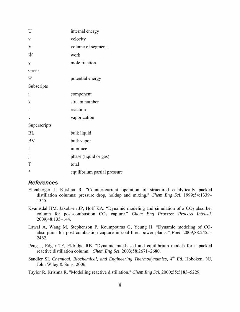
8
U internal energy
v velocity
V volume of segment
work
y mole fraction
Greek
Ψ potential energy
Subscripts
i component
k stream number
r reaction
v vaporization
Superscripts
BL bulk liquid
BV bulk vapor
I interface
j phase (liquid or gas)
T total
* equilibrium partial pressure
References Ellenberger J, Krishna R. "Counter-current operation of structured catalytically packed
distillation columns: pressure drop, holdup and mixing." Chem Eng Sci. 1999;54:1339–1345.
Kvamsdal HM, Jakobsen JP, Hoff KA. “Dynamic modeling and simulation of a CO2 absorber column for post-combustion CO2 capture.” Chem Eng Process: Process Intensif. 2009;48:135–144.
Lawal A, Wang M, Stephenson P, Koumpouras G, Yeung H. “Dynamic modeling of CO2 absorption for post combustion capture in coal-fired power plants.” Fuel. 2009;88:2455–2462.
Peng J, Edgar TF, Eldridge RB. "Dynamic rate-based and equilibrium models for a packed reactive distillation column." Chem Eng Sci. 2003;58:2671–2680.
Sandler SI. Chemical, Biochemical, and Engineering Thermodynamics, 4th Ed. Hoboken, NJ, John Wiley & Sons. 2006.
Taylor R, Krishna R. "Modelling reactive distillation." Chem Eng Sci. 2000;55:5183–5229.

9
Walters MS, Dunia RH, Edgar TF, Rochelle GT. "Two-stage flash for CO2 regeneration: dynamic modeling and pilot plant validation". Presented at GHGT-11, Kyoto, Japan, November 18–22, 2012.
Ziaii S. Dynamic Modeling, Optimization, and Control of Monoethanolamine Scrubbing for CO2 Capture. The University of Texas at Austin. Ph.D. Dissertation. 2012.
1
Thermal Degradation of Activated Tertiary Amine Blends for Carbon Capture from Coal Combustion and Gas Treating
Quarterly Report for October 1 – December 31, 2012
by Omkar Namjoshi
Supported by the Luminant Carbon Management Program
McKetta Department of Chemical Engineering
The University of Texas at Austin
January 31, 2013
Abstract The thermal degradation of activated tertiary amine solvents has been studied this quarter. The thermal degradation of triethanolamine (TEA), dimethylaminoethanol (DMAE), methyldiethanolamine (MDEA), diethylaminoethanol (DEAE), dimethylaminopropanol (DMAP), dimethylaminobutanol (DMAB), ethyldiethanolamine (EDEA), and 2-[2-(Dimethylamino)ethoxy]ethanol (DMAEE) activated by piperazine (PZ) was studied. The thermal degradation of MDEA activated by hexamethylenediamine (HMDA) and 2-(2-aminoethoxy)ethylamine (BAE) was also studied. The solvent composition was as follows for each amine system: 5 m tertiary amine/5 m activator with an initial loading of 0.225 mol CO2/mol alkalinity. Degradation was studied at 135–175 oC. A first-order rate model with respect to parent amine concentration was used to estimate thermal degradation rates.
Tertiary amine pKa does not appear to influence thermal degradation rates of the tertiary amine; however, the structure of the tertiary amine does appear to have a strong effect on thermal degradation. SN2 attack of hydroxyethyl groups is the slowest, followed by ethyl groups and then by methyl groups in PZ-activated tertiary amine solvents. Intermediate secondary amine breakdown products of the tertiary amine can rapidly react with the amine activator and accelerate the loss of the activator if the breakdown product contains a hydroxyethyl functional group.
At 150 oC and with an initial concentration of 5 m tertiary amine/5 m PZ, thermal degradation was quantified for the following amines: TEA (5.81E-4 1/h), MDEA (1.17E-3 1/h), EDEA (7.15E-4 1/h), DMAE (1.50E-3 1/h), DMAP (8.63E-4 1/h), DMAB (8.08E-3 1/h), DMAEE (1.22E-3 1/h). PZ has a higher thermal degradation rate (50–150%) than the tertiary amines in PZ-activated solutions containing DEA, DMAE, MDEA, EDEA, and DEAE, suggesting that reactive intermediate degradation products are responsible for the loss of PZ. However, PZ loss is nearly identical in magnitude to the tertiary amine loss in PZ-activated DMAP and DMAEE, suggesting that the intermediate breakdown product is relatively stable.
HMDA and BAE have thermal degradation rates of about a quarter and a half, respectively, of PZ when used to activate MDEA. HMDA and BAE also have higher rates of thermal

2
degradation than MDEA, suggesting that the reactive intermediates of thermal degradation degrade the activator. PZ-activated DMAB has a loss rate about an order of magnitude greater than other tertiary amines, suggesting that another reaction mechanism is responsible for degradation in addition to SN2 substitution.
Introduction and Motivation
Brief Literature Review Activated tertiary amine solvents find extensive use in removing acid gases from natural gas and synthesis gas sources; they also offer competitive energy performance compared to concentrated PZ when used to capture CO2 from coal-derived flue gas. The work presented in this report will focus on understanding the thermal degradation characteristics of activated-tertiary amine solvents as functions of tertiary amine structure and activator type. Stable tertiary amine solvent blends could serve as drop-in replacements for MDEA/PZ in natural gas or synthesis gas treating applications especially if the acid gas is to be sequestered and used for EOR purposes.
Literature studies suggest that tertiary amines and activated tertiary amines degrade via an SN2 pathway (Namjoshi, 2012). A free nitrogen on either the amine activator or the tertiary amine can attack a protonated tertiary amine. This scheme is presented in Figure 1.
Figure 1: Thermal degradation in tertiary amine solvents is initiated by SN2-type mechanisms where a free amino group attacks a substituent group on a protonated tertiary
amine.
Byproducts of the initial thermal degradation step include a secondary amine and, depending on the attacking species, either a secondary amine, tertiary amine, or quaternary amine. These intermediate breakdown products can be reactive intermediates: tertiary and quaternary amines can undergo SN2 substitution reactions, and secondary amines capable of forming oxazolidinones can react rapidly with either a secondary or primary amine, which includes the parent amine activator used in the tertiary amine blends. An example of the amine-oxazolidinone reaction is presented in Figures 2 and 3; this reaction is generally similar to the amine synthesis reactions presented in the first and second quarter (Rochelle, 2012).
N+
R1
R2
H
R3
N
R4
H
R5
N
R1
R2
HN
+H
R5
R4
R3

3
Figure 2: Scheme showing oxazolidinone formation via primary and secondary amine carbamates.
Figure 3: Scheme showing reaction between a free primary or secondary amine and an oxazolidinone to form substituted polyamines.
Amines Tested Table 1 lists the amines that were tested for this study.
Table 1: List of amines (names, structure, abbreviated names) tested this quarter
Amine Name Abbreviation Structure Role
Piperazine PZ
Activator
Hexamethylenediamine HMDA
Activator
2-(2-Aminoethoxy)ethylamine BAE
Activator
Dimethylaminoethanol DMAE
Tertiary Amine
Dimethylaminopropanol DMAP
Tertiary Amine
Dimethylaminobutanol DMAB
Tertiary Amine
OHN
R
OO-
O
ON R
O- N
R
OOH
+ OH-
NR
OO-
OHO
ON R
NR
OOH
O- + OH
-
O
ONR1
R2
NHR3
N
R3
R2 NH
R1
+ CO2
NH NH
NH2NH2
NH2
ONH2
CH3
NCH3 OH
CH3
NCH3
OH
CH3
NCH3 OH

4
2-[2-(Dimethylamino)ethoxy]ethanol
DMAEE
Tertiary Amine
Diethylaminoethanol DEAE
Tertiary Amine
Methyldiethanolamine MDEA
Tertiary Amine
Ethyldiethanolamine EDEA
Tertiary Amine
Triethanolamine TEA
Tertiary Amine
Experimental Methods Samples were prepared gravimetrically. CO2 was sparged into the solution and measured gravimetrically. Approximately 4 ml of loaded amine solution was placed in 3/8” Swagelok® stainless steel cylinders with a 4.5 ml capacity. The cylinders were sealed and placed in forced convection ovens at set temperatures and removed periodically for analysis. Cation chromatography (Dionex ICS-2100) was used to analyze for parent amine and degradation byproduct; the separation was carried out using a Dionex CS17 column. These methods are described in previous quarterly reports and dissertations (Freeman, 2011) and will not be described in detail here.
All amine solvents were prepared with identical starting concentrations: 5 m tertiary amine/5 m activator with an initial CO2 loading of 0.225 mol CO2/mol alkalinity.
Safety Aspects The existing half-inch Swagelok® stainless steel cylinders previously used for thermal degradation work (including synthesis and nitrosamine studies) have now been retired; 3/8” Swagelok® stainless steel cylinders are exclusively being used. The 3/8” cylinders have given excellent service with no failures over hundreds of analyzed samples. Cylinders will be proactively retired after 10 uses.
CH3
NCH3 O
OH
NOH
CH3
CH3
CH3
NOHOH
N OH
OH
CH3
NOH
OH
OH

5
Results & Analysis
First-Order Rate Models and Arrhenius Temperature Dependency First-order rate models with respect to parent amine concentration were used to estimate thermal degradation rates. These models match the experimental data well and the results from these models can be used to correlate effects of structure and other properties with the rate of degradation. The Arrhenius relationship was used to estimate the activation energy of thermal degradation.
Results Summary Table 2 summarizes the thermal degradation results for the various amines tested. Figures 4 through 8 summarize the data graphically and correlate thermal degradation with structure and pKa.
Table 2: Thermal degradation of various amines tested at initial concentrations of 5 m Activator/5 m tertiary amine at an initial loading of 0.225 mol CO2/mol alkalinity
Tertiary amine
structure
Tert Am. pKa
T
(oC)
Degradation
k1
(hr-1)
Activation
energy
(kJ/mol)
Tertiary Amine/ Activator
Tertiary Amine
PZ Tertiary Amine
Acti-vator
MDEA/HMDA
8.5 150 2.93E-4 7.01E-4
TEA/PZ
7.8 175
150
135
1.16E-2
5.81E-4
1.45E-4
2.37E-2
9.95E-4
1.66E-4
168 189
MDEA/BAE
8.5 150 6.22E-4 1.08E-3
DEAE/PZ
10.0 175
150
7.98E-3
6.56E-4
1.05E-2
9.27E-4
158 153
EDEA/PZ
8.7 150 7.15E-4 1.2E-3
DMAP/PZ
175
150
7.64E-3
8.63E-4
8.91E-3
9.30E-4
138 142
MDEA/PZ
8.5 175 1.03E-2 2.48E-2 137 139
CH3
NOHOH
NOH
OH
OH
CH3
NOHOH
NOH
CH3
CH3
N OH
OH
CH3
CH3
NCH3
OH
CH3
NOHOH

6
150
135
1.17E-3
2.61E-4
2.76E-3
6.33E-4
DMAEE/PZ 150 1.22E-3 1.09E-3
DMAE/PZ
9.4 175
150
135
1.13E-2
1.50E-3
3.23E-4
1.70E-2
2.22E-3
6.16E-4
127 129
DMAB/PZ
150 8.08E-3 5.48E-3
Figure 4: Thermal degradation of 5 m PZ/5 m EDEA at 150 oC with an initial loading of 0.225 mol CO2/mol alkalinity, showing that first-order kinetics can accurately model
thermal degradation.
CH3
NCH3 O
OH
CH3
NCH3 OH
CH3
NCH3 OH
500
800
1100
1400
1700
2000
0 175 350 525 700Par
ent A
min
e C
once
ntr
atio
n,
mm
ol/k
g
Experiment Time, Hours
kEDEA=7.15*10-4 1/h
kPZ=1.2*10-3 1/h

7
Figure 5: Comparison of thermal degradation of tertiary ethanolamines as a function of structure, demonstrating that methyl groups are preferentially attacked over ethyl and hydroxyethyl groups. Conditions: 5 m PZ/5 m tertiary amine, 150 oC, initial loading of
0.225 mol CO2/mol alkalinity
1.E-04
1.E-03
1.E-02
Ter
tiar
y A
min
e D
egra
dat
ion
R
ate,
1/h
Number of Hydroxyethyl Groups
CH3
NCH3 OH
CH3
NOHOH
NOH
OH
OH
N OH
OH
CH3

8
Figure 6: Comparison of thermal degradation of tertiary dimethylamines as a function of structure, demonstrating that DMAB degrades via another mechanism. Conditions: 5 m
PZ/5 m tertiary amine, 150 oC, initial loading of 0.225 mol CO2/mol alkalinity.
Figure 7: Comparison of thermal degradation activation energy of activated tertiary amines as a function of structure, demonstrating that activation energy increases as
degradation rate decreases. Conditions: 5 m PZ/5 m Tertiary Amine, initial loading of 0.225 mol CO2/mol alkalinity.
1.E-04
1.E-03
1.E-02
Ter
tiar
y A
min
e D
egra
dat
ion
Rat
e C
onst
ant,
1/h
Increasing Chain Length
CH3
NCH3 OH
CH3
NCH3
OH
CH3
NCH3 OH
CH3
NCH3 O
OH
1.E-04
1.E-03
1.E-02
1.E-01
Ter
tiar
y A
min
e D
egra
dat
ion
Rat
e C
onst
ant,
1/h
Temperature
175 oC 150 oC 135 oC
CH3
NCH3 OH
CH3
NOHOH
NOH
OH
OH
NOH
CH3
CH3
Ea=127 kJ/mol
Ea=137 kJ/mol
Ea=168 kJ/mol
Ea=158 kJ/mol

9
Figure 8: Comparison of thermal degradation of tertiary amines as a function of pKa, demonstrating that degradation is a strong function of structure and not correlated with
pKa. Conditions: 5 m PZ/5 m tertiary amine, 150 oC, initial loading of 0.225 mol CO2/mol alkalinity.
Role of Structure on Activation Energy and Thermal Degradation Rate Methyl Groups versus Ethyl Groups versus Hydroxyethyl Groups. Tertiary amines with ethyl groups and no methyl groups, such as DEAE and EDEA, have lower thermal degradation rates and appear to have higher activation energies relative to tertiary amines with methyl groups and no ethyl groups, such as DMAE, DMAP, and MDEA. TEA, which only has hydroxyethyl groups, has a significantly higher activation energy of thermal degradation when compared to DMAE, DMAP, and MDEA.
Tertiary amine activators. Both HMDA and BAE had lower rates of degradation compared to PZ when used to activate MDEA. Both HMDA and BAE have higher pKa values than PZ; therefore, tertiary amines activated with either HMDA or BAE will have higher concentrations of activator in the protonated and carbamate forms and a reduced concentration of the protonated tertiary amine relative to MDEA activated by PZ. This might result in the lower rate of thermal degradation as it is initiated by SN2 attack of protonated tertiary amine by a free amine.
Relationship of Thermal Degradation Rates with Tertiary Amine pKa. Activated tertiary amine solvents consisting of a tertiary amine with a high pKa value will have a higher concentration of protonated tertiary amine relative to an activated tertiary amine solvent consisting of a low pKa tertiary amine; in the absence of structural effects, high pKa tertiary amines would degrade more quickly than low pKa tertiary amines. This was not observed to be the case in PZ-activated tertiary amine solvents: EDEA, which has a pKa of 8.7, and DEAE, which has a pKa of 9.9, degrade more slowly than MDEA, which has a pKa of 8.5.
1.E-04
1.E-03
1.E-02T
her
mal
Deg
rad
atio
n R
ate
Con
stan
t
(1/h
)
Increasing pKa ->
NOH
CH3
CH3
CH3
NCH3 OH
N OH
OH
CH3
CH3
NOHOH
NOH
OH
OH
pKa=7.8
pKa=8.5
pKa=8.7
pKa=9.4
pKa=10.0
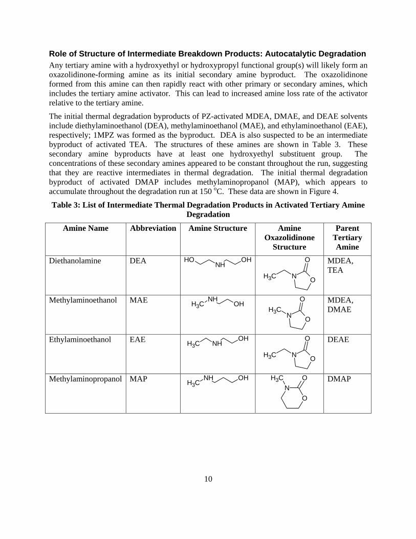
10
Role of Structure of Intermediate Breakdown Products: Autocatalytic Degradation Any tertiary amine with a hydroxyethyl or hydroxypropyl functional group(s) will likely form an oxazolidinone-forming amine as its initial secondary amine byproduct. The oxazolidinone formed from this amine can then rapidly react with other primary or secondary amines, which includes the tertiary amine activator. This can lead to increased amine loss rate of the activator relative to the tertiary amine.
The initial thermal degradation byproducts of PZ-activated MDEA, DMAE, and DEAE solvents include diethylaminoethanol (DEA), methylaminoethanol (MAE), and ethylaminoethanol (EAE), respectively; 1MPZ was formed as the byproduct. DEA is also suspected to be an intermediate byproduct of activated TEA. The structures of these amines are shown in Table 3. These secondary amine byproducts have at least one hydroxyethyl substituent group. The concentrations of these secondary amines appeared to be constant throughout the run, suggesting that they are reactive intermediates in thermal degradation. The initial thermal degradation byproduct of activated DMAP includes methylaminopropanol (MAP), which appears to accumulate throughout the degradation run at 150 oC. These data are shown in Figure 4.
Table 3: List of Intermediate Thermal Degradation Products in Activated Tertiary Amine Degradation
Amine Name Abbreviation Amine Structure Amine Oxazolidinone
Structure
Parent Tertiary Amine
Diethanolamine DEA
MDEA, TEA
Methylaminoethanol MAE
MDEA, DMAE
Ethylaminoethanol EAE
DEAE
Methylaminopropanol MAP
DMAP
NHOHOH O
ONCH3
NHCH3 OH
O
ON
CH3
NHOH
CH3O
ONCH3
NHCH3
OH O
O
N
CH3

11
Figure 4: Plot of normalized (by dilution factor) area of intermediate degradation products seen in PZ-activated DMAP, MDEA, DMAE, and DEAE degradation. MAE, EAE, and
DEA are reactive intermediates whereas MAP is not.
PZ degradation rates are 50–150% greater than the tertiary amine in activated MDEA, DMAE, DEAE, and TEA blends; similar behavior was observed in HMDA- and BAE-activated MDEA. In contrast, the PZ degradation rate is about 10% greater than the tertiary amine degradation rate in the activated DMAP blend. The discrepancy in rates suggests that the oxazolidinone-forming amine intermediate in activated MDEA, DMAE, DEAE, and TEA solvents rapidly reacts with the amine activator. Similar phenomena were observed in the amine synthesis experiments, where it was found that oxazolidinone-forming primary amines with hindered hydroxyethyl groups (e.g., AMP or MIPA) or with hydroxypropyl substituent groups reacted with PZ at 25% the rate of MEA, which has an unhindered hydroxyethyl substituent group (Rochelle, 2011).
Alternate Thermal Degradation Pathways – Tertiary Amine Hydrolysis DMAB activated by PZ was observed to thermally degrade at a rate approximately an order of magnitude greater than other tertiary amines at 150 oC. The rate of PZ degradation is less than DMAB. It is postulated that this behavior is due to the hydrolysis of free DMAB, producing an unstable quaternary amine with a five-membered hetrocyclic backbone. This quaternary amine can, like the protonated DMAB, be attacked by the parent amines present in the solvent. This mechanism is shown in Figure 5.
Figure 5: Hydrolysis of DMAB, forming water and a quaternary amine
Like DMAB, DMAEE could also undergo a hydrolysis step, forming a quaternary amine. However, PZ-activated DMAEE degradation rates were comparable in magnitude to other
0
1000
2000
3000
4000
5000
0 200 400 600 800Nor
mal
ized
Pea
k A
rea
Cou
nts
Experiment Time, Hours
NHCH3 OH
NHCH3
OH
NHOHOH
NHOH
CH3
N
CH3
CH3 OH N+CH3
CH3 + OH-

12
tertiary amines such as DMAP and MDEA, and it is likely that the rates of amine hydrolysis are significantly slower than via a SN2 pathway for DMAEE. Raw chromatography data also suggested that methylaminoethoxyethanol accumulated in degraded samples, which is identical to the behavior observed in PZ-activated DMAP degradation.
In primary diamine degradation it was observed that 1,4-diaminobutane (DAB) degrades about an order of magnitude faster than BAE; these amines have analogous structures to DMAB and DMAEE, respectively. DAB degrades by a ring closing mechanism to form pyrrolidine. The ratio of thermal degradation rates of DAB and BAE is roughly similar to the ratio of thermal degradation rates of DMAB and DMAEE (Namjoshi 2013).
Conclusions 1. At 150 oC and with an initial concentration of 5 m tertiary amine/5 m PZ, thermal
degradation was quantified for the following amines: TEA (5.81E-4 1/h), MDEA (1.17E-3 1/h), EDEA (7.15E-4 1/h), DMAE (1.50E-3 1/h), DMAP (8.63E-4 1/h), DMAB (8.08E-3 1/h), DMAEE (1.22E-3 1/h)
2. PZ has a higher thermal degradation rate (50–150%) than the tertiary amines in PZ-activated solutions containing DEA, DMAE, MDEA, EDEA, and DEAE, suggesting that reactive intermediate degradation products are responsible for the loss of PZ.
3. PZ loss is nearly identical in magnitude to the tertiary amine loss in PZ-activated DMAP and DMAEE, suggesting that the intermediate breakdown product is relatively stable.
4. HMDA and BAE have thermal degradation rates of about a quarter and about a half, respectively, of PZ when used to activate MDEA. HMDA and BAE also have higher rates of thermal degradation than MDEA, suggesting that the reactive intermediates of thermal degradation degrade the activator.
5. PZ-activated DMAB has a loss rate about an order of magnitude greater than other tertiary amines, suggesting that another reaction mechanism is responsible for degradation in addition to SN2 substitution.
6. Tertiary amine pKa does not appear to influence thermal degradation rates of the tertiary amine.
7. The structure of the tertiary amine appears to have a strong effect on thermal degradation. SN2 attack of hydroxyethyl groups is the slowest, followed by ethyl groups and then by methyl groups in PZ-activated tertiary amine solvents.
8. Intermediate secondary amine breakdown products of the tertiary amine can rapidly react with the amine activator and accelerate the loss of the activator if the breakdown product contains a hydroxyethyl functional group.
References Freeman SA. Thermal Degradation and Oxidation of Aqueous Piperazine for Carbon Dioxide
Capture. The University of Texas at Austin. Ph.D. Dissertation. 2011.
Namjoshi O. Thermal Degradation of Activated Tertiary Amine Solvents for Carbon Capture and Gas Treating Applications. The University of Texas at Austin. PhD. Proposal. 2012.
Namjoshi O, Le L, Du Y, Rochelle GT. Thermal degradation of piperazine blends with diamines. Presented at GHGT-11. Kyoto, Japan, November 18-22, 2012.

13
Rochelle GT et al. "CO2 Capture by Aqueous Absorption, Second Quarterly Progress Report 2012." Luminant Carbon Management Program. The University of Texas at Austin. 2012.

1
Oxidation of Amines with High Temperature Cycling
Quarterly Report for October 1 – December 31, 2012
by Alexander K. Voice
Supported by the Luminant Carbon Management Program
McKetta Department of Chemical Engineering
The University of Texas at Austin
January 31, 2013
Abstract Screening of CO2 capture amine solvents for oxidative stability was carried out by cycling the amine to stripper temperatures in the presence of dissolved oxygen (DO). Performance of each amine solvent was assessed using four metrics: amine loss, DO uptake, ammonia production, and total formate production. To cycling systems, the integrated solvent degradation apparatus (ISDA) and high temperature cycling system (HTCS) were used in this evaluation.
Oxidative stability was found to be in the order: 2-amino-2-methyl-1-propanol (AMP) > (PZ) and PZ+2-methyl-piperazine (2MPZ) > methyl-diethanolamine (MDEA) and MDEA+PZ > monoethanolamine (MEA). MEA is the only amine susceptible to oxidation at low temperature; these results provide differentiation among the other oxidatively stable amines.
These four indicators of amine oxidation showed good agreement, with the exception of MDEA. MDEA, MDEA+PZ, and MEA showed similar levels of total formate production and amine loss in the ISDA, however DO uptake in the ISDA and amine loss in the HTCS were both higher for MEA. No ammonia production was observed from MDEA, however formaldehyde and acetaldehyde were observed in the gas phase.
Introduction Low temperature oxidation occurs in the absorber as a result of oxygen in the flue gas. Previous studies have shown that a variety of amines are stable to oxidation at low temperature. These include all tertiary amines, many six-membered ring amines, and some hindered amines (Table 1)

2
Table 1: Summary of amine oxidation screening work at low temperature
Evidence of significant oxidation at absorber
conditions
Ref. Resistant to oxidation at absorber conditions
Ref.
Monoethanolamine [5] All tertiary amines [1]Ethylendiamine [6] Piperazine [13]
1,2-diamino-propane [6] 1-methyl-piperazine [9]Bis-aminoethyl-ether [7] 2-methyl-piperazine [7]
Diethanolamine [5,8] 2-amino-2-methyl-1-propanol [7]Methyl-aminoethanol [8] 3-amino-2-methyl-2-propanol [1]
2-ethoxy-aminoethyl-ether [9] Aminoethyl morpholine [1]3-methylamino-1-propanol [10] 3-amino-propanol [12]
1-amino-2-propanol [12] Potassium β-alaninate [12]aminoethyl-piperazine [7] Potassium α-alaninate [1]
Potassium taurinate [9] Potassium prolinate [11]Potasssium sarcosinate [11]
Potassium glycinate [9]Potassium taurinate [9]
In a real system, the amine is cycled between the low temperature, aerobic environment of the absorber, and the high temperature, anaerobic environment of the stripper. Very little work has studied amine oxidation with representative high temperature cycling. In cycling systems, oxygen dissolves into the solution in the absorber, and reacts in the high temperature zone. In an absorber/stripper system, dissolved oxygen is removed from the solvent when it enters the stripper.
Closmann (2011) conducted high temperature oxidation of MDEA, PZ, and MDEA+PZ in a cycling apparatus up to 125 ºC. The results indicated that the amount of degradation increased when the amine was cycled to higher temperatures, and that PZ was more stable than MDEA to high temperature oxidation. Closmann concluded that the kinetics of oxygen uptake were sufficiently slow to be a function of the high temperature, in other words only part of the dissolved oxygen was consumed with each pass, and the amount depended on the temperature of the system.
The objective of this work is to provide a more complete picture of degradation with high temperature cycling, in particular by testing more amines, at higher temperatures, and by measuring dissolved oxygen uptake.
Experimental Methods
Experimental Methods High temperature oxidation was carried out in two cycling apparatuses. These were the high temperature cycling system (HTCS) and the integrated solvent degradation apparatus (ISDA). The HTCS used air in the oxidative reactor, had an operational pressure limit of 200 psig, and could analyze the gas phase for degradation products. The ISDA used oxygen in the oxidative reactor, had an operational pressure limit of 80 psig, and could analyze for dissolved oxygen.

3
Both apparatuses used a solvent circulation rate of 200 mL/min with a 350 mL hold-up in the oxidative reactor. These apparatuses have been described in greater detail previously (Voice, 2012).
Analytical Methods Amine concentration and total formate were determined using cation and anion chromatography, respectively. Fourier-transform infrared spectroscopy was used for ammonia and aldehyde analysis in the gas phase. A Rosemount Analytical 499ADO was used for dissolved oxygen (DO) analysis in the liquid phase. The kinetics of DO uptake were determined by measuring the concentration of DO before and after the high temperature zone of the reactor. Further details of the analytical methods used in this method are discussed elsewhere.
Cation chromatography (Davis, 2009) Anion chromatography (Sexton, 2008) FTIR (Voice, 2012)
Results Formate production was measured in the ISDA for various amine solutions cycling from 55 to 120 °C. MDEA, MDEA+PZ, and MEA showed similar levels of formate production, whereas PZ and AMP showed resistance to oxidation. Of the solvents studied, AMP offered the most resistance at 120 °C (Figure 1).
Figure 1: Formate production in amine solutions in the ISDA. Cycling from 55 °C to 120 °C at 200 mL/min with 0.4 mM Fe, 0.1 mM Ni, and 0.05 mM Cr. Agitation at 1400
RPM in the oxidative reactor.
0
50
100
150
200
0 50 100 150 200 250
Total Form
ate (mmol/kg)
Exp. Time (hrs)
7 m MDEA
7 m MEA
5 m AMP

4
Dissolved oxygen uptake was measured in the ISDA. Uptake was fastest in 7 m MEA and slowest in AMP (Figure 2). These data agree with data showing relative amine stability in the presence of oxygen both at high and low temperature using other indicators (ammonia production, formate production, and amine loss).
Figure 2: Dissolved oxygen uptake for amine solutions in the ISDA. Conditions: oxidative reactor at 40 °C, 200 mL/min circulation rate, 0.13 L hold-up at high temperature.
0.1
1
Fractional DO Consumption
1/(Reactor T) (1/K)
55 °C 127°C
99 °C
109
121
65
72
78
60 °C
8 m PZEA=56 kJ/mol
7 m MEAEA=60 kJ/mol
4.8 m AMPNo reaction at 130 °C
7 m MDEAEA=49 kJ/mol
74 °C
91

5
Figure 3: Ammonia production and amine loss rates for various amines in the HTCS. Ammonia rates were determined at steady state for each temperature. The temperature of the oxidation reactor is shown for each amine. Circulation at 200 mL/min in the presence
of Fe, Mn, Ni, Cr. Oxidation reactor with air and 1% CO2 (AMP), 0.5% CO2 (PZ, 4/4blend, MEA), or 2% CO2 (MDEA).
Oxidation of amines in the HTCS was estimated at various trim heater temperatures using ammonia production as an indicator of oxidation (Figure 3). Amine loss rates were measured for PZ, AMP, and MDEA over a two-week period. NH3 was a good indicator of oxidation for PZ. AMP has the highest activation energy for oxidation. MDEA did not produce any ammonia, however formaldehyde and acetaldehyde were observed.
Oxidation of 4 m PZ + 4 m 2MPZ (4/4 blend) was a function of the oxidative reactor temperature (Figure 4). A temperature-controlled trim cooler was used with the 4/4 blend to tightly control the oxidative reactor temperature; this was not used with 8 m PZ.
0.01
0.1
1
10Rate (mmol/kg/hr)
1/(Trim heater outlet) (1/K)65 °C 160
7 m MEA, 29‐37 °C (NH3)
8 m PZ, 33‐40 °C(NH3)
4.8 m AMP, 55 °C(NH3)
7 m MDEA, 55 °C (amine)

6
Figure 4: Oxidation of 4 m PZ + 4 m 2MPZ in the HTCS with the oxidation reactor at 40
or 55 °C. Circulation at 200 mL/min with 0.4 mM Fe, 0.1 mM Ni, 0.05 mM Cr, and 0.1 mM Mn. Oxidation reactor with 0.5% CO2 in air.
A summary of amine oxidation screening experiments in the HTCS is shown below in Table 2. Amine loss was difficult to measure precisely due to small changes in concentration and convolution with water concentration. Ammonia production matched amine loss within the error of the measurement for PZ and the 4/4 blend. AMP had significantly greater amine loss than ammonia production.
Table 1: Summary of ammonia and amine loss rates for various amines degraded in the HTCS for two weeks in the presence of air
Solvent Conditions: ox. Rxr. T (°C) / high T (°C), CO2 (%)
Max NH3 rate
Amine loss rate
Lost amine recovered as NH3 at final
(%)
NH3 rate at 120 °C from regression
(ox. Rxr. T.)
High T for 2%
loss/wk (°C)
7 m MEA 30-36 / 120, 0.5 % 4.10 -- -- 3.24 (~40) 75
7 m MDEA 55 / 120, 2 % 0 1.3 ± 0.3 0 1.28 (55) --
8 m PZ 40 / 160, 0.5 % 1.86 1.3 ± 0.5 80 0.51 (35) 119
4 m PZ + 4 m 2MPZ
40 / 150, 0.5 % 1.59 1.5 ± 0.5 50 0.54 (40)
0.80 (55)
115
95
4.8 m AMP 55 / 150, 1 % 1.17 10.7 ± 0.9 16 0.12 (55) 109
Other data for cycling experiments are shown below in Figures 5–8.
0.1
1
NH3 Rate (mmol/kg/hr)
1/(Trim heater outlet) (1/K)
4/4 Blend, Ox. reactor at 55 °C
4/4 Blend, Ox. reactor at 40 °C
65 °C 160 °C
8 m PZ, ox. reactor 33‐39 °C

7
Figure 5: Amine loss and NH3 production for 4.8 m AMP in the HTCS. Cycling from
55 to 150 °C at 200 mL/min with 0.4 mM Fe, 0.1 mM Ni, 0.05 mM Cr, 0.1 mM Mn. Oxidation reactor with 1% CO2 in air.
Figure 6: Amine loss and NH3 production for 8 m PZ and 4 m PZ + 4 m 2MPZ in the
HTCS. Cycling from 40 to 150 °C (4/4blend) or 160 °C (PZ) at 200 mL/min with 0.4 mM Fe, 0.1 mM Ni, 0.05 mM Cr, 0.1 mM Mn.
Oxidation reactor with 0.5 % CO2.
Figure 7: Amine loss and alkalinity loss for 7 m MDEA in the HTCS and ISDA. Cycling from 55 to 120 °C at 200 mL/min with 0.4 mM Fe, 0.1 mM Ni, 0.05 mM Cr, 0.1 mM Mn (HTCS only). Oxidation reactor with 2% CO2 in air
(HTCS) or oxygen (ISDA)
Figure 8: Products formed from oxidation of 7 m MDEA in the HTCS. Cycling from 55 to 120 °C at 200 mL/min with 0.4 mM Fe, 0.1 mM Ni, 0.05 mM Cr, 0.1 mM Mn. Oxidation reactor with 2% CO2 in air (HTCS).
0
500
1000
1500
2000
2500
0 5 10 15
Amount (m
mol/kg)
Exp. Time (hrs)
AMP lossed
NH3 produced
‐110
‐10
90
190
290
390
490
0 5 10 15
Amount (m
mol/kg)
Exp. Time (days)
8 m PZ
4 m PZ + 4 m 2MPZ loss
8 m PZNH3
4 m PZ + 4 m 2MPZ NH3
0
200
400
600
800
1000
1200
0 5 10 15
ISDA MDEA loss5.9 mmol/kg/hr
ISDA alkalinityloss4.4 mmol/kg/hr
HTCS MDEA loss1.3 mmol/kg/hr
HTCS alk.loss
1.1 mmol/kg/hr 0
100
200
300
400
500
600
0 5 10 15
Amount (m
mol/kg)
Exp. Time (days)
Total aldehyde
Formaldehyde
Acetaldehyde
MDEA loss
MAE+DEA
alk loss
Total formate
8
Discussion Prior to this work, oxidation in cycling systems was thought to be caused by the presence of dissolved oxygen, which reacted in the high temperature part of the cycling system. In a real system, this would correspond to the cross exchanger and pipe leading to the top of the stripper prior to flashing off dissolved oxygen.
This work demonstrates that this explanation is too simple in several respects. First, the oxygen uptake measurements and HTCS data show that oxidation continues to increase with greater stripper temperatures beyond the point where all dissolved oxygen has been consumed. Second, the absolute oxidation rates are significantly higher than the rate of oxygen cycling, indicating that either the oxygen stoichiometry (moles oxygen consumed per mole amine degraded) is a function of temperature, or that other oxygen carriers are involved (e.g., oxidized metals, peroxides). Third, the oxidation rate increases with higher oxidative reactor temperatures. If oxidation were only occurring from dissolved oxygen, lower oxidation rates would be expected from higher oxidative reactor temperatures due to lower oxygen solubility. These results show that higher oxidative reactor temperatures act synergistically with high temperature cycling, increasing oxidation either by increasing the concentration of oxygen carriers, or because oxidation occurs both in the high and low temperature parts of the system only when the amine is cycling to high temperature.
Conclusions Conclusions from this work are as follows
All amines found to be stable to oxidation at low temperature oxidized at high temperatures. Amine stability was in the order of AMP > PZ = PZ+2MPZ > MDEA = MDEA+PZ >= MEA.
Dissolved oxygen uptake can be used as an indicator of oxidative stability at high temperature.
Oxidation continued after all dissolved oxygen was consumed; no plateau was observed for high temperature oxidation up to 160 °C.
AMP was the most resistant to oxidation at 120 °C but increased most rapidly at higher temperatures
Ammonia production can be used as an absolute indicator of oxidation for MEA, PZ, and 2MPZ, and as a relative indicator for AMP oxidation.
Oxidized MDEA did not produce any gas phase ammonia; acetaldehyde and formaldehyde were produced.
Oxidation of MDEA with high temperature cycling was first-order in oxygen concentration in the oxidative reactor
Oxidation of 4 m PZ + 4 m 2MPZ increased with higher oxidative reactor temperatures
Future Work A two-week experiment will be performed to determine the amount of MEA converted to ammonia during high temperature oxidation.

9
References Closmann F. Oxidation and thermal degradation of methyldiethanolamine/piperazine in CO2
capture. The University of Texas at Austin. Ph.D. Dissertation. 2011.
Davis, JD. Thermal Degradation of Aqueous Amines Used for Carbon Dioxide Capture. The University of Texas at Austin. Ph.D. Dissertation. 2009.
Sexton AJ. Amine Oxidation in CO2 Capture Processes. The University of Texas at Austin. Ph.D. Dissertation. 2008.
Voice AK, Rochelle GT. “Oxidative degradation of amines with high temperature cycling.” Accepted to Energy Proc. 2013.

1
Aerosol and Volatile Control in CO2 Capture
Quarterly Report for October 1 – December 31, 2012
by Steven Fulk
Supported by the Luminant Carbon Management Program
McKetta Department of Chemical Engineering
The University of Texas at Austin
January 31, 2013
Abstract In this quarter, a concentric-tube particle growth column was designed in more detail. Droplet growth will be measured under varying operating conditions representative of CO2 capture in an amine scrubbing system. The miniature absorber column will have an inner diameter of 1.5 inches with a packed height of up to 6 feet. The gas rate will vary from 25–125 LPM. The solvent rate will vary from 0.05–1.00 GPM corresponding to an L/G range of 6–30 mol/mol under all gas flow rates. A heating jacket along the length of the packed section using externally-circulated oil will maintain isothermal conditions (40 °C) during absorption and provide heat (80 °C) for stripping.
Seed particles will be generated by either salt nuclei from a Brechtel Manufacturing Inc. model 9200 Aerosol Generation System or by injecting vaporized H2SO4 using a syringe pump connected to a heated injection port. Particle count and size will be measured in-situ using a Phase Doppler Particle Analyzer (PDPA). Droplet content will also be measured using in-situ swirl-tubes and inertial impactors connected to an FTIR analyzer. The FTIR will quantify the content and composition of droplets not collected on the upstream gas-particle separators.
Goals for next quarter include continued design and construction of the aerosol growth chamber.
Introduction Volatile emissions are a primary concern for CO2 capture plants using amine scrubbers. Emissions constitute increased economic expense through solvent loss as well as being a source of potentially hazardous environmental pollutants. Compounds found in treated flue gas include contaminants from thermal degradation and oxidation as well as combustion byproducts. Degradation and reaction products have a wide range of toxicity and biodegradation characteristics which potentially represent unacceptable emissions; as a result, recent work has focused on estimating volatile losses and assessing their toxicological impact.
Volatile emissions can be reduced through the use of an absorber column using recycled water as a solvent, called a water wash. Design considerations for water wash systems include liquid distribution methods to adequately wet packing with low liquid rates, and balancing water in the absorber/stripper system by adjusting the total volatile concentration in the wash water. Water

2
wash columns have relatively flat efficiency profiles, meaning the removal efficiency is not a strong function of either the gas or liquid flow rates or the operating temperature.
Emissions with Aerosols Recent pilot plant measurements have shown that normal water wash columns are ineffective at controlling volatile loss of amine and other pollutants due to the presence of aerosols. In 2011, MHI presented pilot test results for both KS-1TM and MEA which showed that emissions were proportional to inlet SO3 concentration (MHI, 2012). Amine levels out of the wash section were 0.4–23.2 ppmv and 0.8–67.5 ppmv for KS-1TM and MEA, respectively, for 0–3 ppmv inlet SO3. Aerosols were visually present at the direct contact cooler (DCC) and wash outlets. At the Maasvlakte pilot plant, TNO and SINTEF jointly tested a 30 wt % MEA CO2 capture unit with a downstream water wash complete with online gas and aerosol phase sampling (TNO, 2012; SINTEF, 2012). Excessive emissions were observed; aerosols, not physical entrainment, were responsible for the increase. Lithium and rubidium carbonate (Li2CO3, Rb2CO3) tracers in the solvent and wash loops verified negligible entrainment. A Brownian demister unit (BDU) was installed downstream of the wash section which reduced emissions to previously simulated levels, indicating the bulk of emissions were contained in the droplet phase. Mean droplet diameters (dDrop) were measured using light extinction coefficients and ranged between 0.76 and 7.88 μm at the BDU inlet and 0.2–1.74 μm at the outlet. The quality of the inlet flue gas and the absolute temperature of the absorber influenced the emission rate. More recently, a baseline study using MEA at the National Carbon Capture Center (NCCC) in Wilsonville, Alabama saw higher amine emissions than expected (NCCC, 2012). The number of absorber beds (2–3), intercoolers (0–2), and inlet SO3 concentration (1.8 and 3.2 ppmv) were varied as part of a parametric test on emission rate. Their work concluded that carry-over was proportional to inlet SO3 and also to the concentration of MEA in the wash water. Emissions were inversely related to absorber temperature. In all studies, aerosols increased emissions roughly 1–2 orders of magnitude.
It is clear from pilot plant observations and emission studies that removing aerosols is a key part of reducing possible releases from amine-based CO2 capture plants. The failure of conventional wash columns and the potential financial impact of particle collectors necessitate fundamental research to identify more practical means of controlling emissions for large scale processes. Understanding interconnectivities of the bulk CO2 removal process operating conditions and aerosol dynamics can provide the necessary insight required to either design or operate a system with the intention of suppressing droplet growth; or conversely, to condition aerosols for easier removal.
Aerosol Column Experiment Designing equipment for particle removal requires proper characterization of the inlet size distribution; however, existing data for droplet sizes out of CO2 absorber columns is limited. The only direct measurement of droplet diameters is the TNO/SINTEF project at the Maasvlakte power plant (TNO, 2012; SINTEF, 2012). In that study, the mean particle diameter at the inlet and exit of the BDU was calculated using light extinction coefficients from in-situ fog analyzers and mass balance data from collected condensate in the BDU catch. Nearly all aerosolized amine was removed in the BDU indicating that the majority of particles were above the cut-diameter (90% removal for < 1 μm) of the filter element. Additional experimental measurement
3
and modeling are required to determine the proper design and placement of mitigation equipment such that cost and impact on the CO2 capture system is minimized.
An aerosol growth model has been utilized to investigate mechanisms of droplet growth for aqueous, amine-laden particles in CO2 absorption columns fitted with downstream wash towers. However, transport processes described therein are complicated and assumptions must be made to allow numerical approximation. The relative length scales of transfer processes for aerosols and bulk absorption differ by several orders of magnitude. Further, transport of various components is thought to occur according to certain limitations, i.e., H2O and PZ are gas-film controlled whereas CO2 is controlled by reaction kinetics; it is unclear if these assumptions hold for a spherical system with fast moving boundary. The stiffness of the current formulation of the differential processes combined with narrow working ranges of correlations used to describe thermodynamics makes simulations of submicron particles intractable. Results from particle simulations may be extrapolated down to the submicron region; however, potential error is likely because of continuum-kinetic length-scale effects and other modeling assumptions. Due to modeling uncertainties, experimental measurement to validate or further refine the aerosol model is warranted.
Column Design A concentric-tube, glass-jacketed column has been designed to measure particle growth exposed to varying gas compositions characteristic of an absorber or water wash. The chamber will contain up to 6 ft of packing inside a 1.5” inner diameter glass-jacketed tube. The column can accommodate random (>315 m2/m3) and structured (500 m2/m3) packing. The packing approximates gas-side mass transfer present in large scale absorber columns. Oil will be circulated in the tubing annulus to maintain isothermal conditions. Aerosols from a La-Mer-Sinclair-type generation system will be injected into a carrier gas (25–125 LPM) introduced at the bottom of the packing. A spray nozzle at the column top will bring in solvent (0.05–1.00 GPM) which will counter-currently contact the aerosol laden gas. CO2 can be removed up to 90% under high L/G conditions. A large L/G will also prevent temperature bulging. The gas phase composition inside the packed section will be controlled by the circulating solvent composition and an upstream gas mixer with mass flow controllers. Figure 1 shows a simplified process flow diagram for the aerosol growth experiment.
Aerosol Generation Aerosols will be generated in a Brechtel Manufacturing Inc. (BMI) model 9200 Aerosol Generation System by atomizing a liquid solution containing latex spheres or dissolved salt delivered by a syringe pump into a high pressure gas stream. Particle count is controlled by the syringe speed. Atomized material is sent to a drying chamber where solvent is vaporized leaving behind only dissolved substance. Use of Polystyrene Latex (PSL) spheres or other dimensionally uniform objects allows creation of mono-disperse particulate. Aqueous aerosols can also be generated; however, controlling the distribution breadth is more difficult.
Aerosols will also be generated by injecting vaporized H2SO4 into the gas stream using a syringe pump. The H2SO4 will recondense in the gas to form small nuclei, similar to those found in FGD scrubbers. The acid delivery system will be a scaled version of the apparatus used to calibrate liquid components on the FTIR system described in Sexton (2008).
Particle concentration will be low enough to avoid coagulation and Brownian collection.

4
Figure 1: Aerosol growth experiment process flow diagram
Aerosol Analysis In-situ measurement of aqueous aerosols is critical. The combination of sampling losses and gas quality changes during sampling and analysis can significantly distort the measured particle distribution. Analysis equipment must be maintained at the temperature of the flue gas; however, many particle counters/sizers have a maximum operating temperature of about 40 °C at 98% non-condensing relative humidity. Most aerosol analyzers are designed for low humidity, ambient particle sampling. Further, internal acceleration of gases during measurement can change the relative humidity leading to particle shrinkage or growth. PSL define this calibration would not capture these effects. Therefore, particle distributions will be measured in-situ by two methods: by interferometry (phase doppler) and size-cut total analysis using FTIR.
PDPA is a differential technique for measuring particle distributions and velocity. Flux of particles through a small, well-defined sample volume in a gas stream eliminates coincidence effects present in integral measurements which rely on reproducing extinction of light using Mie Theory and assuming a particle distribution. A phase doppler-type analyzer will be used to measure the particle distribution before and after the packed section in the aerosol growth column. Viewing windows into the gas ducts and stabilized railing for the transmitter and receiver are all that is required.
A second method for particle analysis will be to size-select aerosols in-situ before total analysis in a hot-gas FTIR system. The particle separators will be sized to take the full gas flow, thereby eliminating isokinetic sampling error. A series of gas-particle separators with different cut diameters will be used in conjunction with an FTIR to produce a cumulative distribution of mass
5
represented as aerosols. The accumulated liquid from captured aerosols will be sampled for composition.
Future Work Goals for next quarter include continued design and initial construction of an aerosol growth chamber. Experiments will be run to validate the aerosol growth model coded into MATLAB®. H2O absorption into salt-core aerosols will represent a baseline modeling and experimental exercise. Generation and growth measurement of H2O/CO2/amine aerosols will be investigated.
References Mitsubishi Heavy Industries (MHI). (August 16, 2011). “Amine Emission Control Technology
of KM CDR ProcessTM.” Presented at the Amine Workshop in Palo Alto, California.
National Carbon Capture Center (NCCC). (July 10, 2012). “National Carbon Capture Center: Post Combustion.” Presented at the 2012 NETL CO2 Capture Technology Meeting.
Netherlands Organization for Applied Scientific Research (TNO). “Emission Reducing Technologies Aerosols.” Presented at UTCCS-1, University of Texas at Austin, January 25, 2012.
Sexton AJ. Amine Oxidation in CO2 Capture Processes. The University of Texas at Austin. Ph.D. Dissertation. 2008.
SINTEF. (January 25, 2012). “Emission Studies at the Maasvlakte CO2 Capture Pilot Plant.” Presented at UTCCS-1, University of Texas at Austin, January 25, 2012.

1
Amine Degradation in Pilot Plants
Quarterly Report for October 1 – December 31, 2012
by Paul Nielsen
Supported by the Luminant Carbon Management Program
McKetta Department of Chemical Engineering
The University of Texas at Austin
January 31, 2013
Abstract In this quarter, a method for detecting formaldehyde and other aldehydes and ketones in degraded solvent was developed. The method consists of reacting 2,4-dinitrophenylhydrazine (DNPH) with degraded solvent to produce an aldehyde-DNPH derivative that can be separated and detected by HPLC with UV. DNPH reacts selectively with aldehydes and ketones, and does not react with alcohols, carboxylic acids, amino acids, amides, or carbamates. Testing previously-collected pilot plant samples, insubstantial amounts of formaldehyde were detected. However, a significant amount of DNPH reacted with the degraded samples, equivalent to 75 mmol/kg of aldehyde in the degraded SRP PZ sample and 130 mmol/kg in the degraded PP2 MEA sample. This indicates the presence of an unidentified significant degradation product that is likely an aldehyde or ketone.
PZ was shown to react with hydrogen peroxide. Total formate accounted for 10% of the total degradation observed. This is an identical ratio to that observed in previous oxidation experiments, indicating that oxidation almost certainly occurs along a radical peroxide pathway. Adding hydrogen peroxide may be an easy way to rapidly simulate oxidation in future experiments.
2.7 mmol/kg of MNPZ was measured at the end of the OE25 batch PZ oxidation experiment. This accounts for 0.1% of the oxidation observed in the experiment.
Introduction Piperazine (PZ) has shown promise as a solvent for carbon dioxide capture, with greater capacity, absorption rate, and thermal and oxidative stability than the baseline monoethanolamine (MEA) solvent. However, PZ degradation has not yet been as thoroughly characterized as MEA, with 25–40% of the mass balance still unknown.
Samples of degraded PZ solvent were collected from the Separations Research Program (SRP) pilot plant at the Pickle Research Campus in Austin, Texas, and from “Pilot Plant 2” (PP2). SRP used a synthetic flue gas mixture simulating a 0.1 MW plant, consisting of air plus 12 kPa CO2, while PP2 used a slipstream of real flue gas from a coal-fired boiler.
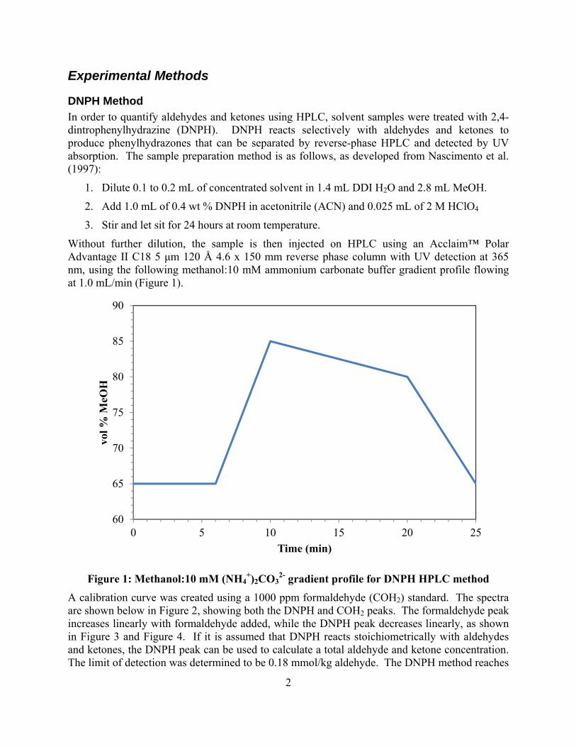
2
Experimental Methods
DNPH Method In order to quantify aldehydes and ketones using HPLC, solvent samples were treated with 2,4-dintrophenylhydrazine (DNPH). DNPH reacts selectively with aldehydes and ketones to produce phenylhydrazones that can be separated by reverse-phase HPLC and detected by UV absorption. The sample preparation method is as follows, as developed from Nascimento et al. (1997):
1. Dilute 0.1 to 0.2 mL of concentrated solvent in 1.4 mL DDI H2O and 2.8 mL MeOH.
2. Add 1.0 mL of 0.4 wt % DNPH in acetonitrile (ACN) and 0.025 mL of 2 M HClO4
3. Stir and let sit for 24 hours at room temperature.
Without further dilution, the sample is then injected on HPLC using an Acclaim™ Polar Advantage II C18 5 μm 120 Å 4.6 x 150 mm reverse phase column with UV detection at 365 nm, using the following methanol:10 mM ammonium carbonate buffer gradient profile flowing at 1.0 mL/min (Figure 1).
Figure 1: Methanol:10 mM (NH4+)2CO3
2- gradient profile for DNPH HPLC method
A calibration curve was created using a 1000 ppm formaldehyde (COH2) standard. The spectra are shown below in Figure 2, showing both the DNPH and COH2 peaks. The formaldehyde peak increases linearly with formaldehyde added, while the DNPH peak decreases linearly, as shown in Figure 3 and Figure 4. If it is assumed that DNPH reacts stoichiometrically with aldehydes and ketones, the DNPH peak can be used to calculate a total aldehyde and ketone concentration. The limit of detection was determined to be 0.18 mmol/kg aldehyde. The DNPH method reaches
60
65
70
75
80
85
90
0 5 10 15 20 25
vol %
MeO
H
Time (min)

3
saturation limit of 3.7 mmol/kg of aldehyde in the derivatized sample being injected in HPLC, above which the DNPH is fully reacted.
Figure 2: DNPH + 0 to 700 μL 1000 ppm COH2 standard HPLC spectra
0
200
400
600
800
1000
1200
1400
8 9 10 11 12 13 14
mA
U
min
0 uL
4 uL
8 uL
20 uL
40 uL
80 uL
200 uL
400 uL
700 uL
DNPH9.2 min
COH212.7 min

4
Figure 3: COH2 calibration curve (peak at 12.7 minutes)
Figure 4: DNPH total aldehydes and ketones calibration curve (peak at 9.2 minutes)
y = 0.008x - 0.0281R² = 0.9987
0
0.5
1
1.5
2
2.5
3
3.5
4
4.5
5
0 100 200 300 400 500
mm
ol/k
g fo
rmal
deh
yde
mAU*min
Saturated
y = -0.0108x + 3.7326R² = 0.9982
0
0.5
1
1.5
2
2.5
3
3.5
4
4.5
5
0 50 100 150 200 250 300 350 400
mm
ol/k
g fo
rmal
deh
yde
mAU*min
Saturated
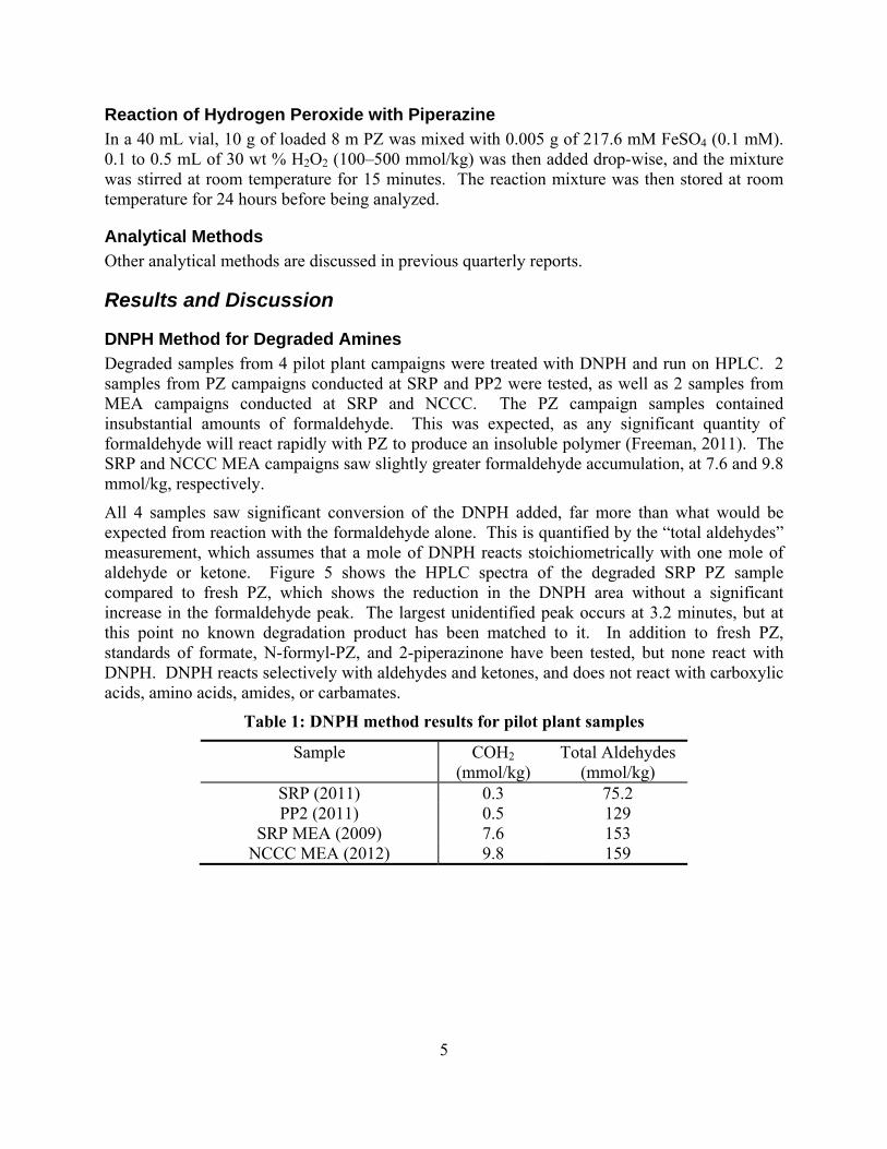
5
Reaction of Hydrogen Peroxide with Piperazine In a 40 mL vial, 10 g of loaded 8 m PZ was mixed with 0.005 g of 217.6 mM FeSO4 (0.1 mM). 0.1 to 0.5 mL of 30 wt % H2O2 (100–500 mmol/kg) was then added drop-wise, and the mixture was stirred at room temperature for 15 minutes. The reaction mixture was then stored at room temperature for 24 hours before being analyzed.
Analytical Methods Other analytical methods are discussed in previous quarterly reports.
Results and Discussion
DNPH Method for Degraded Amines Degraded samples from 4 pilot plant campaigns were treated with DNPH and run on HPLC. 2 samples from PZ campaigns conducted at SRP and PP2 were tested, as well as 2 samples from MEA campaigns conducted at SRP and NCCC. The PZ campaign samples contained insubstantial amounts of formaldehyde. This was expected, as any significant quantity of formaldehyde will react rapidly with PZ to produce an insoluble polymer (Freeman, 2011). The SRP and NCCC MEA campaigns saw slightly greater formaldehyde accumulation, at 7.6 and 9.8 mmol/kg, respectively.
All 4 samples saw significant conversion of the DNPH added, far more than what would be expected from reaction with the formaldehyde alone. This is quantified by the “total aldehydes” measurement, which assumes that a mole of DNPH reacts stoichiometrically with one mole of aldehyde or ketone. Figure 5 shows the HPLC spectra of the degraded SRP PZ sample compared to fresh PZ, which shows the reduction in the DNPH area without a significant increase in the formaldehyde peak. The largest unidentified peak occurs at 3.2 minutes, but at this point no known degradation product has been matched to it. In addition to fresh PZ, standards of formate, N-formyl-PZ, and 2-piperazinone have been tested, but none react with DNPH. DNPH reacts selectively with aldehydes and ketones, and does not react with carboxylic acids, amino acids, amides, or carbamates.
Table 1: DNPH method results for pilot plant samples
Sample COH2 (mmol/kg)
Total Aldehydes (mmol/kg)
SRP (2011) 0.3 75.2 PP2 (2011) 0.5 129
SRP MEA (2009) 7.6 153 NCCC MEA (2012) 9.8 159
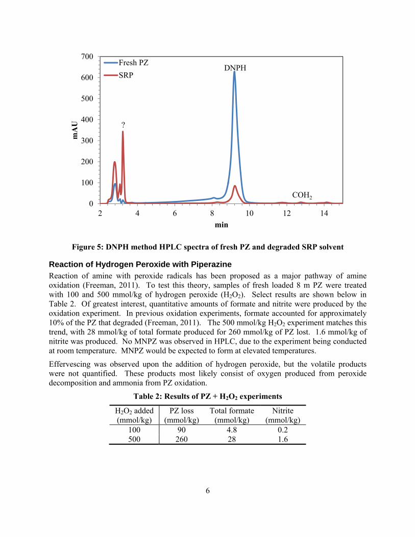
6
Figure 5: DNPH method HPLC spectra of fresh PZ and degraded SRP solvent
Reaction of Hydrogen Peroxide with Piperazine Reaction of amine with peroxide radicals has been proposed as a major pathway of amine oxidation (Freeman, 2011). To test this theory, samples of fresh loaded 8 m PZ were treated with 100 and 500 mmol/kg of hydrogen peroxide (H2O2). Select results are shown below in Table 2. Of greatest interest, quantitative amounts of formate and nitrite were produced by the oxidation experiment. In previous oxidation experiments, formate accounted for approximately 10% of the PZ that degraded (Freeman, 2011). The 500 mmol/kg H2O2 experiment matches this trend, with 28 mmol/kg of total formate produced for 260 mmol/kg of PZ lost. 1.6 mmol/kg of nitrite was produced. No MNPZ was observed in HPLC, due to the experiment being conducted at room temperature. MNPZ would be expected to form at elevated temperatures.
Effervescing was observed upon the addition of hydrogen peroxide, but the volatile products were not quantified. These products most likely consist of oxygen produced from peroxide decomposition and ammonia from PZ oxidation.
Table 2: Results of PZ + H2O2 experiments
H2O2 added (mmol/kg)
PZ loss (mmol/kg)
Total formate (mmol/kg)
Nitrite (mmol/kg)
100 90 4.8 0.2 500 260 28 1.6
0
100
200
300
400
500
600
700
2 4 6 8 10 12 14
mA
U
min
Fresh PZ
SRPDNPH
COH2
?

7
OE25 Nitrosamine Formation OE25 was an oxidation experiment conducted by Freeman in the LGF apparatus. It simulated an extremely high PZ oxidation rate, at 70 °C and with 4 mM Cu2+, and the final sample was thoroughly analyzed for degradation product characterization. However, at the time of the experiment the samples were not tested for MNPZ accumulation. A select number of samples were tested for MNPZ this previous quarter. The results are shown below in Figure 6, along with nitrite accumulation results measured at the time of the experiment 2 years ago. By the end of the experiment, 2.7 mmol/kg of MNPZ had accumulated. This represents approximately 0.1% of the 3200 mmol/kg of PZ that degraded.
The samples had been stored for approximately 2 years before being tested for MNPZ. Extrapolating from kinetic data collected at higher temperatures, the thermal degradation rate of MNPZ at room temperature should be on the order of 2.3*10-10 s-1 (Fine et al., 2012). At this rate, 1–2% of the MNPZ would have degraded before measurement.
Figure 6: MNPZ and nitrite accumulation during OE25 (LGF, 8 m PZ, α = 0.3, 70 °C, 94 kPa O2, 100 mL/min, 4 mM Cu2+, 14 days (Freeman, 2011)) (nitrite analysis from Freeman,
2011)
Conclusions Formaldehyde was not a significant degradation product for any of the pilot plant campaigns studied.
Significant degradation has occurred in the pilot plant samples in the form of currently unquantified aldehydes or ketones, as measured by the reaction of DNPH with the degraded PZ pilot plant samples.
0
0.5
1
1.5
2
2.5
3
0 50 100 150 200 250 300 350
mm
ol/k
g
Hrs
MNPZ
Nitrite

8
Hydrogen peroxide can be used to rapidly oxidize PZ. The degradation products observed from peroxide oxidation are similar to those observed in other experiments, including 10% of degradation in the form of total formate.
2.7 mmol/kg of MNPZ accumulated during OE25 at 70 °C, showing that MNPZ can form from the oxidation of PZ to nitrite even without the addition of nitrite or cycling to higher temperatures. This represents 0.1% of total PZ oxidation.
Future Work
Degradation and Reclaimer Modeling and Literature Review The University of Texas at Austin, URS, and Trimeric have been awarded a proposal to conduct a rigorous literature review of reclaimer sludge disposal by IEAGHG. In support of this, I will conduct a literature review of all published data on amine degradation as well as compiling all useful unpublished degradation data from our lab. Using kinetic and thermodynamic data, complete degradation models for MEA and PZ will be created to estimate amine loss and heat stable salt accumulation in a full-scale CO2 post-combustion capture facility. The models will be created in Excel and will model the process in steady state. If there is sufficient time, dynamic models will be created in MATLAB, to simulate non-continuous reclaimer operation. The models will have the form of Figure 7, which divides the amine scrubbing process into 6 different degradation reactors with 2 additional separation units.
In the absorber packing, oxidation will be modeled using temperature and loading profiles exported from Aspen Plus®, and will be assumed to be plug flow. Oxygen content will be assumed to be constant at the saturation limit (mass transfer limitations will be ignored). The effect of intercooling on oxidation will be determined.
The absorber sump oxidation reactor will be modeled as a continuously-stirred tank reactor (CSTR), with the inlet rich solvent entering saturated with oxygen.
A “heated oxidation” reactor will be included in the model, to estimate plug flow oxidation of the rich amine at high temperatures in the cross exchanger and piping before the stripper.
Any remaining oxygen will be assumed to flash off upon entering the stripper. Loading and temperature profiles will be exported from Aspen Plus® to model thermal degradation in the stripper packing in plug flow conditions. Additional thermal degradation will be modeled in the stripper sump at lean solvent conditions as a CSTR. Alternative stripper configurations, such as 2-stage flash and cold-rich bypass, will be modeled.
The thermal reclaimer will take a slip-stream of lean solvent and heat it to separate the amine as a vapor from a sludge containing nonvolatile degradation products including heat stable salts. If a better VLE model cannot be developed, it will be assumed that the sludge will contain 1 mole of amine per mole of degradation product removed. The flow rate of the reclaimer feed will be set to maintain a steady state in the system, removing all degradation products formed in a single pass of solvent, including additional degradation in the reclaimer.
The recently-developed MNPZ model will be included to determine the expected steady-state values of MNPZ in the solvent and reclaimer sludge for the PZ degradation model.
Some volatile amine will be lost from the solvent in both the absorber and stripper. Amine lost in the absorber overhead will be captured by a water wash, which will be assumed to reduce

9
amine concentration in the flue gas to 1 ppm. The captured amine will either be returned to the lean solvent or purged. Volatile amine, water, and degradation products in the stripper overhead will be separated by the CO2 compressor and returned to the lean solvent. Potential volatile reclaiming processes will be studied to remove volatile degradation products which would otherwise accumulate in the system.
Aerosols will be ignored.
Based on the amount of amine loss to degradation, a solvent makeup rate and cost will be calculated. The cost of treating the reclaimer sludge will be estimated. Multiple strategies for sludge treatment will be studied, including incineration, bio-treatment, and novel process concepts.
Figure 7: Degradation Model
Table 3: Selected recent group degradation publications
Type of Oxidation Paper/Dissertation Oxidation in absorber Sexton, 2008 (MEA); Freeman, 2011 (PZ)
Heated oxidation/cycling Closmann, 2011; Voice et al., 2012 (MEA, PZ, MDEA/PZ) Thermal degradation Davis, 2009 (MEA); Freeman, 2011 (PZ)
Nitrosation Fine et al., 2012
Other Future Work Work is ongoing to determine the source of the “total aldehydes” observed by the DNPH method in the degraded pilot plant samples. Other standards of known and suspected degradation products still need to be tested to determine whether any react with DNPH. The HPLC method will be optimized to better separate the unidentified peaks observed early in the methanol-buffer gradient. This will ultimately help to close the PZ oxidation balance gap.
10
Pilot plant samples will be analyzed from a PZ campaign conducted at Tarong in Australia by CSIRO and from MEA campaigns conducted in Europe by OCTAVIUS.
Safety DNPH is a very dangerous substance. In pure form, it is a flammable solid, and even the 0.4 wt % standard is diluted in acetonitrile, which is also flammable. Skin contact causes redness, itching, and pain, and ingestion can cause cyanosis. It is also potentially carcinogenic. For safety purposes, the diluted DNPH is stored in the “flammables” cabinet, and all work with it is done in a fume hood with safety glasses, gloves, and a lab coat.
References Closmann F. Oxidation and Thermal Degradation of Methyldiethanolamine/Piperazine in CO2
Capture. The University of Texas at Austin. Ph.D. Dissertation. 2011.
Davis JD. Thermal Degradation of Aqueous Amines Used for Carbon Dioxide Capture. The University of Texas at Austin. Ph.D. Dissertation. 2009.
Fine NA, Goldman MJ, Nielsen PT, Rochelle GT. "Managing n-nitrosopiperazine and dinitrosopiperazine." Presented at GHGT-11, Kyoto, Japan November 18-22, 2012.
Freeman SA. Thermal Degradation and Oxidation of Aqueous Piperazine for Carbon Dioxide Capture. The University of Texas at Austin. Ph.D. Dissertation. 2011.
Nascimento RF, Marques JC, Lima Neto BS, De Keukeleire D, Franco DW. "Qualitative and quantitative high-performance liquid chromatographic analysis of aldehydes in Brazilian sugar cane spirits and other distilled alcoholic beverages." J Chromatog A. 1997;782(1):13–23.
Sexton AJ. Amine Oxidation in CO2 Capture Processes. The University of Texas at Austin. Ph.D. Dissertation. 2008.
Voice AK, Closmann F, Rochelle GT. "Oxidative degradation of amines with high-temperature cycling." Presented at GHGT-11, Kyoto, Japan November 18-22, 2012.

1
Quantification of Nitrosamines in Amine Scrubbing
Quarterly Report for October 1 – December 31, 2012
by Nathan Fine
Supported by the Luminant Carbon Management Program
McKetta Department of Chemical Engineering
The University of Texas at Austin
January 31, 2013
Abstract This quarter, a group analysis method was developed for the quantification of nitrosamines in amine scrubbing conditions. The total nitrosamine (TONO) method uses hydrobromic acid to selectively produce nitric oxide (NO) gas from a nitrosamine. The NO is purged from the reactor and enters a chemiluminescent NOx analyzer, which produces a voltage proportional to the NO concentration. The area under the voltage-time curve is integrated and then calibrated with the total nitrosamine concentration. The calibration is linear across three orders of magnitude with a limit of quantification (LOQ) of 0.1 ppm nitrosamine in the amine sample. The LOQ can be easily decreased to 1 ppb by using a more sensitive NOx analyzer.
The Necessity for the Total Nitrosamine Method Nitrosamines as a family are carcinogenic degradation products that can be formed during CO2 scrubbing with amines. Previously, nitrosamines with known standards have been quantified using an HPLC method with UV absorbance. However, many other degradation products will also absorb UV at the same wavelength, making separation difficult. Furthermore, many nitrosamines in amine capture have not been identified and therefore cannot be quantified using the HPLC. Finally, many pertinent nitrosamines have been identified but do not have standards. Since nitrosamines absorb UV with different efficiencies, it is impossible to quantify these nitrosamines using the HPLC method. The TONO method is group-specific to nitrosamines, so it can quantify nitrosamines in heavily degraded amine solutions. The TONO method is also quantitatively equivalent across all nitrosamines, so it can be used in tandem with the HPLC for calibration purposes.
Total Nitrosamine Method Standard Operating Procedure
A diluted amine sample with nitrosamines is injected into a reagent of hydrobromic acid in acetic acid (AcOh) and ethyl acetate (EtAc). The hydrobromic acid denitrosates the protonated nitrosamine, forming NO as shown in Figure 1 (Biggs & Williams, 1975; Ding, Lee, & Eatough, 1998).

2
N
R
R H+ ON
H
N+
N O
R
RH+ BrH
Figure 1: NO Evolution from Nitrosamine in the Presence of Hydrobromic Acid
Nitrogen gas (N2) at 0.8 SLPM and 20 psig flows through a frit into a 1 in. OD glass reactor to sparge the NO (Figures 2 & 3). The reactor is filled with glass beads to provide surface area for the mass transfer of the NO into the gas phase. The diluted NO then travels to a condenser where the gas is cooled using ice water to approximately 10 °C. The cooling knocks out the majority of the EtAc that is stripped along with the NO so that the gas is unsaturated at room temperature. The gas then passes an atmospheric bypass where a small slipstream is allowed to vent. The remaining gas is at atmospheric pressure and is pulled through a Model 14 B/E Thermoelectric Chemiluminescent NOx Analyzer using a vacuum pump.
In the NOx analyzer, the NO reacts with ozone to produce electronically excited nitrogen dioxide (NO2). The NO2 returns to its ground state and gives off a photon at a specific wavelength. The photon hits a photomultiplier where it is converted into a voltage. The voltage is then read using Picolog to give the transient concentration of NO. The voltage-time curve is integrated and calibrated against the concentration of the nitrosamine added. Unknown concentrations of nitrosamines can then be quantified using the voltage integration and the calibration. The NOx analyzer was set to a nominal 5 ppm range but was not calibrated with a standard NO gas. The detection limit should be easily improved by a factor of 100 by using a NOx analyzer capable of ppb NOx level analysis. All tubing leading into the NOx analyzer is Teflon to prevent reaction with NO.
Figure 2: Process Flow Diagram for Total Nitrosamine Apparatus (Not Drawn to Scale)
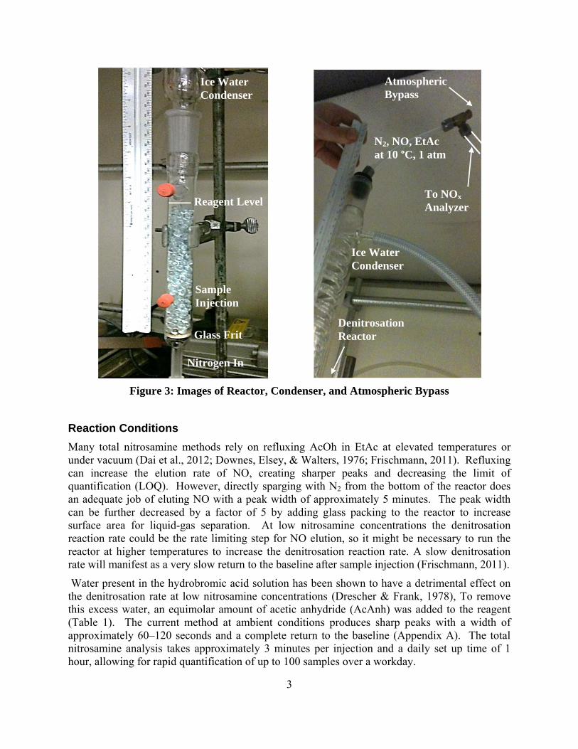
3
Figure 3: Images of Reactor, Condenser, and Atmospheric Bypass
Reaction Conditions
Many total nitrosamine methods rely on refluxing AcOh in EtAc at elevated temperatures or under vacuum (Dai et al., 2012; Downes, Elsey, & Walters, 1976; Frischmann, 2011). Refluxing can increase the elution rate of NO, creating sharper peaks and decreasing the limit of quantification (LOQ). However, directly sparging with N2 from the bottom of the reactor does an adequate job of eluting NO with a peak width of approximately 5 minutes. The peak width can be further decreased by a factor of 5 by adding glass packing to the reactor to increase surface area for liquid-gas separation. At low nitrosamine concentrations the denitrosation reaction rate could be the rate limiting step for NO elution, so it might be necessary to run the reactor at higher temperatures to increase the denitrosation reaction rate. A slow denitrosation rate will manifest as a very slow return to the baseline after sample injection (Frischmann, 2011).
Water present in the hydrobromic acid solution has been shown to have a detrimental effect on the denitrosation rate at low nitrosamine concentrations (Drescher & Frank, 1978), To remove this excess water, an equimolar amount of acetic anhydride (AcAnh) was added to the reagent (Table 1). The current method at ambient conditions produces sharp peaks with a width of approximately 60–120 seconds and a complete return to the baseline (Appendix A). The total nitrosamine analysis takes approximately 3 minutes per injection and a daily set up time of 1 hour, allowing for rapid quantification of up to 100 samples over a workday.
Reagent Level
Sample Injection
Glass Frit
Nitrogen In
Ice Water Condenser
Ice Water Condenser
N2, NO, EtAc at 10 °C, 1 atm
Atmospheric Bypass
To NOx Analyzer
Denitrosation Reactor

4
Table 1: Reactor Conditions for Denitrosation and NO Sparging
Condition Purity Amount
Temperature - 21 °C
Pressure - 14.7 psig
Nitrogen 99.99% 0.8 SLPM
Ethyl Acetate 98% 12 mL
Acetic Acid 99.85% 2 mL
HBr 48% in water 0.4 mL
Acetic Anhydride 99% 0.6 mL
Sample Conditioning
The TONO method can be used to analyze nitrosamine concentration in amine solutions after sample conditioning to dilute the nitrosamine, inhibit artifactual denitrosation, and remove the water. First, the sample needs to be diluted to a nitrosamine concentration of 100 μmol/kg or around 10 ppm. Choosing the correct diluent is non-trivial since unknown nitrosamines will have different solubility limits. Furthermore, diluents similar to water might also inhibit denitrosation in the glass reactor. Acetone has proved to be a good diluent for MNPZ, DNPZ, and NDELA standards. Since acetone is very volatile, it is important to prepare the dilutions in capped vials using a syringe. Diluents can easily be tested for solubility limits by diluting to different concentrations and comparing the slopes of the calibration curves. If the slope of the more dilute sample is steeper, then there is a solubility limit at the dilution level. After dilution, the sample must be scavenged of its water to improve denitrosation rates. A stoichiometric amount of AcAnh is added to the sample to completely react with the water, forming AcOh. The sample is then mixed and allowed to sit for at least 30 minutes before injection.
TONO Method Calibration
Standards of MNPZ, DNPZ, NDELA, and NO2- were diluted in water and then conditioned
following the above method with ethyl acetate as the diluent. Diluted samples between 10 μL and 100 μL were weighed and then injected into the reagent. The resulting curves were integrated and then calibrated against the known moles of nitrosamine in the injected samples. The calibration curves were linear over 1 order of magnitude with R2 values above 0.99 for every case except one (Appendix B). The slopes were then arbitrarily normalized to the slope of MNPZ to give the relative analytical selectivity for each nitrosamine. Since the method is equivalent for each nitrosamine, the slopes should be statistically equivalent (Drescher & Frank, 1978; Kulshrestha, McKinstry, Fernandez, Feelisch, & Mitch, 2010). MNPZ and DNPZ had equivalent slopes when accounting for the second nitrosamine on DNPZ. NDELA had a slightly lower slope, but the NDELA standard was very old which could account for the difference. Nitrite had a very different slope, which is most likely due to solubility issues. After waiting for over an hour, the conditioned nitrite sample still contained two liquid phases.

5
Table 2: Comparison of Calibration Slopes
Nitrosamine MNPZ NDELA DNPZ NO2-
Slope (V∙s/nmol) 1.93 1.7 1.02 2.9
Normalized to MNPZ 1.00 1.14 0.95* 0.67
Determination of TONO Detection Limit
A sample of DNPZ in water was dehydrated and diluted to 182 μmol/kg in acetone following the sample conditioning procedure. The sample was then diluted again to 1.7 μmol/kg in acetone to test the LOQ of the current method. Two injections of the concentrated sample at 30 μL and 70 μL and two injections of the dilute sample at 200 μL and 600 μL were calibrated. (Appendix C). The calibration was linear across all samples with an R2 of 0.9996. When taking into account the dilution factor, this represents three orders of magnitude of linearity. The 200 μL injection yielded a peak approximately ten times the noise level. Extrapolating to three times the noise level gives an LOQ of approximately 0.2 nmol. A 2000 μL injection of an amine sample diluted a factor of 10 containing a nitrosamine with a MW of 100 g/mole would have a sample detection limit of approximately 0.1 ppm. The noise using the current NOx analyzer is approximately 100 times greater than it should be due to a malfunctioning refrigeration unit around the photomultiplier. A more sensitive instrument would theoretically have a detection limit of 1 ppb, which is similar to detection limits reported in literature (Ding et al., 1998; Kulshrestha et al., 2010; Pignatelli et al., 1987).
Preliminary Total Nitrosamine Results The TONO method was used to calibrate the HPLC for the amino-ethylpiperazine nitrosamine (N-AEP). The previous HPLC method used the MNPZ calibration on a mole basis to quantify N-AEP. Using this calibration the overall yield of nitrosation was 80%, with no other products found. A sample from the N-AEP formation experiment was conditioned using ethyl acetate and run through the TONO apparatus with varying injection amounts. The calibration was linear with an R2 of 0.996 (Appendix B); the concentration in the sample was determined by varying the calibration slope to match the calibration slope of MNPZ. Using the TONO method, the overall yield to N-AEP from nitrite was 96%. Thus, the primary amine on AEP did not scavenge any of the nitrite as previously hypothesized. The HPLC method can now be calibrated for N-AEP using the concentration determined from the TONO method.
Safety The MSDSs were read and understood for all chemicals used in the total nitrosamine experiment. AcOH and HBr were stored in the acid cabinet; EtAc and AcAnh were stored in the flammable chemical cabinet. EtAc and AcOH are both volatile and were only used in the hood. The handling of concentrated nitrosamine standards was minimized by using diluted stock solutions. The NOx analyzer outlet gas was vented into the hood.

6
Conclusions A total nitrosamine method using denitrosation of the nitrosamine with HBr was
developed. Gas sparging through the bottom of the reactor and adding glass beads decreased peak
width. Adding acetic anhydride to the denitrosating agent scavenges the water from HBr and
eliminates baseline drift. Total peak width is less than 2 minutes, allowing for rapid quantification. The diluent for samples must be carefully selected to dilute across all nitrosamines in the
sample. Acetic anhydride should be added to the samples before analysis to scavenge any water. The method is quantitative across the three nitrosamine standards tested. The calibration curve is linear through 3 orders of magnitude and passes through zero. The detection limit is around 0.1 ppm but could improve to 1 ppb with a more sensitive
analyzer. N-AEP was calibrated using the TONO The yield of N-AEP formation from nitrite is unity; the primary amine did not scavenge
any nitrite.
Updated Scope of Dissertation NO2 absorption into sulfite solutions NO2 absorption into amine solutions Nitrite formation through amine oxidation Nitrosamine formation under absorber and stripper conditions Nitrosamine thermal decomposition under stripper conditions Nitrosamine volatility under thermal reclaimer conditions Nitrosamine thermal decomposition under reclaimer liquid-phase conditions Nitrosamine UV decomposition under reclaimer gas-phase conditions Nitrosamine concentrations under cycling conditions
References Biggs, I., & Williams, D. "Kinetics and mechanism of the Fischer–Hepp rearrangement and
denitrosation. Part V. The mechanism of denitrosation." J. Chem. Soc., Perkin Trans. 2. 1975; 2141: 107–111.
Dai, N., Shah, A. D., Hu, L., Plewa, M. J., Mckague, B., & Mitch, W. A. "Measurement of Nitrosamine and Nitramine Formation from NOx Reactions with Amines during Amine-Based Carbon Dioxide Capture for Postcombustion Carbon Sequestration." Environmental Science and Technology. 2012; 46: 9793–9801.
Ding, Y., Lee, M., & Eatough, D. "The determination of total nitrite and N-nitroso compounds in atmospheric samples." International journal of Environmental Analytical Chemistry. 1998; 69(3): 243–255.
Downes, M. J., Elsey, T. S., & Walters, C. L. "Determination of a Non-volatile Nitrosamine by Using Denitrosation and a Chemiluminescence Analyser." Analyst. 1976; 101: 742–748.

7
Drescher, G. S., & Frank, C. W. "Estimation of Extractable N-Nitroso Compounds at the Parts- per- Billion Level." Analytical Chemistry. 1978; 50(14): 2118–2121.
Frischmann, M. "Plausibility of Total and Individual Nitrosamine Measurements and Improvements" IEAGHG Seminar, 2011
Kulshrestha, P., McKinstry, K. C., Fernandez, B. O., Feelisch, M., & Mitch, W. "Application of an optimized total N-nitrosamine (TONO) assay to pools: placing N-nitrosodimethylamine (NDMA) determinations into perspective." Environmental Science & Technology. 2010; 44(9): 3369–3375.
Pignatelli, B., Richard, I., Bourgade, M. C., & Bartsch, H. "Improved group determination of total N-nitroso compounds in human gastric juice by chemical denitrosation and thermal energy analysis." The Analyst. 1987; 112(7): 945–949.

8
Appendix A. Representative peaks of NO elution
Diluted in ethyl acetate, acetic anhydride used to scavenge water
0.0
0.5
1.0
1.5
2.0
0 10 20 30 40 50 60 70
Adjusted Signal
(Volts)
Time (minutes)
0.0
0.2
0.4
0.6
0.8
1.0
18 20 22 24 26 28 30 32
Adjusted Signal
(Volts)
Time (minutes)
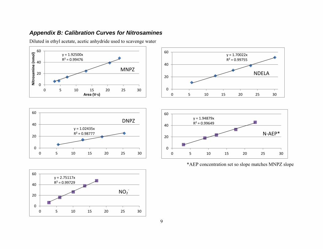
9
Appendix B: Calibration Curves for Nitrosamines
Diluted in ethyl acetate, acetic anhydride used to scavenge water
*AEP concentration set so slope matches MNPZ slope
y = 1.92500xR² = 0.99476
0
20
40
60
0 5 10 15 20 25 30
Nitrosamine (nmol)
Area (V∙s)
MNPZ
y = 1.70022xR² = 0.99755
0
20
40
60
0 5 10 15 20 25 30
y = 1.02435xR² = 0.98777
0
20
40
60
0 5 10 15 20 25 30
y = 1.94879xR² = 0.99649
0
20
40
60
0 5 10 15 20 25 30
y = 2.75117xR² = 0.99729
0
20
40
60
0 5 10 15 20 25 30
NDELA
DNPZ
N‐AEP*
NO2‐

10
Appendix C: Limit of Quantification
Diluted in acetone, acetic anhydride used to scavenge water
y = 0.6214xR² = 0.9997
0
3
6
9
12
0 5 10 15 20
DNPZ (nmol)
Area (V∙s)
‐0.010
0.040
0.090
0.140
27720 27760 27800 27840 27880
Signal adjusted
(Volts)
Time (seconds)

Kinetics of N-nitrosopiperazine formation from nitrite and
piperazine in CO2 capture
Journal: Environmental Science & Technology
Manuscript ID: es-2012-04640f.R1
Manuscript Type: Article
Date Submitted by the Author: n/a
Complete List of Authors: Goldman, Mark; University of Texas at Austin, Department of Chemical Engineering, C0400 Fine, Nathan; University of Texas at Austin, Department of Chemical Engineering, C0400 Rochelle, Gary; University of Texas, Chemical Engineering
ACS Paragon Plus Environment
Environmental Science & Technology

Page 1 of 14
ACS Paragon Plus Environment
Environmental Science & Technology
123456789101112131415161718192021222324252627282930313233343536373839404142434445464748495051525354555657585960

Kinetics of N-nitrosopiperazine formation
from nitrite and piperazine in CO2 capture
Mark J. Goldman, Nathan A. Fine, and Gary T. Rochelle*
The University of Texas at Austin, Department of Chemical Engineering, Luminant Carbon
Management Program, 200 E Dean Keeton St. Stop C0400, Austin, TX 78712-1589
Abstract
Piperazine (PZ) is an efficient amine for carbon capture systems, but it can form N-nitrosopiperazine
(MNPZ), a carcinogen, from nitrogen oxides (NOx) in flue gas from coal or natural gas combustion. The
reaction of nitrite with PZ was studied in 0.1 to 5 mol/dm3 PZ with 0.001 to 0.8 mol CO2/mol PZ at 50 to
135 oC. The reaction forming MNPZ is first order in nitrite, piperazine carbamate species, and hydronium
ion. The activation energy is 84±2 kJ/mole with a rate constant of 8.5×10³±1.4×10
3 dm
6mol
-2s
-1 at
100 °C. The proposed mechanism involves protonation of the carbamate species, nucleophilic attack of
the carbamic acid, and formation of bicarbonate and MNPZ. These kinetics and mechanism will be
useful in identifying inhibitors and other strategies to reduce nitrosamine accumulation in CO2 capture by
scrubbing with PZ or other amines.
Keywords
Nitrosamine, amine scrubbing, piperazine, kinetics
Introduction
CO2 capture by amine scrubbing will be an important technology to mitigate CO2 emissions from coal-
and gas-fired power plants. The process involves scrubbing flue gas with aqueous amine. The amine
reacts with CO2 to form a carbamate. In a stripping column, the carbamate is heated to release CO2 and
regenerate the aqueous amine.1,2
The CO2 can then be sequestered underground or used for enhanced oil
recovery.3 Traditional CO2 removal processes for natural gas treating have used aqueous
monoethanolamine (MEA). Concentrated aqueous piperazine (5 mol/dm3 PZ) is being developed as an
alternative solvent. Piperazine (PZ), a cyclic secondary diamine, absorbs CO2 twice as fast as MEA, has
almost twice the capacity of 7 molal MEA, and resists thermal and oxidative degradation better than
MEA.4
Unfortunately, PZ forms nitrosamines, a class of carcinogenic compounds, at faster rates than MEA under
carbon capture conditions. In pilot plant testing of 5 mol/dm3 PZ on coal-fired flue gas, N-
nitrosopiperazine (MNPZ) was found in the solvent at 1 to 3 mmol/kg.5 MNPZ is a carcinogen with a
TD50 of 8.78 mg/kg/day,6 so the negative environmental implications could hinder application of PZ in
carbon capture.
Nitrosamines in CO2 capture can affect the environment by being directly released from the absorber
column through aerosol formation, which are able to pass through mechanisms that trap volatile amines
Page 2 of 14
ACS Paragon Plus Environment
Environmental Science & Technology
123456789101112131415161718192021222324252627282930313233343536373839404142434445464748495051525354555657585960

and nitrosamines.7,8
Nitrosamines can also be released from accidental spills. After leaving the system,
nitrosamines can then disperse into the environment and affect human health. An understanding of
MNPZ formation is needed to minimize MNPZ accumulation in the solvent so less MNPZ is released into
the environment.
Different nitrogen-containing species can cause nitrosation. NO and NO2, which are present in flue gas,
can form nitrosamines with secondary amines through radical reactions.9,10
Another path for nitrosation
is absorption of NO2 into the solution as nitrite. A previous study suggests that absorption as nitrite
occurs at about the same rate as the direct nitrosation of PZ by bubbling 25 ppm of NO2 and NO through
2.5 mol/dm3 PZ at 44 °C.
2 Although that experiment did not include CO2, the results indicate that
nitrosation could occur by direct reaction with NOx and by reaction with nitrite. This work focuses on the
formation of nitrosamines from aqueous nitrite. The stoichiometry of the reaction to form nitrosamines
from nitrite is shown in Equation 1.
���� � ���� �� ��������� ����� � ��� (1)
Most of the early literature suggested that nitrosation by aqueous nitrite in basic solutions did not occur,11
but in 2002, Choi performed an experiment that indicated that carbon dioxide possibly accelerates the
formation of nitrosamines from nitrite in basic conditions.12
Lv et al. proposed that carbon dioxide
catalyzes N-nitrosodimethylamine formation by forming a carbamate ion and determined that a concerted
mechanism, shown in Figure 1, was favored over a stepwise mechanism.13
Sun et al. modeled reaction
energies of this mechanism and others. They determined the mechanism shown in Figure 1, which
required a solvated activation energy of 45 kcal/mol.14
Figure 1. A mechanism for the CO2-catalyzed nitrosation of dimethylamine modeled by Lv and Sun.14,15
Although these theoretical studies have been done, there have been no experimental studies of nitrosation
by nitrite at high pH in the presence of CO2. This work explores the kinetics of MNPZ formation from
nitrite at conditions of the stripper in amine scrubbing for CO2 capture.
Methods.
Solution Preparation and Heating
A list of chemicals and purities is included in the supplemental information. Aqueous solutions were
made containing 0.1–5 mol/dm3 PZ. The solution chemically and physically absorbed carbon dioxide gas
Page 3 of 14
ACS Paragon Plus Environment
Environmental Science & Technology
123456789101112131415161718192021222324252627282930313233343536373839404142434445464748495051525354555657585960

at atmospheric pressure. These solutions were stored in sealed bottles at room temperature. Before being
heated, sodium nitrite was added to the solutions at 6 to 10 mmol NaNO2 per mol PZ. In one set of
experiments, a phosphate buffer was used to vary pH at low PZ concentrations. These experiments used a
solution of 0.1 mol/dm3 PZ with 0.01 mol/dm
3 KHCO3, which forms carbamate in large yields, and 0.5
mol/dm3 K2HPO4.
9 The pH of the solutions was measured at room temperature and adjusted to the
desired value using KOH.
The solutions for each experiment were placed in five to seven 3/8-inch cylindrical steel tubes with
Swagelok caps. The tubes were placed in convection ovens at 100–135 °C or in water baths at 50–80 °C.
The cylinders were removed at a selected reaction time span and placed in room temperature water to
cool rapidly. Within 48 hours of the cylinders being removed, the samples were transferred to amber
vials and gravimetrically diluted 20x to 50x for analysis.
Analysis Methods
MNPZ and nitrite in the liquid samples were quantified by HPLC with a Polar Advantage 2 column
(Dionex) and UV detection at 240 nm. The HPLC was calibrated with purchased sodium nitrite and
MNPZ. Detailed analytical methods can be found in the supplemental information.
CO2 in the initial solution was determined gravimetrically and confirmed using a total inorganic carbon
method.16
PZ in the sample was prepared gravimetrically and confirmed using an automatic titrator.16
The formation of MNPZ followed a first order dependence on nitrite, so a linear regression was
performed on the nitrite at various times in the oven or water bath. The regression used Equation 2 which
assumes the reaction was first order in nitrite and that all the nitrite formed MNPZ, creating a
conservative measurement of MNPZ.
������� � ��������
�� � ���������� (2)
Equation 3 displays the linearized form of the equation used in analysis.
The regression solved for the observed first order rate constant, kobs. The kobs values obtained under
different conditions can then be compared to determine reaction dependence with other species.
Concentrations of PZ species and pH in solutions containing PZ and CO2 were estimated by the
Independence thermodynamic model developed by Frailie in Aspen Plus®. Detailed descriptions of an
adequate previous model with plots of pH and speciation can be found in the literature.17,18
Results & Discussion
ln ������! � ln ������"#"�"�! � ����� (3)
Page 4 of 14
ACS Paragon Plus Environment
Environmental Science & Technology
123456789101112131415161718192021222324252627282930313233343536373839404142434445464748495051525354555657585960
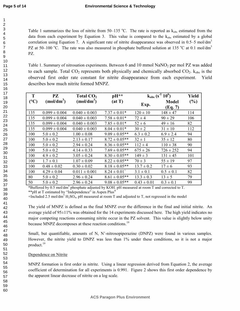
Table 1 summarizes the loss of nitrite from 50–135 oC. The rate is reported as kobs estimated from the
data from each experiment by Equation 3. This value is compared to the kobs estimated by a global
correlation using Equation 7. A significant rate of nitrite disappearance was observed in 0.5–5 mol/dm3
PZ at 50–100 oC. The rate was also measured in phosphate buffered solution at 135
oC at 0.1 mol/dm
3
PZ.
Table 1. Summary of nitrosation experiments. Between 6 and 10 mmol NaNO2 per mol PZ was added
to each sample. Total CO2 represents both physically and chemically absorbed CO2. kobs is the
observed first order rate constant for nitrite disappearance from each experiment. Yield
describes how much nitrite formed MNPZ.
T
(°C)
PZ
(mol/dm3)
Total CO2
(mol/dm3)
pH**
(at T)
kobs (s-1
106) Yield
(%) Exp.
Model
(Eq. 7)
135 0.099 ± 0.004 0.040 ± 0.003 7.37 ± 0.01* 120 ± 10 148 ± 47 114
135 0.099 ± 0.004 0.040 ± 0.003 7.58 ± 0.01* 72 ± 4 90 ± 29 106
135 0.099 ± 0.004 0.040 ± 0.003 7.85 ± 0.01* 52 ± 6 49 ± 16 82
135 0.099 ± 0.004 0.040 ± 0.003 8.04 ± 0.01* 30 ± 2 31 ± 10 112
100 5.0 ± 0.2 1.00 ± 0.08 9.09 ± 0.05** 6.3 ± 0.2 6.9 ± 2.4 94
100 5.0 ± 0.2 2.13 ± 0.17 8.72 ± 0.05** 32 ± 1 35 ± 12 80
100 5.0 ± 0.2 2.94 ± 0.24 8.36 ± 0.05** 112 ± 4 110 ± 38 90
100 5.0 ± 0.2 4.14 ± 0.33 7.69 ± 0.05** 675 ± 26 726 ± 252 94
100 4.9 ± 0.2 3.05 ± 0.24 8.30 ± 0.05** 149 ± 3 131 ± 45 101
100 1.7 ± 0.1 1.07 ± 0.09 8.22 ± 0.05** 70 ± 3 55 ± 19 97
100 0.48 ± 0.02 0.30 ± 0.02 8.18 ± 0.05** 13.7 ± 0.2 17 ± 6 93
100 4.29 ± 0.04 0.011 ± 0.001 8.24 ± 0.01+
3.1 ± 0.1 0.5 ± 0.1 82
80 5.0 ± 0.2 2.96 ± 0.24 8.61 ± 0.05** 13.3 ± 0.3 13 ± 5 79
50 5.0 ± 0.2 2.96 ± 0.24 9.08 ± 0.05** 0.43 ± 0.01 0.3 ± 0.1 99
*Buffered by 0.5 mol/dm3 phosphate adjusted by KOH. pH measured at room T and corrected to T.
**pH at T estimated by “Independence” in Aspen Plus®
+Included 2.5 mol/dm3 H2SO4, pH measured at room T and adjusted to T, not regressed in the model
The yield of MNPZ is defined as the final MNPZ over the difference in the final and initial nitrite. An
average yield of 95±11% was obtained for the 14 experiments discussed here. The high yield indicates no
major competing reactions consuming nitrite occur in the PZ solvent. This value is slightly below unity
because MNPZ decomposes at these reaction conditions.19
Small, but quantifiable, amounts of N, N’-nitrosopiperazine (DNPZ) were found in various samples.
However, the nitrite yield to DNPZ was less than 1% under these conditions, so it is not a major
product.19
Dependence on Nitrite
MNPZ formation is first order in nitrite. Using a linear regression derived from Equation 2, the average
coefficient of determination for all experiments is 0.991. Figure 2 shows this first order dependence by
the apparent linear decrease of nitrite on a log scale.
Page 5 of 14
ACS Paragon Plus Environment
Environmental Science & Technology
123456789101112131415161718192021222324252627282930313233343536373839404142434445464748495051525354555657585960
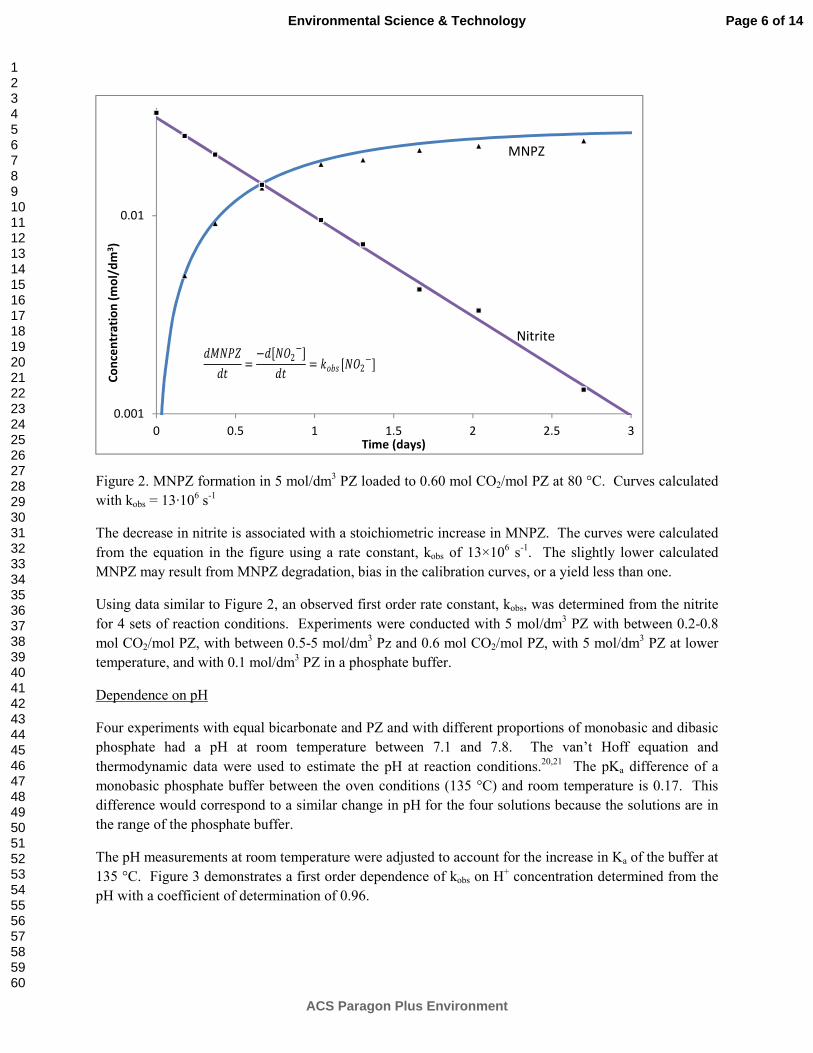
Figure 2. MNPZ formation in 5 mol/dm3 PZ loaded to 0.60 mol CO2/mol PZ at 80 °C. Curves calculated
with kobs = 13·106 s
-1
The decrease in nitrite is associated with a stoichiometric increase in MNPZ. The curves were calculated
from the equation in the figure using a rate constant, kobs of 13×106 s
-1. The slightly lower calculated
MNPZ may result from MNPZ degradation, bias in the calibration curves, or a yield less than one.
Using data similar to Figure 2, an observed first order rate constant, kobs, was determined from the nitrite
for 4 sets of reaction conditions. Experiments were conducted with 5 mol/dm3 PZ with between 0.2-0.8
mol CO2/mol PZ, with between 0.5-5 mol/dm3 Pz and 0.6 mol CO2/mol PZ, with 5 mol/dm
3 PZ at lower
temperature, and with 0.1 mol/dm3 PZ in a phosphate buffer.
Dependence on pH
Four experiments with equal bicarbonate and PZ and with different proportions of monobasic and dibasic
phosphate had a pH at room temperature between 7.1 and 7.8. The van’t Hoff equation and
thermodynamic data were used to estimate the pH at reaction conditions.20,21
The pKa difference of a
monobasic phosphate buffer between the oven conditions (135 °C) and room temperature is 0.17. This
difference would correspond to a similar change in pH for the four solutions because the solutions are in
the range of the phosphate buffer.
The pH measurements at room temperature were adjusted to account for the increase in Ka of the buffer at
135 °C. Figure 3 demonstrates a first order dependence of kobs on H+ concentration determined from the
pH with a coefficient of determination of 0.96.
0.001
0.01
0 0.5 1 1.5 2 2.5 3
Co
nce
ntr
ati
on
(m
ol/
dm
3)
Time (days)
������� � �����2��
�� � �%&' ���2�� Nitrite
MNPZ
Page 6 of 14
ACS Paragon Plus Environment
Environmental Science & Technology
123456789101112131415161718192021222324252627282930313233343536373839404142434445464748495051525354555657585960
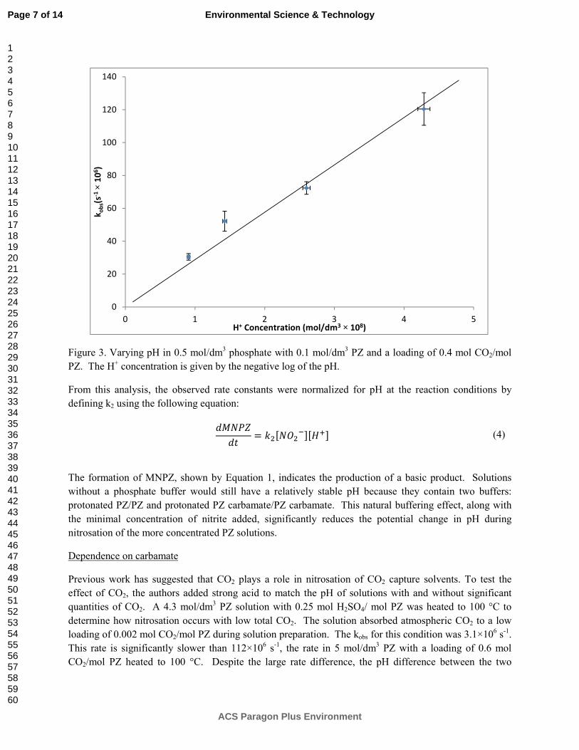
Figure 3. Varying pH in 0.5 mol/dm3 phosphate with 0.1 mol/dm
3 PZ and a loading of 0.4 mol CO2/mol
PZ. The H+ concentration is given by the negative log of the pH.
From this analysis, the observed rate constants were normalized for pH at the reaction conditions by
defining k2 using the following equation:
������� � ����������(� (4)
The formation of MNPZ, shown by Equation 1, indicates the production of a basic product. Solutions
without a phosphate buffer would still have a relatively stable pH because they contain two buffers:
protonated PZ/PZ and protonated PZ carbamate/PZ carbamate. This natural buffering effect, along with
the minimal concentration of nitrite added, significantly reduces the potential change in pH during
nitrosation of the more concentrated PZ solutions.
Dependence on carbamate
Previous work has suggested that CO2 plays a role in nitrosation of CO2 capture solvents. To test the
effect of CO2, the authors added strong acid to match the pH of solutions with and without significant
quantities of CO2. A 4.3 mol/dm3 PZ solution with 0.25 mol H2SO4/ mol PZ was heated to 100 °C to
determine how nitrosation occurs with low total CO2. The solution absorbed atmospheric CO2 to a low
loading of 0.002 mol CO2/mol PZ during solution preparation. The kobs for this condition was 3.1×10⁶ s
-1.
This rate is significantly slower than 112×106 s
-1, the rate in 5 mol/dm
3 PZ with a loading of 0.6 mol
CO2/mol PZ heated to 100 °C. Despite the large rate difference, the pH difference between the two
0
20
40
60
80
100
120
140
0 1 2 3 4 5
ko
bs(
s-1 ×
10
6)
H+ Concentration (mol/dm3 × 108)
Page 7 of 14
ACS Paragon Plus Environment
Environmental Science & Technology
123456789101112131415161718192021222324252627282930313233343536373839404142434445464748495051525354555657585960

experiments was only 0.12±0.06. Since the two solutions with different amounts of carbamate resulted in
large reaction rate differences, total dissolved CO2 significantly catalyzes nitrosation.
To understand how absorbed CO2 affects nitrosation, the speciation of CO2 inside piperazine solution
must be understood. All of the CO2 added to the system can exist as physically absorbed CO2,
bicarbonate, or as a carbamate with PZ. In our experiments, the majority of CO2 exists as a carbamate.
Since PZ contains two secondary amines, a PZ carbamate molecule can either contain an unprotonated
amine, a protonated amine, or a carbamate group on the other amine group. These species are called PZ
carbamate, protonated PZ carbamate, and PZ dicarbamate, respectively. At high pH and low total
dissolved CO2, PZ carbamate dominates. As more CO2 is added, the PZ carbamate concentration starts to
decrease and protonated PZ carbamate and PZ dicarbamate concentrations increase. When the total
dissolved CO2 approaches the amount of PZ, significant bicarbonate concentrations arise, but this
condition is not often seen in carbon capture systems with PZ. More information about speciation can be
found in previous literature.4,18
To discover which species containing CO2 are reactive, the authors used the Independence
thermodynamic model in Aspen Plus® to calculate the pH and speciation of 7 solutions heated to 100
°C.17
From this, the k2 for each set of solutions was determined from Equation 4. A rate constant, kt,
was defined to determine the species that catalyze nitrosation along with the order of concentration
dependence.
�� � ���)�*+"+��, (5)
Each species listed in Table 2 was analyzed in the 7 experiments at 100 °C. For each species in Table 2,
an order of reaction was found that resulted in the smallest relative standard deviation between the 7
experiments, representing the best correlation between reaction rate and the species concentration.
Table 2. Reaction dependence on different carbamate species. Total dissolved CO2 represents all CO2
added to the system. Relative standard deviation of kt for 7 experiments found using Equation 5.
Species Optimized α Relative Standard
Deviation of kt with
optimized α
Relative Standard
Deviation of kt with
α = 1
Physically Dissolved CO2 0.30 0.50 1.46
Bicarbonate 0.50 0.51 0.94
PZ carbamate 0.00 0.74 0.91
Protonated PZ carbamate 0.77 0.19 0.30
PZ dicarbamate 0.39 0.37 1.32
Total CO2 as carbamate 0.87 0.22 0.28
Total Dissolved CO2 1.09 0.17 0.18
The high errors associated with the individual carbamate species is likely due to multiple carbamate
species participating in nitrosation. Multiple PZ carbamate species can catalyze nitrosation as long as the
two amine groups on PZ function semi-independently. Previous research indicates that protonation of the
Page 8 of 14
ACS Paragon Plus Environment
Environmental Science & Technology
123456789101112131415161718192021222324252627282930313233343536373839404142434445464748495051525354555657585960

inactive nitrogen on PZ does not make the other nitrogen-containing group unreactive.22
The ability for
multiple carbamate groups to participate in reaction would explain why none of the individual carbamate
species had both an order of reaction similar to stoichiometric orders of reaction (0.5, 1, 2) and a low
relative error. The total carbamate species correlated better than any particular carbamate species because
of this additive affect. Since the different carbamate species are likely to have slightly different rate
constants, there is some error associated with using the sum of all carbamate species. However,
uncertainties in the speciation model prohibit any meaningful analysis on the individual carbamate rate
constants.
The total dissolved CO2 is a practical way to determine total carbamate concentration in most solutions
since physically dissolved CO2 and bicarbonate are only present at low concentrations. Figure 4
demonstrates this practical correlation in experiments with 0.5 to 5 mol/dm3 PZ over a range of loadings.
Figure 4. Reaction rate dependence on total dissolved CO2 in 0.5, 1.7, and 5 mol/dm3 PZ with 0.6 mol
CO2/mol PZ and 5 mol/dm3 PZ with 0.1, 0.2, 0.3, 0.8 mol CO2/mol PZ.
Using the effect of carbamate, Equation 6 represents a simplified rate equation which agrees with the
experimental data.
������� � �-��������(�����)���� (6)
R2NCOO- corresponds to the carbamate species in the solution, but it is calculated using the total amount
of CO2 added per volume solution. As long as the moles of CO2 are fewer than the moles of PZ, this
approximation will hold. With more CO2 than PZ, significant levels of bicarbonate form.
0
5
10
15
20
25
30
35
40
45
50
0.00 1.00 2.00 3.00 4.00 5.00
k2(L
mo
l-1s-1
* 1
0-3
)
Total Dissolved CO2 (mole/dm3)
Page 9 of 14
ACS Paragon Plus Environment
Environmental Science & Technology
123456789101112131415161718192021222324252627282930313233343536373839404142434445464748495051525354555657585960

Dependence on temperature
Nitrosation is faster at higher temperature. Two effects cause this change: there is more thermal energy to
overcome the activation energy, and the pH decreases with temperature due to the temperature
dependence of the pKa of PZ. After normalizing the rate constant for the pH and total CO2, the activation
energy was determined to be 84±2 kJ/mol (Figure 5).
Figure 5. Reaction rate dependence on temperature, activation energy = 84±2 kJ/mol.
Rate Equation and Model
Using the temperature dependence and Equation 6, a model for MNPZ formation can predict nitrosation
of PZ by aqueous nitrite in the presence of CO2. All of the k3 values, except the experiment with added
sulfuric acid, were normalized to 100 °C and averaged to obtain k3,avg≈8.5×10³±1.4×10
3 L
2mol
-2s
-1.
������� � �-,/01
234 5 6-7-.69:� 6
;<=>?��������(��)��@��1�� (7)
The CO2 loading should be less than 1.0 mol/mol PZ for this model to accurately predict kinetics. This
model might not be applicable in the presence of significant amounts of formaldehyde which can also
catalyze nitrosation at similar conditions as CO2.23
Previously published data on pH of PZ can be used to
determine the hydrogen ion concentration.18
Figure 6 shows how the observed first order rate constants,
kobs, compare to values predicted from Equation 7.
100
1000
10000
100000
0.0024 0.0028 0.0032
k3(d
m6
mo
le-2
s-1)
1/T (K-1)
135 °C , 0.1 mol/dm3 PZ with phosphate buffer
100 °C , 5, 1.7, 0.5 mol/dm3 PZ
80 °C , 5 mol/dm3 PZ
50 °C , 5 mol/dm3 PZ
Page 10 of 14
ACS Paragon Plus Environment
Environmental Science & Technology
123456789101112131415161718192021222324252627282930313233343536373839404142434445464748495051525354555657585960

Figure 6. Application of kinetic model to experimental data. The predicted kobs for each experiment was
obtained from the kinetic model (Equation 7). The line indicates perfect agreement between experimental
and predicted data. The acid experiment was not regressed
In Figure 6, the acid experiment with minimal CO2 shows significantly higher rate than the model
predicts. This indicates that at low carbamate concentrations, a different nitrosation reaction may
dominate.
Mechanism
Figure 7 shows a mechanism that would follow the kinetics in Equation 6. This mechanism is similar to
that proposed by Lv and Sun.14,15
Step 1 is an equilibrium acid-base reaction. Since the pKa of the
carbamate functional group on PZ is around 6.7±0.2 while the pKa of typical PZ solvent is between 7.7
and 9.1, the equilibrium would lie toward the unprotonated carbamate.17,24
Step 2 indicates a nucleophilic
attack on the carbonyl group by the nitrite ion. Step 3 includes the reformation of the carbonyl group
accompanied by the formation of the N-nitrosamine bond in one concerted step. A concerted mechanism
for this step was shown to be energetically favored over a stepwise mechanism.13
Figure 7. The proposed mechanism for nitrosation of PZ in aqueous carbon capture. The R group can
represent NH, NCOO-, or NH2
+.
0.1
1
10
100
1000
0.1 1 10 100 1000
Pre
dic
ted
ko
bs(
s-1
×1
06)
Experimental kobs(s-1×10⁶)
Acid experiment
Page 11 of 14
ACS Paragon Plus Environment
Environmental Science & Technology
123456789101112131415161718192021222324252627282930313233343536373839404142434445464748495051525354555657585960
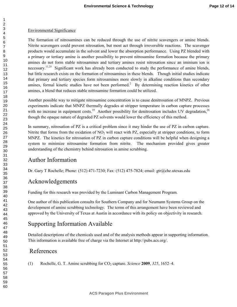
Environmental Significance
The formation of nitrosamines can be reduced through the use of nitrite scavengers or amine blends.
Nitrite scavengers could prevent nitrosation, but most act through irreversible reactions. The scavenger
products would accumulate in the solvent and lower the absorption performance. Using PZ blended with
a primary or tertiary amine is another possibility to prevent nitrosamine formation because the primary
amines do not form stable nitrosamines and tertiary amines resist nitrosation since an iminium ion is
necessary.11,25
Significant work has already been conducted to study the performance of amine blends,
but little research exists on the formation of nitrosamines in these blends. Though initial studies indicate
that primary and tertiary species form nitrosamines more slowly in alkaline conditions than secondary
amines, formal kinetic studies have not been performed.2 By determining reaction kinetics of other
amines, a blend that reduces stable nitrosamine formation could be utilized.
Another possible way to mitigate nitrosamine concentration is to cause denitrosation of MNPZ. Previous
experiments indicate that MNPZ thermally degrades at stripper temperature in carbon capture processes
with no increase in equipment costs.19
Another possibility for denitrosation includes UV degradation,26
though the opaque nature of degraded PZ solvents would lower the efficiency of this method.
In summary, nitrosation of PZ is a critical problem since it may hinder the use of PZ in carbon capture.
Nitrite that forms from the oxidation of NO2 will react with PZ, especially at stripper conditions, to form
MNPZ. The kinetics for nitrosation of PZ in carbon capture conditions will be helpful when designing a
system to minimize nitrosamine formation from nitrite. The mechanism provided gives greater
understanding of the chemistry behind nitrosation in amine scrubbing.
Author Information
Dr. Gary T Rochelle; Phone: (512) 471-7230; Fax: (512) 475-7824; email: [email protected]
Acknowledgements
Funding for this research was provided by the Luminant Carbon Management Program.
One author of this publication consults for Southern Company and for Neumann Systems Group on the
development of amine scrubbing technology. The terms of this arrangement have been reviewed and
approved by the University of Texas at Austin in accordance with its policy on objectivity in research.
Supporting Information Available
Detailed descriptions of the chemicals used and of the analysis methods appear in supporting information.
This information is available free of charge via the Internet at http://pubs.acs.org/.
References
(1) Rochelle, G. T. Amine scrubbing for CO2 capture. Science 2009, 325, 1652–4.
Page 12 of 14
ACS Paragon Plus Environment
Environmental Science & Technology
123456789101112131415161718192021222324252627282930313233343536373839404142434445464748495051525354555657585960

(2) Dai, N.; Shah, A. D.; Hu, L.; Plewa, M. J.; Mckague, B.; Mitch, W. A. Measurement of
Nitrosamine and Nitramine Formation from NO. Environ. Sci. Technol. 2012, 46, 9793–9801.
(3) Jessen, K.; Kovscek, A. R.; Orr, F. M. Increasing CO2 storage in oil recovery. Energ. Converse.
Manage. 2005, 46, 293–311.
(4) Rochelle, G.; Chen, E.; Freeman, S.; Van Wagener, D.; Xu, Q.; Voice, A. Aqueous piperazine as
the new standard for CO2 capture technology. Chem. Eng. J. 2011, 171, 725–733.
(5) Nielsen, P. T.; Li, L.; Rochelle, G. T. Piperazine degradation in pilot plants. Presented at GHGT-
11, Kyoto, Japan, November 20, 2012, to be published in Energy Procedia 2013.
(6) Garcia, H.; Keefer, L.; Lijinsky, W.; Wenyon, C. Carcinogenicity of nitrosothiomorpholine and 1-
nitrosopiperazine in rats. J. Cancer. Res. Clin. Oncol. 1970, 74, 179–184.
(7) Fulk, S. M.; Rochelle, G. T. Modeling aerosols in amine-based CO2 capture. Presented at GHGT-
11, Kyoto, Japan, November 20, 2012, to be published in Energy Procedia 2013.
(8) Kolderup, H.; Hjarbo, K. W.; Mejdell, T.; Huizinga, A.; Tuinman, I.; Zahlsen, K.; Vernstad, K.;
Hyldbakk, A.; Holten, T.; Kvamsdal, H. M.; van Os, P.; da Silva, E. F.; Goetheer, E.; Khakharia,
P. Emission studies at the Maasvlakte CO2 capture pilot plant. Presented at The University of
Texas Conference on CCS, Austin, TX, January 25, 2012.
(9) Kirsch, M.; Korth, H. G.; Sustmann, R.; de Groot, H. Carbon dioxide but not bicarbonate inhibits
N-nitrosation of secondary amines. Evidence for amine carbamates as protecting entities. Chem.
Res. Toxicol. 2000, 13, 451–61.
(10) Challis, B. C.; Kyrtopoulos, S. A. Rapid formation of carcinogenic N-nitrosamines in aqueous
alkaline solutions. Br. J. Cancer. 1977, 35, 693–696.
(11) Douglass, M.; Kabacoff, B. The chemistry of nitrosamine formation, inhibition and destruction. J.
Soc. Cosmet. Chem. 1978, 29, 581–606.
(12) Choi, J.; Valentine, R. L. Formation of N-nitrosodimethylamine (NDMA) from reaction of
monochloramine: a new disinfection by-product. Water Res. 2002, 36, 817–24.
(13) Lv, C. L.; Liu, Y. D.; Zhong, R.; Wang, Y. Theoretical studies on the formation of N-
nitrosodimethylamine. J. Mol. Struc.-Theochem 2007, 802, 1–6.
(14) Sun, Z.; Liu, Y. D.; Zhong, R. G. Carbon dioxide in the nitrosation of amine: catalyst or inhibitor?
J. Phys. Chem. A 2011, 115, 7753–64.
(15) Lv, C.-L.; Liu, Y. D.; Zhong, R.-G. Theoretical investigation of N-nitrosodimethylamine
formation from dimethylamine nitrosation catalyzed by carbonyl compounds. J. Phys. Chem. A
2009, 113, 713–8.
(16) Freeman, S. A. Thermal Degradation and Oxidation of Aqueous Piperazine for Carbon Dioxide
Capture, The University of Texas at Austin, Austin, TX, 2011.
Page 13 of 14
ACS Paragon Plus Environment
Environmental Science & Technology
123456789101112131415161718192021222324252627282930313233343536373839404142434445464748495051525354555657585960

(17) Frailie, P.; Rochelle, G. T. Aspen Plus Independence Model, version 2012; The University of
Texas at Austin: Austin, TX, 2012.
(18) Frailie, P. T.; Plaza, J. M.; Van Wagener, D.H.; Rochelle, G. T. Modeling piperazine
thermodynamics. Energy Procedia 2011, 4, 35–42.
(19) Fine, N. A.; Goldman, M. J.; Nielsen, P. T.; Rochelle, G. T. Managing n-nitrosopiperazine and
dinitrosopiperazine. Presented at GHGT-11, Kyoto, Japan, November 20, 2012, to be published in
Energy Procedia 2013.
(20) Goldberg, R. N.; Kishore, N.; Lennen, R. M. Thermodynamic Quantities for the Ionization
Reactions of Buffers. J. Phys. Chem. Ref. Data. 2002, 31, 231–370.
(21) Atkins, P. W.; de Paula, J. The response of equilibria to temperature. In Physical Chemistry;
Oxford University Press: New York, 2006.
(22) Castro, E. A.; Hormazabal, A.; Santos, J. G. Concerted Mechanism of 4-Cyanobenzoate with
Secondary Alicyclic Amines in Aqueous Ethanol. Int. J. Chem. Kinet. 1997, 30, 267–272.
(23) Casado, J.; Mosquera, M.; Paz, C.; Rodriguez-Prieto, F.; Vázquez-Tat, J. Nitrite Ion as a
Nitrosating Reagent. Nitrosation of Morpholine and Diethylamine in the Presence of
Formaldehyde. J. Chem. Soc. Perkin. 2 1984, 1963–1966.
(24) Scifinder Scholar, online version; Chemical Abstracts Service: Columbus, OH, 2012; RN: 10430-
90-7 (accessed Sept 29, 2012); calculated using ACD/Labs software, version 11.02; ACD/Labs
1994-2012.
(25) Sun, Z.; Liu, Y. D.; Zhong, R. G. Theoretical investigation of N-nitrosodimethylamine formation
from nitrosation of trimethylamine. J. Phys. Chem. A 2010, 114, 455–65.
(26) Stefan, M. I.; Bolton, J. R. UV direct photolysis of N-nitrosodimethylamine (NDMA): kinetic and
product study. Helv. Chim. Acta. 2002, 85, 1416.
Page 14 of 14
ACS Paragon Plus Environment
Environmental Science & Technology
123456789101112131415161718192021222324252627282930313233343536373839404142434445464748495051525354555657585960

For peer review only
An effective multi-loop control system with storage tanks to
improve control performance of CO2 capture
Journal: AIChE Journal
Manuscript ID: Draft
Wiley - Manuscript type: Research Article
Date Submitted by the Author: n/a
Complete List of Authors: Ziaii, Sepideh; University of Texas at Austin, Department of Chemical Engineering, C0400 Rochelle, Gary; The University of Texas at Austin, Chemical Engineering Edgar, Thomas; University of Texas at Austin, Department of Chemical Engineering, C0400
Keywords: Process control, Absorption, Aqueous solutions, Coal, Energy
AIChE Journal
AIChE Journal

For peer review only
1
An effective multi-loop control system with storage tanks to improve control
performance of CO2 capture
Sepideh Ziaii, Gary T. Rochelle, Thomas F. Edgar
McKetta Department of Chemical Engineering, University of Texas at Austin,
Austin, TX 78712-1589
ABSTRACT
A multi-loop feedback control system is proposed to operate CO2 capture with
amine solvent efficiently over wide ranges of power plant operation. This work examines
potential plantwide control structures in operating CO2 capture in a process flow sheet of
a fully integrated dynamic model created in Aspen Custom Modeler®
. This study
illustrated that controlling the reboiler temperature and solvent circulation rate is an
effective strategy in set point tracking and disturbance rejection in response to possible
dynamic scenarios. Power plant load reduction, reboiler steam load reduction and
foaming in the columns are the scenarios simulated for control configuration validation.
This study also presents the effects of liquid residence time in the lean solution tank and
rich solution tank on the dynamic performance of CO2 capture in response to possible
disturbances. Frequency response analysis is employed to illustrate how changing the
holdup time influences the quality of dynamic characteristics such as response time and
dampening oscillations.
KEYWORDS
Monoethanolamine; dynamic modeling; process control; CO2 capture; amine
scrubbing.
INTRODUCTION
Absorption/stripping using aqueous amine is a mature technology commonly used
for removing CO2 from natural gas, hydrogen, and other refinery gases, which makes it
Page 1 of 42
AIChE Journal
AIChE Journal
123456789101112131415161718192021222324252627282930313233343536373839404142434445464748495051525354555657585960

For peer review only
2
applicable to removing CO2 from flue gas in coal-fired power plants. However, the
amine process is energy-intensive and requires economic consideration in both design
and operation. For a coal-fired power plant using post-combustion amine
absorption/stripping for CO2 removal, full-load CO2 capture could reduce net energy
output by 11–40% from that of an equivalent plant without CO2 capture.1
Figure 1 illustrates a standard scheme of an absorption/stripping process including
the control valves. In the absorber, which is operated at atmospheric pressure and 40–
60 °C, the flue gas from a coal-fired plant containing 10–12% CO2 contacts an amine
solution, and CO2 is absorbed into the solution by physical and chemical mechanisms.
The rich solution coming out of the absorber, which typically has a loading of 0.2–0.5
mol CO2/mol amine, is directed to the stripper, operating at 1.5–2 atm and 100–120 °C.
Water vapor accompanying CO2 from the top of the stripper is condensed and returned to
the cycle. The hot lean solution exiting the stripper is cooled by the cold rich solution in a
cross heat exchanger (5–10 °C temperature approach) and is furthered cooled to 40 °C
before entering the absorber.
The bulk of the energy requirement is due to the heat used for solvent
regeneration and the work required to compress CO2 to pipeline pressure for transport to
a storage site. In a typical design, about 50% of the steam is extracted between the
intermediate and low-pressure power plant turbines, expanded in a let-down turbine or
valve, and then sent to the stripper column for solvent regeneration.
Previous work has enhanced the steady state absorption and energy performance
in the conceptual design phase.2-5
In addition to optimizing the process configuration and
solvent selection for the base load, energy use can also be reduced by understanding the
dynamics and exploring effective control configurations for transitional conditions.
Although dynamics and control are very important with respect to operations, there are
very few dynamic models presented for solvent-based absorption/desorption processes.
For example, Kvamsdal et al.6 presented a dynamic model for the absorber and studied
Page 2 of 42
AIChE Journal
AIChE Journal
123456789101112131415161718192021222324252627282930313233343536373839404142434445464748495051525354555657585960

For peer review only
3
the transitional behavior of startup and power plant load variation. Lawal et al.7 combined
the dynamic model of absorber and stripper and simulated operation of the plant in
response to the disturbances imposed by the upstream power plant. Prior studies6-8
have
examined the capture behavior isolated from the power plant and CO2 compression
system.
The first part of this paper presents the design of a control system for a capture
plant using MEA by implementing a dynamic model of integrated absorption/stripping in
Aspen Custom Modeler (ACM®
). The dynamic models of the columns are developed
with a non-equilibrium (rate-based) model. The rate-based approach has been defined and
implemented in several studies on dynamic modeling of reactive distillation columns.
9,10
In addition, by incorporating practical performance models for pumps and the variable
speed CO2 compressor, the model accounts for the operational boundaries created by
compressor and pump limitations. This work is unique since it uses a fully integrated
model to simulate unsteady-state operations and examines the dynamic performance of a
variety of control structures by dynamic simulation.
Developing an effective control system requires implementation of a systematic
and coherent strategy regardless of the fact that it may not provide the complete and
unique solution. The plantwide control procedure recommended by Seborg et al.11
is a
general strategy that can assist the control system designer to determine how to match
controlled and manipulated variables, when to use an advanced control technique, and
how to select an appropriate decoupled multi-loop control system. In contrast to previous
work7-9
that did not follow a systematic strategy, this study follows the steps of this
plantwide control procedure to develop a multi-loop control system that can effectively
handle load variations and disturbances. Partial load operations and foaming in the
columns are two dynamic scenarios simulated in this study to validate suggested control
structures.
Page 3 of 42
AIChE Journal
AIChE Journal
123456789101112131415161718192021222324252627282930313233343536373839404142434445464748495051525354555657585960

For peer review only
4
Steam load reduction in CO2 capture has been identified as an important
operational scenario, but has not been studied with respect to dynamics and strategies of
operation. Coal-fired power plants generate electricity at the base load and might be
expected to run CO2 capture at its full capacity continuously. Operating CO2 capture
flexibly, i.e., implementing an on/off operation, would be economical based on electricity
and CO2 market conditions.12
In this operation all or part of the steam being used for
solvent regeneration or for driving CO2 compression can be used for power generation
with daily peak power demand or high electricity prices.13
Load variation in the upstream power plant is another dynamic operation that
influences capture performance. Understanding the effects and exploring energy efficient
control strategies in response to power plant load variation is an important issue to
investigate for developing an adequate control system. Prior work6,7,14
that simulated the
power plant load variation considered only the changes in flue gas inlet condition. They
neglected the variation of total steam rate in the power cycle because of load variation.
This is an important effect because it affects the operation of stripping and compression
when reboiler steam is extracted from the power turbines. This work combines the model
of the capture plant with a simple steady state model of steam turbines to take into
account steam extraction.
Storage tanks are typically designed for smoothing responses and rejecting
disturbances where the established control structure cannot bring further improvement.15
According to Luyben16
, considering control performance when the tanks and
reactors are designed is very important especially for recycle systems due to the trade-off
existing between design and control. However, tank sizing is typically done by rule of
thumb rather than by evaluating dynamics and control targets. The second part of this
paper examines the role of lean and rich storage tanks in the improvement of capture
dynamic performances.
Page 4 of 42
AIChE Journal
AIChE Journal
123456789101112131415161718192021222324252627282930313233343536373839404142434445464748495051525354555657585960

For peer review only
5
SYSTEM MODELING
The dynamic models developed for the absorber and the stripper are rate-based using film
theory for liquid and vapor phases. They take into account the impact of equilibrium
reactions (for the stripper) and kinetic reactions (for the absorber) on the mass transfer,
thermodynamic non-idealities, and hydraulics of the structured packing. Models for the
reboiler, absorber sump, and storage tanks are equilibrium stages that solve time variant
energy and mass balances. Because the dynamics of heat exchangers, pumps, CO2
compressor, control valves, and steam turbines are relatively fast, their dynamic effects
are ignored by using steady state equations. The details of the thermodynamic model and
physical properties are presented in a previous paper. 8
This section provides the details of the modeling of the absorber column. The formulation
of the stripper was presented in detail in Ziaii et al.8 Similar to the stripper, the absorber
column is divided into a number of segments, and time varying energy and mass balances
are solved at each time step for both phases for each segment. The following assumptions
are made:
1. The variation of the conditions in the radial direction is negligible in both
liquid phase and gas phase.
2. Mixed-flow model is applied to determine the bulk properties, meaning
that the outlet conditions are equal to the bulk conditions for each phase at
each segment.
3. The heat transfer coefficient of the liquid phase is much bigger than that of
the vapor phase due to very high thermal conductivity of aqueous solution;
therefore, the dominant heat transfer resistance is assumed to be in the
vapor phase.
The following equations are mass and energy balances for liquid and gas phases for
components i=CO2, H2O, N2, O2 in the jth
segment of the absorber column:
Page 5 of 42
AIChE Journal
AIChE Journal
123456789101112131415161718192021222324252627282930313233343536373839404142434445464748495051525354555657585960

For peer review only
6
j,ijjcj,ijj,ij
Lj,i
NalDxLxLdt
dM 211
4
π−−= −− (1)
j,ijjcj,ijj,ij
Vj,i
NalDyVyVdt
dM 211
4
π+−= −+ (2)
)2 2
2 2
, ,2
1 1
, ,
( )
4
L L I LLj j j CO j CO jj L L
j j j j c j j L
H O j H O j
h T T N HdEL H L H D l a
dt N H
π− −
− += − − +
(3)
( )2 2 2 2
2
1 1 , , , ,( )4
V
j V V V V I V V
j j j j c j j j j j CO j CO j H O j H O j
dEV H V H D l a h T T N H N H
dt
π+ += − + − + +
(4)
It is assumed that heat transfer coefficient is so high that Ij
Lj TT − =0
Vjj
Vjj
Ljj
Ljj
totalj
HVHVHLHLdt
dE−+−= ++−− 1111 (5)
j,iLj
Ltjjc
Lj,i xChlDM 2
4
π= (6)
j,iVj
Ltjjc
Vj,i yC)h(lDM −= ε
π 2
4 (7)
Lj
Lj
Ltjjc
Lj HChlDE 2
4
π= (8)
Vj
Vj
Ltjjc
Vj HC)h(lDE −= ε
π 2
4 (9)
Lj
Vj
totalj EEE += (10)
Lj
i
Lj,i H
xH
∂∂
= (11)
Vj
i
Vj,i H
yH
∂∂
= (12)
dT)T,ldg(Cp)T(Hx
Hx)T,ldg(HxHxH
j
LT
refTL
refvap
OHOH
V,ref
OHOHrefj
desCOCO
V,refCOCO
Lj
∫+−
+−=
22
222222
∆
∆ (13)
dTCPyHyHVT
refTi
ideal,Vij,i
i
V,refj,ij,i
Vj ∫ ∑∑ += (14)
It is assumed that MEA is a non-volatile solvent and O2 and N2 are not solved in the
solution. The mass flux of CO2 and H2O is calculated from the following equation:
Page 6 of 42
AIChE Journal
AIChE Journal
123456789101112131415161718192021222324252627282930313233343536373839404142434445464748495051525354555657585960

For peer review only
7
)PyP(KGN CO*COCOCO 2222
−= (15)
Where 2COKG is a total mass transfer coefficient that involves the combination of the
resistance to mass transfer in both liquid phase (2COgk ′ ) and gas phase ( )kgCO2
.
222
111
COCOCO kggkKG+
′= (16)
Liquid side mass transfer coefficient,2COgk ′ , is calculated from a correlation as a
function of partial pressure of CO2 based on data provided by Aboudhier et al.17
98442022
.)Pa(Plog.gklog *COCO −−=′ (17)
The mass transfer resistance for H2O in the liquid phase is negligible and H2O mass flux
is calculated from the following equation:
)PyP(KgNOH
*OHOHOH
2222−= (18)
DESIGN BASIS
This study simulates the dynamic operational scenarios in a capture plant initially
designed based on the following inlet conditions and design specifications:
� Gas rate and composition: 5.48 kmol/s, 13% CO2
� Electric rate: 100 MW
� Absorber packing height: 15 m
� Stripper packing height: 10 m
� CO2 removal with 30 wt % MEA: 90%
� Lean loading: 0.233 mole CO2/mole MEA
� Reboiler temperature: 120 °C
� CO2 discharge pressure compressor: 150 bar
� Extracted reboiler steam = 30% total power cycle steam rate
� Steam turbine initial design condition18
:
PHPin
= 290 bar, PIPin
= 60 bar, PLPin
= 2.65 bar, PLPout
= 0.04 bar
Page 7 of 42
AIChE Journal
AIChE Journal
123456789101112131415161718192021222324252627282930313233343536373839404142434445464748495051525354555657585960

For peer review only
8
Figure 1:
DESIGN OF CONTROL SYSTEM
Amine absorption/stripping is a complex process with respect to control due to the liquid
recycle and heat integration between the absorber and the regenerator. A systematic
strategy is required to develop a viable control structure working satisfactorily over a
range of operating conditions. This work assumes that a multi-loop control approach is
sufficient for our control objectives and a multi-variable control system is not necessary.
We employ the plantwide hierarchical design procedure11
to develop control structure
alternatives and evaluate their performance in response to identified disturbances.
For operation of CO2 capture in power plants, it is not required to satisfy any strict
production rate or quality specifications. The most important objective in this energy
intensive plant is to minimize energy consumption when the plant is operated at various
operating loads. Therefore, a real-time optimization should be performed based on
current markets to optimize operating conditions. The responsibility of the control system
is to bring the plant to the optimal condition smoothly and quickly when a disturbance
occurs. Safe operation of equipment such as the pumps and the CO2 compressor should
be addressed in control system design. To operate pumps safely the upstream level must
be controlled to prevent cavitation and running dry. Compressor surge is also an
unwanted condition that should be avoided by implementing a proper control strategy
such as anti-surge control. The stripper pressure should be controlled with minimum
oscillation to protect the overhead CO2 compressor. To minimize thermal degradation of
the solvent the reboiler temperature must be kept below the allowable value, 120 °C, for
MEA. In summary, the following objectives are considered to evaluate control
configurations.
1. Control the plant at optimum set points with a smooth and fast response
during abnormal conditions.
Page 8 of 42
AIChE Journal
AIChE Journal
123456789101112131415161718192021222324252627282930313233343536373839404142434445464748495051525354555657585960

For peer review only
9
2. Minimize oscillation in the inlet condition of the CO2 compressor.
3. Control level on inventories
4. Keep TReboiler ≤120 °C as much as possible during transition time
Identification of potential controlled and manipulated variables and proposing applicable
control structures is the next step in the control system design procedure. Liquid levels in
the inventories, absorber and stripper sumps, and lean and rich storage tanks are process
variables that should be controlled within a practical range. Other than liquid levels, the
task of this work is to identify the potential controlled variables among measurable
process variables. Table 1 lists the available manipulated variables and potential
controlled variables with the location of the measurement and/or the source of an
inferential measurement.
Table 1: Potential manipulated and controlled variables for CO2 capture plant
Process variables
Location/symbol
Liquid level, CV Absorber sump, HA
Liquid level, CV Stripper sump, HS
Liquid level, CV Lean tank, HL
Liquid level, CV Rich tank, HR
Flow rate, CV Reboiler extracted steam , Fs
Flow rate, CV Absorber sump effluent liquid, F1
Flow rate, CV Rich tank effluent liquid, F2
Flow rate, CV Stripper sump effluent liquid, F3
Flow rate, CV Lean tank effluent liquid, F4
Lean loading(xCO2/xMEA), CV Stripper sump effluent, Lldg
(Inferred by density or temperature)
Rich loading(xCO2/xMEA), CV Absorber sump effluent, Rldg
(Inferred by density or temperature)
Pressure, CV Top of the stripper, Ptop
Temperature, CV Reboiler, TReb
CO2 removal, CV
CO2 composition and gas rate are measured
at absorber inlet and outlet gas streams, Rem
Compressor speed, MV CO2 compressor, speed
Page 9 of 42
AIChE Journal
AIChE Journal
123456789101112131415161718192021222324252627282930313233343536373839404142434445464748495051525354555657585960

For peer review only
10
Control valve position, MV Extracted steam valve, Vs
Control valve position, MV Absorber sump downstream valve, V1
Control valve position, MV Rich tank downstream valve, V2
Control valve position, MV Stripper sump downstream valve, V3
Control valve position, MV Lean tank downstream valve, V4
In order to minimize oxidative degradation in the absorber sump, prevent thermal
degradation in the stripper sump, and meet hydraulic requirements in the reboiler, the
sumps are fitted with level controls manipulating downstream valves (V1 and V3), which
have the most direct influence on the controlled variables. Based on simulation,
adjustment of solvent circulation rate is a strategy driving the plant to the optimum
condition during a transitional operation. Therefore, one of the liquid valves (V2 and V4)
is used for this purpose and the other is employed to control tank levels. The following
are two alternatives for controlling tank level by one valve:
1. Control the level of one tank by its downstream valve and let the level in
the other tank vary freely.
2. Control the ratio of the level of tanks by one of the downstream liquid
valves.
By accommodating the inventories with level controls, three manipulated variables
remain to control the plant at the desired operating condition: compressor speed, steam
valve (Vs), and liquid valve (V2 or V4). To set up a multi-loop single input-single output
(SISO) control system, three controlled variables should be selected among the ones
listed in Table 1. A preliminary steady state relative gain array analysis (RGA) is
performed on different sets of CVs by perturbing the MVs. As a result, five control
configurations are found effective; however, some of them show a higher degree of loop
interaction. Table 2 summarizes the different structures of major control loops (excluding
liquid level control loops) along with their computed relative gain array and preferred
MV-CV pairing. The configurations are different in terms of controlled variables and
pairing. Based on this analysis, FL-Lldg-P and FL-T-P configurations appear to be the
least and most interactive systems, respectively.
Page 10 of 42
AIChE Journal
AIChE Journal
123456789101112131415161718192021222324252627282930313233343536373839404142434445464748495051525354555657585960
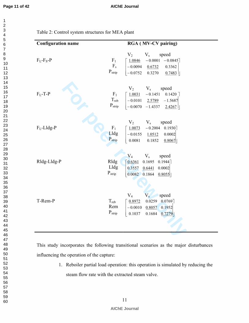
For peer review only
11
Table 2: Control system structures for MEA plant
Configuration name
RGA ( MV-CV pairing)
FL-FS-P F1
Fs
Pstrip
V2 Vs speed
−
−
−−
748303270007520
336206732000940
084500001008461
...
...
...
FL-T-P F1
Treb
Pstrip
V2 Vs speed
−−
−−
−
426724337100700
568715789201010
142001451000311
...
...
...
FL-Lldg-P F1
Lldg
Pstrip
V2 Vs speed
−
−
806701852000810
000200512101550
193002004000731
...
...
...
Rldg-Lldg-P Rldg
Lldg
Pstrip
V4 Vs speed
805501864000820
000206441035570
194401695063610
...
...
...
T-Rem-P Treb
Rem
Pstrip
V4 Vs speed
−
727901684010370
195208057000100
076900259089720
...
...
...
This study incorporates the following transitional scenarios as the major disturbances
influencing the operation of the capture:
1. Reboiler partial load operation: this operation is simulated by reducing the
steam flow rate with the extracted steam valve.
Page 11 of 42
AIChE Journal
AIChE Journal
123456789101112131415161718192021222324252627282930313233343536373839404142434445464748495051525354555657585960

For peer review only
12
2. Power plant load reduction: this scenario is simulated by making
proportional step changes in both flue gas rate and power cycle total steam
rate. According to previous studies6,7
any change in inlet gas composition
is neglected.
3. Foaming in the columns: Foaming in amine solution plants is one of the
leading causes of plant upsets. The expansion of liquid due to passage of
vapor results in liquid buildup on the packing in the bed. Accumulating
liquid in one of the columns leads to reduced liquid holdup in other
inventories and endangers the operation of downstream pumps. Due to
sudden change in holdup the performance of absorption and/or stripping
might be also affected. This work simulates this condition by including a
factor in the hydraulic model of the absorber.
Level ratio control (LRC) on storage tanks is an alternative that replaces a conventional
one-tank level control to balance the liquid holdup between the lean and rich tanks.
Cascade control can provide improved performance over single loop control, especially
control loops that manipulate the variable being exposed to upstream disturbances. This
case study manipulated steam rate and solvent circulation rate, which are likely to vary
because of possible disturbances and fitted the potential control loops with cascade
control. Table 3 provides the list of control configurations with modifications (LRC and
cascade control) applied for the basic version of each structure.
Table 3: Evaluated basic control configurations with modifications
Configuration Alternatives
FL-FS-P Basic, Basic+LRC
FL-T-P Basic, Basic+LRC, Basic+LRC+T cascaded
FL-Lldg-P Basic, Basic+LRC, Basic+LRC+Lldg cascaded
Rldg-Lldg-P Basic, Basic+LRC, Basic+LRC+Lldg cascaded, Basic+LRC+Rldg cascaded,
Page 12 of 42
AIChE Journal
AIChE Journal
123456789101112131415161718192021222324252627282930313233343536373839404142434445464748495051525354555657585960

For peer review only
13
Basic+LRC+Rldg cascaded+ Lldg cascaded
T-Rem-P Basic, Basic+LRC, Basic+LRC+T cascaded, Basic+LRC+Rem cascaded,
Basic+LRC+T cascaded+ Rem cascaded
The dynamic performance of the proposed control structures is evaluated in response to
previously defined disturbances and abnormal conditions. For absorber and stripper
foaming the dynamic results are generated for a 10% step change in the packing bed
liquid holdup while maintaining control of the loops at their initial set points via PI
controllers. For partial load operation, besides looking at small changes in inputs we also
consider a wide range of conditions; that is, 80% and 60% reduction in reboiler and
power plant load respectively. In all cases of partial load operation, the liquid levels are
tightly controlled at their initial set points with PI controllers while the other controlled
variables utilize PI controllers at the optimum set points where the lost work is
minimized. For power plant load reduction it is also assumed that the control objective is
to maintain the removal at its initial design value (90%) as the power plant load varies
along with minimizing lost work at the new state. The tuning parameters of PI controllers
are calculated by using ITAE correlations to maximize the performance of each loop
while other closed control loops are in service.
The simulations of dynamic scenarios with small changes in the magnitude of
inputs have shown that all configurations are able to control the liquid levels in
acceptable ranges without any problem associated with pump operation. For operation
over the narrow range of conditions selected, figures show stripper response because this
variable can represent the overall performance of the plant such as response time and
smoothness of dynamics and determine if the compressor is operating safely during
dynamic scenarios. The following sections present a discussion of dynamic behavior of
the control structure in response to the introduced disturbances.
Page 13 of 42
AIChE Journal
AIChE Journal
123456789101112131415161718192021222324252627282930313233343536373839404142434445464748495051525354555657585960

For peer review only
14
Simulation Results
This section presents a discussion of dynamic performance of the control structures in
response to the introduced disturbances.
Reboiler steam rate reduction
The simulation outputs have shown that replacing level control on one of the tanks by
level ratio control for both tanks did not bring an improvement for all structures
excluding T-Rem-P in which LRC improves the pressure response by eliminating
undesirable oscillations (Figure 2). Based on the results, loading control, either directly
or indirectly performed in structures called FL-Lldg-P, Rldg-Lldg-P and T-Rem-P,
introduces some oscillations in the responses (Figures 2 and 3). Cascade control improves
the dynamics in the cases having oscillatory responses, such as FL-Lldg-P and Rldg-Lldg-
P. FL-T-P does not show oscillatory behavior and so fitting the TC loop with cascade
control does not change the response. Figure 4 compares the pressure response for all the
control structures subject to steam rate reduction. Although FL-Lldg-P and Rldg-Lldg-P
configurations were fitted by cascade control, their responses are not as smooth and fast
as the response of FL-Fs-P and FL-T-P.
Figure 2:
Figure 3:
Figure 4: Power plant load reduction
The effects of power plant load reduction on the capture operation is simulated
with various control structures by considering the dynamic performance with -10% step
changes in both flue gas rate and power cycle steam rate. This study shows that replacing
level control by level ratio control has no significant positive or negative effects on
dynamic responses in all the configurations. Controlling the rich and lean loading by
Page 14 of 42
AIChE Journal
AIChE Journal
123456789101112131415161718192021222324252627282930313233343536373839404142434445464748495051525354555657585960

For peer review only
15
liquid valve position and steam valve position leads to sustained oscillations that make
the plant unstable. Cascading rich loading control loop with a flow controller on the
liquid valve could substantially damp the oscillation and stabilize the system. Cascade
control on the lean loading has no effect on the response (Figure 5).
The basic version of T-Rem-P structure with or without level ratio control
exhibits a dampened response. Cascading either a temperature or a removal control loop
with a flow controller makes the response worse and when both loops are cascaded with
flow controllers, the system becomes unstable with sustained oscillation (Figure 6). This
case is an example of a system in which cascade control has adverse effects on dynamic
performance.
Figure 5:
Figure 6:
Figure 7:
According to Figure 7, by comparing the pressure responses provided by the most
effective version of control configurations to the partial load operation of power plant,
FL-T(cascade)-P and FL-Fs-P have the highest rank in terms of smoothness and minimum
settling time.
RGA is a well known method to pair the manipulated and controlled variables. However,
steady-state analysis shows this method is not always reliable to compare structure with
respect to the dynamic behavior during the transition time. Dynamic simulation shows
that FL-Lldg-P is more interactive than FL-T-P while RGA predicts that FL-Lldg-P is a
less interactive system than FL-T-P since the diagonal elements are much closer to unity
(Table 2).
Page 15 of 42
AIChE Journal
AIChE Journal
123456789101112131415161718192021222324252627282930313233343536373839404142434445464748495051525354555657585960

For peer review only
16
Absorber and stripper foaming scenarios
According to the outputs of simulating absorber and stripper foaming, level ratio
control provides a noticeable improvement on dynamics especially for Rldg-Lldg-P in
which the response is very oscillatory and for T-Rem-P where unstable sustained
oscillation is observed. Applying LRC results in stabilizing and damping the oscillations
(Figures 8 and 9).
Figure 8:
Figure 9:
Figure 10:
Cascade control is not an effective strategy for those control structures to reject the
foaming disturbance. Furthermore it makes the responses worse by introducing damped
or sustained oscillations. The comparison of the control structures (Figure 10) again
shows that FL-T(cascade)-P and FL-Fs-P have the highest rank in terms of smoothness and
minimum settling time.
Partial load operations over a wide range of operating conditions
This part of the study is focused on dynamic performance evaluation over a wide range of
operating conditions when the capture plant is run in one of the two partial load
operations. Two control configurations are selected among those discussed previously for
comparison:
1. FL-T (cascade)-P: because of its best dynamic performance among all
the structures for rejecting disturbances and bringing the plant to the
targeted set points for all scenarios.
2. Rldg(cascade)-Lldg(cascade)-P: because it is a highly interactive
system that produces oscillatory responses; however, it was successful
in set point tracking and disturbance rejection.
Page 16 of 42
AIChE Journal
AIChE Journal
123456789101112131415161718192021222324252627282930313233343536373839404142434445464748495051525354555657585960

For peer review only
17
It should be noted that the storage tanks are fitted with the level ratio control loop. The
objective is to examine those configurations in terms of the ability of controlling the
capture at new operating conditions and running the pumps and compressor safely in
response to the following cases:
1. Partial load operation of reboiler simulated in two phases:
Phase 1: Ramping steam rate from 100% to 20% load in 30 min at
time = 0
Phase 2: Ramping steam rate from 20% to 100% load in 30 min at
time = 60 min
2. Partial load operation of power plant; simulated in two phases:
Phase 1: Ramping flue gas rate and power cycle steam rate simultaneously
from 100% to 40% load in 10 min at time = 0
Phase 2: Ramping flue gas rate and power cycle steam rate simultaneously
from 40% to 100% load in 10 min at time = 60 min
Similar to the previous simulations of operation over a narrow range, this work selected
the set points of level control loops at the initial design values while the other control
loop set points are set at optimal values that have already been obtained by an off-line
steady state optimization. Therefore, in current simulations the set points vary with time
as the load changes.
According to the simulation outputs, both configurations have the ability to deal with
80% load change in the reboiler steam and maintain the stability of the capture plant. The
controlled variables (solvent rate, stripper pressure, lean and rich loading) show fast and
smooth set point tracking during forward and reverse phases of this operation.
A few controlled variables are not being controlled effectively. Reboiler temperature is
one of the variables that show non-smooth dynamic behavior with relatively large
transitional deviations from the set point. This situation is more noticeable for
Page 17 of 42
AIChE Journal
AIChE Journal
123456789101112131415161718192021222324252627282930313233343536373839404142434445464748495051525354555657585960

For peer review only
18
Rldg(cascaded)-Lldg(cascaded)-P where this variable is not controlled directly (Figure
11).
Liquid levels in the tanks are also not controlled well. As shown in Figure 12, the ratio of
levels shows a large drop after 0.5 hour which can result in operational problems such as
cavitation and the lean tank downstream pump running dry.
Figure 11:
Figure 12:
Simulation of the large change in power plant load (60%) shows that FL-T(cascade)-P
perfectly controls the capture at the desired set points with smooth and fast responses for
both forward and reverse operations. Rldg(cascaded)-Lldg(cascaded)-P is not a
successful structure for control nor does it stabilize the plant condition.
As shown in Figure 13, this configuration forces the stripper pressure to follow the set
point initially but just after finishing the input ramp, unstable oscillations are appearing in
the whole system, which results in some operational problems such as saturation of liquid
valves and eventually failure of the simulation. That is why Figure 13 does not show the
complete response of stripper pressure for this configuration.
Figure 13:
FL-T (cascade)-P shows good performance in controlling capture for large changes in
operating conditions. It is able to bring the plant to the new operating condition in less
than five min, which is relatively short for such a system in which the total liquid
residence time is about 11 min.
INFLUENCE OF STORAGE TANKS HOLD UP TIME ON DYNAMICS
The objective of this work is to provide a systematic approach to investigate the influence
of the residence time in the lean and rich tank on the quality of dynamics in response to a
few types of disturbances. In frequency response analysis, which is used to analyze this
Page 18 of 42
AIChE Journal
AIChE Journal
123456789101112131415161718192021222324252627282930313233343536373839404142434445464748495051525354555657585960

For peer review only
19
dynamic system, we apply a sinusoidal input and sketch a graph showing the output
response characteristics versus frequency of the input signal.
Stripper top pressure is selected as the output because it represents the compressor
operation and reflects the whole system dynamic behavior. The variation of flue gas rate,
total steam rate in power cycle, and absorber and stripper bed liquid holdups are
considered as disturbances for this analysis. The plant is fully controlled by the FL-
T(cascade)-P configuration (shown in Figure 14), proved to be the most effective control
structure among the evaluated ones, at initial set points for all control loops. The
simulation is run for each disturbance at a specific input frequency and then the
magnitude of the pressure oscillation is calculated relative to the design value in percent.
Figure 14:
The liquid residence time in absorber sump, stripper sump, absorber bed, and
stripper bed are initialized at 2, 2, 2, and 1 min, respectively, and they do not change
significantly as disturbances are applied. The liquid residence time in the storage tanks is
varied to see the effects on the magnitude of the oscillations.
Figure 15 represents the frequency response to the flue gas rate sinusoidal change. As
seen for all cases of holdup time in the tanks, there is a critical frequency (ωc) where the
maximum magnitude is located. Based on the simulations it is found that the critical
frequency corresponds to the response time of the system to the related input. Since the
frequency is the inverse of time, a higher critical frequency is equivalent to a faster
response of the system. Therefore this graph can elucidate two important dynamic
characteristics: the response time and the magnitude of output change.
Figure 15:
As seen in Figure 15, increasing the τ of the lean tank reduces the response time while at
the same time it increases the magnitude of the oscillation, an undesired effect. Increasing
Page 19 of 42
AIChE Journal
AIChE Journal
123456789101112131415161718192021222324252627282930313233343536373839404142434445464748495051525354555657585960

For peer review only
20
the τ of the rich tank produces a more sluggish response, however, there is an optimum
rich tank holdup between 2 and 10 min that minimizes the magnitude. Figure 16, showing
the dynamic response of the pressure to -10% step change in the flue gas rate, is
consistent with the above discussed results. As observed, a 5-min holdup in the rich tank
shows the minimum magnitude for the inverse response and 10-min holdup in the lean
tank provides the fastest response.
Figure 16:
Figure 17:
The change in the absorber bed liquid holdup (foaming) is the other disturbance in which
the associated frequency response is calculated and shown in Figure 17. Similar to the
flue gas rate change, changing the residence time of the tanks influences the dynamics
both in magnitude and response time. In contrast to the flue gas rate, increasing τ of the
lean tank increases the response time while increasing τ of the rich tank makes the
response faster. As observed in this figure, increasing the residence time in both tanks
reduces the magnitude; however, for the rich tank increasing the time from 5 to 10 min
does not have any benefit but adds an additional amine inventory cost. The step response
shown in Figure 18 confirms the interpretations of frequency response.
Frequency response analysis has shown that holdup time in storage tanks does not have a
significant impact on dynamics when the plant is subjected to the power cycle steam rate
change or stripper foaming.
Figure 18:
4.1 CONCLUSIONS
This paper has developed an effective multi-loop feedback control structure for a
CO2 capture system. Load variation and foaming in columns make this control problem
Page 20 of 42
AIChE Journal
AIChE Journal
123456789101112131415161718192021222324252627282930313233343536373839404142434445464748495051525354555657585960

For peer review only
21
challenging since they involve a combination of disturbance rejection and set point
tracking at the same time.
Frequency response analysis investigated the effects of holdup in storage tanks on
dynamic performance. The frequency plots provide important dynamic performance
information related to the response time and the magnitude of deviation from the target.
1. The most effective multi-loop control structure is to control the solvent rate by
the liquid valve, the reboiler temperature by the steam valve and the stripper
pressure by the compressor speed. Replacing the conventional level control on
one of the lean or rich tanks by a level ratio control not only keeps the liquid
holdup in balance in the tanks but also plays an important role in dampening
oscillations for the column foaming scenarios.
2. Controlling rich or lean loading or any combination such as CO2 removal is
not a proper strategy specifically when the plant has to be operated within
wide ranges of operation.
3. Cascading CO2 loading control loops with the flow controller dampens the
oscillations in response to the load changes, but performs poorly when
foaming occurs in one of the columns.
4. A multi-loop control system with FL-T (cascade)-P configuration with level
ratio control on the storage tanks shows a degree of satisfactory performance,
robustness and safe operation that would avoid the costs of developing an
advanced multivariable system.
5. Increasing the holdup times in lean and rich tanks is not always helpful to
damp the oscillations and reject the disturbances. It may increase either the
magnitude of overshoot and inverse responses or the response time of the
plant.
ACKNOWLEDGMENTS
Page 21 of 42
AIChE Journal
AIChE Journal
123456789101112131415161718192021222324252627282930313233343536373839404142434445464748495051525354555657585960
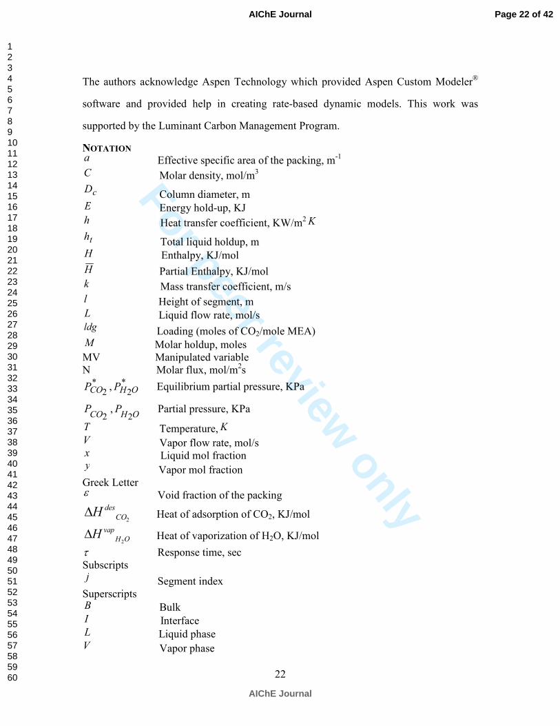
For peer review only
22
The authors acknowledge Aspen Technology which provided Aspen Custom Modeler®
software and provided help in creating rate-based dynamic models. This work was
supported by the Luminant Carbon Management Program.
NOTATION a Effective specific area of the packing, m
-1
C Molar density, mol/m3
cD Column diameter, m
E Energy hold-up, KJ h Heat transfer coefficient, KW/m
2 K
th Total liquid holdup, m H Enthalpy, KJ/mol
H Partial Enthalpy, KJ/mol k Mass transfer coefficient, m/s l Height of segment, m L Liquid flow rate, mol/s ldg Loading (moles of CO2/mole MEA) M Molar holdup, moles
MV Manipulated variable
N Molar flux, mol/m2s
*2COP , *
2OHP Equilibrium partial pressure, KPa
2COP ,
OHP
2 Partial pressure, KPa
T Temperature, K V Vapor flow rate, mol/s x Liquid mol fraction y Vapor mol fraction
Greek Letter ε Void fraction of the packing
2
des
COH∆ Heat of adsorption of CO2, KJ/mol
2
vap
H OH∆ Heat of vaporization of H2O, KJ/mol
τ Response time, sec
Subscripts j Segment index
Superscripts B Bulk I Interface L Liquid phase V Vapor phase
Page 22 of 42
AIChE Journal
AIChE Journal
123456789101112131415161718192021222324252627282930313233343536373839404142434445464748495051525354555657585960

For peer review only
23
REFERENCES
1. Bergerson JA, Lave LB. Baseload coal investment decisions under uncertain carbon
legislation. Environ. Sci. Technol. 2007;41:3431–3436.
2. Freguia S, Rochelle GT. Modeling of CO2 capture by aqueous MEA. AIChE J.,
2003;49:1676–1686.
3. Oyenekan BA, Rochelle GT. Alternative stripper configuration for CO2 capture by
aqueous amines, AIChE J., 2007;53:3144–3154.
4. Plaza JM, Chen E, Rochelle GT. Absorber intercooling in CO2 absorption by
Piperazine promoted Potassium Carbonate. AIChE J. 2010:56: 905–914.
5. Van Wagener DH, Rochelle GT. Stripper configurations for CO2 capture by aqueous
MEA and PZ. Energy Proc. 3011;4: 1323–1330.
6. Kvamsdal HM, Jakobsen JP, Hoff KA. Dynamic modeling and simulation of a CO2
absorber column for post-combustion CO2 capture. Chem. Eng. & Proc.
2009;48:135–144.
7. Lawal A, Wang M, Stephenson P, Koumpouras G, Yeung H. Dynamic modeling and
analysis of post-combustion CO2 chemical absorption process for coal-fired
power plants. Fuel. 2010; 89:2791–2801.
8. Ziaii S, Rochelle GT, Edgar TF. Dynamic modeling to minimize energy use for CO2
capture in power plants by aqueous Monoethanolamine. Ind. Eng. Chem. Res.
2009;48: 6105–6111.
9. Gunaseelan P, Wankat PC. Transient pressure and flow predictions for concentrated
packed absorbers using a dynamic nonequilibrium model. Ind. Eng. Chem. Res.
2002;41:5775–5788.
10. Peng J, Edgar TF, Eldridge RB. Dynamic rate-based and equilibrium models for a
packed reactive distillation column. Chem. Eng. Sci. 2003;58: 2671–2680.
11. Seborg DE, Edgar TF, Mellichamp DA. Process Dynamics and Control (2nd
edition).
New York:Wiley, 2004.
12. Chalmers H, Gibbins J, Leach M. Initial assessment of flexibility of pulverized coal-
fired power plants with CO2 capture. 3rd International Conference on Clean Coal
Technologies for our Future, 2007; Sardinia, Italy.
13. Ziaii S, Cohen SM, Rochelle GT, Edgar TF, Webber ME. Dynamic operation of
amine scrubbing in response to electricity demand and pricing. Energy Proc.
2009;1: 4047–4053.
14. Schach MO, Schneider R, Schramm H, Repke JU. Control structure design for CO2
absorption processes for large operating ranges. PCCC1, 2011: Abu Dhabi.
15. Faanes A, Skogestad S, A systematic approach to the design of buffer tanks. Comp.
& Chem. Eng. 2000;24:1395–1401.
16. Luyben WL. Dynamics and control of recycle systems. 1. simple open-loop and
closed-loop systems. Ind. Eng. Chem. Res. 1993;32: 466–475.
Page 23 of 42
AIChE Journal
AIChE Journal
123456789101112131415161718192021222324252627282930313233343536373839404142434445464748495051525354555657585960
For peer review only
24
17. Aboudheir A, Tontiwachwuthikul P, Idem R. Rigorous model for predicting the
behavior of CO2 absorption into AMP in packed-bed absorption columns. Ind.
Eng. Chem. Res.. 2006;45:2553–2557.
18. Lucquiaud M. Steam cycle options for capture-ready power plants, retrofits and
flexible operation with post combustion CO2 capture. Ph.D. Dissertation,
Imperial College, London, England. 2010.
Page 24 of 42
AIChE Journal
AIChE Journal
123456789101112131415161718192021222324252627282930313233343536373839404142434445464748495051525354555657585960

For peer review only
215x279mm (200 x 200 DPI)
Page 25 of 42
AIChE Journal
AIChE Journal
123456789101112131415161718192021222324252627282930313233343536373839404142434445464748495051525354555657585960

For peer review only
215x279mm (222 x 189 DPI)
Page 26 of 42
AIChE Journal
AIChE Journal
123456789101112131415161718192021222324252627282930313233343536373839404142434445464748495051525354555657585960

For peer review only
215x279mm (180 x 180 DPI)
Page 27 of 42
AIChE Journal
AIChE Journal
123456789101112131415161718192021222324252627282930313233343536373839404142434445464748495051525354555657585960
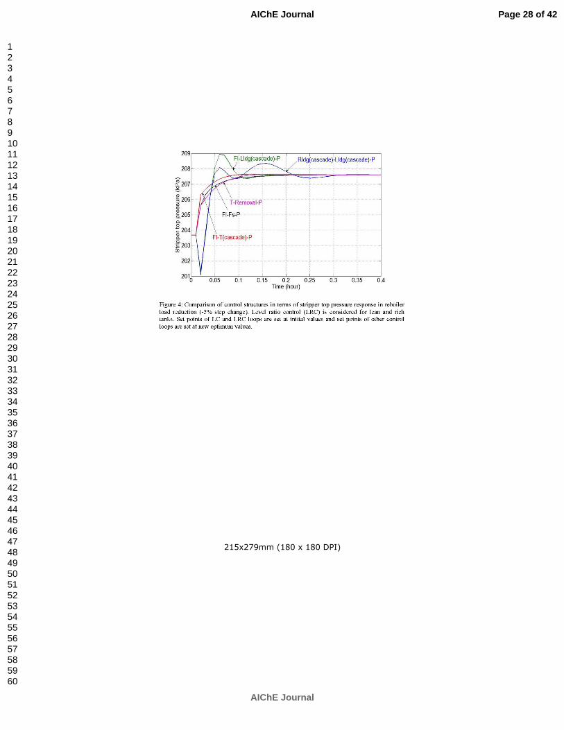
For peer review only
215x279mm (180 x 180 DPI)
Page 28 of 42
AIChE Journal
AIChE Journal
123456789101112131415161718192021222324252627282930313233343536373839404142434445464748495051525354555657585960

For peer review only
215x279mm (222 x 194 DPI)
Page 29 of 42
AIChE Journal
AIChE Journal
123456789101112131415161718192021222324252627282930313233343536373839404142434445464748495051525354555657585960

For peer review only
215x279mm (180 x 180 DPI)
Page 30 of 42
AIChE Journal
AIChE Journal
123456789101112131415161718192021222324252627282930313233343536373839404142434445464748495051525354555657585960

For peer review only
215x279mm (180 x 180 DPI)
Page 31 of 42
AIChE Journal
AIChE Journal
123456789101112131415161718192021222324252627282930313233343536373839404142434445464748495051525354555657585960

For peer review only
215x279mm (180 x 180 DPI)
Page 32 of 42
AIChE Journal
AIChE Journal
123456789101112131415161718192021222324252627282930313233343536373839404142434445464748495051525354555657585960
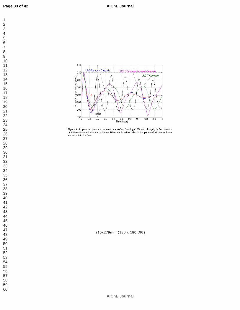
For peer review only
215x279mm (180 x 180 DPI)
Page 33 of 42
AIChE Journal
AIChE Journal
123456789101112131415161718192021222324252627282930313233343536373839404142434445464748495051525354555657585960
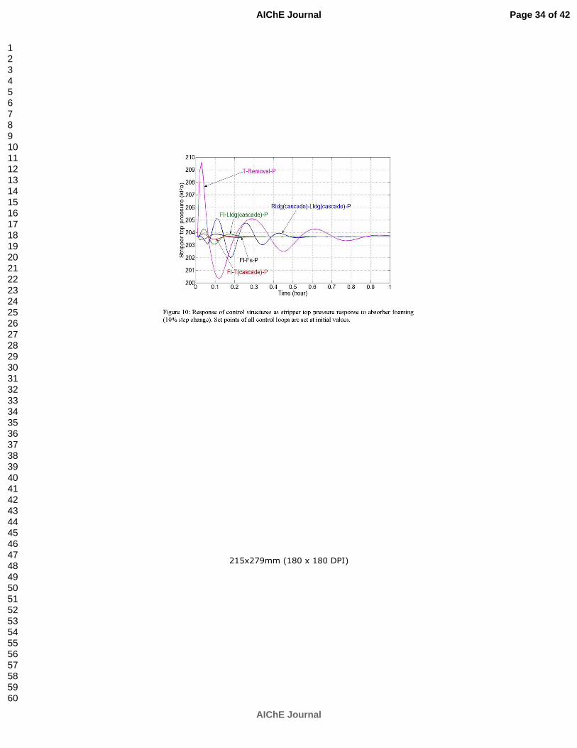
For peer review only
215x279mm (180 x 180 DPI)
Page 34 of 42
AIChE Journal
AIChE Journal
123456789101112131415161718192021222324252627282930313233343536373839404142434445464748495051525354555657585960
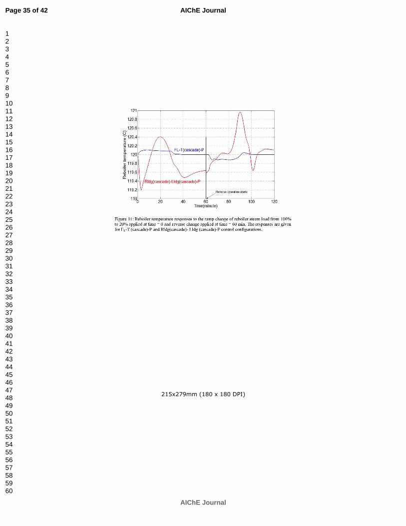
For peer review only
215x279mm (180 x 180 DPI)
Page 35 of 42
AIChE Journal
AIChE Journal
123456789101112131415161718192021222324252627282930313233343536373839404142434445464748495051525354555657585960
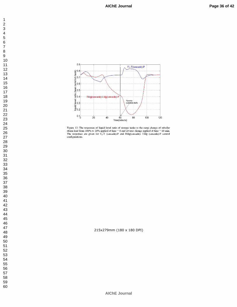
For peer review only
215x279mm (180 x 180 DPI)
Page 36 of 42
AIChE Journal
AIChE Journal
123456789101112131415161718192021222324252627282930313233343536373839404142434445464748495051525354555657585960
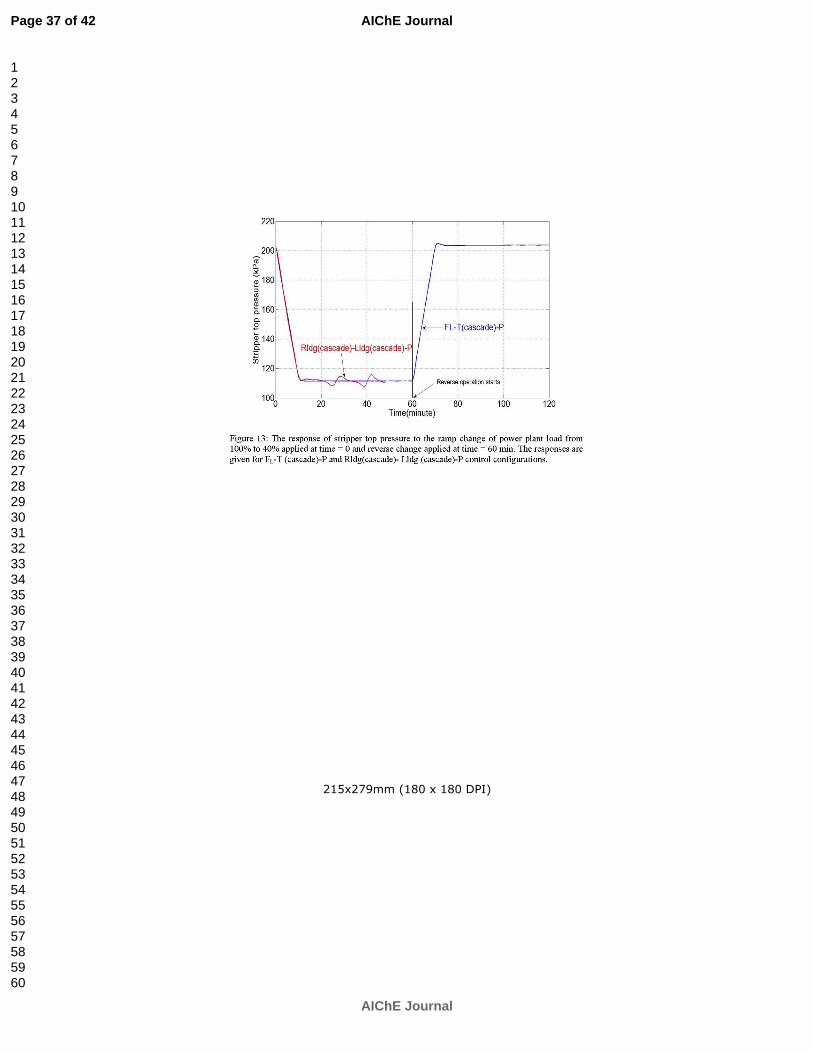
For peer review only
215x279mm (180 x 180 DPI)
Page 37 of 42
AIChE Journal
AIChE Journal
123456789101112131415161718192021222324252627282930313233343536373839404142434445464748495051525354555657585960

For peer review only
215x279mm (180 x 180 DPI)
Page 38 of 42
AIChE Journal
AIChE Journal
123456789101112131415161718192021222324252627282930313233343536373839404142434445464748495051525354555657585960
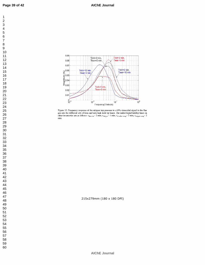
For peer review only
215x279mm (180 x 180 DPI)
Page 39 of 42
AIChE Journal
AIChE Journal
123456789101112131415161718192021222324252627282930313233343536373839404142434445464748495051525354555657585960
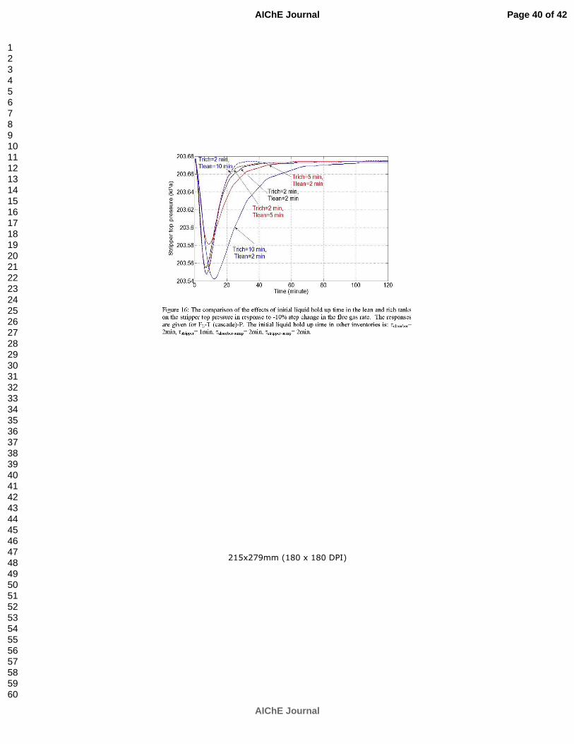
For peer review only
215x279mm (180 x 180 DPI)
Page 40 of 42
AIChE Journal
AIChE Journal
123456789101112131415161718192021222324252627282930313233343536373839404142434445464748495051525354555657585960

For peer review only
215x279mm (180 x 180 DPI)
Page 41 of 42
AIChE Journal
AIChE Journal
123456789101112131415161718192021222324252627282930313233343536373839404142434445464748495051525354555657585960

For peer review only
215x279mm (180 x 180 DPI)
Page 42 of 42
AIChE Journal
AIChE Journal
123456789101112131415161718192021222324252627282930313233343536373839404142434445464748495051525354555657585960
Related Documents