Co-evolving predator and prey robots: Do ‘arms races ...

1

Co-evolving predator and prey robots:Do ‘arms races’ ar ise in ar tificial evolution?

Stefano Nolfi* Dario Floreano~

*Institute of Psychology, National Research CouncilViale Marx 15, Roma, Italy

[email protected]~LAMI - Laboratory of MicrocomputingSwiss Federal Institute of Technology

EPFL, Lausanne, [email protected]

AbstractCo-evolution (i.e. the evolution of two or more competing populations with coupled fitness)has several features that may potentiall y enhance the power of adaptation of artificialevolution. In particular, as discussed by Dawkins and Krebs [3], competing populations mayreciprocally drive one another to increasing levels of complexity by producing an evolutionary“arms race” . In this paper we will investigate the role of co-evolution in the context ofevolutionary robotics. In particular, we will try to understand in what conditions co-evolutioncan lead to “arms races” . Moreover, we will show that in some cases artificial co-evolution hasa higher adaptive power than simple evolution. Finall y, by analyzing the dynamics of co-evolved populations, we will show that in some circumstances well adapted individuals wouldbe better advised to adopt simple but easil y modifiable strategies suited for the currentcompetitor strategies rather than incorporate complex and general strategies that may beeffective against a wide range of opposing counter-strategies.

1. Introduction

Co-evolution (i.e. the evolution of two or more competing populations with coupledfitness) has several features that may potentially enhance the adaptation power ofartificial evolution1.

First, the co-evolution of competing populations may produce increasingly complexevolving challenges. As discussed by Dawkins and Krebs [3] competing populationsmay reciprocally drive one another to increasing levels of complexity by producing anevolutionary “arms race”. Consider for example the well-studied case of two co-evolving populations of predators and prey [16]: the success of predators implies afailure of the prey and conversely, when prey evolve to overcome the predators theyalso create a new challenge for them. Similarly, when the predators overcome the newprey by adapting to them, they create a new challenge for the prey. Clearly thecontinuation of this process may produce an ever-greater level of complexity (althoughthis does not necessarily happen, as we will see below). As Rosin and Belew [20] pointout, it is like producing a pedagogical series of challenges that gradually increase thecomplexity of the corresponding solutions. For an example of how a progressiveincrease in the complexity of the training sample may allow a neural network to learn acomplex task that cannot otherwise be learned see [4].

1 By adaptive power we mean the ability to solve complex tasks. In the context of predator and prey, thismeans the ability to catch a very efficient prey or to escape a very efficient predator.

2

This nice property overcomes the problem that if we ask evolution to find a solutionto a complex task we have a high probabil ity of failure while if we ask evolution to finda solution first to a simple task and then for progressively more complex cases, we aremore likely to succeed. Consider the predators and prey case again. At the beginning ofthe evolutionary process, the predator should be able to catch its prey which have a verysimple behavior and are therefore easy to catch; likewise, prey should be able to escapesimple predators. However, later on, both populations and their evolving challenges willbecome progressively more and more complex. Therefore, even if the selection criterionremains the same, the adaptation task may become progressively more complex.

Secondly, because the performance of the individual in a population depends alsoon the individual strategies of the other population which vary during the evolutionaryprocess, the ability for which individuals are selected is more general2 (i.e., it has tocope with a variety of different cases) than in the case of an evolutionary process inwhich co-evolution is not involved. The generality of the selection criterion is a veryimportant property because the more general the criterion, the larger the number ofways of satisfying it (at least partially) and the greater the probability that better andbetter solutions will be found by the evolutionary process.

Let us again consider the predator and prey case. If we ask the evolutionary processto catch one individual prey we may easily fail. In fact, if the prey is very efficient, theprobability that an individual with a randomly generated genotype may be able to catchit is very low. As a consequence, all individuals will be scored with the same null valueand the selective process cannot operate. On the contrary, if we ask the evolutionaryprocess to find a predator able to catch a variety of different prey, it is much moreprobable that it will find an individual in the initial generations able to catch at least oneof them and then select better and better individuals until one predator able to catch theoriginal individual prey is selected.

Finally, competing co-evolutionary systems are appealing because the ever-changing fitness landscape, due to changes in the co-evolving species is potentiallyuseful in preventing stagnation in local minima. From this point of view, co-evolutionmay have consequences similar to evolving a single population in an ever-changingenvironment. Indeed the environment changes continuously given the fact that the co-evolving species is part of the environment of each evolving population.

Unfortunately a continuous increase in complexity is not guaranteed. In fact, co-evolving populations may cycle between alternative class of strategies that, althoughthey do not produce advantages in the long run, may produce a temporary improvementover the co-evolving population. Imagine, for example, that in a particular momentpopulation A adopts the strategy A1 which gives population A an advantage overpopulation B which adopts strategy B1. Imagine now that there is a strategy B2

(genotypically similar to B1) that gives population B an advantage over strategy A1.Population B will easily find and adopt strategy B2. Imagine now that there is a strategyA2 (genotypically similar to A1) that provides an adaptive advantage over strategy B2.Population A wil l easily find and adopt strategy A2. Finally imagine that previouslydiscovered strategy B1 provides an advantage over strategy A2. Population B will comeback to strategy B1. At this point also population A will come back to strategy A1

2 We will use the term ‘general strategy’ or ‘general solution’ to indicate selected individuals able to copewith different tasks. In the context of predator and prey we will indicate with the term ‘general’ thestrategy adopted by a predator which is able to catch a large number of prey adopting different, notnecessarily complex, strategies.

3

(because, as explained above, it is effective against strategy B1) and the cycle of thesame strategies will be repeated over and over again (Figure 1).

generations

A1 > B1

B2 > A1

A2 > B2

B1 > A2

A1 B1

A1 B2

A2 B2

A2 B1

A1 B1

A1 B2

A2 B2

A2 B1

…….…….

Pop1 Pop2

Figure 1. The same strategies (A1 and A2 in population A) and (B1 and B2 in population B) may beselected over and over again throughout generations as is shown in the right hand side of the figure if theinteraction between them looks li ke what is represented on the left side of the Figure. In this case therepeated cycle corresponds to 4 different combinations of strategies.

Notice how the cycling may involve two or more different strategies for eachpopulation but also two or more different groups of strategies.

Parker [18] was the first to hypothesize that parent-offspring and intersexual ‘armsraces’ may end up in cycles. Dawkins and Krebs [3] noted how this hypothesis can beapplied to asymmetric arms races in general.

Of course this type of phenomenon may cancel out all the previously describedadvantages because, if co-evolution quickly falls into a cycling phase, the number ofdifferent solutions discovered might be quite limited. In fact, there is no need todiscover progressively more complex strategies. It is sufficient to re-discover previouslyselected strategies that can be adopted with a limited number of changes. Moreover, itshould be noted that cycling is not the only possible cause which may prevent theemergence of ‘arms races’ .

In this paper we will investigate the role of co-evolution in the context ofevolutionary robotics. In particular, we will try to understand in which conditions, ifany, co-evolution can lead to “arms races” in which two populations reciprocally driveone another to increasing levels of complexity.

After introducing our experimental framework in section 2.1 and 2.2 we willdescribe the result of a first basic experiment in section 2.3. As we will see, theinnovations produced in this first experiments may easily be lost because theevolutionary process quickly falls into a cycling phase in which the same type ofsolutions are adopted over and over by the two co-evolving populations. In section 2.4we will show how the tendency to cycle between the same type of strategies may bereduced by preserving all previously discovered strategies and by using all of them totest the individual of the current population (we will refer to this technique as ‘Hall ofFame’ co-evolution). We will also point out that this technique, which is biologicallyimplausible, has its own drawbacks. In section 2.5 in fact, we will see how ‘Hall ofFame’ co-evolution does not necessary produce better performance than simple co-evolution. On the contrary, in the case of the experiment described in this section,simple co-evolution tend to outperform ‘Hall of Fame’ co-evolution. In section 2.5 wewill also see how ‘arms races’ can emerge and indeed produce better and better

4

solutions. In section 2.6 we will see how increasing the environmental richness maydecrease the probabil ity to fall in cycling phases. Finally, in section 2.7 we will see howco-evolution can solve problems that evolution alone cannot. In other words, we willshow how in some circumstances co-evolution has an higher adaptive power thanevolution of a single population.

2. Co-evolving predator and prey robots

Several researchers have investigated co-evolution in the context of predators andprey in simulation [11, 12, 1, 2]. More recently, we have tried to investigate thisframework first by using realistic simulations based on the Khepera robot [7, 8] andsubsequently the real robots [9]. Up to now, we replicated on the real robots theexperiments which will be described in section 2.3. By comparing the results obtainedin simulation with those obtained with the real robots in this case we did not observeany significant difference in term of performance and co-evolutionary dynamic.Although, not all the strategies observed in simulation were also observed in theexperiments performed in the real environment. In this case, in fact, the presence ofmuch larger noise filtered out brittle solutions [9].

In this section, we will first describe our experimental framework and the resultsobtained in a simple case. Then, we will describe other experimental conditions moresuitable to the emergence of ‘arms races’ between the two competing populations.

2.1 The experimental framework

As often happens, predators and prey belong to different species with differentsensory and motor characteristics. Thus, we employed two Khepera robots, one ofwhich (the Predator) was equipped with a vision module while the other (the Prey) hada maximum available speed set to twice that of the predator. The prey has a blackprotuberance, which can be detected by the predator everywhere in the environment(see Figure 2). The two species could evolve in a square arena 47 x 47 cm in size withhigh white walls so that predator could always see the prey (within the visual angle) as ablack spot on a white background.

Figure 2. Prey and predator (left to right).

5

Both individuals were provided with eight infrared proximity sensors (six on thefront side and two on the back) which had a maximum detection range of 3-4 cm in ourenvironment. For the predator we considered the K213 module of Khepera which is anadditional turret that can be plugged in directly on top of the basic platform. It consistsof a 1D-array of 64 photoreceptors which provide a linear image composed of 64 pixelsof 256 gray-levels each, subtending a view-angle of 36°. However the K213 modulealso allows detection of the position in the image corresponding to the pixel withminimal intensity. We used this facil ity by dividing the visual field into five sectors ofabout 7° each corresponding to five simulated photoreceptors (see Figure 3). If the pixelwith minimal intensity lay inside the first sector, then the first simulated photoreceptorwould become active; if the pixel lay inside the second sector, then the secondphotoreceptor would become active, etc. From the motor point of view, we set themaximum wheel speed in each direction to 80mm/s for the predator and 160mm/s forthe prey.

Figure 3. Left and center: details of simulation of vision, of neural network architecture, and of geneticencoding. The prey differs from the predator in that it does not have 5 input units for vision. Eight bitscode each synapse in the network. Right: Initial starting position for prey (left, empty disk with smallopening corresponding to frontal direction) and predator (right, back disk with line corresponding tofrontal direction) in the arena. For each competition, the initial orientation is random.

In line with some of our previous work [6], the robot controller was a simpleperceptron comprising two sigmoid units with recurrent connection at the output layer.The activation of each output unit was used to update the speed value of thecorresponding wheel every 100ms. In the case of the predator, each output unit receivedconnections from five photoreceptors and from eight infrared proximity sensors. In thecase of the prey, each output unit received input only from 8 infrared proximity sensors,but its activation value was multiplied by 2 before setting the wheel speed.

In order to keep things as simple as possible and given the small size of theparameter set, we used direct genetic encoding [22]: each parameter (including recurrentconnections and threshold values of output units) was encoded using 8 bits. For thesame reason, the architecture was kept fixed, and only synaptic strengths and outputunits threshold values were evolved. Therefore, the genotype of the predator was 8 x (30synapses + 2 thresholds) bits long while that of prey was 8 x (20 synapses + 2thresholds) bits long. It should be noted that the type of architecture we selected mayconstraint the type of solutions which will be obtained during the evolutionary process.

6

In principle, it would be better to evolve both the architecture and the weights at thesame time. However, how to encode the architecture of the network into the genotype isstill an open and complex research issue in itself. Moreover, even more complexgenotype-to-phenotype mappings (which would allow the evolution of the architecturetoo) might still constrain the evolutionary process in certain, albeit different ways.

Two populations of 100 individuals each were co-evolved for 100 generations.Each individual was tested against the best competitors of the previous generations (asimilar procedure was used in [21, 2]). In order to improve co-evolutionary stability,each individual was tested against the best competitors of the ten previous generations(on this point see also below). At generation 0, competitors were randomly chosenwithin the same generation, whereas in the other 9 initial generations they wererandomly chosen from the pool of available best individuals of previous generations.

For each competition, the prey and the predator were always positioned on ahorizontal line in the middle of the environment at a distance corresponding to half theenvironment width, but always at a new random orientation. The competition endedeither when the predator touched the prey or after 500 motor updates (corresponding to50 seconds at maximum on the physical robot). The fitness function for eachcompetition was simply 1 for the predator and 0 for the prey if the predator was able tocatch the prey and, conversely 0 for the predator and 1 for the prey if the latter was ableto escape the predator. Individuals were ranked after fitness performance in descendingorder and the best 20 were allowed to reproduce by generating 5 offspring each.Random mutation (bit substitution) was applied to each bit with a constant ofprobability pm=0.023.

For each set of experiments we ran 10 replications starting with different randomlyassigned genotypes.

In this paper we will refer to data obtained in simulation. A simulator developedand extensively tested on Khepera by some of us was used [15].

2.2 Measuring adaptive progress in co-evolving populations

In competitive co-evolution the reproduction probabil ity of an organism withcertain traits can be modified by the competitors, that is, changes in one species affectthe reproductive value of specific trait combinations in the other species, It might thushappen that progress achieved by one lineage is reduced or eliminated by the competingspecies. This phenomenon, which is referred to as the “Red Queen Effect” [19], makesit hard to monitor progress by taking measures of the fitness throughout generations. Infact, because fitnesses are defined relative to a co-evolving set of traits in the otherindividuals, the fitness landscapes for the co-evolving individuals vary. As aconsequence, for instance, periods of stasis in the fitness value of the two populationsmay correspond to a period of tightly-coupled co-evolution.

In order to avoid this problem, different measure techniques have been proposed.Cliff and Mil ler [1] have devised a way of monitoring fitness performance by testing the

3 The parameters used in the simulations described in this paper are mostly the same as in the simulationdescribed in [7]. However, in these experiments we used a simpler fitness formula (a binary value insteadof a continuous value proportional to the time necessary for the predator to catch the prey). Moreover, tokeep the number of parameters as small as possible, we did not use crossover. In the previousexperiments, in fact, we did not notice any significant difference in experiments conducted with differentcrossover rates.

7

performance of the best individual in each generation against all the best competingancestors which they call CIAO data (Current Individual vs. Ancestral Opponents).

A variant of this measure technique has been proposed by us and has been calledMaster Tournament [7]. It consists in testing the performance of the best individual ofeach generation against each best competitor of all generations. This latter techniquemay be used to select the best solutions from an optimization point of view (see [7]).Both techniques may be used to measure co-evolutionary progress (i.e. the discovery ofmore general and effective solutions).

2.3 Evolution of predator and prey robots: a simple case.

The results obtained by running a set of experiments with the parameter describedin section 2.1 are shown below. Figure 4 represents the results of the MasterTournament, i.e the performance of the best individual of each generation tested againstall best competitors from that replication. The top graph represents the average result of10 simulations. The bottom graph represents the result of the best run.

0

25

50

75

100

0 25 50 75 100

generations

fitne

ss PredatorPrey

0

25

50

75

100

0 25 50 75 100

generations

fitne

ss Predator

Prey

Figure 4. Performance of the best individuals of each generation tested against all the best opponents ofeach generation (Master Tournament). Performance may range from 0 to 100 because each individual istested once against each best competitor of 100 generations. The top graph shows the average result of 10different replications. The bottom graph shows the result in the best repli cation (i.e. the simulation inwhich predators and prey attain their best performance). Data were smoothed using rolling average overthree data points.

8

These results show that, at least in this case, phases in which both predators andprey produce increasingly better results are sometimes followed by sudden drops inperformance (see the bottom graph of Figure 4). As a consequence, if we look at theaverage result of different replications in which increase and drop phases occur indifferent generations, we observe that performance does not increase at all throughoutgenerations (see the top graph of Figure 4). In other words the efficacy and generality ofthe different selected strategies does not increase evolutionarily. In fact, individuals oflater generations do not necessarily score well against competitors of much earliergenerations (see Figure 5, right side). Similar cases have been described in [2, 21].

The ‘arms races’ hypothesis would be verified if, by measuring the performance ofeach best individual against each best competitor, a picture approximating that shownon the left side of Figure 5 could be obtained. In this ideal situation, the bottom-left partof the square, which corresponds to the cases in which predators belong to more recentgenerations than the prey, is black (i.e. the predator wins). Conversely, the top right partof the square, which corresponds to the cases in which the prey belong to more recentgenerations than the predators, is white (i.e. the prey wins). Unfortunately, what actuallyhappens in a typical run is quite different (see right part of Figure 5). The distribution ofblack and white spots does not differ significantly in the two sub-parts of the square.

Figure 5. Performance of the best individuals of each generation tested against all the best opponents ofeach generation. The black dots represent individual tournaments in which the predators win while thewhite dots represent tournaments in which the prey wins. The picture on the left represents an idealsituation in which predators are able to catch all prey of previous generations and the prey are able toescape all predators of previous generations. The picture on the right represents the result for the bestsimulation (the same shown in Figure 4).

This does not imply that the co-evolutionary process is unable to find interestingsolutions as we will show below (see also [7]). This merely means that effectivestrategies may be lost instead of being retained and refined. Such good strategies, infact, are often replaced by other strategies that, although providing an advantage overthe current opponents, are much less general and effective in the long run. In particular,this type of process may lead to the cycling process described in section 1 in which thesame strategies are lost and re-discovered over and over again.

The cycling between the same class of strategies is actually what happens in theseexperiments. If we take a look at the qualitative aspects of the behavior of the bestindividuals of successive generations we see that in all replications, evolving predatorsdiscover and rediscover two different classes of strategies: (A1) track the prey and try tocatch it by approaching it; (A2) track the prey while remaining more or less in the samearea and attacking the prey only on very special occasions (when the prey is in aparticular position relative to the predator). Similarly the prey cycles between two

9

classes of strategies: (B1) stay still or hidden close to a wall waiting for the predator andeventually trying to escape when the IR sensors detect the predator (notice thatpredators usually keep themselves away from walls to avoid crashes); (B2) move fast inthe environment, avoiding both the predator and the walls.

Now, as in Figure 1, the strategy A1 is generally effective against B1, in fact thepredator will reach the prey if the prey does not move too much and has a good chanceof succeeding given that the prey can only detect predators approaching from certaindirections because of the uneven distributions of the infrared sensors around the body.Strategy B2 is effective against strategy A1 because the prey is faster than the predatorand so, if the predator tries to approach a moving fast prey, it has little chance ofcatching it. Strategy A2 is effective against strategy B2 because, if the prey moves fast inthe environment, the predator may be able to catch it easily by waiting for the prey itselfto come close. Finally, strategy B1 is very effective against strategy A2. In fact if thepredator does not approach the prey and the prey stays still, the prey will never riskbeing caught. This type of relation between different strategies produces a cyclingprocess similar to that described in Figure 1.

predators

100

150

200

250

300

0 2.5 5 7.5 10

speed

dist

ance

G0-24G25-49G50-74G75-99A1

A2

prey

100

150

200

250

300

0 5 10 15 20

speed

dist

ance

G0-24G25-49G50-74G75-99

B1

B2

Figure 6. Position of the best predator and prey of successive generations in the phenotype space (top andbottom graph, respectively). The Y and X axes represent the average speed (i.e. computed as the absolutevalue of the algebraic sum of the two wheels) and the average distance (i.e. the distance in mm between

10

two competing individuals), respectively. Individuals of different generations are shown with differentlabels but, for graphic reasons, individuals of each 25 successive generations are shown with the samelabel. Average speed and distance have been computed by testing the best individual of each generationagainst the best competitor of each generation.

The cycling process is driven in general by prey which after adopting one of thetwo classes of strategies for several generations suddenly shift to the other strategy. Thisswitch forces predators to shift their strategy accordingly. This is also shown in Figure 5(right side) in which the reader can easily see that the main source of variation is on theX-axis which represents how performance vary for prey of different generations.

What actually happens in the experiments is not so simple as in the description wehave just given because of several factors: (1) the strategies described are not singlestrategies but classes of similar strategies. So for example there are plenty of differentways for the predator to approach the prey and different ways may have differentprobabilities of being successful against the same opposing strategies; (2) the advantageor disadvantage of each strategy against another strategy varies quantitatively and isprobabilistic (each strategy has a given probabil ity of beating a competing strategy); (3)populations at a particular generation do not include only one strategy but a certainnumber of different strategies although they tend to converge toward a single one; (4)different strategies may be easier to discover or re-discover than others.

However the cycling process between the different classes of strategies describedabove can be clearly identified. By analyzing the behavior of the best individuals of thebest simulation (the same as that described in Figures 3 and 4), for example, we can seethat the strategy B2 discovered and adopted by prey at generation 21 and thenabandoned after 15 generations is rediscovered and re-adopted at generation 58 and thenat generation 98. Similarly the strategy A2, first discovered and adopted by the predatorat generation 10 and then abandoned after 28 generations for strategy A1, is thenrediscovered at generation 57. Interestingly, however, prey also discover a variation ofstrategy B1 that includes also some of the characteristics of strategy B2. In this case,prey move in circles waiting for the predator as in strategy B1. However, as soon as theydetect the predator with their IR sensors, they start to move quickly exploring theenvironment as in strategy B2. This type of strategy may in principle be effective againstboth strategies A1 and A2. However sometimes prey detect the predator too late,especially when the predator approaches the prey from its left or right rear side which isnot provided with IR sensors.

This cycling dynamics is shown also in Figure 6 which represents the position ofthe best predator and prey of successive generations in a two-dimensional phenotypespace. To represent the phenotype space we considered two measures that arerepresentative of the different strategies: the average speed and the average distancefrom the competitor (these two dimensions have been subjectively chosen to illustratethe qualitative features of the behaviors that we observed). In the case of the prey, twodifferent classes of phenotype corresponding to the strategies B1 and B2 can be clearlyidentified. In the case of predators, on the other hand, a continuum of strategies can beobserved between strategies that can be classified as typically A1 or A2. In both cases,however, examples of each class of strategies can be found in the first and in successivegenerations, indicating that the same type of strategy is adopted over and over again.

11

2.4 Testing individuals against all discovered solutions

In a recent article, Rosin and Belew [20], in order to encourage the emergence of‘arms races’ in a co-evolutionary framework, suggested saving and using as competitorsall the best individuals of previous generations:

So, in competitive coevolution, we have two distinct reasons to saveindividuals. One reason is to contribute genetic material to futuregenerations; this is important in any evolutionary algorithm. Selection servesthis purpose. Eliti sm serves this purpose directly by making complete copiesof top individuals.The second reason to save individuals is for purposes of testing. To ensureprogress, we may want to save individuals for an arbitrarily long time andcontinue testing against them. To this end, we introduce the ‘Hall of Fame’ ,which extends eliti sm in time for purposes of testing. The best individual fromevery generation, is retained for future testing.

From Rosin and Belew [20], pp. 8.

This type of solution is of course implausible from a biological point of view.Moreover, we may expect that, by adopting this technique, the effect of the co-evolutionary dynamic wil l be progressively reduced throughout generations with theincrease in number of previous opponents. In fact, as the process goes on, there is lessand less pressure to discover strategies that are effective against the opponent of thecurrent generation and greater and greater pressure to develop solutions capable ofimproving performance against opponents of previous generations.

However, as the authors show, in some cases this method may be more effectivethan a ‘standard’ co-evolutionary framework in which individuals compete only withopponents of the same or of the previous generation. More specifically, we think, it maybe a way to overcome the problem of the cycling of the same strategies. In thisframework in fact, ad hoc solutions that compete successfully against the opponent ofthe current generation but do not generalize to opponents of previous generations cannotspread in evolving populations.

We applied the Hall of Fame selection regime to our predator and prey frameworkand measured the performance of each best individual against each best competitor(Master Tournament). Results are obtained by running a new set of 10 simulations inwhich each individual is tested against 10 opponents randomly selected from allprevious generations (while in the previous experiments we selected 10 opponents fromthe immediately preceding generations). All the other parameters remain the same. Asshown in Figure 7 and 8, in this case, we obtain a progressive increase in performance.

Figure 7 shows how in this case the average fitness of the best individuals testedagainst all best competitors progressively increases throughout generations, ultimatelyattaining near to optimal performances. Figure 8 shows how this is accomplished bybeing able to beat most of the opponents of previous generations. The results do notexactly match the ideal situation described in Figure 5 (left side) in which predators andprey are able to beat all individuals of previous generations. In the best simulationdescribed in Figure 7 (bottom graph) and Figure 8, for example, there are two phases in

12

which prey are unable to beat most of the predators of few generations before. Thegeneral picture, however, approximates the ideal one.

0

25

50

75

100

0 25 50 75 100

generations

fitne

ss PredatorPrey

0

25

50

75

100

0 25 50 75 100

generations

fitne

ss PredatorPrey

Figure 7. Performance of the best individuals of each generation tested against all the best opponents ofeach generation (Master Tournament). The top graph shows the average result of 10 different replications.The bottom graph shows the result in the best repli cation (i.e. the simulation in which predators and preyattain the best performance). Data were smoothed using a roll ing average over three data points.

Figure 8. Performance of the best individuals of each generation tested against all the best opponents ofeach generation. Black dots represent individual tournaments in which the predators win while white dotsrepresent tournaments in which the prey wins. Result for the best simulation (the same shown in Figure7).

If we look at the individual strategies selected throughout generations in theseexperiments, we see that they are of the same class of those described in the previoussection. However, in this case, the strategies are evolutionarily more stable (i.e. ingeneral they are not suddenly replaced by another strategy of a different class). Thisenables the co-evolutionary process to progressively refine current strategies instead of

13

cycling between different classes of strategies, restarting each time from the same initialstrategy.

The fact that individuals are tested against quite different strategies (i.e. competitorsrandomly selected from all previous generations) should enable the evolutionary processto find strategies that are more general (i.e. that are effective against a larger number ofcounter-strategies) than those obtained in the experiments described in the previoussection. To verify this hypothesis we tested the best 10 predators and prey obtained with‘standard’ co-evolution against the best 10 predators and prey obtained with ‘Hall ofFame’ co-evolution (i.e. the best predator and prey of each replication were selected).As can be seen, ‘ standard’ individuals have a higher probability of defeating ‘standard’individuals than ‘Hall of Fame’ individuals (Figure 9, left side). Similarly, ‘Hall ofFame’ individuals have a higher probabil ity of defeating ‘standard’ individuals than‘Hall of Fame’ individuals (Figure 9, right side). Although, variability in differentreplication is high, these results indicate that, in this case, ‘Hall of Fame’ co-evolutiontends to produce more general solutions than ‘standard’ co-evolution. However,differences in performance are not as great as one could expect from the trends of theMaster Tournaments in the two conditions, which are quite different (we will be returnto this later on).

'standard' individuals

0

0.25

0.5

0.75

1

Predator Prey

'hall of fame' individuals

0

0.25

0.5

0.75

1

Predator Prey

Figure 9. Graphs showing the average performance of the best individuals obtained with standard andwith ‘Hall of Fame’ co-evolution (left and right side, respectively). Performance obtained by testingindividuals against standard and ‘Hall of Fame’ competitors is shown using white and gray histograms,respectively. Vertical bars indicate standard deviation. Individuals are selected by picking the predatorand the prey with the best score in the master tournament of each repli cation. Y-axis indicates thepercentage of defeated competitors. Each column is the results of a separate test (individuals start withdifferent randomly assigned orientations).

2.5 How the length of ‘arms races’ may vary in different conditions.

One of the simplification we adopted in our experiments is that the sensory-motorsystem of the two species is fixed. However, as we will show below, the structure of thesensory system can affect the course of the co-evolutionary process and the length of the‘arms races’ .

One thing to consider in our experiments is that the prey has a limited sensorysystem that enables it to perceive predators only at a very limited distance and not fromall relative directions (there are no IR sensors able to detect predators approaching fromthe rear-left and rear-right side). Given this limitation, the prey cannot improve itsstrategy above a certain level. They can compete with co-evolving predators only bysuddenly changing strategy as soon as predators select an effective strategy againstthem. However, if we increase the richness of the prey’s sensory system we may expect

14

that the prey will be able to overcome well adapted predators by refining their strategyinstead of radically changing their behavior.

0

25

50

75

100

0 25 50 75 100

generations

fitne

ss Predator

Prey

0

25

50

75

100

0 25 50 75 100

generations

fitne

ss Predator

Prey

Figure 10. Experiments with standard co-evolution (i.e., not Hall of Fame) and prey with camera too.Performance of the best individuals of each generation tested against all the best opponents of eachgeneration (Master Tournament). The top graph shows the average result of 10 different repli cations. Thebottom graph shows the result in the best repli cation (i.e. the simulation in which predators and preyattain the best performance). Data were smoothed using a roll ing average over three data points.

To investigate this hypothesis we ran a new set of simulations in which the preyalso was provided with a camera able to detect the predators’ relative position. For theprey we considered another turret under development at LAMI, which consists of an1D-array of 150 photoreceptors which provide a linear image composed of 150 pixels of256 gray levels each subtending a view-angle of 240° [14]. We chose this wider camerabecause the prey, by escaping the predators, will only occasionally perceive opponentsin their frontal direction. As, in the case of predators, the visual field was divided intofive sectors of 48° corresponding to five simulated photoreceptors. As a consequence, inthis experiment, both predator and prey are controlled by a neural network with 13sensory neurons. Moreover, in this case, both predator and prey could see theircompetitors as a black spot against a white background. ‘Standard’ co-evolution wasused (i.e. individuals were tested against the best competitors of the 10 previousgenerations and not against competitors selected from all previous generations as in theexperiments described in section 2.4). All the other parameters remained the same.

If we measure the average performance of the best predators and prey of eachgeneration tested against all the best opponents of each generation (Master Tournament)

15

we see that, although the prey in general overcomes predators4, a significant increase inperformance throughout generations is observed in both populations (Figure 10). Figure11 shows the performance against each competitor for the best replication also shown inFigure 10 (bottom graph).

Figure 11. Performance of the best individuals of each generation tested against all the best opponents ofeach generation. Black dots represent individual tournaments in which the predators win while white dotsrepresent tournaments in which the prey wins. Result for the best simulation (the same as that shown inFigure 10).

These results show how by changing the initial conditions (in this case by changingthe sensory system of one population) ‘arms races’ can continue to produce better andbetter solutions in both populations for several generations without falling into cycles.

Interestingly, in their simulations in which also the sensory system of the two co-evolving populations was under evolution, Cli ff and Miller observed that “.. pursuersusually evolved eyes on the front of their bodies (like cheetahs), while evaders usuallyevolved eyes pointing sideways or even backwards (like gazelles).” [2, pp. 506]5.

To investigate whether also in this case ‘Hall of Fame’ co-evolution outperformsstandard co-evolution we ran another set of experiments identical to those described inthis section but using the ‘Hall of Fame’ selection regime. Figure 12 shows the MasterTournament measures obtained on average in this second set of experiments. Asexpected, performance measured using Master Tournament increased even more in thissecond set of simulations (in particular, a larger increase in performance throughoutgenerations can be observed in the case of prey). However, if we test individualsobtained with standard co-evolution against individuals obtained with ‘Hall of Fame’co-evolution we find that the latter do not outperform the standard individuals (see

4 This may be due to the fact that in this and in the experiments which will be presented in the nextsections the sensory system of the prey have been enriched with respect to the experiments described insection 2.3 and 2.4.5 The authors did not provide enough data in their paper to understand whether their simulations fell intosolution cycles. However, even though both the nervous system and the sensory system were under co-evolution in their case, it seems that Cliff and Miller did not observe any co-evolutionary progress towardincreasingly general solutions. In fact, they report that ‘co-evolution works to produce good pursuers andgood evaders through a pure bootstrapping process, but both types are rather speciall y adapted to theiropponents’ current counter-strategies.” [2, pp. 506]. However, it should be noted that there are severaldifferences between Cli ff and Miller experiments and ours. The fitness function used in their experiments,in fact, is more complex and includes additional constraints that try to force evolution in a certaindirection (e.g. predators are scored for their abil ity to approach the prey and not only for their abil ity tocatch it). Moreover, the genotype-to-phenotype mapping is much more complex in their cases andincludes several additional parameters that may effect the results obtained.

16

Figure 13). On the contrary, individuals obtained with standard co-evolution tend tooutperform individuals obtained with ‘Hall of Fame’ co-evolution.

As can be seen, individuals obtained by means of ‘standard’ co-evolution have ahigher probabil ity of defeating ‘Hall of Fame’ than ‘standard’ competitors (Figure 13,left side). Similarly, ‘Hall of Fame’ prey has a higher probabil ity of defeating ‘Hall ofFame’ than ‘standard’ predators (Figure 13, right side). Notice however that also in thiscase, there is a high variabil ity between different replications. Thus ‘standard’individuals tend to be more effective than individuals obtained by ‘Hall of Fame’ co-evolution. However, ‘Hall of Fame’ predators are more likely to defeat ‘standard’ than'Hall of Fame’ prey.

0

25

50

75

100

0 25 50 75 100

generations

fitne

ss Predator

Prey

Figure 12. Experiments with Hall of Fame; the prey is equipped with vision too. Performance of the bestindividuals of each generation tested against all the best opponents of each generation (MasterTournament). Average result of 10 different replications. Data were smoothed using a roll ing averageover three data points.

'standard' individuals

0

0.25

0.5

0.75

1

Predator Prey

'hall of fame' individuals

0

0.25

0.5

0.75

1

Predator Prey

Figure 13. Graphs showing the average performance of the best individuals obtained with ‘standard’ andwith ‘Hall of Fame’ co-evolution (left and right side, respectively). Performance obtained by testingindividuals against ‘standard’ and ‘Hall of Fame’ competitors is shown using white and gray histograms,respectively. Vertical bars indicate standard deviation. Individuals are selected by picking the predatorand the prey with the best score in the master tournament for each repli cation. Y-axis indicates thepercentage of defeated competitors. Each column is the results of a separate test (individuals start withdifferent randomly assigned orientations).

From these results it may be concluded that although the ‘Hall of Fame’ selectionregime always tends to reduce the probabil ity of falli ng into limit cycles (see Figure 12which shows how progressively more general solutions are selected), it does notnecessarily produce better solutions that ‘standard’ co-evolution (see Figure 13). When,as in the case described in this section, ‘standard’ co-evolution can produce arms racesof significant length, it may outperform ‘Hall of Fame’ co-evolution. Furthermore, bycontinuing the evolutionary process, the ‘Hall of Fame’ selection regime might be even

17

less effective than ‘standard’ co-evolution given that, as mentioned earlier, the co-evolutionary dynamics tends to become progressively less effective throughout thegenerations with an increasing probability of opponents from previous generationsbeing selected.

The fact that the structure of the sensory-motor system of the two species cansignificantly affect the course of the evolutionary process demonstrates the importanceof using real robots instead of simulated agents. Real robots and natural agents, in fact,have sensory-motor apparatus which rely on measures of physical entities (light, speed,etc.), which have limited precision, which are affected by noise etc. Simulated agentsinstead, often adopt sensors and motors which have idealized characteristics (e.g.sensors which have infinite precision or which measure abstract entities such asdistances between objects). Moreover, in the case of simulated agents, the experimentermay unintentionally introduce constraints which channel the experiment in a certaindirection.

2.6 The role of environmental richness

In the previous section we showed how the length of ‘arms races’ (i.e. the numberof generations in which co-evolving populations produce strategies able to defeat aprogressively larger number of counter-strategies) may vary in different conditions. Ifboth co-evolving populations can produce better and better strategies given their initialorganization, ‘arms races’ may last several generations. Conversely, if one or bothpopulations fail to improve their current strategy sufficiently, it is likely that the co-evolutionary dynamics will quickly lead to a limit cycle in which similar strategies arerediscovered over and over again.

Another factor that may prevent the cycling of the same strategies is the richness ofthe environment. In the case of co-evolution, competing individuals are part of theenvironment. This means that part, but not all , of the environment is undergoing co-evolution. We may hypothesize that the probabil ity that a sudden shift in behavior willproduce viable individuals is inversely proportional to the richness of the environmentthat is not undergoing co-evolution. Imagine, for example, that an ability acquired underco-evolution, such as the ability to avoid inanimate obstacles, involves a characteristicof the environment which is not undergoing co-evolution. In this case it is less likelythat a sudden shift in strategy involving the loss of this abil ity wil l be retained. In fact,the acquired character will always have an adaptive value independently of the currentstrategies adopted by the co-evolving population. The same argument applies to anycase in which one population is co-evolving against more than one other population.The probabil ity of retaining changes involving a sudden shift in behavior will decreasebecause, in order to be retained, such changes would have to provide an advantage overboth co-evolving populations.

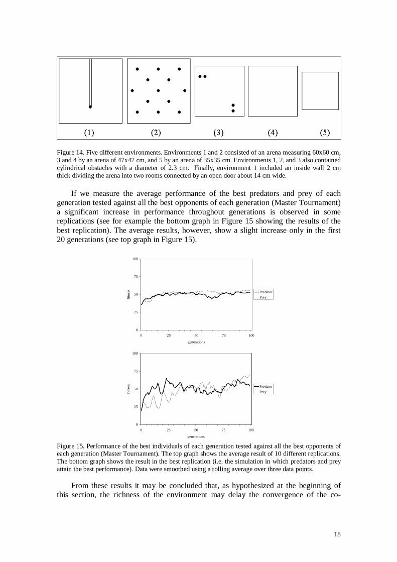
To verify this hypothesis we ran a new set of experiments in which individualsexperienced 5 different environments (i.e. they were tested for 2 epochs in each of the 5environments instead of 10 epochs in the same environment). All the other parameterswere the same as those described in section 2.1. In particular ‘standard’ co-evolutionand prey without camera were used. Figure 14 shows the five environments whichvaried in shape and in the number and type of obstacles within the arena.

18

Figure 14. Five different environments. Environments 1 and 2 consisted of an arena measuring 60x60 cm,3 and 4 by an arena of 47x47 cm, and 5 by an arena of 35x35 cm. Environments 1, 2, and 3 also containedcylindrical obstacles with a diameter of 2.3 cm. Finally, environment 1 included an inside wall 2 cmthick dividing the arena into two rooms connected by an open door about 14 cm wide.

If we measure the average performance of the best predators and prey of eachgeneration tested against all the best opponents of each generation (Master Tournament)a significant increase in performance throughout generations is observed in somereplications (see for example the bottom graph in Figure 15 showing the results of thebest replication). The average results, however, show a slight increase only in the first20 generations (see top graph in Figure 15).

0

25

50

75

100

0 25 50 75 100

generations

fitne

ss Predator

Prey

0

25

50

75

100

0 25 50 75 100

generations

fitne

ss Predator

Prey

Figure 15. Performance of the best individuals of each generation tested against all the best opponents ofeach generation (Master Tournament). The top graph shows the average result of 10 different replications.The bottom graph shows the result in the best repli cation (i.e. the simulation in which predators and preyattain the best performance). Data were smoothed using a roll ing average over three data points.

From these results it may be concluded that, as hypothesized at the beginning ofthis section, the richness of the environment may delay the convergence of the co-

19

evolutionary process towards a limit cycle. On the other hand we should consider thatlarger the number and importance of fixed constraints is, the lower the importance ofthe co-evolutionary dynamic may be. A rich continuum of possibil ities between anextreme in which the environment is constituted only by the competitor and anotherextreme in which the competitor is one within several different sources of constraintsshould be considered. It may be that interesting co-evolutionary dynamics only arise ina given interval between these two extremes.

2.7 How co-evolution can enhance the adaptive power of artificial evolution

In the previous sections we showed how ‘arms races’ between co-evolvingpopulations can arise. At this point we should try to verify whether co-evolution canreally enhance the adaptive power of artificial evolution. In other words, can artificialco-evolution solve tasks that cannot be solved using a simple evolutionary process?

There are two reasons for hypothesizing that co-evolution can have an higheradaptive power than evolution. The first reason is that individuals evolving in co-evolutionary frameworks experience a larger number of different environmental events.The second and more important reason is related to the emergence of ‘arms races’ .

To verify if co-evolution can produce solutions to problems that evolution alone isunable to solve we tried using simple evolution (i.e. an evolutionary process in whichonly a single population was evolved through selective reproduction and mutation).More specifically we tried to evolve predators able to catch the best prey obtained usingartificial co-evolution. Likewise, we tried to evolve prey able to escape the bestpredators obtained by co-evolution. If evolution fails, at least in some cases, we mayconclude that co-evolution is able to select better individuals than simple evolution. Inother words, we may conclude that co-evolution is able to produce solutions toproblems that evolution is unable to solve.

We ran several sets of simulations in which we tried to evolve individuals able tocatch the best co-evolved prey and to escape the best co-evolved predator obtained fromall the experiments described in the previous sections. The parameters used in thesimulations were the same as those described in section 2.1 although only onepopulation was subjected to the evolutionary process (the predator to escape or the preyto be caught remained identical over the entire evolutionary process). As a consequenceindividuals were tested for 10 epochs and 100 generations against exactly the sameopponent. In all cases simple evolution was able to produce better and better individualsuntil optimal or close to optimal performance was obtained.

In order to produce a challenge that was too complex for simple evolution it wasnecessary to change the sensory system of the predator and prey and to use a morecomplex environment than the simple arena involved in most of the experimentsdescribed above.

We ran a new set of co-evolutionary experiments in which predator and prey werenot equipped with cameras but were allowed to use the 8 ambient light sensors added inthe basic Khepera module. Moreover, we included a 1 watt lamp on the top of bothpredator and prey so that each could obtain an indirect measure of the angle anddistance of the other. The genotype of both predator and prey was 8 x (36 synapses + 2thresholds) bits long. As environment, we used an arena measuring 60x60cm with 13cylindrical obstacles (see environment 2 in Figure 14). The ‘standard’ selection regimewas used. For all other parameters the same values described in section 2.1 were used.

20

0

25

50

75

100

0 25 50 75 100

generations

fitne

ss Predator

Prey

0

25

50

75

100

0 25 50 75 100

generations

fitne

ss Predator

Prey

Figure 16. Experiments with the complex environment and predators and prey equipped with ambientlight sensors (‘standard’ co-evolution). Performance of the best individuals of each generation testedagainst all the best opponents of each generation (Master Tournament). The top graph shows the averageresult of 10 different replications. The bottom graph shows the result in the best repli cation (i.e. thesimulation in which predators and prey attain the best performance). Data were smoothed using a roll ingaverage over three data points.

If we look at the Master Tournament performance, we can see how a significantincrease may be observed both on average and in the case of the best replication.Moreover, we can see how, unlike the experiments described in the previous section, inthis case predators of the very first generations have close to null performance. Thisimplies that they are unable to catch most of the prey of succeeding generations.

We then ran a new set of experiments in which simple evolution (i.e. evolution of asingle population against a fixed opponent) was used to select predators able to catchthe best co-evolved prey obtained in the experiments just described. Similarly we usedsimple evolution to select prey able to escape the best co-evolved predators.

Evolving predators only Evolving prey only

1030

5070

90

0

0.2

0.4

0.6

0.8

1

performance

generations

repli cation

1030

5070

90

0.5

0.6

0.7

0.8

0.9

1

performance

generations

repli cation

Figure 17. Performance of evolving predators and prey against fixed co-evolved opponents (left to right,respectively). Each graph shows the results of 10 experiments in which the best prey and predatorobtained in the 10 co-evolutionary experiments described above were used as fixed opponents. Average

21

results of 10 succeeding generations are shown. Results have been sorted on the replication axis toenhance readabil ity.

As can be seen in Figure 17, which shows the performance of the best evolvingpredators and prey, in 8 cases out of 10 simple evolution failed to select predators ableto catch the co-evolved prey (the best individuals of 8 simulations are able to catch theprey less than 15% of the time). Conversely, the best co-evolved predators were able tocatch the best co-evolved prey at least 25% of the time in 9 out of 10 simulations. Thereason why simple evolution was not always successful was that predators of the firstgenerations were scored with a null value (predators were able to catch the fixed preyonce only occasionally, while their offspring usually failed to catch the same prey). As aconsequence, the selection mechanism could not operate.

The fact that in this case co-evolution was able to produce more complexchallenges than in the other experiments described in the previous section seems to bedue to the ability of the prey to use the information coming from the ambient lightsensors. Most of the co-evolved prey waited for the predator until it reached a distanceof about 100 mm and only then did they start to escape. This allowed the prey to forcethe predator to follow them with little chance of catching them given the difference inspeed. Moreover, it eliminated the risk of facing the predator head on by moving fasteven when the predator was far away.

It should be noticed, however, that evolution of a single population can create veryeffective prey against the best of co-evolved predators (see Figure 17, right side). Thisimplies that, in this case, it is always possible to find a simple strategy able to defeateach single individual predator. As we mentioned above, this is what happens for bothpredator and prey in all experiments described in the previous sections.

3. Discussion

Evolutionary Robotics is a promising new approach to the development of mobilerobots able to act quickly and robustly in real environments. One of the most interestingfeatures of this approach is that it is a completely automatic process in which theintervention of the experimenter is practically limited to the specification of a criterionfor evaluating the extent to which evolving individuals accomplish the desired task.However, it is still not clear how far this approach can scale up.

From this point of view, one difficult problem is given by the fact that theprobability that one individual within the initial generations is able to accomplish thedesired task, at least in part, is inversely proportional to the complexity of the task itself.For complex tasks, it is very likely that all individuals of the initial generations arescored with the same zero value and, as consequence, the selection mechanism mightresult in a mere random process. We will refer to this problem as the bootstrap problem.

This problem arises from the fact that in artificial evolution people usually startfrom scratch (i.e. from individuals obtained with randomly generated genotypes). Infact, one possible solution to this problem is the use of ‘ incremental evolution’ . In thiscase, we start with a simplified version of the task and, after we get individuals able tosolve such a simple case, we progressively move to more and more complex cases [5,10, 13]. This type of approach can overcome the bootstrap problem, although it also hasthe negative consequence of increasing the amount of supervision required and the riskof introducing inappropriate constraints. In the case of incremental evolution in fact, theexperimenter should determine not only an evaluation criterion but also a ‘pedagogical’

22

list of simplified criteria. In addition the experimenter should decide when to change theselection criterion during the evolutionary process. Some of these problems may arisealso when the selection criterion includes rewards for sub-components of the desiredbehavior (although, in this case, the selection criterion is left unchanged throughout theevolutionary process) [17].

Another possible solution of the bootstrap problem is the use of co-evolution. Co-evolution of competing populations, in fact, may produce increasingly complexevolving challenges spontaneously without any additional human intervention.Unfortunately, no continuous increase in complexity is guaranteed. For example, the co-evolutionary process may fall into a limit cycle in which the same solutions are adoptedby both populations over and over again (we will refer to this problem as the cyclingproblem). What happens is that at a certain point one population, in order to overcomethe other population, finds it more useful to suddenly change its strategy instead ofcontinuing to refine it. This is usually followed by a similar rapid change of strategy inthe other population. The overall result of this process is that most of the characterspreviously acquired are not appropriate in the new context and therefore are lost.However, later on, a similar sudden change may bring the two populations back to theoriginal type of strategy so that the lost characters are likely to be rediscovered again.

The effect of the cycling problem may be reduced by preserving all the solutionspreviously discovered for testing the individuals of the current generations [20].However, this method has drawbacks that may affect some of the advantages of co-evolution. In fact, as the process goes on there is less and less pressure to discoverstrategies that are effective against the opponent of the current generation and increasingpressure to develop solutions able to improve performance against opponents ofprevious generations which are no longer under co-evolution. While in some casestesting individuals against a sample of all previously selected competitors may producebetter performance (as shown in section 2.4), in other cases this might not be true.Indeed it may even result in less effective individuals (see section 2.5).

We believe that the cycling problem, like the local minima problem in gradient-descent methods (i.e. the risk of getting trapped in a sub-optimal solution when allneighboring solutions produce a decrease in performance), is an intrinsic problem of co-evolution that cannot be eliminated completely. However, as we have shown in sections2.5 and 2.7 the cycling problem does not always affect the co-evolutionary dynamics sostrongly as to prevent the emergence of ‘arms races’ . When both co-evolvingpopulations can produce better and better strategies, ‘arms races’ may last severalgenerations and produce progressively more complex and general solutions. On theother hand, if one or both populations cannot improve their current strategy sufficiently,the co-evolutionary dynamics will probably quickly lead to a limiting cycle in whichsimilar strategies are rediscovered over and over again.

Despite the cycling problem, it can be shown that in some cases co-evolution maysucceed in producing individuals able to cope with very effective competitors (byselecting the competitors at the same time) while simple evolution is unable to do so(see section 2.7). The reason for this is that co-evolution, by selecting also thecompetitors that determine the complexity of the task, is not affected by the ‘bootstrapproblem’. On the other hand, when simple evolution is faced with fixed co-evolvedcompetitors, it may happen that the genetic operators are unable to generate anyindividual able to defeat the competitor, even in a few cases. As a consequence theselection process does not work.

23

Moreover, it should be noted that some factors may limit the cycling problem. Oneof these factors is, as we have shown in section 2.6, the richness of the environment. Inthe case of co-evolution, competing individuals are part of the environment. This meansthat part, but not all of the environment, is undergoing co-evolution. The probability thata sudden shift in behavior will produce viable individuals is inversely proportional tothe richness of the environment that is not undergoing co-evolution. In fact, if anacquired ability involves a characteristic of the environment which is not undergoingco-evolution it is less likely that a sudden shift in strategy involving the loss of such anabil ity wil l be retained. Indeed the acquired character will always have an adaptivevalue independently of the strategies adopted by the co-evolving population. This effectmay be particularly significant in the case of natural evolution in which, in general, theenvironment is much richer than in the case of the experiments performed in artificialevolution.

Another factor that may limit the effect of the cycling problem is ontogeneticplasticity. Plastic individuals, in fact, may be able to cope with different classes ofstrategies adopted by the second population by adapting to the current opponent'sstrategy during their lifetime, thus reducing the adaptive advantage of a sudden shift inbehavior which causes the cycling problem. The experiments described in this paper didnot support this issue (none of the experiments described in this paper involvedontogenetic plasticity). On the effects of some forms of ontogenetic plasticity within aco-evolutionary framework see [8].

3.1 A dynamical view of adaptation

We have thus been able to show that, at least in one case, co-evolution can producea strategy that is too complex for simple evolution to cope with (section 2.7). However,in the other 3 cases examined (see section 2.3, 2.5, and 2.6) evolution was quickly ableto select individuals that proved very effective against such complex strategies. Inparticular this happened also with the strategies obtained in the experiments described insection 2.5 and 2.6 in which Master Tournament measures clearly indicated a progressthroughout generations. This means that, even though more and more general strategieswere selected in these experiments through co-evolution, it was always easy to selectindividuals able to defeat these strategies by starting from scratch. Further proof of thisis that if we look at the performance of the best individuals of the last generations wesee that, even though they score increasingly better against individuals of previousgenerations on average, they may sometimes be defeated by individuals of manygenerations before (see for example Figures 8 and 11).

These results point to the conclusion that in certain tasks it is always possible tofind a simple strategy that is able to defeat another single, albeit complex and general,strategy (although such simple strategy is a specialized strategy, i.e. it is able to defeatonly that individual complex and general strategy and, of course, other similarstrategies). If this is really true, in other words, if completely general solutions do notexist in some cases, we should re-consider the ‘cycling problem’. From this point ofview, the fact of a co-evolutionary dynamics leading to a limit cycle in which the sametype of solutions are adopted over and over again should not be considered as a failurebut as an optimal solution. We cannot complain that co-evolution does not find a moregeneral strategy able to cope with all the strategies adopted by the co-evolvingpopulation during a cycle if such general strategies do not exist. The best that can be

24

done is to select the appropriate strategy for the current counter-strategy, which isactually what happens when the co-evolutionary dynamics ends in a limit cycle.

More generally we can predict that co-evolution wil l lead to a progressive increasein complexity when complete general solutions (i.e. solutions which are successfulagainst all the strategies adopted by previous opponents) exist and can be selected bymodifying the current solutions. Conversely, if complete general solutions do not existor the probability of generating them is too low, co-evolution may lead to a cyclingdynamics in which solutions appropriate to the strategy of the co-evolving populationbut which can also easily be transformed so to match other strategies will be selected. Inother words, when general solutions cannot be found, it becomes important for eachevolving population to be able to dynamically change its own strategy into one of a setof appropriate strategies. From the individuals' point of view, we may say thatindividuals with a predisposition to change in certain directions will be selected.

Interestingly, one can argue that these dynamics may be an ideal situation for theemergence of ontogenetic adaptation. The abil ity to adapt during one's lifetime to theopponent's strategy would in fact produce a significant increase in the adaptation levelof a single individual because ontogenetic adaptations are much faster than phylogeneticones. Therefore, we may hypothesize that, when a co-evolving dynamics leads to alimiting cycle, there will be a high selective pressure in the direction of ontogeneticadaptation. At the same time, the cycling dynamics will create the conditions in whichontogenetic adaptation may more easily arise because, as we have seen, individuals witha predisposition to change in certain directions will be selected. It is plausible to arguethat, for such individuals, a limited number of changes during ontogeny will be able toproduce the required behavioral shift. In other words, we can argue that it will be easierfor co-evolving individuals to change their behavior during their lifetime in order toadopt strategies already selected by their close ancestors thanks to the cycles occurringin previous generations.

Notice that although an individual which has a single strategy able to defeat a set ofcounter-strategies and an individual which posses a set of different strategies able todefeat the same set of counter-strategies are equivalent at a certain level of descriptionthere are some important differences (to distinguish the two cases let us call the former‘ full-general’ and the latter ‘plastic-general’ ). The plastic-general individual should beable to select the right strategy given the current competitor. In other words, should beable to adapt through ontogenetic adaptation. From this point of view the full -generalindividual wil l be more effective because it does not require such adaptation processand may provide immediately the correct answer to the current competitor. On the otherhand, as we said above, it may be that in certain conditions a fully-general individualcannot be selected because a fully-general strategy does not exist or because it is tooimprobable that the evolutionary process is able to find it. In this case the only optionleft is that of plastic-general solutions. However also a plastic-general individual isdifficult to obtain because it implies that such individual should be able to display avariety of different strategies and because it should also be able to select the rightstrategy at the right moment (depending on the behavior of the current competitor).What is interesting is that, when a fully-general strategy cannot be found, co-evolutionwill fall into a cycling dynamics in which a set of ‘specialistic’ strategy will be discoverover and over again. Now, because during this phase the best thing individuals can do toimprove the chances of survival of their offspring is to produce offspring which canevolutionary change their strategy as fast as possible (in other words individuals which

25

have a predisposition to change in certain directions) we may expect that the length ofthe cycles wil l be progressively shortened throughout successive generations. At thispoint, we might speculate that co-evolution might favor the emergence of individualswith the abil ity to modify their behavior during li fetime in the most appropriatedirections (the same directions for which a predisposition to change have beengenetically acquired), if the genotype could allow for some type of phenotypicmodification.

Of course, this is only a hypothesis. The only results we have from the experimentswe described in this paper is that in most of our experiments simple ‘specialist’solutions can be found while fully-general solutions cannot. It remain to be ascertainedif plastic-general solutions (i.e. solutions which consists of a set of simple ‘specialist’solutions and a mechanism for selecting the right one during lifetime) can be selected.Preliminary evidences have been described in [8].

Acknowledgments

We thank the anonymous referees for their valuable suggestions.

References

1. Cli ff , D., & Miller, G. F. (1995). Tracking the red queen: Measurement of adaptive progress in co-evolutionary simulations. In F. Moran, A. Moreno, J. J. Merelo & P. Chacon (Eds.), Advances inArtificial Life: Proceedings of the Third European Conference on Artificial Life, Berlin: SpringerVerlag.

2. Cli ff , D., & Miller, G. F. (1996). Co-evolution of pursuit and evasion II : Simulation methods andresults. In P. Maes, M. Mataric, J-A Meyer, J. Pollack, H. Roitblat & S. Wilson (Eds.), FromAnimals to Animats IV: Proceedings of the Fourth International Conference on Simulation ofAdaptive Behavior, Cambridge, MA: MIT Press-Bradford Books.

3. Dawkins, R., & Krebs, J. R. (1979). Arms races between and within species. Proceedings of theRoyal Society of London B, 205, 489-511.

4. Elman, J. L., Bates, E. A., Johnson, M. H., Karmiloff-Smith, A., Parisi, D., & Plunket, K. (1996).Rethinking Innateness. A Connectionist Perspective on Development. Cambridge, MA: MIT Press.

5. Floreano, D. (1993). Emergence of home-based foraging strategies in ecosystems of neuralnetworks. In J. Meyer, H.L. Roitblat & S.W. Wilson (Eds.), From Animals to Animats II:Proceedings of the Second International Conference on Simulation of Adaptive Behavior,Cambridge, MA: MIT Press-Bradford Books.

6. Floreano, D., & Mondada, F. (1994). Automatic creation of an autonomous agent: Genetic evolutionof a neural-network driven robot. In D. Cliff , F. Husband, J-A. Meyer & S. W. Wilson (Eds.), FromAnimals to Animats III: Proceedings of the Third International Conference on Simulation ofAdaptive Behavior, Cambridge, MA: MIT Press-Bradford Books.

7. Floreano, D., & Nolfi, S. (1997). God save the red queen! Competition in co-evolutionary robotics.In J. R. Koza, D. Kalyanmoy, M. Dorigo, D. B. Fogel, M. Garzon, H. Iba & R. L. Riolo (Eds.),Genetic Programming 1997: Proceedings of the Second Annual Conference, pp. 398-406, SanFrancisco, CA: Morgan Kaufmann.

8. Floreano, D., & Nolfi, S. (1997). Adaptive behavior in competing co-evolving species. In P.Husband & I. Harvey (Eds.), Proceedings of the Fourth European Conference on Artificial Life,Cambridge, MA: MIT Press.

9. Floreano, D., Nolfi, S., & Mondada, F. (1998). Competitive co-evolutionary robotics: From theoryto practice. In R. Pfeifer, B. Blumberg & H. Kobayashi (Eds.), Proceedings of the FifthInternational Conference of the Society for Adaptive Behavior (SAB98), Cambridge, MA: MIT Press

10. Harvey, I., Husbands, P., & Cli ff , D. (1994). Seeing the light: artificial evolution, real vision. In D.Cli ff , P. Husbands, J-A. Meyer & S.W. Wilson (Eds.), From Animals to Animats III : Proceedings of

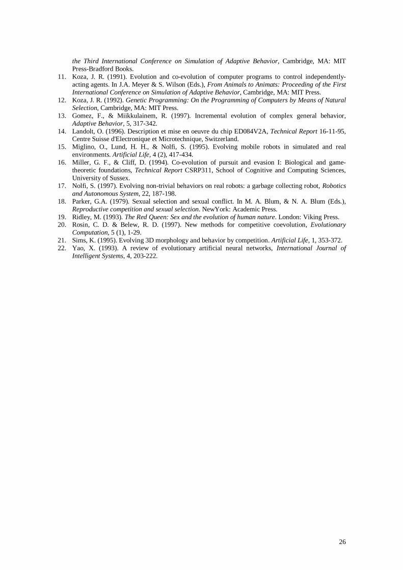
26

the Third International Conference on Simulation of Adaptive Behavior, Cambridge, MA: MITPress-Bradford Books.

11. Koza, J. R. (1991). Evolution and co-evolution of computer programs to control independently-acting agents. In J.A. Meyer & S. Wilson (Eds.), From Animals to Animats: Proceeding of the FirstInternational Conference on Simulation of Adaptive Behavior, Cambridge, MA: MIT Press.

12. Koza, J. R. (1992). Genetic Programming: On the Programming of Computers by Means of NaturalSelection, Cambridge, MA: MIT Press.

13. Gomez, F., & Miikkulainem, R. (1997). Incremental evolution of complex general behavior,Adaptive Behavior, 5, 317-342.

14. Landolt, O. (1996). Description et mise en oeuvre du chip ED084V2A, Technical Report 16-11-95,Centre Suisse d'Electronique et Microtechnique, Switzerland.

15. Miglino, O., Lund, H. H., & Nolfi, S. (1995). Evolving mobile robots in simulated and realenvironments. Artificial Life, 4 (2), 417-434.

16. Mill er, G. F., & Cli ff , D. (1994). Co-evolution of pursuit and evasion I: Biological and game-theoretic foundations, Technical Report CSRP311, School of Cogniti ve and Computing Sciences,University of Sussex.

17. Nolfi, S. (1997). Evolving non-trivial behaviors on real robots: a garbage collecting robot, Roboticsand Autonomous System, 22, 187-198.

18. Parker, G.A. (1979). Sexual selection and sexual confli ct. In M. A. Blum, & N. A. Blum (Eds.),Reproductive competition and sexual selection. NewYork: Academic Press.

19. Ridley, M. (1993). The Red Queen: Sex and the evolution of human nature. London: Viking Press.20. Rosin, C. D. & Belew, R. D. (1997). New methods for competiti ve coevolution, Evolutionary

Computation, 5 (1), 1-29.21. Sims, K. (1995). Evolving 3D morphology and behavior by competition. Artificial Life, 1, 353-372.22. Yao, X. (1993). A review of evolutionary artificial neural networks, International Journal of

Intelligent Systems, 4, 203-222.