CMSC 206 Dictionaries and Hashing

Welcome message from author
This document is posted to help you gain knowledge. Please leave a comment to let me know what you think about it! Share it to your friends and learn new things together.
Transcript
CMSC 206
Dictionaries and Hashing
2
The Dictionary ADT
n a dictionary (table) is an abstract model of a database or lookup table
n like a priority queue, a dictionary stores key-element pairs
n the main operation supported by a dictionary is searching by key
3
Examples
n Telephone directory n Library catalogue n Books in print: key ISBN n FAT (File Allocation Table)
4
The Dictionary ADT
n simple container methods: q size() q isEmpty() q iterator()
n query methods: q get(key) q getAllElements(key)
5
The Dictionary ADT
n update methods: q insert(key, element) q remove(key) q removeAllElements(key)
n special element q NO_SUCH_KEY, returned by an unsuccessful
search
6
The Basic Problem
n We have lots of data to store.
n We desire efficient – O( 1 ) – performance for insertion, deletion and searching.
n Too much (wasted) memory is required if we use an array indexed by the data’s key.
n The solution is a “hash table”.
7
Hash Table
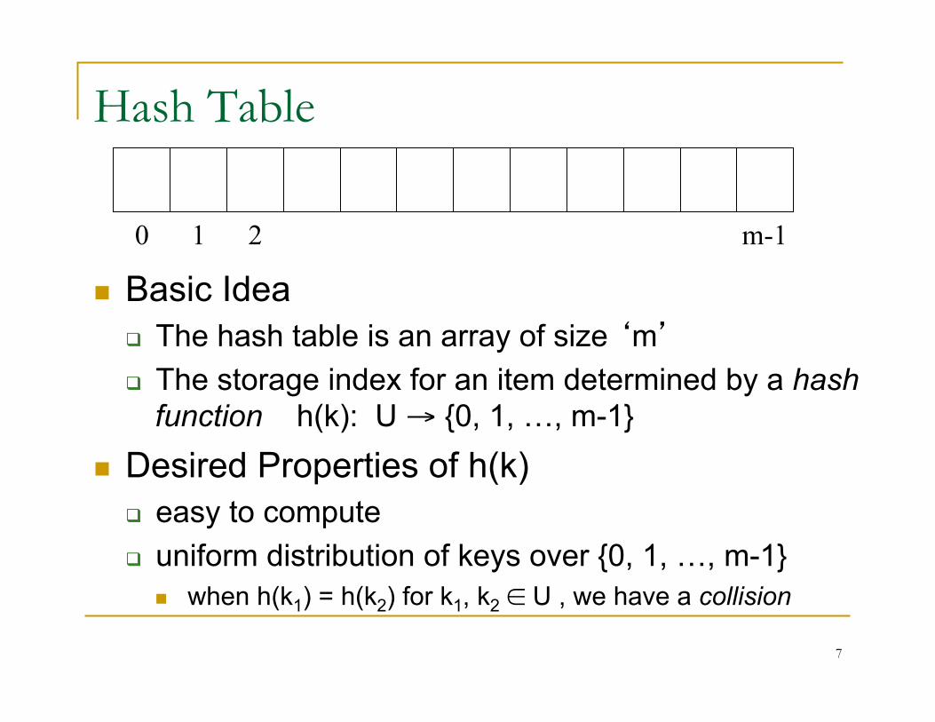
n Basic Idea q The hash table is an array of size ‘m’ q The storage index for an item determined by a hash
function h(k): U → {0, 1, …, m-1} n Desired Properties of h(k)
q easy to compute q uniform distribution of keys over {0, 1, …, m-1}
n when h(k1) = h(k2) for k1, k2 ∈ U , we have a collision
0 1 2 m-1
8
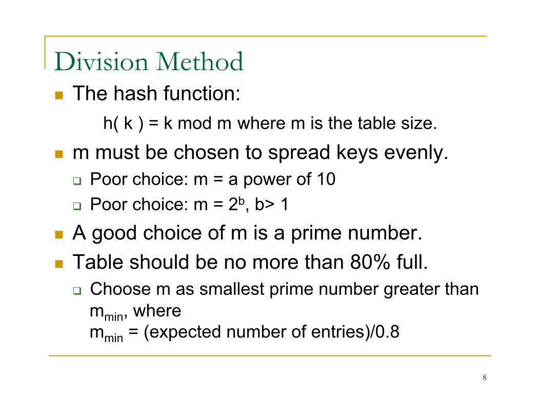
Division Method n The hash function:
h( k ) = k mod m where m is the table size. n m must be chosen to spread keys evenly.
q Poor choice: m = a power of 10 q Poor choice: m = 2b, b> 1
n A good choice of m is a prime number. n Table should be no more than 80% full.
q Choose m as smallest prime number greater than mmin, where mmin = (expected number of entries)/0.8
9
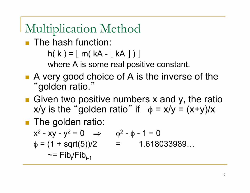
Multiplication Method n The hash function:
h( k ) = ⎣ m( kA - ⎣ kA ⎦ ) ⎦ where A is some real positive constant.
n A very good choice of A is the inverse of the “golden ratio.”
n Given two positive numbers x and y, the ratio x/y is the “golden ratio” if φ = x/y = (x+y)/x
n The golden ratio: x2 - xy - y2 = 0 ⇒ φ2 - φ - 1 = 0 φ = (1 + sqrt(5))/2 = 1.618033989…
~= Fibi/Fibi-1
10
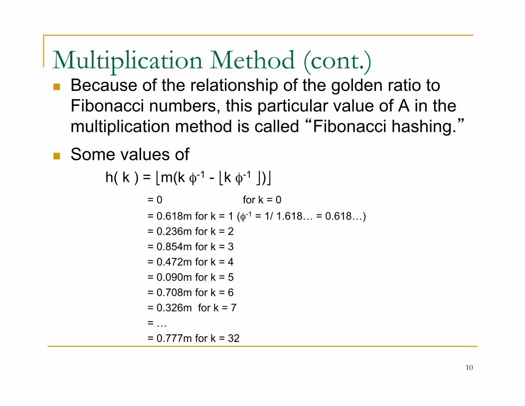
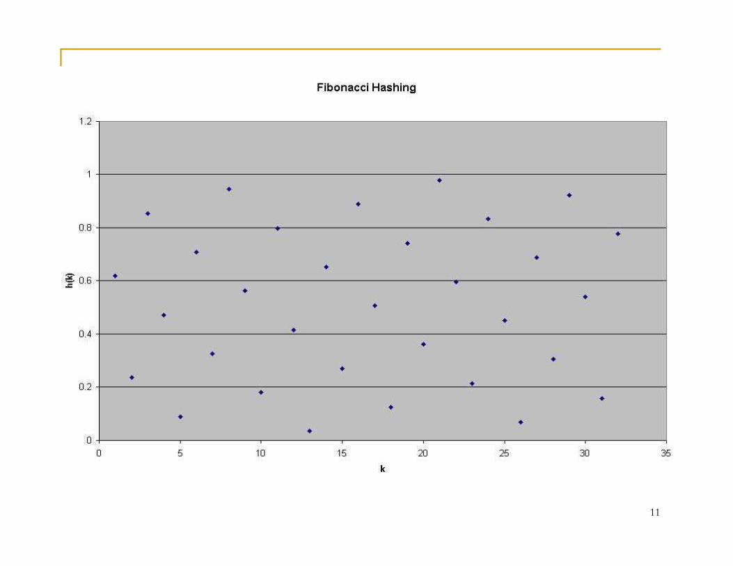
Multiplication Method (cont.) n Because of the relationship of the golden ratio to
Fibonacci numbers, this particular value of A in the multiplication method is called “Fibonacci hashing.”
n Some values of h( k ) = ⎣m(k φ-1 - ⎣k φ-1 ⎦)⎦ = 0 for k = 0 = 0.618m for k = 1 (φ-1 = 1/ 1.618… = 0.618…) = 0.236m for k = 2 = 0.854m for k = 3
= 0.472m for k = 4 = 0.090m for k = 5 = 0.708m for k = 6 = 0.326m for k = 7 = … = 0.777m for k = 32
11
12
Non-integer Keys
n In order to have a non-integer key, must first convert to a positive integer: h( k ) = g( f( k ) ) with f: U → integer g: I → {0 .. m-1}
n Suppose the keys are strings. n How can we convert a string (or characters)
into an integer value?
13
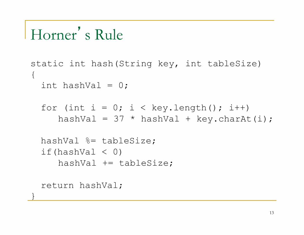
Horner’s Rule
static int hash(String key, int tableSize) { int hashVal = 0; for (int i = 0; i < key.length(); i++) hashVal = 37 * hashVal + key.charAt(i); hashVal %= tableSize; if(hashVal < 0) hashVal += tableSize; return hashVal;
}
14
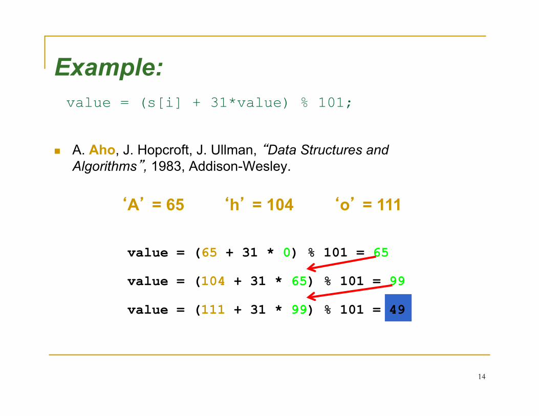
n A. Aho, J. Hopcroft, J. Ullman, “Data Structures and Algorithms”, 1983, Addison-Wesley.
‘A’ = 65 ‘h’ = 104 ‘o’ = 111
value = (65 + 31 * 0) % 101 = 65
value = (104 + 31 * 65) % 101 = 99
value = (111 + 31 * 99) % 101 = 49
Example: value = (s[i] + 31*value) % 101;
15
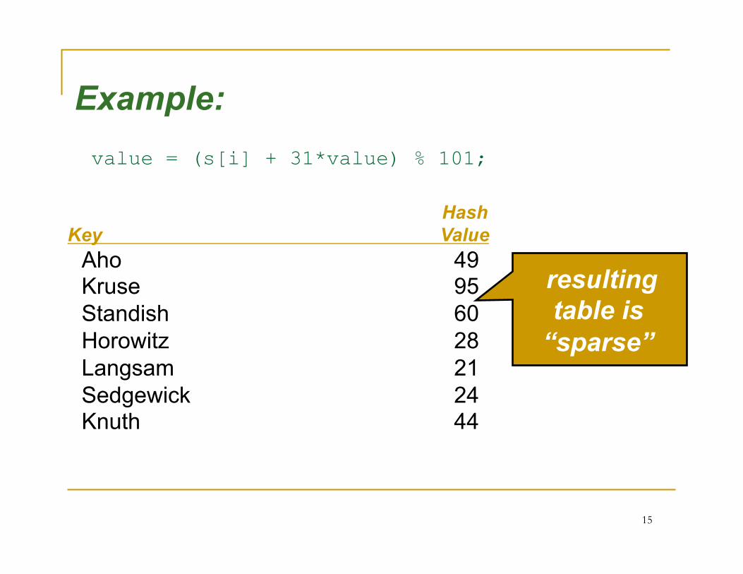
resulting table is
“sparse”
Example: value = (s[i] + 31*value) % 101;
Hash Key Value
Aho 49 Kruse 95 Standish 60 Horowitz 28 Langsam 21 Sedgewick 24 Knuth 44
16
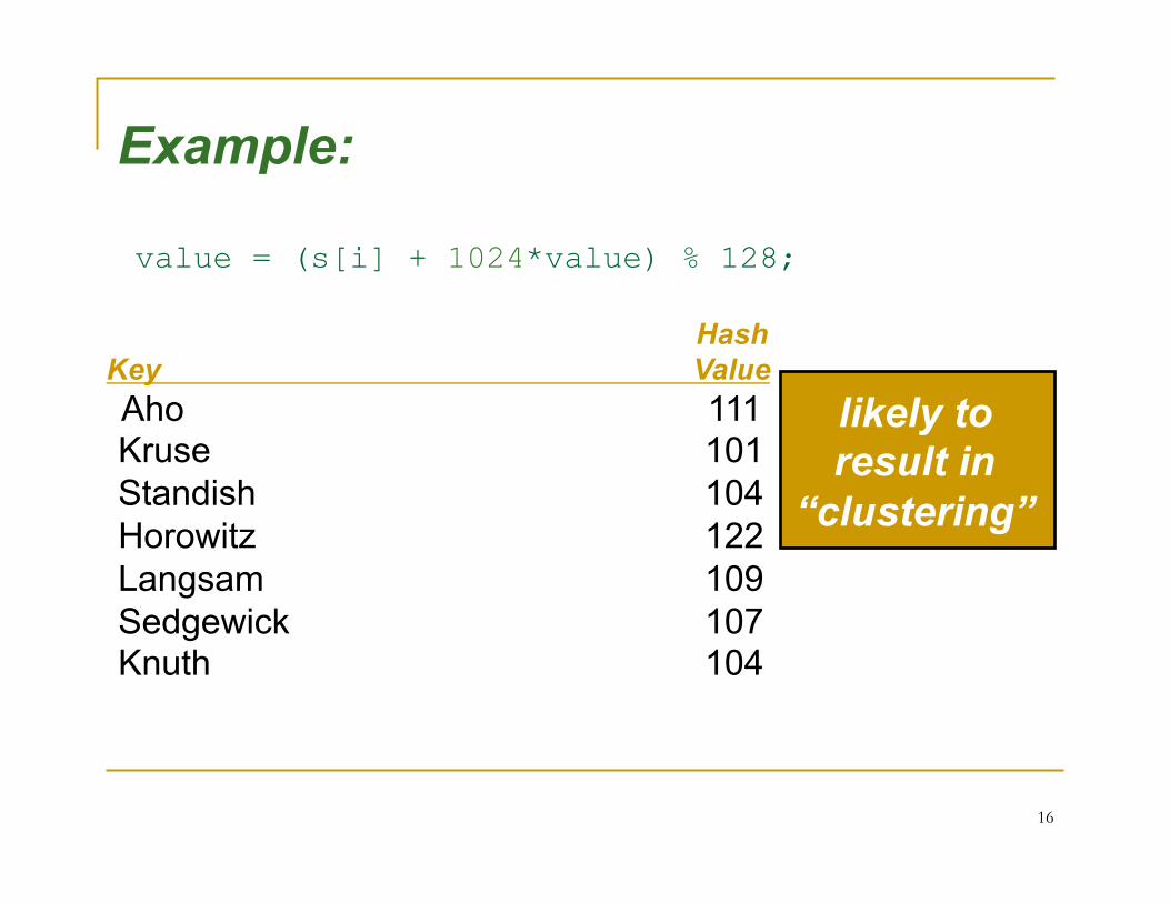
value = (s[i] + 1024*value) % 128;
Example:
likely to result in
“clustering”
Hash Key Value Aho 111 Kruse 101 Standish 104 Horowitz 122 Langsam 109 Sedgewick 107 Knuth 104
17
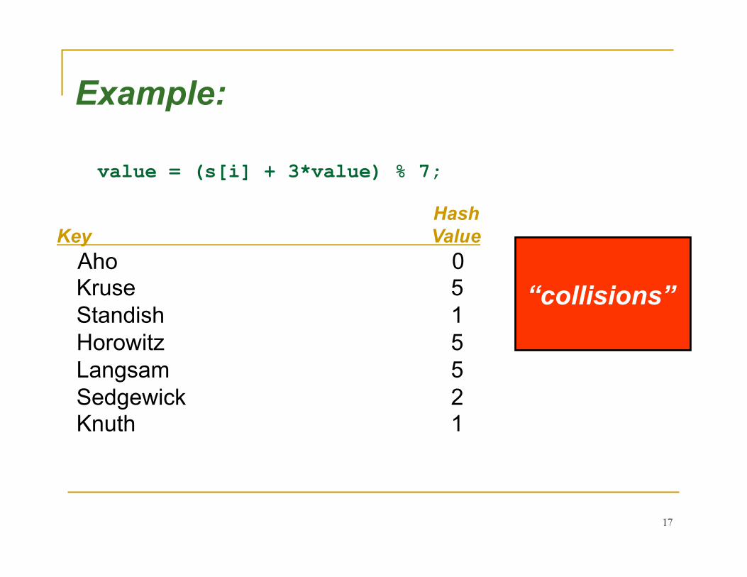
Example:
“collisions”
value = (s[i] + 3*value) % 7;
Hash Key Value
Aho 0 Kruse 5 Standish 1 Horowitz 5 Langsam 5 Sedgewick 2 Knuth 1
18
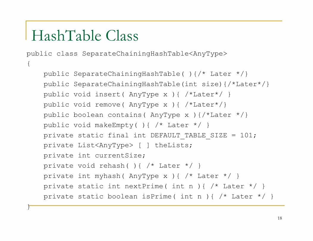
HashTable Class public class SeparateChainingHashTable<AnyType> {
public SeparateChainingHashTable( ){/* Later */}
public SeparateChainingHashTable(int size){/*Later*/}
public void insert( AnyType x ){ /*Later*/ }
public void remove( AnyType x ){ /*Later*/}
public boolean contains( AnyType x ){/*Later */}
public void makeEmpty( ){ /* Later */ }
private static final int DEFAULT_TABLE_SIZE = 101; private List<AnyType> [ ] theLists;
private int currentSize;
private void rehash( ){ /* Later */ }
private int myhash( AnyType x ){ /* Later */ }
private static int nextPrime( int n ){ /* Later */ }
private static boolean isPrime( int n ){ /* Later */ }
}
19
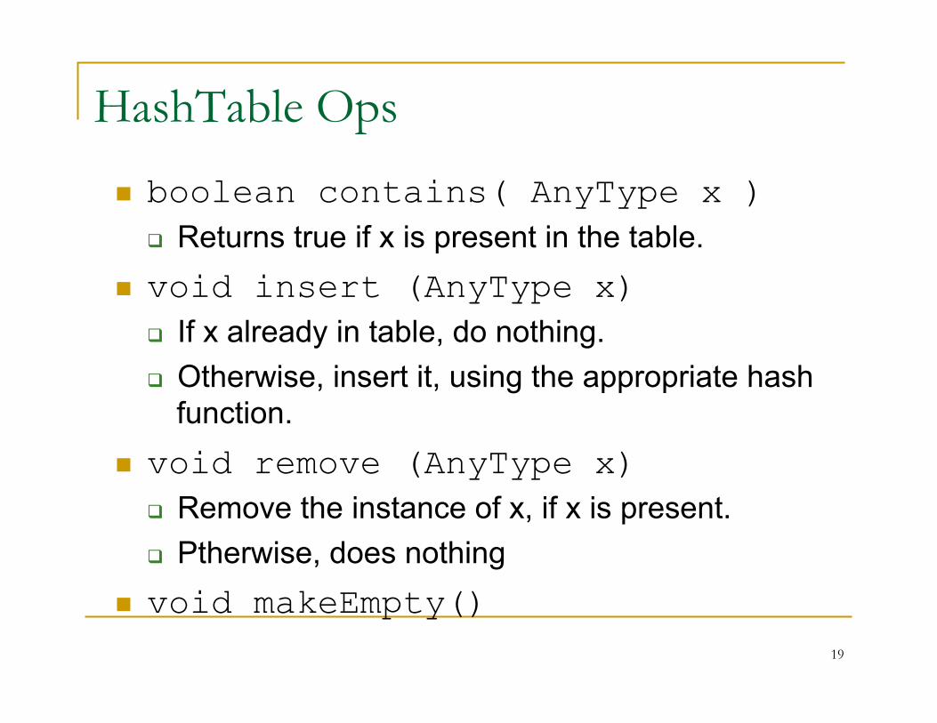
HashTable Ops
n boolean contains( AnyType x ) q Returns true if x is present in the table.
n void insert (AnyType x) q If x already in table, do nothing. q Otherwise, insert it, using the appropriate hash
function. n void remove (AnyType x)
q Remove the instance of x, if x is present. q Ptherwise, does nothing
n void makeEmpty()
20
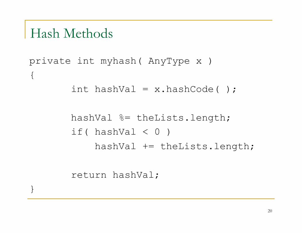
Hash Methods
private int myhash( AnyType x )
{ int hashVal = x.hashCode( );
hashVal %= theLists.length; if( hashVal < 0 )
hashVal += theLists.length;
return hashVal; }
21
Handling Collisions n Collisions are inevitable. How to handle
them? n Separate chaining hash tables
q Store colliding items in a list. q If m is large enough, list lengths are small.
n Insertion of key k q hash( k ) to find the proper list. q If k is in that list, do nothing, else insert k on that list.
n Asymptotic performance q If always inserted at head of list, and no duplicates,
insert = O(1) for best, worst and average cases
22
Hash Class for Separate Chaining
n To implement separate chaining, the private data of the hash table is an array of Lists. The hash functions are written using List functions
private List<AnyType> [ ] theLists;
23
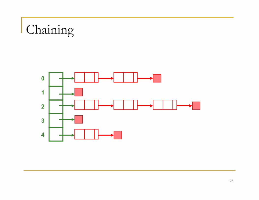
Chaining
0 1 2 3 4
24
Performance of contains( )
n contains q Hash k to find the proper list. q Call contains( ) on that list which returns a
boolean. n Performance
q best:
q worst:
q average
25
Performance of remove( )
n Remove k from table q Hash k to find proper list. q Remove k from list.
n Performance q best
q worst
q average
26
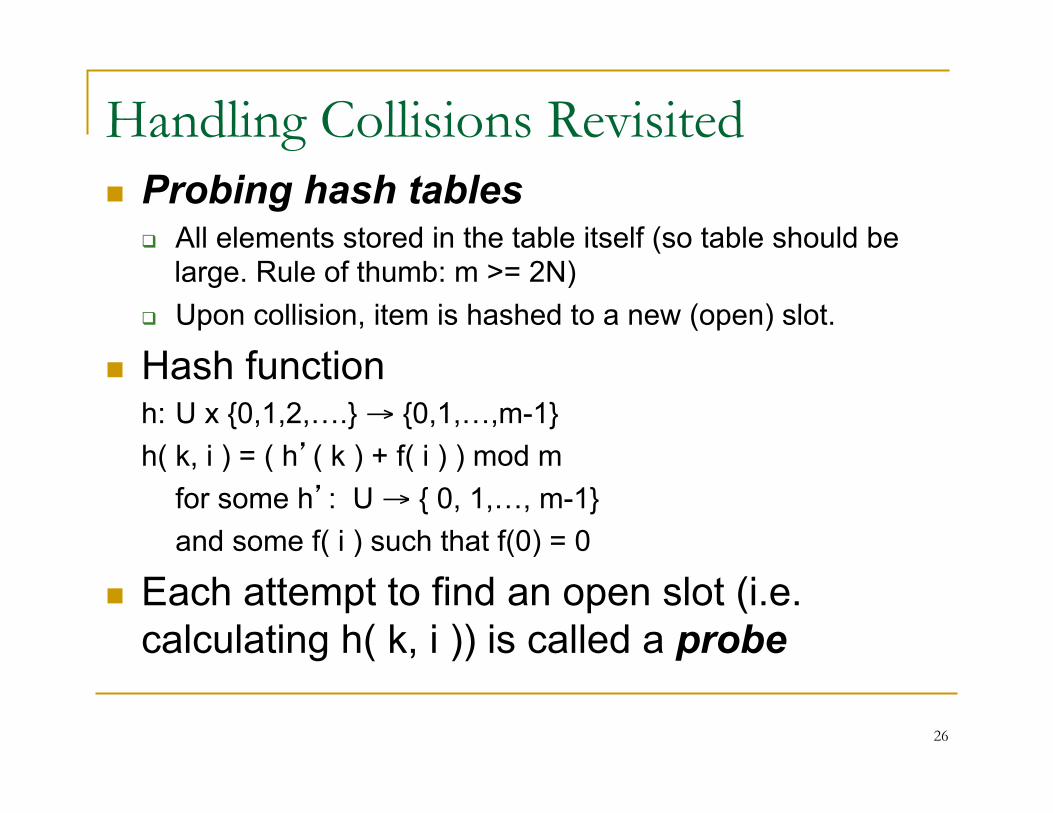
Handling Collisions Revisited n Probing hash tables
q All elements stored in the table itself (so table should be large. Rule of thumb: m >= 2N)
q Upon collision, item is hashed to a new (open) slot.
n Hash function h: U x {0,1,2,….} → {0,1,…,m-1} h( k, i ) = ( h’( k ) + f( i ) ) mod m
for some h’: U → { 0, 1,…, m-1} and some f( i ) such that f(0) = 0
n Each attempt to find an open slot (i.e. calculating h( k, i )) is called a probe
27
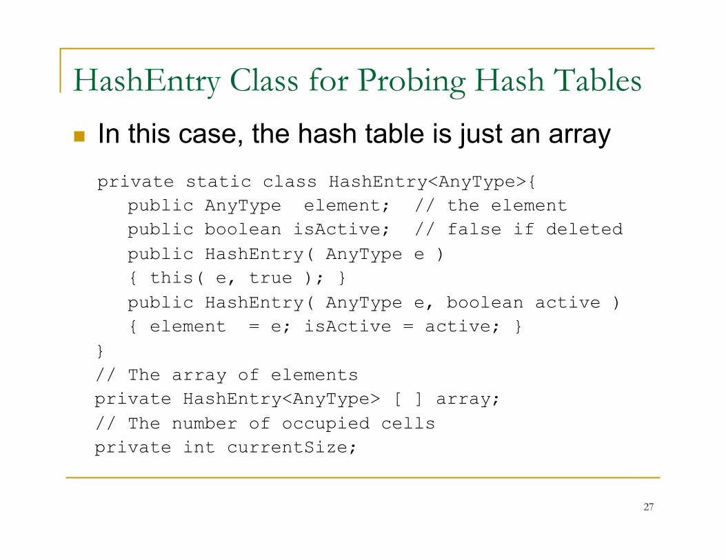
HashEntry Class for Probing Hash Tables
n In this case, the hash table is just an array
private static class HashEntry<AnyType>{ public AnyType element; // the element public boolean isActive; // false if deleted public HashEntry( AnyType e ) { this( e, true ); } public HashEntry( AnyType e, boolean active ) { element = e; isActive = active; } } // The array of elements private HashEntry<AnyType> [ ] array; // The number of occupied cells private int currentSize;
28
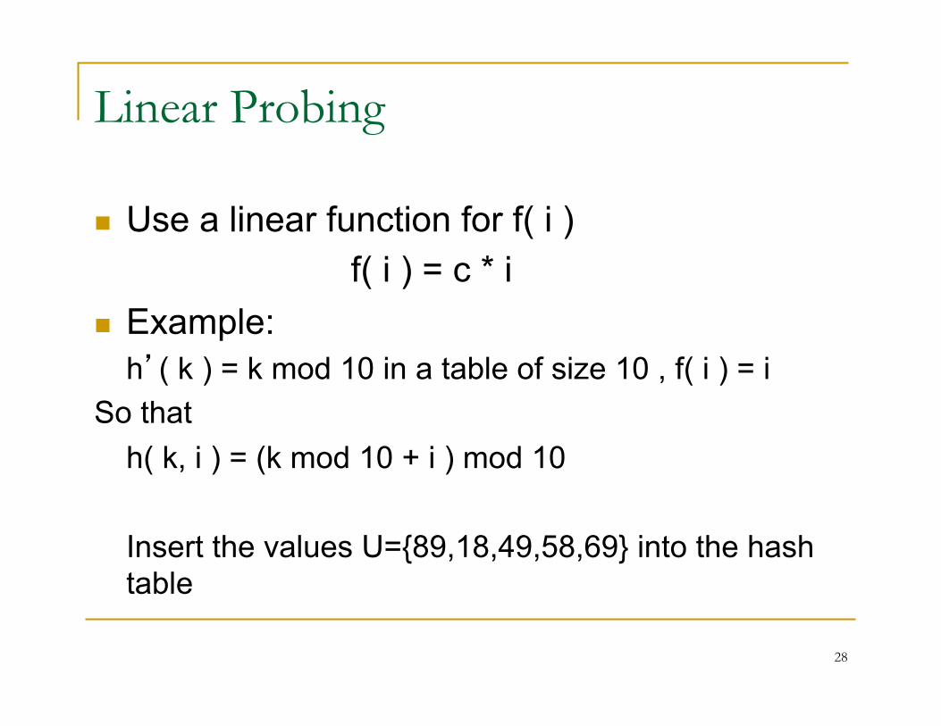
Linear Probing
n Use a linear function for f( i ) f( i ) = c * i
n Example: h’( k ) = k mod 10 in a table of size 10 , f( i ) = i
So that h( k, i ) = (k mod 10 + i ) mod 10
Insert the values U={89,18,49,58,69} into the hash table
29
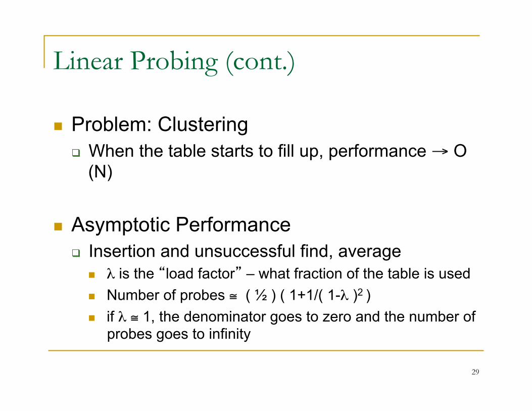
Linear Probing (cont.)
n Problem: Clustering q When the table starts to fill up, performance → O
(N)
n Asymptotic Performance q Insertion and unsuccessful find, average
n λ is the “load factor” – what fraction of the table is used n Number of probes ≅ ( ½ ) ( 1+1/( 1-λ )2 ) n if λ ≅ 1, the denominator goes to zero and the number of
probes goes to infinity
30
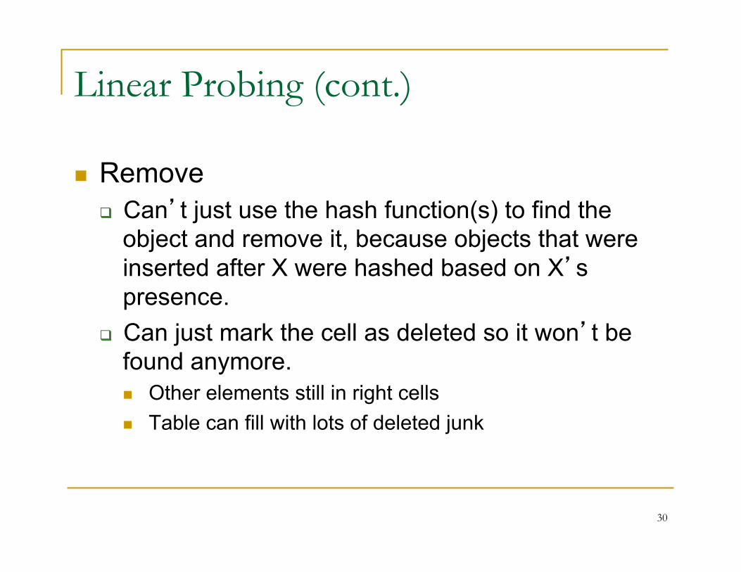
Linear Probing (cont.)
n Remove q Can’t just use the hash function(s) to find the
object and remove it, because objects that were inserted after X were hashed based on X’s presence.
q Can just mark the cell as deleted so it won’t be found anymore. n Other elements still in right cells n Table can fill with lots of deleted junk
31
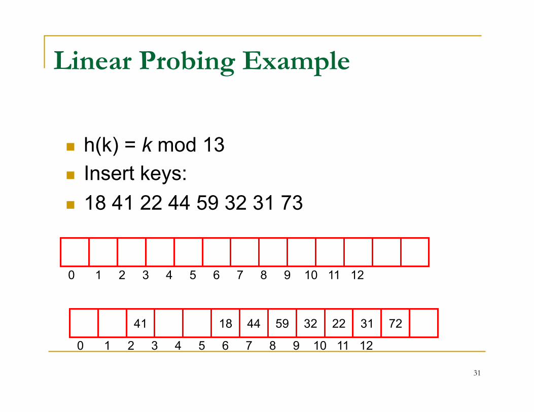
Linear Probing Example
n h(k) = k mod 13 n Insert keys: n 18 41 22 44 59 32 31 73
0 1 2 3 4 5 6 7 8 9 10 11 12
41 18 44 59 32 22 31 72
0 1 2 3 4 5 6 7 8 9 10 11 12
32
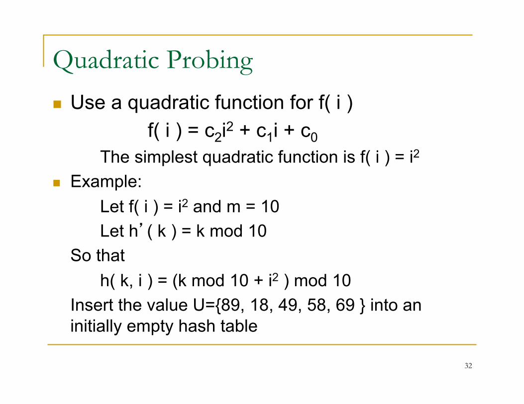
Quadratic Probing
n Use a quadratic function for f( i ) f( i ) = c2i2 + c1i + c0 The simplest quadratic function is f( i ) = i2
n Example: Let f( i ) = i2 and m = 10 Let h’( k ) = k mod 10 So that h( k, i ) = (k mod 10 + i2 ) mod 10 Insert the value U={89, 18, 49, 58, 69 } into an initially empty hash table
33
Quadratic Probing (cont.)
n Advantage: q Reduced clustering problem
n Disadvantages: q Reduced number of sequences q No guarantee that empty slot will be found if λ ≥ 0.5, even if m is prime
q If m is not prime, may not find an empty slot even if λ < 0.5
34
Double Hashing n Let f( i ) use another hash function
f( i ) = i * h2( k ) Then h( k, I ) = ( h’( k ) + i * h2( k ) ) mod m And probes are performed at distances of h2( k ), 2 * h2( k ), 3 * h2( k ), 4 * h2( k ), etc
n Choosing h2( k ) q Don’t allow h2( k ) = 0 for any k. q A good choice:
h2( k ) = R - ( k mod R ) with R a prime smaller than m
n Characteristics q No clustering problem q Requires a second hash function
36
Rehashing
n If the table gets too full, the running time of the basic operations starts to degrade.
n For hash tables with separate chaining, “too full” means more than one element per list (on average)
n For probing hash tables, “too full” is determined as an arbitrary value of the load factor.
n To rehash, make a copy of the hash table, double the table size, and insert all elements (from the copy) of the old table into the new table
n Rehashing is expensive, but occurs very infrequently.
Related Documents