CMIP3 ensemble climate projections over the western tropical Pacific based on model skill

CLIMATE RESEARCHClim Res

Vol. 51: 35–58, 2012doi: 10.3354/cr01046

Published online January 24

1. INTRODUCTION

Christensen et al. (2007) broadly outline tempera-ture and precipitation projections over the Pacificregion, using an ensemble of simulations fromglobal climate models (GCMs) from the Intergov-ernmental Panel on Climate Change (IPCC) 4th As -sessment Report (AR4) archive (now known asPhase 3 of the World Climate Research Project Cli-

mate Model Inter comparison Project, CMIP3; Meehlet al. 2007a). Through an assessment of the currentclimate literature, the AR4 reported that acrossmost of the Pacific region, temperature projectionstend to follow the global average warming rate,although stronger warming occurs in the centralequatorial Pacific and weaker warming occurs inthe south. The strongest increases in precipitationoccur over the Intertropical Convergence Zone

© Inter-Research 2012 · www.int-res.com*Email: [email protected]

CMIP3 ensemble climate projections over the western tropical Pacific based on model skill

Sarah E. Perkins1,2,3,*, Damien B. Irving1,2, Josephine R. Brown2,3, Scott B. Power2,3, Aurel F. Moise2,3, Robert A. Colman2,3, Ian Smith2,3

1Centre for Australian Weather and Climate Research, CSIRO Marine and Atmospheric Research, Aspendale, Victoria 3195, Australia

2Centre for Australian Weather and Climate Research, Bureau of Meteorology, GPO Box 1289, Melbourne, Victoria 3001, Australia

3Present address: ARC Centre of Excellence for Climate System Science, The University of New South Wales, Sydney, NSW 2052 Australia

ABSTRACT: Climate projections provide important information for risk assessment and adapta-tion planning. The CMIP3 archive of global climate model (GCM) simulations has been usedextensively for such projections over land-based regions, but limited attention has been paid tothe western tropical Pacific, where vulnerability is likely to be high. Adaptation policies within thewestern Pacific currently are based on the heavily summarised information within the IPCC fourthassessment report. This study builds upon the IPCC projections by analysing and presenting pro-jections of change from the CMIP3 GCMs and demonstrating spatial differences in projectionsacross the west Pacific domain. Atmospheric fields considered in this paper include surface airtemperature, precipitation, and wind speed and direction for the SRES A2 emission scenario for2080−2099, where the projected change is relative to 1980−1999. Results for all fields are based on3 types of multi-model ensembles: the all-model (ALL) ensemble (19 models), the BEST ensemble(15 models) and the WORST ensemble (4 models). The BEST and WORST ensembles are based onmodel skill in simulating relevant climatic features, drivers and variables, which govern the inter-annual and annual climate of the study region. The WORST ensemble was found to generallyexhibit a statistically significant bias in projections for precipitation, wind speed and wind direc-tion in reference to the ALL ensemble. This bias is always statistically significantly different forsurface air temperature. Some biases are still present in the BEST ensemble for all variables incomparison to the ALL ensemble, and uncertainty is not always reduced when the WORST modelsare eliminated from the ensemble. Overall, we advocate the use of the BEST ensemble when con-sidering domain-wide projections due to the ability of the model members to simulate the currentclimate across the region.

KEY WORDS: CMIP3 climate models · Ensembles · Pacific region · Climate projections

Resale or republication not permitted without written consent of the publisher

Clim Res 51: 35–58, 201236

(ITCZ; Christensen et al. 2007, see also Meehl et al.2007b).

Most island states within the Pacific have a lowadaptive capacity to climate variability and change,especially for extreme weather events (Mimura et al.2007, Nunn 2009). Furthermore, the magnitude ofprojected changes in a given variable or process mayresult in amplified impacts. For example, a 10%reduction in precipitation by 2050 could lead to a20% reduction of the freshwater lens on TarawaAtoll, Kiribati (Mimura et al. 2007). Other impacts in -clude those on agriculture and human health whichare directly related to temperature and precipitationchanges, as well as coastal impacts associated withsea level rise and storm surges (Mimura et al. 2007).The impacts of climate change on many of the Pacificislands may be further exacerbated by their remotelocation and small size (Nunn 2009).

The Asian Development Bank (ADB) ClimateChange Implementation Plan for the Pacific (ADB2009) is used extensively by the Pacific Islands as areference in adaptation and mitigation planning.However, projection data listed in the report is out-dated by more recent peer-reviewed literature.While a very valuable resource, recent research indi-cates that the ADB (2009) report under-estimates therange of sea-level rise (e.g. Lowe & Gregory 2010)and over-states the current confidence in El Niño−Southern Oscillation (ENSO) projections (e.g. Meehlet al. 2007a, Collins et al. 2010). Both the AR4 (Meehlet al. 2007b) and much of the current literature indi-cate that changes in the frequency and severity of ElNiño and La Niña events are uncertain over the 21stcentury (e.g. Guilyardi et al. 2009, Collins et al. 2010).The ADB (2009) report also shows inconsistencieswith the AR4 in temperature and precipitation projec-tions, where changes for 2080−2099 are based on 21GCMs for the A1B scenario for maximum, minimumand the 25th, 50th and 75th percentile changes overthe north and south Pacific (Christensen et al. 2007,their Table 11.1). There is an urgent need to provideprojections based on the latest climate models to thePacific Islands to overcome such inconsistencies, asupdated and improved projections have the potentialto improve adaptation and mitigation planning.

The present study addresses this issue by develop-ing projections for the western Pacific based onCMIP3 GCMs. Projections of change are provided forannual and 6-monthly (i.e. wet season/dry season)surface air temperature (TAS), precipitation (PR),wind speed (WSP) and wind direction (WDIR) over aspatial domain prescribed by the Pacific ClimateChange Science Program (PCCSP; Fig. 1). The

PCCSP is an Australian research program aimed atimproving the availability of climate science informa-tion for 15 developing countries (Palau, FederatedStates of Micronesia, Marshall Islands, Nauru, Kiri-bati, East Timor, Papua New Guinea, SolomonIslands, Vanuatu, Tuvalu, Fiji, Tonga, Samoa, Niueand the Cook Islands). Projections for each variableare analysed for the Special Report on Emission Sce-narios (SRES) A2 (high emissions) scenario (Nakic e -novic et al. 2000), for the overall PCCSP domain (i.e.the area indicated in Fig. 1) as well as 3 feature-basedregions. The feature-based regions are de fined bythe dominating climate features, the South PacificConvergence Zone (SPCZ), the ITCZ, and the WestPacific Monsoon (WPM).

Before projections are derived from climate models,their 20th century simulations are compared with ob -servations qualitatively and quantitatively. This as -sessment is very important since GCMs differ in theirability to simulate key climate variables due to differ-ences in model resolution, parameterization schemes(Liu et al. 2010, Zhang & Song 2010) and the repre-sentation of physical processes (e.g. the carbon cycle,dynamic vegetation, aerosol effects). Many studies(Murphy et al. 2004, Dessai et al. 2005, Piani et al.2005, Perkins et al. 2007, Gleckler et al. 2008, Pierceet al. 2009, Reifen & Toumi 2009, Santer et al. 2009,Smith & Chandler 2010, Brown et al. 2011, Irving etal. 2011) have documented the skill of the CMIP3GCMs for a range of variables and processes using asuite of metrics for various spatial domains. Collec-tively, these studies have shown that a given model’sskill may vary across different climatic fields andregions. Gleckler et al. (2008) concluded that noCMIP3 model performs ‘best’ for every simulatedvariable, nor is any one model above average for allvariables. Irving et al. (2011) and Brown et al. (2011)further demonstrated this for the PCCSP domain.There is evidence that the all-model ensemble (con-sisting of all models with available data), where allmodels are uniformly weighted (i.e. the all-modelensemble average), performs better than any singleGCM, despite the individual model’s performance(Tebaldi & Knutti 2007, Reifen & Toumi 2009, Santeret al. 2009). However there is also evidence, at leastat the regional scale, that rejecting models which per-form poorly over multiple criteria may narrow theuncertainty and range in future projections (Perkinset al. 2009, Sánchez et al. 2009, Knutti et al. 2010).

The approach taken in this paper therefore at -tempts to combine findings and guidelines by studiessuch as Tebaldi & Knutti (2007), Stainforth et al.(2007), Perkins et al. (2009), Knutti et al. (2010) and

Perkins et al.: CMIP3 multi-model projections over the western Pacific

Smith & Chandler (2010). This incorporates a multi-model ensemble (MME) across most models, wheremodels believed to be missing or strongly distortingkey processes are disregarded (Irving et al. 2011).The exclusion of such models has been shown to pro-duce projections which are different to all-modelensemble projections (Perkins et al. 2009). We adoptthis approach here using the extensive regionalassessment of CMIP3 GCMs by Irving et al. (2011) inan attempt to reduce some of the uncertainty infuture projections. The GCMs that are eliminated inthis study were shown by Irving et al. (2011) to bedemonstrably weak in simulating a number of impor-tant aspects of tropical Pacific climate.

While some models left in the MME may still beconsidered ‘outliers’ in their current and/or futureprojections (e.g. their individual projections deviategreatly from the MME mean), they are retained be -cause they demonstrated reasonable skill in simulat-ing the current climate and higher skill than the mod-els excluded. The issue of weighting models basedon their skill in simulating observed climate has beenthe subject of much discussion if equal weighting issufficient (e.g. Giorgi & Mearns 2002, 2003, Murphyet al. 2004, Tebaldi et al. 2006, Räi sänen 2007, Stain-forth et al. 2007, Perkins & Pitman 2009, Sánchez et

al. 2009, Xu et al. 2010). Weigel et al. (2010) con-structed a framework which illustrated that in theory,projection errors within an MME can be reducedwhen participating models are as signed an optimumweighting. However, we stress that constructing opti-mum weights requires very accurate knowledge ofmodel skill, of which there is no consensus as to whatsuch measures constitute. Taking this into considera-tion, Weigel et al. (2010) further show that an incor-rectly weighted MME performs on average worsethan a uniformly weighted MME and therefore advo-cate a uniform weighting as a transparent methodwhich will generally obtain optimum results. Thisframework, combined with re moving the weakestmodels, is also supported by Räisänen (2007) andStainforth et al. (2007).

Furthermore, by eliminating the models with lowerskill outlined by Irving et al. (2011), we have at -tempted to reduce some of the uncertainty in futureprojections (Knutti et al. 2010). Uncertainties in cli-mate projections come from various sources (e.g.Schnei der et al. 2002), and quantifying, as well as re -ducing, these uncertainties is beyond the scope of thispaper. Some aspects of uncertainty not ad dres sedhere are the focus of the IPCC 5th assessment reportprocess. Here we eliminate the least skilful models

37

110°E 120° 130° 140° 150° 160° 170° 180° 170°W 160°

0 500 1000 1500 2000Km

150° 140°

30°

20°

10° S

0°

10°

W a r m p o o l

20° NH

H

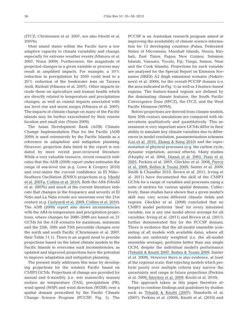
Fig. 1. Locations of the Pacific Climate Change Science Program (PCCSP) partner countries (all of which are labelled) and thedominant features of the regional climate in the western Pacific Ocean. Grey dashed lines indicate the boundary of the

‘PCCSP region’ used in much of the analysis, and orange arrows indicate the dominant wind flows

Clim Res 51: 35–58, 2012

and assign equal weight to the modelsretained.

The remainder of this paper is asfollows. Section 2 describes the dataand methods used in this study, fol-lowed by a summary of how the mainclimate features and drivers of thestudy region are evaluated in theCMIP3 GCMs. Section 3 provides theresults, Section 4 a discussion includ-ing linking changes in variables tochanges in climate drivers and fea-tures and Section 5 a summary andconclusions.

2. DATA AND METHODS

2.1. Study region and model data

The spatial domain of the studyregion considered is shown in Fig. 1,with latitude bounds of 25° S to 20° Nand longitude bounds of 120° E to210° E, i.e. 150° W. The domain waschosen be cause it incorporates allpartner countries of the PCCSP: Pa -lau, Federated States of Micronesia,Mar shall Is lands, Nauru, Kiribati,East Timor, Pa pua New Guinea, Solo -mon Islands, Vanuatu, Tuvalu, Fiji,Tonga, Samoa, Niue and the CookIslands. While these boundaries alsoinclude other countries, projectionsfor these countries are not discussedin this study.

GCM data were obtained from theCMIP3 data archive from the Program for ClimateModel Diagnosis and Intercomparison (PCMDI) atLawrence Livermore National Laboratory (www-pcmdi.llnl.gov/). A total of 19 out of 24 GCMsarchived data for the A2 scenario, which are listedwith their affiliations in Table 1. Atmospheric surfaceresolution among the CMIP3 GCMs ranges from ~2°× 2° (e.g. CSIRO-Mk3.0) to 4° × 5° (e.g. GISS-ER), soall models were regridded to 2.5° × 2.5° using theSCRIP regridder within the Climate Data AnalysisTool (CDAT; www2-pcmdi.llnl.gov/cdat), allowingfor the construction of multi-model ensembles. Pro-jections for the 21st century are constructed for TAS,PR, WSP and WDIR for the SRES A2 emission sce-nario (Nakic e novic et al. 2000) for the period2080−2099 (henceforth called 2090) relative to

1980−1999 (taken from the 20c3m simulation). WSPand WDIR data were not available under the A2 sce-nario for 3 of the models (Table 1). This base periodwas chosen as it represents a climatology of the samelength as the future period, is exactly one centuryearlier, and is included in the time period used to per-form much of the evaluation in Irving et al. (2011),where models are compared to ‘current’ conditions.The choice of this period for evaluation in Irving et al.(2011) was determined by the length and quality ofdata of the reference products, particularly whenconsidering the inclusion of satellite data in 1979.Annual and 6-monthly projections en compassingMay to October (MJJASO) and November to April(NDJFMA) are considered for all variables. For con-sistency, only the first run from each model was used.

38

Model name Model institute (Country)

BCCR-BCM2.0 Bjerknes Centre for Climate Research (Norway)

CCSM3 National Center for Atmospheric Research (USA)

CGCM3.1(T47)a Canadian Centre for Climate Modeling & Analysis(Canada)

CNRM-CM3 Centre National de Recherches Météorologiques(France)

CSIRO-Mk3.0c CSIRO Marine and Atmospheric Research (Australia)

CSIRO-Mk3.5 CSIRO Marine and Atmospheric Research (Australia)

ECHAM5/MPI-OM Max Planck Institute for Meteorology (Germany)

ECHO-Ga Meteorological Institute of the University of Bonn(Germany / Korea)

GFDL-CM2.0 Geophysical Fluid Dynamics Laboratory (USA)

GFDL-CM2.1 Geophysical Fluid Dynamics Laboratory (USA)

GISS-ER Goddard Institute for Space Studies (USA)

INGV-SXGc Instituto Nazionale di Geofisica e Vulcanologia (Italy)

INM-CM3.0b Institute for Numerical Mathematics (Russia)

IPSL-CM4 Institut Pierre Simon Laplace (France)

MIROC3.2 (medres) Center for Climate System Research (Japan)

MRI-CGCM2.3.2a Meteorological Research Institute (Japan)

PCMc National Center for Atmospheric Research (USA)

UKMO-HadCM3 Hadley Centre for Climate Prediction and Research(UK)

UKMO-HadGEM1 Hadley Centre for Climate Prediction and Research(UK)

aHeat flux corrected; bfreshwater/salinity flux adjusted; cdata not availablefor WSP and WDIR

Table 1. CMIP3 model names and their associated institutions for those mod-els that produced simulations for the A2 scenario. Models in bold reside inthe WORST ensemble (i.e. those that were poorer performers) based on theevaluation by Irving et al. (2011). All other models reside in the BEST ensem-ble. Surface air temperature (TAS) and precipitation (PR) data were availablefor all models, but not wind speed (WSP) and direction (WDIR), resulting in

different members and sample sizes in each ensemble

Perkins et al.: CMIP3 multi-model projections over the western Pacific

2.2. Model evaluation and selection

To potentially reduce some of the uncertainty inprojections, this study uses the results of Irving et al.(2011), where the CMIP3 GCMs were evaluated rig-orously over the PCCSP region (see Fig. 1). Generally,the evaluation of a climate model includes comparingthe 20th century model output to observations/reanalyses over the same time period. This assumesthat a model’s performance in simulating the currentclimate will influence its ability to simulate futureconditions. While there is no guarantee that thisassumption will be met (Jun et al. 2008, Knutti 2010),evaluating a model for events that have not yetoccurred is impossible. However, they can be investi-gated if models which perform well in simulating thecurrent climate (i.e. members of the BEST ensemble,see Section 2.3) converge in their future projections.This has been addressed in other re gional studies(e.g. Perkins & Pitman 2009, Perkins et al. 2009) andis a major focus of the current study.

Irving et al. (2011) evaluated the CMIP3 GCMs fortheir ability to simulate 9 key aspects of 20th centuryclimate. This list includes: TAS, WSP, WDIR, and PR;the dominating climate features including the SPCZ(Vincent 1994, Folland et al. 2002), ITCZ (Waliser &Gautier 1993), and WPM (Hendon & Liebmann1990a,b); ENSO (Diaz & Markgraf 2000, van Olden-borgh et al. 2005); the magnitude of spurious climatemodel drift (Power 1995, Covey et al. 2006); and seasurface temperature (SST) trends. For atmospheric(oceanic) evaluation, models were interpolated to acommon 2.5° (1.0°) latitude/longitude grid prior toanalysis. A brief description of how each aspect wasevaluated is given below, and detail is presented inIrving et al. (2011).

For each of PR, TAS, WSP and WDIR, metrics usedto assess each climate model include the phase andamplitude of the seasonal cycle. Over the period1979− 1999 Irving et al. (2011) assessed the ability ofthe models to simulate the:

(1) magnitude of temporal variability associatedwith the annual cycle;

(2) magnitude of temporal variability about theannual cycle;

(3) amplitude of spatial contrasts in climatologicalaverages; and

(4) spatial structure of climatological averages.In evaluating the ability of the CMIP3 climate mod-

els to simulate a realistic SPCZ, Irving et al. (2011)used the SPCZ region (0 to 30° S and 155° E to140° W) of Brown et al. (2011). The mean location ofthe SPCZ over this region was assessed by calculat-

ing the spatial correlation between the modeled andob served December to February (DJF) mean PRfields. Irving et al. (2011) also assessed the ability ofthe mo dels to simulate interannual variability in themean latitude of the SPCZ. The correlation betweenthe mean SPCZ latitude and model Niño 3.4 indexwas calculated and compared with the observed rela-tionship (see Brown et al. 2011 for details).

The mean location of the WPM was assessed by cal-culating the pattern correlation between the mod-eled and observed DJF PR over an appropriate WPMregion (20° S to 20° N and 110° to 160° E). The inten-sity of the WPM has a strongly inverse relationshipwith ENSO (e.g. Zhu & Chen 2002). Therefore, theability of the models to simulate this relationship wasassessed by calculating the correlation between thetotal DJF PR over the WPM region and the model sim-ulated Niño 3.4 index.

Interannual climate variability in the Pacific andsurrounding regions is dominated by ENSO. In orderto simulate a reasonable ENSO simulation, climatemodels need to realistically reproduce the (1) strengthand frequency of ENSO events, (2) spatial pattern ofENSO, and (3) link between ENSO and climate vari-ables such as PR. Property 1 was assessed by calculat-ing the ratio between the standard deviation of mod-eled and observed monthly Niño 3.4 index variabilityover the period 1950−1999. Property 2 was assessedusing the spatial correlation coefficient between mod-eled and observed maps of the temporal correlationbetween mean July to December Niño 3.4 index andthe mean SST anomaly at each grid point over an‘ENSO region’ (25° S to 25° N and 120° to 240° E [i.e.120°W]). Property 3 was assessed as follows. First thetemporal variability in the July to December Niño 3.4index was correlated with temporal variability in Julyto December PR totals at each grid point for both themodels and the observations. The spatial correlationcoefficient between the observational map and thecorresponding map for each model was then calcu-lated. The ratio between the standard deviation of themodel and observed temporal correlation fields wasalso calculated and combined with it as per the S sta-tistic proposed by Taylor (2001).

A persistent problem with some coupled climatemodels is that of spurious climate drift, which is adrift in model climatology that is due to systematicerrors in the climate model and not due to genuineclimate variability or genuine external climate forc-ing (e.g. Power 1995, Covey et al. 2006, Sen Gupta etal. in press). These drifts are a result of errors in sur-face fluxes between the climate model componentsand deficiencies in the model physics, which mean

39

Clim Res 51: 35–58, 2012

that the equilibrium state of the model is differentfrom the initial (usually observationally derived)state. In order to objectively evaluate spurious cli-mate drift in each of the models, the magnitude of thepre-industrial (PIcntrl) linear TAS and PR trend ateach grid point over the PCCSP region was calcu-lated for a 150 yr period, aligning with the 1900−2050period of the 20th century (20c3m) simulation. Thespatial average of these trend magnitudes was takenas a measure of model drift. The method used toaccomplish this is described by Sen Gupta et al. (inpress).

The ability of the CMIP3 models to capture thewarming observed in recent decades was as sessedby calculating the 1950− 1999 linear SST trends,using the 20c3m simulation at each grid point overthe PCCSP re gion. These trends were corrected forspurious model drift by subtracting the linear trendsfrom the 150 yr pre-industrial simulations and com-pared to observed trends by calculating the averagemagnitude of the grid point errors.

Once all of the above assessments were made, Irv-ing et al. (2011) calculated a nor-malised score for each metric using amethod similar to Santer et al. (2009),so that one metric per aspect (i.e. pervariable, feature, ENSO and modeldrift) could be defined. Once theabsolute error for each metric wasobtained, it was normalised by con-verting it to an anomaly (i.e. by sub-tracting the multi-model averagescore) and then dividing that anomalyby the intermodel standard deviation.Good and poor performance was indi-cated by increasingly negative andpositive normalised scores, respec-tively, and for each metric these nor-malised scores had a multi-modelaverage of 0.0 and standard deviationof 1.0. To obtain an indication of over-all model performance on each of the9 key aspects, an average over all rel-evant normalized scores was also cal-culated by Irving et al. (2011) (Fig. 2).

The conclusions of Irving et al.(2011) therefore provide guidance onthe relative skill of the models in sim-ulating climate over the PCCSPregion and which models to eliminatefrom particular projections. Modelsdeemed as the poorest performers byIrving et al. (2011) include INGV-SXG

due to its large drift, GISS-ER as no ENSO signal ispresent, and PCM and INM-CM3.0 as they werefound to be relatively poor performers over numer-ous metrics (Fig. 2). GISS-AOM and GISS-EH arealso poor performers but do not provide data for theA2 scenario and are therefore not relevant to the pre-sent study.

2.3. Model ensembles and projections

Using the results of Irving et al. (2011), we define 3ensembles to provide projections for each variable.These ensembles are (1) the ALL ensemble (all 19 mo -dels), (2) the BEST ensemble, which consists of BCCR-BCM2.0, CCSM3, CGCM3.1(T47), CNRM-CM3,CSIRO-Mk3.0, CSIRO-Mk3.5, ECHAM5/MPI-OM,ECHO-G, GFDL-CM2.0, GFDL-CM2.1, IPSL-CM4,MIROC3.2 (medres), MRI-CGCM2.3.2, UKMO-HadCM3, UKMO-HadGEM1, and (3) the WORSTensemble (INGV-SXG, GISS-ER, INM-CM3.0 andPCM only). Ensemble 2 (BEST) was calculated based

40

Fig. 2. Mean normalised test scores performed by Irving et al. (2011) for all 9key aspects in each of the 19 CMIP3 climate model simulations (includes 5 mod-els not used in this study: CGCM3.1(T63), GISS-EH, MIROC3.2hires, GISS-AOM, FGOALS-g1.0). Increasing negative scores indicate better model perfor-mance. The connected solid black dots represent the average across all aspects.See Table 1 for model descriptions and Table 2 for region locations. Adaptedfrom Fig. 8 of Irving et al. (2011). TAS: surface air temperature; PR: precipita-tion; SPCZ: South Pacific Convergence Zone; ITCZ: Intertropical ConvergenceZone; WPM: West Pacific Monsoon; ENSO: El Niño−Southern Oscillation;

SST: sea surface temperature

Perkins et al.: CMIP3 multi-model projections over the western Pacific

on the performance of the GCMs across all criteria inIrving et al. (2011), where (INGV-SXG, GISS-ER,GISS-EH, INM-CM3.0 and PCM) were omitted fromthe ALL ensemble.

These 3 groups or ensembles of models were usedfor all annual and 6-monthly projections for all vari-ables, that is the same models make up the BEST andWORST ensembles for each variable and time period.While there is strong evidence that any given modeldoes not perform consistently across multiple vari-ables (e.g. Whetton et al. 2007, Gleckler et al. 2008),segregation of the models into ensembles is based onthe overall evaluation scores presented in Irving et al.(2011; our Fig. 2). Furthermore, using the same set ofensembles for all variables allows the present studyto give physically consistent projections across anumber of climate variables, unlike some previousregional studies (e.g. Pitman & Perkins 2008, Perkins& Pitman 2009).

Results in this paper are presented in a similar for-mat to the IPCC AR4 (Meehl et al. 2007b, Christen -sen et al. 2007), showing mean projections of the en -sembles and the corresponding standard deviations.Projections in the AR4 make use of all GCMswhereby taking the mean assigns equal weights toall members, or the ‘one-model-one-vote’ approach(Knutti 2010). As noted above, we take a similar ap -proach in that all members of each of the 3 ensemblesare equally weighted; however we include anotherstep by constructing Ensembles 2 (BEST) and 3(WORST) based on model skill, which allows us to de -termine if projections are altered by the eliminationof certain models. The WORST ensemble is in cludedto illustrate the influence that poorer performingmodels may have on the ALL ensemble; projectionsfrom this ensemble are not recommended for riskassessment and adaptation planning.

All projected changes are calculated individuallyfor each model and the average is taken across allmembers of the respective ensembles. PR and WSPchanges are calculated as percentages relative to thebase period, TAS is presented in degrees Celsius andWDIR is presented as degrees change relative to theensemble median base period direction (also shown).Positive values indicate a clockwise change, and neg-ative values an anticlockwise change.

For each ensemble projection, the standard devia-tion (σ) was calculated to measure intra-ensemblevariability in order to quantify the contrasts betweenthe individual members. Determining if the ensem-ble members have similar projections of change toone another is useful. In the case of the BEST ensem-ble, this can help determine if omitting the less-

skilled models reduces some of the uncertainty bynarrowing the spread of the projected changes, par-ticularly when compared to the ALL ensemble. Fur-thermore, looking at a measure of spatial ensemblevariability can help determine if the uncertainty asso-ciated with a given projection is uniform or if re -gional differences occur and if uncertainty differsacross projection scenarios.

There are 15 models included in the BEST ensem-ble and only 4 in the WORST. This difference inensemble size has an impact on σ. Conclusions byIrving et al. (2011) suggest only 6 models with littleconfidence in simulating the current climate fromthe overall CMIP3 ensemble of 24, of which a totalof only 19 provide data for the A2 scenario. Basedon the overall evaluation performed (Fig. 2), there isnot enough evidence to remove any of the other 18(15). Al though some models have a wide range ofperformance across all aspects, their overall scoresare similar, which makes it hard to distinguishbetween the models any further, resulting in only 4models in the WORST ensemble. While increasingthe size of the WORST ensemble by just 1 or 2 moremembers would increase the respective validity of σ(and have little impact on projections from the BESTensemble), the authors do not find it reasonable tolabel any further models as poor performers, due tothe close proximity of their overall scores (i.e. thereis not enough evidence to take any more modelsfrom the BEST ensemble). Therefore, great care isadvised when considering projections of σ for theWORST ensemble due to is sensitivity for small sam-ples. This ensemble is included as a point of compar-ison with the ALL and BEST ensembles, rather thanas a robust projection.

The statistical significance was calculated betweenthe ALL ensemble and the 2 ensemble subsets for theentire study (PCCSP) region, as well as 3 feature-based regions: the SPCZ, ITCZ and WPM regions.The non-parametric Kolmogorov-Smirnov test (Ste -phens 1970, 1986) was used to determine if the en -semble change of the subset ensemble (BEST,WORST) was significantly different from the ALLensemble. The null hypothesis that the ensemblesubset change for the region is not distinguishablefrom the ALL ensemble change is rejected at the 5%significance level. This was performed to determineif the difference between current model performanceand future projections varies across the domainsaffected by the respective climate features. Since theCMIP3 GCMs can only provide projections at courseresolution, great care needs to be taken when inter-preting both evaluation and projection results at sub-

41

Clim Res 51: 35–58, 2012

regional scales (i.e. those smaller than continental).The size of the PCCSP region and the feature-basedregions were chosen with this in mind.

Projections were also calculated for the B1 and A1BSPES scenarios and also for 20 yr periods centred on2030 and 2055. While not presented, spatial patternsof change and their statistical significance weremostly the same across scenarios and time periodsbut generally of lower magnitude under the loweremission scenarios as well as time periods that occurearlier in the 21st century (see Section 4.1).

3. RESULTS

3.1. Surface air temperature (TAS)

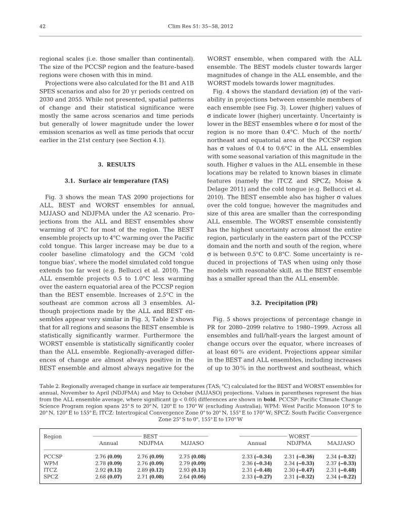
Fig. 3 shows the mean TAS 2090 projections forALL, BEST and WORST ensembles for annual,MJJASO and NDJFMA under the A2 scenario. Pro-jections from the ALL and BEST ensembles showwarming of 3°C for most of the region. The BESTensemble projects up to 4°C warming over the Pacificcold tongue. This larger increase may be due to acooler baseline climatology and the GCM ‘coldtongue bias’, where the model simulated cold tongueextends too far west (e.g. Bellucci et al. 2010). TheALL ensemble projects 0.5 to 1.0°C less warmingover the eastern equatorial area of the PCCSP regionthan the BEST ensemble. Increases of 2.5°C in thesoutheast are common across all 3 ensembles. Al -though projections made by the ALL and BEST en -sembles appear very similar in Fig. 3, Table 2 showsthat for all regions and seasons the BEST ensemble isstatistically significantly warmer. Furthermore theWORST ensemble is statistically significantly coolerthan the ALL ensemble. Regionally-averaged differ-ences of change are almost always positive in theBEST ensemble and almost always negative for the

WORST ensemble, when compared with the ALLensemble. The BEST models cluster towards largermagnitudes of change in the ALL ensemble, and theWORST models towards lower magnitudes.

Fig. 4 shows the standard deviation (σ) of the vari-ability in projections between ensemble members ofeach ensemble (see Fig. 3). Lower (higher) values ofσ indicate lower (higher) uncertainty. Uncertainty islower in the BEST ensembles where σ for most of theregion is no more than 0.4°C. Much of the north/northeast and equatorial area of the PCCSP regionhas σ values of 0.4 to 0.6°C in the ALL ensembleswith some seasonal variation of this magnitude in thesouth. Higher σ values in the ALL ensemble in theselocations may be related to known biases in climatefeatures (namely the ITCZ and SPCZ; Moise &Delage 2011) and the cold tongue (e.g. Bellucci et al.2010). The BEST ensemble also has higher σ valuesover the cold tongue; however the magnitudes andsize of this area are smaller than the correspondingALL ensemble. The WORST ensemble consistentlyhas the highest uncertainty across almost the entireregion, particularly in the eastern part of the PCCSPdomain and the north and south of the region, whereσ is between 0.5°C to 0.8°C. Some uncertainty is re -duced in projections of TAS when using only thosemodels with reasonable skill, as the BEST ensemblehas a smaller spread than the ALL ensemble.

3.2. Precipitation (PR)

Fig. 5 shows projections of percentage change inPR for 2080−2099 relative to 1980−1999. Across allensembles and full/half-years the largest amount ofchange occurs over the equator, where increases ofat least 60% are evident. Projections appear similarin the BEST and ALL ensembles, including increasesof up to 30% in the northwest and southeast, which

42

Region BEST WORST Annual NDJFMA MJJASO Annual NDJFMA MAJJASO

PCCSP 2.76 (0.09) 2.76 (0.09) 2.75 (0.08) 2.33 (−0.34) 2.31 (−0.36) 2.34 (−0.32)WPM 2.78 (0.09) 2.76 (0.09) 2.79 (0.09) 2.36 (−0.34) 2.34 (−0.33) 2.37 (−0.33)ITCZ 2.92 (0.13) 2.89 (0.12) 2.93 (0.13) 2.31 (−0.48) 2.30 (−0.47) 2.31 (−0.48)SPCZ 2.68 (0.07) 2.71 (0.08) 2.64 (0.06) 2.33 (−0.27) 2.31 (−0.32) 2.34 (−0.22)

Table 2. Regionally averaged change in surface air temperatures (TAS; °C) calculated for the BEST and WORST ensembles forannual, November to April (NDJFMA) and May to October (MJJASO) projections. Values in parentheses represent the biasfrom the ALL ensemble average, where significant (p < 0.05) differences are shown in bold. PCCSP: Pacific Climate ChangeScience Program region spans 25° S to 20° N, 120° E to 170° W (excluding Australia); WPM: West Pacific Monsoon 10° S to20° N, 120° E to 155° E; ITCZ: Intertropical Convergence Zone 0° to 20° N, 155° E to 170° W; SPCZ: South Pacific Convergence

Zone 25° S to 0°, 155° E to 170° W

Perkins et al.: CMIP3 multi-model projections over the western Pacific 43

Fig. 3. Ensemble mean surface air temperature (TAS) change for the Pacific Climate Change Science Program (PCCSP) re-gion under the A2 emissions scenario for a 20 yr period centred on 2090 using the 3 model ensembles (ALL, BEST, WORST)

projected annually and 6-monthly (NDJFMA: November to April; MJJASO: May to October)

Fig. 4. Ensemble mean uncertainty (the ensemble variability, measured by the standard deviation) of surface air temperature(TAS) change for the PCCSP region under the A2 scenario for a 20 yr period centred on 2090 using the 3 model ensembles

(ALL, BEST, WORST) projected annually and 6-monthly (NDJFMA: November to April; MJJASO: May to October)

Clim Res 51: 35–58, 2012

encompasses the domain of the SPCZ, during the an -nual and NDJFMA projections (Vincent 1994, Brownet al. 2011), increases of 30 to 40% in the north,which encompasses the range of the ITCZ, during allseasons (Waliser & Gautier 1993); and decreases nearEast Timor during MJJASO. Increases in PR are alsoevident in the WORST ensembles but are slightlysmaller in size over the equator in the annual andMJJASO projections and are larger in the south ofthe region during all periods. Increases in precipita-tion in the north of the region are also less pro-nounced in the WORST ensemble. Projections usingthe BEST ensemble are generally not significantlydifferent from the ALL ensemble (with the exceptionof annual projections over the PCCSP and ITCZregions, and MJJASO projections over the PCCSPand SPCZ re gions). On the other hand, projectionsfrom the WORST ensemble generally are signifi-cantly different from those of the ALL ensemble(Table 3). Similar to TAS, regionally averaged PRbiases are almost always positive in the BEST ensem-bles and almost always negative for the WORSTensembles when compared with the ALL ensemble.That is, there is a greater increase in precipitation inthe BEST models than the WORST models.

Fig. 6 shows the ensemble standard deviationamong each ensemble presented in Fig. 5. Areas ofhigher ensemble variability (up to 100%) correspondto areas of largest increase in Fig. 5 (most notablyover the cold tongue) particularly during MJJASOusing the BEST and ALL ensembles. Values of σ ofup to 50% are associated with the drying over EastTimor during MJJASO, and σ values of 40% occurzonally at 10° N during NDJFMA, which may berelated to ensemble members differing in their ITCZpositioning (not shown). Higher σ values associatedwith the cold tongue show a more zonal pattern inthe WORST ensembles and extend further west. Val-ues of σ in the WORST ensembles are around 10%less in some areas than those of the other 2 ensem-bles, which are comparable to one another. The

smaller ensemble variability in the WORST ensem-ble is likely to be due to the smaller sample size.

3.3. Wind speed (WSP)

Fig. 7 presents changes in WSP for the PCCSPregion. When considering ALL and BEST ensembleprojections, the annual mean WSP decreases by 5 to10% in the north and increases by 5 to 15% south of5° S and in the far northwest. This implies a weaken-ing of the Walker cell along the equator (changes arebetween −5 and −10% between 5° N and 5° S), whichis consistent with other studies (e.g. Vecchi et al.2006, Power & Kociuba 2010). Changes in the south-west are 5% smaller in the BEST ensemble than theyare in the ALL ensemble. Similar north/south spatialpatterns occur during MJJASO; however increases inthe south are pushed towards 10° S and vary be -tween 15 and 45%. Decreases in the centre of theregion are 5% larger in the BEST ensemble than inthe ALL ensemble, and decreases also appear in thewest of the region. Projections for NDJFMA using theBEST ensemble show increases of 5 to 10% in the farnorth and south, increases of 10 to 30% stretchingsouthwest from Papua New Guinea, and increases of30% in the west near East Timor. The rest of theregion shows decreases of around 5%, and mostother projections in the BEST ensemble are generallysimilar to those in the ALL ensemble, with the excep-tion of an increase in the centre of the region. Consid-erable differences are evident in the WORST ensem-bles. Much of the region (particularly the north) hasincreases of up to 30% for the annual mean andincreases exceeding 45% that occur east and west ofPapua New Guinea, related to seasonal shifts of theWPM. Decreases of 10 to 25% oc cur southeast ofPapua New Guinea during NDJFMA, which encom-passes at least part of the SPCZ. Increases of at least45% occur in the northwest during MJJASO, againpossibly related to seasonal shifts in the WPM. In con-

44

Region BEST WORST Annual NDJFMA MJJASO Annual NDJFMA MAJJASO

PCCSP 15.97 (0.82) 16.33 (1.20) 18.85 (0.37) 12.06 (−3.09) 10.62 (−4.51) 17.08 (−1.40)WPM 7.74 (0.22) 9.53 (0.89) 6.72 (−0.34) 6.69 (−0.83) 5.28 (−3.35) 8.34 (1.28)ITCZ 26.28 (2.61) 21.94 (2.57) 37.58 (2.20) 13.88 (−9.79) 9.75 (−9.62) 27.13 (−8.25)SPCZ 17.45 (0.35) 19.62 (0.61) 18.66 (0.32) 15.81 (−1.30) 16.71 (−2.30) 17.15 (−1.19)

Table 3. Regionally averaged change in precipitation (PR; %) from the base period (1980−1999) calculated for the BEST andWORST ensembles for annual, November to April (NDJFMA) and May to October (MJJASO) projections. Values in parenthe-ses represent the bias from the ALL ensemble average, where significant (p < 0.05) differences are shown in bold. See Table 2

legend for region abbreviations and locations

Perkins et al.: CMIP3 multi-model projections over the western Pacific 45

Fig. 5. Ensemble mean precipitation change (%) relative to the base climate period (1980−1999) using the 3 model ensembles(ALL, BEST, WORST) projected annually and 6-monthly (NDJFMA: November to April; MJJASO: May to October). See Fig. 3

legend for complete details

Fig. 6. Ensemble mean uncertainty in precipitation change (%) relative to the base climate period (1980−1999) using the 3 modelensembles (ALL, BEST, WORST) projected annually and 6-monthly (NDJFMA: November to April; MJJASO: May to October).

See Fig. 4 legend for complete details

Clim Res 51: 35–58, 201246

junction with results from NDJFMA, the poorer per-forming models tend to exacerbate increases of WSPover the WPM spatial domain. Wind speeds tend toincrease over much of the region in the WORSTensemble during NDJFMA, with the exception of inand immediately west of Papua New Guinea.

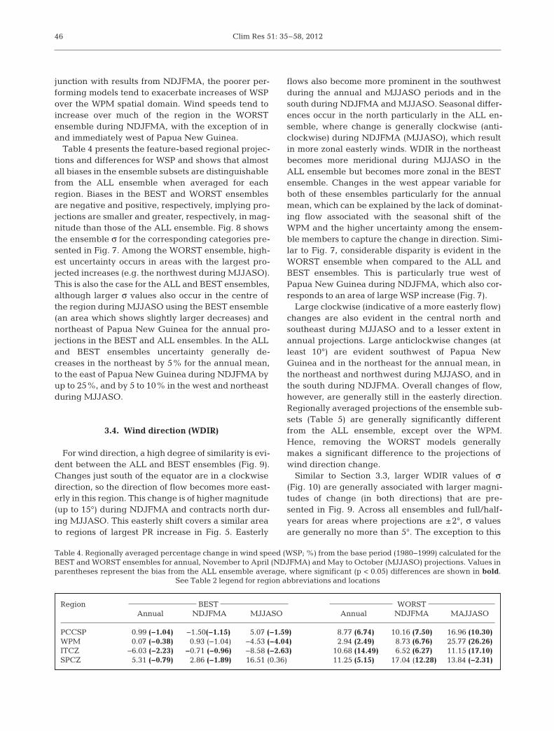
Table 4 presents the feature-based regional projec-tions and differences for WSP and shows that almostall biases in the ensemble subsets are distinguishablefrom the ALL ensemble when averaged for eachregion. Biases in the BEST and WORST ensemblesare negative and positive, respectively, implying pro-jections are smaller and greater, respectively, in mag-nitude than those of the ALL ensemble. Fig. 8 showsthe ensemble σ for the corresponding categories pre-sented in Fig. 7. Among the WORST ensemble, high-est uncertainty occurs in areas with the largest pro-jected increases (e.g. the northwest during MJJASO).This is also the case for the ALL and BEST ensembles,al though larger σ values also occur in the centre ofthe region during MJJASO using the BEST ensemble(an area which shows slightly larger decreases) andnortheast of Papua New Guinea for the annual pro-jections in the BEST and ALL ensembles. In the ALLand BEST ensembles uncertainty generally de -creases in the northeast by 5% for the annual mean,to the east of Papua New Guinea during NDJFMA byup to 25%, and by 5 to 10% in the west and northeastduring MJJASO.

3.4. Wind direction (WDIR)

For wind direction, a high degree of similarity is evi-dent between the ALL and BEST ensembles (Fig. 9).Changes just south of the equator are in a clockwisedirection, so the direction of flow becomes more east-erly in this region. This change is of higher magnitude(up to 15°) during NDJFMA and contracts north dur-ing MJJASO. This easterly shift covers a similar areato regions of largest PR increase in Fig. 5. Easterly

flows also become more prominent in the southwestduring the annual and MJJASO periods and in thesouth during NDJFMA and MJJASO. Seasonal differ-ences occur in the north particularly in the ALL en-semble, where change is generally clockwise (anti-clockwise) during NDJFMA (MJJASO), which resultin more zonal easterly winds. WDIR in the northeastbecomes more meridional during MJJASO in theALL ensemble but becomes more zonal in the BESTensemble. Changes in the west appear variable forboth of these ensembles particularly for the annualmean, which can be explained by the lack of dominat-ing flow associated with the seasonal shift of theWPM and the higher uncertainty among the ensem-ble members to capture the change in direction. Simi-lar to Fig. 7, considerable disparity is evident in theWORST ensemble when compared to the ALL andBEST ensembles. This is particularly true west ofPapua New Guinea during NDJFMA, which also cor-responds to an area of large WSP increase (Fig. 7).

Large clockwise (indicative of a more easterly flow)changes are also evident in the central north andsoutheast during MJJASO and to a lesser extent inannual projections. Large anticlockwise changes (atleast 10°) are evident southwest of Papua NewGuinea and in the northeast for the annual mean, inthe northeast and northwest during MJJASO, and inthe south during NDJFMA. Overall changes of flow,however, are generally still in the easterly direction.Regionally averaged projections of the ensemble sub-sets (Table 5) are generally significantly differentfrom the ALL ensemble, except over the WPM.Hence, removing the WORST models generallymakes a significant difference to the projections ofwind direction change.

Similar to Section 3.3, larger WDIR values of σ(Fig. 10) are generally associated with larger magni-tudes of change (in both directions) that are pre-sented in Fig. 9. Across all ensembles and full/half-years for areas where projections are ±2°, σ valuesare generally no more than 5°. The exception to this

Region BEST WORST Annual NDJFMA MJJASO Annual NDJFMA MAJJASO

PCCSP 0.99 (−1.04) −1.50(−1.15) 5.07 (−1.59) 8.77 (6.74) 10.16 (7.50) 16.96 (10.30)WPM 0.07 (−0.38) 0.93 (−1.04) −4.53 (−4.04) 2.94 (2.49) 8.73 (6.76) 25.77 (26.26)ITCZ −6.03 (−2.23) −0.71 (−0.96) −8.58 (−2.63) 10.68 (14.49) 6.52 (6.27) 11.15 (17.10)SPCZ 5.31 (−0.79) 2.86 (−1.89) 16.51 (0.36) 11.25 (5.15) 17.04 (12.28) 13.84 (−2.31)

Table 4. Regionally averaged percentage change in wind speed (WSP; %) from the base period (1980−1999) calculated for theBEST and WORST ensembles for annual, November to April (NDJFMA) and May to October (MJJASO) projections. Values inparentheses represent the bias from the ALL ensemble average, where significant (p < 0.05) differences are shown in bold.

See Table 2 legend for region abbreviations and locations

Perkins et al.: CMIP3 multi-model projections over the western Pacific 47

Fig. 7. Ensemble mean change in wind speed (%) relative to the base climate period (1980−1999) using the 3 model ensembles(ALL, BEST, WORST) projected annually and 6-monthly (NDJFMA: November to April; MJJASO: May to October). See Fig. 3

legend for complete details

Fig. 8. Ensemble mean uncertainty in wind speed change (%) relative to the base climate period (1980−1999) using the 3 modelensembles (ALL, BEST, WORST) projected annually and 6-monthly (NDJFMA: November to April; MJJASO: May to October).

See Fig. 4 legend for complete details

Clim Res 51: 35–58, 2012

is over the WPM region during MJJASO for the BESTand ALL ensembles, where σ is between 10 and 20°.Values of σ of around 30° occur in these ensemblesover Papua New Guinea and East Timor duringNDJFMA, which coincides with the positioning ofthe WPM during austral summer and areas of up to10° anticlockwise change in Fig. 9. In the BEST andALL ensembles, σ values northwest of Papua NewGuinea are at least 30° for the annual mean. Uncer-tainty in WDIR change tends to be slightly higherover the SPCZ region (σ of 10 to 15°) particularly dur-ing NDJFMA. Uncertainty in projected changes inthe direction of flow is high at 10° N and 10° S duringNDJFMA and MJJASO, respectively. In the WORSTensemble, σ values of at least 10 to 20° occur in thecentral northeast and northwest and southeast dur-ing the annual and NDJFMA, east of Papua NewGuinea during NDJFMA, and in the northeast andnorthwest during MJJASO. All of these are areas oflarger changes in Fig. 9.

4. DISCUSSION

4.1. Ensemble projections and uncertainty

Projections presented for the study region underthe SRES A2 scenario by 2090 show warming temper-atures of around 3°C, PR increases of at least 60%over the equator and 10 to 30% in the north andsouth, PR decreases of up to 20% in the far south andover East Timor during MJJASO, WSP decreases(increases) in the north (south), and winds tendingtowards a more easterly direction. Such projectionsare consistent across the ALL and BEST ensembles;however the WORST ensemble tends to be substan-tially different. Despite similar magnitudes and spa-tial patterns in Figs. 3, 5, 7 & 9 for the BEST and ALLensembles, regionally averaged mean ensemble pro-jections by the BEST ensembles are always signifi-

cantly different from the ALL ensemble for TAS(Table 2), almost always statistically significantly dif-ferent for WSP (Table 4), and statistically signifi-cantly different for some regions and seasons for PRand WDIR (Tables 3 & 5). Furthermore, projectionsfrom the WORST ensembles are always statisticallysignificantly different from the ALL ensemble foreach variable, time period, and region, illustratingthat models which have lower skill in simulating cur-rent conditions produce distinguishably different pro-jections from the other models in the ALL ensemble.Similar results have also been found over otherregions using the CMIP3 GCMs (e.g. Perkins et al.2009).

Uncertainty (in terms of the inter-model spread) isreduced when omitting the less skilled models forTAS projections (Fig. 3) and in some regions for WSP(Fig. 7). However uncertainty is generally compara-ble across the ALL and BEST ensembles for PR(Fig. 5) and WDIR (Fig. 9). Therefore in the latter 2cases we cannot say that some of the uncertainty inprojections of change for the respective variables isreduced when less skilled models are eliminated, atleast over the PCCSP region. While we have goodreason to place higher confidence in the BESTensemble compared to the ALL ensemble and (espe-cially) the WORST ensemble, the spread of the indi-vidual members is not correlated to model ability forPR and WDIR, i.e. members within the BEST ensem-ble do not cluster around projected changes in therespective variables any differently than members inthe corresponding ALL ensemble (Figs. 6 & 10).

By 2030 and 2055 under the B1 and A1B scenarios,projected changes in all variables are similar to thosepresented in this paper but are of smaller magnitude.Changes in TAS by 2030 are up to 1°C for the regionacross all scenarios, seasons and ensembles. By 2055,spatial patterns emerge where the northeast warms0.5°C more than the rest of the PCCSP region. Simi-lar warming patterns in TAS (Fig. 3) are present

48

Region BEST WORST Annual NDJFMA MJJASO Annual NDJFMA MAJJASO

PCCSP 0.61 (0.16) 0.43 (−0.24) −0.39 (0.40) −0.58 (−1.03) 2.20 (1.54) −3.40 (−2.60)WPM −1.06 (−0.19) −1.21 (−0.35) 0.55 (0.21) 0.40 (1.26) 1.40 (2.25) −1.01 (−1.36)ITCZ −0.73 (−0.09) −0.72 (−0.25) −0.64 (0.77) −0.08 (0.56) 2.63 (1.65) −6.40 (−4.99)SPCZ 2.83 (0.50) 1.73 (−0.29) −0.13 (0.30) −0.90 (−3.23) 3.90 (1.88) −2.36 (−1.93)

Table 5. Regionally averaged change in wind direction (WDIR; °) from the base period (1980−1999) calculated for the BEST andWORST ensembles for annual, November to April (NDJFMA) and May to October (MJJASO) projections. Positive changes im-ply a clockwise change relative to the base period flow, negative changes an anticlockwise change. Values in parentheses rep-resent the bias from the ALL ensemble average, where significant (p < 0.05) differences are shown in bold. See Table 2 legend

for region abbreviations and locations

Perkins et al.: CMIP3 multi-model projections over the western Pacific 49

Fig. 9. Ensemble mean change in wind direction (°) using the 3 model ensembles (ALL, BEST, WORST) projected annuallyand 6-monthly (NDJFMA: November to April; MJJASO: May to October). Vectors indicate ensemble mean direction of

flow during the base period. See Fig. 3 legend for complete details

Fig. 10. Ensemble mean uncertainty in wind direction (°) using the 3 model ensembles (ALL, BEST, WORST) projected annuallyand 6-monthly (NDJFMA: November to April; MJJASO: May to October). Since the standard deviation is a measure of spread,this figure represents the spread of wind direction across the ensemble, rather than the distance from North (0°). See Fig. 4 legend

for complete details

Clim Res 51: 35–58, 2012

under the B1 and A1B scenarios by 2090, though thechanges are again smaller in magnitude. TAS valuesof σ are broadly similar across all scenarios and en -sembles in 2030. TAS values of σ are comparableacross the ALL and BEST ensembles under A1B in2055 and 2090, and across all 3 ensembles under B1.Patterns of PR change in 2030 and 2055 under theA1B and B1 scenarios are similar to those in Fig. 5 butare smaller in magnitude. PR values of σ for 2030 and2055 under the A1B and B1 scenarios are similar tothose in Fig. 6, though regions with larger σ are ofsmaller spatial extent. Projections of change in WSPand WDIR and corresponding values of σ across B1and A1B and in 2030 and 2055 are very similar tothose presented in Figs. 7 to 10 but are generallysmaller in magnitude.

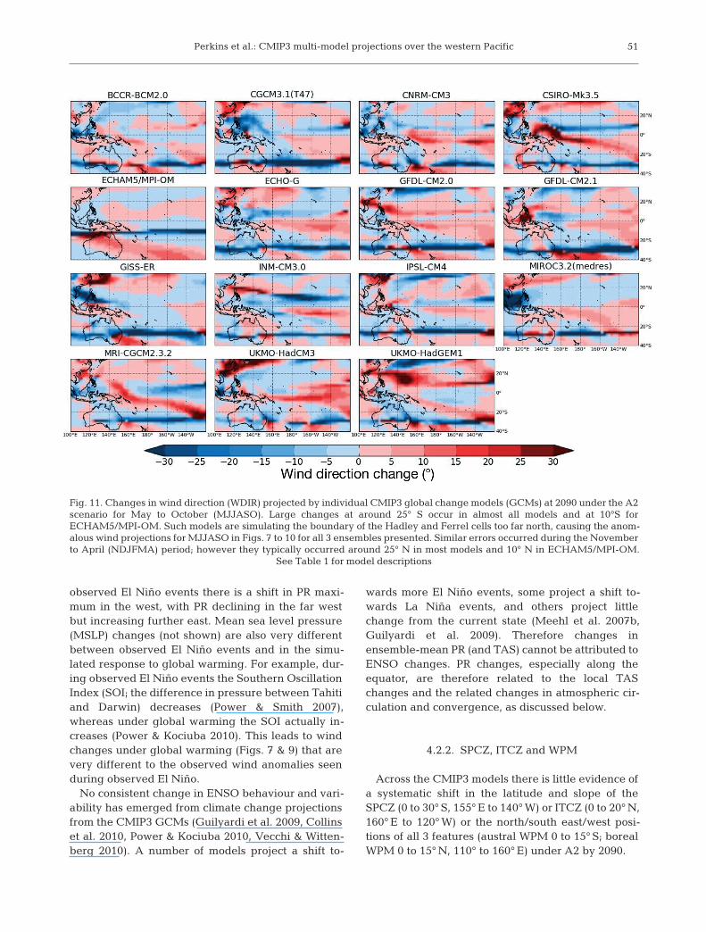
Discrepancies in WSP and WDIR projections and σvalues (Figs. 7 to 10) have also been presented. TheBEST and ALL ensembles show some regions oflarger magnitudes, most notably around 10° N duringNDJFMA (in the east), 10° S during MJJASO (in theeast and west), and 25° S during the annual and MJJASO timescales. The anomalous patterns at 10° Nare generally due to larger changes in just one mem-ber, influencing both the mean change and the stan-dard deviation of the ensembles at these locations.The southern (northern) Hadley and Ferrel cellboundaries of the MPI ECHAM GCM during MJJASO(NDJFMA) occurs at 10° S (10° N), explaining theanomalous projections along these latitudes duringthe respective seasons (see Fig. 11 for MJJASO WDIRchange). The large boundary changes (in terms of di-rection of flow and speed) of the southern Hadley andFerrel cells in individual ensemble members canoccur as far north as 25° S during MJJASO, causingthe anomalous WSP and WDIR bands at this latitudein Figs. 7 to 10 during MJJASO and also in the annualprojections. Wind speed and direction changes there-fore apply at the large scale or regional scale only.This result is also evidence that using only those mod-els with higher skill in simulating changes in the 20thcentury does not always mean that anomalous errorsare removed or that uncertainty is reduced. Metricsthat evaluate changes in the Hadley and Ferrel cellsshould be calculated in future evaluation studies overthe Pacific domain, as well as any other regionlocated, even partially, over the subtropics.

4.2. Changes in drivers and features

Following the approach of the ADB (2009), weattempt to explain changes in the climate of the

Pacific region in relation to changes in ENSO andmajor climate features (SPCZ, ITCZ, WPM). Thesefeatures, as well as ENSO, are important, as they gov-ern the Pacific climate on annual, interannual andlonger timescales. Undertaking this task may deepenthe understanding of the changes in the west Pacificclimate presented above and help us assess thedegree of confidence we might have in the projec-tions in particular regions. Changes in ENSO, SPCZ,ITCZ, and WPM within the CMIP3 GCMs are dis-cussed briefly below.

4.2.1. ENSO

Since a close coupling exists between TAS and SSTsover the Pacific, changes in TAS from the CMIP3GCMs under the A2 scenario by 2090 (Fig. 3) revealthat the maximum increase in SST over the domain oc-curs towards the eastern equatorial area of the PCCSPregion (Meehl et al. 2007b). The maximum SSTchange extends further east in the BEST models andtends to be more restricted to the central Pacific in theWORST models. The changes in the ALL ensembleand in the BEST ensemble somewhat resemble thepattern of SSTs during a typical El Niño event, in thesense that this is also the location of maximum SSTanomalies during El Niño events. Interestingly, the lo-cation of these anomalies in the WORST ensemble isclose to where the Modoki El Niño has its maximumSST anomaly (Ashok et al. 2007). The equatorial east-erlies also weaken under global warming (Fig. 9), asthey do during El Niño events.

Despite some similarities between the projected cli-mate change signal and the observed El Niño temper-ature mean state, the use of the term ‘El Niño-like’ tocharacterize the fingerprint of global warming in thePacific is misleading (e.g. Vecchi & Wittenberg 2010,Collins et al. 2010). This is because the mean patternof warming by 2090 does not imply that the climatewill tend towards conditions experienced during theEl Niño phase of ENSO, which is a measure of cli-mate variability rather than a description of the meanstate. Furthermore, the extent of agreement betweenprojected El Niño patterns and the global warmingsignal in the CMIP3 GCMs is very limited, and insome cases they conflict (Guilyardi et al. 2009, Vec-chi & Wittenberg 2010). In SST projections, for exam-ple, there is no off-equatorial SST cooling underglobal warming (see Fig. 3 for TAS), whereas this pat-tern tends to occur during observed El Niño events.Under global warming, projected PR tends to in -crease along the equator (Fig. 5), whereas during

50

Perkins et al.: CMIP3 multi-model projections over the western Pacific 51

observed El Niño events there is a shift in PR maxi-mum in the west, with PR declining in the far westbut increasing further east. Mean sea level pressure(MSLP) changes (not shown) are also very differentbetween ob served El Niño events and in the simu-lated response to global warming. For example, dur-ing observed El Niño events the Southern OscillationIndex (SOI; the difference in pressure between Tahitiand Darwin) decreases (Power & Smith 2007),whereas under global warming the SOI actually in -creases (Power & Kociuba 2010). This leads to windchanges under global warming (Figs. 7 & 9) that arevery different to the observed wind anomalies seenduring observed El Niño.

No consistent change in ENSO behaviour and vari-ability has emerged from climate change projectionsfrom the CMIP3 GCMs (Guilyardi et al. 2009, Collinset al. 2010, Power & Kociuba 2010, Vecchi & Witten-berg 2010). A number of models project a shift to -

wards more El Niño events, some project a shift to -wards La Niña events, and others project littlechange from the current state (Meehl et al. 2007b,Guil yardi et al. 2009). Therefore changes in ensemble- mean PR (and TAS) cannot be attributed toENSO changes. PR changes, especially along theequator, are therefore related to the local TASchanges and the related changes in atmospheric cir-culation and convergence, as discussed below.

4.2.2. SPCZ, ITCZ and WPM

Across the CMIP3 models there is little evidence ofa systematic shift in the latitude and slope of theSPCZ (0 to 30° S, 155° E to 140° W) or ITCZ (0 to 20° N,160° E to 120° W) or the north/south east/west posi-tions of all 3 features (austral WPM 0 to 15° S; borealWPM 0 to 15° N, 110° to 160° E) under A2 by 2090.

Fig. 11. Changes in wind direction (WDIR) projected by individual CMIP3 global change models (GCMs) at 2090 under the A2scenario for May to October (MJJASO). Large changes at around 25° S occur in almost all models and at 10°S forECHAM5/MPI-OM. Such models are simulating the boundary of the Hadley and Ferrel cells too far north, causing the anom-alous wind projections for MJJASO in Figs. 7 to 10 for all 3 ensembles presented. Similar errors occurred during the Novemberto April (NDJFMA) period; however they typically occurred around 25° N in most models and 10° N in ECHAM5/MPI-OM.

See Table 1 for model descriptions

Clim Res 51: 35–58, 201252

In terms of the SPCZ, the BEST ensemble meanshows no substantial shift in the zonal mean latitudeor slope of the SPCZ during DJF (Fig. A1 in theAppendix), which is when the SPCZ is most intenseand clearly defined. The position of the SPCZ can becalculated using a linear fit to the points of maximumprecipitation in the SPCZ region, as described inBrown et al. (2011). Despite no consistent change inthe position of the SPCZ, the ensemble mean annualand NDJFMA precipitation increases within theSPCZ region, as shown in Fig. 5. For all seasons andannual means, there is an increase in precipitation onand near the equator (Fig. 5), where warmer SSTslead to an expansion of both the ITCZ and SPCZtowards the equator. There is a robust increase (ofaround 15%) in the area of the DJF SPCZ when theconvergence zone is defined using the 6 mm d−1 pre-cipitation contour (Fig. A1 in the Appendix).

In terms of changes in the ITCZ position, the BESTensemble mean shows a small displacement (~0.5°;Fig. A2 in the Appendix) towards the equator inMarch to May (MAM) and June to August (JJA),compared to a mean location at around 8° N. Thesmall value of this change (below the resolution ofmost models) reflects both the method of its calcula-tion (from a line ‘fit’ to maximum rainfall across 80° oflongitude) and its multi-model derivation. Althoughthe mean change is small it reflects a strong consen-sus during these seasons (for example 10 models inMAM show a decrease in latitude compared with anincrease in only 2; Fig. A2) and is physically consis-tent with increased equatorial re gional rainfall.Using the ‘pattern matching’ method of Moise &Delage (2011) there is found to be an increase in thearea of the ITCZ (defined by the 6 mm d−1 contour) inall models during JJA and all but 3 of the CMIP3GCMs during DJF. Increases in JJA range from closeto 0 to over 30%. On average, models have an expan-sion of around 15% by the end of the century in bothDJF and JJA, corresponding to an increase of around5% °C−1 of Pacific warming (Fig. 3). Within this area,rates of precipitation also show general increase,resulting in models averaging a roughly 25%increase in total precipitation in JJA and 30% in DJF.This is consistent with MJJASO and NDJFMA projec-tions in Fig. 5, although the largest fractional precipi-tation increases in the re gion are found south of theITCZ in the climatologically dry equatorial zone.

The WPM also shows an increase in mean precipi-tation (not shown) during both NDJFMA (0.7 mm d−1)and MJJASO (0.8 mm d−1). During the austral WPM,of the 16 models simulating a change in the meanprecipitation rate, 11 do so by increasing both area

and peak values (the maximum PR rate within theWPM), respectively. The average increase in area isaround 5% by 2090 during both the austral andboreal WPM. Four models (GFDL-CM2.0, CSIRO-Mk3.5, ECHAM5/MPI-OM, UKMO-HadCM3) showa relatively strong increase in area and average pre-cipitation during the boreal WPM, which does notoccur during the austral WPM. These are all charac-terised by the ability of these models to provide rea-sonable simulations of ENSO events and ENSO tele-connection patterns. In summary, there is littleevidence of a shift in either of the monsoon precipita-tion patterns, but there is evidence of an increase inboth the extent and the mean precipitation ratewithin the patterns (not shown). This increase ap -pears stronger in the boreal WPM and is consistentwith PR projections in Fig. 5.

The projections in this paper are consistent withthose of other studies (e.g. Christensen et al. 2007,Mimura et al. 2007) and when considering PR(Fig. 4) with the mean change in associated features.However, the lack of model agreement in the posi-tioning of the features and the direction of change(Moise & Delage 2011) and a shift in ENSO towardsa more El Niño or La Niña state (Collins et al. 2010,Power & Kociuba 2010, Vecchi & Wittenberg 2010)hampers the explanation of changes in variables tochanges in the governing drivers and features. Fur-ther research is required to increase understandingof how these features and drivers work, why themodels do not agree and how the models may beimproved so they are better represented. Confi-dently attributing changes in mean climate tochanges in climate features and drivers is thereforedifficult.

4.3. Use of projections for adaptation and impacts

Since the resolution of GCMs is very coarse(approx. 100 × 100 to 400 × 500 km), the informationre quired for some adaptation and impacts planningprojects (e.g. the change of species distributions rela-tive to temperature on the island scale) may not bereadily obtainable from projections like those pre-sented here. This is not to say that projections fromGCMs are redundant for every adaptation andimpacts study. Indeed, many studies have employedGCM projections to determine the effects of a chang-ing climate on many different systems, includinghuman health and morbidity, agriculture, and ecosys-tem types (e.g. Luo et al. 2005, Beaumont et al. 2011).The projections presented in this study could be used

Perkins et al.: CMIP3 multi-model projections over the western Pacific

to determine the effects of climate change on similarsystems within the PCCSP domain. Furthermore, thecurrent study has built on the projections for the re -gion in Mimura et al. (2007) and Christensen et al.(2007) and has clarified and improved upon some ofthe information presented by ADB (2009). Since suchinformation is currently being used for adaptationand impacts policy and planning, the present studymay provide more detail for specific systems. We are,however, aware of the limitations of GCM projec-tions (e.g. resolution) and by no means do we suggestthat our results will be applicable to all adaptationand impacts studies, particularly those that requireprojections at spatial scales finer than those thatGCMs can simulate.

The results in Section 4.2 suggest that cautionshould be exercised when selecting only one or ahandful of models for projections, as unknowinglyselecting models with low skill may produce unrealis-tic climate projections for the region analysed.Indeed small sample sizes should be avoided wher-ever possible, replaced by a multi-model ensembleconsisting of members whose individual skill is con-sidered fit for the purpose (Knutti 2010, Weigel et al.2010). We therefore recommend the use of projec-tions from the BEST ensembles rather than theWORST and ALL ensembles for risk assessment andadaptation planning across the entire PCCSP regionand the feature-based regions therein.

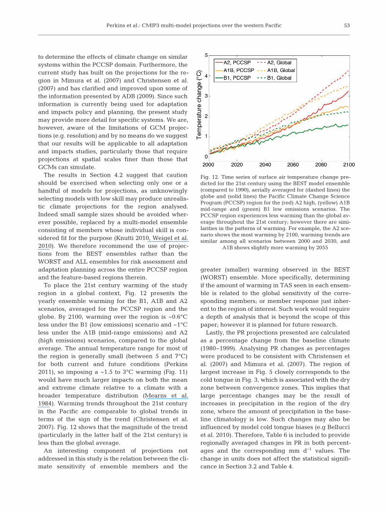
To place the 21st century warming of the studyregion in a global context, Fig. 12 presents theyearly ensemble warming for the B1, A1B and A2scenarios, averaged for the PCCSP region and theglobe. By 2100, warming over the region is ~0.6°Cless under the B1 (low emissions) scenario and ~1°Cless under the A1B (mid-range emissions) and A2(high emissions) scenarios, compared to the globalaverage. The annual temperature range for most ofthe region is generally small (between 5 and 7°C)for both current and future conditions (Perkins2011), so imposing a ~1.5 to 3°C warming (Fig. 11)would have much larger impacts on both the meanand extreme climate relative to a climate with abroader temperature distribution (Mearns et al.1984). Warming trends throughout the 21st centuryin the Pacific are comparable to global trends interms of the sign of the trend (Christensen et al.2007). Fig. 12 shows that the magnitude of the trend(particularly in the latter half of the 21st century) isless than the global average.

An interesting component of projections notaddressed in this study is the relation between the cli-mate sensitivity of ensemble members and the

greater (smaller) warming observed in the BEST(WORST) ensemble. More specifically, determiningif the amount of warming in TAS seen in each ensem-ble is related to the global sensitivity of the corre-sponding members; or member response just inher-ent to the region of interest. Such work would requirea depth of analysis that is beyond the scope of thispaper; however it is planned for future research.

Lastly, the PR projections presented are calculatedas a percentage change from the baseline climate(1980− 1999). Analysing PR changes as percentageswere produced to be consistent with Christensen etal. (2007) and Mimura et al. (2007). The region oflargest increase in Fig. 5 closely corresponds to thecold tongue in Fig. 3, which is associated with the dryzone between convergence zones. This implies thatlarge percentage changes may be the result ofincreases in precipitation in the region of the dryzone, where the amount of precipitation in the base-line climatology is low. Such changes may also beinfluenced by model cold tongue biases (e.g Bellucciet al. 2010). Therefore, Table 6 is included to provideregionally averaged changes in PR in both percent-ages and the corresponding mm d−1 values. Thechange in units does not affect the statistical signifi-cance in Section 3.2 and Table 4.

53

Fig. 12. Time series of surface air temperature change pre-dicted for the 21st century using the BEST model ensemble(compared to 1990), aerially averaged for (dashed lines) theglobe and (solid lines) the Pacific Climate Change ScienceProgram (PCCSP) region for the (red) A2 high, (yellow) A1Bmid-range and (green) B1 low emissions scenarios. ThePCCSP region experiences less warming than the global av-erage throughout the 21st century; however there are simi-larities in the patterns of warming. For example, the A2 sce-nario shows the most warming by 2100, warming trends aresimilar among all scenarios between 2000 and 2030, and

A1B shows slightly more warming by 2055

Clim Res 51: 35–58, 2012

5. CONCLUSIONS

Overall, changes in surface air temperature (TAS)and precipitation (PR) over the study region (Fig. 1)are similar to the projections presented in Chris-tensen et al. (2007) and Mimura et al. (2007) for thePacific region. This is to be expected at least to somedegree, given that the projections are based mostlyon the same GCMs. However, projections presentedby Christensen et al. (2007) and Mimura et al. (2007)are a summary across a wider domain, with no explo-ration into the performance or spread of the models.This paper has presented additional information notprovided by Mimura et al. (2007) and Christensen etal. (2007), including:

(1) projections from GCMs with a Pacific-basedfocus, highlighting spatial and scenario-dependantdifferences;

(2) the separation of ensemble members based onmodel skill, and the comparison of the respectivemean projections to that of the ALL ensemble (thesame all-model ensemble use used in Christensen etal. 2007 and Mimura et al. 2007);

(3) a measure of uncertainty (standard deviation)among members for each of the 3 ensembles ana -lysed (ALL, BEST, WORST);

(4) projections in wind speed (WSP) and wind direc-tion (WDIR); and

(5) mean feature-based regional changes as well asthe mean feature-based regional differences be -tween the BEST and WORST ensemble subsets rela-tive to the ALL ensemble.

Uncertainty (in terms of ensemble member agree-ment) has also been quantified, relationships to key

drivers and features have been discussed, and theregional warming has been compared with globalwarming. In summary this study has found:

(1) Over the PCCSP region, surface air temperatureincreases, precipitation generally increases espe-cially over the equator, wind speed increases anddecreases in the south and north, respectively, andwind direction tends to more easterly flows;

(2) Models with less skill in simulating baselineconditions exhibit significant biases relative to theALL ensemble, where projections are spatially aver-aged at the regional (i.e. PCCSP domain) and sub-regional (i.e. WPM-, ITCZ-, and SPCZ-influencedareas) scale. This result is consistent across annualand 6-monthly projections (Tables 2 to 5);

(3) Uncertainty (as defined by model consensus) isdecreased in some cases for PR, WSP and WDIR, andin all cases for TAS when eliminating models withless skill;

(4) As the large-scale climate features such as theITCZ, SPCZ and the WPM strongly influence meanand seasonal precipitation and atmospheric circula-tion, changes in these variables are likely to be asso-ciated with changes in the climate features. However,disagreement between models about the positionand projected change in the climate features makesexplaining ensemble mean changes in terms of thesefeatures difficult; and

(5) Eliminating GCMs that less skilfully simulatethe regional climate (Irving et al. 2011) does not re -duce all uncertainty from projections (e.g. Jun et al.2008, Knutti 2010) but does provide ensemble projec-tions that are considered more plausible. Differencesbetween projections based on the models retained

54

Region ALL BEST WORST Annual NDJFMA MJJASO Annual NDJFMA MAJJASO Annual NDJFMA MAJJASO

Absolute change (mm)PCCSP 177 90 87 185 96 90 146 68 78WPM 185 94 93 190 99 93 168 76 93ITCZ 190 69 120 210 75 135 111 49 66SPCZ 192 111 80 201 121 81 158 77 80

Relative change (%)PCCSP 15 15 18 16 16 19 12 11 17WPM 8 9 7 8 10 7 7 5 8ITCZ 14 19 35 26 38 22 14 10 27SPCZ 17 19 18 17 20 19 16 17 17

Table 6. Regionally averaged absolute change in precipitation (PR) calculated for the ALL, BEST and WORST ensembles forannual (mm yr−1), November to April (mm half-yr−1; NDJFMA) and May to October (mm half-yr−1; MJJASO) projections andrelative change in precipitation from the base period (1980−1999) for the same periods. Percentage change is as presented in

Fig. 5. All values are rounded to the nearest integer. See Table 2 for region abbreviations and locations

Perkins et al.: CMIP3 multi-model projections over the western Pacific 55

(BEST) and projections using all models (ALL) aregenerally statistically significantly different, espe-cially for TAS.

These results and associated projections may provevaluable to those requiring more detail than that pre-sented in the IPCC AR4. Mimura et al. (2007) statethat regional climate models (RCMs) are essential forproviding quantitative climate projections for the Pa-cific Island nations. However, due to computationand time restraints, RCMs are generally only drivenfor a subset of CMIP3 GCMs and generally for justone emission scenario (e.g. Christensen & Chris-tensen 2007, Kjellström et al. 2007). Futhermore, run-ning simulations forced by every GCM projectionavailable is not practical, especially for numerousRCMs. Whilst RCM projections may provide an extralevel of valuable information, such results would rep-resent a finer resolution sub-sample of the broaderrange of uncertainty. RCM projections should there-fore be interpreted alongside the GCM projections.Lastly, since GCMs are unavoidably used to force fu-ture RCM projections, results from the present studycombined with recommendations made by Irving etal. (2011) may influence which GCMs are chosen fordownscaling by RCMs over the PCCSP region.

Acknowledgements. The research discussed in this paperwas conducted with the support of the Pacific ClimateChange Science Program (PCCSP), a program supported byAusAID, in collaboration with the Department of ClimateChange and Energy Efficiency and delivered by the Bureauof Meteorology and the Commonwealth Scientific andIndustrial Research Organisation (CSIRO). We acknowledgethe modeling groups, the Program for Climate Model Diag-nosis and Intercomparison (PCMDI) and the World ClimateResearch Program’s Working Group on Coupled Modellingfor their roles in making available the CMIP3 multi-modeldataset. Support of this dataset was provided by the Officeof Science, U.S. Department of Energy. More details onmodel documentation are available at the PCMDI website(www-pcmdi.llnl.gov). We also thank J. Richmond for draft-ing the map shown in Fig. 1 and K. Hennessy, P. Whettonand B. Murphy for providing invaluable feedback.

LITERATURE CITED

ADB (Asian Development Bank) (2009) Mainstreaming cli-mate change in ADB operations, climate change imple-mentation plan for the Pacific (2009−2015). MandaluyongCity, Philippines

Ashok K, Behera SK, Rao SA, Weng H, Yamagata T (2007) ElNiño Modoki and its possible teleconnection. J GeophysRes 112: C11007, doi: 10. 1029/ 2006 JC 003798

Beaumont LJ, Pitman A, Perkins S, Zimmermann NE, Yoc-coz NG, Thuiller W (2011) Impacts of climate change onthe world’s most exceptional ecoregions. Proc Natl AcadSci USA 108: 2306−2311

Bellucci A, Gualdi S, Navarra A (2010) The double-ITCZsyndrome in coupled general circulation models: the roleof large-scale vertical circulation regimes. J Clim 23: 1127−1145

Brown JR, Power SB, Delage FB, Colman RA, Moise AF,Murphy BF (2011) Evaluation of the South Pacific Con-vergence Zone in IPCC AR4 climate model simulationsof the twentieth century. J Clim 24: 1565−1582

Collins M, An SI, Cai W, Ganachaud A and others (2010)The impact of global warming on the tropical PacificOcean and El Niño. Nat Geosci 3: 391−397

Covey C, Gleckler PJ, Phillips TJ, Bader DC (2006) Seculartrends and climate drift in coupled ocean-atmospheregeneral circulation models. J Geophys Res 111: D03107,doi: 10. 1029/ 2005 JD 006009

Christensen JH, Christensen OB (2007) A summary of thePRUDENCE model projections of changes in Europeanclimate by the end of this century. Clim Change 81: 7−30

Christensen JH, Hewitson B, Busuioc A, Chen A and others(2007) Regional climate projections. In: Solomon S, QinD, Manning M, Chen Z and others (eds) Climate change2007: the physical science base. Contribution of WorkingGroup I to the Fourth Assessment Report of the Intergov-ernmental Panel on Climate Change. Cambridge Univer-sity Press, Cambridge, p 847−940

Dessai S, Lu X, Hulme M (2005) Limited sensitivity analysisof regional climate change probabilities for the 21st cen-tury. J Geophys Res 110: D19108, doi: 10. 1029/ 2005 JD005919

Diaz HF, Markgraf V (2000) El Niño and the Southern Oscil-lation: multiscale variability and global and regionalimpacts. Cambridge University Press, Cambridge

Folland CK, Renwick JA, Salinger MA, Mullan AB (2002)Relative influences of the Interdecadal Pacific Oscillationand ENSO on the South Pacific Convergence Zone. Geo-phys Res Lett 29: 1643, doi: 10. 1029/ 2001 GL 014201

Giorgi F, Mearns LO (2002) Calculation of average, uncer-tainty range, and reliability of regional climate changesfrom AOGCM simulations via the ‘reliability ensembleaveraging’ (REA) method. J Clim 15: 1141−1158

Giorgi F, Mearns LO (2003) Probability of regional climatechange based on the reliability ensemble averaging(REA) method. Geophys Res Lett 30: 1629, doi: 10. 1029/2003 GL 017130

Gleckler PJ, Taylor KE, Doutriaux C (2008) Performancemetrics for climate models. J Geophys Res 113: D06104doi: 10. 1029/ 2007 JD 008972

Guilyardi E, Wittenberg A, Fedorov A, Collins M and others(2009) Understanding El Niño in ocean−atmosphere gen-eral circulation models: progress and challenges. BullAm Meteorol Soc 90: 325−340

Hendon HH, Liebmann B (1990a) A composite study ofonset of the Australian summer monsoon. J Atmos Sci 47: 2227−2240

Hendon HH, Liebmann B (1990b) The intraseasonal (30−50day) oscillation of the Australian summer monsoon.J Atmos Sci 47: 2909−2923

Irving DB, Perkins SE, Brown JR, Sen Gupta A and others(2011) Evaluating global climate models for the Pacificisland region. Clim Res 49: 169−187

Jun M, Knutti R, Nychka DW (2008) Spatial analysis to quan-tify numerical model bias and dependence. J Am StatAssoc 103: 934−947

Kjellström E, Bärring L, Jacob D, Jones R, Lenderink G,Schär C (2007) Modelling daily temperature extremes:

Clim Res 51: 35–58, 2012

recent climate and future changes over Europe. ClimChange 81: 249−265

Knutti R (2010) The end of model democracy? Clim Change102: 395−404

Knutti R, Abramowitz G, Collins M, Eyring V, Gleckler PJ,Hewitson B, Mearns L (2010) Good practice guidancepaper on assessing and combining multi model climateprojections. In: Stocker TF, Qin D, Plattner GK, Tignor M,Midgley PM (eds) Meeting report of the Intergovernmen-tal Panel on Climate Change expert meeting on assess-ing and combining multi model climate projections.IPCC Working Group I Technical Support Unit, Univer-sity of Bern, Bern, p 1−13

Liu Y, Guo L, Wu G, Wang Z (2010) Sensitivity of ITCZ con-figuration to cumulus convective parameterizations onan aqua planet. Clim Dyn 34: 223−240

Lowe JA, Gregory JM (2010) A sea of uncertainty. How wellcan we predict future sea level rise? Nature Rep ClimChange 4: 42−43

Luo Q, Jones RN, Williams M, Bryan B, Bellotti W (2005)Probabilistic distributions of regional climate change andtheir application in risk analysis of wheat production.Clim Res 29: 41−52

Mearns LO, Katz RW, Schneider SH (1984) Extreme high-temperature events: changes in their probabilities withchanges in mean temperature. J Appl Meteorol 23: 1601−1613

Meehl GA, Covey C, Taylor KE, Delworth T and others(2007a) The WCRP CMIP3 multimodel dataset: a new erain climate change research. Bull Am Meteorol Soc 88: 1383−1394

Meehl GA, Stocker TF, Collins WD, Friedlingstein P and oth-ers (2007b) Global climate projections. In: Solomon S,Qin D, Manning M, Chen Z and others (eds) Climatechange 2007: the physical science basis. Contribution ofWorking Group I to the Fourth Assessment Report on theIntergovernmental Panel on Climate Change. Cam-bridge University Press, Cambridge p 747−845

Mimura N, Nurse L, McLean RF, Agard J and others (2007)Small islands. In: Parry ML, Canziani OF, Palutikof JP,van der Linden PJ, Hanson CE (eds) Climate change2007: impacts, adaptation and vulnerability. Contributionof Working Group II to the Fourth Assessment Report ofthe Intergovernmental Panel on Climate Change. Cam-bridge University Press, Cambridge, p 687−716

Moise AF, Delage FP (2011) New climate model metricsbased on object-orientated pattern matching of precipi-tation. J Geophys Res 116: D12108, doi: 10.1029/ 2010 JD015318

Murphy JM, Sexton DMH, Barnett DN, Jones GS, Webb MJ,Collins M, Stainforth DA (2004) Quantification of model-ling uncertainties in a large ensemble of climate changesimulations. Nature 430: 768−772

Nakic e novic N, Alcamo J, Davis G, de Vries B and others(2000) IPCC special report on emission scenarios. Cam-bridge University Press, Cambridge

Nunn PD (2009) Responding to the challenges of climatechange in the Pacific islands: management and techno-logical imperatives. Clim Res 40: 211−231

Perkins SE (2011) Biases and model agreement in projec-tions of climate extremes over the tropical Pacific. EarthInteract 15: 1−36

Perkins SE, Pitman AJ, Holbrook NJ, McAneney J (2007)Evaluation of the AR4 climate models’ simulated dailymaximum temperature, minimum temperature and pre-

cipitation over Australia using probability density func-tions. J Clim 20: 4356−4376

Perkins SE, Pitman AJ (2009) Do weak AR4 models bias pro-jections of future climate changes over Australia? ClimChange 93: 527−558

Perkins SE, Pitman AJ, Sisson SA (2009) Smaller projectedincreases in 20-year temperature returns over Australia inskill-selected climate models. Geophys Res Lett 36: L06710, doi: 10. 1029/ 2009 GL 037293

Piani C, Frame DJ, Stainforth DA, Allen MR (2005) Con-straints on climate change from a multi-thousand mem-ber ensemble of simulations. Geophys Res Lett 32: L23825, doi: 10.1029/2005GL024452

Pierce DW, Barnett TP, Santer BD, Gleckler PJ (2009) Select-ing global climate models for regional climate changestudies. Proc Natl Acad Sci USA 106: 8441−8446

Pitman AJ, Perkins SE (2008) Regional projections of futureseasonal and annual changes in precipitation and tem-perature over Australia based on skill-selected AR4 mod-els. Earth Interact 12: 1−50

Power SB (1995) Climate drift in a global ocean general cir-culation model. J Phys Oceanogr 25: 1025−1036

Power SB, Kociuba G (2011) The impact of global warmingon the Southern Oscillation Index. Clim Dyn 37:1745–1754

Power SB, Smith IN (2007) Weakening of the Walker Circu-lation and apparent dominance of El Niño both reachrecord levels, but has ENSO really changed? GeophysRes Lett 34: L18702, doi: 10.1029/2007GL030854

Räisänen J (2007) How reliable are climate models? Tellus59: 2−29

Reifen C, Toumi R (2009) Climate projections: past perfor-mance no guarantee of future skill? Geophys Res Lett 36: L13704, doi: 10. 1029/ 2009GL 038082

Sánchez E, Romera R, Gaertner MA, Gallardo C, Castro M(2009) A weighting proposal for an ensemble of regionalclimate models over Europe driven by 1961−2000 ERA40based on monthly precipitation probability density func-tions. Atmos Sci Lett 10: 241−248

Santer BD, Taylor KE, Gleckler PJ, Bonfils C and others(2009) Incorporating model quality information in cli-mate change detection and attribution studies. Proc NatlAcad Sci USA 106: 14778−14783

Schneider SH, Rosencranz A, Niles JO (eds) (2002) Climatechange policy: a survey. Island Press, Washington, DC

Sen Gupta A, Muir LC, Brown JN, Phipps SJ, Durack PJ,Monselesan D, Wijffels SE (in press) Climate drift in theCMIP3 models. J Clim

Smith I, Chandler E (2010) Refining precipitation projectionsfor the Murray Darling Basin of south-east Australia —the effect of sampling model results based on perfor-mance. Clim Change 102: 377−393

Stainforth DA, Allen MR, Tredger ER, Smith LA (2007) Con-fidence, uncertainty and decision-support relevance inclimate predictions. Philos Trans R Soc Lond A 365: 2145−2161

Stephens MA (1970) Use of the Kolmogorov-Smirnov,Cramér-Von Mises and related statistics without exten-sive tables. J R Stat Soc B 32: 115−122

Stephens MA (1986) Tests based on EDF statistics. In: D’Agostino RB, Stephens MA (eds) Goodness-of-fit tech-niques. Marcel Dekker, New York, NY

Taylor KE (2001) Summarizing multiple aspects of modelperformance in a single diagram. J Geophys Res 106: 7183–7192, doi: 10.1029/2000JD900719

56

Perkins et al.: CMIP3 multi-model projections over the western Pacific 57

Tebaldi C, Hayhoe K, Arblaster JM, Meehl GA (2006) Goingto the extremes, an intercomparison of model-simulatedhistorical and future changes in extremes events. ClimChange 79: 185−211

Tebaldi C, Knutti R (2007) The use of the multi-modelensemble in probabilistic climate projections. PhilosTrans R Soc Lond A 365: 2053−2075

van Oldenborgh GJ, Philip SY, Collins M (2005) El Niño in achanging climate: a multi-model study. Ocean Sci 1: 81−95

Vecchi GA, Wittenberg AT (2010) El Niño and our future cli-mate: Where do we stand? Wiley Interdiscip Rev ClimChange 1: 260−270

Vecchi GA, Soden BJ, Wittenberg AT, Held IM, Leetmaa A,Harrison MJ (2006) Weakening of tropical Pacific atmos-pheric circulation due to anthropogenic forcing. Nature441: 73−76

Vincent DG (1994) The South Pacific Convergence Zone(SPCZ): a review. Mon Weather Rev 122: 1949−1970

Waliser DE, Gautier C (1993) A satellite-derived climatology

of the ITCZ. J Clim 6: 2162−2174Weigel AP, Knutti R, Liniger MA, Appenzeller C (2010)

Risks of model weighting in multimodel climate projec-tions. J Clim 23: 4175−4191

Whetton P, Macadam I, Bathols J, O’Grady J (2007) Assess-ment of the use of current climate patterns to evaluateregional enhanced greenhouse response patterns of cli-mate models. Geophys Res Lett 34: L14701, doi: 10. 1029/2007 GL 030025

Xu Y, Gao X, Giorgi F (2010) Upgrades to the reliabilityensemble averaging method for producing probabilisticclimate-change projections. Clim Res 41: 61−81

Zhang GJ, Song X (2010) Convection parameterization, trop-ical Pacific double ITCZ, and upper-ocean biases in theNCAR CCSM3. Part II: coupled feedback and the role ofocean heat transport. J Clim 23: 800−812

Zhun Y, Chen L (2002) The relationship between theAsian/Australian monsoon and ENSO on a quasi-four-year scale. Adv Atmos Sci 19: 727−740

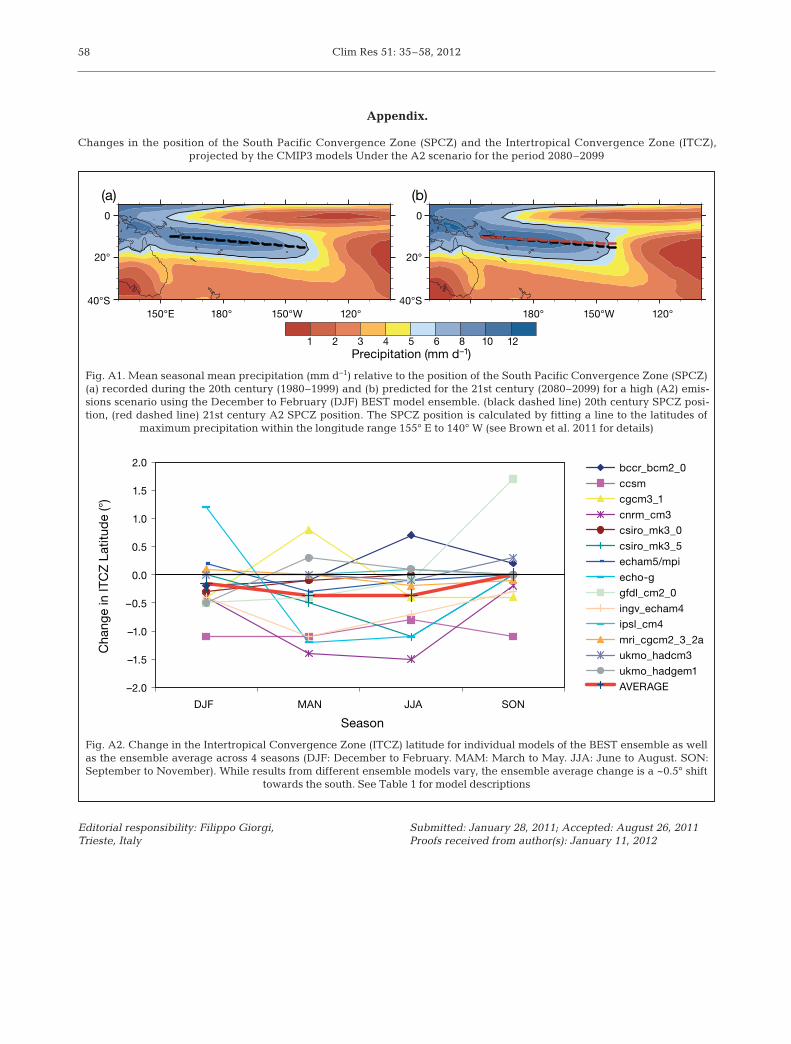
Clim Res 51: 35–58, 201258

(a)0

20°

40°S150°E 150°W 120°180°

0

20°

40°S

1 2 3 4 5Precipitation (mm d–1)

6 8 10 12

150°W 120°180°

(b)

Fig. A1. Mean seasonal mean precipitation (mm d−1) relative to the position of the South Pacific Convergence Zone (SPCZ)(a) recorded during the 20th century (1980−1999) and (b) predicted for the 21st century (2080−2099) for a high (A2) emis-sions scenario using the December to February (DJF) BEST model ensemble. (black dashed line) 20th century SPCZ posi-tion, (red dashed line) 21st century A2 SPCZ position. The SPCZ position is calculated by fitting a line to the latitudes of

maximum precipitation within the longitude range 155° E to 140° W (see Brown et al. 2011 for details)

Appendix.

Changes in the position of the South Pacific Convergence Zone (SPCZ) and the Intertropical Convergence Zone (ITCZ), projected by the CMIP3 models Under the A2 scenario for the period 2080–2099

–2.0

–1.5

–1.0

–0.5

0.0

0.5

1.0

1.5

2.0

Season

DJF MAN JJA SON

Ch

an

ge in

IT

CZ

Latitu

de (°)

bccr_bcm2_0

ccsm

cgcm3_1

cnrm_cm3

csiro_mk3_0

csiro_mk3_5

echam5/mpi

echo-g

gfdl_cm2_0

ingv_echam4

ipsl_cm4

mri_cgcm2_3_2a

ukmo_hadcm3

ukmo_hadgem1

AVERAGE

Fig. A2. Change in the Intertropical Convergence Zone (ITCZ) latitude for individual models of the BEST ensemble as wellas the ensemble average across 4 seasons (DJF: December to February. MAM: March to May. JJA: June to August. SON:September to November). While results from different ensemble models vary, the ensemble average change is a ~0.5° shift

towards the south. See Table 1 for model descriptions

Editorial responsibility: Filippo Giorgi, Trieste, Italy

Submitted: January 28, 2011; Accepted: August 26, 2011Proofs received from author(s): January 11, 2012