Clustering appearance and shape by learning jigsawspages.cs.wisc.edu/~lizhang/courses/cs766-2008f/syllabus/12-06-seg/rosin.pdf · Clustering appearance and shape by learning jigsaws

Clustering appearance and shape by learning jigsaws

Anitha Kannan, John Winn, Carsten Rother

Models for Appearance and Shape

● Histograms– discard spatial info

● Templates– articulation, deformation, variation

● Patch-based approaches– a happy medium– size/shape of the patches is fixed

Jigsaw

● Intended as a replacement for fixed patch model

● Learn a jigsaw image such that:– Pieces are similar in appearance and shape to

multiple regions in training image(s)– All training images can be ~reconstructed

using only pieces from the jigsaw– Pieces are as large as possible for a particular

reconstruction accuracy

Jigsaw Model

μ(z) – intensity value at pixel zλ-1(z) – variance at zl(i) – offset between image pixel i and corresp. jigsaw pixel

Generative Model

Generative Model

● Each offset map entry is a 2D offset mapping point i in the image to pointz = (i – l(i)) mod |J| in the jigsaw, where|J| = (jigsaw width, jigsaw height)

● Product is over image pixels

Generative Model

● E is the set of edges in a 4-connected grid, with nodes representing offset map values

● γ influences the typical jigsaw piece size; set to 5 per channel

● δ( true ) = 1, δ( false ) = 0

Generative Model

● μ0 = 0.5, β = 1, b = 3 times data

precision, a = b2

● Normal-Gamma prior allows for unused portions of the jigsaw to be well-defined

MAP Learning

● Image set is known● Find J, Ls to maximize joint probability● Initialize jigsaw

– Set precisions λ to expected value under the prior

– Set means μ to Gaussian noise with same mean and variance as the data

MAP Learning

● Iteration step 1:

– Given J, I1..N

, update L1..N

using α-expansion

graph-cut algorithm

● Iteration step 2:

● Repeat until convergence

α-expansion Graph-Cut

● Start with arbitrary labeling f● Loop:

– For each label α:● Find f' = arg min E(f') among f' within one α-

expansion of f● If E(f') < E(f), set f := f'● Else return f

α-expansion defined in detail in Fast Approximate EnergyMinimization via Graph Cuts. Yuri Boykov, Olga Veksler, RaminZabih.

Determining Jigsaw Pieces

● For each image, define region boundaries as the places where the offset map changes value.

● Each region thus maps to a contiguous area of the jigsaw.

● Cluster regions based on overlap:– Ratio of intersection to union of the jigsaw

pixels mapped to by the two regions

● Each cluster corresponds to a jigsaw piece.

Toy Example

Epitome

● Another unfixed patch-based generative model

● Patches have fixed size and shape, but not location– Patches can be subdivided (24x24, 12x12,

8x8)– Patches can overlap (average value taken)– Cannot capture occlusion w/o a shape modelEpitome model defined in detail in Epitomic analysis ofappearance and shape. Nebojsa Jojic, Brendan J. Frey, AnithaKannan.

Jigsaw vs. Epitome

Jigsaw for Multiple Images

100 face images from AT&T's Olivetti database

Unsupervised Part Learning

The Good

● Jigsaw allows automatically sized patches● Occlusion is modeled implicitly, i.e. patch

shape is variable● Image segmentation is automatic

– Unsupervised part learning an easy next step

● Jigsaw reconstructions more accurate and better looking than equivalently sized Epitome model reconstructions

The Bad

● At each iteration, must solve a binary graph cut for each jigsaw pixel– 30 minutes to learn 36x36 jigsaw from

150x150 toy image

● No patch transformation– Can add specific transformations with linear

cost increase– Can favor “similar” neighboring offsets in

addition to identical ones

The Questions?

Normalized Cuts and Image Segmentation

Jianbo Shi and Jitendra Malix

Recursive Partitioning

● Segmentation/partitioning inherently hierarchical

● Image segmentation from low-level cues should sequentially build hierarchical partitions– Partitioning done big-picture downward

● Mid- and high-level knowledge can confirm groups are identify repartitioning candidates

Graph Theoretic Approach

● Set of points represented as a weighted undirected graph G = (V,E)– Each point is a node; G is fully-connected– w(i,j) is a function of the similarity between i

and j

● Find a partition of vertices into disjoint sets where by some measure in-set similarity is high, but cross-set similarity is low.

Minimum Graph Cut

● Dissimilarity between two disjoint sets of vertices can be measured as total weight of edges removed:

● The minimum cut defines an optimal bipartitioning

● Can use minimum cut for point clusteringProposed in An Optimal Graph Theoretic Approach to DataClustering: Theory and Its Application to Image Segmentation.Z. Wu and R. Leahy.

Minimum Cut Bias

● Minimum cut favors small partitions– cut(A,B) increases

with the number of edges between A and B

● With w(i,j) inversely proportional to dist(i,j), B = n1 is the minimum cut.

Normalized Cut

● Measure cut cost as a fraction of total edge connections to all nodes

● Any cut that partitions small isolated points will have cut(A,B) close to assoc(A,B)

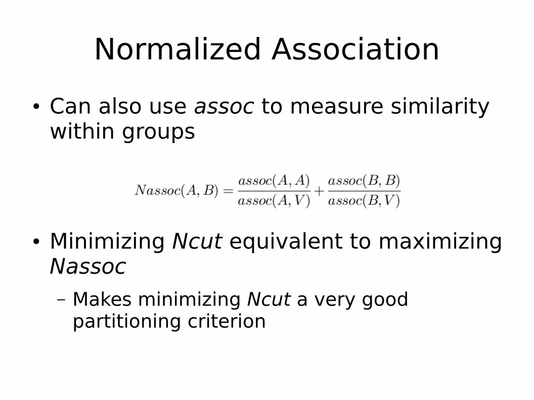
Normalized Association

● Can also use assoc to measure similarity within groups

● Minimizing Ncut equivalent to maximizing Nassoc– Makes minimizing Ncut a very good

partitioning criterion

Minimizing Ncut is NP-Complete

● Reformulate problem:

– For i in V, xi = 1 if i is in A, -1 otherwise

– di = sum

j w(i,j)

Proof by Papadimitriou (1997) anappendix to the paper

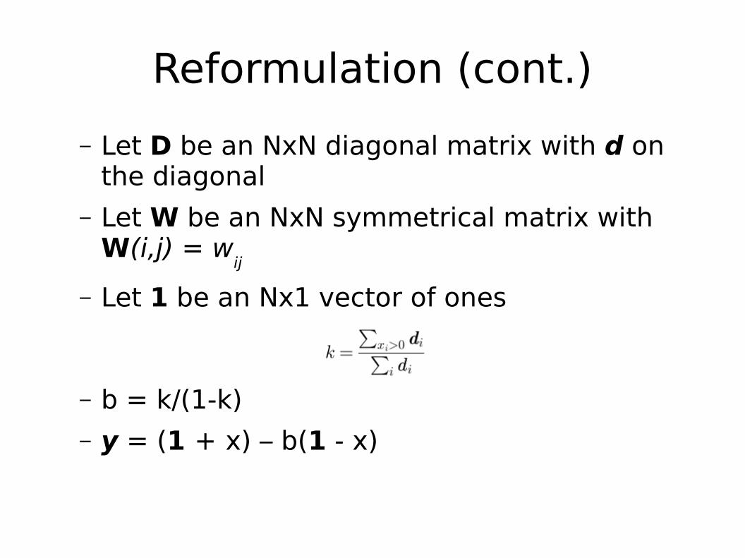
Reformulation (cont.)

– Let D be an NxN diagonal matrix with d on the diagonal

– Let W be an NxN symmetrical matrix with W(i,j) = w

ij

– Let 1 be an Nx1 vector of ones

– b = k/(1-k)– y = (1 + x) – b(1 - x)

Reformulation (cont.)

● This is a Rayleigh quotient– By allowing y to take on real values, can

minimize this by solving the generalized eigenvalue system (D – W)y = λDy.

– But what about the two constraints on y?

with the condition yTD1 = 0 and yi in {1, -b}.

First Constraint

● Transform the previous into a standard eigensystem: D-1/2(D – W)D-1/2z = λz, where z = D1/2y

● z0 = D1/21 is an eigenvector with

eigenvalue 0. Since D-1/2(D – W)D-1/2 is symmetric positive semidefinite, z

0 is the

smallest eigenvector and all eigenvectors are perpendicular to each other.

First Constraint (cont.)

● Translating this back to the general eigensystem:

– y0 = 1 is the smallest eigenvector, with

eigenvalue 0

– 0 = z1

Tz0 = y

1TD1, where y

1 is the second

smallest eigenvector

First Constraint (cont.)

● Since we are minimizing a Rayleigh quotient with a symmetric matrix, we use the following property – under the constraint that x is orthogonal to the j-1 smallest eigenvectors x

1,...,x

j-1, the

quotient is minimized by xj with the eigenvalue λ

j being the minimum value.

For more details see Matrix Computations, G.H. Golub and C.F.Van Loan, and Partitioning Sparse Matrices with Eigenvectors ofGraphs, A. Pothen, H.D. Simon, and K.P. Liou.

Real-valued Solution

● y1 is thus the real valued solution for a

minimal Ncut.– We cannot force a discrete solution – relaxing

the second constraint makes this problem tractable.

– Can transform y1 into a discrete solution by

finding the splitting point such that the resulting partition has the best Ncut(A,B) value.

Lanczos Method

● Graphs are often only locally connected – resulting eigensystem are very sparse

● Only the top few eigenvectors are needed for graph partitioning

● Need very little precision in resulting eigenvectors

● These properties exploited by using Lanczos method; running time approximately O(n3/2)

Recursive Partitioning redux

● After partitioning, the algorithm can be run recursively on each partitioned part– Recursion stops once the Ncut value exceeds

a certain limit, or result is “unstable”– When subdividing an image with no clear way

of breaking it, eigenvector will resemble a continuous function

– Construct a histogram of eigenvector values – if the ratio of minimum to maximum bin size exceeds 0.06, reject partitioning

Simultaneous K-Way Cut

● Since all eigenvectors will be perpendicular, can use third, fourth, etc. smallest to immediately subdivide partitions

● Some such eigenvectors would have failed the stability criteria

● Can use top n eigenvectors to partition, then iteratively merge segments– Mentioned by the paper, but no experimental

results presented

Recursive Two-Way Ncut Algorithm

● Given a set of features, construct weighted graph G, summarize information into W and D

● Solve (D – W)x = λDx for the eigenvectors with the smallest eigenvalues

● Find the splitting point in x1 and bipartition the graph

● Check the stability of the cut and the value of Ncut

● Recursively repartition segmented parts if necessary

Weighting Schemes

● X(i) is the spatial location of node i

● F(i) is a feature vector defined as– F(i) = 1, for point sets

– F(i) = I(i), the intensity value, for brightness

– F(i) = [v, v*s*sin(h), v*s*cos(h)](i), for color segmentation

– F(i) = [|I*f1|,...,|I*f

n|](i), where f

i are DOOG filters, in the case of texture

segmentation

DOOG filters were used to discriminate textures in PreattentiveTexture Discrimination with Early Vision Mechanisms, J. Malikand P. Perona.

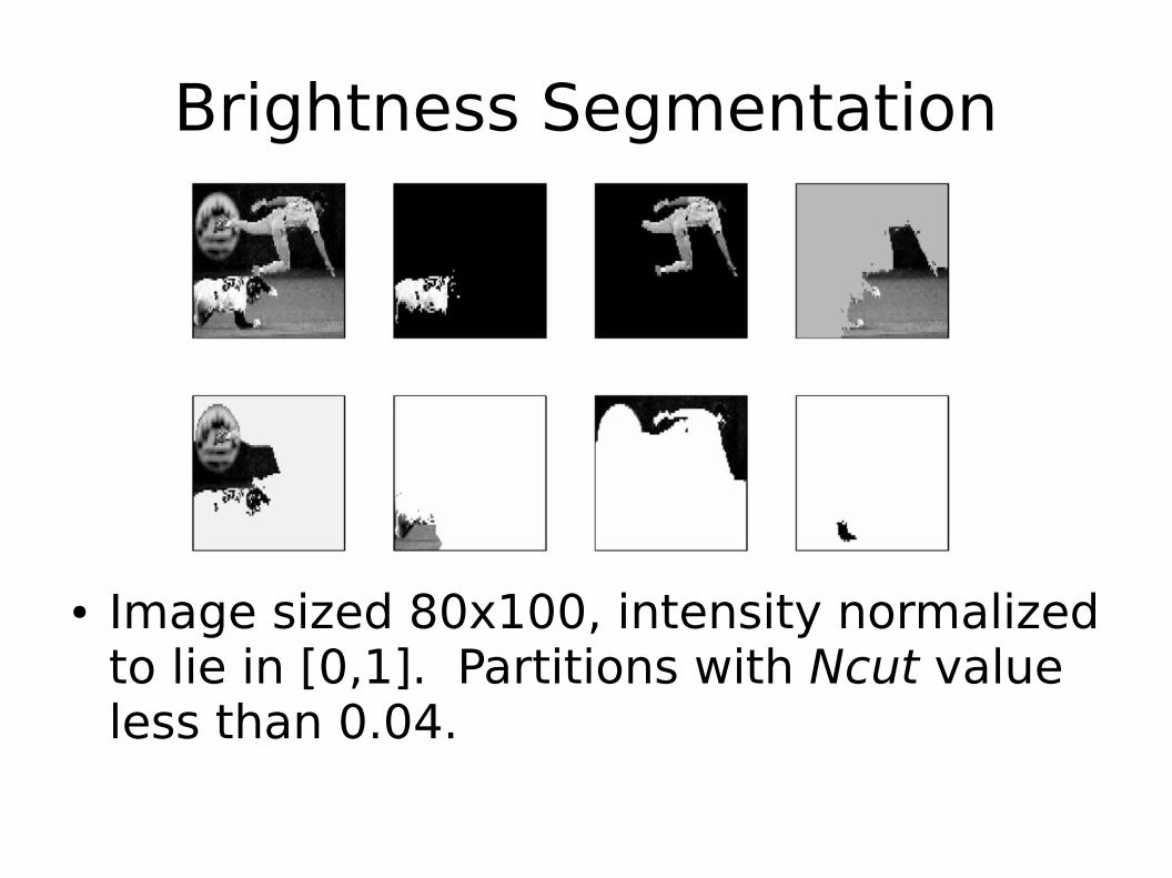
Brightness Segmentation

● Image sized 80x100, intensity normalized to lie in [0,1]. Partitions with Ncut value less than 0.04.

Brightness Segmentation

● 126x106 weather radar image. Ncut value less than 0.08.

Color Segmentation

● 77x107 color image (reproduced in grayscale in the paper). Ncut value less than 0.04.

Texture Segmentation

● Texture features correspond to DOOG filters at six orientations and fix scales.

Motion Segmentation

● Treat the image sequence as spatiotemporal data set.

● Weighted graph is constructed by taking all pixels as nodes and connecting spatiotemporal neighbors.

● d(i,j) represents “motion distance” between pixels i and j.

Motion Distance

● Defined as one minus the cross correlation of motion profiles, where the motion profile estimates the probability distribution of image velocity at each pixel.

Motion Segmentation Results

● Above: two consecutive frames● The head and body have similar motion

but dissimilar motion profiles due to 2D textures.

Questions?