Cloud cci doc - climate.esa.int

ESA Cloud_cci

Validation Report for TOA radiation fluxes

derived with CC4CL for MODIS-Aqua and AVHRR-NOAA18

Issue 1 Revision 0

30 April 2018

Deliverable No.: D-4.1.1

ESRIN/Contract No.: 4000109870/13/I-NB Project Coordinator: Dr. Rainer Hollmann Deutscher Wetterdienst [email protected] Technical Officer: Dr. Simon Pinnock

European Space Agency [email protected]

Document Change Record

Document, Version Date Changes Originator

RTOA v1.0 approved version

26/01/2018 Initial version B. Würzler, Sören Testorp, M. Stengel

Purpose

This document reports the evaluation results for the Climate Research Demonstrator Dataset for top of the atmosphere (TOA) fluxes (CRDD-TOA, D-1.10). This report (RTOA) is deliverable for the final options milestone (CCN-1).

Doc: Cloud_cci_D4.1.1_RTOA_v1.0

Date: 30 April 2018

Issue: 1 Revision: 0 Page 3

Table of Contents

1. Introduction .................................................................................................. 4

1.1 The Cloud_cci project ................................................................................. 4

1.2 Cloud_cci TOA products............................................................................... 5

2. Reference data and evaluation approach ............................................................. 6

2.1 Reference data .......................................................................................... 6

2.1.1 CERES SSF1deg Aqua .............................................................................. 6

2.1.2 CM SAF MSG-GERB ................................................................................. 6

2.2 Diurnal cycle correction for Cloud_cci products ................................................ 6

2.3 Comparisons metrics ................................................................................... 7

3. Evaluation against CERES ................................................................................. 8

3.1 Level-2 Case studies ................................................................................... 8

3.2 Level-3 of shortwave TOA fluxes (Annual means) ............................................. 10

3.3 Level-3 of longwave TOA fluxes (Annual means) ............................................... 11

4. Evaluation against MSG-GERB ........................................................................... 12

4.1 Level-3 of shortwave TOA fluxes (Annual means) ............................................. 12

4.2 Level-3 of longwave TOA fluxes (Annual means) ............................................... 15

5. Summary & Conclusions .................................................................................. 18

6. Glossary ...................................................................................................... 19

7. References .................................................................................................. 21


Date: 30 April 2018


1. Introduction

1.1 The Cloud_cci project

The ESA Cloud_cci project pursues the development of coherent long-term cloud property datasets (Hollmann et al., 2013, Stengel et al., 2015). These product-based climate datasets (formally denoted Thematic Climate Data Records – TCDRs) were derived from accurately calibrated and homogenized radiances (formally denoted Fundamental Climate Data Records – FCDRs). The FCDRs build the basis for the Essential Climate Variable (ECV) datasets. These ECV datasets were derived using the two physical retrieval systems Community Cloud retrieval for Climate (CC4CL; Sus et al., 2017; McGarragh et al., 2017) and Freie Universität Berlin AATSR MERIS Cloud retrieval (FAME-C; Carbajal Henken et al., 2014). CC4CL is an open community code, with algorithm developments taken place during the ongoing project. After applying the retrieval systems for the generation of the Cloud_cci dat sets, the validation of cloud products, the provision of a common data base and the feasibility of accessing the cloud data were implemented and have been maintained. The final processing system builds a sound basis for any future reprocessing of CC4CL and FAME-C based datasets and a potential operational production of cloud data also beyond the expiration of the Cloud_cci project.

The objective of Cloud_cci has been the generation of two product families. The first family is an (A)ATSR/SLSTR-MODIS-AVHRR heritage product group. Products for this family were derived using CC4CL applied to instrument channels matching those available from the AVHRR “heritage” channel set. In this family, cloud properties are separately derived from AATSR/SLSTR (and the ATSR-series), MODIS and AVHRR. The second product family includes cloud properties derived using FAME-C applied to combined AATSR and MERIS measurements set using a synergistic retrieval approach. CC4CL and FAME-C are also able to process successor system data of SLSTR/OLCI on board the Sentinel-3 satellite. Considering the spectral, imaging and observational characteristics of the considered sensors, the following Cloud_cci datasets were defined:

AVHRR-AM (S: NOAA-12, NOAA-15, NOAA-17, Metop-A; A: CC4CL, PC: DWD)

AVHRR-PM (S: NOAA7, NOAA9, NOAA11, NOAA14, NOAA16, NOAA18, NOAA19; A: CC4CL; PC: DWD)

MODIS-Terra (S: Terra; A: CC4CL; PC: DWD)

MODIS-Aqua (S: Aqua; A: CC4CL; PC: DWD)

ATSR2-AATSR (S: ERS-2, Envisat; A: CC4CL; PC: RAL)

MERIS-AATSR (S: Envisat; A: FAME-C; PC: FUB)

where S indicates the satellites covered, A the algorithm used and PC the processing center. Figure 1-1 shows the datasets and the time periods they cover.

Figure 1-1 Overview of Cloud_cci datasets and the time periods they cover.

Within Cloud_cci (i.e. in Option 4) a CC4CL post-processing tool has been developed and implemented that calculates broadband radiative fluxes in each satellite pixel using BUGSrad (Stephens et al., 2001; ATBD-TOAv1), i.e. top and bottom of atmosphere longwave and shortwave radiative fluxes are calculated using the cloud and aerosol properties retrieved from CC4CL. The CC4CL scheme ensures a radiatively consistent set of retrieved cloud properties because it performs the retrieval using all available instrument channels simultaneously.


Date: 30 April 2018


1.2 Cloud_cci TOA products

Two demonstrator datasets have been generated: (1) MODIS-Aqua and (2) AVHRR-NOAA18 both for the year 2008. These two sets are evaluated in this report: global comparisons of Cloud_cci MODIS-Aqua against CERES and regional (within the SEVIRI disk) comparisons of Cloud_cci AVHRR-NOAA18 against CM SAF MSG-GERB. In the following, examples of Cloud_cci MODIS-Aqua and Cloud_cci AVHRR-NOAA18 TOA as well as their consistency is discussed.

Figure 1-2 shows the annual mean values of TOA shortwave outgoing and longwave outgoing for Cloud_cci MODIS and Cloud_cci AVHRR for the year 2008. The mean shortwave fluxes are very similar and agree within 10-15 W/m² with slight higher values for MODIS. The difference seems lowest in marine stratocumulus and polar regions, and highest in regions of strong convection such as the Inner-Tropics. The longwave fluxes also agree well between AVHRR and MODIS. The agreement for the longwave is even better than for shortwave and is within 5 W/m² for most parts of the globe. The difference patterns are similar to the shortwave comparison with additional hot spots in some desert regions.

In Sections 3 and 4 the Cloud_cci TOA data are compared against the Cloud and the Earth’s Radiant Energy System (CERES) and against the CM SAF MSG-GERB TOA radiation products, both reference data being described in more detail in Section 2.

Figure 1-2 Annual mean of shortwave (left) and longwave (right) TOA flux calculated from CC4CL for MODIS-Aqua (upper row) and AVHRR-NOAA18 (middle row) after applying a diurnal cycle correction. Bottom row shows the difference plots of MODIS – AVHRR.


Date: 30 April 2018


2. Reference data and evaluation approach

2.1 Reference data

Two reference datasets were used in this study to evaluate the Cloud_cci data against.

2.1.1 CERES SSF1deg Aqua

CERES (Cloud and the Earth’s Radiant Energy System) is a broadband radiometer operated by NASA on-board the polar orbiting science satellites Terra (EOS-AM) & Aqua (EOS-PM) (see https://ceres.larc.nasa.gov/). CERES measures the radiation leaving the earth at the top of atmosphere. Its biaxial scan mode provides angular flux information, which is used to determine the outgoing short- and longwave flux on a global scale. CERES measures radiation in three different channels, a shortwave channel to measure reflected sunlight, a longwave channel to measure Earth-emitted thermal radiation in the 8-12 μm "window" region, and a total channel to measure all wavelengths of radiation.

In this study we used the SSF1deg (single scanner footprint, 1°x 1° resolution) Edition 4 product of CERES Aqua, containing diurnally corrected monthly averages of radiative fluxes at the top of atmosphere, as well as the SSF (single scanner footprint) Level2 product for individual scene studies. In the following the shortwave and longwave fluxes will be compared to MODIS Aqua based fluxes retrieved with CC4CL. The monthly means from the SSF1deg product were averaged and spatially interpolated on a 0.5°x 0.5° grid to accommodate the Cloud_cci resolution.

2.1.2 CM SAF MSG-GERB

The MSG-GERB TOA fluxes comprise the TOA Reflected Solar (TRS) and the TOA Emitted Thermal (TET) radiation estimates. The records are derived from the Meteosat Visible and InfraRed Imager (MVIRI) and the Spinning Enhanced Visible and InfraRed Imager (SEVIRI) instruments on-board the geostationary MSG satellites (Schmetz et al., 2002). The data covers the Meteosat field of view, which extends from -70° to 70° East as well as from -70° to 70° North and is provided on a regular grid with a spatial resolution of 0.05°x 0.05° (see http://dx.doi.org/10.5676/EUM_SAF_CM/TOA_GERB/V001). As with Cloud_cci AVHRR, the annual mean fluxes, based on monthly averages for the year 2008, are used for the comparison.

Due to a rapidly increasing error in TOA flux with higher viewing zenith angles (VZA), the edges of the investigation area are slightly adjusted by a restriction to VZA lower than 78°. In additional, the high-resolution MSG-GERB data record is transformed to the Cloud_cci resolution of 0.5°x 0.5° using a nearest neighbour resampling. All comparisons are further limited to the GERB field of view, i.e. about 70°W to 70°E and 70°S to 70°N.

2.2 Diurnal cycle correction for Cloud_cci products

Because MODIS-Aqua and AVHRR-NOAA18 sample most parts of the global only twice a day, the sampling error needs to be considered when comparing corresponding products to climatological means (high temporal sampling), as represented by both reference datasets. To minimize the impact of the sampling error on the comparison, a correction factor was derived to present a diurnal cycle corrected (dc-corrected) product.

To calculate the correction factor, the 24 hourly (local time) mean TOA radiation fluxes (i.e. the diurnal cycle) were calculated from one month in 2009 and stratified into land and sea as well as separately for longwave and shortwave TOA fluxes. The result is the monthly mean diurnal cycle for both TOA fluxes and both surface types.

In a second step, the monthly mean values were calculated from (1) all 24 hour data, representing the climatological mean and (2) from certain local times, representing the reduced temporal


Date: 30 April 2018


sampling of a polar-orbiting satellite. Relating the mean of the reduced sampling to the 24h mean a correction factor was inferred, again stratified for land/sea and shortwave/longwave.

For the approximate local overpass time of NOAA-18 and Aqua (2 PM), the 4 dc-correction factors are: 0.668 (shortwave, land), 0.795 (shortwave, sea), 0.987 (longwave, land) and 0.998 (longwave, sea). The DC-correction factors are applied to AVHRR and MODIS Level-3 data only. All Level-3 comparisons in Section 3 and 4 include both the uncorrected and the dc-corrected Cloud_cci TOA products.

2.3 Comparisons metrics

Based on the monthly mean radiation fluxes, the annual mean fluxes of the reflected shortwave and outgoing longwave radiation are calculated for both Cloud_cci products (AVHRR and MODIS)

After the data preparation, the two data records and their differences are visualized. For this purpose, maps with the calculated annual mean TOA radiation fluxes are created in order to provide an overview of the regional characteristics. To visualize the variations between the records, difference plots are created by subtracting Cloud_cci MODIS from CERES and Cloud_cci AVHRR from MSG GERB. For the latter, the absolute as well as the relative differences are calculated and illustrated for the Meteosat field of view. All visualizations are performed for the shortwave as well as the longwave radiation TOA fluxes.

In addition to the maps, scatter plots of the annual mean values are shown together with some statistical measures for the agreement (in the comparisons to MSG-GERB only. For this, the Pearson correlation coefficient, the mean bias, the mean absolute bias and the root mean squared error are calculated between the two datasets, based on the following formulas:

Correlation:

𝑅 = 𝑛(∑ 𝑥𝑦) − (∑ 𝑥)(∑ 𝑦)

√[ 𝑛 ∑ 𝑥² − (∑ 𝑥)²] [ 𝑛 ∑ 𝑦2 − (∑ 𝑦)²] ,

Mean bias:

𝑀𝐵 = 1

𝑛 ∑(𝑆𝑖 − 𝐺𝑖)

𝑛

𝑖=𝑛

,

Mean absolute bias:

𝑀𝐴𝐵 =1

𝑛∑ |𝑆𝑖 − 𝐺𝑖|

𝑛

𝑖=𝑛

,

Root mean square error:

𝑅𝑀𝑆𝐸 = √∑ (𝑥𝑒𝑠𝑡 − 𝑥𝑚𝑒𝑎𝑠)²𝑛

𝑖=1

𝑛 .


Date: 30 April 2018


3. Evaluation against CERES

3.1 Level-2 Case studies

In order to compare the instantaneous short- and longwave fluxes two case studies were performed: One MODIS granule from the 20th of February 2008 over Greenland (Figure 3-1) and another from the 20th of March 2008 above central Africa (Figure 3-2). Since the CERES retrieval is limited on the instrument’s footprint, which is elliptically and varies in size with viewing angle a different number of MODIS pixels and different weights for those pixels have to be used in order to average MODIS data onto the CERES footprint adequately. The collocation was performed according to the ATBD Subsystem 4.4 of CERES.

The scatter plots in Figure 3-1 show a high correlation between the CERES and Cloud_cci with a Pearson correlation coefficient of 0.93 for the short- and longwave fluxes. Colorized are the surface types used by CERES as an indicator if any type of surface causes a systematic bias between both products. In the middle and right column of Figure 3-1 the Cloud_cci MODIS flux and the difference of Cloud_cci MODIS-CERES are depicted. Here, BUGSrad refers to the used radiative transfer model in the CC4CL retrieval of Cloud_cci. As seen in comparison of the annual average (Figure 3-3), the shortwave TOA flux of MODIS is smaller than the retrieved flux from CERES above snowy surfaces. In the longwave regime the scene shows a prominent positive bias towards CERES in the inner part of Greenland while the longwave radiative flux from coastal regions and the surrounding water bodies is smaller in the Cloud_cci product.

Figure 3-1 Shortwave TOA flux comparison between Cloud_cci MODIS and CERES SSF. The presented scene is from the 20th of February 2008, covering the southern part of Greenland.


Date: 30 April 2018


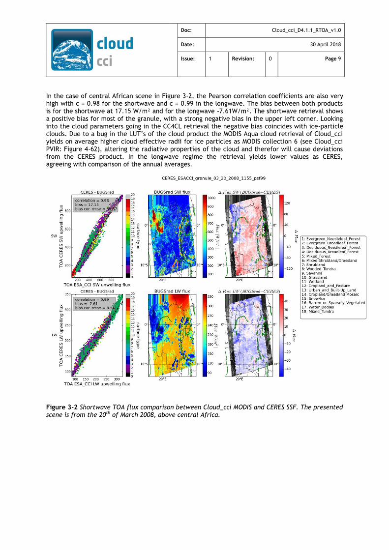
In the case of central African scene in Figure 3-2, the Pearson correlation coefficients are also very high with c = 0.98 for the shortwave and c = 0.99 in the longwave. The bias between both products is for the shortwave at 17.15 W/m² and for the longwave -7.61W/m². The shortwave retrieval shows a positive bias for most of the granule, with a strong negative bias in the upper left corner. Looking into the cloud parameters going in the CC4CL retrieval the negative bias coincides with ice-particle clouds. Due to a bug in the LUT’s of the cloud product the MODIS Aqua cloud retrieval of Cloud_cci yields on average higher cloud effective radii for ice particles as MODIS collection 6 (see Cloud_cci PVIR: Figure 4-62), altering the radiative properties of the cloud and therefor will cause deviations from the CERES product. In the longwave regime the retrieval yields lower values as CERES, agreeing with comparison of the annual averages.

Figure 3-2 Shortwave TOA flux comparison between Cloud_cci MODIS and CERES SSF. The presented scene is from the 20th of March 2008, above central Africa.


Date: 30 April 2018


3.2 Level-3 of shortwave TOA fluxes (Annual means)

The comparison of the TOA fluxes between CERES and Cloud_cci MODIS was performed on annual level for the year 2008. In Figure 3-3 the shortwave outgoing TOA flux of CERES as well as Cloud_cci MODIS are shown. The left column shows the ESA product with diurnal cycle correction, the right one without. Top row is the Cloud_cci product derived with CC4CL, in the middle the CERES product. The bottom row shows the difference between both data sets as Cloud_cci MODIS – CERES. When the MODIS product is not diurnally cycle corrected, the SW flux estimates are more than 100 W/m² higher than the retrieved flux from CERES. An overestimation of the annual shortwave flux is not surprising since the MODIS Aqua measurements take place at 1:30 pm local time, near the maximum of shortwave flux during a day and are not representative of an average daily flux. Applying diurnal cycle correction brings the Cloud_cci product in better agreement with CERES.

The difference Cloud_cci MODIS – CERES is within 100 W/m² globally, except for a region in central Asia, where the difference in flux exceeds 100 W/m². While the difference between both products is characterized by a positive bias in the northern hemisphere and a small negative bias over land in the southern hemisphere, regions with high temporal snow coverage e.g. Greenland and the Antarctic show a strong negative bias.

Figure 3-3 Shortwave TOA flux comparison for the annual averages of 2008: On the left column are diurnally corrected flux estimates, on the right without correction. From top to bottom are shown the: (1) Cloud_cci MODIS product (2) CERES SSF1deg (3) Cloud_cci MODIS – CERES SSF1deg.


Date: 30 April 2018


3.3 Level-3 of longwave TOA fluxes (Annual means)

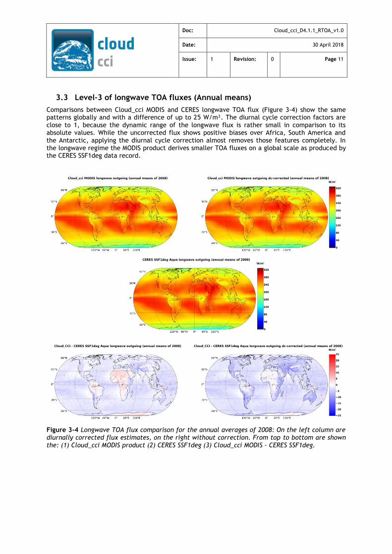
Comparisons between Cloud_cci MODIS and CERES longwave TOA flux (Figure 3-4) show the same patterns globally and with a difference of up to 25 W/m². The diurnal cycle correction factors are close to 1, because the dynamic range of the longwave flux is rather small in comparison to its absolute values. While the uncorrected flux shows positive biases over Africa, South America and the Antarctic, applying the diurnal cycle correction almost removes those features completely. In the longwave regime the MODIS product derives smaller TOA fluxes on a global scale as produced by the CERES SSF1deg data record.

Figure 3-4 Longwave TOA flux comparison for the annual averages of 2008: On the left column are diurnally corrected flux estimates, on the right without correction. From top to bottom are shown the: (1) Cloud_cci MODIS product (2) CERES SSF1deg (3) Cloud_cci MODIS – CERES SSF1deg.


Date: 30 April 2018


4. Evaluation against MSG-GERB

In addition to CERES against Cloud_cci MODIS, the Cloud_cci AVHRR top of the atmosphere (TOA) radiation products are compared against the observations from the Geostationary Earth Radiation Budget (GERB) instruments on-board the Meteosat Second Generation (MSG) satellites (Harries et al., 2005). The corresponding “MVIRI/SEVIRI Data Record” is provided by the Satellite Application Facility on Climate Monitoring (http://www.cmsaf.eu/).

In this study, the annual Level-3 global cloud property products TOA upwelling thermal radiation and TOA upwelling solar radiation for 2008 are compared against the corresponding MSG-GERB products for TOA reflected shortwave as well as TOA emitted longwave radiation. The comparison is performed twice, once with the uncorrected Cloud_cci AVHRR TOA radiation products and once with diurnal-cycle corrected (dc-corrected) TOA fluxes. The comparisons are separate into shortwave (Section 4.1) und longwave (Section 4.2) fluxes.

4.1 Level-3 of shortwave TOA fluxes (Annual means)

Figure 4-1 shows the reflected shortwave TOA fluxes of MSG-GERB and Cloud_cci AVHRR as annual mean values for 2008. The left plot contains the standard Cloud_cci AVHRR product, the middle plot the DC-corrected version and the right plot the GERB TOA fluxes. When comparing the standard AVHRR product with GERB it is noticeable, that the CC4CL derived fluxes are consistently higher. In some cases, the AVHRR TOA shortwave fluxes exceed the GERB estimates by more than 100 W/m². The highest overestimations are located in the Sahara desert, the Arabian Peninsula and the Alps. In contrast, the use of the DC-correction results in a distinctly better agreement with the GERB data records. However, the correction also leads to minor underestimations, especially over the sea and along the coastlines.

Figure 4-1 Shortwave TOA fluxes for the annual averages of 2008: On the left are the Cloud_cci AVHRR flux estimates, in the middle are the DC-corrected TOA fluxes and on the right are the MSG-GERB estimates for shortwave TOA fluxes.

In Figure 4-2, the absolute differences between the annual mean results of both data records are shown as Cloud_cci AVHRR – GERB and Cloud_cci AVHRR (DC-corrected) - GERB, respectively. The differences show the mentioned overestimations, with peaks about more than 100 W/m² at the named regions. Similar to the Cloud_cci MODIS data record, the overestimation is most likely due to the satellite measurement time, which take place at 2:00 PM local time for NOAA-18 AVHRR and is therefore also close to the daily maximum. After the application of the diurnal cycle correction, the differences are in a range from 60 to -60 W/m². Especially the significantly overestimated values in the Sahara desert, the Arabian Peninsula and the Alps were improved, but a small positive bias remains in the northern hemisphere. New is a slightly negative bias in the southern hemisphere, which is more pronounced over land than over sea. Towards the Latitudes beyond -60° a negative bias is increasing over the sea, probably caused by sea ice and snow cover around Antarctica.


Date: 30 April 2018


Figure 4-2 Absolute differences between the shortwave TOA fluxes of Cloud_cci AVHRR and MSG-GERB. Left: Results for the native Cloud_cci product. Right: Results for the diurnal cycle (dc-) corrected Cloud_cci product.

Figure 4-3 Relative differences between the shortwave TOA fluxes of Cloud_cci AVHRR and MSG-GERB. Left: Results for the native Cloud_cci product. Right: Results for the diurnal cycle (dc-) corrected Cloud_cci product.

The same patterns are visible in the results of the relative differences in Figure 4-3. It becomes clear, that the unmodified Cloud_cci AVHRR measurements are partly more than twice as high as the GERB fluxes. This applies in particular to small regions or to regions with high temporal snow cover like the Alps or Iceland. After the DC-correction, the relative differences also show a mainly positive bias in the northern hemisphere and a slightly negative bias in the southern hemisphere.


Date: 30 April 2018


Figure 4-4 show the scatter plots for TOA shortwave fluxes of GERB and Cloud_cci AVHRR before (left) and after the diurnal cycle correction (right). As already observed, the distribution of measured fluxes as well as the regression line displays a significant overestimation by the Cloud_cci AVHRR data record before the DC-correction. Accordingly, the mean bias, mean absolute bias (MAB) and RMSE values are very high with values over 30 W/m². Instead, the Pearson correlation coefficient is already relatively high at 0.86, which illustrates that the global patterns are in good agreement. Applying the DC-correction brings clear improvements for the AVHRR measurements and statistical measures. While the Pearson correlation coefficient has increased to 0.9, the mean bias, MAB and RMSE are significantly reduced. However, the DC-corrected bias about -3.22 W/m² also indicates, that the correction factor is a little too high for most areas.

Overall, after applying of the diurnal cycle correction the remaining over- and underestimations indicate that the correction factor is still too low for regions with high radiation amounts and a strongly pronounced diurnal cycle (e.g. the Sahara desert), but too high for regions with frequent cloud cover, like the rain forests of the southern hemisphere.

Apart from that one can conclude that the agreement between the dc-corrected Cloud_cci AVHRR shortwave TOA flux and MSG-GERB is very good.

Figure 4-4 Comparison between the Cloud_cci AVHRR (left) and the MSG-GERB shortwave flux estimates as well as between the DC-corrected Cloud_cci AVHRR (right) and the MSG-GERB shortwave flux estimates.


Date: 30 April 2018


4.2 Level-3 of longwave TOA fluxes (Annual means)

The annual mean values for 2008 in Figure 4-5 show very similar values and patterns betwwen Cloud_cci AVHRR and MSG-GERB. The longwave TOA flux estimates of Cloud_cci AVHRR and MSG-GERB give highest values up to 300 W/m² for the regions of the eastern Sahara, the Arabian Peninsula and the Atlantic Ocean south of the equator. The lowest flux values are located around Antarctica. As already mentioned at the comparison between MODIS and CERES, the diurnal cycle correction factors about 0.987 (land) and 0.998 (sea) are close to 1, due to the low dynamic range of the diurnal longwave flux. Thus, there are rarely any differences between the Cloud_cci AVHRR annual mean and the DC-corrected Cloud_cci AVHRR annual mean values.

Figure 4-5 Longwave TOA fluxes for the annual averages of 2008: On the left are the Cloud_cci AVHRR flux estimates, in the middle are the DC-corrected AVHRR TOA fluxes and on the right are the GERB estimates for longwave TOA fluxes.

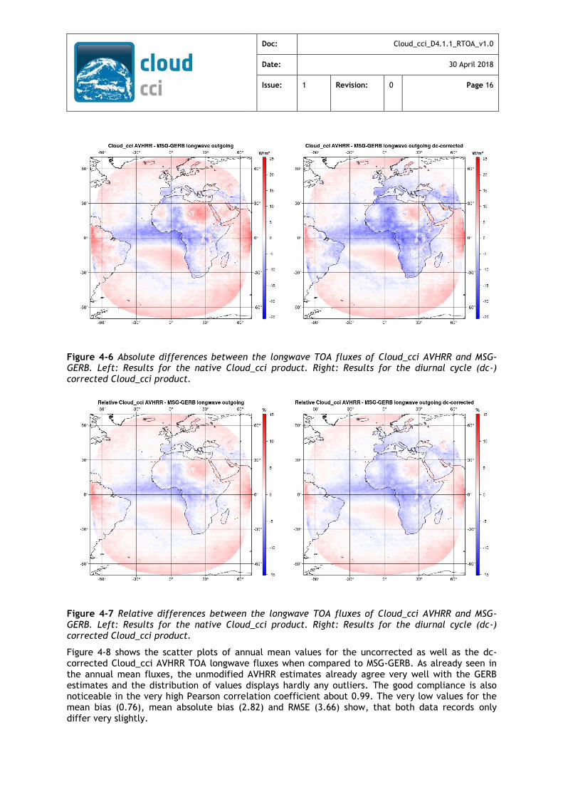
Looking at the absolute differences in Figure 4-6, it is noticeable that the variations between the two data records are in the range from -25 to 25 W/m². The under- and overestimations are therefore significantly lower than with the shortwave flux. The uncorrected flux shows the highest overestimations over the eastern Sahara, South America and slight overestimations over large parts of the oceans.

However, there are also regions with negative biases, mainly over Africa and the Atlantic Ocean. Applying the diurnal cycle correction produces similar changes as with the shortwave TOA flux. While regions with positive biases are decreasing, regions with an already existing negative bias are increasing. Especially over Africa, an increased area with a negative bias is noticeable after the correction. As mentioned before, the remaining overestimations as well as the increasing underestimations indicate that the correction factor is too high or too low for certain regions.

The mentioned patterns and DC-correction changes are also detectable in the relative differences. However, in the Figure 4-7 it becomes clear that the variance between the data records Cloud_cci AVHRR and MSG-GERB is significantly lower in the case of the longwave TOA fluxes. Overall, the under- and overestimations are in a range from -15 to 15%. In addition, applying of the diurnal cycle correction seems to produce higher and more underestimations compared to the reduction of existing overestimations.


Date: 30 April 2018


Figure 4-6 Absolute differences between the longwave TOA fluxes of Cloud_cci AVHRR and MSG-GERB. Left: Results for the native Cloud_cci product. Right: Results for the diurnal cycle (dc-) corrected Cloud_cci product.

Figure 4-7 Relative differences between the longwave TOA fluxes of Cloud_cci AVHRR and MSG-GERB. Left: Results for the native Cloud_cci product. Right: Results for the diurnal cycle (dc-) corrected Cloud_cci product.

Figure 4-8 shows the scatter plots of annual mean values for the uncorrected as well as the dc-corrected Cloud_cci AVHRR TOA longwave fluxes when compared to MSG-GERB. As already seen in the annual mean fluxes, the unmodified AVHRR estimates already agree very well with the GERB estimates and the distribution of values displays hardly any outliers. The good compliance is also noticeable in the very high Pearson correlation coefficient about 0.99. The very low values for the mean bias (0.76), mean absolute bias (2.82) and RMSE (3.66) show, that both data records only differ very slightly.


Date: 30 April 2018


However, it is noticeable that the mean bias is slightly positive and indicates a small overestimation. The application of the DC-correction produces only very slight changes. While the correlation coefficient is still at 0.99, the mean bias has decreased but now shows a general underestimation (-0.64). The MAB and RMSE have increased from 2.82 to 2.99 and from 3.66 to 4.02 W/m². Altogether, the differences between AVHRR and GERB are very low and the results indicate that the DC-correction is possibly unnecessary in the case of the longwave TOA flux.

Figure 4-8 Comparison in scatter plots between the Cloud_cci AVHRR and the MSG-GERB longwave flux estimates. The left plot used the standard Cloud_cci AVHRR longwave TOA flux estimates and the right plot the DC-corrected TOA fluxes.


Date: 30 April 2018


5. Summary & Conclusions

In this study, the evaluation results of the Cloud_cci MODIS and AVHRR TOA radiation fluxes are presented. The study contains a general overview of different data records, the comparison of the annual mean fluxes for long- and shortwave TOA radiation and two case studies on the instantaneous fluxes. Comparisons of Cloud_cci MODIS against CERES and Cloud_cci AVHRR against MSG-GERB were documented. Included in the comparisons was the application of a diurnal cycle correction factor.

Case studies for Greenland and Africa showed high correlation coefficients between instantaneous Cloud_cci MODIS and CERES estimates for the long- and shortwave fluxes. In addition, the case studies revealed a systematic bias over snowy surfaces, which expresses in a general underestimation of the shortwave flux by MODIS. In contrast to this, the snowy surfaces produce an overestimation in the MODIS product for longwave TOA fluxes. Furthermore, the Central African scene illustrated that ice-particle clouds can produce a negative bias in MODIS from the CERES product, due to erroneous ice particle sizes of the cloud retrieval.

The Cloud_cci MODIS Level-3C comparison against CERES displayed large differences in the TOA shortwave flux. Thereby, the predominant overestimations of MODIS were partly more than 100 W/m² higher. The variations are primarily due to incomplete diurnal sampling of MODIS Aqua, which makes the application of the diurnal cycle correction necessary. After applying a dc-correction the agreement to CERES is much improved. Longwave TOA fluxes are very well given Cloud_cci MODIS with differences to CERES being in the range of 25 W/m². On the other hand applying the DC-correction only produces very small improvements for the MODIS longwave estimates.

Cloud_cci AVHRR TOA flux estimates were evaluated against the MSG-GERB TOA fluxes. The comparison showed similar patterns as in the case of MODIS against CERES. Again the estimated TOA shortwave fluxes of the Cloud_cci product showed a distinctive overestimation in the annual mean values. In this context, the relative differences revealed that the AVHRR estimates are partly twice as much as the GERB flux values. As for MODIS, the overestimations of Cloud_cci AVHRR are mainly due to the incomplete diurnal sampling of the observing satellite (NOAA-18). Applying the DC-correction generated large improvements to the shortwave estimates and good agreements to CERES, although some areas with negative bias were created.

Longwave fluxes for Cloud_cci AVHRR show a very good agreement to MSG-GERB, similar to the comparisons of Cloud_cci MODIS to CERES. The application of the DC-correction factor affects the AVHRR product only to a minor extent. The use of the diurnal cycle correction seems not necessary in the case of the TOA longwave flux.

Altogether, the results show that the Cloud_cci data records for TOA fluxes are comparable to reference data records after applying the diurnal cycle correction. Especially the global patterns of TOA radiation fluxes are well detected and the spatial distribution on the global scale hardly differs between the data records. However, it became clear that the application of the diurnal cycle correction is indispensable in the case of the shortwave radiation. There are indications that more advanced correction factors (compared to the static one currently used) will further improve the Cloud_cci results.


Date: 30 April 2018


6. Glossary

AATSR Advanced Along Track Scanning Radiometer

AM ante meridiem – before noon

AVHRR Advanced Very High Resolution Radiometer

CC4CL Community Cloud retrieval for Climate

CERES Cloud and the Earth’s Radiant Energy System

DC diurnal cycle

DWD Deutscher Wetterdienst

ECV Essential Climate Variable

ENVISAT Environmental Satellite

EOS Earth Observation System

ERS2 European Remote-sensing Satellite - 2

FAME-C Freie Universität Berlin AATSR MERIS Cloud

FCDR Fundamental Climate Data Record

GERB Geostationary Earth Radiation Budget

MB Mean bias

MAB Mean absolute bias

MERIS Medium Resolution Imaging Spectrometer

MODIS Moderate Resolution Imaging Spectroradiometer

MSG Meteosat Second Generation

NOAA National Oceanic and Atmospheric Administration

OLCI Ocean and Land Colour Imager

PM post meridiem – after noon


Date: 30 April 2018


RAL Rutherford Appleton Laboratory

RMSE Root Mean Square Error

SLSTR Sea and Land Surface Temperature Radiometer

SSF1deg Single scanner footprint, 1°x 1° resolution

TOA Top of the atmosphere


Date: 30 April 2018


7. References

ATBD-TOAv1, Algorithm Theoretical Baseline Document (ATBD) - CC4CL TOA FLUX – ESA Cloud_cci, Issue 1, Revision: 0, planned date of Issue: 1/3/2016, Available at: http://www.esa-cloud-cci.org/?q=documentation

Carbajal Henken, C.K., Lindstrot, R., Preusker, R. and Fischer, J.: FAME-C: cloud property retrieval using synergistic AATSR and MERIS observations. Atmos. Meas. Tech., 7, 3873–3890, doi:10.5194/amt-7-3873-2014, 2014

Harries, J. E., Russell, J. E., Hanafin, J. A., Brindley, H., Futyan, J., Rufus, J., ... & Mueller, J. (2005). The geostationary earth radiation budget project. Bulletin of the American Meteorological Society, 86(7), 945-960.

Hollmann, R., Merchant, C.J., Saunders, R., Downy, C., Buchwitz, M., Cazenave, A., Chuvieco, E., Defourny, P., de Leeuw, G., Forsberg, R. and Holzer-Popp, T., 2013. The ESA climate change initiative: Satellite data records for essential climate variables. Bulletin of the American Meteorological Society, 94(10), pp.1541-1552.

McGarragh, G. R., Poulsen, C. A., Thomas, G. E., Povey, A. C., Sus, O., Stapelberg, S., Schlundt, C., Proud, S., Christensen, M. W., Stengel, M., Hollmann, R., and Grainger, R. G.: The Community Cloud retrieval for CLimate (CC4CL). Part II: The optimal estimation approach, Atmos. Meas. Tech. Discuss., https://doi.org/10.5194/amt-2017-333, in review, 2017.

Schmetz, J., Pili, P., Tjemkes, S., Just, D., Kerkmann, J., Rota, S., & Ratier, A. (2002). An introduction to Meteosat second generation (MSG). Bulletin of the American Meteorological Society, 83(7), 977-992.

Stengel, M., S. Mieruch, M. Jerg, K.-G. Karlsson, R. Scheirer, B. Maddux, J.F. Meirink, C. Poulsen, R. Siddans, A. Walther, R. Hollmann., The Clouds Climate Change Initiative: Assessment of state-of-the-art cloud property retrieval schemes applied to AVHRR heritage measurements, Remote Sensing of Environment (2015), http://dx.doi.org/10.1016/j.rse.2013.10.035

Sus, O., Stengel, M., Stapelberg, S., McGarragh, G., Poulsen, C., Povey, A. C., Schlundt, C., Thomas, G., Christensen, M., Proud, S., Jerg, M., Grainger, R., and Hollmann, R.: The Community Cloud retrieval for Climate (CC4CL). Part I: A framework applied to multiple satellite imaging sensors, Atmos. Meas. Tech. Discuss., https://doi.org/10.5194/amt-2017-334, in review, 2017.

http://www.esa-cloud-cci.org/?q=documentation

http://www.esa-cloud-cci.org/?q=documentation

Cloud cci doc - climate.esa.int

Documents