Closed-Loop Control Validation of a Morphing Wing Using Wind Tunnel Tests

American Institute of Aeronautics and Astronautics

1

Closed Loop Control Validation of a Morphing Wing using Wind Tunnel Tests

Andrei V. Popov1 and Lucian T. Grigorie.2 École de Technologie Supérieure, Montréal, Québec, H3C 1K3

Ruxandra Botez3 École de Technologie Supérieure, Montréal, Québec, H3C 1K3, Canada

and

Mahmoud Mamou4, Youssef Mebarki4 Institute for Aerospace Research - NRC, Ottawa, Ontario, K1A 0R6, Canada

In this paper, a rectangular finite aspect ratio wing, having a WTEA reference airfoil cross-section, was considered. The wing upper surface was made of a flexible composite material and instrumented with Kulite pressure sensors, and two smart memory alloys actuators. Unsteady pressure signals were recorded and visualized in real time while the morphing wing was being deformed to reproduce various airfoil shapes by controlling the two actuators displacements. The controlling procedure was performed using two methods which are described in the paper. Several wind tunnel test runs were performed for various angles of attack and Reynolds numbers in the 6’×9’ wind tunnel at the Institute for Aerospace Research at the National Research Council Canada (IAR/NRC). The Mach number was varied from 0.2 to 0.3, the Reynolds numbers varied between 2.29 million and 3.36 million, and the angles of attack range was within -1º to 2o. Wind tunnel measurements are presented for airflow boundary layer transition detection using high sampling rate pressure sensors.

Nomenclature α = angle of attack of the wing b = span of wing model c = chord of wing airfoil Cp = pressure coefficient CRIAQ = Consortium for Research and Innovation in Aerospace in Quebec ETS = Ecole de Technologie Superieure FEM = Finite Element Method FFT = Fast Fourier Transform IAR-NRC = Institute for Aerospace Research - National Research Council Canada LVDT = Linear Variable Differential Transducer M = Mach number Re = Reynolds number

1 PhD student, Laboratory of Research in Active Controls, Avionics and AeroServoElasticity LARCASE, 1100 Notre-Dame West Street, Montreal, Quebec, H3C 1K3, Canada, AIAA Member. 2 Post-Doc fellowship, Laboratory of Research in Active Controls, Avionics and AeroServoElasticity LARCASE, 1100 Notre-Dame West Street, Montreal, Quebec, H3C 1K3, Canada, AIAA Member. 3 Professor, Laboratory of Research in Active Controls, Avionics and AeroServoElasticity LARCASE, 1100 Notre-Dame West Street, Montreal, Quebec, H3C 1K3, Canada, AIAA Member. 4 Research Officer, Aerodynamics Laboratory, Institute for Aerospace Research, National Research Council, Montreal Road, Uplands Bldg. U66, Ottawa, Ontario, K1A 0R6, Canada, AIAA Member.


2

RMS = Root Mean Square SMA = Shape Memory Alloy

I. Introduction he present work was performed under the CRIAQ 7.1 Consortium for Research and Innovation in Aerospace in Quebec collaborative project between academia and industries. The project partners were the École de

technologie superieure (ETS), École Polytechnique of Montreal, the Institute for Aerospace Research at the National Research Council Canada (IAR-NRC), Bombardier Aerospace and Thales Avionics. In this project, the laminar flow behavior past aerodynamically morphing wing was improved in order to obtain significant drag reductions.

This collaboration calls for both aerodynamic modeling as well as conceptual demonstration of the morphing principle on real models placed in the wind tunnel. Drag reduction on a wing can be achieved by modification of the airfoil shape which has a direct effect on the laminar-to-turbulent flow transition location. The main objective of this concept is to promote large laminar regions on the wing surface, by delaying the transition location towards the trailing edge. Thus, the wing viscous drag could be reduced over an operating range of flow conditions characterized by a Mach number and angles of attack [1]. The airborne modification of an aircraft wing airfoil shape can be realized continuously to maintain laminar flow over the wing surface as flight conditions change. To achieve such a full operating concept, a closed loop control system concept was developed to control the flow fluctuations over the wing surface with the airfoil skin deformation mechanisms (actuators) [2]. A similar automatic control of boundary layer transition using suction on a flat plane and microphones was presented in ref. [3].

The wing model had a rectangular plan form of aspect ratio of 2 and was equipped with a flexible upper surface skin on which shape memory alloys actuators were installed. The two shape memory alloys actuators (SMA) executed the displacement at the two control points on the flexible skin in order to realize the desired optimized airfoil shapes.

The flexible skin was manufactured in a 4 ply laminate structure in a polymer matrix, with 2 unidirectional Carbon fiber inner plies and 2 hybrid Kevlar/Carbon fiber outer plies. The hybrid Kevlar/Carbon fiber was used in the chord-wise direction, where flexibility was needed for profile modification, while the low-modulus unidirectional carbon fiber was span-wise installed, in which case rigidity was preferred. The total thickness of the skin was 1.3 mm, the total Young modulus was 60 GPa, the Poisson’s ratios were 0.12 for Carbon/Kevlar hybrid and 0.25 for unidirectional Carbon [4].

Figure 1. Cross section of the morphing wing model

As a reference airfoil, a laminar airfoil WTEA was considered; its aerodynamic performance was investigated at

IAR-NRC in the transonic regime in refs. [5,6]. The flow over the reference airfoil upper surface became turbulent in a certain point near the leading edge due to the separation bubble for each airflow case expressed by a combination of Mach number and angle of attack. The separation bubble (the transition between laminar and turbulent flow) appeared due to the steep curvature of the airfoil shape. The principle beyond moving the separation bubble (the transition) towards the trailing edge consisted in changing to a milder curvature of the airfoil shape, which was presented in ref. [7].

The optimized airfoils were previously calculated by modifying the reference airfoil for each airflow condition as combinations of angles of attack and Mach numbers. The optimized airfoil shapes were realized using an optimizing routine that varied the vertical position of each actuator. The optimizing routine was coupled with a spline curve model of the flexible skin and the XFoil CFD code, and then the first generation of optimized airfoils

T


3

C1XX was obtained. The XFoil CFD code is free software in which the eN transition criterion is used, and which was presented in ref. [8, 9]. The imposed conditions of the first optimization were expressed in terms of the transition point position displacement as near as possible to the airfoil trailing edge, while maintaining a constant lift. The first generation of optimized airfoils was tested and validated by scanning using a laser during bench tests, as shown in Fig. 2 [10]. The second generation of optimized airfoils was obtained by coupling the optimizing routine with a Finite Element Model (FEM) of the flexible skin [4] and the XFoil CFD code, and the conditions imposed were to minimize the drag by moving the transition point as near as possible to the trailing edge while maintaining a constant lift [11].

Thirty five optimized airfoils were found for the airflow cases combinations of Mach numbers and angles of attack. Table 1 shows the optimized airfoils shapes denoted by C201 to C235 for angles of attack variations from -1 to 2 degrees, the Mach number variations from 0.2 to 0.3 and the Reynolds numbers variations from 2.29 to 3.37 millions.

0 50 100 150 200 250 300 3500

5

10

15

20

25

30

35

40

45

50

case C127

x (mm)

y (m

m)

Reference airfoil WTEA

Reference scaned modelOptimised airfoil C127

Scaned model C127

0 50 100 150 200 250 300 3500

5

10

15

20

25

30

35

40

45

50

case C130

x (mm)

y (m

m)

Reference airfoil WTEA

Reference scaned modelOptimised airfoil C130

Scaned model C130

Figure 2. Two examples of optimized airfoil shapes for the aerodynamic cases C127 (M=0.275, αααα=1.5º)

and C130 (M=0.3, α α α α=-0.5º)

II. Experimental setup description

A. Mechanical and electrical control system The morphing wing model had a rectangular plan form (chord c = 0.5 m and span b = 2.1 m) and consisted of two parts; one metal fixed part, which was designed to sustain the wing loads at a Mach number of 0.3 and an angle of attack up to 6o, and a morphing part consisted of a flexible skin installed on the wing upper surface and the SMA actuator system (Fig. 1). The flexible skin was required to change its shape through two action points in order to realize the optimized airfoil for the airflow conditions under which the tests were performed.

Table I: Test flow conditions for 35 wing airfoils

Mach

Re (mil.)

Angle of attack (degrees)

-1.00 -0.50 0.00 0.50 1.00 1.50 2.00

0.200 2.29 C201 C202 C203 C204 C205 C206 C207

0.225 2.56 C208 C209 C210 C211 C212 C213 C214

0.250 2.83 C215 C216 C217 C218 C219 C220 C221

0.275 3.10 C222 C223 C224 C225 C226 C227 C228


4

The actuators were composed of two oblique cams sliding rods span-wise positioned that converted the

horizontal movement along the span into vertical motion perpendicular to the chord (Fig. 2). The position of each actuator was given by the mechanical equilibrium between the Ni-Ti alloy SMA wires that pulled the sliding rod in one direction and the gas springs that pulled the sliding rod in the adverse direction. The gas springs role was to counteract the pulling effect of aerodynamical forces acting in wind tunnel over the flexible skin when the SMA’s were inactive. Each sliding rod was actuated by means of three parallel SMA wires connected to a current controllable power supply which was the equivalent of six wires acting together. The pulling action of the gas spring retracted the flexible skin in the undeformed-reference airfoil position, while the pulling action of the SMA wires deployed the actuators in the load mode, i.e. morphed airfoil in the optimized airfoil position (see Fig. 3). The gas springs used for these tests were charged with an initial load of 225 lbf (1000 N) and had a characteristic rigidity of 16.8 lbf / in (2.96 N / mm).

x

z

flexible skin

spring

SMAactuator

rod

roller cam

Firstactuating line

Secondactuating line

Figure 3. Schematics of the flexible skin mechanical actuation

The mechanical SMA actuators system was controlled electrically through an “open loop” control system. The architecture of the wing model open loop control system, SMA actuators and controller is shown in Figure 4. The two SMA actuators have six wires each, which were supplied with power by the two AMREL SPS power supplies, controlled through analog signals by the NI-DAQ USB 6229 data acquisition card. The NI-DAQ was connected to a laptop through a USB connection. A control program was implemented in Simulink, which provided to the power supply unit the needed SMA current intensity through an analog signal as shown in Figure 4. The Simulink control program used as feedback three temperature signals coming from three thermocouples installed on each wire of the SMA actuator, and a position signal from a LVDT sensor connected to the oblique cam sliding rod of each actuator. The temperature signals were used for the overheat protection system that disconnect the current supply to the SMA in case of wire temperature pass over the set limit of 120°C. The position signals served as a feedback for the actuator desired position control. The oblique cam sliding rod had a horizontal versus vertical ratio 3:1; hence the maximum horizontal displacement of the sliding rod by 24 mm was converted into a maximum vertical displacement (8mm) of the actuator.

0.300 3.36 C229 C230 C231 C232 C233 C234 C235


5

Figure 4. Architecture of the morphing wing model control system.

A user-interface was implemented in Matlab/Simulink which allowed the user to choose the optimized airfoils shape from database stored on the computer hard disk and provided to the controller the required vertical displacements in order to obtain the desired optimized airfoil shape. The controller activated the power supplies with the required SMA current intensities through an analog signal as shown in Figure 4. The control signal of 2 V corresponded to a SMA supplied current of 33 A. In practice, the SMA wires were heated at an approximate temperature of 90°C with a current of 10 A. When the actuator reached the desired position the current was shut off and the SMA was cycled in endless heating/cooling cycles through the controller switching command on/off of the current in order to maintain the current position until another desired position or the entire system shut off was required. In support of the discrete pressure instrumentation, infrared thermography (IR) visualization was performed to detect the transition location on the morphing wing upper surface and validate the pressure sensor analysis. The transition detection method using IR was based on the differences in laminar and turbulent convective heat transfer coefficient and was exacerbated by the artificial increase of model-air flow temperature differences. In the resulting images, the sharp temperature gradient separating high temperature (white intensity in image) and low temperature (dark intensity) regions is an indication of the transition location. The infrared camera used was an Agema SC3000 camera, equipped with a 240×320 pixels QWIP detector, operating in the infrared wavelength region of 8-9 µm and cooled to 70°K to reduce thermal noise. The camera provided a resolution of 0.02°C and a maximum frame rate of 60 Hz. It was equipped with the default lens (FOV = 20°×15°), and was installed 1.5 m away from the model with an optical axis oriented in the horizontal plane at about 30° with respect to the wing surface mid-chord normal. Optical access was provided through an opening on the side wall of the test section opposite to the upper surface. More details about the methodology and processing are available in ref. [12]

B. Aerodynamical detection system and graphical user interface The morphing wing goal was to improve laminar flows over the upper surface of the wing. In order to ensure that the improvement is achieved, a detection system was incorporated to the wing model that gives information about the flow characteristics. An array of twelve Kulite pressure sensors was installed on the flexible skin.

The pressure data acquisition was performed using a NI-DAQ USB 6210 card with 16 analog inputs, at a total sampling rate of 250 kilo samples/s. The input channels were connected directly to the wind tunnel analog data acquisition system which was connected to the twelve Kulite sensors. The data acquisition system served as an amplifier and conditioner of the signal at a sampling rate of 15 kilo samples/s. One extra channel was used for the wind tunnel dynamic pressure acquisition to calculate the pressure coefficients Cp’s from the pressure values measured by the twelve pressure sensors. The signal was acquisitioned at sampling rate of 10 kilo samples/s in frames of 1024 points for each channel which allowed a boundary layer pressure fluctuations Fast Fourier Transform spectral decomposition up to 5 kHz for all channels, at a rate of 9.77 samples/s (Figure 5) using Matlab/Simulink software. The plot results were visualized in real time on the computer screen in dedicated windows (see Figure 6) at a rate of 1 sample/s. Figure 6 shows an example of graphical user interface in which all the aerodynamical and morphing shape information were centralized together with the control buttons of the controlling software. The window showed some data about the Mach number, the angle of attack, the airfoil shape of the morphing wing, and the two actuators vertical displacements needed to obtain the desired airfoil shape. In the two plots, were shown the pressure coefficients distribution Cp’s of the twelve Kulite sensors, and the noise of the


6

signal (RMS) of each pressure signal. The left figure shows the wing un-morphed position, while the right figure shows the wing under its morphed position. The results obtained were qualitatively very similar to those obtained in previous studies [13, 14].

In Figure 5.a, the twelve spectra of the pressure signals are shown, for the un-morphed wing. The noise amplitude of the signals is about the same for the whole bandwidth, with the exception being of the first signal channel which has obviously the smallest noise. The laminar-to-turbulent transition is detected by the slight peak of the 4th sensor positioned at 35% of the chord in the Root Mean Squares (RMS) plot shown in Figure 6.a (red curve). The laminar to turbulent transition is not visible in signals spectra from Figure 5.a, but two peaks are visible at 1.7 kHz and 2.8 kHz, which may be due to electromagnetic-induced noise by the Wind Tunnel electrical system. The two peaks were visible all the time during Wind Tunnel Tests, for both un-morphed and morphed configurations.

In Figure 5.b, the twelve spectra of the pressure signals are shown when the wing is morphed. The noise amplitude of the 10th channel is the highest (the green spectra), showing that the laminar-to-turbulent transition occurs in that position. The light blue and blue spectra of the 11th and 12th channels show the turbulent flow noise which is higher than the laminar flow noise, but is lower than the transition flow noise. In Figure 6.b, the transition is detected by the peak of the 10th sensor positioned at 59.2% of the chord in the RMS plot (red curve).

a) Un-morphed configuration b) Morphed configuration

Figure 5. FFT decomposition of the twelve channels pressure signals showing the transition development

in the boundary layer over the morphing wing upper surface


7

a) Un-morphed configuration b) Morphed configuration

Figure 6. Graphical User Interface (GUI) where all the aerodynamical and morphing shape information

are centralized together with the control buttons of the software.

In Figure 6.a, the data display GUI interface is shown. Data for an un-morphed airfoil (black colour) are illustrated. The actuators reference positions correspond to dY1 = 0 mm and dY2 = 0 mm, the Cp distribution calculated by XFoil for the reference airfoil (black curve), and the Cp theoretical values of the sensors (black circles) are displayed. In the lower plot of Figure 6.a is shown the N-factor used by Xfoil to predict transition for the reference airfoil (black curve). In the case of an un-morphed configuration, the predicted transition position was found to be at the 6th position of the sixteen available sensors positions. In the beginning of wind-tunnel tests, a number of sixteen sensors were installed, but due to their removal and re-installation during successive wind tunnel tests, four of them were found defective, therefore a number of twelve sensors remained to be used during the last wind tunnel tests. The Cp distribution and its RMS were illustrated in red star symbols. Results predicted for the morphed airfoil are shown (blue colour) in Figure 6.b. The morphed airfoil coordinates (blue curves), the Cp distribution calculated by XFoil for the optimized airfoil (blue curve) and the Cp theoretical values of the sensors (blue circles) are displayed. In the lower plot of Figure 6.b, the N-factor predicted by Xfoil for transition location prediction is shown for the optimized airfoil (blue curve). In this morphed configuration case, the position of the transition was predicted at the 14th sensor position positioned at 59.2% of the chord. The black (un-morphed) and blue (morphed) curves served as theoretical validations of the red curves reflecting the aerodynamic parameters (Cp and RMS) provided by Kulite sensors plotted on screen in real time with a sampling rate of 1 S/sec. In Figure 6.b is shown the actuated airfoil in the morphed position (dY1 = 4.92 mm and dY2 = 7.24 mm). The transition position was given by the sensor location where the maximum RMS was found, which in this case was the 10th Kulite sensor out of the 12 sensors. The instant visualization allowed us to find the exact position predicted by XFoil. Figure 5.b allows to see the Fast Fourier Transform spectral distribution of the 10th sensor noise (green spectra) having the highest noise in the frequency domain of 4-5 kHz.


8

C. Closed loop control methods Two methods of closed loop control were designed to obtain and maintain the optimized airfoil during the wind tunnel tests:

1) First method used a controller which took, as a reference value, the required displacement of the actuators from a database stored in the computer memory in order to obtain the morphing wing optimized airfoil shape. This method used the position signal feedback from the LVDT sensor connected to the oblique cam sliding rod of each actuator. This method was called “open loop control” due to the fact that this control method does not take direct information from the pressure sensors concerning the wind flow characteristics. The design concept of the controller consists of a PID and an ON/OFF switch that connects and disconnects the SMA to a source of current which heats and lets cooling the SMA to allow its change in its length, this concept was investigated in [2]. The initial input which is the optimized airfoil for any flow condition is chosen manually by the operator from the computer database through a user interface. Then the displacements (dY1 and dY2) that are required to be reproduced by the two control points on the flexible skin are sent to the controller. This controller sends an analog signal 0 – 2 V to the power supply that provide a current of 0 – 20 A / 20 V cc. to the SMA. The SMA will change its length according to the temperature of the wire due to the passing current and will change the position of the actuator which is sensed by a linear variable differential transducer (LVDT). The signal position received from the LVDT is compared to the desired position and the error obtained is fed back to the controller. The PID will control the dynamics of the heating process. If the realized position is greater than the desired position the switch will disconnect the control current letting the SMA wire to cool down. During the cooling down process the SMA will maintain its length due to the hysteretic behaviour. Also the controller uses three thermocouples signals from each SMA wire to monitor the temperature of the wires in order to maintain the temperature under 130 º C limits.

2) Second method used the same controller with the difference that took, as a reference value, the theoretical Cp value calculated by XFoil in the position of the sensor connected through aerodynamic interdependence with the actuator position. The controller used as feed-back the pressure signal coming from the 6th position of the 16 Kulite sensors which was connected to the first actuator, and the pressure signal coming from the 12th position of the 16 Kulite sensors which was connected to the second actuator. Their positions were visualized on Figure 6 at the two corresponding actuator points Act1 and Act2. The theoretical Cp values were compared to the measured Cp values, while the control signal based on the difference between measured and theoretical Cp values was sent to the actuators power supplies. In this case, the method was called “closed loop control” due to the fact that this control method used the pressure information from the Kulite sensors.

1. Open loop control

The schematics of the morphing wing open loop control are shown in Figure 7. The input of the loop was the

optimized airfoil corresponding to the airflow conditions in the wind tunnel, which was requested by the operator to be reproduced by the flexible skin. The optimized airfoil was selected by the operator from the computer database through the graphic interface listbox ‘Airfoil’ and charged into the software by activating the button ‘CHARGE’ (see Figure 6). The software sent actuators coordinates required to reproduce the airfoil displacements (dY1 and dY2) to the controller. When the operator selected the push button ‘Optim’, the controller adjusted the position of the actuators as required. The real position of the actuators was measured through the LVDT and compared with the desired dY1 and dY2 values. The horizontal displacement of the SMA oblique cam/actuator was converted in vertical displacement by division in 3. Figure 6 shows the optimized airfoil C219 obtained through open loop control of the two actuators displacements dY1 = 4.92 mm and dY2 = 7.24 mm. The new shape of the morphing wing obtained through the displacements of the SMA actuators was discussed in paper [10]. The return of the airfoil shape to the reference position was requested by filling up the dialog boxes dY1 = 0 and dY2 = 0 and afterwards using the push button ‘Request’. Any actuators displacements between 0 and 8 mm could be requested by the operator.


9

Figure 7. Open loop control using optimized airfoils database and actuator positions as feed-back

2. Closed loop control

In Figure 8, the schematic of the morphing wing closed loop control is shown. The loop input was the optimized

airfoil for each airflow conditions in the wind tunnel, which was requested by the operator to be reproduced by the flexible skin. The optimized airfoil was selected by the operator from the computer database through the graphic interface list box ‘Airfoil’ and was charged into the software by activating the button ‘CHARGE’ (see Fig. 6). The software launched a subroutine calling the XFoil code that calculated the Cp distribution for various airflow conditions α, M and Re; they were entered as inputs. The operator selected the position of the sensors that were used to give feedback to the controller. In the example shown on Figure 6, the sensor located at the position #6 was selected to close the loop for the first actuator, and the sensor located at the position #12 was selected to close the loop for the second actuator.

When the ‘Close loop’ switch button was activated, the close loop control is activated. The two controllers gave commands to the power supplies that changed the actuators positions. The positions of the actuators had the effect of the shape changing, which had the effect of change of the measured Cp values in the selected points. The controller used as targets the theoretical Cp values calculated by XFoil. When the Cp values of the sensors reached the target values the controller stopped the SMA actuators activation and begun to maintain the Cp values around the target. The control principle was the same as in “open loop control case”, even the controller was the same, with the exception that the Cp values errors were amplified by 10 and the feedback was given through two operator chosen pressure sensors instead of LVDT position sensors.


10

AB

, M (Re)

Optimized

Airfoils

Database

Cp1

Cp2Reference

Airfoil WTEA

+ -

Desired pressure

distribution

ControllerPwr

SupplySMA

actuatorAirflow

1/qinfp1measuredCp1measured

Plant #1

Sensor

A

B

XFoil

Cp distribution

Error

amplification

Kulite

+ -Controller

Pwr

SupplySMA

actuatorAirflow

1/qinfp2measuredCp2measured

Plant #2

Sensor

Error

amplification

Kulite

Plant #1 Plant #2

-Cp1

-Cp2-Cp1measured

-Cp2measured

Figure 8. Closed loop control using optimized airfoils database and Cp values as feed-back.

III. Experimental results obtained in the wind tunnel The following sections outline the experimental results obtained during wind tunnel tests. The tests were performed in the 6’×9’ subsonic wind tunnel at the Institute for Aerospace Research at the National Research Council Canada (IAR/NRC). The wind speed varied between Mach numbers 0.2 (223 ft/s) and 0.3 (335 ft/s) at Reynolds numbers between 2.29 million and 3.36 million (see Table I).

A. Open loop control The following figures show the morphing wing with the actuators at the zero position, i.e. the wing was the

reference airfoil compared to the morphing wing with the actuator in the requested position to obtain the optimized airfoil C226.

In Figure 9 the case M = 0.275 and α = 1° is shown. On the left hand side of Figure 8, there was a turbulent flow

RMS pattern signature which appeared following a small peak in the second signal (CH 2 magenta). The typical RMS pattern signature of transition appeared when the morphing wing actuators were at the C226 optimized airfoil position. The RMS distribution peak at the ninth sensor is shown on the right hand side Fast Fourier Transform decomposition as red signal (CH 9). These plots show that the transition location moved from sensor # 2 to sensor # 9.


11

Figure 9. Reference airfoil versus C226 airfoil results for M = 0.275= 0.275= 0.275= 0.275 and α α α α = 1°

B. Closed loop control Figure 9 shows the wing morphing configurations achieved by using two different control methods. The left

hand sides (LHS) of Figure 10 show the open loop control and the right hand sides (RHS) show the closed loop control data. The difference between the LHS graphs show the control having the actuator positions feedback, while the RHS curves show the control having the -Cp values as feedback.


12

0 50 100 150 200 2500

2

4

6

8

time (s)

dY (

mm

)

0 50 100 150 200 2500.4

0.5

0.6

0.7

0.8

time (s)

-Cp

Wind tunnel test control time history

0 50 100 150 200 25020

40

60

80

time (s)

SM

A T

empe

ratu

re (

deg

C)

0 50 100 150 200 250

0

5

10

time (s)

Con

trol

cur

rent

(A

)

0 50 100 150 200 2500

2

4

6

8

time (s)

dY (

mm

)

0 50 100 150 200 2500.4

0.5

0.6

0.7

0.8

time (s)

-Cp

Wind tunnel test control time history

0 50 100 150 200 25020

40

60

80

time (s)

SM

A T

empe

ratu

re (

deg

C)

0 50 100 150 200 250

0

5

10

time (s)

Con

trol

cur

rent

(A

)

a) b)

Figure 10. C232 airfoil results obtained in a) Open loop, b) Closed loop control

The time histories of the same critical parameters are shown in Fig. 10. The first plots at the top of Fig. 10.a and 10.b, show the theoretical (dashed lines) and measured Cp (solid lines) value for two sensors, #1 in red and #8 in blue, located respectively at x = 38.1 mm and x = 179.6 mm on the airfoil. The second plots display the desired (dotted lines) and realized (solid lines) vertical displacements dY1 and dY2 in mm of the two actuators (first actuator – red line, second actuator – blue line). The last two plots at the bottom of Fig. 10.a and 10.b give the SMA actuators wires temperatures in degrees C, and control current intensity in A respectively.

The LHS plots show the realization of the C232 optimized airfoil using the open loop method, having the displacements dY1 and dY2 as feedback parameters, and using a PID coupled with an ON/OFF switch method controller. The RHS plots show the realization of the C232 optimized airfoil –Cp distribution using the close loop method having the sensors #1 and #7 –Cp values as feedback parameters, using the same PID controller. The discontinuity in the –Cp desired value (blue line) was due to switching the control sensor from #7 to #8 and back. It is observed that the controller obeyed the command and achieved the desired results.


13

a) b)

Figure 11 C232 airfoil results obtained at M = 0.3 and αααα = 0.5 in a) Open loop, b) Closed loop

The aerodynamic effect of the control in open loop versus closed loop at the same airflow configuration and same optimized airfoil command for the C232 airfoil are shown on Figure 11. The LHS plots show the realization of the C232 optimized airfoil using the open loop method having the displacements dY1 and dY2 as feedback parameters (see the black ovals in the figure). The RHS plots show the realization of the C232 optimized airfoil –Cp distribution using the closed loop method having the sensors #1 and #7 –Cp values as feedback parameters (see the black ovals in figure). The slight differences in the aerodynamical configuration shown are dues to zero calibration of the first actuator, which indicated its position with an error of 0.5 mm lower than in reality.


14

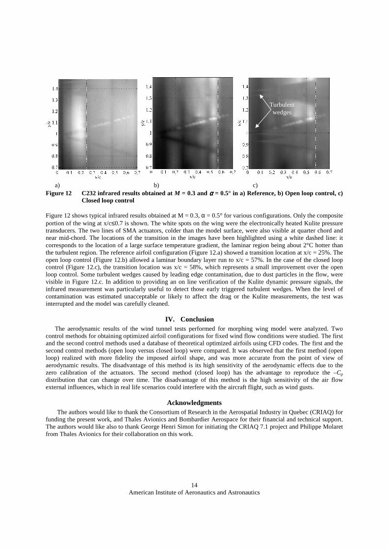
a) b) c) Figure 12 C232 infrared results obtained at M = 0.3 and αααα = 0.5° in a) Reference, b) Open loop control, c)

Closed loop control Figure 12 shows typical infrared results obtained at M = 0.3, α = 0.5° for various configurations. Only the composite portion of the wing at x/c≤0.7 is shown. The white spots on the wing were the electronically heated Kulite pressure transducers. The two lines of SMA actuators, colder than the model surface, were also visible at quarter chord and near mid-chord. The locations of the transition in the images have been highlighted using a white dashed line: it corresponds to the location of a large surface temperature gradient, the laminar region being about 2°C hotter than the turbulent region. The reference airfoil configuration (Figure 12.a) showed a transition location at x/c = 25%. The open loop control (Figure 12.b) allowed a laminar boundary layer run to x/c = 57%. In the case of the closed loop control (Figure 12.c), the transition location was x/c = 58%, which represents a small improvement over the open loop control. Some turbulent wedges caused by leading edge contamination, due to dust particles in the flow, were visible in Figure 12.c. In addition to providing an on line verification of the Kulite dynamic pressure signals, the infrared measurement was particularly useful to detect those early triggered turbulent wedges. When the level of contamination was estimated unacceptable or likely to affect the drag or the Kulite measurements, the test was interrupted and the model was carefully cleaned.

IV. Conclusion The aerodynamic results of the wind tunnel tests performed for morphing wing model were analyzed. Two

control methods for obtaining optimized airfoil configurations for fixed wind flow conditions were studied. The first and the second control methods used a database of theoretical optimized airfoils using CFD codes. The first and the second control methods (open loop versus closed loop) were compared. It was observed that the first method (open loop) realized with more fidelity the imposed airfoil shape, and was more accurate from the point of view of aerodynamic results. The disadvantage of this method is its high sensitivity of the aerodynamic effects due to the zero calibration of the actuators. The second method (closed loop) has the advantage to reproduce the –Cp distribution that can change over time. The disadvantage of this method is the high sensitivity of the air flow external influences, which in real life scenarios could interfere with the aircraft flight, such as wind gusts.

Acknowledgments The authors would like to thank the Consortium of Research in the Aerospatial Industry in Quebec (CRIAQ) for funding the present work, and Thales Avionics and Bombardier Aerospace for their financial and technical support. The authors would like also to thank George Henri Simon for initiating the CRIAQ 7.1 project and Philippe Molaret from Thales Avionics for their collaboration on this work.

Turbulent wedges


15

References [1] Zingg, D. W., Diosady, L., and Billing, L., “Adaptive Airfoils for Drag Reduction at Transonic Speeds,”

AIAA paper 2006-3656, 2006. [2] Popov. A-V., Labib, M., Fays, J., Botez, R.M., 2008, Closed loop control simulations on a morphing laminar

airfoil using shape memory alloys actuators, AIAA Journal of Aircraft, Vol. 45(5), pp. 1794-1803. [3] Rioual, J.-L., Nelson, P., A., Fisher, M., J., 1994, Experiments on the Automatic Control of Boundary-Layer

Transition, AIAA Journal of Aircraft, Vol. 31(6), pp. 1416-1419. [4] Coutu, D., Brailovski, V., Terriault, P., Fischer, C., Experimental validation of the 3D numerical model for an

adaptive laminar wing with flexible extrados, 18th International Conference of Adaptive Structures and Technologies, Ottawa, Ontario, 3-5 October, 2007.

[5] Khalid, M., 1993, Navier Stokes Investigation of Blunt Trailing Edge Airfoils using O-Grids, AIAA Journal of Aircraft, Vol.30, No.3, pp.797-800

[6] Khalid, M., and Jones, D.J., A CFD Investigation of the Blunt Trailing Edge Airfoils in Transonic Flow, Inaugural Conference of the CFD Society of Canada, June, 1993.

[7] Popov. A-V., Botez, R.M., Labib, M., 2008, Transition point detection from the surface pressure distribution for controller design, AIAA Journal of Aircraft, Vol. 45(1), pp. 23-28.

[8] Drela, M., Implicit Implementation of the Full en Transition Criterion, 21st Aplied Aerodynamics Conference, AIAA paper 2003–4066, Orlando, Florida, 2003.

[9] Drela, M., Giles, M., B., 1986, Viscous-Inviscid Analysis of Transonic and Low Reynolds Number Airfoils, AIAA Journal of Aircraft, Vol. 25(10), pp. 1347-1355.

[10] Popov, A., V., Grigorie, L., T., Botez, R.M., Control of a Morphing Wing in Bench Test, 13th Canadian Aeronautical and Aerospace Institute CASI Aeronautics Conference, Kanata, Ontario, 5-7 May, 2009.

[11] Sainmont, C., Paraschivoiu, I., Coutu, D., Multidisciplinary Approach for the Optimization of a Laminar Airfoil Equipped with a Morphing Upper Surface, NATO AVT-168 Symposium on "Morphing Vehicule", Evora, Portugal, 2009.

[12] Mébarki, Y., Mamou, M. and Genest, M., Infrared Measurements of Transition Location on the CRIAQ project Morphing Wing Model, NRC LTR- AL-2009-0075, 2009.

[13] Nitcshe, W., Mirow, P., Dorfler, T., Investigations on Flow Instabilities on Airfoils by Means of Piezofoil –Arrays, Laminar-Turbulent Transition IUTAM Symposium, Toulouse, France, 11-15 September, 1989, pp.129-135.

[14] Mangalam, S. M., Real-Time Extraction of Hydrodynamic Flow Characteristics Using Surface Signature, IEEE Journal of Oceanic Engineering, Vol. 29, No. 3, pp. 622-630, July 2004

Closed-Loop Control Validation of a Morphing Wing Using Wind Tunnel Tests

Documents