MAUSAM, 69, 1 (January 2018), 73-80 551.583 : 551.577.3 (540.27) (73) Climatic variability and prediction of annual rainfall using stochastic time series model at Jhansi in central India SUCHIT K. RAI, A. K. DIXIT, MUKESH CHOUDHARY and SUNIL KUMAR ICAR-Indian Grassland and Fodder Research Institute, Jhansi (U. P.) – 284003, India (Received 12 January 2017, Accepted 10 November 2017) e mail : [email protected] सार – इस शोध प म झासी (25°27ʹ उ. अिश, 78°35ʹ पू. देशितर म.स. तल 271 मी. से अधधक) के 72 व (1939 से 2010 तक) की अवधध के वा आिकड क उपयोग करते ह ु ए वाक वा पूवानुमन देने हेतु एक टककटक टइम ससरीज मॉडल वकससत करने के सलए वा के लदलव क अययन ककय गय ह 77 व अात ् 1939 से 2015 तक की इस लिली अवधध के वा आिकड क वलेण करने से पत चल ह कक इन 77 व म वाक वा 375 से 1510 सम.मी. के लीच रही ह इन 77 व म वा म 4.2 सम.मी ततवा की दर से कमी ही वृतत रही ह दीधाअवधध वाक वा क औसत 908.3 ± 248.2 सम.मी. रह ह जसम सिनत गुणिक 27.3% रह ह इस े म 77 व की अवधध म वा म 319.5 सम.मी. की धगरवट आई ह और यह 1068.4 सम.मी. से घटकर 748.4 सम.मी. हो गई ह इसके सलए 0, 1 और 2 ेणी के आॉटोररेससव (AR) मॉडल क योग एवि वकस ककय गय ह ेणी 2 क आॉटोररेससव मॉडल झासी म 74% व म 20% के घट-ल के स वाक वा क पूवानुमन देने म सफल रह ह वाक वा के पूवानुमन और ेत की गई वा के लीच सहसिलिध (r) म जलवतयक औसत वसिगतत 0.76 पई गई ह इन मॉडल की अनुकू लत और उपयुत क परीण लॉस-पयसा पोटा मनटओ टेट के अकई किटेररयन इफरमेशन त ऐततहससक एवि त ककए गए आिकड की तुलन के आधर पर ककय गय ह ऐततहससक और त ककए गए वा आिकड की आरेखी तुतत एक दूसरे के कफी तनकट ह आॉटो ररेशन (2) मॉडल वर मपत और पूवानुमतनत वा आिकड के लीच तुलन करने पर पट प से पत चलत ह कक झासी म वाक वा क पूवानुमन देने के सलए वकससत ककए गए मॉडल क योग दतपूवाक ककय ज सकत ह ABSTRACT. A study was conducted on rainfall variability/change and to develop a stochastic time series model for annual rainfall prediction using rainfall data for the period of 72 years (1939-2010) at Jhansi (25°27ʹ N latitude, 78°35ʹ E longitude, 271 m above mean sea level).The analysis of long term rainfall data for the period of 77 years i.e., 1939-2015 revealed that annual rainfall varied between 375 to 1510 mm over 77 years with a decreasing trend of 4.2 mm/year. The long term mean annual rainfall is 908.3 ± 248.2 mm with a coefficient of variation of 27.3%. The rainfall of the region had been decreased by 319.5 mm over the period of 77 years from 1068.4 mm to 748.4 mm. Autoregressive (AR) models of order 0, 1 and 2 were tried and developed. The autoregressive model of the order 2 was able to predict the annual rainfall of Jhansi within ±20% in 74% of the years. Correlation (r) between the anomaly of observed and predicted annual rainfall from the climatological mean was 0.76. The goodness of fit and adequacy of models were tested by Box- Pierce Portmanteau test, Akaike information Criterion and by comparison of historical and generated data. The graphical representation between historical and generated rainfall was a very close agreement between them. The comparison between the measured and predicted rainfall by AR (2) model clearly shows that the developed model can be used efficiently for the annual prediction of rainfall at Jhansi. Key words – Akaike information criterion, Autoregressive (AR) models, Box-Pierce Portmanteau test, Long term trend, Seasonal rainfall variation, Stochastic time series model. 1. Introduction The Bundelkhand region is spread over 71618 square kilometers of the central plains and many of the districts are included in the list of most backward districts of India by Planning Commission, GOI. The region supports 18.31 million (79.1% in rural areas) human populations as per the 2011 census with 10.7 million animal population and more than one third of the households in these areas are considered to be Below the Poverty Line (BPL). Agriculture in Bundelkhand is rainfed, diverse, complex, under-invested, risky and vulnerable. In addition, extreme weather conditions, like droughts, short-term rain and flooding in fields add to the uncertainties in agricultural production and seasonal human migrations for the search of employment. The scarcity of water in the semi-arid region, with poor soil and low productivity further aggravates the problem of food security. Climate change in world is always one of the most important aspects in water resources management (Rai et al., 2014;

Welcome message from author
This document is posted to help you gain knowledge. Please leave a comment to let me know what you think about it! Share it to your friends and learn new things together.
Transcript
MAUSAM, 69, 1 (January 2018), 73-80
551.583 : 551.577.3 (540.27)
(73)
Climatic variability and prediction of annual rainfall using stochastic
time series model at Jhansi in central India
SUCHIT K. RAI, A. K. DIXIT, MUKESH CHOUDHARY and SUNIL KUMAR
ICAR-Indian Grassland and Fodder Research Institute, Jhansi (U. P.) – 284003, India
(Received 12 January 2017, Accepted 10 November 2017)
e mail : [email protected]
सार – इस शोध पत्र में झ ाँसी (25°27ʹ उ. अक् ांश, 78°35ʹ प.ू देश ांतर म .स. तल 271 मी. से अधधक) के 72 वर्षों (1939 से 2010 तक) की अवधध के वर्ष ा आांकड़ों क उपयोग करते हुए व र्र्षाक वर्ष ा पवू ानमु न देने हेत ुएक स्ट ककस्स्टक ट इम ससरीज मॉडल र्वकससत करने के सलए वर्ष ा के लदल व क अययययन ककय गय ह 77 वर्षों अर् ात ्1939 से 2015 तक की इस लांली अवधध के वर्ष ा आांकड़ों क र्वश्लेर्षण करने से पत चल ह कक इन 77 वर्षों में व र्र्षाक वर्ष ा 375 से 1510 सम.मी. के लीच रही ह इन 77 वर्षों में वर्ष ा में 4.2 सम.मी प्रततवर्षा की दर से कमी ही प्रवतृत रही ह दीधाअवधध व र्र्षाक वर्ष ा क औसत 908.3 ± 248.2 सम.मी. रह ह स्जसमें सिन्नत गणु ांक 27.3% रह ह इस क्ेत्र में 77 वर्षों की अवधध में वर्ष ा में 319.5 सम.मी. की धगर वट आई ह और यह 1068.4 सम.मी. से घटकर 748.4 सम.मी. हो गई ह इसके सलए 0, 1 और 2 शे्रणी के आॉटोररगे्रससव (AR) मॉडल़ों क प्रयोग एवां र्वक स ककय गय ह शे्रणी 2 क आॉटोररगे्रससव मॉडल झ ाँसी में 74% वर्षों में 20% के घट-लढ़ के स र् व र्र्षाक वर्ष ा क पवू ानमु न देने में सफल रह ह व र्र्षाक वर्ष ा के पवू ानमु न और पे्रक्षक्त की गई वर्ष ा के लीच सहसांलांध (r) में जलव तयक औसत र्वसांगतत 0.76 प ई गई ह इन मॉडल़ों की अनकूुलत और उपयकु्त्त क परीक्ण लॉक्त्स-र्पयसा पोटा मनट ओ टेस्ट के अक ई किटेररयन इन्फ रमेशन तर् ऐततह ससक एवां प्र प्त ककए गए आांकड़ों की तुलन के आध र पर ककय गय ह ऐततह ससक और प्र प्त ककए गए वर्ष ा आांकड़ों की आरेखी प्रस्तुतत एक दसूरे के क फी तनकट ह आॉटो ररगे्रशन (2) मॉडल द्व र म र्पत और पवू ानमु तनत वर्ष ा आांकड़ों के लीच तुलन करने पर स्पष्ट रूप से पत चलत ह कक झ ाँसी में व र्र्षाक वर्ष ा क पवू ानमु न देने के सलए र्वकससत ककए गए मॉडल क प्रयोग दक्त पवूाक ककय ज सकत ह
ABSTRACT. A study was conducted on rainfall variability/change and to develop a stochastic time series model
for annual rainfall prediction using rainfall data for the period of 72 years (1939-2010) at Jhansi (25°27ʹ N latitude,
78°35ʹ E longitude, 271 m above mean sea level).The analysis of long term rainfall data for the period of 77 years i.e., 1939-2015 revealed that annual rainfall varied between 375 to 1510 mm over 77 years with a decreasing trend of
4.2 mm/year. The long term mean annual rainfall is 908.3 ± 248.2 mm with a coefficient of variation of 27.3%. The
rainfall of the region had been decreased by 319.5 mm over the period of 77 years from 1068.4 mm to 748.4 mm. Autoregressive (AR) models of order 0, 1 and 2 were tried and developed. The autoregressive model of the order 2 was
able to predict the annual rainfall of Jhansi within ±20% in 74% of the years. Correlation (r) between the anomaly of
observed and predicted annual rainfall from the climatological mean was 0.76. The goodness of fit and adequacy of models were tested by Box- Pierce Portmanteau test, Akaike information Criterion and by comparison of historical and
generated data. The graphical representation between historical and generated rainfall was a very close agreement
between them. The comparison between the measured and predicted rainfall by AR (2) model clearly shows that the developed model can be used efficiently for the annual prediction of rainfall at Jhansi.
Key words – Akaike information criterion, Autoregressive (AR) models, Box-Pierce Portmanteau test, Long term trend, Seasonal rainfall variation, Stochastic time series model.
1. Introduction
The Bundelkhand region is spread over 71618 square
kilometers of the central plains and many of the districts
are included in the list of most backward districts of India
by Planning Commission, GOI. The region supports 18.31
million (79.1% in rural areas) human populations as per
the 2011 census with 10.7 million animal population and
more than one third of the households in these areas are
considered to be Below the Poverty Line (BPL).
Agriculture in Bundelkhand is rainfed, diverse, complex,
under-invested, risky and vulnerable. In addition, extreme
weather conditions, like droughts, short-term rain and
flooding in fields add to the uncertainties in agricultural
production and seasonal human migrations for the search
of employment. The scarcity of water in the semi-arid
region, with poor soil and low productivity further
aggravates the problem of food security. Climate
change in world is always one of the most important
aspects in water resources management (Rai et al., 2014;
74 MAUSAM, 69, 1 (January 2018)
Palsaniya et al., 2016). Weather parameter such as
precipitation could be practically useful in making
decisions, risk management and optimum usage of water
resources (Baigorria and Jones, 2010; Chattopadhyay and
Chattopadhyay, 2010) in country like India. India has
been traditionally dependent on agriculture as 70% of its
population is engaged in farming. Rainfall in India is
dependent on south-west and north east monsoons, on
shallow cyclonic depression and disturbances and on local
storms. India receives annual precipitation of about
4000 km3 including snowfall. Out of this, monsoon
rainfall is of the order 3000 km3. Climate variability and
change affects individuals and societies. Thus for a given
region it is important before developing a prediction
model. Since, an understanding of the variations of
rainfall is indispensable for the design of water harvesting
structure, development of soil moisture conservation
measures, drainage systems, storm water management
plans etc. (Brissette et. al., 2007). Within agricultural
systems, climate forecasting can increase preparedness
and lead to better social, economic and environmental
outcomes. Information on rainfall is also important in
various types of hydrological studies concerned with the
determination of peak runoff and its volume. Time series
analysis and forecasting has become a major tool in
numerous hydro-meteorological applications, to study
trends and variations of variables like rainfall and many
other environmental parameters (Alexendar et al., 2006,
Kwon et al., 2007). Before designing suitable adaptation
and mitigation strategies for agricultural production
system against changing climate, it becomes inevitable to
analyse the long term variability, rate of rainfall and its
trend. Therefore, forecasting of annual rainfall for
efficient and sustainable utilization of water resources
need to be explored in view of the changing climatic
conditions in Bundelkhand region. Rainfall series are the
hydrological time series composed of deterministic and
stochastic components. In order to consider the
deterministic part, the nuances of the series, which is noise
of signal, have to be eliminated (Tantaneel et al., 2005;
Chakraborty et al., 2014). Thus, the deterministic part can
describe the mathematical characteristics of the series.
However, the dependency of stochastic components of the
series can be analyzed using the autoregressive (AR)
models. Moving average model (MA) or auto regressive
integrated moving average model (ARIMA) & are widely
used to predict annual rainfall. Autoregressive (AR)
model with pth
(0, 1, 2,…n) order is a representation of a
type of random process describe certain time-varying
processes in nature and it specifies that the output variable
depends linearly on its own previous values and on a
stochastic (an imperfectly predictable term), term thus the
model is in the form of a stochastic difference equation.
The random component in time series, which represents
the characteristics that are purely probabilistic, needs
special attention. The data generated through these models
are used for various water resources management. Iyenger
(1982) used stochastic modeling to predict the monthly
rainfall and reported that the developed model is suitable
for a certain range and applicable to particular zone of
climate. Stochastic time series modeling was used to
predict the annual rainfall and runoff in lidar catchment of
South Kashmir (Sherring et al., 2009). Dhar et al. (1982)
analyzed the average rainfall for the north east monsoon
using standard methods. Sundaram and Lakshmi (2014)
tried to predict the monthly rainfall using Box-Jenkins
Seasonal Auto Regressive Integrated Moving
Average model, with 136 years of rainfall data of
Tamilnadu. They analyzed trend, periodicities and
variability for prediction of annual rainfall in Tamilnadu.
Keeping this into mind two aspects were studied (1) to
quantify monthly and seasonal rainfall variability and
trend (2) Prediction of the time series changes by means
of autoregressive models.
2. Materials and method
The annual rainfall data for the period of 77 years
(1939-2015) have been used to analyze monthly, seasonal
rainfall and 71 years (1939-2009) of data have used to
develop stochastic time series model to predict annual
rainfall at Jhansi (25° 27ʹ N latitude, 78° 35ʹ E longitude
and 271 m above mean sea level) and rest five years
(2011-2015) data were used to validate the model for its
evaluation. About 90% of the annual rainfall is received
during June to September and rest 10% in the remaining
period. Autoregressive model was developed using the
method given below:
2.1. Autoregressive model
Let us consider a stationary time series Yt normally
distributed with mean ‘µ’ and variance ‘σ2’ which has an
auto regressive correlation (or time dependent structure)
with constant parameters (Salas and Smith, 1981). The
auto regressive model of order ‘p’, denoted by AR(p)
representing the variable Yt may written as,
(1)
, or
σ (2)
where, Yt is the dependent time series (variable),
is independent of Yt and is normally distributed with
mean zero and variance one, is the mean of annual
rainfall data and are the Autoregressive
parameters.
RAI et al.: CLIMATIC VARIABILITY AND PREDICTION OF ANNUAL RAINFALL 75
TABLE 1
Mean month, seasonal and annual rainfall (1939-2015) of
Jhansi along with standard deviation (SD) and CV(%)
Month/season Rainfall (mm) SD (mm) CV (%)
January 15.2 20.7 135.9
February 13.5 23.8 176.4
March 5.3 12.5 233.5
April 3.8 6.4 169.7
May 12.7 21.5 169.6
June 98.7 105.3 106.7
July 311.6 142.8 45.8
August 252.5 138.7 54.9
September 147.8 140.1 94.8
October 31.4 56.3 179.5
November 8.0 25.2 313.7
December 7.8 21.8 279.1
Monsoon (Jun-Sep) 810.6 236.2 29.1
Post-Monsoon (Oct-Nov) 39.4 59.5 150.9
Winter (Dec-Feb) 35.8 39.5 110.1
Summer (Marc-May) 21.8 27.4 126.0
Annual 908.3 248.2 27.3
The modeling procedure described herein contains
various parts. The first part outlines some preliminary
analysis and criteria for selecting the order of the model to
be fitted to the historical series. The second part estimates
the parameters of the selected model. The third part
describes some tests of goodness of fit based essentially
on tests for independence and normality of the residual,
graphical comparison of the historical and model
correlograms and a model parsimony test. The fourth part
“Optional Tests of the Model’’ deals with further testing
the model by comparing the statistical characteristics of
the historical series with the corresponding characteristics
of the synthetic time series generated with the model. The
last part “Reliability of Estimated Parameters” deals with
determine the confidence limits of the estimated
parameters of the model.
2.1.1. Preliminary analysis and order of the model
The main purpose of this part are to check the
normality of the original series by applying either the
chi-square goodness of fit test or the test of the
skewness coefficient as described by Cochran and
Cox, 1957. If the data is not normal then transform the
non-normal time series into normal. After assuming the
normality of the data, determine autocorrelation and
partial functions described below to find out the order
of the model.
2.1.1.1. Autocorrelation function
Autocorrelation function ( ) of lag ‘k’ was
estimated as proposed by Kottegoda and Horder (1980) :
1
2
1
t t
KN
t ktt
k
YY
YYYYr (3)
Where rk is the Auto correlation function of time
series Yt at lag k, Yt is Stream flow series (observed data),
is Mean of time series (Yt), N are the total number of
discrete values of time series (Yt). The auto correlogram
was used for identifying the order of the model for given
time series as well as for comparing the sample
correlogram with model correlogram. The 95 per cent
probability level for the auto correlation function was
estimated (Anderson, 1942).
2.1.1.2. Partial auto correlation function
The partial autocorrelation was calculated to identify
both the type and order of the model (Durbin, 1960).
(4)
where, PCk, k is the Partial autocorrelation function at
lag ‘k’ and ‘ ’ is the autocorrelation function at lag ‘k’. The 95% probability limit for partial autocorrelation
function was also estimated (Anderson, 1942).
2.2. Estimation of parameter of the selected model
For estimation of the model parameter method of
maximum likelihood will be used (Box and Jenkins,
1970). Consider the sum of cross-products,
zizj + zi+1zj+1 +………+ zN+1-J zN+1-I’
and define,
(5)
where,
D = Difference operator
N = Sample size
76 MAUSAM, 69, 1 (January 2018)
i, j = Maximum possible order
I = Autocorrelation function
Estimation of Autoregressive parameters (
For
(6)
For
(7)
(8)
The variance of white noise ‘σ2 ’ may be estimated
by :
) (9)
For AR(0)
(10)
For AR (1)
) (11)
For AR (2)
(12)
2.2.1. Stationarity conditions of estimated
parameters
Test the stationarity conditions of the estimated
autoregressive parameters ---, by obtaining the p
roots of equation (13-16) and check whether they lie
within the unit circle. In particular, for p = 1 expression
(13) must be met while for p = 2 expression (14-16) must
be met.
(13)
(14)
(15)
(16)
2.3. Tests of goodness of fit of selected model
Port Manteau lack of fit test in
which autocorrelations of the ι are taken as a whole.
In this case equation is applied to determine the
statistics Q:
(17)
L may be the order of 30% of the sample size N. The
statistics Q is approximately X2 (L-p). If Q < X2 (L-p)
then of the expression (17) is independent which in turn
implies that the selected model [AR(P) is adequate or
otherwise , the model is inadequate and another model say
of order p+1] should be selected for analysis.
2.3.1. Test for the parsimony of the parameters
The Akaike Information Criterion (AIC) is also used
for checking whether the order of the fitted model is
adequate compared with other orders of the dependence
model. From equation the AIC for an AR(p) model is
AIC + 2p (18)
where, the maximum likelihood estimates of the
variance. Therefore, a comparison can be made between
the AIC (p) and the AIC (p-1) and AIC (p+1). If the AIC
(p) is less than both the AIC (P-1) and AIC (p+1), then the
AR (p) model is best. Otherwise, the model with less AIC
become the new candidate model. In a way the AIC is a
criterion for the selection of the order of the model, thus
the plot of the AIC (p) against p as well as the plot of the
sample and population partial correlograms could be used
for the final modal selection.
2.4. Optional test of the model
The modeler is usually interested in finding a model
which can replace the historical statistical characteristics
may be the historical mean, standard deviation, skewness
coefficient, correlogram, mean ranges. Therefore the main
purpose of this part is to compare the statistical
characteristics of the generated data with those of the
historical data. Some of statistics such mean forecast
error (MFE), mean absolute error (MAE) and root mean
square error (RMSE) given below were computed to test
the adequacy of the model
where,
(t) = Predicated rainfall
(t) = Observed rainfall
= Number of observation
RAI et al.: CLIMATIC VARIABILITY AND PREDICTION OF ANNUAL RAINFALL 77
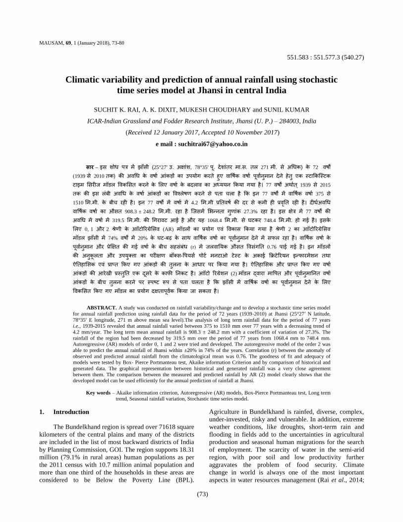
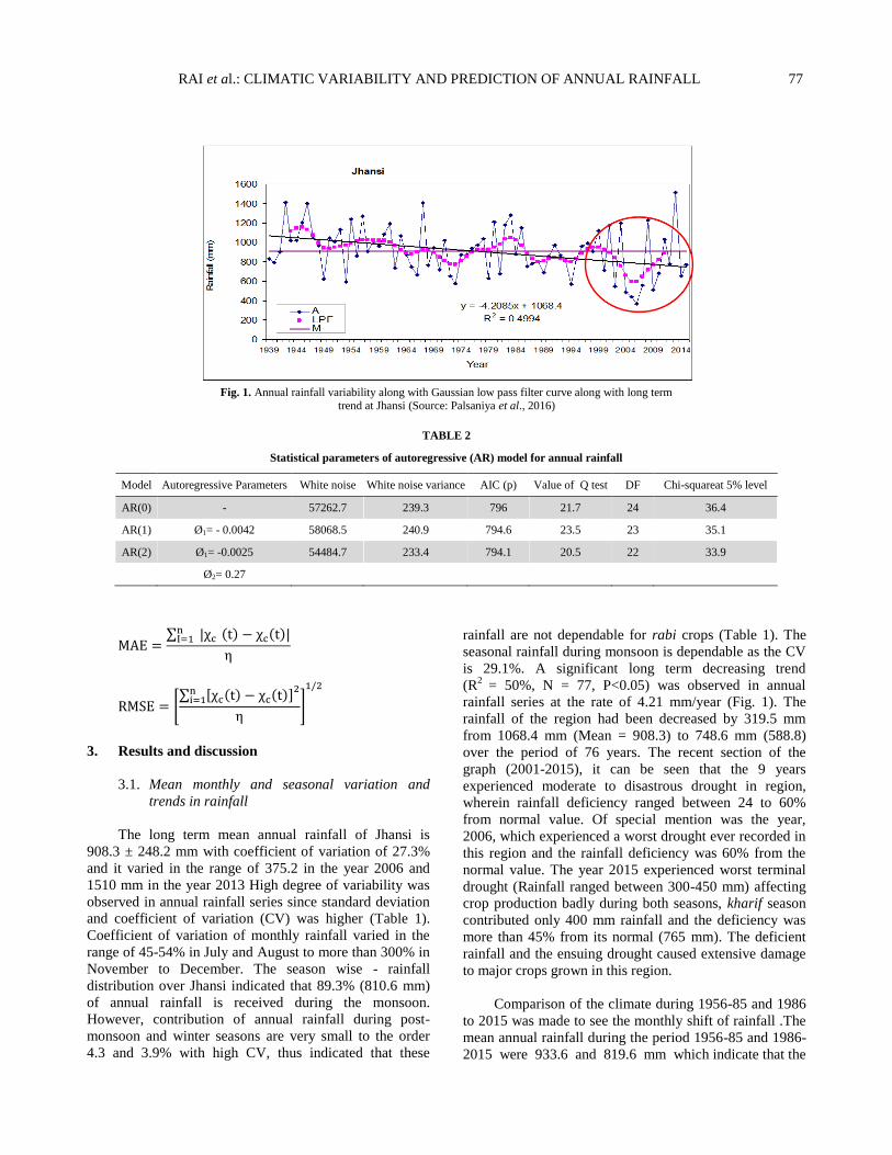
Fig. 1. Annual rainfall variability along with Gaussian low pass filter curve along with long term
trend at Jhansi (Source: Palsaniya et al., 2016)
TABLE 2
Statistical parameters of autoregressive (AR) model for annual rainfall
Model Autoregressive Parameters White noise White noise variance AIC (p) Value of Q test DF Chi-squareat 5% level
AR(0) - 57262.7 239.3 796 21.7 24 36.4
AR(1) Ø1= - 0.0042 58068.5 240.9 794.6 23.5 23 35.1
AR(2) Ø1= -0.0025 54484.7 233.4 794.1 20.5 22 33.9
Ø2= 0.27
3. Results and discussion
3.1. Mean monthly and seasonal variation and
trends in rainfall
The long term mean annual rainfall of Jhansi is
908.3 ± 248.2 mm with coefficient of variation of 27.3%
and it varied in the range of 375.2 in the year 2006 and
1510 mm in the year 2013 High degree of variability was
observed in annual rainfall series since standard deviation
and coefficient of variation (CV) was higher (Table 1).
Coefficient of variation of monthly rainfall varied in the
range of 45-54% in July and August to more than 300% in
November to December. The season wise - rainfall
distribution over Jhansi indicated that 89.3% (810.6 mm)
of annual rainfall is received during the monsoon.
However, contribution of annual rainfall during post-
monsoon and winter seasons are very small to the order
4.3 and 3.9% with high CV, thus indicated that these
rainfall are not dependable for rabi crops (Table 1). The
seasonal rainfall during monsoon is dependable as the CV
is 29.1%. A significant long term decreasing trend
(R2
= 50%, N = 77, P<0.05) was observed in annual
rainfall series at the rate of 4.21 mm/year (Fig. 1). The
rainfall of the region had been decreased by 319.5 mm
from 1068.4 mm (Mean = 908.3) to 748.6 mm (588.8)
over the period of 76 years. The recent section of the
graph (2001-2015), it can be seen that the 9 years
experienced moderate to disastrous drought in region,
wherein rainfall deficiency ranged between 24 to 60%
from normal value. Of special mention was the year,
2006, which experienced a worst drought ever recorded in
this region and the rainfall deficiency was 60% from the
normal value. The year 2015 experienced worst terminal
drought (Rainfall ranged between 300-450 mm) affecting
crop production badly during both seasons, kharif season
contributed only 400 mm rainfall and the deficiency was
more than 45% from its normal (765 mm). The deficient
rainfall and the ensuing drought caused extensive damage
to major crops grown in this region.
Comparison of the climate during 1956-85 and 1986
to 2015 was made to see the monthly shift of rainfall .The
mean annual rainfall during the period 1956-85 and 1986-
2015 were 933.6 and 819.6 mm which indicate that the
78 MAUSAM, 69, 1 (January 2018)
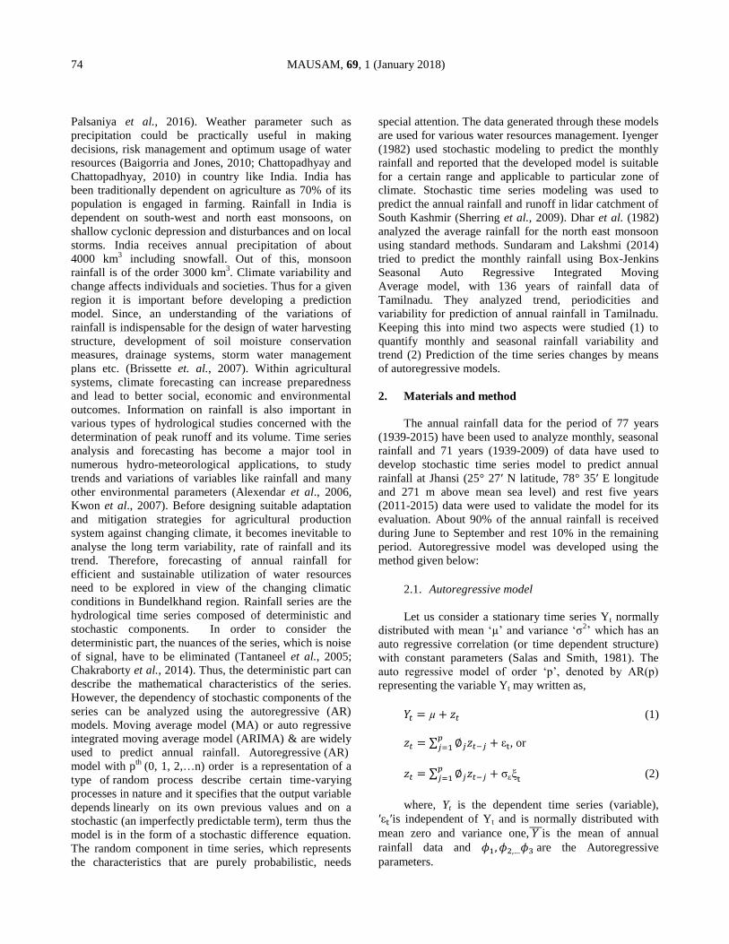
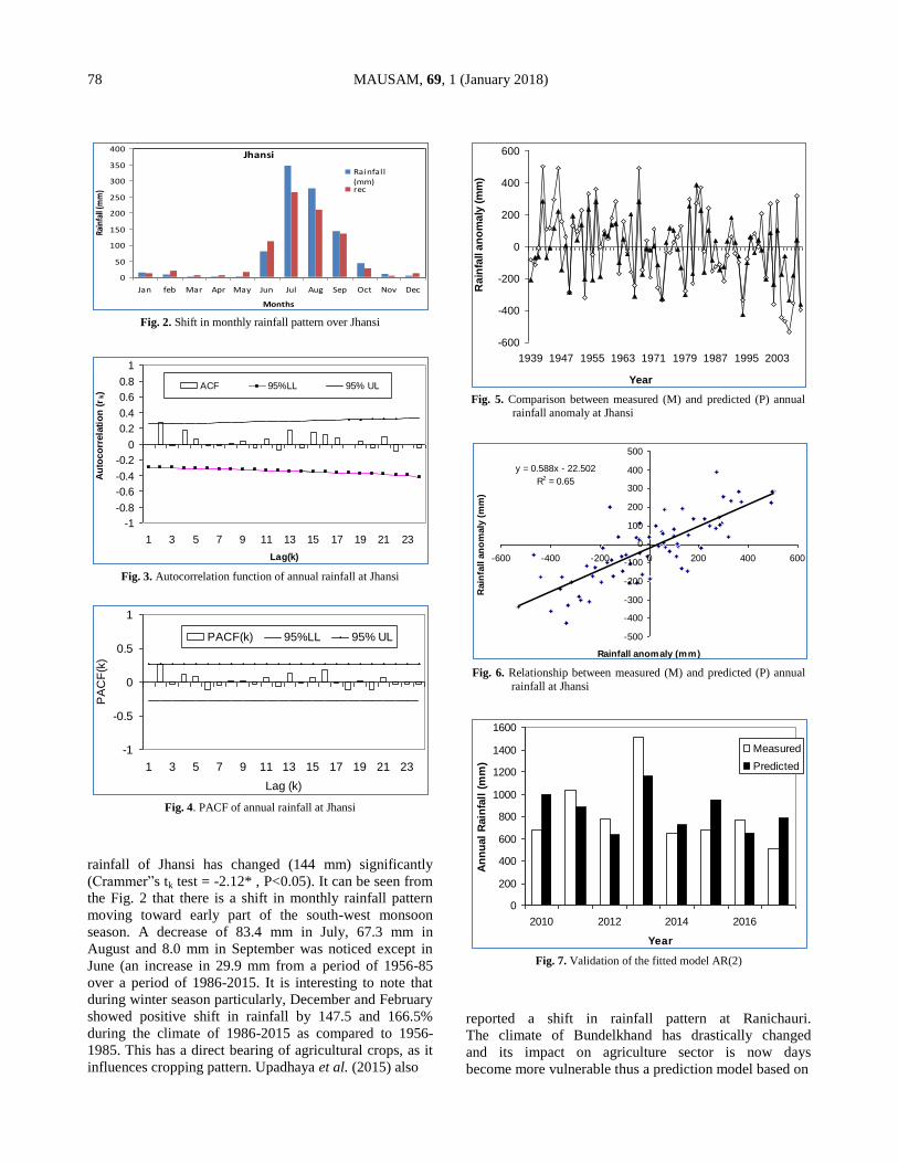
Fig. 2. Shift in monthly rainfall pattern over Jhansi
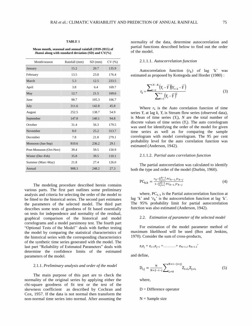
Fig. 3. Autocorrelation function of annual rainfall at Jhansi
Fig. 4. PACF of annual rainfall at Jhansi
rainfall of Jhansi has changed (144 mm) significantly
(Crammer”s tk test = -2.12* , P<0.05). It can be seen from
the Fig. 2 that there is a shift in monthly rainfall pattern
moving toward early part of the south-west monsoon
season. A decrease of 83.4 mm in July, 67.3 mm in
August and 8.0 mm in September was noticed except in
June (an increase in 29.9 mm from a period of 1956-85
over a period of 1986-2015. It is interesting to note that
during winter season particularly, December and February
showed positive shift in rainfall by 147.5 and 166.5%
during the climate of 1986-2015 as compared to 1956-
1985. This has a direct bearing of agricultural crops, as it
influences cropping pattern. Upadhaya et al. (2015) also
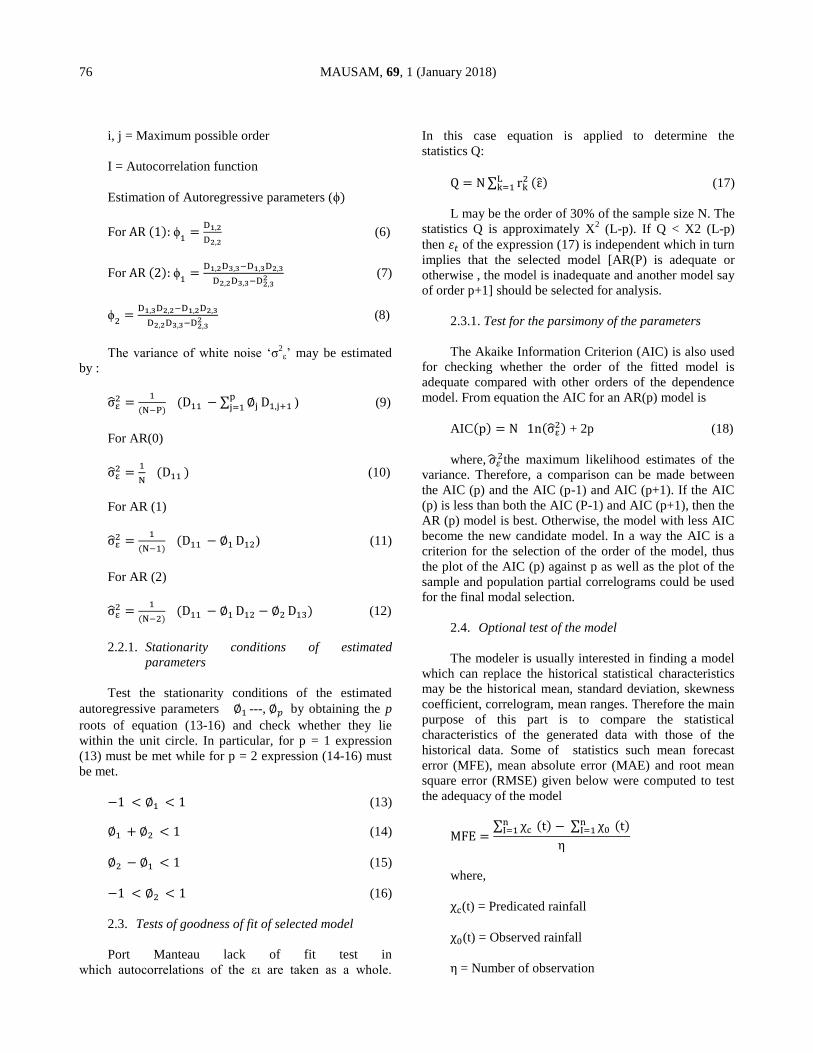
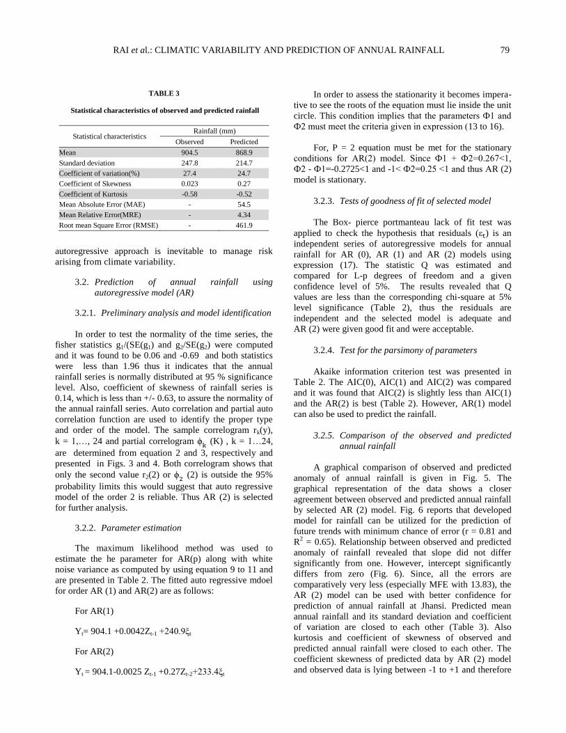
Fig. 5. Comparison between measured (M) and predicted (P) annual
rainfall anomaly at Jhansi
Fig. 6. Relationship between measured (M) and predicted (P) annual
rainfall at Jhansi
Fig. 7. Validation of the fitted model AR(2)
reported a shift in rainfall pattern at Ranichauri.
The climate of Bundelkhand has drastically changed
and its impact on agriculture sector is now days
become more vulnerable thus a prediction model based on
Jhansi
0
50
100
150
200
250
300
350
400
Jan feb Mar Apr May Jun Jul Aug Sep Oct Nov Dec
Months
Rain
fall
(mm
)
Rainfall(mm)rec
-1
-0.8
-0.6
-0.4
-0.2
0
0.2
0.4
0.6
0.8
1
1 3 5 7 9 11 13 15 17 19 21 23
Lag(k)
Au
toco
rrela
tio
n (
rk)
ACF 95%LL 95% UL
-1
-0.5
0
0.5
1
1 3 5 7 9 11 13 15 17 19 21 23
Lag (k)
PA
CF
(k)
PACF(k) 95%LL 95% UL
-600
-400
-200
0
200
400
600
1939 1947 1955 1963 1971 1979 1987 1995 2003
Year
Ra
infa
ll a
no
ma
ly (
mm
)y = 0.588x - 22.502
R2 = 0.65
-500
-400
-300
-200
-100
0
100
200
300
400
500
-600 -400 -200 0 200 400 600
Rainfall anomaly (mm)
Rain
fall a
no
maly
(m
m)
0
200
400
600
800
1000
1200
1400
1600
2010 2012 2014 2016
Year
An
nu
al
Rain
fall
(m
m)
Measured
Predicted
RAI et al.: CLIMATIC VARIABILITY AND PREDICTION OF ANNUAL RAINFALL 79
TABLE 3
Statistical characteristics of observed and predicted rainfall
Statistical characteristics Rainfall (mm)
Observed Predicted
Mean 904.5 868.9
Standard deviation 247.8 214.7
Coefficient of variation(%) 27.4 24.7
Coefficient of Skewness 0.023 0.27
Coefficient of Kurtosis -0.58 -0.52
Mean Absolute Error (MAE) - 54.5
Mean Relative Error(MRE) - 4.34
Root mean Square Error (RMSE) - 461.9
autoregressive approach is inevitable to manage risk
arising from climate variability.
3.2. Prediction of annual rainfall using
autoregressive model (AR)
3.2.1. Preliminary analysis and model identification
In order to test the normality of the time series, the
fisher statistics g1/(SE(g1) and g2/SE(g2) were computed
and it was found to be 0.06 and -0.69 and both statistics
were less than 1.96 thus it indicates that the annual
rainfall series is normally distributed at 95 % significance
level. Also, coefficient of skewness of rainfall series is
0.14, which is less than +/- 0.63, to assure the normality of
the annual rainfall series. Auto correlation and partial auto
correlation function are used to identify the proper type
and order of the model. The sample correlogram rk(y),
k = 1,…, 24 and partial correlogram (K) , k = 1…24,
are determined from equation 2 and 3, respectively and
presented in Figs. 3 and 4. Both correlogram shows that
only the second value r2(2) or (2) is outside the 95%
probability limits this would suggest that auto regressive
model of the order 2 is reliable. Thus AR (2) is selected
for further analysis.
3.2.2. Parameter estimation
The maximum likelihood method was used to
estimate the he parameter for AR(p) along with white
noise variance as computed by using equation 9 to 11 and
are presented in Table 2. The fitted auto regressive mdoel
for order AR (1) and AR(2) are as follows:
For AR(1)
Yt= 904.1 +0.0042Zt-1 +240.9 t
For AR(2)
Yt = 904.1-0.0025 Zt-1 +0.27Zt-2+233.4 t
In order to assess the stationarity it becomes impera-
tive to see the roots of the equation must lie inside the unit
circle. This condition implies that the parameters Ф1 and
Ф2 must meet the criteria given in expression (13 to 16).
For, P = 2 equation must be met for the stationary
conditions for AR(2) model. Since Ф1 + Ф2=0.267<1,
Ф2 - Ф1=-0.2725<1 and -1< Ф2=0.25 <1 and thus AR (2)
model is stationary.
3.2.3. Tests of goodness of fit of selected model
The Box- pierce portmanteau lack of fit test was
applied to check the hypothesis that residuals ( ) is an
independent series of autoregressive models for annual
rainfall for AR (0), AR (1) and AR (2) models using
expression (17). The statistic Q was estimated and
compared for L-p degrees of freedom and a given
confidence level of 5%. The results revealed that Q
values are less than the corresponding chi-square at 5%
level significance (Table 2), thus the residuals are
independent and the selected model is adequate and
AR (2) were given good fit and were acceptable.
3.2.4. Test for the parsimony of parameters
Akaike information criterion test was presented in
Table 2. The AIC(0), AIC(1) and AIC(2) was compared
and it was found that AIC(2) is slightly less than AIC(1)
and the AR(2) is best (Table 2). However, AR(1) model
can also be used to predict the rainfall.
3.2.5. Comparison of the observed and predicted
annual rainfall
A graphical comparison of observed and predicted
anomaly of annual rainfall is given in Fig. 5. The
graphical representation of the data shows a closer
agreement between observed and predicted annual rainfall
by selected AR (2) model. Fig. 6 reports that developed
model for rainfall can be utilized for the prediction of
future trends with minimum chance of error (r = 0.81 and
R2 = 0.65). Relationship between observed and predicted
anomaly of rainfall revealed that slope did not differ
significantly from one. However, intercept significantly
differs from zero (Fig. 6). Since, all the errors are
comparatively very less (especially MFE with 13.83), the
AR (2) model can be used with better confidence for
prediction of annual rainfall at Jhansi. Predicted mean
annual rainfall and its standard deviation and coefficient
of variation are closed to each other (Table 3). Also
kurtosis and coefficient of skewness of observed and
predicted annual rainfall were closed to each other. The
coefficient skewness of predicted data by AR (2) model
and observed data is lying between -1 to +1 and therefore

80 MAUSAM, 69, 1 (January 2018)
AR(2) model preserved the mean and coefficient of
variation better.
3.2.6. Validation and evaluation of the model
Model was validated for the year 2009-2017 using
random variables between -1.23 to 1.1. Developed model
is able to predict annual rainfall fairly well at Jhansi and
the deviation of predicted annual rainfall from observed
lies within the range of ±22% (Fig. 7). The greatest error
in predicting annual rainfall occurred during the 2013 and
2017 and predicted annual rainfall were under
and over estimated by 30 and 35% for the respective
years, respectively. Correlation (r) between the
anomaly of observed and predicted annual rainfall
from the climatological mean was 0.76. Also,
independent validation (n = 8) showed a relationship
(Y = 0.41x - 54.776; R2 = 0.5815) between observed and
predicted anomaly of rainfall revealed that slope did not
differ significantly from one. However, intercept
significantly differs from zero
4. Conclusions
Mean rainfall with their standard deviation (247.8)
and coefficient of variation (27.4%), indicates that inter-
annual variation of rainfall is high. The rainfall of the
region had been decreased by 319.5 mm over the period of
76 years from 1068.4 mm. Also a significant long term
decreasing trend was observed in annual rainfall series
with the rate of 4.2 mm/year. In the recent past 15 years
(2001-2015), 9 years experienced moderate to disastrous
drought in region, wherein rainfall deficiency ranged
between 24 to 60% from normal value. Developed model
[AR (2)] can be utilized for the prediction of annual
rainfall with minimum chance of error (r = 0.81 and
R2
= 0.65). On the basis of estimated errors and statistical
characteristics between observed and predicted values, it
is concluded that the proposed autoregressive AR(2)
model has an operational skill and add value to the
forecast for predicting the annual rainfall of Jhansi, which
can in turn be useful and add value for contingent crop
planning, for efficient and sustainable utilization of water
resources and soil water conservation measures.
Disclaimer : The contents and views expressed in this
research paper/article are the views of the authors and do
not necessarily reflect the views of the organizations they
belong to.
References
Alexander, L. V., Zhang, X., Peterson, T. C., Caesar, J., Gleason, B., Klein Tank, A. M. G., Haylock, M., Collins, D., Trewin, B. and
Rahimzadeh, F., 2006, “Global observed changes in daily
climate extremes of temperature and precipitation”, J. Geophys. Res., 111, 5, 130-145.
Anderson, R. L., 1942, “Distribution of the serial correlation
coefficients”, Annals of Math. Statistics, 13, 1, 716-723.
Baigorria, G. A. and Jones J. W., 2010, “GiST: A Stochastic Model for
Generating Spatially and Temporally Correlated Daily Rainfall
Data”, J. Climate, 23, 22, 5990-6008.
Box, G.E.P. and Jenkins G.M., 1970, “Time series analysis, forecasting
and control. First Ed. Holden-Day Inc., , San Francisco.
Brissette, F. P., Khalili, M. and Leconte, R., 2007, “Efficient stochastic
generation of multi-site synthetic precipitation data”, J. Hydrol.,
345,121-133.
Chakraborty, S., Denis, D. M. and Sherring, A., 2014, “Development of
Time Series Autoregressive Model for prediction of rainfall and
runoff in Kelo Watershed Chhattisgarh”, Int. J. Adv. Eng. Sci. Technol., 2, 2, 153-163.
Chattopadhyay, S. and Chattopadhyay, G., 2010, “Univariate modelling of summer-monsoon rainfall time series: Comparison between
ARIMA and ARNN”, Comptes Rendus Geosciences, 342, 2,
100-107.
Cochran, W. G. and Cox, G. M., 1957, “Experimental Designs”, New
York: John Wiley& Sons, Inc.
Dhar, O.N., Rakhecha, P.R. and Kulkarni, A.K., 1982,“Fluctuations in
northeast monsoon rainfall of Tamilnadu”,Int. J. Climatology, 2,
4, 339-345.
Durbin, J., 1960, “The fitting of time series model”, Rev. Int. Inst. Stat.,
28, p2333.
Iyenger, N. R., 1982, “Stochastic modeling of monthly rainfall”, J.
Hydrology, 57, 375-387.
Kottegoda, N. T. and Horder, M. A., 1980, “Daily flow model rainfall
occurrences using pulse and a transfer function”, J. Hydrology,
47, 215-234.
Kwon, H., Lall, U. and Khalil, A. F., 2007, “Stochastic simulation model
for nonstationary time series using an autoregressive wavelet
decomposition: Applications to rainfall and temperature”, Water Resour. Res., 43, 5, 112-124
Palsaniya, D. R., Rai, S. K., Sharma, P., Satyapriya and Ghosh, P. K., 2016, “Natural resource conservation through weather based
agro-advisory”, Current Science, 111, 2, 110-112.
Rai, S. K., Kumar, Sunil, Rai, A. K., Satyapriya and Palsaniya, D. R.,
2014, “Climate change, variability and rainfall probability for
crop planning in few districts of central india”, Atmospheric and
Climate Sciences, 4, 394-403.
Salas, J. D. and Smith, R. A., 1981, “Physical basis of stochastic model
of annual flows”, Water Resources Research, 17, 2, 428-430.
Sherring, A., Amin, H. A., Mishra A. K. and Alam, M., 2009,
“Stochastic time series modeling for prediction of rainfall and
runoff in lidder catchment of South Kashmir”, Journal of soil and water conservation, 8, 4, 11-15
Sundaram, S. M. and Lakshmi, M., 2014, “Rainfall prediction using seasonal auto regressive integrated moving average model”,
Computer science, 3, 4, 58-60.
Tantanee1, S., Patamatamakul, S., Oki, T., Sriboonlue, V. and Prempree,
T., 2005, “Downscaled Rainfall Prediction Model(DRPM) using
a Unit Disaggregation Curve (UDC)”, Hydrol. Earth Sys. Sci. Discuss., 2, 543-568.
Upadhyay, R. G., Ranjan, R. and Negi, P. S., 2015, “Climatic variability
and trend at Ranichauri (Uttarakhand)”, J. of Agrometerol., 17, 2, 241-243.
Related Documents