Climate spectrum estimation in the presence of timescale errors

Nonlin. Processes Geophys., 16, 43–56, 2009www.nonlin-processes-geophys.net/16/43/2009/© Author(s) 2009. This work is distributed underthe Creative Commons Attribution 3.0 License.

Nonlinear Processesin Geophysics

Climate spectrum estimation in the presence of timescale errors

M. Mudelsee1,2, D. Scholz3,4, R. Rothlisberger1, D. Fleitmann5,6, A. Mangini3, and E. W. Wolff1

1British Antarctic Survey, Cambridge, UK2Climate Risk Analysis, Hannover, Germany3Heidelberg Academy of Sciences, Heidelberg, Germany4Bristol Isotope Group, School of Geographical Sciences, University of Bristol, Bristol, UK5Institute of Geological Sciences, University of Bern, Bern, Switzerland6Oeschger Centre for Climate Change Research, University of Bern, Bern, Switzerland

Received: 3 December 2008 – Revised: 15 January 2009 – Accepted: 15 January 2009 – Published: 5 February 2009

Abstract. We introduce an algorithm (called REDFITmc2)for spectrum estimation in the presence of timescale errors.It is based on the Lomb-Scargle periodogram for unevenlyspaced time series, in combination with the Welch’s Over-lapped Segment Averaging procedure, bootstrap bias correc-tion and persistence estimation. The timescale errors aremodelled parametrically and included in the simulations fordetermining (1) the upper levels of the spectrum of the red-noise AR(1) alternative and (2) the uncertainty of the fre-quency of a spectral peak. Application of REDFITmc2 toice core and stalagmite records of palaeoclimate allowed amore realistic evaluation of spectral peaks than when ignor-ing this source of uncertainty. The results support qualita-tively the intuition that stronger effects on the spectrum es-timate (decreased detectability and increased frequency un-certainty) occur for higher frequencies. The surplus informa-tion brought by algorithm REDFITmc2 is that those effectsare quantified. Regarding timescale construction, not onlythe fixpoints, dating errors and the functional form of theage-depth model play a role. Also the joint distribution ofall time points (serial correlation, stratigraphic order) deter-mines spectrum estimation.

1 Introduction

A classical decomposition of a climate process is into a trendand a noise component. Spectral analysis investigates thenoise component. A Fourier transform into the frequency do-main makes it possible to separate short-term from long-term

Correspondence to: M. Mudelsee([email protected])

variations and to distinguish between cyclical forcing mech-anisms of the climate system and broad-band resonances.Spectral analysis allows to learn about the climate physics.

The major task is to estimate the spectral density function.This poses more difficulties than, for example, linear regres-sion (which may be used for trend estimation) because herewe estimate a function and not just two regression parameters(intercept and slope). Spectral smoothing becomes thereforenecessary, and this brings a tradeoff between estimation vari-ance and frequency resolution.

In the case of evenly spaced records, the multitapersmoothing method achieves the optimal tradeoff (Thomson,1982). The focus of this paper, however, is spectrum estima-tion for unevenly spaced records. Such a situation is ubiqui-tous in palaeoclimatology. In this case the method of choiceis combining the Lomb-Scargle periodogram with Welch’sOverlapped Segment Averaging (Welch, 1967; Lomb, 1976;Scargle, 1982; Schulz and Mudelsee, 2002), which yields anestimation in the time domain and avoids distortions causedby interpolation.

Bootstrap resampling enhances Lomb-Scargle methods byproviding a bias correction. It supplies also a detection testfor a spectral peak against realistic noise alternatives in formof an AR(1) model (which belongs to the wider class of“red noise” processes). We introduce a bootstrap algorithm,called REDFITmc2, which takes into account the effects oftimescale uncertainties on detectability and frequency reso-lution. REDFITmc2 is a further development of the REDFITalgorithm (Schulz and Mudelsee, 2002), which assumes neg-ligible timescale errors.

Palaeoclimate time series from two different archivesserve to illustrate our concept. The first example is anice core from Antarctica, which covers the past 800 ka and

Published by Copernicus Publications on behalf of the European Geosciences Union and the American Geophysical Union.

http://creativecommons.org/licenses/by/3.0/

44 M. Mudelsee et al.: Climate spectrum estimation in the presence of timescale errors

constitutes the, at present, longest glacial archive. The sec-ond is a stalagmite from southern Arabia (Oman), which cov-ers a large portion of the Holocene (last∼11 ka).

2 Method

Let X(T ) be a stationary climate process in continuoustime,T . The one-sided non-normalized power spectral den-sity function, h(f ), wheref ≥0 is frequency, can be de-fined (Priestley, 1981, Chapter 4 therein) via a truncationof X(T ) and a Fourier transformation.h(f ) integrates toVAR[X(T )]=S2, the variance ofX(T ). The power is a mea-sure of the variability (“energy”) within a frequency interval[f ; f +df ].

The spectral theory in the case of a processX(i) in discretetime, T (i), is similar (Priestley, 1981, Sect. 4.8.3 therein),except that the frequency range has an upper bound and thediscrete Fourier transform is invoked to calculateh(f ).

The objective of spectrum analysis is to estimateh(f ) us-ing a time series sample,{t (i), x(i)}ni=1. The time points,t (i), may be unevenly spaced.n is the sample size. The spac-ing is given byd(i)=t (i)−t (i−1), its average is denoted asd. A spectral peak at a frequency,f ′, corresponds to a periodwe denote asTperiod=1/f ′.

2.1 Lomb-Scargle periodogram

An early spectrum estimator is Schuster’s (1898) peri-odogram,I (fj ), which is evaluated at discrete frequencypoints,fj . Scargle (1982) suggested for the case of unevenspacing a new version,

ILS(fj ) = d ·

{[ ∑ni=1 X(i) cos

(2πfj [T (i) − τLomb]

) ]2

∑ni=1

[cos


) ]2

+

[ ∑ni=1 X(i) sin


) ]2

∑ni=1

[sin


) ]2

},

(1)

where Lomb’s (1976) time shift,τLomb, is given via

tan(4π fj τLomb

)=

∑ni=1 sin

(4πfjT (i)

)∑n

i=1 cos(4πfjT (i)

) . (2)

For even spacing (d(i)=d), evenn and frequency pointsfj=1/(nd), . . . , 1/(2d), it follows that τLomb=0 andILS(fj )=I (fj ). To calculateILS(fj ) on the sample level,that is, using the time series sample, plug inx(i) for X(i)

andt (i) for T (i).Scargle’s objective behind introducing the Lomb-Scargle

periodogram was that the probability distribution ofILS(fj )

should be equal to the distribution ofI (fj ). Scargle (1982,1989) showed that this is so (chi-squared distribution) whenX(i) is a Gaussian white noise process (with mean zero andvarianceS2), X(i)=EN(0, S2)(i).

2.2 Welch’s overlapped segment averaging

The periodogram is a suitable estimator of line spectra,where harmonic signal components appear as sharp peaks.To enhance the unfavourable inconsistency of the peri-odogram (i.e., the variance does not decrease withn in-creasing) when (mis-)applied to estimate continuous spec-tra,Welch (1967) advanced the idea of Bartlett (1950) to di-vide a time series{t (i), x(i)}ni=1 into different time segments,calculate the periodograms segment-wise and average themto obtain a reduced estimation variance. Welch (1967) al-lowed the segments to overlap (for example, by 50%), andthe method is called “Welch’s Overlapped Segment Averag-ing” or WOSA procedure. Overlapping has the positive ef-fect that the number of segments, and therefore the numberof averaged periodograms, is increased.

The negative effect of using WOSA (number of segments,n50>1) is that the frequency points, where the periodogramsare calculated, are spaced wider than forn50=1. More pre-cisely,1fj=(n50+1)/(2nd)>1/(nd) for n50>1. This is thesmoothing problem in the spectral domain, the tradeoff be-tween spectral estimation variance and frequency resolution.

Instead of calculating the Lomb-Scargle periodogram atfrequenciesfj=1/(nd), 2/(nd), . . ., there is no hindranceto using a finer frequency grid. The oversampling factor(OFAC) (Schulz and Stattegger, 1997) gives the increase infrequency resolution. Oversampling is mainly for “cosmetic”reasons, to have a smoother curve and to be able to determineprecisely the frequency of a spectral peak. Like interpolationin the time domain, oversampling does not generate new in-formation and cannot solve the smoothing problem.

Welch (1967) showed also that tapering (weighting) thedata pointsX(i) within segments improves the spectrum es-timate in terms of bias, variance and suppression of spuriouspeaks (sidelobes). The overview by Harris (1978) lists theproperties of many taper functions, including the Welch ta-per (negative parabola) that is used in the present paper.

2.3 Bandwidth

The degrees of freedom of the chi-squared distribution of aLomb-Scargle spectrum estimate based on WOSA with 50%overlap and Gaussian distributedX(i) are

ν = 2n50

/(1 + 2c2 − 2c2/n50

), (3)

wherec≤0.5 is a constant representing the taper. A uniformtaper hasc=0.5, a Welch taperc=0.344; further values arelisted by Harris (1978).

The discrete Fourier transform of a pure harmonic process(X(i) composed of sinus and cosinus terms with frequencyf ′) has a peak atf ′. The decay on the flanks of the peak to avalue of 10−6/10≈0.251 times the maximum value defines awidth in frequency, the 6-dB spectral bandwidth,Bs. This isa useful quantity for assessing the frequency resolution, how

Nonlin. Processes Geophys., 16, 43–56, 2009 www.nonlin-processes-geophys.net/16/43/2009/

M. Mudelsee et al.: Climate spectrum estimation in the presence of timescale errors 45

good closely neighboured spectral peaks can theoretically beseparated (Harris, 1978; Nuttall, 1981). The 6-dB bandwidthdepends onn, n50 and the type of taper.

2.4 Bootstrap bias correction

If X(i) is a red-noise process on an unevenly spacedtimescale, perhaps with superimposed peaks in the frequencydomain, the distribution ofILS(fj ) cannot be calculated an-alytically. Here, simulation methods can be used to infer thedistributional properties of the Lomb-Scargle periodogram.Of particular interest is its bias (systematic error).

Monte Carlo experiments (Schulz and Mudelsee, 2002)reveal the bias of the Lomb-Scargle periodogram for anAR(1) process and uneven spacing. The “absolute bias”, ofILS(fj ) as an estimator of non-normalized power,h(f ), canbe substantial. The bias disappears (i.e., becomes smallerthan the “simulation noise”) for an AR(1) process and evenspacing. Also in peak detection, where normalized power,g(f )=h(f )/S2, is analysed, the Lomb-Scargle periodogramexhibits bias. That means, even if the normalization isknown, the bias of the Lomb-Scargle periodogram is signifi-cant, and it is frequency-dependent.

Spectrum estimation for unevenly spaced time series canbe enhanced by combining the WOSA procedure with theLomb-Scargle periodogram (Schulz and Stattegger, 1997). Abias correction for such estimates was devised by Schulz andMudelsee (2002). It uses a bootstrap simulation approachbased on artificially generated AR(1) time series (“surrogatedata”), for which the theoretical spectrum is known (Priest-ley, 1981). The frequency-dependent bias correction factoris calculated as the ratio of the theoretical AR(1) spectrumand the average Lomb-Scargle spectrum. The bias-correctedspectrum estimate ish′(fj ).

2.5 Peak detection by red-noise test

A hypothesis test helps to assess whether peaks (or lows) inthe estimate ofh(f ), denoted ash(f ), are significant or not.Such information is for the climate time series analyst of ma-jor relevance because it helps to filter out the variability, toconstruct and test conceptual climate models – the absolutevalue ofh(f ) is less important. The typical test performedin climate spectral analysis is ofH0: “X(i) is an AR(1) pro-cess, with continuous, red spectrum”, the red-noise hypoth-esis, againstH1: “X(i) has a mixed spectrum, with peak atfj=f ′

j on a red-noise background.”Schulz and Mudelsee (2002) devised the following red-

noise test. The null distribution ofh(f ) is obtained by fittingan AR(1) process to{t (i), x(i)}ni=1, that is, estimating thepersistence time,τ , followed by bootstrap resampling.

The process is given by

X(1) = EN(0, 1)(1), (4)

X(i) = exp{− [T (i) − T (i − 1)] /τ } · X(i − 1)

+EN(0, 1−exp{−2[T (i)−T (i−1)]/τ })(i),

i = 2, . . . , n.

The parameterτ defines the “equivalent autocorrelation co-efficient”,a′, viaa′= exp(−d/τ ) for the case of uneven timespacing. For even spacing,a′ equalsa, the ordinary AR(1)autocorrelation parameter.

Even the estimation ofa (even spacing) is not trivial be-cause of estimation bias. For an AR(1) process with un-known mean, which is the usual case in climatology, the es-timator ofa is

a =

∑ni=2

[X(i) − X

]·[X(i − 1) − X

]∑n

i=2

[X(i) − X

]2, (5)

whereX=∑n

i=1 X(i)/n is the sample mean. The approxi-mate expectation ofa is (Kendall, 1954)

E (a) ≃ a − (1 + 3a) / (n − 1) . (6)

That means,a underestimatesa. Eq. (6) can be used to cor-rect for the negative bias. However, Eq. (6) is valid only fora

not too large (Kendall, 1954). A bias formula applicable alsoto large values (above, say, 0.9) ofa has yet only been de-rived for the simpler case of known mean (Mudelsee, 2001).

Regarding the estimation ofτ (uneven spacing), MonteCarlo simulations (Mudelsee, M.: Climate Time Series Anal-ysis: Classical Statistical and Bootstrap Methods, Springer,Heidelberg, manuscript in preparation) show that the least-squares estimator ofa′= exp(−d/τ ) has a bias similar in sizeto the bias ofa. Mudelsee (2002) presented a least-squaresestimation procedure ofτ with bias correction and bootstrappercentile confidence intervals. Our conclusions for the prac-tice of persistence time estimation (Mudelsee, 2002) are asfollows.

– Large data sizes and not too large values ofτ make biascorrection via the application of Eq. (6) toa′ accurate,

– It may in practice be difficult to show statistically sig-nificant changes ofτ over short time intervals and there-fore be often advisable to assume a constant persistencetime. We use this approach because own analyses (notshown) with the ice core records (Sect. 3.1) dividedinto sub-intervals, do not indicate significant changesin τ . An option that may apply to a situation wherethe physics of the sampled climate system indicates achange in the persistence properties and where also verylong time series are available, may be to consider amodel that divides the time interval into sub-intervalswith specific persistence times. Divine et al. (2008)

www.nonlin-processes-geophys.net/16/43/2009/ Nonlin. Processes Geophys., 16, 43–56, 2009


have recently suggested a similar model (for even spac-ing), accompanied by a maximum likelihood estimationprocedure.

Resampling is done (Schulz and Mudelsee, 2002) via thesurrogate data approach. Instead of (or in addition to) per-forming bootstrap resampling for deriving the null distribu-tion, one may calculate upper (lower) bounds via the chi-squared distribution (Schulz and Mudelsee, 2002). Of prac-tical relevance in climatology, although conventionally ig-nored, should be not only peaks but also lows inh(f ), fre-quency intervals where less power than under an AR(1) hy-pothesis resides. Also the information about the absence ofpower in a frequency range is helpful; it may, for example,support an argumentation that a certain mechanism doesnotplay a role for generating an observed climate phenomenon.

So far we have assumed as a realistic noise alternative anAR(1) process with positive persistence timeτ (uneven spac-ing) or positive autocorrelation parametera (even spacing).This corresponds to a “red” spectrum, with more power forlower than for higher frequencies. Fisher et al. (1985) andAndersen et al. (2006) describe the interesting observationthat postdepositional effects (wind erosion) at a site of an icecore may lead to “blue” noise, with more power for higherfrequencies. This would make, however, the testing of thespectrum alternative problematic. Uneven spacing does notallow to embed a discrete-time, blue-noise process within acontinuous-time, blue-noise process (Robinson, 1977; Chanand Tong, 1987) This means that for uneven spacing it is notpossible to infer uniquely the parameters of the underlyingcontinuous-time process. Embedding is an important prop-erty because it allows a foundation on physics, which worksin continuous time (differential equations). A practical ap-proach to ice core spectrum estimation may be to use extracaution in the interpretation of high-frequency peaks.

2.6 Multiple tests

Assume for convenience even data size, even spacing and nooversampling. If the red-noise hypothesis test for the exis-tence of a spectral peak is to be carried out for one single,pre-defined frequencyf ′

j ∈{fj

}n/2j=1, then selection of the

100(1−α)th percentage point of the red-noise distributionleads to a one-sided hypothesis test with a P-value equal toα.If, what is usually the case, the test is multiple, that means,it is to be carried out for many (if not all) frequencies fromthe set

{fj

}n/2j=1, then a higher frequency-point-wise confi-

dence level,(1−α′) with α′<α, has to be employed to yieldan overall P-value ofα. If a test is performed multiple times,it becomes more likely to find a significant single result.

One may define a “maximum effective number oftest frequencies”,M, via the overall prescribed P-value:(1−α′)M=1−α. For small α and largeM this leads toα′≈α/M. The effective number of frequencies refers to ahypothetical situation whereM frequenciesf ′

j are tested and

the spectrum estimatesh(f ′j ), a set of sizeM, are mutually

independent. For the simple case of even data size, evenspacing, Gaussian distributional shape and periodogram es-timation, independence is fulfilled and the maximum num-ber is M=n/2. If n is odd (other setting unchanged),M=(n−1)/2. Also if the Gaussian assumption is violatednot too strongly, the effects onM should be negligible.

Stronger influence onM can have uneven spacing withLomb-Scargle periodogram estimation (no WOSA). Becausethe periodogram estimates are then no longer independent,M is reduced. Horne and Baliunas (1986) and VanDongenet al. (1997) studied the effects by means of Monte Carlosimulations. If the{t (i)}ni=1 are more or less uniformly dis-tributed, the approximationM≈n/2 is still acceptable. Thisformula may also be applied to series where the timescaleis even with the exception of a few missing observations.However, if the time points are highly clustered in time, oneshould not use the number of points,n, but rather the numberof clusters, to determineM (VanDongen et al., 1997). Theeffects of segmenting (WOSA) onM with Lomb-Scargle orordinary periodogram estimation (no tapering) can be takeninto account by using instead ofn the number of points persegment:M=NINT[n/(n50+1)], see Schulz and Mudelsee(2002). NINT is the nearest integer function. The effectsof tapering could in principle be studied by means of MonteCarlo simulations. Restricting the frequency range where tostudy peaks is an other way to reduceM.

What practical conclusions can be drawn for peak detec-tion in climate spectra? A typical situation is an unevenlyspaced timescale without strong clustering, and where theresearcher is interested also in the longer periods of varia-tions recorded by the time series. Here, Lomb-Scargle pe-riodogram estimation with tapering, WOSA andn50 not toohigh (less than, say, 10) is an option. To have more relia-bility in the low-frequency spectrum portion, one decides tofollow a rule of thumb (Bendat and Piersol, 1986) and re-quires at least two cycles per segment, that is, one sets theminimum test frequencyfj equal to[(2n50)/(nd)]. This alsoreducesM. Regarding the high-frequency spectrum portion,theoretically the uneven spacing allows inferences also forfrequencies above 1/(2d), see Scargle (1982). On the otherhand, an archive may a priori be known not to preserve ahigh-frequency signal, for example a marine sediment coreaffected by bioturbation. Then it would make sense to ignorea part of the high frequencies, leading to a further reductionof M.

2.7 Timescale errors

In palaeoclimatology the timescale is usually expected tohave uncertainties. The time assigned to a sample,T (i), de-termined by dating and constructing an age-depth curve, isexpected to deviate from the true time value,Ttrue(i). In suchcases we write the measured times as



T (i) = Ttrue(i) + Tnoise(i), (7)

i=1, . . . , n, whereTnoise(i) is the error owing to age uncer-tainties. Equivalently, the spacing,d(i), has an error compo-nent.

To recapitulate,T (i) is a sequence of random variablesrepresenting the observed time of a sequence of samples,that is,T (i) is a discrete-time stochastic process (“processlevel”). The sequencet (i) are the actually observed timevalues (“sample level”), a realization of theT (i). The func-tion Ttrue(i) is the true time – uniquely defined, but unknownnumbers. Because of dating errors we cannot expect thatT (i) equalsTtrue(i). Hence, there is a noise component,Tnoise(i). The noise process is not required to have zeromean. This allows for measurement bias, that is, system-atic over- or underestimations. Eq. (7) is a rather general de-scription of uncertain timescales; it may be used for variouscombinations of climate archives and dating techniques.

Timescale errors lead to a distortion of the estimated spec-trum. Two effects are expected:

1. reductions of significance (detectability) of peaks com-pared to a situation with exact timescale and

2. increases of frequency uncertainty for a detected spec-tral peak.

Moore and Thomson (1991) and Thomson and Robinson(1996) studied the influence of a “jittered” spacing on theprocess level. The simple case of independent Gaussian jit-ter,

d(i) = d + EN(0, δ2d )(i), (8)

is analytically tractable.δd is the standard deviation of thespacing error distribution. Its effect on the true continuous-time spectrum,h(f ), amounts (Moore and Thomson, 1991;Wunsch, 2000) to a multiplication by a frequency-dependentfactor:

hdistort(f ) = exp(−4π2 δ2

d f 2)

· h(f ) + c0, (9)

where the constantc0 serves to give the distorted spectrum,hdistort(f ), the nominal area ofS2. This means, timescaleerrors in the form of independent jitter add white noise (c0).As a result, spectral peaks have a reduced detectability.

Several assumptions went into the derivation of Eq. (9) byMoore and Thomson (1991), this limits its applicability tothe practice of climate spectrum estimation.

– No aliasing (h(f )=0 for f >fNy=1/(2d)). This may inpractice be violated to some degree, and lead to power“folded” back into the interval[0; fNy] and, possibly,to spurious spectral peaks. In addition, for unevenlyspaced time series the Nyquist frequency is not well de-fined.

– Independent jitter. This is not realistic for many records(e.g., from ice or sediment cores). Moore and Thom-son (1991) study AR(1) dependence in the jitter equa-tion (Eq. 8), finding potential for larger effects on thespectrum if the dependence is strong. Still it is ques-tionable how relevant the AR(1) jitter model is. Ice coredata could exhibit heteroscedastic jitter owing to com-paction. Timescales derived from layer counting mightbe better described by means of a random walk (i.e., anonstationary AR(1) process with parametera=1) thanby a jitter model. The argument is as follows. If a layeris miscounted (e.g., missed), then this error propagateswithout “damping” to the next layer to be counted. It israther difficult to obtain analytical results in such cases.

– Gaussian jitter distribution. This assumption is notfulfilled without imposing a constraint to guarantee amonotonic age-depth curve. (Moore and Thomson,1991 had the purpose to study other data, in the spatialdomain, where no such constraint is required.)

– Process level. The mentioned paper does not study thespectrum estimators on the sample level, in particular,Lomb-Scargle estimation.

Based on the limited relevance of available analytical re-sults on the effects of realistic types of timescale errorson spectrum estimates (Lomb-Scargle), we suggest a novelnumerical algorithm. It is based on simulations of thetimescale. One mode of it quantifies the reduced detectabil-ity, the other the increased frequency uncertainty.

2.7.1 Algorithm REDFITmc2, mode “a”: peak detection

Algorithm REDFITmc2 adapts the REDFIT algorithm(Schulz and Mudelsee, 2002) to take into account timescaleerrors. Mode “a” of the algorithm performs peak detection.

1. Time series,{t (i), x(i)}ni=1.

2. Bias-corrected Lomb-Scargle spectrum estimate(Schulz and Mudelsee, 2002),h′(fj ).

3. Estimated, bias-corrected persistence time (Mudelsee,2002),τ ′.

4. Determine area,Ah′ , under spectrum within[0; 1/(2d)].

5. Generate AR(1) data,{t (i), x∗

AR(1)(i)}n

i=1after Eq. (4).

6. Use timescale model (an implementation of Eq. 7) tosimulate times,{t∗(i)}ni=1.

7. Bias-corrected Lomb-Scargle spectrum estimate,

h′∗b(fj ), calculated from{t∗(i), x∗

AR(1)(i)}n

i=1.

Spectrum estimate subsequently scaled to areaAh′ .b counts how often Steps 5 to 7 are called.



0 100000 200000 300000 400000 500000 600000 700000 800000

Age [a]

-460

-440

-420

-400

-380

-360

δD [‰

]

3

2

1

0

log(

nssC

a flu

x)[lo

g(µ

g m

–2 a

–1)]

4.0

3.6

3.2

2.8

2.4

2.0

log(

ssN

a flu

x)[lo

g(µ

g m

–2 a

–1)]

0 100000 200000 300000 400000 500000 600000 700000 800000

1 2 3 4 5 6 7 8 9 10 11 12 13 14 15 16 17 18 19 20

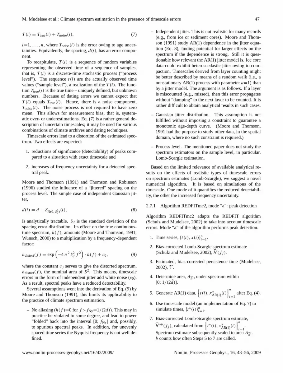
Fig. 1. Ice core EDC, data; δD, 55-cm resolutiondata (n=5785, d=139 a); log(nssCa flux), 100-a means(n=7880, d=102 a) and log(ssNa flux), 100-a means(n=7891, d=102 a). A small number of the 100-a intervalshave no data. Timescale is EDC3 (Parrenin et al., 2007). Verticalgrey lines and numbers indicate marine isotope stages (Lisiecki andRaymo, 2005).

8. Go to Step 5 untilb=B replications exist.

9. Test at eachfj whetherh′(fj ) exceeds a pre-defined

upper percentile of{h′∗b(fj )

}B

b=1.

The selection ofB depends on the size of the percentile;higher percentiles require higher values ofB.

The sets of frequenciesfj at Steps 2 and 7 are identical.Taking into account that the test is usually per-

formed not only at one single frequency but atfj=0, 1/(nd), . . . , 1/(2d) requires to adjust the signif-icance level for a single test. See Sect. 2.6.

2.7.2 Algorithm REDFITmc2, mode “b”: frequency uncer-tainty

Mode “b” of the algorithm quantifies the effect of timescaleerrors on the uncertainty of the frequency of a spectral peak.

1. Time series,{t (i), x(i)}ni=1.

2. Bias-corrected Lomb-Scargle spectrum estimate(Schulz and Mudelsee, 2002),h′(fj ).

3. Estimated, bias-corrected persistence time (Mudelsee,2002),τ ′.

4. Determine area,Ah′ , under spectrum within[0; 1/(2d)].

5. Spectral peak at frequencyf ′j , area under peak,

∫ f ′j +0.5Bs

f ′j −0.5Bs

h′(f )df =γ ·Ah′ .

6. Generate AR(1) data,{t (i), x∗

AR(1)(i)}n

i=1after Eq. (4).

7. Generate sinusoidal data,{t (i), x∗

sin(i)}n

i=1, with

x∗sin(i)= (2γ )1/2 sin

(2πf ′

j t (i)).

8. Mix series:x∗(i)= (1−γ )1/2 x∗AR(1)(i)+x∗

sin(i). Note

thatVAR[X∗(i)

]=(1−γ )+VAR

[X∗

sin(i)]≈1.

9. Use timescale model to resample times,{t∗(i)}ni=1.

10. Bias-corrected Lomb-Scargle spectrum estimate,h′∗b(fj ), calculated from{t∗(i), x∗(i)}ni=1, scaled toareaAh′ under peak atf ′∗

j . b, counter.

11. Go to Step 6 untilb=B (usuallyB=2000 is sufficient(Efron and Tibshirani, 1993)) versions off ′∗

j exist.

12. Calculate standard error, sef ′j, by taking the standard

deviation of{f ′∗b

j

}B

b=1.

3 Examples

We illustrate spectrum estimation using two types of palaeo-climate archives: ice cores and speleothems. We describeshortly the records (proxy variables) and their timescales.The results of the application of the REDFITmc2 algorithmare discussed with a focus on statistical aspects. Climaticinterpretations shall be presented elsewhere.

3.1 Ice core: EPICA Dome C (Antarctica)

The European Project for Ice Coring in Antarctica (EPICA)core from the Dome C site (75◦ S, 123◦ E) has a length of∼3260 m and covers the past∼800 000 a (EPICA Commu-nity Members, 2006; Wolff et al., 2006; Jouzel et al., 2007).We refer to this as the EDC core.

3.1.1 Data

The deuterium isotope (δD) time series (Jouzel et al., 2007)records variations in air temperature at the inversion heightover the EDC site. This proxy may indicate, at a reduced ac-curacy, also the temperature changes over the entire southernhemisphere. The non-sea-salt calcium (nssCa) flux record(Wolff et al., 2006; Rothlisberger et al., 2008) documentsvariations in the climate variable dust (transported fromSouth America to Antarctica). The sea-salt sodium (ssNa)flux (Wolff et al., 2006; Rothlisberger et al., 2008) series is aproxy for changes in the extent of sea ice around Antartica.The nssCa flux and ssNa flux records have rather strongly



skewed data distributions. We employ the logarithmic trans-formation (Rothlisberger et al., 2008) to bring the distribu-tions closer to a symmetric/normal shape.

All three climate variables display long-term variationsduring the late Pleistocene (Fig. 1) and belong potentially tothe set of variables governing the ice-age climate. Spectrumestimates may shed further light to the current understand-ing (Raymo and Huybers, 2008; Rothlisberger et al., 2008)of glacial–interglacial transitions. We follow Jouzel et al.(2007) and divide the interval into an earlier (400–800 ka)and a later (0–400 ka) interval.

3.1.2 Spectra, without timescale errors

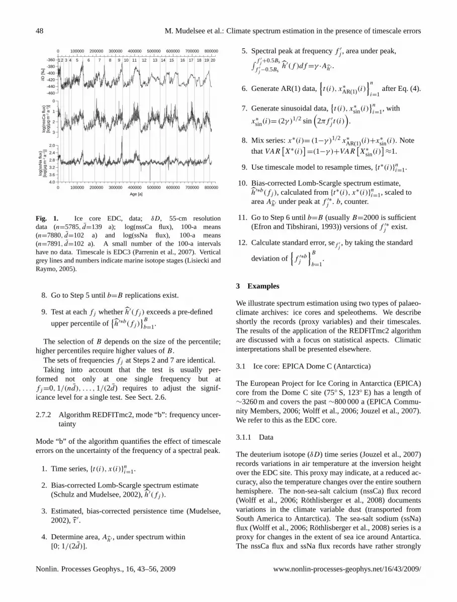
First, we present the raw periodograms (Fig. 2), then the cli-mate spectra calculated with timescale errors ignored (Fig. 3)and compare finally (Sect. 3.1.4) some of these results withthose resulting from taking timescale errors into account.

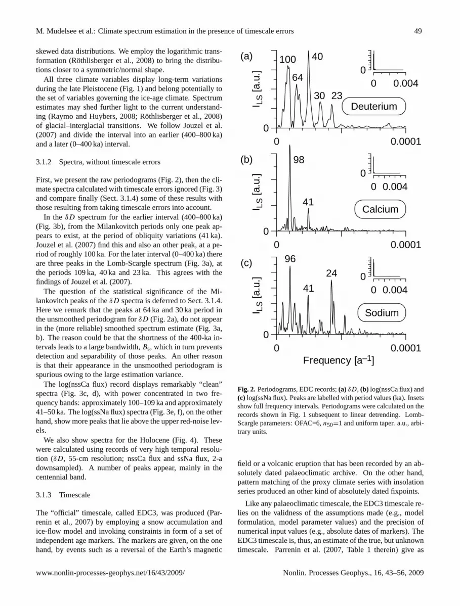
In the δD spectrum for the earlier interval (400–800 ka)(Fig. 3b), from the Milankovitch periods only one peak ap-pears to exist, at the period of obliquity variations (41 ka).Jouzel et al. (2007) find this and also an other peak, at a pe-riod of roughly 100 ka. For the later interval (0–400 ka) thereare three peaks in the Lomb-Scargle spectrum (Fig. 3a), atthe periods 109 ka, 40 ka and 23 ka. This agrees with thefindings of Jouzel et al. (2007).

The question of the statistical significance of the Mi-lankovitch peaks of theδD spectra is deferred to Sect. 3.1.4.Here we remark that the peaks at 64 ka and 30 ka period inthe unsmoothed periodogram forδD (Fig. 2a), do not appearin the (more reliable) smoothed spectrum estimate (Fig. 3a,b). The reason could be that the shortness of the 400-ka in-tervals leads to a large bandwidth,Bs, which in turn preventsdetection and separability of those peaks. An other reasonis that their appearance in the unsmoothed periodogram isspurious owing to the large estimation variance.

The log(nssCa flux) record displays remarkably “clean”spectra (Fig. 3c, d), with power concentrated in two fre-quency bands: approximately 100–109 ka and approximately41–50 ka. The log(ssNa flux) spectra (Fig. 3e, f), on the otherhand, show more peaks that lie above the upper red-noise lev-els.

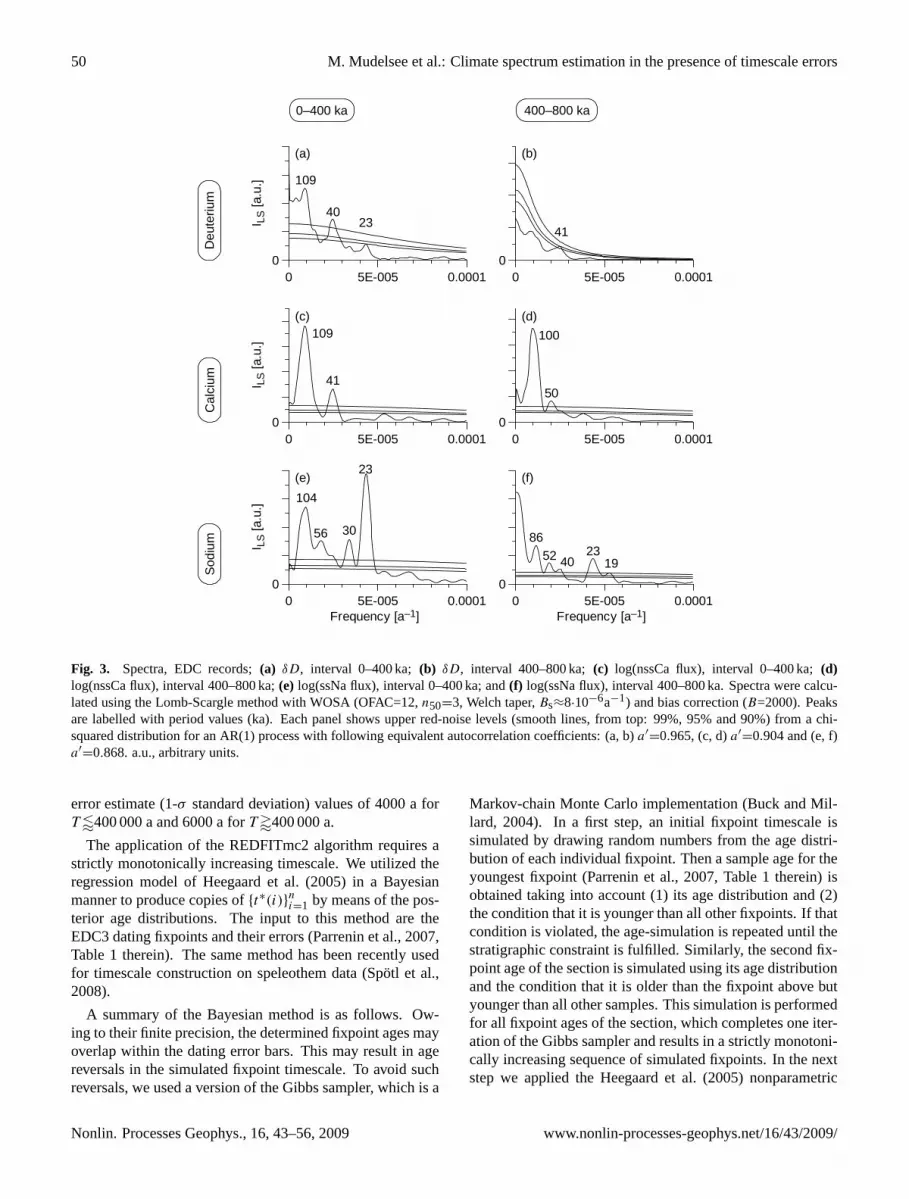
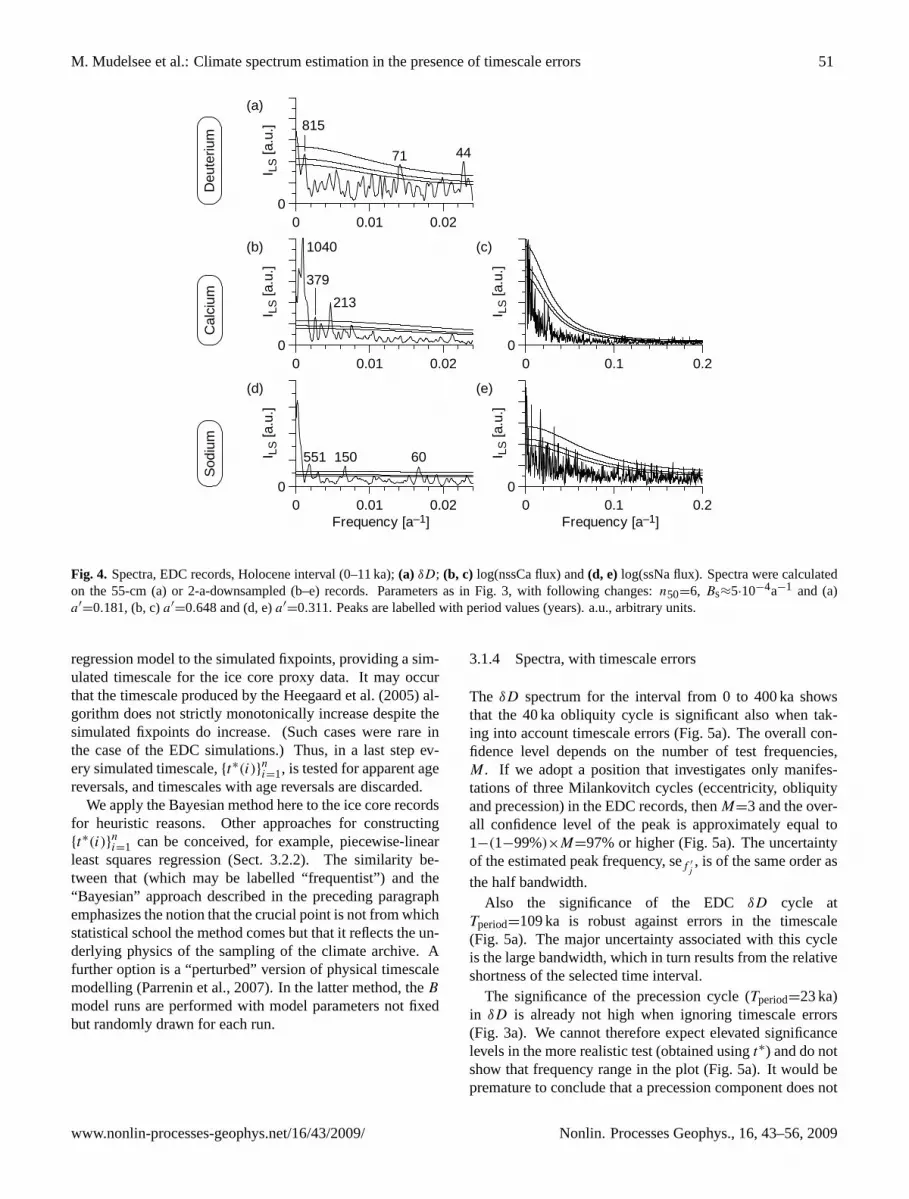
We also show spectra for the Holocene (Fig. 4). Thesewere calculated using records of very high temporal resolu-tion (δD, 55-cm resolution; nssCa flux and ssNa flux, 2-adownsampled). A number of peaks appear, mainly in thecentennial band.

3.1.3 Timescale

The “official” timescale, called EDC3, was produced (Par-renin et al., 2007) by employing a snow accumulation andice-flow model and invoking constraints in form of a set ofindependent age markers. The markers are given, on the onehand, by events such as a reversal of the Earth’s magnetic

0 0.00010

I LS

[a.u

.]

0 0.0040

(a)

0 0.00010

I LS

[a.u

.]

0 0.0040

(b)

0 0.0001Frequency [a–1]

0

I LS

[a.u

.]

0 0.0040

(c)

100

64

40

30 23

98

41

96

41

24

Deuterium

Calcium

Sodium

Fig. 2. Periodograms, EDC records;(a) δD, (b) log(nssCa flux) and(c) log(ssNa flux). Peaks are labelled with period values (ka). Insetsshow full frequency intervals. Periodograms were calculated on therecords shown in Fig. 1 subsequent to linear detrending. Lomb-Scargle parameters: OFAC=6,n50=1 and uniform taper. a.u., arbi-trary units.

field or a volcanic eruption that has been recorded by an ab-solutely dated palaeoclimatic archive. On the other hand,pattern matching of the proxy climate series with insolationseries produced an other kind of absolutely dated fixpoints.

Like any palaeoclimatic timescale, the EDC3 timescale re-lies on the validness of the assumptions made (e.g., modelformulation, model parameter values) and the precision ofnumerical input values (e.g., absolute dates of markers). TheEDC3 timescale is, thus, an estimate of the true, but unknowntimescale. Parrenin et al. (2007, Table 1 therein) give as



0 5E-005 0.00010

I LS

[a.u

.]

0 5E-005 0.00010

I LS

[a.u

.]

0 5E-005 0.0001Frequency [a–1]

0

I LS

[a.u

.]

0 5E-005 0.00010

0 5E-005 0.00010

0 5E-005 0.0001Frequency [a–1]

0

109

4023

109

41

104

56 30

23

8652 40

2319

100

50

41

(a)

(c)

(e)

(b)

(d)

(f)

Deu

teriu

mC

alci

umS

odiu

m

0–400 ka 400–800 ka

Fig. 3. Spectra, EDC records;(a) δD, interval 0–400 ka;(b) δD, interval 400–800 ka;(c) log(nssCa flux), interval 0–400 ka;(d)log(nssCa flux), interval 400–800 ka;(e) log(ssNa flux), interval 0–400 ka; and(f) log(ssNa flux), interval 400–800 ka. Spectra were calcu-lated using the Lomb-Scargle method with WOSA (OFAC=12,n50=3, Welch taper,Bs≈8·10−6a−1) and bias correction (B=2000). Peaksare labelled with period values (ka). Each panel shows upper red-noise levels (smooth lines, from top: 99%, 95% and 90%) from a chi-squared distribution for an AR(1) process with following equivalent autocorrelation coefficients: (a, b)a′=0.965, (c, d)a′=0.904 and (e, f)a′=0.868. a.u., arbitrary units.

error estimate (1-σ standard deviation) values of 4000 a forT /400 000 a and 6000 a forT '400 000 a.

The application of the REDFITmc2 algorithm requires astrictly monotonically increasing timescale. We utilized theregression model of Heegaard et al. (2005) in a Bayesianmanner to produce copies of{t∗(i)}ni=1 by means of the pos-terior age distributions. The input to this method are theEDC3 dating fixpoints and their errors (Parrenin et al., 2007,Table 1 therein). The same method has been recently usedfor timescale construction on speleothem data (Spotl et al.,2008).

A summary of the Bayesian method is as follows. Ow-ing to their finite precision, the determined fixpoint ages mayoverlap within the dating error bars. This may result in agereversals in the simulated fixpoint timescale. To avoid suchreversals, we used a version of the Gibbs sampler, which is a

Markov-chain Monte Carlo implementation (Buck and Mil-lard, 2004). In a first step, an initial fixpoint timescale issimulated by drawing random numbers from the age distri-bution of each individual fixpoint. Then a sample age for theyoungest fixpoint (Parrenin et al., 2007, Table 1 therein) isobtained taking into account (1) its age distribution and (2)the condition that it is younger than all other fixpoints. If thatcondition is violated, the age-simulation is repeated until thestratigraphic constraint is fulfilled. Similarly, the second fix-point age of the section is simulated using its age distributionand the condition that it is older than the fixpoint above butyounger than all other samples. This simulation is performedfor all fixpoint ages of the section, which completes one iter-ation of the Gibbs sampler and results in a strictly monotoni-cally increasing sequence of simulated fixpoints. In the nextstep we applied the Heegaard et al. (2005) nonparametric



0 0.01 0.020

I LS

[a.u

.]

(a)

0 0.01 0.020

I LS

[a.u

.]

(b)

0 0.01 0.02Frequency [a–1]

0

I LS

[a.u

.]

(d)

0 0.1 0.20

I LS

[a.u

.]0 0.1 0.2

Frequency [a–1]

0I L

S [a

.u.]

(c)

(e)

815

71 44

1040

379

213

551 150 60

Deu

teriu

mC

alci

umS

odiu

m

Fig. 4. Spectra, EDC records, Holocene interval (0–11 ka);(a) δD; (b, c) log(nssCa flux) and(d, e) log(ssNa flux). Spectra were calculatedon the 55-cm (a) or 2-a-downsampled (b–e) records. Parameters as in Fig. 3, with following changes:n50=6, Bs≈5·10−4a−1 and (a)a′=0.181, (b, c)a′=0.648 and (d, e)a′=0.311. Peaks are labelled with period values (years). a.u., arbitrary units.

regression model to the simulated fixpoints, providing a sim-ulated timescale for the ice core proxy data. It may occurthat the timescale produced by the Heegaard et al. (2005) al-gorithm does not strictly monotonically increase despite thesimulated fixpoints do increase. (Such cases were rare inthe case of the EDC simulations.) Thus, in a last step ev-ery simulated timescale,{t∗(i)}ni=1, is tested for apparent agereversals, and timescales with age reversals are discarded.

We apply the Bayesian method here to the ice core recordsfor heuristic reasons. Other approaches for constructing{t∗(i)}ni=1 can be conceived, for example, piecewise-linearleast squares regression (Sect. 3.2.2). The similarity be-tween that (which may be labelled “frequentist”) and the“Bayesian” approach described in the preceding paragraphemphasizes the notion that the crucial point is not from whichstatistical school the method comes but that it reflects the un-derlying physics of the sampling of the climate archive. Afurther option is a “perturbed” version of physical timescalemodelling (Parrenin et al., 2007). In the latter method, theB

model runs are performed with model parameters not fixedbut randomly drawn for each run.

3.1.4 Spectra, with timescale errors

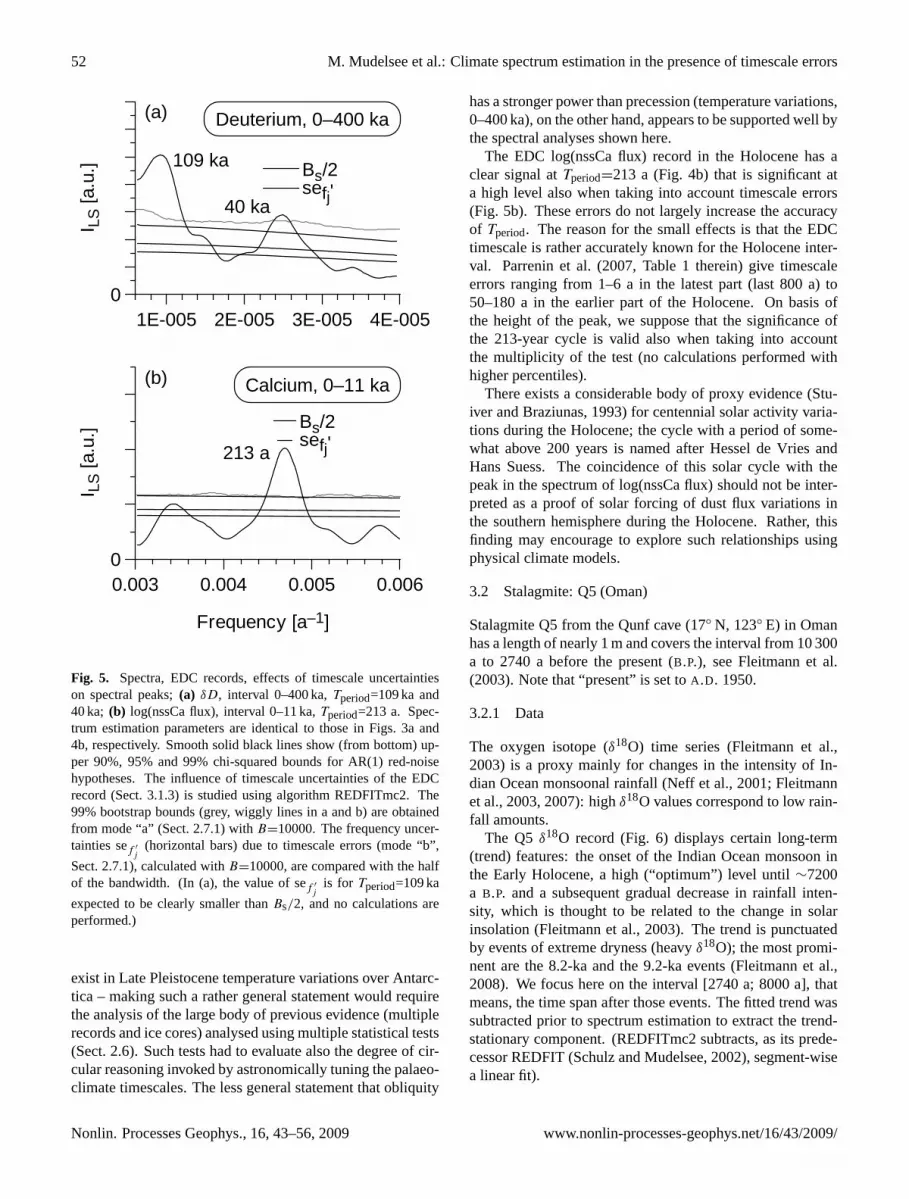
The δD spectrum for the interval from 0 to 400 ka showsthat the 40 ka obliquity cycle is significant also when tak-ing into account timescale errors (Fig. 5a). The overall con-fidence level depends on the number of test frequencies,M. If we adopt a position that investigates only manifes-tations of three Milankovitch cycles (eccentricity, obliquityand precession) in the EDC records, thenM=3 and the over-all confidence level of the peak is approximately equal to1−(1−99%)×M=97% or higher (Fig. 5a). The uncertaintyof the estimated peak frequency, sef ′

j, is of the same order as

the half bandwidth.Also the significance of the EDCδD cycle at

Tperiod=109 ka is robust against errors in the timescale(Fig. 5a). The major uncertainty associated with this cycleis the large bandwidth, which in turn results from the relativeshortness of the selected time interval.

The significance of the precession cycle (Tperiod=23 ka)in δD is already not high when ignoring timescale errors(Fig. 3a). We cannot therefore expect elevated significancelevels in the more realistic test (obtained usingt∗) and do notshow that frequency range in the plot (Fig. 5a). It would bepremature to conclude that a precession component does not



0

I LS

[a.u

.]

1E-005 2E-005 3E-005 4E-005

0

I LS

[a.u

.]

0.003 0.004 0.005 0.006

Frequency [a–1]

40 ka

213 a

(a)

(b)

Deuterium, 0–400 ka

Calcium, 0–11 ka

sefj'Bs/2

sefj'Bs/2

109 ka

Fig. 5. Spectra, EDC records, effects of timescale uncertaintieson spectral peaks;(a) δD, interval 0–400 ka,Tperiod=109 ka and40 ka; (b) log(nssCa flux), interval 0–11 ka,Tperiod=213 a. Spec-trum estimation parameters are identical to those in Figs. 3a and4b, respectively. Smooth solid black lines show (from bottom) up-per 90%, 95% and 99% chi-squared bounds for AR(1) red-noisehypotheses. The influence of timescale uncertainties of the EDCrecord (Sect. 3.1.3) is studied using algorithm REDFITmc2. The99% bootstrap bounds (grey, wiggly lines in a and b) are obtainedfrom mode “a” (Sect. 2.7.1) withB=10000. The frequency uncer-tainties sef ′

j(horizontal bars) due to timescale errors (mode “b”,

Sect. 2.7.1), calculated withB=10000, are compared with the halfof the bandwidth. (In (a), the value of sef ′

jis for Tperiod=109 ka

expected to be clearly smaller thanBs/2, and no calculations areperformed.)

exist in Late Pleistocene temperature variations over Antarc-tica – making such a rather general statement would requirethe analysis of the large body of previous evidence (multiplerecords and ice cores) analysed using multiple statistical tests(Sect. 2.6). Such tests had to evaluate also the degree of cir-cular reasoning invoked by astronomically tuning the palaeo-climate timescales. The less general statement that obliquity

has a stronger power than precession (temperature variations,0–400 ka), on the other hand, appears to be supported well bythe spectral analyses shown here.

The EDC log(nssCa flux) record in the Holocene has aclear signal atTperiod=213 a (Fig. 4b) that is significant ata high level also when taking into account timescale errors(Fig. 5b). These errors do not largely increase the accuracyof Tperiod. The reason for the small effects is that the EDCtimescale is rather accurately known for the Holocene inter-val. Parrenin et al. (2007, Table 1 therein) give timescaleerrors ranging from 1–6 a in the latest part (last 800 a) to50–180 a in the earlier part of the Holocene. On basis ofthe height of the peak, we suppose that the significance ofthe 213-year cycle is valid also when taking into accountthe multiplicity of the test (no calculations performed withhigher percentiles).

There exists a considerable body of proxy evidence (Stu-iver and Braziunas, 1993) for centennial solar activity varia-tions during the Holocene; the cycle with a period of some-what above 200 years is named after Hessel de Vries andHans Suess. The coincidence of this solar cycle with thepeak in the spectrum of log(nssCa flux) should not be inter-preted as a proof of solar forcing of dust flux variations inthe southern hemisphere during the Holocene. Rather, thisfinding may encourage to explore such relationships usingphysical climate models.

3.2 Stalagmite: Q5 (Oman)

Stalagmite Q5 from the Qunf cave (17◦ N, 123◦ E) in Omanhas a length of nearly 1 m and covers the interval from 10 300a to 2740 a before the present (B.P.), see Fleitmann et al.(2003). Note that “present” is set toA .D. 1950.

3.2.1 Data

The oxygen isotope (δ18O) time series (Fleitmann et al.,2003) is a proxy mainly for changes in the intensity of In-dian Ocean monsoonal rainfall (Neff et al., 2001; Fleitmannet al., 2003, 2007): highδ18O values correspond to low rain-fall amounts.

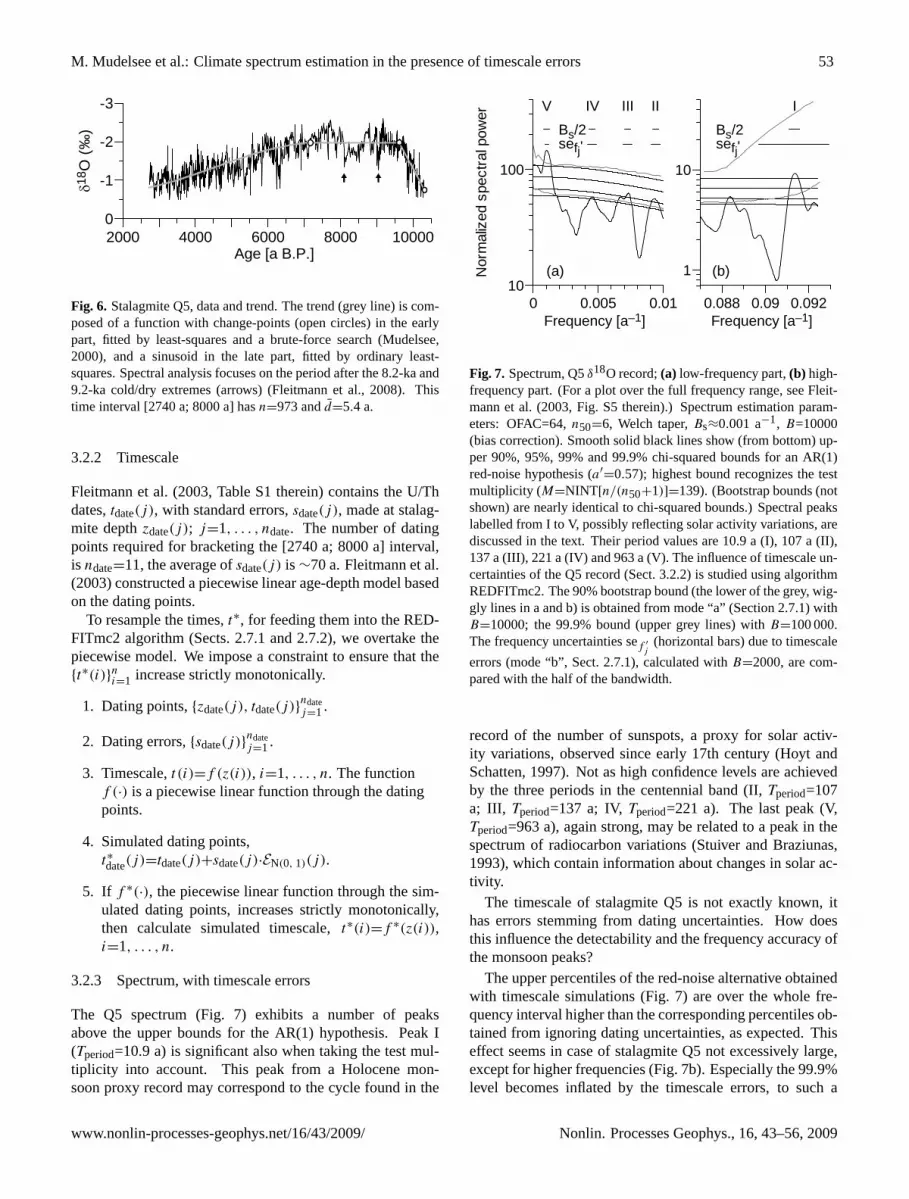
The Q5δ18O record (Fig. 6) displays certain long-term(trend) features: the onset of the Indian Ocean monsoon inthe Early Holocene, a high (“optimum”) level until∼7200a B.P. and a subsequent gradual decrease in rainfall inten-sity, which is thought to be related to the change in solarinsolation (Fleitmann et al., 2003). The trend is punctuatedby events of extreme dryness (heavyδ18O); the most promi-nent are the 8.2-ka and the 9.2-ka events (Fleitmann et al.,2008). We focus here on the interval [2740 a; 8000 a], thatmeans, the time span after those events. The fitted trend wassubtracted prior to spectrum estimation to extract the trend-stationary component. (REDFITmc2 subtracts, as its prede-cessor REDFIT (Schulz and Mudelsee, 2002), segment-wisea linear fit).



2000 4000 6000 8000 10000Age [a B.P.]

0

-1

-2

-3δ18

O (

‰)

Fig. 6. Stalagmite Q5, data and trend. The trend (grey line) is com-posed of a function with change-points (open circles) in the earlypart, fitted by least-squares and a brute-force search (Mudelsee,2000), and a sinusoid in the late part, fitted by ordinary least-squares. Spectral analysis focuses on the period after the 8.2-ka and9.2-ka cold/dry extremes (arrows) (Fleitmann et al., 2008). Thistime interval [2740 a; 8000 a] hasn=973 andd=5.4 a.

3.2.2 Timescale

Fleitmann et al. (2003, Table S1 therein) contains the U/Thdates,tdate(j), with standard errors,sdate(j), made at stalag-mite depthzdate(j); j=1, . . . , ndate. The number of datingpoints required for bracketing the [2740 a; 8000 a] interval,is ndate=11, the average ofsdate(j) is ∼70 a. Fleitmann et al.(2003) constructed a piecewise linear age-depth model basedon the dating points.

To resample the times,t∗, for feeding them into the RED-FITmc2 algorithm (Sects. 2.7.1 and 2.7.2), we overtake thepiecewise model. We impose a constraint to ensure that the{t∗(i)}ni=1 increase strictly monotonically.

1. Dating points,{zdate(j), tdate(j)}ndatej=1 .

2. Dating errors,{sdate(j)}ndatej=1 .

3. Timescale,t (i)=f (z(i)), i=1, . . . , n. The functionf (·) is a piecewise linear function through the datingpoints.

4. Simulated dating points,t∗date(j)=tdate(j)+sdate(j)·EN(0, 1)(j).

5. If f ∗(·), the piecewise linear function through the sim-ulated dating points, increases strictly monotonically,then calculate simulated timescale,t∗(i)=f ∗(z(i)),i=1, . . . , n.

3.2.3 Spectrum, with timescale errors

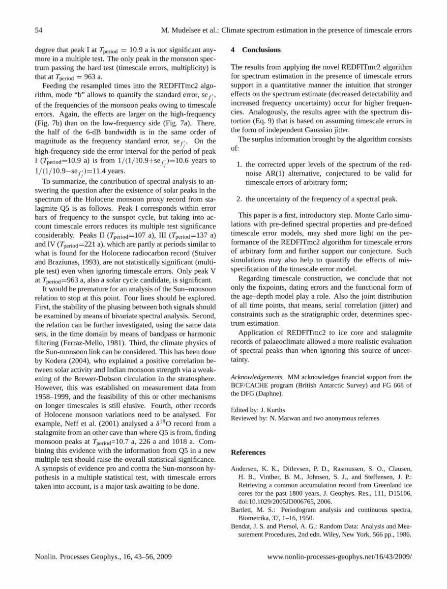
The Q5 spectrum (Fig.7) exhibits a number of peaksabove the upper bounds for the AR(1) hypothesis. Peak I(Tperiod=10.9 a) is significant also when taking the test mul-tiplicity into account. This peak from a Holocene mon-soon proxy record may correspond to the cycle found in the

0 0.005 0.01Frequency [a–1]

10

100

Nor

mal

ized

spe

ctra

l pow

er

0.088 0.09 0.092Frequency [a–1]

1

10

(a) (b)

V IV III II I

sefj'Bs/2

sefj'Bs/2

Fig. 7. Spectrum, Q5δ18O record;(a) low-frequency part,(b) high-frequency part. (For a plot over the full frequency range, see Fleit-mann et al. (2003, Fig. S5 therein).) Spectrum estimation param-eters: OFAC=64,n50=6, Welch taper,Bs≈0.001 a−1, B=10000(bias correction). Smooth solid black lines show (from bottom) up-per 90%, 95%, 99% and 99.9% chi-squared bounds for an AR(1)red-noise hypothesis (a′=0.57); highest bound recognizes the testmultiplicity (M=NINT[n/(n50+1)]=139). (Bootstrap bounds (notshown) are nearly identical to chi-squared bounds.) Spectral peakslabelled from I to V, possibly reflecting solar activity variations, arediscussed in the text. Their period values are 10.9 a (I), 107 a (II),137 a (III), 221 a (IV) and 963 a (V). The influence of timescale un-certainties of the Q5 record (Sect. 3.2.2) is studied using algorithmREDFITmc2. The 90% bootstrap bound (the lower of the grey, wig-gly lines in a and b) is obtained from mode “a” (Section 2.7.1) withB=10000; the 99.9% bound (upper grey lines) withB=100 000.The frequency uncertainties sef ′

j(horizontal bars) due to timescale

errors (mode “b”, Sect. 2.7.1), calculated withB=2000, are com-pared with the half of the bandwidth.

record of the number of sunspots, a proxy for solar activ-ity variations, observed since early 17th century (Hoyt andSchatten, 1997). Not as high confidence levels are achievedby the three periods in the centennial band (II,Tperiod=107a; III, Tperiod=137 a; IV,Tperiod=221 a). The last peak (V,Tperiod=963 a), again strong, may be related to a peak in thespectrum of radiocarbon variations (Stuiver and Braziunas,1993), which contain information about changes in solar ac-tivity.

The timescale of stalagmite Q5 is not exactly known, ithas errors stemming from dating uncertainties. How doesthis influence the detectability and the frequency accuracy ofthe monsoon peaks?

The upper percentiles of the red-noise alternative obtainedwith timescale simulations (Fig. 7) are over the whole fre-quency interval higher than the corresponding percentiles ob-tained from ignoring dating uncertainties, as expected. Thiseffect seems in case of stalagmite Q5 not excessively large,except for higher frequencies (Fig. 7b). Especially the 99.9%level becomes inflated by the timescale errors, to such a



degree that peak I atTperiod = 10.9 a is not significant any-more in a multiple test. The only peak in the monsoon spec-trum passing the hard test (timescale errors, multiplicity) isthat atTperiod = 963 a.

Feeding the resampled times into the REDFITmc2 algo-rithm, mode “b” allows to quantify the standard error, sef ′

j,

of the frequencies of the monsoon peaks owing to timescaleerrors. Again, the effects are larger on the high-frequency(Fig. 7b) than on the low-frequency side (Fig. 7a). There,the half of the 6-dB bandwidth is in the same order ofmagnitude as the frequency standard error, sef ′

j. On the

high-frequency side the error interval for the period of peakI (Tperiod=10.9 a) is from 1/(1/10.9+sef ′

j)=10.6 years to

1/(1/10.9−sef ′j)=11.4 years.

To summarize, the contribution of spectral analysis to an-swering the question after the existence of solar peaks in thespectrum of the Holocene monsoon proxy record from sta-lagmite Q5 is as follows. Peak I corresponds within errorbars of frequency to the sunspot cycle, but taking into ac-count timescale errors reduces its multiple test significanceconsiderably. Peaks II (Tperiod=107 a), III (Tperiod=137 a)and IV (Tperiod=221 a), which are partly at periods similar towhat is found for the Holocene radiocarbon record (Stuiverand Braziunas, 1993), are not statistically significant (multi-ple test) even when ignoring timescale errors. Only peak VatTperiod=963 a, also a solar cycle candidate, is significant.

It would be premature for an analysis of the Sun–monsoonrelation to stop at this point. Four lines should be explored.First, the stability of the phasing between both signals shouldbe examined by means of bivariate spectral analysis. Second,the relation can be further investigated, using the same datasets, in the time domain by means of bandpass or harmonicfiltering (Ferraz-Mello, 1981). Third, the climate physics ofthe Sun-monsoon link can be considered. This has been doneby Kodera (2004), who explained a positive correlation be-tween solar activity and Indian monsoon strength via a weak-ening of the Brewer-Dobson circulation in the stratosphere.However, this was established on measurement data from1958–1999, and the feasibility of this or other mechanismson longer timescales is still elusive. Fourth, other recordsof Holocene monsoon variations need to be analysed. Forexample, Neff et al. (2001) analysed aδ18O record from astalagmite from an other cave than where Q5 is from, findingmonsoon peaks atTperiod=10.7 a, 226 a and 1018 a. Com-bining this evidence with the information from Q5 in a newmultiple test should raise the overall statistical significance.A synopsis of evidence pro and contra the Sun-monsoon hy-pothesis in a multiple statistical test, with timescale errorstaken into account, is a major task awaiting to be done.

4 Conclusions

The results from applying the novel REDFITmc2 algorithmfor spectrum estimation in the presence of timescale errorssupport in a quantitative manner the intuition that strongereffects on the spectrum estimate (decreased detectability andincreased frequency uncertainty) occur for higher frequen-cies. Analogously, the results agree with the spectrum dis-tortion (Eq. 9) that is based on assuming timescale errors inthe form of independent Gaussian jitter.

The surplus information brought by the algorithm consistsof:

1. the corrected upper levels of the spectrum of the red-noise AR(1) alternative, conjectured to be valid fortimescale errors of arbitrary form;

2. the uncertainty of the frequency of a spectral peak.

This paper is a first, introductory step. Monte Carlo simu-lations with pre-defined spectral properties and pre-definedtimescale error models, may shed more light on the per-formance of the REDFITmc2 algorithm for timescale errorsof arbitrary form and further support our conjecture. Suchsimulations may also help to quantify the effects of mis-specification of the timescale error model.

Regarding timescale construction, we conclude that notonly the fixpoints, dating errors and the functional form ofthe age–depth model play a role. Also the joint distributionof all time points, that means, serial correlation (jitter) andconstraints such as the stratigraphic order, determines spec-trum estimation.

Application of REDFITmc2 to ice core and stalagmiterecords of palaeoclimate allowed a more realistic evaluationof spectral peaks than when ignoring this source of uncer-tainty.

Acknowledgements. MM acknowledges financial support from theBCF/CACHE program (British Antarctic Survey) and FG 668 ofthe DFG (Daphne).

Edited by: J. KurthsReviewed by: N. Marwan and two anonymous referees

References

Andersen, K. K., Ditlevsen, P. D., Rasmussen, S. O., Clausen,H. B., Vinther, B. M., Johnsen, S. J., and Steffensen, J. P.:Retrieving a common accumulation record from Greenland icecores for the past 1800 years, J. Geophys. Res., 111, D15106,doi:10.1029/2005JD006765, 2006.

Bartlett, M. S.: Periodogram analysis and continuous spectra,Biometrika, 37, 1–16, 1950.

Bendat, J. S. and Piersol, A. G.: Random Data: Analysis and Mea-surement Procedures, 2nd edn. Wiley, New York, 566 pp., 1986.



Buck, C. E. and Millard, A. R. Tools for Constructing Chronolo-gies: Crossing Disciplinary Boundaries. Springer, London, 257pp., 2004.

Chan, K. S. and Tong, H.: A note on embedding a discrete param-eter ARMA model in a continuous parameter ARMA model, J.Time Ser. Anal., 8, 277–281, 1987.

Divine, D. V., Polzehl, J., and Godtliebsen, F.: A propagation-separation approach to estimate the autocorrelation in a time-series, Nonlin. Processes Geophys., 15, 591–599, 2008,http://www.nonlin-processes-geophys.net/15/591/2008/.

Efron, B. and Tibshirani, R. J.: An Introduction to the Bootstrap.Chapman and Hall, London, 436 pp., 1993.

EPICA Community Members: One-to-one coupling of glacial cli-mate variability in Greenland and Antarctica, Nature, 444, 195–198, 2006.

Ferraz-Mello, S.: Estimation of periods from unequally spaced ob-servations, Astronom. J., 86, 619–624, 1981.

Fisher, D. A., Reeh, N., and Clausen, H. B.: Stratigraphic noise intime series derived from ice cores, Ann. Glaciol., 7, 76–83, 1985.

Fleitmann, D., Burns, S. J., Mudelsee, M., Neff, U., Kramers, J.,Mangini, A., and Matter, A.: Holocene forcing of the Indianmonsoon recorded in a stalagmite from Southern Oman, Science,300, 1737–1739, 2003.

Fleitmann, D., Burns, S. J., Mangini, A., Mudelsee, M., Kramers, J.,Villa, I., Neff, U., Al-Subbary, A. A., Buettner, A., Hippler, D.,and Matter, A.: Holocene ITCZ and Indian monsoon dynamicsrecorded in stalagmites from Oman and Yemen (Socotra), Quat.Sci. Rev., 26, 170–188, 2007.

Fleitmann, D., Mudelsee, M., Burns, S. J., Bradley, R. S., Kramers,J., and Matter, A.: Evidence for a widespread climatic anomalyat around 9.2 ka before present, Paleoceanog., 23, PA1102,doi:1029/2007PA001519, 2008.

Harris, F. J.: On the use of windows for harmonic analysis with thediscrete Fourier transform, Proc. IEEE, 66, 51–83, 1978.

Heegaard, E., Birks, H. J. B., and Telford, R. J.: Relationships be-tween calibrated ages and depth in stratigraphical sequences: Anestimation procedure by mixed-effect regression, The Holocene,15, 612–618, 2005.

Horne, J. H. and Baliunas, S. L.: A prescription for period analysisof unevenly sampled time series, Astrophys. J., 302, 757–763,1986.

Hoyt, D. V. and Schatten, K. H.: The Role of the Sun in ClimateChange. Oxford University Press, New York, 279 pp., 1997.

Jouzel, J., Masson-Delmotte, V., Cattani, O., Dreyfus, G., Falourd,S., Hoffmann, G., Minster, B., Nouet, J., Barnola, J. M., Chap-pellaz, J., Fischer, H., Gallet, J. C., Johnsen, S., Leuenberger, M.,Loulergue, L., Luethi, D., Oerter, H., Parrenin, F., Raisbeck, G.,Raynaud, D., Schilt, A., Schwander, J., Selmo, E., Souchez, R.,Spahni, R., Stauffer, B., Steffensen, J. P., Stenni, B., Stocker, T.F., Tison, J. L., Werner, M., and Wolff, E. W.: Orbital and mil-lennial Antarctic climate variability over the past 800 000 years,Science, 317, 793–796, 2007.

Kendall, M. G.: Note on bias in the estimation of autocorrelation,Biometrika, 41, 403–404, 1954.

Kodera, K.: Solar influence on the Indian Ocean monsoonthrough dynamical processes, Geophys. Res. Lett., 31, L24209,doi:10.1029/2004GL020928, 2004.

Lisiecki, L. E. and Raymo, M. E.: A Plio-Pleistocene stack of57 globally distributed benthicδ18O records, Paleoceanog., 20,

PA1003, doi:10.1029/2004PA001071, 2005.Lomb, N. R.: Least-squares frequency analysis of unequally spaced

data, Astro. Sp. Sc., 39, 447–462, 1976.Moore, M. I. and Thomson, P. J.: Impact of jittered sampling on

conventional spectral estimates, J. Geophys. Res., 96, 18519–18526, 1991.

Mudelsee, M.: Ramp function regression: A tool for quantifyingclimate transitions, Comput. Geosci., 26, 293–307, 2000.

Mudelsee, M.: Note on the bias in the estimation of the serial cor-relation coefficient of AR(1) processes, Stat. Pap., 42, 517–527,2001.

Mudelsee, M.: TAUEST: A computer program for estimating per-sistence in unevenly spaced weather/climate time series, Com-put. Geosci., 28, 69–72, 2002.

Neff, U., Burns, S. J., Mangini, A., Mudelsee, M., Fleitmann, D.,and Matter, A.: Strong coherence between solar variability andthe monsoon in Oman between 9 and 6 kyr ago, Nature, 411,290–293, 2001.

Nuttall, A. H.: Some windows with very good sidelobe behavior,IEEE T. Acoust. Speech, 29, 84–91, 1981.

Parrenin, F., Barnola, J.-M., Beer, J., Blunier, T., Castellano, E.,Chappellaz, J., Dreyfus, G., Fischer, H., Fujita, S., Jouzel, J.,Kawamura, K., Lemieux-Dudon, B., Loulergue, L., Masson-Delmotte, V., Narcisi, B., Petit, J.-R., Raisbeck, G., Raynaud,D., Ruth, U., Schwander, J., Severi, M., Spahni, R., Steffensen,J. P., Svensson, A., Udisti, R., Waelbroeck, C., and Wolff, E.:The EDC3 chronology for the EPICA Dome C ice core, Clim.Past, 3, 485–497, 2007.

Priestley, M. B.: Spectral Analysis and Time Series, AcademicPress, London, 890 pp., 1981.

Raymo, M. E. and Huybers, P.: Unlocking the mysteries of the iceages, Nature, 451, 284–285, 2008.

Robinson, P. M.: Estimation of a time series model from unequallyspaced data, Stoch. Process. Appl., 6, 9–24, 1977.

Rothlisberger, R., Mudelsee, M., Bigler, M., de Angelis, M., Fis-cher, H., Hansson, M., Lambert, F., Masson-Delmotte, V., Sime,L., Udisti, R., and Wolff, E. W.: The Southern Hemisphere atglacial terminations: insights from the Dome C ice core, Clim.Past, 4, 345–356, 2008,http://www.clim-past.net/4/345/2008/.

Scargle, J. D.: Studies in astronomical time series analysis. II. Sta-tistical aspects of spectral analysis of unevenly spaced data, As-trophys. J., 263, 835–853, 1982.

Scargle, J. D.: Studies in astronomical time series analysis.III. Fourier transforms, autocorrelation functions, and cross-correlation functions of unevenly spaced data, Astrophys. J., 343,874–887, 1989.

Schulz, M. and Stattegger, K.: SPECTRUM: Spectral analysis ofunevenly spaced paleoclimatic time series, Comput. Geosci., 23,929–945, 1997.

Schulz, M. and Mudelsee, M.: REDFIT: Estimating red-noisespectra directly from unevenly spaced paleoclimatic time series,Comput. Geosci., 28, 421–426, 2002.

Schuster, A.: On the investigation of hidden periodicities with ap-plication to a supposed 26 day period of meteorological phenom-ena, Terrestr. Magn., 3, 13–41, 1898.

Spotl, C., Scholz, D., and Mangini, A.: A terrestrial U/Th-datedstable isotope record of the penultimate interglacial, Earth Planet.Sci. Lett., 276, 283–292, 2008.


http://www.nonlin-processes-geophys.net/15/591/2008/

http://www.clim-past.net/4/345/2008/


Stuiver, M. and Braziunas, T. F.: Sun, ocean, climate and atmo-spheric14CO2: An evaluation of causal and spectral relation-ships, Holocene, 3, 289–305, 1993.

Thomson, D. J.: Spectrum estimation and harmonic analysis, Proc.IEEE, 70, 1055–1096, 1982.

Thomson, P. J. and Robinson, P. M.: Estimation of second-orderproperties from jittered time series, Ann. Inst. Statist. Math., 48,29–48, 1996.

VanDongen, H. P. A., Olofsen, E., VanHartevelt, J. H., and Kruyt, E.W.: Periodogram analysis of unequally spaced data: The Lombmethod. Leiden University, Leiden, 66 pp., 1997.

Welch, P. D.: The use of Fast Fourier Transform for the estima-tion of power spectra: A method based on time averaging overshort, modified periodograms, IEEE T. Audio Electro., 15, 70–73, 1967.

Wolff, E. W., Fischer, H., Fundel, F., Ruth, U., Twarloh, B., Littot,G. C., Mulvaney, R., Rothlisberger, R., de Angelis, M., Boutron,C. F., Hansson, M., Jonsell, U., Hutterli, M. A., Lambert, F.,Kaufmann, P., Stauffer, B., Stocker, T. F., Steffensen, J. P., Bigler,M., Siggaard-Andersen, M. L., Udisti, R., Becagli, S., Castel-lano, E., Severi, M., Wagenbach, D., Barbante, C., Gabrielli, P.,and Gaspari, V.: Southern Ocean sea-ice extent, productivity andiron flux over the past eight glacial cycles, Nature, 440, 491–496,2006.

Wunsch, C.: On sharp spectral lines in the climate record and themillennial peak, Paleoceanog., 15, 417–424, 2000.


Climate spectrum estimation in the presence of timescale errors

Documents