Climate Sensitivity Estimated From Earth's Climate Historyjeh1/mailings/2012/20120508_ClimateSensitivity.pdf · We discuss sources of uncertainty in our evaluation of climate sensitivity

1

Climate Sensitivity Estimated From Earth's Climate History

James E. Hansen and Makiko Sato

NASA Goddard Institute for Space Studies and Columbia University Earth Institute, New York

ABSTRACT Earth's climate history potentially can yield accurate assessment of climate sensitivity. Imprecise knowledge of glacial-to-interglacial global temperature change is the biggest obstacle to accurate assessment of the fast-feedback climate sensitivity, which is the sensitivity that most immediately affects humanity. Our best estimate for the fast-feedback climate sensitivity from Holocene initial conditions is 3 ± 0.5°C for 4 W/m2 CO2 forcing (68% probability) . Slow feedbacks, including ice sheet disintegration and release of greenhouse gases (GHGs) by the climate system, generally amplify total Earth system climate sensitivity. Slow feedbacks make Earth system climate sensitivity highly dependent on the initial climate state and on the magnitude and sign of the climate forcing, because of thresholds (tipping points) in the slow feedbacks. It is difficult to assess the speed at which slow feedbacks will become important in the future, because of the absence in paleoclimate history of any positive (warming) forcing rivaling the speed at which the human-caused forcing is growing.

1. Introduction Humanity is now the dominant force driving changes of Earth's atmospheric composition and thus future climate (IPCC, 2007a). The largest climate forcing, i.e., the greatest imposed perturbation of the planet's energy balance (IPCC, 2007a; Hansen et al., 2005) is the human-made increase of atmospheric greenhouse gases, especially CO2 from burning of fossil fuels. Earth's response to climate forcings is slowed by the inertia of the global ocean and the great ice sheets on Greenland and Antarctica, which require centuries or longer to approach their full response to a climate forcing. This long response time makes the task of avoiding dangerous human alteration of climate particularly difficult, because the human-made climate forcing is being imposed rapidly, with most of the forcing added in just the past several decades. Thus observed climate changes are only a partial response to the current climate forcing, with further response still "in-the-pipeline" (Hansen et al., 1984). Climate models, numerical simulations of climate, provide one way of estimating the ultimate climate response to climate forcings, but it is difficult to include realistically all of the processes that exist in the real world. Earth's paleoclimate history allows empirical assessment of climate sensitivity, but the input data have large uncertainties. These approaches are usually not fully independent, and surely the most realistic eventual assessments will be ones combining the greatest strengths of both approaches. We use available paleoclimate data, specifically the oxygen isotope record in ocean sediments (Zachos et al., 2008), to estimate past changes of sea level and ocean temperature, and thus obtain a largely empirical estimate of climate sensitivity. We used an earlier version of that data (Zachos et al., 2001) in prior studies (Hansen et al., 2008; Hansen and Sato, 2012), but here we make a change in our simple prescription for separating effects of temperature and ice volume in the oxygen isotope record that should yield more accurate sea level and temperature histories. We discuss sources of uncertainty in our evaluation of climate sensitivity and ways that climate models could be used to test, confirm, and refine current assessments.

2

Fig. 1. (a) Global deep ocean δ18O from Zachos et al. (2008) and (b) deep ocean temperature, with the latter based on the prescription in our present paper. Black data points are 5-point running means of original temporal resolution; red and blue curves have 500 ky resolution.

2. Deep Ocean Temperature and Sea Level in the Cenozoic Era The Cenozoic era, the past 65.5 My, provides a valuable perspective on climate and sea level change (Zachos et al., 2001; Hansen et al., 2008). We present and discuss Cenozoic data prior to introducing specific definitions and evaluations of climate sensitivity, because the Cenozoic climate changes help clarify the roles of different mechanisms for climate change. Carbon dioxide, for example, operates during the Cenozoic as both a dominant climate forcing and a powerful feedback mechanism. Zachos et al. (2008) have made available a data set for variations in the proportion of the heavy oxygen isotope (δ18O) in the shells of deep-ocean-dwelling microscopic shelled animals (foraminifera) in a near-global compilation of ocean sediment cores (Fig. 1a, right scale). The principal difficulty in using this record to estimate global deep ocean temperature is that δ18O in the foraminifera is affected by global ice mass as well as deep ocean temperature. During the early Cenozoic, between 65.5 My and 35 My, Earth was so warm that there was little ice on the planet and deep ocean temperature is approximated by (Zachos et al., 2001).

Tdo(°C ) = -4 δ18O + 12 (for δ18O < 1.75) (1) Hansen et al. (2008) made the approximation that, as Earth became colder and continental ice sheets grew, further increase of δ18O was due in equal parts to deep ocean temperature change and ice mass change.

3

Tdo(°C ) = -2 (δ18O - 4.25) (for δ18O > 1.75) (2)

This assumption of equal division of the change of δ18O into temperature change and ice volume change was suggested by comparing δ18O at the endpoints of the climate change from the nearly ice-free planet at 35 MY (when δ18O ~ 1.75) to the Last Glacial Maximum (LGM), which peaked ~ 20 ky ago. The change of δ18O between these two extreme climate states (~ 3), is twice the change of δ18O due to temperature change alone (~ 1.5), with the latter based on the linear relation (1) and estimates of Tdo ~ 5°C at 35 My and ~ -1°C at the LGM. The above approximation has the merit of simplicity. However, although ice volume change and deep ocean temperature change contributed about equally to δ18O change on average over the full range from 35 My to 20 ky ago, the temperature change portion of the δ18O change must decrease as the deep ocean temperature approaches the freezing point (Waelbroeck et al., 2002). The rapid increase of δ18O in the past few million years was associated with appearance of the massive Laurentide ice sheet in North America, as symbolized by the dark blue bar in the upper part of Fig. 1a (Zachos et al., 2001). Sea level change between the LGM and the Holocene was ~120 m (Fairbanks, 1989; Peltier and Fairbanks, 2006). Thus of the total 180 m sea level change between the ice-free planet and glacial maximum only about one-third (60 m) occurred with the increase of δ18O from its value (~1.75) 35 My ago to its Holocene value (~3.25). Two-thirds (120 m) of the total sea level change occurred with the formation of the Northern Hemisphere ice and likely increase in the volume of Antarctic ice. Thus rather than taking the 180 m sea level change between the nearly ice-free planet of 34 My ago and the LGM as being linear over the entire range (with 90 m for δ18O < 3.25 and 90 m for δ18O > 3.25), it is more realistic to assign 60 m of sea level change to δ18O 1.75-3.25 and 120 m to δ18O > 3.25. The total deep ocean temperature change of 6°C for change of δ18O from 1.75 to 4.75 is then divided two-thirds (4°C) for the δ18O range 1.75-3.25 and 2°C for the δ18O range 3.25-4.75. Algebraically

SL (m) = 60 – 40 (δ18O - 1.75) (for 1.75 < δ18O < 3.25) (3)

SL (m) = – 120 (δ18O - 3.25)/1.65 (for δ18O > 3.25) (4)

Tdo(°C ) = 5 – 8(δ18O – 1.75)/3 (for δ18O < 3.25) (5)

Tdo(°C ) = 1 – 4.4 (δ18O – 3.25)/3 (for δ18O > 3.25) (6) where SL is sea level and its zero point is the late Holocene level. The coefficients in equation (4) and (5) account for the fact that the mean LGM value of δ18O is ~ 4.9. The resulting deep ocean temperature is shown in Fig. 1(b) for the full Cenozoic era. Resulting sea level changes in the Pleistocene are compared with data of Siddall et al. (2003) in Fig. 2c. Our prescription above (equations 3-4) yields sea level maxima of +9.8 m in the Eemian Interglacial period (Marine Isotope Stage 5e) and +7.1 m in the Holsteinian Interglacial (MIS 11), comparable with recent estimates of +7-9 m for MIS 5e (Kopp et al., 2009) and +6-13 m for MIS 11 (Raymo and Mitrovica, 2012). We do not imply that the accuracy of the simple prescription of equations (3-4) competes with these more comprehensive studies, only that these comparisons support the reasonableness of our approximation.

4

Fig. 2. Sea level from δ18O of Zachos et al. (2008), as shown in Fig. 1(a), and equations (3) and (4). Our prescription yields Pliocene sea levels varying between about +20 m and –50 m. Effects of glacial isostatic adjustment create uncertainty in sea level reconstructions based on shoreline geologic data (Raymo et al., 2011), but data from a number of sites suggest Pliocene sea levels as high as +15-25 m (Dowsett et al., 1999; Dwyer and Chandler, 2009). The sea level variations that we find in the early Pliocene (Fig. 2b), when presumably there was no Laurentide ice sheet, are less than in the late Pliocene and Pleistocene, yet the early Pliocene sea level variations are of order 10-25 m and reach heights far above current sea level. Thus the paleo data indicate that Antarctica and Greenland potentially can lose substantial mass in response to global warming, reaching levels that would have enormous impacts on humanity. The deep ocean temperature based on equations 5 and 6 are shown for the Pliocene and Pleistocene in Fig. 3 and for the entire Cenozoic era in Fig. 1. We find below that the change of the temperature history caused by our present two-legged linear approximation is small enough that it does not alter conclusions of Hansen and Sato (2012). However, because the sea levels are more accurate with the present prescription, we expect that the new temperatures are also more accurate and thus the new deep ocean temperature data set should be preferred.

5

Fig. 3. Deep ocean temperature in (a) the Pliocene and Pleistocene, and (b) the last 800,000 years. High frequency variations (black) are 5-point running means of original data (Zachos et al., 2008), while the blue curve has 500 ky resolution. Deep ocean temperature for the entire Cenozoic era is in Fig. 1 (b).

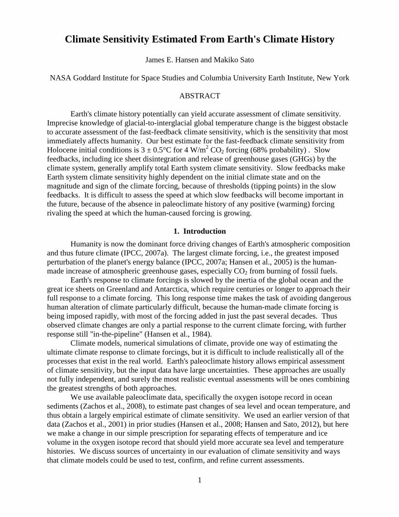
3. Surface Air Temperature Change The temperature of most interest to humanity is that of surface air. Empirical inference of global climate sensitivity requires knowledge of past global surface temperature change. The long time span covered by the deep ocean temperature record makes it an especially attractive data set for studying climate sensitivity, provided that a relationship can be established between deep ocean and surface temperature changes. Following Hansen et al. (2008), we assume that deep ocean temperature change was similar to global mean surface temperature change for Cenozoic climates warmer than today. Temperature change tends to be amplified at high latitudes where deep water forms, relative to global mean change. But high latitude amplification should tend to be at least partially offset by the fact that ocean temperature change is generally smaller than land temperature change. However, deep ocean temperature change does not provide a good indication of surface temperature change when the deep ocean approaches the freezing point, as quantified by Waelbroeck et al. (2002). The empirical data show that deep ocean cooling slows relative to global mean surface cooling as the area of ice and snow on the surface expands, consistent with the fact that the increase of δ18O between the Holocene and LGM was due more to ice sheet growth than to deep ocean cooling. We need observational data to establish an empirical relation between surface temperature change and deep ocean temperature change for the range of climate from the Holocene to the LGM. As a first estimate to be reassessed later, we assume that the LGM-Holocene global surface temperature change was 4.5°C, thus twice as large as the 2.25°C deep ocean temperature change found from δ18O. Given the assumptions that (1) surface and deep ocean temperature changes are similar for climates warmer than the Holocene, and (2) surface temperature change is twice as large as deep ocean temperature change for the Holocene-LGM temperature change, we obtain a Cenozoic surface temperature history (Fig. 4). The absolute temperature scale is obtained by concatenating with the instrumental record (Hansen et al., 2010), assuming the recent 5-year mean temperature is 0.3°C warmer than the Holocene maximum in the ocean core data. The rationale (Hansen et al., 2012) for the latter assumption is that ice sheets in both hemispheres have been losing mass rapidly in the past two decades and sea level is rising at a rate (3 m per

6

Fig. 4. Surface temperature estimate for the past 35 million years, including an expanded time scale for (b) the Pliocene and Pleistocene and (c) the last 800,000 years. The red curve has 500 ky resolution. millennium) much faster than has occurred in the past several thousand years. The 1951-1980 global mean surface temperature is taken to be 14°C (Jones et al., 1999). Uncertainty in the absolute scale will not affect our empirically inferred climate sensitivity.

4. Climate Sensitivity in the Cenozoic Era Climate sensitivity (S) is the equilibrium global surface temperature change (ΔTeq) in response to a specified unit forcing after the planet has come back to energy balance,

S = ΔTeq/F, (7) i.e., climate sensitivity is the eventual (equilibrium) global temperature change per unit forcing. Climate sensitivity depends upon climate feedbacks, the many physical processes that come into play as climate changes in response to a forcing. Positive (amplifying) feedbacks increase the climate response, while negative (diminishing) feedbacks reduce the response. We usually discuss climate sensitivity in terms of global mean temperature response to a 4 W/m2 CO2 forcing. One merit of this standard forcing is that its magnitude is similar to the human-made forcing anticipated in the near-term, thus avoiding the need to continually scale the unit sensitivity to make it of an applicable magnitude. A second merit is that the efficacy of forcings varies from one forcing mechanism to another (Hansen et al., 2005), so it useful to be specific about the forcing mechanism. Finally, the 4 W/m2 CO2 forcing avoids the uncertainty in the exact magnitude of a doubled CO2 forcing [IPCC (2007a) estimate 3.7 W/m2 for doubled CO2 while Hansen et al. (2005) obtain 4.1 W/m2], as well as problems associated with the fact that doubled CO2 forcing varies substantially as the CO2 amount changes [the assumption that each CO2 doubling has the same forcing is meant to approximate the effect of CO2 absorption

7

line saturation, but actually the forcing per doubling increases as CO2 increases (Hansen et al., 2005; Colman and McAvaney, 2009)]. Climate feedbacks are the core of the climate problem. Climate feedbacks can be confusing, because, in climate analyses, what is sometimes a climate forcing is other times a climate feedback. We summarize features of Cenozoic climate change here to help clarify our terminology. More detailed discussion of Cenozoic climate is provided by Zachos et al. (2001) and Hansen et al. (2008). Carbon dioxide change is the principal climate forcing driving the long-term Cenozoic climate change. CO2 amount was of the order of 1000 ppm in the early Cenozoic as a result of emissions from the solid Earth associated with plate tectonics, yielding a climate forcing of more than 10 W/m2 compared with the lowest CO2 levels in the Pleistocene (Hansen et al., 2008). Weak oscillatory climate forcing due to periodic perturbations of Earth's orbit also is present throughout the Cenozoic, and it is instructive to note how the amplitude of the climate response to the "orbital" forcing varies (Fig. 4). As quantified below, the magnitude of these orbital climate oscillations is determined by CO2 and surface albedo changes, with both mechanisms operating as powerful feedbacks. The CO2 changes in this case involve a movement of CO2 among its surface reservoirs, mainly between the ocean and atmosphere. The surface albedo feedback was largely absent in the early Cenozoic, when the planet was too warm for large ice sheets to exist. But by the Pleistocene, when the planet had become cold enough for a large ice sheet to exist in North America, the orbital climate oscillations became huge (Fig. 4b). These facts make it clear that climate sensitivity is a strong function of the initial climate state, and also a function of the sign and magnitude of the forcing. With Holocene initial conditions, e.g., we would expect the potential surface albedo feedback to be large for a negative climate forcing because of the possibility of forming a Northern Hemisphere ice sheet. The empirical evidence on climate change also suggests that climate analysis can be aided by considering climate feedbacks in categories of fast and slow feedbacks. Although climate is always changing, detailed data available for the Pleistocene allow us to choose and compare periods that are in quasi-equilibrium, periods during which there was little change of ice sheet size or GHG amount. For example, we can compare conditions averaged over several millennia in the LGM with mean Holocene conditions. Earth's average energy imbalance within each of these periods had to be a small fraction of 1 W/m2. Such a planetary energy imbalance is very small compared to the boundary condition "forcings", such as changed GHG amount and changed surface albedo, that maintain the glacial-to-interglacial climate change.

5. Fast-Feedback Climate Sensitivity Comparison of the Holocene and the LGM lets us assess the "fast-feedback" climate sensitivity (Hansen et al., 1984; Lorius et al., 1990), because the fast feedback processes will have come to equilibrium with the atmospheric composition of long-lived GHGs (specifically CO2, CH4 and N2O) and the continental surface albedos that existed in both periods. Fast feedbacks include water vapor, clouds, aerosols, and sea ice, for example. Some climate model assessments of fast-feedback climate sensitivity, such as that of Charney et al. (1979), exclude aerosol feedbacks, because of the difficulty of modeling aerosol changes and aerosol effects on clouds. In reality aerosols adjust rapidly as climate changes, e.g., in response to changes of atmospheric water vapor amount, so the climate sensitivity including aerosol changes is of greatest interest. That is fortunate, because only the fast-feedback climate sensitivity including aerosols can be extracted accurately from paleoclimate data. The fast-feedback climate sensitivity is particularly relevant to estimating the climate impact of human-made climate forcings, because the size of ice sheets is not expected to change

8

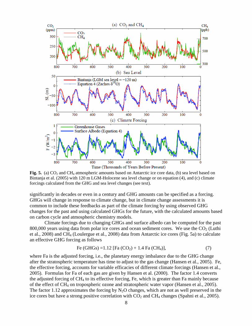
Fig. 5. (a) CO2 and CH4 atmospheric amounts based on Antarctic ice core data, (b) sea level based on Bintanja et al. (2005) with 120 m LGM-Holocene sea level change or on equation (4), and (c) climate forcings calculated from the GHG and sea level changes (see text). significantly in decades or even in a century and GHG amounts can be specified as a forcing. GHGs will change in response to climate change, but in climate change assessments it is common to include these feedbacks as part of the climate forcing by using observed GHG changes for the past and using calculated GHGs for the future, with the calculated amounts based on carbon cycle and atmospheric chemistry models. Climate forcings due to changing GHGs and surface albedo can be computed for the past 800,000 years using data from polar ice cores and ocean sediment cores. We use the CO2 (Luthi et al., 2008) and CH4 (Loulergue et al., 2008) data from Antarctic ice cores (Fig. 5a) to calculate an effective GHG forcing as follows

Fe (GHGs) =1.12 [Fa (CO2) + 1.4 Fa (CH4)], (7)

where Fa is the adjusted forcing, i.e., the planetary energy imbalance due to the GHG change after the stratospheric temperature has time to adjust to the gas change (Hansen et al., 2005). Fe, the effective forcing, accounts for variable efficacies of different climate forcings (Hansen et al., 2005). Formulas for Fa of each gas are given by Hansen et al. (2000). The factor 1.4 converts the adjusted forcing of CH4 to its effective forcing, Fe, which is greater than Fa mainly because of the effect of CH4 on tropospheric ozone and stratospheric water vapor (Hansen et al., 2005). The factor 1.12 approximates the forcing by N2O changes, which are not as well preserved in the ice cores but have a strong positive correlation with CO2 and CH4 changes (Spahni et al., 2005).

9

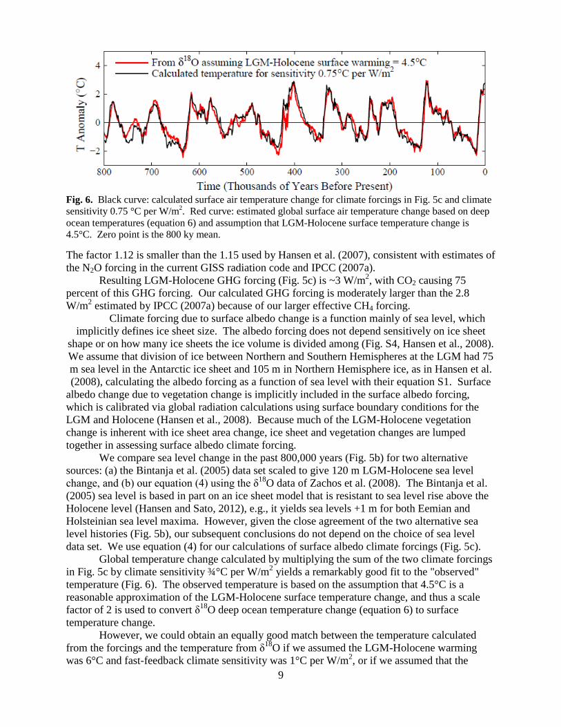
Fig. 6. Black curve: calculated surface air temperature change for climate forcings in Fig. 5c and climate sensitivity 0.75 °C per W/m2. Red curve: estimated global surface air temperature change based on deep ocean temperatures (equation 6) and assumption that LGM-Holocene surface temperature change is 4.5°C. Zero point is the 800 ky mean. The factor 1.12 is smaller than the 1.15 used by Hansen et al. (2007), consistent with estimates of the N2O forcing in the current GISS radiation code and IPCC (2007a). Resulting LGM-Holocene GHG forcing (Fig. 5c) is ~3 W/m2, with CO2 causing 75 percent of this GHG forcing. Our calculated GHG forcing is moderately larger than the 2.8 W/m2 estimated by IPCC (2007a) because of our larger effective CH4 forcing.

Climate forcing due to surface albedo change is a function mainly of sea level, which implicitly defines ice sheet size. The albedo forcing does not depend sensitively on ice sheet

shape or on how many ice sheets the ice volume is divided among (Fig. S4, Hansen et al., 2008). We assume that division of ice between Northern and Southern Hemispheres at the LGM had 75 m sea level in the Antarctic ice sheet and 105 m in Northern Hemisphere ice, as in Hansen et al. (2008), calculating the albedo forcing as a function of sea level with their equation S1. Surface

albedo change due to vegetation change is implicitly included in the surface albedo forcing, which is calibrated via global radiation calculations using surface boundary conditions for the LGM and Holocene (Hansen et al., 2008). Because much of the LGM-Holocene vegetation change is inherent with ice sheet area change, ice sheet and vegetation changes are lumped together in assessing surface albedo climate forcing. We compare sea level change in the past 800,000 years (Fig. 5b) for two alternative sources: (a) the Bintanja et al. (2005) data set scaled to give 120 m LGM-Holocene sea level change, and (b) our equation (4) using the δ18O data of Zachos et al. (2008). The Bintanja et al. (2005) sea level is based in part on an ice sheet model that is resistant to sea level rise above the Holocene level (Hansen and Sato, 2012), e.g., it yields sea levels +1 m for both Eemian and Holsteinian sea level maxima. However, given the close agreement of the two alternative sea level histories (Fig. 5b), our subsequent conclusions do not depend on the choice of sea level data set. We use equation (4) for our calculations of surface albedo climate forcings (Fig. 5c). Global temperature change calculated by multiplying the sum of the two climate forcings in Fig. 5c by climate sensitivity ¾°C per W/m2 yields a remarkably good fit to the "observed" temperature (Fig. 6). The observed temperature is based on the assumption that 4.5°C is a reasonable approximation of the LGM-Holocene surface temperature change, and thus a scale factor of 2 is used to convert δ18O deep ocean temperature change (equation 6) to surface temperature change. However, we could obtain an equally good match between the temperature calculated from the forcings and the temperature from δ18O if we assumed the LGM-Holocene warming was 6°C and fast-feedback climate sensitivity was 1°C per W/m2, or if we assumed that the

10

LGM-Holocene warming was 3°C and climate sensitivity was 0.5°C per W/m2. If LGM cooling is so uncertain as to be anywhere in the range 3-6°C, we can only conclude that the fast-feedback climate sensitivity is 3 ± 1°C for a 4 W/m2 CO2 forcing. Thus accurate knowledge of the global temperature change between glacial and interglacial states is needed for empirical evaluation of fast-feedback climate sensitivity. Before we attempt to assess the implications of Fig. 6 and make our best estimate of fast feedback climate sensitivity, we need to discuss several issues that are involved in estimates of paleoclimate temperature change and climate forcings. Strong dependence of inferred climate sensitivity on assumed LGM cooling is partly responsible for the wide range of estimated climate sensitivity in the scientific literature. Studies of Schmittner et al. (2011) and Schneider von Deimling et al. (2006) provide examples. Schmittner et al. (2011), employing a reduced-complexity climate model constrained by a specific choice of LGM boundary conditions, most importantly MARGO (2009) sea surface temperatures, obtain global LGM cooling of 3°C, from which they infer climate sensitivity 2.3°C (range 1.7-2.6°C, 66% probability) for doubled CO2. Schneider von Deimling et al. (2006), also using an intermediate complexity climate model but different LGM boundary conditions, obtain LGM cooling of 5.8 ± 1.4°C, about twice as large as found by Schmittner et al. (2011). Although the Schneider von Deimling et al. (2006) study does not focus on climate sensitivity, their result would suggest a higher climate sensitivity than that found by Schmittner et al. (2011). These model-based studies provide invaluable insight into the functioning of the climate system, because it is possible to vary processes and parameters independently, thus examining the role and importance of different climate mechanisms. However, the model studies also make clear that the results vary substantially from one model to another, and experience of the past few decades suggests that models are not likely to converge to a narrow range in the near future. Therefore there is considerable merit in also pursuing a complementary approach that estimates climate sensitivity empirically from known climate change and climate forcings. Of course the empirical approach is not fully independent of climate models. Climate forcings, for example, must be computed, and these can be obtained most accurately by using global three-dimensional fields of radiative constituents, which can be constructed with the help of global models. Similarly, the empirical global temperature change is inevitably based on observational data at only a finite number of points. Global climate models can help fill in estimates for the entire planet that are as physically consistent as possible with the data at points of observations. However, if models are used to help define "empirical" global temperature and climate forcing, the models should be used in such a way that their climate sensitivity has little or no significant influence on the calculated global temperature and climate forcing. For example, the best global atmospheric models driven by specified sea surface temperatures can do a good job of simulating global temperature, winds and water vapor distributions. Thus such models can be used to help define the distribution of radiative constituents needed to calculate accurately the global climate forcing for alternative specifications of long-lived GHGs and surface albedo. Similarly, such global models can be used to help define global surface temperature for specified atmospheric composition and surface properties such as sea surface temperature. Before describing our empirical estimate of fast-feedback climate sensitivity, we need to clarify our approach regarding aerosols. The choice of whether aerosols are counted as a climate forcing or as a fast feedback is partly responsible for the broad spread of climate sensitivities in the scientific literature. We have suggested (Hansen and Sato, 2012) that it would be best if natural aerosol changes were defined as a fast feedback, not as a climate forcing. There is nothing inherently wrong with defining aerosol changes to be a forcing, but it is practically impossible to accurately determine the aerosol forcing because it depends sensitively on the geographical and altitude distribution of aerosols, aerosol absorption, and aerosol cloud effects

11

for each of several aerosol compositions. Moreover, aerosols adjust rapidly to a changing climate, so it is logical to include natural aerosol changes in the category of fast feedbacks. The low estimates of climate sensitivity by Chylek and Lohmann (2008) and Schmittner et al. (2011), ~2°C for doubled CO2, are due in part to their inclusion of natural aerosol change as a climate forcing rather than as a fast feedback (as well as the small LGM-Holocene temperature change employed by Schmittner et al., 2011). Chylek and Lohmann (2008) assume a time variable aerosol forcing that reaches 3.3 W/m2 in the LGM, thus larger than the GHG forcing. Such a large variable aerosol forcing is inconsistent with the good fit that GHG plus surface albedo forcings yield with observed temperature change (Fig. 6). This good fit implies that either aerosol forcing is small or its variations are reasonably congruent with global climate change. It is easy to imagine that some aerosol sources, such as certain deserts, might become active rather independently of global mean temperature, but, if so, it appears that these sources are not sufficiently large to leave a big impact on global temperature. Now, before estimating fast-feedback climate sensitivity, we provide rationale for our estimates of LGM-Holocene global temperature change and LGM-Holocene climate forcing. CLIMAP (1981) reconstruction of LGM conditions, with ocean surface temperatures relying heavily upon transfer functions derived from today's distribution of ocean fauna, found little cooling of sea surface temperatures in the tropics and especially the subtropics. Numerous subsequent studies, including data for coral isotopes (Guilderson et al., 2001) and Mg/Ca ratios in pelagic sediments (Lea et al., 2000), suggest that CLIMAP at least moderately underestimated LGM cooling. CLIMAP found tropical ocean surface cooling by only -2.6 ± 1.9°C in the Atlantic Ocean and -0.1 ± 1.2°C in the Pacific Ocean, but a newer analysis by Ballantyne et al. (2005) using more data sources found overall tropical cooling of -2.7 ± 0.5°C. Terrestrial records, including an almost 1 km descent of tropical mountain snowlines (Rind and Peteet, 1985), noble gas concentrations in aquifers (Weyhenmeyer et al., 2000), and alkenones (Bard et al., 1997) provide further evidence that CLIMAP LGM cooling was underestimated. Nevertheless, the recent analysis of Schmittner et al. (2011) using a reduced complexity climate model forced by selected LGM boundary forcings, most notably MARGO (2009) sea surface temperatures, finds LGM cooling comparable to that of CLIMAP (1981). We note that the MARGO analysis excludes some data acquired in the past three decades. We suggest that fruitful models to employ with LGM boundary conditions would be the best available global atmospheric models, which would allow checking against the less ambiguous terrestrial data. Clearly all of the paleo proxy data cannot be accurate, as there are substantial inconsistencies. Global atmospheric simulations driven by alternative sea surface temperature reconstructions, along with the community's expert judgment where there are inconsistencies, should be capable of producing an advance in understanding that has been illusive for 30 years. An alternative evaluation of LGM cooling can be obtained entirely from data, with no involvement of climate models. Shakun and Carlson (2010) employ empirical orthogonal functions and 104 paleoclimate records to characterize LGM-Holocene climate change, finding a global LGM cooling of 4.9°C and reporting this as a minimum cooling, because of a paucity of observations from high latitude continental areas where cooling is expected to have been largest. Given the inconsistencies among proxy data sets, our present assessment of global LGM cooling must be partly subjective. Our central estimate, 4.5°C, chosen with cognizance of discussions in the past three decades as new data sets were compared with CLIMAP, is in the middle of the range in the paleoclimate literature. Given that a global atmospheric model driven by CLIMAP sea surface temperatures yields LGM cooling of 3.6°C (Hansen et al., 1984), and indications that CLIMAP sea surface temperatures are incompatible with terrestrial data as well as with some marine data, we believe it is unlikely that global LGM cooling was much less than 4°C. On the high side, we argue that it is unlikely that global LGM cooling was much more than

12

5°C, because (1) LGM Antarctic cooling averaged over the Vostok (Vimeux et al., 2002) and Dome C (Jouzel et al., 2007) sites was 8-9°C, while both climate models and empirical data typically yield polar amplifications of quasi-equilibrium temperature change close to a factor of two, (2) despite disagreements about LGM ocean temperatures, there is general agreement that LGM cooling was limited in the tropics and subtropics. Our estimate of LGM global cooling is thus 4.5±0.5°C, where 0.5°C is our estimated one standard deviation (σ) uncertainty. This range is meant to imply that there is about a 68% chance that the LGM global cooling was in the range 4-5°C, and about a 95% change that the cooling was in the range 3.5-5.5°C. The other quantity needed to empirically evaluate climate sensitivity is the sum of LGM-Holocene GHG and surface albedo climate forcings. Forcings are obtained by simple radiation calculations, but they have a moderate dependence on climate models, if models are employed to define the global distribution of radiative constituents such as water vapor and clouds. We use effective climate forcings, which includes efficacy of each forcing (Hansen et al., 2005). The efficacy of CO2 is unity, by definition; other forcings include a factor ("efficacy") defining how effective the forcing is in causing global temperature change relative to an equal forcing by CO2. Our estimated LGM-Holocene forcings with 1σ uncertainties are 3±0.3 W/m2 for GHGs (range 2.4-3.6 W/m2 for 95% confidence) and 3±0.7 W/m2 for surface albedo (range 1.6-4.4 W/m2 for 95% confidence). Our GHG forcing differs from 2.8 W/m2 of IPCC (2007a) because of the high efficacy (1.4) that we use for CH4. Our surface albedo forcing is in the range (2-3.3 W/m2) that Taylor et al. (2007) report for several model studies, but smaller than the 3.5 W/m2 that we used in some prior studies because we now include an estimated efficacy of 0.8-0.9 for middle latitude surface albedo forcings (Hansen et al., 1997, 2005). The total LGM-Holocene forcing (GHG + surface albedo) is 6±0.75 W/m2. (range 4.5-7.5 W/m2 for 95% confidence). Our resulting best estimate of fast feedback climate sensitivity is 3 ± 0.5°C for a 4 W/m2 CO2 forcing (0.75 ± 0.125°C per W/m2). Coincidentally the central estimate is the same as the 33-year old estimate 3 ± 1.5°C of Charney et al. (1979). The precision of the estimate based on paleoclimate data, however, is far superior to the model-based estimate of Charney et al. (1979). Indeed, the empirical paleoclimate estimate of climate sensitivity is inherently more accurate than model-based estimates because of the difficulty of simulating cloud changes (NYTimes, 2012), aerosol changes, and aerosol effects on clouds. The paleoclimate estimate could be sharpened further via a focused effort to improve evaluation of the magnitude of LGM global cooling or by an analogous study of the Eemian period.

6. Earth System Sensitivity GHG and surface albedo changes, which are treated as climate forcings for the purpose of evaluating fast-feedback climate sensitivity, are actually slow climate feedbacks. Glacial-interglacial climate swings are initiated by weak climate forcings, especially geographical and seasonal changes of insolation caused by perturbations of Earth's orbit and the tilt of Earth's spin axis (Zachos et al., 2001). The fact that GHG and surface albedo changes were slow feedbacks is confirmed by the fact that the temperature turning points generally precede the GHG and surface albedo maxima and minima (Mudelsee, 2001). Shakun et al. (2012) conclude that CO2 increase preceded surface temperature rise during the last deglaciation, but that is not inconsistent with the fact that GHGs and surface albedo are slow feedbacks. Rather it is an indication of the complexity of transitory deglaciation, when ice discharge has large temporary effects on ocean dynamics and surface temperature (Broecker et al., 1990; Rahmstorf, 1996; Manabe and Stouffer, 1997). Unlike mean glacial and interglacial states, earth is not in energy balance during deglaciation. Ice melt instigated by positive

13

Fig. 7. Schematic diagram of the equilibrium fast-feedback climate sensitivity and Earth system sensitivity that includes surface albedo slow feedbacks. insolation anomalies decreases surface albedo thus has a warming effect, but once deglaciation is underway discharge of icebergs and fresh water to the ocean causes substantial surface cooling of the ocean at even moderate rates of iceberg discharge (Hansen and Sato, 2012). This ocean surface cooling increases the planetary energy imbalance, and this imbalance continues to pump energy into the ocean, providing energy for ice melting despite the surface cooling by icebergs. Climate sensitivity including slow feedbacks is described as "Earth system sensitivity" (Lunt et al., 2010; Pagani et al., 2010; Park and Royer, 2011; Royer et al., 2011). Hansen and Sato (2012) suggest adding slow feedbacks one-by-one, creating a series of increasingly comprehensive Earth system climate sensitivities, which is the approach we follow here. Surface albedo is the first slow feedback that we add to fast feedbacks. The resulting climate sensitivity is relevant to the Cenozoic era, for example, with GHGs specified as climate forcings. Atmospheric CO2 experienced slow long-term changes during the Cenozoic as a result of plate tectonics. The CO2 changes, accompanied by changes of other GHGs (Beerling et al., 2011), are a climate forcing that can be estimated from proxy CO2 measures (Beerling and Royer, 2011) or from carbon cycle models (Berner, 2004). Cenozoic changes of temperature and sea level provide an indication of how the climate sensitivity is affected by surface albedo change. The growing amplitude of glacial-interglacial oscillations as Earth cooled during the Plio-Pleistocene (Fig. 4) is due to an increasing surface albedo feedback as ice sheet area increases. But surface albedo feedback vanishes as the ice sheets disappear. It follows that climate sensitivity including surface albedo effects is a strong function of both the climate state and the sign (positive or negative) of the climate forcing. A schematic diagram (Fig. 7) helps clarify how slow feedbacks affect climate sensitivity, making it more dependent on the initial climate state and the sign of the forcing. The fast-feedback climate sensitivity is a reasonably smooth curve, because the principal fast-feedback mechanisms (water vapor, clouds, aerosols, sea ice) do not have sharp threshold changes. Minor exceptions, such as the fact that Arctic sea ice may disappear with a relatively small increase of climate forcing above the Holocene level, might put a small wave in the fast-feedback curve.

14

Earth currently is probably near a rather flat-bottomed minimum of the fast-feedback climate sensitivity, as suggested by climate model results (Hansen et al., 2005). Our present analysis indicates that the average fast-feedback sensitivity between the Holocene and LGM is 3°C per 4 W/m2 CO2 forcing. Climate sensitivity increases rapidly as the negative forcing becomes large enough for sea ice to form in the subtropics and tropics, leading to Snowball Earth conditions (Kirschvink, 1992). The most recent Snowball Earth conditions occurred about 650 million years ago when the sun was about 6% dimmer than today. a forcing of about -15 W/m2. Earth apparently escaped snowball conditions as volcanic CO2 built up in the atmosphere as a consequence of greatly diminished weathering (Hoffman and Schrag, 2002). Climate sensitivity also increases toward large positive climate forcing, which can push Earth to the runaway greenhouse effect (Ingersoll, 1969), a condition from which there is no escape. Paleoclimate data have the potential to define the schematic climate sensitivity diagram with more quantitative detail. As an example, we mark in Fig. 6 an estimate of GHG climate forcing (+8 W/m2 relative to the Holocene, or about two doublings of CO2 amount) that existed about 55 My ago, just prior to a sudden global warming of at least 5°C, the Paleocene-Eocene Thermal Maximum (PETM, Fig. 1). Perhaps the best candidate for the added climate forcing that caused the PETM warming burst was sudden release of most of the methane hydrates that existed then (Dickens et al., 1995). However, even with the largest methane source that seems plausible, it does not seem possible to match the magnitude of the warming that occurred unless the climate sensitivity was substantially higher than 3°C for a 4 W/m2 forcing (Zeebe et al., 2009). Considering that there were no large ice sheets on Earth in the early Cenozoic, this implies that the fast feedback climate sensitivity was higher than it is today. In order for such paleoclimate data to define the climate sensitivity curve better, it will be necessary to improve our knowledge of past CO2 levels because both the background climate forcing and the PETM burst are dependent upon that knowledge. Our current sketch for climate sensitivity including the surface albedo slow feedback (Fig. 7) is advised by our analysis of Pleistocene climate change in this paper and prior papers (Hansen et al., 2008; Hansen and Sato, 2012), which shows that half of the global temperature change in the past 800,000 years is accounted for by surface albedo change. It follows that the equilibrium climate sensitivity for negative forcings with only the GHGs counted as a forcing is ~6°C for doubled CO2, which is the average for the interval from the Holocene to the LGM. The equilibrium climate sensitivity for a positive (warming) from the Holocene state depends on the magnitude of the forcing. Hansen et al. (2008) conclude that the mean sensitivity over the entire range from the Holocene to a climate just warm enough to lose the Antarctic ice sheet is almost 6°C for doubled CO2, but most of the surface albedo feedback in that range is caused by loss of the Antarctic ice sheet. The decreasing amplitude of glacial-interglacial temperature oscillations between the late Pleistocene and Pliocene (Fig. 4b) suggests that the sensitivity is smaller as climate warms from the Holocene toward a Pliocene-like climate. Thus the estimate of Lunt et al. (2010), that slow feedbacks (reduced ice and increased vegetation cover) increase the sensitivity by a factor of 1.3-1.5 is not inconsistent with the Hansen et al. (2008) estimated sensitivity. Also, in sketching the Earth system climate sensitivity we bear in mind the possibility of a hysteresis effect that makes demise of the Antarctic ice sheet difficult, thus stretching out toward larger forcing the ice sheet addition to the fast-feedback sensitivity. The next slow feedback that we add is the non-CO2 GHGs. The sensitivity including the amplification of the climate response caused by non-CO2 GHGs is relevant to the case in which CO2 is considered to be the principle climate forcing, as may be the case on long time scales as a consequence of plate tectonics. Non-CO2 trace gases are expected to increase as global temperature increases, based on chemical modeling studies (Beerling et al., 2009, 2011). Non-CO2 GHGs contributed 0.75 W/m2 of the LGM-Holocene forcing, thus amplifying CO2 forcing

15

(2.25 W/m2) by one-third (section S1 of Hansen et al., 2008). If non-CO2 trace gases are counted as a fast feedback, the fast-feedback sensitivity becomes 4°C for doubled CO2, and the Earth system sensitivity becomes 8°C for doubled CO2 with the surface albedo feedback included. The equilibrium climate sensitivity diagram (Fig. 7) is unchanged, except the numbers on the x-axis are reduced by the factor 0.75 with the a-axis being the CO2 forcing rather than the GHG forcing. These sensitivities apply for today's initial climate state and negative climate forcings; they are reduced for positive forcings, as discussed above. This sensitivity, non-CO2 gases included as a feedback, is the definition of Earth system sensitivity used by Royer et al. (2011), which may account for the high sensitivities that they estimate. The ultimate Earth system sensitivity includes all fast and slow feedbacks, i.e., surface feedbacks and all GHG feedbacks including CO2. Apparently Sff+sf is remarkably large in the Pleistocene for a negative forcing. No doubt that accounts for the substantial cooling of Earth in the past few million years in response to only small changes of CO2., as well as the increasingly violent glacial-to-interglacial oscillations of the late Pleistocene (Fig. 4). The Earth system sensitivity relevant to humanity now is the sensitivity of the present climate state to a positive (warming) forcing. That sensitivity is not as great as for a negative forcing, but it is much larger than the 3°C fast-feedback climate sensitivity. Our present analysis concerns quasi-equilibrium climate sensitivities. The inertia of the global ocean and ice sheets implies that a quasi-equilibrium response will not be approached on the time scale of a human lifetime. On the other hand, the lifetime of fossil fuel carbon inserted into the climate system is millennia, so the Earth system sensitivity has relevance to the eventual climate response. Moreover, the rapidity with which the human-caused positive forcing is being introduced has no known analog in Earth's history. It is thus exceedingly difficult to foresee the consequences if the human-made climate forcing continues to accelerate.

7. Summary There is a widespread perception that climate sensitivity should be represented by a probability distribution function that is extremely broad, a function that includes rather small climate sensitivities and has a long tail extending to very large sensitivities. That perception, we argue, is wrong. God (Nature) plays dice, but not for such large amounts. We note here several key reasons for perceptions about our knowledge of climate sensitivity. First, there is an emphasis on climate models for studying climate sensitivity with an implicit belief that as long as climate models are deficient in their ability to simulate nature, climate sensitivity remains very uncertain. Model sensitivity is uncertain, to be sure, as illustrated by recent discussion of the difficulty of modeling clouds (Gillis, 2012). Aerosol feedbacks and the effect of these on clouds make a strict modeling approach a daunting task. However, climate science has a number of tools or approaches for assessing climate sensitivity, and the accuracy of the result will be set by the sharpest tool in the toolbox, a description that does not seem to fit pure climate modeling. Second, there is, understandably, an emphasis on analysis of the period disturbed by human climate forcings, especially the past century, and it is found that a broad range of climate sensitivities are consistent with observed climate change, because the net climate forcing is very uncertain. Focus on the era of human-made climate change is appropriate, but, until the large uncertainty in aerosol climate forcing is addressed with adequate observations, ongoing climate change will not provide a sharp definition of climate sensitivity. Third, there is a perception that paleoclimate changes are exceedingly complex, hard to understand, and indicative of a broad spectrum of climate sensitivities. To be sure, as we have emphasized, the huge climate variations in Earth's history emphasize the dependence of climate

16

sensitivity on the initial climate state as well as the dependence on the magnitude and sign of the climate forcing. However, the paleoclimate record, because of its richness, has the potential to provide valuable, and accurate, information on climate sensitivity. We have made a case that the paleoclimate data already restricts the fast-feedback climate sensitivity from Holocene initial conditions to the moderately narrow range 3 ± 0.5°C for a 4 W/m2 CO2 forcing, but this still leaves a large range (2-4°C) for 95 percent confidence. We suggest that the uncertainty could be reduced substantially via appropriate focused efforts to define paleoclimate global temperature change and paleoclimate forcings with the help of the most relevant climate models. In particular the uncertainty in the magnitude of global cooling during the Last Glacial Maximum is a principle constraint on better assessment of the fast-feedback climate sensitivity. The climate research community, interpreting the large array of data now available for the LGM with the help of the best available global three-dimensional models, should be able to define surface conditions with improved accuracy. The large climate change that occurred at the onset of the prior (Eemian) interglacial period would also be a useful period to study. The potential magnitude of the human-made climate forcing and the fact that fossil fuel carbon dioxide will remain in the surface climate system for millennia make it important that we also understand slow climate feedbacks and Earth system climate sensitivity. Indeed, the paleoclimate record already makes clear that, overall, slow feedbacks considerably amplify climate sensitivity. The human-made climate forcing seems to be unique in its rapidity of growth, which demands a research approach that focuses on understanding the relevant processes and on constructing models or other analysis tools that help predict likely outcomes. A focus on improving the data and modeling of relatively rapid events, such as deglaciation and PETM-like rapid warming events may be especially fruitful. Acknowledgments. We thank James Zachos for the deep ocean oxygen isotope data, Mark Chandler, Dorothy Peteet, David Rind for helpful information, Gerry Lenfest (Lenfest Foundation), ClimateWorks, Lee Wasserman (Rockefeller Family Foundation), Stephen Toben (Flora Family Foundation) and NASA program managers Jack Kaye and David Considine for research support. .

References Ballantyne, A.P., Lavine, M., Crowley, T.J., Liu, J. & Baker, P.B. 2005 Meta-analysis of tropical

surface temperatures during the Last Glacial Maximum. Geophys. Res. Lett. 32, L05712. (doi:10.1029/2004GL021217)

Bard E., Rostek, F. & Sonzogni, C. 1997 Interhemispheric synchrony of the last deglaciation inferred from alkenone palaeothermometry. Nature 385, 707-710.

Beerling D.J. & Royer D.L. 2011 Convergent Cenozoic CO2 history. Nat. Geosci. 4, 418-420.

Beerling, D.J., Berner, R.A., Mackenzie, F.T., Harfoot, M. & Pyle, J.A. 2009 Methane and the CH4-related greenhouse effect over the past 400 million years. Am. J. Sci. 309, 97-113.

Beerling, D.J., Fox, A., Stevenson, D.S. & Valdes, P.J. 2011 Enhanced chemistry-climate feedbacks in past greenhouse worlds. . Natl. Acad. Sci. USA. 108, 9770-9775.

Berner, R.A. 2004 The Phanerozoic Carbon Cycle: C02 and O2. Oxford Univ Press, New York, 150 pp.

17

Bintanja, R., van de Wal, R. S. W. & Oerlemans, J. 2005 Modelled atmospheric temperatures and global sea levels over the past million years. Nature 437, 125-128.

Broecker, W.S., et al. 1990 Accelerator Mass-Spectrometric Radiocarbon Measurements on Foraminifera Shells from Deep-Sea Cores. Radiocarbon 32, 119-133.

Charney, J. G., Arakawa, A., Baker, D., Bolin, B., Dickerso, R., Goody, R., Leith, C., Stommel, H.M. & Wunsch, C.I. 1979 Carbon dioxide and climate: a scientific assessment. Washington, DC. National Academy of Sciences Press.

Chylek, P. & Lohmann, U. 2008: Aerosol radiative forcing and climate sensitivity deduced from the last glacial maximum to Holocene transition. Geophys. Res. Lett. 35, L04804

CLIMAP Project Member, McIntyre. A., project leader 1981 Seasonal reconstruction of earth's surface at the last glacial maximum. Geol. Soc. Amer., Map and Chart Series, No. 36.

Colman, R. & McAvaney 2009 Climate feedbacks under a broad range of forcing, Geophys. Res. Lett. 36, L01702.

Dickens, G.R., O'Neil, J.R. Rea, D.K. & Owen, R.M. 1995 Dissociation of oceanic methane hydrate as a cause of the carbon isotope excursion at the end of the Paleocene, Paleoceanography 10, 965-971.

Dowsett, H. J., Barron, J. A., Poore, R. Z., Thompson, R. S., Cronin, T. M., Ishman, S. E. & Willard, D. A. 1999 Middle Pliocene Paleoenvironmental Reconstruction: PRISM 2. U.S. Geological Survey Open File Report 236, 99-535.

Dwyer, G.S. & Chandler, M.A. 2009 Mid-Pliocene sea level and continental ice volume based on coupled benthic Mg/Ca palaeotemperatures and oxygen isotopes. Phil. Trans. R. Soc. A. 367, 157-168.

Fairbanks, R. G. 1989 A 17,000-Year Glacio-Eustatic Sea-Level Record-Influence of Glacial Melting Rates on the Younger Rates on the Younger Dryas Event and Deep-Ocean Circulation. Nature 342, 637-642.

Gillis, J. 2012 Clouds effect on climate change is last bastion for dissenters. New York Times, 30 April, 2012. (http://www.nytimes.com/2012/05/01/science/earth/clouds-effect-on-climate-change-is-last-bastion-for-dissenters.html?_r=1&pagewanted=all)

Guilderson, T.P., Fairbanks, R.G. & Rubenstone, J.L. 2001 Tropical Atlantic coral isotopes: glacial-interglacial sea surface temperatures and climate change. Mar. Geol. 172, 75-89.

Hansen, J. E. & Sato, M. 2012 Paleoclimate implications for human-made climate change. in Climate Change: Inferences from Paleoclimate and Regional Aspects. Berger A., Mesinger, F. & Sijacki, D. (Eds.), Springer, 270 pp.

Hansen, J.E., et al. Takahashi, T. & American Geophysical, U. 1984 Climate processes and climate sensitivity. American Geophysical Union, Washington, D.C., vii, 368 pp.

Hansen, J., Sato, M. & Ruedy, R. 1997 Radiative forcing and climate response. J. Geophys. Res. 102, 6831-6864.

Hansen, J., Sato, M., Ruedy, R., Lacis, A. & Oinas, V. 2000 Global warming in the twenty-first century: An alternative scenario. Proc. Nat. Acad. Sci. USA. 97, 9875-9880.

Hansen, J., et al. 2005 Efficacy of climate forcings. J. Geophys. Res. 110, D18104.

Hansen, J., et al. 2007 Climate change and trace gases. Phil. Trans. R. Soc. A. 305, 1925-1954.

18

Hansen, J., et al. 2008 Target Atmospheric CO2: Where Should Humanity Aim?. Open Atmos. Sci. J. 2, 217-231.

Hansen, J., et al. 2012 Scientific case for avoiding dangerous climate change to protect young people and nature. arXiv 1110.1365.

Hoffman, P.F. & Schrag, D.P. 2002 The snowball Earth hypothesis: Testing the limits of global change. Terra Nova 14, 129-155.

Ingersoll, A.P. 1969 Runaway greenhouse - a history of water on Venus. J. Atmos. Sci. 26, 1191-1198.

Intergovernmental Panel on Climate Change (IPCC), 2007a: Climate Change 2007: The Physical Science Basis. Solomon, S., et al. eds., Cambridge University Press, 996 pp.

Jones, P.D., New, M., Parker, D.E., Martin, S. & Rigor, I.G. 1999 Surface air temperature and its changes over the past 150 years. Rev. Geophys. 37, 173-199.

Jouzel, J., et al. 2007 Orbital and millennial Antarctic climate variability over the past 800,000 years. Science 317, 793-796.

Kirschvink, J.L. 1992 Late Proterozoic low-latitude global glaciation: the snowball earth. In: The Proterozoic Biosphere (J.W. Schopf & C. Klein, eds), pp. 51-52, Cambridge Univ. Press.

Kopp, R. E., Simons, F. J., Mitrovica, J. X., Maloof, A. C. & Oppenheimer, M. 2009 probabilistic assessment of sea level during the last interglacial stage. Nature 462, 863-867.

Lea, D.W., Pak, D.K. & Spero, H.J. 2000 Climate impact of late Quaternary equatorial Pacific sea surface temperature variations. Science, 289, 1719-1724.

Lorius, C., Jouzel, J., Raynaud, D., Hansen, J. & Letreut, H. 1990 The Ice-Core Record - Climate Sensitivity and Future Greenhouse Warming. Nature 347, 139-145.

Loulergue, L., et al. 2008 Orbital and millennial-scale features of atmospheric CH4 over the past 800,000 years. Nature 453, 383-386.

Lunt, D.J., et al. 2010 Earth system sensitivity inferred from Pliocene modelling and data. Nat. Geosci. 3, 60-64.

Luthi, D., et al. 2008 High-resolution carbon dioxide concentration record 650,000-800,000 years before present. Nature 453, 379-382.

Manabe, S. & Stouffer, R.J. 1997 Coupled ocean-atmosphere model response to freshwater input: Comparison to Younger Dryas event. Paleoceanography 12, 321-336.

MARGO Project Members, 2009 Constraints on the magnitude and patterns of ocean cooling at the Last Glacial Maximum. Nat. Geosci. 2, 127.

Mudelsee, M. 2001 The phase relations among atmospheric CO2 content, temperature and global ice volume over the past 420 ka. Quat. Sci. Rev., 20, 583-589.

Pagani, M., Liu, Z.H., LaRiviere, J. & Ravelo, A.C. 2010 High Earth-system climate sensitivity determined from Pliocene carbon dioxide concentrations. Nat. Geosci. 3, 27-30.

Park, J. & Royer, D.L. 2011 Geologic Constraints on the Glacial Amplification of Phanerozoic Climate Sensitivity. Am. J. Sci. 311, 1-26.

19

Peltier, W. R. & Fairbanks, R. G. 2006 Global glacial ice volume and Last Glacial Maximum duration from an extended Barbados sea level record. Quat. Sci. Rev. 25, 3322-3337.

Rahmstorf, S. 1996 On the freshwater forcing and transport of the Atlantic thermohaline circulation. Clim. Dynam. 12, 799-811.

Raymo, M. E. & Mitrovica, J. X. 2012 Collapse of polar ice sheets during the stage 11 interglacial. Nature 483, 453-456.

Raymo, M. E., Mitrovica, J.X. O'Leary, M.J. DeConto, R.M. & Hearty, P.J. 2011 Departures from eustasy in Pliocene sea-level records, Nat. Geosci. 4, 328-332.

Rind, D. & Peteet, D. 1985 Terrestrial conditions at the Last Glacial Maximum and CLIMAP sea-surface temperature estimates: Are they consistent?, Quat. Res. 24, 1-22.

Royer D.L., Pagani, M. & Beerling, D.J. 2012. Geobiological constraints on Earth system sensitivity to CO2 during the Cretaceous and Cenozoic. Geobiology. (doi: 10.1111/j.1472-4669.2012.00320.x)

Schmittner, A., et al. 2011 Climate Sensitivity Estimated from Temperature Reconstructions of the Last Glacial Maximum. Science 334, 1385-1388.

Schneider von Deimling, T., Ganopolski, A., Held, H. & Rahmstorf, S. 2006: How cold was the Last Glacial Maximum?. Geophys. Res. Lett. 33, L14709. (doi:10.1029/2006GL026484)

Shakun, J.D. and Carlson, A.E. 2010 A global perspective on Last Glacial Maximum to Holocene climate change. Quarter. Sci. Rev. 29, 1801-1816.

Shakun, J.D., et al. 2012 Global warming preceded by increasing carbon dioxide concentrations during the last deglaciation. Nature 484, 49-U1506.

Siddall, M., et al. 2003 Sea-level fluctuations during the last glacial cycle. Nature 423, 853-858.

Spahni, R., et al. 2005 Atmospheric methane and nitrous oxide of the late Pleistocene from Antarctic ice cores. Science, 310, 1317-1321.

Taylor, K.E. et al. 2007 Estimating shortwave radiative forcing and response in climate models. J. Clim. 20, 2530-2543.

Vimeux, F., Cuffey, K.M. & Jouzel, J. 2002 New insights into Southern Hemisphere temperature changes from Vostok ice cores using deuterium excess correction. Earth Planet. Sc. Lett, 203, 829-843.

Waelbroeck, C., et al. 2002 Sea-level and deep water temperature changes derived from benthic foraminifera isotopic records. Quatern. Sci. Rev. 21, 295-305.

Weyhenmeyer, C., Burns, S., Weber, H., Aeschback-Hertig, W., Kipfer, R., Loosli, H. & Matter, A. 2000 Cool glacial temperatures and changes in moisture source recorded in Oman groundwaters. Science 287, 842-845.

Zachos, J., Pagani, M., Sloan, L., Thomas, E., & Billups, K. 2001: Trends, rhythms, and aberrations in global climate 65 Ma to present. Science 292, 686-693.

Zachos, J.C., Dickens, G.R. & Zeebe, R.E. 2008 An Early Cenozoic perspective on greenhouse warming and carbon-cycle dynamics. Nature 451, 279-283.

Zeebe, R.E., Zachos, J.C. & Dickens, G.R. 2009 Carbon dioxide forcing alone insufficient to explain Palaeocene-Eocene Thermal Maximum warming. Nat. Geosci. 2, 576-580.