Climate prediction as a multiscale problem: from the ... · Climate prediction as a multiscale problem: from the diurnal scale to the multidecadal climate variability . Pedro Leite

Climate prediction as a multiscale problem: from the diurnal scale to the multidecadal climate variability

Pedro Leite da Silva Dias Laboratório Nacional de Computação Científica/MCTI

Instituto de Astronomia, Geofísica e Ciêncas Atmosféricas/USP

1. Goal : are models able reproduce interaction between diurnal/synoptic, intraseasonal, annual, interannual and decadal variability.

2. High resolution models is a solution - seamless prediction - costly!

1. Multiscaling modeling - understanding scale interactions –

non linear effects 1. Going from the diurnal to intraseasonal with atmospheric

models 2. Possible decadal signal in an atmospheric model with

parameterized diurnal heating 3. Simplified couples atmosphere/ocean models: 3 scale

interaction 2. Future.

Outline

Complexities of SAMS: significant variability at different time scales

The Last Millenium in South America

LIAMCA

600 800 1000 1200 1400 1600 1800 2000-7.5-7.0-6.5-6.0-5.5-5.0-4.5-4.0

Wet

Wet

Dry

δOSouthernBrazil

Years A.D

-7.6-7.8-8.0-8.2-8.4 δO C h i n a

600 800 1000 1200 1400 1600 1800 2000-0.5-1.0-1.5-2.0-2.5-3.0-3.5-4.0

δOFN1Nordeste

LIAMCA

600 800 1000 1200 1400 1600 1800 2000-7.5-7.0-6.5-6.0-5.5-5.0-4.5-4.0

Wet

Wet

Dry

δOSouthernBrazil

Years A.D

-7.6-7.8-8.0-8.2-8.4 δO C h i n a

600 800 1000 1200 1400 1600 1800 2000-0.5-1.0-1.5-2.0-2.5-3.0-3.5-4.0

δOFN1Nordeste

LIAMCA

600 800 1000 1200 1400 1600 1800 2000-7.5-7.0-6.5-6.0-5.5-5.0-4.5-4.0

Wet

Wet

Dry

δOSouthernBrazil

Years A.D

-7.6-7.8-8.0-8.2-8.4 δO C h i n a

600 800 1000 1200 1400 1600 1800 2000-0.5-1.0-1.5-2.0-2.5-3.0-3.5-4.0

δOFN1Nordeste

LIAMCA

600 800 1000 1200 1400 1600 1800 2000-7.5

-7.0

-6.5

-6.0

-5.5

-5.0

-4.5

-4.0

Wet

Wet

Dry

δ18O

Sout

hern

Braz

il

Years A.D

-7.6

-7.8

-8.0

-8.2

-8.4

δ18O

China

600 800 1000 1200 1400 1600 1800 2000-0.5

-1.0

-1.5

-2.0

-2.5

-3.0

-3.5

-4.0

δ18O

FN1

Nor

dest

e

China

NE Brasil

SE Brasil

Dry

Wet

Cruz et al. 2011

Interesting point: •Mud data in Plata => Picomyo and Bermejo River - NW Argentina/Bolivia – summer rain

•Biased towards western part of the Plata •Need marker for the eastern •Different regimes E/W Plata Basin

Work in collaboration with IRD, INPE, USP, UFF,LNCC…

-3

-2

-1

0

1

2

3

1 13 25 37 49 61

-3

-2

-1

0

1

2

3

Northern Amazonia Rainfall Index (NAR)

Southern Amazonia Rainfall Index (SAR)

A

B

Marengo 2004

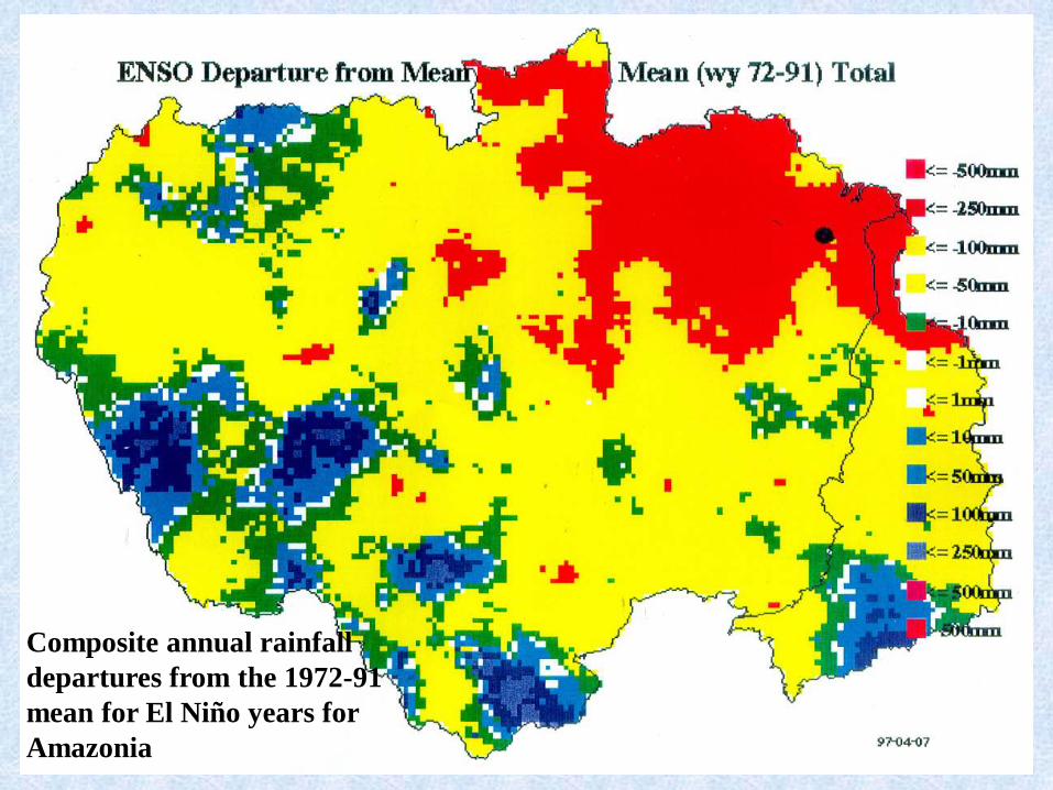
Composite annual rainfall departures from the 1972-91 mean for El Niño years for Amazonia

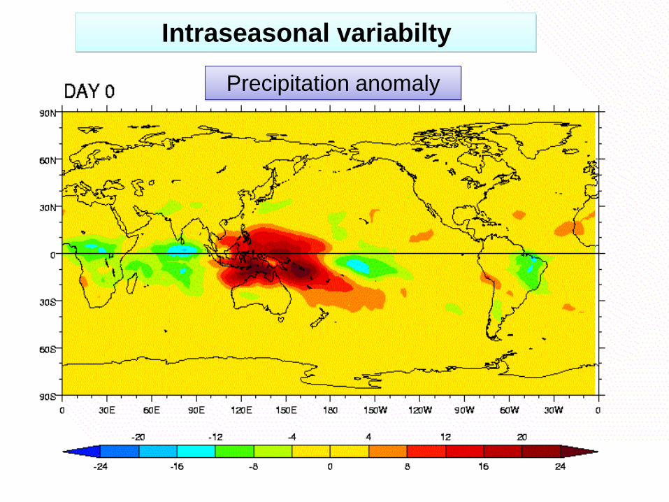
Intraseasonal variabilty

Precipitation anomaly

Herdies et al. 2001

(shaded)

Mean moisture flux and divergence in active and non active phases of the SACZ – 20-60 days.

Diurnal Variability

A general problem with >15d forecasts and seasonal forecasts: • lack of power in the intraseasonal time scale

Power spectra of meridional wind at 40S , 60W – CPTEC – From seasonal forecasting model

S. Ferraz and P. Silva Dias – prep.

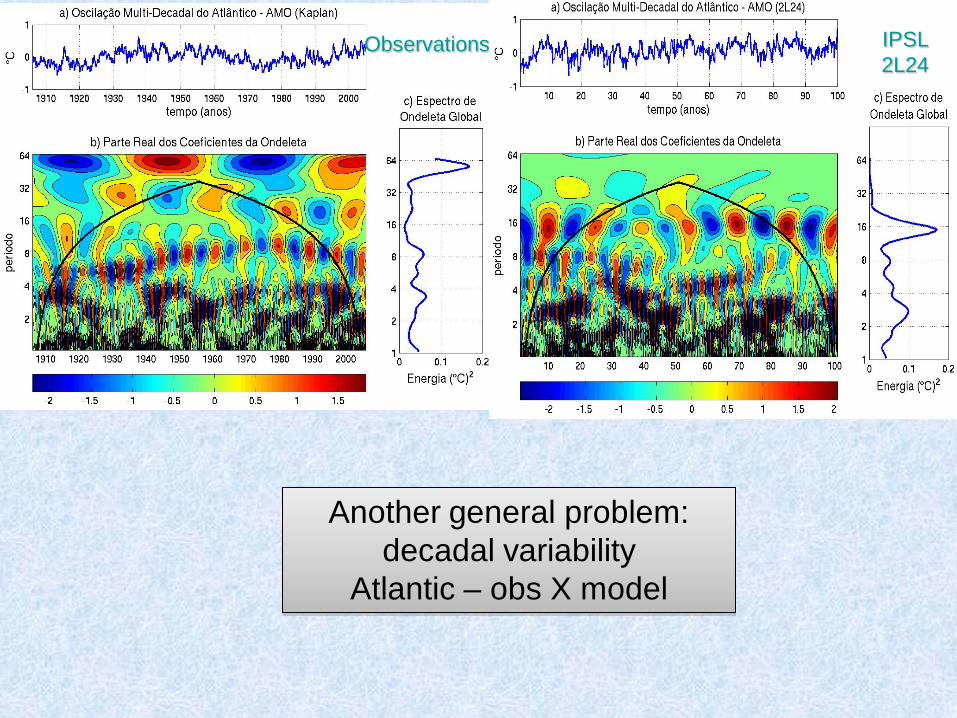
Observations IPSL 2L24

Another general problem: decadal variability

Atlantic – obs X model

Observação

(dados de Mantua et al., 1997)

IPSL 2L24

Decadal variability PDO – obs X model

Another problem with low resolution models:

Clouds in the Amazon

GOES-10 26-27 April 2007

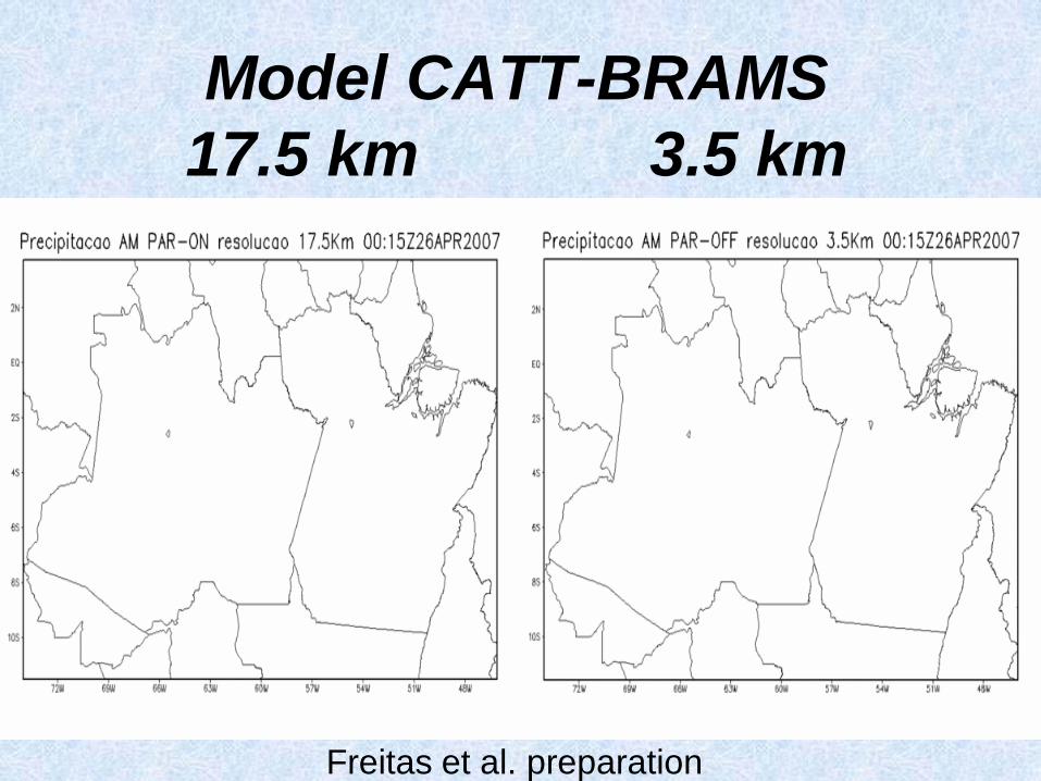
Model CATT-BRAMS 17.5 km 3.5 km

Freitas et al. preparation

The Model for Prediction Across Scales • We are well advanced on developing the

next-generation Model for Prediction Across Scales

• Based on high spectral models or unstructured Voronoi (hexagonal) meshes and selective grid refinement (e.g., OLAM) with finite volume differencing scheme.

• To be utilized for weather, regional and global climate applications.

• Finite volume versions allows for non-hydrostatic (< 10 km horizontal resolution)

• Work towards exascale computing

Nonlinearities: Interaction among different time scales ….

Model Equations:

(1)

N =

u(x,y,t)

v(x,y,t)

Φ(x,y,t)

ξ =

Zonal and meridional Componentes of wind and geopotencial

0 0 FΦ(x,y,t)

F= --u∂u/∂x +v∂u/∂y

u∂v/∂x + v∂v/∂y

u∂φ/∂x +v∂φ/∂y + φ∇.V

Boundary conditions

Zonal periodicity: ξ (x+Lx,y,t)= ξ(x,y,t) (2)

ξ(x,y,t)→0 as y→±∞ (3)

• Shallow-Water model on the equatorial β-plane in the nondimension

form:

Linear operator Forcing terms Nonlinear

terms

Raupp, C. F. M. and Silva Dias, P. L. 2004,2005

Effect of basic flow of January climatology – Stationary mass source

Effect of basic flow of January climatology Source Modulation

00.5

11.5

22.5

33.5

0 2 3 4 6 7 8 10 11 12 14 15 16 18 19 20 22 23

Hour

Sour

ce a

mpl

itude

Question: is it possible for an inertio-gravity wave mode to significantly interact with a Rossby mode so as to lead the latter to undergo significant amplitude modulation?

Governing Equations –simple model with parameterized heat source

Two-layer incompressible equatorial primitive equations:

1111000 divVVVVpyV

tV

−∇•−=∇++∂∂ ⊥

0div 0 =V

0110111 VVVVpyV

tV

∇•−∇•−=∇++∂∂ ⊥

1010

22

2

11

2gπdiv pVS

TcNHV

tp

p

∇•−−=+∂∂

(1a)

(1b)

(1c)

(1d)

N ⇒ Brunt-Vaissala frequency (N ≈ 10-2 s-1 ⇒ Typical tropospheric value)

H ⇒ Top height of the Troposphere (H ≈ 16Km in the tropics);

g ⇒ gravity acceleration (g ≈ 10 ms-2 )

Cp ⇒ thermal capacity of dry air at constant pressure (Cp= 1004J/KKg);

T0 ≈ 15º C (reference value of temperature)

S1 ⇒ thermal forcing (parametric heat source)

Barotropic mode

First baroclinic mode

Example of nonlinear Resonance: Energy in gravity waves (diurnal) interacting with Rossby waves (synoptic) under proper large scale background field => intraseasonal modulation

Nonlinearity => energy transfer among scales Dynamics of resonant interaction through advection terms •Examples:

•Interaction between slow ( O(5-7days) ) and fast modes ( O(1 day or less) ) => intraseasonal scales (20-60 days) Raupp and Silva Dias. (2004,2005,2006, 2008)

•Importance of diurnal variation leading to energy in intraseasonal time scales (Raupp and Silva Dias, 2009,2010)

•Coupled ocean/atmosphere simplified models: interaction between intraseasonal scale ( O(20-60d) ) with interannual (El Nino/La Nina) - O (2-3 yr) => decadal/multidecadal time scales (Enver et al. 2009,2011)

Multiscaling modeling

model for studying multiscaling : from MJO to

Multidecadal variability

Search for Resonant Nonlinear

Interactions - physics coupling

Enver Ramirez ,Carlos Raupp and Pedro L. Silva Dias

Multiscale Perturbative Method

Resonant Nonlinear Interactions

Simplified coupled model resonant interaction: atmospheric Kelvin (moist)(green), Rossby atmosphere (dry – green) and ocean Kelvin (blue)

Simplified models are quite useful for understanding basic interaction mechanisms of the

ocean/atmosphere!!

Clearly show mechanisms responsible for diurnal to decadal variability!!!!!

Conclusion

From Enver, Silva Dias and Raupp (2012 – in preparation)

Thanks!!!

[email protected]