Climate Models and Their · PDF fileClimate Models and Their Evaluation ... Climate Change 2007: The Physical Science Basis. Contribution of ... 8.4 Evaluation of Large-Scale Climate

8

Climate Models

and Their Evaluation

Coordinating Lead Authors:David A. Randall (USA), Richard A. Wood (UK)

Lead Authors:Sandrine Bony (France), Robert Colman (Australia), Thierry Fichefet (Belgium), John Fyfe (Canada), Vladimir Kattsov (Russian Federation),

Andrew Pitman (Australia), Jagadish Shukla (USA), Jayaraman Srinivasan (India), Ronald J. Stouffer (USA), Akimasa Sumi (Japan),

Karl E. Taylor (USA)

Contributing Authors:K. AchutaRao (USA), R. Allan (UK), A. Berger (Belgium), H. Blatter (Switzerland), C. Bonfi ls (USA, France), A. Boone (France, USA),

C. Bretherton (USA), A. Broccoli (USA), V. Brovkin (Germany, Russian Federation), W. Cai (Australia), M. Claussen (Germany),

P. Dirmeyer (USA), C. Doutriaux (USA, France), H. Drange (Norway), J.-L. Dufresne (France), S. Emori (Japan), P. Forster (UK),

A. Frei (USA), A. Ganopolski (Germany), P. Gent (USA), P. Gleckler (USA), H. Goosse (Belgium), R. Graham (UK), J.M. Gregory (UK),

R. Gudgel (USA), A. Hall (USA), S. Hallegatte (USA, France), H. Hasumi (Japan), A. Henderson-Sellers (Switzerland), H. Hendon (Australia),

K. Hodges (UK), M. Holland (USA), A.A.M. Holtslag (Netherlands), E. Hunke (USA), P. Huybrechts (Belgium),

W. Ingram (UK), F. Joos (Switzerland), B. Kirtman (USA), S. Klein (USA), R. Koster (USA), P. Kushner (Canada), J. Lanzante (USA),

M. Latif (Germany), N.-C. Lau (USA), M. Meinshausen (Germany), A. Monahan (Canada), J.M. Murphy (UK), T. Osborn (UK),

T. Pavlova (Russian Federationi), V. Petoukhov (Germany), T. Phillips (USA), S. Power (Australia), S. Rahmstorf (Germany),

S.C.B. Raper (UK), H. Renssen (Netherlands), D. Rind (USA), M. Roberts (UK), A. Rosati (USA), C. Schär (Switzerland),

A. Schmittner (USA, Germany), J. Scinocca (Canada), D. Seidov (USA), A.G. Slater (USA, Australia), J. Slingo (UK), D. Smith (UK),

B. Soden (USA), W. Stern (USA), D.A. Stone (UK), K.Sudo (Japan), T. Takemura (Japan), G. Tselioudis (USA, Greece), M. Webb (UK),

M. Wild (Switzerland)

Review Editors:Elisa Manzini (Italy), Taroh Matsuno (Japan), Bryant McAvaney (Australia)

This chapter should be cited as:Randall, D.A., R.A. Wood, S. Bony, R. Colman, T. Fichefet, J. Fyfe, V. Kattsov, A. Pitman, J. Shukla, J. Srinivasan, R.J. Stouffer, A. Sumi

and K.E. Taylor, 2007: Cilmate Models and Their Evaluation. In: Climate Change 2007: The Physical Science Basis. Contribution of

Working Group I to the Fourth Assessment Report of the Intergovernmental Panel on Climate Change [Solomon, S., D. Qin, M. Manning,

Z. Chen, M. Marquis, K.B. Averyt, M.Tignor and H.L. Miller (eds.)]. Cambridge University Press, Cambridge, United Kingdom and New

York, NY, USA.

590

Climate Models and Their Evaluation Chapter 8

Table of Contents

Executive Summary .................................................... 591

8.1 Introduction and Overview ............................ 594

8.1.1 What is Meant by Evaluation? ............................. 594

8.1.2 Methods of Evaluation ......................................... 594

8.1.3 How Are Models Constructed? ........................... 596

8.2 Advances in Modelling .................................... 596

8.2.1 Atmospheric Processes ....................................... 602

8.2.2 Ocean Processes ................................................ 603

8.2.3 Terrestrial Processes ........................................... 604

8.2.4 Cryospheric Processes........................................ 606

8.2.5 Aerosol Modelling and Atmospheric Chemistry ............................................................ 607

8.2.6 Coupling Advances ............................................. 607

8.2.7 Flux Adjustments and Initialisation ...................... 607

8.3 Evaluation of Contemporary Climate as Simulated by Coupled Global Models........ 608

8.3.1 Atmosphere ......................................................... 608

8.3.2 Ocean .................................................................. 613

8.3.3 Sea Ice ................................................................. 616

8.3.4 Land Surface ....................................................... 617

8.3.5 Changes in Model Performance .......................... 618

8.4 Evaluation of Large-Scale Climate Variability as Simulated by Coupled Global Models ..................................................... 620

8.4.1 Northern and Southern Annular Modes ............. 620

8.4.2 Pacifi c Decadal Variability .................................. 621

8.4.3 Pacifi c-North American Pattern ......................... 622

8.4.4 Cold Ocean-Warm Land Pattern ........................ 622

8.4.5 Atmospheric Regimes and Blocking .................. 623

8.4.6 Atlantic Multi-decadal Variability ........................ 623

8.4.7 El Niño-Southern Oscillation .............................. 623

8.4.8 Madden-Julian Oscillation .................................. 625

8.4.9 Quasi-Biennial Oscillation .................................. 625

8.4.10 Monsoon Variability ............................................ 626

8.4.11 Shorter-Term Predictions Using Climate Models .................................................. 626

8.5 Model Simulations of Extremes ..................... 627

8.5.1 Extreme Temperature .......................................... 627

8.5.2 Extreme Precipitation .......................................... 628

8.5.3 Tropical Cyclones ................................................ 628

8.5.4 Summary ............................................................. 629

8.6 Climate Sensitivity and Feedbacks ............... 629

8.6.1 Introduction ......................................................... 629

8.6.2 Interpreting the Range of Climate Sensitivity Estimates Among General Circulation Models .... 629

Box 8.1: Upper-Tropospheric Humidity and Water Vapour Feedback .............................................. 632

8.6.3 Key Physical Processes Involved in Climate Sensitivity ............................................... 633

8.6.4 How to Assess Our Relative Confi dence in Feedbacks Simulated by Different Models?........ 639

8.7 Mechanisms Producing Thresholds and Abrupt Climate Change ................................... 640

8.7.1 Introduction ......................................................... 640

8.7.2 Forced Abrupt Climate Change ........................... 640

8.7.3 Unforced Abrupt Climate Change ....................... 643

8.8 Representing the Global System with Simpler Models .................................................... 643

8.8.1 Why Lower Complexity? ..................................... 643

8.8.2 Simple Climate Models....................................... 644

8.8.3 Earth System Models of Intermediate Complexity........................................................... 644

Frequently Asked QuestionFAQ 8.1: How Reliable Are the Models Used to Make Projections of Future Climate Change? .................. 600

References ........................................................................ 648

Supplementary Material

The following supplementary material is available on CD-ROM and in on-line versions of this report.Figures S8.1–S8.15: Model Simulations for Different Climate Variables

Table S8.1: MAGICC Parameter Values

591

Chapter 8 Climate Models and Their Evaluation

Executive Summary

This chapter assesses the capacity of the global climate models used elsewhere in this report for projecting future climate change. Confi dence in model estimates of future climate evolution has been enhanced via a range of advances since the IPCC Third Assessment Report (TAR).

Climate models are based on well-established physical principles and have been demonstrated to reproduce observed features of recent climate (see Chapters 8 and 9) and past climate changes (see Chapter 6). There is considerable confi dence that Atmosphere-Ocean General Circulation Models (AOGCMs) provide credible quantitative estimates of future climate change, particularly at continental and larger scales. Confi dence in these estimates is higher for some climate variables (e.g., temperature) than for others (e.g., precipitation). This summary highlights areas of progress since the TAR:

• Enhanced scrutiny of models and expanded diagnostic analysis of model behaviour have been increasingly facilitated by internationally coordinated efforts to collect and disseminate output from model experiments performed under common conditions. This has encouraged a more comprehensive and open evaluation of models. The expanded evaluation effort, encompassing a diversity of perspectives, makes it less likely that signifi cant model errors are being overlooked.

• Climate models are being subjected to more comprehensive tests, including, for example, evaluations of forecasts on time scales from days to a year. This more diverse set of tests increases confi dence in the fi delity with which models represent processes that affect climate projections.

• Substantial progress has been made in understanding the inter-model differences in equilibrium climate sensitivity. Cloud feedbacks have been confi rmed as a primary source of these differences, with low clouds making the largest contribution. New observational and modelling evidence strongly supports a combined water vapour-lapse rate feedback of a strength comparable to that found in General Circulation Models (approximately 1 W m–2 °C–1, corresponding to around a 50% amplifi cation of global mean warming). The magnitude of cryospheric feedbacks remains uncertain, contributing to the range of model climate responses at mid- to high latitudes.

• There have been ongoing improvements to resolution, computational methods and parametrizations, and additional processes (e.g., interactive aerosols) have been included in more of the climate models.

• Most AOGCMs no longer use fl ux adjustments, which were previously required to maintain a stable climate.

At the same time, there have been improvements in the simulation of many aspects of present climate. The uncertainty associated with the use of fl ux adjustments has therefore decreased, although biases and long-term trends remain in AOGCM control simulations.

• Progress in the simulation of important modes of climate variability has increased the overall confi dence in the models’ representation of important climate processes. As a result of steady progress, some AOGCMs can now simulate important aspects of the El Niño-Southern Oscillation (ENSO). Simulation of the Madden-Julian Oscillation (MJO) remains unsatisfactory.

• The ability of AOGCMs to simulate extreme events, especially hot and cold spells, has improved. The frequency and amount of precipitation falling in intense events are underestimated.

• Simulation of extratropical cyclones has improved. Some models used for projections of tropical cyclone changes can simulate successfully the observed frequency and distribution of tropical cyclones.

• Systematic biases have been found in most models’ simulation of the Southern Ocean. Since the Southern Ocean is important for ocean heat uptake, this results in some uncertainty in transient climate response.

• The possibility that metrics based on observations might be used to constrain model projections of climate change has been explored for the fi rst time, through the analysis of ensembles of model simulations. Nevertheless, a proven set of model metrics that might be used to narrow the range of plausible climate projections has yet to be developed.

• To explore the potential importance of carbon cycle feedbacks in the climate system, explicit treatment of the carbon cycle has been introduced in a few climate AOGCMs and some Earth System Models of Intermediate Complexity (EMICs).

• Earth System Models of Intermediate Complexity have been evaluated in greater depth than previously. Coordinated intercomparisons have demonstrated that these models are useful in addressing questions involving long time scales or requiring a large number of ensemble simulations or sensitivity experiments.

592


Developments in model formulation

Improvements in atmospheric models include reformulated dynamics and transport schemes, and increased horizontal and vertical resolution. Interactive aerosol modules have been incorporated into some models, and through these, the direct and the indirect effects of aerosols are now more widely included.

Signifi cant developments have occurred in the representation of terrestrial processes. Individual components continue to be improved via systematic evaluation against observations and against more comprehensive models. The terrestrial processes that might signifi cantly affect large-scale climate over the next few decades are included in current climate models. Some processes important on longer time scales are not yet included.

Development of the oceanic component of AOGCMs has continued. Resolution has increased and models have generally abandoned the ‘rigid lid’ treatment of the ocean surface. New physical parametrizations and numerics include true freshwater fl uxes, improved river and estuary mixing schemes and the use of positive defi nite advection schemes. Adiabatic isopycnal mixing schemes are now widely used. Some of these improvements have led to a reduction in the uncertainty associated with the use of less sophisticated parametrizations (e.g., virtual salt fl ux).

Progress in developing AOGCM cryospheric components is clearest for sea ice. Almost all state-of-the-art AOGCMs now include more elaborate sea ice dynamics and some now include several sea ice thickness categories and relatively advanced thermodynamics. Parametrizations of terrestrial snow processes in AOGCMs vary considerably in formulation. Systematic evaluation of snow suggests that sub-grid scale heterogeneity is important for simulating observations of seasonal snow cover. Few AOGCMs include ice sheet dynamics; in all of the AOGCMs evaluated in this chapter and used in Chapter 10 for projecting climate change in the 21st century, the land ice cover is prescribed.

There is currently no consensus on the optimal way to divide computer resources among: fi ner numerical grids, which allow for better simulations; greater numbers of ensemble members, which allow for better statistical estimates of uncertainty; and inclusion of a more complete set of processes (e.g., carbon feedbacks, atmospheric chemistry interactions).

Developments in model climate simulation

The large-scale patterns of seasonal variation in several important atmospheric fi elds are now better simulated by AOGCMs than they were at the time of the TAR. Notably, errors in simulating the monthly mean, global distribution of precipitation, sea level pressure and surface air temperature have all decreased. In some models, simulation of marine low-level clouds, which are important for correctly simulating sea surface temperature and cloud feedback in a changing climate, has also improved. Nevertheless, important defi ciencies remain in the simulation of clouds and tropical precipitation (with their important regional and global impacts).

Some common model biases in the Southern Ocean have been identifi ed, resulting in some uncertainty in oceanic heat uptake and transient climate response. Simulations of the thermocline, which was too thick, and the Atlantic overturning and heat transport, which were both too weak, have been substantially improved in many models.

Despite notable progress in improving sea ice formulations, AOGCMs have typically achieved only modest progress in simulations of observed sea ice since the TAR. The relatively slow progress can partially be explained by the fact that improving sea ice simulation requires improvements in both the atmosphere and ocean components in addition to the sea ice component itself.

Since the TAR, developments in AOGCM formulation have improved the representation of large-scale variability over a wide range of time scales. The models capture the dominant extratropical patterns of variability including the Northern and Southern Annular Modes, the Pacifi c Decadal Oscillation, the Pacifi c-North American and Cold Ocean-Warm Land Patterns. AOGCMs simulate Atlantic multi-decadal variability, although the relative roles of high- and low-latitude processes appear to differ between models. In the tropics, there has been an overall improvement in the AOGCM simulation of the spatial pattern and frequency of ENSO, but problems remain in simulating its seasonal phase locking and the asymmetry between El Niño and La Niña episodes. Variability with some characteristics of the MJO is simulated by most AOGCMs, but the events are typically too infrequent and too weak.

Atmosphere-Ocean General Circulation Models are able to simulate extreme warm temperatures, cold air outbreaks and frost days reasonably well. Models used in this report for projecting tropical cyclone changes are able to simulate present-day frequency and distribution of cyclones, but intensity is less well simulated. Simulation of extreme precipitation is dependent on resolution, parametrization and the thresholds chosen. In general, models tend to produce too many days with weak precipitation (<10 mm day–1) and too little precipitation overall in intense events (>10 mm day–1).

Earth system Models of Intermediate Complexity have been developed to investigate issues in past and future climate change that cannot be addressed by comprehensive AOGCMs because of their large computational cost. Owing to the reduced resolution of EMICs and their simplifi ed representation of some physical processes, these models only allow inferences about very large scales. Since the TAR, EMICs have been evaluated via several coordinated model intercomparisons which have revealed that, at large scales, EMIC results compare well with observational data and AOGCM results. This lends support to the view that EMICS can be used to gain understanding of processes and interactions within the climate system that evolve on time scales beyond those generally accessible to current AOGCMs. The uncertainties in long-term climate change projections can also be explored more comprehensively by using large ensembles of EMIC runs.

593


by the strong coupling to polar cloud processes and ocean heat and freshwater transport. Scarcity of observations in polar regions also hampers evaluation. New techniques that evaluate surface albedo feedbacks have recently been developed. Model performance in reproducing the observed seasonal cycle of land snow cover may provide an indirect evaluation of the simulated snow-albedo feedback under climate change.

Systematic model comparisons have helped establish the key processes responsible for differences among models in the response of the ocean to climate change. The importance of feedbacks from surface fl ux changes to the meridional overturning circulation has been established in many models. At present, these feedbacks are not tightly constrained by available observations.

The analysis of processes contributing to climate feedbacks in models and recent studies based on large ensembles of models suggest that in the future it may be possible to use observations to narrow the current spread in model projections of climate change.

Developments in analysis methods

Since the TAR, an unprecedented effort has been initiated to make available new model results for scrutiny by scientists outside the modelling centres. Eighteen modelling groups performed a set of coordinated, standard experiments, and the resulting model output, analysed by hundreds of researchers worldwide, forms the basis for much of the current IPCC assessment of model results. The benefi ts of coordinated model intercomparison include increased communication among modelling groups, more rapid identifi cation and correction of errors, the creation of standardised benchmark calculations and a more complete and systematic record of modelling progress.

A few climate models have been tested for (and shown) capability in initial value predictions, on time scales from weather forecasting (a few days) to seasonal forecasting (annual). The capability demonstrated by models under these conditions increases confi dence that they simulate some of the key processes and teleconnections in the climate system.

Developments in evaluation of climate feedbacks

Water vapour feedback is the most important feedback enhancing climate sensitivity. Although the strength of this feedback varies somewhat among models, its overall impact on the spread of model climate sensitivities is reduced by lapse rate feedback, which tends to be anti-correlated. Several new studies indicate that modelled lower- and upper-tropospheric humidity respond to seasonal and interannual variability, volcanically induced cooling and climate trends in a way that is consistent with observations. Recent observational and modelling evidence thus provides strong additional support for the combined water vapour-lapse rate feedback being around the strength found in AOGCMs.

Recent studies reaffi rm that the spread of climate sensitivity estimates among models arises primarily from inter-model differences in cloud feedbacks. The shortwave impact of changes in boundary-layer clouds, and to a lesser extent mid-level clouds, constitutes the largest contributor to inter-model differences in global cloud feedbacks. The relatively poor simulation of these clouds in the present climate is a reason for some concern. The response to global warming of deep convective clouds is also a substantial source of uncertainty in projections since current models predict different responses of these clouds. Observationally based evaluation of cloud feedbacks indicates that climate models exhibit different strengths and weaknesses, and it is not yet possible to determine which estimates of the climate change cloud feedbacks are the most reliable.

Despite advances since the TAR, substantial uncertainty remains in the magnitude of cryospheric feedbacks within AOGCMs. This contributes to a spread of modelled climate response, particularly at high latitudes. At the global scale, the surface albedo feedback is positive in all the models, and varies between models much less than cloud feedbacks. Understanding and evaluating sea ice feedbacks is complicated

594


8.1 Introduction and Overview

The goal of this chapter is to evaluate the capabilities and limitations of the global climate models used elsewhere in this assessment. A number of model evaluation activities are described in various chapters of this report. This section provides a context for those studies and a guide to direct the reader to the appropriate chapters.

8.1.1 What is Meant by Evaluation?

A specifi c prediction based on a model can often be demonstrated to be right or wrong, but the model itself should always be viewed critically. This is true for both weather prediction and climate prediction. Weather forecasts are produced on a regular basis, and can be quickly tested against what actually happened. Over time, statistics can be accumulated that give information on the performance of a particular model or forecast system. In climate change simulations, on the other hand, models are used to make projections of possible future changes over time scales of many decades and for which there are no precise past analogues. Confi dence in a model can be gained through simulations of the historical record, or of palaeoclimate, but such opportunities are much more limited than are those available through weather prediction. These and other approaches are discussed below.

8.1.2 Methods of Evaluation

A climate model is a very complex system, with many components. The model must of course be tested at the system level, that is, by running the full model and comparing the results with observations. Such tests can reveal problems, but their source is often hidden by the model’s complexity. For this reason, it is also important to test the model at the component level, that is, by isolating particular components and testing them independent of the complete model.

Component-level evaluation of climate models is common. Numerical methods are tested in standardised tests, organised through activities such as the quasi-biennial Workshops on Partial Differential Equations on the Sphere. Physical parametrizations used in climate models are being tested through numerous case studies (some based on observations and some idealised), organised through programs such as the Atmospheric Radiation Measurement (ARM) program, EUROpean Cloud Systems (EUROCS) and the Global Energy and Water cycle Experiment (GEWEX) Cloud System Study (GCSS). These activities have been ongoing for a decade or more, and a large body of results has been published (e.g., Randall et al., 2003).

System-level evaluation is focused on the outputs of the full model (i.e., model simulations of particular observed climate variables) and particular methods are discussed in more detail below.

8.1.2.1 Model Intercomparisons and Ensembles

The global model intercomparison activities that began in the late 1980s (e.g., Cess et al., 1989), and continued with the Atmospheric Model Intercomparison Project (AMIP), have now proliferated to include several dozen model intercomparison projects covering virtually all climate model components and various coupled model confi gurations (see http://www.clivar.org/science/mips.php for a summary). By far the most ambitious organised effort to collect and analyse Atmosphere-Ocean General Circulation Model (AOGCM) output from standardised experiments was undertaken in the last few years (see http://www-pcmdi.llnl.gov/ipcc/about_ipcc.php). It differed from previous model intercomparisons in that a more complete set of experiments was performed, including unforced control simulations, simulations attempting to reproduce observed climate change over the instrumental period and simulations of future climate change. It also differed in that, for each experiment, multiple simulations were performed by some individual models to make it easier to separate climate change signals from internal variability within the climate system. Perhaps the most important change from earlier efforts was the collection of a more comprehensive set of model output, hosted centrally at the Program for Climate Model Diagnosis and Intercomparison (PCMDI). This archive, referred to here as ‘The Multi-Model Data set (MMD) at PCMDI’, has allowed hundreds of researchers from outside the modelling groups to scrutinise the models from a variety of perspectives.

The enhancement in diagnostic analysis of climate model results represents an important step forward since the Third Assessment Report (TAR). Overall, the vigorous, ongoing intercomparison activities have increased communication among modelling groups, allowed rapid identifi cation and correction of modelling errors and encouraged the creation of standardised benchmark calculations, as well as a more complete and systematic record of modelling progress.

Ensembles of models represent a new resource for studying the range of plausible climate responses to a given forcing. Such ensembles can be generated either by collecting results from a range of models from different modelling centres (‘multi-model ensembles’ as described above), or by generating multiple model versions within a particular model structure, by varying internal model parameters within plausible ranges (‘perturbed physics ensembles’). The approaches are discussed in more detail in Section 10.5.

8.1.2.2 Metrics of Model Reliability

What does the accuracy of a climate model’s simulation of past or contemporary climate say about the accuracy of its projections of climate change? This question is just beginning to be addressed, exploiting the newly available ensembles of models. A number of different observationally based metrics have been used to weight the reliability of contributing models when making probabilistic projections (see Section 10.5.4).

595


For any given metric, it is important to assess how good a test it is of model results for making projections of future climate change. This cannot be tested directly, since there are no observed periods with forcing changes exactly analogous to those expected over the 21st century. However, relationships between observable metrics and the predicted quantity of interest (e.g., climate sensitivity) can be explored across model ensembles. Shukla et al. (2006) correlated a measure of the fi delity of the simulated surface temperature in the 20th century with simulated 21st-century temperature change in a multi-model ensemble. They found that the models with the smallest 20th-century error produced relatively large surface temperature increases in the 21st century. Knutti et al. (2006), using a different, perturbed physics ensemble, showed that models with a strong seasonal cycle in surface temperature tended to have larger climate sensitivity. More complex metrics have also been developed based on multiple observables in present day climate, and have been shown to have the potential to narrow the uncertainty in climate sensitivity across a given model ensemble (Murphy et al., 2004; Piani et al., 2005). The above studies show promise that quantitative metrics for the likelihood of model projections may be developed, but because the development of robust metrics is still at an early stage, the model evaluations presented in this chapter are based primarily on experience and physical reasoning, as has been the norm in the past.

An important area of progress since the TAR has been in establishing and quantifying the feedback processes that determine climate change response. Knowledge of these processes underpins both the traditional and the metric-based approaches to model evaluation. For example, Hall and Qu (2006) developed a metric for the feedback between temperature and albedo in snow-covered regions, based on the simulation of the seasonal cycle. They found that models with a strong feedback based on the seasonal cycle also had a strong feedback under increased greenhouse gas forcing. Comparison with observed estimates of the seasonal cycle suggested that most models in the MMD underestimate the strength of this feedback. Section 8.6 discusses the various feedbacks that operate in the atmosphere-land surface-sea ice system to determine climate sensitivity, and Section 8.3.2 discusses some processes that are important for ocean heat uptake (and hence transient climate response).

8.1.2.3 Testing Models Against Past and Present Climate

Testing models’ ability to simulate ‘present climate’ (including variability and extremes) is an important part of model evaluation (see Sections 8.3 to 8.5, and Chapter 11 for specifi c regional evaluations). In doing this, certain practical choices are needed, for example, between a long time series or mean from a ‘control’ run with fi xed radiative forcing (often pre-industrial rather than present day), or a shorter, transient time series from a ‘20th-century’ simulation including historical variations in forcing. Such decisions are made by individual researchers, dependent on the particular problem being studied.

Differences between model and observations should be considered insignifi cant if they are within:

1. unpredictable internal variability (e.g., the observational period contained an unusual number of El Niño events);

2. expected differences in forcing (e.g., observations for the 1990s compared with a ‘pre-industrial’ model control run); or

3. uncertainties in the observed fi elds.

While space does not allow a discussion of the above issues in detail for each climate variable, they are taken into account in the overall evaluation. Model simulation of present-day climate at a global to sub-continental scale is discussed in this chapter, while more regional detail can be found in Chapter 11.

Models have been extensively used to simulate observed climate change during the 20th century. Since forcing changes are not perfectly known over that period (see Chapter 2), such tests do not fully constrain future response to forcing changes. Knutti et al. (2002) showed that in a perturbed physics ensemble of Earth System Models of Intermediate Complexity (EMICs), simulations from models with a range of climate sensitivities are consistent with the observed surface air temperature and ocean heat content records, if aerosol forcing is allowed to vary within its range of uncertainty. Despite this fundamental limitation, testing of 20th-century simulations against historical observations does place some constraints on future climate response (e.g., Knutti et al., 2002). These topics are discussed in detail in Chapter 9.

8.1.2.4 Other Methods of Evaluation

Simulations of climate states from the more distant past allow models to be evaluated in regimes that are signifi cantly different from the present. Such tests complement the ‘present climate’ and ‘instrumental period climate’ evaluations, since 20th-century climate variations have been small compared with the anticipated future changes under forcing scenarios derived from the IPCC Special Report on Emission Scenarios (SRES). The limitations of palaeoclimate tests are that uncertainties in both forcing and actual climate variables (usually derived from proxies) tend to be greater than in the instrumental period, and that the number of climate variables for which there are good palaeo-proxies is limited. Further, climate states may have been so different (e.g., ice sheets at last glacial maximum) that processes determining quantities such as climate sensitivity were different from those likely to operate in the 21st century. Finally, the time scales of change were so long that there are diffi culties in experimental design, at least for General Circulation Models (GCMs). These issues are discussed in depth in Chapter 6.

Climate models can be tested through forecasts based on initial conditions. Climate models are closely related to the models that are used routinely for numerical weather prediction, and increasingly for extended range forecasting on seasonal to interannual time scales. Typically, however, models used

596


for numerical weather prediction are run at higher resolution than is possible for climate simulations. Evaluation of such forecasts tests the models’ representation of some key processes in the atmosphere and ocean, although the links between these processes and long-term climate response have not always been established. It must be remembered that the quality of an initial value prediction is dependent on several factors beyond the numerical model itself (e.g., data assimilation techniques, ensemble generation method), and these factors may be less relevant to projecting the long-term, forced response of the climate system to changes in radiative forcing. There is a large body of literature on this topic, but to maintain focus on the goal of this chapter, discussions here are confi ned to the relatively few studies that have been conducted using models that are very closely related to the climate models used for projections (see Section 8.4.11).

8.1.3 How Are Models Constructed?

The fundamental basis on which climate models are constructed has not changed since the TAR, although there have been many specifi c developments (see Section 8.2). Climate models are derived from fundamental physical laws (such as Newton’s laws of motion), which are then subjected to physical approximations appropriate for the large-scale climate system, and then further approximated through mathematical discretization. Computational constraints restrict the resolution that is possible in the discretized equations, and some representation of the large-scale impacts of unresolved processes is required (the parametrization problem).

8.1.3.1 Parameter Choices and ‘Tuning’

Parametrizations are typically based in part on simplifi ed physical models of the unresolved processes (e.g., entraining plume models in some convection schemes). The parametrizations also involve numerical parameters that must be specifi ed as input. Some of these parameters can be measured, at least in principle, while others cannot. It is therefore common to adjust parameter values (possibly chosen from some prior distribution) in order to optimise model simulation of particular variables or to improve global heat balance. This process is often known as ‘tuning’. It is justifi able to the extent that two conditions are met:

1. Observationally based constraints on parameter ranges are not exceeded. Note that in some cases this may not provide a tight constraint on parameter values (e.g., Heymsfi eld and Donner, 1990).

2. The number of degrees of freedom in the tuneable parameters is less than the number of degrees of freedom in the observational constraints used in model evaluation. This is believed to be true for most GCMs – for example, climate models are not explicitly tuned to give a good representation of North Atlantic Oscillation (NAO) variability – but no

studies are available that formally address the question. If the model has been tuned to give a good representation of a particular observed quantity, then agreement with that observation cannot be used to build confi dence in that model. However, a model that has been tuned to give a good representation of certain key observations may have a greater likelihood of giving a good prediction than a similar model (perhaps another member of a ‘perturbed physics’ ensemble) that is less closely tuned (as discussed in Section 8.1.2.2 and Chapter 10).

Given suffi cient computer time, the tuning procedure can in principle be automated using various data assimilation procedures. To date, however, this has only been feasible for EMICs (Hargreaves et al., 2004) and low-resolution GCMs (Annan et al., 2005b; Jones et al., 2005; Severijns and Hazeleger, 2005). Ensemble methods (Murphy et al., 2004; Annan et al., 2005a; Stainforth et al., 2005) do not always produce a unique ‘best’ parameter setting for a given error measure.

8.1.3.2 Model Spectra or Hierarchies

The value of using a range of models (a ‘spectrum’ or ‘hierarchy’) of differing complexity is discussed in the TAR (Section 8.3), and here in Section 8.8. Computationally cheaper models such as EMICs allow a more thorough exploration of parameter space, and are simpler to analyse to gain understanding of particular model responses. Models of reduced complexity have been used more extensively in this report than in the TAR, and their evaluation is discussed in Section 8.8. Regional climate models can also be viewed as forming part of a climate modelling hierarchy.

8.2 Advances in Modelling

Many modelling advances have occurred since the TAR. Space does not permit a comprehensive discussion of all major changes made over the past several years to the 23 AOGCMs used widely in this report (see Table 8.1). Model improvements can, however, be grouped into three categories. First, the dynamical cores (advection, etc.) have been improved, and the horizontal and vertical resolutions of many models have been increased. Second, more processes have been incorporated into the models, in particular in the modelling of aerosols, and of land surface and sea ice processes. Third, the parametrizations of physical processes have been improved. For example, as discussed further in Section 8.2.7, most of the models no longer use fl ux adjustments (Manabe and Stouffer, 1988; Sausen et al., 1988) to reduce climate drift. These various improvements, developed across the broader modelling community, are well represented in the climate models used in this report.

Despite the many improvements, numerous issues remain. Many of the important processes that determine a model’s response to changes in radiative forcing are not resolved by

597


Mo

del

ID, V

inta

ge

Sp

ons

or(

s), C

oun

try

Atm

osp

here

Top

R

eso

luti

ona

R

efer

ence

s

Oce

an

Res

olut

ionb

Z

Coo

rd.,

Top

BC

R

efer

ence

s

Sea

Ice

Dyn

amic

s, L

ead

s R

efer

ence

s

Co

uplin

g

Flux

Ad

just

men

ts

Ref

eren

ces

Land

S

oil,

Pla

nts,

Ro

utin

g

Ref

eren

ces

1: B

CC

-CM

1, 2

005

Bei

jing

Clim

ate

Cen

ter,

Chi

na

top

= 2

5 hP

a T6

3 (1

.9°

x 1.

9°) L

16

Don

g et

al.,

200

0; C

SM

D,

2005

; Xu

et a

l., 2

005

1.9°

x 1

.9°

L30

dep

th, f

ree

surf

ace

Jin

et a

l., 1

999

no r

heol

ogy

or le

ads

Xu

et a

l., 2

005

heat

, mom

entu

m

Yu a

nd Z

hang

, 20

00;

CS

MD

, 200

5

laye

rs, c

anop

y, r

outin

g C

SM

D, 2

005

2: B

CC

R-B

CM

2.0,

200

5B

jerk

nes

Cen

tre

for

Clim

ate

Res

earc

h, N

orw

ay

top

= 1

0 hP

a T6

3 (1

.9°

x 1.

9°) L

31

Déq

ué e

t al

., 19

94

0.5°

–1.5

° x

1.5°

L35

d

ensi

ty, f

ree

surf

ace

Ble

ck e

t al

., 19

92

rheo

logy

, lea

ds

Hib

ler,

1979

; Har

der

, 19

96

no a

dju

stm

ents

Fu

revi

k et

al.,

200

3

Laye

rs, c

anop

y, r

outin

g M

ahfo

uf e

t al

., 19

95;

Dou

ville

et

al.,

1995

; O

ki a

nd S

ud, 1

998

3: C

CS

M3,

200

5N

atio

nal C

ente

r fo

r A

tmos

phe

ric R

esea

rch,

US

A

top

= 2

.2 h

Pa

T85

(1.4

° x

1.4°

) L26

C

ollin

s et

al.,

200

4

0.3°

–1°

x 1°

L40

d

epth

, fre

e su

rfac

e S

mith

and

Gen

t, 2

002

rheo

logy

, lea

ds

Brie

gleb

et

al.,

2004

no a

dju

stm

ents

C

ollin

s et

al.,

200

6

laye

rs, c

anop

y, r

outin

g O

leso

n et

al.,

200

4;

Bra

nste

tter

, 200

1

4: C

GC

M3.

1(T4

7), 2

005

Can

adia

n C

entr

e fo

r C

limat

e M

odel

ling

and

Ana

lysi

s,

Can

ada

top

= 1

hP

a T4

7 (~

2.8°

x 2

.8°)

L31

M

cFar

lane

et

al.,

1992

; Fl

ato,

200

5

1.9°

x 1

.9°

L29

dep

th, r

igid

lid

P

acan

owsk

i et

al.,

1993

rheo

logy

, lea

ds

Hib

ler,

1979

; Fla

to a

nd

Hib

ler,

1992

heat

, fre

shw

ater

Fl

ato,

200

5la

yers

, can

opy,

rou

ting

Vers

eghy

et

al.,

1993

5: C

GC

M3.

1(T6

3), 2

005

top

= 1

hP

a T6

3 (~

1.9°

x 1

.9°)

L31

M

cFar

lane

et

al.,

1992

; Fl

ato

2005

0.9°

x 1

.4°

L29

dep

th, r

igid

lid

Fl

ato

and

Boe

r, 20

01;

Kim

et

al.,

2002

rheo

logy

, lea

ds

Hib

ler,

1979

; Fla

to a

nd

Hib

ler,

1992

heat

, fre

shw

ater

Fl

ato,

200

5la

yers

, can

opy,

rou

ting

Vers

eghy

et

al.,

1993

6: C

NR

M-C

M3,

200

4M

étéo

-Fra

nce/

Cen

tre

Nat

iona

l de

Rec

herc

hes

Mét

éoro

logi

que

s, F

ranc

e

top

= 0

.05

hPa

T63

(~1.

9° x

1.9

°) L

45

Déq

ué e

t al

., 19

94

0.5°

–2°

x 2°

L31

d

epth

, rig

id li

d

Mad

ec e

t al

., 19

98

rheo

logy

, lea

ds

Hun

ke-D

ukow

icz,

199

7;

Sal

as-M

élia

, 200

2

no a

dju

stm

ents

Te

rray

et

al.,

1998

laye

rs, c

anop

y,ro

utin

g M

ahfo

uf e

t al

., 19

95;

Dou

ville

et

al.,

1995

; O

ki a

nd S

ud, 1

998

7: C

SIR

O-M

K3.

0, 2

001

Com

mon

wea

lth S

cien

tifi c

an

d In

dus

tria

l Res

earc

h O

rgan

isat

ion

(CS

IRO

) A

tmos

phe

ric R

esea

rch,

A

ustr

alia

top

= 4

.5 h

Pa

T63

(~1.

9° x

1.9

°) L

18

Gor

don

et

al.,

2002

0.8°

x 1

.9°

L31

dep

th, r

igid

lid

G

ord

on e

t al

., 20

02

rheo

logy

, lea

ds

O’F

arre

ll, 1

998

no a

dju

stm

ents

G

ord

on e

t al

., 20

02la

yers

, can

opy

Gor

don

et

al.,

2002

8: E

CH

AM

5/M

PI-

OM

, 200

5M

ax P

lanc

k In

stitu

te fo

r M

eteo

rolo

gy, G

erm

any

top

= 1

0 hP

a T6

3 (~

1.9°

x 1

.9°)

L31

R

oeck

ner

et a

l., 2

003

1.5°

x 1

.5°

L40

dep

th, f

ree

surf

ace

Mar

slan

d e

t al

., 20

03

rheo

logy

, lea

ds

Hib

ler,

1979

; S

emtn

er, 1

976

no a

dju

stm

ents

Ju

ngcl

aus

et a

l.,

2005

buc

ket,

can

opy,

rou

ting

Hag

eman

n, 2

002;

H

agem

ann

and

D

ümen

il-G

ates

, 200

1

9: E

CH

O-G

, 199

9

Met

eoro

logi

cal I

nstit

ute

of t

he U

nive

rsity

of B

onn,

M

eteo

rolo

gica

l Res

earc

h In

stitu

te o

f the

Kor

ea

Met

eoro

logi

cal A

dm

inis

trat

ion

(KM

A),

and

Mod

el a

nd D

ata

Gro

up, G

erm

any/

Kor

ea

top

= 1

0 hP

a T3

0 (~

3.9°

x 3

.9°)

L19

R

oeck

ner

et a

l., 1

996

0.5°

–2.8

° x

2.8°

L20

d

epth

, fre

e su

rfac

e W

olff

et a

l., 1

997

rheo

logy

, lea

ds

Wol

ff et

al.,

199

7he

at, f

resh

wat

er

Min

et

al.,

2005

buc

ket,

can

opy,

rou

ting

Roe

ckne

r et

al.,

199

6;

Düm

enil

and

Tod

ini,

1992

Tab

le 8

.1. S

elec

ted

mod

el fe

atur

es. S

alie

nt fe

atur

es o

f the

AOG

CMs

parti

cipa

ting

in th

e M

MD

at P

CMDI

are

list

ed b

y IP

CC id

entifi

cat

ion

(ID) a

long

with

the

cale

ndar

yea

r (‘v

inta

ge’)

of th

e fi r

st p

ublic

atio

n of

resu

lts fr

om e

ach

mod

el.

Also

list

ed a

re th

e re

spec

tive

spon

sorin

g in

stitu

tions

, the

pre

ssur

e at

the

top

of th

e at

mos

pher

ic m

odel

, the

hor

izon

tal a

nd v

ertic

al re

solu

tion

of th

e m

odel

atm

osph

ere

and

ocea

n m

odel

s, a

s w

ell a

s th

e oc

eani

c ve

rtica

l coo

rdin

ate

type

(Z

: see

Grif

fi es

(200

4) fo

r defi

niti

ons)

and

upp

er b

ound

ary

cond

ition

(BC:

free

sur

face

or r

igid

lid)

. Als

o lis

ted

are

the

char

acte

ristic

s of

sea

ice

dyna

mic

s/st

ruct

ure

(e.g

., rh

eolo

gy v

s ‘fr

ee d

rift’

assu

mpt

ion

and

incl

usio

n of

ice

lead

s), a

nd

whe

ther

adj

ustm

ents

of s

urfa

ce m

omen

tum

, hea

t or f

resh

wat

er fl

uxes

are

app

lied

in c

oupl

ing

the

atm

osph

ere,

oce

an a

nd s

ea ic

e co

mpo

nent

s. L

and

feat

ures

suc

h as

the

repr

esen

tatio

n of

soi

l moi

stur

e (s

ingl

e-la

yer ‘

buck

et’ v

s m

ulti-

laye

red

sche

me)

and

the

pres

ence

of a

veg

etat

ion

cano

py o

r a ri

ver r

outin

g sc

hem

e al

so a

re n

oted

. Rel

evan

t ref

eren

ces

desc

ribin

g de

tails

of t

hese

asp

ects

of t

he m

odel

s ar

e ci

ted.

598


Mo

del

ID, V

inta

ge

Sp

ons

or(

s), C

oun

try

Atm

osp

here

Top

R

eso

luti

ona

R

efer

ence

s

Oce

an

Res

olut

ionb

Z

Coo

rd.,

Top

BC

R

efer

ence

s

Sea

Ice

Dyn

amic

s, L

ead

s R

efer

ence

s

Co

uplin

g

Flux

Ad

just

men

ts

Ref

eren

ces

Land

S

oil,

Pla

nts,

Ro

utin

g

Ref

eren

ces

10: F

GO

ALS

-g1.

0, 2

004

Nat

iona

l Key

Lab

orat

ory

of N

umer

ical

Mod

elin

g fo

r A

tmos

phe

ric S

cien

ces

and

G

eop

hysi

cal F

luid

Dyn

amic

s (L

AS

G)/

Inst

itute

of A

tmos

phe

ric

Phy

sics

, Chi

na

top

= 2

.2 h

Pa

T42

(~2.

8° x

2.8

°) L

26

Wan

g et

al.,

200

4

1.0°

x 1

.0°

L16

eta,

free

sur

face

Ji

n et

al.,

199

9;

Liu

et a

l., 2

004

rheo

logy

, lea

ds

Brie

gleb

et

al.,

2004

no a

dju

stm

ents

Yu

et

al.,

2002

, 20

04

laye

rs, c

anop

y, r

outin

gB

onan

et

al.,

2002

11: G

FDL-

CM

2.0,

200

5U

.S. D

epar

tmen

t of

Com

mer

ce/

Nat

iona

l Oce

anic

and

A

tmos

phe

ric A

dm

inis

trat

ion

(NO

AA

)/G

eop

hysi

cal F

luid

D

ynam

ics

Lab

orat

ory

(GFD

L),

US

A

top

= 3

hP

a 2.

0° x

2.5

° L2

4 G

FDL

GA

MD

T, 2

004

0.3°

–1.0

° x

1.0°

d

epth

, fre

e su

rfac

e G

nana

des

ikan

et

al.,

2004

rheo

logy

, lea

ds

Win

ton,

200

0;

Del

wor

th e

t al

., 20

06

no a

dju

stm

ents

D

elw

orth

et

al.,

2006

buc

ket,

can

opy,

rou

ting

Mill

y an

d S

hmak

in, 2

002;

G

FDL

GA

MD

T, 2

004

12: G

FDL-

CM

2.1,

200

5

top

= 3

hP

a 2.

0° x

2.5

° L2

4 G

FDL

GA

MD

T, 2

004

with

sem

i-La

gran

gian

tr

ansp

orts

0.3°

–1.0

° x

1.0°

d

epth

, fre

e su

rfac

e G

nana

des

ikan

et

al.,

2004

rheo

logy

, lea

ds

Win

ton,

200

0; D

elw

orth

et

al.,

200

6

no a

dju

stm

ents

D

elw

orth

et

al.,

2006

buc

ket,

can

opy,

rou

ting

Mill

y an

d S

hmak

in, 2

002;

G

FDL

GA

MD

T, 2

004

13: G

ISS

-AO

M, 2

004

Nat

iona

l Aer

onau

tics

and

S

pac

e A

dm

inis

trat

ion

(NA

SA

)/G

odd

ard

Inst

itute

for

Sp

ace

Stu

die

s (G

ISS

), U

SA

top

= 1

0 hP

a 3°

x 4

° L1

2 R

usse

ll et

al.,

199

5;

Rus

sell,

200

5

3° x

4°

L16

mas

s/ar

ea, f

ree

surfa

ceR

usse

ll et

al.,

199

5;

Rus

sell,

200

5

rheo

logy

, lea

ds

Flat

o an

d H

ible

r, 19

92;

Rus

sell,

200

5

no a

dju

stm

ents

R

usse

ll, 2

005

laye

rs, c

anop

y, r

outin

g A

bra

mop

oulo

s et

al.,

19

88; M

iller

et

al.,

1994

14: G

ISS

-EH

, 200

4to

p =

0.1

hP

a 4°

x 5

° L2

0 S

chm

idt

et a

l., 2

006

2° x

2°

L16

den

sity

, fre

e su

rfac

e B

leck

, 200

2

rheo

logy

, lea

ds

Liu

et a

l., 2

003;

S

chm

idt

et a

l., 2

004

no a

dju

stm

ents

S

chm

idt

et a

l., 2

006

laye

rs, c

anop

y, r

outin

g Fr

iend

and

Kia

ng, 2

005

15: G

ISS

-ER

, 200

4N

AS

A/G

ISS

, US

Ato

p =

0.1

hP

a 4°

x 5

° L2

0 S

chm

idt

et a

l., 2

006

4° x

5°

L13

mas

s/ar

ea, f

ree

surf

ace

R

usse

ll et

al.,

199

5

rheo

logy

, lea

ds

Liu

et a

l., 2

003;

S

chm

idt

et a

l., 2

004

no a

dju

stm

ents

S

chm

idt

et a

l., 2

006

laye

rs, c

anop

y, r

outin

g Fr

iend

and

Kia

ng, 2

005

16: I

NM

-CM

3.0,

200

4In

stitu

te fo

r N

umer

ical

M

athe

mat

ics,

Rus

sia

top

= 1

0 hP

a 4°

x 5

° L2

1 A

leks

eev

et a

l., 1

998;

Gal

in e

t al

., 20

03

2° x

2.5

° L3

3 si

gma,

rig

id li

d

Dia

nsky

et

al.,

2002

no r

heol

ogy

or le

ads

Dia

nsky

et

al.,

2002

regi

onal

fres

hwat

er

Dia

nsky

and

Vol

odin

, 20

02; V

olod

in a

nd

Dia

nsky

, 200

4

laye

rs, c

anop

y, n

o ro

utin

g A

leks

eev

et a

l., 1

998;

Vo

lodi

n an

d Ly

koso

ff, 1

998

17: I

PS

L-C

M4,

200

5In

stitu

t P

ierr

e S

imon

Lap

lace

, Fr

ance

top

= 4

hP

a 2.

5° x

3.7

5° L

19

Hou

rdin

et

al.,

2006

2° x

2°

L31

dep

th, f

ree

surf

ace

Mad

ec e

t al

., 19

98

rheo

logy

, lea

ds

Fich

efet

and

Mor

ales

M

aque

da,

199

7; G

ooss

e an

d F

iche

fet,

199

9

no a

dju

stm

ents

M

arti

et a

l., 2

005

laye

rs, c

anop

y, r

outin

g K

rinne

r et

al.,

200

5

18: M

IRO

C3.

2(hi

res)

, 200

4C

ente

r fo

r C

limat

e S

yste

m

Res

earc

h (U

nive

rsity

of

Toky

o), N

atio

nal I

nstit

ute

for

Env

ironm

enta

l Stu

die

s, a

nd

Fron

tier

Res

earc

h C

ente

r fo

r G

lob

al C

hang

e (J

AM

STE

C),

Jap

an

top

= 4

0 km

T1

06 (~

1.1°

x 1

.1°)

L56

K-1

Dev

elop

ers,

200

4

0.2°

x 0

.3°

L47

sigm

a/d

epth

, fre

e su

rfac

e K

-1 D

evel

oper

s, 2

004

rheo

logy

, lea

ds

K-1

Dev

elop

ers,

200

4

no a

dju

stm

ents

K

-1 D

evel

oper

s,

2004

laye

rs, c

anop

y, r

outin

g K

-1 D

evel

oper

s, 2

004;

O

ki a

nd S

ud, 1

998

19: M

IRO

C3.

2(m

edre

s),

2004

top

= 3

0 km

T4

2 (~

2.8°

x 2

.8°)

L20

K

-1 D

evel

oper

s, 2

004

0.5°

–1.4

° x

1.4°

L43

si

gma/

dep

th, f

ree

surf

ace

K-1

Dev

elop

ers,

200

4

rheo

logy

, lea

ds

K-1

Dev

elop

ers,

200

4

no a

dju

stm

ents

K

-1 D

evel

oper

s,

2004

laye

rs, c

anop

y, r

outin

g K

-1 D

evel

oper

s, 2

004;

O

ki a

nd S

ud, 1

998

Tab

le 8

.1 (c

ontin

ued

)

599


Not

es:

a H

oriz

onta

l res

olut

ion

is e

xpre

ssed

eith

er a

s d

egre

es la

titud

e b

y lo

ngitu

de

or a

s a

tria

ngul

ar (T

) sp

ectr

al t

runc

atio

n w

ith a

rou

gh t

rans

latio

n to

deg

rees

latit

ude

and

long

itud

e. V

ertic

al r

esol

utio

n (L

) is

the

num

ber

of

vert

ical

leve

ls.

b

Hor

izon

tal r

esol

utio

n is

exp

ress

ed a

s d

egre

es la

titud

e b

y lo

ngitu

de,

whi

le v

ertic

al r

esol

utio

n (L

) is

the

num

ber

of v

ertic

al le

vels

.

Mo

del

ID, V

inta

ge

Sp

ons

or(

s), C

oun

try

Atm

osp

here

Top

R

eso

luti

ona

R

efer

ence

s

Oce

an

Res

olut

ionb

Z

Coo

rd.,

Top

BC

R

efer

ence

s

Sea

Ice

Dyn

amic

s, L

ead

s R

efer

ence

s

Co

uplin

g

Flux

Ad

just

men

ts

Ref

eren

ces

Land

S

oil,

Pla

nts,

Ro

utin

g

Ref

eren

ces

20: M

RI-

CG

CM

2.3.

2, 2

003

Met

eoro

logi

cal R

esea

rch

Inst

itute

, Jap

an

top

= 0

.4 h

Pa

T42

(~2.

8° x

2.8

°) L

30

Shi

bat

a et

al.,

199

9

0.5°

–2.0

° x

2.5°

L23

d

epth

, rig

id li

d

Yuki

mot

o et

al.,

200

1

free

drif

t, le

ads

Mel

lor

and

Kan

tha,

198

9

heat

, fre

shw

ater

, m

omen

tum

(1

2°S

–12°

N)

Yuki

mot

o et

al.,

20

01; Y

ukim

oto

and

N

oda,

200

3

laye

rs, c

anop

y, r

outin

g S

elle

rs e

t al

., 19

86; S

ato

et a

l., 1

989

21: P

CM

, 199

8N

atio

nal C

ente

r fo

r A

tmos

phe

ric R

esea

rch,

US

A

top

= 2

.2 h

Pa

T42

(~2.

8° x

2.8

°) L

26

Kie

hl e

t al

., 19

98

0.5°

–0.7

° x

1.1°

L40

d

epth

, fre

e su

rfac

e M

altr

ud e

t al

., 19

98

rheo

logy

, lea

ds

Hun

ke a

nd D

ukow

icz

1997

, 20

03; Z

hang

et

al.,

1999

no a

dju

stm

ents

W

ashi

ngto

n et

al.,

20

00

laye

rs, c

anop

y, n

o ro

utin

g B

onan

, 199

8

22: U

KM

O-H

adC

M3,

199

7

Had

ley

Cen

tre

for

Clim

ate

Pre

dic

tion

and

Res

earc

h/M

et

Offi

ce, U

K

top

= 5

hP

a 2.

5° x

3.7

5° L

19

Pop

e et

al.,

200

0

1.25

° x

1.25

° L2

0 d

epth

, rig

id li

d

Gor

don

et

al.,

2000

free

drif

t, le

ads

Cat

tle a

nd C

ross

ley,

19

95

no a

dju

stm

ents

G

ord

on e

t al

., 20

00la

yers

, can

opy,

rou

ting

Cox

et

al.,

1999

23: U

KM

O-H

adG

EM

1,

2004

top

= 3

9.2

km

~1.

3° x

1.9

° L3

8 M

artin

et

al.,

2004

0.3°

–1.0

° x

1.0°

L40

d

epth

, fre

e su

rfac

e R

ober

ts, 2

004

rheo

logy

, lea

ds

Hun

ke a

nd D

ukow

icz,

19

97; S

emtn

er, 1

976;

Li

psc

omb

, 200

1

no a

dju

stm

ents

Jo

hns

et a

l., 2

006

laye

rs, c

anop

y, r

outin

g E

sser

y et

al.,

200

1; O

ki

and

Sud

, 199

8

Tab

le 8

.1 (c

ontin

ued

)

600


Frequently Asked Question 8.1

How Reliable Are the Models Used to Make Projections of Future Climate Change?

There is considerable confi dence that climate models provide credible quantitative estimates of future climate change, particularly at continental scales and above. This confi dence comes from the foundation of the models in accepted physical principles and from their ability to reproduce observed features of current climate and past climate changes. Confi dence in model estimates is higher for some climate variables (e.g., temperature) than for others (e.g., precipitation). Over several decades of development, models have consistently provided a robust and unambiguous picture of signifi cant climate warming in response to increasing greenhouse gases.

Climate models are mathematical representations of the cli-mate system, expressed as computer codes and run on powerful computers. One source of confidence in models comes from the fact that model fundamentals are based on established physi-cal laws, such as conservation of mass, energy and momentum, along with a wealth of observations.

A second source of confidence comes from the ability of models to simulate important aspects of the current climate. Models are routinely and extensively assessed by comparing their simulations with observations of the atmosphere, ocean, cryosphere and land surface. Unprecedented levels of evaluation have taken place over the last decade in the form of organised multi-model ‘intercomparisons’. Models show significant and

increasing skill in representing many important mean climate features, such as the large-scale distributions of atmospheric temperature, precipitation, radiation and wind, and of oceanic temperatures, currents and sea ice cover. Models can also simu-late essential aspects of many of the patterns of climate vari-ability observed across a range of time scales. Examples include the advance and retreat of the major monsoon systems, the seasonal shifts of temperatures, storm tracks and rain belts, and the hemispheric-scale seesawing of extratropical surface pres-sures (the Northern and Southern ‘annular modes’). Some cli-mate models, or closely related variants, have also been tested by using them to predict weather and make seasonal forecasts. These models demonstrate skill in such forecasts, showing they can represent important features of the general circulation across shorter time scales, as well as aspects of seasonal and interannual variability. Models’ ability to represent these and other important climate features increases our confidence that they represent the essential physical processes important for the simulation of future climate change. (Note that the limita-tions in climate models’ ability to forecast weather beyond a few days do not limit their ability to predict long-term climate changes, as these are very different types of prediction – see FAQ 1.2.)

(continued)

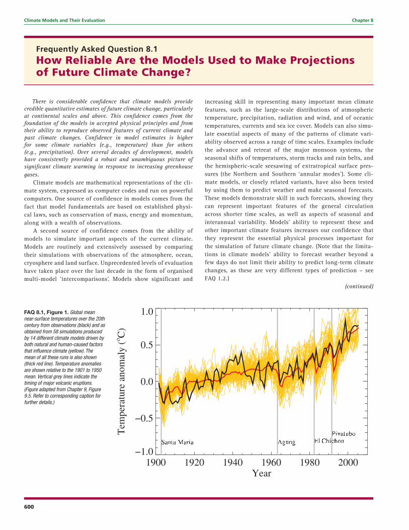
FAQ 8.1, Figure 1. Global mean near-surface temperatures over the 20th century from observations (black) and as obtained from 58 simulations produced by 14 different climate models driven by both natural and human-caused factors that infl uence climate (yellow). The mean of all these runs is also shown (thick red line). Temperature anomalies are shown relative to the 1901 to 1950 mean. Vertical grey lines indicate the timing of major volcanic eruptions. (Figure adapted from Chapter 9, Figure 9.5. Refer to corresponding caption for further details.)

601


A third source of confidence comes from the ability of mod-els to reproduce features of past climates and climate changes. Models have been used to simulate ancient climates, such as the warm mid-Holocene of 6,000 years ago or the last gla-cial maximum of 21,000 years ago (see Chapter 6). They can reproduce many features (allowing for uncertainties in recon-structing past climates) such as the magnitude and broad-scale pattern of oceanic cooling during the last ice age. Models can also simulate many observed aspects of climate change over the instrumental record. One example is that the global temperature trend over the past century (shown in Figure 1) can be mod-elled with high skill when both human and natural factors that influence climate are included. Models also reproduce other ob-served changes, such as the faster increase in nighttime than in daytime temperatures, the larger degree of warming in the Arctic and the small, short-term global cooling (and subsequent recovery) which has followed major volcanic eruptions, such as that of Mt. Pinatubo in 1991 (see FAQ 8.1, Figure 1). Model global temperature projections made over the last two decades have also been in overall agreement with subsequent observa-tions over that period (Chapter 1).

Nevertheless, models still show significant errors. Although these are generally greater at smaller scales, important large-scale problems also remain. For example, deficiencies re-main in the simulation of tropical precipitation, the El Niño-Southern Oscillation and the Madden-Julian Oscillation (an observed variation in tropical winds and rainfall with a time scale of 30 to 90 days). The ultimate source of most such errors is that many important small-scale processes cannot be represented explicitly in models, and so must be included in approximate form as they interact with larger-scale features. This is partly due to limitations in computing power, but also results from limitations in scientific understanding or in the availability of detailed observations of some physical processes. Significant uncertainties, in particular, are associated with the representation of clouds, and in the resulting cloud responses to climate change. Consequently, models continue to display a substantial range of global temperature change in response to specified greenhouse gas forcing (see Chapter 10). Despite such uncertainties, however, models are unanimous in their predic-

tion of substantial climate warming under greenhouse gas in-creases, and this warming is of a magnitude consistent with independent estimates derived from other sources, such as from observed climate changes and past climate reconstructions.

Since confidence in the changes projected by global models decreases at smaller scales, other techniques, such as the use of regional climate models, or downscaling methods, have been specifically developed for the study of regional- and local-scale climate change (see FAQ 11.1). However, as global models con-tinue to develop, and their resolution continues to improve, they are becoming increasingly useful for investigating impor-tant smaller-scale features, such as changes in extreme weather events, and further improvements in regional-scale representa-tion are expected with increased computing power. Models are also becoming more comprehensive in their treatment of the climate system, thus explicitly representing more physical and biophysical processes and interactions considered potentially important for climate change, particularly at longer time scales. Examples are the recent inclusion of plant responses, ocean biological and chemical interactions, and ice sheet dynamics in some global climate models.

In summary, confidence in models comes from their physical basis, and their skill in representing observed climate and past climate changes. Models have proven to be extremely important tools for simulating and understanding climate, and there is considerable confidence that they are able to provide credible quantitative estimates of future climate change, particularly at larger scales. Models continue to have significant limitations, such as in their representation of clouds, which lead to uncer-tainties in the magnitude and timing, as well as regional details, of predicted climate change. Nevertheless, over several decades of model development, they have consistently provided a robust and unambiguous picture of significant climate warming in re-sponse to increasing greenhouse gases.

602


the model’s grid. Instead, sub-grid scale parametrizations are used to parametrize the unresolved processes, such as cloud formation and the mixing due to oceanic eddies. It continues to be the case that multi-model ensemble simulations generally provide more robust information than runs of any single model. Table 8.1 summarises the formulations of each of the AOGCMs used in this report.

There is currently no consensus on the optimal way to divide computer resources among fi ner numerical grids, which allow for better simulations; greater numbers of ensemble members, which allow for better statistical estimates of uncertainty; and inclusion of a more complete set of processes (e.g., carbon feedbacks, atmospheric chemistry interactions).

8.2.1 Atmospheric Processes

8.2.1.1 Numerics

In the TAR, more than half of the participating atmospheric models used spectral advection. Since the TAR, semi-Lagrangian advection schemes have been adopted in several atmospheric models. These schemes allow long time steps and maintain positive values of advected tracers such as water vapour, but they are diffusive, and some versions do not formally conserve mass. In this report, various models use spectral, semi-Lagrangian, and Eulerian fi nite-volume and fi nite-difference advection schemes, although there is still no consensus on which type of scheme is best.

8.2.1.2 Horizontal and Vertical Resolution

The horizontal and vertical resolutions of AOGCMs have increased relative to the TAR. For example, HadGEM1 has eight times as many grid cells as HadCM3 (the number of cells has doubled in all three dimensions). At the National Center for Atmospheric Research (NCAR), a T85 version of the Climate System Model (CSM) is now routinely used, while a T42 version was standard at the time of the TAR. The Center for Climate System Research (CCSR), National Institute for Environmental Studies (NIES) and Frontier Research Center for Global Change (FRCGC) have developed a high-resolution climate model (MIROC-hi, which consists of a T106 L56 Atmospheric GCM (AGCM) and a 1/4° by 1/6° L48 Ocean GCM (OGCM)), and The Meteorological Research Institute (MRI) of the Japan Meteorological Agency (JMA) has developed a TL959 L60 spectral AGCM (Oouchi et al., 2006), which is being used in time-slice mode. The projections made with these models are presented in Chapter 10.

Due to the increased horizontal and vertical resolution, both regional- and global-scale climate features are better simulated. For example, a far-reaching effect of the Hawaiian Islands in the Pacifi c Ocean (Xie et al., 2001) has been well simulated (Sakamoto et al., 2004) and the frequency distribution of precipitation associated with the Baiu front has been improved (Kimoto et al., 2005).

8.2.1.3 Parametrizations

The climate system includes a variety of physical processes, such as cloud processes, radiative processes and boundary-layer processes, which interact with each other on many temporal and spatial scales. Due to the limited resolutions of the models, many of these processes are not resolved adequately by the model grid and must therefore be parametrized. The differences between parametrizations are an important reason why climate model results differ. For example, a new boundary-layer parametrization (Lock et al., 2000; Lock, 2001) had a strong positive impact on the simulations of marine stratocumulus cloud produced by the Geophysical Fluid Dynamics Laboratory (GFDL) and the Hadley Centre climate models, but the same parametrization had less positive impact when implemented in an earlier version of the Hadley Centre model (Martin et al., 2006). Clearly, parametrizations must be understood in the context of their host models.

Cloud processes affect the climate system by regulating the fl ow of radiation at the top of the atmosphere, by producing precipitation, by accomplishing rapid and sometimes deep redistributions of atmospheric mass and through additional mechanisms too numerous to list here (Arakawa and Schubert, 1974; Arakawa, 2004). Cloud parametrizations are based on physical theories that aim to describe the statistics of the cloud fi eld (e.g., the fractional cloudiness or the area-averaged precipitation rate) without describing the individual cloud elements. In an increasing number of climate models, microphysical parametrizations that represent such processes as cloud particle and raindrop formation are used to predict the distributions of liquid and ice clouds. These parametrizations improve the simulation of the present climate, and affect climate sensitivity (Iacobellis et al., 2003). Realistic parametrizations of cloud processes are a prerequisite for reliable current and future climate simulation (see Section 8.6).

Data from fi eld experiments such as the Global Atmospheric Research Program (GARP) Atlantic Tropical Experiment (GATE, 1974), the Monsoon Experiment (MONEX, 1979), ARM (1993) and the Tropical Ocean Global Atmosphere (TOGA) Coupled Ocean-Atmosphere Response Experiment (COARE, 1993) have been used to test and improve parametrizations of clouds and convection (e.g., Emanuel and Zivkovic-Rothmann, 1999; Sud and Walker, 1999; Bony and Emanuel, 2001). Systematic research such as that conducted by the GCSS (Randall et al., 2003) has been organised to test parametrizations by comparing results with both observations and the results of a cloud-resolving model. These efforts have infl uenced the development of many of the recent models. For example, the boundary-layer cloud parametrization of Lock et al. (2000) and Lock (2001) was tested via the GCSS. Parametrizations of radiative processes have been improved and tested by comparing results of radiation parametrizations used in AOGCMs with those of much more detailed ‘line-by-line’ radiation codes (Collins et al., 2006). Since the TAR, improvements have been made in several models to the physical coupling between cloud and convection parametrizations, for example, in the Max Planck Institute (MPI) AOGCM using

603


Tompkins (2002), in the IPSL-CM4 AOGCM using Bony and Emanuel (2001) and in the GFDL model using Tiedtke (1993). These are examples of component-level testing.

In parallel with improvement in parametrizations, a non-hydrostatic model has been used for downscaling. A model with a 5 km grid on a domain of 4,000 x 3,000 x 22 km centred over Japan has been run by MRI/JMA, using the time-slice method for the Fourth Assessment Report (AR4) (Yoshizaki et al., 2005).

Aerosols play an important role in the climate system. Interactive aerosol parametrizations are now used in some models (HADGEM1, MIROC-hi, MIROC-med). Both the ‘direct’ and ‘indirect’ aerosol effects (Chapter 2) have been incorporated in some cases (e.g., IPSL-CM4). In addition to sulphates, other types of aerosols such as black and organic carbon, sea salt and mineral dust are being introduced as prognostic variables (Takemura et al., 2005; see Chapter 2). Further details are given in Section 8.2.5.

8.2.2 Ocean Processes

8.2.2.1 Numerics

Recently, isopycnic or hybrid vertical coordinates have been adopted in some ocean models (GISS-EH and BCCR-BCM2.0). Tests show that such models can produce solutions for complex regional fl ows that are as realistic as those obtained with the more common depth coordinate (e.g., Drange et al., 2005). Issues remain over the proper treatment of thermobaricity (nonlinear relationship of temperature, salinity and pressure to density), which means that in some isopycnic coordinate models the relative densities of, for example, Mediterranean and Antarctic Bottom Water masses are distorted. The merits of these vertical coordinate systems are still being established.

An explicit representation of the sea surface height is being used in many models, and real freshwater fl ux is used to force those models instead of a ‘virtual’ salt fl ux. The virtual salt fl ux method induces a systematic error in sea surface salinity prediction and causes a serious problem at large river basin mouths (Hasumi, 2002a,b; Griffi es, 2004).

Generalised curvilinear horizontal coordinates with bipolar or tripolar grids (Murray, 1996) have become widely used in the oceanic component of AOGCMs. These are strategies used to deal with the North Pole coordinate singularity, as alternatives to the previously common polar fi lter or spherical coordinate rotation. The newer grids have the advantage that the singular points can be shifted onto land while keeping grid points aligned on the equator. The older methods of representing the ocean surface, surface water fl ux and North Pole are still in use in several AOGCMs.

8.2.2.2 Horizontal and Vertical Resolution

There has been a general increase in resolution since the TAR, with a horizontal resolution of order one to two degrees now commonly used in the ocean component of most climate models.

To better resolve the equatorial waveguide, several models use enhanced meridional resolution in the tropics. Resolution high enough to allow oceanic eddies, eddy permitting, has not been used in a full suite of climate scenario integrations due to computational cost, but since the TAR it has been used in some idealised and scenario-based climate experiments as discussed below. A limited set of integrations using the eddy-permitting MIROC3.2 (hires) model is used here and in Chapter 10. Some modelling centres have also increased vertical resolution since the TAR.

A few coupled climate models with eddy-permitting ocean resolution (1/6° to 1/3°) have been developed (Roberts et al., 2004; Suzuki et al., 2005), and large-scale climatic features induced by local air-sea coupling have been successfully simulated (e.g., Sakamoto et al., 2004).

Roberts et al. (2004) found that increasing the ocean resolution of the HadCM3 model from about 1° to 0.33° by 0.33° by 40 levels (while leaving the atmospheric component unchanged) resulted in many improvements in the simulation of ocean circulation features. However, the impact on the atmospheric simulation was relatively small and localised. The climate change response was similar to the standard resolution model, with a slightly faster rate of warming in the Northern Europe-Atlantic region due to differences in the Atlantic Meridional Overturning Circulation (MOC) response. The adjustment time scale of the Atlantic Basin freshwater budget decreased from being of order 400 years to being of order 150 years with the higher resolution ocean, suggesting possible differences in transient MOC response on those time scales, but the mechanisms and the relative roles of horizontal and vertical resolution are not clear.

The Atlantic MOC is infl uenced by freshwater as well as thermal forcing. Besides atmospheric freshwater forcing, freshwater transport by the ocean itself is also important. For the Atlantic MOC, the fresh Pacifi c water coming through the Bering Strait could be poorly simulated on its transit to the Canadian Archipelago and the Labrador Sea (Komuro and Hasumi, 2005). These aspects have been improved since the TAR in many of the models evaluated here.

Changes around continental margins are very important for regional climate change. Over these areas, climate is infl uenced by the atmosphere and open ocean circulation. High-resolution climate models contribute to the improvement of regional climate simulation. For example, the location of the Kuroshio separation from the Japan islands is well simulated in the MIROC3.2 (hires) model (see Figure 8.1), which makes it possible to study a change in the Kuroshio axis in the future climate (Sakamoto et al., 2005).

Guilyardi et al. (2004) suggested that ocean resolution may play only a secondary role in setting the time scale of model El Niño-Southern Oscillation (ENSO) variability, with the dominant time scales being set by the atmospheric model provided the basic speeds of the equatorial ocean wave modes are adequately represented.

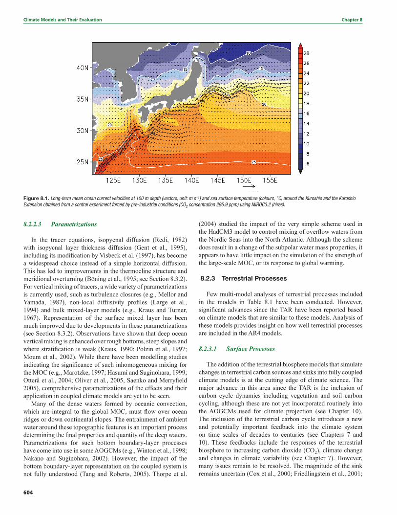
604


8.2.2.3 Parametrizations

In the tracer equations, isopycnal diffusion (Redi, 1982) with isopycnal layer thickness diffusion (Gent et al., 1995), including its modifi cation by Visbeck et al. (1997), has become a widespread choice instead of a simple horizontal diffusion. This has led to improvements in the thermocline structure and meridional overturning (Böning et al., 1995; see Section 8.3.2). For vertical mixing of tracers, a wide variety of parametrizations is currently used, such as turbulence closures (e.g., Mellor and Yamada, 1982), non-local diffusivity profi les (Large et al., 1994) and bulk mixed-layer models (e.g., Kraus and Turner, 1967). Representation of the surface mixed layer has been much improved due to developments in these parametrizations (see Section 8.3.2). Observations have shown that deep ocean vertical mixing is enhanced over rough bottoms, steep slopes and where stratifi cation is weak (Kraus, 1990; Polzin et al., 1997; Moum et al., 2002). While there have been modelling studies indicating the signifi cance of such inhomogeneous mixing for the MOC (e.g., Marotzke, 1997; Hasumi and Suginohara, 1999; Otterå et al., 2004; Oliver et al., 2005, Saenko and Merryfi eld 2005), comprehensive parametrizations of the effects and their application in coupled climate models are yet to be seen.

Many of the dense waters formed by oceanic convection, which are integral to the global MOC, must fl ow over ocean ridges or down continental slopes. The entrainment of ambient water around these topographic features is an important process determining the fi nal properties and quantity of the deep waters. Parametrizations for such bottom boundary-layer processes have come into use in some AOGCMs (e.g., Winton et al., 1998; Nakano and Suginohara, 2002). However, the impact of the bottom boundary-layer representation on the coupled system is not fully understood (Tang and Roberts, 2005). Thorpe et al.

(2004) studied the impact of the very simple scheme used in the HadCM3 model to control mixing of overfl ow waters from the Nordic Seas into the North Atlantic. Although the scheme does result in a change of the subpolar water mass properties, it appears to have little impact on the simulation of the strength of the large-scale MOC, or its response to global warming.

8.2.3 Terrestrial Processes

Few multi-model analyses of terrestrial processes included in the models in Table 8.1 have been conducted. However, signifi cant advances since the TAR have been reported based on climate models that are similar to these models. Analysis of these models provides insight on how well terrestrial processes are included in the AR4 models.

8.2.3.1 Surface Processes

The addition of the terrestrial biosphere models that simulate changes in terrestrial carbon sources and sinks into fully coupled climate models is at the cutting edge of climate science. The major advance in this area since the TAR is the inclusion of carbon cycle dynamics including vegetation and soil carbon cycling, although these are not yet incorporated routinely into the AOGCMs used for climate projection (see Chapter 10). The inclusion of the terrestrial carbon cycle introduces a new and potentially important feedback into the climate system on time scales of decades to centuries (see Chapters 7 and 10). These feedbacks include the responses of the terrestrial biosphere to increasing carbon dioxide (CO2), climate change and changes in climate variability (see Chapter 7). However, many issues remain to be resolved. The magnitude of the sink remains uncertain (Cox et al., 2000; Friedlingstein et al., 2001;

Figure 8.1. Long-term mean ocean current velocities at 100 m depth (vectors, unit: m s–1) and sea surface temperature (colours, °C) around the Kuroshio and the Kuroshio Extension obtained from a control experiment forced by pre-industrial conditions (CO2 concentration 295.9 ppm) using MIROC3.2 (hires).

605


Dufresne et al., 2002) because it depends on climate sensitivity as well as on the response of vegetation and soil carbon to increasing CO2 (Friedlingstein et al., 2003). The rate at which CO2 fertilization saturates in terrestrial systems dominates the present uncertainty in the role of biospheric feedbacks. A series of studies have been conducted to explore the present modelling capacity of the response of the terrestrial biosphere rather than the response of just one or two of its components (Friedlingstein et al., 2006). This work has built on systematic efforts to evaluate the capacity of terrestrial biosphere models to simulate the terrestrial carbon cycle (Cramer et al., 2001) via intercomparison exercises. For example, Friedlingstein et al. (2006) found that in all models examined, the sink decreases in the future as the climate warms.

Other individual components of land surface processes have been improved since the TAR, such as root parametrization (Arora and Boer, 2003; Kleidon, 2004) and higher-resolution river routing (Ducharne et al., 2003). Cold land processes have received considerable attention with multi-layer snowpack models now more common (e.g., Oleson et al., 2004) as is the inclusion of soil freezing and thawing (e.g., Boone et al., 2000; Warrach et al., 2001). Sub-grid scale snow parametrizations (Liston, 2004), snow-vegetation interactions (Essery et al., 2003) and the wind redistribution of snow (Essery and Pomeroy, 2004) are more commonly considered. High-latitude organic soils are included in some models (Wang et al., 2002). A recent advance is the coupling of groundwater models into land surface schemes (Liang et al., 2003; Maxwell and Miller, 2005; Yeh and Eltahir, 2005). These have only been evaluated locally but may be adaptable to global scales. There is also evidence emerging that regional-scale projection of warming is sensitive to the simulation of processes that operate at fi ner scales than current climate models resolve (Pan et al., 2004). In general, the improvements in land surface models since the TAR are based on detailed comparisons with observational data. For example, Boone et al. (2004) used the Rhone Basin to investigate how land surface models simulate the water balance for several annual cycles compared to data from a dense observation network. They found that most land surface schemes simulate very similar total runoff and evapotranspiration but the partitioning between the various components of both runoff and evaporation varies greatly, resulting in different soil water equilibrium states and simulated discharge. More sophisticated snow parametrizations led to superior simulations of basin-scale runoff.

An analysis of results from the second phase of AMIP (AMIP-2) explored the land surface contribution to climate simulation. Henderson-Sellers et al. (2003) found a clear chronological sequence of land surface schemes (early models that excluded an explicit canopy, more recent biophysically based models and very recent biophysically based models). Statistically signifi cant differences in annually averaged evaporation were identifi ed that could be associated with the parametrization of canopy processes. Further improvements in land surface models depends on enhanced surface observations, for example, the use of stable isotopes (e.g., Henderson-Sellers et al., 2004) that allow several components of evaporation to be

evaluated separately. Pitman et al. (2004) explored the impact of the level of complexity used to parametrize the surface energy balance on differences found among the AMIP-2 results. They found that quite large variations in surface energy balance complexity did not lead to systematic differences in the simulated mean, minimum or maximum temperature variance at the global scale, or in the zonal averages, indicating that these variables are not limited by uncertainties in how to parametrize the surface energy balance. This adds confi dence to the use of the models in Table 8.1, as most include surface energy balance modules of more complexity than the minimum identifi ed by Pitman et al. (2004).

While little work has been performed to assess the capability of the land surface models used in coupled climate models, the upgrading of the land surface models is gradually taking place and the inclusion of carbon in these models is a major conceptual advance. In the simulation of the present-day climate, the limitations of the standard bucket hydrology model are increasingly clear (Milly and Shmakin, 2002; Henderson-Sellers et al., 2004; Pitman et al., 2004), including evidence that it overestimates the likelihood of drought (Seneviratne et al., 2002). Relatively small improvements to the land surface model, for example, the inclusion of spatially variable water-holding capacity and a simple canopy conductance, lead to signifi cant improvements (Milly and Shmakin, 2002). Since most models in Table 8.1 represent the continental-scale land surface more realistically than the standard bucket hydrology scheme, and include spatially variable water-holding capacity, canopy conductance, etc. (Table 8.1), most of these models likely capture the key contribution made by the land surface to current large-scale climate simulations. However, it is not clear how well current climate models can capture the impact of future warming on the terrestrial carbon balance. A systematic evaluation of AOGCMs with the carbon cycle represented would help increase confi dence in the contribution of the terrestrial surface resulting from future warming.

8.2.3.2 Soil Moisture Feedbacks in Climate Models

A key role of the land surface is to store soil moisture and control its evaporation. An important process, the soil moisture-precipitation feedback, has been explored extensively since the TAR, building on regionally specifi c studies that demonstrated links between soil moisture and rainfall. Recent studies (e.g., Gutowski et al., 2004; Pan et al., 2004) suggest that summer precipitation strongly depends on surface processes, notably in the simulation of regional extremes. Douville (2001) showed that soil moisture anomalies affect the African monsoon while Schär et al. (2004) suggested that an active soil moisture-precipitation feedback was linked to the anomalously hot European summer in 2003.

The soil moisture-precipitation feedback in climate models had not been systematically assessed at the time of the TAR. It is associated with the strength of coupling between the land and atmosphere, which is not directly measurable at the large scale in nature and has only recently been quantifi ed in models

606


(Dirmeyer, 2001). Koster et al. (2004) provided an assessment of where the soil moisture-precipitation feedback is regionally important during the Northern Hemisphere (NH) summer by quantifying the coupling strength in 12 atmospheric GCMs. Some similarity was seen among the model responses, enough to produce a multi-model average estimate of where the global precipitation pattern during the NH summer was most strongly affected by soil moisture variations. These ‘hot spots’ of strong coupling are found in transition regions between humid and dry areas. The models, however, also show strong disagreement in the strength of land-atmosphere coupling. A few studies have explored the differences in coupling strength. Seneviratne et al. (2002) highlighted the importance of differing water-holding capacities among the models while Lawrence and Slingo (2005) explored the role of soil moisture variability and suggested that frequent soil moisture saturation and low soil moisture variability could partially explain the weak coupling strength in the HadAM3 model (note that ‘weak’ does not imply ‘wrong’ since the real strength of the coupling is unknown).

Overall, the uncertainty in surface-atmosphere coupling has implications for the reliability of the simulated soil moisture-atmosphere feedback. It tempers our interpretation of the response of the hydrologic cycle to simulated climate change in ‘hot spot’ regions. Note that no assessment has been attempted for seasons other than NH summer.

Since the TAR, there have been few assessments of the capacity of climate models to simulate observed soil moisture. Despite the tremendous effort to collect and homogenise soil moisture measurements at global scales (Robock et al., 2000), discrepancies between large-scale estimates of observed soil moisture remain. The challenge of modelling soil moisture, which naturally varies at small scales, linked to landscape characteristics, soil processes, groundwater recharge, vegetation type, etc., within climate models in a way that facilitates comparison with observed data is considerable. It is not clear how to compare climate-model simulated soil moisture with point-based or remotely sensed soil moisture. This makes assessing how well climate models simulate soil moisture, or the change in soil moisture, diffi cult.

8.2.4 Cryospheric Processes

8.2.4.1 Terrestrial Cryosphere

Ice sheet models are used in calculations of long-term warming and sea level scenarios, though they have not generally been incorporated in the AOGCMs used in Chapter 10. The models are generally run in ‘off-line’ mode (i.e., forced by atmospheric fi elds derived from high-resolution time-slice experiments), although Huybrechts et al. (2002) and Fichefet et al. (2003) reported early efforts at coupling ice sheet models to AOGCMs. Ice sheet models are also included in some EMICs (e.g., Calov et al., 2002). Ridley et al. (2005) pointed out that the time scale of projected melting of the Greenland Ice Sheet may be different in coupled and off-line simulations. Presently available thermomechanical ice sheet models do not

include processes associated with ice streams or grounding line migration, which may permit rapid dynamical changes in the ice sheets. Glaciers and ice caps, due to their relatively small scales and low likelihood of signifi cant climate feedback at large scales, are not currently included interactively in any AOGCMs. See Chapters 4 and 10 for further detail. For a discussion of terrestrial snow, see Section 8.3.4.1.

8.2.4.2 Sea Ice

Sea ice components of current AOGCMs usually predict ice thickness (or volume), fractional cover, snow depth, surface and internal temperatures (or energy) and horizontal velocity. Some models now include prognostic sea ice salinity (Schmidt et al., 2004). Sea ice albedo is typically prescribed, with only crude dependence on ice thickness, snow cover and puddling effects.

Since the TAR, most AOGCMs have started to employ complex sea ice dynamic components. The complexity of sea ice dynamics in current AOGCMs varies from the relatively simple ‘cavitating fl uid’ model (Flato and Hibler, 1992) to the viscous-plastic model (Hibler, 1979), which is computationally expensive, particularly for global climate simulations. The elastic-viscous-plastic model (Hunke and Dukowicz, 1997) is being increasingly employed, particularly due to its effi ciency for parallel computers. New numerical approaches for solving the ice dynamics equations include more accurate representations on curvilinear model grids (Hunke and Dukowicz, 2002; Marsland et al., 2003; Zhang and Rothrock, 2003) and Lagrangian methods for solving the viscous-plastic equations (Lindsay and Stern, 2004; Wang and Ikeda, 2004).

Treatment of sea ice thermodynamics in AOGCMs has progressed more slowly: it typically includes constant conductivity and heat capacities for ice and snow (if represented), a heat reservoir simulating the effect of brine pockets in the ice, and several layers, the upper one representing snow. More sophisticated thermodynamic schemes are being developed, such as the model of Bitz and Lipscomb (1999), which introduces salinity-dependent conductivity and heat capacities, modelling brine pockets in an energy-conserving way as part of a variable-layer thermodynamic model (e.g., Saenko et al., 2002). Some AOGCMs include snow ice formation, which occurs when an ice fl oe is submerged by the weight of the overlying snow cover and the fl ooded snow layer refreezes. The latter process is particularly important in the antarctic sea ice system.

Even with fi ne grid scales, many sea ice models incorporate sub-grid scale ice thickness distributions (Thorndike et al., 1975) with several thickness ‘categories’, rather than considering the ice as a uniform slab with inclusions of open water. An ice thickness distribution enables more accurate simulation of thermodynamic variations in growth and melt rates within a single grid cell, which can have signifi cant consequences for ice-ocean albedo feedback processes (e.g., Bitz et al., 2001; Zhang and Rothrock, 2001). A well-resolved ice thickness distribution enables a more physical formulation for ice ridging and rafting events, based on energetic principles. Although parametrizations of ridging mechanics and their relationship

607


with the ice thickness distribution have improved (Babko et al., 2002; Amundrud et al., 2004; Toyota et al., 2004), inclusion of advanced ridging parametrizations has lagged other aspects of sea ice dynamics (rheology, in particular) in AOGCMs. Better numerical algorithms used for the ice thickness distribution (Lipscomb, 2001) and ice strength (Hutchings et al., 2004) have also been developed for AOGCMs.

8.2.5 Aerosol Modelling and Atmospheric Chemistry

Climate simulations including atmospheric aerosols with chemical transport have greatly improved since the TAR. Simulated global aerosol distributions are better compared with observations, especially satellite data (e.g., Advanced Very High Resolution Radar (AVHRR), Moderate Resolution Imaging Spectroradiometer (MODIS), Multi-angle Imaging Spectroradiometer (MISR), Polarization and Directionality of the Earth’s Refl ectance (POLDER), Total Ozone Mapping Spectrometer (TOMS)), the ground-based network (Aerosol Robotic Network; AERONET) and many measurement campaigns (e.g., Chin et al., 2002; Takemura et al., 2002). The global Aerosol Model Intercomparison project, AeroCom, has also been initiated in order to improve understanding of uncertainties of model estimates, and to reduce them (Kinne et al., 2003). These comparisons, combined with cloud observations, should result in improved confi dence in the estimation of the aerosol direct and indirect radiative forcing (e.g., Ghan et al., 2001a,b; Lohmann and Lesins, 2002; Takemura et al., 2005). Interactive aerosol sub-component models have been incorporated in some of the climate models used in Chapter 10 (HadGEM1 and MIROC). Some models also include indirect aerosol effects (e.g., Takemura et al., 2005); however, the formulation of these processes is still the subject of much research.

Interactive atmospheric chemistry components are not generally included in the models used in this report. However, CCSM3 includes the modifi cation of greenhouse gas concentrations by chemical processes and conversion of sulphur dioxide and dimethyl sulphide to sulphur aerosols.

8.2.6 Coupling Advances

In an advance since the TAR, a number of groups have developed software allowing easier coupling of the various components of a climate model (e.g., Valcke et al., 2006). An example, the Ocean Atmosphere Sea Ice Soil (OASIS) coupler, developed at the Centre Europeen de Recherche et de Formation Avancee en Calcul Scientifi c (CERFACS) (Terray et al., 1998), has been used by many modelling centres to synchronise the different models and for the interpolation of the coupling fi elds between the atmosphere and ocean grids. The schemes for interpolation between the ocean and the atmosphere grids have been revised. The new schemes ensure both a global and local conservation of the various fl uxes at the air-sea interface, and track terrestrial, ocean and sea ice fl uxes individually.

Coupling frequency is an important issue, because fl uxes are averaged during a coupling interval. Typically, most AOGCMs evaluated here pass fl uxes and other variables between the component parts once per day. The K-Profi le Parametrization ocean vertical scheme (Large et al., 1994), used in several models, is very sensitive to the wind energy available for mixing. If the models are coupled at a frequency lower than once per ocean time step, nonlinear quantities such as wind mixing power (which depends on the cube of the wind speed) must be accumulated over every time step before passing to the ocean. Improper averaging therefore could lead to too little mixing energy and hence shallower mixed-layer depths, assuming the parametrization is not re-tuned. However, high coupling frequency can bring new technical issues. In the MIROC model, the coupling interval is three hours, and in this case, a poorly resolved internal gravity wave is excited in the ocean so some smoothing is necessary to damp this numerical problem. It should also be noted that the AOGCMs used here have relatively thick top oceanic grid boxes (typically 10 m or more), limiting the sea surface temperature (SST) response to frequent coupling (Bernie et al., 2005).

8.2.7 Flux Adjustments and Initialisation

Since the TAR, more climate models have been developed that do not adjust the surface heat, water and momentum fl uxes artifi cially to maintain a stable control climate. As noted by Stouffer and Dixon (1998), the use of such fl ux adjustments required relatively long integrations of the component models before coupling. In these models, normally the initial conditions for the coupled integrations were obtained from long spin ups of the component models.

In AOGCMs that do not use fl ux adjustments (see Table 8.1), the initialisation methods tend to be more varied. The oceanic components of many models are initialised using values obtained either directly from an observationally based, gridded data set (Levitus and Boyer, 1994; Levitus and Antonov, 1997; Levitus et al., 1998) or from short ocean-only integrations that used an observational analysis for their initial conditions. The initial atmospheric component data are usually obtained from atmosphere-only integrations using prescribed SSTs.

To obtain initial data for the pre-industrial control integrations discussed in Chapter 10, most AOGCMs use variants of the Stouffer et al. (2004) scheme. In this scheme, the coupled model is initialised as discussed above. The radiative forcing is then set back to pre-industrial conditions. The model is integrated for a few centuries using constant pre-industrial radiative forcing, allowing the coupled system to partially adjust to this forcing. The degree of equilibration in the real pre-industrial climate to the pre-industrial radiative forcing is not known. Therefore, it seems unnecessary to have the pre-industrial control fully equilibrated. After this spin-up integration, the pre-industrial control is started and perturbation integrations can begin. An important next step, once the start of the control integration is determined, is the assessment of the control integration climate drift. Large climate drifts can distort both the natural variability

608


(e.g., Inness et al., 2003) and the climate response to changes in radiative forcing (Spelman and Manabe, 1984).

In earlier IPCC reports, the initialisation methods were quite varied. In some cases, the perturbation integrations were initialised using data from control integrations where the SSTs were near present-day values and not pre-industrial. Given that many climate models now use some variant of the Stouffer et al. (2004) method, this situation has improved.

8.3 Evaluation of Contemporary Climate as Simulated by Coupled Global Models

Due to nonlinearities in the processes governing climate, the climate system response to perturbations depends to some extent on its basic state (Spelman and Manabe, 1984). Consequently, for models to predict future climatic conditions reliably, they must simulate the current climatic state with some as yet unknown degree of fi delity. Poor model skill in simulating present climate could indicate that certain physical or dynamical processes have been misrepresented. The better a model simulates the complex spatial patterns and seasonal and diurnal cycles of present climate, the more confi dence there is that all the important processes have been adequately represented. Thus, when new models are constructed, considerable effort is devoted to evaluating their ability to simulate today’s climate (e.g., Collins et al., 2006; Delworth et al., 2006).

Some of the assessment of model performance presented here is based on the 20th-century simulations that constitute a part of the MMD archived at PCMDI. In these simulations, modelling groups initiated the models from pre-industrial (circa 1860) ‘control’ simulations and then imposed the natural and anthropogenic forcing thought to be important for simulating the climate of the last 140 years or so. The 23 models considered here (see Table 8.1) are those relied on in Chapters 9 and 10 to investigate historical and future climate changes. Some fi gures in this section are based on results from a subset of the models because the data set is incomplete.

In order to identify errors that are systematic across models, the mean of fi elds available in the MMD, referred to here as the ‘multi-model mean fi eld’, will often be shown. The multi-model mean fi eld results are augmented by results from individual models available as Supplementary Material (see Figures S8.1 to S8.15). The multi-model averaging serves to fi lter out biases of individual models and only retains errors that are generally pervasive. There is some evidence that the multi-model mean fi eld is often in better agreement with observations than any of the fi elds simulated by the individual models (see Section 8.3.1.1.2), which supports continued reliance on a diversity of modelling approaches in projecting future climate change and provides some further interest in evaluating the multi-model mean results.

Faced with the rich variety of climate characteristics that could potentially be evaluated here, this section focuses on

those elements that can critically affect societies and natural ecosystems and that are most likely to respond to changes in radiative forcing.

8.3.1 Atmosphere

8.3.1.1 Surface Temperature and the Climate System’s Energy Budget

For models to simulate accurately the global distribution of the annual and diurnal cycles of surface temperature, they must, in the absence of compensating errors, correctly represent a variety of processes. The large-scale distribution of annual mean surface temperature is largely determined by the distribution of insolation, which is moderated by clouds, other surface heat fl uxes and transport of energy by the atmosphere and to a lesser extent by the ocean. Similarly, the annual and diurnal cycles of surface temperature are governed by seasonal and diurnal changes in these factors, respectively, but they are also damped by storage of energy in the upper layers of the ocean and to a lesser degree the surface soil layers.

8.3.1.1.1 Temperature Figure 8.2a shows the observed time mean surface

temperature as a composite of surface air temperature over regions of land and SST elsewhere. Also shown is the difference between the multi-model mean fi eld and the observed fi eld. With few exceptions, the absolute error (outside polar regions and other data-poor regions) is less than 2°C. Individual models typically have larger errors, but in most cases still less than 3°C, except at high latitudes (see Figure 8.2b and Supplementary Material, Figure S8.1). Some of the larger errors occur in regions of sharp elevation changes and may result simply from mismatches between the model topography (typically smoothed) and the actual topography. There is also a tendency for a slight, but general, cold bias. Outside the polar regions, relatively large errors are evident in the eastern parts of the tropical ocean basins, a likely symptom of problems in the simulation of low clouds. The extent to which these systematic model errors affect a model’s response to external perturbations is unknown, but may be signifi cant (see Section 8.6).

In spite of the discrepancies discussed here, the fact is that models account for a very large fraction of the global temperature pattern: the correlation coeffi cient between the simulated and observed spatial patterns of annual mean temperature is typically about 0.98 for individual models. This supports the view that major processes governing surface temperature climatology are represented with a reasonable degree of fi delity by the models.

An additional opportunity for evaluating models is afforded by the observed annual cycle of surface temperature. Figure 8.3 shows the standard deviation of monthly mean surface temperatures, which is dominated by contributions from the amplitudes of the annual and semi-annual components of the annual cycle. The difference between the mean of the model results and the observations is also shown. The absolute

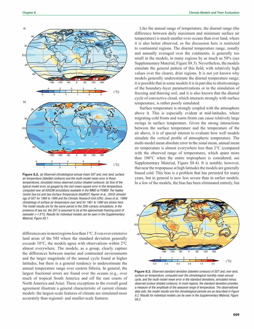
609


Figure 8.2. (a) Observed climatological annual mean SST and, over land, surface air temperature (labelled contours) and the multi-model mean error in these temperatures, simulated minus observed (colour-shaded contours). (b) Size of the typical model error, as gauged by the root-mean-square error in this temperature, computed over all AOGCM simulations available in the MMD at PCMDI. The Hadley Centre Sea Ice and Sea Surface Temperature (HadISST; Rayner et al., 2003) climatol-ogy of SST for 1980 to 1999 and the Climatic Research Unit (CRU; Jones et al., 1999) climatology of surface air temperature over land for 1961 to 1990 are shown here. The model results are for the same period in the 20th-century simulations. In the presence of sea ice, the SST is assumed to be at the approximate freezing point of seawater (–1.8°C). Results for individual models can be seen in the Supplementary Material, Figure S8.1.

Like the annual range of temperature, the diurnal range (the difference between daily maximum and minimum surface air temperature) is much smaller over oceans than over land, where it is also better observed, so the discussion here is restricted to continental regions. The diurnal temperature range, zonally and annually averaged over the continents, is generally too small in the models, in many regions by as much as 50% (see Supplementary Material, Figure S8.3). Nevertheless, the models simulate the general pattern of this fi eld, with relatively high values over the clearer, drier regions. It is not yet known why models generally underestimate the diurnal temperature range; it is possible that in some models it is in part due to shortcomings of the boundary-layer parametrizations or in the simulation of freezing and thawing soil, and it is also known that the diurnal cycle of convective cloud, which interacts strongly with surface temperature, is rather poorly simulated.

Surface temperature is strongly coupled with the atmosphere above it. This is especially evident at mid-latitudes, where migrating cold fronts and warm fronts can cause relatively large swings in surface temperature. Given the strong interactions between the surface temperature and the temperature of the air above, it is of special interest to evaluate how well models simulate the vertical profi le of atmospheric temperature. The multi-model mean absolute error in the zonal mean, annual mean air temperature is almost everywhere less than 2°C (compared with the observed range of temperatures, which spans more than 100°C when the entire troposphere is considered; see Supplementary Material, Figure S8.4). It is notable, however, that near the tropopause at high latitudes the models are generally biased cold. This bias is a problem that has persisted for many years, but in general is now less severe than in earlier models. In a few of the models, the bias has been eliminated entirely, but

Figure 8.3. Observed standard deviation (labelled contours) of SST and, over land, surface air temperature, computed over the climatological monthly mean annual cycle, and the multi-model mean error in the standard deviations, simulated minus observed (colour-shaded contours). In most regions, the standard deviation provides a measure of the amplitude of the seasonal range of temperature. The observational data sets, the model results and the climatological periods are as described in Figure 8.2. Results for individual models can be seen in the Supplementary Material, Figure S8.2.

differences are in most regions less than 1°C. Even over extensive land areas of the NH where the standard deviation generally exceeds 10°C, the models agree with observations within 2°C almost everywhere. The models, as a group, clearly capture the differences between marine and continental environments and the larger magnitude of the annual cycle found at higher latitudes, but there is a general tendency to underestimate the annual temperature range over eastern Siberia. In general, the largest fractional errors are found over the oceans (e.g., over much of tropical South America and off the east coasts of North America and Asia). These exceptions to the overall good agreement illustrate a general characteristic of current climate models: the largest-scale features of climate are simulated more accurately than regional- and smaller-scale features.

610


compensating errors may be responsible. It is known that the tropopause cold bias is sensitive to several factors, including horizontal and vertical resolution, non-conservation of moist entropy, and the treatment of sub-grid scale vertical convergence of momentum (‘gravity wave drag’). Although the impact of the tropopause temperature bias on the model’s response to radiative forcing changes has not been defi nitively quantifi ed, it is almost certainly small relative to other uncertainties.

8.3.1.1.2 The balance of radiation at the top of the atmosphere

The primary driver of latitudinal and seasonal variations in temperature is the seasonally varying pattern of incident sunlight, and the fundamental driver of the circulation of the atmosphere and ocean is the local imbalance between the shortwave (SW) and longwave (LW) radiation at the top of the atmosphere. The impact on temperature of the distribution of insolation can be strongly modifi ed by the distribution of clouds and surface characteristics.

Considering fi rst the annual mean SW fl ux at the ‘top’ of the atmosphere (TOA)1, the insolation is determined by well-known orbital parameters that ensure good agreement between models and observations. The annual mean insolation is strongest in the tropics, decreasing to about half as much at the poles. This largely drives the strong equator-to-pole temperature gradient. As for outgoing SW radiation, the Earth, on average, refl ects about the same amount of sunlight (~100 W m–2 in the annual mean) at all latitudes. At most latitudes, the difference between the multi-model mean zonally averaged outgoing SW radiation and observations is in the annual mean less than 6 W m–2 (i.e., an error of about 6%; see Supplementary Material, Figure S8.5). Given that clouds are responsible for about half the outgoing SW radiation, these errors are not surprising, for it is known that cloud processes are among the most diffi cult to simulate with models (see Section 8.6.3.2.3).

There are additional errors in outgoing SW radiation due to variations with longitude and season, and these can be quantifi ed by means of the root-mean-square (RMS) error, calculated for each latitude over all longitudes and months and plotted in Figure 8.4a (see also Supplementary Material, Figure S8.6). Errors in the complete two-dimensional fi elds (see Supplementary Material, Figure S8.6) tend to be substantially larger than the zonal mean errors of about 6 W m–2, an example of the common result that model errors tend to increase as smaller spatial scales and shorter time scales are considered. Figure 8.4a also illustrates a common result that the errors in the multi-model average of monthly mean fi elds are often smaller than the errors in the individual

model fi elds. In the case of outgoing SW radiation, this is true at nearly all latitudes. Calculation of the global mean RMS error, based on the monthly mean fi elds and area-weighted over all grid cells, indicates that the individual model errors are in the range 15 to 22 W m–2, whereas the error in the multi-model mean climatology is only 13.1 W m–2. Why the multi-model mean fi eld turns out to be closer to the observed than the fi elds in any of the individual models is the subject of ongoing research; a superfi cial explanation is that at each location and

1 The atmosphere clearly has no identifi able ‘top’, but the term is used here to refer to an altitude above which the absorption of SW and LW radiation is negligibly small.

Figure 8.4. Root-mean-square (RMS) model error, as a function of latitude, in simulation of (a) outgoing SW radiation refl ected to space and (b) outgoing LW radiation. The RMS error is calculated over all longitudes and over all 12 months of a climatology formed from several years of data. The RMS statistic labelled ‘Mean Model’ is computed by fi rst calculating the multi-model monthly mean fi elds, and then calculating the RMS error (i.e., it is not the mean of the individual model RMS errors). The Earth Radiation Budget Experiment (ERBE; Barkstrom et al., 1989) observational esti-mates used here are for the period 1985 to 1989 from satellite-based radiometers, and the model results are for the same period in the 20th-century simulations in the MMD at PCMDI. See Table 8.1 for model descriptions. Results for individual models can be seen in the Supplementary Material, Figures S8.5 to S8.8.

611


for each month, the model estimates tend to scatter around the correct value (more or less symmetrically), with no single model consistently closest to the observations. This, however, does not explain why the results should scatter in this way.

At the TOA, the net SW radiation is everywhere partially compensated by outgoing LW radiation (i.e., infrared emissions) emanating from the surface and the atmosphere. Globally and annually averaged, this compensation is nearly exact. The pattern of LW radiation emitted by earth to space depends most critically on atmospheric temperature, humidity, clouds and surface temperature. With a few exceptions, the models can simulate the observed zonal mean of the annual mean outgoing LW within 10 W m–2 (an error of around 5%; see Supplementary Material, Figure S8.7). The models reproduce the relative minimum in this fi eld near the equator where the relatively high humidity and extensive cloud cover in the tropics raises the effective height (and lowers the effective temperature) at which LW radiation emanates to space.

The seasonal cycle of the outgoing LW radiation pattern is also reasonably well simulated by models (see Figure 8.4b). The RMS error for most individual models varies from about 3% of the outgoing LW radiation (OLR) near the poles to somewhat less than 10% in the tropics. The errors for the multi-model mean simulation, ranging from about 2 to 6% across all latitudes, are again generally smaller than those in the individual models.

For a climate in equilibrium, any local annual mean imbalance in the net TOA radiative fl ux (SW plus LW) must be balanced by a vertically integrated net horizontal divergence of energy carried by the ocean and atmosphere. The fact that the TOA SW and LW fl uxes are well simulated implies that the models must also be properly accounting for poleward transport of total energy by the atmosphere and ocean. This proves to be the case, with most models correctly simulating poleward energy transport within about 10%. Although superfi cially this would seem to provide an important check on models, it is likely that in current models compensating errors improve the agreement of the simulations with observations. There are theoretical and model studies that suggest that if the atmosphere fails to transport the observed portion of energy, the ocean will tend to largely compensate (e.g., Shaffrey and Sutton, 2004).

8.3.1.2 Moisture and Precipitation

Water is fundamental to life, and if regional seasonal precipitation patterns were to change, the potential impacts could be profound. Consequently, it is of real practical interest to evaluate how well models can simulate precipitation, not only at global scales, but also regionally. Unlike seasonal variation in temperature, which at large scales is strongly determined by the insolation pattern and confi guration of the continents, precipitation variations are also strongly infl uenced by vertical movement of air due to atmospheric instabilities of

various kinds and by the fl ow of air over orographic features. For models to simulate accurately the seasonally varying pattern of precipitation, they must correctly simulate a number of processes (e.g., evapotranspiration, condensation, transport) that are diffi cult to evaluate at a global scale. Some of these are discussed further in Sections 8.2 and 8.6. In this subsection, the focus is on the distribution of precipitation and water vapour.

Figure 8.5a shows observation-based estimates of annual mean precipitation and Figure 8.5b shows the multi-model mean fi eld. At the largest scales, the lower precipitation rates at higher latitudes refl ect both reduced local evaporation at lower temperatures and a lower saturation vapour pressure of cooler air, which tends to inhibit the transport of vapour from other regions. In addition to this large-scale pattern, captured well by models, is a local minimum in precipitation near the equator in the Pacifi c, due to a tendency for the Inter-Tropical Convergence Zone (ITCZ)2 to reside off the equator. There are local maxima at mid-latitudes, refl ecting the tendency for subsidence to suppress precipitation in the subtropics and for storm systems to enhance precipitation at mid-latitudes. The models capture these large-scale zonal mean precipitation differences, suggesting that they can adequately represent these features of atmospheric circulation. Moreover, there is some evidence provided in Section 8.3.5 that models have improved over the last several years in simulating the annual cycle of the precipitation patterns.

Models also simulate some of the major regional characteristics of the precipitation fi eld, including the major convergence zones and the maxima over tropical rain forests, although there is a tendency to underestimate rainfall over the Amazon. When considered in more detail, however, there are defi ciencies in the multi-model mean precipitation fi eld. There is a distinct tendency for models to orient the South Pacifi c convergence zone parallel to latitudes and to extend it too far eastward. In the tropical Atlantic, the precipitation maximum is too weak in most models with too much rain south of the equator. There are also systematic east-west positional errors in the precipitation distribution over the Indo-Pacifi c Warm Pool in most models, with an excess of precipitation over the western Indian Ocean and over the Maritime Continent. These lead to systematic biases in the location of the major rising branches of the Walker Circulation and can compromise major teleconnection3 pathways, in particular those associated with El Niño (e.g., Turner et al., 2005). Systematic dry biases over the Bay of Bengal are related to errors in the monsoon simulations.

Despite the apparent skill suggested by the multi-model mean (Figure 8.5), many models individually display substantial precipitation biases, especially in the tropics, which often approach the magnitude of the mean observed climatology (e.g., Johns et al., 2006; see also the Supplementary Material, Figures S8.9 and S8.10). Although some of these biases can be attributed to errors in the SST fi eld of the coupled model, even

2 The ITCZ is manifested as a band of relatively intense convective precipitation, accompanied by surface convergence of moisture, which tends to locate seasonally over the warmest surface temperatures and circumnavigates the earth in the tropics (though not continuously).

3 Teleconnection describes the process through which changes in one part of the climate system affect a remote location via changes in atmospheric circulation patterns.

612


Figure 8.5. Annual mean precipitation (cm), observed (a) and simulated (b), based on the multi-model mean. The Climate Prediction Center Merged Analysis of Precipitation (CMAP; Xie and Arkin, 1997) observation-based climatology for 1980 to 1999 is shown, and the model results are for the same period in the 20th-century simulations in the MMD at PCMDI. In (a), observations were not available for the grey regions. Results for individual models can be seen in Supplementary Material, Figure S8.9.

atmosphere-only versions of the models show similarly large errors (e.g., Slingo et al., 2003). This may be one factor leading to a lack of consensus among models even as to the sign of future regional precipitation changes predicted in parts of the tropics (see Chapter 10).

At the heart of understanding what determines the regional distribution of precipitation over land and oceans in the tropics is atmospheric convection and its interaction with large-scale circulation. Convection occurs on a wide range of spatial and temporal scales, and there is increasing evidence that interactions across all scales may be crucial for determining the mean tropical climate and its regional rainfall distributions (e.g., Khairoutdinov et al., 2005). Over tropical land, the diurnal cycle dominates, and yet many models have diffi culty simulating the early evening maximum in rainfall. Instead, they systematically tend to simulate rain before noon (Yang and Slingo, 2001; Dai, 2006), which compromises the energy budget of the land surface. Similarly, the land-sea breezes around the complex system of islands in Indonesia have been implicated

in the failure of models to capture the regional rainfall patterns across the Indo-Pacifi c Warm Pool (Neale and Slingo, 2003). Over the oceans, the precipitation distribution along the ITCZ results from organised convection associated with weather systems occurring on synoptic and intra-seasonal time scales (e.g., the Madden-Julian Oscillation (MJO); see Section 8.4.8). These systems are frequently linked to convectively coupled equatorial wave structures (e.g., Yang et al., 2003), but these are poorly represented in models (e.g., Lin et al., 2006; Ringer et al., 2006). Thus the rain-bearing systems, which establish the mean precipitation climatology, are not well simulated, contributing also to the poor temporal characteristics of daily rainfall (e.g., Dai, 2006) in which many models simulate rain too frequently but with reduced intensity.

Precipitation patterns are intimately linked to atmospheric humidity, evaporation, condensation and transport processes. Good observational estimates of the global pattern of evaporation are not available, and condensation and vertical transport of water vapour can often be dominated by sub-grid scale convective processes which are diffi cult to evaluate globally. The best prospect for assessing water vapour transport processes in humid regions, especially at annual and longer time scales, may be to compare modelled and observed streamfl ow, which must nearly balance atmospheric transport since terrestrial water storage variations on longer time scales are small (Milly et al., 2005; see Section 8.3.4.2).

Although an analysis of runoff in the MMD at PCMDI has not yet been performed, the net result of evaporation, transport and condensation processes can be seen in the atmospheric humidity distribution. Models reproduce the large-scale decrease in humidity with both latitude and altitude (see Supplementary

Material, Figure S8.11), although this is not truly an independent check of models, since it is almost a direct consequence of their reasonably realistic simulation of temperature. The multi-model mean bias in humidity, zonally and annually averaged, is less than 10% throughout most of the lower troposphere compared with reanalyses, but model evaluation in the upper troposphere is considerably hampered by observational uncertainty.

Any errors in the water vapour distribution should affect the outgoing LW radiation (see Section 8.3.1.1.2), which was seen to be free of systematic zonal mean biases. In fact, the observed differences in outgoing LW radiation between the moist and dry regions are reproduced by the models, providing some confi dence that any errors in humidity are not critically affecting the net fl uxes at the TOA. However, the strength of water vapour feedback, which strongly affects global climate sensitivity, is primarily determined by fractional changes in water vapour in response to warming, and the ability of models to correctly represent this feedback is perhaps better assessed with process studies (see Section 8.6).

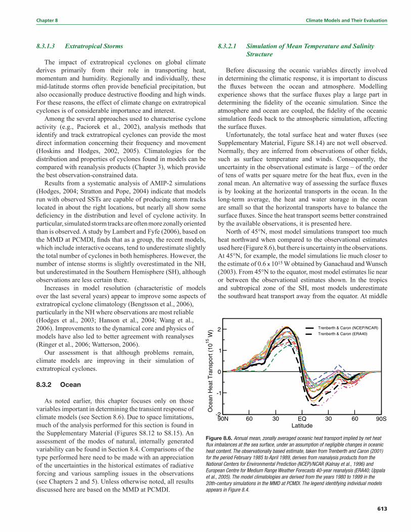
613


8.3.1.3 Extratropical Storms

The impact of extratropical cyclones on global climate derives primarily from their role in transporting heat, momentum and humidity. Regionally and individually, these mid-latitude storms often provide benefi cial precipitation, but also occasionally produce destructive fl ooding and high winds. For these reasons, the effect of climate change on extratropical cyclones is of considerable importance and interest.

Among the several approaches used to characterise cyclone activity (e.g., Paciorek et al., 2002), analysis methods that identify and track extratropical cyclones can provide the most direct information concerning their frequency and movement (Hoskins and Hodges, 2002, 2005). Climatologies for the distribution and properties of cyclones found in models can be compared with reanalysis products (Chapter 3), which provide the best observation-constrained data.

Results from a systematic analysis of AMIP-2 simulations (Hodges, 2004; Stratton and Pope, 2004) indicate that models run with observed SSTs are capable of producing storm tracks located in about the right locations, but nearly all show some defi ciency in the distribution and level of cyclone activity. In particular, simulated storm tracks are often more zonally oriented than is observed. A study by Lambert and Fyfe (2006), based on the MMD at PCMDI, fi nds that as a group, the recent models, which include interactive oceans, tend to underestimate slightly the total number of cyclones in both hemispheres. However, the number of intense storms is slightly overestimated in the NH, but underestimated in the Southern Hemisphere (SH), although observations are less certain there.

Increases in model resolution (characteristic of models over the last several years) appear to improve some aspects of extratropical cyclone climatology (Bengtsson et al., 2006), particularly in the NH where observations are most reliable (Hodges et al., 2003; Hanson et al., 2004; Wang et al., 2006). Improvements to the dynamical core and physics of models have also led to better agreement with reanalyses (Ringer et al., 2006; Watterson, 2006).

Our assessment is that although problems remain, climate models are improving in their simulation of extratropical cyclones.

8.3.2 Ocean

As noted earlier, this chapter focuses only on those variables important in determining the transient response of climate models (see Section 8.6). Due to space limitations, much of the analysis performed for this section is found in the Supplementary Material (Figures S8.12 to S8.15). An assessment of the modes of natural, internally generated variability can be found in Section 8.4. Comparisons of the type performed here need to be made with an appreciation of the uncertainties in the historical estimates of radiative forcing and various sampling issues in the observations (see Chapters 2 and 5). Unless otherwise noted, all results discussed here are based on the MMD at PCMDI.

8.3.2.1 Simulation of Mean Temperature and Salinity Structure

Before discussing the oceanic variables directly involved in determining the climatic response, it is important to discuss the fl uxes between the ocean and atmosphere. Modelling experience shows that the surface fl uxes play a large part in determining the fi delity of the oceanic simulation. Since the atmosphere and ocean are coupled, the fi delity of the oceanic simulation feeds back to the atmospheric simulation, affecting the surface fl uxes.

Unfortunately, the total surface heat and water fl uxes (see Supplementary Material, Figure S8.14) are not well observed. Normally, they are inferred from observations of other fi elds, such as surface temperature and winds. Consequently, the uncertainty in the observational estimate is large – of the order of tens of watts per square metre for the heat fl ux, even in the zonal mean. An alternative way of assessing the surface fl uxes is by looking at the horizontal transports in the ocean. In the long-term average, the heat and water storage in the ocean are small so that the horizontal transports have to balance the surface fl uxes. Since the heat transport seems better constrained by the available observations, it is presented here.

North of 45°N, most model simulations transport too much heat northward when compared to the observational estimates used here (Figure 8.6), but there is uncertainty in the observations. At 45°N, for example, the model simulations lie much closer to the estimate of 0.6 x 1015 W obtained by Ganachaud and Wunsch (2003). From 45°N to the equator, most model estimates lie near or between the observational estimates shown. In the tropics and subtropical zone of the SH, most models underestimate the southward heat transport away from the equator. At middle

Figure 8.6. Annual mean, zonally averaged oceanic heat transport implied by net heat fl ux imbalances at the sea surface, under an assumption of negligible changes in oceanic heat content. The observationally based estimate, taken from Trenberth and Caron (2001) for the period February 1985 to April 1989, derives from reanalysis products from the National Centers for Environmental Prediction (NCEP)/NCAR (Kalnay et al., 1996) and European Centre for Medium Range Weather Forecasts 40-year reanalysis (ERA40; Uppala et al., 2005). The model climatologies are derived from the years 1980 to 1999 in the 20th-century simulations in the MMD at PCMDI. The legend identifying individual models appears in Figure 8.4.

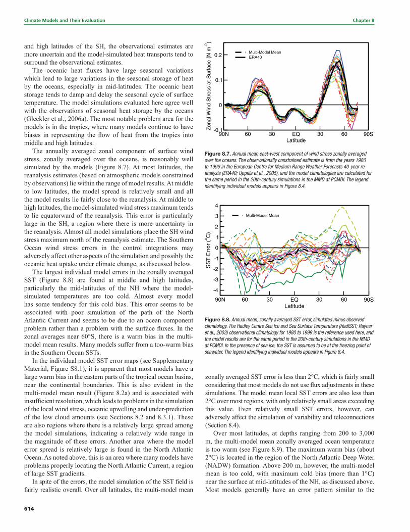
614


and high latitudes of the SH, the observational estimates are more uncertain and the model-simulated heat transports tend to surround the observational estimates.

The oceanic heat fl uxes have large seasonal variations which lead to large variations in the seasonal storage of heat by the oceans, especially in mid-latitudes. The oceanic heat storage tends to damp and delay the seasonal cycle of surface temperature. The model simulations evaluated here agree well with the observations of seasonal heat storage by the oceans (Gleckler et al., 2006a). The most notable problem area for the models is in the tropics, where many models continue to have biases in representing the fl ow of heat from the tropics into middle and high latitudes.

The annually averaged zonal component of surface wind stress, zonally averaged over the oceans, is reasonably well simulated by the models (Figure 8.7). At most latitudes, the reanalysis estimates (based on atmospheric models constrained by observations) lie within the range of model results. At middle to low latitudes, the model spread is relatively small and all the model results lie fairly close to the reanalysis. At middle to high latitudes, the model-simulated wind stress maximum tends to lie equatorward of the reanalysis. This error is particularly large in the SH, a region where there is more uncertainty in the reanalysis. Almost all model simulations place the SH wind stress maximum north of the reanalysis estimate. The Southern Ocean wind stress errors in the control integrations may adversely affect other aspects of the simulation and possibly the oceanic heat uptake under climate change, as discussed below.

The largest individual model errors in the zonally averaged SST (Figure 8.8) are found at middle and high latitudes, particularly the mid-latitudes of the NH where the model-simulated temperatures are too cold. Almost every model has some tendency for this cold bias. This error seems to be associated with poor simulation of the path of the North Atlantic Current and seems to be due to an ocean component problem rather than a problem with the surface fl uxes. In the zonal averages near 60°S, there is a warm bias in the multi-model mean results. Many models suffer from a too-warm bias in the Southern Ocean SSTs.

In the individual model SST error maps (see Supplementary Material, Figure S8.1), it is apparent that most models have a large warm bias in the eastern parts of the tropical ocean basins, near the continental boundaries. This is also evident in the multi-model mean result (Figure 8.2a) and is associated with insuffi cient resolution, which leads to problems in the simulation of the local wind stress, oceanic upwelling and under-prediction of the low cloud amounts (see Sections 8.2 and 8.3.1). These are also regions where there is a relatively large spread among the model simulations, indicating a relatively wide range in the magnitude of these errors. Another area where the model error spread is relatively large is found in the North Atlantic Ocean. As noted above, this is an area where many models have problems properly locating the North Atlantic Current, a region of large SST gradients.

In spite of the errors, the model simulation of the SST fi eld is fairly realistic overall. Over all latitudes, the multi-model mean

zonally averaged SST error is less than 2°C, which is fairly small considering that most models do not use fl ux adjustments in these simulations. The model mean local SST errors are also less than 2°C over most regions, with only relatively small areas exceeding this value. Even relatively small SST errors, however, can adversely affect the simulation of variability and teleconnections (Section 8.4).

Over most latitudes, at depths ranging from 200 to 3,000 m, the multi-model mean zonally averaged ocean temperature is too warm (see Figure 8.9). The maximum warm bias (about 2°C) is located in the region of the North Atlantic Deep Water (NADW) formation. Above 200 m, however, the multi-model mean is too cold, with maximum cold bias (more than 1°C) near the surface at mid-latitudes of the NH, as discussed above. Most models generally have an error pattern similar to the

Figure 8.7. Annual mean east-west component of wind stress zonally averaged over the oceans. The observationally constrained estimate is from the years 1980 to 1999 in the European Centre for Medium Range Weather Forecasts 40-year re-analysis (ERA40; Uppala et al., 2005), and the model climatologies are calculated for the same period in the 20th-century simulations in the MMD at PCMDI. The legend identifying individual models appears in Figure 8.4.

Figure 8.8. Annual mean, zonally averaged SST error, simulated minus observed climatology. The Hadley Centre Sea Ice and Sea Surface Temperature (HadISST; Rayner et al., 2003) observational climatology for 1980 to 1999 is the reference used here, and the model results are for the same period in the 20th-century simulations in the MMD at PCMDI. In the presence of sea ice, the SST is assumed to be at the freezing point of seawater. The legend identifying individual models appears in Figure 8.4.

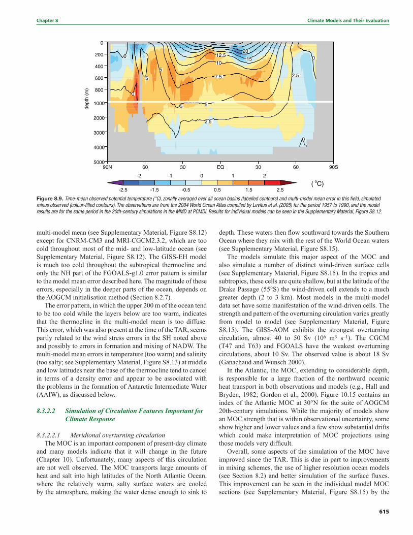
615


multi-model mean (see Supplementary Material, Figure S8.12) except for CNRM-CM3 and MRI-CGCM2.3.2, which are too cold throughout most of the mid- and low-latitude ocean (see Supplementary Material, Figure S8.12). The GISS-EH model is much too cold throughout the subtropical thermocline and only the NH part of the FGOALS-g1.0 error pattern is similar to the model mean error described here. The magnitude of these errors, especially in the deeper parts of the ocean, depends on the AOGCM initialisation method (Section 8.2.7).

The error pattern, in which the upper 200 m of the ocean tend to be too cold while the layers below are too warm, indicates that the thermocline in the multi-model mean is too diffuse. This error, which was also present at the time of the TAR, seems partly related to the wind stress errors in the SH noted above and possibly to errors in formation and mixing of NADW. The multi-model mean errors in temperature (too warm) and salinity (too salty; see Supplementary Material, Figure S8.13) at middle and low latitudes near the base of the thermocline tend to cancel in terms of a density error and appear to be associated with the problems in the formation of Antarctic Intermediate Water (AAIW), as discussed below.

8.3.2.2 Simulation of Circulation Features Important for Climate Response

8.3.2.2.1 Meridional overturning circulationThe MOC is an important component of present-day climate

and many models indicate that it will change in the future (Chapter 10). Unfortunately, many aspects of this circulation are not well observed. The MOC transports large amounts of heat and salt into high latitudes of the North Atlantic Ocean, where the relatively warm, salty surface waters are cooled by the atmosphere, making the water dense enough to sink to

depth. These waters then fl ow southward towards the Southern Ocean where they mix with the rest of the World Ocean waters (see Supplementary Material, Figure S8.15).

The models simulate this major aspect of the MOC and also simulate a number of distinct wind-driven surface cells (see Supplementary Material, Figure S8.15). In the tropics and subtropics, these cells are quite shallow, but at the latitude of the Drake Passage (55°S) the wind-driven cell extends to a much greater depth (2 to 3 km). Most models in the multi-model data set have some manifestation of the wind-driven cells. The strength and pattern of the overturning circulation varies greatly from model to model (see Supplementary Material, Figure S8.15). The GISS-AOM exhibits the strongest overturning circulation, almost 40 to 50 Sv (106 m3 s–1). The CGCM (T47 and T63) and FGOALS have the weakest overturning circulations, about 10 Sv. The observed value is about 18 Sv (Ganachaud and Wunsch 2000).

In the Atlantic, the MOC, extending to considerable depth, is responsible for a large fraction of the northward oceanic heat transport in both observations and models (e.g., Hall and Bryden, 1982; Gordon et al., 2000). Figure 10.15 contains an index of the Atlantic MOC at 30°N for the suite of AOGCM 20th-century simulations. While the majority of models show an MOC strength that is within observational uncertainty, some show higher and lower values and a few show substantial drifts which could make interpretation of MOC projections using those models very diffi cult.

Overall, some aspects of the simulation of the MOC have improved since the TAR. This is due in part to improvements in mixing schemes, the use of higher resolution ocean models (see Section 8.2) and better simulation of the surface fl uxes. This improvement can be seen in the individual model MOC sections (see Supplementary Material, Figure S8.15) by the

Figure 8.9. Time-mean observed potential temperature (°C), zonally averaged over all ocean basins (labelled contours) and multi-model mean error in this fi eld, simulated minus observed (colour-fi lled contours). The observations are from the 2004 World Ocean Atlas compiled by Levitus et al. (2005) for the period 1957 to 1990, and the model results are for the same period in the 20th-century simulations in the MMD at PCMDI. Results for individual models can be seen in the Supplementary Material, Figure S8.12.

616


fact that (1) the location of the deep-water formation is more realistic, with more sinking occurring in the Greenland-Iceland-Norwegian and Labrador Seas as evidenced by the larger stream function values north of the sill located at 60°N (e.g., Wood et al., 1999) and (2) deep waters are subjected to less spurious mixing, resulting in better water mass properties (Thorpe et al., 2004) and a larger fraction of the water that sinks in the northern part of the North Atlantic Ocean exiting the Atlantic Ocean near 30°S (Danabasoglu et al., 1995). There is still room for improvement in the models’ simulation of these processes, but there is clear evidence of improvement in many of the models analysed here.

8.3.2.2.2 Southern Ocean circulationThe Southern Ocean wind stress error has a particularly large

detrimental impact on the Southern Ocean simulation by the models. Partly due to the wind stress error identifi ed above, the simulated location of the Antarctic Circumpolar Current (ACC) is also too far north in most models (Russell et al., 2006). Since the AAIW is formed on the north side of the ACC, the water mass properties of the AAIW are distorted (typically too warm and salty: Russell et al., 2006). The relatively poor AAIW simulation contributes to the multi-model mean error identifi ed above where the thermocline is too diffuse, because the waters near the base of thermocline are too warm and salty.

It is likely that the relatively poor Southern Ocean simulation will infl uence the transient climate response to increasing greenhouse gases by affecting the oceanic heat uptake. When forced by increases in radiative forcing, models with too little Southern Ocean mixing will probably underestimate the ocean heat uptake; models with too much mixing will likely exaggerate it. These errors in oceanic heat uptake will also have a large impact on the reliability of the sea level rise projections. See Chapter 10 for more discussion of this subject.

8.3.2.3 Summary of Oceanic Component Simulation

Overall, the improvements in the simulation of the observed time mean ocean state noted in the TAR (McAvaney et al., 2001) have continued in the models evaluated here. It is notable that this improvement has continued in spite of the fact that nearly all models no longer use fl ux adjustments. This suggests that the improvements in the physical parametrizations, increased resolution (see Section 8.2) and improved surface fl uxes are together having a positive impact on model simulations. The temperature and salinity errors in the thermocline, while still large, have been reduced in many models. In the NH, many models still suffer from a cold bias in the upper ocean which is at a maximum near the surface and may distort the ice-albedo feedback in some models (see Section 8.3.3). In the Southern Ocean, the equatorward bias of the westerly wind stress maximum found in most model simulations is a problem that may affect the models’ response to increasing radiative forcing.

8.3.3 Sea Ice

The magnitude and spatial distribution of the high-latitude climate changes can be strongly affected by sea ice characteristics, but evaluation of sea ice in models is hampered by insuffi cient observations of some key variables (e.g., ice thickness) (see Section 4.4). Even when sea ice errors can be quantifi ed, it is diffi cult to isolate their causes, which might arise from defi ciencies in the representation of sea ice itself, but could also be due to fl awed simulation of the atmospheric and oceanic fi elds at high latitudes that drive ice movement (see Sections 8.3.1, 8.3.2 and 11.3.8).

Although sea ice treatment in AOGCMs has become more sophisticated, including better representation of both the dynamics and thermodynamics (see Section 8.2.4), improvement in simulating sea ice in these models, as a group, is not obvious (compare Figure 8.10 with TAR Figure 8.10; or Kattsov and Källén, 2005, Figure 4.11). In some models, however, the geographic distribution and seasonality of sea ice is now better reproduced.

For the purposes of model evaluation, the most reliably measured characteristic of sea ice is its seasonally varying extent (i.e., the area enclosed by the ice edge, operationally defi ned as the 15% contour; see Section 4.4). Despite the wide differences among the models, the multi-model mean of sea ice extent is in reasonable agreement with observations. Based on 14 of the 15 AOGCMs available at the time of analysis (one model was excluded because of unrealistically large ice extents; Arzel et al., 2006), the mean extent of simulated sea ice exceeds that observed in the NH by up to roughly 1 x 106 km2 throughout the year, whereas in the SH the annual cycle is exaggerated, with too much sea ice in September (~2 x 106 km2) and too little in March by a lesser amount. In many models the regional distribution of sea ice is poorly simulated, even if the hemispheric areal extent is approximately correct (Arzel et al., 2006; Holland and Raphael, 2006; Zhang and Walsh, 2006). The spread of simulated sea ice extents, measured as the multi-model standard deviation from the model mean, is generally narrower in the NH than in the SH (Arzel et al., 2006). Even in the best case (NH winter), the range of simulated sea ice extent exceeds 50% of the mean, and ice thickness also varies considerably, suggesting that projected decreases in sea ice cover remain rather uncertain. The model sea ice biases may infl uence global climate sensitivity (see Section 8.6). There is a tendency for models with relatively large sea ice extent in the present climate to have higher sensitivity. This is apparently especially true of models with low to moderate polar amplifi cation (Holland and Bitz, 2003).

Among the primary causes of biases in simulated sea ice (especially its distribution) are biases in the simulation of high-latitude winds (Bitz et al., 2002; Walsh et al., 2002; Chapman and Walsh, 2007), as well as vertical and horizontal mixing in the ocean (Arzel et al., 2006). Also important are surface heat fl ux errors, which in particular may result from inadequate parametrizations of the atmospheric boundary layer (under stable conditions commonly occurring at night and in the winter over sea ice) and generally from poor simulation

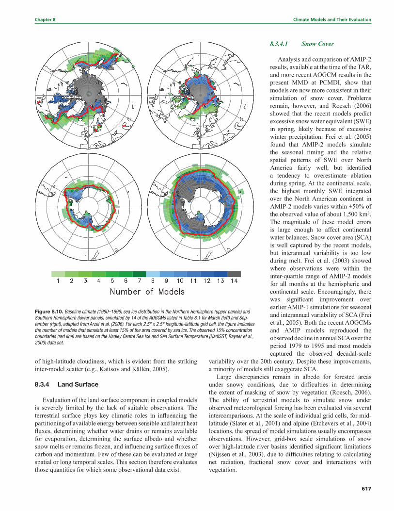
617


of high-latitude cloudiness, which is evident from the striking inter-model scatter (e.g., Kattsov and Källén, 2005).

8.3.4 Land Surface

Evaluation of the land surface component in coupled models is severely limited by the lack of suitable observations. The terrestrial surface plays key climatic roles in infl uencing the partitioning of available energy between sensible and latent heat fl uxes, determining whether water drains or remains available for evaporation, determining the surface albedo and whether snow melts or remains frozen, and infl uencing surface fl uxes of carbon and momentum. Few of these can be evaluated at large spatial or long temporal scales. This section therefore evaluates those quantities for which some observational data exist.

8.3.4.1 Snow Cover

Analysis and comparison of AMIP-2 results, available at the time of the TAR, and more recent AOGCM results in the present MMD at PCMDI, show that models are now more consistent in their simulation of snow cover. Problems remain, however, and Roesch (2006) showed that the recent models predict excessive snow water equivalent (SWE) in spring, likely because of excessive winter precipitation. Frei et al. (2005) found that AMIP-2 models simulate the seasonal timing and the relative spatial patterns of SWE over North America fairly well, but identifi ed a tendency to overestimate ablation during spring. At the continental scale, the highest monthly SWE integrated over the North American continent in AMIP-2 models varies within ±50% of the observed value of about 1,500 km3. The magnitude of these model errors is large enough to affect continental water balances. Snow cover area (SCA) is well captured by the recent models, but interannual variability is too low during melt. Frei et al. (2003) showed where observations were within the inter-quartile range of AMIP-2 models for all months at the hemispheric and continental scale. Encouragingly, there was signifi cant improvement over earlier AMIP-1 simulations for seasonal and interannual variability of SCA (Frei et al., 2005). Both the recent AOGCMs and AMIP models reproduced the observed decline in annual SCA over the period 1979 to 1995 and most models captured the observed decadal-scale

variability over the 20th century. Despite these improvements, a minority of models still exaggerate SCA.

Large discrepancies remain in albedo for forested areas under snowy conditions, due to diffi culties in determining the extent of masking of snow by vegetation (Roesch, 2006). The ability of terrestrial models to simulate snow under observed meteorological forcing has been evaluated via several intercomparisons. At the scale of individual grid cells, for mid-latitude (Slater et al., 2001) and alpine (Etchevers et al., 2004) locations, the spread of model simulations usually encompasses observations. However, grid-box scale simulations of snow over high-latitude river basins identifi ed signifi cant limitations (Nijssen et al., 2003), due to diffi culties relating to calculating net radiation, fractional snow cover and interactions with vegetation.

Figure 8.10. Baseline climate (1980–1999) sea ice distribution in the Northern Hemisphere (upper panels) and Southern Hemisphere (lower panels) simulated by 14 of the AOGCMs listed in Table 8.1 for March (left) and Sep-tember (right), adapted from Arzel et al. (2006). For each 2.5° x 2.5° longitude-latitude grid cell, the fi gure indicates the number of models that simulate at least 15% of the area covered by sea ice. The observed 15% concentration boundaries (red line) are based on the Hadley Centre Sea Ice and Sea Surface Temperature (HadISST; Rayner et al., 2003) data set.

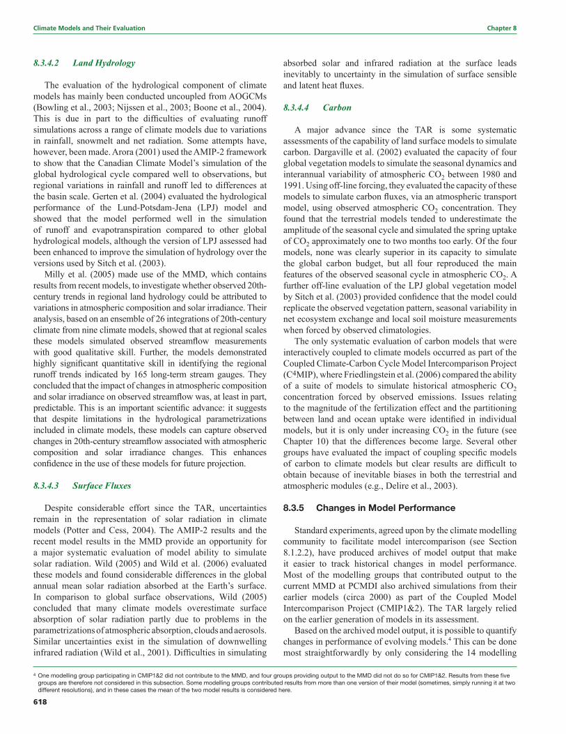
618


4 One modelling group participating in CMIP1&2 did not contribute to the MMD, and four groups providing output to the MMD did not do so for CMIP1&2. Results from these fi ve groups are therefore not considered in this subsection. Some modelling groups contributed results from more than one version of their model (sometimes, simply running it at two different resolutions), and in these cases the mean of the two model results is considered here.

8.3.4.2 Land Hydrology

The evaluation of the hydrological component of climate models has mainly been conducted uncoupled from AOGCMs (Bowling et al., 2003; Nijssen et al., 2003; Boone et al., 2004). This is due in part to the diffi culties of evaluating runoff simulations across a range of climate models due to variations in rainfall, snowmelt and net radiation. Some attempts have, however, been made. Arora (2001) used the AMIP-2 framework to show that the Canadian Climate Model’s simulation of the global hydrological cycle compared well to observations, but regional variations in rainfall and runoff led to differences at the basin scale. Gerten et al. (2004) evaluated the hydrological performance of the Lund-Potsdam-Jena (LPJ) model and showed that the model performed well in the simulation of runoff and evapotranspiration compared to other global hydrological models, although the version of LPJ assessed had been enhanced to improve the simulation of hydrology over the versions used by Sitch et al. (2003).

Milly et al. (2005) made use of the MMD, which contains results from recent models, to investigate whether observed 20th-century trends in regional land hydrology could be attributed to variations in atmospheric composition and solar irradiance. Their analysis, based on an ensemble of 26 integrations of 20th-century climate from nine climate models, showed that at regional scales these models simulated observed streamfl ow measurements with good qualitative skill. Further, the models demonstrated highly signifi cant quantitative skill in identifying the regional runoff trends indicated by 165 long-term stream gauges. They concluded that the impact of changes in atmospheric composition and solar irradiance on observed streamfl ow was, at least in part, predictable. This is an important scientifi c advance: it suggests that despite limitations in the hydrological parametrizations included in climate models, these models can capture observed changes in 20th-century streamfl ow associated with atmospheric composition and solar irradiance changes. This enhances confi dence in the use of these models for future projection.

8.3.4.3 Surface Fluxes

Despite considerable effort since the TAR, uncertainties remain in the representation of solar radiation in climate models (Potter and Cess, 2004). The AMIP-2 results and the recent model results in the MMD provide an opportunity for a major systematic evaluation of model ability to simulate solar radiation. Wild (2005) and Wild et al. (2006) evaluated these models and found considerable differences in the global annual mean solar radiation absorbed at the Earth’s surface. In comparison to global surface observations, Wild (2005) concluded that many climate models overestimate surface absorption of solar radiation partly due to problems in the parametrizations of atmospheric absorption, clouds and aerosols. Similar uncertainties exist in the simulation of downwelling infrared radiation (Wild et al., 2001). Diffi culties in simulating

absorbed solar and infrared radiation at the surface leads inevitably to uncertainty in the simulation of surface sensible and latent heat fl uxes.

8.3.4.4 Carbon

A major advance since the TAR is some systematic assessments of the capability of land surface models to simulate carbon. Dargaville et al. (2002) evaluated the capacity of four global vegetation models to simulate the seasonal dynamics and interannual variability of atmospheric CO2 between 1980 and 1991. Using off-line forcing, they evaluated the capacity of these models to simulate carbon fl uxes, via an atmospheric transport model, using observed atmospheric CO2 concentration. They found that the terrestrial models tended to underestimate the amplitude of the seasonal cycle and simulated the spring uptake of CO2 approximately one to two months too early. Of the four models, none was clearly superior in its capacity to simulate the global carbon budget, but all four reproduced the main features of the observed seasonal cycle in atmospheric CO2. A further off-line evaluation of the LPJ global vegetation model by Sitch et al. (2003) provided confi dence that the model could replicate the observed vegetation pattern, seasonal variability in net ecosystem exchange and local soil moisture measurements when forced by observed climatologies.

The only systematic evaluation of carbon models that were interactively coupled to climate models occurred as part of the Coupled Climate-Carbon Cycle Model Intercomparison Project (C4MIP), where Friedlingstein et al. (2006) compared the ability of a suite of models to simulate historical atmospheric CO2 concentration forced by observed emissions. Issues relating to the magnitude of the fertilization effect and the partitioning between land and ocean uptake were identifi ed in individual models, but it is only under increasing CO2 in the future (see Chapter 10) that the differences become large. Several other groups have evaluated the impact of coupling specifi c models of carbon to climate models but clear results are diffi cult to obtain because of inevitable biases in both the terrestrial and atmospheric modules (e.g., Delire et al., 2003).

8.3.5 Changes in Model Performance

Standard experiments, agreed upon by the climate modelling community to facilitate model intercomparison (see Section 8.1.2.2), have produced archives of model output that make it easier to track historical changes in model performance. Most of the modelling groups that contributed output to the current MMD at PCMDI also archived simulations from their earlier models (circa 2000) as part of the Coupled Model Intercomparison Project (CMIP1&2). The TAR largely relied on the earlier generation of models in its assessment.

Based on the archived model output, it is possible to quantify changes in performance of evolving models.4 This can be done most straightforwardly by only considering the 14 modelling

619


groups that contributed output from both their earlier and more recent models. One important aspect of model skill is how well the models simulate the seasonally varying global pattern of climatically important fi elds. The only monthly mean fi elds available in the CMIP1&2 archive are surface air temperature, precipitation and mean sea level pressure, so these are the focus of this analysis. Although the simulation conditions in the MMD 20th-century simulations were not identical to those in the CMIP1&2 control runs, the differences do not alter the conclusions summarised below because the large-scale climatological features dominate, not the relatively small perturbations resulting from climate change.

A summary of the ability of AOGCMs to simulate the seasonally varying climate state is provided by Figure 8.11, which displays error measures that gauge how well recent models simulate precipitation, sea level pressure and surface temperature, compared with their predecessors. The normalised RMS error shown is a so-called space-time statistic, computed from squared errors, summed over all 12 climatological months and over the entire globe, with grid cell values weighted by the corresponding grid cell area. This statistic can be used to assess the combined contributions of both spatial pattern errors and seasonal cycle errors. The RMS error is divided by the corresponding observed standard deviation of the fi eld to provide a relative measure of the error. In Figure 8.11 this scaling implies that pressure is better simulated than precipitation, and that surface temperature is simulated best of all.

Figure 8.11. Normalised RMS error in simulation of climatological patterns of monthly precipitation, mean sea level pressure and surface air temperature. Recent AOGCMs (circa 2005) are compared to their predecessors (circa 2000 and earlier). Models are categorised based on whether or not any fl ux adjustments were applied. The models are gauged against the following observation-based datasets: Climate Prediction Center Merged Analysis of Precipitation (CMAP; Xie and Arkin, 1997) for precipitation (1980–1999), European Centre for Medium Range Weather Forecasts 40-year reanalysis (ERA40; Uppala et al., 2005) for sea level pressure (1980–1999) and Climatic Research Unit (CRU; Jones et al., 1999) for surface temperature (1961–1990). Before computing the errors, both the observed and simulated fi elds were mapped to a uniform 4° x 5° latitude-longi-tude grid. For the earlier generation of models, results are based on the archived output from control runs (specifi cally, the fi rst 30 years, in the case of temperature, and the fi rst 20 years for the other fi elds), and for the recent generation models, results are based on the 20th-century simulations with climatological periods selected to correspond with observations. (In both groups of models, results are insensitive to the period selected.)

The models in Figure 8.11 are categorised based on whether or not fl ux adjustments were applied (see Section 8.2.7). Of the earlier generation models, 8 of the 14 models were fl ux adjusted, but only two of these groups continue this practice. Several conclusions can be drawn from the fi gure: 1) although fl ux-adjusted models on average have smaller errors than those without (in both generations), the smallest errors in simulating sea level pressure and surface temperature are found in models without fl ux adjustment; 2) despite the elimination of fl ux adjustment in all but two of the recent models, the mean error obtained from the recent suite of 14 models is smaller than errors found in the corresponding earlier suite of models; and 3) models without fl ux adjustment have improved on average, as have the fl ux-adjusted models. An exception to this last statement is the slight increase in mean RMS error for sea level pressure found in non-fl ux-adjusted models. Despite no apparent improvement in the mean in this case, three of the recent generation models have smaller sea level pressure errors than any of the earlier models.

These results demonstrate that the models now being used in applications by major climate modelling groups better simulate seasonally varying patterns of precipitation, mean sea level pressure and surface air temperature than the models relied on by these same groups at the time of the TAR.

620


8.4 Evaluation of Large-Scale Climate Variability as Simulated by Coupled Global Models

The atmosphere-ocean coupled climate system shows various modes of variability that range widely from intra-seasonal to inter-decadal time scales. Successful simulation and prediction over a wide range of these phenomena increase confi dence in the AOGCMs used for climate predictions of the future.

8.4.1 Northern and Southern Annular Modes

There is evidence (e.g., Fyfe et al., 1999; Shindell et al., 1999) that the simulated response to greenhouse gas forcing in AOGCMs has a pattern that resembles the models’ Northern Annular Mode (NAM), and thus it would appear important that the NAM (see Chapters 3 and 9) is realistically simulated. Analyses of individual AOGCMs (e.g., Fyfe et al., 1999; Shindell et al., 1999) have demonstrated that they are capable of simulating many aspects of the NAM and NAO patterns including linkages between circulation and temperature. Multi-model comparisons of winter atmospheric pressure (Osborn, 2004), winter temperature (Stephenson and Pavan, 2003) and atmospheric pressure across all months of the year (AchutaRao et al., 2004), including assessments of the MMD at PCMDI (Miller et al., 2006) confi rm the overall skill of AOGCMs but also identify that teleconnections between the Atlantic and Pacifi c Oceans are stronger in many models than is observed (Osborn, 2004). In some models this is related to a bias towards a strong polar vortex in all winters so that their simulations nearly always refl ect behaviour that is only observed at times with strong vortices (when a stronger Atlantic-Pacifi c correlation is observed; Castanheira and Graf, 2003).

Most AOGCMs organise too much sea level-pressure variability into the NAM and NAO (Miller et al., 2006). The year-to-year variance of the NAM or NAO is correctly simulated by some AOGCMs, while other simulations are signifi cantly too variable (Osborn, 2004); for the models that simulate stronger variability, the persistence of anomalous states is greater than is observed (AchutaRao et al., 2004). The magnitude of multi-decadal variability (relative to sub-decadal variability) is lower in AOGCM control simulations than is observed, and cannot be reproduced in current model simulations with external forcings (Osborn, 2004; Gillett, 2005). However, Scaife et al. (2005) show that the observed multi-decadal trend in the surface NAM and NAO can be reproduced in an AOGCM if observed trends in the lower stratospheric circulation are prescribed in the model. Troposphere-stratosphere coupling processes may therefore need to be included in models to fully simulate NAM variability. The response of the NAM and NAO to volcanic aerosols (Stenchikov et al., 2002), sea surface temperature variability (Hurrell et al., 2004) and sea ice anomalies (Alexander et al., 2004) demonstrate some compatibility with observed variations, though the diffi culties in determining cause and effect in the coupled system limit the conclusions that can be drawn with regards to the trustworthiness of model behaviour.

Like its NH counterpart, the NAM, the Southern Annular Mode (SAM; see Chapters 3 and 9) has signatures in the tropospheric circulation, the stratospheric polar vortex, mid-latitude storm tracks, ocean circulation and sea ice. AOGCMs generally simulate the SAM realistically (Fyfe et al., 1999; Cai et al., 2003; Miller et al., 2006). For example, Figure 8.12 compares the austral winter SAM simulated in the MMD at PCMDI to the observed SAM as represented in the National Centers for Environmental Prediction (NCEP) reanalysis. The main elements of the pattern, the low-pressure anomaly over Antarctica and the high-pressure anomalies equatorward of 60°S are captured well by the AOGCMs. In all but two AOGCMs, the spatial correlation between the observed and simulated SAM is greater than 0.95. Further analysis shows that the SAM signature in surface temperature, such as the surface warm anomaly over the Antarctic Peninsula associated with a positive SAM event, is also captured by some AOGCMs (e.g., Delworth et al., 2006; Otto-Bliesner et al., 2006). This follows from the realistic simulation of the SAM-related circulation shown in Figure 8.12, because the surface temperature signatures of the SAM typically refl ect advection of the climatological temperature distribution by the SAM-related circulation (Thompson and Wallace, 2000).

Although the spatial structure of the SAM is well simulated by the AOGCMs in the MMD at PCMDI, other features of the SAM, such as the amplitude, the detailed zonal structure and the temporal spectra, do not always compare well with the NCEP reanalysis SAM (Miller et al., 2006; Raphael and Holland, 2006). For example, Figure 8.12 shows that the simulated SAM variance (the square of the SAM amplitude) ranges between 0.9 and 2.4 times the NCEP reanalysis SAM variance. However, such features vary considerably among different realisations of multiple-member ensembles (Raphael and Holland, 2006), and the temporal variability of the NCEP reanalysis SAM does not compare well to station data (Marshall, 2003). Thus, it is diffi cult to assess whether these discrepancies between the simulated SAM and the NCEP reanalysis SAM point to shortcomings in the models or to shortcomings in the observed analysis.

Resolving these issues may require a better understanding of SAM dynamics. Although the SAM exhibits clear signatures in the ocean and stratosphere, its tropospheric structure can be simulated, for example, in atmospheric GCMs with a poorly resolved stratosphere and driven by prescribed SSTs (e.g., Limpasuvan and Hartmann, 2000; Cai et al., 2003). Even much simpler atmospheric models with one or two vertical levels produce SAM-like variability (Vallis et al., 2004). These relatively simple models capture the dynamics that underlie SAM variability – namely, interactions between the tropospheric jet stream and extratropical weather systems (Limpasuvan and Hartmann, 2000; Lorenz and Hartmann, 2001). Nevertheless, the ocean and stratosphere might still infl uence SAM variability in important ways. For example, AOGCM simulations suggest strong SAM-related impacts on ocean temperature, ocean heat transport and sea ice distribution (Watterson, 2001; Hall and Visbeck, 2002), suggesting a potential for air-sea interactions to infl uence SAM dynamics. Furthermore, observational

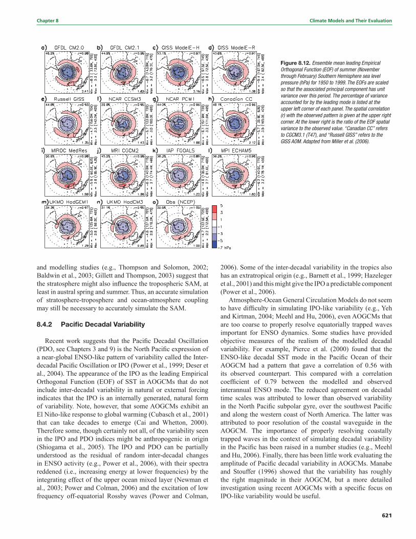
621


Figure 8.12. Ensemble mean leading Empirical Orthogonal Function (EOF) of summer (November through February) Southern Hemisphere sea level pressure (hPa) for 1950 to 1999. The EOFs are scaled so that the associated principal component has unit variance over this period. The percentage of variance accounted for by the leading mode is listed at the upper left corner of each panel. The spatial correlation (r) with the observed pattern is given at the upper right corner. At the lower right is the ratio of the EOF spatial variance to the observed value. “Canadian CC” refers to CGCM3.1 (T47), and “Russell GISS” refers to the GISS AOM. Adapted from Miller et al. (2006).

and modelling studies (e.g., Thompson and Solomon, 2002; Baldwin et al., 2003; Gillett and Thompson, 2003) suggest that the stratosphere might also infl uence the tropospheric SAM, at least in austral spring and summer. Thus, an accurate simulation of stratosphere-troposphere and ocean-atmosphere coupling may still be necessary to accurately simulate the SAM.

8.4.2 Pacifi c Decadal Variability

Recent work suggests that the Pacifi c Decadal Oscillation (PDO, see Chapters 3 and 9) is the North Pacifi c expression of a near-global ENSO-like pattern of variability called the Inter-decadal Pacifi c Oscillation or IPO (Power et al., 1999; Deser et al., 2004). The appearance of the IPO as the leading Empirical Orthogonal Function (EOF) of SST in AOGCMs that do not include inter-decadal variability in natural or external forcing indicates that the IPO is an internally generated, natural form of variability. Note, however, that some AOGCMs exhibit an El Niño-like response to global warming (Cubasch et al., 2001) that can take decades to emerge (Cai and Whetton, 2000). Therefore some, though certainly not all, of the variability seen in the IPO and PDO indices might be anthropogenic in origin (Shiogama et al., 2005). The IPO and PDO can be partially understood as the residual of random inter-decadal changes in ENSO activity (e.g., Power et al., 2006), with their spectra reddened (i.e., increasing energy at lower frequencies) by the integrating effect of the upper ocean mixed layer (Newman et al., 2003; Power and Colman, 2006) and the excitation of low frequency off-equatorial Rossby waves (Power and Colman,

2006). Some of the inter-decadal variability in the tropics also has an extratropical origin (e.g., Barnett et al., 1999; Hazeleger et al., 2001) and this might give the IPO a predictable component (Power et al., 2006).

Atmosphere-Ocean General Circulation Models do not seem to have diffi culty in simulating IPO-like variability (e.g., Yeh and Kirtman, 2004; Meehl and Hu, 2006), even AOGCMs that are too coarse to properly resolve equatorially trapped waves important for ENSO dynamics. Some studies have provided objective measures of the realism of the modelled decadal variability. For example, Pierce et al. (2000) found that the ENSO-like decadal SST mode in the Pacifi c Ocean of their AOGCM had a pattern that gave a correlation of 0.56 with its observed counterpart. This compared with a correlation coeffi cient of 0.79 between the modelled and observed interannual ENSO mode. The reduced agreement on decadal time scales was attributed to lower than observed variability in the North Pacifi c subpolar gyre, over the southwest Pacifi c and along the western coast of North America. The latter was attributed to poor resolution of the coastal waveguide in the AOGCM. The importance of properly resolving coastally trapped waves in the context of simulating decadal variability in the Pacifi c has been raised in a number studies (e.g., Meehl and Hu, 2006). Finally, there has been little work evaluating the amplitude of Pacifi c decadal variability in AOGCMs. Manabe and Stouffer (1996) showed that the variability has roughly the right magnitude in their AOGCM, but a more detailed investigation using recent AOGCMs with a specifi c focus on IPO-like variability would be useful.

622


8.4.3 Pacifi c-North American Pattern

The Pacifi c-North American (PNA) pattern (see Chapter 3) is commonly associated with the response to anomalous boundary forcing. However, PNA-like patterns have been simulated in atmospheric GCM experiments subjected to constant boundary conditions. Hence, both external and internal processes may contribute to the formation of this pattern. Particular attention has been paid to the external infl uences due to SST anomalies related to ENSO episodes in the tropical Pacifi c, as well as those situated in the extratropical North Pacifi c. Internal mechanisms that might play a role in the formation of the PNA pattern include interactions between the slowly varying component of the circulation and high-frequency transient disturbances, and instability of the climatological fl ow pattern. Trenberth et al. (1998) reviewed the myriad observational and modelling studies on various processes contributing to the PNA pattern.

The ability of GCMs to replicate various aspects of the PNA pattern has been tested in coordinated experiments. Until several years ago, such experiments were conducted by prescribing observed SST anomalies as lower boundary conditions for atmospheric GCMs. Particularly noteworthy are the ensembles of model runs performed under the auspices of the European Prediction of Climate Variations on Seasonal to Interannual Time Scales (PROVOST) and the US Dynamical Seasonal Prediction (DSP) projects. The skill of seasonal hindcasts of the participating models’ atmospheric anomalies in different regions of the globe (including the PNA sector) was summarised in a series of articles edited by Palmer and Shukla (2000). These results demonstrate that the prescribed SST forcing exerts a notable impact on the model atmospheres. The hindcast skill for the winter extratropical NH is particularly high during the largest El Niño and La Niña episodes. However, these experiments indicate considerable variability of the responses in individual models, and among ensemble members of a given model. This large scatter of model responses suggests that atmospheric changes in the extratropics are only weakly constrained by tropical SST forcing.

The performance of the dynamical seasonal forecast system at the US NCEP in predicting the atmospheric anomalies given prescribed anomalous SST forcing (in the PNA sector) was assessed by Kanamitsu et al. (2002). During the large El Niño event of 1997 to 1998, the forecasts based on this system with one-month lead time are in good agreement with the observed changes in the PNA sector, with anomaly correlation scores of 0.8 to 0.9 (for 200 mb height), 0.6 to 0.8 (surface temperature) and 0.4 to 0.5 (precipitation). More recently, hindcast experiments have been launched using AOGCMs. The European effort was supported by the Development of a European Multimodel Ensemble System for Seasonal to Interannual Prediction (DEMETER) programme (Palmer et al., 2004). For the boreal winter season, and with hindcasts initiated in November, the model-generated PNA indices exhibit statistically signifi cant temporal correlations with the corresponding observations. The fi delity of the PNA simulations is evident in both the multi-model ensemble means, as well as in the output from individual member models. However,

the strength of the ensemble mean signal remains low when compared with the statistical spread due to sampling fl uctuations among different models, and among different realisations of a given model. The model skill is notably lower for other seasons and longer lead times. Empirical Orthogonal Function analyses of the geopotential height data produced by individual member models confi rm that the PNA pattern is a leading spatial mode of atmospheric variability in these models.

Multi-century integrations have also been conducted at various institutions using the current generation of AOGCMs. Unlike the hindcasting or forecasting experiments mentioned above, these climate simulations are not aimed at reproducing specifi c ENSO events in the observed system. Diagnosis of the output from one such AOGCM integration indicates that the modelled ENSO events are linked to a PNA-like pattern in the upper troposphere (Wittenberg et al., 2006). The centres of action of the simulated patterns are systematically displaced 20 to 30 degrees of longitude west of the observed positions. This discrepancy is evidently linked to a corresponding spatial shift in the ENSO-related SST and precipitation anomaly centres simulated in the tropical Pacifi c. This fi nding illustrates that the spatial confi guration of the PNA pattern in AOGCMs is crucially dependent on the accuracy of ENSO simulations in the tropics.

8.4.4 Cold Ocean-Warm Land Pattern

The Cold Ocean-Warm Land (COWL) pattern indicates that the oceans are relatively cold and the continents are relatively warm poleward of 40°N when the NH is relatively warm. The COWL pattern results from the contrast in thermal inertia between the continents and oceans, which allows continental temperature anomalies to have greater amplitude, and thus more strongly infl uence hemispheric mean temperature. The COWL pattern has been simulated in climate models of varying degrees of complexity (e.g., Broccoli et al., 1998), and similar patterns have been obtained from cluster analysis (Wu and Straus, 2004a) and EOF analysis (Wu and Straus, 2004b) of reanalysis data. In a number of studies, cold season trends in NH temperature and sea level pressure during the late 20th century have been associated with secular trends in indices of the COWL pattern (Wallace et al., 1996; Lu et al., 2004).

In their analysis of AOGCM simulations, Broccoli et al. (1998) found that the original method for extracting the COWL pattern could yield potentially misleading results when applied to a simulation forced by past and future variations in anthropogenic forcing (as is the case with most other patterns, or modes, of climate variability). The resulting spatial pattern was a mixture of the patterns associated with unforced climate variability and the anthropogenic fi ngerprint. Broccoli et al. (1998) also noted that temperature anomalies in the two continental centres of the COWL pattern are virtually uncorrelated, suggesting that different atmospheric teleconnections are involved in producing this pattern. Quadrelli and Wallace (2004) recently showed that the COWL pattern can be reconstructed as a linear combination of the fi rst two EOFs of monthly mean December to March sea level pressure.

623


These two EOFs are the NAM and a mode closely resembling the PNA pattern. A linear combination of these two fundamental patterns can also account for a substantial fraction of the winter trend in NH sea level pressure during the late 20th century.

8.4.5 Atmospheric Regimes and Blocking

Weather, or climate, regimes are important factors in determining climate at various locations around the world and they can have a large impact on day-to-day variability (e.g., Plaut and Simonnet, 2001; Trigo et al., 2004; Yiou and Nogaj, 2004). General Circulation Models have been found to simulate hemispheric climate regimes quite similar to those found in observations (Robertson, 2001; Achatz and Opsteegh, 2003; Selten and Branstator, 2004). Simulated regional climate regimes over the North Atlantic strongly similar to the observed regimes were reported by Cassou et al. (2004), while the North Pacifi c regimes simulated by Farrara et al. (2000) were broadly consistent with those in observations. Since the TAR, agreement between different studies has improved regarding the number and structure of both hemispheric and sectoral atmospheric regimes, although this remains a subject of research (e.g., Wu and Straus, 2004a) and the statistical signifi cance of the regimes has been discussed and remains an unresolved issue (e.g., Hannachi and O’Neill, 2001; Hsu and Zwiers, 2001; Stephenson et al., 2004; Molteni et al., 2006).

Blocking events are an important class of sectoral weather regimes (see Chapter 3), associated with local reversals of the mid-latitude westerlies. The most recent systematic intercomparison of atmospheric GCM simulations of NH blocking (D’Andrea et al., 1998) was reported in the TAR. Consistent with the conclusions of this earlier study, recent studies have found that GCMs tend to simulate the location of NH blocking more accurately than frequency or duration: simulated events are generally shorter and rarer than observed events (e.g., Pelly and Hoskins, 2003b). An analysis of one of the AOGCMs from the MMD at the PCMDI found that increased horizontal resolution combined with better physical parametrizations has led to improvements in simulations of NH blocking and synoptic weather regimes over Europe. Finally, both GCM simulations and analyses of long data sets suggest the existence of considerable interannual to inter-decadal variability in blocking frequency (e.g., Stein, 2000; Pelly and Hoskins, 2003a), highlighting the need for caution when assessing blocking climatologies derived from short records (either observed or simulated). Blocking events also occur in the SH mid-latitudes (Sinclair, 1996); no systematic intercomparison of observed and simulated SH blocking climatologies has been carried out. There is also evidence of connections between North and South Pacifi c blocking and ENSO variability (e.g., Renwick, 1998; Chen and Yoon, 2002), and between North Atlantic blocks and sudden stratospheric warmings (e.g., Kodera and Chiba, 1995; Monahan et al., 2003) but these connections have not been systematically explored in AOGCMs.

8.4.6 Atlantic Multi-decadal Variability

The Atlantic Ocean exhibits considerable multi-decadal variability with time scales of about 50 to 100 years (see Chapter 3). This multi-decadal variability appears to be a robust feature of the surface climate in the Atlantic region, as shown by tree ring reconstructions for the last few centuries (e.g., Mann et al., 1998). Atlantic multi-decadal variability has a unique spatial pattern in the SST anomaly fi eld, with opposite changes in the North and South Atlantic (e.g., Mestas-Nunez and Enfi eld, 1999; Latif et al., 2004), and this dipole pattern has been shown to be signifi cantly correlated with decadal changes in Sahelian rainfall (Folland et al., 1986). Decadal variations in hurricane activity have also been linked to the multi-decadal SST variability in the Atlantic (Goldenberg et al., 2001). Atmosphere-Ocean General Circulation Models simulate Atlantic multi-decadal variability (e.g., Delworth et al., 1993; Latif, 1998 and references therein; Knight et al., 2005), and the simulated space-time structure is consistent with that observed (Delworth and Mann, 2000). The multi-decadal variability simulated by the AOGCMs originates from variations in the MOC (see Section 8.3). The mechanisms, however, that control the variations in the MOC are fairly different across the ensemble of AOGCMs. In most AOGCMs, the variability can be understood as a damped oceanic eigenmode that is stochastically excited by the atmosphere. In a few other AOGCMs, however, coupled interactions between the ocean and the atmosphere appear to be more important. The relative roles of high- and low-latitude processes differ also from model to model. The variations in the Atlantic SST associated with the multi-decadal variability appear to be predictable a few decades ahead, which has been shown by potential (diagnostic) and classical (prognostic) predictability studies. Atmospheric quantities do not exhibit predictability at decadal time scales in these studies, which supports the picture of stochastically forced variability.

8.4.7 El Niño-Southern Oscillation

During the last decade, there has been steady progress in simulating and predicting ENSO (see Chapters 3 and 9) and the related global variability using AOGCMs (Latif et al., 2001; Davey et al., 2002; AchutaRao and Sperber, 2002). Over the last several years the parametrized physics have become more comprehensive (Gregory et al., 2000; Collins et al., 2001; Kiehl and Gent, 2004), the horizontal and vertical resolutions, particularly in the atmospheric component models, have markedly increased (Guilyardi et al., 2004) and the application of observations in initialising forecasts has become more sophisticated (Alves et al., 2004). These improvements in model formulation have led to a better representation of the spatial pattern of the SST anomalies in the eastern Pacifi c (AchutaRao and Sperber, 2006). In fact, as an indication of recent model improvements, some IPCC class models are being used for ENSO prediction (Wittenberg et al., 2006). Despite this progress, serious systematic errors in both the simulated mean climate and the natural variability persist. For example, the

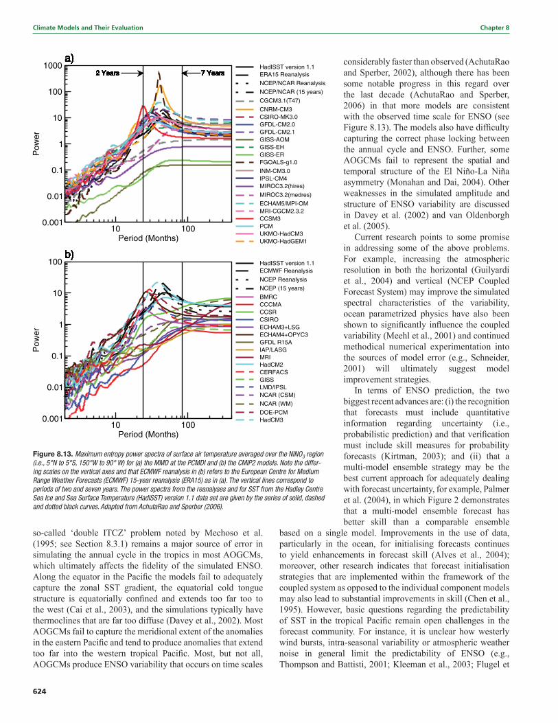
624


so-called ‘double ITCZ’ problem noted by Mechoso et al. (1995; see Section 8.3.1) remains a major source of error in simulating the annual cycle in the tropics in most AOGCMs, which ultimately affects the fi delity of the simulated ENSO. Along the equator in the Pacifi c the models fail to adequately capture the zonal SST gradient, the equatorial cold tongue structure is equatorially confi ned and extends too far too to the west (Cai et al., 2003), and the simulations typically have thermoclines that are far too diffuse (Davey et al., 2002). Most AOGCMs fail to capture the meridional extent of the anomalies in the eastern Pacifi c and tend to produce anomalies that extend too far into the western tropical Pacifi c. Most, but not all, AOGCMs produce ENSO variability that occurs on time scales

considerably faster than observed (AchutaRao and Sperber, 2002), although there has been some notable progress in this regard over the last decade (AchutaRao and Sperber, 2006) in that more models are consistent with the observed time scale for ENSO (see Figure 8.13). The models also have diffi culty capturing the correct phase locking between the annual cycle and ENSO. Further, some AOGCMs fail to represent the spatial and temporal structure of the El Niño-La Niña asymmetry (Monahan and Dai, 2004). Other weaknesses in the simulated amplitude and structure of ENSO variability are discussed in Davey et al. (2002) and van Oldenborgh et al. (2005).

Current research points to some promise in addressing some of the above problems. For example, increasing the atmospheric resolution in both the horizontal (Guilyardi et al., 2004) and vertical (NCEP Coupled Forecast System) may improve the simulated spectral characteristics of the variability, ocean parametrized physics have also been shown to signifi cantly infl uence the coupled variability (Meehl et al., 2001) and continued methodical numerical experimentation into the sources of model error (e.g., Schneider, 2001) will ultimately suggest model improvement strategies.

In terms of ENSO prediction, the two biggest recent advances are: (i) the recognition that forecasts must include quantitative information regarding uncertainty (i.e., probabilistic prediction) and that verifi cation must include skill measures for probability forecasts (Kirtman, 2003); and (ii) that a multi-model ensemble strategy may be the best current approach for adequately dealing with forecast uncertainty, for example, Palmer et al. (2004), in which Figure 2 demonstrates that a multi-model ensemble forecast has better skill than a comparable ensemble

based on a single model. Improvements in the use of data, particularly in the ocean, for initialising forecasts continues to yield enhancements in forecast skill (Alves et al., 2004); moreover, other research indicates that forecast initialisation strategies that are implemented within the framework of the coupled system as opposed to the individual component models may also lead to substantial improvements in skill (Chen et al., 1995). However, basic questions regarding the predictability of SST in the tropical Pacifi c remain open challenges in the forecast community. For instance, it is unclear how westerly wind bursts, intra-seasonal variability or atmospheric weather noise in general limit the predictability of ENSO (e.g., Thompson and Battisti, 2001; Kleeman et al., 2003; Flugel et

Figure 8.13. Maximum entropy power spectra of surface air temperature averaged over the NINO3 region (i.e., 5°N to 5°S, 150°W to 90° W) for (a) the MMD at the PCMDI and (b) the CMIP2 models. Note the differ-ing scales on the vertical axes and that ECMWF reanalysis in (b) refers to the European Centre for Medium Range Weather Forecasts (ECMWF) 15-year reanalysis (ERA15) as in (a). The vertical lines correspond to periods of two and seven years. The power spectra from the reanalyses and for SST from the Hadley Centre Sea Ice and Sea Surface Temperature (HadISST) version 1.1 data set are given by the series of solid, dashed and dotted black curves. Adapted from AchutaRao and Sperber (2006).

625


al., 2004; Kirtman et al., 2005). There are also apparent decadal variations in ENSO forecast skill (Balmaseda et al., 1995; Ji et al., 1996; Kirtman and Schopf, 1998), and the sources of these variations are the subject of some debate. Finally, it remains unclear how changes in the mean climate will ultimately affect ENSO predictability (Collins et al., 2002).

8.4.8 Madden-Julian Oscillation

The MJO (Madden and Julian, 1971) refers to the dominant mode of intra-seasonal variability in the tropical troposphere. It is characterised by large-scale regions of enhanced and suppressed convection, coupled to a deep baroclinic, primarily zonal circulation anomaly. Together, they propagate slowly eastward along the equator from the western Indian Ocean to the central Pacifi c and exhibit local periodicity in a broad 30- to 90-day range. Simulation of the MJO in contemporary coupled and uncoupled climate models remains unsatisfactory (e.g., Zhang, 2005; Lin et al., 2006), partly because more is now demanded from the model simulations, as understanding of the role of the MJO in the coupled atmosphere-ocean climate system expands. For instance, simulations of the MJO in models at the time of the TAR were judged using gross metrics (e.g., Slingo et al., 1996). The spatial phasing of the associated surface fl uxes, for instance, are now recognised as critical for the development of the MJO and its interaction with the underlying ocean (e.g., Hendon, 2005; Zhang, 2005). Thus, while a model may simulate some gross characteristics of the MJO, the simulation may be deemed unsuccessful when the detailed structure of the surface fl uxes is examined (e.g., Hendon, 2000).

Variability with MJO characteristics (e.g., convection and wind anomalies of the correct spatial scale that propagate coherently eastward with realistic phase speeds) is simulated in many contemporary models (e.g., Sperber et al., 2005; Zhang, 2005), but this variability is typically not simulated to occur often enough or with suffi cient strength so that the MJO stands out realistically above the broadband background variability (Lin et al., 2006). This underestimation of the strength and coherence of convection and wind variability at MJO temporal and spatial scales means that contemporary climate models still simulate poorly many of the important climatic effects of the MJO (e.g., its impact on rainfall variability in the monsoons or the modulation of tropical cyclone development). Simulation of the spatial structure of the MJO as it evolves through its life cycle is also problematic, with tendencies for the convective anomaly to split into double ITCZs in the Pacifi c and for erroneously strong convective signals to sometimes develop in the eastern Pacifi c ITCZ (e.g., Inness and Slingo, 2003). It has also been suggested that inadequate representation in climate models of cloud-radiative interactions and/or convection-moisture interactions may explain some of the diffi culties in simulating the MJO (e.g., Lee et al., 2001; Bony and Emanuel, 2005).

Even though the MJO is probably not fundamentally a coupled ocean-atmosphere mode (e.g., Waliser et al., 1999), air-sea coupling does appear to promote more coherent eastward, and, in northern summer, northward propagation at

MJO temporal and spatial scales. The interaction with an active ocean is important especially in the suppressed convective phase when SSTs are warming and the atmospheric boundary layer is recovering (e.g., Hendon, 2005). Thus, the most realistic simulation of the MJO is anticipated to be with AOGCMs. However, coupling, in general, has not been a panacea. While coupling in some models improves some aspects of the MJO, especially eastward propagation and coherence of convective anomalies across the Indian and western Pacifi c Oceans (e.g., Kemball-Cook et al., 2002; Inness and Slingo, 2003), problems with the horizontal structure and seasonality remain. Typically, models that show the most benefi cial impact of coupling on the propagation characteristics of the MJO are also the models that possess the most unrealistic seasonal variation of MJO activity (e.g., Zhang, 2005). Unrealistic simulation of the seasonal variation of MJO activity implies that the simulated MJO will improperly interact with climate phenomena that are tied to the seasonal cycle (e.g., the monsoons and ENSO).

Simulation of the MJO is also adversely affected by biases in the mean state (see Section 8.4.7). These biases include the tendency for coupled models to exaggerate the double ITCZ in the Indian and western Pacifi c Oceans, under-predict the eastward extent of surface monsoonal westerlies into the western Pacifi c, and over-predict the westward extension of the Pacifi c cold tongue. Together, these fl aws limit development, maintenance and the eastward extent of convection associated with the MJO, thereby reducing its overall strength and coherence (e.g., Inness et al., 2003). To date, simulation of the MJO has proven to be most sensitive to the convective parametrization employed in climate models (e.g., Wang and Schlesinger, 1999; Maloney and Hartmann, 2001; Slingo et al., 2005). A consensus, although with exceptions (e.g., Liu et al., 2005), appears to be emerging that convective schemes based on local vertical stability and that include some triggering threshold produce more realistic MJO variability than those that convect too readily. However, some sophisticated models, with arguably the most physically based convective parametrizations, are unable to simulate reasonable MJO activity (e.g., Slingo et al., 2005).

8.4.9 Quasi-Biennial Oscillation

The Quasi-Biennial Oscillation (QBO; see Chapter 3) is a quasi-periodic wave-driven zonal mean wind reversal that dominates the low-frequency variability of the lower equatorial stratosphere (3 to 100 hPa) and affects a variety of extratropical phenomena including the strength and stability of the winter polar vortex (e.g., Baldwin et al., 2001). Theory and observations indicate that a broad spectrum of vertically propagating waves in the equatorial atmosphere must be considered to explain the QBO. Realistic simulation of the QBO in GCMs therefore depends on three important conditions: (i) suffi cient vertical resolution in the stratosphere to allow the representation of equatorial waves at the horizontally resolved scales of a GCM, (ii) a realistic excitation of resolved equatorial waves by simulated tropical weather and (iii) parametrization of the

626


effects of unresolved gravity waves. Due to the computational cost associated with the requirement of a well-resolved stratosphere, the models employed for the current assessment do not generally include the QBO.

The inability of resolved wave driving to induce a spontaneous QBO in GCMs has been a long-standing issue (Boville and Randel, 1992). Only recently (Takahashi, 1996, 1999; Horinouchi and Yoden, 1998; Hamilton et al., 2001) have two necessary conditions been identifi ed that allow resolved waves to induce a QBO: high vertical resolution in the lower stratosphere (roughly 0.5 km), and a parametrization of deep cumulus convection with suffi ciently large temporal variability. However, recent analysis of satellite and radar observations of deep tropical convection (Horinouchi, 2002) indicates that the forcing of a QBO by resolved waves alone requires a parametrization of deep convection with an unrealistically large amount of temporal variability. Consequently, it is currently thought that a combination of resolved and parametrized waves is required to properly model the QBO. The utility of parametrized non-orographic gravity wave drag to force a QBO has now been demonstrated by a number of studies (Scaife et al., 2000; Giorgetta et al., 2002, 2006). Often an enhancement of input momentum fl ux in the tropics relative to that needed in the extratropics is required. Such an enhancement, however, depends implicitly on the amount of resolved waves and in turn, the spatial and temporal properties of parametrized deep convection employed in each model (Horinouchi et al., 2003; Scinocca and McFarlane, 2004).

8.4.10 Monsoon Variability

Monsoon variability (see Chapters 3, 9 and 11) occurs over a range of temporal scales from intra-seasonal to inter-decadal. Since the TAR, the ability of AOGCMs to simulate monsoon variability on intra-seasonal as well as interannual time scales has been examined. Lambert and Boer (2001) compared the AOGCMs that participated in CMIP, fi nding large errors in the simulated precipitation in the equatorial regions and in the Asian monsoon region. Lin et al. (2006) evaluated the intra-seasonal variation of precipitation in the MMD at PCMDI. They found that the intra-seasonal variance of precipitation simulated by most AOGCMs was smaller than observed. The space-time spectra of most model simulations have much less power than is observed, especially at periods shorter than six days. The speed of the equatorial waves is too fast, and the persistence of the precipitation is too long, in most of the AOGCM simulations. Annamalai et al (2004) examined the fi delity of precipitation simulation in the Asian monsoon region in the MMD at PCMDI. They found that just 6 of the 18 AOGCMs considered realistically simulated climatological monsoon precipitation for the 20th century. For the former set of models, the spatial correlation of the patterns of monsoon precipitation between the models exceeded 0.6, and the seasonal cycle of monsoon rainfall was simulated well. Among these models, only four exhibited a robust ENSO-monsoon contemporaneous teleconnection. Cook and Vizy (2006) evaluated the simulation of the 20th-century

climate in North Africa in the MMD at PCMDI. They found that the simulation of North African summer precipitation was less realistic than the simulation of summer precipitation over North America or Europe. In short, most AOGCMs do not simulate the spatial or intra-seasonal variation of monsoon precipitation accurately. See Chapter 11 for a more detailed regional evaluation of simulated monsoon variability.

8.4.11 Shorter-Term Predictions Using Climate Models

This subsection focuses on the few results of initial value predictions made using models that are identical, or very close to, the models used in other chapters of this report for understanding and predicting climate change.

Weather predictionSince the TAR, it has been shown that climate models can be

integrated as weather prediction models if they are initialised appropriately (Phillips et al., 2004). This advance appears to be due to: (i) improvements in the forecast model analyses and (ii) increases in the climate model spatial resolution. An advantage of testing a model’s ability to predict weather is that some of the sub-grid scale physical processes that are parametrized in models (e.g., cloud formation, convection) can be evaluated on time scales characteristic of those processes, without the complication of feedbacks from these processes altering the underlying state of the atmosphere (Pope and Stratton, 2002; Boyle et al., 2005; Williamson et al., 2005; Martin et al., 2006). Full use can be made of the plentiful meteorological data sets and observations from specialised fi eld experiments. According to these studies, some of the biases found in climate simulations are also evident in the analysis of their weather forecasts. This suggests that ongoing improvements in model formulation driven primarily by the needs of weather forecasting may lead also to more reliable climate predictions.

Seasonal predictionVerifi cation of seasonal-range predictions provides a direct

test of a model’s ability to represent the physical and dynamical processes controlling (unforced) fl uctuations in the climate system. Satisfactory prediction of variations in key climate signals such as ENSO and its global teleconnections provides evidence that such features are realistically represented in long-term forced climate simulations.

A version of the HadCM3 AOGCM (known as GloSea) has been assessed for skill in predicting observed seasonal climate variations (Davey et al., 2002; Graham et al., 2005). Graham et al. (2005) analysed 43 years of retrospective six-month forecasts (‘hindcasts’) with GloSea, run from observed ocean-land-atmosphere initial conditions. A nine-member ensemble was used to sample uncertainty in the initial conditions. Conclusions relevant to HadCM3 include: (i) the model is able to reproduce observed large-scale lagged responses to ENSO events in the tropical Atlantic and Indian Ocean SSTs; and (ii) the model can realistically predict anomaly patterns in North

627


Atlantic SSTs, shown to have important links with the NAO and seasonal temperature anomalies over Europe.

The GFDL-CM2.0 AOGCM has also been assessed for seasonal prediction. Twelve-month retrospective and contemporaneous forecasts were produced using a six-member ensemble over 15 years starting in 1991. The forecasts were initialised using global ocean data assimilation (Derber and Rosati, 1989; Rosati et al., 1997) and observed atmospheric forcing, combined with atmospheric initial conditions derived from the atmospheric component of the model forced with observed SSTs. Results indicated considerable model skill out to 12 months for ENSO prediction (see http://www.gfdl.noaa.gov/~rgg/si_workdir/Forecasts.html). Global teleconnections, as diagnosed from the NCEP reanalysis (GFDL GAMDT, 2004), were evident throughout the 12-month forecasts.

8.5 Model Simulations of Extremes

Society’s perception of climate variability and climate change is largely formed by the frequency and the severity of extremes. This is especially true if the extreme events have large and negative impacts on lives and property. As climate models’ resolution and the treatment of physical processes have improved, the simulation of extremes has also improved. Mainly because of increased data availability (e.g., daily data, various indices, etc.), the modelling community has now examined the model simulations in greater detail and presented a comprehensive description of extreme events in the coupled models used for climate change projections.

Some extreme events, by their very nature of being smaller in scale and shorter in duration, are manifestations of either a rapid amplifi cation, or an equilibration at a higher amplitude, of naturally occurring local instabilities. Large-scale and long-duration extreme events are generally due to persistence of weather patterns associated with air-sea and air-land interactions. A reasonable hypothesis might be that the coarse-resolution AOGCMs might not be able to simulate local short-duration extreme events, but that is not the case. Our assessment of the recent scientifi c literature shows, perhaps surprisingly, that the global statistics of the extreme events in the current climate, especially temperature, are generally well simulated by the current models (see Section 8.5.1). These models have been more successful in simulating temperature extremes than precipitation extremes.

The assessment of extremes, especially for temperature, has been done by examining the amplitude, frequency and persistence of the following quantities: daily maximum and minimum temperature (e.g., hot days, cold days, frost days), daily precipitation intensity and frequency, seasonal mean temperature and precipitation and frequency and tracks of tropical cyclones. For precipitation, the assessment has been done either in terms of return values or extremely high rates of precipitation.

8.5.1 Extreme Temperature Kiktev et al. (2003) compared station observations of

extreme events with the simulations of an atmosphere-only GCM (Hadley Centre Atmospheric Model version 3; HadAM3) forced by prescribed oceanic forcing and anthropogenic radiative forcing during 1950 to 1995. The indices of extreme events they used were those proposed by Frich et al. (2002). They found that inclusion of anthropogenic radiative forcing was required to reproduce observed changes in temperature extremes, particularly at large spatial scales. The decrease in the number of frost days in Southern Australia simulated by HadAM3 with anthropogenic forcing is in good agreement with the observations. The increase in the number of warm nights over Eurasia is poorly simulated when anthropogenic forcing is not included, but the inclusion of anthropogenic forcing improves the modelled trend patterns over western Russia and reproduces the general increase in the occurrence of warm nights over much of the NH.

Meehl et al. (2004) compared the number of frost days simulated by the PCM model with observations. The 20th-century simulations include the variations in solar, volcano, sulphate aerosol, ozone and greenhouse gas forcing. Both model simulations and observations show that the number of frost days decreased by two days per decade in the western USA during the 20th century. The model simulations do not agree with observations in the southeastern USA, where the model simulates a decrease in the number of frost days in this region in the 20th century, while observations indicate an increase in this region. Meehl et al. (2004) argue that this discrepancy could be due to the model’s inability to simulate the impact of El Niño events on the number of frost days in the southeastern USA. Meehl and Tebaldi (2004) compared the heat waves simulated by the PCM with observations. They defi ned a heat wave as the three consecutive warmest nights during the year. During the period 1961 to 1990, there is good agreement between the model and observations (NCEP reanalysis).

Kharin et al. (2005) examined the simulations of temperature and precipitation extremes for AMIP-2 models, some of which are atmospheric components of coupled models used in this assessment. They found that models simulate the temperature extremes, especially the warm extremes, reasonably well. Models have serious defi ciencies in simulating precipitation extremes, particularly in the tropics. Vavrus et al. (2006) used daily values of 20th-century integrations from seven models. They defi ned a cold air outbreak as ‘an occurrence of two or more consecutive days during which the local mean daily surface air temperature is at least two standard deviations below the local winter mean temperature’. They found that the climate models reproduce the location and magnitude of cold air outbreaks in the current climate.

Researchers have also established relationships between large-scale circulation features and cold air outbreaks or heat waves. For example, Vavrus et al. (2006) found that ‘the favored regions of cold air outbreaks are located near and downstream

628


from preferred locations of atmosphere blocking’. Likewise, Meehl and Tebaldi (2004) found that heat waves over Europe and North America were associated with changes in the 500 hPa circulation pattern.

8.5.2 Extreme Precipitation

Sun et al. (2006) investigated the intensity of daily

precipitation simulated by 18 AOGCMs, including several used in this report. They found that most of the models produce light precipitation (<10 mm day–1) more often than observed, too few heavy precipitation events and too little precipitation in heavy events (>10 mm day–1). The errors tend to cancel, so that the seasonal mean precipitation is fairly realistic (see Section 8.3).

Since the TAR, many simulations have been made with high-resolution GCMs. Iorio et al. (2004) examined the impact of model resolution on the simulation of precipitation in the USA using the Community Climate Model version 3 (CCM3). They found that the high-resolution simulation produces more realistic daily precipitation statistics. The coarse-resolution model had too many days with weak precipitation and not enough with intense precipitation. This tendency was partially eliminated in the high-resolution simulation, but, in the simulation at the highest resolution (T239), the high-percentile daily precipitation was still too low. This problem was eliminated when a cloud-resolving model was embedded in every grid point of the GCM.

Kimoto et al. (2005) compared the daily precipitation over Japan in an AOGCM with two different resolutions (high res. and med res. of MIROC 3.2) and found more realistic precipitation distributions with the higher resolution. Emori et al. (2005) showed that a high-resolution AGCM (the atmospheric part of high res. MIROC 3.2) can simulate the extreme daily precipitation realistically if there is provision in the model to suppress convection when the ambient relative humidity is below 80%, suggesting that modelled extreme precipitation can be strongly parametrization dependent. Kiktev et al. (2003) compared station observations of rainfall with the simulations of the atmosphere-only GCM HadAM3 forced by prescribed oceanic forcing and anthropogenic radiative forcing. They found that this model shows little skill in simulating changing precipitation extremes. May (2004) examined the variability and extremes of daily rainfall in the simulation of present day climate by the ECHAM4 GCM. He found that this model simulates the variability and extremes of rainfall quite well over most of India when compared to satellite-derived rainfall, but has a tendency to overestimate heavy rainfall events in central India. Durman et al. (2001) compared the extreme daily European precipitation simulated by the HadCM2 GCM with station observations. They found that the GCM’s ability to simulate daily precipitation events exceeding 15 mm per day was good but its ability to simulate events exceeding 30 mm per day was poor. Kiktev et al. (2003) showed that HadAM3 was able to simulate the natural variability of the precipitation intensity index (annual mean precipitation divided by number of days with precipitation less than 1 mm) but was not able to simulate accurately the variability

in the number of wet days (the number of days in a year with precipitation greater than 10 mm).

Using the Palmer Drought Severity Index (PDSI), Dai at al. (2004) concluded that globally very dry or wet areas (PDSI above +3 or below –3) have increased from 20% to 38% since 1972. In addition to simulating the short-duration events like heat waves, frost days and cold air outbreaks, models have also shown success in simulating long time-scale anomalies. For example, Burke et al. (2006) showed that the HadCM3 model, on a global basis and at decadal time scales, ‘reproduces the observed drying trend’ as defi ned by the PDSI if the anthropogenic forcing is included, although the model does not always simulate correctly the regional distributions of wet and dry areas.

8.5.3 Tropical Cyclones

The spatial resolution of the coupled ocean-atmosphere

models used in the IPCC assessment is generally not high enough to resolve tropical cyclones, and especially to simulate their intensity. A common approach to investigate the effects of global warming on tropical cyclones has been to utilise the SST boundary conditions from a global change scenario run to force a high-resolution AGCM. That model run is then compared with a control run using the high-resolution AGCM forced with specifi ed observed SST for the current climate (Sugi et al., 2002; Camargo et al., 2005; McDonald et al., 2005; Bengtsson et al., 2006; Oouchi et al., 2006; Yoshimura et al., 2006). There are also several idealised model experiments in which a high-resolution AGCM is integrated with and without a fi xed global warming or cooling of SST. Another method is to embed a high-resolution regional model in the lower-resolution climate model (Knutson and Tuleya, 1999; Walsh et al., 2004). Projections using these methods are discussed in Chapter 10.

Bengtsson et al. (2006) showed that the global metrics of tropical cyclones (tropical or hemispheric averages) are broadly reproduced by the ECHAM5 model, even as a function of intensity. However, varying degrees of errors (in some cases substantial) in simulated tropical storm frequency and intensity have been noted in some models (e.g., GFDL GAMDT, 2004; Knutson and Tuleya, 2004; Camargo et al., 2005). The tropical cyclone simulation has been shown to be sensitive to the choice of convection parametrization in some cases.

Oouchi et al. (2006) used one of the highest-resolution (20 km) atmospheric models to simulate the frequency, distribution and intensity of tropical cyclones in the current climate. Although there were some defi ciencies in simulating the geographical distribution of tropical cyclones (over-prediction of tropical cyclones between 0° to 10°S in the Indian Ocean, and under-prediction between 0° to 10°N in the western Pacifi c), the overall simulation of geographical distribution and frequency was remarkably good. The model could not simulate the strongest observed maximum wind speeds, and central pressures were not as low as observed, suggesting that even higher resolution may be required to simulate the most intense tropical cyclones.

629


8.5.4 Summary Because most AOGCMs have coarse resolution and large-

scale systematic errors, and extreme events tend to be short lived and have smaller spatial scales, it is somewhat surprising how well the models simulate the statistics of extreme events in the current climate, including the trends during the 20th century (see Chapter 9 for more detail). This is especially true for the temperature extremes, but intensity, frequency and distribution of extreme precipitation are less well simulated. The higher-resolution models used for projections of tropical cyclone changes (Chapter 10) produce generally good simulation of the frequency and distribution of tropical cyclones, but less good simulation of their intensity. Improvements in the simulation of the intensity of precipitation and tropical cyclones with increases in the resolution of AGCMs (Oouchi et al., 2006) suggest that when climate models have suffi cient resolution to explicitly resolve at least the large convective systems without using parametrizations for deep convection, it is likely that simulation of precipitation and intensity of tropical cyclones will improve.

8.6 Climate Sensitivity and Feedbacks

8.6.1 Introduction

Climate sensitivity is a metric used to characterise the response of the global climate system to a given forcing. It is broadly defi ned as the equilibrium global mean surface temperature change following a doubling of atmospheric CO2 concentration (see Box 10.2). Spread in model climate sensitivity is a major factor contributing to the range in projections of future climate changes (see Chapter 10) along with uncertainties in future emission scenarios and rates of oceanic heat uptake. Consequently, differences in climate sensitivity between models have received close scrutiny in all four IPCC reports. Climate sensitivity is largely determined by internal feedback processes that amplify or dampen the infl uence of radiative forcing on climate. To assess the reliability of model estimates of climate sensitivity, the ability of climate models to reproduce different climate changes induced by specifi c forcings may be evaluated. These include the Last Glacial Maximum and the evolution of climate over the last millennium and the 20th century (see Section 9.6). The compilation and comparison of climate sensitivity estimates derived from models and from observations are presented in Box 10.2. An alternative approach, which is followed here, is to assess the reliability of key climate feedback processes known to play a critical role in the models’ estimate of climate sensitivity.

This section explains why the estimates of climate sensitivity and of climate feedbacks differ among current models (Section 8.6.2), summarises understanding of the role of key radiative feedback processes associated with water vapour and lapse rate, clouds, snow and sea ice in climate sensitivity, and assesses the

treatment of these processes in the global climate models used to make projections of future climate change (Section 8.6.3). Finally we discuss how we can assess our relative confi dence in the different climate sensitivity estimates derived from climate models (Section 8.6.4). Note that climate feedbacks associated with chemical or biochemical processes are not discussed in this section (they are addressed in Chapters 7 and 10), nor are local-scale feedbacks (e.g., between soil moisture and precipitation; see Section 8.2.3.2).

8.6.2 Interpreting the Range of Climate Sensitivity Estimates Among General Circulation Models

8.6.2.1 Defi nition of Climate Sensitivity

As defi ned in previous assessments (Cubasch et al., 2001) and in the Glossary, the global annual mean surface air temperature change experienced by the climate system after it has attained a new equilibrium in response to a doubling of atmospheric CO2 concentration is referred to as the ‘equilibrium climate sensitivity’ (unit is °C), and is often simply termed the ‘climate sensitivity’. It has long been estimated from numerical experiments in which an AGCM is coupled to a simple non-dynamic model of the upper ocean with prescribed ocean heat transports (usually referred to as ‘mixed-layer’ or ‘slab’ ocean models) and the atmospheric CO2 concentration is doubled. In AOGCMs and non-steady-state (or transient) simulations, the ‘transient climate response’ (TCR; Cubasch et al., 2001) is defi ned as the global annual mean surface air temperature change (with respect to a ‘control’ run) averaged over a 20-year period centred at the time of CO2 doubling in a 1% yr–1 compound CO2 increase scenario. That response depends both on the sensitivity and on the ocean heat uptake. An estimate of the equilibrium climate sensitivity in transient climate change integrations is obtained from the ‘effective climate sensitivity’ (Murphy, 1995). It corresponds to the global temperature response that would occur if the AOGCM was run to equilibrium with feedback strengths held fi xed at the values diagnosed at some point of the transient climate evolution. It is computed from the oceanic heat storage, the radiative forcing and the surface temperature change (Cubasch et al., 2001; Gregory et al., 2002).

The climate sensitivity depends on the type of forcing agents applied to the climate system and on their geographical and vertical distributions (Allen and Ingram, 2002; Sausen et al., 2002; Joshi et al., 2003). As it is infl uenced by the nature and the magnitude of the feedbacks at work in the climate response, it also depends on the mean climate state (Boer and Yu, 2003). Some differences in climate sensitivity will also result simply from differences in the particular radiative forcing calculated by different radiation codes (see Sections 10.2.1 and 8.6.2.3). The global annual mean surface temperature change thus presents limitations regarding the description and the understanding of the climate response to an external forcing. Indeed, the regional temperature response to a uniform forcing (and even more to a vertically or geographically distributed forcing) is highly inhomogeneous. In addition, climate sensitivity only considers

630


the surface mean temperature and gives no indication of the occurrence of abrupt changes or extreme events. Despite its limitations, however, the climate sensitivity remains a useful concept because many aspects of a climate model scale well with global average temperature (although not necessarily across models), because the global mean temperature of the Earth is fairly well measured, and because it provides a simple way to quantify and compare the climate response simulated by different models to a specifi ed perturbation. By focusing on the global scale, climate sensitivity can also help separate the climate response from regional variability.

8.6.2.2 Why Have the Model Estimates Changed Since the TAR?

The current generation of GCMs5 covers a range of equilibrium climate sensitivity from 2.1°C to 4.4°C (with a mean value of 3.2°C; see Table 8.2 and Box 10.2), which is quite similar to the TAR. Yet most climate models have undergone substantial developments since the TAR (probably more than between the Second Assessment Report and the TAR) that generally involve improved parametrizations of specifi c processes such as clouds, boundary layer or convection (see Section 8.2). In some cases, developments have also concerned numerics, dynamical cores or the coupling to new components (ocean, carbon cycle, etc.). Developing new versions of a model to improve the physical basis of parametrizations or the simulation of the current climate is at the heart of modelling group activities. The rationale for these changes is generally based upon a combination of process-level tests against observations or against cloud-resolving or large-eddy simulation models (see Section 8.2), and on the overall quality of the model simulation (see Sections 8.3 and 8.4). These developments can, and do, affect the climate sensitivity of models.

The equilibrium climate sensitivity estimates from the latest model version used by modelling groups have increased (e.g., CCSM3 vs CSM1.0, ECHAM5/MPI-OM vs ECHAM3/LSG, IPSL-CM4 vs IPSL-CM2, MRI-CGCM2.3.2 vs MRI2, UKMO-HadGEM1 vs UKMO-HadCM3), decreased (e.g., CSIRO-MK3.0 vs CSIRO-MK2, GFDL-CM2.0 vs GFDL_R30_c, GISS-EH and GISS-ER vs GISS2, MIROC3.2(hires) and MIROC3.2(medres) vs CCSR/NIES2) or remained roughly unchanged (e.g., CGCM3.1(T47) vs CGCM1, GFDL-CM2.1 vs GFDL_R30_c) compared to the TAR. In some models, changes in climate sensitivity are primarily ascribed to changes in the cloud parametrization or in the representation of cloud-radiative properties (e.g., CCSM3, MRI-CGCM2.3.2, MIROC3.2(medres) and MIROC3.2(hires)). However, in most models the change in climate sensitivity cannot be attributed to a specifi c change in the model. For instance, Johns et al. (2006) showed that most of the individual changes made during the development of HadGEM1 have a small impact on the climate sensitivity, and that the global effects of the individual changes

largely cancel each other. In addition, the parametrization changes can interact nonlinearly with each other so that the sum of change A and change B does not produce the same as the change in A plus B (e.g., Stainforth et al., 2005). Finally, the interaction among the different parametrizations of a model explains why the infl uence on climate sensitivity of a given change is often model dependent (see Section 8.2). For instance, the introduction of the Lock boundary-layer scheme (Lock et al., 2000) to HadCM3 had a minimal impact on the climate sensitivity, in contrast to the introduction of the scheme to the GFDL atmospheric model (Soden et al., 2004; Johns et al., 2006).

8.6.2.3 What Explains the Current Spread in Models’ Climate Sensitivity Estimates?

As discussed in Chapter 10 and throughout the last three IPCC assessments, climate models exhibit a wide range of climate sensitivity estimates (Table 8.2). Webb et al. (2006), investigating a selection of the slab versions of models in Table 8.1, found that differences in feedbacks contribute almost three times more to the range in equilibrium climate sensitivity estimates than differences in the models’ radiative forcings (the spread of models’ forcing is discussed in Section 10.2).

Several methods have been used to diagnose climate feedbacks in GCMs, whose strengths and weaknesses are reviewed in Stephens (2005) and Bony et al. (2006). These methods include the ‘partial radiative perturbation’ approach and its variants (e.g., Colman, 2003a; Soden and Held, 2006), the use of radiative-convective models and the ‘cloud radiative forcing’ method (e.g., Webb et al., 2006). Since the TAR, there has been progress in comparing the feedbacks produced by climate models in doubled atmospheric CO2 equilibrium experiments (Colman, 2003a; Webb et al., 2006) and in transient climate change integrations (Soden and Held, 2006). Water vapour, lapse rate, cloud and surface albedo feedback parameters, as estimated by Colman (2003a), Soden and Held (2006) and Winton (2006a) are shown in Figure 8.14.

In AOGCMs, the water vapour feedback constitutes by far the strongest feedback, with a multi-model mean and standard deviation for the MMD at PCMDI of 1.80 ± 0.18 W m–2 °C–1, followed by the (negative) lapse rate feedback (–0.84 ± 0.26 W m–2 °C–1) and the surface albedo feedback (0.26 ± 0.08 W m–2 °C–1). The cloud feedback mean is 0.69 W m–2 °C–1 with a very large inter-model spread of ±0.38 W m–2 °C–1 (Soden and Held, 2006).

A substantial spread is apparent in the strength of water vapour feedback that is smaller in Soden and Held (2006) than in Colman (2003a). It is not known whether this smaller spread indicates a closer consensus among current AOGCMs than among older models, differences in the methodology or differences in the nature of climate change integrations between the two studies. In both studies, the lapse rate feedback also shows a substantial spread among models, which is explained

5 Unless explicitly stated, GCM here refers both to AOGCM (used to estimate TCR) and AGCM coupled to a slab ocean (used to estimate equilibrium climate sensitivity).

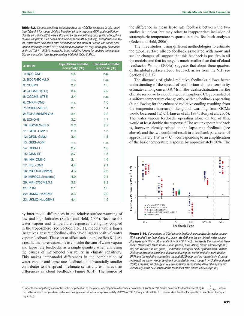
631


by inter-model differences in the relative surface warming of low and high latitudes (Soden and Held, 2006). Because the water vapour and temperature responses are tightly coupled in the troposphere (see Section 8.6.3.1), models with a larger (negative) lapse rate feedback also have a larger (positive) water vapour feedback. These act to offset each other (see Box 8.1). As a result, it is more reasonable to consider the sum of water vapour and lapse rate feedbacks as a single quantity when analysing the causes of inter-model variability in climate sensitivity. This makes inter-model differences in the combination of water vapour and lapse rate feedbacks a substantially smaller contributor to the spread in climate sensitivity estimates than differences in cloud feedback (Figure 8.14). The source of

the difference in mean lapse rate feedback between the two studies is unclear, but may relate to inappropriate inclusion of stratospheric temperature response in some feedback analyses (Soden and Held, 2006).

The three studies, using different methodologies to estimate the global surface albedo feedback associated with snow and sea ice changes, all suggest that this feedback is positive in all the models, and that its range is much smaller than that of cloud feedbacks. Winton (2006a) suggests that about three-quarters of the global surface albedo feedback arises from the NH (see Section 8.6.3.3).

The diagnosis of global radiative feedbacks allows better understanding of the spread of equilibrium climate sensitivity estimates among current GCMs. In the idealised situation that the climate response to a doubling of atmospheric CO2 consisted of a uniform temperature change only, with no feedbacks operating (but allowing for the enhanced radiative cooling resulting from the temperature increase), the global warming from GCMs would be around 1.2°C (Hansen et al., 1984; Bony et al., 2006). The water vapour feedback, operating alone on top of this, would at least double the response.6 The water vapour feedback is, however, closely related to the lapse rate feedback (see above), and the two combined result in a feedback parameter of approximately 1 W m–2 °C–1, corresponding to an amplifi cation of the basic temperature response by approximately 50%. The

Table 8.2. Climate sensitivity estimates from the AOGCMs assessed in this report (see Table 8.1 for model details). Transient climate response (TCR) and equilibrium climate sensitivity (ECS) were calculated by the modelling groups (using atmosphere models coupled to slab ocean for equilibrium climate sensitivity), except those in ital-ics, which were calculated from simulations in the MMD at PCMDI. The ocean heat uptake effi ciency (W m–2 °C–1), discussed in Chapter 10, may be roughly estimated as F2x x (TCR–1 – ECS–1), where F2x is the radiative forcing for doubled atmospheric CO2 concentration (see Supplementary Material, Table 8.SM.1)

AOGCMEquilibrium climate

sensitivity (°C)Transient climate

response (°C)

1: BCC-CM1 n.a. n.a.

2: BCCR-BCM2.0 n.a. n.a.

3: CCSM3 2.7 1.5

4: CGCM3.1(T47) 3.4 1.9

5: CGCM3.1(T63) 3.4 n.a.

6: CNRM-CM3 n.a. 1.6

7: CSIRO-MK3.0 3.1 1.4

8: ECHAM5/MPI-OM 3.4 2.2

9: ECHO-G 3.2 1.7

10: FGOALS-g1.0 2.3 1.2

11: GFDL-CM2.0 2.9 1.6

12: GFDL-CM2.1 3.4 1.5

13: GISS-AOM n.a. n.a.

14: GISS-EH 2.7 1.6

15: GISS-ER 2.7 1.5

16: INM-CM3.0 2.1 1.6

17: IPSL-CM4 4.4 2.1

18: MIROC3.2(hires) 4.3 2.6

19: MIROC3.2(medres) 4.0 2.1

20: MRI-CGCM2.3.2 3.2 2.2

21: PCM 2.1 1.3

22: UKMO-HadCM3 3.3 2.0

23: UKMO-HadGEM1 4.4 1.9

Figure 8.14. Comparison of GCM climate feedback parameters for water vapour (WV), cloud (C), surface albedo (A), lapse rate (LR) and the combined water vapour plus lapse rate (WV + LR) in units of W m–2 °C–1. ‘ALL’ represents the sum of all feed-backs. Results are taken from Colman (2003a; blue, black), Soden and Held (2006; red) and Winton (2006a; green). Closed blue and open black symbols from Colman (2003a) represent calculations determined using the partial radiative perturbation (PRP) and the radiative-convective method (RCM) approaches respectively. Crosses represent the water vapour feedback computed for each model from Soden and Held (2006) assuming no change in relative humidity. Vertical bars depict the estimated uncertainty in the calculation of the feedbacks from Soden and Held (2006).

6 Under these simplifying assumptions the amplifi cation of the global warming from a feedback parameter λ (in W m-2 °C–1) with no other feedbacks operating is , where

λp is the ‘uniform temperature’ radiative cooling response (of value approximately –3.2 W m–2 °C–1; Bony et al., 2006). If n independent feedbacks operate, λ is replaced by (λ1 +

λ2 +...λn ).

1 1 + λ/ λp

632


Box 8.1: Upper-Tropospheric Humidity and Water Vapour Feedback

Water vapour is the most important greenhouse gas in the atmosphere. Tropospheric water vapour concentration diminishes rapidly with height, since it is ultimately limited by saturation-specifi c humidity, which strongly decreases as temperature decreases. Nevertheless, these relatively low upper-tropospheric concentrations contribute disproportionately to the ‘natural’ greenhouse eff ect, both because temperature contrast with the surface increases with height, and because lower down the atmosphere is nearly opaque at wavelengths of strong water vapour absorption.

In the stratosphere, there are potentially important radiative impacts due to anthropogenic sources of water vapour, such as from methane oxidation (see Section 2.3.7). In the troposphere, the radiative forcing due to direct anthropogenic sources of water vapour (mainly from irrigation) is negligible (see Section 2.5.6). Rather, it is the response of tropospheric water vapour to warming itself – the water vapour feedback – that matters for climate change. In GCMs, water vapour provides the largest positive radiative feedback (see Section 8.6.2.3): alone, it roughly doubles the warming in response to forcing (such as from greenhouse gas increases). There are also possible stratospheric water vapour feedback eff ects due to tropical tropopause temperature changes and/or changes in deep con-vection (see Sections 3.4.2 and 8.6.3.1.1).

The radiative eff ect of absorption by water vapour is roughly proportional to the logarithm of its concentration, so it is the frac-tional change in water vapour concentration, not the absolute change, that governs its strength as a feedback mechanism. Calcula-tions with GCMs suggest that water vapour remains at an approximately constant fraction of its saturated value (close to unchanged relative humidity (RH)) under global-scale warming (see Section 8.6.3.1). Under such a response, for uniform warming, the largest frac-tional change in water vapour, and thus the largest contribution to the feedback, occurs in the upper troposphere. In addition, GCMs fi nd enhanced warming in the tropical upper troposphere, due to changes in the lapse rate (see Section 9.4.4). This further enhances moisture changes in this region, but also introduces a partially off setting radiative response from the temperature increase, and the net eff ect of the combined water vapour/lapse rate feedback is to amplify the warming in response to forcing by around 50% (Section 8.6.2.3). The close link between these processes means that water vapour and lapse rate feedbacks are commonly considered together. The strength of the combined feedback is found to be robust across GCMs, despite signifi cant inter-model diff erences, for example, in the mean climatology of water vapour (see Section 8.6.2.3).

Confi dence in modelled water vapour feedback is thus aff ected by uncertainties in the physical processes controlling upper-tro-pospheric humidity, and confi dence in their representation in GCMs. One important question is what the relative contribution of large-scale advective processes (in which confi dence in GCMs’ representation is high) is compared with microphysical processes (in which confi dence is much lower) for determining the distribution and variation in water vapour. Although advection has been shown to establish the general distribution of tropical upper-tropospheric humidity in the present climate (see Section 8.6.3.1), a signifi cant role for microphysics in humidity response to climate change cannot yet be ruled out.

Diffi culties in observing water vapour in the upper troposphere have long hampered both observational and modelling studies, and signifi cant limitations remain in coverage and reliability of observational humidity data sets (see Section 3.4.2). To reduce the im-pact of these problems, in recent years there has been increased emphasis on the use of satellite data (such as 6.3 to 6.7 μm thermal radiance measurements) for inferring variations or trends in humidity, and on direct simulation of satellite radiances in models as a basis for model evaluation (see Sections 3.4.2 and 8.6.3.1.1).

Variations in upper-tropospheric water vapour have been observed across time scales from seasonal and interannual to decadal, as well as in response to external forcing (see Section 3.4.2.2). At tropics-wide scales, they correspond to roughly unchanged RH (see Section 8.6.3.1), and GCMs are generally able to reproduce these observed variations. Both column-integrated (see Section 3.4.2.1) and upper-tropospheric (see Section 3.4.2.2) specifi c humidity have increased over the past two decades, also consistent with roughly unchanged RH. There remains substantial disagreement between diff erent observational estimates of lapse rate changes over recent decades, but some of these are consistent with GCM simulations (see Sections 3.4.1 and 9.4.4).

Overall, since the TAR, confi dence has increased in the conventional view that the distribution of RH changes little as climate warms, particularly in the upper troposphere. Confi dence has also increased in the ability of GCMs to represent upper-tropospheric humidity and its variations, both free and forced. Together, upper-tropospheric observational and modelling evidence provide strong support for a combined water vapour/lapse rate feedback of around the strength found in GCMs (see Section 8.6.3.1.2).

633


surface albedo feedback amplifi es the basic response by about 10%, and the cloud feedback does so by 10 to 50% depending on the GCM. Note, however, that because of the inherently nonlinear nature of the response to feedbacks, the fi nal impact on sensitivity is not simply the sum of these responses. The effect of multiple positive feedbacks is that they mutually amplify each other’s impact on climate sensitivity.

Using feedback parameters from Figure 8.14, it can be estimated that in the presence of water vapour, lapse rate and surface albedo feedbacks, but in the absence of cloud feedbacks, current GCMs would predict a climate sensitivity (±1 standard deviation) of roughly 1.9°C ± 0.15°C (ignoring spread from radiative forcing differences). The mean and standard deviation of climate sensitivity estimates derived from current GCMs are larger (3.2°C ± 0.7°C) essentially because the GCMs all predict a positive cloud feedback (Figure 8.14) but strongly disagree on its magnitude.

The large spread in cloud radiative feedbacks leads to the conclusion that differences in cloud response are the primary source of inter-model differences in climate sensitivity (see discussion in Section 8.6.3.2.2). However, the contributions of water vapour/lapse rate and surface albedo feedbacks to sensitivity spread are non-negligible, particularly since their impact is reinforced by the mean model cloud feedback being positive and quite strong.

8.6.3 Key Physical Processes Involved in Climate Sensitivity

The traditional approach in assessing model sensitivity has been to consider water vapour, lapse rate, surface albedo and cloud feedbacks separately. Although this division can be regarded as somewhat artifi cial because, for example, water vapour, clouds and temperature interact strongly, it remains conceptually useful, and is consistent in approach with previous assessments. Accordingly, and because of the relationship between lapse rate and water vapour feedbacks, this subsection separately addresses the water vapour/lapse rate feedbacks and then the cloud and surface albedo feedbacks.

8.6.3.1 Water Vapour and Lapse Rate

Absorption of LW radiation increases approximately with the logarithm of water vapour concentration, while the Clausius-Clapeyron equation dictates a near-exponential increase in moisture-holding capacity with temperature. Since tropospheric and surface temperatures are closely coupled (see Section 3.4.1), these constraints predict a strongly positive water vapour feedback if relative humidity (RH) is close to unchanged. Furthermore, the combined water vapour-lapse rate feedback is relatively insensitive to changes in lapse rate for unchanged RH (Cess, 1975) due to the compensating effects of water vapour and temperature on the OLR (see Box 8.1). Understanding processes determining the distribution and variability in RH is therefore central to understanding of the water vapour-lapse

rate feedback. To a fi rst approximation, GCM simulations indeed maintain a roughly unchanged distribution of RH under greenhouse gas forcing. More precisely, a small but widespread RH decrease in GCM simulations typically reduces feedback strength slightly compared with a constant RH response (Colman, 2004; Soden and Held, 2006; Figure 8.14).

In the planetary boundary layer, humidity is controlled by strong coupling with the surface, and a broad-scale quasi-unchanged RH response is uncontroversial (Wentz and Schabel, 2000; Trenberth et al., 2005; Dai, 2006). Confi dence in GCMs’ water vapour feedback is also relatively high in the extratropics, because large-scale eddies, responsible for much of the moistening throughout the troposphere, are explicitly resolved, and keep much of the atmosphere at a substantial fraction of saturation throughout the year (Stocker et al., 2001). Humidity changes in the tropical middle and upper troposphere, however, are less well understood and have more TOA radiative impact than do other regions of the atmosphere (e.g., Held and Soden, 2000; Colman, 2001). Therefore, much of the research since the TAR has focused on the RH response in the tropics with emphasis on the upper troposphere (see Bony et al., 2006 for a review), and confi dence in the humidity response of this region is central to confi dence in modelled water vapour feedback.

The humidity distribution within the tropical free troposphere is determined by many factors, including the detrainment of vapour and condensed water from convective systems and the large-scale atmospheric circulation. The relatively dry regions of large-scale descent play a major role in tropical LW cooling, and changes in their area or humidity could potentially have a signifi cant impact on water vapour feedback strength (Pierrehumbert, 1999; Lindzen et al., 2001; Peters and Bretherton, 2005). Given the complexity of processes controlling tropical humidity, however, simple convincing physical arguments about changes under global-scale warming are diffi cult to sustain, and a combination of modelling and observational studies are needed to assess the reliability of model water vapour feedback.

In contrast to cloud feedback, a strong positive water vapour feedback is a robust feature of GCMs (Stocker et al., 2001), being found across models with many different schemes for advection, convection and condensation of water vapour. High-resolution mesoscale (Larson and Hartmann, 2003) and cloud-resolving models (Tompkins and Craig, 1999) run on limited tropical domains also display humidity responses consistent with strong positive feedback, although with differences in the details of upper-tropospheric RH (UTRH) trends with temperature. Experiments with GCMs have found water vapour feedback strength to be insensitive to large changes in vertical resolution, as well as convective parametrization and advection schemes (Ingram, 2002). These modelling studies provide evidence that the free-tropospheric RH response of global coupled models under climate warming is not simply an artefact of GCMs or of coarse GCM resolution, since broadly similar changes are found in a range of models of different complexity and scope. Indirect supporting evidence for model water vapour

634


feedback strength also comes from experiments which show that suppressing humidity variation from the radiation code in an AOGCM produces unrealistically low interannual variability (Hall and Manabe, 1999).

Confi dence in modelled water vapour feedback is dependent upon understanding of the physical processes important for controlling UTRH, and confi dence in their representation in GCMs. The TAR noted a sensitivity of UTRH to the representation of cloud microphysical processes in several simple modelling studies. However, other evidence suggests that the role of microphysics is limited. The observed RH fi eld in much of the tropics can be well simulated without microphysics, but simply by observed winds while imposing an upper limit of 100% RH on parcels (Pierrehumbert and Roca, 1998; Gettelman et al., 2000; Dessler and Sherwood, 2000), or by determining a detrainment profi le from clear-sky radiative cooling (Folkins et al., 2002). Evaporation of detrained cirrus condensate also does not play a major part in moistening the tropical upper troposphere (Soden, 2004; Luo and Rossow, 2004), although cirrus might be important as a water vapour sink (Luo and Rossow, 2004). Overall, these studies increase confi dence in GCM water vapour feedback, since they emphasise the importance of large-scale advective processes, or radiation, in which confi dence in representation by GCMs is high, compared with microphysical processes, in which confi dence is much lower. However, a signifi cant role for microphysics in determining the distribution of changes in water vapour under climate warming cannot yet be ruled out.

Observations provide ample evidence of regional-scale increases and decreases in tropical UTRH in response to changes in convection (Zhu et al., 2000; Bates and Jackson, 2001; Blankenship and Wilheit, 2001; Wang et al., 2001; Chen et al., 2002; Chung et al., 2004; Sohn and Schmetz, 2004). Such changes, however, provide little insight into large-scale thermodynamic relationships (most important for the water vapour feedback) unless considered over entire circulation systems. Recent observational studies of the tropical mean UTRH response to temperature have found results consistent with that of near-unchanged RH at a variety of time scales (see Section 3.4.2.2). These include responses from interannual variability (Bauer et al., 2002; Allan et al., 2003; McCarthy and Toumi, 2004), volcanic forcing (Soden et al., 2002; Forster and Collins, 2004) and decadal trends (Soden et al., 2005), although modest RH decreases are noted at high levels on interannual time scales (Minschwaner and Dessler, 2004; Section 3.4.2.3). Seasonal variations in observed global LW radiation trapping are also consistent with a strong positive water vapour feedback (Inamdar and Ramanathan, 1998; Tsushima et al., 2005). Note, however, that humidity responses to variability or shorter time-scale forcing must be interpreted cautiously, as they are not direct analogues to that from greenhouse gas increases, because of differences in patterns of warming and circulation changes.

8.6.3.1.1 Evaluation of water vapour/lapse rate feedback processes in models

Evaluation of the humidity distribution and its variability in GCMs, while not directly testing their climate change feedbacks, can assess their ability to represent key physical processes controlling water vapour and therefore affect confi dence in their water vapour feedback. Limitations in coverage or accuracy of radiosonde measurements or reanalyses have long posed a problem for UTRH evaluation in models (Trenberth et al., 2001; Allan et al., 2004), and recent emphasis has been on assessments using satellite measurements, along with increasing efforts to directly simulate satellite radiances in models (so as to reduce errors in converting to model-level RH) (e.g., Soden et al., 2002; Allan et al., 2003; Iacono et al., 2003; Brogniez et al., 2005; Huang et al., 2005).

Major features of the mean humidity distribution are reasonably simulated by GCMs, along with the consequent distribution of OLR (see Section 8.3.1). In the important subtropical subsidence regions, models show a range of skill in representing the mean UTRH. Some large regional biases have been found (Iacono et al., 2003; Chung et al., 2004), although good agreement of distribution and variability with satellite data has also been noted in some models (Allan et al., 2003; Brogniez et al., 2005). Uncertainties in satellite-derived data sets further complicate such comparisons, however. Skill in the reproduction of ‘bimodality’ in the humidity distribution at different time scales has also been found to differ between models (Zhang et al., 2003; Pierrehumbert et al., 2007), possibly associated with mixing processes and resolution. Note, however, that given the near-logarithmic dependence of LW radiation on humidity, errors in the control climate humidity have little direct effect on climate sensitivity: it is the fractional change of humidity as climate changes that matters (Held and Soden, 2000).

A number of new tests of large-scale variability of UTRH have been applied to GCMs since the TAR, and have generally found skill in model simulations. Allan et al. (2003) found that an AGCM forced by observed SSTs simulated interannual changes in tropical mean 6.7 μm radiance (sensitive to UTRH and temperature) in broad agreement with High Resolution Infrared Radiation Sounder (HIRS) observations over the last two decades. Minschwaner et al. (2006) analysed the interannual response of tropical mean 250 hPa RH to the mean SST of the most convectively active region in 16 AOGCMs from the MMD at PCMDI. The mean model response (a small decrease in RH) was statistically consistent with the 215 hPa response inferred from satellite observations, when uncertainties from observations and model spread were taken into account. AGCMs have been able to reproduce global or tropical mean variations in clear sky OLR (sensitive to water vapour and temperature distributions) over seasonal (Tsushima et al., 2005) as well as interannual and decadal (Soden, 2000; Allan and Slingo, 2002) time scales (although aerosol or greenhouse gas uncertainties and sampling differences can affect these latter comparisons; Allan et al., 2003). In the lower

635


troposphere, GCMs can simulate global-scale interannual moisture variability well (e.g., Allan et al., 2003). At a smaller scale, a number of GCMs have also shown skill in reproducing regional changes in UTRH in response to circulation changes such as from seasonal or interannual variability (e.g., Soden, 1997; Allan et al., 2003; Brogniez et al., 2005).

A further test of the response of free tropospheric temperature and humidity to surface temperature in models is how well they can reproduce interannual correlations between surface temperature and vertical humidity profi les. Although GCMs are only partially successful in reproducing regional (Ross et al., 2002) and mean tropical (Bauer et al., 2002) correlations, the marked disagreement found in previous studies (Sun and Held, 1996; Sun et al., 2001) has been shown to be in large part an artefact of sampling techniques (Bauer et al., 2002).

There have also been efforts since the TAR to test GCMs’ water vapour response against that from global-scale temperature changes of recent decades. One recent study used a long period of satellite data (1982–2004) to infer trends in UTRH, and found that an AGCM, forced by observed SSTs, was able to capture the observed global and zonal humidity trends well (Soden et al., 2005). A second approach uses the cooling following the eruption of Mt Pinatubo. Using estimated aerosol forcing, Soden et al. (2002) found a model-simulated response of HIRS 6.7 μm radiance consistent with satellite observations. They also found a model global temperature response similar to that observed, but not if the water vapour feedback was switched off (although the study neglected changes in cloud cover and potential heat uptake by the deep ocean). Using radiation calculations based on humidity observations, Forster and Collins (2004) found consistency in inferred water vapour feedback strength with an ensemble of coupled model integrations, although the latitude-height pattern of the observed humidity response did not closely match any single realisation. They deduced a water vapour feedback of 0.9 to 2.5 W m–2 °C–1, a range which covers that of models under greenhouse gas forcing (see Figure 8.14). An important caveat to these studies is that the climate perturbation from Mt Pinatubo was small, not sitting clearly above natural variability (Forster and Collins, 2004). Caution is also required when comparing with feedbacks from increased greenhouse gases, because radiative forcing from volcanic aerosol is differently distributed and occurs over shorter time scales, which can induce different changes in circulation and bias the relative land/ocean response (although a recent AOGCM study found similar global LW radiation clear sky feedbacks between the two forcings; Yokohata et al., 2005). Nevertheless, comparing observed and modelled water vapour response to the eruption of Mt. Pinatubo constitutes one way to test model ability to simulate humidity changes induced by an external global-scale forcing.

At low latitudes, GCMs show negative lapse rate feedback because of their tendency towards a moist adiabatic lapse rate, producing amplifi ed warming aloft. At middle to high latitudes, enhanced low-level warming, particuarly in winter, contributes a positive feedback (e.g., Colman, 2003b), and global feedback strength is dependent upon the meridional warming

gradient (Soden and Held, 2006). There has been extensive testing of GCM tropospheric temperature response against observational trends for climate change detection purposes (see Section 9.4.4). Although some recent studies have suggested consistency between modelled and observed changes (e.g., Fu et al., 2004; Santer et al., 2005), debate continues as to the level of agreement, particularly in the tropics (Section 9.4.4). Regardless, if RH remains close to unchanged, the combined lapse rate and water vapour feedback is relatively insensitive to differences in lapse rate response (Cess, 1975; Allan et al., 2002; Colman, 2003a).

In the stratosphere, GCM water vapour response is sensitive to the location of initial radiative forcing (Joshi et al., 2003; Stuber et al., 2005). Forcing concentrated in the lower stratosphere, such as from ozone changes, invoked a positive feedback involving increased stratospheric water vapour and tropical cold point temperatures in one study (Stuber et al., 2005). However, for more homogenous forcing, such as from CO2, the stratospheric water vapour contribution to model sensitivity appears weak (Colman, 2001; Stuber et al., 2001, 2005). There is observational evidence of possible long-term increases in stratospheric water vapour (Section 3.4.2.3), although it is not yet clear whether this is a feedback process. If there is a signifi cant global mean trend associated with feedback mechanisms, however, this could imply a signifi cant stratospheric water vapour feedback (Forster and Shine, 2002).

8.6.3.1.2 Summary of water vapour and lapse fate feedbacks

Signifi cant progress has been made since the TAR in understanding and evaluating water vapour and lapse rate feedbacks. New tests have been applied to GCMs, and have generally found skill in the representation of large-scale free tropospheric humidity responses to seasonal and interannual variability, volcano-induced cooling and climate trends. New evidence from both observations and models has reinforced the conventional view of a roughly unchanged RH response to warming. It has also increased confi dence in the ability of GCMs to simulate important features of humidity and temperature response under a range of different climate perturbations. Taken together, the evidence strongly favours a combined water vapour-lapse rate feedback of around the strength found in global climate models.

8.6.3.2 Clouds

By refl ecting solar radiation back to space (the albedo effect of clouds) and by trapping infrared radiation emitted by the surface and the lower troposphere (the greenhouse effect of clouds), clouds exert two competing effects on the Earth’s radiation budget. These two effects are usually referred to as the SW and LW components of the cloud radiative forcing (CRF). The balance between these two components depends on many factors, including macrophysical and microphysical cloud properties. In the current climate, clouds exert a cooling effect on climate (the global mean CRF is negative). In response to

636


global warming, the cooling effect of clouds on climate might be enhanced or weakened, thereby producing a radiative feedback to climate warming (Randall et al., 2006; NRC, 2003; Zhang, 2004; Stephens, 2005; Bony et al., 2006).

In many climate models, details in the representation of clouds can substantially affect the model estimates of cloud feedback and climate sensitivity (e.g., Senior and Mitchell, 1993; Le Treut et al., 1994; Yao and Del Genio, 2002; Zhang, 2004; Stainforth et al., 2005; Yokohata et al., 2005). Moreover, the spread of climate sensitivity estimates among current models arises primarily from inter-model differences in cloud feedbacks (Colman, 2003a; Soden and Held, 2006; Webb et al., 2006; Section 8.6.2, Figure 8.14). Therefore, cloud feedbacks remain the largest source of uncertainty in climate sensitivity estimates.

This section assesses the evolution since the TAR in the understanding of the physical processes involved in cloud feedbacks (see Section 8.6.3.2.1), in the interpretation of the range of cloud feedback estimates among current climate models (see Section 8.6.3.2.2) and in the evaluation of model cloud feedbacks using observations (see Section 8.6.3.2.3).

8.6.3.2.1 Understanding of the physical processes involved in cloud feedbacks

The Earth’s cloudiness is associated with a large spectrum of cloud types, ranging from low-level boundary-layer clouds to deep convective clouds and anvils. Understanding cloud feedbacks requires an understanding of how a change in climate may affect the spectrum and the radiative properties of these different clouds, and an estimate of the impact of these changes on the Earth’s radiation budget. Moreover, since cloudy regions are also moist regions, a change in the cloud fraction matters for both the water vapour and the cloud feedbacks (Pierrehumbert, 1995; Lindzen et al., 2001). Since the TAR, there have been some advances in the analysis of physical processes involved in cloud feedbacks, thanks to the combined analysis of observations, simple conceptual models, cloud-resolving models, mesoscale models and GCMs (reviewed in Bony et al., 2006). Major issues are presented below.

Several climate feedback mechanisms involving convective anvil clouds have been examined. Hartmann and Larson (2002) proposed that the emission temperature of tropical anvil clouds is essentially independent of the surface temperature (Fixed Anvil Temperature hypothesis), and that it will thus remain unchanged during climate change. This suggestion is consistent with cloud-resolving model simulations showing that in a warmer climate, the vertical profi les of mid- and upper-tropospheric cloud fraction, condensate and RH all tend to be displaced upward in height together with the temperature (Tompkins and Craig, 1999). However, this hypothesis has not yet been tested with observations or with cloud-resolving model simulations having a fi ne vertical resolution in the upper troposphere. The response of the anvil cloud fraction to a change in temperature remains a subject of debate. Assuming that an increase with temperature in the precipitation effi ciency of convective clouds could decrease the amount of water detrained in the upper troposphere,

Lindzen et al. (2001) speculated that the tropical area covered by anvil clouds could decrease with rising temperature, and that would lead to a negative climate feedback (iris hypothesis). Numerous objections have been raised about various aspects of the observational evidence provided so far (Chambers et al., 2002; Del Genio and Kovari, 2002; Fu et al., 2002; Harrison, 2002; Hartmann and Michelsen, 2002; Lin et al., 2002, 2004), leading to a vigorous debate with the authors of the hypothesis (Bell et al., 2002; Chou et al., 2002; Lindzen et al., 2002). Other observational studies (Del Genio and Kovari, 2002; Del Genio et al., 2005b) suggest an increase in the convective cloud cover with surface temperature.

Boundary-layer clouds have a strong impact on the net radiation budget (e.g., Harrison et al., 1990; Hartmann et al., 1992) and cover a large fraction of the global ocean (e.g., Norris, 1998a,b). Understanding how they may change in a perturbed climate is thus a vital part of the cloud feedback problem. The observed relationship between low-level cloud amount and a particular measure of lower tropospheric stability (Klein and Hartmann, 1993), which has been used in some simple climate models and in some GCMs’ parametrizations of boundary-layer cloud amount (e.g., CCSM3, FGOALS), led to the suggestion that a global climate warming might be associated with an increased low-level cloud cover, which would produce a negative cloud feedback (e.g., Miller, 1997; Zhang, 2004). However, variants of the lower-tropospheric stability measure, which may predict boundary-layer cloud amount as well as the Klein and Hartmann (1993) measure, would not necessarily predict an increase in low-level clouds in a warmer climate (e.g., Williams et al., 2006). Moreover, observations indicate that in regions covered by low-level clouds, the cloud optical depth decreases and the SW CRF weakens as temperature rises (Tselioudis and Rossow, 1994; Greenwald et al., 1995; Bony et al., 1997; Del Genio and Wolf, 2000; Bony and Dufresne, 2005), but the different factors that may explain these observations are not well established. Therefore, understanding of the physical processes that control the response of boundary-layer clouds and their radiative properties to a change in climate remains very limited.

At mid-latitudes, the atmosphere is organised in synoptic weather systems, with prevailing thick, high-top frontal clouds in regions of synoptic ascent and low-level or no clouds in regions of synoptic descent. In the NH, several climate models report a decrease in overall extratropical storm frequency and an increase in storm intensity in response to climate warming (e.g., Carnell and Senior, 1998; Geng and Sugi, 2003) and a poleward shift of the storm tracks (Yin, 2005). Using observations and reanalyses to investigate the impact that dynamical changes such as those found by Carnell and Senior (1998) would have on the NH radiation budget, Tselioudis and Rossow (2006) suggested that the increase in storm strength would have a larger radiative impact than the decrease in storm frequency, and that this would produce increased refl ection of SW radiation and decreased emission of LW radiation. However, the poleward shift of the storm tracks may decrease the amount of SW radiation refl ected (Tsushima et al., 2006). In addition, several

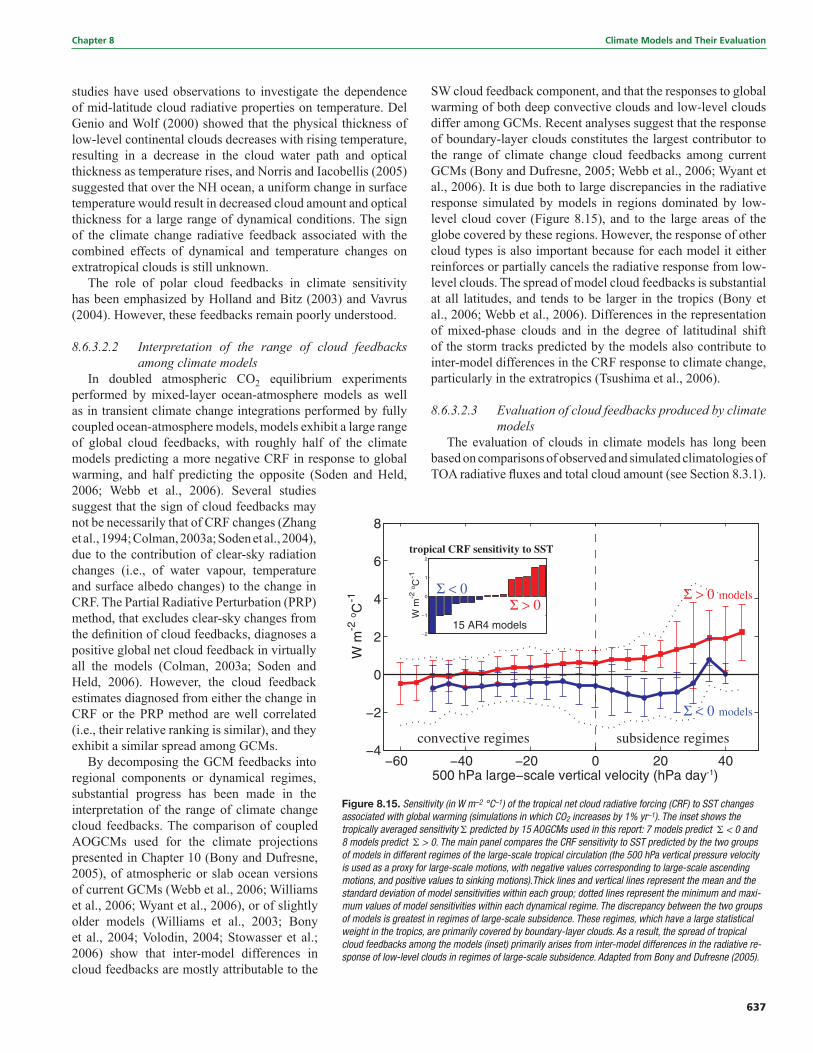
637


studies have used observations to investigate the dependence of mid-latitude cloud radiative properties on temperature. Del Genio and Wolf (2000) showed that the physical thickness of low-level continental clouds decreases with rising temperature, resulting in a decrease in the cloud water path and optical thickness as temperature rises, and Norris and Iacobellis (2005) suggested that over the NH ocean, a uniform change in surface temperature would result in decreased cloud amount and optical thickness for a large range of dynamical conditions. The sign of the climate change radiative feedback associated with the combined effects of dynamical and temperature changes on extratropical clouds is still unknown.

The role of polar cloud feedbacks in climate sensitivity has been emphasized by Holland and Bitz (2003) and Vavrus (2004). However, these feedbacks remain poorly understood.

8.6.3.2.2 Interpretation of the range of cloud feedbacks among climate models

In doubled atmospheric CO2 equilibrium experiments performed by mixed-layer ocean-atmosphere models as well as in transient climate change integrations performed by fully coupled ocean-atmosphere models, models exhibit a large range of global cloud feedbacks, with roughly half of the climate models predicting a more negative CRF in response to global warming, and half predicting the opposite (Soden and Held, 2006; Webb et al., 2006). Several studies suggest that the sign of cloud feedbacks may not be necessarily that of CRF changes (Zhang et al., 1994; Colman, 2003a; Soden et al., 2004), due to the contribution of clear-sky radiation changes (i.e., of water vapour, temperature and surface albedo changes) to the change in CRF. The Partial Radiative Perturbation (PRP) method, that excludes clear-sky changes from the defi nition of cloud feedbacks, diagnoses a positive global net cloud feedback in virtually all the models (Colman, 2003a; Soden and Held, 2006). However, the cloud feedback estimates diagnosed from either the change in CRF or the PRP method are well correlated (i.e., their relative ranking is similar), and they exhibit a similar spread among GCMs.

By decomposing the GCM feedbacks into regional components or dynamical regimes, substantial progress has been made in the interpretation of the range of climate change cloud feedbacks. The comparison of coupled AOGCMs used for the climate projections presented in Chapter 10 (Bony and Dufresne, 2005), of atmospheric or slab ocean versions of current GCMs (Webb et al., 2006; Williams et al., 2006; Wyant et al., 2006), or of slightly older models (Williams et al., 2003; Bony et al., 2004; Volodin, 2004; Stowasser et al.; 2006) show that inter-model differences in cloud feedbacks are mostly attributable to the

SW cloud feedback component, and that the responses to global warming of both deep convective clouds and low-level clouds differ among GCMs. Recent analyses suggest that the response of boundary-layer clouds constitutes the largest contributor to the range of climate change cloud feedbacks among current GCMs (Bony and Dufresne, 2005; Webb et al., 2006; Wyant et al., 2006). It is due both to large discrepancies in the radiative response simulated by models in regions dominated by low-level cloud cover (Figure 8.15), and to the large areas of the globe covered by these regions. However, the response of other cloud types is also important because for each model it either reinforces or partially cancels the radiative response from low-level clouds. The spread of model cloud feedbacks is substantial at all latitudes, and tends to be larger in the tropics (Bony et al., 2006; Webb et al., 2006). Differences in the representation of mixed-phase clouds and in the degree of latitudinal shift of the storm tracks predicted by the models also contribute to inter-model differences in the CRF response to climate change, particularly in the extratropics (Tsushima et al., 2006).

8.6.3.2.3 Evaluation of cloud feedbacks produced by climate

modelsThe evaluation of clouds in climate models has long been

based on comparisons of observed and simulated climatologies of TOA radiative fl uxes and total cloud amount (see Section 8.3.1).

Figure 8.15. Sensitivity (in W m–2 °C–1) of the tropical net cloud radiative forcing (CRF) to SST changes associated with global warming (simulations in which CO2 increases by 1% yr–1). The inset shows the tropically averaged sensitivity Σ predicted by 15 AOGCMs used in this report: 7 models predict Σ < 0 and 8 models predict Σ > 0. The main panel compares the CRF sensitivity to SST predicted by the two groups of models in different regimes of the large-scale tropical circulation (the 500 hPa vertical pressure velocity is used as a proxy for large-scale motions, with negative values corresponding to large-scale ascending motions, and positive values to sinking motions).Thick lines and vertical lines represent the mean and the standard deviation of model sensitivities within each group; dotted lines represent the minimum and maxi-mum values of model sensitivities within each dynamical regime. The discrepancy between the two groups of models is greatest in regimes of large-scale subsidence. These regimes, which have a large statistical weight in the tropics, are primarily covered by boundary-layer clouds. As a result, the spread of tropical cloud feedbacks among the models (inset) primarily arises from inter-model differences in the radiative re-sponse of low-level clouds in regimes of large-scale subsidence. Adapted from Bony and Dufresne (2005).

638


However, a good agreement with these observed quantities may result from compensating errors. Since the TAR, and partly due to the use of an International Satellite Cloud Climatology Project (ISCCP) simulator (Klein and Jakob, 1999; Webb et al., 2001), the evaluation of simulated cloud fi elds is increasingly done in terms of cloud types and cloud optical properties (Klein and Jakob, 1999; Webb et al., 2001; Williams et al., 2003; Lin and Zhang, 2004; Weare, 2004; Zhang et al., 2005; Wyant et al., 2006). It has thus become more powerful and constrains the models more. In addition, a new class of observational tests has been applied to GCMs, using clustering or compositing techniques, to diagnose errors in the simulation of particular cloud regimes or in specifi c dynamical conditions (Tselioudis et al., 2000; Norris and Weaver, 2001; Jakob and Tselioudis, 2003; Williams et al., 2003; Bony et al., 2004; Lin and Zhang, 2004; Ringer and Allan, 2004; Bony and Dufresne, 2005; Del Genio et al., 2005a; Gordon et al., 2005; Bauer and Del Genio, 2006; Williams et al., 2006; Wyant et al., 2006). An observational test focused on the global response of clouds to seasonal variations has been proposed to evaluate model cloud feedbacks (Tsushima et al., 2005), but has not yet been applied to current models.

These studies highlight some common biases in the simulation of clouds by current models (e.g., Zhang et al., 2005). This includes the over-prediction of optically thick clouds and the under-prediction of optically thin low and middle-top clouds. However, uncertainties remain in the observational determination of the relative amounts of the different cloud types (Chang and Li, 2005). For mid-latitudes, these biases have been interpreted as the consequence of the coarse resolution of climate GCMs and their resulting inability to simulate the right strength of ageostrophic circulations (Bauer and Del Genio, 2006) and the right amount of sub-grid scale variability (Gordon et al., 2005). Although the errors in the simulation of the different cloud types may eventually compensate and lead to a prediction of the mean CRF in agreement with observations (see Section 8.3), they cast doubts on the reliability of the model cloud feedbacks. For instance, given the nonlinear dependence of cloud albedo on cloud optical depth, the overestimate of the cloud optical thickness implies that a change in cloud optical depth, even of the right sign and magnitude, would produce a too small radiative signature. Similarly, the under-prediction of low- and mid-level clouds presumably affects the magnitude of the radiative response to climate warming in the widespread regions of subsidence. Modelling assumptions controlling the cloud water phase (liquid, ice or mixed) are known to be critical for the prediction of climate sensitivity. However, the evaluation of these assumptions is just beginning (Doutriaux-Boucher and Quaas, 2004; Naud et al., 2006). Tsushima et al. (2006) suggested that observations of the distribution of each phase of cloud water in the current climate would provide a substantial constraint on the model cloud feedbacks at middle and high latitudes.

As an attempt to assess some components of the cloud response to a change in climate, several studies have investigated the ability of GCMs to simulate the sensitivity of clouds and CRF to interannual changes in environmental conditions. When examining atmosphere-mixed-layer ocean models, Williams

et al. (2006) found for instance that by considering the CRF response to a change in large-scale vertical velocity and in lower-tropospheric stability, a component of the local mean climate change cloud response can be related to the present-day variability, and thus evaluated using observations. Bony and Dufresne (2005) and Stowasser and Hamilton (2006) examined the ability of the AOGCMs of Chapter 10 to simulate the change in tropical CRF to a change in SST, in large-scale vertical velocity and in lower-tropospheric RH. They showed that the models are most different and least realistic in regions of subsidence, and to a lesser extent in regimes of deep convective activity. This emphasizes the necessity to improve the representation and the evaluation of cloud processes in climate models, and especially those of boundary-layer clouds.

8.6.3.2.4 Conclusion on cloud feedbacksDespite some advances in the understanding of the physical

processes that control the cloud response to climate change and in the evaluation of some components of cloud feedbacks in current models, it is not yet possible to assess which of the model estimates of cloud feedback is the most reliable. However, progress has been made in the identifi cation of the cloud types, the dynamical regimes and the regions of the globe responsible for the large spread of cloud feedback estimates among current models. This is likely to foster more specifi c observational analyses and model evaluations that will improve future assessments of climate change cloud feedbacks.

8.6.3.3 Cryosphere Feedbacks

A number of feedbacks that signifi cantly contribute to the global climate sensitivity are due to the cryosphere. A robust feature of the response of climate models to increases in atmospheric concentrations of greenhouse gases is the poleward retreat of terrestrial snow and sea ice, and the polar amplifi cation of increases in lower-tropospheric temperature. At the same time, the high-latitude response to increased greenhouse gas concentrations is highly variable among climate models (e.g., Holland and Bitz, 2003) and does not show substantial convergence in the latest generation of AOGCMs (Chapman and Walsh, 2007; see also Section 11.8). The possibility of threshold behaviour also contributes to the uncertainty of how the cryosphere may evolve in future climate scenarios.

Arguably, the most important simulated feedback associated with the cryosphere is an increase in absorbed solar radiation resulting from a retreat of highly refl ective snow or ice cover in a warmer climate. Since the TAR, some progress has been made in quantifying the surface albedo feedback associated with the cryosphere. Hall (2004) found that the albedo feedback was responsible for about half the high-latitude response to a doubling of atmospheric CO2. However, an analysis of long control simulations showed that it accounted for surprisingly little internal variability. Hall and Qu (2006) show that biases of a number of MMD models in reproducing the observed seasonal cycle of land snow cover (especially the spring melt) are tightly related to the large variations in snow albedo feedback strength

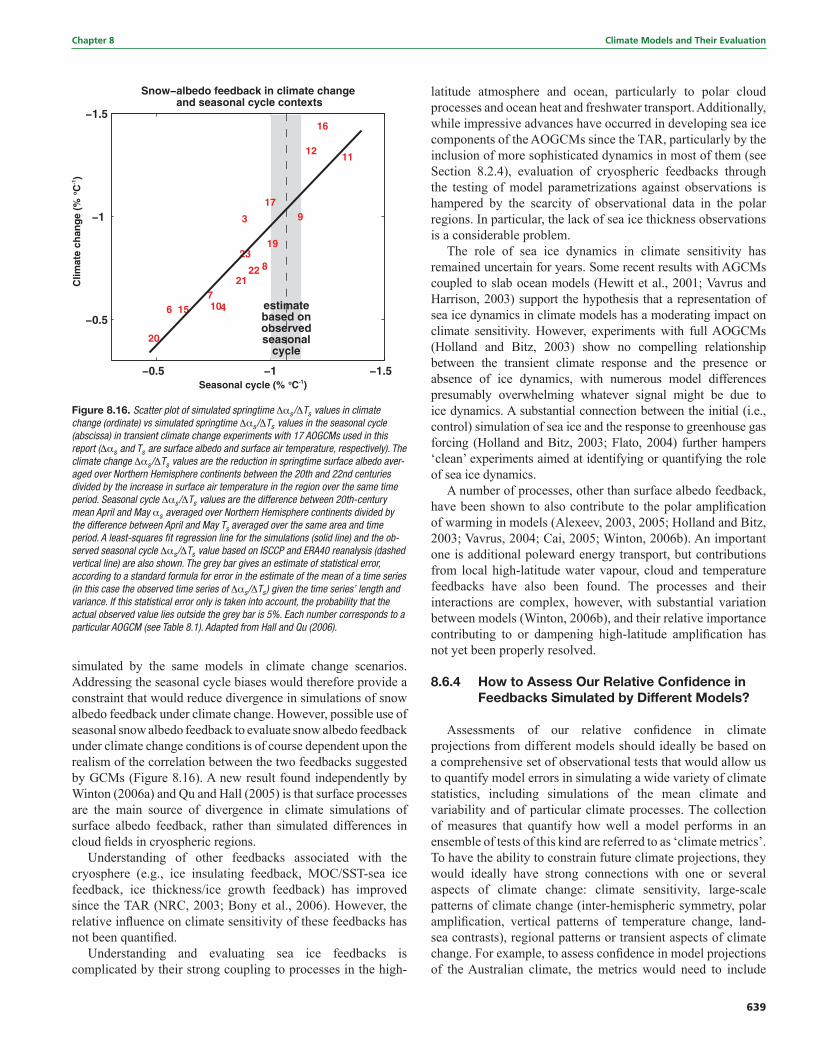
639


simulated by the same models in climate change scenarios. Addressing the seasonal cycle biases would therefore provide a constraint that would reduce divergence in simulations of snow albedo feedback under climate change. However, possible use of seasonal snow albedo feedback to evaluate snow albedo feedback under climate change conditions is of course dependent upon the realism of the correlation between the two feedbacks suggested by GCMs (Figure 8.16). A new result found independently by Winton (2006a) and Qu and Hall (2005) is that surface processes are the main source of divergence in climate simulations of surface albedo feedback, rather than simulated differences in cloud fi elds in cryospheric regions.

Understanding of other feedbacks associated with the cryosphere (e.g., ice insulating feedback, MOC/SST-sea ice feedback, ice thickness/ice growth feedback) has improved since the TAR (NRC, 2003; Bony et al., 2006). However, the relative infl uence on climate sensitivity of these feedbacks has not been quantifi ed.

Understanding and evaluating sea ice feedbacks is complicated by their strong coupling to processes in the high-

latitude atmosphere and ocean, particularly to polar cloud processes and ocean heat and freshwater transport. Additionally, while impressive advances have occurred in developing sea ice components of the AOGCMs since the TAR, particularly by the inclusion of more sophisticated dynamics in most of them (see Section 8.2.4), evaluation of cryospheric feedbacks through the testing of model parametrizations against observations is hampered by the scarcity of observational data in the polar regions. In particular, the lack of sea ice thickness observations is a considerable problem.

The role of sea ice dynamics in climate sensitivity has remained uncertain for years. Some recent results with AGCMs coupled to slab ocean models (Hewitt et al., 2001; Vavrus and Harrison, 2003) support the hypothesis that a representation of sea ice dynamics in climate models has a moderating impact on climate sensitivity. However, experiments with full AOGCMs (Holland and Bitz, 2003) show no compelling relationship between the transient climate response and the presence or absence of ice dynamics, with numerous model differences presumably overwhelming whatever signal might be due to ice dynamics. A substantial connection between the initial (i.e., control) simulation of sea ice and the response to greenhouse gas forcing (Holland and Bitz, 2003; Flato, 2004) further hampers ‘clean’ experiments aimed at identifying or quantifying the role of sea ice dynamics.

A number of processes, other than surface albedo feedback, have been shown to also contribute to the polar amplifi cation of warming in models (Alexeev, 2003, 2005; Holland and Bitz, 2003; Vavrus, 2004; Cai, 2005; Winton, 2006b). An important one is additional poleward energy transport, but contributions from local high-latitude water vapour, cloud and temperature feedbacks have also been found. The processes and their interactions are complex, however, with substantial variation between models (Winton, 2006b), and their relative importance contributing to or dampening high-latitude amplifi cation has not yet been properly resolved.

8.6.4 How to Assess Our Relative Confi dence in Feedbacks Simulated by Different Models?

Assessments of our relative confi dence in climate projections from different models should ideally be based on a comprehensive set of observational tests that would allow us to quantify model errors in simulating a wide variety of climate statistics, including simulations of the mean climate and variability and of particular climate processes. The collection of measures that quantify how well a model performs in an ensemble of tests of this kind are referred to as ‘climate metrics’. To have the ability to constrain future climate projections, they would ideally have strong connections with one or several aspects of climate change: climate sensitivity, large-scale patterns of climate change (inter-hemispheric symmetry, polar amplifi cation, vertical patterns of temperature change, land-sea contrasts), regional patterns or transient aspects of climate change. For example, to assess confi dence in model projections of the Australian climate, the metrics would need to include

Figure 8.16. Scatter plot of simulated springtime Δαs/ΔTs values in climate change (ordinate) vs simulated springtime Δαs/ΔTs values in the seasonal cycle (abscissa) in transient climate change experiments with 17 AOGCMs used in this report (Δαs and Ts are surface albedo and surface air temperature, respectively). The climate change Δαs/ΔTs values are the reduction in springtime surface albedo aver-aged over Northern Hemisphere continents between the 20th and 22nd centuries divided by the increase in surface air temperature in the region over the same time period. Seasonal cycle Δαs/ΔTs values are the difference between 20th-century mean April and May αs averaged over Northern Hemisphere continents divided by the difference between April and May Ts averaged over the same area and time period. A least-squares fi t regression line for the simulations (solid line) and the ob-served seasonal cycle Δαs/ΔTs value based on ISCCP and ERA40 reanalysis (dashed vertical line) are also shown. The grey bar gives an estimate of statistical error, according to a standard formula for error in the estimate of the mean of a time series (in this case the observed time series of Δαs/ΔTs) given the time series’ length and variance. If this statistical error only is taken into account, the probability that the actual observed value lies outside the grey bar is 5%. Each number corresponds to a particular AOGCM (see Table 8.1). Adapted from Hall and Qu (2006).

640


some measures of the quality of ENSO simulation because the Australian climate depends much on this variability (see Section 11. 7).

To better assess confi dence in the different model estimates of climate sensitivity, two kinds of observational tests are available: tests related to the global climate response associated with specifi ed external forcings (discussed in Chapters 6, 9 and 10; Box 10.2) and tests focused on the simulation of key feedback processes.

Based on the understanding of both the physical processes that control key climate feedbacks (see Section 8.6.3), and also the origin of inter-model differences in the simulation of feedbacks (see Section 8.6.2), the following climate characteristics appear to be particularly important: (i) for the water vapour and lapse rate feedbacks, the response of upper-tropospheric RH and lapse rate to interannual or decadal changes in climate; (ii) for cloud feedbacks, the response of boundary-layer clouds and anvil clouds to a change in surface or atmospheric conditions and the change in cloud radiative properties associated with a change in extratropical synoptic weather systems; (iii) for snow albedo feedbacks, the relationship between surface air temperature and snow melt over northern land areas during spring and (iv) for sea ice feedbacks, the simulation of sea ice thickness.

A number of diagnostic tests have been proposed since the TAR (see Section 8.6.3), but few of them have been applied to a majority of the models currently in use. Moreover, it is not yet clear which tests are critical for constraining future projections. Consequently, a set of model metrics that might be used to narrow the range of plausible climate change feedbacks and climate sensitivity has yet to be developed.

8.7 Mechanisms Producing Thresholds and Abrupt Climate Change

8.7.1 Introduction

This discussion of thresholds and abrupt climate change is based on the defi nitions of ‘threshold’ and ‘abrupt’ proposed by Alley et al. (2002). The climate system tends to respond to changes in a gradual way until it crosses some threshold: thereafter any change that is defi ned as abrupt is one where the change in the response is much larger than the change in the forcing. The changes at the threshold are therefore abrupt relative to the changes that occur before or after the threshold and can lead to a transition to a new state. The spatial scales for these changes can range from global to local. In this defi nition, the magnitude of the forcing and response are important. In addition to the magnitude, the time scale being considered is also important. This section focuses mainly on decadal to centennial time scales.

Because of the somewhat subjective nature of the defi nitions of threshold and abrupt, there have been efforts to develop

quantitative measures to identify these points in a time series of a given variable (e.g., Lanzante, 1996; Seidel and Lanzante, 2004; Tomé and Miranda, 2004). The most common way to identify thresholds and abrupt changes is by linearly de-trending the input time series and looking for large deviations from the trend line. More statistically rigorous methods are usually based on Bayesian statistics.

This section explores the potential causes and mechanisms for producing thresholds and abrupt climate change and addresses the issue of how well climate models can simulate these changes. The following discussion is split into two main areas: forcing changes that can result in abrupt changes and abrupt climate changes that result from large natural variability on long time scales. Formally, the latter abrupt changes do not fi t the defi nition of thresholds and abrupt changes, because the forcing (at least radiative forcing – the external boundary condition) is not changing in time. However these changes have been discussed in the literature and popular press and are worthy of assessment here.

8.7.2 Forced Abrupt Climate Change

8.7.2.1 Meridional Overturning Circulation Changes

As the radiative forcing of the planet changes, the climate system responds on many different time scales. For the physical climate system typically simulated in coupled models (atmosphere, ocean, land, sea ice), the longest response time scales are found in the ocean (Stouffer, 2004). In terms of thresholds and abrupt climate changes on decadal and longer time scales, the ocean has also been a focus of attention. In particular, the ocean’s Atlantic MOC (see Box 5.1 for defi nition and description) is a main area of study.

The MOC transports large amounts of heat (order of 1015 Watts) and salt into high latitudes of the North Atlantic. There, the heat is released to the atmosphere, cooling the surface waters. The cold, relatively salty waters sink to depth and fl ow southward out of the Atlantic Basin. The complete set of climatic drivers of this circulation remains unclear but it is likely that both density (e.g., Stommel 1961; Rooth 1982) and wind stress forcings (e.g., Wunsch, 2002; Timmermann and Goosse, 2004) are important. Both palaeoclimate studies (e.g., Broecker, 1997; Clark et al., 2002) and modelling studies (e.g., Manabe and Stouffer, 1988, 1997; Vellinga and Wood, 2002) suggest that disruptions in the MOC can produce abrupt climate changes. A systematic model intercomparison study (Rahmstorf et al., 2005) found that all 11 participating EMICs had a threshold where the MOC shuts down (see Section 8.8.3). Due to the high computational cost, such a search for thresholds has not yet been performed with AOGCMs.

It is important to note the distinction between the equilibrium and transient or time-dependent responses of the MOC to changes in forcing. Due to the long response time scales found in the ocean (some longer than 1 kyr), it is possible that the short-term response to a given forcing change may be very different from the equilibrium response. Such behaviour of the coupled

641


system has been documented in at least one AOGCM (Stouffer and Manabe, 2003) and suggested in the results of a few other AOGCM studies (e.g., Hirst, 1999; Senior and Mitchell, 2000; Bryan et al., 2006). In these AOGCM experiments, the MOC weakens as the greenhouse gases increase in the atmosphere. When the CO2 concentration is stabilised, the MOC slowly returns to its unperturbed value.

As discussed in section 10.3.4, the MOC typically weakens as greenhouse gases increase due to the changes in surface heat and freshwater fl uxes at high latitudes (Manabe et al., 1991). The surface fl ux changes reduce the surface density, hindering the vertical movement of water and slowing the MOC. As the MOC slows, it could approach a threshold where the circulation can no longer sustain itself. Once the MOC crosses this threshold, it could rapidly change states, causing abrupt climate change where the North Atlantic and surrounding land areas would cool relative to the case where the MOC is active. This cooling is the result of the loss of heat transport from low latitudes in the Atlantic and the feedbacks associated with the reduction in the vertical mixing of high-latitude waters.

A common misunderstanding is that the MOC weakening could cause the onset of an ice age. However, no model has supported this speculation when forced with realistic estimates of future climate forcings (see Section 10.3.4). In addition, in idealised modelling studies where the MOC was forced to shut down through very large sources of freshwater (not changes in greenhouse gases), the surface temperature changes do not support the idea that an ice age could result from a MOC shut down, although the impacts on climate would be large (Manabe and Stouffer, 1988, 1997; Schiller et al., 1997; Vellinga and Wood, 2002; Stouffer et al., 2006). In a recent intercomparison involving 11 coupled atmosphere-ocean models (Gregory et al., 2005), the MOC decreases by only 10 to 50% during a 140-year period (as atmospheric CO2 quadruples), and in no model is there a land cooling anywhere (as the global-scale heating due to increasing CO2 overwhelms the local cooling effect due to reduced MOC).

Because of the large amount of heat and salt transported northward and its sensitivity to surface fl uxes, the changes in the MOC are able to produce abrupt climate change on decadal to centennial time scales (e.g., Manabe and Stouffer, 1995; Stouffer et al., 2006). Idealised studies using present-day simulations have shown that models can simulate many of the variations seen in the palaeoclimate record on decadal to centennial time scales when forced by fl uxes of freshwater water at the ocean surface. However, the quantitative response to freshwater inputs varies widely among models (Stouffer et al., 2006), which led the CMIP and Paleoclimate Modelling Intercomparison Project (PMIP) panels to design and support a set of coordinated experiments to study this issue (http://www.gfdl.noaa.gov/~kd/CMIP.html and http://www.pmip2.cnrs-gif.fr/pmip2/design/experiments/waterhosing.shtml).

In addition to the amount of the freshwater input, the exact location of that input may also be important (Rahmstorf 1996, Manabe and Stouffer, 1997; Rind et al., 2001). Designing experiments and determining the realistic past forcings needed

to test the models’ response on decadal to centennial time scales remains to be accomplished.

The processes determining MOC response to increasing greenhouse gases have been studied in a number of models. In many models, initial MOC response to increasing greenhouse gases is dominated by thermal effects. In most models, this is enhanced by changes in salinity driven by, among other things, the expected strengthening of the hydrological cycle (Gregory et al., 2005; Chapter 10). Melt water runoff from a melting of the Greenland Ice Sheet is a potentially major source of freshening not yet included in the models found in the MMD (see Section 8.7.2.2). More complex feedbacks, associated with wind and hydrological changes, are also important in many models. These include local surface fl ux anomalies in deep-water formation regions (Gent, 2001) and oceanic teleconnections driven by changes to the freshwater budget of the tropical and South Atlantic (e.g., Latif et al., 2000; Thorpe et al., 2001; Vellinga et al., 2002; Hu et al., 2004). The magnitudes of the climate factors causing the MOC to weaken, along with the feedbacks and the associated restoring factors, are all uncertain at this time. Evaluation of these processes in AOGCMs is mainly restricted by lack of observations, but some early progress has been made in individual studies (e.g., Schmittner et al., 2000; Pardaens et al., 2003; Wu et al., 2005; Chapter 9). Model intercomparison studies (e.g., Gregory et al., 2005; Rahmstorf et al., 2005; Stouffer et al., 2006) were developed to identify and understand the causes for the wide range of MOC responses in the coupled models used here (see Chapters 4, 6 and 10).

8.7.2.2 Rapid West Antarctic and/or Greenland Ice Sheet Collapse and Meridional Overturning Circulation Changes

Increased infl ux of freshwater to the ocean from the ice sheets is a potential forcing for abrupt climate changes. For Antarctica in the present climate, these fl uxes chiefl y arise from melting below the ice shelves and from melting of icebergs transported by the ocean; both fl uxes could increase signifi cantly in a warmer climate. Ice sheet runoff and iceberg calving, in roughly equal shares, currently dominate the freshwater fl ux from the Greenland Ice Sheet (Church et al., 2001; Chapter 4). In a warming climate, runoff is expected to quickly increase and become much larger than the calving rate, the latter of which in turn is likely to decrease as less and thinner ice borders the ocean; basal melting from below the grounded ice will remain several orders of magnitude smaller than the other fl uxes (Huybrechts et al., 2002). For a discussion of the likelihood of these ice sheet changes and the effects on sea level, see the discussion in Chapter 10.

Changes in the surface forcing near the deep-water production areas seem to be most capable of producing rapid climate changes on decadal and longer time scales due to changes in the ocean circulation and mixing. If there are large changes in the ice volume over Greenland, it is likely that much of this melt water will freshen the surface waters in the

642


high-latitude North Atlantic, slowing down the MOC (see Section 8.7.2.1; Chapter 10). Rind et al. (2001) found that changes in the NADW formation rate could instigate changes in the deep-water formation around Antarctica.

The response of the Atlantic MOC to changes in the Antarctic Ice Sheet is less well understood. Experiments with ocean-only models where the melt water changes are imposed as surface salinity changes indicate that the Atlantic MOC will intensify as the waters around Antarctica become less dense (Seidov et al., 2001). Weaver et al. (2003) showed that by adding freshwater in the Southern Ocean, the MOC could change from an ‘off’ state to a state similar to present day. However, in an experiment with an AOGCM, Seidov et al. (2005) found that an external source of freshwater in the Southern Ocean resulted in a surface freshening throughout the world ocean, weakening the Atlantic MOC. In these model results, the SH MOC associated with Antarctic Bottom Water (AABW) formation weakened, causing a cooling around Antarctica. See Chapters 4, 6 and 10 for more discussion about the likelihood of large melt water fl uxes from the ice sheets affecting the climate.

In summary, there is a potential for rapid ice sheet changes to produce rapid climate change both through sea level changes and ocean circulation changes. The ocean circulation changes result from increased freshwater fl ux over the particularly sensitive deep-water production sites. In general, the possible climate changes associated with future evolution of the Greenland Ice Sheet are better understood than are those associated with changes in the Antarctic Ice Sheets.

8.7.2.3 Volcanoes

Volcanoes produce abrupt climate responses on short time scales. The surface cooling effect of the stratospheric aerosols, the main climatic forcing factor, decays in one to three years after an eruption due to the lifetime of the aerosols in the stratosphere. It is possible for one large volcano or a series of large volcanic eruptions to produce climate responses on longer time scales, especially in the subsurface region of the ocean (Delworth et al., 2005; Gleckler et al., 2006b).

The models’ ability to simulate any possible abrupt response of the climate system to volcanic eruptions seems conceptually similar to their ability to simulate the climate response to future changes in greenhouse gases in that both produce changes in the radiative forcing of the planet. However, mechanisms involved in the exchange of heat between the atmosphere and ocean may be different in response to volcanic forcing when compared to the response to increase greenhouse gases. Therefore, the feedbacks involved may be different (see Section 9.6.2.2 for more discussion).

8.7.2.4 Methane Hydrate Instability/Permafrost Methane

Methane hydrates are stored on the seabed along continental margins where they are stabilised by high pressures and low temperatures, implying that ocean warming may cause hydrate instability and release of methane into the atmosphere (see

Section 4.7.2.4). Methane is also stored in the soils in areas of permafrost and warming increases the likelihood of a positive feedback in the climate system via permafrost melting and the release of trapped methane into the atmosphere. The likelihood of methane release from methane hydrates found in the oceans or methane trapped in permafrost layers is assessed in Chapter 7.

This subsection considers the potential usefulness of models in determining if those releases could trigger an abrupt climate change. Both forms of methane release represent a potential threshold in the climate system. As the climate warms, the likelihood of the system crossing a threshold for a sudden release increases (see Chapters 4, 7 and 10). Since these changes produce changes in the radiative forcing through changes in the greenhouse gas concentrations, the climatic impacts of such a release are the same as an increase in the rate of change in the radiative forcing. Therefore, the models’ ability to simulate any abrupt climate change should be similar to their ability to simulate future abrupt climate changes due to changes in the greenhouse gas forcing.

8.7.2.5 Biogeochemical

Two questions concerning biogeochemical aspects of the climate system are addressed here. First, can biogeochemical changes lead to abrupt climate change? Second, can abrupt changes in the MOC further affect radiative forcing through biogeochemical feedbacks?

Abrupt changes in biogeochemical systems of relevance to our capacity to simulate the climate of the 21st century are not well understood (Friedlingstein et al., 2003). The potential for major abrupt change exists in the uptake and storage of carbon by terrestrial systems. While abrupt change within the climate system is beginning to be seriously considered (Rial et al., 2004; Schneider, 2004), the potential for abrupt change in terrestrial systems, such as loss of soil carbon (Cox et al., 2000) or die back of the Amazon forests (Cox et al., 2004) remains uncertain. In part this is due to lack of understanding of processes (see Friedlingstein et al., 2003; Chapter 7) and in part it results from the impact of differences in the projected climate sensitivities in the host climate models (Joos et al., 2001; Govindasamy et al., 2005; Chapter 10) where changes in the physical climate system affect the biological response.

There is some evidence of multiple equilibria within vegetation-soil-climate systems. These include North Africa and Central East Asia where Claussen (1998), using an EMIC with a land vegetation component, showed two stable equilibria for rainfall, dependent on initial land surface conditions. Kleidon et al. (2000), Wang and Eltahir (2000) and Renssen et al. (2003) also found evidence for multiple equilibria. These are preliminary assessments using relatively simple physical climate models that highlight the possibility of irreversible change in the Earth system but require extensive further research to assess the reliability of the phenomena found.

There have only been a few preliminary studies of the impact of abrupt climate changes such as the shutdown of the MOC on the carbon cycle. The fi ndings of these studies indicate that the

643


shutdown of the MOC would tend to increase the amount of greenhouse gases in the atmosphere (Joos et al., 1999; Plattner et al., 2001; Chapter 6). In both of these studies, only the effect of the oceanic component of the carbon cycle changes was considered.

8.7.3 Unforced Abrupt Climate Change

Formally, as noted above, the changes discussed here do not fall into the defi nition of abrupt climate change. In the literature, unforced abrupt climate change falls into two general categories. One is just a red noise time series, where there is power at decadal and longer time scales. A second category is a bimodal or multi-modal distribution. In practice, it can be very diffi cult to distinguish between the two categories unless the time series are very long – long enough to eliminate sampling as an issue – and the forcings are fairly constant in time. In observations, neither of these conditions is normally met.

Models, both AOGCMs and less complex models, have produced examples of large abrupt climate change (e.g., Hall and Stouffer 2001; Goosse et al., 2002) without any changes in forcing. Typically, these events are associated with changes in the ocean circulation, mainly in the North Atlantic. An abrupt event can last for several years to a few centuries. They bear some similarities with the conditions observed during a relatively cold period in the recent past in the Arctic (Goosse et al., 2003)

Unfortunately, the probability of such an event is diffi cult to estimate as it requires a very long experiment and is certainly dependent on the mean state simulated by the model. Furthermore, comparison with observations is nearly impossible since it would require a very long period with constant forcing which does not exist in nature. Nevertheless, if an event such as the one of those mentioned above were to occur in the future, it would make the detection and attribution of climate changes very diffi cult.

8.8 Representing the Global System with Simpler Models

8.8.1 Why Lower Complexity?

An important concept in climate system modelling is that of a spectrum of models of differing levels of complexity, each being optimum for answering specifi c questions. It is not meaningful to judge one level as being better or worse than another independently of the context of analysis. What is important is that each model be asked questions appropriate for its level of complexity and quality of its simulation.

The most comprehensive models available are AOGCMs. These models, which include more and more components of the climate system (see Section 8.2), are designed to provide the best representation of the system and its dynamics, thereby serving as the most realistic laboratory of nature. Their major limitation

is their high computational cost. To date, unless modest-resolution models are executed on an exceptionally large-scale distributed computed system, as in the climateprediction.net project (http://climateprediction.net; Stainforth et al., 2005), only a limited number of multi-decadal experiments can be performed with AOGCMs, which hinders a systematic exploration of uncertainties in climate change projections and prevents studies of the long-term evolution of climate.

At the other end of the spectrum of climate system model complexity are the so-called simple climate models (see Harvey et al., 1997 for a review of these models). The most advanced simple climate models contain modules that calculate in a highly parametrized way (1) the abundances of atmospheric greenhouse gases for given future emissions, (2) the radiative forcing resulting from the modelled greenhouse gas concentrations and aerosol precursor emissions, (3) the global mean surface temperature response to the computed radiative forcing and (4) the global mean sea level rise due to thermal expansion of sea water and the response of glaciers and ice sheets. These models are much more computationally effi cient than AOGCMs and thus can be utilised to investigate future climate change in response to a large number of different scenarios of greenhouse gas emissions. Uncertainties from the modules can also be concatenated, potentially allowing the climate and sea level results to be expressed as probabilistic distributions, which is harder to do with AOGCMs because of their computational expense. A characteristic of simple climate models is that climate sensitivity and other subsystem properties must be specifi ed based on the results of AOGCMs or observations. Therefore, simple climate models can be tuned to individual AOGCMs and employed as a tool to emulate and extend their results (e.g., Cubasch et al., 2001; Raper et al., 2001). They are useful mainly for examining global-scale questions.

To bridge the gap between AOGCMs and simple climate models, EMICs have been developed. Given that this gap is quite large, there is a wide range of EMICs (see the reviews of Saltzman, 1978 and Claussen et al., 2002). Typically, EMICs use a simplifi ed atmospheric component coupled to an OGCM or simplifi ed atmospheric and oceanic components. The degree of simplifi cation of the component models varies among EMICs.

Earth System Models of Intermediate Complexity are reduced-resolution models that incorporate most of the processes represented by AOGCMs, albeit in a more parametrized form. They explicitly simulate the interactions between various components of the climate system. Similar to AOGCMs, but in contrast to simple climate models, the number of degrees of freedom of an EMIC exceeds the number of adjustable parameters by several orders of magnitude. However, these models are simple enough to permit climate simulations over several thousand of years or even glacial cycles (with a period of some 100 kyr), although not all are suitable for this purpose. Moreover, like simple climate models, EMICs can explore the parameter space with some completeness and are thus appropriate for assessing uncertainty. They can also be utilised to screen the phase space of climate or the history of climate in order to identify interesting time slices, thereby

644


providing guidance for more detailed studies to be undertaken with AOGCMs. In addition, EMICs are invaluable tools for understanding large-scale processes and feedbacks acting within the climate system. Certainly, it would not be sensible to apply an EMIC to studies that require high spatial and temporal resolution. Furthermore, model assumptions and restrictions, hence the limit of applicability of individual EMICs, must be carefully studied. Some EMICs include a zonally averaged atmosphere or zonally averaged oceanic basins. In a number of EMICs, cloudiness and/or wind fi elds are prescribed and do not evolve with changing climate. In still other EMICs, the atmospheric synoptic variability is not resolved explicitly, but diagnosed by using a statistical-dynamical approach. A priori, it is not obvious how the reduction in resolution or dynamics/physics affects the simulated climate. As shown in Section 8.8.3 and in Chapters 6, 9 and 10, at large scales most EMIC results compare well with observational or proxy data and AOGCM results. Therefore, it is argued that there is a clear advantage in having available a spectrum of climate system models.

8.8.2 Simple Climate Models

As in the TAR, a simple climate model is utilised in this report to emulate the projections of future climate change conducted with state-of-the-art AOGCMs, thus allowing the investigation of the temperature and sea level implications of all relevant emission scenarios (see Chapter 10). This model is an updated version of the Model for the Assessment of Greenhouse-Gas Induced Climate Change (MAGICC) model (Wigley and Raper, 1992, 2001; Raper et al., 1996). The calculation of the radiative forcings from emission scenarios closely follows that described in Chapter 2, and the feedback between climate and the carbon cycle is treated consistently with Chapter 7. The atmosphere-ocean module consists of an atmospheric energy balance model coupled to an upwelling-diffusion ocean model. The atmospheric energy balance model has land and ocean boxes in each hemisphere, and the upwelling-diffusion ocean model in each hemisphere has 40 layers with inter-hemispheric heat exchange in the mixed layer.

This simple climate model has been tuned to outputs from 19 of the AOGCMs described in Table 8.1, with resulting parameter values as given in the Supplementary Material, Table S8.1. The applied tuning procedure involves an iterative optimisation to derive least-square optimal fi ts between the simple model results and the AOGCM outputs for temperature time series and net oceanic heat uptake. This procedure attempts to match not only the global mean temperature but also the hemispheric land and ocean surface temperature changes of the AOGCM results by adjusting the equilibrium land-ocean warming ratio. Where data availability allowed, the tuning procedure took simultaneous account of low-pass fi ltered AOGCM data for two scenarios, namely a 1% per year compounded increase in atmospheric CO2 concentration to twice and quadruple the pre-industrial level, with subsequent stabilisation. Before tuning, the AOGCM temperature and heat uptake data was de-drifted by subtracting the respective low-pass fi ltered pre-industrial control run segments. The three tuned parameters in the simple

climate model are the effective climate sensitivity, the ocean effective vertical diffusivity, and the equilibrium land-ocean warming ratio. Values specifi c to each AOGCM for the radiative forcing for CO2 doubling were used in the tuning procedure where available (from Forster and Taylor, 2006, supplemented with values provided directly from the modelling groups). Otherwise, a default value of 3.71 W m–2 was chosen (Myhre et al., 1998). Default values of 1 W m–2 °C–1, 1 W m–2 °C–1 and 8°C were used for the land-ocean heat exchange coeffi cient, the inter-hemispheric heat exchange coeffi cient and the magnitude of the warming that would result in a collapse of the MOC, respectively (see Appendix 9.1 of the TAR).

The obtained best-fi t climate sensitivity estimates differ for various reasons from other estimates that were derived with alternative methods. Such alternative methods include, for example, regression estimates that use a global energy balance equation around the year of atmospheric CO2 doubling or the analysis of slab ocean equilibrium warmings. The resulting differences in climate sensitivity estimates can be partially explained by the non-time constant effective climate sensitivities in many of the AOGCM runs. Furthermore, tuning results of a simple climate model will be affected by the model structure, although simple, and other default parameter settings that affect the simple model transient response.

8.8.3 Earth System Models of Intermediate Complexity

Pictorially, EMICs can be defi ned in terms of the components of a three-dimensional vector (Claussen et al., 2002): the number of interacting components of the climate system explicitly represented in the model, the number of processes explicitly simulated and the detail of description. Some basic information on the EMICs used in Chapter 10 of this report is presented in Table 8.3. A comprehensive description of all EMICs in operation can be found in Claussen (2005). Actually, there is a broad range of EMICs, refl ecting the differences in scope. In some EMICs, the number of processes and the detail of description are reduced to simulate feedbacks between as many components of the climate system as feasible. Others, with fewer interacting components, are utilised in long-term ensemble experiments to investigate specifi c aspects of climate variability. The gap between some of the most complicated EMICs and AOGCMs is not very large. In fact, this particular class of EMICs is derived from AOGCMs. On the other hand, EMICs and simple climate models differ much more. For instance, EMICs as well as AOGCMs realistically represent the large-scale geographical structures of the Earth, like the shape of continents and ocean basins, which is certainly not the case for simple climate models.

Since the TAR, EMICs have intensively been used to study past and future climate changes (see Chapters 6, 9 and 10). Furthermore, a great deal of effort has been devoted to the evaluation of those models through coordinated intercomparisons.

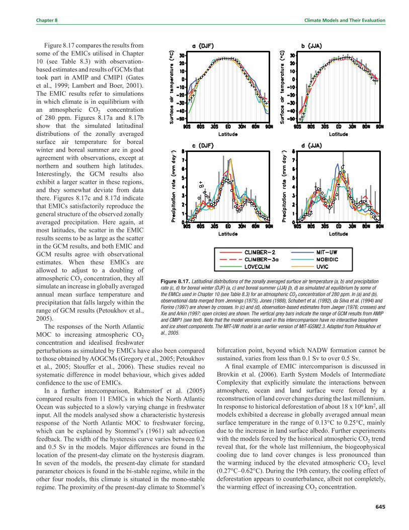
645


Figure 8.17 compares the results from some of the EMICs utilised in Chapter 10 (see Table 8.3) with observation-based estimates and results of GCMs that took part in AMIP and CMIP1 (Gates et al., 1999; Lambert and Boer, 2001). The EMIC results refer to simulations in which climate is in equilibrium with an atmospheric CO2 concentration of 280 ppm. Figures 8.17a and 8.17b show that the simulated latitudinal distributions of the zonally averaged surface air temperature for boreal winter and boreal summer are in good agreement with observations, except at northern and southern high latitudes. Interestingly, the GCM results also exhibit a larger scatter in these regions, and they somewhat deviate from data there. Figures 8.17c and 8.17d indicate that EMICs satisfactorily reproduce the general structure of the observed zonally averaged precipitation. Here again, at most latitudes, the scatter in the EMIC results seems to be as large as the scatter in the GCM results, and both EMIC and GCM results agree with observational estimates. When these EMICs are allowed to adjust to a doubling of atmospheric CO2 concentration, they all simulate an increase in globally averaged annual mean surface temperature and precipitation that falls largely within the range of GCM results (Petoukhov et al., 2005).

The responses of the North Atlantic MOC to increasing atmospheric CO2 concentration and idealised freshwater perturbations as simulated by EMICs have also been compared to those obtained by AOGCMs (Gregory et al., 2005; Petoukhov et al., 2005; Stouffer et al., 2006). These studies reveal no systematic difference in model behaviour, which gives added confi dence to the use of EMICs.

In a further intercomparison, Rahmstorf et al. (2005) compared results from 11 EMICs in which the North Atlantic Ocean was subjected to a slowly varying change in freshwater input. All the models analysed show a characteristic hysteresis response of the North Atlantic MOC to freshwater forcing, which can be explained by Stommel’s (1961) salt advection feedback. The width of the hysteresis curve varies between 0.2 and 0.5 Sv in the models. Major differences are found in the location of the present-day climate on the hysteresis diagram. In seven of the models, the present-day climate for standard parameter choices is found in the bi-stable regime, while in the other four models, this climate is situated in the mono-stable regime. The proximity of the present-day climate to Stommel’s

bifurcation point, beyond which NADW formation cannot be sustained, varies from less than 0.1 Sv to over 0.5 Sv.

A fi nal example of EMIC intercomparison is discussed in Brovkin et al. (2006). Earth System Models of Intermediate Complexity that explicitly simulate the interactions between atmosphere, ocean and land surface were forced by a reconstruction of land cover changes during the last millennium. In response to historical deforestation of about 18 x 106 km2, all models exhibited a decrease in globally averaged annual mean surface temperature in the range of 0.13°C to 0.25°C, mainly due to the increase in land surface albedo. Further experiments with the models forced by the historical atmospheric CO2 trend reveal that, for the whole last millennium, the biogeophysical cooling due to land cover changes is less pronounced than the warming induced by the elevated atmospheric CO2 level (0.27°C–0.62°C). During the 19th century, the cooling effect of deforestation appears to counterbalance, albeit not completely, the warming effect of increasing CO2 concentration.

-1-1

Figure 8.17. Latitudinal distributions of the zonally averaged surface air temperature (a, b) and precipitation rate (c, d) for boreal winter (DJF) (a, c) and boreal summer (JJA) (b, d) as simulated at equilibrium by some of the EMICs used in Chapter 10 (see Table 8.3) for an atmospheric CO2 concentration of 280 ppm. In (a) and (b), observational data merged from Jennings (1975), Jones (1988), Schubert et al. (1992), da Silva et al. (1994) and Fiorino (1997) are shown by crosses. In (c) and (d), observation-based estimates from Jaeger (1976; crosses) and Xie and Arkin (1997; open circles) are shown. The vertical grey bars indicate the range of GCM results from AMIP and CMIP1 (see text). Note that the model versions used in this intercomparison have no interactive biosphere and ice sheet components. The MIT-UW model is an earlier version of MIT-IGSM2.3. Adapted from Petoukhov et al., 2005.

646


Nam

eA

tmo

sphe

rea

Oce

anb

Sea

Icec

Co

uplin

g/F

lux

Ad

just

men

tsd

Land

Sur

face

eB

iosp

here

fIc

e S

heet

sg

E1:

BE

RN

2.5C

C

(Pla

ttne

r et

al.,

200

1;

Joos

et

al.,

2001

)

EM

BM

, 1-D

(ϕ),

NC

L,

7.5°

x 1

5° (S

chm

ittne

r an

d S

tock

er, 1

999)

FG w

ith p

aram

etriz

ed

zona

l pre

ssur

e gr

adie

nt,

2-D

(ϕ, z

), 3

bas

ins,

RL,

IS

O, M

ES

O, 7

.5°x

15°,

L14

(W

right

and

Sto

cker

, 199

2)

0-LT

, 2-L

IT

(Wrig

ht a

nd

Sto

cker

, 199

3)

PM

, NH

, NW

(S

tock

er e

t al

., 19

92;

Sch

mitt

ner

and

S

tock

er, 1

999)

NS

T, N

SM

(S

chm

ittne

r an

d

Sto

cker

, 199

9)

BO

(Mar

chal

et

al.,

1998

), B

T (S

itch

et a

l., 2

003;

G

erb

er e

t al

., 20

03),

BV

(Sitc

h et

al.,

200

3;

Ger

ber

et

al.,

2003

)

E2:

C-G

OLD

STE

IN

(Ed

war

ds

and

Mar

sh,

2005

)

EM

BM

, 2-D

(ϕ,λ

), N

CL,

5°

x 1

0° (E

dwar

ds a

nd

Mar

sh, 2

005)

FG, 3

-D, R

L, IS

O, M

ES

O,

5° x

10°

, L8

(Ed

war

ds

and

M

arsh

, 200

5)

0-LT

, DO

C, 2

-LIT

(E

dw

ard

s an

d

Mar

sh, 2

005)

GM

, NH

, RW

(E

dw

ard

s an

d M

arsh

, 20

05)

NS

T, N

SM

, RIV

(E

dw

ard

s an

d M

arsh

, 20

05)

E3:

CLI

MB

ER

-2

(Pet

oukh

ov e

t al

., 20

00)

SD

, 3-D

, CR

AD

, IC

L, 1

0° x

51°

, L10

(P

etou

khov

et

al.,

2000

)

FG w

ith p

aram

etriz

ed

zona

l pre

ssur

e gr

adie

nt,

2-D

(ϕ, z

), 3

bas

ins,

RL,

2.

5°, L

21 (W

right

and

S

tock

er, 1

992)

0-LT

, DO

C, 2

-LIT

(P

etou

khov

et

al.,

2000

)

NM

, NH

, NW

(P

etou

khov

et

al.,

2000

)

1-LS

T, C

SM

, RIV

(P

etou

khov

et

al.,

2000

)

BO

(Bro

vkin

et

al.,

2002

), B

T (B

rovk

in e

t al

., 20

02),

BV

(Bro

vkin

et

al.,

2002

)

TM, 3

-D, 0

.75°

x

1.5°

, L20

* (C

alov

et

al.,

200

5)

E4:

CLI

MB

ER

-3a

(Mon

toya

et

al.,

2005

)S

D, 3

-D, C

RA

D, I

CL,

7.

5° x

22.

5°, L

10

(Pet

oukh

ov e

t al

., 20

00)

PE

, 3-D

, FS

, IS

O, M

ES

O,

TCS

, DC

*, 3

.75°

x 3

.75°

, L2

4 (M

onto

ya e

t al

., 20

05)

2-LT

, R, 2

-LI

T (F

iche

fet

and

Mor

ales

M

aque

da,

199

7)

AM

, NH

, RW

(M

onto

ya e

t al

., 20

05)

1-LS

T, C

SM

, RIV

(P

etou

khov

et

al.,

2000

)

BO

* (S

ix a

nd M

aier

-R

eim

er, 1

996)

, BT*

(B

rovk

in e

t al

., 20

02),

BV

* (B

rovk

in e

t al

., 20

02)

E5:

LO

VE

CLI

M

(Drie

ssch

aert

, 200

5)Q

G, 3

-D, L

RA

D, N

CL,

T2

1 (5

.6°

x 5.

6°),

L3

(Op

stee

gh e

t al

., 19

98)

PE

, 3-D

, FS

, IS

O, M

ES

O,

TCS

, DC

, 3°

x 3°

, L30

(G

ooss

e an

d F

iche

fet,

19

99)

3-LT

, R, 2

-LI

T (F

iche

fet

and

Mor

ales

M

aque

da,

199

7)

NM

, NH

, RW

(D

riess

chae

rt.,

2005

)1-

LST,

BS

M, R

IV

(Op

stee

gh e

t al

., 19

98)

BO

(Mou

chet

and

Fr

anço

is, 1

996)

, BT

(Bro

vkin

et

al.,

2002

), B

V

(Bro

vkin

et

al.,

2002

)

TM, 3

-D, 1

0 km

x

10 k

m, L

30

(Huy

bre

chts

, 20

02)

E6:

MIT

-IG

SM

2.3

(Sok

olov

et

al.,

2005

)S

D, 2

-D (ϕ

, z),

CR

AD

, IC

L, 4

°, L

11 (S

okol

ov

and

Sto

ne, 1

998)

, C

HEM

* (M

ayer

et a

l.,

2000

)

PE

, 3-D

, FS

, IS

O, M

ES

O,

4° x

4°,

L15

(Mar

shal

l et

al.,

1997

)

3-LT

, 2-L

IT

(Win

ton,

200

0)A

M, G

H, G

W

(Sok

olov

et

al.,

2005

)10

-LS

T, C

SM

(Bon

an

et a

l., 2

002)

BO

(Par

ekh

et a

l., 2

005)

, B

T (F

elze

r et

al.,

200

5),

BV

* (F

elze

r et

al.,

200

5)

E7:

MO

BID

IC

(Cru

cifi x

et

al.,

2002

)Q

G, 2

-D (ϕ

, z),

CR

AD

, N

CL,

5°,

L2

(Gal

lée

et

al.,

1991

)

PE

with

par

amet

rized

zo

nal p

ress

ure

grad

ient

, 2-

D (ϕ

, z),

3 b

asin

s, R

L,

DC

, 5°,

L15

(Hov

ine

and

Fi

chef

et, 1

994)

0-LT

, PD

, 2-L

IT

(Cru

cifi x

et

al.,

2002

)

NM

, NH

, NW

(Cru

cifi x

et

al.,

200

2)1-

LST,

BS

M (G

allé

e et

al.,

199

1)B

O*

(Cru

cifi x

, 200

5), B

T*

(Bro

vkin

et

al.,

2002

), B

V

(Bro

vkin

et

al.,

2002

)

M, 1

-D (ϕ

), 0.

5°

(Cru

cifi x

and

B

erge

r, 20

02)

E8:

UV

IC

(Wea

ver

et a

l., 2

001)

DE

MB

M, 2

-D (ϕ

, λ),

NC

L, 1

.8°

x 3

.6°

(Wea

ver

et a

l., 2

001)

PE

, 3-D

, RG

, IS

O, M

ES

O,

1.8°

x 3

.6°

(Wea

ver

et a

l.,

2001

)

0-LT

, R, 2

-LIT

(W

eave

r et

al.,

20

01)

AM

, NH

, NW

(Wea

ver

et a

l., 2

001)

1-LS

T, C

SM

, RIV

(M

eiss

ner

et a

l., 2

003)

BO

(Wea

ver

et a

l., 2

001)

, B

T (C

ox, 2

001)

, BV

(Cox

, 20

01)

M, 2

-D (ϕ

, λ),

1.8°

x

3.6°

* (W

eave

r et

al

., 20

01)

Tab

le 8

.3. D

escr

iptio

n of

the

EMIC

s us

ed in

Cha

pter

10.

The

nam

ing

conv

entio

n fo

r the

mod

els

is a

s ag

reed

by

all m

odel

ling

grou

ps in

volv

ed. A

n as

teris

k af

ter a

com

pone

nt o

r par

amet

rizat

ion

mea

ns th

at th

is c

ompo

nent

or p

aram

etri-

zatio

n w

as n

ot a

ctiv

ated

in th

e ex

perim

ents

dis

cuss

ed in

Cha

pter

10.

Not

es:

a E

MB

M =

ene

rgy-

moi

stur

e b

alan

ce m

odel

; DE

MB

M =

ene

rgy-

moi

stur

e b

alan

ce m

odel

incl

udin

g so

me

dyn

amic

s; S

D =

sta

tistic

al-d

ynam

ical

mod

el; Q

G =

qua

si-g

eost

rop

hic

mod

el; 1

-D (ϕ

) = z

onal

ly a

nd v

ertic

ally

av

erag

ed; 2

-D(ϕ

, λ) =

ver

tical

ly a

vera

ged

; 2-D

(ϕ, z

) = z

onal

ly a

vera

ged

; 3-D

= t

hree

-dim

ensi

onal

; LR

AD

= li

near

ized

rad

iatio

n sc

hem

e; C

RA

D =

com

pre

hens

ive

rad

iatio

n sc

hem

e; N

CL

= n

on-i

nter

activ

e cl

oud

ines

s;

ICL

= in

tera

ctiv

e cl

oud

ines

s; C

HE

M =

che

mis

try

mod

ule;

hor

izon

tal a

nd v

ertic

al r

esol

utio

ns: t

he h

oriz

onta

l res

olut

ion

is e

xpre

ssed

eith

er a

s d

egre

es la

titud

e x

long

itud

e or

as

spec

tral

tru

ncat

ion

with

a r

ough

tra

nsla

tion

to d

egre

es la

titud

e x

long

itud

e; t

he v

ertic

al r

esol

utio

n is

exp

ress

ed a

s ‘L

m’,

whe

re m

is t

he n

umb

er o

f ver

tical

leve

ls.

b

FG =

fric

tiona

l geo

stro

phi

c m

odel

; PE

= p

rimiti

ve e

qua

tion

mod

el; 2

-D (ϕ

, z) =

zon

ally

ave

rage

d; 3

-D =

thr

ee-d

imen

sion

al; R

L =

rig

id li

d; F

S =

free

sur

face

; IS

O =

isop

ycna

l diff

usio

n; M

ES

O =

par

amet

rizat

ion

of t

he e

ffect

of

mes

osca

le e

dd

ies

on t

race

r d

istr

ibut

ion;

TC

S =

com

ple

x tu

rbul

ence

clo

sure

sch

eme;

DC

= p

aram

etriz

atio

n of

den

sity

-driv

en d

own-

slop

ing

curr

ents

; hor

izon

tal a

nd v

ertic

al r

esol

utio

ns: t

he h

oriz

onta

l res

olut

ion

is

exp

ress

ed a

s d

egre

es la

titud

e x

long

itud

e; t

he v

ertic

al r

esol

utio

n is

exp

ress

ed a

s ‘L

m’,

whe

re m

is t

he n

umb

er o

f ver

tical

leve

ls.

c n-

LT =

n-l

ayer

the

rmod

ynam

ic s

chem

e; P

D =

pre

scrib

ed d

rift;

DO

C =

drif

t w

ith o

cean

ic c

urre

nts;

R =

vis

cous

-pla

stic

or

elas

tic-v

isco

us-p

last

ic r

heol

ogy;

2-L

IT =

tw

o-le

vel i

ce t

hick

ness

dis

trib

utio

n (le

vel i

ce a

nd le

ads)

.

647


Not

es (c

ontin

ued

):d

PM

= p

resc

ribed

mom

entu

m fl

ux; G

M =

glo

bal

mom

entu

m fl

ux a

dju

stm

ent;

AM

= m

omen

tum

fl ux

ano

mal

ies

rela

tive

to t

he c

ontr

ol r

un a

re c

omp

uted

and

ad

ded

to

clim

atol

ogic

al d

ata;

NM

= n

o m

omen

tum

fl ux

ad

just

men

t; G

H =

glo

bal

hea

t fl u

x ad

just

men

t; N

H =

no

heat

fl ux

ad

just

men

t; G

W =

glo

bal

fres

hwat

er fl

ux a

dju

stm

ent;

RW

= r

egio

nal f

resh

wat

er fl

ux a

dju

stm

ent;

NW

= n

o fr

eshw

ater

fl ux

ad

just

men

t.e

NS

T =

no

exp

licit

com

put

atio

n of

soi

l tem

per

atur

e; n

-LS

T =

n-l

ayer

soi

l tem

per

atur

e sc

hem

e; N

SM

= n

o m

oist

ure

stor

age

in s

oil;

BS

M =

buc

ket

mod

el fo

r so

il m

oist

ure;

CS

M =

com

ple

x m

odel

for

soil

moi

stur

e; R

IV =

riv

er r

outin

g sc

hem

e.

f B

O =

mod

el o

f oce

anic

car

bon

dyn

amic

s; B

T =

mod

el o

f ter

rest

rial c

arb

on d

ynam

ics;

BV

= d

ynam

ical

veg

etat

ion

mod

el.

g TM

= t

herm

omec

hani

cal m

odel

; M =

mec

hani

cal m

odel

(iso

ther

mal

); 1-

D (ϕ

) = v

ertic

ally

ave

rage

d w

ith e

ast-

wes

t p

arab

olic

pro

fi le;

2-D

(ϕ, λ

) = v

ertic

ally

ave

rage

d; 3

-D =

thr

ee-d

imen

sion

al; h

oriz

onta

l and

ver

tical

re

solu

tions

: the

hor

izon

tal r

esol

utio

n is

exp

ress

ed e

ither

as

deg

rees

latit

ude

x lo

ngitu

de

or k

ilom

etre

s x

kilo

met

res;

the

ver

tical

res

olut

ion

is e

xpre

ssed

as

‘Lm

’, w

here

m is

the

num

ber

of v

ertic

al le

vels

.

648


References

Abramopoulos, F., C. Rosenzweig, and B. Choudhury, 1988: Improved ground hydrology calculations for global climate models (GCMs): Soil water movement and evapotranspiration. J. Clim., 1, 921–941.

Achatz, U., and J.D. Opsteegh, 2003: Primitive-equation-based low-order models with seasonal cycle, Part II: Application to complexity and nonlinearity of large-scale atmospheric dynamics. J. Atmos. Sci., 60, 478–490.

AchutaRao, K., and K.R. Sperber, 2002: Simulation of the El Niño Southern Oscillation: Results from the coupled model intercomparison project. Clim. Dyn., 19, 191–209.

AchutaRao, K., and K.R. Sperber, 2006: ENSO simulation in coupled ocean-atmosphere models: Are the current models better? Clim. Dyn., 27, 1–15.

AchutaRao, K., et al., 2004: An Appraisal of Coupled Climate Model Simulations. UCRL-TR-202550, Lawrence Livermore National Laboratory, Livermore, CA, 197 pp.

Alexander, M.A., et al., 2004: The atmospheric response to realistic Arctic sea ice anomalies in an AGCM during winter. J. Clim., 17, 890–905.

Alexeev, V.A., 2003: Sensitivity to CO2 doubling of an atmospheric GCM coupled to an oceanic mixed layer: a linear analysis. Clim. Dyn., 20, 775–787.

Alexeev, V.A., P.L. Langen, and J.R. Bates, 2005: Polar amplifi cation of surface warming on an aquaplanet in “ghost forcing” experiments without sea ice feedbacks. Clim. Dyn., 24, 655–666.

Alexeev, V.A., et al., 1998: Modelling of the present-day climate by the INM RAS atmospheric model “DNM GCM”. Institute of Numerical Mathematics, Moscow, Russia, 200 pp.

Allan, R.P., and A. Slingo, 2002: Can current climate forcings explain the spatial and temporal signatures of decadal OLR variations? Geophys. Res. Lett., 29(7), 1141, doi:10.1029/2001GL014620.

Allan, R.P., V. Ramaswamy, and A. Slingo, 2002: A diagnostic analysis of atmospheric moisture and clear-sky radiative feedback in the Hadley Centre and Geophysical Fluid Dynamics Laboratory (GFDL) climate models. J. Geophys. Res., 107(D17), 4329, doi:10.1029/2001JD001131.

Allan, R.P., M.A. Ringer, and A. Slingo, 2003: Evaluation of moisture in the Hadley Centre Climate Model using simulations of HIRS water vapour channel radiances. Q. J. R. Meteorol. Soc., 129, 3371–3389.

Allan, R.P., M.A. Ringer, J.A. Pamment, and A. Slingo, 2004: Simulation of the Earth’s radiation budget by the European Centre for Medium Range Weather Forecasts 40-year Reanalysis (ERA40). J. Geophys. Res., 109, D18107, doi:10.1029/2004JD004816.

Allen, M.R., and W.J. Ingram, 2002: Constraints on future changes in climate and the hydrologic cycle. Nature, 419, 224–231.

Alley, R.B., et al., 2002: Abrupt Climate Changes: Inevitable Surprises. National Research Council, National Academy Press, Washington, DC, 221 pp.

Alves, O., M.A. Balmaseda, D. Anderson, and T. Stockdale, 2004: Sensitivity of dynamical seasonal forecast to ocean initial conditions. Q. J. R. Meteorol. Soc., 130, 647–667.

Amundrud, T.L., H. Mailing, and R.G. Ingram, 2004: Geometrical constraints on the evolution of ridged sea ice. J. Geophys. Res., 109, C06005, doi:10.1029/2003JC002251.

Annamalai, H., K. Hamilton, and K.R. Sperber, 2007: South Asian summer monsoon and its relationship with ENSO in the IPCC AR4 simulations. J. Clim., 20, 1071-1083.

Annan, J.D., J.C. Hargreaves, N.R. Edwards, and R. Marsh, 2005a: Parameter estimation in an intermediate complexity Earth System Model using an ensemble Kalman fi lter. Ocean Modelling, 8, 135–154.

Annan, J.D., et al., 2005b: Effi ciently constraining climate sensitivity with palaeoclimate observations. Scientifi c Online Letters on the Atmosphere, 1, 181–184.

Arakawa, A., 2004: The cumulus parameterization problem: Past, present, and future. J. Clim., 17, 2493–2525.

Arakawa, A., and W.H. Schubert, 1974: Interaction of a cumulus cloud ensemble with the large-scale environment, Part I. J. Atmos. Sci., 31, 674–701.

Arora, V.K., 2001: Assessment of simulated water balance for continental-scale river basins in an AMIP 2 simulation. J. Geophys. Res., 106, 14827–14842.

Arora, V.K., and G.J. Boer, 2003: A representation of variable root distribution in dynamic vegetation models. Earth Interactions, 7, 1–19.

Arzel, O., T. Fichefet, and H. Goosse, 2006: Sea ice evolution over the 20th and 21st centuries as simulated by the current AOGCMs. Ocean Modelling, 12, 401–415.

Babko, O., D.A. Rothrock, and G.A. Maykut, 2002: Role of rafting in the mechanical redistribution of sea ice thickness. J. Geophys. Res., 107, 3113, doi:10.1029/1999JC000190.

Baldwin, M.P., et al., 2001: The quasi-biennial oscillation. Rev. Geophys., 39, 179–229.

Baldwin, M.P., et al., 2003: Stratospheric memory and skill of extended-range weather forecasts. Science, 301, 636–640.

Balmaseda, M.A., M.K. Davey, and D.L.T. Anderson, 1995: Decadal and seasonal dependence of ENSO prediction skill. J. Clim., 8, 2705–2715.

Barkstrom, B., et al., 1989: Earth Radiation Budget Experiment (ERBE) archival and April 1985 results. Bull. Am. Meteorol. Soc., 70, 1254–1262.

Barnett, T.P., et al., 1999: Origins of midlatitude Pacifi c decadal variability. Geophys. Res. Lett., 26, 1453–1456.

Bates, J.J., and D.L. Jackson, 2001: Trends in upper-tropospheric humidity. Geophys. Res. Lett., 28, 1695–1698.

Bauer, M., and A.D. Del Genio, 2006: Composite analysis of winter cyclones in a GCM: Infl uence on climatological humidity. J. Clim., 19, 1652–1672. .

Bauer, M., A.D. Del Genio, and J.R. Lanzante, 2002: Observed and simulated temperature humidity relationships: sensitivity to sampling and analysis. J. Clim., 15, 203–215.

Bell, T.L., M.-D. Chou, R.S. Lindzen, and A.Y. Hou, 2002: Comments on “Does the Earth have an adaptive infrared iris?” Reply. Bull. Am. Meteorol. Soc., 83, 598–600.

Bengtsson, L.K., I. Hodges, and E. Roeckner, 2006: Storm tracks and climate change. J. Clim., 19, 3518–3543.

Bernie, D., S.J. Woolnough, J.M. Slingo, and E. Guilyardi, 2005: Modelling diurnal and intraseasonal variability of the ocean mixed layer. J. Clim., 15, 1190–1202.

Bitz, C.M., and W.H. Lipscomb, 1999: An energy-conserving thermodynamic sea ice model for climate study. J. Geophys. Res., 104, 15669–15677.

Bitz, C.M., G. Flato, and J. Fyfe, 2002: Sea ice response to wind forcing from AMIP models. J. Clim., 15, 523–535.

Bitz, C.M., M.M., Holland, A.J. Weaver, and M. Eby, 2001: Simulating the ice-thickness distribution in a coupled climate model. J. Geophys. Res., 106, 2441–2463.

Blankenship, C.B., and T.T Wilheit, 2001: SSM/T-2 measurements of regional changes in three-dimensional water vapour fi elds during ENSO events. J. Geophys. Res., 106, 5239–5254.

Bleck, R., 2002: An oceanic general circulation model framed in hybrid isopycnic-Cartesian coordinates. Ocean Modelling, 4, 55–88.

Bleck, R., C. Rooth, D. Hu, and L.T. Smith, 1992: Salinity-driven thermocline transients in a wind- and thermohaline-forced isopycnic coordinate model of the North Atlantic. J. Phys. Oceanogr., 22, 1486–1505.

Boer, G.J., and B. Yu, 2003: Climate sensitivity and climate state. Clim. Dyn., 21, 167–176.

Bonan, G.B., 1998: The land surface climatology of the NCAR land surface model (LSM 1.0) coupled to the NCAR Community Climate Model (CCM3). J. Clim., 11, 1307–1326.

Bonan, G.B., K.W. Oleson, M. Vertenstein, and S. Levis, 2002: The land surface climatology of the Community Land Model coupled to the NCAR Community Climate Model. J. Clim., 15, 3123–3149.

649


Böning, C.W., et al., 1995: An overlooked problem in model simulations of the thermohaline circulation and heat transports in the Atlantic Ocean. J. Clim., 8, 515–523.

Bony, S., and K.A. Emanuel, 2001: A parameterization of the cloudiness associated with cumulus convection: Evaluation using TOGA COARE data. J. Atmos. Sci., 58, 3158–3183.

Bony, S., and J.-L. Dufresne, 2005: Marine boundary-layer clouds at the heart of tropical cloud feedback uncertainties in climate models. Geophys. Res. Lett., 32(20), L20806, doi:10.1029/2005GL023851.

Bony, S., and K.A. Emanuel, 2005: On the role of moist processes in tropical intraseasonal variability: cloud-radiation and moisture-convection feedbacks. J. Atmos. Sci., 62, 2770–2789.

Bony, S., K.-M. Lau, and Y.C. Sud, 1997: Sea surface temperature and large-scale circulation infl uences on tropical greenhouse effect and cloud radiative forcing. J. Clim., 10, 2055–2077.

Bony, S., et al., 2004: On dynamic and thermodynamic components of cloud changes. Clim. Dyn., 22, 71–86.

Bony, S., et al., 2006: How well do we understand and evaluate climate change feedback processes? J. Clim., 19, 3445–3482.

Boone, A., V. Masson, T. Meyers, and J. Noilhan, 2000: The infl uence of the inclusion of soil freezing on simulations by a soil-vegetation-atmosphere transfer scheme. J. Appl. Meteorol., 39(9), 1544–1569.

Boone, A., et al., 2004: The Rhone-Aggregation land surface scheme intercomparison project: An overview. J. Clim., 17, 187–208.

Boville, B.A., and W.J. Randel, 1992: Equatorial waves in a stratospheric GCM: Effects of resolution. J. Atmos. Sci., 49, 785–801.

Bowling, L.C., et al., 2003: Simulation of high latitude hydrological processes in the Torne-Kalix basin: PILPS Phase 2(e) 1: Experiment description and summary intercomparisons. Global Planet. Change, 38, 1–30.

Boyle, J.S., et al., 2005: Diagnosis of Community Atmospheric Model 2 (CAM2) in numerical weather forecast confi guration at Atmospheric Radiation Measurement (ARM) sites. J. Geophys. Res., 110, doi:10.1029/2004JD005042.

Branstetter, M.L., 2001: Development of a Parallel River Transport Algorithm and Application to Climate Studies. PhD Dissertation, University of Texas, Austin, TX.

Briegleb, B.P., et al., 2004: Scientifi c Description of the Sea Ice Component in the Community Climate System Model, Version Three. Technical Note TN-463STR, NTIS #PB2004-106574, National Center for Atmospheric Research, Boulder, CO, 75 pp.

Broccoli, A.J., N.-C. Lau, and M.J. Nath, 1998: The cold ocean-warm land pattern: Model simulation and relevance to climate change detection. J. Clim., 11, 2743–2763.

Broecker, W.S., 1997: Thermohaline circulation, the Achilles heel of our climate system: will man-made CO2 upset the current balance? Science, 278, 1582–1588.

Brogniez, H., R. Roca, and L. Picon, 2005: Evaluation of the distribution of subtropical free tropospheric humidity in AMIP-2 simulations using METEOSAT water vapour channel data. Geophys. Res. Lett., 32, L19708, doi:10.1029/2005GL024341.

Brovkin, V., et al., 2002: Carbon cycle, vegetation and climate dynamics in the Holocene: Experiments with the CLIMBER-2 model. Global Biogeochem. Cycles, 16(4), 1139, doi:10.1029/2001GB001662.

Brovkin, V., et al., 2006: Biogeophysical effects of historical land cover changes simulated by six Earth system models of intermediate complexity. Clim. Dyn., 26, 587–600, doi:10.1007/s00382-005-0092-6.

Bryan, F.O., et al., 2006: Response of the North Atlantic thermohaline circulation and ventilation to increasing carbon dioxide in CCSM3. J. Clim., 19, 2382–2397.

Burke, E.J., S.J. Brown, and N. Christidis, 2006: Modelling the recent evolution of global drought and projections for the 21st century with the Hadley Centre climate model. J. Hydrometeorol., 7, 1113–1125.

Cai, M., 2005: Dynamical amplifi cation of polar warming. Geophys. Res. Lett., 32, L22710, doi:10.1029/2005GL024481.

Cai, W.J., and P.H. Whetton, 2000: Evidence for a time-varying pattern of greenhouse warming in the Pacifi c Ocean. Geophys. Res. Lett., 27(16), 2577–2580.

Cai, W.J., P.H. Whetton, and D.J. Karoly, 2003: The response of the Antarctic Oscillation to increasing and stabilized atmospheric CO2. J. Clim., 16, 1525–1538.

Calov, R., et al., 2002: Large-scale instabilities of the Laurentide ice sheet simulated in a fully coupled climate-system model. Geophys. Res. Lett., 29(24), 2216, doi:10.1029/2002GL016078.

Calov, R., et al., 2005: Transient simulation of the last glacial inception. Part I: Glacial inception as a bifurcation of the climate system. Clim. Dyn., 24(6), 545–561.

Camargo, S., A.G. Barnston, and S.E. Zebiak, 2005: A statistical assessment of tropical cyclone activity in atmospheric general circulation models. Tellus, 57A, 589–604.

Carnell, R., and C. Senior, 1998: Changes in mid-latitude variability due to increasing greenhouse gases and sulphate aerosols. Clim. Dyn., 14, 369–383.

Cassou, C., L. Terray, J.W. Hurrell, and C. Deser, 2004: North Atlantic winter climate regimes: Spatial asymmetry, stationarity with time, and oceanic forcing. J. Clim., 17, 1055–1068.

Castanheira, J.M., and H.-F. Graf, 2003: North Pacifi c–North Atlantic relationships under stratospheric control? J. Geophys. Res., 108, 4036, doi:10.1029/2002JD002754.

Cattle, H., and J. Crossley, 1995: Modelling Arctic climate change. Philos. Trans. R. Soc. London Ser. A, 352, 201–213.

Cess, R.D., 1975: Global climate change: an investigation of atmospheric feedback mechanisms. Tellus, 27, 193–198.

Cess, R.D., et al., 1989: Interpretation of cloud-climate feedback as produced by 14 atmospheric general circulation models. Science, 245, 513–516.

Chambers, L.H., B. Lin, and D.F. Young, 2002: Examination of new CERES data for evidence of tropical Iris feedback. J. Clim., 15, 3719–3726.

Chang, F.-L., and Z. Li, 2005: A comparison of the global surveys of high, mid and low clouds from satellite and general circulation models. In: Proceedings of the Fifteenth Atmospheric Radiation Measurement (ARM) Science Team Meeting, Daytona Beach, Florida, 14–18 March 2005. Atmospheric Radiation Measurement Program, US Department of Energy, Washington, DC, http://www.arm.gov/publications/proceedings/conf15/

Chapman, W.L., and J. E. Walsh, 2007: Simulations of arctic temperature and pressure by global coupled models. J. Clim., 20, 609-632.

Chen, D., S.E. Zebiak, A.J. Busalacchi, and M.A. Cane, 1995: An improved procedure for El Niño forecasting. Science, 269, 1699–1702.

Chen, J., B.E. Carlson, and A.D. Del Genio, 2002: Evidence for strengthening of the tropical general circulation in the 1990s. Science, 295, 838–841.

Chen, T.-C., and J.-H. Yoon, 2002: Interdecadal variation of the North Pacifi c wintertime blocking. Mon. Weather Rev., 130, 3136–3143.

Chin, M., et al., 2002: Tropospheric aerosol optical thickness from GOCART model and comparisons with satellite and sun photometer measurements. J. Atmos. Sci., 59, 461–483.

Chou, M.-D., R.S. Lindzen, and A.Y. Hou, 2002: Reply to: “Tropical cirrus and water vapor: An effective Earth infrared iris feedback?”. Atmos. Chem. Phys., 2, 99–101.

Chung, E.S., B.J. Sohn, and V. Ramanathan, 2004: Moistening processes in the upper troposphere by deep convection: a case study over the tropical Indian Ocean. J. Meteorol. Soc. Japan, 82, 959–965.

Church, J.A., et al., 2001: Changes in sea level. In: Climate Change 2001: The Scientifi c Basis. Contribution of Working Group I to the Third Assessment Report of the Intergovernmental Panel on Climate Change [Houghton, J.T., et al. (eds.)]. Cambridge University Press, Cambridge, United Kingdom and New York, NY, USA, pp. 663–693.

Clark, P.U., N.G. Pisias, T.F. Stocker, and A.J. Weaver, 2002: The role of the thermohaline circulation in abrupt climate change. Nature, 415, 863–869.

650


Claussen, M., 1998: On multiple solutions of the atmosphere-vegetation system in present-day climate. Global Change Biol., 4, 549–559.

Claussen, M., 2005: Table of EMICs (Earth System Models of Intermediate Complexity). PIK Report 98, Potsdam-Institut für Klimafolgenforschung, Potsdam, Germany, 55 pp, http://www.pik-potsdam.de/emics.

Claussen, M., et al., 2002: Earth system models of intermediate complexity: closing the gap in the spectrum of climate system models. Clim. Dyn., 18, 579–586.

Collins, M., S.F.B. Tett, and C. Cooper, 2001: The internal climate variability of HadCM3, a version of the Hadley Centre coupled model without fl ux adjustments. Clim. Dyn., 17, 61–81.

Collins, M., D. Frame, B. Sinha, and C. Wilson, 2002: How far ahead could we predict El Niño? Geophys. Res. Lett., 29(10), 1492, doi:10.1029/2001GL013919.

Collins, W.D., et al., 2004: Description of the NCAR Community Atmosphere Model (CAM3.0). Technical Note TN-464+STR, National Center for Atmospheric Research, Boulder, CO, 214 pp.

Collins, W.D., et al., 2006: The Community Climate System Model: CCSM3. J. Clim., 19, 2122–2143.

Colman, R.A., 2001: On the vertical extent of atmospheric feedbacks. Clim. Dyn., 17, 391–405.

Colman, R.A., 2003a: A comparison of climate feedbacks in general circulation models. Clim. Dyn., 20, 865–873.

Colman, R.A., 2003b: Seasonal contributions to climate feedbacks. Clim. Dyn., 20, 825–841.

Colman, R.A., 2004: On the structure of water vapour feedbacks in climate models. Geophys. Res. Lett., 31, L21109, doi:10.1029/2004GL020708.

Cook, K.H., and E.K. Vizy, 2006: Coupled model simulations of the West African monsoon system: 20th century simulations and 21st century predictions. J. Clim., 19, 3681–3703.

Cox, P., 2001: Description of the “TRIFFID” Dynamic Global Vegetation Model. Technical Note 24, Hadley Centre, United Kingdom Meteorological Offi ce, Bracknell, UK.

Cox, P.M., et al., 1999: The impact of new land surface physics on the GCM simulation of climate and climate sensitivity. Clim. Dyn., 15, 183–203.

Cox, P.M., et al., 2000: Acceleration of global warming due to carbon-cycle feedbacks in a coupled climate model. Nature, 408, 184–187.

Cox, P.M., et al., 2004: Amazonian forest dieback under climate-carbon cycle projections for the 21st century. Theor. Appl. Climatol., 78, 137–156, doi:10.1007/s00704-004-0049-4.

Cramer, W., et al., 2001: Global response of terrestrial ecosystem structure and function to CO2 and climate change: results from six dynamic global vegetation models. Global Change Biol., 7, 357–373.

Crucifi x, M., 2005: Carbon isotopes in the glacial ocean: A model study. Paleoceanography, 20, PA4020, doi:10.1029/2005PA001131.

Crucifi x, M., and A. Berger, 2002: Simulation of ocean–ice sheet interactions during the last deglaciation. Paleoceanography, 17(4), 1054, doi:10.1029/2001PA000702.

Crucifi x, M., et al., 2002: Climate evolution during the Holocene: A study with an Earth system model of intermediate complexity. Clim. Dyn., 19, 43–60, doi:10.10007/s00382-001-0208-6.

CSMD (Climate System Modeling Division), 2005: An introduction to the fi rst general operational climate model at the National Climate Center. Advances in Climate System Modeling, 1, National Climate Center, China Meteorological Administration, 14 pp (in English and Chinese).

Cubasch, U., et al., 2001: Projections of future climate changes. In: Climate Change 2001: The Scientifi c Basis. Contribution of Working Group I to the Third Assessment Report of the Intergovernmental Panel on Climate Change [Houghton, J.T., et al. (eds.)]. Cambridge University Press, Cambridge, United Kingdom and New York, NY, USA, pp. 525–582.

da Silva, A.M., C.C. Young, and S. Levitus, 1994: Atlas of Surface Marine Data 1994, NOAA Atlas NESDIS 6. NOAA/NESDIS E/OC21 (6 Volumes). US Department of Commerce, National Oceanographic Data Center, User Services Branch, Washington, DC.

Dai, A., 2006: Precipitation characteristics in eighteen coupled climate models. J. Clim., 19, 4605–4630.

Dai, A., K.E. Trenberth, and T. Qian, 2004: A global data set of Palmer Drought Severity Index for 1870-2002: Relationship with soil moisture and effects of surface warming. J. Hydrometeorol., 5, 1117–1130. PDSI data: http://www.cgd.ucar.edu/cas/catalog/climind/pdsi.html.

Danabasoglu, G., J.C. McWilliams, and P.R. Gent, 1995: The role of mesoscale tracer transports in the global ocean circulation. Science, 264, 1123–1126.

D’Andrea, F., et al., 1998: Northern Hemisphere atmospheric blocking as simulated by 15 atmospheric general circulation models in the period 1979–1988. Clim. Dyn., 14(6), 385–407.

Dargaville, R.J., et al., 2002: Evaluation of terrestrial carbon cycle models with atmospheric CO2 measurements: Results from transient simulations considering increasing CO2, climate, and land-use effects. Global Biogeochem. Cycles, 16, 1092, doi:10.1029/2001GB001426.

Davey, M., et al., 2002: STOIC: A study of coupled GCM climatology and variability in tropical ocean regions. Clim. Dyn., 18, 403–420, doi:10.1007/s00382-001-0188-6.

Del Genio, A.D., and A.B. Wolf, 2000: The temperature dependence of the liquid water path of low clouds in the southern great plains. J. Clim., 13, 3465 3486.

Del Genio, A.D., and W. Kovari, 2002: Climatic properties of tropical precipitating convection under varying environmental conditions. J. Clim., 15, 2597–2615.

Del Genio, A.D., A. Wolf, and M.-S. Yao, 2005a: Evaluation of regional cloud feedbacks using single-column models. J. Geophys. Res., 110, D15S13, doi:10.1029/2004JD005011.

Del Genio, A.D., W. Kovari, M.-S. Yao, and J. Jonas, 2005b: Cumulus microphysics and climate sensitivity. J. Clim., 18, 2376–2387, doi:10.1175/JCLI3413.1.

Delire, C., J.A. Foley, and S. Thompson, 2003: Evaluating the carbon cycle of a coupled atmosphere–biosphere model. Global Biogeochem. Cycles, 17, 1012, doi:10.1029/2002GB001870.

Delworth, T.L., and M.E. Mann, 2000: Observed and simulated multidecadal variability in the Northern Hemisphere. Clim. Dyn., 16(9), 661–676.

Delworth, T., S. Manabe, and R.J. Stouffer, 1993: Interdecadal variations of the thermohaline circulation in a coupled ocean-atmosphere model. J. Clim., 6, 1993–2011.

Delworth, T.L., V. Ramaswamy, and G.L. Stenchikov, 2005: The impact of aerosols on simulated ocean temperature and heat content in the 20th century. Geophys. Res. Lett., 32, L24709, doi:10.1029/2005GL024457.

Delworth, T., et al., 2006: GFDL’s CM2 global coupled climate models – Part 1: Formulation and simulation characteristics. J. Clim., 19, 643–674.

Déqué, M., C. Dreveton, A. Braun, and D. Cariolle, 1994: The ARPEGE/IFS atmosphere model: A contribution to the French community climate modeling. Clim. Dyn., 10, 249–266.

Derber, J., and A. Rosati, 1989: A global oceanic data assimilation system. J. Phys. Oceanogr., 19(9), 1333–1347.

Deser, C., A.S. Phillips, and J.W. Hurrell, 2004: Pacifi c interdecadal climate variability: Linkages between the tropics and North Pacifi c during boreal winter since 1900. J. Clim., 17, 3109–3124.

Dessler, A.E., and S.C. Sherwood, 2000: Simulations of tropical upper tropospheric humidity. J. Geophys. Res., 105, 20155–20163.

Diansky, N.A., and E.M. Volodin, 2002: Simulation of the present-day climate with a coupled atmosphere-ocean general circulation model. Izv. Atmos. Ocean. Phys., 38, 732–747 (English translation).

Diansky, N.A., A.V. Bagno, and V.B. Zalesny, 2002: Sigma model of global ocean circulation and its sensitivity to variations in wind stress. Izv. Atmos. Ocean. Phys., 38, 477–494 (English translation).

Dirmeyer, P.A., 2001: An evaluation of the strength of land-atmosphere coupling. J. Hydrometeorol., 2, 329–344.

Dong, M., et al., 2000: Developments and implications of the atmospheric general circulation model. In: Investigations on the Model System of the Short-Term Climate Predictions [Ding, Y., et al. (eds.)]. China Meteorological Press, Beijing, China, pp. 63–69 (in Chinese).

651


Doutriaux-Boucher, M., and J. Quaas, 2004: Evaluation of cloud thermodynamic phase parametrizations in the LMDZ GCM by using POLDER satellite data. Geophys. Res. Lett., 31, L06126, doi:10.1029/2003GL019095.

Douville, H., 2001: Infl uence of soil moisture on the Asian and African Monsoons. Part II: interannual variability. J. Clim., 15, 701–720.

Douville, H., J.-F. Royer, and J.-F. Mahfouf, 1995: A new snow parameterization for the Meteo-France climate model. Clim. Dyn., 12, 21–35.

Drange, H., et al., 2005: Ocean general circulation modelling of the Nordic Seas. In: The Nordic Seas: An Integrated Perspective [Drange, H., et al. (eds.)]. Geophysical Monograph 158, American Geophysical Union, Washington, DC, pp. 199–220.

Driesschaert, E., 2005: Climate Change over the Next Millennia Using LOVECLIM, a New Earth System Model Including Polar Ice Sheets. PhD Thesis, Université Catholique de Louvain, Louvain-la-Neuve, Belgium, 214 pp, http://edoc.bib.ucl.ac.be:81/ETD-db/collection/available/BelnUcetd-10172005-185914/.

Ducharne, A., et al., 2003: Development of a high resolution runoff routing model, calibration and application to assess runoff from the LMD GCM. J. Hydrol., 280, 207–228.

Dufresne, J.-L., et al., 2002: On the magnitude of positive feedback between future climate change and the carbon cycle. Geophys. Res. Lett., 29(10), doi:10.1029/2001GL013777.

Dümenil, L., and E. Todini, 1992: A rainfall-runoff scheme for use in the Hamburg climate model. In: Advances in Theoretical Hydrology: A Tribute to James Dooge. European Geophysical Society Series on Hydrological Sciences, Vol. 1 [O’Kane, J.P. (ed.)]. Elsevier Press, Amsterdam, pp. 129–157.

Durman, C.F., et al., 2001: A comparison of extreme European daily precipitation simulated by a global model and regional climate model for present and future climates. Q. J. R. Meteorol. Soc., 127, 1005–1015.

Edwards, N.R., and R.J. Marsh, 2005: Uncertainties due to transport-parameter sensitivity in an effi cient 3-D ocean-climate model. Clim. Dyn., 24, 415–433, doi:10.1007/s00382-004-0508-8.

Emanuel, K.A., and M. Zivkovic-Rothman, 1999: Development and evaluation of a convection scheme for use in climate models. J. Atmos. Sci., 56, 1766–1782.

Emori, S., A. Hasegawa, T. Suzuki, and K. Dairaku, 2005: Validation, parameterization dependence and future projection of daily precipitation simulated with an atmospheric GCM. Geophys. Res. Lett., 32, L06708, doi:10.1029/2004GL022306.

Essery, R.H., and J. Pomeroy, 2004: Vegetation and topographic control of wind-blown snow distributions in distributed and aggregated simulations. J. Hydrometeorol., 5(5), 735–744.

Essery, R., M. Best, and P. Cox, 2001: MOSES 2.2 Technical Documentation. Hadley Centre Technical Note No. 30, Hadley Centre for Climate Prediction and Research, UK Met Offi ce, Exeter, UK, http://www.metoffi ce.gov.uk/research/hadleycentre/pubs/HCTN/index.html.

Essery, R.H., J. Pomeroy, J. Parvianen, and P. Storck, 2003: Sublimation of snow from boreal forests in a climate model. J. Clim., 16, 1855–1864.

Etchevers, P., et al., 2004: Validation of the energy budget of an alpine snowpack simulated by several snow models (SnowMIP project). Ann. Glaciol., 38, 150–158.

Farrara, J.D., C.R. Mechoso, and A.W. Robertson, 2000: Ensembles of AGCM two-tier predictions and simulations of the circulation anomalies during winter 1997–1998. Mon. Weather Rev., 128, 3589–3604.

Felzer, B., et al., 2005: Global and future implications of ozone on net primary production and carbon sequestration using a biogeochemical model. Clim. Change, 73, 345–373.

Fichefet, T., and M.A. Morales Maqueda, 1997: Sensitivity of a global sea ice model to the treatment of ice thermodynamics and dynamics. J. Geophys. Res., 102, 12609–12646.

Fichefet, T., et al., 2003: Implications of changes in freshwater fl ux from the Greenland ice sheet for the climate of the 21st century. Geophys. Res. Lett., 30(17), 1911, doi:10.1029/2003GL017826.

Fiorino, M., 1997: PCMDI IPCC ’95 AMIP Analysis: Observations used in the analysis. PCMDI Web. Rep., Program for Climate Model Diagnosis and Intercomparison, Lawrence Livermore National Laboratory, Livermore, CA, http://www-pcmdi.llnl.gov/obs/ipcc/ipcc.obs.dat.htm.

Flato, G.M., 2004: Sea-ice and its response to CO2 forcing as simulated by global climate models. Clim. Dyn., 23, 229–241, doi:10.1007/s00382-004-0436-7.

Flato, G.M., 2005: The Third Generation Coupled Global Climate Model (CGCM3) (and included links to the description of the AGCM3 atmospheric model). http://www.cccma.bc.ec.gc.ca/models/cgcm3.shtml.

Flato, G.M., and W.D. Hibler, 1992: Modeling pack ice as a cavitating fl uid. J. Phys. Oceanogr., 22, 626–651.

Flato, G.M., and G.J. Boer, 2001: Warming asymmetry in climate change simulations. Geophys. Res. Lett., 28, 195–198.

Flugel, M., P. Chang, and C. Penland, 2004: The role of stochastic forcing in modulating ENSO predictability. J. Clim., 17(16), 3125–3140.

Folkins, I., K.K. Kelly, and E.M. Weinstock, 2002: A simple explanation of the increase in relative humidity between 11 and 14 km in the tropics. J. Geophys. Res., 107, doi:10.1029/2002JD002185.

Folland, C.K., T.K. Palmer, and D.E. Parker, 1986: Sahel rainfall and worldwide sea temperatures. Nature, 320, 602–607.

Forster, P.M. de F., and K.P. Shine, 2002: Assessing the climate impact of trends in stratospheric water vapour. Geophys. Res. Lett., 6, doi:10.1029/2001GL013909.

Forster, P.M. de F., and M. Collins, 2004: Quantifying the water vapour feedback associated with post-Pinatubo cooling. Clim. Dyn., 23, 207–214.

Forster, P.M. de F., and K.E. Taylor, 2006: Climate forcings and climate sensitivities diagnosed from coupled climate model integrations. J. Clim., 19, 6181–6194.

Frei, A., J. Miller, and D. Robinson, 2003: Improved simulations of snow extent in the second phase of the Atmospheric Model Intercomparison Project (AMIP-2). J. Geophys. Res., 108(D12), 4369, doi:10.1029/2002JD003030.

Frei, A., J.A. Miller, R. Brown, and D.A. Robinson, 2005: Snow mass over North America: observations and results from the second phase of the Atmospheric Model Intercomparison Project (AMIP-2). J. Hydrometeorol., 6, 681–695.

Frich, P., et al., 2002: Observed coherent changes in climatic extremes during the second half of the twentieth century. Clim. Res., 19, 193–212.

Friedlingstein, P., et al., 2001: Positive feedback between future climate change and the carbon cycle. Geophys. Res. Lett., 28(8), 1543–1546.

Friedlingstein, P., J.-L. Dufresne, P.M Cox, and P. Rayner, 2003: How positive is the feedback between climate change and the carbon cycle? Tellus, 55B, 692–700.

Friedlingstein, P., et al., 2006: Climate–carbon cycle feedback analysis, results from the C4MIP model intercomparison. J. Clim., 19, 3337–3353.

Friend, A.D., and N.Y. Kiang, 2005: Land surface model development for the GISS GCM: Effects of improved canopy physiology on simulated climate. J. Clim., 18, 2883–2902.

Fu, Q., M. Baker, and D.L. Hartmann, 2002: Tropical cirrus and water vapour: an effective Earth infrared iris? Atmos. Chem. Phys., 2, 31–37.

Fu, Q., C.M. Johanson, S.G. Warren, and D.J. Seidel, 2004: Contribution of stratospheric cooling to satellite-inferred tropospheric temperature trends. Nature, 429, 55–58.

Furevik, T., et al., 2003: Description and evaluation of the Bergen climate model: ARPEGE coupled with MICOM. Clim. Dyn., 21, 27–51.

Fyfe, J.C., G.J. Boer, and G.M. Flato, 1999: The Arctic and Antarctic Oscillations and their projected changes under global warming. Geophys. Res. Lett., 11, 1601–1604.

Galin, V. Ya., E.M. Volodin, and S.P. Smyshliaev, 2003: Atmospheric general circulation model of INM RAS with ozone dynamics. Russ. Meteorol. Hydrol., 5, 13–22.

652


Gallée, H., et al., 1991: Simulation of the last glacial cycle by a coupled, sectorally averaged climate–ice sheet model. Part I: The climate model. J. Geophys. Res., 96, 13139–13161.

Ganachaud, A., and C. Wunsch, 2000: Improved estimates of global ocean circulation, heat transport and mixing from hydrographic data. Nature, 408, 453–457.

Ganachaud, A., and C. Wunsch, 2003: Large-scale ocean heat and freshwater transports during the World Ocean Circulation Experiment. J. Clim., 16, 696–705.

Gates, W.L., et al., 1999: An overview of the results of the Atmospheric Model Intercomparison Project (AMIP I). Bull. Am. Meteorol. Soc., 80, 29–55.

Geng, Q., and M. Sugi, 2003: Possible change of extratropical cyclone activity due to enhanced greenhouse gases and sulfate aerosols–Study with a high-resolution AGCM. J. Clim., 16, 2262–2274.

Gent, P.R., 2001: Will the North Atlantic Ocean thermohaline circulation weaken during the 21st century? Geophys. Res. Lett., 28, 1023–1026.

Gent, P.R., J. Willebrand, T.J. McDougall, and J.C. McWilliams, 1995: Parameterizing eddy-induced tracer transports in ocean circulation models. J. Phys. Oceanogr., 25, 463–474.

Gerber, S., et al., 2003: Constraining temperature variations over the last millennium by comparing simulated and observed atmospheric CO2. Clim. Dyn., 20, 281–299.

Gerten, D., et al., 2004: Terrestrial vegetation and water balance–hydrological evaluation of a dynamic global vegetation model. J. Hydrol., 286, 249–270.

Gettelman, A., J.R. Holton, and A.R. Douglass, 2000: Simulations of water vapor in the lower stratosphere and upper troposphere. J. Geophys. Res., 105, 9003–9023.

GFDL GAMDT (The GFDL Global Atmospheric Model Development Team), 2004: The new GFDL global atmosphere and land model AM2-LM2: Evaluation with prescribed SST simulations. J. Clim., 17, 4641–4673.

Ghan, S.J., R. Easter, J. Hudson, and F.-M. Bréon, 2001a: Evaluation of aerosol indirect radiative forcing in MIRAGE. J. Geophys. Res., 106, 5317–5334.

Ghan, S.J., et al., 2001b: Evaluation of aerosol direct radiative forcing in MIRAGE. J. Geophys. Res., 106, 5295–5316.

Gillett, N.P., 2005: Northern Hemisphere circulation. Nature, 437, 496. Gillett, N.P., and D.W.J. Thompson, 2003: Simulation of recent Southern

Hemisphere climate change. Science, 302, 273–275.Giorgetta, M.A., E. Manzini, and E. Roeckner, 2002: Forcing of the

quasi-biennial oscillation from a broad spectrum of atmospheric waves. Geophys. Res. Lett., 29, 1245, doi:10.1029/2002GL014756.

Giorgetta M.A., et al., 2006: Climatology and forcing of the quasi-biennial oscillation in the MAECHAM5 model. J. Clim., 19, 3882–3901.

Gleckler, P.J., K.R. Sperber, and K. AchutaRao, 2006a: The annual cycle of global ocean heat content: observed and simulated. J. Geophys. Res., 111, C06008, doi:10.1029/2005JC003223.

Gleckler, P.J., et al., 2006b: Krakatoa’s signature persists in the ocean. Nature, 439, 675, doi:10.1038/439675a.

Gnanadesikan, A., et al., 2004: GFDL’s CM2 global coupled climate models–Part 2: The baseline ocean simulation. J. Clim., 19, 675–697.

Goldenberg, S.B., C.W. Landsea, A.M. Mestas-Nunez, and W.M. Gray, 2001: The recent increase in Atlantic hurricane activity: Causes and implications. Science, 293, 474–479.

Goosse, H., and T. Fichefet, 1999: Importance of ice-ocean interactions for the global ocean circulation: A model study. J. Geophys. Res., 104, 23337–23355.

Goosse, H., F.M. Selten, R.J. Haarsma, and J.D. Opsteegh, 2003: Large sea-ice volume anomalies simulated in a coupled climate model. Clim. Dyn., 20, 523–536, doi:10.1007/s00382-002-0290-4.

Goosse, H., et al., 2002: Potential causes of abrupt climate events: a numerical study with a three-dimensional climate model. Geophys. Res. Lett., 29(18), 1860, doi:10.1029/2002GL014993.

Gordon, C., et al., 2000: The simulation of SST, sea ice extents and ocean heat transports in a version of the Hadley Centre coupled model without fl ux adjustments. Clim. Dyn., 16, 147–168.

Gordon, H.B., et al., 2002: The CSIRO Mk3 Climate System Model. CSIRO Atmospheric Research Technical Paper No. 60, Commonwealth Scientifi c and Industrial Research Organisation Atmospheric Research, Aspendale, Victoria, Australia, 130 pp, http://www.cmar.csiro.au/e-print/open/gordon_2002a.pdf.

Gordon, N.D., J.R. Norris, C.P. Weaver, and S.A. Klein, 2005: Cluster analysis of cloud regimes and characteristic dynamics of midlatitude synoptic systems in observations and a model. J. Geophys. Res., 110, D15S17, doi:10.1029/2004JD005027.

Govindasamy, B., et al., 2005: Increase of the carbon cycle feedback with climate sensitivity: results from a coupled and carbon climate and carbon cycle model. Tellus, 57B, 153–163.

Graham, R.J., et al., 2005: A performance comparison of coupled and uncoupled versions of the Met Offi ce seasonal prediction general circulation model. Tellus, 57A, 320–339.

Greenwald, T.J., G.L. Stephens, S.A. Christopher, and T.H.V. Haar, 1995: Observations of the global characteristics and regional radiative effects of marine cloud liquid water. J. Clim., 8, 2928–2946.

Gregory, D., et al., 2000: Revision of convection, radiation and cloud schemes in the ECMWF Integrated Forecasting System. Q. J. R. Meteorol. Soc., 126, 1685–1710.

Gregory, J.M., et al., 2002: An observationally based estimate of the climate sensitivity. J. Clim., 15, 3117–3121.

Gregory, J.M., et al., 2005: A model intercomparison of changes in the Atlantic thermohaline circulation in response to increasing atmospheric CO2 concentration. Geophys. Res. Lett., 32, L12703, doi:10.1029/2005GL023209.

Griffi es, S.M., 2004: Fundamentals of Ocean Climate Models. Princeton University Press, Princeton, NJ, 496 pp.

Guilyardi, E., et al., 2004: Representing El Niño in coupled ocean-atmosphere GCMs: the dominant role of the atmospheric component. J. Clim., 17, 4623–4629.

Gutowski, W.J., et al., 2004: Diagnosis and attribution of a seasonal precipitation defi cit in a US regional climate simulation. J. Hydrometeorol., 5(1), 230–242.

Hagemann, S., 2002: An Improved Land Surface Parameter Dataset for Global and Regional Climate Models. Max Planck Institute for Meteorology Report 162, MPI for Meteorology, Hamburg, Germany, 21 pp.

Hagemann, S., and L. Dümenil-Gates, 2001: Validation of the hydrological cycle of ECMWF and NCEP reanalyses using the MPI hydrological discharge model. J. Geophys. Res., 106, 1503–1510.

Hall, A., 2004: The role of surface albedo feedback in climate. J. Clim., 17, 1550–1568.

Hall, A., and S. Manabe, 1999: The role of water vapour feedback in unperturbed climate variability and global warming. J. Clim., 12, 2327–2346.

Hall, A., and R.J. Stouffer, 2001: An abrupt climate event in a coupled ocean-atmosphere simulation without external forcing. Nature, 409(6817), 171–174.

Hall, A., and M. Visbeck, 2002: Synchronous variability in the Southern Hemisphere atmosphere, sea ice and ocean resulting from the annular mode. J. Clim., 15, 3043–3057.

Hall, A., and X. Qu, 2006: Using the current seasonal cycle to constrain snow albedo feedback in future climate change. Geophys. Res. Lett., 33, L03502, doi:10.1029/2005GL025127.

Hall, M.M., and H.L. Bryden, 1982: Direct estimates and mechanisms of ocean heat transport. Deep Sea Res., 29, 339–359.

Hamilton, K., R.J. Wilson, and R.S. Hemler, 2001: Spontaneous stratospheric QBO-like oscillations simulated by the GFDL SKYHI general circulation model. J. Atmos. Sci., 58, 3271–3292.

Hannachi, A., and A. O’Neill, 2001: Atmospheric multiple equilibria and non-Gaussian behaviour in model simulations. Q. J. R. Meteorol. Soc., 127, 939–958.

653


Hansen, J., et al., 1984: Climate sensitivity: analysis of feedback mechanisms. Meteorol. Monogr., 29, 130–163.

Hanson, C.E., J.P. Palutikof, and T.D. Davies, 2004: Objective cyclone climatologies of the North Atlantic - a comparison between the ECMWF and NCEP Reanalyses. Clim. Dyn., 22, 757–769.

Harder, M., 1996: Dynamik, Rauhigkeit und Alter des Meereises in der Arktis. PhD Thesis, Alfred-Wegener-Institut für Polar und Meeresforschung, Bremerhaven, Germany, 124 pp.

Hargreaves, J.C., J.D. Annan, N.R. Edwards, and R. Marsh, 2004: An effi cient climate forecasting method using an intermediate complexity Earth System Model and the ensemble Kalman fi lter. Clim. Dyn., 23, 745–760.

Harrison, E.F., et al., 1990: Seasonal variation of cloud radiative forcing derived from the Earth Radiation Budget Experiment. J. Geophys. Res., 95, 18687–18703.

Harrison, H., 2002: Comments on “Does the Earth have an adaptive infrared iris?”. Bull. Am. Meteorol. Soc., 83, 597.

Hartmann, D.L., and K. Larson, 2002: An important constraint on tropical cloud-climate feedback. Geophys. Res. Lett., 29(20), 1951–1954.

Hartmann, D.L., and M.L. Michelsen, 2002: No evidence for iris. Bull. Am. Meteorol. Soc., 83, 249–254.

Hartmann, D.L., M.E. Ockert-Bell, and M.L. Michelsen, 1992: The effect of cloud type on Earth’s energy balance: Global analysis. J. Clim., 5, 1281–1304.

Harvey, D., et al., 1997: An Introduction to Simple Climate Models Used in the IPCC Second Assessment Report. IPCC Technical Paper 2 [Houghton, J.T., L.G. Meira Filho, D.J. Griggs, and K. Maskell (eds.)]. IPCC, Geneva, Switzerland, 51 pp.

Hasumi, H., 2002a: Sensitivity of the global thermohaline circulation to interbasin freshwater transport by the atmosphere and the Bering Strait throughfl ow. J. Clim., 15, 2516–2526.

Hasumi, H., 2002b: Modeling the global thermohaline circulation. J. Oceanogr., 58, 25–33.

Hasumi, H., and N. Suginohara, 1999: Effects of locally enhanced vertical diffusivity over rough bathymetry on the world ocean circulation. J. Geophys. Res., 104, 23367–23374.

Hazeleger, W., et al., 2001: Decadal upper ocean temperature variability in the tropical Pacifi c. J. Geophys. Res., 106(C5), 8971–8988.

Held, I.M., and B.J. Soden, 2000: Water vapour feedback and global warming. Annu. Rev. Energy Environ., 25, 441– 475.

Henderson-Sellers, A., P. Irannejad, K. McGuffi e, and A.J. Pitman, 2003: Predicting land-surface climates - better skill or moving targets? Geophys. Res. Lett., 30(14), 1777–1780.

Henderson-Sellers, A., K. McGuffi e, D. Noone, and P. Irannejad, 2004: Using stable water isotopes to evaluate basin-scale simulations of surface water budgets. J. Hydrometeorol., 5(5), 805–822.

Hendon, H.H., 2000: Impact of air–sea coupling on the Madden–Julian oscillation in a general circulation model. J. Atmos. Sci., 57, 3939–3952.

Hendon, H.H., 2005: Air sea interaction. In: Intraseasonal Variability in the Atmosphere-Ocean Climate System [Lau, W.K.M., and D.E. Waliser (eds.)]. Praxis Publishing, 436 pp.

Hewitt, C.D., C.S. Senior, and J.F.B. Mitchell, 2001: The impact of dynamic sea-ice on the climate sensitvity of a GCM: a study of past, present and future climates. Clim. Dyn., 17, 655–668.

Heymsfi eld, A.J., and L. Donner, 1990: A scheme for parameterizing ice-cloud water content in general circulation models. J. Atmos. Sci., 47, 1865–1877.

Hibler, W.D., 1979: A dynamic thermodynamic sea ice model. J. Phys. Oceanogr., 9, 817–846.

Hirst, A.C., 1999: The Southern Ocean response to global warming in the CSIRO coupled ocean-atmosphere model. Environ. Model. Software, 14, 227–241.

Hodges, K.I., B.J. Hoskins, J. Boyle, and C. Thorncroft, 2003: A comparison of recent reanalysis data sets using objective feature tracking: storm tracks and tropical easterly waves. Mon. Weather Rev., 131, 2012–2037.

Hodges, K.: Feature based diagnostics from ECMWF/NCEP Analyses and AMIP II: Model Climatologies. In: The Second Phase of the Atmospheric Model Intercomparison Project (AMIP2) [Gleckler, P. (ed.)]. Proceedings of the WCRP/WGNE Workshop, Toulouse, France, pp. 201-204.

Holland, M.M., and C.M. Bitz, 2003: Polar amplifi cation of climate change in coupled models. Clim. Dyn., 21, 221–232, doi:10.1007/s00382-003-0332-6.

Holland, M.M., and M. Raphael, 2006: Twentieth century simulation of the Southern Hemisphere climate in coupled models. Part II: sea ice conditions and variability. Clim. Dyn., 26, 229–245, doi:10.1007/s00382-005-0087-3.

Horinouchi, T., 2002: Mesoscale variability of tropical precipitation: Validation of satellite estimates of wave forcing using TOGA COARE radar data. J. Atmos. Sci., 59, 2428–2437.

Horinouchi, T., and S. Yoden, 1998: Wave-mean fl ow interaction associated with a QBO-like oscillation simulated in a simplifi ed GCM. J. Atmos. Sci., 55, 502–526.

Horinouchi, T., et al., 2003: Tropical cumulus convection and upward-propagating waves in middle-atmospheric GCMs. J. Atmos. Sci., 60, 2765–2782.

Hoskins, B.J., and K.I. Hodges, 2002: New perspectives on the Northern Hemisphere winter storm tracks. J. Atmos. Sci., 59, 1041–1061.

Hoskins, B.J., and K.I. Hodges, 2005: New perspectives on the Southern Hemisphere storm tracks. J. Clim., 18, 4108–4129.

Hourdin, F., et al., 2006: The LMDZ4 general circulation model: Climate performance and sensitivity to parameterized physics with emphasis on tropical convection. Clim. Dyn., 27, 787–813.

Hovine, S., and T. Fichefet, 1994: A zonally averaged, three-basin ocean circulation model for climate studies. Clim. Dyn., 15, 1405–1413.

Hsu, C.J., and F. Zwiers, 2001: Climate change in recurrent regimes and modes of atmospheric variability. J. Geophys. Res., 106, 20145–20160.

Hu, A.X., G.A. Meehl, W.M. Washington, and A. Dai, 2004: Response of the Atlantic thermohaline circulation to increased atmospheric CO2 in a coupled model. J. Clim., 17, 4267–4279.

Huang, X., B.J. Soden, and D.L. Jackson, 2005: Interannual co-variability of tropical temperature and humidity: A comparison of model, reanalysis data and satellite observation. Geophys. Res. Lett., 32, L17808, doi:10.1029/2005GL023375.

Hunke, E.C., and J.K. Dukowicz, 1997: An elastic-viscous-plastic model for sea ice dynamics. J. Phys. Oceanogr., 27, 1849–1867.

Hunke, E.C., and J.K. Dukowicz, 2002: The Elastic-Viscous-Plastic sea ice dynamics model in general orthogonal curvilinear coordinates on a sphere–Effect of metric terms. Mon. Weather Rev., 130, 1848–1865.

Hunke, E.C., and J.K. Dukowicz, 2003: The Sea Ice Momentum Equation in the Free Drift Regime. Technical Report LA-UR-03-2219, Los Alamos National Laboratory, Los Alamos, NM.

Hurrell, J.W., M.P. Hoerling, A.S. Phillips, and T. Xu, 2004: Twentieth century North Atlantic climate change. Part I: assessing determinism. Clim. Dyn., 23, 371–389.

Hutchings, J.K., H. Jasak, and S.W. Laxon, 2004: A strength implicit correction scheme for the viscous-plastic sea ice model. Ocean Modelling, 7, 111–133.

Huybrechts, P., 2002: Sea-level changes at the LGM from ice-dynamics reconstructions of the Greenland and Antarctic ice sheets during the glacial cycles. Quat. Sci. Rev., 21, 203–231.

Huybrechts, P., I. Janssens, C. Poncin, and T. Fichefet, 2002: The response of the Greenland ice sheet to climate changes in the 21st century by interactive coupling of an AOGCM with a thermomechanical ice sheet model. Ann. Glaciol., 35, 409–415.

Iacobellis, S.F., G.M. McFarquhar, D.L. Mitchell, and R.C.J. Somerville, 2003: The sensitivity of radiative fl uxes to parameterized cloud microphysics. J. Clim., 16, 2979–2996.

Iacono, M.J., J.S. Delamere, E.J. Mlawer, and S.A. Clough, 2003: Evaluation of upper tropospheric water vapor in the NCAR Community Climate Model, CCM3, using modeled and observed HIRS radiances. J. Geophys. Res., 108(D2), 4037, doi:10.1029/2002JD002539.

654


Inamdar, A.K., and V. Ramanathan, 1998: Tropical and global scale interactions among water vapour, atmospheric greenhouse effect, and surface temperature. J. Geophys. Res., 103, 32177–32194.

Ingram, W.J., 2002: On the robustness of the water vapor feedback: GCM vertical resolution and formulation. J. Clim., 15, 917–921.

Inness, P.M., and J.M. Slingo, 2003: Simulation of the MJO in a coupled GCM. I: Comparison with observations and atmosphere-only GCM. J. Clim., 16, 345–364.

Inness, P.M., J.M. Slingo, E. Guilyardi, and J. Cole, 2003: Simulation of the MJO in a coupled GCM. II: The role of the basic state. J. Clim., 16, 365–382.

Iorio, J.P., et al., 2004: Effects of model resolution and subgrid scale physics on the simulation of precipitation in the continental United States. Clim. Dyn., 23, 243–258, doi:10.1007/s00382-004-0440-y.

Jaeger, L., 1976: Monatskarten des Niederschlags für die Ganze Erde. Ber. Deutsche Wetterdienstes 139, Germany, 38 pp.

Jakob, C., and G. Tselioudis, 2003: Objective identifi cation of cloud regimes in the tropical western pacifi c. Geophys. Res. Lett., 30, doi:10.1029/2003GL018367.

Jennings, R.L., 1975: Data Sets for Meteorological Research. NCAR-TN/1A, National Center for Atmospheric Research, Boulder, CO, 156 pp.

Ji, M., A. Leetmaa, and V.E. Kousky, 1996: Coupled model predictions of ENSO during the 1980s and the 1990s at the National Centers for Environmental Prediction. J. Clim., 9, 3105–3120.

Jin, X.Z., X.H. Zhang, and T.J. Zhou, 1999: Fundamental framework and experiments of the third generation of the IAP/LASG World Ocean General Circulation Model. Adv. Atmos. Sci., 16, 197–215.

Johns, T.C., et al., 2006: The new Hadley Centre climate model HadGEM1: Evaluation of coupled simulations. J. Clim., 19, 1327–1353.

Jones, C.D., et al., 2005: Systematic optimisation and climate simulation of FAMOUS, a fast version of HadCM3. Clim. Dyn., 25, 189–204.

Jones, P.D., 1988: Hemispheric surface air temperature variations: Recent trends and an update to 1987. J. Clim., 1, 654–660.

Jones, P.D., et al., 1999: Surface air temperature and its variations over the last 150 years. Rev. Geophys., 37, 173–199.

Joos, F., et al., 1999: Global warming and marine carbon cycle feedbacks on future atmospheric CO2. Science, 284, 464–467.

Joos, F., et al., 2001: Global warming feedbacks on terrestrial carbon uptake under the IPCC emission scenarios. Global Biogeochem. Cycles, 15, 891–907.

Joshi, M., et al., 2003: A comparison of climate response to different radiative forcings in three general circulation models: towards an improved metric of climate change. Clim. Dyn., 20, 843–854.

Jungclaus, J.H., et al., 2006: Ocean circulation and tropical variability in the AOGCM ECHAM5/MPI-OM. J. Clim., 19, 3952–3972.

K-1 Model Developers, 2004: K-1 Coupled Model (MIROC) Description. K-1 Technical Report 1 [Hasumi, H., and S. Emori (eds.)]. Center for Climate System Research, University of Tokyo, Tokyo, Japan, 34 pp., http://www.ccsr.u-tokyo.ac.jp/kyosei/hasumi/MIROC/tech-repo.pdf.

Kalnay, E., et al., 1996: The NCEP/NCAR 40-year reanalysis project. Bull. Am. Meteorol. Soc., 77, 437–471.

Kanamitsu, M., et al., 2002: NCEP dynamical seasonal forecast system 2000. Bull. Am. Meteorol. Soc., 83, 1019–1037.

Kattsov, V., and E. Källén, 2005: Future climate change: Modeling and scenarios for the Arctic. In: Arctic Climate Impact Assessment (ACIA). Cambridge University Press, Cambridge, UK, pp. 99–150.

Kemball-Cook, S., B. Wang, and X. Fu, 2002: Simulation of the intraseasonal oscillation in ECHAM-4 model: The impact of coupling with an ocean model. J. Atmos. Sci., 59, 1433–1453.

Khairoutdinov, M., D. Randall, and C. DeMott, 2005: Simulations of the atmospheric general circulation using a cloud-resolving model as a superparameterization of physical processes. J. Atmos. Sci., 62, 2136–2154.

Kharin, V.V., F.W. Zwiers, and X. Zhang, 2005: Intercomparison of near surface temperature and precipitation extremes in AMIP-2 simulations, reanalyses and observations. J. Clim., 18(24), 5201–5223.

Kiehl, J.T., and P.R. Gent, 2004: The Community Climate System Model, Version 2. J. Clim., 17, 3666–3682.

Kiehl, J.T., et al., 1998: The National Center for Atmospheric Research Community Climate Model: CCM3. J. Clim., 11, 1131–1149.

Kiktev, D., D.M.H. Sexton, L. Alexander, and C.K. Folland, 2003: Comparison of modeled and observed trends in indices of daily climate extremes. J. Clim., 16(22), 3560–3571.

Kim, S.-J., G.M. Flato, G.J. Boer, and N.A. McFarlane, 2002: A coupled climate model simulation of the Last Glacial Maximum, Part 1: Transient multi-decadal response. Clim. Dyn., 19, 515–537.

Kimoto, M., N. Yasutomi, C. Yokoyama, and S. Emori, 2005: Projected changes in precipitation characteristics near Japan under the global warming. Scientifi c Online Letters on the Atmosphere, 1, 85–88, doi: 10.2151/sola.2005-023.

Kinne, S., et al., 2003: Monthly averages of aerosol properties: A global comparison among models, satellite, and AERONET ground data. J. Geophys. Res., 108(D20), 4634, doi:10.1029/2001JD001253.

Kirtman, B.P., 2003: The COLA anomaly coupled model: Ensemble ENSO prediction. Mon. Weather Rev., 131, 2324–2341.

Kirtman, B.P., and P.S. Schopf, 1998: Decadal variability in ENSO predictability and prediction. J. Clim., 11, 2804–2822.

Kirtman, B.P., K. Pegion, and S. Kinter, 2005: Internal atmospheric dynamics and tropical indo-pacifi c climate variability. J. Atmos. Sci., 62, 2220–2233.

Kleeman, R., Y. Tang, and A.M. Moore, 2003: The calculation of climatically relevant singular vectors in the presence of weather noise as applied to the ENSO problem. J. Atmos. Sci., 60, 2856–2868.

Kleidon, A., 2004: Global datasets of rooting zone depth inferred from inverse methods. J. Clim., 17, 2714–2722.

Kleidon, A., K. Fraedrich, and M. Heimann, 2000: A green planet versus a desert world: estimating the maximum effect of vegetation on the land surface climate. Clim. Change, 44, 471–493.

Klein, S.A., and D.L. Hartmann, 1993: The seasonal cycle of low stratiform clouds. J. Clim., 6, 1587–1606.

Klein, S.A., and C. Jakob, 1999: Validation and sensitivities of frontal clouds simulated by the ECMWF model. Mon. Weather Rev., 127, 2514–2531.

Knight, J.R, et al., 2005: A signature of persistent natural thermohaline circulation cycles in observed climate. Geophys. Res. Lett., 32, L20708, doi:10.1029/2005GL024233.

Knutson, T.R., and R.E. Tuleya, 1999: Increased hurricane intensities with CO2-induced global warming as simulated using the GFDL hurricane prediction system. Clim. Dyn., 15(7), 503–519.

Knutson, T.R., and R.E. Tuleya, 2004: Impact of CO2-induced warming on simulated hurricane intensity and precipitation: Sensitivity to the choice of climate model and convective parameterization. J. Clim., 17, 3477–3495.

Knutti, R., T.F. Stocker, F. Joos, and G.K. Plattner, 2002: Constraints on radiative forcing and future climate change from observations and climate model ensembles. Nature, 416, 719–723.

Knutti, R., G.A. Meehl, M.R. Allen and D.A. Stainforth, 2006: Constraining climate sensitivity from the seasonal cycle in surface temperature. J. Clim., 19, 4224–4233.

Kodera, K., and M. Chiba, 1995: Tropospheric circulation changes associated with stratospheric sudden warmings: A case study. J. Geophys. Res., 100, 11055–11068.

Komuro, Y., and H. Hasumi, 2005: Intensifi cation of the Atlantic deep circulation by the Canadian Archipelago throughfl ow. J. Phys. Oceanogr., 35, 775–789.

Koster, R.D., et al., 2004: Regions of coupling between soil moisture and precipitation. Science, 305, 1138–1140.

Kraus, E.B., 1990: Diapycnal mixing. In: Climate-Ocean Interaction [Schlesinger, M.E. (ed.)]. Kluwer, Amsterdam, pp. 269–293.

Kraus, E.B., and J.S. Turner, 1967: A one-dimensional model of the seasonal thermocline. II. The general theory and its consequences. Tellus, 19, 98–105.

655


Krinner, G., et al., 2005: A dynamic global vegetation model for studies of the coupled atmosphere-biosphere system. Global Biogeochem. Cycles, 19, GB1015, doi:10.1029/2003GB002199.

Lambert, S.J., and G.J. Boer, 2001: CMIP1 evaluation and intercomparison of coupled climate models. Clim. Dyn., 17, 83–106.

Lambert, S.J., and J. Fyfe, 2006: Changes in winter cyclone frequencies and strengths simulated in enhanced greenhouse gas simulations: Results from the models participating in the IPCC diagnostic exercise. Clim. Dyn., 26, 713–728.

Lanzante, J.R., 1996: Resistant, robust and nonparametric techniques for analysis of climate data: Theory and examples, including applications to historical radiosonde station data. Int. J. Climatol., 16, 1197–1226.

Large, W.G., J.C. McWilliams, and S.C. Doney, 1994: Oceanic vertical mixing: a review and a model with a nonlocal boundary layer parameterization. Rev. Geophys., 32, 363–403.

Larson, K., and D.L. Hartmann, 2003: Interactions among cloud, water vapour, radiation and large-scale circulation in the tropical climate. Part 1: sensitivity to uniform sea surface temperature changes. J. Clim., 15, 1425–1440.

Latif, M., 1998: Dynamics of interdecadal variability in coupled ocean-atmosphere models. J. Clim., 11, 602–624.

Latif, M., E. Roeckner, U. Mikolajewicz, and R. Voss, 2000: Tropical stabilisation of the thermohaline circulation in a greenhouse warming simulation. J. Clim., 13, 1809–1813.

Latif, M., et al., 2001: ENSIP: The El Niño simulation intercomparison project. Clim. Dyn., 18, 255–276.

Latif, M., et al., 2004: Reconstructing, monitoring, and predicting multidecadal scale changes in the North Atlantic thermohaline circulation with sea surface temperatures. J. Clim., 17, 1605–1614.

Lawrence, D.M., and J.M. Slingo, 2005: Weak land–atmosphere coupling strength in HadAM3: The role of soil moisture variability. J. Hydrometeorol., 6, 670–680.

Le Treut, H., Z.X. Li, and M. Forichon, 1994: Sensitivity of the LMD general circulation model to greenhouse forcing associated with two different cloud water parametrizations. J. Clim., 7, 1827–1841.

Lee, M.-I., I.-S. Kang, J.-K. Kim, and B. E. Mapes, 2001: Infl uence of cloud-radiation interaction on simulating tropical intraseasonal oscillation with an atmospheric general circulation model. J. Geophys. Res., 106, 14219–14233.

Levitus, S., and T.P. Boyer, 1994: World Ocean Atlas 1994, Volume 4: Temperature. NOAA NESDIS E/OC21, Washington, DC, 117 pp.

Levitus, S., and J. Antonov, 1997: Variability of Heat Storage of and the Rate of Heat Storage of the World Ocean. NOAA NESDIS Atlas 16, US Government Printing Offi ce, Washington, DC, 6 pp., 186 fi gures.

Levitus, S., J. Antonov, and T. Boyer, 2005: Warming of the world ocean, 1955-2003. Geophys. Res. Lett., 32, L02604, doi:10.1029/2004GLO21592.

Levitus, S., et al., 1998: World Ocean Database 1998, Volume 1: Introduction. NOAA Atlas NESDIS 18, US Government Printing Offi ce, Washington, DC.

Liang, X., Z. Xie, and M. Huang, 2003: A new parameterization for surface and groundwater interactions and its impact on water budgets with the variable infi ltration capacity (VIC) land surface model. J. Geophys. Res., 108, 8613, doi:10.1029/2002JD003090.

Limpasuvan, V., and D.L. Hartmann, 2000: Wave-maintained annular modes of climate variability. J. Clim., 13, 4414–4429.

Lin, B., T. Wong, B.A. Wielicki, and Y. Hu, 2004: Examination of the decadal tropical mean ERBS nonscanner radiation data for the iris hypothesis. J. Clim., 17, 1239–1246.

Lin, B., et al., 2002: The iris hypothesis: A negative or positive cloud feedback? J. Clim., 15, 3–7.

Lin, J.L., et al., 2006: Tropical intraseasonal variability in 14 IPCC AR4 climate models. Part I: Convective signals. J. Clim., 19, 2665–2690.

Lin, W.Y., and M.H. Zhang, 2004: Evaluation of clouds and their radiative effects simulated by the NCAR Community Atmospheric Model against satellite observations. J. Clim., 17, 3302–3318.

Lindsay, R.W., and H.L. Stern, 2004: A new Lagrangian model of Arctic sea ice. J. Phys. Oceanogr., 34, 272–283.

Lindzen, R.S., M.-D. Chou, and A.Y. Hou, 2001: Does the Earth have an adaptative infrared iris? Bull. Am. Meteorol. Soc., 82, 417–432.

Lindzen, R.S., M.-D. Chou, and A.Y. Hou, 2002: Comment on “No evidence for iris”. Bull. Am. Meteorol. Soc., 83, 1345–1349.

Lipscomb, W.H., 2001: Remapping the thickness distribution in sea ice models. J. Geophys. Res., 106, 13989–14000.

Liston, G., 2004: Representing subgrid snow cover heterogeneities in regional and global models. J. Clim., 17, 1381–1397.

Liu, H., et al., 2004: An eddy-permitting oceanic general circulation model and its preliminary evaluations. Adv. Atmos. Sci., 21, 675–690.

Liu, J., et al., 2003: Sensitivity of sea ice to physical parameterizations in the GISS global climate model. J. Geophys. Res., 108, 3053, doi:10.1029/2001JC001167.

Liu, P., et al., 2005: MJO in the NCAR CAM2 with the Tiedtke convective scheme. J. Clim., 18, 3007–3020.

Lock, A.P., 2001: The numerical representation of entrainment in parameterizations of boundary layer turbulent mixing. Mon. Weather Rev., 129, 1148–1163.

Lock, A.P., et al., 2000: A new boundary layer mixing scheme. Part I: Scheme description and SCM tests. Mon. Weather Rev., 128, 3187–3199.

Lohmann, U., and G. Lesins, 2002: Stronger constraints on the anthropogenic indirect aerosol effect. Science, 298, 1012–1015.

Lorenz, D.J., and D.L. Hartmann, 2001: Eddy–zonal fl ow feedback in the Southern Hemisphere. J. Atmos. Sci., 58, 3312–3327.

Lu, J., R.J. Greatbatch, and K.A. Peterson, 2004: Trend in Northern Hemisphere winter atmospheric circulation during the last half of the twentieth century. J. Clim., 17, 3745–3760.

Luo, Z., and W.B. Rossow, 2004: Characterising tropical cirrus life cycle, evolution and interaction with upper tropospheric water vapour using a Lagrangian trajectory analysis of satellite observations. J. Clim., 17, 4541–4563.

Madden, R.A., and P.R. Julian, 1971: Detection of a 40-50 day oscillation in the zonal wind in the tropical Pacifi c. J. Atmos. Sci., 28, 702–708.

Madec, G., P. Delecluse, M. Imbard, and C. Lévy, 1998: OPA Version 8.1 Ocean General Circulation Model Reference Manual. Notes du Pôle de Modélisation No. 11, Institut Pierre-Simon Laplace, Paris, 91 pp., http://www.lodyc.jussieu.fr/opa/Docu_Free/Doc_models/Doc_OPA8.1.pdf.

Mahfouf, J.-F., et al., 1995: The land surface scheme ISBA within the Meteo-France climate model ARPEGE. Part 1: Implementation and preliminary results. J. Clim., 8, 2039–2057.

Maloney, E.D., and D.L. Hartmann, 2001: The sensitivity of the intraseasonal variability in the NCAR CCM3 to changes in convective parameterization. J. Clim., 14, 2015–2034.

Maltrud, M.E., R.D. Smith, A.J. Semtner, and R.C. Malone, 1998: Global eddy-resolving ocean simulations driven by 1985–1995 atmospheric winds. J. Geophys. Res., 103, 30825–30853.

Manabe, S., and R.J. Stouffer, 1988: Two stable equilibria of a coupled ocean-atmosphere model. J. Clim., 1(9), 841–866.

Manabe, S., and R.J. Stouffer, 1995: Simulation of abrupt climate change induced by fresh water input to the North Atlantic Ocean. Nature, 378, 165–167.

Manabe, S., and R.J. Stouffer, 1996: Low-frequency variability of surface air temperature in a 1000-year integration of a coupled atmosphere-ocean-land surface model. J. Clim., 9, 376–393.

Manabe, S., and R.J. Stouffer, 1997: Coupled ocean-atmosphere model response to freshwater input: Comparison to Younger Dryas event. Paleoceanography, 12, 321–336.

Manabe, S., R.J. Stouffer, M.J. Spelman, and K. Bryan, 1991: Transient responses of a coupled ocean atmosphere model to gradual changes of atmospheric CO2. I: Annual mean response. J. Clim., 4, 785–818.

Mann, M.E., R.S. Bradley, and M.K. Hughes, 1998: Global-scale temperature patterns and climate forcing over the past six centuries. Nature, 392, 779–787.

656


Marchal, O., T.F. Stocker, and F. Joos, 1998: A latitude-depth, circulation-biogeochemical ocean model for paleoclimate studies. Tellus, 50B, 290–316.

Marotzke, J., 1997: Boundary mixing and the dynamics of three-dimensional thermohaline circulation. J. Phys. Oceanogr., 27, 1713–1728.

Marshall, G.J., 2003: Trends in the Southern Annular Mode from observations and reanalyses. J. Clim., 16, 4134–4143.

Marshall, J.C., C. Hill, L. Perelman, and A. Adcroft, 1997: Hydrostatic, quasi-hydrostatic and non-hydrostatic ocean modeling. J. Geophys. Res., 102, 5733–5752.

Marsland, S.J., et al., 2003: The Max-Planck-Institute global ocean/sea ice model with orthogonal curvilinear coordinates. Ocean Modelling, 5, 91–127.

Marti, O., et al., 2005: The New IPSL Climate System Model: IPSL-CM4. Note du Pôle de Modélisation No. 26, Institut Pierre Simon Laplace des Sciences de l’Environnement Global, Paris, http://dods.ipsl.jussieu.fr/omamce/IPSLCM4/DocIPSLCM4/FILES/DocIPSLCM4.pdf.

Martin, G.M., et al., 2004: Evaluation of the Atmospheric Performance of HadGAM/GEM1. Hadley Centre Technical Note No. 54, Hadley Centre for Climate Prediction and Research/Met Offi ce, Exeter, UK, http://www.metoffi ce.gov.uk/research/hadleycentre/pubs/HCTN/index.html.

Martin, G.M., et al., 2006: The physical properties of the atmosphere in the new Hadley Centre Global Environmental Model, HadGEM1. Part I: Model description and global climatology. J. Clim., 19, 1274–1301.

Maxwell, R.M., and N.L. Miller, 2005: Development of a coupled land surface and groundwater model. J. Hydrometeorol., 6, 233–247.

May, W., 2004: Simulation of the variability and extremes of daily rainfall during the Indian summer monsoon for present and future times in a global time-slice experiment. Clim. Dyn., 22, 183–204.

Mayer, M., C. Wang, M. Webster, and R. Prinn, 2000: Linking air pollution to global chemistry and climate. J. Geophys. Res., 105, 22869–22896.

McAvaney, B.J., et al., 2001: Model evaluation. In: Climate Change 2001: The Scientifi c Basis. Contribution of Working Group I to the Third Assessment Report of the Intergovernmental Panel on Climate Change [Houghton, J.T., et al. (eds.)]. Cambridge University Press, Cambridge, United Kingdom and New York, NY, USA, pp. 471–523.

McCarthy, M.P., and R. Toumi, 2004: Observed interannual variability of tropical troposphere relative humidity. J. Clim., 17, 3181–3191.

McDonald, R.E., et al., 2005: Tropical storms: representation and diagnosis in climate models and the impacts of climate change. Clim. Dyn., 25, 19–36.

McFarlane, N.A., G.J. Boer, J.-P. Blanchet, and M. Lazare, 1992: The Canadian Climate Centre second-generation general circulation model and its equilibrium climate. J. Clim., 5, 1013–1044.

Mechoso, C.R., et al., 1995: The seasonal cycle over the tropical Pacifi c in general circulation model. Mon. Weather Rev., 123, 2825–2838.

Meehl, G.A., and C. Tebaldi, 2004: More intense, more frequent, and longer lasting heat waves in the 21st century. Science, 305, 994–997.

Meehl, G.A., and A. Hu, 2006: Mega droughts in the Indian monsoon and southwest North America and a mechanism for associated multi-decadal sea surface temperature anomalies. J. Clim., 19, 1605–1623.

Meehl, G.A., C. Tebaldi, and D. Nychka, 2004: Changes in frost days in simulations of twenty-fi rst century climate. Clim. Dyn., 23, 495–511.

Meehl, G.A., et al., 2001: Factors that affect the amplitude of El Niño in global coupled climate models. Clim. Dyn., 17, 515–526.

Meissner, K.J., A.J. Weaver, H.D. Matthews, and P.M. Cox, 2003: The role of land surface dynamics in glacial inception: A study with the UVic Earth System Model. Clim. Dyn., 21, 515–537, doi:10.1007/s00382-003-0352-2.

Mellor, G.L., and T. Yamada, 1982: Development of a turbulence closure model for geophysical fl uid problems. Rev. Geophys., 20, 851–875.

Mellor, G.L., and L. Kantha, 1989: An ice-ocean coupled model. J. Geophys. Res., 94, 10937–10954.

Mestas-Nunez, A.M., and D.B. Enfi eld, 1999: Rotated global modes of non-ENSO sea surface temperature variability. J. Clim., 12, 2734–2745.

Miller, J.R., G.L. Russell, and G. Caliri, 1994: Continental-scale river fl ow in climate models. J. Clim., 7, 914–928.

Miller, R.L., 1997: Tropical thermostats and low cloud cover. J. Clim., 10, 409–440.

Miller, R.L., G.A. Schmidt, and D.T. Shindell, 2006: Forced variations of annular modes in the 20th century IPCC AR4 simulations. J. Geophys. Res., 111, D18101, doi:10.1029/2005JD006323.

Milly, P.C.D., and A.B. Shmakin, 2002: Global modeling of land water and energy balances, Part I: The Land Dynamics (LaD) model. J. Hydrometeorol., 3, 283–299.

Milly, P.C.D., K.A. Dunne, and A.V. Vecchia, 2005: Global pattern of trends in streamfl ow and water availability in a changing climate. Nature, 438, 347–350, doi:10.1038/nature04312.

Min, S.-K., S. Legutke, A. Hense, and W.-T. Kwon, 2005: Climatology and internal variability in a 1000-year control simulation with the coupled climate model ECHO-G—I. Near-surface temperature, precipitation and mean sea level pressure. Tellus, 57A, 605–621.

Minschwaner, K., and A.E. Dessler, 2004: Water vapor feedback in the tropical upper troposphere: model results and observations. J. Clim., 17, 1272–1282.

Minschwaner, K., A.E. Dessler, and S. Parnchai, 2006: Multi-model analysis of the water vapour feedback in the tropical upper troposphere. J. Clim., 19, 5455–5464.

Mitchell, T.D., and P.D. Jones, 2005: An improved method of constructing a database of monthly climate observations and associated high-resolution grids. Int. J. Climatol., 25, 693 712.

Molteni, F., Kuchraski, F., and Corti, S., 2006: On the predictability of fl ow-regime properties on interannual to interdecadal timescales. In: Predictability of Weather and Climate [Palmer, T. and R. Hagedorn (eds.)]. Cambridge University Press, Cambridge, UK.

Monahan, A.H., and A. Dai, 2004: The spatial and temporal structure of ENSO nonlinearity. J. Clim., 17, 3026–3036.

Monahan, A.H., J.C. Fyfe, and L. Pandolfo, 2003: The vertical structure of wintertime climate regimes of the Northern Hemisphere extratropical atmosphere. J. Clim., 16, 2005–2021.

Montoya, M., et al., 2005: The Earth System Model of Intermediate Complexity CLIMBER-3α. Part I: Description and performance for present day conditions. Clim. Dyn., 25, 237–263, doi:10.1007/s00382-005-0044-1.

Mouchet, A., and L. François, 1996: Sensitivity of a global oceanic carbon cycle model to the circulation and to the fate of organic matter: Preliminary results. Phys. Chem. Earth, 21, 511–516.

Moum, J.N., D.R. Caldwell, J.D. Nash, and G.D. Gunderson, 2002: Observations of boundary mixing over the continental slope. J. Phys. Oceanogr., 32, 2113–2130.

Murphy, J.M., 1995: Transient response of the Hadley Centre coupled ocean-atmosphere model to increasing carbon dioxide. Part III: analysis of global-mean response using simple models. J. Clim., 8, 496–514.

Murphy, J.M., et al., 2004: Quantifi cation of modelling uncertainties in a large ensemble of climate change simulations. Nature, 430, 768–772.

Murray, R.J., 1996: Explicit generation of orthogonal grids for ocean models. J. Comput. Phys., 126, 251–273.

Myhre, G., E.J. Highwood, K.P. Shine, and F. Stordal, 1998: New estimates of radiative forcing due to well mixed greenhouse gases. Geophys. Res. Lett., 25, 2715–2718.

Nakano, H., and N. Suginohara, 2002: Effects of bottom boundary layer parameterization on reproducing deep and bottom waters in a World Ocean model. J. Phys. Oceanogr., 32, 1209–1227.

Naud, C.M., A.D. Del Genio, and M. Bauer, 2006: Observational constraints on cloud thermodynamic phase in midlatitude storms. J. Clim., 19, 5273–5288.

Neale, R., and J. Slingo, 2003: The maritime continent and its role in the global climate: A GCM study. J. Clim., 16, 834–848.

Newman, M., G.P. Compo, and M.A. Alexander, 2003: ENSO-forced variability of the PDO. J. Clim., 16, 3853–3857.

Nijssen, B., et al., 2003: Simulation of high latitude hydrological processes in the Torne-Kalix basin: PILPS Phase 2(e) 2: Comparison of model results with observations. Global Planet. Change, 38, 31–53.

657


Norris, J.R., 1998a: Low cloud type over the ocean from surface observations. Part I: relationship to surface meteorology and the vertical distribution of temperature and moisture. J. Clim., 11, 369–382.

Norris, J.R., 1998b: Low cloud type over the ocean from surface observations. Part II: geographical and seasonal variations. J. Clim., 11, 383–403.

Norris, J.R., and C.P. Weaver, 2001: Improved techniques for evaluating GCM cloudiness applied to the NCAR CCM3. J. Clim., 14, 2540–2550.

Norris, J.R., and S.F. Iacobellis, 2005: North pacifi c cloud feedbacks inferred from synoptic-scale dynamic and thermodynamic relationships. J. Clim., 18, 4862–4878.

NRC (National Research Council), 2003: Understanding Climate Change Feedbacks. National Academies Press, Washington, DC, 152 pp.

O’Farrell, S.P., 1998: Investigation of the dynamic sea ice component of a coupled atmosphere sea-ice general circulation model. J. Geophys. Res., 103, 15751–15782.

Oki, T., and Y.C. Sud, 1998: Design of total runoff integrating pathways (TRIP)—A global river channel network. Earth Interactions, 2, 1–37.

Oleson, K.W., et al., 2004: Technical Description of the Community Land Model (CLM). NCAR Technical Note NCAR/TN-461+STR, National Center for Atmospheric Research, Boulder, CO, 173 pp.

Oliver, K.I.C., A.J. Watson, and D.P. Stevens, 2005: Can limited ocean mixing buffer rapid climate change? Tellus, 57A, 676–690.

Oouchi, K., et al., 2006: Tropical cyclone climatology in a global-warming climate as simulated in a 20 km-mesh global atmospheric model: Frequency and wind intensity analyses. J. Meteorol. Soc. Japan, 84, 259–276.

Opsteegh, J.D., R.J. Haarsma, F.M. Selten, and A. Kattenberg, 1998: ECBILT: A dynamic alternative to mixed boundary conditions in ocean models. Tellus, 50A, 348–367.

Osborn, T.J., 2004: Simulating the winter North Atlantic Oscillation: the roles of internal variability and greenhouse gas forcing. Clim. Dyn., 22, 605–623.

Otterå, O.H., et al., 2004: Transient response of the Atlantic meridional overturning circulation to enhanced freshwater input to the Nordic Seas-Arctic Ocean in the Bergen Climate Model. Tellus, 56A, 342–361.

Otto-Bliesner, B.L., et al., 2006: Climate sensitivity of moderate- and low-resolution versions of CCSM3 to preindustrial forcings. J. Clim., 19, 2567–2583.

Pacanowski, R.C., K. Dixon, and A. Rosati, 1993: The GFDL Modular Ocean Model Users Guide, Version 1.0. GFDL Ocean Group Technical Report No. 2, Geophysical Fluid Dynamics Laboratory, Princeton, NJ.

Paciorek, C.J., J.S. Risbey, V. Ventura, and R.D. Rosen, 2002: Multiple indices of Northern Hemisphere cyclone activity, winters 1949-99. J. Clim., 15, 1573–1590.

Palmer, T.N., and J. Shukla, 2000: Editorial (for special issue on DSP/PROVOST). Q. J. R. Meteorol. Soc., 126, 1989–1990.

Palmer, T.N., et al., 2004: Development of a European multimodel ensemble system for seasonal to interannual prediction (DEMETER). Bull. Am. Meteorol. Soc., 85, 853–872.

Pan, Z., et al., 2004: Evaluation of uncertainties in regional climate change simulations. J. Geophys. Res., 106, 17735–17752.

Pardaens, A.K., H.T. Banks, J.M. Gregory, and P.R. Rowntree, 2003: Freshwater transports in HadCM3. Clim. Dyn., 21, 177–195.

Parekh, P., M.J. Follows, and E. Boyle, 2005: Decoupling of iron and phosphate in the global ocean. Global Biogeochem. Cycles, 19, doi:10.1029/2004GB002280.

Pelly, J.L., and B.J. Hoskins, 2003a: A new perspective on blocking. J. Atmos. Sci., 60, 743–755.

Pelly, J.L., and B.J. Hoskins, 2003b: How well does the ECMWF Ensemble Prediction System predict blocking? Q. J. R. Meteorol. Soc., 129, 1683–1702.

Peters, M.E., and C.S. Bretherton, 2005: A simplifi ed model of the Walker circulation with an interactive ocean mixed layer and cloud-radiative feedbacks. J. Clim., 18, 4216–4234.

Petoukhov, V., et al., 2000: CLIMBER-2: A climate system model of intermediate complexity. Part I: Model description and performance for present climate. Clim. Dyn., 16, 1–17.

Petoukhov, V., et al., 2005: EMIC Intercomparison Project (EMIP-CO2): Comparative analysis of EMIC simulations of current climate and equilibrium and transient responses to atmospheric CO2 doubling. Clim. Dyn., 25, 363–385, doi:10.1007/s00382-005-0042-3.

Phillips, T.J., et al., 2004: Evaluating parameterizations in general circulation models: Climate simulation meets weather prediction. Bull. Am. Meteorol. Soc., 85, 1903–1915.

Piani, C., D.J. Frame, D.A. Stainforth, and M.R. Allen, 2005: Constraints on climate change from a multi-thousand member ensemble of simulations. Geophys. Res. Lett., 32, L23825, doi:10.1029/2005GL024452.

Pierce, D.W., T.P. Barnett, and M. Latif, 2000: Connections between the Pacifi c Ocean tropics and midlatitudes on decadal time scales. J. Clim., 13, 1173–1194.

Pierrehumbert, R.T., 1995: Thermostats, radiator fi ns, and the local runaway greenhouse. J. Atmos. Sci., 52, 1784–180.

Pierrehumbert, R.T., 1999: Subtropical water vapour as a mediator of rapid global climate change. In: Mechanisms of Global Climate Change at Millennial Timescales. Geophysical Monograph 112, American Geophysical Union, Washington, DC, pp. 339–361.

Pierrehumbert, R.T., and R. Roca, 1998: Evidence for control of Atlantic subtropical humidity by large scale advection. Geophys. Res. Lett., 25, 4537–4540.

Pierrehumbert, R.T., H. Brogniez, and R. Roca, 2007: On the relative humidity of the Earth’s atmosphere. In: The General Circulation [Schneider, T., and A. Sobel (eds.)]. Princeton University Press, Princeton, NJ, in press.

Pitman, A.J., B.J. McAvaney, N. Bagnoud, and B. Cheminat, 2004: Are inter-model differences in AMIP-II near surface air temperature means and extremes explained by land surface energy balance complexity? Geophys. Res. Lett., 31, L05205, doi:10.1029/2003GL019233.

Plattner, G.-K., F. Joos, T.F. Stocker, and O. Marchal, 2001: Feedback mechanisms and sensitivities of ocean carbon uptake under global warming. Tellus, 53B, 564–592.

Plaut, G., and E. Simonnet, 2001: Large–scale circulation classifi cation, weather regimes, and local climate over France, the Alps, and Western Europe. Clim. Res., 17, 303–324.

Polzin, K.L., J.M. Toole, J.R. Redwell, and R.W. Schmitt, 1997: Spatial variability of turbulent mixing in the abyssal ocean. Science, 276, 93–96.

Pope, V.D., and R.A. Stratton, 2002: The processes governing horizontal resolution sensitivity in a climate model. Clim. Dyn., 19, 211–236.

Pope, V.D., M.L. Gallani, P.R. Rowntree, and R.A. Stratton, 2000: The impact of new physical parametrizations in the Hadley Centre climate model: HadAM3. Clim. Dyn., 16, 123–146.

Potter, G.L., and R.D. Cess, 2004: Testing the impact of clouds on the radiation budgets of 19 atmospheric general circulation models. J. Geophys. Res., 109, doi:10.1029/2003JD004018.

Power, S.B., and R. Colman, 2006: Multi-decadal predictability in a coupled GCM. Clim. Dyn., 26, 247–272.

Power, S.B., M.H. Haylock, R. Colman, and X. Wang, 2006: The predictability of interdecadal changes in ENSO activity and ENSO teleconnections. J. Clim., 19, 4755–4771.

Power, S., et al., 1999: Interdecadal modulation of the impact of ENSO on Australia. Clim. Dyn., 15, 319–324.

Qu, X., and A. Hall, 2005: Surface contribution to planetary albedo variability in cryosphere regions. J. Clim., 18, 5239–5252.

Quadrelli, R., and J.M. Wallace, 2004: A simplifi ed linear framework for interpreting patterns of northern hemisphere wintertime climate variability. J. Clim., 17, 3728–3744.

Rahmstorf, S., 1996: On the freshwater forcing and transport of the Atlantic thermohaline circulation. Clim. Dyn., 12, 799–811.

Rahmstorf, S., et al., 2005: Thermohaline circulation hysteresis: A model intercomparison. Geophys. Res. Lett., 32, L23605, doi:10.1029/2005GL023655.

658


Randall, D.A., et al., 2003: Confronting models with data: The GEWEX Cloud Systems Study. Bull. Am. Meteorol. Soc., 84, 455–469.

Randall, D.A., et al., 2006: Cloud feedbacks. In: Frontiers in the Science of Climate Modeling [Kiehl, J.T., and V. Ramanathan (eds.)]. Proceedings of a symposium in honor of Professor Robert D. Cess.

Raper, S.C.B., T.M.L. Wigley, and R.A. Warrick, 1996: Global sea-level rise: past and future. In: Sea-Level Rise and Coastal Subsidence: Causes, Consequences and Strategies [Milliman, J.D., and B.U. Haq (eds.)]. Kluwer Academic Publishers, Dordrecht, The Netherlands, pp. 11–46.

Raper, S.C.B., J.M. Gregory, and T.J. Osborn, 2001: Use of an upwelling-diffusion energy balance model to simulate and diagnose A/OGCM results. Clim. Dyn., 17, 601–613.

Raphael, M.N., and M.M. Holland, 2006: Twentieth century simulation of the Southern Hemisphere climate in coupled models. Part 1: Large scale circulation variability. Clim. Dyn., 26, 217–228, doi:10.1007/s00382-005-0082-8.

Rayner, N.A., et al., 2003: Global analyses of sea surface temperature, sea ice, and night marine air temperature since the late nineteenth century. J. Geophys. Res., 108(D14), doi:10.1029/2002JD002670.

Redi, M.H., 1982: Oceanic isopycnal mixing by coordinate rotation. J. Phys. Oceanogr., 12, 1154–1158.

Renssen, H., V. Brovkin, T. Fichefet, and H. Goosse, 2003: Holocene climate instability during the termination of the African Humid Period. Geophys. Res. Lett., 30(4), 1184, doi:10.1029/2002GL016636.

Renwick, J.A., 1998: ENSO-related variability in the frequency of South Pacifi c blocking. Mon. Weather Rev., 126, 3117–3123.

Rial, J.A., 2004: Abrupt climate change: chaos and order at orbital and millennial scales. Global Planet. Change, 41, 95–109.

Ridley, J.K., P. Huybrechts, J.M. Gregory, and J.A. Lowe, 2005: Elimination of the Greenland ice sheet in a high CO2 climate. J. Clim., 18, 3409–3427.

Rind, D.G., et al., 2001: Effects of glacial meltwater in the GISS Coupled Atmosphere-Ocean model: Part II. A bipolar seesaw in deep water production. J. Geophys. Res., 106, 27355–27365.

Ringer, M.A., and R.P. Allan, 2004: Evaluating climate model simulations of tropical clouds. Tellus, 56A, 308–327.

Ringer, M.A., et al., 2006: The physical properties of the atmosphere in the new Hadley Centre Global Environmental Model (HadGEM1). Part II: Aspects of variability and regional climate. J. Clim., 19, 1302–1326.

Roberts, M.J., 2004: The Ocean Component of HadGEM1. GMR Report Annex IV.D.3, Met Offi ce, Exeter, UK.

Roberts, M., et al., 2004: Impact of an eddy-permitting ocean resolution on control and climate change simulations with a global coupled GCM. J. Clim., 17, 3–20.

Robertson, A.W., 2001: Infl uence of ocean-atmosphere interaction on the Arctic Oscillation in two general circulation models. J. Clim., 14, 3240–3254.

Robock, A., et al., 2000: The global soil moisture data bank. Bull. Am. Meteorol. Soc., 81, 1281–1299.

Roeckner, E., et al., 1996: The Atmospheric General Circulation Model ECHAM4: Model Description and Simulation of Present-Day Climate. MPI Report No. 218, Max-Planck-Institut für Meteorologie, Hamburg, Germany, 90 pp.

Roeckner, E., et al., 2003: The Atmospheric General Circulation Model ECHAM5. Part I: Model Description. MPI Report 349, Max Planck Institute for Meteorology, Hamburg, Germany, 127 pp.

Roesch, A., 2006: Evaluation of surface albedo and snow cover in AR4 coupled climate models. J. Geophys. Res., 111, D15111, doi:10.1029/2005JD006473.

Rooth, C., 1982: Hydrology and ocean circulation. Prog. Oceanogr., 11, 131–149.

Rosati, A., K. Miyakoda, and R. Gudgel, 1997: The impact of ocean initial conditions on ENSO forecasting with a coupled model. Mon. Weather Rev., 125(5), 754–772.

Ross, R.J., W.P. Elliott, D.J. Seidel, and participating AMIP-II modelling groups, 2002: Lower tropospheric humidity-temperature relationships in radiosonde observations and atmospheric general circulation models. J. Hydrometeorol., 3, 26–38.

Russell, G.L., 2005: 4x3 Atmosphere-Ocean Model Documentation. http://aom.giss.nasa.gov/doc4x3.html.

Russell, G.L., J.R. Miller, and D. Rind, 1995: A coupled atmosphere-ocean model for transient climate change studies. Atmos.-Ocean, 33, 683–730.

Russell, J.L., R.J. Stouffer, and K.W. Dixon, 2006: Intercomparison of the Southern Ocean circulations in IPCC coupled model control simulations. J. Clim., 19, 4560–4575.

Saenko, O.A., and W.J. Merryfi eld, 2005: On the effect of topographically-enhanced mixing on the global ocean circulation. J. Phys. Oceanogr., 35, 826–834.

Saenko, O.A., G.M. Flato, and A.J. Weaver, 2002: Improved representation of sea-ice processes in climate models. Atmos.-Ocean, 40, 21–43.

Sakamoto, T.T., et al., 2004: Far-reaching effects of the Hawaiian Islands in the CCSR/NIES/FRCGC high-resolution climate model. Geophys. Res. Lett., 31, doi:10.1029/2004GL020907.

Sakamoto, T., et al., 2005: Responses of the Kuroshio and the Kuroshio Extension to global warming in a high-resolution climate model. Geophys. Res. Lett., 32, L14617, doi:10.1029/2005GL023384.

Salas-Mélia, D., 2002: A global coupled sea ice-ocean model. Ocean Modelling, 4, 137–172.

Saltzman, B., 1978: A survey of statistical-dynamical models of the terrestrial climate. Adv. Geophys., 20, 183–295.

Santer, B.D., et al., 2005: Amplifi cation of surface temperature trends and variability in the tropical atmosphere. Science, 309, 1551–1556.

Sato, N., et al., 1989: Effects of implementing the simple biosphere model in a general circulation model. J. Atmos. Sci., 46, 2757–2782.

Sausen, R., K. Barthel, and K. Hasselmann, 1988: Coupled ocean-atmosphere models with fl ux correction. Clim. Dyn., 2, 145–163.

Sausen, R., et al., 2002: Climate response to inhomogeneously distributed forcing agents. In: Non-CO2 Greenhouse Gases: Scientifi c Understanding, Control Options and Policy Aspects [van Ham, J., A.P.M. Baede, R. Guicherit, and J.G.F.M. Williams-Jacobse (eds.)]. Millpress, Rotterdam, Netherlands, pp. 377–381.

Schär, C., et al., 2004: The role of increasing temperature variability for European summer heat waves. Nature, 427, 332–336, doi:10.1038/nature02300.

Scaife, A.A., J.R. Knight, C.K. Folland, and G.K. Vallis, 2005: A stratospheric infl uence on the winter NAO and North Atlantic surface climate. Geophys. Res. Lett., 32, L18715.

Scaife, A.A., et al., 2000: Realistic quasi-biennial oscillations in a simulation of the global climate. Geophys. Res. Lett., 27, 3481–3484.

Schiller, A., U. Mikolajewicz, and R. Voss, 1997: The stability of the North Atlantic thermohaline circulation in a coupled ocean-atmosphere general circulation model. Clim. Dyn., 13, 325–347.

Schmidt, G.A., C.M. Bitz, U. Mikolajewicz, and L.B. Tremblay, 2004: Ice-ocean boundary condi tions for coupled models. Ocean Modelling, 7, 59–74.

Schmidt, G.A., et al., 2006: Present day atmospheric simulations using GISS ModelE: Comparison to in-situ, satellite and reanalysis data. J. Clim., 19, 153–192, http://www.giss.nasa.gov/tools/modelE/.

Schmittner, A., and T.F. Stocker, 1999: The stability of the thermohaline circulation in global warming experiments. J. Clim., 12, 1117–1133.

Schmittner, A., C. Appenzeller, and T.F. Stocker, 2000: Enhanced Atlantic freshwater export during El Niño. Geophys. Res. Lett., 27, 1163–1166.

Schneider, E.K., 2001: Causes of differences between the equatorial Pacifi c as simulated by two coupled GCM’s. J. Clim., 15, 2301–2320.

Schneider, S.H., 2004: Abrupt non-linear climate change, irreversibility and surprise. Global Environ. Change, 14, 245–258.

659


Schubert, S., et al., 1992: Monthly Means of Selected Climate Variables for 1985–1989. NASA Technical Memorandum, Goddard Space Flight Center, Greenbelt, MD, 376 pp. Available from the NASA Technical Report Server, Accession Number: 92N29653; Document ID: 19920020410; Report Number: NAS 1.15104565, NASA-TM-104565, REPT-92B00088.

Scinocca, J.F., and N.A. McFarlane, 2004: The variability of modelled tropical precipitation. J. Atmos. Sci., 61, 1993–2015.

Seidel, D.J., and J.R. Lanzante, 2004: An assessment of three alternatives to linear trends for characterizing global atmospheric temperature changes. J. Geophys. Res., 109, D14108, doi:10.1029/2003JD004414.

Seidov, D., E.J. Barron, and B.J. Haupt, 2001: Meltwater and the global ocean conveyor: Northern versus southern connections. Global Planet. Change, 30, 253–266.

Seidov, D., R.J. Stouffer, and B.J. Haupt, 2005: Is there a simple bi-polar ocean seesaw? Global Planet. Change, 49, 19–27.

Sellers, P.J., Y. Mintz, Y.C. Sud, and A. Dalcher, 1986: A simple biosphere model (SiB) for use within general circulation models. J. Atmos. Sci., 43, 505–531.

Selten, F.M., and G. Branstator, 2004: Preferred regime transition routes and evidence for an unstable periodic orbit in a baroclinic model. J. Atmos. Sci., 61, 2267–2268.

Semtner, A.J., 1976: A model for the thermodynamic growth of sea ice in numerical investigations of climate. J. Phys. Oceanogr., 6, 379–389.

Seneviratne, S.I., J.S. Pal, E.A.B. Eltahir, and C. Schär, 2002: Summer dryness in a warmer climate: A process study with a regional climate model. Clim. Dyn., 20, 69–85.

Senior, C.A., and J.F.B. Mitchell, 1993: Carbon dioxide and climate: The impact of cloud parameterization. J. Clim., 6, 393–418.

Senior, C.A., and J.F.B. Mitchell, 2000: The time dependence of climate sensitivity. Geophys. Res. Lett., 27, 2685–2688.

Severijns, C.A., and W. Hazeleger, 2005: Optimising parameters in an atmospheric general circulation model. J. Clim., 18, 3527–3535.

Shaffrey, L., and R. Sutton, 2004: The interannual variability of energy transports within and over the Atlantic Ocean in a coupled climate model. J. Clim., 17, 1433–1448.

Shibata, K., et al., 1999: A simulation of troposphere, stratosphere and mesosphere with an MRI/JMA98 GCM. Papers in Meteorology and Geophysics, 50, 15–53.

Shindell, D.T., R.L. Miller, G.A. Schmidt, and L. Pandolfo, 1999: Simulation of recent northern winter climate trends by greenhouse-gas forcing. Nature, 399, 452–455.

Shiogama, H., M. Watanabe, M. Kimoto, and T. Nozawa, 2005: Anthropogenic and natural forcing impacts on the Pacifi c Decadal Oscillation during the second half of the 20th century. Geophys. Res. Lett., 32, L21714, doi:10.1029/2005GL023871.

Shukla, J., et al., 2006: Climate model fi delity and projections of climate change. Geophys. Res. Lett., 33, L07702, doi:10.1029/2005GL025579.

Sinclair, M.R., 1996: A climatology of anticyclones and blocking for the Southern Hemisphere. Mon. Weather Rev., 124, 245–263.

Sitch, S., et al., 2003: Evaluation of ecosystem dynamics, plant geography and terrestrial carbon cycling in the LPJ dynamic global vegetation model. Global Change Biol., 9, 161–185.

Six, K.D., and E. Maier-Reimer, 1996: Effects of plankton dynamics on seasonal carbon fl uxes in an ocean general circulation model. Global Biogeochem. Cycles, 10, 559–583.

Slater, A.G., et al., 2001: The representation of snow in land-surface schemes: Results from PILPS 2(d). J. Hydrometeorol., 2, 7–25.

Slingo, J.M., P.M. Inness, and K.R. Sperber, 2005: Modelling the Madden Julian Oscillation. In: Intraseasonal Variability of the Atmosphere-Ocean Climate System [Lau, W.K.-M., and D.E. Waliser (eds.)]. Praxis Publishing.

Slingo, J.M., et al., 1996: Intraseasonal oscillations in 15 atmospheric general circulation models: Results from an AMIP Diagnostic Subproject. Clim. Dyn., 12, 325–357.

Slingo, J., et al., 2003: Scale interactions on diurnal to seasonal timescales and their relevance to model systematic errors. Ann. Geophys., 46, 139–155.

Smith, R.D., and P.R. Gent, 2002: Reference Manual for the Parallel Ocean Program (POP), Ocean Component of the Community Climate System Model (CCSM2.0 and 3.0). Technical Report LA-UR-02-2484, Los Alamos National Laboratory, Los Alamos, NM, http://www.ccsm.ucar.edu/models/ccsm3.0/pop/.

Soden, B.J., 1997: Variations in the tropical greenhouse effect during El Niño. J. Clim., 10(5), 1050–1055.

Soden, B.J., 2000: The sensitivity of the tropical hydrological cycle to ENSO. J. Clim., 13, 538–549.

Soden, B.J., 2004: The impact of tropical convection and cirrus on upper tropospheric humidity: A Lagrangian analysis of satellite measurements. Geophys. Res. Lett., 31, L20104, doi:10.1029/2004GL020980.

Soden, B.J., and I.M. Held, 2006: An assessment of climate feedbacks in coupled ocean-atmosphere models. J. Clim., 19, 3354–3360.

Soden, B.J., A.J. Broccoli, and R.S. Hemler, 2004: On the use of cloud forcing to estimate cloud feedback. J. Clim., 17, 3661–3665.

Soden, B.J., R.T. Wetherald, G.L. Stenchikov, and A. Robock, 2002: Global cooling after the eruption of Mount Pinatubo: A test of climate feedback by water vapour. Science, 296, 727–730.

Soden, B.J., et al., 2005: The radiative signature of upper tropospheric moistening. Science, 310(5749), 841–844.

Sohn, B.-J., and J. Schmetz, 2004: Water vapor-induced OLR variations associated with high cloud changes over the tropics: a study from Meteosat-5 observations. J. Clim., 17, 1987–1996.

Sokolov, A., and P. Stone, 1998: A fl exible climate model for use in integrated assessments. Clim. Dyn., 14, 291–303.

Sokolov, A.P., et al., 2005: The MIT Integrated Global System Model (IGSM), Version 2: Model Description And Baseline Evaluation. Report No. 124, Joint Program on the Science and Policy of Global Change, Massachusetts Institute of Technology, Cambridge, MA, http://web.mit.edu/globalchange/www/MITJPSPGC_Rpt124.pdf.

Spelman, M.J., and S. Manabe, 1984: Infl uence of oceanic heat transport upon the sensitivity of a model climate. J. Geophys. Res., 89, 571–586.

Sperber, K.R., S. Gualdi, S. Legutke, and V. Gayler, 2005: The Madden-Julian Oscillation in ECHAM4 coupled and uncoupled GCMs. Clim. Dyn., 25, doi:10.1007/s00382-005-0026-3.

Stainforth, D.A., et al., 2005: Uncertainty in predictions of the climate response to rising levels of greenhouse gases. Nature, 433, 403–406.

Stein, O., 2000: The variability of Atlantic-European blocking as derived from long SLP time series. Tellus, 52A, 225–236.

Stenchikov, G., et al., 2002: Arctic Oscillation response to the 1991 Mount Pinatubo eruption: Effects of volcanic aerosols and ozone depletion. J. Geophys. Res., 107(D24), 4803.

Stephens, G.L., 2005: Cloud feedbacks in the climate system: a critical review. J. Clim., 18, 237–273.

Stephenson, D.B., and V. Pavan, 2003: The North Atlantic Oscillation in coupled climate models: a CMIP1 evaluation. Clim. Dyn., 20, 381–399.

Stephenson, D.B., A. Hannachi, and A. O’Neill, 2004: On the existence of multiple climate regimes. Q. J. R. Meteorol. Soc., 130, 583–605.

Stocker, T.F., D.G. Wright, and L.A. Mysak, 1992: A zonally averaged, coupled atmosphere-ocean model for paleoclimate studies. J. Clim., 5, 773–797.

Stocker, T.F., et al., 2001: Physical climate processes and feedbacks. In: Climate Change 2001: The Scientifi c Basis. Contribution of Working Group I to the Third Assessment Report of the Intergovernmental Panel on Climate Change [Houghton, J.T., et al. (eds.)]. Cambridge University Press, Cambridge, United Kingdom and New York, NY, USA, pp. 419–470.

Stommel, H., 1961: Thermohaline convection with two stable regimes of fl ow. Tellus, 13, 224–230.

Stouffer, R.J., 2004: Time scales of climate response. J. Clim., 17(1), 209–217.

660


Stouffer, R.J., and K.W. Dixon, 1998: Initialization of Coupled Models for Use in Climate Studies: A Review. Research Activities in Atmospheric and Oceanic Modelling, Report No. 27, WMO/TD-No. 865, World Meteorological Organization, Geneva, Switzerland, I.1–I.8.

Stouffer, R.J., and S. Manabe, 2003: Equilibrium response of thermohaline circulation to large changes in atmospheric CO2 concentration. Clim. Dyn., 20(7/8), 759–773.

Stouffer, R.J., A.J. Weaver, and M. Eby, 2004: A method for obtaining pre-twentieth century initial conditions for use in climate change studies. Clim. Dyn., 23, 327–339.

Stouffer, R.J., et al., 2006: Investigating the causes of the response of the thermohaline circulation to past and future climate changes. J. Clim., 19, 1365–1387.

Stowasser, M., and K. Hamilton, 2006: Relationship between shortwave cloud radiative forcing and local meteorological variables compared in observations and several global climate models. J. Clim., 19, 4344–4359.

Stowasser, M., K. Hamilton, and G.J. Boer, 2006: Local and global climate feedbacks in models with differing climate sensitivity. J. Clim., 19, 193–209.

Stratton, R.A., and V.D. Pope, 2004: Modelling the climatology of storm tracks - Sensitivity to resolution. In: The Second Phase of the Atmospheric Model Intercomparison Project (AMIP2) [Gleckler, P. (ed.)]. Proceedings of the WCRP/WGNE Workshop, Toulouse, pp. 207-210.

Stuber, N., M. Ponater, and R. Sausen, 2001: Is the climate sensitivity to ozone perturbations enhanced by stratospheric water vapor feedback? Geophys. Res. Lett., 28, doi:10.1029/2001GL013000.

Stuber, N., M. Ponater, and R. Sausen, 2005: Why radiative forcing might fail as a predictor of climate change. Clim. Dyn., 24, 497–510.

Sud, Y.C., and G.K. Walker, 1999: Microphysics of clouds with the relaxed Arakawa-Schubert Cumulus Scheme (McRAS). Part I: Design and evaluation with GATE Phase III data. J. Atmos. Sci., 56, 3196–3220.

Sugi, M., A. Noda, and N. Sato, 2002: Infl uence of the global warming on tropical cyclone climatology: An experiment with the JMA global model. J. Meteorol. Soc. Japan, 80, 249–272.

Sun, D.-Z., and I.M. Held, 1996: A comparison of modeled and observed relationships between interannual variations of water vapor and temperature. J. Clim., 9, 665–675.

Sun, D.-Z., C. Covey, and R.S. Lindzen, 2001: Vertical correlations of water vapor in GCMs. Geophys. Res. Lett., 28, 259–262.

Sun, Y., S. Solomon, A. Dai, and R. Portmann, 2006: How often does it rain? J. Clim., 19, 916–934.

Suzuki, T., et al., 2005: Projection of future sea level and its variability in a high-resolution climate model: Ocean processes and Greenland and Antarctic ice-melt contributions. Geophys. Res. Lett., 32, L19706, doi:10.1029/2005GL023677.

Takahashi, M., 1996: Simulation of the stratospheric quasi-biennial oscillation using a general circulation model. Geophys. Res. Lett., 23, 661–664.

Takahashi, M., 1999: The fi rst realistic simulation of the stratospheric quasi-biennial oscillation in a general circulation model. Geophys. Res. Lett., 26, 1307–1310.

Takemura, T., et al., 2002: Single scattering albedo and radiative forcing of various aerosol species with a global three-dimensional model. J. Clim., 15, 333–352.

Takemura, T., et al., 2005: Simulation of climate response to aerosol direct and indirect effects with aerosol transport-radiation model. J. Geophys. Res., 110, D02202, doi:10.1029/2004JD005029.

Tang, Y.M., and M.J. Roberts, 2005: The impact of a bottom boundary layer scheme on the North Atlantic Ocean in a global coupled climate model. J. Phys. Oceanogr., 35(2), 202–217.

Terray, L., S. Valcke, and A. Piacentini, 1998: OASIS 2.2 Guide and Reference Manual. Technical Report TR/CMGC/98-05, Centre Europeen de Recherche et de Formation Avancée en Calcul Scientifi que, Toulouse, France.

Thompson, C.J., and D.S. Battisti, 2001: A linear stochastic dynamical model of ENSO. Part II: Analysis. J. Clim., 14, 445–466.

Thompson, D.W.J., and J.M. Wallace, 2000: Annular modes in the extratropical circulation. Part I: Month-to-month variability. J. Clim., 13, 1000–1016.

Thompson, D.W.J., and S. Solomon, 2002: Interpretation of recent Southern Hemisphere climate change. Science, 296, 895–899.

Thorndike, A.S., D.A. Rothrock, G.A. Maykut, and R. Colony, 1975: The thickness distribution of sea ice. J. Geophys. Res., 80, 4501–4513.

Thorpe, R.B., R.A. Wood, and J.F.B. Mitchell, 2004: The sensitivity of the thermohaline circulation response to preindustrial and anthropogenic greenhouse gas forcing to the parameterisation of mixing across the Greenland-Scotland ridge. Ocean Modelling, 7, 259–268.

Thorpe, R.B., et al., 2001: Mechanisms determining the Atlantic thermohaline circulation response to greenhouse gas forcing in a non-fl ux-adjusted coupled climate model. J. Clim., 14, 3102–3116.

Tiedtke, M., 1993: Representation of clouds in large-scale models. Mon. Weather Rev., 121, 3040–3061

Timmermann, A., and H. Goosse, 2004: Is the wind stress forcing essential for the meridional overturning circulation? Geophys. Res. Lett., 31(4), L04303, doi:10.1029/2003GL018777.

Tomé, A., and P.M.A. Miranda, 2004: Piecewise linear fi tting and trend changing points of climate parameters. Geophys. Res. Lett., 31, L02207, doi:10.1029/2003GL019100.

Tompkins, A., 2002: A prognostic parameterization for the subgrid-scale variability of water vapor and clouds in large-scale models and its use to diagnose cloud cover. J. Atmos. Sci., 59, 1917–1942.

Tompkins, A.M., and G.C. Craig, 1999: Sensitivity of tropical convection to sea surface temperature in the absence of large-scale fl ow. J. Clim., 12, 462–476.

Toyota, T., et al., 2004: Thickness dis tribution, texture and stratigraphy, and a simple probabilistic model for dynamical thick ening of sea ice in the southern Sea of Okhotsk. J. Geophys. Res., 109, C06001, doi:10.1029/2003JC002090.

Trenberth, K.E., and J.M. Caron, 2001: Estimates of meridional atmosphere and ocean heat transports. J. Clim., 14, 3433–3443.

Trenberth, K.E., J. Fasullo, and L. Smith, 2005: Trends and variability in column-integrated atmospheric water vapour. Clim. Dyn., 24, 741–758.

Trenberth, K.E., D.P. Stepaniak, J.W. Hurrel, and M. Fiorino, 2001: Quality of re-analyses in the tropics. J. Clim., 14, 1499–1510.

Trenberth, K.E., et al., 1998: Progress during TOGA in understanding and modeling global teleconnection associated with tropical sea surface temperatures. J. Geophys. Res., 103, 14291–14324.

Trigo, R.M., I.F. Trigo, C.C. DaCamra, and T.J. Osborn, 2004: Climate impact of the European winter blocking episodes from the NCEP/NCAR reanalyses. Clim. Dyn., 23, 17–28.

Tselioudis, G., and W.B. Rossow, 1994: Global, multiyear variations of optical-thickness with temperature in low and cirrus clouds. Geophys. Res. Lett., 21, 2211–2214

Tselioudis, G., and W.B. Rossow, 2006: Climate feedback implied by observed radiation and precipitation changes with midlatitude storm strength and frequency. Geophys. Res. Lett., 33, L02704, doi:10.1029/2005GL024513.

Tselioudis, G., Y.-C. Zhang, and W.R. Rossow, 2000: Cloud and radiation variations associated with northern midlatitude low and high sea level pressure regimes. J. Clim., 13, 312–327.

Tsushima, Y., A. Abe-Ouchi, and S. Manabe, 2005: Radiative damping of annual variation in global mean surface temperature: Comparison between observed and simulated feedback. Clim. Dyn., 24, 591–597, doi:10.1007/s00382-005-0002-y.

Tsushima, Y., et al., 2006: Importance of the mixed-phase cloud distribution in the control climate for assessing the response of clouds to carbon dioxide increase: a multi-model study. Clim. Dyn., 27, 113–126, doi:10.1007/s00382-006-0127-7.

Turner, A.G., P.M. Inness and J.M. Slingo, 2005: The role of the basic state in monsoon prediction. Q. J. R. Meteorol. Soc., 131, 781–804.

Uppala, S.M., et al., 2005: The ERA-40 Reanalysis. Q. J. R. Meteorol. Soc., 131, 2961–3012, doi:10.1256/qj.04.176.

661


Valcke, S., E. Guilyardi, and C. Larsson, 2006: PRISM and ENES: A European approach to Earth system modelling. Concurrency and Computation: Practice and Experience, 18(2), 247–262.

Van Oldenborgh, G.J., S.Y. Philip, and M. Collins, 2005: El Nino in a changing climate: a multi-model study. Ocean Sci., 1, 81–95.

Vallis, G.K., E.P. Gerber, P.J. Kushner, and B.A. Cash, 2004: A mechanism and simple dynamical model of the North Atlantic Oscillation and Annular Modes. J. Atmos. Sci., 61, 264 –280.

Vavrus, S., 2004: The impact of cloud feedbacks on Arctic climate under greenhouse forcing. J. Clim., 17, 603–615.

Vavrus, S., and S.P. Harrison, 2003: The impact of sea-ice dynamics on the Arctic climate system. Clim. Dyn., 20, 741–757.

Vavrus, S., J.E. Walsh, W.L. Chapman, and D. Portis, 2006: The behavior of extreme cold air outbreaks under greenhouse warming. Int. J. Climatol., 26, 1133–1147.

Vellinga, M., and R.A. Wood, 2002: Global climate impacts of a collapse of the Atlantic thermohaline circulation. Clim. Change, 54, 251–267.

Vellinga, M., R.A.Wood, and J.M. Gregory, 2002: Processes governing the recovery of a perturbed thermohaline circulation in HadCM3. J. Clim., 15, 764–780.

Verseghy, D.L., N.A. McFarlane, and M. Lazare, 1993: A Canadian land surface scheme for GCMs: II. Vegetation model and coupled runs. Int. J. Climatol., 13, 347–370.

Visbeck, M., J. Marshall, T. Haine, and M. Spall, 1997: Specifi cation of eddy transfer coeffi cients in coarse-resolution ocean circulation models. J. Phys. Oceanogr., 27, 381–402.

Volodin, E.M., 2004: Relation between the global-warming parameter and the heat balance on the Earth’s surface at increased contents of carbon dioxide. Izv. Atmos. Ocean. Phys., 40, 269–275.

Volodin, E.M., and V.N. Lykossov, 1998: Parameterization of heat and moisture processes in the soil-vegetation system: 1. Formulation and simulations based on local observational data. Izv. Atmos. Ocean. Phys., 34(4), 453–465.

Volodin, E.M., and N.A. Diansky, 2004: El-Niño reproduction in a coupled general circulation model of atmosphere and ocean. Russ. Meteorol. Hydrol., 12, 5–14.

Waliser, D.E., K.M. Lau, and J.H. Lim, 1999: The infl uence of coupled sea surface temperatures on the Madden–Julian oscillation: A model perturbation experiment. J. Atmos. Sci., 56, 333–358.

Wallace, J.M., Y. Zhang, and L. Bajuk, 1996: Interpretation of interdecadal trends in Northern Hemisphere surface air temperature. J. Clim., 9, 249–259.

Walsh, J.E., et al., 2002: Comparison of Arctic climate simulations by uncoupled and coupled global models. J. Clim., 15, 1429–1446.

Walsh, K.J.E., K.C. Nguyen and J.L. McGregor, 2004: Fine-resolution regional climate model simulations of the impact of climate change on tropical cyclones near Australia. Clim. Dyn., 22, 47–56.

Wang, B., et al., 2004: Design of a new dynamical core for global atmospheric models based on some effi cient numerical methods. Science in China, Ser. A, 47 Suppl., 4–21.

Wang, G.L., and E.A.B. Eltahir, 2000: Ecosystem dynamics and the Sahel drought. Geophys. Res. Lett., 27, 795–798.

Wang, J., H.L. Cole, and D.J. Carlson, 2001: Water vapor variability in the tropical western Pacifi c from 20-year radiosonde data. Adv. Atmos. Sci., 18(5), 752–766.

Wang, L.R., and M. Ikeda, 2004: A Lagrangian description of sea ice dynamics using the fi nite element method. Ocean Modelling, 7, 21–38.

Wang, S., R.F. Grant, D.L. Verseghy, and T.A. Black, 2002: Modelling carbon dynamics of boreal forest ecosystems using the Canadian land surface scheme. Clim. Change, 55, 451–477.

Wang, W., and M. Schlesinger, 1999: The dependence on convection parameterization of the tropical intraseasonal oscillation simulated by the UIUC 11-layer atmospheric GCM. J. Clim., 12, 1423–1457.

Wang, X.L.L., V.R. Swai, and F.W. Zwiers, 2006: Climatology and changes of extratropical cyclone activity: Comparison of ERA-40 with NCEP-NCAR reanalysis for 1958-2001. J. Clim., 19, 3145–3166.

Warrach, K., H.T. Mengelkamp, and E. Raschke, 2001: Treatment of frozen soil and snow cover in the land surface model SEWAB. Theor. Appl. Climatol., 69(1–2), 23–37.

Washington, W.M., et al., 2000: Parallel Climate Model (PCM) control and transient simulations. Clim. Dyn., 16, 755–774.

Watterson, I.G., 2001: Zonal wind vacillation and its interaction with the ocean: Implications for interannual variability and predictability. J. Geophys. Res., 106, 23965–23975.

Watterson, I.G., 2006: The intensity of precipitation during extratropical cyclones in global warming simulations: a link to cyclone intensity? Tellus, 58A, 82–97.

Weare, B.C., 2004: A comparison of AMIP II model cloud layer properties with ISCCP D2 estimates. Clim. Dyn., 22, 281–292.

Weaver, A.J., O.A. Saenko, P.U. Clark, and J.X. Mitrovica, 2003: Meltwater pulse 1A from Antarctica as a trigger of the Bølling-Allerød warm interval. Science, 299, 1709–1713.

Weaver, A.J., et al., 2001: The UVic Earth System Climate Model: Model description, climatology and application to past, present and future climates. Atmos.-Ocean, 39, 361–428.

Webb, M., C. Senior, S. Bony, and J.-J. Morcrette, 2001: Combining ERBE and ISCCP data to assess clouds in the Hadley Centre ECMWF and LMD atmospheric climate models. Clim. Dyn., 17, 905–922.

Webb, M.J., et al., 2006: On the contribution of local feedback mechanisms to the range of climate sensitivity in two GCM ensembles. Clim. Dyn., 27, 17–38.

Wentz, F.J., and M. Schabel, 2000: Precise climate monitoring using complementary satellite data sets. Nature, 403, 414–416.

Wigley, T.M.L., and S.C.B. Raper, 1992: Implications for climate and sea level of revised IPCC emissions scenarios. Nature, 357, 293–300.

Wigley, T.M.L., and S.C.B. Raper, 2001: Interpretation of high projections for global-mean warming. Science, 293, 451–454.

Wild, M., 2005: Solar radiation budgets in atmospheric model intercomparisons from a surface perspective. Geophys. Res. Lett., 32, doi:10.1029/2005GL022421.

Wild, M., C.N. Long, and A. Ohmura, 2006: Evaluation of clear-sky solar fl uxes in GCMs participating in AMIP and IPCC-AR4 from a surface perspective. J. Geophys. Res., 111, D01104, doi:10.1029/2005JD006118.

Wild, M., et al., 2001: Downward longwave radiation in General Circulation Models. J. Clim., 14, 3227–3239.

Williams, K.D., M.A. Ringer, and C.A. Senior, 2003: Evaluating the cloud response to climate change and current climate variability. Clim. Dyn., 20(7–8), 705–721.

Williams, K.D., et al., 2006: Evaluation of a component of the cloud response to climate change in an intercomparison of climate models. Clim. Dyn., 26, 145–165.

Williamson, D.L., et al., 2005: Moisture and temperature balances at the Atmospheric Radiation Measurement Southern Great Plains Site in forecasts with the Community Atmosphere Model (CAM2). J. Geophys. Res., 110, D15S16, doi:10.1029/2004JD00510.

Winton, M., 2000: A reformulated three-layer sea ice model. J. Atmos. Ocean. Technol., 17(4), 525–531.

Winton, M., 2006a: Surface albedo feedback estimates for the AR4 climate models. J. Clim., 19, 359–365.

Winton, M., 2006b: Amplifi ed Arctic climate change: what does surface albedo feedback have to do with it? Geophys. Res. Lett., 33, L03701, doi:10.1029/2005GL025244.

Winton, M., R. Hallberg, and A. Gnanadesikan, 1998: Simulation of density-driven frictional downslope fl ow in z-coordinate ocean models. J. Phys. Oceanogr., 28, 2163–2174.

Wittenberg, A.T., A. Rosati, N.-C. Lau, and J.J. Ploshay, 2006: GFDL’s CM2 global coupled climate models, Part 3: Tropical Pacifi c climate and ENSO. J. Clim., 19, 698–722.

Wolff, J.-O., E. Maier-Reimer, and S. Lebutke, 1997: The Hamburg Ocean Primitive Equation Model. DKRZ Technical Report No. 13, Deutsches KlimaRechenZentrum, Hamburg, Germany, 100 pp., http://www.mad.zmaw.de/Pingo/reports/ReportNo.13.pdf.

662


Wood, R.A., A.B. Keen, J.F.B. Mitchell, and J.M. Gregory, 1999: Changing spatial structure of the thermohaline circulation in response to atmospheric CO2 forcing in a climate model. Nature, 399, 572–575.

Wright, D.G., and T.F. Stocker, 1992: Sensitivities of a zonally averaged global ocean circulation model. J. Geophys. Res., 97, 12707–12730.

Wright, D.G., and T.F. Stocker, 1993: Younger Dryas experiments. In: Ice in the Climate System, NATO ASI Series, I12 [Peltier, R. (ed.)]. Springer-Verlag, London, pp. 395–416.

Wu, P., R.A. Wood, and P. Stott, 2005: Human infl uence on increasing Arctic river discharges. Geophys. Res. Lett., 32, L02703, doi:10.1029/2004GL021570.

Wu, Q., and D.M. Straus, 2004a: On the existence of hemisphere-wide climate variations. J. Geophys. Res., 109, D06118, doi:10.1029/2003JD004230.

Wu, Q., and D.M. Straus, 2004b: AO, COWL, and observed climate trends. J. Clim., 17, 2139–2156.

Wunsch, C., 2002: What is the thermohaline circulation? Science, 298, 1179–1180.

Wyant, M.C., et al., 2006: A comparison of low-latitude cloud properties and their response to climate change in three US AGCMs sorted into regimes using mid-tropospheric vertical velocity. Clim. Dyn., 27, 261–279.

Xie, P., and P.A. Arkin, 1997: Global precipitation: A 17-year monthly analysis based on gauge observations, satellite estimates, and numerical model outputs. Bull. Am. Meteorol. Soc., 78, 2539–2558.

Xie, S.-P., W.T. Liu, Q. Liu and M. Nonaka, 2001: Far-reaching effects of the Hawaiian Islands on the Pacifi c ocean-atmosphere system. Science, 292, 2057–2060.

Xu, Y., et al., 2005: Detection of climate change in the 20th century by the NCC T63. Acta Meteorol. Sin., Special Report on Climate Change, 4, 1–15.

Yang, G.Y., and J. Slingo, 2001: The diurnal cycle in the tropics. Mon. Weather Rev., 129, 784–801.

Yang, G.Y., B. Hoskins, and J. Slingo, 2003: Convectively coupled equatorial waves: A new methodology for identifying wave structures in observational data. J. Atmos. Sci., 60, 1637–1654.

Yao, M.-S., and A. Del Genio, 2002: Effects of cloud parameterization on the simulation of climate changes in the GISS GCM. Part II: Sea surface temperature and cloud feedbacks. J. Clim., 15, 2491–2503.

Yeh, P. J.-F., and E.A.B. Eltahir, 2005: Representation of water table dynamics in a land surface scheme. Part 1. Model development. J. Clim., 18, 1861–1880.

Yeh, S.-W., and B.P. Kirtman, 2004: Decadal North Pacifi c sea surface temperature variability and the associated global climate anomalies in a coupled GCM. J. Geophys. Res., 109, D20113, doi:10.1029/2004JD004785.

Yin, H., 2005: A consistent poleward shift of the storm tracks in simulations of 21st century climate. Geophys. Res. Lett., 32, L18701, doi:10.1029/2005GL023684.

Yiou, P., and M. Nogaj, 2004: Extreme climatic events and weather regimes over the North Atlantic: When and where? Geophys. Res. Lett., 31, doi:10.1029/2003GL019119.

Yokohata, T., et al., 2005: Climate response to volcanic forcing: Validation of climate sensitivity of a coupled atmosphere-ocean general circulation model. Geophys. Res. Lett., 32, L21710, doi:10.1029/2005GL023542.

Yoshimura, J., M. Sugi, and A. Noda, 2006: Infl uence of greenhouse warming on tropical cyclone frequency. J. Meteorol. Soc. Japan, 84, 405–428.

Yoshizaki, M., et al., 2005: Changes of Baui (Mei-yu) frontal activity in the global warming climate simulated by a non-hydrostatic regional model. Scientifi c Online Letters on the Atmosphere, 1, 25–28.

Yu, Y., and X. Zhang, 2000: Coupled schemes of fl ux adjustments of the air and sea. In: Investigations on the Model System of the Short-Term Climate Predictions [Ding, Y., et al. (eds.)]. China Meteorological Press, Beijing, China, pp. 201–207 (in Chinese).

Yu, Y., Z. Zhang, and Y. Guo, 2004: Global coupled ocean-atmosphere general circulation models in LASG/IAP. Adv. Atmos. Sci., 21, 444–455.

Yu, Y., R. Yu, X. Zhang, and H. Liu, 2002: A fl exible global coupled climate model. Adv. Atmos. Sci., 19(1), 169–190.

Yukimoto, S., and A. Noda, 2003: Improvements of the Meteorological Research Institute Global Ocean-Atmosphere Coupled GCM (MRI-GCM2) and its Climate Sensitivity. CGER’s Supercomputing Activity Report, National Institute for Environmental Studies, Ibaraki, Japan.

Yukimoto, S., et al., 2001: The new Meteorological Research Institute global ocean-atmosphere coupled GCM (MRI-CGCM2)--Model climate and variability. Papers in Meteorology and Geophysics, 51, 47–88.

Zhang, C., 2005: Madden-Julian Oscillation. Rev. Geophys., 43, RG2003, doi:10.1029/2004RG000158.

Zhang, C., B. Mapes, and B.J. Soden, 2003: Bimodality of water vapour. Q. J. R. Meteorol. Soc., 129, 2847–2866.

Zhang, J., and D. Rothrock, 2001: A thickness and enthalpy distribution sea-ice model. J. Phys. Oceanogr., 31, 2986–3001.

Zhang, J., and D. Rothrock, 2003: Modeling global sea ice with a thickness and enthalpy distribution model in generalized curvilinear coordinates. Mon. Weather Rev., 131, 845–861.

Zhang, M., 2004: Cloud-climate feedback: how much do we know? In: Observation, Theory, and Modeling of Atmospheric Variability, World Scientifi c Series on Meteorology of East Asia, Vol. 3 [Zhu et al. (eds.)]. World Scientifi c Publishing Co., Singapore, 632 pp.

Zhang, M.H., R.D. Cess, J.J. Hack, and J.T. Kiehl, 1994: Diagnostic study of climate feedback processed in atmospheric general circulation models. J. Geophys. Res., 99, 5525–5537.

Zhang, M.H., et al., 2005: Comparing clouds and their seasonal variations in 10 atmospheric general circulation models with satellite measurements. J. Geophys. Res., 110, D15S02, doi:10.1029/2004JD005021.

Zhang, X., and J.E. Walsh, 2006: Toward a seasonally ice-covered Arctic Ocean: scenarios from the IPCC AR4 model simulations. J. Clim., 19, 1730–1747.

Zhang, Y., W. Maslowski, and A.J. Semtner, 1999: Impacts of mesoscale ocean currents on sea ice in high-resolution Arctic ice and ocean simulations. J. Geophys. Res., 104(C8), 18409–18429.

Zhu, Y., R.E. Newell, and W.G. Read, 2000: Factors controlling upper-troposphere water vapour. J. Clim., 13, 836–848.

Climate Models and Their · PDF fileClimate Models and Their Evaluation ... Climate Change 2007: The Physical Science Basis. Contribution of ... 8.4 Evaluation of Large-Scale Climate

Documents