Climate model validation and selection for hydrological applications in representative Mediterranean catchments

HESSD10, 9105–9145, 2013

RepresentativeMediterranean

catchments

R. Deidda et al.

Title Page

Abstract Introduction

Conclusions References

Tables Figures

J I

J I

Back Close

Full Screen / Esc

Printer-friendly Version

Interactive Discussion

Discussion

Paper

|D

iscussionP

aper|

Discussion

Paper

|D

iscussionP

aper|

Hydrol. Earth Syst. Sci. Discuss., 10, 9105–9145, 2013www.hydrol-earth-syst-sci-discuss.net/10/9105/2013/doi:10.5194/hessd-10-9105-2013© Author(s) 2013. CC Attribution 3.0 License.

EGU Journal Logos (RGB)

Advances in Geosciences

Open A

ccess

Natural Hazards and Earth System

Sciences

Open A

ccess

Annales Geophysicae

Open A

ccess

Nonlinear Processes in Geophysics

Open A

ccess

Atmospheric Chemistry

and Physics

Open A

ccess

Atmospheric Chemistry

and Physics

Open A

ccess

Discussions

Atmospheric Measurement

Techniques

Open A

ccess

Atmospheric Measurement

Techniques

Open A

ccess

Discussions

Biogeosciences

Open A

ccess

Open A

ccess

BiogeosciencesDiscussions

Climate of the Past

Open A

ccess

Open A

ccess

Climate of the Past

Discussions

Earth System Dynamics

Open A

ccess

Open A

ccess

Earth System Dynamics

Discussions

GeoscientificInstrumentation

Methods andData Systems

Open A

ccess

GeoscientificInstrumentation

Methods andData Systems

Open A

ccess

Discussions

GeoscientificModel Development

Open A

ccess

Open A

ccess

GeoscientificModel Development

Discussions

Hydrology and Earth System

Sciences

Open A

ccess

Hydrology and Earth System

Sciences

Open A

ccess

Discussions

Ocean Science

Open A

ccess

Open A

ccess

Ocean ScienceDiscussions

Solid Earth

Open A

ccess

Open A

ccess

Solid EarthDiscussions

The Cryosphere

Open A

ccess

Open A

ccess

The CryosphereDiscussions

Natural Hazards and Earth System

Sciences

Open A

ccess

Discussions

This discussion paper is/has been under review for the journal Hydrology and Earth SystemSciences (HESS). Please refer to the corresponding final paper in HESS if available.

Climate model validation and selection forhydrological applications inrepresentative Mediterranean catchmentsR. Deidda1,3, M. Marrocu2, G. Caroletti1,3,6, G. Pusceddu2, A. Langousis7,V. Lucarini1,5, M. Puliga1,3, and A. Speranza1,4

1CINFAI, Consorzio Interuniversitario Nazionale per la Fisica delle Atmosfere e delle Idrosfere,Camerino (MC), Italy2CRS4, Centro di Ricerca, Sviluppo e Studi Superiori in Sardegna, Loc. Piscina Manna,Edificio 1, 09010 Pula (CA), Italy3Dipartimento di Ingegneria Civile, Ambientale e Architettura, Università di Cagliari, Piazzad’Armi, 09123 Cagliari, Italy4Dipartimento di Fisica, Università di Camerino, Via Madonna delle Carceri 9,Camerino (MC), Italy5Klimacampus, Institute of Meteorology, University of Hamburg, Germany6Geophysical Institute, University of Bergen, Norway7Department of Civil Engineering, University of Patras, Patras, Greece

9105

http://www.hydrol-earth-syst-sci-discuss.net

http://www.hydrol-earth-syst-sci-discuss.net/10/9105/2013/hessd-10-9105-2013-print.pdf

http://www.hydrol-earth-syst-sci-discuss.net/10/9105/2013/hessd-10-9105-2013-discussion.html

http://creativecommons.org/licenses/by/3.0/

HESSD10, 9105–9145, 2013


catchments

R. Deidda et al.

Title Page



Tables Figures

J I

J I

Back Close

Full Screen / Esc



Discussion

Paper

|D

iscussionP

aper|

Discussion

Paper

|D

iscussionP

aper|

Received: 19 June 2013 – Accepted: 30 June 2013 – Published: 11 July 2013

Correspondence to: R. Deidda ([email protected])

Published by Copernicus Publications on behalf of the European Geosciences Union.

9106





HESSD10, 9105–9145, 2013


catchments

R. Deidda et al.

Title Page



Tables Figures

J I

J I

Back Close

Full Screen / Esc



Discussion

Paper

|D

iscussionP

aper|

Discussion

Paper

|D

iscussionP

aper|

Abstract

This paper discusses the relative performance of several climate models in provid-ing reliable forcing for hydrological modeling in six representative catchments in theMediterranean region. We consider 14 Regional Climate Models (RCMs), from theEU-FP6 ENSEMBLES project, run for the A1B emission scenario on a common 0.22-5

degree (about 24 km) rotated grid over Europe and the Mediterranean. In the validationperiod (1951 to 2010) we consider daily precipitation and surface temperatures fromthe E-OBS dataset, available from the ENSEMBLES project and the data providers inthe ECA&D project. Our primary objective is to rank the 14 RCMs for each catchmentand select the four best performing ones to use as common forcing for hydrological10

models in the six Mediterranean basins considered in the EU-FP7 CLIMB project. Us-ing a common suite of 4 RCMs for all studied catchments reduces the (epistemic)uncertainty when evaluating trends and climate change impacts in the XXI century. Wepresent and discuss the validation setting, as well as the obtained results and, to somedetail, the difficulties we experienced when processing the data. In doing so we also15

provide useful information and hint for an audience of researchers not directly involvedin climate modeling, but interested in the use of climate model outputs for hydrologicalmodeling and, more in general, climate change impact studies in the Mediterranean.

1 Introduction

Climate Models (CMs) are numerical tools to simulate the past, present and future20

of Earth’s climate. Hence, evaluating the accuracy of CMs is a crucial scientific andapplicative objective, not only for the role of models in reconstructing the past andprojecting the future state of the planet, but also because of their increasing relevancein the process of policymaking. For the latter purpose, it is necessary to summarize andevaluate the results originating from an increasing number of Global Climate Models25

(GCMs), providing climate projections over the whole planet. A common practice is

9107





HESSD10, 9105–9145, 2013


catchments

R. Deidda et al.

Title Page



Tables Figures

J I

J I

Back Close

Full Screen / Esc



Discussion

Paper

|D

iscussionP

aper|

Discussion

Paper

|D

iscussionP

aper|

to build multi-model ensembles and study their statistics (mainly ensemble mean andspread). Note, however, that a multi-model ensemble is not statistically homogeneous(i.e. formed by statistically equivalent realizations of a process) and, therefore, using itsmean to approximate the truth and its standard deviation to describe the uncertainty ofthe outputs, could be highly misleading (Lucarini, 2008; Annan et al., 2011).5

In general GCMs are suited to provide large-scale climate predictions, not directlyrelevant to hydrological evaluations at a river basin level, which can be of interest for lo-cal policymaking. In order to refine GCM outputs, the most common approach is to usestatistical and dynamical downscaling tools. Regional Climate Models (RCMs) are high-resolution dynamical models that take advantage of detailed representations of natural10

processes at high spatial resolutions capable of resolving complex topographies andland-sea contrast. However, they are run on a limited domain and thus require bound-ary conditions from a driving GCM (e.g., Giorgi and Mearns, 1999; Wang et al., 2004;Rummukainen, 2010). Thus, (i) the GCM-nested nature of regional climate modelingimplies that RCM climate reconstructions and projections can critically depend on the15

driving GCM (e.g., Christensen et al., 1997; Takle et al., 1999; Lucarini et al., 2007);and (ii) precipitation and other atmospheric quantities, like temperature, although use-ful in improving climate modeling by highlighting and explaining differences in GCM pa-rameterization and representation of climate features, they can hardly be consideredclimate state variables (Lucarini, 2008). The definition of reasonable climate scenarios20

has been an issue of major research efforts by the international scientific community(e.g., Lucarini, 2002; Fowler et al., 2007; Räisänen, 2007; Moss et al., 2010).

A key role in CMs is played by the atmospheric part of the hydrological cycle, notonly because of its strong impact on the energy of atmospheric perturbations, but alsobecause of the contribution of hydrometeors to human activities and the evolution of25

the environment. These contributions range from space-time availability of water re-sources and land policy, to extreme events like mudslides, avalanches, flash floods anddroughts (e.g., Becker and Grünewald, 2003; Roe, 2005; Tsanis et al., 2011; Koutrouliset al., 2013; Muerth et al., 2013). The significant impact of the hydrological cycle to

9108





HESSD10, 9105–9145, 2013


catchments

R. Deidda et al.

Title Page



Tables Figures

J I

J I

Back Close

Full Screen / Esc



Discussion

Paper

|D

iscussionP

aper|

Discussion

Paper

|D

iscussionP

aper|

human communities and the environment is also reflected by the number of studiesfocusing on the use of CM results for hydrological evaluations and assessments (e.g.,Sulis et al., 2011, 2012; van Pelt et al., 2012; Guyennon et al., 2013; Cane et al., 2013;Velázquez et al., 2013). The relevance of this subject has also led many investigationstowards ranking and validating CM performances based on hydrological measures.5

Intercomparison studies have shown that no particular model is best for all variablesand/or regions (e.g., Lambert and Boer, 2001; Gleckler et al., 2008). Most intercompar-ison and validation studies focus on evaluating hydrologically relevant parameters liketemperature, precipitation, and surface pressure (e.g., Perkins et al., 2007; Giorgi andMearns, 2002). Murphy et al. (2004) evaluated the skill of a 53-model ensemble in sim-10

ulating 32 variables (from precipitation to cloud cover and upper-level pressures) to de-termine a Climate Prediction Index (CPI) that could provide an overall model weighting.Based on Murphy et al. (2004) CPI, Wilby and Harris (2006) evaluated climate mod-els used in hydrological applications to create an impact-relevant CPI. The latter wasbased on the average bias of effective summer rainfall, which was found to be the most15

important predictor of annual low flows in the basin studied. Perkins et al. (2007) ranked14 climate models based on their skill to reproduce simultaneously the probability den-sity functions of observed precipitation, and maximum and minimum temperatures over12 regions in Australia. Using results from the Coupled Model Intercomparison Project(CMIP3), Gleckler et al. (2008) ranked climate models by averaging the relative errors20

over 26 variables (precipitation, zonal and meridional winds at the surface and dif-ferent pressure levels, 2 m temperature and humidity, top-of-the-atmosphere radiationfields, total cloud cover etc.). They also showed that defining a single index of modelperformance can be misleading, since it shades a more complex picture of the rela-tive merits of different models. Johnson and Sharma (2009) derived the VCS (Variable25

Convergence Score) skill score to compare the relative performance of a total of 21model runs from nine GCMs and two different emission scenarios in Australia, to theirensemble mean. They applied the VCS score to eight different variables and found thatpressure, temperature, and humidity received the highest scores.

9109





HESSD10, 9105–9145, 2013


catchments

R. Deidda et al.

Title Page



Tables Figures

J I

J I

Back Close

Full Screen / Esc



Discussion

Paper

|D

iscussionP

aper|

Discussion

Paper

|D

iscussionP

aper|

Nevertheless, it is worth mentioning that CM results are currently tested only againstobservational (past) data, and the choice of the observables of interest is crucial fordetermining robust metrics able to audit effectively the models (Lucarini, 2008; Wilby,2010). Unfortunately, data are often of nonuniform quality and quantity, due to e.g.,the non stationarity and non homogeneity caused by changes in the network density,5

instrumentation, temporal sampling, and data collection strategies over time.Recently, the detailed investigation of the behavior of CMs has been greatly facil-

itated by research initiatives aiming at providing open access outputs of simulationsthrough projects like PRUDENCE (for RCMs; http://prudence.dmi.dk/), PCMDI/CMIP3(GCMs included in the IPCC4AR; http://www-pcmdi.llnl.gov), ENSEMBLES (for RCMs;10

http://ensembles-eu.metoffice.com) and STARDEX (for RCMs; http://www.cru.uea.ac.uk/projects/stardex/).

In the framework of ENSEMBLES project, there has been an effort to produce val-ues for some of the hydrologically relevant variables (i.e. precipitation, temperature andsea level pressure), on a regular data grid, based on objective interpolation of the ob-15

servational network. This initiative has continued as a part of the URO4M (EU-FP7)project, which made the observed data fields (E-OBS) available on different grids forthe 1950–2011 time-frame (Haylock et al., 2008; van den Besselaar et al., 2011). Re-cently, the E-OBS fields were newly released on a rotated grid consistent with that usedby ENSEMBLES RCMs over western Europe. Although limited (due to the non-uniform20

spatial density of the observations used to produce the gridded data), the E-OBS fieldsconstitute a reference for evaluating the performance of different CMs in the Europeanand Mediterranean areas; from a technical point of view, they are built for direct com-parisons with ENSEMBLES RCM outputs.

Following these recent initiatives, the European Union has funded the Climate In-25

duced Changes on the Hydrology of Mediterranean Basins project (CLIMB; http://www.climb-fp7.eu), with the aim of producing a future-scenario assessment of cli-mate change for significant hydrological basins of the Mediterranean (Ludwig et al.,2010), including: the Noce and Riumannu river basins in Italy, the Thau coastal lagoon

9110





http://prudence.dmi.dk/

http://www-pcmdi.llnl.gov

http://ensembles-eu.metoffice.com

http://www.cru.uea.ac.uk/projects/stardex/



http://www.climb-fp7.eu



HESSD10, 9105–9145, 2013


catchments

R. Deidda et al.

Title Page



Tables Figures

J I

J I

Back Close

Full Screen / Esc



Discussion

Paper

|D

iscussionP

aper|

Discussion

Paper

|D

iscussionP

aper|

in France, Izmit bay in the Kokaeli region of Turkey, the Chiba river basin in Tunisia,and the Gaza aquifer in Palestine. The Mediterranean lands constitute an especiallyinteresting area for hydrological investigation by climate scientists, given the high riskpredicted by climate scenarios, and the pronounced susceptibility to droughts, extremeflooding, salinization of coastal aquifers and desertification, as a consequence of the5

expected reduction of yearly precipitation and increase of the mean annual tempera-ture.

The general goal of CLIMB project is to reduce the uncertainty of the process ofassessing climate change impacts in the considered catchments. A major source ofuncertainty is certainly related to the wide scattering of climate model outputs. That10

said, our investigation focuses on reducing the uncertainty of climate model forcing,by intercomparing the performances of different RCM results from the ENSEMBLESproject, and selecting a common subset of 4 models to drive hydrological model runsin the catchments. More precisely, this paper uses the newly released E-OBS fields,to: a) evaluate the performance of ENSEMBLES RCMs in dealing with hydrologically15

relevant parameters in six Mediterranean catchments, and b) provide validated data tobe used for hydrological modeling in successive steps of the CLIMB project.

Section 2 introduces CLIMB project in the context of the hydrological basins of in-terest, and Sect. 3 provides detailed information on the RCM datasets used. Section 4describes the methods applied to audit ENSEMBLES past climate simulations, and20

Sect. 5 presents the obtained results, setting them in the context of previous research.Finally, Sect. 6 summarizes the main conclusions of this study.

2 The CLIMB project and the target catchments

As noted in the Introduction, results presented in this paper were produced in theframework of the CLIMB project, aiming at selecting the most accurate ENSEMBLES25

Regional Climate Models (RCMs) to drive hydrological model runs in six (6) significantMediterranean catchments. Figure 1 shows the location of the catchments, and Ta-

9111





HESSD10, 9105–9145, 2013


catchments

R. Deidda et al.

Title Page



Tables Figures

J I

J I

Back Close

Full Screen / Esc



Discussion

Paper

|D

iscussionP

aper|

Discussion

Paper

|D

iscussionP

aper|

ble 1 summarizes their main characteristics. The areas of the catchments range from250 to 3500 km2. Since the horizontal resolution of all ENSEMBLES RCM outputs isapproximately 24 km, all catchments can be embedded within a 4×4 stencil of modelgrid-points. From Table 1 one sees that the catchments differ in terms of their over-all climatic characteristics, ranging from semi-arid (Gaza), Mediterranean (Chiba, Riu5

Mannu, Thau and Kokaeli), to humid continental (Noce) and, thus, they can be consid-ered representative of the Mediterranean area. For a given climate model, the skill inreproducing accurately the local climatic features can be quite different, and the rela-tive (and absolute) skill can vary considerably within the selected ensemble of climatemodel results (see Sect. 5). Since our goal is to account, as much as possible, for all10

uncertainties related to the use of different climate models in different catchments, thevalidation phase described in this paper aims at selecting a common subset of four (4)CMs to drive hydrological model simulations in the considered catchments. In selectingthe four best performing GCM-RCM combinations, we considered the additional con-straint of maintaining at least two different RCMs nested in the same GCM, and two15

different GCMs forcing the same RCM. While the added constraint does not guaranteeselection of the four best overall performing GCM-RCM combinations in each individualcatchment, it allows for diversity of the selected model results in a uniform setting forwhole catchments. In a separate effort, not described in this manuscript, we studiedthe downscaled hydrologically relevant fields of the selected GCM-RCM combinations20

(as discussed in Sect. 4). Those fields account for the small scale variability associ-ated with local topographic features and orographic constraints, crucial for hydrologicalmodeling. While the obtained results will form the subject of an upcoming communica-tion, for completeness, in Sect. 4 we summarize those findings crucial in understandingthe constraints imposed by our validation setting.25

9112





HESSD10, 9105–9145, 2013


catchments

R. Deidda et al.

Title Page



Tables Figures

J I

J I

Back Close

Full Screen / Esc



Discussion

Paper

|D

iscussionP

aper|

Discussion

Paper

|D

iscussionP

aper|

3 Climate models and reference dataset

The intercomparison and validation of CM results were performed for a subset of 14Regional Climate Models (RCMs) from the ENSEMBLES project, run for the A1B emis-sion scenario at 0.22 degree resolution.

The choice of ENSEMBLES RCMs is particularly appealing due to the available5

standardizations: (i) all simulations were run on a common rotated grid of 0.22 degrees(this corresponds to a grid resolution of approximately 24 km at mid-latitudes), assuringan almost perfect overlap of common grid-points; (ii) almost all models cover the 150-yr time-frame from 1951 to 2100 at a daily level. The ENSEMBLES high resolutionRCM runs are based on a standard portfolio of climate scenarios described in the10

Fourth Assessment Report of the International Panel for Climate Change (IPCC4AR;see for instance Solomon et al., 2007). The most complete dataset is given for the A1Bscenario, which is considered as the most realistic.

In ENSEMBLES high resolution runs, each RCM is nested into a larger-scale field.The latter may originate from different GCMs, leading to different GCM-RCM combina-15

tions. For simplicity, we defined an acronym for each GCM and RCM considered in thisstudy, listed in Tables 2 and 3, respectively. In all figures, we use symbols to displayresults from different RCMs, and colours to indicate runs forced by different GCMs.Figure 2 summarizes the combinations of symbols and colours used to display resultsfrom the 14 GCM-RCM combinations considered in this study.20

Following the PCMDI/CMIP3 initiative, the ENSEMBLES project stimulated andguided several climatic centres towards standardization of model grids and outputsand, thus, promoted synergies across different research areas and interdisciplinary ef-forts. Nevertheless, when pre-processing the ENSEMBLES RCM outputs (i.e. beforethe validation phase), we experienced some minor discrepancies, requiring ad hoc25

treatments. Although all issues were manageable, they are worth mentioning, espe-cially for scientists who are (or foresee) using these outputs to run hydrological modelsand perform impact studies:

9113





HESSD10, 9105–9145, 2013


catchments

R. Deidda et al.

Title Page



Tables Figures

J I

J I

Back Close

Full Screen / Esc



Discussion

Paper

|D

iscussionP

aper|

Discussion

Paper

|D

iscussionP

aper|

– For most GCM-RCM combinations, the available time-frames cover the periodfrom 1 January 1951 to 31 December 2100. However, some model outputs exhibitmissing data on the last days of 2100, whereas for other models the missingvalues start at the end of 2099. In addition, two model simulations (i.e. BCM-HIR,HCS-HIR) stop in year 2050, while the BCM-RCA model run starts in 1961.5

– Models HCH-RCA, HCS-CLM, HCS-HRM, HCL-HRM, HCH-HRM, HCS-HIR, andHCL-RCA use a simplified calendar with 12 months of 30 days each (i.e. 360days per year), whereas the remainder use a standard Gregorian calendar with365 days per regular year, and 366 days in leap years. Additionally, among theselast models, some do not account for the leap year exception in 2100. We also10

detected some missing or incomplete data. More precisely, for some models thevalues in the last days of the simulation period are simply set to zero, rather thanto an unambiguous default flag for missing values. While this is not an issue whenworking with temperature fields expressed in K, it may create problems whenconsidering precipitation fields (expressed in Kg m−2 s−1), since it is not apparent15

how to distinguish between missing data and zero precipitation (this is the case,e.g., for the last 390 days of data in the HCL-RCA simulation).

– For some models (see below), dry conditions are indicated by a very small positiveor negative constant value, Pmin, whereas the sea level elevation is set to a con-stant value, zsea, different from zero. More precisely, zsea ≈ 0.046 m for HCH-RCA;20

zsea ≈ 0.300 m for BCM-HIR and HCS-HIR; zsea ≈ 0.732 m and Pmin ≈ −9.0×10−8 Kg m−2 s−1 for ECH-RMO; zsea ≈ −0.002 m and Pmin ≈ 1.7×10−18 Kg m−2 s−1

for ARP-HIR and ECH-HIR; zsea ≈ −0.321 m and Pmin ≈ −1.5×10−11 Kg m−2 s−1

for BCM-RCA, ECH-RCA and HCL-RCA. Also, for the last three models, missingtemperature data at the end of the simulation period are indicated by a minimum25

temperature of 0 K, whereas HCL-HRM simulations exhibit some temperature val-ues on the order of 1025 K. While the origin of the aforementioned discrepanciesin the data cannot be easily identified (e.g. numerical errors, spurious effects of

9114





HESSD10, 9105–9145, 2013


catchments

R. Deidda et al.

Title Page



Tables Figures

J I

J I

Back Close

Full Screen / Esc



Discussion

Paper

|D

iscussionP

aper|

Discussion

Paper

|D

iscussionP

aper|

model parameterizations, routines used to create the netcdf files in the ENSEM-BLES archive, etc.), one should properly treat them before using CM outputs toperform climate change impact studies. For example, unless properly identified,a minimum precipitation threshold may bias rainfall statistics (e.g. the annual frac-tion of dry periods) and, from a practical point of view, influence hydrological and5

meteorological analysis (e.g. drought analysis).

For each considered catchment, the selected set of climate model data was validatedusing the CRU E-OBS dataset from the ENSEMBLES EU-FP6 project, made availableby the ECA&D project (http://www.ecad.eu) and hosted by the Climate Research Unit(CRU) of the Hadley Centre. E-OBS datafiles are gridded observational datasets of10

daily precipitation and temperature, developed on the basis of a European network ofhigh-quality historical measurements. In particular, we used version 5.0 of the E-OBSdataset that covers the period from 1 January 1950 to 30 June 2011, and is available atfour different grid resolutions: 0.25 and 0.5 degree regular latitude-longitude grids, and0.22 and 0.44 degree rotated pole grid. In our analysis, we use the rotated grid at 0.2215

degree resolution, which matches exactly the grid of ENSEMBLES RCMs. Having analmost perfect point-to-point correspondence between ENSEMBLES RCM results andE-OBS reference data, greatly simplifies intercomparison, validation and calibrationactivities, since no interpolation or re-gridding of the data is needed.

There are several additional reasons why the E-OBS dataset is considered to be20

the best available source for temperature and precipitation estimates in the consideredcatchments to pursue model validation: (1) E-OBS data have been obtained throughkriging interpolation, which belongs to the class of best linear unbiased estimators(BLUE); (2) the original data (i.e. prior to interpolation) have been properly corrected tominimize biases introduced by local effects and orography; (3) the 95 % confidence in-25

tervals of the obtained estimates are also distributed, shedding light on the accuracy ofthe calculated areal averages, and (4) the surface elevation fields used for E-OBS inter-polations are available as well. The latter can be used to assess which counterpart ofthe observed differences between ENSEMBLES RCM and E-OBS climatologies can

9115





http://www.ecad.eu

HESSD10, 9105–9145, 2013


catchments

R. Deidda et al.

Title Page



Tables Figures

J I

J I

Back Close

Full Screen / Esc



Discussion

Paper

|D

iscussionP

aper|

Discussion

Paper

|D

iscussionP

aper|

be attributed to different orographic representations and, also, to remove biases in-troduced by elevation differences in the E-OBS and corresponding RCM grid points.For example, to account for different surface elevation models used by ENSEMBLESRCMs and E-OBS, and before calculating CM performance metrics, we used the cor-responding model orographies and a monthly constant lapse rate to translate surface5

temperatures at different elevations to those observed at sea level, as discussed inSect. 4 below. For a more detailed description of the E-OBS dataset, the reader isreferred to Haylock et al. (2008).

4 Metrics for validation

Several studies (see Introduction) have focused on metrics to assess the accuracy10

of climate model results. Note, however, that performance metrics should depend onthe specific use of climate data. In this study, we focus on providing reliable climaticforcing for hydrological applications at a river basin level. For this purpose, one needsto downscale the CM fields at resolutions suitable to run hydrological models and as-sess climate change impacts. In what follows, we summarize the main aspects of the15

downscaling procedure in order to make more clear our validation setting. A detaileddescription of the downscaling procedures, together with obtained results, will form thesubjects of an upcoming communication.

Precipitation downscaling was performed using the multifractal approach describedin Deidda (2000) and Badas et al. (2006), starting from areal averages of daily pre-20

cipitation. The latter were obtained by averaging rainfall values over a 4×4 stencil ofENSEMBLES grid-points centred in each catchment, covering an approximate areaof 100km×100 km. This particular choice allowed to embed all catchments insideequally sized spatial domains. The size of the latter is within the range of space-timescale invariance of rainfall indicated by several studies (Schertzer and Lovejoy, 1987;25

Tessier et al., 1993; Perica and Foufoula-Georgiou, 1996; Venugopal et al., 1999; Dei-dda, 2000; Kundu and Bell, 2003; Gebremichael and Krajewski, 2004; Deidda et al.,

9116





HESSD10, 9105–9145, 2013


catchments

R. Deidda et al.

Title Page



Tables Figures

J I

J I

Back Close

Full Screen / Esc



Discussion

Paper

|D

iscussionP

aper|

Discussion

Paper

|D

iscussionP

aper|

2004, 2006; Gebremichael et al., 2006; Badas et al., 2006; Veneziano et al., 2006;Veneziano and Langousis, 2005, 2010) and, thus, it can be used to define the integralvolume of rainfall to be downscaled to higher resolutions of a few square kilometers.That said, the validation metrics of ENSEMBLES RCM simulations versus E-OBS dataare calculated based on areal rainfall averages over a regular 4×4 grid-point stencil.5

Temperature fields from ENSEMBLES RCMs were downscaled based on the pro-cedure described in Liston and Elder (2006), which combines a spatial interpolationscheme (Barnes, 1964, 1973) with orographic corrections. Although, in the case oftemperature, downscaling starts from the ENSEMBLES resolution (24km×24 km), wedecided to adopt the same validation setting as that for precipitation (i.e. calculate10

areal averages of daily temperatures over a regular 4×4 grid-point stencil). Since tem-perature fields are particularly sensitive to elevation, in order to make homogeneouscomparisons, we first reduced surface temperatures at different elevations to sea level,and then calculated areal averages of daily temperatures over a regular 4×4 grid-pointstencil centered in each catchment. For the former, we used a standard monthly lapse15

rate for the Northern Hemisphere (Kunkel, 1989) and the corresponding ENSEMBLESmodel and E-OBS orographies. This appears to be a reasonable choice since, afterreduction to sea level, the temperature field becomes quite smooth.

In summary, all metrics defined below are used to validate ENSEMBLES RCM sim-ulations vs E-OBS data, using spatial averages of temperature and precipitation over20

a 4×4 grid-point stencil. This choice allows to better study climatic forcing at a commoncatchment scale. An additional advantage is that spatial averaging smooths and filtersout some local biases present in E-OBS fields. These originate from the low density ofobservations, which cannot efficiently capture orographic effects on precipitation andtemperature and, also, cannot account for the high spatial variability of daily rainfall.25

It is worth mentioning that E-OBS dataset is based on observations obtained froma network of land-based stations. Hence, all E-OBS data over sea were masked andset to default missing values. Nevertheless, missing values were also found at somegrid points over land, where the network density is low. An analysis of the data density

9117





HESSD10, 9105–9145, 2013


catchments

R. Deidda et al.

Title Page



Tables Figures

J I

J I

Back Close

Full Screen / Esc



Discussion

Paper

|D

iscussionP

aper|

Discussion

Paper

|D

iscussionP

aper|

over time showed that there are E-OBS grid points over land where the availability ofinterpolated data depends on the period studied. This is due to changes in the obser-vation network between 1950 and 2011. To account for this issue, when calculatingareal averages of daily values over the 4×4 grid-point stencil, we maintained thosepoints with less than 6 yr of missing data (i.e. 10 % of the 60 yr validation period from5

1951 to 2010). To that extent, all validation metrics below were calculated using thosegrid points available for both E-OBS data and ENSEMBLES RCM simulations.

Following the discussion above, let us define Xm(s,y) to be the monthly spatial av-erage of variable X (i.e. X = T ,P for monthly temperatures and rainfall intensities, re-spectively) over an area of approximately 100×100 km (i.e. a 4×4 stencil of ENSEM-10

BLES climate model outputs), produced by climate model m (m = 1, · · ·,14) for month s(s = 1, · · ·,12) in year y (y = 1951,1952, · · ·,2100). According to this notation, let us alsodenote by m = 0 the index for E-OBS. The s-th monthly mean and standard deviationof Xm(s,y) over a Ny yr climatological period starting in year y0 are given by:

µXm(s) =

1Ny

y0+Ny−1∑y=y0

Xm(s,y) (1)15

σXm(s) =

√√√√√ 1Ny −1

y0+Ny−1∑y=y0

[Xm(s,y)−µX

m(s)]2

(2)

The time-window for validation is set to 60 yr from 1951 to 2010, entirely coveredby E-OBS data. Validation of climate model outputs over that period requires compar-ing specific statistics of Xm (m = 1, · · ·,14) to those of E-OBS (i.e. Xm=0). To do so weintroduce average error measures for the absolute differences between statistics of20

the observed (m = 0) and modelled (m = 1, · · ·,14) time series. Setting y0 = 1951 and

9118





HESSD10, 9105–9145, 2013


catchments

R. Deidda et al.

Title Page



Tables Figures

J I

J I

Back Close

Full Screen / Esc



Discussion

Paper

|D

iscussionP

aper|

Discussion

Paper

|D

iscussionP

aper|

Ny = 60 in Eqs. (1) and (2), such error measures for the monthly climatological meansand standard deviations of Xm, over the 60 yr period 1951–2010 are defined as:

EµXm =

112

12∑s=1

|µXm(s)−µX

0 (s)| (3)

EσXm =

112

12∑s=1

|σXm(s)−σX

0 (s)| (4)

In addition, errors in the marginal distribution of Xm can be quantified by averaging5

the absolute differences between the quantiles xm(αi ) of the observed (m = 0) andsimulated (m = 1, · · ·,14) series at different probability levels αi (i = 1, · · ·,n):

EqXm =

1n

n∑i=1

|xm(αi )−x0(αi )| (5)

The above defined error metrics provide information on the reliability of a single vari-able, whereas for subsequent hydrological modeling we need to identify those models10

that perform best for a specific set of variables. As a minimum requirement for hy-drological modeling, we seek for CMs that provide reliable estimates of precipitationand temperature: precipitation is the main source of water in the catchment, whereastemperature controls evaporation and evapotranspiration processes. Thus, in order tocompare the performances of different models m (m = 1, . . .,14) in reproducing, si-15

multaneously, the statistics of the observed precipitation and temperature fields, weintroduce the following dimensionless measures:

εµm =12

EµPm∑M

k=1EµPk

+12

EµTm∑M

k=1EµTk

(6)

9119





HESSD10, 9105–9145, 2013


catchments

R. Deidda et al.

Title Page



Tables Figures

J I

J I

Back Close

Full Screen / Esc



Discussion

Paper

|D

iscussionP

aper|

Discussion

Paper

|D

iscussionP

aper|

εσm =12

EσPm∑M

k=1EσPk

+12

EσTm∑M

k=1EσTk

(7)

where M = 14 is the number of models.Equations (6) and (7) can be used to assess the relative performance of different

models in reproducing the monthly mean and standard deviation of the observed tem-perature and precipitation series.5

5 Results and discussion

5.1 Seasonal distribution of precipitation and temperature

When assessing models’ skills, it is important to examine their ability to reproducethe annual averages and seasonal variability of precipitation and surface temperature.These two variables specify the climate type according to the Köppen–Geiger climate10

classification system. Thus, a first skill measure is the ability of the models to reproducethe local climatic characteristics of specific basins.

Figures 3 and 4 show the mean monthly precipitation and temperature for eachcatchment, calculated using Eq. (1), for the Ny = 60 yr verification period (1951–2010).For the E-OBS observational reference, we use a dotted black line, whereas ENSEM-15

BLES RCM results are plotted using the reference introduced in Fig. 2. Based on theE-OBS seasonal variation of precipitation and temperature, Thau, Riu Mannu, Kokaeliand Chiba are characterized by a Mediterranean climate, with precipitation maxima inwinter, and minima in summer. Gaza, although exhibiting a seasonal cycle of precip-itation similar to the previous basins, is classified as semi-arid due to its low annual20

precipitation and high mean annual temperature. Noce, instead, has a humid conti-nental climate, receiving regular precipitation during the year, with a single maximumduring summer. In essence, although based on a sparse network, E-OBS data repro-

9120





HESSD10, 9105–9145, 2013


catchments

R. Deidda et al.

Title Page



Tables Figures

J I

J I

Back Close

Full Screen / Esc



Discussion

Paper

|D

iscussionP

aper|

Discussion

Paper

|D

iscussionP

aper|

duce quite reasonably the expected seasonal climatological patterns in the consideredcatchments.

In comparing model results on precipitation with E-OBS observational data, Fig. 3clearly shows significant discrepancies between ENSEMBLES RCMs and E-OBS cli-matologies, both in terms of magnitude and, in some cases, the observed seasonal cy-5

cle. In almost all catchments, several RCMs produce higher annual precipitation thanthat observed. More in detail: for Thau, Riu Mannu and Noce, 11 out of 14 modelssimulate higher precipitation amounts for at least ten months of the year. The sameproblem is detected for 9 RCMs in Kokaeli and 8 RCMs in Chiba catchments. An addi-tional observation is that, in all catchments except Gaza, RCMs exhibit a larger relative10

error for high precipitation amounts in summer months. This positive bias is amplifiedin catchments with Mediterranean climate, where RCM precipitation can be up to tentimes higher than the observed one. In Gaza, on the other hand, models are typicallybiased towards lower values of precipitation, with the exception of a handful of models,which are instead biased towards larger precipitation amounts. Note, also, that one15

model, BCM-RCA, produces unrealistic results.A catchment where models’ skills are problematic is Riu Mannu: while E-OBS in-

dicates almost no precipitation during the summer months from June-August, somemodels (HCL-RCA, BCM-HIR, BCM-RCA, HCH-HRM) display relatively high amountsof summer precipitation. Although the skill of RCMs in reproducing seasonal precipita-20

tion is generally weaker during summer, especially for the drier southern and easternEuropean regions (Frei et al., 2006; Maraun et al., 2010), this finding is still surprisingsince several studies indicate that RCMs tend to underestimate precipitation duringsummer (e.g., Jacob et al., 2007).

Figure 3 also shows that, despite the aforementioned biases, almost all models pre-25

dict a reliable seasonal precipitation cycle for Thau, Riu Mannu, Kokaeli, Chiba andGaza catchments. On the contrary, in Noce catchment, RCMs fail to capture the sea-sonal cycle of precipitation: instead of a single maximum during summer, most modelsdisplay a bimodal behaviour, with one maximum before the summer season and one

9121





HESSD10, 9105–9145, 2013


catchments

R. Deidda et al.

Title Page



Tables Figures

J I

J I

Back Close

Full Screen / Esc



Discussion

Paper

|D

iscussionP

aper|

Discussion

Paper

|D

iscussionP

aper|

directly following it. This pattern indicates a humid subtropical climate, typical of mostlowlands in Adriatic Italy, south of the Noce region. A possible reason is that, at 24 kmresolution, RCMs are limited in resolving small-scale features necessary to correctlyreproduce orographic precipitation. Moreover, the observed differences between CMresults and E-OBS observational data might stem from the irregular and sparse net-5

work of E-OBS stations, especially in view of the fact that most stations are located atlow altitudes.

Unsurprisingly, RCMs tend to perform better in modeling surface temperature. Fig-ure 4 shows that all RCMs reproduce a reliable yearly cycle of monthly climatologicaltemperatures (previously reduced to sea level, see Sect. 4). Nevertheless, when com-10

pared to E-OBS, several RCMs exhibit significant biases, often larger than 5 K, whilethe inter-model spread can be as large as 10 K (especially during summer). More indetail: for Noce, HCL-RCA exhibits a negative bias larger than 5 K during winter; forKokaeli, ECH-HIR exhibits a positive bias of about 4 K during winter; whereas for Chiba,HCL-HRM overestimates temperature during summer by 5 K. However, given the good15

representation of the seasonal temperature cycle, these discrepancies can be properlyreduced using simple bias-correction techniques.

5.2 Selection of best performing ENSEMBLES models

Error metrics introduced in Eqs. (3) and (4) were calculated for each ENSEMBLESRCM for the 60 yr verification period from 1951 to 2011, and then plotted for each20

catchment in a separate scatterplot (Fig. 5). One sees that, in all catchments exceptNoce, most models (i.e. 11 out of 14 models in Thau basin; 13 models in Riu Mannuand Kocaeli catchments, and all 14 models in Gaza and Chiba) exhibit errors lowerthan 1.5 mm d−1 in their monthly means, EµP , and lower than 1 mm d−1 in their monthlystandard deviations, EσP . For Noce basin, the corresponding errors are significantly25

larger.Concerning the temperature error metrics EµT and EσT in Fig. 6, one notes that

the error in the monthly means is much larger than the one in the standard deviations:9122





HESSD10, 9105–9145, 2013


catchments

R. Deidda et al.

Title Page



Tables Figures

J I

J I

Back Close

Full Screen / Esc



Discussion

Paper

|D

iscussionP

aper|

Discussion

Paper

|D

iscussionP

aper|

for almost all models and most catchments (i.e. all models in Thau, Riu Mannu andChiba basins, 13 out of 14 models in Kokaeli catchment, and 12 out of 14 models inNoce and Gaza), EµT and EσT are smaller than 3 K and 0.5 K, respectively. Again,one concludes that Noce is the catchment where ENSEMBLES RCMs tend to performworse even for temperature: only 4 out of 14 models exhibit errors smaller than 1.5 K5

in EµT . Note that in Gaza (the second less performing catchment), 8 out of 14 RCMsexhibit errors smaller than 1.5 K in EµT . Concerning Noce basin, it is worth noting thatone cannot easily conclude to what extent the calculated temperature and precipitationerrors originate from limitations of the observation network at high elevations in theAlps.10

Figures 5 and 6 also show that model performances can vary significantly from onecatchment to another. For instance, HCS-CLM is one of the two worst performers forprecipitation in Thau, but it performs best in Noce (see Fig. 5). For all models, precipita-tion errors in Gaza are quite small (see Fig. 5), while temperature errors are significant(see Fig. 6). This means that, as expected, among all considered RCMs it is not possi-15

ble to identify a subset of models that performs best for both variables in all catchments.An option is to base model selection on dimensionless metrics capable of weightingthe errors in the variables of interest, even when the choice is driven by additional con-straints as discussed in Sect. 2. With this aim, we introduced the dimensionless errormetrics in Eqs. (6) and (7) to account for both precipitation and temperature RCM per-20

formances in reproducing E-OBS observational data. Results are presented in Fig. 7,where one sees that the selection of HCH-RCA, ECH-RCA, ECH-RMO, ECH-REMmodels (marked with an additional black circle) are the best choices for Thau, Riu-mannu, Kokaeli and Chiba catchments, under the additional constraint of maintainingtwo different RCMs nested in the same GCM, and two different GCMs forcing the same25

RCM. For Noce and Gaza, where other choices would have been slightly better, theselected 4 models still display good performances.

In order to check the general behaviour of the probability distributions of the simu-lated precipitation and temperature fields against E-OBS, we used Eq. (5) to compute

9123





HESSD10, 9105–9145, 2013


catchments

R. Deidda et al.

Title Page



Tables Figures

J I

J I

Back Close

Full Screen / Esc



Discussion

Paper

|D

iscussionP

aper|

Discussion

Paper

|D

iscussionP

aper|

the mean absolute errors in the quantiles at 100 uniformly spaced probability levels.The results are presented in the scatterplots of Fig. 8. One sees that the 4 selectedmodels display reasonable performances in all considered catchments, thus confirm-ing the selection. To assist the reader in identifying the 4 selected models in all figures,we have drawn thicker the corresponding lines in Figs. 3 and 4, and added black circles5

in all scatterplots (Figs. 5–8).Last but not least, it is interesting to analyze and intercompare the variability of the

mean annual precipitation and temperature over the five 30 yr climatological periodsbetween 1951 and 2100. In Fig. 9, where results for precipitation are presented, oneclearly observes a very large variability in the simulations of the 14 models, with some10

models predicting mean annual precipitation three times higher than others. One alsogets an idea of how drastically the behaviour of a single model can change in differentcatchments. These findings support the need for extensive analyses, as that presentedhere, before proceeding with hydrological modeling in specific catchments. For exam-ple, HEC-HIR model gives the largest annual precipitation in Thau and Noce, greatly15

overestimating E-OBS, while the same model in Riumannu and Gaza gives a verysmall annual precipitation, greatly underestimating E-OBS. The five 30 yr climatologiesfor the 4 selected models are shown in Fig. 9 inside vertical rectangles. Again, onevisually observes that the selection of the 4 models is a reasonable compromise for allcatchments.20

An additional observation one makes is that, for each catchment, the variability inthe 30 yr climatological periods for a single model is much smaller than the variabilityamong different models. Figure 10 shows similar results for temperatures, where thevariability among different models, although still larger than the variability among the30 yr climatological periods for a single model, is of comparable magnitude.25

9124





HESSD10, 9105–9145, 2013


catchments

R. Deidda et al.

Title Page



Tables Figures

J I

J I

Back Close

Full Screen / Esc



Discussion

Paper

|D

iscussionP

aper|

Discussion

Paper

|D

iscussionP

aper|

6 Conclusions

Validation of climate models is typically performed using observational data, by study-ing the skills of different models in reproducing climate features in the study area. Onemajor task is the choice of such observations. This study focuses on providing reliableclimatic forcing for hydrological applications at a river basin level and, therefore, pre-5

cipitation and surface temperature were chosen as verification variables since: (i) theyare used to specify the climate of a region in several climate classification systems,like the Köppen-Geiger one, (ii) they represent a minimum requirement for hydrologi-cal modeling, being respectively the main source of water in the catchments and themain control parameter for evaporation and evapotranspiration, and (iii) precipitation10

and temperature observation networks are the most dense and readily available ones(in contrast to, say, radiation or evapotranspiration measurements).

Another basic problem of model validation is that of selecting appropriate metricsto weight the relative influence of different variables. Since we needed to comparemodel performances in simultaneously reproducing the statistics of temperature and15

precipitation fields, we introduced dimensionless normalized metrics.RCMs have been used in two major scientific projects, PRUDENCE and ENSEM-

BLES, to produce future climate projections for EU. The corresponding model simula-tions have been studied and validated in several recent papers (i.e., Christensen andChristensen, 2007, for PRUDENCE; and Lorenz and Jacob, 2010, for ENSEMBLES).20

While most validation studies examined model performances by focusing on medium-to-large scale areas (e.g. Christensen et al., 2010, studied ENSEMBLES RCM resultsby dividing Europe in several large areas), RCMs were found to only partially reproduceclimate patterns in Europe (Jacob et al., 2007; Christensen et al., 2010).

Our study suggests that, when interest is at relatively small spatial scales associated25

with hydrological catchments, as it is the case of CLIMB project, validation of CM resultsshould be conducted at a single-basin level, rather than at macro-regional scales. Inthis case, it is necessary to check models’ skills in reproducing prescribed observations

9125





HESSD10, 9105–9145, 2013


catchments

R. Deidda et al.

Title Page



Tables Figures

J I

J I

Back Close

Full Screen / Esc



Discussion

Paper

|D

iscussionP

aper|

Discussion

Paper

|D

iscussionP

aper|

at specific river basins, since averaging over quite large areas might bias the assess-ment. For example, for Riu Mannu, Thau and Chiba catchments, model performancescan vary significantly (see Sect. 5), even though these catchments are included in thesame large-scale area in Christensen and Christensen (2007) study.

In this work we validated RCM results at scales suitable to run hydrological mod-5

els and conduct climate impact studies for representative Mediterranean catchments.We found that the performance of a single RCM in reproducing observational data canchange significantly in different river basins. This finding highlights the need for exten-sive analyses of climate model outputs before proceeding with hydrological modelingin specific catchments.10

Another important finding is that, at least for temperature and precipitation studied ata river basin level, the variability in the 30 yr climatological periods for a single modelis much smaller than the variability among different models, as Figs. 9 and 10 clearlyshow. We also stressed that the validation process in complex terrains, as is the case ofthe Alps (Noce catchment), may be significantly affected by weaknesses of model grids15

and the representativeness of the observational network. Actually, it can be problematicto interpret the differences between model outputs and observations, since they mayoriginate from a combination of issues: (a) the model grid is too coarse (e.g., the Nocecase, located in the Alps, where the maximum elevation considered by the modelsis approximately 2500 m, quite lower than real orography); and (b) the observational20

network is too sparse to provide a proper basis for models’ validation.Projects like ENSEMBLES and PRUDENCE stimulated and guided several climatic

centres towards standardization of procedures, model grids and outputs and, thus,promoted synergies across different research areas and interdisciplinary efforts. Nev-ertheless, our study indicates that errors and inconsistencies are still present, suggest-25

ing basin-specific pre-processing of CM outputs before proceeding with hydrologicalmodeling and climate impact assessments.

To what concerns hydrological applications, we note that while our validation-basedmodel selection provides a reasonable indication of the four best performing models

9126





HESSD10, 9105–9145, 2013


catchments

R. Deidda et al.

Title Page



Tables Figures

J I

J I

Back Close

Full Screen / Esc



Discussion

Paper

|D

iscussionP

aper|

Discussion

Paper

|D

iscussionP

aper|

in the considered catchments, some model deficiencies still need to be addressed.Specifically, by applying bias- and quantile-correction techniques, we were able to re-duce the differences between observed and modelled probability distributions. In ad-dition, by accounting for the effects of orography on precipitation, temperature andother variables, and making proper use of downscaling tools, we reproduced local cli-5

mate attributes and, to some extent, the observed small scale variability. These results,as well as hydrological modeling projections in the considered catchments (currentlyaddressed by several working groups of the CLIMB project) will form the subjects offorthcoming communications.

Acknowledgements. This study has been developed within the project CLIMB (Climate Induced10

Changes on the Hydrology of Mediterranean Basins: Reducing Uncertainty and QuantifyingRisk through an Integrated Monitoring and Modeling System, http://www.climb-fp7.eu), fundedby the European Commission’s 7th Framework Programme. We acknowledge the ENSEM-BLES project (http://ensembles-eu.metoffice.com), funded by the EU-FP6 through contractGOCE-CT-2003-505539, and the data providers in the ECA&D project (http://www.ecad.eu)15

for making available RCMs outputs and the E-OBS dataset. CRS4 also ackowledges the con-tribution from Sardinian regional authorities.

References

Annan, J. D., Hargreaves, J. C., and Tachiiri, K.: On the observational assessment of climatemodel performance, Geophys. Res. Lett., 38, L24702, doi:10.1029/2011GL049812, 2011.20

9108Badas, M. G., Deidda, R., and Piga, E.: Modulation of homogeneous space-time rainfall cas-

cades to account for orographic influences, Nat. Hazards Earth Syst. Sci., 6, 427–437,doi:10.5194/nhess-6-427-2006, 2006. 9116, 9117

Barnes, S. L.: A technique for maximazing details in numerical weather map analysis, J. Appl.25

Meteorol., 3, 396–409, 1964. 9117Barnes, S. L.: Mesoscale objective analysis using weighted timesetime observations, NOAA

Tech. Memo. ERL NSSL-62, Tech. rep., National Severe Storms Laboratory, Norman, OK,1973. 9117

9127






http://ensembles-eu.metoffice.com

http://www.ecad.eu

http://dx.doi.org/10.1029/2011GL049812

http://dx.doi.org/10.5194/nhess-6-427-2006

HESSD10, 9105–9145, 2013


catchments

R. Deidda et al.

Title Page



Tables Figures

J I

J I

Back Close

Full Screen / Esc



Discussion

Paper

|D

iscussionP

aper|

Discussion

Paper

|D

iscussionP

aper|

Becker, A. and Grünewald, U.: Flood risk in Central Europe, Science, 300, 1099,doi:10.1126/science.1083624, 2003. 9108

Cane, D., Barbarino, S., Renier, L. A., and Ronchi, C.: Regional climate models downscalingin the Alpine area with multimodel superensemble, Hydrol. Earth Syst. Sci., 17, 2017–2028,doi:10.5194/hess-17-2017-2013, 2013. 91095

Christensen, J. H. and Christensen, O. B.: A summary of the PRUDENCE model projec-tions of changes in European climate by the end of this century, Clim. Change, 81, 7–30,doi:10.1007/s10584-006-9210-7, 2007. 9126

Christensen, J. H., Machenhauer, B., Jones, R., Schär, C., Ruti, P., Castro, M., and Visconti, G.:Validation of present-day regional climate simulations over Europe: LAM simulations with10

observed boundary conditions, Clim. Dynam., 13, 489–506, doi:10.1007/s003820050178,1997. 9108

Deidda, R.: Rainfall downscaling in a space-time multifractal framework, Water Resour. Res.,36, 1779–1794, 2000. 9116

Deidda, R., Badas, M. G., and Piga, E.: Space-time scaling in high-intensity Tropical Ocean15

Global Atmosphere Coupled Ocean-Atmosphere Response Experiment (TOGA-COARE)storms, Water Resour. Res., 40, W02506, doi:10.1029/2003WR002574, 2004. 9116

Deidda, R., Badas, M. G., and Piga, E.: Space-time multifractality of remotely sensed rainfallfields, J. Hydrol., 322, 2–13, doi:10.1016/j.jhydrol.2005.02.036, 2006. 9117

Fowler, H., Blenkinsop, S., and Tebaldi, C.: Linking climate change modelling to impacts studies:20

recent advances in downscaling techniques for hydrological modelling, Int. J. Climatol., 27,1547–1578, 2007. 9108

Frei, C., Schöll, R., Fukutome, S., Schmidli, J., and Vidale, P. L.: Future change of precipitationextremes in Europe: Intercomparison of scenarios from regional climate models, J. Geophys.Res., 111, D06105, doi:10.1029/2005JD005965, 2006. 912125

Gebremichael, M. and Krajewski, W.: Assessment of the statistical characterization of small-scale rainfall variability from radar: analysis of TRMM ground validation datasets, J. Appl.Meteorol., 43, 1180–1199, 2004. 9116

Gebremichael, M., Over, T., and Krajewski, W.: Comparison of the scaling characteristics ofrainfall derived from space-based and ground-based radar observations, J. Hydrometeorol.,30

7, 1277–1294, 2006. 9117Giorgi, F. and Mearns, L. O.: Introduction to special section: regional climate modeling revis-

ited, J. Geophys. Res., 104, 6335–6352, doi:10.1029/98JD02072, 1999. 9108

9128





http://dx.doi.org/10.1126/science.1083624

http://dx.doi.org/10.5194/hess-17-2017-2013

http://dx.doi.org/10.1007/s10584-006-9210-7

http://dx.doi.org/10.1007/s003820050178

http://dx.doi.org/10.1029/2003WR002574

http://dx.doi.org/10.1016/j.jhydrol.2005.02.036

http://dx.doi.org/10.1029/2005JD005965

http://dx.doi.org/10.1029/98JD02072

HESSD10, 9105–9145, 2013


catchments

R. Deidda et al.

Title Page



Tables Figures

J I

J I

Back Close

Full Screen / Esc



Discussion

Paper

|D

iscussionP

aper|

Discussion

Paper

|D

iscussionP

aper|

Giorgi, F. and Mearns, L.: Calculation of average, uncertainty range, and reliability of regionalclimate changes from AOGCM simulations via the Reliability Ensemble Averaging (REA)Method, J. Climate, 15, 1141–1158, 2002. 9109

Gleckler, P. J., Taylor, K. E., and Doutriaux, C.: Performance metrics for climate models, J.Geophys. Res., 113, D06104, doi:10.1029/2007JD008972, 2008. 91095

Guyennon, N., Romano, E., Portoghese, I., Salerno, F., Calmanti, S., Petrangeli, A. B., Tar-tari, G., and Copetti, D.: Benefits from using combined dynamical-statistical downscalingapproaches – lessons from a case study in the Mediterranean region, Hydrol. Earth Syst.Sci., 17, 705–720, doi:10.5194/hess-17-705-2013, 2013. 9109

Haylock, M. R., Hofstra, N., Klein-Tank, A. M. G., Klok, E. J., Jones, P. D., and New, M.: A10

European daily high-resolution gridded data set of surface temperature and precipitation for1950–2006, J. Geophys. Res., 113, D20119, doi:10.1029/2008JD010201, 2008. 9110, 9116

Jacob, D., Baerring, L., Christensen, O. B., Christensen, J. H., de Castro, M., Deque, M.,Giorgi, F., Hagemann, S., Hirschi, M., Jones, R., Kjellstroem, E., Lenderink, G., Rockel, B.,Sanchez, E., Schaer, C., Seneviratne, S. I., Somot, S., van Ulden, A., and van den Hurk, B.:15

An inter-comparison of regional climate models for Europe: model performance in present-day climate, Clim. Change, 81, 31–52, doi:10.1007/s10584-006-9213-4, 2007. 9121

Johnson, F. and Sharma, A.: Measurement of GCM Skill in Predicting Variables Relevant forHydroclimatological Assessments, J. Climate, 22, 4373–4382, doi:10.1175/2009JCLI2681.1,2009. 910920

Koutroulis, A., Tsanis, I., Daliakopoulos, I., and Jacob, D.: Impact of climate change on waterresources status: a case study for Crete Island, Greece, J. Hydrol., 479, 146–158, 2013.9108

Kundu, P. K. and Bell, T. L.: A stochastic model of space-time variability of mesoscale rainfall:Statistics of spatial averages, Water Resour. Res., 39, 1328, doi:10.1029/2002WR001802,25

2003. 9116Kunkel, K. E.: Simple procedures for extrapolation of humidity variables in the mountainous

western United States, J. Climate, 2, 656–669, 1989. 9117Lambert, S. J. and Boer, G. J.: CMIP1 evaluation and intercomparison of coupled climate mod-

els, Clim. Dynam., 17, 83–106, 2001. 910930

Liston, G. E. and Elder, K.: A Meteorological Distribution System for High-Resolution TerrestrialModModel (MicroMet), J. Hydrometeorol., 7, 217–234, 2006. 9117

9129





http://dx.doi.org/10.1029/2007JD008972


http://dx.doi.org/10.1029/2008JD010201

http://dx.doi.org/10.1007/s10584-006-9213-4

http://dx.doi.org/10.1175/2009JCLI2681.1

http://dx.doi.org/10.1029/2002WR001802

HESSD10, 9105–9145, 2013


catchments

R. Deidda et al.

Title Page



Tables Figures

J I

J I

Back Close

Full Screen / Esc



Discussion

Paper

|D

iscussionP

aper|

Discussion

Paper

|D

iscussionP

aper|

Lucarini, V.: Towards a definition of climate science, Int. J. Environ. Pollut., 18, 413–422, 2002.9108

Lucarini, V.: Validation of climate models, in: Encyclopaedia of Global Warming and ClimateChange, edited by: Philander, G., 1053–1057, SAGE, Thousand Oaks, USA, 2008. 9108,91105

Lucarini, V., Danihlik, R., Kriegerova, I., and Speranza, A.: Does the Danube exist? Versionsof reality given by various regional climate models and climatological data sets, J. Geophys.Res., 112, D13103, doi:10.1029/2006JD008360, 2007. 9108

Ludwig, R., Soddu, A., Duttmann, R., Baghdadi, N., S., B., Deidda, R., Marrocu, M., Strunz, G.,Wendland, F., Engin, G., Paniconi, C., Prettenthaler, F., Lajeunesse, I., Afifi, S., Cassiani, G.,10

Bellin, A., Mabrouk, B., Bach, H., and Ammerl, T.: Climate-induced changes on the hydrol-ogy of mediterranean basins – a research concept to reduce uncertainty and quantify risk,Fresen. Environ. Bull., 19, 2379–2384, 2010. 9110

Maraun, D., Wetterhall, F., Ireson, A. M., Chandler, R. E., Kendon, E. J., Widmann, M.,Brienen, S., Rust, H. W., Sauter, T., Themeßl, M., Venema, V. K. C., Chun, K. P., Good-15

ess, C. M., Jones, R. G., Onof, C., Vrac, M., and Thiele-Eich, I.: Precipitation downscalingunder climate change: recent developments to bridge the gap between dynamical modelsand the end user, Rev. Geophys., 48, RG3003, doi:10.1029/2009RG000314, 2010. 9121

Moss, R. H., Edmonds, J. A., Hibbard, K. A., Manning, M. R., Rose, S. K., van Vuuren, D. P.,Carter, T. R., Emori, S., Kainuma, M., Kram, T., Meehl, G. A., Mitchell, J. F. B., Naki-20

cenovic, N., Riahi, K., Smith, S. J., Stouffer, R. J., Thomson, A. M., Weyant, J. P., andWilbanks, T. J.: The next generation of scenarios forc limate change research and assess-ment, Nature, 463, 747–756, 2010. 9108

Muerth, M. J., Gauvin St-Denis, B., Ricard, S., Velázquez, J. A., Schmid, J., Minville, M.,Caya, D., Chaumont, D., Ludwig, R., and Turcotte, R.: On the need for bias correction in25

regional climate scenarios to assess climate change impacts on river runoff, Hydrol. EarthSyst. Sci., 17, 1189–1204, doi:10.5194/hess-17-1189-2013, 2013. 9108

Murphy, J. M., Sexton, D. M. H., Barnett, D., Jones, G. S., Webb, M. J., Collins, M., and Stain-forth, D. A.: Quantification of modelling uncertainties in a large ensemble of climate changesimulations, Nature, 430, 768–772, 2004. 910930

Perica, S. and Foufoula-Georgiou, E.: Model for multiscale disaggregation of spatial rainfallbased on coupling meteorological and scaling descriptions, J. Geophys. Res., 101, 26347–26361, 1996. 9116

9130





http://dx.doi.org/10.1029/2006JD008360

http://dx.doi.org/10.1029/2009RG000314


HESSD10, 9105–9145, 2013


catchments

R. Deidda et al.

Title Page



Tables Figures

J I

J I

Back Close

Full Screen / Esc



Discussion

Paper

|D

iscussionP

aper|

Discussion

Paper

|D

iscussionP

aper|

Perkins, S., Pitman, A., Holbrook, N., and McAneney, J.: Evaluation of the AR4 climate modelssimulated daily maximum temperature, minimum temperature and precipitation over Australiausing probability density functions, J. Climate, 20, 4356–4376, 2007. 9109

Räisänen, J.: How reliable are climate models?, Tellus A, 59, 2–29, doi:10.1111/j.1600-0870.2006.00211.x, 2007. 91085

Roe, G.: Orographic precipitation, Annu. Rev. Comput. Sci., 33, 645–671,doi:10.1146/annurev.earth.33.092203.122541, 2005. 9108

Rummukainen, M.: State-of-the-art with regional climate models, WIREs Climate Change, 1,82–96, doi:10.1002/wcc.8, 2010. 9108

Schertzer, D. and Lovejoy, S.: Physical modeling and analysis of rain and clouds by anysotropic10

scaling of multiplicative processes, J. Geophys. Res., 92, 9693–9714, 1987. 9116Solomon, S., Qin, D., Manning, M., Chen, Z., Marquis, M., Averyt, K. B., Tignor, M., and

Miller, H. L.: Contribution of Working Group I to the Fourth Assessment Report of the In-tergovernmental Panel on Climate Change, Cambridge University Press, Cambridge, UKand New York, NY, USA, 2007. 911315

Sulis, M., Paniconi, C., Rivard, C., Harvey, R., and Chaumont, D.: Assessment of climatechange impacts at the catchment scale with a detailed hydrological model of surface-subsurface interactions and comparison with a land surface model, Water Resour. Res.,47, W01513, doi:10.1029/2010WR009167, 2011. 9109

Sulis, M., Paniconi, C., Marrocu, M., Huard, D., and Chaumont, D.: Hydrologic response to20

multimodel climate output using a physically based model of groundwater/surface water in-teractions, Water Resour. Res., 48, W12510, doi:10.1029/2012WR012304, 2012. 9109

Takle, E. S., Gutowski, W., Arritt, R. W., Pan, Z., Anderson, C. J., da Silva, R. S.,Caya, D., Chen, S.-C., Giorgi, F., Christensen, J., Hong, S.-Y., Juang, H.-M. H., Katzfey, J.,Lapenta, W. M., Laprise, R., Lopez, P., Liston, G. E., McGregor, J., Pielke, A., and25

Roads, J. O.: Project to Intercompare Regional Climate Simulations (PIRCS): descriptionand initial results, J. Geophys. Res., 104, 19443–19461, doi:10.1029/1999JD900352, 1999.9108

Tessier, Y., Lovejoy, S., and Schertzer, D.: Universal multifractals: theory and observations forrain and clouds, J. Appl. Meteorol., 32, 223–250, 1993. 911630

Tsanis, I., Koutroulis, A., Daliakopoulos, I., and Jacob, D.: Severe climate-induced water short-age and extremes in Crete, Clim. Change, 106, 667–677, 2011. 9108

9131





http://dx.doi.org/10.1111/j.1600-0870.2006.00211.x

http://dx.doi.org/10.1111/j.1600-0870.2006.00211.x

http://dx.doi.org/10.1111/j.1600-0870.2006.00211.x

http://dx.doi.org/10.1146/annurev.earth.33.092203.122541

http://dx.doi.org/10.1002/wcc.8

http://dx.doi.org/10.1029/2010WR009167

http://dx.doi.org/10.1029/2012WR012304

http://dx.doi.org/10.1029/1999JD900352

HESSD10, 9105–9145, 2013


catchments

R. Deidda et al.

Title Page



Tables Figures

J I

J I

Back Close

Full Screen / Esc



Discussion

Paper

|D

iscussionP

aper|

Discussion

Paper

|D

iscussionP

aper|

van den Besselaar, E., Haylock, M., Klein-Tank, A., and van der Schrier, G.: A European dailyhigh-resolution observational gridded data set of sea level pressure, J. Geophys. Res., 116,D11110, doi:10.1029/2010JD015468, 2011. 9110

van Pelt, S. C., Beersma, J. J., Buishand, T. A., van den Hurk, B. J. J. M., and Kabat, P.:Future changes in extreme precipitation in the Rhine basin based on global and regional5

climate model simulations, Hydrol. Earth Syst. Sci., 16, 4517–4530, doi:10.5194/hess-16-4517-2012, 2012. 9109

Velázquez, J. A., Schmid, J., Ricard, S., Muerth, M. J., Gauvin St-Denis, B., Minville, M., Chau-mont, D., Caya, D., Ludwig, R., and Turcotte, R.: An ensemble approach to assess hydro-logical models’ contribution to uncertainties in the analysis of climate change impact on wa-10

ter resources, Hydrol. Earth Syst. Sci., 17, 565–578, doi:10.5194/hess-17-565-2013, 2013.9109

Veneziano, D. and Langousis, A.: The areal reduction factor: a multifractal analysis, WaterResour. Res., 41, W07008, doi:10.1029/2004WR003765, 2005. 9117

Veneziano, D. and Langousis, A.: Scaling and Fractals in Hydrology, in: Advances in Data-15

based Approaches for Hydrologic Modeling and Forecasting, edited by: Sivakumar, B. andBerndtsson, R., 107–242, World Scientific, Singapore, 2010. 9117

Veneziano, D., Langousis, A., and Furcolo, P.: Multifractality and Rainfall Extremes: a Review,Water Resour. Res., 42, W06D15, doi:10.1029/2003WR002574, 2006. 9117

Venugopal, V., Foufoula-Georgiou, E., and Sapozhnikov, V.: Evidence of dynamic scaling in20

space-time rainfall, J. Geophys. Res., 104, 31599–31610, 1999. 9116Wang, Y., Leung, L. R., McGregor, J. L., Lee, D. K., Wang, W. C., Ding, Y., and Kimura, F.:

Regional climate modeling: progress, challenges and prospects, J. Meteorol. Soc. Jpn., 82,1599–1628, 2004. 9108

Wilby, R. L.: Evaluating climate model outputs for hydrological applications, Hydrolog. Sci. J.,25

55, 1090–1093, 2010. 9110Wilby, R. L. and Harris, I.: A framework for assessing uncertainties in climate change im-

pacts: low-flow scenarios for the River Thames, UK, Water Resour. Res., 42, W02419,doi:10.1029/2005WR004065, 2006. 9109

9132





http://dx.doi.org/10.1029/2010JD015468





http://dx.doi.org/10.1029/2004WR003765

http://dx.doi.org/10.1029/2003WR002574

http://dx.doi.org/10.1029/2005WR004065

HESSD10, 9105–9145, 2013


catchments

R. Deidda et al.

Title Page



Tables Figures

J I

J I

Back Close

Full Screen / Esc



Discussion

Paper

|D

iscussionP

aper|

Discussion

Paper

|D

iscussionP

aper|

Table 1. Main topographic and 60 yr (1951–2100) climatological characteristics of the consid-ered catchments: area (S), mean elevation (z), mean annual precipitation (P ) and sea leveltemperature (T ), and minimum and maximum values of the monthly averages of precipitationand sea level temperatures.

Catchment (Country) S z P T min/max P min/max T(km2) (m) (mm yr−1) (K) (mm month−1) (K)

1 Thau (France) 250 150 616 288.4 20/87 280.3/297.32 Riu Mannu (Italy) 472 300 466 290.8 3/72 283.2/299.73 Noce (Italy) 1367 1600 851 288.6 40/99 275.7/299.74 Kocaeli (Turkey) 3505 400 545 288.3 13/88 278.7/298.25 Gaza (Palestine) 365 50 217 294.6 0/56 286.6/301.66 Chiba (Tunisia) 286 200 377 292.1 2/60 285.1/300.5

9133





HESSD10, 9105–9145, 2013


catchments

R. Deidda et al.

Title Page



Tables Figures

J I

J I

Back Close

Full Screen / Esc



Discussion

Paper

|D

iscussionP

aper|

Discussion

Paper

|D

iscussionP

aper|

Table 2. Acronyms of the Global Climate Models (GCMs) used as drivers of ENSEMBLESRegional Climate Models (RCMs) considered in this study.

Acronym Climatological center and model

HCH Hadley Centre for Climate Prediction, Met Office, UKHadCM3 Model (high sensitivity)

HCS Hadley Centre for Climate Prediction, Met Office, UKHadCM3 Model (standard sensitivity)

HCL Hadley Centre for Climate Prediction, Met Office, UKHadCM3 Model (low sensitivity)

ARP Meteo-France, Centre National de Recherches Meteorologiques, FranceCM3 Model Arpege

ECH Max Planck Institute for Meteorology, GermanyECHAM5 / MPI OM

BCM Bjerknes Centre for Climate Research, NorwayBCM2.0 Model

9134





HESSD10, 9105–9145, 2013


catchments

R. Deidda et al.

Title Page



Tables Figures

J I

J I

Back Close

Full Screen / Esc



Discussion

Paper

|D

iscussionP

aper|

Discussion

Paper

|D

iscussionP

aper|

Table 3. Acronyms of the Regional Climate Models (RCMs) considered in this study.

Acronym Climatological center and model

RCA Swedish Meteorological and Hydrological Institue (SMHI), SwedenRCA Model

HIR Danish Meteorological Institute (DMI), DenmarkHIRHAM5 Model

CLM Federal Institute of Technology of Zurich (ETHZ), SwitzerlandCLM Model

HRM Hadley Center for Climate Prediction, Met Office, UKHadRM3Q3 Model

RMO Koninklijk Nederlands Meteorologisch Instituut (KNMI), NetherlandsRACMO2 Model

REM Max Planck Institute for Meteorology, Hamburg, GermanyREMO Model

9135





HESSD10, 9105–9145, 2013


catchments

R. Deidda et al.

Title Page



Tables Figures

J I

J I

Back Close

Full Screen / Esc



Discussion

Paper

|D

iscussionP

aper|

Discussion

Paper

|D

iscussionP

aper|

Figure 1: Locations of representative Mediterranean catchments consideredin this study (see also Table 1): 1 - Thau (France), 2 - Riu Mannu (Italy), 3 -Noce (Italy), 4 - Kocaeli (Turkey), 5 - Gaza (Palestine), 6 - Chiba (Tunisia).

Fig. 1. Locations of representative Mediterranean catchments considered in this study (seealso Table 1): 1 – Thau (France), 2 – Riu Mannu (Italy), 3 – Noce (Italy), 4 – Kocaeli (Turkey),5 – Gaza (Palestine), 6 – Chiba (Tunisia).

9136





HESSD10, 9105–9145, 2013


catchments

R. Deidda et al.

Title Page



Tables Figures

J I

J I

Back Close

Full Screen / Esc



Discussion

Paper

|D

iscussionP

aper|

Discussion

Paper

|D

iscussionP

aper|

Figure 2: Combinations of Global Climate Models (GCMs) and RegionalClimate Models (RCMs) considered in this study. In all figures, we use thesame color (symbol) to refer to the same GCM (RCM). Model acronyms areintroduced in Tables 2 and 3.

Fig. 2. Combinations of Global Climate Models (GCMs) and Regional Climate Models (RCMs)considered in this study. In all figures, we use the same color (symbol) to refer to the sameGCM (RCM). Model acronyms are introduced in Tables 2 and 3.

9137





HESSD10, 9105–9145, 2013


catchments

R. Deidda et al.

Title Page



Tables Figures

J I

J I

Back Close

Full Screen / Esc



Discussion

Paper

|D

iscussionP

aper|

Discussion

Paper

|D

iscussionP

aper|

Jan Feb Mar Apr May Jun Jul Aug Sep Oct Nov Dec0

50

100

150

200

250

Mon

thly

Pre

cipi

tatio

n M

ean

µP [m

m]

Catchment "thau" − Validation period: 1951−2010

HCS−HRMHCS−HIRHCS−CLMHCL−HRMHCL−RCAHCH−HRMHCH−RCAECH−REMECH−HIRECH−RMOECH−RCAARP−HIRBCM−HIRBCM−RCAE−OBS


20

40

60

80

100

120

140

Mon

thly

Pre

cipi

tatio

n M

ean

µP [m

m]

Catchment "riumannu" − Validation period: 1951−2010



50

100

150

200

250

300

350

400

Mon

thly

Pre

cipi

tatio

n M

ean

µP [m

m]

Catchment "noce" − Validation period: 1951−2010



20

40

60

80

100

120

140

160

180

Mon

thly

Pre

cipi

tatio

n M

ean

µP [m

m]

Catchment "kokaeli" − Validation period: 1951−2010



50

100

150

200

250

300

Mon

thly

Pre

cipi

tatio

n M

ean

µP [m

m]

Catchment "gaza" − Validation period: 1951−2010



10

20

30

40

50

60

70

80

90

Mon

thly

Pre

cipi

tatio

n M

ean

µP [m

m]

Catchment "chiba" − Validation period: 1951−2010


Figure 3: Mean monthly precipitation (mm) over the 60-yr verification pe-riod (1951-2100) for the 14 ENSEMBLES models and E-OBS. Each subplotdisplays areal averages over a 4×4 grid-point stencil centered in each catch-ment.

Fig. 3. Mean monthly precipitation (mm) over the 60 yr verification period (1951–2100) for the14 ENSEMBLES models and E-OBS. Each subplot displays areal averages over a 4×4 grid-point stencil centered in each catchment.

9138





HESSD10, 9105–9145, 2013


catchments

R. Deidda et al.

Title Page



Tables Figures

J I

J I

Back Close

Full Screen / Esc



Discussion

Paper

|D

iscussionP

aper|

Discussion

Paper

|D

iscussionP

aper|


280

285

290

295

300

305

Mon

thly

Tem

pera

ture

Mea

n (a

t sea

leve

l) µT

[K]




285

290

295

300

305

310

Mon

thly

Tem

pera

ture

Mea

n (a

t sea

leve

l) µT

[K]




275

280

285

290

295

300

305

Mon

thly

Tem

pera

ture

Mea

n (a

t sea

leve

l) µT

[K]




280

285

290

295

300

305

Mon

thly

Tem

pera

ture

Mea

n (a

t sea

leve

l) µT

[K]




285

290

295

300

305

Mon

thly

Tem

pera

ture

Mea

n (a

t sea

leve

l) µT

[K]




285

290

295

300

305

Mon

thly

Tem

pera

ture

Mea

n (a

t sea

leve

l) µT

[K]



Figure 4: Same as Figure 3, but for mean monthly temperatures (K) reducedto sea level.Fig. 4. Same as Fig. 3, but for mean monthly temperatures (K) reduced to sea level.

9139





HESSD10, 9105–9145, 2013


catchments

R. Deidda et al.

Title Page



Tables Figures

J I

J I

Back Close

Full Screen / Esc



Discussion

Paper

|D

iscussionP

aper|

Discussion

Paper

|D

iscussionP

aper|

0 0.5 1 1.5 2 2.5 3 3.5 40

0.5

1

1.5

2

2.5

3

3.5

4

EµP [mm/d]

EσP

[mm

/d]


HCS−HRMHCS−HIRHCS−CLMHCL−HRMHCL−RCAHCH−HRMHCH−RCAECH−REMECH−HIRECH−RMOECH−RCAARP−HIRBCM−HIRBCM−RCA

0 0.5 1 1.5 2 2.5 3 3.5 40

0.5

1

1.5

2

2.5

3

3.5

4

EµP [mm/d]

EσP

[mm

/d]



0 0.5 1 1.5 2 2.5 3 3.5 40

0.5

1

1.5

2

2.5

3

3.5

4

EµP [mm/d]

EσP

[mm

/d]



0 0.5 1 1.5 2 2.5 3 3.5 40

0.5

1

1.5

2

2.5

3

3.5

4

EµP [mm/d]

EσP

[mm

/d]



0 0.5 1 1.5 2 2.5 3 3.5 40

0.5

1

1.5

2

2.5

3

3.5

4

EµP [mm/d]

EσP

[mm

/d]



0 0.5 1 1.5 2 2.5 3 3.5 40

0.5

1

1.5

2

2.5

3

3.5

4

EµP [mm/d]

EσP

[mm

/d]



Figure 5: Scatterplot of errors in the mean and standard deviation ofmonthly precipitation (mm/d) over the 60-yr verification period (1951-2100), computed using Eqs. (3)-(4) for each of the 14 ENSEMBLES modelswith respect to E-OBS observational reference. Each subplot displays arealaverages over a 4×4 grid-point stencil centered in each catchment.

Fig. 5. Scatterplot of errors in the mean and standard deviation of monthly precipitation(mm d−1) over the 60 yr verification period (1951–2100), computed using Eqs. (3) and (4) foreach of the 14 ENSEMBLES models with respect to E-OBS observational reference. Eachsubplot displays areal averages over a 4×4 grid-point stencil centered in each catchment.

9140





HESSD10, 9105–9145, 2013


catchments

R. Deidda et al.

Title Page



Tables Figures

J I

J I

Back Close

Full Screen / Esc



Discussion

Paper

|D

iscussionP

aper|

Discussion

Paper

|D

iscussionP

aper|

0 0.5 1 1.5 2 2.5 3 3.5 40

0.5

1

1.5

2

2.5

3

3.5

4

EµT [K]

EσT

[K]



0 0.5 1 1.5 2 2.5 3 3.5 40

0.5

1

1.5

2

2.5

3

3.5

4

EµT [K]

EσT

[K]



0 0.5 1 1.5 2 2.5 3 3.5 40

0.5

1

1.5

2

2.5

3

3.5

4

EµT [K]

EσT

[K]



0 0.5 1 1.5 2 2.5 3 3.5 40

0.5

1

1.5

2

2.5

3

3.5

4

EµT [K]

EσT

[K]



0 0.5 1 1.5 2 2.5 3 3.5 40

0.5

1

1.5

2

2.5

3

3.5

4

EµT [K]

EσT

[K]



0 0.5 1 1.5 2 2.5 3 3.5 40

0.5

1

1.5

2

2.5

3

3.5

4

EµT [K]

EσT

[K]



Figure 6: Same as Figure 5, but for temperatures (K) reduced to sea level.

Fig. 6. Same as Fig. 5, but for temperatures (K) reduced to sea level.

9141





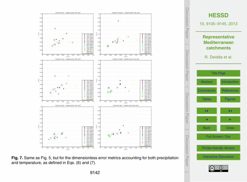
HESSD10, 9105–9145, 2013


catchments

R. Deidda et al.

Title Page



Tables Figures

J I

J I

Back Close

Full Screen / Esc



Discussion

Paper

|D

iscussionP

aper|

Discussion

Paper

|D

iscussionP

aper|

0 0.02 0.04 0.06 0.08 0.1 0.12 0.14 0.16 0.18 0.20

0.02

0.04

0.06

0.08

0.1

0.12

0.14

0.16

0.18

0.2

ε µ [−]

ε σ

[−]



0 0.02 0.04 0.06 0.08 0.1 0.12 0.14 0.16 0.18 0.20

0.02

0.04

0.06

0.08

0.1

0.12

0.14

0.16

0.18

0.2

ε µ [−]

ε σ

[−]



0 0.02 0.04 0.06 0.08 0.1 0.12 0.14 0.16 0.18 0.20

0.02

0.04

0.06

0.08

0.1

0.12

0.14

0.16

0.18

0.2

ε µ [−]

ε σ

[−]



0 0.02 0.04 0.06 0.08 0.1 0.12 0.14 0.16 0.18 0.20

0.02

0.04

0.06

0.08

0.1

0.12

0.14

0.16

0.18

0.2

ε µ [−]

ε σ

[−]



0 0.02 0.04 0.06 0.08 0.1 0.12 0.14 0.16 0.18 0.20

0.02

0.04

0.06

0.08

0.1

0.12

0.14

0.16

0.18

0.2

ε µ [−]

ε σ

[−]



0 0.02 0.04 0.06 0.08 0.1 0.12 0.14 0.16 0.18 0.20

0.02

0.04

0.06

0.08

0.1

0.12

0.14

0.16

0.18

0.2

ε µ [−]

ε σ

[−]



Figure 7: Same as Figure 5, but for the dimensionless error metrics account-ing for both precipitation and temperature, as defined in Eqs. (6)-(7).Fig. 7. Same as Fig. 5, but for the dimensionless error metrics accounting for both precipitation

and temperature, as defined in Eqs. (6) and (7).

9142





HESSD10, 9105–9145, 2013


catchments

R. Deidda et al.

Title Page



Tables Figures

J I

J I

Back Close

Full Screen / Esc



Discussion

Paper

|D

iscussionP

aper|

Discussion

Paper

|D

iscussionP

aper|

0 0.5 1 1.5 2 2.5 3 3.5 4 4.5 5 5.50

0.5

1

1.5

2

2.5

3

3.5

4

4.5

5

5.5

Quantile errors for Temperature [K]

Qua

ntile

err

ors

for

Pre

cipi

tatio

n [m

m/d

]



0 0.5 1 1.5 2 2.5 3 3.5 4 4.5 5 5.50

0.5

1

1.5

2

2.5

3

3.5

4

4.5

5

5.5


Qua

ntile

err

ors

for

Pre

cipi

tatio

n [m

m/d

]



0 0.5 1 1.5 2 2.5 3 3.5 4 4.5 5 5.50

0.5

1

1.5

2

2.5

3

3.5

4

4.5

5

5.5


Qua

ntile

err

ors

for

Pre

cipi

tatio

n [m

m/d

]



0 0.5 1 1.5 2 2.5 3 3.5 4 4.5 5 5.50

0.5

1

1.5

2

2.5

3

3.5

4

4.5

5

5.5


Qua

ntile

err

ors

for

Pre

cipi

tatio

n [m

m/d

]



0 0.5 1 1.5 2 2.5 3 3.5 4 4.5 5 5.50

0.5

1

1.5

2

2.5

3

3.5

4

4.5

5

5.5


Qua

ntile

err

ors

for

Pre

cipi

tatio

n [m

m/d

]



0 0.5 1 1.5 2 2.5 3 3.5 4 4.5 5 5.50

0.5

1

1.5

2

2.5

3

3.5

4

4.5

5

5.5


Qua

ntile

err

ors

for

Pre

cipi

tatio

n [m

m/d

]



Figure 8: Scatterplots of mean absolute errors in the quantiles of daily pre-cipitation and temperature distributions, computed using Eq. (8) for eachof the 14 ENSEMBLES models with respect to E-OBS observational refer-ence. Quantiles are calculated at 100 uniformly spaced probability levels.Each subplot displays areal averages over a 4×4 grid-point stencil centeredin each catchment.

Fig. 8. Scatterplots of mean absolute errors in the quantiles of daily precipitation and tempera-ture distributions, computed using Eq. (8) for each of the 14 ENSEMBLES models with respectto E-OBS observational reference. Quantiles are calculated at 100 uniformly spaced probabil-ity levels. Each subplot displays areal averages over a 4×4 grid-point stencil centered in eachcatchment.

9143





HESSD10, 9105–9145, 2013


catchments

R. Deidda et al.

Title Page



Tables Figures

J I

J I

Back Close

Full Screen / Esc



Discussion

Paper

|D

iscussionP

aper|

Discussion

Paper

|D

iscussionP

aper|

0 2 4 6 8 10 12 14 16 18 20400

500

600

700

800

900

1000

1100

1200

1300

30−

y P

reci

pita

tion

mea

n [m

m/y

]

Catchment "thau" − Interperiod variability (1951−2100)

1 − HCS−HRM2 − HCS−HIR3 − HCS−CLM4 − HCL−HRM5 − HCL−RCA6 − HCH−HRM7 − HCH−RCA8 − ECH−REM9 − ECH−HIR10 − ECH−RMO11 − ECH−RCA12 − ARP−HIR13 − BCM−HIR14 − BCM−RCA15 − E−OBS

0 2 4 6 8 10 12 14 16 18 20200

300

400

500

600

700

800

900

1000

1100

30−

y P

reci

pita

tion

mea

n [m

m/y

]

Catchment "riumannu" − Interperiod variability (1951−2100)


0 2 4 6 8 10 12 14 16 18 20800

1000

1200

1400

1600

1800

2000

2200

2400

2600

2800

30−

y P

reci

pita

tion

mea

n [m

m/y

]

Catchment "noce" − Interperiod variability (1951−2100)


0 2 4 6 8 10 12 14 16 18 20300

400

500

600

700

800

900

1000

1100

1200

30−

y P

reci

pita

tion

mea

n [m

m/y

]

Catchment "kokaeli" − Interperiod variability (1951−2100)


0 2 4 6 8 10 12 14 16 18 200

500

1000

1500

30−

y P

reci

pita

tion

mea

n [m

m/y

]

Catchment "gaza" − Interperiod variability (1951−2100)


0 2 4 6 8 10 12 14 16 18 20100

150

200

250

300

350

400

450

500

550

600

30−

y P

reci

pita

tion

mea

n [m

m/y

]

Catchment "chiba" − Interperiod variability (1951−2100)


Figure 9: Variability of the mean annual precipitation (mm/yr) over the five30-yr climatological periods between 1951 and 2100. Models HCS-HIR andBCM-HIR stop in year 2050. The reference values of E-OBS climatologiesin the two 30-yr periods between 1951-2010 are indicated with empty circlesand horizontal lines. Each subplot displays results based on areal averagesover a 4×4 grid-point stencil centered in each catchment.

Fig. 9. Variability of the mean annual precipitation (mm yr−1) over the five 30 yr climatologicalperiods between 1951 and 2100. Models HCS-HIR and BCM-HIR stop in year 2050. The refer-ence values of E-OBS climatologies in the two 30 yr periods between 1951–2010 are indicatedwith empty circles and horizontal lines. Each subplot displays results based on areal averagesover a 4×4 grid-point stencil centered in each catchment.

9144





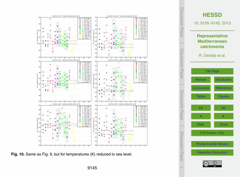
HESSD10, 9105–9145, 2013


catchments

R. Deidda et al.

Title Page



Tables Figures

J I

J I

Back Close

Full Screen / Esc



Discussion

Paper

|D

iscussionP

aper|

Discussion

Paper

|D

iscussionP

aper|

0 2 4 6 8 10 12 14 16 18 20284

286

288

290

292

294

296

30−

y T

empe

ratu

re m

ean

[K]

Catchment "thau" − Interperiod variability (1951−2100)


0 2 4 6 8 10 12 14 16 18 20288

289

290

291

292

293

294

295

296

297

298

30−

y T

empe

ratu

re m

ean

[K]

Catchment "riumannu" − Interperiod variability (1951−2100)


0 2 4 6 8 10 12 14 16 18 20282

284

286

288

290

292

294

296

30−

y T

empe

ratu

re m

ean

[K]

Catchment "noce" − Interperiod variability (1951−2100)


0 2 4 6 8 10 12 14 16 18 20286

287

288

289

290

291

292

293

294

295

30−

y T

empe

ratu

re m

ean

[K]

Catchment "kokaeli" − Interperiod variability (1951−2100)


0 2 4 6 8 10 12 14 16 18 20290

291

292

293

294

295

296

297

298

299

30−

y T

empe

ratu

re m

ean

[K]

Catchment "gaza" − Interperiod variability (1951−2100)


0 2 4 6 8 10 12 14 16 18 20289

290

291

292

293

294

295

296

297

298

299

30−

y T

empe

ratu

re m

ean

[K]

Catchment "chiba" − Interperiod variability (1951−2100)


Figure 10: Same as Figure 9, but for temperatures (K) reduced to sea level.

Fig. 10. Same as Fig. 9, but for temperatures (K) reduced to sea level.

9145





Climate model validation and selection for hydrological applications in representative Mediterranean catchments

Documents