Climate change threatens polar bear populations: a ... · Climate change threatens polar bear populations: a stochastic demographic analysis ... 2Biology Department MS-34, ... (Amstrup

Ecology, 91(10), 2010, pp. 2883–2897� 2010 by the Ecological Society of America

Climate change threatens polar bear populations:a stochastic demographic analysis

CHRISTINE M. HUNTER,1,6 HAL CASWELL,2 MICHAEL C. RUNGE,3 ERIC V. REGEHR,4 STEVE C. AMSTRUP,4

AND IAN STIRLING5

1Department of Biology and Wildlife, Institute of Arctic Biology, University of Alaska, Fairbanks, Alaska 99775 USA2Biology Department MS-34, Woods Hole Oceanographic Institution, Woods Hole, Massachusetts 02543 USA

3U.S. Geological Survey, Patuxent Wildlife Research Center, 12000 Beech Forest Road, Laurel, Maryland 20708 USA4U.S. Geological Survey, Alaska Science Center, 4210 University Drive, Anchorage, Alaska 99508 USA

5Canadian Wildlife Service, 5320 122 Street NW, Edmonton, Alberta T6H3S5 Canada

Abstract. The polar bear (Ursus maritimus) depends on sea ice for feeding, breeding, andmovement. Significant reductions in Arctic sea ice are forecast to continue because of climatewarming. We evaluated the impacts of climate change on polar bears in the southern BeaufortSea by means of a demographic analysis, combining deterministic, stochastic, environment-dependent matrix population models with forecasts of future sea ice conditions from IPCCgeneral circulation models (GCMs). The matrix population models classified individuals byage and breeding status; mothers and dependent cubs were treated as units. Parameterestimates were obtained from a capture–recapture study conducted from 2001 to 2006.Candidate statistical models allowed vital rates to vary with time and as functions of a sea icecovariate. Model averaging was used to produce the vital rate estimates, and a parametricbootstrap procedure was used to quantify model selection and parameter estimationuncertainty. Deterministic models projected population growth in years with more extensiveice coverage (2001–2003) and population decline in years with less ice coverage (2004–2005).LTRE (life table response experiment) analysis showed that the reduction in k in years withlow sea ice was due primarily to reduced adult female survival, and secondarily to reducedbreeding. A stochastic model with two environmental states, good and poor sea ice conditions,projected a declining stochastic growth rate, log ks, as the frequency of poor ice yearsincreased. The observed frequency of poor ice years since 1979 would imply log ks ’� 0.01,which agrees with available (albeit crude) observations of population size. The stochasticmodel was linked to a set of 10 GCMs compiled by the IPCC; the models were chosen for theirability to reproduce historical observations of sea ice and were forced with ‘‘business as usual’’(A1B) greenhouse gas emissions. The resulting stochastic population projections showeddrastic declines in the polar bear population by the end of the 21st century. These projectionswere instrumental in the decision to list the polar bear as a threatened species under the U.S.Endangered Species Act.

Key words: climate change; demography; IPCC; LTRE analysis; matrix population models; polar bear;sea ice; stochastic growth rate; stochastic models; Ursus maritimus.

INTRODUCTION

Climate change is projected to have significant effects

on population dynamics, species distributions and

interactions, food web structure, biodiversity, and

ecosystem processes (Convey and Smith 2006, Parmesan

2006, Grosbois et al. 2008, Keith et al. 2008). The

climate is changing faster in the Arctic than in other

areas (Serreze and Francis 2006, Walsh 2008). For

Arctic marine mammals, the most critical of these

changes involve the sea ice environment (Laidre et al.

2008). The extent of perennial sea ice in the Arctic has

been declining since 1979 at an average rate of 11.3% per

decade (Stroeve et al. 2007, Perovich and Richter-Menge

2009). The summer minimum sea ice extent in 2005 set a

new record, which was broken again in 2007; the ice

extent in 2008 was the second lowest on record. This

trend has led to concerns about Arctic species with

strong associations with sea ice. The polar bear is one of

the most ice-dependent of all Arctic marine mammals

(Amstrup 2003, Laidre et al. 2008). As a top predator, it

is also an important indicator of effects on the Arctic

ecosystem (Boyd et al. 2006).

Arctic sea ice changes have been associated with

negative effects on individuals and populations of polar

bears (Stirling et al. 1999, Obbard et al. 2006, Regehr et

al. 2006, 2009, Rode et al. 2010). Such observations

alone, however, provide few insights into future impacts

of climate, which can be assessed only by linking

population growth models, environmental effects, and

Manuscript received 14 September 2009; revised 8 February2010; accepted 18 February 2010. Corresponding Editor: M. K.Oli.

6 E-mail: [email protected]

2883

forecasts of the future environment. Although challeng-

ing, such assessments are necessary to forecast future

trends and to inform policy debates and legal decisions.

The U.S. Endangered Species Act, for example, requires

an assessment of extinction risks within the ‘‘foreseeable

future’’ (16 U.S. Congress 1531, 1973).

In this paper, we examine the current and projected

future effects of climate change on a population of polar

bears (Ursus maritimus; see Plate 1). Our approach is to

develop stage-structured demographic models that

incorporate the observed responses of the stage-specific

vital rates to sea ice conditions. We then present a novel

approach to connecting these demographic models to

forecasts of future sea ice conditions from IPCC global

circulation models (GCMs). The results reveal effects of

climate on short-term transient dynamics, long-term

population growth rates (deterministic and stochastic)

and environment-dependent stochastic growth in the

nonstationary environment created by climate change.

This study of climate effects was motivated by the

need for an evaluation of polar bear population

viability, following a petition to list the polar bear as a

threatened species under the U.S. Endangered Species

Act (Center for Biological Diversity 2005). The Act

requires an evaluation of current conditions and a

prediction of future risks to the population. This

analysis was a contribution to those goals. The final

listing decision concluded that declines in sea ice in polar

bear habitat, both currently and in the future, pose a

threat to the species, which is likely to become

endangered in the foreseeable future. As a result, the

polar bear was listed as a threatened species in May 2008

(U.S. Fish and Wildlife Service 2008).

Polar bears and sea ice

Polar bears occur in most Arctic areas that are ice

covered for much of the year. They depend on sea ice for

access to their primary prey (ringed seals Phoca hispida

and bearded seals Erignathus barbatus) and for other

aspects of their life history (Stirling and Oritsland 1995,

Stirling et al. 1999, Amstrup 2003). Polar bears prefer

habitat on the continental shelf where they have greater

access to prey. The retreat of sea ice beyond the

continental shelf, and longer ice-free periods during

the summer, are expected to reduce foraging success,

increase nutritional stress, and increase the distances

polar bears must travel between seasonal use areas

(Bergen et al. 2007). In some Arctic regions, the sea ice

melts completely each year and polar bears are forced to

spend the summer on shore. During this time they are

largely food deprived, relying on body fat accumulated

during the previous year. Longer movements over

rougher sea ice and more open water could also increase

the risks of injury or death (Monnett and Gleason

2006), especially for cubs.

Reductions in sea ice extent and/or duration have

been associated with shifts toward more land-based

denning, evidence of nutritional stress, reduced body

condition, reproduction, survival, and body size for

polar bears in parts of their range (Stirling et al. 1999,

Obbard et al. 2006, Stirling and Parkinson 2006,

Fischbach et al. 2007, Regehr et al. 2007, Cherry et al.

2008). In recent years in the southern Beaufort Sea there

have also been more numerous observations of unusual

predation attempts and of drowned, emaciated, and

cannibalized polar bears (Amstrup et al. 2006, Monnett

and Gleason 2006, Stirling et al. 2008).

The study population

We analyzed the population of polar bears in the

southern Beaufort Sea, one of the 19 regions defined by

the IUCN Polar Bear Specialists Group (Aars et al.

2006). This population has previously been studied by

Amstrup et al. (1986, 2001, 2006) and Regehr et al.

(2006). Population size in 2006 was estimated as 1526

(95% confidence interval 1211–1841; Regehr et al. 2006).

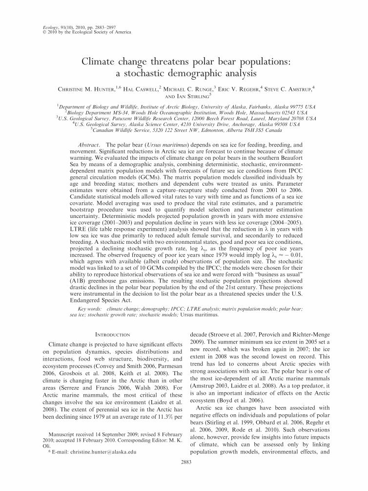
The study area (Fig. 1) lies on the northern coast of

Alaska and adjacent Canada, extending from Wain-

wright, Alaska in the west to Paulatuk, Northwest

Territories, in the east (for details see Amstrup et al.

1986, Regehr et al. 2009). A mark–recapture study of

this population was conducted by the U.S. Geological

Survey and the Canadian Wildlife Service from 2001 to

2006. During this period, polar bears were located using

helicopters in the spring, and captured for marking or

identification. The data set consisted of 818 captures of

627 tagged or radio-collared (approximately 6% of

captures) individuals. A detailed statistical analysis of

these data using multistate mark–recapture methods

(Regehr et al. 2009) provided estimates of the vital rates

used in our models.

Demography and climate change

In this study, we approach the demographic analysis

of climate change effects using a sequence of models, of

increasing sophistication, to explore different aspects of

the problem (cf. Caswell 2001:644). We begin with a

deterministic analysis of population growth in constant

environments characterized by specific amounts of sea

ice. Then we construct a stochastic model with which we

analyze population growth in response to specified

statistical patterns of sea ice fluctuations. Finally, we

link the stochastic models to forecasts of sea ice

fluctuations obtained from the output of a selected set

of GCM climate models. This sequence of models

proceeds from a constant environment, to a fluctuating

but stationary environment, to a fluctuating and

nonstationary environment.

It is well known that demographic analysis can

influence policy decisions. Policy, however, can also

dictate the direction of demographic analyses. In the

case of the Endangered Species Act, classification as a

threatened species requires a finding that the species is at

risk of extinction ‘‘in the foreseeable future.’’ In the case

of the polar bear, the foreseeable future was interpreted

by the U.S. Fish and Wildlife Service as 45 years from

CHRISTINE M. HUNTER ET AL.2884 Ecology, Vol. 91, No. 10

2007 (U.S. Fish and Wildlife Service 2007). Asymptotic

analyses using population growth rates, either stochastic

or deterministic, may not properly address this question,

so our analyses include transient projections with a

particular focus on 45 years, but also longer time periods

to 100 years. Comparisons of conclusions based on

projections of 45 years with those based on asymptotic

population growth rates may be instructive in future

listing decisions.

DEMOGRAPHIC MODEL STRUCTURE

The life cycle

The polar bear is the largest extant ursid. Survival is

relatively high; females as old as 32 years and males as

old as 28 years have been reported (Stirling 1988).

Females become pregnant for the first time in their

fourth or fifth year, and give birth for the first time in

their fifth or sixth year (Cronin et al. 2009). Females

produce litters of one to three cubs in a winter den.

Dependent young remain with their mothers from birth

through the spring of their second year (Stirling 1988,

Amstrup 2003), so the inter-birth interval for females

successfully weaning young is at least 3 years.

Our life cycle model included six stages, based on age

and reproductive status (Fig. 2). Stages 1, 2, and 3

contain nonreproductive females aged 2, 3, and 4 years,

respectively. Stage 4 comprises adult females available to

breed (i.e., without dependent young). Because mothers

and cubs are not independent during the parental care

period, we included these stages as mother–cub units;

stage 5 comprises females accompanied by one or more

cubs of the year, and stage 6 contains females

accompanied by one or more yearling cubs.

This life cycle (Fig. 2) corresponds to a stage-

structured matrix population model:

nðt þ 1Þ ¼ AtnðtÞ ð1Þ

where the vector n(t) gives the number of individuals in

each stage and the matrix At projects the population

from t to t þ 1. The projection interval extends from

April to April, to coincide with sampling, which occurs

in spring when females emerge from the den with their

cubs. The entries in At are defined in terms of lower-level

vital rates: survival, ri(t); breeding, conditional on

survival, bi(t); cub-of-the-year litter survival, rL0(t);

and yearling litter survival, rL1. The survival probabil-

ities, ri(t), are the probabilities of surviving from time t

FIG. 1. The southern Beaufort Sea study area, showing locations of polar bears captured from 2001 to 2006. The dashed line isthe population boundary, established by the International Union for the Conservation of Nature and Natural Resources (IUCN)Polar Bear Specialist Group. The white line is the 300-m bathymetry contour. The inset shows the four circumpolar ecoregionsdefined for polar bears by Amstrup et al. (2008). The figure is modified from Regehr et al. (2009).

October 2010 2885CLIMATE CHANGE AND POLAR BEARS

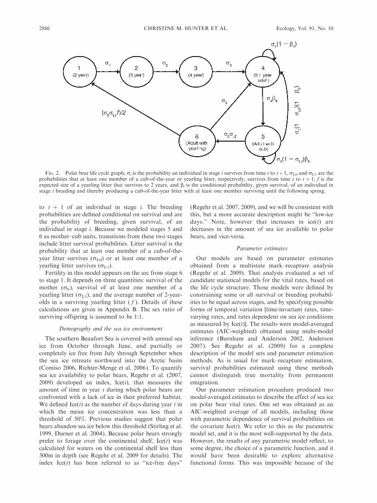
to t þ 1 of an individual in stage i. The breedingprobabilities are defined conditional on survival and are

the probability of breeding, given survival, of anindividual in stage i. Because we modeled stages 5 and

6 as mother–cub units, transitions from these two stagesinclude litter survival probabilities. Litter survival is the

probability that at least one member of a cub-of-the-

year litter survives (rL0) or at least one member of ayearling litter survives (rL1).

Fertility in this model appears on the arc from stage 6to stage 1. It depends on three quantities: survival of the

mother (r6), survival of at least one member of ayearling litter (rL1), and the average number of 2-year-

olds in a surviving yearling litter ( f ). Details of thesecalculations are given in Appendix B. The sex ratio of

surviving offspring is assumed to be 1:1.

Demography and the sea ice environment

The southern Beaufort Sea is covered with annual seaice from October through June, and partially or

completely ice free from July through September whenthe sea ice retreats northward into the Arctic basin

(Comiso 2006, Richter-Menge et al. 2006). To quantifysea ice availability to polar bears, Regehr et al. (2007,

2009) developed an index, Ice(t), that measures theamount of time in year t during which polar bears are

confronted with a lack of ice in their preferred habitat.We defined Ice(t) as the number of days during year t in

which the mean ice concentration was less than athreshold of 50%. Previous studies suggest that polar

bears abandon sea ice below this threshold (Stirling et al.

1999, Durner et al. 2004). Because polar bears stronglyprefer to forage over the continental shelf, Ice(t) was

calculated for waters on the continental shelf less than300m in depth (see Regehr et al. 2009 for details). The

index Ice(t) has been referred to as ‘‘ice-free days’’

(Regehr et al. 2007, 2009), and we will be consistent withthis, but a more accurate description might be ‘‘low-ice

days.’’ Note, however that increases in ice(t) aredecreases in the amount of sea ice available to polar

bears, and vice-versa.

Parameter estimates

Our models are based on parameter estimatesobtained from a multistate mark–recapture analysis

(Regehr et al. 2009). That analysis evaluated a set ofcandidate statistical models for the vital rates, based on

the life cycle structure. Those models were defined byconstraining some or all survival or breeding probabil-

ities to be equal across stages, and by specifying possibleforms of temporal variation [time-invariant rates, time-

varying rates, and rates dependent on sea ice conditionsas measured by Ice(t)]. The results were model-averaged

estimates (AIC-weighted) obtained using multi-modelinference (Burnham and Anderson 2002, Anderson

2007). See Regehr et al. (2009) for a complete

description of the model sets and parameter estimationmethods. As is usual for mark–recapture estimation,

survival probabilities estimated using these methodscannot distinguish true mortality from permanent

emigration.Our parameter estimation procedure produced two

model-averaged estimates to describe the effect of sea iceon polar bear vital rates. One set was obtained as an

AIC-weighted average of all models, including thosewith parametric dependence of survival probabilities on

the covariate Ice(t). We refer to this as the parametric

model set, and it is the most well-supported by the data.However, the results of any parametric model reflect, to

some degree, the choice of a parametric function, and itwould have been desirable to explore alternative

functional forms. This was impossible because of the

FIG. 2. Polar bear life cycle graph; ri is the probability an individual in stage i survives from time t to tþ1, rL0 and rL1 are theprobabilities that at least one member of a cub-of-the-year or yearling litter, respectively, survives from time t to t þ 1, f is theexpected size of a yearling litter that survives to 2 years, and bi is the conditional probability, given survival, of an individual instage i breeding and thereby producing a cub-of-the-year litter with at least one member surviving until the following spring.


short duration of the study. To examine the possible

effects of the functional form used, we also analyzed aset of AIC-weighted estimates from which the models

with parametric covariate dependence were excluded.We refer to this as the non-parametric model set.

Comparison of projections from the parametric andnon-parametric model sets provides a check on theinfluence of the particular functional dependence on

Ice(t) (Regehr et al. 2009).We concluded that survival probabilities (r1–r6, and

rL0) depended on both Ice(t) and time, while breedingprobabilities (b4, b5) were time dependent, decreasing in

2004 and 2005 (Regehr et al. 2009), when the number ofice-free days was particularly high (Table 1).

Confidence intervals, standard errors, and samplingdistributions were obtained using a parametric boot-

strap procedure (details in Regehr et al. 2009). Togenerate a bootstrap sample, we first chose a model with

probability proportional to its AIC weight. A vector ofmark–recapture parameters was then drawn from a

multivariate normal distribution with the estimatedmean and covariance matrix. This procedure was

repeated for a specified number of times (usually10 000) to obtain the bootstrap sample set. The mark–

recapture parameters were transformed as necessary,into demographic parameters, projection matrices,

growth rates, and so on, as appropriate. Confidenceintervals were calculated using the percentile method.

The bootstrap sample contains both model uncertainty(determined by the AIC weights associated with themodels) and parameter estimation uncertainty (deter-

mined by the covariance matrix of the estimates).The only parameters not directly estimated from the

mark-recapture analysis were the survival of yearlinglitters (rL1) and fertility ( f ). Given an estimate of rL0

from the mark–recapture estimation and an independentestimate of the frequency of one-cub and two-cub litters,

it is possible to estimate individual cub survival andsubsequently yearling litter survival, individual yearling

survival, and the average number of two-year olds in asurviving yearling litter, f. Details of these calculations

are given in Appendix B.

DETERMINISTIC DEMOGRAPHY

Deterministic analysis

We used both the parametric and non-parametricmodel-averaged estimates to construct year-specific

projection matrices, At, for each year, 2001–2005. Wecalculated the long-term population growth rate under

the conditions in year t as the dominant eigenvalue, kt,of At. The stable stage distribution and reproductive

value distribution were calculated as the right and lefteigenvectors w and v, respectively, corresponding to k.Life table response experiment (LTRE) methods wereused to quantify the contributions of each of the vital

rates to the differences in population growth rate amongyears (Caswell 1989, 2001). To do so, we collected the

vital rates (survival, litter survival, breeding) into a

parameter vector h, and chose the year 2001 as a

reference condition. The difference in k between the

reference year and year t is decomposed into

kt � k2001 ’X

i

�hðtÞi � hð2001Þ

i

� ]k]hi

ð2Þ

where the sensitivity term is calculated at the mean of

the vital rates for the reference year and year t. Each

term in the summation is the contribution of one of the

vital rates to the difference in k between the reference

year and year t. A parameter may make a small

contribution if it does not differ much among years or

if k is not very sensitive to differences in that parameter.

To examine transient effects, we projected population

growth for 45, 75, and 100 years, using Eq. 1 and an

initial population structure obtained from estimates of

the southern Beaufort Sea population from 2004 to 2006

(Regehr et al. 2006):

n0 ¼ ð 0:106 0:068 0:106 0:461 0:151 0:108 Þ>:ð3Þ

Deterministic results

Estimated population growth rates were greater than

1 under the conditions experienced in 2001–2003 and

less than 1 under the conditions experienced in 2004–

2005 (Table 1). Confidence intervals were wide, but only

a small proportion of the bootstrap samples for years

with more ice-free days (i.e., 2004 and 2005) projected

positive population growth (for complete bootstrap

distributions, see Appendix C, Fig. C2).

Including parametric dependence on sea ice makes

survival higher at low values of Ice, and lower at high

values of Ice, compared to the nonparametric model set

TABLE 1. Deterministic population growth rate kt, with 90%confidence intervals, standard error, proportion of bootstrapsamples ,1, and number of ice-free days [Ice(t)].

Year (t) ktLowerCI

UpperCI SE

Proportion, 1

Ice(t)(days)

Time-invariant model

all 0.997 0.755 1.053 0.105 0.57

Parametric model set

2001 1.059 0.083 1.093 0.269 0.24 902002 1.061 0.109 1.094 0.265 0.24 942003 1.036 0.476 1.107 0.207 0.41 1192004 0.765 0.541 0.932 0.120 1.00 1352005 0.799 0.577 0.959 0.122 0.99 134

Nonparametric model set

2001 1.017 0.810 1.088 0.092 0.43 902002 1.022 0.836 1.088 0.084 0.40 942003 1.075 0.903 1.129 0.077 0.19 1192004 0.801 0.549 1.000 0.135 0.95 1352005 0.895 0.446 1.020 0.185 0.88 134

Notes: Results are shown for the parametric model set,including parametric dependence of vital rates on Ice(t), and forthe nonparametric model set, which permits time variation, butdoes not impose the parametric functional form.


(Regehr et al. 2009). This amplifies the effect of reduced

sea ice on survival, and carries over to the effect of Ice

on population growth rates (Table 1). In our stochastic

models, in which the severity of the impacts of reduced

sea ice play a critical role, we will focus primarily on the

results from the nonparametric model set.

The LTRE results (Table 2) show that the decline in kduring the low sea ice years (2004 and 2005) was

primarily due to reduced survival of adult females (r4,

r5, and r6), and secondarily to reduced breeding

probability (b4). Thus, the estimated reductions in

survival and breeding in years with more ice-free days

translated into dramatic reductions in population

growth rate.

Fig. 3 shows k as a function of Ice(t), based on the

AIC model-weighted parameter estimates, and the time-

specific kt values from the nonparametric weighted

model. The two agree well; population growth rate is

relatively insensitive to sea ice for Ice(t) , 127 days, but

longer ice-free seasons lead to a steep decline in k (Fig.

3). Of course, extrapolation of the response of k beyond

the observed range depends entirely on the logistic

parametric form assumed for the covariate dependence,

and is unreliable. None of our analyses used such

extrapolation.

Transient projections achieved exponential growth

quickly, because the observed population vector (Eq. 3)

is close to the stable stage distribution. Because these

models are linear, population size at time t in the future

relative to initial population size can be interpreted in

terms of the proportional increase or decrease in

population size. To display the transient dynamics and

their uncertainty, we use area plots (Fig. 4 and later).

These plots show the proportion of simulations at any

time falling in a set of categories from drastic population

decline (relative size , 0.001) to large increases (relative

size . 2). The proportion of simulations can be

interpreted as the probability of outcomes, over the

space defined by model uncertainty, parameter uncer-

tainty, and, in our stochastic analyses, uncertainty about

future environmental conditions.

STOCHASTIC DEMOGRAPHY

The deterministic growth rate for a given year

describes the consequences of maintaining those condi-

tions permanently. To construct a stochastic model that

accounts for variation in conditions, we require a

stochastic model for the sea ice environment. To this

end, we classified sea ice conditions as ‘‘good’’ or

‘‘poor,’’ depending on whether they would lead to a

value of k greater or less than one. This corresponds to a

threshold value of Ice ’ 127 days. Consider an

environment in which good and poor years occur

independently, with probability q of a poor year and 1

� q of a good year. In a poor year, the projection matrix

is selected randomly from the matrices for 2004 and

2005; in a good year, the projection matrix is selected

randomly from the matrices for years 2001–2003. The

population grows according to Eq. 1 with

At ¼

Að2001Þ with probability ð1� qÞ=3



Að2004Þ with probability q=2

Að2005Þ with probability q=2:

8>>>><

>>>>:

ð4Þ

This algorithm treats the variability within the good

years, and within the poor years, as crude estimates of

the variation in the vital rates within these categories

TABLE 2. Life table response experiment (LTRE) analysis forpopulation growth rate (k), measured relative to the year2001 for the nonparametric model set.

Param-eter

Contribution to thedifference between

kt and k2001Proportionalcontribution

2002 2003 2004 2005 2002 2003 2004 2005

r1 0.000 0.002 �0.007 �0.003 0.03 0.04 0.03 0.03r2 0.000 0.002 �0.007 �0.003 0.03 0.04 0.03 0.03r3 0.000 0.002 �0.007 �0.003 0.03 0.04 0.03 0.03r4 0.001 0.008 �0.091 �0.045 0.25 0.15 0.42 0.36r5 0.001 0.007 �0.049 �0.017 0.12 0.12 0.23 0.14r6 0.000 0.004 �0.018 �0.008 0.09 0.07 0.08 0.06rL0 0.001 0.012 �0.021 �0.013 0.21 0.22 0.10 0.10b4 0.001 0.011 �0.006 �0.025 0.15 0.19 0.03 0.20b5 0.000 0.002 �0.001 �0.001 0.02 0.03 0.00 0.01f 0.000 0.006 �0.003 �0.002 0.06 0.10 0.01 0.02rL1 0.000 0.002 �0.007 �0.003 0.03 0.03 0.03 0.03

Note: Values are expressed as contributions to the differencebetween kt and k2001 and as a proportion of the total, where ri

is the probability that an individual in stage i survives from timet to t þ 1, rL0 and rL1 are the probabilities that at least onemember of a cub-of-the-year or yearling litter, respectively,survives from time t to tþ 1, f is the expected size of a yearlinglitter that survives to 2 years, and bi is the conditionalprobability, given survival, of an individual in stage i breedingand thereby producing a cub-of-the-year litter with at least onemember surviving until the following spring.

FIG. 3. Deterministic population growth rate, k, as afunction of the number of ice-free days, Ice(t). Diamonds aredeterministic population growth rates for 2001–2005 parameterestimates from the nonparametric model set.


(see Caswell and Kaye 2001 for a similar approach in a

fire model).

This stochastic model abstracts a continuous envi-

ronmental factor into a finite set of discrete environ-

mental states. Such models have been used frequently, as

in studies of fire (Silva et al. 1991, Caswell and Kaye

2001) and hurricanes (Pascarella and Horvitz 1998). A

discrete environment model sacrifices some detail, but in

FIG. 4. Uncertainty analysis of transient deterministic projections. The population is projected forward for 100 years using thevital rates estimated for the specified year in the parametric model set. Area plots show the proportion of 10 000 simulations inwhich the projected population size increased or declined to the specified fraction of the initial population. Simulations weresampled from the bootstrap distribution of parameter values.


our case it avoids errors that would result from

extrapolating the response of the vital rates to Ice

beyond the observed range of Ice. Instead, our

construction assumes that conditions at any value of

Ice . 127 days are no worse than those observed in

2004–2005, and thus our model provides a lower bound

on the effects of future climate change.

Stochastic analysis

The stochastic population growth rate is

log ks ¼ limT!‘

1

TlogjjAT�1 � � �A0n0jj ð5Þ

where ||�|| is the 1-norm and n0 is an arbitrary initial

population vector (e.g., Tuljapurkar 1990). We estimat-

ed log ks by Monte Carlo simulation with T¼10 000. To

evaluate short-term transient population responses, we

generated stochastic projections for 100 years, using the

initial population in Eq. 3. To evaluate the effects of

parameter uncertainty on stochastic growth, we repeated

the calculations using models generated by sampling

from the parametric bootstrap distribution of the vital

rates. Both the long-term growth rates and the short-

term projections include sampling uncertainty, model

uncertainty, and environmental stochasticity.

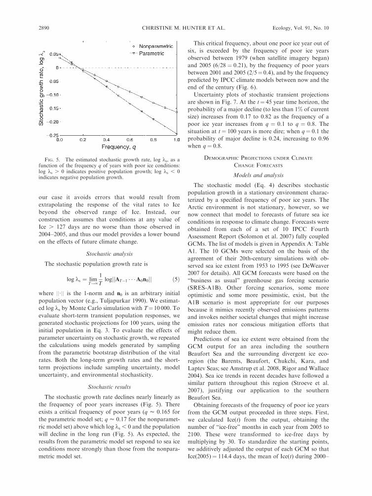
Stochastic results

The stochastic growth rate declines nearly linearly as

the frequency of poor years increases (Fig. 5). There

exists a critical frequency of poor years (q ’ 0.165 for

the parametric model set; q ’ 0.17 for the nonparamet-

ric model set) above which log ks , 0 and the population

will decline in the long run (Fig. 5). As expected, the

results from the parametric model set respond to sea ice

conditions more strongly than those from the nonpara-

metric model set.

This critical frequency, about one poor ice year out of

six, is exceeded by the frequency of poor ice years

observed between 1979 (when satellite imagery began)

and 2005 (6/28 ¼ 0.21), by the frequency of poor years

between 2001 and 2005 (2/5¼ 0.4), and by the frequency

predicted by IPCC climate models between now and the

end of the century (Fig. 6).

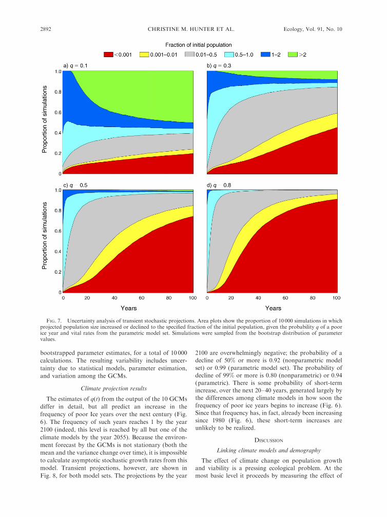
Uncertainty plots of stochastic transient projections

are shown in Fig. 7. At the t¼ 45 year time horizon, the

probability of a major decline (to less than 1% of current

size) increases from 0.17 to 0.82 as the frequency of a

poor ice year increases from q ¼ 0.1 to q ¼ 0.8. The

situation at t¼ 100 years is more dire; when q¼ 0.1 the

probability of major decline is 0.24, increasing to 0.96

when q ¼ 0.8.

DEMOGRAPHIC PROJECTIONS UNDER CLIMATE

CHANGE FORECASTS

Models and analysis

The stochastic model (Eq. 4) describes stochastic

population growth in a stationary environment charac-

terized by a specified frequency of poor ice years. The

Arctic environment is not stationary, however, so we

now connect that model to forecasts of future sea ice

conditions in response to climate change. Forecasts were

obtained from each of a set of 10 IPCC Fourth

Assessment Report (Solomon et al. 2007) fully coupled

GCMs. The list of models is given in Appendix A: Table

A1. The 10 GCMs were selected on the basis of the

agreement of their 20th-century simulations with ob-

served sea ice extent from 1953 to 1995 (see DeWeaver

2007 for details). All GCM forecasts were based on the

‘‘business as usual’’ greenhouse gas forcing scenario

(SRES-A1B). Other forcing scenarios, some more

optimistic and some more pessimistic, exist, but the

A1B scenario is most appropriate for our purposes

because it mimics recently observed emissions patterns

and invokes neither societal changes that might increase

emission rates nor conscious mitigation efforts that

might reduce them.

Predictions of sea ice extent were obtained from the

GCM output for an area including the southern

Beaufort Sea and the surrounding divergent ice eco-

region (the Barents, Beaufort, Chukchi, Kara, and

Laptev Seas; see Amstrup et al. 2008, Rigor and Wallace

2004). Sea ice trends in recent decades have followed a

similar pattern throughout this region (Stroeve et al.

2007), justifying our application to the southern

Beaufort Sea.

Obtaining forecasts of the frequency of poor ice years

from the GCM output proceeded in three steps. First,

we calculated Ice(t) from the output, obtaining the

number of ‘‘ice-free’’ months in each year from 2005 to

2100. These were transformed to ice-free days by

multiplying by 30. To standardize the starting points,

we additively adjusted the output of each GCM so that

Ice(2005)¼ 114.4 days, the mean of Ice(t) during 2000–

FIG. 5. The estimated stochastic growth rate, log ks, as afunction of the frequency q of years with poor ice conditions:log ks . 0 indicates positive population growth; log ks , 0indicates negative population growth.


2005. Second, we transformed the value of Ice(t) to a

binary environmental state, classifying year t as good if

Ice(t) . 127 days, or poor if Ice(t) , 127 days. The third

step was to extract trends in the frequency of poor years

from the sequence of binary outcomes. Such calculations

always require some smoothing; we applied a Gaussian

kernel smoother as described by Copas (1983; see Smith

et al. 2005 for an ecological application similar to this

one). The kernel standard deviation (2.5 years) was

chosen, as suggested by Copas (1983), as a subjective

compromise between smoothing and variation.

Each of the 10 GCMs thus produced a time series of

forecast values of q(t) from 2005 to 2100. We used these

frequencies to project the polar bear population, with

n(0) given by Eq. 3 and At chosen randomly at each time

step with probabilities given by Eq. 4 and the forecast

value of q(t). To evaluate the effects of uncertainty, we

repeated the calculations with each GCM using 1000

FIG. 6. (a) Frequency of poor ice conditions from 1979 to 2006, smoothed with a Gaussian kernel smoother with standarddeviation u¼1.5, 2, and 3 (see Copas 1983). Data are from Fig. 3 in Regehr et al. (2007). (b) The projected probability of a poor iceyear, from 2005 to 2100, from 10 general circulation model (GCM) climate models. Kernel standard deviation¼ 2.5.


bootstrapped parameter estimates, for a total of 10 000

calculations. The resulting variability includes uncer-

tainty due to statistical models, parameter estimation,

and variation among the GCMs.

Climate projection results

The estimates of q(t) from the output of the 10 GCMs

differ in detail, but all predict an increase in the

frequency of poor Ice years over the next century (Fig.

6). The frequency of such years reaches 1 by the year

2100 (indeed, this level is reached by all but one of the

climate models by the year 2055). Because the environ-

ment forecast by the GCMs is not stationary (both the

mean and the variance change over time), it is impossible

to calculate asymptotic stochastic growth rates from this

model. Transient projections, however, are shown in

Fig. 8, for both model sets. The projections by the year

2100 are overwhelmingly negative; the probability of adecline of 50% or more is 0.92 (nonparametric model

set) or 0.99 (parametric model set). The probability ofdecline of 99% or more is 0.80 (nonparametric) or 0.94

(parametric). There is some probability of short-termincrease, over the next 20–40 years, generated largely bythe differences among climate models in how soon the

frequency of poor ice years begins to increase (Fig. 6).Since that frequency has, in fact, already been increasing

since 1980 (Fig. 6), these short-term increases areunlikely to be realized.

DISCUSSION

Linking climate models and demography

The effect of climate change on population growthand viability is a pressing ecological problem. At the

most basic level it proceeds by measuring the effect of

FIG. 7. Uncertainty analysis of transient stochastic projections. Area plots show the proportion of 10 000 simulations in whichprojected population size increased or declined to the specified fraction of the initial population, given the probability q of a poorice year and vital rates from the parametric model set. Simulations were sampled from the bootstrap distribution of parametervalues.


climate-related variables (e.g., temperature) on an

ecological process (e.g., survival). If the process is

related to population growth and the direction of

environmental change can be predicted, then a qualita-

tive prediction of the effect of climate change can be

obtained.

To go beyond such a qualitative prediction requires

information on the sensitivity of the entire life cycle (or

as much of it as possible) to the environment, and a

quantitative prediction of future environmental changes.

In this paper, we obtained such a quantitative prediction

by a novel approach to linking environment-dependent

demographic models to the output of GCMs. This

approach, which is applicable to other species, has three

steps. First, a life cycle model was parameterized as a

function of the environment, in this case, an index of sea

ice extent. Second, a stochastic demographic model was

developed to compute population growth as a function

of environmental conditions and their fluctuations.

Third, a forecast of environmental changes was extract-

ed from GCM output. In our case, that forecast consists

of a time series of the frequency of poor ice conditions.

This approach can be applied to other species and

situations (e.g., Jenouvrier et al. 2009). The discretiza-

tion of the environmental states, as we did here, avoids

the need to extrapolate continuous relationships be-

tween the environment and the vital rates beyond the

range of observed conditions. This makes our predic-

tions of polar bear responses conservative, because no

matter how large Ice(t) becomes, the vital rates in the

model will be no worse than those observed during the

poor ice years of the study. However, given sufficiently

detailed information on both climate and the response

of vital rates, the analysis could use a continuous

environment model (see Jenouvrier et al. 2009 for a

comparison of discrete and continuous approaches).

Uncertainties

Management decisions must often be made in the face

of uncertainty, because information is limited and

environments are variable. Therefore, where possible,

analyses of climate effects should quantify the uncer-

tainty of the results on which management decisions are

based. This was particularly important in the listing

decision for the polar bear, and our analyses purposely

included several different kinds of uncertainty.

Burnham and Anderson (2002) and Anderson (2007)

have emphasized the importance of including model

selection uncertainty along with estimation uncertainty.

Our parametric bootstrap distributions include both

types of uncertainty. We also recognize the uncertainty

involved in parametric specification of the ice-depen-

dence of the vital rates, and therefore analyzed both

nonparametric and parametric model sets. Although

projections based on the nonparametric model set,

excluding parametric ice dependence, are conservative

in the sense of yielding a weaker response to sea ice

conditions, it is important to remember that the

parametric model set is the one most well-supported

by the data. Both analyses lead to the same conclusions

(Fig. 3).

In addition, we used a series of deterministic and

stochastic population models to assess potential popu-

lation response to changing ice conditions. The consis-

tency of results across this series of models strengthens

our inference. Such a sequence is the only way to

quantitatively assess the effects of different types of

uncertainty in assessment of population status and

response to environmental conditions.

Two aspects of the estimation procedures are worth

discussing because they might have artificially reduced

survival probabilities. One is harvest, which is not

FIG. 8. Stochastic simulations of population growth underconditions predicted by 10 IPCC climate models. Area plotsshow the proportion of 10 000 simulations in which projectedpopulation size after t years increased or declined to a specifiedfraction of initial population size for (a) the parametric modelset and (b) the nonparametric model set. Simulations wereobtained as samples of 1000 from the bootstrap distribution ofparameter values, for each climate model.


incorporated in our projections. Polar bears in the

southern Beaufort Sea are subject to regulated hunts by

native user groups in the United States and Canada

(Brower et al. 2002). Hunters are discouraged from

taking females with dependent cubs but subadult

females and adult females without cubs are currently

subject to harvest at a rate of ’0.019 (Regehr et al.

2007). Although the impact of this harvest is included in

the survival estimates for these stages; this level of

harvest has a negligible effect on population growth rate

(Hunter et al. 2007).

The second issue is emigration. Nonrandom tempo-

rary emigration can lead to survival estimates that are

negatively biased at the end of a study. However, Regehr

et al. (2009) investigated this, and found no evidence of

non-random temporary emigration. Although the power

of the analysis was limited due to the short study

duration, available data indicated that temporary

emigration did not create an important bias of survival

rates used in this study. Permanent emigration cannot be

distinguished from mortality. However, radio telemetry

studies, which began in the Beaufort Sea in 1981, have

confirmed that polar bears maintain a high degree of

fidelity to this geographic region. Although individual

animal utilization distributions are very large and

variable, over multi-year periods they do constitute

‘‘home ranges’’ (Amstrup et al. 2000). The permanent

migration of collared animals beyond the Beaufort Sea

region has been so rare that the description of the

movement of the one bear that did permanently

emigrate was deemed worthy of publication (Durner

and Amstrup 1995).

Polar bear population status

Summer sea ice in the Arctic is expected to continue to

decline (e.g., IPCC 2007, Overland and Wang 2007,

Stroeve et al. 2007). Our analyses demonstrate that this

decline poses a serious threat to the continued persis-

tence of the southern Beaufort Sea population of polar

bears. The current southern Beaufort Sea population

numbers about 1500 individuals (Regehr et al. 2006), so

a decline to 1% of current size would almost certainly

imply extinction. The probability of this outcome is

estimated at 0.80–0.94 by the year 2100, which is

certainly a serious risk.

The ice-free period in the southern Beaufort Sea

increased by approximately 50% between 2001–2003 and

2004–2005. At the same time, survival and breeding

probabilities declined (Regehr et al. 2007). The vital

rates estimated in years with low values of Ice(t) led to

positive population growth, but when Ice(t) exceeds

about 127 days, the population growth rate becomes

negative due to reductions in adult survival and breeding

probabilities. Asymptotic and short-term transient

projections showed the same results.

Our stochastic analysis found that a frequency of poor

ice years greater than q ’ 0.17 produces a negative

stochastic growth rate. This critical frequency is less

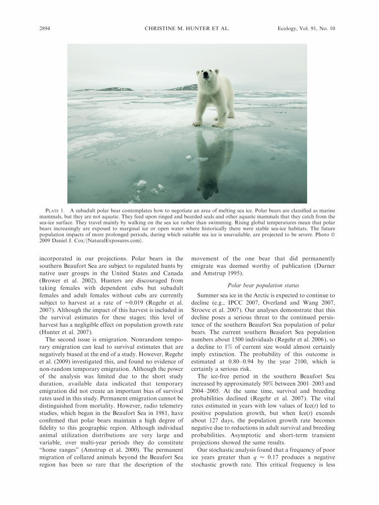
PLATE 1. A subadult polar bear contemplates how to negotiate an area of melting sea ice. Polar bears are classified as marinemammals, but they are not aquatic. They feed upon ringed and bearded seals and other aquatic mammals that they catch from thesea-ice surface. They travel mainly by walking on the sea ice rather than swimming. Rising global temperatures mean that polarbears increasingly are exposed to marginal ice or open water where historically there were stable sea-ice habitats. The futurepopulation impacts of more prolonged periods, during which suitable sea ice is unavailable, are projected to be severe. Photo �2009 Daniel J. Cox/hNaturalExposures.comi.


than the observed frequency of poor years from 1979 to

2005, the available record from satellite imagery. The

observed frequency of poor ice years, q¼ 0.2, from 1979

to 2005 (the available satellite record) exceeds this

threshold, and would lead to a stochastic growth rate of

log ks ¼ �0.012 (parametric model) or �0.006 (non-

parametric model).

Arctic sea ice extent at the end of the summer of 2005

was the lowest ever observed. This record was broken in

2007, and approached in 2008. If thinning multiyear ice,

more extensive open water and albedo effects create

positive feedback loops leading to further reductions

(Maslanik et al. 2007), the fate of polar bears in other

locations, even where populations have been stable (e.g.,

the northern Beaufort Sea) will also be in doubt. Recent

shipboard surveys in the southern Beaufort Sea (Barber

et al. 2009) found summer sea ice there to be even

thinner and more broken than shown in satellite images.

Comparisons of these growth rates estimated here

with trajectories of population size are hampered by the

lack of reliable population size estimates. The claim,

commonly repeated in the press, that worldwide polar

bear populations have increased fourfold since the 1960s

has no basis in the scientific literature (Dykstra 2008).

Some increases in polar bear populations occurred in the

1970s as harvesting was reduced, but there is no evidence

that these increases continued, and such recoveries,

where they occurred, are irrelevant to the effects of

recent changes in the availability of sea ice. In the

southern Beaufort Sea, Amstrup et al. (1986) reported a

crude estimate of population size of N ’ 1800 bears in

the mid-1980s. Regehr et al. (2006) estimated N ’ 1500

bears in 2006. Amstrup et al. (2001) suggested the

population may have remained constant or even

increased between the 1980s and the late 1990s.

However, if the difference between 1800 bears and

1500 bears represents a real decline, and if that decline

occurred over 15 years, it would represent an average

annual growth rate of �0.012. Over 20 years, such a

decline would imply an average annual growth rate of

�0.009. This further suggests that our estimates of

stochastic growth rate are reasonable. This comparison

with our calculated growth rate is very rough, because of

the different sources of historical data and the high

degree of uncertainty around these population estimates.

Nevertheless, the comparison supports the model

results.

The mechanisms linking sea ice to survival and

reproduction of polar bears are not known in detail.

Reduced prey availability no doubt plays a role (Stirling

and Smith 2004), because polar bears are dependent

upon sea ice for capturing prey (Amstrup 2003) and

their preferred foraging area is the water over the

continental shelf. In addition, reduced sea ice extent may

force polar bears to swim longer distances, increasing

their risk of drowning or starvation (Monnett and

Gleason 2006). The thinner ice that reforms after large

summer ice retreats also may be less suitable for polar

bear foraging (Stirling et al. 2008). Reduced sea ice will

undoubtedly also affect other ice-dependent species (see,

e.g., Gaston et al. 2005) and many food web links maybe involved in these effects (Huntington and Moore

2008, Moline et al. 2008).

We have shown that global warming is likely to haveprofoundly negative effects on future growth rates of

polar bear populations. A warmer world will have less

sea ice and hence less polar bear habitat. Geographicalvariation in the nature of sea ice and in predictions of

the retreat of sea ice habitat (Durner et al. 2009) suggests

that polar bears in different parts of their current rangewill be affected at different rates. Nonetheless, our

analyses, which incorporated sea ice and other uncer-

tainties, projected that by mid century, the effects ofglobal warming on polar bears will be severe. If current

GCM outcomes are correct, there is a high probability

that the Beaufort Sea population of polar bears willdisappear by the end of the century. Because all polar

bears are dependent on sea ice for securing their prey, it

is reasonable to expect that the effects of global warmingon polar bears of the southern Beaufort Sea will

ultimately extend to polar bears throughout their range.

This and other related findings provided the primarymotivation for listing polar bears, in May of 2008, as a

threatened species under the U.S. Endangered Species

Act (U.S. Fish and Wildlife Service 2008).

ACKNOWLEDGMENTS

We acknowledge primary funding for model developmentand analysis from the U.S. Geological Survey and additionalfunding from the National Science Foundation (DEB-0343820and DEB-0816514), NOAA, the Ocean Life Institute and theArctic Research Initiative at WHOI, and the Institute of ArcticBiology at the University of Alaska–Fairbanks. Funding for thecapture–recapture effort in 2001–2006 was provided by the U.S.Geological Survey, the Canadian Wildlife Service, the Depart-ment of Environment and Natural Resources of the Govern-ment of the Northwest Territories, and the Polar ContinentalShelf Project, Ottawa, Canada. We thank G. S. York, K. S.Simac, M. Lockhart, C. Kirk, K. Knott, E. Richardson, A. E.Derocher, and D. Andriashek for assistance in the field. D.Douglas and G. Durner assisted with analyses of radiotelemetryand remote sensing sea ice data. We thank J. Nichols, M.Udevitz, E. Cooch, and J.-D. Lebreton for helpful commentsand discussions.

LITERATURE CITED

Aars, J., N. J. Lunn, and A. E. Derocher. 2006. Polar bears:proceedings of the 14th working meeting of the IUCN/SSCpolar bear specialists group. International Union forConservation of Nature and Natural Resources, Gland,Switzerland and Cambridge, UK.

Amstrup, S. C. 2003. Polar bear, Ursus maritimus. Pages 587–610 in G. A. Feldhamer, B. C. Thompson, and J. A.Chapman, editors. Mammals of North America: biology,management, and conservation. Johns Hopkins UniversityPress, Baltimore, Maryland, USA.

Amstrup, S. C., G. Durner, I. Stirling, N. J. Lunn, and F.Messier. 2000. Movements and distribution of polar bears inthe Beaufort Sea. Canadian Journal of Zoology 78:948–966.

Amstrup, S. C., B. G. Marcot, and D. C. Douglas. 2008. ABayesian network modeling approach to forecasting the 21stcentury worldwide status of polar bears. Pages 213–268 inE. T. DeWeaver, C. M. Bitz, and L.-B. Tremblay, editors.


Arctic sea ice decline: observations, projections, mechanisms,and implications. Geophysics monograph series 180. AGU,Washington, D.C., USA.

Amstrup, S. C., T. L. McDonald, and I. Stirling. 2001. Polarbears in the Beaufort Sea: a 30 year mark–recapture casehistory. Journal of Agricultural, Biological, and Environ-mental Statistics 6:221–234.

Amstrup, S. C., I. Stirling, and J. W. Lentfer. 1986. Past andpresent status of polar bears in Alaska. Wildlife SocietyBulletin 14:241–254.

Amstrup, S. C., I. Stirling, T. S. Smith, C. Perham, and G. W.Thiemann. 2006. Recent observations of intraspecific preda-tion and cannibalism among polar bears in the southernBeaufort Sea. Polar Biology 29:997–1002.

Anderson, D. R. 2007. Model-based inference in the lifesciences: a primer on evidence. Springer-Verlag, New York,New York, USA.

Barber, D. G., R. Galley, M. G. Asplin, R. De Abreu, K.Warner, M. Pucko, M. Gupta, S. Prinsenberg, and S. Julien.2009. The perennial pack ice in the southern Beaufort Seawas not as it appeared in the summer of 2009. GeophysicalResearch Letters 36:L24501.

Bergen, S., G. M. Durner, D. C. Douglas, and S. C. Amstrup.2007. Predicting movements of female polar bears betweensummer sea ice foraging habitats and terrestrial denninghabitats of Alaska in the 21st century: proposed methodol-ogy and pilot assessment. Administrative Report. USGSAlaska Science Center, Anchorage, Alaska, USA.

Boyd, I., S. Wanless, and C. J. Camphuysen. 2006. Toppredators in marine ecosystems: their role in monitoring andmanagement. Cambridge University Press, Cambridge, UK.

Brower, C. D., A. Carpenter, M. L. Branigan, W. Calvert, T.Evans, A. S. Fischbach, J. A. Nagy, S. Schliebe, and I.Stirling. 2002. The polar bear management agreement for thesouthern Beaufort Sea: An evaluation of the first ten years ofa unique conservation agreement. Arctic 55:362–372.

Burnham, K. P., and D. R. Anderson. 2002. Model selectionand multimodel inference: a practical information-theoreticapproach. Second edition. Springer-Verlag, New York, NewYork, USA.

Caswell, H. 1989. The analysis of life table responseexperiments. I. Decomposition of effects on populationgrowth rate. Ecological Modelling 46:221–237.

Caswell, H. 2001. Matrix population models. Second edition.Sinauer, Sunderland, Massachusetts, USA.

Caswell, H., and T. Kaye. 2001. Stochastic demography andconservation of an endangered plant (Lomatium bradshawii)in a dynamic fire regime. Advances in Ecological Research32:1–51.

Center for Biological Diversity. 2005. Petition to list the polarbear (Ursus maritimus) as a threatened species under theEndangered Species Act. Before the Secretary of the In-terior 2-16-2005. hhttp://www.biologicaldiversity.org/species/mammals/polar_bear/pdfs/15976_7338.pdfi

Cherry, S. G., A. E. Derocher, I. Stirling, and E. Richardson.2008. Fasting physiology of polar bears in relation toenvironmental change and breeding behavior in the BeaufortSea. Polar Biology 32:383–391.

Comiso, J. C. 2006. Arctic warming signals from satelliteobservations. Weather 61:70–76.

Convey, P., and R. I. L. Smith. 2006. Responses of terrestrialAntarctic ecosystems to climate change. Plant Ecology 182:1–10.

Copas, J. B. 1983. Plotting p against x. Applied Statistics 32:25–31.

Cronin, M. A., S. C. Amstrup, S. L. Talbot, G. K. Sage, andK. S. Amstrup. 2009. Genetic variation, relatedness, andeffective population size of polar bears (Ursus maritimus) inthe southern Beaufort Sea, Alaska. Journal of Heredity 100:681–690.

DeWeaver, E. 2007. Uncertainty in climate model projectionsof Arctic sea ice decline: an evaluation relevant to polar

bears. Administrative Report. USGS Alaska Science Center,Anchorage, Alaska, USA.

Durner, G. M., and S. C. Amstrup. 1995. Movements of a polarbear from northern Alaska to northern Greenland. Arctic 48:338–341.

Durner, G. M., S. C. Amstrup, R. M. Nielson, and T. L.McDonald. 2004. The use of sea ice habitat by female polarbears in the Beaufort Sea. Report to Minerals ManagementService for OCS Study 2004–14. U.S. Geological Survey,Alaska Science Center, Anchorage, Alaska, USA.

Durner, G. M., et al. 2009. Predicting 21st century polar bearhabitat distribution from global climate models. EcologicalMonographs 79:25–58.

Dykstra, P. 2008. Magic number: a sketchy fact about polarbears keeps going . . . and going . . . and going. Society ofEnvironmental Journalists, online article 15, Summer 2008.hhttp://www.sej.org/publications/alaska-and-hawaii/magic-number-a-sketchy-fact-about-polar-bears-keeps-goingand-going-ani

Fischbach, A. S., S. C. Amstrup, and D. C. Douglas. 2007.Landward and eastward shift of Alaskan polar bear denningassociated with recent sea ice changes. Polar Biology 30:1395–1405.

Gaston, A. J., H. G. Gilchrist, and M. L. Mallory. 2005.Variation in ice conditions has strong effects on the breedingof marine birds at Prince Leopold Island, Nunavut.Ecography 28:331–344.

Grosbois, V., O. Gimenez, J.-M. Gaillard, R. Pradel, C.Barbraud, J. Clobert, A. P. Moller, and H. Weimerskirch.2008. Assessing the impact of climate variation on survival invertebrate populations. Biological Reviews 83:357–399.

Hunter, C. M., H. Caswell, M. C. Runge, E. V. Regehr, S. C.Amstrup, and I. Stirling. 2007. Polar bears in the SouthernBeaufort Sea II: demography and population growth inrelation to sea ice conditions. Administrative Report. USGSAlaska Science Center, Anchorage, Alaska, USA.

Huntington, H. P., and S. E. Moore. 2008. Arctic marinemammals and climate change. Ecological Applications18(Supplement):S1–S2.

IPCC 2007. Summary for policymakers. Pages 1–18 in S.Solomon, D. Qin, M. Manning, Z. Chen, M. Marquis, K. B.Averyt, M. Tignor, and H. L. Miller, editors. Climate change2007: the physical science basis. Contribution of WorkingGroup I to the Fourth Assessment Report of the Intergov-ernmental Panel on Climate Change. Cambridge UniversityPress, New York, New York, USA.

Jenouvrier, S., H. Caswell, C. Barbraud, and H. Weimerskirch.2009. Demographic models and IPCC climate projectionspredict the decline of an emperor penguin population.Proceedings of the National Academy of Sciences USA106:1844–1847.

Keith, D. A., H. R. Akcakaya, W. Thuiller, G. F. Midgley,R. G. Pearson, S. J. Phillips, H. M. Regan, M. B. Araujo,and T. G. Rebelo. 2008. Predicting extinction risks underclimate change: coupling stochastic population models withdynamic bioclimatic habitat models. Biology Letters 4:560–563.

Laidre, K. L., I. Stirling, L. F. Lowry, O. Wiig, M. P. Heide-Jorgensen, and S. H. Ferguson. 2008. Quantifying thesensitivity of arctic marine mammals to climate-inducedhabitat change. Ecological Applications (Supplement)18:S97–S125.

Maslanik, J. A., C. Fowler, J. Stroeve, S. Drobot, J. Zwally, D.Yi, and W. Emery. 2007. A younger, thinner Arctic ice cover:Increased potential for rapid, extensive sea-ice loss. Geo-physical Research Letters 34GL032043.

Moline, M. A., N. J. Karnovsky, Z. Brown, G. J. Divoky, T. K.Frazer, C. A. Jacoby, J. J. Torres, and W. R. Fraser. 2008.High latitude changes in ice dynamics and their impact onpolar marine ecosystems. Annals of the New York Academyof Sciences 1134:267–319.


Monnett, C., and J. S. Gleason. 2006. Observations of mortalityassociated with extended open-water swimming by polarbears in the Alaskan Beaufort Sea. Polar Biology 29:681–687.

Obbard, M. E., M. R. L. Cattet, T. Moody, L. Walton, D.Potter, J. Inglis, and C. Chenier. 2006. Temporal trends in thebody condition of southern Hudson Bay polar bears. ClimateChange Research Information Note, No. 3. Applied Re-search and Development Branch, Ontario Ministry ofNatural Resources, Sault Sainte Marie, Ontario, Canada.

Overland, J. E., and M. Wang. 2007. Future regional Arctic seaice declines. Geophysical Research Letters 34GL030808.

Parmesan, C. 2006. Ecological and evolutionary responses torecent climate change. Annual Review of Ecology Evolutionand Systematics 37:637–669.

Pascarella, J. B., and C. C. Horvitz. 1998. Hurricanedisturbance and the population dynamics of a tropicalunderstory shrub: megamatrix elasticity analysis. Ecology79:547–563.

Perovich, D. K., and J. A. Richter-Menge. 2009. Loss of sea icein the Arctic. Annual Review of Marine Science 1:417–441.

Regehr, E. V., S. C. Amstrup, and I. Stirling. 2006. Polar bearpopulation status in the southern Beaufort Sea. Open-FileReport 2006-1337. U.S. Geological Survey, Reston, Virginia,USA.

Regehr, E. V., C. M. Hunter, H. Caswell, S. C. Amstrup, and I.Stirling. 2009. Survival and breeding of polar bears in thesouthern Beaufort Sea in relation to sea ice. Journal ofAnimal Ecology 79:117–127.

Regehr, E. V., C. M. Hunter, H. Caswell, I. Stirling, and S. C.Amstrup. 2007. Polar bears in the southern Beaufort Sea I:Survival and breeding in relation to sea ice conditions, 2001–2006. Administrative Report. USGS Alaska Science Center,Anchorage, Alaska, USA.

Richter-Menge, J., et al. 2006. State of the Arctic report. Specialreport. NOAA/OAR/PMEL, Seattle, Washington, USA.

Rigor, I. G., and J. M. Wallace. 2004. Variations in the age ofArctic sea-ice and summer sea-ice extent. GeophysicalResearch Letters 31GL019492.

Rode, K. D., S. C. Amstrup, and E. V. Regehr. 2010. Reducedbody size and cub recruitment in polar bears associated withsea ice decline. Ecological Applications 20:768–782.

Serreze, M. C., and J. A. Francis. 2006. The arctic amplificationdebate. Climate Change 76:241–264.

Silva, J. F., J. Raventos, H. Caswell, and M. C. Trevisan. 1991.Population responses to fire in a tropical savanna grassAndropogon semiberbis: a matrix model approach. Journal ofEcology 79:345–356.

Smith, M., H. Caswell, and P. Mettler-Cherry. 2005. Stochasticflood and precipitation regimes and the population dynamicsof a threatened floodplain plant. Ecological Applications 15:1036–1052.

Solomon, S., D. Qin, M. Manning, Z. Chen, M. Marquis, K. B.Averyt, M. Tignor, and H. L. Miller, editors. 2007. Climatechange 2007: the physical science basis. Contribution ofWorking Group I to the Fourth Assessment Report of theIntergovernmental Panel on Climate Change. CambridgeUniversity Press, Cambridge, UK.

Stirling, I. 1988. Polar bears. University of Michigan Press, AnnArbor, Michigan, USA.

Stirling, I., N. J. Lunn, and J. Iacozza. 1999. Long-term trendsin the population ecology of polar bears in western HudsonBay in relation to climatic change. Arctic 52:294–306.

Stirling, I., and N. A. Oritsland. 1995. Relationships betweenestimates of ringed seal and polar bear populations in theCanadian Arctic. Canadian Journal of Fisheries and AquaticSciences 52:2594–2612.

Stirling, I., and C. L. Parkinson. 2006. Possible effects ofclimate warming on selected populations of polar bears(Ursus maritimus) in the Canadian Arctic. Arctic 59:261–275.

Stirling, I., E. Richardson, G. W. Thiemann, and A. E.Derocher. 2008. Unusual predation attempts of polar bearson ringed seals in the southern Beaufort Sea: possiblesignificance of changing spring ice conditions. Arctic 60:14–22.

Stirling, I., and T. G. Smith. 2004. Implications of warmtemperatures, and an unusual rain event for the survival ofringed seals on the coast of southeastern Baffin Island. Arctic57:59–67.

Stroeve, J. C., M. M. Holland, W. Meier, T. Scambos, and M.Serreze. 2007. Arctic sea ice decline: faster than forecast.Geophysical Research Letters 34GL029703.

Tuljapurkar, S. 1990. Population dynamics in variable envi-ronments. Springer-Verlag, New York, New York, USA.

U.S. Fish and Wildlife Service. 2007. Endangered andthreatened wildlife and plants: 12-month petition findingand proposed rule to list the polar bear (Ursus maritimus) asthreatened throughout its range. Federal Register 72(5):1064–1099.

U.S. Fish and Wildlife Service. 2008. Endangered andthreatened wildlife and plants: determination of threatenedstatus for the polar bear (Ursus maritimus) throughout itsrange. Final Rule. Federal Register 73:28211–28303.

Walsh, J. E. 2008. Climate of the Arctic marine environment.Ecological Applications 18(Supplement):S3–S22.

APPENDIX A

Projection matrices (Ecological Archives E091-204-A1).

APPENDIX B

Calculation of fertility (Ecological Archives E091-204-A2).

APPENDIX C

IPCC models and bootstrap sampling results (Ecological Archives E091-204-A3).


Climate change threatens polar bear populations: a ... · Climate change threatens polar bear populations: a stochastic demographic analysis ... 2Biology Department MS-34, ... (Amstrup

Documents