Climate change impacts economic analysis in Europe: a sectorial approach

Economic Analysis of Climate Change Impacts in Europe: a Sectoral Approach

Antonio Soria, Juan Carlos Ciscar, Laszlo Szabo (JRC, European Commission)jornadas eoi ‘carbon markets and emission reduction’

17 February 2011, Madrid

The IPTSThe IPTS

The Institute for Prospective Technological Studies (IPTS), based in Sevilla, is one of the 7 scientific institutes of the European Commission's Joint Research Centre (JRC)

Mission

to provide customer-driven support to the EU policy-making process by researching science-based responses to policy challenges that have both a socio-economic and a scientific or technological dimension

Question of Interest:

What are the economic consequences of

climate change in Europe?

- overall order of magnitude

- distribution (space, time, sector)

<Mitigation and Adaptation policies>

White Paper on Adaptation (April 2009)

Literature: few references, mainly based on expert judgement (G1)

TAR IPCC (2001) Stern report (2007)

Source: IPCC 4AR (2007), vol. II, Ch. 20

What is known: aggregate impactsWhat is known: aggregate impacts

What is known: social cost of carbonWhat is known: social cost of carbon(marginal damage)(marginal damage)

Tol (2005) review of literature

• Mean $97/tC

• Standard deviation $203/tC

Key, and controversial, assumptions

• Discount rate

• Equity weighting

What is unknownWhat is unknown

• Non-market effects (e.g. biodiversity, ecosystems)

• Extreme weather risks

• Socially contingent effects

• Long-term catastrophic risks

OutlineOutline

1. Overview of the PESETA project

2. Methodology: the economic CGE model

3. Sectoral results

4. Overall economic impacts

5. Conclusions

About PESETAAbout PESETA

PESETA stands for: Projection of Economic impacts of climate change in Sectors of the European union based on boTtom-up Analyses

Main purpose: Quantitative, multi-sectoral assessment of the monetary estimates of impacts of climate change in Europe

JRC funded projectTo support policymakersLargely based on past DG Research-funded projects

(PRUDENCE, DINAS-Coast, cCASHh, NewExt,…)

Project partners and scopeProject partners and scope

Climate scenarios: DMI, CRU

Six sectoral assessments: Agriculture: U. Politécnica de Madrid Human health: AEA Technology River basin flooding: JRC/IES Coastal systems: FEEM/Southampton U. Tourism: U. Maastricht-ICIS

Coordination and integration into CGE model: JRC/IPTS

Integrated economic impact assessment

Starting point: physical impact estimates

Some sectors provide with direct effects estimates (e.g. river floods)

Overall effects (direct + indirect) assessed with a computable general equilibrium model of Europe

Socioeconomic scenario: GDP, population assumptions

Agriculturemodel

Coastal Systems

model

RiverFlooding

model

Tourismmodel

Stage 1:Modelingfuture climate

Physical impacts

agriculture

Physical impacts coasts

Physical impacts floods

Physical impacts tourism

Stage 2:Modelingphysicalimpacts

Stage 3:Modelingeconomicimpacts

Climate model

General Equilibrium model

Climate data(T, P, SLR)

Economicimpacts

Valuationagriculture

impacts

Valuationcoasts impacts

Valuationfloods impacts

Valuationtourism impacts


Agriculturemodel

Coastal Systems

model

RiverFlooding

model

Tourismmodel

Agriculturemodel

Coastal Systems

model

RiverFlooding

model

Tourismmodel


Physical impacts

agriculture




Physical impacts

agriculture






Climate model



Economicimpacts

Climate model



Economicimpacts


impacts





impacts





impacts





Agriculturemodel

Coastal Systems

model

RiverFlooding

model

Tourismmodel


Physical impacts

agriculture






Climate model



Economicimpacts


impacts





Agriculturemodel

Coastal Systems

model

RiverFlooding

model

Tourismmodel

Agriculturemodel

Coastal Systems

model

RiverFlooding

model

Tourismmodel


Physical impacts

agriculture




Physical impacts

agriculture






Climate model



Economicimpacts

Climate model



Economicimpacts


impacts





impacts





impacts




Grouping Grouping of countriesof countries

Climate Scenarios

Data needs: 50 km resolution; daily and monthly

Selection of scenarios 2011-2040 period: A2 IPCC SRES scenario

data from the Rossby Center 2071-2100 period: data from PRUDENCE

A2, B2 IPCC SRES scenarios 2 regional climate models, RCMs (HIRHAM, RCA) 2 global circulation models, GCMs (HadCM3, ECHAM4)

2.5°C 3.9°C 4.1°C 5.4°C

World population in 2100 (1012) 10.4 15.1 10.4 15.1

World GDP in 2100 (1012, 1990US$) 235 243 235 243

CO2 Concentration (ppm) 561 709 561 709

Δ Temperature (ºC)*World 2.4 3.1 2.3 3.1EU‡ 2.5 3.9 4.3 5.4 Northern Europe 2.9 4.1 3.6 4.7 British Isles 1.6 2.5 3.2 3.9 Central Europe North 2.3 3.7 4.0 5.5 Central Europe South 2.4 3.9 4.4 6.0 Southern Europe 2.6 4.1 4.3 5.6

Δ Precipitation (%)*EU‡ 1 -2 2 -6 Northern Europe 10 10 19 24 British Isles -5 -2 10 5

Central Europe North 3 1 6 -1 Central Europe South 2 -2 -4 -16 Southern Europe -7 -15 -13 -28

Sea Level Rise (high climate sensitivity) (cm) 49 56 51 59

Scenarios

*Increase in the period 2071–2100 compared to 1961–1990. ‡European regions: Southern Europe (Portugal, Spain, Italy, Greece, and Bulgaria), Central Europe South (France, Austria, Czech Republic, Slovakia, Hungary, Romania, and Slovenia), Central Europe North (Belgium, The Netherlands, Germany, and Poland), British Isles (Ireland and UK), and Northern Europe (Sweden, Finland, Estonia, Latvia, and Lithuania).

Four 2080s ScenariosFour 2080s Scenarios

TemperatureTemperature3.9°C (A2 Hadley) 5.4°C (A2 Echam)3.9°C (A2 Hadley) 5.4°C (A2 Echam)

PrecipitationPrecipitation3.9°C (A2 Hadley) 5.4°C (A2 Echam)3.9°C (A2 Hadley) 5.4°C (A2 Echam)

Methodologies for Physical Impacts Assessment

Detailed process modelling Agriculture, DSSAT crop model River basin flooding, LISFLOOD hydrological model Coastal systems, DIVA model

Reduced-form exposure-response functions Tourism Human Health

Economic impact assessment

Starting point: physical impact estimates

Some sectors provide with economic direct effects estimates (e.g. river floods)

Overall effects (direct + indirect) assessed with a computable general equilibrium model of Europe: GEM-E3 model

2. The general equilibrium economic model

The The GEM-E3 GEM-E3 Model:Model:General Equilibrium Model for General Equilibrium Model for Energy-Economics-Environment Energy-Economics-Environment

interactionsinteractions

General equilibriumGeneral equilibrium

• Neoclassical framework• Each agent pursues its own interest• Decentralised information (preferences of

consumers and technology of firms)• Simultaneous optimal behaviour• Interaction of all markets• Interaction of all agents (consumers, firms,

government, rest of the world)

Advantages of CGE modelling

• Consistency• Theory (microeconomics foundations, within a consistent

macroeconomic framework)• Data (Input-output, National Accounts, SAM)

• Structural model (versus reduced-form models): explain behaviour of agents in markets, taking into account institutions

• Transparency• Systematic analysis; not mechanical• Flexibility• Can address a broad range of policy issues

Criticisms / disadvantages of CGE modelling

• Weak empirical validation (calibration versus econometric estimation)

• The critical role of functional forms• Simplification of exogenous elements of the model• Data requirements• Heavy computational load

The GEM-E3 model: European model version

Computable General Equilibrium model

Representing multiple production sectors and countries Integrating energy and environment in the economy

GEM-E3: Standard Version 24 countries, 18 sectors (Eurostat) Perfect competition for all commodity markets Environmental module fully incorporated (All GHGs

included)

The The GEM-E3GEM-E3 model: Production model: Production

Production (output)

CapitalLabourEnergy

Materials bundle

Electricity

LabourMaterails

Fuels bundleFuels

Coal

Gas

Oil

Labour

Materials

Agriculture

Non-market services

Market services

Credit & insurance

Credit & insurance

Telecommunication

Building/ Constr.

Consumer goods

Other equipment

Transport equip.

Electrical goods

Other en. intensive

chemicals

Ferrous, ore, metals

Level 1

Level 2

Level 3

Level 4

Reserves

• Perfect competition

• Nested CES production function

• Fully flexible coefficients

• EU econometric evidence on elasticities

The The GEM-E3GEM-E3 model: Consumption model: Consumption

Intertemporal maximization of consumer’s utility involving consumption,

savings, leisure labour supply also derived

from utility maximization steady state solution used

LES with durable and non-durable goods

Total Income

Leisure

Labour Supply

Consumption

Savings

Investment indwellings

MonetaryAssets

Durable goods Non-durable goods andservices

Cars Heating Systems Electric Appliance

Food Clothing Housing Housing furniture and

operation Medical care and health

expenses Purchased transport Communication recreation, entrertainment etc. Other services Fuels and power Operation of transports

Consumption of non-durableslinked to the use of durables

Disposableincome

3. Sectoral results

AgricultureAgriculture

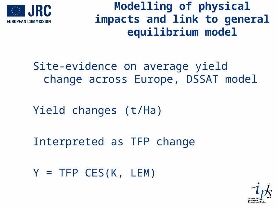
Modelling of physical impacts and link to general equilibrium model

Site-evidence on average yield change across Europe, DSSAT model

Yield changes (t/Ha)

Interpreted as TFP change

Y = TFP CES(K, LEM)

Agriculture

Crop yield changes (t/Ha), production losses and gains

Agriculture: crop yield changes (%)

compared to 1961-1990

B2 HadAM3h A2 HadAM3h B2 ECHAM4 A2 ECHAM42.5°C 3.9°C 4.1°C 5.4°C

Northern Europe 37 39 36 52 62British Isles -9 -11 15 19 20Central Europe North -1 -3 2 -8 16Central Europe South 5 5 3 -3 7Southern Europe 0 -12 -4 -27 15

EU 3 -2 3 -10 17

2025

Coastal SystemsCoastal Systems

Coastal systems: the methodCoastal systems: the method

DIVA model

Impact categories: sea floods, migration, other

Integration into the CGE model: Interpretation of sea flood cost as capital loss Interpretation of migration cost as additional obliged

consumption (welfare loss)

Coastal systems

- No adaptation

- With adaptation

Coastal Systems

people flooded (1000s/year) in main scenarios with high climate sensitivity, without adaptation

B2 HadAM3h A2 HadAM3h B2 ECHAM4 A2 ECHAM4 A2 ECHAM42.5°C 3.9°C 4.1°C 5.4°C high SLR

Northern Europe 20 40 20 56 272British Isles 70 136 86 207 1,279Central Europe North 345 450 347 459 2,398Central Europe South 82 144 85 158 512Southern Europe 258 456 313 474 1,091

EU 775 1,225 851 1,353 5,552

River FloodsRiver Floods

River Floods: the methodologyRiver Floods: the methodology

LISFLOOD model; integration of damages for various return periods (from several ‘representative basins’)

Economic valuation: projection of change in 100-year flood damage for the scenario (relative to control)

Integration into the GEM-E3 model: Damage to residential buildings (additional obliged

consumption) Damage to productive sectors (industry, services,…):

Capital loss Production loss

River Floods

Change in Economic damage (note red means a decrease)

River floods

expected economic damage (million €/year)

B2 HadAM3h A2 HadAM3h B2 ECHAM4 A2 ECHAM4 simulated2.5°C 3.9°C 4.1°C 5.4°C 1961-1990

Northern Europe -325 20 -100 -95 578British Isles 755 2,854 2,778 4,966 806Central Europe North 1,497 2,201 3,006 5,327 1,555Central Europe South 3,495 4,272 2,876 4,928 2,238Southern Europe 2,306 2,122 291 -95 1,224

EU 7,728 11,469 8,852 15,032 6,402

Human healthHuman health

Human Healthaverage annual heat-related (left) and cold-related (right) death rates (per 100,000 population) 3.9°C scenario

Note: using climate-dependent health functions (no acclimatisation)

TourismTourism

TourismTourismTCI scores in summerTCI scores in summer

Ideal

Excellent

Very good

Good

Acceptable

Marginal

Unfavourable

Ideal

Excellent

Very good

Good

Acceptable

Marginal

Unfavourable

Ideal

Excellent

Very good

Good

Acceptable

Marginal

Unfavourable

control

5.45.4°°CC

4.14.1°°CC

Tourism

Change in expenditure receipts (million €)

B2 HadAM3h 2.5ºC

A2 HadAM3h 3.9ºC

B2 ECHAM4 4.1ºC

A2 ECHAM4 5.4ºC

Norhern Europe 443 642 1,888 2,411British Isles 680 932 3,587 4,546Central Europe North 634 920 3,291 4,152Central Europe South 925 1,763 7,673 9,556Southern Europe -824 -995 -3,080 -5,398EU 1,858 3,262 13,360 15,268

4. Overall economic impact

• Effects of 2080s climate • On European economy as of today• Assuming there is no public adaptation, so that priorities for adaptation within the EU can be explored

Annual damage Annual damage

in terms of GDP changes (million €)in terms of GDP changes (million €)

-70000

-60000

-50000

-40000

-30000

-20000

-10000

0

10000

SouthernEurope

Central EuropeSouth

Central EuropeNorth

British Isles NorthernEurope

EU

2.5°C3.9°C

4.1°C

5.4°C

5.4°C, 88 cm SLR

Annual damage Annual damage

in terms of Welfare changes (%)in terms of Welfare changes (%)

-2.0

-1.5

-1.0

-0.5

0.0

0.5

1.0

SouthernEurope

Central EuropeSouth

Central EuropeNorth

British Isles NorthernEurope

EU

2.5°C

3.9°C4.1°C

5.4°C

5.4°C, 88 cm SLR

Sectoral decomposition Sectoral decomposition

of welfare changes (%)of welfare changes (%)

-2.0%

-1.5%

-1.0%

-0.5%

0.0%

0.5%

1.0%2.

5oC

3.9o

C

5.4o

C

5.4i

oC

2.5o

C

3.9o

C

5.4o

C

5.4i

oC

2.5o

C

3.9o

C

5.4o

C

5.4i

oC

2.5o

C

3.9o

C

5.4o

C

5.4i

oC

2.5o

C

3.9o

C

5.4o

C

5.4i

oC

2.5o

C

3.9o

C

5.4o

C

5.4i

oC

Southern Europe Central Europe South Central Europe North British Isles Northern Europe EU

Tourism

River floods

Coastal systems

Agriculture

5. Conclusions

• Integration of various disciplines, consistency requirements• Further research is needed, concerning:

• Costs and benefits of adaptation• Cross-sectoral consistency• Land use modelling • Monte Carlo analysis

http://peseta.jrc.ec.europa.eu/

http://www.pnas.org/content/early/http://www.pnas.org/content/early/2011/01/27/1011612108.abstract2011/01/27/1011612108.abstract

Muchas gracias !

http://www.pnas.org/content/early/2011/01/27/1011612108.abstract

http://www.pnas.org/content/early/2011/01/27/1011612108.abstract

Climate change impacts economic analysis in Europe: a sectorial approach

Documents

diva model

geme3 model

economic direct effects

sam structural model

economic impacts conclusions

climate scenarios data

scope climate scenarios

europe jrc