Welcome message from author
This document is posted to help you gain knowledge. Please leave a comment to let me know what you think about it! Share it to your friends and learn new things together.
Transcript
Climate Change and Restoration of Degraded
Land
Edited by
Arraiza Bermúdez-Cañete, Mª PazUniversidad Politécnica de Madrid, Spain
Santamarta Cerezal, Juan C.Universidad de La Laguna, Canary Islands, Spain
Ioras, FlorinBuckinghamshire New University, United Kingdom
García Rodríguez, José LuísUniversidad Politécnica de Madrid, Spain
Abrudan, Ioan VasileTransilvania University, Romania
Korjus, HennEstonian University of Life Science
Borbála GálosUniversity of West Hungary
Climate Change and Restoration of Degraded Land© 2014 The Authors.
Published by: Colegio de Ingenieros de MontesCalle Cristóbal Bordiú, 19 28003 MadridPhone +34 915 34 60 [email protected]
Depósito Legal: TF 638-2014ISBN: 978-84-617-1377-6590 pp. ; 24 cm.1 Ed: september, 2014
This work has been developed in the framework of the RECLAND Project. It has been funded by the European Union under the Lifelong Learning Programme, Erasmus Programme: Erasmus Multilateral Projects, 526746-LLP-1-2012-1-ES-ERASMUS-EM-CR, MSc Programme in Climate Change and Restoration of Degraded Land.
How to cite this book;
Arraiza, M.P., Santamarta, J.C., Ioras, F., García-Rodríguez, J.L., Abrudan, I.V., Kor-jus, H., Borála, G. (ed.) (2014). Climate Change and Restoration of Degraded Land. Madrid:Colegio de Ingenieros de Montes.
Designed byAlba Fuentes Porto
This book was peer-reviewed�������������������������������������������������Ƥ����������������
3
Contents
CHAPTER 1INTRODUCTION TO CLIMATE CHANGE AND LAND DEGRADATION ���������������������������������15
1 Introduction���������������������������������������������������������������������������������������������������������������������������� 16
2 Extent and rate of land degradation �������������������������������������������������������������������������������������17
3 Land degradation – causes ��������������������������������������������������������������������������������������������������� 20
4 Climatic consequences of land degradation ������������������������������������������������������������������������ 21
5 Climatic factors in land degradation ������������������������������������������������������������������������������������235.1 Rainfall5.2 Floods5.3 Droughts5.4 Solar radiation, temperature and evaporation5.5 Wind
� �����Ƥ���ǡ�������������������������������������������� �������������������������������������������������� 41
� ����������������������������������� ��������������������������������������������������������������������������������� 427.1 Carbon sequestration to mitigate climate change and combat land degradation
� ��������������������������������������������������������������������Ȃ������������� ����������� 448.1 Advocating for enhanced observing systems at national, regional and international levelsǤ� �����������ơ����������������������������8.3 Further enhancing climate prediction capability8.4 Assessing vulnerability and analyzing hazards8.5 Implementing risk management applications8.6 Contributing actively to the implementation of the UN system’s International Strategy for Disaster Reduction (ISDR)8.7 Supporting the strengthening of the capabilities of the Parties and regional institutions with drought-related programmes
� ������������������� ��������������������������������������������������������������������������������������������������������������� 48
Contents
4
CHAPTER 2�1
REFORESTATION UNDER CLIMATE CHANGE IN TEMPERATE, WATER LIMITED REGIONS: CURRENT VIEWS AND CHALLENGES ����������������������������������������������������������������������������������������� 55
1 Introduction���������������������������������������������������������������������������������������������������������������������������� 561.1 Climate, water and forests
� �ơ������������������������������������������������������ ���������������������������������������������������� 58Ǥ� �����ǣ������������������������ơ��������������ƪ��Ǥ� �������������ǣ��ơ����������������������������Ǥ� �������ǣ������������������������ơ����������������������������
� ��������������������������������� ��������������������������������������������������������������������������������������� 623.1 The climatic transition zone at the forest/grassland edge 3.2 The climatic vulnerability of the forest/grassland transition zone3.3 Recently observed climatic impacts 3.4 The hidden threat at the xeric limits: increasing drought 3.5 Considerations for forest management
4 Summary and conclusions ����������������������������������������������������������������������������������������������������� 67
CHAPTER 2�2FORESTS IN A CHANGING CLIMATE ������������������������������������������������������������������������������������������� 71
� ������������������������������������������������������������� ������������������������������������������ 721.1 The threat to xeric limits in SE Europe 1.2 Climatic factors of the xeric distributional limits for beech in SE Europe
� ����������������������������������������������� ��������������������������������������������������������������75
� ��������������������������������������������������������������������������������������������������������������������������753.1 Health and vitality loss due to climatic extremes: case study of beech in SW Hungary 3.2 Analysis of drought events
� ��������������������������� ����������������������������������������������������������������������������������������������������� 79Ǥ� �����������������������Ƥ����������������
5 Final conclusions �������������������������������������������������������������������������������������������������������������������� 815.1 Related websites, projects and videos
CHAPTER 2�3STRUCTURE AND FUNCTIONING OF FOREST ECOSYSTEMS ������������������������������������������������ 85
� �������������������������������������������������������� ������������������������������������������� 851.1 Introduction1.2 Syllabus
Contents
5
�������������������������������������������������Ǧ����������������������������������������� ���912.1 Introduction2.2 Case study: Comparative Water Balance Study of Forest and Fallow Plots 2.3 Conclusions
� ������������ǣ������������������������������� ����������������������������������������������������������������������� 1053.1 Introduction3.2 Ecosystem services of forests3.3 Carbon cycle of forests3.4 Estimations of the carbon content of forests and forest soil at the xeric limit
� ��������������������������������������������������Ǧ����������ǡ������������������������������ ���1174.1 Introduction4.2 Estimation of aridity tolerance from common garden test results4.3 Discussion
CHAPTER 2�4
CLIMATIC EFFECTS OF LAND COVER CHANGE ���������������������������������������������������������������������� 129
1 Introduction ���������������������������������������������������������������������������������������������������������������������������130
�������������������� �������������������������������������������������������������������������������������������������������������������131
���������� ���������������������������������������������������������������������������������������������������������������������������������1353.1 Land Cover Data Arrays3.2 MM5Ǥ� ������Ƥ�����������
4 Results ����������������������������������������������������������������������������������������������������������������������������������� 138
5 Concluding remarks �������������������������������������������������������������������������������������������������������������� 143
�������������������ǡ�������������������� ������������������������������������������������������������������������������� 144
CHAPTER 2�5
AFFORESTATION AS A TOOL FOR CLIMATE CHANGE MITIGATION �������������������������������� 147
1 Introduction ������������������������������������������������������������������������������������������������������������������������� 1481.1 Regional climate projections for Europe Ǥ� ����������ơ��������������������������������������1.3 Research foci
���������� �������������������������������������������������������������������������������������������������������������������������������� 1512.1 Experimental setup 2.2 Main steps of the analyses
Contents
6
3 Results ����������������������������������������������������������������������������������������������������������������������������������� 1543.1 Climate change signal due to emission changeǤ� ����������������������������������������ơ����������Ǥ� ����������������������������������������ơ������������������������������������������3.4 Case study for Hungary3.5 Conclusions
�������������������ǡ�������������������� ������������������������������������������������������������������������������� 158
CHAPTER 3
CLIMATE CHANGE AND WASTE LAND RESTORATION �������������������������������������������������������� 165
� ��������������������������������������������������������� �������������������������������������������� 165
2 W������������������������������������� ȋ���Ȍ ����������������������������������������������������������� 1662.1 Background2.2 Sources of GHG2.3 GHG savings2.4 Biogenic carbon
� ����������������������� �������������������������������������������������������������������������������������������������������1753.1 Potential GHG emissions reductions from materials management3.2 Reducing or avoiding GHG emissions through land management practices3.3 Trends in waste generation and management3.4 Climate impact of waste management practices3.5 Waste prevention
� ���������������������������������Ƥ���������������� ���������������������������������������������������� 201Ǥ� ���������������Ƥ���4.2 Post-closure maintenance4.3 Minimizing impacts on the atmosphereǤ� ����Ƥ���������
CHAPTER 4
WATER MANAGEMENT AND PLANNING �������������������������������������������������������������������������������� 215
� �������������� ��������������������������������������������������������������������������������������������������������������������� 2161.1 Introduction1.2 Water plans1.3 Water plans objetives and strategies1.4 Water budget
Contents
7
1.5 Water planning and climate change1.6 Water management on islands1.7 Useful links
2 Water uses ���������������������������������������������������������������������������������������������������������������������������2252.1 Introduction2.2 Water footprint2.3 Agricultura water uses2.4 Industrial uses2.5 Useful links
� �������������������������� �������������������������������������������������������������������������������������������������� 2293.1 Precipitation3.2 Reservoir related issues3.3 Managed aquifer rechargue3.4 Useful links
� �����������ǡ������������������������ �������������������������������������������������������������������������������� 2344.1 Introduction4.2 Greywater4.3 Desalination of water4.4 Water waste reclamation4.5 Water waste and climate change4.6 Useful links
� �������ƥ�������������������������������������������������������������������������������������������������������������� 2405.1 IntroductionǤ� �������ƥ�������5.3 Water Sustainability Ǥ� �������ƥ�������������������������������������5.5 Useful links
� ���������������������������������� ���������������������������������������������������������������������������������� 2446.1 Introduction6.2 Modelling climate change6.3 Impacts of climate change 6.4 Water quality6.5 Floods6.6 Water scarcity and drought
� �������������������� ������������������������������������������������������������������������������������������������������������ 2817.1 Introduction
Contents
8
7.2 European legislation7.3 Useful links
8 Miscellaneous Hydrology Studies ��������������������������������������������������������������������������������������� 289
CHAPTER 5
EROSION AND HYDROLOGICAL RESTORATION �������������������������������������������������������������������� 299
1 Erosion and Hydrological Restoration �������������������������������������������������������������������������������� 2991.1 The origin of the Forest-Hydrologic Restoration Plan (RHF).1.2 Agro-hydrological Planning.1.3 RHF Action Planning1.4 Complementary actions1.5 Watershed restoration and climate change1.6 Watershed Management Issues1.7 Climate Change Science Needs
� ���������������������������������������������� ������������������������������������������������������������������3172.1 Forest hydrology and watershed management
� ���������������������������������������������������������������������������������� ������� 328
� ���������������������������������� ������������������������������������������������������������������������������������3314.1 The European Flood Alert SystemǤ� �����������������ƪ����������Ǥ�
CHAPTER 6
FOREST FIRE LAND RESTORATION �������������������������������������������������������������������������������������������� 345
� ����Ƥ����ơ������������������ ������������������������������������������������������������������������������������������� 3451.1 Introduction1.2 Fire Severity1.3 Fire Regimes Ǥ� �����ơ������������������1.5 Important Notes
� ����Ƥ�������������������ơ����������������������� ������������������������������������������������������ 3582.1 Introduction2.2 The Knowledge Base2.3 Plant Species Information2.4 Wildlife Species Information2.5 Plant Community Information
Contents
9
� ���������������Ǥ�����Ƥ������������������������� ���������������������������������������������������������������3723.1 Introduction3.2 Role and Function of Structural Components3.3 Retaining Structures3.4 Revetments3.5 Articulated Block Walls3.6 Slope Gratings (Three-Dimensional Cellular Grids)Ǥ� ����Ƥ������������������������
� �����������Ǥ�����Ƥ���������������ơ����������� ��������������������������������������������������������������� 388Ǥ� ����Ǧ���������������ơ������������������������������������4.2 Hillslope Treatments 4.3 Channel Treatments 4.4 Road Treatments Ǥ� ����Ƥ��������������Ǥ����������������
CHAPTER 7
POLLUTED SOILS RESTORATION ������������������������������������������������������������������������������������������������ 413
� ����������������ơ������������������������������� ��������������������������������������������������������� 413Ǥ� ��Ƥ������1.2 Participatory approach in community consultation 1.3 Health risk1.4 Emissions standards1.5 Transport and emergency safety assessment1.6 Impacts of funding
� ����������������������������������������������������������� ���������������������������������������� 4182.1 Thermal desorption2.2 Excavation or dredging2.3 Surfactant enhanced aquifer remediation (SEAR)2.4 Pump and treatǤ� ������Ƥ������������������������2.6 In situ oxidation2.7 Soil vapor extraction2.8 Other technologies
3 Biological degradation �������������������������������������������������������������������������������������������������������� 424
Contents
10
� ����������������������������ǡ�������ǡ����������������������������������������������������������������������� 4274.1 Basics4.2 In situ and ex situ bioremediation4.3 Bioremediation technologiesǤ� �������������������������������ƥ������������
� ���������������� ���������������������������������������������������������������������������������������������������������������� 447
� ������������� ���������������������������������������������������������������������������������������������������������������������� 4516.1 Problem6.2 Sources of contaminants6.3 Chemical fate and mobility6.4 Available technologies
CHAPTER 8
COMBATING CLIMATE CHANGE BY RESTORATION OF DEGRADED LAND ��������������������� 483
����������������������������������������������������������������ǣ����Ƥ�������������������������������� ����������������������������������������������������������������������������������������������������������������������������������� 483
1.1 IntroductionǤ� ��Ƥ��������������������1.3 Evolution
����������ƪ����������������������������������������� �����������������������������������������������������������4882.1 Introduction2.2 The terrestrial carbon cycle2.3 Soil degradationǤ� �������Ƥ�������������������������������
����������ƪ������������������������������������������������������������������ ����������������� 4923.1 Restoration of degraded agricultural land3.2 Restoration of degraded forest land
������������������������������������������������������������� �������������������������������������������4984.1 Introduction4.2 Management Approaches
���������������������������������������������������������� ����������������������������������������������� 510
����������������������������������������������������������������������������������������������� ��� ��������������������������������������������������������������������������������������������������������������������512
6.1 Introduction 6.2 Financing sources
Contents
11
CHAPTER 9
RESEARCH MATTERS – CLIMATE CHANGE GOVERNANCE ��������������������������������������������������523
� �������Ƥ�������������������������� ���������������������������������������������������������������������������������������5231.1 Observations of climate changeǤ� ����������ơ����������������������1.3 Emission scenarios
����������������������������������������������� ��������������������������������������������������������������������5312.1 Intergovernmental Panel on Climate Change (IPCC)2.2 United Nations Framework Convention on Climate Change (UNFCCC)2.3 Kyoto Protocol (KP)2.4 European Commission – DG Clima2.5 Combating climate change within and outside the EU2.6 Adoption of the Kyoto ProtocolǤ � �������������������������������������������������������Ƥ��������������������������������
2.8 EU monitoring and reporting of greenhouse gas emissions under the UNFCC and the Kyoto Protocol2.9 European Climate Change Programme
CHAPTER 10
ADVANCED STATISTICS ��������������������������������������������������������������������������������������������������������������� 557
������������������������������� ��������������������������������������������������������������������������������������������������557Ǥ� ��Ƥ��������������������1.2 What is a linear model?Ǥ� ��Ƥ������������������������1.4 Parameter calculus1.5 Hypothesis test1.6 Theorem
� ������������������������ ���������������������������������������������������������������������������������������������������� 5632.1 The Process2.2 Estimation of the parameters: D0, D1, V
2.Ǥ� ������Ƥ������������Ǥ� ���������������ƥ�����
������������������������������������������ƥ����� �������������������������������������������������������������������5713.1 Analysis of the residuals3.2 Independence hypothesis3.3 Homocedasticity test

Contents
12
������������������� ������������������������������������������������������������������������������������������������������������������5774.1 Analysis of varianceǤ� ��������Ƥ������Ǥ� ������Ƥ�������������������4.4 DFFITS
� ����������������������������������� ��������������������������������������������������������������������������������� 5865.1 Application of the model
Introduction to Climate Change and Land Degradation
Authors
Florin Ioras
Indrachapa Bandara
Chris Kemp
Buckinghamshire New University
Queen Alexandra Road
High Wycombe, Bucks HP11 2JZ
United Kingdom
1Chapter

15
Chapter 1
Buckinghamshire
New University,
United Kingdom
Introduction to Climate Change and Land DegradationFlorin IorasIndrachapa BandaraChris Kemp
ABSTRACT
������Ƥ�����������������������������������������������������������������������������Ƥ�������ȋ�����Ȍ�������������������������������������������������������������the major factors contributing to land degradation. In order to accurately assess sustainable land management practices, the climate resources and the risk of climate-related or induced natural disasters in a region must be known. Land surface is an important part of the climate system and changes of vegetation type can modify the characteristics of the regional atmospheric circulation ���� ���� �����Ǧ������ ��������� ��������� ƪ����Ǥ� ��������� �������������ǡ� ��������������������������� ���� ��������� ����� ƪ��� ���� �������� ��� ���� �������� ��������������������Ǧ�������������������������������������������ƪ������������������ǡ�����potentially, global-scale atmospheric circulation. Surface parameters such as soil ��������ǡ� ������� ��������ǡ� �������������� ���� �������� �������������� �ơ���� �������������� ��� ����������� ������� ���� ��������� �������� ������ �ơ���� ��� ��������Ǧ������������Ǥ�����������������������������������ƪ�������������ƪ�����������emissions which directly alter atmospheric composition and radioactive forcing properties. Land degradation aggravates CO2-induced climate change through the release of CO2 from cleared and dead vegetation and through the reduction of the carbon sequestration potential of degraded land.
Chapter 1
16
��������������������������ƪ�����������������������������������ǡ����������������������Ǥ�Precipitation and temperature determine the potential distribution of terrestrial vegetation and constitute principal factors in the genesis and evolution of soil. ���������������������ƪ����������������������������ǡ������������������������������������and temporal occurrence of grazing and favours nomadic lifestyle. The generally high temperatures and low precipitation in the dry lands lead to poor organic matter production and rapid oxidation. Low organic matter leads to poor aggregation and low aggregate stability leading to a high potential for wind and water erosion. The severity, frequency, and extent of erosion are likely to be altered by changes in rainfall amount and intensity and changes in wind. Impacts of extreme events such as droughts, sand ���������������ǡ�ƪ����ǡ�����������ǡ������Ƥ�������Ǥǡ�����������������������������������with suitable examples. Current advances in weather and climate science to deal more �ơ�������������������������������ơ��������������������������������������������������explained with suitable examples. Several activities promoted by WMO’s programmes around the world help promote a better understanding of the interactions between climate and land degradation through dedicated observations of the climate system; improvements in the application of agro-meteorological methods and the proper assessment and management of water resources; advances in climate science and prediction; and promotion of capacity building in the application of meteorological and hydrological data and information in drought preparedness and management. ������Ƥ���������� �������������������������������������������������� ���������������������������������������������������������������ǡ����������������������������ơ�������������������������������������������������������������������ơ������������������������������������������������ơ������������������������ơ���������������������������������Ǥ�Hence there is an urgent need to monitor the interactions between climate and land degradation. To better understand these interactions, it is also important to identify the sources and sinks of dryland carbon, aerosols and trace gases in drylands. This can ��� �ơ��������� ����� �������� ��������� ���������������������������Ǥ���������������could also help enhance the application of seasonal climate forecasting for more �ơ�������������������������Ǥ
1 INTRODUCTION
�������Ƥ������� ��� ���� ��Ƥ���� ��� ���� ������� �������� ����������� ��� ��������������Ƥ������� ȋ�����Ȍ� ��� Dz����� ������������ ��� ���� ����ǡ� ����Ǧ����� ���� ���� ���Ǧhumid areas resulting from various factors, including climatic variations and human
Introduction to Climate Change and Land Degradation
17
Introduction to Climate Change and Land Degradation
����������dz� ȋ������ ȌǤ� ����������ǡ� ������ ��Ƥ���� ����� ������������ ��� ��Dz���������� ��� ����ǡ� ��� ����ǡ� ����Ǧ����ǡ� ���� ���� ��������� �����ǡ� ��� ���� ����������� ���economic productivity and complexity of rain-fed cropland, irrigated cropland, or range, pasture, forest, and woodlands resulting from land uses or from a process or combination of processes, including processes arising from human activities and habitation patterns, such as: (i) soil erosion caused by wind and/or water; (ii) deterioration of the physical, chemical, and biological or economic properties of soil; and (iii) long-term loss of natural vegetation.”
������������������ǡ������ ������������������������������ơ�������������������������Ǥ����addition, some one billion people in over one hundred countries are at risk. These people include many of the world’s poorest, most marginalized, and politically weak citizens.
Land degradation issue for world food security and the quality of the environment ���������������������Ƥ������������������������� ����������������ά���� �����������land surface can be considered as prime or Class I land, and this must feed the 6.3 billion people today and the 8.2 billion expected in the year 2020 (Reich et al. 2001). Hence land degradation will remain high on the international agenda in the 21st century.
Sustainable land management practices are needed to avoid land degradation. Land degradation typically occurs by land management practices or human development that is not sustainable over a period of time. To accurately assess sustainable land management practices, the climate resources and the risk of climate-related or induced natural disasters in a region must be known. Only when climate resources are paired with potential management or development practices can the land degradation potential be assessed and appropriate mitigation technology considered. The use of climate information must be applied in developing sustainable practices as climatic variation is one of the major factors contributing or even a trigger to land degradation ��������������������������������������������������������������������������ƪ������������degradation.
2 EXTENT AND RATE OF LAND DEGRADATION
Global assessment of land degradation is not an easy task, and a wide range of methods are used, including expert judgement, remote sensing and modeling. �������������ơ��������Ƥ�����������������������ǡ��������������������� ����������������
Chapter 1
18
in the available statistics on the extent and rate of land degradation. Further, most �������������������������������������������������������Ƥ�������ȋ��������������������������and land use) rather than the actual (present) state of the land.
��ơ�����������������������������������������������������������������������������������and/or land degradation. Principal processes of land degradation (Lal et al. 1989) ���������������������������������ǡ����������������������ȋ����������������Ƥ������ǡ�salinization, fertility depletion, and decrease in cation retention capacity), physical degradation (comprising crusting, compaction, hard-setting etc.) and biological degradation (reduction in total and biomass carbon, and decline in land biodiversity). The latter comprises important concerns related to eutrophication of surface water, contamination of ground water, and emissions of trace gases (CO2, CH4, N2O, NOx) from terrestrial/aquatic ecosystems to the atmosphere. Soil structure is the important ��������� ������ơ������������������������������Ǥ�������� ��������������� ���������������������������������� �������� �����������������ơ��������� ���� ������������������������climate, terrain and landscape position, climax vegetation and biodiversity, especially soil biodiversity.
��������������������������������������������������ǯ�����������ǡ������ƥ��������������������Ƥ�������������������ȋ����Ȍ���������������������������������������������ȋ����Ȍ���������������������������������Ǥ�������ά�������������������������������������������ȋ�����ȌǤ�������Ǥά��������������������������������������ǡ�Ǥά������������Ǧ����������������ά���������������Ǧ������������Ǥ�����������������������������������������������ȋǤάȌ������������ȋǤάȌǡ��������������������������ȋάȌǡ�����������ȋάȌ������������ȋǤάȌǤ�
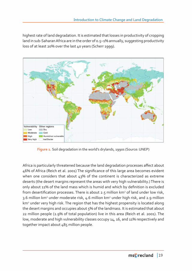
Figure 1 indicates that the areas of the world vulnerable to land degradation cover ������ ά���������������������������Ǥ��������������������ǡ���������������������������������������� ��������� ��� ���� ������ ������������ �ơ������ ��� �������Ƥ������� �������� ���approximately US$ 42 billion each year.
The semi-arid to weakly aridic areas of Africa are particularly vulnerable, as they have fragile soils, localized high population densities, and generally a low-input form of ������������ȋ����ȌǤ�������ά�����������������������������������������Ǥ�
Long-term food productivity is threatened by soil degradation, which is now severe ������� ��� ������� ������� ��� �������������� ά���� ���� ������������� ����ǡ� �����������cropland in Africa, Central America and pastures in Africa. Sub-Saharan Africa has the
Introduction to Climate Change and Land Degradation
19
highest rate of land degradation. It is estimated that losses in productivity of cropping �����������Ǧ����������������������������������� ǤȂά���������ǡ������������������������������������������ά����������������������ȋ�������ȌǤ
Figure 1. Soil degradation in the world’s drylands, 1990s (Source: UNEP)
��������������������������������������������������������������������������ơ����������ά�����������ȋ�����������Ǥ�Ȍ����������Ƥ���������������������������������������������� ���� ���������� ����� ������ ά� ��� ���� ���������� ��� �������������� ��� ��������deserts (the desert margins represent the areas with very high vulnerability.) There is �����������ά������������������������������������������������Ƥ�������������������������������Ƥ����������������Ǥ����������������Ǥ�����������2 of land under low risk, 3.6 million km2 under moderate risk, 4.6 million km2 under high risk, and 2.9 million km2 under very high risk. The region that has the highest propensity is located along ��������������������������������������ά����������������Ǥ��������������������������������������������ȋǤά��������������������Ȍ� ������������������ȋ�����������Ǥ�ȌǤ��������ǡ������������������������������������������������ǡ�ǡ�����ά������������������together impact about 485 million people.
Chapter 1
20
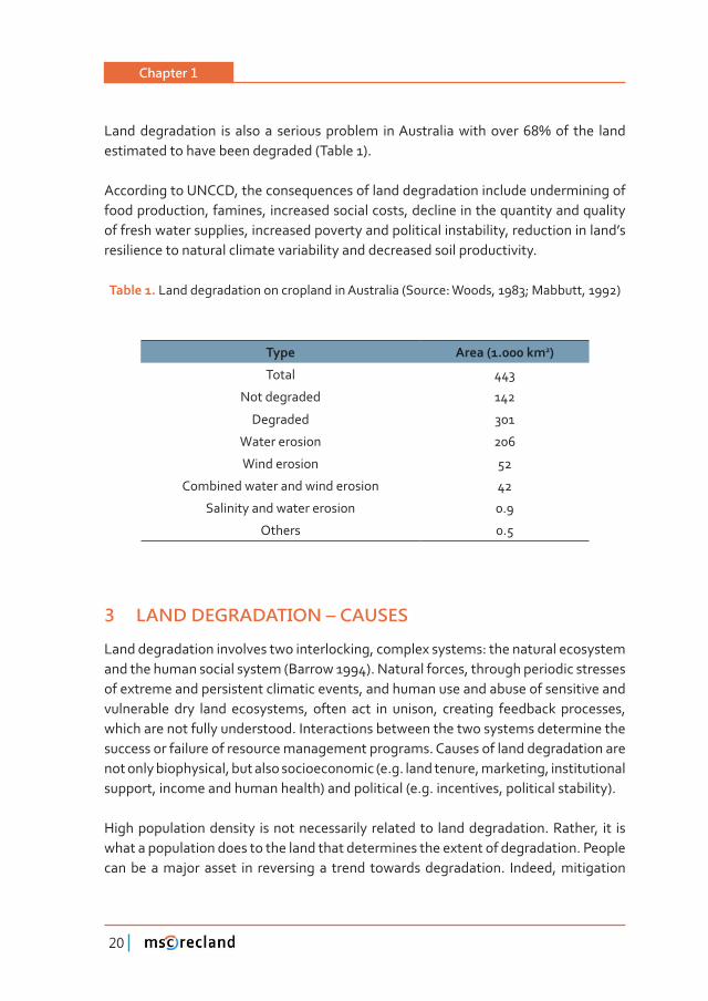
����������������� ��� ������� ���������������� ��������������������������� ���� �����estimated to have been degraded (Table 1).
According to UNCCD, the consequences of land degradation include undermining of food production, famines, increased social costs, decline in the quantity and quality of fresh water supplies, increased poverty and political instability, reduction in land’s resilience to natural climate variability and decreased soil productivity.
Table 1. Land degradation on cropland in Australia (Source: Woods, 1983; Mabbutt, 1992)
���� Area (1.000 km2Ȍ
Total 443
Not degraded 142
Degraded 301
Water erosion 206
Wind erosion 52
Combined water and wind erosion 42
Salinity and water erosion 0.9
Others 0.5
3 LAND DEGRADATION – CAUSES
Land degradation involves two interlocking, complex systems: the natural ecosystem and the human social system (Barrow 1994). Natural forces, through periodic stresses of extreme and persistent climatic events, and human use and abuse of sensitive and vulnerable dry land ecosystems, often act in unison, creating feedback processes, which are not fully understood. Interactions between the two systems determine the success or failure of resource management programs. Causes of land degradation are not only biophysical, but also socioeconomic (e.g. land tenure, marketing, institutional support, income and human health) and political (e.g. incentives, political stability).
High population density is not necessarily related to land degradation. Rather, it is what a population does to the land that determines the extent of degradation. People can be a major asset in reversing a trend towards degradation. Indeed, mitigation
Introduction to Climate Change and Land Degradation
21
Introduction to Climate Change and Land Degradation
of land degradation can only succeed if land users have control and commitment to maintain the quality of the resources. However, they need to be healthy and politically and economically motivated to care for the land, as subsistence agriculture, poverty and illiteracy can be important causes of land and environmental degradation.
There are many, usually confounding, reasons why land users permit their land to degrade. Many of the reasons are related to societal perceptions of land and the values they place on land. The absence of land tenure and the resulting lack of stewardship is a major constraint in some countries to adequate care for the land. Degradation is also a slow imperceptible process and so many people are not aware that their land is degrading.
Loss of vegetation can propagate further land degradation via land surface-atmosphere feedback. This occurs when a decrease in vegetation reduces evaporation ������������������������������ƪ�����������������������������ȋ������Ȍǡ��������������reducing cloud formation. Large-scale experiments in which numerical models of ���� �������� ������������ ����� ����� ���� ����� ����Ƥ������� ����� ������� ����� ���� ������have suggested that large increases in the albedo of subtropical areas should reduce rainfall.
4 CLIMATIC CONSEQUENCES OF LAND DEGRADATION
Land surface is an important part of the climate system. The interaction between land surface and the atmosphere involves multiple processes and feedbacks, all of which may vary simultaneously. It is frequently stressed (Henderson-Sellers et al. 1993; ���ƥ�������Ǥ�Ǣ����������Ǥ�Ȍ������������������������������������������������the characteristics of the regional atmospheric circulation and the largescale external ��������� ƪ����Ǥ� �������� ��� �������� ������� �������� ���������� ����� ����� �������������������������������������ƪ������������������ǯ���������Ǥ
����������������������ǡ����������������������������������������������ƪ��������������������������������������������������Ǧ����������������Ǥ������������������ƪ���������������������������� ������������� ��ƪ������ ���� ��������ǡ� ���������������ǡ� ������Ǧ������atmospheric circulation. For example, changes in forest cover in the Amazon basin �ơ��������ƪ��������������������������������ǡ��������������������ǡ��������������������rainfall (Lean and Warrilow 1989). More recent work shows that these changes in
Chapter 1
22
forest cover have consequences far beyond the Amazon basin (Werth and Avissar 2002).
�������������������������������ơ���������������ƪ���������������������������������locally and globally. El Niño events and land surface change simulations with climate models suggest that in equatorial regions where towering thunderstorms are frequent, disturbing areas hundreds of kilometres on a side may yield global impacts.
Use of a numerical simulation model by Garrett (1982) to study the interactions between convective clouds, the convective boundary layer and a forested surface showed that surface parameters such as soil moisture, forest coverage, and �����������������������������������������ơ�������������������������������������������������������������������ơ���������������Ǧ������������Ǥ
An atmospheric general circulation model with realistic land-surface properties was ���������ȋ��������������������Ȍ������������������������������ơ����������������the extent of earth’s deserts and most regions and it showed a notable correlation between decreases in evapotranspiration and resulting precipitation. It was shown �����������������������ơ�����������������Ǧ������������������������������������������somewhat weaker year-round drought. Some regions, particularly the Sahel, showed an increase in surface temperature caused by decreased soil moisture and latent-heat ƪ��Ǥ
����� ���� ���� ����� ������ �������� ��ƪ������ ������� ƪ����� ���� �� ����������(Houghton 1995; Braswell et al. 1997) which directly alter atmospheric composition and radiative forcing properties. They also change land-surface characteristics and, indirectly, climatic processes. Observations during the HAPEX-Sahel project suggested that a large-scale transformation of fallow savannah into arable crops like millet, may lead to a decrease in evaporation (Gash et al. 1997). Land use and land cover change is an important factor in determining the vulnerability of ecosystems and landscapes to environmental change.
Since the industrial revolution, global emissions of carbon (C) are estimated at 270±30 gigatons (Gt) due to fossil fuel combustion and 136±5 Gt due to land use change and soil cultivation. Emissions due to land use change include those by deforestation, biomass burning, conversion of natural to agricultural ecosystems, drainage of wetlands and soil cultivation. Depletion of soil organic C (SOC) pool has contributed 78±12 Gt of
Introduction to Climate Change and Land Degradation
23
C to the atmosphere, of which about one-third is attributed to soil degradation and accelerated erosion and two-thirds to mineralization (Lal 2004).
Land degradation aggravates CO2-induced climate change through the release of CO2 from cleared and dead vegetation and through the reduction of the carbon sequestration potential of degraded land.
5 CLIMATIC FACTORS IN LAND DEGRADATION
��������������������������ƪ�����������������������������������ǡ�����������������������(Williams and Balling 1996). Precipitation and temperature determine the potential distribution of terrestrial vegetation and constitute principal factors in the genesis ����������������� ����Ǥ�������������������� ��ƪ������� ���������������������ǡ������� ���turn controls the spatial and temporal occurrence of grazing and favours nomadic lifestyle. Vegetation cover becomes progressively thinner and less continuous with decreasing annual rainfall. Dry land plants and animals display a variety of physiological, anatomical and behavioural adaptations to moisture and temperature stresses brought about by large diurnal and seasonal variations in temperature, rainfall and soil moisture.
Williams and Balling (1996) provided a nice description of the nature of dryland soils ������������������������������������������������ơ�����������������������������Ǥ�����generally high temperatures and low precipitation in the dry lands lead to poor organic matter production and rapid oxidation. Low organic matter leads to poor aggregation and low aggregate stability leading to a high potential for wind and water erosion. For example, wind and water erosion is extensive in many parts of Africa. Excluding the ���������������ǡ��������������������ά����������������ǡ�������ά�������������������������������������������������άǡ����������������Ǥ�
�����������������Ȁ�������������������������������������������������������Ƥ��������ǡ��������������ơ�����������������������ƪ��������������Ǥ�������������ǡ����������ǡ�����extent of erosion are likely to be altered by changes in rainfall amount and intensity and changes in wind.
Chapter 1
24
Land management will continue to be the principal determinant of the soil organic matter (SOM) content and susceptibility to erosion during the next few decades, but changes in vegetation cover resulting from short-term changes in weather and near-���������������������������������������ơ����������������������������ǡ���������������semi-arid regions.
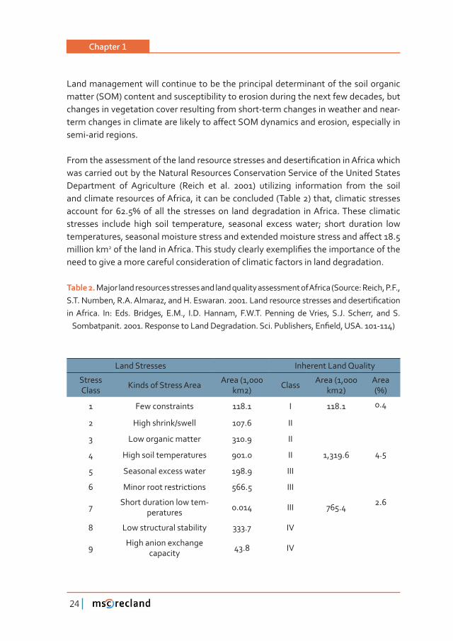
������������������������������������������������������������Ƥ�����������������������was carried out by the Natural Resources Conservation Service of the United States Department of Agriculture (Reich et al. 2001) utilizing information from the soil and climate resources of Africa, it can be concluded (Table 2) that, climatic stresses �������� ���� Ǥά���� ���� ���� ������������ ����������������� ���������Ǥ������� ���������stresses include high soil temperature, seasonal excess water; short duration low ������������ǡ������������������������������������������������������������ơ����Ǥ�million km2����������������������Ǥ���������������������������Ƥ�������������������������need to give a more careful consideration of climatic factors in land degradation.
Table 2. Major land resources stresses and land quality assessment of Africa (Source: Reich, P.F., �Ǥ�Ǥ�������ǡ��Ǥ�Ǥ��������ǡ������Ǥ��������Ǥ�Ǥ�����������������������������������Ƥ�������in Africa. In: Eds. Bridges, E.M., I.D. Hannam, F.W.T. Penning de Vries, S.J. Scherr, and S. �����������Ǥ�Ǥ�����������������������������Ǥ����Ǥ�����������ǡ���Ƥ���ǡ����Ǥ�ǦȌ
Land Stresses Inherent Land Quality
Stress Class Kinds of Stress Area Area (1,000
km2) Class Area (1,000 km2)
Area ȋάȌ
1 Few constraints 118.1 I 118.1 0.4
2 High shrink/swell 107.6 II
3 Low organic matter 310.9 II
4 High soil temperatures 901.0 II 1,319.6 4.5
5 Seasonal excess water 198.9 III
6 Minor root restrictions 566.5 III
7 Short duration low tem-peratures 0.014 III 765.4 2.6
8 Low structural stability 333.7 IV
9 High anion exchange capacity 43.8 IV
Introduction to Climate Change and Land Degradation
25
10 Impeded drainage 520.5 IV 898.0 3.1
11 Seasonal moisture stress 3,814.9 V
12 High aluminum 1,573.2 V
13 Calcareous, gypseous 434.2 V
14 Nutrient leaching 109.9 V 5,932.3 20.2
15 Low nutrient holding capacity 2,141.0 VI
16 High P, N retention 932.2 VI
17 Acid sulfate 16.6 VI
18 Low moisture and nu-trient status 0 VI
19 Low water holding capacity 2,219.5 VI 5,309.3 18.1
20 High organic matter 17.0 VII
21 Salinity/alkalinity 360.7 VII
22 Shallow soils 1,016.9 VII 1,394.7 4.8
23 Steep lands 20.3 VIII
24 Extended low tempera-tures 0 VIII 20.3 0.1
LandArea 29,309.1
WaterBodies 216.7
TotalArea 29,525.8
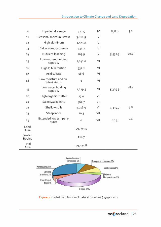
Figure 2. Global distribution of natural disasters (1993-2002)
Chapter 1
26
According to the database of CRED, the Belgium Centre for Research on the Epidemiology of Disasters, weather- climate- and water-related hazards that occurred between 1993-2002, were responsible for 63 per cent of the US$ 654 billion damage caused by all natural disasters. These natural hazards are therefore the most frequent and extensively observed ones (Figure 2) and they all have a major impact on land degradation.
5�1 Rainfall
Rainfall is the most important climatic factor in determining areas at risk of land ���������������������������������Ƥ������Ǥ������������������������������������������������and distribution of plant life, but the variability and extremes of rainfall can lead to soil erosion and land degradation (Figure 3). If unchecked for a period of time, this ������������������������������������Ƥ������Ǥ������������������������������������������distribution of vegetation though land management practices and seemingly benign rainfall events can make land more vulnerable to degradation. These vulnerabilities become more acute when the prospect of climate change is introduced.
Rainfall and temperature are the prime factors in determining the world’s climate and therefore the distribution of vegetation types. There is a strong correlation between rainfall and biomass since water is one of primary inputs to photosynthesis. ��������������� ������� Dz�������� �����dz� ȋ���� ��������� ��������������������� �������������evaporation) to help classify desert (arid) or semi-arid areas (UNEP 1992; Williams and Balling 1986; Gringof and Mersha 2006). Drylands exist because the annual water loss (evaporation) exceeds the annual rainfall; therefore these regions have a ������������������Ƥ���Ǥ�������������������������������������������������������������������������������������������������������Ǥ�����������������������������������Ƥ�����are not so large, some plant life can take hold usually in the form of grasslands or steppes. However, it is these dry lands on the margins of the world’s deserts that are ���������������������������Ƥ������ǡ���������������������������������������������Ǥ�Examples of these regions include the Pampas of South Americas, the Great Russia Steppes, the Great Plains of North America, and the Savannas of Southern Africa and Sahel region of Northern Africa. With normal climatic variability, some years the water ��Ƥ�������������������������������������������������������������������������������������������Ƥ�����������Ǧ������������Ǥ�������������������ǡ������������������������������degradation in the Dust Bowl years of the 1930s in the Great Plains or the nearly two
Introduction to Climate Change and Land Degradation
27
decade long drought in the Sahel in the 1970s and 1980s. It was this period of drought ��������������������������������������������������������Ƥ������Ǥ�
For over a century, soil erosion data has been collected and analyzed from soil scientists, agronomists, geologists, hydrologists, and engineers. From these investigations, scientists have developed a simple soil erosion relationship that incorporates the major soil erosion factors. The Universal Soil Loss Equation (USLE) was developed in the mid-1960s for understanding soil erosion for agricultural applications (Wischmeier and Smith 1978). In the mid-1980’s, it was updated and renamed the Revised Universal Soil Loss Equation (RUSLE) to incorporate the large amount of information that had accumulated since the original and to address land use applications besides agriculture such as soil loss from mined lands, constructions sites, and reclaimed lands. The RUSLE is derived from the theory of soil erosion and from more than 10,000 plot-years of data from natural rainfall plots and numerous rainfall simulations.
���������������Ƥ������ǣ
A = R K L S C P
����������������������������������ȋ�Ȁ��Ȁ����ȌǢ��������������������������Ǧ����ơ�����������factor; K is the soil erodibilty factor; L represents the slope length; S is the slope steepness; C represents the cover management, and P denotes the supporting practices factor (Renard et al. 1997). These factors illustrate the interaction of various climatic, geologic, and human factors and that smart land management practices can minimize soil erosion and hopefully land degradation.
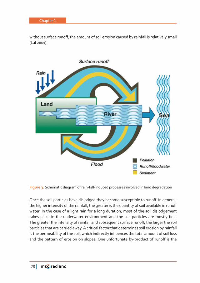
The extremes of either too much or too little rainfall can produce soil erosion that can lead to land degradation. However, soil scientists consider rainfall the most important erosion factor among the many factors that cause soil erosion. Zachar (1982) provides an overview of soil erosion due to rainfall which can erode soil by the force of raindrops, ���������������������������ơǡ�����������ƪ������Ǥ���������������������������������������surface produces a large amount of kinetic energy which can dislodge soil particles. Erosion at this micro-scale can also be caused by easily dissoluble soil material made water soluble by weak acids in the rainwater. The breaking apart and splashing of soil ���������������������������������������Ƥ������������������������ǡ������������������������������������������������������������������������������������ƪ�����������Ǥ��������ǡ�
Chapter 1
28
��������������������ơǡ�������������������������������������������������������������������(Lal 2001).
Figure 3. Schematic diagram of rain-fall-induced processes involved in land degradation
����������������������������������������������������������������������ơǤ�����������ǡ�������������������������������������ǡ������������������������������������������������������ơ�water. In the case of a light rain for a long duration, most of the soil dislodgement ������ ������ ��� ���� ����������� ������������ ���� ���� ����� ���������� ����������� Ƥ��Ǥ������������������������������������������������������������������ơǡ���������������������particles that are carried away. A critical factor that determines soil erosion by rainfall �������������������������������ǡ��������������������ƪ����������������������������������������� ��������������� ����������� ������Ǥ�������������������Ǧ�������� ��� ����ơ� ��� ����
Introduction to Climate Change and Land Degradation
29
corresponding transport of agricultural chemicals and the leaching of these chemicals into the groundwater.
Rainfall intensity is the most important factor governing soil erosion caused by rain (Zachar 1982). Dry land precipitation is inherently variable in amounts and intensities ������� ��� ��������������� ����ơǤ��������� ����ơ� ���������������� ������� ������ ����� ���more humid regions due to the tendency of dry land soils to form impermeable crusts ������ ���� ���������� �������� ������������������ ��� ��������������� �����Ƥ�����������cover or litter. In these cases, soil transport may be an order of magnitude greater per unit momentum of falling raindrops than when the soil surface is well vegetated. The sparser the plant cover, the more vulnerable the topsoil is to dislodgement and �������������������������������������������ơǤ�����ǡ����������������������������������crucial role in soil erosion leading to land degradation. An erratic start to the rainy season along with heavy rain will have a greater impact since the seasonal vegetation will not be available to intercept the rainfall or stabilize the soil with its root structure.
�����Ǧ������ �ơ���� ��� ����������� ��� ��� ���� ��� ���������� ���� ������ �������� ������������that can be used to predict soil erosion. The Water Erosion Prediction Project (WEPP) model is a process-based, distributed parameter, continuous simulation, erosion prediction model for use on personal computers and can be applied at the Ƥ���� ������ ��� ��������� ���������� �������� �������� ������������������ ������ ��������(USDA 2006). It mimics the natural processes that are important in soil erosion. It �����������������������������������������������������ơ����������������Ǥ���������������������ǡ�������������������������������������������������������������������������ơ������occur. The WEPP model includes a number of conceptual components that include: climate and weather (rainfall, temperature, solar radiation, wind, freeze – thaw, snow accumulation and melting), irrigation (stationary sprinkler, furrow), hydrology Ȃ� ȋ��Ƥ��������ǡ� ������������� �������ǡ� ����ơȌǡ� ������ �������� ȋ������������������ǡ�percolation, drainage), soils (types and properties) , crop growth – (cropland, rangeland, forestland), residue management and decomposition, tillage impacts on ��Ƥ������������������������ǡ���������Ȃ�ȋ���������ǡ�����ǡ��������Ȍǡ������������ȋ�����ǡ���������ǡ�and impoundments), sediment delivery, particle sorting and enrichment.
Of special note is the impact of other forms of precipitation on soil erosion (Zachar ȌǤ��������������������ơ��������������������������������������������������������������times that of rain resulting in much more soil surface being destroyed and a greater amount of material being washed away. And if hailstorms are accompanying with heavy rain, as is the case with some thunderstorms, large amounts of soil can be
Chapter 1
30
eroded especially on agricultural land before the crops can stabilize the soil surface. Snow thaw erosion occurs when the soil freezes during the cold period and the ��������� �������� ���������� ���� ����ǡ� ��� ���������� ���� ������� ����� ������ǡ� Ƥ��� ������������������� ��������� ��� ���� ����ơǤ���������������������������������������������������������������������������Ǥ�����ǡ�����������������������������Ƥ�������������������������reduced so that when the thaw arrives, relatively intense soil erosion can take place even though the amount of snow thaw is small. In this situation, the erosive processes ����������������������������������������������������������������������ƪ��������������Ǥ�Leeward portions of mountainous areas are susceptible to this since they are typically drier and have less vegetation and are prone to katabatic winds (rapidly descending air from a mountain range warms very quickly).
5�2 Floods
�������� ������� ����� ���������� ��������� ƪ���� ���� ������ ���������� ���� ���� ���������� ���������� ���������� ���� ������� ���������� ��� ƪ����������� ��� ��������� ��� ����� ���any changes in the vegetation cover in the basins. The loss of vegetation in the headwaters of dryland rivers can increase sediment load and can lead to dramatic change in the character of the river to a less stable, more seasonal river characterised by a rapidly shifting series of channels. However, rainfall can lead to land degradation in other climates, including sub-humid ones. Excessive rainfall events either produced by thunderstorms, hurricanes and typhoons, or mid-latitude low-pressure systems can produce a large amount of water in a short period of time across local areas. �������������������������������� ���� ����������������������������� ������ƪ������Ǥ�Of course, this is a natural phenomenon that has occurred for millions of years and �����������������������������Ǥ�������ƪ�����������������������������ǡ����������������������areas where the problem is most acute.
����� ������������ ��� �������� �������� ���������� ����� ����� ������������� ��ơ������factors at the same time, depending on the type and nature of the phenomenon that �������������ƪ������Ǥ�����������ǡ������������ƪ����ƪ������������������������ơ����heavy rain falling in one area within a larger area of lighter rain, a confusing situation ����������������ƥ���������������������������������ƪ��������������Ǥ������������ƪ�����caused by the heavy rain or storm surges that can sweep inland as part of a tropical cyclone can also be a complex job, as predictions have to include where they will land, the stage of their evolution and the physical characteristics of the coast.
Introduction to Climate Change and Land Degradation
31
To make predictions as accurate as possible, National Hydrological Services (NHSs) and National Meteorological Services (NMSs) under the auspices of the WMO ���������� ƪ���� ������������ ������ ��� ������������� �������������� ���������� ȋ���Ȍǡ�which have become more accurate in recent years, especially for light and moderate ������������������������ǡ���������������������������������������������������ƥ��������predict. So setting up forecasting systems that integrate predictions for weather with those for water-related events is becoming more of a possibility every day, paving the way for a truly integrated approach.
�����������������������������������������������������������������ơ���Ǥ����������������������������������������������������������������ƪ����ǡ�ƪ��������������������������forces with meteorologists, hydrologists, town planners, and civil defense authorities ���������������������������������Ǥ������������������������������������������ƪ�����will mean taking a close look at construction or other activities in and around river channels. Up-to-date and accurate information is essential, through all the available channels: surface observation, remote sensing and satellite technology as well as computer models.
Flood risk assessment and management have been around for decades but recently ����������������������������������������������������Ǥ�������Ƥ��������������������of Integrated Flood Management is integration, expressed simultaneously in ��ơ������ �����ǣ� ��� ���������������� ��� ����������ǡ� ������� ��� �������������ǡ� ������ ���interventions (i.e. structural or non-structural), short or long-term, and a participatory and transparent approach to decision making – particularly in terms of institutional integration and how decisions are made and implemented within the given institutional structure.
Land use planning and water management have to be combined in one synthesized plan through co-ordination between land management and water management authorities to achieve consistency in planning. The rationale for this integration is that the use of land has impacts upon both water quantity and quality. The three main elements of river basin management – water quantity, water quality, and the processes of erosion and deposition – are inherently linked.
���������ǡ���� �����������ƪ�������������������������������������������������Ƥ���key elements (APFM 2004):
• Manage the water cycle as a whole;
Chapter 1
32
• Integrate land and water management;
• Adopt a best mix of strategies;
• Ensure a participatory approach;
• Adopt integrated hazard management approaches.
5�3 Droughts
�������������������������������������������������Ƥ�������������������������������������in a water shortage for some activities or some groups. It is the consequence of a reduction in the amount of precipitation over an extended period of time, usually a season or more in length, often associated with other climatic factors – such as high temperatures, high winds and low relative humidity – that can aggravate the severity of the event. For example, the 2002-03 El Niño related Australian drought (Coughlan et al. 2003), which lasted from March 2002 to January 2003, was arguably one of, if not the, worst short term droughts in Australia’s recorded meteorological history ȋ���������ȌǤ���������������������������������������Ǧ�������������������������ά��������������������������������������������������������Ǧ�����������ǡ������ά������������������������������������������������� ά�ȋ�Ǥ�Ǥǡ�������ǦȌ��������������������ȋ���������Ǧwide rainfall records commenced in 1900). During the 2002-03 droughts Australia ���������������������������Ƥ���ǡ���������������������������������������������������������������������������������ǯ��������������������������������ά�ȋ��������ȌǤ�����Ƥ������������������������������������������������������������ǡ��������������to label this period a truly exception drought.
Extended droughts in certain arid lands have initiated or exacerbated land �����������Ǥ��������������������������������������������ƫ������������ǡ��������������episodes in 1965–1966, 1972–1974, 1981–1984, 1986–1987, 1991–1992, and 1994–1995. The aggregate impact of drought on the economies of Africa can be large: 8–9 per cent of GDP in Zimbabwe and Zambia in 1992, and 4–6 per cent of GDP in Nigeria and Niger in 1984. In the past 25 years, the Sahel has experienced the most substantial and sustained decline in rainfall recorded anywhere in the world within the period of instrumental measurements. The Sahelian droughts in the early 70s ����������������� ��� ������ �����������������������������������Dz��������������������a major environmental emergency” and their long term impacts are now becoming clearer (Figure 4).

Introduction to Climate Change and Land Degradation
33
Figure 4. Types and impacts of draught
Sea surface temperature (SST) anomalies, often related to the El Niño Southern Oscillation (ENSO) or North Atlantic Oscillation (NAO), contribute to rainfall variability in the Sahel. Droughts in West Africa correlate with warm SST in the tropical south Atlantic. Examination of the oceanographic and meteorological data from the period 1901-1985 showed that persistent wet and dry periods in the Sahel were related to contrasting patterns of SST anomalies on a near-global scale (Sivakumar 2006). From 1982 to 1990, ENSO-cycle SST anomalies and vegetative production in Africa ���������������������������Ǥ�������������������������������Ƥ���������������������episodes correlated with rainfall of <1,000 mm yr-1 over certain African regions.

Chapter 1
34
A coupled surface-atmosphere model indicates that – whether anthropogenic factors or changes in SST initiated the Sahel drought of 1968-1973 – permanent loss of Sahel savannah vegetation would permit drought conditions to persist. The �ơ��������������ǡ������������������������������������������������������������ǡ�����increasing surface albedo as plant cover is destroyed, is generally to increase ground and near-surface air temperatures while reducing the surface radiation balance and ������������� ���� ��Ƥ���� ��� ���� ���������� �������� ��� ���� ������ �������Ǧ�����������system (Williams and Balling 1996). This entails increased atmospheric subsidence and consequently further reduced precipitation.
Early warning systems can reduce impacts by providing timely information about the onset of drought (Wilhite et al. 2000) Conventional surface observation stations within National Meteorological Services are one link in the chain, providing essential benchmark data and time series necessary for improved monitoring of the climate ���� ����������� ������Ǥ� ��������� �������� ����������� ����� ��� ������� ƪ��� ��� �����moisture can help in formulating drought index values – typically single numbers, far more useful than raw data for decision-making.
Drought plans should contain three basic components: monitoring and early warning, risk assessment, and mitigation and response (Wilhite and Svoboda 2000) . Because of the slow onset characteristics of droughts, monitoring and early warning systems �������� ���� ����������� ���� ��� �ơ������� ������������������� ����Ǥ��� ���������� �����on accurate and timely assessments to trigger mitigation and emergency response programs.
Various WMO programmes monitor extreme climate events associated with drought, while four monitoring centres – two in Africa, one in China and the Global Information and Early Warning System – provide weather advisories and one and three-month climate summaries. Among other African early warning systems, the Southern Africa Development Community (SADC) monitors the crop and food situation in the region and issues alerts during periods of impending crisis. Such networks can be the backbone of drought contingency planning, coordinated plans for dealing with drought when it comes.
Introduction to Climate Change and Land Degradation
35
5�4 Solar radiation, temperature and evaporation
The only source of energy for the earth is the sun but our world intercepts only a tiny amount of this energy (less than a tenth of 1 percent) to provide the energy for the various biological (photosynthesis) and geophysical (weather and climate) processes for life depends on. The earth system, based on fundamental rules of physics, must emit the same amount of radiation as it receives. Therefore, the complex transfer of energy to satisfy this requirement is the basis for our weather and climate. Solar radiation is highly correlated with cloudiness, and in most dryland climates there are little or no clouds, the solar radiation can be quite intense. In fact, some of the highest known values of solar radiation can be found in places like the Sahara desert. Solar heating of the land surface is the main contribution to the air temperature.
Along with rainfall, temperature is the main factor determining climate and therefore the distribution of vegetation and soil formation. Soil formation is the product of many factors that include: the parent material (rock), topography, climate, biological ��������ǡ����� ����Ǥ����������������� ��������� ��������ơ��������������������������������������������������Ǥ������������������������������������������������ơ�������������moisture, biological activity, rates of chemical reactions, and the types of vegetation. Important chemical reactions in the soil include the nitrogen and carbon cycles.
In the tropics, surface soil temperatures can exceed 55ºC and this intense heat contributes to the cracking of highly-clay soils that expose not only the soil surface but the soil subsurface to water or wind erosion. Of course, these high temperatures will also increase soil evaporation and further reduce available soil moisture for plant growth.
��� ���������� ���� �����ǡ� ���� ������Ǧ����� ������ ���� ����� �� ������� �ơ���� ��� ����composition of the soil by the movement of rocks and stones from various depths to the surface. In high elevations, the freeze-thaw is one factor degrading rock structures, �������������������Ƥ���������������������������������������������������������Ǥ�
Evaporation is the conversion of water from the liquid or solid state into vapour, ���� ���� ��ơ������ ����� ���� ����������Ǥ� �� ������� ��������� ��������� �������� ����evaporating surface and the atmosphere and a source of energy are necessary for evaporation. Solar radiation is the dominant source of energy and sets the broad ���������������������Ǥ�����������������������������������������������ǡ�����Ƥ����������cloud cover, which leads to a high evaporative demand of the atmosphere. In the arid
Chapter 1
36
and semi-arid regions, considerable energy may be advected from the surrounding dry areas over irrigated zones. Rosenberg et al. (1983) lists several studies that have ����������������Dz�������ơ���dz�������������������������������������������������������surface and can cause large evaporative losses in a short period of time.
Climatic factors induce an evaporative demand of the atmosphere, but the actual ��������������������������������ƪ�������������������������������������������������������������������������������������Ǥ�������������������ǡ���������������������������ƪ��������������������������������� ��������������� �������� ���������ǡ� ���� ��������ơ�������turbulence. In the arid and semi-arid regions, the high evaporation which greatly exceeds precipitation leads to accumulation of salts on soil surface. Soils with natric horizon are easily dispersed and the low moisture levels lead to limited biological activity.
5�5 Wind
��������������������������������ơ��������������������������������������������������wind erosion and there is evidence that the frequency of sand storms/dust storms in increasing. It has been estimated that in the arid and semi-arid zones of the world, ά����������������������������ά��������������������������ơ���������������������severe land degradation from wind erosion (Rozanov 1990).
���������Ǧ������������������������������������������ƪ�����������������������������was estimated to be 61 to 366 million tonnes (Middleton 1986). Losses of desert soil ��������������������������������������Ƥ����Ǥ���������������������������������������������long-range transport of desert dust is approximately 1 x 10¹⁶ g year –1.
For Africa, it is estimated that more than 100 million tonnes of dust per annum is blown westward over the Atlantic. The amount of dust arising from the Sahel zone has been reported to be around or above 270 million tons per year which corresponds to a loss of 30 mm per m2 per year or a layer of 20 mm over the entire area (Stahr et al. 1996).
Every year desert encroachment caused by wind erosion buries 210,000 hectares of productive land in China (PRC 1994). It was shown that the annual changes of the frequency of strong and extremely strong sandstorms in China are as follows: 5 times
Introduction to Climate Change and Land Degradation
37
in the 1950s, 8 times in the 1960s, 13 times in the 1970s, 14 times in the 1980s, and 20 times in the 1990s (Ci 1998).
Sand and dust storms are hazardous weather and cause major agricultural and environmental problems in many parts of the world. There is a high on-site as well ��� �ơǦ����� ����� ���� ��� ���� ����� ���� ����� ������Ǥ������ ��������� �������� ����� ���overwhelming tide and strong winds take along drifting sands to bury farmlands, blow out top soil, denude steppe, hurt animals, attack human settlements, reduce ���� �����������ǡ� Ƥ��� ��� ����������� ������� ���� ����� �������� ����� ���������ǡ� �����������������������������ǡ�����������������������������ǡ��ơ����������������������������������������������ǡ��ơ���������������ǡ�������������������������������������������and communication facilities. They accelerate the process of land degradation and cause serious environment pollution and huge destruction to ecology and living environment (Wang Shigong et al. 2001). Atmospheric loading of dust caused by wind ��������������ơ�����������������������������������������������Ǥ
Wind erosion-induced damage includes direct damage to crops through the loss of plant tissue and reduced photosynthetic activity as a result of sandblasting, burial of seedlings under sand deposits, and loss of topsoil (Fryrear 1971; Amburst 1984; �������ȌǤ�����������������������������������������������������������������ơ���������soil resource base and hence crop productivity on a long-term basis, by removing the layer of soil that is inherently rich in nutrients and organic matter. Wind erosion on light sandy soils can provoke severe land degradation and sand deposits on young ���������������ơ����������������������Ǥ�
Calculations based on visibility and wind speed records for 100 km wide dust plumes, centered on eight climate stations around South Australia, indicated that dust transport mass was as high as 10 million tonnes (Butler et al. 1994). Thus dust entrainment during dust events leads to long-term soil degradation, which is ������������������������Ǥ�������������������������������ƥ���������������������������������be quite substantial.
5�5�1 Causes of wind erosion
The occurrence of wind erosion at any place is a function of weather events interacting ����� ����� ���� ����� ����������� �������� ���� �ơ����� ��� ����� ���������ǡ� ������ ����vegetation cover. In regions where long dry periods associated with strong seasonal
Chapter 1
38
���������������������ǡ���������������������������������������������ƥ����������������the soil, and the soil surface is disturbed due to inappropriate management practices, wind erosion usually is a serious problem.
At the southern fringe of the Sahara Desert, a special dry and hot wind, locally termed Harmattan, occurs. These NE or E winds normally occur in the winter season under a high atmospheric pressure system. When the wind force of Harmattan is beyond the threshold value, sand particles and dust particles will be blown away from the land surface and transported for several hundred kilometres to the Atlantic Ocean.
In the Northwest region of India, the convection sand-dust storm that occurs in the season preceding the monsoon is named Andhi (Joseph et al. 1980). It is called Haboob ������������������������������Ǥ��������������Dz�������dz����Dz�����dz����������������Ǥ
In general, two indicators, wind velocity and visibility, are adopted to classify the grade of intensity of sand-dust storms. For instance, the sand-dust storms occurring �����������������������������������������Ƥ��������������������Ǥ����������������Ǧ�����storm develops when wind velocity is at force 6 (Beaufort) degree and visibility varies between 500-1,000 m. The secondary strong sand-dust storm will occur when wind velocity is at force 8 and visibility varies 200-500 m. Strong sanddust storms will take place when wind velocity is at force 9 and visibility is <200 metres.
��������ǡ�������Ǧ����������������Ƥ��������������������������Ǥ������������ơ������������������������������������������Ǧ�����������������Ƥ�������������������������ǡ��������strong sand-dust storms and serious-strong sand-dust storms. When wind velocity is 50 metres per second (m/s) and visibility is <200 metres, the sandstorm is called a strong sand-dust storm. When wind velocity is 25 m/s and visibility is 0-50 metres, the sandstorm is termed a serious sand-dust storm (some regions name it Black windstorm or Black Devil) (Xu Guochang et al. 1979).
���� ��Ƥ�������� ��� ���� ����� ���������� ���� ���� ����� ��� ����� ��� ���� �����������Bureau of Meteorology, which conforms to the worldwide standards of the World Meteorological Organization (WMO). SYNOP present weather [WW] codes are included:
1. Dust storms (SYNOP WW code: 09) are the result of turbulent winds raising large quantities of dust into the air and reducing visibility to less than 1,000 m.
Introduction to Climate Change and Land Degradation
39
2. Blowing dust (SYNOP WW code: 07) is raised by winds to moderate heights above the ground reducing visibility at eye level (1.8 m), but not to less than 1,000 m.
3. Dust haze (SYNOP WW code: 06) is produced by dust particles in suspended transport which have been raised from the ground by a dust storm prior to the time of observation.
4. Dust swirls (or dust devils) (SYNOP WW code: 08) are whirling columns of dust moving with the wind and usually less than 30 m high (but may extend to 300 m or more). They usually dissipate after travelling a short distance.
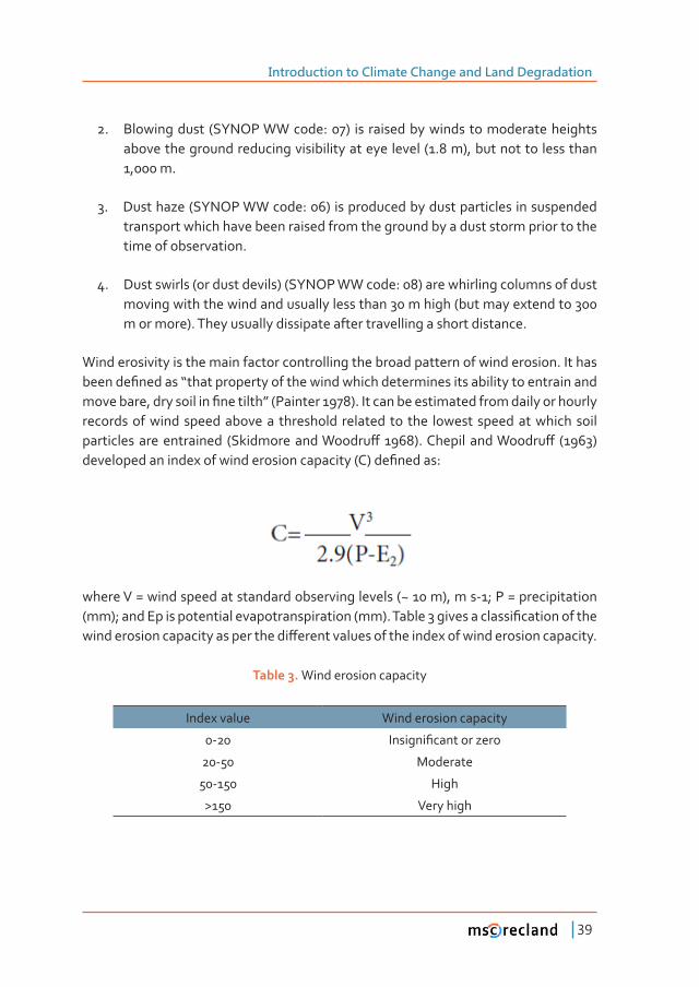
Wind erosivity is the main factor controlling the broad pattern of wind erosion. It has �������Ƥ�������Dz�������������������������������������������������������������������������������ǡ�������������Ƥ��������dz�ȋ�������� ȌǤ������������������������������������������records of wind speed above a threshold related to the lowest speed at which soil ������������������������ ȋ�������������������ơ�ȌǤ�������� ����������ơ� ȋȌ���������������������������������������������ȋ�Ȍ���Ƥ������ǣ
where V = wind speed at standard observing levels (~ 10 m), m s-1; P = precipitation ȋ��ȌǢ����������������������������������������ȋ��ȌǤ������� ���������������Ƥ�������������������������������������������������ơ��������������������������������������������������Ǥ
Table 3. Wind erosion capacity
Index value Wind erosion capacity
0-20 �������Ƥ������������
20-50 Moderate
50-150 High
>150 Very high
Chapter 1
40
When soil movement is sustained, the quantity of soil that can be transported by the wind varies as the cube of the velocity. Models demonstrate that wind erosion ����������������������������������������������Ǥ���������Ǥ�Ǥ����������ǡ���ά����������in mean wind speed greatly increases the frequency with which the threshold is exceeded and thus the frequency of erosion events.
������ ����� ����� �������� �ơ����� ��� ���������� ���� ������ ����� �������� �������� ����� ����������������Ǥ�����������ơ������������������������������������������ȋ����Ȍ�������is a process-based, daily time-step model that predicts soil erosion by simulation of the fundamental processes controlling wind erosion (Wagner 1996). The WEPS model is able to calculate soil movement, estimate plant damage, and predict PM-10 emissions when wind speeds exceed the erosion threshold. It also provides users with �����������������������������������ƪ��ǡ�����������ǡ��������������������Ƥ���������������Ƥ�������������Ǥ����������������������������������������������������������������������four databases. Most of the WEPS submodels use daily weather as the natural driving ������ ���� ����������������������� ������������Ƥ��������������Ǥ���������������������focus on hydrology including the changes in temperature and water status of the soil; soil properties; growth of crop plants; crop plant decomposition; typical management �������������������������ǡ���������ǡ�����������ǡ���������������Ǣ�Ƥ�����������������������wind on a subhourly basis.
5�5�2 Climatic implications of dust storms
���������Ƥ�������������������Ǧ����������������������Ƥ��������������ơ����������������������������Ǥ���������������������������������������������������ƪ������������������������������������ƪ��������������������������������������������������������������������������the optical properties and longevity of clouds. Depending on their properties and in ������������������������������������������ǡ����������������������ƪ����������������������� ������ ���� ������ �������� ��� ��������Ǥ���������ǡ� ����� ��ƪ���� �������������� �����space, thus reducing the amount of energy reaching the surface. Indirectly, they act as condensation nuclei, resulting in cloud formation (Pease et al. 1998). Clouds act as ���Dz�������������������ǡdz���������������������������������������������������������is emitted from the earth. Thus, dust storms have local, national and international implications concerning global warming. Climatic changes in turn can modify the location and strength of dust sources.
Introduction to Climate Change and Land Degradation
41
6 WILD FIRES, LAND DEGRADATION AND ATMOSPHERIC EMISSIONS
������������� ����Ƥ���� ������ ��� ���� ����������� ������ ��� ���� �����Ǥ� ��� ��� ��������������� Ƥ���� ��������� �ơ���� � �������� ��������� ȋ�� ��Ȍ� ��� ������� ���� ����������forest and other lands, 2040 m ha of tropical rain forests due to forest conversion ������������������������������������Ƥ���ǡ���������������������������������������������savannas, woodlands, and open forests. The extent of the soil organic carbon pool doubles that present in the atmosphere and is about two to three times greater than that accumulated in living organisms in all Earth’s terrestrial ecosystems. In such a ��������ǡ������������������������������������������������������������Ƥ����������������������������Ƥ��������������������������������������������������������������Ǥ
�������ǡ� �������� �������ǡ� ������ ��������� ����� Ƥ���ǡ� ��� ���������� ��� �������� �percent of the carbon dioxide, 32 percent of the carbon monoxide, 20 percent of the particulates, and 50 percent of the highly carcinogenic poly-aromatic hydrocarbons produced by all sources (Levine 1990). Current approaches for estimating global emissions are limited by accurate information on area burned and fuel available for burning.
���������� ����� Ƥ���� ���� ������������� ���� ����������� �����Ƥ������� ��� ������ �������emissions of trace gases and particulates from all sources to atmosphere. Natural emissions are responsible for a major portion of the compounds, including non-methane volatile organic compounds (NMVOC), carbon monoxide (CO) and nitric oxide (NO), which determine tropospheric oxidant concentrations. The total NMVOC ƪ����������������������������α�������������ȋ����Ȍ��������������������������������� ��������� ȋάȌǡ� � ������ ���������� ���������� ȋάȌ� ���� � ���Ǧ��������������������ȋάȌǤ
���� ��ƪ������ ��� Ƥ��� ��� ����� ���������������� ȋ����Ǧ������ �������ǡ� ����� ����������ǡ������ �����������ǡ� ��Ƥ��������� �������ǡ� ����� ����������� ����������� �������� ������ǡ� ��ǡ�exchangeable Ca, Mg, K, Na and extractable P) of a semi-arid southern African ���������� ���� ������Ƥ��� ����� ���� �������� �������� ȋȀȂȀȌ� ������������� ����������� Ƥ��� ȋ������� ȌǤ� ���� ��������� ��� ������ ������ ���� ��� Ƥ��� ȋ�����Ƥ���Ȍ� �������� ���� ����� ����� ��� ���� �������� ��������� ���� ���������� ��� ������� �����temperatures and soil compaction in turn leading to lower soil-water content and a ������������������Ƥ����������Ǥ
Chapter 1
42
7 CLIMATE CHANGE AND LAND DEGRADATION
Human activities – primarily burning of fossil fuels and changes in land cover – are modifying the concentration of atmospheric constituents or properties of the Earth’s surface that absorb or scatter radiant energy. In particular, increases in the concentrations of greenhouse gases (GHGs) and aerosols are strongly implicated as contributors to climatic changes observed during the 20th century and are expected to contribute to further changes in climate in the 21st century and beyond. These changes in atmospheric composition are likely to alter temperatures, precipitation patterns, sea level, extreme events, and other aspects of climate on which the natural environment and human systems depend.
According to IPCC (2003), established by WMO and UNEP, ecosystems are subject to many pressures (e.g., land-use change, resource demands, population changes); their extent and pattern of distribution is changing, and landscapes are becoming more fragmented. Climate change constitutes an additional pressure that could change or endanger ecosystems and the many goods and services they provide. Soil properties and processes – including organic matter decomposition, leaching, and soil water ��������Ȃ�����������ƪ������������������������������Ǥ���������������������������������� ������� ������������� ���������������� �ơ�������� �� ����� ������� ��������������� �����yields. Climate change may increase erosion in some regions, through heavy rainfall and through increased wind speed.
CO2-induced climate change and land degradation remain inextricably linked because of feedbacks between land degradation and precipitation. Climate change might exacerbate land degradation through alteration of spatial and temporal patterns in temperature, rainfall, solar radiation, and winds. Several climate models suggest that future global warming may reduce soil moisture over large areas of semiarid grassland in North America and Asia (Manabe and Wetherald 1986). This climate change is likely to exacerbate the degradation of semiarid lands that will be caused by rapidly expanding human populations during the next decade. Emmanuel (1987) �������������������������������������������������������������������������������������climate change expected with a doubling of atmospheric CO2 content.
Water resources are inextricably linked with climate, so the prospect of global climate change has serious implications for water resources and regional development (Riebsame et al. 1995). Climate change – especially changes in climate variability ���������������������ƪ�������Ȃ�������������������������������������������������Ǥ�
Introduction to Climate Change and Land Degradation
43
The greatest impact will continue to be felt by the poor, who have the most limited access to water resources. The impact of changes in precipitation and enhanced ���������������������������������ơ���������������������������������Ǥ��������������that, in the paleoclimate of Africa and in the present climate, lakes and reservoirs respond to climate variability via pronounced changes in storage, leading to complete drying up in many cases. Furthermore, these studies also show that under the present climate regime several large lakes and wetlands show a delicate balance between ��ƪ����������ƪ��ǡ������������������������������������άǡ������������ǡ���������������������������������ƪ��Ǥ
The frequency of episodic transport by wind and water from arid lands is also likely to increase in response to anticipated changes in global climate (Manabe and Wetherlad 1986). Lower soil moisture and sparser vegetative cover would leave soil more susceptible to wind erosion. Reduction of organic matter inputs and increased oxidation of SOM could reduce the long-term water-retention capacity of soil, ������������� �������Ƥ������Ǥ� ��������ǡ� ���������� ����� �������� ���������� ����Ǧblown mineral dust, which may increase absorption of radiation in the atmosphere (Nicholson and Kim 1997).
7�1 Carbon sequestration to mitigate climate change and combat land degradation
The soil organic carbon (SOC) pool to 1-m depth ranges from 30 tons ha-1 in the arid climates to 800 tons ha-1 in organic soils in cold regions (Lal 2007). Conversion of ������������������������������������������������������������������������������ά�����������������������������������ά�����������������������������������������������Ǥ�����depletion is exacerbated when the output of carbon (C) exceeds the input and when soil degradation is severe.
Carbon sequestration implies transferring atmospheric CO2 into long-lived pools and storing it securely so it is not immediately reemitted. Thus, soil C sequestration means increasing SOC and soil inorganic carbon stocks through judicious land use and recommended management practices. Some of these practices include mulch farming, conservation tillage, agroforestry and diverse cropping systems, cover crops and integrated nutrient management, including the use of manure, compost, biosolids, improved grazing, and forest management.
Chapter 1
44
The potential carbon sink capacity of managed ecosystems approximately equals ����������������������������������������������������������ȋ�ȌǤ��ơ�������������������emissions by achievable SOC potential provides multiple biophysical and societal ����Ƥ��Ǥ����������������������������������������������������������������������������crop yield by 20 to 40 kg ha-1 for wheat, 10 to 20 kg ha-1 for maize, and 0.5 to 1 kg ha-1 for cowpeas and could enhance world food security (Lal 2007).
8 UNDERSTANDING THE INTERACTIONS BETWEEN CLIMATE AND LAND DEGRADATION – ROLE OF WMO
WMO is the United Nations specialized agency responsible for meteorology and operational hydrology. WMO provides support to the National Meteorological and Hydrological Services (NMHSs) of its 188 Member States and Territories in their respective missions of observing and understanding weather and climate and providing meteorological and related services in support of national needs. These needs especially relate to protection of life and property, safeguarding the environment and contributing to sustainable development.
�����������Ƥ������������������������������������������������������������������climate system. The systematic observations carried out using standardized methods have provided worldwide data for analysis, research and modelling of the atmosphere and its changing patterns of weather systems. WMO coordinates a global network for the acquisition and exchange of observational data under the Global Observing System of its World Weather Watch Programme. The system comprises some 10 000 stations on land, 1 000 upper-air stations, 7 000 ships, some 3 000 aircraft providing over 150 000 observations daily and a constellation of 16 meteorological, environmental, operational and research satellites. WMO also coordinates a network of three World Meteorological Centres, 35 Regional Specialized Meteorological Centres and 187 National Meteorological Centres. Specialized programmes of observations, including those for chemical constituents of the atmosphere and characteristics of the oceans and their circulations, have led to a better understanding of interactions between the domains of the climate system (the atmosphere, the oceans, the land surface and the cryosphere) and of climate variability and change.
Introduction to Climate Change and Land Degradation
45
�����Ƥ�����ǡ����� ������������ ��� �������������� ���� ������������� �������� ��������and land degradation through dedicated observations of the climate system; improvements in the application of agrometeorological methods and the proper assessment and management of water resources; advances in climate science and prediction; and promotion of capacity building in the application of meteorological and hydrological data and information in drought preparedness and management. In this context, WMO will continue to address the issue of land degradation through its Agricultural Meteorology Programme, Hydrology and Water Resources Programme, �����������������Ƥ�����������������������������ǣ
8�1 Advocating for enhanced observing systems at national, regional and international levels
WMO is committed to work with the Parties to the UNCCD to improve the observing systems for weather, climate and water resources in order to meet the needs of the Convention, and to assist developing countries to strengthen their participation in the collection and use of these observations to meet their commitments to the Convention. In this regard, it is quite relevant to examine the Decisions of the Conference of Parties of the United Nations Framework Convention on Climate Change (UNFCCC) which address the issue of climate observing systems, and the regional workshop ����������������������������������������������������������������ơ���������������the world by the Global Climate Observing System (GCOS) Secretariat co-sponsored by WMO.
8�2 Promoting effective early warning systems
Early warning systems serve as an essential and important alert mechanism for combating land degradation. As meteorological and hydrological hazards are linked with climate variability, regular assessments and authoritative statements on the interpretation and applicability of observational data are needed for the study of climate variability and the implementation of a climate alert system to allow NMHSs ��� ����� ������ ��������� ��� �������� �����Ƥ����� �������� ���������Ǥ� ��������� ���climate-related disasters are becoming feasible from weeks to seasons in advance. WMO’s World Climate Programme will continue to issue routine statements on the state of El Niño or La Niña, which, through the NMHSs, can alert Governments to ensure preparedness against the impacts of El Niño-related anomalies, which
Chapter 1
46
can trigger various disasters. WMO played an active role in the activities of the ad hoc Panel on early warning systems established by the Committee on Science and Technology (CST) of the UNCCD. High on the recommendations of the Panel is the need to undertake a critical analysis of the performance of early warning, monitoring and assessment systems; the improvement of methods for and approaches to the ����������� ��� �������� ���� ����������� ��� �������Ƥ������Ǣ� ���� ���� ������������ ���mechanisms to facilitate an exchange of information focusing in particular on national and subregional networks. WMO’s new major programme on Natural Disaster �������������������������������������������������������������������������������ơ��������the area of early warnings and for taking new initiatives in this area in collaboration with other organizations.
8�3 Further enhancing climate prediction capability
Climate prediction capabilities are being enhanced through the Climate Variability (CLIVAR) project of the World Climate Research Programme (WCRP). The prediction of El Niño and the associated impacts are becoming possible, with reasonable skill, up to few seasons in advance. Related to this, WMO is broadening the implementation of the WMO Climate Information and Prediction Services (CLIPS) project, which is designed to promote the use of climate information and prediction services, capacity building, multi-disciplinary research and the development of new applications. Consensus long-range forecasts on droughts, which were issued at several Regional �������������������ǡ����������������ơ���������������������������������������������from WMO, provide good early warning information to national authorities.
8�4 Assessing vulnerability and analyzing hazards
It is important to analyze vulnerability at the local, national and regional levels which is an important factor in evaluating the adequacy of early warnings. A good tool to ������� ������ ��ơ������ ���������������� ��� ���� �������� ���������������ǡ� �������� ��������������������������������ơ������������������������������������������������������Ǥ���� ����� ������ǡ����������������� ����������� ��������� ���������������������ƪ�������������databases with the support of WMO through the World Climate Programme, as part of the activities of the Inter-Agency Task Force for Disaster Reduction (IATF’s) Working Groups on Climate and Disasters and on Risk Vulnerability and Impact Assessment. This is an important tool for risk communication among policy makers
Introduction to Climate Change and Land Degradation
47
and communities. WMO will continue to assist in developing and managing the relevant climate databases through data rescue and climate database management projects.
8�5 Implementing risk management applications
Risk management approaches need to be employed in combatting droughts and �����������ƪ����Ǥ����������������ǡ���������������ǡ����������������������������������the establishment of partnerships are essential tools for land use and preparedness planning. Several expert teams established by the Commission for Agricultural Meteorology (CAgM) of WMO are examining these issues critically and are issuing ��������� �������� ���� ���� �����Ǥ� ��� ���� ����� ��� ƪ���� ������������ ��������������ǡ�WMO’s Hydrology and Water Resources Programme is implementing the Associated Programme for Flood Management (APFM) in collaboration with the Global Water Partnership, in the context of integrated water resources management. Several ������������������������������������������ơ��������������������������������������������guidance on the development of support systems for sustainable land management and agroclimatic zoning.
8�6 Contributing actively to the implementation of the UN system’s International Strategy for Disaster Reduction (ISDR)
It is to be noted that society’s ability to cope with and adapt to, climate change will depend heavily on its ability to assess how and where weather and climate patterns ��������������������ǡ���������������������������ƪ����������������������������������������communities, and to develop adaptive strategies that will increase the community’s resilience when the next potential disaster strikes. WMO leads the ISDR Working Group on Climate and Disasters.
8�7 Supporting the strengthening of the capabilities of the Parties and regional institutions with drought-related programmes
The capabilities of Parties and regional institutions with drought-related programmes will be strengthened and collaboration will be promoted with other institutions in �������Ǧ� ���� �������Ƥ������Ǧ������ �������ǡ� ����� ��������� ��� ������ǡ� ����ǡ� ������
Chapter 1
48
America and the Caribbean, and the northern Mediterranean region, which are all referred to in the Regional Annexes to the Convention. Examples of such institutions in Africa are the AGRHYMET Centre and the African Centre of Meteorological Applications for Development (ACMAD), both located in Niamey, Niger, the IGAD Climate Prediction and Applications Centre in Nairobi, Kenya and the SADC Drought Monitoring Centre in Gaborone, Botswana. In order to enhance capacity building in the development of National Action Plans within the framework of the Convention, WMO organized Roving Seminars on the Application of Climatic Data �����������Ƥ��������������ǡ����������������������������������������������������Agriculture in Beijing, China in May 2001 and in Antigua and Barbuda in April 2004.
9 FUTURE PERSPECTIVES
������Ƥ���������� �������������������������������������������������� ���������������������������������������������������������������ǡ����������������������������ơ�������������������������������������������������������������������ơ������������������������������������������������ơ������������������������ơ���������������������������������Ǥ�Hence there is an urgent need to monitor the interactions between climate and land degradation. To better understand these interactions, it is also important to identify the sources and sinks of dryland carbon, aerosols and trace gases in drylands. This can ��� �ơ��������� ����� �������� ��������� ���������������������������Ǥ���������������could also help enhance the application of seasonal climate forecasting for more �ơ�������������������������Ǥ
There are serious gaps in the basic meteorological network and observational facilities in many areas, some of them in regions with severe land degradation problems. The most serious single and geographically widespread shortcoming is the lack of information on rainfall intensity. WMO is taking steps to facilitate the development of early warning systems by organizing the development of suitable instruments ��������������������������Ǥ�����������ǡ����������������������ơ��������������������its Members to further investigations of using data from meteorological satellites to ��������������������������������������� ����������� ��ƪ�������� ����������������ǡ�especially over areas inadequately covered by ground-level observations. WMO, �������� ���� ��������ǡ� ��� �������� ��� ��� ����� ��� ���� �ơ���� ��� ������� �����������the role of climate in land degradation and work with various national, regional and international organizations and the civil society in combating and arresting land degradation.
Introduction to Climate Change and Land Degradation
49
REFERENCES
������������ȋȌ������������������������������Ƥ���������ǣ��ơ�����������������Ǥ������� �ǣǦ993 Associated Programme on Flood Management (APFM) (2004) Integrated Flood Mana-gement: Concept paper. APFM Technical Document No. 1. Geneva, Switzerland. http://www.apfm. info/ publications.htm
Barrow CJ (1994) Land degradation. Development and breakdown of terrestrial environments. Cambridge University Press, New York, NY, USA
Braswell BH, Schimel DS, Linder E, Moore B III (1997) The response of global terrestrial ecosys-tems to interannual temperature variability. Science 278:870-872.
Butler PR, Davies WJ, Leys JF (1994) Dust Storms in South Australia on 24-25th May, 1994. Tech-nical Report Number 243. Primary Industries, South Australia
���������ǡ�������ơ����ȋȌ����������������������������������������Ǥ�����������ǣǦ�����������ȋȌ���������������������Ƥ���������������������������������������������������Ƥ-
cation in China. Quatern Sci 5:31-44Coughlan M, Jones D, Plummer N, Watkins A, Trewin B, Dawkins S (2003) Impacts of 2002/2003
El Niño on Australian climate. In: (Plummer N, Flannery M, Mullen C, Trewin B, Watkins A, Wright W, Powell T, Power S (eds.) Proceedings of Droughtcom workshop: Improving the communication of climate information, pp. 7-12
�����������ǡ�������� �ȋȌ������ơ������������������������������������������������������������ǯ��deserts. Quart J Roy Meteorol Soc 122:451-482.
Emanuel KA (1987) The dependence of hurricane intensity on climate. Nature 326:483-485Fryrear DW (1971) Survival and growth of cotton plants damaged by windblown sand. Agron J
63:638-642Fryrear DW (1990) Wind Erosion: Mechanics, Prediction, and Control. Adv Soil Sci 13:187-199Garrett AJ (1982) A parameter study of interactions between convective clouds, the convective
boundary layer and a forested surface. Mon Weather Rev 110:1041-1059Gash JHC, Kabat P, Monteny BA, Amadou M, Bessemoulin P, Billing H, Blyth EM, deBruin HAR,
������� �ǡ���������ǡ����������ǡ���������� ǡ���������ǡ�������� Ǧ�ǡ��������ơ� �ǡ��������ǡ�Sogaard H, Taupin JD, Tuzet A, Verhoef A (1997) The variability of evaporation during the HA-PEX-Sahel intensive observation period. J Hydrol 52:188-189
��������ǡ����������ȋȌ����������������������Ƥ������ǡ����������������������������������-��������������Ǥ���ǣ�������������������Ƥ����������������������������������������������������Events, World Meteorological Organization, WMO/TD No. 1343, Geneva, Switzerland, pp. 12-29.
���������Ǧ���������ǡ� �����������ǡ� �������� ǡ� ���������� ��ǡ� �������� � ǡ����ƥ�� �� ȋȌ�Tropical deforestation: modelling local to regional-scale climate change. J Geophys Res 98: 7289-7315
Houghton RA (1995) Land-use change and the carbon-cycle. Global Change Biol 1:275-287 Jose-�����ǡ����������ǡ���������ȋȌ�Dz�����ǡdz����������������������������������������������Ǥ�Mausam 31:431-442
IPCC (2003) Climate Change 2001: Impacts, Adaptation and Vulnerability. Contribution of Wor-king Group II to the Third Assessment. Published for the Intergovernmental Panel on Climate Change, Cambridge University Press, Cambridge, UK.
Lal R (1988) Soil degradation and the future of agriculture in sub-Saharan Africa. J Soil Water Conserv 43:444-451
Chapter 1
50
Lal R (2001) Soil degradation by erosion. Land Degrad Dev 12:519-539Lal R (2004) Soil carbon sequestration impacts on global climate change and food security. Scien-
ce 304 :1623-1627.Lal R (2007) Soil science in a changing climate. CSA News 52:3-10Lal R, Hall GF, Miller FP (1989) Soil degradation: I. Basic processes. Land Degrad Rehabil 1:51- 69Lean J, Warrilow DA (1989) Simulation of the regional climate impact of Amazon deforestation.
Nature 342:411-413.Levine J (1990) Convener of Chapman Conference on Global Biomass Burning March 19-23, 1990.
Williamsburg, Virginia.Mabbutt JA (1994) Climate change: some likely multiple impacts in Southern Africa. Food Policy 19:165-191Manabe S, Wetherald RT (1986) Reduction in summer soil wetness induced by an increase in at-
mospheric carbon dioxide. Science 232:626-628���ƥ����ǡ����������Ǧ���������ǡ��������ǡ������������ǡ��������� �ȋȌ������������������-
sitivity to tropical deforestation. Global Planet Change 10:97-128Middleton NJ (1986) Dust storms in the Middle East. Jour Arid Env 10:83-96Nicholls N (2004) The changing nature of Australian droughts. Clim Chang 63:323-336Nicholson SE, Kim J (1997) The relationship of the El Niño Southern Oscillation to African rainfall.
Int J Climatol 17:117-135Painter DJ (1978) Wind erosiveness in New Zealand. New Zealand J Sci 21:137-148Pease P, Vatche P, Tchakerian N, Tindale N (1998) Aerosols over the Arabian Sea: geochemistry
and source areas for aeolian desert dust. J Arid Environ 39: 477-496People’s Republic of China (PRC) (1994) China 21st Agenda, China Environmental Science Press,
Beijing, China Reich PF, Numben ST, Almaraz RA, Eswaran H (2001) Land resource stresses �����������Ƥ����������������Ǥ���ǣ�ȋ����������ǡ����������ǡ�����������ǡǤ�������������������ǡ�Scherr SJ, Sompatpanit (eds.). Responses to Land Degradation. Proc. 2nd. International Con-���������������������������������������Ƥ������ǡ����������ǡ���������Ǥ�������������ǡ�����Delhi, India.
Renard KG, Foster GR, Weesies GA, McCool DK, Yoders CD (1997) Predicting Soil Erosion by Wa-ter: A guide to Conservation Planning with the Revised Universal Soil Loss Equation (RUSLE). U.S. Department of Agriculture, Agriculture Handbook No. 703, 404 pp.
Riebsame WE, Strzepek KM, Wescoat JL Jr, Perrit R, Graile GL, Jacobs J, Leichenko R, Magadza C, Phien H, Urbiztondo BJ, Restrepo P, Rose WR, Saleh M, Ti LH, Tucci C, Yates D (1995) Complex river basins. In: (Strzepek KM, Smith JB ed.) As Climate Changes, International Impacts and Implications. Cambridge University Press, Cambridge, United Kingdom, pp. 57-91.
Rosenberg NJ, Blad BL, Verma SB (1983) Microclimate: The Biological Environment. 2nd Edition. John Wiley and Sons, New York, New York. p. 232-233.
����������ȋȌ����������������������������Ƥ������ǣ�������������������������Ǥ���ǣ��������Ƥ-cation revisited: Proceedings of an ad hoc consultative meeting on the assessment of deser-��Ƥ������Ǥ�����Ǧ��Ȁ���ǡ��������Ǥ���Ǥ�Ǧ
Scherr S (1999) Soil Degradation: a threat to developing-country food security by 2020? Inter-national Food Policy Research Institute (IFPRI), Washington Sivakumar MVK (2006) Climate prediction and agriculture: current status and future challenges. Clim Res 33:3-17
�����������ǡ�������ơ����ȋȌ��������������������������������������������������������������-dicting soil loss. Agriculture Handbook No. 346, United States Department of Agriculture Agricultural Research Service
Introduction to Climate Change and Land Degradation
51
����������ȋȌ������Ǧ��������������������������������������������������Ƥ��������������������characteristics in a semi-arid climate of South Africa. J Arid Env 55:160-180
Stahr K, Hermann L, Jahn R (1996) Long distance sand transport in the Sudano –sahelian zone and the consequences of sahel Soil properties. In: Buerkert B, Allison BE, von Oppen M (ed.). ��������������� �����������������������Ǥ�Dz�������������dz� ��������������Ǥ�����������������its control. University of Hohenheim, 5-7th December 1994. Margraf Verlag, Welkersheim, Germany
������ǡ���������ǡ����� Ǧ�ǡ���������ǡ���������� ǡ������ǤǦ�Ǥ�ȋȌ�����������������ơ����������tropical deforestation scenario: A GCM simulation study. J Clim 16:135-178
�����ȋȌ�����������������������Ƥ������ǡ�������������������������������������ǡ��������ǡ�Kenya, 69 pp.
������ȋȌ��������������������������� �����������������Ƥ������� ��� ��������������������-����������������������������Ȁ����������Ƥ������ǡ�����������������������Ǥ������������������Ǥ���-���������������������������������������������Ƥ������Ǥ�����ǡ�������Ǥ
UNSO (1997) Aridity zones and dryland populations. An assessment of population levels in the �����ǯ����������Ǥ��ƥ��������������������Ƥ�������������������ȋ����Ȁ����ȌǤ
USDA (2006) Water Erosion Prediction Project Website of the Agricultural Research Service of the United States Department of Agriculture. http://www.ars.usda.gov/Research/docs.htm?docid=10621
Wagner LE (1996) An overview of the wind erosion prediction system. Proc. of International Con-ference on air Pollution from Agricultural Operations, February 7-9, 1996, Kansas City, MO, pp.73-75. http://www.weru.ksu.edu/weps/docs/wepsoverview.pdf
Wang Shi-gong, Dong Guangrong, Shang Kezheng, Chen Huizhong (2001) Progress of research on understanding sand and dust storms in the world. In: Yang Youlin, Squires V, Lu Qi (ed.) Global alarm: dust and sandstorms from the World’s Drylands. RCU of the United Nations ����������������������������Ƥ�������ȋ�����Ȍǡ���������
Watkins A (2005) The Australian drought of 2005. WMO Bull 54:156-162�������ǡ�����������ȋȌ�����������������������ơ�����������������������������Ǥ� ������������
107 (D20), LBA 55-1 to LBA 55-8.Wilhite DA, Sivakumar MVK, Wood DA (2000) Early warning systems for drought preparedness
and drought management. World Meteoro logical Organization, Geneva, Switzerland. AGM-2, WMO/TD No. 1037, 185 pp.
Wilhite DA and Svoboda MD (2000) Drought early warning systems in the context of drought preparedness and mitigation. In: Wilhite DA, Sivakumar MVK, Wood DA (2000) Early warning systems for drought preparedness and drought management. World Meteorological Organi-zation, Geneva, Switzerland. AGM-2, WMO/TD No. 1037, pp 1-16
����������� ǡ������������ �Ǥ�ȋȌ�����������������������Ƥ������������������Ǥ����ǡ�����ǡ���-nold London, 270 pp.
Wischmeier WH, Smith DD (1978) Predicting rainfall erosion losses – a guide to conservation planning. Agriculture Handbook No. 537. U.S. Department of Agriculture, Washington, DC.
Woods LE (1983) Land Degradation in Australia. AGPS, Canberra, Australia.Xu Guochang, Cheng Minlian, Wu Guoxiong (1979) On an extraordinary heavy sandstorm on April
22nd in Gansu Province. Acta Meteorologica Sinica, 37 (4): 26-35 (in Chinese) Zachar D (1982) Soil Erosion. Chapter 4: Erosion factors and conditions governing soil erosion
���������������������Ǥ������������������Ƥ��������������������ǡ����������ǡ������������Ǥ

Afforestation for Restoration of Land and Climate Change
Mitigation
Authors
Imre Berki
András Bidló
Áron Drüszler
Attila Eredics
Borbála Gálos
Csaba Mátyás
Norbert Móricz
Ervin Rasztovits
University of West Hungary
Bajcsy-Zs, 4, H-9400
Sopron, Hungary
2Chapter

55
Chapter 2.1
University of
West Hungary,
Sopron, Hungary
Reforestation under climate change in temperate, water limited regions: current views and challenges Csaba Mátyás
ABSTRACT
�������������������Ƥ������ �������������ơ�������������� ���� ���������� �������������� ����������� ������������ ȋ��� ����Dz������ ������dzȌ�������������������Ǥ�����������������������ǡ� ����� ������� ���� �������� ��� �������� ���� ���� ������� ������� ƪ��� ����reduce groundwater table level due to higher water use with consequences for water management. The forest/grassland transition zone is especially vulnerable to projected drastic temperature and precipitation shifts in the future. In spite ������������������������ǡ������ơ��������������������ơ��������������������������of regional climate conditions is restricted. Ecologically conscious forest policy and management requires the consideration of local conditions, of projections of future climatic conditions and also of non-forest alternatives of land use. The chapter investigates some of the relevant aspects of the ecological role of forests at the dryland edges on the example of three countries/regions on three continents.
Chapter 2
56
1 INTRODUCTION
In the drought-threatened regions of the Eurasian and North American forest steppe1� ����ǡ� �������������� ���� �ơ����������2
has been long considered as crucial in rehabilitating of degraded, over-exploited �����ǡ����������������������������ǡ�����������������Ƥ���������������������������������climatic conditions.
�������ǡ�������������������������ơ���������ơ�����������������������������������������resources are presently debated. Due to the limited understanding of interactions between physical processes and land cover, the dispute is still unresolved (Ellison et al. 2011), although the opinion prevails that in the forest steppe zone, water consumption ������Ǧ���������������������������������������������������������Ƥ������ǡ���������not achieve the goals of environmental protection (Jackson et al., 2005; Sun et al., 2006; Andréassian, 2004; Brown et al., 2005; Wang, Y. et al., 2008). Projected changes in global climate pose a further challenge on dryland ecosystems, as relatively small changes in the moisture balance may lead to considerable ecological shifts. Forests may even become a factor of increasing climate forcing (Drüszler et al., 2010; Gálos et al., 2011; Mátyás et al., 2009).
1�1 Climate, water and forests
Precipitation and temperature are the ultimate drivers of vegetation distribution on earth. Globally, zonal forests are generally found in areas where annual precipitation exceeds evapotranspiration, and thus forests are both dependent from and the ����������������������������������Ǥ���������������������������������ά�������������
1 Forest steppe is the transition zone to grasslands where (natural) forests largely depend on locally accessible surplus water����� �������ơ��������������� ����������������������� ��� ����������� ����������� ��������Ǥ� �Ǥ�Ǥ������������������������������������������� ��� �����������������ǡ���� ��� �����ƥ����� ���������� ��� ����������������������������������ƪ�����
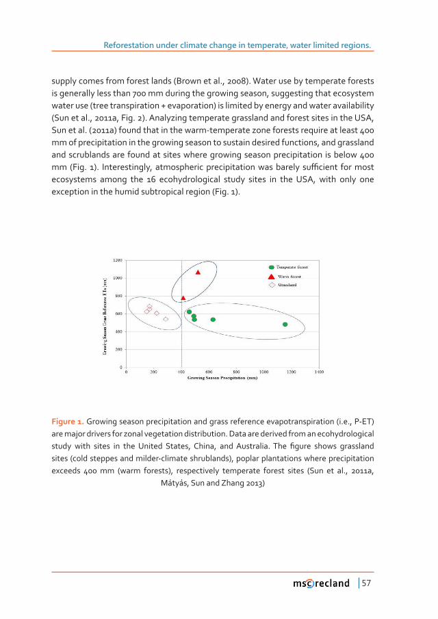
Reforestation under climate change in temperate, water limited regions�
57
supply comes from forest lands (Brown et al., 2008). Water use by temperate forests is generally less than 700 mm during the growing season, suggesting that ecosystem water use (tree transpiration + evaporation) is limited by energy and water availability (Sun et al., 2011a, Fig. 2). Analyzing temperate grassland and forest sites in the USA, Sun et al. (2011a) found that in the warm-temperate zone forests require at least 400 mm of precipitation in the growing season to sustain desired functions, and grassland and scrublands are found at sites where growing season precipitation is below 400 ���ȋ��Ǥ� ȌǤ� �������������ǡ�������������������������������������� ��ƥ������ ���������ecosystems among the 16 ecohydrological study sites in the USA, with only one exception in the humid subtropical region (Fig. 1).
Figure 1. Growing season precipitation and grass reference evapotranspiration (i.e., P-ET) are major drivers for zonal vegetation distribution. Data are derived from an ecohydrological ������ ����� ������ ��� ���� ������� ������ǡ� �����ǡ� �������������Ǥ����� Ƥ����� ������ ����������sites (cold steppes and milder-climate shrublands), poplar plantations where precipitation exceeds 400 mm (warm forests), respectively temperate forest sites (Sun et al., 2011a,
Mátyás, Sun and Zhang 2013)
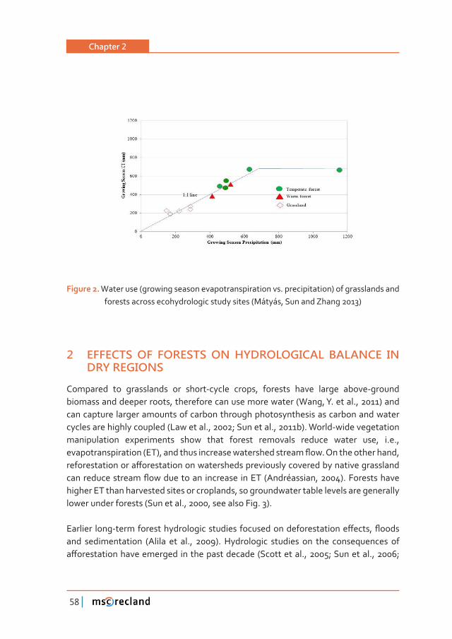
Chapter 2
58
Figure 2. Water use (growing season evapotranspiration vs. precipitation) of grasslands and forests across ecohydrologic study sites (Mátyás, Sun and Zhang 2013)
2 EFFECTS OF FORESTS ON HYDROLOGICAL BALANCE IN DRY REGIONS
Compared to grasslands or short-cycle crops, forests have large above-ground biomass and deeper roots, therefore can use more water (Wang, Y. et al., 2011) and can capture larger amounts of carbon through photosynthesis as carbon and water cycles are highly coupled (Law et al., 2002; Sun et al., 2011b). World-wide vegetation manipulation experiments show that forest removals reduce water use, i.e., �������������������ȋ��Ȍǡ������������������������������������ƪ��Ǥ������������������ǡ�������������������ơ����������������������������������������������������������������������������������ƪ������������� ��������� ������ȋ����±������ǡ�ȌǤ�������������higher ET than harvested sites or croplands, so groundwater table levels are generally lower under forests (Sun et al., 2000, see also Fig. 3).
�������� ����Ǧ������������������������������� ��������������������������ơ����ǡ�ƪ�����and sedimentation (Alila et al., 2009). Hydrologic studies on the consequences of �ơ�������������������������������������������ȋ�����������Ǥǡ�Ǣ����������Ǥǡ�Ǣ�
Reforestation under climate change in temperate, water limited regions�
59
Wang, Y. et al., 2011). In particular, evaluation of worldwide reforestation campaigns has shown that human intervention requires a closer look at the unexpected ������������Ǥ������������������������������������������������ơ������������������������ơ����� ���������� ���������� ����� ��� ������ ������ ȋ���� ��� ��Ǥǡ� ȌǤ� ���� �������������������������������������������ơ������������������������������������ǡ������������restoration, respectively for climate change mitigation, has drawn renewed attention to the relations between forests and water resources in watersheds (Calder, 2002; Brown et al., 2005; Jackson et al., 2005; Trabucco et al., 2008; Malmer et al., 2009) and on a regional scale (Ellison et al., 2011). The hot debate on ‘planting’ or ‘not planting’ policies is especially relevant in arid regions or regions with scarce water resources ȋ���ơǡ�ȌǤ
2�1 China: landcover changes and effects on streamflow
Comprehensive forest hydrological studies that address forest-water relations did not ���������������� �Ǥ�����������Ƥ�����������������������������������������������ȋ����et al., 2008). In dry Northern China, such as the Loess Plateau region, empirical and ��������������������Ƥ�������������������������������������������������������������������������������������Ƥ�������ƪ��������������������������ƪ���ȋ�����������Ǥǡ��Ǣ�2008b; Wang, Y. et al., 2011; Wang, S. et al., 2011).
Recent forest hydrology studies have detected that land cover and land use changes ������������������������������������ƪ������������������������ȋ�����������Ǥǡ��Ǣ��ȌǤ�������������������������������������������������Ǥά�����Ǥά�������������������������������������������������������������ǡ��������ƪ��������������������Ǥά�����Ǥάǡ�������������Ǥ��������������������ƪ��������������������������������������������in the Loess Plateau region (Zhang et al., 2008a). In another 40-year retrospective ������ȋǦȌǡ������������Ǥ�ȋ�Ȍ�����������������ƪ�������������������������� ����������� ��� ���� ������ �������� ��� ������������ ���� ��������� ��� �������ƪ��� �����������Ȁ�������������Ǥ�����������������������������������������Ƥ���������������������������������ƪ������ǦǤ����ǦǤ��������������������������Ǥ���������Ȁ���������������������������������ά����������������������������������������ƪ���in 8 out of the 11 catchments while in the remaining three watersheds precipitation and potential evaporation were more important. Among the soil conservation measures, construction of sediment-trapping dams and reservoirs, and the diversion ���������������������������������������������������������������ƪ��Ǥ�
Chapter 2
60
�������������������ơ�����������������������������ƪ������������������������������ǡ�Wang, Y. et al. (2011) constructed multi-annual water balances for 57 basins to estimate ��������������������������ȋ��Ȍ���������ơ�������������������������Ǧ������������Ǥ������������� ������ ����� �����Ǧ������ �ơ����������� ���� ����� �������� ������������� ������������������������� ������������������������ ������� ������������������� ����ơ�reduction.
2�2 United States: effects of landcover management
Since the late 1930s, numerous ‘paired watershed’ studies have been conducted in ����������� ������� ��� �������� ������������������ �ơ����� ȋ����������� ����� ��������intensities, species conversion, farming as an alternative), on water quality and yield across various climatic and topographic conditions (Ice and Stednick, 2004). In general, humid areas with high precipitation have higher hydrologic response in absolute terms, �����������������������������ƪ��������������������������������������Ǥ�����������ǡ�clear-cutting a deciduous forest in the humid south-eastern US, with an annual ��������������η���ǡ������������ �������������������������ƪ������Ǧ������������ǡ���������� Ǧά����������������������������������ǡ���������������������������practice in the drier area of northern Arizona with an annual precipitation of 500-600 ������� ������� ����������������� �������������������ηά������������������������watersheds. Zou et al. (2009) summarized century-long vegetation manipulation experiment studies in the Colorado River Basin that provide a bounty of knowledge ������ �ơ����� ��� ������� ��� ������� ����������� ��� �������ƪ��� ��������Ǧ��Ƥ���� �����Ǥ�The watershed is situated at the headwaters of streams and rivers that supply much of the water to downstream users in the western United States. The authors found that vegetation can be managed to enhance annual water yields while still providing �������������������������Ǥ������ơ������������������������������������������ƪ�������associated with the precipitation/elevation gradient and, therefore, with vegetation type. An annual water yield increase between 25 and 100 mm could be achieved by implementing vegetation manipulation in the high elevation subalpine and mixed conifer forests, the lower ponderosa pine forests and portions of the low elevation chaparral scrublands. The annual precipitation was generally above 500 mm in areas �������������������������������ƪ���������������Ǥ�������������������������������in water yield were observed from treating sagebrush, pinyon-juniper woodlands and desert scrubs, with an annual precipitation below 500 mm. This study suggests ������������������� ��� ��������������������������� �������������������ơ���� ���������������precipitation is roughly balanced by evapotranspiration demand, i.e., above 500 mm.
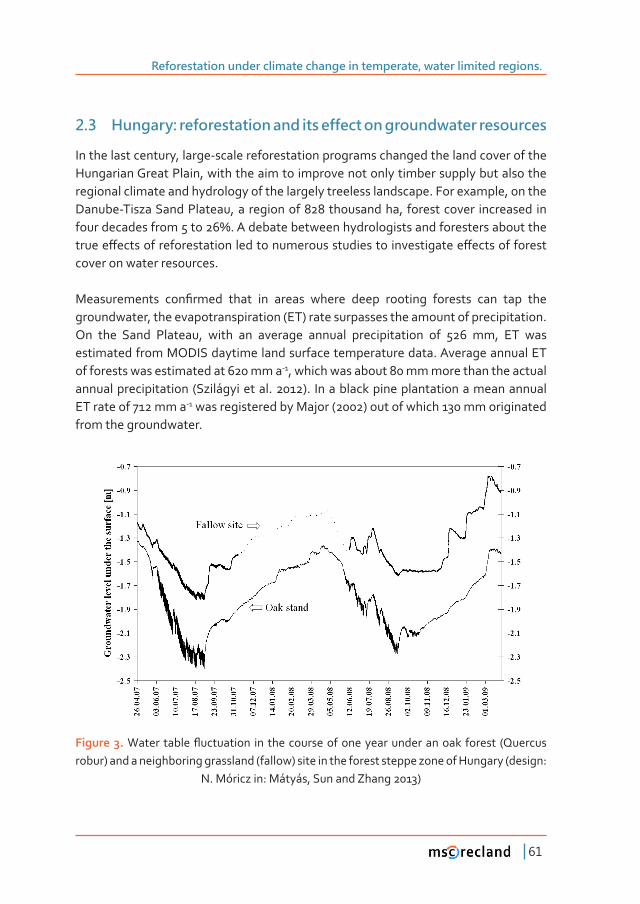
Reforestation under climate change in temperate, water limited regions�
61
2�3 Hungary: reforestation and its effect on groundwater resources
In the last century, large-scale reforestation programs changed the land cover of the Hungarian Great Plain, with the aim to improve not only timber supply but also the regional climate and hydrology of the largely treeless landscape. For example, on the Danube-Tisza Sand Plateau, a region of 828 thousand ha, forest cover increased in ����������������������άǤ�������������������������������������������������������������ơ��������������������������������������������������������������ơ���������������cover on water resources.
������������� ���Ƥ����� ����� ��� ������ ������ ����� �������� �������� ���� ���� ����groundwater, the evapotranspiration (ET) rate surpasses the amount of precipitation. On the Sand Plateau, with an average annual precipitation of 526 mm, ET was estimated from MODIS daytime land surface temperature data. Average annual ET of forests was estimated at 620 mm a-1, which was about 80 mm more than the actual annual precipitation (Szilágyi et al. 2012). In a black pine plantation a mean annual ET rate of 712 mm a-1 was registered by Major (2002) out of which 130 mm originated from the groundwater.
Figure 3. ������������ƪ���������� ��� ������������������������������������������� ȋ��������robur) and a neighboring grassland (fallow) site in the forest steppe zone of Hungary (design:
N. Móricz in: Mátyás, Sun and Zhang 2013)
Chapter 2
62
In other studies the groundwater consumption of forest and of grassland was compared. In a somewhat less harsh climatic environment of 570 mm annual rainfall and a growing season precipitation of 360 mm (i.e. still a potential grassland ������������������������������Ǥ��Ȍǡ�������������������������Ǥ�ά����������������������������������������������������������ȋ���Ǥ����ȌǤ�������ơ�����������however much higher in average groundwater use (oak: 243 mm, fallow: 85 mm). The ������������������������������������� ά����������������������������������������������������������������ά��������������Ǥ������������������������������������������ά�������������������������������������������ǡ���������������������������������������table was deeper during the dry period (Móricz et al. 2012).
Various measurements have shown that in shallow groundwater areas on the Danube-Tisza Sand Plateau forest vegetation may lower water table from 0.5 up to 1.1 m compared to the level below herbaceous vegetation (Major 2002). Under natural conditions, if maximum groundwater level (in April) is deeper than -2.5 m, grassland predominates in this climate.
Measurements revealed that in the Hungarian forest steppe climate zone, forest cover ����� ���� ����������� ��� ������������ ��������� ��� ��� ����ơǡ� ���� ��������� ����������ǡ�near-surface groundwater resources. Due to lower groundwater levels under forests, ������������ �������������������������ǡ������������������������������ƪ��� �������forested patches.
3 THE CHALLENGE OF CHANGING CLIMATE
3�1 The climatic transition zone at the forest/grassland edge
The climatic and biogeographic conditions of the continental plains of South-eastern Europe and of temperate Northeast Asia are very diverse, which is also true for their socio-economic statuses and current problems (i.e. land use change, soil degradation ����������Ƥ������ȌǤ����������������� ������������Ƥ�� ��� ���������������� ������Ǧ������ xeric limit of forests and forest tree species.
Reforestation under climate change in temperate, water limited regions�
63
Xeric (or rear, trailing3) forest limits are at the low latitude, low altitude end of distribution ranges of temperate forest trees, where presence or absence of (climate-)zonal, closed forests is determined by climatic aridity (Mátyás et al., 2009). Xeric limits appear in low-precipitation zones of continental plains, along the foothills of mountain ranges, and at the edges of dry basins in the temperate-continental climate. At the xeric limit, the closed forest belt forms a transition zone (ecotone) toward the open woodland or forest steppe, which dissolves with decreasing precipitation into the true steppe or grassland. The forest/grassland ecotone is dependent on a volatile minimum of rainfall and is therefore sensitive to prolonged droughts. The physical characteristics of the land surface (e.g., albedo, evapotranspiration, roughness etc.) ��������������������������������������������������������������ơ�������������������������and changes in this area.
The forest steppe belt reaches from the plains of Southeast Europe and South Russia into Southern Siberia and North China. Temperate xeric limits exist also on other continents, along the edge of the Prairies of North America, notably from the southwest states of the USA northward into Alberta (Canada). In Southeast Europe, and also in China the transition zone is a densely populated and is an agriculturally ����������������������������������������������ƪ�������������������Ǥ����ƪ����������ǡ����� ��������� ����������� ����� ������� �������� ��� ���������� ��� ��ƥ����� ��� �����ǡ� ���� ���������������������������������������������ǡ�Ƥ����������ǡ���������������������������������Ǥ
����������������� �������������������������������� �����Ƥ�� ������� ������� ȋ��������Ȍ��������Ǥ� ���������� ��� ���������� ����ǡ� ���� ����� ������Ƥ��� ����� ����� ��������� ���characterized by an average precipitation of 563 mm per year, a July mean of 21,5 λ����������������Ƥ�����������ȋ�������������������ȌǤ�������������������������the vegetation period (approximately 320 mm) and frequent summer droughts limit the presence of closed forests except to sites where supplementary water resources are available below ground. Forest crown interception and litter interception may further diminish available water resources even in more humid forested catchments (Gribovszki et al 2006). In forest steppe climate, loss through crown and litter ��������������������������ǦάǤ�������ǡ�����������������������������������������������άǡ����������������������������������������������������ά����������������meager precipitation (Járó 1980). Natural forest cover remains therefore patchy in ���������ǡ����������������������������������������ƪ������������������������������Ǥ
3 The terms in brackets refer to events of postglacial migration, where xeric limits represent ����Dz����dz���������������������������������ǡ�����������������������������
Chapter 2
64
3�2 The climatic vulnerability of the forest/grassland transition zone
The forest-grassland transition zone is especially vulnerable to expected climatic �������� ��� ƪ��� ������ �������� ��� ���� ���������� ��� ���� latitudinal lapse rate. It is generally known that the altitudinal lapse rate for temperature (i.e., the rate of change with increasing elevation) is 5.0 - 6.5 °C/1000 m. The latitudinal (south to north) lapse rate is less recognized. In the temperate zone its mean value is around 6.9 °C/1000 km Ǧ�����ơ��������������������������Ǥ���������������������������������������������������ơ���������������������������������������������������������������������������������Ǥ�A temperature increase of only +1 °C causes a shift upwards along a mountain slope of approximately 170 m. On a plain, the same change triggers a shift of close to 150 km (Jump et al., 2009). This explains the much greater vulnerability of rain-dependent vegetation on plains. Predicted changes may easily trigger the loss of already sparse forest cover, which may lead to the disruption of vital ecological services that the forests provide.
3�3 Recently observed climatic impacts
Across the temperate zone, a relatively rapid increase of annual mean temperature has been observed in recent decades, and the dryland zone in China and Mongolia is no exception. In the last half century, both average temperatures and climatic extremes increased (Qi et al., 2012). For instance, average temperatures in Mongolia increased by more than 2 °C since 1940 and nine out of the ten warmest years occurred �������ȋ��������Ǥǡ�ȌǤ���������������ǡ������������������������������Ƥ����������the past several decades, leading to an unprecedented increase of dry areas (Piao et al., 2010). Growing season anomalies have been generally increasing in China in �����ǣ�������������������������Ƥ�������������������������������������������������declined (Zhao and Running, 2010).
Numerous studies and also IPCC’s 2007 report forecast a decline in growth and production of forests in dry regions. At the same time, analyses of impacts of climate on forests are limited or sporadic. For instance, FAO global statistics do not yet ��������������������ơ�������������������� �����������������Ƥ�������ȋ��ǡ�ȌǤ�������are reports about observed impacts from western North America (Allen et al., 2010; Hogg and Price, 2000), while impacts in Eastern Europe, Central Asia and the Chinese Drylands are less known (Zhang et al., 2008b; Piao et al., 2010; Mátyás, 2010a). It
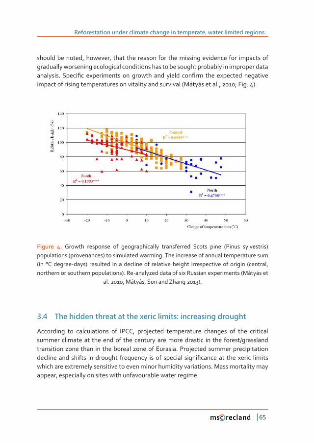
Reforestation under climate change in temperate, water limited regions�
65
should be noted, however, that the reason for the missing evidence for impacts of gradually worsening ecological conditions has to be sought probably in improper data ��������Ǥ������Ƥ�� ������������ ��� ������� ���� ������ ���Ƥ��� ���� ��������� ���������impact of rising temperatures on vitality and survival (Mátyás et al., 2010; Fig. 4).
Figure 4. Growth response of geographically transferred Scots pine (Pinus sylvestris) populations (provenances) to simulated warming. The increase of annual temperature sum (in °C degree-days) resulted in a decline of relative height irrespective of origin (central, northern or southern populations). Re-analyzed data of six Russian experiments (Mátyás et
al. 2010, Mátyás, Sun and Zhang 2013).
3�4 The hidden threat at the xeric limits: increasing drought
According to calculations of IPCC, projected temperature changes of the critical summer climate at the end of the century are more drastic in the forest/grassland transition zone than in the boreal zone of Eurasia. Projected summer precipitation ������������ ������� ����������� ���������� ������ �������� �����Ƥ��������� ���� ������ �������which are extremely sensitive to even minor humidity variations. Mass mortality may appear, especially on sites with unfavourable water regime.
Chapter 2
66
3�5 Considerations for forest management
����������������������������������������������ǡ�������������������������ơ�����������with plantations, returning to close-to-nature forest management seems to be the general trend to mitigate impacts of environmental change (e.g. Xu 2011, see also Mátyás 2010a). The concept is based on the hypothesis that stability and persistence of forest ecosystems is warranted by plant communities having evolved during the past millennia, and enhancing the naturalness of forests will also enhance their stability. The hypothesis is challenged at the xeric limits by numerous constraints, such as
• long-lasting human interference and land use have caused a partial or total loss of natural (woody) plant cover, spontaneous processes of vegetation recovering might be very slow,
• number of native species expected to tolerate expected environmental changes is usually low,
• ��������������������Ǧ��Ǧ������������������������������������������������ơ�����(e.g., grazing and game damages, air pollution) and by the projected climatic changes and extreme events.
These constraints necessitate a considerate revision of the commitment to �����������ǡ� Ƥ���� ��� ���� ��� �������� ��� ����� �������� ����Ǥ� ��� ��� ��������� ����� ����������planned and active human interference is unavoidable in dry lands because the long-�����������������������������ơ����������������������������������������������������be considered.
������Ǧ�ơ������ǡ��������Ƥ�������������������������������������������������������������the consideration of local environmental conditions, of land use alternatives such as restoration of grasslands and scrublands, and the use of the proper technology. ������������ ����� ���� ������� ������� ���Ƥ��� ����� ����������� ���� ��� �������������managed to enhance annual water yields while still providing other ecological ����Ƥ��Ǥ� ���������� �������� ������ ������������� ��� ���������� ���������ǡ� ��� ��������a successful policy of restoration and of adaptation to the expected environmental changes.
Reforestation under climate change in temperate, water limited regions�
67
4 SUMMARY AND CONCLUSIONS
Current views and experiences about the role of forests at dryland margins are �������������Ǥ��������������������������������������������������Ƥ��ǡ�������������������ơ������������������������������������������������������������������������������������ ������� ������� ƪ��� ���� ��� ������� ������ ���� �������� ����� �������� ���� ������management and sustainable development. In the forest steppe climate zone, forest ��������������� ����������� ��������������� ������������ ��� ����ơǡ������������������Ǧsurface groundwater resources.
������ ������ ��ƪ������� ������������ �������� �������Ǥ����������� ��� ��� ��������� ����������������������������������������������������������������������Ƥ������Ǥ���������indicate that in spite of increased evapotranspiration, precipitation changes are �������������������������������������ơ���������������Ǥ�����������������ǡ�����������albedo of forests may even lead to minor temperature rise. It seems that the balance between albedo and actual evapotranspiration determines whether there is a cooling ������������ơ���Ǥ
The forest/grassland ecotone is dependent on a volatile minimum of rainfall and is therefore sensitive to climatic changes. Projected summer precipitation decline and shifts in drought frequency may easily trigger the loss of forest cover, which may lead to the disruption of vital ecological services that the forests provide. Because of the extreme long-term character of forestry, the consideration of projected ����������������ơ��������� ���������� �������� ����� ����������������������Ǥ�����������and growth of forests depend on humidity conditions of the future especially in the dryland transition zone. Concerns about hydrology and climate should be weighed ��������������������������������������������Ǥ������������Ƥ�����������������������������������������������������������������������������������������Ƥ�������ƪ������on ecology of watersheds.
RELATED WEBSITES, PROJECTS AND VIDEOS
������������������������ǣ�����ǣȀȀ���Ǥ�������Ǥ���Ȁ�����ǫ�γ���Ɵ������Land Use, Land Use Change and Forestry (LULUCF): http://forest.jrc.ec.europa.eu/activities/lu-
lucf/Northern Eurasia Earth Science Partnership Initiative (NEESPI): http://neespi.org/MARGINS project: http://margins.ecoclimatology.com/index.htmlExpected climate change and options for EU silviculture (ECHOES): http://www.forestry.gov.uk/
website/forestresearch.nsf/ByUnique/INFD-7NBCPQ
Chapter 2
68
EU targets action on forests: http://www.euractiv.com/sustainability/eu-targets-action-forests-news-299524
EU Green Paper on forest protection and climate change: http://www.euractiv.com/sustainabili-ty/eu-targets-action-forests-news-299524
IPCC AR4: Forestry: http://www.ipcc.ch/publications_and_data/ar4/wg3/en/ch9.html
REFERENCES
�����ǡ��Ǥǡ� �����ǡ� �Ǥ� �Ǥǡ� ���������ǡ� �Ǥǡ� ���� ������ǡ� �Ǥ� ȋȌǤ� ������� ���� ƪ����ǣ� �� ���� ��-radigm sheds light on age-old controversies. Water Resources Research, 45, W08416, doi:10.1029/2008WR007207.
Allen, C. D., Macalady, A. K., Chenchouni, H., Bachelet, D., McDowell, N., Vennetier, M., Kizber-ger, T., et al. (2010). A global overview of drought and heat-induced tree mortality reveals emerging climate change risks of forests. Forest Ecology and Management, 259, 4, 660-684.
����±������ǡ��Ǥ�ȋȌǤ�������������������ǣ���������������������������������������Ƥ��������Ǥ�Jour-nal of Hydrology, 291, 1-27.
Brown, A. E., Zhang, L., McMahon, T. A., Western, A. W., and Vertessy, R.A. (2005). A review of paired catchment studies for determining changes in water yield resulting from alterations in vegetation. Journal of Hydrology, 310, 28-61.
Brown, T. C., Hobbins, M. T., and Ramirez, J. A. (2008). Spatial distribution of water supply in the coterminous United States. Journal of the American Water Resources Association, 44, 6, 1474-1487.
Calder, I. R. (2002). Forests and hydrological services: reconciling public and science perceptions. Land Use and Water Resources Research, 2, 1-12.
Drüszler, Á., Csirmaz, K., Vig, P., and Mika, J. (2010)Ǥ��ơ���������������������������������������temperature and humidity regime in Hungary. In Saikia S. P. (Ed.), Climate Change. Int. Book Distr., Dehra Dun, Uttarakhand, India, 394-418.
Ellison, D., N. Futter, M., and Bishop, K. (2011). On the forest cover-water yield debate: from de-mand- to supply-side thinking. Global Change Biology, doi: 10.1111/j.1365-2486.2011.02589.x.
FAO (2010). Global Forest Resources Assessment 2010. Main report. FAO Forestry Paper 163, Rome
����ǡ��Ǥǡ� ����ǡ��Ǥǡ�����������ǡ��Ǥ�ȋȌǤ��ơ���������������������������������������������������climate change – a case study of Hungary. Acta Silvatica et Lignaria Hungarica, 7, 49-62.
���ơǡ��Ǥ�ȋȌǤ�������������������������ǡ������������������������������������ǣ�����������������sustainable development are we leaving our children? EcoDoc Africa, 39.
���������ǡ��Ǥǡ�������ǡ��Ǥǡ��������ǡ��Ǥ�ȋȌǤ�������ƪ����������������������������������������-ments in the Sopron Hills. Acta Silv. Lign. Hung., 2: 81-92
Hogg, E. H., and Price, D. T. (2000). Postulated feedbacks of deciduous forest phenology on sea-sonal climate patterns in the Western Canadian Interior. Journal of Climate, 13, 4229-4243.
Ice, G. G., and Stednick, J. D. (2004). A century of forest and wildland watershed lessons. Society of American Foresters, Bethesda, Maryland. P287.
Jackson, R. B., Jobbágy, E. B., Avissar, R., Roy, S. B., Barrett, D. J., Cook, C. J., et al. (2005). Trading water for carbon and with biological carbon sequestration. Science, 310, 1944-1947.
��×ǡ��Ǥ� ȋȌǤ�ȏ������������� ������Ǧ��������������������������Ú�Ú��ÝȐǤ����±����������������(Budapest) 73: 7–17. (in Hungarian, with English summary)
Reforestation under climate change in temperate, water limited regions�
69
Jump, A., Mátyás, C., and Penuelas, J. (2009). The paradox of altitude-for-latitude comparisons in species’ range retractions. Trends in Ecology and Evolution, 24, 12, 694-700.
Law, B. E., Falge, E., Gu, L., Baldocchi, D. D., Bakwin, P., Berbigier, P., Davis, K., et al. (2002). Envi-ronmental controls over carbon dioxide and water vapor exchange of terrestrial vegetation. Agricultural and Forest Meteorology, 113, 97-120.
Lu N., Wilske, B., Ni, J., John, R., and Chen J. (2009). Climate change in Inner Mongolia from 1955 through 2005. Environmental Research Letters, 4, 045006.
Major, P. (2002). [Impact of lowland forests on water balance]. Hidrológiai Közlöny (Budapest) 82 (6): 319–324. (in Hungarian, with English summary)
Malmer, A., Murdiyarso, D., Bruijnzeel, L. A., and Ilstedt, U. (2009). Carbon sequestration in tro-pical forests and water: a critical look at the basis for commonly used generalizations. Global Change Biology, 16, 1-6.
Mátyás, C. (Ed.) (2010a). Forests and Climate Change in Eastern Europe and Central Asia. Forests and Climate Change W. Pap. Nr. 8, Rome, FAO, 189 p.
Mátyás, C., Czimber, K. (2000): [Modeling zonal forest associations on the mesoclimatic level: ����������������������������������������������ơ����Ȑ���ǣ����ǡ��Ǥ�ȋ��Ȍǣ�����Ǥǡ��������Ǥ�����������Climate, Debrecen University, 83-97 (in Hungarian, with English summary)
Mátyás, C., Nagy, L., and Ujvári-Jármay, É. (2010). Genetically set response of trees to climatic change, with special regard to the xeric (retreating) limits. Forstarchiv (Hannover), 81, 130-141.
������ǡ��Ǥǡ� ���ǡ�Ǥǡ������ǡ��Ǥ� ȋȌ��ơ����������� ���� �������� ��� ���� �������� �����ǣ� ��������learned and future outlooks. In: Dryland East Asia: Land dynamics amid social and climate change (eds. Chen, J. Wan, S., Henebry, G.,Qi, J., Gutman, G.,Sun, G., Kappas, M.) Ecosystem Science and Applications, HEP Publishers, Beijing, and De Gruyter Publishers, 245-264
Mátyás, C., Vendramin, G. G., and Fady, B. (2009). Forests at the limit: evolutionary-genetic con-sequences of environmental changes at the receding (xeric) edge of distribution. Annals of Forest Science, 66, 800-803.
Móricz, N., Mátyás, C., Berki, I., Rasztovits, E., Vekerdy, Z., Gribovszki, Z., (2012). Comparative water balance study of forest and fallow plots. iForest, 5: 188-196
Piao, S. L., Ciais, P., Huang, Y., Shen, Z. H., Peng, S. S., Li, J. S., et al. (2010). The impacts of climate change on water resources and agriculture in China. Nature, 467, 43-51.
Qi J., Chen, J., Wan, S., and Ai, L. (2012). Understanding the coupled natural and human systems in Dryland East Asia. Environmental Research Letters, 7, 015202.
Scott, D. F., Bruijnzeel, L. A., and Mackensen, J. (2005). The hydrologic and soil impacts of refo-restation in the tropics. In M. Bonell and L.A. Bruijnzeel (Eds), Forests, Water and People in the Humid Tropics. Cambridge University Press, 622-651.
Sun, G., Alstad, K., Chen, J., Chen, S., Ford, C. R., Lin, G., et al. (2011a). A general predictive model for estimating monthly ecosystem evapotranspiration. Ecohydrology, 4, 245-255.
Sun, G., Caldwell, P., Noormets, A., Cohen, E., McNulty, S. G., Treasure, E., et al. (2011b). Ups-caling Key Ecosystem Functions across the Conterminous United States by a Water-Centric Ecosystem Model. Journal of Geophysical Research, 116, G00J05, doi:10.1029/2010JG001573.
Sun, G., Riekerk, H., and Kornak, L. V. (2000). Groundwater table rise after forest harvesting on �������Ǧ�����ƪ�����������������Ǥ�Wetlands, 20, 1, 101-112.
Sun, G., Zhou, G. Y., Zhang, Z. Q., Wei, X. H., McNulty, S. G., and Vose, J. M. (2006). Potential wa-ter yield reduction due to forestation across China. Journal of Hydrology, 328, 548-558.
Chapter 2
70
Szilágyi, J., Kovács, Á. and Józsa, J. (2012). Remote sensing based groundwater recharge estima-tes in the Danube-Tisza Sand Plateau region of Hungary, J. Hydrol. Hydromech., 60, 2012, 1, 64-72
Trabucco, A., Zomer, R. J., Bossio, D. A., van Straaten, O., and Verchot, L. V. (2008). Climate chan-�������������� �������� �ơ����������Ȁ�������������ǣ� �� ������� ��������� ��� ����������� ��������with four case studies. Agricultural Ecosystems and Environment, 126, 81-97.
Wang, S., Fu, B., He, C.-S., Sun, G., and Gao., G.-Y. (2011). A comparative analysis of forest cover and catchment water yield relationships in northern China. Forest Ecology and Management, 262, 7, 1189-1198.
����ǡ��Ǥǡ���ǡ��Ǥǡ�����ǡ��ǤǦ�Ǥǡ����ǡ��Ǥǡ����ǡ�Ǥǡ�������ǡ��Ǥǡ������Ǥ�ȋȌǤ������������ơ����������-transpiration of forest lands and non-forest lands in selected basins of the Loess Plateau of China. Ecohydrology, 4, 277-287.
Wang, Y., Yu, P., Xiong, W., Shen, Z., Guo, M., Shi, Z., et al. (2008). Water yield reduction after �ơ����������� ���� �������� ���������� ��� ���� ��������� ����������������ǡ� ���������� �����Ǥ�Journal of the American Water Resources Association, 44,5, 1086-1097.
���ǡ��Ǥǡ����ǡ�Ǥǡ����ǡ��Ǥǡ�����ǡ� Ǥǡ�����ǡ�Ǥǡ��������ǡ��Ǥ�ȋȌǤ�����������Ǧ������ƪ����������������in China: a 40-year retrospect. Journal of the American Water Resources Association, 44, 5, 1076-1085.
Xu, J. (2011). China’s new forests aren’t so green as they seem. Nature, 477, 371. Zhang, X. P., Zhang, L., McVicar, T. R., Van Niel, T. G., Li, L. T., Li, R., et al. (2008a). Modeling the
�����������ơ���������������������������������ƪ�����������������������ǡ������Ǥ�Hydrological Proceedings, 22, 1996-2004.
�����ǡ��Ǥ��Ǥǡ������ǡ��Ǥǡ�����ǡ� Ǥǡ���������ǡ��Ǥǡ�������������ǡ��Ǥ�ȋ�ȌǤ���������������������ƪ���to changes in climate and land use/cover in the Loess Plateau, China. Water Resources Re-search, 44, W00A07, doi:10.1029/2007WR006711.
Zhao, M. S., and Running, S. W. (2010). Drought induced reduction in global terrestrial net prima-ry production from 2000 through 2009. Science, 329, 940-943.
���ǡ��Ǥ��Ǥǡ���������ǡ��Ǥ�Ǥǡ���������ǡ��Ǥ�ȋȌǤ��������ƪ�����������������������������������-tions along a gradient of precipitation in the Colorado River Basin. Forest Ecology and Mana-gement, 259, 7, 1268-1276.
71
Chapter 2.2
University of
West Hungary,
Sopron, Hungary
Forests in a changing climateImre BerkiErvin Rasztovits
ABSTRACT
�������������������������������������������������������ơ��������������������������the distribution, growth, health and vitality of forests. In the analyses European beech is selected as indicator species. Although it is considered in its optimum highly plastic and adaptable, it becomes climate-sensitive closer to its xeric (lower) distribution limits. The future of beech in Southeast Europe requires ����������������������������������������������������Ƥ������������������������������near their xeric distribution boundary. Even though the low elevation occurrences are uniquely vulnerable to climatic shifts, observations and modelling studies pertaining to this region are particularly scarce.
Out of climatic factors determining the xeric distributional limits for beech, ���������ǯ����������������ȋ��Ȍ������������������������ƪ�������Ǥ������������������������� ��� ������������ ������ ����� ���Ƥ����� ���� ���������� ��� ��������������adaptationof beech and have proven that warming and more arid conditions lead to decline of growth and vitality, while no decline was observed if EQ changed in the opposite direction. The response to weather extremes was investigated in Ƥ���������Ǥ����������������������������������������������������ǡ������������EQ value 40-42 resulted in pest and disease attacks and mass mortality.
The discussed approaches indicate consistently a high level of uncertainty regarding the future of beech at the xeric limit in Southeast Europe. According to Ƥ������������������������������������������������ǡ��������������������Ǧ���������������������������������������������������������ι����������������������������warming in the second half of the century, while higher-elevation occurrences
Chapter 3
72
may remain stable. The interpretation of the results bears some stipulations, such ��� ���� ������������ ��� ����������� ���� ������ ������������� ��� ��ƪ�������� ��������distribution patterns, the unclear role of persistence, natural selection and plasticity and uncertainties of climate projections. Grim projections may probably be partly overwritten by the mentioned stipulations and by careful and prudent human support.
1 CHANGES IN CLIMATE CONDITIONS WITH RESPECT TO FOREST ECOLOGY
Adaptation strategy of forest trees is receiving growing attention in view of expected climatic changes. Scarcity of reliable information on responses to macroclimatic changes is a central problem and obstacle of planning for the future. Inorder to formulate realistic predictions, both the nature of adaptation to past and current climate, and the level of sensitivity to sudden environmental changes have to be understood and properly interpreted. The distribution of European beech extends across ecologically and climatically variable regions. Compared to other wide-spread tree speciesof Europe, it is still the one which was left in a relatively natural condition as – although in a distributional range reduced by man – it was seldom regenerated ����Ƥ������� ���� ���� ������������������������������ �������� ��� �����Ǧ������ �����������relocations such as oaks or Scots pine. Thus, present populations of European beech are still close to a „wild state”. Therefore beech is a well suited model species to study adaptation strategy of long-living, deciduous climax species to climate and to changes of climate. The species is considered climate-sensitive and vulnerable to changes. Therefore its response to predicted large-scale changes of climate is a critical issue.
In this study an attempt is presented to trace, quantify and project the impacts of macroclimatic change on the distribution and vitality of beech, with results interpretable for the practice, as such information is urgently needed to develop adaptation strategies for both forestry and conservation. Investigations were concentrated to the xeric limits in SE Europe. This region, where the retreat of the species is imminent, has been largely neglected by European studies (Jump et al. 2009, Mátyás et al. 2010). We consider the detailed, practice-oriented investigation of climate impacts at the xeric limits of primary importance because especially the low elevation occurrences of beech in the region are uniquely vulnerable to climatic shifts (Mátyás et al. 2010).
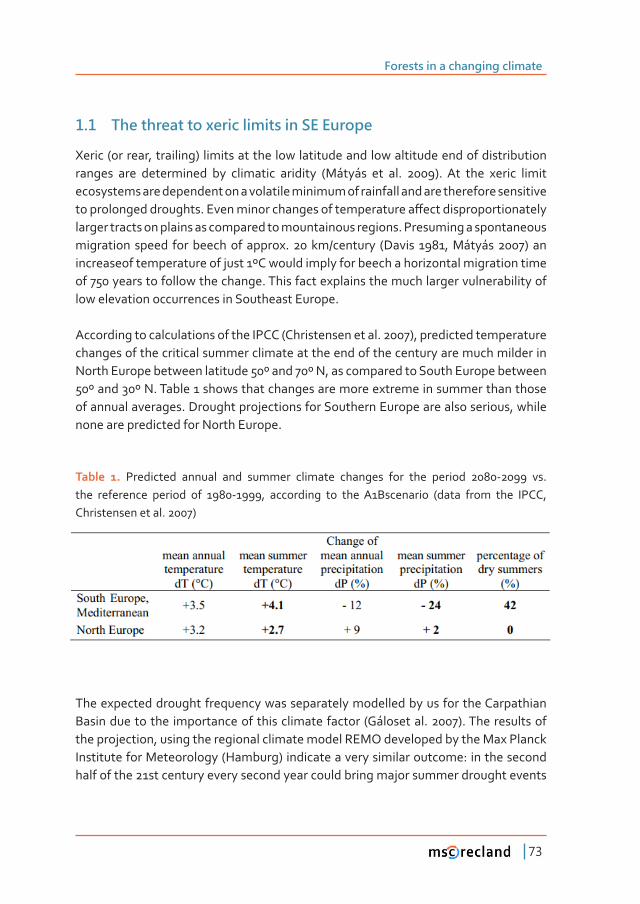
Forests in a changing climate
73
1�1 The threat to xeric limits in SE Europe
Xeric (or rear, trailing) limits at the low latitude and low altitude end of distribution ranges are determined by climatic aridity (Mátyás et al. 2009). At the xeric limit ecosystems are dependent on a volatile minimum of rainfall and are therefore sensitive ���������������������Ǥ������������������������������������ơ�����������������������larger tracts on plains as compared to mountainous regions. Presuming a spontaneous migration speed for beech of approx. 20 km/century (Davis 1981, Mátyás 2007) an increaseof temperature of just 1ºC would imply for beech a horizontal migration time of 750 years to follow the change. This fact explains the much larger vulnerability of low elevation occurrences in Southeast Europe.
According to calculations of the IPCC (Christensen et al. 2007), predicted temperature changes of the critical summer climate at the end of the century are much milder in North Europe between latitude 50º and 70º N, as compared to South Europe between 50º and 30º N. Table 1 shows that changes are more extreme in summer than those of annual averages. Drought projections for Southern Europe are also serious, while none are predicted for North Europe.
Table 1. Predicted annual and summer climate changes for the period 2080-2099 vs. the reference period of 1980-1999, according to the A1Bscenario (data from the IPCC, Christensen et al. 2007)
The expected drought frequency was separately modelled by us for the Carpathian Basin due to the importance of this climate factor (Gáloset al. 2007). The results of the projection, using the regional climate model REMO developed by the Max Planck Institute for Meteorology (Hamburg) indicate a very similar outcome: in the second half of the 21st century every second year could bring major summer drought events
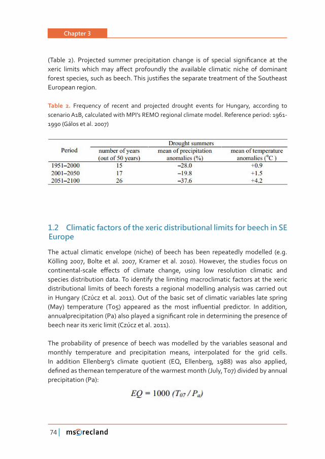
Chapter 3
74
ȋ������ ȌǤ� ���������� ������� �������������� ������� ��� ��� �������� �����Ƥ������ ��� ���������� ������� ���������� �ơ���� ����������� ���� ���������� ��������� ������ ��� �����������������������ǡ��������������Ǥ�����������Ƥ�������������������������������������������European region.
Table 2. Frequency of recent and projected drought events for Hungary, according to scenario A1B, calculated with MPI’s REMO regional climate model. Reference period: 1961-1990 (Gálos et al. 2007)
1�2 Climatic factors of the xeric distributional limits for beech in SE Europe
The actual climatic envelope (niche) of beech has been repeatedly modelled (e.g. Kölling 2007, Bolte et al. 2007, Kramer et al. 2010). However, the studies focus on �����������Ǧ������ �ơ����� ��� �������� ������ǡ� ������ ���� ����������� ��������� ����species distribution data. To identify the limiting macroclimatic factors at the xeric distributional limits of beech forests a regional modelling analysis was carried out in Hungary (Czúcz et al. 2011). Out of the basic set of climatic variables late spring ȋ���Ȍ� ������������ ȋ�Ȍ� ��������� ��� ���� ����� ��ƪ�������� ���������Ǥ� ��� ��������ǡ���������������������ȋ��Ȍ��������������������Ƥ�����������������������������������������beech near its xeric limit (Czúcz et al. 2011).
The probability of presence of beech was modelled by the variables seasonal and monthly temperature and precipitation means, interpolated for the grid cells. In addition Ellenberg’s climate quotient (EQ, Ellenberg, 1988) was also applied, ��Ƥ������������������������������������������������ȋ ���ǡ��Ȍ�������������������precipitation (Pa):
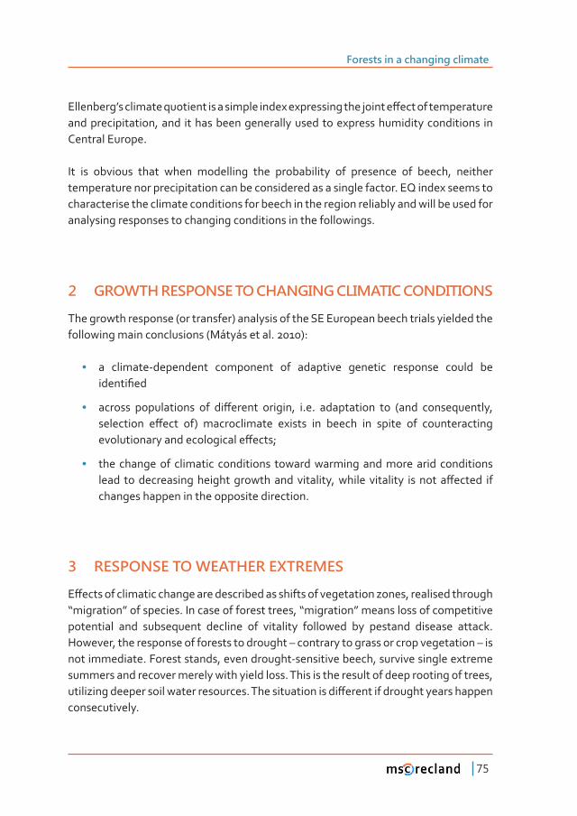
Forests in a changing climate
75
���������ǯ�����������������������������������������������������������ơ�������������������and precipitation, and it has been generally used to express humidity conditions in Central Europe.
It is obvious that when modelling the probability of presence of beech, neither temperature nor precipitation can be considered as a single factor. EQ index seems to characterise the climate conditions for beech in the region reliably and will be used for analysing responses to changing conditions in the followings.
2 GROWTH RESPONSE TO CHANGING CLIMATIC CONDITIONS
The growth response (or transfer) analysis of the SE European beech trials yielded the following main conclusions (Mátyás et al. 2010):
• a climate-dependent component of adaptive genetic response could be ������Ƥ���
• ������� ������������ ��� ��ơ������ ������ǡ� �Ǥ�Ǥ� ����������� ��� ȋ���� ������������ǡ����������� �ơ���� ��Ȍ� ������������� ������� ��� ������ ��� ������ ��� �������������������������������������������ơ����Ǣ�
• the change of climatic conditions toward warming and more arid conditions ����� ����������������������������������������ǡ������� ��������� ��������ơ������ ���changes happen in the opposite direction.
3 RESPONSE TO WEATHER EXTREMES
�ơ�������������������������������������������������������������������ǡ������������������Dz���������dz�����������Ǥ������������������������ǡ�Dz���������dz���������������������������potential and subsequent decline of vitality followed by pestand disease attack. However, the response of forests to drought – contrary to grass or crop vegetation – is not immediate. Forest stands, even drought-sensitive beech, survive single extreme summers and recover merely with yield loss. This is the result of deep rooting of trees, �������������������������������������Ǥ��������������������ơ������������������������������consecutively.
Chapter 3
76
��� ���� ����������� Dz���������� ��������dz� ȋ�������� ��� ��Ǥ� Ȍ� ������ ������������ �����treated as isolated, transient problems related to extreme events, rather than as a consequence of a long-term climate shift. This is because the gradual, relatively slow �������������������������������������������������������ơ�����������������������������limits. Spontaneous climatic selection is driven by recurrent drought eventsand the symptoms of change appear usually quite abruptly. Climatic means in models should be regarded therefore rather as surrogates for extreme events. The long-term, gradual shift of climatic factors has merely predisposingrole. Besides climate, the site conditions, age andstructure of stand play also a predisposing role. Incitingfactors are mainly connected to climatic anomalies especiallyat the xeric limits. Pests or diseases attacking populations of weakenedvitality are then the direct or proximate causes of mortality.
3�1 Health and vitality loss due to climatic extremes: case study of beech in SW Hungary
���� ���������� ����������������� ��Ƥ���� ��� �������� ���� ���� ��� ������� ��������� ��������������������������������������ǡ�Ƥ�������������������������������������������where climatic changes were the strongest, and where the stands are at low elevation and close to the xeric limits. The weakened trees became more sensitive to secondary pests and pathogens and showed symptoms of health deterioration (early leafabscission, sparser crowns, etc.). The extent of climate damages of the drought years 2000–2004 has been investigated in two West Hungarian state forest companies. In 460 damaged forest compartments (total area: 3900 ha) 87.7 thousand cu.m. of damaged timber was harvested. The damaged stands were mostly above 60 years (T. Szép, unpubl. data). The area most damaged was the Zalaegerszeg forest district (Zala county), where mass mortality was triggered in mature beech stands after regeneration cuts, when the canopy closure was opened up. This led to the outbreak of the otherwise harmless beech buprestid (Agrilus viridis). Damage of Biscogniauxia nummulariadisease and of the beech bark beetle (Taphrorychus bicolor) occurred together with the buprestid damage. As a consequence close to 70,000 cu.m. of sanitary felling had to be executed in 2005 in that forestry district alone (Figure 1, Lakatos – Molnár 2009). The type of damage supports the observation of forest protection experts that disturbance of the closed canopy increases the risk of climate damage.
Forests in a changing climate
77
Figure 1. Symptoms of beech decline in 2004 in Zala county, following the damage of Taphrorychus bicolor on thetrunk (Molnár – Lakatos 2009)
3�2 Analysis of drought events
��� ���� ������� ��Ƥ������� ��� �������� �������� �ơ����� �������� ��� ���� Dz������������������dz���������ǡ�������������������������������������������ơ��������������������������Ǥ���� ����������������������������ǡ�������� ����������Ƥ��� ��������������� ���characterise individual years’ weather. Mean temperature of the 3 summer months ���� ����� ���� ���� ������� ��� ������ �������� ��� ����� ���ǯ�ǡ� ��� ������ ������� �ơ�����of individual months (in case of 30-year climate averages, this is not a problem). Investigation of mortality frequency has shown that single drought events did not �������������������������������������Ǥ��������������������������������������������Ƥ���years in some areas, has however resulted in very serious mortality in the investigated beech stands, in one case the population went extinct (Figure 2).
�������������ǡ��ơ�������������������������������������������������������������������beech forest at the xeric limits of distribution. The stand has been selected at the edge of the xeric limit which is indicated by the frequency of droughty years. Years ���������������������Ƥ����������������������������������������������������Ǥ������mortality started in 2003, in the fourth year of consecutive drought, after an extremely ����������Ǥ����������������������� ������������������Ƥ�������������������������ǡ�recurrent drought events of 3 to 4 consecutive years (depending on severity) lead in general to irreversible mass mortality and local extinction (Berki et al. 2009). It was
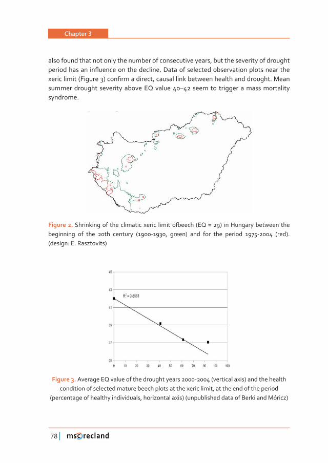
Chapter 3
78
also found that not only the number of consecutive years, but the severity of drought �������������� ��ƪ��������������������Ǥ���������������������������������������������������������ȋ������Ȍ����Ƥ�����������ǡ���������������������������������������Ǥ������summer drought severity above EQ value 40–42 seem to trigger a mass mortality syndrome.
Figure 2.�������������� ������������������� �������Ɵ�����ȋ���γ�Ȍ� �����������������������beginning of the 20th century (1900-1930, green) and for the period 1975-2004 (red). (design: E. Rasztovits)
Figure 3. Average EQ value of the drought years 2000-2004 (vertical axis) and the health condition of selected mature beech plots at the xeric limit, at the end of the period
(percentage of healthy individuals, horizontal axis) (unpublished data of Berki and Móricz)
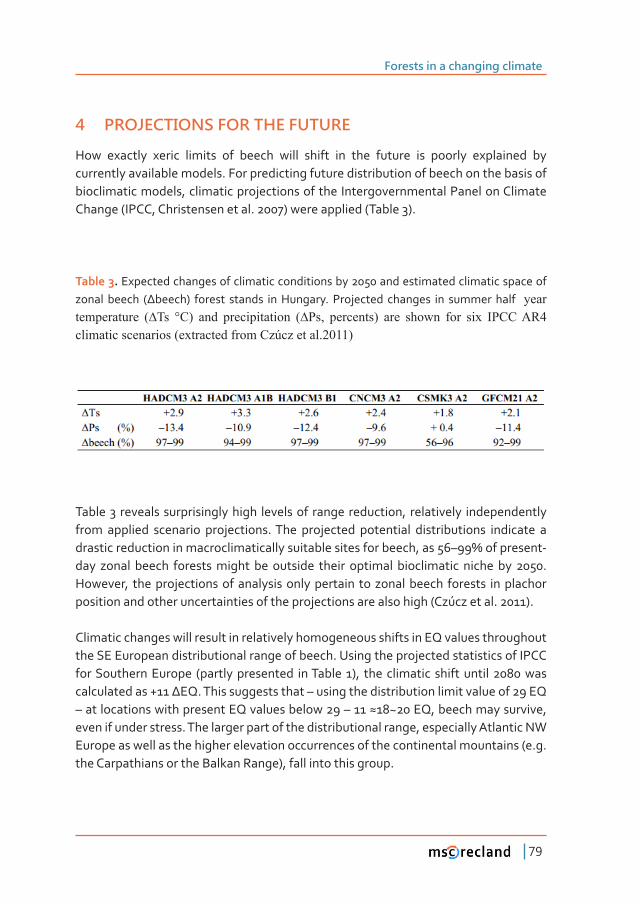
Forests in a changing climate
79
4 PROJECTIONS FOR THE FUTURE
How exactly xeric limits of beech will shift in the future is poorly explained by currently available models. For predicting future distribution of beech on the basis of bioclimatic models, climatic projections of the Intergovernmental Panel on Climate Change (IPCC, Christensen et al. 2007) were applied (Table 3).
Table 3. Expected changes of climatic conditions by 2050 and estimated climatic space of ������ ������ ȋρ�����Ȍ� ������� ������� ����������Ǥ����������� �������� ��� ������������ �year WHPSHUDWXUH� �¨7V� �&�� DQG� SUHFLSLWDWLRQ� �¨3V�� SHUFHQWV�� DUH� VKRZQ� IRU� VL[� ,3&&�$5��FOLPDWLF�VFHQDULRV��H[WUDFWHG�IURP�&]~F]�HW�DO������
Table 3 reveals surprisingly high levels of range reduction, relatively independently from applied scenario projections. The projected potential distributions indicate a ���������������������������������������������������������������ǡ����Ȃά�����������Ǧday zonal beech forests might be outside their optimal bioclimatic niche by 2050. However, the projections of analysis only pertain to zonal beech forests in plachor position and other uncertainties of the projections are also high (Czúcz et al. 2011).
Climatic changes will result in relatively homogeneous shifts in EQ values throughout the SE European distributional range of beech. Using the projected statistics of IPCC for Southern Europe (partly presented in Table 1), the climatic shift until 2080 was ��������������ή�ρ��Ǥ��������������������Ȃ�������������������������������������������Ȃ��������������������������������������������Ȃ��ε���ǡ������������������ǡ�even if under stress. The larger part of the distributional range, especially Atlantic NW Europe as well as the higher elevation occurrences of the continental mountains (e.g. the Carpathians or the Balkan Range), fall into this group.
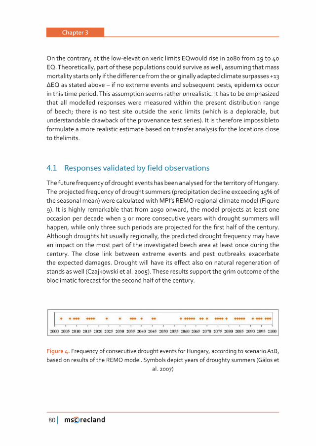
Chapter 3
80
On the contrary, at the low-elevation xeric limits EQwould rise in 2080 from 29 to 40 EQ. Theoretically, part of these populations could survive as well, assuming that mass �������������������������������ơ�����������������������������������������������������ή�ρ�������������������Ȃ������������������������������������������ǡ�����������������in this time period. This assumption seems rather unrealistic. It has to be emphasized that all modelled responses were measured within the present distribution range of beech; there is no test site outside the xeric limits (which is a deplorable, but understandable drawback of the provenance test series). It is therefore impossibleto formulate a more realistic estimate based on transfer analysis for the locations close to thelimits.
4�1 Responses validated by field observations
The future frequency of drought events has been analysed for the territory of Hungary. �������������������������������������������ȋ��������������������������������ά����the seasonal mean) were calculated with MPI’s REMO regional climate model (Figure 9). It is highly remarkable that from 2050 onward, the model projects at least one occasion per decade when 3 or more consecutive years with drought summers will ������ǡ�����������������������������������������������������Ƥ�����������������������Ǥ�Although droughts hit usually regionally, the predicted drought frequency may have an impact on the most part of the investigated beech area at least once during the century. The close link between extreme events and pest outbreaks exacerbate ��������������������Ǥ������������������� �����ơ������������������������������������stands as well (Czajkowski et al. 2005). These results support the grim outcome of the bioclimatic forecast for the second half of the century.
Figure 4. Frequency of consecutive drought events for Hungary, according to scenario A1B, based on results of the REMO model. Symbols depict years of droughty summers (Gálos et
al. 2007)
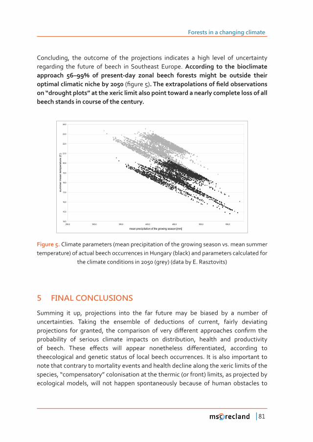
Forests in a changing climate
81
Concluding, the outcome of the projections indicates a high level of uncertainty regarding the future of beech in Southeast Europe. ���������� ��� ���� �������������������� Ȃά� ��� �������Ǧ���� ������ ������ �������� ������ ��� �������� ���������������������������������ȋƤ�����ȌǤ�����������������������Ƥ��������������������Dz�������������dz���������������������������������������������������������������������������������������������������������Ǥ
14,0
15,0
16,0
17,0
18,0
19,0
20,0
21,0
22,0
23,0
24,0
250,0 300,0 350,0 400,0 450,0 500,0 550,0
mean precipitation of the growing season [mm]
sum
mer
mea
n te
mpe
ratu
re (C
)
Figure 5. Climate parameters (mean precipitation of the growing season vs. mean summer temperature) of actual beech occurrences in Hungary (black) and parameters calculated for
the climate conditions in 2050 (grey) (data by E. Rasztovits)
5 FINAL CONCLUSIONS
Summing it up, projections into the far future may be biased by a number of uncertainties. Taking the ensemble of deductions of current, fairly deviating ������������ ���� �������ǡ� ���� ����������� ��� ����� ��ơ������ ����������� ���Ƥ��� ����probability of serious climate impacts on distribution, health and productivity ��� �����Ǥ� ������ �ơ����� ����� ������� ������������ ��ơ����������ǡ� ���������� ���theecological and genetic status of local beech occurrences. It is also important to note that contrary to mortality events and health decline along the xeric limits of the �������ǡ�Dz������������dz�����������������������������ȋ��������Ȍ�������ǡ�����������������ecological models, will not happen spontaneously because of human obstacles to
Chapter 3
82
colonisation and due to the fairly lowmigration speed of beech compared to other deciduous species (Davis 1981, Mátyás 2009, Jump et al. 2009).
Observations of mortality events close to the lower (xeric) limit of the species indicate that ���������� ���� ��������� ��� ������������ ������� ���� ����� ��� ������� ��� ��������������Ǥ������������������������ȋ��������Ȍ������������������������������������������������������������������������������������������������������������������������ �������� ���������� ��������� ���� ���� �������Ǥ The shrinking of future distribution of beech as suggested by various bioclimatic models (e.g. Thuiller et al. 2005, Czúcz et al. 2011) represent probably pessimistic scenarios which may be alleviated not ����� ��� �������������� ��������� ���� ����� ��� �������� ������ �������� ȋ�Ǥ�Ǥ� ����Ƥ�����regeneration and other silvicultural measures, see Mátyás 2010). In the major part of the range the predicted changes will not trigger any decline due to the plasticity of �����������ǣ���������������Dz����������dz���������������ȋ ���ǡ���������� ȌǤ����������be however misleading to expect the same level of persistence and plasticity at the threatened xeric limits as across the rest of the range.
Therefore the forecasts have to be taken serious close to the xeric limits, and especially at low elevations. Field observations near the retracting distributional ����������Ƥ���������������������������������������������������������ȋ��������������Ǥ�2007, Berki et al. 2009). Considering the rapid shrinking of suitable bioclimatic space and the increasing selection pressure of abiotic and biotic stressors at the xeric limits, the results underline the importance of adaptive strategies both for management ������������������������������������Ǥ�����������������������������ǡ���������������Ƥ����studies and further development of prediction methods and modelling (Mátyás 2010).
The results of this study may contribute to the adjustment of adaptation and mitigation policy in forestry and nature conservation, to the revision of rules for deployment of reproductive material and also to validating evolutionary and ecological hypotheses ���������������������������ơ����Ǥ
5�1 Related websites, projects and videos
Forest cover maps, forest type maps for Europe:
http://forest.jrc.ec.europa.eu/activities/forest-mapping/
http://forest.jrc.ec.europa.eu/efdac/applications/viewer/
Forests in a changing climate
83
http://www.euforgen.org/distribution_maps.html
forests and climate change (on maps): http://forest.jrc.ec.europa.eu/activities/climate-change/
climate change impacts on forestry: http://www.forestry.gov.uk/fr/INFD-5Y2HR7
IPCC AR4: Forestry: http://www.ipcc.ch/publications_and_data/ar4/wg3/en/ch9.html
REFERENCES
Berki, I. – Rasztovits, E. – Móricz, N. – Mátyás, C. (2009): Determination of the drought tolerance limit of beech forests and forecasting their future distribution in Hungary. Cereal Research Communications, 37: 613–616.
Bolte, A. – Czajkowski, T. – Kompa, T. (2007): The north-eastern distribution range of European beech – a review. Forestry, 80 (4): 413–429.
Christensen, J.H. – Hewitson, B. – Busuioc, A. – Chen, A. – Gao, X. – Held, I. et al. (2007): Regio-nal Climate Projections. In: Solomon, S., Qin, D., Manning, M., Chen, Z., Marquis, M., Averyt, K.B., Tignor, M. & Miller, H.L. (eds) Climate Change 2007: The Physical Science Basis. Contri-bution of Working Group I to the Fourth Assessment Report of the Intergovernmental Panel on Climate Change. Cambridge University Press, Cambridge, UK. 747–845.
����������ǡ��Ǥ�Ȃ����������Ǥ�Ȃ��������Ǥ�ȋȌǣ����ƪ����������������������������� ����������das Wachstum von Naturverjüngungen der Buche (Fagus sylvatica L.) im nordöstlichen Mit-teleuropa, Allg. Forst- u. Jagdztg. 176: 133–143.
Czúcz B., Gálhidy L. & Mátyás C. (2011). Present and forecasted xeric climatic limits of beech and sessile oak distribution at low altitudes in Central Europe. Ann. For. Sci., 68(1), 99-108
Davis, M. (1981): Quaternary history and stability of forest communities. In: West, D.C., et al. (ed.): Forest succession: concept and application. Springer, New York, 132–153
Ellenberg, H. (1988): Vegetation ecology of Central Europe, 4thed., Cambridge University Press Gálos, B. – Lorenz, Ph. – Jacob, D. (2007): Will dry events occur more often in Hungary in the futu-
re? Env. Res. Letters, 2: 034006 (9pp) doi: 10.1088/1748-9326/2/3/034006 Jump, A.S. – Peñuelas, J. (2005): Running to stand still: adaptation and the response of plants to
rapid climate change. Ecology Lett. 8: 1010–1020 Jump, A. – Mátyás, C. – Peñuelas, J. (2009): The paradox of altitude for latitude comparisons in
species range retractions. (Review) Trends in Ecology and Evolution, 24: 12, 694–700, doi: 10.1016/j.tree.2009.06.007
Kölling, C. (2007): Klimahüllen von 27 Waldbaumarten. AFZ - der Wald, 23: 1242–1244 Kramer, K. – Degen, B. – Buschbom, J. – Hickler, T. – Thuiller, W. – Sykes, M. –De Winter,W. (2010):
Modelling exploration of the future of European beech (Fagus sylvatica L.) under climate change – Range, abundance, genetic diversity and adaptive response. For. Ecol. Managem., 259: 2213–2222.
Lakatos, F. – Molnár, M. (2009): Mass mortality of beech on Southwest Hungary. Acta Silvatica & Ligniaria Hung., 5: 75-–82
������ǡ��Ǥ�ȋȌǣ���������Ƥ��������������������������������������������������������������������ǫ���ǣ�Koskela, J., Buck, A., Teissier DU Cros, E. (eds.): Climate change and forest genetic diversity:
Chapter 3
84
Implications for sustainable forest management in Europe. Bioversity International, Rome, 53–69
Mátyás, C. (2009): Ecological challenges of climate change in Europe’s continental, droughtth-reatened Southeast. In: Groisman, P.Y. –Ivanov S.V. (eds.): Regional aspects of climateter-restrial-hydrologic interactions in non-boreal Eastern Europe. NATO Science Series, Springer Verl., 35–46
Mátyás C. (2010): Forecasts needed for retreating forests (Opinion) Nature, 464: Apr. 29, 1271 Mátyás, C. – VENDRAMIN, G. – FADY, B. (2009): Forests at the limit: evolutionary-genetic con-
sequences of environmental changes at the receding (xeric) edge of distribution. Ann. of Fo-rest Sci., 66: 800–803
Mátyás C., Berki I., Czúcz B., Gálos B., Móricz N. & Rasztovits E. (2010). Future of beech in Sout-heast Europe from the perspective of evolutionary ecology. Acta Silv. & Lign. Hung., 6, 91-110
Thuiller, W. – Richardson, D.M. – Pyšek, P. – Midgley, G.F. – Hughes, G.O. – Rouget, M. (2005): Ni-che-based modelling as a tool for predicting the risk of alien plant invasions at a global scale. Global Change Biol. 11: 2234–2250
Worral,J.J. – Egeland, L. – Eager, T. – Mask, R.A. – Johnson, E.W. – Kemp, P.A. – Shepperd,W.D. (2008): Rapid mortality of Populus tremuloidesin Southwestern Colorado, USA. For. Ecol. Managem., 255: 686–696
85
Chapter 2.3
University of
West Hungary,
Sopron, Hungary
Afforestation for Restoration of Land and Climate Change Mitigation, Part 3�
Structure and functioning of forest ecosystemsAttila Eredics Norbert MóriczAndrás BidlóCsaba Mátyás
1 Forest microclimate and microclimate measuring techniques
1�1 Introduction
Microclimatology is the study of climate on a small scale, as of a city, a valley, but even a hole in the tree trunk has its own microclimate. The microclimate of the forest is one of the most complicated amongst other land cover forms. The reasons for complexity are the levelled structure, the annual variability and the fact that not only ��������������ƪ�����������������ǡ����������������������ơ�������������������������Ǥ������dynamic feedback makes the description and modelling of the forest microclimate �������ƥ����Ǥ������������������������������������������������������������������������� �����ơ�������������������������������������Ǥ������Ƥ������������������������basics of micrometeorology, the structure of the boundary layer and the exchange of energy and water. Typical microclimatological situations such as land-sea and ��������Ǧ������� ������������� ���� ������ ����� ���ƪ���� ���� ��������Ǥ� ������� �����a certain vertical structure, which further complicates the processes. During the vegetation period the canopy is the active surface for the energy transformation, ���� ���� ������ ������ ���� ����� ������� ��ơ������ ������������� ���������� ��� ����horizontal structure. By changing the density and distribution of the canopy, forest ����������������ƪ����������������������������������������������������������������Ǥ�Lastly basic microclimatological measurement techniques are discussed.
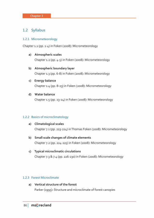
Chapter 3
86
1�2 Syllabus
1�2�1 Micrometeorology
Chapter 1.1 (pp. 1-4) in Foken (2008): Micrometeorology
�Ȍ� ������������������
Chapter 1.2 (pp. 4-5) in Foken (2008): Micrometeorology
�Ȍ� ��������������������������
Chapter 1.3 (pp. 6-8) in Foken (2008): Micrometeorology
�Ȍ� Energy balance
Chapter 1.4 (pp. 8-23) in Foken (2008): Micrometeorology
�Ȍ� Water balance
Chapter 1.5 (pp. 23-24) in Foken (2008): Micrometeorology
1�2�2 Basics of microclimatology
�Ȍ� Climatological scales
Chapter 7.1 (pp. 223-224) in Thomas Foken (2008): Micrometeorology
�Ȍ� ���������������������������������������
Chapter 7.2 (pp. 224-225) in Foken (2008): Micrometeorology
�Ȍ� ����������������������������������
Chapter 7.3 & 7.4 (pp. 226-230) in Foken (2008): Micrometeorology
1�2�3 Forest Microclimate
�Ȍ� ��������������������������������
Parker (1995): Structure and microclimate of forest canopies
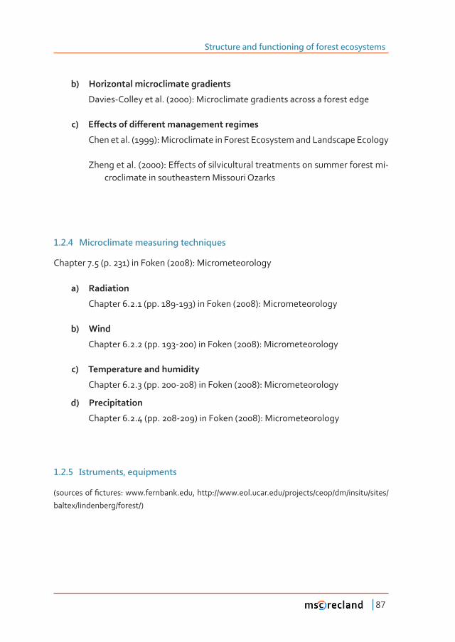
Structure and functioning of forest ecosystems
87
�Ȍ� Horizontal microclimate gradients
Davies-Colley et al. (2000): Microclimate gradients across a forest edge
�Ȍ� �ơ����������ơ������������������������
Chen et al. (1999): Microclimate in Forest Ecosystem and Landscape Ecology
�����������Ǥ�ȋȌǣ��ơ����������������������������������������������������-croclimate in southeastern Missouri Ozarks
1�2�4 Microclimate measuring techniques
Chapter 7.5 (p. 231) in Foken (2008): Micrometeorology
�Ȍ� Radiation
Chapter 6.2.1 (pp. 189-193) in Foken (2008): Micrometeorology
�Ȍ� Wind
Chapter 6.2.2 (pp. 193-200) in Foken (2008): Micrometeorology
�Ȍ� ������������������������
Chapter 6.2.3 (pp. 200-208) in Foken (2008): Micrometeorology
�Ȍ� �������������
Chapter 6.2.4 (pp. 208-209) in Foken (2008): Micrometeorology
1�2�5 Istruments, equipments
ȋ�����������Ƥ������ǣ����Ǥ��������Ǥ���ǡ�����ǣȀȀ���Ǥ���Ǥ����Ǥ���Ȁ��������Ȁ����Ȁ��Ȁ������Ȁ�����Ȁ
baltex/lindenberg/forest/)
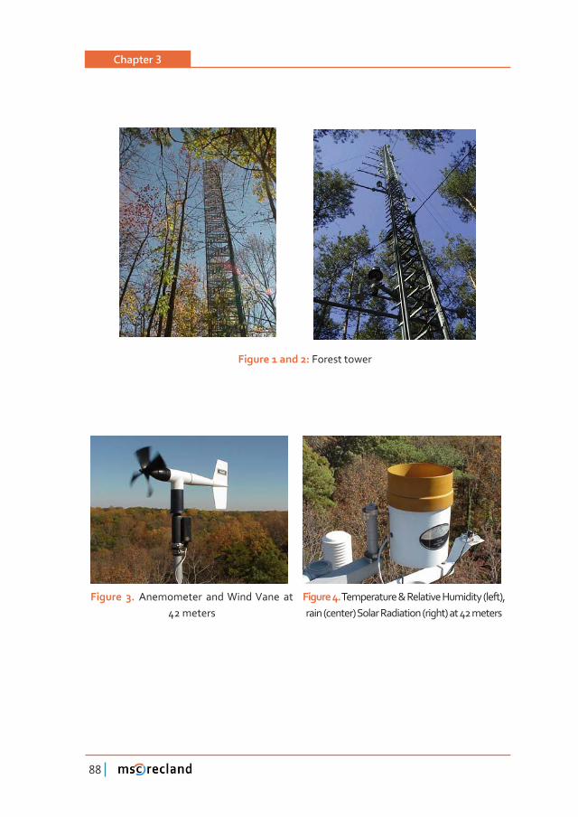
Chapter 3
88
Figure 1 and 2: Forest tower
Figure 3. Anemometer and Wind Vane at 42 meters
Figure 4. Temperature & Relative Humidity (left), rain (center) Solar Radiation (right) at 42 meters
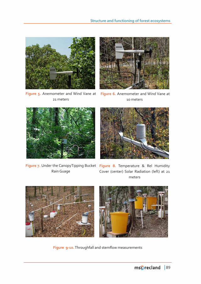
Structure and functioning of forest ecosystems
89
Figure 5. Anemometer and Wind Vane at
21 meters Figure 6. Anemometer and Wind Vane at
10 meters
Figure 7. Under the CanopyTipping Bucket Rain Guage
Figure 8. Temperature & Rel Humidity Cover (center) Solar Radiation (left) at 21
meters
Figure 9-10.���������������������ƪ���������������
Chapter 3
90
RELATED WEBSITES, PROJECTS AND VIDEOS
�������������������������ǣ�
http://forest.jrc.ec.europa.eu/activities/forest-ecosystem-services/
http://www.youtube.com/watch?v=-FVlvWjJeTQ
�������������� ������������������������������ ������ǡ������� ���� ������� ������ȋ������Ȍǣ�
http://www.ileaps.org/?q=node/66
forest microclimate research:
http://www.safeproject.net/projects/earth-atmosphere-linkages/microclimate/������������Ǧ������Ƥ������Ǧ��Ǧ����Ƥ��Ǧ�������Ȁ
http://www.serc.si.edu/labs/forest_ecology/microclimate.aspx
http://www.wsl.ch/fe/walddynamik/projekte/BelCanClim/index_EN
http://www.youtube.com/watch?v=hqVi90B5UOg
REFERENCES
Chen, J., Saunders, S. C., Crow, T. R., Naiman, R. J., Brosofske, K. D., Mroz, G. D., Brookshire, B. L., Franklin, J. F. (1999): Microclimate in Forest Ecosystem and Landscape Ecology. (Variations in local climate can be used to monitor and compare �����ơ����������ơ������������������������Ȍ���������������Ǥ����Ǥ�Ǥ�
Davies-Colley, R. J., Payne, G. W., Elswijk, M. (2000): Microclimate gradients across a forest edge. New Zealand Journal of Ecology (2000) 24(2):111-121.
Foken, T. (2008): Micrometeorology. Springer-Verlag Berlin Heidelberg. ISBN: 978-3-540-74665-2 e-ISBN: 978-3-540-74666-9
Structure and functioning of forest ecosystems
91
Parker, G. G. (1995): Structure and microclimate of forest canopies. Chapter 4 in Lowman, M.D. and Nadkarni, N.M. (eds.) 1995. Forest Canopies. Academic Press 624 pp.
�����ǡ��Ǥǡ�����ǡ� Ǥǡ�����ǡ��Ǥǡ���ǡ��Ǥǡ������ǡ��Ǥǡ� �����ǡ��Ǥ�ȋȌǣ��ơ����������������������treatments on summer forest microclimate in southeastern Missouri Ozarks. Climate Research Vol. 15: 45-59.
�������������������������������ǣ
Chen_(1999)_Microclimate_in_forest_ecosystem.pdf
Davies-Colley_(2000)_Microclimate_gradients_across_a_forest_edge.pdf
Foken_(2008)_Micrometeorology_Chapter_1.1-1.5.pdf
Foken_(2008)_Micrometeorology_Chapter_6.2.1-6.2.4.pdf
Foken_(2008)_Micrometeorology_Chapter_7.1-7.5.pdf
Parker_(1995)_Structure_and_microclimate_of_forest_canopies.pdf
�����ȋȌ�ơ�����������������������������Ǥ���
2 ROLE OF FOREST COVER IN THE HYDROLOGICAL CYCLE - CASE STUDY OF MEASUREMENTS AND MODELLING
2�1 Introduction
Land-atmosphere interactions related to the energy and water cycle are linked by the processes of evapotranspiration. Evapotranspiration is a collective term for all the processes, by which water in the liquid or solid phase at or near the earth’s land surfaces becomes atmospheric water vapour (Dingman 2002). It is the sum of transpiration, interception, bare soil evaporation and evaporation from open water and snow.
Transpiration is the vaporization of water from the saturated interior surfaces of leaves to the surrounding air via microscopic pores called stomata (Hungate and Koch 2003). Stomata open and close in response to environmental factors such as light,
Chapter 3
92
temperature, CO2 concentration and soil water. Interception is the part of the rainfall, which evaporates from the vegetation during and after the precipitation event. Bare soil evaporation is the vaporization of water directly from the mineral soil surface. It is only a small amount under forests because of the litter on the ground (Hewlett 1982).
����������� ��� ���������� ��ƪ�������� ���� ������ ������� �������� ������������� �����������������ǡ������������ơ����������������������������������������������������������Ǥ
����� ����� ������ ȋ���Ȍ� ��� ��Ƥ���� ��� �� ���� ������ ������ ����� ����� ���� ����� ������������ ȋ������ ȌǤ� ��� �ơ����� ���� ���������� ��������� ��������������� ���� ������� ����evapotranspiration from the plant surface. LAI varies temporally with age and ���������Ǥ� ���� ������ ��ơ���� ��������� ������ ������ �����������Ǥ�������������� ��� ��×�ȋȌ�������������������������������������ȋ�����Ǥ����ǤȌ������ơ����������������forest types depending on age and site conditions.
Forests have larger leaf area compared to other vegetated surfaces. Larger LAI warms the surface due to lower albedo. But larger LAI also results in larger roughness length ����� ������� ������������������� ����� ��� �������� ȋ������ ��� ��Ǥ� Ȍǡ������� ��ƪ�����������������������������������������������������ƪ����Ǥ���������������������������������ƪ�������������������������������������������������������������������������������Ǥ��������������������������������������������ơ���ǡ�����������������������������������������feedback of forests on climate. It dominates primarily on the tropical regions leading to cooler and moister atmospheric boundary layer that may feed back to increased �������������� ��� �ơ������� ���� ������Ǧ������ ������������ ȋ�������� ǡ� �������� ��� ��Ǥ�2007).
������������Ƥ������ ��������������������������������ơ�����������������������������������in the canopy. Larger leaf area increase the canopy shading, which leads to cooler air temperatures in the stem area, decrease of net radiation at the soil surface, therefore less bare soil evaporation in summer (Pitman 2003, Chang 2006).
Due to the higher evaporation rate, forests may increase the amount of precipitation. Chang (2006) summarizes the arguments and counterarguments to the possible precipitation-increasing role of forests. It is often assumed that forests enhance the ����������������������������������������ơ��������������������������ǡ����������������an increase of the orographic precipitation. The higher transpiration rate of forests can lead to the increased vapour content of the air, which promotes the condensation and precipitation formation in the forested area. The basic counterargument is that
Structure and functioning of forest ecosystems
93
��������������������������������������������������������ơ���������������������������������and topographic characteristics rather than by forests. For the precipitation formation water vapour content is not enough (Chang 2006).
���������������������������ǡ������������������������������������Ƥ���������������������Ǥ�Rooting depth and the soil texture determine the amount of water that can be stored in the soil, which is potentially available to the vegetation for transpiration (Kleidon ������������ȌǤ�������������������������������������������Ƥ�������������ơ���������������Ƥ�������������ȋ������������������������������������������������Ȍ�������������point (the amount of water in the soil when evapotranspiration ceases; Bonan 2004). Rooting depths have a large variability depending on plant species soil texture and soil water conditions.
Deep roots increase the water uptake and the amount of transpiration. It is an important characteristic in dry spells when moisture of advective origin diminishes. If there is enough moisture in the soil to continue evapotranspiration, local evapotranspiration can be an important contributor to precipitation.
2�2 Case study: Comparative Water Balance Study of Forest and Fallow Plots
2�2�1 Background
The relationship of vegetation cover and groundwater resources has drawn ��������������������Ƥ���������������������������������Ǥ����������������������������������������������������������������������������ȋ�������Ƥ��ǡ������������Ȍ���������������������������ơ�����������ơ�����������ȋ�Ǥ�Ǥ�������Ƭ���������Ȍ������ơ�������������������������ơǤ��������� ���������������������� ��� �������������������������������depth, predominantly in dry regions. In Australia changes of vegetation from woodland to grassland or crops resulted in increases in recharge rates of one to two orders of magnitude (Maitre et al. 1999). The changes were largely due to the altered interception loss and the increased water extraction from the root zone. However, results of paired watershed research agreed only on the direction of the changes, not on their magnitude (Andressian 2004).
Chapter 3
94
Comparative water balance studies of forest and low vegetation covers have generally shown higher water use of forest cover (Nachabe et al. 2005, Schilling 2007). Nachabe et al. (2005) analysed the groundwater consumption in a shallow water table environment and estimated the annual ET for a forested area (1320 mm) and for a pasture (700 mm) using detailed soil moisture and water table monitoring. At the ���������ǡ���������������������������������������ơ�����������������������������������ơ������������������������ȋ�Ǥ�Ǥ���������Ƭ��������ȌǤ����������������������������ǡ���������� ����������� ��������� ��ơ�������ǡ� ��� ��� ������� �����ǡ� ���� �������������������������������������������������Ƥ���������ơ����������������������������Ǥ
���������������������ǡ����� ������������ ��������������� ����������Ƥ�������������������century (IPCC 2007). As a direct consequence of warmer temperatures, the hydrologic cycle will undergo changes with accompanying alteration in the rates of precipitation and evaporation. In Hungary, summer temperatures may increase by up to four degrees by the end of this century, while precipitation is likely to increase in winter and decrease in summer (Gálos et al. 2007).
The impact of climate change on groundwater resources was reviewed lately by Green et al. (2011). Although the uncertainty of predictions for change in groundwater recharge rates and discharge is large (e.g. future climate scenarios and groundwater extraction), numerous studies found that groundwater resources appear to be threatened by future climate change due to increased natural and human water demand.
In light of the water balance uncertainties and the increasing pressures on groundwater resources due to future climate change, a comparative water balance study of an oak forest and fallow vegetation plots was initiated in a drought-threatened lowland environment in Northeastern Hungary. Water balance components were estimated by the Hydrus 1-D numerical model (Simunek et al. 2005), calibrated on measured soil moisture and groundwater levels.
2�2�2 Materials and methods
Study area
The study plots are situated in the Northeast part of Hungary at latitude 47° 58’ N and longitude 21° 42’ E (Fig. 11), built up from sandy river deposits of the early Pleistocene (Borsy et al. 1981). The climte is continental; the mean annual precipitation (1951-
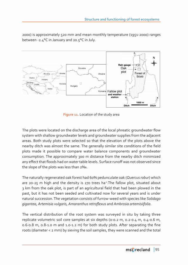
Structure and functioning of forest ecosystems
95
2000) is approximately 520 mm and mean monthly temperature (1951-2000) ranges between -2.4°C in January and 20.5°C in July.
Figure 11. Location of the study area
�������������������������������������������������������������������������������ƪ���system with shallow groundwater levels and groundwater supplies from the adjacent areas. Both study plots were selected so that the elevation of the plots above the ��������������������������������Ǥ����������������������������������������������Ƥ����plots made it possible to compare water balance components and groundwater consumption. The approximately 300 m distance from the nearby ditch minimized �����ơ���������ƪ������������������������������Ǥ�������������ơ������������������������the slope of the plots was less than 2‰.
�����������������������������������������ά�����������������ȋQuercus robur) which are 20-25 m high and the density is 270 trees ha-1.The fallow plot, situated about ���������������������ǡ� ���������������������������Ƥ������������������������� �������past, but it has not been seeded and cultivated now for several years and is under natural succession. The vegetation consists of furrow-weed with species like Solidago ��������ǡ�������������������ǡ�����������������ƪ�����and Ambrosia artemisiifolia.
The vertical distribution of the root system was surveyed in situ by taking three replicate volumetric soil core samples at six depths (0-0.2 m, 0.2-0.4 m, 0.4-0.6 m, ǤǦǤ��ǡ�ǤǦǤ�������ǤǦǤ��Ȍ� ��������� �����������Ǥ������� ����������� ����Ƥ���roots (diameter < 2 mm) by sieving the soil samples, they were scanned and the total
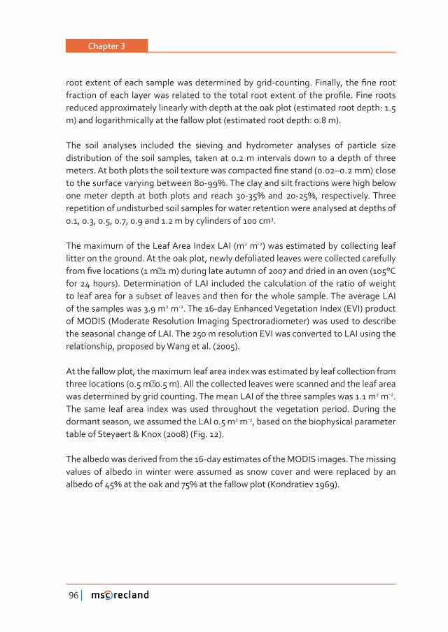
Chapter 3
96
�������������������������������������������������Ǧ��������Ǥ�������ǡ� ����Ƥ������������������������� ������������������������������� ��������������� �������Ƥ��Ǥ�����������reduced approximately linearly with depth at the oak plot (estimated root depth: 1.5 m) and logarithmically at the fallow plot (estimated root depth: 0.8 m).
The soil analyses included the sieving and hydrometer analyses of particle size distribution of the soil samples, taken at 0.2 m intervals down to a depth of three ������Ǥ����������������������������������������������Ƥ���������ȋǤȂǤ���Ȍ��������������������������������������ǦάǤ������������������������������������������������������� ������ ��� ����� ������ ���� ������ Ǧά� ���� Ǧάǡ� ������������Ǥ�������repetition of undisturbed soil samples for water retention were analysed at depths of 0.1, 0.3, 0.5, 0.7, 0.9 and 1.2 m by cylinders of 100 cm3.
The maximum of the Leaf Area Index LAI (m2 m-2) was estimated by collecting leaf litter on the ground. At the oak plot, newly defoliated leaves were collected carefully �����Ƥ�������������ȋ�����Ȍ���������������������������������������������ȋλ��for 24 hours). Determination of LAI included the calculation of the ratio of weight to leaf area for a subset of leaves and then for the whole sample. The average LAI of the samples was 3.9 m2 m-2. The 16-day Enhanced Vegetation Index (EVI) product of MODIS (Moderate Resolution Imaging Spectroradiometer) was used to describe the seasonal change of LAI. The 250 m resolution EVI was converted to LAI using the relationship, proposed by Wang et al. (2005).
At the fallow plot, the maximum leaf area index was estimated by leaf collection from ����������������ȋǤ���Ǥ��ȌǤ���������������������������������������������������������was determined by grid counting. The mean LAI of the three samples was 1.1 m2 m-2. The same leaf area index was used throughout the vegetation period. During the dormant season, we assumed the LAI 0.5 m2 m-2, based on the biophysical parameter table of Steyaert & Knox (2008) (Fig. 12).
The albedo was derived from the 16-day estimates of the MODIS images. The missing values of albedo in winter were assumed as snow cover and were replaced by an ����������ά����������������ά��������������������ȋ�����������ȌǤ
Structure and functioning of forest ecosystems
97
Figure 12. Seasonal change of LAI (Oak plot: dashed line - MODIS data, solid line - applied in the model, Fallow plot: solid line - applied in the model).
�����������������������
Meteorological variables, soil water content and groundwater level were monitored by automatic equipment.
A weather station (iMETOS, Pessl Instruments, Austria) at the fallow plot and an automatic rain-gauge (Rainlog Data Logger, Rainwise, USA) 500m from the oak plot was employed to monitor weather conditions. The volumetric water content ���������������������� ȋ������������������ƪ����������Ȍ�����������������Ǧ�probes (Decagon Devices, Pullman, USA) with a time interval of 15 min. The probes were installed at depths of 0.1, 0.3, 0.5 and 0.7 m.Groundwater level was measured by a Dataqua DA-S-LRB 118 vented pressure transducer (Dataqua Elektronikai Kft., Balatonalmádi, Hungary) with time interval of 15 min. Manual groundwater level measurements were used to verify the reliability of the monitoring.
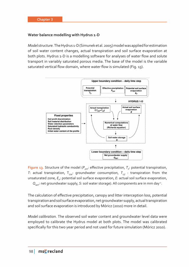
Chapter 3
98
������������������������������������Ǧ�
Model structure. The Hydrus 1-D (Simunek et al. 2005) model was applied for estimation of soil water content changes, actual transpiration and soil surface evaporation at ����������Ǥ��������Ǧ������������������������������������������������ƪ��������������transport in variably saturated porous media. The base of the model is the variable �������������������ƪ���������ǡ�������������ƪ����������������ȋ��Ǥ�ȌǤ
Figure 13. Structure of the model (PEFFǣ��ơ��������������������ǡ�TP: potential transpiration, T: actual transpiration, TGW: groundwater consumption, TUZ : transpiration from the unsaturated zone, EP: potential soil surface evaporation, E: actual soil surface evaporation,
QNET: net groundwater supply, S: soil water storage). All components are in mm day-1.
��������������������ơ��������������������ǡ������������������������������������ǡ�����������transpiration and soil surface evaporation, net groundwater supply, actual transpiration and soil surface evaporation is introduced by Móricz (2010) more in detail.
Model calibration. The observed soil water content and groundwater level data were employed to calibrate the Hydrus model at both plots. The model was calibrated �����Ƥ������������������������������������������������������������������ȋ�×�����ȌǤ
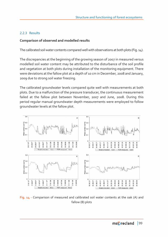
Structure and functioning of forest ecosystems
99
2�2�3 Results
�������������������������������������������
The calibrated soil water contents compared well with observations at both plots (Fig. 14).
The discrepancies at the beginning of the growing season of 2007 in measured versus ��������������������������������������������������������������������������������Ƥ���and vegetation at both plots during installation of the monitoring equipment. There were deviations at the fallow plot at a depth of 10 cm in December, 2008 and January, 2009 due to strong soil water freezing.
The calibrated groundwater levels compared quite well with measurements at both plots. Due to a malfunction of the pressure transducer, the continuous measurement failed at the fallow plot between November, 2007 and June, 2008. During this period regular manual groundwater depth measurements were employed to follow groundwater levels at the fallow plot.
Fig. 14 - Comparison of measured and calibrated soil water contents at the oak (A) and fallow (B) plots
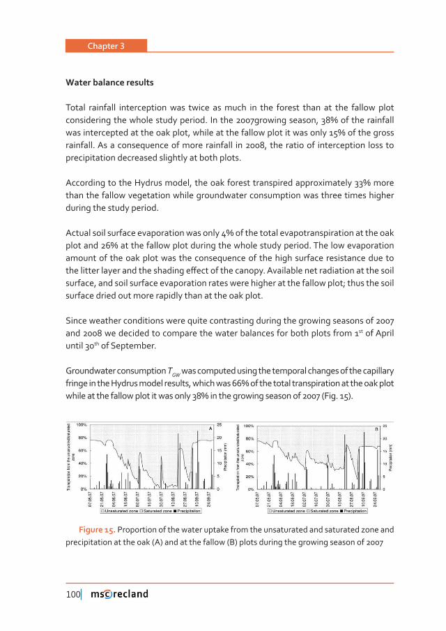
Chapter 3
100
Water balance results
Total rainfall interception was twice as much in the forest than at the fallow plot ����������������������������������Ǥ� ���������������������ǡ�ά������������������������������������������������ǡ��������������������������������������ά��������������rainfall. As a consequence of more rainfall in 2008, the ratio of interception loss to precipitation decreased slightly at both plots.
�����������������������������ǡ�����������������������������������������ά������than the fallow vegetation while groundwater consumption was three times higher during the study period.
�����������������������������������������ά�����������������������������������������������������ά�������������������������������������������������Ǥ���������������������amount of the oak plot was the consequence of the high surface resistance due to ����������������������������������ơ�����������������Ǥ�������������������������������������surface, and soil surface evaporation rates were higher at the fallow plot; thus the soil surface dried out more rapidly than at the oak plot.
Since weather conditions were quite contrasting during the growing seasons of 2007 and 2008 we decided to compare the water balances for both plots from 1st of April until 30th of September.
Groundwater consumption TGW was computed using the temporal changes of the capillary ����������������������������������ǡ����������� ά���������������������������������������������������������������������������������ά���������������������������ȋ��Ǥ�ȌǤ
Figure 15. Proportion of the water uptake from the unsaturated and saturated zone and precipitation at the oak (A) and at the fallow (B) plots during the growing season of 2007
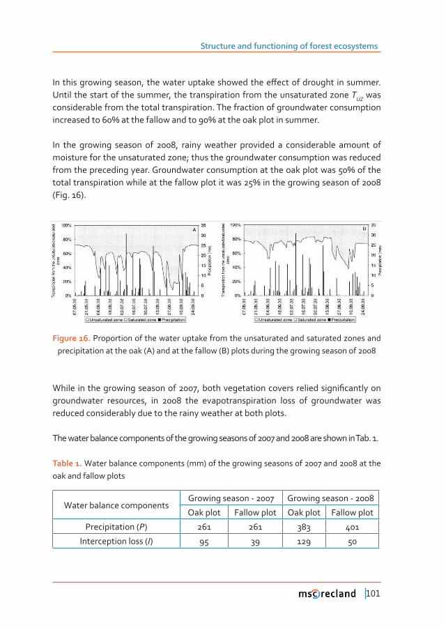
Structure and functioning of forest ecosystems
101
����������������������ǡ������������������������������ơ��������������� ���������Ǥ�Until the start of the summer, the transpiration from the unsaturated zone TUZ was considerable from the total transpiration. The fraction of groundwater consumption �������������ά����������������������ά��������������������������Ǥ
In the growing season of 2008, rainy weather provided a considerable amount of moisture for the unsaturated zone; thus the groundwater consumption was reduced �����������������������Ǥ��������������������������������������������ά������������������������������������������������������������ά���������������������������(Fig. 16).
Figure 16. Proportion of the water uptake from the unsaturated and saturated zones and precipitation at the oak (A) and at the fallow (B) plots during the growing season of 2008
������ �������������������������ǡ������������������������������������Ƥ����������groundwater resources, in 2008 the evapotranspiration loss of groundwater was reduced considerably due to the rainy weather at both plots.
The water balance components of the growing seasons of 2007 and 2008 are shown in Tab. 1.
Table 1. Water balance components (mm) of the growing seasons of 2007 and 2008 at the oak and fallow plots
Water balance componentsGrowing season - 2007 Growing season - 2008
Oak plot Fallow plot Oak plot Fallow plot
Precipitation (P) 261 261 383 401
Interception loss (I) 95 39 129 50
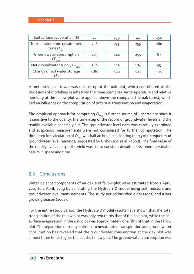
Chapter 3
102
Soil surface evaporation (E) 22 139 41 154
Transpiration from unsaturated zone (TUZ)
208 235 255 260
Groundwater consumption (TGW)
405 144 255 87
Net groundwater supply (QNET) 289 125 184 55
Change of soil water storage (S)
-180 -171 -112 -95
A meteorological tower was not set up at the oak plot, which contributed to the deviations of modelling results from the measurements. Air temperature and relative humidity at the fallow plot were applied above the canopy of the oak forest, which ���������ƪ�������������������������������������������������������������������Ǥ
The empirical approach for computing QNET is further source of uncertainty since it is sensitive to the quality, the time-step of the record of groundwater levels and the ������������������ �����Ƥ�������Ǥ����������������� ����������������������������������and suspicious measurements were not considered for further computation. The time-step for calculation of QNET was half an hour, considering the 15 min frequency of ��������������������������ǡ�����������������������������Ǥ�ȋȌǤ�����Ƥ����������������������������������������Ƥ�������������������������������������������������������������nature in space and time.
2�3 Conclusions
Water balance components of an oak and fallow plot were estimated from 1 April, 2007 to 1 April, 2009 by calibrating the Hydrus 1-D model using soil moisture and groundwater level measurements. The study period included a dry (2007) and a wet growing season (2008).
For the entire study period, the Hydrus 1-D model results have shown that the total transpiration of the fallow plot was only two thirds that of the oak plot, while the soil ����������������������������������������������������������Ƥ��������������������������plot. The separation of transpiration into unsaturated transpiration and groundwater consumption has revealed that the groundwater consumption at the oak plot was almost three times higher than at the fallow plot. The groundwater consumption was
Structure and functioning of forest ecosystems
103
���������������������������������������������������������������������������������fallow plot.
By comparing the dry (2007) and wet (2008) growing seasons, we found that �����������������������������������������������������������������������������growing season, despite the fact that the groundwater level was deeper during the dry period. Thus, during the dry season both vegetation covers relied considerably on the available groundwater resources.
The results of the study have reinforced those previous studies that reported higher groundwater consumption of forests compared to other vegetation covers. ���������ǡ���������ơ��������������������������������������������������������������������������������������������������������������������ơ�������������ǡ������������������������future climate change and human water extraction.
RELATED WEBSITES, PROJECTS AND VIDEOS
Forests and water (FAO): http://www.fao.org/docrep/010/a1598e/a1598e02.htmBooks: http://www.nap.edu/catalog.php?record_id=12223http://www.springer.com/earth+sciences+and+geography/earth+system+sciences/book/978-
94-007-1362-8Forest hydrology research: http://www.forestry.gov.uk/fr/HCOU-4U4JAMwater cycle animation: http://www.youtube.com/watch?v=0_c0ZzZfC8cland cover and hydrology of watersheds: http://www.youtube.com/watch?v=t632Bz8AQoUhttp://www.youtube.com/watch?v=t632Bz8AQoUhttp://www.youtube.com/watch?v=1Nr31_9jJY0&list=PL1JyimMkAKOibeSAzsLZVs56OjFU4p
vi7http://www.youtube.com/watch?v=2cFOYvtJejw&list=PLp5bLxICz17xssk-ftKyQ7zI62M0ExlOfhttp://www.youtube.com/watch?v=D0uAIOT66Wo&list=PLp5bLxICz17xssk-ftKyQ7zI62M0ExlOfhttp://www.youtube.com/watch?v=hU06Vir2Ipchttp://www.youtube.com/watch?v=4yT3nJiJ8Gc&list=PLC30C7F922760EE2F
REFERENCES
�������������ȋȌǤ�������������������ǣ���������������������������������������Ƥ��������Ǥ�Journal of Hydrology 291: 1-27.
Betts RA, PM Cox, SE Lee, FI Woodward (1997). Contrasting physiological and structural vegeta-tion feedbacks in climate change simulations. Nature 387: 796-799
Bonan GB (2004). Biogeophysical feedbacks between land cover and climate. In: R.S. DeFries, G.P. Asner, and R.A. Houghton (eds) Ecosystems and Land Use Change. Geophysical Mono-graph 153: 61-72, American Geophysical Union, Washington, D.C.
Chapter 3
104
Bonan GB (2008). Ecological climatology. Cambridge Univ. Press, Cambridge, ed. 2., 568pBorsy Z, Csongor É, Sárkány S, Szabó I (1981). Phases of blown-sand movements in the North-
East part of the Great Hungarian Plain. Acta Geogr. Debr. 20: 5-33.������ �ǡ��������� ��ȋȌǤ�����������������������������������������������������ơ���������-
getation changes on water yield and evapotranspiration. Journal of Hydrology 55: 3-23. Brovkin V (2002). Climate-vegetation interaction. J. Phys. IV France 12: 57-82 doi: 10.1051/
jp4:20020452Brutsaert W (1982). Evaporation into the atmosphere: theory, history, and applications. D.Reidel,
Hingham MA, 299 p.Cardon GE, Letey J (1992). Plant water uptake terms evaluated for soil water and solute move-
ment models. Soil Science Society of America Journal, 56 (6): 1876-1880.Chang M (2006). Forest Hydrology. An Introduction to Water and Forests. Taylor & Francis Group, USA Dingman S (2002). Physical Hydrology. Prentice Hall, Upper Saddle River. 646pFederer CA, Vörösmarty C, Fekete B (2003). Sensitivity of annual evaporation to soil and root pro-
perties in two models of contrasting complexity. Journal of Hydrometeorology 4: 1276-1290.Gash JHC (1979). An analytical model of rainfall interception by forests. Quarterly Journal of the
Royal Meteorological Society 105: 43-45.Gálos B, Lorenz Ph, Jacob D (2007). Will dry events occur more often in Hungary in the future?
Environmental Research Letters 2, 034006 (9pp) doi: 10.1088/1748-9326/2/3/034006Green TR, Taniguchi M, Kooi H, Gurdak JJ, Allen DM, Hiscock KM, Treidel H, Aureli A (2011). Be-
neath the surface of global change: Impacts of climate change on groundwater. Journal of Hydrology 405: 532-560.
�����������ǡ���������� ǡ����������ȋȌǤ���������ƪ���������������������������������������������������ƪ����������������������������������Ǧ���������ǡ� ���������������������ȋǦȌǣ�ǦǤ
Hewlett J D (1982). Principles of forest hydrology, The University of Georgia Press, Athens, GA 183p
Hydrus 1D for Windows, PC-PROGRESS (2008). [Online: 06 September 2011] URL: http://www.pc-progress.com/en/Default.aspx?HYDRUS-1D.
Hungate BA, GW Koch (2002). Global Environmental Change: Biospheric Impacts and Feedbacks. In J Holton, J Pyle, J Currie (eds.) Encyclopedia of Atmospheric Science Academic Press, Ltd. 876-885
IPCC 2007. Climate change 2007: Synthesis Report. Contribution of Working Groups I, II and III to the Fourth Assessment Report of the Intergovernmental Panel on Climate Change http//:www.ipcc.ch
��×���ȋȌǤ������±����ò��������������±��������Ý�À������Ǥ����±����������������ǣ�Ǧ�Justice CO, Townshend JRG, Vermote EF, Masuoka E, Wolfe RE, El-Saleous N et al. (2002). An
overview of MODIS land data processing and product status. Remote Sensing of Environ-ment 83: 3–15.
Kleidon A and M HEIMANN (1998). Optimised rooting depth and its impacts on the simulated cli-mate of an Atmospheric General Circulation Model. Geophysical Research Letters 25: 345-348
Kleidon A, K Fraedrich, C Low (2007). Multiple steady-states in the terrestrial atmosphere-bios-������������ǣ�����������������������������������������Ƥ������ǫ���������������ǡ�ǣ�Ǧ����ǣ�10.5194/bg-4-707-2007
Kondratiev KY (1969). Radiation in the Atmosphere. Academic Press, New York, USA.
Structure and functioning of forest ecosystems
105
Maitre DCL, Scott DF, Colvin C (1999). A review of information on interactions between vegeta-tion and groundwater. ������������������ 25: 137-152.
Móricz N (2010). Water Balance Study of a Groundwater-dependent Oak Forest. Acta ���������Ƭ������������������ 6: 49-66.
Nachabe M, Shah N, Ross M, Vomacka J (2005). Evapotranspiration of two vegetation covers in a shallow water table environment. Soil Science Society of America Journal 69: 492-499.
�������ȋȌǤ����������������ơǡ������������������ǡ� ������������������������������������������models. Int. J. of Climatol. 23: 479-510 doi: 10.1002/joc.893
Roberts J, Rosier P (2005). The impact of broadleaved woodland on water resources in lowland UK: I. Soil water changes below beech woodland and grass on chalk sites in Hampshire. Hy-drology and Earth System Sciences 9 (6): 596-606.
�������������ȋȌǤ�������������ƪ�������������������������������������������ǡ������ȋ���ȌǤ������-logical Processes 21: 2415-2424.
e��õ���� ǡ����������������ǡ�e�������ȋȌǤ�����������Ǧ����������������������������������the one-dimensional movement of water, heat, and multiple solutes in variably-saturated media. Version 3.0, HYDRUS Software Series 1, Department of Environmental Sciences, Uni-versity of California Riverside, Riverside, CA, pp. 270.
Steyaert LT, Knox RG (2008). Reconstructed historical land cover and biophysical parameters for studies of land-atmosphere interactions within the eastern United States. Journal of Geophy-sical Research 113, D02101, 27 PP, doi: 10.1029/2006JD008277.
Valente F, DAVID JS, GASH JHC (1997). Modelling interception loss for two sparse eucalypt and pine forests in central Portugal using reformulated Rutter and Gash analytical models. Jour-nal of Hydrology, 190: 141-162.
Van Genuchten, MT (1987). A numerical model for water and solute movement in and below the root zone. Research Report No 121, U.S. Salinity laboratory, USDA, ARS, Riverside, California, 221 1987.
Von Hoyningen-Hüne J (1983). Die Interception des Niederschlags in landwirtschaftlichen Be-ständen. Schriftenreihe des DVWK 57: 1-53.
Wang Q, Adiku S, Tenhunen J, Granier A (2005). On the relationship of NDVI with leaf area index in a decidiouos forest site. Remote Sensing of Environment 94: 244-255.
3 CARBON CYCLE: THE ROLE OF FOREST VEGETATION
3.1 Introduction
Climate regulation through carbon sequestration is one of the ecosystem services of forests. They are the largest terrestrial C pool thus can have an important role in climate change mitigation. Exchanges of carbon between forests and the atmosphere ������������ƪ���������������Ǧ�������������������������������Ǥ������������ǡ������������������ Ǧ� ����������� �ơ����������� ���� �������������� Ǧ� ���� ����������� �������� ���carbon storage. Forest soils are also an important pool of carbon. They too are a vital
Chapter 3
106
part of the carbon cycle and can act as both sources and sinks. Forest ecosystems-climate feedbacks under future climate conditions are still large unknowns.
Organic matter production of forests strongly depends on soil, hydrological, and climatic circumstances, at the xeric forest limit primarily on the recurrent summer droughts. In the comparison of climate zones, the strong correlation between organic matter production and climate is obvious. The above-ground dendromass responds strongly to the worsening of climate, irrespective of tree species, while the below-ground parts remain unchanged. The carbon content of humus and soil increases toward drier climate.
3�2 Ecosystem services of forests
There are a number of components to the broad range of ecological services that forests provide. These include (Sousson et al.,1995):
• ����������������������������������������������������������������������������ƪ���through the hydrological system;
• pollution control;
• the maintenance of soil quality and the provision of organic materials through leaf and branch fall;
• the limiting of erosion and protection of soil from the direct impact of rainfall;
• regulating climate (e.g. C-sequestration); and
• being key components of biodiversity both in themselves and as a habitat for other species.
This chapter will focus on the carbon cycle and sequestration of the forest ecosystems.
3�3 Carbon cycle of forests
Forests play a key role in the carbon cycle. Through the process of photosynthesis they ��������� ������������������������� �������������������� ȋƤ�����ȌǤ���������������������������������������������� �������ơ����������������������� ����ǡ� ����ǡ�����ǡ����������������ǡ���������ơ������������������������������������������Ǥ��������������������
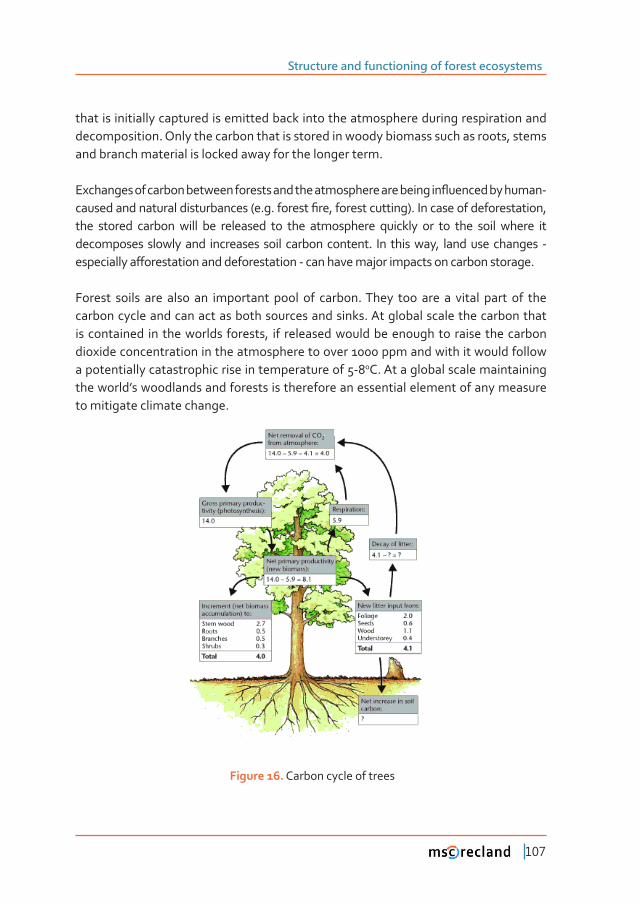
Structure and functioning of forest ecosystems
107
that is initially captured is emitted back into the atmosphere during respiration and decomposition. Only the carbon that is stored in woody biomass such as roots, stems and branch material is locked away for the longer term.
�������������������������������������������������������������������ƪ���������������Ǧ��������������������������������ȋ�Ǥ�Ǥ��������Ƥ��ǡ���������������ȌǤ�������������������������ǡ�the stored carbon will be released to the atmosphere quickly or to the soil where it decomposes slowly and increases soil carbon content. In this way, land use changes - ������������ơ�����������������������������Ǧ�����������������������������������������Ǥ
Forest soils are also an important pool of carbon. They too are a vital part of the carbon cycle and can act as both sources and sinks. At global scale the carbon that is contained in the worlds forests, if released would be enough to raise the carbon dioxide concentration in the atmosphere to over 1000 ppm and with it would follow a potentially catastrophic rise in temperature of 5-8oC. At a global scale maintaining the world’s woodlands and forests is therefore an essential element of any measure to mitigate climate change.
Figure 16. Carbon cycle of trees
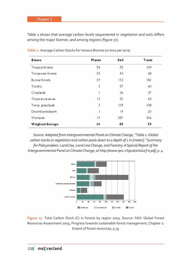
Chapter 3
108
������������������������������������������������������������������������������ơ��������������������������Ǥ�������������������ȋƤ�����ȌǤ
Table 2. Average Carbon Stocks for Various Biomes (in tons per acre)
������ǣ�������������������������������������������������������ǡ�Dz������ǣ��������������������������������������������������������������������������ȏ�����Ȑǡdz�������������������������ǣ���������ǡ�����Ǧ����������ǡ������������Ǥ�������������������������
�����������������������������������������ǡ��������ǣȀȀ���Ǥ����Ǥ��Ȁ���Ȁ��������Ǧ�Ǥ���ǡ��Ǥ�Ǥ�
Figure 17. Total Carbon Stock (C) in forests by region 2005. Source: FAO: Global Forest Resources Assessment 2005, Progress towards sustainable forest management, Chapter 2:
Extent of forest resources, p.35
Structure and functioning of forest ecosystems
109
The natural carbon sinks that can absorb and store carbon are ocean, forests, soil, peat and wetlands. In this way they can have an important role in climate change mitigation. Forest ecosystems are the largest terrestrial C pool of them. They store �����������ά�������������������������������������������������ά����������������������Ǥ������������Ǥ� ȋȌ����� ������������Ǥ� ȋȌ�����������������ơ������������������sequestration between boreal, tropical and temperate forests that should be analyzed together with their biogeophysical feedbacks on the climate to assess the possible �������������Ƥ����������������������Ǥ
Net-growing forests cause sequestration of C. After harvesting the life-cycle of the wood products is decisive. Therefore forest management and societal decisions ���������� �����Ƥ����� ��ƪ��������� ���� ��������������� ȋ ����� ��� ��Ǥ� ȌǤ�����Ƥ������������� �����Ƥ����� ������� ��� ���������� ������������������������ ��� �������� ����� ������������������������������������ȋ���������ơ���������������������������ȌǤ����������option is to foster the slow formation of a stabilized soil C pool. The C sequestration potential in forest soils is large, although smaller than that of agricultural soils (Jandl et al. 2006).
Forest carbon stocks could be potentially conserved and enhanced through a wide range of activities such as:
• Planting and/or regenerating trees on barren or non-forested land, in degraded forests, and in agricultural and urban landscapes. This includes concepts ����� ��� �ơ����������ǡ� �������������ǡ� �����������ǡ� ������� ��������������ǡ� �������restoration, agroforestry, urban forestry and enrichment planting.
• Conserving existing forests and avoiding their degradation or conversion to alternative land use. This includes concepts such as avoided deforestation, Reducing Emissions from Deforestation and Forest Degradation (REDD), and conservation of forest carbon stocks.
• Improved or sustainable forest management using options such as reduced impact logging (RIL), longer rotations, mixed ages and species.
• Managing harvested wood products.
• Soil (including peatland) conservation and rehabilitation.
• Use of forestry products for bioenergy to replace fossil fuel use.
Chapter 3
110
• Tree species improvement to increase biomass productivity and carbon sequestration.
Through the introduced carbon related processes, ecosystems alter the biogeochemical cycles, thereby change the chemical composition of the atmosphere (Pitman, 2003), thus can lead to the increase or to the reduction of the projected climate change signal. Increasing atmospheric CO2 content can lead to reduced terrestrial carbon uptake and greather accumulation of carbon in the atmosphere (Bonan 2008), which is a positive feedback that in turn can result in further global warming. However, the carbon – climate feedbacks under future climate conditions are large unknowns. Global warming will mobilize a certain, still unknown, quantity of soil C due to stimulation of he mineralization rate (Jandl et al. 2006, Booth et al. 2012). Higher CO2 concentrations can also lead to the increase of the stomatal resistance thereby to the inhibition of the transpiration, which can amplify the global warming ȋ���������Ǥ�ǡ��������������������Ǥ�ȌǤ�������������������������Ƥ�������������������������������Ƥ�������������������������������������������������������ǡ���������������������Ƥ���������������������������������������������������������Ǥ
3�4 Estimations��������carbon�������������������������������������������xeric limit
3�4�1 Below- and aboveground carbon stock in the dendromass of native tree species in Hungary
�������ǡ� ��� ��������ǡ� ����� �������� �������� ����������� ������������ ��� ��ơ������ �����species (i.e. beech, hornbeam-oak, sessile oak - Turkey oak, forest steppe: treeless). Beech climate can be characterized by most humid conditions, whereas forest steppe ������������������������������������������Ǥ�����������������������������ơ��������������potential, therefore, any change in the area of climate categories accompanies with variation of organic matter production of the forest ecosystem (Führer et al., 2011a,b).
The ecological value of forest sites can be characterized by organic matter production, �����������ƪ���������������������������������������ǡ���������������������������Ǥ
The organic matter production ability can be characterized in the easiest way by the accumulated timber volume in the growing stock in unit area. It was determined, that in unit area of climate categories used in practice, the organic matter accumulated
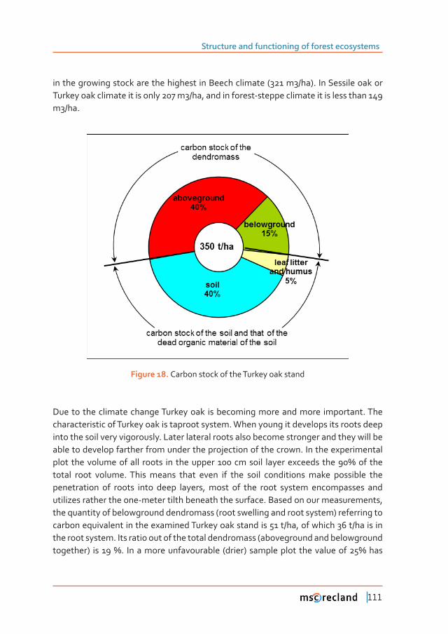
Structure and functioning of forest ecosystems
111
in the growing stock are the highest in Beech climate (321 m3/ha). In Sessile oak or Turkey oak climate it is only 207 m3/ha, and in forest-steppe climate it is less than 149 m3/ha.
Figure 18. Carbon stock of the Turkey oak stand
Due to the climate change Turkey oak is becoming more and more important. The characteristic of Turkey oak is taproot system. When young it develops its roots deep into the soil very vigorously. Later lateral roots also become stronger and they will be able to develop farther from under the projection of the crown. In the experimental ����� ������������������ ������ ��� ������������������� �������������� ����ά���� ����total root volume. This means that even if the soil conditions make possible the penetration of roots into deep layers, most of the root system encompasses and utilizes rather the one-meter tilth beneath the surface. Based on our measurements, the quantity of belowground dendromass (root swelling and root system) referring to carbon equivalent in the examined Turkey oak stand is 51 t/ha, of which 36 t/ha is in the root system. Its ratio out of the total dendromass (aboveground and belowground ��������Ȍ� ����άǤ� ����������������������� ȋ�����Ȍ������������� �������������ά�����
Chapter 3
112
been measured at a similar age Turkey oak stand. Consequently, the favourable ��������������������ơ��������������������������������������������ǡ�����������������dendromass is higher, both in terms of ratio and absolute value. In a warming climate the amount of aboveground dendromass and the organic matter production will decrease (Führer et al. 2011).
3�4�2 Carbon sequestration of forest ecosystems and climate change
The ecophysiological observations and the investigation of the physiological processes of forests depending on weather have clearly proved that water supply in the main growth cycle (May to July) and in the critical months (July and August) ��������������ƪ��������������������������������������������������������������ȋò�����et al. 2011). Relationship between meteorological parameters and girth-growth of trees (proportional with organic matter production) can be characterized by a ������Ƥ��������������������������ȋ��Ȍ��������������������������ȋò����������Ǥ��ȌǤ��������������ǡ�������������������������������������ơ���������������������������������in forestry practise can be described. The smaller is the value of the FAI, the cooler and rainier is the climate (beech climate can be characterized by the lowest, whereas Turkey oak climate by the highest FAI values) FAI shows a causal relationship with the average yearly organic matter production (Führer 2007). The calculated FAI values show strong correlation with the carbon sequestration of the forest stand. Figure 4 shows that under present climate conditions, carbon sequestration is declining with increasing aridity among the forest climate classes.
The results may be utilised for forecasting productivity changes according to various scenarios. Based on the results of regional climate model simulations for the country, summers are projected to be warmer and drier (Gálos et al. 2007). These can result in a drastic shift in the forest climate categories and a species composition change on long-term time basis (Führer et al. 2013). The beech climate is projected to almost ����������������������ǡ�����Ƥ�������������������������������������������������ǡ���������������� ��� ����� ��� ������� ������� �������� ��� ��������� ��� ������Ǥ� ������ ��� Ƥ����� ǡ� ���would lead to less carbon sequestration in the forest dendromass and a decrease in production capacity of stands.
�����������������Ƥ������������������� ����������������������������������������������increase in poor categories. The decrease in yield is caused by decrease of lumbered wood volume and more valuable wood assortments, as well. In case of the projected
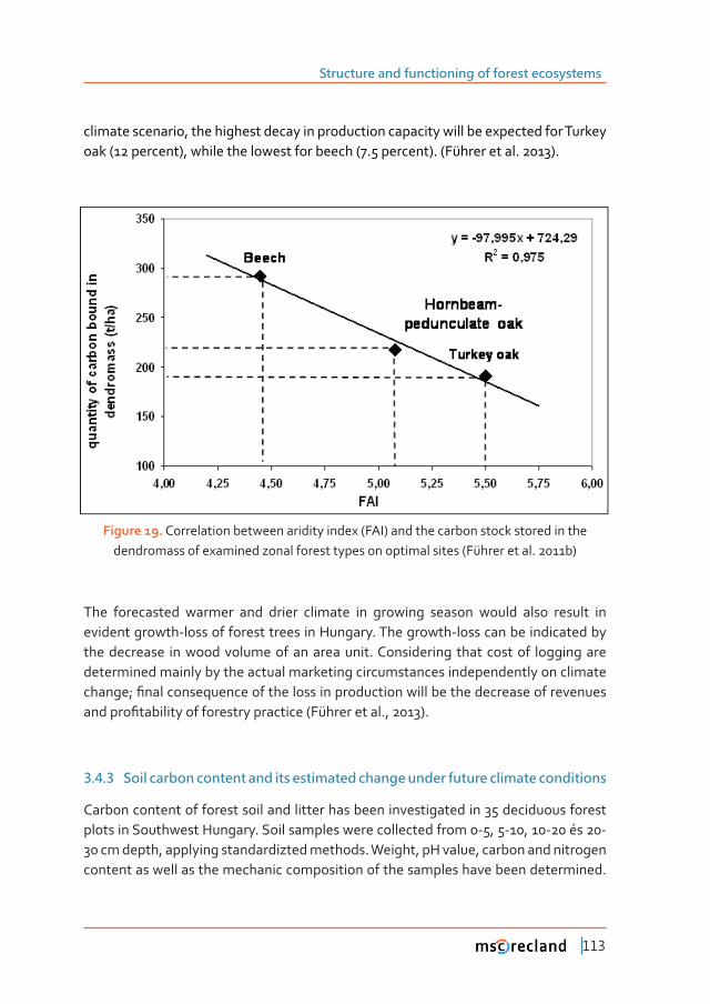
Structure and functioning of forest ecosystems
113
climate scenario, the highest decay in production capacity will be expected for Turkey oak (12 percent), while the lowest for beech (7.5 percent). (Führer et al. 2013).
Figure 19. Correlation between aridity index (FAI) and the carbon stock stored in the dendromass of examined zonal forest types on optimal sites (Führer et al. 2011b)
The forecasted warmer and drier climate in growing season would also result in evident growth-loss of forest trees in Hungary. The growth-loss can be indicated by the decrease in wood volume of an area unit. Considering that cost of logging are determined mainly by the actual marketing circumstances independently on climate ������Ǣ�Ƥ����������������������������������������������������������������������������������Ƥ������������������������������ȋò����������Ǥǡ�ȌǤ�
3�4�3 Soil carbon content and its estimated change under future climate conditions
Carbon content of forest soil and litter has been investigated in 35 deciduous forest plots in Southwest Hungary. Soil samples were collected from 0-5, 5-10, 10-20 és 20-30 cm depth, applying standardizted methods. Weight, pH value, carbon and nitrogen content as well as the mechanic composition of the samples have been determined.
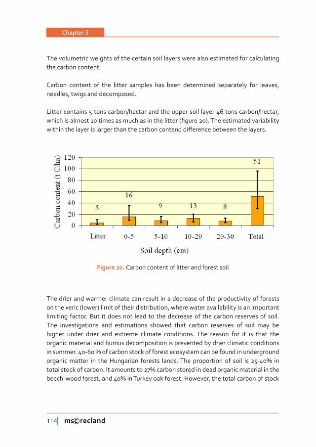
Chapter 3
114
The volumetric weights of the certain soil layers were also estimated for calculating the carbon content.
Carbon content of the litter samples has been determined separately for leaves, needles, twigs and decomposed.
Litter contains 5 tons carbon/hectar and the upper soil layer 46 tons carbon/hectar, ������������������������������������������������ȋƤ�����ȌǤ��������������������������������������������������������������������������������ơ�������������������������Ǥ�
Figure 20. Carbon content of litter and forest soil
The drier and warmer climate can result in a decrease of the productivity of forests on the xeric (lower) limit of their distribution, where water availability is an important limiting factor. But it does not lead to the decrease of the carbon reserves of soil. The investigations and estimations showed that carbon reserves of soil may be higher under drier and extreme climate conditions. The reason for it is that the organic material and humus decomposition is prevented by drier climatic conditions ���������Ǥ�Ǧ�ά�������������������������������������������������������������������������������� ��� �������������� �������� �����Ǥ����� ����������� ��� ����� ��� Ǧά� ������������������������Ǥ���������������ά����������������������������������������������������Ǧ�����������ǡ�����ά���������������������Ǥ��������ǡ���������������������������
Structure and functioning of forest ecosystems
115
of Turkey oak forest ecosystem was smaller, carbon of stock in soil was larger than in soil of beech-wood forest (Bidló et al. 2011).
����������������������������������ơ����������������������������������������������������management.
RELATED WEBSITES, PROJECTS AND VIDEOS
carbon cycle: https://www.e-education.psu.edu/meteo469/node/160
https://www.fas.org/irp/imint/docs/rst/Sect16/Sect16_4.html
http://www.whrc.org/mapping/boreal/modeling.html
UN-REDD Programme: Reducing Emissions from Deforestation and forest Degradation:
http://www.un-redd.org/AboutREDD/tabid/102614/Default.aspx
http://www.thegef.org/gef/pubs/land-use-land-use-change-and-forestry-lulucf-activities
Forests and climate change (FAO) – carbon and GHGs: http://www.fao.org/docrep/005/ac836e/
AC836E03.htm
Soil properties and processes that control soil carbon accumulation: http://www.youtube.com/
watch?v=seJhFW6h_1U
Projects:
http://www.iww.uni-freiburg.de/researchareas/resource-and-carbon-storage
http://www.ucd.ie/carbifor/
http://www.forestry.gov.uk/fr/INFD-633DJ4
http://ucanr.edu/sites/forestry/Carbon/
Forest carbon dynamics; National Forest Sinks Committee Forest Carbon Risk Analysis Project
http://cfs.nrcan.gc.ca/projects/topic/36
Forest carbon sequestration:
http://www.youtube.com/watch?v=D-E-7RMbSZo
http://www.youtube.com/watch?v=5xQnFhIRR88
Chapter 3
116
REFERENCES
����×ǡ��Ǥǡ� �����ǡ��Ǥ���ö��ǡ��Ǥ�V�����Ǥ�ȋȌǤ���������������������������������Ǧ��������������-tedlands, Geophysical Research Abstracts, Vol. 13, EGU2011-7803, 2011, EGU General Assem-bly 2011
Bonan, G.B. 2008. Ecological climatology. Cambridge University Press, UK, 550 p
������Ǥ�Ǥ�Ǥ��������������������������ǣ���������ǡ����������ǡ���������������������Ƥ������forests. Science, 320, 1444–1449, doi: 10.1126/science.1155121
Booth B B B, Jones C D, Collins M, Totterdell I J, Cox P M, Sitch S, Huntingford C, Betts R A, Harris G R, Jon Lloyd: High sensitivity of future global warming to land carbon cycle processes. En-viron. Res. Lett. 2012, 7 024002 (8pp) doi:10.1088/1748-9326/7/2/024002
Führer, E., Horváth, L., Jagodics, A., Machon, A., and Szabados, I., 2011a: Application of a new ��������������������������������������������Ǥ���Ý������ǣ�ȂǤ�
Cao L, Bala G, Caldeira K, Nemani R, Ban-Weissa G: Importance of carbon dioxide physiological forcing to future climate change. Proc. Natl. Acad. Sci. 2010, 107(21):9513-1918.
FAO: Global Forest Resources Assessment 2005, Progress towards sustainable forest manage-ment,
Führer, E., Marosi, Gy., Jagodics, A., and Juhász, I. 2011b: A klímaváltozás egy lehetséges hatása ������Ý���������������ȏ����������ơ������������������������������������������ȐǤ�������Ǥ��Ú��Ǥ�1, 17–28. (in Hungarian)
Führer E., Jagodics A., Juhász I., Marosi Gy., Horváth L. 2013. Ecological and economical impacts ������������������������������������������������Ǥ���Ý������ǣ�Ǧ
Gálos, B., Lorenz, P., and Jacob, D. (2007). Will dry events occur more often in Hungary in the future? Environmental Research Letters, doi: 10.1088/1748-9326/2/3/034006.
Gopalakrishnan R, Bala G, Jayaraman M, Cao L, Nemani R, N H Ravindranath NH: Sensitivity of terrestrial water and energy budgets to CO2-physiological forcing: an investigation using an �ƫ��������������Ǥ��������Ǥ����Ǥ�����Ǥ� ǡ� � �ȋ��ȌǤ����ǣǤȀǦȀȀȀ
Jackson R.B., Randerson J.T., Canadell J.G., Anderson R.G., Avissar R., Baldocchi D.D., Bonan Ǥ�Ǥǡ�����������Ǥǡ���ơ���������Ǥ�Ǥǡ�������Ǥ�Ǥǡ����������Ǥ�Ǥǡ� ��������ǤǤǡ�����������Ǥ�Ǥǡ�Nosetto M.D., & Pataki D.E. (2008). Protecting climate with forests Environ. Res. Lett., 3, 044006 (5pp), doi: 10.1088/1748-9326/3/4/044006
Jandl, R., Rasmussen, K., Tomé, M. and Johnson D.W. 2006. The Role of Forests in Carbon Cycles, Sequestration, and Storage. IUFRO Newsletter, Issue 4. Forest Management and Carbon Se-questration.
Millennium Ecosystem Assessment 2005.
��������Ǥ Ǥ�ȋȌǤ����������������ơǡ������������������ǡ����������������������������������������-te model. Int. J. of Climatol. 23, 479-510, doi: 10.1002/joc.893
Structure and functioning of forest ecosystems
117
4 BIODIVERSITY GENERATION AND CONSERVATION SERVICES - ECOSYSTEM, SPECIES AND GENETIC DIVERSITY
4�1 Introduction
The analysis of quantitative data of common garden tests supports the concept that �������������ơ���������������������������������������������������������ơ����������������change scenarios. Within the distributional range of a species, the response of a population depends on its adaptedness to its local environment. At the xeric limit, selection pressure narrows genetic variation and the increase in frequency of extreme events may result in growth decline and mortality. In the humid part of range, climate �������������������ơ������Ǥ
���� ���������� ��� ��������� ��� ��ơ������ ������������� ��������� ���� �����������that the simultaneous action of plasticity and selection maintains an adaptive non-equilibrium also at genetic level, similar to the one at ecosystem level. In the distributional range of low moisture stress, warming will ease plasticity strain, which leads to ������� ������������� �������� ��� Dz����������dz� ����� �������� �������Ǥ� ���� ���������growth trends in Western and boreal Europe, versus South-eastern-continental and Mediterranean Europe can be explained by the described phenomenon.
��� ��������� ������ �������� ��� ���� ����� �������� ����� �ơ���� Ƥ���� ��� ���� ���� �������(already existing) forest stands, adaptation potential will mainly depend on the level of phenotypic plasticity. The importance of this trait should be recognized not only in breeding and improvement, but also in selection and use of forest reproductive material.
4�1�1 Xeric limits and genetics
Trees, as dominant components of forest ecosystems, are of high ecological importance in the temperate belt and receive much attention with regard to adaptation potential and future risks of diversity loss and extinction. Much of the climate change literature however is based on simulations and models, the genetic background of which are often deduced from results with annuals or other fast reproducing organisms. Genetic analyses of forest trees demonstrate that their
Chapter 3
118
genetic system and diversity parameters are ����������������ơ����� from annual plants or animals (Hamrick et al. 1992).
The crucial problem of realistic interpretation of adaptation to climate change is �����������������������Ƥ����������������ǡ����������������������������Ǥ������������ǡ����������������������������������������ȋDz����������������dzȌǤ������������������������ƥ�����to establish, laborious and time consuming to maintain and measure.
�������� ����������Ƥ����������������������������������������������� ���������� ���changes, is the production biology of forest trees (forest yield science). Large-scale assessments exist in forestry which analyse the response of forest stands to extant �������� ������� �ơ����� ���� �������� ��������� ȋ�Ǥ�Ǥ� �������Ǧ��������� et al. 2006, Lapenis et al. 2005, Kramer and Mohren 2001). For instance, data show for large parts of Western Europe an unprecedented acceleration of forest growth in the recent ���������������ǡ�������������������������ά�ȋ���������et al. 1996). Interpreting ������ ����� ������ ���������� ����������� ��ƥ�������� ��� ��������� ���������� ��� �����populations. These shortcomings emphasise the importance of cross-disciplinary research (Mátyás 2006b).
4�1�2 Bioclimatic modelling of xeric limits needs genetic considerations
Climatic demands of tree species and of forest ecosystems have however attained a sudden actuality in the context of adaptation to predicted climatic changes. Bioclimatic modelling of distribution ranges is based on the concept that distributional patterns depend – among other factors – on the physiological tolerance limits to ����������ơ����Ǥ��������������������������������������������������������������������that physiological tolerance is unquestionably determined by genetics. Tolerance can �����Ƥ�������������������������������������������������Ƥ��������������������Ǥ������������presumably genetically correlated with phenotypic plasticity, i.e. with growth vigour across environments (Weis et al. 2000; Mátyás and Nagy 2005). Limits of tolerance are therefore genetically set and will determine the presence or absence of species (Figure 21).
Thus, adaptive response to environmental stress is ultimately a genetic issue, and correct bioclimatic modelling is strongly dependent on genetically set tolerance limitations.
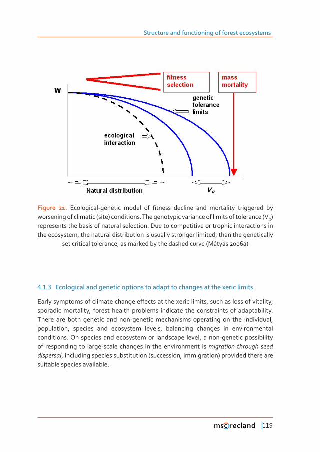
Structure and functioning of forest ecosystems
119
Figure 21. ����������Ǧ�������� ������ ��� Ƥ������ �������� ���� ���������� ���������� ���worsening of climatic (site) conditions. The genotypic variance of limits of tolerance (VG) represents the basis of natural selection. Due to competitive or trophic interactions in the ecosystem, the natural distribution is usually stronger limited, than the genetically
set critical tolerance, as marked by the dashed curve (Mátyás 2006a)
4�1�3 Ecological and genetic options to adapt to changes at the xeric limits
����������������������������������ơ������������������������ǡ�������������������������ǡ�sporadic mortality, forest health problems indicate the constraints of adaptability. There are both genetic and non-genetic mechanisms operating on the individual, population, species and ecosystem levels, balancing changes in environmental conditions. On species and ecosystem or landscape level, a non-genetic possibility of responding to large-scale changes in the environment is migration through seed dispersal, including species substitution (succession, immigration) provided there are suitable species available.
Chapter 3
120
Extensive studies on ����Ǧ��������������ƪ����������������� have shed light also on �����������ơ���������������������������������������������������������������ǡ�������most probably contributes to the unexpectedly high diversity and adaptability of tree populations (Hamrick et alǤ�ȌǤ�����������Ǧ��������������������������������ƪ�������functional across the whole range of distribution. Both mechanisms have however limited importance at the xeric limits, because they rather support the escape of species and genes instead of the persistence in marginal situations.
Genetically set adjustment mechanisms sustain persistence both on population and individual level. On the level of populations, natural selection adjusts the average Ƥ���������������������� ����������������������Ǥ�������������������������������� ����population’s gene pool towards an optimum state is genetic adaptation in the strict �����Ǥ�������������������������������������������������������������������������ơ������������������������������������ƥ�����������������������ǡ��Ǥ�Ǥ������ƥ����������������������� (e.g. Booy et al. 2000, Beaulieu and Rainville 2004). Long-term genetic adaptability is therefore directly depending on the conservation or even reconstruction of broad adaptive genetic variance. The progress of selection will also depend on the intensity of selection pressure, as described by Fisher’s theorem (Mátyás 2004). This progress �������������������������������ƪ����������������Ǥ�
�����������������������ơ��������������������������������������������������������Ǥ����the individual (genotype) level, phenotypic plasticity provides the ability to survive in a wide range of environments, without genetic change in the classic sense. Plasticity is the environmentally sensitive production of alternative phenotypes by given genotypes (DeWitt and Scheiner 2004). Plasticity implies that the phenotypic expression of �����������ƪ�������������������������ǡ��������������������������������������������������������������� ���� ������Ǥ� ��� ���������������ơ������� ����������������������������������ǡ������������������������������������������������������������ƪ��������������environment. Phenotypic plasticity will set the limits of environmental heterogeneity within which a genotype or population can persist in its lifetime. In ecological literature, plasticity is often regarded as a non-genetic adaptation mechanism. It has ����������������� ����� ����� ������ �����Ƥ������������������������������������� ���������selection (Mátyás 2006a).
Structure and functioning of forest ecosystems
121
4�2 Estimation of aridity tolerance from common garden test results
4�2�1 Transfer analysis of common garden data
The principle of this approach is the use of ecological variables to express the change of environment through transfer to the test site. Adaptive responses to changes can be interpreted, generalized and compared more easily if expressed as ecological distances. To observe tolerance and plasticity, populations (provenances) are ��������� �����ơ�������������������� ����������Ǥ��������������������� �����������������������������������������Ƥ�����. The slope of the function represents the sensitivity to changes and possible limits of tolerance. Taking growth and health condition as ����������Ƥ�����ǡ�������������������������������������������ǯ������������������Ƥ������to the variable investigated (precipitation, drought). Thus, growth and survival of populations adapted to a given site, transferred and tested in other environments as part of common-garden tests, can be interpreted as a simulation of ambient changes at the original location. The transfer analysis validates the forecasting of adaptive �����������������ơ���������������������������� (Mátyás and Nagy 2005; Rehfeldt et al. 2003).
4�2�2 Response to changes of climatic environment
Common garden tests of most tree species verify that populations originating from ��ơ������ ��������� ����� �����Ƥ�� ����������� ��� ������ ����������� ���ǡ� �����������ǡ�����������ơ������������������������������������������������������������Ǥ�
���� �ơ���� ��� ������������ ����������� ��� ������� ������� ��� ������������ ���� �����studied in six Scots pine tests situated in the centre of European Russia (Mátyás and �����ȌǤ������������������� ��������������ǡ�����������������������������Ƥ���Ǥ��������������������������ơ�������������������ǡ��������������������������������������height at age 16 in percents of locally adapted populations (relative height, see Figure ȌǤ��������Ƥ����ǡ��������������������������������������������������������������������sums. Tested populations were grouped according to their adaptedness into northern, central and southern groups.
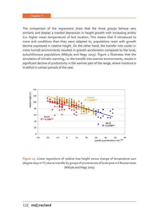
Chapter 3
122
The comparison of the regressions show that the three groups behave very similarly and display a marked depression in height growth with increasing aridity (i.e. higher mean temperature) of test location. This means that if introduced to more arid conditions than they were adapted to, populations react with growth decline expressed in relative height. On the other hand, the transfer into cooler (= more humid) environments resulted in growth acceleration compared to the local, autochthonous populations (Mátyás and Nagy 2005). Figure 2 illustrates that the simulation of climatic warming, i.e. the transfer into warmer environments, results in �����Ƥ������������������������������������������������������������ǡ������������������������Ƥ����������������������������������Ǥ
SouthR2 = 0,1883***
CentralR2 = 0,6999***
Nor thR2 = 0,4708***
0
20
40
60
80
100
120
140
-30 -20 -10 0 10 20 30 40 50 60
Change of temperature sum (oC)
Relat
ive h
eight
(%)
Figure 22. Linear regressions of relative tree height versus change of temperature sum (degree-days in °C) due to transfer by groups of provenances of Scots pine in 6 Russian tests
(Mátyás and Nagy 2005)
Structure and functioning of forest ecosystems
123
4�3 Discussion
4�3�1 Adaptation maintains non-equilibrium state
It seems that the width of local adaptation is extended by phenotypic plasticity of genotypes towards less optimal environments. If environmental conditions improve (= transfer to milder sites), growth response will improve as well. Reaction norm of populations adapted to climates close to the xeric limit, exhibit an increased growth �������������������������������������������Ǥ�������ơ����������������Ƥ�����Ǥ
It indicates that populations under climatic selection pressure adapt to local conditions simultaneously by genetic (natural) selection and by utilizing phenotypic plasticity. With �����������������������������������������������������������������Ȁ������������������������given species, populations toward the climatic limits of distribution display an increasing ����������������������ǡ���ơ�����������������������������Ǥ As similar phenomena have ����� ��������� ��� ��������� ������� ������� �����������ǡ� ��� ��ơ������ �������ǡ������������� ��� ������� �ơ����� ����� ��� ����� ƪ��� ���� ����ƥ������ ������������Ǥ�����migration hypothesis, i.e. that populations colonizing the site had no time yet to adapt locally, might hold at the thermal limits in the north, but not in the rest of the distribution area, and particularly not at the xeric limits. A parsimonious explanation is the assumption of adaptive non-equilibrium (Mátyás et al. 2008).
The proposed hypothesis of adaptive non-equilibrium means that within the distribution area of a (zonal) species, genetic adaptedness in the strict sense can be considered to be in an equilibrium state only in a narrow optimum zone. Approaching the thermal and xeric limits, the local populations get under increasing climatic �������������� ��������������� ��������������������������������ǡ������� �����ơ��������phenotypic plasticity. Genetic diversity is then stabilised in a quasi-equilibrium state (Mátyás et al. 2008).
4�3�2 Conclusions for prediction and bioclimatic modelling of adaptive response
���������������������
����������������������������������������������������������������������Ǥ������ơ������������������������������������������������ơ��������������������������������������������������������ơ�����������������������������������������������������Ǥ�
Chapter 3
124
���� ��������� ��� ����������� ����� ������������ ��� �������� ����� ��ơ��� ���������� ���climatic zones. In the thermal-limited northern-boreal zone, the expected rise of temperature will lead to marked growth acceleration. At lower altitudes, in the temperate-maritime zone, growth will accelerate too, along with increasing or at least unchanged rainfall. In the sub-humid temperate-continental and sub-humid Mediterranean zones, however, even relatively minor temperature increases, coupled with growing drought stress, will trigger loss of compatibility, higher susceptibility to diseases, and increased mortality. At the xeric limits warming leads to relatively fast growth and productivity loss, and selective mortality (Berki and Rasztovits 2004; Mátyás 2005). It should be noted that the described phenomena are generalisations. Substantial deviations may be caused by the genetic system of the species, the ������������Ǧ����������������������������������������������ơ����Ǥ�����������ǡ�������are indications that in certain regions of the boreal zone, where moisture stress is already present due to low precipitation, higher temperatures and increased drought stress may also lead to incremental decline (Lapenis et al. 2005).
������������������������������������������������������
Expectable genetic changes will be minor in the northern part of the distribution range despite the extreme speed of predicted (and already ongoing) changes. Improved growing conditions can be utilized through the plasticity potential of tree populations, without much migration or selection. As inherited plasticity will determine the response to changes, there is little room left for genetic adaptation. In temperate-Atlantic Europe, where moisture stress is predicted to stay low, populations will also ����������ơ��������������������������Ǥ
������������������������������ơ������������������������������������������������ǡ���������������������������������������������Ǥ�����ǡ����������������������������ơ��������������form of irregularly appearing health decline and mortality waves following weather ��������Ǥ� ����� ���������� ������ ����� ���������� ������ �� ������� �ơ���� ��� ���� ��������resources of exposed populations, and if stress situations aggravate, it may lead to local population extinction, even for once well distributed, dominant species (Mátyás et al. 2008). This underlines the importance of management and conservation of forest genetic resources (Ledig and Kitzmiller 1992, Mátyás 2000).
Structure and functioning of forest ecosystems
125
4�3�3 Conclusions for mitigation and management
��� ���� ������ ������� ��� ������������ǡ� ���������� ��� ����� ƪ��� ����� ������� �������������������� ��� ���� ���������Ǥ� ���������� ������������ ƪ����������ǡ� ����� �����������mean temperatures, severity of extremes will increase too: aridity stress will therefore increase, which will cause additional stress at the xeric limits. Fast genetic adaptation is in contradiction with the accepted assumption of strong biological and ecological constraints. At the (zonal) xeric limits, an unlimited adaptation to declining ��������������������������ǡ�������������������������������ơ�����������������Ǥ���������proven by remarkable migrations and area shifts in the geological past (Mátyás et al. 2008).
Therefore the need of human intervention in mitigation has to be underlined (Mátyás 2006a). Due to ecological constraints to spontaneous adaptation, the policy of ����Ƥ����� �������������� ������� ��� ���������� �������� ��� ���������� ������������ ���connectivity, at least with regard to tree species.
4�3�4 Consequences for forest management
����������������������������������������������Ƥ���������������������������������������be questioned. In addition some aspects of forest management should not be overlooked when predicting responses and formulating mitigation strategies. Most ���������ǯ�� �������� �������������� ������ ���� ������ ������������� ��ƪ�����ǡ� ��������managed according to periodic management plans. Especially close to the xeric limit, ������������������������Ǧ��������������������ǡ����������������������������Ƥ����Ǥ��Ǥ�Ǥ�����������ǡ�����������������Ƥ��������������������������������������ά������������������Ǥ�The possibilities left for spontaneous processes, such as migration and succession are limited. Forest stand composition is primarily determined by forest policy and economic considerations. This means also that adjustments in species composition ���� ��� ��������� �������� ���������� ���� ��� ��������� ������� ���� ����� �ơ���������compared to natural, spontaneous processes (Mátyás et al. 2008).
In drought stress climates, increment loss and higher incidence of diseases and pests will challenge the economics of forest operations, and will shift the emphasis towards the maintenance of ecological functions and conservation of stability and of genetic resources (Geburek and Turok 2005).
Chapter 3
126
REFERENCES
Beaulieu, J., A. Rainville 2004. Adaptation to climate change: genetic variation is both a short- and long term solution. The Forestry Chronicle, 81: 5, 704–708
Berki, I., E. Rasztovics 2004. [Research in drought tolerance of zonal tree species, with special regard to sessile oak.] (in Hungarian with English summary) ��ǣ Cs. Mátyás and P. Vig (eds.), ���Ý�±��������Ȃ���������������������Ǥ�������ǡ��������ǡ�Ȃ�
Booy, G.R., J.J. Hendriks, M.J. Smulders [et al ] 2000. Genetic diversity and the survival of popu-lations. Plant Biol., 2(4): 379–395
Briceno-Elizondo, E., G. Garcia-Gonzalo, H. Peltola, J. Matala, S. Kellomäki 2006. Sensitivity of growth of Scots pine, Norway spruce and silver birch to climate change and forest manage-ment in boreal conditions. For. Ecol. Manage., 232: 152–167
DeWitt, T.J., S.M. Scheiner 2004. Phenotypic variation from single genotypes. ��ǣ DeWitt, T.J., S.M. Scheiner (eds.), Phenotypic Plasticity; Functional and Conceptual Approaches. Oxford University Press, 1–9
Geburek, T., J. Turok (eds) 2005. Conservation and Management of Forest Genetic Resources in Europe, Arbora Publ., Zvolen, Slovakia
�������ǡ� Ǥ�Ǥǡ� Ǥ�Ǥ����ǡ��Ǥ�Ǥ��������Ǧ������� Ǥ����������ƪ������������������������������������in woody plants. New Forests 6: 95–124
������ǡ��Ǥǡ�Ǥ��������Ǥ�����Ǧ������ơ�������������������������������������������������������Europe. Alterra Report, No. 194
Lapenis, A., A. Shvidenko, D. Shepaschenko, S. Nilsson, A. Aiyyer 2005. Acclimation of Russian forests to recent changes. Global Change Biology, 11: 2090–2102
Ledig, F.T., J.H. Kitzmiller, 1992. Genetic strategies for reforestation in the face of global climate change. For. Ecol. Manage., 50: 153–169
Mátyás,C. (ed.) 2000. Forest Genetics and Sustainability. Kluwer, Dordrecht
Mátyás,C. 2004. Population, conservation and ecological genetics. ��ǣ Burley, J., J. Evans, J, Youn-gquist (eds.), Encyclopedia of Forest Sciences. Elsevier Major Reference Works, Oxford, Vol 1, 188–197
Mátyás,C. 2006a. Migratory, genetic and phenetic response potential of forest tree populations facing climate change. Acta Silvatica et Ligniaria Hung., 2: 33–46 ȋ����ǣȀȀ����Ǥ����Ǥ��Ȍ
Mátyás, C. 2006b. The missing link: synthesis of forest genetics and ecological research in view of challenges of environmental change. ��ǣ G. von Wühlisch (ed.). Forest Genetics and its Contri-bution to Sustainability. Mitt. BFH, Nr 221, Kommissionsverlag, Hamburg, 1–14
Mátyás, C., L. Nagy 2005. Genetic potential of plastic response to climate change. ��ǣ M. Konnert (ed.), Tagungsberichte, Forum Genetik und Wald 2004. Bav. Centre f. For. Repr. Material, Tei-sendorf, 55–69

Structure and functioning of forest ecosystems
127
������ǡ��Ǥǡ��Ǥ�����ǡ�2Ǥ�������� ������Ǥ������������������������������������������������Ƥ-cation at the xeric forest limit and consequences for bioclimatic modelling. In: Strelcova, K., Cs. Mátyás, A.Kleidon, et al. (eds.) Bioclimatology and natural hazards. Springer Verl., Berlin 2008 179-196 pp.
��������ǡ�Ǥ�Ǥǡ��Ǥ�Ǥ�����������ǡ��Ǥ�Ǥ���������ǡ��Ǥ�Ǥ����������ǡ��Ǥ�Ǥ�����ơǡ��Ǥ�Ǥ����������Ǥ�Assessing population responses to climate in Pinus sylvestris and Larix spp. of Eurasia with climate transfer models. Eurasian J. For. Res., 6 (2): 83–98.
Spiecker, H., K. Mielikäinen, M. Köhl, J.P. Skovsgard (eds.) 1996. Growth trends in European fo-rests. EFI Report 5, Springer Verl., Berlin
Weis, A.E., E.L.Simms, M.E. Hochberg 2000. Will plant vigor and tolerance be genetically corre-lated? Evol. Ecol., 14: 331–352

129
Chapter 2.4
University of
West Hungary,
Sopron, Hungary
Climatic effects of land cover change
Áron Drüszler
ABSTRACT
Geological, paleontological and geomorphologic studies show that the Earth’s climate has always been changing since it came into existence. The climate change itself is self-evident. Therefore the far more serious question is how much does �������� ����������� ��� ������� ������ �������� ������� ���� �������� ƪ�������������� �������� ��� �������Ǥ� ������� ���� ����������� �ơ���� ���� �������� ��������forcing processes (such as solar variability) there are also further anthropogenic ��ƪ����������������������������������������Ǧ����������������������ơ����Ǥ������������changes over time are one of the less successfully reconstructed anthropogenic ��ƪ�����������������Ǥ����������������������������������������������������������������development through the precipitation, temperature, radiation and through the ������� ��� ������� �������� ���� ���� ����������� �������� ����� �ơ���� ���� ��������ȋ������������������������������Ȍ�����������ǡ�����ǡ��������������������ƪ����ǡ������������ơ��������������������������Ǥ����������������������������ơ�������������changes in the CO2 concentration caused by the vegetation changes. This paper �����������������������������������Ƥ��������������������������ơ�������� �����������changes and through one detailed regional example (Hungary) also tries to show the mode of action of historical land cover changes on the regional climate system.
Chapter 5
130
1 INTRODUCTION
Final aim of the climate research is to create correct forecasts for the future. For this ����������������������������������������������������������������ƪ�����������������Ǥ���������������ơ����������������������������������������������������ơ�������� ������changes can help us to achieve this goal.
The atmospheric CO2 concentration increase is well-known since the 18th century. This ����ǡ��������������������ơ�����������������������������ǡ������������������ήǤ���-2 increments of the planetary radiation balance and to ca. 1.5 °C of equilibrium global warming. However, up to the present only +0.74 °C temperature increase was globally ���������ȋ����ǡ�ȌǤ������������������ơ��������������������������������������������internal mechanisms may have the same order of magnitude.
�����������������������ơ������������������������ ������������������ ȋ��������������variability, changes is solar orbital parameters, volcanic activity), there are also further �������������� ��ƪ������ǡ� �Ǥ�Ǥ� ���� �ơ����� ��� �������� ��������ǡ� ����� ������ ������ǡ�stratospheric ozone depletion, black- and organic carbon aerosols and jet contrails, ���Ǥǡ����������������������������������Ǧ����������� �����������ơ����Ǥ������������������������ơ������������������������������������������������������������ȋForster et al., 2007: Table 2.12 on p. 204.)
Land cover changes over time are one of the less successfully reconstructed �������������� ��ƪ������� ��� �������Ǥ� ���� �������� ������ǡ� ����������ǡ�������������������ǡ� ����� ����� ƪ��� ���� ���� ����Ǧ�������� ���������� ��� ��� ����� �����ơ���������������������������Ǥ�������������������������������ơ����������ƥ�������of the vertical exchange between the surface and the atmosphere in the planetary boundary layer. The surface albedo and emissivity modify the short wave and long wave radiation budget. Vegetation controls the partitioning of vertical turbulent ����� ƪ����� �������� ������ ��������� ���� ������� ������ ȋ�����ǡ� Ȍ� �������� ���������Ǧ�����Ƥ�������������������������������������������������Ǥ� ȋ���� ����������������unlimited availability of water from the soil). In addition, the vegetation’s shading �������ƪ���������������������ƪ��Ǥ���������������������������������������������������Ǧsurface temperatures and atmospheric humidity (Drüszler et al., 2010, 2011).
����������������������������������������������Ƥ��������������������������ơ�������������������changes (Section 2.) and through one detailed regional example (Hungary) also tries to show the mode of action of historical land cover changes on the regional climate system (Section 3.).
Climatic effects of land cover change
131
2 LITERATURE REVIEW
It is well known that climate is the main factor of vegetation development through the precipitation, temperature, radiation and through the amount of carbon dioxide (Budyko, 1974; Prentice, 2001; Nemani et al., 2003), but the vegetation changes also �ơ���� ���� �������� ȋ������� ��� �� ��������� ���������Ȍ� ���� ������ǡ� ����ǡ� ������ �������������ƪ����ǡ������������ơ��������������������������Ǥ����������������������������ơ������������������������������2 concentration caused by the vegetation changes (Pielke et al., 1998; Bonan 2002).
If all forests of the Earth were in their natural potential conditions, then their total areas would cover 52-59 million km2 (Ramankutty and Foley, 1998; Klein Goldewijk, 2001). However, mankind uses a substantial part of its continental surface for agriculture and other purposes, e.g. deforestation, urbanization, overgrazing, etc. According �����������ȋȌǡ���Ǥ��ά�����������������������������������������������������������been changed by mankind. Though this process started as early as the stabilization of ����������Ǥ�ǡ���ǡ��������ά���������������������������������������������������������revolution.
The existence of the vegetation feedbacks on climate are already proven by empirical and model studies, on monthly and seasonal averaging and at local, continental and global scales, as well. In a part of these investigations the ocean-atmosphere feedback methodology (Frankignoul et al., 1998; Frankignoul and Kestenare, 2002) was adapted to the case of vegetation-atmosphere feedbacks, utilizing that dynamic memory of these feedbacks is also longer (1-2 months) than that of the atmosphere (1-2 weeks) (Liu et al., 2006; Notaro et al., 2006). In these studies the role of sea-surface temperature for the slow sub-system were played by the fotosynthetically active part of the solar radiation (FPAR), which value can be monitored from the satellites and characterizes the vitality of the vegetation.
According to these computations, the plant development depends mainly on temperature at the temperate latitudes, but it feeds back to the temperature, as ����Ǥ����������������������������������Ǧ�ά�������������Ǧ��������ƪ����������Ǥ�����feedback is the strongest in the cold-belt forests, e.g. in the Northern States of the ��������������ǡ����������������������������Ǥ��������������������ơ��������������strong as 1 °C
Chapter 5
132
At the tropical and subtropical regions, however, the state of vegetation depends �����������������������Ǥ������������������������������������Ƥ������������������������������������ǡ�����������������������������������ά��������������ƪ����������Ǥ���������isolated areas, however, the amplifying feedback on precipitation may be higher than 10 mm/month. Such regions are e.g. North-East Brasilia, East-Africa, East-Asia and Northern part of Australia.
���������������������Ƥ������������� ��� ����������� ������������������������������������in order to obtain new farmland, e.g. in the Amazon basin (Bonan, 2004). Though pastures of the tropical belt exhibit a higher albedo than the forests, it was still computed that some warming is the net result of the forest reduction (Gash et al., 1996, Gash and Nobre, 1997). The most likely cause of this warming is hidden in the root system of the trees, allowing much stronger transpiration in the dry and hot ��������ȋ�������������������ǡ�ȌǤ��������������ơ���������������������ǡ�����������������������������������������������������ơ��������������������ơ�������ǡ����������by model studies, (Bounoua et al., 2002).
The complete deforestation in Amazonia could already reduce the natural atmospheric precipitation, due to reduction of moisture sources for the atmospheric circulation (Lean and Rowntree, 1997). Partial clearing of tropical rainforests, however does not �������������������������������Ǥ���������ǡ�Ƥ����������������������������������������the possibility that existence of warmer spots within the forest cover may cause small-scale circulation, which could increase the convective activity (Roy and Avissar, 2002). Partial deforestation may even increase the precipitation of the Amazon region, itself, which is in coherence with the trends of precipitation observations (Chagnon and Bras, 2005).
��������������������������������������ơ�������������������������������������������������������������������������ȋ������������Ǥǡ� ȌǤ������������������ǡ��������������ơ��������only in the land cover parameters; all atmospheric initial and boundary conditions remained unchanged. In the weather case they chose, the natural vegetation led to intense convective cloudiness (cumulus congestus), but without precipitation. The same atmospheric conditions with the present agricultural land cover led to intense precipitation and thunderstorm activity. In the given period of time, the observations supported the latter case with heavy precipitation (Shaw et al., 1997).
Climatic effects of land cover change
133
In arid and semi-arid regions of our planet, agricultural land cover, overgrazing and ������������������������������Ƥ�������������Ǧ����������������������ǡ������������������cycle and, hence, the climate (Bonan, 2004). Overgrazing increases the surface albedo (Charney, 1975; Charney et al., 1977), which, in turn decreases the temperature and vertical instability. Hence the less convective cloudiness led to decreased precipitation in these belts. Therefore, degradation of the landscape can even enhance permanent drought. The more recent studies also supported that large scale changes in the land cover of the Sahel-belt could lead to decreased precipitation in the North African regions (Xue and Shukla, 1993; Clark et al., 2001).
Spatial contrasts between the dry and the irrigated agricultural lands may lead to strong contrasts in the sensible and latent heat balance of the two surface types (Bonan, 2004). This can induce mesoscale circulation (Avissar and Pielke, 1989; Chen and Avissar, 1994). High evapotranspiration from the irrigated surfaces can cool the near surface layers of the atmosphere, which causes local circulation which is similar to the sea-land circulation. The same contrast may lead the same circulation in the boundary between the hot natural areas and cooler irrigated areas. The irrigation causes cooler climate conditions in Northeastern Colorado in the USA (Chase et al., 1999).
���� �ơ���� ��� ����������� ��� �������� ���� ��� ����� ��� ���� ����������� ����� ������������ ������� ���� ������ ȋ�����ǡ� ȌǤ���ơ�������� ��� ���� ���������� ������ ���� �������ecosystems, which are strongly driven by the presence or absence of snow, can be an important regulating factor even at the larger scales of atmospheric circulation. The taiga warms climate in contrast with the neighbouring tundra vegetation, as shown in several studies (e.g. Thomas and Rowntree, 1992; Beringer et al., 2005).
Calculations based on the land cover dataset of Ramankutty és Foley (1998) show ����� ����������������������ơ����� ����������� ��� ���� ��������������� ���������������forests. In the previous 700 years (between ca. 1000 and 1700 AD) there was no �����Ƥ������ơ������������������������������������������������������������Ǥ��������last 300 years, mean global temperatures increased 0.09 °C and temperatures in the Northern Hemisphere increased 0.15 °C due to land cover changes (Shi et al., 2007). In �������������������������������������������������������������� Ǥ�λ���������������Ƥ�����changes in the tropical and polar regions.
Chapter 5
134
������� �������� ���������� ���� ������ ����������� �ơ���� ��� ����� ������ �������� ���temperature, (Bertrand et al., 2002; Matthews et al., 2003), but these studies did not �����������������������ơ�����������������������������2 content of the atmosphere. This could, however, change the land cover induced temperature changes from cooling to warming!
Between 1850 and 2000, an estimated 156 Gt of Carbon was emitted into the atmosphere due to deforestation (Houghton, 2003). Brovkin et al. (2004) found ����� ����� ������ ���� ������������ ���� Ǧ�ά� ��� ���� ����������������2 emissions, depending on the details of the reconstructions, according to Ramankutty and Foley ȋȌǡ����������������ȋȌǡ�������������ȋȌǤ�������Ǥ��ά���������������������supported by Matthews et al. (2004) applying a similar methodology, i.e. climate-vegetation-carbon-cycle modelling. This means, that land cover changes are among the causes of the CO2- induced global warming.
As fossil fuel burning increased rather fast in the recent century, the relative contribution of the land cover to the atmospheric CO2 uptake decreased (Betts, ȌǤ��������������������������ƪ�����������������ά�����άǡ����� �������ǯ�� ����� ����������������������Ǧ�άǤ����������� �����������������Ǥ� ȋȌǡ���������������������������������ơ�������������������������������������������������������Ǥ�ήǤ�λ�������������������ǦǤ�����������������������ơ������������������change on climate was also estimated by Hansen et al (1998) and further reports were also published by the recent two IPCC Reports (2001, 2007).
����������Ǥ� ȋȌ������������������ �������������������� ������������� �����ơ��������historical land cover changes in Hungary in the second half of the 20th Century were ���������������������������ơ�������������������������2 concentration on the radiation balance of the surface-atmosphere system in the same time period. This relation in the local radiation balance, however, does not allow an analogous comparison with ���� �������� ������������� ���� ��� ���� ����� ��ơ�������� �������� ���� ���� ��������forcing processes. Namely, the greenhouse gases were changing in rather similar way ������������������Ǥ��������������ơ������������������������������������������ǡ��������������ơ�������������������������ơ���������������ơ�������������Ǥ
For further detailed investigations the MM5 high resolution, non-hydrostatic ���������� ������ ���� ����� ��� �������� ���� ��������� �ơ���� ��� ����������� ����� ������changes during the 20th century (Drüszler et al., 2011). This work tries to answer the following questions: (i.) What kind of impact could the land cover changes have
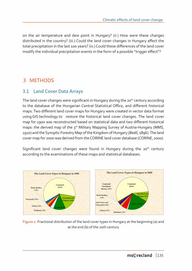
Climatic effects of land cover change
135
on the air temperature and dew point in Hungary? (ii.) How were these changes ��������������������������ǫ�ȋ���ǤȌ������������������������������������������ơ����������������������������������������������ǫ�ȋ��ǤȌ���������������ơ�����������������������������������������������������������������������������������������������Dz���������ơ���dzǫ
3 METHODS
3�1 Land Cover Data Arrays
���������������������������������Ƥ���������������������������th century according ��� ���������������� �����������������������������������ƥ��ǡ�������ơ���������������������Ǥ�������ơ���������������������������������������������������������������������using GIS technology to restore the historical land cover changes. The land cover ���������������������������������������������������������������ơ�����������������maps: the derived map of the 3rd Military Mapping Survey of Austria-Hungary (MMS, 1910) and the Synoptic Forestry Map of the Kingdom of Hungary (���Ý, 1896). The land cover map for 2000 was derived from the CORINE land cover database (CORINE, 2000).
�����Ƥ����� ����� ������ �������� ����� ������ ��� �������� ������� ���� th century according to the examinations of these maps and statistical databases.
The Land Cover Types in Hungary in 1900
Cropland;
61.0%
Grassland and
Pasture; 16.0%
Forest; 12.5%
Water Bodies;
2.3%
Vineyards; 2.5%
Urban; 2.4%
Wetland; 3.2%
The Land Cover Types in Hungary in 2000
Cropland/
Woodland
Mosaic; 1.8%
Wetland; 1.1%
Urban; 5.7%
Fruit Trees and
Vineyards; 2.2%
Water Bodies;
1.9%
Forest; 21.1%
Grassland and
Pasture; 9.6%
Cropland;
56.8%
Figure 1. Fractional distribution of the land cover types in Hungary at the beginning (a) and at the end (b) of the 20th century
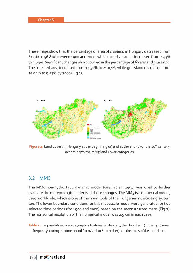
Chapter 5
136
These maps show that the percentage of area of cropland in Hungary decreased from Ǥά����Ǥά��������������ǡ��������������������������������������Ǥά���� ǤάǤ������Ƥ������������������������������������������������forests and grassland. ���������������������������������Ǥά����Ǥάǡ��������������������������������Ǥά����Ǥά�����ȋ��ǤȌǤ
Figure 2. Land covers in Hungary at the beginning (a) and at the end (b) of the 20th century according to the MM5 land cover categories
3�2 MM5
The MM5 non-hydrostatic dynamic model (Grell et al., 1994) was used to further �����������������������������ơ���������������������Ǥ����������������������������ǡ�used worldwide, which is one of the main tools of the Hungarian nowcasting system too. The lower boundary conditions for this mesoscale model were generated for two selected time periods (for 1900 and 2000) based on the reconstructed maps (Fig.2). The horizontal resolution of the numerical model was 2.5 km in each case.
Table 1. �������Ǧ��Ƥ�����������������������������������������ǡ�����������������ȋǦȌ������frequency (during the time period from April to September) and the dates of the model runs
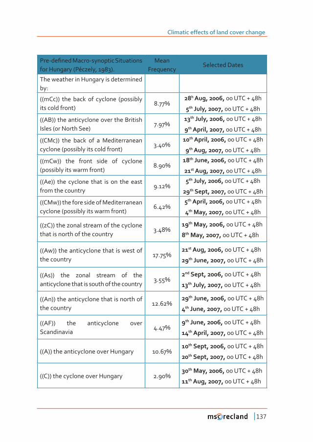
Climatic effects of land cover change
137
���Ǧ��Ƥ���������Ǧ��������������������for Hungary (Péczely, 1983).
Mean Frequency
Selected Dates
The weather in Hungary is determined by:
((mCc)) the back of cyclone (possibly its cold front)
Ǥά28� Aug, 2006, 00 UTC + 48h
5�� July, 2007, 00 UTC + 48h
((AB)) the anticyclone over the British Isles (or North See)
Ǥά13�� July, 2006, 00 UTC + 48h
9��������ǡ�ǡ�00 UTC + 48h
((CMc)) the back of a Mediterranean cyclone (possibly its cold front)
Ǥά10��������ǡ�ǡ�00 UTC + 48h
9�� Aug, 2007, 00 UTC + 48h
((mCw)) the front side of cyclone (possibly its warm front)
Ǥά18�� June, 2006, 00 UTC + 48h
21st Aug, 2007, 00 UTC + 48h
((Ae)) the cyclone that is on the east from the country
Ǥά5�� July, 2006, 00 UTC + 48h
29�������ǡ�ǡ�00 UTC + 48h
((CMw)) the fore side of Mediterranean cyclone (possibly its warm front)
Ǥά5��������ǡ�ǡ�00 UTC + 48h
4�� May, 2007, 00 UTC + 48h
((zC)) the zonal stream of the cyclone that is north of the country
Ǥά19�� May, 2006, 00 UTC + 48h
8�� May, 2007, 00 UTC + 48h
((Aw)) the anticyclone that is west of the country
Ǥά21st Aug, 2006, 00 UTC + 48h
29�� June, 2007, 00 UTC + 48h
((As)) the zonal stream of the anticyclone that is south of the country
Ǥά2nd�����ǡ�ǡ�00 UTC + 48h
13�� July, 2007, 00 UTC + 48h
((An)) the anticyclone that is north of the country
Ǥά29�� June, 2006, 00 UTC + 48h
4�� June, 2007, 00 UTC + 48h
((AF)) the anticyclone over Scandinavia
Ǥά9�� June, 2006, 00 UTC + 48h
14��������ǡ�ǡ�00 UTC + 48h
((A)) the anticyclone over Hungary Ǥά10�������ǡ�ǡ�00 UTC + 48h
20�������ǡ�ǡ�00 UTC + 48h
((C)) the cyclone over Hungary Ǥά30�� May, 2006, 00 UTC + 48h
11�� Aug, 2007, 00 UTC + 48h
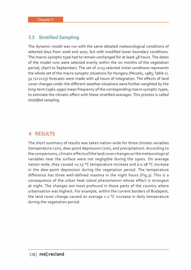
Chapter 5
138
3�3 Stratified Sampling
The dynamic model was run with the same detailed meteorological conditions of ������������������������ǡ��������������Ƥ����������������������������Ǥ�The macro-synoptic type had to remain unchanged for at least 48 hours. The dates of the model runs were selected evenly within the six months of the vegetation ������ǡ�ȋ������������������ȌǤ������������α����������������������������������������the whole set of the macro synoptic situations for Hungary (Péczely, 1983; Table 1). �ȋααȌ�����������������������������������������������Ǥ������ơ���������������������������������������ơ������������������������������������������������������long-term (1961-1990) mean frequency of the corresponding macro synoptic types, ��������������������������ơ���������������������Ƥ�����������Ǥ������������������������������Ƥ�����������.
4 RESULTS
The short summary of results was taken nation-wide for three climate variables (temperature (2m), dew-point depression (2m), and precipitation). According to the comparisons, climatic effects of the land cover changes on the meteorological variables near the surface were not negligible during the 1900s. On average nation-wide, they caused +0.15 °C temperature increase and a 0.18 °C increase in the dew-point depression during the vegetation period. The temperature difference has three well-defined maxima in the night hours (Fig.3). This is a consequence of the urban heat island phenomenon whose effect is strongest at night. The changes are most profound in those parts of the country where urbanisation was highest. For example, within the current borders of Budapest, the land cover change caused an average 1.2 °C increase in daily temperature during the vegetation period.
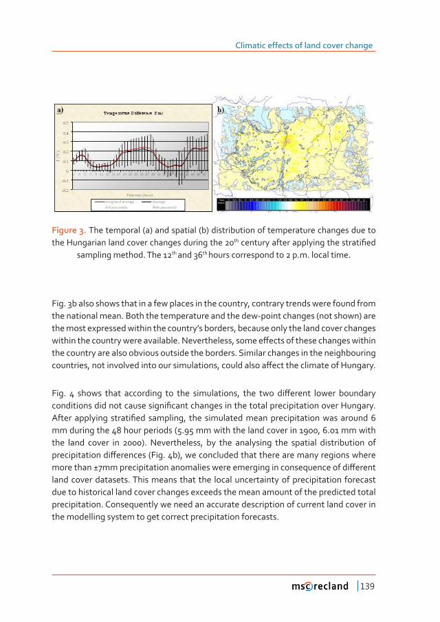
Climatic effects of land cover change
139
Figure 3. The temporal (a) and spatial (b) distribution of temperature changes due to the Hungarian land cover changes during the 20th����������������������������������Ƥ���
sampling method. The 12th and 36th hours correspond to 2 p.m. local time.
Fig. 3b also shows that in a few places in the country, contrary trends were found from the national mean. Both the temperature and the dew-point changes (not shown) are the most expressed within the country’s borders, because only the land cover changes ���������������������������������Ǥ�������������ǡ�������ơ�����������������������������the country are also obvious outside the borders. Similar changes in the neighbouring ���������ǡ����������������������������������ǡ�������������ơ��������������������������Ǥ
��Ǥ� � ������ ����� ���������� ��� ���� �����������ǡ� ���� ���� ��ơ������ ������ ���������������������������������������Ƥ����������������������������������������������������Ǥ���������������� ������Ƥ��� ��������ǡ� ���� �����������������������������������������mm during the 48 hour periods (5.95 mm with the land cover in 1900, 6.01 mm with the land cover in 2000). Nevertheless, by the analysing the spatial distribution of ����������������ơ��������ȋ��Ǥ��Ȍǡ����������������������������������������������������������ΰ�������������������������������������������������������������ơ������land cover datasets. This means that the local uncertainty of precipitation forecast due to historical land cover changes exceeds the mean amount of the predicted total precipitation. Consequently we need an accurate description of current land cover in the modelling system to get correct precipitation forecasts.
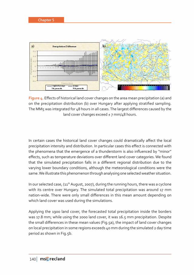
Chapter 5
140
Figure 4. �ơ���������������������������������������������������������������������ȋ�Ȍ�������� ������������������������������� ȋ�Ȍ����������������������������� ������Ƥ��� ��������Ǥ����������������������������������������������Ǥ���������������ơ����������������������
land cover changes exceed ± 7 mm/48 hours.
��� �������� ������ ��������������� ����� ������ �������� ������������������� �ơ���� ���� ����������������������������������������������Ǥ���������������������������ơ�����������������������������������������������������������������������������������ƪ����������Dz�����dz��ơ����ǡ���������������������������������������ơ���������������������������Ǥ��������������� ���� ���������� �������������� ������ ��� �� ��ơ������ ��������� ������������� ���� ��� ����varying lower boundary conditions, although the meteorological conditions were the same. We illustrate this phenomenon through analysing one selected weather situation.
In our selected case, (11th August, 2007), during the running hours, there was a cyclone with its centre over Hungary. The simulated total precipitation was around 17 mm ������Ǧ����Ǥ�������������������������ơ�������� ���������������������������������which land cover was used during the simulations.
Applying the 1900 land cover, the forecasted total precipitation inside the borders was 17.8 mm; while using the 2000 land cover, it was 16.5 mm precipitation. Despite ������������ơ�����������������������������ȋ��Ǥ�Ȍǡ����������������������������������on local precipitation in some regions exceeds 40 mm during the simulated 2 day time period as shown in Fig.5b.
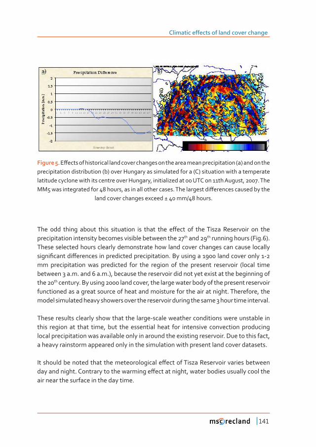
Climatic effects of land cover change
141
Figure 5Ǥ��ơ���������������������������������������������������������������������ȋ�Ȍ������������precipitation distribution (b) over Hungary as simulated for a (C) situation with a temperate latitude cyclone with its centre over Hungary, initialized at 00 UTC on 11th August, 2007. The ����������������������������ǡ����������������������Ǥ���������������ơ����������������������
land cover changes exceed ± 40 mm/48 hours.
���� ���� ������ ������ ����� ���������� ��� ����� ���� �ơ���� ��� ���������� ���������� ��� ����precipitation intensity becomes visible between the 27th and 29th running hours (Fig.6). These selected hours clearly demonstrate how land cover changes can cause locally �����Ƥ�������ơ����������������������������������Ǥ�����������������������������Ǧ�mm precipitation was predicted for the region of the present reservoir (local time between 3 a.m. and 6 a.m.), because the reservoir did not yet exist at the beginning of the 20th century. By using 2000 land cover, the large water body of the present reservoir functioned as a great source of heat and moisture for the air at night. Therefore, the model simulated heavy showers over the reservoir during the same 3 hour time interval.
These results clearly show that the large-scale weather conditions were unstable in this region at that time, but the essential heat for intensive convection producing local precipitation was available only in around the existing reservoir. Due to this fact, a heavy rainstorm appeared only in the simulation with present land cover datasets.
��������������������������������������������ơ���������������������������������������������������Ǥ��������������������������ơ������������ǡ�������������������������������air near the surface in the day time.
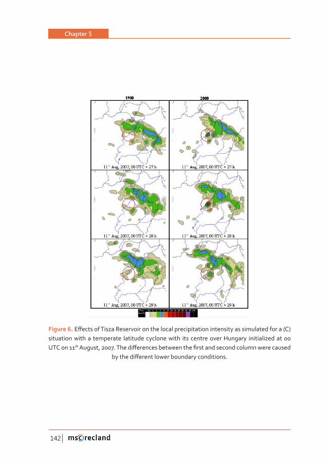
Chapter 5
142
Figure 6. �ơ��������������������������������������������������������������������������������ȋ�Ȍ�situation with a temperate latitude cyclone with its centre over Hungary initialized at 00 UTC on 11th�������ǡ�Ǥ�������ơ��������������������Ƥ����������������������������������
���������ơ�������������������������������Ǥ
Climatic effects of land cover change
143
5 CONCLUDING REMARKS
After the analysis of MM5 dynamic model simulations, we found that the Hungarian land cover changes in the last 100 years caused an increase of +0.15 ° C daily temperature and +0.18 ° C dew-point depression during the vegetation period. This means that the near-surface air over Hungary is now warmer and drier than before due to the land cover change. It is also plausible, that the computed results show the maximum warming and drying over the urban areas. After the comparison of the ���������ơ����������������������������������������������������������������������� ���������� ����� ���� ��������� �ơ����� ��� ����� ������ �������� ���� ���� ����������Ǥ�Consequently, beyond other climate forcing processes, it is necessary to take land cover change into account by the interpretation of climate change in the past and for making scenarios for the future.
��������������������ơ����������������������������������������������������������conditions only, the averaged results may be uncertain due to the relatively few samples of meteorological cases. Nevertheless we conclude that the increase of the daily temperature likely exceeds +0.1 o C, since all types exhibited warming between the 1900 vs. 2000 land cover types, and the increase was larger or equal to 0.1 o C in ���� ���������������Ǥ�����������Ƥ�������������������������������������� ���� �����climatic average from long-term observations, but the order of magnitude in our estimations is probably correct.
�����������������������������������������������������������������������������Ƥ�����impact on the average precipitation nation-wide. However, the impact on the regional distribution of precipitation is considerable, especially under unstable weather conditions. The present study clearly shows that MM5 precipitation forecast is very sensitive to the lower boundary conditions. (All other mesoscale models must also be sensitive). Since the Hungarian Nowcasting System uses the MM5 and WRF models, which work with the same land surface model, it would be reasonable to update the land cover database of these models by using current land cover maps. In addition, it is also necessary to update the land cover parameters of these models. The quality of the weather forecasting would be considerably improved.
Chapter 5
144
6 RELATED WEBSITES, PROJECTS AND VIDEOS
Land use, land use change and forestry:
http://forest.jrc.ec.europa.eu/activities/lulucf/
IPCC special report on forests: http://www.ipcc.ch/ipccreports/sres/land_use/index.php?idp=0
http://unfccc.int/methods/lulucf/items/4122.php
http://ec.europa.eu/clima/policies/forests/lulucf/index_en.htm
http://en.wikipedia.org/wiki/Land_use,_land-use_change_and_forestry
Good Practice Guidance for Land Use, Land-Use Change and Forestry: HTTP://WWW.����ǧ���Ǥ���Ǥ��Ǥ �Ȁ������Ȁ������Ȁ������Ǥ����
REFERENCES
Avissar, R., and R. A. Pielke, 1989: A parameterization of heterogeneous land surface for atmos-pheric numerical models and its impact on regional meteorology, Mon. Wea. Rev., 117: 2113-2136
���Ýǡ��Ǥ�ȋȌǡ�����������������������������������������������ǡ���Ǥ�ǤBeringer, J., F. S. Chapin, C. Thompson, and A. D. McGuire, 2005: Surface energy exchanges along
a tundra-forest transition and feedbacks to climate, Agricultural and Forest Meteorology, 131: 142-161
����������Ǥǡ���������������Ǥǡ������Ƥ���Ǥǡ�������������Ǥǡ�ǣ������������������������������ǣ���sensitivity study. Tellus 54A: 221-244
Betts R.A., 2006: Forcings and feedbacks by land ecosystem changes on climate, Journal de Phy-sique IV, 139: 123-146
Bonan, G. B, 2004: Biogeophysical feedbacks between land cover and climate, Ecosystem and Land Use Change: 61-72
Bonan, G., 2002: ����������������������ǣ��������������������������. Cambridge University Press, 678 pp.
Brovkin, V., Sitch, S., von Bloh, W., Claussen, M., Bauer, E., Cramer, W., 2004: Role of land cover changes for atmospheric CO2 increase and climate change during the last 150 years. Global Change Biol. 10:1253–1266
Budyko, M. I., 1974: Climate and Life. Academic Press, 608 pp.Chagnon, F. J. F., and Bras, R. L., 2005. Contemporary climate change in the Amazon. Geophysical
Research Letters 32: L13703Charney, J. G., 1975: The dynamics of deserts and droughts, Quart. J. Roy. Meteor. Soc. 101: 193-
202
Climatic effects of land cover change
145
�������ǡ� Ǥ�Ǥǡ��Ǥ� Ǥ������ǡ��Ǥ��Ǥ�����ǡ����� Ǥ�����Ƥ���ǡ� ǣ�����������������������������ơ��������albedo change on drought in semiarid regions, J. Atmos. Sci. 34: 1366-1385
Chase , T. N., R. A. Pielke Sr., T. G. F. Kittel, J. S. Baron, T. J. Stohlgren, 1999: Potential impacts on Colorado Rocky Mountain weather due to land use changes on the adjacent Great Plains, J. Geophys. Res. 104: 16673-16690
Chen, F., and R. Avissar, 1994: The impact of land surface wetness heterogeneity on mesoscale �����ƪ����ǡ�J. Appl. Meteor. 33: 1323-1340
Clark, B.D., Xue, Y., Harding, R.J., and P. J. Valdes, 2001: Modeling the impact of land surface de-gradation on the climate of tropical North Africa. J. Climate 14: 1809-1822
CORINE, 2000: Corine land cover 2000 (CLC2000) seamless vector database, ����ǣȀȀ���Ǥ���Ǥ��-����Ǥ��Ȁ����Ǧ���Ǧ����Ȁ����Ȁ������Ǧ����Ǧ�����ǦǦ���Ǧ��������Ǧ������Ǧ��������
Crutzen PJ, 2002: Geology of mankind – the Anthropocene, Nature 415: 23Drüszler, Á., Vig, P., and Csirmaz, K., 2011: Impacts of Hungarian Land Cover Changes on the Re-
gional Climate during the 20th Century; XXVth Conference of the Danubian Countries, Budapest, Hungary, 16-17 June 2011
��ò�����ǡ��Ǥǡ��������ǡ��Ǥǡ����ǡ��Ǥǡ����� Ǥ������ǣ��ơ���������������������������������������temperature and humidity regime in Hungary; ��ǣ��Ǥ��Ǥ��������ǣ���������������, Interna-tional Book Distributors, ISBN: 81-7089-370-4: 394-418
����������ǡ��Ǥǡ������Ǥ����������ǡ�ǣ������������������ƪ�����������ǡ�������ǣ���������������������������������������������������������������Ƥ�Ǥ�Climate Dyn., 19, 622–647.
Frankignoul, C., A. Czaja, and B. L’Heveder, 1998: Air–sea feedback in the North Atlantic and sur-face boundary conditions for ocean models. J. Climate, 11, 2310–2324
Gash, J. H. C., C. A. Nobre, J. M. Roberts, and R. L. Victoria (Eds.), 1996: Amazonian Deforestation and Climate, 611 pp., John Wileyǡ��Ǥ�Ǥ
���ǡ� Ǥ��Ǥ��ǡ������Ǥ��Ǥ������ǡ�ǣ����������ơ�������������������������������ǣ��������������from ABRACOS, Bull. Amer. Meteor. Soc. 78: 823-830
����ǡ�Ǥ�Ǥǡ� Ǥ�������� �����Ǥ�Ǥ�����ơ��ǡ� ǣ��� ������������ ��� ���� th
generation Penn State/ NCAR Mesoscale model (MM5). �������������������ǡ�����Ȁ��Ǧή���ǡ����ǡ�Ǥ
��������ǡ��Ǥǡ�ǣ�������������������������������������ƪ������������������������������������changes in land use and land management 1850-2000. Tellus 55B: 379-390
IPCC, 2001: Climate Change 2001: �����������Ƥ�������Ǥ���������������������������������������������Assessment Report of the Intergovernmental panel on Climate Change (Houghton J.T., et al., eds.), Cambridge University. Press, Cambridge, United Kingdom and New York, USA, 881 p.< http//:www.ipcc.ch>: Chapter 6, 399. pp.
IPCC, 2007: Climate Change 2007: The Physical Science Basis. Contribution of Working Group I to the Fourth Assessment Report of the Intergovernmental Panel on Climate Change [Solomon, S., D. Qin, M. Manning, Z. Chen, M. Marquis, K.B. Averyt, M. Tignor and H.L. Miller (eds.)]. Cambridge University Press, Cambridge, United Kingdom and New York, NY, USA, 996 pp.
Kleidon, A., and M. Heimann, 2000: Assessing the role of deep rooted vegetation in the climate system with model simulations: mechanism, comparison to observations and implications for Amazonian deforestation, Clim. Dyn. 14: 183-199
Klein Goldewijk K, 2001: Estimating global land use change over the past 300 years: The HYDE database, ��������������������ǣ 417-434
Lean, J., and P. R. Rowntree, 1997: Understanding the sensitivity of a GCM simulation of Amazo-�������������������������������Ƥ����������������������������������������������ǡ�J. Climate 10: 1216-1235
Chapter 5
146
Liu, Z., M. Notaro, J. Kutzbach, and N. Liu, 2006: Assessing global vegetation–climate feedbacks from observations. J. Climate, 19, 787–814.
Matthews, H.D., Weaver, A.J., Meissner, K.J., Gillett, N.P., Eby, M., 2004: Natural and anthropo-genic climate change: incorporating historical land cover change, vegetation dynamics and the global carbon cycle. Clim Dyn 22: 461–479
Matthews, H.D., Weaver, A.J., Eby, M., and K.J., Meissner, 2003: Radiative forcing of climate by historical land cover change. Geophys. Res Lett. 30:27-1–27-4
����ǡ� Ǥǡ�����������Ǥ������������Ǥǡ�ǣ��ơ��������������������������������������������������of Eastern Hungary (1951-2000), ��Ý����� 110: 49-62
MMS, 1910: 3rd Military Mapping Survey of Austria-Hungary, published about 1910, http://lazarus.elte.hu/hun/digkonyv/topo/3felmeres.htm
Nemani, R. R., C. D. Keeling, H. Hashimoto, W. M. Jolly, S. C. Piper, C. J. Tucker, R. B. Myneni, and S. W. Running, 2003: Climate-driven increases in global terrestrial net primary production from 1982 to 1999. Science, 300, 1560–1563
Notaro, M., Z. Liu, and J. Williams, 2006: Observed vegetation–climate feedback in the United States. J. Climate, 19, 763–786.
Péczely Gy., 1983: Catalogue of macrosynoptic types in Hungary (1881-1983). Minor Contribu-tions of the Hungarian Meteorological Service, Budapest, vol. 53 (in Hungarian)
Pielke RA, Lee TJ, Copeland JH, Eastman JL, Ziegler CL, Finley CA, 1997: Use of USGS-provided data to improve weather and climate simulations, Ecol. Appl. 7: 3-21
Pielke, R., R. Avissar, M. Raupach, A. J. Dolman, X. Zhen, and A. S. Denning, 1998: Interactions �������������������������������������������������ǣ���ƪ����������������������������Ǥ�Glo-bal Change Biol., 4, 461–475
Prentice, I. C., 2001: Interactions of climate change and the terrestrial biosphere. Geosphere–Biosphere Interactions and Climate, L. O. Bengtsson and C. U. Hammer, Eds., Cambridge Uni-versity Press, 176–195
Ramankutty, N., and Foley JA, 1998: Characterising patterns of Global land use: An analysis of global cropland data, Global Biogeochem. Cy. 12: 667-685
Roy, S., and Avissar R., 2002: Impact of land use/land cover change on regional hydrometeorolo-gy in Amazonia, J. Geophys. Res., 107(D20), 8037
Shaw BL, Pielke RA, Ziegler CL, 1997: A three-dimensional numerical simulation of a Great Plains dryline, Mon. Weather Rev. 125: 1489-1506
Thomas, G., and P. R. Rowntree, 1992: The boreal forests and climate, Quart. J. Roy. Meteor. Soc. 118: 469-497
���ǡ��Ǥǡ����� Ǥ�������ǡ�ǣ�������ƪ�������������������������������������������������Ǥ�������ǣ���-�����Ƥ������ǡ�J. Clim. 6: 2232-2245
147
Chapter 2.5
University of
West Hungary,
Sopron, Hungary
Afforestation as a tool for climate change mitigationBorbála Gálos
ABSTRACT
This chapter introduce the results of regional-scale sensitivity studies carried out ��� �������������������������ơ����������� ���������������������������������������Ǥ�Applying the regional climate model REMO, the projected temperature and precipitation tendencies have been analyzed for summer, based on the results of the A2 IPCC-SRES emission scenario simulation. For the end of the 21st century �������������������ǡ������������������������������������������������������ơ�����of the enhanced greenhouse gas emission. The magnitude of the biogeophysical �ơ����� ��� �ơ�������������� ������������ ��������������������������������������relative to the magnitude of the climate change signal. Based on the simulation results,��ơ����������������������������������������������������������������������the temperate zone thus can reduce the projected climate change. The largest ��������� �ơ����� ��� �ơ����������� ���� ��� ��������� ��� ���������������ǡ� ������������������ǡ����������Ǧ�ά�������������������������������������������������������������ά������������������Ǥ�����������������������������������������ơ��������ơ�������������������������ơ���������������������ǡ��������������������������for Hungary more in detail. Results can help to identify the areas, where forest cover increase is the most favourable and should be supported to reduce the projected climate change. They can build important basis of the future adaptation strategies and forest policy.
Chapter 6
148
1 INTRODUCTION
1�1 Regional climate projections for Europe
�������� �������� ���� �������������� ���������� ��ƪ������ ���� �������� ��� ���� �����Ǥ��������ơ������������������������������������������������������������ǡ����������aerosol compositions as well as by land surface changes (IPCC, 2007). There are several recent EU-projects carried out in the last decade, to provide high-resolution climate change projections with focus on future climate changes and their impacts in Europe (Christensen et al., 2007; Jacob et al., 2008; van der Linden & Mitchell, 2009). These studies are based on the results of regional climate model simulations driven �����ơ�����������Ƥ�������������������������������������Ǥ�������ơ���������������the simulated climatic conditions for the future and for the present time period is the climate change signal. For the 21st century, projected climate change signals for ����������������������������������������������������������ơ����������������������also vary depending on the applied greenhouse gas emission scenario.
For the period 2021-2050 all regional climate models predict a quite robust surface warming in central and eastern Europe. The annual precipitation shows an increase in the northeastern and a decrease in the southwestern regions. (Christensen & Christensen, 2007; Kjellström et al., 2011). At the end of the 21st century, a warming ��������������������������������������ǡ�������������������������������Ƥ����������������21st century. All models agree that the largest warming for summer is projected to occur in the Mediterranean area, southern France and over the Iberian Peninsula. Less warming is projected over the Scandinavian regions. For winter the maximum warming occurs in eastern Europe (Christensen & Christensen, 2007). Results of the regional model simulations show a north-south gradient of annual precipitation changes over Europe, with positive changes in the north (especially in winter) and negative changes in the south (especially over the Mediterranean area in summer). For southern and central Europe the spatial distribution of the projected temperature and precipitation changes in summer refer to a marked shift towards a warmer and drier climate (e.g. Beniston, 2009).
Afforestation as a tool for climate change mitigation
149
1�2 Climatic effects of land use and land cover change
Temperature and precipitation play an important role in determining the distribution of the terrestrial ecosystems that in turn interact with the atmosphere through ��������������� ���� ��������������� ���������Ǥ� ����������� �ơ����� ���� ������������������������� ��� ���� ����� �������ǡ� ������ �������� ���� �������� ������� ƪ����� ����hydrological cycle (biogeophysical feedbacks; Pielke et al., 1998; Pitman, 2003). �������� ��������������� �ơ����ǡ� ����������� ������ ���� ��������������� ������ǡ�thereby change the chemical composition of the atmosphere (Bonan, 2002; Pitman, 2003; Feddema et al., 2005). Forests have larger leaf areas and aerodynamic roughness lengths, lower albedo and deeper roots compared to other vegetated surfaces. They sequester carbon thereby alter the carbon storage of land.
Depending on the region, biogeophysical and biogeochemical feedbacks of land cover on climate can amplify or dampen each other (Arora & Montenegro, 2011). Through these land-atmosphere interactions changes of the land cover and land use due to ��������������������ƪ����������������������������������������������������������or reduction of the projected climate change signals expected from increased atmospheric CO2 concentration (Feddema et al., 2005; Bonan, 2008).
This section focuses on studies of the biogeophysical processes, which represent the ����������������������ơ����������������������������������ơ�������������ǡ�������������time scales. Changes of vegetation cover under future climate conditions enhance the warming trend in Scandinavian Mountains as well as the drying trend in southern Europe, but mitigate the projected increase of temperature in central Europe ȋ��������������Ǥǡ�ȌǤ��������������������������������������������������ơ���������������������������������������������������ǡ�����������������������������ơ�����������carbon cycle (Bonan, 2008). If snow is present, the darker coniferous forest masks the snow cover. It is resulting in lower surface albedo compared to tundra vegetation or bare ground, which leads to higher winter and spring air temperatures (Bonan et al., 1992; Kleidon et al., 2007). Consequently, the change of vegetation from tundra to �������������������������������������������Ƥ���������������������Ǥ������������������maintain high rates of evapotranspiration. In this region, surface warming arising �����������������������������������ơ���������������������������������������������������global temperature increase (Bonan, 2008).
Chapter 6
150
In temperate forests the albedo and evaporative forcings are moderate compared with boreal and tropical forests (Bonan, 2008; Jackson et al., 2008). Climate model studies for the temperate regions showed that replacing forests with agriculture or grasslands reduces the surface air temperatures (Bounoua et al., 2002; Oleson et al., 2004) and the number of summer hot days (Anav et al., 2010). Other studies show opposite results, where temperate forests cool the air compared to grasslands and croplands and contribute to higher precipitation rates in the growing season (Hogg et al., 2000; Sánchez et al., 2007, Gálos et al., 2011; 2012; 2013). In the �������������������������������ơ�����������������������������������������������������summer months (Heck et al., 2001). In the period from April until mid-July potential vegetation cover conditions led to cooler and moister conditions due to the increase of evapotranspiration. In mid-July soil moisture dropped below the critical value and transpiration was almost completely inhibited. It resulted in dryer and warmer summer accelerating the projected climate change. Teuling et al. (2010) pointed out that the role of the forests in the surface energy and water budget is depending on the selected time scale: in the short term, forests contribute to the increase of temperature, but on longer time scales they can reduce the impact of extreme heat weaves.
These studies indicate that forests can enhance or dampen the climate change signal depending on various contrasting vegetation feedbacks, which can diminish or counteract each other. Furthermore the variability of the climatic, soil and vegetation characteristics as well as as well as the description of the land surface processes in ���� �������� �������� ������ ����� ����� ��� ��ƪ������ ��� ���� ���������� ����������Ǧatmosphere interactions.
1�3 Research foci
The climatic feedbacks of land cover changes due to climate change and the regional land use politics as well as the role of the forests in the climate change mitigation on country scale are still unknown. In order to address this topic, our sensitivity study ��� ��������� ��� ���� ��������� �ơ����� ��� �ơ����������� ��� ������� ������ ������� ��������conditions based on the following research questions:
• In which regions does the increase of forest cover enhance/reduce the projected climate change?
Afforestation as a tool for climate change mitigation
151
• �����������������ơ������������������������������������������������������������temperature relative to the climate change signal?
• ���������������������ǡ��������ơ���������������������������Ƥ���������������������point of view?
On country scale, a more detailed case study has been carried out for Hungary. For �������������������������ǡ���������������������������������������������������Ƥ�����increase of summer temperature and a decrease of summer precipitation (Bartholy et al., 2007; Gálos et al., 2007). From ecological point of view Hungary (in the southeastern part of central Europe) has been selected as study region because here, many of the zonal tree species have their lower limit of distribution (Mátyás et al., 2009), which are especially sensitive and vulnerable to the increase of the frequency of climatic extremes, primarily to droughts. In these forests the more frequent and severe droughts at the end of the 20th century already resulted in growth decline, loss of vitality and the decrease of the macroclimatically suitable area of distribution (Berki et al., 2009). Under the projected climate conditions these species may disappear from this region (Berki et al., 2009; Mátyás et al., 2010; Czúcz et al., 2011). In the last ������ǡ� ������ �������ơ��������������� ������������ ����������ǡ������� ����������� �����������������������������������Ǥ�������ƪ���������������������������������������������weather and climate has been investigated by Drüszler et al. (2011). For the future, forests can also have an important role in climate change mitigation. Therefore this case study is concentrating on the possible mitigation of the strong warming and drying of summers projected for the second half of the 21st century.
2 METHODS
Regional climate models have the potential to provide detailed information about ����������������������Ƥ������������������������Ǥ������������������������������������of land cover change in Europe regional scale analyses are essential because of the ��ơ��������������������������������������������������������������������������������������the land surface properties and the related processes.
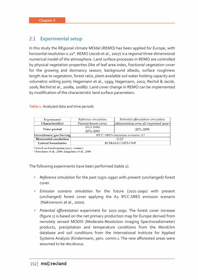
Chapter 6
152
2�1 Experimental setup
In this study the REgional climate MOdel (REMO) has been applied for Europe, with horizontal resolution 0.22°. REMO (Jacob et al., 2007) is a regional three-dimensional numerical model of the atmosphere. Land surface processes in REMO are controlled by physical vegetation properties (like of leaf area index, fractional vegetation cover for the growing and dormancy season, background albedo, surface roughness length due to vegetation, forest ratio, plant-available soil water holding capacity and volumetric wilting point; Hagemann et al., 1999; Hagemann, 2002; Rechid & Jacob, 2006; Rechid et al., 2008a, 2008b). Land cover change in REMO can be implemented �������Ƥ����������������������������������������������������Ǥ�
Table 1. Analyzed data and time periods
The following experiments have been performed (table 1):
• Reference simulation for the past (1971-1990) with present (unchanged) forest cover.
• Emission scenario simulation for the future (2071-2090) with present (unchanged) forest cover applying the A2 IPCC-SRES emission scenario
(Nakicenovic et al., 2000).
• ���������� �ơ����������� experiment for 2071-2090. The forest cover increase ȋƤ�����Ȍ��������������������������������������������������������������������remotely sensed MODIS (Moderate-Resolution Imaging Spectroradiometer) products, precipitation and temperature conditions from the Wordclim database and soil conditions from the International Institute for Applied �����������������ȋ����������ǡ�����Ǥ�����ǤȌǤ����������ơ�������������������assumed to be deciduous.
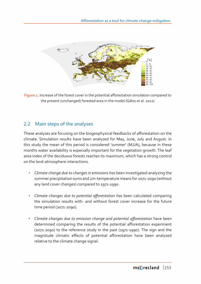
Afforestation as a tool for climate change mitigation
153
Figure 1.������������������������������������������������ơ����������������������������������the present (unchanged) forested area in the model (Gálos et al. 2012)
2�2 Main steps of the analyses
����������������������������������������������������������������ơ������������������climate. Simulation results have been analyzed for May, June, July and August. In this study the mean of this period is considered ‘summer’ (MJJA), because in these months water availability is especially important for the vegetation growth. The leaf area index of the deciduous forests reaches its maximum, which has a strong control on the land-atmosphere interactions.
• Climate change due to changes in emissions has been investigated analyzing the summer precipitation sums and 2m-temperature means for 2071-2090 (without any land cover changes) compared to 1971-1990.
• ����������������������������������ơ�������������� been calculated comparing the simulation results with- and without forest cover increase for the future time period (2071-2090).
• ������������������������������������������������������ơ�����������have been ����������� ���������� ���� �������� ��� ���� ���������� �ơ����������� �����������(2071-2090) to the reference study in the past (1971-1990). The sign and the ���������� ��������� �ơ����� ��� ���������� �ơ����������� ����� ����� ���������relative to the climate change signal.
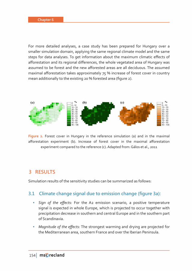
Chapter 6
154
For more detailed analyses, a case study has been prepared for Hungary over a smaller simulation domain, applying the same regional climate model and the same ������ �����������������Ǥ�������� ������������������ ����������������������ơ���������ơ������������������������������ơ�������ǡ���������������������������������������������������������������������������ơ�������������������������������Ǥ����������������������ơ��������������������������������ά������������������������������������������������������������������������ά���������������ȋƤ�����ȌǤ�
Figure 2. Forest cover in Hungary in the reference simulation (a) and in the maximal �ơ����������� ����������� ȋ�ȌǤ� ��������� ��� ������� ������ ��� ���� �������� �ơ�����������
experiment compared to the reference (c). Adapted from: Gálos et al., 2011
3 RESULTS
Simulation results of the sensitivity studies can be summarized as follows:
3�1 Climate change signal due to emission change (figure 3a):
• ����� ��� ���� �ơ����ǣ For the A2 emission scenario, a positive temperature signal is expected in whole Europe, which is projected to occur together with precipitation decrease in southern and central Europe and in the southern part of Scandinavia.
• ������������������ơ����ǣ The strongest warming and drying are projected for the Mediterranean area, southern France and over the Iberian Peninsula.
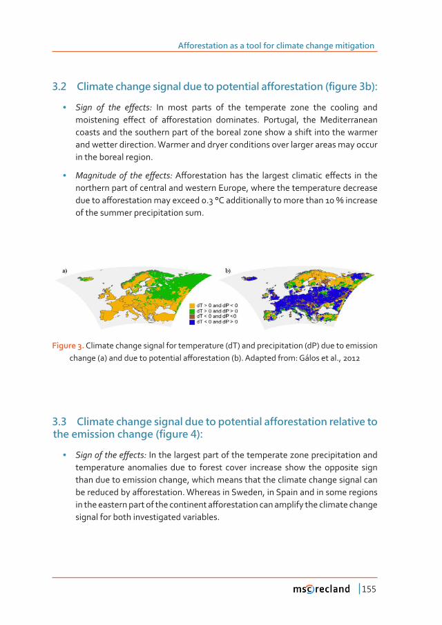
Afforestation as a tool for climate change mitigation
155
3�2 Climate change signal due to potential afforestation (figure 3b):
• ����� ��� ���� �ơ����ǣ In most parts of the temperate zone the cooling and ����������� �ơ���� ��� �ơ����������� ���������Ǥ� ��������ǡ� ���� ��������������coasts and the southern part of the boreal zone show a shift into the warmer and wetter direction. Warmer and dryer conditions over larger areas may occur in the boreal region.
• ���������� ��� ���� �ơ����ǣ��ơ��������������� ���� �������� ��������� �ơ����� ��� ����northern part of central and western Europe, where the temperature decrease ��������ơ����������������������Ǥ�λ�����������������������������ά����������of the summer precipitation sum.
Figure 3. Climate change signal for temperature (dT) and precipitation (dP) due to emission �������ȋ�Ȍ�����������������������ơ�����������ȋ�ȌǤ�������������ǣ�����������Ǥǡ�
3�3 Climate change signal due to potential afforestation relative to the emission change (figure 4):
• �������������ơ����ǣ In the largest part of the temperate zone precipitation and temperature anomalies due to forest cover increase show the opposite sign than due to emission change, which means that the climate change signal can ���������������ơ����������Ǥ������������������ǡ��������������������������������������������������������������������ơ������������������������������������������signal for both investigated variables.
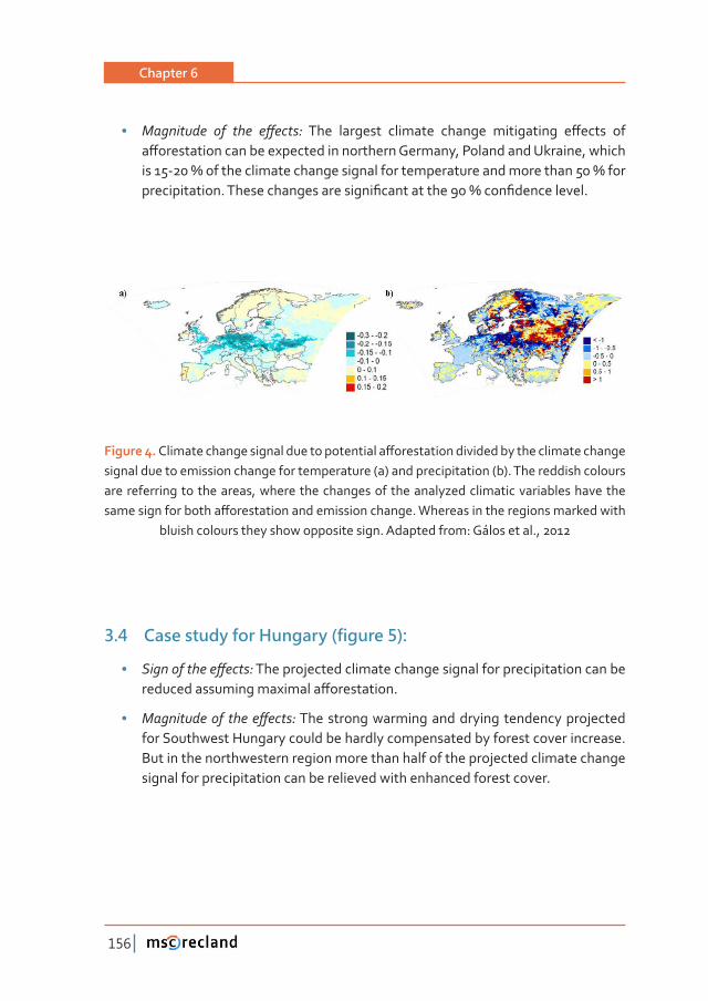
Chapter 6
156
• ���������� ��� ���� �ơ����ǣ� ���� �������� �������� ������� ����������� �ơ����� ����ơ���������������������������������������������ǡ�������������������ǡ����������Ǧ�ά�������������������������������������������������������������ά������������������Ǥ������������������������Ƥ�������������ά����Ƥ�����������Ǥ�
Figure 4. ����������������������������������������ơ�����������������������������������������signal due to emission change for temperature (a) and precipitation (b). The reddish colours are referring to the areas, where the changes of the analyzed climatic variables have the ��������������������ơ������������������������������Ǥ������������������������������������
bluish colours they show opposite sign. Adapted from: Gálos et al., 2012
3�4 Case study for Hungary (figure 5):
• �������������ơ����ǣ The projected climate change signal for precipitation can be ��������������������������ơ����������Ǥ�
• ������������� �����ơ����ǣ The strong warming and drying tendency projected for Southwest Hungary could be hardly compensated by forest cover increase. But in the northwestern region more than half of the projected climate change signal for precipitation can be relieved with enhanced forest cover.
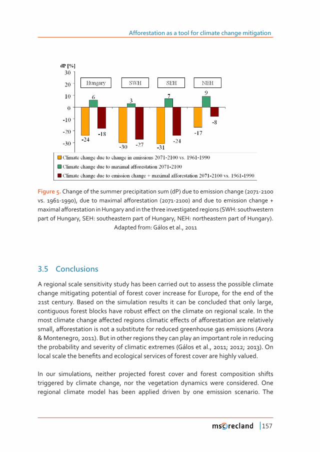
Afforestation as a tool for climate change mitigation
157
Figure 5. Change of the summer precipitation sum (dP) due to emission change (2071-2100 ��Ǥ� ǦȌǡ� ���� ����������� �ơ����������� ȋǦȌ� ���� ���� ��� ��������� ������� ή����������ơ������������������������������������������������������������ȋ���ǣ��������������part of Hungary, SEH: southeastern part of Hungary, NEH: northeastern part of Hungary).
Adapted from: Gálos et al., 2011
3�5 Conclusions
A regional scale sensitivity study has been carried out to assess the possible climate change mitigating potential of forest cover increase for Europe, for the end of the 21st century. Based on the simulation results it can be concluded that only large, ��������������������������������������ơ������������������������������������Ǥ� ����������������������������ơ������������������������ơ���������ơ�������������������������������ǡ��ơ��������������������������������������������������������������������ȋ������& Montenegro, 2011). But in other regions they can play an important role in reducing the probability and severity of climatic extremes (Gálos et al., 2011; 2012; 2013). On ��������������������Ƥ������������������������������������������������������������Ǥ
In our simulations, neither projected forest cover and forest composition shifts triggered by climate change, nor the vegetation dynamics were considered. One regional climate model has been applied driven by one emission scenario. The
Chapter 6
158
simulated impacts can also depend on the representation of the land surface properties and land cover related processes in the model (Boisier et al. 2012). ����������������� ��� ������������������� ���������Ǧ�����������ơ��������� ����������of the related uncertainties. To achieve this, multimodel ensembles of climate model simulations and intercomparison studies are essential, which is the aim of recent EU-projects (e.g. LUCID; de Noblet-Ducoudre et al. 2012).
�����������������������������������������������������ƪ������Ǥ��������������������������������������������������� �������Ƥ��������������������������������������ơ�����(e.g. carbon sequestration of forests and soil). Higher CO2 concentrations can also lead to the increase of the stomatal resistance thereby to the inhibition of the transpiration, which can amplify the global warming (Cao et al. 2010; Gopalakrishnan et al. 2011). Therefore to draw appropriate conclusions for decision makers about the role of the forests in the climate change mitigation and adaptation, the combined �ơ�����������������������Ǥ
������������������������������������Ǥ�From practical point of view, the investigation of the role of the land surface in the climate system gets even more important with the ��������� ���������������������������������������������������������������������ơ���among regions. Therefore regional scale information is substantial about the climatic feedbacks of the future land cover and land use for the adaptation to the climate change in agriculture, forestry and water management. Results of these sensitivity experiments help to identify the areas, where forest cover increase is climatically the ����� ����Ƥ����� ���� ������� ��� ���������� ��� ������� ���� ���������� �������� ������Ǥ�Here, the existing forests should be maintained. Thus the present study provides an important basis for the future adaptation strategies.
4 related websites, projects and videos
Climate change, climate projections
CORDEX: http://www.meteo.unican.es/en/projects/CORDEX
ENSEMBLES: http://www.ensembles-eu.org/
PRUDENCE: http://prudence.dmi.dk/
IPCC AR5 2013 http://www.ipcc.ch/report/ar5/wg1/
Land use/cover change – climate research projects:
Afforestation as a tool for climate change mitigation
159
����Ǧ���������������ǡ�������Ƥ�������������������������ȋ�����Ȍ
http://www.ileaps.org/?q=node/68
International Network Measuring Terrestrial Carbon, Water and Energy Fluxes (FLUXNET)
http://www.ileaps.org/?q=node/66
Climate Change – Terrestrial Adaptation & Mitigation in Europe (CC-TAME)
http://www.cctame.eu/
Operational Potential of Ecosystem Research Applications (OPERAS)
http://operas-project.eu/
IGBP - LUCC
h t t p : / / w w w . i g b p . n e t / r e s e a r c h p r o j e c t s / p a s t p r o j e c t s /landuseandcoverchange.4.1b8ae20 512db692f2a680009062.html
Climatic role of forests
����ǣȀȀ���Ǥ�������Ǥ���Ȁ�����ǫ�γ���Ɵ������
http://www.youtube.com/watch?v=isPGjChdby8
Climate change adaptation
http://www.youtube.com/watch?v=FO46sPwm4xk
REFERENCES
������Ǥǡ�������Ǥ�Ǥǡ���������Ǥ�Ƭ������������Ǥ�ȋȌǤ����������������ơ������������Ǧ�����������������surface climate in the Mediterranean region. Clim. Res., 41, 91-104
�������Ǥ�Ǥ�Ƭ�������������Ǥ�Ǥ�����������������������Ƥ��������������������������ơ������������ơ����Ǥ�Nature Geoscience ,doi: 10.1038/NGEO1182, 5pp
Bartholy J., Pongrácz R. & Gelybó Gy. (2007). Regional climate change expected in Hungary for 2071-2100. Applied Ecology and Environmental Research, 5, 1-17
Berki I., Rasztovits E., Móricz N. & Mátyás Cs. (2009). Determination of the drought tolerance limit of beech forests and forecasting their future distribution in Hungary. Cereal Research Communations, 37, 613-616
Beniston M. (2009). Trends in joint quantiles of temperature and precipitation in Europe since 1901 and projected for 2100. Geophys. Res. Lett., 36, L07707, doi:10.1029/2008GL037119
Boisier, J.P., de Noblet-Ducoudré, N., Pitman, A.J., Cruz, F. T., Delire, C., van den Hurk, B.J.J.M., van der Molen, M.K., Müller, C., Voldoire, A. (2012). Attributing the impacts of land-cover changes �����������������������������������������������������ƪ�������������Ƥ��������ǣ������������������Ƥ����������������������������. J. Geophys. Res. 117: D12116, doi:10.1029/2011JD017106.
Chapter 6
160
������Ǥ�Ǥǡ����������Ǥ�Ƭ�����������Ǥ�Ǥ�ȋȌǤ��ơ����������������������������������������Ǥ�Natu-re, 359, 716-718, doi: 10.1038/359716a0
Bonan G.B., Levis S., Kergoat L. & Oleson K.W. (2002). Landscapes as patches of plant functio-nal types: an integrating concept for climate and ecosystem models. Global Biogeochemical Cycles, 16, 30pp,10.1029/2000GB001360
������Ǥ�Ǥ�Ǥ��������������������������ǣ���������ǡ����������ǡ���������������������Ƥ������forests. Science, 320, 1444–1449, doi: 10.1126/science.1155121
���������Ǥǡ����������Ǥǡ���������Ǥ Ǥǡ����������Ǥǡ�Ƭ�������Ǥ�ȋȌǤ��ơ������������������������������on surface climate. Climatic Change, 52, 29-64
Cao L, Bala G, Caldeira K, Nemani R, Ban-Weissa G (2010): Importance of carbon dioxide physio-logical forcing to future climate change. Proc. Natl. Acad. Sci. 107(21):9513-1918
Christensen J.H., Carter T.R., Rummukainen M., & Amanatidis G. (2007). Evaluating the perfor-mance and utility of regional climate models: the PRUDENCE project. Clim. Change, 81, 1-6, DOI 10.1007/s10584-006-9211-6
Christensen J.H. & Christensen O.B. (2007). A summary of the PRUDENCE model projections of changes in European climate by the end of this century. Clim. Change, 81, 7-30, doi: 10.1007/s10584-006-9210-7
Czúcz B., Gálhidy L. & Mátyás Cs. (2011). Present and forecasted xeric climatic limits of beech and sessile oak distribution at low altitudes in Central Europe. Ann. For. Sci., 68(1), 99-108
��ò�������Ǥǡ������Ǥ�Ƭ����������Ǥ�ȋȌǤ��ơ������������������������������������������������������-tion Distribution in Hungary. Riscuri Si Catastrofe (Risks and Disasters), ISSN: 15845273; I/2011
Feddema J.J., Oleson K.W., Bonan G.B., Mearns L.O., Buja L.E., Meehl G.A. & Washington W.M. (2005). The Importance of Land-Cover Change in Simulating Future Climates. Science, 310, 1674 –1678, doi: 10.1126/science.1118160
Gálos B., Lorenz Ph., & Jacob D. (2007). Will dry events occur more often in Hungary in the future? Environ. Res. Lett., 2, 034006 (9pp), doi: 10.1088/1748-9326/2/3/034006
������Ǥǡ����������Ǥ�Ƭ� ������Ǥ�ȋȌǤ������������������������������������������������������ơ���������ơ����������Ǥ�Environ. Res. Lett. 6, 044010 (9pp), doi:10.1088/1748-9326/6/4/044010
Gálos B., Jacob D. (2012). Regional-scale assessment of the climatic role of forests under future climate conditions. In: Liu, G. (ed). Greenhouse Gases - Emission, Measurement and Manage-ment. ISBN 979-953-307-224-0, 295-314.
Gálos B., Hagemann S., Hänsler A., Kindermann G., Rechid D., Sieck K., Teichmann C. and Jacob �Ǥ�ȋȌǤ������������������������������������������������������ơ���������������������ơ����-tation in Europe. Carbon Balance and Management 8:3 doi:10.1186/1750-0680-8-3
Gopalakrishnan, R. – Bala, G. – Jayaraman, M. – Cao, L. – Nemani, R.N.H. – Ravindranath, N.H. (2011): Sensitivity of terrestrial water and energy budgets to CO2-physiological forcing: an in-����������������������ƫ��������������Ǥ��������Ǥ����Ǥ�����Ǥ���ȋ��ȌǤ����ǣǤȀǦ9326/6/4/044013
Hagemann S., Botzet M., Dümenil L. & Machenhauer M. (1999). Derivation of global GCM boun-dary conditions from 1 km land use satellite data. ������� Max-Planck-Institute for Meteo-rology, Hamburg
Hagemann S. (2002). An improved land surface parameter dataset for global and regional clima-te models. �������, Max-Planck-Institute for Meteorology, Hamburg
Heck P., Lüthi D., Wernli H. & Schär Ch. (2001). Climate impacts of European-scale anthropogenic vegetation changes: A sensitivity study using a regional climate model. Journal of Geophysical Research, 106, 7817-7835, doi: 10.1029/2000JD900673
Afforestation as a tool for climate change mitigation
161
Hogg E.H., Price D.T., & Black T.A. (2000). Postulated feedbacks of deciduous forest phenology on seasonal climate patterns in the Western Canadian interior. Journal of Climate ,13, 4229-4243
IPCC (2007). Climate change 2007: Synthesis Report. Contribution of Working Groups I, II and III to the Fourth Assessment Report of the Intergovernmental Panel on Climate Change http//:www.ipcc.ch
Jackson R.B., Randerson J.T., Canadell J.G., Anderson R.G., Avissar R., Baldocchi D.D., Bonan Ǥ�Ǥǡ�����������Ǥǡ���ơ���������Ǥ�Ǥǡ�������Ǥ�Ǥǡ����������Ǥ�Ǥǡ� ��������ǤǤǡ�����������Ǥ�Ǥǡ�Nosetto M.D., & Pataki D.E. (2008). Protecting climate with forests Environ. Res. Lett., 3, 044006 (5pp), doi: 10.1088/1748-9326/3/4/044006
Jacob D., Bärring L., Christensen O.B., Christensen J.H., de Castro M., Déqué M., Giorgi F., Ha-gemann S., Hirschi M., Jones R., Kjellström E., Lenderink G., Rockel B., Sánchez E., Schär C., Seneviratne S.I., Sommot S., van Ulden A. & van den Hurk B. (2007). An inter-comparison of regional climate models for Europe: model performance in present-day climate. Climatic Change, 81, 31-52, doi: 10.1007/s10584-006-9213-4
Jacob D., Kotova L., Lorenz P., Moseley Ch. & Pfeifer S. (2008). Regional climate modeling acti-vities in relation to the CLAVIER project. Quarterly Journal of the Hungarian meteorological ��������ȋ��Ý�����Ȍǡ�112, 141-153
Kjellström E., Nikulin G., Hansson U., Strandberg G. & Ullerstig A. (2011). 21st century changes in the European climate: uncertainties derived from an ensemble of regional climate model simulations. Tellus, 63A(1), 24-40, doi:10.1111/j.1600-0870.2010.00475
van der Linden P. & Mitchell J.F.B. (eds.) (2009). ���������ǣ�������������������� ���� �������ǣ�����������������������������������������������������������Ǥ���ǡ������ƥ�������������-tre, FitzRoy Road, Exeter EX1 3PB, UK
Mátyás Cs. (2009). Ecological perspectives of climate change in Europe’s continental, drought-threatened Southeast In: Regional aspects of climate-terrestrial-hydrologic interactions in non-boreal Eastern Europe, Groisman P.Y., Ivanov S.V. eds, pp 31-42, NATO Science Series, Springer Verl.
Mátyás C., Berki I., Czúcz B., Gálos B., Móricz N. & Rasztovits E. (2010). Future of beech in Southeast Europe from the perspective of evolutionary ecology. Acta Silv. & Lign. Hung., 6, 91-110
Nakicenovic N. et al. (2000). IPCC Special Report on Emission Scenarios. Cambridge: Cambridge University Press, p 599
de Noblet-Ducoudré, N. and Coauthors (2012): Determining Robust Impacts of Land-Use-Indu-ced Land Cover Changes on Surface Climate over North America and Eurasia: Results from the First Set of LUCID Experiments. J. Climate, 25, 3261–3281.
��������Ǥ�Ǥǡ�������Ǥ�Ǥǡ��������Ǥ�Ƭ��������������Ǥ�ȋȌǤ��ơ���������������������������������American climate: impact of surface datasets and model Biogeophysics. Climate Dynamics, 23, 117–132, doi: 10.1007/s00382-004-0426-9
Pielke R.A., Avissar Sr R., Raupach M., Dolman A.J., Zeng X. & Denning A.S. (1998). Interactions �������������������������������������������������ǣ���ƪ����������������������������Ǥ�Glo-bal Change Biology, 4, 461–475
��������Ǥ Ǥ�ȋȌǤ����������������ơǡ������������������ǡ����������������������������������������-te model. Int. J. of Climatol. 23, 479-510, doi: 10.1002/joc.893
��������Ǥ�Ƭ� ������Ǥ�ȋȌǤ���ƪ����������������������������������������������������������������Europe. Meteorol Z., 15, 99-116

Chapter 6
162
Rechid D., Raddatz T.J. & Jacob D. (2008a). Parameterization of snow-free land surface albedo as a function of vegetation phenology based on MODIS data and applied in climate modelling. Theor. Appl. Climatol., doi: 10.1007/s00704-008-0003-y
Rechid D., Hagemann S. & Jacob D. (2008b). Sensitivity of climate models to seasonal variability of snow-free land surface albedo Theor. Appl. Climatol., doi: 10.1007/s00704-007-0371-8
Sánchez E., Gaertner M.A., Gallardo C., Padorno E., Arribas A. & Castro M. (2007). Impacts of a change in vegetation description on simulated European summer present-day and future climates. Clim. Dyn. 29, 319–332, doi: 10.1007/s00382-007-0240-2
Teuling A.J., Seneviratne S.I., Stoeckli R., Reichstein M., Moors E., Ciais P., Luyssaert S., van den Hurk B., Ammann C., Bernhofer C., Dellwik E., Gianelle D., Gielen B., Gruenwald T., Klumpp K., Montagnani L., Moureaux C., Sottocornola M., & Wohlfahrt G. (2010). Contrasting respon-se of European forest and grassland energy exchange to heatwaves. Nature Geoscience 3(10), 722-727
Wramneby A., Smith B. & Samuelsson P. (2010). Hot spots of vegetation-climate feedbacks under future greenhouse forcing in Europe. J. Geophys. Res., 115, D21119, doi:10.1029/2010JD014307
Climate Change and Waste Land Restoration
Authors
María Paz Arraiza
José Vicente López Álvarez
Belén Vázquez de Quevedo Algora
Ángela García de Arana
Technical University of Madrid
Ciudad Universitaria s/n (ETSI Montes)
28040 - Madrid
Spain
3Chapter

165
Chapter 3
Technical
University of
Madrid
Climate Change and Waste Land RestorationMaría Paz ArraizaJosé Vicente López ÁlvarezBelén Vázquez de Quevedo AlgoraÁngela García de Arana
1 INTRODUCTION TO CLIMATE CHANGE AND WASTE LAND RESTORATION
At a global scale, the waste management sector makes a relatively minor contribution to greenhouse gas (GHG) emissions, estimated at approximately Ǧά� ��� ������ �������������� ���������� ��� Ǥ� �������ǡ� ���� ������ ������� ���in a unique position to move from being a minor source of global emissions to becoming a major saver of emissions. Although minor levels of emissions are released through waste treatment and disposal, the prevention and recovery of wastes (i.e. as secondary materials or energy) avoids emissions in all other sectors of the economy. A holistic approach to waste management has positive consequences for GHG emissions from the energy, forestry, agriculture, mining, transport, and manufacturing sectors.
Waste generation does not result in positive impacts on climate. Waste treatment and disposal can have both positive and negative climate impacts. Therefore, an increasingly key focus of waste management activities is to reduce GHG emissions.
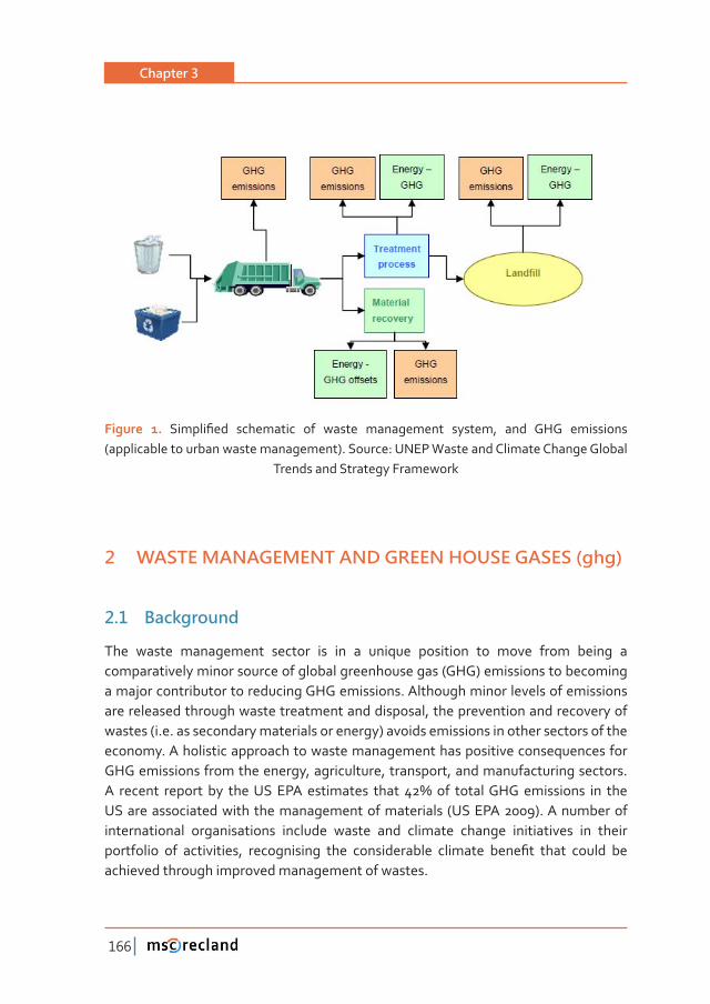
Chapter 3
166
Figure 1.� ������Ƥ��� ���������� ��� ������ ����������� ������ǡ� ���� �� ����������(applicable to urban waste management). Source: UNEP Waste and Climate Change Global
Trends and Strategy Framework
2 WASTE MANAGEMENT AND GREEN HOUSE GASES (ghg)
2�1 Background
The waste management sector is in a unique position to move from being a comparatively minor source of global greenhouse gas (GHG) emissions to becoming a major contributor to reducing GHG emissions. Although minor levels of emissions are released through waste treatment and disposal, the prevention and recovery of wastes (i.e. as secondary materials or energy) avoids emissions in other sectors of the economy. A holistic approach to waste management has positive consequences for GHG emissions from the energy, agriculture, transport, and manufacturing sectors. �� ������� ������� ��� ����������� ���������� ����� ά���� �������� ���������� ��� ����US are associated with the management of materials (US EPA 2009). A number of international organisations include waste and climate change initiatives in their ���������� ��� ����������ǡ� ������������ ���� ������������� �������� ����Ƥ�� ����� ������ ���achieved through improved management of wastes.
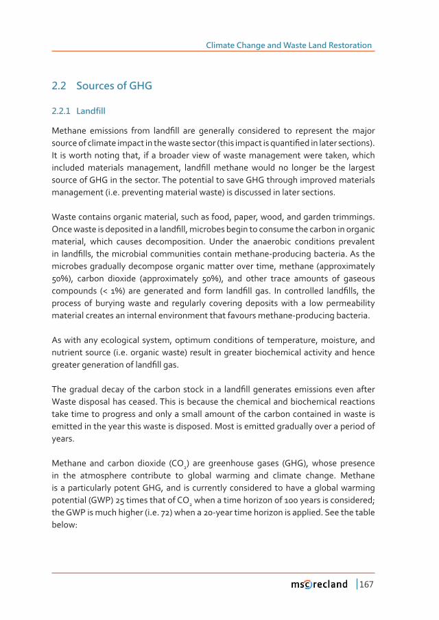
Climate Change and Waste Land Restoration
167
2�2 Sources of GHG
2�2�1 Landfill
�������� ���������� ����� ����Ƥ��� ���� ���������� ����������� ��� ���������� ���� ���������������������������������������������������ȋ���������������������Ƥ��������������������ȌǤ�It is worth noting that, if a broader view of waste management were taken, which �����������������������������ǡ� ����Ƥ����������������� ��� ������� ��� ���� ��������source of GHG in the sector. The potential to save GHG through improved materials management (i.e. preventing material waste) is discussed in later sections.
Waste contains organic material, such as food, paper, wood, and garden trimmings. ���������������������������������Ƥ��ǡ�������������������������������������������������material, which causes decomposition. Under the anaerobic conditions prevalent ��� ����Ƥ���ǡ������������������������������������������Ǧ������������������Ǥ��������microbes gradually decompose organic matter over time, methane (approximately άȌǡ� ������� �������� ȋ�������������� άȌǡ� ���� ������ ������ �������� ��� ������������������ ȋζ� άȌ� ���� ���������� ���� ����� ����Ƥ��� ���Ǥ� ��� ����������� ����Ƥ���ǡ� ����process of burying waste and regularly covering deposits with a low permeability material creates an internal environment that favours methane-producing bacteria.
As with any ecological system, optimum conditions of temperature, moisture, and nutrient source (i.e. organic waste) result in greater biochemical activity and hence ��������������������������Ƥ������Ǥ
��������������������� ����������� ������ ����� ����Ƥ����������������������������������Waste disposal has ceased. This is because the chemical and biochemical reactions take time to progress and only a small amount of the carbon contained in waste is emitted in the year this waste is disposed. Most is emitted gradually over a period of years.
Methane and carbon dioxide (CO2) are greenhouse gases (GHG), whose presence in the atmosphere contribute to global warming and climate change. Methane is a particularly potent GHG, and is currently considered to have a global warming potential (GWP) 25 times that of CO2 when a time horizon of 100 years is considered; the GWP is much higher (i.e. 72) when a 20-year time horizon is applied. See the table below:
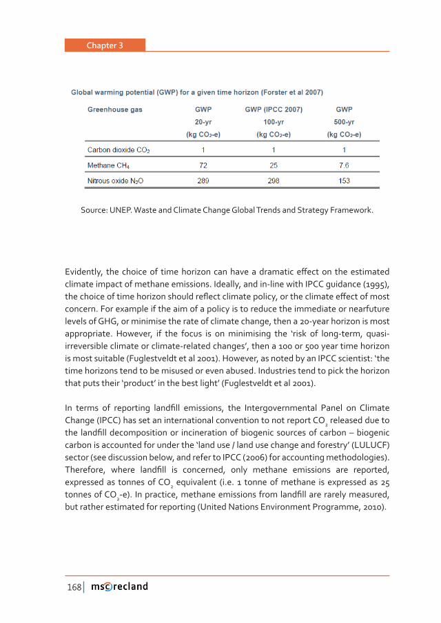
Chapter 3
168
Source: UNEP. Waste and Climate Change Global Trends and Strategy Framework.
���������ǡ� �������������� ����������������������������������ơ������� ��������������climate impact of methane emissions. Ideally, and in-line with IPCC guidance (1995), ������������������������������������ƪ������������������ǡ�����������������ơ������������concern. For example if the aim of a policy is to reduce the immediate or nearfuture levels of GHG, or minimise the rate of climate change, then a 20-year horizon is most appropriate. However, if the focus is on minimising the ‘risk of long-term, quasi-irreversible climate or climate-related changes’, then a 100 or 500 year time horizon is most suitable (Fuglestveldt et al 2001). However, as noted by an IPCC scientist: ‘the time horizons tend to be misused or even abused. Industries tend to pick the horizon that puts their ‘product’ in the best light’ (Fuglestveldt et al 2001).
��� ������ ��� ���������� ����Ƥ��� ���������ǡ� ���� ������������������ ������ ��� ��������Change (IPCC) has set an international convention to not report CO2 released due to ���� ����Ƥ�������������������� ������������������������� ������������������Ȃ����������carbon is accounted for under the ‘land use / land use change and forestry’ (LULUCF) sector (see discussion below, and refer to IPCC (2006) for accounting methodologies). ���������ǡ� ������ ����Ƥ��� ��� ���������ǡ� ����� �������� ���������� ���� ��������ǡ�expressed as tonnes of CO2 equivalent (i.e. 1 tonne of methane is expressed as 25 tonnes of CO2Ǧ�ȌǤ� �����������ǡ����������������������������Ƥ����������������������ǡ�but rather estimated for reporting (United Nations Environment Programme, 2010).
Climate Change and Waste Land Restoration
169
2�2�2 Aerobic composting
Aerobic composting processes directly emit varying levels of methane and nitrous oxide, depending on how the process is managed in practice. Closed systems, such as enclosed maturation bays or housed windrows, reduce emissions through use of air Ƥ������ȋ���������Ƥ�����Ȍ����������������������������������Ǥ�
Compost plants require varying, but usually small, amounts of energy input (with associated ‘upstream’ GHG emissions). Further GHG emissions occur ‘downstream’, depending on the application of the compost product – CO2 will be gradually released as the compost further degrades and becomes integrated with soil-plant systems.
2�2�3 Anaerobic composting
Anaerobic digestion (AD) systems are enclosed in order to capture and contain the biogas generated by the digestion process. GHG emissions from AD facilities are generally limited to system leaks from gas engines used to generate power from biogas, fugitive emissions from system leaks and maintenance, and possible trace amounts of methane emitted during maturation of the solid organic output.
Such systems also consume energy, however plants are generally self-sustaining if appropriately operated (i.e. a portion of the biogas output generates energy for use in-plant). ‘Downstream’ GHG emissions will depend on the application of the matured digestate (as per aerobic compost product). (United Nations Environment Programme, 2010)
2�2�4 Mechanical biological treatment (MBT)
Mechanical biological treatment (MBT) encompasses mechanical sorting of the mixed residual waste fraction, with some recovery of recyclable materials (limited due to �������������Ȍǡ���������������������Ƥ��ǡ��������������������������������������������treatment.
The biological component may include anaerobic digestion with recovery of biogas for energy/heat generation, or aerobic composting to produce a biologically stable product for either land application (limited applicability) or use as refuse-derived fuel
Chapter 3
170
(RDF) to substitute fuel in industrial furnaces (i.e. coincineration in cement kilns). �����������������������������������������������������������ǡ����Ƥ��������ǡ������ǡ�����outputs. GHG emissions associated with MBT are due to energy inputs (although AD systems may be self-sustaining), direct process emissions (this will depend on the air ����������� �������� ������ǡ� ����� ��� �� ���Ƥ����ǡ� ��������� ��� ���� �������� �����������component), gas engine emissions (for AD), and use of the composted organic output ȋ�������������������Ƥ���������������������ȌǤ�������������������������������������������to remediate contaminated land, however most OECD countries strictly regulate the ���������������������������������������ǡ����������������������������������������Ƥ��ǡ�����������������������������������Ƥ�������������Ǥ
2�3 GHG savings
In the context of the current report, the waste sector can save or reduce GHG emissions through several activities:
• Avoiding the use of primary materials for manufacturing through waste avoidance and material recovery (i.e. the GHG emissions associated with the use of primary materials – mostly energy-related – are avoided)
• Producing energy that substitutes or replaces energy derived from fossil fuels (i.e. the emissions arising from the use of waste as a source of energy are generally lower than those produced from fossil fuels).
• ����������������������Ƥ����ȋ�Ǥ�Ǥ�������Ǧ������������������������������������������������ ���������� ����Ƥ��� ����������ǡ� ����� ��� ��������� ���� ����Ȍ� ���� ��������application of compost to soils.
Indeed, depending on which GHG accounting convention is used, the waste sector is ����������������������������������Ƥ�������������������������ǡ������������������ǡ�and energy recovery.
2�3�1 European Environment Agency (EEA)
Using a life-cycle perspective, this report analyses the greenhouse gas emissions from municipal solid waste management in the EU, plus Norway and Switzerland. Among ���������������������������ǡ����Ƥ��������ǣ�
Climate Change and Waste Land Restoration
171
• improved municipal solid waste management in these countries has already cut annual net greenhouse gas (GHG) emissions by 48 million tonnes CO2-equivalent between 1995 and 2008;
• the two main factors responsible for this improvement are reduced methane �������������������Ƥ����������������������������������������������������Ǣ�
• ��� ���� ���������� ������ ����� ���� ����Ƥ��� ���������ǯ�� ������ ���������� �������ǡ�potential life-cycle GHG emissions from municipal waste management in 2020 �����������������������������������������ǡ��������������Ǥ�ά����������������GHG emissions in 2008;
• �� ��������� ���� ��� ����Ƥ������ ������ ���� ���������� ����� �������ǡ� ���������potential net emissions from waste management in 2020 by 78 million tonnes compared to 2008 — an amount slightly greater than Hungary’s total emissions in 2008.
As this report makes clear, better management of municipal solid waste can reduce ����������� ���� ���������� �����Ƥ������Ǥ� ���� ��� ���� ����� ���������ǡ� ���� ��ǯ�� �������������������������������������������Ȅ�����������������������Ƥ������������Ǥ
������� ���� ��������� ��� ���ǡ� ������ ��� �����Ƥ����� �������� ���������� ��������������emissions through better MSW management in the years to 2020.
�����������������������������������ơ�����������������������������������������ǡ�����EEA and its ETC/SCP developed three scenarios on possible future paths for European MSW management:
• scenario 1 assumes business-as-usual (as presented in Figure 2.1);
• ����������������������������������������������������Ƥ������������Ǣ�
• ��������� ���������������������������Ƥ��������������������� �����������������Ǥ�
���������Ƥ������������������������������������������������������������������� Ȃ�ȋ�������Ƥ����������Ȍ����������������������������������������������������for all three scenarios (in columns two, three and four). The net emission reduction is ��������������������ơ�������������������������������������������������������or 2020, as appropriate.
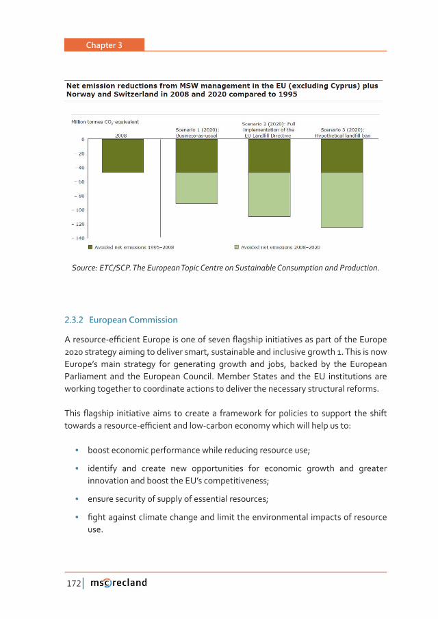
Chapter 3
172
������ǣ����Ȁ���Ǥ��������������������������������������������������������������������Ǥ
2�3�2 European Commission
����������Ǧ�ƥ�����������������������������ƪ�����������������������������������������2020 strategy aiming to deliver smart, sustainable and inclusive growth 1. This is now Europe’s main strategy for generating growth and jobs, backed by the European Parliament and the European Council. Member States and the EU institutions are working together to coordinate actions to deliver the necessary structural reforms.
�����ƪ������� ���������������� ��� ��������� ���������� ������������� ��� �������� ���� ������������������������Ǧ�ƥ�������������Ǧ������������������������������������ǣ�
• boost economic performance while reducing resource use;
• identify and create new opportunities for economic growth and greater innovation and boost the EU’s competitiveness;
• ensure security of supply of essential resources;
• Ƥ���������������������������������������������������������������������������use.
Climate Change and Waste Land Restoration
173
Increasing recycling rates will reduce the pressure on demand for primary raw materials, help to reuse valuable materials which would otherwise be wasted, and reduce energy consumption and greenhouse gas emissions from extraction and processing.
�������������������������� ������ ���� �����Ƥ���������2 emissions. For example, each year the EU disposes of 5.25 billion euro worth of recyclables such as paper, glass, plastics, aluminium and steel.
If this was recycled, the equivalent of 148 million tonnes of CO2 emissions could be avoided annually. Improved management of municipal waste could result in 92 million tons of greenhouse gas emissions avoided in 2020 compared with 1995. At least 500 �����������������������������������������������������������ά���������������Ǥ�
2�3�3 German Federal Ministry for the Environment
Following the entry into force of the Waste Management and Product Recycling Act ���ǡ�����������������������������������������������������������Ƥ�����������������abandoned in the period up to June 2005.
Thanks to a marked increase in separate collection and processing, and also to waste ���������� ��������� �ƥ������������ ���������� ���� ����������������ǡ� ��� ���� �����possible to replace fossil fuels and raw materials. These improvements are entered ��������������������������������ǡ�������������������������Ƥ��������������������������Ǧrelevant emissions and savings in fossil fuels.
�������������������������������������������������������������Ƥ��������Ǥ������������������� ����� �������������������� ����Ƥ��ǡ���������� �����������������������sheet results between 2005 and 2020 are no longer possible on the scale seen between 1990 and 2005. But a potential of over 5 million t CO2 equivalent remains as an important contribution to the German climate protection target.
On the whole, the disposal paths of waste incineration plants and co-incineration display the greatest potential for reducing emissions of greenhouse gases. Waste paper recycling is also of great importance, while all other paths make smaller contributions to climate protection, and even the expenditure involved in the collection of waste is ������������������Ƥ����ǡ����������������������������������ǣ
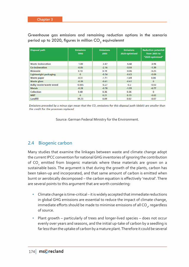
Chapter 3
174
Greenhouse gas emissions and remaining reduction options in the scenario SHULRG�XS�WR�������ÀJXUHV�LQ�PLOOLRQ�&22�HTXLYDOHQPW
Source: German Federal Ministry for the Environment.
2�4 Biogenic carbon
Many studies that examine the linkages between waste and climate change adopt the current IPCC convention for national GHG inventories of ignoring the contribution of CO2 emitted from biogenic materials where these materials are grown on a sustainable basis. The argument is that during the growth of the plants, carbon has been taken-up and incorporated, and that same amount of carbon is emitted when ��������������������������������Ȃ�������������������������ơ���������Ǯ�������ǯǤ�������are several points to this argument that are worth considering:
• Climate change is time-critical – it is widely accepted that immediate reductions in global GHG emissions are essential to reduce the impact of climate change, �����������ơ���������������������������������������������������2, regardless of source.
• Plant growth – particularly of trees and longer-lived species – does not occur evenly over years and seasons, and the initial up-take of carbon by a seedling is far less than the uptake of carbon by a mature plant. Therefore it could be several
Climate Change and Waste Land Restoration
175
���������������ƪ�����������������2 emitted instantaneously from a process (i.e. combustion of biogenic carbon) is re-captured through plant growth.
• The majority of wood, paper, and agricultural materials that enter the waste stream have not been produced through sustainable forestry/land practices – unsustainable practices deplete the carbon stored in forests and soil over time. According to IPCC methodologies for reporting national GHG inventories, if any factor ‘…is causing long-term decline in the total carbon embodied in living biomass (e.g., forests), this net release of carbon should be evident in the calculation of CO2 emissions described in the Agriculture, Forestry and Other Land Use (AFOLU) Volume of the 2006 Guidelines’. However, it is unclear how and whether this information is being recorded in all cases.
• In a national GHG inventory for IPCC purposes, where deforestation and re-growth is accounted for in the land-use category (LULUCF), there may be an argument for ignoring biogenic carbon. However, in an examination of the GHG impact of waste management systems, where solutions are being sought �������������������� �������������������ǡ� ������ ��� �����Ƥ����������� ��������������sources of GHG.
• ���� ����Ƥ��� ����� ������� ����� �� ���������� ��� ������ ��2, irrespective of the source, would seem to be the best indicator of the consequences of the ��ơ�������������Ǥ�������������������������������������������������������ǡ�������ơ�����������������������������Ǥ
3 CLIMATE IMPACT OF WASTE
3�1 Potential GHG emissions reductions from materials management
��������� ���������� ����������� ���������� ����������� ���� ��������� ƪ��� ��������� �� �����Ƥ����� ������� ��� ����Ǧ������ ��� ȋ�Ȍ� ���������Ǥ� ������ ����������management total technical potential scenarios include life cycle GHG emissions. These scenarios represent the estimated emission reductions that would occur if the scenarios presented were achieved, setting aside economic or practical limitations.
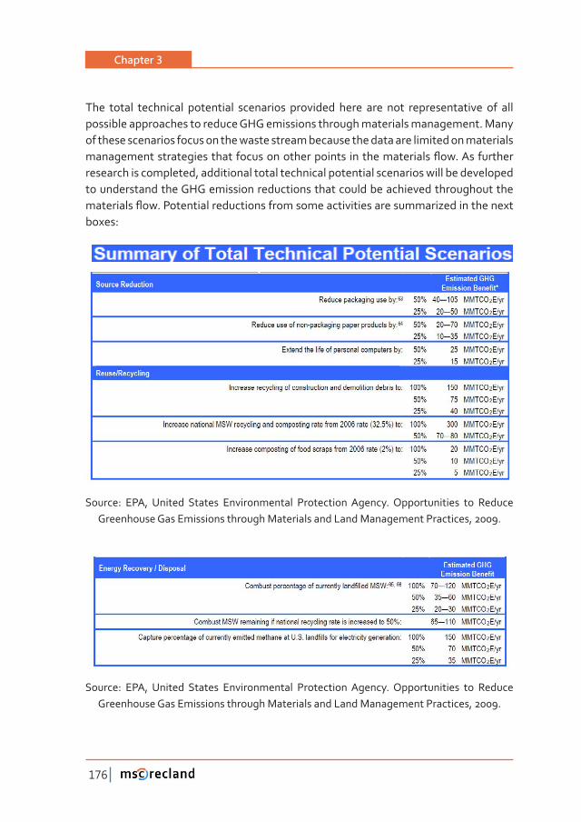
Chapter 3
176
The total technical potential scenarios provided here are not representative of all possible approaches to reduce GHG emissions through materials management. Many of these scenarios focus on the waste stream because the data are limited on materials ������������������������������������������������� �����������������ƪ��Ǥ������������research is completed, additional total technical potential scenarios will be developed to understand the GHG emission reductions that could be achieved throughout the ����������ƪ��Ǥ����������������������������������������������������������������������boxes:
Source: EPA, United States Environmental Protection Agency. Opportunities to Reduce Greenhouse Gas Emissions through Materials and Land Management Practices, 2009.
Source: EPA, United States Environmental Protection Agency. Opportunities to Reduce Greenhouse Gas Emissions through Materials and Land Management Practices, 2009.
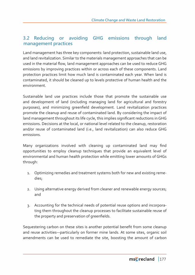
Climate Change and Waste Land Restoration
177
3�2 Reducing or avoiding GHG emissions through land management practices
Land management has three key components: land protection, sustainable land use, and land revitalization. Similar to the materials management approaches that can be ���������������������ƪ��ǡ����������������������������������������������������emissions by improving practices within or across each of these components. Land protection practices limit how much land is contaminated each year. When land is contaminated, it should be cleaned up to levels protective of human health and the environment.
Sustainable land use practices include those that promote the sustainable use and development of land (including managing land for agricultural and forestry ��������Ȍǡ� ���� ����������� �����Ƥ���� �����������Ǥ� ����� ��������������� ����������promote the cleanup and reuse of contaminated land. By considering the impact of �����������������������������������������ǡ�������������������Ƥ���������������������emissions. Decisions at the local, or national level related to the cleanup, restoration and/or reuse of contaminated land (i.e., land revitalization) can also reduce GHG emissions.
����� �������������� ��������� ����� ��������� ��� ������������� ����� ���� Ƥ���opportunities to employ cleanup techniques that provide an equivalent level of environmental and human health protection while emitting lower amounts of GHGs through:
1. Optimizing remedies and treatment systems both for new and existing reme-dies;
2. Using alternative energy derived from cleaner and renewable energy sources; and
3. Accounting for the technical needs of potential reuse options and incorpora-ting them throughout the cleanup processes to facilitate sustainable reuse of ��������������������������������������Ƥ����Ǥ
����������������������������������� �������������������������Ƥ��������������������and reuse activities—particularly on former mine lands. At some sites, organic soil amendments can be used to remediate the site, boosting the amount of carbon
Chapter 3
178
sequestered in the soil and enhancing vegetation growth. This remediation approach also provides a use for some organic soil amendments such as biosolids which may otherwise be a waste product.
Land cleanup activities may also provide recycling opportunities to further bolster EPA’s approaches to materials and land management. For example, reusing and recycling construction and demolition debris from buildings on contaminated land ������������ơ���������������������������������������������Ǣ������������������������reuses both materials and land, but also prevents other land from being used for the disposal of construction and demolition debris.
After cleanup is complete, sustainably reusing land protects the land based carbon sink, by providing sites that can be reused for development, instead of developing �����Ƥ����Ǥ� �������� ������ ��������� ����������� ���� ����� ������� �� ����������associated with the infrastructure expansion needed to connect newly developed �����Ƥ�������������������������������Ǥ����������������������������������������������new land development and denser mixed use development—key aspects of smart growth—will avoid the majority of infrastructure and bio-carbon emissions. Sites can also be ecologically restored to increase the amount of undeveloped land and expand the land-based carbon sink. These are some examples of land management approaches that help reduce GHG emissions:
Carbon Sequestration: EPA is studying the potential carbon sequestration that occurs when soil amendments are used to remediate sites.
����� ��������������: To date, EPA has helped make more than 917,000 acres of previously contaminated lands ready for anticipated use, reducing pressure on �����Ƥ����������������������������������Ǧ�����������������Ǥ����������������������development of renewable energy resources as one particularly promising land ��������������������������������������������������������Ƥ��Ǥ�
�����������: Smart growth has been shown to reduce household vehicle miles ������������ Ǧά�������������������������������������������������Ǥ�����������ǡ�residents of Atlantic Station, a noted smart growth development, drive an average of 13.9 miles per day, compared to a regional average of 33.7 miles per day.
Climate Change and Waste Land Restoration
179
Green Remediation: Green remediation practices are being employed at contaminated sites, which can reduce GHG emissions. For example, some remediation projects use solar energy to operate ground water pump and treat systems; others are reducing construction engine idling time, and using alternative fuels to reduce GHG emissions.
3�3 Trends in waste generation and management
The long-term vision for the waste sector is to establish a circular global economy in which the use of materials and generation of waste are minimised, any unavoidable waste recycled or remanufactured, and any remaining waste treated in a way that causes least damage to the environment and human health or even creating additional value by recovering energy from waste. To achieve this vision, radical changes to supply-chain management, especially to the product and industrial design part of ����������������ǡ�����������Ǥ������Ƥ�����ǡ����������������������������������������Ȃ�with implications for materials at all stages – and be overlaid on the entire supply chain. This requirement is, in turn, expected to motivate innovation. The chapter on manufacturing further elaborates on life-cycle approaches, including closed loop and circular systems in manufacturing.
The waste sector is facing three sets of challenges:
1. Increasing growth in the quantity and complexity of waste streams associated with rising incomes and economic growth;
2. Increasing risk of damage to human health and ecosystems; and
3. The sector’s contribution to climate change.
The exploitation of the earth’s resources continues apace; material use increased eight-fold in the last century (Krausmann et al. 2009). According to the Wuppertal Institute, an average European consumes about 50 tonnes of resources a year, around three times the amount consumed per capita by emerging economies. Furthermore, on average, Europeans dispose twice as much as citizens from emerging economies (Bleischwitz 2009). Per-capita resource use in emerging economies is also increasing considerably while the world’s Least Developed Countries (LDC) are beginning the transition towards an industrial type of societal metabolism, as incomes rise and purchasing power is deployed in consumer spending.
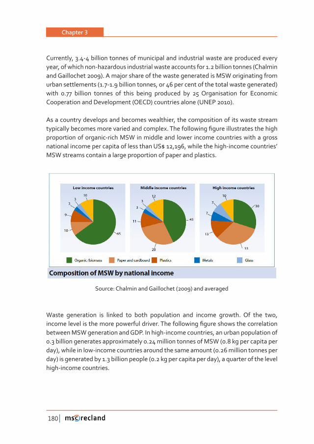
Chapter 3
180
Currently, 3.4-4 billion tonnes of municipal and industrial waste are produced every year, of which non-hazardous industrial waste accounts for 1.2 billion tonnes (Chalmin and Gaillochet 2009). A major share of the waste generated is MSW originating from urban settlements (1.7-1.9 billion tonnes, or 46 per cent of the total waste generated) with 0.77 billion tonnes of this being produced by 25 Organisation for Economic Cooperation and Development (OECD) countries alone (UNEP 2010).
As a country develops and becomes wealthier, the composition of its waste stream �����������������������������������������Ǥ���������������Ƥ��������������������������proportion of organic-rich MSW in middle and lower income countries with a gross national income per capita of less than US$ 12,196, while the high-income countries’ MSW streams contain a large proportion of paper and plastics.
Source: Chalmin and Gaillochet (2009) and averaged
Waste generation is linked to both population and income growth. Of the two, ����������������������������������������Ǥ���������������Ƥ���������������������������between MSW generation and GDP. In high-income countries, an urban population of 0.3 billion generates approximately 0.24 million tonnes of MSW (0.8 kg per capita per day), while in low-income countries around the same amount (0.26 million tonnes per day) is generated by 1.3 billion people (0.2 kg per capita per day), a quarter of the level high-income countries.
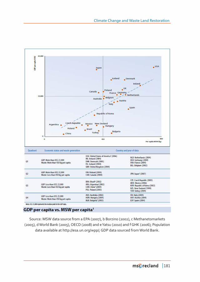
Climate Change and Waste Land Restoration
181
Source: MSW data source from a EPA (2007), b Borzino (2002), c Methanetomarkets (2005), d World Bank (2005), OECD (2008) and e Yatsu (2010) and f GHK (2006); Population
data available at http://esa.un.org/wpp/; GDP data sourced from World Bank.
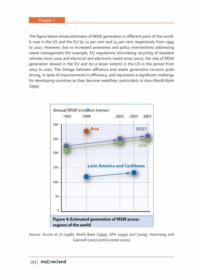
Chapter 3
182
����Ƥ��������������������������������������������������ơ������������������������Ǥ�It rose in the US and the EU by 21 per cent and 14 per cent respectively from 1995 to 2007. However, due to increased awareness and policy interventions addressing waste management (for example, EU regulations stimulating recycling of obsolete vehicles since 2000 and electrical and electronic waste since 2002), the rate of MSW generation slowed in the EU and (to a lesser extent) in the US in the period from � ��� Ǥ����� �������� �������� �ƫ������ ���������� ����������� �������� ������������ǡ������������������������������ƥ������ǡ�����������������������Ƥ���������������for developing countries as they become wealthier, particularly in Asia (World Bank 1999).
Source: Acurio et al (1998), World Bank (1999), EPA (1999) and (2009), Hoornweg and Giannelli (2007) and Eurostat (2010)
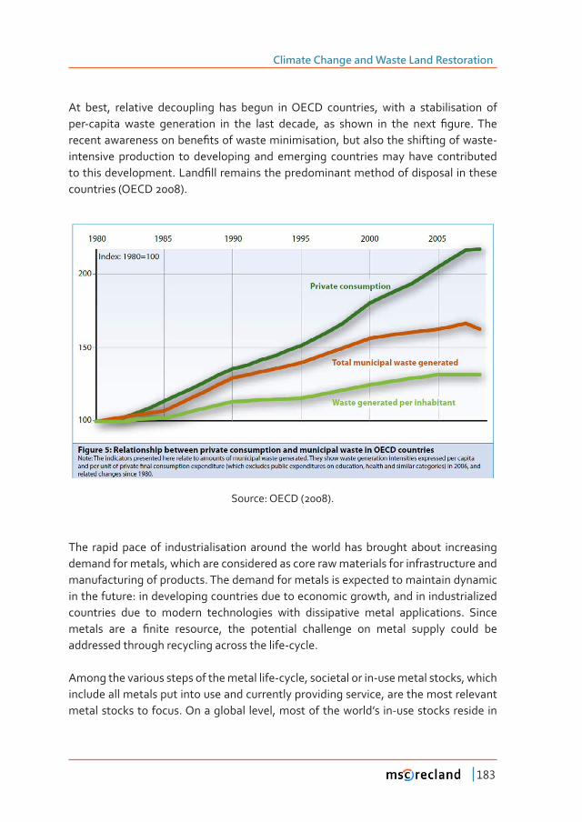
Climate Change and Waste Land Restoration
183
At best, relative decoupling has begun in OECD countries, with a stabilisation of ���Ǧ������� ������ ����������� ��� ���� ����� ������ǡ� ��� ������ ��� ���� ����� Ƥ����Ǥ�����������������������������Ƥ������������������������ǡ�������������������������������Ǧintensive production to developing and emerging countries may have contributed �������������������Ǥ�����Ƥ�������������������������������������������������������countries (OECD 2008).
Source: OECD (2008).
The rapid pace of industrialisation around the world has brought about increasing demand for metals, which are considered as core raw materials for infrastructure and manufacturing of products. The demand for metals is expected to maintain dynamic in the future: in developing countries due to economic growth, and in industrialized countries due to modern technologies with dissipative metal applications. Since ������� ���� �� Ƥ����� ��������ǡ� ���� ���������� ���������� ��� ������ ������� ������ ���addressed through recycling across the life-cycle.
Among the various steps of the metal life-cycle, societal or in-use metal stocks, which include all metals put into use and currently providing service, are the most relevant metal stocks to focus. On a global level, most of the world’s in-use stocks reside in
Chapter 3
184
more developed countries. For instance, Japan and the United States posses the highest in-use stocks and exceed the value of China by 9 and 13 times. Moreover, data suggests that per capita inuse stocks in more-developed countries typically exceed those in less-developed countries by factors of 5 to 10.
One of the key strategies in meeting this increasing demand is to take advantage of anthropogenic mines, or urban stocks, which has a great potential to reduce dependency on virgin metal resources and mitigate the environmental degradation caused by mining activities. However, tremendous weak points have been found in global metal recycling. For instance, mass-scale use of specialty metals like gallium, indium, etc, in the last three decades and the lack of infrastructure for recycling in many developing countries has led to dissipative losses of such metals.
Thus, the recycling rates for some of the metals, especially specialty metals are relatively low. It has been recognized that creating a circular economy is key for increasing metal needs of the future. Setting of appropriate metal recycling infrastructure and services in urban areas - that are tomorrow’s metal mines – is essential and should be given high priority.
The International Resource Panel decisively states that it is important to enhance capacity building, technology transfer and international cooperation in developing countries through international recycling conferences, technological implementation ��������������������Ƥ���������Ƥ���������������������Ǥ
The Panel also highlights three key issues that require urgent attention:
• Research & development. Data acquisition and analysis, recycling technologies ��������ǡ����������� ��������������������������ơ�������������������������� ���the development process. Global data on a large variety of metals on equal spatial and temporal resolution is actually not available
• Stopping illegal waste transport. International organisations like UNEP and OECD have to multiply their engagement in the monitoring and controlling of illegal scrap exports.
• Continuous improvements of legislative systems. The more developed countries should reinforce their attempts to help the less developed countries install appropriate legislative systems and ensure their enforcement in order to take advantage of metal stocks in society.
Climate Change and Waste Land Restoration
185
Waste volumes are not necessarily the most important challenge ahead. Mixed MSW, hazardous health-care waste, and industrial waste streams can impose serious health and ecological risks if these wastes remain uncollected or dumped in uncontrolled ������������������Ƥ��������Ǥ������������������������ǡ������������ǡ����������������������lower than 70 per cent, with more than 50 per cent of the collected waste disposed �������� ������������� ����Ƥ������ ���� ������ � ���� ����� ���������� �������� �������and informal recycling (Chalmin and Gaillochet 2009). Given the amount of valuable components in MSW, the mixing of wastes also means a lost opportunity to recover components that could be recycled and used as new resources.
3�4 Climate impact of waste management practices
Every waste management practice generates GHG, both directly (i.e. emissions from the process itself) and indirectly (i.e. through energy consumption). However, the ���������������� ��������������Ƥ������������������������������������������������net GHGs, accounting for both emissions and GHG savings.
3�4�1 Landfill
���������������������������������������������ǡ���������������������������������Ƥ�������������������������������������������������������Ǥ����������������������������Ƥ���represent the largest source of GHG emissions from the waste sector, contributing around 700 Mt CO2-e (estimate for 2009) (Bogner et al 2007). In comparison, the next largest source of GHG emissions from the management of solid wastes is incineration, estimated to contribute around 40 Mt CO2-e (2009 data estimated in Bogner et al ȋȌȌǤ�����Ƥ�����������������������������������������Ǣ�����������������������������global GHG emissions is believed to be negligible, and related to the management ���������������������������������������������Ƥ������������Ƥ������������ȋ�������������2008).
The next table provides a qualitative summary of the indirect and direct GHG ������������������������������������������Ƥ�����Ǥ������������������������������ǡ�����GHGs are noted, including biogenic CO2.
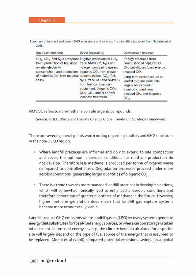
Chapter 3
186
NMVOC refers to non-methane volatile organic compounds.
Source: UNEP. Waste and Climate Change Global Trends and Strategy Framework.
������������������������������������������������������������Ƥ��������������������in the non-OECD region:
• ������ ����Ƥ��� ���������� ���� ��������� ���� ��� ���� ������� ��� ����� �����������and cover, the optimum anaerobic conditions for methane-production do not develop. Therefore less methane is produced per tonne of organic waste (compared to controlled sites). Degradation processes proceed under more aerobic conditions, generating larger quantities of biogenic CO2.
• ������������������������������������������Ƥ����������������������������������ǡ�which will somewhat ironically lead to enhanced anaerobic conditions and therefore generation of greater quantities of methane in the future. However, ������� �������� ����������� ����� ����� ����� ����Ƥ��� ���� �������� ��������become more economically viable.
����Ƥ���������������������������������Ƥ����������ȋ�Ȍ���������������������������energy that substitutes for fossil-fuel energy sources, or where carbon storage is taken ������������Ǥ���������������������������ǡ�����������������Ƥ������������������������Ƥ��site will largely depend on the type of fuel source of the energy that is assumed to be replaced. Monni et al (2006) compared potential emissions savings on a global
Climate Change and Waste Land Restoration
187
��������������Ƥ��������������������������ǡ���������������������2-e where coal-derived energy is assumed to be replaced and 22 Tg CO2-e where natural gas-derived energy is replaced (natural gas is a ‘cleaner’ fuel than coal, therefore there is less ������������Ƥ��������������������������ȌǤ
�������Ǧ�����������ǡ��������� ����Ƥ������� ���� ���������� �������������������������������������������Ȃ�ά����������������������ȋ���������������ǡ�������������ȌǤ�����Ƥ�����������������������������������������������������������������������ά���������������������Ǥ
�������� ������ ���������� ���� �������� ������������� ��� ����Ƥ���� Ȃ� ���Ǧ��������������materials (i.e. plastics), lignin and some lignin-bound cellulose and hemi-cellulose �����������������������������������������������������������������������������Ƥ����(Barlaz 2006). A high proportion of wood waste, for example, may be considered as ���������������������Ƥ��������������������������������������Ǥ���������������������������ǡ�����������������������������������������ǡ���������������������Ƥ����������������of the solution; however, there are myriad other reasons (i.e. ecological, resource use, land use) for not doing this.
�������������������������������������Ƥ������� �����������������������������������������Ƥ��� ���� ����������� ���� �������������� ��� ��� ������ǣ� ���� ��� ���� �������� ����������� �������� ����� ����� �����ǡ� ����� ��� �� ���� ��� ����Ƥ������ �������� ������ �����implemented at a site today, there would still be an existing store of organic material releasing methane, that could be extracted into the future.
����Ƥ�����������������������������������������������������������������������������sector, but the options for reducing this climate impact are available and achievable: ������������������������������������Ƥ�����������������������������Ƥ��������������Ǥ�Neither option is technically complex, and there is a body of knowledge and experience in OECD regions that could be transferred to non-OECD countries.
3�4�2 Thermal treatment
Thermal waste treatment refers to mass-burn incineration, co-incineration (i.e. replacing fossil fuels with refuse-derived fuel (RDF) in conventional industrial ���������ǡ���������������������Ȍǡ�������������������Ƥ������Ǥ�����Ǧ����������������������������������������������������������������Ǥ�������������������Ƥ��������������
Chapter 3
188
considered as emerging technologies, with limited success in treating mixed waste streams. The majority of studies assume that energy is recovered from the thermal treatment of waste, either as heat or electricity, which can equate to a considerable GHG saving (depending on the type of energy displaced). Metals are also recovered ��������������������ǡ���������������������������������������Ƥ��Ǥ
Approximately 130 million tonnes of waste are currently incinerated across 35 ����������ȋ�������������ȌǤ� ����ǡ��������ǡ����������������������ηά��������waste stream through incineration. France, Sweden, the Netherlands and Switzerland also have high rates of incineration (Bogner et al 2007). Incineration is only applied in a limited capacity in the remainder of the OECD countries. There is no incineration of mixed waste practiced in either Australia or New Zealand, largely due to public opposition. Australia, New Zealand, Canada and the US do not have legislation in ����������������������Ƥ������ȋ�Ǥ�Ǥ��������������������������������Ƥ������������ȌǢ���������������Ƥ��� �������� ���� ��������� ���� ����� ���������� ��������� ������Ǥ� ������������� ���mixed wastes is a largely unfeasible option in non-OECD countries due to cost and often unsuitable waste composition.
At the global level, the climate impact of incineration is minor compared to that of ����Ƥ�����ǡ���������������������������2-e in the current year (Bogner et al 2007). Typically only fossil CO2 is counted as a GHG emission from incineration; therefore, ���� �������� �������� ������� ��� ������������� ����� ��� ������� ��ƪ������� ��� ���� �������carbon content of the input waste. Downstream, indirect GHG savings due to energy generation may dominate an estimate of emissions from incineration, depending on the energy assumed to be replaced. The next table provides a qualitative summary of the indirect and direct GHG emissions and savings associated with incineration. To provide a complete picture, all GHGs are noted, including biogenic CO2.
���������������������������������������������������������������������������������Ƥ��streams of wastes, or carefully prepared mixed residual wastes, as part of an integrated and future-thinking waste management system. In many countries, thermal treatment plants require long lead-times (i.e. >10 years) to meet planning ��������ǡ�Ƥ�������ǡ�������������ǡ������������������Ǥ������������ǡ����������������� ��������������������������������������ƪ�����������������������������������ǡ����������������that capacity needs to be planned for carefully. This suggests that such facilities may be part of a longer-term strategy for climate abatement.
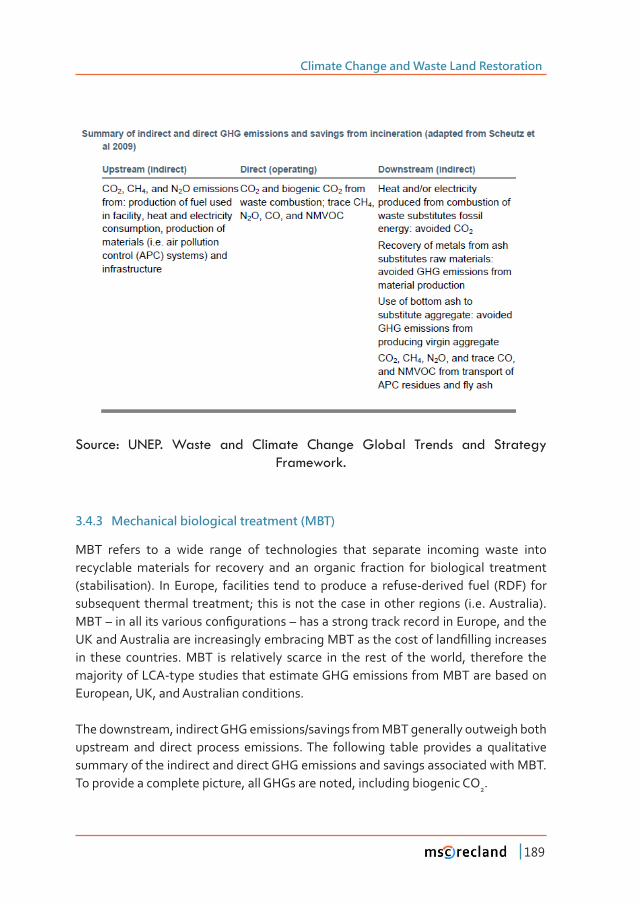
Climate Change and Waste Land Restoration
189
6RXUFH�� 81(3�� :DVWH� DQG� &OLPDWH� &KDQJH� *OREDO� 7UHQGV� DQG� 6WUDWHJ\�Framework.
3�4�3 Mechanical biological treatment (MBT)
MBT refers to a wide range of technologies that separate incoming waste into recyclable materials for recovery and an organic fraction for biological treatment (stabilisation). In Europe, facilities tend to produce a refuse-derived fuel (RDF) for subsequent thermal treatment; this is not the case in other regions (i.e. Australia). ����Ȃ�����������������������Ƥ����������Ȃ������������������������������������ǡ����������������������������������������������������������������������������Ƥ����������������in these countries. MBT is relatively scarce in the rest of the world, therefore the majority of LCA-type studies that estimate GHG emissions from MBT are based on European, UK, and Australian conditions.
The downstream, indirect GHG emissions/savings from MBT generally outweigh both upstream and direct process emissions. The following table provides a qualitative summary of the indirect and direct GHG emissions and savings associated with MBT. To provide a complete picture, all GHGs are noted, including biogenic CO2.
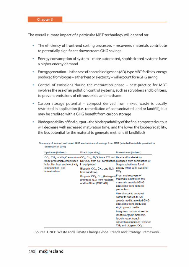
Chapter 3
190
The overall climate impact of a particular MBT technology will depend on:
• �����ƥ���������������Ǧ����������������������Ȃ����������������������������������������������������Ƥ��������������������������
• Energy consumption of system – more automated, sophisticated systems have a higher energy demand
• Energy generation – in the case of anaerobic digestion (AD)-type MBT facilities, energy produced from biogas – either heat or electricity – will account for a GHG saving
• Control of emissions during the maturation phase – best-practice for MBT �������������������������������������������������ǡ��������������������������Ƥ�����ǡ�to prevent emissions of nitrous oxide and methane
• Carbon storage potential – compost derived from mixed waste is usually ��������������������������ȋ�Ǥ�Ǥ�����������������������������������������Ƥ��Ȍǡ����������������������������������Ƥ���������������������
• ��������������������Ƥ�����������Ȃ�����������������������������Ƥ���������������������will decrease with increased maturation time, and the lower the biodegradability, ��������������������������������������������������������ȋ�������Ƥ����Ȍ
Source: UNEP. Waste and Climate Change Global Trends and Strategy Framework.
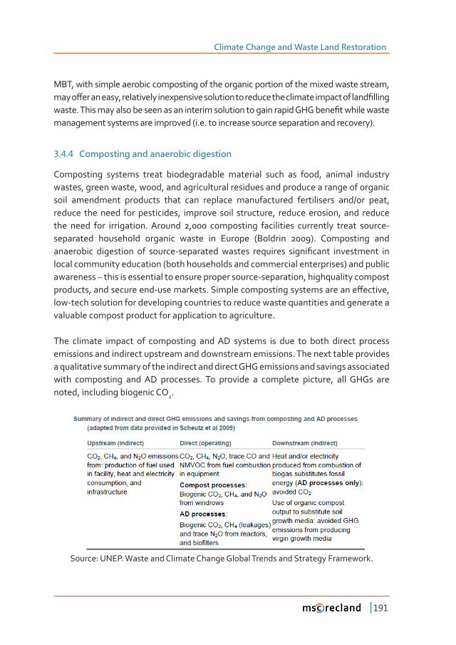
Climate Change and Waste Land Restoration
191
MBT, with simple aerobic composting of the organic portion of the mixed waste stream, �����ơ����������ǡ���������������������������������������������������������������������Ƥ�����������Ǥ������������������������������������������������������������������Ƥ��������������management systems are improved (i.e. to increase source separation and recovery).
3�4�4 Composting and anaerobic digestion
Composting systems treat biodegradable material such as food, animal industry wastes, green waste, wood, and agricultural residues and produce a range of organic soil amendment products that can replace manufactured fertilisers and/or peat, reduce the need for pesticides, improve soil structure, reduce erosion, and reduce the need for irrigation. Around 2,000 composting facilities currently treat source-separated household organic waste in Europe (Boldrin 2009). Composting and ���������� ���������� ��� ������Ǧ���������� ������� ��������� �����Ƥ����� ����������� ���local community education (both households and commercial enterprises) and public awareness – this is essential to ensure proper source-separation, highquality compost ��������ǡ���������������Ǧ�����������Ǥ�����������������������������������ơ������ǡ�low-tech solution for developing countries to reduce waste quantities and generate a valuable compost product for application to agriculture.
The climate impact of composting and AD systems is due to both direct process emissions and indirect upstream and downstream emissions. The next table provides a qualitative summary of the indirect and direct GHG emissions and savings associated with composting and AD processes. To provide a complete picture, all GHGs are noted, including biogenic CO2.
Source: UNEP. Waste and Climate Change Global Trends and Strategy Framework.
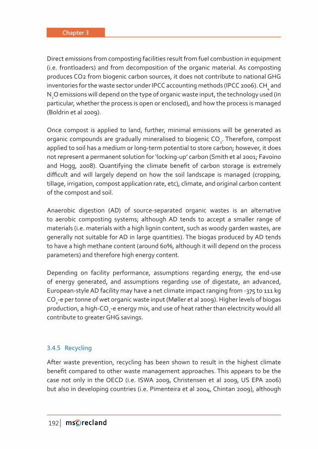
Chapter 3
192
Direct emissions from composting facilities result from fuel combustion in equipment (i.e. frontloaders) and from decomposition of the organic material. As composting produces CO2 from biogenic carbon sources, it does not contribute to national GHG inventories for the waste sector under IPCC accounting methods (IPCC 2006). CH4 and N2O emissions will depend on the type of organic waste input, the technology used (in particular, whether the process is open or enclosed), and how the process is managed (Boldrin et al 2009).
Once compost is applied to land, further, minimal emissions will be generated as organic compounds are gradually mineralised to biogenic CO2. Therefore, compost applied to soil has a medium or long-term potential to store carbon; however, it does not represent a permanent solution for ‘locking-up’ carbon (Smith et al 2001; Favoino ���� ����ǡ� ȌǤ������������� ���� �������� ����Ƥ�� ��� ������� �������� ��� ������������ƥ����� ��������� �������� ������� ��� ���� ���� ����� ���������� ����������� ȋ��������ǡ�tillage, irrigation, compost application rate, etc), climate, and original carbon content of the compost and soil.
Anaerobic digestion (AD) of source-separated organic wastes is an alternative to aerobic composting systems; although AD tends to accept a smaller range of materials (i.e. materials with a high lignin content, such as woody garden wastes, are generally not suitable for AD in large quantities). The biogas produced by AD tends �������������������������������ȋ�������άǡ����������������������������������������parameters) and therefore high energy content.
Depending on facility performance, assumptions regarding energy, the end-use of energy generated, and assumptions regarding use of digestate, an advanced, European-style AD facility may have a net climate impact ranging from -375 to 111 kg CO2-e per tonne of wet organic waste input (Møller et al 2009). Higher levels of biogas production, a high-CO2-e energy mix, and use of heat rather than electricity would all contribute to greater GHG savings.
3�4�5 Recycling
After waste prevention, recycling has been shown to result in the highest climate ����Ƥ�����������������������������������������������Ǥ������������������������case not only in the OECD (i.e. ISWA 2009, Christensen et al 2009, US EPA 2006) but also in developing countries (i.e. Pimenteira et al 2004, Chintan 2009), although
Climate Change and Waste Land Restoration
193
limited data is available. For example, in the US, recycling materials found in MSW resulted in the avoidance of around 183 Mt CO2-e in 2006 (US EPA, 2009). Estimates of GHG savings are generally based on the premise that recycled materials replace an equal – or almost equal – quantity of virgin materials in a closed-loop recycling system (i.e. where material is reprocessed back into the same or a similar product). Industrial symbiosis involves the exchange of resources including by-products among industrial enterprises, which may form ‘recycling clusters’ to facilitate sharing resources.
The next table provides a qualitative summary of the indirect and direct GHG emissions and savings associated with recycling processes. To provide a complete picture, all GHGs are noted, including biogenic CO2.
Source: UNEP. Waste and Climate Change Global Trends and Strategy Framework.
A recent investigation by the UK Waste and Resources Action Programme (WRAP) of ������������������������Ǯ����������������ǡ�����������������������������������ơ��������� �������������� ����Ƥ��� ���� ������ �������������� �������� ����� ������ ������management options’ (WRAP, 2006). The report’s main GHG-related conclusions for �����Ƥ��������������������ǣ
• On average, virgin production of paper followed by incineration with energy recovery consumes twice as much energy as paper recycling; however, the GHG ����Ƥ����������������������������������������������������������������������
Chapter 3
194
by the individual LCA studies (in particular, whether the GHG ‘cost’ of using timber to produce paper is accounted for)
• ������Ǧ����� ���������� ��� ������ �������� ��� ���� �������� ����Ƥ��� ��������� ���������������Ǥ��������������ƥ������������������Ǧ���������������ȋ�Ǥ�Ǥ����������������into aggregate, insulation, or other secondary product) to determine the net GHG impact
• - Where recycled plastic replaces virgin plastic of the same kind in ratio of 1:1 ȋ���������Ȍǡ����������������������������������������������������������������Ƥ��compared to incineration. For every kg of plastic recycled, around 1.5 – 2 kg CO2-e is saved.
• Production of virgin aluminium requires 10-20 times more energy than ���������� ���������Ǥ���������� ��������� ��ơ�������� ��� ������� �������� �������������������������������������������������ǡ����������������������������������Ƥ��in recycling aluminium.
• Production of virgin steel requires around two times as much energy as ���������������������������������������Ǥ���������ǡ������������ơ������������������sources may cause variations in the extent of GHG savings; however there is a ����������������������Ƥ��������������������Ǥ
The role of the informal recycling sector should not be underestimated in developing �������Ǥ� ���� ������ ����� ���������� ����� ������� ά� ��� ���� ������ ����������� ���developing countries (approximately 15 million people) earns their livelihood from waste-picking and the informal recycling sector (Medina 2008).
The economic contribution of waste pickers should also not be overlooked. Informal ���������� ��� ������� �������� ���� ������� ��� ������ ��� �������������� άǡ� ������������������ ����������� ������������� �����ǡ� �������������� ���� ����� ��� ����Ƥ���� ȋ�������2008). In major Indian cities such as Delhi and Bangalore, waste pickers prevent at ������ ά�������������� ��� ����Ƥ��ǡ� ������� ��������������� ���������ǡ�����day in waste collection and disposal costs (Sharholy 2008). Mexican paper mills have strengthened relationships with waste picker associations in order to secure more supply of valuable waste paper.
Climate Change and Waste Land Restoration
195
3�5 Waste prevention
Waste prevention is considered the most important action in the waste hierarchy; ��������������������������������������������������������������������������������ơ���Ǥ�Waste avoidance is critical to decoupling waste generation from economic growth. Within waste prevention there exists a raft of mechanisms that can deliver climate ����Ƥ�ǡ� ����� ��� �������� ����������ǡ� ��������� ��������� ��������������ǡ� ������������consumption and production, etc. The SCP Branch of UNEP is involved in a number of programmes targeting sustainable consumption and production, including collaborations with the International Solid Waste Association (ISWA) on waste minimisation. Various mechanisms have been developed and applied to prevent �������������ǡ���������������������������������ơ��������������������������������Ǥ
Since the early 1990s, the EU has been actively developing waste-related policy measures. The following EU Directives and Strategies have been instrumental in greening the region’s waste management industry: Packaging (1994), Waste ����������������������� ȋȌǡ� ����Ƥ��� ȋȌǡ� ���� ��� �������������� ȋ����� Ȍǡ�Waste Electrical and Electronic Equipment (WEEE 2002), the Thematic Strategy on Waste Prevention and Recycling of Waste and Sustainable Use of Natural Resources (2005), the EU’s revised Waste Framework Directive (2008) and the Raw Material Initiative (2008).
������������ ������������������������� �������������������������������������Ƥ������cost for the EU by € 80 million per year, which is a cost saving of 40 per cent, compared to the cost that prevailed prior to the directive. Meeting the 95 per cent target by 2015 will reduce the cost further by 80 per cent (GHK and Bio Intelligence Service 2006).
Individual countries have also moved forward with waste related regulations and their enforcement. The German Packaging Ordinance introduced in 1991 helped encourage recycling of packaging waste which is collected through a third party organisation. British Columbia Recycling Regulation of 2004 brought about a considerable increase in the proportion of recycled waste in Canada.
Developing-country examples include the Law of the People’s Republic of China on the Prevention and Control of Solid Waste Pollution adopted in 1995, South Africa’s National Waste Management Strategy in 1999, India’s Municipal Waste Management and Handling Rules in 2000, the Philippines’s Ecological Solid Waste Management Act in 2000, Malaysia’s Solid Waste and Public Cleansing Management Act in 2007 and
Chapter 3
196
���������ǯ��������������������������������� ���Ǥ��������������������ơ��������such measures will come from implementation, the existence of these instruments provides a signal of political commitments to greening the waste sector.
��� ������ ��� �������� ������� ������ǡ� ���� ����Ƥ��� ��� ������ ����������� �����������������������Ƥ���������������������������������������������������ǣ��������������net GHG emissions avoided from treatment and disposal of the waste, but there is ����������������������Ƥ�����������������������������������������������������������and manufacturing.
A US EPA study found that, generally, the net GHG emissions for a given material ���� ������� ���� ������� ���������� ���� �������� ���� ����Ƥ������ ȋ��� ���ǡ� ȌǤ������ ���especially true for prevention of paper waste where GHG savings are attributed to increases in forest carbon sequestration (i.e. less use of virgin forest materials to produce paper products equates to less deforestation). A recent report produced by ������������ƥ�����������������������������������������ȋ�������Ȍ����������how GHG emissions could be prevented through alternative management of materials ȋ������ǡ�ȌǤ��������������ά����������������������������������������������management. Strategies discussed in the report include source reduction through improved product design and cleaner production, increasing product durability, and maximising the ease of product disassembly (for recycling).
3�5�1 European Union: The Landfill Directive
����������ǡ���������Ƥ�����������������������������������������������Ǥ� ������������������������������������Ƥ�����������������ǯ���������������������ǡ�������������������waste prevention, followed by re-use, recycling and recovery, and seeks to avoid ����Ƥ�����������������������Ǥ�
��������������������������������������������������ơ�������������������������������management practices is a complex task. The process of diverting biodegradable ���������� ������ ����� ����Ƥ��� ���������� ��� ��ơ������ ������ ��� ���� ���������� ����region studied and has proceeded at varying speeds. In addition, urbanization and population density are obviously important socio-economic drivers for diverting ���������������Ƥ��Ǥ�
Climate Change and Waste Land Restoration
197
��������Ƥ������������ǯ�� �������� ������������ ��������� �������Ǥ�����ǡ� ���� ������������of long-term and intermediate targets has provided a good framework for countries �������Ƥ�������������������������������������Ǥ��������������ǡ�������������������������governments and the European Commission measure progress and keep attention ��� ���� ����� ������Ǥ�������ǡ� ���� ���������ǯ�� ƪ���������� ���� ����� ��� ���������� �����ǡ��ơ��������������������� ������������� ����������������������������ǡ�����������������to match national and regional realities (including existing waste management practices, institutional structures and environmental conditions), and adapt policies ��������������������������Ǥ����������ǡ���������Ƥ�������������������������������������������� ������������������������������������������������������Ƥ�������������������������way.
The strategies usually include a combination of recycling, incineration, and/or mechanical-biological treatment:
• �������� ����Ƥ���� ��� ��� ���������� ������� ���� ��������� ���� ������ �����������������Ǥ�������������������Ƥ�������������������������������������������������������Ƥ������� ������� �����Ȃ������ǡ�����������������������������������������and other low standard sites. Although this probably implies a reduction in total ����Ƥ��� ��������ǡ��������� ����������������������������� ����Ƥ��� ������ �������������������������������������������������������ƥ����������������������������Ǥ
• �����������������������������������������Ƥ�������������������������������������emissions standards.
• Separate collection of biodegradable municipal waste fractions (mainly paper and cardboard, packaging waste, and food and garden waste) is increasingly ��������������������������������������������Ƥ��Ǥ
• Mechanical-biological treatment is used as an alternative option to incineration to treat mixed municipal waste, in fact capacity for mechanical-biological treatment has doubled or tripled in some countries. The countries studied that use this treatment option all use or are planning to use dedicated incineration and co-incineration of the refuse-derived fuel produced to generate energy.
• Since 1999, capacity at composting and anaerobic digestion plants has increased in most countries.
• ��� ����������� ��� ��� ����� �� ����� ��� ���������� ������ ����� ����Ƥ��� ����� ��well-functioning market for compost is needed. This in turn necessitates that the products of biological treatment of biowaste are of good quality.
Chapter 3
198
��� ������������ ���� ����������� ��� ���� ����Ƥ������������ǡ� ���������� ����� ��������������������������������������������������������Ƥ�����Ǥ��������������������������������������������������������������������������������Ƥ����������������������������������������that gate fees should cover all costs involved in the setting up, operating and closing ����Ƥ���Ǥ
It is important to note that when governments and competent waste management authorities set waste management objectives and targets these must be clearly ��Ƥ���Ǥ� ����������� ����� ����� ��� ���������� �������� ���� ������������� ���� �������responsible for meeting them. Cooperation between municipalities or larger geographical units such as provinces or districts plays an important role in ensuring ���������������Ƥ��������������������������� ������������� ������������������������ �������Ƥ��Ǥ
An often overlooked problem in waste recycling is the lack of acceptance of waste-derived products among potential users. Lack of public acceptance is also very often an obstacle for the introduction of waste incineration. People have tackled incineration’s poor reputation in the past by setting ambitious emission standards. Policy measures and instruments that the public traditionally regards positively; for example separate collection of waste paper, can be further strengthened. In addition, regular communication activities are important to keep households and others aware and active in separating waste and participating in home composting schemes.
3�5�2 Waste management in the EU-27
The Sixth Environment Action Programme (2002–2012) sets out the EU’s key environmental objectives. One of the overall goals is to decouple resource use and waste generation from the rate of the economic growth. The programme also targets �� �����Ƥ����ǡ� �������� ���������� ��� ���� �������� ��� ������ ���������� �������� ����������������� ������������ ������ �����Ƥ����� ���������� ��� ���������������������������� ���disposal. It further encourages reuse and aims to reduce the level of hazard, giving preference to recovery and especially recycling, making waste disposal as safe as possible, and ensuring that waste for disposal is treated as close as possible to its source.
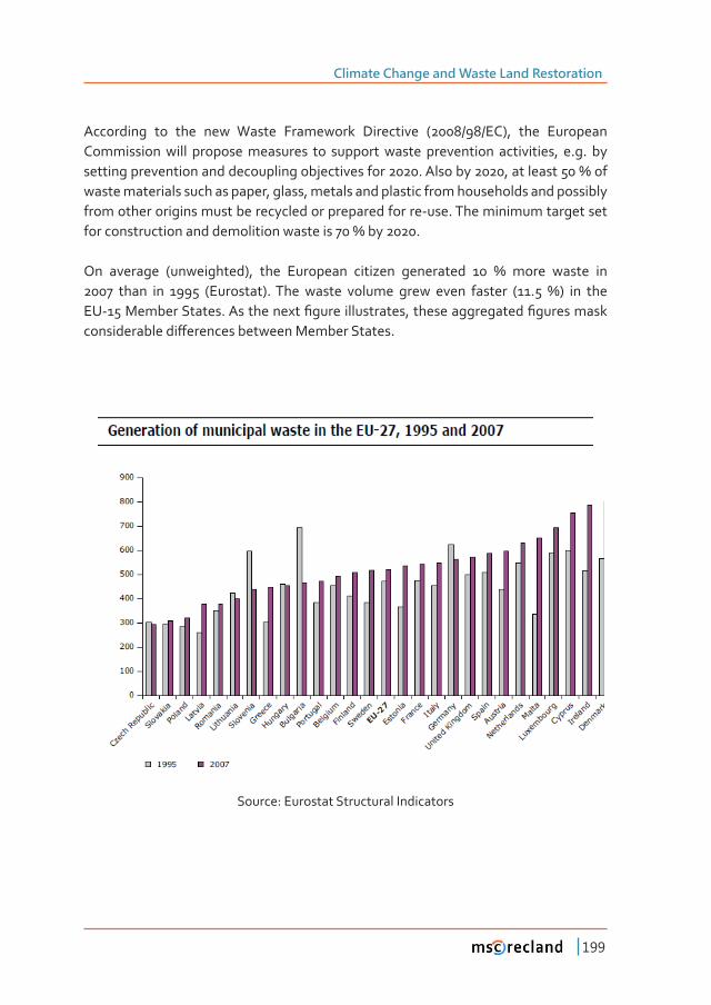
Climate Change and Waste Land Restoration
199
According to the new Waste Framework Directive (2008/98/EC), the European Commission will propose measures to support waste prevention activities, e.g. by �������������������������������������������������Ǥ���������ǡ�����������ά����waste materials such as paper, glass, metals and plastic from households and possibly from other origins must be recycled or prepared for re-use. The minimum target set ������������������������������������������ά����Ǥ�
��� �������� ȋ����������Ȍǡ� ���� ��������� �������� ���������� � ά� ����� ������ ���� ����� ��� � ȋ��������ȌǤ����� ������ ������� ����� ����� ������� ȋǤ�άȌ� ��� ������Ǧ��������������Ǥ�������������Ƥ����������������ǡ������������������Ƥ��������������������������ơ�����������������������������Ǥ�
Source: Eurostat Structural Indicators
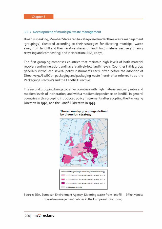
Chapter 3
200
3�5�3 Development of municipal waste management
Broadly speaking, Member States can be categorised under three waste management ‘groupings’, clustered according to their strategies for diverting municipal waste ��������������Ƥ������������� ������������������� ����Ƥ�����ǡ���������� ���������ȋ�������recycling and composting) and incineration (EEA, 2007a).
���� Ƥ���� ��������� ���������� ���������� �������������� ����� ������� ��� ���������������������������������������ǡ�����������������������������Ƥ���������Ǥ�������������������������generally introduced several policy instruments early, often before the adoption of Directive 94/62/EC on packaging and packaging waste (hereinafter referred to as ‘the �������������������ǯȌ�������������Ƥ������������Ǥ�
The second grouping brings together countries with high material recovery rates and �����������������������������ǡ�������������������������������������Ƥ��Ǥ������������countries in this grouping introduced policy instruments after adopting the Packaging �������������ǡ�������������Ƥ����������������Ǥ�
������ǣ����ǡ����������������������������Ǥ��������������������������Ƥ���Ȅ��ơ�����������of waste-management policies in the European Union. 2009.
Climate Change and Waste Land Restoration
201
The third grouping contains those countries whose material recovery and incineration ���������������� ���������������������������� ����Ƥ��� ��� ���������������Ǥ������������comprises the majority of the EU-12 Member States in the process of implementing EU regulations and several, but not all Member States with a 4-year derogation from ��������Ƥ������������� ȋ�Ǥ�Ǥ���������ǡ� ������������������ǡ������ǡ����������ǡ� �������ǡ�Romania, Slovakia and the United Kingdom) or from the Packaging Directive (Greece and Portugal). The geographical distribution of the three groupings is shown in this Ƥ����ǣ
4 MANAGEMENT AND MINIMIZING OF LANDFILL GAS EMISSIONS
����Ƥ������������Ƥ�������Dz������������������������������������������ǡ������������������underground or on the surface for periods of time longer than one year for non-hazardous waste, and exceeding six months for hazardous waste.”
�����������������������������ǡ���������������� �����Ƥ������������������������������of waste at locations properly built and prepared, following the corresponding environmental requirements. Waste disposal is the last option in the hierarchy of waste contained in the European Union management principles.
��� ���� ������� �����ǡ� ���� �������� ������ ��� ��� ������� ����Ƥ��� ��������ǡ� ����������� ���Ǧrecyclable materials (fully optimize waste resources), and to control environmental contaminants (pollutants in the atmosphere, leachate generation and treatment, distinction in the discharge of hazardous waste, inert or non-hazardous waste, etc..).
���������������������������Ƥ�����������������������������������������������������ǡ�as well as the main characteristics (waterways, water bodies and agricultural and urban areas, the existence of groundwater or natural reserves, geological and ���������������� ����������ǡ� ������ ��� ƪ������ǡ� ����������ǡ� ������ ��������� ���landslides, protection of cultural heritage of the area where they will be located) and consider the distances between the boundary of the site and residential and recreational areas.
���������������������������������������������������ơ��������������������Ǧ��������������������������ơ�����������������������Ǥ��������������������ǣ
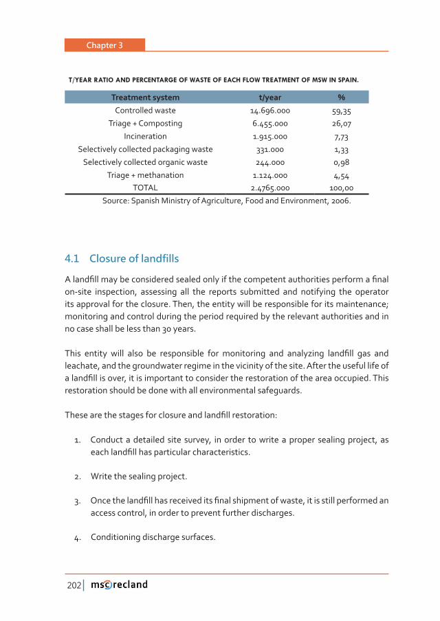
Chapter 3
202
T/YEAR RATIO AND PERCENTARGE OF WASTE OF EACH FLOW TREATMENT OF MSW IN SPAIN.
Treatment system t/year ά
Controlled waste 14.696.000 59,35
Triage + Composting 6.455.000 26,07
Incineration 1.915.000 7,73
Selectively collected packaging waste 331.000 1,33
Selectively collected organic waste 244.000 0,98
Triage + methanation 1.124.000 4,54TOTAL 2.4765.000 100,00
Source: Spanish Ministry of Agriculture, Food and Environment, 2006.
4�1 Closure of landfills
������Ƥ������������������������������������������������������������������������Ƥ����on-site inspection, assessing all the reports submitted and notifying the operator its approval for the closure. Then, the entity will be responsible for its maintenance; monitoring and control during the period required by the relevant authorities and in no case shall be less than 30 years.
����� ������� ����� ����� ��� ������������ ���� ����������� ���� ���������� ����Ƥ��� ���� ����leachate, and the groundwater regime in the vicinity of the site. After the useful life of ������Ƥ����������ǡ�����������������������������������������������������������������Ǥ������restoration should be done with all environmental safeguards.
�����������������������������������������Ƥ��������������ǣ
1. Conduct a detailed site survey, in order to write a proper sealing project, as ���������Ƥ���������������������������������Ǥ
2. Write the sealing project.
3. �������������Ƥ��������������������Ƥ���������������������ǡ��������������������������access control, in order to prevent further discharges.
4. Conditioning discharge surfaces.
Climate Change and Waste Land Restoration
203
5. ��������������ǡ���������������������������������������ǡ�������������Ƥ������������river water and close the outlet passage of the vent gases through the exhaust system of gas. This includes revegetation of the surface. Sealing layers:
- The top layer of waste is covered with a 0.5 m compacted clay mineral layer.
- Layer of high density polyethylene (HDPE) that is covered by a geotextile.
- Gravel drainage layer (not <50 cm), enabling the collection and channeling of rainwater.
- Capa de tierra de 1m de espesor y de naturaleza adecuada a la vegetación que se prevea.
- 1m thickness soil layer suitable for the vegetation.
- Humus soil fertilized with appropriate vegetation to these conditions.
6. ��������������������ơ�����������������Ƥ����������������������ơ�ƪ������������-�������������Ƥ����������������������Ǥ
7. Control leachate extraction placing drainage systems leading to leachate sto-rage ponds.
8. Controlling the extraction of gases and avoid its uncontrolled migration.
9. Monitoring of gas and leachate management during a period of 30 years after closure.
10. ���������������������������������������ơ�������������������Ǥ
11. Waste and soil treatment, as it must be conditioned for revegetation and re-clamation.
4�2 Post-closure maintenance
4�2�1 Production of biogas
���� �������� ��� ������� ��� �� ����Ƥ��� �������� ���������� ���������� ��� ��������������waste producing gases such as methane, carbon dioxide and water vapor mainly, and ���������������������������������ȋ������������Ƥ��ǡ��������ǡ��������ǡ�����������ǡ�etc.)..
Chapter 3
204
The volume and composition of gases generated depends, not only on the content of ���������������������������������������������������ǡ����������������������������Ƥ��������������Ƥ��Ǥ
Gas production is automatically controlled by the gas conduction to control stations �����������������������������������ƪ��ǡ�������������������������Ǥ����������������centralized in a control center using a computerized system.
4�2�2 Exploitation of landfill biogas
���� ��������� ����������� ���� ��� �� ����Ƥ��ǡ����������������� ��������� ���� ����������actions:
• Preparation of wells or chimneys
Essential conditioning to hinder the introduction of air through the surface adjacent ������������ǡ��������������Ǧ����������ȋ�������� ����ƪ�������������������������ȌǤ� ���basically consists of the isolation of the area adjacent to each well of capture, so that �������������������������������������������������������������������������������Ƥ���biogas production by aerobic conditions.
�������������� �������� ��� ���� �������� ��� ���� ����Ƥ�������� ��� ������� ��� ��������� ���possible. The sealing of the wellhead can be ensured by the compaction of clay covering materials in the vicinity of the chimneys, complemented if necessary, placing ���������������Ƥ�����������������������������������������������������Ǥ������system is used to prevent the entry of air and thus oxygen, to the compacted waste.
• Uptake of gas and its conduction
Each wellhead is connected to pipes of high density polyethylene (HDPE) of 110 or 90 ��������������Ǥ����������������������ǡ������������������������������������������ά�to regulation stations.
• Regulation stations
HDPE pipes from wells, form groups according to their closeness. Each set of pipes goes to a collector where the concentration of methane (CH4) and oxygen (O2) is continuously ��������Ǥ�����������������������������������ǡ���������������������������ƪ��Ǥ
Climate Change and Waste Land Restoration
205
The collector of each station leads the gas mixture to the extraction plant; it is centralized in a picture-programmable computer control.
• Extraction system
Mixture gas pipes from regulation stations converge at the entrance of the extraction plant in a single intake manifold. The suction gas is sent to the delivery manifold where it is distributed for use (cogeneration or torch).
The amount of gas that is sent to cogeneration (CHP) must contain a minimum ����������� ��� �����������Ǥ����������ǡ� ��� ���������� ������ ���������� ���� ���� ƪ���direction, depending on the indication of the methane analyzer.
• Cogeneration
Cogeneration is the alternating electric generation by a group of internal combustion engine-electric generator.
• Torch
This is a safety system which burns the excess of gas cogeneration. It must have ��ƥ�����������������������ά��������������������Ǥ
• Gas control
It provides control of gas collection facilities, the analysis, the control of cogeneration based on the quantity and quality of gas produced, and centralization of data in a control center with computer support.
4�3 Minimizing impacts on the atmosphere
• ��������������Ƥ�������������������������������ǣ�
- ά������������������������������������������������������ȋ����������Ȍ�
- ������������������������������������
- ά����ƪ�����ȋ������Ȍ�
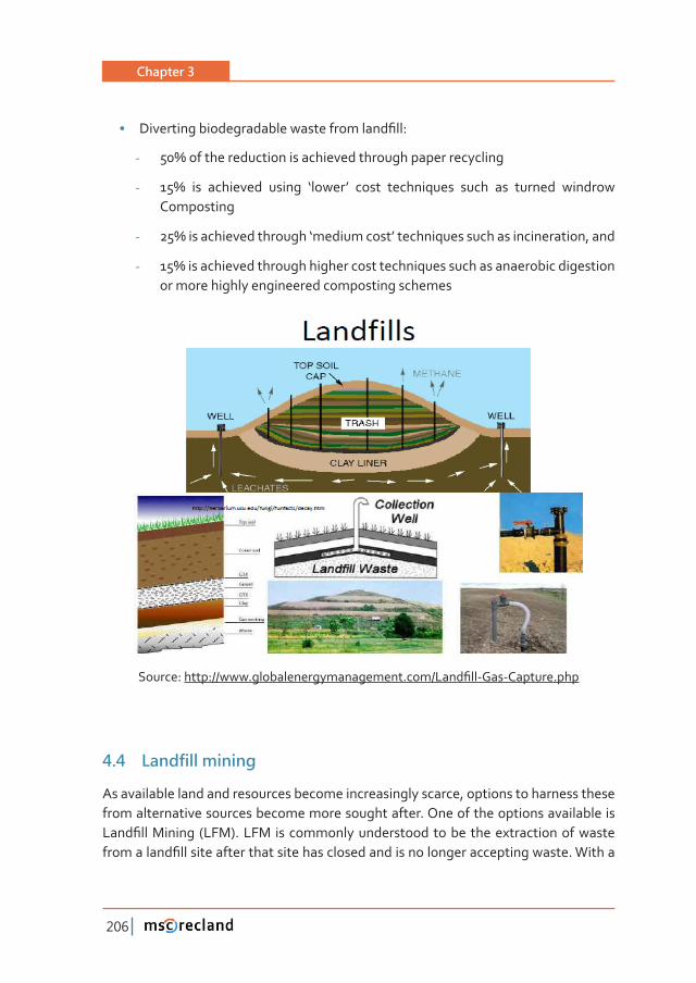
Chapter 3
206
• ���������������������������������������Ƥ��ǣ�
- ������������������������������������������������������
- ά� ��� ��������� ������ Ǯ�����ǯ� ����� ����������� ����� ��� ������� ��������Composting
- ά���������������������Ǯ�����������ǯ��������������������������������ǡ�����
- ������������������������������������������������������������������������or more highly engineered composting schemes
Source: ����ǣȀȀ���Ǥ����������������������Ǥ���Ȁ����Ƥ��Ǧ��Ǧ�������Ǥ���
4�4 Landfill mining
As available land and resources become increasingly scarce, options to harness these from alternative sources become more sought after. One of the options available is ����Ƥ���������� ȋ��ȌǤ���� ����������������������������� �����������������������������������Ƥ�������������������������������������������������������������������Ǥ��������
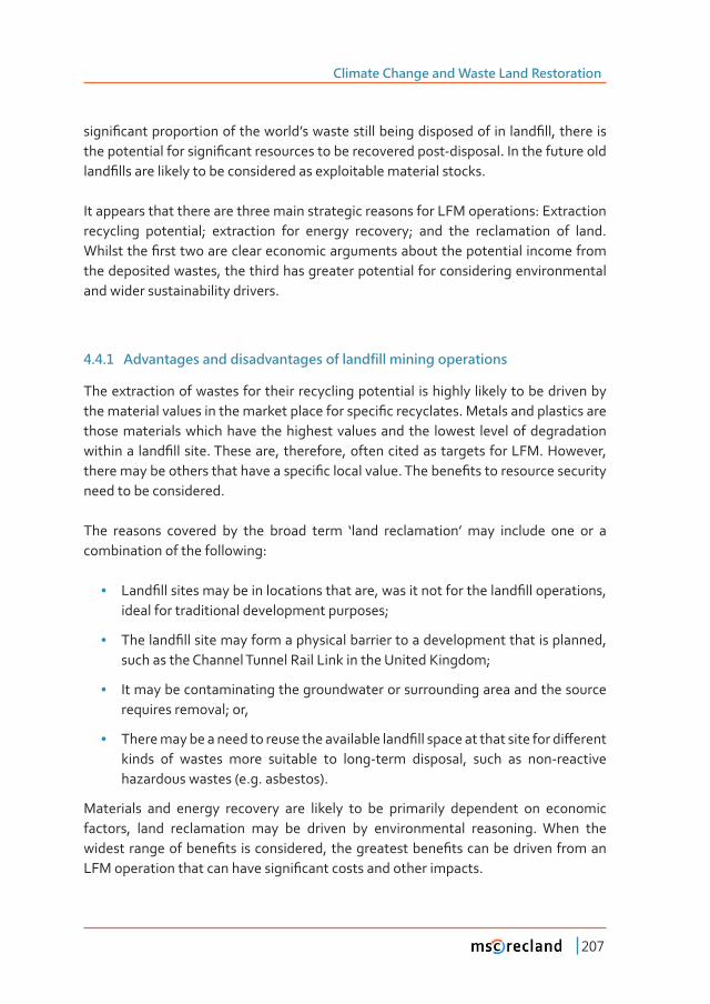
Climate Change and Waste Land Restoration
207
�����Ƥ����������������������������ǯ���������������������������������������Ƥ��ǡ���������������������������������Ƥ�����������������������������������Ǧ��������Ǥ�����������������������Ƥ��������������������������������������������������������������Ǥ
It appears that there are three main strategic reasons for LFM operations: Extraction recycling potential; extraction for energy recovery; and the reclamation of land. �����������Ƥ���������������������������������������������������������������������the deposited wastes, the third has greater potential for considering environmental and wider sustainability drivers.
4�4�1 Advantages and disadvantages of landfill mining operations
The extraction of wastes for their recycling potential is highly likely to be driven by �������������������������������������������������Ƥ������������Ǥ�������������������������those materials which have the highest values and the lowest level of degradation ��������� ����Ƥ�������Ǥ����������ǡ����������ǡ������������������������������Ǥ��������ǡ��������������������������������������Ƥ�������������Ǥ���������Ƥ������������������������need to be considered.
The reasons covered by the broad term ‘land reclamation’ may include one or a combination of the following:
• ����Ƥ�������������������������������������ǡ������������������������Ƥ�������������ǡ�ideal for traditional development purposes;
• ��������Ƥ��������������������������������������������������������������������ǡ�such as the Channel Tunnel Rail Link in the United Kingdom;
• It may be contaminating the groundwater or surrounding area and the source requires removal; or,
• �����������������������������������������������Ƥ����������������������������ơ������kinds of wastes more suitable to long-term disposal, such as non-reactive hazardous wastes (e.g. asbestos).
Materials and energy recovery are likely to be primarily dependent on economic factors, land reclamation may be driven by environmental reasoning. When the ��������������������Ƥ��� �������������ǡ������������������Ƥ���������������������������������������������������������Ƥ����������������������������Ǥ
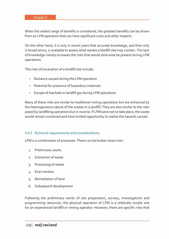
Chapter 3
208
�����������������������������Ƥ����������������ǡ������������������Ƥ���������������������������������������������������������Ƥ����������������������������Ǥ
On the other hand, it is only in recent years that accurate knowledge, and then only ��������������ǡ������������������������������������������Ƥ�������������������Ǥ�����������of knowledge merely increases the risks that would otherwise be present during LFM operations.
���������������������������������Ƥ���������������ǣ�
• Nuisance caused during the LFM operation
• Potential for presence of hazardous materials
• ��������������������������Ƥ����������������������������
Many of these risks are similar to traditional mining operations but are enhanced by ������������������������������������������������Ƥ��Ǥ�������������������������������������������������Ƥ�������������������������������Ǥ�����������������������������ǡ�����������would remain contained and have limited opportunity to realise the hazards caused.
4�4�2 Technical requirements and considerations
LFM is a combination of processes. These can be broken down into:
1. Preliminary works
2. Extraction of waste
3. Processing of waste
4. End-markets
5. Remediation of land
6. Subsequent development
Following the preliminary works of site preparation, surveys, investigations and programming resources, the physical operation of LFM is a relatively simple one �����������������������Ƥ���������������������Ǥ��������ǡ����������������Ƥ�������������
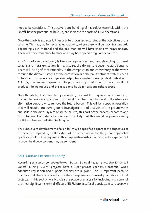
Climate Change and Waste Land Restoration
209
need to be considered. The discovery and handling of hazardous materials within the ����Ƥ�������������������������������ǡ��������������������������ǡ��������������Ǥ
Once the waste is extracted, it needs to be processed according to the objectives of the ������Ǥ�������������������������������������ǡ��������������������������Ƥ������������depending upon material and the end-markets will have their own requirements. ������������������������������������������������������Ƥ���������������������Ǥ�
Any form of energy recovery is likely to require pre-treatment shredding, trommel screens and metal extraction. It may also require drying to reduce moisture content. �������������������Ƥ�������������������������������������������������������������������������������ơ������������������������������������������Ǧ�����������������������to be able to provide a homogenous output for a waste-to-energy plant to deal with. This may need to be completed on site prior to transportation so that only a stabilised product is being moved and the associated haulage costs and risks reduced.
Once the site has been completely excavated, there will be a requirement to remediate the land to remove any residual pollution if the intention is to develop the site for an ��������������������������������������������������Ǥ���������������������Ƥ������������that will require intensive ground investigations and analysis of the groundwater and soils in the area. By removing the source, this part of the process becomes one of containment and decontamination. It is likely that this would be possible using traditional land remediation techniques.
������������������������������������Ƥ���������������Ƥ��������������������������������the scheme. Depending on the extent of the remediation, it is likely that a specialist operator would not be required at this stage and a construction contractor experienced ��������Ƥ�������������������������ƥ�����Ǥ
4�4�3 Costs and benefits to society
According to a study conducted by Van Passel, S., et al. (2012), show that Enhanced ����Ƥ��� ������� ȋ���Ȍ� ��������� ����� �� ������ �������� ��������� ���������� �����adequate regulation and support policies are in place. This is important because ��� ������ ����� ������ ��� ������ �������������������������� ��� ����������Ƥ������ �������projects. In this section we broaden the scope of analysis by including also some of ��������������Ƥ���������������ơ������������������������������������Ǥ��������������ǡ����
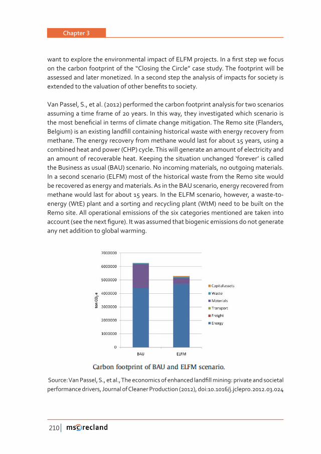
Chapter 3
210
��������������������������������������������������������Ǥ������Ƥ�������������������������������������������������Dz������������������dz�����������Ǥ�����������������������assessed and later monetized. In a second step the analysis of impacts for society is ���������������������������������������Ƥ�������������Ǥ
Van Passel, S., et al. (2012) performed the carbon footprint analysis for two scenarios assuming a time frame of 20 years. In this way, they investigated which scenario is �������������Ƥ������������������������������������������Ǥ���������������ȋ�������ǡ��������Ȍ��������������������Ƥ���������������������������������������������������������methane. The energy recovery from methane would last for about 15 years, using a combined heat and power (CHP) cycle. This will generate an amount of electricity and an amount of recoverable heat. Keeping the situation unchanged ‘forever’ is called the Business as usual (BAU) scenario. No incoming materials, no outgoing materials. In a second scenario (ELFM) most of the historical waste from the Remo site would be recovered as energy and materials. As in the BAU scenario, energy recovered from methane would last for about 15 years. In the ELFM scenario, however, a waste-to-energy (WtE) plant and a sorting and recycling plant (WtM) need to be built on the Remo site. All operational emissions of the six categories mentioned are taken into ��������ȋ�������������Ƥ����ȌǤ��������������������������������������������������������any net addition to global warming.
�������ǣ�����������ǡ��Ǥǡ������Ǥǡ�������������������������������Ƥ���������ǣ����������������������performance drivers, Journal of Cleaner Production (2012), doi:10.1016/j.jclepro.2012.03.024
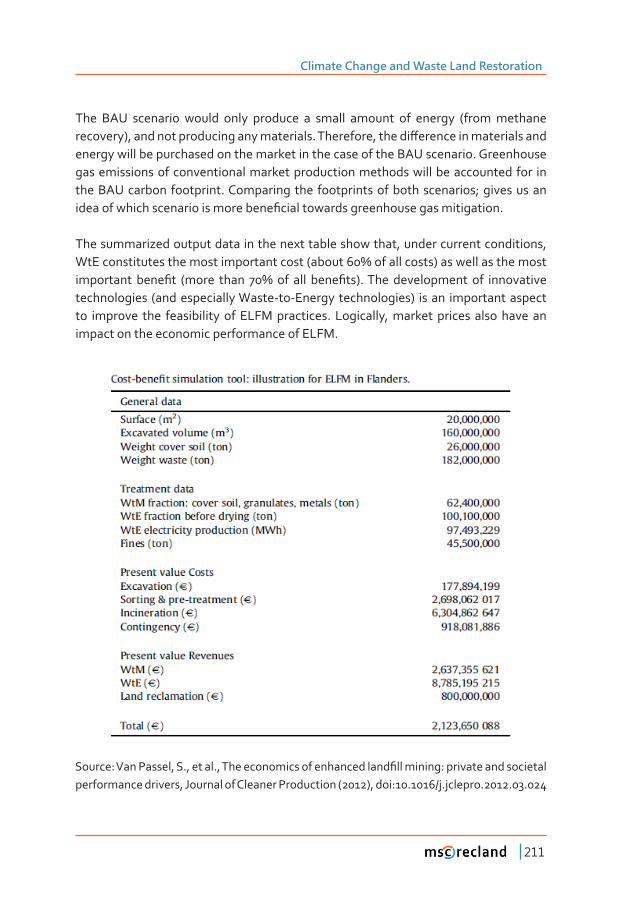
Climate Change and Waste Land Restoration
211
The BAU scenario would only produce a small amount of energy (from methane ��������Ȍǡ��������������������������������Ǥ����������ǡ�������ơ������������������������energy will be purchased on the market in the case of the BAU scenario. Greenhouse gas emissions of conventional market production methods will be accounted for in the BAU carbon footprint. Comparing the footprints of both scenarios; gives us an �����������������������������������Ƥ��������������������������������������Ǥ
The summarized output data in the next table show that, under current conditions, ����������������������������������������ȋ������ά�������������Ȍ������������������������������� ����Ƥ�� ȋ����� ����� ά���� ���� ����Ƥ��ȌǤ����������������� ��� �����������technologies (and especially Waste-to-Energy technologies) is an important aspect to improve the feasibility of ELFM practices. Logically, market prices also have an impact on the economic performance of ELFM.
������ǣ�����������ǡ��Ǥǡ������Ǥǡ�������������������������������Ƥ���������ǣ����������������������performance drivers, Journal of Cleaner Production (2012), doi:10.1016/j.jclepro.2012.03.024
Chapter 3
212
REFERENCES
United Nations Environment Programme. Waste and Climate Change Global Trends and Strategy Framework. 2010.
���ǡ����������������������������Ǥ���������������������Ȅ���������� �������������������Ƥ���from better municipal waste management in Europe. 2011.
��ǡ��������������������Ǥ�����ȋȌ��Ƥ���ǤGerman Federal Ministry for the Environment. Waste Sector’s Contribution to Climate Protec-
tion. 2005Fundación Forum Ambiental. La mejora en la prevención y gestión de los residuos municipales en
España contribuye a la lucha contra el cambio climático. 2012.EPA, Unites States Environmental Protection Agency. Opportunities to reduce greenhouse gas
emissions through materials and land management practices. 2009.UNEP, United Nations Environment Programme. Towards a Green Economy: Pathways to Sustai-
nable Development and Poverty Eradication. 2011.���ǡ����������������������������Ǥ��������������������������Ƥ���Ȅ��ơ�������������������Ǧ��-
nagement policies in the European Union. 2009.����ǡ��������������������������������������Ǥ������������������������Ƥ���������ǡ�Ǥ����������ǡ��Ǥǡ������Ǥǡ�������������������������������Ƥ���������ǣ�������������������������������-
ce drivers,Journal of Cleaner Production (2012), doi:10.1016/j.jclepro.2012.03.024

Water Management and Planning
Authors
Juan C. Santamarta Cerezal
Jonay Neris
Axel Ritter
Luis E. Hernández-Gutiérrez
University of La Laguna
Viana nº 50, planta baja, 38071,
La Laguna - Tenerife
Spain
4Chapter

215
Chapter 4
University of
La Laguna,
Tenerife, Spain
Water Management and PlanningJuan C� Santamarta CerezalJonay NerisAxel RitterLuis E� Hernández-Gutiérrez
ABSTRACT
������ ��� ����ǡ� �������������������������� ��������������� �������Ǥ����� ��ǯ�� ��Ƥ�������������ǡ� ���� ����� ����� ά� ��� ���� �����ǯ�� ������ ������ ��� ���������� ���� ����������������Ǥ�����Ƥ�����������������������������������������������������������������matter. It is well recognised that water planners require a broad set of inter-�������������������������������ơ�����������������������Ǧ�������ǡ�������������������contemporary water management challenges. Solving water-related problems, ��������� �������Ƥ�� ���������� ���� ������� ���� ��������� ����� ������������ ���� ����ability to integrate environmental, social and political considerations into planning practice. The 21st century will be an era of increased global concern regarding the availability of water.
�������ǡ�����������������������������������������������������������Ƥ������������and the population in general. Despite the climate pattern has been changing continuously during the Earth´s history due to changes in the atmosphere, topography, volcanic activity, and other natural factors, this change seems to have been exacerbated recently due to the alteration of the greenhouse gases content in the atmosphere by the humanity. Nowadays, the extent of this change and its �ơ��������������������������������������������������������ƪ���������������������������������ơ���������������������������������Ǥ����������������������������������������������������������������������������������������ơ�����������������������Ǥ�������warming, leaded last century by the climate change, has involved alterations in the temperature, precipitation and evaporation patters. From the point of view of

Chapter 4
216
the water resources, these changes include an increase in the freshwater losses from terrestrial sources (glaciers, ice and snow, lakes, soil moisture, swamps, groundwater, marches and rivers) by evaporation and sublimation from fresh water deposits and transpiration from the vegetation, but also changes in the rainfall quantity and patterns. As a result, climate change has leaded short and long-term alterations in the ��������������������������Ǧ�����������������������ƪ��������������������������������impact on, among others, the quantity but also quality of water resources.
This module focuses on one of those, the issue of water supply planning and resource management, in particular, the planning process, systems analysis methods; institutional framework for water resources engineering; comprehensive integration of engineering, economic, environmental, security, legal, and political considerations in water resources development and management. It further discusses the �������������ǡ� ��������ǡ� ���� ������� ������������� ��� ƪ����ǡ� ��������ǡ� ����ǡ� ����water usage as well as current issues in water quality, water pollution, and water resource regulation.
The overall aim of the module is to develop the skills of the students to know how to plan, develop and manage water resources.
1 WATER PLANNING
1�1 Introduction
Water is an increasingly critical issue at the forefront of global policy change, management and planning. There are growing concerns about water as a renewable resource, its availability for a wide range of users, aquatic ecosystem health, and global issues relating to climate change, water security and water trading.
������ ���������� ����������� ������ ������� ������� ��� �ƥ�����ǡ� ������������ ������� ������ ���������Ǥ������ ������� ������ ��� ����������� �ƥ�������� ���� ��������� �������������������ǡ���������ƪ�������������������������������������������������������ǡ�also considers how water resources can become more integrated and sustainable.
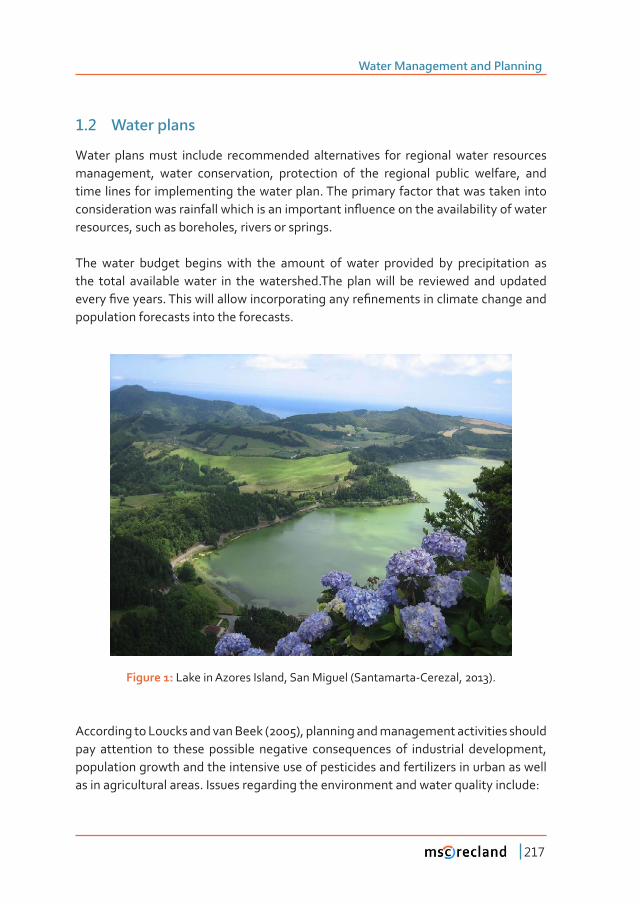
Water Management and Planning
217
1�2 Water plans
Water plans must include recommended alternatives for regional water resources management, water conservation, protection of the regional public welfare, and time lines for implementing the water plan. The primary factor that was taken into ���������������������������������������������������ƪ�����������������������������������resources, such as boreholes, rivers or springs.
The water budget begins with the amount of water provided by precipitation as the total available water in the watershed.The plan will be reviewed and updated ������Ƥ��������Ǥ�������������������������������������Ƥ������������������������������population forecasts into the forecasts.
Figure 1: Lake in Azores Island, San Miguel (Santamarta-Cerezal, 2013).
According to Loucks and van Beek (2005), planning and management activities should pay attention to these possible negative consequences of industrial development, population growth and the intensive use of pesticides and fertilizers in urban as well as in agricultural areas. Issues regarding the environment and water quality include:
Chapter 4
218
• ������������������������������ƪ���������������������������������������
• Threats from aquatic nuisance species
• Threats from the chemical, physical and biological water quality of the watershed’s aquatic resources
• Quality standards for recycled water
• Non-point source pollution discharges, including sediment from erosion
• Inadequate groundwater protection compacts and concerned institutions
1�3 Water plans objetives and strategies
The water plans objetives include;
To introduce a Water Act as well as revise existing laws and regulations to serve as ���������������������������ƥ��������������������������������������������Ǥ
To establish a national level organization responsible for policy formulation; oversee implementation of the policy by concerned agencies; and establish basin-level and local level organizations with supporting laws.
Appropriate water allocation for all user sectors at the national and basin levels:
• ��Ƥ��������������������������������������������������������
• Prioritize water use for the various sectors, i.e., agriculture, domestic, industry, conservation of ecosystem etc
• Promote conjunctive use of surface and groundwater
• Set water-use criteria/proportions for the various sectors from national to basin level
• ������������������������ȋ�������ǡ�ƪ������������������Ȍ
��������������������Ǧ�����ƥ������ǣ
• ������ ��������� ���� Ƥ�������� ������ ���� ������ ����������ǡ� ���� ����������ǡ�the creation of a water market, compensation, taxes and allow users to be responsible for paying for service, wastewater treatment etc

Water Management and Planning
219
• Campaign to create awareness of users about the necessity to share costs and �����������ƥ�������
• Set up a water resources management fund
• Introduce water reuse/recycling
• Introduce water saving technologies
������������������������������ƥ������ǣ
• Rehabilitate existing infrastructures
• Develop a water network/grid both within and among basins, and a distribution system to serve as many users as possible
• Improve the organizational structure and management system
To develop water resources in accordance with potential and needs of various activities, both in terms of quantity and quality with due consideration of the environment. To ��������ƥ�����������������������������������������������������ǣ
• Set clear direction for water resources development both within and outside the country by emphasizing development of water resources within the country to their full potential
��������������������������������������������������������������ƥ�����������������ǣ
• Include water related topic at all levels of educational curriculum
• Promote public awareness and understanding of the importance and ����������������������������������ƥ�����������������
���������� ������ƪ���ǡ����������������������������������������������� ��������������ƥ������ƪ���������������������������������ǣ
• ��������� ƪ���� ���� �������� ����������� ���� ��������������� ������� �����ǡ�employing bothstructural and non-structural measures
• Promote and support local organizations to be capable of reduce and solve ƪ����������������������
• Develop a preparatory process for protection and rehabilitation operations prior, during and
Chapter 4
220
• after disasters
• Set up a forecasting and warning system
• Set guidelines and procedure for water related disaster warning
1�4 Water budget
�������������ά���� ���������ǯ�� �������ǡ����� ��� �����ƥ����� ������������������ ������������������������������������������������������������Ǥ��������������������Ǥά�������������ǯ�������ǡ������Ǥάǡ������������������������������������Ǥάǡ�����������seem surprising because water plays such an important role in weather. The annual precipitation for the earth is more than 30 times the atmosphere’s total capacity to hold water. This fact indicates the rapid recycling of water that must occur between the earth’s surface and the atmosphere.
����������������������������������������������Ƥ������������������������������������������������������������������Ƥ�������ǡ���Ƥ�������������������������������������������Ǥ�A water balance analyzes the input and output of water in an area of a watershed ���������ǡ�������������������������������������������������������������������ơ���������������ǡ��������������ơ����������������������Ǥ
���� ���������������������������� ��� ����� ��� ���������������������������Ƥ�����Ƥ�������surplus water in a watershed taking parameters like rainfall, relative humidity, tem-��������ǡ������������ǡ���������������������������������ƪ���������������������������of the watershed.
������������������������������������������ơ������������������������������������������outputs of water mean water that is stored.
Inputs - Outputs = Change in Storage
Applying these concepts, precipitation is expressed as:
������������
���������������������������������������������������ǡ���������������������ǡ�������ơ���������Ƥ��������Ǥ
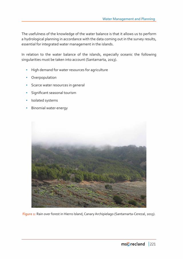
Water Management and Planning
221
The usefulness of the knowledge of the water balance is that it allows us to perform a hydrological planning in accordance with the data coming out in the survey results, essential for integrated water management in the islands.
In relation to the water balance of the islands, especially oceanic the following singularities must be taken into account (Santamarta, 2013).
• High demand for water resources for agriculture
• Overpopulation
• Scarce water resources in general
• �����Ƥ����������������������
• Isolated systems
• Binomial water-energy
Figure 2: Rain over forest in Hierro Island, Canary Archipielago (Santamarta-Cerezal, 2013).
Chapter 4
222
�������� ���������� �������� ��������� �� �������� �������� �������������ǡ� ����ơ� ��������ǡ� ������� ������������ǡ� ���Ǥǡ� ��Ƥ��������� ��� ���� ������������ ������ǡ� ����������which either evaporates (from open water surfaces) or transpirates from vegetation (evapotranspiration), completing the natural cycle back into atmospheric moisture and precipitation. It is necessary to understand this balance or water budget in order to sustain the resource and its environmental and human connections in the watershed. The understanding of the hydrologic cycle on a watershed basis is essential for development and implementation of appropriate watershed management policies and procedures.
A water budget analysis is a computational technique that balances water input and output while accounting for change in storage. On a watershed scale knowledge of these relationships can be used in addressing major decisions relating to such issues as:
• Land use and watershed planning
• Ensuring sustainable development
• Determining the receiving stream capacity for waste discharge
• Assessing risk exposure;
• ������������������������Ƥ������������������
• Reporting environmental conditions and status.
1�5 Water planning and climate change
The most important impacts of Climate Change will be on the Earth’s water cycle. �����������������������������������������������������Ƥ�������������������������������challenge. The water cycle describes the constant movement of water from ocean to atmosphere to the land surface and back to the ocean. On a global scale the total amount of water does not change but where it is distributed does.
Water scarcity is expected to become an ever-increasing problem in the future, for various reasons. First, the distribution of precipitation in space and time is very uneven, leading to tremendous temporal variability in water resources worldwide (Oki et al, 2006).
Water Management and Planning
223
Second, the rate of evaporation varies a great deal, depending on temperature and relative humidity, which impacts the amount of water available to replenish groundwater supplies. The combination of shorter duration but more intense ��������� ȋ�������� ����� ����ơ� ���� ����� ��Ƥ��������Ȍ� ��������� ����� ����������evapotranspiration (the sum of evaporation and plant transpiration from the earth’s land surface to atmosphere) and increased irrigation is expected to lead to groundwater depletion (Konikow and Kendy 2005).
As climate change warms the atmosphere and alters the hydrological cycle, we will continue to witness changes to the amount, timing, form, and intensity of precipitation ���� ���� ƪ������������ �������������ǡ� �������� ��� ���� �������� ��� �������� �����������environments, Already, water-related climate change impacts are being experienced ����������������������������������������������������������ƪ����Ǥ����������������temperatures and changes in precipitation and temperature extremes are projected ����ơ��������������������������������������������������������������������������������ǡ������ ��������ǡ� �������� ���� ���Ȁ���������ǡ� ���� ������ ���� ������������ ƪ���Ǣ� ������factors are expected to lead to further deterioration of water quality as well.
The premises that water planning is best done on a regional level is due to the many variables in climate, water supply, water demand, and legal and institutional constraints to water resources management.
1�6 Water management on islands
Water problems on islands are mainly related to the limited water resources. Due to the limited water resources, water related problems that are common elsewhere as well, such as pollution by wastewater and inadequate water supply systems (mainly huge leakages) become more acute on islands and thus require special attention and appropriate management (Hophmayer, 2012).
Islands depend, as other mainland countries, upon the quality and quantity of their water for their existence and economic activities. However, water management on islands is unique as it is constrained by their size, isolation from the mainland, fragility, �����������������ǡ�������������Ƥ������������������ȋ����Ƥ��������������ǡ�ȌǤ
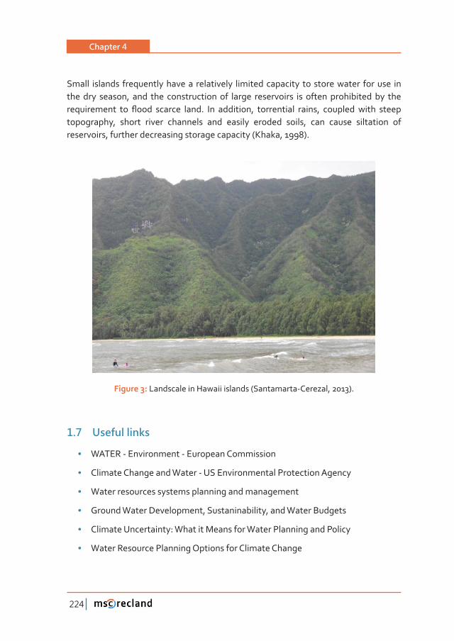
Chapter 4
224
Small islands frequently have a relatively limited capacity to store water for use in the dry season, and the construction of large reservoirs is often prohibited by the ������������ ��� ƪ���� ������� ����Ǥ� ��� ��������ǡ� ����������� �����ǡ� �������� ����� ������topography, short river channels and easily eroded soils, can cause siltation of reservoirs, further decreasing storage capacity (Khaka, 1998).
Figure 3: Landscale in Hawaii islands (Santamarta-Cerezal, 2013).
1�7 Useful links
• WATER - Environment - European Commission
• Climate Change and Water - US Environmental Protection Agency
• Water resources systems planning and management
• Ground Water Development, Sustaninability, and Water Budgets
• Climate Uncertainty: What it Means for Water Planning and Policy
• Water Resource Planning Options for Climate Change
Water Management and Planning
225
2 water uses
2�1 Introduction
An adequate supply of water is essential to ensure continued economic vitality and quality of life. Water use must generally respond to two needs: the need to satisfy the growing demand for water used for human consumption and for production processes (industry, agriculture, recreation), and the need to preserve water quality and protect ���������������Ǥ�������������������������Ƥ������ǡ�����������������ǡ����������������protection of water resources.
The most important water uses are;
• For drinking purpose
• For washing, bathing and cooking etc
• For building construction
• For the generation of steam for industrial use and electricity generation
• For generating hydroelectricity
• As a solvent
• For irrigation purposes
Water is crucial for the economy. Virtually every industry from agriculture, electric power and industrial manufacturing to beverage, apparel, and tourism relies on it to grow and ultimately sustain their business. Generally, the largest percentage of water consumption is attributed to agriculture.
Accounting for water is an essential step toward ensuring that a water utility is sustainable. This is best accomplished when water systems meter use by their customers. Metering helps to identify losses due to leakage and also provides the foundation on which to build an equitable rate structure to ensure adequate revenue to operate the system.
Options for water demand reduction:
• ������ƥ������Ƥ����������������������������
Chapter 4
226
• Landscaping and storm water management
• Grey water use
• Revised irrigation strategies and technologies
• Water pricing
• Education
• Incentives
• �����Ƥ������
Two-thirds of the world’s population is projected to face water scarcity by 2025, ����������������������������ȋȌǤ���������ơ������������������������ǣ
• Birth rate
• Death rate
• Immigration
• Emigration
• Government policies
• Religious and societal beliefs
• Catastrophes
• State of the Economy
2�2 Water footprint
The water-footprint concept was coined in 2002 by Arjen Hoekstra, a professor of water management at University of Twente in the Netherlands. Using data from the UN’s Food and Agricultural Organization, Mr. Hoekstra and other researchers gauged the water content that went into the making of various products and applied those statistics to people’s consumption patterns to get a rough water footprint for average individuals and nations as a whole.
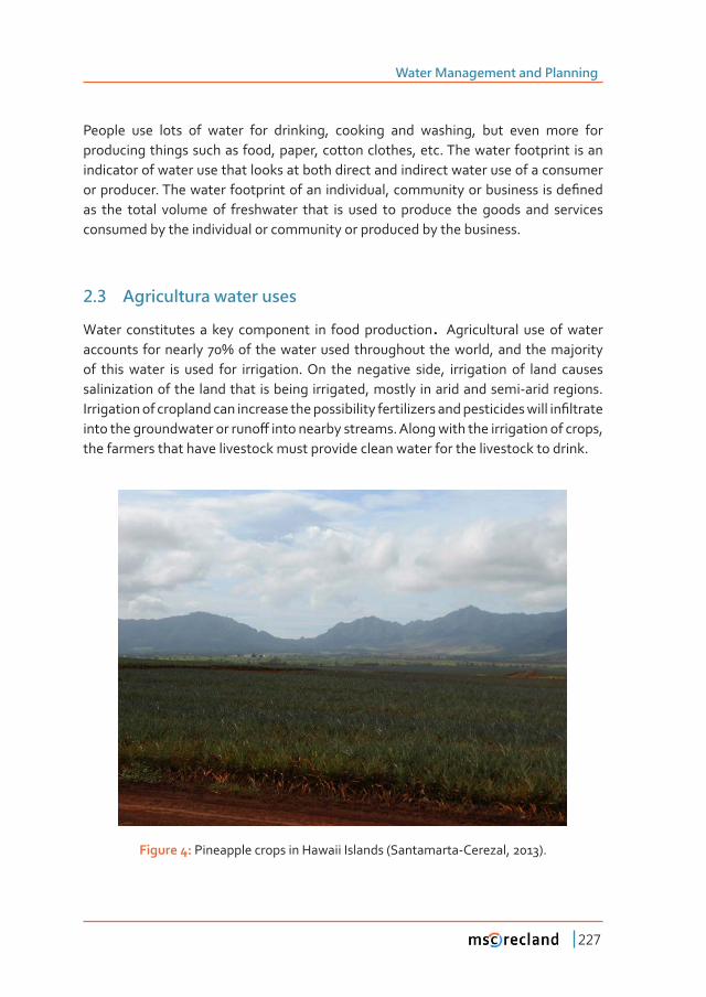
Water Management and Planning
227
People use lots of water for drinking, cooking and washing, but even more for producing things such as food, paper, cotton clothes, etc. The water footprint is an indicator of water use that looks at both direct and indirect water use of a consumer �����������Ǥ�������������������������������������ǡ����������������������������Ƥ����as the total volume of freshwater that is used to produce the goods and services consumed by the individual or community or produced by the business.
2�3 Agricultura water uses
Water constitutes a key component in food production. Agricultural use of water ��������� �����������ά���� �����������������������������������ǡ������������������of this water is used for irrigation. On the negative side, irrigation of land causes salinization of the land that is being irrigated, mostly in arid and semi-arid regions. ��������������������������������������������������������������������������������������Ƥ�����������������������������������ơ��������������������Ǥ�����������������������������������ǡ�the farmers that have livestock must provide clean water for the livestock to drink.
Figure 4: Pineapple crops in Hawaii Islands (Santamarta-Cerezal, 2013).
Chapter 4
228
2�4 Industrial uses
��� ��� ���������� ����� ά� ��� ���������� ������ ���� ��� ����������Ǥ� ������ �����������users include power plants, which use water for cooling or as a power source (i.e. ��������������������Ȍǡ������������� ��Ƥ������ǡ����������������� ���������������������ǡ�and manufacturing plants, which use water as a solvent.
Some power plants use cooling systems that draw water from a lake, river, aquifer, or ocean to cool steam and then return virtually all of it, although at higher temperatures, to the source. Such systems, known as once-through cooling systems, have high withdrawals but low consumption.
Reusing and recycling industrial water can ease the pressure on water resources and avoid the need to discharge to the sewer and/or environment. With appropriate management, which may include treatment, industrial water can be used for a wide range of purposes including industrial uses (e.g. cooling or material washing) or non-����������������ȋ�Ǥ�Ǥ����������������������ƪ������ȌǤ
2�5 Useful links
• What’s your water footprint?
• The EU’s Water Footprint - Institute for Environment and Sustainability
• Water resources across Europe - European Environment Agency
• TEDxOslo - Angela Morelli - The Global Water Footprint of Humanity
• Water Footprint and Conservation projec
Water Management and Planning
229
3 SURFACE WATER EXPLOTATION
3�1 Precipitation
The part of the hydrologic cycle that is of most relevance to water planning is the precipitation;
• ����� �������������� ����� ������ ��� ����� ������ ȋ��Ƥ�������Ȍ� ����� ���� ������� ���become soil moisture, part of which is taken up by plant roots and returned to the atmosphere through the process of transpiration
• �������������������������������������������Ƥ��������ƪ����������������������������and through channels, from which it may be diverted for various consumptive ����������������Ƥ�������������ǡ��������������������������������������������
• When soil moisture storage capacity is exceeded, recharge to groundwater occurs
When rainfall falls on the land surface, typically, depending on the intensity of the ������������������������������������������������������ǡ������������������������Ƥ�����������������������ǡ�������������������������������ơ�����ƪ������������������������������������������������ǡ����������������������������ƪ������������ƪ��Ǥ�
������������������������������ơ����������������������������������������������������������� ���� ����Ǥ������������ �������������������� ��������� ���������� ��������� �����Ƥ������� ��������ǡ��������������������������������ơ������������������������������������������������catchment.
Surface water budget analyses rely heavily on estimates of components instead ��� ������� ������������Ǥ� ��������� �������������� ���� ������ƪ��� ���� �����������water sources, they are typically measured at only a few locations. Evaporation, ����������������������������ǡ���Ƥ��������ǡ��������ƪ���ǡ��������������������������������are generally not measured directly and are therefore estimated. Consequently, the surface water budget calculations presented here have a high degree of uncertainty and should be used with caution.
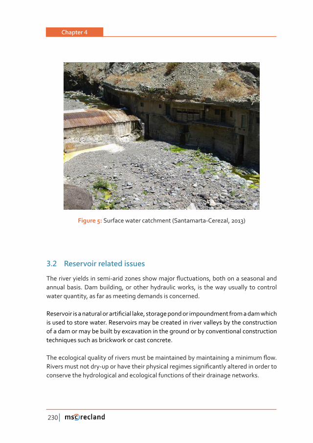
Chapter 4
230
Figure 5: Surface water catchment (Santamarta-Cerezal, 2013)
3�2 Reservoir related issues
������������������������Ǧ����������������������ƪ����������ǡ������������������������annual basis. Dam building, or other hydraulic works, is the way usually to control water quantity, as far as meeting demands is concerned.
������������������������������Ƥ���������ǡ����������������������������������������������is used to store water. Reservoirs may be created in river valleys by the construction of a dam or may be built by excavation in the ground or by conventional construction techniques such as brickwork or cast concrete.
�����������������������������������������������������������������������������ƪ��Ǥ��������������������Ǧ���������������������������������������Ƥ���������������������������conserve the hydrological and ecological functions of their drainage networks.
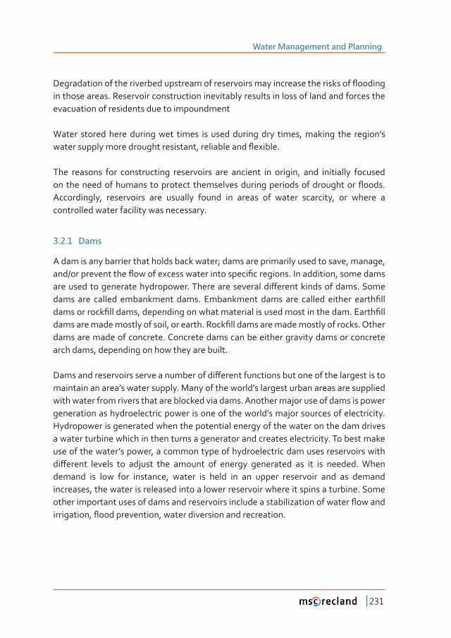
Water Management and Planning
231
�����������������������������������������������������������������������������ƪ�������in those areas. Reservoir construction inevitably results in loss of land and forces the evacuation of residents due to impoundment
Water stored here during wet times is used during dry times, making the region’s �����������������������������������ǡ��������������ƪ������Ǥ
The reasons for constructing reservoirs are ancient in origin, and initially focused ��������������������������������� ����������������������������������������ƪ����Ǥ�Accordingly, reservoirs are usually found in areas of water scarcity, or where a controlled water facility was necessary.
3�2�1 Dams
A dam is any barrier that holds back water; dams are primarily used to save, manage, ���Ȁ���������������ƪ�����������������������������Ƥ���������Ǥ������������ǡ������������������������������������������Ǥ���������������������ơ�������������������Ǥ����������� ���� ������� ����������� ����Ǥ� ����������� ����� ���� ������� ������� �����Ƥ���������������Ƥ�������ǡ���������������������������������������������������Ǥ������Ƥ�������������������������������ǡ���������Ǥ�����Ƥ��������������������������������Ǥ�������dams are made of concrete. Concrete dams can be either gravity dams or concrete arch dams, depending on how they are built.
����������������������������������������ơ���������������������������������������������maintain an area’s water supply. Many of the world’s largest urban areas are supplied with water from rivers that are blocked via dams. Another major use of dams is power generation as hydroelectric power is one of the world’s major sources of electricity. Hydropower is generated when the potential energy of the water on the dam drives a water turbine which in then turns a generator and creates electricity. To best make use of the water’s power, a common type of hydroelectric dam uses reservoirs with ��ơ������ ������� ��� ������� ���� ������� ��� ������� ���������� ��� ��� ��� ������Ǥ������demand is low for instance, water is held in an upper reservoir and as demand increases, the water is released into a lower reservoir where it spins a turbine. Some �����������������������������������������������������������������������������ƪ�����������������ǡ�ƪ��������������ǡ�������������������������������Ǥ
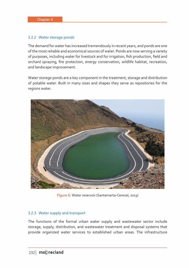
Chapter 4
232
3�2�2 Water storage ponds
The demand for water has increased tremendously in recent years, and ponds are one of the most reliable and economical sources of water. Ponds are now serving a variety �����������ǡ�������������������������������������������������ǡ�Ƥ�������������ǡ�Ƥ���������������� ��������ǡ� Ƥ�������������ǡ� ������� ������������ǡ���������� �������ǡ� ����������ǡ�and landscape improvement.
Water storege ponds are a key component in the treatment, storage and distribution of potable water. Built in many sizes and shapes they serve as repositories for the regions water.
Figure 6: Water reservoir (Santamarta-Cerezal, 2013)
3�2�3 Water supply and transport
The functions of the formal urban water supply and wastewater sector include storage, supply, distribution, and wastewater treatment and disposal systems that provide organized water services to established urban areas. The infrastructure
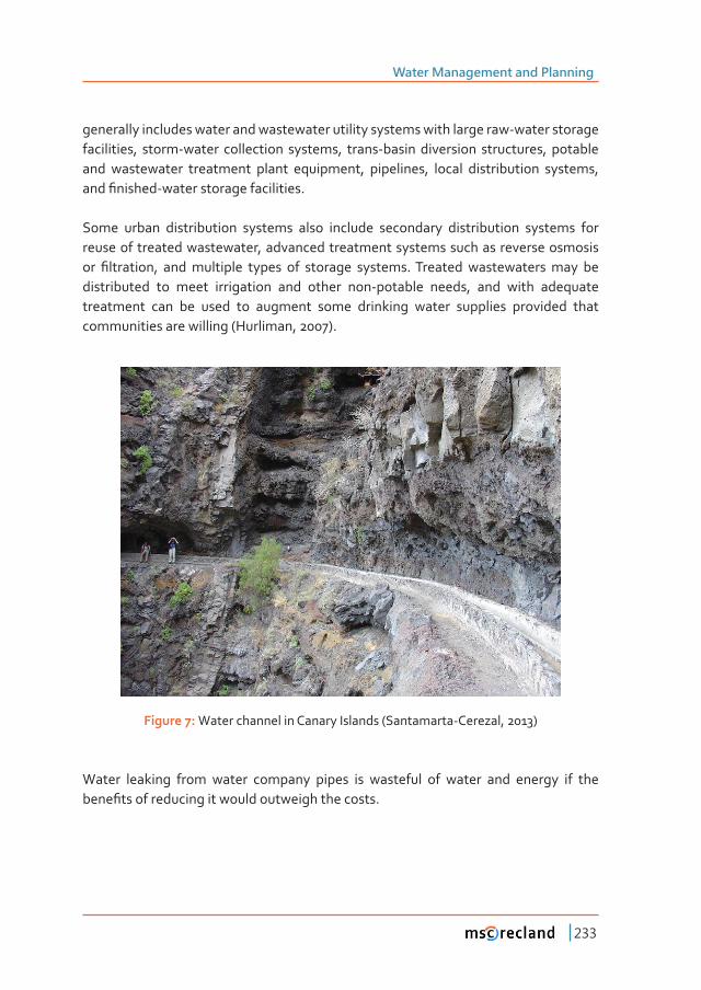
Water Management and Planning
233
generally includes water and wastewater utility systems with large raw-water storage facilities, storm-water collection systems, trans-basin diversion structures, potable and wastewater treatment plant equipment, pipelines, local distribution systems, ����Ƥ������Ǧ������������������������Ǥ
Some urban distribution systems also include secondary distribution systems for reuse of treated wastewater, advanced treatment systems such as reverse osmosis ��� Ƥ��������ǡ� ������������� ������ ��� �������� �������Ǥ��������� ���������������� ���distributed to meet irrigation and other non-potable needs, and with adequate treatment can be used to augment some drinking water supplies provided that communities are willing (Hurliman, 2007).
Figure 7: Water channel in Canary Islands (Santamarta-Cerezal, 2013)
Water leaking from water company pipes is wasteful of water and energy if the ����Ƥ������������������������������������������Ǥ
Chapter 4
234
3�3 Managed aquifer rechargue
Potential sources of recharge water include, but are not limited to, treated wastewater, urban stormwater or groundwater drawn from other aquifers. Some level of pre-treatment of the source water will generally be required prior to recharging the aquifer, depending on the outcome of environmental and health risk assessments.
In urban areas where there’s not enough surface water storage, aquifers can provide a way to store excess water when it becomes available until the time it is needed.
Intentionally injecting or depositing water into an aquifer and then extracting the water for use at a later date is known as managed aquifer recharge. There has been an increasing interest in using managed aquifer recharge as a mechanism to store and later supply an alternative water source for various uses. For example, stormwater could be injected into an aquifer and then later reused for watering parks and gardens in drier seasons.
3�4 Useful links
• Water exploitation index - European Union Open Data Portal - Europa
• Water exploitation-FAO
• Rainwater harvesting
4 WATER WASTE, DESALINATION AND REUSE
4�1 Introduction
The European Union’s Water Framework Directive (WFD) requires member states to systematically develop River Basin Management Plans (RBMP) with measures to achieve good chemical and biological water quality. In the eyes of strengthening regulatory constraints and of the environmental issues at stake, local government entities must deal with the adaptation of their infrastructures and important decision-��������������Ƥ�������������������������������������������Ǥ
Water Management and Planning
235
The discharges of wastewater by industry and households can have considerable ������������ �ơ����� ��� ������ �������� ���ǡ� �����ǡ� ������ ��� ������� ���� ����������health.
Declining water quality is an acute problem around the world, particularly in developing countries where there are notable increases in agricultural and industrial production, coupled with a lack of adequate wastewater treatment.
Through the natural water cycle, the earth has recycled and reused water for millions of years. Water recycling, though, generally refers to projects that use technology to speed up these natural processes.
Reusing and recycling alternative water supplies is a key part of reducing the pressure on our water resources and the environment. Helping us adapt to climate change and population growth. When considering alternative water supplies, you should choose the most appropriate water source, taking into account end use, risk, resource and energy requirements.
The types of water pollutans are:
• Organic wastes: degradable wastes, residuals, some chemicals (detergents, pesticides, oil)
• Inorganic substances: toxic metals, salts, acids, nitrate and phosphorous compounds
• Nonmaterial pollutants: heat, radioactivity
• Infectious agents: bacteria, viruses
It is important that we all reduce the amount of water we use and manage our use of ������������ơ��������Ǥ������������������������������������������������������������������������������������������ƥ������ǡ��������ǣ
• System-wide water loss accounting
• Leak detection and repair
• Pricing that encourages consumer water conservation
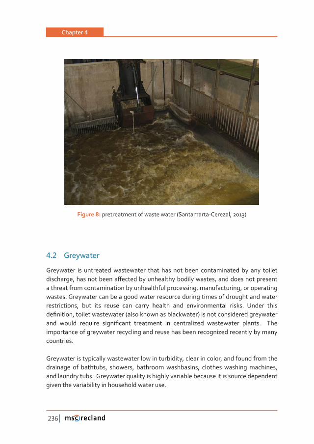
Chapter 4
236
Figure 8: pretreatment of waste water (Santamarta-Cerezal, 2013)
4�2 Greywater
Greywater is untreated wastewater that has not been contaminated by any toilet ���������ǡ���������������ơ��������������������������������ǡ����������������������a threat from contamination by unhealthful processing, manufacturing, or operating wastes. Greywater can be a good water resource during times of drought and water restrictions, but its reuse can carry health and environmental risks. Under this ��Ƥ������ǡ�������������������ȋ������������������������Ȍ��������������������������������� ������ �������� �����Ƥ����� ���������� ��� ������������ ����������� ������Ǥ� � ����importance of greywater recycling and reuse has been recognized recently by many countries.
Greywater is typically wastewater low in turbidity, clear in color, and found from the drainage of bathtubs, showers, bathroom washbasins, clothes washing machines, and laundry tubs. Greywater quality is highly variable because it is source dependent given the variability in household water use.
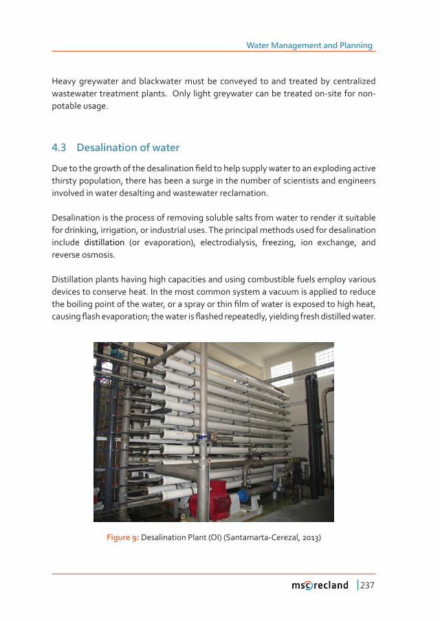
Water Management and Planning
237
Heavy greywater and blackwater must be conveyed to and treated by centralized wastewater treatment plants. Only light greywater can be treated on-site for non-potable usage.
4�3 Desalination of water
��������������������������������������Ƥ������������������������������������������������thirsty population, there has been a surge in the number of scientists and engineers involved in water desalting and wastewater reclamation.
Desalination is the process of removing soluble salts from water to render it suitable for drinking, irrigation, or industrial uses. The principal methods used for desalination include distillation (or evaporation), electrodialysis, freezing, ion exchange, and reverse osmosis.
Distillation plants having high capacities and using combustible fuels employ various devices to conserve heat. In the most common system a vacuum is applied to reduce ������������������������������ǡ��������������������Ƥ�����������������������������������ǡ���������ƪ���������������Ǣ��������������ƪ����������������ǡ�������������������������������Ǥ�
Figure 9: Desalination Plant (OI) (Santamarta-Cerezal, 2013)
Chapter 4
238
Another method of desalination is by electrodialysis. When salt dissolves in water, it splits up into charged particles called ions. Placed in a container with a negative ������������������������������������������������� ���������ǡ� ���� ���������Ƥ����������the membranes as they are attracted toward the electrodes; they become trapped between semipermeable membranes, leaving outside the membranes a supply of desalinated water that can be tapped.
By far the most promising approach is the reverse osmosis process, in which pressure is applied to saltwater to force it through a special membrane. Only pure water passes, leaving concentrated seawater behind.
4�4 Water waste reclamation
Water reuse allows communities to become less dependent on groundwater and surface water sources and can decrease the diversion of water from sensitive ecosystems. Additionally, water reuse may reduce the nutrient loads from wastewater discharges into waterways, thereby reducing and preventing pollution.The term water recycling is generally used synonymously with water reclamation and water reuse.
Recycled water can be used in numerous applications to satisfy most water demands, depending on the level of treatment. The water is treated to meet regulatory guidelines for the intended end use. Typical uses for recycled water include:
• Surface irrigation
• Groundwater recharge
• Wetlands, wildlife hábitat
• Industrial cooling processes
• Landscape and golf course irrigation
• �������ƪ��������������������������
• Food crop irrigation
• Potable reuse (typically recharge of groundwater or surface water to augment drinking water supplies)
Water Management and Planning
239
4�5 Water waste and climate change
There is a need for further research into an environmental accounting system for comparing the climate change impacts of waste management options.Waste is a clear indicator of how much of our natural resources we’re using. The cheaper and more ����������������������ǡ���������������������������������������������������ơ����to waste. Not only is climate change a clear symptom of our over-consumption, it is also a result of our extreme levels of resource use. Waste discharge and wastewater treatment are sources of greenhouse gas emissions. Although carbon dioxide (CO2) and methane (CH4) have been the main focus in climate change calculations and discussions, the potential impact of nitrous oxide (N2O), which is also generated from wastewater treatment plants, is now gaining increased prominence.
Professionals working in waste management and associated areas need to ensure that they are aware of current thinking on climate change and the impact of their area of work on greenhouse gas emissions.
Climate change will likely:
• Contaminate coastal surface and groundwater resources due to sea level rise, resulting in saltwater intrusion into rivers, deltas, and aquifers
• Increase water temperatures, leading to more algal and bacterial blooms that further contaminate water supplies
• �����������������������������������ƪ������ǡ�����������������������������������and wash soil-based pollutants and toxins into waterways
• Contribute to environmental health risks associated with water. For instance, ���������������������������������������������������������ƪ������ǡ�����������������mobilize more pathogens and contaminants
���������������������Ƥ��������������������������������������������������������������water temperature. The increase in water temperatures can lead to a bloom in microbial populations, which can have a negative impact on human health. Additionally, the �����������������������������������������ơ������ơ�����������������������������������due to a species’ sensitivity to temperature. The health of a body of water, such as a �����ǡ�����������������������������������ơ�������������Ǧ�����������������������������ǡ�which is hindered when there is a reduced amount of dissolved oxygen. This occur when water warms and its ability to hold oxygen decreases.
Chapter 4
240
Water and wastewater utilities could reduce energy use by just 10 percent through �������������������������������������Ǧ�ơ������������������������������ƥ������ǡ�collectively.
4�6 Useful links
• Urban Waste Water Directive Overview - European Commission
• Desalination: Solving water problems or creating a new one
• ��������������������������������Ǧ�Dz�������������dz
• World Water Day 2012, Reuse
• Wastewater Treament and Water Reuse Basics
• Dz���������������������dzǡ���������������������������������������������
• Desalination Myths and Misconceptions
5 WATER EFFICIENCY AND SUSTAINABILITY
5�1 Introduction
Conservation of water resources is becoming very important due to climate change ��������ǡ�������������������ǡ�����������������������Ǥ���������������ȋȌ�Dz������is needed to generate energy, and energy is needed to deliver water. Thereby both resources are limiting the other”. In this context, nowadays, there is an increasing ��������� ���Ƥ����������� ���� ������ ����������� ����������������� ��������������������service performance.
�������ƥ�������������������������������������������ǡ����������������������������������the needs of the present generation without compromising the ability of future �������������������������������Ǥ�������������ǡ����������������Ƥ���������������������address the presence of environmental quality in sustainability.
Water Management and Planning
241
������� ������������ ��Ƥ������� ��� ��������������ǡ� ������� �������� ���� ��������������quality as well as its relationship with the other components of sustainability. Thereby, sustainability means the balance between manipulating the environment for meeting as many human needs as possible and preserving the natural processes of the environment.
5�2 Water efficiency
�������ƥ��������������������������������������������������������������������������������������������������������� ����������Ǥ��������ƥ��������������������������������������������� ��������Ǥ���� �����������������ƥ������ǡ��������������������� ��������� ����developing new supplies and for expanding the water infrastructure are reduced. It also diminishes withdrawals from limited freshwater supplies. As a result, there is more water available for future use, and the ambient water quality and aquatic habitat improve (i.e. sustainability is achieved).
������ ������ ����� �ƥ�������� ������ ������������ ��������� ��� ����� ������ǡ� �����������human health and the environment. When reservoir water levels get lower and ground water tables drop, water supplies, human health, and the environment are put at serious risk. For example, lower water levels can contribute to higher concentrations of natural and human pollutants. Less water going down the drain means more water available in the lakes, rivers and streams that we use for recreation and wildlife uses to survive.
���������������ǡ������������������������������������������ơ��������������������������������������ơ�����������������������Ǥ������������������������������������������������������������ǡ� ������������ ��������� ���� Ȃά� ��� ���� ����������� ����� ��� ������ǡ�and most of that is consumed in crop production. In many areas, this water use is unsustainable.
���������������������������������������������������������������ơ�������������������types and climatic region, the supply of some freshwater is an absolute essential for all forms of agriculture. Agricultural activity dominates the use of freshwater and in ���������������� ������� ����������������� ���������ƪ��ǡ���� ����������������������������� ����� ƪ��� ���� �������� ������ ������ �������ǡ� ����� ����������� ����� �������� ���estuarine and coastal ecosystems. In addition, large freshwater abstraction resulted
Chapter 4
242
��� ������������������������������� ��������� ��������Ǥ�������� �ƥ������������ ���� ���agriculture will strongly contribute in the sustainability of this resource.
5�3 Water Sustainability
Water resources sustainability means that development of human activities is compatible with preserving and guarantying adequate living conditions for future �����������Ǥ����������������������������������ƥ����������������������������������and social development while maintaining the resource base and environmental carrying capacity for coming generations.
The resource base concept should be widely interpreted, such that besides the natural resource, it also contains knowledge, infrastructure, technology, durables and human resources. When development converts natural resources into other durable products, this remains part of the overall resource base.
���������������������������ǯ�����������������������ȋǤάȌ�����������������������ǡ�part of it is virtually unreneweable. In contrast, surface water may be considered �� ���������� ��������ǡ� ���� ��� ����������� ����� Ǥά� ��� ���� ���� �����Ǥ� ��� ��������ǡ�in many parts of the world, fresh water resources are scarce and to a large extent Ƥ����Ǥ���������������������������������������������������������������������������������overexploitation by destroying resources for future use, development where water use is not sustainable is ill-planned.
From physical point of view, sustainability water resources means closing the resource cycles and considering the cycles in their integrity (water and nutrient cycles). In agriculture this implies primarily closing or shortening water and nutrient cycles for preventing accumulation or depletion of land and water resources.
������ ���������� �������� ��� �������Ƥ������ǡ� ������ ���� ������������� ��������� ������logging. On the one hand, nutrient depletion leads to loss of fertility, loss of water holding capacity, and in general, reduction of carrying capacity. On the other hand, nutrient accumulation produced eutrophication and pollution. Loss of top-soil results in erosion, land degradation and sedimentation elsewhere.
Water Management and Planning
243
Physical sustainability has to do with closing the cycles within the human dimension. This implies restoring the dynamic equilibria at the appropriate temporal and spatial scales. The latter is relevant, since at a global scale all cycles close.
���� ��� ��������� ������ ��� ����ǡ� ��������������� ��� �������� ��� ���� �ƥ������� ��� ����������Ǥ� ������� �����������������������Ƥ�������������������������� ���ǡ����������������closed, then economic sustainability implies a reduction of scale by short-cutting the ������Ǥ��ƥ��������������������������������������������������������������Ǥ�������������short cycles are: water conservation, to make optimum use of rainfall where it falls ȋ������������������ơ����������������������������������������������ȌǢ�����������������������������������������������������ơ����������������������������������������������������pumped back over considerable distances etc.
Increasing the scale through trade in land- and water-intensive commodities facilitates economic sustainability. This is the virtual water concept, which is an important in ������������������������������������������������������������ƥ��������������������������water intensive products itself. Such concept of virtual water is a tool for an equitable utilisation of water resources. This requires an open and accessible global market and the use of resource-based economic incentives such as resource taxing, as opposed to taxing renewable resources such as labour, which is the general practice today.
�������������������������������������������������������������ơ��������������������ǣ
• Rural scale: water conservation, nutrient and soil conservation, prevention of over-drainage and the recycling of nutrients and organic waste.
• Urban scale: recycling of water, nutrients and waste in both, towns and mega-cities.
• River basin scale: soil and water conservation in the upper catchment, ������������������ơ�����������������������������������������������Ƥ���������������������ǡ�ƪ�������������ǡ�����������������������������������������������Ǥ�
• The global scale: water, nutrient and basic resource cycles are integrated and closed (virtual water concept).
Chapter 4
244
5�4 Water Efficiency Strategies for Sustainability
�ƥ�����������������������������������������������������������������������������������are manifold and depend on the freshwater demanding activity. For example, leak detection programs can reduce the amount of water, pressure, and energy required to deliver the same amount of water to consumers’ taps.
����� �������� ������������ ������������ �������������� ��� �������� �ƥ������� ��������supply-side practices, such as accurate meter reading and leak detection and repair programs, as well as through demand-side strategies, such as conservation-based water rates and public education programs.
Farmers in many countries are subject to legislative restrictions on water use, such that, how to reduce agricultural water use and make water resources more sustainable is an increasingly urgent question. It is a question that requires combined agronomic, physiological, biotechnological/genetic and engineering approaches, which collectively represent ‘water saving agriculture’.
5�5 Useful links
• ��������������������������������Ǧ�ƥ������������
• �����������ƥ�������ȁ������������ȁ�������
6 WATER RESOURCES AND CLIMATE CHANGE
6�1 Introduction
�������������������������������� ����������� ���� �����������Ƥ��������������������population in general. Despite the climate pattern has been changing continuously during the Earth´s history due to changes in the atmosphere, topography, volcanic activity, and other natural factors, this change seems to have been exacerbated recently due to the alteration of the greenhouse gases content in the atmosphere by the humanity.
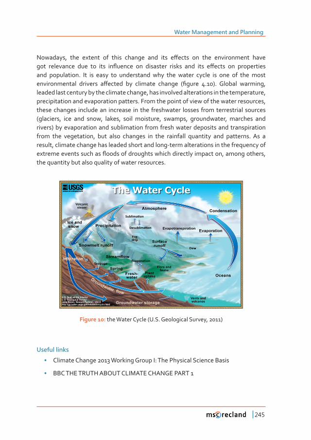
Water Management and Planning
245
��������ǡ� ���� ������� ��� ����� ������� ���� ���� �ơ����� ��� ���� ������������ ��������� ���������� ���� ��� ���� ��ƪ������ ��� ��������� ������ ���� ���� �ơ����� ��� �����������and population. It is easy to understand why the water cycle is one of the most �������������� �������� �ơ������ ��� �������� ������� ȋƤ����� ǤȌǤ� ������ �������ǡ�leaded last century by the climate change, has involved alterations in the temperature, precipitation and evaporation patters. From the point of view of the water resources, these changes include an increase in the freshwater losses from terrestrial sources (glaciers, ice and snow, lakes, soil moisture, swamps, groundwater, marches and rivers) by evaporation and sublimation from fresh water deposits and transpiration from the vegetation, but also changes in the rainfall quantity and patterns. As a result, climate change has leaded short and long-term alterations in the frequency of �����������������������ƪ�����������������������������������������ǡ�������������ǡ�the quantity but also quality of water resources.
Figure 10: the Water Cycle (U.S. Geological Survey, 2011)
Useful links
• Climate Change 2013 Working Group I: The Physical Science Basis
• BBC THE TRUTH ABOUT CLIMATE CHANGE PART 1
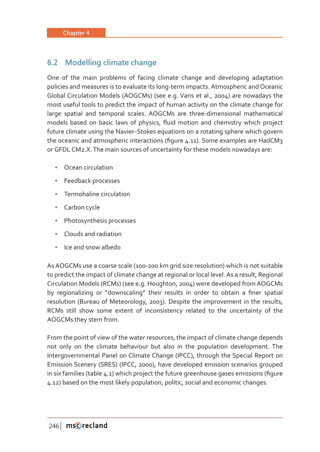
Chapter 4
246
6�2 Modelling climate change
One of the main problems of facing climate change and developing adaptation policies and measures is to evaluate its long-term impacts. Atmospheric and Oceanic Global Circulation Models (AOGCMs) (see e.g. Varis et al., 2004) are nowadays the most useful tools to predict the impact of human activity on the climate change for large spatial and temporal scales. AOGCMs are three-dimensional mathematical ������� ������ ��� ������ ����� ��� �������ǡ� ƪ����������� ���� ���������� ������ ��������future climate using the Navier–Stokes equations on a rotating sphere which govern �����������������������������������������ȋƤ�����ǤȌǤ�������������������������or GFDL CM2.X. The main sources of uncertainty for these models nowadays are:
• Ocean circulation
• Feedback processes
• Termohaline circulation
• Carbon cycle
• Photosynthesis processes
• Clouds and radiation
• Ice and snow albedo
As AOGCMs use a coarse scale (100-200 km grid size resolution) which is not suitable to predict the impact of climate change at regional or local level. As a result, Regional Circulation Models (RCMs) (see e.g. Houghton, 2004) were developed from AOGCMs ��� �������������� ��� Dz�����������dz� ������ �������� ��� ������ ��� ������� �� Ƥ���� ��������resolution (Bureau of Meteorology, 2003). Despite the improvement in the results, RCMs still show some extent of inconsistency related to the uncertainty of the AOGCMs they stem from.
From the point of view of the water resources, the impact of climate change depends not only on the climate behaviour but also in the population development. The Intergovernmental Panel on Climate Change (IPCC), through the Special Report on Emission Scenery (SRES) (IPCC, 2000), have developed emission scenarios grouped ����������������ȋ������ǤȌ�����������������������������������������������������ȋƤ�����4.12) based on the most likely population, politic, social and economic changes.
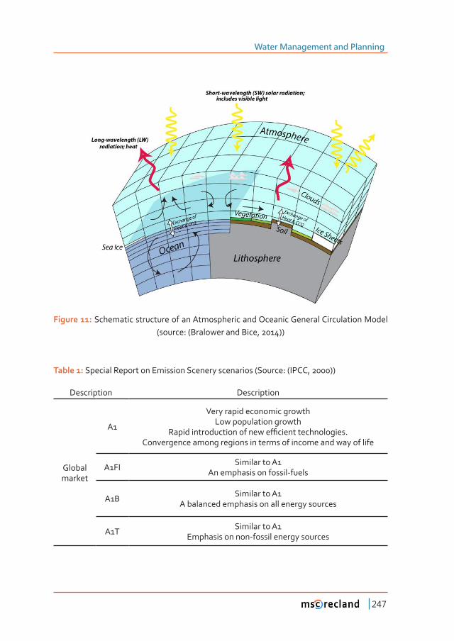
Water Management and Planning
247
Figure 11: Schematic structure of an Atmospheric and Oceanic General Circulation Model (source: (Bralower and Bice, 2014))
Table 1: Special Report on Emission Scenery scenarios (Source: (IPCC, 2000))
Description Description
Global market
A1
Very rapid economic growth Low population growth
���������������������������ƥ������������������Ǥ�Convergence among regions in terms of income and way of life
A1FI Similar to A1An emphasis on fossil-fuels
A1B Similar to A1A balanced emphasis on all energy sources
A1T Similar to A1Emphasis on non-fossil energy sources
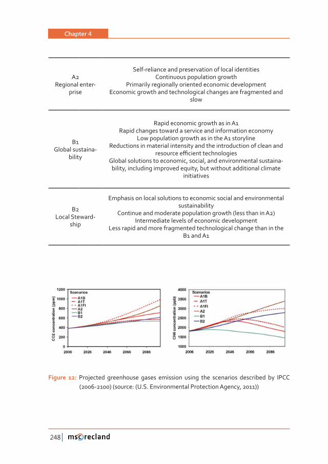
Chapter 4
248
A2Regional enter-
prise
Self-reliance and preservation of local identitiesContinuous population growth
Primarily regionally oriented economic development Economic growth and technological changes are fragmented and
slow
B1Global sustaina-
bility
Rapid economic growth as in A1Rapid changes toward a service and information economy
Low population growth as in the A1 storylineReductions in material intensity and the introduction of clean and
����������ƥ������������������Global solutions to economic, social, and environmental sustaina-
bility, including improved equity, but without additional climate initiatives
B2Local Steward-
ship
Emphasis on local solutions to economic social and environmental sustainability
Continue and moderate population growth (less than in A2)Intermediate levels of economic development
Less rapid and more fragmented technological change than in the B1 and A1
Figure 12: Projected greenhouse gases emission using the scenarios described by IPCC (2006-2100) (source: (U.S. Environmental Protection Agency, 2011))
Water Management and Planning
249
6�2�1 Useful links
• Wikipedia: General Circulation Models
• What is a GCM? - the IPCC Data Distribution Centre
• ���������������ơ����������������������
• IPCC Special Report: Emissions Scenarios (SRES)
6�3 Impacts of climate change
Impacts on water resources by the climate change are temporary and spatially dependent:
• ������������ơ����������������������Ǧ����������������������������������Ǧ�����or gradual and deeper changes in the hydrological cycle such as spatial and �������������������������ƪ����������������ǡ������������������������������������to the climatic change, etc.
• ����������ơ�������������������������������������������������ơ�����������������the alteration of the climatic patterns.
- In general (North Hemisphere), it is expected an increase in the quantity of water resources in northern countries as they become wetter.
- ���� ��������� ������ ������ �ơ���� ��������� ���������� ��� ������������������ ��������� ������������� �ơ������� ������������ ����transpiration processes and their precipitation decrease and become more intense unbalancing hydrological functions such as ����ơǦ��������������Ǥ�
- From the point of view of the quality of the water resources, a substantial decrease in this parameter related to the increase in the water temperature, sediments suspended, nutrients and eutrophication processes could be expected.
Chapter 4
250
- However, particular trends of water resources quantity and quality show a high regional dependence due to the large number of factors involved and impacted by the climate change, and resilience of the ��ơ��������������������������Ǥ�
Due to the importance and high degree of uncertainty arising from its impacts, climate change may be the most challenging issue that world must face nowadays (Watkiss et al., 2005) and including adapting measures in the decision-making processes and ��������������������������������������������������ơ����Ǥ
6�3�1 Temperature and sea level
Based on the prediction models and SRES scenarios described before, projections of climate change impacts on temperature and sea level could be developed (table 4.2). According to these projections, a temperature rise of about 0.1ºC per decade would be expected and of 0.2 ºC projected for the next two decades for all SRES scenarios. The temperature will rise between 1.8 and 4.0 ºC and the sea level rise will range from 18 to 59 cm depending on the scenario. In general, scenario A1F1 is the most extreme mainly due to its rapid economic growth and the use of fossil fuels, whilst scenario B1 show ���������Ƥ��������������������������������������������������ƥ�������������������and the rapid changes toward a service and information economy. Besides, it is very likely that hot extremes, heat waves and heavy precipitation events will continue �������������������������ơ�������������������������������������������������������processes such as ocean circulation, photosynthesis processes, evaporation, etc.
Uncertainty on the predicted impact of climate change on temperature and sea level ��������������������������ơ�����������������������������������Ǥ�������������������� ��ơ������ ������� ����������� ����������������� ��ơ������������ ���� ������ ����calculations to obtain projected future values.
On the other hand, the high temporal and regional dependence of the climate change process is highlighted by the fact that the highest increase in both temperature and sea level are projected to be recorded in the North Pole during the last half of the 21st� �������� ���������� ��� ���� ��ơ������ ����� ���������� ���������� ȋƤ����� ǤȌǤ�Warming is expected to be greatest over land and at most high northern latitudes and least over Southern Ocean and parts of the North Atlantic Ocean.
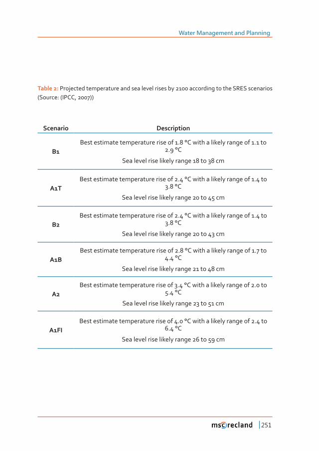
Water Management and Planning
251
Table 2: Projected temperature and sea level rises by 2100 according to the SRES scenarios (Source: (IPCC, 2007))
Scenario �����������
B1Best estimate temperature rise of 1.8 °C with a likely range of 1.1 to
2.9 °C
Sea level rise likely range 18 to 38 cm
A1TBest estimate temperature rise of 2.4 °C with a likely range of 1.4 to
3.8 °C
Sea level rise likely range 20 to 45 cm
B2Best estimate temperature rise of 2.4 °C with a likely range of 1.4 to
3.8 °C
Sea level rise likely range 20 to 43 cm
A1BBest estimate temperature rise of 2.8 °C with a likely range of 1.7 to
4.4 °C
Sea level rise likely range 21 to 48 cm
A2Best estimate temperature rise of 3.4 °C with a likely range of 2.0 to
5.4 °C
Sea level rise likely range 23 to 51 cm
A1FIBest estimate temperature rise of 4.0 °C with a likely range of 2.4 to
6.4 °C
Sea level rise likely range 26 to 59 cm
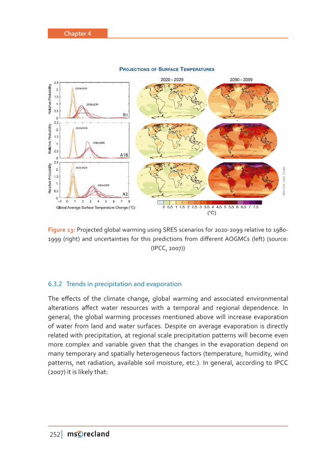
Chapter 4
252
Figure 13: Projected global warming using SRES scenarios for 2020-2099 relative to 1980-� ȋ�����Ȍ� ���� �������������� ���� ����� ������������ �������ơ������������ ȋ����Ȍ� ȋ������ǣ�
(IPCC, 2007))
6�3�2 Trends in precipitation and evaporation
���� �ơ����� ��� ���� �������� ������ǡ� ������� �������� ���� ����������� �������������������������� �ơ���� ������ ���������� ����� �� ��������� ���� ��������� ����������Ǥ� ���general, the global warming processes mentioned above will increase evaporation of water from land and water surfaces. Despite on average evaporation is directly related with precipitation, at regional scale precipitation patterns will become even more complex and variable given that the changes in the evaporation depend on many temporary and spatially heterogeneous factors (temperature, humidity, wind patterns, net radiation, available soil moisture, etc.). In general, according to IPCC (2007) it is likely that:
Water Management and Planning
253
• Tropical cyclones will become more intense, with more heavy precipitation associated with on-going increases of tropical sea surface temperatures
• Extratropical storm tracks are projected to move poleward, with consequent changes in wind, precipitation and temperature patterns
• Sea ice will shrink in both the Arctic and Antarctic under all SRES scenarios. In some projections, arctic late-summer sea ice disappears almost entirely by the latter part of the 21st century
• �������Ǧ�ơ������������������������������
• Heavy precipitation events are very likely to become more common increasing ƪ��������
• Water supplies stored in glaciers and snow cover will be reduced over the course of the century
�������ǡ������������������������������������������������������������ȋƤ�����ǤȌǤ������������������������������Ƥ����������ǣ
• Regional patterns:
- Dry regions are projected to get drier: decrease in fresh water ����������������Ȃά�����������������������������Ǧ�����������������the dry tropics by 2050
- Wet regions are projected to get wetter: increase in fresh water ������������� ��� Ȃά� ��� ����� ���������� ���� ��� ��������� ���������areas by 2050
• Temporal patterns:
- Winter is projected to become wetter in northern latitudes but dryer in southern ones
- Summer is projected to become drier in most areas
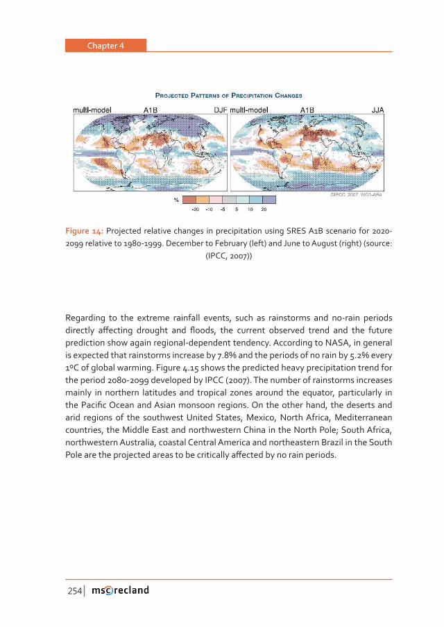
Chapter 4
254
Figure 14: Projected relative changes in precipitation using SRES A1B scenario for 2020-2099 relative to 1980-1999. December to February (left) and June to August (right) (source:
(IPCC, 2007))
Regarding to the extreme rainfall events, such as rainstorms and no-rain periods ��������� �ơ������� �������� ���� ƪ����ǡ� ���� �������� ��������� ������ ���� ���� �������prediction show again regional-dependent tendency. According to NASA, in general ����������������������������������������Ǥά�������������������������������Ǥά�������1ºC of global warming. Figure 4.15 shows the predicted heavy precipitation trend for the period 2080-2099 developed by IPCC (2007). The number of rainstorms increases mainly in northern latitudes and tropical zones around the equator, particularly in ��������Ƥ���������������������������������Ǥ������������������ǡ� ����������������arid regions of the southwest United States, Mexico, North Africa, Mediterranean countries, the Middle East and northwestern China in the North Pole; South Africa, northwestern Australia, coastal Central America and northeastern Brazil in the South �����������������������������������������������ơ������������������������Ǥ
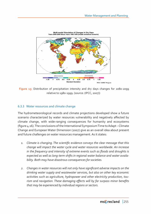
Water Management and Planning
255
Figure 15: Distribution of precipitation intensity and dry days changes for 2080-2099 relative to 1980-1999. (source: (IPCC, 2007))
6�3�3 Water resources and climate change
The hydrometeorological records and climate projections developed show a future ��������� ����������������������� ���������� �������������� ��������������� �ơ���������climate change, with wide-ranging consequences for humanity and ecosystems ȋƤ����� ǤȌǤ��������������������������������������������������������������Ȃ���������Change and European Water Dimension (2007) give as an overall idea about present and future challenges on water resources management. As it states:
Ǥ� �������������������Ǥ������������Ƥ�����������������������������������������������change will impact the water cycle and water resources worldwide. An increase ���������������������������������������������������������ƪ���������������������expected as well as long-term shifts in regional water balance and water availa-bility. Both may have disastrous consequences for societies.
Ǥ� ���������������������������������������������������Ƥ����������������������������drinking water supply and wastewater services, but also on other key economic activities such as agriculture, hydropower and other electricity production, tou-�������������������Ǥ�����������������ơ�����������������������������������Ƥ���that may be experienced by individual regions or sectors.
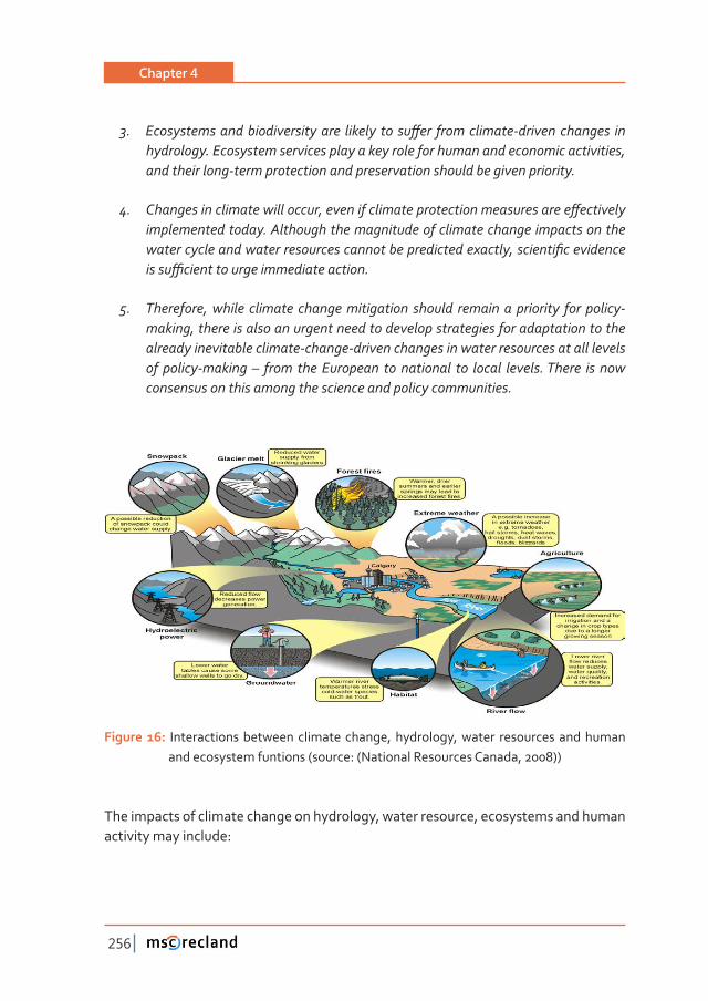
Chapter 4
256
Ǥ� �������������������������������� ������� �����ơ��� ������������Ǧ��������������� ���hydrology. Ecosystem services play a key role for human and economic activities, and their long-term protection and preservation should be given priority.
Ǥ� �����������������������������ǡ������������������������������������������ơ���������implemented today. Although the magnitude of climate change impacts on the �����������������������������������������������������������ǡ��������Ƥ����������������ƥ������������������������������Ǥ
Ǥ� Therefore, while climate change mitigation should remain a priority for policy-making, there is also an urgent need to develop strategies for adaptation to the already inevitable climate-change-driven changes in water resources at all levels of policy-making – from the European to national to local levels. There is now consensus on this among the science and policy communities.
Figure 16: Interactions between climate change, hydrology, water resources and human and ecosystem funtions (source: (National Resources Canada, 2008))
The impacts of climate change on hydrology, water resource, ecosystems and human activity may include:
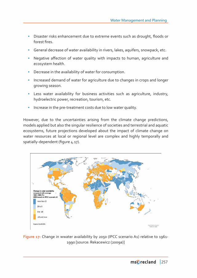
Water Management and Planning
257
• ����������������������������������������������������������������ǡ�ƪ���������������Ƥ���Ǥ
• General decrease of water availability in rivers, lakes, aquifers, snowpack, etc.
• ��������� �ơ������� ��� ������ �������� ����� �������� ��� �����ǡ� ������������ ����ecosystem health.
• Decrease in the availability of water for consumption.
• Increased demand of water for agriculture due to changes in crops and longer growing season.
• Less water availability for business activities such as agriculture, industry, hydroelectric power, recreation, tourism, etc.
• Increase in the pre-treatment costs due to low water quality.
However, due to the uncertainties arising from the climate change predictions, models applied but also the singular resilience of societies and terrestrial and aquatic ecosystems, future projections developed about the impact of climate change on water resources at local or regional level are complex and highly temporally and ���������Ǧ����������ȋƤ�����ǤȌǤ
Figure 17: Change in wwater availability by 2050 (IPCC scenario A1) relative to 1961-1990 [source: Rekacewicz (2009a)]
Chapter 4
258
As is mention by numerous researchers, the climate change can impact on water availability by modifying both quantity and quality of the water resources:
• Impacts on water quality include alteration of physical, chemical and biological ������������������������ơ��������������������������������������������������Ǥ�
• ��������� ���������ơ���� ���� ������������ ��������� ���� �������� ������������� ����societies and ecosystems represented mainly by opposite extreme events.
- ������������������������ƪ����Ǥ
- Water scarcity and drought after no-rainfall periods.
6�3�4 Useful links
• IPCC Fourth Assessment Report: Climate Change 2007 (AR4)
• Time to Adapt - Climate Change and the European Water Dimension
6�4 Water quality
������ ���������� �������� ��ƪ������� ��������� ���� ������������� ���� ���� ��� �������� ����environments. The impact of climate change on water quality could be:
• Related to temperature:
- �ơ����������������������������Ǥ�
- Algae blooms reducing dissolved oxygen.
- Cyanobacteria blooms after the reduction of dissolved oxygen.
• �����������ƪ����������ǣ
- Change in the speed, residence time and dilution capacity of the ������ƪ���Ǥ
- Rise in storm events which increase the occurrence of sewer ����ƪ�����������������������������������������������������Ǥ
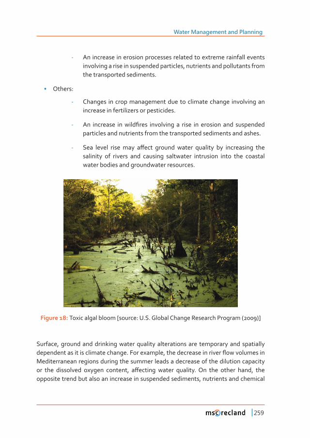
Water Management and Planning
259
- An increase in erosion processes related to extreme rainfall events involving a rise in suspended particles, nutrients and pollutants from the transported sediments.
• Others:
- Changes in crop management due to climate change involving an increase in fertilizers or pesticides.
- ��� ��������� �������Ƥ���� ���������� �� ����� ��� �������� ���� ����������particles and nutrients from the transported sediments and ashes.
- ���� ������ ����� ���� �ơ���� ������� ������ �������� ��� ����������� ����salinity of rivers and causing saltwater intrusion into the coastal water bodies and groundwater resources.
Figure 18: Toxic algal bloom [source: U.S. Global Change Research Program (2009)]
Surface, ground and drinking water quality alterations are temporary and spatially ���������������������������������Ǥ�����������ǡ�����������������������ƪ��������������Mediterranean regions during the summer leads a decrease of the dilution capacity ��� ���� ���������� ������� �������ǡ� �ơ������� ������ �������Ǥ���� ���� ������ ����ǡ� ����opposite trend but also an increase in suspended sediments, nutrients and chemical
Chapter 4
260
due to erosion exacerbation may be expected in northern latitude countries during �������������������������������������������������������������ƪ����������Ǥ
Besides, as it was stated before, future projections developed about the impact of climate change on water quality at local or regional level are complex (Murdoch et al., 2000) and highly temporally and spatially-dependent due to the uncertainties arising from the climate change predictions, models applied but also the singular resilience of societies and terrestrial and aquatic ecosystems.
�����������������������ǡ�������������������������������������ơ���������������������change impact are:
• Temperature
• Suspended particles
• Nutrients
• Salt intrusion into groundwater bodies
6�4�1 Temperature
In general and according to the future projections, an increase in water temperature ��� ��������� ��� �� ������� ��� ���� ������� �������� ȋƤ����� ǤȌǤ� ����������ǡ� ������temperature is related directly to the speed of the biochemical reactions. The rise ��������������������������ơ�������������������ơ�����������ȋ������ǡ�ȌǤ����������in water quality could be expected as a direct result of water warming as biological processes and aeration rate are accelerated by this alteration. However, this trend is �ơ����������������������������������������������������ǡ�������������������������������������������������������������������������ƪ�����������ȋ�������������Ǥǡ�ȌǤ�
Lakes and stagnant water ecosystems are less resilient to the impacts of global ����������������������������������������������������������������������ƪ���Ǥ����������������������������������������������������������������������������Ǧ�������ƪ��������ǡ������ �����������ǡ� ������Ƥ���������� ��������������ǡ��� ���������� ��� �����������input in deeper water tables and bottom water anoxia.
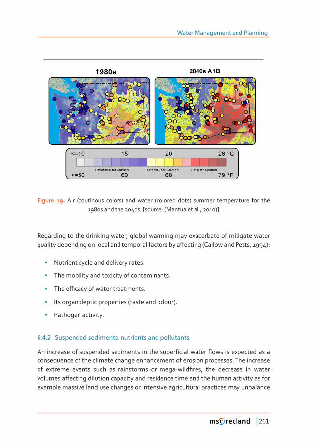
Water Management and Planning
261
Figure 19: Air (coutinous colors) and water (colored dots) summer temperature for the 1980s and the 2040s [source: (Mantua et al., 2010)]
Regarding to the drinking water, global warming may exacerbate of mitigate water ����������������������������������������������������ơ�������ȋ����������������ǡ�Ȍǣ
• Nutrient cycle and delivery rates.
• The mobility and toxicity of contaminants.
• �����ƥ������������������������Ǥ
• Its organoleptic properties (taste and odour).
• Pathogen activity.
6�4�2 Suspended sediments, nutrients and pollutants
��� �������������������������������� ������������Ƥ�����������ƪ���� �����������������consequence of the climate change enhancement of erosion processes. The increase ��� �������� ������� ����� ��� ����������� ��� ����Ǧ����Ƥ���ǡ� ���� ��������� ��� ���������������ơ��������������������������������������������������������������������������example massive land use changes or intensive agricultural practices may unbalance
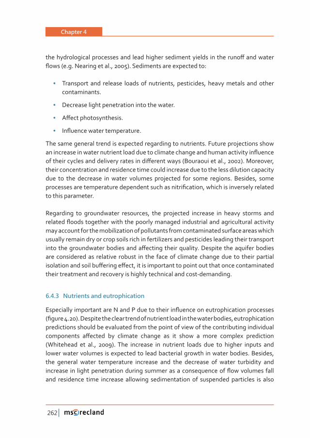
Chapter 4
262
����������������������������������������������������������� �����������ơ�����������ƪ����ȋ�Ǥ�Ǥ��������������Ǥǡ�ȌǤ��������������������������ǣ
• Transport and release loads of nutrients, pesticides, heavy metals and other contaminants.
• Decrease light penetration into the water.
• �ơ������������������Ǥ
• ��ƪ�����������������������Ǥ
The same general trend is expected regarding to nutrients. Future projections show ������������������������������������������������������������������������������ƪ����������������������������������������������ơ�����������ȋ��������������Ǥǡ�ȌǤ���������ǡ�their concentration and residence time could increase due to the less dilution capacity due to the decrease in water volumes projected for some regions. Besides, some �������������������������������������������������Ƥ������ǡ����������������������������to this parameter.
Regarding to groundwater resources, the projected increase in heavy storms and ��������ƪ���������������������������������������������������������������������������may account for the mobilization of pollutants from contaminated surface areas which usually remain dry or crop soils rich in fertilizers and pesticides leading their transport ���������������������������������ơ��������������������Ǥ����������������������������are considered as relative robust in the face of climate change due to their partial ���������������������ơ�������ơ���ǡ�����������������������������������������������������their treatment and recovery is highly technical and cost-demanding.
6�4�3 Nutrients and eutrophication
������������������������������������������������ƪ����������������������������������ȋƤ����� ǤȌǤ�������������������������������������������������������������ǡ����������������predictions should be evaluated from the point of view of the contributing individual ����������� �ơ������ ��� �������� ������� ��� ��� ����� �� ����� �������� �����������(Whitehead et al., 2009). The increase in nutrient loads due to higher inputs and lower water volumes is expected to lead bacterial growth in water bodies. Besides, the general water temperature increase and the decrease of water turbidity and ��������� ��� ����������������������������������������������������ƪ����������������and residence time increase allowing sedimentation of suspended particles is also
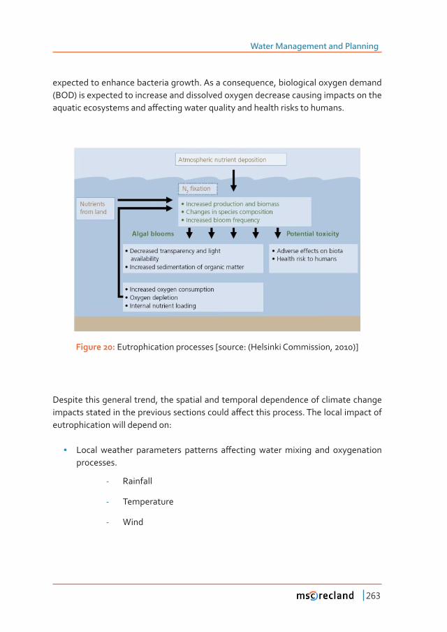
Water Management and Planning
263
expected to enhance bacteria growth. As a consequence, biological oxygen demand (BOD) is expected to increase and dissolved oxygen decrease causing impacts on the ������������������������ơ�����������������������������������������������Ǥ�
Figure 20: Eutrophication processes [source: (Helsinki Commission, 2010)]
Despite this general trend, the spatial and temporal dependence of climate change �����������������������������������������������ơ����������������Ǥ���������������������eutrophication will depend on:
• ������ �������� ����������� ��������� �ơ�������������������� ���� ������������processes.
- Rainfall
- Temperature
- Wind
Chapter 4
264
• ��������ơ�������������������������������������������������������������������������ơ�ƪ��ǣ�
- Soil type and erosionability
- Topography
- Land use
- Vegetation cover
- ����Ƥ���
- Agricultural practices and use of fertilizers and pesticides
• ���������������� ��� ���� ������ ����� �ơ������� ƪ��� �����ǡ� ���������� ����� ����oxygenation processes:
- Volume
- Flow volume and speed
- Shape
- Depth
- Water inputs and outputs
6�4�4 Salt intrusion into groundwater and coastal water bodies
��������������������������ơ������������������Ƥ�����������������������������������saltwater intrusion or the replacement of fresh water by marine water due to the movement of the later into the former through the existing interface layer between them in coastal areas. Regarding to aquifers, the salt intrusion processes generally �������������������������������ȋƤ�����ǤȌǣ�
• Aquifer volume: recharge and exploitation of the groundwater resources impact on the balance between water input and output and, thus, water volume. A ��������� ��������� ƪ��� ��� ���� �������� ���Ȁ��� ��� ��������� ��������� �����������from it may lead an increase in saltwater intrusion.
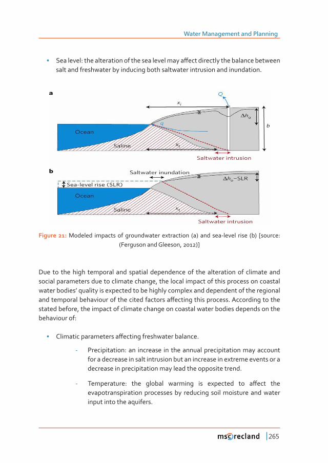
Water Management and Planning
265
• ���������ǣ��������������������������������������ơ���������������������������������salt and freshwater by inducing both saltwater intrusion and inundation.
Figure 21: Modeled impacts of groundwater extraction (a) and sea-level rise (b) [source: (Ferguson and Gleeson, 2012)]
Due to the high temporal and spatial dependence of the alteration of climate and social parameters due to climate change, the local impact of this process on coastal water bodies’ quality is expected to be highly complex and dependent of the regional ���������������������������������������������ơ�������������������Ǥ������������������stated before, the impact of climate change on coastal water bodies depends on the behaviour of:
• ���������������������ơ�������������������������Ǥ
- Precipitation: an increase in the annual precipitation may account for a decrease in salt intrusion but an increase in extreme events or a decrease in precipitation may lead the opposite trend.
- �����������ǣ� ���� ������� �������� ��� ��������� ��� �ơ���� ����evapotranspiration processes by reducing soil moisture and water input into the aquifers.
Chapter 4
266
• Social demands:
- Water demand: the expected increase in population, industrial processes and global warming is expected to lead a general rise in ��������������������������ơ�����������������������������������salt and freshwater inducing salt intrusion in coastal water bodies.
- Land use and agricultural practices: land use and vegetation change may alter the hydrological cycle by modifying the evapotranspiration �������������ơ���������������������������Ǥ�
6�4�5 Useful links
• Water Quality and Future Generations
• Water Quality and the Environment
• ���������������ȁ�������������������������ȁ�������������������
6�5 Floods
������ ���� ������� �������� ��� ������ ������ ���������� ���� �������� ���Ƥ������� ����covering a portion of land not previously covered. They are considered the main threat ������������������������������������������ơ������������������������������������Ǥ
Floods are natural processes which occur in river systems on a regular basis generally by melting snows or heavy rains, but they may occur anywhere related to other exceptional natural disasters such as hurricanes and cyclones including rain storms, tsunamis in coastal environments or volcanic eruptions melting snows, or even human induced causes including incorrect infrastructure planning or wrong land use ����������ȋƤ�����ǤȌǤ
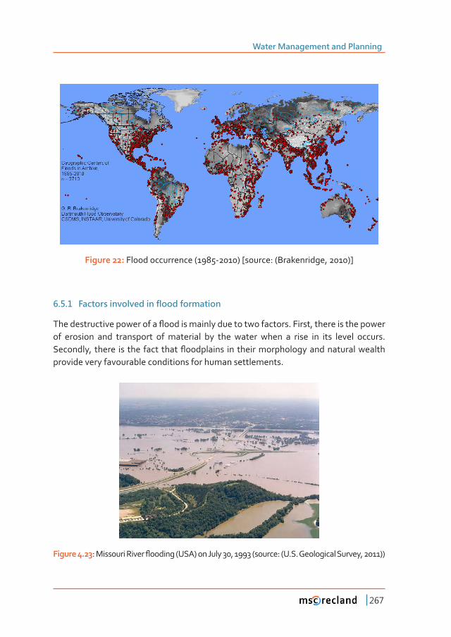
Water Management and Planning
267
Figure 22: Flood occurrence (1985-2010) [source: (Brakenridge, 2010)]
6�5�1 Factors involved in flood formation
���������������������������ƪ��������������������������������Ǥ�����ǡ��������������������of erosion and transport of material by the water when a rise in its level occurs. ��������ǡ� ������ ��� ��������� �����ƪ���������� ���������������������������������������provide very favourable conditions for human settlements.
Figure 4.23ǣ����������������ƪ�������ȋ���Ȍ���� ���� ǡ� �ȋ������ǣ�ȋ�Ǥ�Ǥ�����������������ǡ� ȌȌ
Chapter 4
268
Flooding can happen anywhere, but certain areas are especially prone to serious ƪ������Ǥ���������������������������������������������ƪ�������������ǣ
• Conditioning Factors
- ����������ǣ� ���� ƪ��� ���Ƥ��������� ��� ���� ������� ������������ ����expansion of the water layer whilst sudden changes in slope favour sudden increases in the velocity of water and its concentration.
- Terrain: the lithological composition of the soil determines its drainage and erosion capacity, this determines whether rivers may �����������������������������������������������ƪ��Ǥ
- �����������������ǣ��������������������������ơ������������������ǣ�braided, meandering, rectilinear, which can determine the velocity ��������ǡ�����ƪ���������������������ǡ����Ǥ
• Triggering factors
- Weather and climate change: the intensity of rainfall or melting snow may exceed the capacity of drainage system and cause an ����ƪ��Ǥ
- Seismic: earthquakes can trigger tsunamis that can cause severe ƪ��������������������������Ǥ
- Deforestation: the lack of a well-developed vegetation cover ��������������������ơ��������������Ǥ
- Obstruction of the bed: this can occur when waste, trunks or tailings ����������������ǡ�����������������������������������ƪ������Ǥ�����������������������������������������������������������ƪ���Ǥ
- ������� ���� ���� ���Ƥ������ǣ� ������ ����� ��� ��� ��������� ��� �����������������ơ������������ȋ���������Ȍ�������Ƥ�����������������������the subsoil. Moreover, these favour the deposition of materials on ���� �������� ������ǡ� ������ ����� Ƥ��� ���� ��������� ����� ����� �����increasing the topographic level where water circulates.
- ����������ƪ��������������������������������������������Ǥ
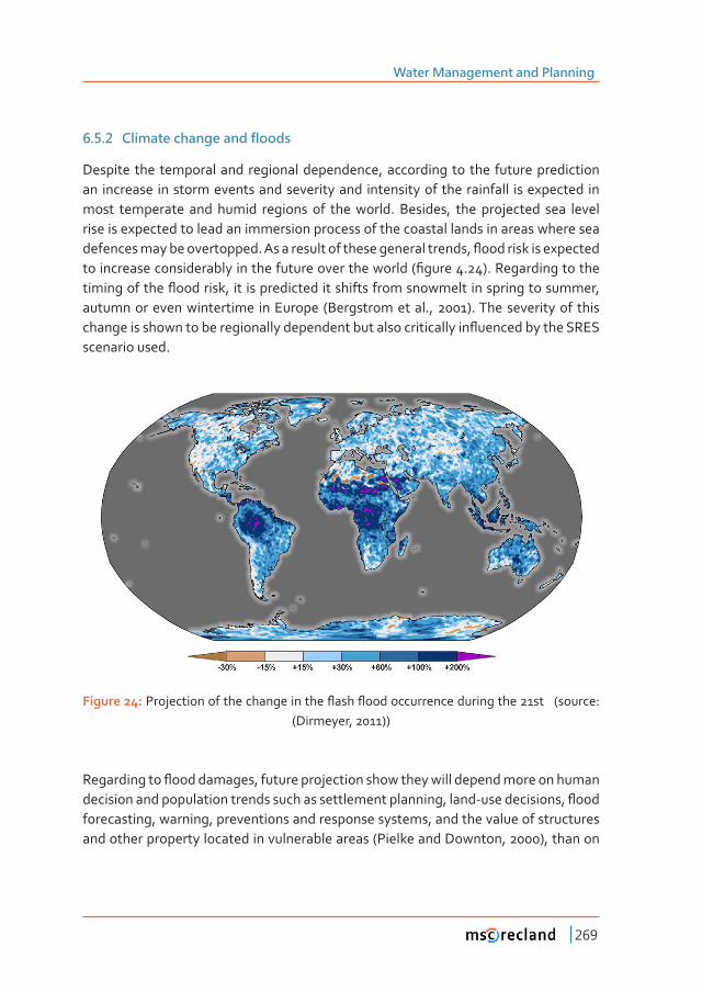
Water Management and Planning
269
6�5�2 Climate change and floods
Despite the temporal and regional dependence, according to the future prediction an increase in storm events and severity and intensity of the rainfall is expected in most temperate and humid regions of the world. Besides, the projected sea level rise is expected to lead an immersion process of the coastal lands in areas where sea ��������������������������Ǥ������������������������������������ǡ�ƪ���������������������������������������������������������������������������ȋƤ�����ǤȌǤ��������������������������������ƪ��������ǡ������������������������������������������������������������ǡ�autumn or even wintertime in Europe (Bergstrom et al., 2001). The severity of this �����������������������������������������������������������������ƪ�������������������scenario used.
Figure 24: ��������������������������������ƪ����ƪ�������������������������������ȋ������ǣ�(Dirmeyer, 2011))
�������������ƪ�����������ǡ�����������������������������������������������������������������������������������������������������������������ǡ�����Ǧ�������������ǡ�ƪ����forecasting, warning, preventions and response systems, and the value of structures and other property located in vulnerable areas (Pielke and Downton, 2000), than on
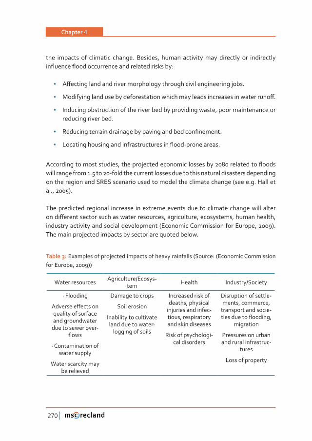
Chapter 4
270
the impacts of climatic change. Besides, human activity may directly or indirectly ��ƪ������ƪ�����������������������������������ǣ
• �ơ���������������������������������������������������������������Ǥ
• ���������������������������������������������������������������������������ơǤ
• Inducing obstruction of the river bed by providing waste, poor maintenance or reducing river bed.
• �����������������������������������������������Ƥ������Ǥ
• ����������������������������������������ƪ���Ǧ�����������Ǥ
�������������������������ǡ����������������������������������������������ƪ�����will range from 1.5 to 20-fold the current losses due to this natural disasters depending on the region and SRES scenario used to model the climate change (see e.g. Hall et al., 2005).
The predicted regional increase in extreme events due to climate change will alter �����ơ������������������������������������ǡ������������ǡ�����������ǡ�������������ǡ�industry activity and social development (Economic Commission for Europe, 2009). The main projected impacts by sector are quoted below.
Table 3: Examples of projected impacts of heavy rainfalls (Source: (Economic Commission for Europe, 2009))
Water resources Agriculture/Ecosys-tem Health Industry/Society
· Flooding
���������ơ��������quality of surface and groundwater
due to sewer over-ƪ���
· Contamination of water supply
Water scarcity may be relieved
Damage to crops
Soil erosion
Inability to cultivate land due to water-
logging of soils
Increased risk of deaths, physical
injuries and infec-tious, respiratory and skin diseases
Risk of psychologi-cal disorders
Disruption of settle-ments, commerce,
transport and socie-������������ƪ������ǡ�
migration
Pressures on urban and rural infrastruc-
tures
Loss of property
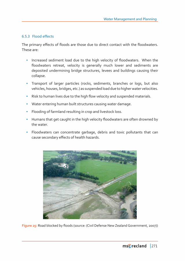
Water Management and Planning
271
6�5�3 Flood effects
�������������ơ��������ƪ����������������������������������������������ƪ���������Ǥ�These are:
• ���������� ��������� ��������� ��� ��������� ��������� ��� ƪ���������Ǥ� ������ ����ƪ���������� �������ǡ� ��������� ��� ���������� ����� ������ ���� ���������� ����deposited undermining bridge structures, levees and buildings causing their collapse.
• Transport of larger particles (rocks, sediments, branches or logs, but also vehicles, houses, bridges, etc.) as suspended load due to higher water velocities.
• ������������������������������������ƪ�����������������������������������Ǥ
• Water entering human built structures causing water damage.
• Flooding of farmland resulting in crop and livestock loss.
• ��������������������������������������������ƪ�������������������������������the water.
• Floodwaters can concentrate garbage, debris and toxic pollutants that can �����������������ơ����������������������Ǥ
Figure 25:�����������������ƪ�����ȋ������ǣ�ȋ�����������������������������������ǡ�ȌȌ
Chapter 4
272
�����������ơ�����������������������������������������������������������ơ����ǣ
• Pollution of drinking water supplies especially if sewerage treatment plants ����ƪ������ ���������� ��� �������� ���������� ������� �ơ����ǡ� ����������� ��� ������developed countries.
• Gas and electrical service may be disrupted.
• Transportation systems may be disrupted, resulting in shortages of food and cleaning-up supplies. In under developed countries, food shortages often lead to starvation.
����Ǧ������ơ�����ȋ����������ơ����Ȍ����ƪ������������ǣ
• �����������������������������������������������������������ƪ������ǡ��������������develop, leaving the old channels dry.
• Destruction of farmland by sediment deposited on farmland (although silt �������������ƪ�������������������������������������������������������������ȌǤ
• Job losses due to the disruption of services, destruction of business, etc. (although jobs may be gained in the construction industry to help rebuild or �������ƪ����������ȌǤ
• Increase in insurance rates.
• Destruction of wildlife habitat.
On average, each year, 196 million people, in over 90 countries, are vulnerable ��� ������������� ƪ������Ǥ� �����������ǡ� �������������� ��� ����� ���������� ����� ������������ ����������������� ��� ��������������Ǥ����������������������������������� ���ƪ�����include Somalia, Morocco and Yemen. Venezuela also belongs to this group but due �����������������Ǥ������������ǡ������������������������������������������ƪ���������������magnitude. Normally, these losses are not taken into account in estimates of damage because they are of low severity. However, they do hinder the development of the �ơ�����������Ǥ
Water Management and Planning
273
6�5�4 Useful links
• A new EU Floods Directive
• Dartmouth Flood Observatory, University of Colorado
• The IPCC, Climate Change, Floods & More - Questions for Gerald Meehl (NCAR) - UConnect Interview
• Flood Lines - Urban Adaption to Climate Change in Hoi An, Vietnam
6�6 Water scarcity and drought
Water scarcity is broadly understood as the lack of adequate quantities of water for �����������������������������������Ǥ��������������������ơ�����������������������fresh water to the population and environment (rainfall patterns, temperature and ������������������ǡ�ƪ����ǡ���������ǡ����ǤȌ�����������������������������������������Ǥ�Regarding to drought, they could be divided into:
• Meteorological drought: when precipitation is below the average.
• Hydrological drought: when river, lakes and groundwater show a low water level.
• Agricultural drought: when soil moisture is below wilting point.
• Environmental drought: a combination of the above mentioned.
Nowadays, approximately 1.2 billion people do not have access to safe drinking water �������������������������������������Ƥ����������������Ǥ����Ǥ���������������������������������������������� ������ ȋƤ�����ǤȌǤ����������������������� ������ ���������������������������������������������Ǥ��������ǡ������������������ƥ��������������������������������������������������������������������������������������������������Ƥ�����any country.
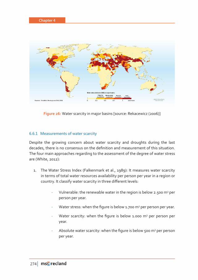
Chapter 4
274
Figure 26: Water scarcity in major basins [source: Rekacewicz (2006)]
6�6�1 Measurements of water scarcity
Despite the growing concern about water scarcity and droughts during the last �������ǡ��������������������������������Ƥ����������������������������������������Ǥ�The four main approaches regarding to the assessment of the degree of water stress are (White, 2012):
1. The Water Stress Index (Falkenmark et al., 1989): It measures water scarcity in terms of total water resources availability per person per year in a region or �������Ǥ���������������������������������������ơ������������ǣ
- Vulnerable: the renewable water in the region is below 2.500 m3 per person per year.
- ������������ǣ����������Ƥ��������������Ǥ��3 per person per year.
- ������ ��������ǣ������ ����Ƥ����� ��� ������ Ǥ��3 per person per year.
- �����������������������ǣ����������Ƥ����������������3 per person per year.
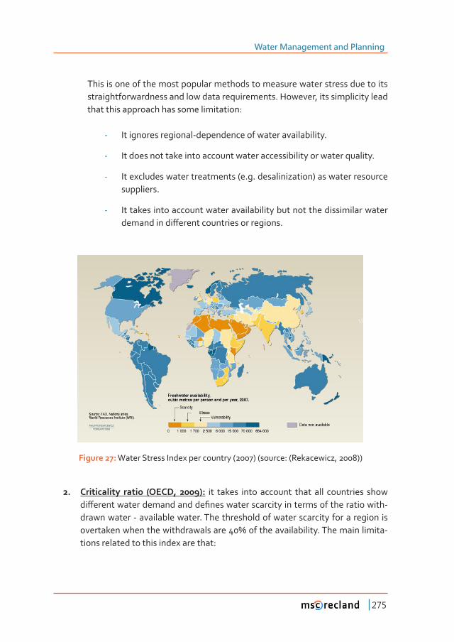
Water Management and Planning
275
This is one of the most popular methods to measure water stress due to its straightforwardness and low data requirements. However, its simplicity lead that this approach has some limitation:
- It ignores regional-dependence of water availability.
- It does not take into account water accessibility or water quality.
- It excludes water treatments (e.g. desalinization) as water resource suppliers.
- It takes into account water availability but not the dissimilar water ������������ơ��������������������������Ǥ
Figure 27: Water Stress Index per country (2007) (source: (Rekacewicz, 2008))
2. ������������ ������ ȋ����ǡ� Ȍǣ it takes into account that all countries show ��ơ�������������������������Ƥ���������������������������������������������-drawn water - available water. The threshold of water scarcity for a region is �����������������������������������ά��������������������Ǥ����������������-tions related to this index are that:
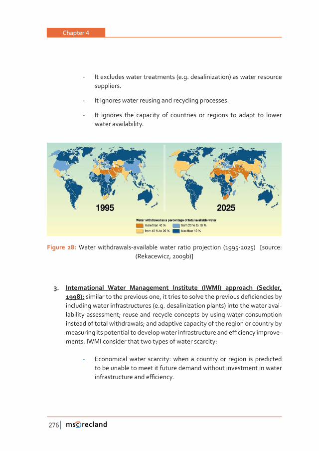
Chapter 4
276
- It excludes water treatments (e.g. desalinization) as water resource suppliers.
- It ignores water reusing and recycling processes.
- It ignores the capacity of countries or regions to adapt to lower water availability.
Figure 28: Water withdrawals-available water ratio projection (1995-2025) [source: (Rekacewicz, 2009b)]
3. �������������� ������ ����������� ���������� ȋ����Ȍ� ��������� ȋ�������ǡ�Ȍǣ����������������������������ǡ����������������������������������Ƥ������������including water infrastructures (e.g. desalinization plants) into the water avai-lability assessment; reuse and recycle concepts by using water consumption instead of total withdrawals; and adaptive capacity of the region or country by �������������������������������������������������������������ƥ��������������-ments. IWMI consider that two types of water scarcity:
- Economical water scarcity: when a country or region is predicted to be unable to meet it future demand without investment in water ��������������������ƥ������Ǥ
Water Management and Planning
277
- Physically water scarcity: when is predicted to be unable to meet its future demand even with such investment.
As some degree of complexity and sophistication has been including in this approach to solve the problems of the previous ones, its main limitations are that:
- Time and data requirements are considerably higher than in previous approaches.
- It still ignores country or region capacity to adapt to a lesser water consumption.
4. ��������������������ȋ��������������Ǥǡ�Ȍǣ this approach takes into account wealth levels into the evaluation of water scarcity by measuring:
- The access to water.
- The water quantity, quality and variability.
- The amount of water used for domestic, food and productive purposes.
- The capacity for water management.
- The environmental issues related to water consumption.
This index was developed to assess water scarcity at local or regional levels due to its high complexity and demand of available data.
6�6�2 Climate change and water scarcity
���� ���������� ��ƪ������ ��� �������� ������� ��� �����������ǡ� �������������� ���� ���Ǧ�����������������������������������������������������������������ơ����������������Ǧarid and arid environments or induce drought periods in more humid or temperate �����Ǥ���������������������ơ�������������������������������������������������ǣ�������water availability and demand. As it was stated in previous sections, the impact of �����������������������������ǡ����������������������Ǧ����������������ơ�������������water quantity and quality and thus its availability for consumption. Besides, climate change alteration of evapotranspiration patterns and water demand by population,
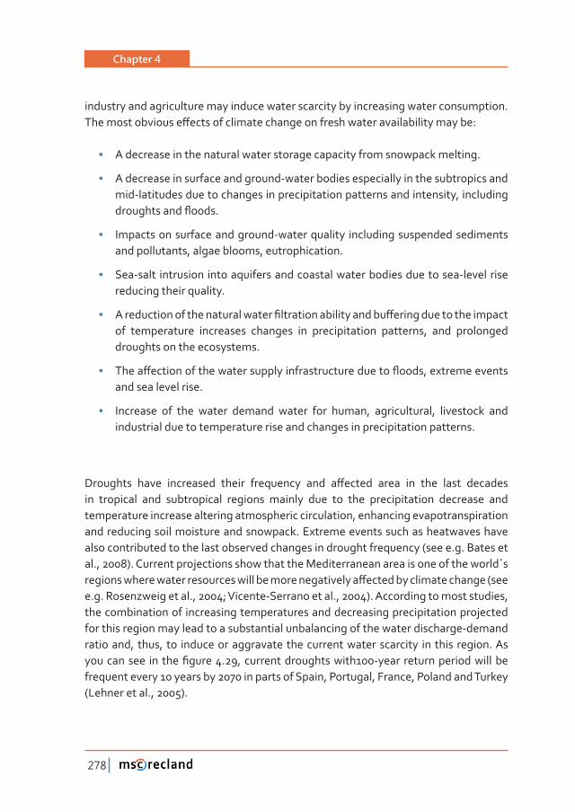
Chapter 4
278
industry and agriculture may induce water scarcity by increasing water consumption. ������������������ơ���������������������������������������������������������ǣ
• A decrease in the natural water storage capacity from snowpack melting.
• A decrease in surface and ground-water bodies especially in the subtropics and mid-latitudes due to changes in precipitation patterns and intensity, including �������������ƪ����Ǥ
• Impacts on surface and ground-water quality including suspended sediments and pollutants, algae blooms, eutrophication.
• Sea-salt intrusion into aquifers and coastal water bodies due to sea-level rise reducing their quality.
• ���������������������������������Ƥ�����������������������ơ������������������������of temperature increases changes in precipitation patterns, and prolonged droughts on the ecosystems.
• �����ơ�������������������������������������������������ƪ����ǡ����������������and sea level rise.
• Increase of the water demand water for human, agricultural, livestock and industrial due to temperature rise and changes in precipitation patterns.
��������� ����� ���������� ������ ���������� ���� �ơ������ ����� ��� ���� ����� ��������in tropical and subtropical regions mainly due to the precipitation decrease and temperature increase altering atmospheric circulation, enhancing evapotranspiration and reducing soil moisture and snowpack. Extreme events such as heatwaves have also contributed to the last observed changes in drought frequency (see e.g. Bates et al., 2008). Current projections show that the Mediterranean area is one of the world´s �������������������������������������������������������ơ������������������������ȋ����e.g. Rosenzweig et al., 2004; Vicente-Serrano et al., 2004). According to most studies, the combination of increasing temperatures and decreasing precipitation projected for this region may lead to a substantial unbalancing of the water discharge-demand ratio and, thus, to induce or aggravate the current water scarcity in this region. As ������������ ��� ����Ƥ�����Ǥǡ����������������������Ǧ����� ����������������������frequent every 10 years by 2070 in parts of Spain, Portugal, France, Poland and Turkey (Lehner et al., 2005).
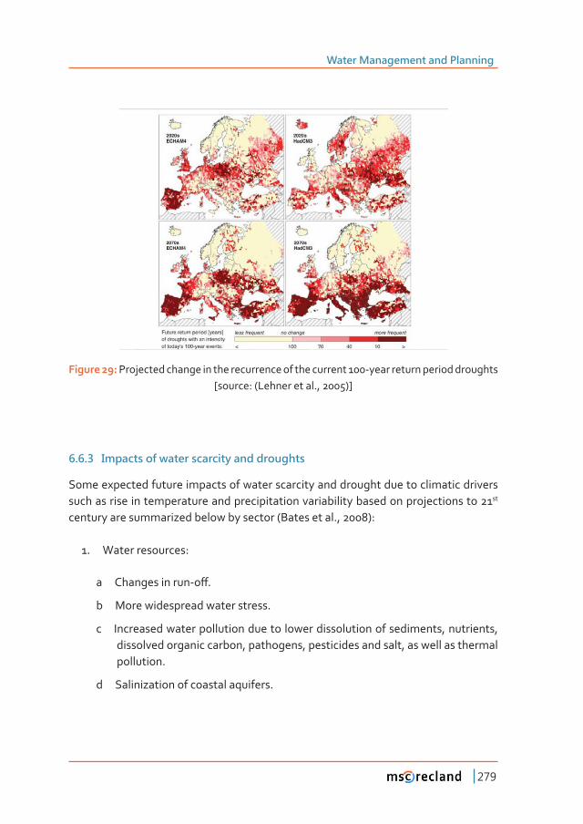
Water Management and Planning
279
Figure 29: Projected change in the recurrence of the current 100-year return period droughts [source: (Lehner et al., 2005)]
6�6�3 Impacts of water scarcity and droughts
Some expected future impacts of water scarcity and drought due to climatic drivers such as rise in temperature and precipitation variability based on projections to 21st century are summarized below by sector (Bates et al., 2008):
1. Water resources:
a ��������������Ǧ�ơǤ
b More widespread water stress.
c Increased water pollution due to lower dissolution of sediments, nutrients, dissolved organic carbon, pathogens, pesticides and salt, as well as thermal pollution.
d Salinization of coastal aquifers.
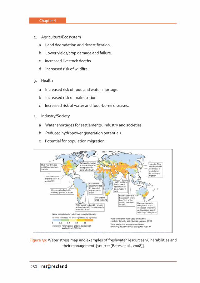
Chapter 4
280
2. Agriculture/Ecosystem
a ����������������������������Ƥ������Ǥ
b Lower yields/crop damage and failure.
c Increased livestock deaths.
d ����������������������Ƥ��Ǥ
3. Health
a Increased risk of food and water shortage.
b Increased risk of malnutrition.
c Increased risk of water and food-borne diseases.
4. Industry/Society
a Water shortages for settlements, industry and societies.
b Reduced hydropower generation potentials.
c Potential for population migration.
Figure 30: Water stress map and examples of freshwater resources vulnerabilities and their management [source: (Bates et al., 2008)]
Water Management and Planning
281
6�6�4 Useful links
• ����������������������������ǣ���Ƥ������������������������
• Water Scarcity & Droughts in the European Union
• Climate change and water
• Water Scarcity
7 EUROPEAN LEGISLATION
7�1 Introduction
The European Union has developed a complete set of legislative tools for the State �������� ��� ������ ��� �������� ������������ ���������Ǥ� ��� �ơ����������� �����ǡ��������pollution, inland waters and discharge of substances. Besides, it range from general ����������������������������������������������������������������������������Ƥ�������as for example the Environment Strategy for the Mediterranean; from Directives to Communications; from general recommendations such as water management to �����Ƥ����������������������������������������������������������������������������Ǣ�from marine to fresh water; from industrial use of water such as industrial emissions to recreation use as for example bathing.
7�2 European legislation
The European legislation on water resources may be divided according to the stated before as follows:
1. General Framework
2. �����Ƥ��������������
3. Marine pollution
4. Regional waters
5. Discharge of substances
Chapter 4
282
Next sections will broaden the main European legislation related to water resources ��������������������������������������������������ƥ������������������������������act established by the European Union (European Commission, 2013).
7�2�1 General Framework
��������������������������������ȋ������������������������Ȍ�
The European Union (EU) has established a Community framework for water protection and management. Firstly, Member States must identify and analyse European waters, on the basis of individual river basin and district. They shall then adopt management plans and pro-grammes of measures adapted to each body of water.
Directive 2000/60/EC of the European Parliament and of the Council of 23 October 2000 �����������������������������������������������������Ƥ�������������������Ǥ
����������������Ǧ�������������������������
������������������������������������������������������������������������Ƥ��������������-cing policies enabling the sustainability of water resources to be boosted.
Communication from the Commission to the Council, European Parliament and Econo-mic and Social Committee: Pricing and sustainable management of water resources.
�������������������������������
Communication from the Commission to the Council, European Parliament and Economic ��������������������ǣ������������������������������������������������������Ǥ
Directive 2007/60/EC of the European Parliament and of the Council of 23 October 2007 ������������������������������������ƪ���������Ǥ
����������������������������
The Commission provides guidelines for addressing sporadic drought and medium- or long-term water scarcity. The guidelines deal with water pricing, water allocation, drought pre-vention and rapid response in the event of a drought, as well as high-quality information and technological solutions tackling water scarcity and droughts.
����������������������������� ����ǣ�Dz�������������������������������������������and droughts in the European Union”.
����������������������������
Due to their volume, discharges of urban waste water are the second most serious cause of water pollution in the form of eutrophication. This Directive seeks to harmonise measures relating to the treatment of such waters at Community level.
Council Directive 91/271/EEC of 21 May 1991 concerning urban waste water treatment.
Water Management and Planning
283
7�2�2 Specific use of water
��������������������������
���� ��������������� ȋ��Ȍ� ��� ��Ƥ����� ���� ���������� �������� ���������� ������ ������intended for human consumption must meet.
Council Directive 98/83/EC of 3 November 1998 on the quality of water intended for human consumption.
����������������������ȋ������Ȍ�
The European Union (EU) lays down rules for the monitoring, assessment and management of the quality of bathing water and for the provision of information on that quality. The aim is twofold, to reduce and prevent the pollution of bathing water, and to inform European citizens of the degree of pollution.
Council Directive 76/160/EEC of 8 December 1975 concerning the quality of bathing water.
����������������������
The European Union (EU) introduces new legislation aimed at improving bathing water quality. This Directive enables water monitoring and management measures to be improved, and information to be made available to the public.
Directive 2006/7/EC of the European Parliament and of the Council of 15 February 2006 concerning the management of bathing water quality and repealing Directive 76/160/EEC.
�������������������Ƥ��Ǧ���������
����������ȀȀ�����������������������������������������������Ǧ�����������������Ǥ�Compliance with these criteria is essential in order to maintain or improve water �������������������������������������Ƥ����������Ǥ
Council Directive 2006/44/EC of 6 September 2006 on the quality of fresh waters ������������������������������������������������������Ƥ�������Ǥ
����������������Ƥ����������
The European Union establishes compulsory quality criteria for Member States’ �����Ƥ���������Ǥ
Directive 2006/113/EC of the European Parliament and of the Council of �������������������������������������������Ƥ���������Ǥ
Chapter 4
284
7�2�3 Marine pollution
������������������������������������
��������������������������������������������������������������������������������������������������������������������������Ǥ��������������������������������������������ǡ�Member States will have to evaluate requirements in the marine areas for which they are responsible. They will then have to draw up and implement coherent management plans in each region, and then monitor their application.
Directive 2008/56/EC of the European Parliament and of the Council of 17 June 2008 �����������������������������������������������������Ƥ����������������������������policy (Marine Strategy Framework Directive).
���������������ǣ��������������������������������������������
This proposal aims to improve the liability and compensation arrangements for pollution damage caused by ships.
Proposal for a regulation of the European Parliament and of the Council on the establishment of a fund for the compensation of oil pollution damage in European waters and related measures.
���������������ǣ������������������������������������
The Community legislation on maritime safety must be adapted at regular intervals to take account of the amendments or the protocols to the international conventions, new resolutions or changes to the codes and compendia of existing technical rules.
Directive 2002/84/EC of the European Parliament and of the Council of 5 November 2002 amending the Directives on maritime safety and the prevention of pollution from ships.
����Ǧ����������������������������������������
The European Union creates a legal framework for imposing penalties in the event of discharges of oil and other noxious substances from ships sailing in its waters.
Directive 2005/35/EC of the European Parliament and of the Council of 7 September 2005 on ship-source pollution and on the introduction of penalties, particularly criminal penalties, for infringements.
���������������ǣ���������������������������������������������
This regulation aims to prohibit organotin compounds (anti-fouling paints) on all ships ����������������������������������������������������������������������������ơ��������these products on the marine environment and human health.
Water Management and Planning
285
Regulation (EC) No 782/2003 of the European Parliament and of the Council of 14 April 2003 on the prohibition of organotin compounds on ships.
���������������ǣ��������������������
This Decision aims to authorise the Member States to become Contracting Parties to ��������������������������������������������������������������������������������Ǥ
Council Decision 2002/762/EC of 19 September 2002 authorising the Member States, in the interest of the Community, to sign, ratify or accede to the International Convention on Civil Liability for Bunker Oil Pollution Damage, 2001 (the Bunkers Convention).
7�2�4 Regional waters
������������������������������������������
Following a request from the European Council, the Commission presents a strategy aimed at developing the Danube Region in a coherent and sustainable way. Emphasis is placed on mobility, energy, innovation, the environment, risk management and security.
Communication from the Commission to the European Parliament, the Council, the Economic and Social Committee and the Committee of the Regions of 8 December 2010, European Union Strategy for Danube Region.
Baltic Sea Strategy
The Commission establishes a strategy to deal with the deterioration of the Baltic Sea, to improve the quality of transport networks and remove obstacles to trade.
Communication from the Commission to the European Parliament, the Council, the European Economic and Social Committee and the Committee of the Regions of 10 June 2009 concerning the European Union Strategy for the Baltic Sea Region.
�������������������������������������������
The Commission outlines the essential features of a coordinated strategy for the Mediterranean basin to protect the marine environment and the coastline of this ���������������������������������� Ǥ������������������������������������������������������������������������������������������������ǡ�Ƥ����������������������������ǡ�����provides for the accomplishment of targeted activities, planned within a common ��������������������Dz��������dzǤ
���������������������������������������������������������ǣ�Dz�������������an environment strategy for the Mediterranean”.
Chapter 4
286
�������������������������������������������������������������
���������������������������������������������������������������������ơ��������������������������ȋ��������ǡ�Ƥ�������ǡ������������ǡ�������������������������ǡ���������change, etc.) facing the Mediterranean basin. It is based on improving governance of ����������ơ����������������������������������������������������������������������environment. The success of this strategy requires enhanced cooperation with the third countries concerned.
Communication from the Commission of 11 November 2009 - Towards an Integrated Maritime Policy for better governance in the Mediterranean.
Black Sea Synergy
The Black Sea region, which includes Bulgaria and Romania, occupies a strategic position between Europe, Central Asia and the Middle East. The European Union ����������������������������������������������������������������������Ƥ����������remove obstacles to the stability, security and prosperity of the countries in this region.
Communication from the Commission to the Council and the European Parliament of 11 April 2007 - Black Sea Synergy - A new regional cooperation initiative.
Danube - Black Sea region
Highlight actions to be taken to improve environmental quality in the Danube - Black Sea region and the outline of a strategy aimed at protecting the environment of the region.
Communication from the Commission: Environmental cooperation in the Danube - Black Sea region.
7�2�5 Discharge of substances
Industrial emissions
���� ��������������� ȋ��Ȍ� ��Ƥ���� ���� ������������ ��� ������� ��� ����������� ���������������� �� ������ ���������� ���������Ǥ� ��� ������������ �� ������� ���������� ���� ����� �����������������ǡ� ��� ����������� ����� ������� ��� ����������Ǥ����� ���������� ��� ��� ������ ���minimise polluting emissions in the atmosphere, water and soil, as well as waste from industrial and agricultural installations, with the aim of achieving a high level of environmental and health protection.
Water Management and Planning
287
Directive 2010/75/EU of the European Parliament and of the Council of 24 November 2010 on industrial emissions (integrated pollution prevention and control).
��������������������������������������������ȋ������Ȍ�
�������������������ȋ��Ȍ���Ƥ�����������������������������������������������������������activities with a high pollution potential must comply. It establishes a procedure for authorising these activities and sets minimum requirements to be included in all permits, particularly in terms of pollutants released. The aim is to prevent or reduce pollution of the atmosphere, water and soil, as well as the quantities of waste arising from industrial and agricultural installations, to ensure a high level of environmental protection.
Directive 2008/1/EC of the European Parliament and of the Council of 15 January 2008 concerning integrated pollution prevention and control.
������������������������������������������������������������
The Commission establishes environmental quality standards so as to limit the ���������������������������������������������������������Ƥ�����������������������������and to health in surface water in the European Union (EU). These standards are coupled with an inventory of discharges, emissions and losses of these substances in order to ascertain whether the goals of reducing or eliminating such pollution have been achieved.
Directive 2008/105/EC of the European Parliament and of the Council of 16 ��������� � ��� �������������� �������� ���������� ��� ���� Ƥ���� ��������� ������ǡ�amending and subsequently repealing Council directives 82/176/EEC, 83/513/EEC, 84/156/EEC, 84/491/EEC, 86/280/EEC and amending Directive 2000/60/EC.
��������������������������������������������
The European Union is establishing a framework to prevent and control groundwater pollution. This includes procedures for assessing the chemical status of groundwater and measures to reduce levels of pollutants.
Directive 2006/118/EC of the European Parliament and of the Council of 12 December 2006 on the protection of groundwater against pollution and deterioration.
Detergents
The legislation on detergents permits improved protection of the environment by ���������������������������������������������ơ������������������������������������detergents. It also increases consumer protection through more complete labelling which includes any substance that could cause allergies.
Chapter 4
288
Regulation (EC) No 648/2004 of the European Parliament and of the Council of 31 March 2004 on detergents.
������������������������������������������������������ȋ����Ȍ�
The Stockholm Convention on persistent organic pollutants (POPs) forms a framework, based on the precautionary principle, which seeks to guarantee the safe elimination of these substances, which are harmful to human health and the environment, as well ��� ����������� ��� ������ ����������� ���� ���Ǥ���������������� ������� � ��������� ����ǡ���������������������������Ǧ�������������������������������������������Ǥ
Council Decision 2006/507/EC of 14 October 2004 concerning the conclusion, on behalf of the European Community, of the Stockholm Convention on Persistent Organic Pollutants.
Agricultural nitrates
�������� ���������� ȀȀ���� ����� ��� �������� ������� �������� ���������� ������� ���nitrates from agricultural sources through a number of measures incumbent on Member States. These measures concern monitoring surface waters and groundwater, designating vulnerable zones, introducing codes of good agricultural practice, adopting action programmes, and evaluating the actions implemented.
Council Directive 91/676/EEC of 12 December 1991 concerning the protection of waters against pollution caused by nitrates from agricultural sources.
Community strategy concerning mercury
In view of the risks mercury poses for human health and the environment, the European ������ȋ��Ȍ������������������������������������������������ǡ���������������������Ƥ��actions, aimed mainly at reducing the quantity and the circulation of mercury within the EU and throughout the world as well as human exposure to this substance.
�������������� ������������������������ �������ǣ�Dz�������������������concerning Mercury”.
����������� ��� ���� �������� ������������ �������� ����������� ��� ���������������������ȋ������Ȍ�
The European Union (EU) lays down harmonised rules to protect the aquatic environment against the discharge of dangerous substances. The new regulations impose in particular the granting of an authorisation for certain pollutant discharges, emission limits for some chemicals and an improvement in the quality of waters under ���������������������Ǥ����������������������������������������������������������������������������������Ǥ
Water Management and Planning
289
Directive 2006/11/EC of the European Parliament and of the Council of 15 February 2006 on pollution caused by certain dangerous substances discharged into the aquatic environment of the Community.
����������������ǣ���������������������������
This Directive prohibits or limits the discharge of certain dangerous substances into groundwater and establishes systematic monitoring of the quality of such water. It will ������������������������������������������������������������Ǥ
Council Directive 80/68/EEC of 17 December 1979 on the protection of groundwater against pollution caused by certain dangerous substances.
7�3 Useful links
• Summaries of EU legislation: Water protection and management
8 MISCELLANEOUS HYDROLOGY STUDIES
World Water Assessment Programme. 2003. Water for People, Water for Life: The United Nations World Water Development Report. UNESCO: Paris.
Kabat, Pavel, Henk van Schaik, et al. 2003. Climate changes the water rules: How wa-ter managers can cope with today’s climate variability and tomorrow’s climate change. Dialogue on Water and Climate: The Netherlands.
Dialogue on Water and Climate. 2002. Coping with Impacts of Climate Variability and Climate Change in Water Management: A Scoping Paper. Dialogue on Water and Climate: The Netherlands.
Nijssen, Bart, Greg M. O’Donnell, Alan F. Hamlet, and Dennis P. Lettenmaier. 2001. Dz��������������������������������������������������������ǡdz����������������ǡ����Ǥ�50, No. 1-2, July, pp. 143-175.
Vörösmarty, Charles J., Pamela Green, Joseph Salisbury, and Richard B. Lammers. Ǥ� Dz���������������������ǣ��������������� ������������������������������-tion Growth,” Science, Vol. 289, 14 July, pp. 284-288.
������ǡ��������Ǥ�Ǥ�Dz�����������������������������������������ǡdz��������������-mental Change, Vol. 9, Suppl. 1, October, pp. S31-S49.
��������ǡ����������Ǥǡ������������Ǥ������Ǥ�Ǥ�Dz�������������������������������-ces,” Climatic Change, Vol. 37, No. 1, September, pp. 7-23.
Chapter 4
290
�����ǡ��������Ǥǡ����������Ǥ���������Ǥ�Ǥ�Dz�������������������������������������Change Assessment Methods,” Climatic Change, Vol. 37, No. 1, September, pp. 25-40.
Major, D. C., A. Omojola, M. Dettinger, R. T. Hanson, R. Sanchez-Rodriguez, 2011: Cli-mate change, water, and wastewater in cities. Climate
Change and Cities: First Assessment Report of the Urban Climate Change Research Network, C. Rosenzweig, W. D. Solecki, S. A. Hammer,
S. Mehrotra, Eds., Cambridge University Press, Cambridge, UK, 113–143.
�������ǡ��Ǥ��Ǥǡ������Ǥ��Ǥ��Ǥ�������Ǥ�Ǥ�Dz���������������������������������������-��Ƥ���������� �����ơ�����������������������������������������������ǡdz����������Change, Vol. 35, No. 4, April, pp. 415-434.
��������ǡ��������Ǥ�Ǥ�Dz����������������������������������ǡdz�������������������Future: Washington, D.C.
����ǡ��Ǥǡ��Ǥ�����������ǡ������Ǥ��������Ǥ�Ǥ�Dz������������������������������������assessments of climate change,” Nature, 358, pp. 119-123.
��������ǡ��Ǥ�Ǥ�Ǥ�Dz������������������������������ǡdz���������������������������of American Geographers, Vol. 93, No. 1, March, pp. 30-41.
������ǡ��Ǥ�Ǥǡ��Ǥ����ǡ������Ǥ�������Ǥ�Ǥ�Dz��������������������������ơ��������Year-Round Water Temperatures in Temperate Zone Lakes,” Climatic Change, Vol. 40, No. 3-4, December, pp. 547-576.
���ǡ��������ǡ��������������Ǥ�Ǥ�Dz���������������������������������������������the Inland Lake - A Case Study of Lake Qinghai, China,” Climatic Change, Vol. 39, No. 4, August, pp. 695-714.
������ǡ� �Ǥ� Ǥ� Dz��������� �������� ��� �������������������� ���� ������� ������������Forest Hydrology,” Climatic Change, Vol. 39, No. 2-3, July, pp. 215-272.
REFERENCES
Arnell, N.W., 1998. Climate change and water resources in britain. Climatic Change 39, 83–110.Bates, B.C., Kundzewicz, Z.W., Wu, S., Palutikof, J.P., 2008. Climate change and water. Technical
paper of the Intergovernmental Panel on Climate Change, IPCC Secretariat, http://www.ipcc.ch/pdf/technical-papers/climate-change-water-en.pdf.
Bergstrom, S., Carlsson, B., Gardelin, M., Lindstrom, G., Pettersson, A., Rummukainen, M., 2001. ������������������������������ơ�����������Ǧ�������������������������������������ǡ�����-mical downscaling and hydrological modelling. Climate Research 16(2), 101-112.
Bouraoui, F., Galbiati, L., Bidoglio, G., 2002. Climate change impacts on nutrient loads in the yorkshire ouse catchment (uk). Hydrology and Earth System Sciences 6(2), 197-209.
Brakenridge, G.R., 2010. Dartmouth Flood Observatory, University of Colorado, http://www.dart-�����Ǥ���Ȁƪ����Ȁ�������Ȁ�����Ǥ����Ǥ
Bralower, T., Bice, D., 2014. Module 04 - introduction to general circulation models, In: https://www.e-education.psu.edu/earth103/node/682, Last.
Water Management and Planning
291
���������������������ǡ� Ǥ����� ����������� �ơ���� ���� �������� ������ǡ�������������� ������������ǡ�����ǣȀȀ���Ǥ���Ǥ���Ǥ��Ȁ����Ȁ����������ơ�������������������Ǥ���Ǥ
Callow, P., Petts, G.E., 1994. The rivers handbook: Hydrological and ecological principles and in-�����Ǥ������������������Ƥ��������������Ǥ�������Ǥ
Civil Defense New Zealand Government, 2007. http://wwwcivildefense.govt.nz.Dirmeyer, P.A., 2011. Center for Ocean-Land-Atmosphere Studies, http://www.earthzine.
���ȀȀȀȀ������Ǧ���Ǧ��������Ǧ��Ǧ�Ǧ��������Ǧ�������Ǧά�άάǦ���Ǧ���Ǧ���Ǧfuture/.
Economic Commission for Europe, 2009. Guidance on water and adaptation to climate change. United Nations Publication, Geneve, pp. 144.
European Commission, 2013. Summaries of EU legislation: Water protection and management, In: http://europa.eu/legislation_summaries/environment/water_protection_management/, Last.
Falkenmark, M., Lundqvist, J., Widstrand, C., 1989. Macro-scale water scarcity requires micro-scale approaches - aspects of vulnerability in semi-arid development. Natural Resources Fo-rum 13(4), 258-267.
Ferguson, G., Gleeson, T., 2012. Vulnerability of coastal aquifers to groundwater use and climate change. Nature Climate Change 2(5), 342-345.
����ǡ� Ǥ�Ǥǡ�������ǡ��Ǥ�Ǥǡ�������ǡ��Ǥ Ǥǡ�Ǥ���������Ǧ���������������������������������������ƪ����risk in england and wales. Natural Hazards 36(1-2), 147-164.
Helsinki Commission, 2010. A conceptual model of the relation of phytoplankton biomass to eu-�����������������ǣȀȀ���Ǥ������ǤƤȀ��������������Ȁ�����Ȁ������������Ȁ���Ȁ�������ȀǤ
��������ǡ� Ǥ�Ǥǡ� Ǥ� ������ �������Ǥ����� ��������� ����Ƥ��Ǥ� ��� ��Ǥ� ���������� �����������Press, Cambridge.
IPCC, 2000. Emissions scenarios. A special report of working group III of the Intergovernmental Panel on Climate Change, Cambridge University Press, Cambridge.
IPCC, 2007. Climate change 2007: Synthesis report. Contribution of working groups I, II and III to the fourth assessment report of the Intergovernmental Panel on Climate Change . IPCC, Geneva, Switzerland.
Khaka, E., 1998. Small islands, big problems, http://www.ourplanet.com/imgversn/94/khaka.html
Lehner, B., Czisch, G., Vassolo, S., 2005. The impact of global change on the hydropower poten-tial of Europe: A model-based analysis. Energy Policy 33(7), 839-855.
Loucks, D.P., van Beek, E., 2005. Water resources systems planning and management. An intro-duction to methods, models and applications, UNESCO publising, Turin.
������ǡ��Ǥ Ǥǡ�������ǡ��Ǥǡ�������ǡ��ǤǤǡ�Ǥ���������������������������������ƪ����������������summertime stream temperature and their possible consequences for freshwater salmon ha-bitat in washington state. Climatic Change 102(1-2), 187-223.
Mimikou, M.A., Baltas, E., Varanou, E., Pantazis, K., 2000. Regional impacts of climate change on water resources quantity and quality indicators. Journal of Hydrology 234, 95-109.
�������ǡ��Ǥ�Ǥǡ������ǡ� Ǥ�Ǥǡ�������ǡ��Ǥ�Ǥǡ�Ǥ������������ơ���������������������������������Ǧ������quality in north america. Journal of the American Water Resources
Association 36(2), 347-366.National Resources Canada, 2008. http://www.nrcan.gc.ca/earth-sciences/products-services/
mapping-product/geoscape/waterscape/bow-river-basin/6091.
Chapter 4
292
�������ǡ��Ǥ�Ǥǡ� �����ǡ��Ǥǡ���ơ���ǡ��Ǥǡ�������ǡ��Ǥǡ����������ǡ��Ǥǡ����������ǡ��Ǥǡ��������������ǡ��Ǥǡ�Nichols, M.H., Nunes, J.P., Renschler, C.S., Souchere, V., van Oost, K., 2005. Modeling respon-���������������������������ơ��������������������������������������Ǥ��������ȋǦȌǡ�ǦǤ
����ǡ�Ǥ�����������������������ǣ������������������������������������Ƥ�������ǡ������ǡ����-ce.
������ǡ��Ǥ�Ǥǡ��������ǡ��Ǥ�Ǥǡ�Ǥ����������������������������ƪ����ǣ�������������������������-tes, 1932-97. Journal of Climate 13(20), 3625-3637.
Rekacewicz, P., 2006. Water scarcity index, Vital Water Graphics 2, http://www.grida.no/graphics-lib/detail/water-scarcity-index_14f3.
Rekacewicz, P., 2008. Freshwater availability, http://www.grida.no/graphicslib/detail/water-scar-city-index_14f3.
Rekacewicz, P., 2009a. The contribution of climate change to declining water availability, Vital Water Graphics 2, http://www.grida.no/graphicslib/detail/the-contribution-of-climate-chan-ge-to-declining-water-availability_12c2#.
Rekacewicz, P., 2009b. Increased global water stress, Vital Water Graphics 2, http://www.grida.no/graphicslib/detail/the-contribution-of-climate-change-to-declining-water-avai-lability_12c2#.
Rosenzweig, C., Strzepek, K.M., Major, D.C., Iglesias, A., Yates, D.N., McCluskey, A., Hillel, D., 2004. Water resources for agriculture in a changing climate: International case studies. Global Environmental Change-Human and Policy Dimensions 14(4), 345-360.
Santamarta-Cerezal, J.C., 2013. Photo-gallery.Santamarta-Cerezal, J.C., 2013. Hidrología y recursos Hídricos en Islas y Terrenos Volcánicos. Te-
nerife: Colegio de Ingenieros de Montes.Seckler, D., 1998. World water demand and supply, 1990 to 2025: Scenarios and issues, Interna-
tional Water Management Institute (IWMI) Research Report 19, Colombo, Sri Lanka.Sullivan, C.A., Meigh, J.R., Giacomello, A.M., Fediw, T., Lawrence, P., Samad, M., Mlote, S.,
Hutton, C., Allan, J.A., Schulze, R.E., Dlamini, D.J.M., Cosgrove, W., Priscoli, J.D., Gleick, P., Smout, I., Cobbing, J., Calow, R., Hunt, C., Hussain, A., Acreman, M.C., King, J., Malomo, S., Tate, E.L., O’Regan, D., Milner, S., Steyl, I., 2003. The water poverty index: Development and application at the community scale. Natural Resources Forum 27(3), 189-199.
U.S. Environmental Protection Agency, 2011. Future atmosphere changes in greenhouse gas and aerosol concentrations, In: http://www.epa.gov/climatechange/science/future.html, Last.
U.S. Geological Survey, 2011. http://ga.water.usgs.gov/edu/watercycle.html.U.S. Global Change Research Program, 2009. Global climate change impacts in the united states,
http://downloads.globalchange.gov/usimpacts/pdfs/water.pdf.United Nations, 2006. Water for life decade, In: http://www.un.org/waterforlifedecade/scarcity.
shtml, Last.Varis, O., Kajander, T., Lemmela, R., 2004. Climate and water: From climate models to water re-
sources management and vice versa. Climatic Change 66(3), 321-344.Vicente-Serrano, S.M., Gonzalez-Hidalgo, J.C., de Luis, M., Raventos, J., 2004. Drought patterns
in the Mediterranean area: The valencia region (eastern Spain). Climate Research 26(1), 5-15.�������ǡ��Ǥǡ��������ǡ��Ǥǡ��������ǡ��Ǥǡ�������Ƥ���ǡ��Ǥǡ� Ǥ��������������������������������������-
ge. Final report commissioned by european commission dg environment. Env.C.2/2004/0088., ��Ǥ������Ǥ��Ȁ�����������Ȁ������Ȁ���ȀƤ���������Ǥ��
Webber, M., 2008. Water vs. Energy. Earth 3.0 1(1).
Water Management and Planning
293
�����ǡ� �Ǥǡ� Ǥ� �������������� ������ ��������ǣ� ��Ƥ�������� ���� ������������ǡ� �� ������-sion Paper 1217. Global Water Forum, Canberra, Australia. http://www.globalwaterforum.���ȀȀȀȀ�������������Ǧ�����Ǧ��������Ǧ��Ƥ�������Ǧ���Ǧ������������ȀǤ
Whitehead, P.G., Wilby, R.L., Battarbee, R.W., Kernan, M., Wade, A.J., 2009. A review of the po-tential impacts of climate change on surface water quality. Hydrological Sciences Journal-Journal Des Sciences Hydrologiques 54(1), 101-123.
Dirmeyer PA (2011). In. ‘ (Center for Ocean-Land-Atmosphere Studies: http://www.earthzine.���ȀȀȀȀ������Ǧ���Ǧ��������Ǧ��Ǧ�Ǧ��������Ǧ�������Ǧά�άάǦ���Ǧ���Ǧ���Ǧfuture/).
Environment Agency, Ofwat, Defra and the Welsh Government (2012). Water resources planning guideline. The guiding principles for developing a water resources management. UK.
���Ǧ���������������������������������������������Ǥ�ȋȌǤ�������������������ƥ������Ǥ�ȋ����-�������������ǣȀȀ�����Ǥ���Ǥ���Ȁ��������������Ȁ�������Ȁ������ƥ������Ǥ���ȌǤ
Economic Commission for Europe (2009) Guidance on water and adaptation to climate change. In. ‘ pp. 144. (United Nations Publication: Geneve).
European Commission (2013) Summaries of EU legislation: Water protection and management. In. ‘ http://europa.eu/legislation_summaries/environment/water_protection_management/).
Falkenmark M., Rockstrom J., (2011). Integrating agricultural water use with the global water Budget. Stockholm International Water Institute SIWI.Sweden.
Falkenmark M, Lundqvist J, Widstrand C (1989) Macro-scale water scarcity requires micro-scale approaches - aspects of vulnerability in semi-arid development. Natural Resources Forum 13(4), 258-267.
Ferguson G, Gleeson T (2012) Vulnerability of coastal aquifers to groundwater use and climate change. Nature Climate Change 2(5), 342-345. doi: 10.1038/nclimate1413.
����� �ǡ����������ǡ��������� �ȋȌ���������Ǧ���������������������������������������ƪ���������in england and wales. Natural Hazards 36(1-2), 147-164. doi: 10.1007/s11069-004-4546-7.
Helsinki Commission (2010) A conceptual model of the relation of phytoplankton biomass to eu-������������� ��Ǥ� Ǯ� ����ǣȀȀ���Ǥ������ǤƤȀ��������������Ȁ�����Ȁ������������Ȁ���Ȁ���-cept/).
��������� �� ȋȌ� Ǯ�������������Ǥ����� �������������Ƥ��Ǥǯ� ��� ���Ǥ� ȋ���������������������Press: Cambridge)
Hoektra A. Et al., (2011). The water footprint assessment manual.Setting the Global Estándar. Earthscan. London, UK.
Hophmayer S., Kadiman T., (2012).Water Management on Islands – Common Issues and Possible Actions. International Workshop on Capacity Building in Water Management for Sustainable Tourism on Islands.
Hurliman, A. (2007). Is recycled water use risky? An urban Australian community’s perspective. Environmentalist, 27 , 83–94 .
IPCC (2000) Emissions scenarios. A special report of working group III of the Intergovernmental Panel on Climate Change. Cambridge University Press, Cambridge
IPCC (2007) Climate change 2007: Synthesis report. Contribution of working groups I, II and III to the fourth assessment report of the Intergovernmental Panel on Climate Change . IPCC, Geneva, Switzerland
Konikow, Leonard and Eloise Kendy, (2005). Groundwater Depletion: A Global Problem. Hydro-geology (13). 317-320.
Chapter 4
294
Lehner B, Czisch G, Vassolo S (2005) The impact of global change on the hydropower poten-tial of Europe: A model-based analysis. Energy Policy 33(7), 839-855. doi: 10.1016/j.en-pol.2003.10.018.
�������� ǡ�������� �ǡ���������� ȋȌ��������� ������� ����������� ������ƪ����������������summertime stream temperature and their possible consequences for freshwater salmon ha-bitat in washington state. Climatic Change 102(1-2), 187-223. doi: 10.1007/s10584-010-9845-2.
Mimikou MA, Baltas E, Varanou E, Pantazis K (2000) Regional impacts of climate change on wa-ter resources quantity and quality indicators. Journal of Hydrology 234, 95-109.
Morison, J.I.L., N.R. Baker, P.M. Mullineaux and W.J. Davies. (2013). Improving water use in crop production. Phil. Trans. R. Soc. B 363: 639-658.
����������ǡ������� �ǡ�����������ȋȌ������������ơ���������������������������������Ǧ���������-lity in north america. Journal of the American Water ResourcesAssociation 36(2), 347-366.
National Resources Canada (2008). In. ‘ http://www.nrcan.gc.ca/earth-sciences/products-servi-ces/mapping-product/geoscape/waterscape/bow-river-basin/6091).
Nearing MA, Jetten V, et al.� ȋȌ�������������������������������������������ơ���������������precipitation and cover. Catena 61(2-3), 131-154. doi: 10.1016/j.catena.2005.03.007.
�����ȋȌ�����������������������ǣ������������������������������������Ƥ�������Ǥ������ǡ������Oki, Taikan and Shinjiro Kanae. (2006). Global Hydrological Cycles and World Water Resources.
Science (313): 5790. 1068-1072.����Ƥ�� ������������ǡ� ȋȌǤ����Ƥ������������������� Ǧ����������������������������� ���������ǡ�
����������������������dzǤ���Ǥ�����Ǥ���Ȁ����Ȁ����Ǧ��������Ƥ��Ǥ���ǫƤ����γ���������ǡ������������ȋȌ����������������������������ƪ����ǣ����������������������������ǡ�
1932-97. Journal of Climate 13(20), 3625-3637. doi: 10.1175/1520-0442(2000)013<3625:padfti>2.0.co;2.
Rekacewicz P (2006) Water scarcity index. In ‘ Vital Water Graphics 2. ‘ http://www.grida.no/gra-phicslib/detail/water-scarcity-index_14f3).
Rekacewicz P (2009a) The contribution of climate change to declining water availability. In ‘ Vi-tal Water Graphics 2. ‘ http://www.grida.no/graphicslib/detail/the-contribution-of-climate-change-to-declining-water-availability_12c2#).
Rekacewicz P (2009b) Increased global water stress. In ‘ Vital Water Graphics 2. ‘ http://www.grida.no/graphicslib/detail/the-contribution-of-climate-change-to-declining-water-avai-lability_12c2#).
Rosenzweig C, Strzepek KM, Major DC, Iglesias A, Yates DN, McCluskey A, Hillel D (2004) Wa-ter resources for agriculture in a changing climate: International case studies. Global En-vironmental Change-Human and Policy Dimensions 14(4), 345-360. doi: 10.1016/j.gloenv-cha.2004.09.003.
Rekacewicz P (2006) Water scarcity index. In ‘ Vital Water Graphics 2. ‘ http://www.grida.no/gra-phicslib/detail/water-scarcity-index_14f3).
Rekacewicz P (2009a) The contribution of climate change to declining water availability. In ‘ Vi-tal Water Graphics 2. ‘ http://www.grida.no/graphicslib/detail/the-contribution-of-climate-change-to-declining-water-availability_12c2#).
Rekacewicz P (2009b) Increased global water stress. In ‘ Vital Water Graphics 2. ‘ http://www.grida.no/graphicslib/detail/the-contribution-of-climate-change-to-declining-water-avai-lability_12c2#)
Rosenzweig C, Strzepek KM, Major DC, Iglesias A, Yates DN, McCluskey A, Hillel D (2004) Wa-ter resources for agriculture in a changing climate: International case studies. Global En-
Water Management and Planning
295
vironmental Change-Human and Policy Dimensions 14(4), 345-360. doi: 10.1016/j.gloenv-cha.2004.09.003.
Santamarta J.C. et al, (2013). Hydrology and Water resources on islands and volcanic regions. Spainsh Forestry Engineers Society. Spain.
Savenije, H.H.G. (2000). Water resources management: concepts and tools. Lecture note. IHE, Delft and University of Zimbabwe, Harare.
Seckler D (1998) World water demand and supply, 1990 to 2025: Scenarios and issues. Internatio-nal Water Management Institute (IWMI) Research Report 19, Colombo, Sri Lanka
Sullivan CA, Meigh JR, et al. (2003) The water poverty index: Development and application at the community scale. Natural Resources Forum 27(3), 189-199. doi: 10.1111/1477-8947.00054.
UNESCO, (2005). Water resources systems planning and management.UNESCO-IHE. (2003). Basics of Water Resources. Course book. Course A. Technical Documents in
Hydrology, PC-CP Series 23. UNESCO-Institute for Water Resources.U.S. Geological Survey (2011). In. ‘ (http://ga.water.usgs.gov/edu/watercycle.html).
U.S. Global Change Research Program (2009) Global climate change impacts in the united states. http://downloads.globalchange.gov/usimpacts/pdfs/water.pdf
Varis O, Kajander T, Lemmela R (2004) Climate and water: From climate models to wa-ter resources management and vice versa. Climatic Change 66(3), 321-344. doi: 10.1023/B:CLIM.0000044622.42657.d4.
Vicente-Serrano SM, Gonzalez-Hidalgo JC, de Luis M, Raventos J (2004) Drought patterns in the Mediterranean area: The valencia region (eastern Spain). Climate Research 26(1), 5-15. doi: 10.3354/cr026005.
WCED: World Commission on Environment and Development. (1987). Our Common Future. Oxford: Oxford University Press. p. 27.
���������ǡ����������ǡ����������ǡ�������Ƥ������ȋȌ����������������������������������������Ǥ�Final report commissioned by european commission dg environment. Env.C.2/2004/0088., ��Ǥ������Ǥ��Ȁ�����������Ȁ������Ȁ���ȀƤ���������Ǥ���
������ �� ȋȌ� �������������� ������ ��������ǣ� ��Ƥ�������� ���� ������������Ǥ� �� ������-sion Paper 1217. Global Water Forum, Canberra, Australia. http://www.globalwaterforum.���ȀȀȀȀ�������������Ǧ�����Ǧ��������Ǧ��Ƥ�������Ǧ���Ǧ������������Ȁ
Whitehead PG, Wilby RL, Battarbee RW, Kernan M, Wade AJ (2009) A review of the potential impacts of climate change on surface water quality. Hydrological Sciences Journal-Journal Des Sciences Hydrologiques 54(1), 101-123. doi: 10.1623/hysj.54.1.101.

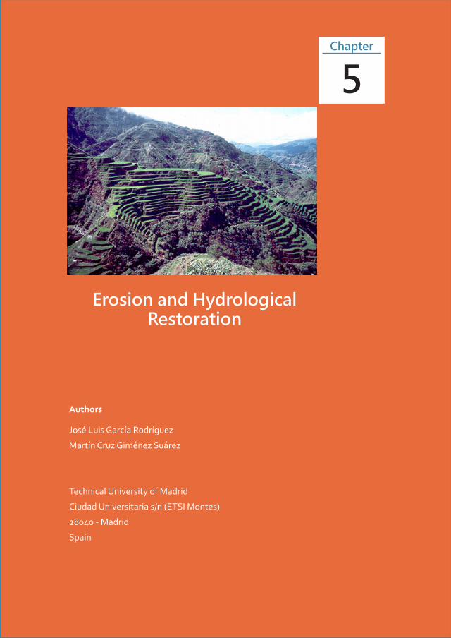
Erosion and Hydrological
Restoration
Authors
José Luis García Rodríguez
Martín Cruz Giménez Suárez
Technical University of Madrid
Ciudad Universitaria s/n (ETSI Montes)
28040 - Madrid
Spain
5Chapter

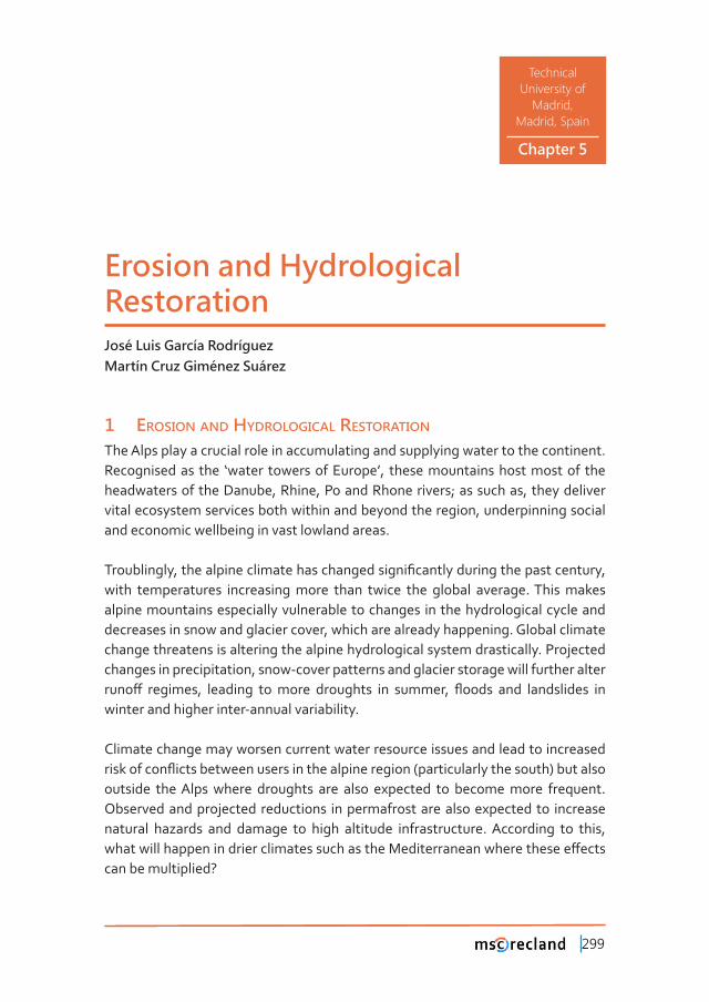
299
Chapter 5
Technical
University of
Madrid,
Madrid, Spain
Erosion and Hydrological RestorationJosé Luis García RodríguezMartín Cruz Giménez Suárez
1 erosion and hydrological restoration
The Alps play a crucial role in accumulating and supplying water to the continent. Recognised as the ‘water towers of Europe’, these mountains host most of the headwaters of the Danube, Rhine, Po and Rhone rivers; as such as, they deliver vital ecosystem services both within and beyond the region, underpinning social and economic wellbeing in vast lowland areas.
�����������ǡ�������������������������������������Ƥ������������������������������ǡ�with temperatures increasing more than twice the global average. This makes alpine mountains especially vulnerable to changes in the hydrological cycle and decreases in snow and glacier cover, which are already happening. Global climate change threatens is altering the alpine hydrological system drastically. Projected changes in precipitation, snow-cover patterns and glacier storage will further alter ����ơ� �������ǡ� �������� �������� ��������� ��� ������ǡ� ƪ����� ���� ����������� ���winter and higher inter-annual variability.
Climate change may worsen current water resource issues and lead to increased �����������ƪ����������������������������������������ȋ����������������������Ȍ����������outside the Alps where droughts are also expected to become more frequent. Observed and projected reductions in permafrost are also expected to increase natural hazards and damage to high altitude infrastructure. According to this, ��������������������������������������������������������������������������ơ�����can be multiplied?
Chapter 5
300
��������ǯ���������������������������������������������������Ǥ����� ά���������������������corresponds to mountain regions, being present in all continents. It is estimated that ά� ��� ���������ǯ�� ����������� ������ ��� ���� ���� ������������ǡ������� ά� ���������the adjacent of the middle and lower basins (FAO, 2000). Consequently, half of the world’s population depends directly or indirectly, on the resources and the social and ecological stability of mountain ecosystems and their watersheds.
The Ministerial Conference on the Protection of Forests in Europe (MCPFE) is the high level forest policy process, addressing all dimensions of sustainable forest management (SFM) in the pan-European region. MCPFE involves 44 countries of the European continent, the European Community and 41observer countries and international organisations (see: http://www. mcpfe.org). The concept of SFM was Ƥ��������Ƥ���������������������������������������������������������������ȋȌ�as: ‘the stewardship and use of forests and forest lands in a way, and at a rate, that maintains their biodiversity, productivity, regeneration capacity, vitality and their ���������� ��� ���Ƥ�ǡ� ���� ���� ��� ���� ������ǡ� ��������� ����������ǡ� ��������� ���� �������functions, at local, national, and global levels, and that does not cause damage to other ecosystems’. Such a concept has been recognised to be consistent with the application of the Ecosystem Approach to forest ecosystems in the pan-European region (MCPFE/PEBLDS, 2006).
The Global Forest Resources Assessment 2010 (FRA 2010) was aimed by FAO member countries during the eighteenth session of the FAO Committee on Forestry (COFO) in March 2007 (FAO, 2007). It is the most comprehensive assessment to date, both in terms of content and contributors. More than 900 people have been involved in the country reporting process alone, including 178 national correspondents and their �����ǡ������������������ǡ����������������������ǡ�������ơǡ����������������������������from around the world.
In this report appear the world´s forest map (Figure 1) and the statistics for regions and subregions used in FRA (2010) and its distribution.
The global distribution of forests can be seen in numerous publications globally or locally (Figures 2 and 3) and appears as green stains focus forest cover worldwide like the Amazon, large parts of Central Africa and the East Asia
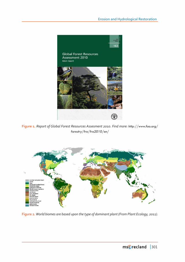
Erosion and Hydrological Restoration
301
Figure 1. ������������������������������������������Ǥ���������ǣ�http://www.fao.org/forestry/fra/fra2010/en/
Figure 2.��������������������������������������������������������ȋ�����������������ǡ�ȌǤ
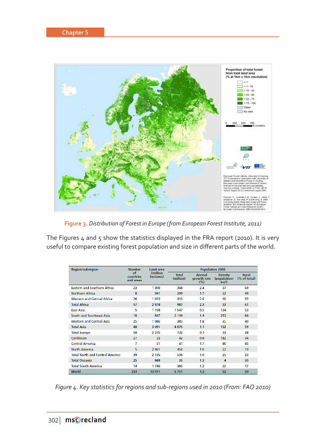
Chapter 5
302
Figure 3. ��������������������������������ȋ�����������������������������ǡ�Ȍ
The Figures 4 and 5 show the statistics displayed in the FRA report (2010). It is very �����������������������������������������������������������ơ������������������������Ǥ
������Ǥ�����������������������������������Ǧ�����������������ȋ���ǣ����Ȍ
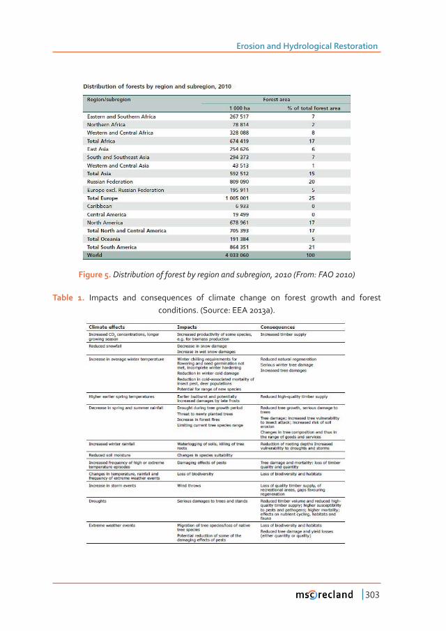
Erosion and Hydrological Restoration
303
Figure 5. ����������������������������������������������ǡ��ȋ���ǣ����Ȍ
Table 1. Impacts and consequences of climate change on forest growth and forest conditions. (Source: EEA 2013a).
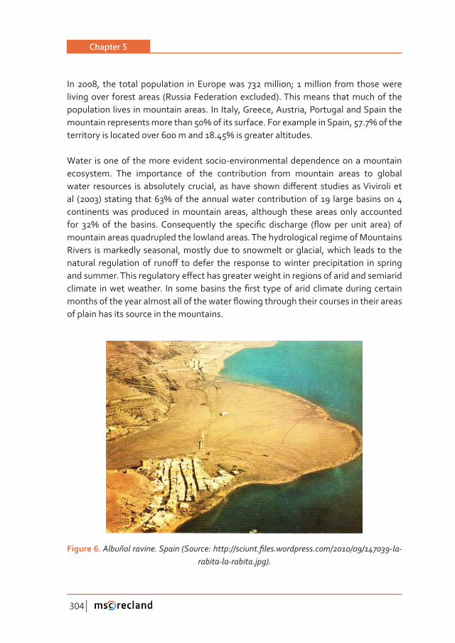
Chapter 5
304
In 2008, the total population in Europe was 732 million; 1 million from those were living over forest areas (Russia Federation excluded). This means that much of the population lives in mountain areas. In Italy, Greece, Austria, Portugal and Spain the ������������������������������ά���������������Ǥ��������������������ǡ�Ǥά�����������������������������������������Ǥά���������������������Ǥ�
Water is one of the more evident socio-environmental dependence on a mountain ecosystem. The importance of the contribution from mountain areas to global ������ ���������� ��� ����������� �������ǡ� ��� ����� ��������ơ������ �������� ������������ ������ ȋȌ��������������ά���� ���������������������������������� �����������������continents was produced in mountain areas, although these areas only accounted ���� ά� ��� ���� ������Ǥ�������������� ���� �����Ƥ�� ���������� ȋƪ��� ���� ����� ����Ȍ� ���mountain areas quadrupled the lowland areas. The hydrological regime of Mountains Rivers is markedly seasonal, mostly due to snowmelt or glacial, which leads to the �������� �������������� ����ơ� ��������� ���� ��������� ���������� �������������� ��� �����������������Ǥ������������������ơ��������������������������������������������������������������� ��������������Ǥ� ��������������� ����Ƥ���� �������������������������������������������������������������������������������ƪ�������������������������������������������of plain has its source in the mountains.
Figure 6Ǥ�����Ó���������Ǥ�������ȋ������ǣ�����ǣȀȀ������ǤƤ���Ǥ���������Ǥ���ȀȀȀǦ��Ǧ������Ǧ��Ǧ������Ǥ���ȌǤ
Erosion and Hydrological Restoration
305
���� ���������ƪ�������������� ���������������������� ��ƪ����� ���������������������mountain environments on the plain, as set Milliman and Syvitki (1992) analyzed � ������� ��� �������� ����������� ����Ƥ��� ����� ά���� ���� ������� ��������� ����� ���������������������������������������������������������������ά������������������Ǥ
Water erosion and restoration of soils have been joined from the beginning of time. ��ơ��������������������������������������������������������������������Ǥ�������������techniques that today continue to be implemented are an evolution of the old soil conservation practices on hillsides whose main objective was to use the ground and keep it.
It was not until the early twentieth century when a culture of Restoration was created through the concern of forest engineers. They became aware of the large amount of sediment that was issued to the drainage network of the basin where they were. In the mainly English-speaking world can associate this philosophy to the Watershed Management, a term that includes not only the technical aspects but is holistically integrating socioeconomic aspects of great value in developing countries.
1�1 The origin of the Forest-Hydrologic Restoration Plan (RHF)�
This is one of the techniques used in Spain and therefore, well known in Latin America’s. It all started with a correction work in mountain streams and their watersheds in the late nineteenth century. By then, deforestation had reached an alarming situation in Europe and in some mountain areas in Spain, especially in the Pyrenees. The roads became impassable and dangerous means by avalanches. The numerous natural phenomena of snow avalanches were happening in many Pyrenean valleys. This meant roadblocks, broken bridges, damage to coastal villages, hydroelectric facilities, etc...
In the Mediterranean region is also happening torrential episodes, mostly linked to ������������������������Dz���������dzǡ���������ƪ������������������������������������ơ���������������������������������Ǥ
��� ��� �������ǡ� ���� Ƥ���� �������� ���� ����� �������� �������� ������� �������������dates back to July 11, 1877, which established the Reforestation and Improving Public Forest as a legal instrument to prevent strong denudation of soils in situations of �������������������Ǥ������Ƥ�������������������������������������������Ǥ��Ǥ������
Chapter 5
306
ǡ�������������������������������������������Ǥ�����Ƥ������������������Dz����������headwaters systematic restocking Plan”, a task that was entrusted to the Corps of Engineers later the Forest Hydrological Services.
����������ǡ���������������������������������������ƪ���������������������������������������������������������������������Ǥ�������ǣ�Dz��������������������������ǡ�������������Corrections et des torrent” (1891). This book devotes a large part the need to combine the correction waterworks torrential channels with restoring their watersheds ������ǡ��������������������������ơ������������������Ǥ����������������������������engineers pioneered the restoration of mountains: �������´t�Ƥ�����������ǡ������������ǡ�or better previously, has not restored its feeder basin.
In the corrector scheme a mountain watershed, which has just been described, vegetation as mountain forest is essential. It stands for stabilizing element of the ����������������������������������Ǣ�����������������������������������Ƥ���������������������������������������������������ơ��������������������������������ƪ������������during periods of heavy rainfall. In resume, the forest is the quintessential natural regulator of water resources. These aspects must be added his great ability to defend the soil against erosion phenomena, both the impact of raindrops on the ground, as ������������������������������������������������������ơ�ƪ���Ǥ
Around 1940 extends the use of the methodological tool of RHF in the Spanish basins due to the development of the Watershed Restoration Program-Forest, adapting to this technique that had already been tried with good results in the correction of mountain torrents.
In mountain areas or basins header reservoirs where there were problems requiring classic torrent control measures, it was logical that they be implemented as such. But large areas of these basins were primarily agricultural and other, that her earrings should not be, was at that time cultivated, in most cases without any soil conservation measure. The transformation of such agricultural uses are based on the Management of the uses, is what would be called Agro-hydrological management at the end of the Land Use, all pre Hydrological Restoration Project-Forest. The reforestation of these ����������������������������������������������������������������������������������was carried out under projects RHF.
Erosion and Hydrological Restoration
307
�����������������Ƥ����������Ƥ�����������������������������������������������������������(Bennett, 1939), which limited land for the cultivation of which were permanent covered book.
As we have seen in the preceding paragraphs, the weight of land use is very important within the RHF in a watershed (Fig. 7). This has led in many cases it has come to distort the original concept and inclusive of restoration of mountain watersheds. However, we should mention that the repopulation of the land on steep slopes, not only helps to reduce water erosion in them, but also improves hydrological conditions.
The general goals in the RHF are the follows:
• The erosion control. Retention by controlling soil erosion, while trying to take advantage of this resource.
• ������������������ƪ���������ƪ������������
• Water redistribution
The formal aspect is of engineering projects, which has been adapted and improved over time, with new tools such as GIS and Remote Sensing which has yielded new results closer to reality and more performances maps accurate. This description will provide the second major objective of all RHF, the Agro-hydrological Management of the basin section included within the project, regardless of that goal. The project must describe, justify and calculate the work and the work carried out in compliance with the draft RHF mentioned in accordance with an action plan to be included therein. Finally, we evaluate the costs and draw the necessary budgets for the implementation of the actions and the work entered in the project according to the established work schedule.
Therefore, the project can be summarized in the following steps:
1. Basin Study in order to obtain all information describing the basin level funda-mental factors such as climate, soil, vegetation and topography.
2. ������������������������ơ���������������������������ǡ�������������������������ǡ�����������������������������ơ������������������������������������Ǥ
3. Schedule a Planning agro-hydrological response of the basin especially their physical capabilities and objectives to be with the project.

Chapter 5
308
4. Describe, justify and calculate the projected works and basin RHF. In addition to establishing a timetable for the completion of the above actions and work.
5. Evaluate the costs and prepare budgets necessary for the execution of the works and in the proposed work.
1.2 Agro-hydrological Planning.
It focuses primarily on the watershed and agronomic intended to regulate land use according to their hydrological behavior taken into account hydrological models, soil conservation and land use. It takes into account hydrological models, soil conservation and land use. An agro-hydrological planning must be based on at least the following ��������������������������������������Ƥ����������������������������������������������������������������������������ơ������������������������������������������������ȋ������ ȌǤ
Table 2. ������ơ����������������������������������������������������Ǥ
Altitudes as watershed areasAreas dominants (headwaters)
Areas dominated (valleys)
Cover class level
The current state of the vegetation.
Provenance
Land use in accordance with suitability
MorphologySlopes
Orientation
GeologyAreas with soil erosion
Areas with piping erosion
Soil Science �������������������ơ������������������������
Protection models of soil
Index of protection soil by vegetation
Parametric erosion models (USLE; RUSLE)
Another erosion models (WEPP;EUROSEM;…)
Phytosociologic IndexBioclimatic Index
Potential Index
Erosion and Hydrological Restoration
309
Actions in the territoryIn the hillslope
In the channel
������Ƥ����������������������
Action zones
Recommended zones
Zones without actions
1�3 RHF Action Planning
To achieve the objectives set out in the draft RHF the next types of actions should be follow:
a) Actions in hillslopes focus on the creation, control and improvement of permanent vegetative cover; constitutes forest restoration, and its main job is Reforestation. These involve:
1. Soil preparation techniques for reforestation
2. Selection of species
3. Polygons of action and forest stands
4. Proposed Measurements
�����������������������ǡ�����Ƥ���������������������������������������������������������development of the plants into the soil with restocking; has a mechanical-hydraulic important content. The second should serve the temperament (auto-ecology) of ���� �������� ���� �������� ���������� ��� ���� ������ �������� ����� ��������� Ƥ����� ����very important. Finally, the third and fourth correspond basically to the technical �����Ƥ����������������������Ǥ
b) Actions in channels. These actions entail design and implementation of hydraulic correction torrential channels, which requires:
• Choice of appropriate structures
• Design and calculation of the structures adopted
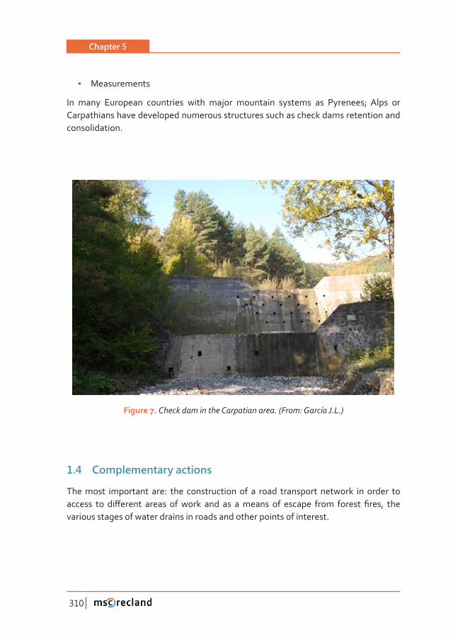
Chapter 5
310
• Measurements
In many European countries with major mountain systems as Pyrenees; Alps or Carpathians have developed numerous structures such as check dams retention and consolidation.
Figure 7. �������������������������������Ǥ�ȋ���ǣ����À�� Ǥ�ǤȌ
1�4 Complementary actions
The most important are: the construction of a road transport network in order to ������� ��� ��ơ������ ������ �������� ���� ��� �������� ��� ������� ����� ������� Ƥ���ǡ� ����various stages of water drains in roads and other points of interest.
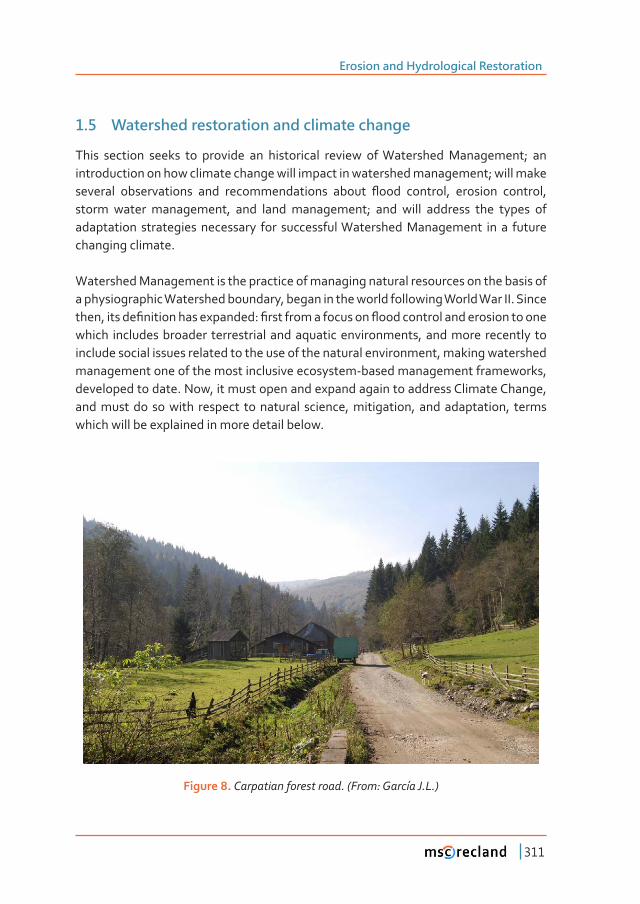
Erosion and Hydrological Restoration
311
1�5 Watershed restoration and climate change
This section seeks to provide an historical review of Watershed Management; an introduction on how climate change will impact in watershed management; will make �������� ������������� ���� ���������������� ������ ƪ���� �������ǡ� �������� �������ǡ�storm water management, and land management; and will address the types of adaptation strategies necessary for successful Watershed Management in a future changing climate.
Watershed Management is the practice of managing natural resources on the basis of a physiographic Watershed boundary, began in the world following World War II. Since ����ǡ�������Ƥ�������������������ǣ�Ƥ��������������������ƪ�������������������������������which includes broader terrestrial and aquatic environments, and more recently to include social issues related to the use of the natural environment, making watershed management one of the most inclusive ecosystem-based management frameworks, developed to date. Now, it must open and expand again to address Climate Change, and must do so with respect to natural science, mitigation, and adaptation, terms which will be explained in more detail below.
Figure 8. ���������������������Ǥ�ȋ���ǣ����À�� Ǥ�ǤȌ

Chapter 5
312
In the 1970’s, it was recognized that urban land forms removed permeable areas and replaced them with impermeable surfaces, thus generating a higher volume of water. This is common in all urban areas to large cities worldwide. This increase in volume ���� ������ �������������� ��� ����������� �������� ����ơǡ� ����� ������������������ǡ� �����������������������������������������������������Ƥ��������Ǥ���������������������������������� �������������������������������������ƪ�����������������������������������streams.
In addition, water quality has been degraded to the point that many streams now ���������������Ƥ���������ơ�����ǡ�����������������Ƥ�����Ǥ����������������������������������������������������������ơ�������������ƪ�������������������������������������valley systems. While new initiatives have been introduced that attempt to reduce the impacts on the natural systems through development, changes continue to occur as a consequence of past and current actions.
Current initiatives and strategies of Watershed Management hinge on working in concert with the dynamic aspects of the natural environment and its features. An example of this (Haley, D. 2000) would include managing the watercourses based upon their valley and stream corridors to allow for the natural process of meandering streams as a component of a larger conveyance feature. This management strategy allows for the evolution of the system through sediment transport issues such as erosion and deposition along a reach of stream. The development of strategies related to natural heritage features on a watershed also allow for an integration of ƪ�����������������������������������������Ǥ��������ǡ������������������������������a watershed is based to some degree on the ability to manage and plan within the system, while allowing natural processes and changes to continue to take place. The watershed and its current management objectives, therefore, inherently allow for some degree of adaptation related to the potential impacts of climate change.
Climate change will bring changes to the atmospheric components of the cycle. Changes in evaporation rates, severity of storms, increased temperatures and ������������������������������������������������������������Ƥ������������������������the natural ecosystem of a watershed.
Erosion and Hydrological Restoration
313
1�6 Watershed Management Issues
Given the nature of the changes which are likely as a result of climate change, it can be expected impacts in virtually all aspects of the strategies and procedures currently in place for managing watersheds. For the sake of clarity, some of the key categories and some of the potential impacts are outlined below.
1�6�1 Flood Control��������� ������������������ ������������ ������� ���������������������������������ƪ������������������������Ǥ���������ƪ����������������������������������������������������giving more intense rainfalls at an altered frequency of occurrence. Additional changes would be an increased number of mid-winter melts as a consequence of warmer winter temperatures. These changes will have varying impacts on individual watersheds and watercourses. Those watercourses sensitive to thunderstorm type ƪ��������������������������������������������������ƪ���������������Ǥ������������������������������������������������������������������ƪ��������������������������ƪ�������������������Ǧ���������������������������������������������������������� ����������������������Ǥ��������������������������������ǯ�ǡ������������������������������ơ�events may also impact other Water Management issues such as reservoir operations.
������������������������ƪ�����������ǡ������������������������������������������������������������������� ����� ������� ����� ����� ��� ������� ���� �ơ����������� ��� ƪ���� �������Ǥ�These intense storms tend to occur with shorter lead times. In addition, with the shift �������� ��������������ǡ��������������� ��������� ���������ƪ������������������������������������������ǡ��������ƪ��������������������ƪ������Ǥ� ��������������������������������������������������ǡ�����ƪ�������������������������������Ǥ
The issue of not only more sever and frequent thunderstorm type events may be compounded by the likelihood of more severe and frequent major tropical storms in ��ơ������������������������Ǥ������������������������������������������������������������������������������ƪ������������������������������������������������������������
Chapter 5
314
1�6�2 Erosion Control
Watershed Management strategies also have been developed on erosion processes ������� ���������Ǥ��������� ��������������������� �������� ��� ����ƪ��������������������������������������Ǥ����������������������������ƪ����������������������������������deposition along the watercourse reaches. As noted previously, urbanization has ��������� ��� �������� ��� ���������������� ���������������� ��� ����ƪ��� ���������� ����ƪ��������������������Ǥ������������������������������������������������������������to create erosion within stable watersheds and further increase erosion problems ������������������������������������������������Ǥ���������ƪ����������������������������Ȁ����������������ƪ�����������������������������������������������������������������ƪ����������������������������Ǥ�����������������������������������������������ǡ��������������������ƪ��ǡ� ���������������Ƥ�������������������������Ǥ������ƪ�������Ǥ�Should climate change lead to increases in the frequency of severe storms and in the ���������������������������������ƪ���ǡ����������������������������������������������������������������������ƪ������������������������ƪ�������Ǥ
An additional area of concern related to erosion centres on a potential increase in freeze / thaw along the stream banks as a consequence of a change in mid-winter melt events. An increase in these events will tend to cause structural failures within the banks, further destabilizing them, increasing mass movements and surface erosion.
1�6�3 Stormwater Management
����������� ����������� ��ƪ����� �� �������� �����Ƥ������ ��������� ��� ���������impacts related to changes within the hydrologic cycle especially due to urbanization. ��������������������������������������������������ƪ�������������������������������which attempts to deal with issues of both water quantity and quality.
Existing facilities will no longer be in position to provide the levels of quality or quantity control they presently provide, and may in some instances be at risk of failure.
1�6�4 Land Management
Watershed Management programs and policies also encompass terrestrial habitats ��� ����� ��� �������Ǥ� ������������ ���������������� �����Ƥ����� ��������ǡ� ����� ��� �������blocks, wetlands, valley and stream corridors, and developing policies or procedures to protect and enhance these features is a major component of management strategies.
Erosion and Hydrological Restoration
315
������������������������������������������������ƪ�������������������������ǡ�������������������������������������������������������������ǡ�����������������Ƥ������������������hydrologic cycle.
�����������������������������������������������Ƥ��������������������������������������features as well. The increase in temperatures will extend growing seasons and allow for additional plant species to enter the watershed, many of which could very well be invasive and force changes in the existing biodiversity.
The changes in temperature may also allow for a movement of additional animal and bird species into the watershed or the movement out of or extinction of existing species. Changes in meteorological inputs such as extended drought periods will ������������������������������ƪ�������������ǡ���������������������������������������������������� ��� ����� �������� ��� ���� ��������� ����������������� �������� ��� ƪ���� ����fauna more resistant to these types of climate changes.
���������� ����������� ����������� ����������� ��ƪ���� ��������� ���� ��������� ����� ������������ƪ����������������������������������������������������������������������������processes which are constantly undergoing change. As such, many of the strategies also �����������������������������������������ƪ��������������������������������������������������atmospheric systems brought about through climate change. The following represent areas where change in policies or programs can and will be necessary if Watershed Management is to continue as a viable ecosystem based management structure.
1�6�5 Surface Hydrology
Modelling of the surface hydrology within a watershed should be updated to allow ��������������������������������������������Ǥ��������������������������������ƪ���simulation, and based upon a water budget approach, will allow for a series of climate variations and their impacts to be reviewed and sensitivities and trends of potential �������� ������Ƥ��Ǥ� ����� ���������ǡ� ����������� ƪ���� ���������� ����� ��� ��������ǡ�������������������ƪ���������������Ƥ���ǡ�������������������������������������������ƪ����������Ǥ�������������������������������������������������������������������������� ���� ƪ������ ����������� ��� �� �����������ǡ� ����� ��� �������ǡ� ���� �������� �����movements to allow for revised channel design standards, and remediation. Planning related to impacted infrastructure such as bridges, culverts, sewers, and outfall structures, needs to be addressed. Flood risk planning and remedial works associated
Chapter 5
316
�����������������������ƪ���������������������������������Ƥ��ǡ������������ǡ������������������� ��������Ǥ������������� ���������� ��� ��������� ƪ���� �������� ����������� ���� ��� ��������ǡ��������������������������������������������������������ƪ���������ǡ���������������������change assessments are developed.
1�6�6 Aquatic Environment
Fisheries management plans will be revised and updated to reflect the most effective way of dealing with climate change impacts through identification of resources which will be sensitive to climate impacts. The management plans will then reflect how these resources could then be protected, enhanced or managed to reflect the long term habitat and species changes.
1�6�7 Ground Environment
Ground natural heritage strategies will include policies and programs which allow both ��������������������������ǡ������������ǡ���������������������������ƪ�������������������and also to allow for the mitigated aspect of the terrestrial environment as a carbon sink to assist in reducing greenhouse gasses in the atmosphere.
1�7 Climate Change Science Needs
�����Ƥ�������������������������������������������������������������ơ������������������can be incorporated into Watershed Management, a great deal of additional study and information will be required. Several areas of additional need are:
• ��������������Ƥ���������������������������������������������������������������scale is required to facilitate any form of modelling and assessment.
• Climate projection improvements should be an assessment of storm frequency change as the typical design approach of looking back to plan forward will likely not remain as a functional tool.
• Studies to look at evaporation changes and their potential impacts to lake and reservoirs levels, droughts and the terrestrial environment.
Erosion and Hydrological Restoration
317
The impacts and resultant changes that are anticipated from climate change on all the natural features and processes presently managed on a watershed basis will be occur over a time frame stretching into the second half of this century. Watershed Management plans are documents which incorporate policies, strategies, and programs designed to manage natural processes over an extended time frame, and as such, provides the ideal platform, and set of tools to allows for adapting to climate change.
2 design oF techniques For water erosion control
According to FAO, Watershed management is the process of formulating and carrying out a course of action involving the manipulation of resources in a watershed �������������������������������������������������ơ������� �����������������������Ǥ�Usually, watershed management must consider the social, economic and institutional factors operating within and outside the watershed area.
��������������������������������������������������������������������ǡ������������Ƥ��������discusses two important terms:
2�1 Forest hydrology and watershed management
A watershed is a geographical area which is drained by a water course. Watershed management encompasses any human action aimed at ensuring a sustainable use of watershed resources.
Watershed management considers the management and conservation of all available natural resources in a comprehensive way. It establishes the link between natural resources management, agricultural production and livelihoods. It provides �� ���������� ��� ��������� ��ơ������ ����� ����� ȋ��������ǡ� �������ǡ� �����������Ȍ� ��� ���integrated way and by following a landscape approach. Watershed management
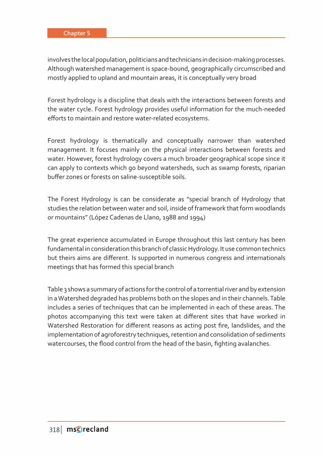
Chapter 5
318
involves the local population, politicians and technicians in decision-making processes. Although watershed management is space-bound, geographically circumscribed and mostly applied to upland and mountain areas, it is conceptually very broad
Forest hydrology is a discipline that deals with the interactions between forests and the water cycle. Forest hydrology provides useful information for the much-needed �ơ����������������������������������Ǧ������������������Ǥ
Forest hydrology is thematically and conceptually narrower than watershed management. It focuses mainly on the physical interactions between forests and water. However, forest hydrology covers a much broader geographical scope since it can apply to contexts which go beyond watersheds, such as swamp forests, riparian ��ơ�����������������������������Ǧ�����������������Ǥ
���� ������ ���������� ��� ���� ��� ������������ ��� Dz�������� ������� ��� ���������� �����studies the relation between water and soil, inside of framework that form woodlands or mountains” (López Cadenas de Llano, 1988 and 1994)
The great experience accumulated in Europe throughout this last century has been fundamental in consideration this branch of classic Hydrology. It use common technics ����������������������ơ�����Ǥ� �����������������������������������������������������meetings that has formed this special branch
Table 3 shows a summary of actions for the control of a torrential river and by extension in a Watershed degraded has problems both on the slopes and in their channels. Table includes a series of techniques that can be implemented in each of these areas. The ������� ������������� ����� ����� ����� ������ ��� ��ơ������ ������ ����� ����� ������� �������������������������������ơ�����������������������������Ƥ��ǡ� ����������ǡ���������implementation of agroforestry techniques, retention and consolidation of sediments ������������ǡ�����ƪ��������������������������������������ǡ�Ƥ�����������������Ǥ
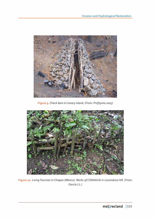
Erosion and Hydrological Restoration
319
Figure 9.���������������������������Ǥ�ȋ���ǣ����������Ȍ
Figure 10. ��������������������������ȋ�±����ȌǤ����������������������������������Ǥ�ȋ���ǣ����À�� Ǥ�ǤȌ
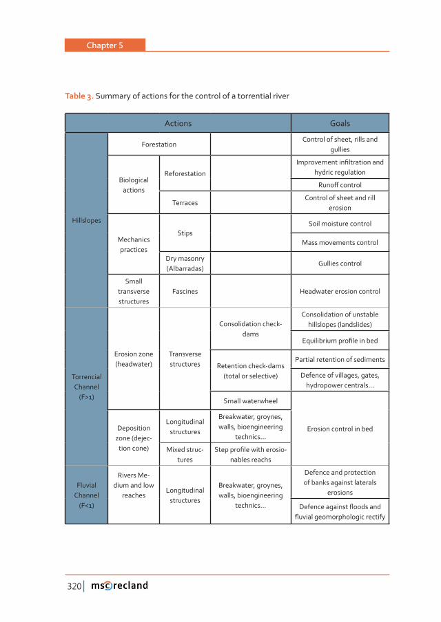
Chapter 5
320
Table 3. Summary of actions for the control of a torrential river
Actions Goals
Hillslopes
ForestationControl of sheet, rills and
gullies
Biological actions
Reforestation
��������������Ƥ�������������hydric regulation
����ơ��������
TerracesControl of sheet and rill
erosion
Mechanics practices
StipsSoil moisture control
Mass movements control
Dry masonry (Albarradas)
Gullies control
Small transverse structures
Fascines Headwater erosion control
Torrencial Channel
(F>1)
Erosion zone (headwater)
Transverse structures
Consolidation check-dams
Consolidation of unstable hillslopes (landslides)
���������������Ƥ���������
Retention check-dams (total or selective)
Partial retention of sediments
Defence of villages, gates, hydropower centrals...
Small waterwheel
Erosion control in bedDeposition zone (dejec-
tion cone)
Longitudinal structures
Breakwater, groynes, walls, bioengineering
technics...
Mixed struc-tures
��������Ƥ��������������-nables reachs
Fluvial Channel
(F<1)
Rivers Me-dium and low
reaches Longitudinal
structures
Breakwater, groynes, walls, bioengineering
technics...
Defence and protection of banks against laterals
erosions
����������������ƪ���������ƪ����������������������������
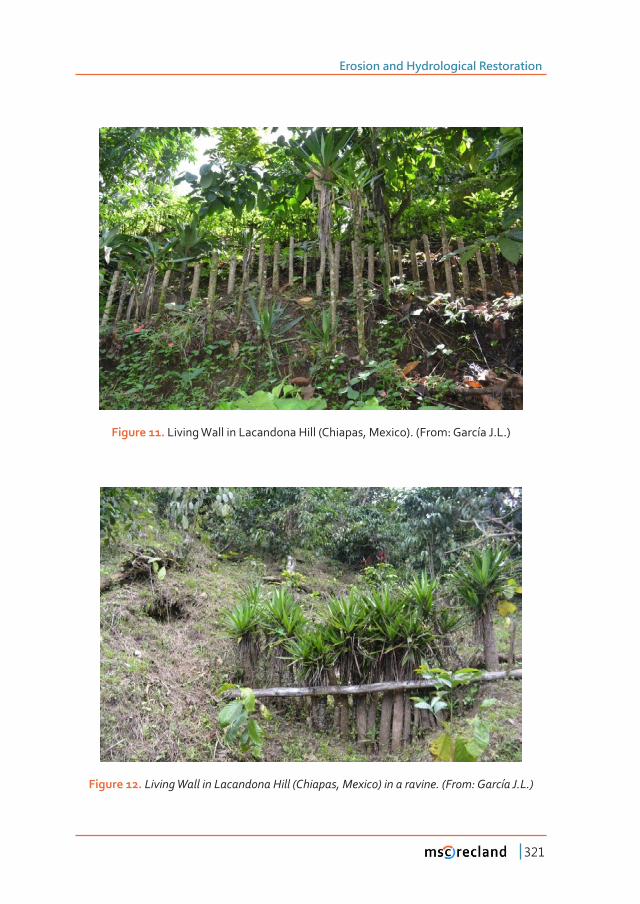
Erosion and Hydrological Restoration
321
Figure 11. Living Wall in Lacandona Hill (Chiapas, Mexico). (From: García J.L.)
Figure 12. ������������������������������ȋ�������ǡ�������Ȍ������������Ǥ�ȋ���ǣ����À�� Ǥ�ǤȌ
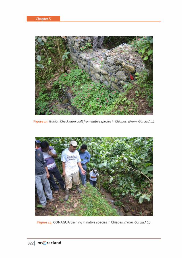
Chapter 5
322
Figure 13.�����������������������������������������������������Ǥ�ȋ���ǣ����À�� Ǥ�ǤȌ
Figure 14. CONAGUA training in native species in Chiapas. ȋ���ǣ����À�� Ǥ�ǤȌ
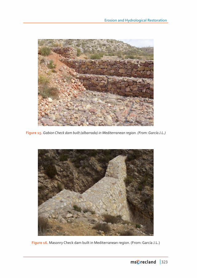
Erosion and Hydrological Restoration
323
Figure 15. ����������������������ȋ���������Ȍ������������������������Ǥ�ȋ���ǣ����À�� Ǥ�ǤȌ
Figure 16. Masonry Check dam built in Mediterranean region. (From: García J.L.)
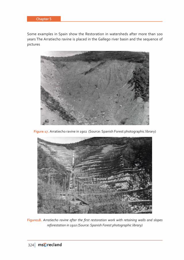
Chapter 5
324
Some examples in Spain show the Restoration in watersheds after more than 100 years The Arratiecho ravine is placed in the Gallego river basin and the sequence of pictures
Figure 17. Arratiecho ravine in 1902 (Source: Spanish Forest photographic library)
Figure18. ����������� ������������� ����Ƥ���� ���������������������� ���������������� ���� �������������������������ȋ������ǣ�����������������������������������Ȍ
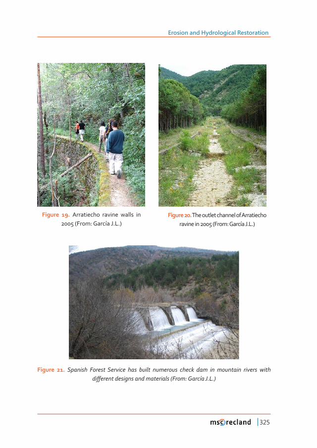
Erosion and Hydrological Restoration
325
Figure 21. Spanish Forest Service has built numerous check dam in mountain rivers with ��ơ����������������������������ȋ���ǣ����À�� Ǥ�ǤȌ
Figure 19. Arratiecho ravine walls in 2005 (From: García J.L.)
Figure 20. The outlet channel of Arratiecho ravine in 2005 (From: García J.L.)
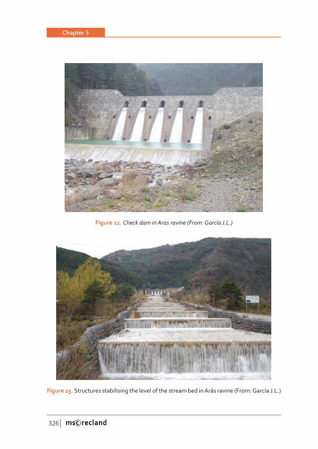
Chapter 5
326
Figure 22. �������������������������ȋ���ǣ����À�� Ǥ�ǤȌ
Figure 23. Structures stabilising the level of the stream bed in Arás ravine (From: García J.L.)
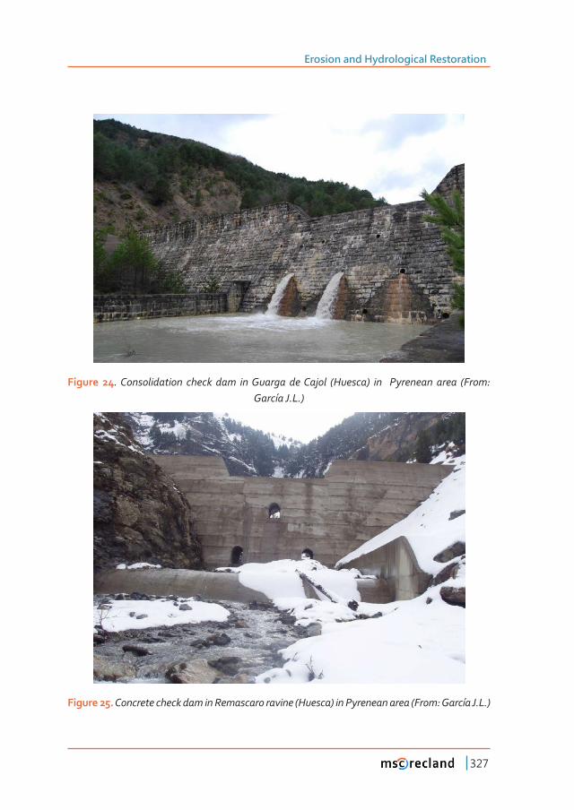
Erosion and Hydrological Restoration
327
Figure 24Ǥ��������������� ������ ���� ��������� ��������� ȋ������Ȍ� ��� � ��������� ����� ȋ���ǣ����À�� Ǥ�ǤȌ
Figure 25.����������������������������������������ȋ������Ȍ������������������ȋ���ǣ����À�� Ǥ�ǤȌ
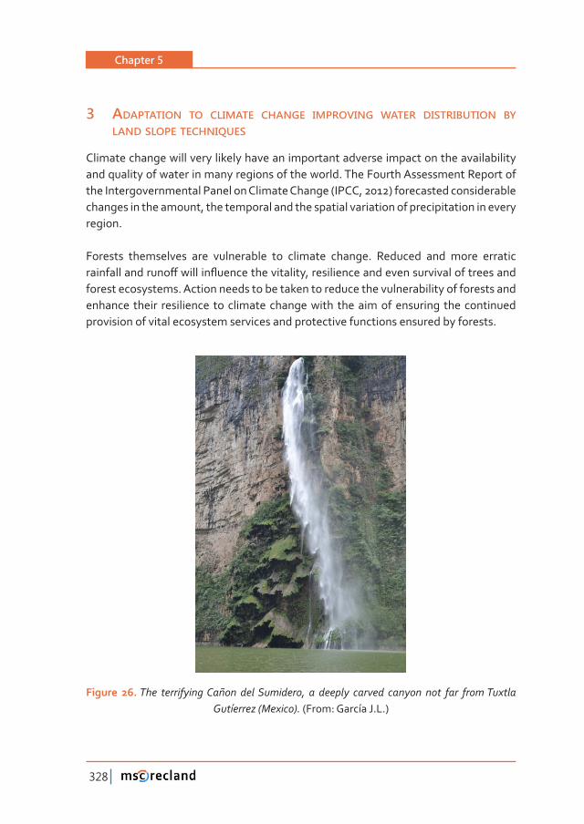
Chapter 5
328
3 adaptation to climate change improving water distribution by land slope techniques
Climate change will very likely have an important adverse impact on the availability and quality of water in many regions of the world. The Fourth Assessment Report of the Intergovernmental Panel on Climate Change (IPCC, 2012) forecasted considerable changes in the amount, the temporal and the spatial variation of precipitation in every region.
Forests themselves are vulnerable to climate change. Reduced and more erratic �����������������ơ��������ƪ������������������ǡ�������������������������������������������forest ecosystems. Action needs to be taken to reduce the vulnerability of forests and enhance their resilience to climate change with the aim of ensuring the continued provision of vital ecosystem services and protective functions ensured by forests.
Figure 26. The terrifying Cañon del Sumidero, a deeply carved canyon not far from Tuxtla ��À������ȋ������ȌǤ�(From: García J.L.)
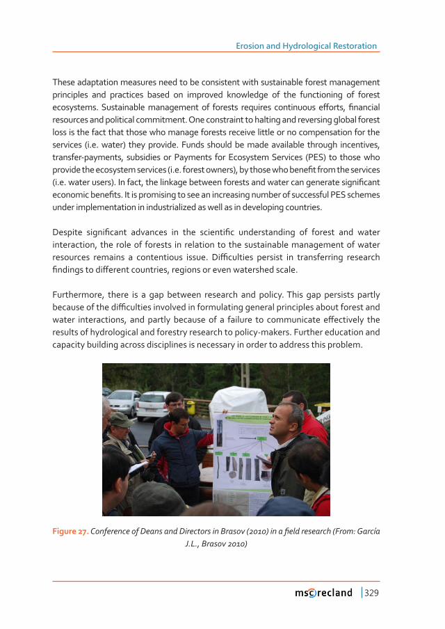
Erosion and Hydrological Restoration
329
These adaptation measures need to be consistent with sustainable forest management principles and practices based on improved knowledge of the functioning of forest ����������Ǥ������������������������ ��� �������� ��������� ����������� �ơ����ǡ� Ƥ��������resources and political commitment. One constraint to halting and reversing global forest loss is the fact that those who manage forests receive little or no compensation for the services (i.e. water) they provide. Funds should be made available through incentives, transfer-payments, subsidies or Payments for Ecosystem Services (PES) to those who �������������������������������ȋ�Ǥ�Ǥ��������������Ȍǡ������������������Ƥ��������������������ȋ�Ǥ�Ǥ������������ȌǤ��������ǡ���������������������������������������������������������Ƥ������������������Ƥ��Ǥ�����������������������������������������������������������������������under implementation in industrialized as well as in developing countries.
�������� �����Ƥ����� ��������� ��� ���� �������Ƥ�� �������������� ��� ������� ���� ������interaction, the role of forests in relation to the sustainable management of water ���������� �������� �� ������������ �����Ǥ� ��ƥ�������� �������� ��� ������������� ���������Ƥ������������ơ���������������ǡ��������������������������������Ǥ
Furthermore, there is a gap between research and policy. This gap persists partly �����������������ƥ�������������������������������������������������������������������������� ������������ǡ� ����������� �������� ��� �� �������� ��� ������������ �ơ��������� ����results of hydrological and forestry research to policy-makers. Further education and capacity building across disciplines is necessary in order to address this problem.
Figure 27.���������������������������������������������ȋȌ������Ƥ�������������ȋ���ǣ����À�� Ǥ�Ǥǡ��������Ȍ
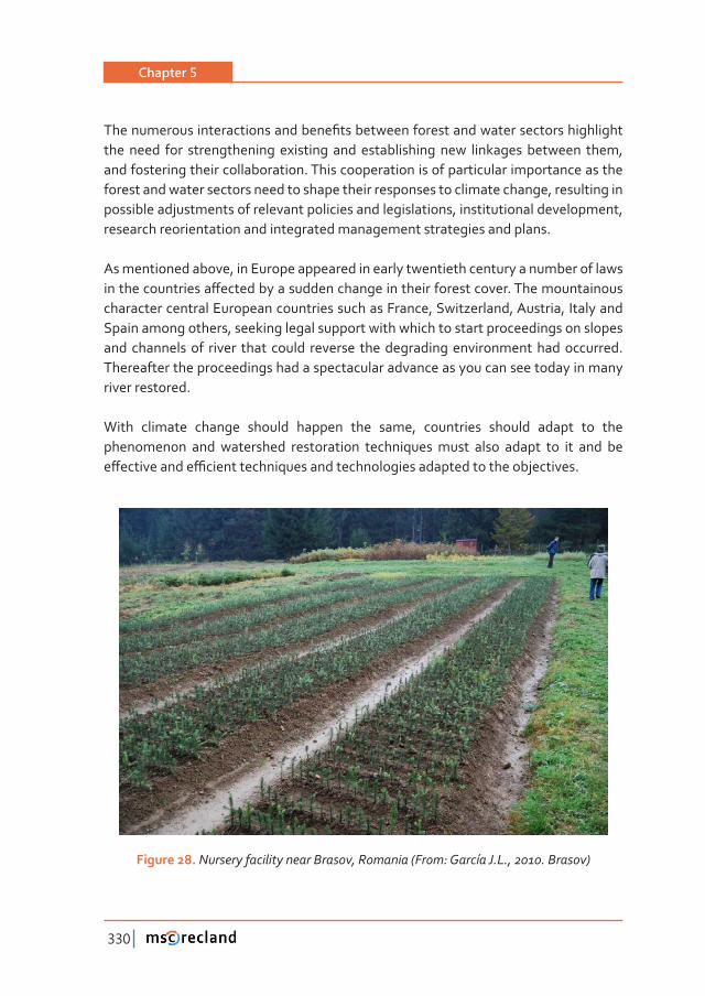
Chapter 5
330
����������������������������������Ƥ����������������������������������������������the need for strengthening existing and establishing new linkages between them, and fostering their collaboration. This cooperation is of particular importance as the forest and water sectors need to shape their responses to climate change, resulting in possible adjustments of relevant policies and legislations, institutional development, research reorientation and integrated management strategies and plans.
As mentioned above, in Europe appeared in early twentieth century a number of laws ������������������ơ����������������������������������������������Ǥ�����������������character central European countries such as France, Switzerland, Austria, Italy and Spain among others, seeking legal support with which to start proceedings on slopes and channels of river that could reverse the degrading environment had occurred. Thereafter the proceedings had a spectacular advance as you can see today in many river restored.
With climate change should happen the same, countries should adapt to the phenomenon and watershed restoration techniques must also adapt to it and be �ơ������������ƥ�����������������������������������������������������������Ǥ
Figure 28. ����������������������������ǡ���������ȋ���ǣ����À�� Ǥ�Ǥǡ�Ǥ�������Ȍ
Erosion and Hydrological Restoration
331
4 Flood control in a changing climate
Floods, storms and other hydro-meteorological events account for around two thirds parts of the damage costs of natural disasters, and these costs have increased since 1980, according to a recent EEA assessment of climate change impacts in Europe.
The observed increase in damage costs from extreme weather events is mainly due to land use change, increases in population, economic wealth and human activities ���������Ǧ�������������������������� ���������Ǥ�������Ƥ������������� ���������������������������������ƪ�����������������������������ǡ��������������������������������������������ǡ�����Ǧ�������������������������������������������ƪ���������Ǥ
In any case, it is likely that rising temperatures in Europe will intensify the ������������� �����ǡ� �������� �������� ��������� ���� �������� ƪ����� �������� �������Ǥ���������������������������������������ƪ�����������������������������������������ǡ�����contribution of climate change to the damage costs from natural disasters is expected to increase in the future due to the projected increase in the intensity and frequency of extreme weather events in many regions.
���������������ǡ�����������������������ǡ�����ǣ�Dz������������ƪ������������������ǡ����can see climate change will be an increasingly important factor. But in many cases, ƪ������������������������������������ǡ��������ǡ�������������������Ȃ������������������������� ƪ������� ��� ������� �������� ���� ��� ������� ����������� �������� ������� ������� ���ƪ���Ǧ�����������Ǥdz
The report, ‘Climate change, impacts and vulnerability in Europe 2012 http://www.���Ǥ������Ǥ��Ȁ�����Ȁ������������Ȁ�������Ǧ������Ǧ�������Ǧ������Ǧ������� Ƥ����that higher average temperatures have been observed across Europe as well as decreasing precipitation in southern regions and increasing precipitation in northern Europe. The Greenland ice sheet, Arctic sea ice and many glaciers across Europe are melting, snow cover has decreased and most permafrost soils have warmed.
�����������������������������������������ǡ�ƪ�������������������������������������damage costs across Europe in recent years. While more evidence is needed to discern the part played by climate change in this trend, growing human activity in hazard-prone areas has been a key factor. Future climate change is expected to add to this vulnerability, as extreme weather events are expected to become more intense and
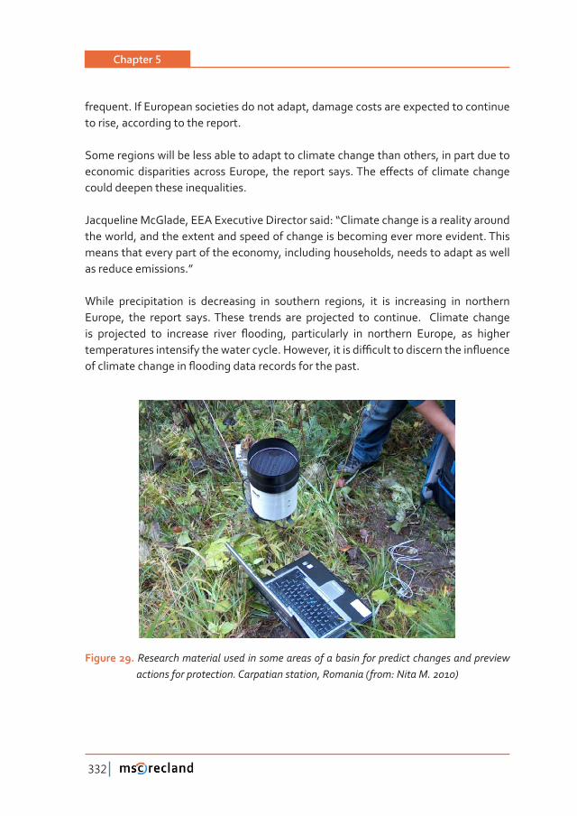
Chapter 5
332
frequent. If European societies do not adapt, damage costs are expected to continue to rise, according to the report.
Some regions will be less able to adapt to climate change than others, in part due to ����������������������������������ǡ� ���� ������� ����Ǥ������ơ�������� ���������������could deepen these inequalities.
����������������ǡ����������������������������ǣ�Dz�����������������������������������the world, and the extent and speed of change is becoming ever more evident. This means that every part of the economy, including households, needs to adapt as well as reduce emissions.”
While precipitation is decreasing in southern regions, it is increasing in northern Europe, the report says. These trends are projected to continue. Climate change ��� ���������� ��� ��������� ������ ƪ������ǡ� ������������� ��� ��������� ������ǡ� ��� ���������������������������������������������Ǥ��������ǡ���������ƥ����������������������ƪ���������������������������ƪ��������������������������������Ǥ
Figure 29. Research material used in some areas of a basin for predict changes and preview ����������������������Ǥ������������������ǡ���������ȋ����ǣ�������Ǥ�Ȍ
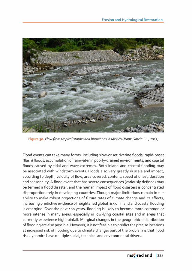
Erosion and Hydrological Restoration
333
Figure 30.���������������������������������������������������ȋ����ǣ����À�� Ǥ�Ǥǡ�Ȍ
�������������������������������ǡ���������������Ǧ���������������ƪ����ǡ������Ǧ������ȋƪ���Ȍ�ƪ����ǡ������������������������������������Ǧ��������������������ǡ�������������ƪ����� ������� ��� ������ ���� ����� ��������Ǥ� ����� ������� ���� �������� ƪ�����������be associated with windstorm events. Floods also vary greatly in scale and impact, ������������������ǡ�������������ƪ��ǡ�������������ǡ��������ǡ���������������ǡ�������������������������Ǥ���ƪ���������������������������������������ȋ������������Ƥ���Ȍ�����������������ƪ������������ǡ�������������������������ƪ������������������������������disproportionately in developing countries. Though major limitations remain in our ������������������������������������������������������������������������� �����ơ����ǡ��������������������������������������������������������������������������������ƪ������������������Ǥ���������������������ǡ�ƪ������������������������������������������more intense in many areas, especially in low-lying coastal sites and in areas that currently experience high rainfall. Marginal changes in the geographical distribution ���ƪ������������������������Ǥ��������ǡ��������������������������������������������������������������������������ƪ����������������������������ǣ�����������������������������ƪ����risk dynamics have multiple social, technical and environmental drivers.
Chapter 5
334
Flood events are the most frequently occurring natural disasters worldwide, and may increase in the future as a result of climate change.
4�1 The European Flood Alert System
��������������ǡ����������ơ��������������������������ƪ����ǡ��������������� �������������ƪ����� ������ �������������������� ������� ��� �������Ǥ��������ƪ��������������������������������������������������������������Ǥ��������ƪ����� ��� ������� ����� ������� ����� � ������ǡ� ���� ������������� ��� ������ ����� ��million people and at least €25 billion in insured economic losses.
��������������ȀȀ���������������������������������������ƪ������������������into force on 26 November, 2007. This Directive now requires Member States to ������������������������������������������������������������������ƪ������ǡ������������ƪ���������������������������������������������������������������������������������������������������������������������ƪ��������Ǥ
Since the beginning of 2003 the European Commission DG Joint Research Centre (JRC) is developing a prototype of European Flood Alert System (EFAS) in close �������������������������������������������������������������Ǥ����� �������Ƥ��������experience gained already during the European Flood Forecasting System (EFFS) ��������Ƥ���������������������������Ǥ
The European Flood Alert System (EFAS) is a research project that aims at improving ��������������������������ƪ�������������ǣ
• ���������� ���� ������������ ��� ������������������ ��� ���� ������������ ��� �� ƪ����before the local systems capture the event with their own monitoring and forecasting systems;
• providing catchment based information that gives downstream authorities ��� ��������� ��� ���� �������� ���� ����������� ƪ���� ���������� ����� ��� ���������countries.
This does not only include the immediate upstream country but also any further potentially useful upstream information. EFAS provides medium-term (3 to 10 ����Ȍ�ƪ���� ���������ǡ������������ơ��������������������� ������ǡ������������������information to the typical short-term (less than 48 hours) forecasts performed by

Erosion and Hydrological Restoration
335
national centres. The challenge of EFAS is to combine all hydrographs, calculated from ��ơ������������Ǧ�����������������������ǡ����������������ƪ�������������������������������������������������ƪ�����������������������Ǥ����������������������������������used as a pre-alert to allow the receiving authorities to be aware of the possibility of ��ƪ����������������Ǥ� ��������������ǡ�������������������� �������ǡ� ������ ���������������������������������������������������ơ������Dz�������dz��������������ǡ��������������approaches and its location and magnitude become more certain, national authorities can act more quickly and accurately, increasing the economic value of their forecasts.
Figure 31. �������������ƪ�������������������
The key tool of Directive 2007/60 is the development of Risk Management Plans Flood, executed before December 2015, regulated in each European country.
Management plans will aim to achieve coordinated action by all levels of government ���������������������������������������������������ƪ�����������������������������of measures that each government should apply in the scope of their powers to achieve the intended target.
��������������������� �����������������������������Ƥ���������������������������������������� ƪ���� ����� ���� �����ǡ� ��� ���������������� ����� ���������� ���������� ������������������Ǥ���������������������������Ƥ�������������������������������������������entire watershed depending on the type of action. Each competent management will be responsible for the approval of its program of measures, establishing coordination mechanisms Plan.
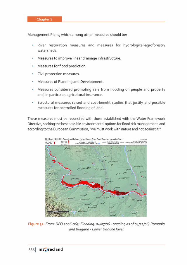
Chapter 5
336
Management Plans, which among other measures should be:
• River restoration measures and measures for hydrological-agroforestry watersheds.
• Measures to improve linear drainage infrastructure.
• �������������ƪ��������������Ǥ
• Civil protection measures.
• Measures of Planning and Development.
• ��������� ����������� ���������� ����� ����� ƪ������� ��� ������� ���� ���������and, in particular, agricultural insurance.
• �������������������� ������� ���� ����Ǧ����Ƥ�� �������� ����� �������� ���� ���������������������������������ƪ��������������Ǥ
These measures must be reconciled with those established with the Water Framework ���������ǡ�����������������������������������������������������ƪ�������������������ǡ�����������������������������������������ǡ�Dz�������������������������������������������Ǥdz
Figure 32. ���ǣ����ǦǢ��������ǣ�ȀȀ�Ǧ���������������ȀȀǢ���������and Bulgaria - Lower Danube River
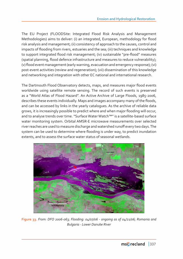
Erosion and Hydrological Restoration
337
The EU Project (FLOODSite: Integrated Flood Risk Analysis and Management �������������Ȍ����������������ǣ�ȋ�Ȍ��������������ǡ���������ǡ�����������������ƪ����risk analysis and management; (ii) consistency of approach to the causes, control and �����������ƪ������������������ǡ����������������������Ǣ�ȋ���Ȍ������������������������������������������������ƪ�������������������Ǣ�ȋ��Ȍ�������������Dz���Ǧƪ���dz����������ȋ����������������ǡ�ƪ���������������������������������������������������������������ȌǢ�ȋ�Ȍ�ƪ���������������������ȋ�������������ǡ����������������������������������ȌǢ�ȋ��Ȍ�post-event activities (review and regeneration); (vii) dissemination of this knowledge and networking and integration with other EC national and international research.
��������������������������������������ǡ�����ǡ��������������������ƪ�����������worldwide using satellite remote sensing. The record of such events is preserved ����� Dz��������������������������dzǤ���������������������������������ǡ� Ǧǡ������������������������������������Ǥ���������������������������������������ƪ����ǡ�and can be accessed by links in the yearly catalogues. As the archive of reliable data �����ǡ�������������������������������������������������������������ƪ�����������������ǡ��������������������������������Ǥ�Dz�������������������dz���������������Ǧ��������������water monitoring system. Orbital AMSR-E microwave measurements over selected ��������������������������������������������������������������ơ���������������Ǥ�������������������������������������������ƪ�������������������ǡ�����������������������extents, and to assess the surface water status of seasonal wetlands.
Figure 33.����ǣ����ǦǢ��������ǣ�ȀȀ�Ǧ���������������ȀȀǢ�������������Bulgaria - Lower Danube River
Chapter 5
338
4�2 Mortality due to flood events�
�����������������������ƪ��������������������������� ���������Ǧ����������������������������Ǥ������������������������Ƥ���ƪ���������������������������������������������������������������ǡ�������������������������������������Ǧƪ������������Ǥ�����������������������������������������������������������������������ƪ���ǡ�����������������������������ǡ������ǡ�����������Ǥ���������������������������������ƪ���Ǧ����������������������limited, but men appear more at risk than women. Those drowning in their own homes are largely the elderly.
4�2�1 Appendix
Directive 2007/60/EC on the assessment and management of flood risks�
�����������������������������������������������������������������������ƪ�����������������change.
(2) Floods are natural phenomena which cannot be prevented. However, some human �����������ȋ������������������������������������������������������������ƪ����������and the reduction of the natural water retention by land use) and climate change �������������������������������������������������������������������ƪ����������Ǥ
(4) Directive 2000/60/EC of the European Parliament and of the Council of 23 October ������������������������������������������������������Ƥ��������������������ȋȌ�requires river basin management plans to be developed for each river basin district in order to achieve good ecological and chemical status, and it will contribute to ����������������ơ��������ƪ����Ǥ��������ǡ����������������������ƪ�����������������������principal objectives of that Directive, nor does it take into account the future changes ���������������ƪ������������������������������������Ǥ
(14) Flood risk management plans should focus on prevention, protection and preparedness. With a view to giving rivers more space, they should consider where ��������� �������������������Ȁ��� ���������������ƪ���������ǡ��������������������� ���prevent and reduce damage to human health, the environment, cultural heritage ���� ��������� ��������Ǥ� ���� ��������� ��� ƪ���� ����� ����������� ������ ������� ���periodically reviewed and if necessary updated, taking into account the likely impacts ���������������������������������������ƪ����Ǥ
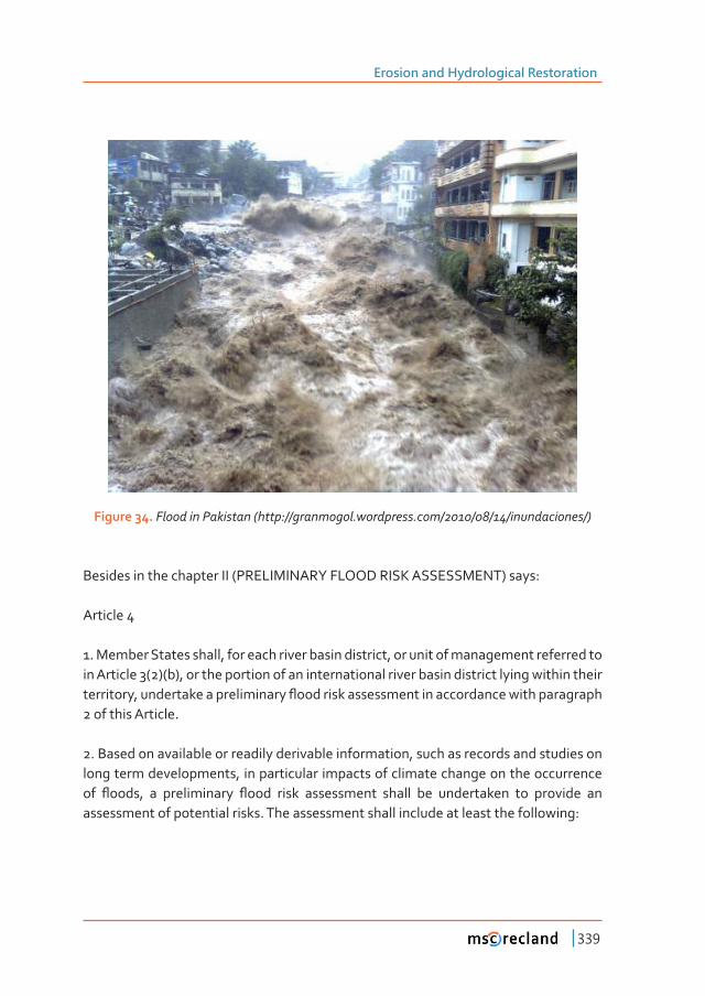
Erosion and Hydrological Restoration
339
Figure 34. �����������������ȋ����ǣȀȀ���������Ǥ���������Ǥ���ȀȀȀȀ������������ȀȌ�
Besides in the chapter II (PRELIMINARY FLOOD RISK ASSESSMENT) says:
Article 4
1. Member States shall, for each river basin district, or unit of management referred to in Article 3(2)(b), or the portion of an international river basin district lying within their ���������ǡ�������������������������ƪ�������������������������������������������������2 of this Article.
2. Based on available or readily derivable information, such as records and studies on long term developments, in particular impacts of climate change on the occurrence ��� ƪ����ǡ� �� ������������ ƪ���� ����� ����������� ������ ��� ����������� ��� �������� ���assessment of potential risks. The assessment shall include at least the following:
Chapter 5
340
a) maps of the river basin district at the appropriate scale including the borders of the river basins, sub-basins and, where existing, coastal areas, showing topography and ��������Ǣ�ȋ�Ȍ����������������������ƪ��������������������������������������������������������Ƥ������������������������������������ǡ����������������ǡ�����������������������economic activity and for which the likelihood of similar future events is still relevant, ����������������ƪ������������������������������������������������������������������impacts they have entailed;
ȋ�Ȍ� �� ������������ ��� ���� �����Ƥ����� ƪ����� ������ ����� ��������� ��� ���� ����ǡ� �����������Ƥ���������������������������������������������������������������������Ǣ����ǡ�����������������������Ƥ������������������������ǡ�����������������ǣ
ȋ�Ȍ���������������������������������������������������������������ƪ���������������health, the environment, cultural heritage and economic activity, taking into account as far as possible issues such as the topography, the position of watercourses and their �������� ������������� ���� ����������������� ���������������ǡ� ���������� ƪ������������� �������� ���������� �����ǡ� ���� �ơ����������� ��� ��������� �������� ƪ���� ��������infrastructures, the position of populated areas, areas of economic activity and long-���������������������������������������������������������������������������ƪ����Ǥ
In the chapter VIII says in the Article 14 in the section 4 about the Climate Change
Article 14
Ǥ�����������������ƪ�������������������ǡ���������������������������������������������in Article 13(1), shall be reviewed, and if necessary updated, by 22 December 2018 and every six years thereafter.
Ǥ�����ƪ������������������������ƪ�������������������������������ǡ������������������updated, by 22 December 2019 and every six years thereafter.
Ǥ�����ƪ���� ��������������������ȋ�Ȍ� ��������� ��������ǡ����� ��������������������ǡ�including the components set out in part B of the Annex, by 22 December 2021 and every six years thereafter.
Ǥ����������������������������������������������������������ƪ�������������������������account in the reviews referred to in paragraphs 1 and 3.
Erosion and Hydrological Restoration
341
REFERENCES
BENNETT, H.H. 1939. Soil conservation. McGraw-Hill and Co., New York, PP 993. ���� �Ǥ�������������������������������������ǡ����Ƥ��������������������������������Ǥ�����ǣȀȀ
www.eea.europa.eu/media/newsreleases/climate-change-evident-across-europe�����Ǥ��������������������ƪ���������������������������Ǥ����ǣȀȀ���Ǥ���Ǥ������Ǥ��Ȁ����������Ȁ�������Ǧ������Ǧ���Ǧƪ���Ǧ�������Ǥ����������������������Ƥ����������Ǥ������������������������������Ǥ������ȀǤ�
Edited by Sheng T.C. RomeFAO 2010 Global Forest Resources. Main report. Paper 163. RomeGARCIA J.L. 2009. La Restauración Hidrológico Forestal, como herramienta de disminución de
la producción de sedimentos.Taller Internacional ISI/GEST/UNESCO- Universidad de Talca. Santiago de Chile. Chile.
GARCIA, J.L. 2010. Procesos de erosión – sedimentación en cauces y cuencas. Chapter 8. Vol. 1 Phi-LAC. Doc Tec. 22. Montevideo
GARCIA J.L. 2011. Conference in the IV International Congress XXXX. IMTA. Tuxtla Gutiérrez. Mé-xico
HALEY D. 2000. Integration of Climate Change into Watershed Management Ontario Water Con-ference, Challenges and Solutions. Ontario Canada.
IPCC 2012. The Fourth Assessment Report of the Intergovernmental Panel on Climate Change.�V��������������������ǡ�Ǥ�Ǥ���������×�����������������������������×�����������ǡ������-
ción FAO, Fomento de tierras y aguas, pp. 182, Roma.
�V��������������������ǡ�Ǥ�Ǥ�����������×��������×���������������������������control de la erosión. TRAGSA-Mundi Prensa, 902 p.
MINTEGUI, J. 2005. Introduce approach to water and forest management strategy, First meeting of the INCO Project Evidence-based Policy for Integrated Control of Forested River Catchments in Extreme Rainfall and Snowmelt, Newcastle University, pp. 24.
MILLIMAN, J. D. AND SYVITKI, J. P. M. (1992) Geophysic/tectonic control of sediment discharge to the ocean: the importance of small mountaneous rivers. J. Geol. 100, 325-344.
SIMON E. de; MINTEGUI J.A.; GARCIA J,L, and Robredo J.C. 1993. La restauración ������×����Ǧ��������������������������������Ƥ��������������������������������ǡ� �����de Andalucía, Consejería de Agricultura y Pesca, pp. 325, Sevilla
VIVIROLI, D. AND R. WEINGARTNER, 2003: Mountains: Sources of the world’s freshwater. ICIMOD Newsletter, 42, Winter, 2-3.
THIERY, E. 1891. Restauration des montagnes, correction des torrents et reboisement, Librairie Polytechnique Ch. Beranger, pp. 480, Paris et Liege.

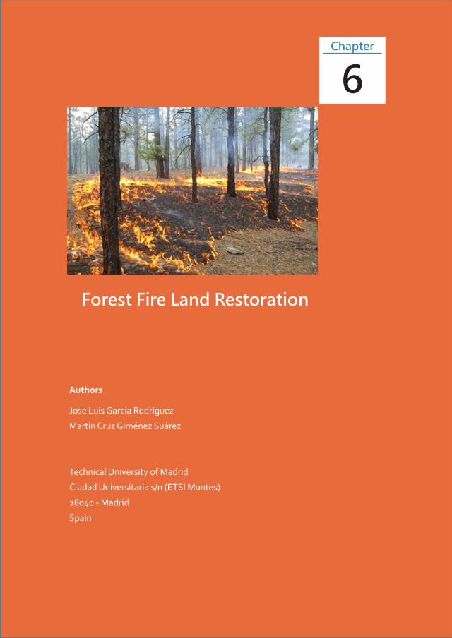
Forest Fire Land Restoration
Authors
Jose Luis García Rodríguez
Martín Cruz Giménez Suárez
Technical University of Madrid
Ciudad Universitaria s/n (ETSI Montes)
28040 - Madrid
Spain
6Chapter

345
Chapter 6
Technical
University of
Madrid,
Madrid, Spain
Forest Fire Land RestorationJose Luis García Rodríguez
Martín Cruz Giménez Suárez
1 postFire eFFects on ecosystems
1�1 IntroductionAll disturbances produce impacts on ecosystems. The level and direction of impact (negative or positive) depends on ecosystem resistance and resilience, as well as on the severity of the disturbance. The variability in resource damage and response ����������������������������������������������������������������������������Ƥ���severity.
������������� ȋ�������������Ȍ� ���������������������������� �����ơ��������Ƥ�������������������Ǥ��������������Ǧ�����������������ǡ�Ƥ���������������������������ơ����������depend on interactions of energy release (intensity), duration, fuel loading and combustion, vegetation type, climate, topography, soil, and area burned.
Fire intensity is an integral part of burn severity, and the terms are often incorrectly �����������������Ǥ�����������������������������������������Ƥ������������������������energy in the fuel-climate environment (DeBano and others 1998). Intensity is measured in terms of temperature and heat yield. Surface temperatures can range from 120 to greater than 2,730 °F (50 to greater than 1,500 °C). Heat yields per unit area can be as little as 59 BTU ft-2 (260 kg-cal m-2) in short, dead grass to as high as 3700 BTU ft-2 (10,000 kg-cal m-2) in heavy logging slash. Rate of spread is an ���������Ƥ������������������������������Ǥ��������-1 (0.5 m week-1) in smouldering �����Ƥ������������������������-1 (25 km hr-1Ȍ���������������������Ƥ���Ǥ
Chapter 6
346
���� ���������� ��� Ƥ��� ��������� ����� �������� ��� ���� ����� ������� ��� ������ ��������������ǡ������������������������������ǡ������������Ǥ������������Ƥ�������Ƥ��������ǡ�such as grass, may be intense in terms of energy release per unit area, but do not ������������������������������������������������ƪ���ǡ�������������ǡ�������������������������������������Ƥ������������������������������Ǥ���������������������������ǡ�����������������������Ƥ���������������������������������������������Ǥ�����������������gradients that develop can be described with a linked-heat transfer model and are a function of moisture and fuel loadings.
����������������Ƥ�������������������������Ƥ��ǡ�����Ƥ��������������������������������as a single quantitative measure that relates to resource impact. Therefore, relative ����������������������Ƥ�����������ǡ�������������������������������Ƥ��������������������������������ǡ�����������������������������������������Ƥ���������������������������Ƥ���ǡ�discrete classes, ranging from low to high.
1�2 Fire Severity
������������������������������������������������Ƥ�������������ȋ����������������������energy is produced) and duration (length of time burning occurs at a particular point) �����������������������������������������������������ƪ������������������������������������������������Ǥ�����������������������������������������������ơ��������Ƥ�����������and soil resources; it can occur along a spectrum from high to low or can be described as a patchwork, mosaic, matrix or mixed-severity event. Some researchers describe a light severity burn as one that burns only surface fuels, leaves the soil covered with ���������� ������������������������ǡ� ���� ������� ��������ơ������������� ȋ�������������(Oe) + humus (Oa) layers). A moderate-severity burn results from a large proportion of the organic material burned away from the surface of the soil and the remaining fuel is deeply charred. A high-severity burn results from all of the organic material burned away from the soil surface, organic material below the surface is consumed or charred. Fire severity has been assessed by numerous methods such as degree of destruction of aboveground live and dead biomass (Neary and others 2005), amount of forest ƪ������������ǡ��������������������ơ������ǡ������������������������������������������Ǥ
������������� �����Ƥ���������������ǣ�Ȍ���������������������������������������������Ƥ�������������������������������������������Ǣ�Ȍ�������������������������ȋ������������ǡ�ƪ����������ǡ��������������������������������ȌǢ�Ȍ����������������������Ƥ��������������������������ȋ�������������ǡ��������ǡ�����������Ƥ���ȌǢ�����Ȍ��������������� �������
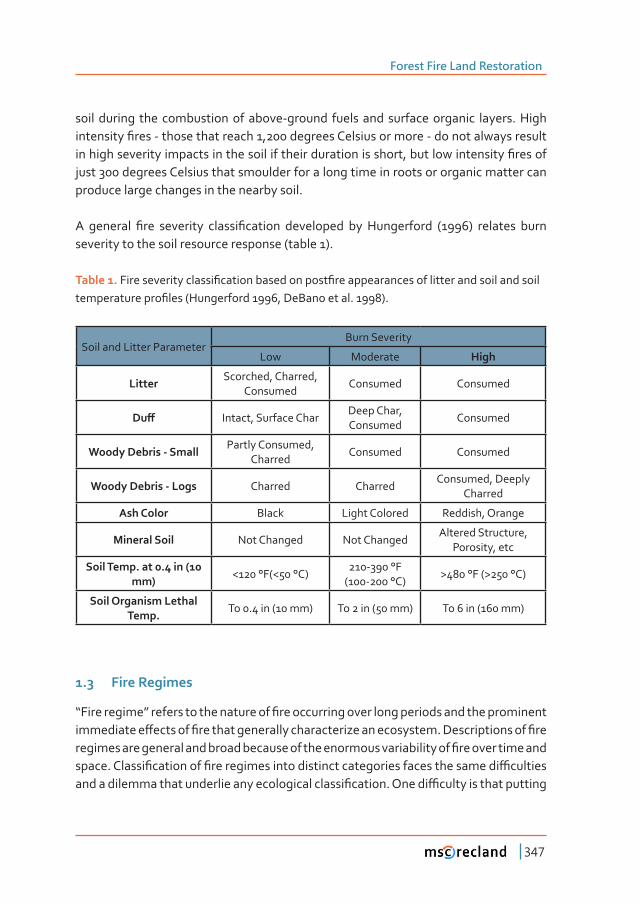
Forest Fire Land Restoration
347
soil during the combustion of above-ground fuels and surface organic layers. High ����������Ƥ����Ǧ������������������ǡ�������������������������Ǧ�������������������������������������������������������������������������������������ǡ�������������������Ƥ�������just 300 degrees Celsius that smoulder for a long time in roots or organic matter can produce large changes in the nearby soil.
�� �������� Ƥ��� ��������� ������Ƥ������� ���������� ��� ����������� ȋȌ� �������� �����severity to the soil resource response (table 1).
Table 1. �������������������Ƥ��������������������Ƥ����������������������������������������������������������Ƥ����ȋ�����������ǡ�������������Ǥ�ȌǤ
Soil and Litter ParameterBurn Severity
Low Moderate ����
LitterScorched, Charred,
ConsumedConsumed Consumed
��ơ Intact, Surface CharDeep Char, Consumed
Consumed
Woody Debris - SmallPartly Consumed,
CharredConsumed Consumed
Woody Debris - Logs Charred CharredConsumed, Deeply
Charred
��������� Black Light Colored Reddish, Orange
Mineral Soil Not Changed Not ChangedAltered Structure,
Porosity, etc
���������Ǥ����Ǥ����ȋ���Ȍ
<120 °F(<50 °C)210-390 °F
(100-200 °C)>480 °F (>250 °C)
�������������������������Ǥ
To 0.4 in (10 mm) To 2 in (50 mm) To 6 in (160 mm)
1.3 Fire Regimes
Dz����������dz�������������������������Ƥ������������������������������������������������������������ơ��������Ƥ�������������������������������������������Ǥ�����������������Ƥ������������������������������������������������������������������������Ƥ����������������������Ǥ�������Ƥ����������Ƥ�����������������������������������������������������ƥ���������������������������������������������������������Ƥ������Ǥ�������ƥ����������������������
Chapter 6
348
boundaries around segments of biological processes that vary continuously involves ����������������������������Ǥ���������������������������������Ƥ�����������������������managers it must be practical and easily communicated, thus free of complexity. Yet ����������������ƪ��������������������������������������ǡ���������������������Ƥ��ǡ����������������������������������������������������������Ǥ��������Ǧ�ơ�����������������������������������������������������������������������������������Ǥ�����Ƥ������������������������� �� ���������� ������ ��� �� �������������������� Ƥ��� ���������� ����Ƥ��� �����������������Ǥ��������������������������������������������������������������������Ƥ���among technical as well as nontechnical audiences.
������Ƥ�����������Ƥ������������������������������������������������������Ƥ���������������������ơ���������������������Ƥ��Ǥ����������������������������������������������������Ƥ������������ǡ�Ƥ��������������ǡ�Ƥ������������ǡ���������Ƥ��ǡ�������������������������ǡ���������������ǡ������������������Ǥ�����������������������Ƥ������������������������������Ǥ�������������������������Ƥ�����������������������������������������������Ƥ�����������������������������������������������������������������������������������Ƥ��Ǥ�������������������Ƥ����������������������������������������������������������������������������������Ƥ����������������������������Ǥ
�����������ȋȌ�������������ȋȌ��������������Ƥ����������Ƥ�����������Ƥ�������������������� ��� �������Ǥ����� �������ǡ� Ƥ��� ���������� ���� ���������ǡ� ������� ���� ������ ������������������������������Ƥ����������������Ƥ�������Ǥ�����ƥ�����������Ƥ���������������� ����� ������� ��������� �����������ǡ� ���������� ������Ƥ������� ��������Ƥ��ǡ� ���� ������stand-replacement because mortality to aboveground vegetation is complete or ������� ��������Ǥ� ���� ���������� �������� ����� ���������� ��� Ƥ��� ��������Ǥ� ��������� ���Ƥ��� ��ƪ����� ȋȌ� ���� ���������� ��� �������� �ơ����� ��� Ƥ��� ����� ������� ����� ������������� ���� ������������ Ƥ��� ������ ���� ȋȌ� ����� ��������� ������� ������ ����� �����������Ǥ��������������������� ������������������������������ ������������Ƥ����ơ����Ǥ��������������������Ƥ�����������������������Ƥ��������������������ǯ��Ƥ������������������������to mortality of the primary tree cover as stand-replacement.
����Ƥ����������������Ƥ�������ȋ������ Ȍ����������������������Ƥ�����������Ǥ����������������Ƥ��������������������������������������������������Ƥ������������������������Ǥ��������Ƥ������������������������������������������������Ƥ����������������������������������� ����������������� ��� �����ơ�������������������ǡ��������������������������������������of the dominant vegetation. It is intended for broadscale applications and for ��������������������Ƥ��ǯ��������������������������������������������������������natural resources.
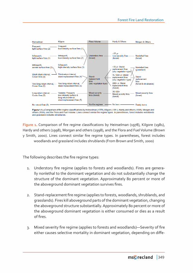
Forest Fire Land Restoration
349
Figure 1.���������������Ƥ��� �������������Ƥ���������������������� ȋȌǡ��������� ȋȌǡ�Hardy and others (1998), Morgan and others (1998), and the Flora and Fuel Volume (Brown �� �����ǡ� ȌǤ� ������ �������� �������� Ƥ��� ������� �����Ǥ� ��� �����������ǡ� ������� ���������
woodlands and grassland includes shrublands (From Brown and Smith, 2000)
����������������������������Ƥ���������������ǣ
1. �����������Ƥ����������ȋ�������� ��� ���������������������ȌǤ����������������-lly nonlethal to the dominant vegetation and do not substantially change the structure of the dominant vegetation. Approximately 80 percent or more of ���������������������������������������������Ƥ���Ǥ
2. �����Ǧ������������Ƥ����������ȋ������������������ǡ����������ǡ�����������ǡ�����grasslands). Fires kill aboveground parts of the dominant vegetation, changing the aboveground structure substantially. Approximately 80 percent or more of the aboveground dominant vegetation is either consumed or dies as a result ���Ƥ���Ǥ
3. ���������������Ƥ����������ȋ��������������������������������ȌȄ������������Ƥ�����������������������������������������������������������ǡ����������������ơ�-
Chapter 6
350
�����������������ǯ�������������������Ƥ��ǡ���������������������������������������Ǧ�replacement.
4. ���Ƥ���������Ȅ�����������������������������������Ƥ��Ǥ�
Most belowground plant parts survive, allowing species that sprout to recover rapidly. This is true of tundra, grasslands, and many shrub- land ecosystems. Some ������������������������������������Dz���������dz�Ƥ����������������������������������that structure and composition of vegetation is similar to the pre-burn condition ��������������������������Ǥ���������Ƥ��������������������������������������������������vegetation for at least a short time, however, we consider grassland ecosystems ��� ����� �����Ǧ������������ Ƥ��� �������Ǥ� �������� ���������ǡ� ������ǡ� ���� �������������������������Ǧ������������Ƥ���������������ǡ������������������������������Ƥ����������������������������������Ƥ������������ǡ�������������������������������������������������ƪ���������������������������������������������Ǥ
����������������������������������Ƥ��� ������������������� ��� ������������������������������������Ǥ��������������������Ƥ���������������������������������ǣ
• ����� ��������������������������� ��������Ƥ������������ �������ǡ������������Ƥ���resistant species and relatively large size.
• ���������������� �����������Ƥ�����������������������������������������������Ǧ�����������ǡ������� �������� ��Ƥ��Ǧ������������������� ���������������� �����Ǥ������ ����� ��� Ƥ��� ������� ���� ���� ����� ����������� ��� ��������� ������Ƥ�������Ǥ���� ��������� ������� �������� ��� ƪ����������� ��� �������� ������� Ƥ���ǡ� ��������changes in burning conditions, and variation in topography, fuels, and stand ����������������������Ǥ�����������������������������������������������Ƥ���������Ǥ�In actuality, a blend of these two mixed severity types probably occurs.
• ���� ��������� ������� ����� ����� ����� ����������� Ƥ���� ������������ ��������understory burns and stand-replacement.
1�4 Fire Effects on Watersheds
Soils, vegetation, and litter are critical to the functioning of hydrologic processes. Watersheds with good hydrologic conditions and adequate rainfall sustain stream ����ƪ���������������������������������������������������������������������Ǥ�����������
Forest Fire Land Restoration
351
Introduction to Climate Change and Land Degradation
hydrologic condition (greater than 75 percent of the ground covered with vegetation ����������Ȍǡ�������������������������������������������������������������ơǡ�������������������Ǥ�����������������������ǡ����������������Ƥ��ǡ������������������������������������are poor (less than 10 percent of the ground surface covered with plants and litter), ������������ơ���������������������������������������������������������������������of magnitude.
������������������ǡ�������������������������������������Ƥ��������������������������� Ƥ��� ��������� ���� ���� ����������� ��� ����������� ������Ǥ� ��� �� ����� ������ ��� Ƥ���severities, the impacts on hydrology and sediment loss can be minimal in the absence of precipitation. However, when a precipitation event follows a large, moderate- to ����Ǧ��������������Ƥ��ǡ����������������������������Ǥ���������������ơǡ������ƪ���ǡ���������������������������������������ơ����Ƥ��������������������������������Ǥ
�����������������������������������ƪ���������������������������ǡ������������Ƥ���������by exposing soils to raindrop impact or creating water repellent conditions. Loss of �������������������������������������������Ƥ����������������������Ǥ���������������into streams, lakes, and riparian zones may degrade water quality and change the geomorphic and hydrologic characteristics of these systems. Soil loss from hillslopes may reduce site productivity.
����������ǡ��������������������������������������������������������Ƥ���������������Ƥ����������������������������� �������������������� �����������������������Ƥ�����������ǡ�climate, precipitation, geology, soils, topography, vegetation type, and proportion of the vegetation burned. Because increases in water yield are primarily due to elimination of plant cover, with subsequent reductions in the transpiration component �����ǡ�ƪ����������������������������������������������������������ǦƤ�����Ǥ�����������������ƪ������������������������������������������������������������������ǡ������this recovery period ranging from a few years to decades.
�����ơ��������Ƥ�����������������������������ƪ�����������������������������������Ǥ�They can produce some of the most profound watershed and riparian impacts that forest managers have to consider. Intense short duration storms that are characterized by high rainfall intensity and low volume have been associated with high stream peak ƪ�������������Ƥ��������������������������Ƥ���Ǥ
Chapter 6
352
Burned watersheds generally respond to rainfall faster than unburned watersheds, ���������������Dzƪ����ƪ����dzǤ������� �������������������������� ����������������ƪ��������������������������ǡ����������������������ǡ������������������Ƥ���������������������������������������������������������Ǥ�����������������������������������Dzƪ����dz�ƪ��ǡ��������������ƪ���� ������������������������������������������������ ����Ǥ���������������� ��������� ��� ������ ƪ��� ������� ���� ����Ǧ����������� ������� ���� �������� ���wildland hydrology, some studies have confounded results because of the combined �����������������ǡ����������������������ơ��������������������������������ǡ���������severity and size of the disturbance in relation to the size of watershed.
1�4�1 Surface Runoff and Erosion
�����������������������������������������������������������Ƥ�����������������������ǡ����ƪ������������������������������������������������������ǡ�����������ǡ�������������������ơ�������������������������������������Ǥ��������������������������������������������������������������������������������������ǡ������������������������������������������Ƥ�����������������������������������Ǥ��������������������Ƥ������������������������Ǥ����2.6 t ac-1 yr-1 (0.1 to 6 Mg ha-1 yr-1) in prescribed burns and from 0.2 to over 49 t ac-1 yr-1 (0.01 to over 110 Mg ha-1 yr-1Ȍ��������Ƥ����ȋ��������������������ȌǤ
Water repellency
���������Ƥ�����������������������Ǧ�����������������������������������������������������erosion responses of catchments. Erosion can occur when ground cover is reduced or ��������ǡ������������������ ��Ƥ������������������� �������ǡ� �Ǥ�Ǥǡ������� ����������� ���high. Fire-induced or enhanced soil water repellency (hydrophobicity) is commonly ��������������������������������������������������������������������������ơ�������������������������������������������Ƥ��Ǥ
Soils do not all exhibit the same degree of water repellency; a water-repellent soil is ������Ƥ�������������������������������������������������������������������Ǥ�������drop penetration time (WDPT) has been used extensively to characterize soil water ����������Ǥ� �������� �������� ����������� ����� Ƥ��ǡ� ����� ��� �������� ��� �������� ��������������������������� ������ǡ��������������������������ơ����������������������������������������������������������ǡ��������������������������������Ǥ����������ơ����� �������� ������� ����� ���� ��������� �ơ����� ��� ������� ������������ ���� ����������������������������Ƥ��ǡ��������������������������������������������������������������Ƥ���Ǥ
Forest Fire Land Restoration
353
1�4�2 Sediment Yield and Channel Stability
�����������Ƥ���� ���� ������ ������� ��� ������ ������ ���ǡ� ����ǡ� ��������� �������ƪ���velocity, sediment delivery to streams, and stream water temperatures, as contrasted ���������������ǡ�����Ǧ�������������������Ƥ���ǡ������������������������������������Ǥ���������������������������������ƪ��������������������������ǡ����������������������concentrations increase proportional to the sediment delivered. Excess sediment is the principal pollutant of stream water associated with forest management and ��� ����������� ���� �������� ������� ��� ���� ���������� ��� �������� ���������Ǥ� ������ Ƥ��ǡ�excess sediment delivery to streams typically occurs after a measurable storm �����Ǥ������������ ��������� �����������Ƥ��� ���� ����������� ��� ������������ ������ ���������������Ǥ������������Ƥ���� ������������������ ���������ǡ�����Ƥ������������������������������������������������Ƥ��Ǥ���������ǡ������������Ƥ���ǡ����������������ǡ��������� ��������� ��� �������� ���������� ������� ��� ������� ƪ���� ������Ǥ��������� ������������������� ���� ��������� ƪ��� ��� �������� ����ơǡ� ������ ��� ��������� ��� ����������������������������������������������Ƥ����������Ƥ��Ǥ���������������ƪ�����������������������little to no bare soil is exposed, there is no mechanism for long-distance transport of sediment to streams, regardless of rainfall event.
In some regions, over 60 percent of the total landscape sediment production over the ����Ǧ��������Ƥ��Ǧ�������Ǥ������������������������������������������Ƥ���������������������Ƥ��Ǥ�������������ǡ�����Ƥ��������������������������������������Ƥ����������������important in minimizing damage to both soil and watershed resources.
������Ƥ���ǡ� ���������������������������������� ����������ƪ������� ��������������������������������������������Ǧ��Ǧ������������������������������������ƪ��Ǥ������������������������ ���������� ������ �������� ���� ���� ���������� �ơ���� Ƥ��� ���� ������ �����������������Ǥ����������������������������������������������������ơ�������Ƥ���Ǥ�����������������������������������������������������������������������������ƥ���������������ǡ��������transient, and extremely variable.
�� ������� ������� �������� ��ƪ����� �� �������� ������������ �������� ��������� ������������� ��������� ���� ������� ƪ��Ǥ� ���������� �������� ������ Ƥ���� ���� ������ �����equilibrium by transporting additional sediment into channels (aggradation). �������ǡ����������������ƪ���������������������Ƥ�������������������������������������(degradation). Sediment transported from burned areas as a result of increased peak ƪ�������������������ơ�������������������ǡ�����������������ǡ������ǡ����������ǡ��������ǡ�������������Ǥ������������������������������������������������Ƥ��������������������������Ǥ
Chapter 6
354
1�4�3 Mass Wasting
����� �������� ��������� ������ �����ǡ� ����������� ������ǡ� ������� ƪ���� ���� �����������������Ǥ����������������������������������������Ƥ���������������������Ǥ������������������� ��������� ��� ���� ����� ���� �����Ƥ����� ��������Ǥ� ������� ���� ����� ������problems when they occur close to stream channels, but they do expose extensive ������������������������������������Ǥ��������ƪ����������������������������������ǡ������dramatic, and main form of mass wasting that delivers sediment to streams. They ���������������������������������ƪ�������������������������������ǡ�����ǡ�����������debris. Debris avalanches occur when the mass of soil material and soil water exceed the sheer strength needed to maintain the mass in place. Steep slopes, logging, road ������������ǡ���������������ǡ�����Ƥ������������������������������������������Ǥ
����� Ƥ��Ǧ����������� ����� ��������� ���� ����������� ����� ������������ ��� ������repellency in soils. Chaparral vegetation in the South-western United States is a high hazard zone because of the tendency to develop water repellent soils. Water ����������� ����� ������� ��������� ���������� ��� ��������� ������ ����Ƥ���Ǥ� ������������������������������������������������������������������������������������������Ƥ������������ �����Ǥ� ��� �������ǡ� ����Ƥ��� ��� ���������� ����������� ��� �������� ���������California increased debris avalanche sediment delivery from 18 to 4,845 yd mi-2 yr-1 (7 to 1,910 m3 km-2 yr-1).
���������������������� ���� ����������������ƪ��� ���������������������ǡ� ��Ƥ�������������� ��������� �������� ����ơ�����������Ƥ���Ǥ���� �����ǡ� �������� ����ơ������� ����������sediment entrainment is the dominate triggering mechanism.
1�4�4 Dry Ravel
Dry ravel is the gravity-induced downslope surface movement of soil grains, aggregates, and rock material, and is a ubiquitous process in semiarid steepland ecosystems. Triggered by animal activity, earthquakes, wind, and perhaps thermal ���������������ǡ����� ��������������������������������� ������������������ƪ��Ǥ������greatly alter the physical characteristics of hillside slopes, stripping them of their protective cover of vegetation and organic litter and removing barriers that were ��������� ��������Ǥ� ������������ǡ� ������� ���� ������������ ���������� Ƥ���ǡ� ������quantities of surface material are liberated and move downslope as dry ravel. Dry ������ ���� ������ ��� ������� ��������Ǧ�������� ���������� �������� ������ Ƥ��� ��� ����������ecosystems.
Forest Fire Land Restoration
355
1�4�5 Water Quality
��������������������ƪ���������Ƥ����������������������������������������ơ��������������������and chemical quality of streams and lakes, depending on the size and severity of the Ƥ��Ǥ� ������� ������� ƪ���� ���� ����������� ������� ��� ����������� ���������� ��� ������ ��������������������������������������������ơ����������������������������������������������������������Ǥ�������������������ơ�������������������������������������������sediments, but substantial changes in anion/cation chemistry can occur.
Undisturbed forest, shrub, and range ecosystems usually have tight cycles for major cations ����������ǡ�������������������������������������������Ǥ�����������������������������ǡ�Ƥ���ǡ�and insect outbreaks interrupt or temporarily terminate uptake by vegetation and may �ơ������������������ǡ�������������������ǡ������Ƥ������ǡ������������������Ǥ�����������������result in the increased concentration of inorganic ions in soil which can be leached to �����������������������ƪ��Ǥ�������������������������������������������������������������������ǡ����������������������������������������ǡ��������������������ơ����Ǥ
�����������������������������������������������Ƥ�������������������������������ȋ��3-N) because it is highly mobile. High NO3-N levels, in conjunction with phosphorus, can cause eutrophication of lakes and streams. Most studies of forest disturbances show increases in NO3-N, with herbicides causing the largest increases.
1�4�6 Precipitation Regime
������ Ƥ��ǡ� ��������� ���������� ���� ��������� ���� ��ƪ������ ���� ������� ��� ���������delivered to a stream channel. The detachment of soil particles by rainsplash or ��������� ƪ��� ���� ������ ��������� ���������� ���� ���������� ��� ����Ƥ�������� ��� ������������� ����������� ������� ��� Ƥ��Ǥ� ��� ���� ��������� ����������ǡ� �������� ����ơ� �����������������������������������������������������������������ǦƤ�����������������������Ƥ������������������Ǥ�������������������������������������������������ǡ�������Ǧ�����������������������������������������������Ƥ������������������ơ����������������������������of the hillslope, which subsequently impacts stream channels. Rainstorm events need to have enough energy to transport sediment. Some researchers determined that rainfall events of >50 mm hr-1 were required to transport material after a fell-���Ǧ����������������Ƥ�������������������������������Ǥ���������������������������������������������Ƥ����������������������ǡ��������������������������������������������������������������Ǧ������������������������������������������������Ƥ������������������������ �������Ǥ� ����� ��� ���� �������� ���������� ��� �������� ����ơ� ����� ����� ���������
Chapter 6
356
where short- duration, high intensity convective rainstorms occur. For example, after ���� � ��ơ���������� ���� ������������ ȋ���Ȍǡ� ���� �����Ǧ��������ǡ� ����Ǧ����������rainstorms (90 mm hr-1) removed ash from the hillslopes, rilled the hillslope surfaces, channelized subtle drainages, which led to a headward extension of the channel network, and deposited sediment in stream channels.
1�4�7 Vegetation Recovery
����ǦƤ�������������������������������������������������������������������������������ǡ�topography, soil characteristics and amount of vegetative recovery. Under moderate ����������Ƥ�����������������������������������������������ƪ���������ǡ��������������ǡ�interception and surface storage capacity for rain are temporarily reduced. Conversely, ����Ƥ��Ǧ������������������������������������������������������������������������������vegetation and ground litter recover. Ground cover protects the soil from raindrop ������������ơ���������������������������ƪ��Ǥ�����������������������������������������ơ���������Ƥ��� ��������� ��������ǡ�����ǦƤ������������������������������ ������������geographic area. Rapid vegetation establishment has been regarded as the most ����Ǧ�ơ���������������������������������Ƥ�������������������������������������Ǥ�
����Ƥ������������������������������������������������������������������������Ǧ������ǡ�������������������������ǡ���������������������������������������������������ơ�����sediment. For example, in the eastern of United States, such costly and dramatic post-Ƥ�������������������ơ�������������������������������Ǥ�������������������Ƥ��ǡ� ���������rates of southern Appalachian watersheds are much faster than western forests due to rapid vegetative re-growth.
���� ��������� �������ǡ� ����� ��� ����������� Ƥ���ǡ� ���� �������� �� ����������� ƪ����increase plant available nutrients, and thin-from-below over-crowded forests. While �����ǡ��������Ƥ�������������������������������������������ǡ��������������������������ǡ�generate volatilization of nutrients and ash entrainment in smoke columns, produce rapid or decreased soil mineralization rates, and result in subsequent nutrient losses through accelerated erosion.
1�4�8 Stream Nitrogen
The potential for increased N03Ǧ�� ����������ƪ����������������� ������������������������ ������������ ��������������� ���� �����Ƥ������� ���� �������� ������ ������Ǥ� ��������������������ơ�������������������Ƥ��������������������������ǡ�������������������������
Forest Fire Land Restoration
357
detectable changes in stream water chemistry after burning. For the few cases where a measurable increase in N03Ǧ�� ���� ��������ǡ� ������� ��� ��������� Ƥ��� ��ƪ�������N03-N delivery to streams. In the spring, less N03-N will be transported to streams when vegetation uptake and microbial immobilization are typically high, compared to burns in the fall when vegetation is dormant.
For example, some studies compared stream N03-N responses from watersheds burned in the fall and those burned in the spring. Two sites burned in the fall showed a stream N03-N response, whereas the sites that were burned in the spring showed no response.
1�5 Important Notes
����������������Ƥ���������ǡ���������������������������������������������������������delivery of sediment and nutrients, particularly nitrate, into the stream channel. Fire ���������������ƪ�����������ơ�������������������Ƥ��������������������������������Ƥ�����������ǡ����������Ƥ�������ǡ�������������������������������������Ǥ�����Ƥ������������������larger and more severe consuming more fuel and releasing more nutrients than �����������Ƥ��ǡ��������������������������������������������������������������������������stream. A wide array of studies, support the following conclusions:
1. �����������������������������ƪ�����������������������������������������������critical to minimizing the magnitude and duration of sediment transport (sur-face erosion), sediment delivery (suspended solids) and subsequent water qua-lity responses,
2. ��������������������������������������������������������������������ǦƤ�������during extreme rainfall events,
3. Generally, water quality responses are much lower in a moderate topography, ������Ƥ�����������ǡ������������������������������
���� ��������� ��ơ�������� ��� ����Ƥ��� �ơ����ǡ� ���������� ���� ����� ���� ��������������������� ���� ��������� ��� Ƥ��� �������������ǡ� ����Ǧ����Ƥ��� ��������������ǡ� ���������������������������ơ����Ǥ
Chapter 6
358
2 postFire assessment Fire eFFects inFormation system
2�1 Introduction
���������ơ������������������������ȋ���Ȍ������������������ǡ������������������������management system, created by the Forest Service of United States Department of Agriculture, that stores and retrieves current information as organized in an encyclopedic fashion and it can be adapted to any region in the world. FEIS provides: �ơ���������������������������ǡ�����������ǡ�������������������������������������������categories: plant species, wildlife species, and plant communities. The community ��������� ��������� ������ ������� ��� ������Ƥ������ǣ� ��� ���������� �����ǡ� �� ��������potential natural vegetation type level (Kuchler, 1964), and a cover type level. For each category and level, the system provides information for various predetermined topics for several subject matter areas.
At present, the knowledge management tools are not powerful enough to save researchers and practitioners precious time and money. The knowledge base is ���� ������ �������� �������� �������� ��� ��� ���� ������� ��� Ƥ��� ���� �������� ���� ������������������Ǥ� ��������������ǡ��������� �����������Ƥ������ �������������������� �������useful.
FEIS was created to deal with exactly this knowledge management problem. The solution involves structuring knowledge: assimilating and thereby compacting research results into an organized framework. While not explicitly designed and developed to conform with a preconceived knowledge management model.
A consequence of poor knowledge management is the perception that knowledge on a particular subject does not exist. Such a perception prevails among many wildland Ƥ�������������������������������������������������������������������ơ��������Ƥ������������ǡ��������ǡ����������������������Ǥ�������������������������������������������Ƥ���in land and resource management has created an unprecedented demand for species-�����Ƥ��Ƥ����ơ����� �����������Ǥ�������������� ������������ ��� ����� ����������������������������ǡ���������ƥ���������������������������ǡ���������������Ƥ���Ǧ��������������Ǥ
����������������ǡ����������������������ƥ������������������������������������������������������������������������������ơ�������������������Ƥ��ǡ���������������ǡ���������������ǡ������������������������������������������Ƥ����������������������������������Ǥ�����������������������������������������������������������������Ƥ����ơ��������������ǡ�
Forest Fire Land Restoration
359
��������ǡ� ���� ������ �����������ǡ� ���� ��������� ������������ ��� ����������� Ƥ��� ������������������Ƥ������������������������Ǥ
2�2 The Knowledge Base
The FEIS knowledge base contains information in three major categories: plant species, wildlife species, and plant communities. The plant communities’ category ��������� ������ ������� ��� ������Ƥ������ǣ� �� ������ ���������� �����ǡ� �� ���������� ��������vegetation type level, and a cover type level. For each category and level, the knowledge base contains a summary of state-of-the- knowledge information for various topics within each of several subject matter areas (Figure 2).
2�3 Plant Species Information
In the FEIS knowledge base, information regarding any plant species is accessed ������ ���� �������Ƥ�� ����� ��� ���� �������� ������ ��� �� �������������� ������������� ������� �������Ƥ�� ����Ǥ����� ������������� ��� �������� ����� ���� Ƥ���� ������ �������� ��� ������������������Ƥ��������������������������������Ǥ�������������������ǡ�����Ƥ��������������the subspecies or the variety is added to the end of the basic six-letter abbreviation. If the above method assigns identical abbreviations for two or more species, the abbreviation is assigned to the species with the widest distribution.
��������������������������������������������Ƥ���������������������������������������Ƥ���ǡ�������ǡ�����������������������������������������Ƥ������Ǥ�����������ǣ�
Lycium andersonii is abbreviated as LYCAND
Pinas contorta var. latifolia is abbreviated as PINCONL
Pinus monophylla is abbreviated as PINMON
Pinus monticola is abbreviated as PINMOT
Plant species summaries in the FEIS knowledge base are organized under the eight subjects shown in Figure 2. A topic-by-topic description of information available in each subject is presented in Table 2.
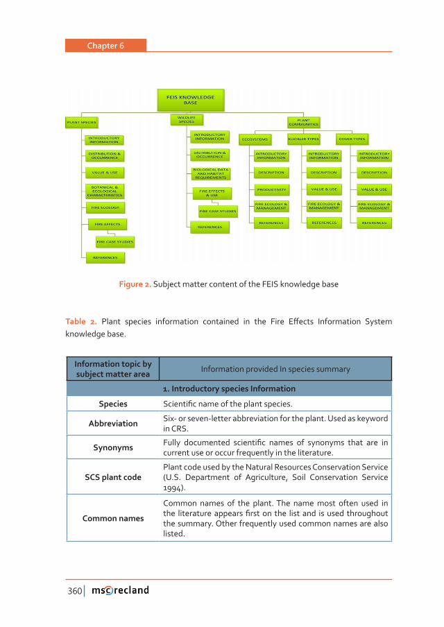
Chapter 6
360
Figure 2. Subject matter content of the FEIS knowledge base
Table 2. ������ �������� ������������ ���������� ��� ���� ���� �ơ����� ������������ �������knowledge base.
���������������������subject matter area Information provided In species summary
Ǥ���������������������������������
������� �������Ƥ���������������������������Ǥ
������������ Six- or seven-letter abbreviation for the plant. Used as keyword in CRS.
Synonyms ����� ����������� �������Ƥ�� ������ ��� ��������� ����� ���� ���current use or occur frequently in the literature.
��������������Plant code used by the Natural Resources Conservation Service (U.S. Department of Agriculture, Soil Conservation Service 1994).
Common names
Common names of the plant. The name most often used in ���� �������������������Ƥ������� ���� ��������� �������������������the summary. Other frequently used common names are also listed.
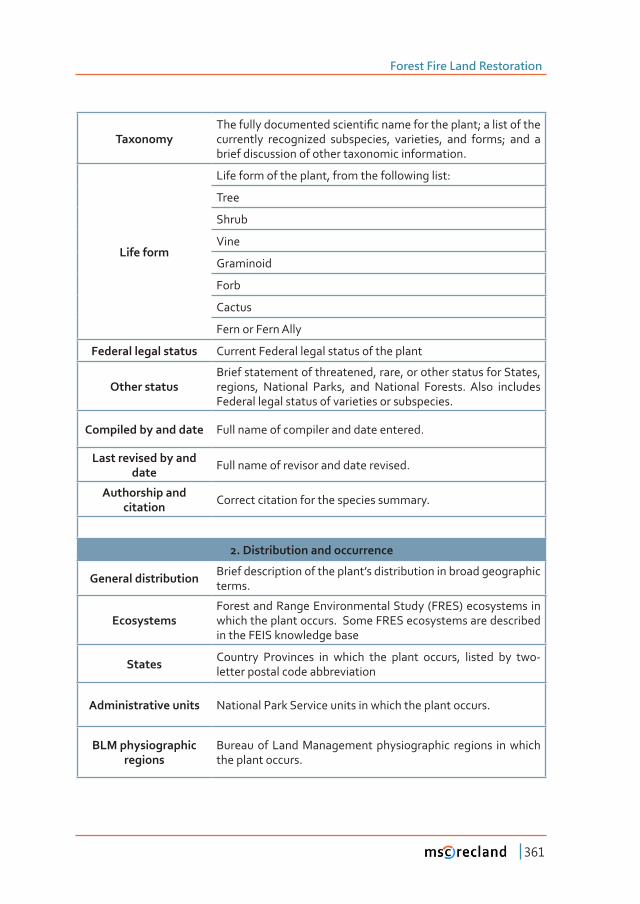
Forest Fire Land Restoration
361
Taxonomy����������������������������Ƥ��������������������Ǣ���������������currently recognized subspecies, varieties, and forms; and a brief discussion of other taxonomic information.
Life form
Life form of the plant, from the following list:
Tree
Shrub
Vine
Graminoid
Forb
Cactus
Fern or Fern Ally
Federal legal status Current Federal legal status of the plant
������������Brief statement of threatened, rare, or other status for States, regions, National Parks, and National Forests. Also includes Federal legal status of varieties or subspecies.
�������������������� Full name of compiler and date entered.
��������������������date Full name of revisor and date revised.
���������������citation Correct citation for the species summary.
2. Distribution and occurrence
General distribution Brief description of the plant’s distribution in broad geographic terms.
EcosystemsForest and Range Environmental Study (FRES) ecosystems in which the plant occurs. Some FRES ecosystems are described in the FEIS knowledge base
States Country Provinces in which the plant occurs, listed by two-letter postal code abbreviation
�������������������� National Park Service units in which the plant occurs.
������������������regions
Bureau of Land Management physiographic regions in which the plant occurs.
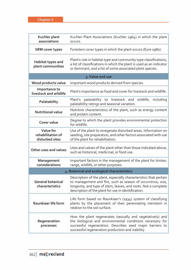
Chapter 6
362
��������������associations
Kuchler Plant Associations (Kuchler 1964) in which the plant occurs.
��������������� Foresters cover types in which the plant occurs (Eyre 1980).
�����������������������������������
�����ǯ������������������������������������������������Ƥ�������ǡ�����������������Ƥ���������������������������������������������������or dominant, and a list of some associated plant species.
3. Value and use
������������������� Important wood products derived from species.
������������������������������������ Plant’s importance as food and cover for livestock and wildlife.
Palatability Plant’s palatability to livestock and wildlife, including palatability ratings and seasonal variation.
����������������� Nutritive characteristics of the plant, such as energy content and protein content.
����������� Degree to which the plant provides environmental protection for wildlife.
Value for ������������������disturbed sites
Use of the plant to revegetate disturbed areas. Information on seeding, site preparation, and other factors associated with use of the plant for rehabilitation.
��������������������� Uses and values of the plant other than those indicated above, such as historical, medicinal, or food use.
Management considerations
Important factors in the management of the plant for timber, range, wildlife, or other purposes.
Ǥ�����������������������������������������
General botanical ���������������
Description of the plant, especially characteristics that pertain ������������������Ƥ��ǡ� �������� ��������������������ǡ� ����ǡ�longevity, and type of stem, leaves, and roots. Not a complete ������������������������������������������Ƥ������Ǥ
Raunkiaer life formLife form based on Raunkiaer’s (1934) system of classifying plants by the placement of their perennating meristem in relation to the soil surface.
Regeneration ���������
How the plant regenerates (sexually and vegetatively) and the biological and environmental conditions necessary for successful regeneration. Describes seed major barriers to successful regeneration production and viability.
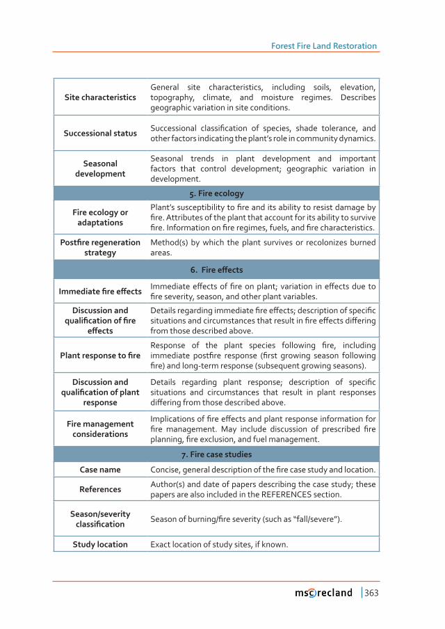
Forest Fire Land Restoration
363
��������������������General site characteristics, including soils, elevation, topography, climate, and moisture regimes. Describes geographic variation in site conditions.
Successional status ������������� ������Ƥ������� ��� �������ǡ� ������ ���������ǡ� ����other factors indicating the plant’s role in community dynamics.
Seasonal �����������
Seasonal trends in plant development and important factors that control development; geographic variation in development.
5. Fire ecology
Fire ecology or �����������
�����ǯ��������������������Ƥ���������������������������������������Ƥ��Ǥ�����������������������������������������������������������������Ƥ��Ǥ����������������Ƥ����������ǡ������ǡ�����Ƥ������������������Ǥ
����Ƥ����������������strategy
Method(s) by which the plant survives or recolonizes burned areas.
Ǥ�������ơ����
����������Ƥ����ơ���� �����������ơ��������Ƥ�����������Ǣ����������� ����ơ��������� ���Ƥ�����������ǡ�������ǡ��������������������������Ǥ
Discussion and �����Ƥ����������Ƥ���
�ơ����
����������������������������Ƥ����ơ����Ǣ���������������������Ƥ����������������������������������������������Ƥ����ơ�������ơ������from those described above.
������������������Ƥ����������� ��� ���� ������ �������� ���������� Ƥ��ǡ� �������������������� ����Ƥ��� ��������� ȋƤ���� �������� ������� ����������Ƥ��Ȍ���������Ǧ��������������ȋ��������������������������ȌǤ�
Discussion and �����Ƥ����������������
��������
�������� ���������� ������ ��������Ǣ� ������������ ��� �����Ƥ��situations and circumstances that result in plant responses ��ơ��������������������������������Ǥ
Fire management considerations
����������������Ƥ����ơ����������������������������������������Ƥ��� ����������Ǥ� ���� �������� ����������� ��� ����������� Ƥ�����������ǡ�Ƥ������������ǡ��������������������Ǥ
7. Fire case studies
Case name �������ǡ����������������������������Ƥ��������������������������Ǥ
References Author(s) and date of papers describing the case study; these papers are also included in the REFERENCES section.
������Ȁ���������������Ƥ������ �����������������ȀƤ������������ȋ��������Dz����Ȁ������dzȌǤ
Study location Exact location of study sites, if known.
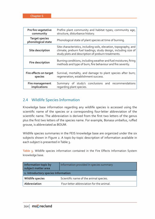
Chapter 6
364
����Ƥ��������������community
���Ƥ��� ������ ���������� ���� �������� �����Ǣ� ���������� ���ǡ�structure, disturbance history.
��������������������������������� Phonological state of plant species at time of burning.
����������������Site characteristics, including soils, elevation, topography, and climate; preburn fuel loadings; study design, including size of study plots and description of preburn treatments.
��������������� ������������������ǡ�������������������������������������Ǣ�Ƥ�����������������������������Ǣ�Ƥ�����������������Ƥ�����������Ǥ
�����ơ����������������������
Survival, mortality, and damage to plant species after burn; regeneration, establishment success.
Fire management ������������
Summary of study’s conclusions and recommendations regarding plant species.
2�4 Wildlife Species Information
Knowledge base information regarding any wildlife species is accessed using the �������Ƥ�� ����� ��� ���� �������� ��� �� �������������� ����Ǧ������� ������������� ��� �����������Ƥ������Ǥ������������������ ����������� ���������Ƥ���� ���� ����������� �������������������Ƥ�����������������������������������Ǥ�����������ǡ����������������ǡ���ơ���grouse, is abbreviated as BOUM.
Wildlife species summaries in the FEIS knowledge base are organized under the six subjects shown in Figure 2. A topic-by-topic description of information available in each subject is presented in Table 3.
Table 3. ��������� �������� ������������ ���������� ��� ���� ���� �ơ����� ������������ �������knowledge base.
���������������������subject matter area
Information provided In species summary
Ǥ���������������������������������
���������������� �������Ƥ����������������������������Ǥ
������������ Four-letter abbreviation for the animal.
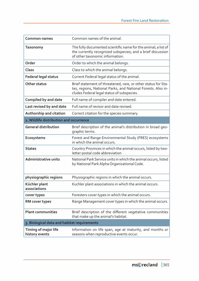
Forest Fire Land Restoration
365
Common names Common names of the animal.
Taxonomy ����������������������������Ƥ���������������������Ǣ�����������the currently recognized subspecies; and a brief discussion of other taxonomic information.
Order Order to which the animal belongs.
Class Class to which the animal belongs.
Federal legal status Current Federal legal status of the animal.
������������ Brief statement of threatened, rare, or other status for Sta-tes, regions, National Parks, and National Forests. Also in-cludes Federal legal status of subspecies.
�������������������� Full name of compiler and date entered.
������������������������ Full name of revisor and date revised.
����������������������� Correct citation for the species summary.
2. Wildlife distribution and occurrence
General distribution Brief description of the animal’s distribution in broad geo-graphic terms.
Ecosystems Forest and Range Environmental Study (FRES) ecosystems in which the animal occurs.
States Country Provinces in which the animal occurs, listed by two-letter postal code abbreviation
�������������������� National Park Service units in which the animal occurs, listed by National Park Alpha Organizational Code.
��������������������� Physiographic regions in which the animal occurs.
�����������associations
Kuchler plant associations in which the animal occurs.
����������� Foresters cover types in which the animal occurs.
�������������� Range Management cover types in which the animal occurs.
Plant communities ������ ������������ ��� ���� ��ơ������ ����������� ������������that make up the animal’s habitat.
Ǥ�����������������������������������������
Timing of major life ��������������
Information on life span, age at maturity, and months or seasons when reproductive events occur.
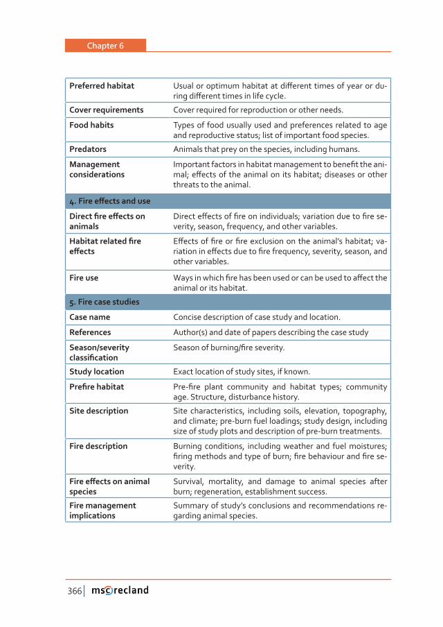
Chapter 6
366
����������������� ������������������������������ơ�������������������������-�������ơ�������������������������Ǥ�
������������������ Cover required for reproduction or other needs.
���������� Types of food usually used and preferences related to age and reproductive status; list of important food species.
Predators Animals that prey on the species, including humans.
Management considerations
�����������������������������������������������Ƥ���������-���Ǣ��ơ�������� �������������� �����������Ǣ�������������������threats to the animal.
Ǥ������ơ������������
�������Ƥ����ơ��������animals
��������ơ��������Ƥ�����������������Ǣ������������������Ƥ�����-verity, season, frequency, and other variables.
����������������Ƥ����ơ����
�ơ��������Ƥ������Ƥ��������������������������ǯ���������Ǣ���-������������ơ������������Ƥ������������ǡ���������ǡ�������ǡ�����other variables.
Fire use ��������������Ƥ������������������������������������ơ��������animal or its habitat.
5. Fire case studies
Case name Concise description of case study and location.
References Author(s) and date of papers describing the case study
������Ȁ���������������Ƥ������
�����������������ȀƤ�����������Ǥ
Study location Exact location of study sites, if known.
���Ƥ���������� ���ǦƤ��� ������ ���������� ���� �������� �����Ǣ� ����������age. Structure, disturbance history.
���������������� Site characteristics, including soils, elevation, topography, and climate; pre-burn fuel loadings; study design, including size of study plots and description of pre-burn treatments.
��������������� Burning conditions, including weather and fuel moistures; Ƥ�����������������������������Ǣ�Ƥ�����������������Ƥ�����-verity.
�����ơ����������������������
Survival, mortality, and damage to animal species after burn; regeneration, establishment success.
Fire management ������������
Summary of study’s conclusions and recommendations re-garding animal species.
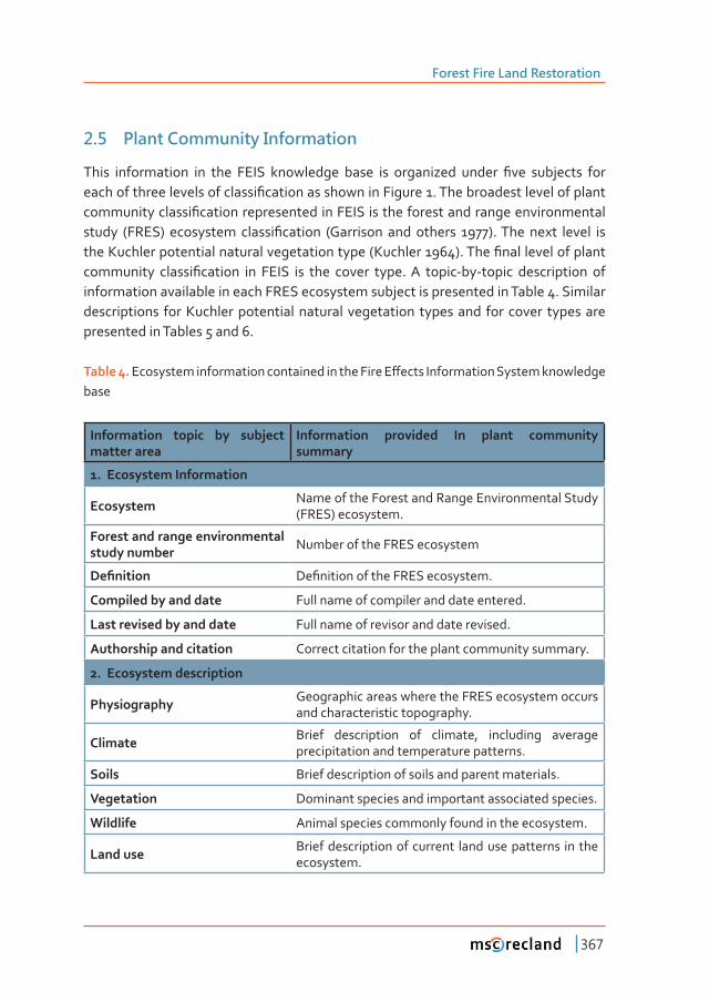
Forest Fire Land Restoration
367
2�5 Plant Community Information
����� ������������ ��� ���� ���� ���������� ����� ��� ���������� ������ Ƥ��� ��������� ����������������������������������Ƥ�������������������������Ǥ���������������������������������������������Ƥ���������������������������������������������������������������������� ȋ���Ȍ� ���������� ������Ƥ������� ȋ�������� ����������� ȌǤ����� ����� ������ �������������������������������������������������ȋ��������ȌǤ�����Ƥ����������������������������� ������Ƥ������� ��� ���� ��� ���� ������ ����Ǥ��� �����Ǧ��Ǧ������ ������������ ���information available in each FRES ecosystem subject is presented in Table 4. Similar descriptions for Kuchler potential natural vegetation types and for cover types are presented in Tables 5 and 6.
Table 4. ��������������������������������������������ơ����������������������������������base
������������ ������ ��� ��������matter area
������������ ��������� ��� ������ ����������summary
1. Ecosystem Information
Ecosystem Name of the Forest and Range Environmental Study (FRES) ecosystem.
������������������������������study number Number of the FRES ecosystem
��Ƥ������ ��Ƥ���������������������������Ǥ
�������������������� Full name of compiler and date entered.
������������������������ Full name of revisor and date revised.
����������������������� Correct citation for the plant community summary.
Ǥ�����������������������
������������ Geographic areas where the FRES ecosystem occurs and characteristic topography.
Climate Brief description of climate, including average precipitation and temperature patterns.
Soils Brief description of soils and parent materials.
Vegetation Dominant species and important associated species.
Wildlife Animal species commonly found in the ecosystem.
Land use Brief description of current land use patterns in the ecosystem.
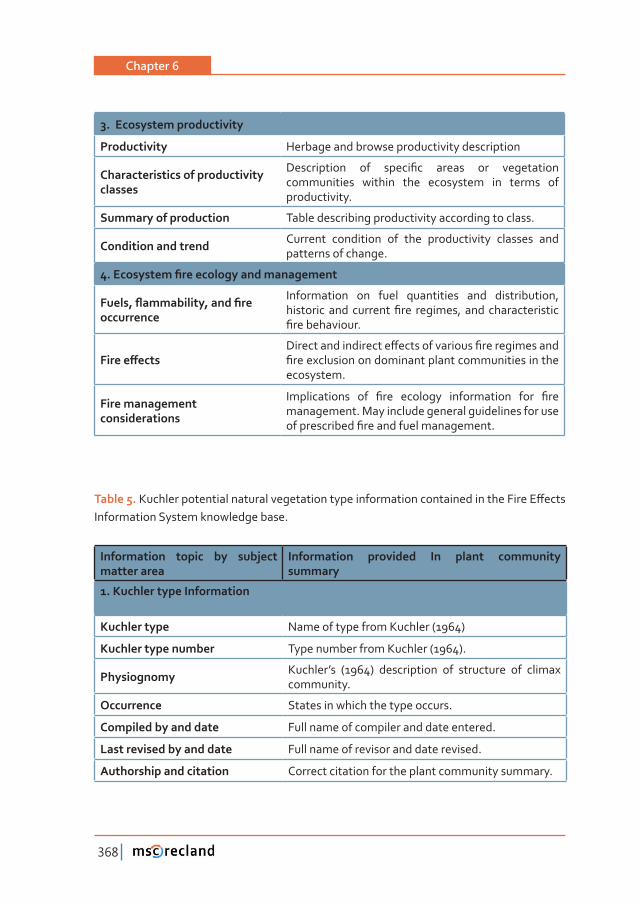
Chapter 6
368
Ǥ������������������������
������������ Herbage and browse productivity description
��������������������������������classes
������������ ��� �����Ƥ�� ������ ��� �����������communities within the ecosystem in terms of productivity.
��������������������� Table describing productivity according to class.
Condition and trend Current condition of the productivity classes and patterns of change.
Ǥ�����������Ƥ�������������������������
����ǡ�ƪ����������ǡ�����Ƥ���occurrence
Information on fuel quantities and distribution, ��������� ������������Ƥ��� �������ǡ� �������������������Ƥ������������Ǥ
�����ơ�������������������������ơ����������������Ƥ���������������Ƥ��������������������������������������������������ecosystem.
Fire management considerations
������������� ��� Ƥ��� �������� ������������ ���� Ƥ���management. May include general guidelines for use ��������������Ƥ����������������������Ǥ
Table 5. ����������������������������������������������������������������������������ơ�����Information System knowledge base.
������������ ������ ��� ��������matter area
������������ ��������� ��� ������ ����������summary
Ǥ�������������������������
������������ Name of type from Kuchler (1964)
������������������� Type number from Kuchler (1964).
����������� Kuchler’s (1964) description of structure of climax community.
Occurrence States in which the type occurs.
�������������������� Full name of compiler and date entered.
������������������������ Full name of revisor and date revised.
����������������������� Correct citation for the plant community summary.
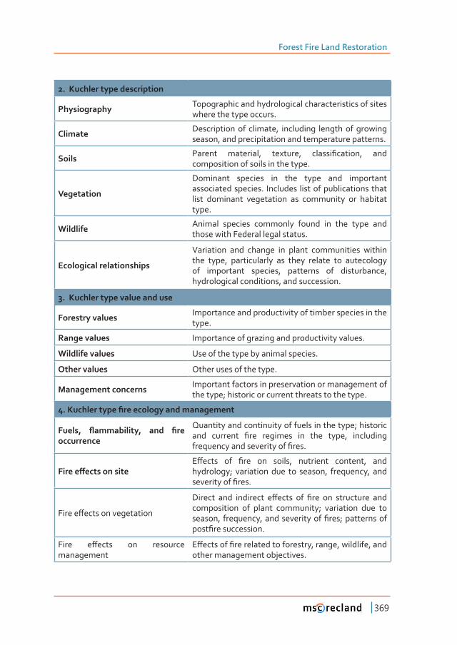
Forest Fire Land Restoration
369
Ǥ��������������������������
������������ Topographic and hydrological characteristics of sites where the type occurs.
Climate Description of climate, including length of growing season, and precipitation and temperature patterns.
Soils ������� ��������ǡ� �������ǡ� ������Ƥ������ǡ� ����composition of soils in the type.
Vegetation
Dominant species in the type and important associated species. Includes list of publications that list dominant vegetation as community or habitat type.
Wildlife Animal species commonly found in the type and those with Federal legal status.
������������������������
Variation and change in plant communities within the type, particularly as they relate to autecology of important species, patterns of disturbance, hydrological conditions, and succession.
Ǥ����������������������������
�������������� Importance and productivity of timber species in the type.
������������ Importance of grazing and productivity values.
��������������� Use of the type by animal species.
������������ Other uses of the type.
Management concerns Important factors in preservation or management of the type; historic or current threats to the type.
Ǥ��������������Ƥ�������������������������
����ǡ� ƪ����������ǡ� ���� Ƥ���occurrence
Quantity and continuity of fuels in the type; historic ���� �������� Ƥ��� �������� ��� ���� ����ǡ� ������������������������������������Ƥ���Ǥ
�����ơ�������������ơ����� ��� Ƥ��� ��� �����ǡ� ��������� �������ǡ� ����hydrology; variation due to season, frequency, and ������������Ƥ���Ǥ
�����ơ������������������
������� ���� ��������� �ơ����� ��� Ƥ��� ��� ���������� ����composition of plant community; variation due to ������ǡ� ���������ǡ�����������������Ƥ���Ǣ�����������������Ƥ�������������Ǥ
���� �ơ����� ��� ���������management
�ơ��������Ƥ����������������������ǡ������ǡ���������ǡ�����other management objectives.
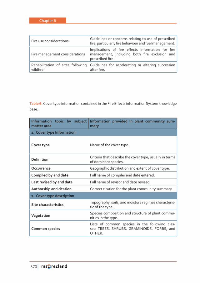
Chapter 6
370
Fire use considerations Guidelines or concerns relating to use of prescribed Ƥ��ǡ��������������Ƥ��������������������������������Ǥ
Fire management considerations������������� ��� Ƥ��� �ơ����� ������������ ���� Ƥ�������������ǡ� ���������� ����� Ƥ��� ���������� ���������������Ƥ��Ǥ
Rehabilitation of sites following ����Ƥ��
Guidelines for accelerating or altering succession ������Ƥ��Ǥ
Table 6. ���������������������������������������������ơ����������������������������������base.
������������ ������ ��� ��������matter area
������������ ��������� ��� ������ ���������� ���-mary
Ǥ������������������������
���������� Name of the cover type.
��Ƥ������ Criteria that describe the cover type; usually in terms of dominant species.
Occurrence Geographic distribution and extent of cover type.
�������������������� Full name of compiler and date entered.
������������������������ Full name of revisor and date revised.
����������������������� Correct citation for the plant community summary.
Ǥ������������������������
�������������������� Topography, soils, and moisture regimes characteris-tic of the type.
Vegetation Species composition and structure of plant commu-nities in the type.
��������������Lists of common species in the following clas-ses: TREES. SHRUBS. GRAMINOIDS. FORBS, and OTHER.
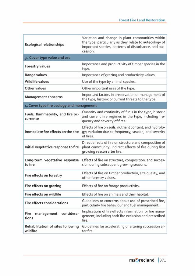
Forest Fire Land Restoration
371
������������������������
Variation and change in plant communities within the type, particularly as they relate to autecology of important species, patterns of disturbance, and suc-cession.
Ǥ��������������������������
�������������� Importance and productivity of timber species in the type.
������������ Importance of grazing and productivity values.
��������������� Use of the type by animal species.
������������ Other important uses of the type.
Management concerns Important factors in preservation or management of the type; historic or current threats to the type.
Ǥ������������Ƥ�������������������������
����ǡ�ƪ����������ǡ� ����Ƥ�����-currence
Quantity and continuity of fuels in the type; historic ���� �������� Ƥ��� �������� ��� ���� ����ǡ� ���������� ���-�����������������������Ƥ���Ǥ
����������Ƥ����ơ�����������������ơ��������Ƥ�����������ǡ�����������������ǡ������������-gy; variation due to frequency, season, and severity ���Ƥ���Ǥ
�������������������������������Ƥ����������ơ��������Ƥ��������������������������������������������������Ǣ� ����������ơ��������Ƥ����������Ƥ�������������������������Ƥ��Ǥ
����Ǧ����� ����������� ������������Ƥ��
�ơ��������Ƥ���������������ǡ������������ǡ�����������-sion during subsequent growing seasons.
�����ơ���������������� �ơ��������Ƥ�����������������������ǡ�������������ǡ�����other forestry values.
�����ơ��������������� �ơ��������Ƥ�������������������������Ǥ
�����ơ���������������� �ơ��������Ƥ�������������������������������Ǥ
�����ơ������������������� ����������������������������������������������Ƥ��ǡ��������������Ƥ��������������������������������Ǥ
Fire management considera-tions
����������������Ƥ����ơ���������������������Ƥ�������-������ǡ����������������Ƥ����������������������������Ƥ��Ǥ
������������������ ������ ��������������Ƥ��
Guidelines for accelerating or altering succession af-����Ƥ��Ǥ

Chapter 6
372
3 erosion control. postFire restoration treatments
3�1 Introduction
Slope protection and erosion control entail the integrated or conjunctive use of plants and structures. Plants can be introduced and established in and around ����������� �������ǡ� ������ ���� ��������� ��� Dz������ ������������dz� �������Ǥ� �������can be introduced, for example, on the benches of tiered retaining wall systems or, alternatively, they can be inserted and established in the interstices or frontal openings of porous revetments, cellular grids, and retaining structures. They can also be introduced in and around check dams.
3�2 Role and Function of Structural Components
Structural components of biotechnical earth support and slope protection systems must be capable of resisting external forces causing sliding, overturning, and bearing capacity failure. In addition these structures must resist internal forces that cause shear, compression, and bending stresses. In the case of revetments or slope armor �������ǡ� ���� ������ ������ ����� ����� ��ƥ������ ������� ���� ������������� ��� �������������������������������������������������������������������ƪ�����������Ǥ�
3�3 Retaining Structures
Retaining structures are designed to resist fairly large, lateral earth forces without excessive displacement or rotation. Gravity structures resist these external forces primarily as a result of their weight. Crib, gabion, cantilever, and reinforced earth walls are examples of gravity structures. Structures with porous faces or frontal openings lend themselves to vegetative treatment. Vegetation can also be introduced on the benches of tiered or stepped-back retaining structures (Figure 3).
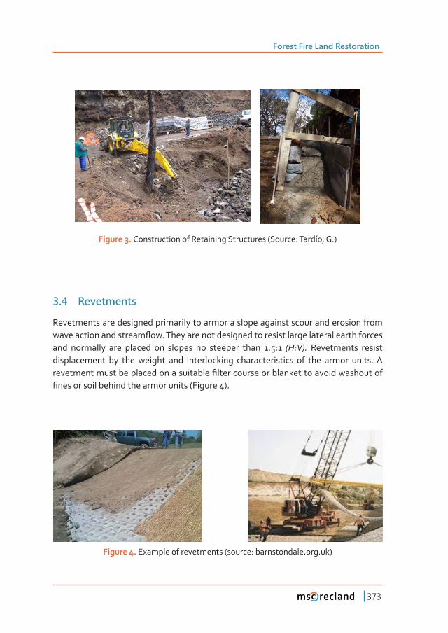
Forest Fire Land Restoration
373
Figure 3. Construction of Retaining Structures (Source: Tardío, G.)
3�4 Revetments
Revetments are designed primarily to armor a slope against scour and erosion from ����������������������ƪ��Ǥ������������������������������������������������������������and normally are placed on slopes no steeper than 1.5:1 ȋ�ǣ�ȌǤ�Revetments resist displacement by the weight and interlocking characteristics of the armor units. A ���������������������������������������Ƥ�������������������������������������������Ƥ�����������������������������������ȋ������ȌǤ
Figure 4. Example of revetments (source: barnstondale.org.uk)
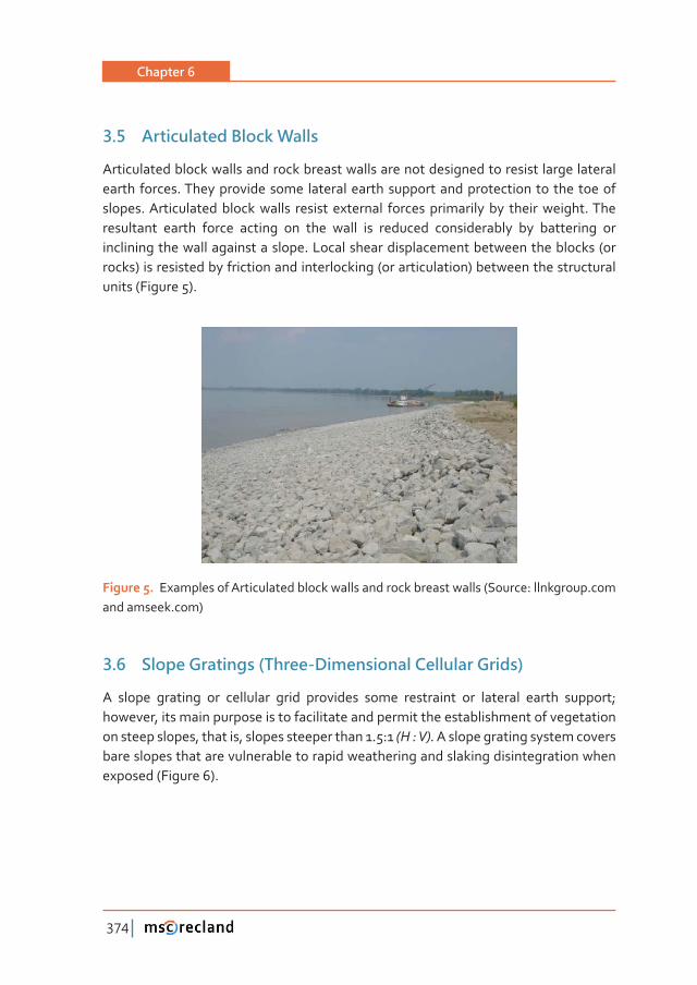
Chapter 6
374
3�5 Articulated Block Walls
Articulated block walls and rock breast walls are not designed to resist large lateral earth forces. They provide some lateral earth support and protection to the toe of slopes. Articulated block walls resist external forces primarily by their weight. The resultant earth force acting on the wall is reduced considerably by battering or inclining the wall against a slope. Local shear displacement between the blocks (or rocks) is resisted by friction and interlocking (or articulation) between the structural units (Figure 5).
Figure 5. Examples of Articulated block walls and rock breast walls (Source: llnkgroup.com and amseek.com)
3�6 Slope Gratings (Three-Dimensional Cellular Grids)
A slope grating or cellular grid provides some restraint or lateral earth support; however, its main purpose is to facilitate and permit the establishment of vegetation on steep slopes, that is, slopes steeper than 1.5:1�ȋ��ǣ��ȌǤ A slope grating system covers bare slopes that are vulnerable to rapid weathering and slaking disintegration when exposed (Figure 6).
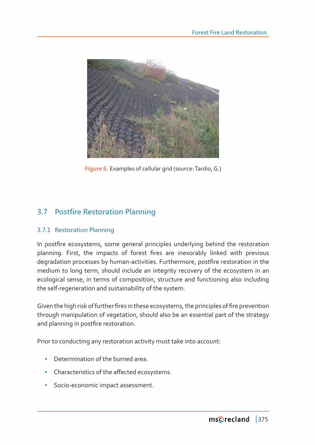
Forest Fire Land Restoration
375
Figure 6. Examples of cellular grid (source: Tardio, G.)
3�7 Postfire Restoration Planning
3�7�1 Restoration Planning
��� ����Ƥ��� ����������ǡ� ����� �������� ����������� ����������� ������� ���� ��������������������Ǥ� ����ǡ� ���� �������� ��� ������� Ƥ���� ���� ����������� ������� ����� ���������������������������������������Ǧ����������Ǥ�����������ǡ�����Ƥ����������������������medium to long term, should include an integrity recovery of the ecosystem in an ecological sense, in terms of composition, structure and functioning also including the self-regeneration and sustainability of the system.
������������������������������Ƥ�����������������������ǡ�������������������Ƥ��������������through manipulation of vegetation, should also be an essential part of the strategy ��������������������Ƥ��������������Ǥ
Prior to conducting any restoration activity must take into account:
• Determination of the burned area.
• ������������������������ơ����������������Ǥ
• Socio-economic impact assessment.
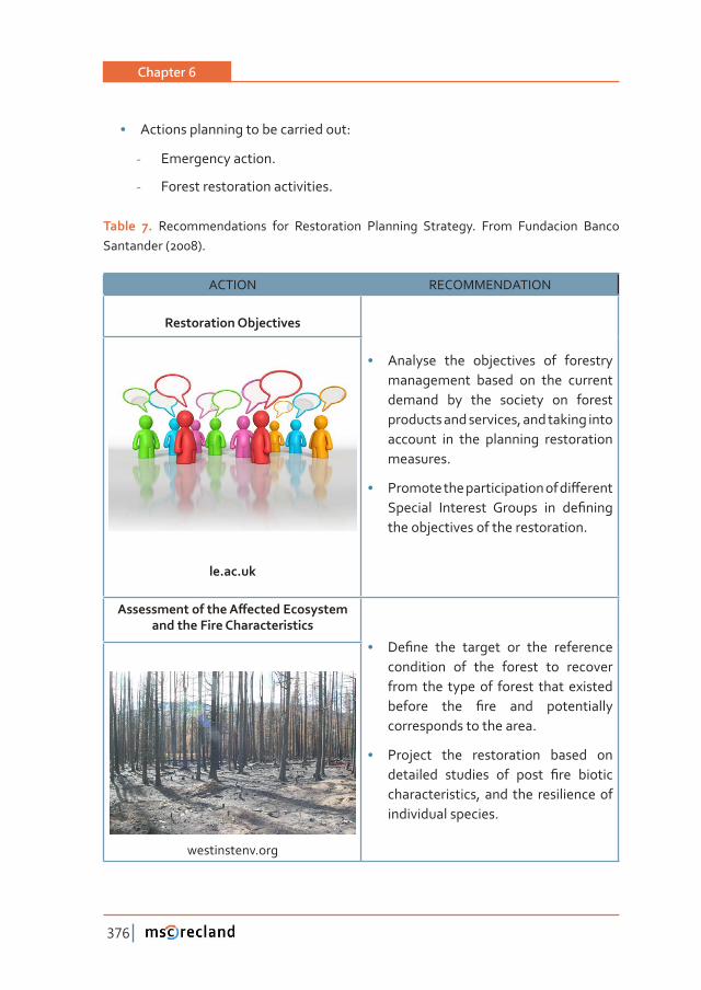
Chapter 6
376
• Actions planning to be carried out:
- Emergency action.
- Forest restoration activities.
Table 7. Recommendations for Restoration Planning Strategy. From Fundacion Banco Santander (2008).
ACTION RECOMMENDATION
����������������������
• Analyse the objectives of forestry management based on the current demand by the society on forest products and services, and taking into account in the planning restoration measures.
• �������������������������������ơ�������������� ��������� ������ ��� ��Ƥ�����the objectives of the restoration.
le.ac.uk
�������������������ơ�������������������������������������������
• ��Ƥ��� ���� ������� ��� ���� ����������condition of the forest to recover from the type of forest that existed ������� ���� Ƥ��� ���� ������������corresponds to the area.
• Project the restoration based on ��������� �������� ��� ����� Ƥ��� �������characteristics, and the resilience of individual species.
westinstenv.org
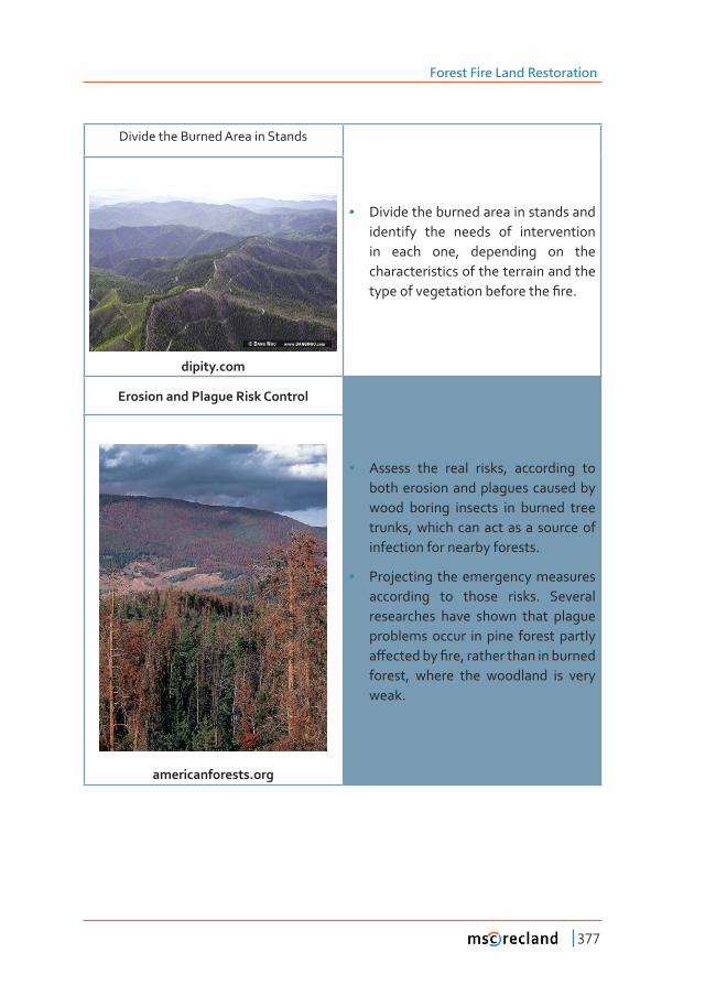
Forest Fire Land Restoration
377
Divide the Burned Area in Stands
• Divide the burned area in stands and identify the needs of intervention in each one, depending on the characteristics of the terrain and the ������������������������������Ƥ��Ǥ
������Ǥ���
Erosion and Plague Risk Control
• Assess the real risks, according to both erosion and plagues caused by wood boring insects in burned tree trunks, which can act as a source of infection for nearby forests.
• Projecting the emergency measures according to those risks. Several researches have shown that plague problems occur in pine forest partly �ơ���������Ƥ��ǡ�����������������������forest, where the woodland is very weak.
americanforests.org
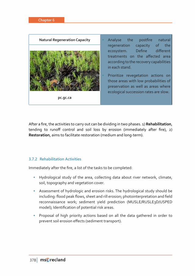
Chapter 6
378
����������������������������� • �������� ���� ����Ƥ��� ��������regeneration capacity of the ���������Ǥ� ��Ƥ��� ��ơ����������������� ��� ���� �ơ������ �����according to the recovery capabilities in each stand.
• Prioritize revegetation actions on those areas with low probabilities of preservation as well as areas where ecological succession rates are slow.
��Ǥ��Ǥ��
��������Ƥ��ǡ����������������������������������������������������������Ǥ�Ȍ���������������, �������� ��� ����ơ� �������� ���� ����� ����� ��� �������� ȋ������������ ������ Ƥ��Ȍǡ� Ȍ�Restoration, aims to facilitate restoration (medium and long-term).
3�7�2 Rehabilitation Activities
����������������������Ƥ��ǡ������������������������������������ǣ
• Hydrological study of the area, collecting data about river network, climate, soil, topography and vegetation cover.
• Assessment of hydrologic and erosion risks. The hydrological study should be ���������ǣ�ƪ���������ƪ���ǡ�����������������������Ǣ�������������������������Ƥ����reconnaissance work; sediment yield prediction (MUSLE/RUSLE3D/USPED �����ȌǢ�������Ƥ������������������������������Ǥ
• Proposal of high priority actions based on all the data gathered in order to ����������������������ơ�����ȋ������������������ȌǤ
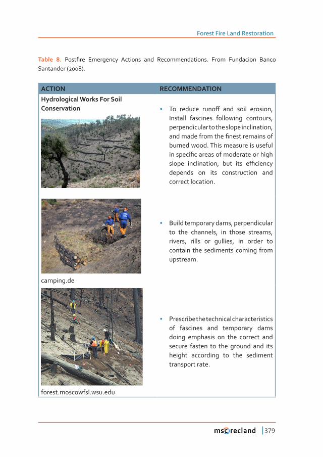
Forest Fire Land Restoration
379
Table 8. ����Ƥ��� ���������� �������� ���� ���������������Ǥ� ���� ��������� ������Santander (2008).
ACTION RECOMMENDATION
Hydrological Works For Soil ������������ • ���� ������� ����ơ� ���� ����� �������ǡ�
Install fascines following contours, perpendicular to the slope inclination, ������������������Ƥ����������������burned wood. This measure is useful ��������Ƥ���������������������������������� �����������ǡ� ���� ���� �ƥ�������depends on its construction and correct location.
camping.de
• Build temporary dams, perpendicular to the channels, in those streams, rivers, rills or gullies, in order to contain the sediments coming from upstream.
forest.moscowfsl.wsu.edu
• Prescribe the technical characteristics of fascines and temporary dams doing emphasis on the correct and secure fasten to the ground and its height according to the sediment transport rate.
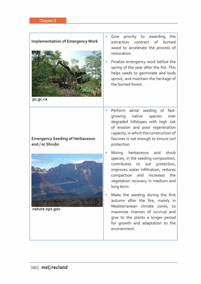
Chapter 6
380
��������������������������������
���Ǥ��Ǥ��
• Give priority to awarding the extraction contract of burned wood to accelerate the process of restoration.
• Finalize emergency work before the �����������������������������Ƥ��Ǥ������helps seeds to germinate and buds sprout, and maintain the heritage of the burned forest.
Emergency Seeding of Herbaceous ����Ȁ����������
�������Ǥ���Ǥ���
• Perform aerial seeding of fast-growing native species over degraded hillslopes with high risk of erosion and poor regeneration capacity, in which the construction of fascines is not enough to ensure soil protection.
• Mixing herbaceous and shrub species, in the seeding composition, contributes to soil protection, ��������� ������ ��Ƥ��������ǡ� ��������compaction and increases the vegetation recovery in medium and long term.
• ����� ���� �������� ������� ���� Ƥ����������� ������ ���� Ƥ��ǡ� ������� ���Mediterranean climate zones, to maximize chances of survival and give to the plants a longer period for growth and adaptation to the environment.
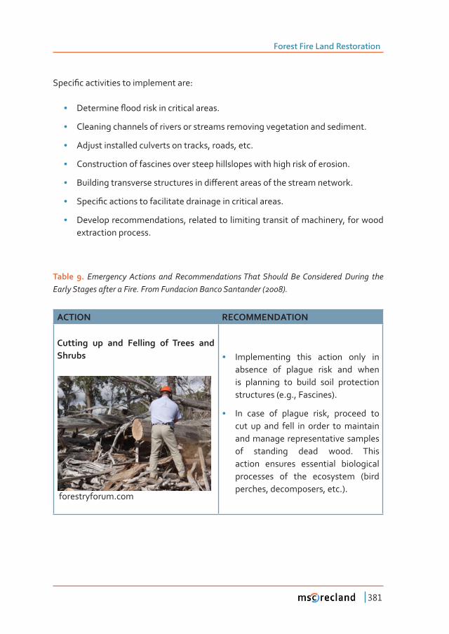
Forest Fire Land Restoration
381
�����Ƥ�����������������������������ǣ
• �����������ƪ��������������������������Ǥ
• �Cleaning channels of rivers or streams removing vegetation and sediment.
• �Adjust installed culverts on tracks, roads, etc.
• �Construction of fascines over steep hillslopes with high risk of erosion.
• �������������������������������������ơ���������������������������������Ǥ
• ������Ƥ��������������������������������������������������Ǥ
• �Develop recommendations, related to limiting transit of machinery, for wood extraction process.
Table 9. Emergency Actions and Recommendations That Should Be Considered During the ������������������������Ǥ������������������������������ȋȌǤ
ACTION RECOMMENDATION
�������� ��� ���� ������� ��� ������ ����������
forestryforum.com
• Implementing this action only in absence of plague risk and when is planning to build soil protection structures (e.g., Fascines).
• In case of plague risk, proceed to cut up and fell in order to maintain and manage representative samples of standing dead wood. This action ensures essential biological processes of the ecosystem (bird perches, decomposers, etc.).
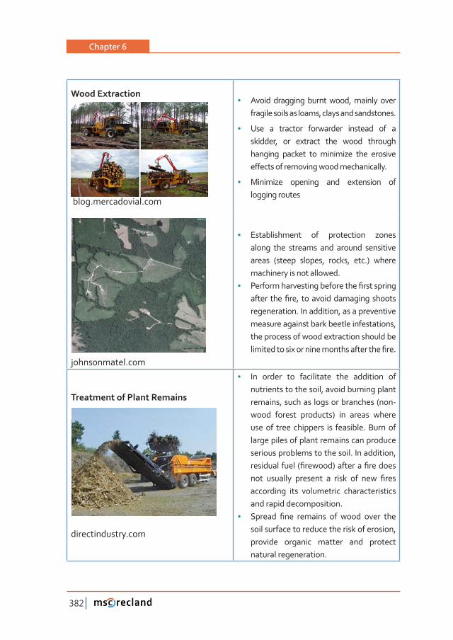
Chapter 6
382
Wood Extraction
blog.mercadovial.com
• Avoid dragging burnt wood, mainly over fragile soils as loams, clays and sandstones.
• Use a tractor forwarder instead of a skidder, or extract the wood through hanging packet to minimize the erosive �ơ����������������������������������Ǥ
• Minimize opening and extension of logging routes
johnsonmatel.com
• Establishment of protection zones along the streams and around sensitive areas (steep slopes, rocks, etc.) where machinery is not allowed.
• ������������������������������Ƥ����������������� ����Ƥ��ǡ� �������������������������regeneration. In addition, as a preventive measure against bark beetle infestations, the process of wood extraction should be ����������������������������������������Ƥ��Ǥ
Treatment of Plant Remains
directindustry.com
• In order to facilitate the addition of nutrients to the soil, avoid burning plant remains, such as logs or branches (non-wood forest products) in areas where use of tree chippers is feasible. Burn of large piles of plant remains can produce serious problems to the soil. In addition, ��������������ȋƤ������Ȍ���������Ƥ������������ �������� �������� �� ����� ��� ���� Ƥ����according its volumetric characteristics and rapid decomposition.
• ������� Ƥ��� �������� ��� ����� ����� ����soil surface to reduce the risk of erosion, provide organic matter and protect natural regeneration.
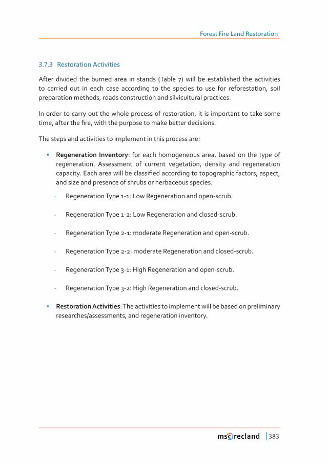
Forest Fire Land Restoration
383
3�7�3 Restoration Activities
After divided the burned area in stands (Table 7) will be established the activities to carried out in each case according to the species to use for reforestation, soil preparation methods, roads construction and silvicultural practices.
In order to carry out the whole process of restoration, it is important to take some ����ǡ�����������Ƥ��ǡ������������������������������������������Ǥ
The steps and activities to implement in this process are:
• ������������� ���������: for each homogeneous area, based on the type of regeneration. Assessment of current vegetation, density and regeneration ��������Ǥ�������������������������Ƥ�����������������������������������ǡ�������ǡ�and size and presence of shrubs or herbaceous species.
- Regeneration Type 1-1: Low Regeneration and open-scrub.
- Regeneration Type 1-2: Low Regeneration and closed-scrub.
- Regeneration Type 2-1: moderate Regeneration and open-scrub.
- Regeneration Type 2-2: moderate Regeneration and closed-scrub.
- Regeneration Type 3-1: High Regeneration and open-scrub.
- Regeneration Type 3-2: High Regeneration and closed-scrub.
• �����������������������: The activities to implement will be based on preliminary researches/assessments, and regeneration inventory.
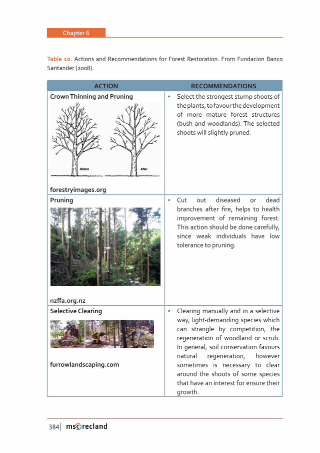
Chapter 6
384
Table 10. Actions and Recommendations for Forest Restoration. From Fundacion Banco Santander (2008).
ACTION RECOMMENDATIONS
��������������������������
forestryimages.org
• Select the strongest stump shoots of the plants, to favour the development of more mature forest structures (bush and woodlands). The selected shoots will slightly pruned.
Pruning
��ơ�Ǥ���Ǥ��
• Cut out diseased or dead ��������� ������ Ƥ��ǡ� ������ ��� �������improvement of remaining forest. This action should be done carefully, since weak individuals have low tolerance to pruning.
������������������
�����������������Ǥ���
• Clearing manually and in a selective way, light-demanding species which can strangle by competition, the regeneration of woodland or scrub. In general, soil conservation favours natural regeneration, however sometimes is necessary to clear around the shoots of some species that have an interest for ensure their growth.
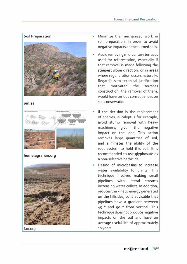
Forest Fire Land Restoration
385
����������������
um.es
• Minimize the mechanized work in soil preparation, in order to avoid negative impacts on the burned soils.
• Avoid removing mid-century terraces used for reforestation, especially if that removal is made following the steepest slope direction, or in areas where regeneration occurs naturally. ����������� ��� ���������� �����Ƥ�������that motivated the terraces construction, the removal of them, would have serious consequences on soil conservation.
����Ǥ��������Ǥ���
• If the decision is the replacement of species, eucalyptus for example, avoid stump removal with heavy machinery, given the negative impact on the land. This action removes large quantities of soil, and eliminates the ability of the root system to hold this soil. It is recommended to use glyphosate as a non-selective herbicide.
fao.org
• Desing of microbasins to increase water availability to plants. This technique involves making small pipelines with lateral streams increasing water collect. In addition, reduces the kinetic energy generated on the hillsides, so is advisable that pipelines have a gradient between 45 ° and 90 ° from vertical. This technique does not produce negative impacts on the soil and have an average useful life of approximately 10 years.
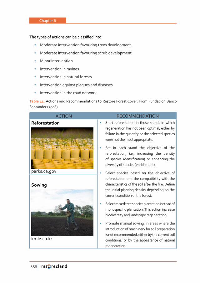
Chapter 6
386
����������������������������������Ƥ�������ǣ
• Moderate intervention favouring trees development
• Moderate intervention favouring scrub development
• Minor intervention
• Intervention in ravines
• Intervention in natural forests
• Intervention against plagues and diseases
• Intervention in the road network
Table 11. Actions and Recommendations to Restore Forest Cover. From Fundacion Banco Santander (2008).
ACTION RECOMMENDATIONReforestation
parks.ca.gov
• Start reforestation in those stands in which regeneration has not been optimal, either by failure in the quantity or the selected species were not the most appropriate.
• Set in each stand the objective of the reforestation, i.e., increasing the density ��� �������� ȋ�����Ƥ������Ȍ� ��� ���������� ����diversity of species (enrichment).
• Select species based on the objective of reforestation and the compatibility with the ��������������������������������������Ƥ��Ǥ���Ƥ���the initial planting density depending on the current condition of the forest.
• Select mixed tree species plantation instead of ���������Ƥ������������Ǥ����������������������biodiversity and landscape regeneration.
• Promote manual sowing, in areas where the introduction of machinery for soil preparation is not recommended, either by the current soil conditions, or by the appearance of natural regeneration.
������
kmle.co.kr
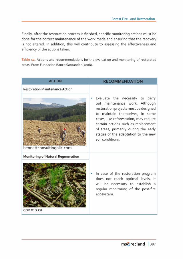
Forest Fire Land Restoration
387
������ǡ����������������������������������Ƥ������ǡ������Ƥ�����������������������������done for the correct maintenance of the work made and ensuring that the recovery ��� ���� �������Ǥ� ��� ��������ǡ� ����� ����� ����������� ��� ���������� ���� �ơ����������� �����ƥ���������������������������Ǥ
Table 12. Actions and recommendations for the evaluation and monitoring of restorated areas. From Fundacion Banco Santander (2008).
ACTION RECOMMENDATION
Restoration Maintenance Action
• Evaluate the necessity to carry out maintenance work. Although restoration projects must be designed to maintain themselves, in some cases, like reforestation, may require certain actions such as replacement of trees, primarily during the early stages of the adaptation to the new soil conditions.
bennettconsultingpllc.com
Monitoring of Natural Regeneration
• In case of the restoration program does not reach optimal levels, it will be necessary to establish a �������� ����������� ��� ���� ����ǦƤ���ecosystem.
gov.mb.ca
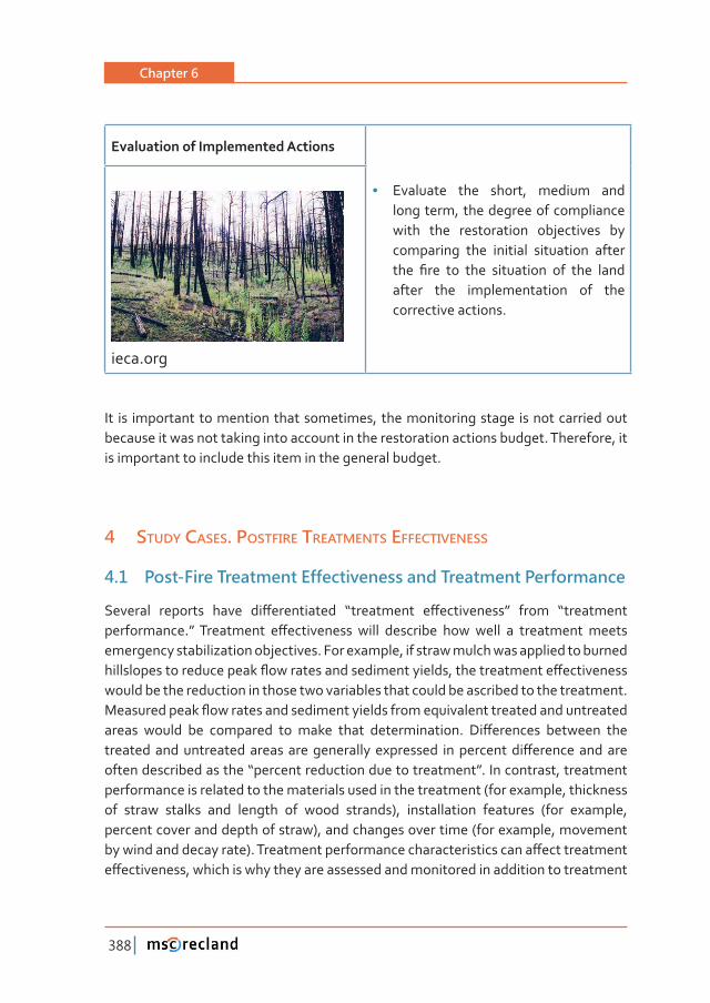
Chapter 6
388
���������������������������������
• Evaluate the short, medium and long term, the degree of compliance with the restoration objectives by comparing the initial situation after ���� Ƥ��� ��� ���� ���������� ��� ���� �����after the implementation of the corrective actions.
ieca.org
It is important to mention that sometimes, the monitoring stage is not carried out because it was not taking into account in the restoration actions budget. Therefore, it is important to include this item in the general budget.
4 study cases. postFire treatments eFFectiveness
4�1 Post-Fire Treatment Effectiveness and Treatment Performance
�������� �������� ����� ��ơ����������� Dz���������� �ơ����������dz� ����� Dz���������������������Ǥdz����������� �ơ����������� ����� ��������� ���� ����� �� ���������� ������emergency stabilization objectives. For example, if straw mulch was applied to burned ��������������������������ƪ����������������������������ǡ����������������ơ�����������would be the reduction in those two variables that could be ascribed to the treatment. ��������������ƪ������������������������������������������������������������������������� ������ ��� ��������� ��� ����� ����� �������������Ǥ� ��ơ�������� �������� �������������������������������� �������������� ���������� �������������ơ��������������������������������������Dz����������������������������������dzǤ������������ǡ�����������performance is related to the materials used in the treatment (for example, thickness of straw stalks and length of wood strands), installation features (for example, percent cover and depth of straw), and changes over time (for example, movement ����������������������ȌǤ��������������������������������������������ơ���������������ơ����������ǡ�����������������������������������������������������������������������
Forest Fire Land Restoration
389
�ơ����������Ǥ� �������ǡ� ���������� ���������� ���������� �ơ����������� ������������ȋ���������ǡ������������������ơǡ������ƪ���ǡ����Ȁ������������������Ȍ����������ƥ��������interpret when combined with measurements of treatment performance.
��������� ���� ����� ��� �������� ���������� �ơ����������� ���� ������� ����������ǡ��������������������������������������������Ƥ���������������������������������ơ������Ǥ��������������������������ơ����Ȁ���������������������������������������������������response research protocol and are generally expensive and labour-intensive. Such studies are challenging to fund and sustain over time. Nonetheless, quantitative �����������ơ������������������ƪ�������������������������Ǥ�
4�2 Hillslope Treatments
Hillslope treatments include grass seeding, contour-felled logs, mulch, and other �������� ��������� ��� ������� �������� ����ơ� ���� ����� ����Ƥ��� ����� ��� ������ ��� �������������Ǥ������� ����������� ���� ��������� ��� �� Ƥ���� ����� ��� �������� �������� ����Ƥ���sediment movement, preventing subsequent deposition in unwanted areas. Consequently, more research has been published on hillslope treatments than on other methods.
4�2�1 Broadcast Seeding
One of the most common restoration practices is broadcast seeding of grasses, �������� ����� ��������Ǥ� ����� �������� ������ Ƥ��� ���� ������ ������������ ���� �����practiced for decades, with the intent to gain useful products from land that will not return to timber production for many years. As an emergency treatment, rapid ���������������������������������������������� �������������Ǧ�ơ������������������������� ������ ��Ƥ�����������������ǡ�������������������������������������������������downstream areas. Grasses are particularly desirable for this purpose because their ���������ǡ� Ƥ������ ����� �������� ��������� ������ ��Ƥ��������� ���� ����� ����� ��� �����Ǥ�Fast-growing non-native species have typically been used. They are inexpensive and readily available in large quantities when an emergency arises.
Legumes are often added to seeding mixes for their ability to increase available ��������� ��� ���� ����� ������ ���� ����Ƥ��� ��������� ƪ���� ���� ����� ���������ǡ� ����������� ������� ��� ������� �������� ���� ������� ����������Ǥ����������������� ��Ƥ���� ����particular areas as germination and establishment success were evaluated. Most
Chapter 6
390
mixes contained annual grasses to provide quick cover and perennials to establish longer term protection. However, non-native species that persist can delay recovery ��� ������� ƪ���� ���� ������������ ������ ������ ������ ���������Ǥ� ��������� �������� �����recommended non-reproducing annuals, such as cereal grains or sterile hybrids that provide quick cover and then die out to let native vegetation reoccupy the site.
4�2�2 Conifer Forest
����� ����������Ƥ���������������������� ����������������������������� �������������������������������������������������������������Ƥ�����������������������������������Ǥ������������� ��������������������������������� �������������������������������Ƥ����������� ����� ������� ���� ����������� ��� ������ ������������� ��� ������� ������ ������ Ƥ��Ǥ�Seeding mixes used in conifer stands often include legumes such as Trifolium repens or �����������ƥ��������to enhance nitrogen status of the soil. Both annual and perennial grasses may be used in mixes with non-native forage species originally tested for range improvement purposes.
����������������������������������������������������������Ƥ��� ����������������������South Dakota (USA) in an area operationally seeded with a mixture of grasses and legumes. Most of the sediment production occurred in two summer storms shortly after erosion- measuring apparatus was set up. Sediment production was inversely ����������������������Ǥ������������������ơ��������������������������������������plant and litter cover than on those with sparse cover. Regression analysis showed ����� ������������� ��� ����ơ������������������������������ ���������������������������������ơ������������������ǡ���������������������������������Ǥ�
Seeded grasses provided greater cover than natural regeneration in a burned area in Oregon (USA). Litter and mulch also developed more rapidly on the seeded sites.
After 4 years, however, all sites had more than 70 percent ground cover. Legume species included in the seeding mix for wildlife forage generally did not survive. Seeded grasses appeared to suppress growth of native shrubs and annual forbs, ������������������������������������������������Ƥ��Ǥ�������������������������������Ǧ�ȋǤ������ǦȌ������������Ƥ�����������������Ƥ������������������Ǥ�
In contrast, another research measured negligible cover produced by seeded species on severely burned plots in Oregon (USA). Total vegetation cover was only 40 percent after 2 years even on lightly burned sites. It suggested that nitrogen fertilization might
Forest Fire Land Restoration
391
have improved vegetation growth. Earlier study found that grass vigor decreased 4 years after seeding along forest roads for erosion control, and re-fertilization in year ���Ǧ������������������������������������������Ǥ����������������Ƥ�������ǡ�������������various grasses and legumes and found that fertilization greatly increased initial cover of most species tested. Fertilization with 45 lb ac-1 (50 kg ha-1) drilled urea �����Ƥ��������������������������������������ǡ�������������������������������������ǡ�on granitic soil in Idaho (USA).
Seeding and fertilizer treatments were compared on separate watersheds in the ����������� ��������� ȋ���Ȍ� ������ �� Ƥ��� ������ �������� ���� ������� ������������������Ǥ�������������������������������������������������Ƥ����������������������������one third, from 5.6 percent on the unseeded watershed to 7.5 to 10.8 percent on the seeded watersheds. Seeded grasses made up 18 to 32 percent of total cover on seeded sites. Nitrate concentration in streams increased immediately after fertilizer application, but subsequently fertilized and unfertilized watersheds had similar stream �����������������Ǥ������������������ǡ���������������������������������������ƪ�������and debris torrents from treated and untreated watersheds alike. In the second year ������Ƥ��ǡ����������������������������������������Ǥ������������������������������Ǧshed and 16.4 to 23 percent on the seeded watersheds. Seeded grasses comprised about 7 percent cover on seeded watersheds. On south-facing slopes, the unseeded watershed had as much or more cover than the seeded ones.
�������������������������������������Ƥ�����������������Ƥ��ǡ����������������������grass present at the time major storms occur is more important than the amount present at the end of the growing season, when it is usually assessed in studies. In ����������������ȋ���Ȍǡ��������������������������������������������������������Ƥ�������increase plant cover or reduce erosion by early December, when that winter’s major ���������������Ǥ���������������� ��������������������������Ƥ������� ���������������������� ���� ��������� �����Ǥ� ������������ ���� ���� ���� �����Ƥ������� ��ơ������ ��������treatments, though it trended lower on the seeded plots. The research pointed out that timing of rainfall is critical to both grass establishment and erosion, and that ��ơ����������������������������������������������ơ����������������������������Ǥ�
�����������ǡ��������������������������������������������Ƥ���������������������������������������������Ƥ������������������������������������������Ƥ���ȋ���ȌǤ�������������������������������������������������������������������Ƥ��ǡ�������������������������������������������������������������Ǥ����������������ơ������� �����������������������������������������������������������������Ƥ���� �������������Ƥ��Ǥ��������������������
Chapter 6
392
���������������������������������������ơ���������������������������������������������������������������Ƥ���ȋ���ȌǤ�����������������������������������������������Ǥ�
��������������������������������������Ƥ����������ǡ�������������������������������and wide adaptability, have been found to be strongly competitive with conifer seedlings in experimental plots. Orchardgrass (Dactylis glomerata), perennial ryegrass (Lolium perenne), and timothy (Phleum pratense) reduced growth of ponderosa pine seedlings in tests conducted in California (USA). Orchardgrass and crested wheatgrass (Agropyron desertorum) reduced ponderosa pine growth in Arizona (USA). Field studies on aerial seeded sites in California found low pine seedling densities on most plots with annual ryegrass cover higher than 40 percent.
�� ��������� ��������� �����Ƥ������� ������ ��������� ��� �������� ������ ����� (Pinus lambertiana) seedlings in plots heavily seeded with annual ryegrass than in unseeded ��������������������Ƥ��������Ƥ�������� ������������������� ȋ���ȌǤ������������������������Ƥ������� ������ ���� ����� ���������� ������� �����Ƥ������� �������������� ������� ���the seeded plots. Ryegrass cover was 49 percent when tree seedlings were planted and 85 percent by mid-summer, while total plant cover was only 24 percent at mid-summer on the control plots. The next summer, a second group of planted pine �������������� �����Ƥ��������������� ��������� ���� ������������ ���������� �������������than on controls. By then, dead ryegrass formed a dense mulch on the seeded plots, ���� ��� ����� ������ ���� �����Ǥ� ������� ������ ������ ���� �����Ƥ������� �������� ��� ����unseeded plots the second year and soil moisture was lower. Ryegrass thus acted ��������������������������������������������������Ƥ���������������Ƥ��ǡ��������������������Ƥ��������������������������������������������������������������������Ǥ���������������������������������������������������������Ƥ�������������������������������it suppressed woody competitors and could itself later be controlled. In their study, however, live ryegrass cover was exceptionally high in many plots during the second �����������Ƥ��Ǥ�
���������� �������� ���� ����ơ� ��� ���������ǡ� �������ǡ� ���� �����Ǧ���������ǡ� ����few researchers have done it. Such research is necessary to determine if seeded �������� �������� �������� ������� ����� �������� ������������Ǥ��������� ����� ��� ����Ƥ���grass seeding on timber sites, soil fertility retention, does not appear to have been investigated. Grass establishment can clearly interfere with native plant growth, and grass varieties that will suppress native shrubs but not conifer seedlings have not yet been developed. The impacts of recent choices for rehabilitation seeding, including
Forest Fire Land Restoration
393
native grasses and cereal grains, on natural and planted regeneration in forest lands have not been studied extensively.
Another study found that rainfall intensity explained more than 80 percent of the variability in sediment yields. After the 2000 Bobcat Fire in Colorado (USA), a single storm with 30 min rainfall intensity of 42 mm hr-1 resulted in 370 kg ha-1 and 950 kg ha-1 sediment yields, on treated (erosion-control with contour log felling, grass seeding, and mulching) and untreated watersheds, respectively.
4�2�3 Mulch
Mulch is material spread over the soil surface to protect it from raindrop impact. Straw ���������������������������Ǥ�����Ǧ�ȋ������ǦȌ������Ƥ������������������������������on burned pine-shrub forest in Spain over an 18-month period with 46 rainfall events. Sediment production was 0.08 to 1.3 t ac-1 (0.18 to 2.92 Mg ha-1) on unmulched plots but only 0.04 to 0.08 t ac-1 (0.09 to 0.18 Mg ha-1) on mulched plots. Other research, tested straw mulch laid down at four rates—0.5, 1, 1.5, and 4 t ac-1 (1.1, 2.2, 3.4, and 9.0 Mg ha-1)—against jute excelsior, and paper for erosion control. Straw was the most ����Ǧ�ơ������������ǡ������������������������������������������������������������������������� �������Ǥ��������������� ������ơ������������������ ���������������������������yarn. The best erosion control came from jute applied over 1.5 t ac-1 (3.4 Mg ha-1) straw. Other researchers studied the use of wheat straw mulch on the 1987 South �������������������������Ƥ��ǡ�������Ǧ�������������������������������������ȋ���ȌǤ������������������������������� ���Ƥ��� ���������������� ������������� �������ǡ�Ƥ�������ǡ� ����areas of extreme erosion hazard. Mulch applied at rates of 2 t ac- 1 (4.5 Mg ha-1), or 1 t ac- 1 (2.2 Mg ha-1) on larger areas, reduced erosion 6 to 10 yd3 ac-1 (11 to 19 m3 ��ǦȌǤ����������������������������������������ơ�����������������������������Ǥ�����������������������������ơ�����������������������������������Ǥǡǡǡ�Ǥǡ�����Ǥ�����Ǧ��(2,4,6, and 8 Mg ha-1) on 5 to 9 percent slopes. Soil loss at 0.9 t ac-1 (2 Mg ha-1) mulch ���������Ƥ���������������ȋǤ�����Ǧǡ�Ǥ������Ǧ��������Ȍ���������Ǥ�����Ǧ�ȋ������ǦȌ�mulch (0.9 t ac-1, 1.81 Mg ha-1 of soil loss). Above 1.8 t ac-1 (4 Mg ha-1) mulch there was no further reduction in soil loss .
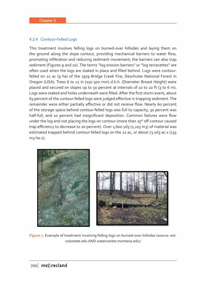
Chapter 6
394
4�2�4 Contour-Felled Logs
This treatment involves felling logs on burned-over hillsides and laying them on ���� ������� ������ ���� ������ �������ǡ� ��������������������� ��������� ��� ������ ƪ��ǡ�������������Ƥ���������������������������������������Ǣ�������������������������������������ȋ������������ȌǤ�����������Dz��������������������dz����Dz���������������dz������������������������������������������������������Ƥ�����������Ǥ������������������Ǧ�felled on 22 ac (9 ha) of the 1979 Bridge Creek Fire, Deschutes National Forest in Oregon (USA). Trees 6 to 12 in (150-300 mm) d.b.h. (Diameter Breast Height) were placed and secured on slopes up to 50 percent at intervals of 10 to 20 ft (3 to 6 m). �������������������������������������������Ƥ����Ǥ�����������Ƥ���������������ǡ������������������������������Ǧ�������������������������ơ���������������������������Ǥ��������������������������������������ơ��������������������������ƪ��Ǥ�����������������of the storage space behind contour-felled logs was full to capacity, 30 percent was ����Ǧ����ǡ� ���� � �������� ���� �������Ƥ����� ����������Ǥ� ������� ��������� ����� ƪ�����������������������������������������������������ȋ����������λ��ơ����������������������ƥ������������������������������ȌǤ������ǡ����ȋǡ��Ȍ�����������������estimated trapped behind contour-felled logs on the 22 ac, or about 73 yd3 ac-1 (135 m3 ha-1).
Figure 7. Example of treatment involving felling logs on burned-over hillsides (source: ext.colostate.edu AND watercenter.montana.edu)
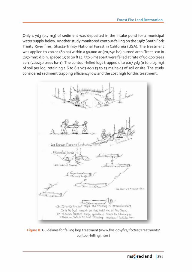
Forest Fire Land Restoration
395
Only 1 yd3 (0.7 m3) of sediment was deposited in the intake pond for a municipal water supply below. Another study monitored contour-felling on the 1987 South Fork ��������������Ƥ���ǡ�������Ǧ����������������������� �������������� ȋ���ȌǤ���������������was applied to 200 ac (80 ha) within a 50,000 ac (20,240 ha) burned area. Trees <10 in (250 mm) d.b.h. spaced 15 to 20 ft (4.5 to 6 m) apart were felled at rate of 80-100 trees ac-1 (200250 trees ha-1). The contour-felled logs trapped 0 to 0.07 yd3 (0 to 0.05 m3) of soil per log, retaining 1.6 to 6.7 yd3 ac-1 (3 to 13 m3 ha-1) of soil onsite. The study ������������������������������ƥ�����������������������������������������������Ǥ�
Figure 8. �������������������������������������ȋ���Ǥ���Ǥ���ȀƤ��Ȁ����Ȁ���Ȁ����������Ȁcontour-fellingi.htm )
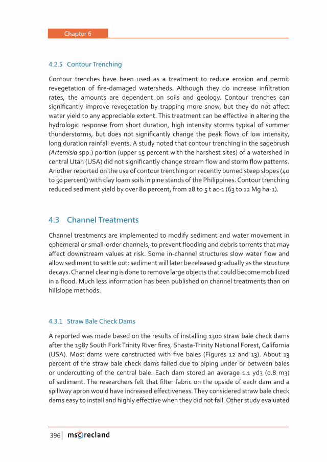
Chapter 6
396
4�2�5 Contour Trenching
Contour trenches have been used as a treatment to reduce erosion and permit ������������� ��� Ƥ��Ǧ�������� ����������Ǥ� ��������� ����� ��� ��������� ��Ƥ���������rates, the amounts are dependent on soils and geology. Contour trenches can �����Ƥ������� �������� ������������� ��� �������������� ����ǡ� ���� ����� ��� ���� �ơ�����������������������������������������Ǥ������������������������ơ�����������������������hydrologic response from short duration, high intensity storms typical of summer �������������ǡ� ���� ����� ���� �����Ƥ������� ������� ���� ����� ƪ���� ��� ���� ���������ǡ�long duration rainfall events. A study noted that contour trenching in the sagebrush (Artemisia spp.) portion (upper 15 percent with the harshest sites) of a watershed in �������������ȋ���Ȍ��������������Ƥ���������������������ƪ�������������ƪ�����������Ǥ�Another reported on the use of contour trenching on recently burned steep slopes (40 to 50 percent) with clay loam soils in pine stands of the Philippines. Contour trenching reduced sediment yield by over 80 percent, from 28 to 5 t ac-1 (63 to 12 Mg ha-1).
4�3 Channel Treatments
Channel treatments are implemented to modify sediment and water movement in ������������������Ǧ��������������ǡ������������ƪ�������������������������������������ơ������������������������� ����Ǥ������ ��Ǧ�������� ����������� �����������ƪ�������allow sediment to settle out; sediment will later be released gradually as the structure decays. Channel clearing is done to remove large objects that could become mobilized �����ƪ���Ǥ������������������������������������������������������������������������hillslope methods.
4�3�1 Straw Bale Check Dams
A reported was made based on the results of installing 1300 straw bale check dams �����������������������������������Ƥ���ǡ�������Ǧ����������������������ǡ������������ȋ���ȌǤ������ ���������� ����������������� Ƥ��� ������ ȋ������� � ���� ȌǤ������� �percent of the straw bale check dams failed due to piping under or between bales or undercutting of the central bale. Each dam stored an average 1.1 yd3 (0.8 m3) �����������Ǥ���������������������������Ƥ���������������������������������������������������������������������������������ơ����������Ǥ�������������������������������������������������������������������ơ�����������������������������Ǥ�����������������������
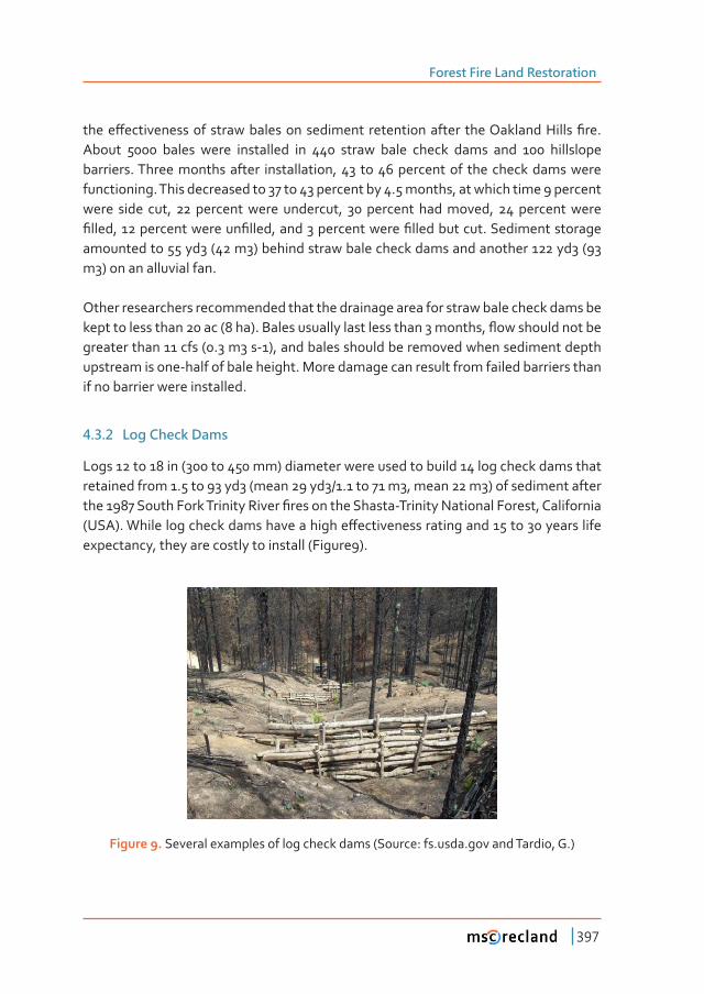
Forest Fire Land Restoration
397
�����ơ�������������� ������������������������ ���������������� ������������������Ƥ��Ǥ�About 5000 bales were installed in 440 straw bale check dams and 100 hillslope barriers. Three months after installation, 43 to 46 percent of the check dams were functioning. This decreased to 37 to 43 percent by 4.5 months, at which time 9 percent were side cut, 22 percent were undercut, 30 percent had moved, 24 percent were Ƥ����ǡ�����������������Ƥ����ǡ�������������������Ƥ������������Ǥ������������������amounted to 55 yd3 (42 m3) behind straw bale check dams and another 122 yd3 (93 m3) on an alluvial fan.
Other researchers recommended that the drainage area for straw bale check dams be ����������������������ȋ���ȌǤ�������������������������������������ǡ�ƪ�����������������greater than 11 cfs (0.3 m3 s-1), and bales should be removed when sediment depth upstream is one-half of bale height. More damage can result from failed barriers than if no barrier were installed.
4�3�2 Log Check Dams
Logs 12 to 18 in (300 to 450 mm) diameter were used to build 14 log check dams that retained from 1.5 to 93 yd3 (mean 29 yd3/1.1 to 71 m3, mean 22 m3) of sediment after �����������������������������Ƥ�����������������Ǧ����������������������ǡ������������ȋ���ȌǤ�����������������������������������ơ��������������������������������������expectancy, they are costly to install (Figure9).
Figure 9. Several examples of log check dams (Source: fs.usda.gov and Tardio, G.)
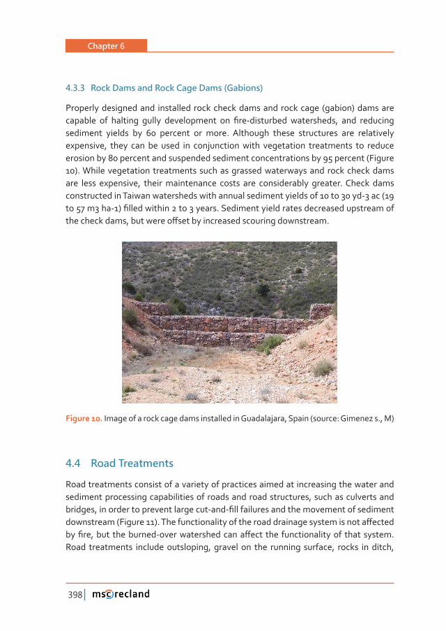
Chapter 6
398
4�3�3 Rock Dams and Rock Cage Dams (Gabions)
Properly designed and installed rock check dams and rock cage (gabion) dams are �������� ��� �������� ������ ������������ ��� Ƥ��Ǧ���������� ����������ǡ� ���� ���������sediment yields by 60 percent or more. Although these structures are relatively expensive, they can be used in conjunction with vegetation treatments to reduce erosion by 80 percent and suspended sediment concentrations by 95 percent (Figure 10). While vegetation treatments such as grassed waterways and rock check dams are less expensive, their maintenance costs are considerably greater. Check dams constructed in Taiwan watersheds with annual sediment yields of 10 to 30 yd-3 ac (19 ��������ǦȌ�Ƥ����������������������Ǥ����������������������������������������������������������ǡ�����������ơ������������������������������������Ǥ�
Figure 10. Image of a rock cage dams installed in Guadalajara, Spain (source: Gimenez s., M)
4�4 Road Treatments
Road treatments consist of a variety of practices aimed at increasing the water and sediment processing capabilities of roads and road structures, such as culverts and �������ǡ������������������������������Ǧ���ǦƤ����������������������������������������������������ȋ������ȌǤ�������������������������������������������������������ơ���������Ƥ��ǡ����� ����������Ǧ��������������������ơ���� ���� ����������������� �����������Ǥ�Road treatments include outsloping, gravel on the running surface, rocks in ditch,
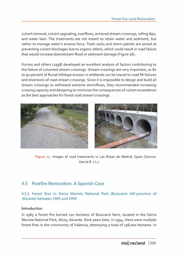
Forest Fire Land Restoration
399
���������������ǡ������������������ǡ�����ƪ���ǡ�������������������������ǡ�������������ǡ�and water bars. The treatments are not meant to retain water and sediment, but rather to manage water’s erosive force. Trash racks and storm patrols are aimed at preventing culvert blockages due to organic debris, which could result in road failure �������������������������������ƪ�����������������������ȋ������ȌǤ�
Furniss and others (1998) developed an excellent analysis of factors contributing to the failure of culverted stream crossings. Stream crossings are very important, as 80 ���������������ƪ�����������������������������������������������������������Ƥ������������and diversions of road-stream crossings. Since it is impossible to design and build all ����������������� ��������������������������ƪ���ǡ� ����� ������������ �����������crossing capacity and designing to minimize the consequences of culvert exceedence as the best approaches for forest road stream crossings.
Figure 11. Images of road treatments in Las Rozas de Madrid, Spain (Source: Garcia R. J.L.)
4�5 Postfire Restoration� A Spanish Case
4�5�1 Forest fires in Sierra Mariola National Park (Buixcarró Hill-province of Alicante) between 1985 and 1994
Introduction
��� � �� ������� Ƥ��� ������� � ��������� ��� ��������×� ����ǡ� �������� ��� ���� �������Mariola National Park, Alcoy, Alicante. Nine years later, in 1994, there were multiple �������Ƥ��������������������������������ǡ�����������������������ǡ���������Ǥ� ���
Chapter 6
400
���������ǡ����������������������������Ƥ���������ơ������ ǡ���������Ǥ� ǡ����������15,000 correspond to Sierra de Mariola and 420 to Buixcarró farm.
Forest condition before the fire
������� ����Ƥ��� ������������� ����������������� �����Ƥ����������������������� ��� �������������� ��� ����� ��������� ���� ������������ ���� ������ ����� ��ơ������ ��������Ǥ�����zones of shades were characterized by the existence of mature sclerophyll forests ���������������������������ǡ�����������������������������������������ȋƤ������ȌǤ�
The zones of sunlight were characterized by coniferous forests like Aleppo pine and heliophilous scrub, dominated by esparto and rosemary.
Restoration plan: Emergency actions implemented
Approval of a plan restricting big game hunting for adequate control of the population of herbivores, in order not to exceed the land carrying capacity.
In order to facilitate the addition of nutrients to the soil, plants remains were chipped and animal traction was used for wood extraction, avoiding the proliferation of drillers and leaving at least 2 percent of the standing burned trees with low degradation, to ensure essential biological processes of the ecosystem (bird perches, decomposers, etc.).
Forestry Management Plan 2003-2013: Depending on land characteristics and the priority of intervention, establishing a restoration plan for the next ten years. Until ǡ��������������������������������������������Ƥ��������������������������Ǥ�
Measures to encourage natural regeneration
• Selective bush clearings, around regenerated trees and species like junipers, hawthorns or kermes.
• Clearing, pruning and crown thinning to achieve viability in regeneration densities. In stands with densities of 6,000 to 8,000 trees per hectare, practiced clearing to reach densities of 800 to 1,000 trees per hectare, with the purpose to later select those trees with the fastest growing or better adaptation to the environment.
• Use of beekeeping with the purpose of promoting pollination and increase the production of viable seeds.
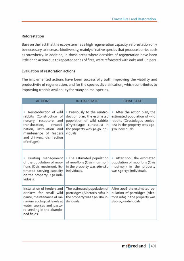
Forest Fire Land Restoration
401
Reforestation
Base on the fact that the ecosystem has a high regeneration capacity, reforestation only be necessary to increase biodiversity, mainly of native species that produce berries such as strawberry. In addition, in those areas where densities of regeneration have been ����������������������������������������������Ƥ���ǡ���������������������������������������Ǥ�
Evaluation of restoration actions
The implemented actions have been successfully both improving the viability and ����������������������������ǡ����������������������������Ƥ������ǡ����������������������improving trophic availability for many animal species.
ACTIONS INITIAL STATE FINAL STATE
• Reintroduction of wild rabbits (Construction of nursery, recapture and translocation, revacci-nation, installation and maintenance of feeders and drinkers, disinfection of refuges).
• Previously to the reintro-duction plan, the estimated population of wild rabbits (Oryctolagus cuniculus) in the property was 30-50 indi-viduals.
• After the action plan, the estimated population of wild rabbits (Oryctolagus cunicu-lus) in the property was 250-320 individuals
• Hunting management of the population of mou-ƪ���� ȋ������������ȌǤ� ��-timated carrying capacity on the property: 150 indi-viduals.
• The estimated population ������ƪ����ȋ������������Ȍ�in the property was 160-180 individuals.
• After 2006 the estimated �����������������ƪ����ȋ�����musimon) in the property was 150-170 individuals.
Installation of feeders and drinkers for small wild game, maintenance of mi-nimum ecological levels at water sources and pastu-re-seeding in the abando-����Ƥ����Ǥ
The estimated population of partridges (Alectoris rufa) in the property was 250-280 in-dividuals.
After 2006 the estimated po-pulation of partridges (Alec-toris rufa) in the property was 480-550 individuals.
Chapter 6
402
Silvicultural treatments (Selective Clearing, Crown Thinning, Pruning, remo-val of burned trees, etc.).
Important regeneration of slow growing species. Trea-ted area until 2007: 118 ha.
Increase of average diameter of oaks:•����������������ǣ�ά•������������������ǣ�ά• Increase of trees height:• In treated Area: 45 cm• In untreated: 28 cm
REFERENCES
�����ǡ� Ǥ��ǤǢ������ǡ� Ǥ��Ǥǡ����Ǥ�ȋȌǤ����������Ƥ����������������ǣ��ơ��������Ƥ������ƪ���Ǥ���ǤTech. Rep. RMRS-GTR-42-vol.2. Ogden, UT: U.S. Department of Agriculture, Forest Service, Rocky Mountain Research Station. 257 pp.
Clinton, B.D., and Vose J.M. (2000). Plant succession and community restoration following felling and burning in the Southern Appalachian Mountains. pp. 22-29 in W.K. Moser, and C.F. Mo-ser (eds.), Fire and forest ecology: innovative silviculture and vegetation management; Tall ��������Ƥ���������������������������������ǡ���Ǥ�Ǣ��������ǦǢ������������ǡ��ǣ������Timbers Research Station.
������ǡ��ǤǤǡ��ǤǤ������ǡ������ǤǤ���������Ǥ�ȋȌǤ����ǯ���ơ������������������Ǥ���������ǣ� ����Wiley & Sons, Inc. 333 pp.
Eyre, F. H., ed. (1980). Forest cover types of the United States and Canada. Washington, DC: So-ciety of American Foresters. 148 pp.
Fischer, W. C., Miller, M., Johnston, C. M., Smith, J. K., Simmerman D. G., Brown, J. K. (1996). Fire �ơ�����������������������ǣ�����ǯ������Ǥ��Ǥ�Ǥ��������������������������Ǥ
Fundación Banco Santander (2008). Manuales de Desarrollo Sostenible. Criterios de restauración de Zonas incendiadas. España. 50 p (In spanish)
Furniss, M.J., T.S. Ledwith, M.A. Love, B. McFadin, S.A. Flanagan. (1998). Response of roads-�������������������������ƪ������������������������ǡ�������ǡ������������������������Ǥ�����Forest Service. Technology and Development Program. 14 pp.
Garrison, G. A.; Bjugstad, A. J.; Duncan, D. A. (1977). Vegetation and environmental features of forest and range ecosystems. Agric. Handbook. 475. Washington, DC: U.S. Department of Agriculture, Forest Service. 68 pp.
Gray D. H., Sotir R. B. (1996). Biotechnical and soil bioengineering slope stabilization: a practical guide for erosion control. Wiley-IEEE. pp 378.
Heinselman, M. L. (1978). Fire in wilderness ecosystems. In: Hendee, John C.; Stankey,George H.;Lucas,Robert C. Wilderness management.Misc.Pub.No.1365. Washington,DC: U.S. De-partment of Agriculture,Forest Service: 249-278.
Hungerford, R.D. (1996). Soils. Fire in Ecosystem Management Notes: Unit II-I. USDA Forest Ser-vice, National Advanced Resource Technology Center, Marana, Arizona.
Kilgore, B. M. (1981). Fire in ecosystem distribution and structure: western forests and scru-blands. In: Mooney, H. A.; Bonnicksen, T. M.; Christensen, N. L.; Lotan, J. E.; Reiners, R. A.,
Forest Fire Land Restoration
403
tech. coords , eds. Fire regimes and ecosystem properties: proceedings of the conferen-ce. 1978 December 11-15; Honolulu, HI. Gen. Tech. Rep. WO-26. Washington DC: U.S. De-partment Agriculture, Forest Service: 58-89.
Kuchler, A. W. (1964). Potential natural vegetation of the conterminous United States. Spec. Publ. 36. New York: American Geographical Society.
������ Ǥ�ȋȌ����������������������������Ƥ��Ǧ�����������������������������Ǥ������������������-��������������������ǣ�����Ƥ����������Ƥ����������������������ǡ�������ǡ�ȂǤ
Lyon, J. L.; Stickney, P. F. (1976). Early vegetal succession following large Northern Rocky Mou-����������Ƥ���Ǥ���ǣ�����������������������������Ƥ��������������������������Ƥ�����������Ǣ�1974 October 8-10; Missoula, MT. Tallahassee, FL: Tall Timber Research Station: 355-375.
�������Ǥ�Ǥǡ�����������Ǥ��Ǥǡ���������Ǥ�Ǥǡ�����������Ǥ�Ǥ�ȋȌǤ������ơ��������������������������-nability: a review and synthesis. Forest Ecology and Management 122 51-71
�����ǡ��Ǥ�ǤǢ�����ǡ��Ǥ��ǤǢ�������ǡ��Ǥ�Ǥǡ����Ǥ�ȋȌǤ����������Ƥ����������������ǣ��ơ��������Ƥ������soils and water. Gen. Tech. Rep. RMRS-GTR-42-vol.4. Ogden,UT: U.S. Department of Agricul-ture, Forest Service, Rocky Mountain Research Station. 250 pp.
�����ơǡ��Ǥ��ǤǢ���������ǡ��Ǥ��Ǥ�ȋȌǤ�����Ƥ���������������������������ǣ�����������������������-tial impacts on reforestation. In: Proceedings, ninth annual forest vegetation management conference, November 3-5, 1987. Redding, CA: Forest Vegetation Management Conference: 111-123.
Raunkiær, C. (1934) The Life Forms of Plants and Statistical Plant Geography. Introduction by A.G. Tansley. Oxford University Press, Oxford. 632 pp.
Robichaud, P.R.; Brown, R.E. (1999). Measuring Rill Erosion Rates in a Steep Forest Environment. Presented at the 1999 American Geophysical Union Spring Meeting, June 1-4, Boston, MA. Poster.
���������ǡ��Ǥ�Ǥ� Ǥ� ���� �ơ����� ��� ��Ƥ��������� ������ ������ �����������Ƥ��� ������������������Mountains, USA. Journal of Hydrology 231-232: 220-229.
���������ǡ��Ǥ�Ǥǡ� Ǥ�Ǥ�������ǡ������ǤǤ������Ǥ�ȋȌǤ�����������������ơ������������������Ƥ�����-habilitation treatments. USDA Forest Service, Rocky Mountain Research Station, Gen. Tech. Rep. RMRS-GTR-63, Fort Collins, CO. 85 pp
���������ǡ��Ǥ��ǤǢ�������ǡ��Ǥ���Ǣ�����ǡ��Ǥ��Ǥ�ȋȌǤ�����ǦƤ��������������ơ�������������������������stabilization Gen. Tech. Rep RMRS-GTR-240 Fort Collins. CO: U.S. Department of Apiculture. Forest Service. Reeky Mountain Research Station. 62 pp.
Schiechtl H. M., Stern R., Barker D. H. (1996). Ground bioengineering techniques for slope protec-tion and erosion control. Blackwell Science. pp 146.
Schiechtl H. M. (1986). FAO Watershed Management Field Manual: Vegetative and soil treatment measures (13/1). Food and Agriculture Organization of the United Nations, 59 pp.
���ƪ��ǡ��Ǥ��Ǥǡ���Ǥ� ȋȌǤ����������������� ��������� �����������������Ǥ�������ǡ���ǣ��������� ����Range Management. 152 pp.
��������ǡ�������Ǥ�ȋȌǤ������������������������������������������������������������Ƥ��ǡ����-thern Idaho. Ogden, UT: U.S. Department of Agriculture, Forest Service, Intermountain Fo-rest and Range Experiment Station: 26 pp.
���������Ǥ�ȋȌǤ�����������×���������������������������Ǥ���������À�������Ƥ����ǡ���������-tura en Ciencias Ambientales, Universidad Politécnica de Madrid. (In spanish-Unpublished)
Chapter 6
404
Links
������ǡ��Ǥ�ȋȌǤ���������������������ǡ�Dz���dz�����Dz���ǯ��Ǥ��������������������������������-tion Service.
http://www.co.santa-cruz.ca.us/FIREDosDontsRESTORATION09.pdf�����ǡ��������ǤǢ�����ǡ��������ǤǢ�������ǡ���������Ǥǡ����Ǥ�ȋȌǤ����������Ƥ����������������ǣ�
�ơ����� ��� Ƥ��� ��� ������ ���� �����Ǥ� �������� ǣ����������� ��������������Ǥ���Ǥ�����Ǥ� ���Ǥ�RMRS-GTR-42-vol.4. Ogden, UT: U.S. Department of Agriculture, Forest Service, Rocky Mou-ntain Research Station. 250 p.
http://forest.moscowfsl.wsu.edu/engr/library/Robichaud/Robichaud2005n/2005n.pdfRobichaud, P., Brown, R. (2002). Silt Fences: An Economical Technique for Measuring Hillslope
Soil Erosion. General Technical Report RMRS-GTR-94. United States Department of Agricul-ture, Forest Service, Rocky Mountain Research Station.
http://www.fs.fed.us/rm/pubs/rmrs_gtr094.pdf���������ǡ��Ǥ�ȋȌǤ�������������������������Ƥ����������ǣ�������������������������������
measures. Food and Agriculture Organization of the United Nations. Rome, Italy. 61 phttp://www.fao.org/DOCREP/006/AD081E/AD081E00.HTM
ANNEX I� DEFINITIONS
Keeping in mind that the literature of watershed rehabilitation contains many terms ����� ������������ǡ� ����������� ���� Ƥ��� �������� ������������ ��� ���������ǡ� ���� �������ǡ���Ƥ�������������������������Ǥ�
Aerial Seeding: See Seeding.
Allelopathy: Inhibition of competing plant growth by exudation of naturally produced, phytotoxic biochemicals.
Annuals (Annual Plants): Plant that completes its growth and life cycle in one growing season.
���Ǧ�����ơ���ǣ������������������������������������������������������������������Ƥ��Ǧ�������������������������������������������������������������Ƥ��Ǥ�
Armored Ford Crossing: Road crossing of a perennial or ephemeral stream at or near the existing cross-section gradient that is generally constructed of large rocks capable of bearing the weight of the vehicles and resisting transport by the stream.
Armoring: Protective covering, such as rocks, vegetation or engineering materials ����������������������������ǡ�Ƥ����������������ǡ��������������������������ƪ���������ƪ�����������Ǥ�
Forest Fire Land Restoration
405
Best Management Practices: Preferred activities which minimize impacts on soil, water, and other resources.
Broadcast seeding: See Seeding.
����� ��������ǣ� ������������ ���� ������������� �������� ��� ���� �ơ����� ��� Ƥ��� �������resources such as soil and vegetation. Fire intensity contributes to severity but does ������������Ƥ�����Ǥ�
Chaparral: Shrub-dominated evergreen vegetation type abundant in low- to mid-level elevations in California and the Southwest.
Channel Clearing: Removal of woody debris from channels by heavy equipment or cable yarding.
Channel Loading: Sediment inputs into ephemeral or perennial stream channels.
���������ǣ����������������������������Ƥ��������������������������������ǡ�����ǡ�������materials, or geotextile fabric designed to stabilize the channel gradient and store a small amount of sediment.
�������Ǧ����������ǣ��������������������������ơ�����������������������������������standing timber (snags) along the contour, delimbing and anchoring the logs, and ����Ƥ��������������������������������������Ǥ����������������������Ǧ��������ǡ���������log terraces, log erosion barriers (LEBs). In some regions, contour-felling describes only felling the standing timber in the direction of the contour but not anchoring or ����Ƥ�����Ǥ�
Contour Furrowing: See Contour Trenching.
Contour Trenching: Construction of trenches on slope contours to detain water and sediment transported by water or gravity downslope generally constructed with light equipment. These are also known as contour terraces or contour furrowing.
Cross Drain: A ditch relief culvert or other structure or shaping of a road surface ���������������������������������������������ƪ��Ǥ�
������������ƪ��ǣ�����������������������������������������������������������ƪ������relief culverts or cross-drain culverts without compromising the integrity of the road surface.
Culvert Riser: Vertical extension of culvert on the uphill side to create a small pond for detaining sediment.
Chapter 6
406
Culvert Upgrading: Replacing existing culverts with large diameter ones. May also include armouring of inlet and outlet areas.
Debris Avalanche: Mass failure of variably sized slope segments characterized by the rapid downhill movement of soil and underlying geologic parent material.
Debris Basin: Specially engineered and constructed basin for storing large amounts of sediment moving in an ephemeral stream channel.
Debris Clearing: See Channel Clearing.
Design Storm: Estimate of rainfall amount and duration over a particular drainage area. Often used in conjunction with the design storm return period, which is the average number of years within which a given hydrological event is equalled or exceeded (i.e., 5-year return period).
Ditch Maintenance: Various maintenance activities to maintain or restore the capacity of ditches to transport water. Activities include sediment and woody debris removal, reshaping, and armouring.
���������ǣ���������������������������������������������������������������ƪ���������gravity and freeze-thaw processes.
���������������������������ǣ������������������������������������������ƪ��������after storm events or snow melt.
Energy Dissipater: Rock, concrete, or impervious material structure which absorbs and reduces the impact of falling water.
Erosion: Detachment and transport of mineral soil particles by water, wind, or gravity
���� ���������ǣ� ����� ��� ������ Ƥ��� ��� ���������� �������� ������� ��� ���� ����Ǧ��������environment in terms of temperature, heat yield per unit mass of fuel, and heat load per unit area.
Fire Severity: See Burn Severity.
Forb: Herbaceous plant other than grasses or grass like plants.
�����ǣ���������������������������������������������������������������������Ƥ�����with rock, stacked or placed to form an erosion resistant structure.
Geotextile (Geowebbing): Fabric, mesh, net, etc. made of woven synthetic or natural materials used to separate soil from engineering material (rocks) and add strength to a structure.
Forest Fire Land Restoration
407
Grade Stabilizer: Structure made of rocks, logs, or plant material installed in ephemeral channels at the grade of the channel to prevent downcutting.
Ground Seeding: See Seeding.
Hand Trenching: Contour trenching done manually rather than mechanically.
Hydrophobic Soil: See Water Repellency.
In-channel Felling: Felling of snags and trees into stream channel to provide additional woody debris for trapping sediment.
��Ƥ��������ǣ�����������������������������������������������������Ǥ�
Lateral Keying: Construction or insertion of log or rock check dam 1.5 to 3 ft (0.4 to 1.0 m) into stream or ephemeral channel banks.
Log Check Dam: See Check Dam.
Log Erosion Barriers (LEBS): see Contour-Felled Logs.
Log Terraces: See Contour-Felled Logs.
Mass Wasting: Movement of large amounts of soil and geologic material downslope by debris avalanches, soil creep, or rotational slumps.
Mg ha-1: Metric ton per hectare or megagram per hectare, equivalent to 0.45 tons per acre (0.45 t ac-1).
����������ǣ� ���� ����������� ��� ������������ ��� ���������� �ơ����� ��� ����������������������������Ƥ������������ǡ����������������������������������������������Ǥ�
Monitoring, Compliance: Monitoring done to assure compliance with Best Management Practices.
����������ǡ� �ơ����������ǣ� ����������� ����� ��� ���������� ���� �ơ����������� ��� ������������������������������������������ơ���Ǥ�
Monitoring, Implementation: Monitoring done to verify installation of treatment was ���������������������Ƥ����������������������������������������Ǥ�
Mulch: Shredded woody organic material, grass, or grain stalks applied to the soil ������������������������������������������������������������������ƪ��Ǥ�
Mychorrhizae: Fungi which symbiotically function with plant roots to take up water and nutrients, thereby greatly expanding plant root systems.
Chapter 6
408
����������ǣ����������� ������������� �����ƪ������������������������ ��� ���� ����������way rather than parallel to it.
����ƪ��ǣ���������ƪ���������������������������������ơ��������������������Ǥ�
Perennials (Perennial Plants): Plants that continue to grow from one growing season to the next.
����������������������������ǣ������������������������ƪ���������������������������year with no dry periods.
Plant Cover: Percentage of the ground surface area occupied by living plants.
Plant Species Richness: Number of plant species per unit area.
Ravel: See Dry Ravel.
Re-bar: Steel reinforcing bar, available in various diameters, used to strengthen concrete or anchor straw bales and wattles.
Regreen: Commercially available sterile wheatgrass hybrid used to stabilize slopes ��������������������Ƥ����������������������������������������������������������Ǥ�
Relief Culvert: Conduit buried beneath road surface to relieve drainage in longitudinal ditch at the toe of a cut slope.
Return Interval: Probabilistic interval for recurrence (1, 2, 5, 10, 20, 50, 100 years etc.) ���������ƪ��ǡ��������������������������������������Ǥ�
����ǣ��������������������ƪ�������ǡ���������������������������������������������Ǥ�
�������������ǣ��������������������������������������������������������ƪ��������������presence of shallow groundwater.
Ripping: See Tilling.
Risk: The chance of failure.
Rock Cage Dam: See Gabion or Check Dam.
�����������ǣ������ ��������� ��������� ����� �� ����� �������������� �ơ� ��� ������ ������section rather than down long segment.
Rotational Slump: Slope failure characterized rotation of the soil mass to a lower angle of repose.
Forest Fire Land Restoration
409
����ơǣ���������� ��������� ������� �������� ������ ��� ������������ ������� ��������� ���snowmelt events.
Sediment: Deposition of soil eroded and transported from locations higher in the watershed.
Sedimentation: Deposition of water, wind, or gravity entrained soil and sediment ��� �������� �����������ǡ� ����� ������ǡ� �������� �������ǡ� �������� �����ǡ� ��������� ƪ���ǡ�terraces, fans, lake bottoms, etc.
���������������ƥ������ǣ�������������������Ǧ��������������������������������������sediment relative to available length of log. Or percent of sediment accumulated behind logs relative to available storage capacity of the logs. Or percent of sediment stored behind logs relative to sediment that was not trapped and moved to the base of a hillslope.
���������������ȋ����������Ȍǣ��������������������������ơ�����������������������������period usually expressed as t ac-1 yr-1 or t ha-1 yr-1.
Seeding: Application of plant seed to slopes by aircraft (Aerial Seeding or Broadcast Seeding), or by ground equipment or manually (Ground Seeding).
Silt Fence: Finely woven fabric material used to detain water and sediments.
Slash Spreading: Dispersal of accumulations of branches and foliage over wider areas.
�����������ǣ�����ǡ������������������������������������������������ƪ����������������Ǥ�
Soil/Site Productivity: Capability of a soil type or site to produce plant and animal biomass in a given amount of time.
Soil Wettability: See Water Repellency.
Storm Duration: Length of time that a precipitation event lasts.
Storm Magnitude: Relative size of precipitation event.
Storm Patrol: Checking and cleaning culvert inlets to prevent blockage during storm ����ơǤ�
Straw Bale Check dam: Check dam made of straw or hay bales often stacked to provide additional storage capacity. Designed to store sediment and/or prevent downcutting.
Chapter 6
410
Straw Wattle: Woven mesh netting (1 ft diameter by 6 to 20 ft in length, 0.3 m diameter ��� Ǥ������ Ǥ������������Ȍ�Ƥ�����������������������������������������������ǡ�������������������������������������Ƥ��������Ǥ�
Stream Bank Armouring: Reinforcing of streambank with rock, concrete, or other material to reduce bank cutting and erosion.
������ƪ��ǣ����������������������������������������Ǥ�
Temporary Fencing: Fencing installed on a grazing allotment or other unit to keep cattle or native ungulates out of burned area.
Terracette: See Contour-Felled Logs.
Tilling: Mechanical turning of the soil with a plow or ripping device. Often used to ���������������Ƥ���������������������������������������������������Ǥ�
Trash Rack: Barrier placed upstream of a culvert to prevent woody debris from becoming jammed into the inlet. Ungulate: Herbivorous animals with hooves, e.g., cow, elk, deer, horses, etc.
Water Bar: Combination of ditch and berm installed perpendicular or skew to road or trail centerline to facilitate drainage of surface water; sometimes nondriveable and used to close a road.
Water Repellency: Tendency of soil to form a hydro- phobic (water resistant) layer �������Ƥ��������������������������������Ƥ�������������������������������������������soil mantle.
Watershed: An area or region bounded peripherally by ridges or divides such that all precipitation falling in the area contributes to its watercourse.
�����������ǣ�����������ơ����������������������Ǥ
Polluted Soils Restoration
Author
Henn Korjus
Estonian University of Life Sciences
Kreutzwaldi, 1, 51014, Tartu
Estonia
7Chapter

413
Chapter 7
Estonian
University of Life
Sciences, Tartu Estonia
Polluted Soils RestorationHenn Korjus
1 background For eFFective remediation technologies
1�1 Definition
Any unwanted substance introduced into the environment is referred to as a Ǯ�����������ǯǤ� ������������ �ơ����� ��� �������� ��� ���� ������������� ����� ���‘pollution’, a process by which a resource (natural or man-made) is rendered ��Ƥ���������ǡ��������������������ǡ����������Ǥ���������������������������������������������ǡ�������������������������������Ƥ����������������������������������them. With pollutant analogues from geothermal and volcanic activities, comets, and space dust which are about 100 t of organic dust per day, the earth is forever a polluted planet. Relative to the pre-industrialization era, industrialization and intensive use of chemical substances such as petroleum oil, hydrocarbons (e.g., aliphatic, aromatic, polycyclic aromatic hydrocarbons (PAHs), BTEX (benzene, toluene, ethylbenzene, and xylenes), chlorinated hydrocarbons like polychlorinated biphenyls (PCBs), trichloroethylene (TCE), and perchloroethylene, nitroaromatic compounds, organophosphorus compounds) solvents, pesticides, and heavy metals are contributing to environmental pollution. Large-scale pollution due to man-made chemical substances and to some extent by natural substances ��� ��� ������� �������� ���Ǥ��������� ���� ���Ǧ�ơ�� ���� ��� ����������� ������ǡ� ����continuous cycling of volatilization and condensation of many organic chemicals such as pesticides have even led to their presence in rain, fog and snow. Every year, about 1.7 to 8.8 million metric tons of oil is released into the world’s water. More
Chapter 7
414
���������������������������������������������������������������������������������������activities including deliberate waste disposal.
���������������������������������������� �Ɋ����� �����ί� soil, depending on the sources ������������������������������������������������ǡ�����Ƥ�������������������������������ǡ�incineration of wastes, and wood treatment processes (Bamforth and Singleton, ȌǤ� ��������������������������������� ������������������������������ơ������PAHs which are the ubiquitous pollutants. Except for a few PAHs used in medicines, dyes, plastics and pesticides, they are rarely of industrial use (US EPA, 1998). Some PAHs and their epoxides are highly toxic, and mutagenic even to microorganisms. ���������� �����Ƥ����������� ����������������� ���������������������������� ��������������������� ����������� ������Ǥ� ����ǡ� ����� ��� ���������� ƪ����ǡ� ������������ǡ����������ǡ�����������ǡ�ƪ������������������������������ƪ������������������������������ǡ�carcinogenic, and degrade slowly. Polychlorinated dibenzodioxins and dibenzofurans are recalcitrant chemicals and some of the congeners with lateral chlorine substitutions at positions 2,3,7 and 8 are carcinogenic to humans (Kaiser, 2000). Many solvents such as TCE and carbon tetrachloride pollute the environments due to large-scale industrial production and anthropogenic uses. Pesticides are regularly used in agricultural- and �������������Ǧ������������������Ǥ��������������ǡ��������������������ơ���������������������������������������������������Ƥ�����������������������������������������the need of their degradation after the intended uses.
The microbial transformation may be driven by energy needs, or a need to detoxify the pollutants, or may be fortuitous in nature (cometabolism). Because of the ubiquitous nature of microorganisms, their numbers and large biomass relative to other living organisms in the earth (Curtis et al., 2002), wider diversity and capabilities in their catalytic mechanisms (Chen et al., 1999 and Paul et al., 2005), and their ability to function even in the absence of oxygen and other extreme conditions (Mishra et al., 2001 and Watanabe, 2001), the search for pollutant-degrading microorganisms, understanding their genetics and biochemistry, and developing methods for their ������������ ��� ���� Ƥ���� ����� ������� ��� ���������� ������ ��������Ǥ� ���� �������advances in metagenomics and whole genome sequencing have opened up new avenues for searching the novel pollutant degradative genes and their regulatory elements from both culturable and non-culturable microorganisms from the environment (Golyshin et al., 2003 and Zhao and Poh, 2008). Compared to other living organisms which can degrade organic pollutants as well as the cost-intensive physical and chemical methods for the cleanup, microorganisms are preferred agents. Their
Polluted Soils Restoration
415
capabilities to degrade organic chemical compounds can be made use of to attenuate the polluted sites.
�������������� ������������deals with the removal of pollution or contaminants from environment (mostly from soil, groundwater, sediment or surface water) for the general protection of human health and the environment or from a industrial site intended for restoration. Remediation is generally subject to regulatory requirements, and also can be based on assessments of human health and ecological risks where no legislated standards exist or where standards are advisory.
In the USA the most comprehensive set of Preliminary Remediation Goals (PRGs) is from the Environmental Protection Agency (EPA) Region 9. A set of standards used in Europe exists and is often called the Dutch standards. The European Union is rapidly moving towards Europe-wide standards, although most of the industrialised nations in Europe have their own standards at present. In Canada, most standards for remediation are set by the provinces individually, but the Canadian Council of Ministers of the Environment provides guidance at a federal level in the form of the Canadian Environmental Quality Guidelines and the Canada-Wide Standards (Canada-Wide Standard for Petroleum Hydrocarbons in Soil).
Once a site is suspected of being contaminated there is a need to assess the contamination. Often the assessment begins with preparation of relevant documents. The historical use of the site and the materials used and produced on site will guide the assessment strategy and type of sampling and chemical analysis to be done. Often nearby sites owned by the same company or which are nearby and have ����� ���������ǡ� ��������� ��� Ƥ����� ���� ����� ������������� ����� ������ ���� ��������land use seems innocuous. For example, a car park may have been levelled by using ��������������������������Ƥ��Ǥ��������������������������������ơ�����������������������nearby sites often through decades of emissions to soil, groundwater, and air. Ceiling dust, topsoil, surface and groundwater of nearby properties should also be tested, both before and after any remediation. This is a controversial step as:
1. No one wants to have to pay for the clean up of the site;
2. If nearby properties are found to be contaminated it may have to be noted on ��������������������ǡ��������������ơ����������������Ǣ
3. No one wants to pay for the cost of assessment.
Chapter 7
416
In the US there has been a mechanism for taxing polluting industries to form a Superfund to remediate abandoned sites, or to litigate to force corporations to remediate their contaminated sites. Other countries have other mechanisms and ������������������������������Dz������dz����������������������������������ǡ�������������land a higher value so that after deducting clean up costs there is still an incentive for a developer to purchase the land, clean it up, redevelop it and sell it.
There are several tools for mapping these sites and which allow the user to view additional information. One such tool is TOXMAP, a Geographic Information System (GIS) from the Division of Specialized Information Services of the United States National Library of Medicine (NLM) that uses maps of the United States to help users visually explore data from the United States Environmental Protection Agency’s (EPA) Superfund and Toxics Release Inventory programs.
1�2 Participatory approach in community consultation
����������������������������Ƥ�����������������������������������������������������consultation. The proponent should both present information to and seek information ������������������Ǥ������������������������������������Dz���������dz������������������childcare, schools, hospitals, and playgrounds as well as community concerns and interests information. Consultation should be open, on a group basis so that each member of the community is informed about issues they may not have individually thought about. An independent chairperson acceptable to both the proponent and the community should be engaged (at proponent expense if a fee is required). Minutes of meetings including questions asked and the answers to them and copies of presentations by the proponent should be available both on the internet and at a local library (even a school library) or community centre.
1�3 Health risk
����������������������� is the increased risk that a receptor (normally a human being living nearby) will face from (the lack of) a remediation project. The use of incremental �����������������������������������������������ȋ�Ǥ�Ǥǡ����������ǡ������������Ȍ��ơ�����and often involves value judgements about the acceptable projected rate of increase in cancer. In some jurisdictions this is 1 in 1,000,000 but in other jurisdictions the acceptable projected rate of increase is 1 in 100,000. A relatively small incremental
Polluted Soils Restoration
417
health risk from a single project is not of much comfort if the area already has a relatively high health risk from other operations like incinerators or other emissions, or if other projects exist at the same time causing a greater cumulative risk or an unacceptably high total risk. An analogy often used by remediators is to compare the risk of the remediation on nearby residents to the risks of death through car accidents or tobacco smoking.
1�4 Emissions standards
Standards are set for the levels of dust, noise, odour, emissions to air and groundwater, and discharge to sewers or waterways of all chemicals of concern or chemicals likely to be produced during the remediation by processing of the contaminants. These are compared against both natural background levels in the area and standards for areas zoned as nearby areas are zoned and against standards used in other recent remediations. Just because the emission is emanating from an area zoned industrial does not mean that in a nearby residential area there should be permitted any exceedances of the appropriate residential standards.
Monitoring for compliance against each standards is critical to ensure that exceedances are detected and reported both to authorities and the local community.
������������ ����������������������������������������������Ƥ��������������������� ���Ƥ��������������������������������������������Ǥ
�����������������������Ƥ������������������Ƥ���������������������������������������doing business. Compliance must be cheaper than to have continuous breaches.
1�5 Transport and emergency safety assessment
Assessment should be made of the risks of operations, transporting contaminated material, disposal of waste which may be contaminated including workers’ clothes, and a formal emergency response plan should be developed. Every worker and visitor entering the site should have a safety induction personalised to their involvement with the site.
Chapter 7
418
1�6 Impacts of funding
The rezoning is often resisted by local communities and local government because of �������������ơ��������������������������������������������������������������������Ǥ�The main impacts during remediation are noise, dust, odour and incremental health ����Ǥ������������������������ǡ�������������ƥ�����������������Ǥ��������������������������������������ƥ�ǡ��������ǡ���������Ƥ����ǡ�������������������������������������������������increased local population.
2 types oF remediation technologies For soils and groundwater
Remediation technologies are many and varied but can be categorised into ex-situ and in-situ��������Ǥ���Ǧ������������� �����������������������ơ����������������subsequent treatment at the surface, In-situ methods seek to treat the contamination without removing the soils. The more traditional remediation approach (used almost exclusively on contaminated sites from the 1970s to the 1990s) consists primarily of ������������������������������������Ƥ���Dz������������dz�����������������Dz��������������dzǤ������������������������������������Ƥ��������������������������������������������extensively in the USA.
2�1 Thermal desorption
Thermal desorption is a technology for soil remediation. During the process a desorber volatilizes the contaminants (e.g. oil, mercury or hydrocarbon) to separate them from especially soil or sludge. After that the contaminants can either be collected or �����������������ơ��������������������Ǥ
2�2 Excavation or dredging
Excavation processes can be as simple as hauling the contaminated soil to a ��������������Ƥ��ǡ���������������������������������������������������������������������volatile organic compounds (VOCs). Recent advancements in bioaugmentation and biostimulation of the excavated material have also proven to be able to remediate ����Ǧ���������������������������ȋ�����Ȍ�������Ǥ�����������������������ơ�������������
Polluted Soils Restoration
419
or bay bottom, then dredging of bay mud or other silty clays containing contaminants may be conducted. Recently, ExSitu Chemical oxidation has also been utilized in the remediation of contaminated soil. This process involves the excavation of the contaminated area into large bermed areas where they are treated using chemical oxidation methods.
2�3 Surfactant enhanced aquifer remediation (SEAR)
Also known as Solubilization and recovery, the Surfactant Enhanced Aquifer Remediation process involves the injection of hydrocarbon mitigation agents or specialty surfactants into the subsurface to enhance desorption and recovery of bound up otherwise recalcitrant non aqueous phase liquid (NAPL).
In geologic formations that allow delivery of hydrocarbon mitigation agents or ���������������������ǡ��������������������������������ơ������������������������������to sites that have been previously unsuccessful utilizing other remedial approaches. This technology is also successful when utilized as the initial step in a multi faceted remedial approach utilizing SEAR then In situ Oxidation, bioremediation enhancement or soil vapor extraction (SVE).
2�4 Pump and treat
Pump and treat involves pumping out contaminated groundwater with the use of a ��������������������������ǡ��������������������������������������������������Ƥ���by slowly proceeding through a series of vessels that contain materials designed to adsorb the contaminants from the groundwater. For petroleum-contaminated sites this material is usually activated carbon in granular form. Chemical reagents such as ƪ���������������������������Ƥ�������������������������������������������������������������������Ǥ����������������������������������������ơ�������������������������������such as BTEX compounds found in gasoline.
For most biodegradable materials like BTEX, MTBE and most hydrocarbons, bioreactors can be used to clean the contaminated water to non-detectable ������Ǥ������ ƪ�������� ���� ������������ ��� ��� ��������� ��� �������� ����� ���� ����������concentrations which will meet or exceed discharge standards for most pollutants.
Chapter 7
420
Depending on geology and soil type, pump and treat may be a good method to quickly ����������������������������������������Ǥ��������������ƥ����������������ƥ������������concentrations to satisfy remediation standards, due to the equilibrium of absorption (chemistry)/desorption processes in the soil. However, pump and treat is typically not the best form of remedation. It is expensive to treat the groundwater, and typically is a very slow process to cleanup a release with pump and treat. It is best suited to control the hydraulic gradient and keep a release from spreading further. Better options of in-situ treatment often include air sparge/soil vapor extraction (AS/SVE) or dual phase extraction/multiphase extraction(DPE/MPE). Other methods include trying to increase the dissolved oxygen content of the groundwater to support microbial degradation of the compound (especially petroleum) by direct injection of oxygen into the subsurface, or the direct injection of a slurry that slowly releases oxygen over time (typically magnesium peroxide or calium oxy-hydroxide).
2�5 Solidification and stabilization
������Ƥ������Ȁ����������������������������������������������������������������������ơ�����������Ƥ��������������������������������������������������������������������ơ����Ǥ����addition CO2 emissions due to the use of cement are also becoming a major obstacle �������������������������������Ƥ������Ȁ����������������������Ǥ
�������������Ȁ������Ƥ������� ��� �� �����������Ȁ���������� ����������� ����� ������� ���the reaction between a binder and soil to stop/prevent or reduce the mobility of contaminants.
• Stabilization - involves the addition of reagents to a contaminated material (e.g. soil or sludge) to produce more chemically stable constituents; and
• ������Ƥ������ - involves the addition of reagents to a contaminated material to impart physical/dimensional stability to contain contaminants in a solid product and reduce access by external agents (e.g. air, rainfall).
��������������������������Ȁ������Ƥ����������������������������������������������������contaminated soils and treatment technology for hazardous wastes in many countries ��� ���� �����Ǥ� �������ǡ� ���� ������� ��� �������������Ȁ������Ƥ������� ������������� ��������������������������ǡ������������������������������������������Ƥ������������ǣ
• ��������������������������������������������������������������Ƥ��Ǣ
Polluted Soils Restoration
421
• �������������������������������������������������������������Ȁ������Ƥ������Ǣ
• uncertainty over the durability and rate of contaminant release from �������������Ȁ������Ƥ�������Ǧ����������������Ǣ
• experiences of past poor practice in the application of cement stabilization processes used in waste disposal in the 1980s and 1990s (ENDS, 1992);
• residual liability associated with immobilized contaminants remaining on-site, rather than their removal or destruction.
2�6 In situ oxidation
New in situ oxidation technologies have become popular, for remediation of a wide range of soil and groundwater contaminants. Remediation by chemical oxidation involves the injection of strong oxidants such as hydrogen peroxide, ozone gas,potassium permanganate or persulfates.
Oxygen gas or ambient air can also be injected to promote growth of aerobic bacteria which accelerate natural attenuation of organic contaminants. One disadvantage of this approach is the possibility of decreasing anaerobic contaminant destructionnatural attenuation where existing conditions enhance anaerobic bacteria which normally live in the soil prefer a reducing environment. In general though, aerobic activity is much faster than anaerobic and overall destruction rates are typically greater when aerobic activity can be successfully promoted.
The injection of gases into the groundwater may also cause contamination to spread faster than normal depending on the site’s hydrogeology. In these cases, injections ����������������������������ƪ�������������������������������������������������contaminants prior to exposure to surface waters or drinking water supply wells.
Migration of metal contaminants must also be considered whenever modifying subsurface oxidation-reduction potential. Certain metals are more soluble in oxidizing environments while others are more mobile in reducing environments.
Chapter 7
422
2�7 Soil vapor extraction
����� ������ ����������� ȋ���Ȍ� ��� ��� �ơ������� ������������ ����������� ���� ����Ǥ� Dz����������������������dz� ȋ���Ȍ� ������������ơ�������������������������������������������������������� ���� ��� ��� ����������� ��������������Ǥ� ���� ���� ���� �������� ��ơ������������������� ��� ������ ���� �ơǦ���� ��������� �������� ���������� ȋ����Ȍ� ����������after vacuum removal of air and vapors (and VOCs) from the subsurface and include granular activated carbon (most commonly used historically), thermal and/or catalytic oxidation and vapor condensation. Generally, carbon is used for low (<500ppmV) VOC concentration vapor streams, oxidation is used for moderate (up to 4,000 ppmV) VOC concentration streams, and vapor condensation is used for high (>4,000 ppmV) VOC concentration vapor streams. Below is a brief summary of each technology.
Ǥ��������������������������ȋ��Ȍ��������������Ƥ���������������������Ǥ������������������ Ƥ����� ���������� ��� ���������� �����Ǥ���� ��� �� ������� ������� ������������������ǡ�produced by heating organic matter, such as coal, wood and coconut shell, in the absence of air, which is then crushed into granules. Activated carbon is positively charged and therefore able to remove negative ions from the water such as organic ����ǡ� �����ǡ� ��������ǡ� ƪ�������� ���� ���������� �������� �������� ��� ����������� �����the activated carbon. The activated carbon must be replaced periodically as it may ������� ���������� ���� ������� ��� ������� ȋ�Ǥ�Ǥ� �������� ����������� �ƥ������� ������������ȌǤ��������������������������ơ�������������������������������Ǥ
Ǥ�������������������ȋ���������������Ȍ�����������������ơ�����������������������������Ǥ�This approach is somewhat controversial because of the risks of dioxins released ��� ���� ����������� �������� ���� �������� ������ ��� �ƫ����� �ơǦ���Ǥ�����������ǡ� ����������������� ������������������ Ƥ�������� ��� �������� ������ �������� ������� ���� ��������������Ǥ�������ơ���������������������������������������������������������������of an extracted vapor stream. The selection of either thermal or catalytic depends on the type and concentration in parts per million by volume of constituent in the vapor stream. Thermal oxidation is more useful for higher concentration (~4,000 ppmV) ��ƪ�������������������ȋ������������������������������������Ȍ��������������������������at ~2,000 ppmV.
• Thermal oxidation which uses a system that acts as a furnace and maintains temperatures ranging from 732 to 800 °C.

Polluted Soils Restoration
423
• Catalytic oxidation which uses a catalyst on a support to facilitate a lower temperature oxidation. This system usually maintains temperatures ranging from 300 to 400 °C.
Ǥ������� ������������� ��� ��������� �ơ��������ơǦ���� ���������� ����������� ���������(>4,000 ppmV) VOC concentration vapor streams. The process involves cryogenically cooling the vapor stream to below 40 degrees Celsius such that the VOCs condensate out of the vapor stream and into liquid form where it is collected in steel containers. The liquid form of the VOCs is referred to as dense non-aqueous phase liquids (DNAPL) when the source of the liquid consists predominantly of solvents or light non-aqueous phase liquids (LNAPL) when the source of the liquid consists predominantly of petroleum or fuel products. This recovered chemical can then be reused or recycled in a more environmentally sustainable or green manner than the alternatives described above. This technology is also known as cryogenic cooling and compression (C3-Technology).
2�8 Other technologies
The treatment of environmental problems through biological means is known as ����������������������������Ƥ�����������������������������������������������������Ǥ�Bioremediation is sometimes used in conjunction with a pump and treat system. In bioremediation, either naturally occurring or specially bred bacteria are used to consume contaminants from extracted groundwater. This is sometimes referred to as a bio-gac system. Many times the groundwater is recycled to allow for continuously ƪ���������������������������������������������������Ǥ�������������� ���������������������������������������������������������ơ����Ƥ��������������������Ǥ������������should then be partially drained. Care must be taken to ensure that a sharp change in the groundwater chemistry does not kill the bacteria (such as a sudden change in pH).
Dual-phase extraction utilizes a soil vapor extraction system that produces a high vacuum resulting in the extraction of both contaminated vapors as well as a limited ����������������������������������Ǥ����������������������������ƥ�������������large amount of energy required by pulling water by vacuum compared to pushing water with a submersible pump.
Mycoremediation is a form of bioremediation, the process of using fungi to return an environment (usually soil) contaminated by pollutants to a less contaminated state.
Chapter 7
424
In an experiment conducted in conjunction with Batelle, a major contributor in the bioremediation industry, a plot of soil contaminated with diesel oil was inoculated with mycelia of oyster mushrooms; traditional bioremediation techniques (bacteria) ��������������������������Ǥ������� ����������ǡ������ �����ά������������ ��������(polycyclic aromatic hydrocarbons) had been reduced to non-toxic components in the mycelial-inoculated plots. It appears that the natural microbial community participates with the fungi to break down contaminants into carbon dioxide and �����Ǥ�����Ǧ���������� ������ ���� ������������� �ơ������� ��� ��������� ����� ���������pollutants (toxic components of petroleum), as well as chlorinated compounds (certain persistent pesticides; Battelle, 2000). Hair mats inoculated with oyster mushrooms were successfully employed in the clean-up of the San Francisco Bay area oil spill in 2007.
The key to mycoremediation is determining the right fungal species to target a �����Ƥ�����������Ǥ���������������������������������������������������������������������������������������������Ǥ�����Ƥ����������������������������������ǡ������������������������Ƥ�������������������������������������������������������Ǥ
3 biological degradation
As much as the diversity in sources and chemical complexities in organic pollutants exists, there is probably more diversity in microbial members and their capabilities to synthesize or degrade organic compounds. Microbial populations even contribute to naturally-occurring hydrocarbons by diagenesis of bacteriohopanetetrol (a membrane constituent) into the formation of hopanoic acids and hydrocarbons such as hopane (Stout et al., 2001). The microbial diversity is larger than what is known from the cultured members (Curtis et al., 2002). However, the metabolic diversity of culturable ��������������� ���� ���������� �������� ��������������� ��� ����ƥ������ ��� �������� ����earth from the anthropogenic pollution. This is largely due to recalcitrant chemicals with substituent or structural elements, which seldom occur in nature (Pieper and Reineke, 2000). But, Singer et al. (2004) were of the opinion that the naturally-occurring tritrophic trinity of microbe–plant–insect interactions has capabilities to produce ���������������������������ơ��������������������������ǡ�������ǡ�����������ǡ���������and misdirect one another among these members and only negligible numbers are truly novel chemicals of anthropogenic origin. Hence, there is a fortuitous evolution of xenobiotic-degrading enzymes from the interactions of microbe–plant–insect.
Polluted Soils Restoration
425
The potential to degrade organic pollutants varies among microbial groups or ��ơ������ ������� ȋ������ ��� �������� ����� �������� ���� ����� ������ ��� ��������������resources in a similar way) and is dose-dependent. For example, mycobacteria are excellent candidates for remediating aged PAH-polluted sites as these organisms have lipophilic surfaces, suitable for uptake of bound pollutants from soil particles and ����������������ƥ��������������������������Ƥ�����������������ȋ�����������Ǥǡ�ȌǤ�Higher doses of PAHs are phytotoxic to algae including microalgae. The inhibitory or toxic components of the pollutant mixture can attenuate the potential of microbial degradation and are important stressors. Organic compounds such as toluene are toxic to microorganisms because they disrupt cell membranes. Providentially, several bacteria develop resistance to solvents by the cis to trans isomerization of fatty acids, increased synthesis of phospholipids, low cell-surface hydrophobicity (modification of the lipopolysaccharide or porines of the outer membrane), and the presence of solvent efflux pump. In the soils polluted by aromatic hydrocarbons, the solvent-tolerant microorganisms are the first to colonize and become predominant in the removal of pollutants (Huertas et al., 1998). Either bioaugmentation with the solvent-tolerant bacteria or modifying these bacteria with an appropriate catabolic potential will provide advantages in bioremediation programs.
The microbial populations of soil or aquatic environments are composed of diverse, synergistic or antagonistic communities rather than a single strain. In the natural environments, biodegradation involves transferring the substrates and products within a well coordinated microbial community, a process referred to as metabolic cooperation (Abraham et al., 2002). It still remains very challenging to introduce all the genes required for degradation for many organic pollutants or stable maintenance of even a single gene or a desired trait such as enhanced degradative capacity in a single organism. Hence, the microbial consortia of ecologically relevant candidate �������������������������������������������������������������������������ơ������environmental stimuli are desired, rather than the single isolate for augmentation (Supaphol et al., 2006).
The reductionist approach to studying biodegradation processes has been very useful so far for understanding individual genes, enzymes and organisms, but the systems biology approach is necessary to examine the complex web of metabolic and regulatory interactions even within a single organism (Pazos et al., 2003 and Trigo et al., 2009). Pazos et al. (2003) considered the biodegradation process as a single interconnecting network (metabolic cooperation), with metabolic activities and ��������������������������������������ƪ�����������������������������������������
Chapter 7
426
boundaries existing between bacterial species. The ‘network theory,’ thus forms a basis for studying the functional properties and mechanisms involved in the organization of biological systems and predicting their responses to environmental (both internal and external) variations (Feist and Palsson, 2008).
Formalization and categorization of many biodegradation reactions and pathways have been done in the University of Minnesota Biocatalysis/Biodegradation Database (UM-BBD) (Ellis et al., 2006). With information on about 900 compounds, 600 enzymes, 1000 reactions and 350 microbial entries, the UM-BBD is useful for applying the system biology approaches. The most likely metabolic pathway for any given compound is predictable using the ‘reaction rules’ for particular functional groups (Ellis et al., 2008). Pazos et al. (2005) developed a database, ‘Metarouter’, based on the information available at the UM-BBD. Using the Metarouter, Gomez et al. (2007) showed the existence of a correlation between the frequency of 149 chemical triads (chemotypes) common in organo-chemical compounds and the global capacity of microorganisms to metabolize them. These authors developed a predictive tool (http://www.pdg.cnb.uam.es/BDPSERVER) which can provide the biodegradative outcome of the compounds as biodegradable or recalcitrant, depending on the �����������������������������Ƥ���Ǥ������������Ǥ�ȋȌ����������������ȋ�Ȍ�������������metabolism of the global biodegradation networks involves transferases, isomerases, hydrolases and ligases, (ii) linear pathways converging on particular intermediates form a funnel topology, (iii) the novel reactions exist in the exterior part of the network, and (iv) the possible pathway between compounds and the central metabolism can be arrived at by considering all the required enzymes in a given organism and intermediate compounds.
Biodegradation in the natural environment is beyond the ‘complete system’ of a single cell, where the ‘system’ is extremely complex involving multiple biotic and abiotic components. Nevertheless, there exists the coordination of microbial communities to mediate and transfer substrates and products between species and communities (Abraham et al., 2002). The application of molecular site assessment (Fleming et al., 1998 and Sayler et al., 1995) and molecular ecological techniques for community ���Ƥ����� ȋ�����������Ǥǡ� Ȍǡ� ������������������������ ������������������������������(Villas-Boas and Bruheim, 2007), and functional genomics and proteomics (Zhao and Poh, 2008) can help in identifying the partners and the patterns of responses to external stimuli within the network and the ‘system complexities’ of contaminated sites. Stable isotope probing (SIP) analyses, either DNA-SIP (Winderl et al., 2010) or RNA-SIP (Bombach et al., 2010), provide opportunities to link microbial diversity with
Polluted Soils Restoration
427
function and identify those culturable as well as yet-to-be cultured organisms which are ����������������������������������Ƥ����ȋ�������ǡ�ȌǤ���������ǡ���������Ǧ�����������approaches such as DNA microarrays, metagenomics, metatranscriptomics, metaproteomics, metabolomics, and whole cell-based biosensors are useful to characterize the contaminated sites, identify new degradative activities and monitor ����������������ƥ������Ǥ
4 bioremediation with bacteria, Fungus, enzymes
4�1 Basics
Bioremediationǡ������������Ƥ�����������������������������������������ǡ��������������or their enzymes to treat the polluted sites for regaining their original condition (Glazer and Nikaido, 1995), has considerable strength and certain limitations. Remediation, whether by biological, chemical or a combination of both means, is the only option as the problem of pollution has to be solved without transferring to the future. As the ���������������������������������������������ơ�������������������������������ǡ���better understanding of the premises together with the limitations of bioremediation ���������������������������Ƥ����������������������������������������Ǥ�
The process of bioremediation depends on the metabolic potential of microorganisms to detoxify or transform the pollutant molecule, which is dependent on both accessibility and bioavailability (Antizar-Ladislao, 2010). There is a considerable debate ���������������������Dz������������������������������������������dz������������������������measurements (Alexander, 2000 and Vasseur et al., 2008). Following entry into the soil environment, pollutants rapidly bind to the mineral and organic matter (solid phases) via a combination of physical and chemical processes. Sorption, complexation and precipitation constitute the pollutant–soil interaction. The ability of soils to release (desorb) pollutants determines its susceptibility to microbial degradation, thereby ��ƪ���������ơ����������������������������������������Ǥ������������������������������the smallest ‘composite units’ in the heterogeneous soil environment, bioavailability ���������������������������������������������������������������������ǡ��Ǥ�Ǥǡ���ơ���������pollutant out of a soil aggregate to the cell attached to the external surface of the aggregate.
Chapter 7
428
�����������������ƪ����������������������������������������������������������������ǡ�����a poorly understood process in bioremediation. There are two schools of thought concerning bioavailability and the consequent biodegradation of organic contaminants (Singh et al., 2008): (i) the pre-requisite release of contaminant from sorbed phase to aqueous phase for its degradation by microorganisms (Harms and Zehnder, 1994 and Shelton and Doherty, 1997), and (ii) biodegradation of the contaminant in the sorbed phase, without being desorbed, by the enzymes (Singh et al., 2003). The degradation of sorbed contaminants can presumably occur via microbially-mediated desorption of contaminants through production of biosurfactants and the development of a steep gradient between solid phase and interfacial contaminant (Tang et al., 1998). Thus, these reports suggest that bioavailability is even species �����Ƥ��ȋ�Ǥ�Ǥǡ��������������������������������������������������������������������������ȌǤ�The organic contaminants can also be degraded without prior desorption. Singh et al. (2003) demonstrated that a soil bacterium, Brevibacterium sp. degraded the pesticide fenamiphos which was intercalated into the cationic-surfactant modified montmorillonite clay (CTMA–Mt–fenamiphos complex). The interlayer space is otherwise inaccessible to the bacterium due to its size of several orders lower than that of the bacteria. The scanning electron microscope analysis showed the surface attachment of bacteria to the surface of the CTMA–Mt–fenamiphos complex, suggesting the involvement of extracellular enzyme in the degradation of fenamiphos, without its prior desorption. The degradation of sorbed contaminants depends on the enrichment and isolation procedures used for obtaining the culturable bacteria. As against the conventional approach of providing the contaminant as a sole carbon source in aqueous medium, the provision of phenanthrene sorbed on a polyacrylic porous resin to the bacterial cultures led to faster degradation of phenanthrene than those isolated by the conventional technique ( Grosser et al., 2000 and Tang et al., 1998).
Aqueous solubility, volatility or reactivity of organic pollutants varies greatly, and all ��� ��������� ��ƪ������ ���������������������� ������������� �����Ǥ����������������ǡ����������������� ������� �������� ���� ��������� ���������� ��� ����� ���� ���� ����������� �ơ���Ǥ�The dissolved form of contaminants in pore water is considered to be bioavailable, �����������������������������������������������������������������������ơ����Ǥ������has led to the ‘pore water hypothesis.’ The equilibrium partitioning theory is applied to estimate the dissolved fraction of pollutant in pore water and to remove the soil to soil differences in toxicological effects. The basic assumption of equilibrium partitioning theory is that the partitioning of an ionic chemical between the mineral and organic matter in soil or sediment and the pore water is at equilibrium, and in
Polluted Soils Restoration
429
each phase the chemical potential which controls its biological activity is the same. The performance of chemical extraction data of nonionic organic chemicals can be improved by organic matter normalization in order to predict the occurrence of toxicity effects.
For highly hydrophobic chemical pollutants which have higher octanol–water �������������ƥ������ȋKow) with log Kow values more than 4, the measured concentration in the pore water is the sum of the free chemical and the fraction sorbed to dissolved organic matter (DOM). To account for the sorbed fraction to DOM, the separation methods for DOM are required (Landrum et al., 1984). The soil–chemical contact time determines the usefulness of pore water hypothesis in measuring bioavailability and predicting the biological effects or the fraction which can be degraded, but not immediately after contamination. There are also variations in bioavailability due to the nature of chemical pollutants, soil types, and other factors such as water content and temperature. Toxicity testing of a pollutant to microorganisms (Ronday et al., 1997) or the use of extracts such as the mild hydroxypropyl-ȕ-cyclodextrin for PAHs (Ling et al., 2010) or the matrix solid-phase microextraction for DDTs (1,1,1-trichloro-2,2-bis(p-chlorophenyl) ethane and its metabolites) (Fang et al., 2010) can provide direct measures of bioavailability. Cornelissen et al. (1998) demonstrated that microbial factors, not bioavailability, were responsible for the persistence of rapidly desorbing fractions of the nondegraded PAHs, and these fractions were found to be ������������ȋ������ άȌ������������������������������������������Ǥ����������������of bioremediation and regulatory measures, the bioavailability in the initial rapid ����������������������������������������������������������������Ƥ�����������������pollutant is to be monitored.
The sequestration of pollutants over time may occur due to the contact and interaction of soil with pollutant molecules. Factors such as organic matter, cation exchange ��������ǡ� ���������� ������ǡ� ����� �������� ���� �������� ����� �ơ���� ���� ����������sequestration (Chung and Alexander, 2002). Sequestration and reduced bioavailability of phenanthrene were reported for a Gram-negative bacterial isolate (strain PS5-2) when the hydrophobic compound entered into nanopores having hydrophobic surfaces (Nam and Alexander, 1998).Sharer et al. (2003) observed that aging caused an increase in sorption for some organic compounds (e.g., 2,4-dichlorophenoxyacetic acid) but not for others (chlorobenzene, ethylene dibromide) on a common soil type. Even a weakly sorbed and easily degraded carbamate insecticide, carbaryl, can be �ơ��������� ������������� ��� ���������� �����ǡ� �������� ���������� ��� ������� ������������������������������������ơ���������������������������ȋ�����������Ǥǡ�ȌǤ������ǡ�����
Chapter 7
430
���������������� ������ ���� �ơ����� ��� ������ ��� ���� ��������Ȃ����������� ��������� �����ơ������������������������������ƥ���������������Ǥ���������������������������������to be considered include: (a) bioavailability and toxicity of parent molecules and ������ ��������� ��� �����ǡ� ȋ�Ȍ� ������������� ���������� ���� ��ơ������ ����������� ���� ������use across the sites, (c) assessment on remobilization of pollutants during the post-remediation period, and (d) determination of environmentally acceptable pollutant end-points in the bioremediated soils. The ‘pollutant (or contaminant) sequestration’ due to the prolonged contact between soil particles and chemical molecules, however, ������ ����� ����� ���� ������� ��� ������������������������Ǥ� ����������ǡ� ��ƥ�������������analytical measurements for determining low levels of new organic pollutants in soils, the absence of base-line values related to their compositional, geographical and distribution patterns, and the complexities in their toxicological interactions (Mas et al., 2010) make the bioavailability measurements of organic pollutants exigent.
Application of surfactants to polluted soils has been used as one of the treatment strategies for increasing the mass transfer of hydrophobic organic contaminants. The surfactants are amphiphilic molecules that contain hydrophilic and hydrophobic moieties; hydrophilic groups can be anionic, cationic, zwitter ionic, and nonionic. The synthetic surfactants contain sulfate, sulfonate or carboxylate group (anionic); quaternary ammonium group (cationic); polyoxyethylene, sucrose, or polypeptide ȋ��������Ȍ� ���� ���� ������������ ������ ��� ����ƥ��ǡ� ���Ƥ��ǡ� �������������ǡ�alkylphenols, or alcohols. The common chemical surfactants such as Triton X-100, Tween 80 and sodium dodecyl sulphate are petroleum-derived products. The zwitter ionic surfactants (e.g., N-dodecyl betaine) which contain both anionic and cationic groups have low critical micelle concentration (CMC) values, more surface active, and high solubilization capacity. Increased desorption rates of sorbed pollutants from soils by the application of surfactants make the pollutants available for remediation (Fu and Alexander, 1995). Solubilization of hydrophobic contaminants is attributed to the incorporation of the molecule into the hydrophobic core of micelles in ��������� ȋ�������� �ơ�ǡ� ȌǤ����� ����������������������������� ��������� ��� ����surfactant-amended remediation are: (i) lowering of interfacial tension, (ii) surfactant solubilization of hydrophobic organic compounds, and (iii) the phase transfer of organic compounds from soil-sorbed to pseudo-aqueous phase (Laha et al., 2009).
Surfactants enhance mobilization and biodegradation of PAHs in soils (Tiehm et al., 1997). Enhanced rates of degradation of naphthalene and phenanthrene in the presence of some nonionic surfactants at applications below their CMC were ���������������������������Ǥ�ȋȌǤ����������ǡ������Ƥ��������������������������������
Polluted Soils Restoration
431
DDT in Triton and Brij 35 surfactants were noticed by Kile and Chiou (1989) below their ���Ǥ��������������������ǡ��ơ���������������������������������������� άǡ��������������to humans, animals and plants, low adsorption to soil, low soil dispersion, and low �����������������������������������������������������������Ƥ����������������ȋ���������et al., 2001). Toxicities of surfactants to soil biota can prevent the biodegradation of pollutants and disturb the balanced ecological functions.
The food-grade surfactants (T-MAZ 28, T-MAZ 10, and T-MAZ 60), the plant-based surfactants (e.g., fruit pericarp from Sapindus mukurossi) or the natural surfactants such as humic acids may be preferred to the synthetic surfactants due to high biodegradability, low toxicity, and higher public acceptance. Microorganisms also produce surfactants (surface-active amphiphilic metabolites such as glycolipids, phospholipids, lipopeptides, lipoproteins, and lipopolysaccharides). These low- and ����Ǧ��������������������������������Ƥ��������������������������������ǡ���������������������������������������ǡ��������������������������������ơ�����ȋ�������Ƥ������������ǡ�2002). The classes of biosurfactant and microbial species which can produce them are numerous, leading to continuous search for the novel biosurfactants (Satpute et al., 2010). However, the in situ application of surfactants to enhance bioavailability of persistent organic pollutants requires careful planning and selection based on the prior information about the fate and behavior of the surfactant and the target pollutant. Caution is required to prevent groundwater contamination via leaching and consequent toxicity to microorganisms. Hence, a good strategy will be to select bacteria that are capable of not only catabolizing the target contaminant but also producing surfactant. More knowledge on the mechanisms of pollutant–surfactant ������������� ����� ������� ��� ��ơ�����ǡ� ��� ���� ���� ��� ������������ǡ� ������������� ������������ǯ�������������������Ƥ�����������������������������ƥ��������������������������Ǥ
4�2 In situ and ex situ bioremediation
��������������� ����������� ���� ���������� ������Ƥ��� ��� in situ or ex situ. In situ bioremediation involves treating the polluted material at the site while ex situ involves the removal of the polluted material to be treated elsewhere (Aggarwal et al., 1990). In situ bioremediation can be described as the process whereby organic pollutants are biologically degraded under natural conditions to either carbon dioxide and water or an attenuated transformation product. It is a low-cost, low maintenance, environment-friendly and sustainable approach for the cleanup of polluted sites. With the need for excavation of the contaminated samples for treatment, the cost
Chapter 7
432
of ex situ bioremediation approaches can be high, relative to in situ methods. In addition, the rate of biodegradation and the consistency of the process outcome differ between the in situ- and ex situ bioremediation methods. While the methods of both in situ and ex situ remediation depend essentially on microbial metabolism, the in situ bioremediation methods are preferred to those of ex situ for ecological restoration of contaminated soil and water environments (Jorgensen, 2007). Three different types of in situ bioremediation process are (i) bioattenuation which depends on the natural process of degradation, (ii) biostimulation where intentional stimulation of degradation of chemicals is achieved by addition of water, nutrient, electron donors or acceptors, and (iii) bioaugmentation where the microbial members with proven capabilities of degrading or transforming the chemical pollutants are added (Madsen, 1991). The suitability of a particular bioremediation technology is determined by several factors, such as site conditions, indigenous population of microorganism, and the type, quantity and toxicity of pollutant chemical species present.
4�2�1 Bioattenuation
During bioattenuation (natural attenuation), the pollutants are transformed to less harmful forms or immobilized. Such transformation and immobilization processes are largely due to biodegradation by microorganisms (Smets and Pritchard, 2003), and to some extent by the reactions with naturally-occurring chemicals and sorption ���������������������Ǥ��������������������������������������������������Ǧ�����Ƥ�ǡ�accepted as methods for treating fuel components (e.g., BTEX) (Atteia and Guillot, 2007), but not for many other classes. The time required for natural attenuation varies considerably with site conditions. Many polluted sites may not require an aggressive �����������������������ǡ������������������������ƥ��������������Ǧ�ơ�������ȋ���������al., 1994 and Mulligan and Yong, 2004). In fact, a variety of bioremediation techniques have been successfully employed at over 400 cleanup sites throughout the USA, ��� ������������ ���� �������������� Ȃά� ������ ����� ������ �������� ������������ǡ�based on the physical and chemical principles. With minimal site disturbance, the post-cleanup costs are also substantially reduced. Consequently, the global demand for bioremediation along with phytoremediation technologies is valued to be about US $1.5 billion per annum (Singh et al., 2009). Industrial and environmental biotechnologies also prefer newer paths, resulting in processes with ‘clean technologies’, with maximum production and fewer residues. Bioattenuation alone becomes inadequate and protracted in many cases since many soils are oligotrophic in nature or lack appropriate microorganisms.
Polluted Soils Restoration
433
4�2�2 Biostimulation
The acceleration of microbial turnover of chemical pollutants generally depends on the supply of carbon, nutrients such as N and P, temperature, available oxygen, soil pH, redox potential, and the type and concentration of organic pollutant itself (Carberry and Wik, 2001). To stimulate microbial degradation, nutrients in the form of fertilizers (water soluble (e.g., KNO3, NaNO3, NH3NO3, K2HPO4 and MgNH4PO4), slow release (e.g., customblen, IBDU, max-bac), and oleophilic (e.g., Inipol EAP22, F1, MM80, S200)) are added (Nikolopoulou and Kalogerakis, 2008). As a thumb rule for oil spill �����������ǡ��������Ȃά�������������������������������������ǣ���������������ǣ������������ȋ��������������Ǥǡ�ȌǤ����������������������������ƥ����������������������������������������������ơ������ �������������������Ǥ�����������������������Ǧ����������strategies and maintenance of control on the degradation rates and the outcomes of ����������������������������������������Ƥ������Ȁ����������������������Ǥ�������������of nutrients such as nitrogen and phosphorus on microbial decomposition of organic ������� ���� ���� ��������� ����������� ������������� ��� ������ �ơ����� ���� ������� ƪ���through natural ecosystems are well known (Sterner and Elser, 2002). Wolicka et al. (2009)optimized the C:N:P ratio (at the level of 100:9:2, 100:10:1 or 250:10:3) before commencing in situ remediation of BTEX.
The ‘ecological stoichiometry’ is concerned with the supplies of nutrients, and their elemental stoichiometry relative to the nutritional demands of the cell’s innate ����������Ǥ����������������Ƥ��������ơ�����������������ȋ��������Ȍ�������������������������ratios on the structure and function of microbial communities (Smith, 2002). Smith et al. (1998) applied the resource-ratio theory to hydrocarbon degradation and demonstrated that the changes in nitrogen and phosphorus supply ratios not only altered the biodegradation rates of hydrocarbons (hexadecane and phenanthrene) ��������������������������������������������������Ƥ������Ǥ������������ǡ�������������in absolute nutrient supply levels, at constant supply ratio, were found to alter total hydrocarbon degrader biomass, with altered rates of hydrocarbon degradation. The ‘resource-ratio approach’ to gain information on the ecophysiological status of pollutant-degrading microorganisms has many practical implications. Basically, it provides the theoretical framework for optimizing nutrient formulation and application in biostimulation approaches.
Chapter 7
434
4�2�3 Bioaugmentation
Often, the biological response lags behind, up to weeks or months, in the polluted sites with no exposure history. The ‘soil activation,’ a concept which is based on the cultivation of biomass from a fraction of a contaminated soil and the subsequent use as an inoculum for bioaugmentation for the same soil was attempted by Otte et al. (1994) for degradation of PCP and PAHs. The soils with microbiota, adapted by prior exposure to degradation of organic pollutants such as hydrocarbons can be a source of microorganisms for remediating soils freshly contaminated with hydrocarbons. �������������ά��������������� ��������� ������ ��� ���������������������������������������������������������Ǧ������������� ȋ��������������Ǥǡ�ȌǤ������������������ơ����of exhaustively bioremediated soils for hydrocarbon degradation was observed by Greenwood et al. (2009). Exposure history and adaptive status of microbial degraders thus determine the lag period of degradation. In addition, ascertaining the history of exposure of chemical pollutants in the contaminated sites has even become �����Ƥ�����������������������������������������������������������������������������(Peters et al., 2005) and for ecological engineering such as the 2010 Gulf of Mexico oil spill case (Mitsch, 2010).
Pre-adaptation of catabolic bacteria to the target environment, prior to inoculation, improves survival, persistence and degradative activities, leading to enhanced remediation of the polluted soil (Megharaj et al., 1997). Sphingomonas sp. RW1 which contained a mini transposon Tn-5 lacZ was pre-adapted to soil by growing in the soil extract medium. The pre-adapted bacterium exhibited better survival and efficient degradation of dibenzo-p-dioxin and dibenzofuran in the polluted soil, compared to the unadapted bacterium, grown only in the nutrient-rich medium. Sudden exposure to stresses in soil (oligotrophic conditions that generally exist in soils, starvation or susceptibility/resistance, etc.) determines the physiological response of bacteria and their subsequent survival and activities.
Pre-exposure and subsequent re-exposure of a chemical pollutant enhances the metabolic potential of microorganisms (Reddy and Sethunathan, 1983). The �������������� ���������� �����Ƥ������������ ������������������Ǧ�������������� �����periods of time is referred to as ‘soil memory.’ The soil memory makes a contribution to the subsequent natural attenuation. Now, in a typical bioaugmentation approach,
Polluted Soils Restoration
435
��������������� ���� �������� ��� �� ��������� ����� ��� ������� ������Ƥ������� ���Ȁ���degradation. There are many reports on bioaugmentation for treatment of soils containing organic pollutants (Brunner et al., 1985). Gilbert and Crowley (1998) found that the repeated application of carvone-induced bacteria enhanced biodegradation ���������������Ǥ�������������ƥ�������������������������ǡ���������������������ơ������������������������������������ơ��������������������������������������������Ǥ��������and Phillips (2004) suggested the use of microbial mats which occur in nature ��� ������Ƥ��� ������������ ��� �������������� ���� ��������� ��� ���������� ��������contaminants by degrading and completely mineralizing the contaminants. Wolicka et al. (2009)applied aerobic microbial communities, selected from those adapted to utilize one type of BTEX compound, for bioremediation of soil contaminated with BTEX.
A successful strategy for in situ bioremediation can be the combination, in a single ���������� ������� ��� ��� �� ����������� ���������� ����������ǡ� ��� ��ơ������ ����������abilities with genetic traits that provide selective advantages in a given environment (Diaz, 2004). The present strain selection procedures dwell on isolating ‘superbugs’ with high resilience to environmental stresses, those harboring catabolically superior enzymes, and those species that are not human pathogens (Singer et al., 2005). Most laboratory strains which are capable of degrading organic pollutants constitute a fraction of culturable microorganisms, making only small contributions to bioaugmentation (Watanabe, 2001). Paul et al. (2005) also pointed out that only a fraction of total microbial diversity has been harnessed so far while the genetic resource for degradation of recalcitrant and xenobiotic pollutants is vast.
�����������������ơ����� ������������� ������������������������ ��� ������� �ƥ������ǡ�competitiveness and adaptability, relative to the indigenous members of natural communities. For example, the well known bacteria capable of degrading PCBs in laboratory culture media survived poorly in natural soils, and when these strains were inoculated to remediate PCB-contaminated soils, the resultant was the failure of bioaugmentation (Blasco et al., 1995). Further investigations revealed that formation of an antibiotic compound, protoanemonin, from 4-chlorocatechol via the classical 3-oxoadipate pathway by the native microorganisms was the reason for poor survival of the introduced specialist PCB-degrading strains. Indeed, bioaugmentation itself is undesirable in all the environmentally sensitive locations, especially those protected ��������������������������������ƪ������������Ǥ������������Ǥ�ȋȌ�������������������������of using a free enzyme-based product to remediate water bodies contaminated with atrazine. The ecological or environmental issues associated with degrading
Chapter 7
436
organisms can be circumvented by this strategy. The soils do have exoenzymes (cell-free enzymes) which include proteases, and the presence of proteases along with other inhibitors may limit the longevity of free enzymes applied for bioremediation. ��������Ǧ�����������������������������������������������ƥ������������������������������������������ơ���������Ǧ��������������������ȋ�����������������������Ȍǡ������������be applied in cases where the enzyme activity (e.g., most oxygenases) is lost when the cells are broken (Scott et al., 2008). Orica Watercare (Australia) has commercialized ��������Ƥ���������������Ǧ��������������������������������������������������������������������������������������������������������������������ơ������Ǥ�������������ǡ�����technical feasibility of such strategy needs careful evaluation for many contaminants or their mixtures. Immobilizing enzymes on suitable carriers will make them more stable and resistant to changes in pH, temperature and substrate concentrations (Gainfreda and Rao, 2004 and Kandelbauer et al., 2004). Other limitations for enzymes include: (a) expensive production costs for pure enzymes, (b) reduced activity due to sorption in soils requiring repeated doses, and (c) the issues with delivery of enzymes, immobilized enzymes in particular, to come in contact with the pollutant in the contaminated site. Selection of suitable carrier materials for immobilizing enzymes will not only help to increase their longevity but also allow their re-use thus making ��������������Ǧ�ơ������Ǥ���������������������������������������������������������microorganisms may lower production costs of pure enzymes. Also, more research is required into the mechanisms of delivery of enzymes for their in situ application.
Most of the biosurfactants are anionic or nonionic; the structure is a characteristic �������������������������������������������������������������Ƥ��������������������(Mulligan and Gibbs, 1993 and Zhang and Miller, 1995). Relative to a synthetic surfactant (Tween-80), the biosurfactant (rhamnolipid) was found to enhance the solubility and the subsequent degradation of phenanthrene by Sphingomonas sp. (Pei et al., 2010). The biosurfactants can be toxic or even utilized preferentially by the pollutant-degrading microorganisms. But, the application of biosurfactant-producing ���� ���������Ǧ���������� ��������������� �ơ���� ����� ����������� ��� �� �����������supply of biodegradable surfactant and the ability to degrade pollutant(s) ( Moran et al., 2000 and Rahman et al., 2002). In a recent report, Hua et al. (2010) demonstrated that a salt-tolerant Enterobacter cloacae mutant could be used as an agent for bioaugmentation of petroleum- and salt-contaminated soil due to increased K+ accumulation inside and exopolysaccharide level outside the cell membrane.
Polluted Soils Restoration
437
��������������� �������� ��ơ�������� ��� �������� ������ ��� ��������� ���� ����� Ƥ������in the polluted environment. This process can be accelerated by applying genetic engineering techniques. The recombinant DNA and other molecular biological ����������� ����� �������� ȋ�Ȍ� �����Ƥ������ǡ� ����������ǡ� ���Ȁ��� ����Ƥ������� ��� ����targeted genes that encode the enzymes in the metabolic pathways, (ii) minimization of pathway bottlenecks, (iii) enhancement of redox and energy generation, and (iv) recruiting heterologous genes to give new characteristics (Liu et al., 2006, Shimizu, 2002 and Timmis and Piper, 1999). Various genetic approaches have been developed and used to optimize the enzymes, metabolic pathways and organisms relevant for biodegradation (Pieper and Reineke, 2000). New information on the metabolic routes and bottlenecks of degradation is still accumulating, requiring the need to reinforce the available molecular toolbox (Stegmann, 2001). Nevertheless, the introduced ����������������ǡ����������������������Ƥ�����������ǡ������������������������������the regulatory and metabolic network for proper expression (Cases and Lorenzo, 2005).
������ ���� ����� ���������� ����� ���� Ƥ���� �������� ��� ������������ ��������������������������ȋ���Ȍǡ���������������������������������������Ƥ��������������������energy demands imposed by the presence of foreign genetic material in the cells (Saylor and Ripp, 2000 and Singh et al., 2011). More importantly, there remains a great risk of mobile genetic elements entering the environment and being acquired by undesirable organisms. The biotechnological innovations for making GEMs are numerous. According to Pandey et al. (2005), the advances such as the programmed �������������������������������������������Ȃ����Ǧ�����������ȋ�Ȍ�������������Ƥ�����������help to develop ‘suicidal genetically engineered microorganisms’ (S-GEMs) that ���� ����� ��� ����� ���� �ƥ������ ��������������Ǥ� ����������������� ����� ���� Ƥ����application because of strict regulations for the release of GEMs into the environment ȋ������������������ǡ�ȌǤ��������������������������Ƥ������������ ������������������������������ ���� ������������ ƪ���������� ��ǡ� ����������� �� ������������catabolic plasmid (pUTK21), mutagenized by transposon insertion of lux genes (Ripp et al., 2000). The transition of genetically engineered microorganisms from ����������������������Ƥ������������������������������������������������������������on the population dynamics of introduced genetically engineered microorganisms ��� ���� Ƥ���� ���� ����� �������������� �������� ��� ���������� ����� ����������� ��� ����engineered organisms under nutrient and other stresses (Cases and Lorenzo, 2005). The bioengineering and environmental release of those engineered microorganisms has to overcome several obstacles which include inconsistencies in risk assessment ����������� ���� ������� ������� ��������� ������� ������ �ơ������� ������������ ��� ����
Chapter 7
438
Ƥ���Ǥ� ���������� ��� ����������� ���������� ����� ��� ����� �������� ���� ���������� ����local stressful conditions for genetic engineering to enhance the biodegradation capabilities will be more advantageous over other bacterial strains. We hope, in 5 to ���������������ǡ�������������������Ƥ�����������������������������������������������for alleviation or prevention of any perceived risks and eventually gaining public and regulatory acceptance in bioremediation of contaminated sites.
4�3 Bioremediation technologies
Bioremediation technologies based on the principles of biostimulation and bioaugmentation include bioventing, land farming, bioreactor, and composting. ���������� ����������������������������ơ������ ���������������������� ��� ���������experimentation and acceptance, the choice of technology option can be made considering many factors which include the class of organic contaminants and the cost of operation. Sebate et al. (2004) proposed a protocol for biotreatability assays �������������ǡ������������������������������������������������������������Ǥ��������Ƥ����phase, the type and metabolic activity of indigenous microorganisms at the polluted site and the presence of possible inhibitors are to be assayed to know whether ������������������������������������Ǥ��������������������ǡ�������ƪ�������������������ǡ�surfactant, and specialized inocula amendment are to be evaluated in microcosms to identify the appropriate treatment for the polluted site. Recently, Bento et al. ȋȌ����������������������������������������Ǧ�����Ƥ���������������������������������������������������������������������������������������������������ơ������������������biodegradation. These conclusions were drawn from a comparative study on natural attenuation, biostimulation and bioaugmentation on degradation of total petroleum hydrocarbons (TPHs) in contaminated soils collected from Long Beach, California, �����������������ǡ������Ǥ� ������������� ��� �����������ǡ� ������ƥ����������� ������of remediation can be achieved by the use of various methods ranging from minimal intervention (bioattenuation), through in situ introduction of nutrients and/or bacterial inocula, improvements of physicochemical conditions or development of novel methods (Romantschuk et al., 2000).
������������������������������������ƪ�������������������������������������������������and sorption which refers to both adsorption, occurring on surfaces (e.g., between a charged compound and clay) and absorption, i.e., the sorption beyond the surface ��������������������������Ƥ�������������������ȋ�Ǥ�Ǥǡ���������������������������������ȌǤ�The soil sorption of neutral, and hydrophobic compounds is dependent on soil and
Polluted Soils Restoration
439
sediment organic content; one of the useful parameters for describing sorption of �������ǡ��������������������������������������������������������������ƥ������ȋ���Ȍ������ ��� ����������� ��� �������ȋ��������ơ������Ǥǡ� ȌǤ���� ��������������������������treatment, the pollutants as substrates must be available and accessible either to microorganisms or their extracellular enzymes for metabolism to occur. Another important limiting factor is microbial movement. Because of low bioavailability and accessibility of pollutants, biphasic (‘hockey stick’) kinetics of biodegradation, consisting of an initial period of fast degradation, followed by a second, much slower phase, is commonly observed in soils and sediments during bioremediation (Semple et al., 2004). These constraints drive a constant demand for developing innovative treatment methods.
4�3�1 Composting
Traditionally, the practice of composting is intended to reduce volume and water content of vegetable wastes, to destroy pathogens, and to remove odor-producing compounds. This technology is now applied for handling polluted soil or sediments ��� ���� ������ ����ǣ� ȋ�Ȍ� ����������� ��� ��������� ������ ���� �ƥ������ �����������ǡ�and (ii) addition of composted materials. Additions of composted material were found to improve degradation of two herbicides, benthiocarb (S-4-chlorobenzyl diethylthiocarbamate) and MCPA (4-chloro-2-methylphenoxyacetic acid) in soil (Duah-Yentumi and Kuwatsuka, 1980). Van Gestel et al. (2003) reported that the impact of diesel on the composting process was negligible when soil was spiked with diesel oil and mixed with biowaste (vegetable, fruit and garden waste) at a 1:10 ratio (fresh weight) and composted in a monitored composting bin system. The spent mushroom waste from Pleurotus ostreatus was found to degrade and mineralize DDT in soil (Purnomo et al., 2010). On the contrary, Alvey and Crowley (1995)observed that additions of compost suppressed soil mineralization of atrazine relative to rates in unamended soils or in soils amended with starch or rice hulls, probably due to the high nitrogen content of the compost.
The critical parameters for composting depend on the type of contaminants and ���������������� ��� ��� ����� ���� ����������Ǥ����� ����������� �ƥ������� ������������depends on temperature and soil/waste amendment ratio as the two important operating parameters for bioremediation (Antizar-Ladislao et al., 2005). According to Baheri and Meysami (2002), the increase in the bulking agents such as peat moss, ������������������ǡ������ƪ����ǡ���������������������������������������ά�����������
Chapter 7
440
������������Ȃά������������������������������������������������������Ǥ������������study, the soil amendment with sludge-only or compost-only in a ratio of 1:0.1, 1:0.3, 1:0.5, and 1:1 (soil/amendment, wet weight basis) increased the rates, but higher mix ratios did not increase the degradation rates of total petroleum hydrocarbons correspondingly (Namkoong et al., 2002). For the optimum removal of aged PAH during composting, Guerin (2000) recommended to keep moisture and amendment ratio constant. During the composting-bioremediation, not only the contaminant but also the waste amendment and the operating conditions will determine the rate of biodegradation.
������������������� ����������������������� ����Ƥ���� ��������� ��������������������during composting. Heat which is generated by microbial metabolism is trapped in the compost matrix and most of the microbial decomposition and biomass formation occur during the thermophilic stage of composting. The mixing of remediated soil ����� ������������� ����� ���� ��������� ���� �ơ����������� ��� ����������� �������� ��������������� ����� ����� ����������� ��������������� �����Ƥ������� ��ƪ������� ����������degradation in the composting process (Hwang et al., 2001). The mineralization may be only a small fraction of pollutant degradation, with other prominent fates being partial degradation to secondary compounds, volatilization, and adsorption to compost (Buyuksonmez et al., 1999). In the composting matrices, microorganisms can degrade pollutants into innocuous compounds, transform pollutants into less toxic substances and/or aid in locking up the chemical pollutants within the organic matrix, thereby reducing pollutant bioavailability. Even in the compost remediation strategy, the bioavailability and biodegradability of pollutants are the two most important �����������������������������������������ƥ������� ȋ������������Ǥǡ�ȌǤ����������Ǥ�ȋȌ� ������� ����� ���� �ƥ������� ��� ����������� ���������� ��ơ����� ������ ����manually turned compost, inoculated manually turned compost, continuously aerated compost and intermittently aerated compost for bioremediating sewage sludge contaminated with PAHs, with the intermittently aerated compost treatment showing higher removal rate of high molecular weight PAHs. Composting or the use of composted materials can be applied to the bioremediation of polluted soils. However, the nature of waste or soil organic matter that consists of humic materials play an important role in binding of the contaminants such as PAHs and making them accessible to microbes for degradation. Plaza et al. (2009) reported that composting �����������������Ƥ���������Ƥ���������������������������������������������������������humic material fraction including loss of aliphatic materials, an increased polarity and aromatic polycondensation resulting in a decrease in PAH-binding. Recently, Sayara et al. (2010) demonstrated that stable composts in municipal solid wastes enhanced
Polluted Soils Restoration
441
biodegradation of PAH particularly during the initial phase of composting. Humic material which accumulates with an increase in stability of the compost is known to act like a surfactant and plays an important role in releasing PAHs sorbed to the soil. PAH degradation mostly occurs during mesophilic stage of composting, while thermophilic stage is inhibitory for biodegradation (Antizar-Ladislao et al., 2004,Haderlein et al., 2006 and Sayara et al., 2009).
Similar to any other technology, composting has both advantages and limitations. Addition of compost to contaminated soil for bioremediation makes it a sustainable technology since the biodegradable organic waste in the compost is being utilized for ����Ƥ�������������Ǥ�����ǡ���������������������������������������ǡ������������������������������� ��������Ǥ�������� ����������� ���� ������������ ���� ���������� ���� ��ơ������mechanisms such as mineralization by microbial activity, transformation to products, volatilization, and formation of nonextractable bound residues with organic matter. The fate of nonextractable bound residues of contaminants in composting is another area of interest that requires more research into their release, behavior and risk. One ��� ������������������������������������������ ��� ����������ƥ����������������������microorganisms involved during various stages of composting, the thermophilic stage �������������ǡ��������������������������������Ǥ��������ǡ��������������ƪ�������������������the role of the thermophilic stage of composting in bioremediation of contaminants. Added to this complexity is the fate of bound residues and whether or not they pose a risk in the future. Knowledge about (a) the nature and activity of microorganisms involved in various stages of composting, and (b) the degree of stability of compost and its humic matter content will greatly assist in better designing of composting as a bioremediation strategy for contaminated soils.
4�3�2 Electrobioremediation
Electrobioremediation as a hybrid technology of bioremediation and electrokinetics for the treatment of hydrophobic organic compounds is becoming popular. It involves passage through polluted soil of a direct current between appropriately distributed electrodes and uses microbiological phenomena for pollutant degradation and electrokinetic phenomena for the acceleration and orientation of transport of pollutants (or their derivatives) and the pollutant-degrading microorganisms (Chilingar �����Ǥǡ��������������Ǥǡ�ȌǤ�������������������������������������������������Ƥ��������about 0.2 to 2.0 V cmí 1 to soil (Saichek and Reddy, 2005) and the basic phenomena which make up electrokinetic remediation are diffusion, electrolysis, electroosmosis,
Chapter 7
442
electrophoresis, and electromigration. Since the present electrokinetic approaches mainly aim at pollutant extraction through transport over large distances, the impact of direct current on organism–soil interactions and organism–compound is often neglected (Wick et al., 2007). Shi et al. (2008) showed that direct current (X = 1 V cmí 1; J = 10.2 mA cmí 2) as typically used for electrobioremediation ��������������������������ơ����������������������������Ǧ�������������������������(Sphingomonas���Ǥ���Ȍǡ�����������Ǧ������������������������������ά����������intracellular ATP levels and yet remained unaffected on all other levels of cellular integrity and functionality. Information on the direct reduction or oxidation of the pollutant at the electrode and the changes in microbial community due to generation of hydrogen or oxygen at the electrode is limited.
Luo et al. (2005) developed the non-uniform electrokinetic system with periodic polarity-reversal to accelerate the movement and in situ biodegradation of phenol in a sandy loam soil. Although reversing the polarity of an electric field increased the consumption of electricity, a higher and more uniform removal of phenol from the soil was observed. The 2-dimensional (2-D) non-uniform electric field enhanced the in situ bioremediation process by promoting the mass transfer of organics to degrading bacteria. When tested at bench-scale with a sandy loam soil and 2,4-dichlorophenol ȋǡǦ���Ȍ���������������������� ����������������ǡ� ����Ǧ�����Ǧ�����������������Ƥ��������������� ���� ����������� ���� ���� ��������� ��� ǡǦ���Ǥ� ������ Ǥά� ��� ǡǦ����������������������������������������������������Ǥά��������������������rotational mode, which also maintained remediation uniformity in soil, in 15 days (Fan et al., 2007). In an electrochemical cell packed with an inert support, the application of low intensity electric current led to the degradation of hexadecane as well as higher biomass production by Aspergillus niger (Velasco-Alvarez et al., 2011).
During electrobioremediation, the transport of PAH-degrading bacteria, Sphingo-monas sp. L138 and Mycobacterium frederiksbergense LB501 from the surface into the subsurface occurred due to electroosmosis (Wick et al., 2004). Niqui-Arroyo and Ortega-Calvo (2007) integrated biodegradation and electroosmosis for the enhanced removal of PAHs from the creosote-polluted soils. The residual concentrations of to-tal biodegradable PAHs, remaining after bioremediation in soil slurries, were two-fold lower in electrokinetically pretreated soils than in untreated soils. The remediation rate of in situ bioremediation will be otherwise very slow due to limited mass transfer of pollutants to the degrading bacteria. Very recently, Maillacheruvu and Chinchoud (2011) demonstrated synergistic removal of contaminants by the electrokinetically transported aerobic microbial consortium.
Polluted Soils Restoration
443
There are limitations with electrobioremediation technology that need to be overcome, and these include: (i) solubility of the pollutant and its desorption from the soil matrix, (ii) the availability of the right type of microorganisms at the site of contamination, (iii) the ratio between target and nontarget ion concentrations, (iv) ���������������������������������ƪ���� ����������������������ǡ� ȋ�Ȍ������������������anomalies found at sites, such as large quantities of iron or iron oxides, large rocks ���������ǡ����� ȋ��Ȍ� �����������������ơ������������������������������������������������membrane breakdown or changes in the physicochemical surface properties of microbial cells.
4�3�3 Microbe-assisted phytoremediation
�����������ơ������������������������� �������������Ǧ����������������ơ������������������������������ơ�������Ǥ�������������������������������������������������������������doses can inhibit, a phenomenon referred to as ‘hormesis’ (Calabrese and Blain, 2009). In general, plants can promote dissipation of organic pollutants by immobilization, removal, and promotion of microbial degradation. Some organic compounds are transported across plant membranes, released through leaves via evapotranspiration (phytovolatilization) or extracted, transported and accumulated in plant tissues (phytoextraction) or degraded via enzymatic processes (phytodegradation). Some of the non-volatile compounds are sequestered in planta and are less bioavailable (phytostabilization). Several limitations of bioremediation such as the inability of degrading microorganisms to compete with indigenous microflora, insufficient microbial activities at sub-surface, poor support of native as well as pollutant-degrading microflora by available or limiting nutrients, heterogeneity of bioavailable contaminants, and toxic or inhibitory compounds in the pollutant mixture requires the union of phytoremediation and other bioremediation strategies (Gerhardt et al., 2009).
Plants have several kilometers of roots per hectare, suggesting the potential of pollutant degradation in the rhizosphere (Boyajian and Carreira, 1997). Sugars, �������������ǡ����������������������������������������������������� Ȃά���������ǯ��photosynthate are deposited in soils (Kumar et al., 2006), and the carbon cycling from CO2 assimilation by plants to root exudation to incorporation to microbial biomass to microbial respiration takes about just 5 h (Ostle et al., 2003). In the rhizosphere which is dependent on morphology, proportion of fine roots, water and nutrient conditions, root exudation, and associated microbial communities, there may be
Chapter 7
444
either promotion or competition between the pollutant degraders and other microbial members.Ma et al. (2010) suggested from a meta-analysis that the activity of PAH decomposers in soil is more likely to be enhanced by root activities than to be inhibited by other microorganisms in the rhizosphere, despite the variations due to species, habitats, contamination types and doses. The complex aromatic compounds such as flavonoids and coumarins which aid microbial colonization of roots are structurally similar to PCBs, PAHs and PHC, providing opportunities as the analogue-enrichment for stimulating degradative pathways in microorganisms (Holden and Firestone, 1997). Rhizoremediation, an integral component of phytoremediation can occur naturally ��� ���� ��� ���������� ��� ������������ �����Ƥ�� ���������Ǧ���������� ��������� ��� ������growth promoting microorganisms (Gerhardt et al., 2009). Since the root depth of herbaceous plants varies from plant to plant, from soil to soil, and season to season, the presence of contaminants in soils which is deeper than the root zone of plants requires excavation, other agronomic practices or selection of trees with deeper roots. Nevertheless, most of the recalcitrant organic contaminants are typically found in the top few cm of the soil. Dendroremediation, which is a type of phytoremediation using trees may be useful in attenuating certain pollutants such as 2,4,6-trinitrotoluene and trichloroethylene from soil and groundwater (Susarla et al., 2002).
Plants produce many secondary plant metabolites (SPMEs) which include allelopathic chemicals, root exudates, phytohormones/phytoalexins, phytosiderophores, and phytoanticipins and are derived from isoprenoid, phenylpropanoid, alkaloid or fatty acid/polyketide pathways (Hadacek, 2002). Singer et al. (2004)argued that SPMEs are pollutant analogues within the network of suprametabolism, having implications for predicting the fate of pollutants. Gilbert and Crowley, 1998 and Kim et al., 2003 showed that SPMEs such as limonene, cymene, carvone and pinene enhanced degradation of PCBs. Pseudomonas putida PCL1444, isolated from the rhizosphere of ������� �����ƪ���� cv. Barmultra when grown in PAH-polluted soil degraded the PAHs and protected the plant from the pollutant, by efficient utilization of root exudates for growth and high transcription of naphthalene catabolic genes (Kupier et al., 2002). Narasimhan et al. (2003) applied the rhizosphere metabolomics-driven approach, which has been referred to profiling of root exudates for identification of targeted compounds for creating the nutritional bias, to degrade PCBs (2Cl-biphenyl, 4Cl-biphenyl and Aroclor 1254 at 53 ȝM) in the rhizosphere of Arabidopsis. The growth of gfp-taggedPseudomonas putida PML2 was increased due to the exudation of SPMEs such as phenylpropanoids and consequently PCB degradation was enhanced. The rhizosphere metabolomics-driven approach will become an important tool for engineering phytoremediation systems.
Polluted Soils Restoration
445
The activity and the numbers of the pollutant-degrading endophytes are both plant- and contaminant-dependent (Siciliano et al., 2001). Contaminants such as TCE and methyl tert-butyl ether which are routinely assimilated in the transpiration ��������� ��� ������� ���� ��� ��������� �ơ��������� ��� ���� ���������Ǧ����������endophytes. Methylobacterium sp. strain BJ001, a phytosymbiotic bacterium isolated from tissue culture plantlets of Populus deltoides�α�nigra DN34 was found to transform 2,4,6-trinitrotoluene and mineralize hexahydro-1,3,5-trinitro-1,3,5-triazine and octahydro-1,3,5,7-tetranitro-1,3,5-tetrazocine to CO2 (Van Aken et al., 2004). Barac et al. (2004) demonstrated that the engineered endophyte (Burkholderia cepacia strain L.S.2.4 containing the toluene-degrading plasmid, pTOM), when applied to surface-sterilized yellow lupine seeds led not only to the protection against the phytotoxic effects of toluene but also decreased emissions from the transpiration stream of its host. The pollutant-degrading endophytes are relatively free from the competition for nutrients and water among the colonizers in the rhizosphere. Greater opportunities for employing the endophyte-assisted phytoremediation, either through naturally-occurring or engineered endophytes exist, especially for the mobile pollutants. Phytostimulation of pollutant degradation by microorganisms in the rhizosphere or inside the plants can offer many economic and environmental advantages compared to the conventional strategies employed in biostimulation. But, the disadvantages include hydrophobicity and chemical stability of pollutants that influence the phytostabilization and the rates of degradation by the associated ���������������ȋ��������������Ǥǡ�Ȍǡ������������������������������������Ƥ�������structure and activities of pollutant-degrading microorganisms (Corgie et al., 2004). �������ǡ������������������ ��� ����Ƥ���� �������������������������������������������include the inability to mitigate plant stress factors and non-availability of suitable methods for the assessment of phytoremediation (Gerhardt et al., 2009).
4�4 Bioremediation monitoring and efficacy testing
����������� ���� �ƥ����� �������� ���� ��������������� ���� ���������� ���� ���� ������������ �ƥ������� ���� ���������Ǥ� ������ ��� �� ������� ����� ��� ����� ���� �ƥ����Ǥ� ����‘conservative biomarkers’, the internal markers such as dimethyl chrysene which are ��������������������������������������ƥ�����������������������ȋ�����������Ǥǡ�ȌǤ�The concentration of an individual pollutant can be normalized to the internal marker ���������������������������������Ƥ������������������� ��������������������������������during the remediation process. Indices such as the carbon preference index, average chain length and various n-alkane/acyclic isoprenoid ratios which are used for the
Chapter 7
446
���������Ƥ��������������������������������������������������������������������������the plant- or microbe-derived hydrocarbons from the hydrocarbons of petrogenic or anthropogenic origin. The epicuticular waxes derived from leaf cuticles are generally abundant with odd-numbered n-alkane peaks in the range of C25–C31, while the even-numbered carbon compounds are abundant in petroleum. The carbon preference indices indicating the ratio of odd-numbered to even-numbered carbon compounds provide information on the predominance of phytogenic or petrogenic hydrocarbon contamination (Jeng, 2006).
Several microbiological methods are currently employed for the general soil ������������������Ǥ���������������������ƥ������������������������������������������ �������� ���������� ���������ǡ��������������� �����Ƥ�� ����������������������������microbial members or genes, and microbial processes and activities since factors such as water content, temperature and many others determine the course of attenuation. The global regulatory networks in which sets of operons, scattered on the bacterial genome and representing disparate functions such as response to nutrient starvation are coordinately controlled in microorganisms (Gottesman, 1984). ���� ������� ������������� ���� �ơ������ ��������� ������ ���� ��������� ��� ���� ���������regulation (Reitzer, 2003) or the involvement of cra, crp and relA/spoT modulons and the accumulated levels of alarmone guanosine 3ƍ,5ƍ-bis(diphosphate) and cAMP (Hardiman et al., 2007) can be the basis of a means to monitor changes in nutrient limitation of microbial response during the bioremediation process. Many functional genes namely, nahAc, alkB and xylE which are involved in the degradation of naphthalenes, n-alkanes and toluene, respectively are known from the cultured microorganisms. With optimized assays, the functional gene abundances which seem �����ƪ��������������������������������������������������������������������������������ƥ�����������������������ȋ��������������Ǥǡ�ȌǤ���������ǡ���������Ǥ�ȋȌ����������culture-based method, real-time polymerase chain reaction of genes such as phenol hydroxylase, ring-hydroxylating toluene monooxygenase, naphthalene dioxygenase, toluene monooxygenase, toluene dioxygenase and biphenyl dioxygenase, and ����������� ��������� ���� ���������������� Ƥ������������� ��������� ���� ���������������������� ��� ��������� ���� �ơ����������� ��� ��������������� ��� �� ����������������������� ����Ǥ���������� �����Ƥ�� ������� �������� ȋ���Ȍ� ��������� ���� ��������recently as a powerful tool to quantify and/or distinguish biodegradation from other abiotic processes such as sorption, volatilization etc. of contaminants like chlorinated solvents (TCE, PCE, DCE) and aromatic hydrocarbons (benzene, toluene, xylene, ������ �������ǡ� �����������ǡ� ���ǤȌ� ���� ��� ���Ƥ��� ���������� ��������������� �������natural attenuation process in the contaminated aquifers ( Fischer et al., 2007,Fischer
Polluted Soils Restoration
447
et al., 2008, Hunkeler et al., 2005 and Meckenstock et al., 2004). In stable carbon isotope analysis, the lighter isotope is preferentially utilized by microorganisms leaving behind the heavier isotope thereby resulting in a distinct fractionation pattern among 12C and 13C.
Toxicity testing should be an integral part of the bioremediation program since a reduction in toxicity is a necessary characteristic of bioremediation process. The toxicity of a pollutant to microorganisms is also regarded as a direct measure of bioavailability (Ronday et al., 1997). Megharaj et al. (2000) suggested that chemical analysis in conjunction with bioassays were necessary for toxicological estimations. Despite the importance of toxicological assays, only few bioremediation studies have attempted to include one or two such assays. The toxicity of fuel spills followed by bioremediation treatment was assessed by Microtox measurements, seed germination and plant growth assays (Leung et al., 1997 and Wang and Bartha, 1990). Although the standardized toxicity test system such as Microtox which employs �������Ƥ������, a bioluminescent marine bacterium, has certain advantages, the ecological relevance of toxicity tests can be improved by use of ecologically relevant (aquatic or terrestrial) ���������������� ����� ��ơ������ �������� ������Ǥ� ���� �ƥ����� ��� ���������������(bioaugmentation with Pseudomonas sp. strain ADP or biostimulation with citrate) of atrazine-contaminated soils was tested by ecotoxicological endpoints such as plant biomass production, earthworm reproduction, microalgae growth, and cladoceran reproduction (Chelinho et al., 2010). Since no single organism is consistently sensitive to all pollutants, it is pertinent to include a battery of bioassays, by involving members from different trophic levels of the food chain. Every bioremediation technology thus requires the use of experimental controls and performance indicators for both process optimization and implementation of regulatory decisions.
5 phytoremediation
Phytoremediation is an emerging green technology that uses plants to remediate soil, sediment, surface water, and groundwater environments contaminated with toxic metals, organics, and radionuclides (Pradhan et al., 1998).
����������������� ��� ��� �ơ������ǡ� ���Ǧ���������ǡ� ���� ������������ ������ ��������������������Ǥ� ��� ������������Ǧ�ơ�����������������������������������������������methods of removing hazardous compounds from the soil. Phytoremediation is
Chapter 7
448
a natural, aesthetically pleasing low-cost technology. It is socially accepted by surrounding communities and regulatory agencies as a potentially elegant and beautiful technology.
Although phytoremediation has been employed to remediate environments contaminated with metals, radionuclides, organics, etc. there appear to be many more works on the search for hyperaccumulators of metals than any other topic. In fact, most publications appear to deal with phytoextraction of metal contaminants. Besides, most phytoremediation review papers focus on the phytoextraction of metals and dedicate only a few paragraphs to the phytoremediation of organics.
As overwhelmingly positive results have become available regarding the ability of plants to degrade certain organic compounds, more and more people are getting involved in the phytoremediation of organic contaminants. Actually, the concept of using plants to remediate soils contaminated with organic pollutants is based on observations that disappearance of organic chemicals is accelerated in vegetated soils compared with surrounding nonvegetated bulk soils (Burken and Schnoor, 1996 and Cunningham and Berti, 1993).
Phytoremediation of organic contaminants has generally focused on three classes of compounds: chlorinated solvents, explosives and petroleum hydrocarbons. Nonetheless, in recent years, researchers have begun to address the potential of phytoremediation to treat other organic contaminants including polynuclear aromatic hydrocarbons (PAHs) and polychlorinated biphenyls (PCBs).
Although correlations between agronomic performance and phytoremediation potential are yet to be determined, better agronomic performance of the plant ���� �������� ����������������Ǥ� ������� ����� ���� ����� �ơ������ ��� ���������� ���contaminated soils are healthier and more persistent and will produce healthier root systems and greater top growth.
������ ���� ���� ��ơ������ ����������� ���� ���� ����������������� ��� ��������ǣ� direct phytoremediation and phytoremediation explanta ( Anderson et al., 1993, Cunningham et al., 1995 and Salt et al., 1998). The latter is based on the secretion by plants of their photosynthate in root exudates, which support the growth and metabolic activities of diverse fungal and bacterial communities in the rhizosphere. Some organic compounds in root exudates (i.e., phenolics, organic acids, alcohols, proteins) may serve as carbon and nitrogen sources for growth and long-term survival
Polluted Soils Restoration
449
of microorganisms that are capable of degrading organic pollutants. Densities of rhizospheric bacteria can be as much as two to four orders of magnitude greater than populations in the surrounding bulk soils as well as displaying a greater range of metabolic.
�������������������������������������������������������������������ơ����������������among plant species. This has led some research groups to screen for plant species that exude phenols capable of supporting PCB-degrading bacteria (Fletcher and Hedge, 1995 and Salt et al., 1998). Since not all plants produce and release the same types of phenolics (Rao, 1990), it would be expected that some plants may preferentially harbor PCB-degrading (polychlorinated phenols) bacteria in their ������������ ȋ������������Ǥǡ� ȌǤ������������������� ȋȌ� ������������ơ������perennial plants for release of phenols that could support PCB-degrading microbes and found that mulberry (Morus rubra L.) had many attributes that would favor its use in phytoremediation efforts.
Rhizospheric microorganisms may also accelerate remediation processes by volatilizing organics such as PAHs (polynuclear aromatic hydrocarbons) or by increasing the production of humic substances from organic pollutants (Cunningham et al., 1996 and Dec and Bollag, 1994). Similar experiments have been performed to remediate soils contaminated with TCE (trichloroethylene) and TNT (trinitrotoluene).
In addition to secreting organic compounds that support the growth and activities of rhizospheric microorganisms, plants also release a number of enzymes into soils and waters and these enzymes degrade organic contaminants. Soil enzymes derived from plant sources include laccases, dehalogenases, nitroreductases, nitrilases and peroxidases. Field tests of plant-derived nitroreductases and laccases showed �����Ƥ����� ������������ ��� ����������� ������� ȋ���ǡ� �����������Ǧ������������ǡ�and mononitrodiaminotoluene) and triaminotoluene, respectively (Wolfe et al., 1993). Boyajian and Carreira (1997) reported on the ability of nitroreductase to degrade various additional nitroaromatic compounds. Similarly, other studies have examined the ability of a nitrilase to degrade 4-chlorobenzonitrile and of halogenases to metabolize hexachloroethane and TCE (Wenzel et al., 1999). The degree of enzyme release into soils and sediments remains poorly understood but the measured half-life of these enzymes suggests they may actively degrade soil contaminants for days following their release from plant tissues (Schnoor et al., 1995).
Chapter 7
450
The presence of plant-derived enzymes capable of degrading environmentally problematic xenobiotics will no doubt be exploited for the development of future phytoremediation strategies (Salt et al., 1998).
By analogy with the phytoextraction of metals, direct uptake of organic contaminants is primarily limited by the availability of the target compound and uptake mechanisms (Salt et al., 1998). With a few notable exceptions, movement of organics into plants occurs via the liquid phase of the soil, which has been extensively investigated in plants for uptake of pesticides and herbicides (Briggs et al., 1982, Paterson et al., 1990 and Topp et al., 1986).
The primary factors that govern the uptake of xenobiotics are the physicochemical �������������������������������ǡ��Ǥ�Ǥǡ������������Ǧ�������������������ƥ�����ǡ�����Kow, acidity constant, pKa, concentration and others (Wenzel et al., 1999). Organics that are most likely to be taken up by plants are moderately hydrophobic compounds with �������Ȃ�������������������ƥ��������������������Ǥ�����ȋ�������������Ǥǡ�ǡ��������al., 1988 and Wenzel et al., 1999). In addition to factors that govern the bioavailability ��� ��������� ���� ������ǡ� ������ �������� ��� ��� �� �����Ƥ����� ���������� ��� ���� �������and translocation of organics among plant species, as observed for nitrobenzene (MacFarlane et al., 1990) and atrazine ( Anderson and Walton, 1995 and Burken and �������ǡ� ȌǤ� ��ơ�������� ��� ������������������� ������ ����� ���� ������ ��� ����� ����������ơ����������������������������������������������������ơ�������Ǥ
As mentioned above, bioavailability of organics in soils appears to be a primary �����������������ơ����������������������������������������������ȋ����������������Ǥǡ�1996, Schnoor et al., 1995 and Salt et al., 1998). The application of soil amendments has �����������������������������������������������������������Dz�������dz�ȋ�������������� Dz����������dzȌ������� ���������������� ����������Ǥ��������������ǡ� �������� ���������have not been made in relation to organic uptake of plants. The use of synthetic (triton X-100, SDS) and naturally-produced biosurfactants (rhamnolipids) to enhance the apparent water solubility and bacterial degradation of organic contaminants is well documented (Bragg et al., 1994, Desai and Banat, 1997,Providenti et al., 1995, Van Dyke et al., 1993 and Zajic and Panchel, 1976). It has also been reported (Brusseau et al., 1997) that cyclodextrins increase the solubilities of both organics and metals. Potential advantages of using biosurfactants or cyclodextrins which have the ability to solubilize both organics and metals (Miller, 1995 and Nivas et al., 1996) could be instrumental in remediation of soils with mixed contaminants.
Polluted Soils Restoration
451
If plants are to be used for phytoextraction of organic contaminants it is essential to determine the fate of the parent compounds and their metabolites. The partitioning of organics between roots and aboveground tissues varies considerably depending on the chemical in question. Following uptake, organic compounds may have multiple fates: they may be translocated to other plant tissues and subsequently volatilized, they may undergo partial or complete degradation or they may be transformed to less toxic compounds and bound in plant tissues to nonavailable forms. Schroll et al. (1994) found that hexachlorobenzene (HBC) and octachlorodibenzo-p-dioxin (OCDD) could be taken up by roots or leaves but that no translocation from roots to shoots or vice versa was observed. On the other hand, root and foliar uptake of the herbicides chlorobenzene and trichloroacetic (TCA) was followed by translocation in both directions (Wenzel et al., 1999). Preferential concentration in the roots has also been documented for TNT and aniline and in shoots for hexahydro-1,3,5-trinitro-1,3,5-trizazine (RDX), phenol, and quinoline following uptake by roots (Cataldo et al., 1987, Fellows et al., 1996 and Wenzel et al., 1999).
Most organics appear to undergo some degree of transformation in plant cells before being sequestered in vacuoles or bound to insoluble cellular structures, such as lignin (Salt et al., 1998). However, few chemicals appear to be fully mineralized by plants to water and CO2, and where this does occur, it represents only a small percentage of the total parent compound (Newman et al., 1997). This property puts plants at a relative disadvantage compared with bacteria in degrading organic pollutants. In addition, the possibility that plant metabolites of pollutants may be more toxic than ������������������������������������ƥ�����������������������������������������������organics.
6 metal removal
6�1 Problem
Metals contamination is a persistent problem at many contaminated sites, ��������������ά����������������������� �����������������Ǥ�������������������occurring metals at these sites are lead (Pb), chromium (Cr), arsenic (As), zinc (Zn), cadmium (Cd), copper (Cu), and mercury (Hg). Figure 1 summarizes the frequency with which these metals occur at restoration sites in USA.
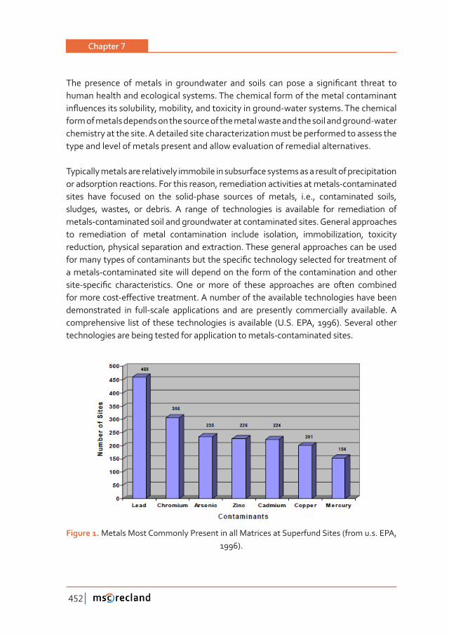
Chapter 7
452
���� ��������� ���������� ��� ������������ ���� ������ ���� ����� �� �����Ƥ����� ������� ���human health and ecological systems. The chemical form of the metal contaminant ��ƪ���������������������ǡ���������ǡ�����������������������Ǧ�������������Ǥ��������������form of metals depends on the source of the metal waste and the soil and ground-water chemistry at the site. A detailed site characterization must be performed to assess the type and level of metals present and allow evaluation of remedial alternatives.
Typically metals are relatively immobile in subsurface systems as a result of precipitation or adsorption reactions. For this reason, remediation activities at metals-contaminated sites have focused on the solid-phase sources of metals, i.e., contaminated soils, sludges, wastes, or debris. A range of technologies is available for remediation of metals-contaminated soil and groundwater at contaminated sites. General approaches to remediation of metal contamination include isolation, immobilization, toxicity reduction, physical separation and extraction. These general approaches can be used ��������������������������������������������Ƥ���������������������������������������a metals-contaminated site will depend on the form of the contamination and other ����Ǧ�����Ƥ�� ���������������Ǥ� ���� ��� ����� ��� ������ ����������� ���� ������ ����������������������Ǧ�ơ����������������Ǥ��������������������������������������������������demonstrated in full-scale applications and are presently commercially available. A comprehensive list of these technologies is available (U.S. EPA, 1996). Several other technologies are being tested for application to metals-contaminated sites.
Figure 1. Metals Most Commonly Present in all Matrices at Superfund Sites (from u.s. EPA, 1996).
Polluted Soils Restoration
453
6�2 Sources of contaminants
Surface water and groundwater may be contaminated with metals from wastewater discharges or by direct contact with metals-contaminated soils, sludges, mining wastes, and debris. Metal-bearing solids at contaminated sites can originate from a wide variety of sources in the form of airborne emissions, process solid wastes, sludges ���������Ǥ���������������������������ƪ����������������������������������������������on a macroscopic and microscopic scale. Variations in contaminant concentration ����������� ��ƪ������ ���� ���������������������������� ������������������ ����������options.
6�2�1 Airborne Sources
Airborne sources of metals include stack or duct emissions of air, gas, or vapor streams, and fugitive emissions such as dust from storage areas or waste piles. Metals from airborne sources are generally released as particulates contained in the gas stream. Some metals such as arsenic, cadmium, and lead can also volatilize during high-temperature processing. These metals will convert to oxides and condense as Ƥ�����������������������������������������������������������ȋ�����������Ǥǡ�ȌǤ
Stack emissions can be distributed over a wide area by natural air currents until dry and/or wet precipitation mechanisms remove them from the gas stream. Fugitive emissions are often distributed over a much smaller area because emissions are made near the ground. In general, contaminant concentrations are lower in fugitive emissions compared to stack emissions. The type and concentration of metals ������������������������������������������������������Ǧ�����Ƥ������������Ǥ
6�2�2 Process Solid Wastes
Process solid wastes can result from a variety of industrial processes. These metal-bearing solid wastes are disposed above ground in waste piles or below ground or �������������������Ƥ���Ǥ�����������������������������������������������ǡ�ƪ�����ǡ������sands, abrasive wastes, ion exchange resins, spent catalysts, spent activated carbon, and refractory bricks (Zimmerman and Coles, 1992). The composition of the process ��������ƪ������������������ǡ���������ǡ�����������������������������������������������considered in evaluating the contaminated matrix.
Chapter 7
454
Because waste piles are above ground, they are exposed to weathering which can disperse the waste pile to the surrounding soil, water and air and can result in �������������������������������Ƥ���������������������������������������Ǥ��������������������Ƥ�����������������������������������������������������������������������������Ƥ����������Ǥ�����������������Ƥ������������������������������������Ƥ�����������������������or groundwater or via wind and surface erosion.
6�2�3 Sludges
The composition of sludges depends on the original waste stream and the process from which it was derived. Sludges resulting from a uniform wastestream, such as wastewater treatment sludges, are typically more homogeneous and have more uniform matrix characteristics. Sludge pits, on the other hand, often contain a mixture of wastes that have been aged and weathered, causing a variety of reactions to occur. Sludge pits often require some form of pretreatment before wastes can be treated or recycled (Smith et al., 1995).
6�2�4 Soils
Soil consists of a mixture of weathered minerals and varying amounts of organic matter. Soils can be contaminated as a result of spills or direct contact with contaminated waste streams such as airborne emissions, process solid wastes, sludges, or leachate ��������������������Ǥ�������������������������� �������� ��� ��ƪ������������������������of the soil and groundwater (Sposito, 1989; Evans, 1989). Factors such as pH, Eh, ion ��������� ��������ǡ� ���� ������������Ȁ��������������������������������������� �ơ����metal solubility.
6�2�5 Direct Ground-Water Contamination
����������� ���� ��� ������������������������� ��������� ��� ��Ƥ��������� ��� ���������from land disposal of solid wastes, liquid sewage or sewage sludge, leachate from mine tailings and other mining wastes, deep-well disposal of liquid wastes, seepage from industrial waste lagoons, or from other spills and leaks from industrial metal processing facilities (e.g., steel plants, plating shops, etc.). A variety of reactions may ������������ ��ƪ�������������������������������������������������������� ����������
Polluted Soils Restoration
455
acid/base, precipitation/dissolution, oxidation/ reduction, sorption or ion exchange. Precipitation, sorption, and ion exchange reactions can retard the movement of metals in groundwater. The rate and extent of these reactions will depend on factors such as pH, Eh, complexation with other dissolved constituents, sorption and ion exchange capacity of the geological materials, and organic matter content. Ground-������ƪ��������������������������ƪ�����������������������������������������Ǥ
6�3 Chemical fate and mobility
���������������������������������� �������������������������������������Ƥ����������the chemical form and speciation of the metal (Allen et al., 1991). The mobility of metals in ground-water systems is hindered by reactions that cause metals to adsorb or precipitate, or chemistry that tends to keep metals associated with the solid phase and prevent them from dissolving. These mechanisms can retard the movement of metals and also provide a long-term source of metal contaminants (NRC, 1994). While the various metals undergo similar reactions in a number of aspects, the extent and nature of these reactions varies under particular conditions. In Figure 2, for example, the extent of sorption of several metal cations and anions onto iron oxide is shown as a function of pH for a particular background electrolyte composition. It may be seen there that lead sorbs extensively at much lower pH values than zinc or cadmium (Kinniburgh et al., 1976).
The chemical form and speciation of some of the more important metals found at ��������������������������������������Ǥ�������ƪ�����������������������������������mobility of these compounds is also discussed.
6�3�1 Pb
The primary industrial sources of lead (Pb) contamination include metal smelting and processing, secondary metals production, lead battery manufacturing, pigment and chemical manufacturing, and lead-contaminated wastes. Widespread contamination due to the former use of lead in gasoline is also of concern. Lead released to groundwater, surface water and land is usually in the form of elemental lead, lead oxides and hydroxides, and leadmetal oxyanion complexes (Smith et al., 1995).
Chapter 7
456
Lead occurs most commonly with an oxidation state of 0 or +II. Pb(II) is the more common and reactive form of lead and forms mononuclear and polynuclear oxides and hydroxides. Under most conditions Pb2+ and lead-hydroxy complexes are the most stable forms of lead (Smith et al., 1995). Low solubility compounds are formed by complexation with inorganic (Cl-, CO3
2-, SO42-, PO4
3-) and organic ligands (humic and fulvic acids, EDTA, amino acids) (Bodek et al., 1988). Lead carbonate solids form ������������������ ��� ��������� ������� ���������������� ���Ƥ����������������������present under reducing conditions.
Most lead that is released to the environment is retained in the soil (Evans, 1989). The ��������������������ƪ���������������������������������������������������ǡ�������������ǡ�precipitation, and complexation with sorbed organic matter. These processes limit the amount of lead that can be transported into the surface water or groundwater. The relatively volatile organolead compound tetramethyl lead may form in anaerobic sediments as a result of alkyllation by microorganisms (Smith et al., 1995).
The amount of dissolved lead in surface water and groundwater depends on pH and the concentration of dissolved salts and the types of mineral surfaces present. In ������������������������Ǧ�������������ǡ��������Ƥ�������������������������������������and occurs as precipitates (PbCO3, Pb2O, Pb(OH)2, PbSO4), sorbed ions or surface coatings on minerals, or as suspended organic matter.
6�3�2 Cr
Chromium(Cr) is one of the less common elements and does not occur naturally in elemental form, but only in compounds. Chromium is mined as a primary ore product in the form of the mineral chromite, FeCr2O4. Major sources of Cr contamination include releases from electroplating processes and the disposal of chromium containing wastes (Smith et al., 1995).
Cr(VI) is the form of chromium commonly found at contaminated sites. Chromium can also occur in the +III oxidation state, depending on pH and redox conditions. Cr (VI) is the dominant form of chromium in shallow aquifers where aerobic conditions exist. Cr(VI) can be reduced to Cr(III) by soil organic matter, S 2- and Fe 2+ ions under anaerobic conditions often encountered in deeper groundwater. Major Cr(VI) species include chromate (CrO4 2-) and dichromate (Cr2O7
2-) which precipitate readily in the presence of metal cations (especially Ba 2+, Pb 2+, and Ag +). Chromate and dichromate
Polluted Soils Restoration
457
also adsorb on soil surfaces, especially iron and aluminum oxides. Cr(III) is the dominant form of chromium at low pH (<4). Cr 3+ forms solution complexes with NH3, OH-, Cl-, F-, CN-, SO4 2-, and soluble organic ligands. Cr(VI) is the more toxic form of chromium and is also more mobile. Cr(III) mobility is decreased by adsorption to clays and oxide minerals below pH 5 and low solubility above pH 5 due to the formation of Cr(OH)3(s) (Chrotowski et al., 1991).
Chromium mobility depends on sorption characteristics of the soil, including clay content, iron oxide content and the amount of organic matter present. Chromium can ������������������������������ơ������������������������������������������������������Ǥ�Soluble and unadsorbed chromium complexes can leach from soil into groundwater. The leachability of Cr(VI) increases as soil pH increases. Most of chromium released into natural waters is particle associated, however, and is ultimately deposited into the sediment (Smith et al., 1995).
6�3�3 As
Arsenic (As) is a semimetallic element that occurs in a wide variety of minerals, mainly as As2O3, and can be recovered from processing of ores containing mostly copper, lead, zinc, silver and gold. It is also present in ashes from coal combustion. Arsenic exhibits fairly complex chemistry and can be present in several oxidation states (-III, 0, III, V) (Smith et al., 1995).
In aerobic environments, As(V) is dominant, usually in the form of arsenate (AsO4 3-) in various protonation states: H3AsO4, H2AsO4 -, HAsO4 2-, AsO4 3-. Arsenate, and other anionic forms of arsenic behave as chelates and can precipitate when metal cations are present (Bodek et al., 1988). Metal arsenate complexes are stable only under certain conditions.
As(V) can also coprecipitate with or adsorb onto iron oxyhydroxides under acidic and moderately reducing conditions. Coprecipitates are immobile under these conditions but arsenic mobility increases as pH increases (Smith et al., 1995).
Under reducing conditions As(III) dominates, existing as arsenite (AsO3 3-) and its
protonated forms: H3AsO3, H2AsO3 -, HAsO3
2-. Arsenite can adsorb or coprecipitate ����������� ���Ƥ���� ���� ���� �� ����� �ƥ����� ���� ������ ������� ���������Ǥ� ����������arsenic and arsine, AsH3, may be present under extreme reducing conditions.
Chapter 7
458
Biotransformation (via methylation) of arsenic creates methylated derivatives of arsine, such as dimethyl arsine HAs(CH3)2 and trimethylarsine As(CH3)3 which are highly volatile.
Since arsenic is often present in anionic form, it does not form complexes with simple anions such as Cl- and SO4 2-. Arsenic speciation also includes organometallic forms such as methylarsinic acid (CH3)AsO2H2 and dimethylarsinic acid (CH3)2AsO2H. Many arsenic compounds sorb strongly to soils and are therefore transported only over short distances in groundwater and surface water. Sorption and coprecipitation with hydrousiron oxides are the most important removal mechanisms under most environmental conditions (Krause and Ettel, 1989; Pierce and Moore, 1982). Arsenates can be leached easily if the amount of reactive metal in the soil is low. As(V) can also be mobilized under reducing conditions that encourage the formation of As(III), under alkaline and saline conditions, in the presence of other ions that compete for sorption sites, and in the presence of organic compounds that form complexes with arsenic (Smith et al., 1995).
6�3�4 Zn
Zinc (Zn) does not occur naturally in elemental form. It is usually extracted from mineral ores to form zinc oxide (ZnO). The primary industrial use for Zinc is as a corrosion-resistant coating for iron or steel (Smith et al., 1995).
Zinc usually occurs in the +II oxidation state and forms complexes with a number of anions, amino acids and organic acids. Zn may precipitate as Zn(OH)2(s), ZnCO3(s), ZnS(s), or Zn(CN)2(s). Zinc is one of the most mobile heavy metals in surface waters and groundwater because it is present as soluble compounds at neutral and acidic pH values. At higher pH values, zinc can form carbonate and hydroxide complexes which control zinc solubility. Zinc readily precipitates under reducing conditions and in highly polluted systems when it is present at very high concentrations, and may coprecipitate with hydrous oxides of iron or manganese (Smith et al., 1995).
Sorption to sediments or suspended solids, including hydrous iron and manganese oxides, clay minerals, and organic matter, is the primary fate of zinc in aquatic environments. Sorption of zinc increases as pH increases and salinity decreases.
Polluted Soils Restoration
459
6�3�5 Cd
Cadmium (Cd) occurs naturally in the form of CdS or CdCO3. Cadmium is recovered �������Ǧ������������������������������Ƥ���������������ǡ����������������Ǥ������������cadmium contamination include plating operations and the disposal of cadmium-containing wastes (Smith et al., 1995).
The form of cadmium encountered depends on solution and soil chemistry as well as treatment of the waste prior to disposal The most common forms of cadmium include Cd 2+, cadmium-cyanide complexes, or Cd(OH)2 solid sludge (Smith et al., 1995). Hydroxide (Cd(OH)2) and carbonate (CdCO3) solids dominate at high pH whereas Cd 2+ and aqueous sulfate species are the dominant forms of cadmium at lower pH (<8). Under reducing conditions when sulfur is present, the stable solid CdS(s) is formed. Cadmium will also precipitate in the presence of phosphate, arsenate, chromate and other anions, although solubility will vary with pH and other chemical factors.
Cadmium is relatively mobile in surface water and ground-water systems and exists primarily as hydrated ions or as complexes with humic acids and other organic ligands (Callahan et al., 1979). Under acidic conditions, cadmium may also form complexes with chloride and sulfate. Cadmium is removed from natural waters by precipitation and sorption to mineral surfaces, especially oxide minerals, at higher pH values (>pH 6). �����������������������������������������������������Ǥ��������������������ƪ�������by the cation exchange capacity (CEC) of clays, carbonate minerals, and organic matter present in soils and sediments. Under reducing conditions, precipitation as CdS controls the mobility of cadmium (Smith et al., 1995).
6�3�6 Cu
������� ȋ��Ȍ� ���������������������������������� ���������������Ƥ�����������������Ǥ�Mining activities are the major source of copper contamination in groundwater and surface waters. Other sources of copper include algicides, chromated copper arsenate (CCA) pressuretreated lumber, and copper pipes. Solution and soil chemistry strongly ��ƪ������������������������������� ���������Ǧ�������������Ǥ� ����������ǡ���ƥ��������alkaline systems, CuCO3 is the dominant soluble copper species. The cupric ion, Cu 2+, and hydroxide complexes, CuOH+ and Cu(OH)2, are also commonly present. Copper ������ ������� ��������� ��������������� ������ �����Ǥ����� �ƥ����� ������ ���� ��������

Chapter 7
460
increases as pH increases and ionic strength decreases. In anaerobic environments, when sulfur is present CuS(s) will form.
Copper mobility is decreased by sorption to mineral surfaces. Cu 2+ sorbs strongly to mineral surfaces over a wide range of pH values (Dzombak and Morel, 1990). The cupric ion (Cu 2+) is the most toxic species of copper. Copper toxicity has also been demonstrated for CuOH+ and Cu2(OH)2 2+ (LaGrega et al., 1994).
6�3�7 Hg
���� �������� ������� ����������� ��� ���� ���Ƥ��� ���� ��������Ǥ��������� ȋ��Ȍ� ��� ��������recovered as a by-product of ore processing (Smith et al., 1995). Release of mercury from coal combustion is a major source of mercury contamination. Releases from manometers at pressure measuring stations along gas/oil pipelines also contribute to mercury contamination. After release to the environment, mercury usually exists in mercuric (Hg 2+), mercurous (Hg2 2+), elemental (Hgo), or alkyllated form (methyl/ethyl mercury). The redox potential and pH of the system determine the stable forms of mercury that will be present. Mercurous and mercuric mercury are more stable under oxidizing conditions. When mildly reducing conditions exist, organic or inorganic mercury may be reduced to elemental mercury, which may then be converted to alkyllated forms by biotic or abiotic processes. Mercury is most toxic in its alkyllated forms which are soluble in water and volatile in air (Smith et al., 1995).
Hg(II) forms strong complexes with a variety of both inorganic and organic ligands, making it very soluble in oxidized aquatic systems (Bodek et al., 1988). Sorption to soils, sediments, and humic materials is an important mechanism for removal of mercury from solution. Sorption is pH-dependent and increases as pH increases. ���������������������������������������������������������������������Ƥ����ȋ������et al., 1995).
Under anaerobic conditions, both organic and inorganic forms of mercury may be converted to alkyllated forms by microbial activity, such as by sulfur-reducing bacteria. Elemental mercury may also be formed under anaerobic conditions by demethylation of methyl mercury, or by reduction of Hg(II). Acidic conditions (pH<4) also favor the formation of methyl mercury, whereas higher pH values favor precipitation of HgS(s) (Smith et al., 1995).
Polluted Soils Restoration
461
6�4 Available technologies
6�4�1 Site characterization and establishment of remediation goals
The physical and chemical form of the metal contaminant in soil or water strongly ��ƪ������� ���� ���������� ��� ���� ������������ ������������ ���������� ��������Ǥ�Information about the physical characteristics of the site and the type and level of contamination at the site must be obtained to enable accurate assessment of site contamination and remedial alternatives.
The importance of adequate, well-planned site characterization to selection of an ������������ ����Ǧ�ơ������� ������������ ��������� ���� ����� ���������� ����� ������(e.g., CII, 1995) but cannot be overemphasized. The contamination in the groundwater and soil should be characterized to establish the type, amount, and distribution of ����������������������ơ�����������Ǥ
Once the site has been characterized, the desired level of each contaminant in soil and groundwater must be determined. This is done by comparison of observed contaminant concentrations with soil and ground-water quality standards for a ����������� �����������������ǡ������������������������ ����Ǧ�����Ƥ�� ���������������Ǥ�Remediation goals for metals may be set as desired concentrations in groundwater, as total metal concentration in soil, as leachable metal in soil, or as some combination of these.
6�4�2 General remediation approaches
Several technologies exist for the remediation of metals-contaminated soil and �����Ǥ�����������������������������������������Ƥ������������������������������������to remediation: isolation, immobilization, toxicity reduction, physical separation and extraction. These are the same general approaches used for many types of contaminants in the subsurface (LaGrega et al., 1994). As is usually the case, combinations of one or more of these approaches are often used for more cost-�ơ���������������������������������������Ǥ�
Chapter 7
462
Isolation
Isolation technologies attempt to prevent the transport of contaminants by containing them within a designated area. These technologies can be used to prevent further contamination of groundwater when other treatment options are not physically or economically feasible for a site. Contaminated sites may also be isolated temporarily in order to limit transport during site assessment and site remediation.
A) Capping
Capping systems are used to provide an impermeable barrier to surface water ��Ƥ��������� ��� ������������� ����� ���� ����������� ��� �������� �������� ��� �������������to the surrounding surface water or groundwater. Secondary objectives include controlling gas and odor emissions, improving aesthetics, and providing a stable surface over a contaminated site.
Capping also eliminates risks associated with dermal contact and/or incidental ingestion of surface soils, but if this is the primary goal for the site and surface water ��Ƥ�������������������������ǡ��������������������������������������������������Ǥ
Capping provides a range of design options that includes simple single-layer caps and more complex multilayer systems (Rumer and Ryan, 1995; U.S. EPA, 1991). Design selection depends on site characteristics, remedial objectives and risk factors associated with the site. A variety of materials are available for use in capping systems �������������������������������������Ƥ��������������������������������������������������parts of the cap.
Synthetic membranes such as high-density polyethylene are also available for incorporation into capping systems. Surface water controls, such as ditches and dikes are usually included to help control drainage from the cap. Multilayered capping systems may also include a hard cover and/or a layer of topsoil to separate the underlying layers from the ground surface. Revegetation is promoted in order to ���������������������ǡ��������������������������������ơ���������ǡ��������������������water from the soil by evapotranspiration (Rumer and Ryan, 1995).
Polluted Soils Restoration
463
B) Subsurface Barriers
Subsurface barriers may be used to isolate contaminated soil and water by controlling the movement of groundwater at a contaminated site. These barriers are designed to reduce the movement of contaminated groundwater from the site, or to restrict ����ƪ���������������������������������������������������������������ȋ����������Ryan, 1995).
������������������������������������������������������������ƪ�����������������Ǥ�����ơ�������������������������������������������ǡ����������������������������������������a continuous, low-permeability layer, such as clay or competent bedrock, below the contaminated area (U.S. EPA, 1985; Rumer and Ryan, 1995). If an impermeable layer is not available, a ground-water extraction system must be used to prevent transport of contaminants under the barrier. Vertical barriers may be installed upstream, downstream, or completely surrounding the site and are often implemented in ��������������������������������������������� �������������� ��Ƥ��������Ǥ������������circumferential barriers can prevent the escape of contamination from the site by �����������Ƥ������������������������������������������������
a hydraulic gradient in the inward direction. Vertical barriers are often limited to depths achievable with backhoe excavation technology for trenches, i.e., to about 10 m (U.S. EPA, 1985).
Slurry walls are usually constructed in a vertical trench excavated under a slurry that ����������������������������������������������Ƥ�������������������������� �������������� �������� ���� ����� ��� ƪ����� ��� ���� ������������ ����� ȋ���������ǡ� ȌǤ��� ����������beam method (Slurry Systems, Inc.) is also available in which the beam penetrates the ground and slurry materials are injected into the soil (with assistance from a high pressure/low volume jet if needed). Two options exist for the slurry composition. The soil-bentonite (SB) slurry wall is the most common type, and comprises a bentonite-water slurry that is mixed with a soil engineered to harden upon addition to the slurry (Rumer and Ryan, 1995). The trench can also be excavated under a portland cement-bentonite-water slurry that is left to harden and form a cement-bentonite (CB) slurry wall (LaGrega et al., 1994). Available technologies for installation of slurry walls allow installation to depths up to 40 m.
Chapter 7
464
Slurry walls are the most common type of vertical barrier due to their low relative cost. The use of slurry walls can be limited by the topography, geology, and type ����������������������������Ǥ�����������ǡ�������������������ƪ��������������������������Ƥ����� ������ ���� ������� �����Ǥ� ����ǡ� ����� ������������ǡ� ����� ��� �������������organics and strong acids/bases, can degrade SB materials and prevent the application of SB slurry walls at some sites (Rumer and Ryan, 1995).
Other available vertical barriers include grout curtains and sheet piles. Grout curtains �������������������������������������������������������ƪ����������������������������������������������������������������������������ƪ�����������������������������������ȋ�Ǥ�Ǥ����ǡ�ȌǤ�����ƪ���������������Ǧ������������������������������������������������������������������������������ƪ�������������������������������������������Ǥ��������materials used to construct grout curtains include cement, clays, alkali-silicate, and organic polymers (Rumer and Ryan, 1995). Clays are the most widely used grouting materials due to their low cost. This technique is more expensive than slurry walls and its use is therefore usually limited to sealing voids in existing rock.
Sheet piles usually comprise steel pilings that are driven into the formation to create a wall to contain the groundwater. Sheet piles are seldom used at contaminated sites due to concerns about wall integrity. This method is generally limited to isolation of shallow contamination (12-15 m) distributed over a relatively small area (U.S. EPA, 1985), or used in conjunction with a soil-bentonite slurry when site conditions prevent the use of conventional slurry walls (Rumer and Ryan, 1995).
Technologies for the construction of horizontal barriers are under investigation. Horizontal barriers would enable control of the downward migration of contaminants by lining the site without requiring excavation of the contaminated matrix. The technologies under investigation include grout injection by vertical boring and horizontal drilling. The vertical boring method is similar to the construction of grout ������������������������������������������������Ƥ�����������������������������������������of vertical boreholes to create an impermeable horizontal layer. Problems with this method include soil compaction by the large drill rigs situated over the contaminated area. Also, the vertical boreholes would provide access to the deeper layers and may therefore increase vertical migration of contaminants. Horizontal drilling involves the use of directional drilling techniques to create the horizontal grout layer.
Polluted Soils Restoration
465
Horizontal barriers may also be used in conjunction with vertical barriers at sites where a natural aquitard is not present. In this case, the vertical barrier could key into the horizontal barrier to prevent the transport of contaminants under the vertical barrier (Smith et al., 1995).
Immobilization
Immobilization technologies are designed to reduce the mobility of contaminants by changing the physical or leaching characteristics of the contaminated matrix. Mobility is usually decreased by physically restricting contact between the contaminant and the surrounding groundwater, or by chemically altering the contaminant to make it more stable with respect to dissolution in groundwater. The aqueous and solid phase chemistry of metals is conducive to immobilization by these techniques. A variety of methods are available for immobilization of metal contaminants, including those that use chemical reagents and/or thermal treatment to physically bind the contaminated soil or sludge. Most immobilization technologies can be performed ex situ or in situ. In situ processes are preferred due to the lower labor and energy requirements, but �������������������������������������������Ƥ�����������������Ǥ
A) Solidification/Stabilization
������Ƥ������� ���� �������������� ȋ�Ȁ�Ȍ� ��������������� ������������� ���� ���� �����commonly selected treatment options for metals-contaminated sites (Conner, 1990). ������Ƥ������� ��������� ���� ���������������������Ƥ���������� ��������������������������contaminated material.
�������������ǡ� ����� ��������� ��� ��� Ƥ������ǡ� �������� ��������� �� ��������� ��������� ����������� ���� ������ ��� �� ����� ������� ����Ǥ����� �������� ��������� ���� ������Ƥ������Ȁstabilization treatment processes involves mixing or injecting treatment agents to ����������������������Ǥ� �����������������ǡ���������������ǡ�ƪ�����ǡ������������������slag, and organic binders such as bitumen are used to form a crystalline, glassy or polymeric framework around the waste. The dominant mechanism by which metals are immobilized is by precipitation of hydroxides within the solid matrix (Bishop et al., 1982; Shively et al., 1986).
S/S technologies are not useful for some forms of metal contamination, such as species that exist as anions (e.g., Cr(VI), arsenic) or metals that don’t have low-solubility hydroxides (e.g., mercury). S/S may not be applicable at sites containing
Chapter 7
466
wastes that include organic forms of contamination, especially if volatile organics are present. Mixing and heating associated with binder hydration may release organic vapors. Pretreatment, such as air stripping or incineration, may be used to remove ���� ��������� ���� �������� ���������� ���������� �������������Ȁ������Ƥ������� ȋ������ �����Ǥǡ�ȌǤ���������������������Ȁ�����������������������������ơ����������������������composition of the contaminated matrix, the amount of water present, and the �������������������Ǥ��������������������������������������������Ƥ������Ȁ��������������process by inhibiting bonding of the waste to the binding material, retarding the setting of the mixtures, decreasing the stability of the matrix, or reducing the strength �������������Ƥ��������ȋ�Ǥ�Ǥ����ǡ��ȌǤ
Cement-based binders and stabilizers are common materials used for implementation of S/S technologies (Conner, 1990). Portland cement, a mixture of Ca-silicates, aluminates, aluminoferrites, and sulfates is an important cement-based material. Pozzolanic materials which consist of small spherical particles formed by coal �����������ȋ��������ƪ�����Ȍ�����������������������������ǡ������������������������for S/S. Pozzolans exhibit cement-like properties, especially if the silica content is high. Portland cement and pozzolans can be used alone or together to obtain optimal properties for a particular site (U.S. EPA, 1989).
Organic binders may also be used to treat metals through polymer microencapsulation. ����� �������� ����� �������� ���������� ����� ��� �������ǡ� ������������ǡ� ����ƥ��ǡ������������������������Ƥ������ ����������������� ��������������������Ǥ������������encapsulation, the organic materials are heated and mixed with the contaminated matrix at elevated temperatures (120° to 200°C). The organic materials polymerize, agglomerate the waste and the waste matrix is encapsulated (U.S. EPA, 1989). Organics are volatilized and collected and the treated material is extruded for disposal or possible reuse (e.g., as paving material) (Smith et al., 1995). The contaminated material may require pretreatment to separate rocks and debris and dry the feed material. Polymer encapsulation requires more energy and more complex equipment than cement-based S/S operations. Bitumen (asphalt) is the cheapest and most common thermoplastic binder (U.S. EPA, 1989).
S/S is achieved by mixing the contaminated material with appropriate amounts of ������Ȁ����������� ���������Ǥ������������� ����� ���� ������ ��� ����� �� ������Ƥ����������and contain the waste. The cure time and pour characteristics of the mixture and the Ƥ������������������ ������������������������������������������������ ȋ����������cement, pozzolan, water) of the binder/stabilizer.

Polluted Soils Restoration
467
Ex situ S/S can be easily applied to excavated soils because methods are available to provide the vigorous mixing needed to combine the binder/stabilizer with the contaminated material. Pretreatment of the waste may be necessary to screen and crush large rocks and debris. Mixing can be performed via in-drum, in-plant or area mixing processes. In-drum mixing may be preferred for treatment of small volumes of waste or for toxic wastes. Inplant processes utilize rotary drum mixers for batch processes or pug mill mixers for continuous treatment. Larger volumes of waste may be excavated and moved to a contained area for area mixing. This process involves layering the contaminated material with the stabilizer/binder, and subsequent ������������������������������������������Ǥ������������Ƥ�������������������������available for ex situ S/S treatment. Smaller pilot-scale plants can treat up to 100 tons of contaminated soil per day, while larger portable plants typically process 500 to over 1000 tons per day (Smith et al., 1995).
S/S techniques are available to provide mixing of the binder/stabilizer with the contaminated soil in situ. In situ S/S is less labor and energy intensive than ex situ process that require excavation, transport and disposal of the treated material. In situ S/S is also preferred if volatile or semi volatile organics are present because excavation would expose these contaminants to the air (U.S. EPA, 1990a). However the presence of bedrock, large boulders, cohesive soils, oily sands and clays may preclude the ������������������������Ȁ���������������Ǥ�������������������ƥ����������������������������complete mixing through in situ processes.
Mixing of the binder and contaminated matrix may be achieved using in-place mixing, vertical auger mixing or injection grouting. In-place mixing is similar to ex situ area mixing except that the soil is not excavated prior to treatment. The in situ process is useful for treating surface or shallow contamination and involves spreading and mixing the binders with the waste using conventional excavation equipment such as draglines, backhoes or clamshell buckets. Vertical auger mixing uses a system of augers to inject and mix the binding reagents with the waste. Larger (2-4 m diameter) augers are used for shallow (3-12 m) drilling and can treat 500-1000 m3 per day (Ryan ����������ǡ� Ǣ� ����������������ǡ� ȌǤ�������������������Ȁ������Ƥ�������ȋ������ �m) can be achieved by using ganged augers (up to 1 m in diameter each) that can treat 150-400 m3per day. Finally injection grouting may be performed to inject the binder containing suspended or dissolved reagents into the treatment area under pressure. The binder permeates the surrounding soil and cures in place (Smith et al., 1995).
Chapter 7
468
B) Vitrification
The mobility of metal contaminants can be decreased by high-temperature treatment of the contaminated area that results in the formation of vitreous material, usually an oxide solid. During this process, the increased temperature may also volatilize and/or destroy organic contaminants or volatile metal species (such as Hg) that must be ���������� ���� ���������������������Ǥ�����������������������������������Ƥ�������������������������������������������������������������������������������Ǥ������Ƥ�����������be performed ex situ or in situ, although in situ processes are preferred due to the lower energy requirements and cost (U.S. EPA, 1992a).
�������������������������������Ƥ���������������������������������������ǡ�������������ǡ�������ǡ� �������ǡ� �������� ���� �����Ƥ������ǡ� �ơǦ���� ����������� ���� ���������ǡ� ����forming or casting of the melted product. The energy requirement for melting is the �����������������ƪ���������������������������������Ƥ������Ǥ���ơ������������������������can be used for this purpose, depending on local energy costs. Process heat losses and water content of the feed should be controlled in order to minimize energy ������������Ǥ������Ƥ����������������������������������������������������������������������������������������ǡ���������Ȁ��������������Ǥ����������Ƥ�������������������������������������������Ƥ��ǡ����������ǡ�����������������������������ȋ�����������Ǥǡ�ȌǤ
��� ����� �����Ƥ������� ȋ���Ȍ� ��������� �������� ��������� �������� �������� ���� ����� ������ ���array of electrodes inserted vertically into the contaminated region. Each setting of four electrodes is referred to as a melt. If the soil is too dry, it may not provide ��ƥ������������������������������������������ƪ�����������������������������ȋ����������������������Ȍ�������������������������������������������������������������ƪ��������for the current. Resistance heating in the starter path melts the soil. The melt grows outward and down as the molten soil usually provides additional conductance for the current. A single melt can treat up to 1000 tons of contaminated soil to depths of 6 m, at a typical treatment rate of 3 to 6 tons per hour.
���������������������������������������������������������������������Ƥ������������Ǥ���������������������������������������Ƥ��������������������������������������������������������and solidify as it cools. If the alkali content (as Na2O and K2O) of the soil is too high ȋ�Ǥ���άȌ�������������������������������������������������������������������������(Buelt and Thompson, 1992).
Polluted Soils Restoration
469
Toxicity and/or Mobility Reduction
Chemical and/or biological processes can be used to alter the form of metal contaminants in order to decrease their toxicity and/or mobility.
A) Chemical Treatment
Chemical reactions can be initiated that are designed to decrease the toxicity or mobility of metal contaminants. The three types of reactions that can be used for this purpose are oxidation, reduction, and neutralization reactions. Chemical oxidation changes the oxidation state of the metal atom through the loss of electrons. Commercial oxidizing agents are available for chemical treatment, including potassium permanganate, hydrogen peroxide, hypochlorite and chlorine gas. Reduction reactions change the oxidation state of metals by adding electrons. Commercially available reduction reagents include alkali metals (Na, K), sulfur �������ǡ����Ƥ��������ǡ��������������������Ǥ�������������������������������������������oxidation or reduction can detoxify, precipitate, or solubilize the metals (NRC, 1994).
Chemical neutralization is used to adjust the pH balance of extremely acidic or basic soils and/or groundwater. This procedure can be used to precipitate insoluble metal salts from contaminated water, or in preparation for chemical oxidation or reduction.
Chemical treatment can be performed ex situ or in situ. However in situ chemical agents must be carefully selected so that they do not further contaminate the treatment area. The primary problem associated with chemical treatment is the ��������Ƥ���������������������������������Ǥ����������Ȁ�����������������������������matrix to treat one metal will also target other reactive metals and can make them more toxic or mobile (NRC, 1994). Also, the long-term stability of reaction products is of concern since changes in soil and water chemistry might reverse the selected reactions.
Chemical treatment is often used as pretreatment for S/S and other treatment technologies. Reduction of Cr(VI) to Cr(III) is the most common form of chemical treatment and is necessary for remediation of wastes containing Cr(VI) by precipitation or S/S. Chromium in its Cr(III) form is readily precipitated by hydroxide over a wide ������������������Ǥ������Ƥ������������������������������������ȋ��Ȍ����������Ǥ���������may be treatable by chemical oxidation since arsenate, As(V), is less toxic, soluble and
Chapter 7
470
mobile than arsenite, As(III). Bench-scale work has indicated that arsenic stabilization may be achieved by precipitation and coprecipitation with Fe(III) (Smith et al., 1995).
B) Permeable Treatment Walls
Treatment walls remove contaminants from groundwater by degrading, transforming, �����������������������������������������������������������ƪ����������������������trenches containing reactive material within the subsurface (Vidic and Pohland, 1996). Several methods are available for installation of permeable treatment walls, some of which employ slurry wall construction technology to create a permeable reactive curtain. The reactive zone can use physical, chemical and biological processes, or a ��������������������Ǥ�����������Ǧ������ƪ���������������������������������������inducing a hydraulic gradient in the direction of the treatment zone or channeling ������Ǧ������ƪ�����������������������������ȋ���ǡ�ȌǤ
Several types of treatment walls are being tried for arresting transport of metals in groundwater at contaminated sites. Trench materials being investigated include zeolite, hydroxyapatite, elemental iron, and limestone (Vidic and Pohland, 1996). Applications of elemental iron for chromium (VI) reduction and limestone for lead precipitation and adsorption are described below.
C) Elemental Iron
��������� Ƥ����� ����� ���������� ����� ����� ������ �������� ���� ������������ ���metalscontaminated sites. While investigations of this technology have focused largely on treatment of halogenated organic compounds, studies are being performed to assess the applicability to remediation of inorganic contaminants (Powell et al., 1994).
Low oxidation-state chemical species can serve as electron donors for the reduction of higher oxidation-state contaminants. This ability can be exploited to remediate metals that are more toxic and mobile in higher oxidation states, such as Cr(VI). Results of column experiments performed by Powell et al. (1994) and batch experiments performed by Cantrell et al. (1995) showed that chromate reduction was ������������������������������������Ƥ�������������������������������������������������Ǥ���Ƥ������������������������ ������������� ��������������� �����Ǥ�Ǥ�������������������Management Research Laboratory to investigate the use of zero-valent iron for
Polluted Soils Restoration
471
chromium remediation at the U.S. Coast Guard air support base near Elizabeth City, North Carolina. Preliminary results indicate that the test barrier has reduced chromate in the groundwater to below detection limits (Wilson, 1995).
D) Limestone Barriers
The use of limestone treatment walls has been proposed for sites with metals contamination, in particular former lead acid battery recycling sites which have lead and acid contamination in groundwater and soil. In such cases, a limestone trench can provide neutralization of acidic groundwater. The attendant rise in pH promotes immobilization of any dissolved lead through precipitation and/or adsorption onto minerals. A limestone trench system is in design for implementation at the Tonolli Superfund site in Nesquehoning, Pennsylvania (U.S. EPA, 1992b).
There is some experience in the coal mining industry with use of limestone in the manner anticipated for the Tonolli site. Most of this experience has been acquired ������ǡ��������������������� Dz������� ����������������dz����� ����������� ȋ�������and McCoy, 1990). Since that time, numerous limestone drain systems have been ���������� ��������������� ����� Ƥ���� ������ ȋ���������� ��� ��������ǡ��������������ǡ� ����Pennsylvania) in an attempt to control acid mine drainage. Summaries of installations and evolving design considerations are provided in Hedin and Nairn (1992), Hedin et al. (1994), and Hedin and Watzlaf (1994).
Design and operating guidelines for the anoxic limestone drains have for the most part �����������������������������������������Ǥ�����ƪ�ǡ����������������������������������large, #3 or #4 (baseball size) limestone rocks. Anoxic mine water is directed to the limestone drain, which is installed with a soil cover to inhibit contact with air. Hedin ����������ȋȌ�������������Dz���������������������������������������������������gravel have failed, apparently because of plugging problems.” Preliminary review of the literature on design of anoxic limestone drains indicates primary concern with maintenance of anoxic conditions in the drains. If high dissolved concentrations of Fe are present and aerobic conditions develop, insoluble ferric hydroxide can form ���� ����� ���� ���������ǡ� ���������� ��� ���ơ������Ǥ������ ������������������ ���������are also a concern, as aluminum hydroxide can precipitate and yield the same kind of coating problems. With use of large diameter stones, plugging is prevented even if precipitation occurs and the stones become coated with precipitate. Available ���������� ����� ���� ������� ���������� ������� ��������� ����� ����� ���� ��� �ơ������� ���
Chapter 7
472
raising the pH of strongly acidic water. Hedin and Watzlaf (1994) reviewed operating data for 21 limestone drain systems. The data they compiled showed fairly consistent increases in pH of highly acidic mine drainage (at pH 2.3 to 3.5) to pH values in the range of 6.0 to 6.7.
Thus, there is clearly precedent for employing the limestone drain approach with ��������Ƥ�����������������������������������������������������Ǥ�����������ȋ�Ǥ�Ǥǡ��������������������Ȍ�����������������������������������������Ƥ������������������������relatively short duration operating experience. However, experience to date indicates �������� ����� ���������� ������ �������� ���� �������� �ơ��������� ������ ������������conditions, especially anoxic or low-oxygen groundwater, for at least several years.
E) Biological Treatment
Biological treatment technologies are available for remediation of metals-contaminated sites. These technologies are commonly used for the remediation of organic contaminants and are beginning to be applied for metal remediation, although most applications to date have been at the bench and pilot scale (Schnoor, 1997). Biological treatment exploits natural biological processes that allow certain plants and microorganisms to aid in the remediation of metals. These processes occur through a variety of mechanisms, including adsorption, oxidation and reduction reactions, and methylation ( Means and Hinchee, 1994).
F) Bioaccumulation
Bioaccumulation involves the uptake of metals from contaminated media by living organisms or dead, inactive biomass. Active plants and microorganisms accumulate metals as the result of normal metabolic processes via ion exchange at the cell walls, complexation reactions at the cell walls, or intra- and extracellular precipitation and complexation reactions.
Adsorption to ionic groups on the cell surface is the primary mechanism for metal adsorption by inactive biomass. Accumulation in biomass has been shown to be as �ơ������� ��� ����� ���� ��������� ������� ����������� �������� ����������� ȋ������ ����Hinchee, 1994).
Polluted Soils Restoration
473
G) Phytoremediation
������������������������������������Ƥ�����������������������������������������������Ǥ�Some plants have developed the ability to remove ions selectively from the soil to regulate the uptake and distribution of metals. Most metal uptake occurs in the root system, usually via absorption, where many mechanisms are available to prevent metal toxicity due to high concentration of metals in the soil and water. Potentially useful phytoremediation technologies for remediation of metals-contaminated sites �����������������������ǡ�����������������������������Ƥ���������ȋ�Ǥ�Ǥ����ǡ��ȌǤ
H) Phytoextraction
Phytoextraction employs hyperaccumulating plants to remove metals from the soil ����������������������������������������������������Ǥ�������������������������Ƥ������� �� ����������� ���� �������� ��� ������ Ǥά� ��������ǡ� ������ǡ� ������� ��� ������� ��� ά�zinc, manganese in the aboveground shoots on a dry weight basis. The aboveground shoots can be harvested to remove metals from the site and subsequently disposed as hazardous waste or treated for the recovery of the metals.
I) Phytostabilization
Phytostabilization involves the use of plants to limit the mobility and bioavailability of metals in soil. Phytostabilizers are characterized by high tolerance of metals in surrounding soils but low accumulation of metals in the plant. This technique may be used as an interim containment strategy until other remediation techniques can be developed, or as treatment at sites where other methods would not be economically feasible.
J) Rhizofiltration
�����Ƥ��������� �������� ������� ����� ������������� ������������ ���� ����������ǡ�concentration and precipitation by plant roots. This technique is use to treat �������������������������������������������������ơ��������������������������������������� ���� ������� ��������� �������������Ǥ������������� ������� ��������� �ơ������� �������������������������������������������������ǡ������Ƥ���������������������������������������������������������������������Ǥ�����������������������������������������Ƥ���������
Chapter 7
474
�������������������������������������ơ����������������� ����������Ǧ�������������wastewater.
K) Bioleaching
Bioleaching uses microorganisms to solubilize metal contaminants either by direct action of the bacteria, as a result of interactions with metabolic products, or both. Bioleaching can be used in situ or ex situ to aid the removal of metals from soils. This process is being adapted from the mining industry for use in metals remediation. ��������������� ������������ ���� ������������ ���� ���� ������ ��Ƥ���ǡ� ���� ��� ���� �����of mercury bioreduction (to elemental mercury) is thought to be responsible for mobilization of mercury salts (Means and Hinchee, 1994).
L) Biochemical Processes
Microbially mediated oxidation and reduction reactions can be manipulated for metal remediation. Some microorganisms can oxidize/reduce metal contaminants directly while others produce chemical oxidizing/reducing agents that interact with the metals ����ơ�������������������������������Ǥ�������������������������������������������be oxidized through microbial processes, and arsenic and iron are readily reduced in the presence of appropriate microorganisms. The mobility of metal contaminants is ��ƪ�������������������������������Ǥ���������������������������������������������������or decrease metal mobility (Means and Hinchee, 1994).
Methylation involves attaching methyl groups to inorganic forms of metal ions to form organometallic compounds. Methylation reactions can be microbially mediated. Organometallic compounds are more volatile than inorganic metals and this process can be used to remove metals through volatilization and subsequent removal from the gas stream. However, organometallics are also more toxic and mobile than other metal forms and may potentially contaminate surrounding surface waters and groundwater (Means and Hinchee, 1994).
�������������������
Physical separation is an ex situ process that attempts to separate the contaminated material from the rest of the soil matrix by exploiting certain characteristics of the metal and soil. Physical separation techniques are available that operate based on particle size, particle density, surface and magnetic properties of the contaminated
Polluted Soils Restoration
475
����Ǥ����������������������������ơ��������������������������������������������������������particles in the soil or if the metal is sorbed to soil particles that occur in a particular size fraction of the soil. Physical separation is often used as a form of pretreatment in order to reduce the amount of material requiring subsequent treatment (Rosetti, 1993). Several techniques are available for physical separation of contaminated soils ���������� ���������ǡ� ������Ƥ������ǡ� �������� �������������ǡ���������� ����������� ����������ƪ�������Ǥ
Screening separates soils according to particle size by passing the matrix through a sieve with particular size openings. Smaller particles pass through the sieve and leave larger particles behind, however, the separation is not always complete. Screening may be performed as a stationary process or with motion using a wet or dry process stream (Smith et al., 1995).
������Ƥ������������������������������������������������������������������������������������� �������������� ȋ�����������Ƥ������Ȍ�������� ȋ���� ������Ƥ������ȌǤ������������Ƥ�������is more common for soil separation and may be performed using a non-mechanical, ��������������������������������Ƥ���ȋ�������ǡ�ȌǤ
Gravity concentration relies on gravity and one or more other forces (centrifugal force, velocity gradients, etc.) that may be applied to separate particles on the basis �������������ơ�������Ǥ�����������������������������������������������������������hydrocyclone, jig, spiral concentrator, or shaking table (Rosetti, 1993).
�����ƪ�����������������ƪ�������������������������������������������������������Ǥ����this process, air is sparged from the bottom of a tank or column that contains a slurry of the contaminated material. Some metals and minerals attach to the air bubbles ������������������������������������ǡ�����������������������Ǥ������ƪ���������������used to remove metals that attach to air bubbles, or to remove other minerals while the metal remains in the slurry (Rosetti, 1993).
������������������������������������������������������������Ƥ�������������������������������������Ƥ���������� ������������ơ�������� ����������������������������������� ����separation. Low intensity wet magnetic separators are the most common magnetic separation devices. This process can recover a wide variety of minerals and is particularly successful for separating ferrous from nonferrous minerals (Allen and Torres, 1991).
Chapter 7
476
Extraction
Metals-contaminated sites can be remediated using techniques designed to extract the contaminated fraction from the rest of the soil, either in situ or ex situ. Metal extraction can achieved by contacting the contaminated soil with a solution �����������������������������ȋ������������������������������ƪ������Ȍ����������������������processes. The contaminated fraction of soil and/or process water is separated from the remaining soil and disposed or treated.
Soil Washing
Soil washing can be used to remove metals from the soil by chemical or physical treatment methods in aqueous suspension. Soil washing is an ex situ process that requires soil excavation prior to treatment. Chemical treatment involves addition of extraction agents that react with the contaminant and leach it from the soil (Elliot and Brown, 1989; Ellis and Fogg, 1985; Tuin and Tels, 1990). The liquid containing the contaminants is separated from the soil resulting in a clean solid phase. Physical treatment is achieved by particle size separation technologies adapted from mineral processing to concentrate the contaminant in a particular size fraction (Allen and Torres, 1991).
Fine particles (<63 :m) often contain the majority of contaminated material because they bind contaminants strongly due to their large and reactive surface area. Many �������� ����� �������� ����������� �������� ��� ��������� ���� Ƥ��� ��������� ����� ����remainder of the soil in order to reduce the amount of material for subsequent treatment or disposal (Rosetti, 1993).
�������������������������������������������������������������Ƥ�����������ǡ��Ǥ�Ǥǡ�������oxide, coatings are present on particles in larger size fractions (Van Ben Schoten et al., 1994).
Preliminary Screening
After excavation, the soil undergoes preliminary screening and preparation in order ���������������������������������������������������������������Ǥ����������Ƥ�����������������������������������������������������������������������ơ������������������������large rocks to the site (Rosetti, 1993).
Polluted Soils Restoration
477
Secondary Screening
Most soil washing processes employ secondary screening to segregate the particles ����� ��ơ������ ����� ���������ǡ� �������� �������� � ��� ���� � ��Ǥ� ����� ����������screening processes involve making an aqueous slurry of the soil stream and wet screening/sieving of the slurry. The particles in this size range are considered less ������������� ����� ����Ƥ���� �������������������� ��������� ��� ���� �������� �����������after separation from the water (Rosetti, 1993).
Chemical Treatment
Chemical treatment may be used to solubilize contaminants from the most contaminated fraction of the soil. Chemical treatment is performed in an aqueous slurry of the contaminated material to which an extracting agent is added. The extraction is performed in a mixing vessel or in combination with the physical treatment stage. The type of extractant used will depend on the contaminants present and the characteristics of the soil matrix. Many processes manipulate the acid/base chemistry of the slurry to leach contaminants from the soil (Tuin and Tels, 1990). However, if a very low pH is required concerns about dissolution of the soil matrix may arise. Chelating agents (e.g., EDTA) selectively bind with some
metals and may be used to solubilize contaminants from the soil matrix (Elliot and Brown, 1989). Oxidizing and reducing agents (e.g., hydrogen peroxide, sodium borohydride) provide yet another option to aid in solubilization of metals since chemical oxidation/ reduction can convert metals to more soluble forms (Assink and Rulkens, 1989; Tuin et al., 1987). Finally, surfactants may be used in extraction of metals from soil (U.S. EPA, 1996b).
Physical Treatment
��������� ���������� ��� ����� ��� ��������� ���� ������������� ��������ǡ� �������� ����Ƥ���materials, from the rest of the soil matrix. Physical separation may be performed alone or in conjunction with chemical treatment, as in most soil washing processes. The most common method for physical separation in soil washing uses rotary attrition scrubbers to isolate the contaminated particles. The rotation of the slurry causes contact between large particles, resulting in attrition of the larger particles which ��������� ���� ������������ ���� ������������� Ƥ���� ��� ���� ������Ǥ����� ������������
Chapter 7
478
�������������������������������������������������������Ƥ������������Ǥ�����������������are also available to perform similar separations (Rosetti, 1993).
����������������������������������������������������������Ƥ�����������������������Ǥ������� �������� ���� ���������� ���� Ƥ��� ��������� ����������ǡ� ���������������������������Ƥ���ǡ���������������Ƥ���ǡ���������������������ǡ�������������������������ȋ�������ǡ�ȌǤ� ����� ƪ�������� ���� ��� ����� ��� �������� ��������� ���� ��������� ����������processes into one step. For this method, extracting agent is added to the soil before ��� ������� ���� ������ ƪ�������� ����Ǥ����� ������� ��� �������� ��� ���� ������ ��� ������� ������������������������Ƥ����ȋζ�ǣ�Ȍ������������������������������������������ �������ƪ�������������ȋ�������ǡ�ȌǤ
A) Dewatering
�����������������������Ƥ����������������������������������������������������������ǡ�����������������������������Ǥ�����Ƥ����������������������������������������������Ƥ��������Ƥ������������������������������������Ƥ��Ǥ�����������������������������������������������������������������������������������������������������������������Ƥ������������Ǥ������fraction is considered clean and can be returned to the site.
B) Water Treatment
The contaminated water from rinsing and dewatering steps is treated by manipulating the solution chemistry to separate the contaminant from the extractant if possible. Contaminants can then be removed from solution, most commonly by precipitation ����������������ǡ���������������������������������������� �����������������Ƥ���Ǥ�The extracting agent and process water can be recycled for reuse.
C) Pyrometallurgical Extraction
Pyrometallurgical technologies use elevated temperature extraction and processing for removal of metals from contaminated soils. Soils are treated in a high-temperature furnace to remove volatile metals from the solid phase. Subsequent treatment steps may include metal recovery or immobilization. Pyrometallurgical treatment requires �����������������������������ƥ�������������������������������������������������������������������������������������� ��� �����ơǦ���Ǥ�������������� �����������������������
Polluted Soils Restoration
479
physical treatment to provide optimum particle size. Pyrometallurgical processes usually produce a metal-bearing waste slag, but the metals can also be recovered for reuse (U.S. EPA, 1996c).
D) In Situ Soil Flushing
�������������ƪ�������������������������������������������������������������������������that they can be extracted without excavating the contaminated materials. An aqueous extracting solution is injected into or sprayed onto the contaminated area to mobilize the contaminants usually by solubilization. The extractant can be applied by surface ƪ������ǡ�����������ǡ�������Ƥ����ǡ���������������������������������������ǡ���������Ƥ�����������������������������Ƥ�����������������ȋ�Ǥ�Ǥ����ǡ��ȌǤ����������������������������the contaminated material the extractant solution is collected using pump-and-treat methods for disposal or treatment and reuse. Similar extracting agents are used for in ����������ƪ�����������������������ǡ����������������Ȁ�����ǡ�����������������ǡ����������Ȁreducing agents and surfactants/ cosolvents. Also, water can be used alone to remove water-soluble contaminants such as hexavalent chromium. The applicability of in situ �����ƪ������������������������������������������������������ ���������������Ǧ�����Ƥ������������ǡ� ������������������ ������������ǡ� ����� ��ƪ������ ������������ ��� �������� �������������������� ������������� ���� ��� �ơ��������� �������� ���� ƪ������� ��������������collection wells (NRC,1994).
E) Electrokinetic Treatment
Electrokinetic remediation technologies apply a low density current to contaminated soil in order to mobilize contaminants in the form of charged species. The current is applied by inserting electrodes into the subsurface and relying on the natural �������������������������ȋ����������������������Ȍ�����ơ���������������������ǡ����������particulates through the soil.
Water and/or chemical solutions can also be added to enhance the recovery of metals by this process. Positively charged metal ions migrate to the negatively charged electrode, while metal anions migrate to the positively charged electrode. Electrokinetic treatment concentrates contaminants in the solution around the electrodes. The contaminants are removed from this solution by a variety of processes, including electroplating at the electrodes, precipitation/coprecipitation at
Chapter 7
480
the electrodes, complexation with ion exchange resins, or by pumping the water from the subsurface and treating it to recover the extracted metals (Smith et al, 1995).
Electrokinetic treatment is most applicable to saturated soils with low ground-water ƪ�����������������������������������������Ǥ������ƥ��������������������������������������������������ƪ���������������������������������������������������ǡ�������������soil, soil structure, and interfacial chemistry of the soil.
REFERENCES
Alkorta, I., Garbisu, C. 2001. Phytoremediation of organic contaminants in soils. Bioresource Te-chnology, 79:273-276.
Evanko, C.R., Dzombak, D.A. 1997. Remediation of Metals-Contaminated Soils and Groundwa-ter. GWRTAC, Technology Evaluation Report TE-97-01, 53 p.
Megharaj, M., Ramakrishnan, B., Venkateswarlu, K., Sethunathan, N., Naidu, R. 2011.Bioreme-diation approaches for organic pollutants: A critical perspective. Environment International, 37: 1362–1375.
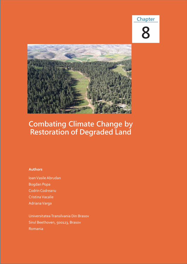
Combating Climate Change by Restoration of Degraded Land
Authors
Ioan Vasile Abrudan
Bogdan Popa
Codrin Codreanu
Cristina Vacalie
Adriana Varga
Universitatea Transilvania Din Brasov
Sirul Beethoven, 500123, Brasov
Romania
8Chapter

483
Chapter 8
Universitatea
Transilvania Din
Brasov
Brasov, Romania
Combating Climate Change by Restoration of Degraded LandIoan Vasile Abrudan
Bogdan Popa
Codrin Codreanu
Cristina Vacalie
Adriana Varga
1 restoration oF degraded land in the context oF climate change: deFinitions and historical evolution
������ǣ Mansourian, S., (2005) Overview of Forest Restoration Strategies and Terms. In Mansourian, S., Vallauri, D., Dudley, N., Forest Restoration in Landscapes - Beyond Planting Trees, pp. 8-17, Springer.
1�1 Introduction
When forests are lost or degraded, we lose far more than just the trees that they contain. Forests provide a large number of goods and services, including habitat for species, homeland for indigenous peoples, recreational areas, food, medicines, and environmental services such as soil stabilisation. And as forest areas are reduced, pressure on remaining forests increases.
�ơ����������������������������������������������������������Ǥ��������ǡ������������������Ƥ��� �����Ǧ������ �ơ����������� ��� �������������� ȋ������� ������ ����� ��������������� �������Ȍǡ� ������ ����� ����� �������� ������������� ����Ƥ��Ǥ� ����� ���� �����the approach taken by many governments that are seeking to support a timber industry or create jobs or, equally, those who have taken a simplistic approach to
Chapter 8
484
ƪ��������������������������������Ǥ������������������ǡ�����������������������Ǧ�������original forests, a near-impossible feat in areas where millennia of human intervention ���������Ƥ�������������������������������������Ǥ�
�������ơ�����������������������������������������ơ�����������������������������������some confusion or misconceptions. We attempt here to cover most of the terminology used in English taken from the Society for Ecological Restoration International ȋ����Ȍǡ������������������������������������������������������Ƥ�������������ơ������terminologies and concepts. It must be noted that this complexity is also apparent and sometimes exacerbated when translating these terms into other languages.
1�2 Definitions and examples
1�2�1 Ecological Restoration
����������� ������������ ��� ��Ƥ���� ��� ���� �������� ��� ���������� ���� ��������� ��� ���ecosystem that has been degraded, damaged, or destroyed. It is an intentional activity that initiates or accelerates the recovery of an ecosystem with respect to its health, integrity, and sustainability.
Example 1: In 2000, in an attempt to re-create a native wild wood, the Scottish nongovernmental organisation (NGO), Borders Forest Trust, together with many partners, bought a 600-hectare plot of land, Carrifran, in the Southern Uplands of Scotland in order to restore its original forest. Thanks to fossil pollen buried deep in peat, it was possible to identify the nature of the variety of species previously found on this now near-denuded site and therefore to develop a restoration plan that aimed to re-create the species’ mix that had occurred in the past. Thousands of native tree seeds from surviving woodland remnants in the vicinity were collected. A total of 103.13 hectares (165,008 trees) have been planted at Carrifran since the start of the project. The upper part of the site is being allowed to regenerate naturally.
1�2�2 Rehabilitation
Rehabilitation emphasises the reparation of ecosystem processes, productivity, and services, whereas the goals of restoration also include the reestablishment of the preexisting biotic integrity in terms of species’ composition and community structure.
Combating Climate Change by Restoration of Degraded Land
485
Example 2: Bamburi Cement’s quarries in Mombasa (Kenya) were once woodland expanses covering 1,200 hectares. Starting in 1971, experiments began with the rehabilitation of the disused quarries. In the face of badly damaged soils, three tree ��������������������������������������� ������ƥ�����������������������ǣ�����������equisetifolia, Conocarpus lancifolius, and the coconut palm. The Casuarina is nitrogen Ƥ����� ���� ��� �������� ���� ����� ��������ǡ� ��������� ��� ��� ��������� ������ ����� ����������������������Ǥ���������������������������������Ǧǡ�ƪ���Ǧǡ���������Ǧ�������������������Ǥ�The decomposition of the Casuarina leaf litter was initially very slow due to high protein content, thus impeding the nutrient cycling process, although this problem was overcome by introducing a local red-legged millipede that feeds on the dry leaves and starts the decomposition process. Today this area contains more than 200 coastal forest species and a famous nature trail, attracting 100,000 visitors a year since opening in 1984.
1�2�3 Reclamation
Reclamation is a term commonly used in the context of mined lands in North America and the United Kingdom. It has as its main objectives the stabilisation of the terrain, assurance of public safety, aesthetic improvement, and usually a return of the land to what, within the regional context, is considered to be a useful purpose.
Example 3: A large open-cut bauxite mine at Trombetas in Pará state in central Amazonia is located in an area of relatively undisturbed evergreen equatorial moist forest. A reclamation programme has been developed to restore the original forest cover as far as possible. The project has treated about 100 hectares of mined land per year for the last 15 years. First, the mined site was levelled and topsoil replaced to a depth of about 15 cm using topsoil from the site that was removed and stockpiled (for lessthan 6 months) prior to mining. Next, the site was deep-ripped to a depth of 90cm (1-m spacing between rows). Trees were planted along alternate rip lines at 2-m spacings (2500 trees per hectare) using direct seeding, stumped saplings, or potted seedlings. Some 160 local tree species were tested for their suitability in the programme, and more than 70 species from the local natural forests are now routinely used. After 13 years most sites have many more tree and shrub species than those initially planted because of seeds stored in the topsoil or colonisation from the surrounding forest. Not surprisingly, the density of these new colonists is greater at sites near intact forest, but dispersal was evident up to 640 m away from old-growth forest. The new species, most of which have small seed, have been brought to the site by birds, bats, or terrestrial mammals.
Chapter 8
486
1�2�4 Afforestation/Reforestation
�ơ��������������� �������������� ������ ��� ��������Ƥ����� ����������������� �����ǡ� ��� ����former case where no trees existed before. In addition, in the context of the U.N.’s ��������������������������������������ȋ�����Ȍ�����������������������ǡ������Ƥ����Ƥ�����������������������������������������������ơ����������Ǥ
�ơ����������� ��� ��Ƥ���� ��� ���������� ��� Dz���� ������� �����Ǧ�������� �����������of land that has not been forested for a period of at least 50 years to forested land through planting, seeding, and/or human induced promotion of natural seed sources.”
Example 4: During the middle years of the 20th century, very large areas of longdeforested land were planted in Scotland by the state forestry body, initially as a strategic resource. In contrast to the Borders Forest Trust project described above, �������ơ��������������������������Ǧ��������������������������ǡ� ���������������������monocultures, mainly of Sitka spruce from Alaska (Picea sitchensis) or Norway spruce (Picea abies) from mainland Europe. Planting was generally so dense that virtually no understorey plant species developed.
�������������� ��� ��Ƥ������� ������������� Dz����������� �����Ǧ�������� �����������of nonforested land to forested land through planting, seeding, and/or the human-induced promotion of natural seed sources, on land that was forested but that has been converted to nonforested land.”
Example 5: In Madagascar, large plantation projects were planned in the early 1970s ������������������������������Dz������������Ǥdz�����������ǡ������������������� �������ǡ� � �������� ��� ���������� ������ ���Ǥ������ �������� �������� �����Ƥ�����social and political tensions, as the local population systematically opposed a project ����������������������������������������Ƥ�Ǥ
��������Ƥ����������������������������������������������������������������������������������������������������������������Ǥ������������ǡ��������������������������������Ƥ���Ǥ�Because of its complexity, large-scale restoration requires a mixture of responses from practical to political and many practitioners are at a loss as to where to begin.
Some practical guidance is available:
Combating Climate Change by Restoration of Degraded Land
487
• The Society for Ecological Restoration (SERI) has developed guidelines for restoration (see Guidelines for Developing and Managing Ecological Restoration Projects, 2000, at www.ser.org).
• The International Tropical Timber Organisation (ITTO) developed some guidelines on the restoration, management, and rehabilitation of degraded and secondary tropical forests.
• The International Union of Forest Research Organisations (IUFRO) runs a special programme on correct usage of technical terms in forestry called SilvaVoc, available on its Web site: www.iufro.org/science/special/silvavoc/.
• �����������������������ȋ���Ȍ����� ������Ƥ�����������������������������where to restore (see Geography of Hope Update, When and Where to Consider Restoration in Ecoregional Planning at www.conserveonline.org).
• In 2003, IUCN and WWF published a book, by David Lamb and Don Gilmour, 19 Rehabilitation and Restoration of Degraded Forests, which covers site-based techniques to restoration (summarised in a paper in this manual) but also highlights some of the gaps.
• Cambridge Press has produced a Handbook of Ecological Restoration, 20 which is a two-volume handbook containing a large amount of material on the diverse aspects of restoration.
1�3 Evolution
Source: Uriel N. Safriel (2007) The Assessment of Global Trends in Land Degradation. In MannavaV.K. Sivakumar and Ndegwa Ndiang’ui. Climate and Land Degradation, pp 2-36, Springer Berlin Heidelberg New York.
The motivation for quantitative assessment of land degradation at a global scale is its recognition as an environmental issue of global societal implications. Yet, due to the ���Ǧ���������Ƥ����������Dz����������������dz�����������������������Ƥ��������ǡ�����Ƥ����������������������������������������������������������������ơ��� ��� ����selection of measurable attributes of land degradation, in the quality of the data sets, and in their spatial coverage. This resulted in a plethora of degradation estimates ��������ά����ά���������������������������ά����ά�����������������������Ǥ���������ǡ�����Ƥ��������ά�������������ȋ���������������������ǡ������������ά�����������land) has been cited more than the others. Though likely to be overly exaggerated
Chapter 8
488
(because it stands for a combination of degradation degree of a land unit and its spatial extent within the mapping unit of which it is a part), this high estimate has apparently served well the globality notion of the dryland degradation syndrome, essential to rallying support for international development assistance under the UNCCD. This �������������������������������������������Dz�����������������Ƥ������dz��������������the UNCCD some 70 non-dryland developing countries (compared to 93 developing dryland country Parties) which experience land degradation that is not included in ������� ������������ ��� �������Ƥ������ǡ� ������ ����� �������� ������������ �����Ƥ��� ���Dz�������Ƥ������dzǤ�������������������������������������ǡ��������������������������������� ��� ������������Ƥ������������� �������ơ� Dz�������Ƥ������dz������ Dz��������������dz�������Dz������dz�����������Ƥ������Ǥ�������������������������������������������������������������Ƥ�����������������������������������������������������������������������������������policy- and decision-making.
Though soil degradation featured highly in the currently available global degradation assessments, remotely-sensed vegetation attributes not only assess the most valued but threatened ecosystem service, but are also amenable for assessment at the global scale. However, caution is required when using this tool especially in drylands where productivity is tightly linked to rainfall variations. The monitoring required to meet the ��������������������������������������������Ƥ�������������������������������������������������Ƥ������� ������ǡ� ������ ���� ��� ���������� ���� ������Ǧ������� ����� ����� �������Ƥ��������������������Ƥ�������������Ǥ�������������������������������������������������of the land from those due to rainfall features, the ratio of NPP to rainfall (RUE) could be useful were it not negatively correlated with rainfall itself. An alternative method for detecting degradation trends, the Residual NPP Trends (RESTREND) is currently under development. It is based on an analysis of the residuals of the productivity-rainfall relationship throughout a time period for each pixel in the explored region. �� �������������� �����Ƥ����� ��������� ����������� ��� ���� ���������� ��� ����� ������Ƥ��� ��degradation trend, and the slope stands for its magnitude. To be reliable on a global ������ ����� �� ������Ǧ�������� ��������� ������ ������ ���� �������� Ƥ���� ��������������������������������������Ƥ������Ǥ
2 carbon Fluxes and the restoration oF degraded soil
Source: FAO (2004) Carbon sequestration in dryland soils, 129 pp, (http://www.fao.org/docrep/007/y5738e/y5738e0a.htm#TopOfPage)
Combating Climate Change by Restoration of Degraded Land
489
2�1 Introduction
Land-use change and soil degradation are major processes for the release of CO2 to the atmosphere. The increase in greenhouse gases (GHGs) in the atmosphere is now recognized to contribute to climate change (IPCC, 2001). Although uncertainties remain regarding the causes, consequences and extent of climate change, it is believed that human activities are having an impact on the energy balance of the �����Ǥ�������ƪ�����������������������������������������������������ǦƤ�����������Ǥ������concern has led to the 1997 international agreement in Kyoto (the so-called Kyoto Protocol), whereby most countries are committed to reducing their GHG emissions to the atmosphere. In this context, new strategies and policies within the international framework have been developed for the implementation of agriculture and forestry management practices that enhance carbon sequestration (CS) both in biomass and soils. These activities are included in Articles 3.3 and 3.4 of the Kyoto Protocol (KP) �����������������Dz��������ǡ�����Ǧ�����������������������dz�ȋ�����Ȍ�ȋ����ǡ�ȌǤ
The importance of these activities is that any action taken to sequester C in biomass and soils will generally increase the organic matter content of soils, which in turn will have a positive impact on environmental, agricultural and biodiversity aspects of ecosystems. The consequences of an increase in soil carbon storage can include increases in soil fertility, land productivity for food production and security, and prevention of land degradation. Therefore, they might constitute win - win situations.
A proper analysis of the impact of climate change must also consider other global concerns such as loss of biodiversity, changes in land use, growing food demand, and soil degradation. International United Nations conventions exist regarding these problems: the Convention on Biological Diversity (CBD), the Convention to Combat �������Ƥ�������ȋ���Ȍǡ����������������������������������ǡ����������������������������related United Nations programmes, e.g. the United Nations Environment Programme (UNEP), and the United Nations Development Programme (UNDP). Other initiatives, such as the Millennium Ecosystem Assessment, funded internationally by the World Bank, the United Nations Global Environment Facility (GEF), etc., aim to determine the state of the earth’s ecosystems, trying to take into consideration all global problems and the interactions among them.
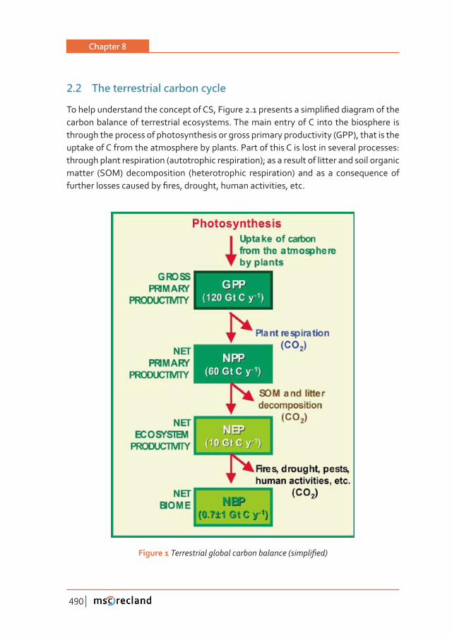
Chapter 8
490
2�2 The terrestrial carbon cycle
������������������������������������ǡ�������Ǥ������������������Ƥ������������������carbon balance of terrestrial ecosystems. The main entry of C into the biosphere is through the process of photosynthesis or gross primary productivity (GPP), that is the uptake of C from the atmosphere by plants. Part of this C is lost in several processes: through plant respiration (autotrophic respiration); as a result of litter and soil organic matter (SOM) decomposition (heterotrophic respiration) and as a consequence of �������������������������Ƥ���ǡ��������ǡ�����������������ǡ����Ǥ
Figure 1 ����������������������������������ȋ������Ƥ��Ȍ
Combating Climate Change by Restoration of Degraded Land
491
2�3 Soil degradation
�������������������������������������ȋ����ǡ�Ȍǡ�������������������������Ƥ������������������Ǥ�������������������������������������������ǡ���������������������������Ƥ�����amounts of C. Therefore, the potential for sequestering C through the rehabilitation of drylands is substantial (FAO, 2001). Lal (2000) estimated the magnitude of the potential for sequestering C in soils in terrestrial ecosystems at 50 - 75 percent of the historic carbon loss. Furthermore, Lal hypothesized that annual increase in atmospheric CO2 concentration could be balanced out by the restoration of 2 000 000 000 ha of degraded lands, to increase their average carbon content by 1.5 ������Ȁ��������������������������Ǥ���������Ƥ��������������������Ǥ�����������������degraded agricultural lands could have direct environmental, economic, and social ����Ƥ�������������������Ǥ����������ǡ���������������������������������������������������improvement in degraded soils, plant productivity and the consequent food safety and alleviation of poverty in dryland regions.
�����ơ������������������������������������Ƥ��������ơ����������������������Ǥ����������change leads to a loss in vegetation cover and subsequent loss in organic C in soils and soil quality. The processes of plant productivity, soil degradation and CS are closely linked. A decline in soil quality leads to a reduction in the soil organic C pool, and an increase in the emission of CO2 to the atmosphere. The decline in soil quality and structure leads to a loss in the capacity to retain water, and therefore in plant productivity.
2�4 Desertification and carbon sequestration
�����ơ���������������Ƥ������������������������������ǣ
• loss in soil aggregation
• ��������������������Ƥ�����������������
• reduction in soil water storage · increase in erosion potential
• ����������������ǡ���ƥ�������������������������
• disruption of biogeochemical cycles C, N, phosphorous, sulphur alterations in water and energy balance
• loss of soil resilience
Chapter 8
492
���� ��� ������ �ơ����� ����������� ���� ��������� �����2 to the atmosphere. Lal (2001) �������������������������������������������Ƥ������Ǥ�����������������������Ǧ������Ȁ���(Swift et al., 1994) on a land area of 1 020 000 000 ha (UNEP, 1991), the total historic C loss would amount to 8 - 12 Pg C. Similarly, vegetation degradation has led to a C loss of 4 - 6 Mg C/ha on 2 600 000 000 ha, adding up to 10 - 16 Pg C. The total C loss ���������������������������Ƥ���������������Ǧ������Ǥ������������������Ǧ����������the C lost (18 - 28 Pg) can be re-sequestered (IPCC, 1996) through soil and vegetation �����������ǡ�������������������������������������������������Ƥ�������������������Ǧ��Pg C (Lal, 2001). These estimates provide an idea about the loss of C as a result of �������Ƥ����������������������������������������������������������������������������Ǥ
Opportunities for improved land management as well as increasing CS should be developed in these areas. Agricultural systems contribute to carbon emissions through the use of fossil fuels in farm operations and through practices that result in loss of �����������������������Ǥ������������������ǡ����������������������ơ������������������when accumulating organic matter in the soil, or when aboveground woody biomass is increased, which then acts either as a permanent sink or used as an energy source ����������������������������Ǥ������������������������������Ƥ��ǡ����������������������Ƥ��ǡ�to be obtained from increased CS in drylands should be an additional incentive for stronger support for reforestation and agriculture in drylands.
Although drylands have been studied (Heathcote, 1983; Thomas, 1997), the impact of �������Ƥ���������������������������������������������������������������������Ƥ�������control on CS in dryland ecosystems have not been widely investigated. There are few ������������ǡ�����������������������Ǥ�������������ǡ������������������������Ƥ�����������������������������������Ƥ�������������������������������������������Ǥ�������������������������������������������������ǡ������������������������ơ�����������������������������Ǥ
3 carbon Fluxes and the restoration oF degraded agricultural and Forest lands
3�1 Restoration of degraded agricultural land
Source: Wade, M. R., Gurr, G. M., & Wratten, S. D. (2008). Ecological restoration of farmland: progress and prospects. Philosophical Transactions of the Royal Society B: Biological Sciences, 363(1492), 831-847.
Combating Climate Change by Restoration of Degraded Land
493
The goal of ecological restoration is to shift an ecosystem towards its pre-disturbed state with respect to ecosystem structure, function and composition (Hobbs & Norton 1996). The approach emphasizes the use of quantitative practices for measuring and restoring ecosystem ‘health’, including its ability to deliver ecosystem services (Costanza et al. 1997). Sustainable agriculture ‘refers to the ability of a farm ��������������������������Ƥ���������������������������������������ǡ�������������������ǡ������Ƥ������������������������������������������������������������������������conserving resources for the use of future generations. The continuity of production ���������������������������������������������������ơ������������������Ǥ�Ǯ�������ǯ�primarily refers to the land use comprising temporary or permanent crops and pastures. For the purposes of the review, this also includes non-crop vegetation, such as hedgerows and remnants of native vegetation, and waterways that are situated on farmland, but not plantation timber or farm forestry. Although farmland is often derived from grassland and woodland, these habitat types per se are generally excluded from the review unless the principles involved in the restoration of these habitats are relevant to that of farmland (Hooper et al. 2002; Ryan et al. 2002).
What causes farmland to become degraded and what are the symptoms of farmland in need of ecological restoration? Farmland and its environs are susceptible to inadvertent or deliberate degradation in their physical, chemical and biological condition by a range of farming activities that primarily result in changes to air quality, biological diversity, climate, soil condition and the quality and quantity of water (reviewed by Meyer & Turner 1992; Matson et al. 1997; Stoate et al. 2001; Robinson & Sutherland 2002; Tilman et al. 2002; Benton et al. 2003; Millennium Ecosystem Assessment 2005). Soil erosion results from the loss of vegetation cover due to �������ǡ������������������������Ǥ�������������������������ǡ����������ǡ������Ƥ�����������salinization of soils are caused by cultivation, drainage, irrigation and tree removal. �������������������������������������������������������������������������������ơǦ�������������� ��� ����ǡ� ����������� ���� ���������ǡ� �Ǥ�Ǥ� ������������ ��� ������� �ƫ����Ǥ� ������������ ������� ����ơ��������������������������������������� ���±�Ǧ�����ǡ�����������������������������ƪ���������Ǧ�������������������������������������������������Ǥ�����������global impacts on atmospheric constituents (principally carbon dioxide, methane and ����������������Ȍ�������������ȋ����ƪ��������������������������Ȍ�����������������������removal, biomass burning, fertilizers and livestock. Finally, land cover changes lead to both habitat loss and fragmentation, which threaten aquatic and terrestrial taxa (Meyer & Turner 1992; Matson et al. 1997; Stoate et al. 2001; Robinson & Sutherland 2002; Tilman et al. 2002).
Chapter 8
494
Symptoms of degraded farmland include algal blooms and pesticide residues in waterways, pest outbreaks, plant disease epidemics such as ‘rural dieback’ of native Australian eucalypts, which is principally caused by the root rot fungus Phytophthora cinnamomi, and disease epidemics of livestock, such as foot and mouth disease and ��ƪ��������������ȋ��ǡ�Ǯ�����ƪ�ǯȌǤ������������ǡ�����������������������������������ǡ���������������������������������������ǡ���������������Ƥ�������������������������������with herbicides, and a general reduction in species richness and abundance of plants and animals (Wills 1993; Stoate et al. 2001; Tilman et al. 2002; Millennium Ecosystem Assessment 2005).
Importantly, agricultural practices have both local and landscape-scale impacts that transcend farm boundaries (Meyer & Turner 1992; Benton et al. 2003; Cramer & Hobbs Ǣ�����������������Ǥ�ȌǤ������� �������Ƥ������� ������������������ơ�������������shortened crop rotation cycles and increasing input of agrochemicals. On a landscape �����ǡ�Ƥ���������������������������������������ǡ��������������������Ƥ��������������with few or no non-crop habitats remaining (Tscharntke et al. 2005). The total annual ��������� ȋ�ơǦ����Ȍ� ������ ��� ������������ ��� �������� ���������� ȋ���ǡ� ����� ���� �����Ȍǡ�biodiversity and human health (pathogens and pesticides) have been estimated for the United Kingdom at £1149–3907 million between 1990 and 1996 (Pretty et al. 2000) and £1514 million in 2000 (Pretty et al. 2005), and for the USA at £3256–9678 ������������ȋ����������Ƭ���ơ��ȌǤ�����������������haí1 of arable land and permanent pasture for the United Kingdom (UK) in 1996 and £17–55haí1 of arable land in the USA.
����������������������������������������������������������Ƥ��������������������������ǡ�the pivotal paper by Costanza et al. (1997) calculated the combined economic value of three ecosystem services (biological control, pollination and food production) from worldwide cropland to be USD$128.8 (£73.802) billion per year or USD$92 (£53) per ha. A caveat here is that Costanza et al. (1997) assigned a nil value to the ecosystem service of habitats or refugia for resident and transient taxa because this service ‘do(es) not occur or (is) known to be negligible’, hence the true value of cropland is likely to be underestimated. Nevertheless, by these calculations, the worldwide ecosystem ������������Ƥ���������������������������������������� haí1yrí1, yet the external costs of intensive agriculture in countries like the UK are £208haí1yrí1. Equally compelling ���������������������������������������������Ƥ���������������������������������������������������Ǥ������������ �����������������Ƥ������������������������������������pest control, ecotourism, pollination and waste disposal (Pimentel et al. 1997). It is evident that more sustainable agricultural practices in conjunction with ecological
Combating Climate Change by Restoration of Degraded Land
495
restoration methods on farmland are necessary to reduce the unacceptably high external costs of agriculture that are borne by the community. In addition, ‘ecological engineering’ techniques are available to enhance ecosystem services on farmland, �����������������������������������������������Ƥ�������������������������������������for biological pest control and contribute to biodiversity in general.
Agriculture and biodiversity conservation have been traditionally viewed as incompatible, with agriculture considered a major driver of species loss for many plant and animal taxa, such as bumble-bees (Bombus spp.) and bird species like skylarks (Alauda arvensis L.) since 1945 (Stoate et al. 2001; Robinson & Sutherland 2002). Agriculture represents the dominant land use throughout much of Western ������������������Ƥ������������������������������������������������������������������Ǥ�Agroecosystems, however, are very hostile to a wide diversity of species owing to ������������������������������������������������������Ƥ�������������������������������Ƥ������� ��� ��������� ���Ǥ� ������ǡ� ������ ��� �� ��������� ���� ������Ƥ��� ���������systems to be applied to increasingly consolidated land areas, leading to the loss of ���Ǧ�������������ǡ���������Ƥ�������������������������ǡ������������������������������traditional mixed arable and livestock farming. As a result, remnant native vegetation �����������������������������ơ����������������������������������Ǯ�����ǯ�������Ƥ����corners join. These nodes can be rich ‘hotspots’ of invertebrate, vertebrate and plant ����������ȋ��������Ƭ��������� ȌǤ���������ǡ�����������������Ƥ��������������������������the cropping systems themselves, including greater pesticide and fertilizer usage and shorter fallow periods (Stoate et al. 2001; Pywell et al. 2005). However, more recently, ������������������ ������������������������������������ơ����� �������������������of the value of natural, undisturbed remnants and to a better recognition of the role ����������������Ƥ������������������������������������������������������ȋ��������������al. 2005). As Novacek & Cleland (2001) pointed out ‘we are obviously past any point �����������������������������������������������Ǯ��������ǯ����������������ƥ��������������job. Greater attention must be placed on human-dominated landscapes that surround the less disrupted areas. In this way, agriculture can make important contributions to ����Ǧ������������������ǡ����������������Ƥ���������������������������������������������ơ������ ��������� �����Ǥ��������� ����� �������������������������������� ����������������� ��ơ������ �������� ������ ������� ����������� ������������� Ƥ����� ȋ������������ ��� ��Ǥ�2004) and improved biological pest control and crop pollination may directly increase farmers’ income (gVWPDQ et al. 2003; Ricketts et al. 2004).
Chapter 8
496
3�2 Restoration of degraded forest land
Source: Biringer, J., and Lara J. Hansen J. L., (2005) Restoring Forest Landscapes in the Face of Climate Change. In Mansourian, S., Vallauri, D., Dudley, N., Forest Restoration in Landscapes - Beyond Planting Trees, pp. 31-41, Springer.
Climate change is arguably the greatest contemporary threat to biodiversity. It is ���������ơ������������������������������������������������������������������������more dramatic as the climate continues to change due to anthropogenic greenhouse gas emissions into the atmosphere, mostly from fossil fuel combustion.
������ ������������ ��� ����� ����� ��ƥ����� ��� �������� ������ǡ� ��� ���� ����������� ���seen as a possible adaptive management approach for enhancing the resilience of ecosystems to these changes.
Climate change will result in added physical and biological stresses to forest ecosystems, including drought, heat, increased evapotranspiration, altered seasonality of hydrology, pests, disease, and competition; the strength and type of �ơ�������������������������������Ǥ�����������������������������������������Ǧ���������threats to forest biodiversity, including overharvesting, invasive species, pollution,and land conversion.
This will result in forest ecosystems changing in composition and location. Therefore, in order to increase the potential for success, it will be necessary to consider these changes when designing restoration projects. On the other hand, restoration projects can also be viewed as a key aspect of enhancing ecosystem resilience to climate change. Human development has resulted in habitat loss, fragmentation, and degradation. ��Ƥ��������� ��� ������������������������������ơ����������������������� ����������������protecting the ecosystem’s natural ability to respond to stress and change. Research ��������� ����� ����� �������� �������������� Dz�������dz����� ������� ������������� ���������point, which can draw on their own internal diversity to have natural adaptation or acclimation potential and therefore greater resilience. Any restoration activities that enhance the ecological health of a system can thus be seen as creating or increasing ����������������ơ���������������������������������������������������������Ǥ�����������be mentioned that there are obvious limits to the rate and extent of change that even a robust system can tolerate.
Combating Climate Change by Restoration of Degraded Land
497
As a result it is only prudent to conduct restoration for enhancing resilience in tandem ������ơ���������������������������������������ǡ���������������������������������Ǥ
For many with a forestry background, carbon dioxide sequestration might seem a concomitant advantage to restoration projects, which can aid in reduction of atmospheric concentrations of greenhouse gases. While forests do hold carbon, and their loss does release carbon, their long-term capacity to act as a reliable sink ��� ���� ����������������������ǡ������������ �����ơ�����������������ǡ� ��������� ����������strategy. Where restoration is promoted with a focus on capturing carbon, an analysis of climate change impacts should be integrated into project planning to determine �����������������������������������������������Ƥ��Ǥ�������������������������������Ƥ��������� ����������������������������� ������ǡ� �����������ǡ� ��������������������ơ�������� ������� ������� ���������Ǥ� ����� �������� ��� ����������� ����������Ǧ��������� �ơ�����are not yet plentiful, due to relatively recent revelations about the scale and impact that climate change will have on ecosystems. However, the global temperature has risen 0.7°C as atmospheric concentrations have risen and extinctions and large-scale ecosystem changes are expected. A number of forest types are already being negatively impacted, including tropical mountain cloud forests, dry forests, and forests in the boreal zone, and climate-related extinctions are already thought to have occurred, for example amongst amphibians. Along the coasts, the rising sea level is increasing the vulnerability of mangroves. Restoration as a means to ensure healthy ecosystem structure and function will have a large part to play in adapting ecosystems to these broad-scale changes.
Framework for Understanding Intersection of Resilience-Building and Forest Restoration and Protection:
1. Protection: For some forests protection alone will not increase resilience to climate change. Many tropical montane cloud forests provide a case in point. Australia’s Wet ��������������������������������������������������������ά���������������������������warming of 1 degree Celsius, which will leave amphibians and other cool-adapted species no upland migration options as conditions become warmer and drier.
2. Sequestration via restoration: Many examples exist where the planting of trees stores carbon but is not coordinated with conservation or resilience-raising advantages. Nonnative trees, such as Eucalyptus, are often planted solely for the �����������Ƥ�ǡ� ������� �������������������������������������� ���� ���������ǡ� �������������������������ơ�������������������������Ǥ
Chapter 8
498
3. Resilience/adaptation: Restoration is but one of the many types of management options that increase resilience. For example, actions that respond to changing ��������������������������������������������������Ƥ��������������������������������forestry that will receive special attention with the advent of climate change. Activities �������������������ƥ����������������������������������������������������Ǥ������������ǡ������������������������������ ����������� �����ƥ��������������Ǧ������������������that 75 percent less mangrove wood is needed for cooking, thereby increasing the resilience of the system by reducing harvest levels. Such actions decrease degradation of the mangrove and raise the probability that it will be equipped to respond to the �ơ����������������������Ǥ
4. Sequestration and resilience/adaptation: Restoration and resilience go hand in hand when the impacts of climate change are taken into account in project planning. Whether passive or active restoration, activities target those areas that will be more suitable to climate change, and encourage use of species that will be hardier under new climatic conditions (successful seed dispersers, for example).
5. Intersection of protection, sequestration, and resilience/adaptation: Creating ��ơ�����������������������������������������������������������������������������������impacts of climate change while at the same time sequestering carbon. This scenario is similar to the one above, except that restoration is focussed on increasing the resilience of protected areas by expanding boundaries to increase suitable habitat under changing climatic conditions.
6. Protection and adaptation: Protection can lead to increased resilience to the impacts of climate change, where suitable habitat is intact, and the expansion of boundaries is possible to accommodate species’ needs with a changing climate. A ������������������������������������������������Ƥ����������������������������������forest stands, functional groups and keystone species, and climate refugia.
4 mitigating climate change by restoration oF degraded lands
Source: Alan J. Franzluebbers and Paul C. Doraiswamy (2007) Carbon sequestration and land degradation. In MannavaV.K. Sivakumar and Ndegwa Ndiang’ui. Climate and Land Degradation, pp 343-356, Springer Berlin Heidelberg New York.
Combating Climate Change by Restoration of Degraded Land
499
Storing carbon in soil as organic matter is not only a viable strategy to sequester CO2 from the atmosphere, but is vital for improving the quality of soil. This presentation describes (1) C sequestration concepts and rationale, (2) relevant management approaches to avoid land degradation and foster C sequestration, and (3) a summary of research quantifying soil C sequestration. The three primary greenhouse gases (CO2, CH4, and N2O) derived from agriculture have increased dramatically during the past century. Conservation management practices can be employed to sequester C in soil, counter land degradation, and contribute to economic livelihoods on farms. Trees can accumulate C in perennial biomass of above-ground and below-ground growth, as well as in the deposition of soil organic matter. Minimal disturbance of the soil surface with conservation tillage is critical in avoiding soil organic C loss ����������������������������������������Ǥ������������������������Ǧά��ǡ�����therefore, application to land promotes soil organic C sequestration and provides readily-available, recycled nutrients to crops. Green manures can be used to build soil fertility, often with leguminous plant species having symbiotic root associations with ��������ǦƤ����� ��������Ǥ����������� ����� ������ ���������� ��� ���������� ����� ��������C when managed properly, but can also be degraded due to overgrazing, careless management, and drought leading to accelerated soil erosion and undesirable species composition. Opportunities exist to capture and retain greater quantity of C from crop and grazing systems when the two systems are integrated. Fertilization is needed to achieve production goals, but when applied excessively it can lead to environmental pollution, especially when considering the energy and C cost of manufacture and transport. Agricultural conservation management strategies to sequester CO2 from the atmosphere into soil organic matter will also likely restore degraded land and/or avoid further land degradation.
4�1 Introduction
Land degradation is an insidious process that threatens the sustainability of agriculture, not only in the arid and semi-arid regions, but also in the sub-humid and humid regions, as a result of the loss of agro-ecosystem capacity to meet its full potential. Resulting from complex, and little understood, interactions among periodic weather stresses, extreme climatic events, and management decisions, land degradation is a serious global concern in a world searching for sustainable development to meet the needs of a rapidly increasing human population, to reverse the negative impacts of our choices on the environment in which we live, and to fairly distribute the world’s �����������������������������Ƥ�����������Ǥ
Chapter 8
500
Atmospheric concentration of radiatively active trace gases [also called greenhouse gases (GHGs)] has been increasing dramatically during the past several centuries (IPCC 2001). Several of the important GHGs in the atmosphere are derived, at least partially, from agricultural activities. Three of the most important GHGs related to agricultural activities are carbon dioxide (CO2), methane (CH4), and nitrous oxide (N2�ȌǤ������������������������� ����������� ά���� ��������������������������������GHGs. The source of this CO2 is dominantly from fossil fuel combustion. Since 1750, the concentration of CO2���������������άǡ������������������������4 has increased άǡ���������������������������2����������������άǤ�����������ǡ��������������������������������� ��������������������������������� �����������ά���� �����������ǯ��total GHG emission.
Global concern for the rising atmospheric concentration of GHGs is also increasing, because of the important implications of these gases on global warming. Potentially dramatic consequences of even relatively minor climate change could cause devastating weather-related occurrences, such as increased frequency and duration ��� ��������ǡ����������������� ���� ������� ƪ������� ������ǡ� �������� ���������� ����intensity of tornadoes and cyclones, and melting of polar ice caps that could threaten abundant human civilizations along coastal continental areas.
Understanding the linkages between agricultural land-use activities and GHG dynamics should help society to strengthen its resolve to avoid these potentially ��������������������������������ơ��������������������������������������������������functioning and overcome human-induced land degradation.
Rising concentration of atmospheric CO2 has been largely attributed to expanding use of fossil fuels as an energy source. Reducing net GHG emission is possible by:
• ����������������������������������������������������������ƥ�����
• Relying more on low-C energy sources, such as
- Capturing solar energy
- Generating wind power
- Harvesting biofuels
• Sequestering C
Combating Climate Change by Restoration of Degraded Land
501
������� �������������� ���� ��� ��Ƥ���� ��� ���� ����Ǧ����� �������� ��� �� ��� �����the accumulation of CO2 in the atmosphere can be reduced or slowed. Carbon sequestration can occur globally in one of several compartments:
• Terrestrial biosphere
• Underground in geologic formations
• Oceans
This focuses on the terrestrial biosphere, which is directly manipulated by agriculture through changes in vegetation and soil disturbance. Carbon sequestration in the terrestrial biosphere can be accomplished by:
• ����������� ��������Ƥ���������� ��������������2 by terrestrial vegetation with emphasis on enhancing physiology and rate of photosynthesis of vascular plants.
• Retaining C in plant materials and enhancing the transformation of C to soil organic matter.
• Reducing the emission of CO2 from soils caused by heterotrophic oxidation of soil organic C.
• Increasing the capacity of deserts and degraded lands to sequester C.
Storing C in soil as organic matter is not only a viable strategy to sequester C from the atmosphere, but is also essential in improving the quality of soil. Soil organic matter plays a vital role in:
• Soil fertility, by slowly supplying nitrogen and many other essential elements and molecules to plants through mineralization/immobilization turnover.
• Water cycling, by contributing to soil aggregation and water-holding capacity.
• Soil biodiversity, by providing the C and energy sources needed for soil biological community development.
• ��������������������Ƥ������ǡ����������������������������ǡ�����������������ǡ�and biological activity.
• Biogeochemical cycling, by storing and delivering many globally important elements interacting through the atmosphere, hydrosphere, lithosphere, and biosphere.
Chapter 8
502
4�2 Management Approaches
The terrestrial C cycle can be simply divided into the two primary processes of photosynthetic uptake of CO2 from the atmosphere (i.e., C input) and respiration of CO2 from living organisms back to the atmosphere (i.e., C output). On a global scale under steady-state conditions, rates of C input and output have often been ��������������������ȋ������������ȌǤ������������������������������ơ����ǡ����������ǡ�must recognize the inherent balance between these processes.
Maximizing C input to the terrestrial biosphere from the atmosphere is possible in agricultural systems through a variety of management options, including:
• Plant selectionǡ� �������� ������ ��ơ�������� ��� ��������������� ��������� ������among species, cultivars, and varieties. Perennial plant species often have advantages over annual crops at capturing C, because of a longer growing season and more extensive root distribution (Liebig et al. 2005). However, selection of appropriate annual crops in rotation sequence can maximize growth potential ������ �������� ������������Ǥ� �� ����������� �ơ���� ���� �������� ��� ������������high-biomass producing energy crops to maximize photosynthetic capture of CO2 (Baral and Guha 2004).
• Tillage management, whereby the type and frequency of tillage is used to �������� ��������� �����Ƥ�� ������ �������������������Ǥ��������� ��� ������ ����� ���improve the physical condition of soil so that crops can achieve maximum growth potential, but it is also a tool that disturbs soil and promotes oxidation of soil organic matter (Franzluebbers 2004).
• Fertilization management, whereby the source, rate, timing, and placement of ����������� ����������������������������������������������Ǥ���ƥ�����������������and adequate nutrient supply are essential management considerations to maximize genetic potential of plants (Lal and Bruce 1999), but the high energy cost of mining and manufacturing inorganic sources of nutrients must be recognized as a source of GHG emission (Schlesinger 2000).
• Integrated management, whereby pests can be adequately controlled and environmental and socio-economic consequences of agricultural activities can be balanced with agronomic production considerations (Makumba et al. 2007).
Combating Climate Change by Restoration of Degraded Land
503
Minimizing C loss from soil to the atmosphere has also been a major focus of agricultural research on C sequestration. Management options to minimize C loss from soil include:
• Reducing soil disturbance by less intensive tillage and erosion control (Lal et al. 1998).
• More fully utilizing available soil water, which not only promotes optimum plant growth, but also reduces the oxidative capacity of soil microorganisms to decompose soil organic matter and crop residues (Lal 2004).
• Maintaining surface residue cover to increase plant water use and production. Surface residue cover also fosters greater fungal abundance in the soil microbial community, which promotes greater stabilization of soil aggregates and resistance of soil organic C to decomposition (Nichols and Wright 2004).
In agriculture, there are many management practices that can be employed to sequester C and counter land degradation. The following sections describe some key management practices to combat land degradation. How these management practices might also contribute to soil C sequestration will be highlighted.
4�2�1 Tree Plantings
Trees can accumulate C in perennial biomass of above-ground and below-ground growth, as well as in the deposition of soil organic matter. The intentional mixing of trees or other woody perennials with agricultural crops, pastures, and/or livestock ��� ��Ƥ���� ��� ������������Ǥ� ������������� ��������� ���� ����������� ���� �������������������������������ơ��������������������������������������������������ȋ�����ȌǤ�This section focuses on agroforestry-related changes in C accumulation rather than on natural or planted forests.
Issues of importance in agroforestry systems are:
• Climate
• Selecting adapted species
• Soil conditions
• Plant density
• Intended use
Chapter 8
504
• Spatial arrangement of trees and other land uses.
The types of agroforestry practices include complex agroforestry systems, boundary plantings, hedgerow intercropping, and improved fallow (Albrecht and Kandji 2003). Carbon sequestration potential of tropical agroforestry systems has been estimated.
From plantation survey data in Australia (400-600 mm zone), mean C accumulation rate of 3.8 Mg ha-1 yr-1 occurred in the woody biomass from a variety of tree species. In the central Philippines, C sequestration in the above-ground biomass of Leucaena leucocephala during 6 years of growth was estimated at 10.7 Mg C ha-1 yr-1 (Lasco and Suson 1999).
Carbon accumulation in the soil is the major sink for hedgerow intercropping systems used to produce biomass for improving soil fertility. In Nigeria, L. Leucocephala and Gliricidia sepium intercropping systems sequestered 0.20 Mg C ha-1 yr-1 in the topsoil compared with sole cropping (Kang et al 1999). From two experiments in Malawi (6 to 9-year studies), a G. sepium intercropping system sequestered soil organic C at a rate of 1.2 Mg ha-1 yr-1 in the surface soil (0-20 cm), but at a rate of 6.2 to 11.7 Mg ha-1 yr-1 when calculated to a depth of 0-200 cm (Makumba et al. 2007). Deep rooting of the ���������������������������������������������ơ�������������������Ǥ�������������������RothC models in Sudan and Nigeria, soil organic C accumulation with tree plantings was estimated at 0.10 ± 0.05 Mg ha-1 yr-1 (Farage et al. 2007).
4�2�2 Conservation-Tillage Cropping
Minimal disturbance of the soil surface is critical in avoiding soil organic matter loss from erosion and microbial decomposition. Successful conservation-tillage cropping systems have been developed and evaluated throughout the world. As part of a system for conservation agriculture, conservation-tillage cropping can improve plant production, reduce environmental pollution, and store a greater quantity of soil organic C.
��������� ����������� ���� ��ƪ������ ���� ������� ��� ����� �������� �� ��������� ��� ���sequestered with adoption of conservation tillage. With more extreme dry and/or wet conditions, soil organic C sequestration tended to be highest in milder and warm-wet climatic regions of North America. Mean soil organic C sequestration in North America is estimated at 0.33 Mg C ha-1 yr-1. In the warm-moist climatic region of the southeastern USA, adding a cover crop to a conservation-tillage system can nearly
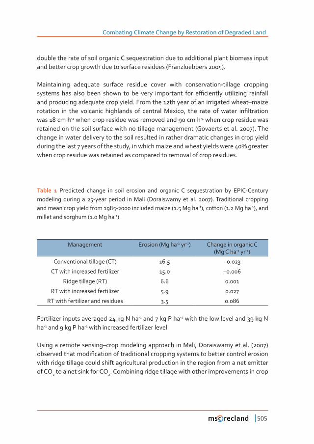
Combating Climate Change by Restoration of Degraded Land
505
double the rate of soil organic C sequestration due to additional plant biomass input and better crop growth due to surface residues (Franzluebbers 2005).
Maintaining adequate surface residue cover with conservation-tillage cropping �������� ���� ����� ����� ������ ��� ��� ����� ���������� ���� �ƥ�������� ���������� ���������and producing adequate crop yield. From the 12th year of an irrigated wheat–maize ��������� ��� ���� ��������� ���������� ��� ��������������ǡ� ���� ����� ��� ������ ��Ƥ���������was 18 cm h-1 when crop residue was removed and 90 cm h-1 when crop residue was retained on the soil surface with no tillage management (Govaerts et al. 2007). The change in water delivery to the soil resulted in rather dramatic changes in crop yield ���������������� �������������������ǡ�������������������������������������� ά���������when crop residue was retained as compared to removal of crop residues.
Table 1 Predicted change in soil erosion and organic C sequestration by EPIC-Century modeling during a 25-year period in Mali (Doraiswamy et al. 2007). Traditional cropping and mean crop yield from 1985-2000 included maize (1.5 Mg ha-1), cotton (1.2 Mg ha-1), and millet and sorghum (1.0 Mg ha-1)
Management Erosion (Mg ha-1 yr-1) Change in organic C (Mg C ha-1 yr-1)
Conventional tillage (CT) 16.5 –0.023
CT with increased fertilizer 15.0 –0.006
Ridge tillage (RT) 6.6 0.001
RT with increased fertilizer 5.9 0.027
RT with fertilizer and residues 3.5 0.086
Fertilizer inputs averaged 24 kg N ha-1 and 7 kg P ha-1 with the low level and 39 kg N ha-1 and 9 kg P ha-1 with increased fertilizer level
Using a remote sensing–crop modeling approach in Mali, Doraiswamy et al. (2007) ������������������Ƥ�����������������������������������������������������������������with ridge tillage could shift agricultural production in the region from a net emitter of CO2 to a net sink for CO2. Combining ridge tillage with other improvements in crop
Chapter 8
506
����������� ������ ������� ����� �������� ��� Ǧά� ��� ����� ���������� ��� ������������cropping systems with conventional tillage (table 4.1).
4�2�3 Animal Manure Application
�����������������������������Ǧά��ǡ���������������������������������������������organic C sequestration. In a review of studies conducted in the southeastern USA, �������� ������������������� �������������������� ������ ���� ��� �����Ƥ������������ ��� �����organic C only when evaluations were conducted for more than 2 years. Conversion ����������������������������������������������ή�ά��������������������Ǥ���������������organic C has been shown to increase with animal manure application, very few whole-system data have been collected. Manure application may simply transfer C from one land to another, while investing energy in transport and handling operations. A full C accounting approach is needed to adequately assess manure application as a viable C sequestration strategy.
Other long-term studies on farmyard (FYM) application to soil have clearly shown its ����Ƥ�������������������ǡ������������������ǡ���������������������������Ǥ�������Ǧ�����Ƥ������������������������ȋ�λ�ǡ����Ȍǡ�����������������������������Ǥ�ΰ�Ǥ����C ha-1 yr-1 with FYM (10 Mg ha-1 yr-1) compared to without FYM (Kapkiyai et al. 1999). ����������������������ǡ��ΰ�ά����������������������������������Ǥ��������������������(5.3 Mg ha-1Ȍ�����ά��������������������������������Ǥ
�����Ǧ�����Ƥ��������������������������ȋ�λ�ǡ����Ȍǡ�����������������������������0.21 ± 0.01 Mg C ha-1 yr-1 with FYM (5 Mg ha-1 yr-1) compared to without FYM (Agbenin ����������ȌǤ��������������������Ǧ��Ƥ����������ǡ����������������������������ΰ�����ha-1 yr-1 with FYM.
�����Ǧ�����Ƥ������������������������ǡ� ������ ȋ�λ�ǡ����Ȍǡ� �������������������greater with FYM (3.9 g kg-1) than without FYM (3.3 g kg-1) (Manna et al. 2007). Total ����������������ά��������������������������������������������Ǥ
�������ǡ����������������������������������������������ơ�����������������������Ǥ������Ǧ�����Ƥ���������������������������ǡ�������ȋ���Ȍǡ��������������������������by 0.56 ± 0.02 Mg C ha-1 yr-1 with FYM (10 Mg ha-1 yr-1) compared to without FYM (Kundu et al. 2007). Above-ground crop biomass production with FYM (6.4 Mg ha-1) was 2.4 times greater than without FYM application.
Combating Climate Change by Restoration of Degraded Land
507
�����Ǧ�����Ƥ������������������������ȋ�λ�ǡ����Ȍǡ�����������������������������Ǥ�Mg C ha-1 yr-1 with FYM (7.5 Mg ha-1 yr-1) compared to without FYM (Govi et al. 1992). ���������Ƥ��������������������������ά���������������������ά�����������Ǥ
In a 20-year study of pearl millet–wheat cropping in India (26 °C, 440 mm), soil organic C increased with increasing FYM application rate. However as a percentage of C �������������ǡ���������������������������������������������ƥ������������������������soil (Gupta et al. 1992).
���������� ���� ��������� ��ƪ������ ��� ������� ������� ������������ ��� ����� �������� ��storage, temperature regime appears to have a greater impact than precipitation ������Ǥ� ���������� ����� ��� ����� ���� � ή� ά� ����� �������� ����� ������� ������� ���������������� ������� �������ǡ���������������ή�ά� ��� �������� �������Ǥ������� ������������������ή�ά��������������������������������ǡ�����������������������������ή�άǤ�These data are consistent with environmental controls on soil microbial activity and suggest that future research will require increasing acknowledgement of the linkage between climate and potential C sequestration.
4�2�4 Green-Manure Cropping Systems
Green manures are used to build soil fertility, often with plant species having the ������������Ƥ�����������������������������������������������������������������������Ƥ�������������Ǥ�������������������������������������������������������������������can be subsequently stored in soil organic matter.
On an abandoned brick-making site in southeastern China (16.5 °C, 1600 mm), �������������������������������������������������������Ƥ������������������������������organic C sequestration of 0.36 ± 0.40 Mg C ha-1 yr-1 (Zhang and Fang 2007). With soybean as a green manure for 8 years in Columbia (27 °C, 2240 mm), maize yield with green manure (4.2 Mg ha-1Ȍ�����ά�����������������������������������ȋ��������et al. 2006). Soil organic C did not change during the 8 years of green manuring, probably because of rapid decomposition caused by abundant precipitation, warm temperature, and nutritious residue quality.
At the end of 12 years of Sesbania green manuring in India (24 °C, 715 mm), soil organic C sequestration was 0.09 ± 0.03 Mg C ha-1 yr-1 (Singh et al. 2007). At the end of 13 years of wheat/soybean–maize cropping with and without vetch as a green manure cover crop in southern Brazil (21 °C, 1740 mm), soil organic C sequestration was í0.30
Chapter 8
508
± 0.15 Mg C ha-1 yr-1 under conventional tillage and 0.66 ± 0.26 Mg C ha-1 yr-1 under zero tillage (Sisti et al. 2004). These data suggest that climatic conditions, green manure ����������������ǡ����������������������������������������������������������������ơ�������soil organic C change with green manuring.
4�2�5 Improved Grassland Management
Degradation of permanent grasslands can occur from accelerated soil erosion, compaction, drought, and salinization. Strategies to sequester soil organic C in grasslands must, by necessity, improve the quality of grasslands. Strategies for restoration should include:
• Enhancing soil cover
• �����������������������������������������������ơ�����������������
Achieving a balance between agricultural harvest and environmental protection is needed (i.e., stocking density should be optimized). On an oak-grassland in central ����������ȋλ�ǡ����Ȍǡ������� ��Ƥ����������������������������������������������cover. However, cattle stocking density played an even larger role in controlling water ��Ƥ������������������Ǥ
Establishment of bermudagrass pasture following long-term cropping in Georgia ����ȋλ�ǡ����Ȍ���������� ��������Ƥ��������������������������������������������Ƥ���� ��������������������Ǥ�������������������������������������������������������������������������������������������������Ƥ����������ǡ��Ǥ�Ǥ������������������������������rate was 0.30 Mg C ha-1 yr-1 when forage was removed as hay, 0.65 Mg C ha-1 yr-1 when forage remained unharvested, and 1.40 Mg C ha-1 yr-1 when forage was grazed moderately to moderately heavy by cattle during the summer (Franzluebbers et al. 2001).
4�2�6 Cropland-Grazing land Rotation
Opportunities exist to capture a greater quantity of C from crop and grazing systems when the two systems are integrated, because:
• Ligno-cellulosic plant materials can be utilized by ruminant animals
• Manure is deposited directly on the land
Combating Climate Change by Restoration of Degraded Land
509
• Weeds can be managed with management rather than chemicals
���������������� �������������� ������������Ǧ�������� ��������ǡ� �����Ƥ����� ����������exists to avoid loss of soil organic C that can accumulate during a perennial pasture phase. In Uruguay, soil erosion averaged 19 Mg ha-1 under conventional-tillage continuous cropping, 7 Mg ha-1 under conventional-tillage crop–pasture rotation, 3 Mg ha-1 under no-tillage continuous cropping, and <2 Mg ha-1 under under no-tillage crop–pasture rotation (Garcia-Prechac et al. 2004). Soil or ganic C with crop–pasture rotation was also greater than with continuous cropping in both tillage systems. In the long-term, crop yield was enhanced with crop–pasture rotation than with continuous cropping, especially with no tillage (Garcia-Prechac et al. 2004).
In Argentina, rotations with <7 years of conventional-tillage cropping alternated with >3 years of perennial pasture were able to maintain soil organic C and other important soil properties within acceptable limits to avoid degradation (Studdert et al. 1997). Diaz-Zorita et al. (2002) found that cattle grazing in crop–pasture rotations compacted surface soil only under conventional tillage, but not under no tillage. The ability of soil to resist compaction under no tillage was attributed to greater structural stability.
�������Ǧ�����������������������������������ǡ���ƥ���������������������������������������crops and livestock to achieve greater agricultural sustainability through enhanced ��������� �������ǡ� ������� ����� �������ǡ� ���� �������Ƥ������� ��� ������������� ������������(Katsvairo et al. 2006, Franzluebbers 2007).
4�2�7 Optimal Fertilization
����������������������������������������������������Ƥ����������������������������������soils, especially in soils exhausted by years of (a) soil erosion, (b) intensive disturbance with tillage, and (c) continuous harvest of products that remove large quantities of nutrients. On the other hand, excessive fertilization can occur when maximum agronomic prescriptions exist without regard for economic and environmental consequences. Today, the C cost of fertilization has become increasingly scrutinized (Schlesinger 1999; Izaurralde et al. 2000).
In a review of data available from the warm-moist climatic region of the southeastern USA, there was a positive response of soil organic C with the application of N fertilizer. The mean N fertilizer rate to achieve maximum soil organic C sequestration was 171
Chapter 8
510
kg N ha-1 yr-1, within the range of values often reported to maximize plant yield. However, when considering the C cost of N fertilizer (i.e. C costs of manufacture, distribution, and application), the optimum N fertilizer rate was 107-120 kg N ha-1 yr-1 based on C costs of 0.98 to 1.23 kg C kg-1 N fertilizer (Izaurralde et al. 1998, West and Marland 2002). Also accounting for the global warming potential of assumed N2O emission associated with N fertilizer application (1.586 kg C kg-1 N fertilizer; �����Ȍǡ����������������������������������������ơ�����������������������������24-37 kg N ha-1 yr-1 to achieve soil organic C sequestration of 0.07-0.11 Mg C ha-1 yr-1 (Franzluebbers 2005).
5 adapting restoration oF degraded land to climate change
Source: Biringer, J., and Lara J. Hansen J. L., (2005) Restoring Forest Landscapes in the Face of Climate Change. In Mansourian, S., Vallauri, D., Dudley, N., Forest Restoration in Landscapes - Beyond Planting Trees, pp. 31-41, Springer.
After completing vulnerability analysis to determine how a forest system may be impacted by changing climatic conditions, the next step is to look at the range of adaptation options available in order to promote resilience.
����ơ���������������������������������������������������������������������������Ȅspecies or functions, for example—will be most vulnerable to change, together with consideration of which parts of the system are crucial for ecosystem health. An array of options pertinent to adapting forests to climate change are available, both to apply to forest communities at high risk from climate change impacts as well as for those whose protection should be prioritised given existing resilience. Long-term resilience of species will be enabled where natural adaptation processes such as migration, ���������ǡ� ���� ������� ��� ���������� ���� �������� ��� ����� ������ ���� ��� ��ƥ������connectivity and habitat size within the landscape.
Restoration can provide a series of critical interventions to reduce climate change impacts. Basic tenets of restoration for adaptation include working on a larger scale to increase the amount of available options for ecosystems, inclusion of corridors for ��������������������������ǡ����������������ơ���ǡ���������������������������������������the restoration approach. Key approaches are as follows:
Combating Climate Change by Restoration of Degraded Land
511
Reduce fragmentation and provide connectivity: Noss (2000) provides an overview of ��������������ơ�������������������������������ǡ������������������������������������������Ǥ�Dz������ơ����dz������������������������������������������������������������ratio of edge to interior habitat increases. Eventually, the ability of a forest to withstand debilitating impacts is broken. Fragmentation of forest ecosystems also contributes to a loss of biodiversity as exotic, weedy species with high dispersal capacities are favoured and many native species are inhibited by isolation. Restoration strategies ������� ���������� ������ ������ Ƥ���� ��� ������ ������ ������ ������������� ���� ��������existing forest fragments into a more coherent whole.
����������ơ�������������ƪ����������������������ǣ�����Ƥ����������������������������������are not well suited to a dynamic environment unless individual areas are extremely �����Ǥ������ ��������� �������ǡ� ��ơ��� ������ ������ �������� ��������� ����������� ������������ ��� ����������� ������� ��������� ������� ����������Ǥ� ��ơ��� ������ ��������� ���������� ����� ��� ���� ��������� ��� ���� ���������� ����� ���� ������������ ��ơ���� ������������������ �������������� ���� ����� �������Ǥ� ��ơ��� ������ ������� �������� ��� �����ǡ� ����managers of protected areas and surrounding lands must demonstrate considerable ƪ������������������������������������������������������������������������������������������������������������������Ǥ��������Ƥ���������������ơ�����������������������������montane cloud forests can be made based on research that shows that the upwind �ơ����� �������������������� �������� ��������������� ������������������ ����Ǥ�����������forest around protected areas, for example to supply timber through continuous cover forestry, or for nontimber forest products, watershed protection, or as recreational areas, could help maintain the quality of the protected area in the face of climate change.
Maintain genetic diversity and promote ecosystem health via restoration: Adaptation to ������������������������������������������������������������������������������Ǥ��ơ�����to maintain genetic diversity should be applied, particularly in degraded landscapes or within populations of commercially important trees (where genetic diversity is often low due to selective harvesting). In such places where genetic diversity has been reduced, restoration, especially using seed sources from lower elevations or latitudes, can play a vital role in maintaining ecosystem resilience. Hogg and Schwarz (1997) suggest that assisted regeneration could be used in southern boreal forests in Canada where drier conditions may decrease natural regeneration of conifer species. Similarly, genotypes of beach pine forests in British Columbia may need assistance in redistributing across the landscape in order to maintain long-term productivity. In addition, species that are known to be more resilient to impacts in a given landscape
Chapter 8
512
������������Ƥ�����������������������������Ǥ�����������ǡ��������������������������������������������������������Ƥ������������������������������������������������������������������������Ƥ���Ǥ
6 Financial mechanisms to promote restoration oF degraded land in the context oF climate change
Sourceǣ� ��������������ǡ��������������� ���� ����� �����Ƥ����������� ������� ������������in landscapes. In Mansourian, S., Vallauri, D., Dudley, N., Forest Restoration in Landscapes - Beyond Planting Trees, pp. 161-176, Springer.
6�1 Introduction
The economic, social, and biodiversity values of forests are increasingly being recognised, and many countries have understood the need to better manage their forest resources. At the same time, in 1997 the Intergovernmental Panel on Forests ȋ��Ȍ���������������������Ƥ���������������������������ƥ�����������������������������management, development, or conservation of forests. With the threat of worsening forest depletion in many parts of the world leading to further degradation of forest goods and services, it is recognised that there is a critical need to explore new and ����������� ����� ��� Ƥ�������� ��������� ������� ����������� ���� ������������ǡ�including the restoration of forest resources.
Forest landscape restoration is a long-term process and will generally require sustained sources of funding. All too often, overreliance on grants means that funds can only be ��������� ���� �����Ǧ�������������ǡ������� ����� ����Ǧ�ơ���� �������� ���� �������������������������ơ���Ǥ������ǡ��������ǡ�����������������������������������ǡ���������������������������������Ǧ�����Ƥ�������������������������������������������������������������Ǥ�������������Ƥ������������������������������������������������������������������������public and private, foreign public and private, and international organisations, including NGOs. Depending on the objective of the forestry activities (environmental ������������ǡ� ������������ ������ ���� ������ ������ǡ� ����������� ��������Ȍǡ� ��ơ������Ƥ��������������������������������Ǥ��������ǡ��������Ƥ������������������������������changing, and a wave of economic liberalisation is providing impetus for increased ����������������������������Ǥ����������������������������Ƥ���������������������������the private sector for restoration activities. In light of declining external public funding
Combating Climate Change by Restoration of Degraded Land
513
and weak prospects for new and additional public funding of overseas development ����������� ��� ��������ǡ� �������� �������� ƪ���� ���������� ���������� �������������� ����restoration initiatives.
�������� ���Ƥ���������������������� ����������������������������� ���������������� �������������Ǧ�������������������������������������������������������������������Ƥ�������������Ǥ�This requires estimating and recognising the economic values of forests and therefore ������������ ���� ����Ƥ��� ��������� ��� ���������� ������ ������� ������Ǥ����� ������������or loss of these values can then be more realistically weighted against other possible uses of the land. In a landscape context, it then becomes possible to better select areas ���������������������������ơ����������ǡ��������������������������������������������������������������Ƥ����������ơ����Ǥ�������������������������������������������������������services and setting up mechanisms where money is transferred to pay these prices.
One way to do this is by selling environmental services of forests, such as carbon �������������ǡ� ���������� ����������ǡ� ���� ������������ǡ� ��� Ƥ������ �����������Ȅ��mechanism called payments for environmental services (PES). The PES mechanisms ensure that those who supply environmental services are paid by those who use these services. These range from public payments to self-organised private deals. For example, private companies such as downstream bottling companies pay upstream communities for sustainably managing the forests in the watershed that provide services such as watershed protection on which the bottling companies depend. At the basis of sustainable watershed management should be restoration, where the key is convincing investors that such activities will ensure sustainable environmental ��������� ��� ������������ Dz����������� ������ǡdz� �������� ������� ���������� ������������������Ƥ�������������������������������������Ǥ����������������������������������for carbon sequestration; energy companies could invest money in restoration projects to increase the carbon sequestration service of forests for the purpose of ����������������������ơ����ǡ���������������������������������������Ǥ
6�2 Financing sources
6�2�1 Financing from Domestic Public Sources
General strategies to increase public sources for large-scale restoration involve activities like improving expenditure policies on forestry, reforming macroeconomic policies (including taxes and subsidies), and putting in place new incentives, subsidies,
Chapter 8
514
and technical and institutional changes to support restoration that provides wider ����Ƥ��Ǥ� ��� ��ǡ� �������ǡ� ����� ���������� ��� �������� ���� ��������������� ��������� ���������������������������������������������������ƥ����������������������������������������������������ƥ�����������������������Ǥ���������������������������������������������public funding are to ensure the proper pricing of forest goods and services (through charges, policies that demand full-cost pricing, permits, licensing, etc.) or setting ��� �������� ������� ������ ������ ����� ���������� ������ ��� Ƥ������ �����Ƥ�� ����������������������Ǥ�����������������������������������������������������������������Ƥ�����������fund restoration upstream.
6�2�2 Multilateral and Bilateral Donors
����� �������������� ������ ������ǡ� �ơ������������������������������������� ��������funds from multi- and bilateral aid. In general, however, environment is no longer a top priority of development and cooperation agencies, and it has now been mainstreamed in all development activities under the new sector approach embraced by many donor agencies. Therefore, successful proposals for forest landscape restoration from multilateral and bilateral donors increasingly need to explain how forest landscape restoration activities will address poverty alleviation. Furthermore, it is also useful to use ODA to leverage private funding for restoration. The World Bank’s Sustainable Forest Market Transformation Initiative (SFMTI) is a good example, which promotes private sector participation in forest management.
6�2�3 Private Not-for-Profit Sources
�����������Ǧ���Ǧ���Ƥ���������� ��������Ƥ�����������������������������������������ǡ�international foundations, and NGOs for forest landscape restoration activities. ����������������������������������������������������������Ƥ������������������ǡ�of which environment trust funds or foundations are particularly interesting for ���������� Ƥ�������� ��� �������� ��������� ����������� ��� �������Ǥ� ������ ������ ����not philanthropic foundations. Rather, they raise money to carry out their own �������������������������Ƥ��������������� �������������������������������������focusses. The main purpose of setting up a trust fund has traditionally been to provide long-term stable funding for national parks and other protected areas or small grants to local NGOs and community groups for projects aimed at conserving biodiversity and using natural resources more sustainably. Such trust funds could be set up to support the restoration of forest values over the long term.
Combating Climate Change by Restoration of Degraded Land
515
6�2�4 Private for-Profit Sources
�����������Ǧ���Ƥ�����������������������������������������������������������������������investments from large international corporations. Household investments will have ����ơ��������������������������ơ��������Ǧ���������Ƥ�����������������������������������Ǥ�����������Ƥ��������������������������������������������������������������������ǡ�for example, alternative livelihoods, roads, schools, and so on. On the other hand, a ����������Ǧ��������Ƥ���������������������������������������������ǡ����ǡ�����������ǡ�and mining companies can be mobilised to pay for forest restoration as compensation for environmental disruption they may cause. This motivation may also come from business ethics and thus be part of a company’s public relations campaign. An example is where environmental NGOs are invited by a plantation company to restore part of their land according to standards compatible with forest landscape restoration. Lastly, engaging conventional capital markets by channelling capital toward forest management and restoration has potential.
6�2�5 Payments for Forest Goods and Services
������Ǧ������ Ƥ�������� ���� ����� ����������� ���� ������������ ���� ��� ����� ��������real opportunities for mobilising funds for forest landscape restoration. A good �������������������������������������������� ������������Ƥ�����������ǡ�����������Stewardship Council (FSC), which developed a market for sustainably produced �����������������������������������������������������������������Ƥ����Ǥ�������������payments for environmental services, a good example is the increase in projects that �����������������������������������������������Ƥ��������������������������������������������������������������Ǥ���������������������������Ƥ�����������������������innovative funding for forest landscape restoration.
6�2�6 International Systems of Payments for the Environmental Commons
There has been some progress at international level to pay for the global commons. The best known is the Global Environmental Facility (GEF), which provides partial grant funding to eligible countries for projects that address threats to the environment in four areas: biodiversity loss, climate change, ozone depletion, and degradation of international waters. Under its biodiversity programme, the GEF can �������������������������������������������������Ƥ�����������������ǡ������������������ecosystems.
Chapter 8
516
Funding from GEF for forest landscape restoration could be mobilised under this area. In a landscape context, it will be possible to initiate a restoration activity with public funding in order to address immediate livelihood needs (e.g., provision of traditional medicines, reduction in people’s vulnerability). In the longer term, and still within the ����������� ��������������� ���� �������������������� �����������Ƥ��ǡ� ��������������possible to ensure sustained funding by the private sector in order to meet additional ����Ƥ���ȋ�������������Ƥ����������������������������ǡ�������������ȌǤ
REFERENCES
Agbenin, J. O., & Goladi, J. T. (1997). Carbon, nitrogen and phosphorus dynamics under conti-�����������������������ƪ�������������������������������������������������������������������of northern Nigeria. Agriculture, ecosystems & environment, (1), 17-24.
Albrecht, A., & Kandji, S. T. (2003). Carbon sequestration in tropical agroforestry systems. Agri-culture, ecosystems & environment, (1), 15-27.
Baral, A., & Guha, G. S. (2004). Trees for carbon sequestration or fossil fuel substitution: the issue ����������Ǥ������������Ƥ�Ǥ�Biomass and Bioenergy,(1), 41-55.
�������ǡ��Ǥ��Ǥǡ��������ǡ��Ǥǡ����������ǡ��Ǥǡ����ǡ� �Ǥ��Ǥǡ�Ƭ������ǡ��Ǥ��Ǥ� ȋȌǤ����������ơ��������maize yield in a Colombian savanna oxisol: Soil organic matter and P fractions. Soil and Tillage Research, (1), 131-142.
Benton T.G, Vickery J.A, Wilson J.D. Farmland biodiversity: is habitat heterogeneity the key?Trends Ecol. Evol. 2003;19:182–188.
Biringer, J., and Lara J. Hansen J. L., (2005) Restoring Forest Landscapes in the Face of Climate Change. In Mansourian, S., Vallauri, D., Dudley, N., Forest Restoration in Landscapes - Be-yond Planting Trees, pp. 31-41, Springer.
Costanza R, et al. The value of the world’s ecosystem services and natural capital. Nature. 1997; 387: 253–260.
Cramer V.A, Hobbs R.J. Assessing the ecological risk from secondary salinity: a framework ad-dressing questions of scale and threshold responses. Austral Ecol. 2005;30:537–545.
�Çƴ��Ǧ������ǡ��Ǥǡ�������ǡ�Ǥ��Ǥǡ�Ƭ�����ǡ� Ǥ��Ǥ�ȋȌǤ���������������Ǧ��������������������������-gement for sustainable crop production in the subhumid and semiarid Pampas of Argenti-na. Soil and Tillage Research, (1), 1-18.
Doraiswamy, P. C., McCarty, G. W., Hunt Jr, E. R., Yost, R. S., Doumbia, M., & Franzluebbers, A. J. (2007). Modeling soil carbon sequestration in agricultural lands of Mali. Agricultural Sys-tems, (1), 63-74.
FAO (2004) Carbon sequestration in dryland soils, 129 pp, (http://www.fao.org/docrep/007/y5738e/y5738e0a.htm#TopOfPage)
FAO. 2001. Farming systems and poverty. Improving farmer’s livelihoods in a changing world, by J. Dixon, A. Gulliver & D. Gibbon. Rome, and World Bank, Washington DC.
Farage, P. K., Ardö, J., Olsson, L., Rienzi, E. A., Ball, A. S., & Pretty, J. N. (2007). The potential for soil carbon sequestration in three tropical dryland farming systems of Africa and Latin Ame-rica: A modelling approach. Soil and Tillage Research, (2), 457-472.
Combating Climate Change by Restoration of Degraded Land
517
Franzluebbers A.J. and Doraiswamy P.C., (2007) Carbon sequestration and land degradation. In MannavaV.K. Sivakumar and Ndegwa Ndiang’ui. Climate and Land Degradation, pp 343-356, Springer Berlin Heidelberg New York
Franzluebbers, A. J. (2005). Soil organic carbon sequestration and agricultural greenhouse gas emissions in the southeastern USA. Soil and Tillage Research, (1), 120-147.
Franzluebbers, A. J. (2007). Integrated crop–livestock systems in the southeastern USA. Agro-nomy Journal, (2), 361-372.
������������ǡ��Ǥ� Ǥǡ������ơǡ�Ǥǡ�Ƭ����ǡ��Ǥ��Ǥ�ȋȌǤ���������������������������������ơ��������soil organic matter. Soil organic matter in sustainable agriculture, 227-268.
Franzluebbers, A. J., Stuedemann, J. A., & Wilkinson, S. R. (2001). Bermudagrass Management in the Southern Piedmont USA. Soil Science Society of America Journal, (3), 834-841.
���Ç�Ǧ��±����ǡ�Ǥǡ������ǡ��Ǥǡ�����Ǧ������ǡ�Ǥǡ�Ƭ������ǡ� Ǥ��Ǥ�ȋȌǤ���������������Ǧ��������������Ȃ���-ture rotations in Uruguay. Soil and Tillage Research, (1), 1-13.
Govaerts, B., Fuentes, M., Mezzalama, M., Nicol, J. M., Deckers, J., Etchevers, J. D., ... & Sayre, �Ǥ��Ǥ�ȋȌǤ���Ƥ��������ǡ��������������ǡ�����������������������������������������������������ơ������ �������ǡ� ������������ ����� ��������������������Ǥ�Soil and Tillage Research, (1), 209-219.
���ǡ��Ǥǡ���������ǡ��Ǥǡ���������ǡ��Ǥǡ�Ƭ������ǡ��Ǥ�ȋȌǤ���ƪ�������������Ǧ����������������������-lizer applications on soil humic substances: A study by electrofocusing. Soil Science, (1), 8-13.
Gupta, A. P., Narwal, R. P., Antil, R. S., & Dev, S. (1992). Sustaining soil fertility with organic-C, N, P, and K by using farmyard manure and fertilizer-N in a semiarid zone: A long-term study. Arid Land Research and Management,(3), 243-251.
Heathcote, R. 1983. ����������ǣ��������������������. London, Longman.Hobbs R.J, Norton D.A. Towards a conceptual framework for restoration ecology. Restor.
Ecol.1996;4:93–110.Hogg, E., and Schwarz, A. 1997. Regeneration of planted across climatic moisture gradients on
the Canadian prairies: implications for distribution and climate change. Journal of Biogeogra-phy 24:527–534.
Hooper E, Condit R, Legendre P. Responses of 20 native tree species to reforestation strategies for abandoned farmland in Panama. Ecol. Appl. 2002;12:1626–1641.
IPCC. 1996. ���������������Ǥ��������ǡ���������������������������������������������ǣ��������-Ƥ�ǡ�������������������. Working Group II. Cambridge, UK, Cambridge University Press.
IPCC. 2000. Land use, land use change and forestry. A special report of the IPCC. Cambridge, UK, Cambridge University Press.
IPCC. 2001. ��������������ǣ������������Ƥ�������. Cambridge, UK, Cambridge University Press.Izaurralde, R. C. C., McGill, W. B., & Rosenberg, N. J. (2000). Carbon cost of applying nitrogen
fertilizer. Science, (PNNL-SA-37500).Izaurralde, R. C., McGill, W. B., Bryden, A., Graham, S., Ward, M., Dickey, P., ... & Stewart, B. A.
ȋȌǤ��������Ƥ����������������������������������������������������������������������������-nadian prairie soils. Management of carbon sequestration in soil., 433-446.
Kang, B. T., Caveness, F. E., Tian, G., & Kolawole, G. O. (1999). Longterm alley cropping with four �������������������������Ƥ���������������������������Ȃ�ơ�����������������������ǡ���������-mical properties and nematode population. Nutrient cycling in Agroecosystems, (2), 145-155.
Chapter 8
518
Kapkiyai, J. J., Karanja, N. K., Qureshi, J. N., Smithson, P. C., & Woomer, P. L. (1999). Soil organic matter and nutrient dynamics in a Kenyan nitisol under long-term fertilizer and organic input management. Soil Biology and Biochemistry, (13), 1773-1782.
Katsvairo, T. W., Wright, D. L., Marois, J. J., Hartzog, D. L., Rich, J. R., & Wiatrak, P. J. (2006). Sod–Livestock Integration into the Peanut–Cotton Rotation. ����������������, (4), 1156-1171.
Keesing V, Wratten S.D. Integrating plant and insect conservation. In: Maxted N, Ford-Lloyd B.V, Hawkins J.G, editors. Plant genetic conservation.�&KDSPDQ��+DOO��/RQGRQ��8.��������SS�����±����
Kundu, S., Bhattacharyya, R., Prakash, V., Ghosh, B. N., & Gupta, H. S. (2007). Carbon seques-tration and relationship between carbon addition and storage under rainfed soybean–wheat rotation in a sandy loam soil of the Indian Himalayas. Soil and Tillage Research, (1), 87-95.
Lal, R. (2004). Soil carbon sequestration to mitigate climate change.Geoderma, (1), 1-22.Lal, R. 2000. World cropland soils as a source or sink for atmospheric carbon. Adv. Agron., 71:
145 - 191.Lal, R. 2001. World cropland soils as a source or sink for atmospheric C. Adv. Agron., 71: 145 - 174.Lal, R., & Bruce, J. P. (1999). The potential of world cropland soils to sequester C and mitigate the
������������ơ���Ǥ�Environmental Science & Policy, (2), 177-185.Lal, R., Follett, R. F., Kimble, J., & Cole, C. V. (1999). Managing US cropland to sequester carbon in
soil. Journal of Soil and Water Conservation, (1), 374-381.LASCO, R. D., & SUSON, P. D. (1999). A LEUCAENA LEUCOCEPHALA—BASED INDIGENOUS
FALLOW SYSTEM IN CENTRAL PHILIPPINES: THE NAALAD SYSTEM. International Tree Crops Journal, (2), 161-174.
Liebig, M. A., Johnson, H. A., Hanson, J. D., & Frank, A. B. (2005). Soil carbon under switchgrass stands and cultivated cropland. Biomass and Bioenergy,(4), 347-354.
Makumba, W., Akinnifesi, F. K., Janssen, B., & Oenema, O. (2007). Long-term impact of a gliri-cidia-maize intercropping system on carbon sequestration in southern Malawi. Agriculture, ecosystems & environment, (1), 237-243.
Manna, M. C., Swarup, A., Wanjari, R. H., Mishra, B., & Shahi, D. K. (2007). Long-term fertiliza-����ǡ������������ ��������ơ�������������������������������������������Ǥ Soil and Tillage Re-search, (2), 397-409.
Mansourian, S., (2005) Overview of Forest Restoration Strategies and Terms. In Mansourian, S., Vallauri, D., Dudley, N., Forest Restoration in Landscapes - Beyond Planting Trees, pp. 8-17, Springer.
��������Ǥ�ǡ���������Ǥ ǡ��������Ǥǡ��������Ǥ Ǥ���������������������Ƥ���������������������������-ties. Science.�����;277:504–508.
Meyer W.B, Turner B.L., II Human population growth and global land-use/cover change. Annu. Rev. Ecol. Syst. 1992;23:39–61.
Millennium Ecosystem Assessment 2005 Ecosystems and human well-being: synthesis. Wash-ington, DC: Island Press. See http://www.maweb.org/proxy/Document.356.aspx.
Nair, P. R. (1993). An introduction to agroforestry. Springer.�������ǡ��Ǥ��Ǥǡ�������ǡ��Ǥ�Ǥǡ������ơǡ�Ǥǡ�Ƭ����ǡ��Ǥ��Ǥ�ȋȌǤ����������������������������������������
matter in agroecosystems. Soil organic matter in sustainable agriculture, 179-198.Noss, 2000. Managing forests for resistance and resilience to climate change: a report to World
Wildlife Fund U.S., 53 pages.
Combating Climate Change by Restoration of Degraded Land
519
gVWPDQ Ö, Ekbom B, Bengtsson J. Yield increase attributable to aphid predation by ground-living polyphagous natural enemies in spring barley in Sweden. Ecol. Econ. 2003;45:149–158.
����������ǡ���������ǡ�����������ǡ��������ǡ�������ǡ������ ǡ�������ǡ����������ǡ����ơ��Ǥ������-���������������������������Ƥ������������������Ǥ�����������Ǥ�����;47:747–757.
Pretty J.N, Ball A.S, Lang T, Morison J.I.L. Food miles and farm costs: an assessment of the full cost of the UK weekly food basket. Food Policy.�����;30:1–19.
Pretty J.N, Brett C, Gee D, Hine R.E, Mason C.F, Morison J.I.L, Raven H, Rayment M.D, van der Bijl G. An assessment of the total external costs of UK agriculture.�$JULF��6\VW������;65:113–136.
Pywell R.F, Warman E.A, Carvell C, Sparks T.H, Dicks L.V, Bennett D, Wright A, Chritchley C.N.R, Sherwood A. Providing foraging resources for bumblebees in intensively farmed landscapes.Biol. Conserv.�����;121:479–494.
Robinson R.A, Sutherland W.J. Post-war changes in arable farming and biodiversity in Great Bri-tain. J. Appl. Ecol. 2002;39:157–176.
������Ǥ ǡ���������Ǥ ǡ���ơ����ǡ��������Ǥ�ǡ�����������Ǥ Ǥ����������������� ���� �������������� ���Australia and its relationship to scale, productivity and sustainability. Forest Ecol. Mana-ge.2002;171:133–152.
Safriel U.N. (2007) The Assessment of Global Trends in Land Degradation. In MannavaV.K. Si-vakumar and Ndegwa Ndiang’ui. Climate and Land Degradation, pp 2-36, Springer Berlin Heidelberg New York.
SCHLESINGER, W. H. (1997). Biogeochemistry: an analysis of global change.Schlesinger, W. H. (1999). Carbon sequestration in soils. Science, (5423), 2095.Schlesinger, W. H. (2000). Carbon sequestration in soils: some cautions amidst optimism. Agricul-
ture, Ecosystems & Environment, (1), 121-127.��������ǡ�����������������������������Ƥ�������������������������������������������Ǥ����������-
rian, S., Vallauri, D., Dudley, N., Forest Restoration in Landscapes - Beyond Planting Trees, pp. 161-176, Springer
Silberbauer L, Yee M, Del Socorro A, Wratten S, Gregg P, Bowie M. Pollen grains as markers to track the movements of generalist predatory insects in agroecosystems. Int. J. Pest Mana-ge.2004;50:165–171.
�����ǡ�Ǥǡ� �����ǡ��Ǥ��Ǥǡ�Ƭ������ǡ��Ǥ� ȋȌǤ����������������������������������ơ�����������-sical properties of a soil under the rice–wheat system in Punjab, India. Soil and Tillage Re-search, (1), 229-238.
Sisti, C. P., dos Santos, H. P., Kohhann, R., Alves, B. J., Urquiaga, S., & Boddey, R. M. (2004). Change in carbon and nitrogen stocks in soil under 13 years of conventional or zero tillage in southern Brazil. Soil and tillage research,(1), 39-58.
Stoate C, Boatman N.D, Borralho R.J, Rio Carvalho C, de Snoo G.R, Eden P. Ecological impacts of ��������������Ƥ����������������Ǥ� Ǥ��������Ǥ������Ǥ�ǢǣȂǤ
Studdert, G. A., Echeverría, H. E., & Casanovas, E. M. (1997). Crop-pasture rotation for sustaining the quality and productivity of a Typic Argiudoll. Soil Science Society of America Journal, (5), 1466-1472.
Swift, M.J., Seward, P.D., Frost, P.G.H., Qureshi, J.N. & Muchena, F.N. 1994. Longterm experi-ments in Africa: developing a database for sustainable land use under global change. InR.A. Leigh & Johnston A.E., eds. Long-term experiments in agricultural and ecological sciences, pp. 229 - 251. Wallingford, UK, CAB International.
�����������Ǥ�ǡ���ơ���Ǥ�Ǥ���������������������������������������������������������������Ǥ����Ǥ� Ǥ�Agric. Sustain. 2004;2:1–20.
Chapter 8
520
Thomas, D.S.G. 1997. Arid environments: their nature and extent. In D.S.G. Thomas, ed. Arid zone �������������ǣ��������ǡ����������������������������, pp. 3 - 12. UK, J. Wiley & Sons.
Tilman D, Cassman K.G, Matson P.A, Naylor R, Polasky S. Agricultural sustainability and intensive production practices. Nature.�����;418:671–677.
����������� �ǡ� ������ �ǤǦ�ǡ� ������� �ǡ� ���ơ��Ǧ��������� �ǡ� ������ �Ǥ� ���������� ���������������� ������������� �������Ƥ������� ���� ������������Ȅ���������� �������� ����������Ǥ� ����Ǥ�Lett.2005;8:857–874.
UNEP. 1991. �����������������Ƥ��������������������������������������������������������������������������������Ƥ������. Nairobi. 79 pp.
UNEP. 1992. ����������������������Ƥ������. Nairobi.Wade, M. R., Gurr, G. M., & Wratten, S. D. (2008). Ecological restoration of farmland: progress and
prospects. Philosophical Transactions of the Royal Society B: Biological Sciences, 363(1492), 831-847.
West, T. O., & Marland, G. (2002). A synthesis of carbon sequestration, carbon emissions, and �����������ƪ�����������������ǣ����������������������������� ��������������������Ǥ�Agriculture, Ecosystems & Environment, (1), 217-232.
Wills R.T. The ecological impact of Phytophthora cinnamomi�LQ�WKH�6WLUOLQJ�5DQJH�1DWLRQDO�3DUN��:HVWHUQ�$XVWUDOLD��$XVW��-��(FRO������;18:145–159.
�����ǡ��Ǥ��Ǥǡ�Ƭ����ǡ��Ǥ��Ǥ�ȋȌǤ��ơ��������������ǡ����������������������������������������������quality at an abandoned brick making site. Soil and Tillage Research, (1), 87-93.

Research Matters – Climate Change Governance
Authors
Ioan Vasile Abrudan
Bogdan Popa
Codrin Codreanu
Cristina Vacalie
Adriana Varga
Universitatea Transilvania Din Brasov
Sirul Beethoven, 500123, Brasov
Romania
9Chapter

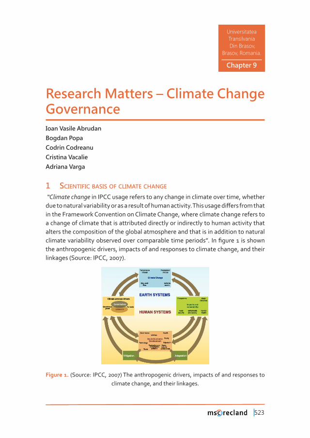
523
Chapter 9
Universitatea
Transilvania
Din Brasov,
Brasov, Romania.
Research Matters – Climate Change GovernanceIoan Vasile Abrudan
Bogdan Popa
Codrin Codreanu
Cristina Vacalie
Adriana Varga
1 scientiFic basis oF climate change �Dz���������������in IPCC usage refers to any change in climate over time, whether �����������������������������������������������������������Ǥ��������������ơ��������������in the Framework Convention on Climate Change, where climate change refers to a change of climate that is attributed directly or indirectly to human activity that alters the composition of the global atmosphere and that is in addition to natural ���������������������������������������������������������dzǤ� ���Ƥ������ ���������the anthropogenic drivers, impacts of and responses to climate change, and their linkages (Source: IPCC, 2007).
Figure 1. (Source: IPCC, 2007) The anthropogenic drivers, impacts of and responses to climate change, and their linkages.
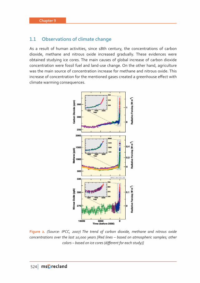
Chapter 9
524
1�1 Observations of climate change
As a result of human activities, since 18th century, the concentrations of carbon dioxide, methane and nitrous oxide increased gradually. These evidences were obtained studying ice cores. The main causes of global increase of carbon dioxide concentration were fossil fuel and land-use change. On the other hand, agriculture was the main source of concentration increase for methane and nitrous oxide. This ������������������������������������������������������������������������ơ���������climate warming consequences.
Figure 2Ǥ� ȋ������ǣ� ����ǡ� Ȍ� ���� ������ ��� ������� �������ǡ� �������� ���� �������� ������������������������������ �����ǡ�������ȏ���� ������Ȃ�����������������������������Ǣ�������
�������Ȃ��������������������ȋ��ơ��������������������ȌȐ
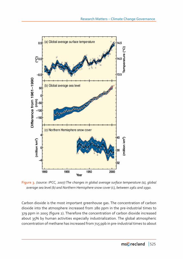
Research Matters – Climate Change Governance
525
Figure 3. ȋ������ǣ�����ǡ�Ȍ���������������������������������������������������ȋ�Ȍǡ��������������������������ȋ�Ȍ������������������������������������ȋ�Ȍǡ��������������Ǥ
Carbon dioxide is the most important greenhouse gas. The concentration of carbon dioxide into the atmosphere increased from 280 ppm in the pre-industrial times to ���������ȋƤ�����ȌǤ���������������������������������������������������������������ά�������������������������������� �����������������Ǥ������������������������concentration of methane has increased from 715 ppb in pre-industrial times to about
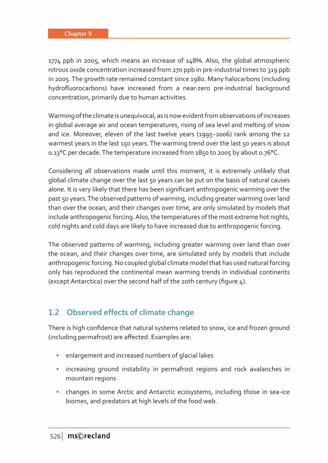
Chapter 9
526
����� ���ǡ���������������� ������������ άǤ�����ǡ� ����������� ������������nitrous oxide concentration increased from 270 ppb in pre-industrial times to 319 ppb in 2005. The growth rate remained constant since 1980. Many halocarbons (including �����ƪ�����������Ȍ� ����� ���������� ����� �� ����Ǧ����� ���Ǧ����������� �����������concentration, primarily due to human activities.
Warming of the climate is unequivocal, as is now evident from observations of increases in global average air and ocean temperatures, rising of sea level and melting of snow and ice. Moreover, eleven of the last twelve years (1995–2006) rank among the 12 warmest years in the last 150 years. The warming trend over the last 50 years is about 0.13°C per decade. The temperature increased from 1850 to 2005 by about 0.76°C.
Considering all observations made until this moment, it is extremely unlikely that global climate change over the last 50 years can be put on the basis of natural causes �����Ǥ��������������������������������������������Ƥ������������������������������������past 50 years. The observed patterns of warming, including greater warming over land than over the ocean, and their changes over time, are only simulated by models that include anthropogenic forcing. Also, the temperatures of the most extreme hot nights, cold nights and cold days are likely to have increased due to anthropogenic forcing.
The observed patterns of warming, including greater warming over land than over the ocean, and their changes over time, are simulated only by models that include anthropogenic forcing. No coupled global climate model that has used natural forcing only has reproduced the continental mean warming trends in individual continents ȋ�����������������Ȍ����������������������������������������ȋƤ�����ȌǤ
1�2 Observed effects of climate change
�����������������Ƥ������������������������������������������ǡ�����������������������ȋ��������������������Ȍ������ơ�����Ǥ�������������ǣ�
• enlargement and increased numbers of glacial lakes
• increasing ground instability in permafrost regions and rock avalanches in mountain regions
• changes in some Arctic and Antarctic ecosystems, including those in sea-ice biomes, and predators at high levels of the food web.
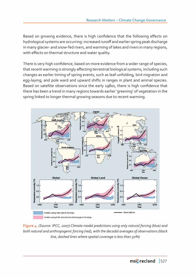
Research Matters – Climate Change Governance
527
�������������������������ǡ� ������ �������� ���Ƥ������ ����� ���� �����������ơ������������������������������������������ǣ���������������ơ�����������������������������������in many glacier- and snow-fed rivers, and warming of lakes and rivers in many regions, ������ơ�������������������������������������������Ǥ�
����������������������Ƥ�����ǡ�����������������������������������������������������ǡ����������������������������������ơ�������������������������������������ǡ����������������changes as earlier timing of spring events, such as leaf-unfolding, bird migration and egg-laying; and pole ward and upward shifts in ranges in plant and animal species. �������������������������������������������������ǡ������� �����������Ƥ�����������there has been a trend in many regions towards earlier ‘greening’ of vegetation in the spring linked to longer thermal growing seasons due to recent warming.
Figure 4. ȋ������ǣ�����ǡ�Ȍ������������������������������������������������������ȋ����Ȍ�����both natural and anthropogenic forcing (red), with the decadal averages of observations (black
����ǡ��������������������������������������������������άȌ�
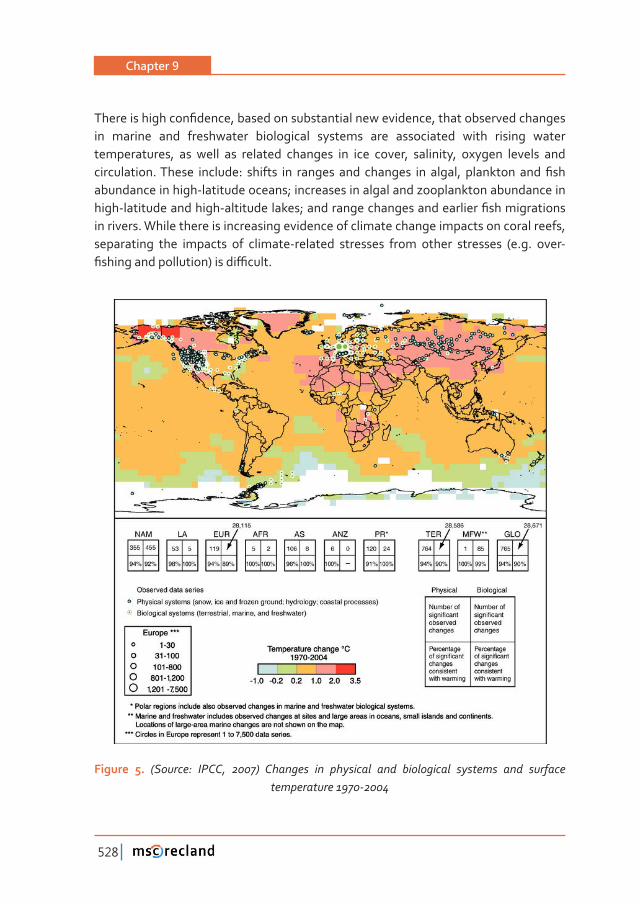
Chapter 9
528
�����������������Ƥ�����ǡ����������������������������������ǡ�����������������������in marine and freshwater biological systems are associated with rising water temperatures, as well as related changes in ice cover, salinity, oxygen levels and �����������Ǥ������� �������ǣ� ������� ��� ������� ���� �������� ��� �����ǡ� ��������� ���� Ƥ���abundance in high-latitude oceans; increases in algal and zooplankton abundance in ����Ǧ�����������������Ǧ��������������Ǣ�������������������������������Ƥ��������������in rivers. While there is increasing evidence of climate change impacts on coral reefs, separating the impacts of climate-related stresses from other stresses (e.g. over-Ƥ�������������������Ȍ������ƥ����Ǥ
Figure 5.� ȋ������ǣ� ����ǡ� Ȍ� �������� ��� ��������� ���� ����������� �������� ���� ��������������������Ǧ
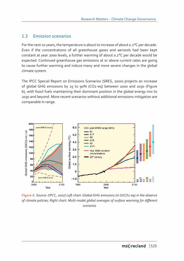
Research Matters – Climate Change Governance
529
1�3 Emission scenarios
For the next 20 years, the temperature is about to increase of about 0.2°C per decade. Even if the concentrations of all greenhouse gases and aerosols had been kept constant at year 2000 levels, a further warming of about 0.1°C per decade would be expected. Continued greenhouse gas emissions at or above current rates are going to cause further warming and induce many and more severe changes in the global climate system.
The IPCC Special Report on Emissions Scenarios (SRES, 2000) projects an increase ��� ��������� ���������� ��� � ��� ά� ȋ��Ǧ��Ȍ� �������� � ���� � ȋ������6), with fossil fuels maintaining their dominant position in the global energy mix to 2030 and beyond. More recent scenarios without additional emissions mitigation are comparable in range.
Figure 6.�������ǣ�ȋ����ǡ�Ȍ�����������ǣ�������������������ȋ������Ǧ��Ȍ�����������������������������������Ǣ������������ǣ������Ǧ�����������������������������������������������ơ������
scenarios
Chapter 9
530
The key uncertainties of the drivers and projections of future climate changes and their impacts as presented in Climate Change 2007 - Synthesis report are:
• Uncertainty in the equilibrium climate sensitivity creates uncertainty in the expected warming for a given CO2-eq stabilization scenario. Uncertainty in the carbon cycle feedback creates uncertainty in the emissions trajectory required to achieve a particular stabilization level.
• ������� ��ơ��� ������������� ��� ������ ���������� ��� ���� ��������� ��� ��ơ������feedbacks in the climate system, particularly cloud feedbacks, oceanic heat uptake and carbon cycle feedbacks, although progress has been made in these �����Ǥ�����ǡ� ���� ���Ƥ������ ��� ������������ ��� ������� ���� ����� ���������� ȋ�Ǥ�Ǥ�temperature) than for others (e.g. precipitation), and it is higher for larger spatial scales and longer time averaging periods.
• Aerosol impacts on the magnitude of the temperature response, on clouds and on precipitation remain uncertain.
• Future changes in the Greenland and Antarctic ice sheet mass, particularly due ������������������ƪ��ǡ�����������������������������������������������������������level rise projections. The uncertainty in the penetration of the heat into the oceans also contributes to the future sea level rise uncertainty.
• Large-scale ocean circulation changes beyond the 21st century cannot be reliably assessed because of uncertainties in the melt water supply from the Greenland ice sheet and model response to the warming.
• Projections of climate change and its impacts beyond about 2050 are strongly scenario and model-dependent, and improved projections would require improved understanding of sources of uncertainty and enhancements in systematic observation networks.
• Impacts research is hampered by uncertainties surrounding regional projections of climate change, particularly precipitation.
• Understanding of low-probability/high-impact events and the cumulative impacts of sequences of smaller events, which is required for risk-based approaches to decision-making, is generally limited.
Research Matters – Climate Change Governance
531
2 the international response to climate change
Climate change was internationally recognized as a serious problem in February 1979 in Geneva when the First World Climate Conference sponsored by the WMO took place (Robledo & Masera, 2007). In response to this issue, an international environmental treaty named United Nations Framework Convention on Climate Change was adopted by the United Nations Conference on Environment and Development (UNCED) at ����Dz����������������dz����Ǥ�������Ƥ��������ǡ������������������������������������Kyoto Protocol, that established legally binding emissions targets for industrialized countries, and created innovative mechanisms to assist these countries in meeting these targets. Recognizing the needs of policymakers for authoritative and up-to-������������Ƥ�� �����������ǡ� �������������������������������������� ȋ���Ȍ���������UN Environmental Programme (UNEP) established the Intergovernmental Panel on Climate Change (IPCC) in 1988 (Robledo & Masera, 2007).
2�1 Intergovernmental Panel on Climate Change (IPCC)
(Source: www.ipcc.org)
The Intergovernmental Panel on Climate Change was created in 1988. It was set up by the World Meteorological Organization (WMO) and the United Nations Environment ��������ȋ����Ȍ��������ơ��������������������������������������������������������������������������������������Ƥ����������������������������������������ǯ���������Ǥ�����initial task for the IPCC as outlined in the UN General Assembly Resolution 43/53 of 6 December 1988 was to prepare a comprehensive review and recommendations with respect to the state of knowledge of the science of climate change; social and economic impact of climate change, possible response strategies and elements for inclusion in a possible future international convention on climate. Today the ����ǯ�� ����� �������ǡ������Ƥ���� ����������������������� ���������ǡ� DzǤǤǤ����������������������������ǡ� ���������ǡ� ����� ���� ������������ ������ ���� �������Ƥ�ǡ� ���������� ���������Ǧ����������������������������������������������������������Ƥ�������������������human-induced climate change, its potential impacts and options for adaptation and mitigation. IPCC reports should be neutral with respect to policy, although they may �������������������������������������Ƥ�ǡ��������������������Ǧ��������������������������to the application of particular policies.”
Chapter 9
532
���� �������Ƥ�� ��������� �������� ��� ��� ���� Ƥ���� ����� ����������� ������� ��� �unveiled the importance of climate change as a topic deserving a political platform among countries to tackle its consequences. It therefore played a decisive role in leading to the creation of the United Nations Framework Convention on Climate Change (UNFCCC), the key international treaty to reduce global warming and cope with the consequences of climate change.
�����������������������������������������������������������������������������������Ƥ��reports about climate change produced worldwide, the Assessment Reports. It ������������������������������������������������������� ����������������������Ƥ��technical matters through Special Reports, Technical Papers and Methodology Reports. Methodologies and guidelines were prepared to help Parties under the UNFCCC in preparing their national greenhouse gas inventories.
The IPCC Second Assessment Report of 1995 provided key input in the way to the adoption of the Kyoto Protocol in 1997. The Third Assessment Report came out in ǡ��������������������������������Ǥ�Dz���������������dzǡ����������������������������������������������������������Ƥ����������������������������������������������climate and led the organization to be honored with the Nobel Peace Prize at the end of that same year.
Along with Comprehensive Assessment Reports, the IPCC has produced several Special Reports on various topics of growing interest, and many other papers and contributions to the advancements of the climate change science.
���� �������������� ��� ���� �������Ƥ�� ���������� ��� ���� ����� ��� ���� ����� ���� �����growing greatly, both in terms of authors and contributors involved in the writing and the reviewing of the reports and of geographic distribution and topics covered by the reports.
The IPCC is an intergovernmental body. It is open to all member countries of the United Nations (UN) and WMO. Currently 195 countries are members of the IPCC. Governments participate in the review process and the plenary Sessions, where main decisions about the IPCC work programme are taken and reports are accepted, adopted and approved. The IPCC Bureau Members, including the Chair, are also elected during the plenary Sessions.
Research Matters – Climate Change Governance
533
����������������������Ƥ������������������������������ǡ���������������������������������������� ��� �������� ��������� ���� ��������� �������Ƥ�� ������������ ��� ���������makers. By endorsing the IPCC reports, governments acknowledge the authority of �������������Ƥ���������Ǥ�������������������������������������������������Ǧ�������������yet policy-neutral, never policy-prescriptive.
2�1�1 The structure of IPCC
(Source: www.ipcc.org)
The IPCC is currently organized in 3 Working Groups and a Task Force. They are ������������������������������������ȋ���Ȍǡ����������������������Ƥ��������������������by the Government of the developed country co-chair of that Working Group/Task Force:
• Working Group I - The Physical Science Basis of Climate Change - Assesses the ����������������Ƥ��������������������������������������������������Ǥ����������topics assessed by WG I include: changes in greenhouse gases and aerosols in the atmosphere; observed changes in air, land and ocean temperatures, rainfall, glaciers and ice sheets, oceans and sea level; historical and paleoclimatic perspective on climate change; biogeochemistry, carbon cycle, gases and aerosols; satellite data and other data; climate models; climate projections, causes and attribution of climate change.
• Working Group II - Climate Change Impacts, Adaptation and Vulnerability - Assesses the vulnerability of socio-economic and natural systems to climate change, negative and positive consequences of climate change, and options for adapting to it. It also takes into consideration the inter-relationship between vulnerability, adaptation and sustainable development. The assessed information is considered by sectors (water resources; ecosystems; food & forests; coastal systems; industry; human health) and regions (Africa; Asia; Australia & New Zealand; Europe; Latin America; North America; Polar Regions; Small Islands).
• Working Group III - Mitigation of Climate Change - Assesses options for mitigating climate change through limiting or preventing greenhouse gas emissions and enhancing activities that remove them from the atmosphere. The main economic sectors are taken into account, both in a near-term and in a long-term perspective. The sectors include energy, transport, buildings,
Chapter 9
534
industry, agriculture, forestry, waste management. The WG analyses the costs ���� ����Ƥ��� ��� ���� ��ơ������ ����������� �������������ǡ� ������������ ����� ����available instruments and policy measures. The approach is more and more solution-oriented.
Working Groups also meet at the Plenary at the level of Representatives of Governments. The main objective of the Task Force on National Greenhouse Gas ��������������������������������Ƥ���������������������������������������������������of national GHG emissions and removals. In addition to the Working Groups and Task Force, further Task Groups and Steering Groups may be established for a limited or �����������������������������������Ƥ�������������������Ǥ
2�1�2 Task Force on National Greenhouse Gas Inventories (TFI)
The TFI was established by the IPCC, at its 14th session (October 1998), to oversee the IPCC National Greenhouse Gas Inventories Programme (IPCC-NGGIP). This programme had been undertaken since 1991 by the IPCC WG I in close collaboration with the Organization for Economic Co-operation and Development (OECD) and the International Energy Agency (IEA). In 1999, the Technical Support Unit (TSU) set up at the Institute for Global Environmental Strategies (IGES) in Japan took over this programme in accordance with a decision taken by the IPCC at its 14th session.
The objectives of the TFI are:
• �����������������Ƥ���������������������Ǧ������������������������������������the calculation and reporting of national GHG emissions and removals, and
• to encourage the widespread use of this methodology by countries participating in the IPCC and by signatories of the United Nations Framework Convention on Climate Change (UNFCCC).
2�1�3 Assessment reports
The IPCC has published four comprehensive assessment reports reviewing the latest climate science, as well as a number of special reports on particular topics. These reports are prepared by teams of relevant researchers selected by the Bureau from government nominations.
The IPCC reports were published:
Research Matters – Climate Change Governance
535
• �Ǧ�����Ƥ���������������������ǡ��������������������������������ǡ�
• 1995 - the second assessment report (SAR)
• 2001 - the third assessment report (TAR)
• 2007 - fourth assessment report (AR4)
����Ƥ���������������������������������������������Ǥ
Each assessment report is in three volumes, corresponding to Working Groups I, II and ���Ǥ��������Ƥ��ǡ�Dz���������������dz������������������������������������������������ǡ�which covers the basic science of climate change.
2�2 United Nations Framework Convention on Climate Change (UNFCCC)
(Source: www.unfccc.int)
In 1992, countries joined an international treaty, the United Nations Framework Convention on Climate Change, to cooperatively consider what they could do to limit average global temperature increases and the resulting climate change, and to cope with whatever impacts were, by then, inevitable.
By 1995, countries realized that emission reductions provisions in the Convention were inadequate. They launched negotiations to strengthen the global response to climate change, and, two years later, adopted the Kyoto Protocol. The Kyoto Protocol legally binds developed countries to emission reduction targets. The Protocol’s Ƥ���� ����������� ������� �������� ��� � ���� ����� ��� Ǥ� ��� ���� ��� ������ǡ�governments of the Parties to the Kyoto Protocol decided that a second commitment ������ǡ��������������ǡ����������������������������������������Ƥ���������������period. The length of the second commitment period is to be determined: it will be �������Ƥ����������������������Ǥ
There are now 195 Parties to the Convention. The UNFCCC secretariat supports all institutions involved in the international climate change negotiations, particularly the Conference of the Parties (COP), the subsidiary bodies (which advise the COP), and the COP Bureau (which deals mainly with procedural and organizational issues arising from the COP and also has technical functions).
Chapter 9
536
At the very heart of the response to climate change, however, lies the need to reduce emissions. In 2010, governments agreed that emissions need to be reduced so that global temperature increases are limited to below 2 degrees Celsius.
No mandatory limits on greenhouse gas emissions were drawn up. Instead, the treaty ���������������������ȋ�������Dz���������dzȌ�����������������������������������������Ǥ�The principal update is the Kyoto Protocol, which has become much better known than the UNFCCC itself. The UNFCCC entered into force on 21 March 1994. Today, it ��������Ǧ��������������������Ǥ������������������������������Ƥ������������������are called Parties to the Convention.
The ultimate objective of the Convention is to stabilize greenhouse gas concentrations Dz������������������������������������������������������ȋ�������������Ȍ�������������������������������������Ǥdz����������������Dz���������������������������������������������Ǧ��������ƥ��������������������������������������������������������������ǡ�����������that food production is not threatened, and to enable economic development to proceed in a sustainable manner.”
���� Ƥ���� ���������� ����� ��� ������ ���� ��� ���������� ��������� ����������� ����inventories of greenhouse gas (GHG) emissions and removals. These levels were used to create the 1990 benchmark levels for accession of Annex I countries to the Kyoto Protocol. Also, these levels were used for the commitment of those countries to GHG reductions.
The parties to the convention have met annually from 1995 in Conferences of the Parties (COP) to assess progress in dealing with climate change. In 1997, the Kyoto Protocol was concluded and established legally binding obligations for developed countries to reduce their greenhouse gas emissions.
���������������������������Ƥ�����ǣ
• Annex I countries: industrialized countries and economies in transition
• Annex II countries: developed countries which pay for costs of developing countries
• Non Annex I countries: Developing countries.
Research Matters – Climate Change Governance
537
������ ���������������������������Ƥ�����������������������������������������������emission levels of greenhouse gasses to targets that are mainly set below their 1990 levels. They may do this by allocating reduced annual allowances to the major operators within their borders. These operators can only exceed their allocations if ����������������������������ǡ�����ơ�����������������������������������������������agreed by all the parties to UNFCCC.
Annex II countries are a sub-group of the Annex I countries. They comprise the OECD members, excluding those that were economies in transition in 1992.
Developing countries are not required to reduce emission levels unless developed countries supply enough funding and technology. Setting no immediate restrictions under UNFCCC serves three purposes:
• it avoids restrictions on their development, because emissions are strongly linked to industrial capacity
• ����� ���� ����� ���������� �������� ��� �������� ������ ���������� ����� ��ƥ������meeting their emissions targets
• they get money and technologies for low-carbon investments from Annex II countries.
Developing countries may volunteer to become Annex I countries when they are ��ƥ�����������������Ǥ
2�2�1 Mitigation of climate change
(Source: www.unfccc.int)
Reducing Emissions from Deforestation and forest Degradation (REDD)
�������������������Dz������������������������������������������������������������������������������������������������dz�����Ƥ������������������������������������������eleventh session in Montreal (December 2005).
The IPCC (2007) estimated emissions from deforestation in the 1990s to be at 5.8 GtCO2/year. It also noted that reducing and/or preventing deforestation and preventing the release of carbon emissions into the atmosphere is the mitigation option with the largest and most immediate carbon stock impact in the short term per hectare and per year globally.

Chapter 9
538
Parties to the UNFCCC process recognized the contribution of greenhouse gas emissions from deforestation in developing countries to climate change and the need to take action to reduce such emissions. After a two-year process, the COP adopted �� ��������� ��� Dz��������� ���������� ����� �������������� ��� ����������� ���������ǣ�approaches to stimulate action” (Decision 2/CP.13). The decision provides a mandate for several elements and actions by Parties relating to reducing emissions from deforestation and forest degradation in developing countries:
• ���������������������������������������������ơ����Ǣ
• Support for and facilitate capacity-building, technical assistance and transfer of technology relating to methodological and technical needs and institutional needs of developing countries;
• Explore a range of actions, identify options and undertake demonstration activities to address drivers of deforestation and enhance forest carbon stocks due to sustainable management of forests; and
• �����������������������������������ơ��������������������Ǥ�
The decision also provides a set of indicative guidance for the implementation and evaluation of demonstration activities. Parties are also encouraged to apply the IPCC Good Practice Guidance for Land Use, Land-Use Change and Forestry for estimating and reporting of emissions and removals.
In 2008 and 2009, policy approaches and positive incentives relating to reducing emissions from deforestation and forest degradation in developing countries and the role of conservation, sustainable management of forests, and enhancement of forest carbon stocks in developing countries have been considered under the process of the Bali Action Plan.
UN REDD Programme
(Source: www.un-redd.org/)
The UN-REDD Programme is the United Nations Collaborative initiative on Reducing Emissions from Deforestation and forest Degradation (REDD) in developing countries. The Programme was launched in September 2008 to assist developing countries prepare and implement national REDD+ strategies, and builds on the convening power and expertise of the Food and Agriculture Organization of the United Nations

Research Matters – Climate Change Governance
539
(FAO), the United Nations Development Programme (UNDP) and the United Nations Environment Programme (UNEP).
�������������������������������������������������������������������ǡ�����Ǧ����Ƥ��and Latin America, of which 16 are receiving support to National Programme activities. These 16 countries are: Bolivia, Cambodia, Democratic Republic of the Congo (DRC), Ecuador, Indonesia, Nigeria, Panama, Papua New Guinea, Paraguay, the Philippines, Republic of Congo, Solomon Islands, Sri Lanka, Tanzania, Viet Nam and Zambia. To-date, the UN-REDD Programme’s Policy Board has approved a total of US$67.3 million for National Programmes in these 16 partner countries. These funds help to support the development and implementation of national REDD+ strategies.
UN-REDD Programme countries not receiving direct support to national programmes engage with the Programme in a number of ways, including as observers to the Programme’s Policy Board, and through participation in regional workshops and knowledge sharing, facilitated by the Programme’s interactive online workspace. These countries are: Argentina, Bangladesh, Benin, Bhutan, Cameroon, Central African Republic, Chile, Colombia, Costa Rica, Ethiopia, Gabon, Ghana, Guatemala, Guyana, Honduras, Ivory Coast, Kenya, Malaysia, Mexico, Mongolia, Myanmar, Nepal, Pakistan, Peru, South Sudan, Sudan, Suriname and Uganda.
Land Use, Land-Use Change and Forestry
(Source: www.unfccc.int)
Forests, through growth of trees and an increase in soil carbon, contain a large part ����������������������������Ǥ�����������������������Ƥ������������������������Ǥ�������forest vegetation stores 283 Gt of carbon in its biomass, 38 Gt in dead wood and 317 Gt in soils (top 30 cm) and litter. The total carbon content of forest ecosystems has been estimated at 638 Gt for 2005, which is more than the amount of carbon in the entire atmosphere. This standing carbon is combined with a gross terrestrial uptake of carbon, which was estimated at 2.4 Gt a year, a good deal of which is sequestration by forests. Approximately half of the total carbon in forest ecosystems is found in forest biomass and dead wood.
Other terrestrial systems also play an important role. Most of the carbon stocks of croplands and grasslands are found in the below-ground plant organic matter and soil.
Chapter 9
540
Human activities, through land use, land-use change and forestry (LULUCF) activities, �ơ�����������������������������������������������������������������������������������and between the terrestrial ecosystem and the atmosphere.
Management and/or conversion of land uses (e.g. forests, croplands and grazing �����Ȍ��ơ����������������������������ǡ����������Ǥ�������������������������� �ǡ�deforestation in the tropics and forest re-growth in temperate and boreal zones remained the major factors contributing to emissions and removals of greenhouse gases (GHG) respectively. Estimated CO2 emissions associated with land-use change, averaged over the 1990s, were 0.5 to 2.7 GtC yr-1, with a central estimate of 1.6 GtCyr-1.
The role of LULUCF activities in the mitigation of climate change has long been recognized. Mitigation achieved through activities in the LULUCF sector, either by increasing the removals of GHGs from the atmosphere or by reducing emissions by �������ǡ�����������������������Ǧ�ơ������Ǥ
General mitigation options could include forest-related activities such as reducing emissions from deforestation and degradation, enhancing the sequestration rate in new or existing forests, and using wood fuels and wood products as substitutes for fossil fuels and more energy-intensive materials. A variety of options for mitigation of GHG emissions also exists in other land systems. The most prominent example is agriculture, where options include improved crop and grazing land management (e.g., improved agronomic practices, nutrient use, tillage and residue management), restoration of organic soils that are drained for crop production, and restoration of degraded lands.
However, the main drawback of LULUCF activities is their potential reversibility and non-permanence of carbon stocks as a result of human activities, (with the release of ���������������������Ȍǡ��������������ȋ�Ǥ�Ǥ��������Ƥ��������������Ȍǡ������������������change, including climate change.
According to the FAO (2005), deforestation, mainly conversion of forests to agricultural land, continues at an alarming rate of approximately 13 million hectares per year (for the period 1990–2005). Deforestation results in immediate release of the carbon originally stored in the trees as CO2 emissions (with small amounts of CO and CH4), particularly if the trees are burned and the slower release of emissions from the decay of organic matter. The IPCC WGIII (2007) estimated emissions from deforestation in the 1990s to be at 5.8 GtCO2/yr. The IPCC also notes that reducing
Research Matters – Climate Change Governance
541
and/or preventing deforestation is the mitigation option with the largest and most immediate carbon stock impact in the short term per hectare and per year globally as the release of carbon as emissions into the atmosphere is prevented.
LULUCF sector under the Convention
Under the Convention, the commitments by Parties to mitigate climate change are ��Ƥ���� ��� �������� Ǥ������� ������������ ����� ����� �������� �������ǯ� ������� ������ơ����������� ��������������������� ������ �����Ƥ��������������� ���������������������priorities, objectives and circumstances. Article 4 has references to commitments relating to the land use, land-use change and forestry sector:
• Article 4, paragraph 1(a): Develop, periodically update, publish and make available to the Conference of the Parties, in accordance with Article 12, national inventories of anthropogenic emissions by sources and removals by sinks of all greenhouse gases (GHGs)1 not controlled by the Montreal Protocol, using comparable methodologies to be agreed upon by the Conference of the Parties.
• Article 4, paragraph 1(d): Promote sustainable management, and promote and cooperate in the conservation and enhancement, as appropriate, of sinks and reservoirs of all GHGs not controlled by the Montreal Protocol, including biomass, forests and oceans as well as other terrestrial, coastal and marine ecosystems.
LULUCF under the Kyoto Protocol
Several Articles of the Kyoto Protocol make provisions for the inclusion of land use, ����Ǧ����������������������������������������������������������������ơ������������������the Kyoto Protocol and contribute to the mitigation of climate change.
In Article 2, sub-paragraphs 1(a) (ii) and (iii), Annex I Parties, in meeting their emission reduction commitments under Article 3, shall implement and/or further elaborate policies and measures to protect and enhance sinks and reservoirs of greenhouse gases (GHGs) not controlled by the Montreal Protocol, promote sustainable forest ����������ǡ��ơ�����������������������������������������������������������������Ǥ�
1 Including inventories of GHG emissions and removals from the LULUCF sector
Chapter 9
542
Annex I Parties must report emissions by sources and removals by sinks of GHGs resulting from LULUCF activities, in accordance with Article 3, paragraphs 3 and 4. Under Article 3.3 of the Kyoto Protocol, Parties decided that net changes in GHG emissions by sources and removals by sinks through direct human-induced LULUCF ����������ǡ�������������ơ����������ǡ�����������������������������������������������������1990, can be used to meet Parties’ emission reduction commitments. Under Article 3.4 of the Kyoto Protocol, Parties may elect additional human-induced activities related ��� ������ �����Ƥ�����ǡ� ������� ����������ǡ� ��������� ����������ǡ� �������� �����management and revegetation, to be included in their accounting of anthropogenic ���������������������������������Ƥ���������������������Ǥ� ��������������ǡ�����������������������������Ƥ������������Ƥ���������������������Ǥ������������������������stock and GHG emissions relating to LULUCF activities under Article 3, paragraphs 3 and 4 must be reported for each year of the commitment period, beginning with the start of the commitment period, or with the start of the activity, whichever is later. When LULUCF activities under Articles 3.3 and 3.4 result in a net removal of GHGs, an Annex I Party can issue removal units (RMUs) on the basis of these activities as part of meeting its commitment under Article 3.1.
In addition, under Article 3, paragraph 7, for the purpose of calculating the assigned amount, an Annex I Party for which land-use change and forestry constituted a net source of GHG emissions in 1990 shall include in their 1990 emissions base year or period the aggregate anthropogenic carbon dioxide equivalent emissions by sources minus removals by sinks in 1990 from land-use change [according to paragraph 5(b) in the annex to 13/CMP.1, this refers to: all emissions by sources minus removals by sinks reported in relation to the conversion of forests (deforestation)].
���� ��� ���� ƪ������� ����������� ��� ���� ������ ��������� ����� ����������� ���� ����implementation of LULUCF project activities by Parties. The clean development mechanism (CDM) under the Kyoto Protocol (Article 12) allows for the implementation ���������������������������ǡ�������������ơ����������������������������ǡ�������Ǧ������I countries. These project activities assist Annex I Parties in achieving compliance with their emission reduction commitments under Article 3, while simultaneously assisting non-Annex I Parties to achieve sustainable development.
Under joint implementation (Article 6), an Annex I Party may implement projects that increase removals by sinks in another Annex I country. The emissions reduction units (ERUs) generated from such a project can be used by the former to meet its emission reduction target. Any project under Article 6 aimed at enhancing anthropogenic
Research Matters – Climate Change Governance
543
��������� ��� ������ ������ �������� ��� ��Ƥ�������ǡ� ����������� �����ǡ� ����������� ����guidelines under Article 3, paragraphs 3 and 4, of the Kyoto Protocol.
2�2�2 Reporting GHG inventories
(Source: www.unfccc.int)
The quality and credibility of GHG inventories rely on the integrity of the methodologies used, the completeness of reporting, and the procedures for compilation of data. To promote the provision of credible and consistent GHG information, the Conference of Parties (COP) has developed standardized requirements for reporting national inventories.
The UNFCCC reporting guidelines on annual inventories require Parties included in Annex I to the Convention (Annex I Parties), by 15 April each year, to provide annual national GHG inventories covering emissions and removals of direct GHGs (CO2, CH4, N2O, HFCs, PFCs and SF6) from six sectors (Energy, Industrial processes, Solvents, Agriculture, LULUCF, Waste), and for all years from the base year or period to the most recent year.
Under the UNFCCC reporting guidelines for Annex I Parties, inventory submissions are in two parts:
• Common reporting format (CRF) – a series of standardized data tables containing mainly numerical information and submitted electronically
• National Inventory Report (NIR) – a comprehensive description of the methodologies used in compiling the inventory, the data sources, the institutional structures and quality assurance and control procedures
����Ǧ������������ ������� ������������ ������� �������� ��ƥ������ �������������� ����data to enable the reader to understand the underlying assumptions and calculations of the reported emission estimates.
The NIR as established by decision 18/CP.8 is one element of the annual greenhouse gas (GHG) inventory that is required to be submitted to the UNFCCC by Annex I Parties to the Convention. The other elements of this submission include the reporting of GHG emissions by sources and removals by sinks and any other additional information in support of this submission.
Chapter 9
544
Annex I Parties that are also Parties to the Kyoto Protocol are also required to report supplementary information required under Article 7, paragraph 1, of the Kyoto Protocol, with the inventory submission due under the Convention, in accordance with paragraph 3(a) of decision 15/CMP.1.
The review of GHG inventories comprises three stages. Each stage complements the previous one, and ensures that the process as a whole provides a thorough and technical assessment of the inventory and of conformity with the UNFCCC and IPCC guidelines.
• Initial check: immediate quality assurance check to verify that the inventory submission is complete and in the correct format. The result is a status report whose main purpose is to provide a brief check of completeness of the inventory submission, mainly based on the CRF.
• Synthesis and assessment: Part I compile and compare basic inventory information, such as emission trends, activity data and implied emission factors, across Parties and over time. Part II provides a ‘preliminary assessment’ of the �������������������������������Ǥ�����������Ƥ�������������������������������������assessment is an important input to the individual review stage.
• Individual review: international teams of sectoral inventory experts examine the data, methodologies and procedures used in preparing the national inventory. Reviews are conducted as a centralized review, where 5–8 inventories are reviewed by an expert review team (ERT) convened at the secretariat; a desk review, where 3–5 inventories are reviewed by experts based in their home countries; or an in-country review, where a single inventory is reviewed by an ERT in the Party under review. This is the most important and detailed review stage.
2�3 Kyoto Protocol (KP)
(Source: www.unfccc.int)
The Kyoto Protocol is an international agreement linked to the United Nations Framework Convention on Climate Change, adopted in Kyoto, Japan, on 11 December 1997. The major feature of the Kyoto Protocol is that it sets binding targets for 37 industrialized countries and the European community for reducing greenhouse gas ȋ�Ȍ����������Ǥ�������������� �����������������Ƥ������� ������������� � ����������������Ƥ��Ǧ������������ǦǤ�������������������������������������������������
Research Matters – Climate Change Governance
545
the Convention is that while the Convention encouraged industrialized countries to stabilize GHG emissions, the Protocol commits them to do so.
Recognizing that developed countries are principally responsible for the current high levels of GHG emissions in the atmosphere as a result of more than 150 years of industrial activity, the Protocol places a heavier burden on developed nations under �����������������Dz�������������ơ���������������������������Ǥdz�
��������������������ǡ��������������������������������Ƥ������ǡ�����������ǡ�������������accession by Parties to the UNFCCC. Parties to the UNFCCC that have not signed the Protocol may accede to it at any time.
The Kyoto Protocol sets binding emission reduction targets for 37 industrialized countries ����������������������������������Ƥ���������������������Ǥ��������ǡ������������������������������������Ƥ�������������������������������������������������������������Ƥ��Ǧ����������������Ǥ������������������������������������������������������Ǥ����only binds developed countries because it recognizes that they are largely responsible for the current high levels of GHG emissions in the atmosphere, which are the result of more than 150 years of industrial activity. KP places a heavier burden on developed �����������������������������������ǣ���������Dz�������������ơ�������������������������dzǤ
The Protocol entered into force on 16 February 2005 in accordance with Article 23, that is the ninetieth day after the date on which not less than 55 Parties to the UNFCCC, ��������������������������������������������������������������������������������ά����the total carbon dioxide emissions for 1990 of the Parties included in Annex I, have �����������������������������������Ƥ������ǡ�����������ǡ����������������������Ǥ
Currently, there are 192 Parties (191 States and 1 regional economic integration organization) to the Kyoto Protocol to the UNFCCC. The total percentage of Annex I ���������������������ǤάǤ
2�3�1 Mechanisms of Kyoto Protocol
(Source: www.unfccc.int)
Countries with commitments under the Kyoto Protocol to limit or reduce greenhouse gas emissions must meet their targets primarily through national measures. As an additional means of meeting these targets, the Kyoto Protocol introduced three
Chapter 9
546
������Ǧ������ ����������ǡ� �������� ��������� ����� ��� ���� ������ ��� ���� Dz�������market.”
The Kyoto mechanisms are:
• Emissions Trading
• The Clean Development Mechanism (CDM)
• Joint Implementation (JI)
Emissions Trading
Parties with commitments under the Kyoto Protocol (Annex B Parties) have accepted targets for limiting or reducing emissions. These targets are expressed as levels of �����������������ǡ����Dz����������������ǡdz����������Ǧ������������������Ǥ����������������������������������������Dz���������������������dz�ȋ����ȌǤ������������trading, as set out in Article 17 of the Kyoto Protocol, allows countries that have ������������������������Ǧ����������������������������������Dz����dz�Ǧ���������������������capacity to countries that are over their targets. Thus, a new commodity was created in the form of emission reductions or removals. Since carbon dioxide is the principal greenhouse gas, people speak simply of trading in carbon. Carbon is now tracked and �������������������������������Ǥ����������������������Dz�������������Ǥdz
Clean Development Mechanism (CDM)
���������� ���������������������� ȋ���Ȍǡ� ��Ƥ���� ����������� � ��� ���� ��������ǡ�allows a country with an emission-reduction or emission-limitation commitment under the Kyoto Protocol (Annex B Party) to implement an emission-reduction �������� ��� ����������� ���������Ǥ��������������� ���� ����� ��������� �����Ƥ��� ���������reduction (CER) credits, each equivalent to one tonne of CO2, which can be counted towards meeting Kyoto targets. The mechanism is seen by many as a trailblazer. It is ����Ƥ����������ǡ�������������������������������������������������������ǡ������������������������������������ơ��������������ǡ�����Ǥ�������������������������������������ǡ����� �������ǡ� �� ������ �������Ƥ������� �������� ������ ������ ������� ��� ���� ������������� ��������������Ǧ�ƥ�������������Ǥ�������������������������� �����������������������������������������������ǡ��������������������������������������������ƪ�����������������they meet their emission reduction or limitation targets.
Research Matters – Climate Change Governance
547
Joint Implementation (JI)
�����������������������Dz������ ��������������ǡdz���Ƥ�����������������������������Protocol, allows a country with an emission reduction or limitation commitment under the Kyoto Protocol (Annex B Party) to earn emission reduction units (ERUs) from an emission-reduction or emission removal project in another Annex B Party, each equivalent to one tonne of CO2, which can be counted towards meeting its ������������Ǥ� ���������������������ơ��������������ƪ���������������Ǧ�ƥ��������������� ���Ƥ���������������� �����������������������ǡ������� �������������������Ƥ��� �����foreign investment and technology transfer.
The Kyoto mechanisms:
• Stimulate sustainable development through technology transfer and investment
• Help countries with Kyoto commitments to meet their targets by reducing emissions or removing carbon from the atmosphere in other countries in a cost-�ơ����������
• Encourage the private sector and developing countries to contribute to ��������������������ơ����
Accounting, Reporting & Review under the Kyoto Protocol
���� ������ ��������ǯ�� �ơ����������� ����� ������� ����� ���� ��������� �������ǣ� ��������Parties follow the Protocol’s rulebook and comply with their commitments; and whether the emissions data used to assess compliance is reliable. Recognizing this, the Kyoto Protocol and Marrakesh Accords, adopted by CMP 1 in Montreal, Canada, in December 2005, include a set of monitoring and compliance procedures to enforce the Protocol’s rules, address any compliance problems, and avoid any error in calculating emissions data and accounting for transactions under the three Kyoto mechanisms (emissions trading, clean development mechanism and joint implementation) and activities related to land use, land use change and forestry (LULUCF).
The Protocol’s monitoring procedures are based on existing reporting and review procedures under the Convention, building on experience gained in the climate change process over the past decade. They also involve additional accounting procedures that are needed to track and record Parties’ holdings and transactions of
Chapter 9
548
���������������������Ǧ�����������������������ȋ����Ȍǡ������Ƥ�����������������������(CERs) and emission reduction units (ERUs) - and removal units (RMUs) generated by LULUCF activities.
Articles 5, 7 and 8 of the Kyoto Protocol address reporting and review of information by Annex I Parties under the Protocol, as well as national systems and methodologies for the preparation of greenhouse gas inventories.
• Article 5 commits Annex I Parties to having in place, no later than 2007, national systems for the estimation of greenhouse gas emissions by sources and removals by sinks (Article 5.1). It also states that, where agreed methodologies (that is, the revised 1996 IPCC Guidelines for National Greenhouse Gas Inventories) �����������������������������������������������ǡ�������������Dz�����������dz�should be applied (Article 5.2).
• Article 7 requires Annex I Parties to submit annual greenhouse gas inventories, as well as national communications, at regular intervals, both including supplementary information to demonstrate compliance with the Protocol. In addition, Article 7 states that the Conference of the Parties serving as the meeting of the Parties to the Protocol (CMP) shall decide upon modalities for ������������������������������������������������Ƥ���������������������Ǥ�
• Article 8 establishes that expert review teams will review the inventories, and national communications submitted by Annex I Parties.
The Protocol states that guidelines for national systems, adjustments, the preparation of inventories and national communications, as well as for the conduct of expert �������ǡ� ������� ��� �������� ��� �������� ��� ���� Ƥ���� �������� ȋ���� Ȍǡ� ���� ����������reviewed thereafter.
2�4 European Commission – DG Clima
(Source: http://ec.europa.eu/dgs/clima)
���������������Ǧ��������������������������ȋDz�������dzȌ����������������������������2010, climate change being previously included in the remit of DG Environment of the European Commission. It leads international negotiations on climate, helps the EU to deal with the consequences of climate change and to meet its targets for 2020, as well as develops and implements the EU Emissions Trading System.
Research Matters – Climate Change Governance
549
2�5 Combating climate change within and outside the EU
Given the necessity to keep global average temperature increase below 2 degrees Celsius compared to pre-industrial levels, DG CLIMA develops and implements cost �ơ����������������������������������������������������������������������������������for the EU to meet its targets for 2020 and beyond, especially with regard to reducing its greenhouse gas emissions. Its policies also aim at protecting the ozone layer and at ensuring that the climate dimension is appropriately present in all Community policies and that adaptation measures will reduce the European Union’s vulnerability to the impacts of climate change.
The Directorate-General for Climate Action is at the forefront of international �ơ�����������������������������Ǥ���������������������������������������������������the international negotiations in the areas of climate change and ozone depleting substances and coordinates bi-lateral and multi-lateral partnerships on climate change and energy with third countries.
��������������������� ����������� ��������������������������������ȋDz������dzȌ�and promotes its links with other carbon trading systems with the ultimate aim of building an international carbon trading market. Furthermore, it monitors the implementation of Member States’ emission reduction targets in the sectors outside �����������ȋDz�ơ��������������������dzȌǤ
It also promotes the development and demonstration of low carbon and adaptation technologies, especially through the development and implementation of cost �ơ������� ����������� ����������� ���� ������ ����������� ȋ�Ǥ�Ǥ� ������� �������� �����������ǡ�ƪ���������������ǡ���������������������������ǡ����������ƥ����������������ǡ�����������������������Ȍ���������������������������������������������������Ƥ��������support schemes.
Combating climate change is a top priority for the EU. Europe is working hard to cut its greenhouse gas emissions substantially while encouraging other nations and regions to do likewise. At the same time, the EU is developing a strategy for adapting to the impacts of climate change that can no longer be prevented. Reining in climate change carries a cost, but doing nothing will be far more expensive in the long run. Moreover, investing in the green technologies that cut emissions will also create jobs and boost the economy.
Chapter 9
550
The European Union has long been a driving force in international negotiations that led to agreement on the two United Nations climate treaties, the UN Framework Convention on Climate Change (UNFCCC) in 1992 and the Kyoto Protocol in 1997.
The Kyoto Protocol requires the 15 countries that were EU members at the time (‘EU-ǯȌ� ������������������������������������� �������Ǧ�����������ά��������levels. Emissions monitoring and projections show that the EU-15 is well on track to meet this target.
In 2007 EU leaders endorsed an integrated approach to climate and energy policy ���� ���������� ��� ������������� ������� ����� �� ������� ������Ǧ�ƥ�����ǡ� ���� �������economy. They made a unilateral commitment that Europe would cut its emissions by ���������ά���������������Ǥ����������������������������������������������a package of binding legislation.
�����������������ơ�������������������������������������������� ά���� ǡ��������������that other major emitting countries in the developed and developing worlds commit to do their fair share under a future global climate agreement. This agreement should ������ơ�������������������� ������������������������ǯ��Ƥ���������������������������have expired.
The Cancún Agreement, a balanced and substantive package of decisions adopted at the end of the UN Climate Conference in Mexico (December 2010), represents an important step on the road to building a comprehensive and legally binding framework for climate action for the period after 2012.
The UNFCCC commits the EU and its Member States to develop, periodically update, publish and report to the Conference of the Parties national inventories of anthropogenic emissions by sources and removals by sinks of all greenhouse gases not controlled by the Montreal Protocol on substances that deplete the ozone layer (greenhouse gases), using comparable methodologies agreed upon by the Conference of the Parties.
The UNFCCC commits all Parties to formulate, implement, publish and regularly update national, and where appropriate, regional programmes containing measures to mitigate climate change by addressing anthropogenic emissions by sources and removals by sinks of all greenhouse gases.
Research Matters – Climate Change Governance
551
2�6 Adoption of the Kyoto Protocol
�����������������������������������������������ǡ��������Ƥ�����������ǡ����������������the commitment by developed countries to aim at returning, individually or jointly, their emissions of carbon dioxide and other greenhouse gases not controlled by the Montreal Protocol to the Convention for the Protection of the Ozone Layer to 1990 levels by the year 2000 was inadequate for achieving the Convention’s long-term objective of preventing dangerous anthropogenic interference with the climate system.
The Conference further agreed to begin a process to enable appropriate action to be taken for the period beyond 2000, through the adoption of a protocol or another legal instrument. This process resulted in the adoption on 11 December 1997 of the Kyoto Protocol to the United Nations Framework Convention on Climate Change.
2�7 EU and Member States jointly responsible for the quantified emission reduction commitment
����������������������������������������������Ƥ����������������������������ǡ�����������the framework of and together with a regional economic integration organization. When the Protocol was signed in New York on 29 April 1998, the EU declared that ����������������������������������Ƥ������������������������������������������������jointly.
��������������� ���Ƥ��� �����������������ǡ� ��������������������������������� �������������������� ���� ���� ���Ƥ������� ��� ���� ��� ��� ���� ������Ƥ��� ��������� ����������commitment. Consequently, Member States individually and collectively have the obligation to take all appropriate measures, whether general or particular, to ensure ���Ƥ�����������������������������������������������������������������������������������ǡ�����������������ǯ��������Ƥ���������������������������������������������������ǡ����facilitate the achievement of this commitment and to abstain from any measure that could jeopardize the attainment of this commitment.
�������������������������������������������������������������������������ά�������1990 levels by 2008-2012. Most of the Member States that joined the EU in 2004 have ���������������Ǥ��������������������������������������Ǧά�������������������������Ǧ��Party to the UNFCCC and thus has no target.
Chapter 9
552
2�8 EU monitoring and reporting of greenhouse gas emissions under the UNFCC and the Kyoto Protocol
Given the UNFCCC and the Kyoto Protocol requirements, there is a need for thorough monitoring and regular assessment of EU greenhouse gas emissions and the measures ���������������������������������������������Ƥ�������������������������������������be analyzed in good time. Therefore, it is appropriate for the European Commission ����������������ơ�������������������������������������������������������������������of the EU greenhouse gas inventory, the evaluation of progress, the preparation of reports, as well as review and compliance procedures enabling the EU to comply with its reporting obligations under the Kyoto Protocol, as laid down in the political agreements and legal decisions taken at the seventh Conference of the Parties to the �������������������ȋDz���������������������dzȌǤ
The European Environment Agency assists the Commission, as appropriate, with monitoring activities, especially in the scope of the EU inventory system, and in the ������������������������������������������������������Ƥ��������������������������under the UNFCCC and the Kyoto Protocol.
Since the objectives of complying with the EU’s commitments under the Kyoto Protocol, in particular the monitoring and reporting requirements laid down therein, ������ǡ���������������������ǡ������ƥ����������������������������������������������therefore be better achieved at EU level, the EU may also adopt measures.
2�9 European Climate Change Programme
The European Commission has taken many climate-related initiatives since 1991, �������������������Ƥ�����������������������������������������������ȋ��2) emissions ��������������������ƥ������Ǥ��������������ǣ�����������������������������������������renewable energy, voluntary commitments by car makers to reduce CO2 emissions by ά�������������������������������������������������Ǥ
However, it is clear that action by both Member States and the European Community needs to be reinforced if the EU is to succeed in cutting its greenhouse gas emissions ���ά������������������Ǧǡ����������������������������������Ǥ
Research Matters – Climate Change Governance
553
The EU Council of Environment Ministers acknowledged the importance of taking further steps at Community level by asking the Commission to put forward a list of priority actions and policy measures.
The Commission responded in June 2000 by launching the European Climate Change Programme (ECCP). The goal of the ECCP is to identify and develop all the necessary elements of an EU strategy to implement the Kyoto Protocol.
������������������� ����Ƥ��������� ȋǦȌ� ������������� ���� �������������������stakeholders working together, including representatives from the Commission’s ��ơ������������������ȋ��Ȍǡ������������������ǡ����������������������������������Ǥ�The second European Climate Change Programme (ECCP II) was launched in October 2005.
REFERENCES
Robledo, C., & Masera, O. (2007). ���������������������Ȁ�������������������������REDUCING EMISSIONS FROM FOREST DEGRADATION AND DEFORESTATION AND IMPLICA-TIONS FOR TROPICAL FORESTS AND TROPICAL TIMBER PRODUCERS. Port Moresby, Papua New Guinea: INTERNATIONAL TROPICAL TIMBER COUNCIL.
IPCC, 2007: Climate Change 2007: Synthesis Report. Contribution of Working Groups I, II and III to the Fourth Assessment Report of the Intergovernmental Panel on Climate Change [Core Writing Team, Pachauri, R.K and Reisinger, A. (eds.)]. IPCC, Geneva, Switzerland, 104 pp.
http://unfccc.int - Acessed June 2012http://www.ipcc.ch/ - Acessed June 2012http://ec.europa.eu/clima - Acessed June 2012www.un-redd.org/ - Acessed June 2012


Advanced Statistics
Author
Susana Martín
Technical University of Madrid
Ciudad Universitaria s/n (ETSI Montes)
28040 - Madrid
Spain
10Chapter


557
Chapter 10
Technical
University of
Madrid,
Madrid, Spain.
Advanced Statistics Susana Martín
1 basic concepts in statistics
�����������ǡ����������������������������������������������������ǣ�Dz����������ǯ�����ǡ��������������������Ƥ����Ǥdz����������������������������ȋ���������������������������������ƥ�����Ȍ� ����� Dz���� ������� ��� �������ǯ�� ��������� �������� ��������������� �����ơ�����������������������������������������������������������Ǥdz
���� �������� ��� ����� �������� ��� ����� ���� ��������� Ƥ������ ������� �������ǯ�� ������of view rather than Pelham’s. The purpose of this chapter is to serve as a quick refresher course that will make the rest of this subject more useful. Before going further into a detailed discussion of statistics, we have to remind that (a) statistics is a branch of mathematics and (b) statistics is its own very precise language.
1�1 Definition of Statistics
����������� ��� ���� �������� ����� ������ ����� ���� ����������ǡ� ������Ƥ������ǡ� ��������ǡ�and interpretation of numerical facts or data, and that, by use of mathematical theories of probability, imposes order and regularity on aggregates of more or less disparate elements.
Random experiments:
A random experiment is an experiment in which:

Chapter 10
558
• All outcomes of the experiment are known in advance
• Any performance of the experiment results in an outcome that is not known in advance
• And the experiment can be repeated under identical conditions
Sample space:
��������������������������������������������ǡ�ȳǡ�����������������������������������������������������������Ǥ������������Ƥ����ǡ���Ƥ����������Ƥ��������������Ǥ
The pair (ȳǡ�A ) where A �������ɐǦ������������������������������ȳǤ����������������A is an event.
The Linear Model:
One of the main methods of applied Statistics is the Linear Model. The linear model involves the simplest and seemingly most restrictive statistical properties: independence, normality, constancy of variance, and linearity. However, the model and the statistical methods associated with it are surprisingly versatile and robust. A deep knowledge of these models makes the use of advanced statistical tools easier. Since most advanced tools are generalizations of the linear model.
����ǣȀȀ�����Ǥ�����Ǥ���Ǥ��Ȁ�����Ȁ������Ȁ�����Ȁ������ά������ά��ά����������ǡά
��ά��Ǥ���
1�2 What is a linear model?
A linear model is simply a relationship between one random variable and one or more mathematical variables qualitative or quantitative.
���� �������Ƥ��������� ��� ����������� ����� ��� �� ������� ��������� ��� ��������Ǥ� �������statistical methods are widely used as part of this learning process:
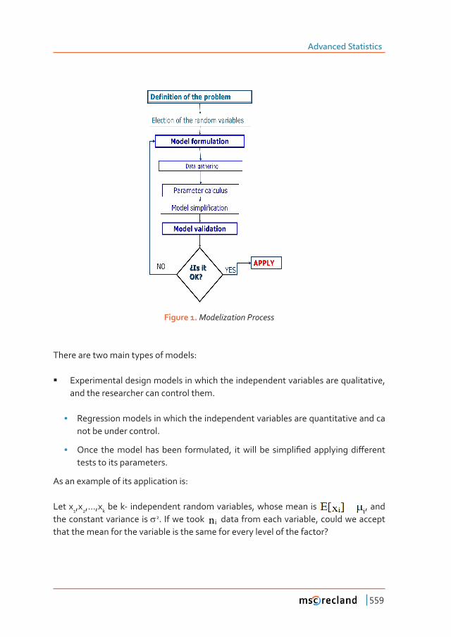
Advanced Statistics
559
Figure 1. Modelization Process
There are two main types of models:
�� Experimental design models in which the independent variables are qualitative, and the researcher can control them.
• Regression models in which the independent variables are quantitative and ca not be under control.
• ����� ������������������� ����������ǡ� �������� ��� ������Ƥ��������������ơ������tests to its parameters.
As an example of its application is:
Let x1,x2,...,xk be k- independent random variables, whose mean is , and the constant variance is V2. If we took QL data from each variable, could we accept that the mean for the variable is the same for every level of the factor?
Chapter 10
560
H0=P1=P2=...=Pk
This formulation is very frequent in environmental studies: soil behaviour with ��ơ���������������ǡ�����������������������Ƥ�����ǡ����������������������ǡ����ǤǤ
1�3 Definition of a linear model
Let X=(X1, X2,..., Xn) be a random vector, let A be a matrix nxk Ȁ��ζ� of known constants aij (values of the independent variables), with �γǡǤǤ�Ǣ��γǡǤǤǤǡ�Ǥ and let E be a unknown vector of parameters, then the vector X=(X1, X2,..., Xn) follows a linear model if it can be formulated as:
X=EA’+H
Where H=(H1,H2,...Hn) is a vector of random variables unmeasurable and they also ���Ƥ���������ȏHi]=0 (mean is 0), V(Hi)=V
2, they are independent and follow the Normal distribution.
The model in a matrix way is:
So:
....
���������Ƥ������ǣ�Let X=(X1, X2,..., Xn) be a random vector, and let A be a matrix nxk Ȁ��ζ� of known constants aLM , �γǡǤǤ�Ǣ��γǡǤǤǤǡ�Ǥ let E be a unknown vector of parameters, the distribution of X����Ƥ�����������������������ǣ
$ =(>;@ cE

Advanced Statistics
561
1�4 Parameter calculus
We can apply two methods to estimate the parameters:
1. Least quadratic error. The objective of the method is to minimize the following expression:
� �� � ¦H E�E� HH �
L''$;'$;'PLQ
2. Maximum Likelihood method. The likelihood function, in this case, is:
� �� �
� � ¸¸¹
·¨¨©
§E��E�
V�
VS ¦
VE
�Q
�LLNN�L�L�QQ�� a���a[
��H[S
��[�����[I
1�5 Hypothesis test
This hypothesis is about vectorE ǡ������������������������������������������Ƥ���������ǣ
� =+�+� cE
Where H is a known matrix with size rxk and of rank �ζγ�.
So the hypothesis is:
So:
...

Chapter 10
562
(r equations with r constraints the vector E ���Ƥ�����������������������������ȌǤ
To complete the model in (6.1), we make the following additional assumptions about vector H=(H1,H2,...Hn):
��� Hi are independent
2. It follows the Gauss Distribution
3. var(HiȌγɐ2 for all i 1, 2, . . . , n, the variance of H or x does not depend on the
values of A (homoscedasticity, homogeneous variance or constant variance.)
4. - . This implies that xi depends only on ai and that all other variation in xi is random.
Any of these assumptions may fail to hold with real data. A plot of the data will often reveal departures from assumptions
1�6 Theorem
Let be the model X=EA’+H
where A is a known matrix nxk of Rank �ζ�, E an unknown vector of parameters, and H=(H1,H2,...Hn) a vector of random variables no measurable, independent that follow the Normal distribution N(0,V2). When the value of the maximum-likelihood parameter F to test H0:EH’=0 , where H is a matrix rxk with rank �ζγ�ǡ FtF0 this hypothesis will be ��������������������Ƥ��D .
We can demonstrate that F is:
� �� � � �� �� �� �''
'''''' ��
AXAXAXAXAXAXF
EEEEEE
��
����
�������

Advanced Statistics
563
Where E is the maximum-likelihood estimator of E and �E of E under the null hypothesis.
The random variable ȏȋ�Ǧ�ȌȀ�Ȑ follows the F-snedecor distribution with (r,n-k) freedom degrees under +� .
2 simple linear regression
The simple linear regression model for n observations can be written as
The designation simple indicates that there is only one x to predict the response y, and linear means that the model is linear in D0 D1. Actually, it is the assumption
x + =YE i10i DD@> that is linear.
For example, a model such as is linear in D0 D1, whereas the model is not linear.
We assume that yi�����ɂi are random variables and that the values of xi are known constants, which means that the same values of x=(x1, x2,..., xn) would be used in repeated sampling.
We make the following additional assumptions about vector H=(H1,H2,...Hn):
��� Hi are independent
2. It follows the Gauss Distribution
3. var(HiȌγɐ2 for all i 1, 2, . . . , n, the variance of H or y does not depend on the
values of X (homoscedasticity, homogeneous variance or constant variance.)
4. - . This implies that x + =YE i10i DD@>
If these assumptions are hold, then the least-squares estimators are unbiased and have minimum variance among all linear unbiased estimators.
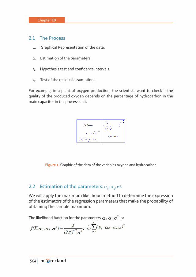
Chapter 10
564
2�1 The Process
1. Graphical Representation of the data.
2. Estimation of the parameters.
3. �����������������������Ƥ���������������Ǥ
4. Test of the residual assumptions.
For example, in a plant of oxygen production, the scientists want to check if the quality of the produced oxygen depends on the percentage of hydrocarbon in the main capacitor in the process unit.
Figure 2. Graphic of the data of the variables oxygen and hydrocarbon
2�2 Estimation of the parameters: D0, D1, V2�
We will apply the maximum likelihood method to determine the expression of the estimators of the regression parameters that make the probability of obtaining the sample maximum.
The likelihood function for the parameters D� D� V� is:

Advanced Statistics
565
The values of D� D� V� are obtained from:
The estimators are the following, after processing the equations above:
x - Y =x - nY= ii
in
1=i0 DDD ˆˆˆ ¦
The regression model for the i- component of vector Y is
)x-x( + Y =Y i1i Dˆ
Where nx=x i
n
1=i¦
The estimation of the variance is the following:
¦ ¦ ��ˆˆˆ ien
)x--y(n1= i10i
2n
1=i
2 DDV
On the second hand, the value of the residual ei or error of the model is:
x - - y =e i10ii DD ˆˆ ���������������ơ��������������������������������������������������one:
So e��Q=ˆ L�
Q
�=L
� ¦V is the quadratic mean of the residuals.
But the n-residuals ��������������������������Ǥ��������������Ƥ������������������������appear in the process of the maximum likelihood method:
� =eL¦
0 =x e ii¦
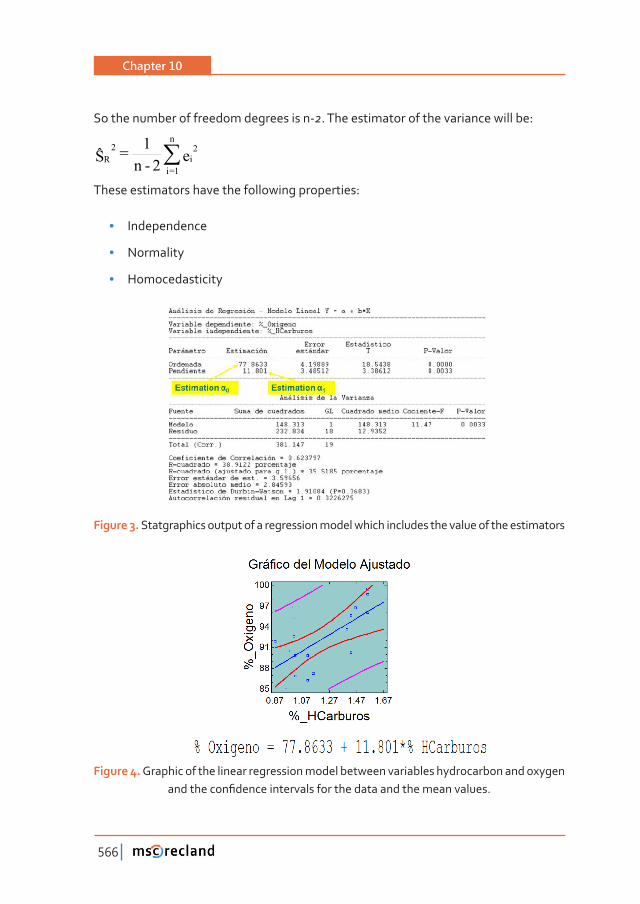
Chapter 10
566
So the number of freedom degrees is n-. The estimator of the variance will be:
e�-Q�=6 L
�Q
�=L5� ¦
These estimators have the following properties:
• Independence
• Normality
• Homocedasticity
Figure 3. Statgraphics output of a regression model which includes the value of the estimators
Figure 4. Graphic of the linear regression model between variables hydrocarbon and oxygen �����������Ƥ������������������������������������������������Ǥ�

Advanced Statistics
567
2�3 Simplification tests
��������������������������������������������������������Ƥ���������Ǥ�
Ǧ�����Ƥ��������������������������������������ǣ
H0: D1=0
This expression according to the formulation of the general linear model is:
�=
K
K� ( �=+ �+
�
���� ¸
¸¹
·¨¨©
§DDcE
The simplest expression of matrix H is:
H=(0,1).
Statistic F:
Under the null hypothesis, that is, when �=�D , the estimators are:
Y =0�D ; �=ˆ ��D ;
So the estimator F is:
The statistic ȋ�ǦȌȀ� follows the distribution F-sneadecor with ȋǡ� �ǦȌ degrees of freedom, which is the square of the t-student distribution with ȋ�ǦȌ degrees of freedom.
If ȋ�ǦȌη��then the hypothesis is rejected. In the case of the t-student distribution, the null hypothesis is rejected when:

Chapter 10
568
Where C’����������������������Ǧ��������������������������������Ƥ����������������������������Ƥ�����������Ǥ
Ǧ������������������Ƥ������������������������������������������������Ǥ�Ƚγ
The hypothesis is:
H0:D0=0
This expression according to the formulation of the general linear model is:
The simplest expression of matrix H is:
H=(0,1).
Statistic F:
Under the null hypothesis, that is, when �=�D , the estimators are:
�=�ˆ( ��D ;
X
YX=
i2
n
1=i
ii
n
1=i1
¦
¦��ˆ(D ;
So the statistic F is:
�=K
K� ( �=+ �+
�
���� ¸
¸¹
·¨¨©
§DDcE

Advanced Statistics
569
The statistic ȋ�ǦȌȀ� follows the distribution F-sneadecor with ȋǡ� �ǦȌ degrees of freedom, which is the square of the t-student distribution with ȋ�ǦȌ degrees of freedom.
( D� )0 can be expressed in function of D� :
As a result, F is:
If ȋ�ǦȌη��then the hypothesis is rejected. In the case of the t-student distribution, the null hypothesis is rejected when:
Where C’����������������������Ǧ������������������������������Ƥ����������������������������Ƥ�����������Ǥ�
Ǧ�������ǡ���������������� are both zero.
This expression according to the formulation of the general linear model is:

Chapter 10
570
The simplest expression of matrix H is:
¸¹
ᬩ
§
��
�� = + Statistic F:
Under the null hypothesis, that is, when 0=0D , 0 =1D , the estimators are:
�=�ˆ( ��D ; �=�ˆ( ��D ; Yn1 = i
2n
1=i
2 ¦��ˆ(V
AS a result, F is:
If ȋ�ǦȌη��then the hypothesis is rejected.
���Ƥ�������������������������������D0 ,D1 :
Let D-1 ǡ�����������������Ƥ�����ǡ����������������������������D0 is:
� �
� �
� �
� � ¸
¸¸¸
¹
·
¨
¨¨¨
©
§
��
���
��
���
¦
¦¦
¦
¦¦
�
� n
ii
n
ii
n
iii
nn
ii
n
ii
n
iii
n
XXnn
XXxt
XXnn
XXYt
�
�
�
�
�
���
�����
�
�
�
�
�
���
�����
��(
ˆˆˆ�
��(
ˆˆˆ
DDD
DDD DD
And for D1 is:
� �
� �
� �
� � ¸
¸¸¸
¹
·
¨
¨¨¨
©
§
��
���
��
���
¦
¦
¦
¦
�
� n
ii
n
iii
nn
ii
n
iii
n
YYn
YYt
XXn
XYt
�
�
�
���
�����
�
�
�
���
�����
��(
ˆˆˆ�
��(
ˆˆˆ
DDD
DDD DD

Advanced Statistics
571
2�4 Correlation coefficient
�������������������ƥ������������������������������������������������������������Ǥ�
������������������������ƥ�������������Ǧ�����������������������������������������������two variables.
3 hypothesis tests oF the correlation coeFFicient
1 H0: U=0 and H1: Uz0
In this case, the statistic is ��
�r
rnt�
� . It follows the Student distribution
with (n-2) degrees of freedom.
2 H0: U=U0 z0 frente a H1: UzU0
is the statistic used in this test. It follows the Gauss distribution
with the following parameters.
� ��
�var�
n
z
3�1 Analysis of the residuals
Normality hypothesis
• ���Ǧ��������������������������������Ƥ�����ǣ
- �����������������������Ǧ
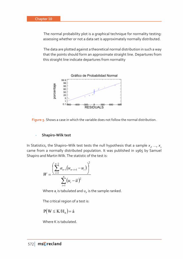
Chapter 10
572
The normal probability plot is a graphical technique for normality testing: assessing whether or not a data set is approximately normally distributed.
The data are plotted against a theoretical normal distribution in such a way that the points should form an approximate straight line. Departures from this straight line indicate departures from normality
Gráfico de Probabilidad Normal
-900 -600 -300 0 300 600 900RESIDUALS
0.115
2050809599
99.9
porc
enta
je
Figure 5. Shows a case in which the variable does not follow the normal distribution.
- �������Ǧ���������
In Statistics, the Shapiro–Wilk test tests the null hypothesis that a sample x1, ..., xn came from a normally distributed population. It was published in 1965 by Samuel Shapiro and Martin Wilk. The statistic of the test is:
� �
� �¦
¦
���
�
¸¹
ᬩ
§�
n
ii
n
iiinn
uu
uuaW
�
�
���
���
Where ai is tabulated and ui, is the sample ranked.
The critical region of a test is:
� � á.�+W3 � d
Where K is tabulated.

Advanced Statistics
573
- �������ǯ�����Ǧ������������ǣ
It tests a null hypothesis stating that the frequency distribution of certain events observed in a sample is consistent with a particular theoretical distribution. The events considered must be mutually exclusive and have total probability..
The value of the test-statistic is
where
= Pearson’s cumulative test statistic, which asymptotically approaches a
distribution.
Oi= an observed frequency;
Ei= an expected (theoretical) frequency, asserted by the null hypothesis;
n= the number of cells in the table.
The chi-squared statistic can then be used to calculate a p-value by comparing the value of the statistic to a chi-squared distribution. The number of degrees of freedom is equal to the number of cells n, minus the reduction in degrees of freedom, p.
- ����������Ǧ������������
The Kolmogorov–Smirnov test (K–S test) is a nonparametric test for the equality of continuous, one-dimensional probability distributions that can be used to compare a sample with a reference probability distribution (one-sample K–S test), or to compare two samples (two-sample K–S test). The ����������Ȃ������������������������Ƥ������������������������������������distribution function of the sample and the cumulative distribution function of the reference distribution, or between the empirical distribution functions of two samples. The null distribution of this statistic is calculated under the
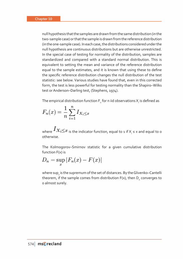
Chapter 10
574
null hypothesis that the samples are drawn from the same distribution (in the two-sample case) or that the sample is drawn from the reference distribution (in the one-sample case). In each case, the distributions considered under the null hypothesis are continuous distributions but are otherwise unrestricted. In the special case of testing for normality of the distribution, samples are standardized and compared with a standard normal distribution. This is equivalent to setting the mean and variance of the reference distribution �����������������������������ǡ����� ��� �������������������������������Ƥ������������Ƥ�������������������������������������������������������������������statistic: see below. Various studies have found that, even in this corrected form, the test is less powerful for testing normality than the Shapiro–Wilks test or Anderson–Darling test, (Stephens, 1974).
The empirical distribution function Fn for n iid observations Xi������Ƥ������
where is the indicator function, equal to 1 if Xi�����������������otherwise.
The Kolmogorov–Smirnov statistic for a given cumulative distribution function F(x) is
where supx is the supremum of the set of distances. By the Glivenko–Cantelli theorem, if the sample comes from distribution F(x), then Dn converges to 0 almost surely.
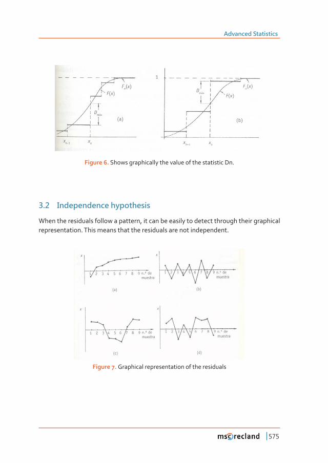
Advanced Statistics
575
Figure 6. Shows graphically the value of the statistic Dn.
3�2 Independence hypothesis
When the residuals follow a pattern, it can be easily to detect through their graphical representation. This means that the residuals are not independent.
Figure 7. Graphical representation of the residuals

Chapter 10
576
Two of the most applied tests are:
• �������������������ƥ�����ǣ
��������ƥ�������������������������������������������������������������������one separated k position in the same sample.
� �� �
� �¦
¦
� �
�
�� n
ii
n
kikii
xx
xxxxkr
�
�
��(
Where k is the lag
Figure 8. �����������������������ơ������������������������������������������Ǥ
• Durbin-Watson test
The statistic in this case is:
� �
¦
¦
��
n
ii
n
iii
e
eeD
�
�
�
��

Advanced Statistics
577
Where ei are the residuals
If D=0 there is a positive dependence in the residuals.
If D=2 the residuals are independent.
If D=4 there is a negative dependence in the residuals
3�3 Homocedasticity test
There are some tests that allow the tests of this assumption apart from the graphical test. This tests are the Bartlett test, the C of Cochran test, the Harley test and the Levene test. The conditions under these tests can be applied are:
Table 1. Requirements to apply the homocedasticity tests
TestNormality ����������
������������Ȁ�������
Bartlett Yes Anyone
Cochran Anyone Equal
Hartley Yes Equal
Levene Anyone Anyone
4 model evaluation
There are several ways to validate a regression model. This chapter focuses on:
• Analysis of variance
• ��������Ƥ������
• ������Ƥ���������������������������
• ������Ƥ������������ƪ��������������

Chapter 10
578
4�1 Analysis of variance
We can break the variability of the variable into components:
� � � � � �¦¦¦
��� �n
ii
n
iii
n
ii yyyyyy
�
�
�
�
�
� ˆˆ
So the Total Sum of Squares is the Regression Sum of Squares + Error (or Residual) Sum of Squares
We can organize the results of a simple linear regression analysis in an ANOVA table, ����Ƥ�����������������Ǥ
Figure 9. ANOVA table of a simple regression model
Figure 10. ANOVA table with the variables and the statistics

Advanced Statistics
579
The statistic F is used to test the hypothesis:
H0: E[Y/X]= D 0 versus H1: E[Y/X]= X + 10 DD
Or H0: �� D vs H1: �� zD for short
4�2 Lack of fit test
This is an F test for checking whether a linear regression function is inadequate in describing the trend in the data:
150140130120110100 90 80 70 60
700
600
500
400
300
200
100
0
Length
Wei
ght
S = 54.0115 R-Sq = 83.6 % R-Sq(adj) = 82.9 %Weight = -393.264 + 5.90235 Length
Regression Plot
Figure 11. F test for checking whether a linear regression function is inadequate in describing the trend in the data
Do the data suggest that a linear function is inadequate in describing the relationship between the length and weight of an alligator?
�������������������������������������������������������������������������Ƥ�Ǥ������12 shows the notation we are going to apply in this process.
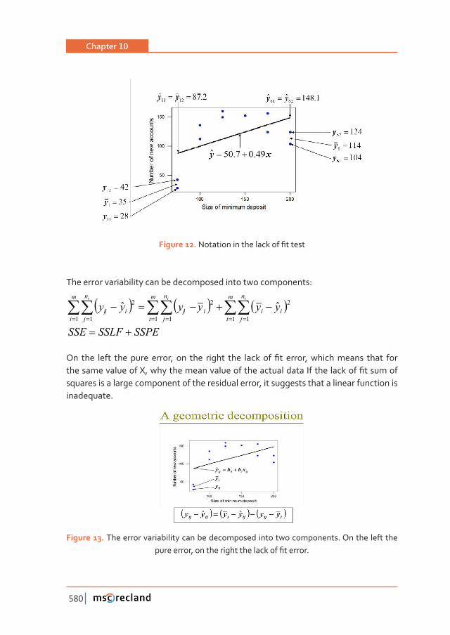
Chapter 10
580
Figure 12. ������������������������Ƥ������
The error variability can be decomposed into two components:
� � � � � �¦ ¦ ¦¦¦¦
��� �m
i
m
i
m
i
n
jii
n
jiij
n
jiij
iii
yyyyyy� � � �
�
�
�
�
� ˆˆ
SSPESSLFSSE �
��� ���� ����� ���� ����� �����ǡ� ��� ���� ������ ���� ����� ��� Ƥ�� �����ǡ������������� ����� �����������������������ǡ������������������������������������������������������Ƥ���������squares is a large component of the residual error, it suggests that a linear function is inadequate.
Figure 13. The error variability can be decomposed into two components. On the left the ����������ǡ��������������������������Ƥ�������Ǥ

Advanced Statistics
581
The degrees of freedom are, SSE has n-2, SSLF has m-2 and SSPE m-c
So the expanded Analysis of Variance is:
��������������� H0: Ɋi = Ƚ+ȽXi
���������������������� HA: Ɋi�δ�Ƚ+ȽXi
MSPEMSLFF *
Figure 14. Example of the study of the alligator
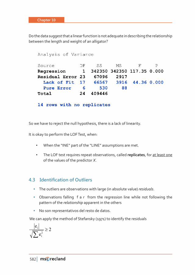
Chapter 10
582
Do the data suggest that a linear function is not adequate in describing the relationship between the length and weight of an alligator?
So we have to reject the null hypothesis, there is a lack of linearity.
It is okay to perform the LOF Test, when:
• ���������Dz���dz�������������Dz����dz��������������������Ǥ
• The LOF test requires repeat observations, called ����������, for at least one of the values of the predictor X.
4�3 Identification of Outliers
• The outliers are observations with large (in absolute value) residuals.
• Observations falling f a r from the regression line while not following the pattern of the relationship apparent in the others
• No son representativos del resto de datos.
We can apply the method of Stefansky (1971) to identify the residuals
�e
e�L
L t¦
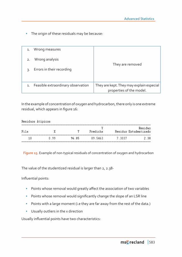
Advanced Statistics
583
• The origin of these residuals may be because:
1. Wrong measures
2. Wrong analysis
3. Errors in their recordingThey are removed
1. Feasible extraordinary observation They are kept. They may explain especial properties of the model.
In the example of concentration of oxygen and hydrocarbon, there only is one extreme ��������ǡ������������������Ƥ�����ǣ
Figure 15. Example of non-typical residuals of concentration of oxygen and hydrocarbon
The value of the studentized residual is larger than 2, 2.38-
��ƪ��������������ǣ
• ������������������������������������ơ������������������������������������
• ��������������������������������Ƥ��������������������������������������
• Points with a large moment (i.e they are far away from the rest of the data.)
• Usually outliers in the x direction
����������ƪ���������������������������������������ǣ

Chapter 10
584
They are outliers, i.e. graphically they are far from the pattern described by the other ������ǡ�������������������������������������������������� �����ơ���������������������than for the other points.
• They are in a position of high leverage, meaning that the value of the variable x is far from the mean x . Observations with very low or very high values of x are in positions of high leverage.
The leverage points are detected from the following expression which measures the ��ƪ������������������������������������������������ƥ������Ǥ
+\y;;�;�;ȕ;y � �
The diagonal of matrix H is a measure of the distance between the observation i to the center of the space of X. There is leverage if this value if larger tan:
x�Q�K�
Q
�LLL¦
Figure 16. ��ơ������������������ƪ��������������Ǥ�����������������������������ǡ�������������������ƪ��������������

Advanced Statistics
585
4�4 DFFITS
���������������������������ƪ��������������������������������������������Ǥ�
�����QL K6
yy')),76
LL��L�
�L�LL
�
�L�y is the adjusted value of yi when we do not use the observation i
A point is analyzed if:
QK�')),76 LLL ¦!
���Ƥ����� ǡ�����������������������������������Ȃ��������������������������������������������������������������Ǥ����������������ǡ��������������������������������Ƥ��������ơ�������������������������������������Ǥ��������������ƪ�������������Ǩ��
Figure 17Ǥ��ơ�������������ƪ�������������������������������������

Chapter 10
586
Another example:
The correct answer is C
Because this point has a large moment and is far from the rest of the data, it is an ��ƪ�������� �����Ǥ� � ��� ����� ���������� �������ǡ� ���� ������ ��� ���� ��������������������change.
II. This point is not an outlier with respect to the model because as you can see in the residual plot, it does not have a large residual (It follows the regression pattern of the data).
III. By looking at both the scatterplot and the residual plot, you can see that the yellow point is an outlier in the x direction (far right of the rest of the data).
5 transFormation oF a random variable
������������������������Ƥ�����������������������������������ǡ����������������������can take place depending on the relation between the variance and the moment of Y.

Advanced Statistics
587
Table 2. Transformations of variable Y
�����������������ɐ2 and E[y] Transformation
ɐ2 ~ Constant y’=y
ɐ2 ~ E[y] y’= y1/2
ɐ2 ~ E[y] [1-E[y]] y’=1/sen(y1/2),
ɐ2 ~ E[y]2 Y’=ln(y)
ɐ2 ~ E[y]3 Y’= y-1/2
ɐ2 ~ E[y]4 Y’= y-1
5�1 Application of the model
��������������������Ƥ�����������������������ǡ���������������������������������������for the moment of Y:
For the prediction:
� �¸¸
¹
·
¨¨
©
§ ���r� �
[[
���
UHV
�UHV�
UHV�Qi����� 6[[6
Q66tyy .
������������������ǣ
� �¸¸
¹
·
¨¨
©
§ ��r� �
[[
���
UHV
�UHV
�Qi���[|y� 6[[6
Q6tì�(�\�[
�
��������������Ƥ�������������������������������������ǣ
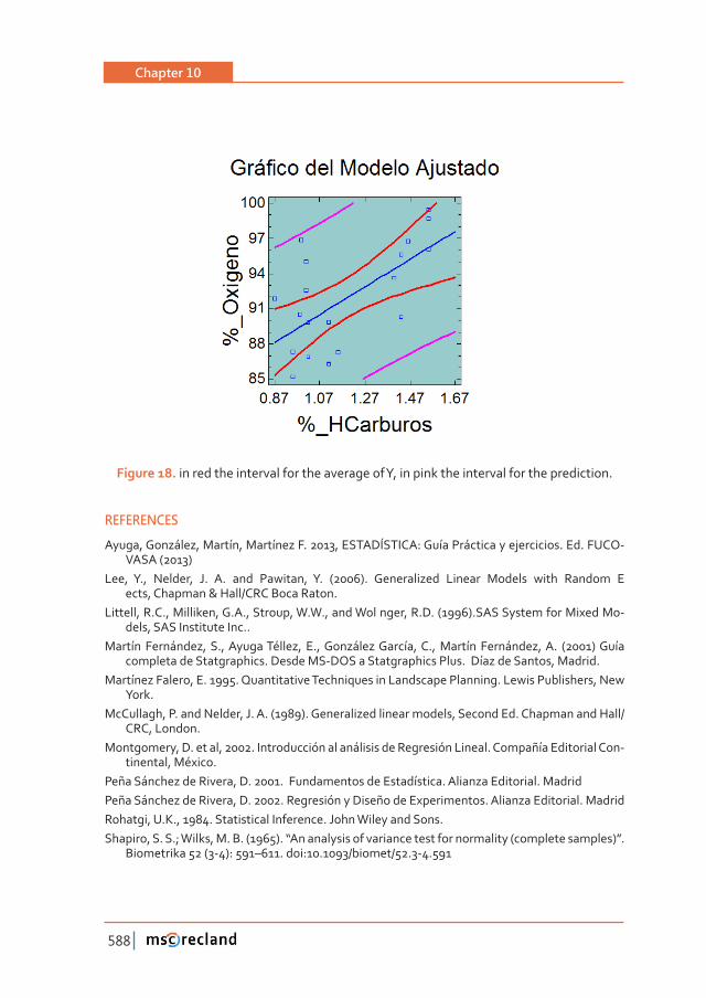
Chapter 10
588
Figure 18. in red the interval for the average of Y, in pink the interval for the prediction.
REFERENCES
Ayuga, González, Martín, Martínez F. 2013, ESTADÍSTICA: Guía Práctica y ejercicios. Ed. FUCO-VASA (2013)
Lee, Y., Nelder, J. A. and Pawitan, Y. (2006). Generalized Linear Models with Random E ects, Chapman & Hall/CRC Boca Raton.
Littell, R.C., Milliken, G.A., Stroup, W.W., and Wol nger, R.D. (1996).SAS System for Mixed Mo-dels, SAS Institute Inc..
Martín Fernández, S., Ayuga Téllez, E., González García, C., Martín Fernández, A. (2001) Guía completa de Statgraphics. Desde MS-DOS a Statgraphics Plus. Díaz de Santos, Madrid.
Martínez Falero, E. 1995. Quantitative Techniques in Landscape Planning. Lewis Publishers, New York.
McCullagh, P. and Nelder, J. A. (1989). Generalized linear models, Second Ed. Chapman and Hall/CRC, London.
Montgomery, D. et al, 2002. Introducción al análisis de Regresión Lineal. Compañía Editorial Con-tinental, México.
Peña Sánchez de Rivera, D. 2001. Fundamentos de Estadística. Alianza Editorial. MadridPeña Sánchez de Rivera, D. 2002. Regresión y Diseño de Experimentos. Alianza Editorial. MadridRohatgi, U.K., 1984. Statistical Inference. John Wiley and Sons. �������ǡ��Ǥ��ǤǢ������ǡ��Ǥ��Ǥ�ȋȌǤ�Dz�������������������������������������������ȋ����������������ȌdzǤ�
Biometrika 52 (3-4): 591–611. doi:10.1093/biomet/52.3-4.591

Advanced Statistics
589
��������ǡ��Ǥ��Ǥ�ȋȌǤ�Dz����������������������������������������������������dzǤ� ����������the American Statistical Association (American Statistical Association) 69 (347): 730–737. doi:10.2307/2286009. JSTOR 2286009.

Related Documents