Climate and biogeochemical response to a rapid melting of the West Antarctic Ice Sheet during interglacials and implications for future climate

Climate and biogeochemical response to a rapid meltingof the West Antarctic Ice Sheet during interglacialsand implications for future climate

L. Menviel,1 A. Timmermann,2 O. Elison Timm,2 and A. Mouchet3

Received 16 November 2009; revised 18 October 2010; accepted 27 October 2010; published 31 December 2010.

[1] We study the effects of a massive meltwater discharge from the West Antarctic Ice Sheet (WAIS) duringinterglacials onto the global climate‐carbon cycle system using the Earth system model of intermediatecomplexity LOVECLIM. Prescribing a meltwater pulse in the Southern Ocean that mimics a rapiddisintegration of the WAIS, a substantial cooling of the Southern Ocean is simulated that is accompanied byan equatorward expansion of the sea ice margin and an intensification of the Southern HemisphericWesterlies. The strong halocline around Antarctica leads to suppression of Antarctic Bottom Water (AABW)formation and to subsurface warming in areas where under present‐day conditions AABW is formed. Thissubsurface warming at depths between 500 and 1500 m leads to a thermal weathering of the WAISgrounding line and provides a positive feedback that accelerates the meltdown of the WAIS. Our modelresults further demonstrate that in response to the massive expansion of sea ice, marine productivity in theSouthern Ocean reduces significantly. A retreat of the WAIS, however, does not lead to any significantchanges in atmospheric CO2. The climate signature of a WAIS collapse is structurally consistent withavailable paleoproxy signals of the last interglacial MIS5e.

Citation: Menviel, L., A. Timmermann, O. E. Timm, and A. Mouchet (2010), Climate and biogeochemical response to a rapidmelting of the West Antarctic Ice Sheet during interglacials and implications for future climate, Paleoceanography, 25, PA4231,doi:10.1029/2009PA001892.

1. Introduction

[2] The West Antarctic Ice Sheet (WAIS) is a marine‐based ice sheet and may hence be very susceptible to var-iations in sea level and ocean temperature [Bindschadler,1998]. Increasing sea level may destabilize the main iceshelves in Antarctica which may subsequently accelerate theflow of inland glaciers into the ocean and hence lead tofurther sea level rise. Moreover, subsurface ocean warmingcan destabilize the WAIS from below, triggering an erosionof the grounding line and leading to further melting [Rignotand Jacobs, 2002; Payne et al., 2004]. The magnitude ofthese processes is very difficult to assess, which severelyhampers our skill to predict global sea level rise in thecoming centuries [Oppenheimer and Alley, 2004]. A partialcollapse of the WAIS would lead to a global sea level rise ofabout 3 to 6 m [Oppenheimer, 1998; Bamber et al., 2009].[3] Presence of young diatoms and relatively high levels

of Beryllium in late Pleistocene sediments from the RossSea indicate that the WAIS retreated substantially duringinterglacial periods of the Pleistocene [Scherer et al., 1998].Recent paleostudies [Hearty et al., 2007; Carr et al., 2010]

showed that the sea level was up to 9 m higher than todayduring Marine Isotope Stage 5e (MIS5e, ∼123 ka B.P.),making MIS5e an interesting candidate to study the poten-tial collapse of the WAIS [Mercer, 1978]. In addition, acombined ice sheet/ice shelf model simulated several WAIScollapses during the Pleistocene [Pollard and DeConto,2009] in phase with strong austral summer insolationanomalies. During MIS5e, the model simulated a significantretreat of the WAIS, but not a complete collapse.[4] Variations in benthic d18O and abundance of diatoms

in a marine sediment core from the Ross Sea indicated or-bitally paced retreats of the WAIS during the Pliocene[Naish et al., 2009]. This finding was also confirmed by theAntarctic ice sheet modeling study [Pollard and DeConto,2009]. Considering that the WAIS retreated substantiallyin the past, when the Antarctic climate was about 3°Cwarmer than today [Kim and Crowley, 2000] and theatmospheric CO2 was as high as 400 ppmv [Van Der Burghet al., 1993; Raymo et al., 1996; Pagani et al., 2010], theWAIS could potentially retreat as a result of increasinggreenhouse gases in the future. It is therefore timely to betterunderstand the possible consequences of a WAIS retreatonto the climate and the biogeochemical cycle.[5] Recent modeling studies have documented the climate

response to massive meltwater pulses into the SouthernOcean. Using state‐of‐the‐art coupled general circulationmodels, Richardson et al. [2005], Stouffer et al. [2007] andMa et al. [2010] find that the addition of freshwater at highsouthern latitudes leads to a stabilization of the water column,

1Climate and Environmental Physics, Oeschger Centre for ClimateChange Research, University of Bern, Bern, Switzerland.

2IPRC, SOEST, University of Hawai’i, Honolulu, Hawaii, USA.3Departement AGO, Université de Liège, Liège, Belgium.

Copyright 2010 by the American Geophysical Union.0883‐8305/10/2009PA001892

PALEOCEANOGRAPHY, VOL. 25, PA4231, doi:10.1029/2009PA001892, 2010

PA4231 1 of 12

which inhibits deep convection and therefore the formationof Antarctic Bottom Water (AABW). At high southernlatitudes, the surface air and ocean temperature decreasesignificantly, while an oceanic subsurface warming issimulated. Consistently, these modeling studies also dem-onstrate that Southern Hemispheric Westerlies strengthenin response to the freshwater perturbation. Moreover, dueto a decrease of the meridional density gradient, the Ant-arctic Circumpolar Current (ACC) weakens in all of thesemodeling experiments.[6] The biogeochemical response to Antarctic meltwater

pulses has, to our knowledge, not been studied before. Themain rationale of our study is to evaluate the impact of arapid disintegration of the interglacial WAIS, on globalclimate and the carbon cycle using the Earth system modelof intermediate complexity LOVECLIM. We expect that thederived climatic fingerprints of such an event could help inthe interpretation of paleoclimate proxy data in the SouthernHemisphere.[7] In section 2, we describe the experimental setup of our

modeling experiments. Section 3 focuses on the climate andbiogeochemical response to a collapse of the WAIS duringinterglacials of the Pleistocene and CO2 doubling condi-tions. A previously overlooked positive feedback betweenice sheet and ocean that might lead to an accelerated dis-integration of the WAIS is also described. Finally, section 4discusses our main results in the light of past and futureclimate change.

2. Experimental Setup

[8] The model used in this study is the model of inter-mediate complexity LOVECLIM (LOch‐Vecode‐Ecbilt‐CLio‐agIsm Model), version 1.1. The atmospheric compo-nent of the coupled model LOVECLIM is ECBilt [Opsteeghet al., 1998], a spectral T21, three‐level model, based onquasi‐geostrophic equations extended by estimates of theneglected ageostrophic terms [Lim et al., 1991] in order toclose the equations at the equator. The sea ice‐ocean com-ponent of LOVECLIM, CLIO [Goosse et al., 1999; Goosseand Fichefet, 1999; Campin and Goosse, 1999] consists of afree‐surface primitive equation model with 3° × 3° resolu-tion, coupled to a thermodynamic‐dynamic sea ice model.Coupling between atmosphere and ocean is done via theexchange of freshwater, momentum and heat fluxes.

[9] The terrestrial vegetation module of LOVECLIM,VECODE [Brovkin et al., 1997] has recently been coupledto the LOVECLIM model [Renssen et al., 2005]. VECODEsimulates the dynamical vegetation changes and the terres-trial carbon cycle in response to climatic conditions (annualmean temperatures, annual precipitation and other derivedclimatic quantities such as growing degree days, seasonalityof rainfall). Two plant functional types, grass and trees,describe the vegetation cover. For each land grid cell, VE-CODE calculates the fractional coverage with grass andtrees and the fractional desert area. Terrestrial net primaryproduction is a function of temperature and precipitation aswell as atmospheric CO2 concentrations. The producedorganic carbon is aggregated in four compartments: leaves,stems and roots, woody residues, and dead organic matter inthe soil (humus). The conversion rates among these fourterrestrial carbon reservoirs have characteristic time scalesranging from 1 year to 800 years. The conversion ratesdepend on primary production and temperature. A moredetailed description is given in Brovkin et al. [2002]. In theLOVECLIM version employed here, the feedback from thevegetation to the atmosphere is only given by surface albedochanges. Other factors such as evapotranspiration and sur-face roughness are neglected.[10] LOCH is a three‐dimensional global model of the

oceanic carbon cycle Mouchet and Francois [1996]. Thepresent version of the model is described by Goosse et al.[2010]. The prognostic state variables considered in themodel are dissolved inorganic carbon (DIC), total alkalinity,phosphates (PO4

3−), organic products, oxygen and silica.LOCH is fully coupled to CLIO, with the same time step. Inaddition to their biogeochemical transformations tracers inLOCH experience the circulation field predicted by CLIO.LOCH computes the export production from the fate of aphytoplankton pool in the euphotic zone (0–120 m). Thephytoplankton growth depends on the availability of nu-trients (PO4

3−) and light, with a weak temperature depen-dence. A grazing process together with natural mortalitylimit the primary producers biomass and provide the sourceterm for the organic matter sinking to depth. The otherprocesses described in the model include remineralization,carbonate precipitation and dissolution as well as opal pro-duction. LOCH does not include sedimentary processes butnevertheless takes into account carbonate compensationmechanisms. The atmospheric CO2 content is updated foreach ocean time step.

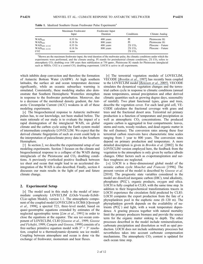
Table 1. Idealized Southern Ocean Freshwater Pulse Experimentsa

Maximum FreshwaterInput

Freshwater InputDuration Conditions Climate Analog

WAIS400 0.35 Sv 400 years PI Pleistocene IGWAIS800 0.18 Sv 800 years PI Pleistocene IGWAIS400−2CO2 0.35 Sv 400 years 2X CO2 Pliocene ‐ FutureWAIS800−2CO2 0.18 Sv 800 years 2X CO2 Pliocene ‐ FutureCO2 none 2X CO2

aShown are the maximum freshwater input, the total duration of the meltwater pulse, the climatic conditions under which theexperiments were performed, and the climate analog. PI stands for preindustrial climate conditions, 2X CO2 refers toatmospheric CO2 doubling over 100 years then stabilization at 750 ppmv, Pleistocene IG stands for Pleistocene interglacialsuch as MIS5e. CO2 is a control CO2 doubling experiment. LOCH is active in all experiments.

MENVIEL ET AL.: CLIMATE RESPONSE TO ANTARCTIC MELTWATER PA4231PA4231

2 of 12

[11] To estimate the impact of a collapse of the WestAntarctic Ice Sheet during interglacial periods on the climateand carbon cycle, we perform a set of highly idealized ex-periments (Table 1). To mimic a rapid disintegration of theWAIS, we assume an idealized freshwater release of about2.2 × 106 km3 into the area 163°E–11°E, 70°S–80°S, whichencompasses the Ross, Amundsen, Bellingshausen andWeddell Seas. This scenario is reasonable given the esti-mates of Lythe et al. [2001]: the total volume of the present‐day WAIS including ice shelves and the volume of thegrounded ice sheet below sea level are 3.6 × 106 km3 and1 × 106 km3, respectively. As Oppenheimer [1998] esti-mated the mean time to collapse the WAIS in the future at500 to 700 years, we designed two scenarios in which acollapse is obtained in 400 and 800 years, respectively.[12] In experiment WAIS400, we prescribe a triangular‐

shaped freshwater pulse with a total duration of 400 yearsattaining a maximum strength of 0.35 Sv after 200 years(Figure 1, bottom left). Once the freshwater input ceases welet the model run for another 600 years. In experimentWAIS800, the freshwater input is set constant at 0.18 Sv andhas a total duration of 800 years. Experiments WAIS400and WAIS800 are performed under preindustrial conditions,start from experiment PIN and serve as analogs of inter-glacial times of the Pleistocene such as MIS5e. The pre-industrial steady state (PIN) was obtained by forcingLOVECLIM with 278 ppmv of atmospheric CO2 during500 years, then allowing the atmospheric CO2 to varyfreely during 2000 years.[13] Naish et al. [2009] and Pollard and DeConto [2009]

also suggested that collapses of the WAIS occurred duringthe Pliocene when the climate was about 3°C warmer thantoday [Kim and Crowley, 2000] and the atmospheric CO2

was as high as 400 ppmv [Van Der Burgh et al., 1993;

Raymo et al., 1996; Pagani et al., 2010]. Since in the ver-sion of LOVECLIM used here, an atmospheric CO2 dou-bling leads to a ∼ 3°C increase in global mean temperature,we perform two additional experiments, called WAIS400−2CO2

and WAIS800−2CO2, forced with an atmospheric CO2

content of 750 ppmv. From these experiments we can thenevaluate the impact of a collapse of the WAIS for futureclimate and Pliocene conditions.[14] Experiments WAIS400−2CO2

and WAIS800−2CO2use

the same freshwater forcing as WAIS400 and WAIS800.These experiments start from a present day run and are thentransiently forced with linearly increasing CO2 concentra-tion attaining 750 ppmv in 100 years. The atmospheric CO2

concentration is subsequently kept constant at 750 ppmv.Experiments WAIS400−2CO2

and WAIS800−2CO2are com-

pared to a control CO2 doubling experiment (CO2). CO2 isforced with the same atmospheric CO2 forcing as inWAIS400−2CO2

but no freshwater pulse is applied.[15] The experiments performed in this study are highly

idealized, but given the uncertainty in our knowledge of thetiming of past WAIS collapses, we think these idealizedexperiments provide a good first‐ order approximation ofthe climate and biogeochemical responses during intergla-cial WAIS retreats.

3. Impact of a WAIS Collapse DuringInterglacials and CO2 Doubling Conditions

3.1. Climate Response

[16] The Southern Ocean freshwater perturbation pre-scribed in WAIS400 leads to a freshening of the surfacewaters lowering the surface density (not shown) andincreasing the stratification. The formation of a strong hal-ocline and the associated increased stability of the water

Figure 1. (top) Maximum overturning circulation in the bottom cell of the Southern Ocean (Sv) forexperiments WAIS400 (black) and WAIS800 (dashed grey). (bottom) Anomalous freshwater flux inthe Southern Ocean (Sv) for experiments WAIS400 (black) and WAIS800 (dashed grey).

MENVIEL ET AL.: CLIMATE RESPONSE TO ANTARCTIC MELTWATER PA4231PA4231

3 of 12

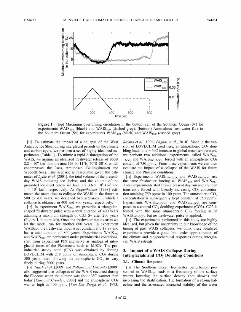
column inhibit deep convection in the Southern Ocean (notshown) thus leading to a breakdown of Antarctic BottomWater (AABW) formation. This is evidenced in the globallyaveraged meridional stream function (Figure 2). The bottomoverturning cell that is associated with the formation ofAABW reduces in strength from 17 to 3 Sv (Figure 1).These large‐scale transport changes of AABW in turnincrease the cross‐equatorial export of North Atlantic DeepWater (NADW) into the Southern Hemisphere. Relativelywarm NADW has to upwell in the Southern Ocean, whichhas a secondary effect on the stratification field in theSouthern Ocean.[17] As waters are relatively warm at depth in the

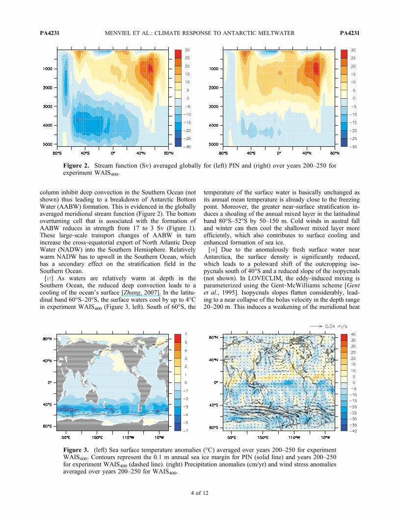
Southern Ocean, the reduced deep convection leads to acooling of the ocean’s surface [Zhang, 2007]. In the latitu-dinal band 60°S–20°S, the surface waters cool by up to 4°Cin experiment WAIS400 (Figure 3, left). South of 60°S, the

temperature of the surface water is basically unchanged asits annual mean temperature is already close to the freezingpoint. Moreover, the greater near‐surface stratification in-duces a shoaling of the annual mixed layer in the latitudinalband 80°S–52°S by 50–150 m. Cold winds in austral falland winter can then cool the shallower mixed layer moreefficiently, which also contributes to surface cooling andenhanced formation of sea ice.[18] Due to the anomalously fresh surface water near

Antarctica, the surface density is significantly reduced,which leads to a poleward shift of the outcropping iso-pycnals south of 40°S and a reduced slope of the isopycnals(not shown). In LOVECLIM, the eddy‐induced mixing isparameterized using the Gent‐McWilliams scheme [Gentet al., 1995]. Isopycnals slopes flatten considerably, lead-ing to a near collapse of the bolus velocity in the depth range20–200 m. This induces a weakening of the meridional heat

Figure 2. Stream function (Sv) averaged globally for (left) PIN and (right) over years 200–250 forexperiment WAIS400.

Figure 3. (left) Sea surface temperature anomalies (°C) averaged over years 200–250 for experimentWAIS400. Contours represent the 0.1 m annual sea ice margin for PIN (solid line) and years 200–250for experiment WAIS400 (dashed line). (right) Precipitation anomalies (cm/yr) and wind stress anomaliesaveraged over years 200–250 for WAIS400.

MENVIEL ET AL.: CLIMATE RESPONSE TO ANTARCTIC MELTWATER PA4231PA4231

4 of 12

transport to high southern latitudes [Stocker et al., 2007].The estimated bolus heat flux anomaly (see Stocker et al.[2007] for details of the calculation) amounts to about−0.11 K/year at year 200 over the latitudinal band 55°S–65°S and in the depth range 20–250 m. This is equivalent to adecrease in heat transport of about 0.08 PW, which mayexplain a fraction of the 0.7°C cooling seen in this area.[19] These surface cooling processes are further amplified

by the sea ice albedo feedback. The annual mean sea icemargin shifts equatorward by 4° during the Southern Oceanfreshwater pulse phase, reaching the Southern tip of SouthAmerica (Figure 3). Increased surface albedo due to thesimulated sea ice expansion cools the lower atmosphere byabout 4°C.[20] Under CO2 doubling conditions, the results are

qualitatively similar to those under preindustrial conditions;however, the amplitude of the changes is greater in WAIS800−2CO2 than in WAIS800. In experiment WAIS400−2CO2 theocean surface also cools by up to 4°C in the latitudinal band40°S–60°S compared to CO2 and the sea ice retreats moreslowly in the Southern Ocean. Moreover, at year 200, theannual sea ice edge extends about 5° equatorward in thePacific and Atlantic sectors of the Southern Ocean forWAIS400−2CO2 compared to CO2. As a result the loweratmosphere over the latitudinal band 60°S–90°S is about4°C cooler in WAIS400−2CO2 compared to CO2.[21] Two mechanisms have recently been proposed to

explain the cooling response of the Southern Hemispherenorth of Drake passage: wave propagation [Ivchenko et al.,2006] and the Wind‐Evaporation SST (WES) feedback [Maet al., 2010]. We found that the WES feedback plays animportant role in cooling the Southern Hemisphere equa-torward of the Subtropical Front. The WES feedback resultsfrom the fact that negative SST anomalies in the easternparts of the southern ocean basins are accompanied bystrengthened trade winds, which lead to enhanced coolingvia increased evaporation.[22] In response to the freshwater forcing and the resulting

SST and sea ice anomalies, Southern Hemispheric Wester-lies intensify substantially (Figure 3, right). The meridionaltemperature gradient increase between 20°S and 50°S isresponsible for the wind intensification through the thermalwind balance. By enhancing evaporation of the surfacewaters, the stronger Westerlies contribute to the cooling ofsurface waters in the latitudinal band 50°S–35°S. In addi-tion, the enhanced Westerlies lead to stronger upwelling atabout 60°S and increased northward Ekman transport.[23] In spite of an intensification of the zonally averaged

Southern Hemispheric Westerlies by about 20%, the Ant-arctic Circumpolar Current (ACC) weakens by about 25%.This can be explained by a reduction of the meridionaldensity gradient induced by low saline surface waters nearAntarctica and the associated geostrophic response of theACC.[24] In the Northern Hemisphere, a significant warming

response is found over a small area in the northern NorthAtlantic (50°W–0°, 60°N–80°N) (Figure 3, left). Such afeature was also simulated by Richardson et al. [2005],Stouffer et al. [2007] and Ma et al. [2010], even though thespecific location where this warming occurred appears to be

strongly model dependent. The warming simulated byRichardson et al. [2005] is located in the Labrador and Ir-minger Seas, while Ma et al. [2010] obtain a warmingat about 50°N over the Pacific and Atlantic Oceans. Stoufferet al. [2007] do not describe the regional details of thewarming obtained at high northern latitude.[25] The enhanced temperature gradient in the Southern

Hemisphere induces a strengthening of the southeasterlytrade winds, while the reduced temperature gradient in theNorthern Hemisphere leads to a weakening of the north-easterly trades (Figure 3, right). The inter hemispheric SSTgradient induces a northward shift of the ITCZ and thusdrier conditions in the Southern Hemisphere and wetterconditions in the Northern Hemisphere.[26] The climatic changes discussed above are observed

during the four seasons but are slightly more pronouncedduring austral winter.[27] The climate response to a Southern Ocean meltwater

pulse obtained with LOVECLIM is quite similar to the oneobtained with more complex models such as HadCM3[Richardson et al., 2005], FOAM [Ma et al., 2010] and theGFDL R30 model [Stouffer et al., 2007]. A more detaileddescription of the climate response to Southern Oceanmeltwater pulses obtained with the LOVECLIM Earth sys-tem model is also provided by Swingedouw et al. [2009].[28] As already discussed by Swingedouw et al. [2009],

the duration and amplitude of the Southern Hemisphericmeltwater pulse play an important role in determining theoverall characteristics of the climate response. As can beseen in Figure 4, the duration of the climatic response is afunction of the length of the meltwater pulse. After resumingto unperturbed conditions, the Southern Ocean salinityanomaly (Figure 4, top left) dissipates quickly due to thenorthward Ekman transport and the upwelling of Circum-polar Deep Waters (CDW), in accordance with the results ofTrevena et al. [2008]. Less than 10 years after the end of themeltwater pulse the Southern Ocean salinity anomaly hasdissipated for all experiments, irrespective of the back-ground climate conditions.[29] We also find that the amplitudes of the Southern

Ocean climate anomalies are proportional to the rate ofmeltwater discharge. Air temperature anomalies averagedover 60°S–90°S amount to about −4.2°C for WAIS400 and−1°C for WAIS800 (Figure 4, top right).

3.2. Subsurface Warming in the Southern Ocean

[30] Changes in stratification, mixing, convection andEkman pumping in the Southern Ocean also lead to sub-stantial subsurface temperature anomalies (Figure 5). Sub-surface temperatures at depths of 500–1500 m and south of60°S increase by up to 1.1°C in WAIS400. This warming canbe attributed to the fact that deep convection near Antarcticaand the formation of AABW are strongly inhibited due tothe freshwater perturbation. A similar subsurface warmingwas obtained as a result of the suppression of the AABWformation due to weaker Southern Hemispheric Westerlies[Menviel et al., 2008]. In the Ross and Weddell Seas coldAABW is replaced by warmer Circumpolar Deep Waters(CDW). A temperature‐salinity scatterplot of the SouthernOcean waters (not shown) indicates that during the period of

MENVIEL ET AL.: CLIMATE RESPONSE TO ANTARCTIC MELTWATER PA4231PA4231

5 of 12

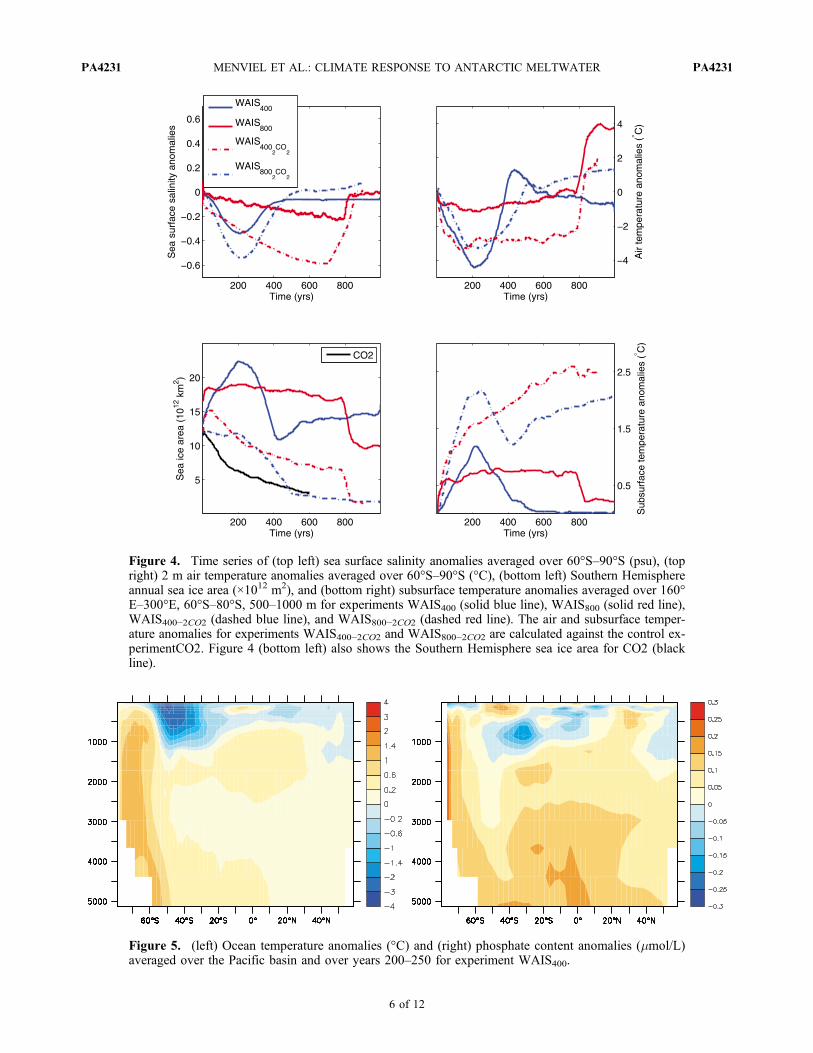
Figure 5. (left) Ocean temperature anomalies (°C) and (right) phosphate content anomalies (mmol/L)averaged over the Pacific basin and over years 200–250 for experiment WAIS400.

Figure 4. Time series of (top left) sea surface salinity anomalies averaged over 60°S–90°S (psu), (topright) 2 m air temperature anomalies averaged over 60°S–90°S (°C), (bottom left) Southern Hemisphereannual sea ice area (×1012 m2), and (bottom right) subsurface temperature anomalies averaged over 160°E–300°E, 60°S–80°S, 500–1000 m for experiments WAIS400 (solid blue line), WAIS800 (solid red line),WAIS400−2CO2 (dashed blue line), and WAIS800−2CO2 (dashed red line). The air and subsurface temper-ature anomalies for experiments WAIS400−2CO2 and WAIS800−2CO2 are calculated against the control ex-perimentCO2. Figure 4 (bottom left) also shows the Southern Hemisphere sea ice area for CO2 (blackline).

MENVIEL ET AL.: CLIMATE RESPONSE TO ANTARCTIC MELTWATER PA4231PA4231

6 of 12

reduced Bottom Water formation, Circumpolar Deep water(CDW) fills most of the intermediate and deep SouthernOcean.[31] Figure 4 (bottom right) shows the ocean temperature

anomalies averaged over 60°S–80°S, 160°E–60°W and over500–1000 m depth. The anomalies generated amount toabout 1.2°C for WAIS400 and 0.7°C for WAIS800, respec-tively. Under CO2 doubling conditions, the subsurfacetemperature increase in the Southern Ocean is even morepronounced. The anomalies compared to CO2 amount to2.2°C for WAIS400−2CO2 and 2.5°C for WAIS800−2CO2.[32] Other coupled modeling studies also simulated a

subsurface water warming near Antarctica of about 1.5°C[Stouffer et al., 2007; Trevena et al., 2008; Ma et al., 2010;Swingedouw et al., 2009] due to reduced formation of coldAABW. Trevena et al.’s [2008] modeling study is per-formed with an OGCM coupled to an Energy BalanceModel (EBM) that uses fixed climatological winds. A sig-nificant subsurface warming was simulated, without theintensification of the Southern Hemispheric Westerliesfound in more complex models. Moreover, using LOVE-CLIM, Swingedouw et al. [2009] conducted a SouthernOcean meltwater experiment with fixed climatological pre-industrial winds. In this experiment a ∼ 2°C subsurfacewarming was simulated at high southern latitudes, sug-gesting that changes in the surface winds do not play amajor role in the high southern latitude subsurface warmingduring the Southern Ocean freshwater pulse experiment.[33] The West Antarctic Ice Sheet grounding line in the

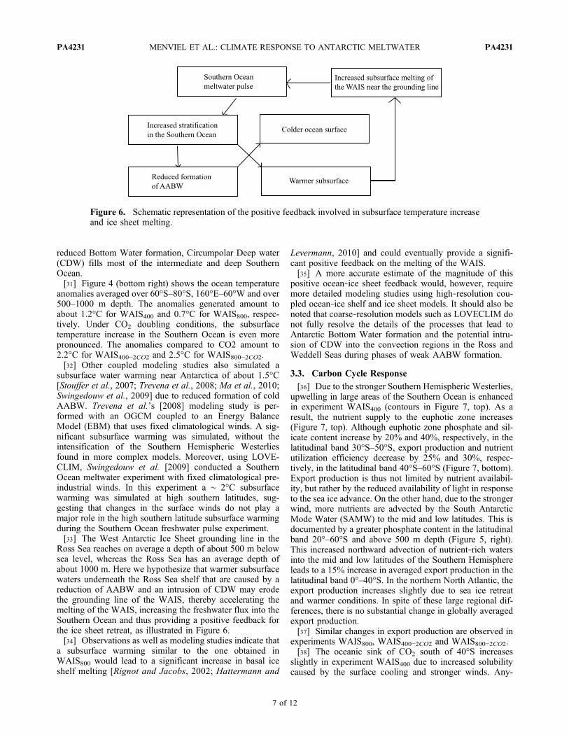
Ross Sea reaches on average a depth of about 500 m belowsea level, whereas the Ross Sea has an average depth ofabout 1000 m. Here we hypothesize that warmer subsurfacewaters underneath the Ross Sea shelf that are caused by areduction of AABW and an intrusion of CDW may erodethe grounding line of the WAIS, thereby accelerating themelting of the WAIS, increasing the freshwater flux into theSouthern Ocean and thus providing a positive feedback forthe ice sheet retreat, as illustrated in Figure 6.[34] Observations as well as modeling studies indicate that

a subsurface warming similar to the one obtained inWAIS800 would lead to a significant increase in basal iceshelf melting [Rignot and Jacobs, 2002; Hattermann and

Levermann, 2010] and could eventually provide a signifi-cant positive feedback on the melting of the WAIS.[35] A more accurate estimate of the magnitude of this

positive ocean‐ice sheet feedback would, however, requiremore detailed modeling studies using high‐resolution cou-pled ocean‐ice shelf and ice sheet models. It should also benoted that coarse‐resolution models such as LOVECLIM donot fully resolve the details of the processes that lead toAntarctic Bottom Water formation and the potential intru-sion of CDW into the convection regions in the Ross andWeddell Seas during phases of weak AABW formation.

3.3. Carbon Cycle Response

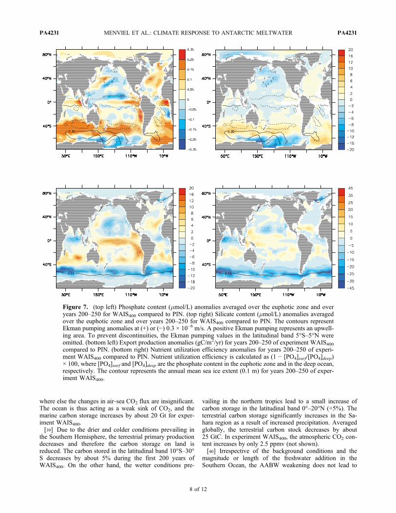
[36] Due to the stronger Southern Hemispheric Westerlies,upwelling in large areas of the Southern Ocean is enhancedin experiment WAIS400 (contours in Figure 7, top). As aresult, the nutrient supply to the euphotic zone increases(Figure 7, top). Although euphotic zone phosphate and sil-icate content increase by 20% and 40%, respectively, in thelatitudinal band 30°S–50°S, export production and nutrientutilization efficiency decrease by 25% and 30%, respec-tively, in the latitudinal band 40°S–60°S (Figure 7, bottom).Export production is thus not limited by nutrient availabil-ity, but rather by the reduced availability of light in responseto the sea ice advance. On the other hand, due to the strongerwind, more nutrients are advected by the South AntarcticMode Water (SAMW) to the mid and low latitudes. This isdocumented by a greater phosphate content in the latitudinalband 20°–60°S and above 500 m depth (Figure 5, right).This increased northward advection of nutrient‐rich watersinto the mid and low latitudes of the Southern Hemisphereleads to a 15% increase in averaged export production in thelatitudinal band 0°–40°S. In the northern North Atlantic, theexport production increases slightly due to sea ice retreatand warmer conditions. In spite of these large regional dif-ferences, there is no substantial change in globally averagedexport production.[37] Similar changes in export production are observed in

experiments WAIS800, WAIS400−2CO2 and WAIS800−2CO2.[38] The oceanic sink of CO2 south of 40°S increases

slightly in experiment WAIS400 due to increased solubilitycaused by the surface cooling and stronger winds. Any-

Figure 6. Schematic representation of the positive feedback involved in subsurface temperature increaseand ice sheet melting.

MENVIEL ET AL.: CLIMATE RESPONSE TO ANTARCTIC MELTWATER PA4231PA4231

7 of 12

where else the changes in air‐sea CO2 flux are insignificant.The ocean is thus acting as a weak sink of CO2, and themarine carbon storage increases by about 20 Gt for exper-iment WAIS400.[39] Due to the drier and colder conditions prevailing in

the Southern Hemisphere, the terrestrial primary productiondecreases and therefore the carbon storage on land isreduced. The carbon stored in the latitudinal band 10°S–30°S decreases by about 5% during the first 200 years ofWAIS400. On the other hand, the wetter conditions pre-

vailing in the northern tropics lead to a small increase ofcarbon storage in the latitudinal band 0°–20°N (+5%). Theterrestrial carbon storage significantly increases in the Sa-hara region as a result of increased precipitation. Averagedglobally, the terrestrial carbon stock decreases by about25 GtC. In experiment WAIS400, the atmospheric CO2 con-tent increases by only 2.5 ppmv (not shown).[40] Irrespective of the background conditions and the

magnitude or length of the freshwater addition in theSouthern Ocean, the AABW weakening does not lead to

Figure 7. (top left) Phosphate content (mmol/L) anomalies averaged over the euphotic zone and overyears 200–250 for WAIS400 compared to PIN. (top right) Silicate content (mmol/L) anomalies averagedover the euphotic zone and over years 200–250 for WAIS400 compared to PIN. The contours representEkman pumping anomalies at (+) or (−) 0.3 × 10−6 m/s. A positive Ekman pumping represents an upwell-ing area. To prevent discontinuities, the Ekman pumping values in the latitudinal band 5°S–5°N wereomitted. (bottom left) Export production anomalies (gC/m2/yr) for years 200–250 of experiment WAIS400compared to PIN. (bottom right) Nutrient utilization efficiency anomalies for years 200–250 of experi-ment WAIS400 compared to PIN. Nutrient utilization efficiency is calculated as (1 − [PO4]surf/[PO4]deep)× 100, where [PO4]surf and [PO4]deep are the phosphate content in the euphotic zone and in the deep ocean,respectively. The contour represents the annual mean sea ice extent (0.1 m) for years 200–250 of exper-iment WAIS400.

MENVIEL ET AL.: CLIMATE RESPONSE TO ANTARCTIC MELTWATER PA4231PA4231

8 of 12

significant changes in the size of the different carbonreservoirs.

4. Discussion and Conclusion

[41] Our model results show that a Southern Oceanmeltwater pulse leads to a significant cooling over Antarc-tica as well as in the Southern Ocean. Even though theSouthern Hemisphere Westerlies strengthen significantly,the ACC weakens. These results are in overall qualitativeagreement with other Southern Ocean meltwater pulsestudies performed with CGCMs [Richardson et al., 2005;Stouffer et al., 2007; Ma et al., 2010] under interglacialconditions. We found that an increase of sea ice leads to adecrease in marine export production south of 40°S. How-ever, it should be noted that our model does not include ironlimitation. Changes in export production therefore do nottake into account any possible changes in iron supply to theeuphotic zone, nor do they capture different non‐Redfieldprocesses. In contrast, the greater transport of nutrients fromhigh southern latitudes to low latitude leads to enhancedmarine export production in the latitudinal band 0°–40°S.Overall, the addition of freshwater in the Southern Oceandoes not lead to significant changes in the different carbonreservoirs.[42] In our simulations a rapid collapse of the WAIS leads

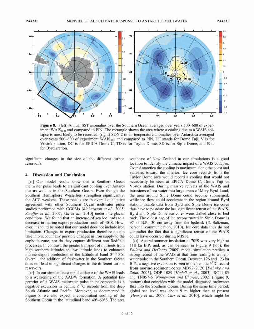
to a weakening of the AABW formation. A potential fin-gerprint of a WAIS meltwater pulse in paleorecords is anegative excursion in benthic d13C records from the deepSouth Atlantic and Pacific. Moreover, as documented inFigure 8, we also expect a concomitant cooling of theSouthern Ocean in the latitudinal band 40°–60°S. The area

southeast of New Zealand in our simulations is a goodlocation to identify the climatic impact of a WAIS collapse.Over Antarctica the cooling is maximum along the coast andvanishes toward the interior. Ice core records from theTaylor Dome area would record a cooling that would notnecessarily be seen at EPICA Dome C, Dome Fuji orVostok station. During massive retreats of the WAIS andintrusions of sea water into large areas of Mary Byrd Land,the area around Siple Dome could become submerged,while ice flow could accelerate in the region around Byrdstation. Usable data from Byrd and Siple Dome ice coresthus have to postdate the last significant retreat of the WAIS.Byrd and Siple Dome ice cores were drilled close to bedrock. The oldest age of ice reconstructed in Siple Dome is97 ka B.P., 30 cm away from the bedrock (E. Saltzman,personal communication, 2010). Ice core data thus do notcontradict the fact that a significant retreat of the WAIScould have occurred during MIS5e.[43] Austral summer insolation at 70°S was very high at

118 ka B.P. and, as can be seen in Figure 9 (top), thePollard and DeConto [2009] model simulation predicts astrong retreat of the WAIS at that time leading to a melt-water pulse in the Southern Ocean. Between 126 and 123 kaB.P., a negative excursion is seen in the benthic d13C recordfrom marine sediment cores MD97‐2120 [Pahnke andZahn, 2005], ODP 1089 [Hodell et al., 2003], RC11‐83and TN057‐6 [Ninnemann and Charles, 2002] (Figure 9,bottom) that coincides with the model‐diagnosed meltwaterflux into the Southern Ocean. During the same time period,global sea level was about 9 m higher than at present[Hearty et al., 2007; Carr et al., 2010], which might be

Figure 8. (left) Annual SST anomalies over the Southern Ocean averaged over years 500–600 of exper-iment WAIS800 and compared to PIN. The rectangle shows the area where a cooling due to a WAIS col-lapse is most likely to be recorded. (right) SON 2 m air temperature anomalies over Antarctica averagedover years 500–600 of experiment WAIS800 and compared to PIN. DF stands for Dome Fuji, V is forVostok station, DC is for EPICA Dome C, TD is for Taylor Dome, SD is for Siple Dome, and B isfor Byrd station.

MENVIEL ET AL.: CLIMATE RESPONSE TO ANTARCTIC MELTWATER PA4231PA4231

9 of 12

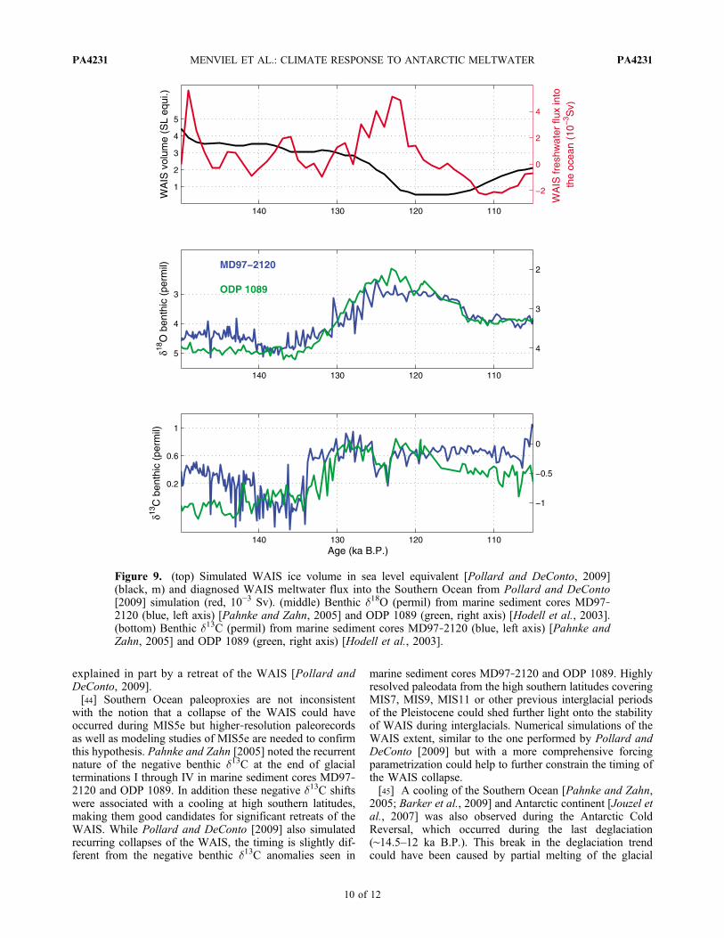
explained in part by a retreat of the WAIS [Pollard andDeConto, 2009].[44] Southern Ocean paleoproxies are not inconsistent

with the notion that a collapse of the WAIS could haveoccurred during MIS5e but higher‐resolution paleorecordsas well as modeling studies of MIS5e are needed to confirmthis hypothesis. Pahnke and Zahn [2005] noted the recurrentnature of the negative benthic d13C at the end of glacialterminations I through IV in marine sediment cores MD97‐2120 and ODP 1089. In addition these negative d13C shiftswere associated with a cooling at high southern latitudes,making them good candidates for significant retreats of theWAIS. While Pollard and DeConto [2009] also simulatedrecurring collapses of the WAIS, the timing is slightly dif-ferent from the negative benthic d13C anomalies seen in

marine sediment cores MD97‐2120 and ODP 1089. Highlyresolved paleodata from the high southern latitudes coveringMIS7, MIS9, MIS11 or other previous interglacial periodsof the Pleistocene could shed further light onto the stabilityof WAIS during interglacials. Numerical simulations of theWAIS extent, similar to the one performed by Pollard andDeConto [2009] but with a more comprehensive forcingparametrization could help to further constrain the timing ofthe WAIS collapse.[45] A cooling of the Southern Ocean [Pahnke and Zahn,

2005; Barker et al., 2009] and Antarctic continent [Jouzel etal., 2007] was also observed during the Antarctic ColdReversal, which occurred during the last deglaciation(∼14.5–12 ka B.P.). This break in the deglaciation trendcould have been caused by partial melting of the glacial

Figure 9. (top) Simulated WAIS ice volume in sea level equivalent [Pollard and DeConto, 2009](black, m) and diagnosed WAIS meltwater flux into the Southern Ocean from Pollard and DeConto[2009] simulation (red, 10−3 Sv). (middle) Benthic d18O (permil) from marine sediment cores MD97‐2120 (blue, left axis) [Pahnke and Zahn, 2005] and ODP 1089 (green, right axis) [Hodell et al., 2003].(bottom) Benthic d13C (permil) from marine sediment cores MD97‐2120 (blue, left axis) [Pahnke andZahn, 2005] and ODP 1089 (green, right axis) [Hodell et al., 2003].

MENVIEL ET AL.: CLIMATE RESPONSE TO ANTARCTIC MELTWATER PA4231PA4231

10 of 12

WAIS into the Southern Ocean [Weaver et al., 2003] as theglacial WAIS was significantly larger than at present[Conway et al., 1999]. Transient modeling studies of the lastdeglaciation could shed light onto the possible role ofsouthern origin freshwater pulses in shaping the AntarcticCold Reversal. Additional paleorecords from the SouthernOcean would also provide further insight into the occurrenceof meltwater pulses from the Antarctic ice sheet and theirassociated climate and biogeochemical responses.[46] As a collapse of the WAIS probably occurred in the

past, further warming in the future due to increased green-house gas content in the atmosphere could also induce asignificant retreat of the WAIS. Under CO2 doubling con-ditions and according to our model simulations the rapidaddition of freshwater into the Southern Ocean leads to anegative feedback in the lower atmosphere and at the sur-face of the ocean. The lower atmosphere air temperature andthe temperature at the surface of the Southern Oceanincrease more slowly when the AABW is weakened. Theretreat of the Southern Hemispheric sea ice edge is delayedin experiments WAIS400−2CO2 and WAIS800−2CO2 comparedto experiment CO2. This negative feedback was alreadydiscussed by Swingedouw et al. [2008]. However, we havealso shown that as a result of freshwater addition in theSouthern Ocean, the subsurface temperature around theAntarctic coast increases significantly. Under present‐dayconditions, subsurface warming has been shown to accel-erate the melting of Antarctic ice shelves and ice sheetsat their grounding lines [Rignot and Jacobs, 2002; Payneet al., 2004]. Several factors contribute to the large sub-surface warming in the Southern Ocean: increased stratifi-cation, reduction of AABW formation as well as intrusion

of CDW. This increase is even more pronounced under CO2

doubling conditions than under preindustrial conditions, andcould subsequently induce further melting of the Antarcticice shelf and erode the WAIS near the ice sheet‐oceaninterface. A retreat of the WAIS in the future could thus beaccelerated through this positive feedback.[47] In this study, to simulate a collapse of the WAIS,

freshwater was added over an area extending from the Rossto the Weddell Sea. In reality, when the WAIS collapses,probably a massive iceberg release takes place, and only apart is directly released as liquid water. In a recent study,Jongma et al. [2009] suggested that a dynamic distributionof melting icebergs in the Southern Ocean might lead to lessstratification compared to an homogeneous input of fresh-water and therefore to a less efficient weakening of theAABW. In addition, the latent heat flux due to the meltingiceberg might lead to enhanced formation of sea ice andgreater brine rejection, providing a negative feedback to theAABW weakening. To better quantify the impact of a col-lapse of the WAIS on climate, a similar study should beperformed with an interactive iceberg model.

[48] Acknowledgments. This research was supported by NSF grant1010869. Additional support was provided by the Japan Agency forMarine‐Earth Science and Technology (JAMSTEC), by NASA throughgrant NNX07AG53G, and by NOAA through grant NA09OAR4320075,which sponsor research at the International Pacific Research Center. A.Mouchet acknowledges support from the Belgian Science Policy (BELSPOcontract SD/CS/01A). We thank D. Pollard for making his ice sheet modelsimulation data available to us. We thank G. Filippelli and two anonymousreviewers for their helpful comments. This is IPRC publication 734 andSOEST publication 8043.

ReferencesBamber, J. L., R. E.M. Riva, B. L. A. Vermeersen,and A. M. LeBrocq (2009), Reassessment ofthe potential sea‐level rise from a collapse ofthe West Antarctic Ice Sheet, Science, 324,901–903, doi:10.1126/science.1169335.

Barker, S., P. Diz, M. J. Vautravers, J. Pike,G. Knorr, I. R. Hall, and W. S. Broecker(2009), Interhemispheric Atlantic seesawresponse during the last deglaciation, Nature,457, 1097–1102, doi:10.1038/nature07770.

Bindschadler, R. A. (1998), The future of theWest Antarctic Ice Sheet, Science, 282,428–429, doi:10.1126/science.282.5388.428.

Brovkin, V., A. Ganopolski, and Y. Svirezhev(1997), A continuous climate‐vegetation clas-sification for use in climate‐biosphere studies,Ecol. Modell., 101, 251–261, doi:10.1016/S0304-3800(97)00049-5.

Brovkin, V., J. Bendtsen, M. Claussen,A. Ganopolski, C. Kubatzki, V. Petoukhov,and A. Andreev (2002), Carbon cycle, vegeta-tion, and climate dynamics in the Holocene:Experiments with the CLIMBER‐2 model,Global Biogeochem. Cycles, 16(4), 1139,doi:10.1029/2001GB001662.

Campin, J. M., and H. Goosse (1999), Parame-terization of density‐driven downsloping flowfor a coarse‐resolution ocean model in z‐coor-dinate, Tellus, Ser. A, 51, 412–430.

Carr, A. S., M. D. Bateman, D. L. Roberts, C. V.Murray‐Wallace, Z. Jacobs, and P. J. Holmes(2010), The last interglacial sea‐level highstand on the southern Cape coastline of South

Africa, Quat. Res., 73, 351–363, doi:10.1016/j.yqres.2009.08.006.

Conway, H., B. L. Hall, G. H. Denton, A. M.Gades, and E. D. Waddington (1999), Pastand Future Grounding‐Line Retreat of theWest Antarctic Ice Sheet, Science, 286, 280–283, doi:10.1126/science.286.5438.280.

Gent, P. R., J. Willebrand, T. J. Dougall, andJ. C. McWilliams (1995), Parameterizingeddy‐induced transports in ocean circulationmodels, J. Phys. Oceanogr., 25, 463–474,doi:10.1175/1520-0485(1995)025<0463:PEITTI>2.0.CO;2.

Goosse, H., and T. Fichefet (1999), Importanceof ice‐ocean interactions for the global oceancirculation: A model study, J. Geophys. Res.,104(C10), 23,337–23,355, doi:10.1029/1999JC900215.

Goosse, H., E. Deleersnijder, T. Fichefet, andM. H. England (1999), Sensitivity of a globalcoupled ocean‐sea ice model to the parame-terization of vertical mixing, J. Geophys.Res., 104(C6), 13,681–13,695, doi:10.1029/1999JC900099.

Goosse, H., et al. (2010), Description of theEarth system model of intermediate complex-ity LOVECLIM version 1.2, Geosci. ModelDev., 3, 309–390, doi:10.5194/gmdd-3-309-2010.

Hattermann, T., and A. Levermann (2010),Response of Southern Ocean circulation toglobal warming may enhance basal ice shelf

melting around Antarctica, Clim. Dyn., 35(5),741–756, doi:10.1007/s00382-009-0643-3.

Hearty, P. J., J. T. Hollin, A. C. Neumann, M. J.O’Leary, and M. McCulloch (2007), Globalsea‐level fluctuations during the Last Intergla-ciation (MIS 5e), Quat. Sci. Rev., 26, 2090–2112, doi:10.1016/j.quascirev.2007.06.019.

Hodell, D. A., K. A. Venz, C. D. Charles, andU. S. Ninnemann (2003), Pleistocene verticalcarbon isotope and carbonate gradients in theSouth Atlantic sector of the Southern Ocean,Geochem. Geophys. Geosyst., 4(1), 1004,doi:10.1029/2002GC000367.

Ivchenko, V. O., V. B. Zalesny, M. R.Drinkwater, and J. Schröter (2006), A quickresponse of the equatorial ocean to Antarcticsea ice/salinity anomalies, J. Geophys. Res.,111, C10018, doi:10.1029/2005JC003061.

Jongma, J. I., E. Driesschaert, T. Fichefet,H. Goosse, and H. Renssen (2009), The effectof dynamic‐thermodynamic icebergs on theSouthern Ocean climate in a three‐dimensionalmodel, Ocean Modell., 26, 104–113.

Jouzel, J., et al. (2007), Orbital and millennialAntarctic climate variability over the past800,000 years, Science , 317 , 793–796,doi:10.1126/science.1141038.

Kim, S. J., and T. J. Crowley (2000), IncreasedPliocene North Atlantic Deep Water: Causeor consequence of Pliocene warming?, Paleo-ceanography, 15, 451–455, doi:10.1029/1999PA000459.

MENVIEL ET AL.: CLIMATE RESPONSE TO ANTARCTIC MELTWATER PA4231PA4231

11 of 12

Lim, G. H., J. R. Holton, and J. M. Wallace(1991), The structure of the ageostrophic windfield in baroclinic waves, J. Atmos. Sci., 48,1733–1745, doi:10.1175/1520-0469(1991)048<1733:TSOTAW>2.0.CO;2.

Lythe, M. B., D. G. Vaughan, and the BEDMAPConsortium (2001), BEDMAP: A new icethickness and subglacial topographic modelof Antarctica, J. Geophys. Res., 106, 11,335–11,351, doi:10.1029/2000JB900449.

Ma, H., L. Wu, and L. Chun (2010), Global tele-connections in response to freshening over theAntarctic Ocean, J. Clim., doi:10.1175/2010JCLI3634.1, in press.

Menviel, L., A. Timmermann, A. Mouchet, andO. Timm (2008), Climate and marine carboncycle response to changes in the strength of thesouthern hemispheric westerlies,Paleoceanogra-phy, 23, PA4201, doi:10.1029/2008PA001604.

Mercer, J. H. (1978), Glacial development andtemperature trends in the Antarctic and inSouth America, in Antarctic Glacial Historyand World Paleoenvironments, pp. 73–79, A.A. Balkema, Rotterdam, Netherlands.

Mouchet, A., and L. M. Francois (1996), Sensi-tivity of a Global Oceanic Carbon CycleModel to the circulation and to the fate oforganic matter: Preliminary results, Phys.Chem. Earth, 21, 511–516, doi:10.1016/S0079-1946(97)81150-0.

Naish, T., et al. (2009), Obliquity‐paced Plio-cene West Antarctic ice sheet oscillations,Nature , 458 , 322–328 , do i : 10 .1038 /nature07867.

Ninnemann, U. S., and C. D. Charles (2002),Changes in the mode of Southern Ocean circu-lation over the last glacial cycle revealed byforaminiferal stable isotopic variability, EarthPlanet. Sci. Lett., 201, 383–396, doi:10.1016/S0012-821X(02)00708-2.

Oppenheimer, M. (1998), Global warming andthe stability of the West Antarctic Ice Sheet,Nature, 393, 325–332, doi:10.1038/30661.

Oppenheimer, M., and R. B. Alley (2004), TheWest Antarctic Ice Sheet and long term cli-mate policy, Clim. Change , 64 , 1–10,doi:10.1023/B:CLIM.0000024792.06802.31.

Opsteegh, J. D., R. J. Haarsma, F. M. Selten, andA. Kattenberg (1998), ECBILT: A dynamic

alternative to mixed boundary conditions inocean models, Tellus, Ser. A., 50, 348–367.

Pagani, M., Z. Liu, J. LaRiviere, and A. C. Ravelo(2010), High Earth‐system climate sensitivitydetermined from Pliocene carbon dioxideconcentrations, Nat. Geosci., 3, 27–30,doi:10.1038/ngeo724.

Pahnke, K., and R. Zahn (2005), Southern Hemi-sphere water mass conversion linked withNorth Atlantic climate variability, Science,307, 1741–1746, doi:10.1126/science.1102163.

Payne, A. J., A. Vieli, A. P. Shepherd, D. J.Wingham, and E. Rignot (2004), Recent dra-matic thinning of largest west antarctic icestream triggered by oceans, Geophys. Res.Lett., 31, L23401, doi:10.1029/2004GL021284.

Pollard, D., and R. M. DeConto (2009), ModellingWest Antarctic ice sheet growth and collapsethrough the past five million years, Nature,458, 329–332, doi:10.1038/nature07809.

Raymo,M.E., B.Grant,M.Horowitz, andG. H. Rau(1996), Mid‐Pliocene warmth: Strongergreenhouse and stronger conveyor,Mar. Micro-paleontol., 27, 313–326, doi:10.1016/0377-8398(95)00048-8.

Renssen, H., H. Goosse, T. Fichefet, V. Brovkin,E. Driesschaert, and F. Wolk (2005), Simulat-ing the Holocene climate evolution at northernhigh latitudes using a coupled atmosphere‐seaice‐ocean‐vegetation model, Clim. Dyn., 24,23–43, doi:10.1007/s00382-004-0485-y.

Richardson, G., M. R. Wadley, K. J. Heywood,and D. P. Stevens (2005), Short‐term climateresponse to a freshwater pulse in the SouthernOcean, Geophys. Res. Lett., 32, L03702,doi:10.1029/2004GL021586.

Rignot, E., and S. S. Jacobs (2002), Rapid bot-tom melting widespread near Antarctic IceSheet grounding lines, Science, 296, 2020–2023, doi:10.1126/science.1070942.

Scherer, R. P., A. Aldahan, W. Tulaczyk,G. Possnert, H. Englehardt, and B. Kamb(1998), Pleistocene collapse of the West Ant-arctic Ice Sheet, Science , 281 , 82–85,doi:10.1126/science.281.5373.82.

Stocker, T. F., A. Timmermann, M. Renold, andO. Timm (2007), Effects of salt compensationon the climate model response in simulationsof large changes of the Atlantic Meridional

Overturning Circulation, J. Clim., 20, 5912–5928, doi:10.1175/2007JCLI1662.1.

Stouffer, R. J., D. Seidov, and B. J. Haupt(2007), Climate response to external sourcesof freshwater: North Atlantic versus the South-ern Ocean, J. Clim., 20, 436–448, doi:10.1175/JCLI4015.1.

Swingedouw, D., T. Fichefet, P. Huybrechts,H. Goosse, E. Driesschaert, and M.‐F. Loutre(2008), Antarctic ice‐sheet melting providesnegative feedbacks on future climate warming,Geophys. Res. Lett., 35, L17705, doi:10.1029/2008GL034410.

Swingedouw, D., T. Fichefet, H. Goosse, andM.‐F. Loutre (2009), Impact of transient fresh-water releases in the Southern Ocean on theAMOC and climate, Clim. Dyn., 33, 365‐381, doi:10.1007/s00382-008-0496-1.

Trevena, J., W. P. Sijp, and M. H. England(2008), Stability of Antarctic Bottom Waterformation to freshwater fluxes and implica-tions for global climate, J. Clim., 21, 3310–3326, doi:10.1175/2007JCLI2212.1.

Van Der Burgh, J., H. Visscher, D. Dilcher,and M. Kürschner (1993), Paleoatmosphericsignatures in Neogene fossil leaves, Science,260, 1788–1790, doi:10.1126/science.260.5115.1788.

Weaver, A. J., O. A. Saenko, P. U. Clark, andJ. X. Mitrovica (2003), Meltwater pulse 1Afrom Antarctica as a trigger of the Bølling‐Allerød warm interval, Science, 299, 1709–1713, doi:10.1126/science.1081002.

Zhang, J. (2007), Increasing Antarctic sea iceunder warming atmospheric and ocean condi-tions, J. Clim., 20, 2515–2529, doi:10.1175/JCLI4136.1.

L. Menviel, Climate and EnvironmentalPhysics, Oeschger Centre for Climate ChangeResearch, University of Bern, Sidlerstr. 5, CH‐3012 Bern, Switzerland. ([email protected])A. Mouchet, Département AGO, Université de

Liège, Alle du 6 Aot, 17 Bt. B5c, B‐4000 Liège,Belgium.O. E. Timm and A. Timmermann, IPRC,

SOEST, University of Hawai’i, 2525 CorreaRd., Honolulu, HI 96822, USA.

MENVIEL ET AL.: CLIMATE RESPONSE TO ANTARCTIC MELTWATER PA4231PA4231

12 of 12