1 UNIT – I INTRODUCTION TO DATA STRUCTURES, SEARCHING AND SORTING Basic Concepts: Introduction to Data Structures: A data structure is a way of storing data in a computer so that it can be used efficiently and it will allow the most efficient algorithm to be used. The choice of the data structure begins from the choice of an abstract data type (ADT). A well-designed data structure allows a variety of critical operations to be performed, using as few resources, both execution time and memory space, as possible. Data structure introduction refers to a scheme for organizing data, or in other words it is an arrangement of data in computer's memory in such a way that it could make the data quickly available to the processor for required calculations. A data structure should be seen as a logical concept that must address two fundamental concerns. 1. First, how the data will be stored, and 2. Second, what operations will be performed on it. As data structure is a scheme for data organization so the functional definition of a data structure should be independent of its implementation. The functional definition of a data structure is known as ADT (Abstract Data Type) which is independent of implementation. The way in which the data is organized affects the performance of a program for different tasks. Computer programmers decide which data structures to use based on the nature of the data and the processes that need to be performed on that data. Some of the more commonly used data structures include lists, arrays, stacks, queues, heaps, trees, and graphs. Classification of Data Structures: Data structures can be classified as Simple data structure Compound data structure Linear data structure Non linear data structure

Welcome message from author
This document is posted to help you gain knowledge. Please leave a comment to let me know what you think about it! Share it to your friends and learn new things together.
Transcript
1
UNIT – I INTRODUCTION TO DATA STRUCTURES, SEARCHING AND SORTING
Basic Concepts: Introduction to Data Structures:
A data structure is a way of storing data in a computer so that it can be used efficiently and it will allow the most efficient algorithm to be used. The choice of the data structure begins from the choice of an abstract data type (ADT). A well-designed data structure allows a variety of critical operations to be performed, using as few resources, both execution time and memory space, as possible. Data structure introduction refers to a scheme for organizing data, or in other words it is an arrangement of data in computer's memory in such a way that it could make the data quickly available to the processor for required calculations.
A data structure should be seen as a logical concept that must address two fundamental concerns.
1. First, how the data will be stored, and
2. Second, what operations will be performed on it.
As data structure is a scheme for data organization so the functional definition of a data structure should be independent of its implementation. The functional definition of a data structure is known as ADT (Abstract Data Type) which is independent of implementation. The way in which the data is organized affects the performance of a program for different tasks. Computer programmers decide which data structures to use based on the nature of the data and the processes that need to be performed on that data. Some of the more commonly used data structures include lists, arrays, stacks, queues, heaps, trees, and graphs.
Classification of Data Structures:
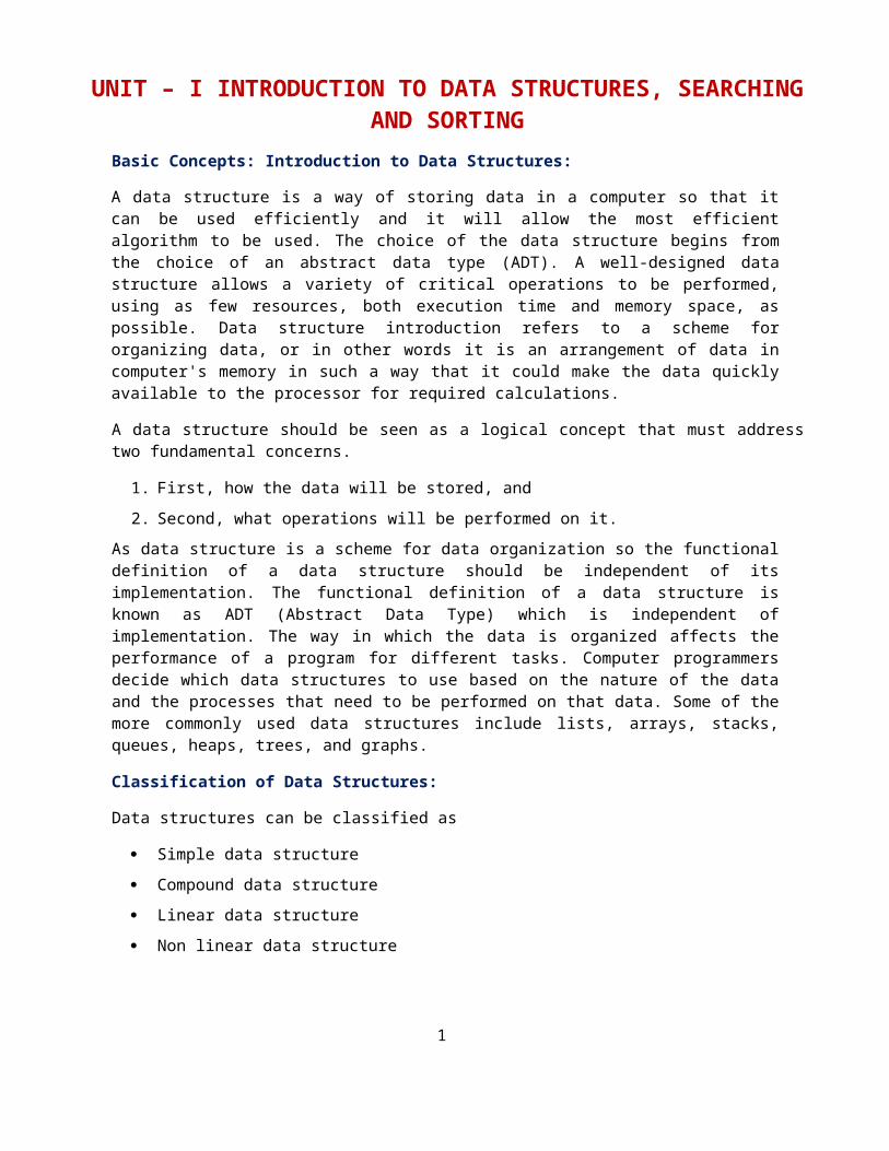
Data structures can be classified as
Simple data structure
Compound data structure
Linear data structure
Non linear data structure
[Fig 1.1 Classification of Data Structures]
2
Simple Data Structure:Simple data structure can be constructed with the help of primitive data structure. A primitive data structure used to represent the standard data types of any one of the computer languages. Variables, arrays, pointers, structures, unions, etc. are examples of primitive data structures.Compound Data structure:Compound data structure can be constructed with the help of any one of the primitive data structure and it is having a specific functionality. It can be designed by user. It can be classified as
Linear data structure
Non-linear data structure
Linear Data Structure:
Linear data structures can be constructed as a continuous arrangement of data elements in the memory. It can be constructed by using array data type. In the linear Data Structures the relationship of adjacency is maintained between the data elements.
Operations applied on linear data structure:The following list of operations applied on linear data structures
1. Add an element2. Delete an element3. Traverse4. Sort the list of elements5. Search for a data elementFor example Stack, Queue, Tables, List, and Linked Lists.
Non-linear Data Structure:
Non-linear data structure can be constructed as a collection of randomly distributed set of data item joined together by using a special pointer (tag). In non-linear Data structure the relationship of adjacency is not maintained between the data items.
Operations applied on non-linear data structures:The following list of operations applied on non-linear data structures.1. Add elements2. Delete elements3. Display the elements4. Sort the list of elements5. Search for a data elementFor example Tree, Decision tree, Graph and Forest
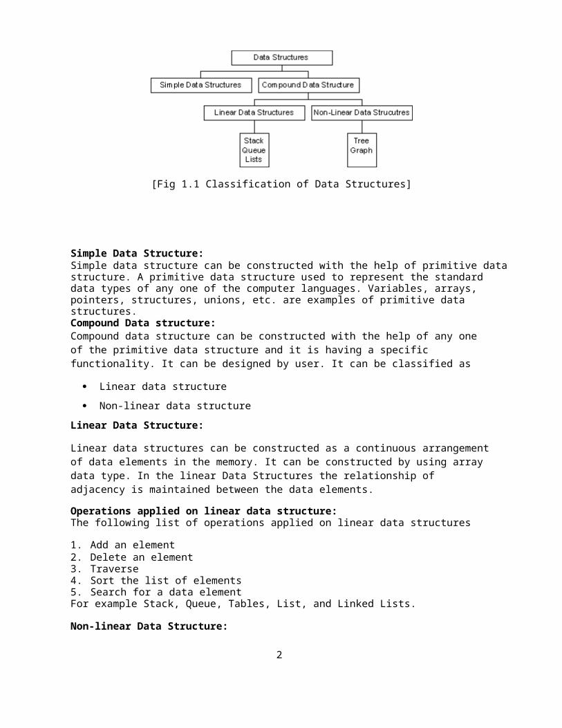
Abstract Data Type:
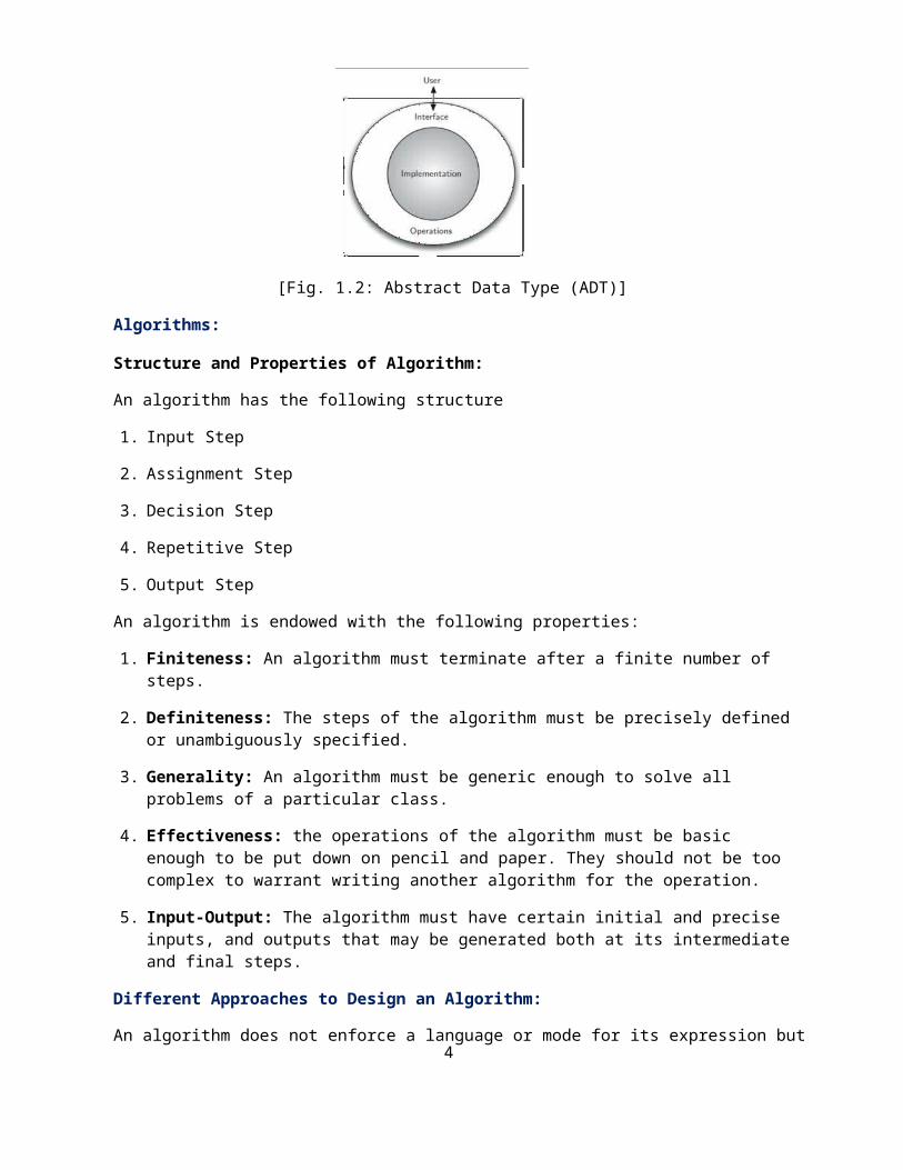
An abstract data type, sometimes abbreviated ADT, is a logical description of how we view the data and the operations that are allowed without regard to how they will be implemented. This means that we are concerned only with what data is representing and not with how it will eventually be constructed. By providing this level of abstraction, we are creating an encapsulation around the data. The idea is that by encapsulating the details of the implementation, we are hiding them from the user’s view. This is called information hiding. The implementation of an abstract data type, often referred to as a data structure, will require that we provide a physical view of the data using some collection of programming constructs and primitive data types.
3
[Fig. 1.2: Abstract Data Type (ADT)]
Algorithms:
Structure and Properties of Algorithm:
An algorithm has the following structure
1. Input Step
2. Assignment Step
3. Decision Step
4. Repetitive Step
5. Output Step
An algorithm is endowed with the following properties:
1. Finiteness: An algorithm must terminate after a finite number of steps.
2. Definiteness: The steps of the algorithm must be precisely defined or unambiguously specified.
3. Generality: An algorithm must be generic enough to solve all problems of a particular class.
4. Effectiveness: the operations of the algorithm must be basic enough to be put down on pencil and paper. They should not be too complex to warrant writing another algorithm for the operation.
5. Input-Output: The algorithm must have certain initial and precise inputs, and outputs that may be generated both at its intermediate and final steps.
Different Approaches to Design an Algorithm:
An algorithm does not enforce a language or mode for its expression but only demands adherence to its properties.
Practical Algorithm Design Issues:
1. To save time (Time Complexity): A program that runs faster is a better program.
2. To save space (Space Complexity): A program that saves space over a competing program is considerable desirable.
4
Efficiency of Algorithms:
The performances of algorithms can be measured on the scales of time and space. The performance of a program is the amount of computer memory and time needed to run a program. We use two approaches to determine the performance of a program. One is analytical and the other is experimental. In performance analysis we use analytical methods, while in performance measurement we conduct experiments.
Time Complexity: The time complexity of an algorithm or a program is a function of the running time of the algorithm or a program. In other words, it is the amount of computer time it needs to run to completion.
Space Complexity: The space complexity of an algorithm or program is a function of the space needed by the algorithm or program to run to completion.
The time complexity of an algorithm can be computed either by an empirical or theoretical approach. The empirical or posteriori testing approach calls for implementing the complete algorithms and executing them on a computer for various instances of the problem. The time taken by the execution of the programs for various instances of the problem are noted and compared. The algorithm whose implementation yields the least time is considered as the best among the candidate algorithmic solutions.
Analyzing Algorithms
Suppose M is an algorithm, and suppose n is the size of the input data. Clearly the complexity f(n) of M increases as n increases. It is usually the rate of increase of f(n) with some standard functions. The most common computing times are
O(1), O(log2 n), O(n), O(n log2 n), O(n2), O(n3), O(2n)
Example:
5
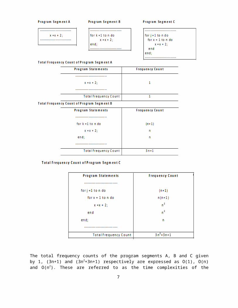
The total frequency counts of the program segments A, B and C given by 1, (3n+1) and (3n 2+3n+1) respectively are expressed as O(1), O(n) and O(n2). These are referred to as the time complexities of the program segments since they are indicative of the running times of the program segments. In a similar manner space complexities of a program can also be expressed in terms of mathematical notations,
6
which is nothing but the amount of memory they require for their execution.Reasons for analyzing algorithms:
1. To predict the resources that the algorithm requires Computational Time(CPU consumption).
Memory Space(RAM consumption).
Communication bandwidth consumption.
2. To predict the running time of an algorithm
Total number of primitive operations executed.
Recursive Algorithms:
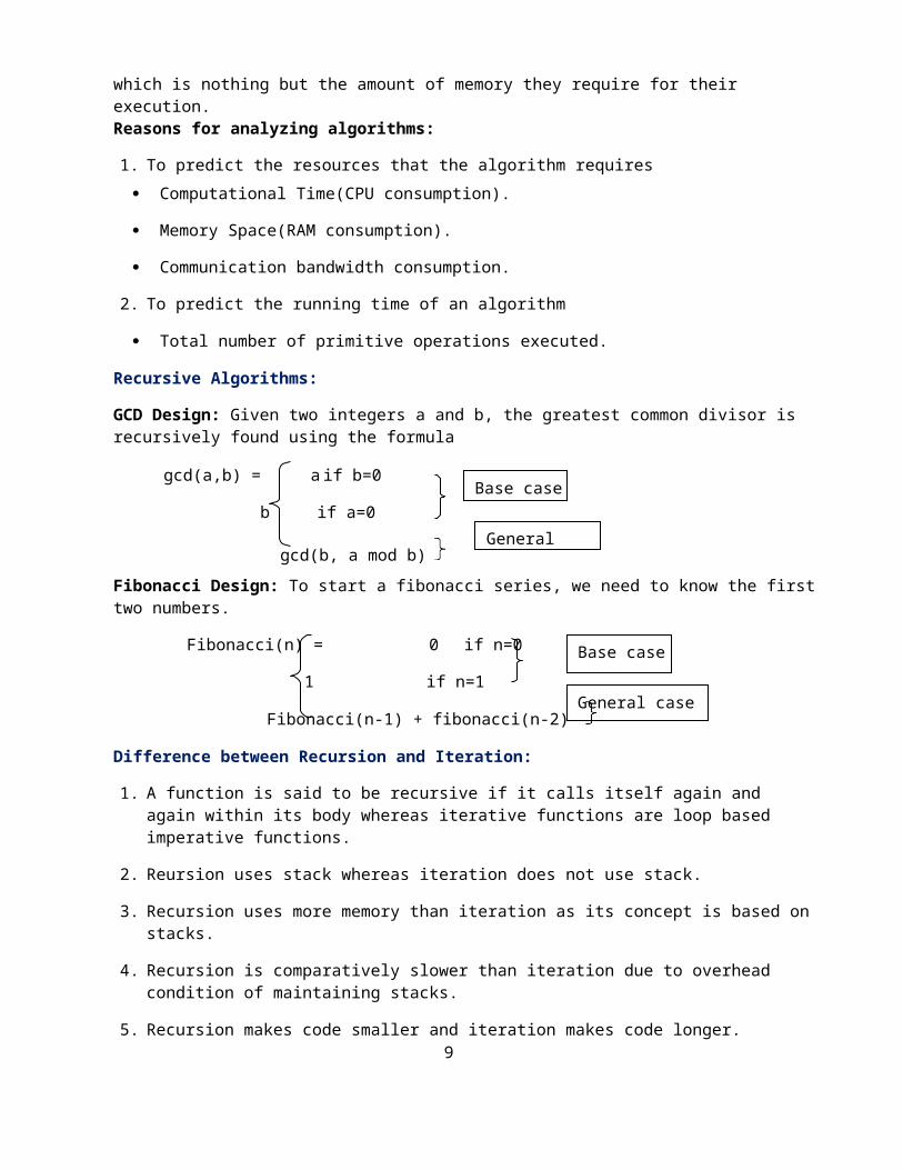
GCD Design: Given two integers a and b, the greatest common divisor is recursively found using the formula
gcd(a,b) = a if b=0
b if a=0
gcd(b, a mod b)
Fibonacci Design: To start a fibonacci series, we need to know the first two numbers.
Fibonacci(n) = 0 if n=0
1 if n=1
Fibonacci(n-1) + fibonacci(n-2)
Difference between Recursion and Iteration:
1. A function is said to be recursive if it calls itself again and again within its body whereas iterative functions are loop based imperative functions.
2. Reursion uses stack whereas iteration does not use stack.
3. Recursion uses more memory than iteration as its concept is based on stacks.
4. Recursion is comparatively slower than iteration due to overhead condition of maintaining stacks.
5. Recursion makes code smaller and iteration makes code longer.
6. Iteration terminates when the loop-continuation condition fails whereas recursion terminates when a base case is recognized.
7. While using recursion multiple activation records are created on stack for each call where as in iteration everything is done in one activation record.
8. Infinite recursion can crash the system whereas infinite looping uses CPU cycles repeatedly.
9. Recursion uses selection structure whereas iteration uses repetetion structure.
General case
Base case
General case
Base case
7
Types of Recursion:
Recursion is of two types depending on whether a function calls itself from within itself or whether two functions call one another mutually. The former is called direct recursion and the later is called indirect recursion. Thus there are two types of recursion:
Direct Recursion
Indirect Recursion
Recursion may be further categorized as:
Linear Recursion
Binary Recursion
Multiple Recursion
Linear Recursion:
It is the most common type of Recursion in which function calls itself repeatedly until base condition [termination case] is reached. Once the base case is reached the results are return to the caller function. If a recursive function is called only once then it is called a linear recursion.
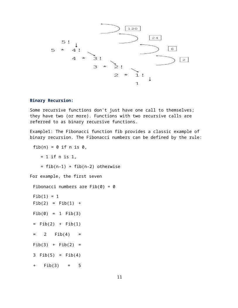
Binary Recursion:
Some recursive functions don't just have one call to themselves; they have two (or more). Functions with two recursive calls are referred to as binary recursive functions.
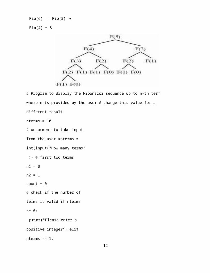
Example1: The Fibonacci function fib provides a classic example of binary recursion. The Fibonacci numbers can be defined by the rule:
fib(n) = 0 if n is 0,
= 1 if n is 1,
= fib(n-1) + fib(n-2) otherwise
For example, the first seven Fibonacci numbers are
Fib(0) = 0
8
Fib(1) = 1Fib(2) = Fib(1) + Fib(0) = 1
Fib(3) = Fib(2) + Fib(1) = 2
Fib(4) = Fib(3) + Fib(2) = 3
Fib(5) = Fib(4) + Fib(3) = 5
Fib(6) = Fib(5) + Fib(4) = 8
# Program to display the Fibonacci sequence up to n-th term where n is provided by the user
# change this value for a different result
nterms = 10
# uncomment to take input from the user
#nterms = int(input("How many terms? "))
# first two terms
n1 = 0
n2 = 1
count = 0
# check if the number of terms is valid
if nterms <= 0:
print("Please enter a positive integer")
elif nterms == 1:
print("Fibonacci sequence upto",nterms,":")
print(n1)
else:
9
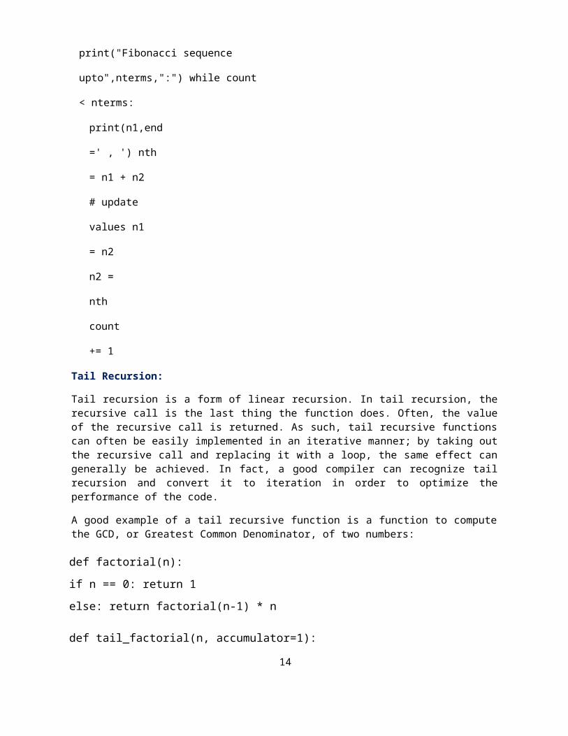
print("Fibonacci sequence upto",nterms,":")
while count < nterms:
print(n1,end=' , ')
nth = n1 + n2
# update values
n1 = n2
n2 = nth
count += 1
Tail Recursion:
Tail recursion is a form of linear recursion. In tail recursion, the recursive call is the last thing the function does. Often, the value of the recursive call is returned. As such, tail recursive functions can often be easily implemented in an iterative manner; by taking out the recursive call and replacing it with a loop, the same effect can generally be achieved. In fact, a good compiler can recognize tail recursion and convert it to iteration in order to optimize the performance of the code.
A good example of a tail recursive function is a function to compute the GCD, or Greatest Common Denominator, of two numbers:
def factorial(n):
if n == 0: return 1
else: return factorial(n-1) * n
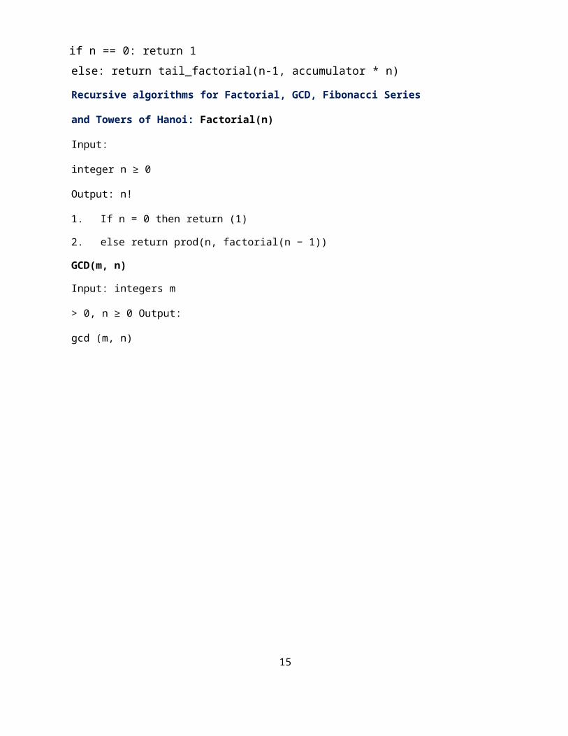
def tail_factorial(n, accumulator=1):
if n == 0: return 1else: return tail_factorial(n-1, accumulator * n)
Recursive algorithms for Factorial, GCD, Fibonacci Series and Towers of Hanoi:
Factorial(n)
Input: integer n ≥ 0
Output: n!
1. If n = 0 then return (1)
2. else return prod(n, factorial(n − 1))
GCD(m, n)
Input: integers m > 0, n ≥ 0
Output: gcd (m, n)
10
1. If n = 0 then return (m)
2. else return gcd(n,m mod n)
Time-Complexity: O(ln n)
Fibonacci(n)
Input: integer n ≥ 0
Output: Fibonacci Series: 1 1 2 3 5 8 13………………………………..
1. if n=1 or n=2
2. then Fibonacci(n)=1
3. else Fibonacci(n) = Fibonacci(n-1) + Fibonacci(n-2)
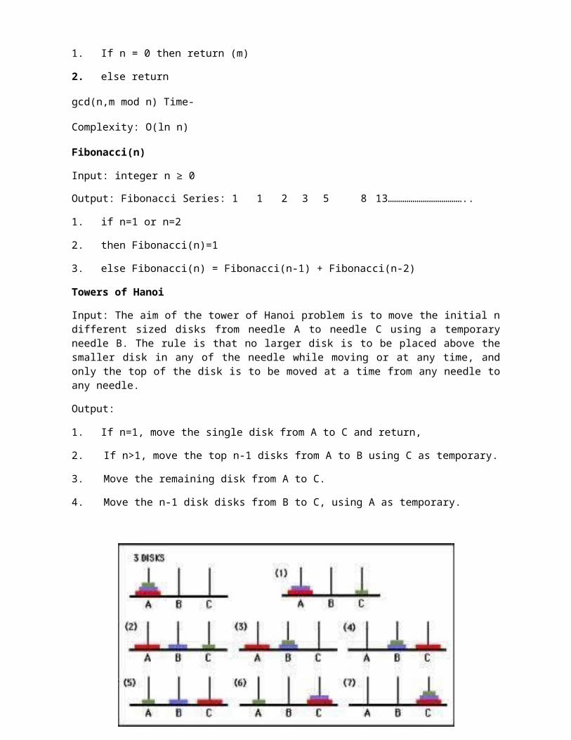
Towers of Hanoi
Input: The aim of the tower of Hanoi problem is to move the initial n different sized disks from needle A to needle C using a temporary needle B. The rule is that no larger disk is to be placed above the smaller disk in any of the needle while moving or at any time, and only the top of the disk is to be moved at a time from any needle to any needle.
Output:
1. If n=1, move the single disk from A to C and return,
2. If n>1, move the top n-1 disks from A to B using C as temporary.
3. Move the remaining disk from A to C.
4. Move the n-1 disk disks from B to C, using A as temporary.
11
def TowerOfHanoi(n , from_rod, to_rod, aux_rod):if n == 1:
print "Move disk 1 from rod",from_rod,"to rod",to_rod
return
TowerOfHanoi(n-1, from_rod, aux_rod, to_rod)
print "Move disk",n,"from rod",from_rod,"to rod",to_rod
TowerOfHanoi(n-1, aux_rod, to_rod, from_rod)
n = 4
TowerOfHanoi(n, 'A', 'C', 'B')
Searching Techniques:
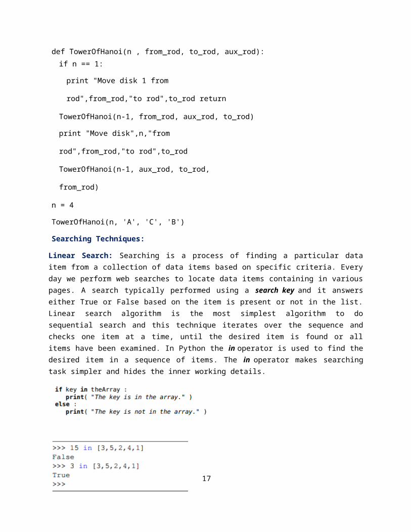
Linear Search: Searching is a process of finding a particular data item from a collection of data items based on specific criteria. Every day we perform web searches to locate data items containing in various pages. A search typically performed using a search key and it answers either True or False based on the item is present or not in the list. Linear search algorithm is the most simplest algorithm to do sequential search and this technique iterates over the sequence and checks one item at a time, until the desired item is found or all items have been examined. In Python the in operator is used to find the desired item in a sequence of items. The in operator makes searching task simpler and hides the inner working details.
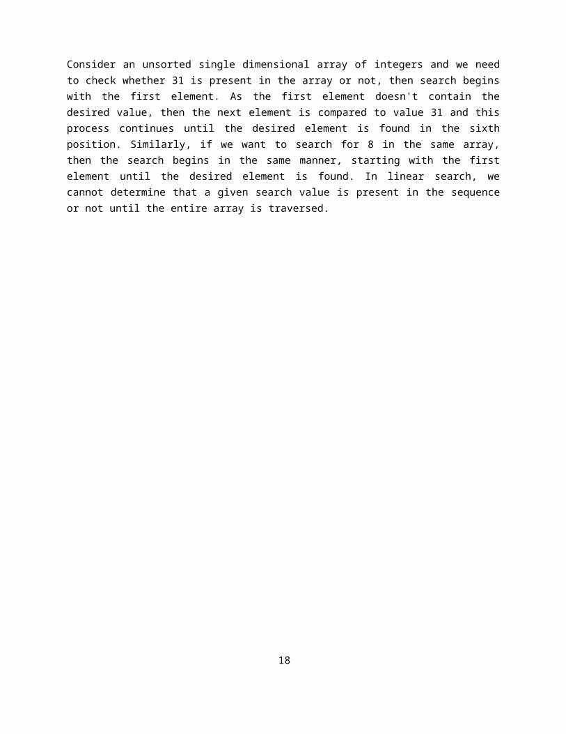
Consider an unsorted single dimensional array of integers and we need to check whether 31 is present in the array or not, then search begins with the first element. As the first element doesn't contain the desired value, then the next element is compared to value 31 and this process continues until the desired element is found in the sixth position. Similarly, if we want to search for 8 in the same array, then the search begins in the same manner, starting with the first element until the desired element is found. In linear search, we cannot determine that a given search value is present in the sequence or not until the entire array is traversed.
12
Source Code:
def linear_search(obj, item, start=0): for i in range(start, len(obj)):
if obj[i] == item: return i
return -1 arr=[1,2,3,4,5,6,7,8]x=4 result=linear_search(arr,x) if result==-1:
print ("element does not exist") else:
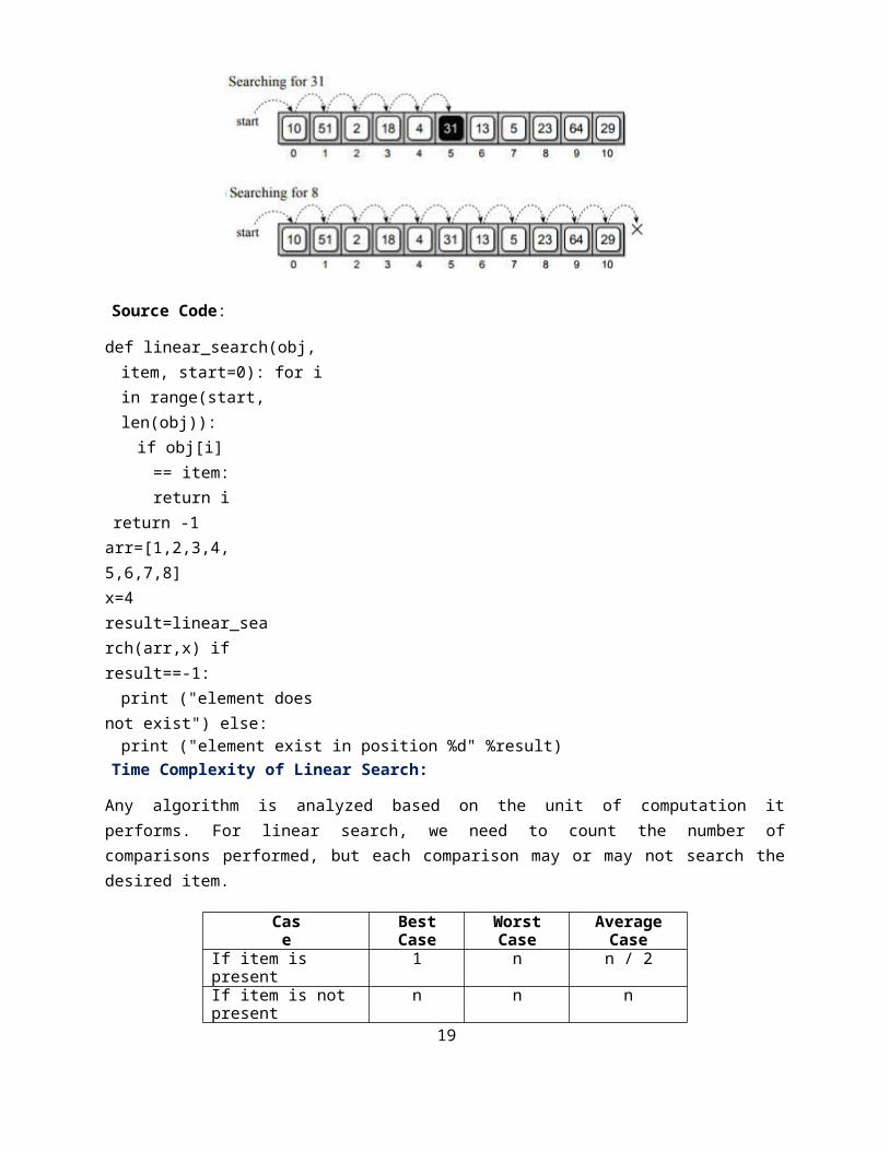
print ("element exist in position %d" %result)Time Complexity of Linear Search:
Any algorithm is analyzed based on the unit of computation it performs. For linear search, we need to count the number of comparisons performed, but each comparison may or may not search the desired item.
Case Best Case Worst Case Average Case
If item is present 1 n n / 2
If item is not present n n n
Binary Search: In Binary search algorithm, the target key is examined in a sorted sequence and this algorithm starts searching with the middle item of the sorted sequence.
a. If the middle item is the target value, then the search item is found and it returns True.
b. If the target item < middle item, then search for the target value in the first half of the list.
c. If the target item > middle item, then search for the target value in the second half of the list.
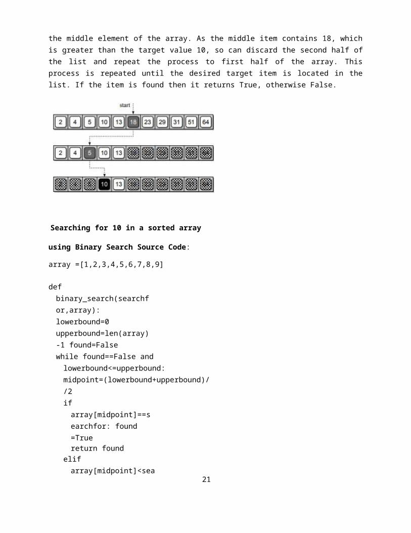
In binary search as the list is ordered, so we can eliminate half of the values in the list in each iteration. Consider an example, suppose we want to search 10 in a sorted array of elements, then we first determine
13
the middle element of the array. As the middle item contains 18, which is greater than the target value 10, so can discard the second half of the list and repeat the process to first half of the array. This process is repeated until the desired target item is located in the list. If the item is found then it returns True, otherwise False.
Searching for 10 in a sorted array using Binary Search
Source Code:
array =[1,2,3,4,5,6,7,8,9]
def binary_search(searchfor,array): lowerbound=0 upperbound=len(array)-1 found=Falsewhile found==False and lowerbound<=upperbound:
midpoint=(lowerbound+upperbound)//2if array[midpoint]==searchfor:
found =Truereturn found
elif array[midpoint]<searchfor: lowerbound=midpoint+1
else:upperbound=midpoint-1
return found
searchfor=int(input("what are you searching for?")) if binary_search(searchfor,array):
print ("element found") else:
print ("element not found")Time Complexity of Binary Search:
In Binary Search, each comparison eliminates about half of the items from the list. Consider a list with n items, then about n/2 items will be eliminated after first comparison. After second comparison, n/4 items
14
of the list will be eliminated. If this process is repeated for several times, then there will be just one item left in the list. The number of comparisons required to reach to this point is n/2i = 1. If we solve for i, then it gives us i = log n. The maximum number is comparison is logarithmic in nature, hence the time complexity of binary search is O(log n).
Case Best Case Worst Case Average Case
If item is present 1 O(log n) O(log n)
If item is not present O(log n) O(log n) O(log n)
Fibonacci Search: It is a comparison based technique that uses Fibonacci numbers to search an element in a sorted array. It follows divide and conquer approach and it has a O(log n) time complexity. Let the element to be searched is x, then the idea is to first find the smallest Fibonacci number that is greater than or equal to length of given array. Let the Fibonacci number be fib(n th Fibonacci number). Use (n-2)th Fibonacci number as index and say it is i, then compare a[i] with x, if x is same then return i. Else if x is greater, then search the sub array after i, else search the sub array before i.
Source Code:
# Python3 program for Fibonacci search. from bisect import bisect_left
# Returns index of x if present, else # returns -1def fibMonaccianSearch(arr, x, n):
# Initialize fibonacci numbers fibMMm2 = 0 # (m-2)'th Fibonacci No. fibMMm1 = 1 # (m-1)'th Fibonacci No.fibM = fibMMm2 + fibMMm1 # m'th Fibonacci
# fibM is going to store the smallest# Fibonacci Number greater than or equal to n while (fibM < n):
fibMMm2 = fibMMm1 fibMMm1 = fibMfibM = fibMMm2 + fibMMm1
# Marks the eliminated range from front offset = -1;
# while there are elements to be inspected.# Note that we compare arr[fibMm2] with x. # When fibM becomes 1, fibMm2 becomes 0 while (fibM > 1):
15
# Check if fibMm2 is a valid location i = min(offset+fibMMm2, n-1)
# If x is greater than the value at# index fibMm2, cut the subarray array # from offset to iif (arr[i] < x):
fibM = fibMMm1 fibMMm1 = fibMMm2fibMMm2 = fibM - fibMMm1 offset = i
# If x is greater than the value at # index fibMm2, cut the subarray # after i+1elif (arr[i] > x):
fibM = fibMMm2fibMMm1 = fibMMm1 - fibMMm2 fibMMm2 = fibM - fibMMm1
# element found. return index else :
return i
# comparing the last element with x */ if(fibMMm1 and arr[offset+1] == x):
return offset+1;
# element not found. return -1 return -1
# Driver Codearr = [10, 22, 35, 40, 45, 50, 80, 82, 85, 90, 100]n = len(arr) x = 80print("Found at index:",
fibMonaccianSearch(arr, x, n))Time Complexity of Fibonacci Search:
Time complexity for Fibonacci search is O(log2 n)
Sorting Techniques:
Sorting in general refers to various methods of arranging or ordering things based on criteria's (numerical, chronological, alphabetical, hierarchical etc.). There are many approaches to sorting data and each has its own merits and demerits.
16
Bubble Sort:
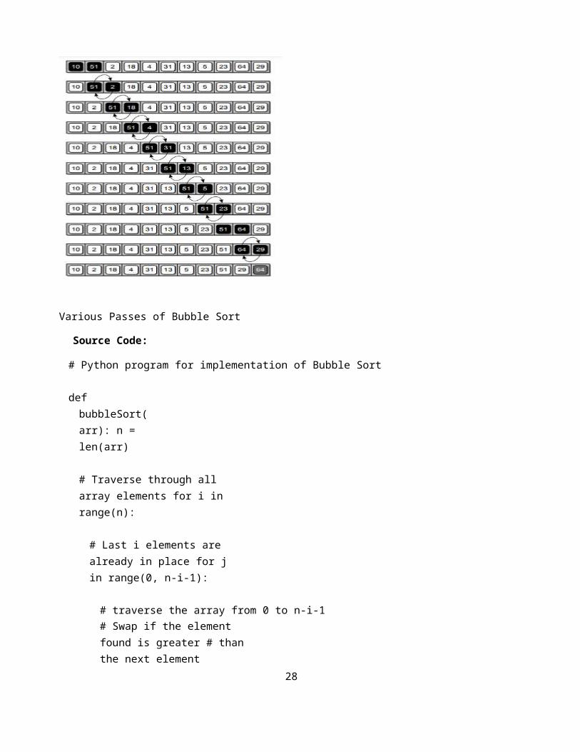
This sorting technique is also known as exchange sort, which arranges values by iterating over the list several times and in each iteration the larger value gets bubble up to the end of the list. This algorithm uses multiple passes and in each pass the first and second data items are compared. if the first data item is bigger than the second, then the two items are swapped. Next the items in second and third position are compared and if the first one is larger than the second, then they are swapped, otherwise no change in their order. This process continues for each successive pair of data items until all items are sorted.
Bubble Sort Algorithm:
Step 1: Repeat Steps 2 and 3 for i=1 to 10
Step 2: Set j=1
Step 3: Repeat while j<=n
(A) if a[i] < a[j]
Then interchange a[i] and a[j]
[End of if]
(B) Set j = j+1
[End of Inner Loop]
[End of Step 1 Outer Loop]
Step 4: Exit
Various Passes of Bubble Sort
17
Source Code:
# Python program for implementation of Bubble Sort
def bubbleSort(arr): n = len(arr)
# Traverse through all array elements for i in range(n):
# Last i elements are already in place for j in range(0, n-i-1):
# traverse the array from 0 to n-i-1# Swap if the element found is greater # than the next elementif arr[j] > arr[j+1] :
arr[j], arr[j+1] = arr[j+1], arr[j]
# Driver code to test abovearr = [64, 34, 25, 12, 22, 11, 90]
bubbleSort(arr)
print ("Sorted array is:") for i in range(len(arr)):
print ("%d" %arr[i])
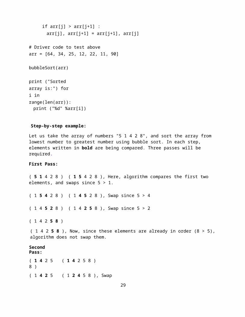
Step-by-step example:
Let us take the array of numbers "5 1 4 2 8", and sort the array from lowest number to greatest number using bubble sort. In each step, elements written in bold are being compared. Three passes will be required.
First Pass:
( 5 1 4 2 8 ) ( 1 5 4 2 8 ), Here, algorithm compares the first two elements, and swaps since 5 > 1.
( 1 5 4 2 8 ) ( 1 4 5 2 8 ), Swap since 5 > 4
( 1 4 5 2 8 ) ( 1 4 2 5 8 ), Swap since 5 > 2
( 1 4 2 5 8 )
( 1 4 2 5 8 ), Now, since these elements are already in order (8 > 5), algorithm does not swap them.
18
Second Pass:
( 1 4 2 5 8 ) ( 1 4 2 5 8 )
( 1 4 2 5 8 ) ( 1 2 4 5 8 ), Swap since 4 > 2
( 1 2 4 5 8 ) ( 1 2 4 5 8 )
( 1 2 4 5 8 ) ( 1 2 4 5 8 )Now, the array is already sorted, but our algorithm does not know if it is completed. The algorithm needs one whole pass without any swap to know it is sorted.
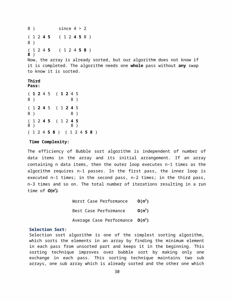
Third Pass:
( 1 2 4 5 8 ) ( 1 2 4 5 8 )
( 1 2 4 5 8 ) ( 1 2 4 5 8 )
( 1 2 4 5 8 ) ( 1 2 4 5 8 )( 1 2 4 5 8 ) ( 1 2 4 5 8 )
Time Complexity:
The efficiency of Bubble sort algorithm is independent of number of data items in the array and its initial arrangement. If an array containing n data items, then the outer loop executes n-1 times as the algorithm requires n-1 passes. In the first pass, the inner loop is executed n-1 times; in the second pass, n-2 times; in the third pass, n-3 times and so on. The total number of iterations resulting in a run time of O(n2).
Worst Case Performance O(n2)
Best Case Performance O(n2)
Average Case Performance O(n2)
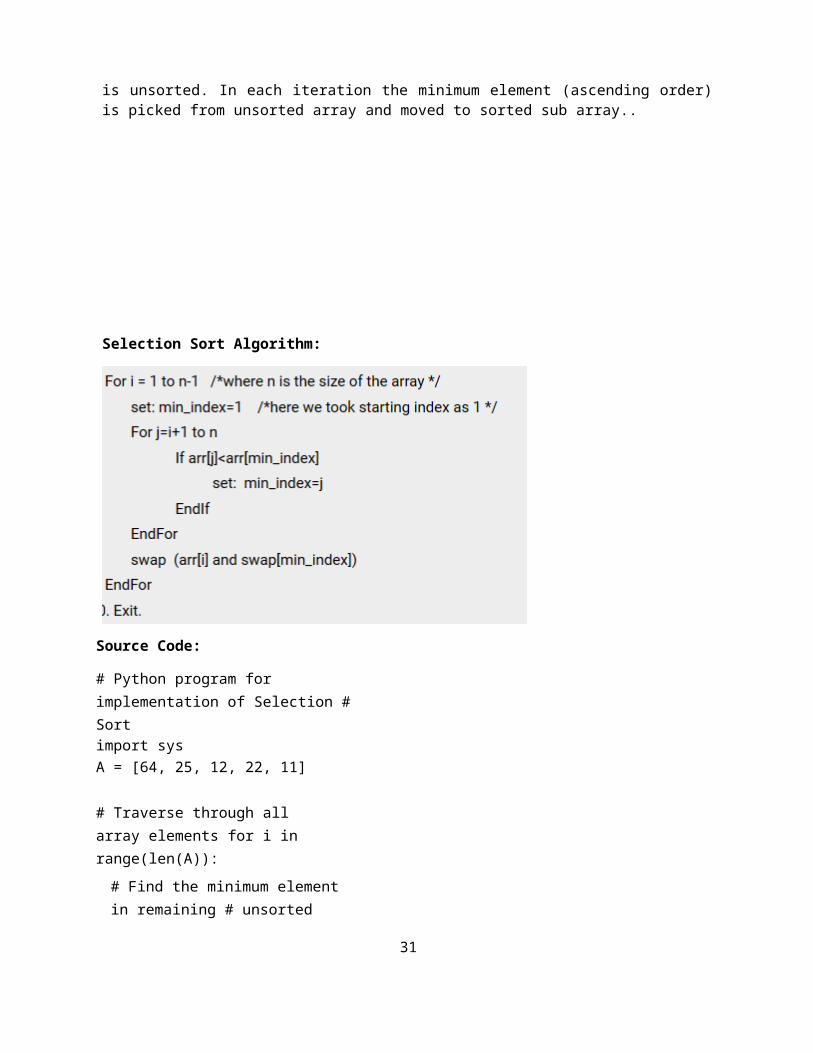
Selection Sort:Selection sort algorithm is one of the simplest sorting algorithm, which sorts the elements in an array by finding the minimum element in each pass from unsorted part and keeps it in the beginning. This sorting technique improves over bubble sort by making only one exchange in each pass. This sorting technique maintains two sub arrays, one sub array which is already sorted and the other one which is unsorted. In each iteration the minimum element (ascending order) is picked from unsorted array and moved to sorted sub array..
19
Selection Sort Algorithm:
Source Code:
# Python program for implementation of Selection # Sortimport sysA = [64, 25, 12, 22, 11]
# Traverse through all array elements for i in range(len(A)):
# Find the minimum element in remaining # unsorted arraymin_idx = ifor j in range(i+1, len(A)):
if A[min_idx] > A[j]:min_idx = j
# Swap the found minimum element with # the first elementA[i], A[min_idx] = A[min_idx], A[i]
# Driver code to test above print ("Sorted array")for i in range(len(A)):
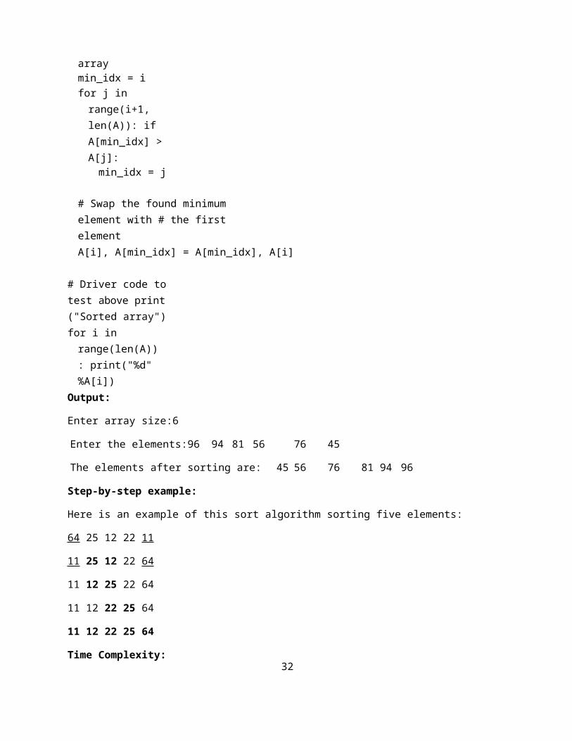
print("%d" %A[i])Output:
Enter array size:6
20
Enter the elements:96 94 81 56 76 45
The elements after sorting are: 45 56 76 81 94 96
Step-by-step example:
Here is an example of this sort algorithm sorting five elements:
64 25 12 22 11
11 25 12 22 64
11 12 25 22 64
11 12 22 25 64
11 12 22 25 64
Time Complexity:
Selection sort is not difficult to analyze compared to other sorting algorithms since none of the loops depend on the data in the array. Selecting the lowest element requires scanning all n elements (this takes n − 1 comparisons) and then swapping it into the first position. Finding the next lowest element requires scanning the remaining n − 1 elements and so on, for (n − 1) + (n − 2) + ... + 2 + 1 = n(n − 1) / 2 ∈ O(n2) comparisons. Each of these scans requires one swap for n − 1 elements (the final element is already in place).
Worst Case Performance O(n2)
Best Case Performance O(n2)
Average Case Performance O(n2)
21
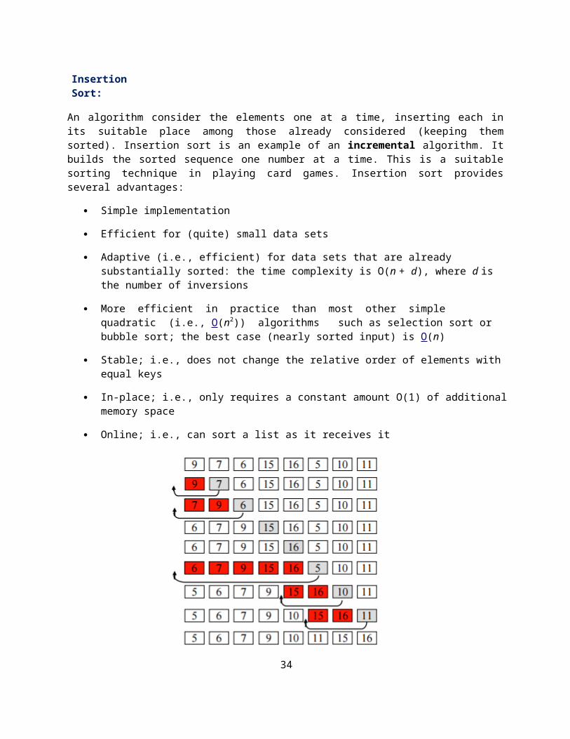
Insertion Sort:
An algorithm consider the elements one at a time, inserting each in its suitable place among those already considered (keeping them sorted). Insertion sort is an example of an incremental algorithm. It builds the sorted sequence one number at a time. This is a suitable sorting technique in playing card games. Insertion sort provides several advantages:
Simple implementation
Efficient for (quite) small data sets
Adaptive (i.e., efficient) for data sets that are already substantially sorted: the time complexity is O(n + d), where d is the number of inversions
More efficient in practice than most other simple quadratic (i.e., O(n2)) algorithms such as selection sort or bubble sort; the best case (nearly sorted input) is O(n)
Stable; i.e., does not change the relative order of elements with equal keys
In-place; i.e., only requires a constant amount O(1) of additional memory space
Online; i.e., can sort a list as it receives it
Source Code:
# Python program for implementation of Insertion Sort
# Function to do insertion sort def insertionSort(arr):
# Traverse through 1 to len(arr) for i in range(1, len(arr)):
22
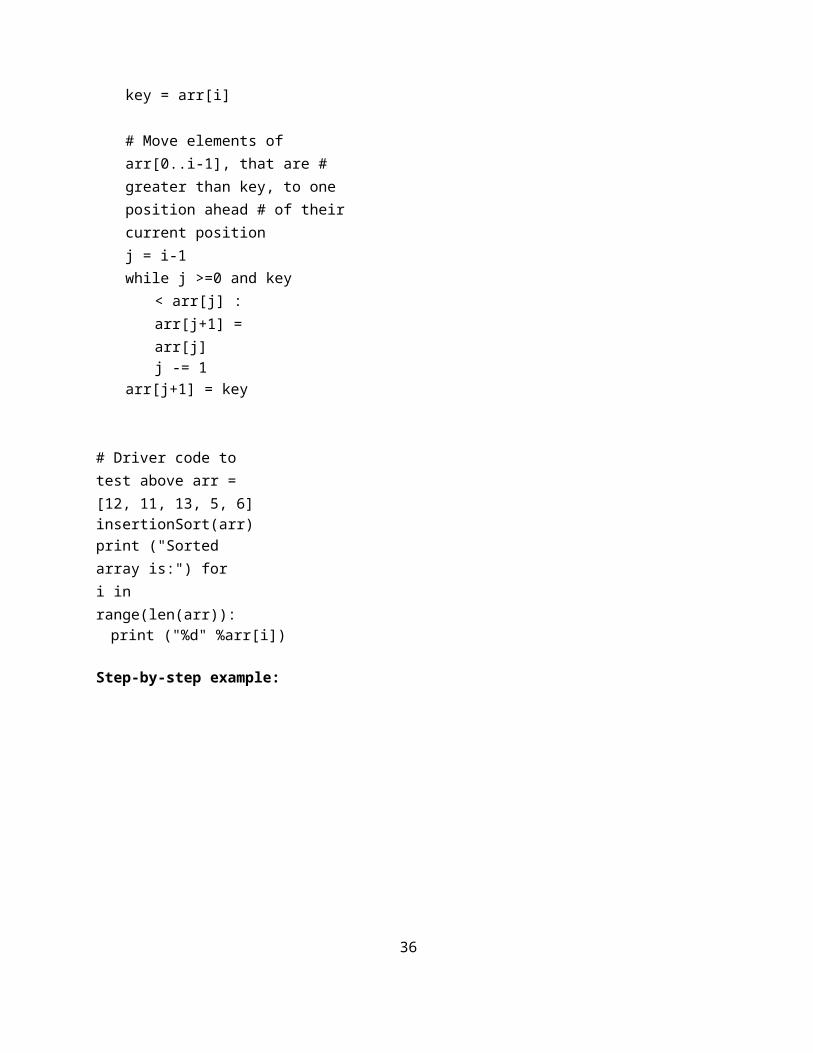
key = arr[i]
# Move elements of arr[0..i-1], that are # greater than key, to one position ahead # of their current positionj = i-1while j >=0 and key < arr[j] :
arr[j+1] = arr[j]j -= 1
arr[j+1] = key
# Driver code to test above arr = [12, 11, 13, 5, 6]insertionSort(arr)print ("Sorted array is:") for i in range(len(arr)):
print ("%d" %arr[i])
Step-by-step example:
23
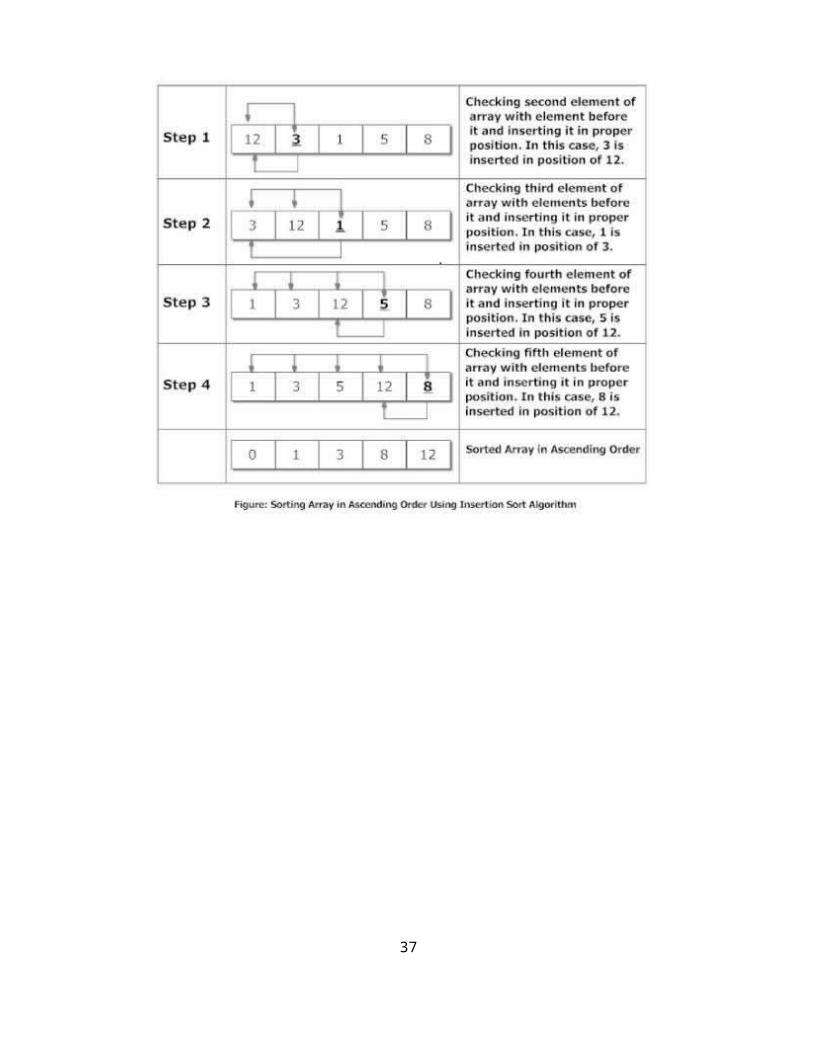
Suppose, you want to sort elements in ascending as in above figure. Then,
1. The second element of an array is compared with the elements that appear before it (only first element in this case). If the second element is smaller than first element, second element is inserted in the position of first element. After first step, first two elements of an array will be sorted.
2. The third element of an array is compared with the elements that appears before it (first and second element). If third element is smaller than first element, it is inserted in the position of first element. If third element is larger than first element but, smaller than second element, it is inserted in the position of second element. If third element is larger than both the elements, it is kept in the position as it is. After second step, first three elements of an array will be sorted.
3. Similarly, the fourth element of an array is compared with the elements that appear before it (first, second and third element) and the same procedure is applied and that element is inserted in the proper position. After third step, first four elements of an array will be sorted.
If there are n elements to be sorted. Then, this procedure is repeated n-1 times to get sorted list of array.
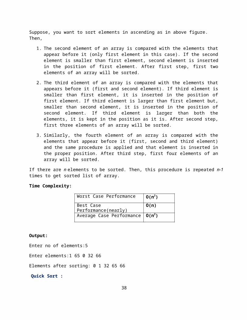
Time Complexity:
Worst Case Performance O(n2)
Best Case Performance(nearly) O(n)
Average Case Performance O(n2)
Output:
Enter no of elements:5
Enter elements:1 65 0 32 66
Elements after sorting: 0 1 32 65 66
Quick Sort :
Quick sort is a divide and conquer algorithm. Quick sort first divides a large list into two smaller sub- lists: the low elements and the high elements. Quick sort can then recursively sort the sub-lists.
The steps are:
1. Pick an element, called a pivot, from the list.
2. Reorder the list so that all elements with values less than the pivot come before the pivot, while all elements with values greater than the pivot come after it (equal values can go either way). After this partitioning, the pivot is in its final position. This is called the partition operation.
3. Recursively apply the above steps to the sub-list of elements with smaller values and separately the sub-list of elements with greater values.
The base case of the recursion is lists of size zero or one, which never need to be sorted.
24
Quick sort, or partition-exchange sort, is a sorting algorithm developed by Tony Hoare that, on average, makes O(n log n) comparisons to sort n items. In the worst case, it makes O(n2) comparisons, though this behavior is rare. Quick sort is often faster in practice than other O(n log n) algorithms. It works by first of all by partitioning the array around a pivot value and then dealing with the 2 smaller partitions separately. Partitioning is the most complex part of quick sort. The simplest thing is to use the first value in the array, a[l] (or a[0] as l = 0 to begin with) as the pivot. After the partitioning, all values to the left of the pivot are <= pivot and all values to the right are > pivot. The same procedure for the two remaining sub lists is repeated and so on recursively until we have the entire list sorted.
Advantages:
One of the fastest algorithms on average.
Does not need additional memory (the sorting takes place in the array - this is called in-placeprocessing).
Disadvantages: The worst-case complexity is O(N2)
Source Code:
# Python program for implementation of Quicksort Sort
# This function takes last element as pivot, places # the pivot element at its correct position in sorted # array, and places all smaller (smaller than pivot) # to left of pivot and all greater elements to right # of pivotdef partition(arr,low,high):
i = ( low-1 ) # index of smaller element pivot = arr[high] # pivot
for j in range(low , high):
# If current element is smaller than or # equal to pivotif arr[j] <= pivot:
# increment index of smaller element i = i+1arr[i],arr[j] = arr[j],arr[i]
arr[i+1],arr[high] = arr[high],arr[i+1] return ( i+1 )
# The main function that implements QuickSort # arr[] --> Array to be sorted,# low --> Starting index, # high --> Ending index
25
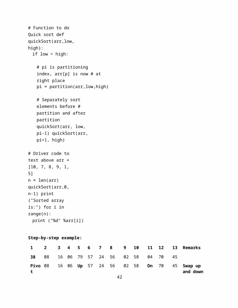
# Function to do Quick sort def quickSort(arr,low,high):
if low < high:
# pi is partitioning index, arr[p] is now # at right placepi = partition(arr,low,high)
# Separately sort elements before # partition and after partition quickSort(arr, low, pi-1) quickSort(arr, pi+1, high)
# Driver code to test above arr = [10, 7, 8, 9, 1, 5]n = len(arr) quickSort(arr,0,n-1) print ("Sorted array is:") for i in range(n):
print ("%d" %arr[i])
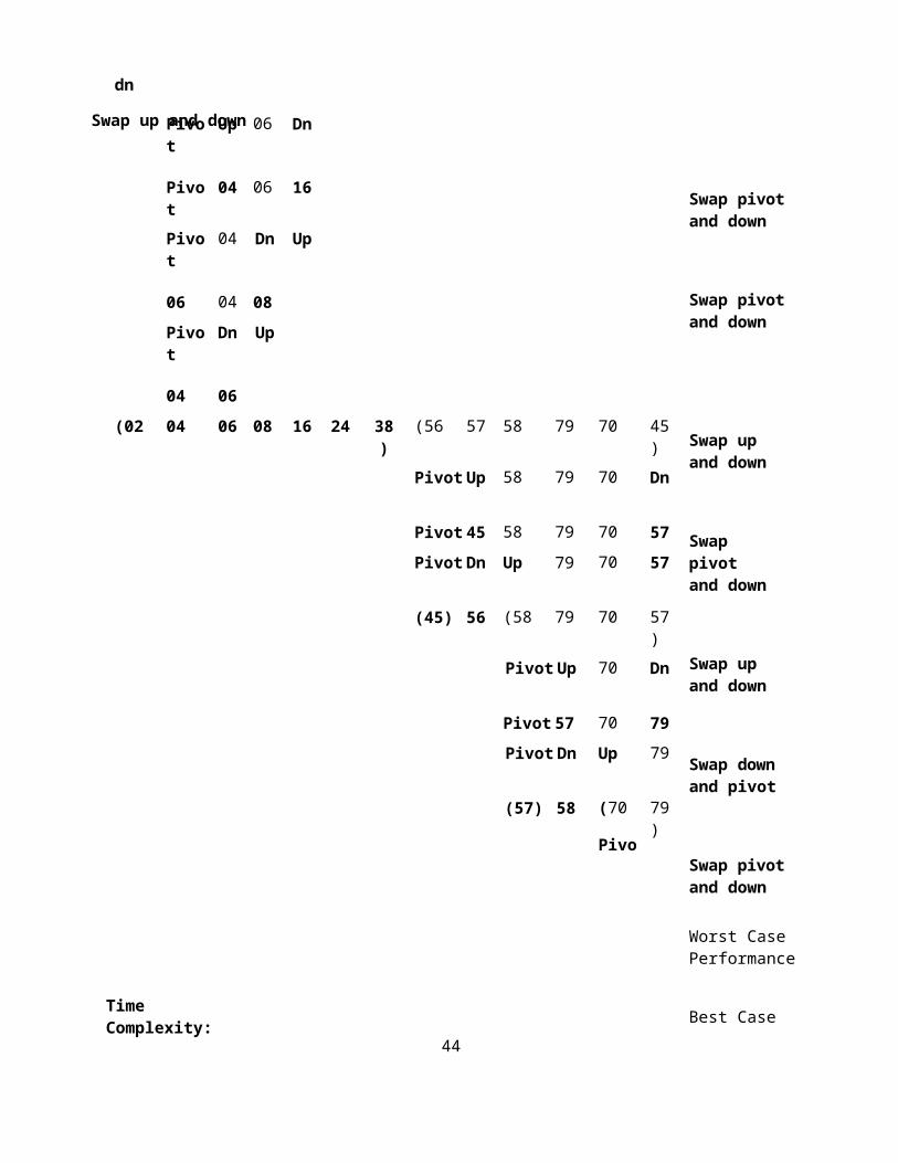
Step-by-step example:
1 2 3 4 5 6 7 8 9 10 11 12 13 Remarks
38 08 16 06 79 57 24 56 02 58 04 70 45
Pivot 08 16 06 Up 57 24 56 02 58 Dn 70 45 Swap up and down
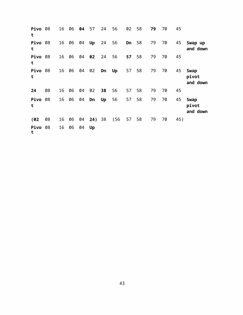
Pivot 08 16 06 04 57 24 56 02 58 79 70 45
Pivot 08 16 06 04 Up 24 56 Dn 58 79 70 45 Swap up and down
Pivot 08 16 06 04 02 24 56 57 58 79 70 45
Pivot 08 16 06 04 02 Dn Up 57 58 79 70 45 Swap pivot and down
24 08 16 06 04 02 38 56 57 58 79 70 45
Pivot 08 16 06 04 Dn Up 56 57 58 79 70 45 Swap pivot and down
(02 08 16 06 04 24) 38 (56 57 58 79 70 45)
Pivot 08 16 06 04 Up
26
Swap up and down
Swap pivot and down
Swap pivot and down
Swap up and down
Swap pivot and down
Swap up and down
Swap down and pivot
Swap pivot and down
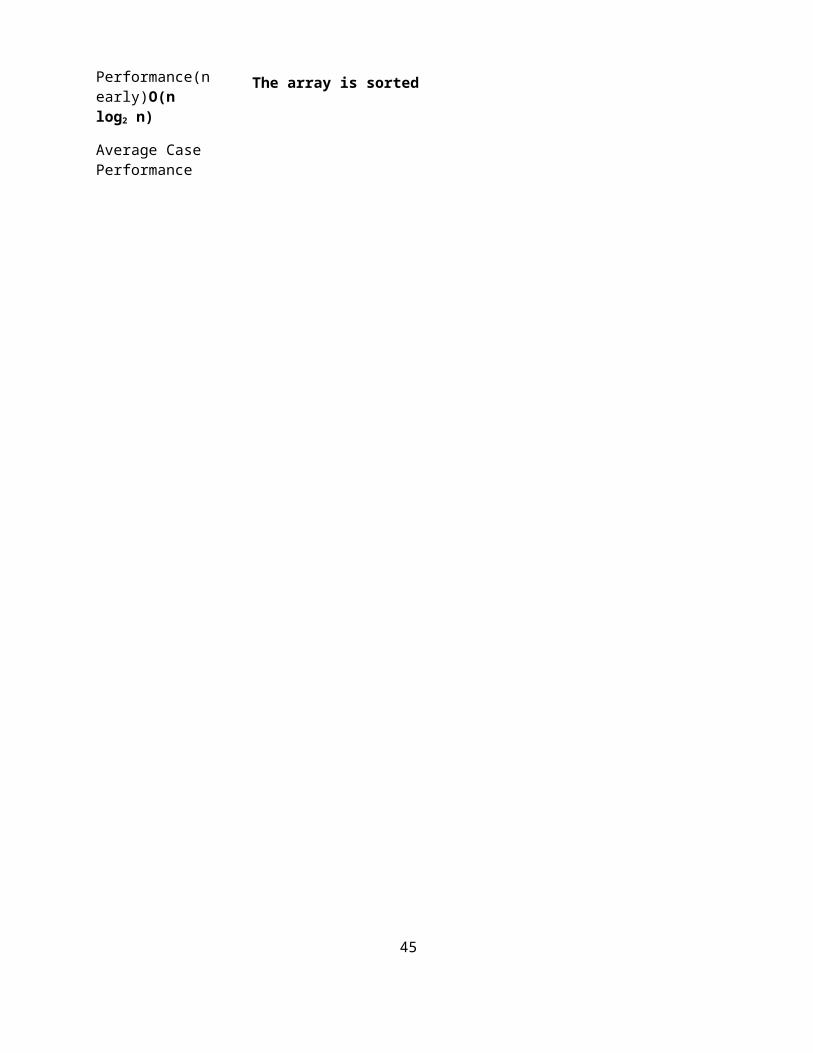
Time Complexity:
Worst Case Performance O(n2)
Best Case Performance(nearly) O(n log2 n)
Average Case Performance O(n log2 n)
The array is sorted
dn
Pivot Up 06 Dn
Pivot 04 06 16
Pivot 04 Dn Up
06 04 08
Pivot Dn Up
04 06
(02 04 06 08 16 24 38) (56 57 58 79 70 45)
Pivot Up 58 79 70 Dn
Pivot 45 58 79 70 57
Pivot Dn Up 79 70 57
(45) 56 (58 79 70 57)
Pivot Up 70 Dn
Pivot 57 70 79
Pivot Dn Up 79
(57) 58 (70
Pivot
79)
Up
Dn
02 04 06 08 16 24 38 45 56 57 58 70 79
27
Merge Sort:
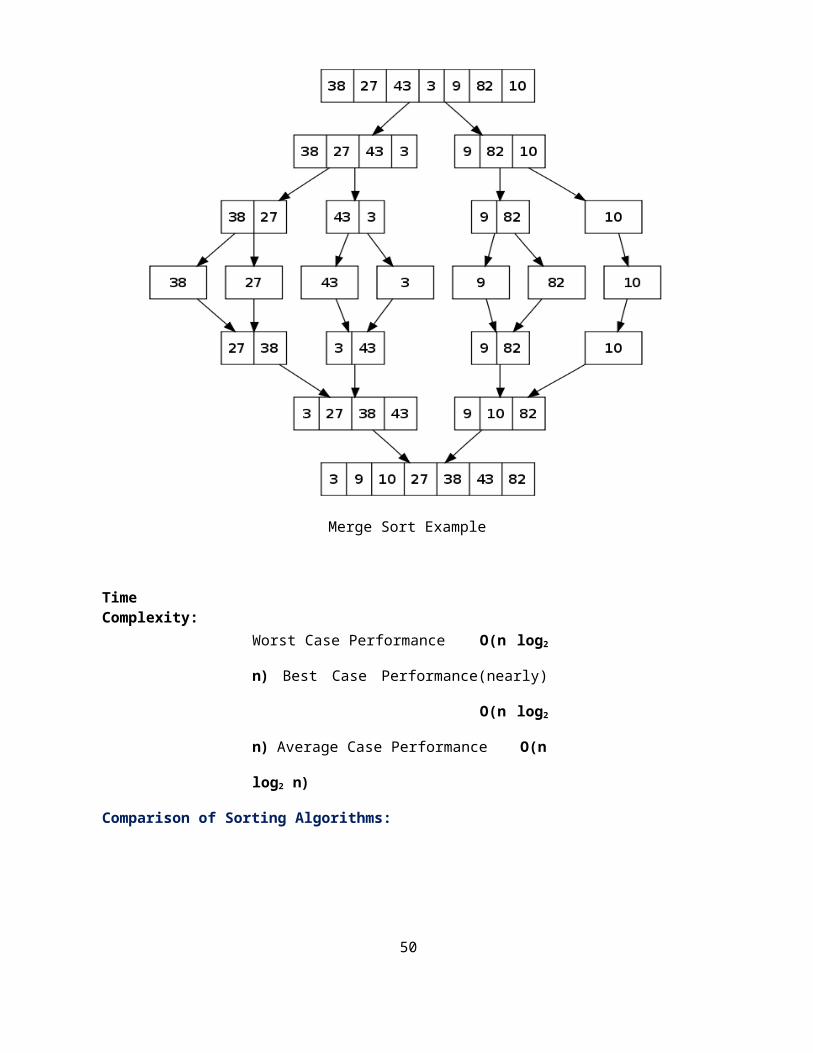
Merge sort is based on Divide and conquer method. It takes the list to be sorted and divide it in half to create two unsorted lists. The two unsorted lists are then sorted and merged to get a sorted list. The two unsorted lists are sorted by continually calling the merge-sort algorithm; we eventually get a list of size 1 which is already sorted. The two lists of size 1 are then merged.
Merge Sort Procedure:
This is a divide and conquer algorithm.
This works as follows :
1. Divide the input which we have to sort into two parts in the middle. Call it the left part and right part.
2. Sort each of them separately. Note that here sort does not mean to sort it using some other method. We use the same function recursively.
3. Then merge the two sorted parts.
Input the total number of elements that are there in an array (number_of_elements). Input the array (array[number_of_elements]). Then call the function MergeSort() to sort the input array. MergeSort() function sorts the array in the range [left,right] i.e. from index left to index right inclusive. Merge() function merges the two sorted parts. Sorted parts will be from [left, mid] and [mid+1, right]. After merging output the sorted array.
MergeSort() function:
It takes the array, left-most and right-most index of the array to be sorted as arguments. Middle index (mid) of the array is calculated as (left + right)/2. Check if (left<right) cause we have to sort only when left<right because when left=right it is anyhow sorted. Sort the left part by calling MergeSort() function again over the left part MergeSort(array,left,mid) and the right part by recursive call of MergeSort function as MergeSort(array,mid + 1, right). Lastly merge the two arrays using the Merge function.
Merge() function:
It takes the array, left-most , middle and right-most index of the array to be merged as arguments.
Finally copy back the sorted array to the original array.
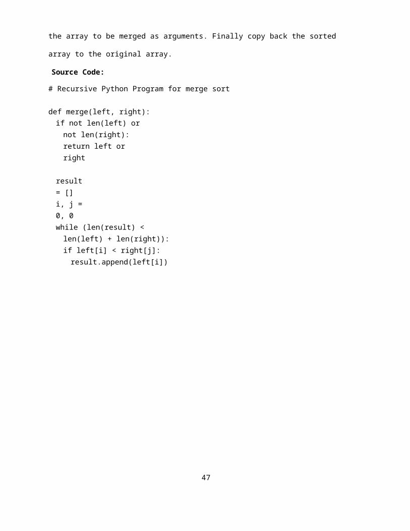
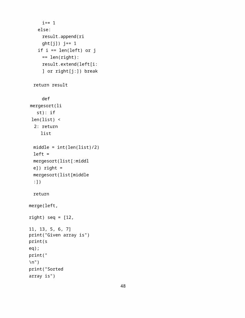
Source Code:
# Recursive Python Program for merge sort
def merge(left, right):if not len(left) or not len(right):
return left or right
result = [] i, j = 0, 0while (len(result) < len(left) + len(right)):
if left[i] < right[j]:result.append(left[i])
28
i+= 1else:
result.append(right[j]) j+= 1
if i == len(left) or j == len(right): result.extend(left[i:] or right[j:]) break
return result
def mergesort(list): if len(list) < 2:
return list
middle = int(len(list)/2)left = mergesort(list[:middle]) right = mergesort(list[middle:])
return merge(left, right)
seq = [12, 11, 13, 5, 6, 7]print("Given array is")print(seq); print("\n")print("Sorted array is") print(mergesort(seq))
Step-by-step example:
29
Merge Sort Example
Time Complexity:
Worst Case Performance O(n log2 n)
Best Case Performance(nearly) O(n log2 n)
Average Case Performance O(n log2 n)
Comparison of Sorting Algorithms:
30
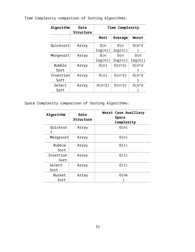
Time Complexity comparison of Sorting Algorithms:
Algorithm Data Structure Time Complexity
Best Average Worst
Quicksort Array O(n log(n)) O(n log(n)) O(n^2)
Mergesort Array O(n log(n)) O(n log(n)) O(n log(n))
Bubble Sort Array O(n) O(n^2) O(n^2)
Insertion Sort Array O(n) O(n^2) O(n^2)
Select Sort Array O(n^2) O(n^2) O(n^2)
Space Complexity comparison of Sorting Algorithms:
Algorithm Data Structure Worst Case Auxiliary Space Complexity
Quicksort Array O(n)
Mergesort Array O(n)
Bubble Sort Array O(1)
Insertion Sort Array O(1)
Select Sort Array O(1)
Bucket Sort Array O(nk)
31
UNIT – II LINEAR DATA STRUCTURESStacks Primitive Operations:
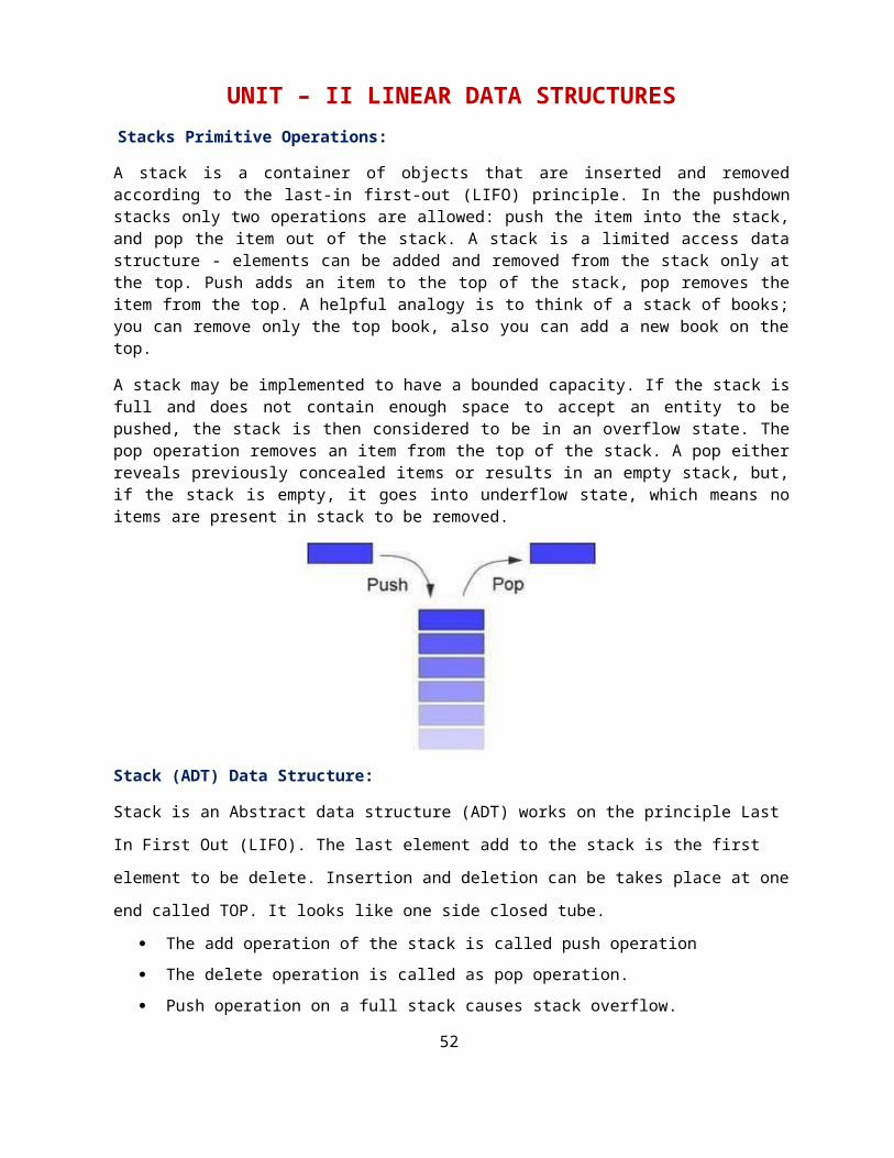
A stack is a container of objects that are inserted and removed according to the last-in first-out (LIFO) principle. In the pushdown stacks only two operations are allowed: push the item into the stack, and pop the item out of the stack. A stack is a limited access data structure - elements can be added and removed from the stack only at the top. Push adds an item to the top of the stack, pop removes the item from the top. A helpful analogy is to think of a stack of books; you can remove only the top book, also you can add a new book on the top.
A stack may be implemented to have a bounded capacity. If the stack is full and does not contain enough space to accept an entity to be pushed, the stack is then considered to be in an overflow state. The pop operation removes an item from the top of the stack. A pop either reveals previously concealed items or results in an empty stack, but, if the stack is empty, it goes into underflow state, which means no items are present in stack to be removed.
Stack (ADT) Data Structure:
Stack is an Abstract data structure (ADT) works on the principle Last In First Out (LIFO). The last
element add to the stack is the first element to be delete. Insertion and deletion can be takes place at one
end called TOP. It looks like one side closed tube.
The add operation of the stack is called push operation
The delete operation is called as pop operation.
Push operation on a full stack causes stack overflow.
Pop operation on an empty stack causes stack underflow.
SP is a pointer, which is used to access the top element of the stack.
If you push elements that are added at the top of the stack;
In the same way when we pop the elements, the element at the top of the stack is deleted.
32
Operations of stack:
There are two operations applied on stack they are
1. push
2. pop.
While performing push & pop operations the following test must be conducted on the stack.
1) Stack is empty or not
2) Stack is full or not
Push:
Push operation is used to add new elements in to the stack. At the time of addition first check the stack is
full or not. If the stack is full it generates an error message "stack overflow".
Pop:
Pop operation is used to delete elements from the stack. At the time of deletion first check the stack is
empty or not. If the stack is empty it generates an error message "stack underflow".
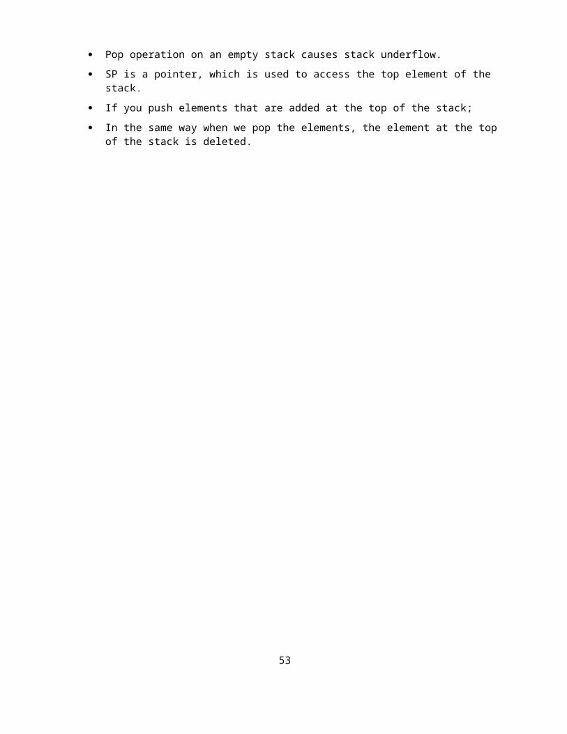
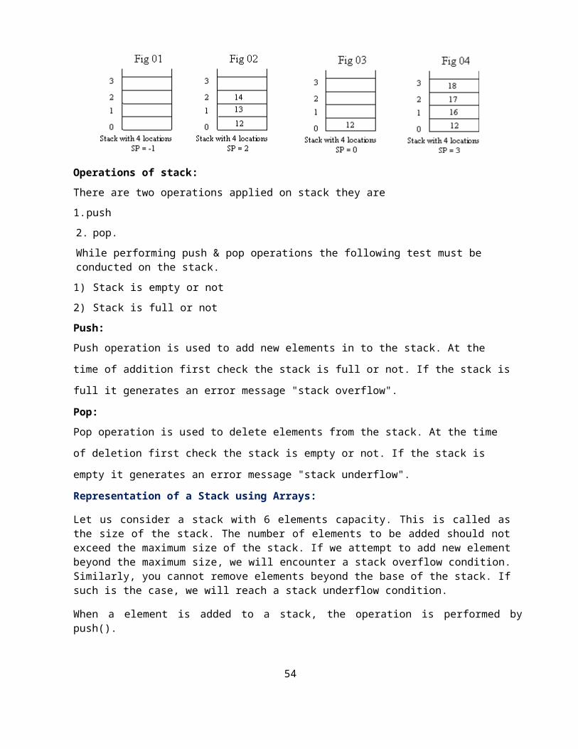
Representation of a Stack using Arrays:
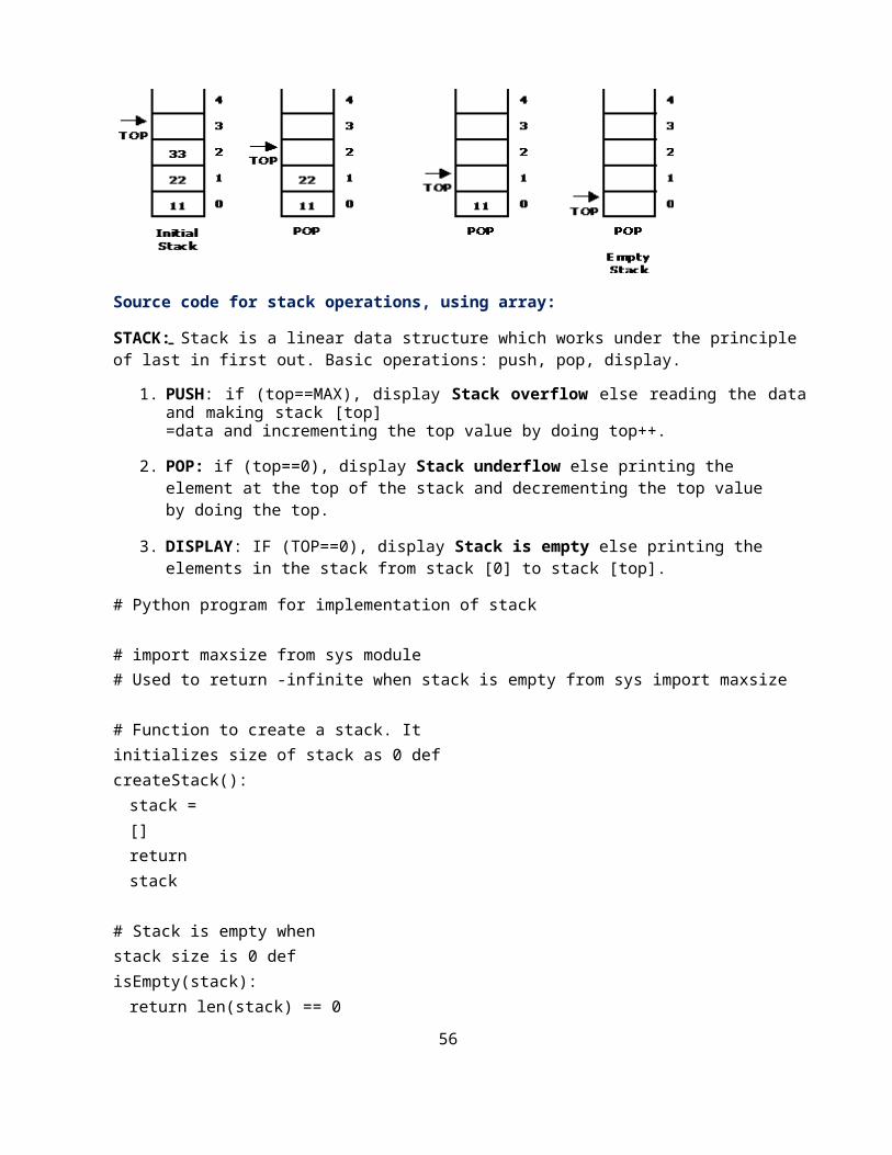
Let us consider a stack with 6 elements capacity. This is called as the size of the stack. The number of elements to be added should not exceed the maximum size of the stack. If we attempt to add new element beyond the maximum size, we will encounter a stack overflow condition. Similarly, you cannot remove elements beyond the base of the stack. If such is the case, we will reach a stack underflow condition.
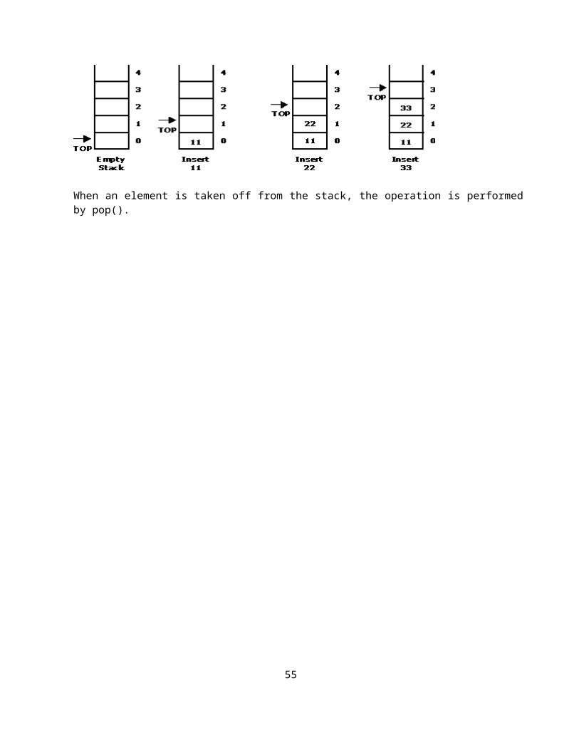
When a element is added to a stack, the operation is performed by push().
When an element is taken off from the stack, the operation is performed by pop().
33
Source code for stack operations, using array:
STACK: Stack is a linear data structure which works under the principle of last in first out. Basic operations: push, pop, display.
1. PUSH: if (top==MAX), display Stack overflow else reading the data and making stack [top]=data and incrementing the top value by doing top++.
2. POP: if (top==0), display Stack underflow else printing the element at the top of the stack and decrementing the top value by doing the top.
3. DISPLAY: IF (TOP==0), display Stack is empty else printing the elements in the stack from stack [0] to stack [top].
# Python program for implementation of stack
# import maxsize from sys module# Used to return -infinite when stack is empty from sys import maxsize
# Function to create a stack. It initializes size of stack as 0 def createStack():
stack = [] return stack
# Stack is empty when stack size is 0 def isEmpty(stack):
return len(stack) == 0
# Function to add an item to stack. It increases size by 1 def push(stack, item):
stack.append(item) print("pushed to stack " + item)
# Function to remove an item from stack. It decreases size by 1 def pop(stack):
if (isEmpty(stack)): print("stack empty")
34
return str(-maxsize -1) #return minus infinite
return stack.pop()
# Driver program to test above functions stack = createStack()print("maximum size of array is",maxsize) push(stack, str(10))push(stack, str(20)) push(stack, str(30))print(pop(stack) + " popped from stack") print(pop(stack) + " popped from stack") print(pop(stack) + " popped from stack") print(pop(stack) + " popped from stack") push(stack, str(10))push(stack, str(20)) push(stack, str(30))print(pop(stack) + " popped from stack")Linked List Implementation of Stack:
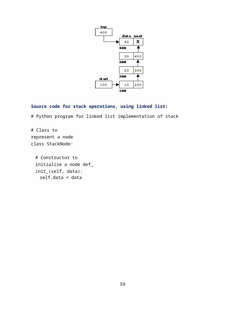
We can represent a stack as a linked list. In a stack push and pop operations are performed at one end called top. We can perform similar operations at one end of list using top pointer.
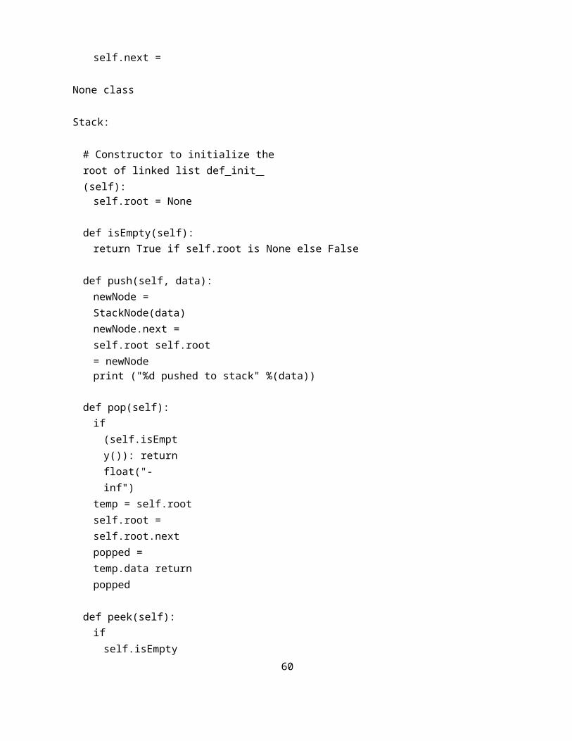
Source code for stack operations, using linked list:
# Python program for linked list implementation of stack
# Class to represent a node class StackNode:
# Constructor to initialize a node def init (self, data):
self.data = data
35
self.next = None
class Stack:
# Constructor to initialize the root of linked list def init (self):
self.root = None
def isEmpty(self):return True if self.root is None else False
def push(self, data):newNode = StackNode(data) newNode.next = self.root self.root = newNodeprint ("%d pushed to stack" %(data))
def pop(self):if (self.isEmpty()):
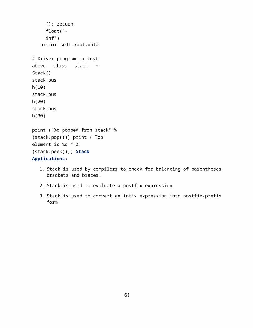
return float("-inf")temp = self.root self.root = self.root.next popped = temp.data return popped
def peek(self):if self.isEmpty():
return float("-inf")return self.root.data
# Driver program to test above class stack = Stack()stack.push(10) stack.push(20) stack.push(30)
print ("%d popped from stack" %(stack.pop())) print ("Top element is %d " %(stack.peek())) Stack Applications:
1. Stack is used by compilers to check for balancing of parentheses, brackets and braces.
2. Stack is used to evaluate a postfix expression.
3. Stack is used to convert an infix expression into postfix/prefix form.
36
4. In recursion, all intermediate arguments and return values are stored on the processor‟s stack.
5. During a function call the return address and arguments are pushed onto a stack and on return they are popped off.
6. Depth first search uses a stack data structure to find an element from a graph.
In-fix- to Postfix Transformation:
Procedure:
Procedure to convert from infix expression to postfix expression is as follows:
1. Scan the infix expression from left to right.
2. a) If the scanned symbol is left parenthesis, push it onto the stack.
b) If the scanned symbol is an operand, then place directly in the postfix expression (output).
c) If the symbol scanned is a right parenthesis, then go on popping all the items from the stack and place them in the postfix expression till we get the matching left parenthesis.
d) If the scanned symbol is an operator, then go on removing all the operators from the stack and place them in the postfix expression, if and only if the precedence of the operator which is on the top of the stack is greater than (or equal) to the precedence of the scanned operator and push the scanned operator onto the stack otherwise, push the scanned operator onto the stack.
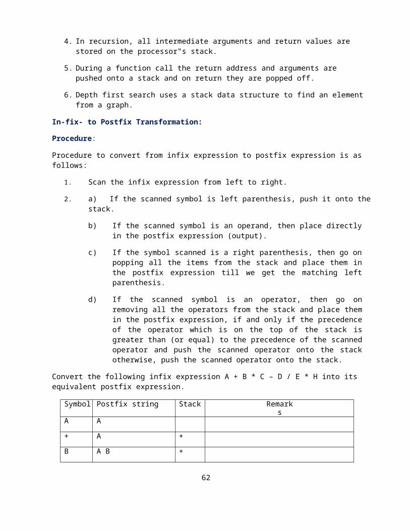
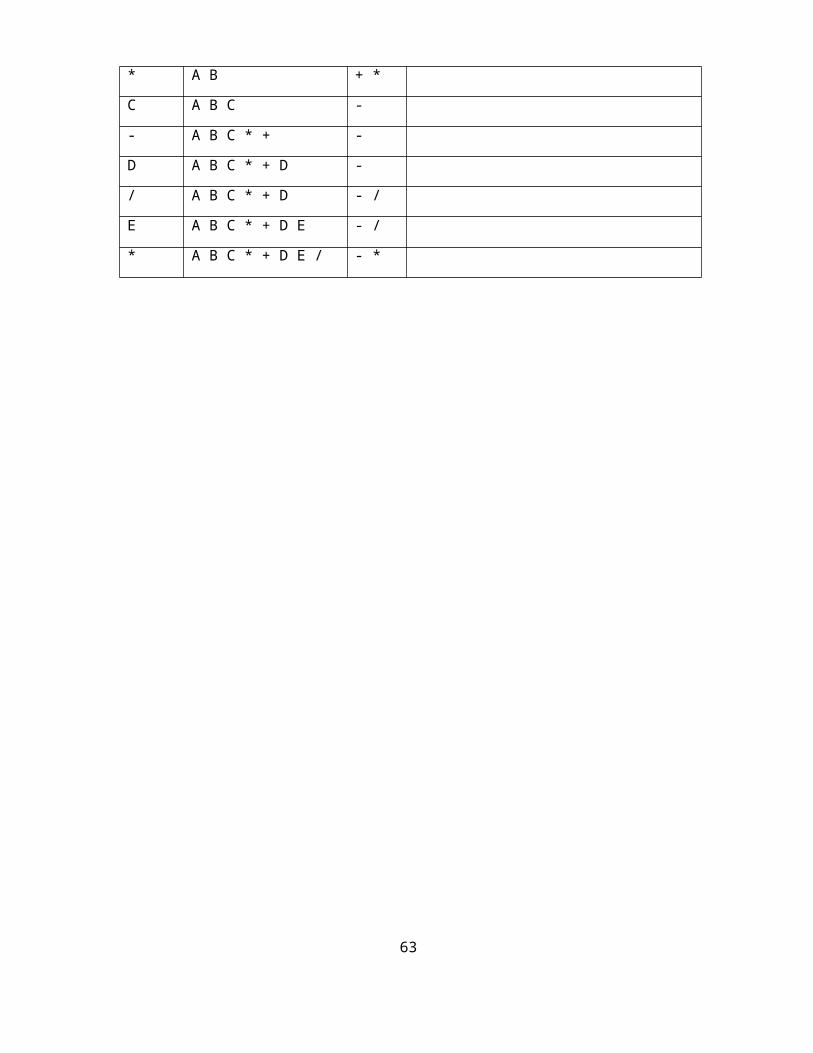
Convert the following infix expression A + B * C – D / E * H into its equivalent postfix expression.
Symbol Postfix string Stack Remarks
A A
+ A +
B A B +
* A B + *
C A B C -
- A B C * + -
D A B C * + D -
/ A B C * + D - /
E A B C * + D E - /
* A B C * + D E / - *
37
H A B C * + D E / H - *
End of string A B C * + D E / H * -
The input is now empty. Pop the output symbols from the stack until it is empty.
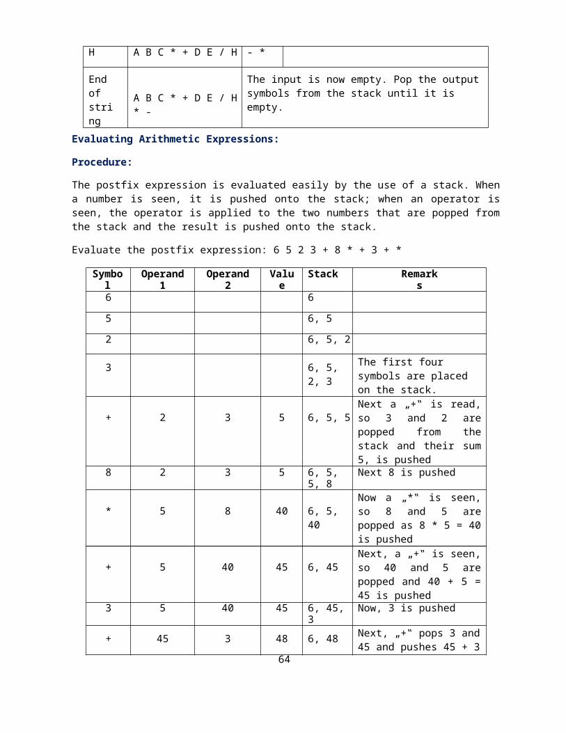
Evaluating Arithmetic Expressions:
Procedure:
The postfix expression is evaluated easily by the use of a stack. When a number is seen, it is pushed onto the stack; when an operator is seen, the operator is applied to the two numbers that are popped from the stack and the result is pushed onto the stack.
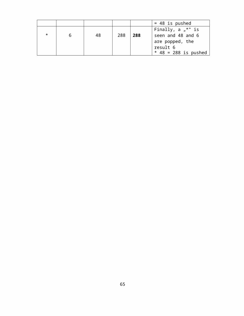
Evaluate the postfix expression: 6 5 2 3 + 8 * + 3 + *
Symbol Operand 1 Operand 2 Value Stack Remarks
6 6
5 6, 5
2 6, 5, 2
3 6, 5, 2, 3 The first four symbols are placed on the stack.
+ 2 3 5 6, 5, 5Next a „+‟ is read, so 3 and 2 are popped from the stack and their sum 5, is pushed
8 2 3 5 6, 5, 5, 8 Next 8 is pushed
* 5 8 40 6, 5, 40Now a „*‟ is seen, so 8 and 5 are popped as 8 * 5 = 40 is pushed
+ 5 40 45 6, 45Next, a „+‟ is seen, so 40 and 5 are popped and 40 + 5 = 45 is pushed
3 5 40 45 6, 45, 3 Now, 3 is pushed
+ 45 3 48 6, 48 Next, „+‟ pops 3 and 45 and pushes 45 + 3 = 48 is pushed
* 6 48 288 288Finally, a „*‟ is seen and 48 and 6 are popped, the result 6* 48 = 288 is pushed
38
Basic Queue Operations:
A queue is a data structure that is best described as "first in, first out". A queue is another special kind of list, where items are inserted at one end called the rear and deleted at the other end called the front. A real world example of a queue is people waiting in line at the bank. As each person enters the bank, he or she is "enqueued" at the back of the line. When a teller becomes available, they are "dequeued" at the front of the line.
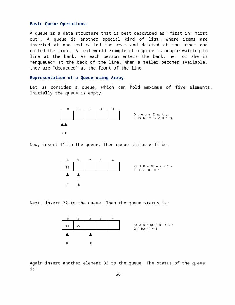
Representation of a Queue using Array:
Let us consider a queue, which can hold maximum of five elements. Initially the queue is empty.
0 1 2 3 4
F R
Q u e u e E mp t yF RO NT = RE A R = 0
Now, insert 11 to the queue. Then queue status will be:
0 1 2 3 4
11
F R
RE A R = RE A R + 1 = 1 F RO NT = 0
Next, insert 22 to the queue. Then the queue status is:
0 1 2 3 4
11 22
F R
RE A R = RE A R + 1 = 2 F RO NT = 0
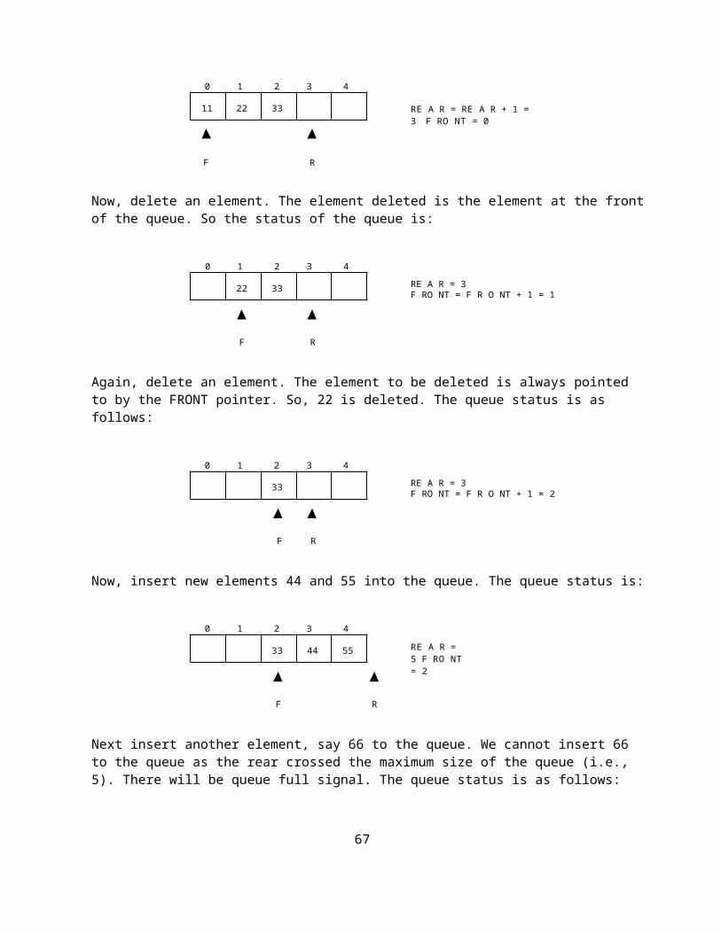
Again insert another element 33 to the queue. The status of the queue is:
39
0 1 2 3 4
11 22 33
F R
RE A R = RE A R + 1 = 3 F RO NT = 0
Now, delete an element. The element deleted is the element at the front of the queue. So the status of the queue is:
0 1 2 3 4
22 33
F R
RE A R = 3F RO NT = F R O NT + 1 = 1
Again, delete an element. The element to be deleted is always pointed to by the FRONT pointer. So, 22 is deleted. The queue status is as follows:
0 1 2 3 4
33
F R
RE A R = 3F RO NT = F R O NT + 1 = 2
Now, insert new elements 44 and 55 into the queue. The queue status is:
0 1 2 3 4
33 44 55
F R
RE A R = 5 F RO NT = 2
Next insert another element, say 66 to the queue. We cannot insert 66 to the queue as the rear crossed the maximum size of the queue (i.e., 5). There will be queue full signal. The queue status is as follows:
40
0 1 2 3 4
33 44 55
F R
RE A R = 5 F RO NT = 2
Now it is not possible to insert an element 66 even though there are two vacant positions in the linear queue. To over come this problem the elements of the queue are to be shifted towards the beginning of the queue so that it creates vacant position at the rear end. Then the FRONT and REAR are to be adjusted properly. The element 66 can be inserted at the rear end. After this operation, the queue status is as follows:
0 1 2 3 4RE A R = 4 F RO NT = 0
F R
This difficulty can overcome if we treat queue position with index 0 as a position that comes after position with index 4 i.e., we treat the queue as a circular queue.
Procedure for Queue operations using array:
In order to create a queue we require a one dimensional array Q(1:n) and two variables front and rear. The conventions we shall adopt for these two variables are that front is always 1 less than the actual front of the queue and rear always points to the last element in the queue. Thus, front = rear if and only if there are no elements in the queue. The initial condition then is front = rear = 0.
The various queue operations to perform creation, deletion and display the elements in a queue are as follows:
1. insertQ(): inserts an element at the end of queue Q.
2. deleteQ(): deletes the first element of Q.
3. displayQ(): displays the elements in the queue.
Linked List Implementation of Queue: We can represent a queue as a linked list. In a queue data is deleted from the front end and inserted at the rear end. We can perform similar operations on the two ends of a list. We use two pointers front and rear for our linked queue implementation.
33 44 55 66
41
Source Code:
front = 0
rear = 0
mymax = 3
# Function to create a stack. It initializes size of stack as 0
def createQueue():
queue = []
return queue
# Stack is empty when stack size is 0
def isEmpty(queue):
return len(queue) == 0
# Function to add an item to stack. It increases size by 1
def enqueue(queue,item):
queue.append(item)
# Function to remove an item from stack. It decreases size by 1
def dequeue(queue):
if (isEmpty(queue)):
return "Queue is
empty"
item=queue[0]
del queue[0]
return item
# Driver program to test above functions
queue = createQueue()
while True:
print("1 Enqueue")
print("2 Dequeue")
print("3 Display")
print("4 Quit")
42
ch=int(input("Enter choice"))
if(ch==1):
if(rear < mymax):
item=input("enter item")
enqueue(queue, item)
rear = rear + 1
else:
print("Queue is full")
elif(ch==2):
print(dequeue(queue))
elif(ch==3):
print(queue)
else:
break
Applications of Queues:
1. It is used to schedule the jobs to be processed by the CPU.
2. When multiple users send print jobs to a printer, each printing job is kept in the printing queue. Then the printer prints those jobs according to first in first out (FIFO) basis.
3. Breadth first search uses a queue data structure to find an element from a graph.
Disadvantages of Linear Queue:
There are two problems associated with linear queue. They are:
Time consuming: linear time to be spent in shifting the elements to the beginning of the queue.
Signaling queue full: even if the queue is having vacant position.
Round Robin Algorithm:
The round-robin (RR) scheduling algorithm is designed especially for time-sharing systems. It is similar to FCFS scheduling, but pre-emption is added to switch between processes. A small unit of time, called a time quantum or time slices, is defined. A time quantum is generally from 10 to 100 milliseconds. The ready queue is treated as a circular queue. To implement RR scheduling
We keep the ready queue as a FIFO queue of processes.
New processes are added to the tail of the ready queue.
43
The CPU scheduler picks the first process from the ready queue, sets a timer to interrupt after 1 time quantum, and dispatches the process.
The process may have a CPU burst of less than 1 time quantum.
o In this case, the process itself will release the CPU voluntarily.
o The scheduler will then proceed to the next process in the ready queue.
Otherwise, if the CPU burst of the currently running process is longer than 1 time quantum,
o The timer will go off and will cause an interrupt to the OS.
o A context switch will be executed, and the process will be put at the tail of the ready queue.
o The CPU scheduler will then select the next process in the ready queue.
The average waiting time under the RR policy is often long. Consider the following set of processes that arrive at time 0, with the length of the CPU burst given in milliseconds: (a time quantum of 4 milliseconds)
Burst Waiting Turnaround
Process Time Time Time
24 6 30
3 4 7
3 7 10
Average - 5.66 15.66
Using round-robin scheduling, we would schedule these processes according to the following chart:
44
DEQUE(Double Ended Queue):
A double-ended queue (dequeue, often abbreviated to deque, pronounced deck) generalizes a queue, for which elements can be added to or removed from either the front (head) or back (tail).It is also often called a head-tail linked list. Like an ordinary queue, a double-ended queue is a data structure it supports the following operations: enq_front, enq_back, deq_front, deq_back, and empty. Dequeue can be behave like a queue by using only enq_front and deq_front , and behaves like a stack by using only enq_front and deq_rear.
The DeQueue is represented as follows.
DEQUE can be represented in two ways they are
1) Input restricted DEQUE(IRD)
2) output restricted DEQUE(ORD)
The output restricted DEQUE allows deletions from only one end and input restricted DEQUE allow insertions at only one end. The DEQUE can be constructed in two ways they are
1) Using array
2)Using linked list
Operations in DEQUE
1. Insert element at back
2. Insert element at front
3. Remove element at front
4. Remove element at back
45
46
Applications of DEQUE:
1. The A-Steal algorithm implements task scheduling for several processors (multiprocessor scheduling).
2. The processor gets the first element from the deque.
3. When one of the processor completes execution of its own threads it can steal a thread from another processor.
4. It gets the last element from the deque of another processor and executes it.
Circular Queue:
Circular queue is a linear data structure. It follows FIFO principle. In circular queue the last node is connected back to the first node to make a circle.
Circular linked list fallow the First In First Out principle
Elements are added at the rear end and the elements are deleted at front end of the queue
Both the front and the rear pointers points to the beginning of the array.
It is also called as “Ring buffer”.
Items can inserted and deleted from a queue in O(1)
time. Circular Queue can be created in three ways they are
1. Using single linked list
2. Using double linked list
3. Using arrays
47
Representation of Circular Queue:
Let us consider a circular queue, which can hold maximum (MAX) of six elements. Initially the queue is empty.
F R
1 Q u e u e E mp t y4 M A X = 6
F RO NT = RE A R = 0 C O U NT = 0
C irc u lar Q u e u e
Now, insert 11 to the circular queue. Then circular queue status will be:
F
R
F RO NT = 04 RE A R = ( RE A R + 1) % 6 = 1
C O U NT = 1
C irc u lar Q u e u e
Insert new elements 22, 33, 44 and 55 into the circular queue. The circular queue status is:
FR
50
11
4 55 22 1 F RO NT = 0, RE A R = 5 RE A R = RE A R % 6 = 5 C O U NT = 5
44 33
3 2
C irc u lar Q u e u e
Now, delete an element. The element deleted is the element at the front of the circular queue. So, 11 is deleted. The circular queue status is as follows:
23
05
23
1
11
05
48
R
F
F RO NT = (F R O NT + 1) % 6 = 14 RE A R = 5
C O U NT = C O U NT - 1 = 4
C irc u lar Q u e u e
Again, delete an element. The element to be deleted is always pointed to by the FRONT pointer. So, 22 is deleted. The circular queue status is as follows:
R
F RO NT = (F R O NT + 1) % 6 = 24 RE A R = 5
C O U NT = C O U NT - 1 = 3
F
C irc u lar Q u e u e
Again, insert another element 66 to the circular queue. The status of the circular queue is:
R
4 F RO NT = 2RE A R = ( RE A R + 1) % 6 = 0 C O U NT = C O U NT + 1 = 4
F
C irc u lar Q u e u e
Now, insert new elements 77 and 88 into the circular queue. The circular queue status is:
23
33 44
22 155
05
23
33 44
155
05
23
33 44
155
66
05
49
5 0
66 77
4 55
3
88 1
44 33 2 R
F
F RO NT = 2, RE A R = 2 RE A R = RE A R % 6 = 2 C O U NT = 6
C irc u lar Q u e u e
Now, if we insert an element to the circular queue, as COUNT = MAX we cannot add the element to circular queue. So, the circular queue is full.
55
UNIT-3 LINKED LISTS
Linked lists and arrays are similar since they both store collections of data. Array is the most common data structure used to store collections of elements. Arrays are convenient to declare and provide the easy syntax to access any element by its index number. Once the array is set up, access to any element is convenient and fast.
The disadvantages of arrays are:
• The size of the array is fixed. Most often this size is specified at compile time. This makes the programmers to allocate arrays, which seems "large enough" than required.
• Inserting new elements at the front is potentially expensive because existing elements need to be shifted over to make room.
• Deleting an element from an array is not possible. Linked lists have their own strengths and weaknesses, but they happen to be strong where arrays are weak.
Generally array's allocates the memory for all its elements in one block whereas linked lists use an entirely different strategy. Linked lists allocate memory for each element separately and only when necessary.
Linked List Concepts:
A linked list is a non-sequential collection of data items. It is a dynamic data structure. For every data item in a linked list, there is an associated pointer that would give the memory location of the next data item in the linked list. The data items in the linked list are not in consecutive memory locations. They may be anywhere, but the accessing of these data items is easier as each data item contains the address of the next data item.
Advantages of linked lists:
Linked lists have many advantages. Some of the very important advantages are:
1. Linked lists are dynamic data structures. i.e., they can grow or shrink during the execution of a program.
2. Linked lists have efficient memory utilization. Here, memory is not preallocated. Memory is allocated whenever it is required and it is de-allocated (removed) when it is no longer needed.
3. Insertion and Deletions are easier and efficient. Linked lists provide flexibility in inserting a data item at a specified position and deletion of the data item from the given position.
4. Many complex applications can be easily carried out with linked lists.
Disadvantages of linked lists:
1. It consumes more space because every node requires a additional pointer to store address of the next node.
2. Searching a particular element in list is difficult and also time consuming.
Types of Linked Lists:
Basically we can put linked lists into the following four items:
1. Single Linked List.2. Double Linked List.3. Circular Linked List.
56
4. Circular Double Linked List.
A single linked list is one in which all nodes are linked together in some sequential manner. Hence, it is also called as linear linked list.
A double linked list is one in which all nodes are linked together by multiple links which helps in accessing both the successor node (next node) and predecessor node (previous node) from any arbitrary node within the list. Therefore each node in a double linked list has two link fields (pointers) to point to the left node (previous) and the right node (next). This helps to traverse in forward direction and backward direction.
A circular linked list is one, which has no beginning and no end. A single linked list can be made a circular linked list by simply storing address of the very first node in the link field of the last node.
A circular double linked list is one, which has both the successor pointer and predecessor pointer in the circular manner.
57
Applications of linked list:
1. Linked lists are used to represent and manipulate polynomial. Polynomials are expression containing terms with non zero coefficient and exponents. For example: P(x) = a0 Xn + a1 Xn-1 + …… + an-1 X + an
2. Represent very large numbers and operations of the large number such as addition, multiplication and division.
3. Linked lists are to implement stack, queue, trees and graphs. 4. Implement the symbol table in compiler construction.
Single Linked List:
A linked list allocates space for each element separately in its own block of memory called a "node". The list gets an overall structure by using pointers to connect all its nodes together like the links in a chain. Each node contains two fields; a "data" field to store whatever element, and a "next" field which is a pointer used to link to the next node. Each node is allocated in the heap using malloc(), so the node memory continues to exist until it is explicitly de-allocated using free(). The front of the list is a pointer to the “start” node.
A single linked list
The beginning of the linked list is stored in a "start" pointer which points to the first node. The first node contains a pointer to the second node. The second node contains a pointer to the third node, ... and so on. The last node in the list has its next field set to NULL to mark the end of the list. Code can access any node in the list by starting at the start and following the next pointers.
The start pointer is an ordinary local pointer variable, so it is drawn separately on the left top to show that it is in the stack. The list nodes are drawn on the right to show that they are allocated in the heap.
The basic operations in a single linked list are:
• Creation.
• Insertion.
• Deletion.
• Traversing.
Creating a node for Single Linked List:
Creating a singly linked list starts with creating a node. Sufficient memory has to be allocated for creating a node. The information is stored in the memory.
58
Insertion of a Node:
One of the most primitive operations that can be done in a singly linked list is the insertion of a node. Memory is to be allocated for the new node (in a similar way that is done while creating a list) before reading the data. The new node will contain empty data field and empty next field. The data field of the new node is then stored with the information read from the user. The next field of the new node is assigned to NULL. The new node can then be inserted at three different places namely:
• Inserting a node at the beginning.
• Inserting a node at the end.
• Inserting a node at intermediate position.
Inserting a node at the beginning.
Inserting a node at the end:
59
Inserting a node into the single linked list at a specified intermediate position other than beginning and end.
Deletion of a node:
Another primitive operation that can be done in a singly linked list is the deletion of a node. Memory is to be released for the node to be deleted. A node can be deleted from the list from three different places namely.
• Deleting a node at the beginning.
• Deleting a node at the end.
• Deleting a node at intermediate position.
Deleting a node at the beginning:
60
Deleting a node at the end:
Deleting a node at Intermediate position:
The following steps are followed, to delete a node from an intermediate position in the list (List must contain more than two node).
Traversal and displaying a list (Left to Right):
To display the information, you have to traverse (move) a linked list, node by node from the first node, until the end of the list is reached.
Traversing a list involves the following steps:
• Assign the address of start pointer to a temp pointer.
• Display the information from the data field of each node. The function traverse () is used for traversing and displaying the information stored in the list from left to right.
Using a header node:
A header node is a special dummy node found at the front of the list. The use of header node is an alternative to remove the first node in a list. For example, the picture below shows how the list with data 10, 20 and 30 would be represented using a linked list without and with a header node:
61
Note that if your linked lists do include a header node, there is no need for the special case code given above for the remove operation; node n can never be the first node in the list, so there is no need to check for that case. Similarly, having a header node can simplify the code that adds a node before a given node n.
Note that if you do decide to use a header node, you must remember to initialize an empty list to contain one (dummy) node, you must remember not to include the header node in the count of "real" nodes in the list.
It is also useful when information other than that found in each node of the list is needed. For example, imagine an application in which the number of items in a list is often calculated. In a standard linked list, the list function to count the number of nodes has to traverse the entire list every time. However, if the current length is maintained in a header node, that information can be obtained very quickly. 3.5. Array based linked lists: Another alternative is to allocate the nodes in blocks. In fact, if you know the
62
maximum size of a list a head of time, you can pre-allocate the nodes in a single array. The result is a hybrid structure – an array based linked list.
shows an example of null terminated single linked list where all the nodes are allocated contiguously in an array.
Double Linked List: A double linked list is a two-way list in which all nodes will have two links. This helps in accessing both successor node and predecessor node from the given node position. It provides bi- directional traversing. Each node contains three fields:
Left link. Data. Right link.
The left link points to the predecessor node and the right link points to the successor node. The data field stores the required data.
Many applications require searching forward and backward thru nodes of a list. For example searching for a name in a telephone directory would need forward and backward scanning thru a region of the whole list.
The basic operations in a double linked list are:
Creation. Insertion. Deletion. Traversing.
63
A double linked list is shown in figure
The beginning of the double linked list is stored in a "start" pointer which points to the first node. The first node‟s left link and last node‟s right link is set to NULL.
Creating a node for Double Linked List:
Creating a double linked list starts with creating a node. Sufficient memory has to be allocated for creating a node. The information is stored in the memory.
Double Linked List with 3 nodes:
Inserting a node at the beginning:
Inserting a node at the end:
64
Inserting a node at an intermediate position:
Deleting a node at the beginning:
Deleting a node at the end:
Deleting a node at Intermediate position:
65
Traversal and displaying a list (Left to Right):
To display the information, you have to traverse the list, node by node from the first node, until the end of the list is reached. The function traverse_left_right() is used for traversing and displaying the information stored in the list from left to right.
Traversal and displaying a list (Right to Left):
To display the information from right to left, you have to traverse the list, node by node from the first node, until the end of the list is reached. The function traverse_right_left() is used for traversing and displaying the information stored in the list from right to left.
Circular Single Linked List:
It is just a single linked list in which the link field of the last node points back to the address of the first node. A circular linked list has no beginning and no end. It is necessary to establish a special pointer called start pointer always pointing to the first node of the list. Circular linked lists are frequently used instead of ordinary linked list because many operations are much easier to implement. In circular linked list no null pointers are used, hence all pointers contain valid address.
Creating a circular single Linked List with „n‟ number of nodes:
The basic operations in a circular single linked list are:
• Creation.
• Insertion.
• Deletion.
• Traversing.
66
Inserting a node at the beginning:
Inserting a node at the end:
Deleting a node at the beginning:
Deleting a node at the end:
67
Circular Double Linked List:
A circular double linked list has both successor pointer and predecessor pointer in circular manner. The objective behind considering circular double linked list is to simplify the insertion and deletion operations performed on double linked list. In circular double linked list the right link of the right most node points back to the start node and left link of the first node points to the last node.
A circular double linked list is shown in figure
Creating a Circular Double Linked List with „n‟ number of nodes
The basic operations in a circular double linked list are:
• Creation.
• Insertion.
• Deletion.
• Traversing.
Inserting a node at the beginning:
68
Inserting a node at the end:
Inserting a node at an intermediate position:
Deleting a node at the beginning:
69
Deleting a node at the end:
Deleting a node at Intermediate position:
Comparison of Linked List Variations:
The major disadvantage of doubly linked lists (over singly linked lists) is that they require more space (every node has two pointer fields instead of one). Also, the code to manipulate doubly linked lists needs to maintain the prev fields as well as the next fields; the more fields that have to be maintained, the more chance there is for errors.
The major advantage of doubly linked lists is that they make some operations (like the removal of a given node, or a right-to-left traversal of the list) more efficient.
The major advantage of circular lists (over non-circular lists) is that they eliminate some extra-case code for some operations (like deleting last node). Also, some applications lead naturally to circular list representations. For example, a computer network might best be modeled using a circular list.
Polynomials:
A polynomial is of the form: i n i ∑ ci
Where, ci is the coefficient of the ith term and
n is the degree of the polynomial
Some examples are:
5x2 + 3x + 1
12x3 – 4x
5x4 – 8x3 + 2x2 + 4x1 + 9x0
70
It is not necessary to write terms of the polynomials in decreasing order of degree. In other words the two polynomials 1 + x and x + 1 are equivalent.
The computer implementation requires implementing polynomials as a list of pairs of coefficient and exponent. Each of these pairs will constitute a structure, so a polynomial will be represented as a list of structures.
A linked list structure that represents polynomials 5x4 – 8x3 + 2x2 + 4x1 + 9x0
Addition of Polynomials:
To add two polynomials we need to scan them once. If we find terms with the same exponent in the two polynomials, then we add the coefficients; otherwise, we copy the term of larger exponent into the sum and go on. When we reach at the end of one of the polynomial, then remaining part of the other is copied into the sum.
To add two polynomials follow the following steps:
• Read two polynomials
• Add them.
• Display the resultant polynomial.
84
UNIT – IV NON LINEAR DATA STRUCTURESTrees Basic Concepts:
A tree is a non-empty set one element of which is designated the root of the tree while the remaining elements are partitioned into non-empty sets each of which is a sub-tree of the root.
A tree T is a set of nodes storing elements such that the nodes have a parent-child relationship that satisfies the following
• If T is not empty, T has a special tree called the root that has no parent.
• Each node v of T different than the root has a unique parent node w; each node with parent w is a child of w.
Tree nodes have many useful properties. The depth of a node is the length of the path (or the number of edges) from the root to that node. The height of a node is the longest path from that node to its leaves. The height of a tree is the height of the root. A leaf node has no children -- its only path is up to its parent.
Binary Tree:
In a binary tree, each node can have at most two children. A binary tree is either empty or consists of a node called the root together with two binary trees called the left subtree and the right subtree.
85
Tree Terminology:
Leaf node
A node with no children is called a leaf (or external node). A node which is not a leaf is called an internal node.
Path: A sequence of nodes n1, n2, . . ., nk, such that ni is the parent of ni + 1 for i = 1, 2,. . ., k - 1. The length of a path is 1 less than the number of nodes on the path. Thus there is a path of length zero from a node to itself.
Siblings: The children of the same parent are called siblings.
Ancestor and Descendent If there is a path from node A to node B, then A is called an ancestor of B and B is called a descendent of A.
Subtree: Any node of a tree, with all of its descendants is a subtree.
Level: The level of the node refers to its distance from the root. The root of the tree has level O, and the level of any other node in the tree is one more than the level of its parent.
The maximum number of nodes at any level is 2n.
Height:The maximum level in a tree determines its height. The height of a node in a tree is the length of a longest path from the node to a leaf. The term depth is also used to denote height of the tree.
Depth:The depth of a node is the number of nodes along the path from the root to that node.
Assigning level numbers and Numbering of nodes for a binary tree: The nodes of a binary tree can be numbered in a natural way, level by level, left to right. The nodes of a complete binary tree can be numbered so that the root is assigned the number 1, a left child is assigned twice the number assigned its parent, and a right child is assigned one more than twice the number assigned its parent.
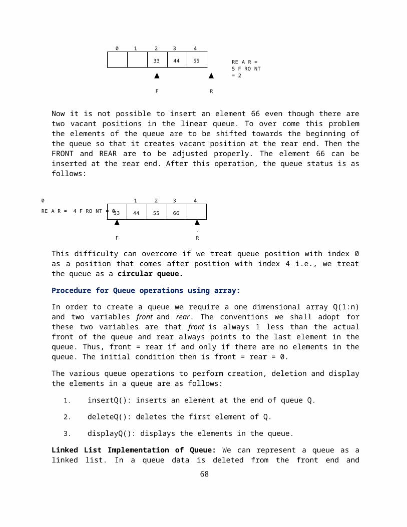
86
Properties of Binary Trees:
Some of the important properties of a binary tree are as follows:
1. If h = height of a binary tree, then
a. Maximum number of leaves = 2h
b. Maximum number of nodes = 2h + 1 - 1
2. If a binary tree contains m nodes at level l, it contains at most 2m nodes at level l + 1.
3. Since a binary tree can contain at most one node at level 0 (the root), it can contain at most 2l node at level l.
4. The total number of edges in a full binary tree with n node is n - 1.
Strictly Binary tree:
If every non-leaf node in a binary tree has nonempty left and right subtrees, the tree is termed a strictly binary tree. Thus the tree of figure 7.2.3(a) is strictly binary. A strictly binary tree with n leaves always contains 2n - 1 nodes.
Full Binary Tree:
A full binary tree of height h has all its leaves at level h. Alternatively; All non leaf nodes of a full binary tree have two children, and the leaf nodes have no children.
A full binary tree with height h has 2h + 1 - 1 nodes. A full binary tree of height h is a strictly binary tree all of whose leaves are at level h.
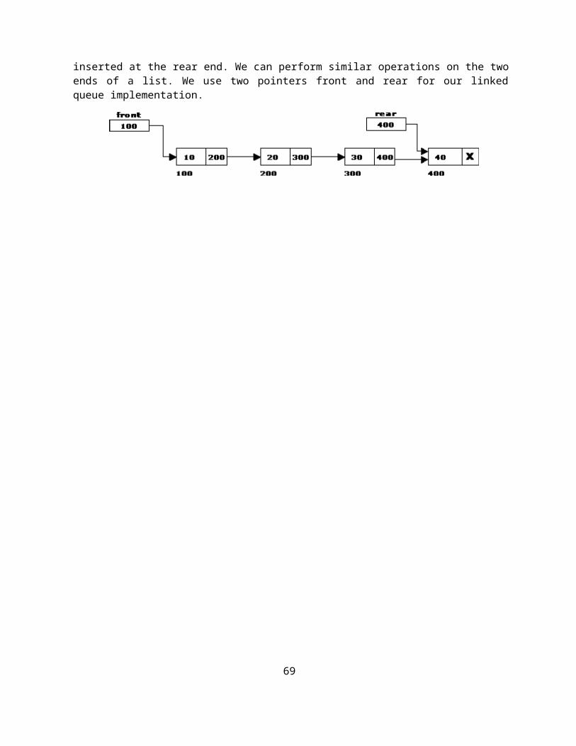
87
For example, a full binary tree of height 3 contains 23+1 – 1 = 15 nodes.
Complete Binary Tree:
A binary tree with n nodes is said to be complete if it contains all the first n nodes of the above numbering scheme.
A complete binary tree of height h looks like a full binary tree down to level h-1, and the level h is filled from left to right.
Perfect Binary Tree:
A Binary tree is Perfect Binary Tree in which all internal nodes have two children and all leaves are at same level.Following are examples of Perfect Binary Trees.
18
/ \
15 30
/ \ / \
40 50 100 40
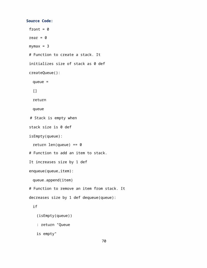
88
18
/ \
15 30
A Perfect Binary Tree of height h (where height is number of nodes on path from root to leaf) has 2 h – 1 node.
Example of Perfect binary tree is ancestors in family. Keep a person at root, parents as children, parents of parents as their children.
Balanced Binary Tree:
A binary tree is balanced if height of the tree is O(Log n) where n is number of nodes. For Example, AVL tree maintain O(Log n) height by making sure that the difference between heights of left and right subtrees is 1. Red-Black trees maintain O(Log n) height by making sure that the number of Black nodes on every root to leaf paths are same and there are no adjacent red nodes. Balanced Binary Search trees are performance wise good as they provide O(log n) time for search, insert and delete.
Representation of Binary Trees:
1. Array Representation of Binary Tree
2. Pointer-based.
Array Representation of Binary Tree:
A single array can be used to represent a binary tree.
For these nodes are numbered / indexed according to a scheme giving 0 to root. Then all the nodes are numbered from left to right level by level from top to bottom. Empty nodes are also numbered. Then each node having an index i is put into the array as its ith element.
In the figure shown below the nodes of binary tree are numbered according to the given scheme.
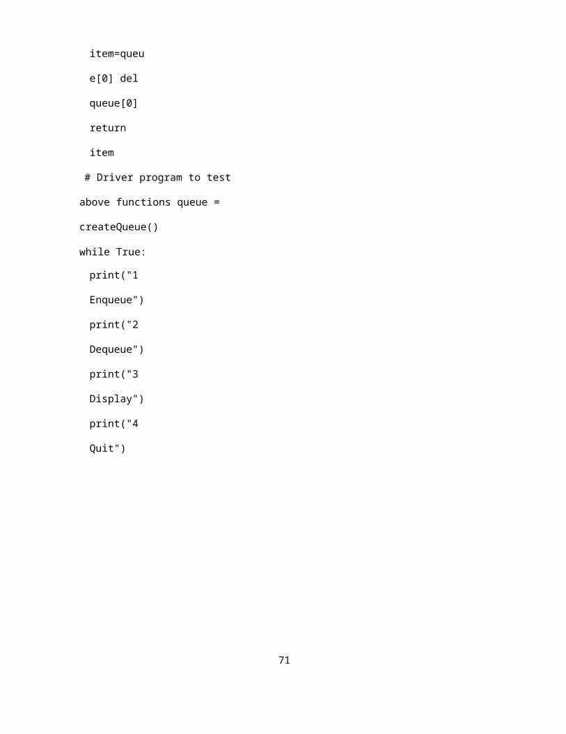
89
The figure shows how a binary tree is represented as an array. The root 3 is the 0 th element while its leftchild 5 is the 1 st element of the array. Node 6 does not have any child so its children i.e. 7 th and 8 th
element of the array are shown as a Null value.
It is found that if n is the number or index of a node, then its left child occurs at (2n + 1) th position and right child at (2n + 2) th position of the array. If any node does not have any of its child, then null value is stored at the corresponding index of the array.
The following program implements the above binary tree in an array form. And then traverses the tree in inorder traversal.
Linked Representation of Binary Tree (Pointer based):
Binary trees can be represented by links where each node contains the address of the left child and the right child. If any node has its left or right child empty then it will have in its respective link field, a null value. A leaf node has null value in both of its links.
Binary Tree Traversals:
Traversal of a binary tree means to visit each node in the tree exactly once. The tree traversal is used in all t it.
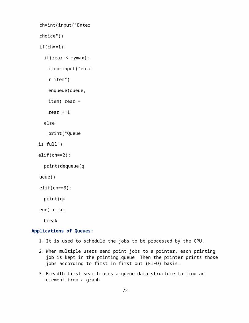
90
In a linear list nodes are visited from first to last, but a tree being a non linear one we need definite rules. Th ways to traverse a tree. All of them differ only in the order in which they visit the nodes.
The three main methods of traversing a tree are:
Inorder Traversal Preorder Traversal Postorder Traversal
In all of them we do not require to do anything to traverse an empty tree. All the traversal methods are basefunctions since a binary tree is itself recursive as every child of a node in a binary tree is itself a binary tree.
Inorder Traversal:
To traverse a non empty tree in inorder the following steps are followed recursively.
Visit the Root Traverse the left subtree Traverse the right subtree
The inorder traversal of the tree shown below is as follows.
Preorder Traversal:
Algorithm Pre-order(tree)
1. Visit the root.2. Traverse the left sub-tree, i.e., call Pre-order(left-sub-tree)3. Traverse the right sub-tree, i.e., call Pre-order(right-sub-tree)
Post-order Traversal:
Algorithm Post-order(tree)
1. Traverse the left sub-tree, i.e., call Post-order(left-sub-tree)
91
2. Traverse the right sub-tree, i.e., call Post-order(right-sub-tree)3. Visit the root.
Binary Search Tree:
Binary Search Tree, is a node-based binary tree data structure which has the following properties: The left sub-tree of a node contains only nodes with keys less than the node’s key. The right sub-tree of a node contains only nodes with keys greater than the node’s key. The left and right sub-tree each must also be a binary search tree.
There must be no duplicate nodes.
The above properties of Binary Search Tree provide an ordering among keys so that the operations like search, minimum and maximum can be done fast. If there is no ordering, then we may have to compare every key to search a given key.
Searching a keyTo search a given key in Binary Search Tree, we first compare it with root, if the key is present at root, we return root. If key is greater than root’s key, we recur for right sub-tree of root node. Otherwise we recur for left sub-tree.
Priority Queues
Priority Queue is an extension of queue with following properties.1) Every item has a priority associated with it.2) An element with high priority is dequeued before an element with low priority.3) If two elements have the same priority, they are served according to their order in the queue.
A typical priority queue supports following operations. insert(item, priority): Inserts an item with given priority. getHighestPriority(): Returns the highest priority item. deleteHighestPriority(): Removes the highest priority item.
Implementation priority queue
Using Array: A simple implementation is to use array of following structure.
insert() operation can be implemented by adding an item at end of array in O(1) time.
getHighestPriority() operation can be implemented by linearly searching the highest priority item in
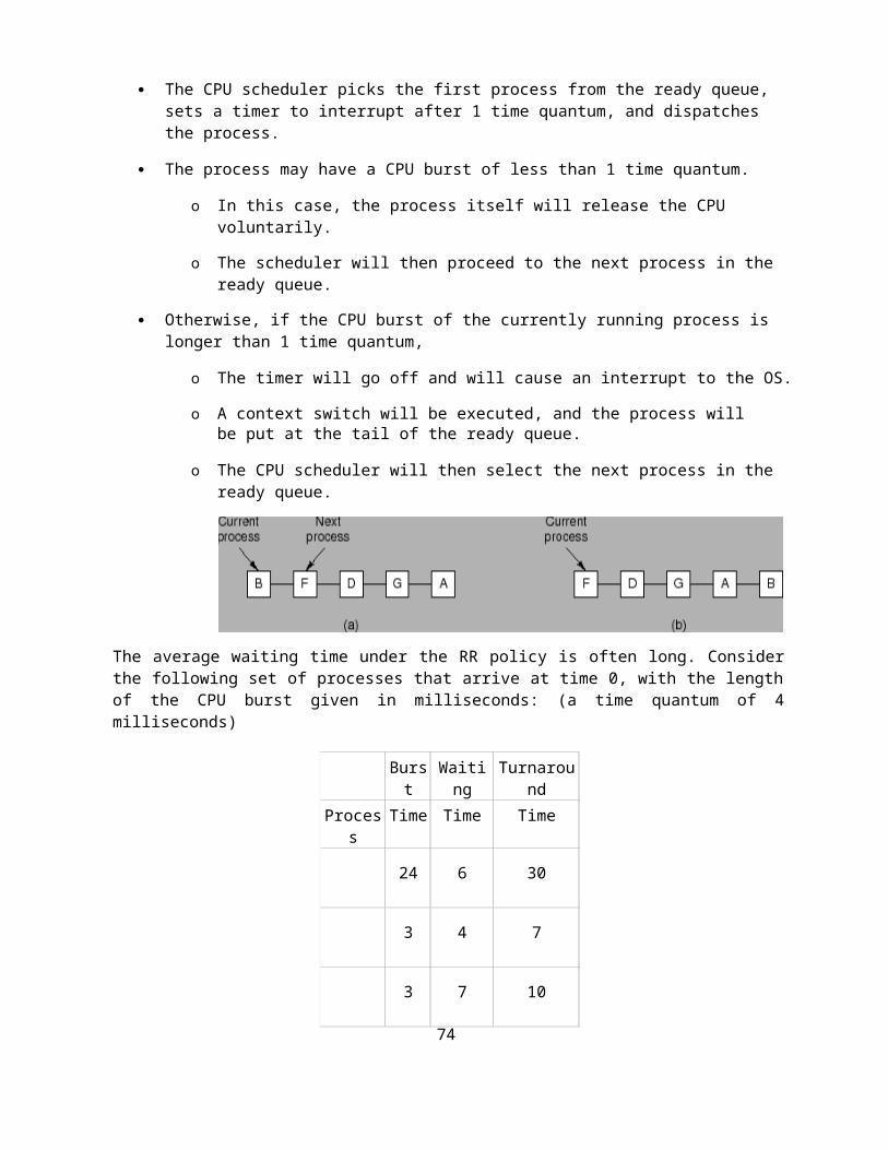
92
array. This operation takes O(n) time.
deleteHighestPriority() operation can be implemented by first linearly searching an item, then removing the item by moving all subsequent items one position back.
We can also use Linked List, time complexity of all operations with linked list remains same as array. The advantage with linked list is deleteHighestPriority() can be more efficient as we don’t have to move items.
Applications of Priority Queue:1) CPU Scheduling2) Graph algorithms like Dijkstra’s shortest path algorithm, Prim’s Minimum Spanning Tree, etc3) All queue applications where priority is involved.
Application of Trees:
1. One reason to use trees might be because you want to store information that naturally forms a hierarchy. For example, the file system on a computer:
file system———–
/ <-- root
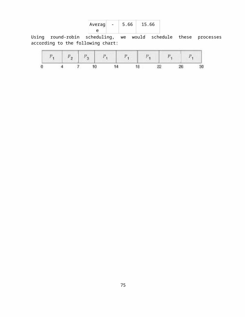
93
/ \... home
/ \ugrad course/ / | \
... cs101 cs112 cs113
2. If we organize keys in form of a tree (with some ordering e.g., BST), we can search for a given key in moderate time (quicker than Linked List and slower than arrays). Self-balancing search trees like AVL and Red-Black trees guarantee an upper bound of O(logn) for search.
3) We can insert/delete keys in moderate time (quicker than Arrays and slower than Unordered Linked Lists). Self-balancing search trees like AVL and Red-Black trees guarantee an upper bound of O(logn) for insertion/deletion.
4) Like Linked Lists and unlike Arrays, Pointer implementation of trees don’t have an upper limit on number of nodes as nodes are linked using pointers.
The following are the common uses of tree.1. Manipulate hierarchical data.2. Make information easy to search (see tree traversal).3. Manipulate sorted lists of data.4. As a workflow for compositing digital images for visual effects.5. Router algorithmsBasic Graph Concepts:
Graph is a data structure that consists of following two components:1. A finite set of vertices also called as nodes.2. A finite set of ordered pair of the form (u, v) called as edge.
The pair is ordered because (u, v) is not same as (v, u) in case of directed graph (di-graph). The pair of form (u, v) indicates that there is an edge from vertex u to vertex v. The edges may contain weight/value/cost.
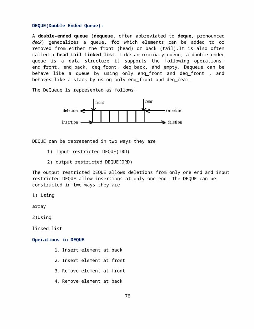
94
Graph and its representations:
Graphs are used to represent many real life applications: Graphs are used to represent networks. The networks may include paths in a city or telephone network or circuit network. Graphs are also used in social networks like linkedIn, facebook. For example, in facebook, each person is represented with a vertex(or node). Each node is a structure and contains information like person id, name, gender and locale.
Following is an example undirected graph with 5 vertices.
Following two are the most commonly used representations of graph.1. Adjacency Matrix2. Adjacency List
There are other representations also like, Incidence Matrix and Incidence List. The choice of the graph representation is situation specific. It totally depends on the type of operations to be performed and ease of use.
Adjacency Matrix:
Adjacency Matrix is a 2D array of size V x V where V is the number of vertices in a graph. Let the 2D array be adj[][], a slot adj[i][j] = 1 indicates that there is an edge from vertex i to vertex j. Adjacency matrix for undirected graph is always symmetric. Adjacency Matrix is also used to represent weighted graphs. If adj[i][j] = w, then there is an edge from vertex i to vertex j with weight w.
The adjacency matrix for the above example graph is:
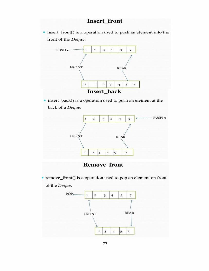
100
Adjacency Matrix Representation of the above graph
Pros: Representation is easier to implement and follow. Removing an edge takes O(1) time. Queries like whether there is an edge from vertex ‘u’ to vertex ‘v’ are efficient and can be done O(1).
Cons: Consumes more space O(V^2). Even if the graph is sparse (contains less number of edges), it consumes the same space. Adding a vertex is O(V^2) time.
Adjacency List:
An array of linked lists is used. Size of the array is equal to number of vertices. Let the array be array[]. An entry array[i] represents the linked list of vertices adjacent to the ith vertex. This representation can also be used to represent a weighted graph. The weights of edges can be stored in nodes of linked lists. Following is adjacency list representation of the above graph.
Adjacency List Representation of the above Graph
Breadth First Traversal for a Graph
Breadth First Traversal (or Search) for a graph is similar to Breadth First Traversal of a tree The only catch here is, unlike trees, graphs may contain cycles, so we may come to the same node again. To avoid processing a node more than once, we use a boolean visited array.
For example, in the following graph, we start traversal from vertex 2. When we come to vertex 0, we look for all adjacent vertices of it. 2 is also an adjacent vertex of 0. If we don’t mark visited vertices, then 2 will be processed again and it will become a non-terminating process. Breadth First Traversal of the following graph is 2, 0, 3, 1.
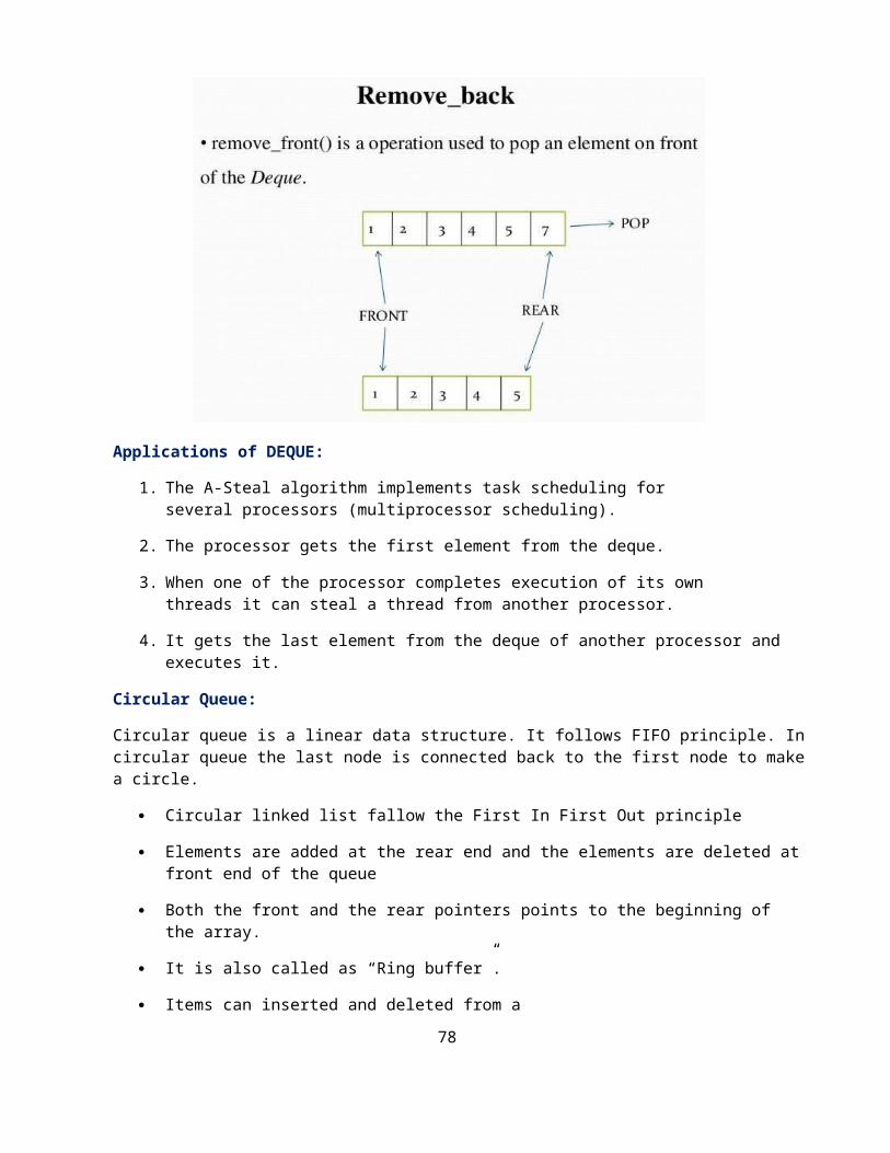
101
Algorithm: Breadth-First Search Traversal
BFS(V, E, s)
for each u in V − {s}
do color[u] ← WHITE d[u] ← infinity π[u] ← NIL color[s] ← GRAY
d[s] ← 0 π[s] ← NIL Q ← {}ENQUEUE(Q, s)
while Q is non-emptydo u ← DEQUEUE(Q)
for each v adjacent to udo if color[v] ← WHITE
then color[v] ← GRAY d[v] ← d[u] + 1
π[v] ← uENQUEUE(Q, v)
DEQUEUE(Q)color[u] ← BLACK
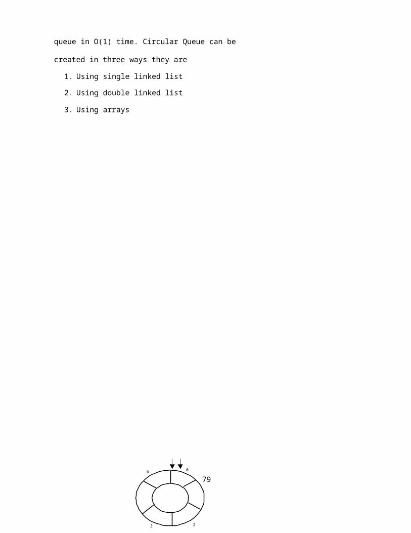
102
Applications of Breadth First Traversal
1) Shortest Path and Minimum Spanning Tree for unweighted graph In unweighted graph, the shortest path is the path with least number of edges. With Breadth First, we always reach a vertex from given source using minimum number of edges. Also, in case of unweighted graphs, any spanning tree is Minimum Spanning Tree and we can use either Depth or Breadth first traversal for finding a spanning tree.
2) Peer to Peer Networks. In Peer to Peer Networks like BitTorrent, Breadth First Search is used to find all neighbor nodes.
3) Crawlers in Search Engines: Crawlers build index using Bread First. The idea is to start from source page and follow all links from source and keep doing same. Depth First Traversal can also be used for crawlers, but the advantage with Breadth First Traversal is, depth or levels of built tree can be limited.
4) Social Networking Websites: In social networks, we can find people within a given distance ‘k’ from a person using Breadth First Search till ‘k’ levels.
5) GPS Navigation systems: Breadth First Search is used to find all neighboring locations.
6) Broadcasting in Network: In networks, a broadcasted packet follows Breadth First Search to reach all nodes.
7) In Garbage Collection: Breadth First Search is used in copying garbage collection using Cheney’s algorithm.
8) Cycle detection in undirected graph: In undirected graphs, either Breadth First Search or Depth First Search can be used to detect cycle. In directed graph, only depth first search can be used.
9) Ford–Fulkerson algorithm In Ford-Fulkerson algorithm, we can either use Breadth First or Depth First Traversal to find the maximum flow. Breadth First Traversal is preferred as it reduces worst case time complexity to O(VE2).
10) To test if a graph is Bipartite We can either use Breadth First or Depth First Traversal.
11) Path Finding We can either use Breadth First or Depth First Traversal to find if there is a path between two vertices.
12) Finding all nodes within one connected component: We can either use Breadth First or Depth First Traversal to find all nodes reachable from a given node.
Depth First Traversal for a Graph
Depth First Traversal (or Search) for a graph is similar to Depth First Traversal of a tree. The only catch here is, unlike trees, graphs may contain cycles, so we may come to the same node again. To avoid processing a node more than once, we use a boolean visited array. For example, in the following graph, we start traversal from vertex 2. When we come to vertex 0, we look for all adjacent vertices of it. 2 is also an adjacent vertex of 0. If we don’t mark visited vertices, then 2 will be processed again and it will become a non-terminating process. Depth First Traversal of the
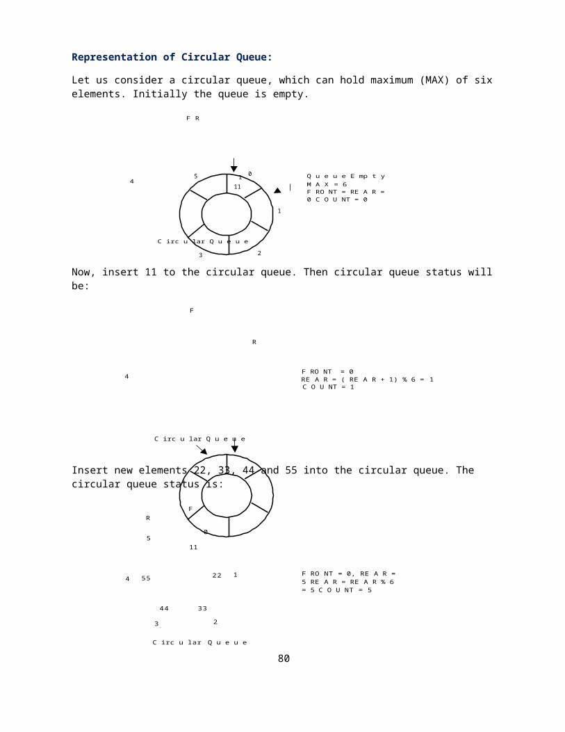
103
following graph is 2, 0, 1, 3
Algorithm Depth-First Search
The DFS forms a depth-first forest comprised of more than one depth-first trees. Each tree is made of edges (u, v) such that u is gray and v is white when edge (u, v) is explored. The following pseudocode for DFS uses a global timestamp time.
DFS (V, E)
for each vertex u in V[G]do color[u] ← WHITE
π[u] ← NILtime ← 0
for each vertex u in V[G]do if color[u] ← WHITE
then DFS-Visit(u)
DFS-Visit(u)
color[u] ← GRAY time ← time + 1 d[u] ← timefor each vertex v adjacent to u
do if color[v] ← WHITEthen π[v] ← u
DFS-Visit(v) color[u] ← BLACK time ← time + 1f[u] ← time
Applications of Depth First Search
Depth-first search (DFS) is an algorithm (or technique) for traversing a graph.
Following are the problems that use DFS as a building block.
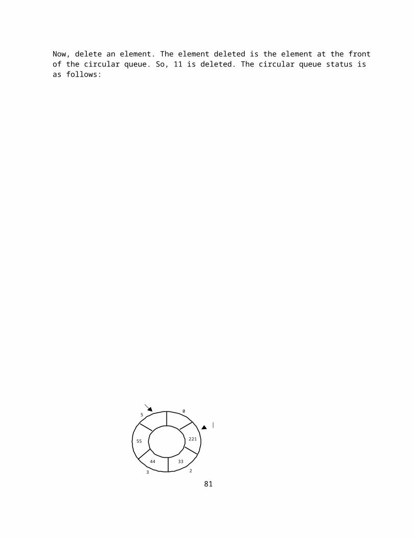
104
1) For an unweighted graph, DFS traversal of the graph produces the minimum spanning tree and all pair shortest path tree.
2) Detecting cycle in a graphA graph has cycle if and only if we see a back edge during DFS. So we can run DFS for the graph and check for back edges. (See this for details)
3) Path FindingWe can specialize the DFS algorithm to find a path between two given vertices u and z.i) Call DFS(G, u) with u as the start vertex.ii) Use a stack S to keep track of the path between the start vertex and the current vertex.iii) As soon as destination vertex z is encountered, return the path as the contents of the stack
4) Topological Sorting
5) To test if a graph is bipartiteWe can augment either BFS or DFS when we first discover a new vertex, color it opposite its parents, and for each other edge, check it doesn’t link two vertices of the same color. The first vertex in any connected component can be red or black! See this for details.
6) Finding Strongly Connected Components of a graph A directed graph is called strongly connected if there is a path from each vertex in the graph to every other vertex. (See this for DFS based also for finding Strongly Connected Components)
C program to implement the Graph Traversal(a) Breadth first traversal(b) Depth first traversal
DFS search starts from root node then traversal into left child node and continues, if item found it stops otherwise it continues. The advantage of DFS is it requires less memory compare to Breadth First Search (BFS).
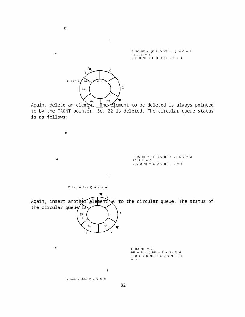
105
UNIT – V BINARY TREES AND HASHINGBinary Search Trees:
An important special kind of binary tree is the binary search tree (BST). In a BST, each node stores some information including a unique key value, and perhaps some associated data. A binary tree is a BST iff, for every node n in the tree:
All keys in n's left subtree are less than the key in n, and All keys in n's right subtree are greater than the key in n.
In other words, binary search trees are binary trees in which all values in the node’s left subtree are less than node value all values in the node’s right subtree are greater than node value.
Here are some BSTs in which each node just stores an integer key:
These are not BSTs:
In the left one 5 is not greater than 6. In the right one 6 is not greater than 7.
The reason binary-search trees are important is that the following operations can be implemented efficiently using a BST:
insert a key value determine whether a key value is in the tree remove a key value from the tree print all of the key values in sorted order
Let's illustrate what happens using the following BST:
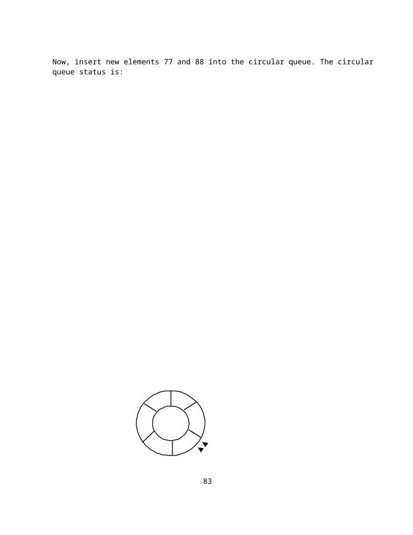
106
and searching for 12:
What if we search for 15:
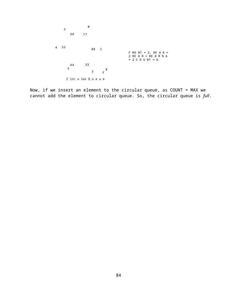
110
Properties and Operations:
A BST is a binary tree of nodes ordered in the following way:
1. Each node contains one key (also unique)2. The keys in the left subtree are < (less) than the key in its parent node3. The keys in the right subtree > (greater) than the key in its parent node4. Duplicate node keys are not allowed.
Inserting a node
A naïve algorithm for inserting a node into a BST is that, we start from the root node, if the node to insert is less than the root, we go to left child, and otherwise we go to the right child of the root. We continue this process (each node is a root for some sub tree) until we find a null pointer (or leaf node) where we cannot go any further. We then insert the node as a left or right child of the leaf node based on node is less or greater than the leaf node. We note that a new node is always inserted as a leaf node. A recursive algorithm for inserting a node into a BST is as follows. Assume we insert a node N to tree T. if the tree is empty, the we return new node N as the tree. Otherwise, the problem of inserting is reduced to inserting the node N to left of right sub trees of T, depending on N is less or greater than T. A definition is as follows.
Insert(N, T) = N if T is empty= insert(N, T.left) if N < T= insert(N, T.right) if N > T
Searching for a nodeSearching for a node is similar to inserting a node. We start from root, and then go left or right until we find (or not find the node). A recursive definition of search is as follows. If the node is equal to root, then we return true. If the root is null, then we return false. Otherwise we recursively solve the problem for T.left or T.right, depending on N < T or N > T. A recursive definition is as follows.Search should return a true or false, depending on the node is found or not. Search(N, T) = false if T is empty
= true if T = N

111
= search(N, T.left) if N < T= search(N, T.right) if N > T
Deleting a node
A BST is a connected structure. That is, all nodes in a tree are connected to some other node. For example, each node has a parent, unless node is the root. Therefore deleting a node could affect all sub trees of that node. For example, deleting node 5 from the tree could result in losing sub trees that are rooted at 1 and 9.
Hence we need to be careful about deleting nodes from a tree. The best way to deal with deletion seems to be considering special cases. What if the node to delete is a leaf node? What if the node is a node with just one child? What if the node is an internal node (with two children). The latter case is the hardest to resolve. But we will find a way to handle this situation as well.Case 1 : The node to delete is a leaf nodeThis is a very easy case. Just delete the node 46. We are done
Case 2 : The node to delete is a node with one child.This is also not too bad. If the node to be deleted is a left child of the parent, then we connect the left pointer of the parent (of the deleted node) to the single child. Otherwise if the node to be deleted is a right child of the parent, then we connect the right pointer of the parent (of the deleted node) to single child.
112
Case 3: The node to delete is a node with two childrenThis is a difficult case as we need to deal with two sub trees. But we find an easy way to handle it. First we find a replacement node (from leaf node or nodes with one child) for the node to be deleted. We need to do this while maintaining the BST order property. Then we swap leaf node or node with one child with the node to be deleted (swap the data) and delete the leaf node or node with one child (case 1 or case 2)
Next problem is finding a replacement leaf node for the node to be deleted. We can easily find this as follows. If the node to be deleted is N, the find the largest node in the left sub tree of N or the smallest node in the right sub tree of N. These are two candidates that can replace the node to be deleted without losing the order property. For example, consider the following tree and suppose we need to delete the root 38.
Then we find the largest node in the left sub tree (15) or smallest node in the right sub tree (45) and replace the root with that node and then delete that node. The following set of images demonstrates this process.
Let’s see when we delete 13 from that tree.
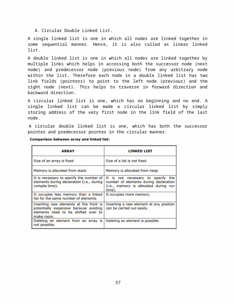
113
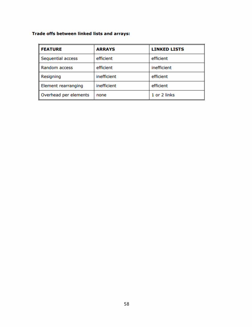
114
Balanced Search Trees:
A self-balancing (or height-balanced) binary search tree is any node-based binary search tree that automatically keeps its height (maximal number of levels below the root) small in the face of arbitrary item insertions and deletions. The red–black tree, which is a type of self-balancing binary search tree, was called symmetric binary B-tree. Self-balancing binary search trees can be used in a natural way to construct and maintain ordered lists, such as priority queues. They can also be used for associative arrays; key-value pairs are simply inserted with an ordering based on the key alone. In this capacity, self-balancing BSTs have a number of advantages and disadvantages over their main competitor, hash tables. One advantage of self-balancing BSTs is that they allow fast (indeed, asymptotically optimal) enumeration of the items in key order, which hash tables do not provide. One disadvantage is that their lookup algorithms get more complicated when there may be multiple items with the same key. Self-balancing BSTs have better worst-case lookup performance than hash tables (O(log n) compared to O(n)), but have worse average-case performance (O(log n) compared to O(1)).
Self-balancing BSTs can be used to implement any algorithm that requires mutable ordered lists, to achieve optimal worst-case asymptotic performance. For example, if binary tree sort is implemented with a self-balanced BST, we have a very simple-to-describe yet asymptotically optimal O(n log n) sorting algorithm. Similarly, many algorithms in computational geometry exploit variations on self-balancing BSTs to solve problems such as the line segment intersection problem and the point location problem efficiently. (For average-case performance, however, self-balanced BSTs may be less efficient than other solutions. Binary tree sort, in particular, is likely to be slower than merge sort, quicksort, or heapsort, because of the tree-balancing overhead as well as cache access patterns.)
Self-balancing BSTs are flexible data structures, in that it's easy to extend them to efficiently record additional information or perform new operations. For example, one can record the number of nodes in each subtree having a certain property, allowing one to count the number of nodes in a certain key range with that property in O(log n) time. These extensions can be used, for example, to optimize database queries or other list-processing algorithms.AVL Trees:
An AVL tree is another balanced binary search tree. Named after their inventors, Adelson- Velskii and Landis, they were the first dynamically balanced trees to be proposed. Like red-black trees, they are not perfectly balanced, but pairs of sub-trees differ in height by at most 1, maintaining an O(logn) search time. Addition and deletion operations also take O(logn) time.
Definition of an AVL tree: An AVL tree is a binary search tree which has the following properties:
1. The sub-trees of every node differ in height by at most one.2. Every sub-tree is an AVL tree.
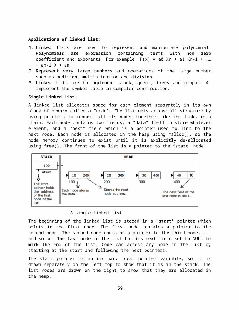
115
Balance requirement for an AVL tree: the left and right sub-trees differ by at most 1 in height.
For example, here are some trees:
Yes this is an AVL tree. Examination shows that each left sub-tree has a height 1 greater than each right sub-tree.
No this is not an AVL tree. Sub-tree with root 8 has height 4 and sub-tree with root 18 has height 2.An AVL tree implements the Map abstract data type just like a regular binary search tree, the only difference is in how the tree performs. To implement our AVL tree we need to keep track of a balance factor for each node in the tree. We do this by looking at the heights of the left and right subtrees for each node. More formally, we define the balance factor for a node as the difference between the height of the left subtree and the height of the right subtree.
balanceFactor=height(leftSubTree)−height(rightSubTree)
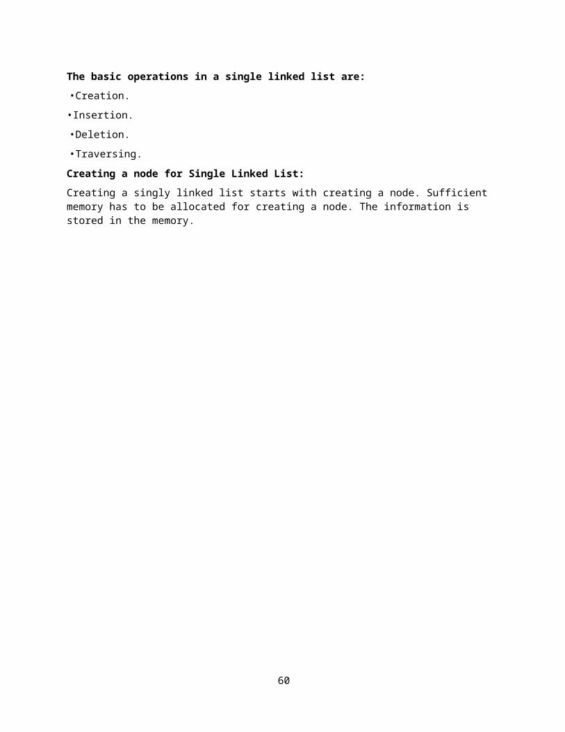
116
Using the definition for balance factor given above we say that a subtree is left-heavy if the balance factor is greater than zero. If the balance factor is less than zero then the subtree is right heavy. If the balance factor is zero then the tree is perfectly in balance. For purposes of implementing an AVL tree, and gaining the benefit of having a balanced tree we will define a tree to be in balance if the balance factor is -1, 0, or 1. Once the balance factor of a node in a tree is outside this range we will need to have a procedure to bring the tree back into balance. Figure shows an example of an unbalanced, right-heavy tree and the balance factors of each node.
Properties of AVL Trees
AVL trees are identical to standard binary search trees except that for every node in an AVL tree, the height of the left and right subtrees can differ by at most 1 (Weiss, 1993, p:108). AVL trees are HB-k trees (height balanced trees of order k) of order HB-1.
The following is the height differential formula:
When storing an AVL tree, a field must be added to each node with one of three values: 1, 0, or-1. A value of 1 in this field means that the left subtree has a height one more than the right subtree. A value of -1 denotes the opposite. A value of 0 indicates that the heights of both subtrees are the same. Updates of AVL trees require up to rotations, whereas updating red-black trees can be done using only one or two rotations (up to color changes). For this reason, they (AVL trees) are considered a bit obsolete by some.
Sparse AVL trees
Sparse AVL trees are defined as AVL trees of height h with the fewest possible nodes. Figure 3 shows sparse AVL trees of heights 0, 1, 2, and 3.
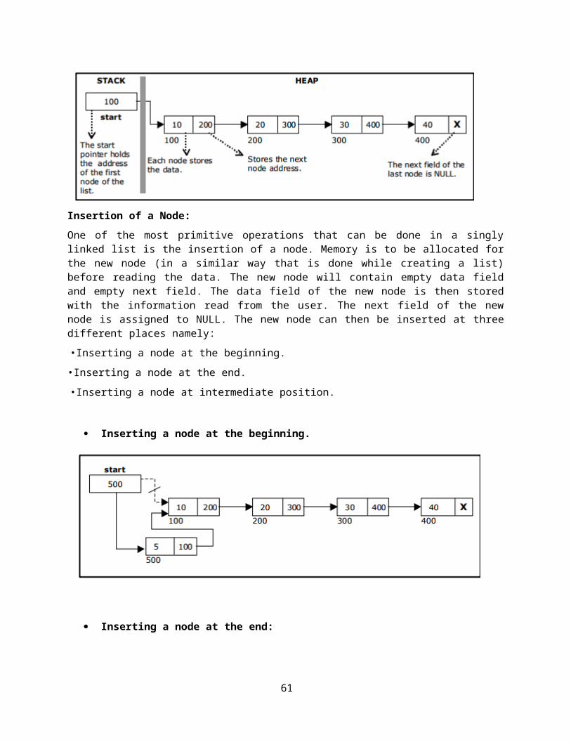
117
Figure Structure of an AVL tree
Introduction to M-Way Search Trees:
A multiway tree is a tree that can have more than two children. A multiway tree of order m (or an m-way tree) is one in which a tree can have m children.
As with the other trees that have been studied, the nodes in an m-way tree will be made up of key fields, in this case m-1 key fields, and pointers to children.
Multiday tree of order 5
To make the processing of m-way trees easier some type of order will be imposed on the keys within each node, resulting in a multiway search tree of order m (or an m-way search tree). By definition an m-way search tree is a m-way tree in which:
Each node has m children and m-1 key fields The keys in each node are in ascending order. The keys in the first i children are smaller than the ith key The keys in the last m-i children are larger than the ith key
4-way search tree
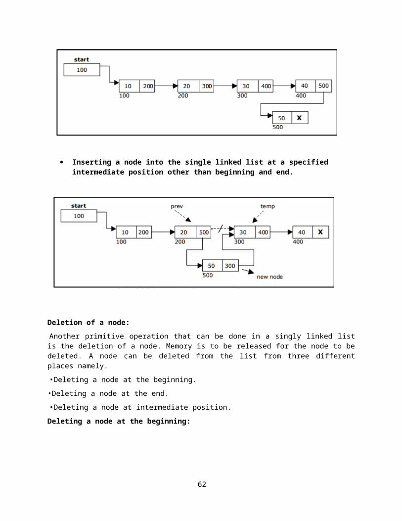
118
M-way search trees give the same advantages to m-way trees that binary search trees gave to binary trees - they provide fast information retrieval and update. However, they also have the same problems that binary search trees had - they can become unbalanced, which means that the construction of the tree becomes of vital importance.B Trees:
An extension of a multiway search tree of order m is a B-tree of order m. This type of tree will be used when the data to be accessed/stored is located on secondary storage devices because they allow for large amounts of data to be stored in a node.
A B-tree of order m is a multiway search tree in which:
1. The root has at least two subtrees unless it is the only node in the tree.2. Each nonroot and each nonleaf node have at most m nonempty children and at least m/2
nonempty children.3. The number of keys in each nonroot and each nonleaf node is one less than the number of
its nonempty children.4. All leaves are on the same level.
These restrictions make B-trees always at least half full, have few levels, and remain perfectly balanced.
Searching a B-tree
An algorithm for finding a key in B-tree is simple. Start at the root and determine which pointer to follow based on a comparison between the search value and key fields in the root node. Follow the appropriate pointer to a child node. Examine the key fields in the child node and continue to follow the appropriate pointers until the search value is found or a leaf node is reached that doesn't contain the desired search value.
Insertion into a B-tree
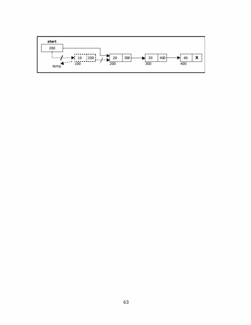
119
The condition that all leaves must be on the same level forces a characteristic behavior of B- trees, namely that B-trees are not allowed to grow at the their leaves; instead they are forced to grow at the root.
When inserting into a B-tree, a value is inserted directly into a leaf. This leads to three common situations that can occur:
1. A key is placed into a leaf that still has room.2. The leaf in which a key is to be placed is full.3. The root of the B-tree is full.
Case 1: A key is placed into a leaf that still has room
This is the easiest of the cases to solve because the value is simply inserted into the correct sorted position in the leaf node.
Inserting the number 7 results in:
Case 2: The leaf in which a key is to be placed is full
In this case, the leaf node where the value should be inserted is split in two, resulting in a new leaf node. Half of the keys will be moved from the full leaf to the new leaf. The new leaf is then incorporated into the B-tree.
The new leaf is incorporated by moving the middle value to the parent and a pointer to the new leaf is also added to the parent. This process is continues up the tree until all of the values have "found" a location.
Insert 6 into the following B-tree:
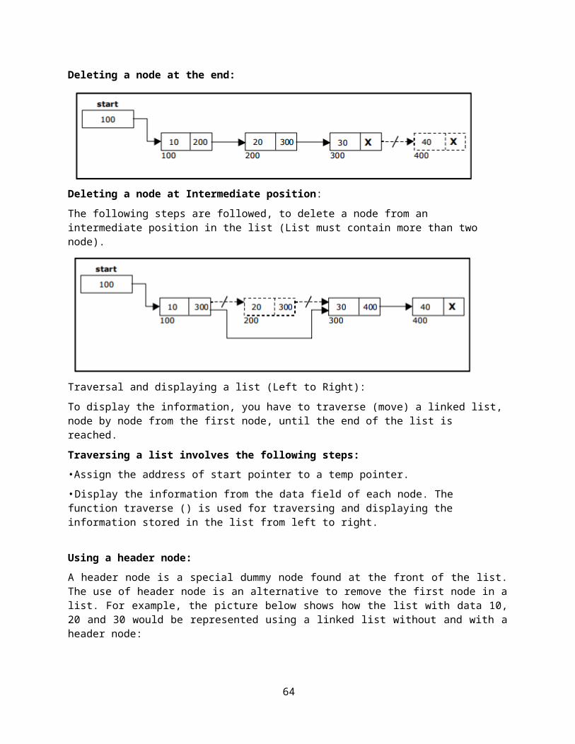
results in a split of the first leaf node:
The new node needs to be incorporated into the tree - this is accomplished by taking the middle value and inserting it in the parent:
Case 3: The root of the B-tree is full
The upward movement of values from case 2 means that it's possible that a value could move up to the root of the B-tree. If the root is full, the same basic process from case 2 will be applied and a new root will be created. This type of split results in 2 new nodes being added to the B-tree.
Inserting 13 into the following tree:
120
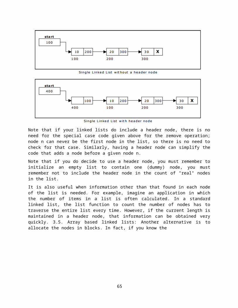
Results in:
The 15 needs to be moved to the root node but it is full. This means that the root needs to be divided:
The 15 is inserted into the parent, which means that it becomes the new root node:
Deleting from a B-tree
As usual, this is the hardest of the processes to apply. The deletion process will basically be a
121
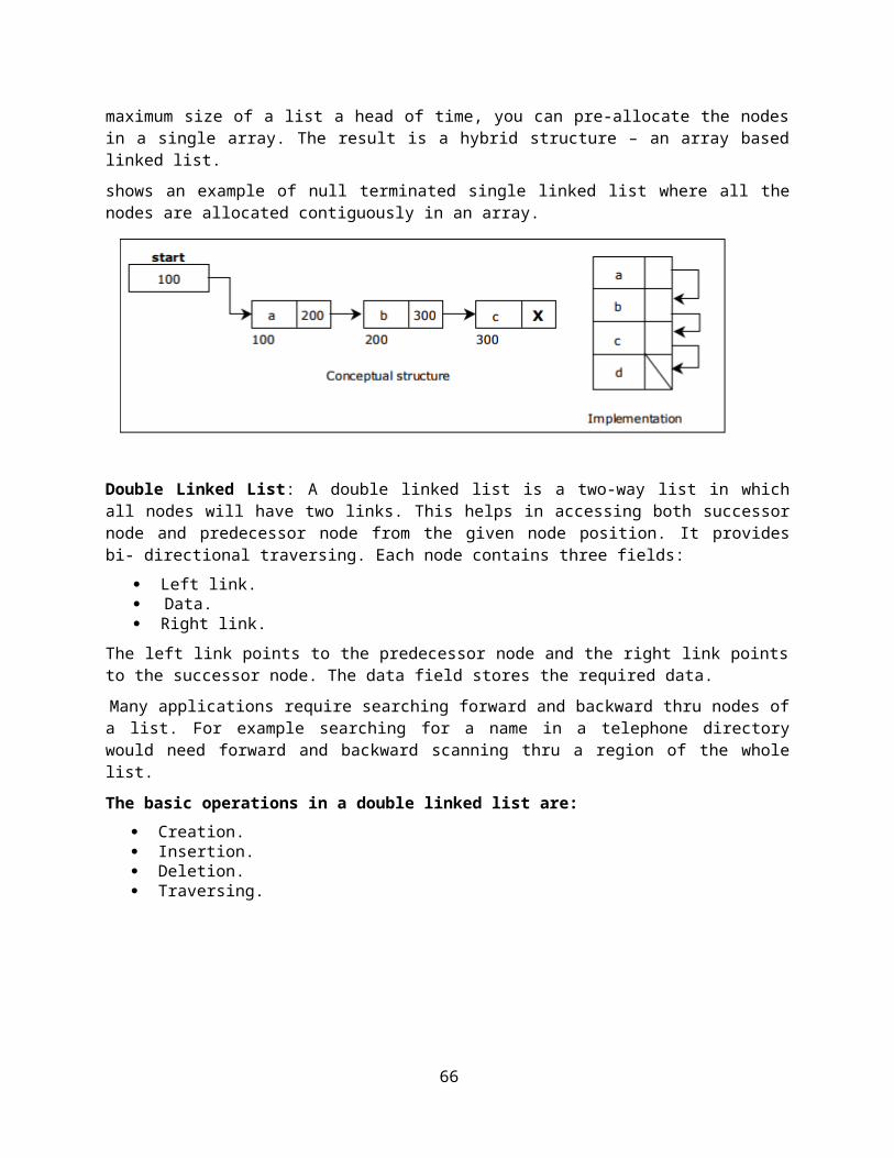
reversal of the insertion process - rather than splitting nodes, it's possible that nodes will be merged so that B-tree properties, namely the requirement that a node must be at least half full, can be maintained.
There are two main cases to be considered:
1. Deletion from a leaf2. Deletion from a non-leaf
Case 1: Deletion from a leaf
1a) If the leaf is at least half full after deleting the desired value, the remaining larger values are moved to "fill the gap".
Deleting 6 from the following tree:
results in:
1b) If the leaf is less than half full after deleting the desired value (known as underflow), two things could happen:
Deleting 7 from the tree above results in:
122
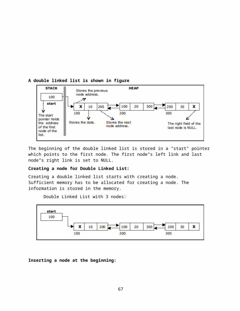
1b-1) If there is a left or right sibling with the number of keys exceeding the minimum requirement, all of the keys from the leaf and sibling will be redistributed between them by moving the separator key from the parent to the leaf and moving the middle key from the node and the sibling combined to the parent.
Now delete 8 from the tree:
1b-2) If the number of keys in the sibling does not exceed the minimum requirement, then the leaf and sibling are merged by putting the keys from the leaf, the sibling, and the separator from the parent into the leaf. The sibling node is discarded and the keys in the parent are moved to "fill the gap". It's possible that this will cause the parent to underflow. If that is the case, treat the parent as a leaf and continue repeating step 1b-2 until the minimum requirement is met or the root of the tree is reached.
Special Case for 1b-2: When merging nodes, if the parent is the root with only one key, the keys from the node, the sibling, and the only key of the root are placed into a node and this will become the new root for the B-tree. Both the sibling and the old root will be discarded.
123
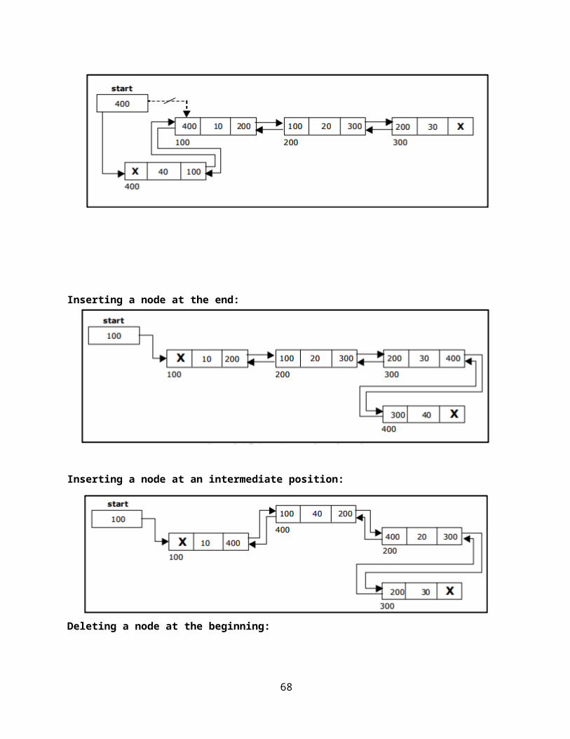
Case 2: Deletion from a non-leaf
This case can lead to problems with tree reorganization but it will be solved in a manner similar to deletion from a binary search tree.
The key to be deleted will be replaced by its immediate predecessor (or successor) and then the predecessor (or successor) will be deleted since it can only be found in a leaf node.
Deleting 16 from the tree above results in:
The "gap" is filled in with the immediate predecessor:
124
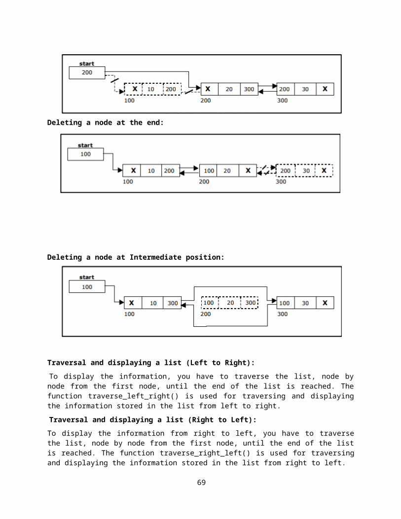
and then the immediate predecessor is deleted:
If the immediate successor had been chosen as the replacement:
Deleting the successor results in:
The vales in the left sibling are combined with the separator key (18) and the remaining values. They are divided between the 2 nodes:
125
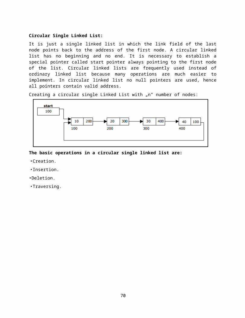
and then the middle value is moved to the parent:
Hashing and Collision:
Hashing is the technique used for performing almost constant time search in case of insertion, deletion and find operation. Taking a very simple example of it, an array with its index as key is the example of hash table. So each index (key) can be used for accessing the value in a constant search time. This mapping key must be simple to compute and must helping in identifying the associated value. Function which helps us in generating such kind of key-value mapping is known as Hash Function.
In a hashing system the keys are stored in an array which is called the Hash Table. A perfectly implemented hash table would always promise an average insert/delete/retrieval time of O(1).
Hashing Function:
A function which employs some algorithm to computes the key K for all the data elements in the set U, such that the key K which is of a fixed size. The same key K can be used to map data to a hash table and all the operations like insertion, deletion and searching should be possible. The values returned by a hash function are also referred to as hash values, hash codes, hash sums, or hashes.
126
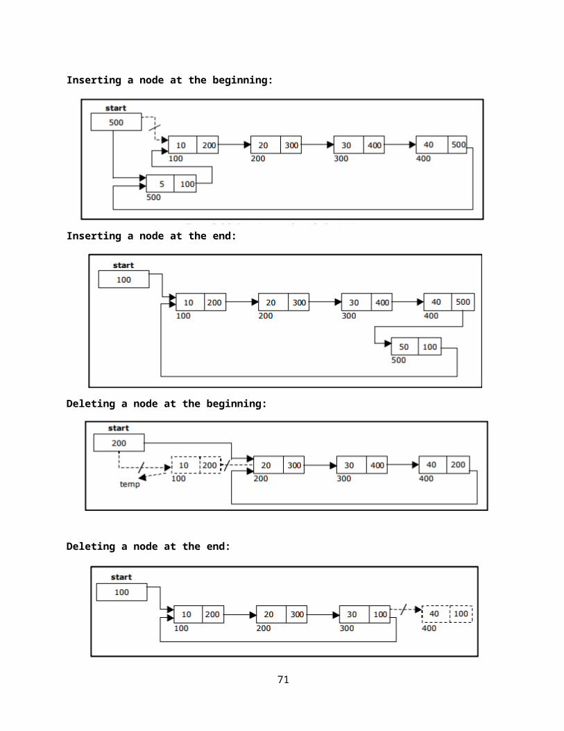
Hash Collision:
A situation when the resultant hashes for two or more data elements in the data set U, maps to the same location in the has table, is called a hash collision. In such a situation two or more data elements would qualify to be stored / mapped to the same location in the hash table.
Hash collision resolution techniques:
Open Hashing (Separate chaining):
Open Hashing, is a technique in which the data is not directly stored at the hash key index (k) of the Hash table. Rather the data at the key index (k) in the hash table is a pointer to the head of the data structure where the data is actually stored. In the most simple and common implementations the data structure adopted for storing the element is a linked-list.
n this technique when a data needs to be searched, it might become necessary (worst case) to traverse all the nodes in the linked list to retrieve the data.
Note that the order in which the data is stored in each of these linked lists (or other data structures) is completely based on implementation requirements. Some of the popular criteria are insertion order, frequency of access etc.
Closed hashing (open Addressing)
In this technique a hash table with pre-identified size is considered. All items are stored in the hash table itself. In addition to the data, each hash bucket also maintains the three states: EMPTY, OCCUPIED, DELETED. While inserting, if a collision occurs, alternative cells are tried until an empty bucket is found. For which one of the following technique is adopted.
127
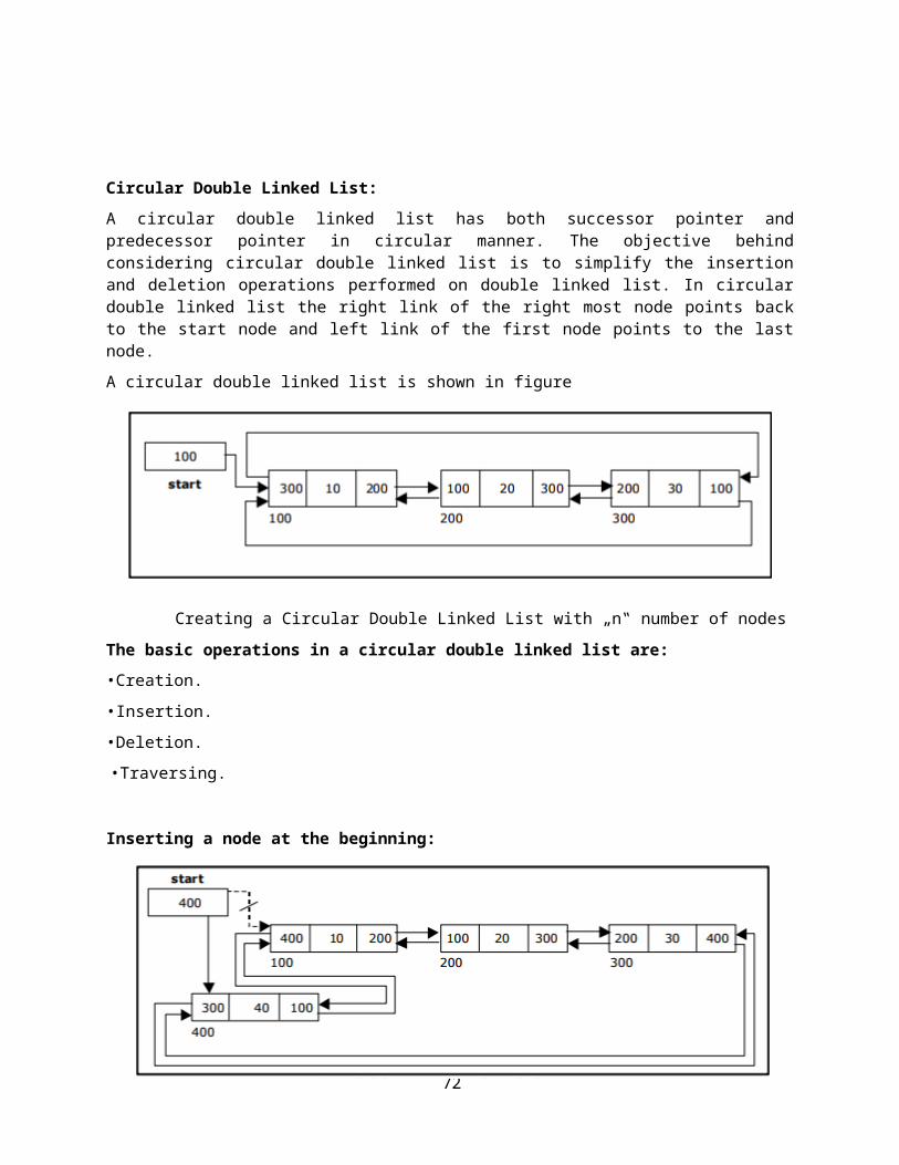
1. Liner Probing
2. Quadratic probing
3. Double hashing (in short in case of collision another hashing function is used with the key value as an input to identify where in the open addressing scheme the data should actually be stored.)
A comparative analysis of Closed Hashing vs Open Hashing
Open Addressing Closed AddressingAll elements would be stored in the Hash table itself. No additional data structure is needed.
Additional Data structure needs to be used to accommodate collision data.
In cases of collisions, a unique hash key must be obtained.
Simple and effective approach to collision resolution. Key may or may not be unique.
Determining size of the hash table, adequate enough for storing all the data is difficult.
Performance deterioration of closed addressing much slower as compared to Open addressing.
State needs be maintained for the data (additional work)
No state data needs to be maintained (easier to maintain)
Uses space efficiently Expensive on spaceApplications of Hashing:
A hash function maps a variable length input string to fixed length output string -- its hash value, or hash for short. If the input is longer than the output, then some inputs must map to the same output -- a hash collision. Comparing the hash values for two inputs can give us one of two answers: the inputs are definitely not the same, or there is a possibility that they are the same. Hashing as we know it is used for performance improvement, error checking, and authentication. One example of a performance improvement is the common hash table, which uses a hash function to index into the correct bucket in the hash table, followed by comparing each element in the bucket to find a match. In error checking, hashes (checksums, message digests, etc.) are used to detect errors caused by either hardware or software. Examples are TCP checksums, ECC memory, and MD5 checksums on downloaded files . In this case, the hash provides additional assurance that the data we received is correct. Finally, hashes are used to authenticate messages. In this case, we are trying to protect the original input from tampering, and we select a hash that is strong enough to make malicious attack infeasible or unprofitable.
Construct a message authentication code (MAC)
Digital signature
Make commitments, but reveal message later
Timestamping
128
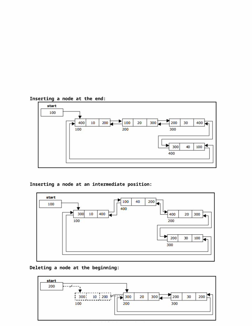
Key updating: key is hashed at specific intervals resulting in new key
129
Related Documents